Embed Size (px)
Citation preview
Universidad Autonoma de Madrid
Facultad de Ciencias
Departamento de la Materia Condensada
Dissipation in finite systems: SemiconductorNEMS, graphene NEMS, and metallic
nanoparticles
A thesis presented by
Cesar Oscar Seoanez Erkell
under the supervision of
Dr. Francisco Guinea Lopez
Profesor de Investigacion
Instituto de Ciencia de Materiales de Madrid (CSIC)
and tutored by
Prof. Guillermo Gomez Santos
Departamento de la Materia Condensada
Universidad Autonoma de Madrid
Madrid, 2007

ii
To my parents and grandparents

iv
Resumen
Los procesos de decoherencia y disipacion en sistemas mesoscopicos han sidoobjeto en las ultimas decadas de gran interes dado su papel clave en el estudio yutilizacion de fenomenos cuanticos a escalas cada vez mayores. Los espectaculareslogros alcanzados en las tecnicas de fabricacion y medicion han permitido el disenode nanoestructuras moviles que habilmente combinadas con otros protagonistas de lahistoria fısica reciente, tales como puntos cuanticos o gases electronicos de baja di-mensionalidad, otorgan la fascinante oportunidad de estudiar la interaccion electron-fonon cuanto a cuanto, con un potencial tecnologico prometedor. En la mayorıa de lasaplicaciones vislumbradas, ası como para la observacion de comportamiento cuanticoen variables mecanicas macroscopicas tales como el centro de masas de resonadoresmicrometricos, es imprescindible una minimizacion de los procesos disipativos que per-turban la dinamica vibracional de estos sistemas. En consecuencia se esta llevando acabo un gran esfuerzo actualmente en el analisis y modelizacion de los mismos, tantodesde un punto de vista experimental como teorico.
Esta tesis forma parte de dicho esfuerzo. En concreto, dos de las tres partesen que se divide estan consagradas a la modelizacion de algunos de los principalesmecanismos de friccion presentes en dos clases de sistemas nanoelectromecanicos(NEMS): nanoresonadores construidos a partir de heteroestructuras de semiconduc-tor, y nanoresonadores en los que la parte movil es un compuesto de carbono de bajadimensionalidad, bien sea una lamina de grafeno o un nanotubo.
En el primer caso nos hemos centrado en los procesos superficiales de absorcionde energıa mecanica asociados al acabado imperfecto, la presencia de impurezas y laestructura superficial parcialmente desordenada, invocando las similitudes existentescon los procesos de atenuamiento de ondas acusticas en materiales amorfos. El re-sultado es un modelo de espines acoplados al conjunto de modos vibracionales delresonador, analizado por medio de tecnicas desarrolladas para el estudio del Spin-Boson Model y de procesos de relajacion. Asimismo se modelizan los posibles efectosnegativos que conlleva la deposicion de electrodos metalicos sobre las estructuras desemiconductor.
Los osciladores de compuestos de carbono presentan una serie de peculiaridadesque los diferencian de sus homologos semiconductores, destacando su alto grado decristalinidad y caracter metalico o semimetalico. Ello implica la prevalencia de mecan-ismos de friccion distintos, varios de los cuales se modelizan, destacando la excitacionde pares electron-hueco en el resonador debido a cargas distribuidas por la estructura,estudiada con metodos perturbativos autoconsistentes.
vi
La tercera y ultima parte se dedica a otro tipo de sistema mesoscopico, laspartıculas nanometalicas, cuya respuesta optica viene dominada por la excitacioncolectiva denominada plasmon de superficie. La presencia en el espectro de excita-ciones electronicas de pares electron-hueco acoplados al plasmon provoca su progre-sivo atenuamiento tras ser excitado inicialmente por un campo electrico externo, porejemplo un laser. Este proceso se puede considerar como ejemplo de entorno disipa-tivo con un numero finito de grados de libertad en interaccion con el subsistema deinteres, el plasmon. Los efectos que esta finitud conlleva en la modelizacion teoricade la dinamica electronica son analizados en detalle, justificando la validez de ciertasaproximaciones asumidas hasta ahora sin demostracion previa.
Conclusiones.
La friccion a bajas temperaturas asociada a los distintos procesos superficialesen resonadores de semiconductor ha sido modelizada adaptando el Standard Tun-neling Model utilizado para explicar las propiedades acusticas de solidos amorfos a∼ 0.01 . T . 1 K. El orden de magnitud ası como la debil dependencia con latemperatura observada en los experimentos es cualitativamente reproducida. Sin em-bargo, llegar a un acuerdo cuantitativo se antoja difıcil hasta que no se posea unconocimiento mas detallado de los procesos y defectos estructurales presentes en elresonador.
Diversos mecanismos disipativos presentes en nanoresonadores de grafeno y nan-otubos han sido analizados, obteniendo, al igual que en el caso previo, dependenciasparametricas de los mismos en funcion de las variables fısicas relevantes del sistema,como la temperatura y dimensiones caracterısticas. La importancia relativa de losmismos en funcion del regimen (amplitud de vibracion, temperatura) ha sido estable-cida, predominando a bajas temperaturas la disipacion ohmica debido a excitacioneselectronicas en el seno del resonador y a altas temperaturas la atenuacion por proce-sos termoelasticos.
Se ha presentado un modelo muy utilizado en el estudio de la dinamica de plas-mones superficiales y de la respuesta optica de clusters metalicos, analizando la co-herencia interna de dicho esquema teorico, justificando varios puntos clave del mismoque hasta ahora se habıan tomado como validos sin justificacion rigurosa. De dichoanalisis se obtiene asimismo informacion sobre los tiempos caracterısticos de evoluciondel plasmon y del resto de excitaciones electronicas acopladas al mismo, lo cual per-mite fundamentar una aproximacion Markoviana a la hora de estudiar la dinamicadel sistema acoplado plasmon - pares electron-hueco.
Abstract
The physics of decoherence and dissipation in mesoscopic systems has attractedgreat interest, given its key role in the study and use of quantum phenomena at everlarger scales. The spectacular achievements in fabrication and measurement tech-niques have opened the doors to the design of mobile nanostructures which, combinedin smart ways with other recent cornerstones like quantum dots or low-dimensionalelectron gases, grant the fascinating opportunity to study electron-phonon interac-tions at an individual level, with a promising technological potential. In most of theenvisioned applications, as well as to observe quantum behavior in macroscopic me-chanical variables like the center-of-mass of micrometric resonators, a minimizationof the dissipative processes perturbing the vibrational dynamics of these systems iscompulsory. Consequently strong efforts are being made to analyze and model them,both from the experimental as well as from the theoretical sides.
This thesis exemplifies these efforts. Specifically, two out of the three parts con-stituting it are consecrated to the modeling of some of the main friction mechanismsfound in two kinds of nanoelectromechanical systems (NEMS): nanoresonators builtfrom semiconductor heterostructures, and nanoresonators whose mobile part is a low-dimensional carbon compound, be it graphene or a nanotube.
In the first case we have focussed in the surface processes absorbing mechanicalenergy, related to the imperfect finish, presence of impurities and partially disorderedsurface structure. Similarities with acoustic wave damping in amorphous solids havebeen invoked to build an adaptation of the Standard Tunneling Model which aimsto provide a low temperature description of such processes. The result is a model ofspins coupled to the ensemble of vibrational eigenmodes of the resonator, which is an-alyzed by means of techniques developed for the study of the Spin-Boson Model andrelaxation processes. Possible negative effects due to metallic electrodes deposited ontop of the semiconductor structures are also modeled.
Oscillators made from carbon compounds, demonstrated for the first time thisyear, display a series of peculiarities distinguishing them from their semiconductorcounterparts, specially their high degree of crystallinity and semimetal or metal char-acter. The prevailing friction mechanisms thus differ, several out of which are mod-eled, with the excitation of electron-hole pairs in the resonator due to charges distrib-uted throughout the device dominating at low temperatures and small vibrationalamplitudes.
The third and last part is devoted to another kind of mesoscopic system, namelynanometallic clusters, whose optical response is dominated by the so-called surface
viii
plasmon collective excitation. The presence in the electronic excitation spectrum ofone-body electron-hole pairs coupled to the plasmon causes its progressive dampingafter its initial excitation by an external electric field, e.g. a laser pulse. This processmay be considered as an example of finite dissipative environment interacting with thesubsystem subject of our interest, the plasmon. The consequences of this finiteness onthe theoretical modeling of the electronic dynamics are analyzed in detail, justifyingthe validity of several approximations assumed until now to hold without proof. Thisstudy will also shed some light on the characteristic times of the different electronicdegrees of freedom, providing a basis for the use of a Markovian approximation in theanalysis of the plasmon dynamics of nanometric clusters.
Acknowledgments
Looking back at these years of PhD, I really consider myself a very fortunate per-son. All the people next to me have always given their support and courage wheneverI needed it. I have met many good, generous, idealistic and hardworking people,whose invaluable examples have been extremely stimulating, and a reason to reflectand rejoice. I start with my advisor, Paco Guinea. His efficacy, optimism and hu-mility are simply impressive. Making use of his deep physical intuition and thoroughknowledge of numerous fields he introduced me to fascinating research fields and alsogave me the possibility to assist to several schools and workshops, where I could meetphysicists and friends from many countries. Indeed, in some of them I met for the firsttime some of the people with whom I had the luck to collaborate, like Raj Mohantyand Rodolfo Jalabert.Two stages abroad have been fundamental to get to this point, one with AntonioCastro-Neto in Boston and another with Rodolfo Jalabert in Strasbourg and Augs-burg. In both cases they, together with their collaborators, made their best to helpme in every issue to make me feel like at home, and with them I could also learndifferent ways of doing physics, a very enriching experience. Here go my thanks toAntonio, Raj, Silvia, Marco, Guiti, Alexei and Johan (BU), and to Rodolfo, Dietmar,Guillaume and Gert (IPCMS/U. Augsburg), and all the rest of nice and helping peo-ple I met there. I appreciate as well very much the effort made by Sebastian Vieira,Adrian Bachtold, Enrique Louis, Rodolfo Jalabert and Pablo Esquinazi to be part ofthe dissertation committee, and the work done by Guillermo Gomez-Santos as tutor.In any case, most of the time was spent here in Madrid, in a wonderful group ofthe Condensed Matter Theory Department at the ICMM. I doubt I will ever againfind a working place where I feel so comfortable. Moreover, there were many of usdoing the PhD, so we could share this experience, having often great fun. If youare bored or feel depressed just knock on the door of offices 128 or 130, ”mano desanto”, as we say in spanish. Thank you so much for everything, Juan Luis, Alberto,Debb, Suzana, Javi, Rafas, Felix, Ramon, Geli, Luis, Virginia, Tobıas, Leni, Belen,Berni, Marıa, David, Fernando, Carlos, Samuel, Juan, Ana and Ma Jose. In the caseof Geli, Ramon, Tobıas, Pilar, Carlos, Alberto, Javi and Juan Luis thank you verymuch for helping me with my computer and physics-related doubts. Special thanksalso to Sonia, Angel, Antonio, Cayetana and Puri, thank you for your sympathy andattentions.Some words of gratitude cannot be skipped for my friends outside the ICMM, yoursupport is also very important to me: Javi, Jose, Hector, Juan, Teo, Alfredo, Fatima,Nuria, Ana, Abelardo, Juan, Rocıo, Izaskun, Angela, Julio, Amadeo, Mario, Ful, Au-relio, Sabrina... I also thank my spanish and swedish family, which I know is alwaysthere in the good and bad circumstances: tıo Mariano, tıa Pili, Pilar, Esther, Aniana,Titti, Lars-Johan..., and my grandparents, who unfortunately are now gone.And of course I am most indebted to my parents, your 28 years of love and care areimpossible to balance, I cannot ask for more, tusen tack!

x Acknowledgments
Citations to Previously Published Work
Parts of the contents of this work can be found in the following publications:
• C. Seoanez, F. Guinea and A. H. Castro-Neto (2007). Dissipation due totwo-level systems in nano-mechanical devices. Europhysics Letters 78, 60002,preprint archive cond-mat/0611153.
• C. Seoanez, F. Guinea and A. H. Castro-Neto (2007). Surface dissipation inNEMS: Unified description with the Standard Tunneling Model, and effects ofmetallic electrodes.. Sent to Physical Review B.
• C. Seoanez, G. Weick, R.A. Jalabert and D. Weinmann (2007). Friction ofthe surface plasmon by high-energy particle-hole pairs: Are memory effects im-portant?. The European Physical Journal D 44, 351, preprint archive cond-mat/0703720.
• C. Seoanez, F. Guinea and A. H. Castro-Neto (2007). Dissipation in grapheneand nanotube resonators. Physical Review B 76, 125427, preprint archivearXiv:07042225.
Contents
Title Page . . . . . . . . . . . . . . . . . . . . . . . . . . . . . . . . . . . . iDedication . . . . . . . . . . . . . . . . . . . . . . . . . . . . . . . . . . . . iiiResumen y conclusiones . . . . . . . . . . . . . . . . . . . . . . . . . . . . vAbstract . . . . . . . . . . . . . . . . . . . . . . . . . . . . . . . . . . . . . viiAcknowledgments . . . . . . . . . . . . . . . . . . . . . . . . . . . . . . . . ixCitations to Previously Published Work . . . . . . . . . . . . . . . . . . . xiContents . . . . . . . . . . . . . . . . . . . . . . . . . . . . . . . . . . . . . xiiList of Figures . . . . . . . . . . . . . . . . . . . . . . . . . . . . . . . . . . xviList of Tables . . . . . . . . . . . . . . . . . . . . . . . . . . . . . . . . . . xviii
I Dissipation in semiconductor NEMS 1
1 NEMS 31.1 Introduction: current research topics . . . . . . . . . . . . . . . . . . 31.2 Semiconductor NEMS fabrication . . . . . . . . . . . . . . . . . . . . 51.3 Motion transduction of mechanical eigenmodes in semiconductor NEMS 7
1.3.1 Magnetomotive scheme . . . . . . . . . . . . . . . . . . . . . . 81.3.2 Coupling to SETs and other sensitive electronic probes . . . . 9
1.4 Nanoscale elasticity theory: Vibrational eigenmodes of long and thinrods . . . . . . . . . . . . . . . . . . . . . . . . . . . . . . . . . . . . 9
1.5 Dissipative mechanisms damping the vibrational eigenmodes of semi-conductor nanoresonators . . . . . . . . . . . . . . . . . . . . . . . . 111.5.1 Extrinsic mechanisms . . . . . . . . . . . . . . . . . . . . . . . 111.5.2 Intrinsic mechanisms . . . . . . . . . . . . . . . . . . . . . . . 14
2 Surface dissipation in semiconductor NEMS at low temperatures 172.1 Introduction . . . . . . . . . . . . . . . . . . . . . . . . . . . . . . . . 172.2 Damping of acoustic waves in amorphous solids: Standard Tunneling
Model . . . . . . . . . . . . . . . . . . . . . . . . . . . . . . . . . . . 182.3 Theoretical analysis of the damping of phonons due to TLSs . . . . . 21
2.3.1 Resonant dissipation . . . . . . . . . . . . . . . . . . . . . . . 222.3.2 Dissipation of symmetric non-resonant TLSs . . . . . . . . . . 22
xii
Contents xiii
2.3.3 Contribution of biased TLSs to the linewidth: relaxation ab-sorption . . . . . . . . . . . . . . . . . . . . . . . . . . . . . . 28
2.3.4 Comparison between contributions to Q−1. Relaxation preva-lence. . . . . . . . . . . . . . . . . . . . . . . . . . . . . . . . . 30
2.4 Extensions to other devices . . . . . . . . . . . . . . . . . . . . . . . 312.4.1 Cantilevers, nanopillars and torsional oscillators . . . . . . . . 312.4.2 Effect of the flexural modes on the dissipation of torsional modes 31
2.5 Frequency shift . . . . . . . . . . . . . . . . . . . . . . . . . . . . . . 332.5.1 Relation to the acoustic susceptibility . . . . . . . . . . . . . . 332.5.2 Expressions for the frequency shift . . . . . . . . . . . . . . . 33
2.6 Applicability and further extensions of the model. Discussion . . . . . 342.7 Dissipation in a metallic conductor . . . . . . . . . . . . . . . . . . . 352.8 Conclusions . . . . . . . . . . . . . . . . . . . . . . . . . . . . . . . . 38
II Friction mechanisms in graphene and carbon nanotube-based resonators 41
3 Graphene-based structures: promising materials 433.1 From 3D to 0D, 1D and 2D . . . . . . . . . . . . . . . . . . . . . . . 433.2 Graphene . . . . . . . . . . . . . . . . . . . . . . . . . . . . . . . . . 46
4 Dissipative processes in graphene resonators 534.1 Introduction . . . . . . . . . . . . . . . . . . . . . . . . . . . . . . . . 53
4.1.1 Experimental setup . . . . . . . . . . . . . . . . . . . . . . . . 534.1.2 Quality factors measured . . . . . . . . . . . . . . . . . . . . . 544.1.3 Damping mechanisms present in graphene resonators . . . . . 55
4.2 Estimates for the damping caused by the different mechanisms . . . . 584.2.1 Coupling to fixed charges in the SiO2 substrate . . . . . . . . 584.2.2 Ohmic losses at the graphene sheet and the metallic gate. . . . 604.2.3 Breaking and healing of surface bonds: Velcro effect. . . . . . 634.2.4 Fluctuating charge noise: Dissipation due to two-level systems. 634.2.5 Other friction mechanisms . . . . . . . . . . . . . . . . . . . . 65
4.3 Extension to nanotube oscillators. . . . . . . . . . . . . . . . . . . . . 664.4 Conclusions. . . . . . . . . . . . . . . . . . . . . . . . . . . . . . . . . 67
III Dissipation of collective excitations in metallic nanopar-ticles 69
5 Metallic clusters: optical response and collective excitations 715.1 From atoms to bulk . . . . . . . . . . . . . . . . . . . . . . . . . . . . 715.2 Surface plasmon excitation . . . . . . . . . . . . . . . . . . . . . . . . 74
xiv Contents
5.2.1 Probing and using the surface plasmon . . . . . . . . . . . . . 76
6 Electronic dynamics in metallic nanoparticles: theoretical model 81
6.1 Electronic hamiltonian: relative and collective coordinates . . . . . . 81
6.2 Mean-field approximation and second quantization of the hamiltonian 84
6.3 Surface plasmon linewidth and finite size effects . . . . . . . . . . . . 86
6.3.1 Mechanisms causing the decay of the surface plasmon . . . . . 86
6.3.2 Landau damping and the double-counting problem . . . . . . 88
6.4 The surface plasmon as a superposition of low-energy particle-hole ex-citations . . . . . . . . . . . . . . . . . . . . . . . . . . . . . . . . . . 90
6.4.1 Separable interaction ansatz . . . . . . . . . . . . . . . . . . . 90
6.4.2 Linear response theory and Random Phase Approximation forthe surface plasmon . . . . . . . . . . . . . . . . . . . . . . . . 92
6.4.3 Fast decay of dph. Plasmon state built from low-energy p-hexcitations . . . . . . . . . . . . . . . . . . . . . . . . . . . . . 96
6.4.4 Separation of the reduced and additional particle-hole subspaces 100
6.5 Dynamics of the relative-coordinate system . . . . . . . . . . . . . . . 102
6.6 Conclusions . . . . . . . . . . . . . . . . . . . . . . . . . . . . . . . . 104
A Appendix to Chapter 1 107
A.1 Modes’ equations of motion of quasi-1D resonators. . . . . . . . . . . 107
A.1.1 Elasticity basics. . . . . . . . . . . . . . . . . . . . . . . . . . 107
A.1.2 The case of a rod. . . . . . . . . . . . . . . . . . . . . . . . . . 108
B Appendix to Chapter 2 111
B.1 Some details about the Standard Tunneling Model. . . . . . . . . . . 111
B.1.1 Distribution function of the TLSs . . . . . . . . . . . . . . . . 111
B.1.2 Determination of values for P0 and ∆∗ . . . . . . . . . . . . . 112
B.1.3 Predominant coupling of the strain to the asymmetry . . . . . 114
B.2 Path integral description of the dissipative two-state system. . . . . . 115
B.2.1 Derivation of the spectral function for the case of the modes ofa quasi-1D nanoresonator . . . . . . . . . . . . . . . . . . . . 118
B.3 Dissipation from symmetric non-resonant TLSs . . . . . . . . . . . . 120
B.3.1 Spectral function of a single TLS coupled to the subohmic bend-ing modes . . . . . . . . . . . . . . . . . . . . . . . . . . . . . 120
B.3.2 Value of Atotoff−res(ω0) . . . . . . . . . . . . . . . . . . . . . . . 121
B.3.3 The off-resonance contribution for T > 0 . . . . . . . . . . . . 121
B.4 Q−1 due to the delayed response of biased TLSs (relaxation mechanism)124
B.5 Derivation of Q−1rel (ω0, T ), eq.(2.23) . . . . . . . . . . . . . . . . . . . 127
B.6 Derivation of eq.(2.27) . . . . . . . . . . . . . . . . . . . . . . . . . . 128
Contents xv
C Appendix to Chapter 4 129C.1 Electron-phonon coupling: friction in terms of the susceptibility χ . . 129
C.1.1 Damping of a phonon mode due to Coulomb interactions be-tween charges in a device . . . . . . . . . . . . . . . . . . . . . 129
C.1.2 Clean metal susceptibility . . . . . . . . . . . . . . . . . . . . 130C.1.3 Dirty metal susceptibility . . . . . . . . . . . . . . . . . . . . 131C.1.4 Microscopic derivation of eq.(4.15) . . . . . . . . . . . . . . . 132
C.2 Imχ, Q−1 and temperature dependence of friction . . . . . . . . . . . 133C.2.1 Temperature dependence of Imχ, Q−1 due to excitation and
relaxation of e-h pairs . . . . . . . . . . . . . . . . . . . . . . 133C.2.2 Temperature dependence of energy loss due to excitation and
relaxation of e-h pairs . . . . . . . . . . . . . . . . . . . . . . 135C.2.3 Extension to a generic system + bath . . . . . . . . . . . . . . 136
C.3 Charge impurity density in SiO2 and the SiO2-Si interface . . . . . . 136C.3.1 Estimate of the charge concentration, and comparison with
numbers given in other references to fit experiments . . . . . . 137C.3.2 Thickness of the charged layer in the doped Si gate . . . . . . 138C.3.3 Information about the SiO2 surface and structure. Conclusions
from experiments with carbon nanotubes . . . . . . . . . . . . 138C.4 Screening of the potentials at the graphene sheet and Si gate . . . . . 140C.5 Dissipation due to two-level systems in graphene resonators . . . . . . 142
C.5.1 Model and vibrating modes of a 2D sheet . . . . . . . . . . . . 142C.5.2 Losses due to the ohmic bath. Temperature dependence . . . 144
D Appendix to Chapter 6 147D.1 Dipole matrix element from single-particle mean-field states . . . . . 147D.2 Lowest energy of the particle-hole spectrum . . . . . . . . . . . . . . 150D.3 Density of states at a fixed angular momentum l, ρl(ε) . . . . . . . . 151D.4 Local density of the dipole matrix element . . . . . . . . . . . . . . . 154D.5 Density of particle-hole excitations . . . . . . . . . . . . . . . . . . . 156
Bibliography 157
List of Figures
1.1 Quantum superpositions with mechanical resonators . . . . . . . . . . 51.2 NEMS examples . . . . . . . . . . . . . . . . . . . . . . . . . . . . . . 61.3 NEM resonator fabrication: Nanomachining . . . . . . . . . . . . . . 81.4 NEMS detection and driving schemes . . . . . . . . . . . . . . . . . . 101.5 Flexural and torsional modes of a cantilever . . . . . . . . . . . . . . 111.6 Linear dependence of Q with the surface-to-volume ratio . . . . . . . 131.7 Limits to Q imposed by the thermoelastic mechanism . . . . . . . . . 14
2.1 Sketch of the nanoresonators with surface imperfections limiting Q . . 182.2 Amorphous quartz structure with several Two-State candidates, and
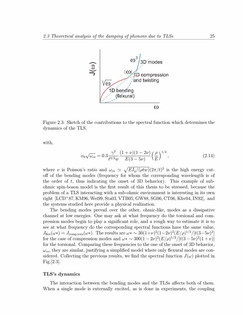
double well potential . . . . . . . . . . . . . . . . . . . . . . . . . . . 212.3 Sketch of the contributions to the spectral function which determines
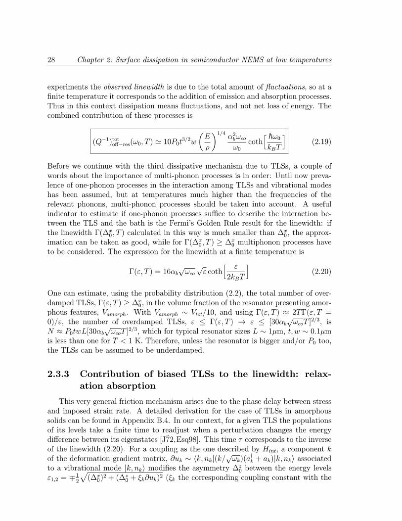
the dynamics of the TLS. . . . . . . . . . . . . . . . . . . . . . . . . 252.4 Schematic view of the energy absorption due to TLSs, and representa-
tion of their spectral functions . . . . . . . . . . . . . . . . . . . . . . 262.5 Schematic representation of the effect of delay in the relaxation mech-
anism . . . . . . . . . . . . . . . . . . . . . . . . . . . . . . . . . . . 292.6 Low temperature dependence of Q for several doubly clamped beams 312.7 Sketch of the dissipation due to e-h excitations in the electrode layer . 36
3.1 Carbon orbitals . . . . . . . . . . . . . . . . . . . . . . . . . . . . . . 443.2 Examples of carbon allotropes . . . . . . . . . . . . . . . . . . . . . . 453.3 Graphene and its derivates . . . . . . . . . . . . . . . . . . . . . . . . 473.4 Graphene’s relativistic dispersion relation . . . . . . . . . . . . . . . . 493.5 Scheme of a graphene-based resonator . . . . . . . . . . . . . . . . . . 50
4.1 Graphene resonator’s setups . . . . . . . . . . . . . . . . . . . . . . . 544.2 Q of graphene-based resonators as a function of their thickness . . . . 55
5.1 HREM image of an Ag nanoparticle . . . . . . . . . . . . . . . . . . . 725.2 Schematic representation of the surface plasmon mode . . . . . . . . 755.3 Application of noble metal nanoparticles as biological tracers . . . . . 775.4 Relaxation processes after excitation of the surface plasmon by a laser 78
xvi
List of Figures xvii
5.5 Time evolution of differential transmission ∆T /T for Cu nanoparticles 79
6.1 Self-consistent mean-field potential V from TDLDA numerical calcu-lations . . . . . . . . . . . . . . . . . . . . . . . . . . . . . . . . . . . 85
6.2 Linear scaling with size of the surface plasmon’s lifetime . . . . . . . 886.3 Graphical solution of a secular equation of the kind (6.42) . . . . . . 966.4 RPA sum showing how the plasmon is built from low-energy p-h exci-
tations . . . . . . . . . . . . . . . . . . . . . . . . . . . . . . . . . . . 986.5 Plot of the Fourier transform of C(t), Σ(∆ε) . . . . . . . . . . . . . . 103
B.1 Particle in a double well and multiple instanton trajectory . . . . . . 116B.2 Evolution with ∆x0 of several relevant parameters . . . . . . . . . . . 127
D.1 Effective radial potential V effl . . . . . . . . . . . . . . . . . . . . . . 152
List of Tables
4.1 Parameters used in the estimates presented in the chapter, adapted tothe systems studied in [BvdZV+07]. Bulk data taken from [Pie93]. . . 57
4.2 Contribution of the mechanisms considered in section 4.2 to the inversequality factor Q−1(T ) of the systems studied in [BvdZV+07]. . . . . . 58
C.1 Estimate of the parameters of the bath, for γ ∼ 1 eV. . . . . . . . . . 144
xviii
Part I
Dissipation in semiconductorNEMS
1

Chapter 1
NEMS
1.1 Introduction: current research topics
Nanoelectromechanical systems (NEMS) constitute a recent fascinating subjectof current research, both from fundamental and application-oriented points of view[Cra00, Cle02, Ble04, ER05, SR05]. Inheritors of the bigger microelectromechanicalsystems (MEMS), they are mesoscopic solid-state devices with a special ingredient:one resonating component, with some of its characteristic dimensions lying in thesubmicron regime, whose mechanical motion is integrated into an electrical circuit.Typically this moving element can be a bridge, a pillar, or a cantilever, one of whosemechanical eigenmodes is excited and measured. Two features of these eigenmodesare essential to explain the potential of NEMS: First, due to its small dimensions,their modes vibrate at very high frequencies ω0, currently from tens of MHz to GHz(microwave frequencies). This is desirable if one wishes to study the quantum regimewhere thermal fluctuations are smaller than the energy of a phonon, kT < ~ω0 (forGHz frequencies, milliKelvin suffice), and also for several high-speed signal processingcomponents [Bli05,HFZ+05,BQKM07].
Second, and perhaps more important, they exhibit extremely low damping, mea-sured in terms of the so-called quality factor
Q(ω0) =ω0
∆ω0, (1.1)
where ∆ω0 is the measured linewidth, reaching often Q ∼ 105 or higher. This trans-lates, for example in the case of NEMS-based single-electron transistors, into powerdissipation rates several orders of magnitude below the ones of common CMOS-based transistors found in standard microprocessors operating at similar frequen-cies [BQKM07]. Thus, NEMS-based computing technology constitutes a very attrac-tive alternative for applications demanding GHz or lower clock-speeds, robustnessand/or operation at high temperatures (T > 200oC).
3
4 Chapter 1: NEMS
Apart from nanoscale versions of Babbage’s 18th-century mechanical computers,these two features open the scope for many other technological applications, amongwhom ultrasensitive sensors and actuators clearly outstand. Their working princi-ple is easy: The interaction of the resonator with other elements of the circuitry,like charges if the vibrating element is charged, or with elements of the environmentoutside the device, cause measurable shifts in the frequency of the eigenmode. Thesensitivity depends crucially on the small dimensions of the device and the linewidth∆ω0 of the mode, currently achieving sub-attonewton force detection [MR01] andmass sensing of individual molecules [KLER04]. Other successes include single-spindetection [RBMC04], study of Casimir forces at the nanometer scale [DLC+05], high-precision thermometry [HKC+07] or in-vitro single-molecule biomolecular recogni-tion [DKEM06].
But leaving aside applications, they are also proving as very powerful tools infundamental research:
• They allow for a study of electron-phonon interactions at a single quantumlevel, with setups prepared for the study of single electrons interacting withsingle phonons, or the analysis of single electrons shuttled via mechanical motion[EWZB01].
• At low enough temperatures several manifestations of a quantum behavior of themechanical oscillator have been observed, or are expected to appear, like [Ble04]:
– Zero-point motion detection and back-action forces due to the measure-ment process [LBCS04, NBL+06]. A displacement sensitivity of 10−4Aisneeded, attainable with current cantilevers.
– Avoiding back-action forces, quantum non-demolition measurements of en-ergy eigenstates [SDC04,JLB07,MZ07,Jac07].
– Quantization of thermal conductance [Ble99,SHWR00].
– Quantum tunneling between macroscopically distinct mechanical states,with several proposals for applications in quantum computing [CLW01,GC05,SHN06,XWS+06], see fig.(1.1).
– Preparation of minimum-uncertainty quantum squeezed states with a po-sition uncertainty below that of zero-point fluctuations [RSK05a,RSK05b].
Figure (1.2) shows some beautiful examples of setups for some of the applicationsmentioned above.The study of quantum superpositions of mechanical degrees of freedom in NEMS
is also a straight way to assess two important issues: i) The validity of quantum me-chanics for ever larger systems [Leg02], and ii) The theoretical framework explainingenvironmentally-induced decoherence [LCD+87,Wei99], a part of which we will use
1.2 Semiconductor NEMS fabrication 5
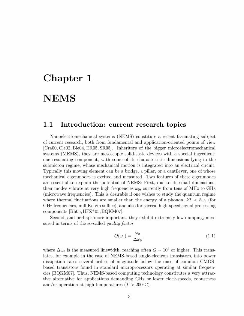
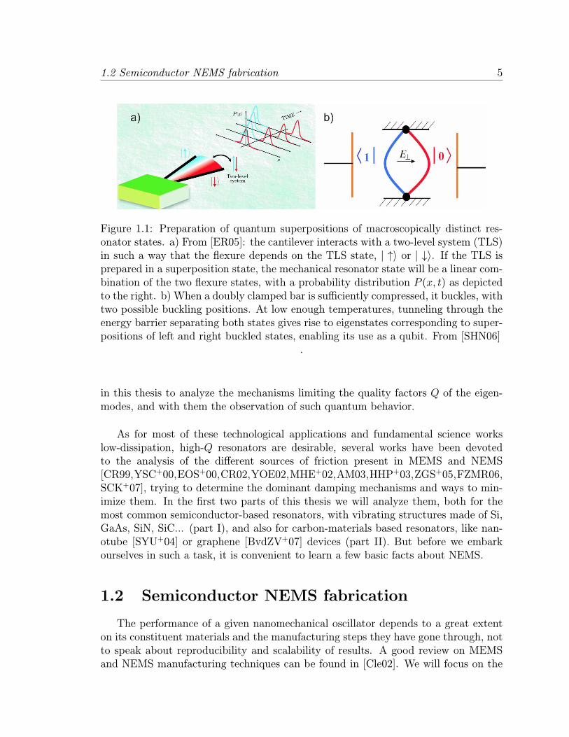
Figure 1.1: Preparation of quantum superpositions of macroscopically distinct res-onator states. a) From [ER05]: the cantilever interacts with a two-level system (TLS)in such a way that the flexure depends on the TLS state, | ↑〉 or | ↓〉. If the TLS isprepared in a superposition state, the mechanical resonator state will be a linear com-bination of the two flexure states, with a probability distribution P (x, t) as depictedto the right. b) When a doubly clamped bar is sufficiently compressed, it buckles, withtwo possible buckling positions. At low enough temperatures, tunneling through theenergy barrier separating both states gives rise to eigenstates corresponding to super-positions of left and right buckled states, enabling its use as a qubit. From [SHN06]
.
in this thesis to analyze the mechanisms limiting the quality factors Q of the eigen-modes, and with them the observation of such quantum behavior.
As for most of these technological applications and fundamental science workslow-dissipation, high-Q resonators are desirable, several works have been devotedto the analysis of the different sources of friction present in MEMS and NEMS[CR99,YSC+00,EOS+00,CR02,YOE02,MHE+02,AM03,HHP+03,ZGS+05,FZMR06,SCK+07], trying to determine the dominant damping mechanisms and ways to min-imize them. In the first two parts of this thesis we will analyze them, both for themost common semiconductor-based resonators, with vibrating structures made of Si,GaAs, SiN, SiC... (part I), and also for carbon-materials based resonators, like nan-otube [SYU+04] or graphene [BvdZV+07] devices (part II). But before we embarkourselves in such a task, it is convenient to learn a few basic facts about NEMS.
1.2 Semiconductor NEMS fabrication
The performance of a given nanomechanical oscillator depends to a great extenton its constituent materials and the manufacturing steps they have gone through, notto speak about reproducibility and scalability of results. A good review on MEMSand NEMS manufacturing techniques can be found in [Cle02]. We will focus on the
6 Chapter 1: NEMS
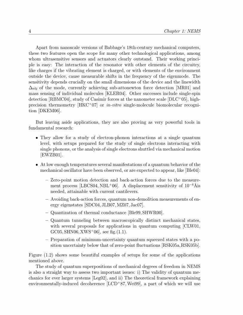
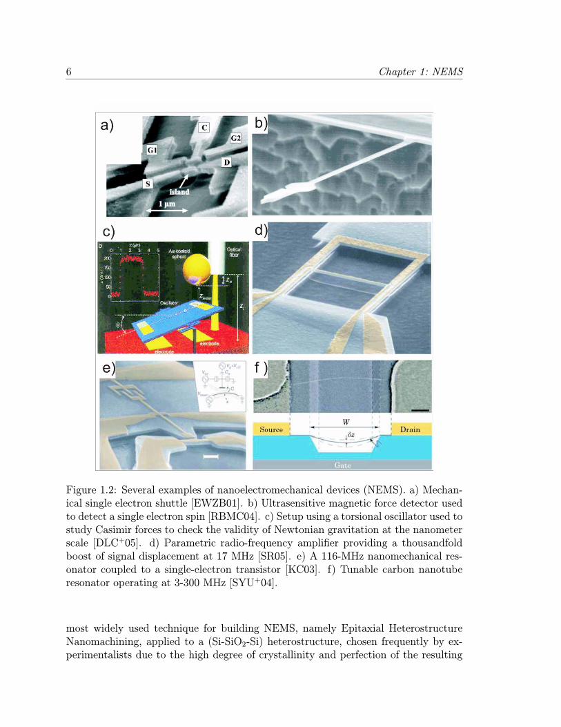
Figure 1.2: Several examples of nanoelectromechanical devices (NEMS). a) Mechan-ical single electron shuttle [EWZB01]. b) Ultrasensitive magnetic force detector usedto detect a single electron spin [RBMC04]. c) Setup using a torsional oscillator used tostudy Casimir forces to check the validity of Newtonian gravitation at the nanometerscale [DLC+05]. d) Parametric radio-frequency amplifier providing a thousandfoldboost of signal displacement at 17 MHz [SR05]. e) A 116-MHz nanomechanical res-onator coupled to a single-electron transistor [KC03]. f) Tunable carbon nanotuberesonator operating at 3-300 MHz [SYU+04].
most widely used technique for building NEMS, namely Epitaxial HeterostructureNanomachining, applied to a (Si-SiO2-Si) heterostructure, chosen frequently by ex-perimentalists due to the high degree of crystallinity and perfection of the resulting
1.3 Motion transduction of mechanical eigenmodes in semiconductor NEMS 7
resonators, and more concretely in a study of dissipation with which we will compareour predictions [ZGS+05,SGC07a,SGC07b,SCK+07].
The starting heterostructure is fabricated by oxygen ion implantation in a crys-talline Si wafer, followed by a high-temperature annealing of several hours, and iscommonly known as SIMOX (Separation by IMplantation of OXigen) wafer. Duringthe second step the previously formed mixed buried layer Si-SiO2 becomes purifiedthrough oxygen migration, constituting a separated SiO2 smooth buried layer, belowa single-crystal recrystallized Si top layer. Typically, this single-crystal top layer, outof which our resonator will be carved, contains a relatively large number of defects,mostly threading dislocations running from the SiO2 layer to this one, with typicaldefect densities of about 103−105/cm2. The top layer presents variations in thickness∼ 10 nm, as does the silicon oxide underneath.To create the suspended structure, the wafer is subject to the nanomachining
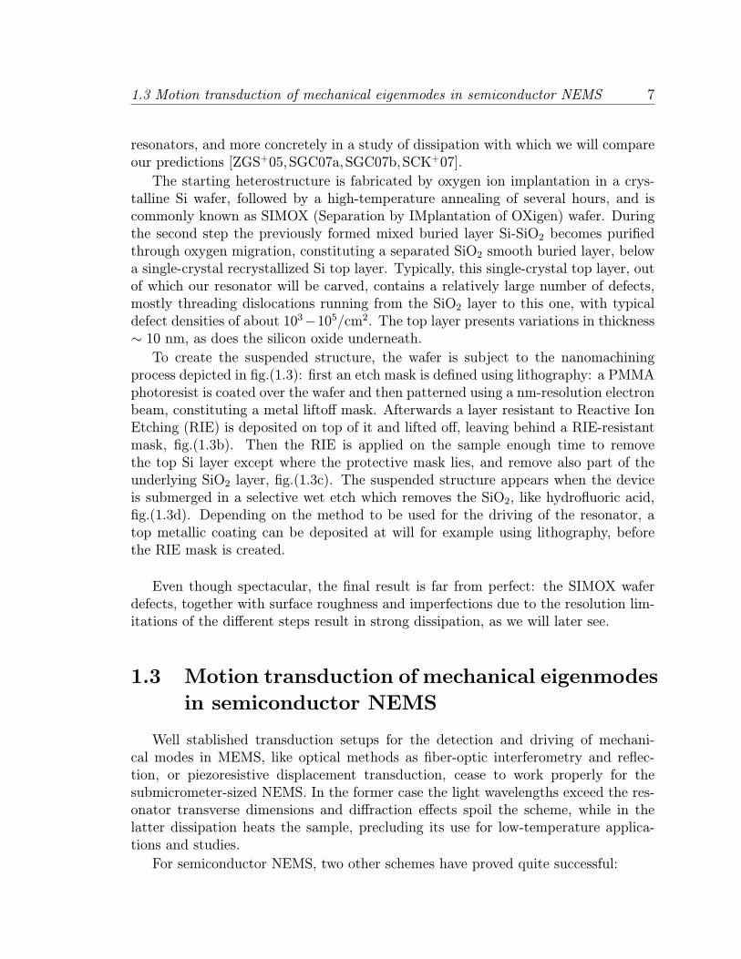
process depicted in fig.(1.3): first an etch mask is defined using lithography: a PMMAphotoresist is coated over the wafer and then patterned using a nm-resolution electronbeam, constituting a metal liftoff mask. Afterwards a layer resistant to Reactive IonEtching (RIE) is deposited on top of it and lifted off, leaving behind a RIE-resistantmask, fig.(1.3b). Then the RIE is applied on the sample enough time to removethe top Si layer except where the protective mask lies, and remove also part of theunderlying SiO2 layer, fig.(1.3c). The suspended structure appears when the deviceis submerged in a selective wet etch which removes the SiO2, like hydrofluoric acid,fig.(1.3d). Depending on the method to be used for the driving of the resonator, atop metallic coating can be deposited at will for example using lithography, beforethe RIE mask is created.
Even though spectacular, the final result is far from perfect: the SIMOX waferdefects, together with surface roughness and imperfections due to the resolution lim-itations of the different steps result in strong dissipation, as we will later see.
1.3 Motion transduction of mechanical eigenmodes
in semiconductor NEMS
Well stablished transduction setups for the detection and driving of mechani-cal modes in MEMS, like optical methods as fiber-optic interferometry and reflec-tion, or piezoresistive displacement transduction, cease to work properly for thesubmicrometer-sized NEMS. In the former case the light wavelengths exceed the res-onator transverse dimensions and diffraction effects spoil the scheme, while in thelatter dissipation heats the sample, precluding its use for low-temperature applica-tions and studies.
For semiconductor NEMS, two other schemes have proved quite successful:
8 Chapter 1: NEMS
Figure 1.3: From [Cle02]. Building a nanoresonator using Epitaxial HeterostructureNanomachining. (a) The process starts with a previously fabricated heterostructure,such as the SIMOX (Separation by IMplantation of OXigen) Si-SiO2-Si shown. (b)Using electron beam lithography a mask is etched. (c) Anisotropic dry etch such asReactive Ion Etching. (d) The oxide layer is removed using a selective SiO2 wet etch,obtaining in this way the suspended structure. Metallization of the top layer can beperformed lithographically before the process.
1.3.1 Magnetomotive scheme
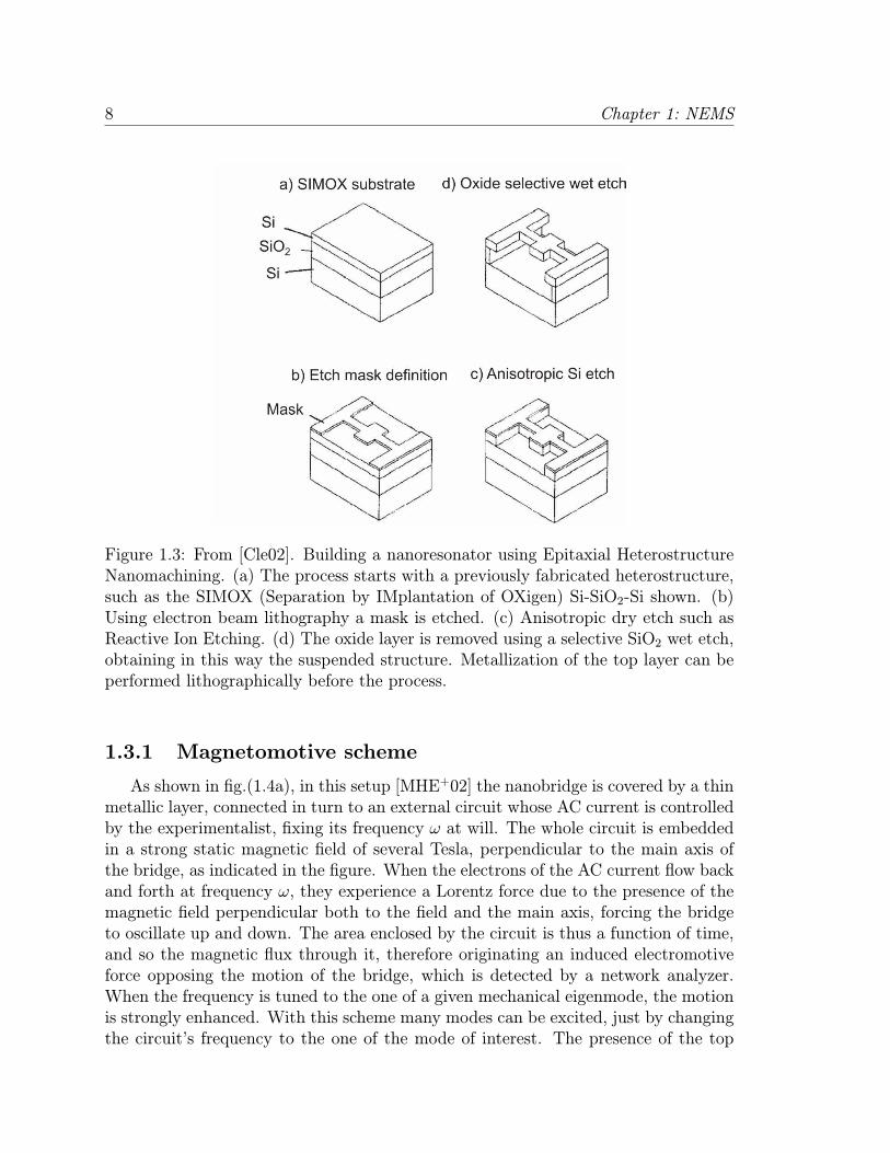
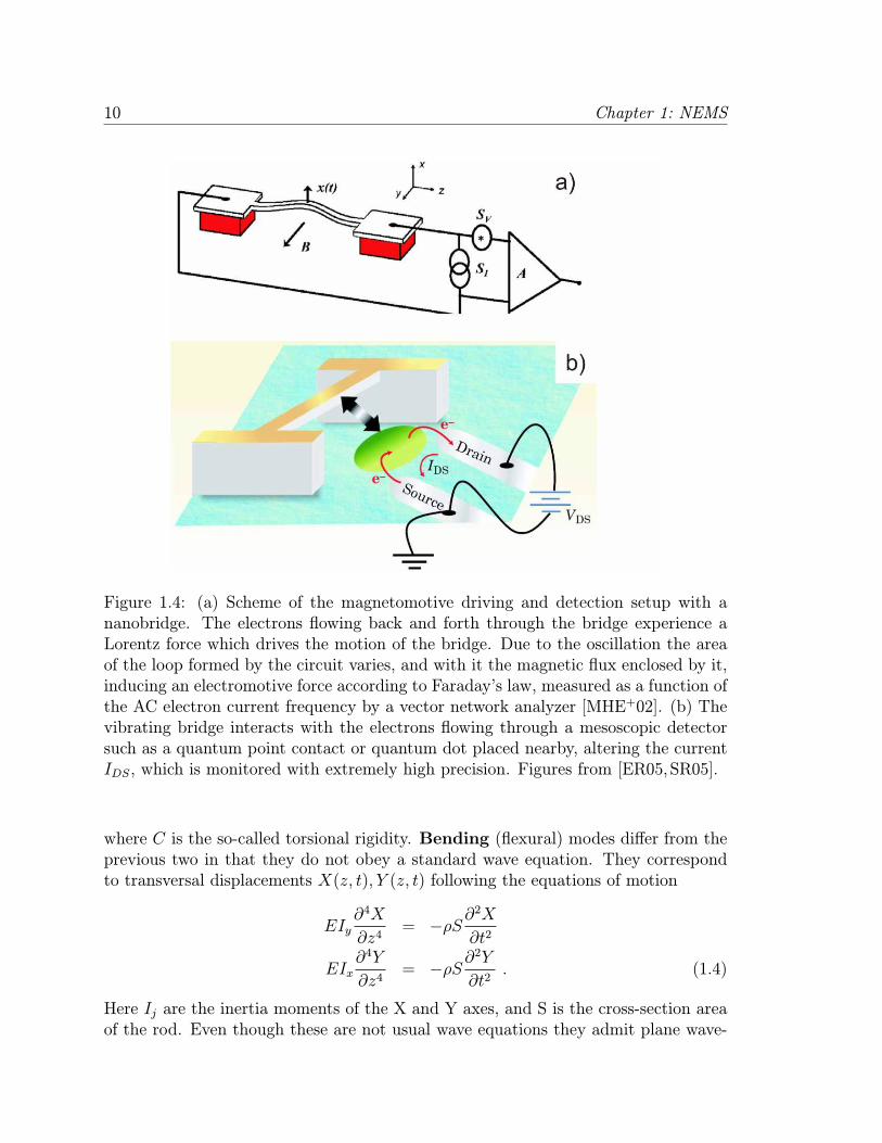
As shown in fig.(1.4a), in this setup [MHE+02] the nanobridge is covered by a thinmetallic layer, connected in turn to an external circuit whose AC current is controlledby the experimentalist, fixing its frequency ω at will. The whole circuit is embeddedin a strong static magnetic field of several Tesla, perpendicular to the main axis ofthe bridge, as indicated in the figure. When the electrons of the AC current flow backand forth at frequency ω, they experience a Lorentz force due to the presence of themagnetic field perpendicular both to the field and the main axis, forcing the bridgeto oscillate up and down. The area enclosed by the circuit is thus a function of time,and so the magnetic flux through it, therefore originating an induced electromotiveforce opposing the motion of the bridge, which is detected by a network analyzer.When the frequency is tuned to the one of a given mechanical eigenmode, the motionis strongly enhanced. With this scheme many modes can be excited, just by changingthe circuit’s frequency to the one of the mode of interest. The presence of the top
1.4 Nanoscale elasticity theory: Vibrational eigenmodes of long and thin rods 9
metallic layer adds extra dissipative sources which will be analyzed later.
1.3.2 Coupling to SETs and other sensitive electronic probes
The magnetomotive driving can be used in combination with more elements closeto the resonator, to study electron-phonon interactions in a previously unexploredregime, with a single-electron single-phonon control. This can be achieved by cou-pling our magnetomotively driven charged resonator to a mesoscopic device whoseconductance can be controlled and measured with great accuracy, like quantum dots,quantum point contacts or single-electron transistors (SETs) [KC03], as schematicallydepicted in fig.(1.4b). Using similar ideas but different geometries, fascinating deviceslike single-electron mechanical shuttles have been demonstrated [EWZB01,SB04].
1.4 Nanoscale elasticity theory: Vibrational eigen-
modes of long and thin rods
Regarding the elastic properties of nanoresonators, it is clear that as size shrinks apoint is reached when classical continuum mechanics ceases to be a good approxima-tion. Nevertheless, for the sizes of current semiconductor nanorods and wavelengthsof the modes excited (∼ 50nm - 10µm), much bigger than typical interatomic spac-ing, continuum approximations continue to hold [SB98,LB99,SB02,SBNI02,LBT+03,Ble04], and classical elasticity theory, using bulk concepts like Young’s modulus Eor Poisson’s coefficient ν, predicts with reasonable accuracy the eigenmodes observedin experiments. In Appendix A.1 a brief review of continuum elasticity concepts andthe derivation of the equations for the different modes present in quasi-1D resonatorsis given. Here we state the main results. For a long and thin rod, considering smalldeviations from equilibrium and wavelengths bigger than the transversal dimensions,three kinds of vibrational modes are found, namely longitudinal, flexural and tor-sional.
Longitudinal (or compressional) modes are as those found in bulk 3D solidsbut occur only along the direction of the main axis, chosen to be the Z axis, withthe Z-component uz of the local displacement field ui = x′i − xi,eq obeying the waveequation
∂2uz
∂z2=
ρ
E
∂2uz
∂t2, (1.2)
ρ being the mass density. Torsional vibrations, like the one of fig.(1.5b), are para-metrized in terms of the twisting angle φ(z), which obeys the wave equation
C∂2φ
∂z2= ρI
∂2φ
∂t2(1.3)
10 Chapter 1: NEMS
Figure 1.4: (a) Scheme of the magnetomotive driving and detection setup with ananobridge. The electrons flowing back and forth through the bridge experience aLorentz force which drives the motion of the bridge. Due to the oscillation the areaof the loop formed by the circuit varies, and with it the magnetic flux enclosed by it,inducing an electromotive force according to Faraday’s law, measured as a function ofthe AC electron current frequency by a vector network analyzer [MHE+02]. (b) Thevibrating bridge interacts with the electrons flowing through a mesoscopic detectorsuch as a quantum point contact or quantum dot placed nearby, altering the currentIDS, which is monitored with extremely high precision. Figures from [ER05,SR05].
where C is the so-called torsional rigidity. Bending (flexural) modes differ from theprevious two in that they do not obey a standard wave equation. They correspondto transversal displacements X(z, t), Y (z, t) following the equations of motion
EIy∂4X
∂z4= −ρS∂
2X
∂t2
EIx∂4Y
∂z4= −ρS∂
2Y
∂t2. (1.4)
Here Ij are the inertia moments of the X and Y axes, and S is the cross-section areaof the rod. Even though these are not usual wave equations they admit plane wave-
1.5 Dissipative mechanisms damping the vibrational eigenmodes of semiconductornanoresonators 11
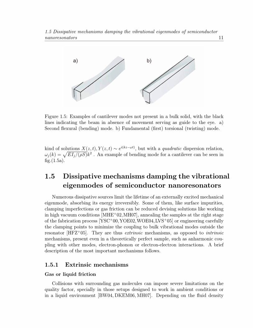
Figure 1.5: Examples of cantilever modes not present in a bulk solid, with the blacklines indicating the beam in absence of movement serving as guide to the eye. a)Second flexural (bending) mode. b) Fundamental (first) torsional (twisting) mode.
kind of solutions X(z, t), Y (z, t) ∼ ei(kz−ωt), but with a quadratic dispersion relation,ωj(k) =
√EIj/(ρS)k
2 . An example of bending mode for a cantilever can be seen infig.(1.5a).
1.5 Dissipative mechanisms damping the vibrational
eigenmodes of semiconductor nanoresonators
Numerous dissipative sources limit the lifetime of an externally excited mechanicaleigenmode, absorbing its energy irreversibly. Some of them, like surface impurities,clamping imperfections or gas friction can be reduced devising solutions like workingin high vacuum conditions [MHE+02,MH07], annealing the samples at the right stageof the fabrication process [YSC+00,YOE02,WOE04,LVS+05] or engineering carefullythe clamping points to minimize the coupling to bulk vibrational modes outside theresonator [HFZ+05]. They are thus extrinsic mechanisms, as opposed to intrinsicmechanisms, present even in a theoretically perfect sample, such as anharmonic cou-pling with other modes, electron-phonon or electron-electron interactions. A briefdescription of the most important mechanisms follows.
1.5.1 Extrinsic mechanisms
Gas or liquid friction
Collisions with surrounding gas molecules can impose severe limitations on thequality factor, specially in those setups designed to work in ambient conditions orin a liquid environment [BW04, DKEM06,MH07]. Depending on the fluid density
12 Chapter 1: NEMS
several regimes appear which have to be analyzed with different frameworks, rangingfrom free molecular to continuum limits. Q increases with decreasing pressure P ,and for P < 1 mTorr it can be safely disregarded as the main frictional force fornanoresonators with Q ≥ 104 [MHE+02,ER05].
Heating linked to the actuation or detection setup
In the magnetomotive scheme the flow of electrons through the metallic top layeris not ballistic, and heating of the layer is generated through their inelastic collisions,which in turn heats the semiconductor substrate underneath. Fortunately for theusual current densities this effect seems to be irrelevant compared to others [MHE+02].In schemes using actuation and detection lasers illuminating the resonator, heatingmay play a more significant role, but we will not study it further in this thesis.
Noise introduced by the external electrical circuit
The external circuitry can be a source of extra damping and frequency shift, dueto its finite impedance. This effect can be used for applications requiring an externalcontrol of linewidth, like signal processing [CR99,Sch02].
Clamping (attachment) losses
This mechanism corresponds to the transfer of energy from the resonator modeto acoustic modes at the contacts and beyond to the substrate through the anchor-age areas [JI68, PJ04]. The motion of the resonator forces as well a motion of theatoms linking it to the rest of the device, irradiating in this way elastic energy to itssurroundings. This mechanism can be of special relevance for short and thick beams,while for long and thin ones it plays a secondary role [HFZ+05,FZMR06].
Surface roughness and imperfections
As mentioned previously, the structures obtained through current methods presenta certain degree of roughness of ∼ 10 nm. On top of this, adsorbed impurities, dis-locations and surface reconstruction processes are all coupled to the local atomicdisplacements linked to the resonator’s motion, absorbing energy from the vibra-tional eigenmode and transmitting it irreversibly to the rest of degrees of freedom ofthe system. These imperfections and impurities also exist in the core of the resonatorstructure, but to a lesser degree as in the case of its surface, exposed to the envi-ronment and with atoms less bound than in the bulk, more susceptible to thermalrearrangements. Strong evidence has been accumulated of the increasing role playedby surfaces as the resonator sizes shrink and surface-to-volume ratios grow, being thedominating friction source in thin nanobeams at low temperatures: i) The qualityfactor Q roughly scales linearly with the former ratio [YSC+00,ER05], as shown in
1.5 Dissipative mechanisms damping the vibrational eigenmodes of semiconductornanoresonators 13
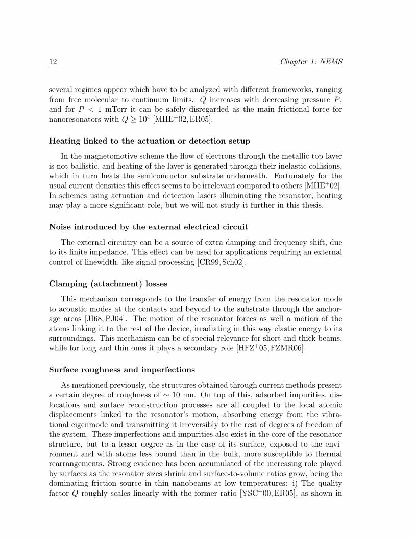
Figure 1.6: From ref. [ER05]. Evolution of reported quality factors in monocrystallinemechanical resonators with size, showing a decrease with linear dimension, i.e., withincreasing surface-to-volume ratio, indicating a dominant role of surface-related losses.
fig.(1.6), ii) Q has been observed to increase up to an order of magnitude when thesystem went through a thermal treatment [YOE00,WOE04, LVS+05] or the surfacewas deoxidized [YOE02]. In the next chapter we will study in depth these surface-related losses, dominant for thin beams at low temperatures, precisely the interestingregime where quantum effects show up if a very high Q is reached. Surface wavescan be also excited by the vibrational eigenmode due to the roughness, but at lowtemperatures this process becomes strongly suppressed [MHE+02], and thus will beignored in our study.
Generation of e-h pairs in the metallic electrode due to electron-phononcoupling
In the magnetomotive scheme, where the semiconductor bridge is covered witha thin metallic top layer, the flowing electrons feel the Coulomb potential generatedby static charges in the device and substrate. When the oscillating part is set intomotion, this potential is time-dependent, and gives the chance to the electrons toabsorb part of the mechanical energy stored in the eigenmode, creating e-h pairs. Wewill study this mechanism in the next chapter.
14 Chapter 1: NEMS
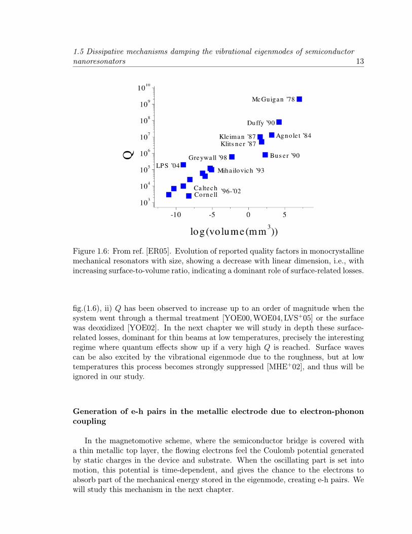
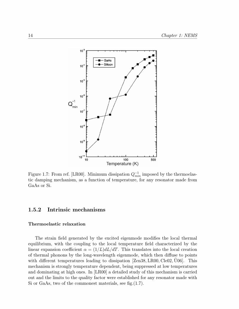
Figure 1.7: From ref. [LR00]. Minimum dissipation Q−1min imposed by the thermoelas-tic damping mechanism, as a function of temperature, for any resonator made fromGaAs or Si.
1.5.2 Intrinsic mechanisms
Thermoelastic relaxation
The strain field generated by the excited eigenmode modifies the local thermalequilibrium, with the coupling to the local temperature field characterized by thelinear expansion coefficient α = (1/L)dL/dT . This translates into the local creationof thermal phonons by the long-wavelength eigenmode, which then diffuse to pointswith different temperatures leading to dissipation [Zen38, LR00, Cle02, U06]. Thismechanism is strongly temperature dependent, being suppressed at low temperaturesand dominating at high ones. In [LR00] a detailed study of this mechanism is carriedout and the limits to the quality factor were established for any resonator made withSi or GaAs, two of the commonest materials, see fig.(1.7).
1.5 Dissipative mechanisms damping the vibrational eigenmodes of semiconductornanoresonators 15
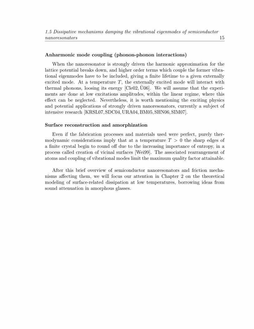
Anharmonic mode coupling (phonon-phonon interactions)
When the nanoresonator is strongly driven the harmonic approximation for thelattice potential breaks down, and higher order terms which couple the former vibra-tional eigenmodes have to be included, giving a finite lifetime to a given externallyexcited mode. At a temperature T , the externally excited mode will interact withthermal phonons, loosing its energy [Cle02, U06]. We will assume that the experi-ments are done at low excitations amplitudes, within the linear regime, where thiseffect can be neglected. Nevertheless, it is worth mentioning the exciting physicsand potential applications of strongly driven nanoresonators, currently a subject ofintensive research [KRSL07,SDC04,URA04,BM05,SHN06,SIM07].
Surface reconstruction and amorphization
Even if the fabrication processes and materials used were perfect, purely ther-modynamic considerations imply that at a temperature T > 0 the sharp edges ofa finite crystal begin to round off due to the increasing importance of entropy, in aprocess called creation of vicinal surfaces [Wei99]. The associated rearrangement ofatoms and coupling of vibrational modes limit the maximum quality factor attainable.
After this brief overview of semiconductor nanoresonators and friction mecha-nisms affecting them, we will focus our attention in Chapter 2 on the theoreticalmodeling of surface-related dissipation at low temperatures, borrowing ideas fromsound attenuation in amorphous glasses.

16 Chapter 1: NEMS
Chapter 2
Surface dissipation insemiconductor NEMS at lowtemperatures
2.1 Introduction
In this chapter we will try to provide a unified theoretical framework to describethe processes taking place at the surface of nanoresonators at low temperatures,which have been observed to dominate dissipation of their vibrational eigenmodes inthis regime, see fig.(2.1). This is certainly a challenging task, since as we have seenmany different dynamical processes and actors come into play (excitation of adsorbedmolecules, movement of lattice defects or configurational rearrangements), some ofwhom are not yet well characterized, so simplifications need to be made. We willprovide such a scheme, based on the following considerations:
• Experimental observations indicate that surfaces of otherwise monocrystallineresonators acquire a certain degree of roughness, impurities and disorder, re-sembling an amorphous structure [LTBP99,Wei99].
• In amorphous solids the damping of acoustic waves at low temperatures is suc-cessfully explained by the Standard Tunneling Model [AHV72, Phi72, Phi87,Esq98], which couples the acoustic phonons to a set of Two-Level Systems(TLSs) representing the low-energy spectrum of all the degrees of freedom ableto exchange energy with the strain field associated to the vibration.
We will describe the attenuation of vibrations in nanoresonators due to theiramorphous-like surfaces in terms of an adequate adaptation of the Standard Tunnel-ing Model. We start reviewing such model, and some concepts and techniques used toanalyze the spin-boson hamiltonian appearing in it. Then we proceed to apply in theproper way the Standard Tunneling Model to the non-bulk nanoresonator geometry.
17
18 Chapter 2: Surface dissipation in semiconductor NEMS at low temperatures
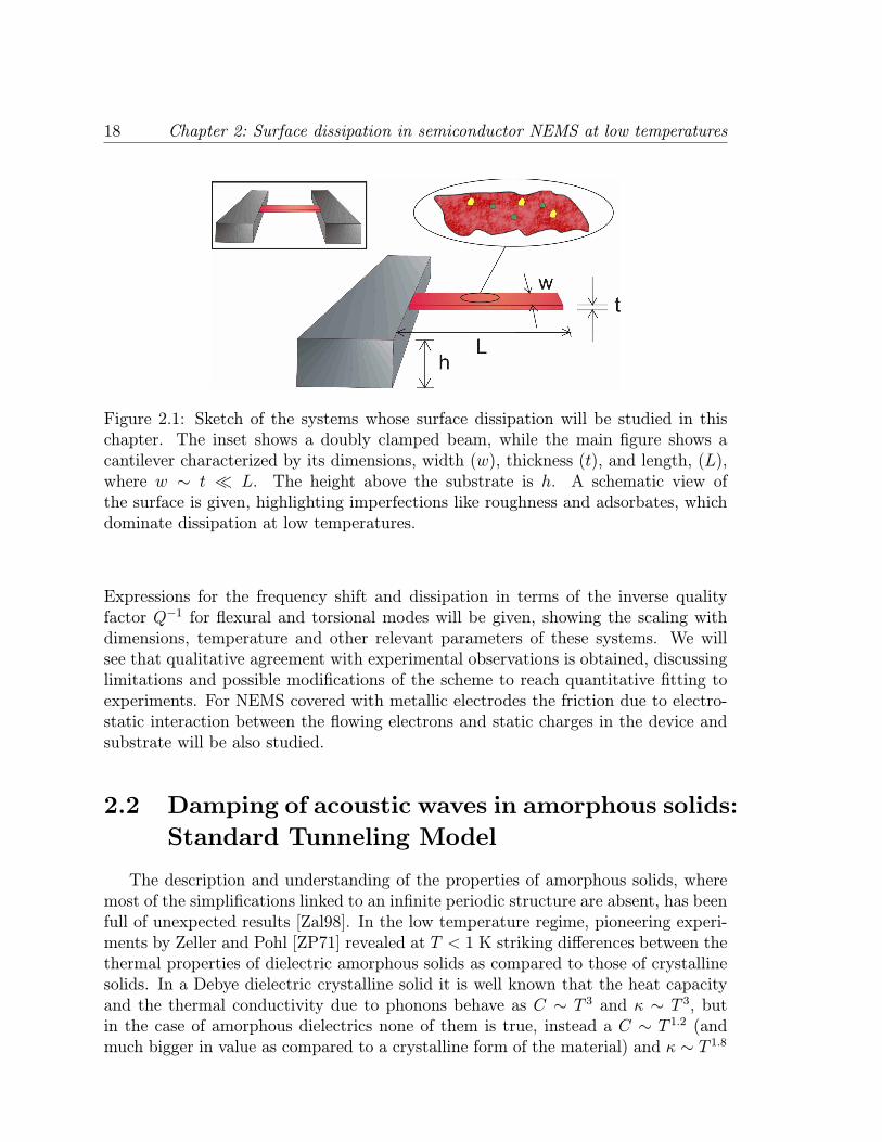
Figure 2.1: Sketch of the systems whose surface dissipation will be studied in thischapter. The inset shows a doubly clamped beam, while the main figure shows acantilever characterized by its dimensions, width (w), thickness (t), and length, (L),where w ∼ t L. The height above the substrate is h. A schematic view ofthe surface is given, highlighting imperfections like roughness and adsorbates, whichdominate dissipation at low temperatures.
Expressions for the frequency shift and dissipation in terms of the inverse qualityfactor Q−1 for flexural and torsional modes will be given, showing the scaling withdimensions, temperature and other relevant parameters of these systems. We willsee that qualitative agreement with experimental observations is obtained, discussinglimitations and possible modifications of the scheme to reach quantitative fitting toexperiments. For NEMS covered with metallic electrodes the friction due to electro-static interaction between the flowing electrons and static charges in the device andsubstrate will be also studied.
2.2 Damping of acoustic waves in amorphous solids:
Standard Tunneling Model
The description and understanding of the properties of amorphous solids, wheremost of the simplifications linked to an infinite periodic structure are absent, has beenfull of unexpected results [Zal98]. In the low temperature regime, pioneering experi-ments by Zeller and Pohl [ZP71] revealed at T < 1 K striking differences between thethermal properties of dielectric amorphous solids as compared to those of crystallinesolids. In a Debye dielectric crystalline solid it is well known that the heat capacityand the thermal conductivity due to phonons behave as C ∼ T 3 and κ ∼ T 3, butin the case of amorphous dielectrics none of them is true, instead a C ∼ T 1.2 (andmuch bigger in value as compared to a crystalline form of the material) and κ ∼ T 1.8
2.2 Damping of acoustic waves in amorphous solids: Standard Tunneling Model 19
behavior is observed. Apart from this, a heat release as a function of time is ob-served on long time scales: after a sample is heated and then rapidly cooled downto some temperature T0, in adiabatic conditions the sample begins gradually to heatitself afterwards. Moreover, measuring their acoustic properties at low temperatures,which a priori were expected to be similar to those found in crystalline solids dueto the long-wavelength vibrations involved, the following dependence on the acousticintensity was obtained [HAS+72]: at low intensities, as the temperature is loweredthe mean free path of the phonon decreases, while at high intensities a monotonousincrease is observed.
Several theoretical scenarios were developed to explain these low-temperature fea-tures, the most successful of whom was the so-called Standard Tunneling Model,proposed simultaneously by Phillips and Anderson et al. [AHV72,Phi72].The tunneling model claims the existence of the following states, intrinsic to
glasses: an impurity, an atom or cluster of atoms within the disordered structurewhich present in their configurational space two energy minima separated by an en-ergy barrier (similarly to the dextro/levo configurations of the ammonia molecule),as depicted schematically in fig.(2.2a). These states can be modeled as a degree offreedom tunneling between two potential wells. At low temperatures only the twolowest eigenstates have to be considered, characterized by the bias ∆z0 between thewells and the tunneling rate ∆x0 through the barrier, see fig.(2.2b). This correspondsto the Two-Level System (TLS) hamiltonian:
H0 = ∆x0σx +∆
z0σz , (2.1)
where σi are Pauli matrices. Due to the disorder of the structure, a broad range ofvalues for the TLSs parameters ∆z0 and ∆
x0 is expected to appear for the ensemble of
TLSs present in the amorphous solid. In order to be operative, the Standard Tun-neling Model has to specify the properties of this ensemble in terms of a probabilitydistribution P (∆x0 ,∆
z0). The form of P (∆
x0 ,∆
z0) can be inferred from general consider-
ations [AHV72,Phi72], as detailed in Appendices B.1.1 and B.1.2, and is furthermoresupported by experiments [Esq98]. The result is
P (∆x0 ,∆z0) =
P0
∆x0, (2.2)
with P0 ∼ 1044J−1m−3, ∆x0 > ∆min (∆min fixed by the time needed to obtaina spectrum around the resonance frequency of the excited eigenmode), and ε =√(∆x0)
2 + (∆z0)2 < εmax, estimated to be of the order of 5 K.
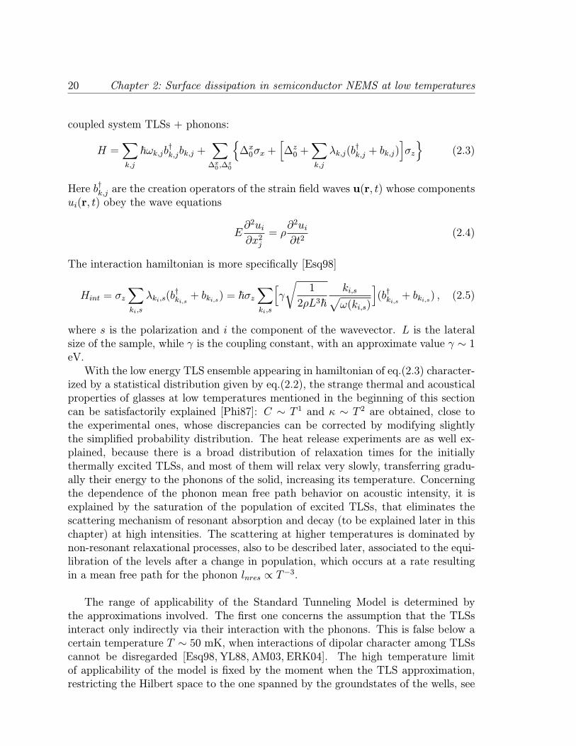
A last feature necessary to calculate the damping of acoustic waves caused bythese low energy excitations is the coupling TLSs - phonons. As justified in AppendixB.1.3, the lattice distortions caused by the propagation of the wave affect mainly theTLSs asymmetry ∆z0, with the following final form for the hamiltonian describing the
20 Chapter 2: Surface dissipation in semiconductor NEMS at low temperatures
coupled system TLSs + phonons:
H =∑
k,j
~ωk,jb†k,jbk,j +∑
∆x0 ,∆z0
∆x0σx +
[∆z0 +
∑
k,j
λk,j(b†k,j + bk,j)
]σz
(2.3)
Here b†k,j are the creation operators of the strain field waves u(r, t) whose componentsui(r, t) obey the wave equations
E∂2ui
∂x2j= ρ
∂2ui
∂t2(2.4)
The interaction hamiltonian is more specifically [Esq98]
Hint = σz∑
ki,s
λki,s(b†ki,s+ bki,s) = ~σz
∑
ki,s
[γ
√1
2ρL3~ki,s√ω(ki,s)
](b†ki,s + bki,s) , (2.5)
where s is the polarization and i the component of the wavevector. L is the lateralsize of the sample, while γ is the coupling constant, with an approximate value γ ∼ 1eV.With the low energy TLS ensemble appearing in hamiltonian of eq.(2.3) character-
ized by a statistical distribution given by eq.(2.2), the strange thermal and acousticalproperties of glasses at low temperatures mentioned in the beginning of this sectioncan be satisfactorily explained [Phi87]: C ∼ T 1 and κ ∼ T 2 are obtained, close tothe experimental ones, whose discrepancies can be corrected by modifying slightlythe simplified probability distribution. The heat release experiments are as well ex-plained, because there is a broad distribution of relaxation times for the initiallythermally excited TLSs, and most of them will relax very slowly, transferring gradu-ally their energy to the phonons of the solid, increasing its temperature. Concerningthe dependence of the phonon mean free path behavior on acoustic intensity, it isexplained by the saturation of the population of excited TLSs, that eliminates thescattering mechanism of resonant absorption and decay (to be explained later in thischapter) at high intensities. The scattering at higher temperatures is dominated bynon-resonant relaxational processes, also to be described later, associated to the equi-libration of the levels after a change in population, which occurs at a rate resultingin a mean free path for the phonon lnres ∝ T−3.
The range of applicability of the Standard Tunneling Model is determined bythe approximations involved. The first one concerns the assumption that the TLSsinteract only indirectly via their interaction with the phonons. This is false below acertain temperature T ∼ 50 mK, when interactions of dipolar character among TLSscannot be disregarded [Esq98, YL88, AM03, ERK04]. The high temperature limitof applicability of the model is fixed by the moment when the TLS approximation,restricting the Hilbert space to the one spanned by the groundstates of the wells, see
2.3 Theoretical analysis of the damping of phonons due to TLSs 21
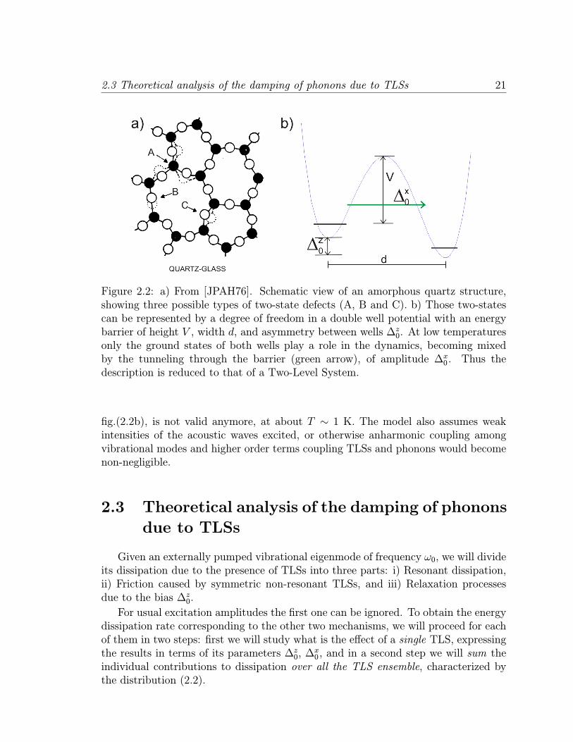
Figure 2.2: a) From [JPAH76]. Schematic view of an amorphous quartz structure,showing three possible types of two-state defects (A, B and C). b) Those two-statescan be represented by a degree of freedom in a double well potential with an energybarrier of height V , width d, and asymmetry between wells ∆z0. At low temperaturesonly the ground states of both wells play a role in the dynamics, becoming mixedby the tunneling through the barrier (green arrow), of amplitude ∆x0 . Thus thedescription is reduced to that of a Two-Level System.
fig.(2.2b), is not valid anymore, at about T ∼ 1 K. The model also assumes weakintensities of the acoustic waves excited, or otherwise anharmonic coupling amongvibrational modes and higher order terms coupling TLSs and phonons would becomenon-negligible.
2.3 Theoretical analysis of the damping of phonons
due to TLSs
Given an externally pumped vibrational eigenmode of frequency ω0, we will divideits dissipation due to the presence of TLSs into three parts: i) Resonant dissipation,ii) Friction caused by symmetric non-resonant TLSs, and iii) Relaxation processesdue to the bias ∆z0.
For usual excitation amplitudes the first one can be ignored. To obtain the energydissipation rate corresponding to the other two mechanisms, we will proceed for eachof them in two steps: first we will study what is the effect of a single TLS, expressingthe results in terms of its parameters ∆z0, ∆
x0 , and in a second step we will sum the
individual contributions to dissipation over all the TLS ensemble, characterized bythe distribution (2.2).
22 Chapter 2: Surface dissipation in semiconductor NEMS at low temperatures
2.3.1 Resonant dissipation
Those TLSs with their unperturbed excitation energies close to ω0 will resonatewith the mode, exchanging energy quanta, with a rate proportional to the mode’sphonon population nω0 to first order. For usual excitation amplitudes ∼ 0.1− 1A thevibrational mode is so populated (as compared with the thermal population) that theresonant TLSs become saturated, and their contribution to the transverse (flexural)
wave attenuation becomes negligible, proportional to n−1/2ω0 [AHSD74].
2.3.2 Dissipation of symmetric non-resonant TLSs
Dissipation caused by a single TLS
We will analyze here the dynamical behavior of one TLS coupled to the phononensemble:
H = ∆x0σx +∆z0σz +
∑
k,j
λk,j σz(b†k,j + bk,j) +
∑
k,j
~ωk,jb†k,jbk,j (2.6)
This hamiltonian is nothing but the well-known spin-boson model, which applies toa great variety of physical phenomena related to open dissipative systems, and hasbeen subject of intensive theoretical work [LCD+87,Wei99]. We will use some ofthis knowledge to describe the dynamics of the single TLS in terms of the spectralfunction
A(ω) ≡∑
n
|〈0 |σz|n〉|2 δ(ω − ωn + ω0) (2.7)
where |n〉 is an excited state of the total system TLS plus vibrations. We will seehow this function describes the absorption properties of a symmetric TLS coupled toa vibrational ensemble through the operator σz.The analysis of the spin-boson model for a TLS with asymmetry ∆z0 6= 0 is much
more cumbersome than the symmetric TLS case, if one tries to use the kind of tech-niques described in [LCD+87] that work for the symmetric case. Thus, to learn aboutthe effect of the asymmetry ∆z0 in the absorption spectrum of the TLS we will makea different kind of analysis, studying the delayed response of a TLS due to its bias∆z0, and finally see its signatures in the absorption spectrum. A natural division ofdissipative mechanisms will arrive as a consequence of this analysis: one contribution,the relaxation mechanism, will correspond to the presence of the bias, while the otherwill describe the dissipation occurring independently of the presence or absence ofbias.
The techniques we will use for the analysis of the symmetric case are all de-scribed in [LCD+87], mainly i) Simple renormalization-group arguments to obtaineffective or ”dressed” values ∆xeff , ∆
zeff of the TLS parameters from ∆
x0 , ∆
z0 due to
2.3 Theoretical analysis of the damping of phonons due to TLSs 23
the interaction with high energy vibrational modes, ii) Characterization of the in-teraction with the different kinds of vibrational modes based on the criteria derivedin the non-interacting blip approximation (NIBA, see Appendix B.2 for a brief re-view on the basic concepts and results), iii) Second-order perturbation theory in theinteraction term of (2.6). These techniques are adequate for the regime where theStandard Tunneling Model holds, described just before the beginning of this section,and work better for very low vibration amplitudes of the externally excited vibra-tional mode. Even within the linear regime of the mode, above a certain amplitudeother approaches designed to study strongly driven TLSs become more suited todescribe the dynamics of at least part of the ensemble of TLSs, namely numericalmethods as Quantum Monte Carlo [EW92, LWW98] or Numerical RenormalizationGroup [BTV03, BLTV05, ABV07,Wv07], or theoretical studies of the driven spin-boson model [GSSW93,GH98]. We will assume that the TLSs in resonance with theexternally excited mode are saturated and thus do not contribute significantly to itsdissipation, while for the rest of TLSs the vibration is assumed to be sufficiently weakfor the techniques i), ii) and iii) to hold.
Spin-boson model for an almost symmetric TLS interacting with the nanores-onator modes
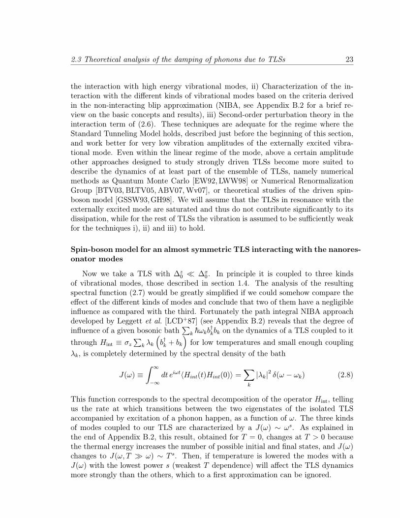
Now we take a TLS with ∆z0 ∆x0 . In principle it is coupled to three kindsof vibrational modes, those described in section 1.4. The analysis of the resultingspectral function (2.7) would be greatly simplified if we could somehow compare theeffect of the different kinds of modes and conclude that two of them have a negligibleinfluence as compared with the third. Fortunately the path integral NIBA approachdeveloped by Leggett et al. [LCD+87] (see Appendix B.2) reveals that the degree ofinfluence of a given bosonic bath
∑k ~ωkb
†kbk on the dynamics of a TLS coupled to it
through Hint ≡ σz∑k λk
(b†k + bk
)for low temperatures and small enough coupling
λk, is completely determined by the spectral density of the bath
J(ω) ≡∫ ∞
−∞dt eiωt〈Hint(t)Hint(0)〉 =
∑
k
|λk|2 δ(ω − ωk) (2.8)
This function corresponds to the spectral decomposition of the operator Hint, tellingus the rate at which transitions between the two eigenstates of the isolated TLSaccompanied by excitation of a phonon happen, as a function of ω. The three kindsof modes coupled to our TLS are characterized by a J(ω) ∼ ωs. As explained inthe end of Appendix B.2, this result, obtained for T = 0, changes at T > 0 becausethe thermal energy increases the number of possible initial and final states, and J(ω)changes to J(ω, T ω) ∼ T s. Then, if temperature is lowered the modes with aJ(ω) with the lowest power s (weakest T dependence) will affect the TLS dynamicsmore strongly than the others, which to a first approximation can be ignored.
24 Chapter 2: Surface dissipation in semiconductor NEMS at low temperatures
Focussing on the case of a TLS coupled to the vibrations present in a rod, thestarting hamiltonian is
H = ∆x0σx +∆z0σz + σzF(∂iuj) +Helastic (2.9)
where ∂iuj is a component of the deformation gradient matrix, F is an arbitrary func-tion, and Helastic represents the elastic energy stored due to the atomic displacements,which will correspond in second quantization to the last term in eq.(2.6). Changingbasis to the energy eigenstates of the TLS, eq.(2.9) becomes H = εσz + [(∆
x0/ε)σx +
(∆z0/ε)σz]F(∂iuj) + Helastic. We are considering for the moment only slightly biasedTLSs for whom ∆z0 ∆0, so the last term can be ignored. A further expansion of Fto lowest order in the displacement, together with a π/4 rotation of the eigenbasis,leads to:
H = εσx + γ(∆x0/ε)σz∂iuj +Helastic , (2.10)
where γ is the coupling constant, assumed to be as in amorphous 3D solids γ ∼ 1 eV.The atomic displacements can be decomposed into the normal vibrational modes,
which for the cuasi-1D case of nanorods are the ones obeying eqs.(1.2-1.4). Thevibrational modes of a beam with fixed ends have a discrete spectrum, but we willapproximate them by a continuous distribution. This approximation will hold as longas many vibrational modes become thermally populated, kT ~ωfund, where ωfundis the frequency of the lowest mode. The condition is fulfilled in current experimentalsetups. The derivation of the second quantized version of the sort of eq.(2.6) foreach of the modes and the corresponding spectral functions J(ω) are described inAppendix B.2.1. Here we state the main results:The compression and twisting modes lead to an ohmic spectral function for ω
2πc/R (R being a typical transversal dimension of the rod and c the sound velocity),when the rod is effectively 1D. In terms of the Young modulus of the material, E,and the mass density, ρ, we get: Jcomp(ω) = αc|ω|, where,
αc = γ2(2π2ρtw)−1(E/ρ)−3/2 . (2.11)
A factor (∆x0/ε)2 has been thrown away, as we consider almost symmetric TLS with
∆x0 ∼ ε. We will proceed similarly with the other modes. The twisting modesare defined by the torsional rigidity, C = µt3w/3 (µ is a Lande coefficient), andI =
∫dSx2 = t3w/12 (where S is the cross-section). The corresponding spectral
function is given by: Jtorsion(ω) = αt|ω|, where
αt = γ2C(8π2µtwρI)−1(ρI/C)3/2 . (2.12)
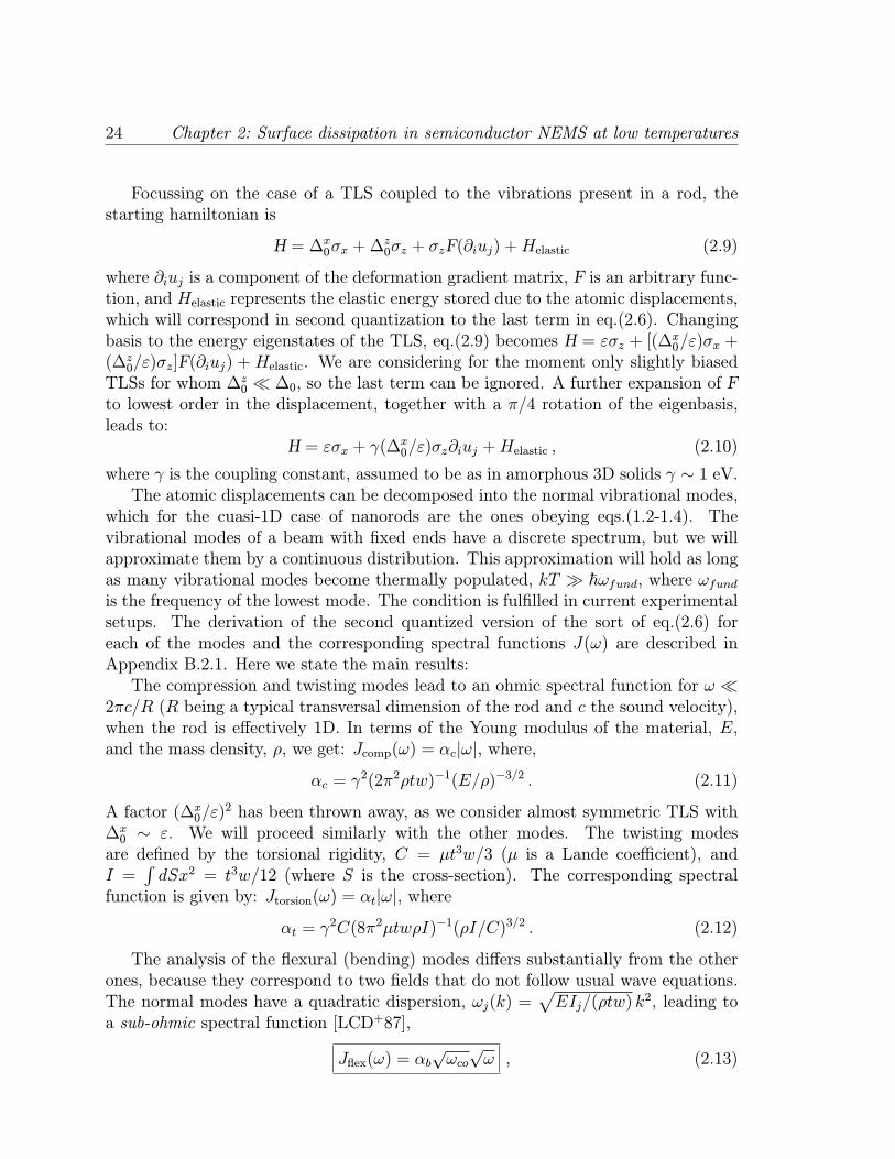
The analysis of the flexural (bending) modes differs substantially from the otherones, because they correspond to two fields that do not follow usual wave equations.The normal modes have a quadratic dispersion, ωj(k) =
√EIj/(ρtw) k
2, leading toa sub-ohmic spectral function [LCD+87],
Jflex(ω) = αb√ωco√ω , (2.13)
2.3 Theoretical analysis of the damping of phonons due to TLSs 25
Figure 2.3: Sketch of the contributions to the spectral function which determines thedynamics of the TLS.
with,
αb√ωco = 0.3
γ2
t3/2w
(1 + ν)(1− 2ν)E(3− 5ν)
( ρE
)1/4, (2.14)
where ν is Poisson’s ratio and ωco '√EIy/(ρtw)(2π/t)
2 is the high energy cut-off of the bending modes (frequency for whom the corresponding wavelength is ofthe order of t, thus indicating the onset of 3D behavior). This example of sub-ohmic spin-boson model is the first result of this thesis to be stressed, because theproblem of a TLS interacting with a sub-ohmic environment is interesting in its ownright [LCD+87, KM96,Wei99, Sta03, VTB05, GW88, SG06, CT06, Khv04, IN92], andthe systems studied here provide a physical realization.The bending modes prevail over the other, ohmic-like, modes as a dissipative
channel at low energies. One may ask at what frequency do the torsional and com-pression modes begin to play a significant role, and a rough way to estimate it is tosee at what frequency do the corresponding spectral functions have the same value,Jflex(ω∗) = Jcomp,tors(ω∗). The results are ω∗ ∼ 30(1+ν)2(1−2ν)2(E/ρ)1/2/[t(3−5ν)2]for the case of compression modes and ω∗ ∼ 300(1− 2ν)2(E/ρ)1/2/[t(3− 5ν)2(1+ ν)]for the torsional. Comparing these frequencies to the one of the onset of 3D behavior,ωco, they are similar, justifying a simplified model where only flexural modes are con-sidered. Collecting the previous results, we find the spectral function J(ω) plotted inFig.[2.3].
TLS’s dynamics
The interaction between the bending modes and the TLSs affects both of them.When a single mode is externally excited, as is done in experiments, the coupling
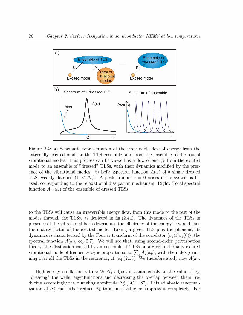
26 Chapter 2: Surface dissipation in semiconductor NEMS at low temperatures
Figure 2.4: a) Schematic representation of the irreversible flow of energy from theexternally excited mode to the TLS ensemble, and from the ensemble to the rest ofvibrational modes. This process can be viewed as a flow of energy from the excitedmode to an ensemble of ”dressed” TLSs, with their dynamics modified by the pres-ence of the vibrational modes. b) Left: Spectral function A(ω) of a single dressedTLS, weakly damped (Γ < ∆x0). A peak around ω = 0 arises if the system is bi-ased, corresponding to the relaxational dissipation mechanism. Right: Total spectralfunction Atot(ω) of the ensemble of dressed TLSs.
to the TLSs will cause an irreversible energy flow, from this mode to the rest of themodes through the TLSs, as depicted in fig.(2.4a). The dynamics of the TLSs inpresence of the vibrational bath determines the efficiency of the energy flow and thusthe quality factor of the excited mode. Taking a given TLS plus the phonons, itsdynamics is characterized by the Fourier transform of the correlator 〈σz(t)σz(0)〉, thespectral function A(ω), eq.(2.7). We will see that, using second-order perturbationtheory, the dissipation caused by an ensemble of TLSs on a given externally excitedvibrational mode of frequency ω0 is proportional to
∑j Aj(ω0), with the index j run-
ning over all the TLSs in the resonator, cf. eq.(2.18). We therefore study now A(ω).
High-energy oscillators with ω ∆x0 adjust instantaneously to the value of σz,”dressing” the wells’ eigenfunctions and decreasing the overlap between them, re-ducing accordingly the tunneling amplitude ∆x0 [LCD
+87]. This adiabatic renormal-ization of ∆x0 can either reduce ∆
x0 to a finite value or suppress it completely. For
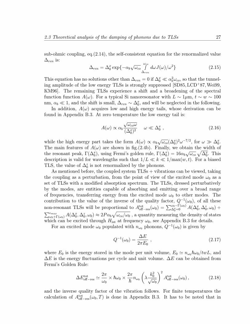
2.3 Theoretical analysis of the damping of phonons due to TLSs 27
sub-ohmic coupling, eq.(2.14), the self-consistent equation for the renormalized value∆ren is:
∆ren = ∆x0 exp−αb
√ωco
ωco
∫∆ren
dωJ(ω)/ω2 (2.15)
This equation has no solutions other than ∆ren = 0 if ∆x0 α2bωco, so that the tunnel-
ing amplitude of the low energy TLSs is strongly suppressed [SD85,LCD+87,Wei99,KM96]. The remaining TLSs experience a shift and a broadening of the spectralfunction function A(ω). For a typical Si nanoresonator with L ∼ 1µm, t ∼ w ∼ 100nm, αb 1, and the shift is small, ∆ren ∼ ∆x0 , and will be neglected in the following.In addition, A(ω) acquires low and high energy tails, whose derivation can be
found in Appendix B.3. At zero temperature the low energy tail is:
A(ω) ∝ αb
√ωcoω
(∆x0)2
ω ∆x0 , (2.16)
while the high energy part takes the form A(ω) ∝ αb√ωco(∆
x0)2ω−7/2, for ω ∆x0 .
The main features of A(ω) are shown in fig.(2.4b). Finally, we obtain the width ofthe resonant peak, Γ(∆x0), using Fermi’s golden rule, Γ(∆
x0) = 16αb
√ωco√∆x0 . This
description is valid for wavelengths such that 1/L k 1/max(w, t). For a biasedTLS, the value of ∆z0 is not renormalized by the phonons.As mentioned before, the coupled system TLSs + vibrations can be viewed, taking
the coupling as a perturbation, from the point of view of the excited mode ω0 as aset of TLSs with a modified absorption spectrum. The TLSs, dressed perturbativelyby the modes, are entities capable of absorbing and emitting over a broad rangeof frequencies, transferring energy from the excited mode ω0 to other modes. Thecontribution to the value of the inverse of the quality factor, Q−1(ω0), of all these
non-resonant TLSs will be proportional to Atotoff−res(ω0) =∑ω0−Γ(ω0)∆x0=0
A(∆x0 ,∆z0, ω0) +∑εmax
ω0+Γ(ω0)A(∆x0 ,∆
z0, ω0) ≈ 2Pαb
√ωco/ω0 , a quantity measuring the density of states
which can be excited through Hint at frequency ω0, see Appendix B.3 for details.For an excited mode ω0 populated with nω0 phonons, Q
−1(ω0) is given by
Q−1(ω0) =∆E
2πE0, (2.17)
where E0 is the energy stored in the mode per unit volume, E0 ' nω0~ω0/twL, and∆E is the energy fluctuations per cycle and unit volume. ∆E can be obtained fromFermi’s Golden Rule:
∆Etotoff−res '2π
ω0× ~ω0 ×
2π
~nω0
(λk20√ω0
)2Atotoff−res(ω0) , (2.18)
and the inverse quality factor of the vibration follows. For finite temperatures thecalculation of Atotoff−res(ω0, T ) is done in Appendix B.3. It has to be noted that in
28 Chapter 2: Surface dissipation in semiconductor NEMS at low temperatures
experiments the observed linewidth is due to the total amount of fluctuations, so at afinite temperature it corresponds to the addition of emission and absorption processes.Thus in this context dissipation means fluctuations, and not net loss of energy. Thecombined contribution of these processes is
(Q−1)totoff−res(ω0, T ) ' 10P0t3/2w(E
ρ
)1/4α2bωco
ω0coth[ ~ω0kBT
](2.19)
Before we continue with the third dissipative mechanism due to TLSs, a couple ofwords about the importance of multi-phonon processes is in order: Until now preva-lence of one-phonon processes in the interaction among TLSs and vibrational modeshas been assumed, but at temperatures much higher than the frequencies of therelevant phonons, multi-phonon processes should be taken into account. A usefulindicator to estimate if one-phonon processes suffice to describe the interaction be-tween the TLS and the bath is the Fermi’s Golden Rule result for the linewidth: ifthe linewidth Γ(∆x0 , T ) calculated in this way is much smaller than ∆
x0 , the approx-
imation can be taken as good, while for Γ(∆x0 , T ) ≥ ∆x0 multiphonon processes haveto be considered. The expression for the linewidth at a finite temperature is
Γ(ε, T ) = 16αb√ωco√ε coth
[ ε
2kBT
](2.20)
One can estimate, using the probability distribution (2.2), the total number of over-damped TLSs, Γ(ε, T ) ≥ ∆x0 , in the volume fraction of the resonator presenting amor-phous features, Vamorph. With Vamorph ∼ Vtot/10, and using Γ(ε, T ) ≈ 2TΓ(ε, T =0)/ε, the number of overdamped TLSs, ε ≤ Γ(ε, T ) → ε ≤ [30αb
√ωcoT ]
2/3, isN ≈ P0twL[30αb
√ωcoT ]
2/3, which for typical resonator sizes L ∼ 1µm, t, w ∼ 0.1µmis less than one for T < 1 K. Therefore, unless the resonator is bigger and/or P0 too,the TLSs can be assumed to be underdamped.
2.3.3 Contribution of biased TLSs to the linewidth: relax-
ation absorption
This very general friction mechanism arises due to the phase delay between stressand imposed strain rate. A detailed derivation for the case of TLSs in amorphoussolids can be found in Appendix B.4. In our context, for a given TLS the populationsof its levels take a finite time to readjust when a perturbation changes the energydifference between its eigenstates [J72,Esq98]. This time τ corresponds to the inverseof the linewidth (2.20). For a coupling as the one described by Hint, a component kof the deformation gradient matrix, ∂uk ∼ 〈k, nk|(k/
√ωk)(a
†k + ak)|k, nk〉 associated
to a vibrational mode |k, nk〉 modifies the asymmetry ∆z0 between the energy levelsε1,2 = ∓12
√(∆x0)
2 + (∆z0 + ξk∂uk)2 (ξk the corresponding coupling constant with the
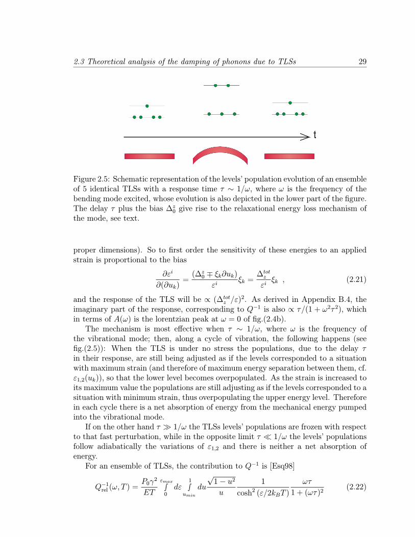
2.3 Theoretical analysis of the damping of phonons due to TLSs 29
Figure 2.5: Schematic representation of the levels’ population evolution of an ensembleof 5 identical TLSs with a response time τ ∼ 1/ω, where ω is the frequency of thebending mode excited, whose evolution is also depicted in the lower part of the figure.The delay τ plus the bias ∆z0 give rise to the relaxational energy loss mechanism ofthe mode, see text.
proper dimensions). So to first order the sensitivity of these energies to an appliedstrain is proportional to the bias
∂εi
∂(∂uk)=(∆z0 ∓ ξk∂uk)
εiξk =
∆totzεi
ξk , (2.21)
and the response of the TLS will be ∝ (∆totz /ε)2. As derived in Appendix B.4, theimaginary part of the response, corresponding to Q−1 is also ∝ τ/(1 + ω2τ 2), whichin terms of A(ω) is the lorentzian peak at ω = 0 of fig.(2.4b).The mechanism is most effective when τ ∼ 1/ω, where ω is the frequency of
the vibrational mode; then, along a cycle of vibration, the following happens (seefig.(2.5)): When the TLS is under no stress the populations, due to the delay τin their response, are still being adjusted as if the levels corresponded to a situationwith maximum strain (and therefore of maximum energy separation between them, cf.ε1,2(uk)), so that the lower level becomes overpopulated. As the strain is increased toits maximum value the populations are still adjusting as if the levels corresponded to asituation with minimum strain, thus overpopulating the upper energy level. Thereforein each cycle there is a net absorption of energy from the mechanical energy pumpedinto the vibrational mode.If on the other hand τ 1/ω the TLSs levels’ populations are frozen with respect
to that fast perturbation, while in the opposite limit τ 1/ω the levels’ populationsfollow adiabatically the variations of ε1,2 and there is neither a net absorption ofenergy.For an ensemble of TLSs, the contribution to Q−1 is [Esq98]
Q−1rel (ω, T ) =P0γ
2
ET
εmax
∫0dε
1
∫umin
du
√1− u2u
1
cosh2 (ε/2kBT )
ωτ
1 + (ωτ)2(2.22)
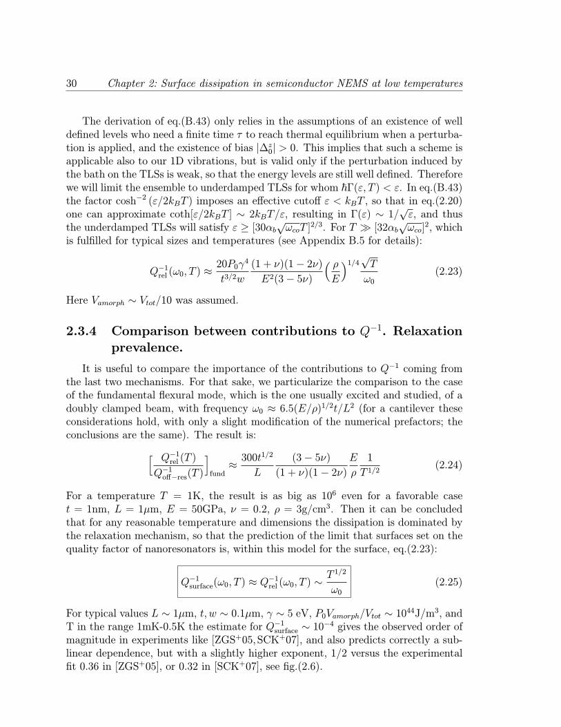
30 Chapter 2: Surface dissipation in semiconductor NEMS at low temperatures
The derivation of eq.(B.43) only relies in the assumptions of an existence of welldefined levels who need a finite time τ to reach thermal equilibrium when a perturba-tion is applied, and the existence of bias |∆z0| > 0. This implies that such a scheme isapplicable also to our 1D vibrations, but is valid only if the perturbation induced bythe bath on the TLSs is weak, so that the energy levels are still well defined. Thereforewe will limit the ensemble to underdamped TLSs for whom ~Γ(ε, T ) < ε. In eq.(B.43)the factor cosh−2 (ε/2kBT ) imposes an effective cutoff ε < kBT , so that in eq.(2.20)one can approximate coth[ε/2kBT ] ∼ 2kBT/ε, resulting in Γ(ε) ∼ 1/
√ε, and thus
the underdamped TLSs will satisfy ε ≥ [30αb√ωcoT ]
2/3. For T [32αb√ωco]
2, whichis fulfilled for typical sizes and temperatures (see Appendix B.5 for details):
Q−1rel (ω0, T ) ≈20P0γ
4
t3/2w
(1 + ν)(1− 2ν)E2(3− 5ν)
( ρE
)1/4√Tω0
(2.23)
Here Vamorph ∼ Vtot/10 was assumed.
2.3.4 Comparison between contributions to Q−1. Relaxation
prevalence.
It is useful to compare the importance of the contributions to Q−1 coming fromthe last two mechanisms. For that sake, we particularize the comparison to the caseof the fundamental flexural mode, which is the one usually excited and studied, of adoubly clamped beam, with frequency ω0 ≈ 6.5(E/ρ)1/2t/L2 (for a cantilever theseconsiderations hold, with only a slight modification of the numerical prefactors; theconclusions are the same). The result is:
[ Q−1rel (T )
Q−1off−res(T )
]
fund≈ 300t
1/2
L
(3− 5ν)(1 + ν)(1− 2ν)
E
ρ
1
T 1/2(2.24)
For a temperature T = 1K, the result is as big as 106 even for a favorable caset = 1nm, L = 1µm, E = 50GPa, ν = 0.2, ρ = 3g/cm3. Then it can be concludedthat for any reasonable temperature and dimensions the dissipation is dominated bythe relaxation mechanism, so that the prediction of the limit that surfaces set on thequality factor of nanoresonators is, within this model for the surface, eq.(2.23):
Q−1surface(ω0, T ) ≈ Q−1rel (ω0, T ) ∼T 1/2
ω0(2.25)
For typical values L ∼ 1µm, t, w ∼ 0.1µm, γ ∼ 5 eV, P0Vamorph/Vtot ∼ 1044J/m3, andT in the range 1mK-0.5K the estimate for Q−1surface ∼ 10−4 gives the observed order ofmagnitude in experiments like [ZGS+05,SCK+07], and also predicts correctly a sub-linear dependence, but with a slightly higher exponent, 1/2 versus the experimentalfit 0.36 in [ZGS+05], or 0.32 in [SCK+07], see fig.(2.6).
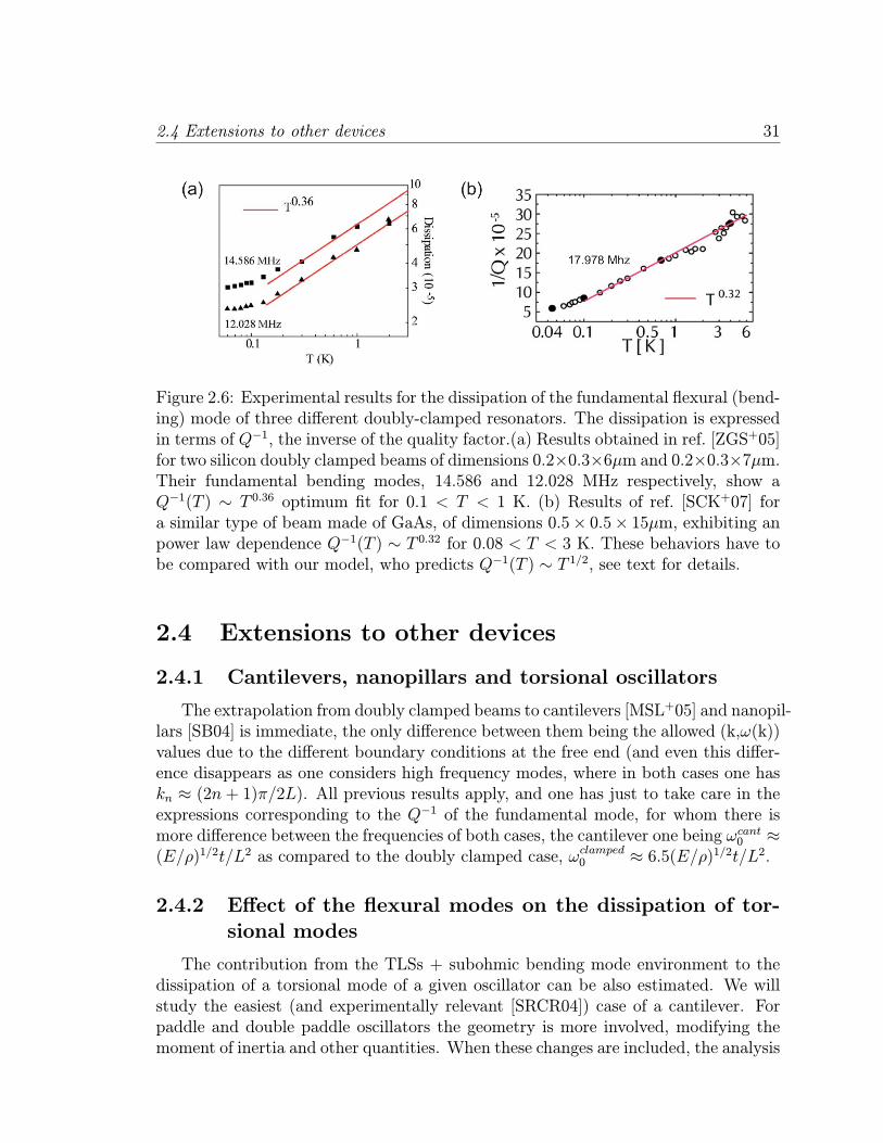
2.4 Extensions to other devices 31
Figure 2.6: Experimental results for the dissipation of the fundamental flexural (bend-ing) mode of three different doubly-clamped resonators. The dissipation is expressedin terms of Q−1, the inverse of the quality factor.(a) Results obtained in ref. [ZGS+05]for two silicon doubly clamped beams of dimensions 0.2×0.3×6µm and 0.2×0.3×7µm.Their fundamental bending modes, 14.586 and 12.028 MHz respectively, show aQ−1(T ) ∼ T 0.36 optimum fit for 0.1 < T < 1 K. (b) Results of ref. [SCK+07] fora similar type of beam made of GaAs, of dimensions 0.5× 0.5× 15µm, exhibiting anpower law dependence Q−1(T ) ∼ T 0.32 for 0.08 < T < 3 K. These behaviors have tobe compared with our model, who predicts Q−1(T ) ∼ T 1/2, see text for details.
2.4 Extensions to other devices
2.4.1 Cantilevers, nanopillars and torsional oscillators
The extrapolation from doubly clamped beams to cantilevers [MSL+05] and nanopil-lars [SB04] is immediate, the only difference between them being the allowed (k,ω(k))values due to the different boundary conditions at the free end (and even this differ-ence disappears as one considers high frequency modes, where in both cases one haskn ≈ (2n + 1)π/2L). All previous results apply, and one has just to take care in theexpressions corresponding to the Q−1 of the fundamental mode, for whom there ismore difference between the frequencies of both cases, the cantilever one being ωcant0 ≈(E/ρ)1/2t/L2 as compared to the doubly clamped case, ωclamped0 ≈ 6.5(E/ρ)1/2t/L2.
2.4.2 Effect of the flexural modes on the dissipation of tor-
sional modes
The contribution from the TLSs + subohmic bending mode environment to thedissipation of a torsional mode of a given oscillator can be also estimated. We willstudy the easiest (and experimentally relevant [SRCR04]) case of a cantilever. Forpaddle and double paddle oscillators the geometry is more involved, modifying themoment of inertia and other quantities. When these changes are included, the analysis
32 Chapter 2: Surface dissipation in semiconductor NEMS at low temperatures
follows the same steps we will show.
Relaxation absorption. We assume, based on the previous considerations onthe predominant influence of the flexural modes on the TLSs dynamics, as comparedwith the influence of the other modes, that the lifetime τ = Γ−1 of the TLSs isgiven by eq.(2.20). The change in the derivation of the expression for Q−1 comes ineq.(2.21), where the coupling constant ξtorsk is different, which translates simply, ineq.(B.43), into substituting γ2 ↔ γ2tors, and the corresponding prediction for Q
−1rel
Q−1rel (ω0, T ) ≈20P0γ
2torsγ
2
t3/2w
(1 + ν)(1− 2ν)E2(3− 5ν)
( ρE
)1/4√Tω0
, (2.26)
where now ω0 is the frequency of the corresponding flexural mode. The range oftemperatures and sizes for which this result applies is the same as in the case of anexcited bending mode.
Dissipation of symmetric non-resonant TLSs The modified excitation spec-trum of the TLS’s ensemble, Atotoff−res(ω0, T ), remains the same, and the change hap-pens in the matrix element of the transition probability of a mode |k0, n0〉 appearingin eq.(2.18), (λk20/
√ω0)
2. The operator yielding the coupling of the bath to thetorsional mode which causes its attenuation is the interaction term of the hamil-tonian, which for twisting modes is given by eq.(B.30). In Appendix B.6 a de-tailed derivation of eq.(2.27) is shown. The main results are stated here. Again,Q−1(ωj) = ∆E/2πE0, where the energy E0 stored in a torsional mode φj(z, t) =A sin[(2j − 1)πz/(2L)] sin(ωjt) per unit volume is E0 = A2ω2jρ(t
2 + w2)/48 (z is thecoordinate along the main axis of the rod). Expressing the amplitude A in terms ofphonon number nj, the energy stored in mode |kj, nj〉 is
E0(kj, n) =1
2
~ωj(t3w + w3t)L
(t2 + w2)(2nj + 1) , (2.27)
the energy fluctuations in a cycle of such a mode is
∆E =2π
ωj× ~ωj ×
2π
~γ2~ωj16Ltwµ
njAtotoff−res(ωj, T ) , (2.28)
and the inverse quality factor
(Q−1)totoff−res(ω0, T ) ≈ 0.04γ4P
t3/2w
ρ1/4(1 + ν)2(1− 2ν)E9/4(3− 5ν)
1√ω0coth[ω0T
](2.29)
For sizes and temperatures as the ones used for previous estimates the relaxationcontribution dominates dissipation.
2.5 Frequency shift 33
2.5 Frequency shift
Once the quality factor is known the relative frequency shift can be obtained viaa Kramers-Kronig relation (valid in the linear regime), because both are related tothe imaginary and real part, respectively, of the acoustic susceptibility. First we willdemonstrate this, and afterwards expressions for beam and cantilever will be derivedand compared to experiments.
2.5.1 Relation to the acoustic susceptibility
In absence of dissipative mechanisms, the equation for the bending modes is givenby −(12ρ/t2)∂2X/∂t2 = E∂4X/∂z4. The generalization in presence of friction is
−12ρt2
∂2X
∂t2= (E + χ)
∂4X
∂z4(2.30)
Where χ is a complex-valued susceptibility. Inserting a solution of the form X(z, t) =Aei(kx−ωt), where k is now a complex number, one gets the dispersion relation ω =√t2(E + χ)/(12ρ)k2. Now, assuming that the relative shift and dissipation are small,
implying Re(χ) << E , Im(k) << Re(k), the following expressions for the frequencyshift and inverse quality factor are obtained in terms of χ:
Q−1 = ∆ω/ω = −Im(χ)/Eδω/ω = Re(χ)/2E
(2.31)
Therefore a Kramers-Kronig relation for the susceptibility can be used to obtain therelative frequency shift:
δω
ω(ω, T ) = − 1
2πP
∫ ∞
−∞dω′
Q−1(ω′, T )
ω′ − ω, (2.32)
where P means here the principal value of the integral.
2.5.2 Expressions for the frequency shift
Relaxation processes of biased, underdamped TLSs dominate the perturbations ofthe ideal response of the resonator, as we have already shown for the inverse qualityfactor. For most of the frequency range, ω ≥ [30αb
√ωcoT ]
2/3, Q−1(ω, T ) ≈ A√T/ω ,
with A defined by eq.(2.23). The associated predicted contribution to the frequencyshift, using eq.(2.32), is
δω
ω(ω, T ) ≈ − A
2π
√T
ωlog[∣∣∣1−
ω
[30αb√ωcoT ]2/3
∣∣∣]
(2.33)
34 Chapter 2: Surface dissipation in semiconductor NEMS at low temperatures
For low temperatures, ω [30αb√ωcoT ]
2/3, the negative shift grows towards zero as
δω/ω(ω, T ) ∼ −√T log[ω/T 2/3], reaching at some point a maximum value, and de-
creasing for high temperatures, ω < [30αb√ωcoT ]
2/3, as δω/ω(ω, T ) ∼ 1/T 1/6. Eventhough the prediction of a peak in δω/ω(T ) qualitatively matches the few experimen-tal results currently available [ZGS+05,SCK+07], it does not fit them quantitatively.
2.6 Applicability and further extensions of the model.
Discussion
As mentioned, the predictions obtained within this theoretical framework domatch qualitatively experimental results in terms of observed orders of magnitudefor Q−1(T ), weak sublinear temperature dependence, and presence of a peak in thefrequency shift temperature dependence. But quantitative fitting is still to be reached,while on the experimental side more experiments need to be done at low temperaturesto confirm the, until now, few results [ZGS+05,SCK+07].
Applicability. The several simplifications involved in the model put certain con-straints, some of which are susceptible of improvement. We enumerate them firstand discuss some of them afterwards: i) The probability distribution P (∆x0 ,∆
z0), bor-
rowed from amorphous bulk systems, may be different for the case of the resonator’ssurface, ii) The assumption of non-interacting TLSs, only coupled among them in anindirect way through their coupling to the vibrations, breaks down at low enoughtemperatures, where also the discreteness of the vibrational spectrum affects our pre-dictions iii) When temperatures rise above a certain value, high energy phonons with3D character dominate dissipation, the two-state description of the degrees of free-dom coupled to the vibrations is not a good approximation, and thermoelastic lossesbegin to play an important role, iv) For strong driving, anharmonic coupling amongmodes has to be considered, and some steps in the derivation of the different mech-anisms, which assumed small perturbations, must be modified. This will be the caseof resonators driven to the nonlinear regime, where bistability and other phenomenatake place.
The solution to issue i) is intimately related to a better knowledge of the sur-face and the different physical processes taking place there. Recent studies try toshed some light on this question [CRB07], and from their results a more realisticP (∆x0 ,∆
z0) could be derived, which remains for future work. Before that point, it is
easier to wonder about the consequences of a dominant kind of dissipative processwhich corresponded to a set of TLSs with a well defined value of ∆x0 and a narrowdistribution of ∆z0’s of width ∆1, as was suggested for single-crystal silicon [Phi88].Following [Phi88], a Q−1(T ) ∼
√T behavior is obtained for low temperatures T < ∆1
if Γ(∆x0 , T ) < ω, and a Q−1(T ) ∼ 1/√T if Γ(∆x0 , T ) > ω, while at high temperatures
T > ∆1 a constant Q−1(T ) ∼ Q0 is predicted for both cases. These predictions do not
2.7 Dissipation in a metallic conductor 35
match better with experiments than the results obtained with P (∆x0 ,∆z0) ∼ P0/∆
x0 ,
so issue i) remains open.
We try now to have a first estimate of the temperature for which interactionsbetween TLSs cannot be ignored. Following the ideas presented in [Esq98], we willestimate the temperature T∗ at which the dephasing time τint due to interactions isequal to the lifetime τ(T ) = Γ−1(T ) defined in eq.(2.20), for the TLSs that contributemost to dissipation, which are those with ε ∼ ∆x0 ∼ T . For them τ−1(T ) = Γ(T ) ≈40αb√ωco√T . The interactions between the TLSs are dipolar, described by Hint =∑
i,j U1,2σz1σz2, with U1,2 = b12/r
312, b12 verifying 〈b12〉 ≈ 0, 〈|b12|〉 ≡ U0 ≈ γ2/E
[YL88, Esq98]. From the point of view of a given TLS the interaction affects itsbias, ∆zj = (∆
z0)j +
∑i Uijσ
zj , causing fluctuations of its phase δεj(t), which have an
associated τint defined by δεj(τint)τint ∼ 1. These fluctuations are caused by thoseTLSs which, within the time τint, have undergone a transition between their twoeigenstates, affecting through the interaction Hint the value of the bias of our TLS.At a temperature T , the most fluctuating TLSs are those such that ε ∼ ∆x0 ∼ T , andtheir density can be estimated, using P (∆x0 ,∆
z0), as nT ≈ P0kT . They will fluctuate
with a characteristic time τ(T ) ≈ [40αb√ωco√T ]−1, so for a time t < τ(T ) the amount
of these TLSs that have made a transition is roughly n(t) ≈ P0kT t/τ(T ). For adipolar interaction like the one described above, the average energy shift is relatedto n(t) by [BH77] δε(t) ≈ U0n(t). Substituting it in the equation defining τint, andimposing τint(T∗) = τ(T∗) gives the transition temperature T∗ ≈ [6αb
√ωco/(U0P0)]
2.For example, for a resonator like the silicon ones studied in [ZGS+05], L = 6µm,t = 0.2µm, w = 0.3µm, the estimated onset of interactions is at T∗ ≈ 10mK.An upper limit Thigh of applicability of the model due to high energy 3D vibrational
modes playing a significant role can be easily derived by imposing Thigh = ω3Dmin. The
frequency ω3Dmin corresponds to phonons with wavelength comparable to the thicknessof the sample, ω3Dmin = 2π
√E/ρ/t. The condition is very weak, as the value for
example for silicon resonators reads Thigh ≈ 400/t, with t given in nm. At muchlower temperatures the two-state description of the degrees of freedom coupled to thevibrations ceases to be realistic, with a high temperature cutoff in the case of themodel applied to amorphous bulk systems of T ∼ 5K.
2.7 Dissipation in a metallic conductor
Many of the current realizations of nanomechanical devices monitor the systemby means of currents applied through metallic conductors attached to the oscillators.The vibrations of the device couple to the electrons in the metallic part. This couplingis useful in order to drive and measure the oscillations, but it can also be a sourceof dissipation. We will apply here the techniques described in [GJS04, Gui05] (seealso [WP95]) in order to analyze the energy loss processes due to the excitations inthe conductor.
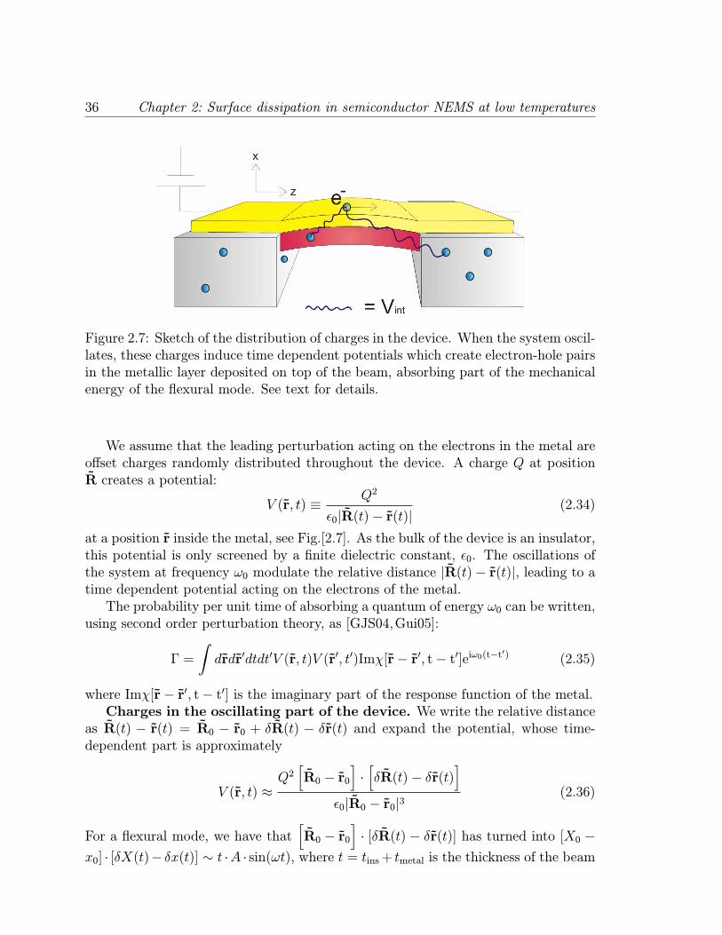
36 Chapter 2: Surface dissipation in semiconductor NEMS at low temperatures
Figure 2.7: Sketch of the distribution of charges in the device. When the system oscil-lates, these charges induce time dependent potentials which create electron-hole pairsin the metallic layer deposited on top of the beam, absorbing part of the mechanicalenergy of the flexural mode. See text for details.
We assume that the leading perturbation acting on the electrons in the metal areoffset charges randomly distributed throughout the device. A charge Q at positionR creates a potential:
V (r, t) ≡ Q2
ε0|R(t)− r(t)|(2.34)
at a position r inside the metal, see Fig.[2.7]. As the bulk of the device is an insulator,this potential is only screened by a finite dielectric constant, ε0. The oscillations ofthe system at frequency ω0 modulate the relative distance |R(t)− r(t)|, leading to atime dependent potential acting on the electrons of the metal.The probability per unit time of absorbing a quantum of energy ω0 can be written,
using second order perturbation theory, as [GJS04,Gui05]:
Γ =
∫drdr′dtdt′V (r, t)V (r′, t′)Imχ[r− r′, t− t′]eiω0(t−t′) (2.35)
where Imχ[r− r′, t− t′] is the imaginary part of the response function of the metal.Charges in the oscillating part of the device. We write the relative distance
as R(t) − r(t) = R0 − r0 + δR(t) − δr(t) and expand the potential, whose time-dependent part is approximately
V (r, t) ≈Q2[R0 − r0
]·[δR(t)− δr(t)
]
ε0|R0 − r0|3(2.36)
For a flexural mode, we have that[R0 − r0
]· [δR(t) − δr(t)] has turned into [X0 −
x0] · [δX(t)− δx(t)] ∼ t ·A · sin(ωt), where t = tins+ tmetal is the thickness of the beam
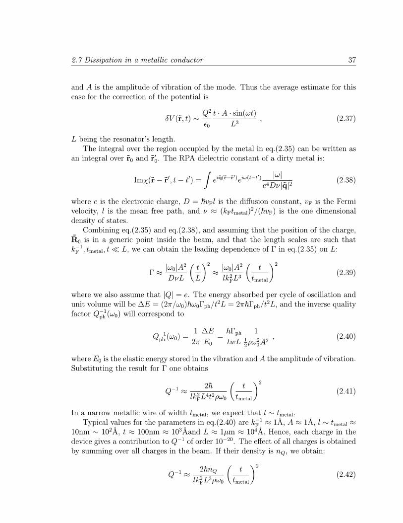
2.7 Dissipation in a metallic conductor 37
and A is the amplitude of vibration of the mode. Thus the average estimate for thiscase for the correction of the potential is
δV (r, t) ∼ Q2
ε0
t · A · sin(ωt)L3
, (2.37)
L being the resonator’s length.The integral over the region occupied by the metal in eq.(2.35) can be written as
an integral over r0 and r′0. The RPA dielectric constant of a dirty metal is:
Imχ(r− r′, t− t′) =∫eiq(r−r
′)eiω(t−t′) |ω|e4Dν|q|2
(2.38)
where e is the electronic charge, D = ~vFl is the diffusion constant, vF is the Fermivelocity, l is the mean free path, and ν ≈ (kFtmetal)2/(~vF) is the one dimensionaldensity of states.Combining eq.(2.35) and eq.(2.38), and assuming that the position of the charge,
R0 is in a generic point inside the beam, and that the length scales are such thatk−1F , tmetal, t L, we can obtain the leading dependence of Γ in eq.(2.35) on L:
Γ ≈ |ω0|A2
DνL
(t
L
)2≈ |ω0|A
2
lk2FL3
(t
tmetal
)2(2.39)
where we also assume that |Q| = e. The energy absorbed per cycle of oscillation andunit volume will be ∆E = (2π/ω0)~ω0Γph/t2L = 2π~Γph/t2L, and the inverse qualityfactor Q−1ph (ω0) will correspond to
Q−1ph (ω0) =1
2π
∆E
E0=~ΓphtwL
112ρω20A
2, (2.40)
where E0 is the elastic energy stored in the vibration and A the amplitude of vibration.Substituting the result for Γ one obtains
Q−1 ≈ 2~lk2FL
4t2ρω0
(t
tmetal
)2(2.41)
In a narrow metallic wire of width tmetal, we expect that l ∼ tmetal.Typical values for the parameters in eq.(2.40) are k−1F ≈ 1A, A ≈ 1A, l ∼ tmetal ≈
10nm ∼ 102A, t ≈ 100nm ≈ 103Aand L ≈ 1µm ≈ 104A. Hence, each charge in thedevice gives a contribution to Q−1 of order 10−20. The effect of all charges is obtainedby summing over all charges in the beam. If their density is nQ, we obtain:
Q−1 ≈ 2~nQlk2FL
3ρω0
(t
tmetal
)2(2.42)
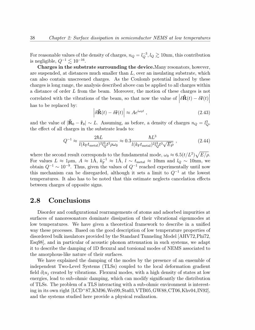
38 Chapter 2: Surface dissipation in semiconductor NEMS at low temperatures
For reasonable values of the density of charges, nQ = l−3Q , lQ & 10nm, this contribution
is negligible, Q−1 . 10−16.Charges in the substrate surrounding the device.Many resonators, however,
are suspended, at distances much smaller than L, over an insulating substrate, whichcan also contain unscreened charges. As the Coulomb potential induced by thesecharges is long range, the analysis described above can be applied to all charges withina distance of order L from the beam. Moreover, the motion of these charges is not
correlated with the vibrations of the beam, so that now the value of∣∣∣δR(t)− δr(t)
∣∣∣has to be replaced by: ∣∣∣δR(t)− δr(t)
∣∣∣ ≈ Aeiω0t , (2.43)
and the value of |R0 − r0| ∼ L. Assuming, as before, a density of charges nQ = l3Q,the effect of all charges in the substrate leads to:
Q−1 ≈ 2~Ll(kFtmetal)2l3Qt
2ρω0≈ 0.3 ~L3
l(kFtmetal)2l3Qt3√Eρ
, (2.44)
where the second result corresponds to the fundamental mode, ω0 ≈ 6.5(t/L2)√E/ρ.
For values L ≈ 1µm, A ≈ 1A, k−1F ≈ 1A, l ∼ tmetal ≈ 10nm and lQ ∼ 10nm, weobtain Q−1 ∼ 10−9. Thus, given the values of Q−1 reached experimentally until nowthis mechanism can be disregarded, although it sets a limit to Q−1 at the lowesttemperatures. It also has to be noted that this estimate neglects cancelation effectsbetween charges of opposite signs.
2.8 Conclusions
Disorder and configurational rearrangements of atoms and adsorbed impurities atsurfaces of nanoresonators dominate dissipation of their vibrational eigenmodes atlow temperatures. We have given a theoretical framework to describe in a unifiedway these processes. Based on the good description of low temperature properties ofdisordered bulk insulators provided by the Standard Tunneling Model [AHV72,Phi72,Esq98], and in particular of acoustic phonon attenuation in such systems, we adaptit to describe the damping of 1D flexural and torsional modes of NEMS associated tothe amorphous-like nature of their surfaces.We have explained the damping of the modes by the presence of an ensemble of
independent Two-Level Systems (TLSs) coupled to the local deformation gradientfield ∂iuj created by vibrations. Flexural modes, with a high density of states at lowenergies, lead to sub-ohmic damping, which can modify significantly the distributionof TLSs. The problem of a TLS interacting with a sub-ohmic environment is interest-ing in its own right [LCD+87,KM96,Wei99,Sta03,VTB05,GW88,CT06,Khv04,IN92],and the systems studied here provide a physical realization.
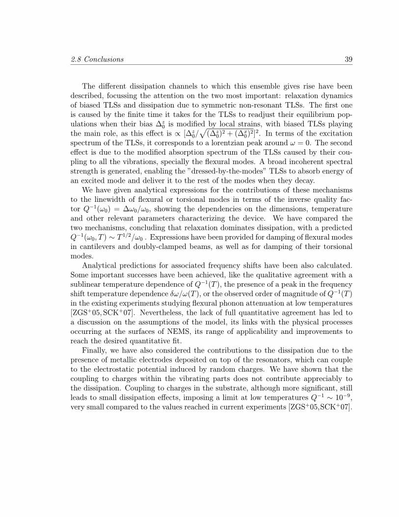
2.8 Conclusions 39
The different dissipation channels to which this ensemble gives rise have beendescribed, focussing the attention on the two most important: relaxation dynamicsof biased TLSs and dissipation due to symmetric non-resonant TLSs. The first oneis caused by the finite time it takes for the TLSs to readjust their equilibrium pop-ulations when their bias ∆z0 is modified by local strains, with biased TLSs playingthe main role, as this effect is ∝ [∆z0/
√(∆z0)
2 + (∆x0)2]2. In terms of the excitation
spectrum of the TLSs, it corresponds to a lorentzian peak around ω = 0. The secondeffect is due to the modified absorption spectrum of the TLSs caused by their cou-pling to all the vibrations, specially the flexural modes. A broad incoherent spectralstrength is generated, enabling the ”dressed-by-the-modes” TLSs to absorb energy ofan excited mode and deliver it to the rest of the modes when they decay.We have given analytical expressions for the contributions of these mechanisms
to the linewidth of flexural or torsional modes in terms of the inverse quality fac-tor Q−1(ω0) = ∆ω0/ω0, showing the dependencies on the dimensions, temperatureand other relevant parameters characterizing the device. We have compared thetwo mechanisms, concluding that relaxation dominates dissipation, with a predictedQ−1(ω0, T ) ∼ T 1/2/ω0 . Expressions have been provided for damping of flexural modesin cantilevers and doubly-clamped beams, as well as for damping of their torsionalmodes.Analytical predictions for associated frequency shifts have been also calculated.
Some important successes have been achieved, like the qualitative agreement with asublinear temperature dependence of Q−1(T ), the presence of a peak in the frequencyshift temperature dependence δω/ω(T ), or the observed order of magnitude of Q−1(T )in the existing experiments studying flexural phonon attenuation at low temperatures[ZGS+05, SCK+07]. Nevertheless, the lack of full quantitative agreement has led toa discussion on the assumptions of the model, its links with the physical processesoccurring at the surfaces of NEMS, its range of applicability and improvements toreach the desired quantitative fit.Finally, we have also considered the contributions to the dissipation due to the
presence of metallic electrodes deposited on top of the resonators, which can coupleto the electrostatic potential induced by random charges. We have shown that thecoupling to charges within the vibrating parts does not contribute appreciably tothe dissipation. Coupling to charges in the substrate, although more significant, stillleads to small dissipation effects, imposing a limit at low temperatures Q−1 ∼ 10−9,very small compared to the values reached in current experiments [ZGS+05,SCK+07].
40 Chapter 2: Surface dissipation in semiconductor NEMS at low temperatures
Part II
Friction mechanisms in grapheneand carbon nanotube-based
resonators
41

Chapter 3
Graphene-based structures:promising materials
3.1 From 3D to 0D, 1D and 2D
The versatility of carbon atoms to form all kinds of compounds with completelydifferent properties can be hardly overemphasized [Pie93]. When carbon atoms com-bine to constitute a solid, they can form two types of bonds [MGM06,GMM06], seefig.(3.1): the very strong sp3 bonds present in diamonds, where each atom has fourfirst-neighbors located in the vertices of a tetrahedron whose center is occupied bythat atom; and the more versatile sp2 bonds, with three identical coplanar sp bondsforming 120o angles between them, plus a fourth p-type orbital perpendicular to thatplane. As a result an hexagonal honeycomb lattice with closest-neighbor distancesof 1.4A tends to form, with in-plane σ orbitals giving rigidity to the lattice andout-of-plane π orbitals providing delocalized charge carriers.
The stacking of these planes creates graphite, a highly anisotropic material thanksto the differences between the intra and inter plane bonds. The former are strongcovalent bonds, whereas the latter are weak van der Waals forces, explaining theeasiness with which the planes can slide one over the other, basis of the lubricantproperties of graphite. Indeed, a band-structure calculation renders hopping ampli-tudes tab = 2.4 eV between nearest neighbors within a plane and tc = 0.3 eV betweenatoms of consecutive planes, separated by 3.5A. This anisotropy led Wallace alreadyin 1947 [Wal47] to propose a simplified model where the interaction between planesis neglected, and a single graphite plane is studied to obtain approximately the elec-tronic properties of graphite, viewing it as a 3D solid formed by the stacking of 2Dindependent hexagonal crystals.
Fortunately for the mesoscopics community this is not the end of the story ofcarbon compounds. The angles formed by the in-plane σ orbitals can be modifiedto a certain extent, so that not only hexagons but also pentagons or heptagons of
43
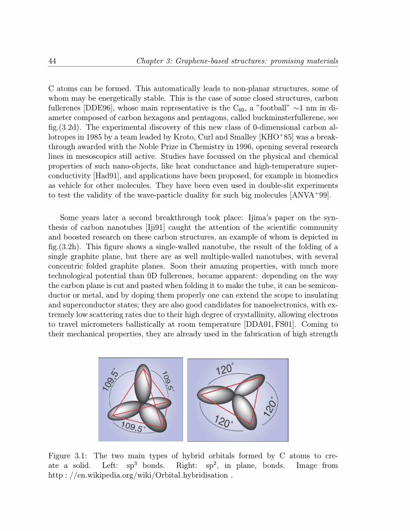
44 Chapter 3: Graphene-based structures: promising materials
C atoms can be formed. This automatically leads to non-planar structures, some ofwhom may be energetically stable. This is the case of some closed structures, carbonfullerenes [DDE96], whose main representative is the C60, a ”football” ∼1 nm in di-ameter composed of carbon hexagons and pentagons, called buckminsterfullerene, seefig.(3.2d). The experimental discovery of this new class of 0-dimensional carbon al-lotropes in 1985 by a team leaded by Kroto, Curl and Smalley [KHO+85] was a break-through awarded with the Noble Prize in Chemistry in 1996, opening several researchlines in mesoscopics still active. Studies have focussed on the physical and chemicalproperties of such nano-objects, like heat conductance and high-temperature super-conductivity [Had91], and applications have been proposed, for example in biomedicsas vehicle for other molecules. They have been even used in double-slit experimentsto test the validity of the wave-particle duality for such big molecules [ANVA+99].
Some years later a second breakthrough took place: Ijima’s paper on the syn-thesis of carbon nanotubes [Iji91] caught the attention of the scientific communityand boosted research on these carbon structures, an example of whom is depicted infig.(3.2h). This figure shows a single-walled nanotube, the result of the folding of asingle graphite plane, but there are as well multiple-walled nanotubes, with severalconcentric folded graphite planes. Soon their amazing properties, with much moretechnological potential than 0D fullerenes, became apparent: depending on the waythe carbon plane is cut and pasted when folding it to make the tube, it can be semicon-ductor or metal, and by doping them properly one can extend the scope to insulatingand superconductor states; they are also good candidates for nanoelectronics, with ex-tremely low scattering rates due to their high degree of crystallinity, allowing electronsto travel micrometers ballistically at room temperature [DDA01, FS01]. Coming totheir mechanical properties, they are already used in the fabrication of high strength
Figure 3.1: The two main types of hybrid orbitals formed by C atoms to cre-ate a solid. Left: sp3 bonds. Right: sp2, in plane, bonds. Image fromhttp : //en.wikipedia.org/wiki/Orbital hybridisation .
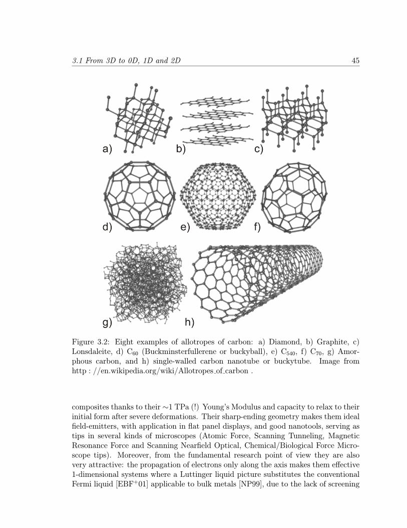
3.1 From 3D to 0D, 1D and 2D 45
Figure 3.2: Eight examples of allotropes of carbon: a) Diamond, b) Graphite, c)Lonsdaleite, d) C60 (Buckminsterfullerene or buckyball), e) C540, f) C70, g) Amor-phous carbon, and h) single-walled carbon nanotube or buckytube. Image fromhttp : //en.wikipedia.org/wiki/Allotropes of carbon .
composites thanks to their ∼1 TPa (!) Young’s Modulus and capacity to relax to theirinitial form after severe deformations. Their sharp-ending geometry makes them idealfield-emitters, with application in flat panel displays, and good nanotools, serving astips in several kinds of microscopes (Atomic Force, Scanning Tunneling, MagneticResonance Force and Scanning Nearfield Optical, Chemical/Biological Force Micro-scope tips). Moreover, from the fundamental research point of view they are alsovery attractive: the propagation of electrons only along the axis makes them effective1-dimensional systems where a Luttinger liquid picture substitutes the conventionalFermi liquid [EBF+01] applicable to bulk metals [NP99], due to the lack of screening
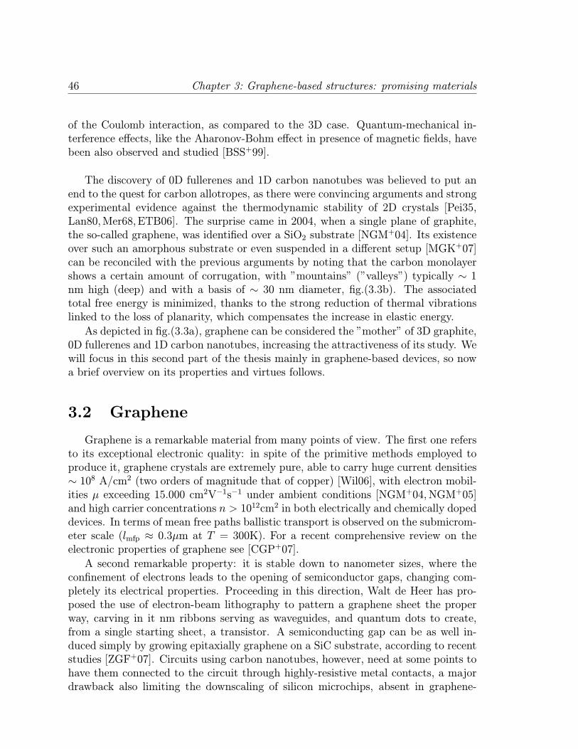
46 Chapter 3: Graphene-based structures: promising materials
of the Coulomb interaction, as compared to the 3D case. Quantum-mechanical in-terference effects, like the Aharonov-Bohm effect in presence of magnetic fields, havebeen also observed and studied [BSS+99].
The discovery of 0D fullerenes and 1D carbon nanotubes was believed to put anend to the quest for carbon allotropes, as there were convincing arguments and strongexperimental evidence against the thermodynamic stability of 2D crystals [Pei35,Lan80,Mer68,ETB06]. The surprise came in 2004, when a single plane of graphite,the so-called graphene, was identified over a SiO2 substrate [NGM
+04]. Its existenceover such an amorphous substrate or even suspended in a different setup [MGK+07]can be reconciled with the previous arguments by noting that the carbon monolayershows a certain amount of corrugation, with ”mountains” (”valleys”) typically ∼ 1nm high (deep) and with a basis of ∼ 30 nm diameter, fig.(3.3b). The associatedtotal free energy is minimized, thanks to the strong reduction of thermal vibrationslinked to the loss of planarity, which compensates the increase in elastic energy.
As depicted in fig.(3.3a), graphene can be considered the ”mother” of 3D graphite,0D fullerenes and 1D carbon nanotubes, increasing the attractiveness of its study. Wewill focus in this second part of the thesis mainly in graphene-based devices, so nowa brief overview on its properties and virtues follows.
3.2 Graphene
Graphene is a remarkable material from many points of view. The first one refersto its exceptional electronic quality: in spite of the primitive methods employed toproduce it, graphene crystals are extremely pure, able to carry huge current densities∼ 108 A/cm2 (two orders of magnitude that of copper) [Wil06], with electron mobil-ities µ exceeding 15.000 cm2V−1s−1 under ambient conditions [NGM+04, NGM+05]and high carrier concentrations n > 1012cm2 in both electrically and chemically dopeddevices. In terms of mean free paths ballistic transport is observed on the submicrom-eter scale (lmfp ≈ 0.3µm at T = 300K). For a recent comprehensive review on theelectronic properties of graphene see [CGP+07].
A second remarkable property: it is stable down to nanometer sizes, where theconfinement of electrons leads to the opening of semiconductor gaps, changing com-pletely its electrical properties. Proceeding in this direction, Walt de Heer has pro-posed the use of electron-beam lithography to pattern a graphene sheet the properway, carving in it nm ribbons serving as waveguides, and quantum dots to create,from a single starting sheet, a transistor. A semiconducting gap can be as well in-duced simply by growing epitaxially graphene on a SiC substrate, according to recentstudies [ZGF+07]. Circuits using carbon nanotubes, however, need at some points tohave them connected to the circuit through highly-resistive metal contacts, a majordrawback also limiting the downscaling of silicon microchips, absent in graphene-
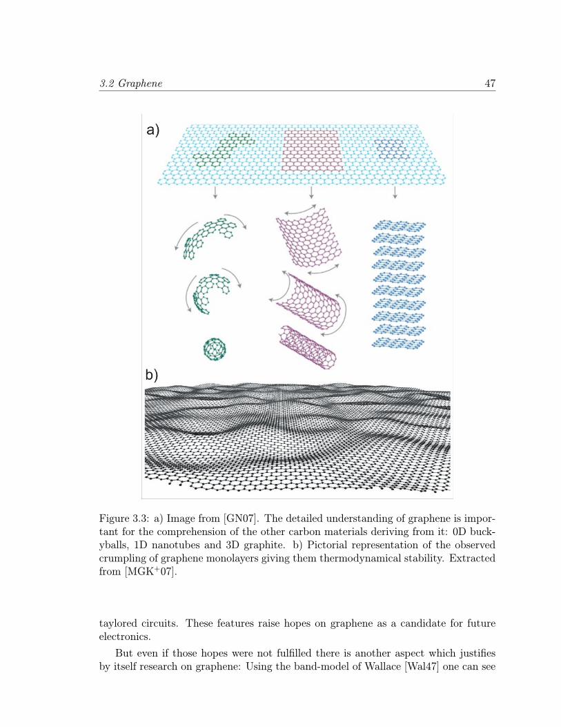
3.2 Graphene 47
Figure 3.3: a) Image from [GN07]. The detailed understanding of graphene is impor-tant for the comprehension of the other carbon materials deriving from it: 0D buck-yballs, 1D nanotubes and 3D graphite. b) Pictorial representation of the observedcrumpling of graphene monolayers giving them thermodynamical stability. Extractedfrom [MGK+07].
taylored circuits. These features raise hopes on graphene as a candidate for futureelectronics.
But even if those hopes were not fulfilled there is another aspect which justifiesby itself research on graphene: Using the band-model of Wallace [Wal47] one can see
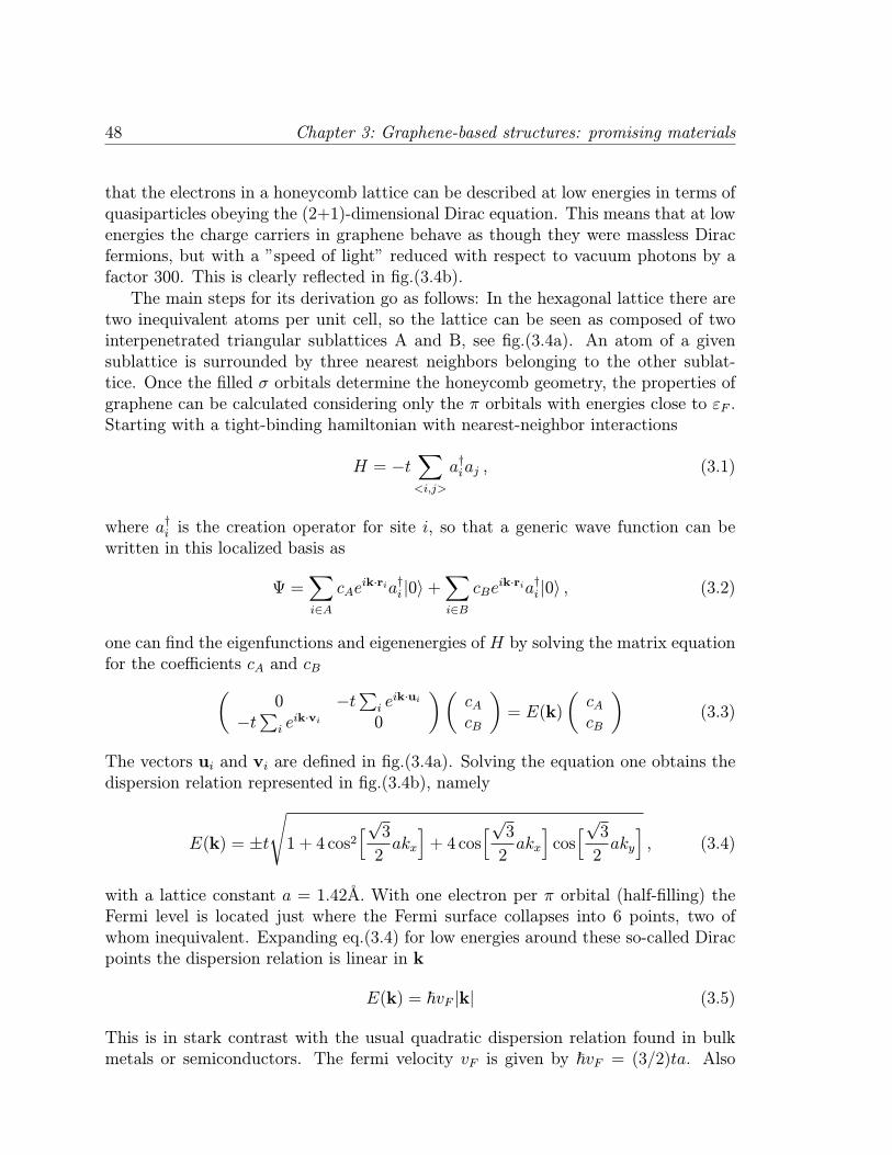
48 Chapter 3: Graphene-based structures: promising materials
that the electrons in a honeycomb lattice can be described at low energies in terms ofquasiparticles obeying the (2+1)-dimensional Dirac equation. This means that at lowenergies the charge carriers in graphene behave as though they were massless Diracfermions, but with a ”speed of light” reduced with respect to vacuum photons by afactor 300. This is clearly reflected in fig.(3.4b).The main steps for its derivation go as follows: In the hexagonal lattice there are
two inequivalent atoms per unit cell, so the lattice can be seen as composed of twointerpenetrated triangular sublattices A and B, see fig.(3.4a). An atom of a givensublattice is surrounded by three nearest neighbors belonging to the other sublat-tice. Once the filled σ orbitals determine the honeycomb geometry, the properties ofgraphene can be calculated considering only the π orbitals with energies close to εF .Starting with a tight-binding hamiltonian with nearest-neighbor interactions
H = −t∑
<i,j>
a†iaj , (3.1)
where a†i is the creation operator for site i, so that a generic wave function can bewritten in this localized basis as
Ψ =∑
i∈A
cAeik·ria†i |0〉+
∑
i∈B
cBeik·ria†i |0〉 , (3.2)
one can find the eigenfunctions and eigenenergies of H by solving the matrix equationfor the coefficients cA and cB
(0 −t
∑i eik·ui
−t∑i eik·vi 0
)(cAcB
)= E(k)
(cAcB
)(3.3)
The vectors ui and vi are defined in fig.(3.4a). Solving the equation one obtains thedispersion relation represented in fig.(3.4b), namely
E(k) = ±t
√
1 + 4 cos2[√32akx
]+ 4 cos
[√32akx
]cos[√32aky
], (3.4)
with a lattice constant a = 1.42A. With one electron per π orbital (half-filling) theFermi level is located just where the Fermi surface collapses into 6 points, two ofwhom inequivalent. Expanding eq.(3.4) for low energies around these so-called Diracpoints the dispersion relation is linear in k
E(k) = ~vF |k| (3.5)
This is in stark contrast with the usual quadratic dispersion relation found in bulkmetals or semiconductors. The fermi velocity vF is given by ~vF = (3/2)ta. Also

3.2 Graphene 49
Figure 3.4: a) Graphene lattice can be seen as composed of two interpenetratedtriangular sublattices A and B, with sublattice vectors ui and vi. b) Plot of graphene’sbandstructure as derived with a simple band-model for the honeycomb lattice [Wal47],eq.(3.4). When the graphene layer is neutral, the Fermi level is situated just at the6 so-called Fermi points, one of whom is zoomed at the right. At low energies, thedispersion relation around those Fermi points is linear, relativistic-like, E = ~vF |k| .Image from [Wil06].
within this low energy subspace around the Dirac points, one can Taylor-expand andderive a low-energy effective model:
H ≈ 32ta
(0 δkx + iδky
δkx − iδky 0
)= ~vF (kxσx + kyσy) , (3.6)
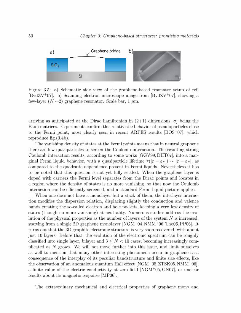
50 Chapter 3: Graphene-based structures: promising materials
Figure 3.5: a) Schematic side view of the graphene-based resonator setup of ref.[BvdZV+07]. b) Scanning electron microscope image from [BvdZV+07], showing afew-layer (N ∼2) graphene resonator. Scale bar, 1 µm.
arriving as anticipated at the Dirac hamiltonian in (2+1) dimensions, σj being thePauli matrices. Experiments confirm this relativistic behavior of pseudoparticles closeto the Fermi point, most clearly seen in recent ARPES results [BOS+07], whichreproduce fig.(3.4b).The vanishing density of states at the Fermi points means that in neutral graphene
there are few quasiparticles to screen the Coulomb interaction. The resulting strongCoulomb interaction results, according to some works [GGV99,DHT07], into a mar-ginal Fermi liquid behavior, with a quasiparticle lifetime τ(|ε − εF |) ∼ |ε − εF |, ascompared to the quadratic dependence present in Fermi liquids. Nevertheless it hasto be noted that this question is not yet fully settled. When the graphene layer isdoped with carriers the Fermi level separates from the Dirac points and locates ina region where the density of states is no more vanishing, so that now the Coulombinteraction can be efficiently screened, and a standard Fermi liquid picture applies.When one does not have a monolayer but a stack of them, the interlayer interac-
tion modifies the dispersion relation, displacing slightly the conduction and valencebands creating the so-called electron and hole pockets, keeping a very low density ofstates (though no more vanishing) at neutrality. Numerous studies address the evo-lution of the physical properties as the number of layers of the system N is increased,starting from a single 2D graphene monolayer [NGM+04,NMM+06,Tho06,PP06]. Itturns out that the 3D graphite electronic structure is very soon recovered, with aboutjust 10 layers. Before that, the evolution of the electronic spectrum can be roughlyclassified into single layer, bilayer and 3 ≤ N < 10 cases, becoming increasingly com-plicated as N grows. We will not move further into this issue, and limit ourselvesas well to mention that many other interesting phenomena occur in graphene as aconsequence of the interplay of its peculiar bandstructure and finite size effects, likethe observation of an anomalous quantum Hall effect [NGM+05,ZTSK05,NMM+06],a finite value of the electric conductivity at zero field [NGM+05,GN07], or unclearresults about its magnetic response [MP06].
The extraordinary mechanical and electrical properties of graphene mono and
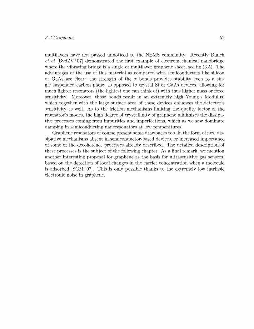
3.2 Graphene 51
multilayers have not passed unnoticed to the NEMS community. Recently Bunchet al [BvdZV+07] demonstrated the first example of electromechanical nanobridgewhere the vibrating bridge is a single or multilayer graphene sheet, see fig.(3.5). Theadvantages of the use of this material as compared with semiconductors like siliconor GaAs are clear: the strength of the σ bonds provides stability even to a sin-gle suspended carbon plane, as opposed to crystal Si or GaAs devices, allowing formuch lighter resonators (the lightest one can think of) with thus higher mass or forcesensitivity. Moreover, those bonds result in an extremely high Young’s Modulus,which together with the large surface area of these devices enhances the detector’ssensitivity as well. As to the friction mechanisms limiting the quality factor of theresonator’s modes, the high degree of crystallinity of graphene minimizes the dissipa-tive processes coming from impurities and imperfections, which as we saw dominatedamping in semiconducting nanoresonators at low temperatures.Graphene resonators of course present some drawbacks too, in the form of new dis-
sipative mechanisms absent in semiconductor-based devices, or increased importanceof some of the decoherence processes already described. The detailed description ofthese processes is the subject of the following chapter. As a final remark, we mentionanother interesting proposal for graphene as the basis for ultrasensitive gas sensors,based on the detection of local changes in the carrier concentration when a moleculeis adsorbed [SGM+07]. This is only possible thanks to the extremely low intrinsicelectronic noise in graphene.

52 Chapter 3: Graphene-based structures: promising materials
Chapter 4
Dissipative processes in grapheneresonators
4.1 Introduction
In this chapter we will analyze several dissipative mechanisms affecting grapheneresonators, both mono- and multilayer, like the ones fabricated by Bunch et al[BvdZV+07], comparing them with the semiconductor-based NEMS we have stud-ied in the first part of the thesis. We start with a brief description of these devices.
4.1.1 Experimental setup
The heart of the setup consists of a mono- or multilayer graphene sheet exfoliatedon top of a previously patterned trench etched in a SiO2 surface, figs.(3.5) and (4.1a).This SiO2 layer, ∼300 nm thick, is thermally grown from a starting underlying crys-talline Si wafer. The movement of the sheet is detected with a fast photodiode bylooking at variations in the intensity of the reflected light from a 632.8 nm He-Ne laserfocussed on the resonator, which are due to the size variation of the interferometerformed by the suspended graphene sheet and the silicon back plane, see fig.(4.1b).Bunch et al use two different driving schemes to induce motion:
Electrical drive
As shown in Fig.(4.1a), a gate voltage Vg is applied between the graphene andthe silicon layers, with both a static (DC) component and a small time-varying (AC)one, inducing a charge q = CgVg, where Cg is the capacitance between the two layers.The attraction between the charges of the two layers causes an electrostatic forcedownward on the graphene. The total electrostatic force on the sheet is
Fel =1
2C ′gV
2g '
1
2C ′gV
DCg
(V DCg + 2δVg
)=1
2C ′g
(V DCg
)2+ C ′gV
DCg δVg (4.1)
53
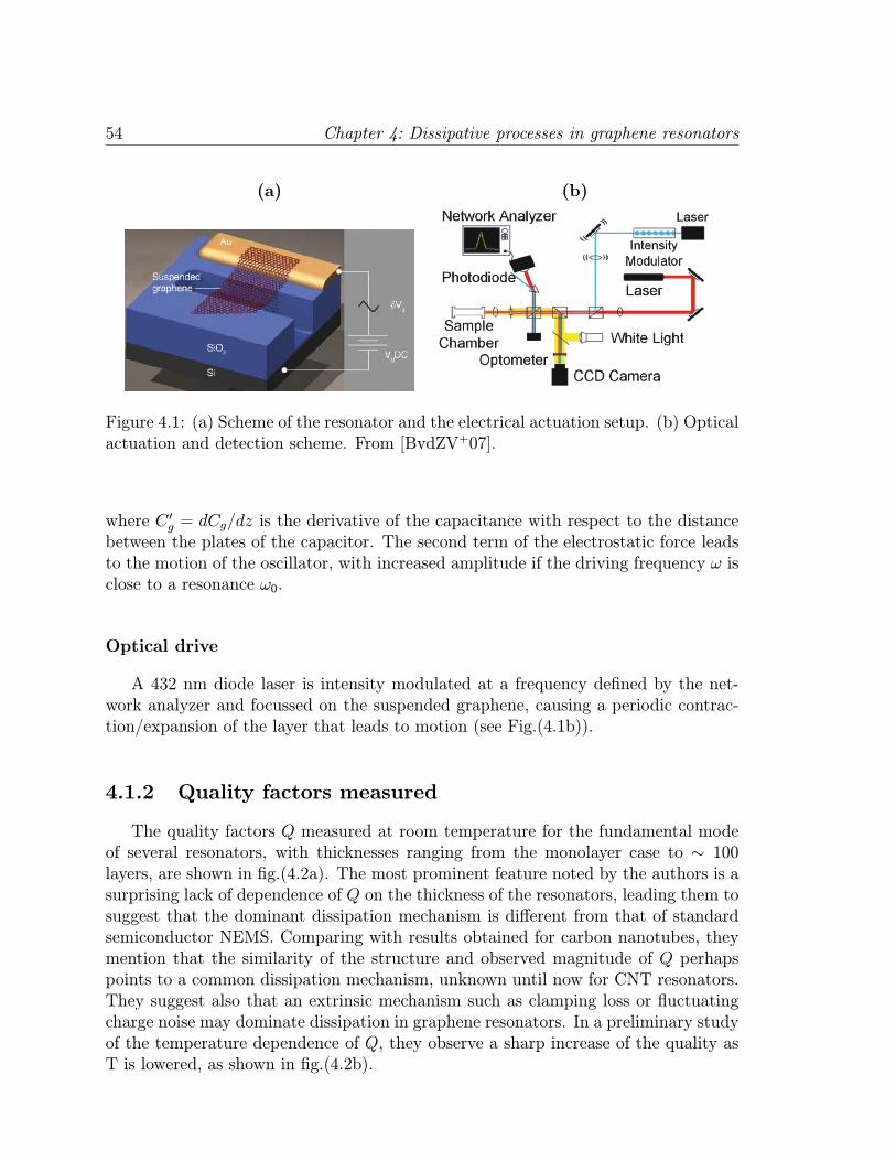
54 Chapter 4: Dissipative processes in graphene resonators
(a) (b)
Figure 4.1: (a) Scheme of the resonator and the electrical actuation setup. (b) Opticalactuation and detection scheme. From [BvdZV+07].
where C ′g = dCg/dz is the derivative of the capacitance with respect to the distancebetween the plates of the capacitor. The second term of the electrostatic force leadsto the motion of the oscillator, with increased amplitude if the driving frequency ω isclose to a resonance ω0.
Optical drive
A 432 nm diode laser is intensity modulated at a frequency defined by the net-work analyzer and focussed on the suspended graphene, causing a periodic contrac-tion/expansion of the layer that leads to motion (see Fig.(4.1b)).
4.1.2 Quality factors measured
The quality factors Q measured at room temperature for the fundamental modeof several resonators, with thicknesses ranging from the monolayer case to ∼ 100layers, are shown in fig.(4.2a). The most prominent feature noted by the authors is asurprising lack of dependence of Q on the thickness of the resonators, leading them tosuggest that the dominant dissipation mechanism is different from that of standardsemiconductor NEMS. Comparing with results obtained for carbon nanotubes, theymention that the similarity of the structure and observed magnitude of Q perhapspoints to a common dissipation mechanism, unknown until now for CNT resonators.They suggest also that an extrinsic mechanism such as clamping loss or fluctuatingcharge noise may dominate dissipation in graphene resonators. In a preliminary studyof the temperature dependence of Q, they observe a sharp increase of the quality asT is lowered, as shown in fig.(4.2b).
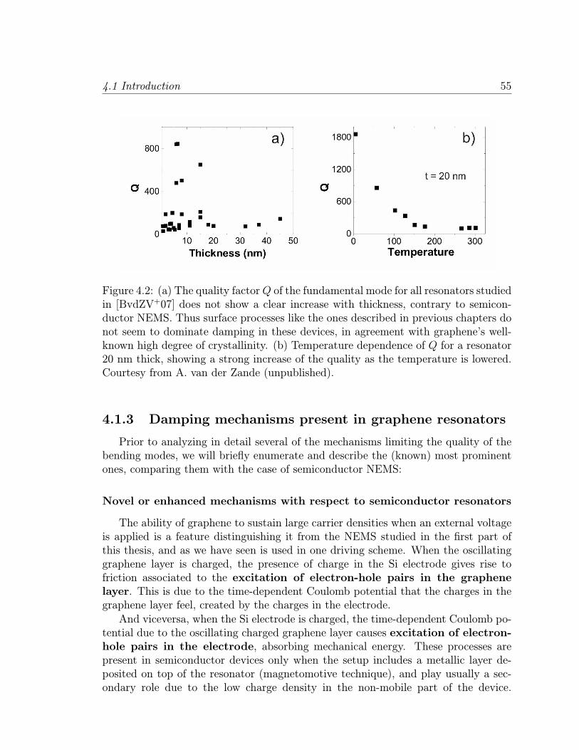
4.1 Introduction 55
Figure 4.2: (a) The quality factorQ of the fundamental mode for all resonators studiedin [BvdZV+07] does not show a clear increase with thickness, contrary to semicon-ductor NEMS. Thus surface processes like the ones described in previous chapters donot seem to dominate damping in these devices, in agreement with graphene’s well-known high degree of crystallinity. (b) Temperature dependence of Q for a resonator20 nm thick, showing a strong increase of the quality as the temperature is lowered.Courtesy from A. van der Zande (unpublished).
4.1.3 Damping mechanisms present in graphene resonators
Prior to analyzing in detail several of the mechanisms limiting the quality of thebending modes, we will briefly enumerate and describe the (known) most prominentones, comparing them with the case of semiconductor NEMS:
Novel or enhanced mechanisms with respect to semiconductor resonators
The ability of graphene to sustain large carrier densities when an external voltageis applied is a feature distinguishing it from the NEMS studied in the first part ofthis thesis, and as we have seen is used in one driving scheme. When the oscillatinggraphene layer is charged, the presence of charge in the Si electrode gives rise tofriction associated to the excitation of electron-hole pairs in the graphenelayer. This is due to the time-dependent Coulomb potential that the charges in thegraphene layer feel, created by the charges in the electrode.And viceversa, when the Si electrode is charged, the time-dependent Coulomb po-
tential due to the oscillating charged graphene layer causes excitation of electron-hole pairs in the electrode, absorbing mechanical energy. These processes arepresent in semiconductor devices only when the setup includes a metallic layer de-posited on top of the resonator (magnetomotive technique), and play usually a sec-ondary role due to the low charge density in the non-mobile part of the device.
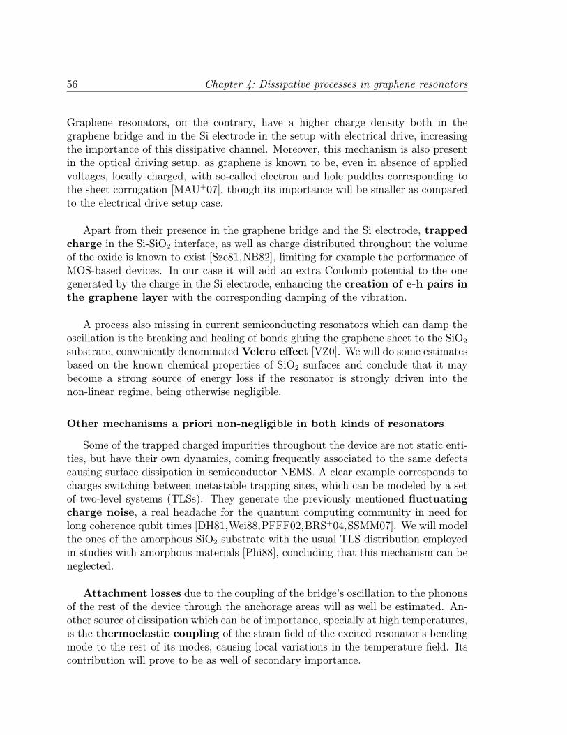
56 Chapter 4: Dissipative processes in graphene resonators
Graphene resonators, on the contrary, have a higher charge density both in thegraphene bridge and in the Si electrode in the setup with electrical drive, increasingthe importance of this dissipative channel. Moreover, this mechanism is also presentin the optical driving setup, as graphene is known to be, even in absence of appliedvoltages, locally charged, with so-called electron and hole puddles corresponding tothe sheet corrugation [MAU+07], though its importance will be smaller as comparedto the electrical drive setup case.
Apart from their presence in the graphene bridge and the Si electrode, trappedcharge in the Si-SiO2 interface, as well as charge distributed throughout the volumeof the oxide is known to exist [Sze81,NB82], limiting for example the performance ofMOS-based devices. In our case it will add an extra Coulomb potential to the onegenerated by the charge in the Si electrode, enhancing the creation of e-h pairs inthe graphene layer with the corresponding damping of the vibration.
A process also missing in current semiconducting resonators which can damp theoscillation is the breaking and healing of bonds gluing the graphene sheet to the SiO2substrate, conveniently denominatedVelcro effect [VZ0]. We will do some estimatesbased on the known chemical properties of SiO2 surfaces and conclude that it maybecome a strong source of energy loss if the resonator is strongly driven into thenon-linear regime, being otherwise negligible.
Other mechanisms a priori non-negligible in both kinds of resonators
Some of the trapped charged impurities throughout the device are not static enti-ties, but have their own dynamics, coming frequently associated to the same defectscausing surface dissipation in semiconductor NEMS. A clear example corresponds tocharges switching between metastable trapping sites, which can be modeled by a setof two-level systems (TLSs). They generate the previously mentioned fluctuatingcharge noise, a real headache for the quantum computing community in need forlong coherence qubit times [DH81,Wei88,PFFF02,BRS+04,SSMM07]. We will modelthe ones of the amorphous SiO2 substrate with the usual TLS distribution employedin studies with amorphous materials [Phi88], concluding that this mechanism can beneglected.
Attachment losses due to the coupling of the bridge’s oscillation to the phononsof the rest of the device through the anchorage areas will as well be estimated. An-other source of dissipation which can be of importance, specially at high temperatures,is the thermoelastic coupling of the strain field of the excited resonator’s bendingmode to the rest of its modes, causing local variations in the temperature field. Itscontribution will prove to be as well of secondary importance.
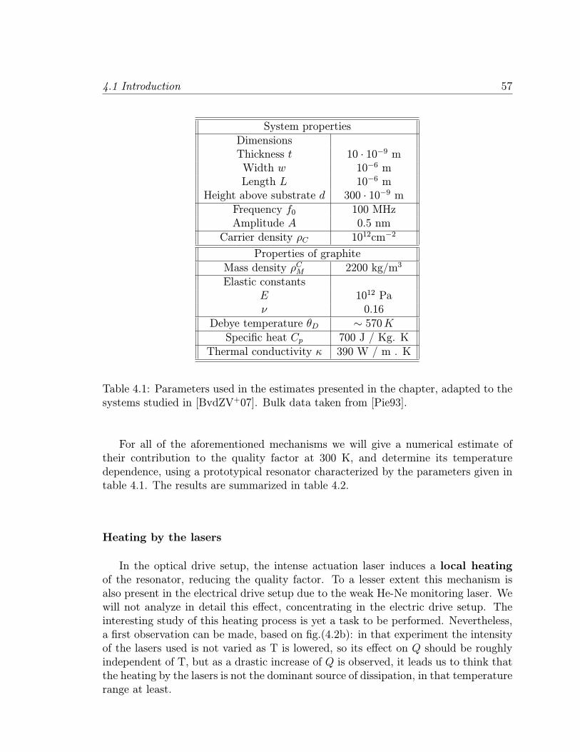
4.1 Introduction 57
System propertiesDimensionsThickness t 10 · 10−9 mWidth w 10−6 mLength L 10−6 m
Height above substrate d 300 · 10−9 mFrequency f0 100 MHzAmplitude A 0.5 nm
Carrier density ρC 1012cm−2
Properties of graphiteMass density ρCM 2200 kg/m3
Elastic constantsE 1012 Paν 0.16
Debye temperature θD ∼ 570KSpecific heat Cp 700 J / Kg. K
Thermal conductivity κ 390 W / m . K
Table 4.1: Parameters used in the estimates presented in the chapter, adapted to thesystems studied in [BvdZV+07]. Bulk data taken from [Pie93].
For all of the aforementioned mechanisms we will give a numerical estimate oftheir contribution to the quality factor at 300 K, and determine its temperaturedependence, using a prototypical resonator characterized by the parameters given intable 4.1. The results are summarized in table 4.2.
Heating by the lasers
In the optical drive setup, the intense actuation laser induces a local heatingof the resonator, reducing the quality factor. To a lesser extent this mechanism isalso present in the electrical drive setup due to the weak He-Ne monitoring laser. Wewill not analyze in detail this effect, concentrating in the electric drive setup. Theinteresting study of this heating process is yet a task to be performed. Nevertheless,a first observation can be made, based on fig.(4.2b): in that experiment the intensityof the lasers used is not varied as T is lowered, so its effect on Q should be roughlyindependent of T, but as a drastic increase of Q is observed, it leads us to think thatthe heating by the lasers is not the dominant source of dissipation, in that temperaturerange at least.
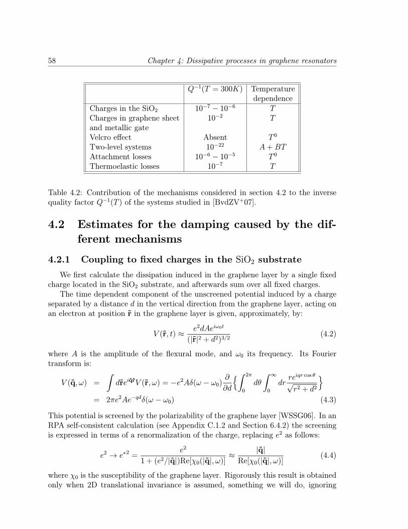
58 Chapter 4: Dissipative processes in graphene resonators
Q−1(T = 300K) Temperaturedependence
Charges in the SiO2 10−7 − 10−6 TCharges in graphene sheet 10−2 Tand metallic gateVelcro effect Absent T 0
Two-level systems 10−22 A+BTAttachment losses 10−6 − 10−5 T 0
Thermoelastic losses 10−7 T
Table 4.2: Contribution of the mechanisms considered in section 4.2 to the inversequality factor Q−1(T ) of the systems studied in [BvdZV+07].
4.2 Estimates for the damping caused by the dif-
ferent mechanisms
4.2.1 Coupling to fixed charges in the SiO2 substrate
We first calculate the dissipation induced in the graphene layer by a single fixedcharge located in the SiO2 substrate, and afterwards sum over all fixed charges.The time dependent component of the unscreened potential induced by a charge
separated by a distance d in the vertical direction from the graphene layer, acting onan electron at position r in the graphene layer is given, approximately, by:
V (r, t) ≈ e2dAeiω0t
(|r|2 + d2)3/2(4.2)
where A is the amplitude of the flexural mode, and ω0 its frequency. Its Fouriertransform is:
V (q, ω) =
∫dreiqrV (r, ω) = −e2Aδ(ω − ω0)
∂
∂d
∫ 2π
0
dθ
∫ ∞
0
drreiqr cos θ√r2 + d2
= 2πe2Ae−qdδ(ω − ω0) (4.3)
This potential is screened by the polarizability of the graphene layer [WSSG06]. In anRPA self-consistent calculation (see Appendix C.1.2 and Section 6.4.2) the screeningis expressed in terms of a renormalization of the charge, replacing e2 as follows:
e2 → e∗2 =e2
1 + (e2/|q|)Re[χ0(|q|, ω)]≈ |q|Re[χ0(|q|, ω)]
(4.4)
where χ0 is the susceptibility of the graphene layer. Rigorously this result is obtainedonly when 2D translational invariance is assumed, something we will do, ignoring
4.2 Estimates for the damping caused by the different mechanisms 59
border effects. At low energy and momenta the value of the susceptibility tends tothe compressibility (density of states) of the electrons in the layer. For the monolayerand multilayer cases we have:
lim|q|→0,ω→0
Re[χ0(|q|, ω)] =
kF~vF
N = 1Nγ~2v2F
N 6= 1 (4.5)
where N is the number of layers and γ is the interlayer hopping element. The resultfor the monolayer can be immediately obtained assuming a linear dispersion relationε(k) = ~vFk, while for a stack with N layers, the model with one interlayer hoppingelement [GCP06] has been used, which gives rise to 2N low energy bands, most ofwhich show a quadratic dispersion.Using Fermi’s golden rule applied to the perturbation potential of eq.(4.2) screened
as described in eq.(4.4) one arrives at eq.(C.6) of Appendix C.1.1 for the width of thegraphene mode. Fourier transforming to momentum space (v(q, ω) = v(−q, ω)):
Γph ≈∫d2q|v(q)|2Imχ0(q, ω0) . (4.6)
The low energy and momentum limit of graphene layers Imχ0(q, ω0) is given by[WSSG06,GCP06]
Imχ0(q, ω0) ≈
|ω|kFv2F|q|
N = 1|ω|γ2N3/2v2F|q|
√ρ
N 6= 1(4.7)
where, for N 6= 1, ρ is the total carrier density. This last expressions are valid forlengths bigger than the mean free path, l lmfp.The energy absorbed per cycle of oscillation and unit volume will be ∆E =
(2π/ω0)~ω0Γph/twL = 2π~Γph/twL, and the inverse quality factor Q−1ph (ω0) will cor-respond to
Q−1ph (ω0) =1
2π
∆E
E0=~ΓphtwL
112ρω20A
2=2~ΓphMω20A
2, (4.8)
where E0 is the elastic energy stored in the vibration and M is the total mass ofthe resonator. Calculating eq.(4.6) and substituting in eq.(4.8) for a single graphenelayer, a single charge turns out to give a contribution to the inverse quality factor of:
Q−1 ∼ 1
kFd
2~Mω0d2
(4.9)
where kF = π√ρC , and ρC is the density of carriers in the graphene sheet. We can
estimate this density as a function of the gate voltage Vg treating our system as acapacitor [NGM+04],
ρC =ε0 ε
e
Vg
d(4.10)
60 Chapter 4: Dissipative processes in graphene resonators
where ε0 is the permittivity of free space, ε the relative permittivity of the materialbetween the charged plates of the capacitor (in this case the graphene layer and theSi), and d the distance between the plates. In the region where the layer is suspended,ε = 1, and for typical voltages applied Vg ∼ 100 V the resulting carrier density turnsout to be ρC ∼ 2 · 1012 cm−2. Thus kFd ∼ 102− 103 1. Eq.(4.9) can be generalizedto a graphene sheet with N layers using eq.(4.7):
Q−1 ∼ 1√Nρd
2~Mω0d2
(4.11)
The suppression with the number of layers is due to the increased screening in thissystem.
The total contribution to the inverse quality factor is obtained by multiplyingeqs.(4.9) or (4.11) by the total number of charges Nch. An upper bound to the ef-fective surface density of local charges, deduced from some models for the electricconductivity of graphene [NM07,HAS06], is ρch ∼ 1012cm−2. In Appendix C.3 somefacts about these charges are collected from the literature, and an independent es-timate for ρch is made, obtaining a smaller value, eq.(C.28). The reason for thisdiscrepancy is still unclear to us. Using the first estimate for ρch and the parametersin Table[4.1], we find Nch ∼ 104 and Q−1 ∼ 10−11 at low temperatures.This mechanism leads to ohmic dissipation, as the energy is dissipated into electron-
hole pairs in the metallic graphene layer. Hence, as deduced in Appendix C.2.1, thetemperature dependence of this mechanism is given by Q−1(T ) ∼ Q−1(0)×(kT/~ω0) ,and Q−1 ∼ 10−6 at 300 K.The analysis presented here does not consider the additional screening due to the
presence of a metallic gate. In that case, one needs to add to the potential from astatic charge, eq.(4.2), a contribution from the image charge induced by the gate.This effect will reduce the coupling between the graphene layer and charges in thevicinity of the gate.
4.2.2 Ohmic losses at the graphene sheet and the metallic
gate.
The electrons in the vibrating graphene layer induce a time dependent potentialon the metallic gate which is sometimes part of the experimental setup. The energyis transferred to electron-hole pairs created at the gate or at the graphene layer.These processes contribute to the energy loss and decoherence of electrons in metallicconductors near gates [GJS04,Gui05].
The coupling between charge fluctuations in the two metallic systems is due to
4.2 Estimates for the damping caused by the different mechanisms 61
long range electrostatic interactions. The corresponding hamiltonian is
H =1
2
∫
C
vscr(z, r, t)ρC(z, r, t) +
∫
G
vscr(0, r′, t)ρG(r′)
(4.12)
+
∫
C
1
2ρM twΠ2 +
1
2
Et3w
12
[(∂2φ∂x2
)2+(∂2φ∂y2
)2]
where the indices G and C stand for the gate and graphene layer, respectively. ρMis the mass density of the graphene sheet, and t, w,E its thickness, width and Youngmodulus, whereas φ(r, t) represents the vibrating amplitude field of bending modesand Π = ∂L/∂φ is its conjugate momentum (L is the Lagrangian). The self-consistentscreened potentials vscr(z, r, t), vscr(0, r, t) are calculated as a function of the barepotentials v0(z, r, t), v0(0, r, t) in Appendix C.4.As in the case of eq.(4.2), the time-dependent part of the bare potentials couples
the electronic degrees of freedom and the mechanical ones through the charge ρ(r)and amplitude of the vibrational mode, Aq, and would give rise to a term in thequantized hamiltonian of the form
Hint ∝ ρ(r)Aq ∝ (b†q + bq)∑
k,k′
[c†k+k′
ck + h.c] (4.13)
where Aq and ρ(r) have been expressed in terms of creation and annihilation operatorsof phonons (q, ωq) and electrons of a 2D Fermi gas, respectively.But a realistic model requires taking into account the screening of the potential
associated to these charge fluctuations. In terms of the screened potentials, the in-duced broadening of the mode (q, ωq) of the graphene layer is, extrapolating eq.(C.6)of Appendix C.1.1 to this case, as [GJS04]
Γ(ωq) =∑
α=G,C
∫d3r
∫d3r′ReVαscr(r, ωq)×ReVαscr(r′, ωq)×Imχα [r− r′, ωq]
(4.14)
The static screening properties, limq→0Reχα(q, 0), of the graphene layer and the gate
are determined by their electronic compressibilities (densities of states), νC and νG
respectively. We will assume that the distance between the graphene and the gateis much larger than the electronic elastic mean free path in either material, so thattheir polarizability is well approximated by the one of a diffusive dirty metal, seeAppendices C.1.3 and C.1.4:
χα(q, ω) ≈ ναDα|q|2
Dα|q|2 + iω(4.15)
where Dα = vαFlα is the diffusion constant, and lα is the elastic mean free path. The
two dimensional conductivity is gα = kαF lα.
62 Chapter 4: Dissipative processes in graphene resonators
We have assumed the gate to be quasi two dimensional. This approximation isjustified when the distance between the gate and the graphene layer is much largerthan the width of the gate. Appendix C.3.2 shows how for typical oxide thicknessesand voltages applied it is fulfilled. In this situation, the broadening of the mode,eq.(4.14), can be expressed, analogously to eq.(4.6), as
Γ(ωq) ≈∫d2k|vscr(d, k, ωq)|2ImχC + |vscr(0, k, ωq)|2ImχG
(4.16)
The screened potentials for a graphene layer oscillating in an eigenmode (q, ωq)of amplitude Aq, have in a first approximation only one momentum component,
vscr(k, ωq) = vscr(q, ωq)δ(k− q), and these components are (see Appendix C.4)
vscr(d, q, ωq) =q
[χC
(eqd+e−qd
)−2χGeqd
]ρCAqe
−qd
2χCχG
(1−e−2qd
)
vscr(0, q, ωq) =|q|[−νC(e2qd+1
)+2νG
]ρ0Aqe
−qd
2νCνG
(1−e−2qd
)
(4.17)
where q = |q| and ρC is the charge density in the graphene layer. The results forΓ(ωq) and Q
−1(ωq) can be formulated in terms of the total charge in the graphenelayer, QC =
∫d2rρC ≈ L× w × ρC .
In the limit of short separation between the layers, d L, which is the situationpresent in current experimental setups, substitution of eq.(4.17) into eq.(4.16) leadsto
Γ(ω0) ≈ω0A
2Q2C4d2
( 1
νCDC+(νG
νC
)2 1
νGDG
)(4.18)
The limit D|q|2 ω for the imaginary part of the susceptibility of a dirty metal,Imχ(q, ω) ≈ ων/D|q|2, has been used, and is justified in Appendix C.1.3. The firstterm in the summation describes losses at the graphene sheet, and the second at thegate. The associated inverse quality factor, according to eq.(4.8), is given by
Q−1(ω0) ≈~Q2C2Mω0d2
( 1
νCDC+(νG
νC
)2 1
νGDG
)(4.19)
To make numerical estimates, we use the parameters in Table [4.1], with νC(E) =E/2π~2v2F , vF ≈ 106 m/s for a single layer of graphene, and νC(E) = (Nγ)/~2v2Ffor a stack of N layers [GCP06]. Carriers in graphene stacks have large mobilities[NGM+04], and we take DCνC ≈ 103. Typical charge densities for the graphenelayer are, as discussed in the previous subsection, ρC ∼ 1012cm−2, leading to a totalcharge QC ∼ 104. For these parameters, the contribution of the graphene sheetis Q−1 ∼ 10−8. The relative contribution from the gate depends on the distance
4.2 Estimates for the damping caused by the different mechanisms 63
to the graphene sheet. For a Si layer with DGνG ≈ 103 and at short distances, thecontribution to the damping from the gate is of the same order as that of the graphenesheet.
Damping is associated to the creation of e-h pairs in a metal, which implies thatthis mechanism is ohmic. The inverse quality factor should thus increase linearly withtemperature as described in Appendix C.2.1, leading to Q−1 ∼ 10−2 at 300 K.
4.2.3 Breaking and healing of surface bonds: Velcro effect.
In the fabrication process of the device, the graphene flake is deposited on thesilica (SiO2) substrate. The surface properties of silica are largely determined by thenature of silanol (SiOH) groups present there [MM90], due to the hydroxyl functionalgroup that has chemical reactivity, as compared to the inert siloxane (Si-O-Si) surface[SG95]. In Appendix C.3.3 more information relevant to us is given on silica and itssurface.
Graphene becomes linked to the silica surface through hydrogen bonds createdby those silanol groups. When the flake is set into motion, some of this bonds mayrepeatedly break and heal (the Velcro effect [VZ0]), causing dissipation of the energystored in the vibration. Numerical estimates are difficult to make, but neverthelesstwo qualitative arguments showing that its role in the damping is probably negligiblecan be presented:
i) This mechanism is expected to be temperature independent, in contrast with thestrong decrease of friction observed as temperature is lowered [BvdZV+07], fig.(4.2b).
ii) The elastic energy stored in a typical graphene oscillator of lateral dimensionsw ∼ 1µm is E0 = (1/2)ρw2tω20A2 ∼ 10eV, when the amplitude is A ∼ 1nm. Thismeans about ∼ 10−5eV per nm2. On the other hand, the energy per hydrogen bondis about 10−1eV, and typical radical densities at SiO2 surfaces are [DPX98] ∼ 1nm−2.Hence the elastic energy available on average for each hydrogen bond is much less thanthe energy stored in the bond. Only rare fluctuations, where a significant amount ofenergy is concentrated in a small area will be able to break bonds, and in this way toinduce energy dissipation. Note, however, that this argument ceases to be valid forvery large amplitudes & 30nm. For higher amplitudes, this mechanism can inducesignificant losses.
4.2.4 Fluctuating charge noise: Dissipation due to two-level
systems.
As we have seen in Part I of this thesis, in an amorphous material an atom or a fewatoms can have two nearly degenerate configurations. A vibration modifies the energydifference between these situations, and this coupling leads to the damping of acousticphonons in amorphous SiO2 [Esq98]. We have seen this mechanism is expected to
64 Chapter 4: Dissipative processes in graphene resonators
dominate friction in many semiconductor NEMS [MHE+02]. But with graphene res-onators, we expect the graphene sheet to show a high degree of crystallinity, so wewill only consider two-level systems (TLSs) in the rest of the structure.The TLSs can only dissipate energy if they are coupled in some way to the vi-
brating graphene sheet. A possible mechanism is the existence of charge impuritiesassociated to these defects (fluctuating charges), which are electrostatically coupledto the conducting electrons in the graphene.We expect this mechanism to be less effective in the device considered here than
in NEMs made of semiconducting materials, as now the TLSs reside in the SiO2substrate, not in the vibrating structure. The coupling, arising from long rangeforces, will be in comparison accordingly suppressed, by a factor of order (a/d)n,where a is a length comparable to the interatomic separation, and n describes thedecay of the coupling (n = 1 for the Coulomb potential between charged systems).The temperature dependence of the contribution of TLSs to Q−1 is determined by
the density of states of the modes coupled to the TLSs and the distribution of TLSsin terms of their paramenters (tunneling amplitude ∆x0 and bias ∆
z0) [SGC07a].The
hamiltonian describing the coupling of the effective TLS’s and the oscillating graphenesheet is given by [SGC07a]
H = ε σx + γ∆x0εσz∑
k
λk(bk + b†-k) +
∑
k
~ωkb†kbk (4.20)
where ε =√(∆x0)
2 + (∆z0)2, γ is the coupling constant, which will be strongly sup-
pressed in these devices as compared to attenuation of acoustic waves in amorphousmaterials, γ ∼ 1eV×(a/d)n, b†k represent the phonon creation operators associated tothe different vibrational modes of a sheet, and
∑k λk(bk+b
†-k) represents the coupling
to the strain tensor uik. There are two types, compression modes (longitudinal waves)and bending modes. The damping is due to the initial transfer of energy from thevibrational mode studied by the experimentalists to the TLSs, which in a second steptransfer this energy to the rest of the modes. The properties of the spin-boson model,eq.(4.20), are fully determined by the power-law s of the spectral function [LCD+87],J(ω) ≡
∑k |γλk∆x0/ε|
2δ(ω − ωk) ∼ αω1−sco ωs, where ωk is the frequency of mode k,
α is an adimensional constant and ωco is the upper cutoff of the phonon bath. Forthis system, compression modes gives rise to a superohmic, s = 2, bath, while thebending modes constitute an ohmic bath, s = 1, and thus will prevail as a source ofdissipation at low temperatures [LCD+87]. We will therefore restrict our analysis tothe dissipation caused by the ohmic component of the vibrational spectrum.A detailed calculation of the dissipation due to this mechanism is carried out inAppendix C.5. Here we state the main results. One arrives at J(ω) = αω, with
α ≈ 4(γ∆x0ε
)2ρ1/2M (1 + ν)3/2(1− ν)1/2
~t2E3/2(9 + 3ν1−2ν )
(4.21)
4.2 Estimates for the damping caused by the different mechanisms 65
Here ν is the Poisson ratio of graphene. Choosing fairly symmetrical TLSs, ∆x0/ε ∼ 1,for the parameters in table 4.1, α ∼ 10−5× (a/d)2n, very small. The relaxation of theTLSs dissipates the energy of the vibration, giving rise to the following expression forthe inverse quality factor [Esq98],
Q−1(ω, T ) =Pγ2
EkT
∫ εmax
0
dε
∫ 1
umin
duω
u√1− u2
C(ω, T ) (4.22)
where u = ∆r/ε, εmax ∼ 5 K, and (u√1− u2)−1 comes from the probability density
of TLS’s in an amorphous solid, like SiO2. Q−1(ω, T ) is a function of C(ω, T ), the
Fourier transform of the correlation function C(t, T ) = 〈σz(t)σz(0)〉T . For biasedTLSs and α 1 an extensive analysis of C(ω, T ) is performed in [Wei99], whereseveral expressions are provided in different limits. Using them, the estimate forQ−1(ω, T ) follows:
Q−1(ω, T ) ≈ Pγ2
E~ω
4π3αεmax +
π2
3α2kT
, kT > εmax
Q−1(ω, T ) ≈ Pγ2αE~ω
4π3kT, kT < εmax
(4.23)
In the range of temperatures of current experiments (5K<T<300K), the depen-dence of dissipation with T is weak, and Q−1 ∼ 10−6 × (a/d)4 ∼ 10−22. The mainuncertainty of the calculation has been the use of the TLSs’ distribution assumedfor amorphous solids [Phi87], but due to the small value of α a weak dissipation isexpected also with a modified distribution. Thus the conclusion is that the relativeimportance of TLSs damping is much smaller for graphene than for other NEMsdevices [CR02,Ble04,ER05].
4.2.5 Other friction mechanisms
Attachment losses.
The main expressions needed are given in [PJ04]. When d t, and d is muchsmaller than the wavelength of the radiated elastic waves in the SiO2 substrate, thecontribution to the inverse quality factor is given by
Q−1 ≈ w
L
( td
)2√ρCME
C(1− (νO)2)ρOME
O(4.24)
where the superscript O applies to the silicon oxide, and νO stands for Poisson’s ratio.The range of values of the quality factor varies from Q−1 ≈ 5 · 10−6 for a graphenemonolayer, to Q−1 ≈ 5·10−3 for a stack with 30 layers and t = 10nm. These quantitiesprobably overestimate the attachment losses, as they do not include the impedanceat the SiO2-graphene interface.This damping process due to energy irradiated away from the resonator should
not depend on temperature.
66 Chapter 4: Dissipative processes in graphene resonators
Thermoelastic effects.
When the phonon mean free path of the acoustic phonons is shorter than thewavelength of the mode under study, the acoustic phonons can be considered a dis-sipative environment coupled to the mode by anharmonic terms in the ionic poten-tial [Zen38, LR00, U06]. These anharmonic effects are described by the expansioncoefficient, α, and the thermal conductivity, κ. We follow the analysis in [Zen48]. Fora rectangular beam vibrating at a frequency ω the inverse quality factor is
Q−1Z (T ) =Eα2T
Cp
ωτZ
1 + (ωτZ)2(4.25)
where E is the Young Modulus, Cp is the specific heat at a constant pressure, andτZ is the thermal relaxation time associated with the mode, which in the case ofa flexural vibration is given by τZ = t2Cp/(π
2κ). This estimate assumes that thegraphene sheet is weakly deformed, and that the typical relaxation time is associatedto the diffusion of phonons over distances comparable to the thickness of the sheet.
Although better approximations are available in the literature [LR00], eq.(4.25) isenough for an estimate of the order of magnitude of Q−1. Using the parameters fromtable[4.1], for t = 10 nm and f ∼ 100 MHz, we find that ωτZ 1, and
Q−1Z (T = 300K) ≈Eα2Tωt2
π2κ∼ 5 · 10−7 (4.26)
4.3 Extension to nanotube oscillators.
The analysis presented here can be extended, in a straightforward way, to systemswhere the oscillating part is a nanotube.
We expect in these devices a larger impedance between the modes of the nanotubeand those of the substrate, so that attachment losses will be suppressed with respectto the estimate presented here for graphene.
The damping mechanisms which require long range forces between the movingcharges in the nanotube and degrees of freedom of the substrate (fluctuating andstatic charges) will not be significantly changed. A nanotube of length L at distanced from the substrate will interact with a substrate area of order (L+d)×d. A similarestimate for a graphene sheet of length L and width w gives an area ∼ (L+d)×(w+d).As L ∼ w ∼ d ∼ 1µm, the two areas are comparable.On the other hand, ohmic losses induced in the nanotube will be reduced with
respect to the two dimensional graphene sheet, as the number of carriers is lower inthe nanotube.
Finally, we expect a longer phonon mean free path in the nanotube, which impliesthat thermoelastic effects will be reduced .
4.4 Conclusions. 67
4.4 Conclusions.
We have considered six possible dissipation mechanisms which may lead to damp-ing in a graphene mesoscopic oscillator. The main results are summarized in Table[4.2].We expect that the calculations give the correct order of magnitude and dependenceon external parameters.We find that at high temperatures the leading damping mechanism is the ohmic
losses in the metallic gate and the graphene sheet. This effect depends quadraticallywith the total charge at the graphene sheet, which can be controlled by the gatevoltage.When speaking about the room temperature prevailing damping source, however,
a disturbing fact obtained in ref. ( [BvdZV+07]) has to be noted: the independence ofthe magnitude of Q at room temperatures for both the optical and electrical drivingsetups. Unless a mechanism like optical heating were of the order of the predicteddissipation due to ohmic losses, we are missing something. In principle optical heatingdoes not seem to be an important friction source, as it should lead to an almosttemperature independent Q(T ), contradicting results like the one shown in fig.(4.2b).At low temperatures attachment losses limit the quality of the vibration. If the
resonator is strongly driven, a new damping mechanism may come into play, theVelcro effect, which may limit substantially the quality factor as compared with theslightly driven case. The high crystallinity of the resonators eliminates the mainsource of dissipation in semiconducting resonators, namely surface-related effectiveTLSs coupled to the local strain field.These conclusions apply with only slight modifications to carbon nanotube-based
resonators.A deeper knowledge on the charge distribution throughout the device as a func-
tion of the parameters characterizing the fabrication process and the operation ofthe resonator for the different setups would prove of great interest, as it may leadto substantial improvements in the quality factor through the design of charge min-imization strategies, and shed some light on the prevailing damping mechanisms forthese devices. More measurements of the quality factor as a function of temperaturewould be also desirable for these purposes.

68 Chapter 4: Dissipative processes in graphene resonators
Part III
Dissipation of collective excitationsin metallic nanoparticles
69

Chapter 5
Metallic clusters: optical responseand collective excitations
5.1 From atoms to bulk
1 Nanometer-sized systems are the natural playground where the crossover fromatomic-like to bulk behavior is observed. Among the simplest and most studied onesare clusters of alkaline or noble metal atoms, with radii a between 0.5 and several nm(few atoms to hundreds of thousands, respectively, see Fig. 5.1). The simpler elec-tronic structure of alkaline atoms renders the theoretical modeling of alkaline clusterseasier as compared to the case of noble metals (with both s and d electrons), but theirhigh reactivity imposes stringent conditions on their production: clusters cannot beformed embedded in a solid matrix, so they are created, starting from an alkalinevapor at a high temperature, by expansion into vacuum within an inert carrier gasflux, a method called seeded beam expansion [KKS82]. Noble metals circumvent thisproblem, allowing for a more controlled fabrication and study by ion implantationin an inert matrix and subsequent high temperature annealing [DYN+99,OKNS00].Moreover, their chemical stability is required for their use as biological markers, oneof their most promising applications [BTM+02,CTB+03]. We will comment furtheron this issue later.
The crossover size to observe bulk behavior depends on the physical property un-der study, and is moreover never clearcut. Two ingredients are the main responsiblesof several new and interesting phenomena occurring in this interregnum. On the onehand, the spectrum of the electronic states remains discrete, with the energy levelsbroadened by the interactions with the environment. On the other, interferences andcoherent behavior of electrons happen due to their coherent motion inside the system:
1For a very good and detailed review on the issues covered in this chapter see [Wei06]. It hasbeen the main bibliographic source of this chapter and the beginning of the next.
71
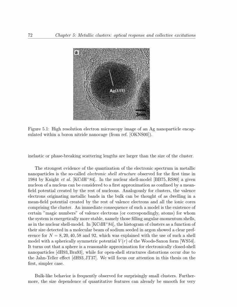
72 Chapter 5: Metallic clusters: optical response and collective excitations
Figure 5.1: High resolution electron microscopy image of an Ag nanoparticle encap-sulated within a boron nitride nanocage (from ref. [OKNS00]).
inelastic or phase-breaking scattering lengths are larger than the size of the cluster.
The strongest evidence of the quantization of the electronic spectrum in metallicnanoparticles is the so-called electronic shell structure observed for the first time in1984 by Knight et al. [KCdH+84]. In the nuclear shell-model [BB75,RS80] a givennucleon of a nucleus can be considered to a first approximation as confined by a mean-field potential created by the rest of nucleons. Analogously for clusters, the valenceelectrons originating metallic bands in the bulk can be thought of as dwelling in amean-field potential created by the rest of valence electrons and all the ionic corescomprising the cluster. An immediate consequence of such a model is the existence ofcertain ”magic numbers” of valence electrons (or correspondingly, atoms) for whomthe system is energetically more stable, namely those filling angular-momentum shells,as in the nuclear shell-model. In [KCdH+84], the histogram of clusters as a function oftheir size detected in a molecular beam of sodium seeded in argon showed a clear pref-erence for N = 8, 20, 40, 58 and 92, which was explained with the use of such a shellmodel with a spherically symmetric potential V (r) of the Woods-Saxon form [WS54].It turns out that a sphere is a reasonable approximation for electronically closed-shellnanoparticles [dH93,Bra93], while for open-shell structures distortions occur due tothe Jahn-Teller effect [dH93,JT37]. We will focus our attention in this thesis on thefirst, simpler case.
Bulk-like behavior is frequently observed for surprisingly small clusters. Further-more, the size dependence of quantitative features can already be smooth for very
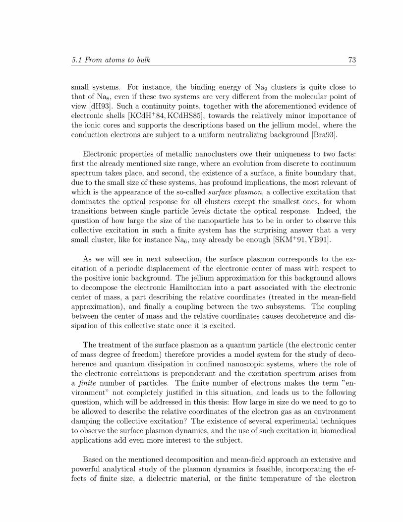
5.1 From atoms to bulk 73
small systems. For instance, the binding energy of Na9 clusters is quite close tothat of Na8, even if these two systems are very different from the molecular point ofview [dH93]. Such a continuity points, together with the aforementioned evidence ofelectronic shells [KCdH+84, KCdHS85], towards the relatively minor importance ofthe ionic cores and supports the descriptions based on the jellium model, where theconduction electrons are subject to a uniform neutralizing background [Bra93].
Electronic properties of metallic nanoclusters owe their uniqueness to two facts:first the already mentioned size range, where an evolution from discrete to continuumspectrum takes place, and second, the existence of a surface, a finite boundary that,due to the small size of these systems, has profound implications, the most relevant ofwhich is the appearance of the so-called surface plasmon, a collective excitation thatdominates the optical response for all clusters except the smallest ones, for whomtransitions between single particle levels dictate the optical response. Indeed, thequestion of how large the size of the nanoparticle has to be in order to observe thiscollective excitation in such a finite system has the surprising answer that a verysmall cluster, like for instance Na6, may already be enough [SKM
+91,YB91].
As we will see in next subsection, the surface plasmon corresponds to the ex-citation of a periodic displacement of the electronic center of mass with respect tothe positive ionic background. The jellium approximation for this background allowsto decompose the electronic Hamiltonian into a part associated with the electroniccenter of mass, a part describing the relative coordinates (treated in the mean-fieldapproximation), and finally a coupling between the two subsystems. The couplingbetween the center of mass and the relative coordinates causes decoherence and dis-sipation of this collective state once it is excited.
The treatment of the surface plasmon as a quantum particle (the electronic centerof mass degree of freedom) therefore provides a model system for the study of deco-herence and quantum dissipation in confined nanoscopic systems, where the role ofthe electronic correlations is preponderant and the excitation spectrum arises froma finite number of particles. The finite number of electrons makes the term ”en-vironment” not completely justified in this situation, and leads us to the followingquestion, which will be addressed in this thesis: How large in size do we need to go tobe allowed to describe the relative coordinates of the electron gas as an environmentdamping the collective excitation? The existence of several experimental techniquesto observe the surface plasmon dynamics, and the use of such excitation in biomedicalapplications add even more interest to the subject.
Based on the mentioned decomposition and mean-field approach an extensive andpowerful analytical study of the plasmon dynamics is feasible, incorporating the ef-fects of finite size, a dielectric material, or the finite temperature of the electron
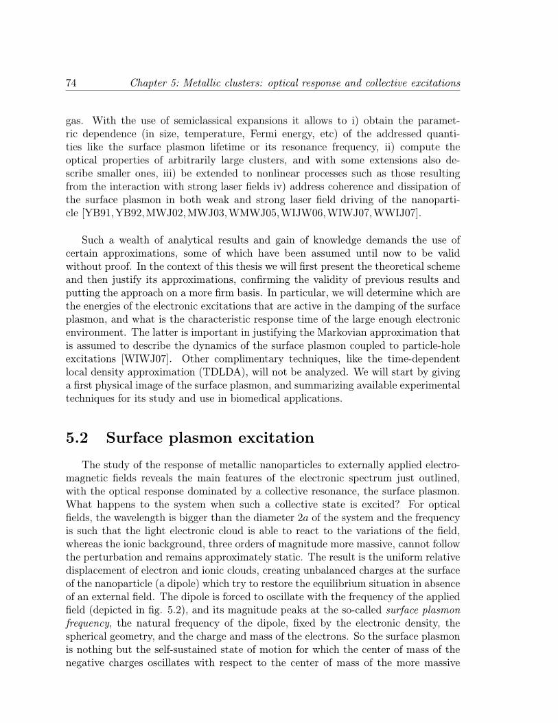
74 Chapter 5: Metallic clusters: optical response and collective excitations
gas. With the use of semiclassical expansions it allows to i) obtain the paramet-ric dependence (in size, temperature, Fermi energy, etc) of the addressed quanti-ties like the surface plasmon lifetime or its resonance frequency, ii) compute theoptical properties of arbitrarily large clusters, and with some extensions also de-scribe smaller ones, iii) be extended to nonlinear processes such as those resultingfrom the interaction with strong laser fields iv) address coherence and dissipation ofthe surface plasmon in both weak and strong laser field driving of the nanoparti-cle [YB91,YB92,MWJ02,MWJ03,WMWJ05,WIJW06,WIWJ07,WWIJ07].
Such a wealth of analytical results and gain of knowledge demands the use ofcertain approximations, some of which have been assumed until now to be validwithout proof. In the context of this thesis we will first present the theoretical schemeand then justify its approximations, confirming the validity of previous results andputting the approach on a more firm basis. In particular, we will determine which arethe energies of the electronic excitations that are active in the damping of the surfaceplasmon, and what is the characteristic response time of the large enough electronicenvironment. The latter is important in justifying the Markovian approximation thatis assumed to describe the dynamics of the surface plasmon coupled to particle-holeexcitations [WIWJ07]. Other complimentary techniques, like the time-dependentlocal density approximation (TDLDA), will not be analyzed. We will start by givinga first physical image of the surface plasmon, and summarizing available experimentaltechniques for its study and use in biomedical applications.
5.2 Surface plasmon excitation
The study of the response of metallic nanoparticles to externally applied electro-magnetic fields reveals the main features of the electronic spectrum just outlined,with the optical response dominated by a collective resonance, the surface plasmon.What happens to the system when such a collective state is excited? For opticalfields, the wavelength is bigger than the diameter 2a of the system and the frequencyis such that the light electronic cloud is able to react to the variations of the field,whereas the ionic background, three orders of magnitude more massive, cannot followthe perturbation and remains approximately static. The result is the uniform relativedisplacement of electron and ionic clouds, creating unbalanced charges at the surfaceof the nanoparticle (a dipole) which try to restore the equilibrium situation in absenceof an external field. The dipole is forced to oscillate with the frequency of the appliedfield (depicted in fig. 5.2), and its magnitude peaks at the so-called surface plasmonfrequency, the natural frequency of the dipole, fixed by the electronic density, thespherical geometry, and the charge and mass of the electrons. So the surface plasmonis nothing but the self-sustained state of motion for which the center of mass of thenegative charges oscillates with respect to the center of mass of the more massive
5.2 Surface plasmon excitation 75
Figure 5.2: Schematic representation of the surface plasmon resonance in small metal-lic clusters. The wavelength λ of the exciting electrical field E(t) is much larger thanthe diameter 2a of the cluster. Thus, the electrical field throughout the nanoparticleis nearly uniform. The shaded regions symbolize the ionic background, while thedashed circles represent the electronic cloud. The ”-” and ”+” signs account for theuncompensated negative and positive charges. The electrical field exerts a force onthe positively charged ions and an equal force on the electrons in the opposite direc-tion, separating their centers of mass mainly due to the motion of the light electrons.The ions, being much more massive, remain almost at rest. The resulting surfacecharges create a dipolar restoring field (thick arrow) opposing E(t).
ionic cores.
Applying classical Maxwell’s equations to the case of a dielectric metal spherewith appropiate boundary conditions, Mie obtained in 1908 [KV95, Mie08] a firstestimate for this frequency, the classical Mie frequency ωM = ωp/
√3, where ωp =
(4πnee2/me)
1/2 is the bulk plasma frequency and e, me, and ne denote the elec-tronic charge, mass, and density, respectively. In a real cluster surface effects leadto a small reduction of the surface plasmon frequency with respect to the Mie valueωM [Bra93,GGI02,WIJW06]. Typical values for the surface plasmon energy are aboutseveral eV, belonging thus to the energy range corresponding to bound single-particlestates [BB94].
76 Chapter 5: Metallic clusters: optical response and collective excitations
5.2.1 Probing and using the surface plasmon
Several techniques show and use the existence of the surface plasmon to studyelectronic properties of metallic clusters. We will mention three of them:
Photoabsorption experiments
The cluster is illuminated by a light of a certain frequency, and the amount ofabsorbed photons is determined and given in terms of the photoabsorption crosssection σ(ω), which is the probability that the system absorbs a photon times thearea illuminated by the photon beam. The presence of the single-particle statesderived in the electronic shell model should be signalled by several peaks in σ(ω), butthey are usually overwhelmed by the peak of the collective excitation [BCLS93], thusindicating a substantial transfer of spectral weight to build the surface plasmon.
Noble metal nanoclusters as biological markers
An ideal optical label for large molecules should generate an intense optical signal;it should also be small, durable, chemically inert, and apt to bind to the molecule ofinterest in a controlled manner. Noble metal clusters meet all of these requirementswhen illuminated with a frequency close to the one of their surface plasmons. Theyovercome the main shortages present in other candidates like fluorescent dyes ornanocrystals of II-VI semiconductors, as they do not photobleach like the formerand do neither optically saturate at reasonable exciting intensities like the latter.Several techniques take advantage of the excitation of the surface plasmon as a meansto track the nanoparticle adhered to the molecule of interest: nanoparticles biggerthan 40 nm in diameter can be imaged, based on Rayleigh scattering, in an opticalmicroscope by illuminating in dark-field at the plasmon frequency [SSMS00], withdifferential interference contrast (DIC) and video enhancement [JG88], or with totalinternal reflection [SGH+00]. For smaller nanoparticles, whose Rayleigh scattering istoo small to be detected, local heating associated to its strong light absorption causesa temperature change which can be monitored by a sensitive interference methodsimilar to DIC [BTM+02], see fig. 5.3.
Pump-probe experiments: plasmon dynamics
The use of femtosecond pulsed lasers in time-resolved pump-probe spectroscopyhas rendered possible to experimentally address the surface plasmon dynamics [BHMD00,FVF+00, LKLA99,LUCS01]. An initial ultrashort laser pulse lasting around a hun-dred femtoseconds pumps energy into the nanoparticle by exciting the surface plas-mon mode. After a certain time delay a second, much weaker, pulse, the probe laser,tests the absorption spectrum of the hot electron gas in the cluster. By repeatingthe experiment for several values of the delay an image of the time evolution of the
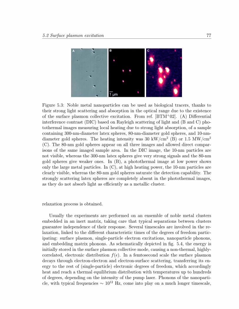
5.2 Surface plasmon excitation 77
Figure 5.3: Noble metal nanoparticles can be used as biological tracers, thanks totheir strong light scattering and absorption in the optical range due to the existenceof the surface plasmon collective excitation. From ref. [BTM+02]. (A) Differentialinterference contrast (DIC) based on Rayleigh scattering of light and (B and C) pho-tothermal images measuring local heating due to strong light absorption, of a samplecontaining 300-nm-diameter latex spheres, 80-nm-diameter gold spheres, and 10-nm-diameter gold spheres. The heating intensity was 30 kW/cm2 (B) or 1.5 MW/cm2
(C). The 80-nm gold spheres appear on all three images and allowed direct compar-isons of the same imaged sample area. In the DIC image, the 10-nm particles arenot visible, whereas the 300-nm latex spheres give very strong signals and the 80-nmgold spheres give weaker ones. In (B), a photothermal image at low power showsonly the large metal particles. In (C), at high heating power, the 10-nm particles areclearly visible, whereas the 80-nm gold spheres saturate the detection capability. Thestrongly scattering latex spheres are completely absent in the photothermal images,as they do not absorb light as efficiently as a metallic cluster.
relaxation process is obtained.
Usually the experiments are performed on an ensemble of noble metal clustersembedded in an inert matrix, taking care that typical separations between clustersguarantee independence of their response. Several timescales are involved in the re-laxation, linked to the different characteristic times of the degrees of freedom partic-ipating: surface plasmon, single-particle electron excitations, nanoparticle phonons,and embedding matrix phonons. As schematically depicted in fig. 5.4, the energy isinitially stored in the surface plasmon collective mode, causing a non-thermal, highly-correlated, electronic distribution f(ε). In a femtosecond scale the surface plasmondecays through electron-electron and electron-surface scattering, transferring its en-ergy to the rest of (single-particle) electronic degrees of freedom, which accordinglyheat and reach a thermal equilibrium distribution with temperatures up to hundredsof degrees, depending on the intensity of the pump laser. Phonons of the nanoparti-cle, with typical frequencies ∼ 1012 Hz, come into play on a much longer timescale,
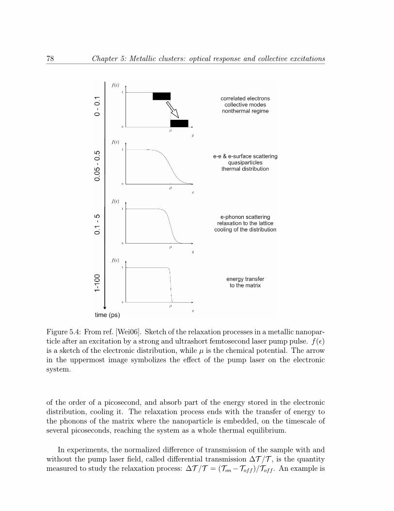
78 Chapter 5: Metallic clusters: optical response and collective excitations
Figure 5.4: From ref. [Wei06]. Sketch of the relaxation processes in a metallic nanopar-ticle after an excitation by a strong and ultrashort femtosecond laser pump pulse. f(ε)is a sketch of the electronic distribution, while µ is the chemical potential. The arrowin the uppermost image symbolizes the effect of the pump laser on the electronicsystem.
of the order of a picosecond, and absorb part of the energy stored in the electronicdistribution, cooling it. The relaxation process ends with the transfer of energy tothe phonons of the matrix where the nanoparticle is embedded, on the timescale ofseveral picoseconds, reaching the system as a whole thermal equilibrium.
In experiments, the normalized difference of transmission of the sample with andwithout the pump laser field, called differential transmission ∆T /T , is the quantitymeasured to study the relaxation process: ∆T /T = (Ton−Toff )/Toff . An example is
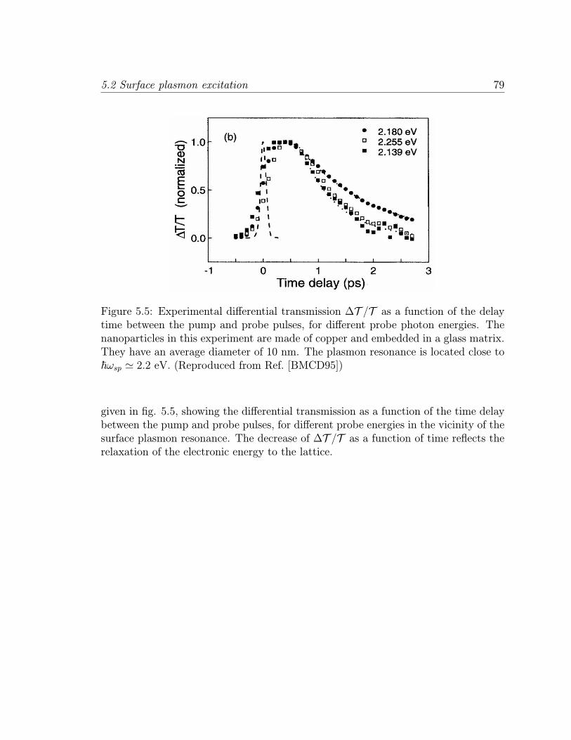
5.2 Surface plasmon excitation 79
Figure 5.5: Experimental differential transmission ∆T /T as a function of the delaytime between the pump and probe pulses, for different probe photon energies. Thenanoparticles in this experiment are made of copper and embedded in a glass matrix.They have an average diameter of 10 nm. The plasmon resonance is located close to~ωsp ' 2.2 eV. (Reproduced from Ref. [BMCD95])
given in fig. 5.5, showing the differential transmission as a function of the time delaybetween the pump and probe pulses, for different probe energies in the vicinity of thesurface plasmon resonance. The decrease of ∆T /T as a function of time reflects therelaxation of the electronic energy to the lattice.

80 Chapter 5: Metallic clusters: optical response and collective excitations
Chapter 6
Electronic dynamics in metallicnanoparticles: theoretical model
This chapter describes a very successful theoretical framework for the analyticaldescription of the electron dynamics in metallic clusters, expressed in terms of twotypes of excited states, the single-particle e-h excitations, and the many-body surfaceplasmon collective state. In a basis of relative + center of mass electronic coordinates,e-h and surface plasmon excitations will correspond to the relative and center of masscoordinates, respectively. Some key assumptions needed for the conceptual soundnessof the model will be underlined, whose justification will be provided in the final partof the chapter.
6.1 Electronic hamiltonian: relative and collective
coordinates
The systems we will analyze are neutral, spherical, metallic nanoparticles of ra-dius a containing N valence electrons. They thus have, as mentioned in the previouschapter, closed angular momentum shells (N = 8, 20, 40, 58..., the so-called ”magicnumbers” [Bra93]). We will work within the adiabatic Born-Oppenheimer approx-imation [AM76], treating the ions as static, compared with the lighter and fastervalence electrons. Moreover, we will work within the jellium approximation, whichneglects effects of the ionic structure and treats the ions as a continuous, homoge-neous positively charged background of total charge +Ne, producing a charge densityin the case of a spherical nanoparticle ρi(r) = (Ne/V )Θ(a− r), with V = 4πa3/3 thevolume of the cluster and Θ(x) the Heaviside step function. The subsequent modelis simple enough to be applied for the description of big clusters containing up toseveral thousands of atoms, and the effects linked to the ionic structure turn out tobe important only for the smallest cases, N < 10 [Bra93].
81
82 Chapter 6: Electronic dynamics in metallic nanoparticles: theoretical model
The electronic hamiltonian for an alkaline-metal nanoparticle in vacuum is in thiscontext given by
H =N∑
i=1
[ p2i2me
+ U(ri)]+e2
2
∑
i,j=1(i6=j)
1
|ri − rj|, (6.1)
where e and me are the electronic charge and mass, ri is the position of the ith con-
duction electron, ri = |ri|, pi is the associated momentum, and U(r) represents theelectrostatic interaction between the electrons and the ionic background.
For a noble metal cluster embedded in a dielectric medium, the electron-electroninteraction in (6.1) is modified by the presence of the d-electrons and the matrix interms of two dielectric constants εd and εm, and the expression for the Coulomb po-tential is much more cumbersome due to the loss of translational invariance. For athorough study of this case see [Wei06,WMWJ05].
The shape of the confining potential U(r) for a charged sphere of radius a andtotal charge +Ne, harmonic inside the nanoparticle with the Mie frequency ωM =√Ne2/mea3 and Coulomb-like outside, can be readily obtained using Gauss’s theo-rem,
U(r) =Ne2
2a3(r2 − 3a2)Θ(a− r)− Ne2
rΘ(r − a) (6.2)
If the many-body eigenstates |f〉 and eigenenergies Ef of the hamiltonian (6.1) areknown, the photoabsorption cross section σ(ω) can be calculated using Fermi’s goldenrule [Mer70]
σ(ω) =4πe2ω
3c
∑
f
|〈f |z|0〉|2δ(~ω − Ef + E0) (6.3)
The ground state is |0〉, and the electric field is assumed to be along the z axis. Fromσ(ω) the frequency ωpl and linewidth γpl of the surface plasmon are immediatelyobtained. But the calculation of the many-body eigenstates becomes exceedinglydifficult for clusters bigger than a few electrons, and further approximation schemeshave to be developed.
The most useful one starts by changing the electronic coordinate basis to thecenter of mass R =
∑i ri/N and relative coordinates r
′i = ri−R. The corresponding
conjugated momenta are P =∑i pi and p
′i = pi − P/N , respectively, and (6.1)
becomes
H =P2
2Nme+Hrel +
N∑
i=1
[U(|r′i +R|)− U(r′i)] (6.4)
6.1 Electronic hamiltonian: relative and collective coordinates 83
where the hamiltonian for the relative-coordinate system reads
Hrel =N∑
i=1
[ p′i 2
2me+ U(r′i)
]+e2
2
∑
i,j=1(i6=j)
1
|r’i − r’j|(6.5)
A first glance comparing eqs. (6.1) and (6.5) may make us wonder where is the differ-ence between them, and what is our motivation to go from (6.1) to (6.4). Regardingthe difference between hamiltonians, note that one of the relative coordinates is afunction of the rest, as
∑i r′i = 0. The change of variables, on the other hand, is
justified as it is the right one if we are interested in the study of the surface plas-mon collective excitation, which was shown in the previous chapter to correspond toelectronic center-of-mass oscillations.Assuming small displacements for the center of mass, |R| a, the dependence
on the relative coordinates in the last term of (6.4) drops out, U(|r′ +R|)− U(r′) 'R · ∇U(r′) + (1/2)(R · ∇)2U(r′), where derivatives are taken at r′ = r. Choosing theoscillation axis of the center of mass in the z-direction, R = Zez, one obtains with(6.2)
R · ∇U(r′) = Zmeω2M
[z′Θ(a− r′) + z′a3
r′3Θ(r′ − a)
](6.6)
(R · ∇)2U(r′) = Z2Ne2[ 1a3Θ(a− r′) + 1− 3 cos
2 θ′
r′3Θ(r′ − a)
]' Z2
Ne2
a3Θ(a− r′)
where in the last line a second-order coupling in Z between the center-of-mass andthe relative-coordinate system for r′ > a has been neglected as compared with thefirst-order one expressed in the second term of the right-hand side of the first line.Inserting (6.6) into (6.4),
H =P2
2Nme+1
2
Ne2
a3R2
N∑
i=1
Θ(a− ri) +Hrel +Hc = Hcm +Hrel +Hc , (6.7)
where the coupling Hc between the center-of-mass and the relative coordinates is, tofirst order in the displacement R of the center of mass
Hc =N∑
i=1
R · ∇U(r′i)∣∣∣R=0
, (6.8)
with R · ∇U(r′i)∣∣∣R=0given in (6.6). Notice that due to the spread of the electrons’
wavefunctions outside the geometrical boundary of the cluster, r = a, there is a finiteprobability for them to have ri > a, which due to the sum over Θ(a − ri) in (6.7),results in a reduction of the center-of-mass oscillation frequency from the classical
84 Chapter 6: Electronic dynamics in metallic nanoparticles: theoretical model
Mie value, ωM = ωM√1−Nout/N < ωM . This quantum correction is the so-called
spill-out effect [dH93,Bra93,KV95].The structure of (6.7) is typical for quantum dissipative systems [Wei99]: The sys-
tem under study (Hcm) is coupled via Hc to an environment or ”heat bath” describedby Hrel. The system-environment coupling results in dissipation and decoherence ofthe collective excitation.
6.2 Mean-field approximation and second quanti-
zation of the hamiltonian
The presence in Hrel of electronic interactions makes the problem still a formi-dable one and demands further simplifications. A mean-field approximation for therelative-coordinates’ degrees of freedom, together with a second quantization proce-dure, will render a tractable hamiltonian suited for the study of collective excitationsin metallic clusters.
The harmonic oscillator hamiltonian Hcm for the center-of-mass is quantized asusual with bosonic creation and annihilation operators [BF04],
b =√NmeωM2~ Z + i√
2Nme~ωMPZ
b† =√NmeωM2~ Z − i√
2Nme~ωMPZ
(6.9)
where PZ is the conjugated momentum to Z. Eigenstates |n〉 of Hcm satisfy b|n〉 =√n|n − 1〉 and b†|n〉 =
√n+ 1|n + 1〉, and Hcm is expressed in terms of b and b†,
subtracting the zero-point energy ~ωM/2, as
Hcm = ~ωMb†b (6.10)
In the mean-field approximation for the hamiltonian Hrel, eq.(6.5), we forget thefact that one of the relative coordinates is not independent of the rest (hopefullycausing 1/N errors which become negligible as the number of electrons N grows),and substitute Hrel by the mean-field approximation of eq.(6.1), mimicking the effectof the rest of electrons on a given one with an effective one-body potential V (r) feltby the latter:
Hrel ≈N∑
i=1
Hsc[r′i, p′i] =
N∑
i=1
[ p′i 2
2me+ V (r′i)
](6.11)
We have used V (r) = V (r), valid for a spherical nanocluster. Numerical calculationsusing time-dependent local density approximation (TDLDA) within the spherical jel-lium model at zero temperature provide information about the shape of the potential
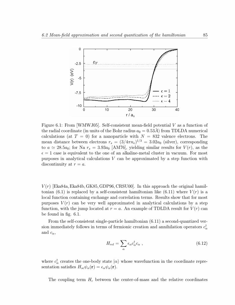
6.2 Mean-field approximation and second quantization of the hamiltonian 85
Figure 6.1: From [WMWJ05]. Self-consistent mean-field potential V as a function ofthe radial coordinate (in units of the Bohr radius a0 = 0.53A) from TDLDA numericalcalculations (at T = 0) for a nanoparticle with N = 832 valence electrons. Themean distance between electrons rs = (3/4πne)
1/3 = 3.02a0 (silver), correspondingto a ' 28.5a0; for Na rs = 3.93a0 [AM76], yielding similar results for V (r), as theε = 1 case is equivalent to the one of an alkaline-metal cluster in vacuum. For mostpurposes in analytical calculations V can be approximated by a step function withdiscontinuity at r = a.
V (r) [Eka84a,Eka84b,GK85,GDP96,CRSU00]. In this approach the original hamil-tonian (6.1) is replaced by a self-consistent hamiltonian like (6.11) where V (r) is alocal function containing exchange and correlation terms. Results show that for mostpurposes V (r) can be very well approximated in analytical calculations by a stepfunction, with the jump located at r = a. An example of TDLDA result for V (r) canbe found in fig. 6.1.
From the self-consistent single-particle hamiltonian (6.11) a second-quantized ver-sion immediately follows in terms of fermionic creation and annihilation operators c†αand cα,
Hrel =∑
α
εαc†αcα , (6.12)
where c†α creates the one-body state |α〉 whose wavefunction in the coordinate repre-sentation satisfies Hscψα(r) = εαψα(r).
The coupling term Hc between the center-of-mass and the relative coordinates
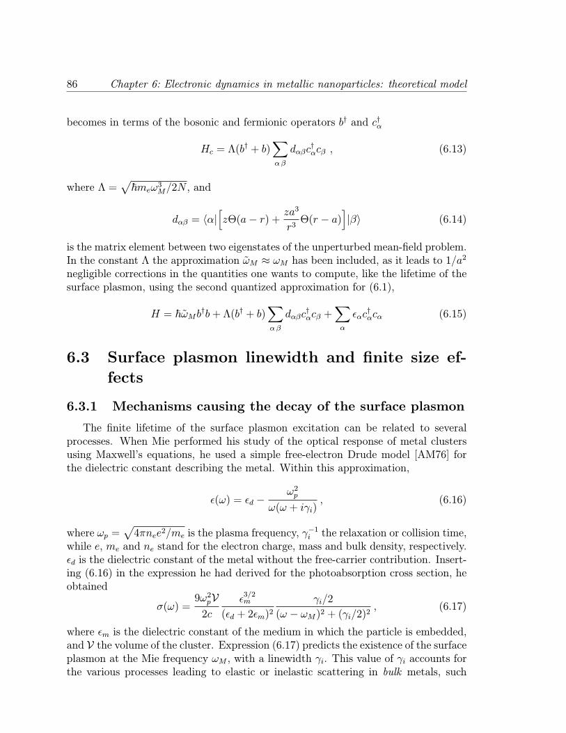
86 Chapter 6: Electronic dynamics in metallic nanoparticles: theoretical model
becomes in terms of the bosonic and fermionic operators b† and c†α
Hc = Λ(b† + b)
∑
αβ
dαβc†αcβ , (6.13)
where Λ =√~meω3M/2N , and
dαβ = 〈α|[zΘ(a− r) + za3
r3Θ(r − a)
]|β〉 (6.14)
is the matrix element between two eigenstates of the unperturbed mean-field problem.In the constant Λ the approximation ωM ≈ ωM has been included, as it leads to 1/a
2
negligible corrections in the quantities one wants to compute, like the lifetime of thesurface plasmon, using the second quantized approximation for (6.1),
H = ~ωMb†b+ Λ(b† + b)∑
αβ
dαβc†αcβ +
∑
α
εαc†αcα (6.15)
6.3 Surface plasmon linewidth and finite size ef-
fects
6.3.1 Mechanisms causing the decay of the surface plasmon
The finite lifetime of the surface plasmon excitation can be related to severalprocesses. When Mie performed his study of the optical response of metal clustersusing Maxwell’s equations, he used a simple free-electron Drude model [AM76] forthe dielectric constant describing the metal. Within this approximation,
ε(ω) = εd −ω2p
ω(ω + iγi), (6.16)
where ωp =√4πnee2/me is the plasma frequency, γ
−1i the relaxation or collision time,
while e, me and ne stand for the electron charge, mass and bulk density, respectively.εd is the dielectric constant of the metal without the free-carrier contribution. Insert-ing (6.16) in the expression he had derived for the photoabsorption cross section, heobtained
σ(ω) =9ω2pV2c
ε3/2m
(εd + 2εm)2γi/2
(ω − ωM)2 + (γi/2)2, (6.17)
where εm is the dielectric constant of the medium in which the particle is embedded,and V the volume of the cluster. Expression (6.17) predicts the existence of the surfaceplasmon at the Mie frequency ωM , with a linewidth γi. This value of γi accounts forthe various processes leading to elastic or inelastic scattering in bulk metals, such
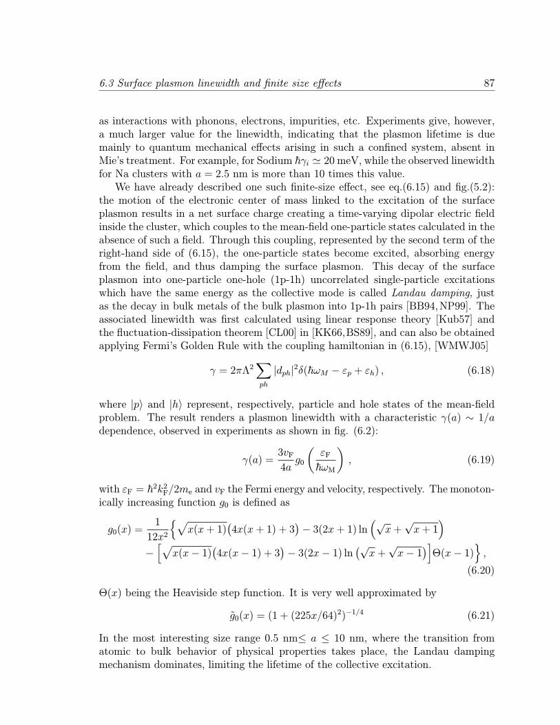
6.3 Surface plasmon linewidth and finite size effects 87
as interactions with phonons, electrons, impurities, etc. Experiments give, however,a much larger value for the linewidth, indicating that the plasmon lifetime is duemainly to quantum mechanical effects arising in such a confined system, absent inMie’s treatment. For example, for Sodium ~γi ' 20 meV, while the observed linewidthfor Na clusters with a = 2.5 nm is more than 10 times this value.We have already described one such finite-size effect, see eq.(6.15) and fig.(5.2):
the motion of the electronic center of mass linked to the excitation of the surfaceplasmon results in a net surface charge creating a time-varying dipolar electric fieldinside the cluster, which couples to the mean-field one-particle states calculated in theabsence of such a field. Through this coupling, represented by the second term of theright-hand side of (6.15), the one-particle states become excited, absorbing energyfrom the field, and thus damping the surface plasmon. This decay of the surfaceplasmon into one-particle one-hole (1p-1h) uncorrelated single-particle excitationswhich have the same energy as the collective mode is called Landau damping, justas the decay in bulk metals of the bulk plasmon into 1p-1h pairs [BB94,NP99]. Theassociated linewidth was first calculated using linear response theory [Kub57] andthe fluctuation-dissipation theorem [CL00] in [KK66,BS89], and can also be obtainedapplying Fermi’s Golden Rule with the coupling hamiltonian in (6.15), [WMWJ05]
γ = 2πΛ2∑
ph
|dph|2δ(~ωM − εp + εh) , (6.18)
where |p〉 and |h〉 represent, respectively, particle and hole states of the mean-fieldproblem. The result renders a plasmon linewidth with a characteristic γ(a) ∼ 1/adependence, observed in experiments as shown in fig. (6.2):
γ(a) =3vF4a
g0
(εF
~ωM
), (6.19)
with εF = ~2k2F/2me and vF the Fermi energy and velocity, respectively. The monoton-ically increasing function g0 is defined as
g0(x) =1
12x2
√x(x+ 1)
(4x(x+ 1) + 3
)− 3(2x+ 1) ln
(√x+√x+ 1
)
−[√
x(x− 1)(4x(x− 1) + 3
)− 3(2x− 1) ln
(√x+√x− 1
)]Θ(x− 1)
,
(6.20)
Θ(x) being the Heaviside step function. It is very well approximated by
g0(x) = (1 + (225x/64)2)−1/4 (6.21)
In the most interesting size range 0.5 nm≤ a ≤ 10 nm, where the transition fromatomic to bulk behavior of physical properties takes place, the Landau dampingmechanism dominates, limiting the lifetime of the collective excitation.
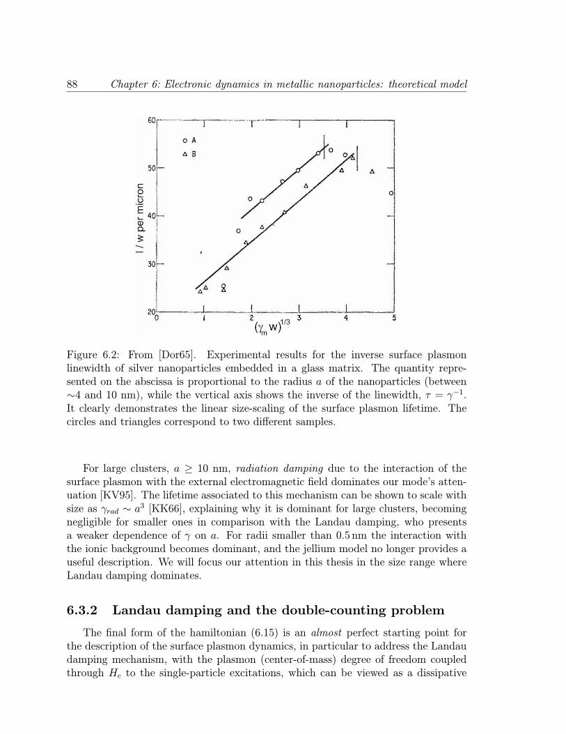
88 Chapter 6: Electronic dynamics in metallic nanoparticles: theoretical model
Figure 6.2: From [Dor65]. Experimental results for the inverse surface plasmonlinewidth of silver nanoparticles embedded in a glass matrix. The quantity repre-sented on the abscissa is proportional to the radius a of the nanoparticles (between∼4 and 10 nm), while the vertical axis shows the inverse of the linewidth, τ = γ−1.It clearly demonstrates the linear size-scaling of the surface plasmon lifetime. Thecircles and triangles correspond to two different samples.
For large clusters, a ≥ 10 nm, radiation damping due to the interaction of thesurface plasmon with the external electromagnetic field dominates our mode’s atten-uation [KV95]. The lifetime associated to this mechanism can be shown to scale withsize as γrad ∼ a3 [KK66], explaining why it is dominant for large clusters, becomingnegligible for smaller ones in comparison with the Landau damping, who presentsa weaker dependence of γ on a. For radii smaller than 0.5 nm the interaction withthe ionic background becomes dominant, and the jellium model no longer provides auseful description. We will focus our attention in this thesis in the size range whereLandau damping dominates.
6.3.2 Landau damping and the double-counting problem
The final form of the hamiltonian (6.15) is an almost perfect starting point forthe description of the surface plasmon dynamics, in particular to address the Landaudamping mechanism, with the plasmon (center-of-mass) degree of freedom coupledthrough Hc to the single-particle excitations, which can be viewed as a dissipative
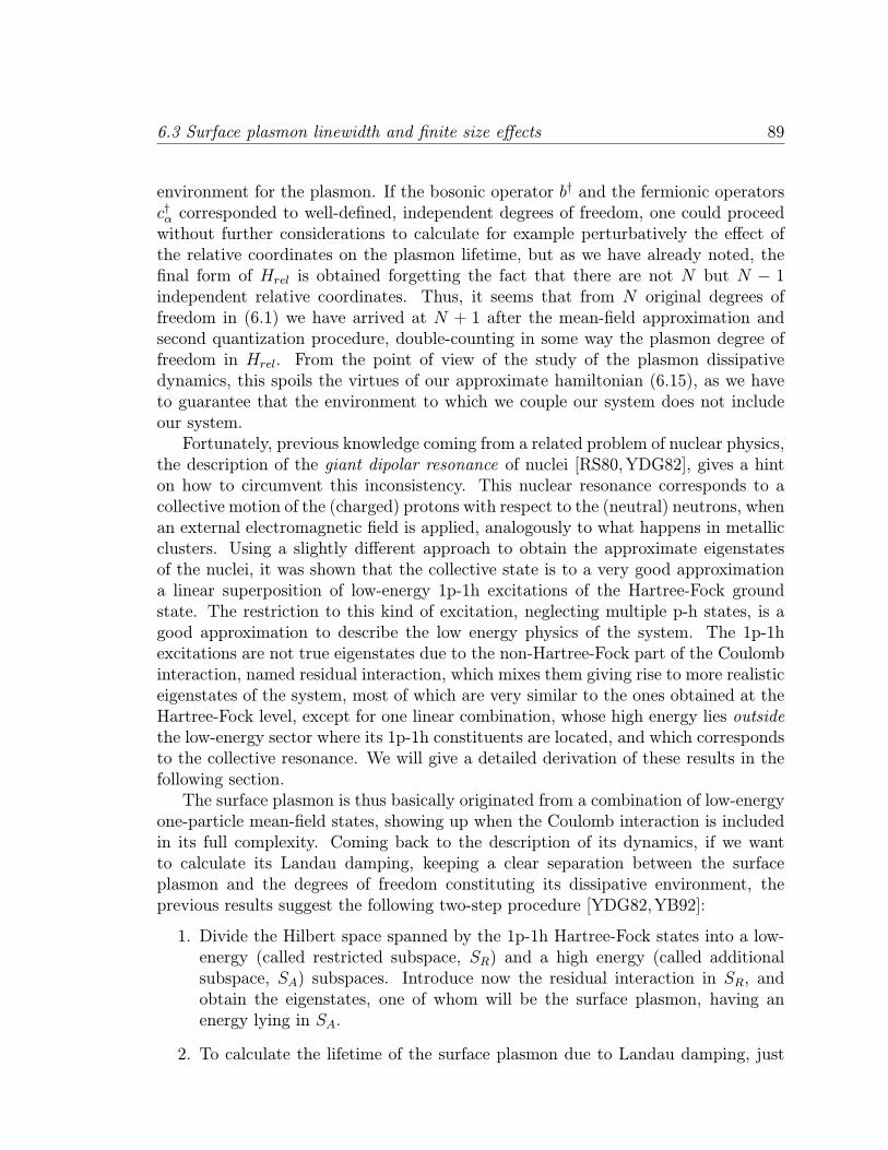
6.3 Surface plasmon linewidth and finite size effects 89
environment for the plasmon. If the bosonic operator b† and the fermionic operatorsc†α corresponded to well-defined, independent degrees of freedom, one could proceedwithout further considerations to calculate for example perturbatively the effect ofthe relative coordinates on the plasmon lifetime, but as we have already noted, thefinal form of Hrel is obtained forgetting the fact that there are not N but N − 1independent relative coordinates. Thus, it seems that from N original degrees offreedom in (6.1) we have arrived at N + 1 after the mean-field approximation andsecond quantization procedure, double-counting in some way the plasmon degree offreedom in Hrel. From the point of view of the study of the plasmon dissipativedynamics, this spoils the virtues of our approximate hamiltonian (6.15), as we haveto guarantee that the environment to which we couple our system does not includeour system.Fortunately, previous knowledge coming from a related problem of nuclear physics,
the description of the giant dipolar resonance of nuclei [RS80,YDG82], gives a hinton how to circumvent this inconsistency. This nuclear resonance corresponds to acollective motion of the (charged) protons with respect to the (neutral) neutrons, whenan external electromagnetic field is applied, analogously to what happens in metallicclusters. Using a slightly different approach to obtain the approximate eigenstatesof the nuclei, it was shown that the collective state is to a very good approximationa linear superposition of low-energy 1p-1h excitations of the Hartree-Fock groundstate. The restriction to this kind of excitation, neglecting multiple p-h states, is agood approximation to describe the low energy physics of the system. The 1p-1hexcitations are not true eigenstates due to the non-Hartree-Fock part of the Coulombinteraction, named residual interaction, which mixes them giving rise to more realisticeigenstates of the system, most of which are very similar to the ones obtained at theHartree-Fock level, except for one linear combination, whose high energy lies outsidethe low-energy sector where its 1p-1h constituents are located, and which correspondsto the collective resonance. We will give a detailed derivation of these results in thefollowing section.The surface plasmon is thus basically originated from a combination of low-energy
one-particle mean-field states, showing up when the Coulomb interaction is includedin its full complexity. Coming back to the description of its dynamics, if we wantto calculate its Landau damping, keeping a clear separation between the surfaceplasmon and the degrees of freedom constituting its dissipative environment, theprevious results suggest the following two-step procedure [YDG82,YB92]:
1. Divide the Hilbert space spanned by the 1p-1h Hartree-Fock states into a low-energy (called restricted subspace, SR) and a high energy (called additionalsubspace, SA) subspaces. Introduce now the residual interaction in SR, andobtain the eigenstates, one of whom will be the surface plasmon, having anenergy lying in SA.
2. To calculate the lifetime of the surface plasmon due to Landau damping, just
90 Chapter 6: Electronic dynamics in metallic nanoparticles: theoretical model
apply Fermi’s Golden Rule using the residual interaction coupling the plasmonto the quasi-continuum of states in SA degenerate with it.
In the context of the calculation of Landau damping using (6.1), the residual inter-action is given by Hc, and to avoid the mixing of the surface plasmon and what weconsider its environment, we just have to determine a safe energy cutoff ∆εc belowthe surface plasmon frequency ωpl such that (i) the value of ωpl is insensitive to theincrease of ∆εc, showing that the relevant low-energy Hartree-Fock 1p-1h excitationsbuilding up the surface plasmon lie below it, and (ii) only 1p-1h excitations above∆εc, which can be thus regarded as belonging to a subspace independent of the sur-face plasmon, are included in Fermi’s Golden Rule sum. The latter excitations areby definition SA, so that the linewidth has an expression
γ ∝∑
ph∈SA
|〈p|z|h〉|2δ(~ωpl − εp + εh) (6.22)
Here ph is a particle-hole excitation composed of a particle with energy εp and a holewith energy εh. In this calculation of γ the concrete estimate for the value of ∆εc isirrelevant as long as ∆εc < ωpl [YB92], but the approximate theoretical descriptionof other physical quantities might depend on the cutoff. For example, if one uses(6.15) to study the decay and decoherence of the surface plasmon, the timescales thatcharacterize the dynamics of the electronic environment in SA [WIWJ07] depend onthe cutoff energy. Moreover, it has been shown in [WIJW06] that the environment-induced redshift of the resonance frequency depends logarithmically on the cutoff.We will in the following section derive an estimate for this cutoff based on sound
physical arguments.
6.4 The surface plasmon as a superposition of low-
energy particle-hole excitations
To show this fact and find an estimate for ∆εc we will forget in this section aboutthe model based in a separation of center-of-mass plus relative coordinates describedin the beginning of previous section, whose main result was eq. (6.15), and useinstead the approach borrowed from the description of giant dipolar resonances innuclei which has already been briefly introduced.
6.4.1 Separable interaction ansatz
We now obtain the simplest model which starting from a mean-field approach in-cludes the essential features of the Coulomb interaction originating the surface plas-mon. The starting point is the simplest, mean-field approximation of the hamiltonian
6.4 The surface plasmon as a superposition of low-energy particle-hole excitations 91
(6.1), where the one-body electronic states obtained come from a self-consistent cal-culation like the TDLDA one (fig. 6.1). The problem with this naive approximation isthat it fails to describe the ability of the Coulomb interaction to create self-sustainedcollective excitations, like the surface plasmon we want to study. We have to introducean additional component δV (r) to the self-consistent potential V (r) which capturesthis feature of the Coulomb interaction. To obtain δV (r), we recall the fact thatthe occurrence of collective vibrational modes in a system governed by independent-particle motion can be understood in terms of the variations in the average one-bodypotential produced by an oscillation in the nanoparticle electronic density. Such vari-ations in the one-particle potential give rise to excitations in the electronic motion,and a self-sustained collective motion is obtained if the induced density variations areequal to those needed to generate the oscillating potential [BB75].
In our case, from the several collective modes susceptible of appearing in oursystem we focus our attention on the simplest, dipolar in character, surface plasmon.Starting from the knowledge of the existence of such a mode, the procedure to obtainthe associated δV (r) is then straightforward: calculate the variation in the averageone-body potential V (r) produced by an electronic density variation δn(r) linked tothe excitation of the collective mode. This was done in [WMWJ05], as follows:Assuming that at equilibrium the electron density is uniform within a sphere of
radius a, ne(r) = neΘ(a − r), a rigid displacement with a magnitude Z along thez-direction changes the density at r from ne(r) to ne(r − R) = ne(r) + δne(r). Tofirst order in the field R = Zez, δne(r) = −R · ∇ne(r) = Zne cos(θ)δ(r − a), whereθ = arccos(r · ez/|r|). The related change in the mean-field potential seen by theelectrons is thus
δV (r,R) =
∫d3r′δne(r
′)VC(r, r′) (6.23)
where VC(r, r′) denotes the Coulomb interaction between electrons. The term δH
which has to be added to the mean-field hamiltonian (6.11) is then
δH =N∑
i=1
δV (R, r′i) (6.24)
A simple expression for δV (r,R) can be obtained, given the spherical symmetry ofthe problem, using a multipolar decomposition for the Coulomb interaction [Jac75],namely
δV (r,R) = Z4πnee
2
3
[zΘ(a− r) + za3
r3Θ(r − a)
], (6.25)
so δV (r,R) is actually the same as R · ∇U(r), eq.(6.4). A further simplificationis obtained if we remember that, even though the electronic wavefunctions spreadoutside the geometrical boundaries of the nanocluster, giving rise to small quantumcorrections like the spill-out effect, the expected influence of the exact form of δV (r,R)
92 Chapter 6: Electronic dynamics in metallic nanoparticles: theoretical model
for r > a is very small. We can then simplify δV by extending its dipolar characteralso for r > a, δV (r,R) ≈ (4πnee2/3)Z · z, with a resulting separable form for δH
δH ≈ 1
2N
4πnee2
3
N∑
i j
zizj (6.26)
where Z =∑Ni zi/N has been used. The term separable applies to those interactions
satisfying V (xi, xj) ∼ f(xi) · f(xj), f(x) being a generic function of x, like (6.26).The results that would be obtained without the use of this approximation wouldinclude 1/N corrections to the ones we will present, like the estimate for ∆εc, so forour purposes we can work using the separable ansatz. Expressed in terms of themean-field hamiltonian basis |α〉, the second-quantized version of (6.26) reads
δH =∑
αβγδ
λdαγd∗δβc†αc†βcδcγ , (6.27)
where dαγ = 〈α|z|γ〉 are dipole matrix elements and λ is a positive constant.
6.4.2 Linear response theory and Random Phase Approxi-
mation for the surface plasmon
We will analyze the response of the nanocluster to a time-dependent weak ex-ternal perturbation, and obtain this response in a self-consistent way, leading to theRPA theory of response. The result will be written in terms of a response function,yet to be defined, whose poles determine the energies of the excited states. We willparticularize to the separable potential of the dipolar field (6.27), and see what areits effects on the energies of the self-consistent mean-field states. We will obtain asecular equation for those RPA eigenenergies, and show how to solve it graphically.
We follow [BB94] and [RS80]. Suppose we know the stationary one-particle eigen-states |i〉 and eigenenergies ei of the mean-field, time-independent hamiltonian (6.11),and now introduce a time-dependent external perturbation Vx(r, t) = Vx(r)e
iωt of agiven frequency ω, interacting with the system through its particle density n(r),
Hint(t) =
∫drVx(r, t)n(r) (6.28)
Then, the correction to the eigenstates of the system is, to first order in Hint(t),
φ′i(t) =[φi +
1
2
∑
j
〈j|Vx(r)|i〉( eiωt
ei − ej − ~ω+
e−iωt
ei − ej + ~ω
)]e−ieit/~ , (6.29)
6.4 The surface plasmon as a superposition of low-energy particle-hole excitations 93
where φi is the single-particle wave function of state |i〉. The particle density becomesnow n(r, t) =
∑occi |φ′i(r, t)|2 = n0(r) + δn(r)eiωt, with
δn(r) =occ∑
i
∑
j
〈j|Vx(r)|i〉〈i|n(r)|j〉( 1
ei − ej − ~ω+
1
ei − ej + ~ω
). (6.30)
We now define the independent particle retarded response function R0 for the densitychange at r induced by a potential field at r′, as
R0(r, r′, ω) =occ∑
i
∑
j
〈j|n(r)|i〉〈i|n(r′)|j〉( 1
ei − ej − ~ω+
1
ei − ej + ~ω
), (6.31)
In terms of R0, the response to an arbitrary perturbation potential can be calculatedfrom the integral,
δn(r, ω) =
∫dr′R0(r, r′, ω)Vx(r
′). (6.32)
This is the independent particle response, but one more ingredient has to be includedto construct the RPA theory of response. So far the only perturbation was theexternal field, but it is clear that the induced density oscillation δn(r, ω) will causethe self-consistent field to oscillate at the same frequency as well. We can define thechange of the mean-field potential with respect to small density changes in terms ofthe functional derivative δV (r)/δn(r′).In the case of an external long-wavelength fieldwe have seen that the main modification to the mean-field potential is the presence ofa dipolar electric field, described in (6.27). In terms of δV (r)/δn(r′) the time-varyingmean field is then
δV (r) =
∫dr′
δV (r)
δn(r′)δn(r′) (6.33)
Adding this potential to the external potential, we obtain the implicit equation forthe self-consistent density,
δnRPA(r, ω) =
∫drR0(r, r2, ω)
Vx(r2) +
∫dr′
δV (r2)
δn(r′)δnRPA(r
′)
(6.34)
It is more useful to express the self-consistent density in terms of the external field,defining in this way the RPA response function RRPA (we will always work withretarded response functions, so it will be assumed in the following, and not mentionedexplicitly as ”retarded”),
δnRPA(r, ω) =
∫dr′RRPA(r, r′, ω)Vx(r
′) . (6.35)
From (6.34) and (6.35) follows the implicit equation that the RPA response functionmust satisfy:
RRPA(r, r′, ω) = R0(r, r′, ω) +
∫dr2dr3R
0(r, r2, ω)δV (r2)
δn(r3)RRPA(r3, r
′, ω) (6.36)
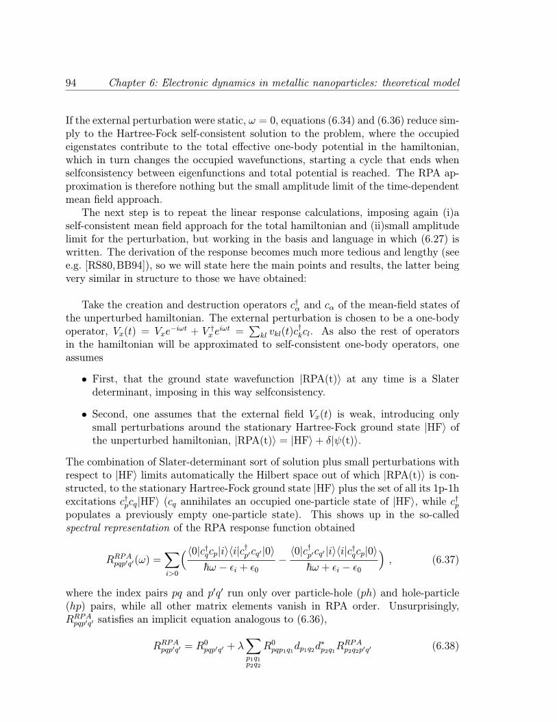
94 Chapter 6: Electronic dynamics in metallic nanoparticles: theoretical model
If the external perturbation were static, ω = 0, equations (6.34) and (6.36) reduce sim-ply to the Hartree-Fock self-consistent solution to the problem, where the occupiedeigenstates contribute to the total effective one-body potential in the hamiltonian,which in turn changes the occupied wavefunctions, starting a cycle that ends whenselfconsistency between eigenfunctions and total potential is reached. The RPA ap-proximation is therefore nothing but the small amplitude limit of the time-dependentmean field approach.The next step is to repeat the linear response calculations, imposing again (i)a
self-consistent mean field approach for the total hamiltonian and (ii)small amplitudelimit for the perturbation, but working in the basis and language in which (6.27) iswritten. The derivation of the response becomes much more tedious and lengthy (seee.g. [RS80,BB94]), so we will state here the main points and results, the latter beingvery similar in structure to those we have obtained:
Take the creation and destruction operators c†α and cα of the mean-field states ofthe unperturbed hamiltonian. The external perturbation is chosen to be a one-bodyoperator, Vx(t) = Vxe
−iωt + V †x eiωt =
∑kl vkl(t)c
†kcl. As also the rest of operators
in the hamiltonian will be approximated to self-consistent one-body operators, oneassumes
• First, that the ground state wavefunction |RPA(t)〉 at any time is a Slaterdeterminant, imposing in this way selfconsistency.
• Second, one assumes that the external field Vx(t) is weak, introducing onlysmall perturbations around the stationary Hartree-Fock ground state |HF〉 ofthe unperturbed hamiltonian, |RPA(t)〉 = |HF〉+ δ|ψ(t)〉.
The combination of Slater-determinant sort of solution plus small perturbations withrespect to |HF〉 limits automatically the Hilbert space out of which |RPA(t)〉 is con-structed, to the stationary Hartree-Fock ground state |HF〉 plus the set of all its 1p-1hexcitations c†pcq|HF〉 (cq annihilates an occupied one-particle state of |HF〉, while c†ppopulates a previously empty one-particle state). This shows up in the so-calledspectral representation of the RPA response function obtained
RRPApqp′q′(ω) =∑
i>0
(〈0|c†qcp|i〉〈i|c†p′cq′|0〉
~ω − εi + ε0−〈0|c†p′cq′|i〉〈i|c†qcp|0〉~ω + εi − ε0
), (6.37)
where the index pairs pq and p′q′ run only over particle-hole (ph) and hole-particle(hp) pairs, while all other matrix elements vanish in RPA order. Unsurprisingly,RRPApqp′q′ satisfies an implicit equation analogous to (6.36),
RRPApqp′q′ = R0pqp′q′ + λ
∑
p1q1p2q2
R0pqp1q1dp1q2d∗p2q1
RRPAp2q2p′q′ (6.38)
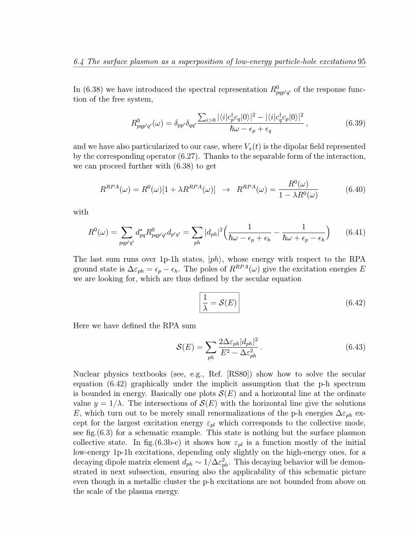
6.4 The surface plasmon as a superposition of low-energy particle-hole excitations 95
In (6.38) we have introduced the spectral representation R0pqp′q′ of the response func-tion of the free system,
R0pqp′q′(ω) = δpp′δqq′
∑i>0 |〈i|c†pcq|0〉|2 − |〈i|c†qcp|0〉|2
~ω − εp + εq, (6.39)
and we have also particularized to our case, where Vx(t) is the dipolar field representedby the corresponding operator (6.27). Thanks to the separable form of the interaction,we can proceed further with (6.38) to get
RRPA(ω) = R0(ω)[1 + λRRPA(ω)] → RRPA(ω) =R0(ω)
1− λR0(ω)(6.40)
with
R0(ω) =∑
pqp′q′
d∗pqR0pqp′q′dp′q′ =
∑
ph
|dph|2( 1
~ω − εp + εh− 1
~ω + εp − εh
)(6.41)
The last sum runs over 1p-1h states, |ph〉, whose energy with respect to the RPAground state is ∆εph = εp − εh. The poles of RRPA(ω) give the excitation energies Ewe are looking for, which are thus defined by the secular equation
1
λ= S(E) (6.42)
Here we have defined the RPA sum
S(E) =∑
ph
2∆εph|dph|2
E2 −∆ε2ph. (6.43)
Nuclear physics textbooks (see, e.g., Ref. [RS80]) show how to solve the secularequation (6.42) graphically under the implicit assumption that the p-h spectrumis bounded in energy. Basically one plots S(E) and a horizontal line at the ordinatevalue y = 1/λ. The intersections of S(E) with the horizontal line give the solutionsE, which turn out to be merely small renormalizations of the p-h energies ∆εph ex-cept for the largest excitation energy εpl which corresponds to the collective mode,see fig.(6.3) for a schematic example. This state is nothing but the surface plasmoncollective state. In fig.(6.3b-c) it shows how εpl is a function mostly of the initiallow-energy 1p-1h excitations, depending only slightly on the high-energy ones, for adecaying dipole matrix element dph ∼ 1/∆ε2ph. This decaying behavior will be demon-strated in next subsection, ensuring also the applicability of this schematic pictureeven though in a metallic cluster the p-h excitations are not bounded from above onthe scale of the plasma energy.
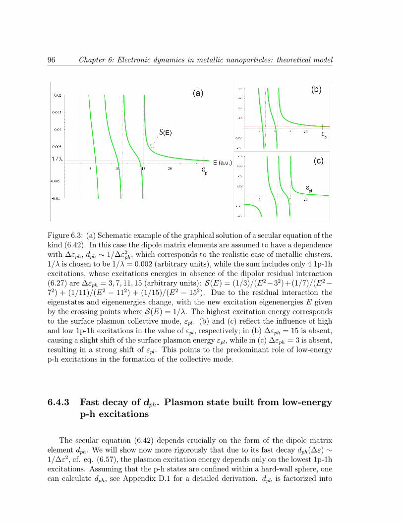
96 Chapter 6: Electronic dynamics in metallic nanoparticles: theoretical model
Figure 6.3: (a) Schematic example of the graphical solution of a secular equation of thekind (6.42). In this case the dipole matrix elements are assumed to have a dependencewith ∆εph, dph ∼ 1/∆ε2ph, which corresponds to the realistic case of metallic clusters.1/λ is chosen to be 1/λ = 0.002 (arbitrary units), while the sum includes only 4 1p-1hexcitations, whose excitations energies in absence of the dipolar residual interaction(6.27) are ∆εph = 3, 7, 11, 15 (arbitrary units): S(E) = (1/3)/(E2−32)+(1/7)/(E2−72) + (1/11)/(E2 − 112) + (1/15)/(E2 − 152). Due to the residual interaction theeigenstates and eigenenergies change, with the new excitation eigenenergies E givenby the crossing points where S(E) = 1/λ. The highest excitation energy correspondsto the surface plasmon collective mode, εpl. (b) and (c) reflect the influence of highand low 1p-1h excitations in the value of εpl, respectively; in (b) ∆εph = 15 is absent,causing a slight shift of the surface plasmon energy εpl, while in (c) ∆εph = 3 is absent,resulting in a strong shift of εpl. This points to the predominant role of low-energyp-h excitations in the formation of the collective mode.
6.4.3 Fast decay of dph. Plasmon state built from low-energy
p-h excitations
The secular equation (6.42) depends crucially on the form of the dipole matrixelement dph. We will show now more rigorously that due to its fast decay dph(∆ε) ∼1/∆ε2, cf. eq. (6.57), the plasmon excitation energy depends only on the lowest 1p-1hexcitations. Assuming that the p-h states are confined within a hard-wall sphere, onecan calculate dph, see Appendix D.1 for a detailed derivation. dph is factorized into
6.4 The surface plasmon as a superposition of low-energy particle-hole excitations 97
radial and angular parts [YB92]
dph = AmpmhlplhRlplh(εp, εh) . (6.44)
The angular part is expressed in terms of Wigner-3j symbols as
Ampmhlplh= (−1)mp
√(2lp + 1)(2lh + 1)×
(lp lh 10 0 0
)(lp lh 1−mp mh 0
)(6.45)
and sets the selection rules for the total and azimuthal angular momenta, respectively:
lp = lh ± 1 , mp = mh (6.46)
The radial part depends on the energies of the p-h states as
Rlplh(εp, εh) =2~2
mea
√εpεh
∆ε2ph. (6.47)
With the help of equations (6.44)–(6.47) and using the aforementioned dipole selectionrules (6.46), we can write the RPA sum (6.43) as
S(E) = 32k−2F
3
(εF
kFa
)2 ∑
nh,lhnp,lp=lh±1
flpεpεh
(E2 −∆ε2ph)∆ε3ph, (6.48)
where nh and np are radial quantum numbers. We have defined flp = lh+1 if lp = lh+1and flp = lh if lp = lh− 1. Using the semiclassical quantizations (D.24) and (D.25) ofAppendix D.2, we finally obtain the result shown in Figure 6.4.In the figure we show (solid black line) the resulting E-dependence of (6.48). The
crossings of this curve with the horizontal dotted one with height 1/λ yield the exci-tation spectrum within the RPA. The lowest p-h energy estimated in Appendix D.2is
∆εmin 'εF
kFa/π. (6.49)
The existence of a gap in the excitation spectrum of the dipole operator stems fromthe quantization of the states in a hard-wall sphere and the dipole selection rules.Whenever the energy E coincides with a p-h excitation energy ∆εph, we have adivergence in S(E) (see vertical grey lines in Fig. 6.4). For the lowest energies Eof the interval considered the sum is dominated by the term associated with thedivergence closest to E. On the other hand, for the largest energies E, the fast decayof dph with ∆εph means that the divergences are only relevant for energies extremelyclose to them. Away from the divergences the sum is dominated by the contributionsarising from the low-energy p-h excitations.
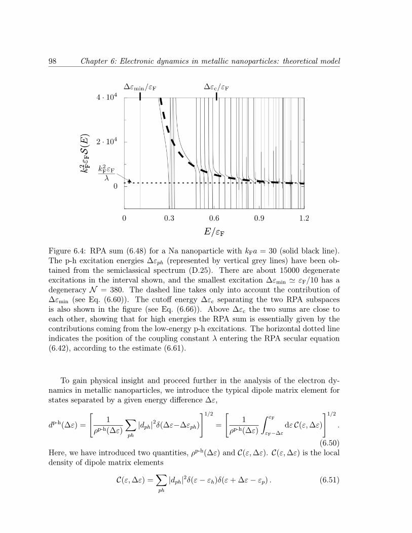
98 Chapter 6: Electronic dynamics in metallic nanoparticles: theoretical model
Figure 6.4: RPA sum (6.48) for a Na nanoparticle with kFa = 30 (solid black line).The p-h excitation energies ∆εph (represented by vertical grey lines) have been ob-tained from the semiclassical spectrum (D.25). There are about 15000 degenerateexcitations in the interval shown, and the smallest excitation ∆εmin ' εF/10 has adegeneracy N = 380. The dashed line takes only into account the contribution of∆εmin (see Eq. (6.60)). The cutoff energy ∆εc separating the two RPA subspacesis also shown in the figure (see Eq. (6.66)). Above ∆εc the two sums are close toeach other, showing that for high energies the RPA sum is essentially given by thecontributions coming from the low-energy p-h excitations. The horizontal dotted lineindicates the position of the coupling constant λ entering the RPA secular equation(6.42), according to the estimate (6.61).
To gain physical insight and proceed further in the analysis of the electron dy-namics in metallic nanoparticles, we introduce the typical dipole matrix element forstates separated by a given energy difference ∆ε,
dp-h(∆ε) =
[1
ρp-h(∆ε)
∑
ph
|dph|2δ(∆ε−∆εph)
]1/2=
[1
ρp-h(∆ε)
∫ εF
εF−∆εdε C(ε,∆ε)
]1/2.
(6.50)Here, we have introduced two quantities, ρp-h(∆ε) and C(ε,∆ε). C(ε,∆ε) is the localdensity of dipole matrix elements
C(ε,∆ε) =∑
ph
|dph|2δ(ε− εh)δ(ε+∆ε− εp) . (6.51)
6.4 The surface plasmon as a superposition of low-energy particle-hole excitations 99
As shown in Appendix D.4, this can be expressed as
C(ε,∆ε) = 1
3π2a2
∆ε2F( ε
∆ε
), (6.52)
whereF (x) = (2x+ 1)
√x(x+ 1)− ln
(√x+√x+ 1
). (6.53)
For ∆ε ε, equation (6.52) simplifies to
C(ε,∆ε) ' 2a2
3π2ε2
∆ε4. (6.54)
In expression (6.50),
ρp-h(∆ε) =∑
ph
δ(∆εph −∆ε)δlh,lp±1δmh,mp (6.55)
is the density of p-h excitations with energy ∆ε respecting the dipole selection rules.In order to simplify the presentation, we do not consider spin degeneracy factors. InAppendix D.5 we show that for ∆ε εF we have
ρp-h(∆ε) ' (kFa)4
4π2∆ε
ε2F, (6.56)
and therefore in such a limit the typical matrix element (6.50) can be approximatedby
dp-h(∆ε) ' 2√2k−1F√3kFa
( εF∆ε
)2. (6.57)
To check the validity of our estimate of the typical dipole matrix element, there isan exact sum rule
∑ph∆εph|dp-h|2 = (3/4π)~2N/2me [LS91,YB92], satisfied also in
the presence of Coulomb interactions between electrons. Performing the sum using(6.57)
EF∑
ph
∆εph|dp-h(∆ε)|2 '∫ EF
∆εmin
d∆ε∆ε[∫ EF
EF−∆εdεC(ε,∆ε)
](6.58)
one obtains about 70% of the exact result (3/4π)~2N/2me [Bra93]. This is quitereasonable regarding all the approximations we made to obtain (6.57).In order to emphasize once more the importance of the low-energy p-h excitations,
we present in Figure 6.4 (dashed line) the contribution to the RPA sum coming onlyfrom the infrared p-h excitation energy with the appropriate degeneracy factor N(see Eq. (D.27) in App. D.2). Indeed, we can estimate (6.43) as
S(E) ≈ N ×2∆εmin
[dp-h(∆εmin)
]2
E2 −∆ε2min. (6.59)
100 Chapter 6: Electronic dynamics in metallic nanoparticles: theoretical model
With the results (6.49), (6.57), and (D.27), we obtain
S(E) ≈ 64k−2F
3π5(kFa)
3 εF
E2 − (εFπ/kFa)2. (6.60)
While in the lower part of the energy interval in Figure 6.4 the two curves exhibitconsiderable discrepancies, in the second half of the interval they are very close (exceptof course at the divergences). Since the collective excitation is found in this lastinterval, we see that it is mainly the low-energy p-h excitations that are relevant forthe definition of the collective excitation.Since the resonance energy is known from experiments, we can obtain the value
of the coupling constant λ. Indeed, using the estimate (6.60) evaluated at E = ~ωMin the secular equation (6.42), we obtain
1
λ' 64k
−2F
3π5(kFa)
3 εF
(~ωM)2(6.61)
to leading order in kFa 1. Notice that this result is consistent with the estimateobtained from the energy-weighted sum rule given in [YB92]. For the case studiedin Figure 6.4, our estimate (6.61) yields k2FεF/λ ≈ 1600. As the radius a increasesthe lowest p-h energy decreases like 1/a, the degeneracy at this value increases as a2,and the density of p-h excitations contributing to (6.43), ρp-h(∆ε), grows as a4. Thisincrease in the number of excitations contributing to the sum is partially cancelled bythe 1/a behaviour of the typical dipole matrix element, resulting in a decrease of thecoupling constant λ proportional to the number of particles in the cluster, λ ∼ 1/a3,and a value of the plasmon frequency which remains almost unaffected. Therefore,for a larger nanoparticle size, the divergences shown in Figure 6.4 would be moredense in energy, starting at a lower energy, and the vertical scale would increase asa3, thus obtaining a similar value for the plasmon excitation energy ~ωM.
6.4.4 Separation of the reduced and additional particle-hole
subspaces
As we have shown in the last section, the high-energy part of the p-h spectrum isnot crucial for the determination of the energy of the collective excitation. In whatfollows we make this statement more quantitative and estimate the upper-boundcutoff ∆εc of the low-energy excitations that we need in order to obtain a stableposition of the surface plasmon.In order to obtain a quantitative estimate of the cutoff, we require that by changing
it from ∆εc to (3/2)∆εc, the position of the plasmon changes only by a fraction of itslinewidth γ, the smallest energy scale with experimental significance. Our criterionleads to the condition
S∆εc(~ωM) = S 32∆εc(~ωM + ~γ) , (6.62)
6.4 The surface plasmon as a superposition of low-energy particle-hole excitations101
with the RPA sum S that has been defined in (6.43). The additional subscript refersto the upper bound of the p-h energies.The left-hand side of (6.62) can be estimated according to
S∆εc(~ωM) '∫ ∆εc
∆εmin
d∆ε ρp-h(∆ε)2∆ε[dp-h(∆ε)
]2
(~ωM)2 −∆ε2, (6.63)
with dp-h and ρp-h as defined in (6.50) and (6.55), respectively. Using (6.56) and(6.57), we obtain
S∆εc(~ωM) '4k−2F3π2
(kFa
εF
~ωM
)2(1
∆εmin− 1
∆εc
)(6.64)
to leading order in kFa. Similarly,
S 32∆εc(~ωM + ~γ) '
4k−2F3π2
(kFa
εF
~ωM
)2(1− 2γ
ωM
)(1
∆εmin− 2
3∆εc
). (6.65)
Using the expressions (6.19) and (6.49) for γ and ∆εmin, respectively, finally yieldsaccording to the criterion (6.62) the main result of this chapter, an estimate for thecutoff energy based on sound physical arguments
∆εc 'π
9g0(εF/~ωM)~ωM , (6.66)
with the function g0 defined in (6.20). For Na clusters, we have εF/~ωM = 0.93 andour criterion yields a value ∆εc ' (3/5)εF.We have verified the robustness of our criterion (6.62) by exploring different phys-
ical parameters, like the size of the cluster. Indeed, it can be seen in Figure 6.4 thatabove ∆εc the RPA sum evaluated from (6.48) (solid line) and the estimate (6.60)(dashed line) are close to each other, showing that for high energies the RPA sum isessentially given by the contributions coming from the low-energy p-h excitations. Wehave checked that this feature of ∆εc is independent of the size a of the nanoparticle.In order to have a well-defined collective excitation, the cutoff energy ∆εc must
obviously be larger than the minimal p-h excitation energy (6.49). For Na, we findthat this condition is already verified with only N = 20 conduction electrons inthe nanoparticle, in agreement with the experiments of reference [SKM+91] and thenumerical calculations of reference [YB91].Eq. (6.66) is the key ingredient we needed to avoid the problem of the clear
separation between the plasmon and its environment, as discussed in section 6.3.2.The splitting in low ∆εph < ∆εc and high-energy ∆εph > ∆εc p-h excitations givesphysical soundness to the method based on the separation of the electronic degreesof freedom into centre-of-mass and relative coordinates [GGI02,WIJW06,WMWJ05,
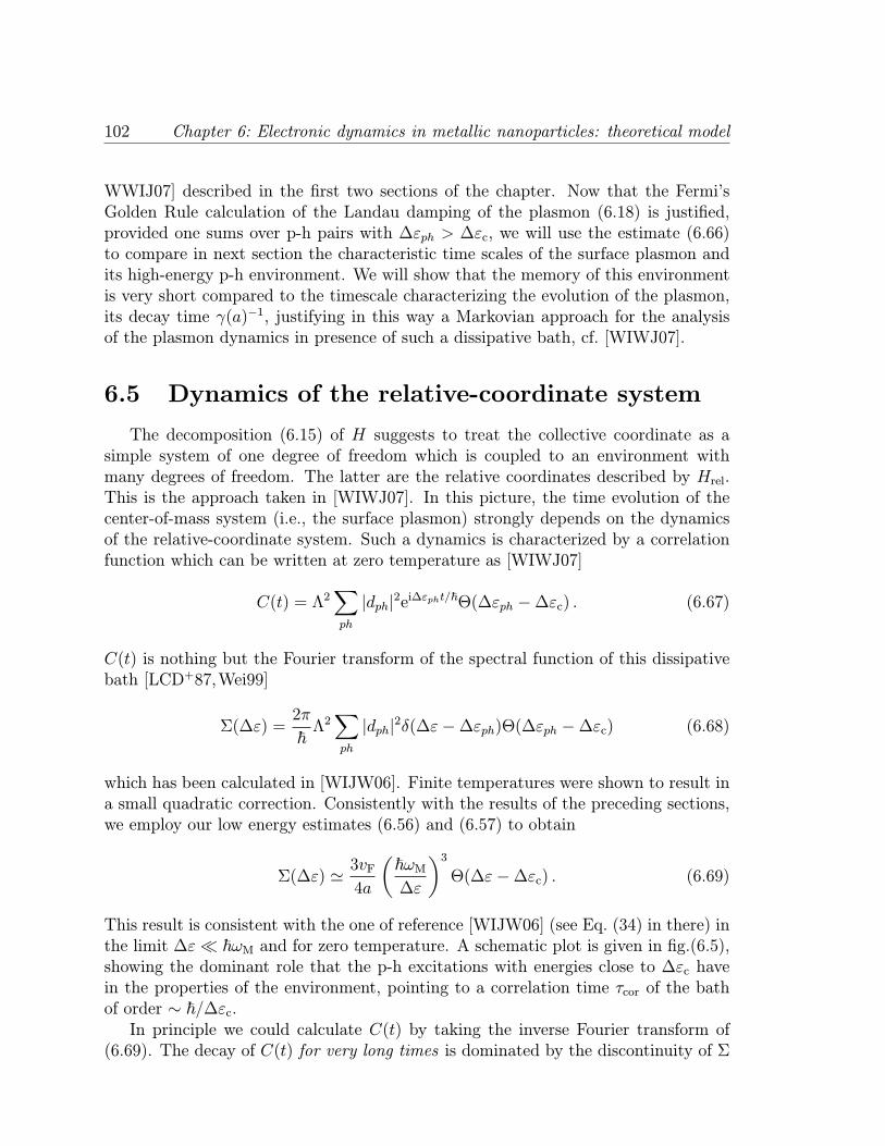
102 Chapter 6: Electronic dynamics in metallic nanoparticles: theoretical model
WWIJ07] described in the first two sections of the chapter. Now that the Fermi’sGolden Rule calculation of the Landau damping of the plasmon (6.18) is justified,provided one sums over p-h pairs with ∆εph > ∆εc, we will use the estimate (6.66)to compare in next section the characteristic time scales of the surface plasmon andits high-energy p-h environment. We will show that the memory of this environmentis very short compared to the timescale characterizing the evolution of the plasmon,its decay time γ(a)−1, justifying in this way a Markovian approach for the analysisof the plasmon dynamics in presence of such a dissipative bath, cf. [WIWJ07].
6.5 Dynamics of the relative-coordinate system
The decomposition (6.15) of H suggests to treat the collective coordinate as asimple system of one degree of freedom which is coupled to an environment withmany degrees of freedom. The latter are the relative coordinates described by Hrel.This is the approach taken in [WIWJ07]. In this picture, the time evolution of thecenter-of-mass system (i.e., the surface plasmon) strongly depends on the dynamicsof the relative-coordinate system. Such a dynamics is characterized by a correlationfunction which can be written at zero temperature as [WIWJ07]
C(t) = Λ2∑
ph
|dph|2ei∆εpht/~Θ(∆εph −∆εc) . (6.67)
C(t) is nothing but the Fourier transform of the spectral function of this dissipativebath [LCD+87,Wei99]
Σ(∆ε) =2π
~Λ2∑
ph
|dph|2δ(∆ε−∆εph)Θ(∆εph −∆εc) (6.68)
which has been calculated in [WIJW06]. Finite temperatures were shown to result ina small quadratic correction. Consistently with the results of the preceding sections,we employ our low energy estimates (6.56) and (6.57) to obtain
Σ(∆ε) ' 3vF4a
(~ωM∆ε
)3Θ(∆ε−∆εc) . (6.69)
This result is consistent with the one of reference [WIJW06] (see Eq. (34) in there) inthe limit ∆ε ~ωM and for zero temperature. A schematic plot is given in fig.(6.5),showing the dominant role that the p-h excitations with energies close to ∆εc havein the properties of the environment, pointing to a correlation time τcor of the bathof order ∼ ~/∆εc.In principle we could calculate C(t) by taking the inverse Fourier transform of
(6.69). The decay of C(t) for very long times is dominated by the discontinuity of Σ
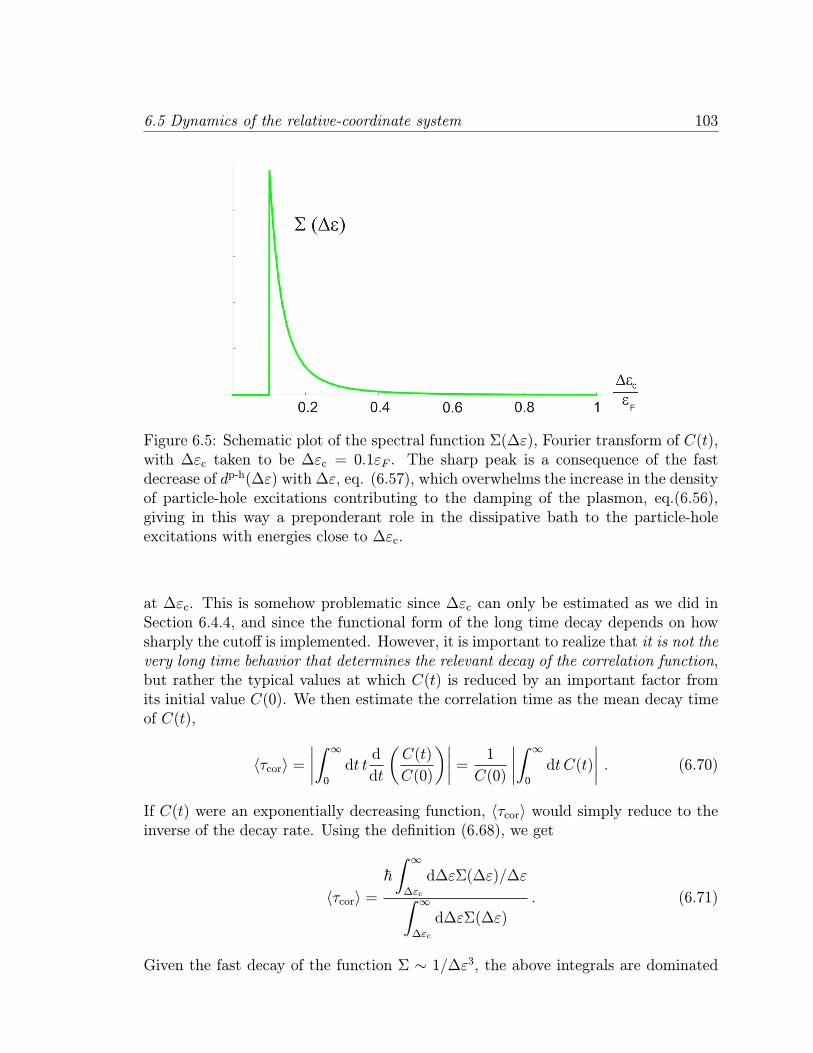
6.5 Dynamics of the relative-coordinate system 103
Figure 6.5: Schematic plot of the spectral function Σ(∆ε), Fourier transform of C(t),with ∆εc taken to be ∆εc = 0.1εF . The sharp peak is a consequence of the fastdecrease of dp-h(∆ε) with ∆ε, eq. (6.57), which overwhelms the increase in the densityof particle-hole excitations contributing to the damping of the plasmon, eq.(6.56),giving in this way a preponderant role in the dissipative bath to the particle-holeexcitations with energies close to ∆εc.
at ∆εc. This is somehow problematic since ∆εc can only be estimated as we did inSection 6.4.4, and since the functional form of the long time decay depends on howsharply the cutoff is implemented. However, it is important to realize that it is not thevery long time behavior that determines the relevant decay of the correlation function,but rather the typical values at which C(t) is reduced by an important factor fromits initial value C(0). We then estimate the correlation time as the mean decay timeof C(t),
〈τcor〉 =∣∣∣∣
∫ ∞
0
dt td
dt
(C(t)
C(0)
)∣∣∣∣ =1
C(0)
∣∣∣∣
∫ ∞
0
dt C(t)
∣∣∣∣ . (6.70)
If C(t) were an exponentially decreasing function, 〈τcor〉 would simply reduce to theinverse of the decay rate. Using the definition (6.68), we get
〈τcor〉 =~∫ ∞
∆εc
d∆εΣ(∆ε)/∆ε
∫ ∞
∆εc
d∆εΣ(∆ε)
. (6.71)
Given the fast decay of the function Σ ∼ 1/∆ε3, the above integrals are dominated
104 Chapter 6: Electronic dynamics in metallic nanoparticles: theoretical model
by their lower limit ∆εc and we have
〈τcor〉 '2
3
~∆εc
. (6.72)
Since ∆εc is of the order of (3/5)εF, we see that the response time (or correlationtime) of the electronic environment is of the order of its inverse Fermi energy.The estimate of the characteristic response time of the electronic environment is
crucial in justifying the Markovian approximation used in [WIWJ07]. In that work,the degrees of freedom corresponding to the relative coordinates were integrated outand treated as an incoherent heat bath that acts on the collective coordinate. Suchan approach relies on the fast response of the environment as compared to the timeevolution of the surface plasmon. The typical scale for the latter is the inverse of thedecay rate, τsp = 1/γ. Using (6.19) and (6.66), we therefore have
τsp
〈τcor〉=
π
9[g0(εF/~ωM)]2~ωMεF
kFa . (6.73)
For the example of Na nanoparticles worked in Section 6.4.3, we have τsp/〈τcor〉 ' kFa.This is a safe limit since in not too small nanoparticles, kFa 1. As the size of thecluster increases, the applicability of the Markovian approximation is more justified.This is expected since the electronic bath has more and more degrees of freedom,approaching an “environment” in the sense of quantum dissipation. Since the physicalparameters of alkaline nanoparticles entering (6.73) are close to that of noble-metalclusters, the dynamics of the surface plasmon can be expected to be Markovian inthat case too.
6.6 Conclusions
We have studied the role of particle-hole excitations on the dynamics of the surfaceplasmon. A key concept in this analysis is the separation into low-energy excitationswhich lead to the collective excitation once they are mixed by the residual dipolarinteraction, and high-energy excitations that act as an environment damping theresonance. Using the random phase approximation and assuming the separabilityof the residual interaction, we have established a criterion for estimating the cutoffenergy separating the low- and high-energy subspaces. The resulting cutoff energy isapproximately (3/5)εF for the case of Na nanoparticles.Since the number of electrons in the cluster is finite, the assumption that the high-
energy particle-hole excitations act on the collective excitation as an environment,introducing friction in its dynamics, may be questionable. What settles this issue isthe ratio between the typical evolution time of the collective excitation and the oneof the high-energy particle-hole excitations. The former is given by the inverse of
6.6 Conclusions 105
the plasmon linewidth, while the latter is obtained from the decay of the correlationfunction of the environment. We have found that this ratio improves with increasingcluster size. Even for a small cluster with a = 1nm, the ratio is approximately 10,justifying the use of the Markovian approximation which assumes a fast time evolutionof the environment with respect to the one of the collective excitation.The relevance of memory effects in the electronic dynamics of small clusters is
of current interest, due to the advance in time-resolved experimental techniques[BHMD00, FVF+00, LKLA99, LUCS01]. First-principle calculations have recentlyaddressed this issue by comparing time-dependent density functional theories withand without memory effects for small gold clusters [KB06]. For very small clusters(N < 8) memory effects were shown to be important. It has to be noted, how-ever, that the memory considered in [KB06] is that of the electron gas as a whole,while we are concerned in this work with the memory arising from the dynamicalevolution of the relative-coordinate subsystem. It would be interesting to considercluster sizes intermediate between the ones considered in the present work and thoseof reference [KB06] in order to study the emergence of memory effects.
106 Chapter 6: Electronic dynamics in metallic nanoparticles: theoretical model
Appendix A
Appendix to Chapter 1
A.1 Modes’ equations of motion of quasi-1D res-
onators.
A.1.1 Elasticity basics.
We will follow ref. [LL59]. The starting point is to define the displacement vectorof a given point xi in the solid, ui = x′i − xi, representing the difference betweenthe coordinates of the same point before and after the deformation. The relatedmagnitude that appears everywhere in the theory of elasticity is the so-called straintensor (symmetric by definition):
uik =1
2
( ∂ui∂xk+∂uk
∂xi+∂ul
∂xi
∂ul
∂xk
)' 12
( ∂ui∂xk+∂uk
∂xi
)(A.1)
Then the stress tensor σik is defined, considering the forces Fi exerted on a smallvolume dV due to the deformation of a body:
∫FidV =
∫∂σik
∂xkdV =
∮σikdSk → Fi =
∂σik
∂xk(A.2)
With these two quantities one can study the thermodynamics of the deformation:take a deformed body and suppose there is a small variation in the deformation, sothat ui → ui + δui, then the internal work done by the internal forces is given by
∫∂σik
∂xkδuidV (A.3)
We will consider bodies at a fixed temperature T , so the thermodynamic potential wewill use is the free energy F = U − TS, with a variation of F in a small deformationat a constant T given by dF = σikduik, implying σik = ∂F/∂uik
∣∣T. Now, for small
deformations, choosing as non-deformed state the one in absence of external forces, we
107
108 Appendix A: Appendix to Chapter 1
can expand F as a function of uik, obtaining F =12λiklmuikulm, so that σik = λiklmulm
(Hooke’s law). For an isotropic body the expression reduces to F = F0+(λ/2)u2ii+µu
2ik
(λ and µ are the Lame coefficients), which can be reexpressed as
F = µ(uik −
1
3δikull
)2+K
2u2ll , K = λ+
2
3µ (A.4)
defining the rigidity modulus K. If the deformation is homogeneous (the strain ten-sor is constant throughout the body), and more specifically a simple extension orcompression along the z axis, one has
σzz = E × uzz , (A.5)
defining the Young modulus,
E =9Kµ
3K + µ(A.6)
The ratio between transversal contraction uxx and longitudinal elongation uzz is Pois-son’s coefficient
ν = −uxxuzz=1
2
3K − 2µ3K + µ
. (A.7)
A.1.2 The case of a rod.
We start defining a local coordinate system (ξ, η, ζ), attached to the point, thatcoincides with (x, y, z) in the absence of deformation (the rod is then along the Z axis).
Next we define ~Ω = d~φ/dl, the rate of variation of the relative rotation angle betweenthe local coordinate systems of two adjacent points (dl is taken along the bar’s main
axis). For example, a pure bending has ~Ω = Ωη~η. Now we define a coordinate systemfixed in space, independent of the rod, with respect to whom a point in the rod willbe given by a vector ~r. The tangent vector at that point is given by ~t = d~r/dl, andthe curvature by d~t/dl, with modulus 1/R, defining the curvature radius. For a slightbending one has
~Ω = ~t ∧ d~t
dl' ~t ∧ d
2~r
dz2=(− d2Y
dz2,d2X
dz2, 0)
(A.8)
In terms of ~Ω the free energy of a rod is deduced to be
Frod =1
2
∫ I1EΩ
2ξ + I2EΩ
2η + CΩ
2ζ
dl (A.9)
where I1 and I2 are the principal inertia moments of the section of the rod, and C isthe so-called torsional rigidity. In the case of a slight bending the expression reducesto
Fbending =E
2
∫ I1
(d2Xdz2
)2+ I2
(d2Ydz2
)2dz (A.10)
Now we will deduce the equations for the modes as slight deviations from the equilib-rium situation, and the first step towards our goal is the analysis of the equilibriumequations.
A.1 Modes’ equations of motion of quasi-1D resonators. 109
Equilibrium conditions.
If there are external forces ~Fext applied to the rod, and external moments ~Mextassociated with them, the rod will suffer a deformation until the internal forces andmoments compensate the external ones, so in equilibrium one must have
~Fext + ~Fint = 0~Mext + ~Mint = 0
Considering the case of slight bending, for which ~Ω is given by eq.(A.8), the internal
moment ~Mint associated to the internal stresses is ~Mint bending = (−EI1Y ′′, EI2X ′′, 0),where the double prime represents ∂2/∂z2. Taking a small volume of length dl and
supposing an external force per unit length along the rod ~Fext = ~K = (Kx, Ky, Kz),
the first of the equilibrium equations results in d~F/dl = − ~K, and the second ind ~Mint+ [d~l ∧ ~K] = 0→ d ~Mint/dl = ~F ∧~t. Deriving the second equation with respectto l, and taking into account the small value of d~t/dl (slight bending), one arrives at
d2 ~Mint/dl2 = ~t ∧ ~K, so that
EI2 ∂
4X/∂z4 = KxEI1 ∂
4Y/∂z4 = Ky(A.11)
and the internal forces will be given byFx = −EI2X ′′′Fy = −EI1Y ′′′
Mode’s equations.
To obtain the equations of motion of an elastic medium, we start from Newton’sequation equating the product of mass and acceleration to the internal forces themass is subject to
ρui =∂σik
∂xk(A.12)
In the simplest case of longitudinal vibrations we have, using eq.(A.5)
ρuz =∂σzk
∂xk→ ∂2uz
∂z2=
ρ
E
∂2uz
∂t2(A.13)
This is the usual wave equation with linear dispersion relation. For the bending(flexural) case, the equations of motion are obtained just by substituting −Kx and−Ky in the equilibrium equations (A.11) by ρSX and ρSY (S = transversal sectionof the rod):
EIy∂4X
∂z4= −ρS∂
2X
∂t2
EIx∂4Y
∂z4= −ρS∂
2Y
∂t2. (A.14)
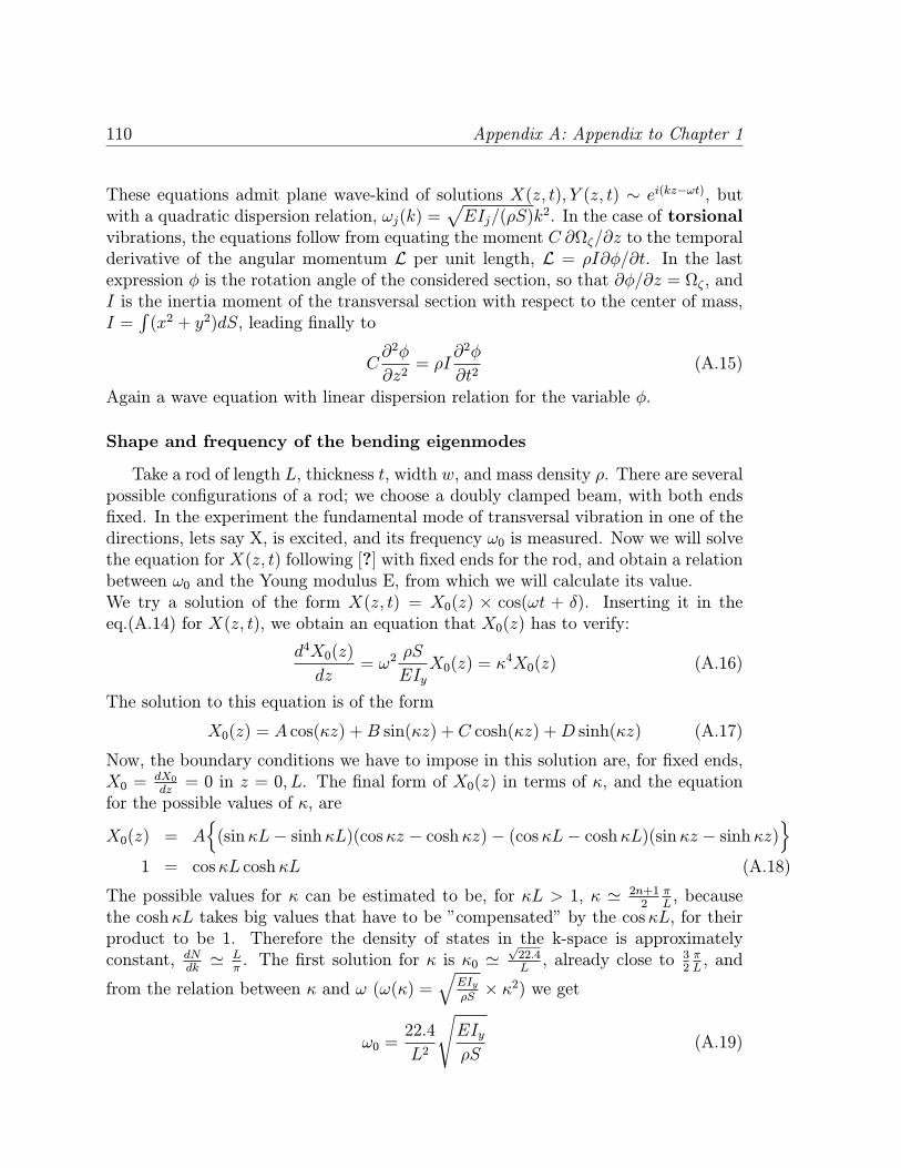
110 Appendix A: Appendix to Chapter 1
These equations admit plane wave-kind of solutions X(z, t), Y (z, t) ∼ ei(kz−ωt), butwith a quadratic dispersion relation, ωj(k) =
√EIj/(ρS)k
2. In the case of torsionalvibrations, the equations follow from equating the moment C ∂Ωζ/∂z to the temporalderivative of the angular momentum L per unit length, L = ρI∂φ/∂t. In the lastexpression φ is the rotation angle of the considered section, so that ∂φ/∂z = Ωζ , andI is the inertia moment of the transversal section with respect to the center of mass,I =∫(x2 + y2)dS, leading finally to
C∂2φ
∂z2= ρI
∂2φ
∂t2(A.15)
Again a wave equation with linear dispersion relation for the variable φ.
Shape and frequency of the bending eigenmodes
Take a rod of length L, thickness t, width w, and mass density ρ. There are severalpossible configurations of a rod; we choose a doubly clamped beam, with both endsfixed. In the experiment the fundamental mode of transversal vibration in one of thedirections, lets say X, is excited, and its frequency ω0 is measured. Now we will solvethe equation for X(z, t) following [?] with fixed ends for the rod, and obtain a relationbetween ω0 and the Young modulus E, from which we will calculate its value.We try a solution of the form X(z, t) = X0(z) × cos(ωt + δ). Inserting it in theeq.(A.14) for X(z, t), we obtain an equation that X0(z) has to verify:
d4X0(z)
dz= ω2
ρS
EIyX0(z) = κ
4X0(z) (A.16)
The solution to this equation is of the form
X0(z) = A cos(κz) +B sin(κz) + C cosh(κz) +D sinh(κz) (A.17)
Now, the boundary conditions we have to impose in this solution are, for fixed ends,X0 =
dX0dz= 0 in z = 0, L. The final form of X0(z) in terms of κ, and the equation
for the possible values of κ, are
X0(z) = A(sinκL− sinhκL)(cosκz − coshκz)− (cosκL− coshκL)(sinκz − sinhκz)
1 = cosκL coshκL (A.18)
The possible values for κ can be estimated to be, for κL > 1, κ ' 2n+12πL, because
the coshκL takes big values that have to be ”compensated” by the cosκL, for theirproduct to be 1. Therefore the density of states in the k-space is approximatelyconstant, dN
dk' Lπ. The first solution for κ is κ0 '
√22.4L, already close to 3
2πL, and
from the relation between κ and ω (ω(κ) =√EIyρS× κ2) we get
ω0 =22.4
L2
√EIy
ρS(A.19)
Appendix B
Appendix to Chapter 2
B.1 Some details about the Standard Tunneling
Model.
B.1.1 Distribution function of the TLSs
From ref. [Phi87]. The tunneling model proposes the existence of an ensemble ofTLSs, each one characterized by a hamiltonian:
H0 = ∆x0σx +∆
z0σz (B.1)
The task is to determine the probability density distribution P (∆x0 ,∆z0) of the TLSs
in terms of ∆x0 and ∆z0. A simplified expression for the tunneling amplitude as a
function of the potential barrier height V and width d is
∆x0 = ~Ωe−λ = ~Ωe−d(2mV/~2)1/2 (B.2)
where ~Ω is approximately equal to the average of the ground states of both isolatedwells, and m is the particle mass.Typical values for λ can be estimated demanding that ∆x0 must be approximatelyequal to kT if the tunneling state is to contribute to thermal properties at a temper-ature T . At 1 K this requires a tunnel splitting of 10−4 eV, which with ~Ω ∼ 10−2eV gives approximately λ ∼ 5. This is equivalent to a bare proton tunneling across abarrier of 0.1 eV with d = 0.7 A.For ∆z0 it is argued that the distribution function must be symmetric because bothpositive and negative values of ∆z0 are equally likely. The scale of energy variationis determined by the thermal energy available at the glass-transition temperature Tgwhere the fluctuating local potentials of the liquid are frozen in the structure. SinceTg is between 200 and 1000 K for most glasses, this energy is about 0.05 eV, muchlarger than the thermal energy available at 1 K. The low temperature properties are
111
112 Appendix B: Appendix to Chapter 2
therefore sensitive to the center of a broad symmetric distribution, so that P (∆x0 ,∆z0)
can be taken as independent of ∆z0.In the case of the dependence on ∆x0 , due to the exponential dependence of ∆
x0 on λ,
only a relatively small range of λ’s is sampled for a large range of ∆x0 and over thislimited range the distribution of λ can be assumed constant. This leads immediatelyto P (∆x0 ,∆
z0) = P0/∆
x0 . This result is slightly modified by a logarithmic factor if the
distribution of λ varies slowly with the energy, but we will ignore this dependence.The limits of the possible values for ∆x0 and ∆
z0, and the value of P0, can be deduced
from experiments (see next subsection).
B.1.2 Determination of values for P0 and ∆∗
The value P0 ∼ 1044J−1m−3 is obtained by the experimentalists through experi-ments of heat release in amorphous solids, as follows (the derivations in this appendixfollow very closely the explanations appearing in ref. [Esq98]): An amorphous solid istaken which is at a temperature T1, and cooled down very fast to a temperature T0.The slower TLSs, which were, as all the rest, in thermal equilibrium at a temperatureT1, do not have time to follow the cooling of the system, so they equilibrate with thesurroundings releasing part of their energy and heating up the rest of the solid, untilit reaches another temperature T2 > T0. One can calculate the time dependence of
the heat release as Q(t) = N↑(t)ε = (1/2)˙N(t)ε, where N↑ is the number of TLSs
in the excited state, ε is the energy of such a state, and N = N↓ − N↑. Then, as-suming that the dynamical behavior of N(t) can be described by the relaxation timeapproximation
d[N(t)− N0(T )]dt
= −N(t)− N0(T )τ(T )
(B.3)
where τ(T ) is the relaxation time of a TLS with energy difference ε at a temperatureT . Taking T =const., one arrives at
˙N(t) = N
(tanh
ε
2kBT0− tanh ε
2kBT1
)e−t
τ(T0)
τ(T0)(B.4)
so that the heat release is given by
Q(t) =1
2εN(tanh
ε
2kBT0− tanh ε
2kBT1
)e−t
τ(T0)
τ(T0)(B.5)
Replacing the total number N of TLSs by the distribution in terms of ε and u (ε =√∆2x +∆
2z and u = ∆x/ε) and the volume V of the sample, the result is
Q(t) =P0V
2
∫ εmax
0
dεεN(tanh
ε
2kBT0− tanh ε
2kBT1
)·∫ 1
umin
du1
u√1− u2
e− tτ(T0)
τ(T0)(B.6)
B.1 Some details about the Standard Tunneling Model. 113
Notice that τ(T0) is a function of ε and u. For low temperatures τ(T0) can beapproximated by the FGR result
τ−1FGR(ε,∆x, T ) =4
π
γ2
ρ~4∆2xε
v5coth[ ε
2kT
](B.7)
so that
Q(t) =P0V
2
∫ εmax
0
dεεN(tanh
ε
2kBT0−tanh ε
2kBT1
)·∫ τmax
τmin
dτFGRP (ε, τFGR)e
−t/τ(T0)
τFGR(T0)(B.8)
For usual experimental conditions and most glasses the last integral is insensitive tothe limits of integration, and moreover, it can be shown that the main contribution tothe heat release comes from TLSs with ε ≈ 2kBT1 and τ ≈ t. For the case ε εmax,(B.8) leads to
Q(t) =π2k2B24
P0V(T21 − T 20 )
1
te−t/τmax (B.9)
For t < 0.1 τmax the result is independent of τmax and we obtain
Q(t) =π2k2B24
P0V(T21 − T 20 )
1
t(B.10)
Fitting the heat release experiments to this formula determines P0. There are othertypes of measurements that can be used for this purpose, but this is the most accu-rate one, as the coupling constant γ characterizing the coupling of the TLSs to theacoustic waves does not appear.
Regarding the upper cutoff of the distribution of TLSs, ∆∗, again the experiments,in this case sound velocity ones, fix a minimum of about 5 K for oxide glasses, reason-ing as follows: The interaction of elastic waves with TLSs results in a relative changeof the sound velocity
δv
v= − 1
V
∑
TLS
γ2
2ρv2~χ′(ω) , (B.11)
where χ(ω) = χ′(ω) + iχ′′(ω) is the susceptibility of a single defect. At low tem-peratures the relaxation rates of thermal TLSs are much smaller than the exter-nal frequency ω, ωτ 1; then only the ’resonant’ part of the susceptibility, χ′ =(∆2x/ε
3) tanh[ε/2kT
], is relevant. Summing according to the distribution P (∆x,∆z) =
P0/∆x, the result is
δv
v=γ2P0
ρv2log(T/Tref ) (Γ ω kBT/~) (B.12)
where Tref is a reference temperature. This result is used to fit the experiments onthe low-temperature sound velocity of various glasses. The logarithmic law arisesfrom thermal TLSs with small bias ∆z, i.e. with ∆x close to temperature, and due tothe fact that this behavior has been observed up to several K, it has been concludedthat ∆∗x/kB is at least about 5 K.
114 Appendix B: Appendix to Chapter 2
B.1.3 Predominant coupling of the strain to the asymmetry
Given the energy of a TLS as ε = (∆2x + ∆2z)1/2, the coupling to strain fields e
may be represented by the deformation potential
D =dε
de=∆zε
d∆zde+∆xε
d∆xde
. (B.13)
In the standard tunneling model the second term is neglected, with a resulting cou-pling
D =dε
de≈ ∆z
ε
d∆zde
. (B.14)
Experimental support is given in ref. [And86], where the following considerations aremade: As there is a distribution of ∆x and ∆z, there will be a distribution n(ε,D)in D. Due to the coupling D the TLSs influence the low-temperature behavior ofthe volume thermal-expansion coefficient β, β ∝ n0〈D〉, and ultrasonic attenuationα, α ∝ n0〈D2〉 (the averages are over the distribution of TLSs). From attenuationmeasurements 〈D2〉1/2 ≈ 1 eV, and from thermal expansion measurements 〈D〉 ≈10−3 eV, so n(D) is a very broad and almost symmetric distribution. Now, to justifyeq.(B.14) the author first proves that 〈D2〉 and n0 are almost independent of pressureP, for values of P up to 1000 atm and more. This, together with the observed linearvariation of α with temperature, indicates that the distribution n(ε,D) is essentiallyindependent of pressure. This is needed in order to get information from experimentsof ultrasonic attenuation where a pressure is applied at low temperature (0.5 K). TheTLSs affecting the propagation of sound are mainly those with energies close to 0.5K, and as increasing pressure is applied, TLSs which were in this region get out fromit, and others, which were originally out, replace them. Given the high pressuresexerted (up to 1300 atm), and the value of 〈D2〉, the lack of change observed inthe population of TLSs around 0.5 K can only be explained if, for a TLS, when apressure is applied (equivalent to a variation of local strain), the energy as a functionof pressure first decreases and then increases, id est, D has to change sign at somepoint as P increases. The most natural explanation is to assume that the main effectof pressure is to change the relative positions of the two wells of the double-wellpotential (B.14), so that the product ∆z
εd∆zdechanges sign at a certain moment (due
to the change of sign of ∆z), keeping the absolute value approximately constant. IfD depended mainly on the second term of eq.(B.13), to explain the experiments thesize of the tunneling barrier would have first to increase with P and then to decrease,which seems more unlikely.
B.2 Path integral description of the dissipative two-state system. 115
B.2 Path integral description of the dissipative two-
state system.
We will here remind the reader about the fundamental concepts underlying thederivation of some of the results stated in section 2.3.2. For a more detailed presenta-tion of the basics see [FV63,Sim05,PIW], and for a detailed study of the spin-bosonproblem using a path integral approach see [LCD+87,Wei99].
A formulation of Quantum Mechanics different from the canonical one developedby Schrodinger and Heisenberg but equivalent to it was developed by Richard Feyn-man in the fourties [Fey48], the Path Integral formulation, based on the followingpostulates [PIW]:
1. The probability for any fundamental event is given by the square modulus of acomplex amplitude.
2. The amplitude for some event is given by adding together all the histories whichinclude that event.
3. The amplitude a certain history contributes is proportional to eiS/~, where S isthe action of that history, or time integral of the Lagrangian.
This approach is often used in semiclassical physics, where the transition from classi-cal to quantum behavior of a system is studied. In terms of path integrals the classicalbehavior is obtained imposing ~ → 0, because in this way the interferences betweenthe contributions eiS[x(t)]/~ of neighboring paths x(t) will cancel out except for thoseclose to the path for which δS/δx(t) = 0 (imposing of course the proper boundaryconditions at the initial and final time), which is by definition the classical trajectory.The first quantum corrections will be obtained by considering also the contributionsof the paths close to the classical solution, something usually done using stationaryphase approximation calculations [Sim05], where the otherwise unmanageable inte-grals reduce to Gaussian integrals.
Feynman’s ideas constitute also a very convenient framework to study the dy-namics of open quantum systems, where a subsystem focus of our interest is notisolated but coupled to many external degrees of freedom (its ”bath” or ”environ-ment”) [FH65]. In the path integral approach, one starts with a generic path integralcontaining all the possible histories followed by all the variables of the composite”subsystem + environment” system. As we are only interested in the variables de-scribing the subsystem, the second step is to integrate out the rest of variables as bestas we can, analogously to what is done in studies involving reduced density matrices.Typically, the resulting integral, now containing only the variables of the subsystem,contains an action S composed of two parts, the action Sisol of the variables of the
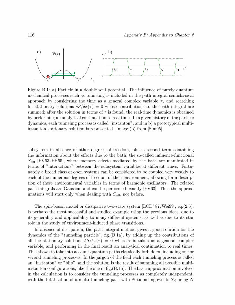
116 Appendix B: Appendix to Chapter 2
Figure B.1: a) Particle in a double well potential. The influence of purely quantummechanical processes such as tunneling is included in the path integral semiclassicalapproach by considering the time as a general complex variable τ , and searchingfor stationary solutions δS/δx(τ) = 0 whose contributions to the path integral aresummed; after the solution in terms of τ is found, the real-time dynamics is obtainedby performing an analytical continuation to real time. In a given history of the particledynamics, each tunneling process is called ”instanton”, and in b) a prototypical multi-instanton stationary solution is represented. Image (b) from [Sim05].
subsystem in absence of other degrees of freedom, plus a second term containingthe information about the effects due to the bath, the so-called influence-functionalSinfl [FV63, FH65], where memory effects mediated by the bath are manifested interms of ”interactions” between the subsystem variables at different times. Fortu-nately a broad class of open systems can be considered to be coupled very weakly toeach of the numerous degrees of freedom of their environment, allowing for a descrip-tion of these environmental variables in terms of harmonic oscillators. The relatedpath integrals are Gaussian and can be performed exactly [FV63]. Thus the approx-imations will start only when dealing with Sinfl, not before.
The spin-boson model or dissipative two-state system [LCD+87,Wei99], eq.(2.6),is perhaps the most successful and studied example using the previous ideas, due toits generality and applicability to many different systems, as well as due to its starrole in the study of environment-induced phase transitions.
In absence of dissipation, the path integral method gives a good solution for thedynamics of the ”tunneling particle”, fig.(B.1a), by adding up the contributions ofall the stationary solutions δS/δx(τ) = 0 where τ is taken as a general complexvariable, and performing in the final result an analytical continuation to real times.This allows to take into account quantum paths classically forbidden, including one orseveral tunneling processes. In the jargon of the field each tunneling process is calledan ”instanton” or ”blip”, and the solution is the result of summing all possible multi-instanton configurations, like the one in fig.(B.1b). The basic approximation involvedin the calculation is to consider the tunneling processes as completely independent,with the total action of a multi-tunneling path with N tunneling events SN being N
B.2 Path integral description of the dissipative two-state system. 117
times the action of a single-tunneling path, SN = N × S1, or expressed in terms ofblips, there is no interaction among them.When a dissipative environment of harmonic oscillators is coupled to this system,
the path integral resulting from integrating out the oscillators’ degrees of freedomintroduces, as previously told, an influence-functional Sinfl[|x(τ) − x(τ ′)|] that pro-vides memory to the dynamics. Now the result can be again expressed in terms ofsums over multi-blip paths, but interactions play a role and complicate enormouslythe calculation. Leggett et al. introduced the so-called non-interacting blip approx-imation (NIBA), which basically limits the memory effects to the inclusion of thecontribution to the action S corresponding to interaction between two consecutiveperiods separated by a tunneling process.The success of this approximation lies in its numerous virtues, two out of which
we highlight here for our purposes: i) It is a controlled approximation, with a clearlydefined range of validity (basically low temperatures and weak tunneling amplitudeas compared to the characteristic frequency of the ground states of the wells) andwell defined expansion parameters, ii) It turns out to be a good description in a verybroad range of cases, from baths leading to a weak damping to baths leading to asuppression of tunneling and localization of the particle.Remember that the Hilbert space of the system described in fig.(B.1a) is reduced
in the spin-boson model to the two ground states of the wells, represented by aspin up and spin down (〈σz〉 = 1 for the left well ground state and 〈σz〉 = −1 forthe right well ground state, for example). These two states become mixed by thetunneling amplitude ∆x0 , introducing spin-flip processes in the dynamics. The basicresult obtained within NIBA for the time evolution P (t) = 〈σz(t)〉 starting at t = 0in a given well, 〈σz(t = 0)〉 = 1, is
P (t) =1
2πi
∫
C
eλt[λ+ f(λ)]−1dλ , (B.15)
where C is the standard Bromwich contour, and
f(λ) ≡ ∆2x∫ ∞
0
cos[Q1(t)
]exp−
[λt+Q2(t)
], (B.16)
with Qi(t) defined by
Q1(t) ≡∫ ∞
0
J(ω)
ω2sin[ωt]dω
Q2(t) ≡∫ ∞
0
J(ω)
ω2(1− cos[ωt]) coth[~ω/2kBT ]dω (B.17)
The function J(ω) appearing in the integrals is the spectral density of the bath,
J(ω) =
∫ ∞
−∞dt eiωt〈Hint(t)Hint(0)〉 . (B.18)
118 Appendix B: Appendix to Chapter 2
At T = 0, up to second order in perturbation theory, it can be rewritten as
J(ω) =∑
k
|λk|2 δ(ω − ωk) (B.19)
J(ω) reflects the evolution as a function of ω of the amount of possible transitions(fluctuations) from a starting initial state (at T = 0 the ground state) to all finalstates for whom an energy ~ω has been exchanged between our subsystem and theoscillators’ bath.
Many of the oscillators’ baths found in nature, like phonons in solids or e-h ex-citations in metals, display a spectral density J(ω) ∼ ωs up to a certain cutoff (e.g.the Debye frequency in the case of phonons). A very important result states thatwhenever NIBA is applicable, the power s of J(ω) is the crucial factor determiningthe effect that the environment exerts on the TLS (〈σz(t)〉) dynamics. As explainedwith an example in Appendices C.2.1 and C.2.3, at finite temperatures T ω theamount of accessible transitions thanks to the thermal energy present in the systemdetermines J(ω, T > 0), leading to J(ω, T ) ∼ T s.
B.2.1 Derivation of the spectral function for the case of the
modes of a quasi-1D nanoresonator
The starting point is the hamiltonian (2.10), where ∂iuj is a component of thedeformation gradient matrix. In the case of the bending modes of a rod of dimensionsL, t and w, and mass density ρ, there are two variablesX(z), Y (z) obeying eqs.(A.14).One can thus express X(z), Y (z) in terms of bosonic operators, for example X(0) =∑k
√~/(2ρtwLωk)(a†k + ak). We can relate this variables to the strain field ∂iuj
through the free energy F:
Frod =1
2
∫dzEIy
(∂2X∂z2
)2+ EIx
(∂2Y∂z2
)2=1
2
∫dz
∫dS1
2λ∑
i
u2ii + µ∑
i,k
u2ik
≈ 1
2
∫dz
∫dS(3
2λ+ 9µ)u2ij (B.20)
extracting an average equivalence for one component uij, uij ≈ 2√EIy/(3λ+ 18µ)tw∂
2X/∂z2.The interaction term in the hamiltonian is then
Hint = ~σz∑
k
λk2√ωk(a†k + ak)
= ~σz∑
ij
∑
k
[2γ∆x0ε
√EIy
(3λ+ 18µ)tw
√1
2ρtw~L
](kij)2√ωijk
(aij†k + aijk )(B.21)
B.2 Path integral description of the dissipative two-state system. 119
So we have approximately 9 times the same hamiltonian, once for each uij, and thecorresponding spectral function J(ω) will be nine times the one calculated for
Hint = ~σz∑
k
λk2√ωk(a†k + ak)
' ~σz∑
k
[2γ∆x0ε
√EIy
(3λ+ 18µ)tw
√1
2ρtw~L
] k2√ωk(a†k + ak) (B.22)
For this hamiltonian J(ω) is given by
J(ω) =1
2π
∑
k
[2γ∆x0ε
√EIy
(3λ+ 18µ)tw
√1
2ρtw~Lk2√ωk
]2δ(ω − ωk) (B.23)
Taking the continuum limit ( 1L
∑k →
1π
∫dk):
J(ω) =2L
(2π)2
∫ kmax
kmin
dk[2γ∆x0ε
√EIy
(3λ+ 18µ)tw
√1
2ρtw~L
]2 k4
ωkδ(ω − ωk) (B.24)
Using the dispersion relation ωj(k) =√EIj/(ρab) × k2 = c × k2 we express the
integral in terms of the frequency:
J(ω) =L
(2π)2
∫ ωco
ωmin
dωk√c ωk
[2γ∆x0ε
√EIy
(3λ+ 18µ)tw
√1
2ρtw~L
]2 k4
ωkδ(ω − ωk)
=L
(2π)2
[2γ∆x0ε
√EIy
(3λ+ 18µ)tw
√1
2ρtw~L
]2√ωc5/2
(B.25)
Jflex(ω) is just 9 times this, eq.(2.14).
For the compression and twisting modes the derivation follows analogous steps.Longitudinal or compression modes correspond to the displacement vector ui obeyingthe wave equation (A.13). Hence, there are plane waves with linear dispersion relation
ωk =√Eρk. The strain field ∂u appears in the hamiltonian coupled to a TLS located
at z = 0. The quantized u(0) and ∂u |z=0 are given by
u(0) =∑
k
√~
2ρtwLωk(a†k + ak) , ∂u |z=0=
√~
2ρtwL
∑
k
k√ωk(a†k + ak) (B.26)
The hamiltonian is:
H = εσx + ~σz∑
k
[γ∆x0ε
√1
2ρtwL~k√ωk
](a†k + ak) +
∑
k
~ωk(a†kak + h.c.)
= εσx + ~σz∑
k
λk(a†k + ak) +
∑
k
~ωk(a†kak + h.c.) (B.27)
120 Appendix B: Appendix to Chapter 2
With such a form for the coupling the spectral function is given by eq.(2.11).The twisting or torsional modes obey the wave equation (A.15). In analogy with
the previous case we can quantize φ and get the same results for φ(0) and ∂φ |z=0 asfor u(0) and ∂u |z=0, just substituting ρ by ρI and E by C. But in our hamiltonianthe coupling term involves ∂u |z=0 and not ∂φ |z=0, so the latter has to be expressedin terms of the former. Proceeding as with the bending modes:
Frod =1
2
∫dzC
(∂φ
∂z
)2=1
2
∫dz
∫dS4µ
[(∂ux
∂z
)2+
(∂uy
∂z
)2]
≈ 1
2
∫dz
∫dS8µ
(∂ux
∂z
)2(B.28)
Approximating further∫dS8µ
(∂ux
∂z
)2≈ 8µab
(∂ux
∂z
)2= C
(∂φ
∂z
)2(B.29)
the equivalence ∂u |z=0= ∂ux/∂z =√C/(8µtw)∂φ |z=0 is found. Therefore in this
case one has an interaction term in the hamiltonian
Hint = ~σz∑
k
γ∆x0ε
√C
8µtw
√1
2ρI~Lk√ωk(a†k + ak) (B.30)
leading to an ohmic spectral function, eq.(2.11), as in the previous case.
B.3 Dissipation from symmetric non-resonant TLSs
B.3.1 Spectral function of a single TLS coupled to the sub-
ohmic bending modes
We follow the method of ref. [Gui85]. The form of A(ω), the spectral function ofa single TLS, for frequencies ω ε and ω ε can be estimated using perturbationtheory. Without the interaction, the ground state |a〉 of the TLS is the antisymmetriccombination of the ground states of the two wells, and the excited state is the sym-metric one, |s〉. We will use Fermi’s Golden Rule applied to the subohmic spin-bosonhamiltonian, H = εσx + ~λσz
∑k
[k2√ωk
](a†k + ak) +
∑k ~ω(k)a
†kak, where ak is the
annihilation operator of a bending mode k. Considering only the low energy modesω(k) ε, to first order the ground state and a state with energy ω(k) are given by
|g〉 ' |a〉 −λk2√ωk
2εa†k|s〉+ ... ,
|k〉 ' a†k|a〉 −λk2√ωk
2ε|s〉+ ... . (B.31)
B.3 Dissipation from symmetric non-resonant TLSs 121
We estimate the behavior of A(ω) by taking the matrix element of σz between thesetwo states, obtaining (remember that ω(k) ∝ k2)
A(ω) ∼~αb√ωco√ω
ε2+ ... , ω(k) ε. (B.32)
The expression in the numerator is proportional to the spectral function of the cou-pling, J(ω) = αb
√ωco√ω. Now we turn our attention to the case ω(k) ε, where
the ground state |g〉 and an excited state |k〉 can be written as
|g〉 ' |a〉 −λk2/√ωk
~ωk + 2εa†k|s〉+ ... ,
|k〉 ' a†k|a〉+λk2/√ωk
~ωk − 2ε|s〉+ ... . (B.33)
The matrix element 〈0|σz|k〉 is ∼ λk2√ωk
4ε(~ωk)2
, leading to
A(ω) ∼αb√ωcoε
2
~3ω7/2+ ... , ω(k) ε. (B.34)
B.3.2 Value of Atotoff−res(ω0)
Now we will add the contributions of all the non-resonant TLSs using the probabil-ity distribution P (∆x0 ,∆
z0) = P0/∆
x0 [AHV72,Phi72]. For the case of weak coupling,
αb < 1/2 and ω0 ≥ (2αb)2ωco, which is the one found in experiments, one has
Atotoff (ω0) ∼∫ εmax
~[ω0+Γ(ω0)]d∆x0
∫ ∆x0
−∆x0d∆z
P
∆x0
~αb√ωco√ω0
(∆x0)2
+
∫ ~[ω0−Γ(ω0)]
~(2αb)2ωcod∆x0
∫ ∆x0
−∆x0d∆z
P
∆x0
αb√ωco(∆
x0)2
~3ω7/20
obtaining the result Atotoff−res(ω0) ≈ 2Pαb√ωco/ω0.
B.3.3 The off-resonance contribution for T > 0
Using the same scheme, the modifications due to the temperature will appear inthe density of states of absorption and emission of energy corresponding to a ”dressed”TLS, A(ε, ω, T ). Now there will be a probability for the TLS to be initially in theexcited symmetric state, |s〉, proportional to exp[−ε/kT ], and to emit energy ~ωgiving it to our externally excited mode, |k, n〉, thus compensating the absorption ofenergy corresponding to the opposite case (transition from |a〉|k, n〉 to |s〉|k, n− 1〉),but contributing in an additive manner to the total amount of fluctuations, which
122 Appendix B: Appendix to Chapter 2
are the ones defining the linewidth of the vibrational mode observed in experiments,fixing the value of Q−1(ω, T ). The expression for A(ε, ω, T ) is given by
A(ω, T ) =1
Z
∑
i
∑
f
|〈i|σz|f〉|2e−EikT δ[~ω − (Ef − Ei)] (B.35)
We consider a generic state |ia〉 = |a〉|k1n1, ..., kjnj, ...〉 or |is〉 = |s〉|k1n1, ..., kjnj, ...〉,and states that differ from it in ~ωj,
|fa±〉 = |a〉|k1n1, ..., kjnj ± 1, ...〉 , |fs±〉|s〉|k1n1, ..., kjnj ± 1, ...〉 (B.36)
As for T = 0, we will correct them to first order in the interaction hamiltonianHint = ~λσz
∑k
√ωk(a
†k + ak), and then calculate the square of the matrix element
of σz, |〈i|σz|f〉|2.Elements |〈ia,s|σz|fa+,s+〉|2 correspond to absorption by the ”dressed” TLS of an
energy ~ωj from the mode kj, while elements |〈ia,s|σz|fa−,s−〉|2 correspond to emissionand ”feeding” of the mode with a phonon ~ωj. The expressions for the initial statesare
|ia〉 = |a〉|k1n1, ..., kjnj, ...〉 → |a〉|k1n1, ..., kjnj, ...〉+∑
ki3ni>0
~λ√niωi~ωi − 2ε
|s〉|...kini − 1...〉
−∑
∀ki
~λ√(ni + 1)ωi~ωi + 2ε
|s〉|...kini + 1...〉
|is〉 = |s〉|k1n1, ..., kjnj, ...〉 → |s〉|k1n1, ..., kjnj, ...〉+∑
ki3ni>0
~λ√niωi~ωi + 2ε
|a〉|...kini − 1...〉
−∑
∀ki
~λ√(ni + 1)ωi~ωi − 2ε
|a〉|...kini + 1...〉 (B.37)
and, for example, the state |fa+〉 is given by
|fa+〉 = |a〉|k1n1, ..., kjnj + 1, ...〉 →
|a〉|k1n1, ..., kjnj + 1, ...〉+∑
ki3ni>0,i6=j
~λ√niωi~ωi − 2ε
|s〉|...kini − 1...kjnj + 1...〉
+~λ√(nj + 1)ωj~ωj − 2ε
|s〉|...kjnj...〉 −∑
∀ki,i6=j
~λ√(ni + 1)ωi~ωi + 2ε
|s〉|...kini + 1...kjnj + 1...〉
−~λ√(nj + 2)ωj~ωj + 2ε
|s〉|...kjnj + 2...〉 (B.38)
with similar expression for the rest of states. The value of |〈ia,s|σz|fa+,s+〉| (absorp-
tion) is |〈ia,s|σz|fa+,s+〉| =∣∣∣λ√(nj+1)ωj4ε
(~ωj)2−4ε2
∣∣∣ , with nj = 0, 1, ..., while for emission the
B.3 Dissipation from symmetric non-resonant TLSs 123
result is |〈ia,s|σz|fa−,s−〉| =∣∣∣ λ√njωj4ε
(~ωj)2−4ε2
∣∣∣, with nj = 1, .... Taking the limits we con-sidered at T = 0 (~ωj ε and ~ωj ε) the results are the same as for T = 0for absorption, except for a factor (nj + 1), and we also have now the possibility ofemission, with the same matrix element but with the factor nj:
Absorption
∼ (nj+1)~αb
√ωco√ω
ε2~ωj ε
∼ (nj+1)αb√ωcoε2
~3ω7/2 , ~ωj ε
Emission
∼ nj~αb
√ωco√ω
ε2~ωj ε
∼ njαb√ωcoε2
~3ω7/2 , ~ωj ε(B.39)
Now we have to sum over all initial states, and noting that the first order correctionto the energy of any eigenstate is 0, the partition function, Z, is easy to calculate,everything factorizes, and the result is, for example in the case ~ωj ε:
Aabs(ε, ωj, T ) =1
Z
∞∑
i6=j,ni=0
∞∑
nj=0
~αb√ωco√ωj
ε2(nj + 1)e
−~ωjnjkT e−
~Pi niωikT
=~αb√ωco
ε2
√ωj
1− e−~ωjkT
Aem(ε,−ωj, T ) =1
Z
∞∑
i6=j,ni=0
∞∑
nj=1
~αb√ωco√ωj
ε2nje
−~ωjnjkT e−
~Pi niωikT
=~αb√ωco
ε2
√ωje
−~ωjkT
1− e−~ωjkT
(B.40)
In Aabs(ε, ωj, T ) we have added the contributions from the matrix elements
|〈ia|σz|fa+〉|2eεkT + |〈is|σz|fs+〉|2e
−εkT = |〈ia|σz|fa+〉|2[e
εkT + e
−εkT ] (B.41)
The sum of exponentials cancels with the partition function of the TLS (appearing asa factor in the total Z), leading in this way to the expression above (the same appliesfor Aem(ε,−ωj, T )). The total fluctuations will be proportional to their sum, whichthus turns out to be at this level of approximation ∝ cotanh[~ωj/kT]:
Adiss(ε, ωj, T ) = Aabs(ε, ωj, T ) + Aem(ε,−ωj, T ) = Adiss(ε, ωj, T = 0)cotanh[~ωjkT
]
(B.42)In fact, this result applies for any other type of modes, independently of its dispersionrelation, provided the coupling hamiltonian is linear in σz and (a
†−k + ak) and every-
thing is treated at this level of perturbation theory. Moreover, it can be proven that ifone has an externally excited mode with an average population 〈nj〉 , and fluctuationsaround that value are thermal-like, with a probability ∝ exp[−|nj − 〈nj〉|/kT )], onerecovers again the same temperature dependence, ∝ cotanh[~ωj/kT].
124 Appendix B: Appendix to Chapter 2
B.4 Q−1 due to the delayed response of biased TLSs
(relaxation mechanism)
The derivation presented here is based mainly on pages 396-406 of ref. [Esq98].We want to deduce the formula for the relaxation contribution to the attenuation ofacoustic waves:
Q−1(ω, T ) =P0γ
2
ρv2
∫ εmax
0
dε
∫ 1
umin
du
√1− u2u
1
kT
1
cosh2[ε/2kT
] ωτ
1 + (ωτ)2(B.43)
Consider a set of TLSs with a difference of energy between their two eigenstatesε = ε2 − ε1 and with instantaneous occupation fractions n1 and n2, that obey
1 = n1 + n2n1 = −ν21n1 + ν12n2
(B.44)
where ν12 and ν21 are the transition rates due to the interaction of the TLS with thephonons, which reflect the finite response time of the TLS to a perturbation. Thisdelayed response is responsible, together with the finite bias ∆z0 > 0, of the dissipation(B.43), as we shall demonstrate. We will simplify the elasticity tensors and treat themas scalars. If we apply a periodic stress σ(t) = σ0e
−iωt we perturb the energy levels,in the linear response approximation, according to
εα(σ) = εα(0)− v0λαijσij , εα(u) = εα(0)− v0pαijuij (B.45)
where
• v0 is the unit cell volume,
• λαij = −(1/v0)∂εα/∂σij is the elastic dipole of state α (also defined as the strainuij created by a homogeneous distribution of c defects per mole, λ
αij = ∂uij/∂c
α),
• pαij = −(1/v0)∂εα/∂uij is the so-called double force tensor (defined too as thestress σij created by a homogeneous distribution of c defects per mole, p
αij =
∂σij/∂cα)
Note that from the first definition of pαij one can see that it is approximately propor-tional to the deformation potential γαij , γ
αij ' (1/2)∂∆αz /∂uij = −v0pαij . This last
quantity is related to our coupling constant γij ∼ γ of the interaction hamiltonianHint through γij = 2(γ
2ij − γ1ij). So returning again to the applied periodic stress,
it perturbs the energy levels, causing a variation in the TLS populations and thecorresponding strain, according to uTLSij = cαλ
αij . We want to find an expression
relating ∆uTLSij and σ(t), from which we can deduce the associated dynamic com-pliance ∆S(ω) = ∆u/σ. S(ω) is the inverse of the relative change of the elastic
B.4 Q−1 due to the delayed response of biased TLSs (relaxation mechanism) 125
stiffness, δC(ω) = σ/∆u, the magnitude giving us the frequency shift and qualityfactor (eq.(B.43)) due to relaxational processes of TLSs.We start dividing the instantaneous occupation fraction n1(t) as
n1(t) = n01 +∆n1(t) + δn1(t), (B.46)
where n01 is the equilibrium value in the absence of stress, ∆n1(t) the perturbation tothe equilibrium value due to the applied stress,
∆n1(t) =dn1
dε
∂ε
∂σσ0e
−iωt = ∆n1e−iωt, (B.47)
n1(t) = n01 + ∆n1(t) is the instantaneous equilibrium value, δn1(t) is the deviationfrom the instantaneous equilibrium value due to the delayed response of the defects,and ∆n1(t) = ∆n1(t) + δn1(t) is the deviation from the static equilibrium in theabsence of applied stress,
∆n1(t) = ∆n1e−iωt . (B.48)
The definitions of ∆n1(t) and δn1(t) imply that their amplitudes are complex, becausethey include a phase lag between the excitation and the response, due to the finitetime needed for reaching the instantaneous equilibrium according to (B.44). Thestrain ∆uTLSij we need to compute ∆S(ω) is that due to ∆n1, which is
∆u = λ1∆n1 + λ2∆n2 =c
v0
∂ε
∂σ∆n1 (B.49)
Now we want to extract the value of the complex phase appearing in eq.(B.48), andfor that sake we have to manipulate a bit the rate equation (B.44): we begin using thecondition for the equilibrium values of the populations (detailed balance condition),
dn1(t)
dt= 0 → n1(t)ν21 = n2(t)ν12 (B.50)
With this relation we transform (B.44) into
dn1(t)
dt= −δn1(t)
τ(B.51)
where τ−1 = ν12 + ν21. (B.51) indicates that the rate of change of the population isproportional to the deviation from the instantaneous equilibrium. Noting that
dn1(t)
dt=d∆n1(t)
dt= −iω∆n1(t) (B.52)
andδn1(t) = ∆n1(t)−∆n1(t) (B.53)
126 Appendix B: Appendix to Chapter 2
and using (B.51), one obtains
∆n1 =∆n11− iωτ
= ∆n1
[ 1
1 + (ωτ)2+ i
ωτ
1 + (ωτ)2
](B.54)
So the dynamic compliance can be written as
∆S(ω) =∆u
σ=
c
v0
dn1
dε
( ∂ε∂σ
)2 1
1− iωτ(B.55)
When one compares this result to the static compliance, it appears that the dynamicresponse function is obtained multiplying the static one by (1 − iωτ)−1. With thedynamic modulus δC(ω) an equivalent expression can be derived, with the roles of uand σ exchanged,
δCijhk(ω) =σ
∆u=
c
v0
∑
αβ
∂nα
∂εβ
∂εα
∂uij
∂εβ
∂uhk
1
1− iωτ(B.56)
Now, this can be rewritten observing that
∂nα
∂εβ= βnα(nβ − δαβ) and
∑
α
nα = 1 (B.57)
leading to
δCijhk(ω) =c
v0βnαnβ
( ∂εβ
∂uij− ∂εα
∂uij
)( ∂εβ
∂uhk− ∂εα
∂uhk
) 1
1− iωτ(B.58)
To get to (B.43) we need a couple more transformations of this expression. First, ifthe energies of the eigenstates under strain u are given by
ε1,2(u) = ∓1
2
√(∆x)2 + (∆z +
∑
ij
γijuij)2 , (B.59)
then eq.(2.21) is obtained, so that, together with the definition ε = ε2 − ε1, and theequivalence n1n2 = (1/4)sech
2(ε/2kBT), results in
δCijhk(ω) =c
v0
(∆zε
)2γijγhk
β
4sech2(ε/2kBT)
1
1− iωτ(B.60)
This is the result for a concentration of c defects per mole of TLSs with fixed ε and∆z. In the case of an amorphous solid one has instead a probability distribution interms of the parameters ∆x and ∆z, g(∆x,∆z)d∆xd∆z = P0/∆xd∆xd∆z, which canbe expressed with the variables ε =
√(∆x)2 + (∆z)2 and u = ∆z/ε as g(ε, u)dεdu =
P0/(u√1− u2)dεdu , with ε running from 0 to εmax and u from umin to 1. Writing
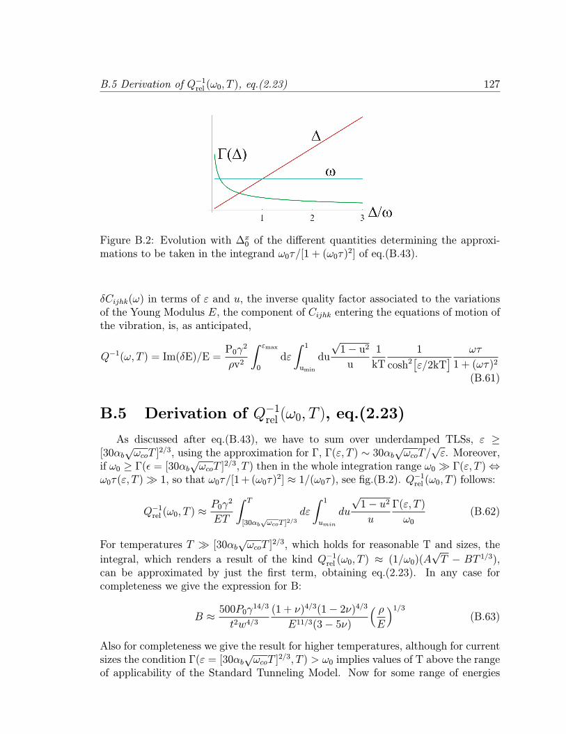
B.5 Derivation of Q−1rel (ω0, T ), eq.(2.23) 127
Figure B.2: Evolution with ∆x0 of the different quantities determining the approxi-mations to be taken in the integrand ω0τ/[1 + (ω0τ)
2] of eq.(B.43).
δCijhk(ω) in terms of ε and u, the inverse quality factor associated to the variationsof the Young Modulus E, the component of Cijhk entering the equations of motion ofthe vibration, is, as anticipated,
Q−1(ω, T ) = Im(δE)/E =P0γ
2
ρv2
∫ εmax
0
dε
∫ 1
umin
du
√1− u2u
1
kT
1
cosh2[ε/2kT
] ωτ
1 + (ωτ)2
(B.61)
B.5 Derivation of Q−1rel (ω0, T ), eq.(2.23)
As discussed after eq.(B.43), we have to sum over underdamped TLSs, ε ≥[30αb
√ωcoT ]
2/3, using the approximation for Γ, Γ(ε, T ) ∼ 30αb√ωcoT/
√ε. Moreover,
if ω0 ≥ Γ(ε = [30αb√ωcoT ]
2/3, T ) then in the whole integration range ω0 Γ(ε, T )⇔ω0τ(ε, T ) 1, so that ω0τ/[1+ (ω0τ)2] ≈ 1/(ω0τ), see fig.(B.2). Q−1rel (ω0, T ) follows:
Q−1rel (ω0, T ) ≈P0γ
2
ET
∫ T
[30αb√ωcoT ]2/3
dε
∫ 1
umin
du
√1− u2u
Γ(ε, T )
ω0(B.62)
For temperatures T [30αb√ωcoT ]
2/3, which holds for reasonable T and sizes, the
integral, which renders a result of the kind Q−1rel (ω0, T ) ≈ (1/ω0)(A√T − BT 1/3),
can be approximated by just the first term, obtaining eq.(2.23). In any case forcompleteness we give the expression for B:
B ≈ 500P0γ14/3
t2w4/3(1 + ν)4/3(1− 2ν)4/3
E11/3(3− 5ν)
( ρE
)1/3(B.63)
Also for completeness we give the result for higher temperatures, although for currentsizes the condition Γ(ε = [30αb
√ωcoT ]
2/3, T ) > ω0 implies values of T above the rangeof applicability of the Standard Tunneling Model. Now for some range of energies
128 Appendix B: Appendix to Chapter 2
Γ(ε, T ) > ω0, and the range of integration is divided into two regions, one whereω0τ 1 and one where the opposite holds:
Q−1rel (ω0, T ) =P0γ
2
ET
∫ 1
umin
du
√1− u2u
× (B.64)
∫ [16αb√ωco2T/√ω0]2
[30αb√ωcoT ]2/3
dε ω0τ(ε, T ) +
∫ T
[16αb√ωco2T/
√ω0]2
dε1
ω0τ(ε, T )
The final result is Q−1rel (ω0, T ) ≈ −7P0γ2ω0/T + A√T/ω0 − CT/ω20, with A defined
by eq.(2.23) and C by:
C ≈ 1500P0γ6
t3w2(1 + ν)2(1− 2ν)2
E3(3− 5ν)2( ρE
)1/2(B.65)
All the results for Q−1rel (ω0, T ) have to be multiplied by the fraction of volume of theresonator presenting amorphous features, Vamorph/(twL).
B.6 Derivation of eq.(2.27)
To calculate classically the energy stored of a torsional mode φj(z, t) = A sin[(2j−1)πz/(2L)] sin(ωjt) we just calculate the kinetic energy in a moment where the elasticenergy is zero, for example at time t = 0. If an element of mass is originally at position(x, y, z) (x, y transversal coordinates), with a torsion φ(z, t) it moves to
r(t) =(√
x2 + y2 ·cos[arccos
x√x2 + y2
+φ],√x2 + y2 ·sin
[arccos
x√x2 + y2
+φ], z)
(B.66)The kinetic energy at time t = 0 is
E0 =
∫ L
0
dz
∫ t/2
−t/2dx
∫ w/2
−w/2dy · 12ρ∣∣∣dr
dt
∣∣∣2
t=0(B.67)
Substituting the expression for ~r(t) in the integrand, one arrives at
E0 =
∫ L
0
dz
∫ t/2
−t/2dx
∫ w/2
−w/2dy · 12ρA2ω2j sin
2[(2j − 1)π
2Lz](x2 + y2)
=1
48A2ω2jρL(t
3w + w3t) (B.68)
In terms of the creation and annihilation operators
φj(z, t) =~
2LρIωj(a†j + aj)e
i(kjz−ωt) , (B.69)
so the mean square of its amplitude is 〈φ2j〉 = A2/2 = ~(2n+1)/[2LρIωj]. Substitutingthis in eq.(B.68) the eq.(2.27) for E0 is obtained.
Appendix C
Appendix to Chapter 4
C.1 Electron-phonon coupling: friction in terms
of the susceptibility χ
C.1.1 Damping of a phonon mode due to Coulomb interac-
tions between charges in a device
We have seen in subsection 6.4.2 how the response of system to a given externalperturbing field can be expressed, for weak perturbations, in terms of a susceptibilityor response function. To be more concrete, we started from an interaction hamiltonianHint acting as a perturbation on the initial one, H0, and its eigenfunctions φi,
Hint =
∫drV (r, t)ρ(r) (C.1)
where ρ(r) =∑k,k′ [c
†k+k′
ckeik′r+h.c.] is the charge operator, and the potential is an
oscillating function of frequency ω, V (r, t) = V (r)eiωt. We saw in 6.4.2 that to linearorder in Hint the variation in the particle density n(r, t) =
∑occi |φ′i(r, t)|2 with respect
to the case in absence of perturbation can be expressed as
δn(r) =
∫dr′χ(r, r′, ω)V (r′). (C.2)
This can be taken as the definition of the retarded density-density response functionχ for the charge density change at r induced by a potential field at r′. In terms of agiven approximation for the single-particle eigenstates |i〉 and eigenenergies ei of thetotal hamiltonian Htot = H0 +Hint, it is expressed as
χ(r, r′, ω) =occ∑
i
∑
j
〈j|n(r)|i〉〈i|n(r′)|j〉( 1
ei − ej − ~ω+
1
ei − ej + ~ω
). (C.3)
129
130 Appendix C: Appendix to Chapter 4
The response frequencies of the system are given by the poles of the response function,which depend in turn on the approximation of the basis. For convenience we willgeneralize eq.(C.3) in terms of the N -body states |α〉 of our system composed of Nfermions. |α〉 can be given, for example, by a Slater determinant of one-body states|i〉. We assume that the system starts in its ground state |0〉 (T=0 case). We definethe fermionic creation operators c†i creating one-body states |i〉, so that
χ(i, j, ω) =∑
α
〈α|c†icj|0〉〈0|c†jci|α〉
( 1
ε0 − εα − ~ω+
1
ε0 − εα + ~ω
). (C.4)
Now we are interested in the probability per unit time that the field V (r, t) trans-fers energy ~ω to the system. According to Fermi’s Golden Rule of second-orderperturbation theory the probability we are looking for is given by
Γ(V, ω) =2π
~∑
α
|〈α|V |0〉|2δ(~ω − εα + ε0) (C.5)
Here V =∑i,j〈j|V (r, t)|i〉c
†icj is the operator corresponding to V (r, t) in the second-
quantized basis c†i . Eq.(C.5) can be expressed in terms of χ by providing the latterwith an imaginary part through the addition of a small term iη to ω, and then usingthe relation Im[1/(x− iη)] = πδ(x). In this way we obtain the expression for Γ usedin the thesis,
Γ(V, ω) =
∫drdr′V (r)V (r′)Imχ(r, r′, ω) . (C.6)
Now the goal is to use a good approximation for the susceptibility function of oursystem.
C.1.2 Clean metal susceptibility
Suppose that our system is a metal. When the presence of impurities, electron-phonon collisions and electron-electron interactions is such that the collision frequencyν = 1/τ of an electron is much less than the frequencies ω we are interested in, ωτ 1,and/or the mean free path is much longer than the length scales L we study, vF τ L,we are in the clean metal limit [NP99], where the susceptibility can be expressed interms of elementary excitations. If one neglects electron-electron interactions (freeelectron gas), the retarded susceptibility is given by the bare bubble diagram:
χR0 (q, ω) =1
V
∑
k,σ
nF (εk)− nF (εk+q)εk − εk+q + ~ω + iη
, (C.7)
where V is the volume of the system, nF (ε) is the Fermi function, εk − εk+q are theexcitation energies of the quasiparticles and η → 0. The response of the system is
C.1 Electron-phonon coupling: friction in terms of the susceptibility χ 131
determined by the excitation of these one-body quasiparticle states, corresponding tozeroes of the real part of the denominator. The main effect of the inclusion of Coulombinteractions among electrons is the appearance of collective excitations, formed by asuperposition of one-body states, called plasmons in the case of the electron gas.Their presence is manifested for example in an RPA calculation. RPA is the resultof summing, for the interacting electron gas, the most important diagrams of eachorder [BF04], which turn out to be the ones of the bubbles, and these diagramsincrease their importance as the density increases, so RPA is the high density limitof the interacting electron gas. The RPA result is the following:
χRRPA(q, ω) =χR0 (q, ω)
1− VCoul(q)χR0 (q, ω), (C.8)
where VCoul represents the Coulomb potential. The response will show peaks againin the zeroes of the real part of the denominator of χR0 (q, ω), but now also when1− VCoul(q)χR0 (q, ω) = 0, which corresponds to collective excitations.
C.1.3 Dirty metal susceptibility
When due to the presence of impurities, electron-phonon collisions and electron-electron interactions the collision frequency ν = 1/τ of an electron is higher than thefrequencies ω we are interested in, ωτ 1, and the mean free path is much shorterthan the length scales L we study, vF τ L, one enters the so-called hydrodynamicregime [NP99]. A given quasiparticle is subject to many collisions during one periodof the exciting external field. It is thus completely ”thermalized” well before it cansample the periodicity of the field. Therefore the best way to proceed is to assumethat the collisions act to bring about everywhere a state of local thermodynamicequilibrium, and use just macroscopic ”local” quantities (density, current, pressure,etc) to describe the state of the system; the response to the external field may beobtained by using the usual laws of thermodynamics and hydrodynamics. For highenough temperatures one arrives at an expression for the response function χ(q, ω)which contains a peak corresponding to the plasmon and a continuous backgroundarising from thermal diffusion. This background is the one described by eq.(4.15).Taking into account the plasmon contribution, eq.(4.15) becomes
χ(q, ω) =νDq2
Dq2 − ω2τ − iω, (C.9)
The plasmon contribution to the dissipation of the vibrational modes we study inthis thesis can be safely neglected. Basically one has to see if Dq2 ω2τ in eachof the layers (graphene and inversion layer in the Si-SiO2 interface). In both casesone can take Dν ∼ 103, τ = l/vF ∼ 10−7/106 ∼ 10−13 s (assuming l ∼ 100 nm),q ∼ 1/L ∼ 106 m−1, D = vF l ∼ 1011m2/s. The density of states (DOS) of a stack
132 Appendix C: Appendix to Chapter 4
of N graphene layers is νC = Nγ/~2v2F , being γ ∼ 0.3 eV the interlayer hoppingelement. The DOS of the approximately two-dimensional electron gas lying in theinversion layer Si-SiO2 is ν2DEG ∼ m ∗ /π~2, with m∗ ∼ 0.3me− the effective massof the electrons in Si. Using these values, N ∼ 10, and for the frequencies of theoscillators analyzed, ω ∼ 100 MHz, one immediately verifies that indeed
Dq2 ω, ω2τ → Imχ(q, ω) ≈ νω
Dq2(C.10)
The inequalities are quite large, so there is place for substantial variations of l or Nand they will still hold, justifying our use of eq.(4.15) and the limit Dq2 ω, ω2τ .
C.1.4 Microscopic derivation of eq.(4.15)
We sketch the analysis presented in [AS06]. This form of the susceptibility canbe derived assuming a distribution of short-range scattering centers represented bypotentials, creating an V (r) =
∑i Vimp(r − ri). To calculate propagators and phys-
ical magnitudes one has to perform in a final step a disorder average 〈...〉dis =∫DV P [V ](...), where the probability measure P [V ] describes the statistical proper-ties of the potential V . In most applications it is sufficient to implement a Gaussian
distribution, P [V ] = exp[− 12γ2
∫ddrddr′V (r)K−1(r− r′)V (r′)
], where γ measures the
strength of the potential andK describes its spatial correlation profile, 〈V (r)V (r′)〉dis =γ2K(r − r′). Very often one finds that the finite spatial correlation of V does notmatter, in which case one may set K(r) = δ(r), so that
〈...〉dis =∫DV exp
[− 12γ2
∫ddrV 2(r)
](C.11)
For length scales longer than the mean free path, so that the electrons experiencemultiple scattering, details of the form chosen for the potential V (r) are quicklyerased.In practice, this average is very difficult to perform, and a series of techniques
have been developed for mapping it into a different form. For example, in the replicafield theory, the expectation value of an operator O is written in terms of a source Jintroduced conveniently in the action of the path integral representing the replicated
partition function, ZR[J ] =∫D(Ψ, Ψ) exp
[−∑Ra=1 S[Ψ
a, Ψa, J ]],
〈O〉 = −(∂/∂J) lnZ[J ] = limR→0
1
R
∂ZR[J ]
∂J= limR→0
1
R
R∑
a=1
〈O(Ψa, Ψa)〉Ψ (C.12)
When performing now the disorder average of the functional ZR[J ] over the distribu-tion P [V ], the result is the presence of a new effective interaction term in the action
C.2 Imχ, Q−1 and temperature dependence of friction 133
of the system, with respect to the case without disorder:
〈Z[J ]〉dis =∫D(Ψ, Ψ) exp
[−
R∑
a=1
S|V=0[Ψa, Ψa]+R∑
a=1
]γ2
2
∑
mn
∫ddrΨam(r)Ψ
am(r)Ψ
bn(r)Ψ
bn(r)
(C.13)Then, one can apply perturbation theory to this interaction term to know whatare the disorder averaged values of observables, or in our case of the susceptibility,using diagrammatic theory and an ansatz for the imaginary part of the self-energycorrection to the fermion propagator, ImΣ(ωn) = −sgn(ωn)/2τ , where τ is the so-called elastic scattering time, related to the elastic mean free path l by τ ≡ l/vF .One can see that this parameter is related to the potential strength γ2 of the disorderpotential by τ−1 = 2πνγ2, where ν is the density of states. Usually γ2 is expressedthrough τ from the outset. The main results are
〈G(x,y; τ)〉dis = G(x,y; τ)|V=0e−|x−y|/2l
〈χ(r, τ)〉dis =T
Ld
∑
q,ωm
eiqr+iωmτνDq2
|ωm|+Dq2(C.14)
where χ(r, τ) is the density-density correlation function (the susceptibility of a dirtymetal).
C.2 Imχ, Q−1 and temperature dependence of fric-
tion
In order to make a connection between theory and experimental data a first pointthat has to be kept in mind is the following: Q−1, the linewidth observed in thefrequency domain of the response to an external driving force, does not correspondexclusively to an irreversible loss of energy of the mode (damping), but to all theprocesses which alter the phonon population of an excited mode of a certain frequency,including both increases and decreases of population. That is, Imχ, Q−1 correspondto the fluctuations of the given mode due to its coupling to other degrees of freedomof the system, giving a finite lifetime of the mode (k0, nk0) subject of study due toany kind of process, including those increasing nk0 . Friction, instead, correspondsjust to processes involving a decrease of nk0 .
C.2.1 Temperature dependence of Imχ, Q−1 due to excitation
and relaxation of e-h pairs
Friction experienced by, for example, traveling charged particles through a hostmetal due to the excitation of e-h pairs has been subject of intensive research since a
134 Appendix C: Appendix to Chapter 4
long time [Gui84]. In the graphene resonator’s case a similar effect produces absorp-tion and fluctuations of energy, but there is an important difference with the previousexample: we are studying the linewidth of a single bending mode of a well-definedwavevector q and frequency ωq, so we will not sum over frequencies to calculate thetotal absorption and fluctuations of the resonator’s vibrational modes due to thismechanism. More specifically, we want to calculate
Γ(ωq, T ) =
∫d3r
∫d3r′ReVscr(r, ωq)ReVscr(r
′, ωq)Imχ[r− r′, ωq,T] (C.15)
And for this we need Imχ[r − r′, ωq, T ]. To obtain the dependence with T we canrecall the fact that, embedded in Imχ, what we are looking for is the sum of e-h transitions that absorb an energy ωq from the vibrational mode (q, ωq) throughHint plus desexcitations that transfer an energy ωq to that mode. We will begin byanalyzing the T = 0 case, where only the former can take place, so that dissipation andfluctuations are indistinguishable. We will see that for a given frequency ω EF/~,the e-h transitions available are proportional to ω, independently of the dimension ofthe fermionic bath. It is a direct consequence of the exclusion principle through therestrictions imposed by the Fermi distribution functions nF (E) = 1/[1 + exp[(E −EF )/kBT ]] appearing. Taking for example a 3D Fermi gas, with dispersion relation
E =∑i
~2k2i2m, the probability of exciting an e-h pair of frequency ω will be proportional
to the number of such pairs available, P (ω),
P (ω) =
∫d3k
∫d3k′nF (E(k))
[1− nF (E(k′))
]δ(ω − E(k)− E(k′)
~
)(C.16)
Expressing the integrals in terms of energies and making the approximation ~ω EF ,
P (ω) ∝∫ ∞
0
dE√E(E + ~ω)nF (E)[1− nF (E + ~ω)]
=
∫ EF
EF−~ωdE√E(E + ~ω) ' EF × ~ω ∼ ω (C.17)
In the case we took a fermionic bath of a different dimension, the only difference inthe calculation would arise in the factor which in the 3D case is
√E(E + ~ω), which
will be in general a function f(E, ~ω). But as long as this is a smooth function ofE and ~ω, for ~ω EF we can approximate f(E, ~ω) ≈ f(EF , 0) and arrive againat P (ω) ∼ ω. At T = 0 only excitations of e-h pairs from the ground state canoccur, so the net absorption rate involving excitations of frequency ω will be indeedproportional to ω.At finite temperatures there will be absorption and emission processes. First we willcalculate the number of e-h excitations of a certain frequency ω which will cause
C.2 Imχ, Q−1 and temperature dependence of friction 135
energy absorption, as in the T = 0 case:
P (ω, T ) =
∫dnk
∫dnk′nF (E(k)/kBT )
[1− nF (E(k′)/kBT )
]δ(ω − E(k)− E(k′)
~
)
(C.18)For frequencies and temperatures such that ~ω kBT EF one can approximate
P (ω, T ) ∝∫ ∞
0
dEf(E, ~ω)nF (E/kBT )[1− nF ([E + ~ω]/kBT )]
≈ f(EF , 0)
∫ ∞
0
dEnF (E/kBT )[1− nF (E/kBT )]
= f(EF , 0)× kBT ×∫ ∞
0
dxnF (x)[1− nF (x)] ∼ T (C.19)
So for excitation frequencies much smaller than the temperature the number of avail-able excitations absorbing energy is proportional to T , and roughly independent of ω.The number of desexcitations compensating this absorption processes has a similarexpression:
P ′(ω, T ) ∝∫ ∞
0
dEf(E, ~ω)nF ([E + ~ω]/kBT )[1− nF (E/kBT )], (C.20)
and is also proportional to T , leading to Imχ(T ), Q−1(T ) ∼ T .
C.2.2 Temperature dependence of energy loss due to excita-
tion and relaxation of e-h pairs
The net amount of energy absorbed by the fermionic environment of e-h pairs offrequency ω at a finite temperature, A(ω, T ), for ~ω kBT EF , is proportionalto
A(ω, T ) ∝ P (ω, T )−P ′(ω, T ) ∝∫ ∞
0
dEf(E, ~ω)nF (E/kBT )−nF ([E+~ω]/kBT )
,
(C.21)and it can be approximated as
A(ω, T ) ∝ f(EF , 0)
∫ ∞
0
dEnF (E/kBT )− nF ([E + ~ω]/kBT )
= f(EF , 0)× kBT ×∫ −(EF−~ω)/kBT
−EF /kBTdxnF (x)
≈ f(EF , 0)×1
1 + e−EF /kBT× ~ω ∼ ω (C.22)
The net absorption of energy due to pairs of frequency ω is therefore to a first ap-proximation proportional to ω and independent of T .
136 Appendix C: Appendix to Chapter 4
C.2.3 Extension to a generic system + bath
Suppose that the subsystem subject of study, characterized by the index k, iscoupled linearly to a bath of excitations,
Hint ∝ (c†k + ck)×∑
q
λq(b†q + bq), (C.23)
where c†kand b†q represent subsystem and bath creation operators, respectively. We
can calculate at T = 0
Jgen(ω) =
∫ ∞
−∞dt eiωt〈Hint(t)Hint(0)〉 ∼ ωs , (C.24)
which as we saw in Appendix B.2 reflects the evolution as a function of ω, up to secondorder in perturbation theory, of the amount of possible transitions (fluctuations) froma starting initial state (at T = 0 the ground state) to all final states for whom anenergy ~ω has been exchanged between our subsystem and the bath. As temperaturegrows, for T ω, the amount of accessible transitions thanks to the thermal energypresent in the system will consequently grow as T s, so that Imχ(T ), Q−1(T ) ∼ T s, atleast when the perturbation Hint is not too strong.
C.3 Charge impurity density in SiO2 and the SiO2-
Si interface
From refs. [Sze81, NB82]. In ref. [Sze81] they speak of four types of interfacetrapped charges:
1. Just in the interface, due to the interruption of the periodic lattice struc-ture, there is the so-called interface-trapped charge Qit. Densities as low asQit ∼ 1010 cm−2 are achieved by low-temperature (450oC) hydrogen annealing.These charges are associated to traps, called interface traps, which change oc-cupancy with gate bias changes and have energy levels distributed throughoutthe bandgap. Interface traps characteristic of thermal oxidation are donor typein the upper half of the bandgap.
2. Close to the Si-SiO2 interface there are also charge centers called oxide fixedcharge, Qfc, predominantly positive, immobile and with fixed charge when agate voltage is applied. Experiments locate it within 30 A of the interface.
3. There are positive mobile ionic charges, Qm, related to trace contamination byalkali metal ions, causing reliability problems in semiconductor devices operatedat high temperatures and voltages. Films impervious to mobile ions, such as
C.3 Charge impurity density in SiO2 and the SiO2-Si interface 137
Si3N4 can prevent mobile ionic charge contamination of the oxide during devicelife, but there is no such film in our case. Effective densities Qm ∼ 1010 cm−2can be achieved without films.
4. There are oxide traps associated with defects in SiO2, which are usually electri-cally neutral, and are charged by introducing electrons and holes into the oxide,originating oxide trapped charge.
5. During the diffusion of oxigen creating the oxide layer, if the process is fastenough, a considerable amount of dopant impurities (B, P, As or Sb) may beleft in the oxide, although their diffusion coefficients in silicon dioxide are verysmall compared to the ones in silicon. In [YOTT79] experiments were madewhere up to 20% of the phosphorous was trapped inside the oxide during theoxidation in wet oxygen process at temperatures between 750 and 900oC.
These charges give rise to a charge density in the oxide layer, ρox. Unfortunately,the published literature lacks the information on this quantity for oxides used inMEMS applications. What has been extracted from high-frequency capacitance-voltage curves of MOS capacitors is the effective interface charge density Qf , whichcorresponds to
Qf =
∫ tox
0
x
toxρoxdx+Qit (C.25)
In [FKDB02] they mention that the breakdown field value for SiO2 is ∼ 1 V/nm.This means that in typical graphene experiments, where the potentials are about 100V applied through an oxide layer 300 nm thick, the field is 1/3 of the breakdown field,so most probably all the potentially chargeable impurities within the oxide will becharged. Indeed, in [KHDS02] a field of about 0.03 V/nm was sufficient to polarizethe SiO2 dielectric, and in [RFTJ02] they mention that the bulk oxide traps becomecharged with injection of electrons from the nanotube at gate fields above 0.03 V/nm.
C.3.1 Estimate of the charge concentration, and comparison
with numbers given in other references to fit experi-
ments
From the experimental Qf values in [AP87], where a MOS setup with a 200 nmoxide layer, and p-type silicon (the most common choice for mass-produced chips)with doping NA = 4 · 1015 cm−3 was the subject of the measurements, the authorsin [WS04] extract the value of the quantity
Qox =
∫ tox
0
ρoxdx+Qit, (C.26)
138 Appendix C: Appendix to Chapter 4
where tox is the thickness of the oxide layer, assuming several distributions of chargein the oxide. If one chooses the charges to be concentrated in a layer of 20 nm startingfrom the interface and Qit = 0, the result is
ρox ∼ 1.5 · 1016 charges/cm3 (C.27)
If instead of that one assumes a uniform distribution of charge throughout the oxide,the result is
ρox ∼ 3 · 1015 charges/cm3 (C.28)
C.3.2 Thickness of the charged layer in the doped Si gate
From [Sze81]. When one applies a voltage between the graphene and the p-dopedSi electrode, the first effect at low voltages (∼ 1 V) is to populate the intergapstates associated with the impurities, creating a region of a certain thickness whereall impurities are charged, so there the charge density is just the doping NA, which fora typical low-doped Si wafer is NA ∼ 1015 − 1016cm−3. For that scale of voltages thethickness soon reaches a maximum value Wm before the complete depletion regime isreached. This value can be calculated as
Wm =
√4εskBT ln(NA/ni)
q2NA, (C.29)
where εs ∼ 11.9ε0 is the dielectric constant of Si, ni ∼ 1010 cm−3 its intrinsic doping(everything at room temperature), and q the electron charge. For a low-doped Siwafer one has Wm ∼ 450 nm. The complete depletion regime is reached when thevoltages applied are enough to curve the bands close to the Si-SiO2 interface untilthe Fermi level reaches the bottom of the conduction band. Due to the high densityof states of the band the charge density will increase dramatically in a narrow region∼ 10 nm thick as the voltage is further raised, overwhelming the amount of chargecorresponding to the intergap states, so for high voltages (for example typical valuesV ∼ 100 V) the approximation of a 2D charged Si layer is reasonable for typical oxidethicknesses tSiO2 ∼ 300 nm.The voltage that really matters is the one at the Si-SiO2 interface, which can be
safely taken as of the order of the potential applied between the electrodes.
C.3.3 Information about the SiO2 surface and structure. Con-
clusions from experiments with carbon nanotubes
The strong adherence of the graphene layer to the SiO2 substrate is probably dueto the presence of Hydroxyl groups in the surface of the latter, which form hydrogenbonds with the carbon layer. When setting the graphene sheet into periodic motion,
C.3 Charge impurity density in SiO2 and the SiO2-Si interface 139
a repeated breaking and healing of some these bonds (like a Velcro) can be a source ofshort-wavelength phonons which carry away part of the energy initially stored in theresonator, thus damping its motion. How many OH’s are there? In ref. [SG95] theyanalyze Hydroxyl groups on a well-defined silica surface, and mention that isolatedSi-OH will survive anneals at over 1000 oC, presumably because there is nowhere forthe hydrogen to go: it needs to find another hydrogen to be removed as H2 or evenH2O. As the concentration of H at the surface is reduced this becomes increasinglyimprobable. Adding hydrogen atoms from e.g. a hydrogen plasma helps desorb theremaining isolated Si-OH, but in any case the surface density of a previously fully hy-droxylated surface after high-temperature annealing is ∼ 1 OH/nm2 = 1014OH/cm2.This is in agreement with another experiment [DPX98], which estimates a surfacedensity of isolated silanol groups on a flat silica surface of about 9 · 1013silanol/cm2,thus supporting the idea of either a simultaneous breaking of a great number hydro-gen bonds, for a resonator ∼ 1µm wide, or no breaking of bonds at all.
The presence of oxide trapped charges within the SiO2 and of other surface impu-rities has attracted the attention in several studies where its influence and possible usein carbon nanotube field-effect transistors has been contemplated [FKDB02,RFTJ02,KJV+03, FTK+06]. The most interesting conclusion for us is the one of [KJV+03],where they show after systematic studies that there is a monolayer or submono-layer of water molecules hydrogen bonded to the Si-OH silanol groups all over theSiO2 surface, which cannot be removed by pumping in vacuum over extended peri-ods of time at room temperature. These molecules can store charge when a volt-age is applied between the CNT and the underlying p-doped Si backgate, and arethe main cause of hysteresis in I-V cycles, much more than the underlying oxidetrapped charges within the SiO2 substrate. These bulk charges were invoked incor-rectly in [FKDB02,RFTJ02] as the main cause of hysteresis.
Returning to the surface water molecules, they manage in [KJV+03] to estimatethe charging per H2O to be roughly 0.1|e| per molecule.They also suggest ways to get rid of the molecules by combining i) thermal anneal-
ing in a dry atmosphere with simultaneous passivation of the surface with PMMA,which links strongly to the silanol groups and is also hydrophobic, ii) the permanentimmersion of the passivated surfaces in dry oxygen atmosphere. In [FTK+06] theyalso point out that a PMMA coating of the oxide surface changes locally the dielectricconstant (it is 3.3-3.9 at 60 KHz, and 2.2-3.2 at 1 MHz, a bit smaller than the one ofthe oxide, 3.9).
In [FTK+06] they say that logically the regions in the oxide which will be firstcharged will be those subject to the highest fields, which in the case of nanotubes willbe close to the nanotube. They also estimate that trapped charges close to the CNTare expected to produce potential fluctuations on the length scale of the screening
length λscr ∼√εCNTεox
tCNT tox ∼ 40 nm (εCNT ∼ 20, tCNT ∼ 3 nm is the diameter of
140 Appendix C: Appendix to Chapter 4
the CNT and tox = 100 nm is the oxide thickness in their case). This formula forestimating the screening length is derived in [YOL92].
C.4 Screening of the potentials at the graphene
sheet and Si gate
The equations for the selfconsistent potentials vscr(z, r− r′, ω) as a function of thebare potentials vj0(z, r− r′, ω) are given by
vscr(d, r− r′, ω) = vC0 (d, r− r′, ω) + vG0 (d, r− r′, ω) (C.30)
+
∫
C
dr1
∫
C
dr2vCoul(d, r− r1, ω)χC(r1 − r2, ω)vscr(d, r2 − r′, ω)
+
∫
G
dr3
∫
G
dr4vCoul(d, r− r3, ω)χG(r3 − r4, ω)vscr(0, r4 − r′, ω)
vscr(0, r− r′, ω) = vG0 (0, r− r′, ω) + vC0 (0, r− r′, ω)
+
∫
G
dr1
∫
G
dr2vCoul(0, r− r1, ω)χG(r1 − r2, ω)vscr(0, r2 − r′, ω)
+
∫
C
dr3
∫
C
dr4vCoul(0, r− r3, ω)χC(r3 − r4, ω)vscr(d, r4 − r′, ω) ,
where for example in the first equation vC0 (d, r − r′, ω) represents the bare potentialexperienced by a point charge e in the graphene layer due to the presence of chargesin that same layer, while vG0 (d, r− r′, ω) is the bare potential experienced by a pointcharge e in the graphene layer due to the presence of charges in the Si plane. vCoul isthe two-dimensional bare Coulomb potential. These equations simplify considerablyin the q space, assuming 2D translational invariance:
vscr(d, q, ω) = vC0 (d, q, ω)e
qd + vG0 (d, q, ω)+
+ vqχC(q, ω)vscr(d, q, ω) + vqe
−qdχG(q, ω)vscr(0, q, ω)
vscr(0, q, ω) = vC0 (0, q, ω) + v
G0 (d, q, ω)e
qd+
+ vqe−qdχC(q, ω)vscr(d, q, ω) + vqχ
G(q, ω)vscr(0, q, ω)(C.31)
, where vq = 2πe2/|q| is the Fourier transform of the Coulomb potential in two
dimensions, and where vG0 (0, q, ω) and vC0 (d, q, ω) have been expressed in terms of
vG0 (d, q, ω) and vC0 (0, q, ω). Now we can calculate vscr(d, q, ω) and vscr(0, q, ω) in
C.4 Screening of the potentials at the graphene sheet and Si gate 141
terms of the rest of the variables,
(vscr(d)vscr(0)
)=
(1− vqχC −vqe−qdχG−vqe−qdχC 1− vqχG
)−1×(eqd 11 eqd
)(vC0 (0)vG0 (d)
)(C.32)
The dependence on q and ω has been omitted for the sake of clarity. Now, if weare interested only in the long wavelenght limit vqχ
C , vqχG 1, the last equation
simplifies to(vscr(d)vscr(0)
)=
1
v2qχCχG(1− e−2qd
) × (C.33)
×
vq
(χCe−qd − χGeqd
)vq
(−χG + χC
)
vq
(−χC + χG
)vq
(χGe−qd − χCeqd
)
(vC0 (0)vG0 (d)
)
Values of vC0 (0, q, ω) and vG0 (d, q, ω)
Now we will calculate the parts of these terms which will give rise to a couplingto the vibration. When the graphene layer is set into motion with a bending modeof wavevector q and amplitude Aq, the potential v
C0 (0, r, t) of a point charge e in the
Si plane due to the charge in the graphene layer is
vC0 (0, r, t) =1
2
∫
C
dr′vCoul(r− r′, z′)ρ(r′, z′, t)
=1
2
∫
C
dr′2πe2ρ0√
(r− r′)2 + (d+ Aqei(qr′−ωqt))2
≈ 1
2
∫
C
dr′2πe2ρ0√(r− r′)2 + d2
+1
2
∫
C
dr′2πe2ρ0Aqe
i(qr′−ωqt)d((r− r′)2 + d2
)3/2
≈ f(r) + πe2ρ0Aqe−dqei(qr−ωqt) (C.34)
where in the third line an expansion for small Aq has been performed. The Fouriertransform for ω 6= 0 is
vC0 (0, k, ω′) = πe2ρ0Aqe
−dqδ(k− q)δ(ω′ − ωq) , |q| = 1/L (C.35)
Similarly, the potential of a point charge in the oscillating graphene sheet due to thecharge in the Si plane vG0 (d), is
vG0 (d, r, t) =1
2
∫
G
dr′2πe2ρ0√
(r− r′)2 + (d+ Aqei(qr−ωqt))2≈ f(r) + πe2ρ0Aqe
i(qr−ωqt)
(C.36)
142 Appendix C: Appendix to Chapter 4
leading to the same expression as eq.(C.35) but without the factor e−qd
vG0 (d, k, ω′) = vC0 (0, k, ω
′)eqd (C.37)
Substituting (C.35,C.37) in eq.(C.33), one obtains eq.(4.17).
C.5 Dissipation due to two-level systems in graphene
resonators
C.5.1 Model and vibrating modes of a 2D sheet
The hamiltonian describing the coupling of the effective TLS’s and the oscillatinggraphene sheet is given by [SGC07a]
H = ε σx + γ∆x0εσz∑
k
λk(bk + b†-k) +
∑
k
~ωkb†kbk (C.38)
where ε =√(∆x0)
2 + (∆z0)2, b†k represent the phonon creation operators associated to
the different vibrational modes of a sheet, and∑k λk(bk+b
†-k) represents the coupling
to the strain tensor uik. There are two types, compression modes (longitudinal waves)and bending modes. The equations governing the former are [LL59]
ρE∂2ux∂t2= 11−ν2
∂2ux∂x2+ 12(1+ν)
∂2ux∂y2+ 12(1−ν)
∂2uy∂x∂y
ρE
∂2uy∂t2= 11−ν2
∂2uy∂y2+ 12(1+ν)
∂2uy∂x2+ 12(1−ν)
∂2ux∂x∂y
(C.39)
Choosing a solution eikxx−ωt the equations simplify to wave equations:
∂2ux
∂t2− E
ρ(1− ν2)∂2ux
∂x2= 0 ,
∂2uy
∂t2− E
2ρ(1 + ν)
∂2uy
∂x2= 0 (C.40)
so that the speed of the longitudinal (vl =√E/ρ(1− ν2)) and transversal (vt =√
E/2ρ(1 + ν)) waves are different. Therefore we will have two types of compressionmodes, longitudinal and transversal, each parametrized with a vector k in the plane.The expression for the local deformations associated to the longitudinal componentin second quantization is
ul(0) =∑
k
√~
2ρtwLωk(blk + b
†,l-k) , ∂ul =
√~
2ρtwL
∑
k
kl√ωk(blk + b
†,l-k) (C.41)
and similarly for the transversal one. They give rise to an interaction hamiltonian
Hint = ~σz∑
j=x,y
∑
i=l,t
∑
k
[γ∆x0ε
√1
2~ρtwLkij√ωikj
](a†,i−kj + a
ikj)
= ~σz∑
j=x,y
∑
i=l,t
∑
k
γeffkij√ωikj
(a†,i−kj + aikj) (C.42)
C.5 Dissipation due to two-level systems in graphene resonators 143
which has an associated superohmic spectral function
J(ω) =∑
j=x,y
∑
i=l,t
∑
k
γ2eff(kij)
2
ωikjδ(ω − ωikj) = αc ω
2 , (C.43)
with αc given by
αc =Lw
(2π)2γ2eff
[ 1v4l+1
v4t
]=
1
(2π)2
(γ∆x0ε
)2 12~ρt
[(ρ(1− ν2)E
)2+(2ρ(1 + ν)
E
)2].
(C.44)In the case of the bending modes the governing equation is
ρtw∂2z
∂t2+
Et2
12(1− ν2)42z = 0 (C.45)
so there is a non-linear dispersion relation, ω = k2√Et2/12ρ(1− ν2). To obtain the
approximate relation between the coordinate z which will have the bosonic opera-tors associated, and the strain tensor uik appearing in the interaction part of thehamiltonian, we equate two expressions for the elastic free energy,
Fsheet =Et3
24(1− ν2)
∫dxdy
[(∂2z∂x2+∂2z
∂y2
)2+ 2(1− ν)
( ∂2z
∂x∂y
)2− ∂2z
∂x2∂2z
∂y2
]
=Et
2(1 + ν)
∫dxdy
[u2ik +
ν
1− 2νull
](C.46)
and obtain an average relation
〈uij〉 ≈ t
√1
3(1− ν)(9 + 3ν1−2ν )
〈∂2z
∂x2〉 . (C.47)
With this information Hint reads
Hint = ~σz∑
j=x,y
∑
l,m=1,2,3
∑
k
[γ∆x0ε
t√3(1− ν)(9 + 3ν
1−2ν )
1√2~twLρ
(klmj )2
√ωlmkj
](a†,lm−kj +a
lmkj) .
(C.48)Proceeding as with the previous modes, the spectral function associated turns out tobe ohmic:
J(ω) = αω , α =9√3
π
(γ∆x0ε
)2ρ1/2(1 + ν)3/2(1− ν)1/2
~t2E3/2(9 + 3ν1−2ν )
(C.49)
We will restrict ourselves to the study of dissipation caused by the ohmic bath ofbending modes, which will prevail at low temperatures over the superohmic bath ofcompression modes.
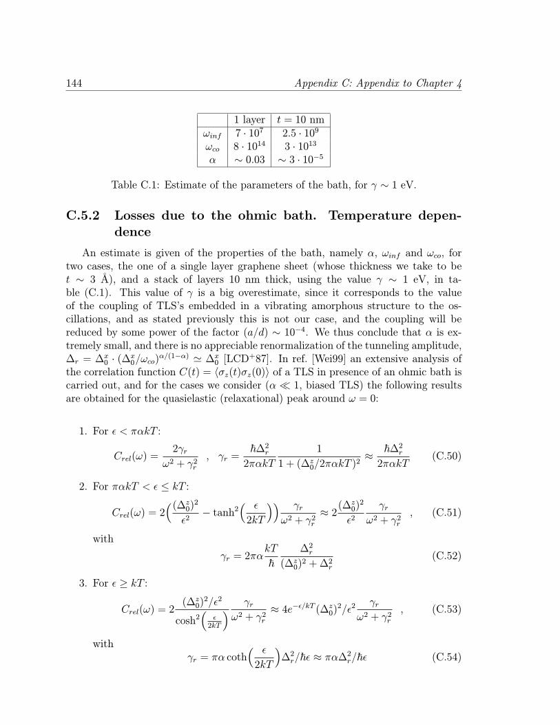
144 Appendix C: Appendix to Chapter 4
1 layer t = 10 nmωinf 7 · 107 2.5 · 109ωco 8 · 1014 3 · 1013α ∼ 0.03 ∼ 3 · 10−5
Table C.1: Estimate of the parameters of the bath, for γ ∼ 1 eV.
C.5.2 Losses due to the ohmic bath. Temperature depen-
dence
An estimate is given of the properties of the bath, namely α, ωinf and ωco, fortwo cases, the one of a single layer graphene sheet (whose thickness we take to bet ∼ 3 A), and a stack of layers 10 nm thick, using the value γ ∼ 1 eV, in ta-ble (C.1). This value of γ is a big overestimate, since it corresponds to the valueof the coupling of TLS’s embedded in a vibrating amorphous structure to the os-cillations, and as stated previously this is not our case, and the coupling will bereduced by some power of the factor (a/d) ∼ 10−4. We thus conclude that α is ex-tremely small, and there is no appreciable renormalization of the tunneling amplitude,∆r = ∆
x0 · (∆x0/ωco)α/(1−α) ' ∆x0 [LCD+87]. In ref. [Wei99] an extensive analysis of
the correlation function C(t) = 〈σz(t)σz(0)〉 of a TLS in presence of an ohmic bath iscarried out, and for the cases we consider (α 1, biased TLS) the following resultsare obtained for the quasielastic (relaxational) peak around ω = 0:
1. For ε < παkT :
Crel(ω) =2γr
ω2 + γ2r, γr =
~∆2r2παkT
1
1 + (∆z0/2παkT )2≈ ~∆2r2παkT
(C.50)
2. For παkT < ε ≤ kT :
Crel(ω) = 2((∆z0)2
ε2− tanh2
( ε
2kT
)) γr
ω2 + γ2r≈ 2(∆
z0)2
ε2γr
ω2 + γ2r, (C.51)
with
γr = 2παkT
~∆2r
(∆z0)2 +∆2r
(C.52)
3. For ε ≥ kT :
Crel(ω) = 2(∆z0)
2/ε2
cosh2(ε2kT
) γr
ω2 + γ2r≈ 4e−ε/kT (∆z0)2/ε2
γr
ω2 + γ2r, (C.53)
withγr = πα coth
( ε
2kT
)∆2r/~ε ≈ πα∆2r/~ε (C.54)
C.5 Dissipation due to two-level systems in graphene resonators 145
These expressions for Crel(ω) substitute the one found usually in the context of sound
attenuation in amorphous solids due to 3D acoustic modes, C3Drel (ω) =(∆z0)
2/ε2
cosh2(ε/2kT )Γ
ω2+Γ2,
and they will enter into the expression for the dissipation as follows:
Q−1(ω, T ) =Pγ2
EkT
∫ εmax
0
dε
∫ 1
umin
du1
u√1− u2
ωC(ω) (C.55)
where u = ∆r/ε, εmax ∼ 5 K, and (u√1− u2)−1 comes from the probability density
of TLS’s in an amorphous solid, like SiO2.When kT > εmax there will be TLS’s only in the regimes of eqs. (C.50) and (C.51), andmoreover, thanks to the very low value of α and the range of ω typical of experimentswe will have γr < ω for all values of u, so that γr/(ω
2 + γ2r ) ≈ γr/ω2, and
Q−1(ω, T ) =Pγ2
EkT
∫ παkT
0
dε
∫ 1
umin
du1
u√1− u2
2ε2u2
2π~ωαkT
+
∫ εmax
παkT
dε
∫ 1
umin
du1
u√1− u2
2(1− u2)2παkTu2
~ω
≈ Pγ2
E~ω
4π3αεmax +
π2
3α2kT
(C.56)
So for high temperatures it will give a constant contribution to dissipation, plus aweak (due to the prefactor α2) linear T dependence.In the case of lower temperatures, kT < εmax, there are some TLS’s in the regimecorresponding to eq. (C.53), and again one can approximate γr/(ω
2 + γ2r ) ≈ γr/ω2
thanks to the low α, leading to
Q−1(ω, T ) =Pγ2
EkT
∫ παkT
0
dε
∫ 1
umin
du1
u√1− u2
2ε2u2
2π~ωαkT
+
∫ kT
παkT
dε
∫ 1
umin
du1
u√1− u2
2(1− u2)2παkTu2
~ω
+
∫ εmax
kT
dε
∫ 1
umin
du1
u√1− u2
4(1− u2)e−ε/kT παu2ε
~ω
≈ Pγ2
E~ω
4π3αkT +
π2
3α2kT +
8π√eαkT
≈ Pγ2α
E~ω
4π3+8π√e
kT (C.57)
Thus, at low temperatures the contribution from TLS’s to attenuation is linear inT. These tendencies come basically from the ohmic character of the vibrational bathand the probability density function of the TLS’s. In case the TLS’s resided in acrystalline material, or for some other reason their distribution function differed fromthe one of amorphous solids, changes in the behavior of Q−1(T, ω) are to be expected.

146 Appendix C: Appendix to Chapter 4
Appendix D
Appendix to Chapter 6
D.1 Dipole matrix element from single-particle mean-
field states
The derivation given in this section is borrowed from [Wei06]. We want to calculatethe dipole matrix element dαβ defined in (6.14)
dαβ = 〈α|[zΘ(a− r) + za3
r3Θ(r − a)
]|β〉 (D.1)
For that sake we need a description of the eigenstates |α〉 of the mean-field Hamil-tonian (6.11). The TDLDA numerical calculations briefly presented in Sec. 6.2informus on the shape of the self-consistent mean field potential V (r), as shown in Fig. 6.1.It suggests that for analytical calculations, V (r) can be approximated by a sphericalwell of radius a and finite height V0, V (r) = V0Θ(r − a), where V0 = εF + W , εFand W being the Fermi energy and the work function of the considered nanoparticle,respectively.Because of the spherical symmetry of the problem, the one-particle wave functions
ψεlm(r) =uεl(r)
rY ml (θ, φ) (D.2)
decompose into radial and angular parts given by the spherical harmonics Y ml (θ, φ),where l and m are the angular momentum quantum numbers. The radial wavefunctions uεl(r) satisfy the reduced Schrodinger equation
[− ~
2
2me
d2
dr2+~2l(l + 1)2mer2
+ V (r)]uεl(r) = εuεl(r) (D.3)
with the conditions uεl(0) = 0 and limr→∞[uεl(r)/r] = 0. This yields the single-particle eigenenergies ε in the mean-field potential V (r). Thus, the matrix elements
147
148 Appendix D: Appendix to Chapter 6
dαβ can be separated into an angular part Amαmβlαlβ
and a radial part Rlαlβ(εα, εβ),
dph = Amαmβlαlβ
Rlαlβ(εα, εβ) . (D.4)
With (D.1), we have
Amαmβlαlβ=
∫ π
0
dθ sin θ
∫ 2π
0
dφY mαlα∗(θ, φ) cos θY
mβlβ(θ, φ) (D.5)
which can be expressed in terms of Wigner-3j symbols [Edm60] as
Amαmβlαlβ= (−1)mα
√(2lα + 1)(2lβ + 1)×
(lα lβ 10 0 0
)(lα lβ 1−mα mβ 0
). (D.6)
The Wigner-3j symbols contain the dipole selection rules lα = lβ ± 1 and mα = mβ.Concerning Rlαlβ(εα, εβ), in the limit of strong electronic confinement V0 εF ,
the single-particle wave function vanishes outside the nanoparticle, enabling us totake the following approximation
Rlαlβ(εα, εβ) '∫ a
0
dru∗εαlα(r)ruεβ lβ(r) (D.7)
The commutator of r with the self-consistent Hamiltonian Hsc = p2/2me+V (r) reads
[r,Hsc] =i~me
pr , (D.8)
where pr is the conjugated momentum to the variable r. Calculating the matrixelement of this commutator between two single-particle eigenstates |α〉 and |β〉 of Hscthen allows to write
〈α|r|β〉 = i~me(εβ − εα)
〈α|pr|β〉 . (D.9)
Now we use [pr, Hsc] = −i~ dV/dr to obtain
〈α|pr|β〉 = −i~
εβ − εα〈α|dV
dr|β〉 , (D.10)
and substituting in (D.9) one gets
〈α|r|β〉 = ~2
me(εβ − εα)2〈α|dV
dr|β〉 , (D.11)
so that the radial part of the dipole matrix element can be reexpressed as a functionof dV/dr as
Rlαlβ(εα, εβ) '~2
me(εβ − εα)2
∫ a
0
dru∗εαlα(r)dV
druεβ lβ(r) , (D.12)
D.1 Dipole matrix element from single-particle mean-field states 149
which for an approximate step potential such as ours, V (r) = V0Θ(r − a), leads to
Rlαlβ(εα, εβ) '~2
me(εβ − εα)2V0u
∗εαlα(a)uεβ lβ(a) . (D.13)
For V0 →∞ and r ≤ a, the regular solutions of (D.3) satisfying uεl(a) = 0 are givenby
uεl(r) =
√2
a3/2rjl(kr)
jl+1(ka), (D.14)
where jν(z) are spherical Bessel functions of the first kind [AIS70], and k =√2meε/~.
The condition jl(ka) = 0 yields the quantization of the single-particle states in theinfinitely deep spherical well. Inserting now the radial wave function (D.14) into(D.13),
Rlαlβ(εα, εβ) =~2
mea(εβ − εα)2V0
jlα(kαa)
jlα+1(kαa)
jlβ(kβa)
jlβ+1(kβa). (D.15)
Now, for r → a+, uεl(r) → 0 and V (r) = V0 → ∞, so that the radial Schrodingerequation (D.3) takes the form
[− ~
2
2me
d2
dr2+ V0
]uεl(r) = 0 . (D.16)
With k0 =√2meV0/~, the physical solution of this equation is
uεl(r → a+) ∼ e−k0r . (D.17)
Thenduεl
dr
∣∣∣r→a+= −k0uεl(r → a+) , (D.18)
and imposing the continuity of the radial wave function and of its derivative withrespect to r at r = a, we obtain
duεl
dr
∣∣∣r→a−= −k0uεl(r → a−) . (D.19)
Therefore, using (D.14)
limV0→∞
[√2meV0~
jl(ka)]= −djl(kr)
dr
∣∣∣r=a= −kdjl(η)
dη
∣∣∣η=ka
. (D.20)
Using the recurrence relation [AIS70]
l
ηjl(η)−
djl
dη= jl+1(η) (D.21)
150 Appendix D: Appendix to Chapter 6
and the fact that jl(η) = jl(ka) = 0, we reach the final result for the radial matrixelement [YB92]
Rlαlβ(εα, εβ) =2~2
mea
√εαεβ
(εα − εβ)2. (D.22)
Note that the dipole selection rule lα = lβ ± 1 appearing in the angluar matrixelement (D.6) implies that εα 6= εβ, and thus (D.22) does not diverge. Furthermore,it decreases with increasing energy |εα − εβ| of the dipole transition |α〉 → |β〉.
D.2 Lowest energy of the particle-hole spectrum
Using the large ka expansion of (D.14) (semiclassical high-energy limit), the quan-tisation condition reads
ka = π
(l
2+ n
)(D.23)
with l and n non-negative integers. The energy of a single-particle (hole) state is re-lated to its wavevector kp(h), its total angular momentum lp(h), and its radial quantumnumber np(h) as
εp(h) =~2k2p(h)2me
= εF
(π
kFa
)2( lp(h)2+ np(h)
)2. (D.24)
Thus, the energy of a p-h excitation entering the RPA sum (6.48) is
∆εph = εF
(π
kFa
)2(lp − lh2+ np − nh
)×(lp + lh2+ np + nh
). (D.25)
Notice that using the exact quantum mechanical spectrum in (6.48) would not changesignificantly the result depicted in Figure 6.4, since the approximation (D.23) is veryreliable for states close to the Fermi energy. We have also checked that generating thep-h excitation energies randomly in the RPA sum (6.43) does not affect the physicalpicture of Figure 6.4. Indeed, the main ingredient to understand such a picture is thefast decay of the dipole matrix element with the p-h energy.The expressions for the dipole matrix element (6.47) as well as for the typical
dipole matrix element (6.57) diverge in the limit of a small p-h energy. It is thereforecrucial for our analysis to determine the appropriate minimal p-h energy ∆εmin thatrenders this divergence unphysical.This can be achieved by imposing the dipole selection rules in (D.25) and that
the energy difference is minimal. The first condition dictates that lh = lp ± 1 andmh = mp. Therefore there are two ways of obtaining the minimal energy difference:np = nh with lp = lh + 1 and np = nh + 1 with lp = lh − 1. In both cases we have
∆εmin 'εF
kFa/π
kh
kF. (D.26)
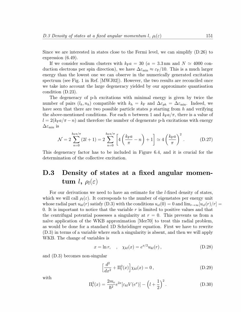
D.3 Density of states at a fixed angular momentum l, ρl(ε) 151
Since we are interested in states close to the Fermi level, we can simplify (D.26) toexpression (6.49).If we consider sodium clusters with kFa = 30 (a = 3.3 nm and N ' 4000 con-
duction electrons per spin direction), we have ∆εmin ≈ εF/10. This is a much largerenergy than the lowest one we can observe in the numerically generated excitationspectrum (see Fig. 1 in Ref. [MWJ02]). However, the two results are reconciled oncewe take into account the large degeneracy yielded by our approximate quantisationcondition (D.23).The degeneracy of p-h excitations with minimal energy is given by twice the
number of pairs (lh, nh) compatible with kh = kF and ∆εph = ∆εmin. Indeed, wehave seen that there are two possible particle states p starting from h and verifyingthe above-mentioned conditions. For each n between 1 and kFa/π, there is a value ofl = 2(kFa/π−n) and therefore the number of degenerate p-h excitations with energy∆εmin is
N = 2kFa/π∑
n=0
(2l + 1) = 2
kFa/π∑
n=0
[4
(kFa
π− n)+ 1
]' 4(kFa
π
)2. (D.27)
This degeneracy factor has to be included in Figure 6.4, and it is crucial for thedetermination of the collective excitation.
D.3 Density of states at a fixed angular momen-
tum l, ρl(ε)
For our derivations we need to have an estimate for the l-fixed density of states,which we will call ρl(ε). It corresponds to the number of eigenstates per energy unitwhose radial part ukl(r) satisfy (D.3) with the conditions uεl(0) = 0 and limr→∞[uεl(r)/r] =0. It is important to notice that the variable r is limited to positive values and thatthe centrifugal potential possesses a singularity at r = 0. This prevents us from anaıve application of the WKB approximation [Mer70] to treat this radial problem,as would be done for a standard 1D Schrodinger equation. First we have to rewrite(D.3) in terms of a variable where such a singularity is absent, and then we will applyWKB. The change of variables is
x = ln r, , χkl(x) = ex/2ukl(r) , (D.28)
and (D.3) becomes non-singular
[ d2
dx2+Π2l (x)
]χkl(x) = 0 , (D.29)
with
Π2l (x) =2me~2
e2x[εklV (ex)]−
(l +1
2
)2. (D.30)
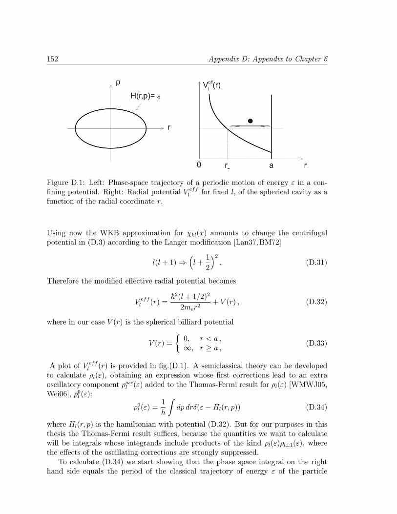
152 Appendix D: Appendix to Chapter 6
Figure D.1: Left: Phase-space trajectory of a periodic motion of energy ε in a con-fining potential. Right: Radial potential V effl for fixed l, of the spherical cavity as afunction of the radial coordinate r.
Using now the WKB approximation for χkl(x) amounts to change the centrifugalpotential in (D.3) according to the Langer modification [Lan37,BM72]
l(l + 1)⇒(l +1
2
)2. (D.31)
Therefore the modified effective radial potential becomes
V effl (r) =~2(l + 1/2)2
2mer2+ V (r) , (D.32)
where in our case V (r) is the spherical billiard potential
V (r) =
0, r < a ,∞, r ≥ a ,
(D.33)
A plot of V effl (r) is provided in fig.(D.1). A semiclassical theory can be developedto calculate ρl(ε), obtaining an expression whose first corrections lead to an extraoscillatory component ρoscl (ε) added to the Thomas-Fermi result for ρl(ε) [WMWJ05,Wei06], ρ0l (ε):
ρ0l (ε) =1
h
∫dp drδ(ε−Hl(r, p)) (D.34)
where Hl(r, p) is the hamiltonian with potential (D.32). But for our purposes in thisthesis the Thomas-Fermi result suffices, because the quantities we want to calculatewill be integrals whose integrands include products of the kind ρl(ε)ρl±1(ε), wherethe effects of the oscillating corrections are strongly suppressed.To calculate (D.34) we start showing that the phase space integral on the right
hand side equals the period of the classical trajectory of energy ε of the particle
D.3 Density of states at a fixed angular momentum l, ρl(ε) 153
confined in the V effl (r) shown in fig.(D.1)
∫dp drδ(ε−Hl(r, p)) = τl(ε) (D.35)
The delta function can be expressed as
δ(ε−Hl(r, p)) =∑
(r′,p′) such thatH(r′,p′)=ε
δ(r − r′, p− p′)|∇H(r′, p′)|
, (D.36)
where δ(r − r′, p − p′) fulfills∫dp drδ(r − r′, p − p′)f(r, p) = f(r′, p′), for a generic
function f(r, p). Therefore the surface integral (D.35) is converted by the sum overdelta functions into a line integral over the trajectory in phase space whose energyis fixed at the value ε. The denominator can be reexpressed with the aid of theHamilton equations satisfied by the classical trajectory:
dp
dt= −∂H
∂r,
dr
dt=∂H
∂p, (D.37)
so that |∇H(r′, p′)| =√[∂H/∂r]2 + [∂H/∂p]2 becomes
√dr2 + dp2/dt = dl/dt. Sub-
stituting in (D.35):
∫dp dr
∑
(r′,p′) such thatH(r′,p′)=ε
δ(r − r′, p− p′)|∇H(r′, p′)|
=
∮dl1
dl/dt=
∮dt = τl(ε) . (D.38)
The next step is to calculate τl(ε). For that sake we use the classical action functional
S[ε, τl] =
∫ τl
0
[ p2
2m− V effl (r)
]dt+ ετl =
∫ r(t=τl)
r(t=0)
dr · p , (D.39)
which satisfies ∂S/∂ε = τl. We will calculate S using its last form in terms of r andp, recalling the fact that for a trajectory of fixed energy
p2
2m+ V effl (r) = ε → p =
√2m(ε− V effl (r)) (D.40)
The value of S can then be calculated as
S[ε, τl] =
∫ r(t=τ)
r(t=0)
dr · p = 2∫ r=a
r−(ε)
dr
√2m(ε− V effl (r)) . (D.41)
The value of the turning point r−(ε) on the left of the classically allowed region isgiven by the condition V effl (r−(ε)) = ε, i.e., r−(ε) = ~(l+1/2)/
√2meε, see fig.(D.1).
154 Appendix D: Appendix to Chapter 6
Substituting the form of the potential V effl (r) in the integral (D.41), after a straigh-forward calculation we get
S[ε, τl] = 2~[√(2mεa2/~2)−
(l +1
2
)2−(l +1
2
)arccos
( l + 1/2√(2mεa2/~2)
)], (D.42)
and the period τl is obtained performing the partial derivative with respect to ε,obtaining in this way the desired Thomas-Fermi estimate for the partial density ofstates:
τl(ε) =~√(2mεa2/~2)−
(l + 1
2
)2
ε→ ρl(ε) ' ρ0l (ε) =
√(2mεa2/~2)−
(l + 1
2
)2
2πε(D.43)
D.4 Local density of the dipole matrix element
Equation (6.51) defines the local density of dipole matrix elements connectingstates at energies ε and ε + ∆ε. We used particle and hole states in our definition,since this is the main interest of our work. But note that the calculation presented inthis appendix is not restricted to that case and can be easily extended to any states.The result would be of course unchanged.Local densities of matrix elements of arbitrary operators have been thoroughly
studied as they can be easily connected with physical properties, ranging from far-infrared absorption in small particles [MR97] to electronic lifetimes of quantum dots[GJS04]. A semiclassical theory for the local density of matrix elements has beendeveloped [FP86,Wil87,EFMW92], where (6.51) can be expressed as a smooth partgiven by correlations along classical trajectories plus a periodic orbit expansion. Wewill not follow here this general procedure, but continue to use the simple form ofthe dipole matrix elements (6.44) for states confined in a hard-wall sphere and thesemiclassical approximation applied to the radial (fixed l) problem [MWJ02,MWJ03,WMWJ05].Using the l-fixed density of states (D.43) we can write with the help of equations
(D.4, D.6, D.22)
C(ε,∆ε) =∑
αβ
(Amαmβlαlβ
)2(Rlαlβ(εα, εβ)
)2δ(ε− εα)δ(ε+∆ε− εβ)
=
∫ ∞
0
dεα∑
lαmα
ρlα(εα)
∫ ∞
0
dεβ∑
lβmβ
ρlβ(εβ)(Amαmβlαlβ
)2(Rlαlβ(εα, εβ)
)2δ(ε− εα)δ(ε+∆ε− εβ)
=∑
lαmα,lβmβ
ρlα(ε)ρlβ(ε+∆ε)(Amαmβlαlβ
)2(Rlαlβ(εα, εβ)
)2(D.44)
D.4 Local density of the dipole matrix element 155
Amαmβlαlβ
6= 0 only if mα = mβ and lα = lβ ± 1, therefore
C(ε,∆ε) =(2~2
ma
)2 ε(ε+∆ε)∆ε4
∑
lα,mα,lβ=lα±1
ρlα(ε)ρlβ(ε+∆ε)(Amαmαlαlβ
)2(D.45)
We first perform the sum over lβ:
∑
lβ=lα±1
(Amαmαlαlβ
)2ρlβ(ε+∆ε) =
(Amαmαlαlα+1
)2ρlα+1(ε+∆ε) +
(Amαmαlαlα−1
)2ρlα−1(ε+∆ε)
=(lα + 1−mα)(lα + 1 +mα)
(2lα + 1)(2lα + 3)ρlα+1(ε+∆ε) +
(lα −mα)(lα +mα)(2lα − 1)(2lα + 1)
ρlα−1(ε+∆ε)(D.46)
and then over mα:
lα∑
mα=−lα
(lα + 1−mα)(lα + 1 +mα) =1
3(lα + 1)(2lα + 1)(2lα + 3),
lα∑
mα=−lα
(lα −mα)(lα +mα) =1
3lα(2lα − 1)(2lα + 1), (D.47)
yielding
C(ε,∆ε) =(2~2
mea
)2εε′
3∆ε4×lmax∑
lh=0
%lh(ε) [(lh + 1)%lh+1(ε′) + lh%lh−1(ε
′)] (D.48)
where lmax is the maximum allowed lh for an energy ε, while ε′ = ε + ∆ε. In the
semiclassical limit we can take lh ' lh + 1 1 and convert the sum into an integral.Thus,
C(ε,∆ε) =2
3
(2~2
ma
)2 ε(ε+∆ε)∆ε4
∫ lmax
0
dl l
√2mεa2/~2 − l22πε
√2m(ε+∆ε)a2/~2 − l22π(ε+∆ε)
=1
6π2
(2~2
ma
)2 1∆ε4
∫ y
0
dl l√y2 − l2
√y′2 − l2 (D.49)
where y2 = 2mεa2/~2 and y′2 = y2 + 2m∆ε a2/~2.Changing variables now to u = l2,du = 2ldl, we get
C(ε,∆ε) =1
12π2
(2~2
ma
)2 1∆ε4
∫ y2
0
du√y2 − u
√y′2 − u (D.50)
Using the results of ref. [GR00] we obtain
∫ y2
0
du√y2 − u
√y′2 − u = (y
′2 − y2)2
8ln[∣∣∣y′ − yy′ + y
∣∣∣]+(y′2 + y2)yy′
4(D.51)
And substituting the values of y and y′ one arrives at the desired expression (6.52).
156 Appendix D: Appendix to Chapter 6
D.5 Density of particle-hole excitations
The density of p-h excitations with energy ∆ε is defined in (6.55) and can bewritten as
ρp-h(∆ε) =
∫ εF
εF−∆εdεh∑
lh
(2lh + 1)%lh(εh)× [%lh+1(εh +∆ε) + %lh−1(εh +∆ε)] .
(D.52)Using the semiclassical density of states (D.43) and performing the sum in the limitlh 1, we obtain
ρp-h(∆ε) ' ∆ε2
8π2
(2mea
2
~2
)2 ∫ εF
εF−∆εdεh
F (εh/∆ε)
εh(εh +∆ε), (D.53)
where the function F has been defined in (6.53). Performing the remaining integralover the hole energy in the limit ∆ε εF is straightforward and leads to the result(6.56).
Bibliography
[ABV07] F. B. Anders, R. Bulla, and M. Vojta, Equilibrium and non-equilibriumdynamics of the sub-ohmic spin-boson model, Phys. Rev. Lett. 98 (2007),210402.
[AHSD74] W. Arnold, S. Hunklinger, S. Stein, and K. Dransfeld, Nonlinear ultra-sonic attenuation in glasses, J. Non Cryst. Sol. 14 (1974), 192.
[AHV72] P.W. Anderson, B.I. Halperin, and C.M. Varma, Anomalous low-temperature thermal properties of glasses and spin glasses. (ultrasonicattenuation and magnetic impurity systems), Philos. Mag. 25 (1972), 1.
[AIS70] M. Abramowitz and eds. I.A. Stegun, Handbook of mathematical func-tions, 9th ed., Dover, New York, 1970.
[AM76] N.W. Ashcroft and N.D. Mermin, Solid state physics, Harcourt, Or-lando, 1976.
[AM03] K.-H. Ahn and P. Mohanty, Quantum friction of micromechanical res-onators at low temperatures, Phys. Rev. Lett. 90 (2003), 085504.
[And86] A.C. Anderson, On the coupling between two-level states and strains inamorphous solids, J. Non-Crys. Solids 85 (1986), 211.
[ANVA+99] M. Arndt, O. Nairz, J. Voss-Andreae, C. Keller, G. van der Zouw, andA. Zeilinger, Wave-particle duality of C60, Nature 401 (1999), 680.
[AP87] A.I. Akinwande and J.D. Plummer, Quantitative modeling of si/sio2interface fixed charge: I. experimental results, J. Electrochem. Soc. 134(1987), 2565.
[AS06] A. Altland and B. Simons, Condensed matter field theory, CambridgeUniversity Press, 2006.
[BB75] A. Bohr and B.R.Mottelson, Nuclear structure, vol. ii, Benjamin, NewYork, 1975.
157
158 Bibliography
[BB94] G.F. Bertsch and R.A. Broglia, Oscillations in finite quantum systems,Cambridge University Press, 1994.
[BCLS93] C. Brechignac, P. Cahuzac, J. Leygnier, and A. Sarfati, Optical responseof large lithium clusters: Evolution toward the bulk, Phys. Rev. Lett. 70(1993), 2036.
[BF04] H. Bruus and K. Flensberg, Many-body quantum theory in condensedmatter physics : An introduction, Oxford University Press, 2004.
[BH77] J.L. Black and B.I. Halperin, Spectral diffusion, phonon echoes, andsaturation recovery in glasses at low temperatures, Phys. Rev. B 16(1977), 2879.
[BHMD00] J.-Y. Bigot, V. Halte, J.-C. Merle, and A. Daunois, Electron dynamicsin metallic nanoparticles, Chem. Phys. 251 (2000), 181.
[Ble99] M.P. Blencowe, Quantum energy flow in mesoscopic dielectric struc-tures, Phys. Rev. B 59 (1999), 4994.
[Ble04] M. Blencowe, Quantum electromechanical systems, Phys. Rep. 395(2004), 159.
[Bli05] R.H. Blick et al., Focus on nano-electromechanical systems, New J. Phys.7 (2005), Editorial.
[BLTV05] R. Bulla, H. Lee, N. Tong, and M. Vojta, Numerical renormalizationgroup for quantum impurities in a bosonic bath, Phys. Rev. B 71 (2005),045122.
[BM72] M.V. Berry and K.E. Mount, Semiclassical approximations in wave me-chanics, Rep. Prog. Phys. 35 (1972), 315.
[BM05] R. L. Badzey and P. Mohanty, Coherent signal amplification in bistablenanomechanical oscillators by stochastic resonance, Nature 437 (2005),995.
[BMCD95] J.-Y. Bigot, J.-C. Merle, O. Cregut, and A. Daunois, Electron dynamicsin copper metallic nanoparticles probed with femtosecond optical pulses,Phys. Rev. Lett. 75 (1995), 4702.
[BOS+07] A. Bostwick, T. Ohta, T. Seyller, K. Horn, and E. Rotenberg, Quasi-particle dynamics in graphene, Nature Physics 3 (2007), 36.
[BQKM07] R. H. Blick, H. Qin, H.-S. Kim, and R. Marsland, A nanomechanicalcomputer-exploring new avenues of computing, New J. Phys. 9 (2007),241.
Bibliography 159
[Bra93] M. Brack, The physics of simple metal clusters: self-consistent jelliummodel and semiclassical approaches, Rev. Mod. Phys. 65 (1993), 677.
[BRS+04] T. M. Buehler, D.J. Reilly, R.P. Starrett, V.C. Chan, A.R. Hamilton,A.S. Dzurak, and R.G. Clark, Observing sub-microsecond telegraph noisewith the radio frequency single electron transistor.
[BS89] M. Barma and V. Subrahmanyam, Optical absorption in small metalparticles, J. Phys.: Condens. Matter 1 (1989), 7681.
[BSS+99] A. Bachtold, C. Strunk, J.-P. Salvetat, J.-M. Bonard, L. Forro, T. Nuss-baumer, and C. Schonenberger, Aharonov bohm oscillations in carbonnanotubes, Nature 397 (1999), 673.
[BTM+02] D. Boyer, P. Tamarat, A. Maali, B. Lounis, and M. Orrit, Photothermalimaging of nanometer-sized metal particles among scatterers, Science297 (2002), 1160.
[BTV03] R. Bulla, N.-H. Tong, and M. Vojta, Numerical renormalization groupfor bosonic systems and application to the sub-ohmic spin-boson model,Phys. Rev. Lett. 91 (2003), 170601.
[BvdZV+07] J. Scott Bunch, Arend M. van der Zande, Scott S. Verbridge, Ian W.Frank, David M. Tanenbaum, Jeevak M. Parpia, Harold G. Craig-head, and Paul L. McEuen, Electromechanical resonators from graphenesheets, Science 315 (2007), 490.
[BW04] R. B. Bhiladvala and Z. J. Wang, Effect of fluids on the q factor and res-onance frequency of oscillating micrometer and nanometer scale beams,Phys. Rev. E 69 (2004), 036307.
[CGP+07] A.H. Castro Neto, F. Guinea, N.M.R. Peres, K.S. Novoselov, and A.K.Geim, The electronic properties of graphene, Rev. Mod. Phys. (to ap-pear) (2007).
[CL00] P.M. Chaikin and T.C. Lubensky, Principles of condensed matterphysics, Cambridge University Press, Cambridge, 2000.
[Cle02] A. N. Cleland, Foundations of nanomechanics, Springer (Berlin), 2002.
[CLW01] S. M. Carr, W. E. Lawrence, and M. N. Wybourne, Accessibility ofquantum efects in mesomechanical systems, Phys. Rev. B 64 (2001),220101(R).
160 Bibliography
[CR99] A. N. Cleland and M. L. Roukes, External control of dissipation in ananometer-scale radiofrequency mechanical resonator, Sens. ActuatorsA 72 (1999), 256.
[CR02] , Noise processes in nanomechanical resonators, J. Appl. Phys.92 (2002), 2758.
[Cra00] H. G. Craighead, Nanoelectromechanical systems, Science 250 (2000),1532.
[CRB07] M. Chu, R. E. Rudd, and M. P. Blencowe, The role of reconstructedsurfaces in the intrinsic dissipative dynamics of silicon nanoresonators.
[CRSU00] F. Calvayrfac, P.-G. Reinhard, E. Suraud, and C.A. Ullrich, Nonlinearelectron dynamics in metal clusters, Phys. Rep. 337 (2000), 493.
[CT06] A. Chin and M. Turlakov, Coherent-incoherent transition in the sub-ohmic spin-boson model, Phys. Rev. B 73 (2006), 075311.
[CTB+03] L. Cognet, C. Tardin, D. Boyer, D. Choquet, P. Tamarat, and B. Lounis,Single metallic nanoparticle imaging for protein detection in cells, Proc.Natl. Acad. Sci. U.S.A. 100 (2003), 11350.
[DDA01] M.S. Dresselhaus, G. Dresselhaus, and Ph. Avouris, Carbon nanotubes,Springer Verlag, 2001.
[DDE96] M.S. Dresselhaus, G. Dresselhaus, and P.C. Eklund, Science of fullerenesand carbon nanotubes, Academic Press, 1996.
[DH81] P. Dutta and P.M. Horn, Low-frequency fluctuations in solids: 1 / fnoise, Rev. Mod. Phys. 53 (1981), 497.
[dH93] W.A. de Heer, The physics of simple metal clusters: experimental aspectsand simple models, Rev. Mod. Phys. 65 (1993), 611.
[DHT07] S. Das Sarma, E.H. Hwang, and W.-K. Tse, Many-body interaction ef-fects in doped and undoped graphene: Fermi liquid versus non-fermiliquid, Phys. Rev. B 75 (2007), 121406(R).
[DKEM06] J. Dorignac, A. Kalinowski, S. Erramilli, and P. Mohanty, Dynamicalresponse of nanomechanical oscillators in immiscible viscous fluid for invitro biomolecular recognition, Phys. Rev. Lett. 96 (2006), 186105.
[DLC+05] R. S. Decca, D. Lopez, H. B. Chan, E. Fischbach, D. E. Krause, andC. R. Jamell, Constraining new forces in the casimir regime using theisoelectronic technique, Phys. Rev. Lett. 94 (2005), 240401.
Bibliography 161
[Dor65] R.H. Doremus, Optical properties of small silver particles, J. Chem.Phys. 42 (1965), 414.
[DPX98] Y. Dong, S.V. Pappu, and Z. Xu, Detection of local density distributionof isolated silanol groups on planar silica surfaces using nonlinear opticalmolecular probes, Anal. Chem. 70 (1998), 4730.
[DYN+99] Z. Dai, S. Yamamoto, K. Narumi, A. Miyashita, and H. Naramoto, Goldnanoparticle fabrication in single crystal sio2 by mev au ion implanta-tion and subsequent thermal annealing, Nucl. Instr. and Meth. B 149(1999), 108.
[EBF+01] R. Egger, A. Bachtold, M.S. Fuhrer, M. Bockrath, D.H. Cobden, andP.L. McEuen, Luttinger liquid behavior in metallic carbon nanotubes,Lecture Notes in Physics, vol. 579, Springer Verlag, 2001.
[Edm60] A.R. Edmonds, Angular momentum in quantum mechanics (second edi-tion), Princeton University Press, Princeton, 1960.
[EFMW92] B. Eckhardt, S. Fishman, K. Muller, and D. Wintgen, Semiclassicalmatrix elements from periodic orbits, Phys. Rev. A 45 (1992), 3531.
[Eka84a] W. Ekardt, Dynamical polarizability of small metal particles: Self-consistent spherical jellium background model, Phys. Rev. Lett. 52(1984), 1925.
[Eka84b] ,Work function of small metallic particles: Self-consistent spher-ical jellium-background model, Phys. Rev. B 29 (1984), 1558.
[EOS+00] S. Evoy, A. Olkhovets, L. Sekaric, J. M. Parpia, H. G. Craighead, andD. W. Carr, Temperature-dependent internal friction in silicon nano-electromechanical systems, Appl. Phys. Lett. 77 (2000), 2397.
[ER05] K. L. Ekinci and M. L. Roukes, Nanoelectromechanical systems, Rev.Sci. Inst. 76 (2005), 061101.
[ERK04] P. Esquinazi, M. A. Ramos, and R. Konig, Acoustic properties of amor-phous solids at very low temperatures: The quest for interacting tunnel-ing states, J. Low Temp. Phys. 135 (2004), 27.
[Esq98] P. Esquinazi (ed.), Tunneling systems in amorphous and crystallinesolids, Springer (Berlin), 1998.
[ETB06] J.W. Evans, P.A. Thiel, and M.C. Bartelt, Morphological evolution dur-ing epitaxial thin film growth: Formation of 2d islands and 3d mounds,Sur. Sci. Rep. 61 (2006), 1.
162 Bibliography
[EW92] R. Egger and U. Weiss, Quantum monte carlo simulation of the dynam-ics of the spin-boson model, Z. Phys. B - Condensed Matter 89 (1992),97.
[EWZB01] A. Erbe, C. Weiss, W. Zwerger, and R. H. Blick, Nanomechanical res-onator shuttling single electrons at radio frequencies, Phys. Rev. Lett.87 (2001), 096106.
[Fey48] R. P. Feynman, Space-time approach to non-relativistic quantum me-chanics, Rev. Mod. Phys. 20 (1948), 367.
[FH65] R. P. Feynman and A. R. Hibbs, Quantum physics and path integrals,McGraw-Hill, New York, 1965.
[FKDB02] M. S. Fuhrer, B. M. Kim, T. Du1rkop, and T. Brintlinger, High-mobilitynanotube transistor memory, Nano Lett. 2 (2002), 755.
[FP86] M. Feingold and A. Peres, Distribution of matrix elements of chaoticsystems, Phys. Rev. A 34 (1986), 591.
[FS01] L. Forro and C. Schonenberger, Carbon nanotubes, materials for thefuture, Europhys. News. 32 (2001), 86.
[FTK+06] M. Freitag, J.C. Tsang, J. Kirtley, A. Carlsen, J.Chen, A. Troeman,H. Hilgenkamp, and Ph. Avouris, Electrically excited, localized infraredemission from single carbon nanotubes, Nano Lett. 6 (2006), 1425.
[FV63] R. P. Feynman and F. L. Vernon, Jr., The theory of a general quantumsystem interacting with a linear dissipative system, Ann. Phys. (N.Y.)24 (1963), 118.
[FVF+00] N. Del Fatti, F. Vallee, C. Flytzanis, Y. Hamanaka, and A. Naka-mura, Electron dynamics and surface plasmon resonance nonlinearitiesin metal nanoparticles, Chem. Phys. 251 (2000), 215.
[FZMR06] X. L. Feng, C. A. Zorman, M. Mehregany, and M. L. Roukes, Dissipationin single-crystal 3c-sic ultra-high frequency nanomechanical resonators.
[GC05] M. R. Geller and A. N. Cleland, Superconducting qubits coupled to nano-electromechanical resonators: An architecture for solid-state quantum-information processing, Phys. Rev. A 71 (2005), 032311.
[GCP06] F. Guinea, A. H. Castro Neto, and N. M. R. Peres, Electronic states andlandau levels in graphene stacks, Phys. Rev. B 73 (2006), 245426.
Bibliography 163
[GDP96] E.K.U. Gross, J.F. Dobson, and M. Petersilka, Density functional theoryof time-dependent phenomena, Topics in Current Chemistry, vol. 181,Springer, Berlin, 1996.
[GGI02] L.G. Gerchikov, C. Guet, and A.N. Ipatov, Multiple plasmons and an-harmonic effects in small metallic clusters, Phys. Rev. A 66 (2002),053202.
[GGV99] J. Gonzalez, F. Guinea, and M. A. H. Vozmediano, Marginal-fermi-liquid behavior from two-dimensional coulomb interaction, Phys. Rev. B59 (1999), R2474.
[GH98] M. Grifoni and P. Hanggi, Driven quantum tunneling, Phys. Rep. 304(1998), 229.
[GJS04] F. Guinea, R. A. Jalabert, and F. Sols, Electronic lifetimes in ballisticquantum dots electrostatically coupled to metallic environments, Phys.Rev. B 70 (2004), 085310.
[GK85] E.K.U. Gross and W. Kohn, Local density-functional theory offrequency-dependent linear response, Phys. Rev. Lett. 55 (1985), 2850.
[GMM06] F. Guinea, M.P. Lopez-Sancho, and M.A.H. Vozmediano, Carbon basedmaterials magnetism, ch. 15, p. 353, Elsevier Science, 2006.
[GN07] A. K. Geim and K. S. Novoselov, The rise of graphene, Nature Materials6 (2007), 183.
[GR00] Gradshteyn and Ryzhik, Table of integrals, series, and products, Acad-emic Press, 2000.
[GSSW93] M. Grifoni, M. Sassetti, J. Stockburger, and U. Weiss, Nonlinear re-sponse of a periodically driven damped two-state system, Phys. Rev. E48 (1993), 3497.
[Gui84] F. Guinea, Friction and particle-hole pairs, Phys. Rev. Lett. 53 (1984),1268.
[Gui85] , Dynamics of simple dissipative systems, Phys. Rev. B 32(1985), 4486.
[Gui05] , Electronic dephasing in wires due to metallic gates, Phys. Rev.B 71 (2005), 045424.
[GW88] R. Gorlich and U. Weiss, Specific heat of the dissipative two level system,Phys. Rev. B 38 (1988), 5245.
164 Bibliography
[Had91] R.C. Haddon et. al., Conducting films of C60 and C70 by alkali-metaldoping, Nature 350 (1991), 320.
[HAS+72] S. Hunklinger, W. Arnold, St. Stein, R. Nava, and K. Dransfeld, Satu-ration of the ultrasonic absorption in vitreous silica at low temperatures,Phys. Lett. A 42 (1972), 256.
[HAS06] E. H. Hwang, S. Adam, and S. Das Sarma, Carrier transport in 2dgraphene layers, Phys. Rev. Lett. 98 (2006), 186806.
[HFZ+05] X. M. H. Huang, X. L. Feng, C. A. Zorman, M. Mehregany, andM. Roukes, Vhf, uhf and microwave frequency nanomechanical res-onators, New J. Phys. 7 (2005), 247.
[HHP+03] A. Husain, J. Hone, H. W. C. Postma, X. M. H. Huang, T. Drake,M. Barbic, A. Scherer, and M. L. Roukes, Nanowire-based very-high-frequency electromechanical resonator, Appl. Phys. Lett. 83 (2003),1240.
[HKC+07] M. A. Hopcroft, B. Kim, S. Chandorkar, R. Melamud, M. Agarwal,C. M. Jha, G. Bahl, J. Salvia, H. Mehta, H. K. Lee, R. N. Candler, andT. W. Kenny, Using the temperature dependence of resonator qualityfactor as a thermometer, Appl. Phys. Lett. 91 (2007), 013505.
[Iji91] S. Ijima, Helical microtubules of graphitic carbon, Nature 354 (1991),56.
[IN92] G. L. Ingold and Yu. V. Nazarov, Single charge tunneling, Plenum Press(New York), 1992.
[J72] J. Jackle, On the ultrasonic attenuation in glasses at low temperatures,Z. Physik 257 (1972), 212.
[Jac75] J.D. Jackson, Classical electrodynamics (second edition), John Wiley &Sons, New York, 1975.
[Jac07] K. Jacobs, Engineering quantum states of a nanoresonator via a simpleauxiliary system, Phys. Rev. Lett. 99 (2007), 117203.
[JG88] M. P. Sheetz J. Gelles, B. J. Schnapp, Tracking kinesin-driven move-ments with nanometre-scale precision, Nature 331 (1988), 450.
[JI68] Y. Jimbo and K. Itao, J. Horological Inst. Jpn. 47 (1968), 1.
[JLB07] K. Jacobs, P. Lougovski, and M. Blencowe, Continuous measurement ofthe energy eigenstates of a nanomechanical resonator without a nonde-molition probe, Phys. Rev. Lett. 98 (2007), 147201.
Bibliography 165
[JPAH76] J. Jackle, L. Piche, W. Arnold, and S. Hunklinger, Elastic effects ofstructural relaxation in glasses at low temperatures, J. Non-Crys. Solids20 (1976), 365.
[JT37] H.A. Jahn and E. Teller, Stability of polyatomic molecules in degener-ate electronic state. i. orbital degeneracy, Proc. R. Soc. London A 161(1937), 220.
[KB06] Y. Kurzweil and R. Baer, Quantum memory effects in the dynamics ofelectrons in gold clusters, Phys. Rev. B 73 (2006), 075413.
[KC03] R.G. Knobel and A.N. Cleland, Nanometre-scale displacement sensingusing a single-electron transistor, Nature 424 (2003), 291.
[KCdH+84] W.D. Knight, K. Clemenger, W.A. de Heer, W.A. Saunders, and M.Y.Chou, Electronic shell structure and abundances of sodium clusters,Phys. Rev. Lett. 52 (1984), 2141.
[KCdHS85] W.D. Knight, K. Clemenger, W.A. de Heer, and W.A. Saunders, Polar-izability of alkali clusters, Phys. Rev. B 31 (1985), 2539.
[KHDS02] H.E. Katz, X.M. Hong, A. Dodabalapur, and R. Sarpeshkar, Organicfield-effect transistors with polarizable gate insulators, J. Appl. Phys. 91(2002), 1572.
[KHO+85] H.W. Kroto, J.R. Heath, S.C. O’Brien, R.F. Curl, and R.E. Smalley,C60: Buckminsterfullerene, Nature 318 (1985), 162.
[Khv04] D. V. Khveshchenko, Quantum impurity models of noisy qubits, Phys.Rev. B 69 (2004), 153311.
[KJV+03] W. Kim, A. Javey, O. Vermesh, Q. Wang, Y. Li, and H. Dai, Hysteresiscaused by water molecules in carbon nanotube field-effect transistors,Nano Lett. 3 (2003), 193.
[KK66] A. Kawabata and R. Kubo, Electronic properties of fine metallic par-ticles. ii. plasma resonance absorption, J. Phys. Soc. Jpn. 21 (1966),1765.
[KKS82] M.M. Kappes, R.W. Kunz, and E. Schumacher, Production of largesodium clusters (nax, x < 65) by seeded beam expansions, Chem. Phys.Lett. 91 (1982), 413.
[KLER04] X. M. H. Huang K. L. Ekinci and M. L. Roukes, Ultrasensitive nano-electromechanical mass detection, Appl. Phys. Lett. 84 (2004), 4469.
166 Bibliography
[KM96] S. Kehrein and A. Mielke, On the spin-boson model with a sub-ohmicbath, Phys. Lett. A 219 (1996), 313.
[KRSL07] I. Katz, A. Retzker, R. Straub, and R. Lifshitz, Signatures for a classicalto quantum transition of a driven nonlinear nanomechanical resonator,Phys. Rev. Lett. 99 (2007), 040404.
[Kub57] R. Kubo, Statistical-mechanical theory of irreversible processes. i. gen-eral theory and simple applications to magnetic and conduction prob-lems, J. Phys. Soc. Japan 12 (1957), 570.
[KV95] U. Kreibig and M. Vollmer, Optical properties of metal clusters,Springer-Verlag, Berlin, 1995.
[Lan37] R.E. Langer, On the connection formulas and the solutions of the waveequation, Phys. Rep. 51 (1937), 669.
[Lan80] Landau & Lifshitz, Statistical physics, part i, Pergamon, Oxford, 1980.
[LB99] X. Li and B. Bhushan, Micro/nanomechanical characterization of ce-ramic films for microdevices, Thin Solid Films 340 (1999), 210.
[LBCS04] M. D. LaHaye, O. Buu, B. Camarota, and K. C. Schwab, Approachingthe quantum limit of a nanomechanical resonator, Science 304 (2004),74.
[LBT+03] X. Li, B. Bhushan, K. Takashima, C.W. Baek, and Y.K. Kim, Mechan-ical characterization of micro/nanoscale structures for mems/nems ap-plications using nanoindentation techniques, Ultramicroscopy 97 (2003),481.
[LCD+87] A. J. Leggett, S. Chakravarty, A. T. Dorsey, M. P. A. Fisher, A. Garg,and W. Zwerger, Dynamics of the dissipative two-state system, Rev.Mod. Phys. 59 (1987), 1.
[Leg02] A. J. Leggett, Testing the limits of quantum mechanics: motivation,state of play, prospects, J. Phys: Condens. Matter 14 (2002), R415.
[LKLA99] B. Lamprecht, J.R. Krenn, A. Leitner, and F.R. Aussenegg, Resonantand off-resonant light-driven plasmons in metal nanoparticles studied byfemtosecond-resolution third-harmonic generation, Phys. Rev. Lett. 83(1999), 4421.
[LL59] L. D. Landau and E. M. Lifshitz, Theory of elasticity, Pergamon Press(London), 1959.
Bibliography 167
[LR00] R. Lifshitz and M.L. Roukes, Thermoelastic damping in micro- andnanomechanical systems, Phys. Rev. B 61 (2000), 5600.
[LS91] E. Lipparini and S. Stringari, Collective excitations in deformed alkalimetal clusters, Z. Phys. D 18 (1991), 193.
[LTBP99] X. Liu, E. J. Thompson, B. E. White Jr., and R. O. Pohl, Low-temperature internal friction in metal films and in plastically deformedbulk aluminum, Phys. Rev. B 59 (1999), 11767.
[LUCS01] Y.-H. Liau, A.N. Unterreiner, Q. Chang, and N.F. Scherer, Ultrafastdephasing of single nanoparticles studied by two-pulse second-order in-terferometry, J. Phys. Chem. B 105 (2001), 2135.
[LVS+05] X. Liu, J. F. Vignola, H. J. Simpson, B. R. Lemon, B. H. Houston,and D. M. Photiadis, A loss mechanism study of a very high q siliconmicromechanical oscillator, J. Appl. Phys. 97 (2005), 023524.
[LWW98] A. Luck, M. Winterstetter, and Ulrich Weiss, Quantum monte carlosimulations of driven spin-boson systems, Phys. Rev. E 58 (1998), 5565.
[MAU+07] J. Martin, N. Akerman, G. Ulbricht, T. Lohmann, J. H. Smet, K. von Kl-itzing, and A. Yacoby, Observation of electron-hole puddles in grapheneusing a scanning single electron transistor.
[Mer68] N.D. Mermin, Crystalline order in two dimensions, Phys. Rev. 176(1968), 250.
[Mer70] E. Merzbacher, Quantum mechanics, John Wiley & Sons, New York,1970.
[MGK+07] J. C. Meyer, A. K. Geim, M. I. Katsnelson, K. S. Novoselov, T. J. Booth,and S. Roth, The structure of suspended graphene sheets, Nature 446(2007), 60.
[MGM06] M.P. Lopez-Sancho, F. Guinea, and M.A.H. Vozmediano, Nuevas formasde carbono, 100@cias UNED 9 (2006), 64.
[MH07] M. J. Martin and B. H. Houston, Gas damping of carbon nanotube os-cillators, Appl. Phys. Lett. 91 (2007), 103116.
[MHE+02] P. Mohanty, D. A. Harrington, K. L. Ekinci, Y. T. Yang, M. J. Murphy,and M. L. Roukes, Intrinsic dissipation in high-frequency micromechan-ical resonators, Phys. Rev. B 66 (2002), 085416.
168 Bibliography
[Mie08] G. Mie, Beitrage zur optik truber medien, speziell kolloidaler met-allosungen, Ann. Phys. (Leipzig) 25 (1908), 377.
[MM90] B.A. Morrow and A.J. McFarlan, Chemical reactions at silica surfaces,J. Non-Crys. Sol. 120 (90), 61.
[MP06] T. Makarova and F. Palacio (eds.), Carbon based materials magnetism,Elsevier Science, 2006.
[MR97] B. Mehlig and K. Richter, Semiclassical linear response: Far-infraredabsorption in ballistic quantum systems, Phys. Rev. Lett. 80 (1997),1936.
[MR01] H. J. Mamin and D. Rugar, Sub-attonewton force detection at millikelvintemperatures, Appl. Phys. Lett. 79 (2001), 3358.
[MSL+05] R. Mukhopadhyay, V. V. Sumbayev, M. Lorentzen, J. Kjems, P. A.Andreasen, and F. Besenbacher, Cantilever sensor for nanomechanicaldetection of specific protein conformations, Nano Lett. 5 (2005), 2385.
[MWJ02] R. Molina, D. Weinmann, and R.A. Jalabert, Oscillatory size depen-dence of the surface plasmon linewidth in metallic nanoparticles, Phys.Rev. B 65 (2002), 155427.
[MWJ03] R.A. Molina, D. Weinmann, and R.A. Jalabert, Oscillatory behavior andenhancement of the surface plasmon linewidth in embedded noble metalnanoparticles, Eur. Phys. J. D 24 (2003), 127.
[MZ07] I. Martin and W. H. Zurek, Measurement of energy eigenstates by a slowdetector, Phys. Rev. Lett. 98 (2007), 120401.
[NB82] E.H. Nicollian and J.R. Brews, Mos physics and technology, Wiley-Interscience (New York), 1982.
[NBL+06] A. Naik, O. Buu, M. D. LaHaye, A. D. Armour, A. A. Clerk, M. P.Blencowe, and K. C. Schwab, Cooling a nanomechanical resonator withquantum back-action, Nature 443 (2006), 193.
[NGM+04] K. S. Novoselov, A. K. Geim, S. V. Morozov, D. Jiang, Y. Zhang, S. V.Dubonos, I. V. Grigorieva, and A. A. Firsov, Electric field effect inatomically thin carbon films, Science 306 (2004), 666.
[NGM+05] K. S. Novoselov, A. K. Geim, S. V. Morozov, D. Jiang, M. I. Katsnelson,I. V. Grigorieva, S. V. Dubonos, and A. A. Firsov, Two-dimensional gasof massless dirac fermions in graphene, Nature 438 (2005), 197.
Bibliography 169
[NM07] K. Nomura and A.H. MacDonald, Quantum transport of massless diracfermions in graphene, Phys. Rev. Lett. 98 (2007), 076602.
[NMM+06] K.S. Novoselov, E. McCann, S.V. Morozov, V.I. Falko, M.I. Katsnel-son, U. Zeitler, D. Jiang, F. Schedin, and A.K. Geim, Unconventionalquantum hall effect and berry’s phase of 2pi in bilayer graphene, NaturePhysics 2 (2006), 177.
[NP99] P. Nozieres and D. Pines, The theory of quantum liquids (third edition),Perseus Books (Cambridge, Massachusets), 1999.
[OKNS00] T. Oku, T. Kusunose, K. Niihara, and K. Suganuma, Chemical synthesisof silver nanoparticles encapsulated in boron nitride nanocages, J. Mater.Chem. 10 (2000), 255.
[Pei35] R.E. Peierls, Quelques proprietes typiques des corpses solides, Ann. I.H. Poincare 5 (1935), 177.
[PFFF02] E. Paladino, L. Faoro, G. Falci, and R. Fazio, Decoherence and 1/f noisein josephson qubits, Phys. Rev. Lett. 88 (2002), 228304.
[Phi72] W.A. Phillips, Tunneling states in amorphous solids, J. Low Temp.Phys. 7 (1972), 351.
[Phi87] W. A. Phillips, Two-level states in glasses, Rep. Prog. Phys. 50 (1987),1657.
[Phi88] W.A. Phillips, Comment on ”two-level systems observed in the mechan-ical properties of single-crystal silicon at low temperatures”, Phys. Rev.Lett. 61 (1988), 2632.
[Pie93] H.O. Pierson, Handbook of carbon, graphite, diamond and fullerenes- properties, processing and applications, William Andrew Publish-ing/Noyes, New York, 1993.
[PIW] http : //en.wikipedia.org/wiki/Path integral formulation
[PJ04] D. M. Photiadis and J. A. Judge, Attachment losses of high q oscillators,Applied Physics Letters 85 (2004), 482.
[PP06] B. Partoens and F.M. Peeters, From graphene to graphite: Electronicstructure around the k point, Phys. Rev. B 74 (2006), 075404.
[RBMC04] D. Rugar, R. Budakian, H.J. Mamin, and B.W. Chui, Single spin detec-tion by magnetic resonance force microscopy, Nature 430 (2004), 329.
170 Bibliography
[RFTJ02] M. Radosavljevic, M. Freitag, K. V. Thadani, and A. T. Johnson, Non-volatile molecular memory elements based on ambipolar nanotube fieldeffect transistors, Nano Lett. 2 (2002), 761.
[RS80] P. Ring and P. Schuck, The nuclear many-body problem, Springer-Verlag,Berlin, 1980.
[RSK05a] R. Ruskov, K. Schwab, and A. N. Korotkov, Quantum nondemolitionsqueezing of a nanomechanical resonator, IEEE transactions on nan-otechnology 4 (2005), 132.
[RSK05b] , Squeezing of a nanomechanical resonator by quantum nonde-molition measurement and feedback, Phys. Rev. B 71 (2005), 235407.
[SB98] S. Sundararajan and B. Bhushan, Micro/nanotribological studies ofpolysilicon and sic films for mems applications, Wear 217 (1998), 251.
[SB02] , Development of afm-based techniques to measure mechanicalproperties of nanoscale structures, Sens. Actuators A 101 (2002), 338.
[SB04] D. V. Scheible and R. H. Blick, Silicon nanopillars for mechanical single-electron transport, Appl. Phys. Lett. 84 (2004), 4632.
[SBNI02] S. Sundararajan, B. Bhushan, T. Namazu, and Y. Isono, Mechanicalproperty measurements of nanoscale structures using an atomic forcemicroscope, Ultramicroscopy 91 (2002), 111.
[Sch02] K. Schwab, Spring constant and damping constant tuning of nanome-chanical resonators using a single-electron transistor, Appl. Phys. Lett.80 (2002), 1276.
[SCK+07] S.-B. Shim, J. S. Chun, S. W. Kang, S. W. Cho, S. W. Cho, Y. D.Park, P. Mohanty, N. Kim, and J. Kim, Micromechanical resonatorsfabricated from lattice-matched and etch-selective gaas/ingap/gaas het-erostructures, Appl. Phys. Lett. 91 (2007), 133505.
[SD85] H. Spohn and R. Dumcke, Quantum tunneling with dissipation and theising model over R, J. Stat. Phys. 41 (1985), no. 389.
[SDC04] D. H. Santamore, A. C. Doherty, and M. C. Cross, Quantum nondemo-lition measurement of fock states of mesoscopic mechanical oscillators,Phys. Rev. B 70 (2004), 144301.
[SG95] O. Sneh and S.M. George, Thermal stability of hydroxyl groups on awell-defined silica surface, J. Phys. Chem. 99 (1995), 4639.
Bibliography 171
[SG06] T. Stauber and F. Guinea, Entanglement and dephasing of quantumdissipative systems, Phys. Rev. A 73 (2006), 042110.
[SGC07a] C. Seoanez, F. Guinea, and A. H. Castro Neto, Dissipation due to two-level systems in nano-mechanical devices, Europhys. Lett. 78 (2007),60002.
[SGC07b] , Surface dissipation in nems: Unified description with the stan-dard tunneling model, and effects of metallic electrodes.
[SGH+00] C. Sonnichsen, S. Geier, N. E. Hecker, G. von Plessen, J. Feldmann,H. Ditlbacher, B. Lamprecht, J. R. Krenn, F. R. Aussenegg, V. Z-H. Chan, J. P. Spatz, and M. Moller, Spectroscopy of single metal-lic nanoparticles using total internal reflection microscopy, Appl. Phys.Lett. 77 (2000), 2949.
[SGM+07] F. Schedin, A.K. Geim, S.V. Morozov, D. Jiang, E.H. Hill, P. Blake,and K.S. Novoselov, Detection of individual gas molecules absorbed ongraphene, Nature Materials 6 (2007), 652.
[SHN06] S. Savel’ev, X. Hu, and F. Nori, Quantum electromechanics: qubits frombuckling nanobars, New J. Phys. 8 (2006), 105.
[SHWR00] K. Schwab, E. A. Henriksen, J. M. Worlock, and M. L. Roukes, Mea-surement of the quantum of thermal conductance, Nature 404 (2000),974.
[Sim05] B. Simmons, Quantum condensed matter field theory, 2005,http : //www.tcm.phy.cam.ac.uk/ bds10/tp3.html.
[SIM07] S.-B. Shim, M. Imboden, and P. Mohanty, Synchronized oscillation incoupled nanomechanical oscillators, Science 316 (2007), 95.
[SKM+91] K. Selby, V. Kresin, J. Masui, M. Vollmer, W.A. de Heer, A. Schei-demann, and W.D. Knight, Photoabsorption spectra of sodium clusters,Phys. Rev. B 43 (1991), 4565.
[SR05] K. C. Schwab and M. L. Roukes, Putting mechanics into quantum me-chanics, Phys. Today July (2005), 36.
[SRCR04] L.B. Sharos, A. Raman, S. Crittenden, and R. Reifenberger, Enhancedmass sensing using torsional and lateral resonances in microcantilevers,Appl. Phys. Lett. 84 (2004), 4638.
172 Bibliography
[SSMM07] A. Shnirman, G. Schon, I. Martin, and Y. Makhlin, 1/f noise and two-level systems in josephson qubits, vol. Electron Correlation in New Ma-terials and Nanosystems, Nato Science Series, no. 241, p. 343, SpringerNetherlands, 2007.
[SSMS00] S. Schultz, D. R. Smith, J. J. Mock, and D. A. Schultz, Single-targetmolecule detection with nonbleaching multicolor optical immunolabels,Proc. Natl. Acad. Sci. U.S.A. 97 (2000), 996.
[Sta03] T. Stauber, Universal asymptotic behavior in flow equations of dissipa-tive systems, Phys. Rev. B 68 (2003), 125102.
[SYU+04] V. Sazonova, Y. Yaish, H. Ustunel, D. Roundy, T. A. Arias, and P. L.McEuen, A tunable carbon nanotube electromechanical oscillator, Nature431 (2004), 284.
[Sze81] S.M. Sze, Physics of semiconductor devices, Wiley-Interscience (NewYork), 1981.
[Tho06] J. Thomas, Research highlights: Graphene: Through thick and thin, Na-ture Nanotechnology doi:10.1038/nnano.2006.143 (December 2006).
[U06] H. Ustunel, Quantitative prediction of the elastic and anelastic phenom-ena on the nanometer scale, Ph.D. thesis, Cornell University, IthacaNY, 2006.
[URA04] H. Ustunel, D. Roundy, and T. A. Arias,Modelling a suspended nanotubeoscillator.
[VTB05] M. Vojta, N. H. Tong, and R. Bulla, Quantum phase transitions in thesub-ohmic spin-boson model: Failure of the quantum-classical mapping,Phys. Rev. Lett. 94 (2005), 070604.
[VZ0] A. M. Van Der Zande, private communication.
[Wal47] P.R. Wallace, The band theory of graphite, Phys. Rev. 71 (1947), 622.
[Wei88] M.B. Weissman, 1/f noise and other slow, nonexponential kinetics incondensed matter, Rev. Mod. Phys. 60 (1988), 537.
[Wei99] U. Weiss, Quantum dissipative systems, World Scientific (Singapore),1999.
[Wei06] G. Weick, Quantum dissipation and decoherence of collec-tive excitations in metallic nanoparticles, Ph.D. thesis, Uni-versite Louis Pasteur, Strasbourg and Universitat Augsburg,
Bibliography 173
2006, http : //deposit.ddb.de/cgi− bin/dokserv?idn = 981745679&dok var = d1&dok ext = pdf&filename = 981745679.pdf.
[WIJW06] G. Weick, G. Ingold, R.A. Jalabert, and D. Weinmann, Surface plasmonin metallic nanoparticles: Renormalization effects due to electron-holeexcitations, Phys. Rev. B 74 (2006), 165421.
[Wil87] M. Wilkinson, A semiclassical sum rule for matrix elements of classicallychaotic systems, J. Phys. A 20 (1987), 2415.
[Wil06] M. Wilson, Electrons in atomically thin carbon sheets behave like mass-less particles, Physics Today January (2006), 21.
[WIWJ07] G. Weick, G.-L. Ingold, D. Weinmann, and R.A. Jalabert, Sidebands inthe light absorption of driven metallic nanoparticles, Eur. Phys. J. D 44(2007), 359.
[WMWJ05] G. Weick, R. Molina, D. Weinmann, and R.A. Jalabert, Lifetime of thefirst and second collective excitations in metallic nanoparticles, Phys.Rev. B 72 (2005), 115410.
[WOE04] D.F. Wang, T. Ono, and M. Esashi, Thermal treatments and gas ad-sorption influences on nanomechanics of ultra-thin silicon resonatorsfor ultimate sensing, Nanotechnology 15 (2004), 1851.
[WP95] B. E. White Jr. and R. O. Pohl, Elastic properties of thin films, Mat.Res. Soc. Symp., vol. 356, 1995, p. 567.
[WS54] R.D. Woods and D. Saxon, Diffuse surface optical model for nucleon-nuclei scattering, Phys. Rev. 95 (1954), 577.
[WS04] Y. Wu and M.A. Shannon, Theoretical analysis of the effect of staticcharges in silicon-based dielectric thin films on micro- to nanoscale elec-trostatic actuation, J. Micromech. Microeng. 14 (2004), 989.
[WSSG06] B. Wunsch, T. Stauber, F. Sols, and F. Guinea, Dynamical polarizationof graphene at finite doping, New. Journ. Phys. 8 (2006), 318.
[Wv07] A. Weichselbaum and J. von Delft, Sum-rule conserving spectral func-tions from the numerical renormalization group, Phys. Rev. Lett. 99(2007), 076402.
[WWIJ07] G. Weick, D. Weinmann, G.-L. Ingold, and R.A. Jalabert, Anomaly inthe relaxation dynamics close to the surface plasmon resonance, Euro-phys. Lett. 78 (2007), 27002.
174 Bibliography
[XWS+06] F. Xue, Y.D Wang, C.P. Sun, H. Okamoto, H. Yamaguchi, andK. Semba, Controllable coupling between flux qubit and nanomechani-cal resonator by magnetic field.
[YB91] C. Yannouleas and R.A. Broglia, Collective and single-particle aspectsin the optical response of metal microclusters, Phys. Rev. A 44 (1991),5793.
[YB92] C. Yannouleas and R. A. Broglia, Landau damping and wall dissipationin large metal clusters, Ann. Phys. 217 (1992), 105.
[YDG82] C. Yannouleas, M. Dworzecka, and J.J. Griffin, Nuclear dissipation asdamping of collective motion in the time-dependent rpa : (i). the micro-scopic model, Nucl. Phys. A 379 (1982), 256.
[YL88] C. C. Yu and A. J. Leggett, Comm. Cond. Mat. Phys. 14 (1988), 231.
[YOE00] J. Yang, T. Ono, and M. Esashi, Surface effects and high quality fac-tors in ultrathin single-crystal silicon cantilevers, Appl. Phys. Lett. 77(2000), 3860.
[YOE02] J. L. Yang, T. Ono, and M. Esashi, Energy dissipation in submicrome-ter thick single-crystal silicon cantilevers, J. Microelectromech. Syst. 11(2002), 775.
[YOL92] R-H Yan, A. Ourmazd, and K.F. Lee, Scaling the si mosfet: From bulkto so1 to bulk, IEEE Trans. Elec. Dev. 39 (1992), 1704.
[YOTT79] K. Yagi, K. Oyu, M. Tamura, and T. Tokuyama, Carrier-concentrationreduction in high-dose phosphorus-implanted silicon caused by wet-oxygen oxidation, Appl. Phys. Lett. 35 (1979), 275.
[YSC+00] K. Y. Yasumura, T. D. Stowe, E. M. Chow, T. Pfafman, T. W. Kenny,B. C. Stipe, and D. Rugar, Quality factors in micron- and submicron-thick cantilevers, J. Microelectromech. Syst. 9 (2000), 117.
[Zal98] R. Zallen, The physics of amorphous solids, Wiley, New York, 1998.
[Zen38] C. Zener, Internal friction in solids ii. general theory of thermoelasticinternal friction, Phys. Rev. 53 (1938), 90.
[Zen48] , Elasticity and anelasticity of metals, The University of ChicagoPress (Chicago), 1948.
Bibliography 175
[ZGF+07] S.Y. Zhou, G.-H. Gweon, A.V. Fedorov, P.N. First, W.A. de Heer,D.-H. Lee, F. Guinea, A.H. Castro Neto, and A. Lanzara, Substrate-induced band gap opening in epitaxial graphene, Nature Materials Oc-tober (2007).
[ZGS+05] G. Zolfagharkhani, A. Gaidarzhy, S.-B. Shim, R.L. Badzey, and P. Mo-hanty, Quantum friction in nanomechanical oscillators at millikelvintemperatures, Phys. Rev. B 72 (2005), 224101.
[ZP71] R. C. Zeller and R. O. Pohl, Thermal conductivity and specific heat ofnoncrystalline solids, Phys. Rev. B 4 (1971), 2029.
[ZTSK05] Y. Zhang, Y.-W. Tan, H.L. Stormer, and P. Kim, Experimental obser-vation of the quantum hall effect and berry’s phase in graphene, Nature438 (2005), 201.


