Distributed Markovian segmentation: Application to MR brain scans

Pattern Recognition 40 (2007) 3467–3480www.elsevier.com/locate/pr

Distributed Markovian segmentation:Application to MR brain scans

Nathalie Richarda,b,c, Michel Dojata,b,c,∗, Catherine Garbayb,c

aINSERM, U594, Neuroimagerie fonctionnelle et métabolique, Grenoble F-38043, FrancebCNRS, UMR 5525, Techniques de l’Imagerie, de la Modélisation et de la Cognition, Grenoble F-38706, France

cUniversité Joseph Fourier, Grenoble F-38043, France

Received 7 February 2006; received in revised form 16 March 2007; accepted 20 March 2007

Abstract

A situated approach to Markovian image segmentation is proposed based on a distributed, decentralized and cooperative strategy for modelestimation. According to this approach, the EM-based model estimation is performed locally to cope with spatially varying intensity distributions,as well as non-homogeneities in the appearance of objects. This distributed segmentation is performed under a collaborative and decentralizedstrategy, to ensure the consistency of segmentation over neighboring zones, and the robustness of model estimation in front of small samples.Specific coordination mechanisms are required to guarantee the proper management of the corresponding processing, which are implementedin the framework of a reactive agent-based architecture. The approach has been experimented on phantoms and real 1.5 T MR brain scans. Thereported evaluation results demonstrate that this approach is particularly appropriate in front of complex and spatially variable image models.� 2007 Pattern Recognition Society. Published by Elsevier Ltd. All rights reserved.

Keywords: Hidden Markov field; Medical imaging; Neuroimaging; Multi-agent

1. Introduction

Image segmentation consists in finding a correspondencebetween radiometric information and symbolic labeling. Inthis context, statistical frameworks appear as powerful tools,where gray level and label images are modeled using randomfields and dedicated probabilistic models. Image segmenta-tion then consists in recovering hidden data, the labels, fromnoisy and blurred observed data, the gray levels [1]. Theexpectation–maximization (EM) algorithm [2] is widely usedto estimate the parameters of the relevant probabilistic models.Moreover, to account for spatial dependencies between vox-els, hidden Markov random field (HMRF) models have beenlargely proposed [1,3–5]. These models give interesting resultsto segment homogeneously noisy regions, but require variousapproximations to become efficiently tractable and remain ingeneral computationally intensive.

∗ Corresponding author. INSERM-UJF U594, CHU de Grenoble-PavillonB, BP 217, 38043 Grenoble Cedex 09, France. Tel.: +33 4 76 76 57 48;fax: +33 4 76 76 58 96.

E-mail addresses: [email protected] (N. Richard),[email protected] (M. Dojat), [email protected](C. Garbay).

0031-3203/$30.00 � 2007 Pattern Recognition Society. Published by Elsevier Ltd. All rights reserved.doi:10.1016/j.patcog.2007.03.019

HMRF models have in particular been used in the context ofreal-world and challenging applications, such as magnetic res-onance (MR) brain scan segmentation [6–10]. New difficultiesarise in this context:

• the volume of data is huge (10 Mb for a typical MR scan)because of the high resolution and three-dimensionality ofthe MR images.

• the anatomy of cerebral structures is extremely complex: dueto the folding of the brain the cerebral organs are tiny intricateand subject to severe deformations leading to the formation ofsulci. The folding process also results in a high inter-subjectvariability.

• the radiometric characteristics of these structures show highvariability and low specificity due to a collection of imageacquisition artifacts (white noise, bias field, and partial vol-ume effect).

As a consequence, intensity distributions and spatial corre-lation between voxels are difficult to model in an appropriateway, and there is a vast amount of literature describing new ap-proaches to cope with intensity non-uniformity [6,7,11–15] andpartial volume effect [16–18].Additional sources of information

http://www.elsevier.com/locate/pr

mailto:[email protected]



3468 N. Richard et al. / Pattern Recognition 40 (2007) 3467–3480

may furthermore be inserted in the form of a priori probabilitymaps to constraint the segmentation process [9,19,20].

Modeling therefore becomes a heavy and complex processand the number of parameters to estimate increases in propor-tion, which results in a kind of “over-modeling”, a tendencywhich may be observed in many fields of computer vision.

We propose in this paper another way to tackle this complex-ity, in which, rather than augmenting the number of models,and thus the “a priori” put over data, the guiding principle is toreduce the gap between image information and models. A situ-ated modeling strategy is proposed according to this principlewhose main characteristics are:

• the launching of distributed EM processes working au-tonomously over small image partitions, to ensure adaptationto local specificities of the zone under interest and robust-ness to spatial intensity non-homogeneities across imagestructures.

• the development of a cooperative strategy, based on modelchecking and interpolation, to ensure the consistency of thelocally estimated models over a neighborhood.

• the specification of a decentralized and opportunistic control,based on model propagation, to constraint the processing ofhard-to-estimate models.

• the introduction of specific coordination mechanisms em-bedded into a dedicated multi-agent design, to alleviate thecomputational burden introduced by the proposed approach.

The structure of the paper is as follows. Section 2 is devotedto the presentation of Markovian framework and its discussionin the context of MR brain scan segmentation. The proposedarchitecture is described in Section 3. Experimental results ob-tained from phantoms and real 1.5 T MR brain scans are pre-sented in Section 4 and discussed in Section 5.

2. Markovian frameworks and their application to MRIbrain scan segmentation

In a first part, we introduce the standard HMRF frameworks,flexible tools for combining different models that provide a re-alistic description of complex images. Such frameworks allowfor efficiently tackling image white noise, which affects class-intensity range and leads to the overlapping of intensity dis-tributions. In a second part, we report specific extensions thathave been proposed in the literature for modeling intra-classsmooth intensity variations in the context of MR brain scan seg-mentation. We conclude by discussing the limitations of theseapproaches in the light of the proposed strategy.

2.1. HMRF-based framework

In this paragraph, we summarize the principles of Markovianmodeling. Then we detail the EM algorithm, which is widelyused to estimate the model parameters.

2.1.1. Image modelingThe observed intensity image y = {y1, . . . , yN } and the la-

bel image z = {z1, . . . , zN } are modeled as random fields,

denoted, respectively, as Y={Y1, . . . ,YN } and Z={Z1,. . . ,ZN },where N is the number of voxels in the 3D lattice V. The fieldZ={Zi, i ∈ V } denotes the labeling of the image voxels amongK possible classes, function of the observations Y={Yi, i ∈ V }.It takes values into {e1, . . . , eK}, where ek is a binary vector oflength K, with the kth component coding for the kth class is setto 1 and all other components set to 0. As the observation vari-able system Y is considered as conditionally independent givenZ, the conditional probability distribution p(y|z�y) of the ob-served intensities y depending on the hidden data z can be writ-ten as p(y|z)=∏

i∈V p(yi |zi, �y). A simple model for a prioriprobability distributions is the uniform distribution, where thevariables Zi are independent of each others, and follows a so-called finite independent mixture model. With MRF models thedefinition of more complex a priori probability distributions isintroduced, accounting for the spatial correlation between labelsassigned to neighboring voxels (e.g. 26 neighbors for a secondorder neighboring system). The hidden data Z is then modeledas a discrete MRF, with a probability distribution p(z|�z), de-fined by an energy U and depending on a spatial parameter�z, as p(z|�z)=W−1 exp(−U(z)). W is a normalization con-stant, called partition function, W = ∑

z′ exp(−U(z′)). Moredetails on the definition and proprieties of MRF models can befound for instance in Refs. [1,4]. The conditional probabilitydistributions are domain dependent. For gray levels, they cangenerally be described using a Gaussian probability density g,whose mean and standard deviation are tissue class dependent:

�y = {�k, �k, k ∈ {1, . . . , K}}, p(yi |zi = ek)=g(yi, �k, �k).

The conditional field Z given Y=y can be computed, accord-ing to the Bayes rule. It is a Markov field, as Z, whose energyfunction (by neglecting the constant term) is given by

U(z|y, �) = U(z|�z) −∑

i∈S

log g(yi |zi, �y) (1)

with � = (�y, �z). The second term, the so-called data attachterm, concerns the image intensity, while the first term consistsin a regularization term used to introduce spatial correlation inthe labeling. This term is often modeled with a simple Pottsmodel:

U(z|�) = �

2

∑

i

∑

j∈N(i)

ztizj ,

where zt denotes the transpose of z, N(i) the set of neighborsat each site I and �z consists in a spatial parameter �.

2.1.2. Model parameter estimation using the EM algorithmSeveral parameter estimation steps are necessary to correctly

estimate model parameters. Strategies have been proposed thatalternate parameter estimation and intermediary classificationof voxels. A maximum a posteriori (MAP) restoration of thehidden data [21], a biased estimator following [4], or condi-tional probabilities of the hidden data, are used for parameterestimation. With the latter, the EM algorithm [2], which aims atmaximizing the likelihood p(y|�) of the model � = (�y, �z)

N. Richard et al. / Pattern Recognition 40 (2007) 3467–3480 3469

knowing the observed data y, is classically used. Two steps areiterated:

(1) the E (expectation) step, where values involved in the com-putation of the expectation of the model complete log-likelihood

Q(�|�(q)) = E[log p(y, Z|�)|y, �(q)] (2)

are evaluated;(2) the M (maximization) step, where � is updated as follows:

�(q+1) = arg max�

Q(�|�(q)).

A well-known property of the algorithm is that the modellikelihood increases with q and converges to a local maximumlikelihood estimate [22]. The algorithm has, however, somelimitations: its sensibility to the initial conditions and a possiblyslow convergence or a convergence to a local maximum.

For independent Gaussian mixture models, the direct com-putation of the algorithm is possible. For HMRF models, thecomputation of the complete log-likelihood (2) is intensive, de-pending on the partition function. Tractable solutions such asmean field or mean field like approximations have been pro-posed [4,5]. The Markovian field z is then approximated ateach iteration of the EM algorithm with an independent vari-able system z̃ = {z̃1, . . . , z̃N }, by neglecting for each voxel thefluctuations of its neighbors, set to constant values correspond-ing to their mean values, to MAP restoration of hidden data orto other constant. The a priori probability distribution of z thenbecomes p(z|�z) ≈ ∏

i∈V p(zi |z̃N(i)) and consequently, the Estep of the EM algorithm consists in computing for each valueof i ∈ {1, . . . , N} and k ∈ {1, . . . , K}:

p(q+1)ik = g(yi |(�k, �k)

(q))p(zi = ek|z̃(q)

N(i), �(q)z )

∑Kl=1g(yi |(�l , �l )

(q))p(zi = el |z̃(q)

N(i), �(q)z )

, (3)

where

p(zi = ek|z̃(q)

N(i), �(q)z ) = exp(−U(zi = ek|z̃(q)

N(i), �(q)z ))

∑Kl=1 exp(−U(zi = el |z̃(q)

N(i), �(q)z ))

.

At the M step, the computation of the intensity model �y isthen performed using

�(q+1)k =

∑i∈V p

(q+1)ik yi

∑i∈V p

(q+1)ik

, (4)

(�(q+1)k )2 =

∑i∈V p

(q+1)ik (yi − �k)

2

∑i∈V p

(q+1)ik

. (5)

The computation of the spatial model parameters �z could beperformed, as well, using mean-field like approximation [4,9].

Knowing model parameters, the image segmentation is gen-erally performed according to the MAP rule, i.e. in maximizingin z the conditional probability p(z|y, �). When HMRF modelsare involved, the direct computation of the MAP classification

is also intractable. As a solution, algorithms such as the simu-lated annealing (SA) or iterated conditional modes (ICM) fromRef. [4] have been proposed. With this latter algorithm, rely-ing on iterative local minimizations, the convergence is guar-anteed after a few iterations. Given the data y and the otherlabels of z, the algorithm sequentially updates the label at siteiz

(q)i according to z

(q)i =arg maxzip(zi|ZN(i)=z

(q−1)

N(i) y), where

z(q)j = z

(q−1)j for each j �= i.

2.2. Refinements for intra-class smooth intensity variationmodeling

Because of various acquisition artifacts, modeling extensionshave to be introduced for MR brain scan segmentation. Themain extension is motivated by the observed intra-tissue inten-sity spatial non-uniformity.

2.2.1. Image modelingTwo main approaches have been proposed for modeling spa-

tial intensity non-uniformity. In the first approach, a multi-plicative bias field b = {bi, i ∈ V } is introduced to model thewhole image intensity alteration independently on tissue classes[10,13–15,23,24]. Generally, a log-transform of the image in-tensity is applied on the image y before segmentation to onlyhave to estimate the additional bias field and consequently toreduce computational burden. In the second approach, intensitynon-uniformity is considered as tissue-dependent and spatiallyvarying intensity models �y are introduced [7,11,12,25]. Theimage intensity probability density becomes

p(yi |zi = ek) = g(yi, �ki , �ki) (6)

with �y = {�ki , �ki , k ∈ {1, . . . , K}, i ∈ {1, . . . , N}}.A more realistic image modeling is then provided, which in

turn requires the estimation of a larger number of parameters.Based on the estimation procedure adopted, authors considered,as spatially varying, mean and standard deviation parameters{�k, �k} [7,11,24] following (6) or only �k parameter [12,25]following the intensity model:

�y = {�ik, �k, k ∈ {1, . . . , K}, i ∈ {1, . . . , N}}. (7)

Intensity variations across the image occur in a smooth andslow way. Polynomial or spline functions are generally intro-duced to ensure smoothness for bias field [13,14,23,24,26] orfor spatially varying intensity models [12,25]. Alternative ap-proaches have also been proposed based on filtering techniques[15,27] or MRF model [6].

2.2.2. Model parameter estimation: local versus globalstrategies

Strategies proposed to estimate parameters for spatially vary-ing intensity models can be classified as global or local. Forthe former, two strategies can be considered. The first strat-egy consists in estimating, before the segmentation step, themultiplicative bias field via homomorphic filtering [28] or inmaximizing a quality criterion of the image intensity distribu-tion [13,23]. The second strategy consists in the estimation of


intensity non-uniformity, based on an intermediate voxel clas-sification, and then in the voxels classification, based on thecurrent non-uniformity estimation. This strategy is often ap-plied using the GEM (generalized EM) algorithm [10,14]. Thelocal strategy consists in subdividing the image volume intoa subset of possibly overlapping partitions and in estimatinglocally distributed tissue intensity distributions. The underly-ing hypothesis is that intensity non-uniformity can be locallyneglected. These local models may then be used to estimatesmooth functions modeling the multiplicative bias field [24],the spatial variation of intensity model parameters [11] or tocompute these parameters via linear interpolation [7].

Two different procedures are used to perform local estima-tion: the first one consists in fitting an independent mixturemodel to each local intensity distribution (histogram) [11,24]before a global segmentation step, where an MRF a priorimodel is eventually defined to introduce correlation in voxellabeling; the second proposed procedure [7] uses an EM-likealgorithm to estimate locally and iteratively the parameters ofthe HMRF model. Local estimation steps of the intensity modelparameters are then interleaved with global classification steps.A better robustness of the estimation procedure to large amountof noise can be expected from this second approach, thanksto the introduction of the HMRF model from the estimationstep.

2.2.3. ConclusionSeveral adaptations of the standard Markovian approach have

been proposed to account for the specificities of MR imageprocessing. In particular, spatially varying intensity modelshave been introduced to account for the presence of a tissue-dependent non-uniformity. In opposition to this global mod-eling approach, we propose the deployment of a local esti-mation strategy, based on a 3D partitioning of the image vol-ume. Intuitively, local estimation can be more robust to non-homogeneities and allow for the adaptation of the analysis tothe local specificities of the zone under interest. Our results(see Section 4) confirm this assumption.

However, they are two major drawbacks to local estimation:first of all, the models are estimated independently, which maylead to inconsistent labeling; secondly, they are estimated onsmall tissue samples, which may lead to modeling errors. Moregenerally, local modeling is known to be sensitive to any ab-normality occurring in the zone under interest.

According to the local approaches proposed in the literature[7,11,24] these problems may be solved, at least partially, byinterpolating models over neighboring partitions. Our first pos-tulate is that, in addition to collaborative model estimation, afully decentralized launching of the EM processes is necessaryto ensure a proper approach to local estimation. According tothis approach, model checking, propagation and interpolationare interleaved, to ensure (i) the robust initialization of the EMprocess over easy-to-model partitions and (ii) the propagationof the obtained information to hard-to-model ones. In addition,the control put over the EM process allows alleviating the com-putational burden of the processing.

The second postulate of this paper is that the proposed archi-tecture and processing strategy, although discussed in the lightof a specific application, are sufficiently general to support awide range of applications.

3. A distributed, decentralized and cooperative approachfor situated Markovian segmentation

A situated approach to Markovian image segmentation is de-scribed in this section. The design is based on distributed agentsthat are launched over small partitions in the image and workin a decentralized and cooperative way. The approach borrowsfrom reactive artificial intelligence the principle of autonomy:each agent autonomously acquires the required knowledge toreach its own goal. From situated cognition, it borrows the prin-ciple of context-aware processing: each agent is situated in alocal context evolving under the constraint of its neighborhood.From multi-agent theory, it borrows the principle of cooper-ation: each agent interacts with its acquaintances to reach itsgoal.

3.1. System overview

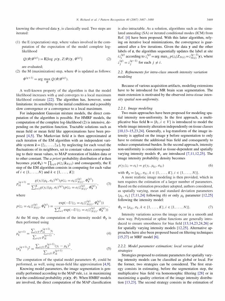
The system is composed of autonomous agents, which aresituated spatially and work in cooperation under a decentralizedcontrol (see Fig. 1). They are created, activated, deactivatedand destroyed by a system manager, which also simulates theirparallel execution. Each agent makes its own decisions in areactive and contextual way. To this end, it is provided withseveral behaviors that are triggered under control of the agentbehavior manager, according to the finite state automatonshown in Fig. 2. The agents own a private information space

Fig. 1. System design overview: the system is composed of autonomous agentsthat are situated (at a specific location on the image to process a given subsetof data) and cooperative (they interact to segment the image). The agents sharea common information base where is stored a priori knowledge, informationincrementally extracted from the image during local and coordinated EMprocesses and the set of maps required for the image segmentation. Theinformation extracted becomes dynamically a new knowledge source, whichis used to constrain the execution of the following treatments. The agents arecoordinated (blue arrows) in order to perform their processing tasks.


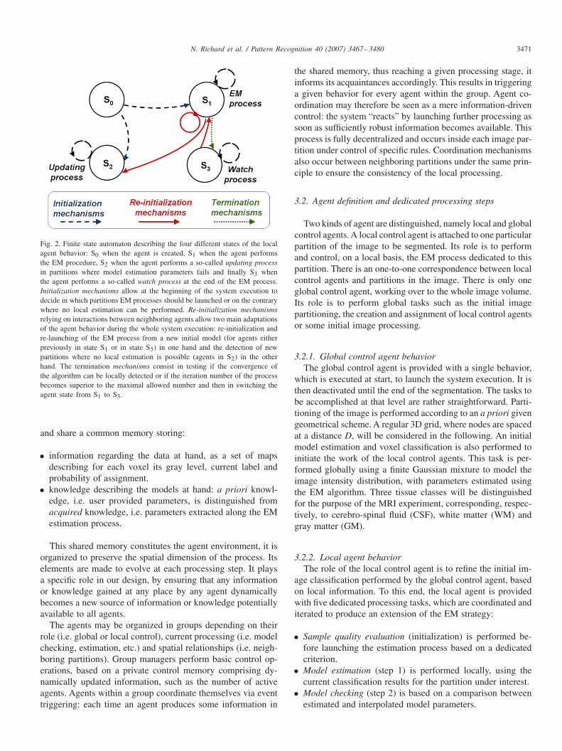
Fig. 2. Finite state automaton describing the four different states of the localagent behavior: S0 when the agent is created, S1 when the agent performsthe EM procedure, S2 when the agent performs a so-called updating processin partitions where model estimation parameters fails and finally S3 whenthe agent performs a so-called watch process at the end of the EM process.Initialization mechanisms allow at the beginning of the system execution todecide in which partitions EM processes should be launched or on the contrarywhere no local estimation can be performed. Re-initialization mechanismsrelying on interactions between neighboring agents allow two main adaptationsof the agent behavior during the whole system execution: re-initialization andre-launching of the EM process from a new initial model (for agents eitherpreviously in state S1 or in state S3) in one hand and the detection of newpartitions where no local estimation is possible (agents in S2) in the otherhand. The termination mechanisms consist in testing if the convergence ofthe algorithm can be locally detected or if the iteration number of the processbecomes superior to the maximal allowed number and then in switching theagent state from S1 to S3.

and share a common memory storing:

• information regarding the data at hand, as a set of mapsdescribing for each voxel its gray level, current label andprobability of assignment.

• knowledge describing the models at hand: a priori knowl-edge, i.e. user provided parameters, is distinguished fromacquired knowledge, i.e. parameters extracted along the EMestimation process.

This shared memory constitutes the agent environment, it isorganized to preserve the spatial dimension of the process. Itselements are made to evolve at each processing step. It playsa specific role in our design, by ensuring that any informationor knowledge gained at any place by any agent dynamicallybecomes a new source of information or knowledge potentiallyavailable to all agents.

The agents may be organized in groups depending on theirrole (i.e. global or local control), current processing (i.e. modelchecking, estimation, etc.) and spatial relationships (i.e. neigh-boring partitions). Group managers perform basic control op-erations, based on a private control memory comprising dy-namically updated information, such as the number of activeagents. Agents within a group coordinate themselves via eventtriggering: each time an agent produces some information in

the shared memory, thus reaching a given processing stage, itinforms its acquaintances accordingly. This results in triggeringa given behavior for every agent within the group. Agent co-ordination may therefore be seen as a mere information-drivencontrol: the system “reacts” by launching further processing assoon as sufficiently robust information becomes available. Thisprocess is fully decentralized and occurs inside each image par-tition under control of specific rules. Coordination mechanismsalso occur between neighboring partitions under the same prin-ciple to ensure the consistency of the local processing.

3.2. Agent definition and dedicated processing steps

Two kinds of agent are distinguished, namely local and globalcontrol agents. A local control agent is attached to one particularpartition of the image to be segmented. Its role is to performand control, on a local basis, the EM process dedicated to thispartition. There is an one-to-one correspondence between localcontrol agents and partitions in the image. There is only oneglobal control agent, working over to the whole image volume.Its role is to perform global tasks such as the initial imagepartitioning, the creation and assignment of local control agentsor some initial image processing.

3.2.1. Global control agent behaviorThe global control agent is provided with a single behavior,

which is executed at start, to launch the system execution. It isthen deactivated until the end of the segmentation. The tasks tobe accomplished at that level are rather straightforward. Parti-tioning of the image is performed according to an a priori givengeometrical scheme. A regular 3D grid, where nodes are spacedat a distance D, will be considered in the following. An initialmodel estimation and voxel classification is also performed toinitiate the work of the local control agents. This task is per-formed globally using a finite Gaussian mixture to model theimage intensity distribution, with parameters estimated usingthe EM algorithm. Three tissue classes will be distinguishedfor the purpose of the MRI experiment, corresponding, respec-tively, to cerebro-spinal fluid (CSF), white matter (WM) andgray matter (GM).

3.2.2. Local agent behaviorThe role of the local control agent is to refine the initial im-

age classification performed by the global control agent, basedon local information. To this end, the local agent is providedwith five dedicated processing tasks, which are coordinated anditerated to produce an extension of the EM strategy:

• Sample quality evaluation (initialization) is performed be-fore launching the estimation process based on a dedicatedcriterion.

• Model estimation (step 1) is performed locally, using thecurrent classification results for the partition under interest.

• Model checking (step 2) is based on a comparison betweenestimated and interpolated model parameters.


• Model interpolation is performed over a neighborhood, usingthe current estimation results from neighboring partitions.

• Voxel labeling (step 3) corresponds to the mere classificationof voxels based on the current model.

Model estimation and voxel labeling correspond, respec-tively, to the M-step (Eqs. (4) and (5)) and the E-step (Eq. (3),where z̃ is taken as the intermediary classification results ob-tained with the ICM algorithm) of the EM algorithm. We havechosen a simple Potts model whose spatial parameter � is setto a predefined value (equal to 0.3) and progressively increasedfrom an initial value (0.1), while applying the ICM algorithm.We have introduced a spatially varying Gaussian mixture model(6) to model the intensity non-uniformity and a polynomial in-terpolation of the locally estimated intensity models. In thisway, intensity models are smoothly variable, close to the localmodel in the center of the partition and close to neighboringmodels at the partition boundaries.

The model checking is added to the classical EM steps, tocontrol the evolution of the distributed processes. To this end,the interpolated model �interp(j)

y = {�nterp(j)k , �nterp(j)

k , k ∈{1, . . . , K}} for each partition j is computed using a weightedmean �nterp(j)

k =∑l∈N(j)�

(j)k ·wjl and �nterp(j)

k =∑l∈N(j)�

(j)k ·

wjl where wjl is the weight for the lth neighboring model,which is inversely proportional to the distance between parti-tions (such as

∑lwjl = 1). The distance between the interpo-

lated model and the current model (estimated locally or previ-ously interpolated) is compared to a threshold in order to decideif the current model can be conserved or has to be corrected.The threshold is computed using the standard deviation of theinterpolated local model as follows:

��(j)k = K� · �nterp(j)

k and ��(j)k = K� · �nterp(j)

k . (8)

To be noticed is the fact that this threshold does not resume to aglobal, a priori defined parameter. On the contrary, it dependson the dynamics observed over the partition under interest, thussituating the analysis and its control.

3.3. Coordination and control mechanisms

Agent coordination and control are performed according tothe finite state automaton presented in Fig. 2. According to thisscheme, local control agents can reach four possible states thatdetermine their behavior. They are created in the initial stateS0, from which they normally reach state S1 to perform theEM process. State S3 is reached by the end of the EM processindependently for each agent. State S2 plays a dedicated rolewith respect to the overall control strategy: it may be reachedeither in case of a low quality of the data samples, potentiallyhampering the quality of model estimation, or in case of a lowconsistency of the estimated model, thus hampering the qualityof voxel classification.

3.3.1. State by state description of agent behavior• S0 is the initial state for every local control agent. From

this state it may either reach S1 and enter the standard EM

process, or reach S2 to proceed to model interpolation, de-pending on a local criterion evaluating the quality of thesamples on which the EM process would be launched (ini-tialization mechanisms). Currently, this local criterion relieson the number of voxels required to correctly estimate modelparameters.

• Agents in S1 perform the EM process and alternate estima-tion, checking and classification on a local basis. The conver-gence of this process is detected when the log-likelihood ofthe model is maximized or when a maximal number of itera-tions (N1) is reached. The agent then switches from S1 to S3(termination mechanisms). Note that any inconsistency de-tected during the model checking step may result in switch-ing from S1 to S2 (re-initialization mechanisms), to ensurethe quality of further processing.

• Agents in S2 proceed to model interpolation based on mod-els computed in their neighborhood (updating process). Thisinterpolation is followed by a voxel labeling step to ensurethe overall consistency of the processing.

• S3 is reached upon termination of the EM process, which cor-responds to the completion of the local agent task. However,agents in that state may be re-activated to account for thepotential evolution of models in their neighborhood (watch-ing process). Model checking is launched in that case, whichmay result in switching to state S1 again and thus launchingagain the EM process in case the final model reveals no morevalid.

Agents in S2 and S3 are inactive. They are re-activated as soonas a model changes in their close neighborhood. To this end, theagent-driven modification of a model, occurring at any placeand in any state, results in the propagation of activation requestsin the agent neighborhood. These propagation mechanisms en-sure the system reactivity. Model checking, which is performedunder state-dependent threshold, ensures the fine adaptation ofthe overall modeling processing to the situations.

Note finally that re-launching the EM process may only oc-cur a predefined number of times (N2). When this number isattained, it is considered that model parameter estimation is notpossible for the partition at hand. As a consequence, the corre-sponding local agent switches from state S1 or S3 to state S2.

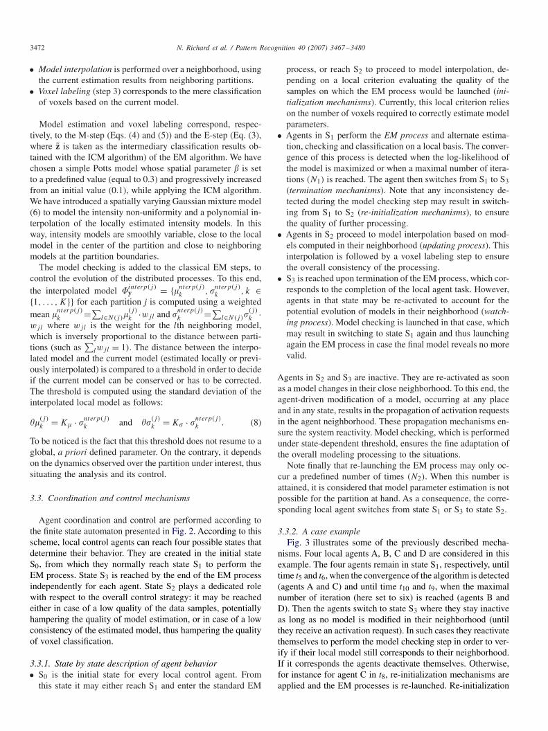
3.3.2. A case exampleFig. 3 illustrates some of the previously described mecha-

nisms. Four local agents A, B, C and D are considered in thisexample. The four agents remain in state S1, respectively, untiltime t5 and t6, when the convergence of the algorithm is detected(agents A and C) and until time t10 and t9, when the maximalnumber of iteration (here set to six) is reached (agents B andD). Then the agents switch to state S3 where they stay inactiveas long as no model is modified in their neighborhood (untilthey receive an activation request). In such cases they reactivatethemselves to perform the model checking step in order to ver-ify if their local model still corresponds to their neighborhood.If it corresponds the agents deactivate themselves. Otherwise,for instance for agent C in t8, re-initialization mechanisms areapplied and the EM processes is re-launched. Re-initialization


Fig. 3. Illustration of the EM process termination mechanisms and re-initialization mechanisms. Top: the states taken by each agents A, B, C and D duringthe system execution (t1–t12) Middle: processing steps performed depending on (1) the detected events: convergence of the EM algorithm, maximal iterationnumber reached, model correction during the model checking step and (2) “stimuli” received from neighboring regions: the activation requests exchanged byneighboring agents. Bottom: legend indicating the meaning of the different symbols used.

mechanisms also take place for agent still in state S1, for in-stance for agents B in t3 and D in t1 and t2.

3.4. Conclusion

Overall, the proposed modeling strategy may be seen as anextension of the standard EM process. The proposed frameworkmay be characterized by the following properties:

• Local adaptation: based on the proposed spatial distribution,the EM processes work on a local basis, which account forpotential bias or non-homogeneity in the intensity distribu-tions.

• Robustness in front of atypical situations: sample qualityevaluation together with model checking allows to detectproblematic situations and to react accordingly, thus ensuringthe robustness of model estimation.

• Reactivity: the dynamics of model estimation depends notonly on the local situation at hand (convergence of the EMprocess) but also on the evolution of models in the neigh-borhood, thus avoiding trapping the analysis within the localspecificities of some configuration.

• Convergence: the final inactivation of all agents is guar-anteed based on the introduction of a maximal numberfor iterations and for re-initializations and of a minimalthreshold for the distance between models to propagatechanges.

Thanks to these specific properties, the extended EM processthat we propose allows the development of a context-basedregulation of model estimation, which reveals powerful in thedifficult domain of MR image segmentation.

4. Experiments

We evaluated our system qualitatively on real MRI brainscans and quantitatively on realistic MRI phantoms. Segmenta-tions were performed on a PC pentium, 2 GB RAM, 3.4 GHz.For both kinds of images, we compared our results with thoseobtained with two segmentation systems based on the esti-mation of a multiplicative bias field performed alternativelywith the image segmentation. In one system the bias field ismodeled with a polynomial function and in the second caseit is estimated with the filtering based approach proposed inRef. [15].

4.1. Quantitative experiments

A quantitative evaluation was performed based on phantomimages generated using the BrainWeb simulator [29]. Startingwith images where tissue classification was known, we createdseveral volumes with various noise (3%, 5%, 7% and 9%), andintensity non-uniformity (20% and 40%) levels. We use the Jac-card coefficient TP/(TP+FP+FN) to evaluate segmentation for


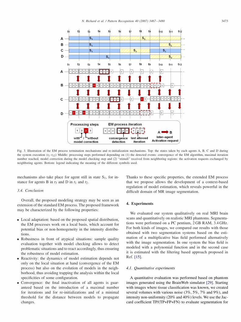
Fig. 4. Segmentation results using the Jaccard coefficient for both WM and GM tissues function of the partition size at 20% (left) and 40% (right) of intensitynon-uniformity for three levels of noise (3%, 5% and 7%).

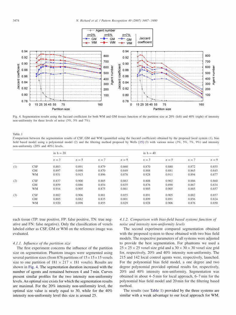
Table 1Comparison between the segmentation results of CSF, GM and WM (quantified using the Jaccard coefficient) obtained by the proposed local system (1), biasfield based model using a polynomial model (2) and the filtering method proposed by Wells [15] (3) with various noise (3%, 5%, 7%, 9%) and intensitynon-uniformity (20% and 40%) levels.

in h = 20 in h = 40

n = 3 n = 5 n = 7 n = 9 n = 3 n = 5 n = 7 n = 9

(1) CSF 0.883 0.891 0.879 0.860 0.870 0.880 0.872 0.855GM 0.897 0.890 0.870 0.849 0.888 0.881 0.865 0.845WM 0.931 0.915 0.896 0.878 0.928 0.911 0.894 0.877

(2) CSF 0.837 0.900 0.885 0.863 0.808 0.902 0.886 0.860GM 0.859 0.886 0.854 0.835 0.876 0.890 0.867 0.834WM 0.916 0.905 0.875 0.861 0.905 0.905 0.885 0.857

(3) CSF 0.882 0.906 0.881 0.855 0.891 0.905 0.882 0.857GM 0.885 0.882 0.835 0.801 0.899 0.891 0.856 0.824WM 0.920 0.898 0.855 0.829 0.928 0.906 0.876 0.850

each tissue (TP: true positive, FP: false positive, TN: true neg-ative and FN: false negative). Only the classification of voxelslabeled either as CSF, GM or WM on the reference image wasevaluated.

4.1.1. Influence of the partition sizeThe first experiment concerns the influence of the partition

size on segmentation. Phantom images were segmented usingseveral partition sizes (from 876 partitions of 15×15×15 voxelssize to one partition of 181 × 217 × 181 voxels). Results areshown in Fig. 4. The segmentation duration increased with thenumber of agents and remained between 4 and 7 min. Curvespresent similar profiles for the two intensity non-uniformitylevels. An optimal size exists for which the segmentation resultsare maximal. For the 20% intensity non-uniformity level, theoptimal size value is nearly equal to 30, while for the 40%intensity non-uniformity level this size is around 25.

4.1.2. Comparison with bias-field based systems function ofnoise and intensity non-uniformity levels

The second experiment compared segmentation obtainedwith the proposed system to those obtained with two bias fieldmodels. The respective parameters of all systems were adjustedto provide the best segmentation. For phantoms we used a25×25×25 voxel size grid and a 30 ×30 ×30 voxel size gridfor, respectively, 20% and 40% intensity non-uniformity. The215 and 142 local control agents were, respectively, launched.For the polynomial bias field model, a one degree and twodegree polynomial provided optimal results for, respectively,20% and 40% intensity non-uniformity. Segmentation wasobtained in about 4–5 min for local approach, 6–7 min for thepolynomial bias field model and 20 min for the filtering basedmethod.

The results (see Table 1) provided by the three systems aresimilar with a weak advantage to our local approach for WM.


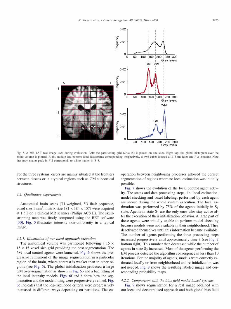
Fig. 5. A MR 1.5 T real image used during evaluation. Left: the partitioning grid (D = 15) is placed on one slice. Right top: the global histogram over theentire volume is plotted. Right, middle and bottom: local histograms corresponding, respectively, to two cubes located at B-8 (middle) and F-2 (bottom). Notethat gray matter peak in F-2 corresponds to white matter in B-8.

For the three systems, errors are mainly situated at the frontiersbetween tissues or in atypical regions such as GM subcorticalstructures.

4.2. Qualitative experiments

Anatomical brain scans (T1-weighted, 3D flash sequence,voxel size 1 mm3, matrix size 181 × 184 × 157) were acquiredat 1.5 T on a clinical MR scanner (Philips ACS II). The skull-stripping map was firstly computed using the BET software[30]. Fig. 5 illustrates intensity non-uniformity in a typicalimage.

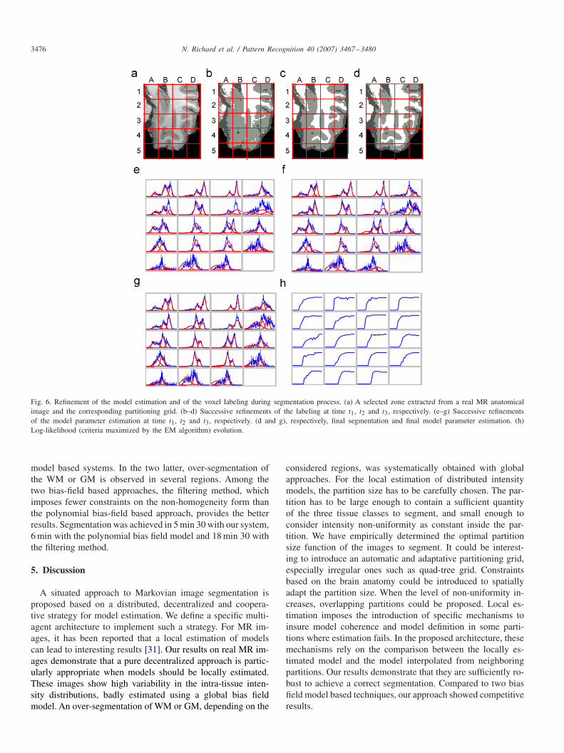
4.2.1. Illustration of our local approach executionThe anatomical volume was partitioned following a 15 ×

15 × 15 voxel size grid providing the best segmentation. The689 local control agents were launched. Fig. 6 shows the pro-gressive refinement of the image segmentation in a particularregion of the brain, where contrast is weaker than in other re-gions (see Fig. 5). The global initialization produced a largeGM over-segmentation as shown in Fig. 6b and a bad fitting ofthe local intensity models. Figs. 6f and h show how the seg-mentation and the model fitting were progressively refined. Fig.6e indicates that the log-likelihood criteria were progressivelyincreased in different ways depending on partitions. The co-

operation between neighboring processes allowed the correctsegmentation of regions where no local estimation was initiallypossible.

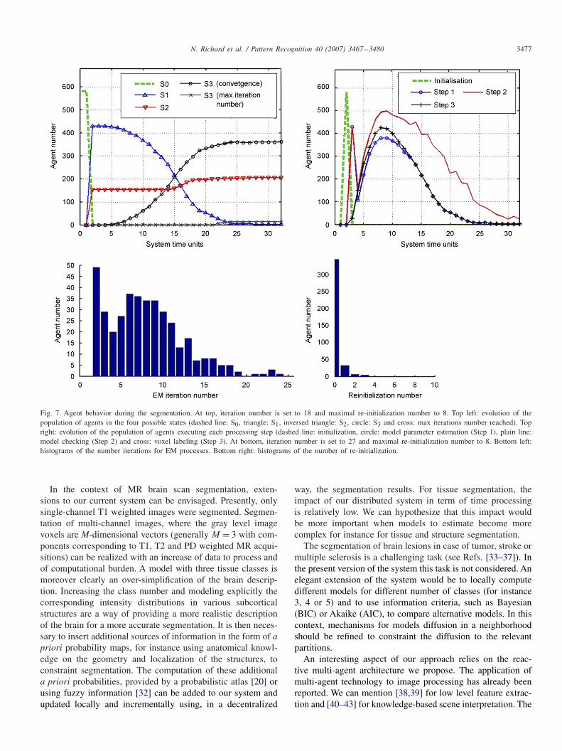
Fig. 7 shows the evolution of the local control agent activ-ity. The states and data processing steps, i.e. local estimation,model checking and voxel labeling, performed by each agentare shown during the whole system execution. The local es-timation was performed by 75% of the agents initially in S1state. Agents in state S1 are the only ones who stay active af-ter the execution of their initialization behavior. A large part ofthese agents were initially unable to perform model checkingbecause models were not available in their neighborhood. Theydeactivated themselves until this information became available.The number of agents performing the three processing stepsincreased progressively until approximately time 8 (see Fig. 7bottom right). This number then decreased while the number ofagents in state S3 increased. Most of the agents performing theEM process detected the algorithm convergence in less than 10iterations. For the majority of agents, models were correctly es-timated locally or from neighborhood and re-initialization wasnot needed. Fig. 8 shows the resulting labeled image and cor-responding probability maps.

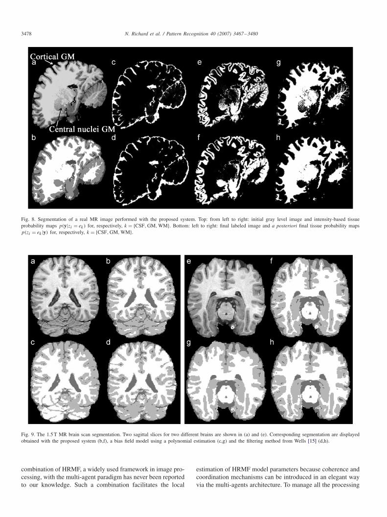
4.2.2. Comparison with the bias field model based systemsFig. 9 shows segmentation for a real image obtained with

our local and decentralized approach and both global bias field


Fig. 6. Refinement of the model estimation and of the voxel labeling during segmentation process. (a) A selected zone extracted from a real MR anatomicalimage and the corresponding partitioning grid. (b–d) Successive refinements of the labeling at time t1, t2 and t3, respectively. (e–g) Successive refinementsof the model parameter estimation at time t1, t2 and t3, respectively. (d and g), respectively, final segmentation and final model parameter estimation. (h)Log-likelihood (criteria maximized by the EM algorithm) evolution.

model based systems. In the two latter, over-segmentation ofthe WM or GM is observed in several regions. Among thetwo bias-field based approaches, the filtering method, whichimposes fewer constraints on the non-homogeneity form thanthe polynomial bias-field based approach, provides the betterresults. Segmentation was achieved in 5 min 30 with our system,6 min with the polynomial bias field model and 18 min 30 withthe filtering method.

5. Discussion

A situated approach to Markovian image segmentation isproposed based on a distributed, decentralized and coopera-tive strategy for model estimation. We define a specific multi-agent architecture to implement such a strategy. For MR im-ages, it has been reported that a local estimation of modelscan lead to interesting results [31]. Our results on real MR im-ages demonstrate that a pure decentralized approach is partic-ularly appropriate when models should be locally estimated.These images show high variability in the intra-tissue inten-sity distributions, badly estimated using a global bias fieldmodel. An over-segmentation of WM or GM, depending on the

considered regions, was systematically obtained with globalapproaches. For the local estimation of distributed intensitymodels, the partition size has to be carefully chosen. The par-tition has to be large enough to contain a sufficient quantityof the three tissue classes to segment, and small enough toconsider intensity non-uniformity as constant inside the par-tition. We have empirically determined the optimal partitionsize function of the images to segment. It could be interest-ing to introduce an automatic and adaptative partitioning grid,especially irregular ones such as quad-tree grid. Constraintsbased on the brain anatomy could be introduced to spatiallyadapt the partition size. When the level of non-uniformity in-creases, overlapping partitions could be proposed. Local es-timation imposes the introduction of specific mechanisms toinsure model coherence and model definition in some parti-tions where estimation fails. In the proposed architecture, thesemechanisms rely on the comparison between the locally es-timated model and the model interpolated from neighboringpartitions. Our results demonstrate that they are sufficiently ro-bust to achieve a correct segmentation. Compared to two biasfield model based techniques, our approach showed competitiveresults.


Fig. 7. Agent behavior during the segmentation. At top, iteration number is set to 18 and maximal re-initialization number to 8. Top left: evolution of thepopulation of agents in the four possible states (dashed line: S0, triangle: S1, inversed triangle: S2, circle: S3 and cross: max iterations number reached). Topright: evolution of the population of agents executing each processing step (dashed line: initialization, circle: model parameter estimation (Step 1), plain line:model checking (Step 2) and cross: voxel labeling (Step 3). At bottom, iteration number is set to 27 and maximal re-initialization number to 8. Bottom left:histograms of the number iterations for EM processes. Bottom right: histograms of the number of re-initialization.

In the context of MR brain scan segmentation, exten-sions to our current system can be envisaged. Presently, onlysingle-channel T1 weighted images were segmented. Segmen-tation of multi-channel images, where the gray level imagevoxels are M-dimensional vectors (generally M = 3 with com-ponents corresponding to T1, T2 and PD weighted MR acqui-sitions) can be realized with an increase of data to process andof computational burden. A model with three tissue classes ismoreover clearly an over-simplification of the brain descrip-tion. Increasing the class number and modeling explicitly thecorresponding intensity distributions in various subcorticalstructures are a way of providing a more realistic descriptionof the brain for a more accurate segmentation. It is then neces-sary to insert additional sources of information in the form of apriori probability maps, for instance using anatomical knowl-edge on the geometry and localization of the structures, toconstraint segmentation. The computation of these additionala priori probabilities, provided by a probabilistic atlas [20] orusing fuzzy information [32] can be added to our system andupdated locally and incrementally using, in a decentralized

way, the segmentation results. For tissue segmentation, theimpact of our distributed system in term of time processingis relatively low. We can hypothesize that this impact wouldbe more important when models to estimate become morecomplex for instance for tissue and structure segmentation.

The segmentation of brain lesions in case of tumor, stroke ormultiple sclerosis is a challenging task (see Refs. [33–37]). Inthe present version of the system this task is not considered. Anelegant extension of the system would be to locally computedifferent models for different number of classes (for instance3, 4 or 5) and to use information criteria, such as Bayesian(BIC) or Akaike (AIC), to compare alternative models. In thiscontext, mechanisms for models diffusion in a neighborhoodshould be refined to constraint the diffusion to the relevantpartitions.

An interesting aspect of our approach relies on the reac-tive multi-agent architecture we propose. The application ofmulti-agent technology to image processing has already beenreported. We can mention [38,39] for low level feature extrac-tion and [40–43] for knowledge-based scene interpretation. The


Fig. 8. Segmentation of a real MR image performed with the proposed system. Top: from left to right: initial gray level image and intensity-based tissueprobability maps p(y|zi = ek) for, respectively, k = {CSF, GM, WM}. Bottom: left to right: final labeled image and a posteriori final tissue probability mapsp(zi = ek |y) for, respectively, k = {CSF, GM, WM}.

Fig. 9. The 1.5 T MR brain scan segmentation. Two sagittal slices for two different brains are shown in (a) and (e). Corresponding segmentation are displayedobtained with the proposed system (b,f), a bias field model using a polynomial estimation (c,g) and the filtering method from Wells [15] (d,h).

combination of HRMF, a widely used framework in image pro-cessing, with the multi-agent paradigm has never been reportedto our knowledge. Such a combination facilitates the local

estimation of HRMF model parameters because coherence andcoordination mechanisms can be introduced in an elegant wayvia the multi-agents architecture. To manage all the processing


steps required in HMRF we introduce situated and decentral-ized agents with appropriate control rules. The local processlaunching and termination are in this way adapted dynamicallyto the local gray level characteristics and to the local and globalsegmentation contexts. The detection of partitions where no es-timation is possible is refined during the whole system execu-tion. Then, the system spends more time to segment the moredifficult regions. The use of sophisticated agent communica-tion language was not required and would greatly hamper theefficiency of the system. The parallel execution of distributedtreatments is currently simulated. The framework could easilybe adapted to a parallel hardware environment to speed up thesegmentation process.

Although evaluate face to a specific application, we considerthat the architecture and mechanisms we propose could supportvarious applications in computer vision.

References

[1] S. Geman, D. Geman, Stochastic relaxation, Gibbs distributions ans theBayesian restoration of images, IEEE Trans. Pattern Anal. Mach. Intell.6 (1984) 721–741.

[2] A. Dempster, N. Laird, D. Rubin, Maximum likelihood from incompletedata via the EM algorithm, J. R. Statis. Soc. B 39 (1977) 1–38.

[3] J. Besag, Statistical analysis of non-lattice data, Statistician 24 (1975)179–195.

[4] G. Celeux, F. Forbes, N. Peyrard, EM procedures using mean field-likeapproximations for Markov model-based image segmentation, PatternRecognition 36 (2003) 131–144.

[5] J. Zhang, The mean field theory in EM procedures for Markov randomfields, IEEE Trans. Signal Process. 40 (1992) 2570–2583.

[6] K. Held, E.R. Kops, B.J. Krause, W.M. Wells 3rd, R. Kikinis, H.W.Muller-Gartner, Markov random field segmentation of brain MR images,IEEE Trans. Med. Imaging 16 (1997) 878–886.

[7] J.C. Rajapakse, J.N. Giedd, J.L. Rapoport, Statistical approach tosegmentation of single-channel cerebral MR images, IEEE Trans. Med.Imaging 16 (1997) 176–186.

[8] S. Sanjay-Gopal, T.J. Hebert, Bayesian pixel classification using spatiallyvariant finite mixtures and the generalized EM algorithm, IEEE Trans.Image Process. 7 (1998) 1014–1028.

[9] K. Van Leemput, F. Maes, D. Vandermeulen, P. Suetens, Automatedmodel-based tissue classification of MR images of the brain, IEEE Trans.Med. Imaging 18 (1999) 897–908.

[10] Y. Zhang, M. Brady, S. Smith, Segmentation of brain MR images througha hidden Markov random field model and the expectation–maximizationalgorithm, IEEE Trans. Med. Imaging 20 (2001) 45–57.

[11] T.J. Grabowski, R.J. Frank, N.R. Szumski, C.K. Brown, H. Damasio,Validation of partial tissue segmentation of single-channel magneticresonance images of the brain, Neuroimage 12 (2000) 640–656.

[12] J.L. Marroquin, B.C. Vemuri, S. Botello, F. Calderon, A. Fernandez-Bouzas, An accurate and efficient Bayesian method for automaticsegmentation of brain MRI, IEEE Trans. Med. Imaging 21 (2002)934–945.

[13] J.G. Sled, A.P. Zujdenbos, A. Evans, A non parametric method forautomatic correction of nonuniformity in MRI data, IEEE Trans. Med.Imaging 17 (1998) 87–97.

[14] K. Van Leemput, F. Maes, D. Vandermeulen, P. Suetens, Automatedmodel-based bias field correction in MR images of the brain, IEEETrans. Med. Imaging 18 (1999) 885–896.

[15] W.L. Wells, L. Grimson, R. Kikinis, F.A. Jolesz, Adaptative segmentationof MRI data, IEEE Trans. Med. Imaging 15 (1996) 429–442.

[16] H.S. Choi, D.R. Haynor, Y. Kim, Partial volume tissue classification ofmultichannel magnetic resonance images—a mixel model, IEEE Trans.Image Process. 10 (1991) 1531–1540.

[17] P. Santago, H.D. Gage, Statistical models of partial volume effect, IEEETrans. Image Process. 11 (1995) 1531–1540.

[18] K. Van Leemput, F. Maes, D. Vandermeulen, P. Suetens, A unifyingframework for partial volume segmentation of brain MR Images, IEEETrans. Med. Imaging 22 (2003) 105–119.

[19] J. Ashburner, K.J. Friston, Unified segmentation, Neuroimage 26 (2005)839–851.

[20] B. Fischl, D.H. Salat, E. Busa, M. Albert, M. Dietrich, C. Haselgrove,A. van der Kouwe, R. Killiany, D. Kennedy, S. Klaveness, A. Montillo,N. Makris, B. Rosen, A.M. Dale, Whole brain segmentation: automatedlabeling of neuroanatomical structures in the human brain, Neuron 33(2002) 341–355.

[21] J. Besag, On the statistical analysis of dirty pictures, J. R. Statis. Soc.B 48 (1986) 259–302.

[22] C. Wu, On the convergence properties of the EM algorithm, Ann. Stat11 (1983) 95–103.

[23] B.L. Likar, M.A. Viergever, F. Pernus, Retrospective correction of MRintensity inhomogeneity by information minimization, IEEE Trans. Med.Imaging 20 (2001) 1398–1410.

[24] D.W. Shattuck, S.R. Sandor-Leahy, K.A. Schaper, D.A. Rottenberg, R.M.Leahy, Magnetic resonance image tissue classification using a partialvolume model, Neuroimage 13 (2001) 856–876.

[25] L. Nocera, J.C. Gee, Robust partial volume tissue classification ofcerebral MRI scans, in: K.M. Hanson (Eds.), SPIE Medical Imaging,SPIE-ISOE, 1997, pp. 312–322.

[26] M. Styner, C. Brechbuhler, G. Szekely, G. Gerig, Parametric estimate ofintensity inhomogeneities applied to MRI, IEEE Trans. Med. Imaging19 (2000) 153–165.

[27] R. Guillemaud, M. Brady, Estimating the bias field of MR images, IEEETrans. Med. Imaging 16 (1997) 238–251.

[28] B.H. Brinkman, A. Manduca, R.A. Robb, Optimized homomorphicunsharp masking for MR grayscale inhomogeneity correction, IEEETrans. Med. Imaging 17 (1998) 161–171.

[29] D.L. Collins, A.P. Zijdenbos, V. Kollokian, J.G. Sled, N.J. Kabani, C.J.Holmes, A.C. Evans, Design and construction of a realistic digital brainphantom, IEEE Trans. Med. Imaging 17 (1998) 463–468.

[30] S. Smith, Fast robust automated brain extraction, Human Brain Mapping17 (2002) 143–155.

[31] J.B. Arnold, J.-S. Liow, K.A. Schaper, J.J. Stern, J.G. Sled, D.W.Shattuck, A.J. Worth, M.S. Cohen, R.M. Leahy, J.C. Mazziotta, D.A.Rottenberg, Qualitative and quantitative evaluation of six algorithmsfor correcting intensity nouniformity effects, Neuroimage 13 (2001)931–943.

[32] V. Barra, J.Y. Boire, A general framework for the fusion of anatomicaland functional medical images, Neuroimage 13 (2001) 410–424.

[33] L. Aït-ali, S. Prima, P. Hellier, B. Carsin, G. Edan, C. Barillot, STREM:a robust multidimensional parametric method to segment MS lesions inMRI, in: Eighth International Conference on Medical Image Computingand Computer-Assisted Intervention, MICCAI’2005, Palm Springs, USA,2005, pp. 409–416.

[34] A. Cappelle, C. Fernandez-Maloigne, Evidential segmentation schemeof multi-echo MR images for the detection of brain tumors usingneighborhood information, Inf. Fusion 5 (2004) 203–216.

[35] M.R. Kaus, S.K. Warfield, A. Nabavi, P.M. Black, F.A. Jolesz, R. Kikinis,Automated segmentation of MR images of brain tumors, Radiology 218(2001) 586–591.

[36] M. Prastawa, E. Bullitt, S. Ho, G. Gerig, A brain tumor segmentationframework based on outlier detection, Med. Image Anal. 8 (2004)275–283.

[37] K. Van Leemput, F. Maes, D. Vandermeulen, P. Suetens, Automatedsegmentation of multiple sclerosis lesions by model outlier detection,IEEE Trans. Med. Imaging 20 (2001) 677–688.

[38] E. Duschesnay, J.-J. Montois, Y. Jacquelet, Cooperative agents societyorganized as an irregular pyramid: a mammography segmentationapplication, Pattern Recognition Lett. 24 (2003) 2435–2445.

[39] J. Liu, Y.Y. Tang, Adaptative image segmentation with distributedbehavior-based agents, IEEE Trans. Pattern Anal. Mach. Intell. 21 (1999)544–551.


[40] A. Boucher, A. Doisy, X. Ronot, C. Garbay, A society of goal orientedagents for the analysis of living cells, Artif. Intell. Med. 14 (1998)183–199.

[41] E.G.P. Bovenkamp, J. Dijkstra, J.G. Bosch, J.H.C. Reiber, Multi-agentsegmentation of IVUS images, Pattern Recognition 37 (2004) 647–663.

[42] L. Heutte, A. Nosary, T. Paquet, A multiple agent architecture forhandwritten text recognition, Pattern Recognition 37 (2004) 665–674.

[43] V. Rodin, A. Benzinou, A. Guillaud, P. Ballet, F. Harrouet, J. Tisseau, J.Le Bihan, An immune oriented multi-agent system for biological imageprocessing, Pattern Recognition 37 (2004) 631–645.

About the Author—NATHALIE RICHARD received her engineering degree from the University de Compiégne in 1998 and the Ph.D. degree in computerscience from the Institut National polytechnique de Grenoble 〈http://www.inpg.fr/〉 in 2004. In 2004, she joined the INSA in Lyon where she was a teachingfellow at the Electrical Engineering department and a research fellow at the CREATIS laboratory (CNRS/INSERM/INSA/UCBL). Since 2006, she is aposdoctoral researcher at the Ecole Nationale Superieure des Telecommunications (ENST). Her research interests include artificial intelligence in medicine,Markov Random Fields and Deformable Models.

About the Author—MICHEL DOJAT is Research Engineer at Institut National de la Santé et de la Recherche Médicale. He received his engineering diplomafrom Institut National des Sciences Appliquées de Lyon in 1982, his PhD in Informatics in 1992 from University de Compiégne and his ’Habilitation à Dirigerdes Recherches’ in 1999 from University J. Fourier de Grenoble. Since 1988, he is with INSERM and his research interests are in artificial intelligence inmedicine, physiological signal and medical images processing and analysis. He is member of the editorial board of Artificial Intelligence in Medicine Journal,was the program chair of the AIME conference in 2003. He is IEEE member.

About the Author—CATHERINE GARBAY received the Ph.D. degree in computer science from the Institut National polytechnique de Grenoble〈http://www.inpg.fr/〉 in 1979. She joined the CNRS in 1980 where she holds the position of research director. She is deputy director of the LIG (Labora-toire d’Informatique de Grenoble) since 2007. Her research interests include multi-agent system design, and man–machine communication with application tomedical signal and image interpretation.

http://www.inpg.fr/

http://www.inpg.fr/

Documents

Distributed Markovian segmentation: Application to MR brain scans