Do Crude Petroleum Imports Affect GDP of Turkey?

Journal of Applied Finance & Banking, vol. 5, no. 4, 2015, 61-72

ISSN: 1792-6580 (print version), 1792-6599 (online)

Scienpress Ltd, 2015

Do Crude Petroleum Imports Affect GDP of Turkey?

Meliha Ener1, Cüneyt Kɪlɪç2 and Feyza Balan3

Abstract

This study examines the dynamic linkages between crude petroleum imports and GDP of

Turkey. The vector autoregression analysis is carried on quarterly data for the period

1998Q1 to 2013Q2. This study utilized the generalized approach to forecast error variance

decomposition and impulse response analysis which have many advantages against the

traditional orthogonalized approach. The empirical results suggest that petroleum imports

have positive impact on GDP until the second quarter. But, after the second quarter crude

petroleum imports have negative impact on GDP. The results of the Granger causality test

showed that crude petroleum imports granger caused GDP at 5% significance level, but not

vice versa. Moreover, the generalized variance decomposition analysis exerted that the

imports of crude petroleum shocks have only a small effect on GDP initially. However,

after eighth quarters, the imports of crude petroleum shocks explain 31.7 pct. of the GDP,

whereas 26.46 pct. of the variation in imports of crude petroleum shocks is explained by

GDP shocks.

JEL classification numbers: O49, 053, Q41

Keywords: Vector autoregression, Generalized impulse responses, GDP, Crude petroleum

imports, Turkey

1 Introduction

Petrol has been one of the mostly used and therefore consumed sources among other energy

sources. Petrol consumption trends have been on the rise in recent years due to the factors

such as progress in technology by the help of globalization, industrialization, increasing

numbers of world population, urbanization, transportation and logistics services. Compared

to the increase in demand for petrol; capacity increases in petrol supply cannot be achieved

since it is not a renewable energy source leading to the result of increased petrol prices.

1Canakkale Onsekiz Mart University. 2Canakkale Onsekiz Mart University. 3Canakkale Onsekiz Mart University.

Article Info: Received : February 15, 2015. Revised : March 9, 2015.

Published online : July 1, 2015

62 Meliha Ener et al.

Parallel to the increase in petrol consumption, the increase in petrol prices initially raises

the production costs of nations and causes cost inflation. The increase in production cost

decreases the production volume, resulting in the reduction of total demand.

This study aims to analyze the dynamic relationship between the imports of crude

petroleum and GDP for Turkey. For this purpose, empirical literature on the relationship

between the two variables will be discussed, then the data set and the methodology that will

be used in the application part of the study will be explained and finally empirical results

will be evaluated.

2 Literature Review

The literature focused on the relationship between energy consumption and income dates

back to the late 1970s. Kraft and Kraft (1978), in their pioneering work, concluded that

GDP leads energy consumption in U.S. for the period from 1947 to 1974.

Ebohon (1996) analyzed the causal relationship between energy consumption and

economic growth in Nigeria and Tanzania. The empirical results indicate that there is a

simultaneous causal relationship between energy consumption and economic growth for

both countries.

Masih and Masih (1996) investigated whether there is a long-run relationship between

energy consumption and real income for India, Pakistan, Malaysia, Singapore, Indonesia,

and Philippines. The empirical results show that temporal causality results imply at least

one-way Granger causality, either unidirectional or bi-directional for India, Pakistan, and

Indonesia while the simple bivariate vector autoregressive models didn’t show any

causality relationship for the non-integrated systems in Malaysia, Singapore, and

Philippines (Chima, 2005).

Soyas and Sari (2003) tested whether there exists the causal relationship between GDP and

energy consumption for the period 1950-1992 in the top 10 emerging countries and the G-

7 countries using cointegration and vector error-correction techniques,. They found bi-

directional causality in Argentina, uni-directional causality with energy consumption

leading GDP in Turkey, France, West Germany and Japan, and the causality with GDP

leading energy consumption in Italy and Korea.

Chima (2005) employed a macroeconomic model based on Multiple Model estimation in

order to determine the relationship between energy consumption and GDP in the United

States for the period of 1949-2003. Results based on the tools of methodology used in the

study indicate that causality was bi-directional, running from energy to the components of

GDP and from GDP to energy consumption.

Webb (2006) applied dynamic panel data techniques to panel of 73 countries for which oil

is not a significant export in order to find price and income elasticities of oil consumption

in transportation, the industrial sector and other sectors including commercial and

residential. According to Webb (2006)’s the results of empirical research, the transportation

sector is the only sector where an increase in the price of crude oil has a statistically and

economically important effect.

Korap (2007) examined the long and short-run causal links between the changes in energy

consumption, real income growth and domestic inflation in the Turkish economy for the

period of 1968-2005. The authors considered the energy consumption with three different

models, comprising of total energy consumption, residential and commercial energy

consumption, and industrial energy consumption. As a result of their study, energy policies

Do Crude Petroleum Imports Affect GDP of Turkey? 63

designed in the framework of the expectations have the power of affecting domestic

inflation significantly. In addition, they find that energy conservation policies may cause to

various detrimental results for the economic growth process in the case of the use of

industrial energy consumption data.

Lescaroux and Mignon (2008) investigated the short-run and long-run links between oil

prices and various variables representative of economic activity: gross domestic product,

consumer price index, household consumption, unemployment rate, and share prices over

the period of 1960-2005. The authors find the direction of causality generally from oil

prices to the other variables. According to Lescaroux and Mignon (2008)’s short-run

empirical results can be summarized as: i) the impact of oil prices on consumption is

generally weak. ii) Oil prices have a large effect on consumer price index for United Arab

Emirates, UK, Mexico and Libya. iii) Oil prices have a large influence on the

unemployment rate in the US, Luxembourg, France, Canada and Venezuela. iv) There is

no causality running from oil prices to GDP for the group of oil-exporting countries. Finally,

oil price movements have strongly negative influence on share prices on the short run.

According to their long-run empirical results, the majority of long-run relation concerns

GDP, unemployment rate and share prices.

Lee and Chang (2008) investigated the causal relationship between energy consumption

and GDP over the period 1971-2002 for 16 Asian countries. According to their study, there

exists a unidirectional long-run relationship running from energy consumption to economic

growth, while there doesn’t exist a short-run relationship between economic growth and

energy consumption. Similarly, Huang et al. (2008) also investigated that the causal

relationship between energy consumption and economic growth for 82 countries from 1972

to 2002. Using panel VAR approach, Huang et al. (2008) found that there exists no causal

relationship between energy consumption and GDP in the low income countries, economic

growth affects energy consumption positively in the middle income countries and in the

high income countries economic growth affects energy consumption negatively.

Uğurlu and Ünsal (2009) used VAR models with annual data from 1971 to 2007, to analyze

the short-run relationship between crude petroleum imports and economic growth in Turkey.

In their analysis, Uğurlu and Ünsal (2009) found that the effect of shock in any of these two

variables on the other variable is generally negative, but after three years, the effect has

died out.

Leesombatpiboon (2009) measured the elasticity of economic growth with respect to oil

consumption and oil prices for the Thai economy. Empirical results show that a sharp 10

percent decrease in oil prices would cause economic growth to shrink by 2 percent while a

sharp 10 percent increase in oil prices would lead output growth to a fall by about 0.5

percent within the same year. This finding is interpreted as that an oil supply disruption is

usually associated with a rapid rather than gradual increase in oil prices and an economy

cannot adjust immediately to that shock.

Aktas et al. (2010) examined the dynamic linkages between oil prices and macro-economic

variables as GNP, inflation, unemployment and ratio of exports to imports in Turkey over

the period of 1991-2008. Using VAR model in order to exert these linkages, Aktas et al.

(2010) concluded that a rise in oil prices do not have any substantial impact on macro-

economic variables. They also found that the responses of macro-economic variables to oil

price shocks become stable aftermath of one year.


3 Data and Methodology

3.1 Data

In the analysis of Turkey, we used quarterly, seasonally-adjusted data from 1998Q1 to

2013Q2. The dataset included the following variables:

gdp_sa: Real gross domestic product at constant prices (thousand TL)

imp_pet: Imports of crude petroleum (metric tons)

The variable of gdp_sa is obtained from Central Bank of the Republic of Turkey, and the

variable of imp_pet is taken from Turkish Statistical Institute. In order to carry out the paper,

E views 7.0 is used.

3.2 Methodology

The empirical methodology adopted in this study involves the estimation of unrestricted

vector autoregressive (VAR) model. This model is used to generate impulse response

functions to determine the responsiveness of the imports of crude petroleum to shocks to

real GDP in the short-run. Moreover, Granger causality test and variance decomposition

analysis are used to analyze the effect of crude petroleum imports on GDP.

3.2.1 Unit root characteristics

Test for stationary condition for time series is becoming vital. It is generally observed that

regression estimates generated through standard estimation for non-stationary time series

are misleading (Akram, 2011). The stationarity or non-stationarity of a series can strongly

influence its behavior and properties. If the variables in the regression model are not

stationary, then it can be proved that the standard assumptions for asymptotic analysis will

not be valid (Vosvrda, 2013). According to Yule (1926), who introduced spurious

regression problem and further analyzed by Granger and Newbold (1974)

using non-stationary time series steadily diverging from long-run mean

will produce biased standard errors, which causes to unreliable correlations and unbiased

estimations within the regression analysis leading to unbounded variance process.

Several different time series unit root tests are available. But the two popular unit root tests

widely have been used in the applied econometric literature. These are Dickey-Fuller (DF)

test proposed by Dickey and Fuller (1979) and the Phillips-Perron (PP) test proposed by

Phillips and Perron (1988). The null hypothesis of both PP and DF test is that the variable

contains a unit root, and alternative is that the variable was generated by a stationary process.

The DF and PP tests differ mainly in how they treat serial correlation in the test regressions.

DF tests use a parametric autoregressive structure to capture serial correlation, while PP

tests use non-parametric corrections. We used ADF and PP tests to examine the stationarity

of the time series in this study.

3.2.2 Basic VAR Model

Following seminal work by Sims (1980), the vector autoregression (VAR) approach has

become increasingly popular in analysis of dynamic economic systems and has been

developed as a powerful modeling technique. As VAR models generally are based on the

statistical representation of the dynamic behavior of time series data with minimal

restriction on the underlying economic structure and can be easily estimated, they have


become increasingly popular in both economics and finance (Wu and Zhou, 2010).

A basic p-lag VAR model can be written the following form:

0 1 1 2 2 ...t t t p t p ty A y y y t=1,2,…,T

where )'...,,( ,21 ntttt yyyy and ty is a (nx1) vector of economic time series, ’s are (nxn)

coefficient matrices, and t is a (nx1) vector of residuals. The residual vector is assumed

to have zero mean, zero autocorrelation and time invariant covariance matrix (Wu and

Zhou, 2010). A critical component in the specification of VAR models, which are widely

used in analysis of the effects of structural shocks, is the determination of the lag length of

the VAR. Braun and Mittnik (1993) show that estimates of a VAR whose lag length differs

from the true lag length are inconsistent as are the impulse response functions and variance

decompositions derived from the estimated VAR. Similarly, Lütkepohl (1993) indicates

that selecting a higher order lag length than the true lag length causes an increase in the

mean-square-errors of the VAR and contrarily, selecting a lower order lag length causes

autocorrelated errors (Ozcicek and Mcmillin, 1999). The number of lags is usually

determined explicitly using model selection criteria. The general approach is to fit VAR(p)

models with orders p=0,…,pmax and choose the value of p which minimizes some model

selection criteria as the Akaike Information Criteria (AIC), the Schwarz-Bayesian

Information Criteria (BIC), and the Hannan-Quinn (HQ). Once the lag length is determined,

the VAR is re-estimated using the appropriate sample (Zivot and Wang, 2003).

Three important functions of VARs are their use for testing granger causality, impulse

response and variance decomposition analysis. An important implication of VAR is their

use for causality analysis. To test for the causal relationship between two variables

researchers have used granger causality test which pointed out by Granger (1969). Granger

called a variable y2t causal for a variable y1t if the information in past and present values of

y2t significantly contribute to forecast y1t for some future period; otherwise it is said to fail

granger-cause y2t. Clearly, the notion of granger causality does not imply true causality. It

only implies forecasting ability (Zivot and Wang, 2003). Second implication from VAR

estimation is impulse response functions (IRFs) values. These values help to estimate how

a unit shock in impulse variable is responded by response variable keeping others constant.

An impulse response function measures the time profile of the effect of shocks at a given

point in time on the (expected) future values of variables in a dynamical system (Pesaran

and Shin 1998). Other implication from VAR estimation is forecast error variance

decompositions (FEVD). FEVD measure the contribution of each type of shock to the

forecast error variance. Both computations are useful in assessing how shocks to economic

variables reverberate through a system. Explicitly, the variance decomposition separates

the variation in an endogenous variable into the component shocks to the VAR (Meniago

et al. 2013).

In this paper, we use the generalized impulse response functions (GIRF) proposed by

Pesaran and Shin (1998) instead of the basic IRF, since basic IRF have got several

drawbacks. The results of the IRF are strongly affected by the ordering of variables. But

the generalized impulse responses are invariant to the reordering of the variables in the

VAR. Another drawback of the IRF is related with the omission of variables. Omitting

important variables in the model may lead to major distortions in the impulse responses and

structural interpretations of the results (Meniago et al. 2013; Pesaran and Shin 1998).


Briefly, the generalized approach is invariant to the ordering of the variables in the VAR

and produces one unique result.

4 Empirical Results

4.1 Unit Root Tests

Many macro-economic time series contains a unit root. In such a situation, the data need to

be made stationary in order to make a VAR analysis. Unit root tests are important in the

investigation of the stationarity of a time series. Because, the presence of non-stationary the

series makes many standard hypothesis tests invalid. Before conducting any dynamic

analysis, stationarity of the two time series should be investigated using the augmented

Dickey–Fuller (ADF) test and Phillips-Perron (PP) test for the null hypothesis of unit root.

Two versions of these tests were considered, i.e. with a constant only and with a constant

and trend.

Unit root test results are shown in Table 1. Table 1 reports the resulting values of the unit

root tests for the two time series. The variable of imp_pet is stationary variable, but gdp_sa

become I(0) after taking the first difference. Therefore, our VAR contains gdp_sa first

differenced and imp_pet while tg is a trend variable which is used as an exogenous variable

in the estimation VAR system.

Table 1: Unit Root Tests

Variable

ADF PP

Constant Trend Constant Constant Trend Constant gdp_sa -2.639

[0.26]

0.213

[0.97]

-2.571

[0.29]

0.559

[0.98]

∆gdp_sa -5.880*

[0.00]

-5.821*

[0.00]

-5.877*

[0.00]

-5.814*

[0.00]

imp_pet -4.425*

[0.00]

-3.600*

[0.00]

-4.337*

[0.00]

-3.600*

[0.00]

* Significant at the 1% confidence level. Numbers in brackets are p-values. The max lag

lengths were set to 5 and Schwarz Bayesian Criterion was used to determine the optimal

lag length. Variable used in differenced form is reported with ∆ as a prefix with its name.

4.2 VAR Estimation

After analyzing the data for unit root an important step for VAR analysis is to determine

the lag length for the model. Different tests are being used in the literature for VAR lag

order selection purposes. Popular are the final prediction error (FPE), AIC, BIC, HQ, and

Likelihood Ratio (LR) test.

Table 2 reports that the appropriate number of lag length of the VAR model through the

information criterions. Table 2 showed that the optimal lag length for the VAR model

suggested according to LR, FPE, AIC, SC, HQ was 1 lag. Thus we used lag length 1 for

our model.


Table 2: Lag Length Selection of the Model

Lag LogL LR FPE AIC SC HQ

0 -1655.558 NA 1.89e+23 59.26992 59.41458 59.32600

1 -1641.614 25.898* 1.32e+23* 58.977* 59.200* 59.024*

2 -1639.239 4.239926 1.40e+23 58.97283 59.40683 59.14109

3 -1635.902 5.721079 1.44e+23 58.99649 59.57517 59.22084

4 -1630.764 8.441463 1.39e+23 58.95584 59.67918 59.23628

5 -1627.895 4.507193 1.45e+23 58.99626 59.86427 59.33279

Note: * Indicates lag order selected by the criterion; LR: sequential modified LR test

statistic (each test at 5% level); FPE: Final Prediction Error; AIC: Akaike Information

Criterion; SC: Schwarz Information Criterion; HQ: Hannan-Quinn Information Criterion.

VAR results from Turkey’s time series data are given in Table 3. The results indicate that

the impact of the crude petroleum imports increases (imp_pet) on GDP is both statistically

significant at 10% and negative.

Table 3: Vector Autoregressive Results

dgdp_sa imp_pet

dgdp_sa(-1) 0.271975 0.011284

(0.12535) (0.17459)

[ 2.16976] [ 0.06463]

imp_pet(-1) -0.168277 0.484446

(0.08430) (0.11742)

[-1.99609] [ 4.12562]

c 1117868. 3232282.

(545471.) (759771.)

[ 2.04936] [ 4.25429]

tg -1581.407 -15102.23

(4517.12) (6291.76)

[-0.35009] [-2.40032]

R-squared 0.145138 0.468542

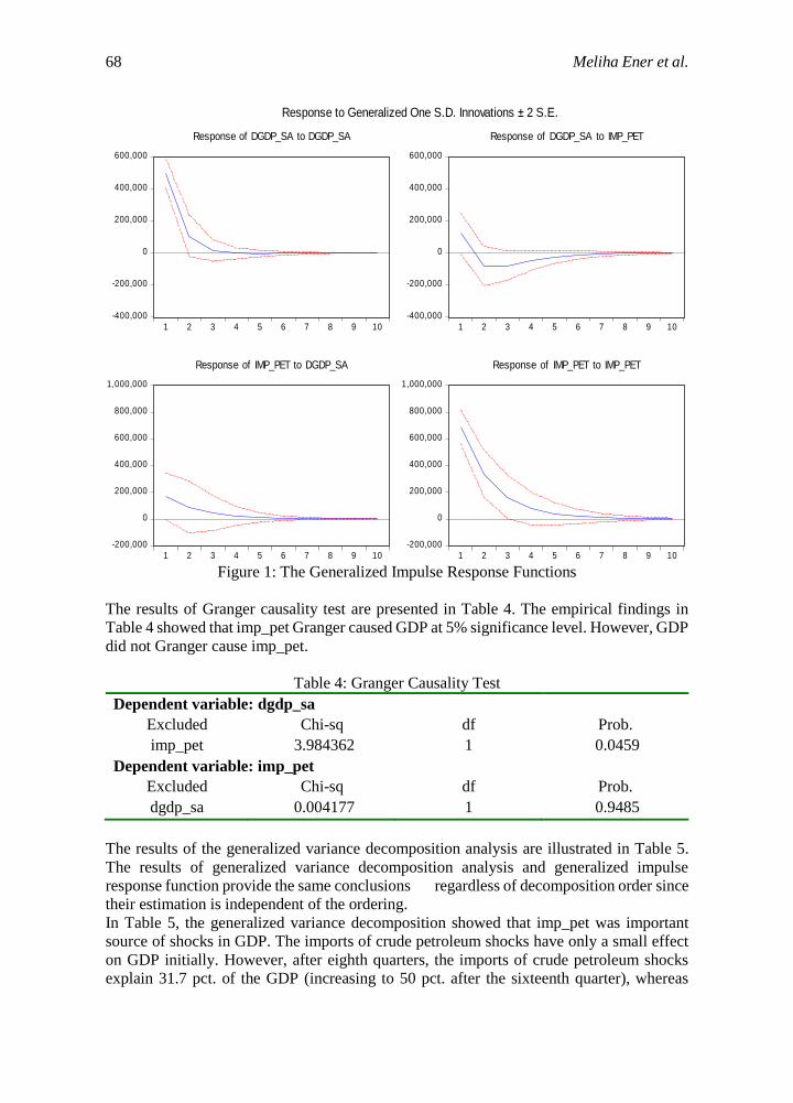
As we mentioned above, the interpretation of the VAR model can brought to light

through the generalized variance decomposition analysis and the estimation

of the generalized impulse response functions. The generalized impulse response

functions are showed in Figure 1.

The impulse response functions of the model showed that a positive shock to GDP led to a

positive and significant response of the imports of crude petroleum from the first quarter

until the fifth quarter, but aftermath of the fifth quarter the response of the imports of crude

petroleum declined gradually and become insignificant. Moreover, Figure 1 showed that a

positive shock to the imports of crude petroleum led to an increase in GDP until the second

quarter. Aftermath of the second quarter a positive shock to the imports of crude petroleum

led to a decrease in GDP and the response of GDP to crude petroleum imports declined

gradually.


Figure 1: The Generalized Impulse Response Functions

The results of Granger causality test are presented in Table 4. The empirical findings in

Table 4 showed that imp_pet Granger caused GDP at 5% significance level. However, GDP

did not Granger cause imp_pet.

Table 4: Granger Causality Test

Dependent variable: dgdp_sa

Excluded Chi-sq df Prob.

imp_pet 3.984362 1 0.0459

Dependent variable: imp_pet

Excluded Chi-sq df Prob.

dgdp_sa 0.004177 1 0.9485

The results of the generalized variance decomposition analysis are illustrated in Table 5.

The results of generalized variance decomposition analysis and generalized impulse

response function provide the same conclusions regardless of decomposition order since

their estimation is independent of the ordering.

In Table 5, the generalized variance decomposition showed that imp_pet was important

source of shocks in GDP. The imports of crude petroleum shocks have only a small effect

on GDP initially. However, after eighth quarters, the imports of crude petroleum shocks

explain 31.7 pct. of the GDP (increasing to 50 pct. after the sixteenth quarter), whereas

-400,000

-200,000

0

200,000

400,000

600,000

1 2 3 4 5 6 7 8 9 10

Response of DGDP_SA to DGDP_SA

-400,000

-200,000

0

200,000

400,000

600,000

1 2 3 4 5 6 7 8 9 10

Response of DGDP_SA to IMP_PET

-200,000

0

200,000

400,000

600,000

800,000

1,000,000

1 2 3 4 5 6 7 8 9 10

Response of IMP_PET to DGDP_SA

-200,000

0

200,000

400,000

600,000

800,000

1,000,000

1 2 3 4 5 6 7 8 9 10

Response of IMP_PET to IMP_PET

Response to Generalized One S.D. Innovations ± 2 S.E.


26.46 pct. of the variation in imports of crude petroleum shocks is explained by GDP shocks

(increasing to 33.26 pct after the sixteenth quarter).

Table 5: The Generalized Variance Decomposition of GDP and the Imports of Crude

Petroleum

Variance Decomposition of dgdp_sa

Period dgdp_sa imp_pet

4 99.75955 0.240448

8 68.22652 31.77348

12 67.00793 32.99207

16 51.11958 48.88042

20 49.48295 50.51705

Variance Decomposition of imp_pet

Period dgdp_sa imp_pet

4 5.880849 94.11915

8 26.46227 73.53773

12 34.20461 65.79539

16 33.26158 66.73842

20 31.47503 68.52497

4.3 Model’s Specification Tests

4.3.1 Stability Condition Test

Lastly model’s estimates are further tested for stability through eigenvalues stability

condition. If the modulus of each eigenvalue of companion matrix is strictly less than 1,

then the VAR model is stable. Eigenvalues modulus for the selected country gives results

that all eigenvalues are inside the unit circle. Thus our VAR model fulfills the stability

condition. Eigenvalues stability test graph and table for the country obtained from E-views

7 are reported in Figure 2 and Table 6, respectively.

Figure 2: Roots of Companion Matrix

-1.5

-1.0

-0.5

0.0

0.5

1.0

1.5

-1.5 -1.0 -0.5 0.0 0.5 1.0 1.5

Inverse Roots of AR Characteristic Polynomial


Table 6: Eigenvalue Stability Condition

Eigenvalue Modulus

0.475097 0.475097

0.281323 0.281323

No root lies outside the unit circle.

VAR satisfies the stability condition.

4.3.2 Lag Order Autocorrelation Test

VAR estimates are also tested for lag order autocorrelation. Lagrange-Multiplier (LM) test

for residual autocorrelation suggested by Johansen (1995) is applied. The null hypothesis

of the test is no autocorrelation at lag orders. LM residual test results are presented in Table

7. According to Table 7, we can’t reject the null hypothesis in the selected VAR (1) model.

Therefore, our VAR model has no lag order autocorrelation.

Table 7: VAR Residual Serial Correlation LM Test

Lags LM-Stat Prob

1 2.125728 0.7126

2 5.451021 0.2441

3 2.875122 0.5789

4 9.639104 0.0470

5 1.892419 0.7555

5 Conclusion

The relationship between the imports of crude petroleum and GDP has a special importance

in designing discretionary macroeconomic policies for stabilization purposes for developed

as well as developing countries. Thus revealing and the magnitude the direction of this

relation between the series give important signal in policy implementation process so as to

assess the long-run course of the energy policies to economic agents and policy makers.

This paper examines the dynamic linkages between crude petroleum imports and GDP of

Turkey. The vector autoregression analysis is carried on quarterly data for the period

1998Q1 to 2013Q2. This study utilized the generalized approach to forecast error variance

decomposition and impulse response analysis which have many advantages against the

traditional orthogonalized approach. According to the empirical findings, crude petroleum

imports have positive impact on GDP until the second quarter. But, after the second quarter

crude petroleum imports have negative impact on GDP. When analyzing the impact of GDP

on crude petroleum imports, we have evidence that a positive shock to GDP led to a positive

and significant response of the imports of crude petroleum from the first quarter until the

fifth quarter, but aftermath of the fifth quarter the response of the imports of crude

petroleum declined gradually. Moreover, the results of the Granger causality test showed

that crude petroleum imports granger caused GDP at 5% significance level, but not vice

versa. The generalized variance decomposition analysis exerted that the imports of crude


petroleum shocks have only a small effect on GDP initially. However, after eighth quarters,

the imports of crude petroleum shocks explain 31.7 pct. of the GDP, whereas 26.46 pct. of

the variation in imports of crude petroleum shocks is explained by GDP shocks.

Consequently, we can say that the import of crude petroleum is important variable on the

variation of GDP of Turkey.

References

[1] Muhammad Akram, Do Crude Oil Price Changes Affect Economic Growth of India,

Pakistan and Bangladesh?, Högskolan Dalarna, Economics D-Level Thesis, 2011.

[2] Erkan Aktaş, Çiğdem Özenç and Feyza Arıca, The Impact of Oil Prices in Turkey on

Macroeconomics, MPRA Paper No. 8658, 2010.

[3] Braun, Phillip. A. and Stefan Mittnik, Misspecifications in Vector Autoregressions

and Their Effects on Impulse Responses and Variance Decompositions. Journal of

Econometrics 59, 1993, 319-41.

[4] Central Bank of the Republic of Turkey, < http://evds.tcmb.gov.tr/>

[5] Christopher M. Chima, Empirical Study of the Relationship between Energy

Consumption and Gross Domestic Product In The U.S.A., International Business &

Economics Research Journal, 4(12), 2005, 101-112.

[6] David A. Dickey and Wayne A. Fuller, Distribution of the estimators for

autoregressive time series with a unit root, Journal of the American Statistical

Association, 74, 1979, 427–431.

[7] Obas John Ebohon, Energy, Economic Growth and Causality in Developing Countries.

A Case Study of Tanzania and Nigeria, Energy Policy, 24(3), 1996, 447-453.

[8] Clive W. J Granger, Investing Causal Relations by Econometric Models and Cross-

Spectral Methods, Econometrica, 37, 1969, 424-95.

[9] Clive W.J Granger, Paul Newbold, 1974. Spurious regressions in econometrics,

Journal of Econometrics 2, 1974, 111–120

[10] Bwo-Nung Huang, M.J. Hwang, C.W. Yang, Causal relationship between energy

consumption and GDP growth revisited: A dynamic panel data approach, Ecological

Economics, 6(7), 2008, 41-54.

[11] Levent Korap, Testing Causal Relationships between Energy Consumption, Real

Income and Prices: Evidence from Turkey, Beykent University Journal of Social

Sciences, 1(2), 2007, 1-29.

[12] John Kraft and Arthur Kraft, On the relationship between energy and GNP, Journal

of Energy and Development, 3, 1978, 401-403.

[13] Chien-Chiang Lee and Chun-Ping Chang, Energy consumption and economic growth

in Asian economies: A more comprehensive analysis using panel data, Resource and

Energy Economics, 30(1), 2008, 50–65.

[14] Poonpat Leesombatpiboon, A Multivariate Cointegration Analysis of the Role of Oil

in The Thai Macroeconomy, Ph.D. Dissertation, the George Washington University,

Washington, D.C., 2009.

[15] François Lescaroux and Valérie Mignon, On The Influence of Oil Prices On Economic

Activity and Other Macroeconomic and Financial Variables, OPEC Energy Review,

32(4), 2008, 343–380.


[16] Christelle Meniago, Janine Mukuddem-Petersen, Mark. A. Petersen and Gisele Mah,

Shocks and Household Debt in South Africa: A Variance Decomposition and GIRF

Analysis, Mediterranean Journal of Social Sciences, 4(3), September 2013, 379-388.

[17] Ömer Ozcicek and Douglas McMillin, Lag length selection in vector autoregressive

models: Symmetric and asymmetric lags, Applied Economics, 31, 1999, 517–524.

[18] M. Hashem Pesaran and Yongcheol Shin, Generalized Impulse Response Analysis in

Linear Multivariate Models, Economic Letters, 58(1), 1998, 7-29.

[19] Peter C.B. Phillips and Pierre Perron, Testing for a unit root in time series regression,

Biometrika, 75, 1988, 335–346.

[20] Uğur Soytas and Ramazan Sarı, Energy consumption and GDP: Causality relationship

in G-7 countries and emerging markets, Energy Economics, 25, 2003, 33–37.

[21] Christopher Sims, Macroeconomics and Reality, Econometrica, 48, 1980, 1-48.

[22] Turkish Statistical Institute, <http://www.tcmb.gov.tr/>.

[23] Erginbay Uğurlu and Aydın Ünsal, Ham Petrol İthalatı ve Ekonomik Büyüme:

Türkiye, 10. Türkiye Ekonometri ve İstatistik Kongresi 27-29 Mayıs 2009, Atatürk

Üniversitesi, Erzurum.

[24] Miloslav S Vosvrda, Stationarity and Unit Root Testing.

<http://vosvrdaweb.utia.cas.cz/cykly/Stationarity%20and%20Unit%20Root%20Test

ing.pdf> (06.10.2013).

[25] Michael Webb, Analysis for Oil Consumption with Dynamic Panel Data Models.

From a Thesis, Supervised by Dr Chirok Han and Professor Viv Hall, August, 2006.

[26] Yangru Wu and Xing Zhou, Handbook of Quantitative Finance and Risk Management.

Editors: Cheng-Few Lee, Alice Lee, John Lee, Springer New York Dordrecht

Heidelberg London, 2010.

[27] George U Yule, Why do we sometimes get nonsense correlations between time series?

A study in sampling and the nature of time series, Journal of the Royal Statistical

Society 89, 1926, 1-64.

[28] Eric Zivot and Jiahui Wang, Vector Autoregressive Models For Multivariate Time

Series with S-Plus. Springer 2003.

http://vosvrdaweb.utia.cas.cz/cykly/Stationarity%20and%20Unit%20Root%20Testing.pdf

http://vosvrdaweb.utia.cas.cz/cykly/Stationarity%20and%20Unit%20Root%20Testing.pdf

Documents

Do Crude Petroleum Imports Affect GDP of Turkey?