Do private sectors deficits matter? - Cepal

o private sectors deficits matter?

Manuel Marfán

D

S E

R I

E

temas de coyuntura

11

Special Studies UnitExecutive Secretariat, ECLAC

Santiago, Chile, October 2000

This document was prepared by Manuel Marfán, Expert in EconomicDevelopment, Economic Commission for Latin America and the Caribbean(ECLAC).

The views expressed in this document, which has been reproducedwithout formal editing, are those of the authors and do not necessarily reflectthe views of the Organization.

United Nations PublicationLC/L.1435-PISBN: 92-1-121281-2Copyright © United Nations, October 2000. All rights reservedSales No.: E.00.II.G.113Printed in United Nations, Santiago, Chile

Applications for the right to reproduce this work are welcomed and should be sent to theSecretary of the Publications Board, United Nations Headquarters, New York, N.Y.10017, U.S.A. Member States and their governmental institutions may reproduce thiswork without prior authorization, but are requested to mention the source and inform theUnited Nations of such reproduction.

CEPAL - SERIE Temas de coyuntura N° 11

3

Contents

Summary ...................................................................................... 5Introduction .................................................................................... 7I. A simple version .................................................................... 9II. Opening the capital account ............................................ 13III. Policy options ....................................................................... 17Appendix

A. A simple version ............................................................... 23B. Opening the capital account .............................................. 24C. A “suply-side” version ...................................................... 24D. A dollarized economy version .......................................... 25

Serie Temas de coyuntura: Issues published ..................... 27

FiguresFigure 1 Selected variables prior to recession ........................... 8Figure 2 Simple version equilibrium......................................... 11


5

Summary

During the 1990s, recurrent crises linked to abrupt changes inthe direction of international financial flows have been observed. Boththe Mexican crisis of 1994-1995 and the Asian crisis of 1997-1998 hadimportant propagation effects and exhibited high levels of contagionthat were underestimated. Observers have tried to identify the ex-antesources of vulnerability and policy mismanagement. Once more,economists have increased the volume of knowledge arising fromtraumatic episodes. Among other implications, the profession is nowconcerned about the optimal exchange rate regime, the sustainability oflarge current account deficits, the vulnerability of malfunctioningfinancial systems, the propagation effects of highly leveraged hedgefunds, and risks linked to currency mismatches and to the termstructure of external liabilities. The purpose of this article is toemphasize the links between external vulnerability and excessdomestic expenditure explained by private sector behaviour.

The motivation is based on the feature that at the eve of theirrespective crises, Mexico and most of the Southeast Asian economiesin which the last crisis detonated exhibited significant current accountdeficits while their fiscal accounts were under control. This was alsothe case of Chile in 1996-1997, prior to its own recession. The mix oflarge current account deficits and fiscal balance or fiscal surplusimplies that the origin of excess domestic expenditure –and ofvulnerability– was non-fiscal.

Do private sector deficits matter?

6

What are the macroeconomic consequences of an excess of non-fiscal expenditure? What arethe consequences of inconsistent policy targets? Which should be the consistent policy responses?These are the main questions tackled in this paper by means of a formal analytical model. Insection A we develop the case of an open economy with no voluntary financial flows, and analysethe effects of inconsistent policy targets. Two relevant and intuitive conclusions are that fiscalpolicy crowds out private expenditure, and that inflation is the natural outcome of inconsistentpolicy targets. In section B we develop the case with an open capital account, where the conclusionsare that inconsistent policy targets generate external vulnerability rather than inflation, and thatprivate expenditure crowds out fiscal policy. Moreover, in the context of consistent targets, fiscalpolicy needs to accommodate any excess of private expenditure to avoid external vulnerability. Thatis to say, the larger the level of private expenditure funded by external financing, the larger therequirement of fiscal effort to adjust to a consistent equilibrium. In section C we argue that if fiscalpolicy cannot be crowded out beyond a politically feasible level of fiscal surplus, a consistentequilibrium needs additional policy instruments. We analyse the case of a Tobin tax and the case ofa flexible tax as alternatives to an adaptive fiscal policy. Finally, we present a number of specialcases in the Appendix which prove the robustness of our conclusions.


7

Introduction

During the 1990s, recurrent crises linked to abrupt changes inthe direction of international financial flows have been observed. Boththe Mexican crisis of 1994-1995 and the Asian crisis of 1997-1998 hadimportant propagation effects and exhibited high levels of contagionthat were underestimated. Observers have tried to identify the ex-antesources of vulnerability and policy mismanagement. Once more,economists have increased the volume of knowledge arising fromtraumatic episodes. Among other implications, the profession is nowconcerned about the optimal exchange rate regime, the sustainability oflarge current account deficits, the vulnerability of malfunctioningfinancial systems, the propagation effects of highly leveraged hedgefunds, and risks linked to currency mismatches and to the termstructure of external liabilities. The purpose of this article is toemphasize the links between external vulnerability and excessdomestic expenditure explained by private sector behaviour.

The motivation is based on the feature that at the eve of theirrespective crises, Mexico and most of the Southeast Asian economiesin which the last crisis detonated exhibited current account deficitswhile their fiscal accounts were under control. This was also the caseof Chile in 1996-1997, prior to its own recession.


8

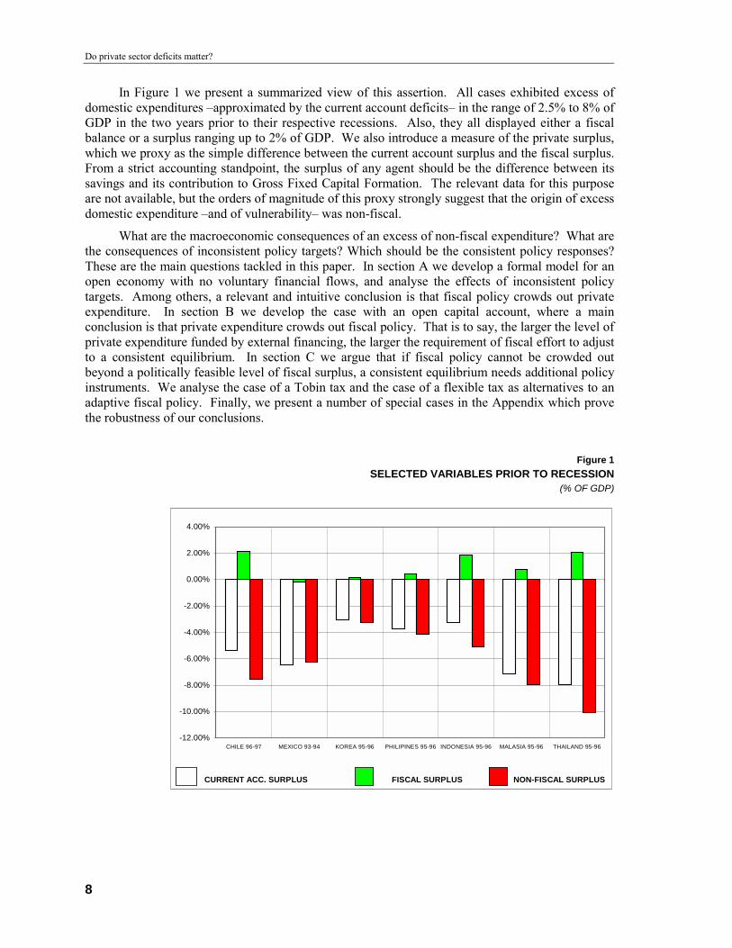
In Figure 1 we present a summarized view of this assertion. All cases exhibited excess ofdomestic expenditures –approximated by the current account deficits– in the range of 2.5% to 8% ofGDP in the two years prior to their respective recessions. Also, they all displayed either a fiscalbalance or a surplus ranging up to 2% of GDP. We also introduce a measure of the private surplus,which we proxy as the simple difference between the current account surplus and the fiscal surplus.From a strict accounting standpoint, the surplus of any agent should be the difference between itssavings and its contribution to Gross Fixed Capital Formation. The relevant data for this purposeare not available, but the orders of magnitude of this proxy strongly suggest that the origin of excessdomestic expenditure –and of vulnerability– was non-fiscal.

What are the macroeconomic consequences of an excess of non-fiscal expenditure? What arethe consequences of inconsistent policy targets? Which should be the consistent policy responses?These are the main questions tackled in this paper. In section A we develop a formal model for anopen economy with no voluntary financial flows, and analyse the effects of inconsistent policytargets. Among others, a relevant and intuitive conclusion is that fiscal policy crowds out privateexpenditure. In section B we develop the case with an open capital account, where a mainconclusion is that private expenditure crowds out fiscal policy. That is to say, the larger the level ofprivate expenditure funded by external financing, the larger the requirement of fiscal effort to adjustto a consistent equilibrium. In section C we argue that if fiscal policy cannot be crowded outbeyond a politically feasible level of fiscal surplus, a consistent equilibrium needs additional policyinstruments. We analyse the case of a Tobin tax and the case of a flexible tax as alternatives to anadaptive fiscal policy. Finally, we present a number of special cases in the Appendix which provethe robustness of our conclusions.

Figure 1SELECTED VARIABLES PRIOR TO RECESSION

(% OF GDP)

-12.00%

-10.00%

-8.00%

-6.00%

-4.00%

-2.00%

0.00%

2.00%

4.00%

CHILE 96-97 MEXICO 93-94 KOREA 95-96 PHILIPINES 95-96 INDONESIA 95-96 MALASIA 95-96 THAILAND 95-96

CURRENT ACC. SURPLUS FISCAL SURPLUS NON-FISCAL SURPLUS


9

I. A simple version

The balance of payments current account can be definedaccording to three accounting identities. First, it is the sum of thebalance of trade, the balance of financial and non-financial servicesand net current transfers. Second, it is the difference between GNPand domestic expenditure (the difference between investment andnational savings). Third, it is the difference between the change ininternational reserves and the capital account surplus. Whatever thetransmission mechanisms within an economy, these identities shouldprevail. The relation between the exchange rate and the currentaccount surplus varies depending on which definition we take. Insome cases, it is the actual level of the exchange rate and its actual rateof change what matter. In others, it is the expected level and itsexpected rate of change the relevant driving forces. An analyticalframework that simultaneously considers the actual and expectedexchange rate and their respective rates of change may be extremelycomplex. To avoid these complexities, we develop a model where allthe identities are expressed either in terms of rate of change or in termsof their change relative to the level of GNP.

This first basic case assumes an exogenous capital account (novoluntary financial flows), an assumption that is removed in thefollowing sections. The model assumes that there exists a GNP rate ofgrowth that, all other things being equal, allows a sustainable path forthe balance of payments current account. Let yx be the externalequilibrium rate of growth, which can be expanded by means of a realdepreciation (e – p). The left-hand side of equation (1) represents ameasurement of the current account surplus as the difference betweensuch a consistent GNP rate of growth and actual growth (y). As long as


10

y exceeds yx + d (e – p), there would be a current account deficit beyond the threshold ofvulnerability1. The right-hand side of equation (1) also represents the current account. In this case,it does so as the difference between GNP growth (y) and domestic expenditure pressure which, inturn, is the sum of the pressure of fiscal policy (g) and of private expenditure (q - a0 (r – p*)), wherer is the nominal interest rate and p* is expected inflation2.

(1) a1 (yx + d (e – p) – y) = B = y – [g + q – a0 (r – p*)] IS

Equation (2) represents the equilibrium condition where the rate of growth of real moneybalances (m – p) is a function of output growth and the nominal interest rate.

(2) m – p = b0 y – b1 r LM

Equation (3) states that inflation (p) is a weighted average between nominal depreciation (e)and expected inflation (p*), plus a function of the gap between actual GNP growth and potentialGNP growth (yd)3:

(3) p = c0 e + (1 – c0 ) p* + c1 (y – yd) ; 0 < c0 < 1 Phillips Curve4

In this simple initial version we assume the absence of voluntary financial flows. Thus, thereis a constraint on the current account deficit:

(4) y ≤ yx + d (e – p) External constraint5

Finally, we assume that the authority sets its policy instruments in order to minimize thedeviations with respect to a zero inflation target and a target rate of growth of ytarget:

(5) L = Min [p2 + (y – ytarget)2] Loss function

The model assumes that the private sector sets its expectations rationally (x* = E[x] for all x),but does not react instantaneously to surprises. The authority, which minimizes L, may takeadvantage of this rigidity in a non-systematic way. The endogenous variables are y, p, and either r,m or e, depending on the policy regime (fixed or floating exchange rate; passive or active monetarypolicy).

Assuming a binding equation (4) –i.e., with equality in (4)–, the final outcome is independentof the policy regime. In the absence of surprises (i.e., when x = x* ∀ x), then6

(6) y = [c0 yx + c1d yd] / (c0 + c1d) = ŷ

(7) p = (1-c0) d (ytarget – ŷ) / (c0 + c1d)

(8) e – p = c1 (yd – yx) / (c0 + c1d)

(9) ŷ – g = q – a0 (r – p*)

• Growth is a weighted average of the two constraints for growth (yx and yd),and is independent of the growth target ytarget (equation 6).

1 A value of zero for the left-hand side of equation (1) does not necessarily mean that the current account is strictly balanced. All that

it means is that the current account is sustainable.2 Strictly speaking, the right-hand side of equation (1) should consider the change in the real interest rate. In an end-of-period model,

such a change is with respect to the beginning-of-period interest rate, which is a constant by definition. So, the change in the interestrate is a function of its end-of-period level.

3 Notice that yd is a measure of domestic or internal factor markets equilibrium.4 In the appendix we develop the model with a “supply-side” version for this equation. Although the main conclusions do not vary, we

prefer to stick to this equation in the main text to allow for positive inflationary effects of a nominal depreciation.5 Notice that equation (4) is equivalent to B ≥ 0.6 See section A of the Appendix for the solution when unanticipated shocks occur.


11

• Inflation depends on the gap between the growth target ytarget and actual growth ŷ(equation 7).

• Real currency depreciation depends on the gap between yd and yx (equation 8).

• Private expenditure is crowded out by fiscal policy, since the equilibrium interestrate must fulfill expression (9).

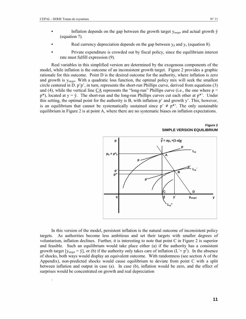
Real variables in this simplified version are determined by the exogenous components of themodel, while inflation is the outcome of an inconsistent growth target. Figure 2 provides a graphicrationale for this outcome. Point D is the desired outcome for the authority, where inflation is zeroand growth is ytarget. With a quadratic loss function, the optimal policy mix will seek the smallestcircle centered in D. p’p’, in turn, represents the short-run Phillips curve, derived from equations (3)and (4), while the vertical line CA represents the “long-run” Phillips curve (i.e., the one where p =p*), located at y = ŷ. The short-run and the long-run Phillips curves cut each other at p*’. Underthis setting, the optimal point for the authority is B, with inflation p’ and growth y’. This, however,is an equilibrium that cannot be systematically sustained since p’ ≠ p*’. The only sustainableequilibrium in Figure 2 is at point A, where there are no systematic biases on inflation expectations.

Figure 2SIMPLE VERSION EQUILIBRIUM

In this version of the model, persistent inflation is the natural outcome of inconsistent policytargets. As authorities become less ambitious and set their targets with smaller degrees ofvoluntarism, inflation declines. Further, it is interesting to note that point C in Figure 2 is superiorand feasible. Such an equilibrium would take place either (a) if the authority has a consistentgrowth target [ytarget = ŷ], or (b) if the authority only takes care of inflation (L´= p2). In the absenceof shocks, both ways would display an equivalent outcome. With randomness (see section A of theAppendix), non-predicted shocks would cause equilibrium to deviate from point C with a splitbetween inflation and output in case (a). In case (b), inflation would be zero, and the effect ofsurprises would be concentrated on growth and real depreciation

.

y

y = ayx +(1-a)y

p0 = p*0

p

p'

p'

p

p

p´p*´

0

LG

y´

A

B

C D

LG´

LG"

ytarget y

^

^


13

II. Opening the capital account

In the full version of the model we maintain the first threeequations:

(1.B) a1 (yx + d (e – p) – y) = y – [g + q – a0 (r – p*)] IS

(2.B) m – p = b0 y – b1 r LM

(3.B) p = c0 e + (1 – c0) p* + c1 (y – yd); 0 < c0 < 1 Phillips Curve

In the presence of perfect capital mobility, current accountdeficits may be financed by financial flows. Thus, equation (4) of thesimple version is replaced by an interest rate arbitrage condition, whererx represents the external interest rate, e* is the expected nominaldepreciation, and λ is a position parameter7:

(4.B) r = rx + e* + λ, Arbitrage Condition

We also split the authorities’ targets, assuming a central bankand a fiscal authority (government) which display different policytargets. The central bank minimizes inflation:

(5.B) LB = Min [p2] Loss Function (Central bank)

The government, in turn, cares about growth, and sets g in orderto minimize the expected rate of growth with respect to its target ytarget:

7 To avoid algebraic complexities, we have not explicitly included interest payments in the current account (equation (1.B)). This

could be the case when financial flows are linked to fixed rate assets, so that interest payments are independent of the spot interestrate and are implicitly included in yx.


14

(6.B) LG = Min [(yG – ytarget)2] Loss Function (Government)

As a general notation, x* and xG represent the respective expectations of the private sectorand the government for any variable x.

The central bank reacts instantaneously to surprises. The private sector continues to set itsexpectations rationally, but these are not adjusted instantaneously to surprises. The governmentalso sets its expectations rationally, but it is the slowest of the participants in the model8. Fiscalpolicy is always in the information set of the private sector9.

The final outcome does not depend on whether the exchange rate floats or is fixed, althoughthe transmission mechanisms vary from one version to the other.

In the absence of surprises (i.e., when x = x* = xG, ∀ x)

(7.B) p = 0

(8.B) y = ytarget

(9.B) e = c1 (yd – ytarget) / c0

(10.B) B = a1 (c0 + c1d) (ŷ – ytarget) / c0

(11.B) g = ytarget – [q – a0 (rx + λ + e)]

• The central bank achieves its inflation target (equation 7.B).

• The government also achieves its growth target (equation 8.B).

• Nominal (and real) exchange rate depreciation and the current account (B) areinversely correlated with the growth target (equations 9.B and 10.B).

• An inconsistent growth target implies a systematic bias towards currencyappreciation and current account deterioration (equations 9.B and 10.B). In the simpleversion, such an inconsistent targeting caused inflation.

• Fiscal policy depends on the growth target ytarget, and the expected value of privateexpenditure (equation 11.B). Notice that private expenditure crowds out fiscal policyinstead of the other way around.

The intuition behind this outcome is simple. The central bank can achieve its target since itreacts instantaneously to surprises, and has only one policy target and one independent policyinstrument (either e or m, depending on the exchange rate regime). The government can alsoachieve its growth target in the short run, since the inflationary pressures of an excess of growth canbe avoided by means of a currency appreciation. This, in turn, is feasible as long as externalfinancing is available. Currency appreciation and excess growth would both deteriorate the currentaccount. Fiscal policy must accommodate to changes in private sector expenditures since equation(1) –or (1.B)– must prevail.

8 This means that fiscal policy is set in advance by a budget law. Once the law is in place, there are no degrees of freedom to

introduce changes in fiscal policy. The private sector uses this information to set its own expectations and acts accordingly, but itcannot react to surprises. Implicitly, it is assumed that contracts cannot be changed instantaneously. The central bank can react tosurprises. Moreover, it can be a source of surprises.

9 Algebraically, the model is solved in the following steps. First, the central bank optimizes its loss function for given (exogenous)values of expected variables and fiscal policy. Thus, a reaction function is derived for the central bank. Second, the private sectorsets its expectations solving the model in expected values, given an exogenous fiscal policy, and given the central bank’s reactionfunction. Private sector behavioural functions are derived. Third, the government sets g in order to optimize its loss function inexpected values, given the behavioural functions of the private sector and given the central bank reaction function. Steps one and twoare repeated with the value of g thus determined.


15

In section B of the Appendix we develop the case when there are surprises. In that case, thecentral bank still achieves its target (p = 0), and the effect of surprises would be concentrated ongrowth, the exchange rate and the current account.

A relevant special case arises when the government is concerned about vulnerability. In thatcase, the target for setting fiscal policy should consider the current account balance:

(6’.B) LG = Min [(yG – d (eG – pG) – yxG)2] Loss Function (Government)

The outcome is equivalent to the one where ytarget = ŷG, and, in the absence of surprises,almost replicates that of the simple version:

(7’.B) p = 0

(8’.B) y = ŷ

(9’.B) e – p = e = c1 (yd – yx) / (c0 + c1d)

(10’.B) B = 0

(11’.B) g = ŷ – [q – a0 (rx + λ + e)]

• Private expenditure crowds out fiscal policy, since g must fulfill equation (11’.B).That is to say, the public sector budget constraint would be given by an overall target fordomestic expenditure.

• With shocks, volatility would concentrate on y, e and B, as in the previous case(see section B of the Appendix).

The main difference with respect to the simple case is that private expenditure crowds outfiscal policy instead of being the other way around. In fact, equations (11.B) and (11’.B) aresignificant to an understanding of recent events when dynamic economies faced external shocks. Ineffect, a consistent fiscal policy should provide enough slack to private spending.

That argument is unbounded in our setting, in the sense that it does not depend on whetherthe initial situation exhibits a fiscal surplus or a deficit. The fiscal constraint in this model is not theavailability of public revenues –or the budget constraint–, but an overall (public plus private)expenditure constraint.

In sections C and D of the Appendix we develop two special cases. In section C we replacethe Phillips Curve (3.B) for a “supply-side” version. The one considered so far allows forinflationary effects of exchange rate movements, whether expected or not. In section C of theAppendix, we assume a Phillips Curve such that when all expectations are fulfilled, GNP growthcannot deviate from its domestic equilibrium (y = yd). In this case, and in the absence of surprises,growth is always determined by its domestic constraint, while yx is irrelevant for that purpose.However, fiscal policy continues to be decisive for a consistent exchange rate and a consistentcurrent account, and private expenditure still crowds out fiscal policy.

In section D of the Appendix we develop the case of a dollarized economy, in which theoverall balance of payments determines the changes in the money supply. In the absence ofautonomous monetary and exchange rate policies, the sole policy instrument is fiscal policy (g).Under such a setting, inflation plays the role of the real exchange rate (with the opposite sign). Anexpansionary fiscal policy allows for larger GNP growth, but at the cost of raising inflation anddeteriorating the current account. A consistent current account and GNP growth can be attained bymeans of an appropriate fiscal policy, but, since inflation plays the role of the exchange rate,inflation depends on the gap between yd and yx. The outcome of fiscal policy being crowded out byprivate expenditure is still valid under this setting.


16

We have followed an analysis of short-run equilibrium in a context of rational expectationsand open capital account. Although we have concentrated mostly on the case in which GNP growthmay be affected by demand, in section C of the Appendix we develop the case where short-rungrowth is driven by aggregate supply. We also analysed the case of a dollarized economy. Someresults vary depending on the case, but there are two conclusions that are valid in all cases:

• Fiscal policy is the key decision variable for attaining a consistent current account.

• Private expenditure crowds out fiscal policy.


17

III. Policy options

In the simple case in which there are no voluntary financialflows, there were two disciplining factors operating. First, anautonomous and independent monetary policy could be implemented,which allowed the economic authority to keep overall privateexpenditure under control. Second, the outcome of fiscal policyvoluntarism was an inflationary pressure, which could be prevented byre-stating consistent policy targets.

In the case of perfect capital mobility, these discipliningelements disappear. The outcome of inconsistent policy targets isexternal vulnerability, measured as the combination of an inconsistentcurrent account and currency appreciation. Also, the authority has noways to keep private expenditures within prudent boundaries, and noindividual private agent has microeconomic incentives to cooperate insolving a macroeconomic problem. The most that the government cando is to implement a conservative fiscal policy. If such a conservativeapproach allowed a reduction in fiscal deficits, our arguments wouldend here. The policy dilemma arises when a fiscal balance or even aprudent fiscal surplus is not enough, as was the case of the countriesconsidered in Figure 1 of the Introduction.

The political economy of a fiscal surplus is not simple wherewelfare effects are associated with fiscal policy. Once a structuralfiscal surplus has been achieved, it is not clear that to continue limitinggovernment expenditures (or expanding taxes) in the face of excessprivate expenditure is optimal.

To analyse policy options we develop a variant of the previousversion.


18

Assume gB is the fiscal policy such as (11’B), consistent with a loss function that optimizesthe current account surplus (such as 6’.B). Also, assume gm is the maximum fiscal effort that thegovernment is willing and able to perform in a democratic environment. For the sake of theargument, assume that such a gm already implies a fiscal surplus to avoid the case of a weakgovernment and to concentrate in the case where the main driving force for a vulnerable currentaccount behavior is excess private spending. Then,

gm > gB ⇒ B < 0

The setting in this case implies a source of vulnerability, given that a deteriorating currentaccount and an appreciating currency would coexist.

Consider, now, the case where the central bank cares not only about inflation, but where thecurrent account is also part of its concern.

(5.C) L”B = Min [p2+ {a1 (yx + d (e – p) – y)}2] Loss Function (Central bank)

From the previous arguments, the government’s loss function would be:

(6.C) L”G = Max [gm; gB] Loss Function (Government)

Finally, assume that the central bank gains a policy instrument by introducing a Tobin tax (λ,of equation (4.B), becomes a policy instrument).

In this event a consistent outcome is re-attained (case of no surprises):

(7.C) p = 0

(8.C) B = 0

(9.C) y = ŷ

(10.C) e – p = e = c1 (yd – yx) / (c0 + c1d)

(11.C) ŷ – gm = q – a0 (rx + e* + λ)

• The central bank achieves its goals on inflation and B (equations 7.C and 8.C).

• Growth and real depreciation are consistent (equations 9.C and 10.C).

• Fiscal policy crowds out private expenditure (from expression 11.C, which must befulfilled by λ).

The intuition behind this version is straightforward. The central bank can achieve twoindependent goals from the moment that it has access to two independent policy instruments (eithere or m, depending on the exchange rate regime, and λ). In particular, λ controls the cost of credit tothe private sector and, thus, excess private expenditure can be contained. The government re-gainsdegrees of freedom to perform an independent fiscal policy.

The same outcome may be achieved with the introduction of any policy instrument thatallows the monitoring of private expenditures. For instance, we may think of introducing a flexibletax τ instead of the Tobin tax, such that private expenditures are represented by [q – τ – a0 (rx + e* +λ)]. Such a tax should not have inflationary effects, in order to avoid complexities. All that isneeded is that it should affect private expenditure and be flexible enough to be handled along thecycle.

Each of these policy options has its benefits and shortcomings, which we briefly analyse inthe following paragraphs:

a. Adaptive fiscal policy: This is the case in which we concentrated in section B above.In the absence of other policy instruments to handle domestic expenditure, a


19

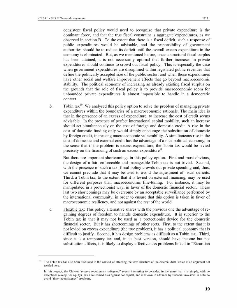
consistent fiscal policy would need to recognize that private expenditure is thedominant force, and that the true fiscal constraint is aggregate expenditures, as weobserved in section B. To the extent that there is a fiscal deficit, such a response ofpublic expenditures would be advisable, and the responsibility of governmentauthorities should be to reduce its deficit until the overall excess expenditure in theeconomy is eliminated. But, as we mentioned before, once a structural fiscal surplushas been attained, it is not necessarily optimal that further increases in privateexpenditures should continue to crowd out fiscal policy. This is especially the casewhen government expenditures are disciplined within legislated public revenues thatdefine the politically accepted size of the public sector, and when those expenditureshave other social and welfare improvement effects that go beyond macroeconomicstability. The political economy of increasing an already existing fiscal surplus onthe grounds that the role of fiscal policy is to provide macroeconomic room forunbounded private expenditures is almost impossible to handle in a democraticcontext.

b. Tobin tax10: We analysed this policy option to solve the problem of managing privateexpenditures within the boundaries of a macroeconomic rationale. The main idea isthat in the presence of an excess of expenditure, to increase the cost of credit seemsadvisable. In the presence of perfect international capital mobility, such an increaseshould act simultaneously on the cost of foreign and domestic credit. A rise in thecost of domestic funding only would simply encourage the substitution of domesticby foreign credit, increasing macroeconomic vulnerability. A simultaneous rise in thecost of domestic and external credit has the advantage of a nice political economy, inthe sense that if the problem is excess expenditure, the Tobin tax would be leviedprecisely on the financing of such an excess expenditure11.

But there are important shortcomings in this policy option. First and most obvious,the design of a fair, enforceable and manageable Tobin tax is not trivial. Second,with the presence of such a tax, fiscal policy crowds out private spending and, thus,we cannot preclude that it may be used to avoid the adjustment of fiscal deficits.Third, a Tobin tax, to the extent that it is levied on external financing, may be usedfor different purposes than macroeconomic fine-tuning. For instance, it may bemanipulated in a protectionist way, in favor of the domestic financial sector. Theselast two shortcomings may be overcome by an acceptable surveillance performed bythe international community, in order to ensure that this option is taken in favor ofmacroeconomic resiliency, and not against the rest of the world.

c. Flexible tax: This policy alternative shares with the previous one the advantage of re-gaining degrees of freedom to handle domestic expenditure. It is superior to theTobin tax in that it may not be used as a protectionist device for the domesticfinancial sector. But it has shortcomings of other sorts. First, to the extent that it isnot levied on excess expenditure (the true problem), it has a political economy that isdifficult to justify. Second, it has design problems as difficult as a Tobin tax. Third,since it is a temporary tax and, in its best version, should have income but notsubstitution effects, it is likely to display effectiveness problems linked to “Ricardian

10 The Tobin tax has also been discussed in the context of affecting the term structure of the external debt, which is an argument not

tackled here.11 In this respect, the Chilean “reserve requirement safeguard” seems interesting to consider, in the sense that it is simple, with no

exceptions (except for equity), has a welcomed bias against hot capital, and is known in advance by financial investors in order toavoid “time-inconsistency” problems.


20

equivalence” effects. Finally, like the previous option, it may be used to postpone anecessary elimination of a fiscal deficit.

d. Increasing national savings: A different line of thought is to introduce reforms toincrease national savings. Of course, this is a more structural means of solving theproblem of excess expenditure. But this is also a field where neither theoretical norempirical analysis are conclusive on how to encourage national savings. To increasecompulsory savings is more of the type of option c, above. Increasing governmentsavings is more of the type of a. And policy options to increase voluntary privatesavings usually reduce public sector savings, with an unpredictable effect on nationalsavings. Institutional reforms that may promote re-investment of profits and/orchanges in private sector confidence, economic predictability and saving habits arewelcome and superior to any of the previous options, but their likely effects mightnot be of the magnitude and timeliness needed.


21

Appendix


23

A. A simple version

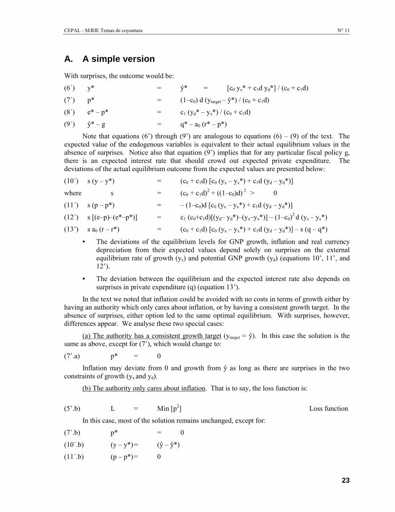
With surprises, the outcome would be:

(6´) y* = ŷ* = [c0 yx* + c1d yd*] / (c0 + c1d)

(7´) p* = (1–c0) d (ytarget – ŷ*) / (c0 + c1d)

(8´) e* – p* = c1 (yd* – yx*) / (c0 + c1d)

(9´) ŷ* – g = q* – a0 (r* – p*)

Note that equations (6’) through (9’) are analogous to equations (6) – (9) of the text. Theexpected value of the endogenous variables is equivalent to their actual equilibrium values in theabsence of surprises. Notice also that equation (9’) implies that for any particular fiscal policy g,there is an expected interest rate that should crowd out expected private expenditure. Thedeviations of the actual equilibrium outcome from the expected values are presented below:

(10´) s (y – y*) = (c0 + c1d) [c0 (yx – yx*) + c1d (yd – yd*)]

where s = (c0 + c1d)2 + ((1–c0)d) 2 > 0

(11´) s (p – p*) = – (1–c0)d [c0 (yx – yx*) + c1d (yd – yd*)]

(12´) s [(e–p)–(e*–p*)] = c1 (c0+c1d)[(yd– yd*)–(yx–yx*)] – (1–c0)2 d (yx – yx*)

(13’) s a0 (r – r*) = (c0 + c1d) [c0 (yx – yx*) + c1d (yd – yd*)] – s (q – q*)

• The deviations of the equilibrium levels for GNP growth, inflation and real currencydepreciation from their expected values depend solely on surprises on the externalequilibrium rate of growth (yx) and potential GNP growth (yd) (equations 10’, 11’, and12’).

• The deviation between the equilibrium and the expected interest rate also depends onsurprises in private expenditure (q) (equation 13’).

In the text we noted that inflation could be avoided with no costs in terms of growth either byhaving an authority which only cares about inflation, or by having a consistent growth target. In theabsence of surprises, either option led to the same optimal equilibrium. With surprises, however,differences appear. We analyse these two special cases:

(a) The authority has a consistent growth target (ytarget = ŷ). In this case the solution is thesame as above, except for (7’), which would change to:

(7’.a) p* = 0

Inflation may deviate from 0 and growth from ŷ as long as there are surprises in the twoconstraints of growth (yx and yd).

(b) The authority only cares about inflation. That is to say, the loss function is:

(5’.b) L = Min [p2] Loss function

In this case, most of the solution remains unchanged, except for:

(7´.b) p* = 0

(10´.b) (y – y*)= (ŷ – ŷ*)

(11´.b) (p – p*)= 0


24

(12´.b) [(e–p) – (e*–p*)] = c1 [(yd – yd*) – (ŷ – ŷ*)] / c0

The expected values of all variables are the same in both cases. But surprises in case (b) donot affect inflation, as they do in case (a), while growth and real depreciation are more affected bysurprises in case (b) than in case (a). If the loss function (5) represents the true value for theauthority, the outcome of case (a) would be superior to one of case (a). That is to say, consistenttargets would lead to a better outcome than forgetting about growth.

B. Opening the capital account

With surprises, the solution would be:

(7”.B) p* = 0

(8”.B) y* = ytarget

(9”.B) e* = c1 (yd* – ytarget) / c0

(10”.B) B* = a1 (c0 + c1d) (ŷ* – ytarget) / c0

(11”.B) g = ytarget – [qG – a0 (rxG + λG + eG)]

Again, the expected values have analogous expressions to the case with no surprises analysedin the text. Also, this outcome replicates the conclusion of the text that, for a given growth target,fiscal policy is crowded out by (expected) private expenditure rather than the other way around.

The deviations of the actual outcome with respect to their expected values are:

(12”.B) p – p* = 0

(13”.B) h(h–a0c1)(y – ytarget) = c0 [h (q – qG) – a0 c1 (q – q*)]

– a0 c0 [h (rx – rxG) – a0 c1 (rx – rx*)]

+ a1 c0 [h (yx – yxG) – a0 c1 (yx – yx

*)]

+ c1 [h (a1 d – a0) (yd– ydG) + a0 (1+a1) (yd– yd

*)]

where h = c0 (1+a1) + a1 c1 d > 0

(14”.B) e – e* = c1 [(yd – yd*) – (y – ytarget)] / c0

(15”.B) B – B* = a1 (c0 + c1d) [(ŷ – ŷ*) – (y – ytarget)] / c0

Notice that even with surprises the central bank always achieves its inflationary target(equation 12”.B). Notice also that the right-hand side of equation (13”.B) is the sum of deviations ofthe actual values of exogenous variables (q, rx, yx and yd) and their values expected either by thegovernment or by the private sector. When all expectations are fulfilled, y = ytarget.

C. A “supply-side” version

Equation (3) of the model assumes the presence of a trade-off between inflation and output.The idea was to give room to inflationary effects of nominal currency depreciation. However, themain outcome does not critically depend on this assumption. In this version, we assume thefollowing Phillips Curve equation:

(3.C) p = p* + c0 (e – e*) + c1 (y – yd) Phillips Curve

Note that in this version, whenever expectations are fulfilled (p = p* and e = e*), growth isdetermined by the internal constraint only (y = yd). An important difference with respect to


25

previous versions is that authorities cannot systematically attain a growth target different than yd.The current account and the exchange rate, however, do not have an obvious consistent behavior,unless the fiscal authority has a consistent target for the current account. To present this argument,we assume the following setting for the loss functions:

(5.C) LB = Min [p2] Loss Function (Central bank)

(6.C) L”G = Max [gm; gB] Loss Function (Government)

a. In the absence of surprises (x = x* = xG, ∀ x), and with g = gB, the solution is:

(7.C) p = 0

(8.C) y = yd

(9.C) B = 0

(10.C) e – p = eB = (yd – yx) / d

(11.C) gB = yd – (q – a0 (rx + e + λ))

• The central bank achieves its goal (equations 7.C).

• Growth is determined by its internal equilibrium (equations 8.C).

• B and real depreciation are consistent (equations 9.C and 10.C).

• Private expenditure crowds out fiscal policy (from expression (11.C).

b. In the absence of surprises (x = x* = xG, ∀ x), and with g = gm = gB + θ

(7’.C) p = 0

(8’.C) y = yd

(9’.C) B = – d θ / (a1d – a0)

(10’.C) e – eB = – θ / (a1d – a0)

• The central bank achieves its goal (equation 7’.C).

• Growth is determined by internal equilibrium (equation 8’.C).

• B and currency depreciation would accommodate the excess of expenditure in aninconsistent way (equations 9’.C and 10’.C) 12.

In this supply-side version, the introduction of a current account balance as a target for thecentral bank and λ as a policy instrument allows for the correction of inconsistencies. Also, fiscalpolicy would crowd out private expenditure, as in the case developed in the text.

D. A dollarized economy version

In a dollarized economy (or in a currency-board regime) there is no exchange rate policy andmoney supply is endogenous and changes proportionally to the overall balance of payments. Thisintroduces an analytical complication in the model, which is tackled by the following procedure:

12 The denominator in expressions (8’.C) and (10’.C) has an uncertain sign. The ambiguity arises since, when expectations are fulfilled,

depreciation has a mixed effect on total expenditure: a positive effect since depreciation improves the current account (a1d), and anegative effect since expected depreciation increases the cost of credit (a0) and, therefore, reduces private expenditure. When adepreciation is expansionary (i.e., when a1d – a0 > 0), there would be a trend toward an increasing current account deficit (B < 0) andan appreciating currency (e > 0).


26

First, we accommodate equations (1.B) and (3.B) of the text such that e = e* = 0, we initiallyremove the assumption of perfect capital mobility, and we define a balance of payments equation in(4.D):

(1.D) y = g + q – a0 (r – p*) + a1 (yx – d p – y) IS

(2.D) m – p = b0 y – b1 r LM

(3.D) p = (1 – c0 ) p* + c1 (y – yd) Phillips Curve

(4.D) m = f0 (yx – d p – y) + f1 (r – rx – λ) Balance of Payments

Second, we derive the equations, and look for the outcome in limits, when f1 → ∞.Since the only policy instrument is fiscal policy, the model is solved in its expected version, and thesolution depends on the government’s loss function. First, we try with the two initial targets:

(5.D) L = Min [pG 2 + (yG – ytarget)2] Loss function (Government)

In the absence of surprises, the final outcome of this version is:

(6.D) p = c0 c1 (ytarget – yd) / (c02 + c1

2)(7.D) y = (c0

2 ytarget + c12 yd) / (c0

2 + c12)

(8.D) B = yx – d p – y = yx – yd

– c0 (c0 + dc1) (ytarget – yd) / (c02 + c1

2)

(9.D) g + q – a0 (rx – λ – p) = y – a1 (yx – d p – y)

• With two targets and one policy instrument, neither of the targets is achieved (equations6.D and 7.D).

• A voluntarist target for growth is inflationary and deteriorates the current account(equation 6.D).

• Private expenditure crowds out fiscal policy, since g must fulfill equation (9.D).For a consistent outcome, we alternatively try:

(5’.D) L = Min [(yx – d p – yG)2] Loss function (Government)

In the absence of surprises, the final outcome in this version is:

(6’.D) p = c1 (yx – yd) / (c0 + dc1)

(7’.D) y = (c0 yx + dc1 yd) / (c0

+ dc1) = ŷ

(8’.D) B = yx – d p – y = 0

(9’.D) g + q – a0 (rx – λ – p) = ŷ

• Inflation plays the role of the exchange rate (equation 6’.D).

• Growth and the current account are consistent (equations 7’.D and 8’.D).

• Fiscal policy is crowded out by private expenditure, since g must fulfill equation (9’.D).


27

Issues published1 Reforming the international financial architecture: consensus and divergence, José Antonio Ocampo

(LC/L.1192-P), N° de venta: E.99.II.G.6 (US$ 10.00), 1999.www2 Finding solutions to the debt problems of developing countries. Report of the Executive Committee on

Economic and Social Affairs of the United Nations (New York, 20 May 1999) (LC/L.1230-P), N° deventa: E.99.II.G.5 (US$ 10.00), 1999.www

3 América Latina en la agenda de transformaciones estructurales de la Unión Europea. Unacontribución de la CEPAL a la Cumbre de Jefes de Estado y de Gobierno de América Latina y el Caribe yde la Unión Europea (LC/L.1223-P), N° de venta: S.99.II.G.12 (US$ 10.00), 1999.www

4 La economía brasileña ante el Plan Real y su crisis, Pedro Sáinz y Alfredo Calcagno (LC/L.1232-P),Nº de venta: S.99.II.G.13 (US$ 10.00), 1999 .www

5 Algunas características de la economía brasileña desde la adopción del Plan Real, Renato Baumann yCarlos Mussi (LC/L.1237-P), Nº de venta: S.99.II.G.39 (US$ 10.00), 1999 www

6 Internacional financial reform: the broad agenda, José Antonio Ocampo (LC/L.1255-P), Nº de venta:E.99.II.G.40 (US$ 10.00), 1999 www

7 El desafío de las nuevas negociaciones comerciales multilaterales para América Latina y el Caribe(LC/L.1277-P), Nº de venta: S.99.II.G.50 (US$ 10.00), 1999 www

8 Hacia un sistema financiero internacional estable y predecible y su vinculación con el desarrollo social(LC/L.1347-P), No de venta: S.00.II.G.31 (US$ 10.00), 2000. www

9 Fortaliciendo la institucionalidad financiera en Latinoamérica, Manuel Agosín, (LC/L.1433-P), No deventa: S.00.II.G.111 (US$ 10.00), 2000 www

10 La supervisión bancaria en América Latina en los noventa, Ernesto Livacic y Sebastián Saez(LC/L.1434-P), No de venta: S.00.II.G.112 (US$10.00), 2000. www

11 Do private sector deficits matter?, Manuel Marfán (LC/L.1435-P), No de venta: E.00.II.G.113(US$10.00), 2000. www

! Readers wishing to obtain the above publications can do so by writing to the following address: ECLAC, Special Studies Unit,Casilla 179-D, Santiago de Chile.

! Publications available for sale should be ordered from the Distribution Unit, ECLAC, Casilla 179-D, Santiago, Chile, Fax (562) 2102069, [email protected].

• www : These publications are also available on the Internet: http://www.eclac.cl

temas de coyunturaSerie

Name: ................................................................................................................................

Activity: ............................................................................................................................

Address: ............................................................................................................................

Postal code, city, country: .................................................................................................

Tel.: ......................Fax: ........................ E.mail address: ...................................................

Documents

Do private sectors deficits matter? - Cepal