The Mommy Effect: Do Women Anticipate the

Employment Effects of Motherhood?

Ilyana Kuziemko, Jessica Pan, Jenny Shen, Ebonya Washington∗

December 31, 2020

Abstract

The birth of a first child is a major life transition, particularly for women, and recentwork documents it still leads to large declines in female labor supply. We make threerelated arguments about women’s ability to predict the effects of motherhood on theiremployment. First, we present a variety of evidence from the US and UK that moderncohorts of women underestimate these effects. This underestimate is largest for thosewith college degrees and who themselves had working mothers. We show that thisoptimism about post-baby working life is new; earlier cohorts of mothers underestimatedtheir post-baby labor supply. Second, an important implication of this finding is that,at the time they are making decisions over post-secondary education, young womenunderestimate the probability they will be stay-at-home mothers. This underestimationthus provides a potential resolution to the puzzle of why, despite plateauing labor-force attachment since 1990, women in the US continue to increase human-capitalinvestment. Third, we explain why women today underestimate maternal employmentcosts using a two-generation model alongside evidence that the costs have recentlyincreased after decades of decline. In our model, women, especially those who saw theirown mothers work, invest in human capital under the assumption that the employmentcosts of motherhood would continue to fall. We show that roughly in the 1980s, however,key costs begin to rise.

Key words: fertility, labor supply, gender normsJEL codes: J16, J13, J22, D84

∗We thank seminar participants at Aarhus University, Cornell, Dartmouth, GRIPS, NBERSummer Institute (joint Labor Studies-Children meeting), MIT, NUS, Princeton, SOLE, Tinber-gen Institute, UCLA Anderson, University of Chicago Harris School, and Yale-NUS. We bene-fited from helpful discussions with Claudia Goldin, Raquel Fernandez, Henrik Kleven, SureshNaidu, Claudia Olivetti, Emily Oster, and Richard Rogerson. Courtney Burke, Elisa Jacome,Rais Kamis, Tammy Tseng and especially Lim Zhi Hao, Stephanie Hao, Elena Marchetti-Bowick and Paola G. Villa Paro have provided excellent research assistance. Kuziemko: Princetonand NBER (kuziemko@princeton.edu); Pan: National University of Singapore, IZA, and CEPR(jesspan@nus.edu.sg); Shen: Princeton (jenny.shen@princeton.edu); Washington: Yale and NBER(ebonya.washington@yale.edu).

1 Introduction

The birth of a first child is a major life transition. It is arguably more significant than

retirement, marriage or any educational milestone, especially for women. Motherhood is at

once incredibly common (even at low points throughout U.S. history, generally more than

eighty percent of women eventually give birth to at least one child) and yet difficult to

envision ex ante (the titles of a popular series of pregnancy and parenting books all begin

with the words “What to expect. . . ”).

Maternal labor supply is likely to be a particularly difficult aspect of motherhood for

young women to forecast. While the vast majority of women in the US and other rich

countries work before motherhood (and have done so for decades), the labor supply of mothers

has changed dramatically over time. In the US, it rose rapidly between 1960 and 1980. It has

since plateaued and in fact slightly decreased since 1990 (we show these trends in Appendix

Figure A.1, along with those from several other rich countries). Moreover, whether a mother

works while her children are young remains a controversial subject.1 While there is a rich

literature in economics assessing whether individuals and households prepare sufficiently for

retirement, there is little work examining whether they form correct expectations about

parenthood or exploring the implications of mistaken expectations thereof.

In this paper, we make three related arguments about women’s ability to anticipate the

employment costs of motherhood, which we define as the time, effort or money required for

mothers to raise their children in a manner they deem appropriate, while also working outside

the home. Examples of these costs might include the emotional cost of being separated from

the child while at work, the per-hour cost of a nanny or day-care service, guilt over (perceived

or real) underperformance as an employee or mother, or diminished sleep or other aspects

of wellbeing due to working while also performing childcare activities.2

First, we present a variety of evidence that women in modern cohorts (those born in the

1A few recent articles include, “I’m not ‘just’ a stay-at-home mother,” NYT, 2019,https://www.nytimes.com/2020/04/17/parenting/stay-at-home-mom.html. “Regret be-ing a stay-at-home mom? Would you ever admit it?” Forbes, 2020, https://www.forbes.

com/sites/terinaallen/2020/04/25/regret-being-a-stay-at-home-mom-would-you-ever-

admit-it/?sh=11463bd123c9. The topic played a role in the 2012 election when a surrogate forPresident Obama said that candidate Mitt Romney’s wife had “never worked” (Ann Romney wasa full-time mother and home-maker).

2See Bertrand (2013), who finds that among college-educated mothers, those with a careerreport being more unhappy, stressed, and tired than stay-at-home mothers. See Fortin (2005) for alonger discussion of feelings of guilt among working mothers.

1

late 1960s through the 1970s, who have only recently completed or are nearing completion of

their child-bearing years) have underestimated the employment costs of motherhood. Second,

an important implication of such underestimation is that, pre-motherhood, women make

human capital decisions under the belief that being a working mother is easier than it turns

out to be, and we show that educated women are indeed the ones who most underestimate

the “mommy effect” on employment. Our evidence thus provides a potential resolution to

the puzzle of why, despite plateauing labor-force attachment since 1990, women in the U.S.

continue to increase human capital investment in the form of costly education (they are now

substantially more educated than men, see Appendix Figure A.2) and job experience (in

part by delaying motherhood, see Appendix Figure A.3). Third, we present evidence that

helps explain why women underestimate the employment costs of motherhood: while these

costs were falling for their mothers’ generation, they have in fact plateaued or increased more

recently.

We develop each of these arguments using data from the U.S. and the U.K. We begin

by replicating in our data the main results from the recent “child penalty” literature (see,

e.g., Kleven et al., 2018 using Danish data; Angelov et al., 2016 using Swedish data; and

Byker, 2016, Chung et al., 2017, and Goldin and Mitchell, 2017 using U.S. data).3 Consistent

with past work, we find large and significant employment declines (roughly thirty percentage

points) in female employment probability after the first birth. Having a college degree and

growing up with a working mother predict smaller declines, but even for these groups the

declines are economically and statistically significant (thus echoing the results in Bertrand

et al., 2010 on female MBAs). As noted, these “child penalties” are by now well documented,

but little if any work has studied whether women anticipate these large employment declines.

And if not, why not?

We show a variety of evidence that, prior to motherhood, women underestimate how hard

it is to work while being a mother. If the impact of motherhood on the ability to manage both

work and family commitments is indeed unexpected in the short run, then women’s beliefs

about the appropriate balance between home and market work should change discontinuously

3Papers that have used other methods to examine the question of children and women’s laborsupply include, of course, Angrist and Evans (1998), who focus on developing credible instrumentsfor the birth of a third child. More recently, Lundborg et al. (2017) argue that, conditional onundergoing in vitro fertility (IVF) treatment, its success is sufficiently random to serve as a validinstrument for fertility. While event-studies cannot formally address endogeneity of fertility, inter-estingly, Kleven et al. (2018) shows that the event-study estimate of the effect of a third birth linesup closely to the IV-based estimate using twins or sex composition as an IV for a third birth.

2

upon the birth of the first child, as this event allows them to update their beliefs with new

information. Our U.K. data include a consistently worded set of questions on gender roles

and work-family balance (e.g., degree of agreement with statements such as “a woman and

her family would all be happier if she goes out to work” or “both husbands and wives should

contribute financially”) in repeated interviews across time, allowing us to use event-study

methods to measure how attitudes change with the arrival of a first child. We show that,

before motherhood, most women say that work does not inhibit women’s ability to be good

wives and mothers, but after the birth of their first child they become significantly more

negative toward female employment, consistent with having underestimated the impact of

motherhood on employment. The effect is significantly stronger for women who are more

educated and whose own mothers worked while they were children. Thus, while these groups

display smaller employment declines, they nonetheless appear to shift their beliefs the most

upon the first birth.

We provide two additional pieces of evidence that women, and especially those with a

college degree and who themselves had a working mother, underestimate the employment

cost of motherhood. While not measured in the years immediately before and after the birth

of the first child as in the event-study analysis, we perform a “long” difference-in-differences

analysis using a U.S. survey of high-school students that then follows up on them in their

thirties. One of the questions asked both in high school and in the later follow-up is the

importance placed on career success (worded in the future tense in the tenth-grade survey

and in the present tense in the follow-up survey). We show that relative to women without

children, mothers in this sample downgrade the importance of career success relative to their

tenth-grade expectations. This divergence in stated importance of career between parents

and non-parents does not occur for men in the sample. Like the UK event-study results,

the decline of mothers’ career ambition relative to other women is largest for more educated

women and those who grew up with working mothers.

As a final piece of evidence that women who are most likely to invest in education are also

those who ex-ante underestimate the difficulty of motherhood, we use a retrospective question

asking if raising children is harder than the respondent expected. Not only are women much

more likely to agree with that sentiment than are men, college-educated women are in fact

the most likely to agree (and there is no such education gradient for men).

All of the evidence described above on the underestimate of the employment costs of

motherhood come from women born in the late 1960s or in the 1970s (whose first births

3

occur mostly in the 1990s and early 2000s). Did women always underestimate the employment

effects of having a child, or is this lack of anticipation unique to these cohorts? We use a

combination of true panel data and synthetic panel data to compare how young women in

high school forecast their prime-age labor supply versus its actual realization twenty years

later. We gathered a variety of data sources that allow us to perform this exercise for a

six-decade period—beginning with high school students in the early 1960s and continuing

through today.

Consistent with the results documented above, in recent decades, female high school

seniors vastly underestimate the likelihood they will be at home full-time twenty years later.

From roughly 1985 onward (so, birth cohorts from the late 1960s onward), no more than

two percent say they will be home-makers or stay-at-home moms at age forty, but in reality

roughly twenty percent of them will be. However, we show, consistent with Goldin (1990),

this overestimate of future labor supply is a sharp reversal from a previous underestimate.

In the 1960s, the large majority of high-school girls predicted they would be full-time home-

makers in their thirties, significantly underestimating their future labor supply. Between

1968 and 1978, the share of high-school seniors expecting to be housewives plummets from

two-thirds to one-tenth. Importantly, we show that young women from the 1970s onward

desire and expect to be mothers (of two or more children), but not, apparently, stay-at-home

mothers.

That recent cohorts of women seem to systematically underestimate the employment

consequences of motherhood—and thus overestimate their future labor-market attachment—

begs the question of how they could get such an important prediction so substantially wrong.

After all, motherhood is a very common event and they could in principle learn from the

experience of their own mothers and that of their peers. We close the paper with our preferred

explanation: that the employment costs of motherhood have risen relative to those experienced

by their own mothers. While we do not formally test and reject other explanations, we show

that this explanation accommodates all the results described above and we provide a variety

of evidence that supports this proposed increase in costs.

We start by presenting a simple model of a woman’s education and employment choices

when her future employment costs of motherhood are uncertain. When making human cap-

ital decisions, she forms predictions over the level of her own future employment costs by

observing her own mother’s employment costs, but she inherits the costs her mother faced

with some noise (which may or may not have a mean of zero). We first show that the model

4

yields under very general conditions two of our most striking empirical results: that educated

women exhibit smaller employment “mommy effects” than their less educated counterparts,

but at the same time appear the most “surprised” by the high employment cost of moth-

erhood (in terms of their greater updating of beliefs about work-family gender roles and

their larger retrospective expressions of surprise at how hard motherhood is). Women in our

model choose higher levels of education—which raises the return to market work ex post and

thus results in higher labor supply post-motherhood—in part because they underestimate

the cost of motherhood ex ante. We show that these results hold regardless of whether the

average employment costs of motherhood have increased or decreased for the current gener-

ation relative to the previous one. That these results hold under relatively general conditions

not only bolsters the credibility of the model, but also serves as a “proof of concept” for the

empirical results. We then show that some of our other central results—that unconditional

on education women in modern cohorts appear to underestimate the costs of motherhood—

holds if and only if costs have, on average, increased for today’s mothers relative to earlier

cohorts.

To complement this theory-based argument that the cost of motherhood must have risen,

we provide a collage of empirical evidence suggesting that, while the cost almost surely fell

during much of the twentieth century, it appears to have recently risen along some important

metrics, especially since the 1990s. Some of this evidence we take from past literature and

some, to the best of our knowledge, we provide for the first time. For example, as we review

in more detail in Section 5, past work has emphasized the decline in the cost of motherhood

over the middle decades of the 20th century due to technological advances (e.g., household

appliances and advances in infant formula) and links these falling costs to the large rise in

female LFPR over the same period. We argue that those advances may have fully played out

and in fact more recent developments (e.g., research advocating the benefits of breastmilk

over formula) may have effectively increased the costs of motherhood. Indeed, in both the

US and the UK, we show that breastfeeding rates have increased significantly over the

past several decades, especially since the 1990s. Similarly, while the underlying cause is still

debated, time-use data show that mothers invest more hours in child-rearing than their own

mothers did.

Finally, consistent with our claim of a u-shape pattern over time in the costs of moth-

erhood, we show that beginning in the late 1990s, large majorities of mothers tell survey

takers that motherhood is harder today than for their own mothers and that they are more

5

involved in their children’s lives than their mothers were in theirs. By contrast, mothers

surveyed in the 1950s and 1960s report that motherhood is easier for them than that it was

for their own mothers. In the conclusion, we briefly take up the question of why the costs

of motherhood may have increased over recent decades, but otherwise leave that important

question to future work.

Beyond the literature on employment “child penalties” we already discussed, we also con-

tribute to an extensive economics literature on gender-role norms, and in particular how they

change over time.4 For example, Goldin (2006) suggests that innovations in contraception

may have contributed to altering women’s identity in the 1960s and 1970s. Fernandez et al.

(2004) argue that men growing up in families with working mothers appear to have devel-

oped more liberal gender-role attitudes.5 Related, perhaps, to the slowdown in labor market

convergence we noted earlier, Fortin (2005) shows that while birth cohorts have become more

liberal regarding norms about women in the workplace, this trend has recently plateaued

in OECD countries. We show that gender-role attitudes appear to exhibit life-cycle effects:

women themselves adopt more traditional attitudes after they become mothers.

Of course, the idea that motherhood changes women’s priorities is hardly original, and

appears frequently in the popular press.6 To the best of our knowledge, we are the first to

examine how gender-role norms regarding employment change after parenthood in a formal

event-study framework. We are aware of a small number of academic papers, mostly from

sociology, that examine similar questions, all using panel data from high-income countries

(Grinza et al., 2017; Baxter et al., 2015; Shafer and Malhotra, 2011; Jarrallah et al., 2016;

Vespa, 2009). But these panels tend to be short (in some cases, only two waves), and thus

these analyses cannot perform event studies to determine if any estimated effect on attitudes

is coincident with motherhood or instead driven by trends.

The remainder of the paper is organized as follows. Section 2 reports our results on

4Recent contributions to this literature have focused on norms in the marriage market or withincouples. Bertrand et al. (2015) and Kleven et al. (2016) provide a variety of evidence that couplesfollow the norm that husbands should out-earn their wives. Bursztyn et al. (2017) show that tradi-tional gender-role norms remain relevant even among career-oriented MBA students—anticipationof the marriage market appears to limit the public signaling of career ambitions of single femaleMBA students.

5On the other hand, Alesina et al. (2013) highlight the long-term persistence of gender norms,showing that ethnicities and countries whose ancestors practiced plough cultivation (which is moresuited to male labor) have lower rates of female labor force participation even today.

6See, e.g., “What Happens to Women’s Ambitions in the Years After College,” in The At-lantic, December 2016. https://www.theatlantic.com/business/archive/2016/12/ambition-interview/486479/.

6

the effect of motherhood on labor supply. Section 3 provides a variety of evidence that

women underestimate the employment effects of motherhood, including event-study analysis

of how women’s gender-role attitudes change in the years surrounding the first birth, how

they answer retrospective questions about parenthood being harder than expected, and how

they downgrade the importance of their own careers as a function of parenthood. Section

4 examines the accuracy with which female high school students forecast their future labor

supply, showing that over a short period in the 1970s, high-school girls went from significantly

under-estimating their future labor supply to significantly over-estimating it. Section 5 relies

on both theoretical and empirical evidence to argue that the reason why modern cohorts of

women have not anticipated the costs of motherhood is because these costs recently increased

in an unpredictable manner. Section 6 concludes and poses some questions for future work.

2 How does motherhood affect employment?

As our motivating question is whether women anticipate the large post-baby declines in their

employment, we begin by documenting the employment declines themselves. We provide only

a brief summary of the data sources here and much greater detail in Appendix B.

2.1 Sampling restrictions and data sources

A substantial portion of the empirical work in this section and the next involves event-study

analysis. We thus adopt sample restrictions with that exercise in mind. Our preferred sample

will include only those individuals whom we observe at least once before and once after the

“event” of the birth of a first child, so that all subjects help identify a standard difference-

in-difference estimate of the effect of parenthood (though in robustness checks we will add

back in subjects who remain childless or had children before entering the sample, to serve

as controls). We also, whenever possible, require that we observe respondents over the full

period of their most likely child-bearing years (between ages 20 and 40).7 Thus, whenever

possible, we restrict cohorts to those who, were they to have a child between ages twenty

and forty, the birth would be observed in our sample period.

7The one exception is the British Household Panel Survey (BHPS). As the BHPS only spans 18years (with a later additional booster sample spanning only about 10 years), imposing the 20-40age restriction is impossible. Instead of imposing the 20-40 restriction, we require our main sampleof women to be at least 16 years old at the start of our panel. For our control samples of childlesswomen, we require that we observe them at some point at age 29, the median age at first birthamong women in our treatment sample.

7

2.1.1 British Household Panel Survey

The British Household Panel Survey (BHPS) is a longitudinal survey that runs from 1991

through 2009. This dataset is unique in that it asks consistently worded questions about

gender norms in repeated interviews, which we describe in more detail in the next section.

Col. (1) of Table 1 shows summary statistics for women in our preferred sample in the BHPS.

The sample restrictions described above leave us with a total of 681 women. On average, in

our analysis sample, we observe individuals 4.1 times pre-birth and 6.6 times after. While

we do not impose perfect balance for our event-time figures, it is reassuring to know that we

observe parents several times before and after their first birth so that trends are unlikely to

be explained by composition changes.

2.2 U.S. panel data sources

We make use of three commonly used sources of U.S. panel data: the “Young Women”

component of the National Longitudinal Surveys of Young and Mature Women (hereafter

NLSW), the National Longitudinal Survey of Youth (NLSY), and the Panel Study of Income

Dynamics (PSID).

Women in the NLSW were 14-24 when first interviewed in 1968; the last interviews

occurred in 2003. For the most part, we can only examine employment outcomes with these

data, as there are no questions on gender-role attitudes that are asked consistently over time

(the NLSY occasionally asks about gender norms, but these questions are scattered over

many years and not sufficiently frequent to perform an event-study analysis). However, we

will make use of a variable that asks women in 1968 about their employment and parenthood

expectations when they are 35. Our sampling criteria include only women who were born

between 1948 and 1954 (so they are roughly in their sixties today). Our preferred sampling

criteria leave us with 1,413 women. Summary statistics are presented in col. (2) of Table 1.

The NLSY begins interviewing young men and women between the ages of 14 and 22

in 1979 and continues through 2014. Again, to ensure that we observe the full period of

respondents’ most likely child-bearing ages, we only include the 1959-1964 cohorts (so our

sample is born roughly ten years after their NLSW counterparts). These sampling criteria

leave us with 2,256 women. Summary statistics for this preferred NLSY sample appear in

col. (3) of Table 1.

Our final U.S. panel data source is the PSID. While it begins in 1968 (and continues

through today), our preferred analysis sample includes all individuals for whom we observe

8

the first birth after 1979 (because the employment outcomes we most use are not coded

consistently before this date). To meet our usual requirement that we observe individuals

between the ages of twenty and forty, our preferred sample includes only the 1957-1975

cohorts, leaving us with 1,007 women. Col. (4) of Table 1 displays summary statistics for

our PSID sample. On average, the women in our sample are born about five (fifteen) years

after those in the NLSY79 (NLSW68).

Due to slightly different definitions, we cannot compare all variables across the BHPS

and our U.S. datasets, but where we can, the differences are as expected. Note that even

the PSID, our most recent U.S. panel dataset, samples women who are from slightly earlier

cohorts than the BHPS. Consistent with having later cohorts in the BHPS and the general

tendency of the British to delay childbirth relative to Americans (recall Appendix Figure

A.3), individuals in all our U.S. samples have their first child at a younger age than do women

in the BHPS and also have more children in the period in which we observe them.8 Consistent

with the evidence in Figure A.2, the summary statistics show that American women are

more likely to have completed university education than their British counterparts, despite

coming from earlier cohorts. American women in the PSID and NLSY79 samples are also

significantly more likely to have obtained a college degree than their counterparts in the

NLSW68, consistent with the rapid growth in female college graduation rates in the US

between the 1950s and 1970s cohorts (Goldin et al., 2006).

2.3 Event-study specifications

Much of our analysis examining the short- and medium-run changes associated with parent-

hood makes use of a basic event-study methodology, defining the first child’s year of birth as

the “event,” following Kleven et al. (2018). Specifically, we model a given outcome yit (e.g.,

current employment) for person i in year t as:

yit =τ=τmax∑τ=−6, 6=−2

βτ · 1[τ = t− ci] +∑a

γa · 1[a = Ageit] + δt + εit. (1)

We index event time (time relative to birth of a child) by τ . The variable 1[τ = t − ci] is

defined as follows: ci denotes the calendar year in which person i had their first child, so

1[τ = t − ci] is an indicator for person i in year t having had their first child τ years ago.

8Our British panel is also shorter than our American panels, so the U.K. women are also lesslikely to have completed their fertility by the end of the panel.

9

Negative values of τ indicate having a first child |τ | years in the future. In the summation

term, we omit the event-time indicating two years before the first birth. The τ = −6 (or

τ = τmax) term in fact includes all years greater than or equal to six years before (or τmax

years after) the first birth, and these coefficients are not plotted in the event-study graphs.

The value for τmax depends on the length of the sample period in a given panel dataset,

but we are typically able to look 5-10 years after the first birth. We control for a vector of

calendar-year fixed effects (δt) and a vector of age-in-years fixed effects (∑

a 1[a = Ageit]).

The error term is εit. We cluster standard errors at the individual level.

This specification normalizes the event time τ = −2 to zero, though in our figures we

will often add to all coefficients the raw mean of the outcome variable at τ = −2 to facilitate

comparisons across different subgroups in both levels and changes. Note that we normalize

τ = −2 instead of the standard τ = −1 because pregnancy may have an effect of interest as

well.

We present our results by plotting the βτ coefficients, to show the evolution of our outcome

variables relative to the event of parenthood, conditional on year and age fixed effects. To

summarize the effects more succinctly, we will typically present alongside the event-study

graphs: (a) the average of all post-period coefficients (i.e., coefficients on event-time τ = 0

through the final plotted coefficient in the figures); (b) the slope and significance of the pre-

period coefficients, to gauge pre-trends; and (c) a pre-trend-adjusted average of post-period

coefficients. This final statistic is based on the following specification:

yit =τ=τmax∑τ=−1

βτ · 1[τ = t− ci] + λ · τit +∑a

γa · 1[a = Ageit] + δt + εit, (2)

where all notation is as in equation (1) and the λ·τit term captures the projected pre-trend. As

we allow all post-period coefficients (plus the year of pregnancy) to vary freely but restrict the

pre-period (i.e., periods -5 to -2) to take a linear form, the post-period coefficients represent

any post-period changes after netting out the projected (pre-pregnancy) pre-trend.

If the pre-trend coefficient λ is itself not significant, then we tend to prefer the equation

(1) specification. We are fortunate that in almost all cases, netting out the projected pre-

trend makes little difference to our conclusions.

10

2.4 Main results

We begin our analysis by examining the share of women who are currently employed, be-

fore and after the birth of a first child. Figure 1(a) shows the event-study coefficients from

equation (1), estimated on our U.K. data, which defines currently employed as having a paid

job. Two years before the birth of a child (so roughly one year before pregnancy), 91 percent

of women are working (recall that the coefficient for τ = −2 is merely the raw mean at

τ = −2), a rate nearly as high as that for men who will become fathers in two years (not

shown). There is a very slight, insignificant, negative pre-trend. The year before the birth

exhibits a very modest decline, likely due to pregnancy, and it is swamped by the large,

thirty percentage-point decline in the year of the birth.

Above the event-study graph, we report the average of the six post-period coefficients

and its level of significance. This average 33 percentage point decline is only slightly reduced

to 29 percentage points when we project forward the (insignificant) pre-trend.

Figure 1(b) replicates this event-study figure for our U.S. data sources and finds very

similar results. As we might expect, the employment decline is slightly smaller for the more

modern cohorts in the PSID and NLSY than in the NLSW. To avoid clutter and because

there is little visual evidence for concern, we do not adjust for pre-trends in these graphs.

It is worth emphasizing that Figure 1 and our other event-study figures plot event-study

coefficients (how employment changes relative to τ = −2, conditional on all the controls in

equation 1) and thus except for τ = −2 (which is, by construction, normalized to the raw

mean in that year) raw means cannot be read off the figure. For example, for each of our four

panel datasets, female employment is on a positive, secular trend, which we capture with the

year fixed effects. So, in raw levels, women do increasingly return to work as time passes after

the birth of their first child, but not any faster than the year fixed effects and other controls

would predict. Appendix Figure A.4 demonstrates this same point in a slightly different

manner, using childless women as the counterfactual instead of modeling the counterfactual

with year and age fixed effects as we do in Figures 1(a) and 1(b) (following Kleven et al.,

2018). We use the NLSY and plot employment for childless women, generating a “placebo

event” of childbirth (see the figure notes for more detail). We then compare this series to

employment outcomes for women who become mothers (where both series are simply raw

means in event-time). For the most part, the childless-women series is increasing slightly each

year, as is the series for mothers, except for the large decrease in the year of childbirth.9 In

9The same exercise for the other three panel datasets is available upon request.

11

the paper, for the sake of exposition, we will often refer to an outcome as rising or declining

upon motherhood. However, such a statement rarely refers to raw levels, but instead to

changes conditional on the controls in the event-study specification.

How do our results compare to existing work? Figure 1 very closely parallels the results

in Kleven et al. (2018), which uses Danish register data drawing from the 1955-1973 birth

cohorts. Like us, they find little evidence of pre-birth pre-trends, a large effect the year of

the birth, and little if any long-run recovery. Our effect sizes, however, are much larger—

Danish mothers are roughly twelve percentage points less likely to work than they were

before motherhood, whereas the decline for for U.S. and British women of similar cohorts

is two to three times as large. In general, Denmark has a much higher female labor force

participation rate than the UK or US (and in fact, higher than essentially any other country),

and comparing our results to those using Danish data suggests that a large part of the

difference likely comes from women’s different responses to motherhood.10

2.5 Heterogeneity and other results

Our goal in this subsection is to examine heterogeneity along dimensions related to our

hypothesis, namely human-capital formation and expectations about future labor supply.

Here we estimate the difference in employment responses by distinct and mutually exhaustive

groups X = 1 and X = 0, where X is a dummy variable such as college completion. We

begin by estimating the following equation:

yit =τ=τmax∑τ=−6, 6=−2

βτ · 1[τ = t− ci] +∑a

γa · 1[a = Ageit] + δt+

1[X = 1] ·

[τ=τmax∑τ=−5

βX=1τ · 1[τ = t− ci] +

∑a

γX=1a · 1[a = Ageit] + δt

]+ εit.

(3)

This equation is based on our main event-study equation (1), but it fully interacts the event-

study coefficients, the age fixed effects, and the time fixed effects with the dummy variable

1[X = 1]. So, in the case of college completion, the event-time, age and year fixed effects

are allowed to have unrestricted differences for those who did and did not finish college. As

10Smaller effect sizes in Denmark may be explained by the country’s more generous parental-leaveand child-care policy. In addition to covering 52 weeks of parental leave, the Danish governmentguarantees all children between the ages of six months and five years a spot in heavily subsidizedchild-care facilities. By contrast, U.K. and especially U.S. parental leave is much less generous, apoint to which we briefly return in Section 5.

12

the post-baby declines in employment for each subgroup (as well as the differences in those

declines), we report in Figure 2 the average of the post-period coefficients (and its confidence

interval) for each subgroup. We then report the difference in the post-period average for each

group and its level of significance.11

We choose X variables that relate to human capital investment and expectations. Specif-

ically, whenever data permit, we split each of our samples by whether the respondent (a)

completed college; (b) had a working mother herself; (c) had, pre-motherhood, positive views

toward working mothers; and (d) planned, pre-motherhood, to work after having a baby,

though we defer discussion of (d) until Section 4.

Figure 2 shows these results. Subfigure (a) shows that for each of our four datasets, a

college degree mutes the “mommy effect” on employment, in most cases in a statistically

and economically significant manner. However, because the baseline employment decline is

so large, even the smaller responses for these more educated women mean that they still

have substantial and significant declines post-baby (as shown in the figure, the confidence

intervals for these subgroups do not come close to including zero). To avoid clutter, we do not

report in these figures the pre-trends from the underlying event-study graphs nor pre-trend-

adjusted post-period averages, but we show all of the actual event-study graphs in Appendix

Figure A.5 and differential pre-trends do not appear to be a concern (in fact, adjusting for

pre-trends would make the difference in the “mommy effects” between subgroups reported

in Figure 2 even larger).

A similar but more muted pattern appears in all of our datasets with respect to being

raised by a working mother: such women have smaller employment declines in three of our

four datasets (though none of the differences are statistically significant). A similar pattern

appears for having “pro-working-mother” values pre-baby (see figure notes and Appendix B

for more detail on how this variable is defined in our datasets).

In summary, this section provides a variety of evidence showing the large, negative em-

ployment effects of motherhood, replicating past work in other countries. While the effects

for later cohorts in the US (PSID and NLSY) appear to be somewhat smaller than for older

cohorts (NLSW), in both the US and UK they remain large: roughly thirty percentage points.

To put this decline in perspective, in the most recent CPS, employment rates are 23 percent-

11So, for the X = 0 group, the average of the post-period coefficients is given by the post-period βτ coefficients. For the X = 1 group, it is given by the sum of the post-period βτ and βX=1

τ

coefficients. The difference in post-period effects between the two groups is given by the post-periodβX=1τ coefficients.

13

age points lower for 65-69 year-olds than for 60-64 year-olds.12 Thus, our estimated “mommy

effect” is comparable to a retirement effect. We now turn to whether women anticipate this

large change in their labor supply.

3 Do women anticipate the “mommy effect?”

There have been several dynamic labor supply models from the macro literature that attempt

to jointly explain women’s fertility, human capital and employment decisions (or some subset

of these decisions). Most of these models (e.g., Attanasio et al., 2008; Blundell et al., 2016;

Adda et al., 2017) assume that agents have perfect foresight of how children will affect labor

supply and thus plan accordingly.13 This section provides several pieces of evidence that

questions that assumption and suggests that women systematically underestimate the effect

of motherhood on employment. This underestimate manifests in the short run (i.e., in the

years right before the first birth) as well as earlier in their lives (i.e., when they are in high

school and making post-secondary human capital decisions).

3.1 Effect of parenthood on views toward female employment

We begin by exploring whether women’s beliefs about the proper balance between family

responsibilities versus market work change upon having a child. If, as we argue, women un-

derestimate the costs of motherhood, then the event of the first birth serves as an information

shock and thus beliefs should be updated.

3.1.1 Data on attitudes toward female employment

To measure how beliefs change, we make use of six questions in the BHPS. These questions

are in the form of statements about the proper role of women in the workplace versus the

home, and respondents are asked to state their agreement with each statement on a 1–5 scale

(e.g., “All in all, family life suffers when the woman has a full time job,” “Both the husband

and wife should contribute to the household income”). If needed, we reverse the order of

the responses so that each question is increasing in the pro-female-employment direction.

We then standardize each of these variables and sum them. Appendix Table A.1 provides

summary statistics for this “omnibus” measure of summed standardized variables as well as

each component (and the wording of each component statement). Note that, in contrast to

12See https://www.bls.gov/cps/cpsaat03.pdf.13An important exception is Fernandez (2013), which we return to in Section 5.

14

the employment question, which is asked every year, the BHPS asks these six gender-role

questions every other year, so we expect point estimates to be noisier given the smaller

sample.

We refer to this omnibus variable as our index of gender-roles regarding work and family,

or simply gender-roles index, for expositional ease. To provide a sense of magnitudes, we

show in Appendix Table A.1 that women are generally 0.77 units more in the pro-work (that

is, agreeing that it is good for women to combine family and work) direction than are men.

This index has strengths and weaknesses. A strength is that all the questions refer to

the desirability of wives and mothers working outside the home. One could imagine instead

questions about gender stereotypes, but not about employment (e.g., “On average, women

and men have equal innate intelligence”), which would be less germane to our hypothesis.

Another strength is that the question is abstract and does not specifically ask about the

respondent’s own household, as such a question would not lend itself to event-study anal-

ysis. The BHPS statements are about households in general and thus respondents without

children can still answer these questions.

A weakness is one that arises for any type of subjective response: it is impossible to know

exactly what the respondent means when she answers. But because statements in the BHPS

are not about one’s own situation but about the appropriate responsibilities for men and

women generally, in principle a woman who perfectly anticipates the costs of motherhood

should give the same response before and after becoming a parent. By contrast, a woman

who overestimated (underestimated) the employment costs of motherhood should change

her answer in a pro- (anti-) work direction once she learns how easy (hard) motherhood

actually is and thus how realistic or desirable it is for mothers to work while raising children.

Our implicit assumption is that respondents are answering this question about households

in general, but are using their own experiences to inform these answers.

3.1.2 Main results

Figure 3 shows the results of our event-study analysis of gender-role attitudes. The birth

of the first child is associated with women moving 1.2 units in the anti-work direction on

our omnibus gender-roles index. The effects of childbirth on our gender-roles index take

about two years to be fully realized: attitudes become somewhat more anti-work the year

of pregnancy and then move more in the anti-work direction over the subsequent two years.

Beyond that point, they stabilize and show no evidence of recovery. Appendix Figure A.7

15

shows a smaller, but also significant, effect for fathers in the same direction (becoming more

negative toward working women).

Figure 3 reports a negative, though slight and insignificant, pre-trend. Projecting this

pre-trend forward over the next seven years reduces the post-period average to 0.64, but it

remains highly significant. Even this smaller estimate is economically significant—it is nearly

as large as the male-female difference in the gender-norms index reported in Appendix Table

A.1.

As we did with the employment event-study results, we can use childless women to

generate a counterfactual instead of modeling it with year and age fixed effects. Figure 4

performs this exercise. As we might expect, women who do not have children during our

sample period give more pro-work answers than women who will have children, even before

the latter group become mothers. We see the same sharp decline as in Figure 3 in pro-

female-work sentiment among mothers in the year of the birth and the following year, after

which their answers stabilize. The implied magnitude of the growth in the difference between

mothers and the control group of women who do not have children in our data is very close

to that in Figure 3 as well: approximately a one-point decline.

As noted, this omnibus index is composed of six underlying questions. In Appendix Fig-

ure A.8 we show how women’s views evolve for each component of our omnibus measure,

returning to our standard specification. Of the six components, five show statistically sig-

nificant movement in the anti-work direction and one (“pre-school child suffers if mother

works”) shows an insignificant movement in the pro-work direction.14

3.1.3 Heterogeneous effects

As with the employment results, we focus in particular on heterogeneity by college comple-

tion and own mother’s employment. As we have fewer results to display, we simply show

each of the corresponding event-study graphs in Figure 5. Subfigures (a) and (b) show re-

sults for those without and with a college degree, respectively. The change in norms is more

pronounced among college-educated women: while in the pre-period they have more posi-

tive attitudes toward female employment than their less educated counterparts, they move

nearly 1.5 points (roughly twice the male-female difference) in the anti-work direction upon

14We have no intuition for why this question moves in the opposite direction of the others, but donote it is the only question that refers specifically to pre-school children, so is somewhat misalignedin terms of our event-study and difference-and-difference assumption that the event is the birthitself.

16

motherhood. The difference in responses between the two groups is even more pronounced if

pre-trends are projected forward. The estimated effect for the college educated barely moves

(as their pre-trends are flat), but the effect becomes insignificant for those without a college

degree.

Splitting the sample by whether the subject reports that her own mother worked tells

a similar story. For those who grew up with a stay-at-home mother, there is no significant

decline in the gender-norms index upon the first birth, with or without the pre-trend adjust-

ment. For those whose mothers did work, there is a large move in the anti-work direction,

significant with or without the pre-trend adjustment.

It is worth emphasizing the different patterns revealed by the heterogeneity analysis for

the gender-norms outcome than for the employment outcome. For the latter, we saw that

education and having a working mother was somewhat protective against larger employment

declines. The patterns here are reversed. Even though they have smaller employment effects,

these women seem more “surprised” by motherhood in that the event of first birth made

them update their beliefs to a greater extent.

One important implication of this pattern of results is that it is harder to dismiss the

norms results as mere avoidance of cognitive dissonance (Festinger, 1957). One might worry

that women voice more anti-work views merely because they themselves have stopped work-

ing, but if that dynamic were driving the results, we would expect to see a larger change in

views among those who exhibit the largest changes in employment.

3.2 Evidence from retrospective questions

We interpret the results from the BHPS norms questions as demonstrating that, prior to

motherhood, women on average underestimate the employment costs of motherhood (and

this underestimation is concentrated among the more educated). We complement this analy-

sis with retrospective questions from the PSID. In 1997, 2001, 2007, and 2013 the PSID asks

subjects with children if parenthood is harder than they thought it would be (the average

birth cohort among respondents to this question is 1968, similar to our BHPS event-study

sample). Importantly, this question is posed to both primary child-care givers (primarily

mothers) and secondary child-care givers (primarily fathers), though the response rate for

the latter group is lower. We cannot investigate how this question evolves in event time,

as it is not posed to individuals until they become parents. We can, however, determine

whether educated women are more likely to agree with this statement than their less ed-

17

ucated counterparts, which would be consistent with our reading that educated mothers’

larger change in responses to the gender-role questions in the previous subsection represents

a greater pre-baby underestimate of the costs of motherhood.

Table 2 shows results from regressing an indicator variable for the subject reporting

that parenting was “harder than I thought” on a college-degree indicator and a vector of

standard covariates (which we vary to probe robustness). We perform this regression for

women (cols. 1–4) and men (cols. 5–7) separately. Before discussing the regression coefficients,

it is interesting to note the large differences in the mean of the dependent variable by gender:

whereas 51 percent of mothers with children age six and under report having underestimated

how hard parenting would be, only 40 percent of fathers with similarly aged children respond

the same way.15 Most striking, in col. (1) we see that those mothers with a college degree

are 16 percentage points more likely to agree than their less educated counterparts, an effect

robust to adding controls (col. 2). It remains significant (though smaller) when we include

mothers of older children (col. 3). For men (cols. 5–6), education is not a significant predictor

of agreement with this sentiment. For this outcome, having a working mother does not seem

to be an important mediator, for either men or women.

3.3 Evolution of career ambition from high school to prime-age

To our knowledge, the BHPS is the only dataset that asks repeated, norms-related questions

at a sufficiently high frequency to allow us to perform an event-study analysis of how norms

change in the years surrounding the first birth. However, other datasets are useful for long-

differences analysis. In particular, the Longitudinal Study of American Youth (LSAY) surveys

a representative group of U.S. students (all from the early- to mid-1970s birth cohorts) in high

school and then again in 2007. As we detail in Appendix B.5, the main objective of the LSAY

is to examine high school students’ interest in science, technology, engineering and math

(STEM) and whether they pursue STEM careers later in life. For our purposes, however,

we make use of questions the LSAY asks in tenth grade and in 2007, asking respondents

to assess the importance of career success in their lives: (1) not important, (2) somewhat

15Respondents were asked to rank the truth of the statement “Being a parent is harder than Ithought it would be” on a scale of (1) “not at all true” to (5) “completely true.” Responses for ourregression sample are as follows: 16 percent of women and 22 percent of men select (1) “not at alltrue;” 11 percent of women and 21 percent of men select (2); 22 percent of women and 21 percentof men select (3), 18 percent of women and 20 percent of men select (4), and 33 percent of womenand 17 percent of men select (5) “completely true.”

18

important, (3) very important.16 While the question asked of students and the question asked

of adults are not identical word-for-word , they are the closest we can find to a question that

asks respondents to assess the personal importance of career over time. These questions of

course differ from our BHPS index on feelings toward women working, as it does not ask

about gender or motherhood or even attitudes more generally. Instead, it asks respondents

to prioritize work-related success in their own lives.

We begin by modeling the 2007 level of self-reported career importance as a function of

motherhood and the respondent’s tenth-grade answer. Col. (1) of Table 3 replicates the main

result from Figure 3: that motherhood is associated with women changing their views in an

anti-work direction, in this case about the importance of career success in her own life. While

it is difficult to compare this result to our BHPS event-study results, the point estimate in

col. (1) is equal to about one-fifth of a standard deviation of the dependent variable, whereas

the event-study analysis in Figure 3 suggests about one-third of a standard deviation change

(though of course the outcome is different and the change in the outcome is measured over

a much shorter time interval). Col. (2) shows that the result is robust to adding a standard

set of controls (all measured at grade ten and thus not endogenous to the decision to have

a child). In col. (3) we employ a more restrictive specification, modeling the difference in

self-reported importance between 2007 and grade ten (in effect restricting the coefficient on

Importance in grade 10 to equal -1). The coefficient is unchanged, though less precise and

loses significance.

We use the specification with the outcome in changes to simplify the heterogeneity anal-

ysis, which we examine in the remainder of the table. First, we show that the downgrading

of career importance for mothers relative to non-mothers is significantly larger for college-

educated women (col. 4). It is also significantly larger for respondents who report in high

school that their own mother worked (col. 5). A nice feature of the LSAY is that it evalu-

ates math and science aptitude of the high-school respondents, so we use the score on these

tests (proxied as an indicator variable for scoring above the median) as a unique measure

of investment in future career. We find the same pattern, that the downgrading of career

16The exact wording of the question posed in high school is as follows: “Now I would like to readyou a list of goals you may or may not have for your life. For each goal—as I read it—I would likeyou to tell me if it is very important, somewhat important, or not important to you. First, beingsuccessful in your line of work.” The exact wording of the question posed to the adults in 2007 is asfollows: “Now, please think about your goals or things that are important to you in life. For eachof the goals listed below, please indicate if this goal is very important to you, somewhat important,or not important...Having accomplished something important in my work.”

19

importance post-baby is concentrated among women who in high school scored in the top

half of the distribution on math (col. 6) and science (col. 7).

Appendix Table A.2 replicates Table 3, but for the men in the sample. None of the

coefficients on parenthood (cols. 1–3) or interactions thereof with proxies for human capi-

tal investment (cols. 4–7) are significant. Individuals downgrading career importance after

parenthood—driven by those who appeared in high school to be investing in human capital

or seeing their own mothers work—is a phenomenon unique to women in our data.

4 Women’s expectations versus realizations of labor supply over

six decades

In the previous section, we presented a collage of evidence that women underestimate the

employment costs of motherhood. Almost all of this evidence comes from the late 1960s

and 1970s birth cohorts, who are for the most part having children in the 1990s and early

2000s. To the best of our knowledge, the data required to replicate the exact analysis in

Section 3 for older cohorts do not exist. We can, however, compare—over a longer period

of time—how young women in high school estimate their prime-age labor supply with the

actual realizations. We perform this exercise for the 1940s birth cohorts onward, using a

combination of actual panel data and synthetic panels.

4.1 Data and variable definitions

Some of the analysis in this section makes use of the NLSW68 and the NLSY79, and some

relies on data we have yet to introduce. Summary statistics for these supplementary data

sources can be found in Appendix Table A.3 and more details on the data can be found in

Appendix B.6. We provide a brief overview below.

Monitoring the Future (MTF) is an ongoing study of the behaviors, attitudes, and values

of a nationally representative sample of U.S. students. We examine twelfth-graders’ responses

to a question on the type of work they expect they will be doing at age thirty. Specifically,

the question asks, “What kind of work do you think you will be doing when you are 30 years

old? Mark the one that comes closest to what you expect to be doing.” There are fifteen

occupational categories from which students can choose, with “home-maker” as one option.

See Appendix B.6 for a list of the occupations provided by the MTF for this question (as

well as the list of occupations offered to respondents in the other data sources we describe

20

in this subsection).

The NLSY79 asks respondents what they plan to be doing at age 35. Unlike in the MTF,

respondents can only choose among four options: “working at current job,” “working at a

different job,” “married, raising a family,” and “other.” Respondents who indicate that they

plan to be “married, raising a family” are then asked a follow-up question about whether

they also plan to be working outside the home at age 35. We define expected home-maker

in the NLSY79 to be those who indicate planning to be “married and/or raising a family”

and not working outside the home at age 35.

For years prior to 1977, we can in principle rely on the NLSW68. However, we are con-

cerned that the NLSW68 may overstate the share being categorized as “home-maker,” since

respondents are forced to choose between motherhood and work. Specifically, respondents

are asked the first question from the NLSY79 but then those who choose “married, raising a

family” are not asked the follow-up question on whether they also plan to work outside of the

home. We thus supplement this earlier period with three additional, cross-sectional surveys:

the 1961 and 1962 Purdue Opinion Panels of high school students grades 9–12 and a 1961

Gallup opinion poll of young high school, college, and non-students. The Purdue Opinion

Panel asks “What kind of job do you expect to have 20 years from now?” and respondents

can choose between twelve possible occupations, including “housewife.” Respondents in the

Gallup poll were instead asked the open-ended question “What do you expect to be doing

when you are 40 years old?” Responses were organized into 18 categories. We use the “house

wife,” “home maker,” “house work,” and “raising children” category as our definition of

expected homemaker. In both surveys, we restrict our data to female high school seniors, to

match the MTF.17

How do we compare the expectations of teenagers to their actual behavior once they

are in their thirties? For the longitudinal surveys, we simply compare the expectations and

realizations of the same group of individuals (so, we look only at those individuals who

both answer the expectations question in their teens and report their realized employment

status in their mid-thirties).18 For the cross-sectional surveys (i.e., the MTF, and the Purdue

17A potential concern is that the term “housewife” or “homemaker” is dated and has beenreplaced by the more modern “stay-at-home mom,” and that this antiquated language potentiallylowers the share of women who would see themselves in this role. Using Google Ngrams, we findthat both “housewife” and “homemaker” are still used far more often than “stay-at-home mom”through 2008 (the last year NGrams provides data). Moreover, the term “stay-at-home mom” isalmost never used until the late 1990s.

18The MTF does appear to include a longitudinal component, but the data are not shared and

21

and Gallup surveys), we compare respondents to their “synthetic selves” in the CPS 12-20

years later (this twelve-to-twenty-year range accounts for the fact that the MTF asks about

expectations at age 30, twelve years after age 18; the NLSY79 at age 35, seventeen years

after; the Purdue “twenty years later;” and the Gallup at age forty, twenty-two years later).

That is, we compare answers regarding expectations at age 18 to realizations averaged over

the ages 30 to 40.19

4.2 Results

Figure 6 depicts several series of expectations (displayed with hollow markers) and realiza-

tions (displayed with solid markers). We describe these results chronologically. The earliest

expectation results we have are from the Gallup survey, from 1961, and the Purdue surveys,

from 1961 and 1962. Reassuringly, results from these surveys agree with each other: fifty-five

to sixty percent of women in all surveys predict that in their late thirties they will be home-

makers. In general, these shares are quite similar to those based on eighteen-year-olds in the

NLSW from later in the decade (though are somewhat lower, lending some credence to our

concern that the NLSW might slightly overstate the share relative to the other surveys, due

to the way the question is posed). Consistent with Goldin (1990) and Goldin (2006), we find

that, in the NLSW, roughly two-thirds of young women in 1968 expect to be home-makers

at age 35, with this share falling over the following two years.20

Comparing these expectations to the realized labor supply of women twelve to twenty

years later, we see that eighteen-year-old women in the 1960s vastly underestimated their

future labor supply (again consistent with Goldin’s earlier work). Comparing their expec-

tations to the behavior of their future, synthetic selves in the CPS, women in the Purdue

and Gallup surveys overestimate the probability they would be housewives by about fifty

percent. As the actual housewife share declines rapidly over the next ten years, the women

in the NLSW in fact make more severe (by a factor of two) overestimates of their future

housewife status. This result holds whether we compare the NLSW68 women to their future

in fact we can find few citations that make use of these data. Not even codebooks appear to bepublished.

19In previous versions, we matched each expectation to the exact future age to which it referred.Results are nearly identical, though far more cluttered visually.

20Our panel data sources, the NLSW68 and the NLSY79, ask expectations questions severaltimes. The points plotted in Figure 6, however, use only the data from the year a respondent turns18, to match the MTF. A small concern is that some of these 18 year-olds will have seen the questionin previous waves of the survey. Readers concerned with this potential anchoring bias can simplyignore the points after 1968 and after 1979 for the NLSW68 and the NLSY79, respectively.

22

selves in later waves of the study or to their synthetic selves in the CPS—reassuringly, the

two series are very close to each other.

Between the high school classes of 1968 and 1978, young women’s tendency to underes-

timate their future labor supply disappears and in fact reverses. In 1968, over sixty percent

predict they will be housewives, by 1974 that share falls to one-third and by 1978 to roughly

ten percent. While up through the 1974 high school class, young women were overestimating

the probability of being a housewife, from 1978 onward, every high school class in our data

underestimates it. For the late 1970s high school classes (when we can compare the MTF

and the NLSY79, as their samples overlap in terms of birth cohorts during this period) the

magnitude of the underestimate is very similar whether we compare MTF respondents to

their synthetic selves in the CPS or the NLSY79 respondents to their own future selves:

around ten percent of respondents predict they will be housewives, but in reality nearly

twenty percent will be. Since about 1990, less than two percent of our MTF sample predicts

they will be housewives at age thirty, whereas the actual housewife share in the CPS has not

declined appreciably since 1980 (it has bounced between 15 and 18 percent).21

One natural explanation for the results in Figure 6 is that more recent cohorts of young

women are underestimating their fertility—perhaps they expect or want fewer children rel-

ative to previous cohorts or expect to have fewer children than they actually do. That is,

instead of underestimating the employment costs of motherhood, they simply underestimate

the probability of motherhood itself. In fact, Appendix Figure A.9 shows that, if anything,

female high school seniors in the MTF report substantially higher desired fertility than their

actual realizations. Moreover, young adult women between the ages of 17 and 20 in the Na-

tional Survey of Family Growth (NSFG) overestimate their future fertility. As such, young

women desire and expect to have children, but, at the same time, do not connect motherhood

with home-making.

21This result that young women seem unconcerned or unaware about the future challenges ofchild-rearing echos recent work by Lordan and Pischke (2016). In a survey experiment, they ask18-year-olds to make pairwise choices between possible careers and then to explain in an open-endedformat why they made those choices. No students, male or female, mention the need for flexibilityor childcare, but focus instead on the attributes of the job. The disregard for the future challengesof childcare suggested by their and our results is consistent with speculation in Bertrand (2018):“It is also possible that women today more than in the past believe (rationally or not) that theycan ‘have it all.’ ”

23

4.3 Related results and discussion

Taken together, these results indicate that there has been a sharp reversal in the accuracy

of young women’s predictions of their future labor supply. Throughout the 1960s and early

1970s, we find that young women are largely overestimating the probability that they will be

home-makers. From 1978 through the early 21st century, we instead find that young women

are increasingly underestimating this probability. As such, since the late 1970s, women who

are on the cusp of making key human capital investment decisions appear to substantially

overestimate their future attachment to the labor market.

Indeed, returning to subfigure (d) of Figure 2, we see that in more modern cohorts,

whether you plan to work in your prime-age years has little, if any, predictive power over the

size of the child penalty. In the NLSY79 cohorts, young women who say they plan to work

exhibit essentially the same employment decline post-baby as do other women. However,

in older cohorts, when the majority of young women did not say that they planned to be

working in their thirties and forties, predicting that you would in fact work provided real

informational content. The smaller employment declines for these women relative to others

is economically and statistically significant.

Ethnographic evidence supports the idea that women in modern cohorts indeed plan to

work full-time during motherhood and are thus surprised when they drop out of the labor

force or shift to part-time work. Schank and Wallace (2018) extensively interview 43 of their

Northwestern sorority sisters who graduated, like they did, in the early 1990s (so were born

in the early 1970s).22 This sample is obviously not representative of all U.S. women from

these cohorts, but they are of interest to our inquiry as they reflect high-achieving women

who have made sizable investments in education.23 Whereas all these women anticipated

high-powered careers while in college and most left college for graduate degrees or jobs with

long hours, only eight of the thirty-four who became mothers maintained full-time jobs.

Fifteen moved to flexible or part-time work and eleven fully dropped out of the labor force.

22The authors describe sororities at Northwestern being unlike typical sororities at other U.S.universities with “no hazing and a lot of studying.” Women joined sororities at Northwestern tomake friends and to gain a sense of belonging in a large school. As a result, according to the authors,the women in the sample were more economically diverse and academically accomplished than onemight assume based on the typical sorority.

23As a reference, we compared the labor market outcomes of the Northwestern sorority sistersto women in our PSID sample, which, among our various U.S. datasets, most closely resembledthe Northwestern graduates in age. Of the 34 sorority sisters who became mothers, 68% worked insome capacity post-baby. In our PSID sample, approximately 79% of comparable women (collegegraduate mothers in their early 40s) were working.

24

Almost all the women who moved to flexible work or dropped out express surprise at the

outcome. “I wasn’t planning on staying home with my son after he was born,” one mother

said, “but once he was born, I realized something had to give and I needed to figure out

what.” Said another: “I never wanted to stay home with my kids, ever,” but six weeks after

the birth of her first child, the woman decided not to return to work. As the authors write,

only two of the eleven mothers who dropped out of the labor force planned to do so before

the actual birth.

In summary, this section has shown a variety of evidence consistent with the claim that,

during the years they make their key human capital decisions, women in modern cohorts do

not fully anticipate the effects of motherhood on employment. Given how large this effect

remains and how common an occurrence motherhood is, our results so far raise the question

of why women today would fail to anticipate these effects. We now turn to this question.

5 Why do women today underestimate the effects of motherhood?

The results in Section 2 further contribute to the growing literature that motherhood is

associated with large and lasting declines in employment, even for modern cohorts. The

evidence from Section 3 suggests these women were surprised by the challenges of working

motherhood. In heterogeneity analysis, we show that this “surprise” is especially pronounced

among the college educated and women whose own mothers worked. Indeed, as we demon-

strated in the previous section, as they approach the end of high school the vast majority

of young women today (and over the past few decades) plan to become mothers but also to

work outside the home nonetheless. The massive increases in human capital investment they

made relative to older cohorts (and relative to men of their own generation) suggest they

were indeed preparing for long-term employment. This overestimation of future labor supply

is a new development: as late as the 1950 birth cohort (those graduating from high school

in late 1960s), the vast majority of female high school students expected to be full-time

home-makers in their thirties.

To explain this pattern of results, we hypothesize that the employment costs of motherhood

are higher for current mothers than they would have predicted by observing their own mothers

or projecting from past trends. Such an explanation has a number of attractive features. It

explains why young women now (but not in earlier cohorts) overestimate the likelihood they

will work in their thirties. It also explains why they have invested so much in education

and have delayed childbirth despite, since roughly 1990, seeing no increase in labor force

25

attachment (because they were making investment decisions under the mistaken assumption

of high, future labor force attachment, due to their underestimation of motherhood costs).

We begin this section with a simple model of women’s educational investment decisions

in the face of uncertain employment costs of motherhood. We first show that it yields, under

quite general conditions, two of the more striking results from the paper: that, compared to

their less educated counterparts, college-educated women exhibit smaller employment effects

of motherhood (recall Section 2.5, where we show that this result holds across all four of our

datasets), but at the same time they are also more “surprised” by how hard motherhood

actually is (recall Section 3.1, where we show their attitudes change more in the anti-work

direction on work-family balance questions in the BHPS and Section 3.2 where they are more

likely to say in the PSID that parenthood is harder than they anticipated). We show that

this result holds whether or not the average cost of motherhood has increased or decreased

relative to the previous generation.

We then show that the model predicts some of our other key results—namely, that women

on average update their attitudes in the anti-work direction upon motherhood and report

that parenthood is harder than they expected—only when the costs of motherhood have

increased on average across generations.

We complement this theory-based argument with a collage of empirical evidence that

while the cost of motherhood fell during much of the twentieth century, by some important

metrics, it has recently risen. Some of this evidence we take from existing literature and

some, to the best of our knowledge, we provide here for the first time.

5.1 Modeling women’s education and employment as a function of expected

employment costs of motherhood

We present a simple, two-period model in which women predict the employment costs asso-

ciated with their future children based on their observations of their own mother (though we

explore implications of a three-generation model at the end). In particular, when they are

making human capital decisions, they can over- or underestimate these future costs (which

leads to under- and overestimates, respectively, of their future labor supply). In this sense,

our model takes Fernandez (2013) as inspiration. She explicitly models how women form

beliefs over the effect of working on family life, using signals they inherit from their own

mothers as well as common signals embodied in the current female labor force participation

rate. While our paper focuses much more on empirical evidence and our model is simpler

26

and less micro-founded, we share her view that it is legitimately hard for women to predict

the costs of working post-motherhood. As she writes: “It is not an exaggeration to state

that, throughout the last century, the consequences of women’s (market) work have been a

subject of great contention and uncertainty.”

5.1.1 Assumptions and set-up

Let utility u(c, h) be a quasi-linear function of consumption c and labor h (for hours worked,

say). Specifically, assume that

u(c, h) = c− hγ+1

γ + 1,

where γ > 0.

Women’s consumption will be equal to market wages net of employment costs of mother-

hood (both per hour) times labor supply (in hours). Market wages are w = w + β · e, where

w is the base wage for those without higher education (e = 0) and β > 0 is the hourly return

to higher education (e = 1). Acquiring higher education e = 1 costs some “tuition” α > 0,

while e = 0 is free.

We view “employment costs of motherhood” very broadly, as any cost mothers endure

during work. Recall, from the introduction, that these might include the per-hour cost of a

nanny or day-care service, the emotional or psychic cost of being separated from the child

while at work, the sense of guilt at underperforming as a mother or colleague, or simply lack

of sleep due to working while also performing childcare activities.

Actual employment costs for a given woman i are µi, but she predicts this cost with

some error δi. In particular, she observes her mother’s employment costs, µi + δi, but she

only inherits the µ component. The δ component was her mother’s “luck” (good or bad) and

is not passed down to the daughter. This luck is the sum of (i) a generational component

λ and (ii) an idiosyncratic component ε. For example, generational “good luck” in terms of

low employment costs could be raising children in an era when formula is viewed as no worse

than breastmilk. Idiosyncratic good luck might include having had a very understanding

supervisor at work or having parents or in-laws who live in close proximity and can provide

free child care. But the young woman in our problem cannot distinguish between µi and

δi and instead uses the sum as the best signal of her own, future employment costs of

motherhood.24

24Note also that women in our model are naive in the sense that they do not take into account

27

Assume further that µ ∼ U [0, 1] and δ ∈ {λ − ε, λ + ε} with equal probability, where λ

and ε > 0 are both constants. Note that λ can take negative values (for much of the analysis

below, λ will drop out, but allowing E(δ) 6= 0 will be useful later). We assume µ and δ

are independent. For simplicity, we further assume no taxes and that w is sufficiently large

such that w − µ − δ is always greater than zero (so mothers’ predicted effective wages are

always positive). Note that this assumption as well as modeling motherhood costs as per-hour

instead of having some fixed components means that variation in labor supply comes fully

from the intensive margin, despite the importance of the extensive margin shown consistently

in empirical research on female labor supply. We leave this important refinement to future

work.

We abstract away from many possible dimensions of heterogeneity. There is no variation

in fertility in our model: women become mothers with probability one and we ignore issues

related to delaying or timing childbirth. Unlike many models of human capital, we ignore

any variation in “ability” and thus the effective return to and cost of education do not vary

along this dimension.

The implicit timing of the model is as follows (and depicted in Appendix Figure D.1):

A woman i makes her education decision e ∈ {0, 1} assuming that her future employment

costs of motherhood are µi + δi, but then will make her actual labor-supply decision after

this uncertainty is resolved and her actual costs, µi, are revealed to her. While this timing is

helpful to keep in mind, the problem can in fact be collapsed to a single decision: the woman’s

(only) problem is to optimally choose education ei ∈ {0, 1}. Once she chooses ei and once

her true costs µi are revealed to her, her labor supply is given by a simple optimization

problem and thus can be viewed as deterministic. Note that, as we are assuming away many

other dimensions of heterogeneity, variation in optimal e∗i comes entirely from variation in

expected employment costs, µi + δi.

Working backward, the woman calculates her predicted utility for each ei ∈ {0, 1}. This

comparison requires calculating, for each ei ∈ {0, 1}, the optimal predicted labor supply h∗i

given her assumptions about employment costs µi + δi and then determining the value of ei

that yields higher utility. We describe key characteristics of both the predicted labor supply

h∗ and actual labor supply h∗ in the Appendix.

that δ is drawn from a distribution and instead just assume employment costs will be µ + δ withprobability one.

28

5.2 Predictions yielded by the model

Claim 1. Women who choose e = 1 will on average work more (post-baby) than women who

choose e = 0.

Proof. See Appendix D.

The intuition is relatively simple. Women who choose e = 1 have higher wages, and

because the utility function is quasi-linear, there is no income effect of higher wages on labor

supply. While some women with e = 0 will supply more labor than some women with e = 1

(because some women with e = 1 will have much higher employment costs of motherhood

than they had expected because their own mothers had very good luck), on average those

with e = 1 work more.

Note that to connect this result directly to the empirical work, we need to add slightly

more detail to the timing of the model. We have effectively collapsed the model into a single

period (i.e., women make their education decision based on expected costs of motherhood,

and then instantaneously have a child and have their true costs revealed to them). If we

instead assume that women all have a (perhaps brief) pre-baby period where everyone works

some maximum “full-time” hours (which is roughly what we see in our data), then the

claim maps not only into educated women having higher post-baby labor supply, but also

exhibiting smaller employment “mommy effects.”

The next result states that, even though more educated women have smaller mommy ef-

fects with respect to employment, they are nonetheless the most “surprised” by the demands

of motherhood.

Claim 2. The average forecast error for women with e = 1 is less than the average forecast

error for women with e = 0. That is, E[δ | e = 1] < E[δ | e = 0].

Proof. See Appendix D.

Note that we mean “smaller” as in either “less positive” or “more negative,” so we refer

here to both the sign and magnitude of the error, not just the magnitude, which is often the

relevant statistic in other forecasting contexts.

A “less positive” or “more negative” δ means that actual employment costs µ will be

greater than expected costs µ+δ, thus leading to “surprise” by the challenges of motherhood.

Intuitively, women whose mothers draw a low δ will, all else equal, be more likely to invest

29

in e = 1, because they assume (based on their own mother’s experience) low employment

costs of motherhood for themselves and thus high future labor supply. Put differently, they

choose e = 1 in part because they assume smaller employment costs of motherhood relative

to women who choose e = 0.

As is made clearer in the proofs, Claims 1 and 2 hold for any value of “generational

luck” λ. That is, they hold if the previous generation had on average lower, higher or equal

employment costs of motherhood relative to the current generation. The model thus, under

fairly general assumptions, yields our results on heterogeneity by college education in how

much norms change (Figure 5, subfigures a and b), how parenthood is harder than predicted

(Table 2) and downgrading of career importance post-baby (Table 3, col. 4). It also, by

simple extension, yields the heterogeneity results by own mother worked in how much norms

change (Figure 5, subfigures c and d) and the downgrading of career importance (Table 3,

col. 5), as in the model, observing her mother having low employment costs of motherhood

is the reason she chooses to attend college.

Next, we show that our unconditional results on belief-updating (i.e., that, on aver-

age, women’s gender-role attitudes move in the anti-female-employment direction after baby

and that they report parenthood being harder than they expected) hold if and only if the

employment costs of motherhood have increased for the current generation relative to the

previous.

Claim 3. E[µ+ δ] < E[µ] iff λ < 0.

Proof. See Appendix D.

To convey the key intuition of our model, we need only two generations. If daughters

assume they will inherit their mothers’ costs but then costs on average grow, then our model

can explain the key results in our paper. Extending to a three-generation (i.e., grandmother,

mother, and daughter) set-up of the model actually relaxes the conditions needed to generate

“surprise” among daughters. In this set-up, the daughter considers not only the level of her

mother’s costs, but also the trend of these costs across generations, defined by the change

between her grandmother and mother. If that trend suggests falling costs, then instead of

needing an increase in costs to “surprise” the daughter, a mere plateauing or slowing of the

rate of decline would suffice.

In the next subsection, we present a collage of evidence that motherhood costs fell from

the 1920s until (depending on the measure) the 1970s or 1980s (where the year here refers not

30

to mother’s birth cohort but the years she is having and raising children). Shortly thereafter,

most costs (e.g., share breastfeeding, time spent with children) began to rise, and have

continued to rise through today. Others (e.g., gender norms and division of household labor)

moved significantly in the egalitarian direction until the 1980s, when they plateaued.

5.3 Empirical evidence on the evolution of the costs of motherhood across co-

horts

5.3.1 Costs that follow a U-shaped pattern over time

Several macroeconomists have modeled the rise of working mothers over much of the twen-

tieth century as a function of declining costs of motherhood. Greenwood et al. (2005) argues

that electrification liberated women from household chores, chronicling the dramatic de-

cline in time cost associated with tasks such as laundry and cooking. Albanesi and Olivetti

(2016) focus more on the biological aspects of motherhood. They show that the health costs

of pregnancy and delivery fell dramatically beginning in the 1920s, due to pharmaceutical

innovations such as sulfa drugs and antibiotics as well as the modernization of obstetric prac-

tices, all of which dramatically reduced mortality and morbidity associated with childbirth.

Moreover, the quality of infant formula improved substantially over this time, minimizing

the need for mothers to breastfeed, a major time cost associated with infants. Until formula

and piped water, the alternatives were either risky (cow’s milk) or limited to the very affluent

(wet nurses).

The data we collect on breastfeeding documents the dramatic decline in the practice from

the 1920s through the 1970s, as can be seen in Figure 7. Over 85 percent of U.S. mothers

report breastfeeding in 1925. That share declines steadily until an abrupt reversal around

1970. Indeed, by 1965, only twenty percent of U.S. mothers report ever having breastfed.

Since then, nursing has regained all the ground it lost to the introduction of formula, and

is now as common as it was in the 1920s. We do not have U.K. data going back as far as

our U.S. data, but we show that nursing has become far more common in the U.K. as well,

with the “ever breastfed share” rising from roughly 45 to 80 percent between 1975 and 2010.

While we focus on “breastfeeding at all” because it is the measure we can best compare

across time and countries, Appendix Figure A.10 shows that alternative measures follow the

same U -shaped pattern over time.

The reversal is not surprising, as mothers today are encouraged to breastfeed exclusively

for at least six months and formula is deemed a distant, second-best option. The U.K.

31

National Health Services (NHS) recommend: “Exclusive breastfeeding (breast milk only) is

recommended for around the first six months of your baby’s life.” Moreover, the NHS lists as

a “myth” the claim that formula provides comparable benefits to breastmilk. The American

Academy of Pediatricians official policy statement on breastfeeding reads: “The American

Academy of Pediatrics reaffirms its recommendation of exclusive breastfeeding for about six

months, followed by continued breastfeeding as complementary foods are introduced, with

continuation of breastfeeding for 1 year or longer as mutually desired by mother and infant.”25

Interestingly, while scientific and technological advances tend to save time, breastfeeding is

an example where advances in understanding and evidence made the scientific and medical

community modify recommendations in a manner that required more time from mothers

(and exclusively mothers, as obviously breastfeeding cannot be out-sourced to the father).26

Ramey and Ramey (2010) have documented another time cost that has risen since the

1980s: time spent with children. Figure 7 presents trends similar to theirs based on time-use

data.27 Our time-use data only go back to 1965, but we do see a decline in time spent with

children from 1965 to 1975, consistent with our other U -shaped series. In 1975, women spent

only seven hours a week with their children on average. We see a gentle rise over the next

ten years, and then between 1985 and today women double the weekly time spent with their

children.

Finally, we note that the cost of one of the most common substitutes for maternal inputs

into child-rearing—professional childcare services—has grown steadily in real terms since the

early 1980s. Figure 7 documents a 65 percent increase since the 1980s.

Do women themselves perceive that the costs of motherhood have risen since they were

themselves being parented? It is certainly possible that the increased costs we highlight

above (i.e., time costs of child-rearing, prevalence of nursing, and monetary cost of childcare

services) are offset by other factors we do not observe. We thus gather all surveys we can find

that ask women if they think being a mother today is easier or harder than a generation ago

(Appendix B.8 provides exact question wording and dates as well as other details; most of

25See https://www.nhs.uk/conditions/pregnancy-and-baby/your-breastfeeding-

questions/ and http://pediatrics.aappublications.org/content/129/3/e827.full#

content-block, respectively.26The debate on the benefits of breastfeeding versus formula is active and at times heated, but

it is beyond the scope of our paper.27The main results in Ramey and Ramey (2010) are split by education and regression-adjusted,

whereas to match the rest of our series in Figure 7 we pool across education groups and plot theraw means. The overall rising trends appear very similar.

32

the data are from CBS and ABC opinion polls). As Figure 7 shows, from the 1990s onward,

the vast majority of women (between sixty and eighty percent) agree that motherhood is

harder for them than it was for their own mother’s generation. Of course, mothers today

are more likely to work than their own mothers were, and thus perhaps they feel they have

it harder because they are being asked to both work and raise children. But on the specific

question of the demands of child-rearing, 56 percent of current mothers say they are more

involved in their child’s life than their own mothers were in theirs, with only four percent

saying they are less involved (not shown in figure).28

Importantly, mothers in the previous generation did not feel the same way. Indeed, moth-

ers interviewed in the years around the trough of the u-shaped cost graph indeed perceived

that things were easier for them. In 1955, less than forty percent reported that they felt

raising children was harder for them than for their own mother, and in the 1960s the share

was below twenty percent (though note that the 1960s question is slightly different than the

others, asking whether “my job as a homemaker is harder than my mother’s”). The 1955

survey went on to ask why women felt it was easier (or harder) and the most common re-

sponse category referred to helpful technological advances and improved standard of living

(echoing the themes in Albanesi and Olivetti, 2016 and Greenwood et al., 2005).29

5.3.2 Costs that declined then plateaued

If the “daughters” in our model take into account the decline in costs that occurred between

their grandmothers and mothers, then a mere plateauing of these costs would lead them

to underestimate their own employment costs of motherhood. In Figure 8, we document a

number of costs that display such a pattern. Interestingly, they each involve some notion of

gender equity.

28The remainder say they are equally involved. ABC/Good Housekeeping poll of women,2006. See https://ropercenter.cornell.edu/ipoll/study/31086592/questions#0f05d2ac-

a498-4799-96ca-7e439b94f587.29The increase in the costs of motherhood relative to past generations is echoed in ethnographic

accounts as well. Schank and Wallace (2018) attribute the increased costs to growing societalanxiety around children being out of the care of their mothers, which was fueled by Hollywoodand the media (e.g., stories about day care scandals and kidnapping) as the numbers of women inthe workforce rose. Today parents spend more time shepherding children from place to place andsupervising children as it is less socially acceptable to leave children unattended. “All the placeswhere parenting has evolved into a hyper-strategized act—from what goes into a school lunchboxto which of the ridiculous number of extracurricular activities a kid is signed up for—require anincrement of time that used to be devoted to something else being consumed by parenting.”

33

The father taking on a greater role in child-rearing obviously helps working mothers by

relaxing their time budget constraint. From 1966 to 1985, the share of total housework plus

childcare that fathers performed grew dramatically: the mother-to-father ratio of hours spent

on such work declined from 4.5 to 2.5 over that period. It declined more slowly over the next

decade or so, and since then has remained stuck at around a two-to-one ratio. Since women

are still doing (in total hours) much more of this type of work than men, the stalling cannot

be due to a floor or ceiling effect. Thus, a mother in the early 2000s who had expected

household division of labor to continue its decades-long trend toward equality would have

been surprised at how little house- and child-care-work her spouse performed.

Ethnographic accounts refer to women being surprised at the traditional division of child-

care labor. Schank and Wallace (2018) write that even respondents who felt they were in

“egalitarian” marriages pre-baby found that “once children arrived, though, the second shift

reared its head—and vaulted the balance toward women doing the lion’s share of the par-

enting work.”

Maternal employment remains a sensitive subject, suggesting that stigma costs play a

role in mothers’ decisions to work. Fernandez et al. (2004) argue that World War II served

as a negative shock to this stigma cost, as mothers were told it was their patriotic duty to

work, and that this change in norms may have passed on to future generations. While we

cannot find consistently worded questions on norms that date back to the 1940s, Figure 8

shows a dramatic increase between 1970 and 1990 in the acceptance of mothers working and

having careers. Since then, however, these proxies remain almost totally flat, both for adults

in their prime child-raising years (25 to 44) and high school seniors.

5.4 Discussion

We have so far provided evidence that the family component of work-family balance has

become more difficult for mothers. But perhaps (instead or additionally) workplaces have

become more hostile to mothers. In many ways, workplaces are, in principle at least, more

family-friendly than in the past. In 1975, U.K. maternity leave policy entitled eligible women

to twenty-nine weeks of leave, of which only six were paid (Gregg et al., 2007). Since then,

eligibility has expanded, as has the length of leave, currently at fifty-two weeks, of which

twenty are paid (Glassdoor, 2016). Government provision and subsidization of daycare has

also expanded since 1999 (Gregg et al., 2007). The US has much less generous support of

working mothers, though it, too, has increased over time. Today, about fourteen percent of

34

the civilian U.S. workforce has access to paid family leave (which includes maternity leave).30

Of course, in practice, there are important countervailing trends. Goldin (2014) and

Bertrand (2018) document the rise in the returns paid to long hours. Since women remain

the chief providers of child care and tend to work fewer hours in the labor market, they are

especially penalized in occupations that are characterized by these high and growing rewards

to working long hours, many of which are highly remunerated.31

While again only suggestive, ethnographic evidence supports the view that whether or

not workplaces have become more or less accommodating to working mothers, the demands

on the “life” side of work-life balance has certainly grown. After describing a long list of tasks

associated with childcare, one of the working mothers interviewed by Schank and Wallace

(2018) says: “Then I go to work, where I can rest.”

6 Conclusion

This paper contributes evidence to a growing literature showing that, despite huge increases

in women’s human capital investment, there remains a large and lasting negative effect of

motherhood on women’s labor force attachment. We view our chief contribution, however,

as demonstrating that women do not appear to accurately anticipate this “mommy effect”

on employment. They now substantially overestimate the likelihood that they will be in

the labor force during their chief child-rearing years, suggesting that they may be making

education and other human-capital investment decisions under mistaken assumptions.

We rationalize this behavior with a simple model. One implication of the model is that

the costs of motherhood have risen in a manner today’s cohort of mothers was likely unable

to predict. In the final part of the paper, we add further evidence to recent work suggesting

that such an increase, likely starting in the 1980s, indeed took place.

30See http://www.pewresearch.org/fact-tank/2017/03/23/access-to-paid-family-leave-varies-widely-across-employers-industries/.

31Cha and Weeden (2014) argue that the rising returns to long hours, coupled with the gender gapin the propensity to work overtime, plays a role in accounting for the slow convergence of the genderwage gap from 1979 to 2009. Indeed, there is abundant empirical evidence that women, particularlythose with young children, place a higher value on flexibility at work and shorter work hoursrelative to men (Flabbi and Moro, 2012, Mas and Pallais, 2017 and Wiswall and Zafar, 2017). Notsurprisingly, women respond to the challenges of combining career and family by disproportionatelysorting into family-friendly firms or public sector jobs after the birth of their first child (Hotz et al.,2017 and Pertold-Gebicka et al., 2016) and making occupational choices with these considerationsin mind (Wasserman, 2018).

35

We offer three suggestions for future work. First, if current cohorts of women indeed over-

estimate their future labor supply (as we claim), are they in fact over-investing in education?

Chen and Chevalier (2012) argue that female medical students systematically over-invest in

education: given that female doctors work significantly fewer hours than male doctors, they

argue that, from a purely pecuniary perspective, these students should have instead become

physicians’ assistants. Other papers have instead examined the social return of the rise of

women’s educational attainment. For example, Currie and Moretti (2003) show that exoge-

nous increases in educational opportunities for adolescent women correlate with improved

birth outcomes when these women become mothers. Yet other papers have emphasized the

marriage market returns to women’s education (Lefgren and McIntyre, 2006; Oreopoulos

and Salvanes, 2011; Kaufmann et al., 2015; Bruze, 2015), though it is important to note that

these returns are private, not social, returns, as they are likely zero-sum. Related work argues

women may invest in education as insurance against the risk of divorce, which had been ris-

ing during the second half of the twentieth century (Bronson, 2014; DiPrete and Buchmann,

2006). Our work suggests that, especially if employment declines post-motherhood remain

large, non-labor market returns to female education are perhaps just as important to study

as labor-market returns.

Second, throughout this paper we have taken as given that the employment costs of

motherhood might change over time due to technological developments or changes in norms,

but future work might focus on why they change.32 On face, it is deeply puzzling that at

a moment when women are more prepared than ever for long careers in the labor market,

norms would change in a manner that encourages them to spend more time at home.

Finally, it will be interesting to revisit our analysis in the future as today’s young women

(the daughters and younger sisters of the women on which we focus in this paper) progress

through adulthood and early middle-age. Younger women today are still writing their own

stories as students, workers and (for most, but likely less than in past generations) mothers.33

We look forward to future work documenting how employment costs of motherhood change

and how well today’s young women anticipate them.

32A small number of recent papers suggest that the rise in involved parenting (and increasein time spent on children), particularly among educated parents, could be due to factors such asthe increase in competition for slots in top colleges (Ramey and Ramey, 2010) and increases ininequality (Doepke and Zilibotti, 2017).

33While there is still some debate whether the decline in U.S. fertility since the early 2000s ismerely a postponing of fertility, there has been no catch-up since then and today the U.S. fertilityrate is the lowest ever recorded. The pattern is similar in other rich countries.

References

Adda, J., Dustmann, C. and Stevens, K. (2017). The career costs of children. Journalof Political Economy, 125 (2), 293–337.

Albanesi, S. and Olivetti, C. (2016). Gender roles and medical progress. Journal ofPolitical Economy, 124 (3), 650–695.

Alesina, A., Giuliano, P. and Nunn, N. (2013). On the origins of gender roles: Womenand the plough. The Quarterly Journal of Economics, 128 (2), 469–530.

Angelov, N., Johansson, P. and Lindahl, E. (2016). Parenthood and the gender gapin pay. Journal of Labor Economics, 34 (3), 545–579.

Angrist, J. and Evans, W. (1998). Children and their parents’ labor supply: Evidencefrom exogenous variation in family size. American Economic Review, 88 (3), 450–77.

Attanasio, O., Low, H. and Sanchez-Marcos, V. (2008). Explaining changes in femalelabor supply in a life-cycle model. American Economic Review, 98 (4), 1517–52.

Baxter, J., Buchler, S., Perales, F. and Western, M. (2015). A life-changing event:First births and men’s and women’s attitudes to mothering and gender divisions of labor.Social Forces, 93 (3), 989–1014.

Bertrand, M. (2013). Career, family, and the well-being of college-educated women. Amer-ican Economic Review, 103 (3), 244–50.

— (2018). Coase lecture: The glass ceiling. Economica, 85 (338), 205–231.

—, Goldin, C. and Katz, L. F. (2010). Dynamics of the gender gap for young professionalsin the financial and corporate sectors. American Economic Journal: Applied Economics,2 (3), 228–55.

—, Kamenica, E. and Pan, J. (2015). Gender identity and relative income within house-holds. The Quarterly Journal of Economics, 130 (2), 571–614.

Blundell, R., Costa Dias, M., Meghir, C. and Shaw, J. (2016). Female labor supply,human capital, and welfare reform. Econometrica, 84 (5), 1705–1753.

Bronson, M. A. (2014). Degrees are forever: Marriage, educational investment, and life-cycle labor decisions of men and women.

Bruze, G. (2015). Male and female marriage returns to schooling. International EconomicReview, 56 (1), 207–234.

Bursztyn, L., Fujiwara, T. and Pallais, A. (2017). ‘Acting wife’: Marriage marketincentives and labor market investments. American Economic Review, 107 (11), 3288–3319.

Byker, T. (2016). The opt-out continuation: Education, work, and motherhood from 1984to 2012. The Russell Sage Foundation Journal of the Social Sciences, 2 (4), 34—–70.

Cha, Y. and Weeden, K. A. (2014). Overwork and the slow convergence in the gendergap in wages. American Sociological Review, 79 (3), 457–484.

Chen, M. K. and Chevalier, J. A. (2012). Are women overinvesting in education? evi-dence from the medical profession. Journal of Human Capital, 6 (2), 124–149.

Chung, Y., Downs, B., Sandler, D. H. and Sienkiewicz, R. (2017). The Parental

37

Gender Earnings Gap in the United States. Tech. rep., U.S. Census Bureau Working Paper,CES 17-68.

Currie, J. and Moretti, E. (2003). Mother’s education and the intergenerational trans-mission of human capital: Evidence from college openings. The Quarterly journal of eco-nomics, 118 (4), 1495–1532.

DiPrete, T. A. and Buchmann, C. (2006). Gender-specific trends in the value of educa-tion and the emerging gender gap in college completion. Demography, 43 (1), 1–24.

Doepke, M. and Zilibotti, F. (2017). Parenting with style: Altruism and paternalism inintergenerational preference transmission. Econometrica, 85 (5), 1331–1371.

Fernandez, R. (2013). Cultural change as learning: The evolution of female labor forceparticipation over a century. American Economic Review, 103 (1), 472–500.

Fernandez, R., Fogli, A. and Olivetti, C. (2004). Mothers and sons: Preference for-mation and female labor force dynamics. The Quarterly Journal of Economics, 119 (4),1249–1299.

Festinger, L. (1957). A Theory of Cognitive Dissonance. Row, Peterson & Co.

Flabbi, L. and Moro, A. (2012). The effect of job flexibility on female labor market out-comes: Estimates from a search and bargaining model. Journal of Econometrics, 168 (1),81–95.

Fortin, N. M. (2005). Gender role attitudes and the labour-market outcomes of womenacross oecd countries. Oxford Review of Economic Policy, 21 (3), 416–438.

Glassdoor (2016). Which Countries in Europe Offer the Fairest Paid Leave and Unem-ployment Benefits? Tech. rep., Llewellyn Consulting.

Goldin, C. (1990). Understanding the gender gap: An economic history of Americanwomen. Oxford University Press, New York.

— (2006). The quiet revolution that transformed women’s employment, education, and fam-ily. American Economic Review, 96 (2), 1–21.

— (2014). A grand gender convergence: Its last chapter. The American Economic Review,104 (4), 1091–1119.

—, Katz, L. F. and Kuziemko, I. (2006). The homecoming of american college women:The reversal of the college gender gap. Journal of Economic Perspectives, 20 (4), 133–133.

— and Mitchell, J. (2017). The new life cycle of women’s employment: Disappearinghumps, sagging middles, expanding tops. Journal of Economic Perspectives, 31 (1), 161–82.

Greenwood, J., Seshadri, A. and Yorukoglu, M. (2005). Engines of liberation. TheReview of Economic Studies, 72 (1), 109–133.

Gregg, P., Gutierrez-Domenech, M. and Waldfogel, J. (2007). The employmentof married mothers in great britain, 1974-2000. Economica, 74 (296), 842–864.

Grinza, E., Devicienti, F., Rossi, M. and Vannoni, D. (2017). How Entry into Par-enthood Shapes Gender Role Attitudes: New Evidence from Longitudinal UK Data. Tech.rep., Working Paper.

Hotz, J. V., Johansson, P. and Karimi, A. (2017). Parenthood, family friendly firms,

38

and the gender gaps in early work careers. Tech. rep., NBER Working Paper No. 24173.

Jarrallah, Y., Perales, F. and Baxter, J. (2016). Parenthood and men’s and women’sgender-role attitudes: Does child’s gender matter? Tech. rep., Working Paper.

Kaufmann, K. M., Messner, M. and Solis, A. (2015). Elite higher education, the mar-riage market and the intergenerational transmission of human capital. Tech. rep., Workingpaper.

Kleven, H., Landais, C. and Søgaard, J. (2016). The breadwinner notch: A bunchingapproach to estimating reference-dependent preferences. Unpublished manuscript, LondonSchool Econ.

Kleven, H. J., Landais, C. and Søgaard, J. E. (2018). Children and gender inequality:Evidence from Denmark. Tech. rep., NBER Working Paper No. 24219.

Lefgren, L. and McIntyre, F. (2006). The relationship between women’s education andmarriage outcomes. Journal of Labor Economics, 24 (4), 787–830.

Lordan, G. and Pischke, J.-S. (2016). Does Rosie like riveting? Male and female occu-pational choices. Tech. rep., National Bureau of Economic Research.

Lundborg, P., Plug, E. and Rasmussen, A. W. (2017). Can women have children anda career? iv evidence from ivf treatments. American Economic Review, 107 (6), 1611–37.

Mas, A. and Pallais, A. (2017). Valuing alternative work arrangements. American Eco-nomic Review, 107 (12), 3722–59.

Oreopoulos, P. and Salvanes, K. G. (2011). Priceless: The nonpecuniary benefits ofschooling. Journal of Economic Perspectives, 25 (1), 159–84.

Pertold-Gebicka, B., Petold, F. and Datta Gupta, N. (2016). Employment adjust-ments around childbirth. Tech. rep., IZA Discussion Paper No. 9685.

Ramey, G. and Ramey, V. A. (2010). The rug rat race. Brookings Papers on EconomicActivity.

Schank, H. and Wallace, E. (2018). The Ambition Decisions: What Women Know AboutWork, Family, and the Path to Building a Life. Viking.

Shafer, E. F. and Malhotra, N. (2011). The effect of a child’s sex on support fortraditional gender roles. Social Forces, 90 (1), 209–222.

Vespa, J. (2009). Gender ideology construction: A life course and intersectional approach.Gender and Society, 23 (3), 363–387.

Wasserman, M. (2018). Hours constraints, occupational choice, and gender: Evidence frommedical residents. Tech. rep., Working Paper.

Wiswall, M. and Zafar, B. (2017). Preference for the workplace, investment in humancapital, and gender. The Quarterly Journal of Economics, 133 (1), 457–507.

39

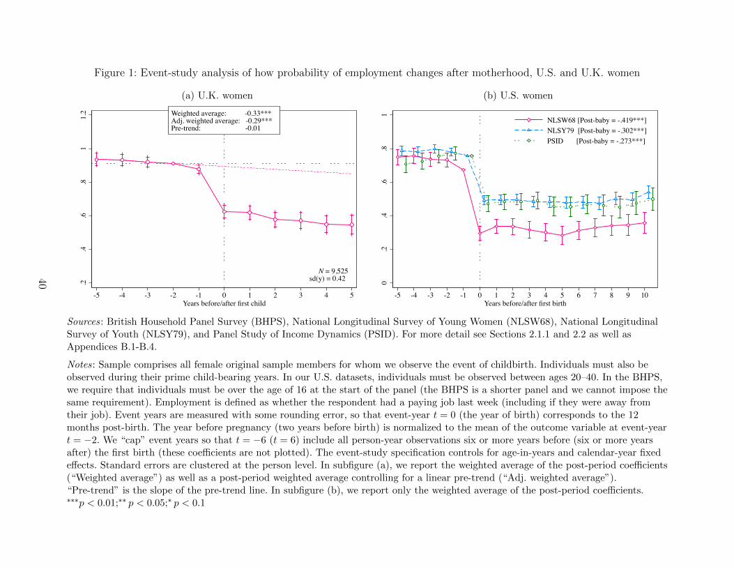
Figure 1: Event-study analysis of how probability of employment changes after motherhood, U.S. and U.K. women

(a) U.K. women

Weighted average: -0.33***Adj. weighted average: -0.29***Pre-trend: -0.01

.2.4

.6.8

11.

2

-5 -4 -3 -2 -1 0 1 2 3 4 5Years before/after first child

N = 9,525 sd(y) = 0.42

(b) U.S. women

0.2

.4.6

.81

-5 -4 -3 -2 -1 0 1 2 3 4 5 6 7 8 9 10Years before/after first birth

NLSW68 [Post-baby = -.419***]NLSY79 [Post-baby = -.302***]PSID [Post-baby = -.273***]

Sources: British Household Panel Survey (BHPS), National Longitudinal Survey of Young Women (NLSW68), National LongitudinalSurvey of Youth (NLSY79), and Panel Study of Income Dynamics (PSID). For more detail see Sections 2.1.1 and 2.2 as well asAppendices B.1-B.4.

Notes: Sample comprises all female original sample members for whom we observe the event of childbirth. Individuals must also beobserved during their prime child-bearing years. In our U.S. datasets, individuals must be observed between ages 20–40. In the BHPS,we require that individuals must be over the age of 16 at the start of the panel (the BHPS is a shorter panel and we cannot impose thesame requirement). Employment is defined as whether the respondent had a paying job last week (including if they were away fromtheir job). Event years are measured with some rounding error, so that event-year t = 0 (the year of birth) corresponds to the 12months post-birth. The year before pregnancy (two years before birth) is normalized to the mean of the outcome variable at event-yeart = −2. We “cap” event years so that t = −6 (t = 6) include all person-year observations six or more years before (six or more yearsafter) the first birth (these coefficients are not plotted). The event-study specification controls for age-in-years and calendar-year fixedeffects. Standard errors are clustered at the person level. In subfigure (a), we report the weighted average of the post-period coefficients(“Weighted average”) as well as a post-period weighted average controlling for a linear pre-trend (“Adj. weighted average”).“Pre-trend” is the slope of the pre-trend line. In subfigure (b), we report only the weighted average of the post-period coefficients.∗∗∗p < 0.01;∗∗ p < 0.05;∗ p < 0.1

40

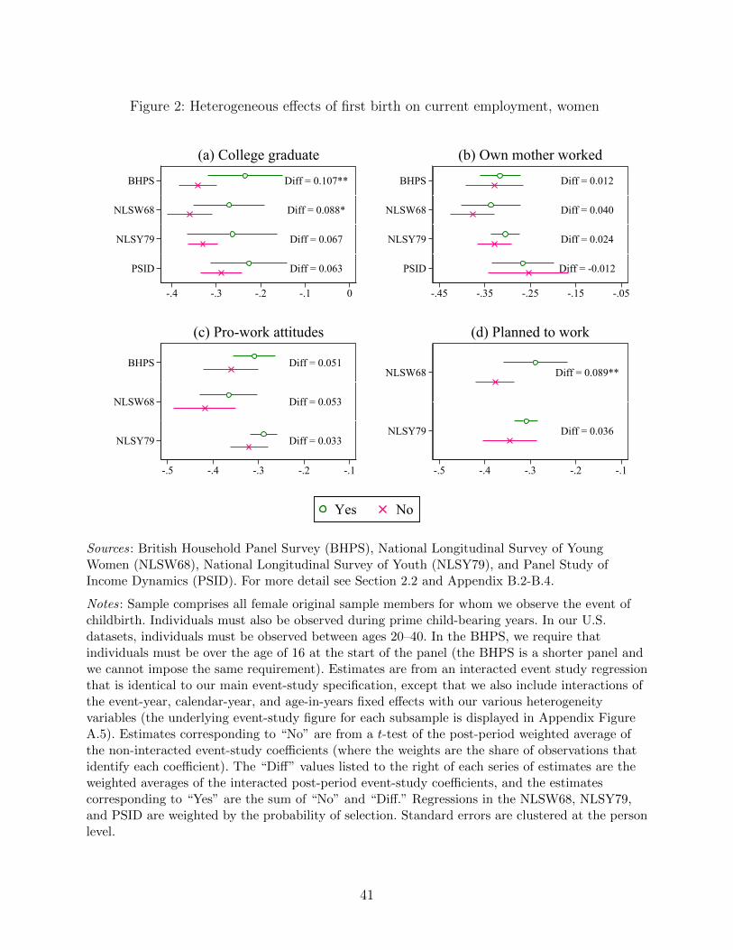
Figure 2: Heterogeneous effects of first birth on current employment, women

Diff = 0.107**

Diff = 0.088*

Diff = 0.067

Diff = 0.063

BHPS

NLSW68

NLSY79

PSID

-.4 -.3 -.2 -.1 0

(a) College graduateDiff = 0.012

Diff = 0.040

Diff = 0.024

Diff = -0.012

BHPS

NLSW68

NLSY79

PSID

-.45 -.35 -.25 -.15 -.05

(b) Own mother worked

Diff = 0.051

Diff = 0.053

Diff = 0.033

BHPS

NLSW68

NLSY79

-.5 -.4 -.3 -.2 -.1

(c) Pro-work attitudes

Diff = 0.089**

Diff = 0.036

NLSW68

NLSY79

-.5 -.4 -.3 -.2 -.1

(d) Planned to work

Yes No

Sources: British Household Panel Survey (BHPS), National Longitudinal Survey of YoungWomen (NLSW68), National Longitudinal Survey of Youth (NLSY79), and Panel Study ofIncome Dynamics (PSID). For more detail see Section 2.2 and Appendix B.2-B.4.

Notes: Sample comprises all female original sample members for whom we observe the event ofchildbirth. Individuals must also be observed during prime child-bearing years. In our U.S.datasets, individuals must be observed between ages 20–40. In the BHPS, we require thatindividuals must be over the age of 16 at the start of the panel (the BHPS is a shorter panel andwe cannot impose the same requirement). Estimates are from an interacted event study regressionthat is identical to our main event-study specification, except that we also include interactions ofthe event-year, calendar-year, and age-in-years fixed effects with our various heterogeneityvariables (the underlying event-study figure for each subsample is displayed in Appendix FigureA.5). Estimates corresponding to “No” are from a t-test of the post-period weighted average ofthe non-interacted event-study coefficients (where the weights are the share of observations thatidentify each coefficient). The “Diff” values listed to the right of each series of estimates are theweighted averages of the interacted post-period event-study coefficients, and the estimatescorresponding to “Yes” are the sum of “No” and “Diff.” Regressions in the NLSW68, NLSY79,and PSID are weighted by the probability of selection. Standard errors are clustered at the personlevel.

41

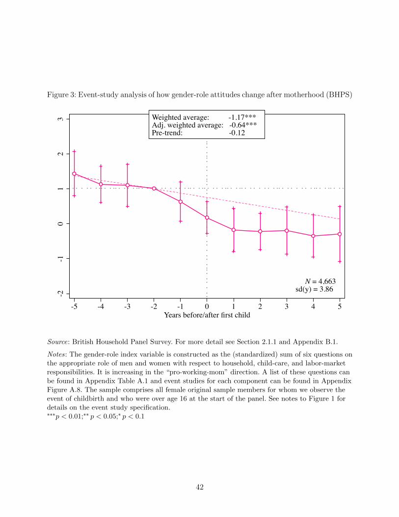
Figure 3: Event-study analysis of how gender-role attitudes change after motherhood (BHPS)

Weighted average: -1.17***Adj. weighted average: -0.64***Pre-trend: -0.12

-2-1

01

23

-5 -4 -3 -2 -1 0 1 2 3 4 5Years before/after first child

N = 4,663 sd(y) = 3.86

Source: British Household Panel Survey. For more detail see Section 2.1.1 and Appendix B.1.

Notes: The gender-role index variable is constructed as the (standardized) sum of six questions onthe appropriate role of men and women with respect to household, child-care, and labor-marketresponsibilities. It is increasing in the “pro-working-mom” direction. A list of these questions canbe found in Appendix Table A.1 and event studies for each component can be found in AppendixFigure A.8. The sample comprises all female original sample members for whom we observe theevent of childbirth and who were over age 16 at the start of the panel. See notes to Figure 1 fordetails on the event study specification.∗∗∗p < 0.01;∗∗ p < 0.05;∗ p < 0.1

42

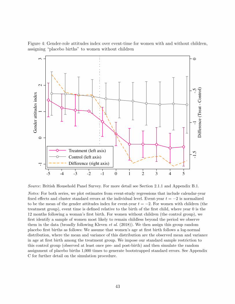
Figure 4: Gender-role attitudes index over event-time for women with and without children,assigning “placebo births” to women without children

-1.5

-1-.5

0D

iffer

ence

(Tre

at -

Con

trol)

-10

12

3G

ende

r atti

tude

s ind

ex

-5 -4 -3 -2 -1 0 1 2 3 4 5

Treatment (left axis)Control (left axis)Difference (right axis)

Source: British Household Panel Survey. For more detail see Section 2.1.1 and Appendix B.1.

Notes: For both series, we plot estimates from event-study regressions that include calendar-yearfixed effects and cluster standard errors at the individual level. Event-year t = −2 is normalizedto be the mean of the gender attitudes index for event-year t = −2. For women with children (thetreatment group), event time is defined relative to the birth of the first child, where year 0 is the12 months following a woman’s first birth. For women without children (the control group), wefirst identify a sample of women most likely to remain childless beyond the period we observethem in the data (broadly following Kleven et al. (2018)). We then assign this group randomplacebo first births as follows: We assume that women’s age at first birth follows a log-normaldistribution, where the mean and variance of this distribution are the observed mean and variancein age at first birth among the treatment group. We impose our standard sample restriction tothis control group (observed at least once pre- and post-birth) and then simulate the randomassignment of placebo births 1,000 times to generate bootstrapped standard errors. See AppendixC for further detail on the simulation procedure.

43

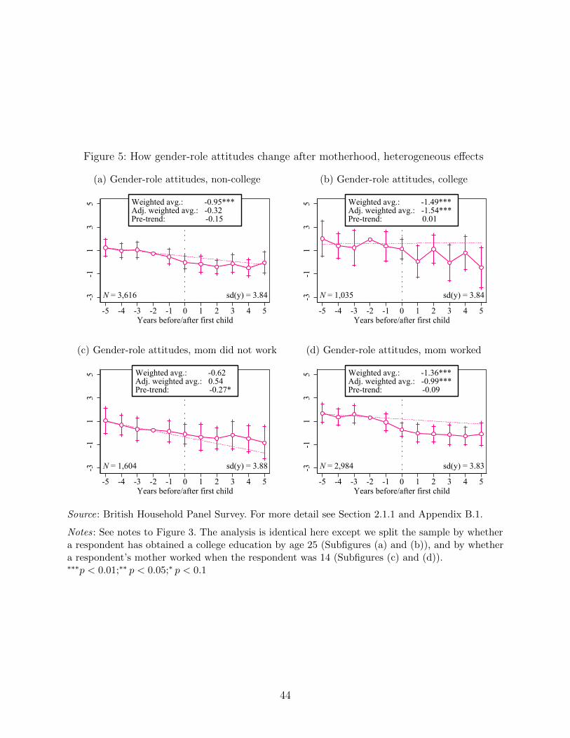
Figure 5: How gender-role attitudes change after motherhood, heterogeneous effects

(a) Gender-role attitudes, non-college

Weighted avg.: -0.95***Adj. weighted avg.: -0.32Pre-trend: -0.15

N = 3,616 sd(y) = 3.84-3-1

13

5

-5 -4 -3 -2 -1 0 1 2 3 4 5Years before/after first child

(b) Gender-role attitudes, college

Weighted avg.: -1.49***Adj. weighted avg.: -1.54***Pre-trend: 0.01

N = 1,035 sd(y) = 3.84-3-1

13

5-5 -4 -3 -2 -1 0 1 2 3 4 5

Years before/after first child

(c) Gender-role attitudes, mom did not work

Weighted avg.: -0.62Adj. weighted avg.: 0.54Pre-trend: -0.27*

N = 1,604 sd(y) = 3.88-3-1

13

5

-5 -4 -3 -2 -1 0 1 2 3 4 5Years before/after first child

(d) Gender-role attitudes, mom worked

Weighted avg.: -1.36***Adj. weighted avg.: -0.99***Pre-trend: -0.09

N = 2,984 sd(y) = 3.83-3-1

13

5

-5 -4 -3 -2 -1 0 1 2 3 4 5Years before/after first child

Source: British Household Panel Survey. For more detail see Section 2.1.1 and Appendix B.1.

Notes: See notes to Figure 3. The analysis is identical here except we split the sample by whethera respondent has obtained a college education by age 25 (Subfigures (a) and (b)), and by whethera respondent’s mother worked when the respondent was 14 (Subfigures (c) and (d)).∗∗∗p < 0.01;∗∗ p < 0.05;∗ p < 0.1

44

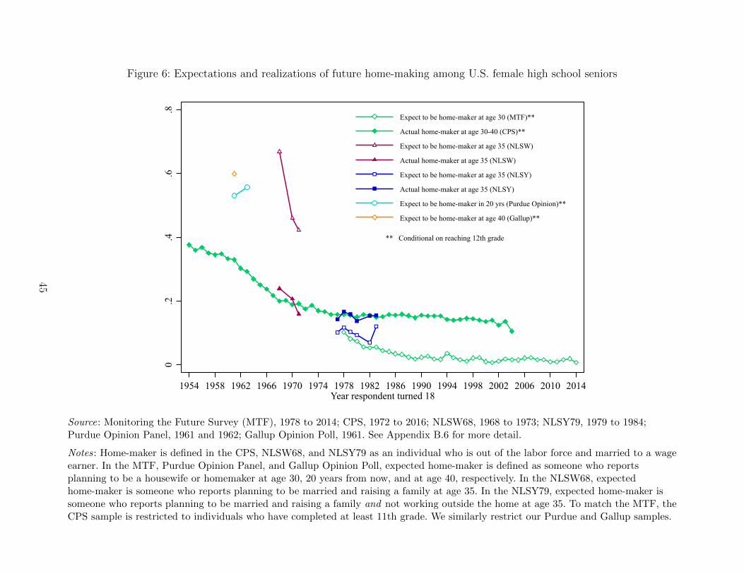
Figure 6: Expectations and realizations of future home-making among U.S. female high school seniors

** Conditional on reaching 12th grade

0.2

.4.6

.8

1954 1958 1962 1966 1970 1974 1978 1982 1986 1990 1994 1998 2002 2006 2010 2014Year respondent turned 18

Expect to be home-maker at age 30 (MTF)**

Actual home-maker at age 30-40 (CPS)**

Expect to be home-maker at age 35 (NLSW)

Actual home-maker at age 35 (NLSW)

Expect to be home-maker at age 35 (NLSY)

Actual home-maker at age 35 (NLSY)

Expect to be home-maker in 20 yrs (Purdue Opinion)**

Expect to be home-maker at age 40 (Gallup)**

Source: Monitoring the Future Survey (MTF), 1978 to 2014; CPS, 1972 to 2016; NLSW68, 1968 to 1973; NLSY79, 1979 to 1984;Purdue Opinion Panel, 1961 and 1962; Gallup Opinion Poll, 1961. See Appendix B.6 for more detail.

Notes: Home-maker is defined in the CPS, NLSW68, and NLSY79 as an individual who is out of the labor force and married to a wageearner. In the MTF, Purdue Opinion Panel, and Gallup Opinion Poll, expected home-maker is defined as someone who reportsplanning to be a housewife or homemaker at age 30, 20 years from now, and at age 40, respectively. In the NLSW68, expectedhome-maker is someone who reports planning to be married and raising a family at age 35. In the NLSY79, expected home-maker issomeone who reports planning to be married and raising a family and not working outside the home at age 35. To match the MTF, theCPS sample is restricted to individuals who have completed at least 11th grade. We similarly restrict our Purdue and Gallup samples.

45

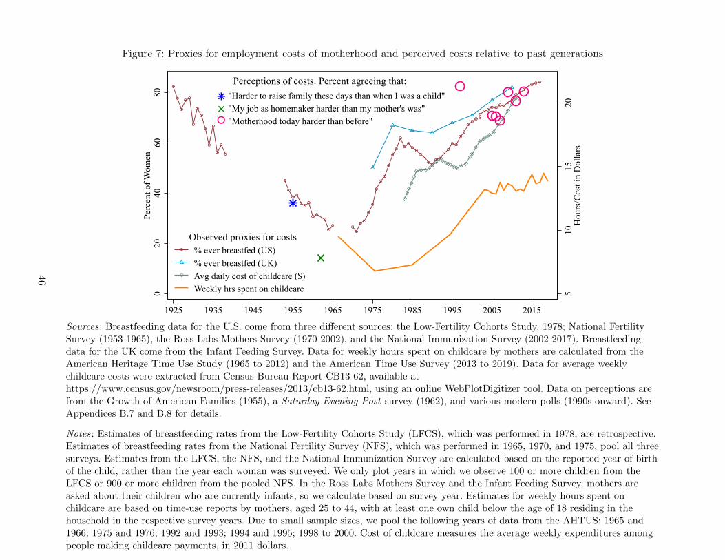
Figure 7: Proxies for employment costs of motherhood and perceived costs relative to past generations

×+×°

Perceptions of costs. Percent agreeing that: "Harder to raise family these days than when I was a child" "My job as homemaker harder than my mother's was" "Motherhood today harder than before"

020

4060

80Pe

rcen

t of W

omen

510

1520

Hou

rs/C

ost i

n D

olla

rs

1925 1935 1945 1955 1965 1975 1985 1995 2005 2015

% ever breastfed (US)% ever breastfed (UK)Avg daily cost of childcare ($)Weekly hrs spent on childcare

Observed proxies for costs

Sources: Breastfeeding data for the U.S. come from three different sources: the Low-Fertility Cohorts Study, 1978; National FertilitySurvey (1953-1965), the Ross Labs Mothers Survey (1970-2002), and the National Immunization Survey (2002-2017). Breastfeedingdata for the UK come from the Infant Feeding Survey. Data for weekly hours spent on childcare by mothers are calculated from theAmerican Heritage Time Use Study (1965 to 2012) and the American Time Use Survey (2013 to 2019). Data for average weeklychildcare costs were extracted from Census Bureau Report CB13-62, available athttps://www.census.gov/newsroom/press-releases/2013/cb13-62.html, using an online WebPlotDigitizer tool. Data on perceptions arefrom the Growth of American Families (1955), a Saturday Evening Post survey (1962), and various modern polls (1990s onward). SeeAppendices B.7 and B.8 for details.

Notes: Estimates of breastfeeding rates from the Low-Fertility Cohorts Study (LFCS), which was performed in 1978, are retrospective.Estimates of breastfeeding rates from the National Fertility Survey (NFS), which was performed in 1965, 1970, and 1975, pool all threesurveys. Estimates from the LFCS, the NFS, and the National Immunization Survey are calculated based on the reported year of birthof the child, rather than the year each woman was surveyed. We only plot years in which we observe 100 or more children from theLFCS or 900 or more children from the pooled NFS. In the Ross Labs Mothers Survey and the Infant Feeding Survey, mothers areasked about their children who are currently infants, so we calculate based on survey year. Estimates for weekly hours spent onchildcare are based on time-use reports by mothers, aged 25 to 44, with at least one own child below the age of 18 residing in thehousehold in the respective survey years. Due to small sample sizes, we pool the following years of data from the AHTUS: 1965 and1966; 1975 and 1976; 1992 and 1993; 1994 and 1995; 1998 to 2000. Cost of childcare measures the average weekly expenditures amongpeople making childcare payments, in 2011 dollars.

46

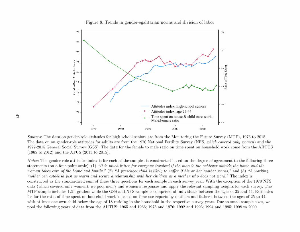
Figure 8: Trends in gender-egalitarian norms and division of labor

01

23

45

Rat

io o

f Tim

e Sp

ent

-1-.8

-.6-.4

-.20

.2.4

.6.8

Gen

der-

Rol

e A

ttitu

des

Inde

x

1970 1980 1990 2000 2010

Attitudes index, high-school seniorsAttitudes index, age 25-44Time spent on house & child-care-work,Male:Female ratio

Sources: The data on gender-role attitudes for high school seniors are from the Monitoring the Future Survey (MTF), 1976 to 2015.The data on on gender-role attitudes for adults are from the 1970 National Fertility Survey (NFS, which covered only women) and the1977-2015 General Social Survey (GSS). The data for the female to male ratio on time spent on household work come from the AHTUS(1965 to 2012) and the ATUS (2013 to 2015).

Notes: The gender-role attitudes index is for each of the samples is constructed based on the degree of agreement to the following threestatements (on a four-point scale): (1) “It is much better for everyone involved if the man is the achiever outside the home and thewoman takes care of the home and family,” (2) “A preschool child is likely to suffer if his or her mother works,” and (3) “A workingmother can establish just as warm and secure a relationship with her children as a mother who does not work.” The index isconstructed as the standardized sum of these three questions for each sample in each survey year. With the exception of the 1970 NFSdata (which covered only women), we pool men’s and women’s responses and apply the relevant sampling weights for each survey. TheMTF sample includes 12th graders while the GSS and NFS sample is comprised of individuals between the ages of 25 and 44. Estimatesfor for the ratio of time spent on household work is based on time-use reports by mothers and fathers, between the ages of 25 to 44,with at least one own child below the age of 18 residing in the household in the respective survey years. Due to small sample sizes, wepool the following years of data from the AHTUS: 1965 and 1966; 1975 and 1976; 1992 and 1993; 1994 and 1995; 1998 to 2000.

47

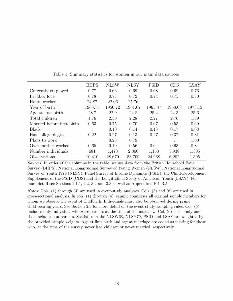
Table 1: Summary statistics for women in our main data sources

BHPS NLSW NLSY PSID CDS LSAYCurrently employed 0.77 0.63 0.69 0.68 0.69 0.76In labor foce 0.78 0.73 0.72 0.74 0.75 0.80Hours worked 24.87 22.06 25.76 . . .Year of birth 1968.75 1950.72 1961.67 1965.87 1968.08 1973.15Age at first birth 28.7 22.9 24.8 25.4 24.3 25.6Total children 1.76 2.30 2.28 2.27 2.76 1.49Married before first birth 0.63 0.75 0.70 0.67 0.55 0.69Black . 0.10 0.14 0.13 0.17 0.08Has college degree 0.22 0.27 0.13 0.27 0.37 0.31Plans to work . 0.25 0.79 . . 1.00Own mother worked 0.65 0.40 0.56 0.64 0.63 0.84Number individuals 681 1,478 2,360 1,153 3,938 1,305Observations 10,410 28,679 58,700 24,968 6,202 1,305

Sources: In order of the columns in the table, we use data from the British Household PanelSurvey (BHPS), National Longitudinal Survey of Young Women (NLSW), National LongitudinalSurvey of Youth 1979 (NLSY), Panel Survey of Income Dynamics (PSID), the Child-DevelopmentSupplement of the PSID (CDS) and the Longitudinal Study of American Youth (LSAY). Formore detail see Sections 2.1.1, 2.2, 3.2 and 3.3 as well as Appendices B.1-B.5.

Notes: Cols. (1) through (4) are used in event-study analyses. Cols. (5) and (6) are used incross-sectional analysis. In cols. (1) through (4), sample comprises all original sample members forwhom we observe the event of childbirth. Individuals must also be observed during primechild-bearing years. See Section 2.3 for more detail on the event-study sampling rules. Col. (5)includes only individual who were parents at the time of the interview. Col. (6) is the only onethat includes non-parents. Statistics in the NLSW68, NLSY79, PSID and LSAY are weighted bythe provided sample weights. Age at first birth and age at marriage are coded as missing for thosewho, at the time of the survey, never had children or never married, respectively.

48

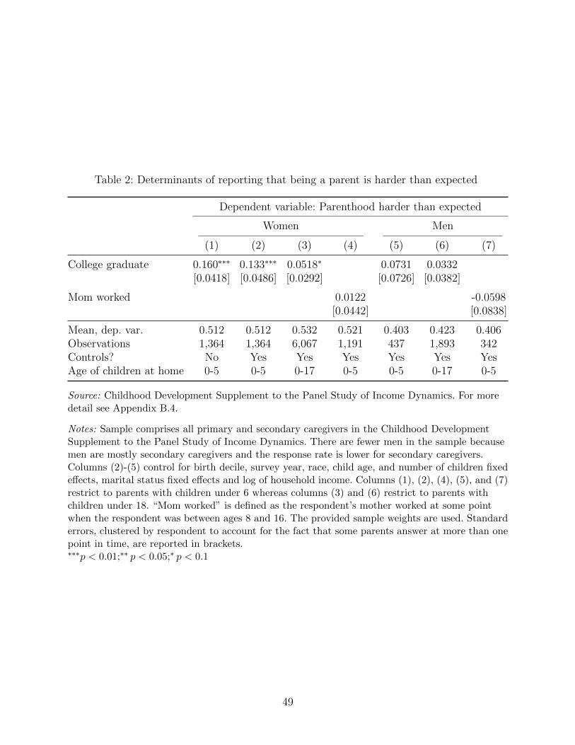
Table 2: Determinants of reporting that being a parent is harder than expected

Dependent variable: Parenthood harder than expected

Women Men

(1) (2) (3) (4) (5) (6) (7)

College graduate 0.160∗∗∗ 0.133∗∗∗ 0.0518∗ 0.0731 0.0332[0.0418] [0.0486] [0.0292] [0.0726] [0.0382]

Mom worked 0.0122 -0.0598[0.0442] [0.0838]

Mean, dep. var. 0.512 0.512 0.532 0.521 0.403 0.423 0.406Observations 1,364 1,364 6,067 1,191 437 1,893 342Controls? No Yes Yes Yes Yes Yes YesAge of children at home 0-5 0-5 0-17 0-5 0-5 0-17 0-5

Source: Childhood Development Supplement to the Panel Study of Income Dynamics. For moredetail see Appendix B.4.

Notes: Sample comprises all primary and secondary caregivers in the Childhood DevelopmentSupplement to the Panel Study of Income Dynamics. There are fewer men in the sample becausemen are mostly secondary caregivers and the response rate is lower for secondary caregivers.Columns (2)-(5) control for birth decile, survey year, race, child age, and number of children fixedeffects, marital status fixed effects and log of household income. Columns (1), (2), (4), (5), and (7)restrict to parents with children under 6 whereas columns (3) and (6) restrict to parents withchildren under 18. “Mom worked” is defined as the respondent’s mother worked at some pointwhen the respondent was between ages 8 and 16. The provided sample weights are used. Standarderrors, clustered by respondent to account for the fact that some parents answer at more than onepoint in time, are reported in brackets.∗∗∗p < 0.01;∗∗ p < 0.05;∗ p < 0.1

49

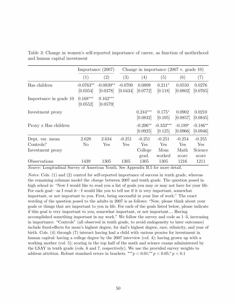
Table 3: Change in women’s self-reported importance of career, as function of motherhoodand human capital investment

Importance (2007) Change in importance (2007 v. grade 10)

(1) (2) (3) (4) (5) (6) (7)

Has children -0.0763∗∗ -0.0839∗∗ -0.0700 0.0809 0.211∗ 0.0550 0.0276[0.0354] [0.0378] [0.0434] [0.0772] [0.118] [0.0802] [0.0765]

Importance in grade 10 0.168∗∗∗ 0.162∗∗∗

[0.0552] [0.0579]

Investment proxy 0.244∗∗∗ 0.175∗ 0.0902 0.0210[0.0832] [0.105] [0.0857] [0.0845]

Proxy x Has children -0.206∗∗ -0.333∗∗∗ -0.189∗ -0.186∗∗

[0.0925] [0.125] [0.0966] [0.0946]

Dept. var. mean 2.628 2.634 -0.251 -0.251 -0.251 -0.254 -0.255Controls? No Yes Yes Yes Yes Yes YesInvestment proxy College Mom Math Science

grad. worked score scoreObservations 1439 1305 1305 1305 1305 1216 1211

Source: Longitudinal Survey of American Youth. See Appendix B.5 for more detail.

Notes: Cols. (1) and (2) control for self-reported importance of success in tenth grade, whereasthe remaining columns model the change between 2007 and tenth grade. The question posed inhigh school is: “Now I would like to read you a list of goals you may or may not have for your life.For each goal—as I read it—I would like you to tell me if it is very important, somewhatimportant, or not important to you. First, being successful in your line of work.” The exactwording of the question posed to the adults in 2007 is as follows: “Now, please think about yourgoals or things that are important to you in life. For each of the goals listed below, please indicateif this goal is very important to you, somewhat important, or not important.... Havingaccomplished something important in my work.” We follow the survey and code as 1–3, increasingin importance. “Controls” (all observed in tenth grade, to avoid endogeneity to later outcomes)include fixed-effects for mom’s highest degree, for dad’s highest degree, race, ethnicity, and year ofbirth. Cols. (4) through (7) interact having had a child with various proxies for investment inhuman capital: having a college degree by the 2007 interview (col. 4); having grown up with aworking mother (col. 5); scoring in the top half of the math and science exams administered bythe LSAY in tenth grade (cols. 6 and 7, respectively). We use the provided survey weights toaddress attrition. Robust standard errors in brackets. ∗∗∗p < 0.01;∗∗ p < 0.05;∗ p < 0.1

50

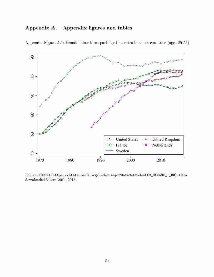
Appendix A. Appendix figures and tables

Appendix Figure A.1: Female labor force participation rates in select countries (ages 25-54)

4050

6070

8090

1970 1980 1990 2000 2010

United States United KingdomFrance NetherlandsSweden

Source: OECD (https://stats.oecd.org/Index.aspx?DataSetCode=LFS_SEXAGE_I_R#). Datadownloaded March 20th, 2018.

51

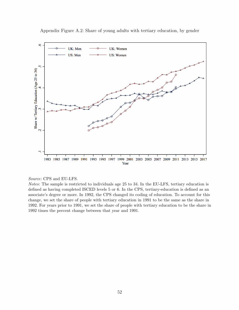
Appendix Figure A.2: Share of young adults with tertiary education, by gender

Source: CPS and EU-LFS.Notes: The sample is restricted to individuals age 25 to 34. In the EU-LFS, tertiary education isdefined as having completed ISCED levels 5 or 6. In the CPS, tertiary-education is defined as anassociate’s degree or more. In 1992, the CPS changed its coding of education. To account for thischange, we set the share of people with tertiary education in 1991 to be the same as the share in1992. For years prior to 1991, we set the share of people with tertiary education to be the share in1992 times the percent change between that year and 1991.

52

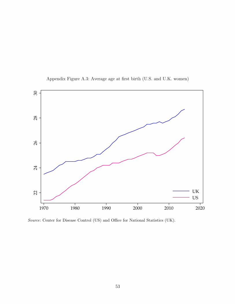
Appendix Figure A.3: Average age at first birth (U.S. and U.K. women)

2224

2628

30

1970 1980 1990 2000 2010 2020

UKUS

Source: Center for Disease Control (US) and Office for National Statistics (UK).

53

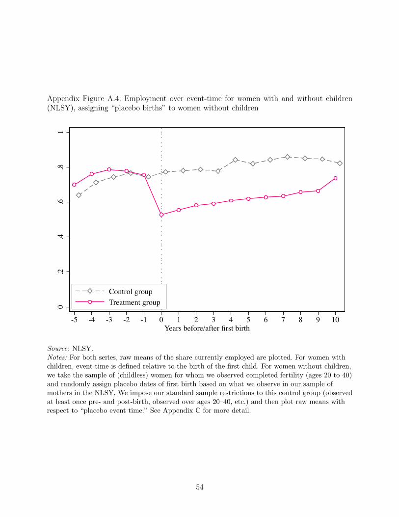
Appendix Figure A.4: Employment over event-time for women with and without children(NLSY), assigning “placebo births” to women without children

0.2

.4.6

.81

-5 -4 -3 -2 -1 0 1 2 3 4 5 6 7 8 9 10Years before/after first birth

Control groupTreatment group

Source: NLSY.Notes: For both series, raw means of the share currently employed are plotted. For women withchildren, event-time is defined relative to the birth of the first child. For women without children,we take the sample of (childless) women for whom we observed completed fertility (ages 20 to 40)and randomly assign placebo dates of first birth based on what we observe in our sample ofmothers in the NLSY. We impose our standard sample restrictions to this control group (observedat least once pre- and post-birth, observed over ages 20–40, etc.) and then plot raw means withrespect to “placebo event time.” See Appendix C for more detail.

54

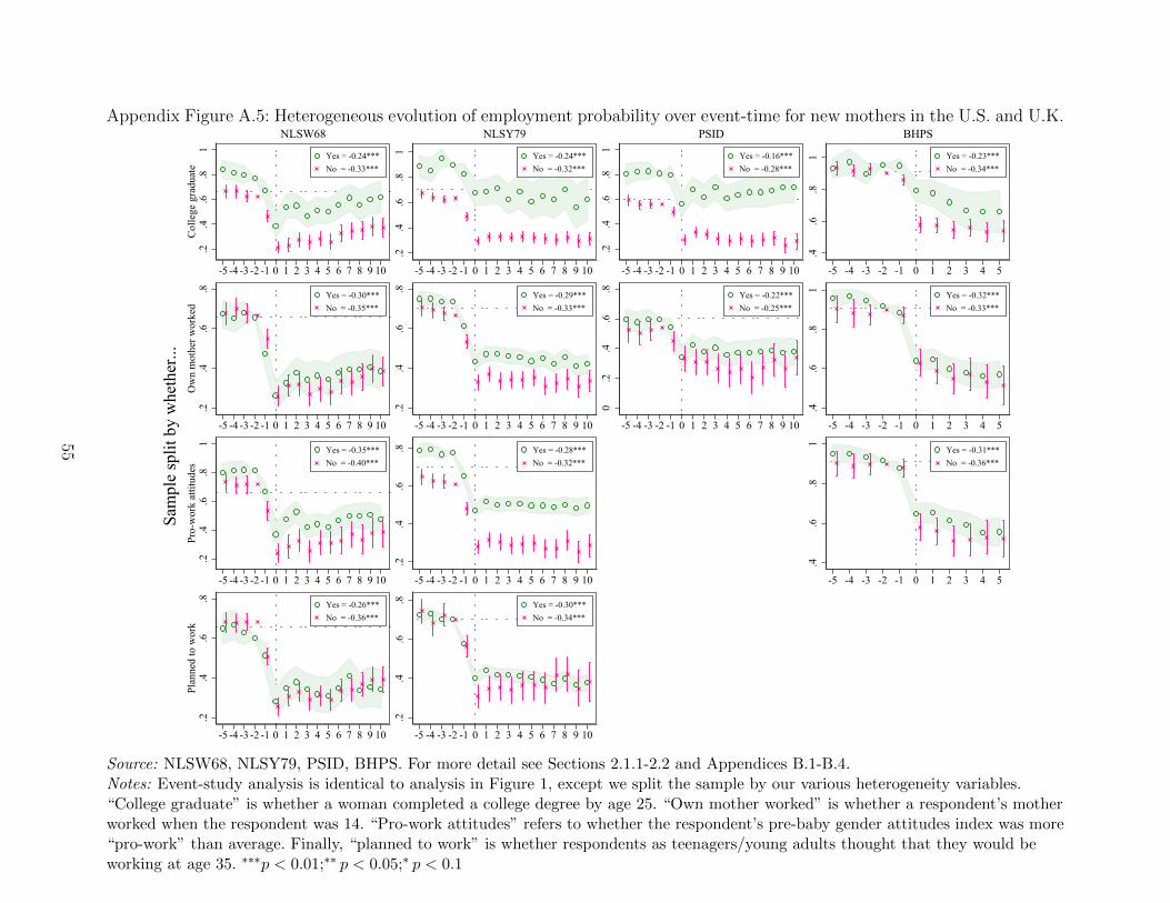
Appendix Figure A.5: Heterogeneous evolution of employment probability over event-time for new mothers in the U.S. and U.K.

.2.4

.6.8

1C

olle

ge g

radu

ate

-5 -4 -3 -2 -1 0 1 2 3 4 5 6 7 8 9 10

Yes = -0.24***No = -0.33***

NLSW68

.2.4

.6.8

Ow

n m

othe

r wor

ked

-5 -4 -3 -2 -1 0 1 2 3 4 5 6 7 8 9 10

Yes = -0.30***No = -0.35***

.2.4

.6.8

1Pr

o-w

ork

attit

udes

-5 -4 -3 -2 -1 0 1 2 3 4 5 6 7 8 9 10

Yes = -0.35***No = -0.40***

.2.4

.6.8

Plan

ned

to w

ork

-5 -4 -3 -2 -1 0 1 2 3 4 5 6 7 8 9 10

Yes = -0.26***No = -0.36***

.2.4

.6.8

1

-5 -4 -3 -2 -1 0 1 2 3 4 5 6 7 8 9 10

Yes = -0.24***No = -0.32***

NLSY79

.2.4

.6.8

-5 -4 -3 -2 -1 0 1 2 3 4 5 6 7 8 9 10

Yes = -0.29***No = -0.33***

.2.4

.6.8

-5 -4 -3 -2 -1 0 1 2 3 4 5 6 7 8 9 10

Yes = -0.28***No = -0.32***

.2.4

.6.8

-5 -4 -3 -2 -1 0 1 2 3 4 5 6 7 8 9 10

Yes = -0.30***No = -0.34***

.2.4

.6.8

1

-5 -4 -3 -2 -1 0 1 2 3 4 5 6 7 8 9 10

Yes = -0.16***No = -0.28***

PSID

0.2

.4.6

.8

-5 -4 -3 -2 -1 0 1 2 3 4 5 6 7 8 9 10

Yes = -0.22***No = -0.25***

.4.6

.81

-5 -4 -3 -2 -1 0 1 2 3 4 5

Yes = -0.23***No = -0.34***

BHPS

.4.6

.81

-5 -4 -3 -2 -1 0 1 2 3 4 5

Yes = -0.32***No = -0.33***

.4.6

.81

-5 -4 -3 -2 -1 0 1 2 3 4 5

Yes = -0.31***No = -0.36***

Sam

ple

split

by

whe

ther

...

Source: NLSW68, NLSY79, PSID, BHPS. For more detail see Sections 2.1.1-2.2 and Appendices B.1-B.4.Notes: Event-study analysis is identical to analysis in Figure 1, except we split the sample by our various heterogeneity variables.“College graduate” is whether a woman completed a college degree by age 25. “Own mother worked” is whether a respondent’s motherworked when the respondent was 14. “Pro-work attitudes” refers to whether the respondent’s pre-baby gender attitudes index was more“pro-work” than average. Finally, “planned to work” is whether respondents as teenagers/young adults thought that they would beworking at age 35. ∗∗∗p < 0.01;∗∗ p < 0.05;∗ p < 0.1

55

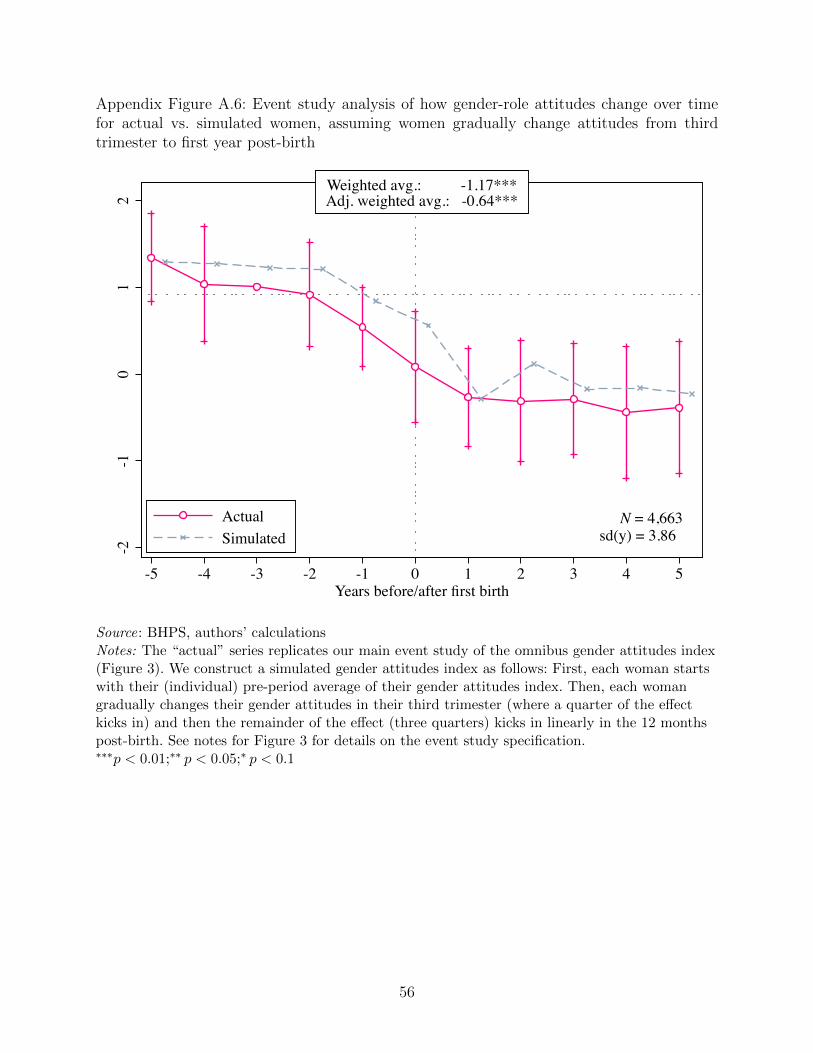
Appendix Figure A.6: Event study analysis of how gender-role attitudes change over timefor actual vs. simulated women, assuming women gradually change attitudes from thirdtrimester to first year post-birth

Weighted avg.: -1.17***Adj. weighted avg.: -0.64***

N = 4,663sd(y) = 3.86

-2-1

01

2

-5 -4 -3 -2 -1 0 1 2 3 4 5Years before/after first birth

ActualSimulated

Source: BHPS, authors’ calculationsNotes: The “actual” series replicates our main event study of the omnibus gender attitudes index(Figure 3). We construct a simulated gender attitudes index as follows: First, each woman startswith their (individual) pre-period average of their gender attitudes index. Then, each womangradually changes their gender attitudes in their third trimester (where a quarter of the effectkicks in) and then the remainder of the effect (three quarters) kicks in linearly in the 12 monthspost-birth. See notes for Figure 3 for details on the event study specification.∗∗∗p < 0.01;∗∗ p < 0.05;∗ p < 0.1

56

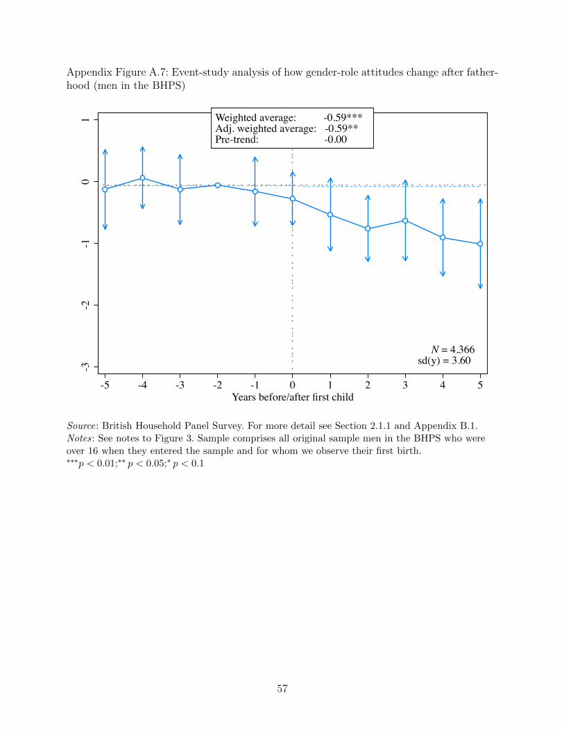
Appendix Figure A.7: Event-study analysis of how gender-role attitudes change after father-hood (men in the BHPS)

Weighted average: -0.59***Adj. weighted average: -0.59**Pre-trend: -0.00

-3-2

-10

1

-5 -4 -3 -2 -1 0 1 2 3 4 5Years before/after first child

N = 4,366 sd(y) = 3.60

Source: British Household Panel Survey. For more detail see Section 2.1.1 and Appendix B.1.Notes: See notes to Figure 3. Sample comprises all original sample men in the BHPS who wereover 16 when they entered the sample and for whom we observe their first birth.∗∗∗p < 0.01;∗∗ p < 0.05;∗ p < 0.1

57

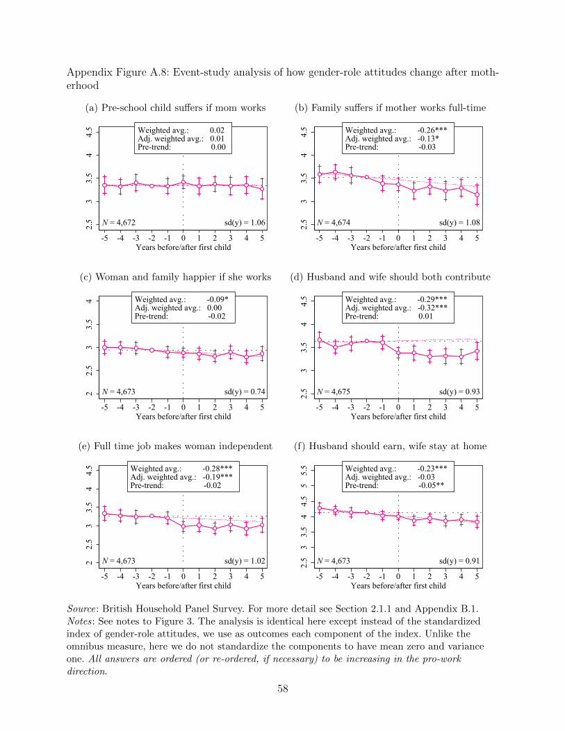
Appendix Figure A.8: Event-study analysis of how gender-role attitudes change after moth-erhood

(a) Pre-school child suffers if mom works

Weighted avg.: 0.02Adj. weighted avg.: 0.01Pre-trend: 0.00

N = 4,672 sd(y) = 1.062.5

33.

54

4.5

-5 -4 -3 -2 -1 0 1 2 3 4 5Years before/after first child

(b) Family suffers if mother works full-time

Weighted avg.: -0.26***Adj. weighted avg.: -0.13*Pre-trend: -0.03

N = 4,674 sd(y) = 1.082.5

33.

54

4.5

-5 -4 -3 -2 -1 0 1 2 3 4 5Years before/after first child

(c) Woman and family happier if she works

Weighted avg.: -0.09*Adj. weighted avg.: 0.00Pre-trend: -0.02

N = 4,673 sd(y) = 0.7422.

53

3.5

4

-5 -4 -3 -2 -1 0 1 2 3 4 5Years before/after first child

(d) Husband and wife should both contribute

Weighted avg.: -0.29***Adj. weighted avg.: -0.32***Pre-trend: 0.01

N = 4,675 sd(y) = 0.932.5

33.

54

4.5

-5 -4 -3 -2 -1 0 1 2 3 4 5Years before/after first child

(e) Full time job makes woman independent

Weighted avg.: -0.28***Adj. weighted avg.: -0.19***Pre-trend: -0.02

N = 4,673 sd(y) = 1.0222.

53

3.5

44.

5

-5 -4 -3 -2 -1 0 1 2 3 4 5Years before/after first child

(f) Husband should earn, wife stay at home

Weighted avg.: -0.23***Adj. weighted avg.: -0.03Pre-trend: -0.05**

N = 4,673 sd(y) = 0.912.5

33.

54

4.5

55.

5

-5 -4 -3 -2 -1 0 1 2 3 4 5Years before/after first child

Source: British Household Panel Survey. For more detail see Section 2.1.1 and Appendix B.1.Notes: See notes to Figure 3. The analysis is identical here except instead of the standardizedindex of gender-role attitudes, we use as outcomes each component of the index. Unlike theomnibus measure, here we do not standardize the components to have mean zero and varianceone. All answers are ordered (or re-ordered, if necessary) to be increasing in the pro-workdirection.

58

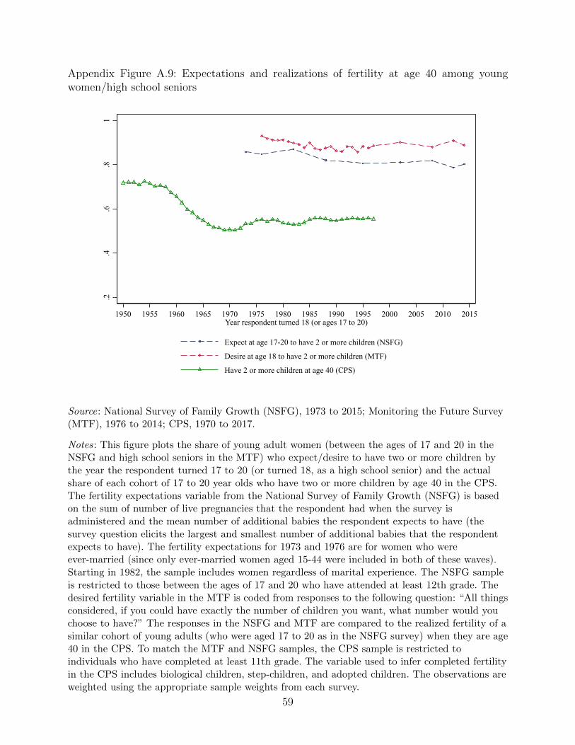
Appendix Figure A.9: Expectations and realizations of fertility at age 40 among youngwomen/high school seniors

.2.4

.6.8

1

1950 1955 1960 1965 1970 1975 1980 1985 1990 1995 2000 2005 2010 2015Year respondent turned 18 (or ages 17 to 20)

Expect at age 17-20 to have 2 or more children (NSFG)

Desire at age 18 to have 2 or more children (MTF)

Have 2 or more children at age 40 (CPS)

Source: National Survey of Family Growth (NSFG), 1973 to 2015; Monitoring the Future Survey(MTF), 1976 to 2014; CPS, 1970 to 2017.

Notes: This figure plots the share of young adult women (between the ages of 17 and 20 in theNSFG and high school seniors in the MTF) who expect/desire to have two or more children bythe year the respondent turned 17 to 20 (or turned 18, as a high school senior) and the actualshare of each cohort of 17 to 20 year olds who have two or more children by age 40 in the CPS.The fertility expectations variable from the National Survey of Family Growth (NSFG) is basedon the sum of number of live pregnancies that the respondent had when the survey isadministered and the mean number of additional babies the respondent expects to have (thesurvey question elicits the largest and smallest number of additional babies that the respondentexpects to have). The fertility expectations for 1973 and 1976 are for women who wereever-married (since only ever-married women aged 15-44 were included in both of these waves).Starting in 1982, the sample includes women regardless of marital experience. The NSFG sampleis restricted to those between the ages of 17 and 20 who have attended at least 12th grade. Thedesired fertility variable in the MTF is coded from responses to the following question: “All thingsconsidered, if you could have exactly the number of children you want, what number would youchoose to have?” The responses in the NSFG and MTF are compared to the realized fertility of asimilar cohort of young adults (who were aged 17 to 20 as in the NSFG survey) when they are age40 in the CPS. To match the MTF and NSFG samples, the CPS sample is restricted toindividuals who have completed at least 11th grade. The variable used to infer completed fertilityin the CPS includes biological children, step-children, and adopted children. The observations areweighted using the appropriate sample weights from each survey.

59

Appendix Figure A.10: Evolution of various measures of breastfeeding prevalence

Source: Data sources for the US: Ross Labs Mothers Survey (RLMS), the National ImmunizationSurvey (NIS), and the National Fertility Survey (NFS). Data source for the UK: Infant FeedingSurvey (IFS).

Notes: Estimates of breastfeeding rates from the National Fertility Survey, which was performedin 1965, 1970, and 1975, pool all three surveys. Estimates from both the NFS and the NIS arecalculated based on the reported year of birth of the child. For the NFS, we only plot years inwhich estimates come from 900 or more observations. In the RLMS and IFS, mothers are askedabout their children who are currently infants. In these surveys, the survey year, rather than theyear of birth of the child, is used.

60

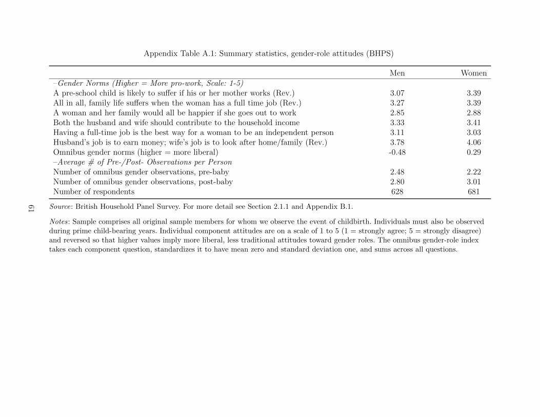
Appendix Table A.1: Summary statistics, gender-role attitudes (BHPS)

Men Women–Gender Norms (Higher = More pro-work, Scale: 1-5)A pre-school child is likely to suffer if his or her mother works (Rev.) 3.07 3.39All in all, family life suffers when the woman has a full time job (Rev.) 3.27 3.39A woman and her family would all be happier if she goes out to work 2.85 2.88Both the husband and wife should contribute to the household income 3.33 3.41Having a full-time job is the best way for a woman to be an independent person 3.11 3.03Husband’s job is to earn money; wife’s job is to look after home/family (Rev.) 3.78 4.06Omnibus gender norms (higher = more liberal) -0.48 0.29–Average # of Pre-/Post- Observations per PersonNumber of omnibus gender observations, pre-baby 2.48 2.22Number of omnibus gender observations, post-baby 2.80 3.01Number of respondents 628 681

Source: British Household Panel Survey. For more detail see Section 2.1.1 and Appendix B.1.

Notes: Sample comprises all original sample members for whom we observe the event of childbirth. Individuals must also be observedduring prime child-bearing years. Individual component attitudes are on a scale of 1 to 5 (1 = strongly agree; 5 = strongly disagree)and reversed so that higher values imply more liberal, less traditional attitudes toward gender roles. The omnibus gender-role indextakes each component question, standardizes it to have mean zero and standard deviation one, and sums across all questions.

61

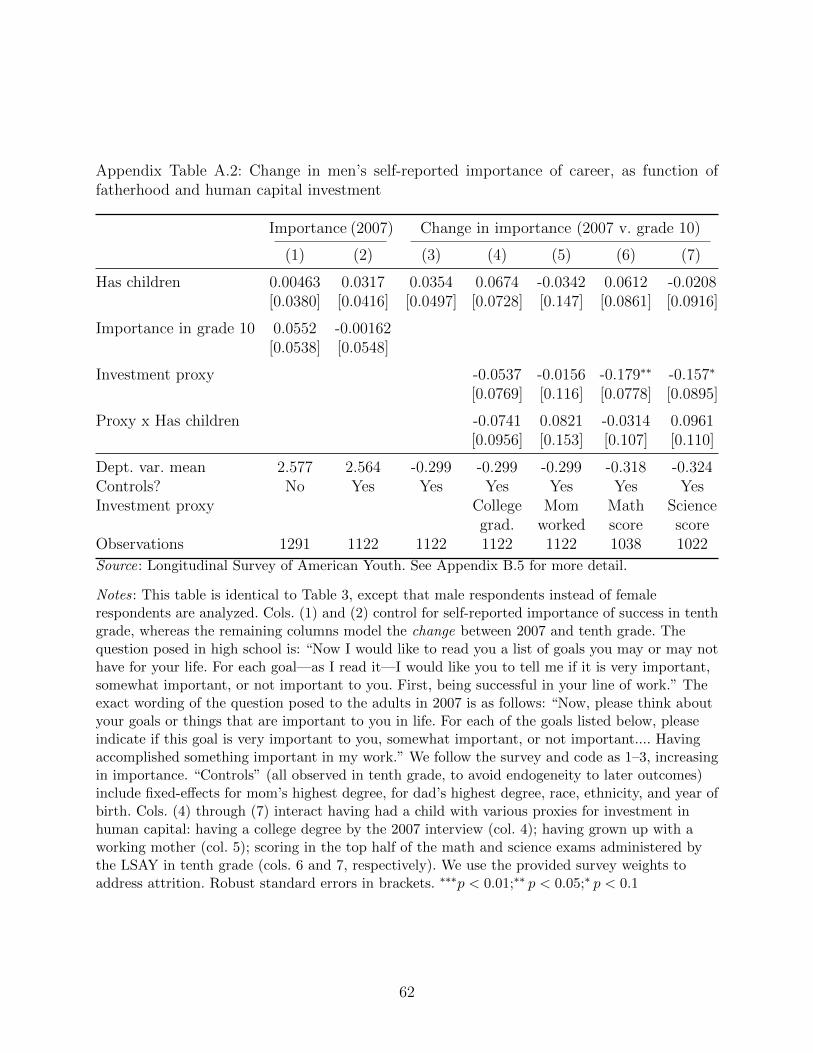
Appendix Table A.2: Change in men’s self-reported importance of career, as function offatherhood and human capital investment

Importance (2007) Change in importance (2007 v. grade 10)

(1) (2) (3) (4) (5) (6) (7)

Has children 0.00463 0.0317 0.0354 0.0674 -0.0342 0.0612 -0.0208[0.0380] [0.0416] [0.0497] [0.0728] [0.147] [0.0861] [0.0916]

Importance in grade 10 0.0552 -0.00162[0.0538] [0.0548]

Investment proxy -0.0537 -0.0156 -0.179∗∗ -0.157∗

[0.0769] [0.116] [0.0778] [0.0895]

Proxy x Has children -0.0741 0.0821 -0.0314 0.0961[0.0956] [0.153] [0.107] [0.110]

Dept. var. mean 2.577 2.564 -0.299 -0.299 -0.299 -0.318 -0.324Controls? No Yes Yes Yes Yes Yes YesInvestment proxy College Mom Math Science

grad. worked score scoreObservations 1291 1122 1122 1122 1122 1038 1022

Source: Longitudinal Survey of American Youth. See Appendix B.5 for more detail.

Notes: This table is identical to Table 3, except that male respondents instead of femalerespondents are analyzed. Cols. (1) and (2) control for self-reported importance of success in tenthgrade, whereas the remaining columns model the change between 2007 and tenth grade. Thequestion posed in high school is: “Now I would like to read you a list of goals you may or may nothave for your life. For each goal—as I read it—I would like you to tell me if it is very important,somewhat important, or not important to you. First, being successful in your line of work.” Theexact wording of the question posed to the adults in 2007 is as follows: “Now, please think aboutyour goals or things that are important to you in life. For each of the goals listed below, pleaseindicate if this goal is very important to you, somewhat important, or not important.... Havingaccomplished something important in my work.” We follow the survey and code as 1–3, increasingin importance. “Controls” (all observed in tenth grade, to avoid endogeneity to later outcomes)include fixed-effects for mom’s highest degree, for dad’s highest degree, race, ethnicity, and year ofbirth. Cols. (4) through (7) interact having had a child with various proxies for investment inhuman capital: having a college degree by the 2007 interview (col. 4); having grown up with aworking mother (col. 5); scoring in the top half of the math and science exams administered bythe LSAY in tenth grade (cols. 6 and 7, respectively). We use the provided survey weights toaddress attrition. Robust standard errors in brackets. ∗∗∗p < 0.01;∗∗ p < 0.05;∗ p < 0.1

62

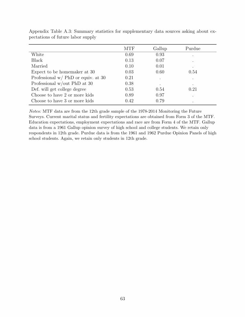
Appendix Table A.3: Summary statistics for supplementary data sources asking about ex-pectations of future labor supply

MTF Gallup PurdueWhite 0.69 0.93 .Black 0.13 0.07 .Married 0.10 0.01 .Expect to be homemaker at 30 0.03 0.60 0.54Professional w/ PhD or equiv. at 30 0.21 . .Professional w/out PhD at 30 0.38 . .Def. will get college degree 0.53 0.54 0.21Choose to have 2 or more kids 0.89 0.97 .Choose to have 3 or more kids 0.42 0.79 .

Notes: MTF data are from the 12th grade sample of the 1978-2014 Monitoring the FutureSurveys. Current marital status and fertility expectations are obtained from Form 3 of the MTF.Education expectations, employment expectations and race are from Form 4 of the MTF. Gallupdata is from a 1961 Gallup opinion survey of high school and college students. We retain onlyrespondents in 12th grade. Purdue data is from the 1961 and 1962 Purdue Opinion Panels of highschool students. Again, we retain only students in 12th grade.

63

Appendix B. Data Appendix

B.1 BHPS

The BHPS started in 1991 with 5,500 households (10,300 individuals), known as the “originalsample.” Since then, the sample has grown in various ways. First, the main survey is onlyadministered to adults, so children in original sample households “age in” to the surveyupon turning 16. These “agers-in” and all other original sample members are continuouslytracked as they form new households, and the individuals in these new households are alsointerviewed so long as they live with an original sample member. (If these new-comers moveout of the household, they are no longer tracked.) One notable exception is that some will“marry in” to the sample and be tracked permanently if they have a child with an originalsample member. Children born to original sample members are automatically counted asoriginal sample members.

The BHPS has also grown via the addition of new booster samples. Between 1997 and2001, the BHPS roughly doubled in size with the addition of 5,000 households (8,600 in-dividuals) out of concerns that the original sample under-represented Scotland, Wales, andNorthern Ireland. In 2009, the BHPS became subsumed under the “Understanding Soci-ety” dataset, which, including BHPS households, tracked roughly 40,000 households (50,000individuals) in the UK. While Understanding Society maintained most questions from theBHPS, it notably dropped several of the gender-roles questions we are most interested in,so our main results focus on the BHPS through 2008, for the sake of consistency across ourmain outcome variables. Results that include data from Understanding Society are not muchdifferent from results using BHPS through 2008 only and are available upon request.

Our preferred analysis sample imposes the restriction that we observe each person atleast once before becoming a parent and at least once after, so that all observations helpidentify the main effect of parenthood. Our sample comprises only those who were originalsample members, i.e. those who were interviewed in the first wave and not those who marryinto the sample later on. Because our panel is relatively short (18 waves) compared to ourU.S. panel data sources, we exclude children who age into the sample because, in order tomeet our restriction that we see the event of the birth of their first child, these individualswould disproportionately have children early (and, relatedly, would be disproportionatelyfemale, as women tend to have children at a younger age than men).

The BHPS conducts fertility history interviews for all respondents at the second waveafter entry into the sample, and from this set of questions, we can identify parents whohave had children before the BHPS starts. Unfortunately, this fertility history is not askedagain after the second wave, so we look to the household grid, which lists all individualswho live in a household together as well as some basic demographic information, such asdate of birth. Importantly for our purposes, this grid also includes relationships betweenhousehold members, so we can link children to their parents and construct a full fertilityhistory for each parent in our sample. This is largely the same method suggested by theBHPS. Unfortunately, because a parent must be living with their child in order to identifybirth dates, we undercount fathers, as (we hypothesize) they on average are less likely to beliving with their children than are mothers. Relative to a BHPS quality profile conducted atwave 13, we slightly over-count mothers (692 versus 673) and undercount fathers (567 versus

64

653).Our main employment outcome variable is defined as equal to 1 if an individual had a

paying job last week and includes people who, for example, were on maternity leave. Hoursworked is the typical hours that an individual works within a given year, and is coded aszero if the individual is not working (including not looking for work). Thus, an individualmay be on maternity leave in the week prior to a survey, but their usual hours worked mightbe greater than zero, since a respondent can interpret the question to be about when theirhours prior to maternity leave.

We also examine a range of questions on an individuals’ opinions on gender roles in thehousehold. Appendix Table A.1 summarizes these questions. While 9 questions are availablein total, we only choose a subset of 6 that pertain to the impacts of a woman working. Thesestatements, asked on a scale of 1 (strongly agree) to 5 (strongly disagree) are: (1) A preschool child is likely to suffer if his or her mother works, (2) All in all, family life sufferswhen the woman has a full time job, (3) A woman and her family would all be happier if shegoes out to work, (4) Both the husband and wife should contribute to the household income,(5) Having a full-time job is the best way for a woman to be an independent person, and (6)A husband’s jobs is to earn money; a wife’s job is to look after the home and family.

We take the individual gender-roles questions and construct an omnibus measure as fol-lows. First, since some questions are phrased in a gender “liberal” manner (i.e. men andwomen should take on equal roles in the household) and others are phrased in a gender“conservative” manner (i.e. men and women should take on distinct roles in the household),we reverse some questions as necessary so that all are increasing in the gender liberal di-rection. We then standardize each variable so that they have a mean of zero and standarddeviation of one, and sum them up.

B.2 NLSW 1968

B.2.1. Survey Design and Sample

We make use only of the “young women” component of the NLSW68. (While the NationalLongitudinal Surveys of Young and Mature Women include an older “mature women” sam-ple, they have for the most part had their first child before entering the sample.) The “youngwomen” component of the NLSW68 is a sample of 5,159 women born between 1941 and 1954.The women were aged 14-24 when first interviewed in 1968 and aged 49-62 when last in-terviewed in 2003. During the last wave of the survey 55.4% of the original sample wasinterviewed.

The sample is represented by a multi-stage probability sample drawn by the CensusBureau from 1,900 primary sampling units. In order to provide reliable statistics for blackrespondents, the NLSW68 oversampled the black population at about twice the expected rateof the total population. Black respondents make up approximately 28 percent of the sample,compared to 11 percent of the population at the time. Probability-of-selection weights createdby the NLSW68 correct for this bias.

65

B.2.2. Sample Selection

Our sample comprises all respondents in the National Longitudinal Survey of Women whomeet the following criteria: (1) We observe them at least once before and after the birth oftheir first child, (2) We observe them for the first time by age 20 and for the last time afterage 40. We include people who drop out at some point in the sample.

In a given year, it is possible to observe a respondent’s employment status, but not thenumber of hours they worked last week, or vise versa. Thus, for a respondent to be includedin our sample, we must observe each of the three outcomes variables (“working now”, “inlabor force now”, “hours worked last week”).

B.2.3. Employment Status

Employment status is obtained from combining two NLSW68-created variables: employmentstatus recode (ESR), available every 1-3 years from 1968 to 1993, and monthly labor recode(MLR), available every other year from 1995 to 2003. Although not exactly the same, thetwo variables are very similar. Employment status recode specifies whether the respondentwas working, with a job but not at work, laid off and looking for work, unemployed, goingto school, keeping house, unable to work, or retired. Monthly labor recode specifies whetherthe respondent was employed and at work, employed but absent, unemployed and laid off,unemployed and looking for work, retired, or disabled.

We code respondents as “working now” if they report working (employed and at work)and as “not working” if they report any other activity in the ESR (MLR). Negative valuesof each variable, which are assigned when respondents refuse to answer, do not know theanswer, or are not interviewed, are coded as missing.

We code respondents as “in labor force” if they report working, having a job but notworking, looking for work, or being laid off (employed and at work, employed but absent,unemployed and laid off, unemployed and looking for work) and as “not in labor force” ifthey report any other type of activity in the ESR (MLR). Negative values of each variable,which are assigned when respondents refuse to answer, do not know the answer, or are notinterviewed, are coded as missing.

B.2.4. Hours Worked

Between 1968 and 1993, the NLSW68 asks respondents the number of hours they worked inthe previous week. We assign this variable to be “hours worked.” Respondents deemed to benot working (“working now” = 0) are assumed to have worked zero hours last week.

After 1993, the NLSW68 asks respondents the number of hours worked at their main joband at their other job. We assign our “hours worked” variable to be the sum of these twovariables. Again, respondents deemed to be not working (“working now” = 0) are assumedto have worked zero hours last week.

B.2.5. Date of Birth of 1st Child

The NLSW68 does not consistently ask respondents for the date of birth of their children.Thus, to determine the date of birth of respondents’ first and second children, we combine

66

several categories of variables pertaining to children’s date of birth and take the minimumand second minimum value among these.

Between 1968 and 1993, the NLSW68 asks respondents directly about the date of birth oftheir children. In 1973, the NLSW68 records the date of birth of each child a respondent hashad in their lifetime. In 1978, 1983, 1985, 1987, 1988, 1991, and 1993 the NLSW68 recordsthe date of birth of each child the respondent has had since their last interview.

Post 1993, the NLSW68 does not explicitly ask for dates of birth of children, but in-stead asks for a demographic information, including date of birth, for each member of thehousehold. We include these variables in our calculation of minimum date of birth only if thehousehold member is a child of the respondent (relationship to respondent equal to child,son, or daughter).

To determine the first (second) child’s date of birth, we take the minimum (second mini-mum) date of birth among all date of birth variables described above. Children with missingmonths of birth but non-missing years of birth are assumed to have been born in September(the most common birth month).

B.2.6. Event Time

The event time variable is calculated by determining the number of months between thedate of birth of the respondent’s first child and the current interview, dividing by 12, androunding down.

B.2.7. Other Demographic Information

Education: Each year, the NLSW68 records the highest completed grade and highestcollege degree obtained by respondents. We define having a college degree as whethera respondent had a college degree at age 25. Respondents who report completing lessthan 16 years of school are coded as having no college degree.

Age: Age is calculated by determining the number of months between the respondent’sdate of birth and the current interview, dividing this number by 12, and rounding down.Unknown interview months are assumed to be March.

Mom Worked: In 1968, respondents were asked whether their mother worked whenthey were 14. Responses of yes are coded as 1, responses of no are coded as 0, and allother values are coded as missing.

Planned to Work at Age 35: In 1968, respondents were asked what they plan to bedoing at age 35. Responses of working at a different job and working at the same jobare coded as 1. Responses of married, keeping house, other, or do not know are codedas 0. All other values are coded as missing.

67

B.3 NLSY 1979

B.3.1. Survey Design and Sample

The NLSY79 is a sample of 12,686 men and women born between 1957 and 1964. They wereaged 14-22 when first interviewed in 1979 and aged 50-57 when last interviewed in 2014.

The NLSY79 purposefully over samples economically disadvantaged, Hispanic, and blackyouth. Approximately 25 percent of the sample is black and 16 percent of the sample isHispanic, compared to their share of population which was around twelve and six percent,respectively, at the time. The inclusion of probability-of-selection weights corrects for thisover sampling.

B.3.2. Sample Selection

Our sample comprises all respondents in the National Longitudinal Survey of Youth whomeet the following criteria: (1) We observe them at least once before and after the birth oftheir first child, (2) We observe them for the first time by age 20 and for the last time afterage 40. We include people who drop out at some point in the sample.

In a given year, it is possible to observe a respondent’s employment status, but not thenumber of hours they worked last week, or vise versa. Thus, for a respondent to be includedin our sample, we must observe each of the three outcomes variables (“working now”, “inlabor force now”, “hours worked last week”).

B.3.3. Employment Status

The NLSY79 records respondents’ employment status for each week between 1978 and thedate of their last interview. To determine a respondent’s current employment status, we usethe employment status variable corresponding to week the respondent was interviewed.

We code respondents as “working now” if their employment status is a job number (valuesof 100 through 3000) as as “not working” if they report not working, being unemployed,being out of the labor force, or being in active military service. All other values are codedas missing.

We code respondents as “in labor force” if their employment status is a job number orthey report being unemployed and as “not in labor force” if they report being out of thelabor force or in active military service. All other values are coded as missing.

B.3.4. Hours worked

As with employment status, the NLSY79 records the number of hours respondents worked foreach week between 1978 and the date of their last interview. We assign this variable, in theweek-year corresponding to each interview, to be “hours worked.” Respondents deemed tobe not working (“working now” = 0) are assumed to have worked zero hours in the previousweek.

68

B.3.5. Date of Birth of 1st Child

The NLSY79 provides the date of birth for each of the respondent’s children. We take theminimum date of birth among all children as the birthday of the first (second) child.

B.3.6. Event Time

NLSY79 provides the date of interview for each wave. The event time variable was calculatedby determining the number of months between the birth of the respondent’s first child andthe current interview, dividing by 12, and rounding down to the nearest whole number.

B.3.7. Other Demographic Information

Education: Each year, the NLSY79 records the highest completed grade. We assignthe highest grade completed to be the respondent’s maximum highest grade reportedamong all years. A respondent is assumed to have a college degree if they have com-pleted 16 or more years of schooling.

Age: Age is calculated by determining the number of days between the respondent’sdate of birth and the current interview, dividing this number by 365, and roundingdown. Unknown interview months are assumed to be March and unknown interviewdays are assumed to be the 15th.

Mom Worked: In 1979, respondents were asked whether their mother worked whenthey (the respondents) were 14 years old. Responses of yes are coded as 1, responsesof no are coded as 0, and all other values are coded as missing.

Planned to Work at Age 35: In 1979-1984 respondents were asked what they planto be doing at age 35. Responses of working at a different job and working at the samejob are coded as 1. Responses of married, keeping house, other, or do not know arecoded as 0. All other values are coded as missing.

B.4 PSID

B.4.1. Survey Design and Sample

The PSID started in 1968 with a national sample of about 4,800 U.S. households. This ini-tial sample was made up of two sub-samples. The first was a cross-sectional national sampleconducted by the Survey Research Center (SRC) that produced about 2,900 interviews. Thesecond was a sample of low-income families conducted by the Survey of Economic Oppor-tunity (SEO) that produced about 1,900 interviews. The low income sample had unequalselection probabilities as it was limited to SMSAs and non-SMSAs in the southern region.By construction, the PSID oversamples low-income households.

In 1997 and 1999 the PSID added an immigrant booster sample of about 500 households.Those eligible for this sample must have immigrated to the US after 1968 or have been born1969 or later to people not in the US in 1968.

The PSID includes probability-of-selection weights that are designed to adjust for theoversampling of low-income households and for differential attrition. They are especially

69

important given the combination of SEO and SRC samples that made up the original PSIDsample. Weights are also adjusted every five years (1969, 1974, etc) for cumulative panelattrition.

PSID follows sample members no matter their living arrangements: if they split off andform a new household, then that household is added to the sample and each of its membersare interviewed; if they have children, then each of their children are interviewed.

B.4.2. Sample Selection

Our sample comprises all respondents in the Panel Study of Income Dynamics who meetthe following criteria: (1) We observe them at least once before and after the birth of theirfirst child, (2) We observe them for the first time by age 20 and for the last time afterage 40, and (3) They either begin in or are born into a household in the “core sample” –that is, a household randomly selected to be included in the sample. We include those whoare added later on in “booster” samples that increase representation among immigrant andLatino populations and include people who drop out at some point in the sample.

In a given year, it is possible to observe a respondent’s employment status, but not thenumber of hours they worked last week, or vise versa. Thus, for a respondent to be includedin our employment sample, we must observe each of the two outcomes variables (“workingnow” and “in labor force now”).

B.4.3. Employment Status

Employment status in the PSID is obtained from the individual employment status variables,available from 1979 to 2015. The variable specifies whether the respondent is working now,temporarily laid off, unemployed and looking for work, retired, permanently disabled, keepinghouse, or a student.

We code respondents as “working now” if they report working now and coded as “notworking” if they report being temporarily laid off, unemployed and looking for work, retired,permanently disabled, keeping house, or a student. All other values are coded as missing.

We code respondents as “in labor force” if they report working now, being temporarilylaid off, unemployed and looking for work. They are coded as “not in labor force” if theyreport retired, permanently disabled, keeping house, or a student. All other values are codedas missing.

B.4.4. Date of Birth of 1st Child

To determine the date of birth of respondent’s first child, we use the childhood and adoptionhistory file. We limit the data to birth records (as opposed to adoption records), so the dateof birth of first and second children correspond only to birth children.

If the child’s month of birth is missing, we assume they were born in September. If thechild is listed as having been born in winter, spring, summer, or fall we assume they wereborn in January, April, July, and October, respectively. If the child’s birth year is missing,we code the date of birth as missing. The minimum date of birth among all the respondent’sbirths is taken to be the date of birth of the first child.

70

B.4.5. Event Time

The event time variable is calculated by determining the number of months between thedate of birth of the respondent’s first child and the current interview, dividing by 12, androunding to the nearest whole number.

B.4.6. Other Demographic Information

Education: In each survey wave, the PSID records the number of years of educationa respondent has received. A respondent is coded as having a college degree if theyreport having completed 16 or more years of schooling by age 25.

Age: To determine age, we rely on the PSID variable which asks respondent’s fortheir age at the time of the interview. We then calculated an imputed age – equal tothe number of months between the respondent’s date of birth and current interview,divided by 12, and rounded down. If the reported age is more than two years from theimputed age or if the current age is lower than a previously reported age, we replacethe age variable with our imputed age variable.

B.4.7. Childhood Development Supplement (CDS)

In 1997 PSID began to supplement its main data collection with a survey targeting 0-12 yearold children and their parents. Original CDS respondents were interviewed an additional twotimes, in 2002 and 2007. In 2014, the CDS continued with a new cohort of 0-17 year oldchildren and their parents.

CDS asks children’s primary and second caregivers a variety of questions relating toparenthood. Primary caregivers are defined, in order of precedence, as the biological, step,foster, or adoptive mother of the child, the “wife” of a a PSID head who is father to thechild, the biological, step, foster, or adoptive father of the child, the legal guardian of thechild, and the adult in the household unit who takes primary responsibility for the child.Thus, primary caregivers are almost always women. Secondary caregivers (known as othercaregivers after 1997), are defined, in order of precedence, as the biological, step, foster, oradoptive father of the child, the grandmother of the child, the boyfriend or girlfriend of theprimary caregiver, another adult relative of the child, and another adult non-relative of thechild.

Our analysis uses the “parenting is hard” question in the CDS. The question asks care-givers to rank on a 5 point scale how much they agree or disagree with the statement “being aparent is harder than I thought it would be.” A value of 1 corresponds to “strongly disagree”whereas a value of 5 corresponds to “strongly agree.” The “parenting is hard” question isasked to both primary and secondary caregivers in 1997, 2002, and 2007 but only to primarycaregivers in 2014.

Having a college degree is defined as having a college degree by age 25. “Mom worked”is defined as whether a respondent’s mother worked when the respondent was between ages8-16.

71

B.5 Longitudinal Study of American Youth

The Longitudinal Study of American Youth (LSAY) was commissioned by the NationalScience Foundation (NSF). The objective of the LSAY was to study the tendency and deter-minants of U.S. adolescents to pursue a career in science, technology, engineering and math(STEM).

“Cohort one” of the LSAY sampled over 2,800 tenth-graders in 1987. These students werethus born in the early 1970s. “Cohort two” were in seventh grade at this time (in middleschools that served as feeder schools to the high schools sampled in Cohort one). Thesestudents were thus born in the mid-1970s.

While the students were initially followed only for a few years after high school, in 2006the NSF provided additional funding to make a major effort to recontact all the originalLSAY participants. The large majority of participants were identified and interviewed in2007. Interviews occurred as well in the following years, though because of attrition withsmaller sample size.

To maximize sample size, we pool cohorts one and two. We gather data from tenthgrade for both cohorts (so, the first year of interviews for cohort one and the fourth yearof interviews for cohort two). Choosing tenth grade as the first year in a long-differencesanalysis maximizes our sample. We use 2007 as the final year for both cohorts (so, Cohortone is roughly 36 and cohort two 32), again because later follow-up years after 2007 sufferfrom attrition and thus reduce sample size.

Given the two-cohort structure of the data collection, we control for year-of-birth fixedeffects in the regression analysis.

Our main outcome variable comes from the 2007 survey, which asks all respondents(including those not working) about the importance of career success. The question (varR325C in the ICPSR version of the data that we use) reads as follows: “Now, please thinkabout your goals or things that are important to you in life. For each of the goals listedbelow, please indicate if this goal is very important to you, somewhat important, or notimportant.... Having accomplished something important in my work.” We follow the surveyand code as 1–3, increasing in importance.

We compare the answer to this question with a similar question posed in tenth grade (varGA6A): “Now I would like to read you a list of goals you may or may not have for your life.For each goal—as I read it—I would like you to tell me if it is very important, somewhatimportant, or not important to you. First, being successful in your line of work.”

We use as independent variables questions about fertility and investment in human cap-ital. In particular, whether you have a child born by 2007 (var R13A3); whether you hada college degree by 2007 (R25G); whether your own mother worked (MOTHOCC); yourscore an math and science tests administered by the survey in tenth grade (GMTHIRT andGSCIIRT, respectively).

We downloaded the data from the LSAY homepage on ICPSR: https://www.icpsr.umich.edu/web/ICPSR/studies/30263.

72

B.6 Data sources asking expectations of future labor supply and fertility

B.6.1. Monitoring the Future

The Monitoring the Future (MTF) survey is an annual cross-sectional survey of Americanyouth. It was first conducted in 1975 and includes about 16,000 high school seniors fromapproximately 133 public and private high schools in the contiguous United States. Beginningin 1991, the MTF added nationally representative samples of 8th and 10th graders, althoughwe do not make use of them in this paper.

The MTF uses a multi-stage random sampling procedure to create a nationally represen-tative sample of students from each grade. In the first two stages, researchers select particulargeographic areas and (with probability proportionate to size) one or more schools in eacharea. The last stage involves selecting students within each school. In a given school, up to350 students can be selected. Typically, in schools with fewer than 350 students, all studentsare included. In larger schools, entire classrooms are randomly sampled.

Our analysis makes use of a question that asks respondents the type of work they expectthey will be doing at age thirty. Specifically, the question asks, “What kind of work do youthink you will be doing when you are 30 years old? Mark the one that comes closest to whatyou expect to be doing.” There are fifteen possible occupational categories that studentscan choose from, with “home-maker” as one possible option. Other possible choices includelaborer; service worker; operative or semi-skilled worker; sales clerk in a retail store; clericalor office worker; craftsman or skilled worker, sales representative; protective service; manageror administrator; professional without doctoral degree; professional with doctoral degree orequivalent; owner of small business; farm owner/manager; and military service. Below is a listof example occupations provided in the MTF questionnaire for each occupational category.

Job Group MTF 1976 MTF2016car washer custodian

sanitary worker material moverfarm laborer maid

landscape workerfarm worker

cookfood preparer or food service

worker including fast food waiter waiter/waitressbarber call center worker janitor stock clerk

gas station attendant order filler practical nurse nursing aide/orderly

beautician teacher assistantchildcare worker

garage worker bus or truck driver taxicab maintenance or repair worker

bus or truck driver assembly line workerassembly line worker

welder

shoe salesperson cashierdepartment store clerk supervisor of retail workers

drugstore clerk

bank teller secretary bookkeeper receptionist secretary bookkeeper

typist supervisor of office workerspostal clerk or carrier bank teller

ticket agent postal clerk or carrier

carpenter carpenterelectrician mechanicbric layer machinistmechanic weldermachinist

tool and die makertelephone installer

Laborer

Service worker

Operative or semi-skilled worker

Sales clerk in a retail store

Clerical or office worker

Craftsman or skilled worker

73

Job Group MTF 1976 MTF2016insurance agent insurance agent

real estate broker real estatebond salesman

Protective service police officer policefireman firefighter

detective paramedic

office manager office managersales manager government official

school administrator sales managergovernment official

registered nurse registered nurselibrarian school teacherengineer accountantarchitect architect

social worker artisttechnician information technology workeraccountant

actorartist

musician

lawyer lawyerphysician physician

dentist dentistscientist scientist

college professor college professor

restaurant ownershop owner

Farm owner, farm managerMilitary serviceFull-time homemaker or housewife

Manager or administrator

Sales representative

Professional without doctoral degree

Professional with doctoral degree or equivalent

Owner of small business

For desired fertility, we make use of the question: “All things considered, if you couldhave exactly the number of children you want, what number would you choose to have?”Raw data and documentation for this survey can be found at https://www.icpsr.umich.

edu/web/ICPSR/series/35.

B.6.2. Purdue Opinion Panels

We also make use of the 1961 and 1962 Purdue Opinion Panels of high school studentsgrades 9-12. Students selected for the sample participate in three to four surveys in a schoolyear. The same panel of students takes part in all surveys within a school year; however,the panel changes every school year. The 1961 survey was conducted in March of that yearwhile the 1962 survey was conducted in September; hence, the group of students polleddiffers between these surveys. We restrict our sample to female high school seniors in eachsurvey. The panel asks “What kind of job do you expect to have 20 years from now?”and respondents can choose between twelve possible occupations, including “housewife.”Other possible occupations include salesman; owner of factory or small business; professional-teacher, doctor, musician, musician, scientist; office worker; clerk in a store; farm or ranchowner; farm or construction laborer; factory worker or mechanic; big business management;deliveryman, truck driver; and carpenter, plumber, electrician. Raw data and documentationfor this survey can be found at https://ropercenter.cornell.edu/CFIDE/cf/action/

catalog/abstract.cfm?type=&start=&id=&archno=USPOP1961-063&abstract=.

B.6.3. Gallup

We also use a 1961 Gallup Opinion Poll of young high school, college, and non students. Weagain restrict our sample to female high school seniors. The Gallup poll asks respondents theopen-ended question “What do you expect to be doing when you are 40 years old?” Responseswere organized into 18 categories. We use the “house wife,” “home maker,” “house work,”and “raising children” as our definition of expected homemaker. Other categories includeteacher, sports coach, professor; scientist, physicist, biologist, chemist, medical research,

74

psychologist, research; business executive, own business, industry, management, businessadministration; minister, missionary, social worker; engineering, research engineer, managingengineer; entertainment, actor, broadcasting; medicine, dentist, psychiatry; lawyer; farmer,rancher, agriculture; armed services; government work; sales, clerical: secretary, sales clerk,office worker; nurse; mechanic, machinist, tool and dye maker; skilled trade: electrician,plumber, carpenter, mason, electronics; contracting, building construction, excavating; andartist, cartoonist, designer, draftsman, decorator. Raw data and documentation for thissurvey can be found at https://ropercenter.cornell.edu/CFIDE/cf/action/catalog/

abstract.cfm?type=&start=&id=&archno=USAIPOSPPOS1961-544&abstract=.

B.6.4. National Survey of Family Growth

The National Survey of Family Growth (NSFG) began in 1973 and is designed to be na-tionally representative of ever-married women 15 to 44 years of age in the civilian, non-institutionalized population of the U.S. Starting in 1982, the sample was extended to in-clude women aged 15 to 44 regardless of marital status. For the 1973, 1976, 1982 waves ofthe NSFG, the fertility expectations variable is based on the total number of births thatthe respondent expected. This variable is constructed by the NSFG based on the sum of thenumber of existing births reported by the respondent and the central number of additionalbabies expected (obtained from taking the mean of the smallest and largest number of ad-ditional babies expected). For the 1988, 1995, 2002, 2006-2010, 2011-2013, and 2013-2015waves of the NSFG, we compute fertility expectations based on the sum of number of livepregnancies that the respondent had when the survey is administered and the central numberof additional babies the respondent expects to have. To ensure that the sample size is suffi-ciently large to estimate fertility expectations of young adult women, we restrict the sampleto women between the ages of 17 to 20. To match the MTF sample, we further restrict thesample to those who have attended at least 12th grade. Raw data and documentation frothis survey can be found at https://www.cdc.gov/nchs/nsfg/about_nsfg.htm.

B.7 Data sources used to proxy “employment costs of motherhood”

B.7.1. Low-Fertility Cohorts Study

We use breastfeeding data from the 1978 Low-Fertility Cohorts Study (ICPSR 4698). Thesample consists of 1049 white, ever-married women born in the United States between July1, 1900 and June 30, 1910. The study asks respondents about the birthyears of their first16 live births and whether each was ever breastfed. We define the breastfeeding rate as thepercentage of children born in each reported birthyear who were ever breastfed and only plotrates for birthyears with 100 or more observations (i.e. the 14 years between 1925 and 1939).The average number of observations per year is 130.7. Raw data and documentation for thissurvey can be found at https://www.icpsr.umich.edu/web/ICPSR/studies/4698.

B.7.2. National Fertility Survey

We also use breastfeeding data from the 1965, 1970, and 1975 waves of the National FertilitySurvey (ICPSR 20002, 20003, and 4334 respectively) of currently married women living in the

75

United States. The NFS is the successor of the 1955 and 1960 Growth of American Familiessurveys. The 1965 NFS survey asks respondents about the birthyears of their first 18 livebirths and whether each was ever breastfed; the 1970 survey asks only about the first birthand the 1975 survey asks about the first 12. We pool responses from all three surveys anddefine the breastfeeding rate as the percentage of children born in each reported birthyearwho were ever breastfed. We only plot rates for birthyears with 900 or more observations(i.e. the 13 years between 1953 and 1965). The average number of observations per year is1199.8. Raw data and documentation for all three surveys can be found at https://www.

icpsr.umich.edu/web/ICPSR/series/220/studies.

B.7.3. Ross Labs Mothers Survey

We also use the Ross Labs Mothers Survey to estimate breastfeeding rates in the US between1970 and 2002. Surveys were sent to a nationally representative sample of new mothers bymail. Prior to January 1997, mothers received surveys when their babies turned 6 months old;in later years, surveys also were sent to mothers of babies that were 1 to 12 months old. Thesurvey asks what type of milk their babies received in the hospital, at one week, in the last30 days, and most often in the last week; possible choices include breast milk, commerciallyavailable infant formulas, and cow’s milk. The data are then weighted by geography, race,and mother’s age and education. We plot estimates of the percentage of infants in each surveyyear between 1970 and 2002 that were ever breastfed. Data and documentation for this surveycan be found at http://web.archive.org/web/20070101180255/http://www.ross.com:

80/images/library/BF_Trends_2002.pdf.

B.7.4. National Immunization Survey

Finally, we estimate US breastfeeding rates for children born between 2002 and 2017 usingdata from the National Immunization Survey. The survey is conducted annually by telephoneusing random-digit dialing; the sample includes households with children and teens in the 50states and the District of Columbia. Since January 2003, all respondents with children 19 to35 months old are asked questions about breastfeeding. Breastfeeding rates are calculated bychild’s birthyear rather than survey year; thus, each birthyear can consist of responses fromup to three survey years. The NIS releases breastfeeding rates for children in a birthyearwhen approximately two-thirds of children born that year have been surveyed. Prior to2009, the rates were replaced the following year with final rates based on all the childrensurveyed in the birthyear; however, starting from 2009, the CDC reports one final rate basedon two survey years only. We plot estimates of the percentage of babies born in each yearbetween 2002 and 2017 that were ever breastfed, as defined by the question “Was [child]ever breastfed or fed breast milk?” Data and documentation for this survey can be found athttps://www.cdc.gov/breastfeeding/data/nis_data/index.htm.

B.7.5. Infant Feeding Survey

For our estimates of breastfeeding rates from the UK, we use data from the Infant Feed-ing Survey, started in 1975 and administered in five year intervals until 2010. The 1975

76

survey was conducted only in England and Wales; surveys from 1980 onward include Scot-land, and surveys from 1990 onward also include Northern Ireland. Each survey consistsof questionnaires sent to mothers in three stages: the first when their babies are approx-imately six weeks old, the second when their babies are around four to six months old,and the third when their babies are around eight to ten months old. The data are thenweighted to be representative of all mothers who gave birth in the sampling period ineach country by mother’s age and socioeconomic status. For consistency, we plot esti-mates of initial breastfeeding rates among Stage 1 mothers (those with babies around sixweeks old) for England and Wales only for all survey years between 1975 and 2010. Dataand documentation for this survey can be found at https://digital.nhs.uk/data-and-

information/publications/statistical/infant-feeding-survey.

B.7.6. American Heritage Time Use Survey and American Time Use Survey

We use the American Heritage Time Use Survey (AHTUS, 1965 to 2012) and American TimeUse Survey (ATUS, 2013 to 2019) to measure average time spent on childcare (in minutes perday). The AHTUS and ATUS are national time-diary based samples and provide nationallyrepresentative estimates of how, where, and with whom Americans spent their time. Thesample includes mothers aged 25 to 44, with no reported disability, and with at least oneown child below the age of 18 residing in the household in the respective survey years. Due tosmall sample sizes, we pool the following years of data from the AHTUS: 1965 and 1966; 1975and 1976; 1992 and 1993; 1994 and 1995; and 1998 to 2000. The total time spent on householdwork is the sum of reported time spent on housework (act undom) and childcare (act chcare).Raw data and documentation for these surveys can be found at https://www.ahtusdata.

org/ahtus/about.shtml for the AHTUS and https://www.bls.gov/tus/data.htm for theATUS.

B.7.7. General Social Survey and National Fertility Survey

Trends in gender-role attitudes among prime-age individuals are estimated based on datafrom the 1977 to 2015 General Social Survey (GSS) and the 1970 National Fertility Survey(NFS). The GSS is a nationally representative survey of adults in the U.S. conducted since1972. Our analysis makes use of responses to the following three questions that were askedconsistently from 1977 to 2015 (on a four-point scale):

1. FEFAM : It is much better for everyone involved if the man is the achiever outside thehome and the woman takes care of the home and family.

2. FECHLD : A working mother can establish just as warm and secure a relationship withher children as a mother who does not work.

3. FEPRESCH : A preschool child is likely to suffer if his or her mother works.

The sample is restricted to men and women between the ages of 25 and 44. To constructthe index of gender-role attitudes, we first standardize the responses to each of the threequestions to have a mean of zero and standard deviation of one in each survey year. Wecompute the aggregate individual-level sexism index by taking the average of the normalized

77

responses in each survey year for each individual. The relevant sampling weights are appliedfor each survey. Data and documentation for this survey can be found at https://www.

icpsr.umich.edu/icpsrweb/ICPSR/series/00028.To obtain an earlier measure of gender-role attitudes, we use data from the 1970 National

Fertility Survey (also described in Section B.7.2). The 1970 NFS examines marital fertilityand family planning in the U.S. and contains similar questions on gender-role attitudes asthe GSS. The survey includes ever-married women who were born after July 1, 1925. Thequestions used to construct the gender-role attitude index for 1970 are very similar to in theGSS and were also measured on using a four point scale. Respondents who indicated thatthey were ”Uncertain or don’t know” to any of the three questions are coded as missing. Wefollow the same procedure as that outlined for the GSS to construct the attitude index forthe NFS. The relevant sampling weights are applied. Data and documentation for this surveycan be found at https://www.icpsr.umich.edu/web/ICPSR/studies/20003/summary.

B.7.8. Weekly childcare costs

Data for average weekly childcare costs were extracted from Census Bureau Report CB13-62,available at https://www.census.gov/newsroom/press-releases/2013/cb13-62.html, us-ing an online WebPlotDigitizer tool. Cost of childcare measures the average weekly expen-ditures among people making childcare payments, in 2011 dollars.

B.8 Data sources used to measure mothers’ perceived costs relative to previousgenerations

B.8.1. Growth of American Families

We use the 1955 wave of the Growth of American Families survey (ICPSR 20000). The sampleconsists of 2713 married women aged 18-39 living in the United states. We restrict the sampleto women with at least one birth. The 1955 GAF survey asks respondents “Do you feel thatit is easier or harder to raise a family these days than when you were a child?”; we code awoman as agreeing with the statement “It is harder to raise a family these days than when Iwas a child” if she answered “harder” or “harder, qualified.” Other possible answers includeeasier; easier, qualified; pro-con; and don’t know, depends. Raw data and documentation forthis survey can be found at https://www.icpsr.umich.edu/web/ICPSR/studies/20000.

B.8.2. Attitudes of American Women

We also use the 1962 Attitudes of American Women survey sponsored by the SaturdayEvening Post. The sample consists of married women (including divorced, widowed, andseparated) aged 60 or younger and never-married women aged 25 to 60 from 227 non-ruralinterviewing areas in all parts of the United States; we restrict the sample to women with atleast one child under the age of 18. The survey asks “Is your job as a homemaker harder oreasier than your mother’s was?”; possible answers include harder, easier, and the same. Wecode a woman as agreeing with the statement “My job as a homemaker is harder than mymother’s was” if she answered “harder.” Raw data and documentation for this survey canbe found at https://ropercenter.cornell.edu/ipoll/study/31089519.

78

B.8.3. Modern (post-1990) polls

Finally, we use several modern surveys that ask about the perceived costs of motherhood.Specifically, we pool data on women aged 25-45, with at least one child below the age of 18,from following surveys:

• the Pew State of the Union Mother’s Day Poll from 1997 (https://www.pewresearch.org/politics/dataset/state-of-the-union-mothers-day-poll);

• the Washington Post DC-Region Moms Poll from 2005 (ICPSR 4324, https://www.icpsr.umich.edu/icpsrweb/ICPSR/studies/4324)

• the ABC News Mother’s Day Poll from 2006 (ICPSR 4655, https://www.icpsr.

umich.edu/web/ICPSR/studies/4655);

• the Pew Marriage/Parenthood survey from 2007 (https://www.pewsocialtrends.org/dataset/marriageparenthood/); and

• the CBS Monthly National Polls from April 2009 (ICPSR 26947, https://www.icpsr.umich.edu/icpsrweb/ICPSR/studies/26947), April 2011 (ICPSR 33962, https://www.icpsr.umich.edu/icpsrweb/ICPSR/studies/33962), May 2011 (ICPSR 33963,https://www.icpsr.umich.edu/icpsrweb/ICPSR/studies/33963) and April 2013 (ICPSR34997, https://www.icpsr.umich.edu/icpsrweb/ICPSR/studies/34997).

The 1997 and 2007 Pew surveys ask respondents “In general, do you think it’s easierto be a mother today than it was 20 or 30 years ago, more difficult, or about the same?”;possible answers include easier, more difficult, and about the same.

The 2005 Washington Post survey asks respondents “Do you think motherhood todayis more demanding than it was for the previous generation, less demanding, or about thesame?”; possible answers include more, less, and about the same.

The 2006 ABC News survey asks respondents “Compared to when you were a child, ingeneral, do you think being a mother today is harder, easier, or about the same?”; possibleanswers include easier, harder, and about the same.

The CBS surveys ask respondents “Compared to when you were a child, in general, doyou think being a mother today is harder, easier, or about the same?”; possible answersinclude easier, harder, and about the same.

We code a woman as agreeing with the statement “Motherhood today is harder thanbefore” if she answered “more difficult” to the Pew surveys, “more demanding” to the Wash-ington Post survey, or “harder” to the ABC or CBS surveys.

79

Appendix C. Placebo births analysis

We describe our procedure for our placebo births analysis in this section, as seen in Figure4 and Appendix Figure A.4. For women without children (the control group), we identifya sample of women most likely to remain childless beyond the period we observe them inthe data and assign placebo births in the following manner (broadly following Kleven et al.(2018)): We generate predictions of childlessness by estimating a linear probability modelof childlessness on a sample of women who have completed their fertility (i.e., are over age40 at the end of our panel in 2009) and use estimates from this model to predict lifetimechildlessness for women who have not yet completed their fertility (i.e., are under age 40in 2009). In particular, we regress childlessness on whether the respondent’s mother workedwhen the respondent was 14, education-category fixed effects, income-quartile fixed effects,and birth-cohort fixed effects. We then select the top X% of women with respect to predictedchildlessness and code them as being childless. We set X to equal the share of women in ourdata who are age forty and over and are childless (about 25 percent in our sample). We thenassign this group random placebo first births as follows: We assume that women’s age atfirst birth follows a log-normal distribution, where the mean and variance of this distributionare the observed mean and variance in age at first birth among the treatment group. Weimpose our standard sample restrictions to this control group (observed at least once pre-and post-birth, do not age into the sample, etc.).

80

Appendix D. Full model with proofs

D.1 Overview

In our model, a young woman forms an estimate of her employment cost of motherhood, whichdetermines her educational decisions. She forms this estimate by observing her own mother,but this estimate is subject to two types of forecasting errors. First, her mother’s generationmight have higher or lower mean costs of motherhood than her generation. Second, relativeto the rest of her cohort, her own mother may have had idiosyncratic (mean-zero) higheror lower costs of motherhood. While a mother’s employments costs are informative of herdaughter’s employment costs, neither of these two error terms gets passed on to her.

D.1.1. Assumptions and set-up

Let utility u(c, h) be a quasi-linear function of consumption c and labor h (for hours worked,say). Specifically, assume that

u(c, h) = c− hγ+1

γ + 1,

where γ > 0.Women’s consumption will be equal to market wages net of employment costs of mother-

hood (both per hour) times labor supply (in hours). Market wages are w = w+β ·e, where wis the wage for those without higher education (i.e., e = 0) and β > 0 is the hourly return tohigher education (i.e., e = 1). Acquiring higher education e = 1 costs some “tuition” α > 0,while obtaining e = 0 is free.

We view “employment costs of motherhood” very broadly, as any cost mothers endureduring work. These might include, for example, the per-hour cost of a nanny or day-careservice or the emotional or psychic cost of being separated from the child while at work.Actual employment costs for a given woman i are µi, but she predicts this cost with someerror δi. In particular, she observes her mother’s employment costs, µi + δi, but she onlyinherits the µ component. The δ component was her mother’s “luck” (good or bad) and isnot passed down to the daughter. This luck is the sum of a generational component, which wecall λ and an idiosyncratic component, which we call ε. For example, generational “good luck”would include giving birth at a time when experts deemed formula preferable to breastmilk,which lowers the employment cost of motherhood. Idiosyncratic good luck would includehaving a very flexible supervisor at work or parents or in-laws who live in close proximityand can provide free child care. But the young woman in our problem cannot distinguishbetween µi and δi and instead uses the sum as the best signal of her own, future employmentcosts of motherhood.34

Assume further that µ ∼ U [0, 1] and δ ∈ {λ − ε, λ + ε} with equal probability, where λand ε > 0 are both constants. Note that λ can take negative values (for much of the analysisbelow, λ will drop out, but allowing E(δ) 6= 0 will be useful in some predictions), if, for

34Note also that women in our model are naive in the sense that they do not take into accountthat δ is drawn from a distribution and instead just assume employment costs will be µ + δ withprobability one.

81

example, the previous generation had on average lower employment costs of motherhoodthan the index generation. We assume µ and δ are independent. For simplicity, we furtherassume no taxes and that w is sufficiently large such that w − µ− δ is always greater thanzero (so mothers’ predicted effective wages are always positive). Ruling out corner solutionsmakes the intuition clearer, though this simplification undoubtedly loses some connection tothe real world where the participation margin is a key element of female labor supply.

We abstract away from many possible dimensions of heterogeneity. There is no variationin fertility in our model: women become mothers with probability one and we ignore issuesrelated to delaying or timing childbirth. Unlike many models of human capital, we ignoreany variation in “ability” and thus the effective return to and cost of education do not varyalong this dimension.

The implicit timing of the model is as follows (and depicted in Figure D.1): A womani makes her education decision assuming that her future employment costs of motherhoodare the same as her mother’s, i.e., µi + δi. But she will then make her actual labor supplydecision h∗i after this uncertainty is resolved and her actual costs, µi, are revealed to her.

While this timing is helpful to keep in mind, the problem in fact can be collapsed to asingle decision: the woman’s (only) problem is to optimally choose whether to obtain highereducation e = 1 or instead remain at e = 0. Once she chooses ei ∈ {0, 1} and once hertrue costs µi are revealed to her, her labor supply is given by a simple optimization problemand thus can be viewed as deterministic. Note that, as we are assuming away many otherdimensions of heterogeneity, variation in optimal e∗i comes entirely from variation in expectedemployment costs, µi+δi. Since all that matters in our two-generation set-up is the differencebetween mothers’ and daughters’ employment costs of motherhood, we have normalized thedaughter’s generational and idiosyncratic luck to zero. At the end of this appendix section,we consider a three-generation problem.

Working backward, the woman calculates her predicted utility for each e ∈ {0, 1}. Thiscomparison requires calculating the optimal predicted h∗ given her assumptions about em-ployment costs of motherhood for each e ∈ {0, 1} and then choosing the one for which realizedutility is higher. For a given e and prediction of employment costs µ+δ, the optimal predictedh∗ is given by (dropping subscripts for notational convenience):

∂

∂h

[(w + βe− µ− δ)h− αe− hγ+1

γ + 1

]= 0.

This first-order condition yields the following predicted labor-supply function:

h∗ = (w + βe− µ− δ)1γ . (4)

Note that, as we would expect, predicted hours will increase in wages (and thus education,as education increases wages) and decreases in hourly employment costs.35

The woman takes her optimal predicted h∗ for each of the two possible levels of education

35As utility is quasi-linear, there is no income effect and thus the substitution effect dominatesand labor supply is always a positive function of wages, consistent with a long line of empiricalwork suggesting that women (relative to men) increase labor supply more in response to increasesin effective wages.

82

e ∈ {0, 1} and determines which yields higher utility. She thus compares the following twoexpressions:

u(h∗(e = 0)) = (w − µ− δ)︸ ︷︷ ︸effective wage

if e = 0

·

h∗(e=0)︷ ︸︸ ︷(w − µ− δ)

1γ −

[(w − µ− δ)

1γ

]1+γ

1 + γ(5)

and

u(h∗(e = 1)) =

effective wage if e = 1︷ ︸︸ ︷(w + β − µ− δ) ·

h∗(e=1)︷ ︸︸ ︷(w + β − µ− δ)

1γ −α−

[(w + β − µ− δ)

1γ

]1+γ

1 + γ. (6)

After some algebra, it is easy to show that expression (6) will be greater than (5) (i.e.,the woman will choose e = 1) iff:

(w + β − µ− δ)1+γγ − (w − µ− δ)

1+γγ > α

1 + γ

γ. (7)

Note that we will assume that β1+γγ < α1+γ

γ, or else all women would choose to obtain

higher education e = 1.36

The inequality in equation (7) yields the standard results that a higher tuition cost αdeters college-going. Similarly, as 1+γ

γ> 0 (in fact, it is greater than 1) by assumption, the

LHS of the equation is increasing in β so more women will choose e = 1 as the return toeducation rises. Similarly, all else equal, a lower µ increases the likelihood of choosing e = 1.

More novel to our model is the effect of misestimation of employment costs of motherhoodon the college-going decision. The LHS of equation (7) is decreasing in µ+δ.37 So, for a givenµ, women who under-estimate child-care costs (δ < 0) will obtain more education than thesame women who over-estimates them. Recall that this under-estimation arises because shenaively assumes she will inherit her mother’s “good luck” in terms of lower employmentcosts, whereas in reality she inherits only the permanent term, µ.

D.2 Predictions yielded by the model

Claim 1. Women who choose e = 1 will on average work more (post-baby) than those whochoose e = 0.

36To see this claim, note that the LHS of equation (7) is increasing in w−µ−δ, which we assume

is greater than zero by assumption. Thus, the LHS is always greater than β1+γγ , the value of the

expression when w − µ− δ = 0. Thus, unless β1+γγ < α1+γ

γ , all women regardless of their µ and δvalues would choose e = 1.

37This claim follows from 1+γγ > 1 and can be easily shown by taking the derivative of the

expression with respect to µ+ δ.

83

Proof. We first prove the following useful lemma:

Lemma 1. For a given set of parameter values {w, β, γ, α, λ, ε} s.t. β1+γγ < α 1+γ

γ(to avoid

corner solutions) the following three statements hold:(a) If the error term δ = λ − ε, then there exists some unique cutoff value µ′ ∈ R such

that the woman will choose e = 1 iff µ < µ′.(b) If the error term δ = λ + ε, then there exists some unique cutoff value µ′′ ∈ R such

that the woman will choose e = 1 iff µ < µ′′.(c) These cutoff values are such that µ′ > µ′′.

Proof. (a) We assume the error term is δ = λ − ε. Consider the following function f(µ)defined by the LHS of equation (7):

f(µ) := (w + β − µ− δ)1+γγ − (w − µ− δ)

1+γγ .

Note that f(µ) is continuous and strictly decreasing. It is also unbounded, as f(µ)→∞ asµ→ −∞.

Let µ1 := w − (λ− ε), then f(µ1) = β1+γγ , as we are assuming in (a) that the error term

is δ = λ− ε. Since f is continuous, strictly decreasing and unbounded, we can find µ2 < µ1

such that f(µ2) > α1+γγ> β

1+γγ = f(µ1). Note that α 1+γ

γ> β

1+γγ follows from our technical

assumption to avoid corner solutions.We thus have that f is continuous on a closed, bounded interval [µ2, µ1] ⊂ R, so by the

intermediate value theorem, there exists some µ′ ∈ (µ2, µ1) such that f(µ′) = α 1+γγ

(i.e., that

the RHS and LHS of equation 7) are equal. Further, as f is strictly decreasing, we know thisµ′ is unique.

Thus, for any µ < µ′, we have f(µ) > f(µ′). That is, for any µ < µ′, we have

(w + β − µ− δ)1+γγ − (w − µ− δ)

1+γγ > α

1 + γ

γ,

so the woman will choose e = 1 iff µ < µ′, when she observes error term δ = λ− ε.

(b) A parallel argument establishes a unique µ′′ such that she will choose e = 1 iff µ < µ′′,when she observes error term δ = λ+ ε.

(c) Note that f(µ) is everywhere greater when δ = λ−ε than when δ = λ+ε. Thus, f (whichrecall is simply the LHS of equation 7) will equal α 1+γ

γ(the RHS of equation 7) for a strictly

larger value of µ (because f is strictly decreasing) when δ = λ − ε than when δ = λ + ε.Thus, µ′ > µ′′.

While we have now proved the Lemma as it is stated, note that we have only shown theexistence of some unique µ′, µ′′ ∈ R, not necessarily µ′, µ′′ ∈ [0, 1]. We will heretofore alwaysassume values for {w, β, α, γ, λ, ε} such that 0 < µ′′ < µ′ < 1 to rule out situations whereeveryone or no one receives higher education. Figure D.2 provides a set of such parametervalues and shows a graphical derivation of µ′, µ′′.

84

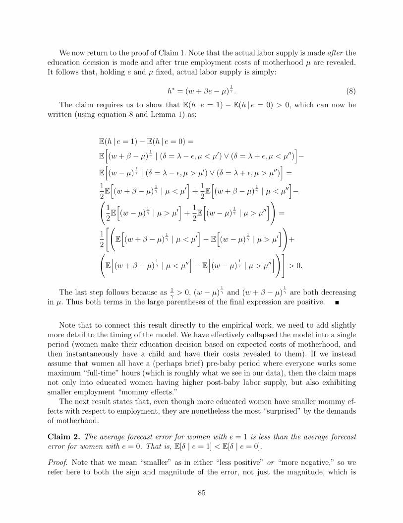
We now return to the proof of Claim 1. Note that the actual labor supply is made after theeducation decision is made and after true employment costs of motherhood µ are revealed.It follows that, holding e and µ fixed, actual labor supply is simply:

h∗ = (w + βe− µ)1γ . (8)

The claim requires us to show that E(h | e = 1) − E(h | e = 0) > 0, which can now bewritten (using equation 8 and Lemma 1) as:

E(h | e = 1)− E(h | e = 0) =

E[(w + β − µ)

1γ | (δ = λ− ε, µ < µ′) ∨ (δ = λ+ ε, µ < µ′′)

]−

E[(w − µ)

1γ | (δ = λ− ε, µ > µ′) ∨ (δ = λ+ ε, µ > µ′′)

]=

1

2E[(w + β − µ)

1γ | µ < µ′

]+

1

2E[(w + β − µ)

1γ | µ < µ′′

]−(

1

2E[(w − µ)

1γ | µ > µ′

]+

1

2E[(w − µ)

1γ | µ > µ′′

])=

1

2

[(E[(w + β − µ)

1γ | µ < µ′

]− E

[(w − µ)

1γ | µ > µ′

])+(

E[(w + β − µ)

1γ | µ < µ′′

]− E

[(w − µ)

1γ | µ > µ′′

])]> 0.

The last step follows because as 1γ> 0, (w − µ)

1γ and (w + β − µ)

1γ are both decreasing

in µ. Thus both terms in the large parentheses of the final expression are positive.

Note that to connect this result directly to the empirical work, we need to add slightlymore detail to the timing of the model. We have effectively collapsed the model into a singleperiod (women make their education decision based on expected costs of motherhood, andthen instantaneously have a child and have their costs revealed to them). If we insteadassume that women all have a (perhaps brief) pre-baby period where everyone works somemaximum “full-time” hours (which is roughly what we see in our data), then the claim mapsnot only into educated women having higher post-baby labor supply, but also exhibitingsmaller employment “mommy effects.”

The next result states that, even though more educated women have smaller mommy ef-fects with respect to employment, they are nonetheless the most “surprised” by the demandsof motherhood.

Claim 2. The average forecast error for women with e = 1 is less than the average forecasterror for women with e = 0. That is, E[δ | e = 1] < E[δ | e = 0].

Proof. Note that we mean “smaller” as in either “less positive” or “more negative,” so werefer here to both the sign and magnitude of the error, not just the magnitude, which is

85

often what is relevant in other forecasting contexts. From the Lemma, we know that e = 1iff event a or event b occurs, where event a corresponds to (δ = λ+ ε) ∧ (µ < µ′′) and eventb corresponds to (δ = λ− ε) ∧ (µ < µ′). Recall that µ and δ are independent.

We can thus write:

E[δ | e = 1] = E[δ | a]P (a)

P (a) + P (b)+ E[δ | b] P (b)

P (a) + P (b)=

(λ+ ε)P (δ = λ+ ε) · P (µ < µ′′)

P (δ = λ+ ε) · P (µ < µ′′) + P (δ = λ− ε) · P (µ < µ′)+

(λ− ε) P (δ = λ− ε) · P (µ < µ′)

P (δ = λ+ ε) · P (µ < µ′′) + P (δ = λ− ε) · P (µ < µ′)=

(λ+ ε)12µ′′

12µ′′ + 1

2µ′

+ (λ− ε)12µ′

12µ′′ + 1

2µ′

=

λ

(µ′′ + µ′

µ′′ + µ′

)+ ε

(µ′′ − µ′

µ′′ + µ′

)= λ+ ε

(µ′′ − µ′

µ′′ + µ′

).

We follow a parallel argument to derive E[δ | e = 0]. Now, e = 0 if either event a′ or b′

occur, where a′ is (δ = λ+ ε) ∧ (µ > µ′′) and b′ is (δ = λ− ε) ∧ (µ > µ′).

E[δ | e = 0] = E[δ | a′] P (a′)

P (a′) + P (b′)+ E[δ | b′] P (b′)

P (a′) + P (b′)=

(λ+ ε)P (δ = λ+ ε) · P (µ > µ′′)

P (δ = λ+ ε) · P (µ > µ′′) + P (δ = λ− ε) · P (µ > µ′)+

(λ− ε) P (δ = λ− ε) · P (µ > µ′)

P (δ = λ+ ε) · P (µ > µ′′) + P (δ = λ− ε) · P (µ > µ′)=

(λ+ ε)12(1− µ′′)

12(1− µ′′) + 1

2(1− µ′)

+ (λ− ε)12(1− µ′)

12(1− µ′′) + 1

2(1− µ′)

=

λ+ ε

(µ′ − µ′′

2− µ′ − µ′′

).

We thus have:

E[δ | e = 1]− E[δ | e = 0] =[λ+ ε

(µ′′ − µ′

µ′′ + µ′

)]−

[λ+ ε

(µ′ − µ′′

2− µ′ − µ′′

)]=

ε

(µ′′ − µ′

µ′′ + µ′

)− ε

(µ′ − µ′′

2− µ′ − µ′′

)< 0,

as µ′′ < µ′ from Lemma 1 and the denominators of both terms in the final line are positive

86

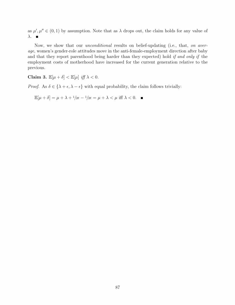
as µ′, µ′′ ∈ (0, 1) by assumption. Note that as λ drops out, the claim holds for any value ofλ.

Now, we show that our unconditional results on belief-updating (i.e., that, on aver-age, women’s gender-role attitudes move in the anti-female-employment direction after babyand that they report parenthood being harder than they expected) hold if and only if theemployment costs of motherhood have increased for the current generation relative to theprevious.

Claim 3. E[µ+ δ] < E[µ] iff λ < 0.

Proof. As δ ∈ {λ+ ε, λ− ε} with equal probability, the claim follows trivially:

E[µ+ δ] = µ+ λ+ 1/2ε− 1/2ε = µ+ λ < µ iff λ < 0.

87

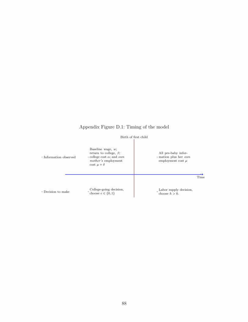
Appendix Figure D.1: Timing of the model

Information observed

Time

Decision to make

Birth of first child

College-going decision,choose e ∈ {0, 1}

Labor supply decision,choose h > 0.

Baseline wage, w;return to college, β;college cost α; and ownmother’s employmentcost µ+ δ

All pre-baby infor-mation plus her ownemployment cost µ

88

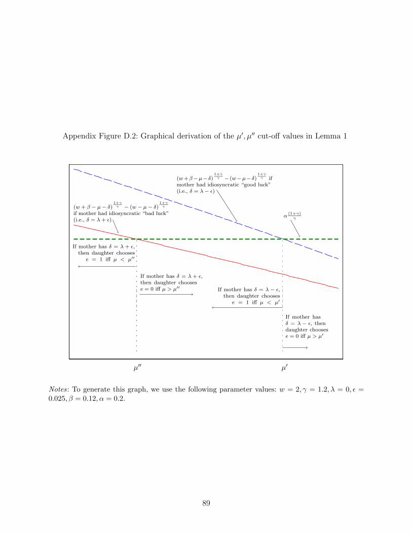
Appendix Figure D.2: Graphical derivation of the µ′, µ′′ cut-off values in Lemma 1

If mother has δ = λ + ε,then daughter chooses

e = 1 iff µ < µ′′

If mother has δ = λ + ε,then daughter choosese = 0 iff µ > µ′′ If mother has δ = λ − ε,

then daughter choosese = 1 iff µ < µ′

If mother hasδ = λ − ε, thendaughter choosese = 0 iff µ > µ′

µ′′ µ′

(w + β − µ− δ)1+γγ − (w − µ− δ)

1+γγ

if mother had idiosyncratic “bad luck”(i.e., δ = λ+ ε)

(w+β−µ− δ)1+γγ − (w−µ− δ)

1+γγ if

mother had idiosyncratic “good luck”(i.e., δ = λ− ε)

α(1+γ)γ

Notes: To generate this graph, we use the following parameter values: w = 2, γ = 1.2, λ = 0, ε =0.025, β = 0.12, α = 0.2.

89