Domain connected graph: the skeleton of a closed 3D shape for animation

Visual Comput (2005)DOI 10.1007/s00371-005-0357-4 O R I G I N A L A R T I C L E

Fu-Che WuWan-Chun MaRung-Huei LiangBing-Yu ChenMing Ouhyoung

Domain connected graph: the skeleton ofa closed 3D shape for animation

Published online: 24 November 2005© Springer-Verlag 2005

F.-C. Wu () · W.-C. MaNational Taiwan University, Taiwanjoyce, [email protected]

R.-H. LiangMing Chuan University, [email protected]

B.-Y. ChenNational Taiwan University, [email protected]

M. OuhyoungNational Taiwan University, [email protected]

Abstract In previous research, threemain approaches have been employedto solve the skeleton extractionproblem: medial axis transform(MAT), generalized potential fieldand decomposition-based methods.These three approaches have beenformulated using three differentconcepts, namely surface variation,inside energy distribution, and theconnectivity of parts. By combiningthe above mentioned concepts, thispaper creates a concise structure torepresent the control skeleton of anarbitrary object.First, an algorithm is proposed todetect the end, connection and jointpoints of an arbitrary 3D object.These three points comprise theskeleton, and are the most importantto consider when describing it. Inorder to maintain the stability of thepoint extraction algorithm, a prong-

feature detection technique anda level iso-surfaces function-basedon the repulsive force field was em-ployed. A neighborhood relationshipinherited from the surface able todescribe the connection relationshipof these positions was then defined.Based on this relationship, theskeleton was finally constructed andnamed domain connected graph(DCG). The DCG not only preservesthe topology information of a 3Dobject, but is also less sensitivethan MAT to the perturbation ofshapes. Moreover, from the results ofcomplicated 3D models, consisting ofthousands of polygons, it is evidentthat the DCG conforms to humanperception.

Keywords Skeleton · Medial axistransform · Domain connected graph

1 Introduction

There are many methods to represent a 3D shape: bound-ary representations (b-rep), constructive solid geometry(CSG), implicit surfaces, and skeletal surfaces, as wellas volume-based, point-based, and parameterization-basedapproaches. According to Pizer et al.’s suggestion [34],the skeletal surface method is a good way to representshape because there are many applications directly re-lated to a skeleton, such as object matching [18], anima-tion [43], collision detection, and mesh editing [26]. Ingeneral, the skeleton-based method embeds local infor-

mation and conforms more directly to human perceptionthan other shape descriptions, and therefore it is suit-able for handling a significant component as a unit. Be-cause of its concise properties, the skeleton-based methodis more efficient than other representations in computa-tion [34].

However, the requirements for a skeleton differ witheach application. For example, object matching may re-quire skeletons to preserve principal features such asmorphology (e.g. branching and termination) and geo-metrical information. Therefore, these skeletons can beregarded as major keys and then used to find similaritiesamong objects [18]. On the other hand, object recon-

F.-C. Wu et al.

struction requires a kind of skeleton that can reconstructthe complete geometrical information of the original sur-face [16]. The requirements must address the specificneeds of various applications. When comparing almostidentical shapes with only minor differences, it is ac-ceptable to have the same skeleton; however, for surfacerepresentations, two different shapes require two differentskeletons.

Although skeleton related applications have attracteda great deal of attention, it is not easy to extract a skeletonfrom an arbitrary shape that is at once robust, mean-ingful and manageable. Extracting a skeleton from a 3Dobject is more difficult than from a 2D object [46]. More-over, when handling different kinds of source models,such as non-manifold models, models containing holes,or models consisting of many parts, many problems areencountered. Since providing this method for all kindsof models is not the major focus of this research, a pre-process procedure was used to convert the input modelsinto 2-manifold meshes without boundaries, consistingof anywhere from thousands to tens of thousands ofpolygons.

MAT is made from maximal contact spheres (or disks),found both inside and outside the object or the outline.A MAT consists of many spheres with different radii, usedto encode an object. Consequently, if the curvature of theobject surface varies, MAT needs to describe this vari-ation precisely to produce numerous links for its skele-ton. By definition, MAT is sensitive to the variation ofboundaries, or noise on its boundaries [10]. Amenta etal. [1] go into in more detail; small perturbations in anobject’s boundary can induce large features in the medialaxis. Some parts, however, of the medial axis are unsta-ble, while other parts, corresponding to significant ob-ject features impervious to noise, are quite stable. A MATskeleton consists of medial surfaces, curves and lines. Itis a complex structure that is hard to handle as a con-trol skeleton. The purpose of this research is to pro-vide a skeleton that is suitable for further manipulation,such as skeleton-driven deformation [9]. In the opinionof the authors, certain properties must first be taken intoconsideration.

– SimplicityBecause the extracted skeleton is desired for use in ani-mation as a control skeleton, it must be simple and easyto control.

– StabilityTwo similar shapes should have two similar skeletons.If the shape of two objects only varies slightly, theirskeletal structures should remain almost exactly thesame.

– MeaningfulnessThe skeleton will be simplified to consist of only majorprong parts without completely representing the detailsof a shape, such as width, surface noises, etc. Based on

Fig. 1. Three main point types in a DCG skeleton: joint point, endpoint, and connection point

Kimia’s paper [22], the medial axis plays a major rolewithin the human visual system. Therefore, a skeletonthat conforms to human perception is preferred.

– NeutralityBecause the authors want to bind the surface to theskeleton so that it can be distorted in any direction, theskeleton needs to be located at the medial axis. Hence,it is less biased around its surrounding surface.

– HierarchicalEach part in the skeleton has a different priority. Ac-cording to the priority of each node in the skeleton, theskeleton’s hierarchical properties can be applied to theproblems of progressive refinement in transmission orof level-of details (LODs).

The main idea of DCG is to represent a skeleton witha few linked points: a minimal number of points are se-lected to cover the whole surface, which is similar to theprocess of decomposition, where each part is representedas a meaningful unit in an object. Based on this idea,a main part is represented by a joint point, a prong part ismodeled by an end point, and a variation on the skeleton isdescribed by a connection point. This approach, illustratedin Fig. 1, is an intuitive concept, and has been explored inthe past [3, 5, 24, 39]. As well, the DCG skeletons of prim-itive models are shown in Fig. 2.

Fig. 2a–f. The DCG skeleton of primitive models: a Cube; b brick;c Tetrahedron; d pyramid; e sphere; f cylinder

Domain connected graph: the skeleton of a closed 3D shape for animation

2 Related work

Previous work regarding skeleton extraction can be di-vided into three categories: MAT, generalized poten-tial field, and decomposition-based approaches. Thesemethods define different types of skeletons, and havebeen combined to construct a novel representation thatavoids their respective disadvantages. In an abstract sense,MAT focuses on shape variation. Therefore, it is suit-able for depicting the details of the surface, and canbe used to construct a preliminary model at the initialstage.

Since MAT is the basic definition of a skeleton, othermethods also share the features of MAT. The potentialfield method focuses on the volume of an object, so itcan be utilized to evaluate where a skeleton point wouldbe suitable. The decomposition process can divide an ob-ject into many parts connected via linked points, andthus, a small number of meaningful connection pointscan be chosen to describe the variation of the skele-ton.

2.1 Medial axis transform

The MAT-based skeleton is a kind of reduced representa-tion, and provides region-based shape features. Since itssymmetrical properties are derived from its surface, it issuitable for reconstructing the original shape [44].

It is common to use Voronoi diagrams to construct theMAT skeleton of a 2D shape [29, 32]. Since the skeletonextracted by a Voronoi diagram contains many undesirablelinks, methods for pruning and reducing bifurcation havebeen proposed to solve these problems [7, 12, 27]. Choiand Seidel [11] haave suggested a MAT pruning methodwhereby the one-sided Hausdorff distance of MAT isbounded, with respect to the boundary perturbation. Og-niewicz [31] proposes a residual function to measure thesignificance of skeleton edges. Attali and Montanvert [2]have shown that noises on the boundary can be mod-eled by a parameter graph, suggesting that noisy skeletonbranches can possibly be characterized by a small maxi-mal separation angle or thickness.

Sheehy et al. [36] have proposed an algorithm based onthe domain Delaunay triangulation of a relatively sparsedistribution of points, in order to construct the medial sur-face. After employing the Delaunay triangulation process,an adaptive refinement strategy is adopted to assemblethe topology of the medial surface using a traversal of theclassified tetrahedra in the triangulation.

Amenta et al. [1] have proposed the “power crust”algorithm for MAT approximation and 3D surface re-construction. First, a Voronoi diagram is constructed.Then, a subset of Voronoi vertices are selected as poles.A weighted Voronoi diagram is then constructed fromthese poles and named the power diagram. These poles aresubsequently labeled either inside or outside. The faces

of the power diagram separating the cells of inside andoutside poles constitute the power crust. The regular tri-angulation faces connecting the inside poles make up thepower shape.

Tam and Heidrich [41] have proposed an approach forMAT that removes unwanted artifacts while preservingfine features. Their method prunes the axis by using anintuitive global threshold base on noise size, and then au-tomatically reconstructs the fine features by extending theremaining branches.

Leymarie et al. [24] have proposed that the shock scaf-fold is, in fact, a hierarchical and summarized organizationof the 3D medial axis, in the form of a graph representa-tion. The shock scaffold is represented as a directed graph,where the medial points are the nodes in the structure, andthe medial curves the links. The medial sheets are thenrepresented by hyperlinks.

2.2 Generalized potential field

Another skeleton extraction approach is to use a distancefield. In order to construct a distance field and extract theskeleton, voxel-based methods are frequently used. Thebasic methodology consists of constructing the distancefield of an arbitrary object and then finding the local maxi-mums of said distance field. The skeleton is then generatedby connecting these local maxima. A skeleton based onthese approaches is generally simpler than ones generatedusing MAT, since MAT-based approaches usually includea thinning or shrinking process. They focus on where themost important part inside an object is, and in doing so,ignore the shape variation. Thus, the “thinning” is done atthe cost of approximation, resulting in a non-unique skele-tal representation. The problem of how to determine thepoint that indicates the end of a skeleton is, however, onethat needs to be solved.

In 2D cases, Leymarie and Levine [25] implemented a2D MAT (or grassfire transformation) by minimizing thedistance field energy of an active contour model, the ini-tial position of which is at the boundary of a given shape.Grigorishin et al. [17] have proposed using an electrostaticfield to depict the inside energy, where select corner pointsare chosen on the boundary as starting points, used to trackthe skeleton path. Zhu [48] has proposed a stochastic al-gorithm to compute a skeleton in two phases. The firstphase is to find some line segments in favor of parallelismand symmetry; the second phase of the process computesthe axes and junctions. Siddiqi et al. [39] propose a shockgraph, whereby structural descriptions are derived fromthe singularities of a curved evolution process that acts onbounding contours.

Moreover, Borgefors et al. [8] have proposed a volumethinning approach when computing a skeleton for voxel-based approaches. This skeletonization method is per-formed in two major steps. The first step reduces the ob-ject to a surface skeleton. The second reduces the surface

F.-C. Wu et al.

skeleton to a curve skeleton. Zhou and Toga [47] have pro-posed a voxel-coding method, which performs a recursivevoxel-by-voxel propagation, and then generates the skele-ton by using the Euclid and geodesic distance fields of anobject. Bitter et al. [4] have proposed extracting a skeletonusing volumetric data generated by a penalized-distancealgorithm. Based on the distance field, the algorithm findsthe furthest voxels as the centerline, which in turn formsthe initial skeleton. The skeleton is then refined recur-sively by discarding voxels near the centerline. Wade andParent [43] also present an automated algorithm for gen-erating a control skeleton based on voxel data, in whichthey use a thinning process, generated from the voxel data,to get their preliminary result. First, a central point is se-lected from this result as a root point, and then, the furthestpoint is found iteratively to represent the end point. Fi-nally, a control skeleton is formed by constructing a linkbetween this point and the root point.

In addition to utilizing voxel data, some approachesthat focus on the extraction of a skeleton directly froma boundary also exist. Sherbrooke et al. [37] and Cul-ver et al. [14] have proposed an approach that first findsa seam and designates it to be the starting point, thensearches for the path of the medial axis. Chung et al. [13]assume that each face of a polygonal object producesa force field; each point on the boundary is pushed bythis force field, which finally converges to a balanced pos-ition. This position is then labeled as a potential skeleton.In the end, all of these potential skeletons are connectedto produce the main skeleton. Siddiqi et al. [38] proposethe Hamilton–Jacobi skeleton method, which can obtainthe internal medial axis of an object, given its bound-ing curve or surface, by simulating the grassfire flow asa Hamilton–Jacobi equation using the Euclidean distancefunction. Li et al. [26] directly simplified the object meshto get the skeleton. Based on the idea of edge contrac-tion, their process iterates until all triangles have collapsedinto edges or vertices. In other words, they are left withonly skeletal edges, whose union is the skeleton of themesh.

In previous work [28], the authors proposed a thinning-like process that uses a radial basis function as the distancefunction in order to thin the surface of the object sur-face of the object, thus forming the skeleton. The resultsshown in Fig. 3 are similar to the current approach. How-ever, the previous approach was not stable in some casessuch as the ‘donut-like” model, since there is no guar-antee of constructing a radial basis function that keepsthe monotonically increasing property well inside anobject.

2.3 Decomposition-based method

This type of method has received much attention recently.It extracts a one-dimensional skeleton based on the Reebgraph. The idea of the Reeb graph is to use a continuous

Fig. 3. Previous results based on radial basis functions

function, usually a height function, to describe the topo-logical structure and to reveal the topological changes,such as merging or splitting. Based on a continuous func-tion, the target object can be divided into many parts.Connecting the center position of all parts forms the mainskeleton [40]. However, it can easily be seen that usinga height function to construct the Reeb graph does notguarantee the result to be Euclidean-invariant, which isvery important in shape analysis.

Since different functions may generate different Reebgraphs, Lazarus and Verroust [23, 42] replaced the heightfunction with the geodesic distance function, which is cal-culated by the Dijkstra algorithm; the generated skeletonis called a “level set diagram” (LSD). Unfortunately, LSDdepends on the selection of its source points. This resultsin the possibility of different LSDs being produced fromthe same model. Mortara and Patane [30] chose sourcepoints in high curvature regions to guarantee results thatare Euclidean-invariant. Hilaga et al. [18] proposed a tech-nique called “topology matching” that compares the mul-tiresolutional Reeb graphs (MRGs) of 3D objects in orderto evaluate their similarities.

Katz and Tal [20] introduce an angular distance tomeasure shape variation, in order to identify a mean-ingful part. This approach, however, is not suitable fora “donut-like” shape. Biasotti [3] proposed creating an ex-tended Reeb graph (ERG) by using a slicing strategy froma height map. With the extraction and classification of in-fluence zones of critical points, the set of nodes of theERG is completely defined. Each node codes the label ofthe critical area and its boundary components; thus, it is anabstract topological description.


Fig. 4. Different stages in skeleton generation algorithm

3 Overview

The goal of this research is to find a concise skeleton thatis suitable for editing the model and generating an ani-mation object. To avoid the complex structure of a MATskeleton, the skeleton was designed to be composed ofa set of important points with linkages. There are threemain stages for constructing a control skeleton.

– Feature detection: This initial procedure detectswhere the skeletal points of a 3D model can be suitablyrepresented.

– Connection construction:To preserve the topology relationship of the originalmesh, the neighborhood relationship of each featurepoint is inherited from surface edge connectivity.

– Re-mapping for shape variation:The variation of shape cannot be suitably described bytwo feature points connected by a straight line. There-fore, a repulsive force field is introduced to force theskeletal path to follow the shape’s varied form.

When discriminating a representative or small featurein 3D shape, it is not easy to find an absolute crite-rion. Based on experiments, a prong-feature detection al-gorithm was developed to discern where the significationfeatures are. All other features in the shape, assumed to benoise, were ignored. Next, a skeleton structure was con-structed to connect these signification features, therebyforming the main/principal skeleton.

To select the most important feature points as thedomain points, a procedure was developed to evaluatewhich parts constitute suitable end features, connec-tion features, and joint features. Figure 4 shows differ-ent stages in the algorithm. The input model is shownin Fig. 4(a). A Voronoi diagram was then constructedto locate initialized candidates (Fig. 4(b)). Domain ballswere first extracted (Fig. 4(c)). An end feature is locallyfar from the main part: a geodesic distance is meas-ured on the surface, and then a watershed algorithmis applied to detect where an “end feature” is located(Fig. 4(d))[45]. Then, a visibility repulsive force field isintroduced, and all other features except the “end features”are adjusted to the local minima that constitute “con-nection points” (Fig. 4(e)). Following this, a neighbor-

hood relationship from mesh connectivity is determined(Fig. 4(f)); a point that has more than two connectionlinkages is a labeled as a “joint point”. Finally, a snakealgorithm based on the repulsive force field is applied,and all linkages are adjusted to fit the shape variation(Fig. 4(g)).

In the following excerpt, the repulsive force field willfirst be introduced. Based on this force field, the positionwhere a skeleton is suitable to be located can be evalu-ated. Since an accurate computation of this field is time-consuming, in order to reduce the complexity of the task,only a few candidates are selected. In the initial stage, theVonoroi diagram is introduced to locate these candidates.Next, a prong-feature detection algorithm is presented. Fi-nally, the method of constructing the connection to assem-ble the final skeleton is described.

4 Repulsive force field

Since it is necessary to identify the most important partinside a shape, a generalized potential field based on thelevel iso-surface function is introduced. The concept of thelevel iso-surface function is shown in Fig. 5.

Assume that shape S is defined on space Ω. A iso-surface function f based on the shape S can partitionthe space into f(x) < 0, f(x) = 0, and f(x) > 0 to rep-resent outside the shape, the boundary of the shape,and inside the shape, respectively [35]. Since we areonly concerned with the level property of the poten-tial field inside the shape, the function is defined asfollows. A level iso-surface function is a distance func-tion on a space Ω. If such function f : R3 → R is de-fined on the space Ω, all points on the boundary have

Fig. 5. The level iso-surface func-tion

F.-C. Wu et al.

maximal values. Moreover, a location near the bound-ary has a higher value. For example, let d be the inverseof a shortest distance function, it satisfies the followingproperties:

1. If p ∈ S, ∀q ∈ S → d(p) > d(q), where S is the interiorof S.

2. If p and q are two points inside a shape S, ‖p‖ <‖q‖ → d(p) > d(q), where ‖p‖ is the shortest distancefrom position p to the boundary.The balanced positions of the function d are the can-

didates of MAT, which consist of some faces and lines.Since the shortest distance is determined based on onlyone position on the boundary, the result is unstable andsensitive to noise. We want to construct a function that hasonly one global minimal point in a convex shape. Thus,a repulsive force field is defined as F(x) = ∫ r

rn dθ, wherer is the distance from x to the boundary in the direction r,and a discrete form is

F(p) =∑

0≤α<2π;0≤β<π

uα,β

‖p‖n ,

where uα,β is a unit sample ray, and α and β are anglesin the spherical coordinate. A level iso-surface functionf(x) can be defined as ‖F(x)‖. When n → ∞, the repul-sive force field is dominated by the shortest distance, andthus f(x) ∝ d(x). In some sense, n is a term for a smooth-ing effect. Each position receives more boundary influencefor a smaller n. As shown in Fig. 6, the inner level of theiso-surface function is smoother with a smaller n. In ourimplementation, we adopt n = 1.

Fig. 6. The different n effects on the level iso-surface function forn = 100, 1, and 0.01, respectively

5 Initial stage

In this section, some internal points on the skeleton thatrepresent or correspond to a wide surface portion aresought out. Points on the MAT are good starting points,since they lie on the symmetry axis of the shape. It isintuitive to locate the medial axis by using the Voronoidiagram [1]. The regions separated by the Voronoi dia-grams are called Voronoi cells. For 2D points, the cellsare convex polygons; for 3D points, the cells are convex

polyhedra. Each face of a cell is equidistant between twopoints in a discrete set. Thus, a set of points on these faceslies roughly along the medial axis [19]. Bradshaw andO’Sullivan [6] have presented a sphere-trees constructionalgorithm to perform efficient collision handling. The firstpart of the algorithm ensures that a set of medial spherescovers the object’s surface. The second phase of the adap-tive algorithm is to improve the current approximation byadding more sample points. Based on Bradshaw’s imple-mentation, these Voronoi nodes are selected to be initialcandidates. For constructing the Voronoi diagram, a setof sample points are constructed on an object’s surface.After constructing the Voronoi diagram, each node findsits shortest distance to the boundary as its radius to forma Voronoi ball.

However, the node directly extracted from the Voronoidiagram left in this form remains too complex. For thepurpose of stability, the effects of small variations on theshape need to be removed. There are many works that ad-dress this problem in 2D [11, 15]. Based on their ideas,the solution can be divided into two main concepts: oneis to ignore small variations on the surface; the other is tofind the principal data from the noise of the preliminaryresults. Using the former concept, Choi [11] developeda one-sided stability theory that enlarges the range of cov-erage of each skeletal point. In this way, small variationson the shape can be ignored. In the latter concept, Fos-key [15] defines a θ-simplified medial axis based on theseparation angle to extract the principal part from theMAT.

In our experience, a detailed skeleton composed ofmany points is usually affected by noise or by small vari-ations of the surface; on the other hand, a rough skeleton(composed by few points) can be too loose to representsignificant features. To avoid the noise effect, in this ap-proach, only the important feature points in the first stagewere kept. Then other necessary points were iteratively re-covered in order to preserve the variation of the originalshape. Good feature points were located at the axial pos-ition and the noise effect on the surface was ignored.

Since larger radius means more range of coverage,a priority sequence of Voronoi balls under shape S can bedefined, and each Voronoi ball labeled by the followingnumerical sequence. Let Bi be a Voronoi ball, with radiusρi . If ρ1 > ρ2 > · · · > ρn > · · · , then B1, B2, · · · Bn, · · · isa domain sequence.

Definition 1 (The domain ball). Let B1, B2, · · · Bn, · · ·be a domain sequence. The domain ball can be definedby inserting a Voronoi ball iteratively, based on sequentialpriority, and retaining its non-intersecting status. BD =Bi |

n⋂

i=1Bi = ∅, where n is the maximal number .

After calculating the radii of all the Voronoi balls,some were chosen iteratively, based on the magnitude


of their radii. Once a maximal ball is chosen, it willdelete all neighboring balls that could possibly touch it.In order to decrease the number of balls, a minimal dis-tance constraint between each ball was also introduced.Figure 7 shows the result of the domain balls. Althoughnot a unique a representation of the shape, calculations canbe based on these initial candidates to obtain a final result.

Fig. 7. The domain balls for a 3Dmodel in the shape of the digit eight

6 Prong-feature detection

Since a prong-feature may indicate the existence ofa main skeleton, a prong-feature detection algorithm ispresented [45]. First, a normalized scale function is con-structed on the input mesh to describe the position ofa potential prong. The scale function is then calculatedusing the sum of the geodesic distance from each vertexamong the mesh to the evaluated vertex [23]. To ensurethat the calculation of the geodesic distance approximatesthe real value, a remesh pre-process is required.The scalefunction is defined in the following equation:

f(v) =∑

∀vi∈S

geodesic(v, vi),

where v is the vertex on the shape S. The results are asfollows (Fig. 8).

In order to find these prong features, a watershed al-gorithm is applied. First, all vertices are sorted by scalefunction value. Then, the maximum value of the vertexis picked up as the first prong feature and marked as tra-versed. As feature detection must be focused upon, thewater level decreases iteratively from a maximum value.To understand how the watershed algorithm is applied tothe mesh data with greater ease, the mesh data is repre-sented in a parameterization form to describe the mappingrelationship between the 3D and 2D cases. As viewedin Fig. 9, the left side illustrates a model after calculat-ing its scale function based on its geodesic distance. Theright side shows a parameterization: the mapping of the3D mesh into a 2D map. The black line indicates the mesh

Fig. 8. From the scale function, a higher value indicates a prongfeature denoted by the color green

Fig. 9. The mesh data in a parameterization form

on the 3D model. From this image, five green dots can beseen. These are the highest values among the mesh, andare also the prong features to be detected.

In Fig. 10, decreasing water levels are shown, in orderto detect the local maximum. The function value is rep-resented by the height. There are five local maxima that

Fig. 10. The local maximum of a continue function is detected bythe watershed algorithm

F.-C. Wu et al.

must be detected. The green mask represents the waterlevel, which iteratively decreases. The new prong featurewill be detected if it is not connected with the traversedregion. Initially, the water level is set up to start at thehighest value and then to decrease incrementally. If thewater level decreases rapidly, as might possibly happenin this case, two prong features will become one. Thus,the decreasing levels of water affects the sensitivity ofa prong feature. The prong shape’s valley value, dividedby its peak value, is defined as the smoothness ratio. Ifthe smoothness ratio is larger than the threshold, the resultwill be a small prong, and will be ignored. Each non-traversed vertex in the sorting sequence will reset the wa-ter level, i.e. its function value is multiplied by the smooth-ness ratio. Consequently, all vertices can be marked astraversed if their function value is above the water leveland if they are a neighbor of the traversed set. If the ver-tex is not in the traversed set, it is a new prong feature.Thus, the nearest domain point to a prong feature is anend point.

An algorithm has been presented in order to detectthe prong-features on a 3D mesh. The procedure includesa ratio for smoothness that can be adjusted to suit differentapplications. According to the experiences of the authors,for most models, setting the smoothness ratio to 0.85 wasfound to be suitable for detecting significant prong fea-tures.

7 Connection construction

In the previous section, the domain balls and end pointswere constructed. All domain points except end points arecandidates in need of refinement. The refining process isbased on the repulsive force field. For each point pi , weuse the repulsive force to push it to a new position pi+1:

pi+1 = pi + F(pi)× step.

The iterative process stops when the position reachesa local minimum ‖F(pi)‖ < ‖F(pi+1)‖. To describe theshrinking process, Fig. 12(a) shows that a point under therepulsive force field moves from the boundary and shrinksinto the local minima. The shrinking paths are representedby the red lines. Because the shape contains two areas,

Fig. 11a–c. The results are shown in different decreasing levels.a Fifteen features are detected when the smoothness ratio is set to1.0. b Six features are detected when the smoothness ratio is set to0.85. c A skeleton is constructed based on these prong features

Fig. 12a,b. A point receives the repulsive force from the boundary.a, b are 2D and 3D cases, respectively

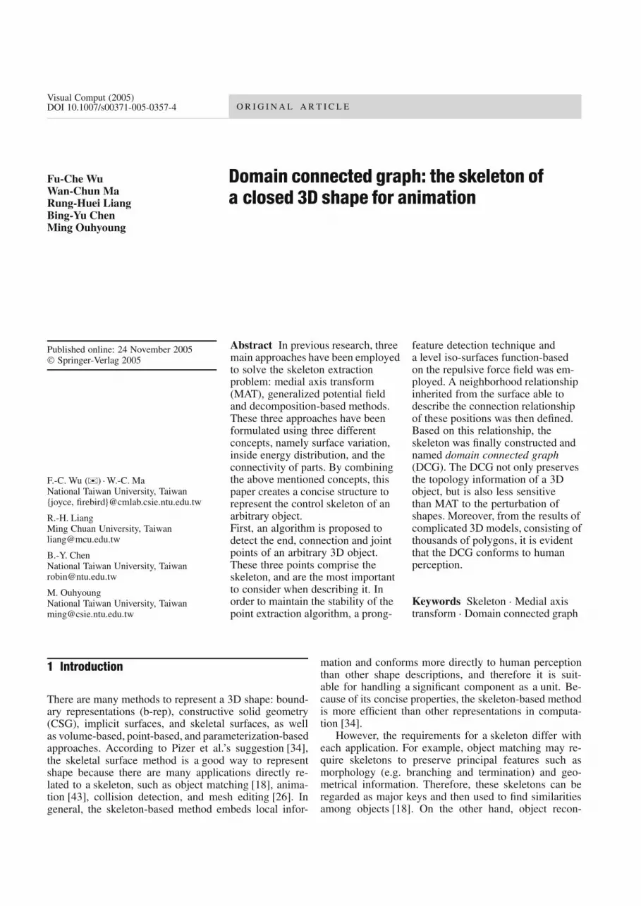
there are two local minima inside which are representedby the blue circles. Due to the numerical inaccuracy of thestep, not all the points will stop at an exact position. Inpractice, all intermediate points will converge to a locationwithin a small range, which depends on the iterative step.To solve this problem simply, without substantial loss,these final positions are merged in a given range to obtaina single domain point, which is regarded as a connectionpoint. Figure 13(b) shows the shrinking process. However,a connection point is an intermediate point to help recoverthe whole topological information. Each point representsa local part.

A joint feature potentially connects more than twoskeletal linkages. The topology relationship needs to be


Fig. 13. The domain points are shrunk under the repulsive forcefield to form the connection points (larger blue balls)

recovered to show how things are connected. To recoverthe connectivity of domain points, the relationship be-tween surface and domain points first needs to be deter-mined. Thus, based on the connectivity of the surface, theconnectivity of domain points can be induced.

Definition 2 (Face connectivity). Connectivity is a neigh-borhood relation denoted as ⇔

c. If two faces share an

edge, the two faces have connectivity. Let a face A bebounded with some boundary edges ∂A. Thus, for twofaces Ai, Aj , if ∂Ai ∩∂Aj = ∅ → Ai ⇔

cAj .

Definition 3 (Domain surface). DS is defined as a sur-face region belonging to a domain point DP. Each do-main point has a domain surface that can be described bythis point. A domain point can find at least one shortestdistance of point on the surface. A face that contains thispoint is called a primitive visible face denoted by Apv.1. Apv ∈ DS(p).2. Let Ai ⇔

cAj and Aj ∈ DS(p), then, Ai ∈ DS(p) if and

only if ∀q ∈ DP, ‖Ai p‖ < ‖Aiq‖.

Definition 4 (Domain point connectivity). Let DS(p),DS(q) be represented as the domain surface of domainpoint p, q, respectively. If ∃Ai ⇔

cAj, Ai ∈ DS(p), Aj ∈

DS(q) → p ⇔c

q.

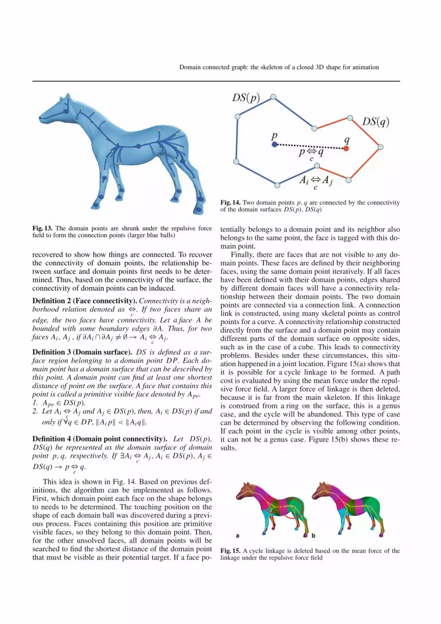
This idea is shown in Fig. 14. Based on previous def-initions, the algorithm can be implemented as follows.First, which domain point each face on the shape belongsto needs to be determined. The touching position on theshape of each domain ball was discovered during a previ-ous process. Faces containing this position are primitivevisible faces, so they belong to this domain point. Then,for the other unsolved faces, all domain points will besearched to find the shortest distance of the domain pointthat must be visible as their potential target. If a face po-

Fig. 14. Two domain points p, q are connected by the connectivityof the domain surfaces DS(p), DS(q)

tentially belongs to a domain point and its neighbor alsobelongs to the same point, the face is tagged with this do-main point.

Finally, there are faces that are not visible to any do-main points. These faces are defined by their neighboringfaces, using the same domain point iteratively. If all faceshave been defined with their domain points, edges sharedby different domain faces will have a connectivity rela-tionship between their domain points. The two domainpoints are connected via a connection link. A connectionlink is constructed, using many skeletal points as controlpoints for a curve. A connectivity relationship constructeddirectly from the surface and a domain point may containdifferent parts of the domain surface on opposite sides,such as in the case of a cube. This leads to connectivityproblems. Besides under these circumstances, this situ-ation happened in a joint location. Figure 15(a) shows thatit is possible for a cycle linkage to be formed. A pathcost is evaluated by using the mean force under the repul-sive force field. A larger force of linkage is then deleted,because it is far from the main skeleton. If this linkageis construed from a ring on the surface, this is a genuscase, and the cycle will be abandoned. This type of casecan be determined by observing the following condition.If each point in the cycle is visible among other points,it can not be a genus case. Figure 15(b) shows these re-sults.

Fig. 15. A cycle linkage is deleted based on the mean force of thelinkage under the repulsive force field

F.-C. Wu et al.

From the previous definition, the connectivity of thedomain point is inherited from the connectivity of thedomain surface. After constructing the connectivity re-lationship among domain points, a connectivity countingfunction C(DP) can be defined to report how many con-nectivity relationships each domain point contains. Thejoint point is defined as J = DP|C(DP) > 2.

Now the geodesic distance function, end points, andjoint points have been found. The re-mapping process willbe described in greater detail in the following section.

8 Re-mapping

To describe the variation of the shape faithfully, a re-mapping procedure on these skeletal points among a link-age is required. Additionally, such a procedure must beused to ensure the links are within the object’s field.

Lemma 1 (Skeletal point). Let P = x|n · x = c be a cut-ting plane, where n is the normal, c is the distance fromthe origin to the plane. A cutting plane can divide an ob-ject into two parts. Each part contains one domain point.Thus, the cutting plane contains at least one skeletal point.SP = p|p = fmin(p) , n · p = c, where fmin is an evalua-tion function to determine where the placement of a skele-tal point is suitable on the cutting plane

For two parts to be connected in a shape there must bea skeletal point to connect them. The location of a skele-tal point is determined by its local shape attributes, such asscale and connectivity [33]. The scale relates to geometryto obtain correct skeletonization. The connectivity relatesto the topology, and concerns itself with how things areconnected. If two domain points have a connectivity rela-tionship, there is a link between these two points. Initialpoints can be generated to represent this link. To beginwith, selected points are sampled along a straight line torepresent a connection link. Here, a snake [21] algorithm(active contour model) is invoked to adjust these points so

Fig. 16. The model is represented by the geodesic distance func-tion. A purple ball indicates a joint point. A red ball indicates anend point

that they correspond to a skeletal curve. An active contourmodel is generated by adjusting a contour to minimize anenergy function:

Esnake = Einternal + Eexternal,

where Einternal and Eexternal are the internal and ex-ternal energy, respectively. The internal energy is the partthat depends on the intrinsic properties of the link, such aslength or curvature. Eexternal means external energy, andits value depends on the generalized potential field. Theposition of each point is adjusted on the constrained plane,which is perpendicular to the original straight line. Whenthe energy of the active contour model is minimized, theresulting skeleton is obtained. Figure 17 shows the defor-mation process of a connection link.

Fig. 17. The deformation process of a link, where the green pointsbetween two red points (end point and joint point) are pushed bythe generalized force field to the final position

9 Results

Figure 19 shows the DCG of nine typical 3D models,and Table 1 shows the execution times for the differentstages. The timing statistics were obtained using an In-tel Pentium-M 1 GHz processor notebook PC with a 512Mbytes memory. In the time statistics, the watershed al-gorithm is not listed, because in this step, its operator isonly to check the function value of each vertex, and thus,its computation time is less than a second. Currently, there-mapping procedure consumes the most CPU time, andthe working process takes has not yet been optimized.

Our algorithm includes four main parts, as follows.(1) Computation of the Voronoi diagram. (2) Geodesicdistance on the mesh. (3) Watershed on the surface (endfeature detection). (4) Snake algorithm on 3D potentialfield. For n vertices of a model, the computation complex-ity of algorithm steps (1), (2) and (3) are O(n2). Thus,


Fig. 18. Using the project’s results,an animation sequence is producedfrom Maya

Table 1. Execution time statistics for nine 3D models on a Pentium-M 1 GHz notebook PC

Model Face number Voronoi diagram Geodesic distance Connection construction Re-mapping(min.:sec.) (min.:sec.) (min.:sec.) (min.:sec.)

dragon 7315 00:56 00:13 01:43 05:16eight 1536 00:06 00:05 00:12 00:54

octopus 8648 01:06 00:45 05:28 13:01dinosaur 5605 00:33 00:22 01:29 03:24bunny 6343 00:27 00:14 06:14 15:01hand 9936 01:33 00:25 03:04 27:01rhino 7678 01:06 00:26 02:09 07:43

cheetah 5345 00:33 00:15 01:14 03:19rabbit 2174 00:11 00:10 00:24 02:27

this process is not feasible for a large model. The complex-ity of the snake algorithm is not easy to determine fromthe vertex number. It is based on the shape variation andthe number of skeletal points. However, for efficiency andconvergency, we limit the iterative loop of the optimiza-tion process to no more than one hundred times. The resultis acceptable. To avoid long computation times, the ori-ginal models have been simplified first into any number ofpolygons, from one to ten thousand. Figures 20, 21, 22, 23show more results. Their skeleton data in Maya format areavailable at: http://graphics.csie.ntu.edu.tw/DCG/.

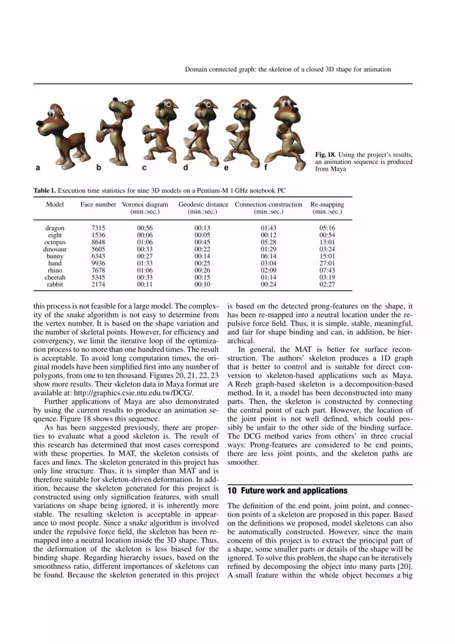
Further applications of Maya are also demonstratedby using the current results to produce an animation se-quence. Figure 18 shows this sequence.

As has been suggested previously, there are proper-ties to evaluate what a good skeleton is. The result ofthis research has determined that most cases correspondwith these properties. In MAT, the skeleton consists offaces and lines. The skeleton generated in this project hasonly line structure. Thus, it is simpler than MAT and istherefore suitable for skeleton-driven deformation. In add-ition, because the skeleton generated for this project isconstructed using only signification features, with smallvariations on shape being ignored, it is inherently morestable. The resulting skeleton is acceptable in appear-ance to most people. Since a snake algorithm is involvedunder the repulsive force field, the skeleton has been re-mapped into a neutral location inside the 3D shape. Thus,the deformation of the skeleton is less biased for thebinding shape. Regarding hierarchy issues, based on thesmoothness ratio, different importances of skeletons canbe found. Because the skeleton generated in this project

is based on the detected prong-features on the shape, ithas been re-mapped into a neutral location under the re-pulsive force field. Thus, it is simple, stable, meaningful,and fair for shape binding and can, in addition, be hier-archical.

In general, the MAT is better for surface recon-struction. The authors’ skeleton produces a 1D graphthat is better to control and is suitable for direct con-version to skeleton-based applications such as Maya.A Reeb graph-based skeleton is a decomposition-basedmethod. In it, a model has been deconstructed into manyparts. Then, the skeleton is constructed by connectingthe central point of each part. However, the location ofthe joint point is not well defined, which could pos-sibly be unfair to the other side of the binding surface.The DCG method varies from others’ in three crucialways: Prong-features are considered to be end points,there are less joint points, and the skeleton paths aresmoother.

10 Future work and applications

The definition of the end point, joint point, and connec-tion points of a skeleton are proposed in this paper. Basedon the definitions we proposed, model skeletons can alsobe automatically constructed. However, since the mainconcern of this project is to extract the principal part ofa shape, some smaller parts or details of the shape will beignored. To solve this problem, the shape can be iterativelyrefined by decomposing the object into many parts [20].A small feature within the whole object becomes a big

F.-C. Wu et al.

Fig. 19. Results from different kinds of models. For performance consideration, the models have been simplified. The number of faces areunder ten thousand


Fig. 20. More results with skeleton data are available at http://www.cmlab.csie.ntu.edu.tw/cml/g/DCG/

F.-C. Wu et al.

Fig. 21. Results


Fig. 22. Results

F.-C. Wu et al.

Fig. 23. Results


feature when a sub-part is scaled into a unit. The decom-position process cuts an object with a cutting plane. On thecutting plane, a connection point can be found in order toconnect the two parts. Thus, a decomposed part must havea connection point on its shape to connect to the originalskeleton.

Based on current results, each meaningful part is ex-tracted and represented as a concise form. This research issuitable for many applications. In animation, each domainpoint is an easily controllable point. In object matching,the resulting skeleton could be a primary key for compar-ing the similarity of 3D objects [18]. However, it is onlysuitable for comparing the similarity of the skeletal struc-ture, and not for extracting the exact object. In mesh edit-ing, each domain surface can be handled as a unit. In meshcompression, residual between domain point and its de-scribed surface is small and the connectivity relationshipis simple, making efficient compression very possible.Furthermore, the level of detail and a progressive displayare also possible, based on the resulting skeleton of thisresearch. In some applications, if a very concise form isnot needed, connecting the domain balls at the first stagewill quickly generate a prototype. Finally, for symmetri-cal shapes such as hands and legs, because their skeletonsare calculated individually, they may not be exactly sym-metrical. The symmetrical properties of a skeleton are,however, an issue worthy of exploration in the future.

11 Conclusions

In this paper, a concise representation of the skeleton ofan arbitrary shape is proposed. The nodes of the graph are

named domain points (significant points inside the shape),which can represent the local properties of a shape. Thedomain points are classified into three categories: jointpoints, end points, and connection points. In this paper,the concept and the definition of the DCG was introduced.Moreover, using an algorithm to generate the graph hasbeen proposed, and as well, the differences between theDCG skeleton and the traditional MAT skeleton are de-scribed, explaining the advantages of the DCG. Given anarbitrary 3D shape, the proposed skeletonization methodcan extract both topological and geometrical information.The resulting skeleton can converge in limited computa-tional time and is completely inside the boundary of a 3Dshape. This is a concise, stable and meaningful representa-tion of a general 3D object and can avoid the problems ofnoise-sensitivity encountered in MAT. Furthermore, thereare fewer restrictions on these types of 3D models, a prob-lem often faced by the radial basis function-based ap-proaches.

Acknowledgement The authors would like to thank the review-ers for their helpful suggestions. We thank 3DCAFE1 for pro-viding all 3D models used in this paper. This work was donewhile Rung-Huei Liang was a postdoctoral researcher at NationalTaiwan University. This work was partially supported by the Na-tional Science Council and the Ministry of Education of Taiwanunder contract nos. NSC93-2213-E-002-084, NSC94-2213-E-002-097, NSC92-2622-E-002-002, NSC92-2213-E-002-015, NSC92-2218-E-002-056 and 89E-FA06-2-4-8 and Silicon Integrated Sys-tems(SiS) Education Foundation. Their support is gratefully ac-knowledged.

1 http://www.3dcafe.com

References1. Amenta, N., Choi, S., Kolluri, R.: The

power crust. In: Proc. SM 2001,pp. 249–260 (2001)

2. Attali, D., Montanvert, A.: Modeling noisefor a better simplification of skeletons. In:Proc. IEEICIP 1996 3, pp.13–16 (1996)

3. Biasotti, S., Falcidieno, B., Spagnuolo, M.:Surface shape understanding based onextended reeb graphs. In: Rana, S., Wood,J.(eds.) Surface Topological Data Structures:An Introduction for GeographicalInformation Science, pp.87–103. Wiley,New York (2004)

4. Bitter, I., Kaufman, A.E., Sato, M.:Penalized-distance volumetric skeletonalgorithm. IEEE TVCG 7(3), pp. 195-206(2001)

5. Blum, H.: A Transformation for ExtractingNew Descriptors of Shape. MIT Press,pp. 362–380 (1967)

6. Bradshaw, G., O’Sullivan C.: Adaptivemedial-axis approximation for sphere-tree

construction. ACM TOG 23(1), pp. 1–26(2004)

7. Borgefors, G., Nyström, I.: Efficient shaperepresentation by minimizing the set ofcentres of maximal discs/spheres. PattRecog Lett 18, 465–472 (1997)

8. Borgefors, G., Nyström, I., di Baja, G.S.:Computing skeletons in three dimensions.Patt Recog 32, 1225–1236 (1999)

9. Capell, S., Green, S., Curless, B.,Duchamp, T., Popovic, Z.: Interactiveskeleton-driven dynamic deformations.ACM TOG 21(3), pp. 586–593 (Proc.SIGGRAPH 2002) (2002)

10. Choi, H.I., Choi, S.W., Moon, H.P.:Mathematical Theory of Medial AxisTransform. Pac J Math 181(1), 57–87(1997)

11. Choi, S.W., Seidel, H.P.: One-sidedstability of medial axis transform. LectureNotes in Computer Science, Vol. 2191,pp. 132–139 (2001)

12. Choi, W.-P., Lam., K.-M., Siu, W.-C.:Extraction of the Euclidean skeleton basedon a connectivity criterion. Patt Recog 36,721–729 (2003)

13. Chung, J.-H., Tsai, C.-H., Ko, M.-C.:Skeletonization of three-dimensional objectusing generalized potential field. IEEETrans Patt Anal Mach Intell 22(11),1241–1251 (2000)

14. Culver, T., Keyser, J., Manocha, D.:Accurate computation of the medial axis ofa polyhedron. Proceedings of ACMSymposium on Solid Modeling andApplications, pp. 179–190 (1999)

15. Foskey, M., Lin, M.C., Manocha, D.:Efficient computation of a simplified medialaxis. Proceedings of ACM Symposium onSolid Modeling and Applications,pp. 96–107 (2003)

16. Giblin, P., Kimia, B. B.: A formalclassification of 3d m.a. points andtheir local geometry. IEEE Trans Patt

F.-C. Wu et al.

Anal Mach Intell 26(2), 238–251(2004)

17. Grigorishin, T., Abdel-Hamid, G., Yang,Y.H.: Skeletonization: an electrostaticfield-based approach. Patt Anal Appl 1,163–177 (1998)

18. Hilaga, M., Shinagawa, Y., Kohmura, T.,Kunii T. L.: Topology matching for fullyautomatic similarity estimation of 3dshapes. SIGGRAPH 2001 ConferenceProceedings, pp. 203–212 (2001)

19. Hubbard, P.M.: Approximating polyhedrawith spheres for time-critical collisiondetectio. ACM TOG 15(3), 179–210 (1996)

20. Katz, S., Tal, A.: Hierarchical meshdecomposition using fuzzy clustering andcuts. SIGGRAPH 2003 ConferenceProceedings, pp. 954–961 (2003)

21. Kass, M., Witkin ,A., Terzopoulos, D.:Snakes: active contour models.International J Comput Vis 1, 321–331(1987)

22. Kimia, B.B.: On the role of medialgeometry in human vision. JPhysiology-Paris 97(2-3), 155–190 (2003)

23. Kimia, F., Verroust, A.: Level set diagramsof polyhedral objects. In: ACM Symposiumon Solid Modeling and Applications,pp. 130–140 (1999)

24. Leymarie, F.F., Kimia, B., Giblin, B.,Towards, P.J.: Surface regularization viamedial axis transitions. InternationalConference on Pattern Recognition,pp. 123–126 (2004)

25. Leymarie, F.F., Levine, M.D.: Simulatingthe grassfire transform using an activecontour model. IEEE Trans Patt Anal MachIntell 14(1), 56–75 (1992)

26. li, x.-t., woon, t.-w., tan, t.-s., huang, z.-y.:decomposing polygon meshes forinteractive applications. Proceedings ofACM Symposium on Interactive 3DGraphics, pp. 35–42 (2001)

27. Nilsson, F., Danielsson, P.-E.: Finding theminimal set of maximum disks for binaryobjects. Graph Model Im Proc 59(1), 55–60(1997)

28. Ma, W.-C., Wu, F.-C., Ouhyoung M.:Skeleton extraction of 3d objects withradial basis function. Proceedings of ShapeModelling International 2003, pp. 207–215(2003)

29. Mayya, N., Rajan, V.T.: Voronoi diagramsof polygons: a framework for shaperepresentation. Proceedings of IEEEConference on Computer Vision andPattern Recognition, pp. 638–643 (1994)

30. Mortara, M., Patane, G.: Affine-invariantskeleton of 3D shapes. Proceedings ofShape Modeling International 2002,pp. 245–278 (2002)

31. Ogniewicz, R.: Automatic medial axispruning by mapping characteristics ofboundaries evolving under the Euclideangeometric heat flow onto voronoi skeletons.Technical Report 95-4, Harvard RoboticsLaboratory (1995)

32. Ogniewicz, R., Ilg, M.: Voronoi skeletons:theory and applications. Proceedings ofIEEE Conference on Computer Vision andPattern Recognition, pp. 63–69 (1992)

33. Palenichka, R.M., Zaremba, M.B.:Multi-scale model-based skeletonization ofobject shapes using self-organizing maps.International Conference on PatternRecognition 2002, pp. 10143–10147(2002)

34. Pizer, S.M., Thall, A.L., Chen, D.T. Chen:M-reps: a new object representation forgraphics. Proceedings of the IEEEConference on Computer Vision andPattern Recognition, pp. 638–643 (1994)

35. Savchenko, V.V., Pasko, A.A., Okunev,O.G., Kunii T.L.: Function representationof solids reconstructed from scatteredsurface points and contours. Comput GraphForum 14(4), 181–188 (1995)

36. Sheehy, D.J., Armstrong, C.G., Robinson,D.J.: Shape description by medial axisconstruction. IEEE Trans Visual ComputGraph 2(1), 62–72 (1996)

37. Sherbrooke, E.C., Sherbrooke, Patrikalakis,N.M., Brisson, E.: Computation of themedial axis transform of 3D polyhedra.

Proceedings of ACM Symposium on SolidModeling and Applications, pp. 187–199(1995)

38. Siddiqi, K., Bouix, S., Tannenbaum, A.R.,Zucker, S.W.: Hamilton–Jacobi skeletons.Int J Comput Vis 48(3), 215–231 (2002)

39. Siddiqi, K., Shokoufandeh, A., Dickinson,S.J., Zucker, S.W.: Shock graphs and shapematching. International Conference onComputer Vision, pp. 222–229 (1998)

40. Shinagawa, Y., Kunii, T.L.: Constructinga Reeb graph automatically from crosssections. IEEE Comput Graph Appl 11(6),44–51 (1991)

41. Tam, R., Heidrich, W.: Feature-preservingmedial axis noise removal. ECCV2002,pp. 672–686 (2002)

42. Verroust, A., Lazarus, F.: Extractingskeletal curves from 3d scattered data.Visual Comput 16(1), 15–25 (2000)

43. Wade, L., Parent, R.E.: Automatedgeneration of control skeletons for use inanimation. Visual Comput 18(2), 97–110(2002)

44. Wolter, F.-E.: Cut locus and medial axis inglobal shape interrogation andrepresentation. Technical Report, MIT(1993)

45. Wu, F.C., Chen, B.Y., Liang, R.H.,Ouhyoung, M.: Prong features detection ofa 3d model based on the watershedalgorithm. ACM SIGGRAPH2004 Sketches(2004)

46. Wyvill, G., Handley, C.: Thethermodynamics of shape. Proceedings ofShape Modeling International 2001, pp. 2–8(2001)

47. Zhou, Y., Toga, A.: Efficient skeletonizationof volumetric objects. IEEE Trans VisualComput Graph 5(3), 195–206 (1999)

48. Zhu, S.-C.: Stochastic jump-diffusionprocess for computing medial axes inmarkov random fields. IEEE Trans PatternAnal Mach Intell 21(11), 1158–1169 (1999)


FU-CHE WU received the B.S. degree in Me-chanical Engineering from Feng Chia University,Taichung, in 1987, the M.S. degree in Com-puter Science and Information Engineering fromthe National Chiao Tung University, Hsinchu, in1996, and the Ph.D. degree in Computer Scienceand Information Engineering from the NationalTaiwan University, Taipei, in 2005. His researchinterests are mainly in shape analysis, geometricmodeling, and computer animation, particularlyrelated to skeleton extraction.

WAN-CHUN MA received his BS degree inComputer Science and Information Engineer-ing from National Taiwan University, Taipei, in2000. He is currently a Ph.D. student in theCommunication and Multimedia Laboratory ofthe Department of Computer Science and Infor-mation Engineering at the National Taiwan Uni-versity. His research interests include shape an-

alysis, skeleton extraction, reflectance, and real-time rendering.

RUNG-HUEI LIANG is an assistant professorin the Dept. of Computer and CommunicationEngineering at Ming Chuan University. His re-search interests include facial/gesture recogni-tion and virtual reality applications. He receivedthe B.S. and Ph.D. degrees in Computer Sciencefrom the National Taiwan University, Taipei, in1992 and 1997, respectively. He is a member ofACM SIGGRAPH.

BING-YU CHEN received the B.S. and M.S.degrees in Computer Science and InformationEngineering from the National Taiwan Univer-sity, Taipei, in 1995 and 1997, respectively, andreceived the Ph.D. degree in Information Sciencefrom the University of Tokyo, Japan, in 2003.He has been an assistant professor in the Depart-

ment of Information Management and the Grad-uate Institute of Networking and Multimedia ofthe National Taiwan University since 2003. Hisresearch interests mainly lie in computer graph-ics, geometric modeling, web and mobile graph-ics. He is a member of IICM, ACM, and IEEE.

MING OUHYOUNG is a professor at the Gradu-ate Institute of Networking and Multimedia andthe Department of Computer Science and Infor-mation Engineering, National Taiwan University.His research interests include computer graph-ics, virtual reality and multimedia systems. Hereceived a B.S. and an M.S. degree in ElectricalEngineering from National Taiwan University,and a Ph.D from the University of North Car-olina at Chapel Hill. He is a member of IEEEand ACM.

Documents

Domain connected graph: the skeleton of a closed 3D shape for animation