A note on Esteban Maito's calculation

of the secular pro�t rate in Germany

Gérard DUMÉNIL Dominique LÉVY

January 2016

Contents

1 Introduction 2

2 Data 4

2.1 Income . . . . . . . . . . . . . . . . . . . . . . . . . . . . . 4

2.2 Capital . . . . . . . . . . . . . . . . . . . . . . . . . . . . . 5

3 A critical assessment 6

3.1 The lack of coherence . . . . . . . . . . . . . . . . . . . . . 6

3.2 The treatment of self-employed income as pro�ts . . . . . . 7

4 Six pro�t rates 8

4.1 A cumulative chain of corrections . . . . . . . . . . . . . . 8

4.2 Straightforward estimates . . . . . . . . . . . . . . . . . . 9

4.3 Pro�t rates in Maito's papers and worksheet . . . . . . . . 9

4.4 Assessing consequences (Maito's second paper) . . . . . . . 10

4.5 Pro�t rates in Agriculture and Business . . . . . . . . . . . 12

5 Conclusion: A secular upward trend of the pro�t rate? 13

Contact: gerard.dumenil@u-paris10.fr

Website: http://www.jourdan.ens.fr/levy/

1

1 Introduction

This paper is a note on Esteban Maito's calculations of the pro�t rate

in Germany since the mid-19th century. We began to work on Maito's

paper as it was discussed during a session during a Workshop in King's

College 1 (2014). We received a revised version when we sent the �rst draft

of this note to Maito (2015, The ��nal draft�).

This calculation is part of a gigantic and, in this respect quite impres-

sive, research program, whose outcome was the determination of a �global

pro�t rate� over a period of about one and a half century. The result is

spectacular, since a steady decline of the global pro�t rate is revealed,

thus, fully vindicating Marx's analysis and nurturing Maito's conviction

of the key importance of the tendency for the pro�t rate to fall in Marx's

thesis regarding the �transience� of capitalism.

Fourteen countries is much less than the entire globe, but still a lot, and

the mid-19th century is a very early point of departure. Although, years

ago, we put forward a similar calculation for the U.S. economy since 1869,

we believe such ambitious calculations must be considered cautiously.

Long-term estimates are di�cult. Data sets have been produced by

historians of the economy, but the sources are scant and strong assump-

tions must be made. Thomas Piketty and Gabriel Zucman collected the

results of these historical investigations for a number of countries and

placed the series on the web, solving, at least, the problem of the access

to data sets. 2 In the appendix to his paper, Maito refers to Piketty's and

Zucman's tables. We decided to check the calculation for the �rst country

in the list, namely Germany for which very high pro�tability levels are

revealed during the second half of the 19th century in Maito's papers.

The basis of Piketty's and Zucman's estimates and, therefore, the

source of Maito calculations for the early decades in Germany is the book

by Walther Ho�mann, also the earlier co-authored book with Heinz Müller

(Ho�mann and Müller, 1959; Ho�mann, 1965). Much more research and

competence would be required to assess Ho�mann's sources and their pos-

1. Workshop on Crises and Transformation of Capitalism: Marx's investigations

and contemporary analysis 27-8 May 2015 in King's College London, organized by

Alex Callinicos and Eduardo da Motta e Albuquerque.

2. http://piketty.pse.ens.fr/en/capitalisback.

2

sible use for a calculation of pro�t rates. This is not, anyhow, the object

of the present note limited to Maito's use of Ho�mann data, while the

relevance of these data is hypothesized. We limit the investigation to the

19th century and the beginning of the 20th century to World War I.

Maito sent us an excel �le where his estimates in the second paper are

more carefully described. This is the basis of what follows. In Maito's �rst

paper, the pro�t rate for Germany in his Figure 2 �uctuated between 30

percent and 50 percent during the 1870s and 1880s, that is, signi�cantly

higher than in his second paper and as shown in the series read in the

worksheet we received, where the pro�t rate �uctuates between 25 percent

and 40 percent during the two decades.

Our assessment is straightforward:

1. Maito's estimates in one or the other of his calculations are not reliable

due the incoherent treatment of the various components of pro�ts and

capital.

2. The correction made from one paper to the next is not appropriate.

3. The required corrections has large consequences. The average pro�t

rate during the 1870s and 1880s in Maito's worksheet and second paper

is 28 percent. The average pro�t rate during the same decades is, in our

calculation, 6.3 percent.

In any instance, beginning with such low pro�t rates during the second

half of the 19th century, no calculation of pro�t rates for the early 21th

century could support the thesis of a downward trend.

This note does not investigate Maito's calculations for other countries.

In the Figure 5 of Maito's second paper, pro�t rates of about 50 percent

are shown after 1850 in the Netherlands and Sweden. It is hard to imagine

the coexistence of such rates with the corrected estimates of 6.3 percent

for Germany during the same years.

More work is obviously necessary and seems actually underway. The

research program in Li, Xiao, and Zhu 2007 is less ambitious. The United

States and the United Kingdom are considered since the 19th century,

Japan since 1905, and countries of the Euro zone from 1963 onward. With

respect to Germany, one can cite the work by Thomas Weiÿ 2015. We will

not discuss here the methods used in such studies.

3

2 Data

The section successively considers the data on income and capital from

Ho�mann, as in Piketty's and Zucmann's �le.

2.1 Income

The data on income are from the worksheet DataDE1c of Piketty and

Zucmann. 3 The notation and the de�nitions of the variables are respec-

tively shown in the �rst and second columns of Table 1. (The notation

is ours.) The last column provides the column letters of the series in

Piketty's and Zucman's worksheet.

Table 1 � Incomes in Ho�man's data (Worsheet DataDE1c)

Symbol Variable Column

YK Total capital income X

YB Business capital income Y

YH Housing capital income Z

YA Agricultural capital income AA

YF Net foreign capital income AB

YL Total labor income AD

α Share of self-employed in Total

labor income (1882-1907)

BR

One can check that YK = YB + YH + YA + YF . (In Ho�mann's data, there

is no Government income. 4)

A well-known di�culty in the assessment of various categories of in-

come is the existence of self-employed workers (SEWs). In worksheet

DataDE1c, data concerning the share, α, of the number of SEWs in the

total employed population (self-employed and salaried workers) is only

provided for the period 1882-1907. In Maito's worksheet (column X), ad-

ditional data are given for the period 1868-1881 and after 1907. (The

3. Germany.xls. http://piketty.pse.ens.fr/en/capitalisback.

4. A very small Capital income of the Government can be found in Worksheet

DataDE1c, Column AR, derived from another source.

4

series varies linearly with time and can reasonably be retropolated for the

earlier years, 1851-1867.) The number of SEWs is, therefore:

Number of self-employed workers = α Total number of workers

Under the assumption made by Maito that the average income of a SEW

is equal to the average income of a worker (from any category), the total

income of SEWs is:

YS = αYL

The key issue is to determine whether this income must be considered

as labor income, capital income (pro�ts), or a mix of labor and capital

incomes. Maito treats the total of self-employed income as pro�ts.

Finally, Maito's de�nition of pro�ts is:

Pro�ts = Total capital income + Self-employed income

Π = YK + YS

2.2 Capital

The same worksheet provides data on private and government �xed

assets. Tables 2 and 3 are built along the same lines as Table 1.

Table 2 � Private �xed assets in Ho�man's data (DataDE1c)

Symbol Variable Column

AN Non�nancial assets BT

AL Land BU

AA Agricultural �xed assets (excluding land) BW

AB Business assets BX

AH Houses BY

One can check that AN = AL + AA + AB + AH .

5

Table 3 � Government �xed assets in Ho�man's data (DataDE1c)

Symbol Variable Column

AG Government �xed assets CH

AE Public buildings CI

AR Public railways at market value CJ

AK Public constructions CN

One can check that AG = AE + AR + AK .

The de�nition given by Maito of Government �xed assets, AP , excludes

Public buildings, and conserves Public railways and Public constructions:

AP = AG − AE = AR + AK

Finally, Maito's de�nition of Capital (government and private) is:

Capital = Business assets + Government �xed assets

K = AB + AP

This de�nition is narrow, as it excludes Agricultural �xed assets.

3 A critical assessment

Two criticisms are put forward regading the lack of coherence in the

de�nitions of pro�t rates and the questionable treatment of the income of

self-employed workers.

3.1 The lack of coherence

Maito's pro�t rate calculated according to his de�nition of pro�ts and

capital is:

rM =Π

K=

YK + YSAB + AP

with YK = YB + YH + YA + YF (1)

The de�nitions of pro�ts in the numerator of the pro�t rate and capital

in the denominator in Equation 1 are not compatible:

6

1. Since Agricultural capital income is part of pro�ts, Agricultural �xed

assets (an important component of capital in those years) must be added

to capital besides AB and AP . Excluding the price of land from capital is

a reasonable option given the complexity of the issue (Section 4.5).

2. A second incoherent treatment is that housing capital income is in-

cluded as a component of pro�ts while Houses are not part of capital.

Housing capital income is the sum of rents actually paid to owner and pri-

marily �ctitious rents that the owners of self-occupied homes would pay

to themselves. Such incomes cannot be treated as components of capital

income in the determination of a pro�t rate à la Marx. Thus, the best

option to ensure the consistency of the ratio is to exclude both housing

income and capital.

3. In a similar manner, Net foreign capital income is included as a com-

ponent of pro�ts while the corresponding capital (a stock of securities) is

not part of capital. The best option is also to exclude both pro�ts and

capital.

4. It is not possible to include (a selected fraction of) the Government

�xed assets within capital, since no pro�t is considered in the data for

this capital despite the inclusion of Railways. (The fact that government

investment in infrastructures contributes to the pro�tability of �rms is of

another nature and would require a speci�c investigation.)

3.2 The treatment of self-employed income as pro�ts

It is not possible to consider the total of self-employed income as prof-

its. SEWs�small farmers, craftmen, and the like�are also workers.

Within contemporary national accounting frameworks two distinct se-

ries, respectively the income of SEWs and wages (total labor compensa-

tion), are considered. On this basis, a �wage equivalent� can be deter-

mined for SEWs under the assumption that their labor would be paid at

the same rate as salaried workers. This average wage is then multiplied

by the number of SEWs, yielding a �wage equivalent� for SEWs, and the

excess of self-employed income over this wage equivalent can be treated

as a �pro�t equivalent�. The two �equivalents� are, respectively, added to

wages or pro�ts.

7

In Ho�mann's data, the only available series is Total labor income,

YL, including the income of SEWs, and the share, α, of SEWs in total

employment. Maito assumes that SEWs are paid at the same rate as

other workers. Under this assumption, there should logically exist no

�pro�t equivalent� and thus nothing to add to Total capital income. But,

as mentioned earlier, Maito treats the entire share of SEWs in labor income

as pro�ts.

4 Six pro�t rates

This section establishes the link between Maito's estimates of the pro�t

rate and what could be, in our opinion, a relevant de�nition. This de�-

nition is nothing else that the straightforward average pro�t rate of Agri-

culture and Business. Section 4.4 is here the key section devoted to the

quantitive assessment of Maito's miscalculations (as in Figure 2). We �-

nally further discuss the results obtained for Agriculture and Business,

separely and jointly considered.

4.1 A cumulative chain of corrections

As suggested in the previous sections, Maito's pro�t rate, rM , in Equa-

tion 1, must be corrected in various respects. The subscript in the notation

used for r indicates the number of corrections, as corrections are cumula-

tive:

1. Correcting for the omittance of agricultural capital. r1 is de�ned as rMbut including Agricultural �xed assets in capital in the denominator:

r1 = Π/(K + AA)

2. Further correcting for Housing capital income and Net foreign capital

income. Housing capital income and and Net foreign capital income are

subtracted from pro�ts in the numerator since the corresponding assets

are not included in the denominator:

r3 = (Π − YH − YF )/(K + AA)

8

3. Further correcting for the inclusion of Public �xed capital in capital.

Public Fixed Capital is subtracted from capital in the denominator:

r4 = (Π − YH − YF )/(K + AA − AP )

4. Further correcting for the treatment of the income of SEWs as pro�ts.

Self-employed income is subtracted from pro�ts:

r5 = (Π − YH − YF − YS)/(K + AA − AP )

4.2 Straightforward estimates

The chain of the �ve above corrections leads to the determination of

the average pro�t rate for two sectors of the economy, namely Agriculture

and Business, which could have actually been the straightforward point

of departure of the derivation of pro�t rates from Ho�mann's data:

r5 = rAB = (YA + YB)/(AA + AB)

This �nding suggests the separate calculation of the pro�t rates of the two

sectors which can also be directly determined from the data:

rA = YA/AA and rB = YB/AB

4.3 Pro�t rates in Maito's papers and worksheet

Three alternative series are actually involved in Maito's pro�t rates:

1. Maito's pro�t rate as calculated above is slightly di�erent from the

pro�t rate read in his �le and shown in his second paper. To distinguish

between the two rates, we use the notation rM1 for Maito's pro�t rate as

in Equation 1, and rM2 as read in Maito's table.

2. A major di�erence is observed between the pro�t rate in Maito's wor-

sheet and second paper, and the series shown in Figure 1 of his �rst paper.

In the series used in the �rst paper, only Business �xed assets were con-

sidered, instead of the joint consideration of Business �xed assets and two

components of Government �xed assets in the second paper (while the

de�nition of pro�ts is the same):

rM3 =YC + YSAB

=YB + YH + YA + YF + YS

AB

9

As can be expected, when the narrower de�nition of capital was used, the

ensuing pro�t rate was even larger. As contended in Section 3.1, Maito's

new de�nition is not an improvement in any sense.

55

50

45

40

35

30

25

20

15

10

5

0

1875 1885 1895 1905 1915

1870�1913

..........................................................................................................

....................................................................................................................................................................................................................................................................

.........................................................................................................................................................................

.......................................................................................................

...........................................................

...........................................................

..............................................................................................................................................

.............................................................................................

.................................................................

...................................

..................................................................

..................................................................................

..........................................................................

.............................................................

rM1

rM2

rM3

Figure 1 � Three de�nitions of pro�t rates from Maito

rM1 is the result of our calculation of the pro�t rate using Maito's de�nition. rM2 is

the pro�t rate �read� from Maito's worksheet and shown in his second paper. (The

negligible di�erence between the two series is due to discrepancies in the data.) They

both strikingly di�er from rM3, the reconstruction of Maito's series in Figure 1 of his

�rst paper.

The three estimates for rM1 , rM2 , and rM3 are shown in Figure 1. The

minor di�erence between rM1 and rM2 is due to the discrepancy between

two measures of National income, namely �National income, expenditure

approach�, and �National income, income approach�. The major di�erence

is between rM3 and the two other rates. Our reconstruction in rM3 is

straightforwardly evocative of Maito's curve for Germany in Figure 1 of

his �rst paper, except for the latter years where rM3 declines less than in

Maito's �gure.

The discussion in the following section abstracts from Maito's measure

in his �rt paper and focuses on his worksheet and second paper.

4.4 Assessing consequences (Maito's second paper)

Figure 2 shows the values of four pro�t rates, rM1, r1, r2 and r3.

(In Maito's worksheet, reservations are made concerning the unreliable

character, as mentioned by Piketty, of the data prior to 1870. The results

10

of the calculation for earlier years, given Ho�mann's data, are presented

in our �gure only for information purposes.)

35

30

25

20

15

10

5

0

1855 1865 1875 1885 1895 1905 1915

1851�1913

..........................................................................................

........................................................................

..........................................................................................................

............................................................................................................................................................................

............................................................................................................................................................................................................

...............................................................................................................................

.................................................................................

............................................

...................

...................................................

......................

.......................................................................................................

........................

.................................................................................

........................................................................................

.....................................................

.................

...................................

......................................

........................................................

...................

....................

..................................................................................................

...............

........................................

......................

...........................

......................................................

......................

..............................

...................................

.......................

..........

...................

.....................................................................................................................................

...................

........................................................

rM1

r1

r4

r5

(a)

(b)

Figure 2 � Alternative uses of Ho�mann's data: The gradual corrrection of

Maito's pro�t rates in Germany during the second half of the 19th century

The de�nitions of pro�t rates are given in Section 4.1, beginning with Maito's

pro�t rate rM1 as read in his worksheet. r5 is the outcome of �ve cumulative

corrections, 5.5 percent in the 1870s compared to 28.4 percent for rM1 . As

suggested by Arrow (a), the main correction is the introduction of consideration

of Agricultural �xed assets into Maito's calculation.

At the bottom of the set of curves, one can observe the pro�le of r5,

cumulating the �ve corrections, also the average pro�t rate of Business

and Agriculture considered jointly, which we consider as the most realistic

measurement given Ho�mann's data. The values and trend observed for

r5 reveal a upward trend from 5 to 9 percent, to be compared to Maito's

estimates, rM1 , on top of the �gure, with pro�t rates four or �ve times

larger and a declining trend from 30 percent to less than 20 pecent during

the period.

A closer examination of Figure 2 shows that the major miscalculation

in Maito's estimates is the exclusion of the �xed capital of Agriculture

(whose e�ect is symbolically represented by Arrow (a)) to which about 20

percentage points (within almost 30) can be imputed during the �rst half

of the period. A second di�erence of about 5 or 6 percentage points is the

e�ect of the treatment of the total income of SEWs as pro�ts (Arrow (b)).

About two percentage points can be pinned on the treatment of Houses

and Public capital. (Net foreign capital income is negligible.)

11

4.5 Pro�t rates in Agriculture and Business

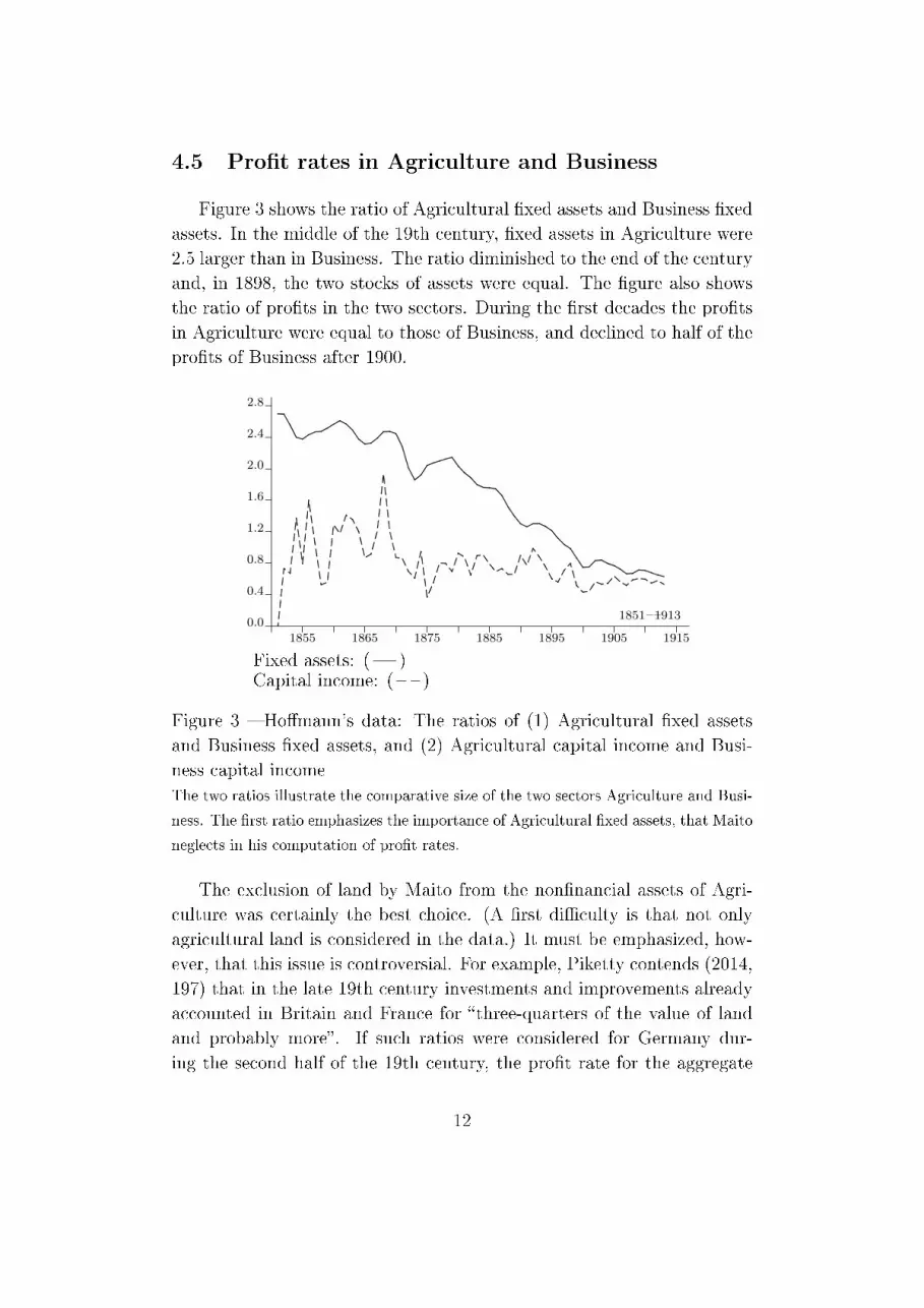
Figure 3 shows the ratio of Agricultural �xed assets and Business �xed

assets. In the middle of the 19th century, �xed assets in Agriculture were

2.5 larger than in Business. The ratio diminished to the end of the century

and, in 1898, the two stocks of assets were equal. The �gure also shows

the ratio of pro�ts in the two sectors. During the �rst decades the pro�ts

in Agriculture were equal to those of Business, and declined to half of the

pro�ts of Business after 1900.

2.8

2.4

2.0

1.6

1.2

0.8

0.4

0.0

1855 1865 1875 1885 1895 1905 1915

1851�1913

....................................................................................

......................................................................................

.........................................................................................................

...................................

...........................................................................................................................................................................................................................................................................................................................................................................................

....

......

...

......

...

......

...

......

...

......

.........................................................................................................................................................................................................................

......

...

......

...

......

...

......

...

......

...............................................................................

...................................................................................................................................................................

..........................................................................................................

......................................

.............................................................

...................................................................................

.....................................................

.............................................

...................................

Fixed assets: ( )Capital income: ( )

Figure 3 � Ho�mann's data: The ratios of (1) Agricultural �xed assets

and Business �xed assets, and (2) Agricultural capital income and Busi-

ness capital income

The two ratios illustrate the comparative size of the two sectors Agriculture and Busi-

ness. The �rst ratio emphasizes the importance of Agricultural �xed assets, that Maito

neglects in his computation of pro�t rates.

The exclusion of land by Maito from the non�nancial assets of Agri-

culture was certainly the best choice. (A �rst di�culty is that not only

agricultural land is considered in the data.) It must be emphasized, how-

ever, that this issue is controversial. For example, Piketty contends (2014,

197) that in the late 19th century investments and improvements already

accounted in Britain and France for �three-quarters of the value of land

and probably more�. If such ratios were considered for Germany dur-

ing the second half of the 19th century, the pro�t rate for the aggregate

12

economy would be further dramatically reduced. We do not know how

Ho�mann solved these problems. This is, however, an example of what

we meant in the introduction to this paper, referring to the necessary

critical assessment of Ho�mann's sources and methods.

12

10

8

6

4

2

0

1855 1865 1875 1885 1895 1905 1915

1851�1913

........................................................................................................................................................................................................................................

............................................................................................................................

......................................................................................................................................

..........................................

.......................................................................................................

.........................................................

......................................................

..............................

..................................................

.........................................................

...................................................................................................

..................................................................................................

..................................

.......................

..................................................................................................................................................................................................................

......

...

......

...

......

...

......

.....................................................................

.................................................................................................................................

......................................................................................................................................

.....................................................

...................................................

........................................................................................................................................

....................................................................................................

...................................................................................

........................

.......................

......................

.................

...................

..................................

................................

............................................

.............................................

.................................

.................

rAB

rA

rB

Figure 4 � Ho�mann's data: The pro�t rate of Agriculture and Business

rA and rB are respectively the pro�t rates of Agriculture and Business, straightfor-

wardly derived from Ho�mann's data, that is, the simplest and best measures of prof-

itability in Germany during these data. rAB is the average pro�t rate for the two

sectors. The rise of the pro�t rate of Agriculture from 1875 onward reveals a catching-

up of the pro�tability of the sector with business rates, and is at the origin of the

upward trend of the average pro�t rate of the two sectors.

Figure 4 shows the pro�t rates in Agriculture and Business, and in

the average of the two sectors as in r5 = rAB. Agriculture was not only

large but also pro�table. The main result is that, though the pro�t rate

of Business was larger than the pro�t rate of Agriculture during the �rst

half of the period, the strict limitation to Business would not have yielded

a decline of the pro�t rate prior to World War I.

5 Conclusion: A secular upward trend

of the pro�t rate?

To sum up, in our opinion, a number of miscalculations in Maito's

attempt to determine secular pro�t rates in Germany led to unrealistic

estimates, and the dramatic historical downward trend of the pro�t rate

13

from the 19th century to World War I vanishes when the necessary correc-

tions are made. Beginning with the low values of pro�t rates revealed in

Ho�mann's data for the 1870s and 1880s, it is hard to imagine a historical

declining trend up to the early 21st in these measures.

This does not mean, obviously, that the framework of trajectories à la

Marx and the thesis of the historical character of capitalism are disproved.

First, the relevance of Ho�mann's data in a calculation of pro�t rates

cannot be taken for granted; second, the dynamics of capitalism are more

complex (Duménil and Lévy, 2016).

14

References

G. Duménil and D. Lévy. Technology and distribution in managerial capi-

talism. The chain of historical trajectories à la Marx and countertenden-

tial traverses. Paris, 2016.

W. Ho�mann. Das Wachstum der deutschen Wirtschaft seit der Mitte des

19. Jahrhunderts. Springer Verlag, Berlin, 1965.

W. Ho�mann and H. Müller. Das deutsche Volkseinkommen 1851-1957.

Mohr, Tübingen, 1959.

M. Li, F. Xiao, and A. Zhu. Long waves, institutional changes, and his-

torical trends: A study of the long-term movement of the pro�t rate in

the capitalist world-economy. Journal of World-Systems Research, XIII

(1):33-54, 2007.

E. Maito. The historical transience of capital. The down-

ward trend in the rate of pro�t since the XIX cen-

tury. Third World KLEMS Conference, 2014. URL

https://thenextrecession.files.wordpress.com/2014/04/

maito-esteban-the-historical-transience-of-capital-the-

downward-tren-in-the-rate-of-profit-since-xix-century.pdf.

E. Maito. The historical transience of capital. The down-

ward trend in the rate of pro�t since the XIX cen-

tury. Universidad de Buenos Aires, 2015. URL

https://www.academia.edu/6849268/Maito_Esteban_Ezequiel

_-_The_historical_transience_of_capital_The_downward_trend

_in_the_rate_of_profit_since_XIX_century_final_draft.

T. Piketty. Capital in the Twenty-First Century. The Belknap Press of

Harvard University Press, Cambridge, MA, 2014.

T. Weiÿ. The rate of return in Germany - An empirical study.

Berlin Steglitz, 2015. URL http://www.boeckler.de/pdf/v_2015

_10_24_weiss.pdf.

15