Embed Size (px)
Citation preview
Dynamic Coarse Graining in Complex System Simulation
Yuzhen Xue, Pete J. Ludovice, Martha A. Grover
Abstract— The high computational burden in complex systemsimulation, particularly for a polymer system, prohibits longterm simulation that provides information to predict the systemattributes. We propose a coarse graining simulation method,stemming from our earlier work on state reduction througha modified local feature analysis (LFA), so that, based onshort term system dynamics, one can automatically identifya low number of “seeds” based on correlations in the dynamicmotion of all states. The trajectories of the "seeds" are thenextrapolated. A simple matrix transformation is proposed tocalculate trajectories of the whole system from the extrapolated"seed" trajectories. As the recovered system dynamics arederived from the low dimensional seed trajectories, we call itcoarse grained dynamics. Simulation is carried out to illustratethe application of the developed algorithm to the PVC polymerdynamics.
I. INTRODUCTIONThe high computational burden in complex system simu-
lation prohibits long term simulation to predict the systemattributes. In particular, for a polymer molecular dynamics(MD) simulation, composed of multiple polymer chains,which is defined by a large collection of discrete atoms,their interactions, and the resulting dynamic trajectories, thesimulation time is typically on the order of nanoseconds,while the relaxation time of the polymer ranges from 1-1000 s [7]. The high computational burden in polymersimulation is due to simulating many atoms while resolvingfast vibrational atomic time scales.Intermediate order, which occurs in many polymers, e.g.
polyvinyl chloride (PVC) [14] and poly(n-butyl methacry-late) as well as specialty polymers such as poly(trimethylsilyl propyne) [6], [22] and poly(norbornene) [1], [2], [9],[18], is a structural order that is in between the crystallineand amorphous states [13]. Polymers that show intermedi-ate order have potential applications including membraneseparation, photolithography and catalyst substrates. As theintermediate order is responsible for the useful propertiesof these polymers, in the polymer study we are interestedin modeling the process for polymeric materials to evolveand reach intermediate levels of structural order. Intermediateorder is in general detected from the wide angle x-raydiffraction (WAXD) curves. WAXD is an X-ray diffractiontechnique that is often used to determine the crystallinestructure of polymers.The initial object of our study is on PVC, where inter-
mediate order produces a unique thermoreversible gelationproperty that makes PVC applicable to flexible applica-tions. Some corporations are disrupting the order of highly
School of Chemical & Biomolecular Engineering, Georgia In-stiture of Technology, Atlanta, GA 30332, [email protected],[email protected], [email protected]
crystalline polymers such as poly(paraphenylene) to createintermediate order because it results in a polymer withgood mechanical properties that is easier to process than itscrystalline counterpart.As in general the computational capability does not allow
us to simulate the process for a polymer to evolve enough toreach the desirable state, e.g. intermediate order, where wecan analyze the system properties, we seek a model reductionapproach to reduce the simulation burden.Methods for coarse-graining of molecular simulations,
by grouping nearby atoms, have been developed to speedup molecular dynamics simulations [4], [15], but due tothe complexity of polymer tacticity, the size of the groupshas been limited to one monomer. However, much greaterspeedup is still needed. An automated method for modelreduction and system identification could provide a com-plementary approach for computational reduction, such asequation-free computing [11]. However, identifying an ap-propriate reduced-order state for equation-free computingremains a challenging problem [5], even for a simple fluid.In our earlier work [19] we proposed a modified local
feature analysis [16], [19], [21] algorithm and applied it ina polymer simulation. This algorithm automatically iden-tifies “seed” atoms, based on correlations in the dynamicmotion of all atoms. In this paper, we intend to extend ourearlier work and propose a modeling method for moleculardynamics simulations of polymers, which combines featuresfrom equation-free computing with polymer coarse-graining.We call this method dynamic coarse graining. Althoughthe algorithm to be proposed is applicable to any complexdynamic system, as our first concern is the polymer system,we will describe it in the polymer context.
II. PROBLEM DESCRIPTION
Consider a polymer system simulated with MD. Forsimplicity we will focus on the dynamics of the back-bone carbons. Assume that the polymer system has Nnumber of backbone carbons. After subtracting the overalltranslational and rotational motion, the dynamics of thepolymer system is represented by its trajectory x(t) ={x1(t), x2(t), ..., xN (t)}T ∈ RN×1, where xi(t) denotes thestate value of the i th backbone carbon at time t. Given thatobservations of s time steps are available, we have
x(1 : s) =
⎧⎨⎩ x1(1 : s)...
xN (1 : s)
⎫⎬⎭ ∈ RN×s
Moreover, as the motion of the polymer chains is threedimensional, we extend the motion of atoms at time i
2011 American Control Conferenceon O'Farrell Street, San Francisco, CA, USAJune 29 - July 01, 2011
978-1-4577-0079-8/11/$26.00 ©2011 AACC 5031
into three vectors, which in turn introduces the equivalenttrajectory x(1 : L) ∈ RN×L, where L = 3s. In generalLÀ N. Then we construct the correlation matrix as
Ri,j =
¿xi − xistd(xi)
,xj − xjstd(xj)
À, hXi, Xji
thusR = X ×XT
where R ∈ RN×N , X ∈ RN×L, xi, Xi ∈ R1×L, xi denotesthe mean value and std(xi) denotes the standard deviationof xi. Note that in real applications, we can assume that Ris full rank because of the noise contained in X due to thestochastic nature of MD.We clarify that R is the matrix derived from a short term
detailed simulation. The LFA based state reduction algorithmwill be applied to R to pick out the “seeds”, that is, the atomswith the most representative dynamics.
III. DYNAMICS COARSE GRAINING BASED ON LFAA. Local Feature AnalysisThe objective of LFA is to provide a topographic repre-
sentation for all system states through a reduced basis set,i.e. local features. LFA stems from PCA (please see [19]or [16] for detailed description of PCA) and preserves allthe information of PCA. However, unlike PCA which has aglobal basis set, i.e. basis that span over all the states, LFAprovides a localized basis set. Moreover, as has been pointedout in [3] and [21], the LFA basis is more stable over theshift of sampling windows, e.g. windows of length L withdifferent starting time.Considering the correlation matrix R ∈ RN×N described
in Sec. II, LFA kernel functions are defined as
K(l, k) =rPi=1Ψi(l)
1√λiΨi(k)
where k, l ∈ {1, · · · ,N}, K(l, k) is the (l, k) entry ofmatrix K ∈ RN×N , λi and Ψi are the i th eigenvalueand eigenvector of R respectively, and r is the number ofdominant eigenvalues determined through PCA according toλ1 > . . . > λr À λr+1 > . . . > λN . Define the projectioncoefficients of any Φ ∈ RN×1 onto the state variable xl,l = 1, . . . , N as
ol =NPk=1
K(l, k)Φ(k) ≡rPi=1
ΨTi Φ√λiΨi(l) (1)
where ol ∈ R is the LFA output (feature). We can see thatK(l, k) is a topographic kernel as the output ol from Φ onlyrelies on the components of the eigenvectors correspondingto xl. Letting o = [o1, · · · , oN ]T , we have
o = KΦ = ΨΛ−12ΨTΦ (2)
where Λ = diag(λ1, . . . ,λr), and Ψ ∈ RN×r is the matrixthat contains the r dominant eigenvectors. Through LFA, anyΦ ∈ RN×1 can be approximated with minimum mean squareerror that is the same as in PCA, by
Φrec = K(−1)o (3)
where K(−1) with entries K(−1)(l, k) =rPi=1Ψi(l)
√λiΨi(k), k, l ∈ {1, · · · , N}, is the approximate
inverse of K [16].The reconstruction in (3) is with N local features, i.e. o,
such that the locality is achieved at the price that the numberof features are extended to N À r, much larger than that inthe PCA case. A sparsification step is thus critical in orderto get rid of the redundant local features.In our earlier work [19], a novel sparsification algorithm
was derived. Rather than empirically searching based onmultiple linear regression among the whole state set, seee.g. [12], [16], [20], [21], the newly developed algorithmin [19] involves a simple matrix calculation and offers cleartheoretical foundation for sparsification.
B. LFA sparsificationIn this section we briefly introduce the modified LFA
sparsification algorithm proposed in [19]; interested readersmay refer to [19] for more details.Consider X ∈ RN×L in Section II with rank(X) = N ,
given any Φ ∈ RN×1 there exists P ∈ R1×L such thatΦ = XPT .Defining the local feature matrix O ∈ RN×L as
O , KX = ΨΛ−12ΨTX (4)
it is easy to see that rank(O) = r. From (2) and (4) weobtain
o = OPT (5)
DefiningM , ΨTO
then M has the singular value decomposition
M = V ΣUT (6)
where U ∈ RL×r, Σ ∈ Rr×r, V ∈ Rr×r. It can easily beshown that there exists O ∈ RN×r
such that
O = OUT (7)
The following proposition derived in [19] shows that thereconstruction (3) can be based on only r correctly chosenlocal features, i.e. or ∈ Rr×1.Proposition 1: There exists a matrix K(−1)
r ∈ RN×r andor ∈ Rr×1, the subvector of o, such that
Φrec = K(−1)o = K(−1)
r or
Defining the index set S that corresponds to the indices ofentries in o that comprise or, we have
S ∈ {{k1, · · · , kr}, rank(Or) = r}where Or ∈ Rr×r is the submatrix of O by including onlythe rows with indices {k1, · · · , kr}. Given Or, the kernelfunction K(−1)
r = ΨΛ12ΨrO
−Tr O
−1r , where Ψr ∈ Rr×r is
the submatrix of Ψ by including the rows corresponding toindex set S.Prop. 1 tells us that any Φ can be approximately recon-
structed based on only r local features, or, as long as the
5032
corresponding Or matrix has rank(Or) = r. We clarifythat the choice of index set S is not unique. The process ofchoosing the most representative r local features is calledsparsification. There are practical considerations in favor oftheir judicious choice. In [16] it is suggested to chooseindices set S such that Oki , Okj are the least dependentfor any ki 6= kj , ki, kj ∈ S, where Oki is the k th
i row ofO. Such a set S is corresponding to the most representativelocal features.Definition 1: The index of dependency between two vec-
torsOi,Oj is defined as ρij =|hOi,Oji|kOikkOjk ; a small ρ indicates
that Oi, Oj are highly independent.
C. Dynamic Coarse Graining Algorithm
By sparsification, we find index set S = {k1, · · · , kr}through identifying the least dependent vectorsOk1 , · · · ,Okr , so that or = [ok1 , · · · , okr ]T arethe most representative local features, correspondingto “seed” states, xk1 , · · · , xkr , with kernel matrixK(−1)r = ΨΛ
12ΨrO
−Tr O
−1r . As xkl , l ∈ {1, · · · , r},
is the “seed” state and xkl(1 : L), l ∈ {1, · · · , r} is the“seed” trajectory, from (4) we can view the counterpartOkl , l ∈ {1, · · · , r}, also as a time series of length Lcorresponding to the most representative local features, thuswe call Okl the “seed” dynamics (trajectories).Next we describe the dynamic coarse graining algorithm.
The idea is to develop the relationship between trajectoriesof Xi, i ∈ {1, · · · , N} and “seed” trajectories Okl , l ∈{1, · · · , r} as well as to identify the time series model of“seed” trajectories so that, by extrapolating the seed trajec-tories, we can recover the dynamics of Xi, i ∈ {1, · · · ,N}in the future time. As the recovery of the whole systemdynamics is derived from the dynamics of r “seeds”, wename our algorithm “dynamic coarse graining algorithm”.Define X , ΨΨTX as the filtered X , i.e. X without the
non-principal components. We have the following claims.Claim 1: The Euclidean norm between X and X is°°°X −X
°°°2= °(pλr+1), where °(
pλr+1) means the
order ofpλr+1.
Proof: Proof is trivial using the definition of Euclideannorm of matrix.From the above claim, we see that X can approximate X
with error °(pλr+1), which is small if λr+1 is small.Claim 2: Ok1 , . . . ,Okr form the basis to reconstruct X,
and X = ΨΛ12ΨTC
⎡⎢⎣ Ok1...Okr
⎤⎥⎦ , where C = OO−1r .Proof: Proof is derived directly from the definition of
O, C and X.Now we see that the dynamics Xj of any state j can
be reconstructed by the seed dynamics {Ok1 , · · · ,Okr}.That is, X can be reconstructed, with small 2-norm errorpλr+1, through seed dynamics {Ok1 , · · · ,Okr} during s
time period.Claim 3: Considering the system discussed above, choose
fl,p so that
O(p)kl(t) = fl,p(t), l ∈ {1, · · · , r}, p ∈ {x, y, z}, 1 6 t 6 s
(8)where O(p)
kl(t) denotes to the entry in Okl that corresponds
to the value in the p direction at time step t. (Recall theconstruction of X matrix in Sec. II, and note that vectorOkl is composed of O
(p)kl(t), 1 6 t 6 s, p ∈ {x, y, z}.)
Assuming that s is long enough so that (8) and the linearrelationship in Claim 2 stay the same for M À s, then
X(p)(M) = ΨΛ12ΨTC
⎡⎢⎣ fk1,p(M)...
fkr,p(M)
⎤⎥⎦ (9)
where X(p) denotes the extrapolation of X(p) ∈ RN×s, thesubmatrix of X ∈ RN×L corresponding to the p direction.
Proof: Proof is obtained directly from Claim 2 andthe assumption O(j)
kl(M) = fl,p(M), l ∈ {1, · · · , r}, j ∈
{x, y, z}.This claim assumes that the complete system information
can be obtained from the system dynamics over time period sand that the linear transformation in Claim 2 is enough to de-scribe the relationship between X and Okl , l ∈ {1, · · · , r}.However, this is usually not true so we can only approximateX(p) based on fl,p, l ∈ {1, · · · , r}, p ∈ {x, y, z}. Throughtime series identification techniques, e.g. neural network,genetic algorithm, wavelet or simply linear fitting methodsin the Matlab system identification toolbox, we can fit eachtime series O(p)
klby fl,p so that
O(p)kl(1 : s) ≈ fl,p(1 : s), l ∈ {1, · · · , r}, p ∈ {x, y, z}
Although the real system is not necessary linear, we canassume that, for relatively short time M , s ¿ M ¿∞, the linear relationship in Claim 2 can provide a goodapproximation. Thus we can approximate the dynamics ofX at time M by (9).Based on the discussion above, we propose the dynamic
coarse graining algorithm:Algorithm 1:1) Record trajectory data for s time steps and constructR, O and O matrices;
2) Find the most representative local feature indicesk1, · · · , kr and calculate the C matrix;
3) Identify fl,p based on O(p)kl(1 : s), l ∈ {1, · · · , r};
4) Recover X(p)j (t) in terms of fl,p(t), l ∈ {1, · · · , r}
through (9), s < t ≤M, j ∈ {1, · · · , N}We remark here if the dynamics is a slow process, given
limited time, we may not be able to collect enough data tomodel the whole system. Moreover, linear approximation toa nonlinear relationship will be inaccurate as time goes on.We call this the undersampling problem. Aware of this, weadopt a iterative scheme similar to that in [10], [17] to modelthe long term system dynamics.Algorithm 2:
5033
1) Run the detailed simulation for time duration s, adoptAlgorithm 1 to choose seed dynamics Okl and extrap-olate them to time step M , approximate X(M) basedon Okl(M).
2) Map X(M) back to real trajectories x(M) by mul-tiplying the standard deviation and adding the meanvalue; go to Step 1.
Note here the iterative algorithm allows the algorithm torepresent system dynamics over different time duration s byselecting different seed dynamics and recovery formula (9).
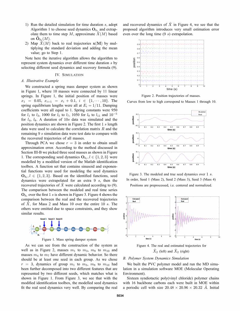
IV. SIMULATIONA. Illustrative ExampleWe constructed a spring mass damper system as shown
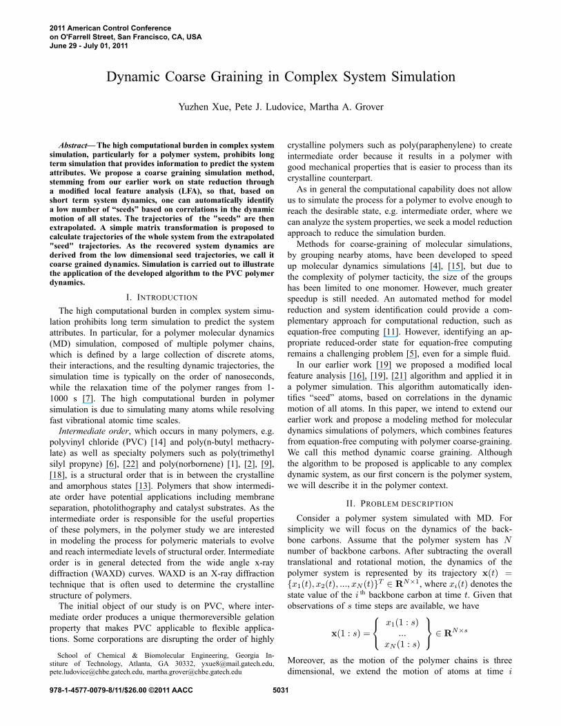
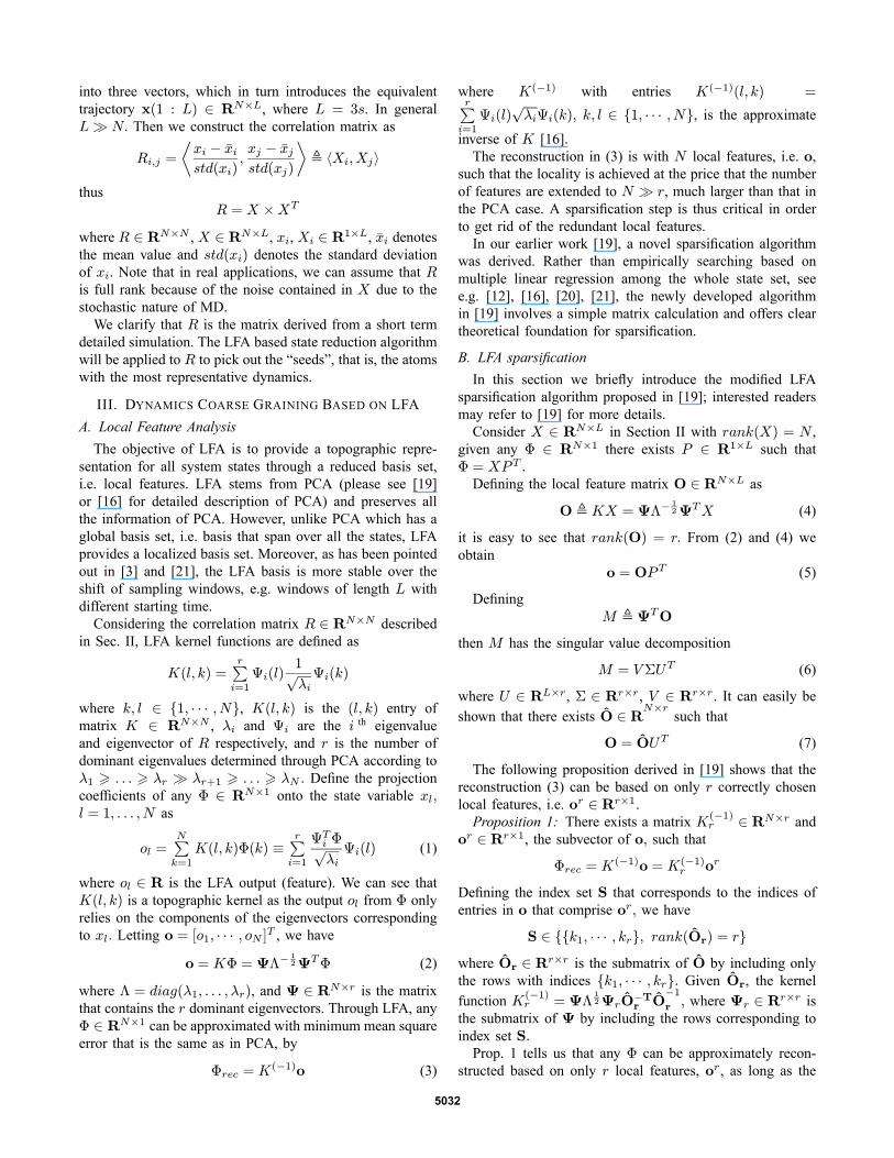
in Figure 1, where 10 masses were connected by 11 linearsprings. In Figure 1, the initial position of masses werex1 = 0.05, xi+1 = xi + 0.1, i ∈ {1, · · · , 10}. Thespring equilibrium lengths were all at Ei = 1/11. Dampingcoefficients were all equal to 1. Spring constants were 950for l1 to l3, 1000 for l5 to l7, 1050 for l9 to l11 and 10−5for l4, l8. A duration of 10s data was simulated and theposition dynamics are shown in Figure 2. The first 1 s lengthdata were used to calculate the correlation matrix R and theremaining 9 s simulation data were test data to compare withthe recovered trajectories of all masses.Through PCA we chose r = 3 in order to obtain small
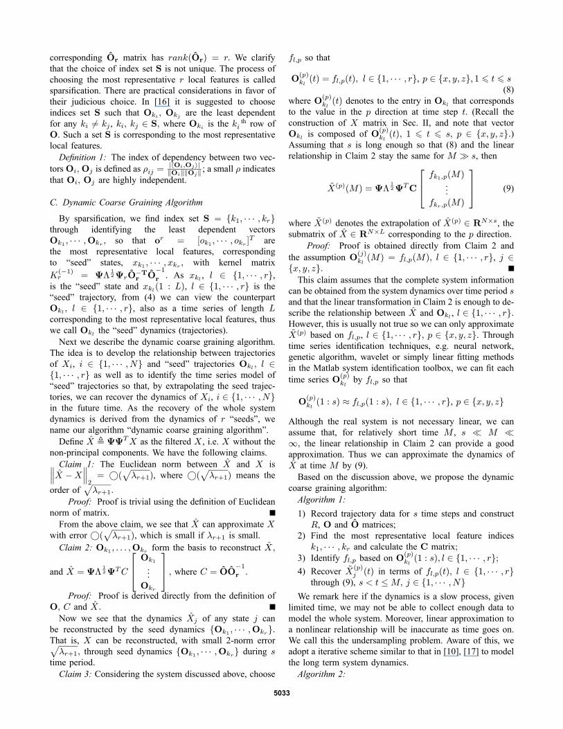
approximation error. According to the method discussed inSection III-B we picked three seed masses as shown in Figure1. The corresponding seed dynamics Okl , l ∈ {1, 2, 3} weremodelled by a modified version of the Matlab identificationtoolbox. A function set that contains sinusoid and exponen-tial functions were used for modeling the seed dynamicsOkl , l ∈ {1, 2, 3}. Based on the identified functions, seeddynamics were extrapolated for an extra 9 s, then therecovered trajectories of X were calculated according to (9).The comparison between the modeled and real time seriesOkl over the first 1 s is shown in Figure 3. Figure 4 shows thecomparison between the real and the recovered trajectoriesof X, for Mass 2 and Mass 10 over the entire 10 s. Theothers were omitted due to space constraints, and they showsimilar results.
Figure 1. Mass spring damper system
As we can see from the construction of the system aswell as in Figure 2, masses m1 to m3, m8 to m10 andmasses m4 to m7 have different dynamic behavior. So thereshould be at least one seed in each group. As we choser = 3, dynamics of group m1 to m3, m8 to m10 hadbeen further decomposed into two different features that arerepresented by two different seeds, which matches what isshown in Figure 1. From Figure 3, we see that with themodified identification toolbox, the modelled seed dynamicsfit the real seed dynamics very well. By comparing the real
and recovered dynamics of X in Figure 4, we see that theproposed algorithm introduces very small estimation erroreven over the long time (9 s) extrapolation.
0 1 2 3 4 5 6 7 8 9 100
0.1
0.2
0.3
0.4
0.5
0.6
0.7
0.8
0.9
1
time (s)
posi
tion
Figure 2. Position trajectories of masses.
Curves from low to high correspond to Masses 1 through 10.
0 0.1 0.2 0.3 0.4 0.5 0.6 0.7 0.8 0.9 1-0.2
0
0.2
time (s)po
sitio
n
0 0.1 0.2 0.3 0.4 0.5 0.6 0.7 0.8 0.9 1-0.2
0
0.2
time (s)
posi
tion
0 0.1 0.2 0.3 0.4 0.5 0.6 0.7 0.8 0.9 1-0.1
0
0.1
time (s)
posi
tion
ModeledReal
Figure 3. The modeled and true seed dynamics over 1 s.In order, Seed 1 (Mass 2), Seed 2 (Mass 3), Seed 3 (Mass 4)
Positions are preprocessed, i.e. centered and normalized.
0 2 4 6 8 10-6
-4
-2
0
2
4
6
8
time (s)
posit
ion
EstimatedReal
0 2 4 6 8 10-6
-4
-2
0
2
4
6
time (s)
posit
ion
EstimatedReal
Figure 4. The real and estimated trajectories forX2 (left) and X2 (right)
B. Polymer System Dynamics SimulationWe built the PVC polymer model and run the MD simu-
lation in a simulation software MOE (Molecular OperatingEnvironment).Sixteen syndiotactic poly(vinyl chloride) polymer chains
with 16 backbone carbons each were built in MOE withina periodic cell with size 20.48 × 20.96 × 20.32 A. Initial
5034
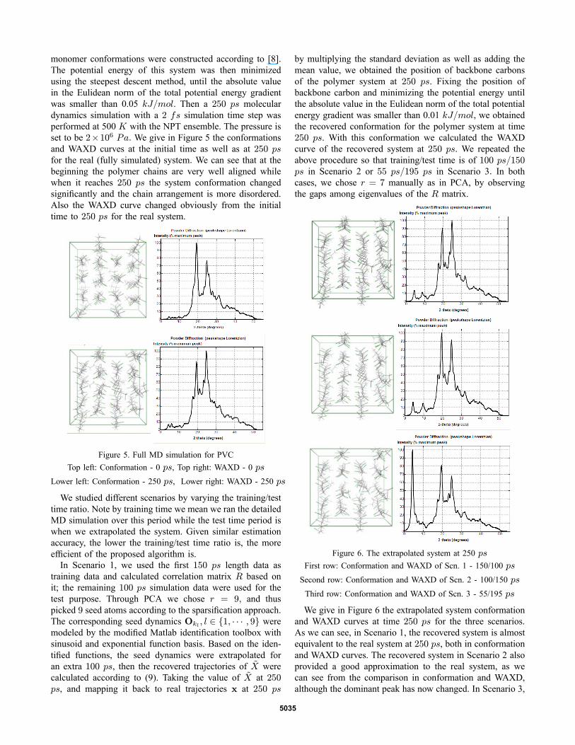
monomer conformations were constructed according to [8].The potential energy of this system was then minimizedusing the steepest descent method, until the absolute valuein the Eulidean norm of the total potential energy gradientwas smaller than 0.05 kJ/mol. Then a 250 ps moleculardynamics simulation with a 2 fs simulation time step wasperformed at 500 K with the NPT ensemble. The pressure isset to be 2×10⁶ Pa. We give in Figure 5 the conformationsand WAXD curves at the initial time as well as at 250 psfor the real (fully simulated) system. We can see that at thebeginning the polymer chains are very well aligned whilewhen it reaches 250 ps the system conformation changedsignificantly and the chain arrangement is more disordered.Also the WAXD curve changed obviously from the initialtime to 250 ps for the real system.
Figure 5. Full MD simulation for PVCTop left: Conformation - 0 ps, Top right: WAXD - 0 ps
Lower left: Conformation - 250 ps, Lower right: WAXD - 250 ps
We studied different scenarios by varying the training/testtime ratio. Note by training time we mean we ran the detailedMD simulation over this period while the test time period iswhen we extrapolated the system. Given similar estimationaccuracy, the lower the training/test time ratio is, the moreefficient of the proposed algorithm is.In Scenario 1, we used the first 150 ps length data as
training data and calculated correlation matrix R based onit; the remaining 100 ps simulation data were used for thetest purpose. Through PCA we chose r = 9, and thuspicked 9 seed atoms according to the sparsification approach.The corresponding seed dynamics Okl , l ∈ {1, · · · , 9} weremodeled by the modified Matlab identification toolbox withsinusoid and exponential function basis. Based on the iden-tified functions, the seed dynamics were extrapolated foran extra 100 ps, then the recovered trajectories of X werecalculated according to (9). Taking the value of X at 250ps, and mapping it back to real trajectories x at 250 ps
by multiplying the standard deviation as well as adding themean value, we obtained the position of backbone carbonsof the polymer system at 250 ps. Fixing the position ofbackbone carbon and minimizing the potential energy untilthe absolute value in the Eulidean norm of the total potentialenergy gradient was smaller than 0.01 kJ/mol, we obtainedthe recovered conformation for the polymer system at time250 ps. With this conformation we calculated the WAXDcurve of the recovered system at 250 ps. We repeated theabove procedure so that training/test time is of 100 ps/150ps in Scenario 2 or 55 ps/195 ps in Scenario 3. In bothcases, we chose r = 7 manually as in PCA, by observingthe gaps among eigenvalues of the R matrix.
Figure 6. The extrapolated system at 250 psFirst row: Conformation and WAXD of Scn. 1 - 150/100 ps
Second row: Conformation and WAXD of Scn. 2 - 100/150 ps
Third row: Conformation and WAXD of Scn. 3 - 55/195 ps
We give in Figure 6 the extrapolated system conformationand WAXD curves at time 250 ps for the three scenarios.As we can see, in Scenario 1, the recovered system is almostequivalent to the real system at 250 ps, both in conformationand WAXD curves. The recovered system in Scenario 2 alsoprovided a good approximation to the real system, as wecan see from the comparison in conformation and WAXD,although the dominant peak has now changed. In Scenario 3,
5035
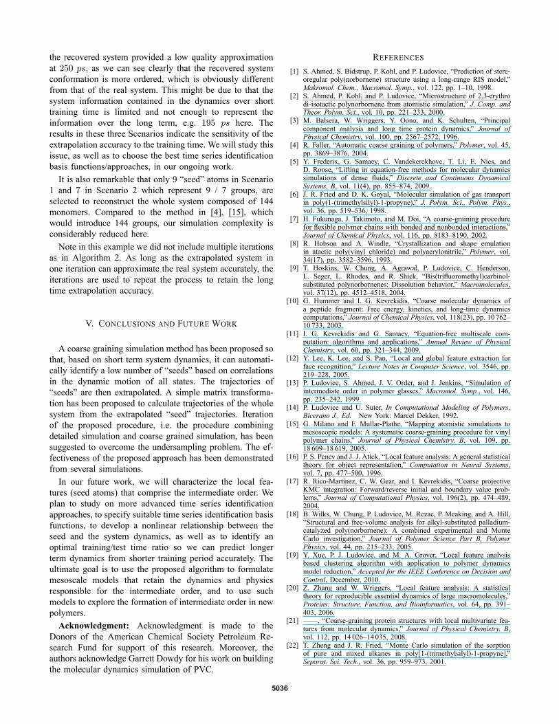
the recovered system provided a low quality approximationat 250 ps, as we can see clearly that the recovered systemconformation is more ordered, which is obviously differentfrom that of the real system. This might be due to that thesystem information contained in the dynamics over shorttraining time is limited and not enough to represent theinformation over the long term, e.g. 195 ps here. Theresults in these three Scenarios indicate the sensitivity of theextrapolation accuracy to the training time. We will study thisissue, as well as to choose the best time series identificationbasis functions/approaches, in our ongoing work.It is also remarkable that only 9 “seed” atoms in Scenario
1 and 7 in Scenario 2 which represent 9 / 7 groups, areselected to reconstruct the whole system composed of 144monomers. Compared to the method in [4], [15], whichwould introduce 144 groups, our simulation complexity isconsiderably reduced here.Note in this example we did not include multiple iterations
as in Algorithm 2. As long as the extrapolated system inone iteration can approximate the real system accurately, theiterations are used to repeat the process to retain the longtime extrapolation accuracy.
V. CONCLUSIONS AND FUTURE WORK
A coarse graining simulation method has been proposed sothat, based on short term system dynamics, it can automati-cally identify a low number of “seeds” based on correlationsin the dynamic motion of all states. The trajectories of“seeds” are then extrapolated. A simple matrix transforma-tion has been proposed to calculate trajectories of the wholesystem from the extrapolated “seed” trajectories. Iterationof the proposed procedure, i.e. the procedure combiningdetailed simulation and coarse grained simulation, has beensuggested to overcome the undersampling problem. The ef-fectiveness of the proposed approach has been demonstratedfrom several simulations.In our future work, we will characterize the local fea-
tures (seed atoms) that comprise the intermediate order. Weplan to study on more advanced time series identificationapproaches, to specify suitable time series identification basisfunctions, to develop a nonlinear relationship between theseed and the system dynamics, as well as to identify anoptimal training/test time ratio so we can predict longerterm dynamics from shorter training period accurately. Theultimate goal is to use the proposed algorithm to formulatemesoscale models that retain the dynamics and physicsresponsible for the intermediate order, and to use suchmodels to explore the formation of intermediate order in newpolymers.
Acknowledgment: Acknowledgment is made to theDonors of the American Chemical Society Petroleum Re-search Fund for support of this research. Moreover, theauthors acknowledge Garrett Dowdy for his work on buildingthe molecular dynamics simulation of PVC.
REFERENCES[1] S. Ahmed, S. Bidstrup, P. Kohl, and P. Ludovice, “Prediction of stere-
oregular poly(norbornene) structure using a long-range RIS model,”Makromol. Chem., Macromol. Symp., vol. 122, pp. 1–10, 1998.
[2] S. Ahmed, P. Kohl, and P. Ludovice, “Microstructure of 2,3-erythrodi-isotactic polynorbornene from atomistic simulation,” J. Comp. andTheor. Polym. Sci., vol. 10, pp. 221–233, 2000.
[3] M. Balsera, W. Wriggers, Y. Oono, and K. Schulten, “Principalcomponent analysis and long time protein dynamics,” Journal ofPhysical Chemistry, vol. 100, pp. 2567–2572, 1996.
[4] R. Faller, “Automatic coarse graining of polymers,” Polymer, vol. 45,pp. 3869–3876, 2004.
[5] Y. Frederix, G. Samaey, C. Vandekerckhove, T. Li, E. Nies, andD. Roose, “Lifting in equation-free methods for molecular dynamicssimulations of dense fluids,” Discrete and Continuous DynamicalSystems, B, vol. 11(4), pp. 855–874, 2009.
[6] J. R. Fried and D. K. Goyal, “Molecular simulation of gas transportin poly(1-(trimethylsilyl)-1-propyne),” J. Polym. Sci., Polym. Phys.,vol. 36, pp. 519–536, 1998.
[7] H. Fukunaga, J. Takimoto, and M. Doi, “A coarse-graining procedurefor flexible polymer chains with bonded and nonbonded interactions,”Journal of Chemical Physics, vol. 116, pp. 8183–8190, 2002.
[8] R. Hobson and A. Windle, “Crystallization and shape emulationin atactic poly(vinyl chloride) and polyacrylonitrile,” Polymer, vol.34(17), pp. 3582–3596, 1993.
[9] T. Hoskins, W. Chung, A. Agrawal, P. Ludovice, C. Henderson,L. Seger, L. Rhodes, and R. Shick, “Bis(trifluoromethyl)carbinol-substituted polynorbornenes: Dissolution behavior,” Macromolecules,vol. 37(12), pp. 4512–4518, 2004.
[10] G. Hummer and I. G. Kevrekidis, “Coarse molecular dynamics ofa peptide fragment: Free energy, kinetics, and long-time dynamicscomputations,” Journal of Chemical Physics, vol. 118(23), pp. 10 762–10 733, 2003.
[11] I. G. Kevrekidis and G. Samaey, “Equation-free multiscale com-putation: algorithms and applications,” Annual Review of PhysicalChemistry, vol. 60, pp. 321–344, 2009.
[12] Y. Lee, K. Lee, and S. Pan, “Local and global feature extraction forface recognition,” Lecture Notes in Computer Science, vol. 3546, pp.219–228, 2005.
[13] P. Ludovice, S. Ahmed, J. V. Order, and J. Jenkins, “Simulation ofintermediate order in polymer glasses,” Macromol. Symp., vol. 146,pp. 235–242, 1999.
[14] P. Ludovice and U. Suter, In Computational Modeling of Polymers,Bicerano J., Ed. New York: Marcel Dekker, 1992.
[15] G. Milano and F. Mullar-Plathe, “Mapping atomistic simulations tomesoscopic models: A systematic coarse-graining procedure for vinylpolymer chains,” Journal of Physical Chemistry, B, vol. 109, pp.18 609–18 619, 2005.
[16] P. S. Penev and J. J. Atick, “Local feature analysis: A general statisticaltheory for object representation,” Computation in Neural Systems,vol. 7, pp. 477–500, 1996.
[17] R. Rico-Martínez, C. W. Gear, and I. Kevrekidis, “Coarse projectiveKMC integration: Forward/reverse initial and boundary value prob-lems,” Journal of Computational Physics, vol. 196(2), pp. 474–489,2004.
[18] B. Wilks, W. Chung, P. Ludovice, M. Rezac, P. Meaking, and A. Hill,“Structural and free-volume analysis for alkyl-substituted palladium-catalyzed poly(norbornene): A combined experimental and MonteCarlo investigation,” Journal of Polymer Science Part B, PolymerPhysics, vol. 44, pp. 215–233, 2005.
[19] Y. Xue, P. J. Ludovice, and M. A. Grover, “Local feature analysisbased clustering algorithm with application to polymer dynamicsmodel reduction,” Accepted for the IEEE Conference on Decision andControl, December, 2010.
[20] Z. Zhang and W. Wriggers, “Local feature analysis: A statisticaltheory for reproducible essential dynamics of large macromolecules,”Proteins: Structure, Function, and Bioinformatics, vol. 64, pp. 391–403, 2006.
[21] ——, “Coarse-graining protein structures with local multivariate fea-tures from molecular dynamics,” Journal of Physical Chemistry, B,vol. 112, pp. 14 026–14 035, 2008.
[22] T. Zheng and J. R. Fried, “Monte Carlo simulation of the sorptionof pure and mixed alkanes in poly[1-(trimethylsilyl)-1-propyne],”Separat. Sci. Tech., vol. 36, pp. 959–973, 2001.
5036