Embed Size (px)
Citation preview

Dynamic Consistency of Conditional SimpleTemporal Networks via Mean Payoff Games:
a Singly-Exponential Time DC-Checking
Carlo CominDepartment of Mathematics
University of Trento, Trento, [email protected]
Romeo RizziDepartment of Computer ScienceUniversity of Verona, Verona, Italy
Abstract—Conditional Simple Temporal Network (CSTN) isa constraint-based graph-formalism for conditional temporalplanning. It offers a more flexible formalism than the equivalentCSTP model of Tsamardinos, Vidal and Pollack, from whichit was derived mainly as a sound formalization. Three notionsof consistency arise for CSTNs and CSTPs: weak, strong, anddynamic. Dynamic consistency is the most interesting notion, butit is also the most challenging and it was conjectured to be hard toassess. Tsamardinos, Vidal and Pollack gave a doubly-exponentialtime algorithm for deciding whether a CSTN is dynamically-consistent and to produce, in the positive case, a dynamicexecution strategy of exponential size. In the present work weoffer a proof that deciding whether a CSTN is dynamically-consistent is coNP-hard and provide the first singly-exponentialtime algorithm for this problem, also producing a dynamic execu-tion strategy whenever the input CSTN is dynamically-consistent.The algorithm is based on a novel connection with Mean PayoffGames, a family of two-player infinite games played on finitegraphs, well known for having applications in model-checkingand formal verification. The presentation of such connection ismediated by the Hyper Temporal Network model, a tractablegeneralization of Simple Temporal Networks whose consistencychecking is equivalent to determining Mean Payoff Games. Inorder to analyze the algorithm we introduce a refined notion ofdynamic-consistency, named ε-dynamic-consistency, and presenta sharp lower bounding analysis on the critical value of thereaction time ε where the CSTN transits from being, to notbeing, dynamically-consistent. The proof technique introduced inthis analysis of ε is applicable more generally when dealing withlinear difference constraints which include strict inequalities.
Index Terms—Conditional Simple Temporal Networks, Dy-namic Consistency, Mean Payoff Games, Hyper Temporal Net-works, Singly-Exponential Time, Reaction Time Analysis.
I. INTRODUCTION AND MOTIVATION
In temporal planning and temporal scheduling, SimpleTemporal Networks (STNs) [9] are directed weighted graphs,where nodes represent events to be scheduled in time andarcs represent temporal distance constraints between pairsof events. Recently, STNs have been generalized into Hy-per Temporal Networks (HyTNs) [7], [8] by consideringweighted directed hypergraphs, where each hyperarc modelsa disjunctive temporal constraint called hyper-constraint. Thecomputational equivalence between checking the consistencyof HyTNs and determining winning regions in Mean Payoff
Games (MPGs) [3], [10], [17] was pointed out as well in [7],[8], where the approach was shown to be robust thanks toextensive experimental evaluations [2], [7], [8]. Mean PayoffGames are a family of two-player infinite games played onfinite graphs, well known for having theoretical interest incomputational complexity, being it one of the few (natural)problems lying in NP∩ coNP, as well as various applicationsin model-checking and formal verification [11].
The present work unveils that HyTNs and MPGs are a natu-ral underlying combinatorial model for checking the dynamic-consistency of conditional temporal problems. We focus onConditional Simple Temporal Problems (CSTP) [16] and ontheir graph-based counterpart Conditional Simple TemporalNetworks (CSTN) [12], a constraint-based model for condi-tional temporal planning. The CSTN formalism extends STNsin that: (1) some of the nodes are called observation eventsand to each of them is associated a boolean variable, to bedisclosed only at execution time; (2) labels (i.e. conjunctionsover the literals) are attached to all nodes and constraints,to indicate the situations in which each of them is required.The planning agent must schedule all the required nodes,meanwhile respecting all the required temporal constraintsamong them. This extended framework allows for the off-line construction of conditional plans that are guaranteed tosatisfy complex temporal constraints. Importantly, this canbe achieved even while allowing for the decisions about theprecise timing of actions to be postponed until executiontime, in a least-commitment manner, thereby adding flexibilityand making it possible to adapt the plan dynamically, duringexecution, in response to the observations made [16].
Three notions of consistency arise for CSTNs: weak, strong,and dynamic. Dynamic consistency (DC) is in fact the mostinteresting one, as it requires the existence of conditionalplans where decisions about the precise timing of actions arepostponed until execution time, but it anyhow guarantees thatall the relevant constraints will be ultimately satisfied. Still,it is the most challenging and it was conjectured to be hardto assess by Tsamardinos, Vidal and Pollack [16]. Indeed,the best-so-far algorithm for deciding whether a CSTN isdynamically-consistent is doubly-exponential time [16]. It first
arX
iv:1
505.
0082
8v4
[cs
.DS]
17
Jul 2
015

builds an equivalent Disjunctive Temporal Problem (DTP) ofsize exponential in the input CSTN, and then applies to itan exponential time DTP’s algorithm to check its consistency.However, this approach turns out to be limitative in practice:to the best of our knowledge, some experimental studies haveshown that the resolution procedures, as well as the heuristics,for solving general DTPs becomes quite burdensome with∼ 30, 35 DTP’s variables [13]–[15], thus dampening thepractical applicability of the approach.
Contribution: In the present work we first offer a proofthat deciding whether a CSTN is dynamically-consistent iscoNP-hard. Secondly, and most importantly, we unveil a con-nection between the problem of checking dynamic-consistencyof CSTNs and that of determining MPGs, thus providingthe first sound-and-complete singly-exponential time algorithmfor this same task of deciding the dynamic-consistency andyielding a dynamic execution strategy for CSTNs. The algo-rithm can actually be applied to a wider class of problemsand it is based on representing any given instance on anexponential sized network, as first suggested in [16]. Thedifference, however, is that we propose to map CSTNs onHyTNs/MPGs rather than on DTPs. This makes a relevant dif-ference since the consistency check for HyTNs can be reducedto MPGs determination [7], [8], which is amenable to practicaland effective pseudo-polynomial time algorithms (indeed, inseveral cases the resolution methods for determining MPGsexhibit even a strongly-polynomial time behaviour [1], [2],[4], [8]). To summarize, we obtain an improved upper boundon the theoretical time complexity of the DC-checking forCSTNs (i.e., from 2-EXP to NE ∩ coNE) together with afaster DC-checking procedure, which can be used on CSTNswith a larger number of propositional variables and eventnodes. At the heart of the algorithm a suitable reduction toMPGs is mediated by the HyTN model, i.e., the algorithmdecides whether a CSTN is dynamically-consistent by solvinga carefully constructed MPG. As a final contribution, in orderto analyze the algorithm, we introduce a novel and refinednotion of dynamic-consistency, named ε-dynamic-consistency,and present a sharp lower bounding analysis on the criticalvalue of the reaction time ε where the CSTN transits frombeing, to not being, dynamically-consistent. We believe thatthis contributes to clarifying (with respect to previous liter-ature [12], [16]) the role played by the reaction time ε inchecking the dynamic-consistency of CSTNs. Furthermore, theproof technique introduced in this analysis of ε is applicablemore in general when dealing with linear difference constraintswhich include strict inequalities, therefore, it may be useful inthe analysis of other models of temporal constraints.
Organization: In Section II A we recall the basic formal-ism, terminology and known results on CSTPs and CSTNs.Section II B is devoted to recall the HyTN model, its com-putational equivalence with MPGs and the related algorithmicresults. Section III tackles on the algorithmics of dynamic-consistency: firstly, we provide a coNP-hardness lower bound,then, we describe the connection with HyTNs/MPGs andpresent a (pseudo) singly-exponential time DC-checking pro-
cedure. Section IV is devoted to present a sharp lower bound-ing analysis on the critical value of the reaction time ε wherethe CSTN transits from being, to not being, dynamically-consistent. In Section V some related works are discussed.The paper concludes in Section VI.
II. BACKGROUND
In order to provide a formal support to the present work,this section recalls the basic formalism, terminology andknown results on CSTPs and CSTNs. Since the forthcomingdefinitions are mostly inherited from the literature, the readeris referred to [16] and [12] for an intuitive semantic discussionand for some clarifying examples of the very same model.
To begin with, our graphs are directed and weighted on thearcs. Thus, if G = 〈V,A〉 is a graph, then every arc a ∈ Ais a triplet 〈u, v, wa〉 where u = t(a) ∈ V is the tail of a,v = h(a) ∈ V is the head of a, and wa = w(u, v) ∈ Z theweight of a. The following definition recalls Simple TemporalNetworks (STNs) [9], as they provide a powerful and generaltool for representing conjunctions of minimum and maximumdistance constraints between pairs of temporal variables.
Definition 1 (STNs). An STN [9] is a weighted directedgraph whose nodes are events that must be placed on the realtime line and whose arcs, called standard arcs, express binaryconstraints on the allocations of their end-points in time.
An STN G = 〈V,A〉 is called consistent if it admits afeasible scheduling, i.e., a scheduling φ : V 7→ R such thatφ(v) ≤ φ(u) + w(u, v) for all arcs 〈u, v, w(u, v)〉 ∈ A.
A. Conditional Simple Temporal Networks
In 2003, Tsamardinos, Vidal and Pollack introduced theConditional Simple Temporal Problem (CSTP) as an extensionof standard temporal constraint-satisfaction models used innon-conditional temporal planning. A CSTP augments anSTN to include observation events. Each observation eventhas a boolean variable (or proposition) associated with it.When the observation event is executed, the truth-value ofits associated proposition becomes known. In addition, eachevent and each constraint has a label that restricts the scenariosin which it plays a role. Although not included in the formaldefinition, Tsamardinos, et al. discussed some supplementaryreasonability assumptions that any well-defined CSTP mustsatisfy. Subsequently, those conditions have been analyzed andformalized in [12], leading to the sound notion of ConditionalSimple Temporal Network (CSTN), which is now recalled.
Let P be a set of boolean variables, a label is any (possiblyempty) conjunction of variables, or negations of variables,drawn from P . The empty label is denoted by λ. The labeluniverse of P , denoted P ∗, is the set of all (possibly empty)labels whose literals are drawn from P . Two labels, `1 and `2,are called consistent, denoted1 by Con(`1, `2), when `1 ∧ `2is satisfiable. A label `1 subsumes a label `2, denoted1 bySub(`1, `2), when `1 ⇒ `2 holds. We are now in the positionto recall the definition of CSTNs.
1The notation Con(·, ·) and Sub(·, ·) is inherited from [12], [16].

Definition 2 (CSTNs). A Conditional Simple Temporal Net-work (CSTN) is a tuple 〈V,A,L,O,OV, P 〉 where:• V is a finite set of events; P = p1, . . . , p|P | is a finite
set of boolean variables (or propositions);• A is a set of labeled temporal constraints each having the
form 〈v− u ≤ w(u, v), `〉, where u, v ∈ V , w(u, v) ∈ Z,and ` ∈ P ∗;
• L : V → P ∗ is a function that assigns a label to eachevent in V ; OV ⊆ V is a finite set of observation events;O : P → OV is a bijection that associates a uniqueobservation event O(p) = Op to each proposition p ∈ P ;
• The following reasonability assumptions must hold:(WD1) for any labeled constraint 〈v−u ≤ w, `〉 ∈ A thelabel ` is satisfiable and subsumes both L(u) and L(v);intuitively, whenever a constraint v−u ≤ w is required tobe satisfied, then its endpoints u and v must be scheduled(sooner or later) by the planning agent;(WD2) for each p ∈ P and each u ∈ V such that eitherp or ¬p appears in L(u), we require: Sub(L(u), L(Op)),and 〈Op−u ≤ −ε, L(u)〉 ∈ A for some ε > 0; intuitively,whenever a label L(u) of an event node u containsproposition p, and u gets eventually scheduled, then theobservation event Op must be scheduled strictly before uby the planning agent.(WD3) for each labeled constraint 〈v − u ≤ w, `〉 andp ∈ P , for which either p or ¬p appears in `, it holdsthat Sub(`, L(Op)); intuitively, assuming a required con-straint contains proposition p, then the observation eventOp must be scheduled (sooner or later) by the planner.
Example 1. Fig. 1 depicts an example of a CSTN Γ1 havingthree event nodes A, B and C as well as two observationevents Op and Oq .
A B C
Op
p?
Oq
q?
10
−10
3, p¬q 2, q
0
5
0
9
0
10
1,¬p
Fig. 1: A CSTN Γ = 〈V,A,L,O,OV, P 〉 having twoobservation events Op and Oq . Formally, we have V =A,B,C,Op,Oq, P = p, q, OV = Op,Oq, L(v) = λfor every v ∈ V , O(p) = Op,O(q) = Oq . The set of labeledtemporal constraints is: A = 〈C − A ≤ 10, λ〉, 〈A − C ≤−10, λ〉, 〈B − A ≤ 3, p ∧ ¬q〉, 〈A − B ≤ 0, λ〉, 〈Op − A ≤5, λ〉, 〈A − Op ≤ 0, λ〉, 〈Oq − A ≤ 9, λ〉, 〈A − Oq ≤0, λ〉, 〈C −B ≤ 2, q〉, 〈C −Op ≤ 10, λ〉, 〈C −Oq ≤ 1,¬p〉.
In the following definitions we will implicitly refer to some
CSTN which is denoted Γ = 〈V,A,L,O,OV, P 〉.
Definition 3 (Scenario). A scenario over a set P of booleanvariables is a truth assignment s : P → >,⊥, i.e., s is afunction that assigns a truth value to each proposition p ∈ P .The set of all scenarios over P is denoted ΣP . If s ∈ ΣP isa scenario and ` ∈ P ∗ is a label, then s(`) ∈ >,⊥ denotesthe truth value of ` induced by s in the natural way.
Notice that any scenario s ∈ ΣP can be described by meansof the label `s , l1∧· · ·∧l|P | such that, for every 1 ≤ i ≤ |P |,the literal li ∈ pi,¬pi satisfies s(li) = >.
Example 2. Consider the set of propositional variables P =p, q. The scenario s : P → >,⊥ defined as s(p) = > ands(q) = ⊥ can be compactly described by the label `s = p∧¬q.
Definition 4 (Scheduling). A scheduling for a subset of eventsU ⊆ V is a function φ : U → R that assigns a real number toeach event in U . The set of all schedules over U is denoted ΦU .
Definition 5 (Scenario Restriction). Let s ∈ ΣP be a scenario.The restriction of V and A w.r.t. s are defined as follows:• V +
s , v ∈ V | s(L(v)) = >;• A+
s , 〈u, v, w〉 | ∃` 〈v − u ≤ w, `〉 ∈ A, s(`) = >.The restriction of Γ w.r.t. s is defined as Γ+
s , 〈V +s , A
+s 〉.
Finally, it is worth to introduce the notation V +s1,s2 , V +
s1∩V+s2 .
We remark that the restriction Γ+s is always an STN.
Definition 6 (Execution Strategy). An execution strategy forΓ is a mapping σ : ΣP → ΦV such that, for any scenarios ∈ ΣP , the domain of the scheduling σ(s) is V +
s . The setof execution strategies of Γ is denoted by SΓ. The executiontime of an event v ∈ V +
s in the schedule σ(s) ∈ ΦV +s
isdenoted by [σ(s)]v .
Definition 7 (Scenario History). Let σ ∈ SΓ be an executionstrategy, let s ∈ ΣP be a scenario and let v ∈ V +
s be anevent. The scenario history scHst(v, s, σ) of v in the scenarios for the strategy σ is defined as: scHst(v, s, σ) , (p, s(p)) |p ∈ P, Op ∈ V +
s ∩ OV, [σ(s)]Op < [σ(s)]v.
The scenario history can be compactly expressed by theconjunction of the literals corresponding to the observationscomprising it. Thus, we may treat a scenario history as thoughit were a label.
Definition 8 (Viable Execution Strategy). We say that σ ∈ SΓ
is a viable execution strategy if, for each scenario s ∈ ΣP ,the scheduling σ(s) ∈ ΦV is feasible for the STN Γ+
s .
Definition 9 (Dynamic Consistency). An execution strategyσ ∈ SΓ is called dynamic if, for any s1, s2 ∈ ΣP and anyevent v ∈ V +
s1,s2 , the following implication holds:
Con(scHst(v, s1, σ), s2)⇒ [σ(s1)]v = [σ(s2)]v.
We say that Γ is dynamically-consistent if it admits σ ∈ SΓ
which is both viable and dynamic. The problem of checkingwhether a given CSTN is dynamically-consistent is namedCSTN-DC.
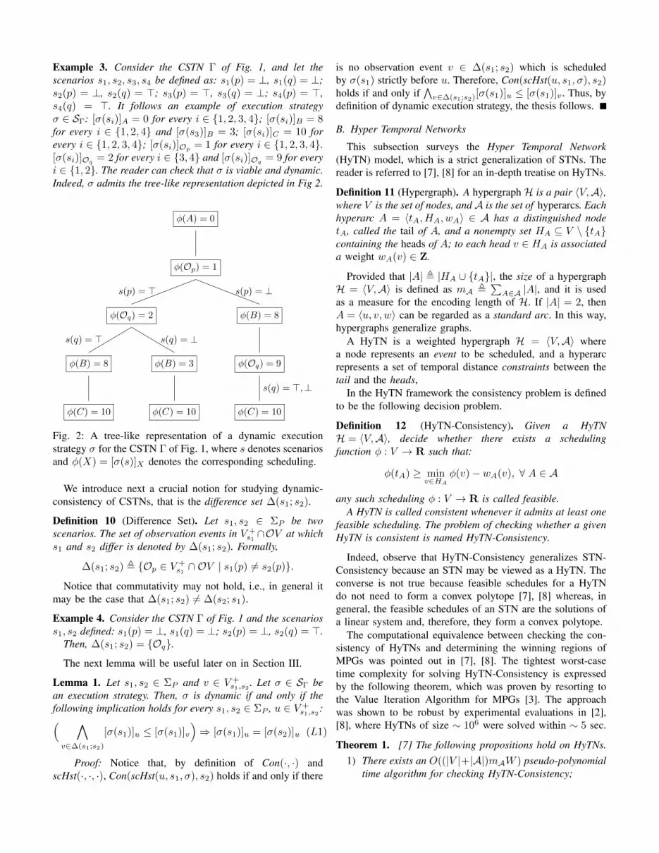
Example 3. Consider the CSTN Γ of Fig. 1, and let thescenarios s1, s2, s3, s4 be defined as: s1(p) = ⊥, s1(q) = ⊥;s2(p) = ⊥, s2(q) = >; s3(p) = >, s3(q) = ⊥; s4(p) = >,s4(q) = >. It follows an example of execution strategyσ ∈ SΓ: [σ(si)]A = 0 for every i ∈ 1, 2, 3, 4; [σ(si)]B = 8for every i ∈ 1, 2, 4 and [σ(s3)]B = 3; [σ(si)]C = 10 forevery i ∈ 1, 2, 3, 4; [σ(si)]Op = 1 for every i ∈ 1, 2, 3, 4.[σ(si)]Oq = 2 for every i ∈ 3, 4 and [σ(si)]Oq = 9 for everyi ∈ 1, 2. The reader can check that σ is viable and dynamic.Indeed, σ admits the tree-like representation depicted in Fig 2.
φ(A) = 0
φ(Op) = 1
φ(B) = 8
φ(Oq) = 9
φ(C) = 10
s(q) = >,⊥
φ(Oq) = 2
φ(B) = 3
φ(C) = 10
φ(B) = 8
φ(C) = 10
s(q) = > s(q) = ⊥
s(p) = > s(p) = ⊥
Fig. 2: A tree-like representation of a dynamic executionstrategy σ for the CSTN Γ of Fig. 1, where s denotes scenariosand φ(X) = [σ(s)]X denotes the corresponding scheduling.
We introduce next a crucial notion for studying dynamic-consistency of CSTNs, that is the difference set ∆(s1; s2).
Definition 10 (Difference Set). Let s1, s2 ∈ ΣP be twoscenarios. The set of observation events in V +
s1 ∩OV at whichs1 and s2 differ is denoted by ∆(s1; s2). Formally,
∆(s1; s2) , Op ∈ V +s1 ∩ OV | s1(p) 6= s2(p).
Notice that commutativity may not hold, i.e., in general itmay be the case that ∆(s1; s2) 6= ∆(s2; s1).
Example 4. Consider the CSTN Γ of Fig. 1 and the scenarioss1, s2 defined: s1(p) = ⊥, s1(q) = ⊥; s2(p) = ⊥, s2(q) = >.
Then, ∆(s1; s2) = Oq.
The next lemma will be useful later on in Section III.
Lemma 1. Let s1, s2 ∈ ΣP and v ∈ V +s1,s2 . Let σ ∈ SΓ be
an execution strategy. Then, σ is dynamic if and only if thefollowing implication holds for every s1, s2 ∈ ΣP , u ∈ V +
s1,s2 :( ∧v∈∆(s1;s2)
[σ(s1)]u ≤ [σ(s1)]v
)⇒ [σ(s1)]u = [σ(s2)]u (L1)
Proof: Notice that, by definition of Con(·, ·) andscHst(·, ·, ·), Con(scHst(u, s1, σ), s2) holds if and only if there
is no observation event v ∈ ∆(s1; s2) which is scheduledby σ(s1) strictly before u. Therefore, Con(scHst(u, s1, σ), s2)holds if and only if
∧v∈∆(s1;s2)[σ(s1)]u ≤ [σ(s1)]v . Thus, by
definition of dynamic execution strategy, the thesis follows.
B. Hyper Temporal Networks
This subsection surveys the Hyper Temporal Network(HyTN) model, which is a strict generalization of STNs. Thereader is referred to [7], [8] for an in-depth treatise on HyTNs.
Definition 11 (Hypergraph). A hypergraph H is a pair 〈V,A〉,where V is the set of nodes, andA is the set of hyperarcs. Eachhyperarc A = 〈tA, HA, wA〉 ∈ A has a distinguished nodetA, called the tail of A, and a nonempty set HA ⊆ V \ tAcontaining the heads of A; to each head v ∈ HA is associateda weight wA(v) ∈ Z.
Provided that |A| , |HA ∪ tA|, the size of a hypergraphH = 〈V,A〉 is defined as mA ,
∑A∈A |A|, and it is used
as a measure for the encoding length of H. If |A| = 2, thenA = 〈u, v, w〉 can be regarded as a standard arc. In this way,hypergraphs generalize graphs.
A HyTN is a weighted hypergraph H = 〈V,A〉 wherea node represents an event to be scheduled, and a hyperarcrepresents a set of temporal distance constraints between thetail and the heads,
In the HyTN framework the consistency problem is definedto be the following decision problem.
Definition 12 (HyTN-Consistency). Given a HyTNH = 〈V,A〉, decide whether there exists a schedulingfunction φ : V → R such that:
φ(tA) ≥ minv∈HA
φ(v)− wA(v), ∀ A ∈ A
any such scheduling φ : V → R is called feasible.A HyTN is called consistent whenever it admits at least one
feasible scheduling. The problem of checking whether a givenHyTN is consistent is named HyTN-Consistency.
Indeed, observe that HyTN-Consistency generalizes STN-Consistency because an STN may be viewed as a HyTN. Theconverse is not true because feasible schedules for a HyTNdo not need to form a convex polytope [7], [8] whereas, ingeneral, the feasible schedules of an STN are the solutions ofa linear system and, therefore, they form a convex polytope.
The computational equivalence between checking the con-sistency of HyTNs and determining the winning regions ofMPGs was pointed out in [7], [8]. The tightest worst-casetime complexity for solving HyTN-Consistency is expressedby the following theorem, which was proven by resorting tothe Value Iteration Algorithm for MPGs [3]. The approachwas shown to be robust by experimental evaluations in [2],[8], where HyTNs of size ∼ 106 were solved within ∼ 5 sec.
Theorem 1. [7] The following propositions hold on HyTNs.1) There exists an O((|V |+|A|)mAW ) pseudo-polynomial
time algorithm for checking HyTN-Consistency;

2) There exists an O((|V |+|A|)mAW ) pseudo-polynomialtime algorithm such that, given in input any consistentHyTN H = (V,A), then it returns as output a feasiblescheduling φ : V → R of H;
Here, W , maxA∈A,v∈HA |wA(v)|.
III. ALGORITHMICS OF DYNAMIC-CONSISTENCY
To start with, we offer the following coNP-hardness lowerbound on CSTN-DC.
Theorem 2. CSTN-DC is coNP-hard.
Proof: We reduce 3-SAT to the complement of CSTN-DC. Let ϕ be a boolean formula in 3CNF. Let X be the set ofvariables and let C = C0, . . . , Cm−1 be the set of clausescomprising ϕ =
∧m−1j=0 Cj .
(1) Let Nϕ be the CSTN 〈V ϕ, Aϕ, Lϕ,Oϕ,OV ϕ, Pϕ〉,where: V ϕ , X ∪ C, and all the nodes are given emptylabel, i.e., Lϕ(v) = λ for every v ∈ V ϕ; Pϕ , OV ϕ , X;Oϕ is the identity function; for every u, v ∈ OV ϕ we have〈u − v ≤ 0, λ〉 ∈ Aϕ; for every x ∈ X and C ∈ C we have〈x−C ≤ −1, λ〉 ∈ Aϕ; for each j = 0, . . . ,m−1 and for eachliteral ` ∈ Cj , we have 〈Cj − C(j+1)mod m ≤ −1, `〉 ∈ Aϕ.Notice that |V ϕ| = n+m and |Aϕ| = n2 + nm+ 3m.
(2) Assume that ϕ is satisfiable. Let ν be a satisfying truth-assignment of ϕ. In order to prove that Nϕ is not dynamically-consistent, observe that the restriction of Nϕ w.r.t. the scenarioν is a non-consistent STN. Indeed, if for every j = 0, . . . ,m−1 we pick a standard arc 〈Cj − C(j+1)mod m ≤ −1, `j〉 with`j being a literal in Cj such that ν(`j) = >, then we obtaina negative circuit.
(3) Assume that ϕ is unsatisfiable. In order to prove that Nϕ
is dynamically-consistent, we exhibit a viable and dynamicexecution strategy σ for Nϕ. First, schedule every x ∈ X atσ(x) , 0. Therefore, by time 1, the planner has full knowledgeof the observed scenario ν. Since ϕ is unsatisfiable, thereexists an index jν such that ν(Cjν ) = ⊥. At this point, setσ(C(jν+k)mod m) , k for k = 1, . . . ,m. The reader can verifythat σ is viable and dynamic for Nϕ.
It remains currently open whether CSTN-DC lies inPSPACE and whether it is PSPACE-hard.
A. ε-Dynamic-Consistency
In CSTNs, decisions about the precise timing of actions arepostponed until execution time, when informations meanwhilegathered at the observation nodes can be taken into account.However, the planner is allowed to factor in an outcome, anddifferentiate its strategy according to it, only strictly after theoutcome has been observed (whence the strict inequality inDefinition 7). Notice that this definition does not take intoaccount the reaction time, which, in most applications, is non-negligible. In order to deliver algorithms that can also dealwith the reaction time ε of the planner, we employ a refinednotion of dynamic-consistency.
Definition 13 (ε-dynamic-consistency). Given any CSTN〈V,A,L,O,OV, P 〉 and any real number ε ∈ (0,+∞), an
execution strategy σ ∈ SΓ is ε-dynamic if it satisfies all theHε-constraints, namely, for any two scenarios s1, s2 ∈ ΣPand any event u ∈ V +
s1,s2 , the execution strategy σ satisfiesthe following constraint, which is denoted Hε(s1; s2;u):
[σ(s1)]u ≥ min([σ(s2)]u∪[σ(s1)]v+ε | v ∈ ∆(s1; s2)
)We say that a CSTN Γ is ε-dynamically-consistent if it admitsσ ∈ SΓ which is both viable and ε-dynamic. The problem ofchecking whether a given CSTN is ε-dynamically-consistent isnamed CSTN-ε-DC.
It follows directly from Definition 13 that, whenever σ ∈ SΓ
satisfies some Hε(s1; s2;u), then σ satisfies Hε′(s1; s2;u) forevery ε′ ∈ (0, ε] as well. This proves the following lemma.
Lemma 2. If Γ is ε-dynamically-consistent, for some ε > 0,then Γ is ε′-dynamically-consistent for every ε′ ∈ (0, ε].
Given any dynamically-consistent CSTN, we may ask forthe maximum reaction time ε of the planner beyond which thenetwork is no longer dynamically-consistent.
Definition 14 (Reaction time ε). Let ε = ε(Γ) be the greatestreal number ε such that Γ is ε-dynamically-consistent.
If Γ is dynamically-consistent, then ε(Γ) exists finite andε(Γ) > 0, as it is now proved in Lemma 3.
Lemma 3. Let σ be a dynamic execution strategy for theCSTN Γ. Then, there exists a sufficiently small real numberε ∈ (0,+∞) such that σ is ε-dynamic.
Proof: Let s1, s2 ∈ ΣP be two scenarios and let usconsider any event u ∈ V +
s1,s2 . Since σ is dynamic, then byLemma 1 the following implication necessarily holds:( ∧v∈∆(s1;s2)
[σ(s1)]u ≤ [σ(s1)]v
)⇒ [σ(s1)]u ≥ [σ(s2)]u (∗)
Notice that, w.r.t. Lemma 1, we have relaxed the equality[σ(s1)]u = [σ(s2)]u in the implicand of (L1) by introducingthe inequality [σ(s1)]u ≥ [σ(s2)]u. At this point, we convert(∗) from implicative to disjunctive form, first by applying therule of material implication2, and then De Morgan’s law3.From this, we see that the following disjunction must hold:
[σ(s1)]u ≥ [σ(s2)]u ∨∨
v∈∆(s1;s2)
[σ(s1)]u > [σ(s1)]v (∗∗)
Then, we argue that there exists a real number ε ∈ (0,+∞)such that the following disjunction holds as well:
[σ(s1)]u ≥ [σ(s2)]u ∨∨
v∈∆(s1;s2)
[σ(s1)]u ≥ [σ(s1)]v + ε.
In fact, since the disjunction (∗∗) necessarily holds, thenone can define ε to be the minimum among all the valuesε(s1; s2;u) ∈ (0,+∞) such that for every 〈s1, s2, u〉 ∈ΣP ×ΣP ×V +
s1,s2 the following is satisfied: ε(s1; s2;u) = 1 if
2The rule of material implication: |= p⇒ q ⇐⇒ ¬p ∨ q3De Morgan’s law: |= ¬(p ∧ q) ⇐⇒ ¬p ∨ ¬q

[σ(s1)]u ≥ [σ(s2)]u; otherwise, ε(s1; s2;u) = min[σ(s1)]u−[σ(s1)]v | v ∈ ∆(s1, s2), [σ(s1)]u > [σ(s1)]v.
This implies that σ satisfies every Hε-constraint of Γ, andthus that σ is ε-dynamic.
Lemma 4. Let σ be an ε-dynamic execution strategy for theCSTN Γ, for some ε ∈ (0,+∞). Then, σ is dynamic.
Proof: For the sake of contradiction, let us suppose that σis not dynamic. Let F be the non-empty set of all the triplets〈u, s1, s2〉 ∈ V +
s1,s2 × ΣP × ΣP , for which the implication(L1) does not hold. Then, 〈u, s1, s2〉 ∈ F if and only if thefollowing two hold:
1) [σ(s1)]u ≤ [σ(s1)]v for every v ∈ ∆(s1; s2);2) [σ(s1)]u 6= [σ(s2)]u.
Let 〈u, s1〉 , arg min[σ(s1)]u | ∃s2 〈u, s1, s2〉 ∈ F bean event whose scheduling time is minimum and for which(1) and (2) hold. Since 〈u, s1〉 is minimum in time, then[σ(s1)]u ≤ [σ(s2)]u for every s2 ∈ ΣP such that 〈u, s1, s2〉 ∈F ; moreover, since 〈u, s1, s2〉 ∈ F , then [σ(s1)]u 6= [σ(s2)]uby (2), so that [σ(s1)]u < [σ(s2)]u. At this point, recall thatσ is ε-dynamic by hypothesis, hence [σ(s1)]u < [σ(s2)]uimplies that there exists v ∈ ∆(s1; s2) such that [σ(s1)]u ≥[σ(s1)]v + ε > [σ(s1)]v , but this inequality contradicts (1).Indeed, F = ∅ and σ is thus dynamic.
In Section IV, the following theorem is proved.
Theorem 3. For any dynamically-consistent CSTN Γ, whereV is the set of events and ΣP is the set of scenarios, we havethat ε(Γ) ≥ |ΣP |−1|V |−1.
Notice that, in Definition 9, dynamic-consistency was de-fined by strict-inequality and equality constraints. However, byTheorem 4, dynamic-consistency can also be defined in termsof Hε-constraints only (i.e., no strict-inequalities are required).
Theorem 4. Let ε , |ΣP |−1|V |−1. Then, Γ is dynamically-consistent if and only if Γ is ε-dynamically-consistent.
By Theorem 4, any algorithm for checking ε-dynamic-consistency can be used to check dynamic-consistency as well.
B. A Singly-Exponential Time Algorithm for CSTN-DC
In this section, we present the first singly-exponential timealgorithm for solving CSTN-DC, also producing a dynamicexecution strategy whenever the input CSTN is dynamically-consistent. Hereafter, let us denote N0 , N \ 0. The mainresult of this paper is summarized in the following theorem,which is proven in this section.
Theorem 5. The following two propositions hold.
1) There exists an O(|ΣP |2|A|2 + |ΣP |3|A||V ||P | +|ΣP |4|V |2|P |)WD time algorithm deciding CSTN-ε-DCon input 〈Γ, ε〉, for any CSTN Γ = 〈V,A,L,O,OV, P 〉and any rational number ε = N/D where N,D ∈ N0.In particular, given any ε-dynamically-consistent CSTNΓ, the algorithm returns as output a viable and ε-dynamic execution strategy for Γ.
2) There exists an O(|ΣP |3|A|2|V | + |ΣP |4|A||V |2|P | +|ΣP |5|V |3|P |)W time algorithm for checking CSTN-DCon any input Γ = 〈V,A,L,O,OV, P 〉. In particular,given any dynamically-consistent CSTN Γ, the algorithmreturns a viable and dynamic execution strategy for Γ.
Here, W , maxa∈A |wa|.
We now present the reduction from CSTN-DC to HyTN-Consistency.
Firstly, we argue that any CSTN can be viewed as a succinctrepresentation which can be expanded into an exponentialsized STN. The Expansion of CSTNs is introduced below.
Definition 15 (Expansion 〈V ExΓ ,ΛEx
Γ 〉). Let Γ be a CSTN〈V,A,L,O,OV, P 〉. Consider the distinct STNs 〈Vs, As〉, onefor each scenario s ∈ ΣP , defined as follows:
Vs , vs | v ∈ V +s and As , 〈us, vs, w〉 | 〈u, v, w〉 ∈ A+
s .
We define the expansion 〈V ExΓ ,ΛEx
Γ 〉 of Γ as follows:
〈V ExΓ ,ΛEx
Γ 〉 ,⟨ ⋃s∈ΣP
Vs,⋃s∈ΣP
As
⟩.
Notice that Vs1 ∩ Vs2 = ∅ whenever s1 6= s2 and that〈V Ex
Γ ,ΛExΓ 〉 is an STN with at most |V Ex
Γ | ≤ |ΣP | |V | nodesand at most |ΛEx
Γ | ≤ |ΣP | |A| standard arcs.We now show that the expansion of a CSTN can be enriched
with some hyperarcs in order to model ε-dynamic-consistency,by means of a particular HyTN which is denoted Hε(Γ).
Definition 16 (HyTN Hε(Γ)). Given any ε ∈ (0,+∞) andany CSTN Γ = 〈V,A,L,O,OV, P 〉, a corresponding HyTNdenoted by Hε(Γ) can be defined as follows:• For every scenarios s1, s2 ∈ ΣP and every event u ∈V +s1,s2 , define a hyperarc α = αε(s1; s2;u) as follows
(with the intention to model Hε(s1; s2;u), see Def. 13):
αε(s1; s2;u) , 〈tα, Hα, wα〉,
where:– tα , us1 is the tail of the hyperarc α;– Hα , us2 ∪∆(s1; s2) is the set of the heads;– wα(us2) , 0; wα(v) , −ε for each v ∈ ∆(s1; s2).
• Consider the expansion 〈V ExΓ ,ΛEx
Γ 〉 of Γ. Then, Hε(Γ) isdefined as Hε(Γ) , 〈V Ex
Γ ,AHε〉, where,
AHε , ΛExΓ ∪
⋃s1,s2∈ΣPu∈V +
s1,s2
αε(s1; s2;u).
Notice that each αε(s1; s2;u) has size |αε(s1; s2;u)| =O(∆(s1; s2)) = O(|P |). In Fig. 3, Algorithm 1 presents thepseudocode for constructing Hε(Γ). An excerpt of the HyTNcorresponding to the CSTN of Fig. 1 is depicted in Fig. 4.
The following theorem establishes the connection betweendynamic-consistency of CSTNs and consistency of HyTNs.
Theorem 6. Given any CSTN Γ = 〈V,A,L,O,OV, P 〉,there exists a sufficiently small real number ε ∈ (0,+∞)such that Γ is dynamically-consistent if and only if Hε(Γ)

is consistent. Moreover, Hε(Γ) has at most |VHε | ≤ |ΣP | |V |nodes, |AHε | = O(|ΣP | |A|+ |ΣP |2|V |) hyperarcs, and it hassize at most mAHε = O(|ΣP | |A|+ |ΣP |2|V | |P |).
Proof: For any ε > 0, let Hε(Γ) = 〈V ExΓ ,AHε〉 be the
HyTN of Definition 16.(1) Firstly, we prove that, for any ε > 0, Hε(Γ) is consistent
if and only if Γ is ε-dynamically-consistent. (⇒) Given anyfeasible scheduling φ : V Ex
Γ → R for Hε(Γ), let σφ(s) ∈SΓ be the execution strategy defined as: [σφ(s)]v , φ(vs),for every vs ∈ V E
Γ , where v ∈ V and s ∈ ΣP . Notice thateach hyperarc αε(s1; s2;u) is satisfied by φ if and only if thecorresponding Hε-constraint Hε(s1; s2;u) is satisfied by σφ;moreover, recall that ΛEx
Γ ⊆ AHε , and that ΛExΓ contains all
the original standard difference constraints of Γ. At this point,since φ is feasible for Hε(Γ), then σφ must be viable andε-dynamic for Γ. Hence, Γ is ε-dynamically-consistent.
(⇐) Given any viable and ε-dynamic execution strategy σ ∈SΓ, for some ε > 0, let φσ : V Ex
Γ → R be the scheduling ofHε(Γ) defined as: φσ(vs) , [σ(s)]v for every vs ∈ V Ex
Γ , wherev ∈ V and s ∈ ΣP . Also in this case we have ΛEx
Γ ⊆ AHε , anda moment’s reflection reveals that each hyperarc αε(s1; s2;u)is satisfied by φσ if and only if Hε(s1; s2;u) is satisfied byσ. At this point, since σ is viable and ε-dynamic for Γ, thenφσ must be feasible for Hε(Γ). Hence Hε(Γ) is consistent.
(2) At this point, by composition with (1), Lemma 3 impliesthat there exists a sufficiently small ε > 0 such that Γ isdynamically-consistent if and only if Hε(Γ) is consistent.
(3) The size bounds follow directly from Definition 16.The pseudo-code for checking CSTN-ε-DC is given in
Algorithm 2, whereas the pseudo-code for checking CSTN-DC is provided in Algorithm 3. The latter algorithm goesas follows. Firstly, it computes a sufficiently small ε > 0by resorting to Theorem 4, i.e., ε = |ΣP |−1|V |−1 (at line 1of Algorithm 3). Secondly, it constructs Hε(Γ) (at line 1 ofAlgorithm 2) and then it scales every hyperarc’s weight toZ (at lines 2-3). Thirdly, Hε(Γ) is solved with the HyTN-Consistency algorithm underlying Theorem 1 (at line 4), i.e.,an instance of the HyTN-Consistency problem is solved byreduction to the decision problem for MPGs. If the HyTN-Consistency algorithm outputs YES, together with a feasiblescheduling φ of Hε(Γ), then the time values of φ are scaledback to size w.r.t. ε and then 〈YES, φ〉 is returned as output(lines 5-8); otherwise, the output is simply NO (at line 10).
Remark 1. The same algorithm, with essentially the sameupper bound on its running time and space, work also in casewe allow for arbitrary boolean formulae as labels, rather thanjust conjunctions. At the same time, hyperarc constraints canalso be allowed inside the input CSTNs, besides the standardarc constraints. Under this prospect, our algorithm actuallysolves a larger family of conditional temporal networks, thatwe may call Conditional Hyper Temporal Networks (CHyTNs).
Remark 2. We remark that the HyTN/MPG algorithm that isat the heart of our approach requires integral weights (i.e., itrequires that w(u, v) ∈ Z for every (u, v) ∈ A), and we could
Algorithm 1: construct_H(Γ, ε)
Input: a CSTN Γ , 〈V,A, L,O,OV, P 〉, a rational ε > 01 foreach (s ∈ ΣP ) do2 Vs ← vs | v ∈ V +
s ;3 As ← as | a ∈ A+
s ;4 V Ex
Γ ← ∪s∈ΣP Vs;5 ΛEx
Γ ← ∪s∈ΣPAs;6 foreach (s1, s2 ∈ ΣP AND u ∈ V +
s1,s2 ) do7 tα ← us1 ;8 Hα ← us2 ∪∆(s1; s2);9 wα(us2)← 0;
10 foreach v ∈ ∆(s1; s2) do11 wα(vs1)← −ε;12 αε(s1; s2;u)← 〈tα, Hα, wα〉;
13 AHε ← ΛExΓ ∪
⋃s1,s2∈ΣPu∈V +
s1,s2
αε(s1; s2;u);
14 Hε(Γ)← 〈V ExΓ ,AHε〉;
15 return Hε(Γ);
Algorithm 2: check_CSTN-ε-DC(Γ, ε)
Input: a CSTN Γ , 〈V,A, L,O,OV, P 〉, a rational numberε , N/D, for N,D ∈ N0
1 Hε(Γ)← construct_H(Γ, ε); // ref. Algorithm 12 foreach (A = 〈tA, HA, wA〉 ∈ AHε(Γ) AND h ∈ HA) do3 wA(h)← wA(h)D; // scale weights to Z
4 φ← check_HyTN-Consistency(Hε(Γ)); // ref. Thm 15 if (φ is a feasible scheduling of Hε(Γ)) then6 foreach (event node v ∈ VHε(Γ)) do7 φ(v)← φ(v)/D; // re-scale back to size w.r.t ε
8 return 〈YES, φ〉;9 else
10 return NO;
Algorithm 3: check_CSTN-DC(Γ)
Input: a CSTN Γ , 〈V,A, L,O,OV, P 〉1 ε← |ΣP |−1|V |−1; // ref. Thm. 42 return check_CSTN-ε-DC(Γ, ε);
Fig. 3: Solving CSTN-DC by reduction to HyTN-Consistency.
not play it differently [7], [8]. Moreover, the algorithm alwayscomputes integral solution to HyTN/MPGs and, therefore, italways computes rational feasible schedules for the CSTNsgiven in input. As such, this “requirement“ actually turns outto be a plus in practice. To conclude, it is indeed integralitythat allows us to analyze the algorithm quantitatively and topresent a sharp lower bounding analysis on the critical valueof the reaction time ε, where the CSTN transits from being,to not being, dynamically consistent. We believe that theseissues deserve much attention, going into them required analgorithmic discrete approach to the notion of numbers.
Now, the correctness and the time complexity of Algo-rithm 3 is analyzed. To begin, notice that some of the temporalconstraints introduced during the reduction step depends on a

sufficiently small parameter ε > 0, whose magnitude turns outto depend on the size of the input CSTN. It is now proved thatthe time complexity of the algorithm depends multiplicativelyon D, provided that ε = N/D for some N,D ∈ N0. InSection IV we will present a sharp lower bounding analysison ε, from which the (pseudo) singly-exponential time boundfollows as corollary. So, assume for a moment line 1 to bevalid, we prove it in Theorem 3. As a corollary of Theorem 6,we have that Algorithm 3 correctly decides CSTN-DC. Themost time expensive step of the algorithm is clearly line 4 ofAlgorithm 2, which resorts to Theorem 1 in order to solve aninstance of HyTN-Consistency. From Theorem 6 we have anupper bound on the size of Hε(Γ), while Theorem 1 gives usa pseudo-polynomial upper bound for the computation time.Also, recall that we scale weights by a factor D at lines 2-3of Algorithm 2, where ε = N/D for some N,D ∈ N0. Thus,by composition, Algorithm 3 decides CSTN-DC in a time T|Γ|which is bounded as follows, where W , maxa∈A |wa|:
T|Γ| = O((|VHε(Γ)|+ |AHε(Γ)|)mAHε (Γ))WD.
Whence, the following holds:
T|Γ| = O(|ΣP |2|A|2 + |ΣP |3|A||V ||P |+ |ΣP |4|V |2|P |)WD.
By Theorem 3, it is sufficient to check ε-dynamic-consistency for ε = |ΣP |−1|V |−1. An O(|ΣP |3|V ||A|2 +|ΣP |4|A||V |2|P | + |ΣP |5|V |3|P |)W worst-case time boundfollows for Algorithm 3. Since |ΣP | ≤ 2min(|P |,l) (where `is the number of distinct labels that appear in Γ), the singly-exponential time bound follows. This proves Theorem 5.
IV. BOUNDING ANALYSIS ON THE REACTION TIME ε
In this section we present an asymptotically sharp lowerbound for ε(Γ), that is the critical value of reaction time wherethe CSTN transits from being, to not being, dynamically-consistent. The proof technique introduced in this analysis isapplicable more in general, when dealing with linear differ-ence constraints which include strict inequalities. Moreover,this bound implies that Algorithm 3 is a (pseudo) singly-exponential time algorithm for solving CSTN-DC. To begin,we are going to provide a proof of Theorem 3, but let us firstintroduce some further notation.
Let Γ , 〈V,A,L,O,OV, P 〉 be a dynamically-consistentCSTN. By Theorem 6, there exists ε > 0 such that Hε(Γ) isconsistent. Then, let φ : V Ex
Γ → R be a feasible scheduling forHε(Γ). For any hyperarc A = 〈tA, HA, wA〉 ∈ AHε , define astandard arc aA as follows:
aA , 〈tA, h, wA(h)〉, where h , arg minh∈HA
(φ(h)− wA(h)
).
Then, notice that the network Tφε (Γ) , 〈V ExΓ ,⋃A∈AHε
aA〉is an STN. Moreover, φ is feasible for Tφε (Γ). At this point,assuming v ∈ V Ex
Γ , consider the fractional part rv of φv , i.e.,
rv , φv − bφvc.
Then, let R , rvv∈V ExΓ
be the set of all the fractional parts.Sort R by the common ordering on R and assume that S ,
As4Bs4Cs4Os4p
ps4 = >Os4q qs4 = >
Os1q qs1 = ⊥Os1pps1 = ⊥
Cs1 Bs1 As1
[10, 10]
2 0
[0, 5]
[0, 9]
10
[10, 10]
0
[0, 5]
[0, 9]
10
1
0
−ε
−ε
0
−ε
−ε
0
−ε
−ε
0
−ε
0
−ε
0
−ε
−ε
0
−ε
−ε
0
−ε
−ε
0
−ε
0
−ε
Fig. 4: An excerpt of the HyTN Hε(Γ) corresponding tothe CSTN Γ of Fig. 1, in which two scenarios, s4 ands1, are considered and the corresponding hyper-constraintsH(s4; s1;u) are depicted as dotted hyperarcs.
r1, . . . , rk is the resulting ordered set without repetitions,i.e., |S| = k, S = R, r1 < . . . < rk. Now, let pos(v) be theindex position such that:
1 ≤ pos(v) ≤ k and rpos(v) = rv.
Then, we define a new fractional part as follows:
r′v ,pos(v)− 1
|ΣP ||V |(NFP)
also, we define a new scheduling function as follows:
φ′v , bφvc+ r′v (NSF)
Remark 3. Notice that (NFP) doesn’t alter the orderingrelation among the fractional parts, i.e.,
r′u < r′v ⇐⇒ ru < rv, for any u, v ∈ V ExΓ ,
moreover, observe that (NSF) doesn’t change the value of anyintegral part, i.e.,
bφ′uc = bφuc, for any u ∈ V ExΓ .
We are now in the position to prove Theorem 3.Proof of Theorem 3: Let Γ be dynamically-consistent, by
Theorem 6 there exists ε′ > 0 such that Hε′(Γ) is consistentand admits some feasible scheduling φ : V Ex
Γ → R. Letε , |ΣP |−1|V |−1. We argue that φ′, as defined in (NSF),is a feasible scheduling for the STN Tφε (Γ). Indeed, everydifference constraint of Tφε (Γ) is of the form φv − φu ≤ w,for some w ∈ Z or w = −ε. Consider the case w ∈ Z. Then,

φ′v − φ′u ≤ w holds because of Remark 3. Now, consider thecase w = −ε. Then, φv − φu ≤ −ε implies φv 6= φu. Hence,by Remark 3, we have φ′v 6= φ′u. At this point, observe thatthe difference between φ′u and φ′v is therefore at least ε, i.e.,
φ′u − φ′v ≥ |ΣP |−1|V |−1 = ε.
That is to say, φ′v−φ′u ≤ −ε. This proves that φ′ is a feasiblescheduling for the STN Tφε (Γ). Since Tφε (Γ) is thus consistent,then Hε(Γ) is consistent as well. Therefore, by Theorem 6,the CSTN Γ is ε-dynamically-consistent.
At this point, a natural question is whether the lower boundgiven by Theorem 3 can be improved up to ε(Γ) = Ω(|V |−1).In turn, this would improve the time complexity for Algo-rithm 3 by a factor |ΣP |. However, the following theoremshows that this is not the case by exhibiting a CSTN for whichε(Γ) = 2−Ω(|P |). This proves that the lower bound given byTheorem 3 is (almost) asymptotically sharp.
Theorem 7. For each n ∈ N0 there exists a CSTN Γn suchthat ε(Γn) < 2−n+1 = 2−|P
n|/3+1, where Pn is the set ofboolean variables of Γn.
Proof:For each n ∈ N0, define a CSTN Γn ,
〈V n, An, Ln,On,OV n, Pn〉 as follows. See Fig. 5 fora clarifying illustration.• V n , Xi, Yi, Zi | 1 ≤ i ≤ n;• An , B ∪
⋃ni=1 Ci ∪
⋃n−1i=1 Di ∪ E
where:– B , 〈X1 − v ≤ 0, λ〉 | v ∈ V n ∪ 〈Z1 − X1 ≤
1, X1 ∧ Y1〉;– Ci , 〈Yi − Xi ≤ 2,¬Xi〉, 〈Xi − Yi ≤−2,¬Xi〉, 〈Zi−Yi ≤ 2,¬Yi〉, 〈Yi−Zi ≤ −2,¬Yi〉;
– Di , 〈Xi+1 − Xi ≤ 5, Zi〉, 〈Xi − Xi+1 ≤−5, Zi〉, 〈Xi+1 − Yi〉 ≤ 5,¬Zi〉, 〈Yi − Xi+1 ≤−5,¬Zi〉, 〈Zi+1 − Yi ≤ 5, Zi ∧Xi+1 ∧ Yi+1〉, 〈Yi −Zi+1 ≤ −5, Zi∧Xi+1∧Yi+1〉, 〈Zi+1−Zi ≤ 5,¬Zi∧Xi+1∧Yi+1〉, 〈Zi−Zi+1 ≤ −5,¬Zi∧Xi+1∧Yi+1〉;
– E , 〈Yn − Xn ≤ 2,¬Xn〉, 〈Xn − Yn ≤−2,¬Xn〉, 〈Zn − Yn ≤ 2,¬Yn〉, 〈Yn − Zn ≤−2,¬Yn〉;
• Ln(v) , λ for every v ∈ V n; OV n , V n; On(v) , vfor every v ∈ OV n; Pn , V n.
We exhibit a viable and dynamic execution strategy σn :ΣPn → ΦV n for Γn.
Let δini=1 and ∆ini=1 be two real valued sequences s.t.:
(1) ∆1 , 1; (2) 0 < δi < ∆i; (3) ∆i , min(δi−1,∆i−1−δi−1).
Then, the following also holds for every 1 ≤ i ≤ n:
(4) 0 < ∆i ≤ 2−i+1,
where the equality holds if and only if δi = ∆i/2.In what follows, provided that s ∈ ΣP and ` ∈ P ∗, we will
denote 1s(`) , 1 if s(`) = > and 1s(`) , 0 if s(`) = ⊥.We are ready to define σn(s) for any s ∈ ΣP :• [σn(s)]X1 , 0;
Y1
Y1?
X10X1?
Z1
Z1?
Y2
Y2?
X2
X2?
Z2
Z2?
Yn
Yn?
Xn
Xn?
Zn
Zn?
1, X1Y1
[2],¬X1 [2],¬Y1[5], Z1 [5],¬Z1X2Y2
[5],¬Z1 [5], Z1X2Y2
[2],¬X2 [2],¬Y2
[5],¬Z2 [5], Z2X3Y3
[5], Z2 [5],¬Z2X3Y3
[2],¬Xn [2],¬Yn
[5], Zn−1 [5],¬Zn−1XnYn[5],¬Zn−1 [5], Zn−1XnYn
Fig. 5: A CSTN Γn such that ε(Γn) = 2−Ω(|Pn|).
• [σn(s)]Y1, δ11s(X1) + 21s(¬X1);
• [σn(s)]Z1, 1s(X1∧Y1) + (2 + [σn(s)]Y1
)1s(¬X1∨¬Y1);• [σn(s)]Xi , 5 + [σn(s)]Xi−11s(Zi−1) +
+ [σn(s)]Yi−11s(¬Zi−1), for any 2 ≤ i ≤ n;
• [σn(s)]Yi , [σn(s)]Xi + δi1s(Xi) + 21s(¬Xi), for any2 ≤ i ≤ n;
• [σn(s)]Zi ,(5 + [σn(s)]Yi−1
1s(Zi−1) ++ [σn(s)]Zi−11s(¬Zi−1)
)1s(Xi∧Yi) +
+ (2 + [σn(s)]Yi)1s(¬Xi∨¬Yi), for any 2 ≤ i ≤ n;It is not difficult to prove, by induction on n ≥ 1, that σn isviable and dynamic for Γn.
Here we show that ε(Γn) < 2−n+1 = 2−|Pn|/3+1 for every
n ≥ 1. Let us consider the following scenario s for 1 ≤ i ≤ n:
s(Xi) , s(Yi) , >; s(Zi) ,
>, if δi ≤ ∆i/2⊥, if δi > ∆i/2
.
We assume that σ is an execution strategy for Γn and studynecessary conditions to ensure that σ is viable and dynamic,provided that the observations follow scenario s. First, σ mustschedule X1 at time [σ(s)]X1
= 0. Then, since s(X1) = >,

we must have 0 < [σ(s)]Y1< 1, because of the constraint
(Z1−X1 ≤ 1, X1∧Y1). Stated otherwise, it is necessary that:
0 < [σ(s)]Y1 − [σ(s)]X1 < ∆1.
After that, since s(Y1) = >, then σ must schedule Z1 at time[σ(s)]Z1
= 1 = ∆1. A moment’s reflection reveals that almostidentical necessary conditions now recur for X2, Y2, Z2, withthe crucial variation that it will be necessary to require:0 < [σ(s)]Y2
< ∆2. Indeed, proceeding inductively, it willbe necessary that for every 1 ≤ i ≤ n and every n ∈ N0:
0 < [σ(s)]Yi − [σ(s)]Xi < ∆i.
As already observed in (4), we have 0 < ∆n ≤ 2−n+1. Thus,any viable and dynamic execution strategy σ for Γn mustsatisfy:
0 < [σ(s)]Yn − [σ(s)]Xn <1
2n−1=
1
2|Pn|/3−1.
Thus, once the planner has observed the outcome s(Xn) = >from the observation event Xn, then he must react by schedul-ing Yn within time 2−n+1 = 2−|P
n|/3+1 in the future w.r.t.[σ(s)]Xn . Then ε(Γn) < 2−n+1 = 2−|P
n|/3+1 any n ≥ 1.
V. RELATED WORKS
This section discusses of some alternative approaches of-fered by the current literature. Recall that the article ofTsamardinos, et al. [16] has been discussed already in theintroduction. The work of Cimatti, et al. [5] provided thefirst sound-and-complete algorithm for checking the dynamic-controllability of CSTNs with Uncertainty (CSTNU) and thusit can be employed for checking the dynamic-consistency ofCSTNs as a special case. The algorithm reduces to the problemof solving Timed Game Automata (TGA). Nevertheless, noworst-case bound on the time complexity of the procedure wasprovided in [5]. We observe that solving TGAs is a problemof much higher complexity than solving MPGs, compare thefollowing known facts: solving 1-player TGAs is PSPACE-complete and solving 2-player TGAs is EXP-complete; on thecontrary, the problem of determining MPGs lie in NP∩ coNPand it is currently an open problem to prove whether it lies inP. Indeed, the algorithm in [5] is not singly-exponential timebounded. Finally, a sound algorithm for checking the dynamic-controllability of CSTNUs was given by Combi, Hunsberger,Posenato in [6]. However, it was not shown to be complete.To the best of our knowledge, it is currently open whether ornot it can be extended in order to prove completeness.
VI. CONCLUSION
We gave the first singly-exponential time algorithm to checkthe dynamic-consistency of CSTNs, also yielding dynamic ex-ecution strategies. The algorithm actually manages a few moregeneral variants of the problem, where labels are not requiredto be conjunctions and hyperarc constraints can be empolyedin the input CSTNs, besides the classical binary constraints. Tosummarize, at the heart of the algorithm a reduction to MPGsis mediated by the HyTN model. The CSTN is dynamically-consistent if and only if the corresponding MPG is everywhere
won, and a dynamic execution strategy can be convenientlyread out by an everywhere winning positional strategy. Thesize of this MPG is at most polynomial in the number ofthe possible scenarios; as such, the term at the exponent islinear, at worst, in the number of the observation events. Thesame holds for the running time of the resulting algorithm. Infuture works we would like to settle the exact computationalcomplexity of CSTN-DC, as well as to extend our approachin order to check the dynamic-controllability of CSTN withUncertainty [12]. Finally, an extensive experimental evaluationis on the way.
Acknowledgment: This work was partially supported byDepartment of Computer Science, University of Verona, Italyunder Ph.D. grant “Computational Mathematics and Biology“.
REFERENCES
[1] X. Allamigeon, P. Benchimol, and S. Gaubert. The tropical shadow-vertex algorithm solves mean payoff games in polynomial time onaverage. In ICALP 2014, Copenhagen, Denmark, July 8-11, 2014,Proceedings, Part I, pages 89–100, 2014.
[2] L. Brim and J. Chaloupka. Using strategy improvement to stay alive.Int. J. Found. Comput. Sci., 23(3):585–608, 2012.
[3] L. Brim, J. Chaloupka, L. Doyen, R. Gentilini, and J.F. Raskin. Fasteralgorithms for mean-payoff games. Formal Methods in System Design,38(2):97–118, 2011.
[4] K. Chatterjee, M. Henzinger, S. Krinninger, and D. Nanongkai.Polynomial-time algorithms for energy games with special weight struc-tures. Algorithmica, 70(3):457–492, 2014.
[5] A. Cimatti, L. Hunsberger, A. Micheli, R. Posenato, and M. Roveri.Sound and complete algorithms for checking the dynamic controllabilityof temporal networks with uncertainty, disjunction and observation. In21st Intern. Symp. on Temp. Repres. and Reasoning, TIME 2014, Verona,Italy, pages 27–36, 2014.
[6] C. Combi, L. Hunsberger, and R. Posenato. An algorithm for checkingthe dynamic controllability of a conditional simple temporal networkwith uncertainty. In ICAART 2013 - Proc. of the 5th Intern. Conf. onAgents and Artif. Intell., Vol. 2, Spain, 2013, pages 144–156, 2013.
[7] C. Comin, R. Posenato, and R. Rizzi. A tractable generalization ofsimple temporal networks and its relation to mean payoff games. In 21thInternational Symposium on Temporal Representation and Reasoning(TIME 2014), Verona, Italy, Sept 2014.
[8] C. Comin, R. Posenato, and R. Rizzi. Hyper temporal networks. CoRR,abs/1503.03974, 2015.
[9] R. Dechter, I. Meiri, and J. Pearl. Temporal constraint networks.Artificial Intelligence, 49(1–3):61–95, 1991.
[10] A. Ehrenfeucht and J. Mycielski. Positional strategies for mean payoffgames. International Journal of Game Theory, 8(2):109–113, 1979.
[11] E. Gradel, W. Thomas, and T. Wilke, editors. Automata Logics, andInfinite Games: A Guide to Current Research. Springer-Verlag NewYork, Inc., New York, NY, USA, 2002.
[12] L. Hunsberger, R. Posenato, and C. Combi. The dynamic controllabilityof conditional stns with uncertainty. In Proc. of the Plan. and PlanExec. for Real-World Syst.: Princip. and Pract. (PlanEx), ICAPS-2012,page 121–128, Atibaia, Sao Paulo, Brazil, 2012.
[13] M. D. Moffitt and M. E. Pollack. Applying local search to disjunctivetemporal problems. In IJCAI-05, Proceedings of the Nineteenth Interna-tional Joint Conference on Artificial Intelligence, Edinburgh, Scotland,UK, pages 242–247, 2005.
[14] A. Oddi. Constraint-based strategies for the disjunctive temporalproblem: Some new results. In Proceedings of the Sixth EuropeanConference on Planning, 2014.
[15] I. Tsamardinos and M. E. Pollack. Efficient solution techniques fordisjunctive temporal reasoning problems. Artif. Intell., 151(1-2):43–89,2003.
[16] I. Tsamardinos, T. Vidal, and M. Pollack. Ctp: A new constraint-basedformalism for conditional, temporal planning. Constraints, 8(4):365–388, 2003.
[17] U. Zwick and M. Paterson. The complexity of mean payoff games ongraphs. Theoretical Computer Science, 158:343–359, 1996.


