2  

CONTENTS    

Introduction pag.4

Chapter 1 pag.7

1.1 Magnonic Crystals pag.10

1.2 Excitation and detection of SWs pag.12

1.3 Ferromagnetic Resonance Technique pag.14

1.4 Brillouin Scattering Technique pag.15

1.5Goldostone, pseudo-Goldstone and soft modes in magnetic system pag.17

Chapter 2 pag.25

2.1 Dynamical matrix method pag.27

2.2 Formalism pag.28

2.2.1 Notation pag.29

2.2.2 Energy density pag.30

2.2.3 Equations of motion pag.35

2.3 Scattering cross section pag.41

Chapter 3 pag.46

3.1 Sample preparation and experimental setup pag.46

3.2 Collective mode classification and discussion pag.48

3.3 Phenomenological model for the reorientational phase transition pag.54

3.4 Demagnetizing field of the most relevant collective modes pag.58

3.5 Dynamic critical phenomena and universal behaviour pag.65

 3  

Conclusions pag.71

References pag.74

Acknowledgements pag.77

                         

                       

  4  

INTRODUCTION  

 

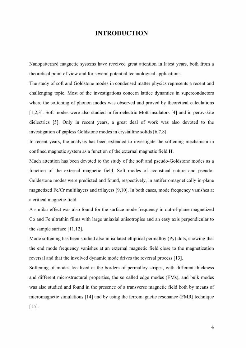
Nanopatterned magnetic systems have received great attention in latest years, both from a

theoretical point of view and for several potential technological applications.

The study of soft and Goldstone modes in condensed matter physics represents a recent and

challenging topic. Most of the investigations concern lattice dynamics in superconductors

where the softening of phonon modes was observed and proved by theoretical calculations

[1,2,3]. Soft modes were also studied in ferroelectric Mott insulators [4] and in perovskite

dielectrics [5]. Only in recent years, a great deal of work was also devoted to the

investigation of gapless Goldstone modes in crystalline solids [6,7,8].

In recent years, the analysis has been extended to investigate the softening mechanism in

confined magnetic system as a function of the external magnetic field H.

Much attention has been devoted to the study of the soft and pseudo-Goldstone modes as a

function of the external magnetic field. Soft modes of acoustical nature and pseudo-

Goldestone modes were predicted and found, respectively, in antiferromagnetically in-plane

magnetized Fe/Cr multilayers and trilayers [9,10]. In both cases, mode frequency vanishes at

a critical magnetic field.

A similar effect was also found for the surface mode frequency in out-of-plane magnetized

Co and Fe ultrathin films with large uniaxial anisotropies and an easy axis perpendicular to

the sample surface [11,12].

Mode softening has been studied also in isolated elliptical permalloy (Py) dots, showing that

the end mode frequency vanishes at an external magnetic field close to the magnetization

reversal and that the involved dynamic mode drives the reversal process [13].

Softening of modes localized at the borders of permalloy stripes, with different thickness

and different microstructural properties, the so called edge modes (EMs), and bulk modes

was also studied and found in the presence of a transverse magnetic field both by means of

micromagnetic simulations [14] and by using the ferromagnetic resonance (FMR) technique

[15].

 5  

The scope of this thesis is to study the magnetic properties of a particular type of

nanopatterned periodically system: the soft magnonic modes in Permalloy antidot lattices

with fixed lattice constant and with circular holes having different diameters.

Indeed, static and dynamic properties of ferromagnetic two-dimensional (2D) antidots

lattices (ADL) as prototypes of magnonic crystals have been investigated in detail in recent

past [16]. An investigation of the frequency dependence on H for ADLs with different holes

size was carried out using the FMR technique and by describing the field evolution of the

most relevant modes with the Kittel equation [17]. EMs and softening of the resonance

modes was found with Brillouin light scattering (BLS) technique [18].

The approach that will be used is a micromagnetic method based on a numerical tool called

dynamical matrix method (DMM). The advantage of this method is to reproduce very

accurately the dynamics inside the periodic system due to the subdivision of the sample in

nanometric cells of the order of the exchange length. It will be very stimulating selecting

among the modes, resulting from this micromagnetic analysis, the relevant modes of

physical interest. In this way a comparison with experimental data is possible. In this

respect, the influence of circular holes on the dynamic excitations will be considered, under

the assumption of validity of the Bloch theorem. Of course, the periodicity will be cause the

formation of band gaps at boundaries Brillouin Zone (BZ). In practice, these holes act as

scattering centers for the spin wave (SW) and are responsible for Bragg diffraction, similarly

to electronic case, causing the opening of band gap. It is the finite size of these holes that

dramatically makes the difference in the previous analogy with electrons. In fact, the

demagnetizing field, which is different from zero especially around the holes due to surface

magnetic charges, is strongly affected by the presence of circular holes.

So, the final aims of this thesis are to prove the existence of soft modes in 2D ADLs by

studying the softening of the Edge Mode (EM) and of the Fundamental (F) mode (the quasi-

uniform mode of the spectrum) frequencies, both characterized by the presence of finite

frequency gaps; then, going to smaller and smaller diameters of holes, shown that the

limiting behaviour of these ADLs can be approximated with film ones, as expected going to

continuum. Also a comparison with the stripe behaviour was done, in approximation of

“effective field”. Least but not last, we propose the base of a new point of view for studying

  6  

this softening mechanism in terms of dynamic critical behaviour of collective modes in 2D

magnonic crystals (represented in this work by 2D ADLs) as function of the external

magnetic field, for a fixed temperature. The theory of critical dynamic behaviour in terms of

this new variable should be worked out, in analogy to that developed for temperature.

However, some basis steps have been made in this thesis with the definition of a sort of

universality behaviour and of a sort of critical exponent, based on a scaling law that we have

found and that can be generalized to all 2D periodic ferromagnetic nanostructure.

                                               

 7  

CHAPTER 1  

To the best of our knowledge, there is not in the literature a theoretical and experimental

evidence for the soft modes in 2D extended and periodic magnetic nanostructure. The

hidden physics at the basis of this softening mechanism can be explained using a simple

phenomenological model that describes the occurring reorientation and continuous phase

transition of the magnetization.

In presence of spontaneously broken continuous symmetry new types of excitations appear,

which cost very little energy at long wavelength. Such “Goldstone modes” are, in fact,

nothing but sound modes propagating through the solid. They lead to long-range correlations

within the ordered phase, and give rise to large fluctuation effects in low dimensions. As a

result any finite temperature ordering is suppressed in dimension d≤2, for systems with

continuous symmetry.

In the simplest example of critical phenomena, the order parameter displays discrete

symmetry, as it can point only in two directions (up or down). In this case, any excitations

above the ground state cost a finite energy, since a domain wall has to be created to reverse

the spin in a given region. In other words, we have a finite gap for elementary excitations,

which for the ground state is of the order E~ J (energy needed to flip a single spin).

Excitations are created as an activated process, i.e. need energy for being activated; their

density is of the order 𝑒!!!

!".

In many ordered phases, however, there exist an order parameter characterized by

continuous symmetry. A prototype is the Heisenberg (isotropic) ferromagnet, where the

magnetization m is a three components vector that can point in any direction. The energy of

any configuration is described by the Heisenberg Hamiltonian that is invariant with respect

to a global rotation of all the spins by an arbitrary angle. We can immediately guess that a

deformation that will cost us not zero but in fact very little energy is the one that is an almost

uniform rotation, i.e. the one corresponding to a long-wavelenght spin wave (SW).

From a classical point of view, a SW represents a phase coherent precession of microscopic

vectors of magnetization of the magnetic medium. We can therefore view the Heisenberg

  8  

magnet as a deformable elastic medium, where the deformations we described are nothing

but the transverse acoustic waves propagating through the spin system, these wave

excitations dominate the behaviour in low dimensions.

The first experimental evidence for the existence of SWs came from measurements of

thermodynamic properties of ferromagnets, in particular the temperature dependence of the

saturation magnetization. The Bloch law is an indirect confirmation of the existence of SWs

in nature. The first direct observation was made using ferromagnetic resonance for the case

of uniform precession, which can be viewed as a SW with zero wave vectors; later Brillouin

light scattering experiment confirmed the existence of SWs also with non-zero wave vectors.

In some respects SWs can be considered as a magnetic analogue of the sound or light wave.

Experimental and theoretical research has demonstrated that SWs exhibit most of the

properties presents in other types of waves: excitation and propagation, interference and

diffraction, focusing and self-focusing, tunnelling and Doppler effect as well as formation of

SW envelope solitons.

Recently SWs are observed and extensively studied in laterally confined magnetic structure

and in these media SWs quantization is found: the quantization is due to the lateral finite

size effect. The main direction in studying of magnonics is connected with the ability of

SWs to carry and process information on the nanoscale. Research is particularly challenging

due to the presence of several peculiar characteristic that makes the difference between SWs

and sound or light wave. The dispersion relation ω k for SWs is highly dispersive and also

the starting point depends from the applied field as well as from the ferromagnetic sample’s

size. Furthermore, the law governing the dispersion relation is anisotropic even in the case

of an isotropic magnetic medium; all these properties are useful because enable us for the

manipulations.

The exchange and dipolar interactions, dominating in different length scale, are responsible

for the different interactions that govern the SWs [19].

Very interesting properties associated to the laterally confined isolated nanostructures were

found in the SWs spectrum: in magnetic elements of different shapes and of different

materials, the SW modes can also have a nondispersive behaviour. Because of the small

lateral dimensions, dots were in a single domain state and their magnetization orientation

 9  

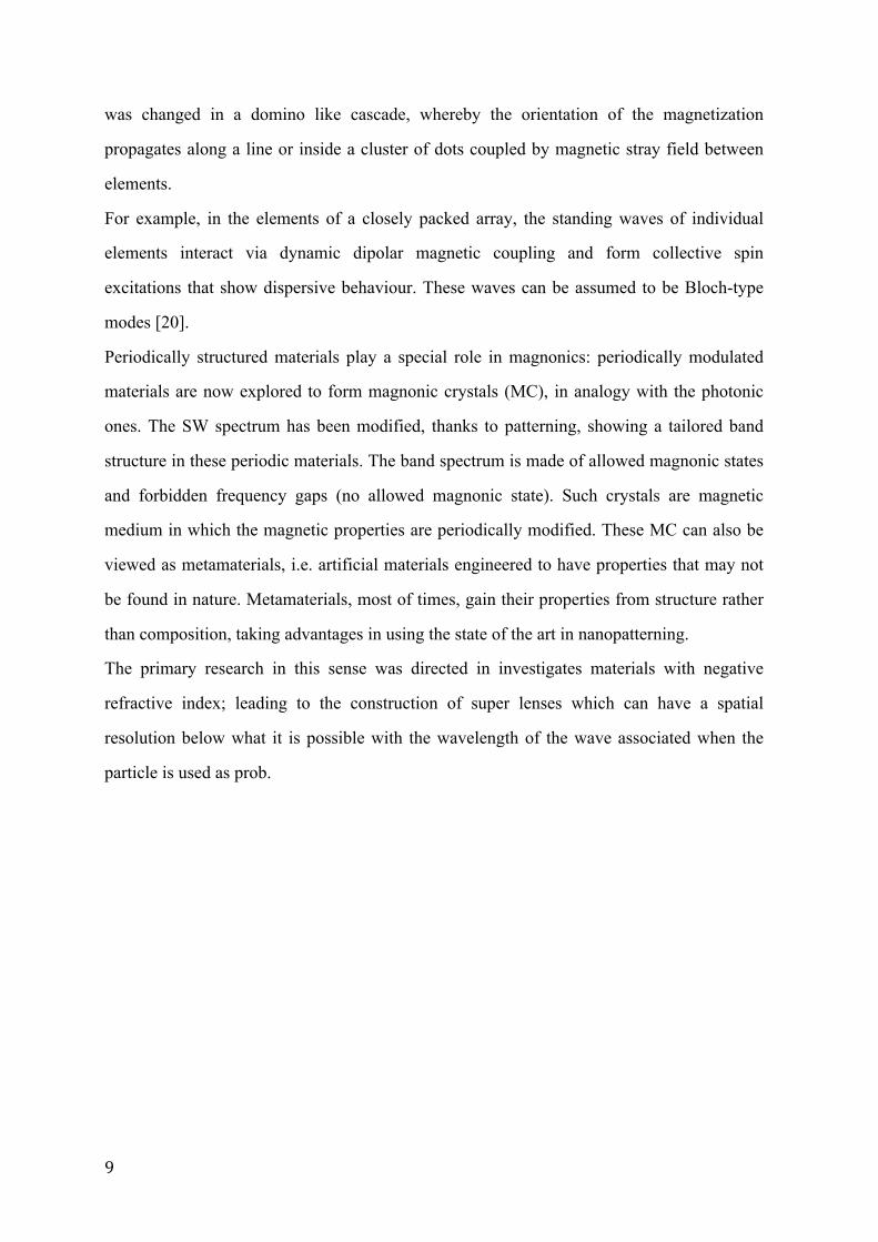
was changed in a domino like cascade, whereby the orientation of the magnetization

propagates along a line or inside a cluster of dots coupled by magnetic stray field between

elements.

For example, in the elements of a closely packed array, the standing waves of individual

elements interact via dynamic dipolar magnetic coupling and form collective spin

excitations that show dispersive behaviour. These waves can be assumed to be Bloch-type

modes [20].

Periodically structured materials play a special role in magnonics: periodically modulated

materials are now explored to form magnonic crystals (MC), in analogy with the photonic

ones. The SW spectrum has been modified, thanks to patterning, showing a tailored band

structure in these periodic materials. The band spectrum is made of allowed magnonic states

and forbidden frequency gaps (no allowed magnonic state). Such crystals are magnetic

medium in which the magnetic properties are periodically modified. These MC can also be

viewed as metamaterials, i.e. artificial materials engineered to have properties that may not

be found in nature. Metamaterials, most of times, gain their properties from structure rather

than composition, taking advantages in using the state of the art in nanopatterning.

The primary research in this sense was directed in investigates materials with negative

refractive index; leading to the construction of super lenses which can have a spatial

resolution below what it is possible with the wavelength of the wave associated when the

particle is used as prob.

 

  10  

1.1 Magnonic Crystals    Magnonic crystals (MC) consist in a periodic magnetic system: the spectrum of magnons, in

these systems, has a band structure and contains band gaps. The artificial periodic structure

modifies the original magnons’ spectrum so we can allow or forbidden specific frequency

range, acting only on the nanopatterning of the crystal. This mean, physically speaking, that

modifying the absolute value of the period we are changing the energy (dipolar or exchange)

that dominate the interactions leading to SW’ spectra. In periodically nanopatterned

magnetic media, are formed minibands consisting of allowed SW frequencies and forbidden

frequency gaps, depending on the structure created [21].

Due to the complex geometry of these systems, take into account analytically the long-range

magneto-dipole interaction presents different troubles, so numerical methods must be used.

MCs can be arranged in one dimensional (1D) two dimensional (2D) and three dimensional

(3D) array of magnetic nanostructure.

Examples of planar 1D array are the stripes [22] and the interacting dots with different

shapes [23,24]. The spectrum of magnons, clearly, shows a band structure with BZ

boundaries determined by the artificial periodicity.

Instead, the 2D MCs consists of periodically arranged dots (or anti-dots) interacting along

the two in-plane directions. The position and the width of band gaps in spectrum were

investigated as a function of the period of the structure and the depth of modulation of the

magnetic parameters, because it was found that they deeply affect each other. In this thesis,

we are interest in anti-dots 2D periodic system so it is necessary clearly define what they

are: anti-dots (AD) consist of a mesh of non-magnetic holes embedded into a continuous

magnetic film of magnetic material, permalloy (Py) in our case; they have been proposed as

candidates for ultrahigh density storage media.

In recent years the static properties of ADs have been widely investigated. Because of the

race to the smallest, reading and writing speeds in magnetic storage device are getting closer

to the time scale of spin dynamics pushing the research intensify dynamics study.

In AD nanostructure, collective magnetic excitations in form of Bloch waves can have

dispersive behaviour. The eigenfrequencies of SWs are determined by the spin stiffness, the

 11  

absolute value of the saturation magnetization, the Bloch wave vector and the relative

orientation between the magnetization vector and the wave vector. Depending on the hole’

size, SWs are dominated by short-range dynamic exchange interactions or long-range

dipolar interactions. Both these interactions regulate the characteristic slope of the SW

dispersion relation [21].

At the present state of art, in science and technology, magnonic device can be seen as the

solution for the fabrication of nanometer-scaled microwave device due to the magnons’

wavelength: orders of magnitude shorter than electromagnetic ones (in GHz range). They

may offer well miniaturizing prospective and new features, not available in photonic and

electronic devices. For example, the more precise and the easier manipulation obtained with

and external magnetic field. Also, the storage capacity of this device is powerful, thanks to

the stability of the magnetic ground-state.

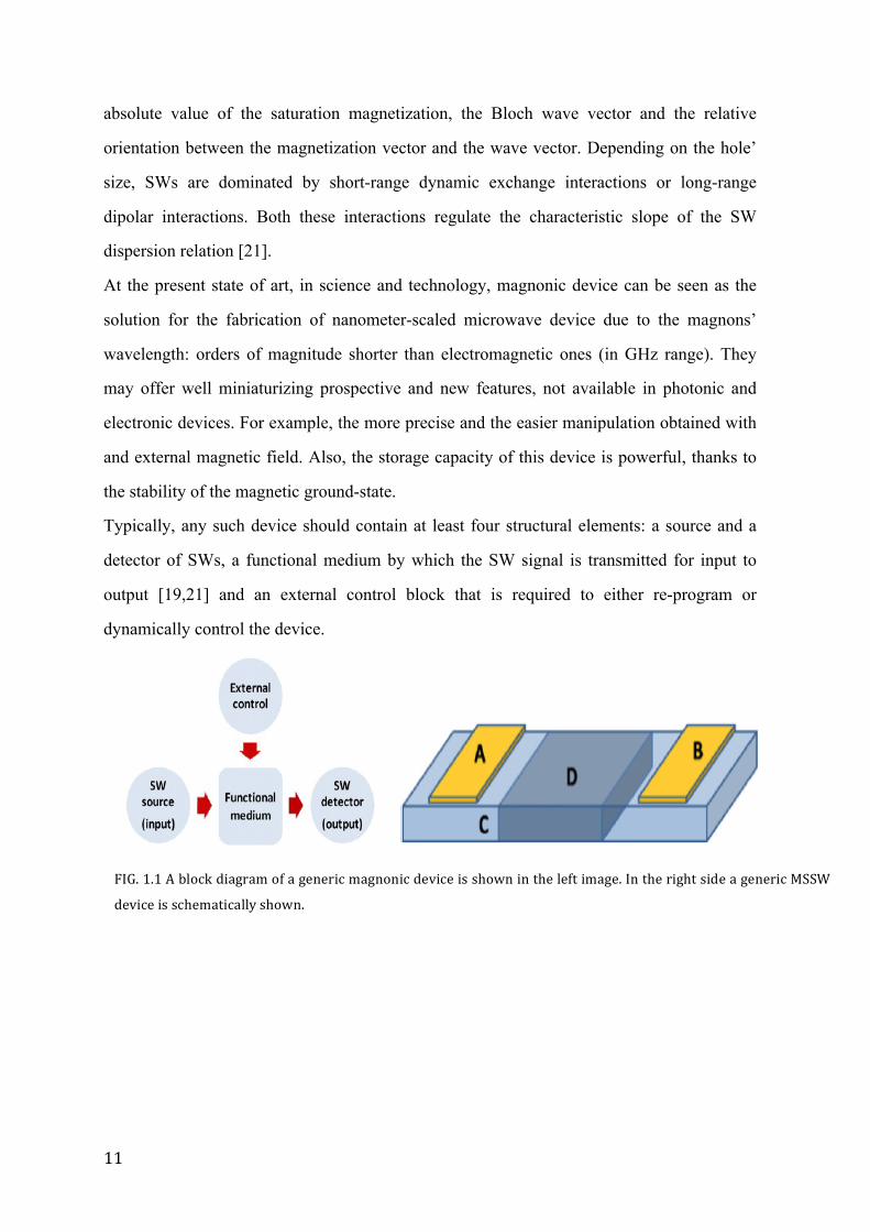
Typically, any such device should contain at least four structural elements: a source and a

detector of SWs, a functional medium by which the SW signal is transmitted for input to

output [19,21] and an external control block that is required to either re-program or

dynamically control the device.

   

           

FIG.  1.1  A  block  diagram  of  a  generic  magnonic  device  is  shown  in  the  left  image.  In  the  right  side  a  generic  MSSW  

device  is  schematically  shown.    

 

  12  

1.2 Excitation and detection of SWs    To excite the precessional motion of magnetization, one can use harmonic or pulsed

magnetic field, such as dc spin polarized currents. These stimulations can be referred to be

as a pump. Also basic interactions and phenomena could make easier the detection; the main

problem, present in all the known techniques, is the difficulties in match the frequency and

wavelength of SW in the pump (probe) spectra.

Historically, the first experimental technique used to detect precession of magnetization was

the ferromagnetic resonance technique (FMR). This technique consists in measuring spectra

of the absorption of microwaves in a cavity containing the magnetic sample. It is

conventionally used to study magnetization dynamics at frequencies up to 100 GHz. At

higher frequencies, the mismatch between the linear momentum of free-space

electromagnetic radiation (photon) and that of magnon increasingly so much that prohibits

an efficient coupling. So, higher frequencies require different techniques to detect the

excitations.

VNA-FMR is a relatively new improvement of the FMR spectroscopy: indeed VNA-FMR

highlights the use of a broadband Vector Network Analyser (VNA) operated in the GHz

frequency regime. Microwaves are applied to a waveguide and then they excite SWs that in

turn induce a high-frequency voltage, due to precessing magnetization. With this technique

it is possible to measure spectra of both the amplitude and phase change of microwaves

passing through a magnetic sample integrated with the waveguide. The geometrical

parameters of the waveguide are very important because determine the spatial distribution of

the magnetic field and wavelength spectrum addressed by the microwave field.

This technique is limited by the resolution of lithographical tools used to pattern the

waveguide as well as the noise in the circuit and Joule losses in narrow waveguide. Thanks

to large penetration depth of microwaves, both thin and bulk samples can be investigated by

VNA-FMR.

Last, but not least there is the Brillouin light scattering (BLS) technique; it is based on the

phenomenon of Brillouin-Mandelstam inelastic scattering pumped magnons. The

frequencies and the wave vector of photons are shifted by amounts equal to the respectively

 13  

scattering magnons; this make easier a direct mapping of the magnonic dispersion in the

reciprocal space. The sensitivity of BLS depends on the optical skin depth of the material

and requires a high surface quality of the studied samples. The higher frequency modes,

having an optical character, with magnetic moments precessing out of phase, reduces the

BLS signal from such modes dramatically; while the lower frequency modes, having an

acoustical character, are characterized by in phase precession of magnetic moments and give

strong BLS signal [19].

In next paragraph we will explain in more details the FMR and BLS technique.

 

  14  

1.3 Ferromagnetic resonance technique  

 

Ferromagnetic resonance is a spectroscopic technique to probe the magnetization of

ferromagnetic materials. It is a standard tool for probing SWs and spin dynamics. The basic

setup for an FMR experiment is a microwave resonant cavity with an electromagnet. The

resonant cavity is fixed at a frequency in the super high frequency band. A detector is placed

at the end of the cavity to detect the microwaves. To observe spin resonance

experimentally, the specimen is placed in a constant field 𝐻 of a few thousand Oersted or

several tenths of a Tesla in the air gap of the electromagnet. Doing this causes the spins to

precess about the direction of 𝐻, at a frequency proportional to 𝐻. This frequency is known

as the Larmor frequency. At the same time the specimen is subjected to an alternating field,

at right angles to 𝐻 in the form of a microwave traveling in a waveguide. When the

frequency of the microwave field equals the frequency of precession, the system is in

resonance; a receiver placed on the other side of the specimen indicates a sharp drop of

transmitted microwave’s power.

The precession frequency of the magnetization depends on the orientation of the material,

the strength of the magnetic field, as well as the macroscopic magnetization of the sample.

Generally, the resonance is observed at a frequency given by 𝜔! = 𝛾 𝐵𝐻 !!with 𝜔! the

resonance frequency, H is the intensity of the applied magnetic field, and B take into

account the shape of the sample [25]. Energy losses, at resonance frequencies, that convert

the oscillatory motion of the electron spins in heating the sample, determine the width of the

resonance peak.

 

 

 

 

 

 

 

 15  

1.4 Brillouin Light Scattering  

 

BLS technique is used to detect SWs and acoustic phonons and its apparatus has a tandem

Fabrì-Perot interferometer. BLS spectra are recorded in the backscattering configuration by

using a Sandercock-type high-contrast and high-resolution (3+3) tandem Fabry-Pérot

interferometer in the Damon-Eshbach scattering geometry, where the wave vector 𝑞 is

perpendicular to 𝐻.

The light source is a laser with wavelength 𝜆! = 532𝑛𝑚; light is polarized in the incident

plane (polarization p) and then it is focused on the sample. The scattered light is collected

and then it is directed towards the interferometer. Fabry-Pérot interferometer analyse the

presence of light with wavelength different from 𝜆! (incident wavelength). Afterwards, the

frequency of the scattered light, with wavelength 𝜆! ≠ 𝜆!, is detected by the photomultiplier.

A system made up of diaphragms and filters is used to select only a particular frequency

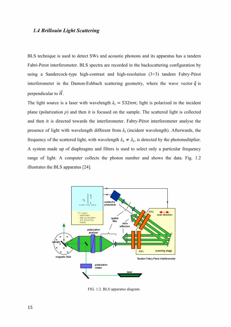
range of light. A computer collects the photon number and shows the data. Fig. 1.2

illustrates the BLS apparatus [24].

 

 FIG. 1.2. BLS apparatus diagram.

       

  16  

The light wave is incident on the magnetic system; an inelastic process takes place. The light

wave, with wavelength 𝜆! and wave vector 𝑘!, is scattered by a spin wave, with wavelength

λ and wave vector 𝑘.

The wave characterized by λ and 𝑘  is the spin wave created or destroyed by the light wave.

The scattered light wave is characterized by 𝜔! and 𝑘!. Wave vectors and frequencies must

satisfy the following conservation rules:

𝜔! = 𝜔! ± 𝜔 (1.4.1)

𝑘! = 𝑘! ± 𝑘 (1.4.2)

However, these conservation rules are valid for infinite magnetic system and are not fulfilled

in laterally confined due to quantization effects.

The sign + indicates the destruction of SW (Stokes process) and the sign – is referred to

the creation of SW (anti-Stokes process). In order to change the magnitude of the wave

vector, the incidence angle of light,ϑ , is varied. The angle is linked to 𝑞, by the relation

𝑞 = !!!sin𝜗. In these BLS measurements ϑ varies from 0° to 62° that correspond to values

of the wave vector from 0 rad/cm to 52.08 10 rad/cm× . In the experiment the sample is

saturated with an external field 500 OeH = .

 

 

 

 

 

 

 

 

 

 

 

 

 

 17  

1.5 Goldostone, pseudo-Goldstone and soft modes in magnetic systems  

 

In order to have a more complete understanding of the softening mechanism of low-

frequency modes occurring in two-dimensional periodic magnetic systems, that will be

discussed in the following chapter 3, it is useful to outline the main motivation leading to the

soft modes’ study presented in this thesis. This is done by introducing the definition of the

so called Goldstone modes in classical and non-relativistic ferromagnetic system by calling

them, more properly, pseudo-Goldstone and soft modes; finally, by presenting a theoretical

evidence for their existence in the calculated spin wave spectrum of magnetic multilayers.

We first recall the Goldstone theorem and its non relativistic analogous. The Goldstone

theorem states that a relativistic quantum field theory with a broken symmetry must have a

zero-mass particle [26]. In this framework, broken symmetry means that the vacuum state is

not invariant under the continuous group of transformations generated by the total charge.

After its general formulation, Lange studied a non-relativistic statement of the Goldstone

theorem [27] within a quantum system. It has been proved that a non-relativistic system with

a broken symmetry will have an excitation mode with no energy gap in the long-wavelength

limit, so long as the interactions in the theory have finite range. To prove it, the Heisenberg

model of ferromagnetism is employed. However, the theorem can be applied not only to

ferromagnets but also to other several physical systems like, for examples, superfluids and

superconductors.

The Heisenberg Hamiltonian is given by

𝐻!"#! = − 𝐽!"𝑆! ∙ 𝑆!!∈!.!

!

!!!

                               (1.5.1)  

where 𝐽!" is the exchange constant between the spins at neighbouring sites i and j; the j index

labels the nearest-neighbours (n.n) with j > i and 𝑆!  𝑎𝑛𝑑  𝑆! are the spin operators.

This Hamiltonian is invariant under the continuous rotation group generated by any

component of the total spin operator. The natural consequence is that the Hamiltonian

commutes with a member of this group, namely

𝑆! ,𝐻!"#! = 0                                                (1.5.2)

  18  

with 𝑆! = 𝑆!!!!!! the x component of the total spin 𝑆, representing the x-th generator of the

infinitesimal rotation 𝑈! 𝜙 = 1− !!𝜙 ∙ 𝑆 , through the angles 𝜙!.

The commutation between the two operators can be proved straightforwardly. For the sake

of simplicity we prove it for a one-dimensional chain of spins, but the proof can be easily

extended also to two- and three-dimensional systems. Equation (1.5.2) in explicit form reads

𝑆!!!

!!!

, 𝐽!  !±!𝑆! ∙ 𝑆!±!

!

!!!

= 𝐽!  !±!

!

!!!

𝑆!! , 𝑆! ∙ 𝑆!±! + 𝐽!  !±!

!

!!!

𝑆!±!!  , 𝑆! ∙ 𝑆!±!

= 0                          (1.5.3)

The last result comes from the following rule: 𝑆!±!! , 𝑆! ∙ 𝑆!±! = − 𝑆!! , 𝑆! ∙ 𝑆!±!          ∀𝑗. This,

in turn, implies that the Hamiltonian of the system is invariant under the continuous rotation,

that is 𝑆!𝐻!"#! − 𝐻!"#!𝑆! = 0 ⇒ 𝐻!!"#! = 𝐻!"#! being 𝐻′!"#! = 𝑆!!!𝐻!"#!𝑆! . However,

the ferromagnetic ground state has a definite magnetization along a given spatial direction.

In other terms, if the state represents the ground state magnetized along the z-axis then the

state is a ground state different from one in which the magnetization is rotated by an angle 𝜙

around the x-axis. More specifically

𝑒!" !!!!

!!! 0 = !0            

such that !0 ≠ 0 . Therefore, the ground state is of lower symmetry than the Hamiltonian

and a continuous symmetry breaking occurs. The symmetry breaking refers to the O(3)

rotational symmetry. By considering the spectral weight function, in the form

𝐿 𝑘,𝜔 = 𝑑𝑡  𝑒!"#!!!∙(!!!!!)!

!

0 𝑆!! 𝑡 , 𝑆!!(0) 0

!∈!

                           (1.5.4)

where Ω is the volume of the system, in combo with the equal-time commutation relation

0 𝑆!! 𝑡 , 𝑆!!(0) 0 = 𝑖𝜇𝛿!" 0 𝑆!!(𝑡) 0                                        (1.5.5)

the proof of the Goldstone theorem can be reduced, under the assumption of short-range

interactions with the k wave vector, into a simple relation:

lim!→!

𝐿(𝑘,𝜔) = 𝑖2𝜋𝜇𝛿 𝜔                                              (1.5.6)

𝜇 = 0 𝑆!! 0 is the magnetization per site.

 19  

According to Eq. (1.5.4) the spectral weight function exhibits a peak exactly at the angular

frequency 𝜔 = 0. This shows that the limiting energy of a sequence of excitations with

finite wave vector vanishes as 𝑘 → 0, as consequences are present diffusion branches in the

spectrum having vanishing energy gap.

To demonstrate this, starting from the spectral weight function, a sequence of functions

𝜆!(𝜔) should be introduced and it should be proved that they satisfies the following

properties:

lim!→!

𝜆! 𝜔 = 𝜆 𝜔 = lim!→!

𝐿 𝑘,𝜔                                (1.5.7)

𝑑𝜔𝜆! 𝜔 = 2𝜋𝑖𝜇                                  (1.5.8)

12𝜋 𝑑𝜔𝜔!𝜆!(𝜔) = 0                      0 < 𝑚 ≤ 𝑛.                                  (1.5.9)

The existence of Goldstone modes was proved theoretically, for example, in magnetic

multilayers with antiferromagnetic coupling [28]. As said before, the fact that this modes

were found in presence of an external applied magnetic field which breaks the O(3)

rotational symmetry justify the more proper name pseudo-Goldstone or soft modes with

vanishing frequency. These modes belong to the family of acoustical modes and they can be

defined, in analogy to acoustical phonons, as collective excitations where the spin

precession is “in-phase”; having also no energy cost in the infinite wavelength limit.

The mean-field Hamiltonian expressed as an energy per unit area S, i.e. 𝐸 = 𝐻𝑆 where H is

the total energy of the system (corresponding to the Hamiltonian), for layered structures

composed by NL ferromagnetic layers can be expressed in the following form:

𝐸 = 𝐸!! + 𝐸!! + 𝐸!"#!!

!!!!

!!!

!!

!!!

                                         (1.5.10)

where 𝐸!! is the anisotropy (including also the magnecrystalline) energy of the i-th layer: in-

plane uniaxial and shape anisotropies, 𝐸!! is the Zeeman energy of the i-th layer and 𝐸!"#!! is

the short range exchange energy between the i-th and (i+1)-th layer. The exchange

interaction includes both the bilinear and the biquadratic terms. In addition to these

contributions, the long-range dipolar energy among the different layers should be included.

  20  

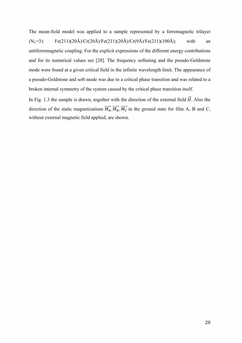
The mean-field model was applied to a sample represented by a ferromagnetic trilayer

(NL=3): Fe(211)(20Å)/Cr(20Å)/Fe(211)(20Å)/Cr(9Å)/Fe(211)(100Å); with an

antiferromagnetic coupling. For the explicit expressions of the different energy contributions

and for its numerical values see [28]. The frequency softening and the pseudo-Goldstone

mode were found at a given critical field in the infinite wavelength limit. The appearance of

a pseudo-Goldstone and soft mode was due to a critical phase transition and was related to a

broken internal symmetry of the system caused by the critical phase transition itself.

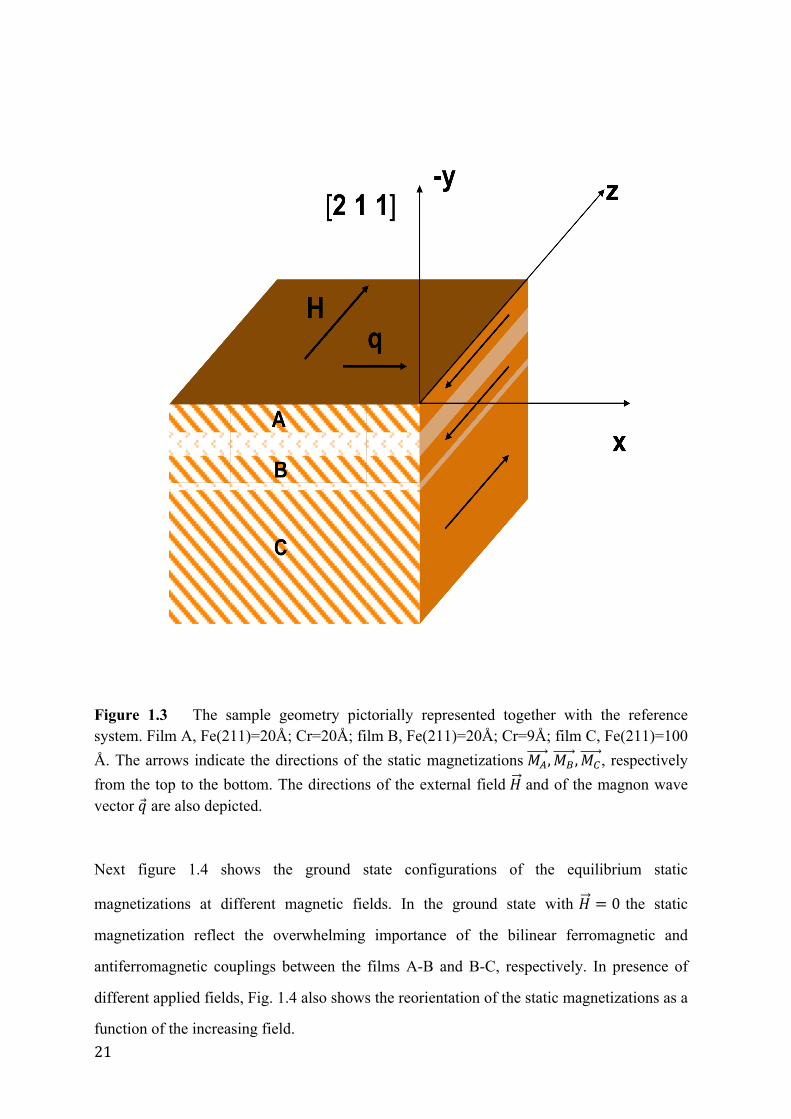
In Fig. 1.3 the sample is drawn, together with the direction of the external field 𝐻. Also the

direction of the static magnetizations 𝑀!,𝑀! ,𝑀! in the ground state for film A, B and C,

without external magnetic field applied, are shown.

 21  

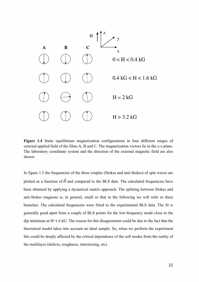
Figure 1.3 The sample geometry pictorially represented together with the reference system. Film A, Fe(211)=20Å; Cr=20Å; film B, Fe(211)=20Å; Cr=9Å; film C, Fe(211)=100 Å. The arrows indicate the directions of the static magnetizations 𝑀!,𝑀! ,𝑀! , respectively from the top to the bottom. The directions of the external field 𝐻 and of the magnon wave vector 𝑞 are also depicted. Next figure 1.4 shows the ground state configurations of the equilibrium static

magnetizations at different magnetic fields. In the ground state with 𝐻 = 0 the static

magnetization reflect the overwhelming importance of the bilinear ferromagnetic and

antiferromagnetic couplings between the films A-B and B-C, respectively. In presence of

different applied fields, Fig. 1.4 also shows the reorientation of the static magnetizations as a

function of the increasing field.

  22  

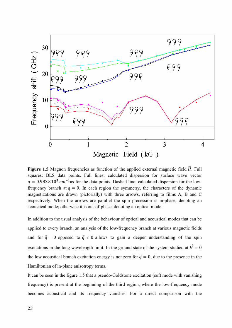
Figure 1.4 Static equilibrium magnetization configurations in four different ranges of external applied field of the films A, B and C. The magnetization vectors lie in the x-z plane. The laboratory coordinate system and the direction of the external magnetic field are also shown. In figure 1.5 the frequencies of the three couples (Stokes and anti-Stokes) of spin waves are

plotted as a function of 𝐻 and compared to the BLS data. The calculated frequencies have

been obtained by applying a dynamical matrix approach. The splitting between Stokes and

anti-Stokes magnons is, in general, small so that in the following we will refer to three

branches. The calculated frequencies were fitted to the experimental BLS data. The fit is

generally good apart from a couple of BLS points for the low-frequency mode close to the

dip minimum at H=1.6 kG. The reason for this disagreement could be due to the fact that the

theoretical model takes into account an ideal sample. So, when we perform the experiment

this could be deeply affected by the critical dependence of the soft modes from the reality of

the multilayer (defects, roughness, intermixing, etc).

 23  

Figure 1.5 Magnon frequencies as function of the applied external magnetic field 𝐻. Full squares: BLS data points. Full lines: calculated dispersion for surface wave vector 𝑞 = 0.983×10!  𝑐𝑚!!as for the data points. Dashed line: calculated dispersion for the low-frequency branch at 𝑞 = 0. In each region the symmetry, the characters of the dynamic magnetizations are drawn (pictorially) with three arrows, referring to films A, B and C respectively. When the arrows are parallel the spin precession is in-phase, denoting an acoustical mode; otherwise it is out-of-phase, denoting an optical mode. In addition to the usual analysis of the behaviour of optical and acoustical modes that can be

applied to every branch, an analysis of the low-frequency branch at various magnetic fields

and for 𝑞 = 0 opposed to 𝑞 ≠ 0 allows to gain a deeper understanding of the spin

excitations in the long wavelength limit. In the ground state of the system studied at 𝐻 = 0

the low acoustical branch excitation energy is not zero for 𝑞 = 0, due to the presence in the

Hamiltonian of in-plane anisotropy terms.

It can be seen in the figure 1.5 that a pseudo-Goldstone excitation (soft mode with vanishing

frequency) is present at the beginning of the third region, where the low-frequency mode

becomes acoustical and its frequency vanishes. For a direct comparison with the

  24  

measurements of soft modes, the ferromagnetic resonance technique could be used being

particularly suitable in the infinite wavelength limit.

For H = 1.6 kG there is a critical phase transition. It is known that, in the presence of a

critical phase transition, a spontaneous breaking of the symmetry may occur and pseudo-

Goldstone modes may be present. The competition between the Zeeman and the biquadratic

exchange interaction, which are dominant over the other terms, lowers the symmetry and

causes the appearance of pseudo-Goldstone modes. The lowering of the symmetry is related

to the presence of a more ordered phase where the three magnetizations are almost collinear.

However, note that in this case the broken symmetry is not the global O(3) rotational

symmetry, that is already broken due to the presence of both anisotropy and Zeeman

contributions, but a local symmetry more strictly related with the ground state

magnetization. This means that, if we map the semi classical mean-field model into a

quantum model, the Hamiltonian 𝑯 = 𝑯𝒂𝒏𝒊 +𝑯𝒆𝒙𝒄𝒉 +𝑯𝒁𝒆𝒆𝒎𝒂𝒏 written in the long

wavelength limit does not commute with a member of the rotation group O(3), namely

𝑆! ,𝑯 ≠ 0                                (1.5.11)

The Hamiltonian is thus non-invariant under the operation of the rotation group and this also

occurs at H=0 due to the in-plane anisotropy. However, at a given critical field, a local and

intrinsic symmetry is broken and the ground state magnetization has thus a lower symmetry

with respect to the Hamiltonian. This mechanism cannot be put on an equal footing as the

continuous broken symmetry mechanism described above for explaining the appearance of

Goldstone modes, but we interpret this as a lowering of the symmetry. As a result, a pseudo-

Goldstone or soft mode with vanishing frequency of acoustical nature in the infinite

wavelength limit appears at a given critical field.

           

 25  

CHAPTER 2    In this chapter we describe the dynamical matrix method, that is the micromagnetic

approach used to calculate spin mode frequencies. At this scope, we also introduce the

formalism and the notation used to explain this method.

The dynamical matrix method is a hybrid of micromagnetic simulations and a dynamical

matrix approach; it was developed to study the quantized spin excitations in laterally

confined system. Initially, was formulated for isolated magnetic nanoelements and then it

has been generalized to the case of interacting nanoelements[29]. It is a prototype of finite-

difference methods and represents an eigenvalue/eigenvector problem. The scope of this

method is to find the frequencies and profiles of the spin modes, which are associated to the

eigenvalues and to the eigenvectors of a dynamical matrix.

In a micromagnetic simulation, the sample is divided into cells and the magnetization is

assumed uniform within each cell and to precess about its equilibrium direction under the

influence of the external field and the dipolar and exchange forces, due to all the spins in the

system.

It can be considered the analogous of the dynamical matrix formalism used to find atomic

vibration (phonons) in crystalline solids. In the magnetic case, the only difference lie in the

potential that is due to the Zeeman field and to the dipolar and exchange interactions; this

obviously complicate a lot the calculation of the modes.

The dynamical matrix contains the second derivatives of the density energy coming from a

second order expansion of the density energy around the equilibrium. This method was

already used to study the spin excitations in magnetic multilayers with ferro- or anti-

ferromagnetic coupling.

The eigenvalue/eigenvector problem can be set as a complex generalized Hermitian

eigenvalue problem. The method presents several advantages: a single calculation yields the

frequencies and the eigenvectors of all the modes of any symmetry, it is applicable to a

particle of any shape (within the nanometric range), and the computation time is reasonably.

This means that it is possible to determine, after a single iteration, the frequencies and the

profiles of all spin-modes, independently of the ground-state magnetization. The main

  26  

restriction of the method is its applicability to confined magnetic systems whose spin

dynamics is assumed purely precessional with no dissipative effects. Of course, this is true

only in a first approximation, since in real magnetic systems the intrinsic damping process

plays an important role. In order to select the representative modes of the spectrum and to

compare them with the ones observed by means of the experimental techniques, the

differential scattering cross-section has to be evaluated both for non-interacting and

interacting magnetic particles.

The first application of the dynamical matrix method were on chains of dipolarly interacting

rectangular dots representing a one-dimensional array and of two-dimensional arrays formed

by circular disks. In this thesis we apply this method to study the collective mode dynamics

in arrays of holes embedded into a thin ferromagnetic film. This calculation is done by

including, in the energy density computation also the exchange interaction between

micromagnetic cells belonging to two adjacent primitive cells.

                                               

 27  

2.1 The Dynamical Matrix Method (DMM)    The procedure consist in discretize the system, i.e. divide in N cells, assume static and

dynamic magnetization constant in each cell; the magnetic energy is therefore written as

sum over the cells. The equation of motion is then transformed from an ordinary differential

equation to a linear homogeneous system of 2N equations, the variables being the small

angular deviations of the magnetization from the equilibrium state in each cell.

Provided that the equilibrium state is calculated, the problem takes the form of a generalized

Hermitian eigenvalue problem. The matrix elements can be written analytically, the only

approximation and the computing requirements come from the numerical solution of the

eigenvalue problem. Its size obviously increases with the number of cells N.

The equation of motion are written in the form of a complex generalized Hermitian

eigenvalue problem:

𝐴𝒗 = 𝜆𝐵𝒗                                  (2.1.1)

Where B is the Hessian matrix containing the second derivatives of the energy at

equilibrium, A is the Hermitian matrix; λ are the eigenvalues, 𝒗 the corresponding

eigenvectors; B is always defined positive or semi-positive because the energy minimum

implies that the second derivatives of energy are defined positive (or semi-positive).

𝜆 =𝛾

𝑀!𝜔      ⇒ 𝑡ℎ𝑒  𝑒𝑖𝑔𝑒𝑛𝑣𝑎𝑙𝑢𝑒𝑠  𝑔𝑖𝑣𝑒𝑠  𝑢𝑠  𝑡ℎ𝑒  𝑓𝑟𝑒𝑞𝑢𝑒𝑛𝑐𝑖𝑒𝑠

𝒗 = 𝛿𝜙!, 𝛿𝜃!,… , 𝛿𝜙! , 𝛿𝜃! !          

⇒ 𝑡ℎ𝑒  𝑒𝑖𝑔𝑒𝑛𝑣𝑒𝑐𝑡𝑜𝑟𝑠  𝑔𝑖𝑣𝑒𝑠  𝑢𝑠  𝑡ℎ𝑒  𝑠𝑝𝑎𝑡𝑖𝑎𝑙  𝑝𝑟𝑜𝑓𝑖𝑙𝑒𝑠

  28  

2.1 Formalism

 

This section deals with the review of the formalism used in this method. As stated above, it

is a finite-difference micromagnetic approach developed in the linear regime of spin

dynamics by considering small deviations from the equilibrium magnetization.

In first subsection we shortly state the notation use; we then move to calculate the different

contributions of the energy density entering into the dynamical matrix. Finally, the equations

of motion for an isolated magnetic element are cast in the form of a linear and homogeneous

system that can be solved as a complex generalized Hermitian eigenvalue problem. In last

subsection, it is shown the generalization to interacting magnetic nanoparticles by including

into the dynamical matrix the Bloch condition. Finally, the cross section is calculated.  

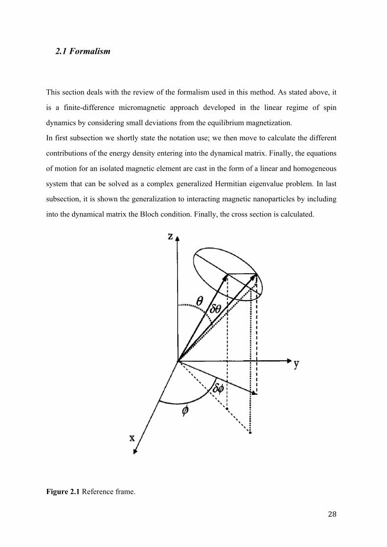
 Figure 2.1 Reference frame.

 29  

2.2.1 Notation    The reference frame used is that of figure 2.1; the z-axis is oriented along the normal to the

particle and the x-y plane lies on the particle plane. According to this reference frame, the

configuration of the vector 𝑀, representative of the magnetic dipole momentum, is identified

through the polar angles θ and φ.

If we assume that the magnetization vector 𝑀 is placed along the generic direction (vector in

bold-line), Fig. 2.1, it can be expressed in Cartesian coordinates by

𝑀(𝑡) = 𝑀! sin𝜃 𝑡 cos𝜙 𝑡 , sin𝜃 𝑡 sin𝜙 𝑡 , cos𝜃 𝑡 ,                          (2.2.1)  

Being 𝑀! the saturation magnetization value and the time dependence of the angles θ and φ

expressed as

𝜃 𝑡 = Θ+ 𝛿𝜃 𝑡 ,                              (2.2.2)

𝜙 𝑡 = Φ+ 𝛿𝜙 𝑡 .                            (2.2.3)

Where (Θ,Φ) represents the static (equilibrium) orientation of the magnetization obtained by

solving the stationary problem (𝑀 = 0), for whatever effective field and magnetization

distributions. Instead, δθ(t) and δφ(t) are the small polar and azimuthal deviations from

equilibrium, respectively.

In the micromagnetic calculations, the magnetic system is subdivided into N cells: square

based prisms of lateral size d and height L. Each micromagnetic cell is identified by a single

index k(j) that runs from 1 to N; hence, Mk is the magnetization in the k-th cell and

𝑟!" = 𝑟! − 𝑟! is the distance between k-th and j-th cell. The index has been chosen so that the

first line of the rectangular matrix (𝑋×𝑌) corresponds to 𝑘 = 1,… ,𝑌 and the second line to

𝑘 = 𝑌 + 1,… ,2𝑌 etc.

X(Y) is the number of cells along x(y), while Z is the number of cells along z.

We define for each cell the reduced magnetization  𝑚! = 𝑀!/𝑀!; the total energy density of

the system is a function of 𝜙!  𝑎𝑛𝑑  𝜃!: 𝐸 = 𝐸(𝜃! ,𝜙!) ,where k varies from 1 to N.

     

  30  

2.2.2 Energy density    First of all, we starting lists the various energy terms that compose the total micromagnetic

energy density, then we will analyses them in details: Zeeman energy, exchange energy,

demagnetizing energy and anisotropy energy. The energy density is defined as 𝐸 = 𝐸/𝑉,

where 𝐸 is the energy of the system and V its volume.

In the presence of external magnetic field 𝐻, the Zeeman energy density can be written in

the form

𝐸!"# = −𝜇!𝑀!𝐻 ∙ 𝑚!

!

!!!

                               (2.2.4)    

Where 𝜇! is the vacuum permeability. In micromagnetic theory, the exchange energy can be

expressed as a volume integral of the form

𝐸!"#! = 𝐴 (∇𝑚!)!𝑑𝑉!

!!!

;                              (2.2.5)

The integral is performed on the volume of a general magnetic particle, A is the exchange

stiffness constant, and ∇ is the gradient applied to a given component of the magnetization.

In this case the magnetization is independent of z. Use the first-neighbours model, the

exchange energy density can also be written

𝐸!"#! = 𝐴1−𝑚! ∙𝑚!

𝑎!"!

!

!!!

!

!!!

                       (2.2.6)

𝑎!" stands for the distance between the centres of two adjacent cell of index k and n; k

varies over all micromagnetic cells, n runs over the neighbours of the k-th cell. For edge

cells, it is necessary to impose boundary conditions.

In order to calculate the demagnetizing energy density, we use the method of demagnetizing

tensor; in what follows, we use the dipolar terms instead of the demagnetizing ones because

the higher-order terms of the expansion vanish in the practical cases examined.

According to demagnetizing tensor method, the energy density can be written as:

 31  

𝐸!"# =12 𝜇! 𝑀! ∙ 𝑁

!"

𝑀!

= 𝜇!𝑀!!

2 (𝑚!" 𝑚!" 𝑚!")×𝑁!! 𝑁!" 𝑁!"𝑁!" 𝑁!! 𝑁!"𝑁!" 𝑁!" 𝑁!!

𝑚!"𝑚!"𝑚!"!"

 (2.2.7)

This equation includes the self-energy and the 3×3 matrix N represent the demagnetizing

tensor. Each component of the demagnetizing tensor is related to the interaction between

two rectangular surfaces S and S'. Under the assumption of uniform magnetization, by using

a version of the Gauss’ theorem, the demagnetizing tensor can be written in the following

way

𝑁 𝑟!" =1𝑉 𝑑𝑆

!!

𝑑𝑆′

𝑟 − 𝑟′!!!

                 (2.2.8)

Where 𝑉 = 𝑙!!𝑑 is the volume of the micromagnetic cell, with 𝑙! the cell size and d the

height. Due to the four-fold symmetry and since 𝑟!" ≡   (𝑥,𝑦, 𝑧) all components can be

expressed in terms of 𝑁!! 𝑥,𝑦, 𝑧 𝑎𝑛𝑑  𝑁!" 𝑥,𝑦, 𝑧 only, of course with suitable

permutations of the variables x, y, z.

The next energy term is the magnetocrystalline uniaxial anisotropy; it is an energy density,

function of the angle 𝛼!  between the magnetization of the single cell 𝑚!and the easy axis of

generic direction given by the unit vector 𝑢.

𝐸!"# = 𝐾(!)𝑠𝑖𝑛!𝛼!

!

!!!

= 𝐾 ! 1− 𝑐𝑜𝑠!𝛼! = 𝐾 ! 1− 𝑚! ∙ 𝑢 !!

!!!

!

!!!

                     (2.2.9)

Here, 𝐾(!) is the first-order anisotropy uniaxial coefficient.

Because of the presence of second derivatives of energy density terms entering in the

expression for the dynamical matrix components, it is necessary to calculate them from the

above formulas.

Just before doing this, we calculate the second derivatives of the magnetization with the

respect to the polar angle θ, φ that represent the degrees of freedom of the system.

𝜕𝑚!

𝜕𝜙!= − sin𝜃! sin𝜙! , sin𝜃! cos𝜙! , 0                                                (2.2.10)

  32  

𝜕𝑚!

𝜕𝜃!= cos𝜃! cos𝜙! , cos𝜃! sin𝜙! , sin𝜃!                                (2.2.11)

𝜕!𝑚!

𝜕𝛿𝜙!!= − sin𝜃! cos𝜙! ,− sin𝜃! sin𝜙! , 0 ;                            (2.2.12)

𝜕!𝑚!

𝜕𝛿𝜃!𝜕𝛿𝜙!= − cos𝜃! sin𝜙! , cos𝜃! cos𝜙! , 0 ;                    (2.2.13)

𝜕!𝑚!

𝜕!𝛿𝜃!!= − sin𝜃! cos𝜙! ,− sin𝜃! sin𝜙! ,− cos𝜃! .          (2.2.14)

The second derivatives of the energy density are calculated at equilibrium. To simplify a

little bit the notation, we derive with respect to δθk and δθl implying that one or two of the

two generic variables could be also δφ.

Zeeman energy density:

𝜕𝐸!"#𝜕𝜃!

= −𝑀!𝐻 ∙𝜕𝑚!

𝜕𝜃!                                                                                                                    (2.2.15)

𝜕!𝐸!"#𝜕𝛿𝜃!𝜕𝛿𝜃!

= −𝜇!𝑀!𝐻 ∙𝜕!𝑚!

𝜕𝛿𝜃!𝜕𝛿𝜃!  𝑖𝑓  𝑙 = 𝑘

0        𝑖𝑓  𝑙 ≠ 𝑘.                                      (2.2.16)

Exchange energy density: As said before, the nearest-neighbour model is taken into account

in the calculation of exchange contribution. It is useful to state also the first derivative

expression, due to manipulations that have to be performed. The first derivative with respect

to 𝛿𝜃!includes in the sum two terms in which i stands for one of the nearest neighbours; the

first term correspond to n=k, the second to n≠k. Thanks to proper change of indices, the

following equation is obtained:

𝜕𝐸!"#!𝜕𝛿𝜃!

= −𝐴1𝑎!"!

𝜕𝑚!

𝜕𝛿𝜃!

!

!!!

∙𝑚! − 𝐴1𝑎!"!

!

!!!

𝑚! ∙𝜕𝑚!

𝜕𝛿𝜃!

= −2𝐴1𝑎!"!

𝜕𝑚!

𝜕𝛿𝜃!

!

!!!

∙𝑚!                    (2.2.17)

The sum over n is made up over the nearest-neighbours of the k-th cell.

The second derivatives are

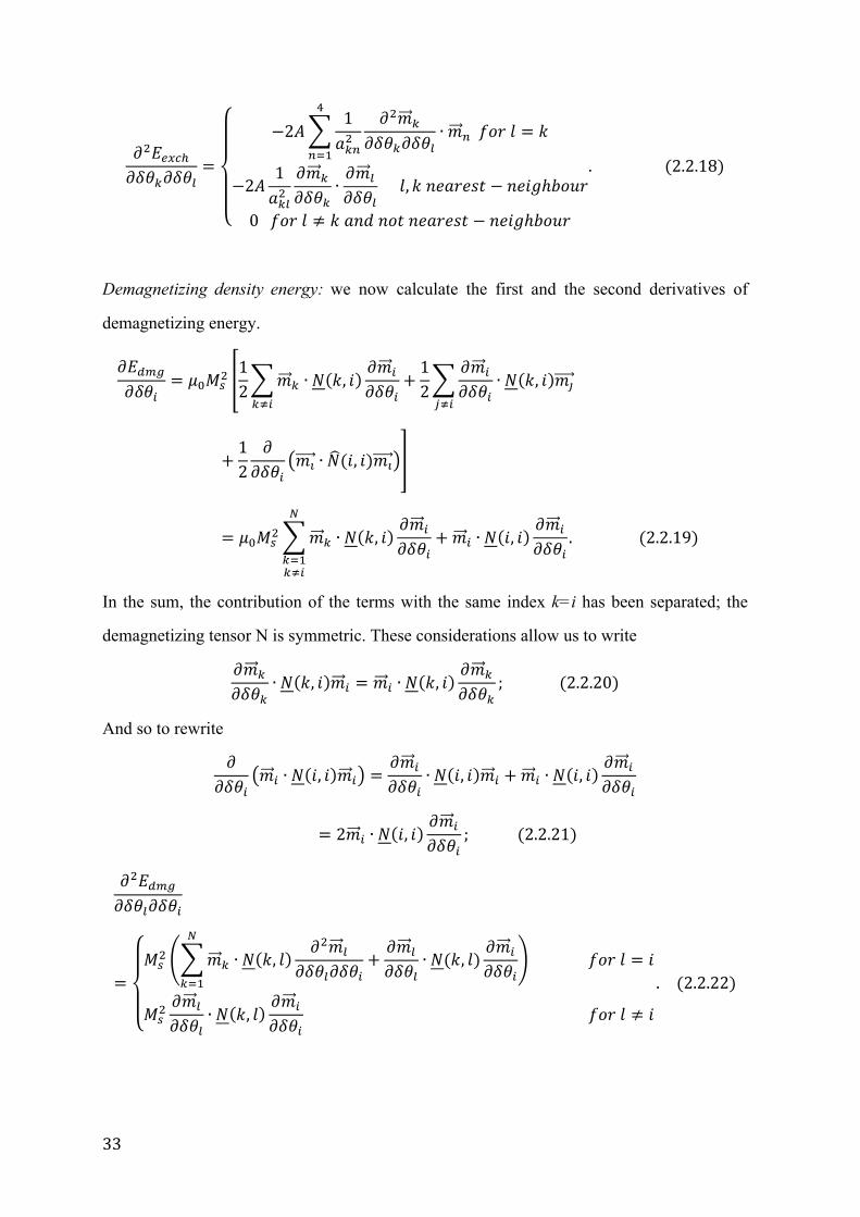
 33  

𝜕!𝐸!"#!𝜕𝛿𝜃!𝜕𝛿𝜃!

=

−2𝐴1𝑎!"!

𝜕!𝑚!

𝜕𝛿𝜃!𝜕𝛿𝜃!∙𝑚!    𝑓𝑜𝑟  𝑙 = 𝑘

!

!!!

−2𝐴1𝑎!"!

𝜕𝑚!

𝜕𝛿𝜃!∙𝜕𝑚!

𝜕𝛿𝜃!          𝑙, 𝑘  𝑛𝑒𝑎𝑟𝑒𝑠𝑡 − 𝑛𝑒𝑖𝑔ℎ𝑏𝑜𝑢𝑟

0      𝑓𝑜𝑟  𝑙 ≠ 𝑘  𝑎𝑛𝑑  𝑛𝑜𝑡  𝑛𝑒𝑎𝑟𝑒𝑠𝑡 − 𝑛𝑒𝑖𝑔ℎ𝑏𝑜𝑢𝑟

.                                      (2.2.18)

Demagnetizing density energy: we now calculate the first and the second derivatives of

demagnetizing energy.

𝜕𝐸!"#𝜕𝛿𝜃!

= 𝜇!𝑀!! 12 𝑚! ∙ 𝑁 𝑘, 𝑖

𝜕𝑚!

𝜕𝛿𝜃!+12

!!!

𝜕𝑚!

𝜕𝛿𝜃!!!!

∙ 𝑁 𝑘, 𝑖 𝑚!

+12

𝜕𝜕𝛿𝜃!

𝑚! ∙ 𝑁(𝑖, 𝑖)𝑚!

= 𝜇!𝑀!! 𝑚! ∙ 𝑁 𝑘, 𝑖

𝜕𝑚!

𝜕𝛿𝜃!+𝑚! ∙ 𝑁 𝑖, 𝑖

𝜕𝑚!

𝜕𝛿𝜃!.                                  (2.2.19)                  

!

!!!!!!

In the sum, the contribution of the terms with the same index k=i has been separated; the

demagnetizing tensor N is symmetric. These considerations allow us to write

𝜕𝑚!

𝜕𝛿𝜃!∙ 𝑁 𝑘, 𝑖 𝑚! = 𝑚! ∙ 𝑁 𝑘, 𝑖

𝜕𝑚!

𝜕𝛿𝜃!;                            (2.2.20)

And so to rewrite

𝜕𝜕𝛿𝜃!

𝑚! ∙ 𝑁 𝑖, 𝑖 𝑚! =𝜕𝑚!

𝜕𝛿𝜃!∙ 𝑁 𝑖, 𝑖 𝑚! +𝑚! ∙ 𝑁 𝑖, 𝑖

𝜕𝑚!

𝜕𝛿𝜃!

= 2𝑚! ∙ 𝑁 𝑖, 𝑖𝜕𝑚!

𝜕𝛿𝜃!;                        (2.2.21)

𝜕!𝐸!"#𝜕𝛿𝜃!𝜕𝛿𝜃!

=𝑀!! 𝑚! ∙ 𝑁 𝑘, 𝑙

𝜕!𝑚!

𝜕𝛿𝜃!𝜕𝛿𝜃!+𝜕𝑚!

𝜕𝛿𝜃!∙ 𝑁(𝑘, 𝑙)

𝜕𝑚!

𝜕𝛿𝜃!

!

!!!

                             𝑓𝑜𝑟  𝑙 = 𝑖

𝑀!! 𝜕𝑚!

𝜕𝛿𝜃!∙ 𝑁 𝑘, 𝑙

𝜕𝑚!

𝜕𝛿𝜃!                                                                                                                                                    𝑓𝑜𝑟  𝑙 ≠ 𝑖

.        (2.2.22)

  34  

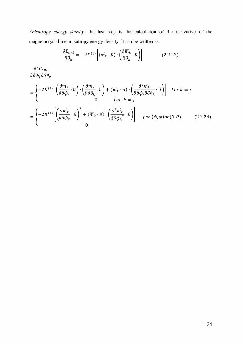
Anisotropy energy density: the last step is the calculation of the derivative of the

magnetocrystalline anisotropy energy density. It can be written as

𝜕𝐸!"#𝜕𝜃!

= −2𝐾 ! 𝑚! ∙ 𝑢 ∙𝜕𝑚!

𝜕𝜃!∙ 𝑢                                  (2.2.23)

𝜕!𝐸!"#𝜕𝛿𝜙!𝜕𝛿𝜃!

= −2𝐾 ! 𝜕𝑚!

𝜕𝛿𝜙!∙ 𝑢 ∙

𝜕𝑚!

𝜕𝛿𝜃!∙ 𝑢 + 𝑚! ∙ 𝑢 ∙

𝜕!𝑚!

𝜕𝛿𝜙!𝜕𝛿𝜃!∙ 𝑢        𝑓𝑜𝑟  𝑘 = 𝑗

0                              𝑓𝑜𝑟    𝑘 ≠ 𝑗    

= −2𝐾(!) 𝜕𝑚!

𝜕𝛿𝜙!∙ 𝑢

!

+ 𝑚! ∙ 𝑢 ∙𝜕!𝑚!

𝜕𝛿𝜙!! ∙ 𝑢

0

           𝑓𝑜𝑟   𝜙,𝜙 𝑜𝑟(𝜃,𝜃)                        (2.2.24)

 35  

2.2.3. Equations of motions    We start from deriving equations of motion in the simplest case of an isolated magnetic

particle, then extending in the proper way to interacting particles.

The equations of motion can be put into a linear and homogeneous system containing

explicitly the energy derivatives at equilibrium. In the case of a magnetic spin system, which

undergoes a purely precessional motion, the equation that rules the process is the Landau-

Lifshitz equation expressed as a torque equation involving the effective field and the

magnetization itself.

Since we are interested in study a conservative system we derive the equations from the

Hamiltonian ones, so will be derived following a semiclassical approach. Also, the model

will be first derived in the so-called macrospin approximation, where the material is

considered as uniformly magnetized.

It is well known from classical mechanics that in presence of conservative sources, the

system Hamiltonian H coincides with the total mechanical energy 𝐸. Hence,  𝑯 ≡ 𝐸 = 𝑇 −

𝑈, where T is the kinetic energy and U is the potential (defined as –V, V potential energy).

By defining the Lagrangian variables of the problem with qn, where n=1,2… is the number

of degrees of freedom corresponding to the dynamic variables, and the corresponding

conjugate momenta with pn, the Hamiltonian equations in the 2n canonical variables (qn,pn)

take the form

𝜕𝑞!𝜕𝑡 =

𝜕𝑯𝜕𝑝!

,                        (2.2.25)

𝜕𝑝!𝜕𝑡 = −

𝜕𝑯𝜕𝑞!

.                      (2.2.26)

For the specific case, the dynamic variables referred to the k-cell are the small deviations

from equilibrium of the azimuthal and polar angles:

𝑞! = 𝛿𝜙,            𝑞! = 𝛿𝜃,

Where 1 (2) labels the first (second) variable.

To determine the conjugate momenta, it is necessary the angular momentum relation with

the magnetic momentum of a rigid body with a fixed point

  36  

𝑙 =1𝛾 𝜇 =

𝑣!𝑀!

𝛾 𝑚,                    (2.2.27)

Where γ is the gyromagnetic ratio and vc the volume of the magnetic moment.

So since q1 represents a rotation about the z-axis of the magnetic dipole, its conjugate

momentum p1 corresponds to the z component of the variation of the angular momentum

𝑝! = 𝛿𝑙! =𝑣!𝑀!

𝛾 𝛿𝑚! = −𝑣!𝑀!

𝛾 sin𝜃 𝛿𝜃,                  (2.2.28)

Where 𝑚 is the unit magnetization vector, stated above, normalized to the saturation

magnetization Ms. With completely analogous argument, p2 can be determined; in fact, q2 is

a rotation of the dipole moment around an axis of unitary vector 𝜙! = − sin𝜙 𝑒! + cos𝜙 𝑒!

in the x-y plane at an angle 𝜙! = 𝜙 + 𝜋 2 from the x-axis. Therefore, p2 corresponds to the

projection of the variation of the angular momentum along the 𝜙! vector:

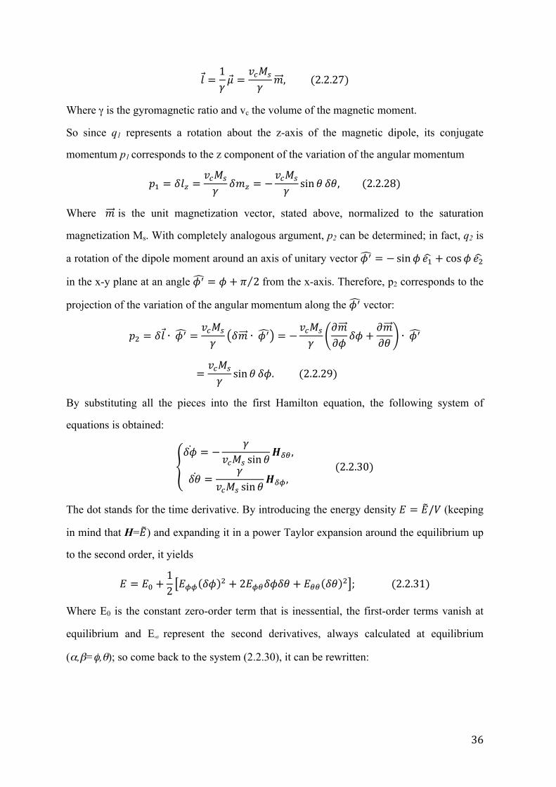
𝑝! = 𝛿𝑙 ∙  𝜙! =𝑣!𝑀!

𝛾 𝛿𝑚 ∙  𝜙! = −𝑣!𝑀!

𝛾𝜕𝑚𝜕𝜙 𝛿𝜙 +

𝜕𝑚𝜕𝜃 ∙  𝜙!

=𝑣!𝑀!

𝛾 sin𝜃 𝛿𝜙.                    (2.2.29)

By substituting all the pieces into the first Hamilton equation, the following system of

equations is obtained:

𝛿𝜙 = −𝛾

𝑣!𝑀! sin𝜃𝑯!" ,

𝛿𝜃 =𝛾

𝑣!𝑀! sin𝜃𝑯!" ,

                               (2.2.30)

The dot stands for the time derivative. By introducing the energy density 𝐸 = 𝐸/𝑉 (keeping

in mind that H=𝐸) and expanding it in a power Taylor expansion around the equilibrium up

to the second order, it yields

𝐸 = 𝐸! +12 𝐸!! 𝛿𝜙 ! + 2𝐸!"𝛿𝜙𝛿𝜃 + 𝐸!! 𝛿𝜃 ! ;                            (2.2.31)

Where E0 is the constant zero-order term that is inessential, the first-order terms vanish at

equilibrium and Eαβ represent the second derivatives, always calculated at equilibrium

(α,β=φ,θ); so come back to the system (2.2.30), it can be rewritten:

 37  

𝛿𝜙 = −𝛾

𝑀! sin𝜃𝐸!"𝛿𝜙 + 𝐸!!𝛿𝜃 ,

𝛿𝜃 =𝛾

𝑀! sin𝜃𝐸!!𝛿𝜙 + 𝐸!"𝛿𝜃 .

                               (2.2.32)

By inserting the time dependence in the form 𝑒!"#, where ω is the angular frequency of the

given collective mode, the system of equations of motions reads:

−𝐸!"sin𝜃 𝛿𝜙 −

𝐸!!sin𝜃 𝛿𝜃 − 𝜆𝛿𝜙 = 0,

𝐸!!sin𝜃 𝛿𝜙 +

𝐸!"sin𝜃 𝛿𝜃 − 𝜆𝛿𝜃 = 0.

                                         (2.2.33)

This linear and homogeneous system of equations can be shortly expressed as an eigenvalue

problem,

𝐶𝒗 = 𝜆𝒗,                                                                        (2.2.34)  

with 𝜆 = 𝑖 𝑀! 𝛾 𝜔 the complex eigenvalue of the problem and

𝐶 =−𝐸!"sin𝜃 −

𝐸!!sin𝜃

𝐸!!sin𝜃

𝐸!"sin𝜃

,                      (2.2.35)

Being 𝐶a real, but not symmetric, matrix and 𝒗 = (𝛿𝜙, 𝛿𝜃)!. However, this system can also

be recast as a complex generalized Hermitian eigenvalue problem

𝐴𝒗 = 𝜆𝐵𝒗,                                                                    (2.2.36)

Where 𝐵 is the Hessian matrix expressed by the second derivatives of the energy density at

equilibrium:

𝐵 =𝐸!! 𝐸!"𝐸!" 𝐸!!

,                                        (2.2.37)

𝐴 = 0 𝑖 sin𝜃−𝑖 sin𝜃 0 .                    (2.2.38)

It should be noted that 𝐴 is Hermitian and 𝐵 is real and symmetric; so that, all the

corresponding eigenvalues 𝜆 = 𝛾 𝑀!𝜔 are real quantities.

The Taylor expansion equation can be generalized to the case of N interacting magnetic

momenta, where each momentum is identified with a micromagnetic cell, taking the form:

𝐸 = 𝐸! +12 𝐸!!!!𝛿𝜙!𝛿𝜙! + 2𝐸!!!!𝛿𝜙!𝛿𝜃! + 𝐸!!!!𝛿𝜃!𝛿𝜃!

!

!!!

!

!!!

.                                                  (2.2.39)

  38  

The total energy density is given by 𝐸 = 𝐸!"# + 𝐸!"#! + 𝐸!"# + 𝐸!"# where the different

terms were stated before. Substituting this new energy expansion in the Hamiltonian system,

we get

𝛿𝜙! = −𝛾

𝑀! sin𝜃!𝐸!!!!𝛿𝜙! + 𝐸!!!!𝛿𝜃! ,

!

!!!

𝛿𝜃! =𝛾

𝑀! sin𝜃!𝐸!!!!𝛿𝜙! + 𝐸!!!!𝛿𝜃!

!

!!!

.

                                                     (2.2.40)

Again by introducing the time dependence in the form 𝑒!"#, obtain the system of equations

of motion composed by 2N linear and homogeneous equations:

−𝐸!!!!sin𝜃!

𝛿𝜙!

!

!!!

+ −𝐸!!!!sin𝜃!

𝛿𝜃!

!

!!!

− 𝜆𝛿𝜙! = 0,                                          (2.2.41)

𝐸!!!!sin𝜃!

𝛿𝜙!

!

!!!

+𝐸!!!!sin𝜃!

𝛿𝜃!

!

!!!

− 𝜆𝛿𝜃! = 0.                                                        (2.2.42)

k that run from 1 to N. The 𝛿𝜃! , 𝛿𝜙! (the eigenvectors of the problem) represent the small

angular deviation from the equilibrium position in the l-th micromagnetic cell. The system

above, have solution if the determinant is zero. Also in this case the problem can be recast as

an eigenvalue problem, in analogy with the macrospin system, using eq. (2.2.34) and the

eigenvector 𝒗 = 𝛿𝜙!, 𝛿𝜃!, 𝛿𝜙!𝛿𝜃!,… , 𝛿𝜙!𝛿𝜃! ! , 𝐶 is the matrix whose elements are

expressed as

𝐶!!!!,!!!! = −𝐸!!!!sin𝜃!

𝐶!!!!,!! = −𝐸!!!!sin𝜃!

𝐶!!,!!!! =𝐸!!!!sin𝜃!

𝐶!!,!! =𝐸!!!!sin𝜃!

𝑘 = 1…𝑁, 𝑙 = 1…𝑁.                            (2.2.43)

Analogously to the case of a macrospin system, the matrix 𝐶 is real but not symmetric and

the eigenvalues are complex. This matrix can be seen as composed by two submatrices 2×2

for each pair of values (k,l). In the diagonal submatrices (k=l) the following relation is

verified:

 39  

𝐶!!!!,!!!! = −𝐶!!,!! .                            (2.2.44)

For the elements of two different submatrices (k,l) and (l,k) that are not diagonal (k≠l), the

following symmetries hold:

sin𝜃! 𝐶!!!!,!!!! = − sin𝜃! 𝐶!!,!! ,                (2.2.45)

sin𝜃! 𝐶!!!!,!! = sin𝜃! 𝐶!!!!,!! ,                      (2.2.46)

sin𝜃! 𝐶!!,!!!! = sin𝜃! 𝐶!!,!!!!,                        (2.2.47)

sin𝜃! 𝐶!!,!! = − sin𝜃! 𝐶!!!!,!!!!.                (2.2.48)

As for the macrospin approximation, the equations of motion can also be rewritten as

complex generalized Hermitian eigenvalue problem

𝐴𝒗 = 𝜆𝐵𝒗,

where 𝐵 is the Hessian matrix containing the second derivatives and given by

𝐵!!!!,!!!! = 𝐸!!!!𝐵!!!!,!! = 𝐸!!!!𝐵!!,!!!! = 𝐸!!!!𝐵!!,!! = 𝐸!!!!

𝑘 = 1…𝑁, 𝑙 = 1…𝑁;                                  (2.2.49)

Again, this matrix is real and symmetric. Moreover, since the static magnetization

corresponds to a minimum of the energy and the matrix is Hessian, it is also defined

positive.

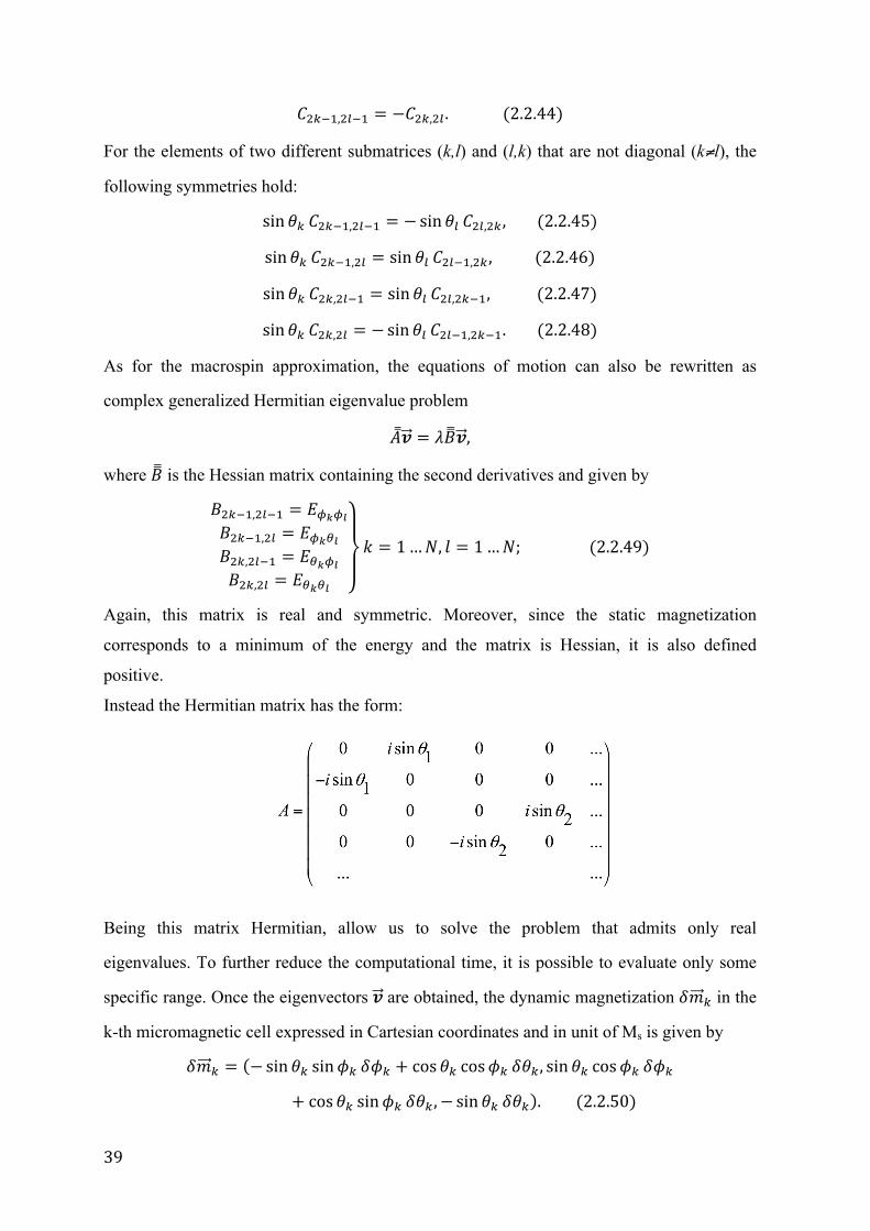
Instead the Hermitian matrix has the form:

Being this matrix Hermitian, allow us to solve the problem that admits only real

eigenvalues. To further reduce the computational time, it is possible to evaluate only some

specific range. Once the eigenvectors 𝒗 are obtained, the dynamic magnetization 𝛿𝑚! in the

k-th micromagnetic cell expressed in Cartesian coordinates and in unit of Ms is given by

𝛿𝑚! = − sin𝜃! sin𝜙! 𝛿𝜙! + cos𝜃! cos𝜙! 𝛿𝜃! , sin𝜃! cos𝜙! 𝛿𝜙!

+ cos𝜃! sin𝜙! 𝛿𝜃! ,− sin𝜃! 𝛿𝜃! .                  (2.2.50)

  40  

For each solution of the eigenvalue problem, the collection of all 𝛿𝑚! defines the mode

profile. It should be remarked that 𝛿𝑚! is a complex vector, because 𝛿𝜃! , 𝛿𝜙! are in general

complex.

Now, we derive the expression of the components of the generic dynamic magnetization

𝛿𝑚:

𝛿𝑚 =𝜕𝑚𝜕𝜙 𝛿𝜙 +

𝜕𝑚𝜕𝜃 𝛿𝜃

= − sin𝜃 sin𝜙 𝛿𝜙 + cos𝜃 cos𝜙 𝛿𝜃, sin𝜃 cos𝜙 𝛿𝜙

+ cos𝜃 sin𝜙 𝛿𝜃,− sin𝜃 𝛿𝜃                                                                                                  (2.2.51)

yielding to

𝛿𝑚 ! = 𝑠𝑖𝑛!𝜃𝛿𝜙! + 𝛿𝜃!.                                            (2.2.52)

Due to these equations, now we are able to calculate the tangential and the radial

components of the dynamic magnetization in each k micromagnetic cell. Define α being the

angle between the radial direction and the x-axis, in the k-th cell;

𝛼! = − tan!!𝑥!𝑦!+ 𝜋            𝑖𝑓  𝑦! < 0                                        (2.2.53)

then, the magnetization components are:

𝛿𝑚! = cos𝛼! 𝛿𝑚! + sin𝛼! 𝛿𝑚!  ,                                      (2.2.54)

𝛿𝑚! = − sin𝛼! 𝛿𝑚! + cos𝛼! 𝛿𝑚!  .                            (2.2.55)

 

         

 41  

2.3 Scattering cross section    

The framework used to obtain the magnonic bands is an extension of the DMM, originally

introduced for calculating the normal modes of single magnetic elements.

We assume that the dynamic magnetization 𝛿𝑚(𝑟), solution of the linearized equation of

motion in a periodic system, has the form of a Bloch wave:  𝛿𝑚 𝑟 = 𝛿𝑚 𝑟 𝑒!!∙!; where

𝛿𝑚 𝑟 has the artificial periodicity of the magnonic crystal and the exponential part is a

plane wave with q Bloch vector and r in-plane vector.

Magnonic modes can thus be seen as propagating waves modulated by the arrays. In

particular, for the 2D case the Bravais lattice vector takes the generic form 𝑅 = 𝑛!𝑎! +

𝑛!𝑎!; with a1, a2 primitive vectors, 0≤ ni <Ni with i=1,2 and Ni the number of cells along the

ai direction and N=N1N2.

The way in which magnetic antidots (dots) interact amongst them is due to both to the

exchange interaction between primitive cells [30] and to the interdot dipolar magnetic

interaction. Since this interaction is relatively weak it can be considered as a perturbation

and the nomenclature assign to each collective mode is the same used for single dot

(antidot): the collective mode mainly localized in the centre of the element and without

nodes is the fundamental (F), the Damon-Eshbach-like (nDE) modes having nodal planes

parallel to the local direction of the static magnetization M, while the ones having the

perpendicular nodal planes are typical of backwardlike (nBA) modes; finally, the end modes

(nEM) are localized at the edge of each element in the direction of the magnetization. Mixed

modes are also present in calculation but not detected by the experiments.

The dynamical matrix method, as stated above, gives us all the possible modes of spin

excitation; furthermore, the number of possible value is proportional to the number of

microcells taken into account in calculation. This means that the result of the computation is

really a large number of modes. So it is necessary select among them only the ones that have

physical relevance.

To do this it is useful to calculate the scattering cross section: using the expression of

differential cross section we are able to interpret our magnetic results, only the modes that

have a significant cross section could be physically relevant. The evaluation of the

  42  

differential scattering cross section allow us to assign unambiguously to a given spin wave

mode a given BLS peak.

The interaction between light and matter can be evaluated thanks to the coupling between

the incident electric field and the dielectric tensor of the material under study. In fact, the

thermal fluctuations excite the spin’s normal modes that provoke the magnetization to

precess around its equilibrium position, leading to a dynamic magnetization. This precession

yields to a modulation of the complex refractive index of the material, proportional to

dielectric tensor too. For these considerations may seem plausible make a hypothesis of

proportionality between the oscillation of the dielectric tensor and the dynamic

magnetization:

𝛿𝜀!" = 𝐾!"#𝑚! + 𝐺!"#$!"!

𝑚!𝑚!                          (2.3.1)

where K and G are the complex magneto-optic constant of the first (Faraday effect) and

second(Coutton-Mouton) order, respectively.

The mµ, mν are the dynamic magnetization components. In our case, simple considerations

leads to a dielectric tensor in which only the in-plane directions are nonzero and the G factor

is negligible.

The dielectric tensor, taken all these considerations into account, can be written as

𝛿𝜀 =0 0 −𝐾𝑚!0 0 𝐾𝑚!

𝐾𝑚! −𝐾𝑚! 0;                                      (2.3.2)

Note that it’s a traceless antisymmetric tensor, only four out-of-diagonal elements have

nonzero contribution.

The interaction, between the modulated refraction index and the incident electric field,

induced a total electric dipole moment in the material different from zero; the dipole’s

oscillating frequency is that of the incident light minus (plus) the spin normal mode

frequency (Stokes or Anti-Stokes). The dipoles’ distribution leads to the scattered light

wave, expressed by the scattered electric field.

The scattered electric field has nonzero components only when the polarization has nonzero

components; for example, if we have the incoming light wave with p-polarization, the

outgoing (scattered) one’s has s-polarization.

 43  

The differential cross section, associated to each magnonic mode of the spectrum, turns out

to be proportional to the square modulus of the amplitude of the scattered field, 𝐸!"#$$ and

takes the form

!!!!!!" !⟶!

= 𝐶𝑁 𝜔! − 𝜔!! ∆!!! ∙!!!

!!!!!!∆!∙!! 𝒓 !𝒓!"##

!

!! ! 𝛿 Ω− 𝜔! − 𝜔 ;            (2.3.3)

Where the σ is the scattering cross section, dΩ is the differential solid angle, the subscript p

and s indicated the polarization of the incident and scattered light, respectively. C is a

constant depending on geometric and optical parameters, 𝑁 𝜔! − 𝜔 is the Bose-Einstein

thermal factor where ω’ and ω are the frequency on the incident and scattered light; the sum

is performed over the illuminated cells, finally 𝐸! is the amplitude of the incident electric

field.

Let’s see how to derive this cross section formula for interacting magnetic elements in a

more rigorous way.

Following the same formalism used for continuous film and for single element, the

calculation of the scattering cross section in two-dimensional arrays of interacting antidots

requires, such as for dots, first to express the amplitude of the scattered electric field.

The propagation equation of the waves, in a magnetic medium with perturbed dielectric

constant, can be expand to the first order in the fluctuation (anti-Stoke process) as:

∇×∇×𝐸!"#$$ +1𝑐! 𝜀!

𝜕!

𝜕𝑡! 𝛿𝐸 = −1𝑐! 𝛿𝜀

𝜕!

𝜕𝑡! 𝐸!                                  (2.3.4)

𝐸! is the incident electric field at zero order, ε0 is the dielectric constant of the unperturbed

medium, 𝛿𝜀 is the tensor representing the fluctuation of the polarization and

𝐸!"#$$(𝑥,𝑦, 𝑧, 𝑡) = 𝐸!"#$$(𝑧)𝑒!(!!!!!!!!!!!!!) is the electric field of the scattered wave. The

electric field under consideration is time-dependent and p-polarized, so 𝐸! 𝑥,𝑦, 𝑧, 𝑡 =

E! 𝑧 𝑒!(!!!!!!!!!"); where 𝐸0 is the incident electric field amplitude.

By introducing the Fourier transform of Escatt with respect to x, y, z, t, we can rewrite the

previous equation in terms of the electric field (incident and scattered) amplitudes:

  44  

𝑘′∥! −𝜕!

𝜕𝑧! 𝐸!"#$$ −𝜔!!

𝑐! 𝜀!𝐸!"#$$

= −𝜔!

2𝜋 ! !𝑐!𝛿𝜀 𝐸!𝑒! ∆!!!!∆!!! 𝑒! !!!

! !𝑑𝑥𝑑𝑦𝑑𝑡;      (2.3.5)

With ∆𝑘! = 𝑘! − 𝑘!! ,𝛼 = 𝑥,𝑦. In particular, the components of the light incident wave

vector are 𝑘! = 𝑘∥ cos𝜙 , 𝑘! = 𝑘∥ sin𝜙, where φ is the angle between the incidence plane

and the x-z plane. In the same manner, the components of the scattered wave vector read

𝑘′! = 𝑘′∥ cos𝜙 , 𝑘′! = 𝑘′∥ sin𝜙, respectively.

So, the equation can be solved thanks to the introduction of the Green’s function g(z,z') and

the use of the Green’s method. The solution can thus be written in the form:

𝐸!"#$$ 𝑧 = −𝜔!

2𝜋 ! !𝑐!𝑔 𝑧, 𝑧! 𝛿𝜀 𝑥,𝑦, 𝑧!, 𝑡

×𝐸! 𝑧! 𝑒!∆!∙!𝑒!∆!"𝑑𝑥𝑑𝑦𝑑𝑧!𝑑𝑡 ,                    (2.3.6)

Where the Green’s function g(z, z’) is the same as the one defined for multilayers.

Analogously to the case of continuous film, expressing 𝛿𝜀 in terms of the dynamic

magnetization amplitudes and integrating over z leads to

𝐸!"#$$ ∝ 𝛿 Ω− 𝜔! − 𝜔 𝑒!∆!∙!𝐴(!"#$

𝒓)𝑑𝒓                              (2.3.7)

with r=x, y and 𝛿 Ω− 𝜔! − 𝜔 is the Dirac delta, Ω is the angular frequency of the given

collective mode. The integral is extended to the zone illuminate by light. The quantity A(r) is

expressed as the integral over z of contributions proportional to the polarization; the integral

over z contains four terms associated to scattering so that the scattering field refers to four

scattering channels. Each of these terms contains the magneto-optic complex constant K

expressing the first-order magneto-optic, or Faraday, effect and is proportional to the first-

order contribution of the dynamic magnetization to the differential scattering cross section.

Due to the surface periodicity and taking into account the Bloch theorem, summing over the

illuminated cells N, the integral in the formula can be substituted by 𝑒!(∆!!!)∙!!!!!!! …!"##

yielding to:

𝐸!"#$$ ∝ 𝛿 Ω− 𝜔! − 𝜔 𝑒! ∆!!! ∙!!!

!!!!× 𝑒!∆!∙!𝐴 𝒓 𝑑𝒓

!"##∝ 𝐹𝑆.                                  (2.3.8)

 45  

Where 𝐹 = 𝑒!(∆!!!)∙!!!!!!! is a factor depending on the Bloch wave vector, 𝐹 =

𝐹(𝜃,𝜃!,𝒒) and 𝑆 = 𝑒!∆!∙!𝐴 𝒓 𝑑𝒓!"## is a term related to the scattered field obtained for the

single dot (antidot). The quantity A(r) is a linear combination of the components of the

dynamic magnetization. The differential scattering cross section is thus proportional to a

term depending on the single dot times a factor whose form depends on the extension of the

illuminated area.

The differential scattering cross section states at the top of this section is obtained by

performing the square modulus of 𝐸!"!!!.

     

   

   

   

  46  

Chapter 3    Until now, we have seen from where is came out the ideas at the basis of this work and the

theory used both to accomplish the calculation and to correctly define the physical system.

In this chapter will be explain in all the details both the experimental data and the results of

the DMM simulations. Last, but not least the continuum limit behaviour (to stripe and to

film) and the universality behaviour, with its scaling law and the critical exponent, are

discussed.

 

 3.1 Sample preparation and experimental setup

   We have performed a systematic investigation of the dependence of the magnetic normal

modes on the magnetic field H for four arrays of ADLs having fixed lattice constant

a=420nm and circular holes of different diameters di (separation si) with i =1, 2, 3, 4:

d1=140nm (s1=280nm), d2=180nm (s2=240nm), d3=220nm (s3=200nm), d4=260nm

(s4=160nm).

ADLs were fabricated over a large area (4×4mm2) on commercially available Si substrates

using deep ultraviolet (DUV) lithography at 248nm exposing wavelength followed by e-

beam deposition of Py (Ni80Fe20) films with thickness L=30nm. The e-beam deposition was

followed by ultrasonic assisted lift-off process [31] in OK73 resist thinner. The Scanning

Electron Microscopy (SEM) images [32] of the four samples are shown in Fig. 3.1. BLS

measurements were performed in the backscattering configuration using a high-contrast

(3+3) tandem Fabry-Perot interferometer. Spectra were recorded by focusing light at normal

incidence upon the sample surface, i.e. at centre of the first Brillouin zone (1BZ) where the

transferred wave vector is K=0, and by varying the intensity of H from 2 kOe to zero. H was

applied along a symmetry direction of the ADL, the y-axis.

 47  

 

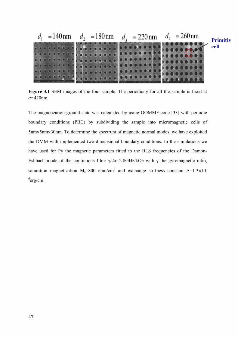
Figure 3.1 SEM images of the four sample. The periodicity for all the sample is fixed at a=420nm.  

The magnetization ground-state was calculated by using OOMMF code [33] with periodic

boundary conditions (PBC) by subdividing the sample into micromagnetic cells of

5nm×5nm×30nm. To determine the spectrum of magnetic normal modes, we have exploited

the DMM with implemented two-dimensional boundary conditions. In the simulations we

have used for Py the magnetic parameters fitted to the BLS frequencies of the Damon-

Eshbach mode of the continuous film: γ/2π=2.8GHz/kOe with γ the gyromagnetic ratio,

saturation magnetization Ms=800 emu/cm3 and exchange stiffness constant A=1.3×10-

6erg/cm.

 

 

 

 

 

 

Primitive cell

  48  

3.2 Collective mode classification and discussion

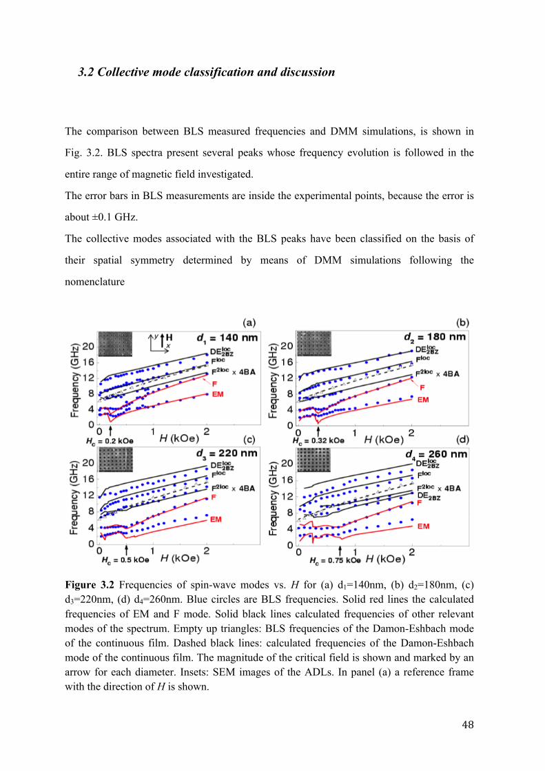
The comparison between BLS measured frequencies and DMM simulations, is shown in

Fig. 3.2. BLS spectra present several peaks whose frequency evolution is followed in the

entire range of magnetic field investigated.

The error bars in BLS measurements are inside the experimental points, because the error is

about ±0.1 GHz.

The collective modes associated with the BLS peaks have been classified on the basis of

their spatial symmetry determined by means of DMM simulations following the

nomenclature

 

Figure 3.2 Frequencies of spin-wave modes vs. H for (a) d1=140nm, (b) d2=180nm, (c) d3=220nm, (d) d4=260nm. Blue circles are BLS frequencies. Solid red lines the calculated frequencies of EM and F mode. Solid black lines calculated frequencies of other relevant modes of the spectrum. Empty up triangles: BLS frequencies of the Damon-Eshbach mode of the continuous film. Dashed black lines: calculated frequencies of the Damon-Eshbach mode of the continuous film. The magnitude of the critical field is shown and marked by an arrow for each diameter. Insets: SEM images of the ADLs. In panel (a) a reference frame with the direction of H is shown.

 49  

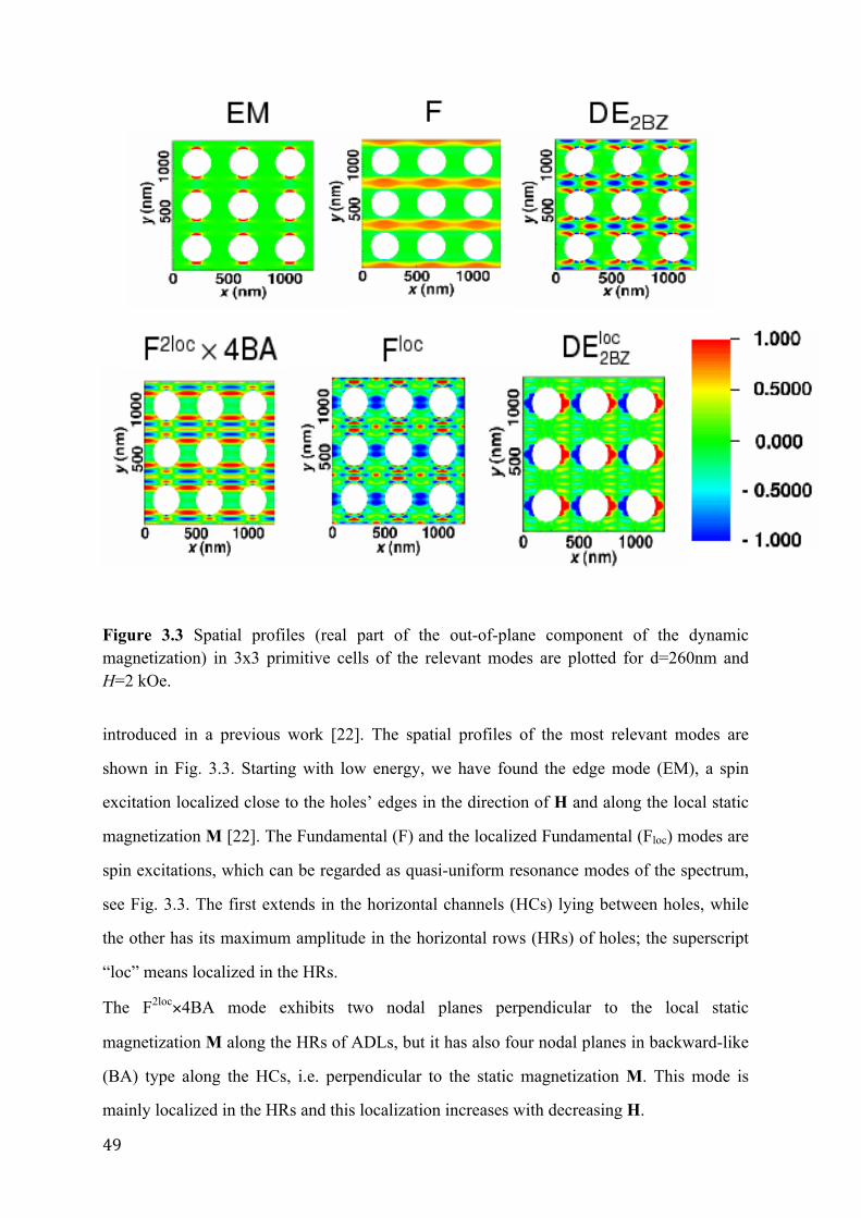
Figure 3.3 Spatial profiles (real part of the out-of-plane component of the dynamic magnetization) in 3x3 primitive cells of the relevant modes are plotted for d=260nm and H=2 kOe.  

introduced in a previous work [22]. The spatial profiles of the most relevant modes are

shown in Fig. 3.3. Starting with low energy, we have found the edge mode (EM), a spin

excitation localized close to the holes’ edges in the direction of H and along the local static

magnetization M [22]. The Fundamental (F) and the localized Fundamental (Floc) modes are

spin excitations, which can be regarded as quasi-uniform resonance modes of the spectrum,

see Fig. 3.3. The first extends in the horizontal channels (HCs) lying between holes, while

the other has its maximum amplitude in the horizontal rows (HRs) of holes; the superscript

“loc” means localized in the HRs.

The F2loc×4BA mode exhibits two nodal planes perpendicular to the local static

magnetization M along the HRs of ADLs, but it has also four nodal planes in backward-like

(BA) type along the HCs, i.e. perpendicular to the static magnetization M. This mode is

mainly localized in the HRs and this localization increases with decreasing H.

  50  

At high frequency we have detected the Damon-Eshbach-like (DE) mode, named 𝐷𝐸!!"!"#

where 2Bz indicates that this mode has the largest calculated cross-section in the second BZ

[34,35]. Note that the calculated scattering cross-section of this mode is non-negligible up to

K close to the centre of the 1BZ and vanishes at K=0. Its detection in the BLS spectra at

K=0 is due to finite collection angle camera objective used [35], as well as to unavoidable

small experimental misalignment of H with the vertical rows of holes; this leads to further

demagnetizing effects that can alter the mode profiles. In the sample with d4 =260nm, we

have found the DE2BZ mode which is mainly concentrated in the HCs and exhibits the same

cross-section features as the 𝐷𝐸!!"!"# . For this diameter the large demagnetizing field in the

HCs can deform the spatial profile of the detected DE2BZ mode which becomes detectable at

K=0.

The calculated frequencies are in very good agreement with BLS measurements for all the

diameters apart from an underestimation of the measured EM frequencies (on average of

about 0.5 GHz). Moreover, 𝐷𝐸!!"!"# theoretical frequencies are larger than the measured ones

on average of about 1 GHz for d3=220nm and d4=260nm. These discrepancies can be

attributed to the fact that the periodic distribution of fabricated holes tends to become more

irregular with increasing hole size. The general trend is the decrease of the frequencies by

decreasing the intensity H of the external magnetic field. Very interestingly, for all the

samples analysed, in according also with DMM simulations, we have found the softening

occurrence in both the F and the EM mode when the external magnetic field is reduced

below a critical field Hc. By inspection of Fig. 3.2, ones notes that Hc monotonically

increases upon increasing the hole diameters; its calculated values, by means of

micromagnetical simulations, for each diameter are: a) Hc(d1)=0.2 kOe; b) Hc(d2)=0.32

kOe; c) Hc(d3)=0.5 kOe; d) Hc(d4)=0.75 kOe.

Moreover, at critical field the calculated frequency curves exhibit a finite gap whose value

decrease by decreasing the holes diameter. These trends are confirmed by the BLS

measurements, although in the experiments the softening is less pronounced, especially for

d4=260nm. This discrepancy between theory and experiment may be ascribed to the size and

shape distribution of the holes that could mask the observation of frequency softening for

 51  

large diameters. For d3=220nm and d4=260nm the simulations predict a further minimum

for the EM frequency below Hc due to a sudden jump of M towards the x-direction.

In Fig. 3.2 the BLS and the calculated frequencies of the Damon-Eshbach mode of the

unpattern reference film are also shown as empty up triangles and dashed black lines,

respectively.

It is important to remark that the softening does not involve only the lowest-frequency mode

of the spectrum, the EM, but also the F one [13]. This is in contrast with the mode softening

and magnetization reversal in isolated nanorings, where only the lowest-frequency mode

softens [36]. The softening of the two modes can be understood by observing the evolution

of the mode localization as a function of the direction of M.

When a strong magnetic field is applied, the magnetization in every cell is almost parallel to

H. The EM is localized along the direction of application (y-direction in our case) close to

the holes edges, while the F mode extends in the HCs. When H< Hc a continuous rotation of

M from the hard axis, placed along the principal symmetry axis (y-direction), towards the

easy axis [37], at 45° in the plane formed by M and y-axis, takes place. Note that, due to the

four-fold in-plane anisotropy, the continuous rotation of the magnetization towards the other

easy-axis, at -45°, would be equivalent.

The continuous phase transition associated to the rotation of M corresponds to a lowering of

the symmetry, taking place with decreasing H. This means that the phase where M is aligned

along y direction (H> Hc) is more ordered with respect to that where M forms an angle of

45° with the y direction (H< Hc). By decreasing H, the spatial localization of the F and EM

mode follows the rotation of M and, as a consequence, their amplitude is mainly

concentrated along the diagonal of the primitive cell (see figure 3.5)  

Figure 3.4 ADLs square lattice with a periodicity of the system; the direction of K and H are also displayed. The 1BZ in the reciprocal space is drawn.

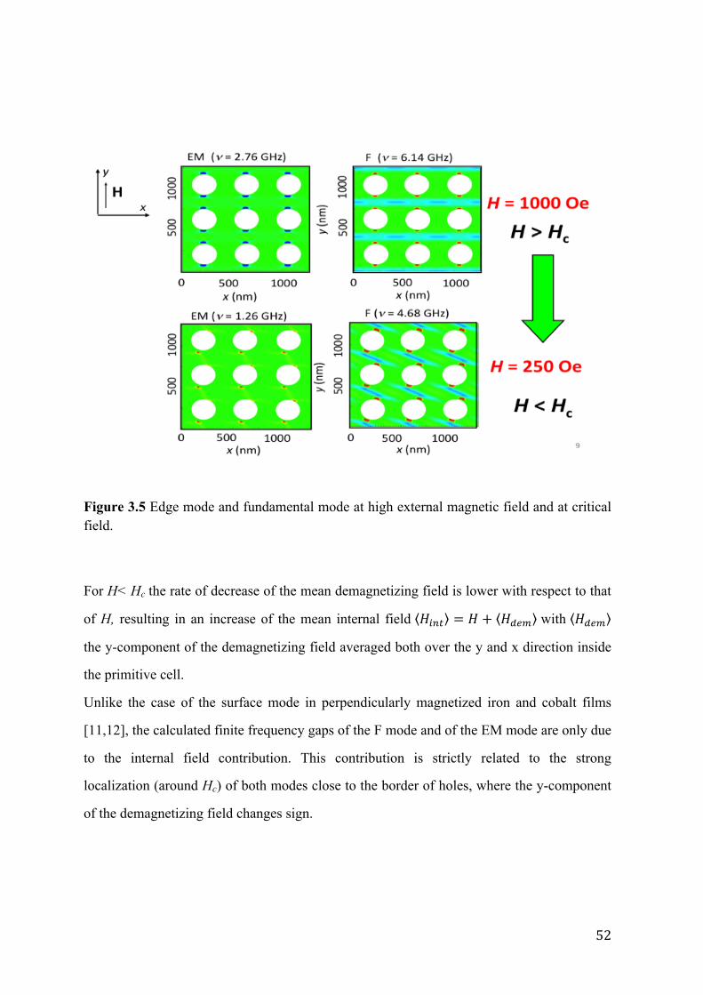
  52  

Figure 3.5 Edge mode and fundamental mode at high external magnetic field and at critical field.

For H< Hc the rate of decrease of the mean demagnetizing field is lower with respect to that

of H, resulting in an increase of the mean internal field 𝐻!"# = 𝐻 + 𝐻!"# with 𝐻!"#

the y-component of the demagnetizing field averaged both over the y and x direction inside

the primitive cell.

Unlike the case of the surface mode in perpendicularly magnetized iron and cobalt films

[11,12], the calculated finite frequency gaps of the F mode and of the EM mode are only due

to the internal field contribution. This contribution is strictly related to the strong

localization (around Hc) of both modes close to the border of holes, where the y-component

of the demagnetizing field changes sign.

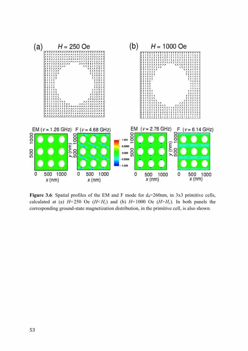
 53  

Figure 3.6: Spatial profiles of the EM and F mode for d4=260nm, in 3x3 primitive cells, calculated at (a) H=250 Oe (H<Hc) and (b) H=1000 Oe (H>Hc). In both panels the corresponding ground-state magnetization distribution, in the primitive cell, is also shown.  

  54  

3.3. Phenomenological model for the reorientational phase transition  

 

Straightforwardly, it is possible to obtain a simple expression of the critical field Hc by

minimizing the energy density of the system E under the assumption of uniform

magnetization:

𝐸 = −𝐻𝑀! cos𝜙 + 2𝜋𝑀!! 𝑁!! 𝑐𝑜𝑠!𝜙                                (3.3.1)

Where 𝑁!! is the mean demagnetizing factor, y diagonal component of the mean

demagnetizing tensor.

The energy density minimization is performed with respect to 𝜙 and by taking into account

that, for H>Hc, the magnetization is aligned along the hard axis (𝜙 = 0). The non-trivial

solution can be expressed as a function of the first-order y component of the mean

demagnetizing field 𝐻!"# (!):

cos𝜙 = −𝐻

𝐻!"#!                                                  (3.3.2)

With 𝐻!"# (!) = −4𝜋𝑀! 𝑁!! . Hence, the critical field turns out to be

𝐻! = − 𝐻!"# ! ≅ − 𝐻!"#                  (3.3.3)

In all the calculations the average procedure has been performed in two steps. First, we have

calculated the average over the micromagnetic cells along the y direction, according to

OOMMF with PBCs. By doing this average, we have found that the numerical curve can be

fitted by a Gaussian distribution centred at the middle of the primitive cell (x0) of the form

𝑦 = 𝐵𝑒!(!!!!)!

!!! where 𝐵 = !

(!!)!!!

with A the amplitude and 𝜎! the variance of the

distribution. The mean demagnetizing field 𝐻!"# is then obtained by averaging the

Gaussian function over the size of the primitive cell along x, namely

𝐻!"# =𝐵𝑎 𝑒!

(!!!!)!!!!

!/!

!!/!

𝑑𝑥

=𝐴

2𝑎𝜎! erf𝑎 − 2𝑥! 𝜎2 2

+ 𝑒𝑟𝑓(𝑎 + 2𝑥!)𝜎

2 2                                        (3.3.4)

 55  

Where erf is the error function. The values of Hc calculated by using (3.3.3) and (3.3.4) are

in agreement with the DMM values, with only slight differences. The average along the y

direction has been performed, in practice, along the separation between holes.

It has also been found that the calculated finite gap increases for increasing diameter,

confirming the trend shown by the measured gaps. At the centre of the 1BZ, both the EM

and the F mode are collective soft modes of acoustical nature with infinite Bloch

wavelength, but at the critical field it is required a finite energetic cost to excite them. This

means that, although the spins precess in-phase, there is an energy contribution of

demagnetizing nature that raises their frequencies, leading to the appearance of a gap.

From this point of view, soft modes found in these periodic AD lattices cannot be regarded

as zero-soft modes or pseudo-Goldstone modes, as it was found in antiferromagnetically

coupled multilayers [9,10]. They have also a different behaviour with respect to soft end

modes driving the magnetization reversal process in isolated elliptical dots, whose

frequencies vanish at the critical field [13]. Last but not least, note that collective modes at

higher frequencies do not exhibit a softening behaviour; this is because either they are

mostly localized in the HRs of holes (where the magnetization rotation is less accentuated),

such as Floc and F2locx4BA modes, or they exhibit DE nodal planes that attenuate the

influence of the magnetization rotation (DE2BZ and 𝑫𝑬!!"!"# modes).

To better understand the phenomenology at the base of this phase transition, we have decide

to investigate further; in particular, in the direction of smaller and smaller diameter. In fact,

if we were right, going to the limit of continuum our ADLs have to tend to film’s behaviour.

This means that the EM mode must vanish, for 𝑑 → 0, and the F one must became like the F

mode of the film.

Other three diameters 𝑑 = 100𝑛𝑚,𝑑 = 60𝑛𝑚,𝑑 = 20𝑛𝑚 were investigated, by means of

OOMMF and DMM simulations, and what it was observed is exactly what we expected.

The results for 𝑑 = 100𝑛𝑚 is that the frequency minimum of both modes decrease such as

the critical field; this means that the phase transition still occur and takes on value still in

good match with the theoretical model predictions. But what is really interesting is that for

diameter smaller than 100nm, the phase transition disappeared. In fact, for 𝑑 = 60𝑛𝑚,𝑑 =

20𝑛𝑚 there is no more rotation of the magnetization under what we will expect is the

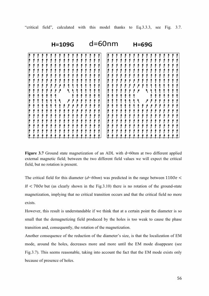
  56  

“critical field”, calculated with this model thanks to Eq.3.3.3, see Fig. 3.7.

 

Figure 3.7 Ground state magnetization of an ADL with d=60nm at two different applied external magnetic field; between the two different field values we will expect the critical field, but no rotation is present.  

The critical field for this diameter (d=60nm) was predicted in the range between 110𝑂𝑒 <

𝐻 < 70𝑂𝑒 but (as clearly shown in the Fig.3.10) there is no rotation of the ground-state

magnetization, implying that no critical transition occurs and that the critical field no more

exists.

However, this result is understandable if we think that at a certain point the diameter is so

small that the demagnetizing field produced by the holes is too weak to cause the phase

transition and, consequently, the rotation of the magnetization.

Another consequence of the reduction of the diameter’s size, is that the localization of EM

mode, around the holes, decreases more and more until the EM mode disappeare (see

Fig.3.7). This seems reasonable, taking into account the fact that the EM mode exists only

because of presence of holes.

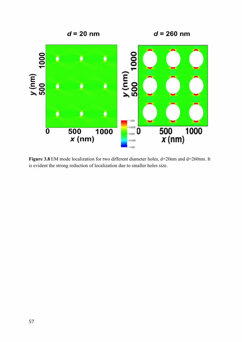
 57  

 Figure 3.8  EM mode localization for two different diameter holes, d=20nm and d=260nm. It is evident the strong reduction of localization due to smaller holes size.    

 

 

 

 

 

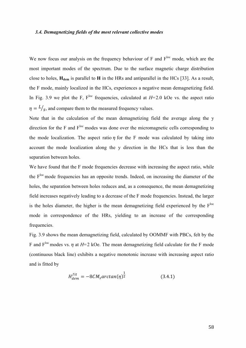
  58  

3.4. Demagnetizing fields of the most relevant collective modes

 

 

We now focus our analysis on the frequency behaviour of F and Floc mode, which are the

most important modes of the spectrum. Due to the surface magnetic charge distribution

close to holes, Hdem is parallel to H in the HRs and antiparallel in the HCs [33]. As a result,

the F mode, mainly localized in the HCs, experiences a negative mean demagnetizing field.

In Fig. 3.9 we plot the F, Floc frequencies, calculated at H=2.0 kOe vs. the aspect ratio

𝜂 = 𝐿 𝑠, and compare them to the measured frequency values.

Note that in the calculation of the mean demagnetizing field the average along the y

direction for the F and Floc modes was done over the micromagnetic cells corresponding to

the mode localization. The aspect ratio 𝜂 for the F mode was calculated by taking into

account the mode localization along the y direction in the HCs that is less than the

separation between holes.

We have found that the F mode frequencies decrease with increasing the aspect ratio, while

the Floc mode frequencies has an opposite trends. Indeed, on increasing the diameter of the

holes, the separation between holes reduces and, as a consequence, the mean demagnetizing

field increases negatively leading to a decrease of the F mode frequencies. Instead, the larger

is the holes diameter, the higher is the mean demagnetizing field experienced by the Floc

mode in correspondence of the HRs, yielding to an increase of the corresponding

frequencies.

Fig. 3.9 shows the mean demagnetizing field, calculated by OOMMF with PBCs, felt by the

F and Floc modes vs. 𝜂 at H=2 kOe. The mean demagnetizing field calculate for the F mode

(continuous black line) exhibits a negative monotonic increase with increasing aspect ratio

and is fitted by

𝐻!"#!"# = −8𝐶𝑀!𝑎𝑟𝑐𝑡𝑎𝑛 𝜂

!!                                                                (3.4.1)

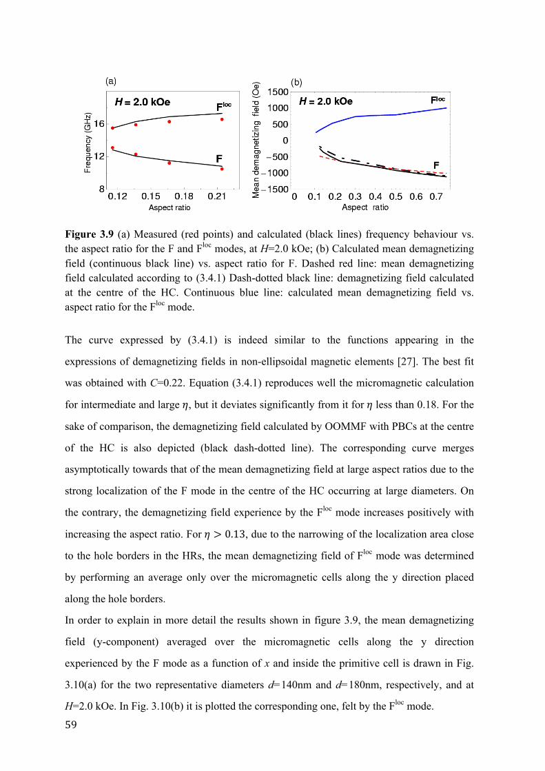
 59  

Figure 3.9 (a) Measured (red points) and calculated (black lines) frequency behaviour vs. the aspect ratio for the F and Floc modes, at H=2.0 kOe; (b) Calculated mean demagnetizing field (continuous black line) vs. aspect ratio for F. Dashed red line: mean demagnetizing field calculated according to (3.4.1) Dash-dotted black line: demagnetizing field calculated at the centre of the HC. Continuous blue line: calculated mean demagnetizing field vs. aspect ratio for the Floc mode.  

The curve expressed by (3.4.1) is indeed similar to the functions appearing in the

expressions of demagnetizing fields in non-ellipsoidal magnetic elements [27]. The best fit

was obtained with C=0.22. Equation (3.4.1) reproduces well the micromagnetic calculation

for intermediate and large 𝜂, but it deviates significantly from it for 𝜂 less than 0.18. For the

sake of comparison, the demagnetizing field calculated by OOMMF with PBCs at the centre

of the HC is also depicted (black dash-dotted line). The corresponding curve merges

asymptotically towards that of the mean demagnetizing field at large aspect ratios due to the

strong localization of the F mode in the centre of the HC occurring at large diameters. On

the contrary, the demagnetizing field experience by the Floc mode increases positively with

increasing the aspect ratio. For 𝜂 > 0.13, due to the narrowing of the localization area close

to the hole borders in the HRs, the mean demagnetizing field of Floc mode was determined

by performing an average only over the micromagnetic cells along the y direction placed

along the hole borders.

In order to explain in more detail the results shown in figure 3.9, the mean demagnetizing

field (y-component) averaged over the micromagnetic cells along the y direction

experienced by the F mode as a function of x and inside the primitive cell is drawn in Fig.

3.10(a) for the two representative diameters d=140nm and d=180nm, respectively, and at

H=2.0 kOe. In Fig. 3.10(b) it is plotted the corresponding one, felt by the Floc mode.

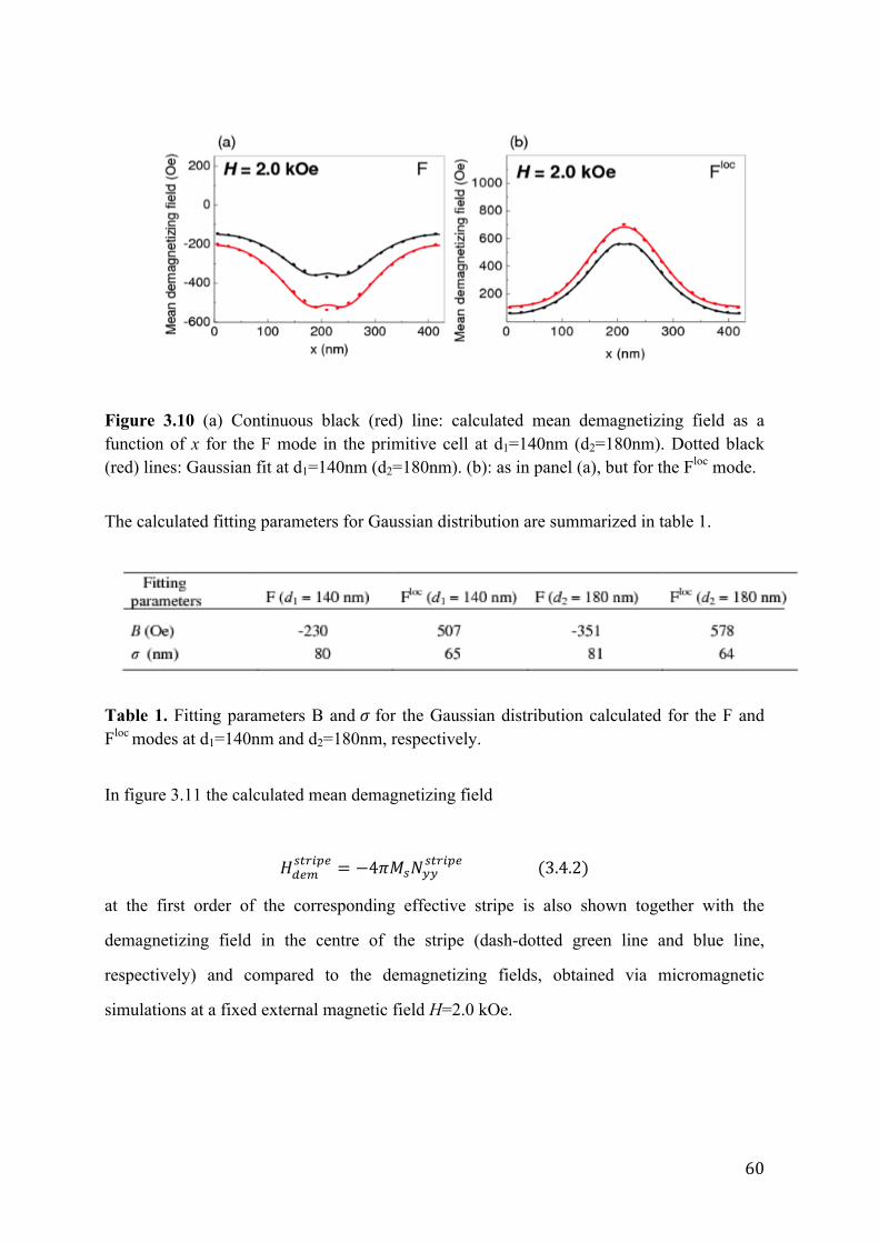
  60  

 Figure 3.10 (a) Continuous black (red) line: calculated mean demagnetizing field as a function of x for the F mode in the primitive cell at d1=140nm (d2=180nm). Dotted black (red) lines: Gaussian fit at d1=140nm (d2=180nm). (b): as in panel (a), but for the Floc mode.

The calculated fitting parameters for Gaussian distribution are summarized in table 1.

Table 1. Fitting parameters B and 𝜎 for the Gaussian distribution calculated for the F and Floc modes at d1=140nm and d2=180nm, respectively.  

In figure 3.11 the calculated mean demagnetizing field

𝐻!"#!"#$%& = −4𝜋𝑀!𝑁!!

!"#$%&                                      (3.4.2)  

at the first order of the corresponding effective stripe is also shown together with the

demagnetizing field in the centre of the stripe (dash-dotted green line and blue line,

respectively) and compared to the demagnetizing fields, obtained via micromagnetic

simulations at a fixed external magnetic field H=2.0 kOe.

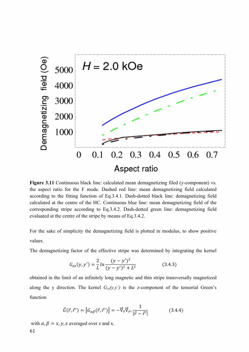
 61  

 Figure 3.11 Continuous black line: calculated mean demagnetizing filed (y-component) vs. the aspect ratio for the F mode. Dashed red line: mean demagnetizing field calculated according to the fitting function of Eq.3.4.1. Dash-dotted black line: demagnetizing field calculated at the centre of the HC. Continuous blue line: mean demagnetizing field of the corresponding stripe according to Eq.3.4.2. Dash-dotted green line: demagnetizing field evaluated at the centre of the stripe by means of Eq.3.4.2.    

For the sake of simplicity the demagnetizing field is plotted in modulus, to show positive

values.

The demagnetizing factor of the effective stripe was determined by integrating the kernel

𝐺!! 𝑦,𝑦! =2𝐿 𝑙𝑛

(𝑦 − 𝑦!)!

(𝑦 − 𝑦!)! + 𝐿!                                              (3.4.3)

obtained in the limit of an infinitely long magnetic and thin stripe transversally magnetized

along the y direction. The kernel Gzz(y,y’) is the z-component of the tensorial Green’s

function

𝐺 𝑟, 𝑟! = 𝐺!"(𝑟, 𝑟!) = −∇!∇!!1

𝑟 − 𝑟′                                    (3.4.4)  

with 𝛼,𝛽 = 𝑥,𝑦, 𝑧 averaged over z and x.

 

   

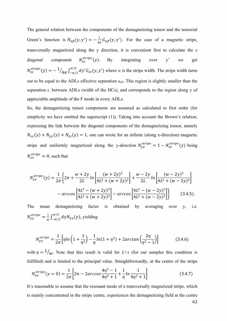
  62  

The general relation between the components of the demagnetizing tensor and the tensorial

Green’s function is 𝑁!"(𝑦,𝑦!) = − !!!𝐺!"(𝑦,𝑦!) . For the case of a magnetic stripe,

transversally magnetized along the y direction, it is convenient first to calculate the z

diagonal component 𝑁!!!"#$%& 𝑦 . By integrating over y’ we get

𝑁!!!"#$%& 𝑦 = − 1 4𝜋 𝑑𝑦!𝐺!!(𝑦,𝑦!)

!/!!!/! where w is the stripe width. The stripe width turns

out to be equal to the ADLs effective separation seff. This region is slightly smaller than the

separation s, between ADLs (width of the HCs), and corresponds to the region along y of

appreciable amplitude of the F mode in every ADLs.

So, the demagnetizing tensor components are assumed as calculated to first order (for

simplicity we have omitted the superscript (1)). Taking into account the Brown’s relation,

expressing the link between the diagonal components of the demagnetizing tensor, namely

𝑁!! 𝑦 + 𝑁!! 𝑦 + 𝑁!! 𝑦 = 1, one can wrote for an infinite (along x-direction) magnetic

stripe and uniformly magnetized along the y-direction 𝑁!!!"#$%& = 1− 𝑁!!

!"#$%&(𝑦) being

𝑁!!!"#$%& = 0, such that

𝑁!!!"#$%& 𝑦 =

12𝜋 2𝜋 +

𝑤 + 2𝑦2𝐿 𝑙𝑛

(𝑤 + 2𝑦)!

4𝐿! + (𝑤 + 2𝑦)! +𝑤 − 2𝑦2𝐿 𝑙𝑛

(𝑤 − 2𝑦)!

4𝐿! + (𝑤 − 2𝑦)!

− 𝑎𝑟𝑐𝑐𝑜𝑠4𝐿! − 𝑤 + 2𝑦 !

4𝐿! + 𝑤 + 2𝑦 ! − 𝑎𝑟𝑐𝑐𝑜𝑠4𝐿! − (𝑤 − 2𝑦)!

4𝐿! + (𝑤 − 2𝑦)!                     3.4.5 .  

The mean demagnetizing factor is obtained by averaging over y, i.e.

𝑁!!!"#$%& = !

!𝑑𝑦𝑁!!(𝑦)

!/!!!/! , yielding

𝑁!!!"#$%& =

12𝜋 𝜂𝑙𝑛 1+

1𝜂! −

1𝜂 𝑙𝑛 1+ 𝜂! + 2𝑎𝑟𝑐𝑡𝑎𝑛

2𝜂𝜂! − 1                                (3.4.6)  

with 𝜂 = 𝐿 𝑤. Note that this result is valid for L<s (for our samples this condition is

fulfilled) and is limited to the principal value. Straightforwardly, at the centre of the stripe

𝑁!!!"#$%& 𝑦 = 0 =

12𝜋 2𝜋 − 2𝑎𝑟𝑐𝑐𝑜𝑠

4𝜂! − 14𝜂! + 1+

1𝜂 𝑙𝑛

14𝜂! + 1                                                              (3.4.7)  

It’s reasonable to assume that the resonant mode of a transversally magnetized stripe, which

is mainly concentrated in the stripe centre, experiences the demagnetizing field at the centre

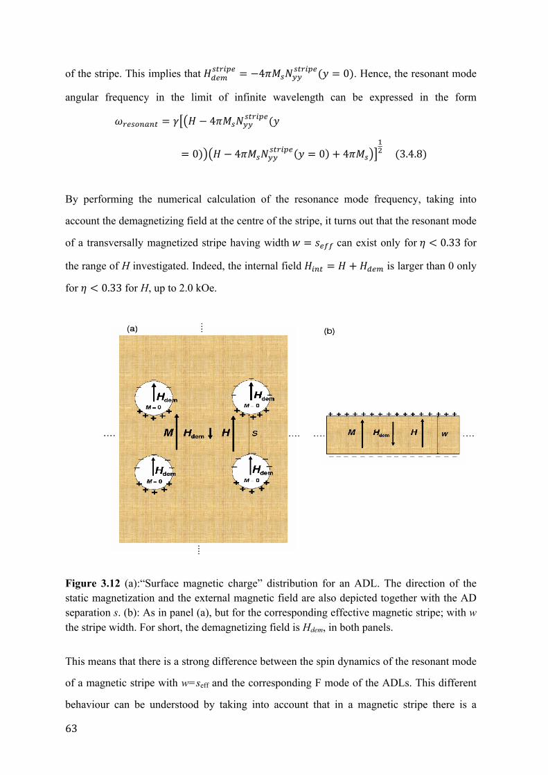
 63  

of the stripe. This implies that 𝐻!"#!"#$%& = −4𝜋𝑀!𝑁!!

!"#$%&(𝑦 = 0). Hence, the resonant mode

angular frequency in the limit of infinite wavelength can be expressed in the form

𝜔!"#$%&%' = 𝛾 𝐻 − 4𝜋𝑀!𝑁!!!"#$%&(𝑦

= 0) 𝐻 − 4𝜋𝑀!𝑁!!!"#$%& 𝑦 = 0 + 4𝜋𝑀!

!!          (3.4.8)

By performing the numerical calculation of the resonance mode frequency, taking into

account the demagnetizing field at the centre of the stripe, it turns out that the resonant mode

of a transversally magnetized stripe having width 𝑤 = 𝑠!"" can exist only for 𝜂 < 0.33 for

the range of H investigated. Indeed, the internal field 𝐻!"# = 𝐻 + 𝐻!"# is larger than 0 only

for 𝜂 < 0.33 for H, up to 2.0 kOe.  

 Figure 3.12 (a):“Surface magnetic charge” distribution for an ADL. The direction of the static magnetization and the external magnetic field are also depicted together with the AD separation s. (b): As in panel (a), but for the corresponding effective magnetic stripe; with w the stripe width. For short, the demagnetizing field is Hdem, in both panels.  

This means that there is a strong difference between the spin dynamics of the resonant mode

of a magnetic stripe with w=seff and the corresponding F mode of the ADLs. This different

behaviour can be understood by taking into account that in a magnetic stripe there is a

  64  

continuous distribution of “surface magnetic charges” if compared to the discontinuous

distribution typical of ADLs. This larger “surface magnetic charge” density leads to a larger

demagnetizing field with respect to the corresponding one of the ADLs. A pictorial sketch of

the “surface magnetic charge” distribution in a periodic ADL (with typical periodicity and

diameter range discussed before) and in the corresponding effective stripe is shown in Fig.

3.12.

 

 65  

3.5 Dynamic critical phenomena and universal behaviour  

 

We now focus more deeply on the universal behaviour at the basis of the frequency

softening mechanism characterizing the two-lowest modes, the EM and F mode,

respectively as a function of the external field. The results obtained for 2D ADLs can be

considered general and extended to other 2D magnonic crystal and periodic magnetic

systems where the softening of the lowest-frequency excitations of the spectrum occurs.

After the pioneering work of Halperin and Hohenberg [38] on the generalization of scaling

laws to dynamical properties of critical phenomena, several attempts were done to apply the

new formulation to different physical systems in order to determine the dynamic universality

classes and dynamical critical exponents. Among them, also remarkable results were

obtained for magnetic systems studied by using the Ising model, the X-Y model or the

Heisenberg model. However, these studies were carry out by investigating the critical

behaviour of dynamic excitations as a function of temperature.

In this thesis, we propose a preliminary study of the dynamic critical behaviour of collective

modes, in 2D magnonic crystals represented by 2D ADLs, as a function of the external

magnetic field for a fixed temperature. Hence, the temperature is replaced by another

thermodynamic variable: typical of ferromagnetic systems is given by the applied magnetic

field. Unlike the case of dynamic critical behaviour studied as a function of temperature in

presence of dissipation effects, the dynamics of our system is purely conservative. Indeed, it

was based on the DMM; according to which there is not relaxation towards equilibrium, due

to the absence of the damping term in the Hamiltonian.

As already outlined previously, the critical phase transition, marked by a softening of

lowest-mode frequencies, takes place at a given critical field that depend on the diameter. In

particular, it was demonstrated both by micromagnetic simulations with DMM and by

measurements carried on, with BLS, that the critical field decreases with decreasing the

holes diameter. Also, this trend can be described in a more general way by studying the

dependence of the critical field on a geometric in-plane ratio 𝑟 = 𝑑 𝑠 with d holes diameter

and s the separation between adjacent HRs (or vertical rows) of ADLs, as shown in Fig.

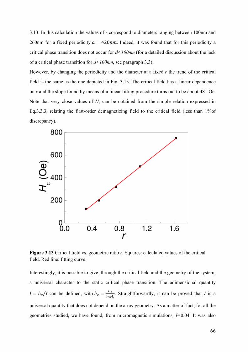
  66  

3.13. In this calculation the values of r correspond to diameters ranging between 100nm and

260nm for a fixed periodicity 𝑎 = 420𝑛𝑚. Indeed, it was found that for this periodicity a

critical phase transition does not occur for d<100nm (for a detailed discussion about the lack

of a critical phase transition for d<100nm, see paragraph 3.3).

However, by changing the periodicity and the diameter at a fixed r the trend of the critical

field is the same as the one depicted in Fig. 3.13. The critical field has a linear dependence

on r and the slope found by means of a linear fitting procedure turns out to be about 481 Oe.

Note that very close values of Hc can be obtained from the simple relation expressed in

Eq.3.3.3, relating the first-order demagnetizing field to the critical field (less than 1%of

discrepancy).

Figure 3.13 Critical field vs. geometric ratio r. Squares: calculated values of the critical field. Red line: fitting curve. Interestingly, it is possible to give, through the critical field and the geometry of the system,

a universal character to the static critical phase transition. The adimensional quantity

𝐼 = ℎ! 𝑟 can be defined, with ℎ! =!!

!!!!. Straightforwardly, it can be proved that I is a

universal quantity that does not depend on the array geometry. As a matter of fact, for all the

geometries studied, we have found, from micromagnetic simulations, I=0.04. It was also

 67  

found with analytical calculations. This universal relation has a considerable advantage: by

using it, one can immediately get Hc whatever array periodicity and diameter, for all allowed

range (r>0.3) where it was predicted the presence of a critical phase transition.

As done for characterizing the phases across a critical phase transition as a function of the

temperature, the critical phase transition can be described quantitatively by an order

parameter that we name static order parameter (SOP). The “ordered” phase is the one

corresponding to H> Hc, while the “disordered” phase is present for H< Hc. one notice that

the “ordered” phase has also a lower symmetry with respect to that of the “disordered”

phase. It is useful to define an adimensional SOP in the form

Ψ =𝑀!

𝑀! !                    (3.5.1)  

expressed by the averaged y-component of the static magnetization at a given field H

approaching Hc normalized to the averaged y-component of the static magnetization at the

critical field.

According to the above definition, the order parameter has its maximum value in the

“ordered” phase for H> Hc (approximately almost 1, by taking into account the small

deviations from the y-direction close to the holes present also for high external field) and

reduces its magnitude for H< Hc in the “disordered” phase. However, the definitions of

“ordered” and “disordered” phase are in this context different from the usual ones gives for

critical phase transitions as a function of temperature.

The “ordered” phase is characterized by a magnetization oriented along the y-direction and

parallel to the external field. Hence, the word “ordered” is referred to the order of the

ground-state along the direction of the external magnetic field. Instead, the “disordered”

phase refers to a static magnetization not anymore collinear with the external magnetic field

and progressively rotating away from the y-direction, giving raise to a disorder of the

ground-state magnetization.

Since the analysis is focused on spin precession around the equilibrium magnetization, the

critical phase transition can be studied also from a dynamic point of you and of dynamic

critical phenomena can be investigated. In this respect, this means that also the dynamic

properties of the studied system become critical and one can define a dynamic critical

exponent expressing the degree of softening of the lowest frequency modes (either EM or F

  68  

mode) in the vicinity of the critical field. The universality is expressed by means of

universal quantities related to the dynamic critical exponent that are independent of the

geometry studied.

We now discuss the scaling law fulfilled by the mode frequency in the small interval around

the critical point represented by Hc. Keep in mind that the dynamic critical exponent

introduced in this study is different from one defined in the theory of dynamic critical

phenomena in magnets, studied as function of temperature. Indeed, within that theory the

dynamical critical exponent was associated to the response function and to the dynamic

scaling hypothesis for relaxation time was fulfilled. Instead, in this study no response

function was considered and the studied dynamics is purely conservative.

In order to write down the scaling law we have defined an adimensional quantity: the

reduced field ℎ = !!!!!!

, expressing the small deviation from the critical field. In the vicinity

of Hc the frequency scaling law can thus be written in the form

𝜈! ∝   ℎ !!                        (3.5.2)  

with 𝜆! the critical exponent. We have determined the critical exponents associated to the

frequency curve of the EM and of the F mode, respectively, through a fitting procedure.

Interestingly, for both modes the curvature of the frequency is the same for 𝐻 → 𝐻!! and for

𝐻 → 𝐻!!  (ℎ → 0∗). For example, by means of numerical calculations, we have found that

the critical exponent associated to the EM (F) is 𝜆!" = 0.35  (𝜆! = 0.15) for d=180nm. The

fitting coefficient in front of the reduced field h (𝜈! = 𝐴! ℎ !!) evaluated as the average

value in the two regions is 𝐴!" = 0.40  𝐺𝐻𝑧  (𝐴! = 0.55  𝐺𝐻𝑧). Instead, for d=260nm the

result of the fit was 𝜆!" = 0.12   𝜆! = 0.05 and different values were obtained for the

other diameters. As an example, in Fig. 3.14 the calculated frequency curves of the EM and

of the F mode: for d=180nm, in the right small interval of the magnetic field (350

Oe<H<450 Oe) are shown (black) and the resulting fitting curves 𝜈! = 𝐴! ℎ !! (red) are

drawn.

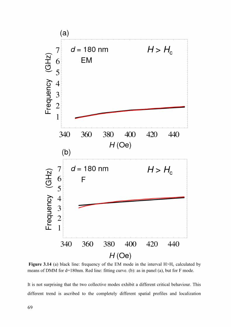
 69  

 Figure 3.14 (a) black line: frequency of the EM mode in the interval H>Hc calculated by means of DMM for d=180nm. Red line: fitting curve. (b): as in panel (a), but for F mode.  

It is not surprising that the two collective modes exhibit a different critical behaviour. This

different trend is ascribed to the completely different spatial profiles and localization

  70  

features of the two collective modes. However, we have found that the ratio of the two

exponents is the same, independently of the diameter investigated: in particular, 𝛽! =!!

!!"=

0.4. This means that the ratio of the frequency curvature for the two soft modes, in the

vicinity of the critical point, does not depend on the geometric ratio r. Even if the quantity

𝛽! is not exactly a critical exponent, it can be regarded as a universal quantity, having the

meaning of a critical exponent. As a result, the behaviour of the lowest-frequency collective

modes is universal in the infinite wavelength limit, namely for 𝑘 = 0.

On this basis, it is possible to define a dynamic universality class characterizing 2D ADLs as

prototype of 2D magnonic crystals. This definition should be similar to the one given for

static universality classes in the study of critical phenomena as a function of temperature.

The 2D magnetic system characterized by the same Hamiltonian and by the same symmetry

of the order parameter as that of the system discussed in this thesis, should have the same

ratio 𝛽!. Note that, at fixed dimensionality D=2, we expect dynamic universality classes

characterized by critical exponents different from the ones typical of the static case. This

investigation could represent the next step of this study.

     

 

 

 

 

 

 

 

 

 

 

 

 

 

 

 71  

Conclusions

In conclusion, in this thesis, we have investigated the static and the dynamic properties of

magnonic modes in a particular prototype of magnonic crystal: 2D Py ADLs with holes size

in the nanometric range. The analysis has been performed largely within theoretical

arguments and simulation instruments using both a micromagnetic formalism extended to

periodic patterns and an analytical formulation. By means of this approach the eigenvalues

of the system, which represent the mode frequencies, have been found. The evaluation of the

corresponding eigenvectors, instead, allowed us to classify the collective excitations. The

calculated dispersion of mode frequencies has been determined along the ΓΧ-direction,

which is of high symmetry, of the reciprocal lattice.

Also experimental measurements, performed only on four reference samples (holes

diameters ranging from 260nm to 140nm), using BLS technique were done and, being in

good agreement with calculated dispersion, gave a direct proof of correctness of theoretical

predictions.

The softening of the two lowest-frequency modes, i.e. the EM and the F mode, is the

consequence of a continuous phase transition of the static magnetization that progressively

rotates from the hard to the easy in-plane direction. Micromagnetic simulations have

confirmed the observation of the softening, so as have done the measurements performed by

BLS technique. A simple phenomenological model, based on the minimization of the energy

density of the system, was developed to derive an analytical expression of the critical field

that turns out to be equal and opposite in sign to the demagnetizing field, calculated to the

first order.

It was also found that frequencies of soft modes exhibit a finite gap at the critical field, due

to the internal field contributions related to their localization features. In fact, the analysis of

the frequencies, as a function of the external magnetic field, revealed that their behaviour is

strictly linked to the inhomogeneity of the internal field. Moreover, the different trend of the

frequencies at high external magnetic field of the most relevant collective modes, namely F

  72  

and Floc modes, as function of the aspect ratio, was explained in terms of opposite

demagnetizing fields.

Moreover, it was demonstrated both by micromagnetic simulations with DMM and by

measurements carried on with BLS that the critical field decreases with decreasing the holes

diameter. This behaviour is present until the critical phase transition exists; indeed, both the

DMM and the OOMMF simulations clearly shows that below d=100nm magnetization

rotation towards the easy-axis occurs no more.

Studying the limit to continuum (film) of the AD, i.e. reducing the hole diameter to zero, we

have found not only that the critical phase transition disappeared but also that the frequency

modes dispersion tends to become the same as the films’ one, as we expected.

Least, but absolutely not last, we have seen that defining an adimensional quantity I in terms

of magnetic and geometric parameters we have been able to characterized the critical phase

transition as a universal phenomenon. Moreover, a static order parameter has also been

defined as function of static ground-state magnetization. Since the analysis was focused on

spin precession around the equilibrium magnetization, the critical phase transition was also

investigated in terms of dynamic critical properties. This was performed by means of the

definition of a sort of dynamic critical exponent representing the degree of softening of the

lowest frequency modes in the vicinity of the critical point. The idea of defining these

universal quantities came from an attempt of rewriting the theory of critical phase transition,

usually studied as function of temperature, in terms of another thermodynamic variable

given by the critical field.

Some of these results are important also for the potential applications of these patterned

structures as magnonic devices. In fact, the AD behaves not only as waveguide for spin

wave, but can also acts as filter.

Other possible future perspectives could be the study of band structure as function of lattice

periodicity and diameter, in the nanometric and submicrometric range, to get a full

comprehension for engineering applications.

However, we believe that the real novelty of this study consists in identifying a universal

behaviour of mode dynamics in two-dimensional magnonic crystal. This could be the

 73  

starting point for develop a new formalism in terms of scaling laws analogous to the ones

developed by Halperin-Hohenberg and Widom-Kadanoff-Wilson.

  74  

References

[1] Wang W, Sun J and Li S 2011 Appl. Phys. Lett. 99 082504.

[2] Tenne D A, Clark M A, James A R, Chen K and Xi X X 2001 Appl. Phys. Lett. 79 3836.

[3] Weber F, Rosenkranz S, Castellan J -P, Osborn R, Karapetrov G, Hott R, Heid R,

Bohnen K –P and Alatas A 2011 Phys. Rev. Lett. 107 266401.

[4] Kohmoto T, Masui M, Abe M, Moriyasu T and Tanaka K 2011 Phys. Rev. B 83 064304.

[5] Sakai H, Fujioka J, Fukuda T, Bahramy M S, Okuyama D, Arita R, Arima T, Baron A Q

R, Taguchi Y and Tokura Y 2012 Phys. Rev. B 86 104407.

[6] Kendziora, C A, Sergienko I A, Jin R, He J, Keppens V, Sales B C and Mandrus D 2005

Phys. Rev. Lett. 95 125503.

[7] Radzihovsky L and Lubensky T C 2011 Phys. Rev. E 83 051701.

[8] Côté R, Jobidon J -F and H. A. Fertig H A 2008 Phys. Rev. B 78 085309.

[9] Wang R W and Mills D L 1994 Phys. Rev. B 50 3931.

[10] Zivieri R, Giovannini L and Nizzoli F 2000 Phys. Rev. B 62 14950.

[11] Dutcher J R, Heinrich B, Cochran J F, Steigerwald D A and Egelhoff W F 1988 J.

Appl. Phys. 63 3464.

[12] Stamps R L and Hillebrands B 1991 Phys. Rev. B 43 3532.

[13] Montoncello F, Giovannini L, Nizzoli F, Vavassori P, Grimsditch M, Ono T, Gubbiotti

G, Tacchi S and Carlotti G 2007 Phys. Rev. B 76 024426.

[14] McMichael R D and Maranville B B 2006 Phys. Rev. B 74 024424.

[15] Maranville B B, McMichael R D and Abraham D W 2007 Appl. Phys. Lett. 90 232504.

 75  

[16] Neusser S, Duerr G, Tacchi S, Madami M, Sokolovskyy M L, Gubbiotti G, Krawczyk

M and Grundler D 2011 Phys. Rev. B 84 094454.

[17] Ding J, Tripathy D and Adeyeye A O 2011 J. Appl. Phys. 109 07D304.

[18] Tacchi S, Madami M, Gubbiotti G, Carlotti G, Adeyeye A O, Neusser S, Botters B and

Grundler D 2010 IEEE Trans. on Magnetics 46 172.

[19] Kruglayak V V Demokritov S O Grundler D 2010 J. Phys. D: Appl. Phys. 43 264001.

[20] Vysotskiï S L Nikitov Yu S A Filimonov A 2005 Exp. Theor. Phys. 101 547.

[21] Neusser S and Grundler D 2009 Adv. Mater. 21 2927-2932.

[22] Chumak A V et al. 2009 Appl. Phys. Lett. 95 262508.

[23] Tacchi S et al. 2011 Phys. Rev. Lett. 107, 127204.

[24] Kruglyak V V et al. 2010 Phys. Rev. Lett. 104, 027201.

[25] Carlotti G and Gubbiotti G 1999 La Rivista del Nuovo Cimento 22, 1.

[26] Goldstone J Salam A and Weinberg S 1961 1962 127, Nuovo Cimento 19, 154, 965.

[27] Lange R. V. 1966 Phys. Rev. 146 301.

[28] Zivieri R, Giovannini L and Nizzoli F 2000 Phys. Rev. B 62, 14950.

[29] Giovannini L, Montoncello F and Nizzoli F 2007 Phys. Rev. B 75 024416.

[30] Zivieri R et al. 2012 2Phys. Rev. B 85, 012403.

[31] Singh Navab Goolaup S and Adeyeye A O 2004 Nanotechnology 15, 1539.

[32] Ding J Tripathy D and Adeyeye A.O. 2011 Appl. Phys. 109, 07D304.

[33] OOMMF User’s Guide, Version 1.0, edited by M. Donahue and D. Porter; interagency

report NISTIR 6376, National Institute of Standards and Technology, Gaithersburg, MD.

[34] Zivieri R 2012 Solid State Physics 63 151.

[35] Zivieri R et al. 2011 Phys. Rev. B 83 054431.

  76  

[36] Montoncello F, Giovannini L, Nizzoli F, Tanigawa H, Ono T, Gubbiotti G, Madami M,

Tacchi S and Carlotti G 2008 Phys. Rev. B 78 104421.

[37] Wang C C, Adeyeye A O and Singh N 2006 Nanotechnology 17 1629.

[38] Halperin B I and Hohenberg P C 1967 Phys. Rev. Lett. 19 700

 

 

 

 

 

 

 

 

 

 

 

 

 

 

 

 

 

 

 

 

 77  

Acknowledgements

I wish to thank my supervisor and co-, the prof. L. Giovannini and the prof. R. Zivieri, for

their big contributions, given both during the two-year degree and for the hours devoted to

develop the thesis with me.

Besides, I would also to thank my friends and classmates, with which I shared the weight of

the most difficult exams or simply vented momentarily frustration.

Least, but not last I would like to thank affectionately my family for the backing and in

particular my parents, my brother Marco and my cousin Giorgia for the support, emotional

and economic, and for having been close to me, despite the 800km between us.