Dynamic lot sizing with product returns

Ruud H. Teunter∗

Department of Management Science, Lancaster University Management School,

Lancaster, LA1 4YX, UK,

tel/fax: +44-1524-594326/844885, e-mail: r.teunter@lancaster.ac.uk

Z. Pelin Bayındır

Department of Industrial and Systems Engineering, University of Florida,

303 Weil Hall, PO Box 116595, Gainesville, FL 32611-6595, USA,

tel(ext.)/fax: +1-352-3921464(2053)/3537, e-mail: bayindir@ise.ufl.edu

Wilco van den Heuvel

Econometric Institute and Erasmus Research Institute of Management,

Erasmus University Rotterdam,

PO Box 1738, Burg. Oudlaan 50, 3000 DR Rotterdam, The Netherlands,

tel/fax: +31-10-4081321/9162, e-mail: wvandenheuvel@few.eur.nl

Econometric Institute Report EI 2005-17

April 18, 2005

Abstract

We address the dynamic lot sizing problem for systems with product returns. The de-

mand and return amounts are deterministic over the finite planning horizon. Demands can be

satisfied by manufactured/procured new items, but also by remanufactured returned items.

The objective is to determine those lot sizes for manufacturing and remanufacturing that

∗corresponding author

1

minimize the total cost composed of holding cost for returns and serviceable products and

set-ups costs. Two different set-up cost schemes are considered; there is either a joint set-up

cost for manufacturing and remanufacturing (single production line) or separate set-up costs

(dedicated production lines). For the joint set-up cost case, we present an exact, polynomial

time dynamic programming algorithm. For both cases, we propose a number of heuristics

and test them in an extensive numerical study.

Keywords: inventory management, lot sizing, reverse logistics

1 Introduction

Dynamic lot sizing, i.e., planning manufacturing/production orders over a number of future

periods in which demand is dynamic and deterministic, is one of the most extensively researched

topics in production and inventory control. See Silver, Pyke, and Peterson [15] for a general

overview, and Brahimi et al. [2] for a recent and extensive review of single item models. However,

the literature on dynamic lot sizing with product returns, where remanufacturing of those returns

is an alternative for manufacturing, is very scarce.

Remanufacturing can be defined as the recovery of returned products, often involving disas-

sembly, cleaning, testing, part replacement/repair, and reassembly operations, after which they

are as-good-as-new. The latter term distinguishes remanufacturing from other recovery types

such as material and energy recycling. See Thierry et al. [20] for a comparison of recovery types.

Environmental legislation, societal pressure, and economic opportunities have motivated

many firms to get involved with product remanufacturing, especially over the past 10 years.

Products that are nowadays remanufactured include machine tools, medical instruments, copiers,

automobile engines, computers, aviation equipment, telephone equipment, and tires (see Ferrer

[4] [5], Kandebo [10], Lund [12], Sivinski and Meegan [16], Sprow [17], and Thierry et al. [20]).

The scientific literature on remanufacturing and product recovery in general has also been

growing at an increasing rate over the past two decades. Overviews are provided by Fleischmann

et al. [6], Guide et al. [8], and Gupta and Gungor [9]. For a discussion of more recent results

we refer to Dekker et al. [3]. However, there are just a few papers on lot sizing for the systems

2

with remanufacturing option.

Richter and Sombrutzki [13] and Richter and Weber [14] study special cases of the problem.

In the first model, it is assumed that the number of returns is sufficient for satisfying all demands

without delay, and therefore manufacturing is not considered. The second model does consider

the manufacturing option. However, results are only derived for the special case that the number

of returns in the first period is at least as large as the total demand over the planning horizon.

So in fact, the manufacturing option is not needed in the second model either, but may be used

for economic reasons if holding returns is very costly.

Golany et al. [7] study the problem without restrictive assumptions on the number of returns.

They show that the lot sizing problem with remanufacturing can be formulated as a network

flow problem. Using this formulation, they prove that the problem is NP-hard for general

concave costs. For the special case with linear costs and hence zero set-up costs, they provide a

polynomial-time algorithm.

Beltran and Krass [1] study the lot sizing problem with returns that can be directly reused,

i.e., for which no remanufacturing is needed. They show that it suffices to consider solutions that

satisfy the “zero-inventory property”, and use this property to develop a dynamic programming

(DP) algorithm with cubic time-complexity that determines the optimal manufacturing and

disposal decisions for the case of concave cost functions. If procurement cost and disposal cost

are non-decreasing over time, then the problem can be solved in quadratic time.

In this paper we study the lot sizing problem with remanufacturing of returns, without

restrictions on the number of returns and with set-up costs included. Two different set-up cost

schemes are considered. In the first model variant, there is a joint set-up cost for manufacturing

and remanufacturing, which is suitable if manufacturing and remanufacturing operations are

performed on the same production line using the same production resources. In the second model

variant, there are separate set-up costs for manufacturing and remanufacturing, in line with

situations where there are separate production lines. Note that all four above discussed papers

assumed separate cost functions for manufacturing and remanufacturing, but none proposed

algorithms without return restrictions and with set-up costs included.

For the problem with a joint set-up cost, we will show that the zero-inventory property and

3

a “remanufacture-first” property hold. Using those properties, we derive an exact DP algorithm

and prove that its time-complexity is polynomial in the length of the planning horizon. The

algorithm is a generalization of the famous Wagner-Whitin algorithm for the lot sizing problems

without returns. We further propose generalizations of the Silver-Meal, Least Unit Cost, and

Part Period Balancing heuristics, and test them in an extensive numerical experiment.

For the problem with separate set-up costs, we show that the above mentioned properties

no longer hold. We again propose generalizations of the Silver-Meal, Least Unit Cost, and Part

Period Balancing heuristics and test them in an extensive numerical experiment.

The remainder of the paper is organized as follows. In Section 2, the model is presented.

The case with a joint set-up cost is treated in Section 3. The exact algorithm is presented, and

the heuristics are described and tested. Section 4 deals with separate set-up costs. Heuristics

are described and tested. We end with conclusions and offer directions for future research in

Section 5.

2 Model

Table 1 lists the notations that will be used.

** PLACE TABLE 1 HERE **

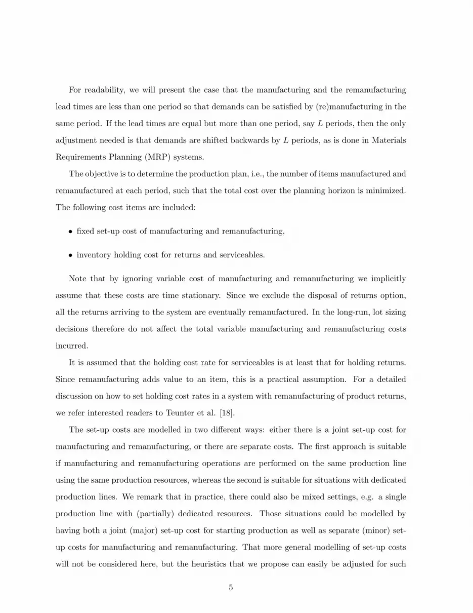
We address lot sizing problems for systems with product returns. Demands and returns

are known for all periods of the planning horizon. Demands can be satisfied by manufac-

tured/procured new items and by remanufactured returned items. In Figure 1, a simple sketch

of the system is depicted.

** PLACE FIGURE 1 HERE **

Note that there is no disposal option for returned products. Recent research by Van der

Laan and Salomon [11] and Teunter and Vlachos [19] has shown that such an option will not

lead to a considerable cost reduction, unless the return rate is unrealistically high (above 90%)

and the demand rate is very small (less than 10 per year).

4

For readability, we will present the case that the manufacturing and the remanufacturing

lead times are less than one period so that demands can be satisfied by (re)manufacturing in the

same period. If the lead times are equal but more than one period, say L periods, then the only

adjustment needed is that demands are shifted backwards by L periods, as is done in Materials

Requirements Planning (MRP) systems.

The objective is to determine the production plan, i.e., the number of items manufactured and

remanufactured at each period, such that the total cost over the planning horizon is minimized.

The following cost items are included:

• fixed set-up cost of manufacturing and remanufacturing,

• inventory holding cost for returns and serviceables.

Note that by ignoring variable cost of manufacturing and remanufacturing we implicitly

assume that these costs are time stationary. Since we exclude the disposal of returns option,

all the returns arriving to the system are eventually remanufactured. In the long-run, lot sizing

decisions therefore do not affect the total variable manufacturing and remanufacturing costs

incurred.

It is assumed that the holding cost rate for serviceables is at least that for holding returns.

Since remanufacturing adds value to an item, this is a practical assumption. For a detailed

discussion on how to set holding cost rates in a system with remanufacturing of product returns,

we refer interested readers to Teunter et al. [18].

The set-up costs are modelled in two different ways: either there is a joint set-up cost for

manufacturing and remanufacturing, or there are separate costs. The first approach is suitable

if manufacturing and remanufacturing operations are performed on the same production line

using the same production resources, whereas the second is suitable for situations with dedicated

production lines. We remark that in practice, there could also be mixed settings, e.g. a single

production line with (partially) dedicated resources. Those situations could be modelled by

having both a joint (major) set-up cost for starting production as well as separate (minor) set-

up costs for manufacturing and remanufacturing. That more general modelling of set-up costs

will not be considered here, but the heuristics that we propose can easily be adjusted for such

5

a situation.

Without loss of generality, we can assume that the initial stocks of serviceables and returns

are both zero and that there is a positive demand in the first period. To see this, consider the

general problem with possibly non-zero stocks Ir0 of returns and Is

0 of serviceables at the end

of period 0. It is obvious that the first set-up should be placed in the first period f for which

cumulative demand∑f

i=1 Di is larger than Is0 . The relevant lot sizing problem is therefore from

that period f with positive demand onwards, and starts with Is0−∑f−1

i=1 Di < Df serviceables and

Ir0 +∑f−1

i=1 Ri returns in stock at the end of period f−1. This problem can easily be transformed

to an equivalent problem with zero initial (at the end of period f − 1) stocks by subtracting

Is0 −

∑f−1i=1 Di from the demand in period f and adding Ir

0 +∑f−1

i=1 Ri to the return in period f .

Therefore, any general lot sizing problem with non-zero initial stocks can be transformed to an

equivalent problem with zero initial stocks and positive demand in the first period.

3 Joint set-up cost for manufacturing and remanufacturing

The lot sizing problem under the joint manufacturing and remanufacturing set-up cost can be

modelled as a mixed integer linear programming problem (MILP) as follows:

minT∑

t=1{Kδt + hrIr

t + hsIst }

subject to

Irt−1 + Rt − xr

t = Irt for t = 1, . . . , T (1)

Ist−1 + xr

t + xmt −Dt = Is

t for t = 1, . . . , T (2)

xrt + xm

t ≤ Mtδt for t = 1, . . . , T (3)

δt ∈ {0, 1}, xrt , xm

t , Irt , Is

t ≥ 0 for t = 1, . . . , T,

where Mt =∑T

i=t Di for t = 1, . . . , T . Constraints (1) and (2) assure the inventory balance in

return and serviceable stocks, respectively. Constraints (3) keep track of the set-ups; whenever

a manufacturing or a remanufacturing lot is produced, a set-up is made and the production (the

6

sum of the amount manufactured and remanufactured) in period t will never exceed the total

demand in periods t, . . . , T .

Next, we will derive some optimality conditions that will provide the basis for an exact

dynamic programming algorithm and a number of heuristics. The conditions are presented in

the form of two lemmas.

The first lemma states that for any optimal solution, the stock at the beginning of any period

with a set-up is zero. This lemma is a generalization of the well-known zero-inventory property

for the original lot sizing problem without returns.

Lemma 1 Any optimal solution satisfies the zero-serviceable-inventory-property: for any period

with a set-up it holds that the stock of serviceables at the beginning of the period is zero, i.e.,

Ist−1δt = 0 for t = 1, 2, . . . , T .

Proof Consider any solution π. Since the initial stock (at the end of period 0) of serviceables is

zero, the property obviously holds for the first period (in which there is a set-up since demand is

positive). Now consider any other period t ≥ 2 with a set-up under solution π, and let t′ denote

the preceding period with a set-up. So, t′ and t are successive set-up periods under solution

π. We shall complete the proof by showing that if the stock of serviceables is positive at the

beginning of period t, then an alternative feasible solution π′ with lower cost can be constructed.

We consider two cases. Case 1: π only remanufactures in period t′. Then π′ remanufactures one

less item in t′ and one more in t. Case 2: π manufactures in period t′. Then π′ manufactures

one less item in t′ and one more in t. For both cases, it is clear that π′ is feasible, and that π and

π′ have the same number of set-ups and therefore the same set-up cost. However, the difference

in holding cost for returns and serviceables under solutions π and π′ is (hs − hr)(t− t′) > 0 for

Case 1 and hs(t− t′) > 0 for Case 2. �

We remark that Lemma 1 can also be used to solve the MILP more efficiently by adding the

constraints Ist−1 ≤ (1− δt)

∑Ti=t Di for t = 1, 2, . . . , T .

The second lemma shows that priority is given to remanufacturing option, i.e. that any

optimal solution only manufactures in a certain period if the initial stock of returns at the

beginning of that period is insufficient for remanufacturing the entire lot.

7

Lemma 2 Any optimal solution satisfies the following property: in every period where items

are manufactured, the stock of returns at the end of that period is zero, i.e., Irt xm

t = 0 for

t = 1, 2, . . . , T .

Proof Consider any solution π that does not satisfy the property. Then there must be some

period t, 1 ≤ t ≤ T , with manufacturing and with a positive stock of returns at the end. An

alternative solution π′ is to manufacture one less item and remanufacture one more item in period

t, and to manufacture one more item and remanufacture one less item during the first period

after t in which π remanufactures (if there is remanufacturing after period t). Clearly, solution

π′ is feasible. Policies π and π′ have the same number of set-ups and therefore the same set-up

costs. Furthermore, it is clear that they have the same holding cost for serviceables. However,

solution π′ has a lower holding cost for returns. Therefore, solution π cannot be optimal. �

3.1 Exact dynamic programming algorithm

The dynamic programming algorithm that is proposed in this section is a generalized version of

the one proposed by Wagner and Whitin [22] for solving the dynamic lot sizing problem without

returns. See Table 1 for notations. Note that, for ease of presentation, some of the notations

are also used for period 0.

The algorithm starts by considering period 0 only. Clearly, the stock of returns at the end of

that period is 0. So, S0 = {0}, f0(0) = 0, and f0 = 0. The algorithm then recursively solves the

lot sizing problem until period k = 1, 2, . . . , T by deriving Sl,k (for all l = 1, . . . , k), Sk, fl,k(n)

(for all l = 1, . . . , k and n ∈ Sl,k), fk(n) (for all n ∈ Sk), and fk. The recursive equations are

derived below.

Consider the problem until period k. If the last set-up is in period l, l = 1, 2, . . . , k, then

all the returns in periods l + 1 until k, i.e.∑k

i=l+1 Ri, will be in stock at the end of period k.

Moreover, if there are returns left in stock at the end of period l, then those items will also be

in stock at the end of period k. From Lemma 2 it follows that there can only be returns left in

stock at the end of period l if the stock at the end of period l− 1 plus the returns in period l is

larger than the size of the order in period l. Using Lemma 1 it follows that the size of the order

8

in period l is∑k

i=l Di. We therefore get

Sl,k =⋃

j∈Sl−1

(

j + Rl −k∑

i=l

Di

)+

+k∑

i=l+1

Ri

. (4)

Clearly, we further have

Sk =k⋃

l=1

Sl,k. (5)

Next, we derive the recursive expression for fl,k(n). As explained above, if the last set-up is

in period l, then the stock of returns at the end of period k is equal to∑k

i=l+1 Ri plus any stock

that may be left at the end of period l. Two cases are distinguished.

• There is no stock left at the end of period l. Since remanufacturing is preferred to man-

ufacturing (Lemma 2), this case occurs if the stock at the end of period l − 1 plus the

returns Rl in period l is at most the order size∑k

i=l Di in period l. The associated holding

cost for returns in periods l, . . . , k is hr∑k

i=l+1(k + 1 − i)Ri, since the returns in period

i, i = l + 1, . . . , k, incur a holding cost at the end of periods i, . . . , k. The associated

holding cost for serviceables in periods l, . . . , k is hsk∑

i=l+1

(i − l)Di, since the items that

satisfy the demands in period i, i = l + 1, . . . , k, incur a holding cost at the end of periods

l, l + 1, . . . , k − 1.

• Some stock is left at the end of period l. Then the stock at the end of period k is

more than∑k

i=l+1 Ri. To attain stock level n at the end of period k, there should be

n −∑k

i=l+1 Ri left at the end of period l and hence (since Lemma 2 implies that there

is no manufacturing) n −∑k

i=l+1 Ri − Rl +∑k

i=l Di = n +∑k

i=l(Di − Ri) left at the

end of period l− 1. The associated holding cost for returns in periods l, . . . , k is therefore

hr((

n−∑k

i=l+1 Ri

)(k − l + 1) +

∑ki=l+1(k + 1− i)Ri

)= hr

(n(k − l + 1)−

∑ki=l+1(i− l)Ri

).

The associated holding cost for serviceables in periods l, . . . , k is the same as for the first

case.

9

So, we get

fl,k(n) =

minj∈Sl−1|j+Rl≤

k∑i=l

Di

fl−1(j)

+ K + hsk∑

i=l+1

(i− l)Di

+hrk∑

i=l+1

(k + 1− i)Ri(i− l)Di for n =k∑

i=l+1

Ri

fl−1(n +k∑

i=l

(Di −Ri)) + K + hsk∑

i=l+1

(i− l)Di

+hr

(n(k − l + 1)−

k∑i=l+1

(i− l)Ri

)for n ∈ Sl,k \

{k∑

i=l+1

Ri

}(6)

Clearly, we further have

fk(n) = minl∈{1,...,k}|n∈Sl,k

fl,k(n) for n ∈ Sk (7)

and

fk = minn∈Sk

fk(n) for k = 1, . . . , T. (8)

Using the above results, we formulate the algorithm in the frame below. Step 1 initializes the

values for period 0 and then sets the current period k to 1. In the recursive Step 2, the optimal

lot sizes until period k is determined. When k = T is reached, the algorithm goes to the final

Step 3, where the optimal lot sizes are determined ‘backwards’. This backward determination

of the optimal lot sizes is similar to that for the original lot sizing problem without product

returns. We do not describe it mathematically, since that is straightforward and would require

additional notations.

10

Dynamic Programming algorithm for joint set-up cost

Step 1: S0 := {0}, f0(0) = 0, f0 = f0(0) = 0. k := 1.

Step 2: For all l = 1, . . . , k, determine Sl,k using (4). Determine Sk using (5).

For all l = 1, . . . , k and all n ∈ Sl,k, determine fl,k(n) using (6).

For all n ∈ Sk, determine fk(n) using (7). Determine fk using (8).

Step 3: If k = T then go to Step 4.

else k := k + 1, and go to Step 2.

Step 4: The minimal cost until period t, t = 1, . . . , T is fT .

The corresponding lot sizes can be determined backwards.

Below we will prove that the algorithm runs in polynomial time. We start by stating two lemmas

on the cardinality of sets Sk and Sl,k.

Lemma 3 For 1 ≤ k ≤ T we have that |Sk| = O(k2).

Proof Consider some solution up to period k satisfying Lemmas 1 and 2. By definition, the set

Sk contains all possible ending inventories of returns Irk at the end of period k, possibly including

zero. Now assume that we have some positive ending inventory, i.e., Irk > 0. Furthermore, let q,

1 ≤ q ≤ k, be the last period before k satisfying Irq−1 = 0. So, Ir

t > 0 for all t = q, . . . , k. Such

a period exists because Ir0 = 0. We consider the following two cases.

• There is no production in periods q, . . . , k. This implies that all returns in those periods

accumulate, so that

Irk =

k∑t=q

Rt.

Note that there is positive demand and therefore production in period 1. Hence, q ≥ 2

and this case gives k − 1 possible values of Irk .

11

• Let p, q ≤ p ≤ k, be the first period after q with non-zero production. Because Irt > 0 for

t = q, . . . , k, there is no manufacturing in periods p, . . . , k. Otherwise Lemma 2 would be

violated. This implies that all demands in periods p, . . . , k must be satisfied by the returns

in periods q, . . . , k (if possible), so that

Irk =

k∑t=q

Rt −k∑

t=p

Dt.

Note that q = 1 implies that p = 1. Furthermore, because q ≤ p ≤ k, for q ≥ 2 this case

gives 12k(k − 1) + 1 possible values of Ir

k .

So in total, we have 1 + (k− 1) + (12k(k− 1) + 1) = 1

2k(k + 1) + 1 = O(k2) possible values of Irk ,

which implies that |Sk| = O(k2). �

Lemma 4 For 1 ≤ k ≤ T we have that |Sl,k| = O((l − 1)2).

Proof This follows directly from (4) and Lemma 3. �

Theorem 1 The DP algorithm runs in O(T 4) time.

Proof We will show that the time it takes to calculate all values of (6), (7), and (8) is at most

O(T 4) for each of the equations.

• Equation (6) Consider any fixed periods k and l for which 1 ≤ l ≤ k ≤ T . It takes O((l −

1)2) time to compute fl,k(n) for n =∑k

i=l+1 Ri because |Sl−1| = O((l − 1)2) (see Lemma

4). Furthermore, for a fixed n ∈ Sl,k \{∑k

i=l+1 Ri

}it takes constant time to calculate

fl,k(n). So fl,k(n) can be computed in O((l− 1)2) time for all n ∈ Sl,k \{∑k

i=l+1 Ri

}, and

hence fl,k(n) can be calculated in O((l − 1)2) for all n ∈ Sl,k. Because there are O(T 2)

combinations of k and l, the computation of fl,k(n) takes O(T 4) time in total.

• Equation (7) For any fixed period k (1 ≤ k ≤ T ) and fixed n ∈ Sl,k, the computation of

fk(n) takes O(k) time. Because |Sl,k| = O((l − 1)2) (see Lemma 4) and 1 ≤ k ≤ T , the

computation of fk(n) can be performed in O(T 4) time in total.

• Equation (8) Because |Sk| = O(k2) (see Lemma 3), it follows immediately that fk can be

calculated in O(k2) time for any fixed period k (1 ≤ k ≤ T ). So it takes O(T 3) time to

compute all values of fk.

12

Therefore, the algorithm runs in O(T 4) + O(T 4) + O(T 3) = O(T 4) time. �

Although the optimal solution can be found in polynomial time, in practice one often uses

heuristics to solve lot sizing problems. In general a heuristic approach is easier to understand

and to implement (for example in an ERP package). Therefore, we consider some extensions of

well-known lot sizing heuristics in the next section.

3.2 Heuristics

The most well-known heuristics for original lot sizing problems without returns are Silver Meal

(SM), Least Unit Cost (LUC), and Part Period Balancing (PPB). See e.g. Silver, Pyke, and

Peterson [15] for detailed descriptions. All three heuristics are myopic in the sense that they

focus solely on the next order and ignore costs associated with future orders. Moreover, they

only consider solutions that satisfy the zero-inventory property. The SM heuristic chooses the

order that minimizes the cost per period. The LUC heuristic chooses the order that minimizes

the cost per ordered unit. The PPB heuristic chooses the lot size that minimizes the difference

between the set-up cost and the total holding cost. We propose modified versions of these three

heuristics.

Since the zero-inventory property still holds for situations with returns (see Lemma 1) the

restriction to solutions that satisfy this property remains justified. Further, based on Lemma 2,

it is logical to restrict to remanufacture-first solutions. The only modification for the original

heuristics that is required concerns the calculation of the total cost associated with an order.

The modified cost expression is derived below.

Let Cl,k(m) denote the total cost in interval [l, k] if the stock of returns (determined by the

previous lot-sizing decisions) at the end of period l − 1 is m, and an order is placed in period l

that is sufficient until period k, that is of size∑k

i=l Di. Clearly, there are returns left in stock

at the end of period l if and only if the stock m at the end of period l − 1 plus the returns Rl

in period l is larger than the order size∑k

i=l Di. If items are left in stock at the end of period l,

then they will remain in stock until the end of period k. So, the associated return holding cost

is hr(k − l + 1)(m + Rl −

∑ki=l Di

)+. Expressions for the return holding costs associated with

13

returns after period l and for serviceable holding costs can easily be derived using arguments

similar to those that lead to (6). This gives

Cl,k(m) = K + hr

(k − l + 1)

(m + Rl −

k∑i=l

Di

)+

+k∑

i=l+1

(k + 1− i)Ri

+ hsk∑

i=l+1

(i− l)Di. (9)

All three heuristics use this modified cost expression, and are otherwise unchanged from the

original version.

3.3 Numerical experiment

Four different types of demand and return patterns are considered: stationary, linearly increas-

ing, linearly decreasing, and seasonal. The mean return rate is set to either 30%, 50%, or 70%

of mean demand. The total number of demand and return patterns considered are 10 and 18,

respectively. For each pattern, four series of realizations are generated, so that the total number

of demand and return series are 40 and 72, respectively.

The serviceable holding cost per period is normalized at 1. The remanufacturing holding

cost is relatively small (0.2), moderate (0.5), or large (0.8). For the joint/separate set-up costs,

3 values are considered. We remark that based on some preliminary investigations, these cost

values are chosen such that during the planning horizon, which is fixed at 12 periods, the number

of periods with a set-up for the optimal solution varies between 2 and 6.

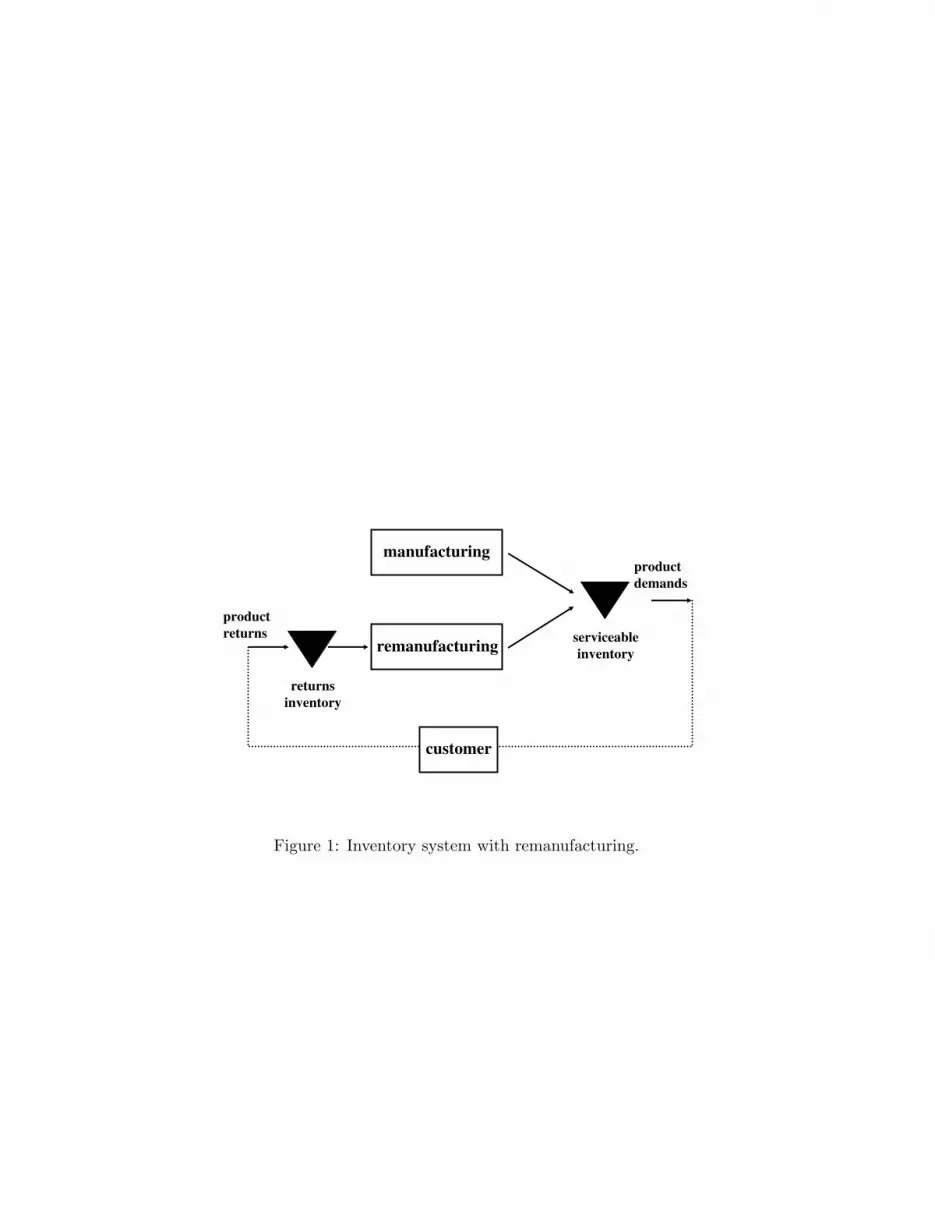
For details on the demand and return patterns, and on the cost parameter values, we refer

to Table 2.

** PLACE TABLE 2 HERE **

A full factorial design is applied, so that the total number of examples is 40× 72× 3× 3 =

25, 920. We measure the performance of a heuristic by the percentage increase in the total cost

compared to an optimal solution, which we refer to as the “error”.

A first important result is that the average error over all examples for PPB (24.8%) is

much larger than that for SM (3.0%) and LUC (4.2%). Apparently, balancing ordering and

holding costs does not lead to a near-optimal solution. Indeed, further analysis of all optimal

solutions revealed that, on average, the division of total cost into holding and set-up is not 50-50

14

but roughly 40-60. The poor performance of PPB can be further explained by the combined

effect of fluctuations in returns and demands. Silver, Pyke, and Peterson [15] report that for

traditional systems without returns, the performance of PPB is negatively effected by increased

fluctuations.

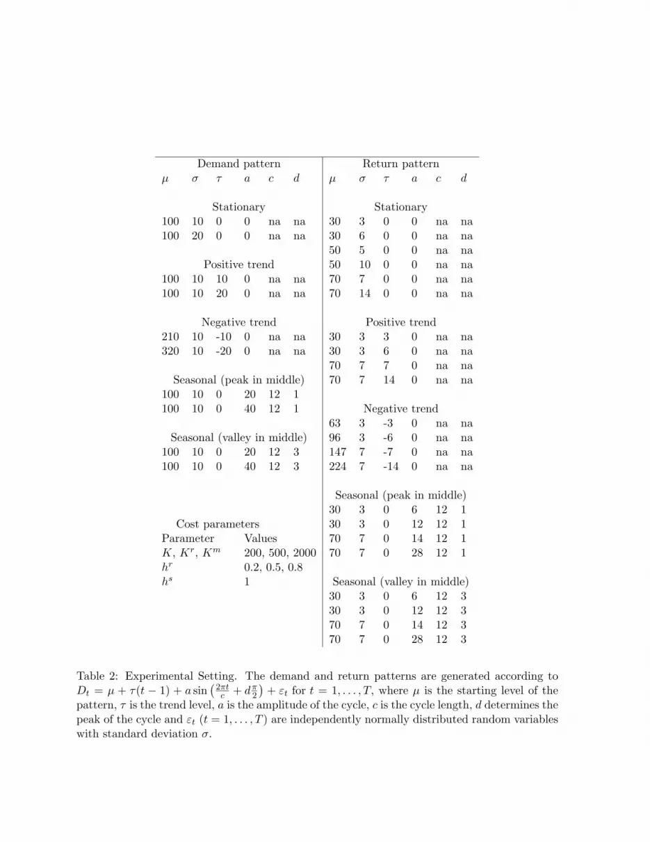
Next, we perform a sensitivity analysis to determine the effects of the demand pattern, return

pattern, return rate, and cost parameters on the performance of the heuristics. The results are

summarized in Table 3. Our discussion of the results will therefore concentrate on the SM and

LUC heuristics, because of their overall superior performance compared to PPB.

** PLACE TABLE 3 HERE **

It appears that under most demand and cost settings, SM performs slightly better then LUC.

SM performs significantly better for seasonal demand, especially if fluctuations are large. The

performances of both SM and LUC are quite robust with respect to the demand and return

patterns. As expected, increased demand fluctuations generally (though not for all patterns)

deteriorate the performances of SM and LUC. An increase in the return rate or in the unit

holding cost of returns also affect the performances negatively. However, both heuristics have

an average error of less than 5% under all scenarios for the return rate and for the return holding

cost.

Cost values have a larger influence on the performances. It especially appears that the larger

the set-up cost, the poorer the performance. However, it is important to realize that the poorer

performance for larger set-up costs is (mainly) caused by the larger order sizes and hence smaller

numbers of orders. Due to the myopic shortsighted nature of the heuristics, the last order in

a heuristic solution is often much too small. For K = 2000 there are typically just 2 orders

over the planning horizon, compared to 6 on average for K = 200, and therefore the relative

effect on the cost of a too small last order is larger. In other words, the poorer performance

for larger set-up costs is due to the relatively smaller planning horizon (in terms of number of

orders placed) and does not result from unsuitability of the proposed heuristics for large K.

15

4 Separate set-up costs for manufacturing and remanufacturing

The MILP formulation is similar to that for the joint set-up cost case except for the separation

of the set-up cost.

minT∑

t=1{Krδr

t + Kmδmt + hrIr

t + hsIst }

subject to

Irt−1 + Rt − xr

t = Irt for t = 1, . . . , T (10)

Irt−1 + xr

t + xmt −Dt = Is

t for t = 1, . . . , T (11)

xrt ≤ Mtδ

rt for t = 1, . . . , T (12)

xmt ≤ Mtδ

mt for t = 1, . . . , T (13)

δrt , δm

t ∈ {0, 1}, xrt , xm

t , Irt , Is

t ≥ 0 and Mt =T∑

i=t

Di for t = 1, . . . , T

Recall from Section 3 that for the case with a joint set-up cost, optimal solution for the

problem satisfies zero-inventory and remanufacture-first properties. These properties enabled

us to construct an exact algorithm of polynomial time-complexity. The following simple example

shows that the properties no longer hold when there are separate set-up costs. Let Kr = 10,

Km = 10, hr = 1, hs = 2, T = 2, D1 = 2, D2 = 100, R1 = 1, and R2 = 98. It is easy to check

that the optimal solution is to manufacture 3 products in period 1 and remanufacture 99 in

period 2, with corresponding total cost 23. This solution satisfies neither of the two properties.

Therefore, we are not able to develop a polynomial DP algorithm for the case with separate

set-up costs.

In fact, we conjecture that the problem with separate set-up costs is NP-hard. Besides the

fact that the zero-inventory property and the remanufacture-first property no longer hold, there

is another result that strongly points in this direction. Van den Heuvel [21] shows that the

problem becomes NP-hard when variable (re)manufacturing costs are included, even under the

condition that the variable cost for manufacturing is larger than that for remanufacturing (which

16

will typically hold if remanufacturing is motivated economically). It can easily be shown for the

joint set-up cost problem with inclusion of variable costs under these conditions, that the two

properties still hold, the DP algorithm can still be applied, and therefore the problem remains

polynomially solvable. So, apparently, it is not the inclusion of variable costs but the separation

of set-up costs which is responsible for the NP-hardness.

We will propose and test a number of heuristics. As for the joint set-up cost problem,

these heuristics are generalized versions of the well-known Silver-Meal, Least Unit Cost, and

Part Period Balancing heuristics for systems without remanufacturing. All three heuristics

simultaneously determine the manufacturing and the remanufacturing order sizes. We also

tested heuristics that determine the order sizes sequentially, first for remanufacturing and then

for manufacturing based on the remaining ‘net demand’. However, it turned out that their

performances were very poor compared to those of the simultaneous heuristics. Therefore, the

sequential heuristics will not be presented.

4.1 Heuristics

The generalized versions of the well-known Silver-Meal, Least Unit Cost, and Part Period Bal-

ancing heuristics only consider solutions that satisfy the zero-inventory property for serviceables.

Although, as discussed above, Lemma 1 does not hold in general for the separate set-up cost

problem, we expect that for most realistic cases, a near-optimal solution that satisfies the zero-

inventory property exists. The extensive numerical study in Section 4.2 will confirm that the

cost increase of the best zero-inventory solution compared to the optimal solution is generally

less than 2%.

The heuristics do consider solutions that not always remanufacture first. This is essential,

since there can be situations with large set-up costs and few returns available, where it is clearly

better to keep the returns in stock for now and manufacture only, rather than to remanufacture

as well as manufacture. Therefore, besides remanufacture-first orders, the heuristics consider

manufacture-only orders. Next, we will derive cost expressions for both types of orders.

The expression for the cost associated with a remanufacture-first order is similar to that

for the case with joint set-up costs. Expression (9) only needs to be modified by including

17

the set-up costs if a (re)manufacturing order is placed. Let I(condition) denote the indicator

function, which is one if the condition is satisfied and zero otherwise. Using similar arguments

as those leading to (9), we get the following expression for the cost CRl,k(m) in interval [l, k] if

the returns stock at the end of period l − 1 is m and a remanufacture-first order is placed in l

that is sufficient until k.

CRl,k(m) = I(m + Rl > 0)Kr + I(m + Rl <

k∑i=l

Di)Km + hsk∑

i=l+1

(i− l)Di

+hr

(k − l + 1)

(m + Rl −

k∑i=l

Di

)+

+k∑

i=l+1

(k + 1− i)Ri

(14)

If a manufacturing-only order is placed in period l for interval [l, k] and the returns stock

at the end of period l − 1 is m, then the returns stock at the end of period i, i = l, . . . , k, is

m +∑t

s=l Rs. The corresponding cost is therefore

CMl,k(m) = Km + hsk∑

i=l+1

(s− l)Di + hr

((k − l + 1)m +

k∑i=l+1

(k + 1− i)Ri

)(15)

Aside from the consideration of two order types and the corresponding modified cost expres-

sions, the heuristics are identical to the original ones for systems with manufacturing only.

4.2 Numerical experiment

The same demand patterns, return patterns, and cost parameter values are considered as in the

previous experiment, but of course the set-up costs for manufacturing and remanufacturing can

now have different values. See Table 2. The total number of examples is 77, 760.

We start by justifying the focus on heuristics that only consider solutions satisfying the zero-

inventory property. For 38.1% of the examples, there is in fact an optimal solution that satisfies

this property. For 52.5% of the examples, the cost increase of the best zero-inventory solution

(determined by solving the MILP model with additional restirctions in Cplex) compared to the

optimal solution is less than one per cent. The average cost increase over all examples is less

than two per cent.

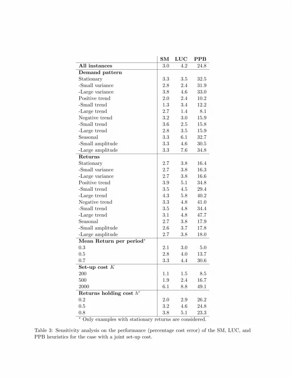
The computational results can be found in Table 4.

** PLACE TABLE 4 HERE **

18

As for the case with a joint set-up cost, the first apparent result is that the PPB performs

much worse than SM and LUC for all demand/return patterns and cost values. Furthermore,

SM again performs slightly better than LUC under most scenarios. The average error over all

examples is 8.3% for SM, 9.0% for LUC, and 19.8% for PPB.

Most of the sensitivity results with respect to demand/return patterns and costs are also

similar to those for the joint set-up cost case. Recall that for the joint set-up cost case, it was

observed that an increase in the set-up cost lead to a poorer performance of all heuristics. This

was explained by reduced number of orders and hence the (relatively) stronger effect of a too

small last order. For the separate set-up cost case, we see the same effect from an increase in

the manufacturing set-up cost. However, an increase in the remanufacturing set-up cost has

the opposite effect; the performances of all heuristics improve. A look at the optimal solutions

provided the following explanation. In cases where remanufacturing set-up is more costly than

a manufacturing set-up, the optimal solution often place no remanufacturing batches at all, and

neither do the heuristic solutions. As is known from the literature, the heuristics perform well

in pure manufacturing situations.

5 Conclusion

A general version of the lot sizing problem with remanufacturing of returns was analyzed. Two

different models were considered with either joint or separate costs for manufacturing and re-

manufacturing set-ups. For both models, the lot sizing problem was formulated as a mixed

integer program (MIP). The problem with a joint set-up cost turned out to be least complex.

Based on the so-called zero-inventory and remanufacture-first properties, a polynomial DP al-

gorithm was provided. For situations with separate set-up costs, these properties no longer hold

and the problem is conjectured to be NP-hard.

In practise, heuristic procedures will often be preferred to the exact MIP formulations and

even to the DP algorithm. We therefore presented modified versions of the well-known Silver-

Meal (SM), Least Unit Cost (LUC), and Part Period Balancing (PPB) heuristics, both under a

joint set-up cost and under separate set-up costs. An extensive numerical experiment revealed

19

that for both models, SM performs slightly better than LUC and a lot better than PPB.

For the joint set-up cost model, the cost error (increase in total cost compared to the optimal

solution) is just 3.0% on average. Moreover, the performance of SM is robust with respect to

demand/return patterns and cost parameter values, as long as the set-up cost is not so large that

the number of set-ups during the planning horizon reduces to 1 or 2. We therefore recommend

the use of SM in practise for systems with a joint set-up cost.

For the separate set-up cost model, the performance of SM is also quite robust. However,

the average cost error of 8.4% is considerable. Some improvement can be expected if SM is

applied in a rolling horizon setting, which it is likely to be in practise, but the substantial cost

error does provide an incentive to explore alternative heuristics. This is one direction for further

research.

Other interesting research avenues are to prove the conjecture that the problem is NP-hard

for separate set-up costs, and to modify and test heuristics for ‘mixed’ cases with a joint set-up

cost as well as separate set-up costs, or with an even more general set-up cost function.

References

[1] J.L. Beltran and D. Krass. Dynamic lots sizing with returning items and disposals. IIE

Transactions, 34:437–448, 2002.

[2] N. Brahimi, S. Dauzere-Peres, N.M. Najid, and A. Nordli. Single item lot sizing problems.

European Journal of Operational Research, 168:1–16, 2006.

[3] R. Dekker, M. Fleischmann, K. Inderfurth, and L.N. van Wassenhove. Reverse Logistics:

Quantitative Models for Closed-Loop Supply Chains. Springer-Verlag, Berlin Heidelberg,

2004.

[4] G. Ferrer. The economics of personal computer remanufacturing. Resources, Conservation

and Recycling, 21:79–108, 1997.

[5] G. Ferrer. The economics of tire remanufacturing. Resources, Conservation and Recycling,

19:221–255, 1997.

20

[6] M. Fleischmann, J.M. Bloemhof-Ruwaard, R. Dekker, E. van der Laan J.A.E.E. van Nunen,

and L.N. van Wassenhove. Quantitative models for reverse logistics: a review. European

Journal of Operational Research, 103:1–17, 1997.

[7] B. Golany, J. Yang, and G. Yu. Economic lot-sizing with remanufacturing options. IIE

Transactions, 33:995–1003, 2001.

[8] V.D.R. Guide, V. Jayaraman, R. Srivastava, and W.C. Benton. Supply-chain management

for recoverable manufacturing systems. Interfaces, 30(3):125–142, 2000.

[9] S.M. Gupta and A. Gungor. Issues in environmentally conscious manufacturing and product

recovery. Computers and Industrial Engineering, 36(4):811–853, 1999.

[10] S.W. Kandebo. Grumman, U.S. navy under way in f-14 remanufacturing program. Aviation

Week and Space Technology, December 17th:44–45, 1990.

[11] E. van der Laan and M. Salomon. Production planning and inventory control with re-

manufacturing and disposal. European Journal of Operational Research, 102(2):264–278,

1997.

[12] R. Lund. Remanufacturing. Technology Review, 87(2):18–23, 1984.

[13] K. Richter and M. Sombrutzki. Remanufacturing planning for the reverse wagner/whitin

models. European Journal of Operational Research, 121:304–315, 2000.

[14] K. Richter and J. Weber. The reverse wagner/whitin model with variable manufacturing

and remanufacturing cost. International Journal of Production Economics, 71:447–456,

2001.

[15] E.A. Silver, D.F. Pyke, and R. Peterson. Inventory Management and Production Planning

and Scheduling. John Wiley and Sons, New York, 1998.

[16] J.A. Sivinski and S. Meegan. Case study: Abbott labs formalized approach to remanufac-

turing. In APICS Remanufacturing Seminar Proceedings, pages 27–30, 1993.

[17] E. Sprow. The mechanics of remanufacture. Manufacturing Engineering, pages 38–45, 1992.

21

[18] R.H. Teunter, E. Van der Laan, and K. Inderfurth. How to set the holding cost rates in

average cost inventory models with reverse logistics? OMEGA The International Journal

of Management Science, 28:409–415, 2000.

[19] R.H. Teunter and D. Vlachos. On the necessity of a disposal option for returned products

that can be remanufactured. International Journal of Production economics, 75:257–266,

2002.

[20] M. Thierry, M. Salomon, J.A.E.E. van Nunen, and L.N. van Wassenhove. Strategic issues

in product recovery management. California Management Review, 37(2):114–135, 1995.

[21] W. van den Heuvel. Econometric institute report. Technical Report EI 2004-46, Econo-

metric Institute, Erasmus University Rotterdam, The Netherlands, 2004.

[22] H.M. Wagner and T.M. Whitin. Dynamic version of the economic lot size model. Manage-

ment Science, 5:89–96, 1958.

Acknowledgement: Dr. Ruud H. Teunter and Dr. Z. Pelin Bayındır were researchers at the

Econometric Institute, Erasmus University Rotterdam when this study was initiated.

22

manufacturing

remanufacturingserviceable

inventory

product

returns

product

demands

customer

returns

inventory

Figure 1: Inventory system with remanufacturing.

GeneralT Planning horizont Index for periods in the planning horizon, t = 1, . . . , TRt Number of returns received at the beginning of period tDt Number of items demanded in period tK (joint) set-up costKr (separate) Set-up cost for remanufacturingKm (separate) Set-up cost for manufacturinghr Unit holding cost for returns per periodhs Unit holding cost of end-items (serviceables) per period

Mixed integer linear programming (MILP) formulationxr

t Number of items remanufactured in period txm

t Number of items manufactured in period tIrt Inventory level of returns at the end of period t

Ist Inventory level of serviceables at the end of period t

δt (joint) 0-1 indicator variable for remanufacturing set-up in period tδrt (separate) 0-1 indicator variable for remanufacturing set-up in period t

δmt (separate) 0-1 indicator variable for manufacturing set-up in period t

M Large integerDynamic programming (DP) algorithm

fk Minimum cost in periods 1, . . . , k (if periods k + 1, . . . , T are ignored)fk(n) Minimum cost in periods 1, . . . , k (if periods k + 1, . . . , T are ignored)

with n returns in stock at the end of period kfl,k(n) Minimum cost in periods 1, . . . , k if the last order is placed in periods l

with n returns in stock at the end of period kSk Set of possible returns stock levels at the end of period kSl,k Set of possible returns stock levels at the end of period k

if the last order is placed in periods l

HeuristicsCl,k(m) (joint) Cost in interval [l, k] if the returns stock at the end of period l − 1 is m

and an order is placed in period l that is sufficient until period kCRl,k(m) (separate) Cost in interval [l, k] if the returns stock at the end of period l − 1 is m

and a remanufacture-first order is placed in l that is sufficient until kCMl,k(m) (separate) Cost in interval [l, k] if the returns stock at the end of period l − 1 is m

and a manufacture only order is placed in l that is sufficient until kI(condition) Indicator function, which is one if the condition is satisfied and zero otherwise

Table 1: Notations.

Demand pattern Return patternµ σ τ a c d µ σ τ a c d

Stationary Stationary100 10 0 0 na na 30 3 0 0 na na100 20 0 0 na na 30 6 0 0 na na

50 5 0 0 na naPositive trend 50 10 0 0 na na

100 10 10 0 na na 70 7 0 0 na na100 10 20 0 na na 70 14 0 0 na na

Negative trend Positive trend210 10 -10 0 na na 30 3 3 0 na na320 10 -20 0 na na 30 3 6 0 na na

70 7 7 0 na naSeasonal (peak in middle) 70 7 14 0 na na

100 10 0 20 12 1100 10 0 40 12 1 Negative trend

63 3 -3 0 na naSeasonal (valley in middle) 96 3 -6 0 na na

100 10 0 20 12 3 147 7 -7 0 na na100 10 0 40 12 3 224 7 -14 0 na na

Seasonal (peak in middle)30 3 0 6 12 1

Cost parameters 30 3 0 12 12 1Parameter Values 70 7 0 14 12 1K, Kr, Km 200, 500, 2000 70 7 0 28 12 1hr 0.2, 0.5, 0.8hs 1 Seasonal (valley in middle)

30 3 0 6 12 330 3 0 12 12 370 7 0 14 12 370 7 0 28 12 3

Table 2: Experimental Setting. The demand and return patterns are generated according toDt = µ + τ(t − 1) + a sin

(2πtc + dπ

2

)+ εt for t = 1, . . . , T, where µ is the starting level of the

pattern, τ is the trend level, a is the amplitude of the cycle, c is the cycle length, d determines thepeak of the cycle and εt (t = 1, . . . , T ) are independently normally distributed random variableswith standard deviation σ.

SM LUC PPBAll instances 3.0 4.2 24.8Demand patternStationary 3.3 3.5 32.5-Small variance 2.8 2.4 31.9-Large variance 3.8 4.6 33.0Positive trend 2.0 2.4 10.2-Small trend 1.3 3.4 12.2-Large trend 2.7 1.4 8.1Negative trend 3.2 3.0 15.9-Small trend 3.6 2.5 15.8-Large trend 2.8 3.5 15.9Seasonal 3.3 6.1 32.7-Small amplitude 3.3 4.6 30.5-Large amplitude 3.3 7.6 34.8ReturnsStationary 2.7 3.8 16.4-Small variance 2.7 3.8 16.3-Large variance 2.7 3.8 16.6Positive trend 3.9 5.1 34.8-Small trend 3.5 4.5 29.4-Large trend 4.3 5.8 40.2Negative trend 3.3 4.8 41.0-Small trend 3.5 4.8 34.4-Large trend 3.1 4.8 47.7Seasonal 2.7 3.8 17.9-Small amplitude 2.6 3.7 17.8-Large amplitude 2.7 3.8 18.0Mean Return per period∗

0.3 2.1 3.0 5.00.5 2.8 4.0 13.70.7 3.3 4.4 30.6Set-up cost K200 1.1 1.5 8.5500 1.9 2.4 16.72000 6.1 8.8 49.1Returns holding cost hr

0.2 2.0 2.9 26.20.5 3.2 4.6 24.80.8 3.8 5.1 23.3∗ Only examples with stationary returns are considered.

Table 3: Sensitivity analysis on the performance (percentage cost error) of the SM, LUC, andPPB heuristics for the case with a joint set-up cost.

SM LUC PPBAll instances 8.3 9.0 19.8DemandStationary 8.1 8.7 21.4-Small variance 7.6 7.8 21.2-Large variance 8.6 9.5 21.7Positive trend 7.4 7.7 15.8-Small trend 7.4 7.8 16.8-Large trend 7.4 7.7 14.8Negative trend 9.5 9.3 17.2-Small trend 9.4 9.0 17.7-Large trend 9.6 9.6 16.7Seasonal 8.3 9.6 22.3-Small amplitude 7.8 8.5 21.6-Large amplitude 8.8 10.8 23.0ReturnsStationary 7.5 8.2 16.2-Small variance 7.5 8.2 16.2-Large variance 7.4 8.2 16.3Positive trend 10.9 11.6 23.1-Small trend 10.4 11.1 21.2-Large trend 11.4 12.1 25.0Negative trend 8.9 9.9 30.7-Small trend 8.0 9.2 30.4-Large trend 9.8 10.5 31.0Seasonal 7.3 7.9 15.4-Small amplitude 7.3 7.8 15.4-Large amplitude 7.3 7.9 15.5Mean Return per period∗

0.3 5.6 6.5 11.00.5 8.0 8.9 18.00.7 8.9 9.3 19.7Manufacturing set-up cost Km

200 6.2 7.6 17.0500 6.9 7.2 18.02000 11.8 12.2 24.6Remanufacturing set-up cost Kr

200 11.3 11.3 27.1500 9.0 9.6 21.52000 4.7 6.1 10.8Returns holding cost hr

0.2 5.5 6.0 12.10.5 8.3 9.1 22.10.8 11.2 11.9 25.4∗ Only examples with stationary returns are considered.

Table 4: Sensitivity analysis on the performance (percentage cost error) of the SM, LUC, andPPB heuristics for the case with separate set-up costs.