Dynamic real-time prediction of flood inundation probabilities

Hydrotogical Sciences—Journal—des Sciences Hydrologiques, 43(2) April 1998 181

Dynamic real-time prediction of flood inundation probabilities

RENATA ROMANOWICZ* & KEITH BEVEN Centre for Research on Environmental Systems and Statistics, Institute of Environmental and Biological Sciences, Lancaster University, Lancaster LAI 4YO, UK

Abstract The Bayesian Generalised Likelihood Uncertainty Estimation (GLUE) methodology, previously used in rainfall-runoff modelling, is applied to the distributed problem of predicting the space and time varying probabilities of inundation of all points on a flood plain. Probability estimates are based on conditioning predictions of Monte Carlo realizations of a distributed quasi-two-dimensional flood routing model using known levels at sites along the reach. The methodology can be applied in the flood forecasting context for which the iV-step ahead inundation probability estimates can be updated in real time using telemetered information on water levels. It is also shown that it is possible to condition the N-step ahead forecasts in real time using the (uncertain) on-line predictions of the downstream water levels at the end of the reach obtained from an adaptive transfer function model calibrated on reach scale inflow and outflow data.

Prévision dynamique de la probabilité de l'inondation en temps réel Résumé La méthodologie bayésienne GLUE (Generalised Likelihood Uncertainty Estimation), précédemment utilisée dans la modélisation pluie-débit, est ici appliquée à la prévision distribuée, dans le temps et l'espace, des probabilités d'inondation en chaque point d'une plaine inondable. L'estimation distributee de la probabilité est basée sur un conditionnement des simulations de type Monte Carlo d'un modèle de propagation bi-dimensionnel. Le conditionnement utilise les mesures disponibles du niveau de l'eau à quelques stations situées le long du tronçon de rivière. La méthodologie peut être utilisée pour la prévision en temps réal, à échéance de iVpas de temps. Dans ce cas, les estimations de probabilité peuvent être révisées en utilisant des télémesures. On montre aussi qu'il est possible de conditionner les prévisions distribuées en temps réel en utilisant les prévisions (incertaines) du niveau de l'eau à la sortie du tronçon qui sont obtenues à l'aide d'un modèle adaptif de type fonction de transfert, initialement calé sur les données d'entrée et de sortie du tronçon de rivière.

INTRODUCTION

Traditionally, model calibration has not been considered to be a major problem in the application of flood wave models. The roughness parameters required can either be estimated from the nature of the channel and flood plains and, if some previous event water level observations are available, some calibration of these prior estimates can be carried out, including allowing that roughness parameters may vary with water level (Fread, 1985). The assumption has generally been that, if the downstream water levels are simulated satisfactorily, then so will the distributed inundation

* Now at: Westlakes Scientific Consulting, Princess Royal Building, Ingwell Hall, Moor Row, Cumbria CA24 3JZ, UK.

Open for discussion until 1 October 1998

182 Renata Romanowicz & Keith Seven

predictions. This may not be true. Multiple simulations using randomly chosen parameter values carried out as part of this study have revealed that there may be many combinations of roughness parameters that are consistent with downstream water level predictions but that produce very different inundation predictions.

This should, in fact, be expected. Most distributed flood wave models are very simple representations of reality, as indicated by their reliance on quasi-empirical roughness formulations and coefficients as parameters. The geometric representation of the channel and flood plain areas also tends to be greatly simplified, based on elevation cross sections spaced along the reach of interest, but not taking account of the fully three-dimensional nature of the flows in the channel and in the flood plain. In addition, such models require parameter values to be specified for every element in the solution mesh. In terms of the very large number of parameters thereby required, the models are grossly overparameterized with respect to the data available for calibration, thereby placing great reliance on the a priori estimation of the required reach scale or effective parameters required. The dimensionality of the parameter space is generally reduced by assuming constant effective parameter values over many reach elements, lacking better information, but this only adds to the approximate nature of such models.

Thus, as a result of these limitations, it should also be expected that predictions of flood inundation should be uncertain. In the past this uncertainty has been considered primarily as a function of the uncertainty in the magnitude of an event for a given return period. First define the 100 year event, then predict the inundated areas. This remains an important source of uncertainty for the design problem but it is also clear that these limitations might lead to considerable uncertainty in the forecasting case which will also require updating of the inundation forecasts in real time as the event progresses. To the authors' knowledge this is the first study to address the problem of forecasting distributed probabilities of inundation and their updating in real time.

The problem has been examined using a coarse element quasi-two-dimensional model of the River Culm flood plain in Devon, UK. The model used is simple enough to allow multiple runs of the model for different parameter sets while incorporating the nonlinear effects associated with the flood plain geometry and flow processes. The underlying hypothesis is that there are sufficient uncertainties associated with the representation of the flood plain geometry, in the values of the roughness parameters, and in the observational data, that little predictive capability may be lost in having a less accurate model of the flow dynamics. It is better to be able to assess the probabilities of inundation using the simpler model. It is not the intention here to test this hypothesis, but rather to demonstrate a practical methodology for predicting probabilities of inundation in real time in the face of predictive uncertainty.

The approach rejects the idea that there is an optimum set of parameters which will give maximum goodness-of-fit measures with respect to the observations; instead it evaluates the ranges of feasible parameters after conditioning on the observations and allowing for random errors in the series of inflows and other observations and model structural error (Beven & Binley, 1992; Beven, 1996). The conditioning is

Dynamic real-time prediction of flood inundation probabilities \ 83

applied here within a Bayesian framework which allows the updating of the resulting posterior distributions of the predictions as new observations become available. The approach has been outlined for the flood inundation case by Romanowicz et al. (1996). The "observations" are taken from another, more hydraulically correct, two-dimensional, depth integrated, finite element model (RMA-2) to allow the use of intermediate stage measurements within the reach. It is recognized that the RMA-2 finite element model does, itself, have limited accuracy in reproducing the actual observations of levels and discharges (Bates et al., 1992) but its predictions of water levels are believable if treated as observations.

In this paper the possibility of updating the posterior distribution of predictions by on-line few hour ahead predictions of downstream water levels is investigated. The on-line predictions are obtained using the adaptive gain linear transfer function approach (Young, 1984) as demonstrated in the flood forecasting context by Lees etal. (1994). Similar methods have been used for upstream to downstream flow predictions for some time. Transfer functions are derived from observed upstream and downstream hydrographs and can then be used for JV-step ahead prediction of downstream water levels or flow given an upstream input curve. The method is used here with real-time parameter updating and includes the estimation of prediction errors. Such methods are not, however, easily used for distributed inundation predictions. Thus the transfer function and distributed modelling approaches have been combined to allow the modification of inundation probabilities in real time, including AT-step ahead predictions of the probability of flooding at any point.

DESCRIPTION OF THE DISTRIBUTED FLOOD INUNDATION MODEL

The coarse element flood inundation model used here is similar to the quasi-two-dimensional model of Cunge et al. (1976). This model uses resistance terms in the form of Manning-Strickler laws, and neglects the inertial terms in the flow equation. It assumes that the flow builds up slowly on the flood plains and hence the storage and resistance terms are more important than inertial and acceleration terms in the flow equation. The model is run on an event basis and requires the specification of an upstream level or flow, initial conditions for the distributed storages, and downstream boundary conditions. The general structure of the model consists of an interconnected sequence of rows of nonlinear storage cells. It is assumed that there is a unique relationship between the storage of each cell and the height of the water surface, as well as the cross section-height and wetted perimeter-height relationships at the boundaries of each cell. These functions are derived from the geometry of the river and the flood plain, taking account of the valley slope in each element, and have the form of look-up tables. Given a predicted storage within each element, the inundation can be mapped back into space given the geometry of the flood plain. In general, any geometry can be used, including the most detailed digital elevation data; here, the representation of the geometry has been constrained by the elevation data points that were available for the study reach. It would be possible to use hysteretic look-up tables to mimic the dynamic storage-level functions more closely but this has not been done here.

184 Renata Romanowicz & Keith Beven

The roughness coefficients scaling the flow on the flood plains and in the channel are used as the calibration parameters in the calibration stage of the problem. Each reach of the valley is represented as three elements, viz, one channel and two flood plain elements. Thus, for each reach at least five roughness or conveyance coefficients need to be specified, for downstream flow in the channel, downstream flow on each of the flood plain elements, and for the exchanges between the channel and flood plain elements. Transitions from weir-type flow over a flood embankment to fully submerged conditions can be treated in the model. For the downstream boundary condition the assumption of uniform flow parallel to the river slope was implemented. Lateral inflows have been ignored in the current study (as in the detailed finite element model of the site). A detailed description of the model is given in Romanowicz et al. (1996).

THE STUDY SITE AND AVAILABLE DATA

The model has been applied on a 13 km reach of the lower course of the River Culm, in Devon, UK, where modelling studies using RMA-2 had already been reported by Anderson & Bates (1994) and Bates et al. (1992). The elevation data are in the form of a vector of irregular (x, y, z) values, giving the elevations of points situated on cross sections of the channel and the flood plains, and are the same as used in the finite element model.

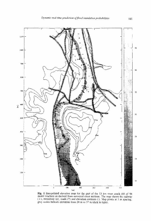
The coarse element model on which the GLUE calculations are based requires storage-level functions for each channel and flood plain element. A total of 94 sets of sloping channel and flood plain elements has been used to represent the 13 km reach, one set between each surveyed cross section available. The storage-elevation table for each element requires interpolation of the elevation data between the available cross sections. As two different space resolutions are needed for the channel and on the flood plain, typical spatial interpolation schemes cannot be applied. Hence a specific cross-sectional data interpolation scheme was developed in MATLAB. The interpolated elevation map for part of river reach containing 45 cross sections is shown on Fig. 1, which also shows the railway, motorway and roads in the area (which in places control the extent of flooding), taken from a digitized 1:10 000 map and overlaid onto the interpolated elevations.

Observations of water levels at the upstream and downstream ends of the river reach are available for six different events in which flooding occurred. Two of these events have been simulated by the detailed finite element model of Bates et al. (1992). One of the objectives of this study was to examine the value of multiple level measurement sites on the conditioning of the parameter sets and the uncertainty in the inundation predictions. Intermediate level data were not available from the field so 12 "observation sites" were taken from the simulation results of the finite element model, made up of channel and flood plain water level time series at the downstream end of each of six sections spanning the total 13 km length. Channel and flood plain roughness coefficients for each sub-reach within each of the six sections were assumed to be constant.

Dynamic real-time prediction of flood inundation probabilities 185

'* t i9m ' -

•35m

H

Fig. 1 Interpolated elevation map for the part of the 13 km river reach (45 of 94 model reaches) as derived from surveyed cross sections. The map shows the railway (+), motorway (o), roads (*) and elevation contours (•). Map pixels at 1 m spacing, grey scales indicate elevation from 24 m to 37 m (dark to light).


Results were available for two different events together with the upstream and downstream water level measurements. One of the events (30 January 1990) had a single peak with a return period of about 1 year. The second event (26^28 January 1984) was double peaked with a return period of the order of 5 years.

BAYESIAN UNCERTAINTY ESTIMATION USING GLUE

The Generalised Likelihood Uncertainty Estimation (GLUE) methodology (Beven & Binley, 1992) reformulates the model calibration problem into the estimation of posterior probabilities of model responses, thereby avoiding the idea that there is an optimum parameter set. It uses Monte Carlo sampling of the parameter space. The methodology is based on Bayes formula (Box & Tiao, 1992):

f(9)L(9|z) f(9|z) = — — (1)

f(z) where z is the vector of observations, f(9 |z) is the posterior distribution (probability density) of sets of random parameter values 0 given the data, f(9) is the prior probability density of the parameter sets, f(z) is a scaling factor and L(0|z) represents a likelihood function for the parameter set 9 given the observation set z obtained from the forward modelling. This form assumes that the data z are fixed at their observed values while the parameter sets 9 are treated as random variables (Wetherill, 1981). This allows the introduction of prior distributions for the parameters.

Equation (1) can be applied sequentially as new data become available and the existing posterior distribution, based on (N - 1) calibration periods, is used as the prior for the new data in the Mh calibration period. Thus:

f(9|zl5 ..., zN) cc f(6|z„ ..., z ^ L ^ K ) (2)

where L(9|zw) is the likelihood function of parameters 9 given observations zN, i.e. the information about 9 from the Mh calibration period.

Errors between the observed and modelled flows or water levels along the river reach together with the assumed prior distributions of parameters are used to build the posterior likelihood, reflecting the model performance (Romanowicz et al., 1996). In this way it is possible to incorporate the information from observations from different time periods and/or sites using the Bayesian updating of equation (2). Models with parameter sets that are not considered to fit the data will be given a low or zero posterior likelihood value. The predictions of the remaining (retained) models are weighted by the posterior likelihood associated with that parameter set. In this way probabilities of flooding at any point or time step may be estimated. The nonlinearities of the modelling and any interactions between different parameters are retained implicitly in the likelihood weights associated with each parameter set and its predictions.

Dynamic real-time prediction offload inundation probabilities 187

THE LIKELIHOOD FUNCTION AND THE POSTERIOR DISTRIBUTION

An important step in this procedure is the choice of an adequate model for the prediction errors. This will affect the choice of an appropriate likelihood measure. The purpose of such a choice is to form a series of residual errors that are independent. For independent errors the evaluation of a posterior probability density function consists of the T multiplications of the conditional probability function for each observation of the error given previous data, where T is the number of time steps simulated. Romanowicz et al. (1996) have based a likelihood function on an additive error model (ô, = y - y„ where y and y, are realizations of simulated and observed water levels, respectively), assuming a Gaussian distribution of errors with first order correlation.

Under these assumptions the likelihood function is defined as:

L(0,ii,CT,a|z) = C-f(9,u.,a,a) -(27ia2) "( l-a2) exp -—jyv{\i,u,Q) L 2cr

(3)

where z denotes the observations (water levels in the channel and on the flood plains), u. is the mean residual, a is the variance of the residuals, a is the first order correlation coefficient of the residuals, C is the normalizing constant, f(0,u,a,oc) denotes the prior distribution of the parameter sets of the hydraulic and error models and F̂ is:

^(n,a,e) = ( l - a 2 ) ( ô ; - ^ ) 2 + X [ s ; - u - a ( 8 ; _ ] ^ L i ) ]

The resulting predictive distribution of water levels Zf conditioned on the calibration data z in the discrete (parameter set) case will then be given by:

P(Z, < y\z) = H > - ' ^ ' ^ n f(e,4>|z) (4) e • ^ c j / ( l - - a " ) )

From equation (4) one can evaluate the confidence limits for the water levels at the observation sites. The corresponding probabilities of exceedence (quantiles) assigned to modelled variables (flows or water heights in the channel and on the flood plains) determine the probability surfaces which depend on the posterior distribution of the parameters conditioned on the observations. Note that in this procedure the parameters need be treated only as sets of values. Any parameter interactions are then reflected implicitly in the calculated posterior distributions. This feature of the approach is especially advantageous in the case of a distributed model where parameters are often very interdependent. The marginal distributions for individual parameters or groups of parameters can be calculated by an integration of the posterior distribution over the rest of the parameters if needed (Romanowicz et al., 1994).


REAL TIME FORECASTING OF PROBABILITIES OF INUNDATION

Given some event data on which to base the conditioning of parameter sets described above, the Bayesian GLUE approach can provide estimates of the predicted probability of flooding for any new event in the form of a map of probability contours over the flood plain, given the input hydrograph for that event. Romanowicz et al. (1996) have shown how this can be done using the simplified routing model described above. They randomly varied the channel and flood plain roughness coefficients for each of the six sections of reaches within the ranges shown in Table 1. The predictions of each simulation were then evaluated using the likelihood measure of equation (3), with the RMA-2 simulated levels at the end of each channel section being treated as "observations". Note again that the aim was not to compare the two models, but to use the finite element predictions as an "observed" data set to provide the intermediate level information for conditioning the Monte Carlo simulations using the likelihood measure of equation (3).

Table 1 Ranges of roughness coefficients used in simulations for the fth cross section, (Kfl) for the flood plain and (Kci)ïoi the channel (m"3 s"1).

*M 15 25

«c.l

15 25

Kf,2

4 25

K,2 4 25

Kf,3

5 30

*o 5 30

KfA

5 50

KcA

5 50

Kf_5

1 25

Kc,5

1 25

Kr,6

1 25

Kc,6

1 25

The parameter set likelihoods, after this conditioning, can be considered to be prior estimates conditioned on those past data but it is often the case that telemetered data are available in real time during an event. It is also then necessary to implement a procedure for updating the estimates of inundation probabilities as the new event unfolds, and, if possible, project the predictions N steps ahead to the required flood warning horizon.

One algorithm for the on-line evaluation of probabilities of inundation consists of the following steps: (a) historical data are used to derive prior likelihood distributions at the start of the

predictions up to time t < t0; (b) on-line simulations are performed using the sample of retained parameter sets

over the N time steps to t = t0 + NAt, conditioned on the available level or flow data to time t0, and the spatial predictions are stored; N will generally be limited by the flood wave celerity in the reach (or more precisely by the forward characteristic of the solution emanating from x = 0 at t = t0), but can be extended by using predictions of, or assumptions about, the inflow hydrograph at future time steps, perhaps using a rainfall-runoff model;

(c) posterior probabilities of inundation at times t = t0 + NAt are evaluated using Bayesian conditioning of the prior likelihoods at time ta;

(d) as telemetered observations arrive, the likelihoods for the parameter sets are updated to time t0 = t0 + At using the new water level observations from all available sites; and


(e) the posteriors at the new time t0 become the priors for the forecast conditioning at times t0 + NAt and the algorithm reverts to step (b). Note that in this updating algorithm, it is the likelihoods associated with the

predictions that are updated, avoiding the need to update either parameter values or state variables within the nonlinear models. There is no need to attempt to update the predictions themselves which will always be consistent with the input flows supplied and a particular parameter set. However, if the observed behaviour starts to drift from the predictions based on the prior likelihood distribution, then the likelihoods will change to give more weight to the parameter sets giving more accurate predictions for the current event. The procedure uses the sample of quasi-two-dimensional models themselves as predictors of the nonlinear flood wave dynamics into the future forecast horizon. The models must be re-ran from the current time t0 as each new telemetered data set is received.

At many sites the forecast lead time limit associated with the flood wave celerity may be shorter than the desired warning period. Past experience suggests, however, that it might be possible to extend the conditioning period by predicting downstream flows into the future using linear transfer function techniques (Young, 1984). Such techniques have been applied at Lancaster University for an operational flood warning system (Lees et al., 1994). The inflow to outflow transfer function (TF) can be estimated off-line from previous events but, since the model is linear, it can be set within an adaptive framework and updated as an event occurs. Lees et al. (1994), in an application to forecast flood levels for the town of Dumfries, Scotland, used a single adaptive gain parameter that was recursively updated on the basis of the current observations of discharges and inflows. They also extended the lead time of the forecasts using transfer functions with artificially long time delays. Uncertainty in the transfer function forecasts of the downstream levels could be evaluated. This provided additional data for conditioning the quasi-two-dimensional model predictions of water levels along the reach into the future, thus giving updated forecasts of the probabilities of inundation. Again the transfer function predictions can be applied repeatedly as each new set of telemetered time step data is received.

The operation of the inundation model remains dependent on the availability of inflow data. Longer period inundation forecasts will necessarily require the prediction of the inflows a few hours ahead to enable the simulation of the future time periods. The posterior probabilities of inundation should then incorporate the inflow forecast error and the corresponding error of water level forecasts (Tarantula, 1987). Lees et al. (1994) have already successfully combined transfer function for rainfall to flow, using a nonlinear rainfall filter and flow to flow predictions in their forecasting system, but in that case made no attempt to predict patterns of inundation.

SIMULATION RESULTS: CONDITIONING ON HISTORICAL DATA

The uncertainty analysis was performed on the simulation results from Monte Carlo realizations of the quasi-two-dimensional model. The parameter sets were sampled from uniform distributions over specified parameter ranges. Each parameter set was made up of 12 parameters, with one flood plain roughness and one channel


roughness for each of the six sections above the measurement sites. Previous work reported in Romanowicz et al. (1996) suggested that the parameters in each reach could be considered independently and that the lateral transfer coefficient values could be fixed.

Each model used the full 94 sub-reaches defined by the elevation cross sections as calculation elements, with one channel element and two flood-plain elements in each sub-reach. The look-up tables required in each sub-reach were derived from the interpolated elevation data. The simulations were carried out by a FORTRAN implementation of the model on the Lancaster University PARAMID parallel processing system, consisting of multiple Intel i860 processors linked by transputers. An iterative implicit method of time integration was used, with a check on the size of time steps to maintain stability. To minimise the influence of the initial condition, the steady state solutions for each new set of parameters were evaluated, given a specified initial discharge through the reach.

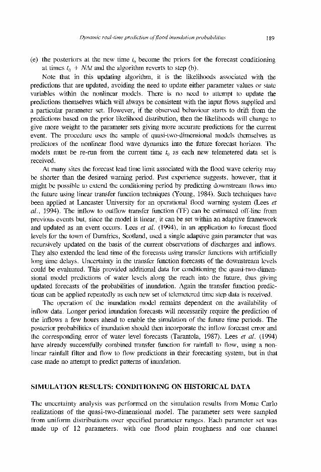
A total of 3000 Monte Carlo realizations of the flood routing model were conditioned on the level data for the one-in-one year event data (30 January 1990) using the GLUE methodology and the likelihood measure of equation (3). The downstream hydrograph predictions for this event, after conditioning on the event data for all six sets of distributed level "measurements" (actually taken from the RMA-2 simulation) are shown in Fig. 2. The resulting distribution of likelihood

90% confidence limits, channel

0 2 4 6 8 10 12 14 16 18 t ime [h]

Fig. 2 Downstream hydrograph predictions for the January 1990 event, conditioned on the available level data (+) (taken from the RMA-2 predictions) for that event. (•) denote lower and upper 90% confidence limits; (-) denote median of model predictions.


90% confidence limits, channel

2.5

2

J.1.5

0.5

0 0 5 10 15 20 25 30 35 40 45 50

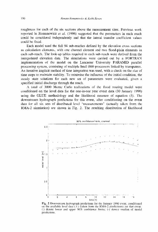
time [h] Fig. 3 Downstream hydrograph predictions for the January 1984 event, conditioned only on the RMA-2 predicted level data (+) for the January 1990 event. (•) denote lower and upper 90% confidence limits; (-) denote median of model predictions.

weights serves as a prior distribution for the later simulation of the one-in-five year event data (January 1984). The simulated uncertainty bounds for the January 1984 downstream hydrograph, conditioned only on the event of January 1990, are shown in Fig. 3, while predicted quantités of inundation depth along part of the reach from Hele to Columbjohn Bridge for the right hand flood plain are shown in Fig. 4, which also shows the three "measured" levels for this event (which were not used in the determination of the likelihood weights for this event).

SIMULATION RESULTS: DYNAMIC REAL-TIME INUNDATION PREDICTIONS

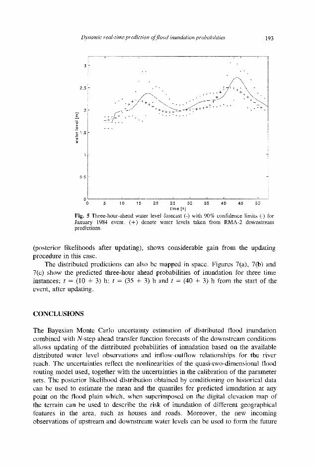
During an event it will be possible to improve the prior inundation predictions using the type of real time conditioning algorithm outlined above. A transfer function model for upstream to downstream levels was calibrated using water level measurements from one of the available events (22 December 1979-5 January 1980). This forms the prior estimate of the transfer function that is then modified adaptively during the event. This allows the prediction of downstream levels, with an associated uncertainty, N hours ahead, in this case three hours ahead, given an input hydro-graph up to time t0. Figure 5 shows the three-hour ahead prediction uncertainty bounds for the January 1984 event. Each Monte Carlo realization of the distributed inundation model can then be associated with its prior likelihood from conditioning


5 10 1_5 20 25 30 35 40

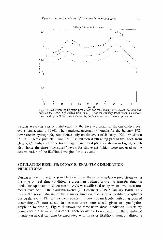
0 0.2 0.4 0.6 0.8 1 Fig. 4 Predicted quantiles of water levels for the January 1984 event for the right hand flood plain element along the river reach for 45 cross sections conditioned on level data from six observation sites for the January 1990 event, at (a) t = 10; (b) t = 35; and (c) t = 40 h from the beginning of the event. Stars indicate the water levels taken from RMA-2 at the downstream end of sections 3, 4 and 5.

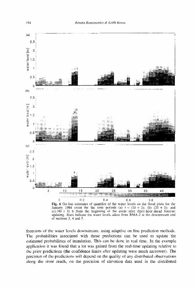
on the historical data, conditioning on the telemetered observations during the event up to the current time and a likelihood evaluated in real time for how well it conforms to the prediction of the transfer function model. These may be combined using Bayes equation (2). Figure 6 shows the estimated quantiles of inundation depths for the same 45 cross sections as in Fig. 4, in this case for three-hour ahead predictions conditioned on the three-hour ahead transfer function predictions. Comparison of Fig. 4 (inundation predictions based on prior likelihoods) with Fig. 6


3

2.5

_ 2

>

S

1

0.5

Ci 0 5 10 15 20 25 30 35 40 45 50

time [h]

Fig. 5 Three-hour-ahead water level forecast (-) with 90% confidence limits (•) for January 1984 event. (+) denote water levels taken from RMA-2 downstream predictions.

(posterior likelihoods after updating), shows considerable gain from the updating procedure in this case.

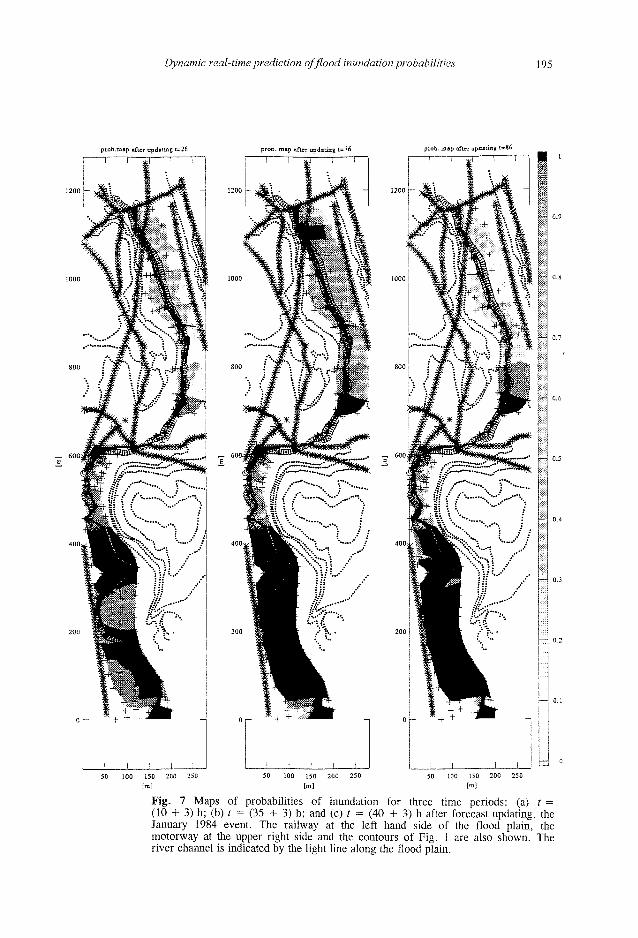
The distributed predictions can also be mapped in space. Figures 7(a), 7(b) and 7(c) show the predicted three-hour ahead probabilities of inundation for three time instances: t = (10 + 3) h; t = (35 + 3) h and t = (40 + 3) h from the start of the event, after updating.

CONCLUSIONS

The Bayesian Monte Carlo uncertainty estimation of distributed flood inundation combined with TV-step ahead transfer function forecasts of the downstream conditions allows updating of the distributed probabilities of inundation based on the available distributed water level observations and inflow-outflow relationships for the river reach. The uncertainties reflect the nonlinearities of the quasi-two-dimensional flood routing model used, together with the uncertainties in the calibration of the parameter sets. The posterior likelihood distribution obtained by conditioning on historical data can be used to estimate the mean and the quantiles for predicted inundation at any point on the flood plain which, when superimposed on the digital elevation map of the terrain can be used to describe the risk of inundation of different geographical features in the area, such as houses and roads. Moreover, the new incoming observations of upstream and downstream water levels can be used to form the future


2.5

E 2

S 1.5; Q i

I '! 0.5

K'^-stfWilwf

0 0.2 0.4 0.6 0.8 1 Fig. 6 On-line estimates of quantités of the water levels on the flood plain for the January 1984 event for the time periods (a) t = (10 + 3); (b) (35 + 3); and (e) (40 + 3) h from the beginning of the event after three-hour-ahead forecast updating. Stars indicate the water levels taken from RMA-2 at the downstream end of sections 3, 4 and 5.

forecasts of the water levels downstream, using adaptive on-line prediction methods. The probabilities associated with those predictions can be used to update the estimated probabilities of inundation. This can be done in real time. In the example application it was found that a lot was gained from the real-time updating relative to the prior predictions (the confidence limits after updating were much narrower). The precision of the predictions will depend on the quality of any distributed observations along the river reach, on the precision of elevation data used in the distributed


prob. map after updating t=76 prob. map after updating t=86

K*" % 'i

100 150 200 250 50 100 150 200 250

[ml

Fig. 7 Maps of probabilities of inundation for three time periods: (a) t = (10 + 3) h; (b) t = (35 + 3) h; and (c) t = (40 + 3) h after forecast updating, the January 1984 event. The railway at the left hand side of the flood plain, the motorway at the upper right side and the contours of Fig. 1 are also shown. The river channel is indicated by the light line along the flood plain.


modelling, on the dynamics of the flood inundation model and on the precision of the transfer function forecasts. The lead time of the distributed forecasting will be limited by the availability of inflow forecasts and the speed of the flood wave propagation in the system.

Acknowledgements This work has been supported by NERC grant GR3/8950. J. Tawn, W. Tych and K. Buckley from Lancaster University are thanked for their help. P. Bates and R. Harrison from Bristol University are thanked for the data which allowed the calibration of the model. D. Walling and the former NRA South West Region are thanked for the data on water levels at Woodmill and Rewe gauging stations. The clarity of the presentation has been greatly improved following the comments of two anonymous referees.

REFERENCES

Anderson, M. G. & Bates, P. D. (1994) Initial testing of a two dimensional finite element model for floodplain inundation. Proc. Roy. Soc. Series A 444, 149-159.

Bates, P. D., Baird, L., Anderson, M. G., Walling, D. E. & Simm, D. (1992) Modelling floodplain using a 2-dimensional finite element model. Earth Surf. Processes and Landforms 17, 577-588.

Beven, K. J. & Binley, A. (1992) The future of distributed models: model calibration and uncertainty prediction. Hydrol. Processes 6, 279-298.

Beven, K. J. (1996) The limits of splitting: hydrology. The Science of the Total Environment 183, 89-97. Box, G. E. P. & Tiao, G. C. (1992) Bayesian Inference in Statistical Analysis, 7-79. Wiley, Chichester. Cunge, J. A., Holy, F. M. Jr & Verwey, A. (1976) Practical Aspects of Computational River Hydraulics. Pitman,

London. Fread, D. L. (1985) Channel routing. In: Hydrological Forecasting (ed. by M. G. Anderson & T. P. Burt), 437-503.

Wiley, Chichester. Lees, M., Young, P. C , Ferguson, S., Beven, K. J. & Burns, J. (1994) An adaptive flood warning scheme for the

River Nith at Dumfries. In: River Flood Hydraulics (ed. by W. R, White & J. Watts), 65-75. Wiley, Chichester. Romanowicz, R., Beven K. & Tawn, J. (1994) Evaluation of predictive uncertainty in nonlinear hydrological models

using a Bayesian approach. In: Statistics for the Environment 2, Water Related Issues (ed. by V. Barnett & K. F. Turkman), 297-315. Wiley, Chichester.

Romanowicz, R. J., Beven, K. J. & Tawn, J. (1996) Bayesian calibration of flood inundation models. In: Floodplain Processes (ed. by M. G. Anderson, D. E. Walling & P. D. Bates), 333-360. Wiley, Chichester.

Tarantola, A. (1987) Inverse Problems Theory, Methods for Data Fitting and Model Parameter Estimation, 181-188. Elsevier, The Netherlands.

Wetherill, G. B. (1981) Intermediate Statistical Methods, 47-102. Chapman and Hall, London. Young, P. C. (1984) Recursive Estimation and Time Series Analysis. An Introduction, 66, 129. Springer-Verlag, Berlin.

Received 9 September 1996; accepted 10 July 1997

Documents

Dynamic real-time prediction of flood inundation probabilities