JOURNAL OF

wind engineering

Journal of Wind Engineering ~ ~ and Industrial Aerodynamics 69-71 (1997) 631-646 ELSEVIER

Dynamic wind pressures acting on a tall building model - proper orthogonal decomposition

Hiro tosh i Kikuch i a'*, Yukio T a m u r a b, Hi rosh i U e d a c, K a z u k i Hibi a

a Institute of Technology, Shimizu Corporation, Tokyo, Japan b Tokyo Institute of Polytechnics, Kanagawa, Japan

c Chiba Institute of Technology, Chiba, Japan

Abstract

Dynamic wind pressures acting on buildings are complicated functions of both time and space. Earlier studies have applied the proper orthogonal decomposition (POD) technique to such random wind pressure fields to identify hidden deterministic structures. In this study, the POD technique is applied to fluctuating wind pressures acting on a tall building model, and the following facts are found: the along-wind and across-wind forces can be approximated by only a few dominant modes, while the torsional moment requires approximately 10 modes; and the wind-induced response of a tall building has a maximum evaluation error of less than 6% with the reconstruction of the dominant modes.

1. Introduction

Dynamic wind pressures on buildings fluctuate spatio-temporally in a complicated manner. Several studies have been concluded on this random phenomenon by applying the proper orthogonal decomposition (POD) technique to investigate the systematic structure hidden in the fluctuating pressure fields [1-7]. In this study, the P O D technique is applied to dynamic wind pressures on a tall building model with a square plane in order to investigate the properties of these pressures and the characteristics of the building's response to them.

2. Wind-tunnel experiment

The experiments were conducted in a boundary layer wind tunnel with a 2.6 m x 2.4m cross-section. Two different approaching winds with a length scale of

* Corresponding author.

0167-6105/97/$17.00 © 1997 Published by Elsevier Science B.V. All rights reserved. PII S01 67-6105(97)00193- I

632 H. Kikuchi et al./J. Wind Eng. Ind. Aerodyn. 69 71 (1997) 631 646

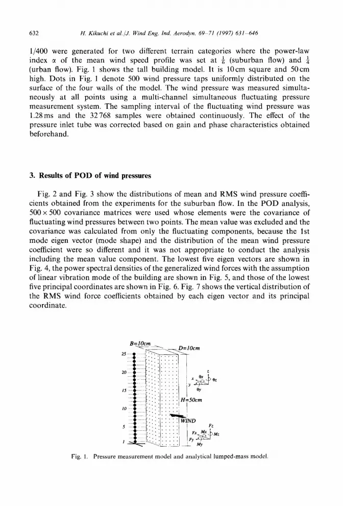
1/400 were generated for two different terrain categories where the power-law index ~ of the mean wind speed profile was set at ~ (suburban flow) and ¼ (urban flow). Fig. 1 shows the tall building model. It is 10cm square and 50cm high. Dots in Fig. 1 denote 500 wind pressure taps uniformly distributed on the surface of the four walls of the model. The wind pressure was measured simulta- neously at all points using a multi-channel simultaneous fluctuating pressure measurement system. The sampling interval of the fluctuating wind pressure was 1.28ms and the 32768 samples were obtained continuously. The effect of the pressure inlet tube was corrected based on gain and phase characteristics obtained beforehand.

3. Results of P O D of wind pressures

Fig. 2 and Fig. 3 show the distributions of mean and RMS wind pressure coeffi- cients obtained from the experiments for the suburban flow. In the P O D analysis, 500 x 500 covariance matrices were used whose elements were the covariance of fluctuating wind pressures between two points. The mean value was excluded and the covariance was calculated from only the fluctuating components, because the 1st mode eigen vector (mode shape) and the distribution of the mean wind pressure coefficient were so different and it was not appropriate to conduct the analysis including the mean value component. The lowest five eigen vectors are shown in Fig. 4, the power spectral densities of the generalized wind forces with the assumption of linear vibration mode of the building are shown in Fig. 5, and those of the lowest five principal coordinates are shown in Fig. 6. Fig. 7 shows the vertical distribution of the RMS wind force coefficients obtained by each eigen vector and its principal coordinate.

B=1.~OOcm

lo iiii • .L.

D= l Ocm

Y x ~ , ez

H=5Ocm I

WIND Fz

Fx.~+Mz Fy " ~

~' My

Fig. 1. Pressure measurement model and analytical lumped-mass model.

H. Kikuchi et al./J. Wind Eng. Ind. Aerodyn. 69-71 (1997) 631-646 633

///'l

-0~8

!:

-0.8 '~:

lO.6;, ". - 0 . 5 ' , ' , ,

t I

o., -o.~

Fig. 2. Mean wind pressure coefficient (suburban flow).

Fig. 3.

~q

0.22

/' 0.2J

/ i o~, t 0.14 0.35 I~

/o 3 o 2,1 .050 I /~)2~

WIND

RMS wind pressure coefficient (suburban flow).

1st mode: The 1st mode shape is bilaterally antisymmetric as shown in Fig. 4a. The power spectral density of the 1st mode principal coordinate in Fig. 6 is quite similar to the across-wind generalized wind force in Fig. 5, and the reduced frequencies at peaks are the same. This implies that the 1st mode strongly reflects periodic vortex-shedding as already pointed out by Lee [1] and Kareem et al. [3]. As shown in Fig. 7b, the RMS across-wind force coefficient derived from the 1st mode is distributed similarly to the original one, and is dominant in magnitude. It is noted that the contribution of the 1st mode to the across-wind force is significant, but its contribution to the

634 H. Kikuchi et al./J. Wind Eng. Ind. Aerodyn. 69-71 (1997) 631 646

I 05

f " o~-

,I I [ / /

I, I

I Or

', ~1 \ \

, \ \ ,

/ ' 0 3 " : 7 O0 /

/i ° !I o - .o, - ~°~i . . . . . 1103

os o:i 'J',,' ,

06 04; 104

: ::: Iflh',l'" o7 Os i ! ; i l r , i ! ! :

N i l 1

I i , ,

(a) lstmode shape (b) 2ndmode shape

\ , / ~ ,%/ -~ /,~ oi I _o, : , i

o 4 ~ i ,' / / J

,',,ti o. j 'os

't"/'~'~ti~4 - t - -06 --1 ' ' ' 04 11 [ / j , \ '~', 03

] 9 31 ,~,

1 ,, "ol -I 04 04 ,'±o:

wn,m

(c) 3rd mode shape

/ i ; " I o , ~ ' . o

: ] z , ,~ !

a,a 00

. . . . . . , S \ - ~ " 05" l

. . . . 03 o, I / \\] - o . i - i oo

, i / o ~ - o i ,

I,,I, ),~ o: \ -- DI ' . . . . . ) ( j . . . .

(d) 4th mode shape

J

i ' i

LO2

0 4

o 6

~ O l p T - - lot ~ -o i

, - - r, ~, ~ d = 0 . 8 i ! 0.~ !I I "

L !02J ( : ,~ . , [ ,'

, ,. ) olo . . ' ~ / t . '

' . . o4, \ 0 4 . /

\ "oz~ \, = 0 2 ' \

~ 0 5 "

(e) 5th mode shape

Fig. 4. Eigen vectors (mode shapes) for the lowest five modes (suburban flow): (a) mode shape, (c) 3rd mode shape, (d) 4th mode shape and (e) 5th mode shape.

1st mode shape, (b) 2nd

along-wind force in Fig. 7a is almost negligible. The contribution from the 1st mode is also significant to the RMS torsional moment coefficient in Fig. 7c-1. This is because the 1st mode is antisymmetric and the mode shape at the side wall is localized at the leading edge near the mid-height.

2nd mode: The 2nd mode shape is bilaterally symmetric, as shown in Fig. 4b. There is a higher value area around the center of the windward wall and a nearly uniform distribution is observed at the side walls as well as the leeward wall. Thus, the 2nd mode eigen vector is similar to the mean wind pressure distribution. This means that the 2rid mode is closely represented by the quasi-steady characteristics of the pressure field. The power spectral density of the 2nd mode principal coordinate in Fig. 6 is similar to that of the along-wind generalized force shown in Fig. 5. The RMS along-wind force derived from the 2nd mode, shown in Fig. 7a, is similar to the original one. On the other hand, the RMS across-wind force coefficient derived from the 2nd mode is insignificant as shown in Fig. 7b.

1t. Kikuchi et al./d. Wind Eng. Ind. Aerodyn. 69-71 (1997) 631-646 635

Fig. 5.

l o o . . . . . . . . i . . . . . . . . i . . . . . . . . ]

I across-wind force ~ 10 -j Vy

~.E 10-2 e t along-wind forc

~ lO-S

~. l o .4

Atorsional. moment , o - 5 . . . . . . . . . . . . . . . . .

10 s 10- 2 10 1 loo nB/U

Power spectral densities of generalized forces (suburban flow).

Fig. 6.

lO 2 1st mode

101

2nd mode

~ o ~ °°"" "" °t

~ 10 1 / / / ~ : ~

a. 102 ~ ~4th mode

10- s . . . . . . . . . . . . . . . . . . 10 -s 10- 2 10 -1 10 o

nB/U

Power spectral densities of principal coordinates for the lowest five modes (suburban flow).

636 H. Kikuchi et al./J. Wind Eng. Ind. Aerodyn. 69-71 (1997) 631-646

1.0

0 . 8

0.6

0.4

0.2

i h

i ~ mode:

0.0 0.0 0.1 0.2

(a) along-wind force

• original ---~-- 1st mode

• 2nd mode ---~-- 3rd mode

• 4th mode . . . . . . 5th mode

i ~ ] ~ , ~ o r i g i n a l

0.3 0.4 0.5 rms C F x

1.0 o, o . ~ "o "'0

"o "o original q

0.8 5th mode + qb " k ~ /

0.6 o,

.or"

l

0.4 "o. d.d.el c(Zu,:/ "o [~

'o O' 0.2 "o

d

0.0 ~ ~" 0.0 0.1 0.2 0.3 0.4 0.5 r m s C F y

(b) across-wind force

1.0 ? 9 )D

c? "q

0.8 ~ b

Q 'EJ

0.6 ? q

t,4 , 5th mode D. 0.4

o t~ 6

0.2 '~ ? 9 1st mode

0.00.00 ~ i 0.02 0.04

(c- 1) torsional moment

= ariginal ---r,-- 1st mode

• 2nd mode- . . . . . . 3rd mode

• 4th mode ...... 5th mode

/ original

\ I

0.06 0.08 0.06 0.08 r m s C M z r m s C M z

(c-2) to r s iona l m o m e n t

1.0 t ~x.-'x.

lOth mode ['~. ~ 16th mode

0.8 [ ' ~ a ~ k k = ,Othmode -"lIi,,t mo e ___~.. 16th mode 18th mode

0.6

04

0.2 ~ ~.? ~k ~ ~

0.00.00 ~ 0.02 0.04

Fig. 7. Vertical distribution of RMS wind force coefficients derived from each principal mode (suburban flow): (a) along-wind force, (b) across-wind force, (c-l) torsional moment and (c-2) torsional moment.

H. Kikuchi et al./J. Wind Eng. Ind. Aerodyn. 69-71 (1997) 6 3 1 - 6 4 6 637

0.5,1 ' ' 0.2 H ' ' I

-0.5 100 150 200 250 300 350 4 0 0 (sac)

(a) Along-wind force coefficient derived from the 4th mode

0 . 5 , 0 2 t L I . . . . . • • > 5 . , ,

-0.5 100 150 200 250 300 350 400 (sac)

(b) Across-wind force coefficient derived from the 5th mode

Fig. 8. Temporal variations of fluctuating wind force coefficients (suburban flow): (a) along-wind force coefficient derived from the 4th mode and (b) across-wind force coefficient derived from the 5th mode.

3rd mode: The 3rd mode shown in Fig. 4c is also bilaterally symmetric, and there is a high-value area near the top of the leading edge on the side walls. The RMS along-wind force coefficient derived from the 3rd mode is distributed vertically with a node at a height of 0.6H as shown in Fig. 7a. There is essentially no contribution to the RMS across-wind force coefficient in Fig. 7b by the 3rd mode. Incidentally, no effect of vortex-shedding is observed on the power spectral density of the 3rd mode principal coordinate in Fig. 6, which is similar to that of the along-wind generalized force in Fig. 5.

4th mode: The 4th mode shape shown in Fig. 4d is also bilaterally symmetric. There are high-value regions at heights 0.8H and 0.2H on the windward wall with opposite signs. Fig. 8a shows the temporal variation of the fluctuating along-wind forces at 0.SH and 0.2H derived from the 4th mode. It is noticeable that the fluctuations of the 4th mode along-wind forces at these two different heights are mutually out of phase. Thus, the 4th mode causes the rotational effect on the building model in the along- wind direction•

5th mode: The 5th mode shape shown in Fig. 4e is bilaterally antisymmetric, having opposite signs at the top and base. The modes on the windward and the leeward walls have the same signs as the adjacent side walls. The RMS across-wind force coefficient derived from the 5th mode is large at heights 0.8H and 0.2H with a node at height 0.4H. In these two vertical regions, the wind pressure in the across-wind direction is fluctuating out of phase, as shown in Fig. 8b. Thus, the 5th mode causes the rotational effect on the building model in the across-wind direction. Fig. 6 shows that the power spectral density of the 5th mode principal coordinate has a peak at the same reduced frequency as that of the across-wind generalized force• The RMS torsional moment coefficient derived from the 5th mode, shown in Fig. 7c-1, is large near 0.8H and 0.2H.

638 H, Kikuchi et al./J. Wind Eng. Ind. Aerodyn. 69-71 (1997) 631-646

Fig. 7c-2 shows vertical distributions of the RMS torsional moment coefficient for suburban flow derived from the 10th, 13th, 16th, and 18th modes, which are selected because of their large contribution. It is a special feature of the torsional moment that the contribution of relatively high modes is significant.

Similar results are obtained for urban flow. However, because of the increasing turbulence, the associated energy with vortex-shedding is reduced, and the contribu- tion from each mode and the order are different from the case of suburban flow. A similar trend has been reported by Lee [1] and Kareem et al. [3J.

4. Reconstructed wind forces

Fig. 9a shows the vertical distribution of wind force coefficients reconstructed from the selected dominant modes for the suburban flow. The 2nd, 3rd, and 4th modes were selected for along-wind force; the 1st and 5th modes for across-wind force; and the 1st, 5th, 10th, 1 lth, 13th, 14th, 16th, 18th, 21st, and 31st modes for torsional moment. The original wind force coefficients are also shown for comparison. It is seen that the along-wind force coefficient reconstructed from the three selected modes yields very good agreement with the original one. The across-wind force coefficient reconstructed by the two selected modes closely approximates the original one. The agreement is

1.0 ~ original

and ]~ "N. rms t-, I 0.8 ~th modes f ~k~ r m s L . Fy ..I

I I 0.4

" _r ~ lstand5th~ ~ I 10 selected~ rms ~Mz t I modes modes~f i m ° d e s ; / t

L Oi I 0.2 0.3 0.4 0.5 o . o o

rcn$CFx,CFy,CMz

(a) suburban flow *1 1,5,10,11,13,14,16,18,21 and 31stmodes

1.0

0.8 *2

10 selected modes

0.6

0.4

0,2

0.00. 0

ltah '~da ~

i i 0.1 0.2 0.3

= original

2nd and 3rd modes 0.4 0.5

rms Cr~" CFy , CM z (b) urban flow *2 2,3,8,9,10,12,14,15,17 and 22nd modes

Fig. 9. Vertical distributions of RMS wind force coefficients reconstructed by selected dominant modes: (a) suburban flow *1 1,5,1031,13,14,16,18,21 and 31st modes and (b) urban flow *2 2,3,8,9,10,12,14,15,17 and 22rid modes.

H. K ikuch i et a l . /J . Wind Eng. Ind. Aerodyn . 6 9 - 7 1 (1997) 631 646 639

0.50

~. 0.00

Flow:l/6 -0.50

100

\ original

i i i i

120 140 160 180 200 t i m e ( s e c )

(a) Along-wind generalized force coefficient from the lowest 5 modes

0.50 . . . .

-0.50 Fl°w:l/6 ' °r iginalL---- - - '~ ~

100 120 140 160 180 200 time(sec)

(b) Across-wind generalized force coefficient from the lowest 5 modes

O.lO lowest 10 nlodes

d ooo

Flow:l~6 original .,.-'-"~': ' ' -0.10 ~ ~ ' ~ ~/

100 120 140 160 180 200 t i m e ( s e c )

(c) Generalized torsional moment coefficient from the lowest 10 modes

Fig. 10. Temporal variations of generalized wind force coefficients reconstructed from some lowest modes, suburban flow. (a) Along-wind generalized force coefficient from the lowest 5 modes, (b) across-wind generalized force coefficient from the lowest 5 modes and (c) generalized torsional moment coefficient from the lowest 10 modes.

particularly noticeable near the top, which provides a response analysis with a desir- able tendency. The torsional moment coefficient reconstructed from the ten selected modes is also in good general agreement with the original one. Similar results are obtained for urban flow, as shown in Fig. 9b, although the combination of modes is different. The temporal variations of generalized wind force coefficients reconstructed from several lower modes are shown in Fig. 10a-10c for suburban flow. Fig. 10a and Fig. 10b are the along-wind and across-wind generalized forces reconstructed from the lowest five modes, respectively. Good agreement is observed between the recon- structed forces and the original forces. Fig. 10c shows the generalized torsional moment coefficient reconstructed from the lowest ten modes. There is some discrep- ancy at higher frequency components. Fig. l l a - l l c show the temporal variations of the generalized wind force coefficients reconstructed by only the selected dominant modes, which are the same modes as those used in Fig. 9a. It should be noted that a well approximated time series of wind forces can be reconstructed using far fewer

640 H. K ikuch i e t al . /J . W i n d Eng. Ind. Aerodyn . 69 71 (1997) 6 3 1 - 6 4 6

modes by appropriately selecting dominant modes. Tables 1 and 2 show the error rates of the wind forces reconstructed by various mode combinations. Here, the error rate is defined as the ratio of the root mean square of the difference between the original and the reconstructed forces to the standard deviation of the original one. Fig. 12a and Fig. 13a show the power spectral densities of the reconstructed general- ized wind forces for suburban flow and urban flow, respectively. It is seen that the wind forces reconstructed from the selected dominant modes fairly well represent the frequency characteristics of the original wind forces. Incidentally, the power spectral densities of wind forces reconstructed from the lowest fifty modes shown in Fig. 12b and Fig. 13b are not different from those reconstructed from the fewer selected modes in Fig. 12a and Fig. 13a.

0.50

o.oo

I Flow:l/6 original -0.50 I . . . . . . . . . , , , ,

100 120 140 160 180 200 time(sec)

(a) Along-wind generalized force coefficient from the 2nd, 3rd and 4th modes

0.50 ' ' ~ 1st and 5tl~ modes ^ '

-0.50 100 120 140 160 180 200

time(sec)

(b) Across-wind generalized force coefficient from the 1 st and 5th modes

0.10

~,4~" original

do.oo

-0.10 100 120 140 160 180 200

time(sec )

(c) Generalized torsional moment coefficient from the ten selected modes

(1,5,10,11,13,14,16,18,21 lnd 31st modes)

Fig. 11. Temporal variations of generalized wind force coefficients reconstructed from the selected dominant modes, suburban flow. (a) Along-wind generalized force coefficients from the 2nd, 3rd and 4th modes, (b) across-wind generalized force coefficient from the 1st and 5th modes and (c) generalized torsional moment coefficient from the ten selected modes (1,5,10,11,13,14,16,18,21 and 31st modes).

H. Kikuchi et al./J. Wind Eng. Ind. Aerodyn. 69 71 (1997) 631-646 641

Tab le 1 Recons t ruc t ion e r ror of genera l ized forces ( suburban flow)

G G M~

2nd, 3rd and 4 th modes 32.6 - - - - 1st and 5th m o d e s - - 8.9 - - 10 selected modes a - - - - 32.0

Lowest 5 m o d e s 31.7 8.5 73.1 Lowest 10 modes 9.0 8.7 70.3 Lowest 50 modes 2.4 1.1 7.3

a 1,5,10,11,13,14,16,18,21 and 31st modes.

Table 2 Recons t ruc t ion e r ror of general ized forces (u rban flow)

G G M~

1st, 4 th and 5th m o d e s 30.3 - - - - 2nd and 3rd m o d e s - - 14.0 10 selected modes a - - 32.0 Lowest 5 modes 29.5 13.0 75.7

Lowest 10 modes 19.0 10.8 39.5 Lowest 50 modes 2.4 1.4 4.9

" 2,3,8,9,10,12,14,15,17 and 22nd modes.

10 °

'4 ' 1s t a n d 5th

l O'2 ~- 4th mandodes --/ [

10-51 , , A,,,,, ~',"~,",~,,~,~,,~,~'~Jll; 0.001 0.01 0.1 1

n B / U

(a) R e c o n s t r u c t e d f r o m se lec ted d o m i n a n t m o d e s

10 ° . . . . . . . . I ' '-'~'-"'Z'l-longmu . . . . . . . .

I 0 l Fy

10 -s , ,,,¢//,,,,i . . . . . . . . i 0 .001 0.01 0.1 1

n B / U

". I 0 z

10 "3

(b) R e c o n s t r u c t e d f r o m the l o w e s t 50 m o d e s

Fig. 12. P o w e r spect ra l densi t ies of recons t ruc ted genera l ized wind forces ( suburban flow): (a) reconstruc- ted from selected d o m i n a n t modes and (b) recons t ruc ted from the lowest 50 modes.

6 4 2 H. Kikuchi et al./J. Wind Eng. Ind. Aerodyn. 69-71 (1997) 631 646

10 ° i 1111111] ' " f ' " ' l i , i , , l ~ l I

t - - - original

10_1 ! 2ndand3rdmodes

15~tt~4th'a,~ ~ A Fy

~ 1 0 "2

~ 10-3

1 0 4

15.17 and 22nd modes)

10-5 . . . . . . . . I , L L I m d I J i l t I ~

0 . 0 0 1 0 .01 0.1 1 n B / U

(a) Reconstructed from selected dominant modes

10 o , i , l , , ~ l I , , , , i r . ~ ] . , l l l l .

- - original lowest 50 m o d e s

lO-' I ~ yy

10 4

10"5 . . . . . . . . I . . . . . , , , I , , , , , , ~ 1

0 . 0 0 1 0 .01 0.1 n B / U

(b) Reconstructed from the lowest 50 modes

-2 10

"~ 10-3

Fig. 13. Power spectral densities of reconstructed generalized wind forces (urban flow): (a) reconstructed from selected dominant modes and (b) reconstructed from the lowest 50 modes.

5. Results of response analysis

Time-domain response analyses were conducted for the 25-lumped-mass sys- tem shown in Fig. 1, where each mass has three degrees of freedom: along-wind across-wind and torsion. The natural period of the fundamental vibration mode of the building model was set at 5 s for both translational directions, and 1.3 s for torsion. The damping ratio to the critical value was set at 2% for the fundamental mode. The mean wind speed at the top (H = 200m) was set at 55m/s assuming a 100-yr-recurrence wind speed in Tokyo. A response analysis was conducted for 600s with wind forces comprising the selected dominant modes according to the previous section. Fig. 14a-14d show the vertical distributions of maximum and RMS values of dynamic displacement, shear force, overturning moment, and torsional moment, respectively, for suburban flow. Fig. 15 and Fig. 16 show examples of temporal variations of building responses for suburban flow and urban flow, respectively. Table 3 summarizes the maximum and RMS values and corresponding error rates for the top displacements and base torsional mo- ment. The responses using the wind forces reconstructed by the selected domi- nant modes agree very well with the original responses, and the maximum error is less than 6%.

tl. Kikuchi et al./,L Wind Eng. lnd. Aerodyn. 69-71 (1997) 631-646 643

t ~ ~, t~x oypf ~ ' a ,Qy~o~gi,~o b ~ [ ~ ~ oQx(2nd,3rdand4thmodes)

I 9. ~ ~2nd ,3rdand : : t ~% ~Q~lstandSthmodes)

b r~ ginal

l @ ~ ~ 1st and5th ~P¢¢ I? , ~ r~l o,~,,.at

~ , 6 max .

,07 1 ' ......... - - - ,0 t ~ ~ ~ . Dxforlginal) . [~t~ ~ , l~original) .

~11 4th modes) 0 t~ ~ l s t and 5th modes)

0 10 20 30 40 50 60 4000 Displacement (cm) Qx,~y (XIO4N)

(a) Displacement (b) Shear Force

200 ~ 200 ~ • Mzforiginal) • Mx(original) ~. ~ o Mz(selectedlOmodes) ~, aMy(original) o Mxflst and 5th modes) 5.o.5.~c~_..~.. " -- max ~ d and 4th modes) 5. b . . . . . . . . . .

15o ~ \ ~ . ~ 15o

00 100 ~° ' ' ~¢~"Y~ ' l~and ! ~

o o 0 2500 5000 0 100 200

Mr, My ( XlO 8Nm) Mz(XIO 8Nm) (c) Overturning Moment (d) Torsional Moment

Fig. 14. Maximum and RMS values due to response analysis (suburban flow): (a) displacement, (b) shear force, (c) overturning moment and (d) torsional moment.

644 H . K i k u c h i e t a l . / J . W i n d E n g . Ind . A e r o d y n . 6 9 71 ( 1 9 9 7 ) 6 3 1 - 6 4 6

. . . . . . . . . . or iginal

. T n d , 3 t d ~ n d 4 ~ h n c c h s - ~ . . ~ . . .. ..'"

i i

160 180 2 0 0 time(secl

. . . . . . . . . . or iginal

5o

o

"~ Flow : I/6 ¢~ -50 i i

100 120 140

(a) Along-wind displacement Dx -~ 100

~ o

-1 O0 V'low : 1/6 i ~ i i

100 120 140 160 180 200

(b) Across-wind displacement Dy ~,~sec) . . . . . . . . . . or ig inal

0 .02 . . . .

.~ O. O0

-0 .02 100 120 140 160 180 2 0 0

(c) Torsional Angle 0 ~ e ~ ;

Fig. 15. Temporal variations of the top responses analyzed using wind forces reconstructed by the selected dominant modes (suburban flow): (a) along-wind displacement Dx, (b) across-wind displacement D~, and (c) torsional angle 0.

Table 3 Result of the response analysis (suburban flow)

Dx (cm) Dr (cm) Mz ( x lO000tfm)

max (error) rms (error) max (error) rms (error) max (error) rms (error)

Original 21.3 6.67 56.6 16.82 123 34 2nd, 3rd and 4th modes 22.5 (5.6) 6.46 (3.1) 1st and 5th modes 53.7 (5.1) 15.86 (5.7) 10 selected modes 55.5 (1.9) 16.47 (2.1) 130 (5.7) 35 (2.9) Lowest 5 modes 22.3 (4.7) 6.48 (2.8) 53.7 (5.1) 15.87 (5.6) 68 (44.7) 19 (44.1) Lowest 10 modes a 21.8 (2.3) 6.54 (1.9) 53.2 (6.0) 15.60 (7.3) 71 (42.2) 20 (41.2) Lowest 50 modes 22.0 (3.3) 6.59 (1.2) 56.7 (0.2) 16.78 (0.2) 122 (0.8) 33 (2.9)

a 1,5,10,11,13,14,16,18,21 and 31st modes.

H. K i k u c h i e t al . /J . W i n d Eng. Ind. Aerodyn . 6 9 - 7 1 (1997) 631 646 645

.......... original 50 . . . .

~ l A . . _ . . . - - - l s t , 4 t h a n d S t h m o d e s [

"~ -50 100 120 140 160 180 200

(a) Along-wind displacement Dx ~,~(sec) .......... original

100 , , , , I I 2nd a n d 3 r d m o d e s

-1001 ~ i ~ 100 120 140 160 180 200

(b) Across-wind displacement Dy n.~tsec; 0.02 .......... original

~ 0 . 0 0 .~ " . ..

0 O2 100 120 140 160 180 200

(c) Torsional Angle 0 ~,~sec)

Fig. 16. Temporal variations of the top responses analyzed using wind forces reconstructed by the selected dominant modes (urban flow): (a) along-wind displacement D~, (b) across-wind displacement D r and (c) torsional angle 0.

6. Concluding remarks

The proper orthogonal decomposition of wind pressures acting on a tall building model with a square plane and the wind-induced response of the model were analyzed, and the following facts are pointed out.

(1) Bilaterally symmetric modes (e.g., the 2nd, 3rd, and 4th modes for the suburban flow) are dominant for along-wind force, while the bilaterally antisymmetric modes (e.g., the 1st and 5th modes for the suburban flow) are dominant for across-wind force. In the torsional moment, mainly the antisymmetric modes are dominant.

(2) The along-wind and across-wind forces can be approximated by only a few dominant modes, while the torsional moment requires approximately ten modes.

(3) The wind-induced response of a tall building model can be predicted with less than 6% error by using only the above mentioned dominant modes.

Acknowledgements

The authors would like to acknowledge discussions with Prof. B. Bienkiewicz of Colorado State University.

646 H. Kikuchi et al./J. Wind Eng. ind Aerodyn. 69 71 (1997) 631-646

References

[-1] B.E. Lee, The effects of turbulence on the surface pressure field of a square prism. J. Fluid Mech. 69 (1975) 263 282.

[2] R.J. Best, J.D. Holmes, Use of eigenvalues in the covariance integration method for determination of wind load effects. J. Wind Eng. Ind. Aerodyn. 13 (1983) 359--370.

[3] A. Kareem, J.E. Cermak, Pressure fluctuations on a square building model in boundary-layer flows, J. Wind Eng. lnd, Aerodyn. 16 (1984) 17M1.

[4] B. Bienkiewicz, H. Hee-Jung, Y. Sun, Proper orthogonal decomposition of roof pressure, J. Wind Eng. Ind. Aerodyn. 50 (1993) 193-202.

[5] B. Bienkiewicz, Y. Tamura, H.J. Ham, H. Ueda, K. Hibi, Proper orthogonal decomposition and reconstruction of multi-channel roof pressure, in: Proc. 3rd Asia Pacific Symp. on Wind Engineering, Hong Kong, 1993, pp. 711 716.

[6] Y. Tamura, H. Ueda, H. Kikuchi, K. Hibi, S. Suganuma, B. Bienkiewicz, Proper orthogonal decompo- sition study of approach wind-building pressure correlation, Proc. 9th Int. Conf. on Wind Engineering, vol. IV, India, 1995, pp. 2115 2126.

1-7] H. Ueda, K. Hibi, Y. Tamura, K. Fujii, Multi-channel Simultaneous Fluctuating Pressure Measure- ment System and Its Applications, J. Wind Eng. Ind. Aerodyn. 51 (1994) 93-104.