Linear Algebra and its Applications 402 (2005) 272–290www.elsevier.com/locate/laa

Dynamical characterization of the Lyapunovform of matrices

Victor Ayala a, Fritz Colonius b, Wolfgang Kliemann c,∗aDepartamento de Matematicas, Universidad Catolica del Norte, Antofagasta, Chile

bInstitut für Mathematik, Universität Augsburg, 86135 Augsburg, GermanycDepartment of Mathematics, Iowa State University, Ames, IA 50011, USA

Received 21 October 2003; accepted 11 January 2005Available online 11 March 2005

Submitted by R.A. Brualdi

Abstract

Using methods from topological dynamics a dynamical characterization of the Lyapunovform for matrices is given. It is based on an analysis of the induced flows on the projectivespace, the Grassmannians, and the flag manifold.© 2005 Elsevier Inc. All rights reserved.

AMS classification: 15A21; 37B25

Keywords: Lyapunov normal form; Chain transitivity; Morse decompositions; Grassmann graphs

1. Introduction

Spectral properties of matrices can be characterized in various ways: Thealgebraic approach via the characteristic polynomial yields the eigenvalues andcorresponding (generalized) eigenspaces resulting in the Jordan normal form. Thelinear-algebraic approach using similarity of matrices again results in a character-ization via the Jordan form. Furthermore, the dynamical approach via diffeomorphic

∗ Corresponding author.E-mail addresses: vayala@ucn.cl (V. Ayala), fritz.colonius@math.uni-augsburg.de (F. Colonius),

kliemann@iastate.edu (W. Kliemann).

0024-3795/$ - see front matter � 2005 Elsevier Inc. All rights reserved.doi:10.1016/j.laa.2005.01.019

V. Ayala et al. / Linear Algebra and its Applications 402 (2005) 272–290 273

conjugacy of linear flows eAtx and eBtx again implies similarity of the matrices A

and B. If one weakens ‘diffeomorphic conjugacy’ to ‘homeomorphic conjugacy’ (orhomeomorphic equivalence), homeomorphic conjugacy of eAtx and eBtx is equiva-lent (in case there are no eigenvalues on the imaginary axis) to the dimensions of thestable (or unstable) subspaces of A and B being equal.

In applications, such as nonlinear differential equations, one is often interested inmatrix normal forms that are ‘rougher’ than the Jordan form, and finer than the char-acterization via stable subspaces: typical examples are the idea of invariant manifoldsin dynamical systems theory, or stability and stabilizability of control systems. Theseapproaches work with the exponential growth behavior of a flow eAtx and are thusinterested in the real parts of the eigenvalues and the corresponding subspace decom-position (Lyapunov normal form). While this form can, of course, be derived fromthe Jordan form, there is no obvious dynamical characterization of the Lyapunovnormal form in Rd .

In this paper we derive dynamical characterizations of the Lyapunov form formatrices. In Section 2 we start with a short review of known results on dynamicalcharacterizations of spectral properties of matrices via their linear flows in Rd . Thenwe introduce the Lyapunov normal form in Sections 3 and 4 recalls some generalfacts on conjugacies and equivalences. Section 5 characterizes the Lyapunov formby looking at the induced flows on projective space and the existence of homeo-morphisms which respect the finest Morse decomposition, i.e., map Morse sets ontoMorse sets and respect their order. Section 6 studies the induced flows on the flagmanifold. It turns out that the Morse sets and their order on the full flag do not char-acterize the Lyapunov form. Instead, also the projections to the Grassmannians andthe order of the corresponding Morse sets has to be taken into account. This resultsin a constructive characterization via an order graph which we call the Grassmanngraph associated to a matrix.

2. Conjugacy and equivalence for linear flows in Rd

In this section we review some of the known concepts and results for the dynami-cal characterization of matrices. We denote the set of d × d matrices with real entriesby gl(d, R), and the set of invertible matrices by Gl(d, R). The space of vector fieldson a manifold M is denoted by X(M).

Recall the following definitions of conjugacy and equivalence for vector fields,compare, e.g., [5,7,8].

Definition 2.1. Two vector fields X, Y ∈ X(M) are:

(i) Ck-equivalent (k � 1) if there exists a (local) Ck diffeomorphism h : M →M such that h takes orbits of ϕ(t, x) (of X) onto orbits of ψ(t, y) (of Y ),preserving the orientation (but not necessarily parametrization by time), i.e.

274 V. Ayala et al. / Linear Algebra and its Applications 402 (2005) 272–290

a. for each x ∈ M there is a strictly increasing and continuous parametrizationmap τx : R → R such that h(ϕ(t, x)) = ψ(τx(t), h(x)) or, equivalently,

b. for all x ∈ M and δ > 0 there exists ε > 0 such that for all t ∈ (0, δ) wehave h(ϕ(t, x)) = ψ(t ′, h(x)) for some t ′ ∈ (0, ε).

(ii) Ck-conjugate (k � 1) if there exists a (local) Ck diffeomorphism h : M → M

such that h(ϕ(t, x)) = ψ(t, h(x)) for all x ∈ M and t ∈ R.

Usually, C0-equivalence is called topological equivalence, and C0-conjugacy iscalled topological conjugacy or simply conjugacy.

Given two matrices A, B ∈ gl(d, R) with associated linear flows ϕ(t, x) = eAtx

and ψ(t, x) = eBtx with x ∈ Rd and t ∈ R, equivalence and conjugacy of the linearflows is summarized in the following facts.

Proposition 2.2. The linear flows ϕ and ψ in Rd are Ck-conjugate for k � 1 iff ϕ

and ψ are linearly conjugate, i.e., the conjugacy map h is a linear map in Gl(d, R),

iff A and B are similar, i.e., A = T BT −1 for some T ∈ Gl(d, R).

Each of these statements implies that A and B have the same eigenvalue structureand (up to a linear transformation) the same (generalized) eigenspace structure. Inparticular, the Ck-conjugacy classes are exactly the Jordan form equivalence classesin gl(d, R).

Proposition 2.3. The linear flows ϕ and ψ in Rd are Ck-equivalent for k � 1 iffϕ and ψ are linearly equivalent, i.e., the equivalence map h is a linear map inGl(d, R), iff A = αT BT −1 for some positive real number α and T ∈ Gl(d, R).

Each of these statements implies that A and B have the same (real) Jordan struc-ture and their eigenvalues differ by a positive constant. Hence the Ck- equivalenceclasses are the Jordan form classes modulo a positive constant.

Proposition 2.4. If A and B are hyperbolic (i.e., there are no eigenvalues on theimaginary axis), then the linear flows ϕ and ψ in Rd are C0-equivalent (and C0-conjugate) iff the dimensions of the stable subspaces (and hence the dimensions ofthe unstable subspaces) of A and B agree.

Recall that the set of hyperbolic matrices is open and dense in gl(d, R). A matrixA is hyperbolic iff it is structurally stable in gl(d, R), i.e., there exists a neighborhoodU ⊂ gl(d, R) such that all B ∈ U are topologically equivalent to A.

Remark 2.5. The characterization of Ck-conjugacies in Proposition 2.2 remainstrue for Lipschitz conjugacies, since by Rademacher’s theorem a Lipschitz

V. Ayala et al. / Linear Algebra and its Applications 402 (2005) 272–290 275

continuous map is differentiable on a dense subset. Hence Lipschitz conjugaciesdo not fill the gap between C0- and C1-conjugacies.

3. The Lyapunov decomposition of matrices

Each similarity class in gl(d, R) is uniquely determined by its real Jordan form,except for the order of the Jordan blocks. We now define several Lyapunov-typeforms for matrices that reflect the real part of the spectrum and the associated sub-spaces in Rd .

From the Jordan form J (A) we construct the Lyapunov normal form L(A) of A

as follows:Let λ1 < · · · < λm be the distinct real parts of the eigenvalues of A, with asso-

ciated Lyapunov spaces Li = ⊕j Jj,i where the Jj,i are the subspaces of Rd cor-

responding to the Jordan blocks of J (A) whose eigenvalues have real part λi . Notethat Rd = ⊕m

i=1 Li .

Definition 3.1. The Lyapunov normal form L(A) of a matrix A ∈ gl(d, R) is thediagonal matrix

�1 0·

·0 �m

with �i =

λi 0

·0 λi

,

where λi is the real part of an eigenvalue of A and the block size of �i is the dimen-sion di = dim Li of the Lyapunov space Li . The blocks are arranged according tothe order λ1 < . . . < λm. Two matrices A and B are called Lyapunov equivalent ifL(A) = L(B).

The λi are called the Lyapunov exponents of A. Note that Lyapunov equivalence isan equivalence relation on gl(d, R). Each class has a unique representative given bym real numbers λ1 < · · · < λm and m natural numbers di = dim Li , the dimensionof the ith Lyapunov space.

Remark 3.2. Alternatively, the Lyapunov normal form of a matrix can be obtainedin the following way. For A ∈ gl(d, R) there exist unique matrices S, N ∈ gl(d, R)

such that A = S + N , SN = NS, S is semisimple and N is nilpotent (see [4], p. 116,Theorem 1). Note that A and S are Lyapunov equivalent. The complexification of thesemisimple part S is diagonalizable. Denote by S∗(A) the matrix formed with the realpart of this diagonal matrix, ordered according to the (real) diagonal elements. ThenS∗(A) is the Lyapunov normal form L(A) of A.

276 V. Ayala et al. / Linear Algebra and its Applications 402 (2005) 272–290

Remark 3.3. The set of all classes of Lyapunov equivalent matrices in gl(d, R) canbe parametrized as follows:

(i) a natural number m with 1 � m � d , denoting the number of different Lya-punov exponents;

(ii) a (continuous) parameter of m variables µ ∈ R × (R+)m−1 describing the vec-tor of Lyapunov exponents (λ1, . . . , λm), where µ1 = λ1 and µi = λi − λi−1,for i = 2, . . . , m;

(iii) a discrete index set Im ⊂ {1, . . . , d − (m − 1)}m−1 describing the dimensionsof the Lyapunov spaces (L1, . . . , Lm), where Im(i) = dim Li for i = 1, . . . ,

m − 1 with∑m−1

i=1 Im(i) =: nm � d − 1 and dim Lm = d − nm.

The cardinality of Im is as follows.

Proposition 3.4. For dimension d � 3 and for m distinct Lyapunov exponents thecardinality of Im describing the number of possible Lyapunov classes is determinedas follows:

(i) m = 1 or d implies card(Im) = 1;(ii) m = 2 or d − 1 implies card(Im) = d − 1;

(iii) otherwise card(Im) is given by the formula with m − 2 terms

card(Im) =d−m+1∑

j1=1

j1∑

j2=1

· · ·ji−4∑

ji−3=1

ji−3∑

ji−2=1

ji−2.

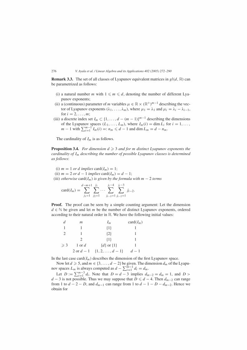
Proof. The proof can be seen by a simple counting argument: Let the dimensiond ∈ N be given and let m be the number of distinct Lyapunov exponents, orderedaccording to their natural order in R. We have the following initial values:

d m Im card(Im)

1 1 {1} 1

2 1 {2} 1

2 {1} 1

� 3 1 or d {d} or {1} 1

2 or d − 1 {1, 2, . . . , d − 1} d − 1

In the last case card(Im) describes the dimension of the first Lyapunov space.Now let d � 5, and m ∈ {3, . . . , d − 2} be given. The dimension dm of the Lyapu-

nov spaces Lm is always computed as d − ∑m−1i=1 di = dm.

Let D := ∑m−3i=1 di . Note that D = d − 3 implies dm−2 = dm = 1, and D >

d − 3 is not possible. Thus we may suppose that D � d − 4. Then dm−2 can rangefrom 1 to d − 2 − D, and dm−1 can range from 1 to d − 1 − D − dm−2. Hence weobtain for

V. Ayala et al. / Linear Algebra and its Applications 402 (2005) 272–290 277

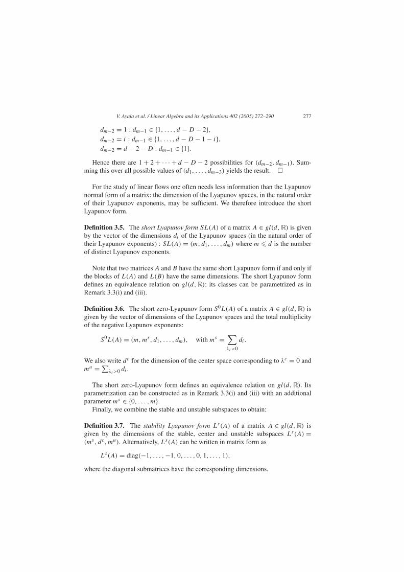
dm−2 = 1 : dm−1 ∈ {1, . . . , d − D − 2},dm−2 = i : dm−1 ∈ {1, . . . , d − D − 1 − i},dm−2 = d − 2 − D : dm−1 ∈ {1}.

Hence there are 1 + 2 + · · · + d − D − 2 possibilities for (dm−2, dm−1). Sum-ming this over all possible values of (d1, . . . , dm−3) yields the result. �

For the study of linear flows one often needs less information than the Lyapunovnormal form of a matrix: the dimension of the Lyapunov spaces, in the natural orderof their Lyapunov exponents, may be sufficient. We therefore introduce the shortLyapunov form.

Definition 3.5. The short Lyapunov form SL(A) of a matrix A ∈ gl(d, R) is givenby the vector of the dimensions di of the Lyapunov spaces (in the natural order oftheir Lyapunov exponents) : SL(A) = (m, d1, . . . , dm) where m � d is the numberof distinct Lyapunov exponents.

Note that two matrices A and B have the same short Lyapunov form if and only ifthe blocks of L(A) and L(B) have the same dimensions. The short Lyapunov formdefines an equivalence relation on gl(d, R); its classes can be parametrized as inRemark 3.3(i) and (iii).

Definition 3.6. The short zero-Lyapunov form S0L(A) of a matrix A ∈ gl(d, R) isgiven by the vector of dimensions of the Lyapunov spaces and the total multiplicityof the negative Lyapunov exponents:

S0L(A) = (m, ms, d1, . . . , dm), with ms =∑

λi<0

di.

We also write dc for the dimension of the center space corresponding to λc = 0 andmu = ∑

λi>0 di .

The short zero-Lyapunov form defines an equivalence relation on gl(d, R). Itsparametrization can be constructed as in Remark 3.3(i) and (iii) with an additionalparameter ms ∈ {0, . . . , m}.

Finally, we combine the stable and unstable subspaces to obtain:

Definition 3.7. The stability Lyapunov form Ls(A) of a matrix A ∈ gl(d, R) isgiven by the dimensions of the stable, center and unstable subspaces Ls(A) =(ms, dc, mu). Alternatively, Ls(A) can be written in matrix form as

Ls(A) = diag(−1, . . . , −1, 0, . . . , 0, 1, . . . , 1),

where the diagonal submatrices have the corresponding dimensions.

278 V. Ayala et al. / Linear Algebra and its Applications 402 (2005) 272–290

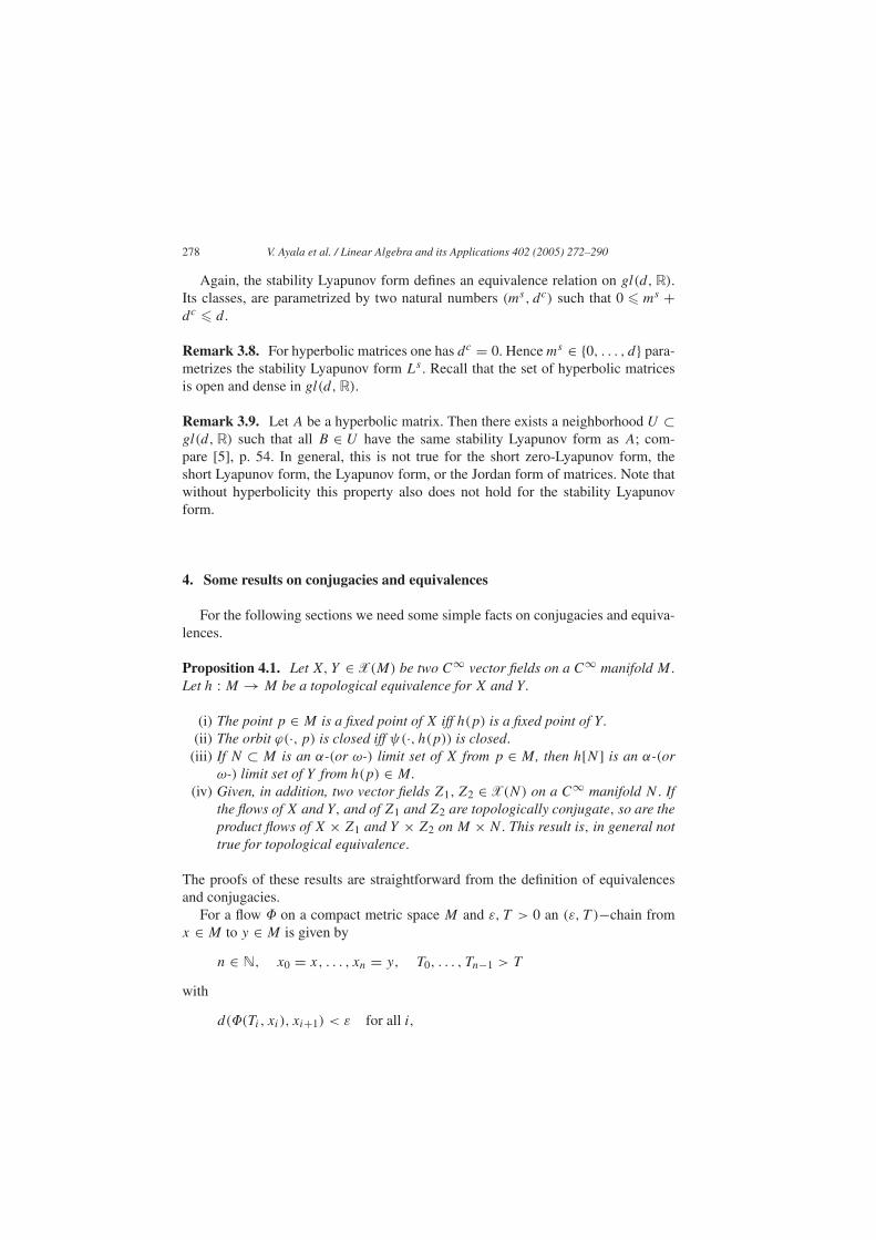
Again, the stability Lyapunov form defines an equivalence relation on gl(d, R).Its classes, are parametrized by two natural numbers (ms, dc) such that 0 � ms +dc � d .

Remark 3.8. For hyperbolic matrices one has dc = 0. Hence ms ∈ {0, . . . , d} para-metrizes the stability Lyapunov form Ls . Recall that the set of hyperbolic matricesis open and dense in gl(d, R).

Remark 3.9. Let A be a hyperbolic matrix. Then there exists a neighborhood U ⊂gl(d, R) such that all B ∈ U have the same stability Lyapunov form as A; com-pare [5], p. 54. In general, this is not true for the short zero-Lyapunov form, theshort Lyapunov form, the Lyapunov form, or the Jordan form of matrices. Note thatwithout hyperbolicity this property also does not hold for the stability Lyapunovform.

4. Some results on conjugacies and equivalences

For the following sections we need some simple facts on conjugacies and equiva-lences.

Proposition 4.1. Let X, Y ∈ X(M) be two C∞ vector fields on a C∞ manifold M.

Let h : M → M be a topological equivalence for X and Y.

(i) The point p ∈ M is a fixed point of X iff h(p) is a fixed point of Y.

(ii) The orbit ϕ(·, p) is closed iff ψ(·, h(p)) is closed.

(iii) If N ⊂ M is an α-(or ω-) limit set of X from p ∈ M , then h[N] is an α-(orω-) limit set of Y from h(p) ∈ M .

(iv) Given, in addition, two vector fields Z1, Z2 ∈ X(N) on a C∞ manifold N. Ifthe flows of X and Y, and of Z1 and Z2 are topologically conjugate, so are theproduct flows of X × Z1 and Y × Z2 on M × N. This result is, in general nottrue for topological equivalence.

The proofs of these results are straightforward from the definition of equivalencesand conjugacies.

For a flow � on a compact metric space M and ε, T > 0 an (ε, T )−chain fromx ∈ M to y ∈ M is given by

n ∈ N, x0 = x, . . . , xn = y, T0, . . . , Tn−1 > T

with

d(�(Ti, xi), xi+1) < ε for all i,

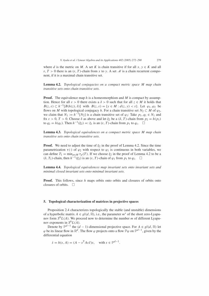
V. Ayala et al. / Linear Algebra and its Applications 402 (2005) 272–290 279

where d is the metric on M . A set K is chain transitive if for all x, y ∈ K and allε, T > 0 there is an (ε, T )-chain from x to y. A set M is a chain recurrent compo-nent, if it is a maximal chain transitive set.

Lemma 4.2. Topological conjugacies on a compact metric space M map chaintransitive sets onto chain transitive sets.

Proof. The equivalence map h is a homeomorphism and M is compact by assump-tion. Hence for all ε > 0 there exists a δ > 0 such that for all z ∈ M it holds thatB(z, ε) ⊂ h−1[B(h(z), δ)] with B(z, ε) = {y ∈ M : d(z, y) < ε}. Let ϕ1, ϕ2 beflows on M with topological conjugacy h. For a chain transitive set N2 ⊂ M of ϕ2,we claim that N1 := h−1[N2] is a chain transitive set of ϕ1: Take p1, q1 ∈ N1 andfix ε > 0, T > 0. Choose δ as above and let ξ2 be a (δ, T )-chain from p2 = h(p1)

to q2 = h(q1). Then h−1(ξ2) =: ξ1 is an (ε, T )-chain from p1 to q1. �

Lemma 4.3. Topological equivalences on a compact metric space M map chaintransitive sets onto chain transitive sets.

Proof. We need to adjust the time of ξ2 in the proof of Lemma 4.2. Since the timeparametrization τ(·) of ϕ2 with respect to ϕ1 is continuous in both variables, wecan define T1 = minp∈M τp(T ). If we choose ξ2 in the proof of Lemma 4.2 to be a(δ, T1)-chain, then h−1(ξ2) is an (ε, T )-chain of ϕ1 from p1 to q1. �

Lemma 4.4. Topological equivalences map invariant sets onto invariant sets andminimal closed invariant sets onto minimal invariant sets.

Proof. This follows, since h maps orbits onto orbits and closures of orbits ontoclosures of orbits. �

5. Topological characterization of matrices in projective spaces

Proposition 2.4 characterizes topologically the stable (and unstable) dimensionsof a hyperbolic matrix A ∈ gl(d, R), i.e., the parameter ms of the short zero-Lyapu-nov form S0L(A). We proceed now to determine the number m of different Lyapu-nov exponents in S0L(A).

Denote by Pd−1 the (d − 1)-dimensional projective space. For A ∈ gl(d, R) letϕ be its linear flow in Rd . The flow ϕ projects onto a flow Pϕ on Pd−1, given by thedifferential equation

s = h(s, A) = (A − sTAsI)s, with s ∈ Pd−1.

280 V. Ayala et al. / Linear Algebra and its Applications 402 (2005) 272–290

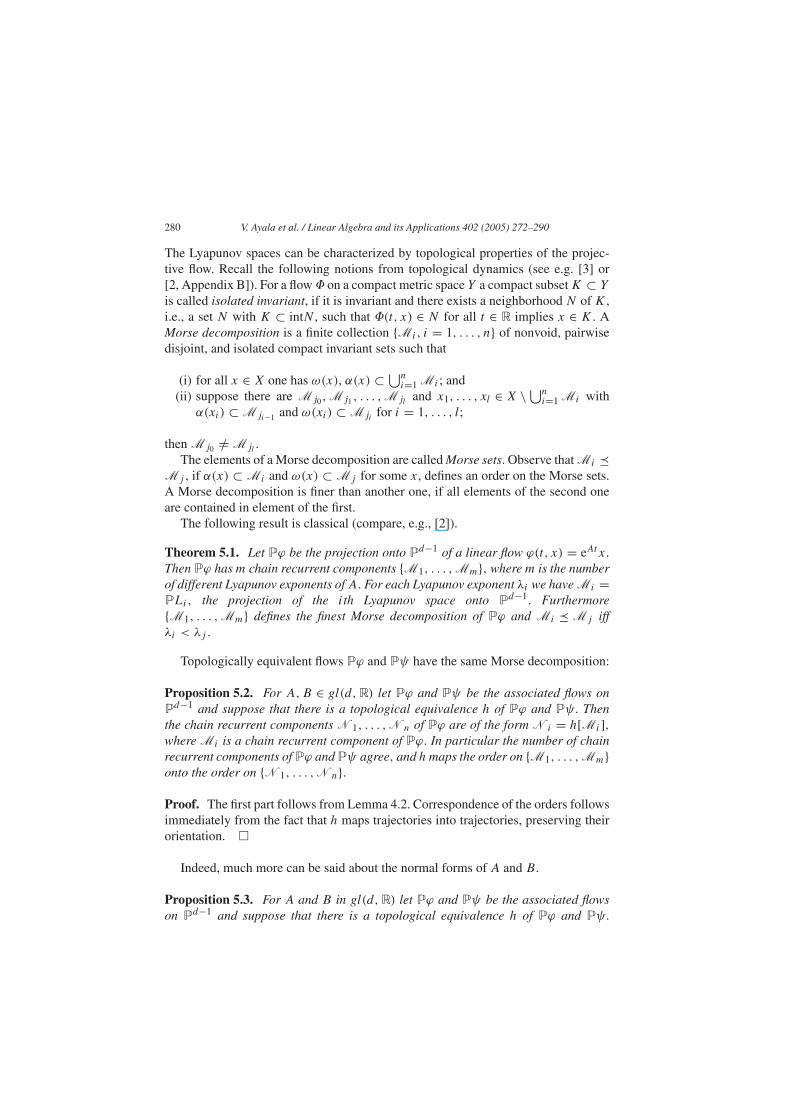
The Lyapunov spaces can be characterized by topological properties of the projec-tive flow. Recall the following notions from topological dynamics (see e.g. [3] or[2, Appendix B]). For a flow � on a compact metric space Y a compact subset K ⊂ Y

is called isolated invariant, if it is invariant and there exists a neighborhood N of K ,i.e., a set N with K ⊂ intN , such that �(t, x) ∈ N for all t ∈ R implies x ∈ K . AMorse decomposition is a finite collection {Mi , i = 1, . . . , n} of nonvoid, pairwisedisjoint, and isolated compact invariant sets such that

(i) for all x ∈ X one has ω(x), α(x) ⊂ ⋃ni=1 Mi ; and

(ii) suppose there are Mj0 ,Mj1 , . . . ,Mjland x1, . . . , xl ∈ X \ ⋃n

i=1 Mi withα(xi) ⊂ Mji−1 and ω(xi) ⊂ Mji

for i = 1, . . . , l;

then Mj0 /= Mjl.

The elements of a Morse decomposition are called Morse sets. Observe that Mi �Mj , if α(x) ⊂ Mi and ω(x) ⊂ Mj for some x, defines an order on the Morse sets.A Morse decomposition is finer than another one, if all elements of the second oneare contained in element of the first.

The following result is classical (compare, e.g., [2]).

Theorem 5.1. Let Pϕ be the projection onto Pd−1 of a linear flow ϕ(t, x) = eAtx.

Then Pϕ has m chain recurrent components {M1, . . . ,Mm}, where m is the numberof different Lyapunov exponents of A. For each Lyapunov exponent λi we have Mi =PLi, the projection of the ith Lyapunov space onto Pd−1. Furthermore{M1, . . . ,Mm} defines the finest Morse decomposition of Pϕ and Mi � Mj iffλi < λj .

Topologically equivalent flows Pϕ and Pψ have the same Morse decomposition:

Proposition 5.2. For A, B ∈ gl(d, R) let Pϕ and Pψ be the associated flows onPd−1 and suppose that there is a topological equivalence h of Pϕ and Pψ. Thenthe chain recurrent components N1, . . . ,Nn of Pϕ are of the form Ni = h[Mi],where Mi is a chain recurrent component of Pϕ. In particular the number of chainrecurrent components of Pϕ and Pψ agree, and h maps the order on {M1, . . . ,Mm}onto the order on {N1, . . . ,Nn}.

Proof. The first part follows from Lemma 4.2. Correspondence of the orders followsimmediately from the fact that h maps trajectories into trajectories, preserving theirorientation. �

Indeed, much more can be said about the normal forms of A and B.

Proposition 5.3. For A and B in gl(d, R) let Pϕ and Pψ be the associated flowson Pd−1 and suppose that there is a topological equivalence h of Pϕ and Pψ.

V. Ayala et al. / Linear Algebra and its Applications 402 (2005) 272–290 281

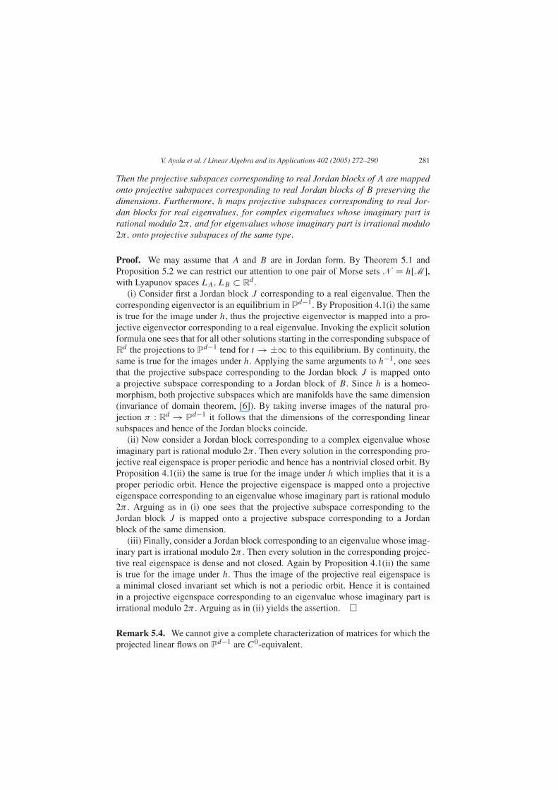
Then the projective subspaces corresponding to real Jordan blocks of A are mappedonto projective subspaces corresponding to real Jordan blocks of B preserving thedimensions. Furthermore, h maps projective subspaces corresponding to real Jor-dan blocks for real eigenvalues, for complex eigenvalues whose imaginary part isrational modulo 2π, and for eigenvalues whose imaginary part is irrational modulo2π, onto projective subspaces of the same type.

Proof. We may assume that A and B are in Jordan form. By Theorem 5.1 andProposition 5.2 we can restrict our attention to one pair of Morse sets N = h[M],with Lyapunov spaces LA, LB ⊂ Rd .

(i) Consider first a Jordan block J corresponding to a real eigenvalue. Then thecorresponding eigenvector is an equilibrium in Pd−1. By Proposition 4.1(i) the sameis true for the image under h, thus the projective eigenvector is mapped into a pro-jective eigenvector corresponding to a real eigenvalue. Invoking the explicit solutionformula one sees that for all other solutions starting in the corresponding subspace ofRd the projections to Pd−1 tend for t → ±∞ to this equilibrium. By continuity, thesame is true for the images under h. Applying the same arguments to h−1, one seesthat the projective subspace corresponding to the Jordan block J is mapped ontoa projective subspace corresponding to a Jordan block of B. Since h is a homeo-morphism, both projective subspaces which are manifolds have the same dimension(invariance of domain theorem, [6]). By taking inverse images of the natural pro-jection π : Rd → Pd−1 it follows that the dimensions of the corresponding linearsubspaces and hence of the Jordan blocks coincide.

(ii) Now consider a Jordan block corresponding to a complex eigenvalue whoseimaginary part is rational modulo 2π . Then every solution in the corresponding pro-jective real eigenspace is proper periodic and hence has a nontrivial closed orbit. ByProposition 4.1(ii) the same is true for the image under h which implies that it is aproper periodic orbit. Hence the projective eigenspace is mapped onto a projectiveeigenspace corresponding to an eigenvalue whose imaginary part is rational modulo2π . Arguing as in (i) one sees that the projective subspace corresponding to theJordan block J is mapped onto a projective subspace corresponding to a Jordanblock of the same dimension.

(iii) Finally, consider a Jordan block corresponding to an eigenvalue whose imag-inary part is irrational modulo 2π . Then every solution in the corresponding projec-tive real eigenspace is dense and not closed. Again by Proposition 4.1(ii) the sameis true for the image under h. Thus the image of the projective real eigenspace isa minimal closed invariant set which is not a periodic orbit. Hence it is containedin a projective eigenspace corresponding to an eigenvalue whose imaginary part isirrational modulo 2π . Arguing as in (ii) yields the assertion. �

Remark 5.4. We cannot give a complete characterization of matrices for which theprojected linear flows on Pd−1 are C0-equivalent.

282 V. Ayala et al. / Linear Algebra and its Applications 402 (2005) 272–290

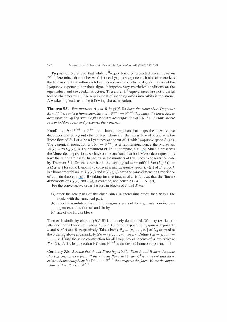
Proposition 5.3 shows that while C0-equivalence of projected linear flows onPd−1 determines the number m of distinct Lyapunov exponents, it also characterizesthe Jordan structure within each Lyapunov space (and, obviously, not the size of theLyapunov exponents nor their sign). It imposes very restrictive conditions on theeigenvalues and the Jordan structure. Therefore, C0-equivalences are not a usefultool to characterize m. The requirement of mapping orbits into orbits is too strong.A weakening leads us to the following characterization.

Theorem 5.5. Two matrices A and B in gl(d, R) have the same short Lyapunovform iff there exist a homeomorphism h : Pd−1 → Pd−1 that maps the finest Morsedecomposition of Pϕ onto the finest Morse decomposition of Pψ, i.e., h maps Morsesets onto Morse sets and preserves their orders.

Proof. Let h : Pd−1 → Pd−1 be a homeomorphism that maps the finest Morsedecomposition of Pϕ onto that of Pψ , where ϕ is the linear flow of A and ψ is thelinear flow of B. Let λ be a Lyapunov exponent of A with Lyapunov space LA(λ).The canonical projection π : Rd → Pd−1 is a submersion, hence the Morse setM(λ) = π(LA(λ)) is a submanifold of Pd−1; compare, e.g., [6]. Since h preservesthe Morse decompositions, we have on the one hand that both Morse decompositionshave the same cardinality. In particular, the numbers of Lyapunov exponents coincideby Theorem 5.1. On the other hand, the topological submanifold h(π(LA(λ))) =π(LB(µ)) for some Lyapunov exponent µ and Lyapunov space LB(µ) of B. Since h

is a homeomorphism, π(LA(λ)) and π(LB(µ)) have the same dimension (invarianceof domain theorem, [6]). By taking inverse images of π it follows that the (linear)dimensions of LA(λ) and LB(µ) coincide, and hence SL(A) = SL(B).

For the converse, we order the Jordan blocks of A and B via

(a) order the real parts of the eigenvalues in increasing order, then within theblocks with the same real part,

(b) order the absolute values of the imaginary parts of the eigenvalues in increas-ing order, and within (a) and (b) by

(c) size of the Jordan block.

Then each similarity class in gl(d, R) is uniquely determined. We may restrict ourattention to the Lyapunov spaces LA and LB of corresponding Lyapunov exponentsλ and µ of A and B, respectively. Take a basis BA = {x1, . . . , xn} of LA adapted tothe ordering above and similarly BB = {y1, . . . , yn} for LB . Define T xi = yi for i =1, . . . , n. Using the same construction for all Lyapunov exponents of A, we arrive atT ∈ GL(d, R). Its projection PT onto Pd−1 is the desired homeomorphism. �

Corollary 5.6. Assume that A and B are hyperbolic. Then A and B have the sameshort zero-Lyapunov form iff their linear flows in Rd are C0-equivalent and thereexists a homeomorphism h : Pd−1 → Pd−1 that respects the finest Morse decompo-sition of their flows in Pd−1.

V. Ayala et al. / Linear Algebra and its Applications 402 (2005) 272–290 283

Proof. The proof combines Proposition 2.4 and Theorem 5.5. �

While Theorem 5.5 and Corollary 5.6 characterize the short (zero)−Lyapunovform of a matrix A in gl(d, R), they are unsatisfactory in the sense that they arenot constructive. The next section provides a constructive characterization using theinduced flow on the flag manifold.

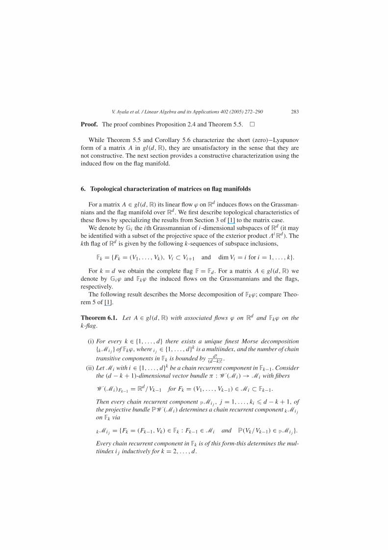
6. Topological characterization of matrices on flag manifolds

For a matrix A ∈ gl(d, R) its linear flow ϕ on Rd induces flows on the Grassman-nians and the flag manifold over Rd . We first describe topological characteristics ofthese flows by specializing the results from Section 3 of [1] to the matrix case.

We denote by Gi the ith Grassmannian of i-dimensional subspaces of Rd (it maybe identified with a subset of the projective space of the exterior product �iRd ). Thekth flag of Rd is given by the following k-sequences of subspace inclusions,

Fk = {Fk = (V1, . . . , Vk), Vi ⊂ Vi+1 and dim Vi = i for i = 1, . . . , k}.For k = d we obtain the complete flag F = Fd . For a matrix A ∈ gl(d, R) we

denote by Giϕ and Fkϕ the induced flows on the Grassmannians and the flags,respectively.

The following result describes the Morse decomposition of Fkϕ; compare Theo-rem 5 of [1].

Theorem 6.1. Let A ∈ gl(d, R) with associated flows ϕ on Rd and Fkϕ on thek-flag.

(i) For every k ∈ {1, . . . , d} there exists a unique finest Morse decomposition{kMij } of Fkϕ, where ij ∈ {1, . . . , d}k is a multiindex, and the number of chain

transitive components in Fk is bounded by d!(d−k)! .

(ii) Let Mi with i ∈ {1, . . . , d}k be a chain recurrent component in Fk−1. Considerthe (d − k + 1)-dimensional vector bundle π : W(Mi ) → Mi with fibers

W(Mi )Fk−1 = Rd/Vk−1 for Fk = (V1, . . . , Vk−1) ∈ Mi ⊂ Fk−1.

Then every chain recurrent component PMij , j = 1, . . . , ki � d − k + 1, ofthe projective bundle PW(Mi ) determines a chain recurrent component kMij

on Fk via

kMij = {Fk = (Fk−1, Vk) ∈ Fk : Fk−1 ∈ Mi and P(Vk/Vk−1) ∈ PMij }.Every chain recurrent component in Fk is of this form-this determines the mul-tiindex ij inductively for k = 2, . . . , d.

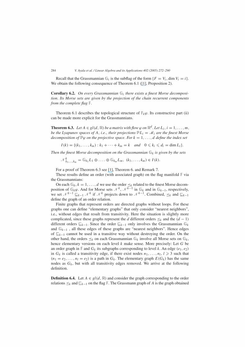
284 V. Ayala et al. / Linear Algebra and its Applications 402 (2005) 272–290

Recall that the Grassmannian Gi is the subflag of the form {F = Vi, dim Vi = i}.We obtain the following consequence of Theorem 6.1 ([1], Proposition 2).

Corollary 6.2. On every Grassmannian Gi there exists a finest Morse decomposi-tion. Its Morse sets are given by the projection of the chain recurrent componentsfrom the complete flag F.

Theorem 6.1 describes the topological structure of Fkϕ. Its constructive part (ii)can be made more explicit for the Grassmannians.

Theorem 6.3. Let A ∈ gl(d, R) be a matrix with flow ϕ on Rd . Let Li, i = 1, . . . , m,

be the Lyapunov spaces of A, i.e., their projections PLi = Mi are the finest Morsedecomposition of Pϕ on the projective space. For k = 1, . . . , d define the index set

I (k) = {(k1, . . . , km) : k1 + · · · + km = k and 0 � ki � di = dim Li}.Then the finest Morse decomposition on the Grassmannian Gk is given by the sets

Nkk1,...,km

= Gk1L1 ⊕ . . . . ⊕ GkmLm, (k1, . . . , km) ∈ I (k).

For a proof of Theorem 6.3 see [1], Theorem 6. and Remark 7.These results define an order (with associated graph) on the flag manifold F via

the Grassmannians:On each Gk , k = 1, . . . , d we use the order �k related to the finest Morse decom-

position of Gkϕ. And for Morse sets Nk , Nk−1 in Gk and in Gk−1, respectively,we set Nk−1 k−1 Nk if Nk projects down to Nk−1. Combined, �k and k−1define the graph of an order relation.

Finite graphs that represent orders are directed graphs without loops. For thesegraphs one can define “elementary graphs” that only consider “nearest neighbors”,i.e., without edges that result from transitivity. Here the situation is slightly morecomplicated, since these graphs represent the d different orders �k and the (d − 1)

different orders k−1. Since the order k−1 only involves the Grassmannian Gk

and Gk−1 , all these edges of these graphs are “nearest neighbors”. Hence edgesof k−1 cannot be used in a transitive way without destroying the order. On theother hand, the orders �k on each Grassmannian Gk involve all Morse sets on Gk ,hence elementary versions on each level k make sense. More precisely: Let G bean order graph in F and Gk its subgraphs corresponding to level k. An edge (e1, e2)

in Gk is called a transitivity edge, if there exist nodes n1, . . . , nl , l � 3 such that(n1 = e2, . . . , nl = e2) is a path in Gk . The elementary graph E(Gk) has the samenodes as Gk , but with all transitivity edges removed. We arrive at the followingdefinition.

Definition 6.4. Let A ∈ gl(d, R) and consider the graph corresponding to the orderrelations �k and k−1 on the flag F. The Grassmann graph of A is the graph obtained

V. Ayala et al. / Linear Algebra and its Applications 402 (2005) 272–290 285

from this graph by replacing on each level k (i.e., in each Grassmannian) the corre-sponding subgraph by its elementary version.

One easily checks that the Grassmann graph of a matrix A is unique.

Remark 6.5. Theorem 6.3 describes an indexing system for the finest Morse decom-position on each Grassmannian Gk and hence on the complete flag F that correspondsto the parametrization of the short Lyapunov form via Definition 3.3(i) and (iii), seecomment after Definition 3.5.

For the following examples we will use a different indexing system that is a littlemore intuitive. Let A ∈ gl(d, R) have the short Lyapunov form (m, d1, . . . , dm) with∑m

i=1 di = d . Then the finest Morse decomposition associated to the flow Pϕ onPd−1 has m Morse sets {M1, . . . ,Mm} that are linearly ordered (Theorem 5.1). Weassociate the canonical basis {e1, . . . , ed} in Rd with the Morse sets in such a waythat each Morse set Mi corresponds to di basis vectors (in the respective orders),i.e.,

M1 ∼ {e1, . . . , ed1},Mi ∼ {eαi

, . . . , eβi} where αi = ∑i−1

j=1 dj + 1, βi = ∑ij=1 dj .

On G1 = Pd−1 we index the Morse decomposition simply as Mi . Each Morseset on G2 has two indices (j1, j2) and Mi Mj1,j2 iff i ∈ {j1, j2}. Several of thesets Mj1,j2 on G2 may be identical. In this case we use the index pair with smallestnumbers in each entry. Observe that the order relations are retained. Continuing forG2, . . . , Gd we obtain unique indexes for all Morse sets on Gk , and hence on theflag F.

As described above, the order k can be read off the indexes immediately and k

can be constructed explicitly. Furthermore, we have for the orders �k on Gk:

M(j1,...,jk) �k M(j ′1,...,j

′k)

iff ji � j ′i for all i = 1, . . . , k.

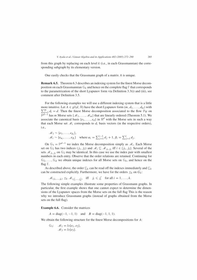
The following simple examples illustrate some properties of Grassmann graphs. Inparticular, the first example shows that one cannot expect to determine the dimen-sions of the Lyapunov spaces from the Morse sets on the full flag This is the reasonwhy we introduce Grassmann graphs (instead of graphs obtained from the Morsesets on the full flag).

Example 6.6. Consider the matrices

A = diag(−1, −1, 1) and B = diag(−1, 1, 1).

We obtain the following structure for the finest Morse decompositions for A:

G1: M1 = ls{e1, e2},M3 = ls{e3}.

286 V. Ayala et al. / Linear Algebra and its Applications 402 (2005) 272–290

G2: M1,2 = ls{e1, e2},M1,3 = {ls{x, e3}, with x ∈ ls{e1, e2}}.

G3: M1,2,3 = ls{e1, e2, e3}.This leads to the Grassmann graph of A

M1,2,3↗ ↖

M1,2 −→ M1,3↑ ↗ ↑M1 −→ M3

.

In the same way one obtains the Grassmann graph of B

M1,2,3↗ ↖

M1,2 −→ M2,3↑ ↖ ↑M1 −→ M2

.

On the other hand, the Morse sets in the full flag are given for A and B by

M1,2,3M1,2M1

�

M1,2,3M1,3M3

and

M1,2,3M1,2M1

�

M1,2,3M2,3M2

,

respectively. Thus in the full flag the numbers and the orders of the Morse sets coin-cide, while the Grassmann graphs are different.

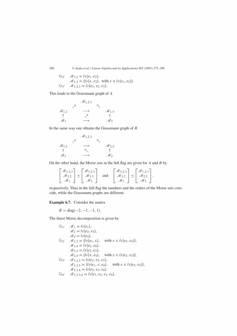
Example 6.7. Consider the matrix

B = diag(−2, −1, −1, 1).

The finest Morse decomposition is given by

G1: M1 = ls{e1},M2 = ls{e2, e3},M4 = ls{e4}.

G2: M1,2 = {ls{e1, x}, with x ∈ ls{e2, e3}},M1,4 = ls{e1, e4},M2,3 = ls{e2, e3},M2,4 = {ls{x, e4}, with x ∈ ls{e2, e3}}.

G3: M1,2,3 = ls{e1, e2, e3},M1,2,4 = {ls{e1, x, e4}, with x ∈ ls{e2, e3}},M2,3,4 = ls{e2, e3, e4}.

G4: M1,2,3,4 = ls{e1, e2, e3, e4}.

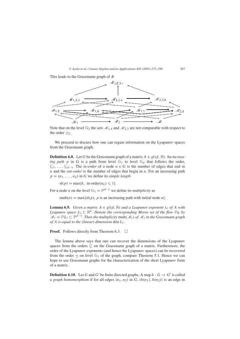
V. Ayala et al. / Linear Algebra and its Applications 402 (2005) 272–290 287

This leads to the Grassmann graph of B

Note that on the level G2 the sets M1,4 and M2,3 are not comparable with respect tothe order �2.

We proceed to discuss how one can regain information on the Lyapunov spacesfrom the Grassmann graph.

Definition 6.8. Let G be the Grassmann graph of a matrix A ∈ gl(d, R). An increas-ing path p in G is a path from level G1 to level Gd that follows the order,1, . . . , d−1. The in-order of a node n ∈ G is the number of edges that end inn and the out-order is the number of edges that begin in n. For an increasing pathp = (n1, . . . , nd) in G we define its simple length

sl(p) = max{k, in-order(nk) � 1}.For a node n on the level G1 = Pd−1 we define its multiplicity as

mult(n) = max{sl(p), p is an increasing path with initial node n}.

Lemma 6.9. Given a matrix A ∈ gl(d, R) and a Lyapunov exponent λi of A withLyapunov space Li ⊂ Rd . Denote the corresponding Morse set of the flow Pϕ byMi = PLi ⊂ Pd−1. Then the multiplicity mult(Mi ) of Mi in the Grassmann graphof A is equal to the (linear) dimension dim Li.

Proof. Follows directly from Theorem 6.3. �

The lemma above says that one can recover the dimensions of the Lyapunovspaces from the orders on the Grassmann graph of a matrix. Furthermore, theorder of the Lyapunov exponents (and hence the Lyapunov spaces) can be recoveredfrom the order � on level G1 of the graph, compare Theorem 5.1. Hence we canhope to use Grassmann graphs for the characterization of the short Lyapunov formof a matrix.

Definition 6.10. Let G and G′ be finite directed graphs. A map h : G → G′ is calleda graph homomorphism if for all edges (n1, n2) in G, (h(n1), h(n2)) is an edge in

288 V. Ayala et al. / Linear Algebra and its Applications 402 (2005) 272–290

G′. Furthermore, h is a graph isomorphism if h is bijective and h and h−1 are graphhomomorphisms.

Theorem 6.11. The short Lyapunov form SL(A) and SL(B) are identical for twomatrices A, B ∈ gl(d, R) iff the Grassmann graphs of A and B are isomorphic.

Proof. Let the Grassmann graphs G(A) and G(B) be isomorphic.

(i) We construct the orders � and as follows. The only node with out-order 0is the unique node nl on the highest level l. All nodes n for which there isan edge (n, nl) are on the level l − 1. All nodes n′ that are not on level l − 1and for which there is an edge (n′, n) with n on level l − 1, are on level l − 2,etc.This algorithm stops after l′ steps, i.e., after determining the nodes on levell′, and all nodes are associated with some level. Then l − l′ + 1 = d , the dimen-sion of the underlying Rd . We reindex the levels such that the smallest level is 1.Then, the edges between nodes on the same level k determines the order �k . Andedges between nodes on levels k − 1 and k determine the order k−1. Note thatthe node corresponding to the Morse set M1 on G1 is the unique node with in-order 0.

(ii) The length of any increasing path (n1, n2, . . . , nd) determines the dimensionof the underlying space Rd .

(iii) For each node in level G1, its multiplicity defines the dimension of the corre-sponding Lyapunov space.

(i)–(iii) mean that for any matrix its short Lyapunov form can be uniquely recon-structed from the Grassmann graph, hence isomorphic Grassmann graphs belong tomatrices with identical short Lyapunov form. Vice versa, short Lyapunov forms deter-mine Grassmann graphs by their construction (based on Theorems 6.1 and 6.3). �

Remark 6.12. Given a finite directed graph G without loops, there is a constructivealgorithm to decide if G is the Grassmann graph of a matrix. G needs to have aunique edge nl with out-order 0 (and a unique edge with in-order 0; this edge corre-sponds to the Morse set M1).Starting from the “maximal” edge gl , we proceed as insteps (i)–(iii) from the proof of Theorem 6.11 to identify nodes on the different levelsas well as the multiplicities of each edge on the lowest level 1. (Note that one can use thesame procedure if the graphs within each level have not been replaced by their elemen-tary versions; then one has to perform this replacement here.) With this information weuse Theorem 6.3 to construct the Grassmann graph based on the order on level 1 andthe multiplicity of the nodes. The graph so constructed is compared to the graph G todecide whether it is indeed the Grassmann graph of a matrix.

Remark 6.13. Graph isomorphisms define an equivalence relation on the set of allgraphs. The corresponding equivalence classes of Grassmann graphs can be

V. Ayala et al. / Linear Algebra and its Applications 402 (2005) 272–290 289

parametrized as in Remark 3.3(i) and (iii). This parametrization corresponds to theconstruction of the finest Morse decomposition on the Grassmannians Gk as inTheorem 6.3.

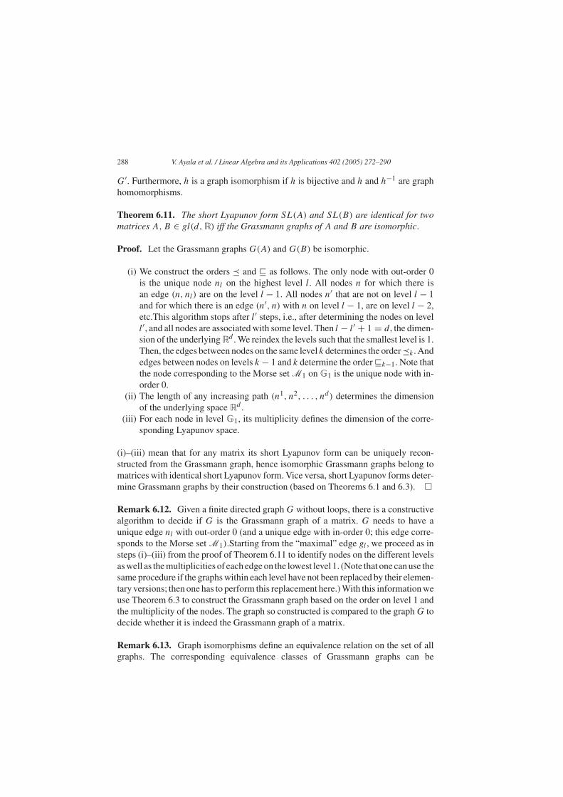
Example 6.14. Consider the two matrices

A =

−2 0 0 00 −1 0 00 0 −1 00 0 0 1

, B =

−2 1 0 0−1 −2 0 00 0 −1 00 0 0 1

.

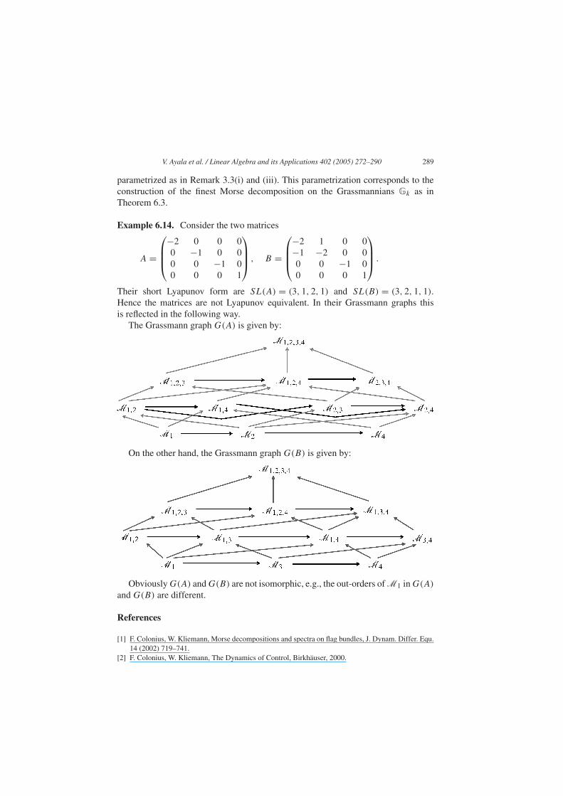
Their short Lyapunov form are SL(A) = (3, 1, 2, 1) and SL(B) = (3, 2, 1, 1).Hence the matrices are not Lyapunov equivalent. In their Grassmann graphs thisis reflected in the following way.

The Grassmann graph G(A) is given by:

On the other hand, the Grassmann graph G(B) is given by:

Obviously G(A) and G(B) are not isomorphic, e.g., the out-orders of M1 in G(A)

and G(B) are different.

References

[1] F. Colonius, W. Kliemann, Morse decompositions and spectra on flag bundles, J. Dynam. Differ. Equ.14 (2002) 719–741.

[2] F. Colonius, W. Kliemann, The Dynamics of Control, Birkhäuser, 2000.

290 V. Ayala et al. / Linear Algebra and its Applications 402 (2005) 272–290

[3] C. Conley, Isolated invariant sets and the Morse index, CBMS Regional Conference Series, no. 38,American Mathematical Society, 1978.

[4] M. Hirsch, S. Smale, Differential Equations, Dynamical Systems and Linear Algebra, AcademicPress, 1974.

[5] J. Palis, W. de Melo, Geometric Theory of Dynamical Systems, Springer-Verlag, 1982.[6] F. Warner, Foundations of Differentiable Manifolds and Lie Groups, Springer-Verlag, 1983.[7] S. Wiggins, Introduction to Applied Nonlinear Dynamical Systems and Applications, Springer-Ver-

lag, 1996.[8] D.K. Arrowsmith, C.M. Place, An Introduction to Dynamical Systems, Cambridge University Press,

1990.