Embed Size (px)
Citation preview

Dynamical Systems
Version 0.1
Dennis Pixton
E-mail address : [email protected]
Department of Mathematical Sciences
Binghamton University
Copyright 2009–2010 by the author. All rights reserved. The most current versionof this book is available at the website
http://www.math.binghamton.edu/dennis/dynsys.html.
This book may be freely reproduced and distributed, provided that it is reproducedin its entirety from one of the versions which is posted on the website above at thetime of reproduction. This book may not be altered in any way, except for changesin format required for printing or other distribution, without the permission of theauthor.

Contents
Chapter 1. Discrete population models 11.1. The basic model 11.2. Discrete dynamical systems 21.3. Some variations 31.4. Steady states and limit states 5Exercises 6
Chapter 2. Continuous population models 82.1. The basic model 82.2. Continuous dynamical systems 102.3. Some variations 112.4. Steady states and limit states 182.5. Existence and uniqueness 20Exercises 24
Chapter 3. Discrete Linear models 273.1. A stratified population model 273.2. Matrix powers, eigenvalues and eigenvectors. 303.3. Non negative matrices 333.4. Networks; more examples 343.5. Complex eigenvalues 39Exercises 42
Chapter 4. Linear models: continuous version 464.1. The exponential function 464.2. Some models 524.3. Phase portraits 59Exercises 67
Chapter 5. Non-linear systems in two dimensions 695.1. A predator-prey model 695.2. Linearization 755.3. Conservation of energy and the pendulum problem 81
i

CONTENTS ii
5.4. Limit cycles 875.5. Stability 945.6. Bifurcations 99Exercises 105
Chapter 6. Higher dimensions and chaos 1116.1. The horseshoe 1116.2. Encoding the horseshoe 1196.3. Time dependent systems 1256.4. Strange attractors 129Exercises 130
Appendix A. Review 132A.1. Complex numbers 132A.2. Partial derivatives 134A.3. Exact differential equations 136
Appendix B. Maple notes 138B.1. Basic operations 138B.2. Linear algebra 138B.3. Differential equations 138
Appendix C. Extra problems 143

CHAPTER 1
Discrete population models
1.1. The basic model
The first example is based on a simple population model. Suppose that a popu-lation of rabbits lives on an island (so the population is not affected by immigrationfrom the outside, or emigration to the outside). The population is observed once peryear. We’ll use x for the number of rabbits, and t for the time, measured in years.
In each year a certain number of rabbits die, and this number is proportional tothe number that are present at the start of the year. The proportionality constant cis the “death rate” or “mortality rate”. That is, in one year cx rabbits die and aresubtracted from the population of x. Similarly, a number of rabbits are born, andthis number is also proportional to the number that are present at the start of theyear. The proportionality constant b is the “birth rate”. That is, in in one year bxrabbits are born and are added to the population of x rabbits. The net effect of thiscan be summarized as follows:
If the population at some time is x then the population one year later will bex + bx − cx = (1 + b − c)x. If we write r = b − c, the net growth rate, then we canrewrite this as (1 + r)x.
Thus we have a function F which specifies how the population changes duringone year. In this case, F (x) = (1 + r)x. Once we know this function and we knowthe starting population x we can calculate the population any number of years laterby iterating the function F . We will often use the alternate parameter k = 1 + r.For later reference we present this example as:
Example 1.1. F (x) = (1+r)x = kx, for real numbers x. The parameter r is thenet growth rate; it must be > −1. The alternate parameter is k = 1 + r, so k > 0.
For example, suppose the population is 1000 and the net growth rate is 0.1. Then,after one year, the population will be F (1000) = (1 + .1) · 1000 = 1100. To find thepopulation after another year just apply the function F to the population 1100, toget F (1100) = (1 + .1) · 1100 = 1210. Then we can find the population after threeyears by another application: F (1210) = 1.1 · 1210 = 1331. Thus if the populationis x then, after three years, the population is obtained by iterating F three times,starting with x, so (using the general formula), we obtain F (F (F (x))). We calculate
1

1.2. DISCRETE DYNAMICAL SYSTEMS 2
this by applying the function F three times, starting with x:
x→ F (x) = (1 + r)x
(1 + r)x→ F(
(1 + r)x)
= (1 + r) · (1 + r)x = (1 + r)2x
(1 + r)2x→ F(
(1 + r)2x)
= (1 + r) · (1 + r)2x = (1 + r)3x.
It should be clear (and it is easy to prove by induction) that, for any number ofyears t, the population after t years is (1 + r)tx, or ktx. We will use the notationF t(x) for the t-fold iteration of F , so F t(x) = (1 + r)tx in this case. In terms offunctional composition, F t = F F F · · · F (where there are t copies of F ), sothis really is, in a sense, “F to the tth power”. As special cases, F 1 is just F , andF 0 is the identity function; that is, F 0(x) = x.
Once we have this formula for F t(x) we can make some observations about pop-ulation growth:
(1) Although (1 + r)tx makes mathematical sense for x < 0, this doesn’t make sensein the model, since populations cannot be negative.
(2) (1 + r)tx is defined mathematically for all real numbers t (with some worries if1+ r is 0 or negative), but there is no meaningful sense in which we can iterate afunction t times, where t is not a non-negative integer. [We can make sense of F t
when t is a negative integer, by iterating the inverse function F−1, if it exists.](3) F t(0) = 0 for all t.(4) If r > 0 then (1 + r) > 1, so (1 + r)t → ∞ as t → ∞. Hence F t(x) → ∞ as
t→ ∞ if x > 0.(5) If −1 ≤ r < 0 then 0 ≤ (1+r) < 1, so (1+r)t → 0 as t→ ∞. Hence F t(x) → ∞
as t→ ∞.(6) If r = 0 then F t(x) = x for all t and all x.
This is a very simplistic model of population growth. Here are a few criticisms:
(1) F t(x) will generally yield non-integer values.(2) F t(x) → ∞ can’t happen: eventually there will be no space for the rabbits on
the island.(3) No model can really predict exact numbers of rabbits, since there will always be
some random fluctuations.(4) The model assumes that the net growth rate is constant, independent of both t
and x.
1.2. Discrete dynamical systems
Before modifying this model we isolate the features of the model that constitutea discrete dynamical system:

1.3. SOME VARIATIONS 3
In general, we will work with two variables, x and t. We always think of t as time,but the interpretation of x will depend on the particular application. In general, thevalues of x are called the states of the system. In most cases it will be necessary tospecify more than just one number to describe the state of the system, so in mostcases we will consider x to be a vector, and we’ll refer to it as the state vector of thesystem. The transition rule for the system is a function F that transforms the statex at one time to the start F (x) one time unit later. Then we can represent the stateof the system t time units later by iterating F ; that is, we calculate F t(x).
Essentially, it is the iterated function F t which constitutes the dynamical system,although we often simply refer to the transition rule F as the dynamical system. Itis called a discrete dynamical system to emphasize the fact that t is measured indiscrete steps, so the values of t are restricted to integers – usually positive integers.
Note that the transition rule must be a function of x alone; it does not dependon t. We will see later how to accommodate transition rules that do depend on t.Also, the transition rule is a well-defined function. Hence, the dynamical system isdeterministic, in the sense that the values of x and t uniquely determine the valueof F t(x).
The first example above illustrates these features. The state vector x is onedimensional – that is, it is just a number. The transition rule is F (x) = (1 + r)x,and the state at time t is given by F t(x) = (1 + r)tx for t = 0, 1, 2, 3, . . . .
The first example illustrates some common features of dynamical systems:First, the domain of x is usually restricted. That is, state vectors cannot be
arbitrary, but are limited to a particular set of values, sometimes called the statespace. For example, in our population model the values of x cannot be negative.
Second, the transition rule usually incorporates one or more parameters. Theseare quantities that are constant for a specific instance of the dynamical system, andwhich, in applications, are either determined empirically or are adjusted externally.For example, in our original population model the birth and death rates are param-eters. The model only depends on their difference, so it is reasonable to talk of justone parameter, the net growth rate, r.
Here’s an important property of dynamical systems:
Proposition 1.2. F t F s = F t+s.
1.3. Some variations
We now consider two variations on the original model.The first variation involves external interaction with the population. We envision
a yearly addition to (or subtraction from) the population. For example, if r < 0,so the population is dying out, we might add a number of rabbits each year tostabilize the population. If r > 0, so the population is incresing without limit, we

1.3. SOME VARIATIONS 4
might remove a number of rabbits each year in order to keep the population fromexploding. This gives the following example:
Example 1.3. F (x) = (1+r)x+A = kx+A, for real numbers x. The parameterA is any real number, and k and 1 + r are defined as in Example 1.1.
The effect of this model is that, each year, A rabbits are added to the population.In this model the addition occurs at the end of the year, just before the populationis counted. [If the addition occured at the beginning of the year then the transitionrule would be F (x) = (1 + r)(x+ A). Of course A might be negative, in which caserabbits are removed rather than added.
Iterating a few times gives
F 1(x) = kx+ A
F 2(x) = F (F (x)) = F (kx+ A) = k(kx+ A) + A = k2x+ A+ Ak
F 3(x) = F (F 2(x)) = F (k2x+ A+ Ak) = k(k2x+ A+ Ak)) + A
= k3x+ A+ Ak + Ak2
F 4(x) = k4x+ A+ Ak + Ak2 + Ak3.
The pattern should now be clear; the general form is
F t(x) = ktx+ A(
1 + k + k2 + · · · + kt−1)
.
If you look up the geometric series you will find a formula for the sum in parentheses.If k 6= 1 this allows us to write
(1.1) F t(x) = ktx+ A · kt − 1
k − 1= ktx+ A · 1 − kt
1 − k.
We now look at a second variation on the basic model.Instead of looking at the effect of adding population from the outside we consider
a way of adjusting the growth rate r to take into account the effects of overcrowding.The idea is that if the population x becomes too large then the rabbits on our islandwill not be able to find enough to eat, so we expect that the death rate will go up.Also, they will be less healthy, so we expect the birth rate to go down. In otherwords, we expect that the net growth rate will decrease as the population increases.
Our new variation amounts to replacing the constant growth rate r with a func-tion of x, which is approximately equal to r for small values of x but which decreasesas x increases. The simplest function that satisfies these conditions is a linear func-tion of the form r − αx where α is a positive constant. There are many othercandidates for a variable growth rate, but we will concentrate on this one because ofits simplicity. This gives us the next example:

1.4. STEADY STATES AND LIMIT STATES 5
Example 1.4. F (x) = (1 + r − αx)x = (k − αx)x = kx− αx2 for real numbersx. tThe parameter α is a positive real number, and k and 1 + r are defined as inExample 1.1.
We can iterate this:
F 1(x) = kx− αx2
F 2(x) = F (F (x)) = k(kx− αx2) − α(kx− αx2)2
= k2x− α(k + k2)x2 + 2α2kx3 − α3x4.
However, the calculations rapidly become very messy – in fact, F t(x) is a complicatedpolynomial of degree 2t in x, and there is no simple general form for it.
On the other hand, it is easy to calculate as many iterations as we need in aspecific case. For example, let r = .1 and α = .0001. Starting with x = 2000 wecalculate
F 1(x) = 1800(1.2)
F 2(x) = 1656
F 3(x) = 1547
F 4(x) = 1462
F 5(x) = 1394
F 6(x) = 1339
F 7(x) = 1294
F 8(x) = 1256
F 9(x) = 1224
F 10(x) = 1196
Notice that F t(2000) is decreasing as t increases, although r > 0. It is not clear,without further analysis, whether this decrease continues, or what the limiting valueis.
1.4. Steady states and limit states
A steady state of a dynamical system is a state x0 so that F t(x0) = x0 for allvalues of t. For example, in our original model, 0 is a steady state, since F t(0) =(1 + r)t · 0 = 0 for all t.
Since F t is defined by iterating F this is the same as finding a state for whichF (x0) = x0. In general, such a value x0 is called a fixed point for F . Often suchfixed points can be found by just solving an algebraic equation. For example, in
EXERCISES 6
our second model, F (x) = kx + A, so we can find the fixed points of F by solvingF (x) = x for x, as follows:
kx+ A = x
A = x− kx = (1 − k)x
x =A
1 − k
If A and 1 − k = r both have the same sign then x0 =A
1 − k> 0 so it represents a
population, and this population will not change with time.
Next, suppose that x1 is a state of a dynamical system. If F t(x1) converges to astate x2 as t→ ∞ and x2 6= x1 then x2 is called a limit state of the system. We willneed to modify this definition later, but this is sufficient for simple examples. Forexample, in our original model, 0 is a limit state if −1 ≤ r < 0 since in that casek = 1 + r < 1 so F t(x) = ktx → ∞ for any x. On the other hand, if k > 1 then0 is not a limit state, since F t(x) = ktx → ±∞ as t → ∞ if x 6= 0. It is true thatF t(0) → 0 as t→ ∞ in this case, since 0 is a steady state; but 0 is not a limit stateof the system since we required x2 6= x1 in the definition.
The examples above show that a steady state may – or may not – be a limitstate. In the other direction we have:
Proposition 1.5. If F is continuous then any limit state is a steady state.
Proof. Suppose that F t(x1) → x2 as t → ∞. Then, if we replace t with t + 1,we also have F t+1(x1) → x2. But we can write F t+1(x1) = F (F t(x1)). If we take thelimit in this equation as t→ ∞ and use the fact that F is continuous we get
x2 = limt→∞
F t(x1) = limt→∞
F (F t(x1)) = F(
limt→∞
F t(x1))
= F (x2),
so F (x2) = x2. Since x2 is a fixed point of F it is a steady state.
Exercises
1.1. Find the limit states (if any) of Example 1.3. Compare with the steady states.You should get different answers depending on the sign of r.
1.2. Use a calculator to compute several values of F t(x) for x = 500, using the samesystem as for (1.2). You should find that the states are now increasing, ratherthan decreasing as in (1.2).
1.3. Find the steady states of Example 1.4, using the same parameters as for (1.2).
EXERCISES 7
1.4. Example 1.4 has two states x which satisfy F (x) = 0. One is 0. Find the otherone, in terms of k and α; call this state M . In a population model we need torestrict x to be between 0 and M , since F (x) < 0 if x < 0 or x > M . Demonstratethis graphically, by plotting the equation y = F (x). [This is a parabola. Wheredoes it cross the axis? Is it concave up or down?]
1.5. Example 1.4 has two steady states; one is 0. Find the other in terms of k and α.Is the second steady state between 0 and M?
1.6. Using Example 1.4: Find the maximum value of F (x) in terms of k and α.
1.7. Consider the discrete dynamical system defined by the transition rule F (x) = kx2,where k is a positive constant. Find F 2(x), F 3(x), F 4(x). Can you see the generalform for F t(x)? What can you say about limit states?

CHAPTER 2
Continuous population models
2.1. The basic model
We now reconsider Example 1.1 with the assumption that the birth and deathproperties occur at the same rate throughout the year. In this case we still have a netgrowth parameter r, which is again interpreted as the net change in the populationper unit of population, per unit of time. In other words, starting with a populationx, the change in the population after one unit of time (a year in the rabbit example)is rx. But now we reinterpret this to mean that the population changes at a constantrate of r throughout the year. This means that, in a small interval ∆t of time, thechange in the population is given by
∆x = rx∆t.
In fact, this formula is not correct for large values of ∆t, but it becomes more preciseas ∆t becomes smaller. This leads us to rewrite this equation as
∆x
∆t= rx
and then take a limit:
Example 2.1.dx
dt= rx, where x = x(t) is a real function of t. The parameter r
is the instantaneous net growth rate; it can be any real number.
Just as in the discrete case we want to investigate what happens in the futureaccording to this model. However, there is no transition function F , so there isnothing that we can iterate to determine F t. Rather, we must determine F t by
solving the differential equationdx
dt= rx. We will often use the notation x′ for
the derivative of x with respect to t, so this differential equation is more compactlywritten as x′ = rx.
There is a notational complication here. In the case of a discrete system weinterpreted x as a simple variable, giving our population at a fixed time, and thenlater values of the population were determined as F t(x), by iteration of the transitionfunction. However, in the differential equation x′ = rx, x is a function of t, not asimple variable. Our interpretation is that, at an initial time t = 0 the function x has
8

2.1. THE BASIC MODEL 9
a fixed value, say x(0) = x0, and then x(t), for later time, represents the populationt units of time later. In other words,
F t(x0) = x(t), ) where x′ = rx and x(0) = x0.
Here we resolve the ambiguity in interpreting x by using x0 to indicate a fixed valueof x.
Thus in order to see the future population F t(x0) we need to solve the differentialequation x′ = rx, together with the initial value condition x(0) = x0.
Here is a procedure for solving this, and many similar initial value problems:
(1) Rewrite the equationdx
dt= rx in differential form:
dx = rx dt.
(2) Rearrange the equation so that all references to x, including dx, are on the lefthand side and all references to t, including dt, are on the right hand side:
dx
x= r dt.
(In this case it does not really matter whether the parameter r is kept with thet’s or with the x’s.)
(3) Find the indefinite integrals of both side. Do not forget the constant of
integration!∫
dx
x=
∫
r dt
ln |x(t)| = rt+ C
Only one constant of integration is necessary: in effect, the two constants arecombined into one and put on the right hand side.
(4) Solve for x:
|x(t)| = ert+C = eCert
x(t) = ±eCert = Bert.
We defined the constant B as ±eC to simplify the expression.(5) Plug in t = 0, remember that x(0) = x0, and solve for the arbitrary constant B
in terms of x0:x0 = x(0) = Ber·0 = Be0 = B,
so B = x0.(6) Plug in this value for B in the formula for x(t) and interpret x(t) as F t(x0):
x(t) = Bert = x0ert,
so F t(x0) = x0ert.
2.2. CONTINUOUS DYNAMICAL SYSTEMS 10
(7) Finally, since there were some dubious steps in this procedure (remember, wedivided by x, which might be 0), check the answer by verifying that x(0) = x0
and thatd
dtx(t) =
d
dtert is equal to rx(t) = r · x0e
rt. When you do this you will
find that the solution is valid even when x0 = 0; but the derivation above mustexclude x = 0 and, also, x0 = B = ±eC 6= 0. So we found an extra solution byverifying the answer.
We now have a formula which describes how an initial value of the populationchanges as a function of t: F t(x0) = x0e
rt. As in the discrete case, we interpret bothx0 and t as variables in this expression. However, now t can be any real number, notjust an integer.
It is important to realize that the parameter r has a different meaning here thanin Example 1.1. For example, in the numeric example following Example 1.1 weused r = 0.1 and x0 = 1000 and obtained 1000 · (1 + .1) = 1100 as the populationafter one year. However, in our continuous model, the population after one year is1000 · er·1 = 1000 · e0.1 = 1105.17.
This difference might be familiar in terms of interest calculations. If we reinterpret1000 rabbits as 1000 dollars and the island as a savings account, then the net growthrate of .1 corresponds to an interest rate of 10% per year. In the discrete case weconsider that this interest is calculated and added to the money in the account once,at the end of one year. A more common practice is to calculate the interest once per
quarter; in this case the interest rate per quarter would be r · ∆t = 0.1 · 1
4= 0.025,
so interest of 2.5% is calculated and added to the account at the end of each quarter.Since the added interest is used when calculating the next interest payment the banksays that this interest is “compounded quarterly”; the effect is that, at the end offour quarters, the amount in the account is 1000 · (1.025)4 = 1103.81 instead of1100. Of course, some accounts might compound the interest monthly, in wich case
the amount would be 1000 ·(
1 +0.1
12
)12
= 1000 ∗ (1.008333...)12 = 1104.71 after
12 months. If the interest is compounded daily then the amount after a year is
1000 ·(
1 +0.1
365
)365
= 1105.16. Many accounts take this subdivision of the year to
the limit and say that the interest is “compounded continuously”. In this case theamount after one year would be 1000 · e0.1 = 1105.17.
2.2. Continuous dynamical systems
Before modifying this model we isolate the features of the model that constitutea discrete dynamical system:

2.3. SOME VARIATIONS 11
n general, we will work with two variables, x and t. We always think of t as time,but the interpretation of x will depend on the particular application. In general, thevalues of x are called the states of the system. In most cases it will be necessary tospecify more than just one number to describe the state of the system, so in mostcases we will consider x to be a vector, and we’ll refer to it as the state vector ofthe system. The evolution of the system is governed by a differential equation of the
formdx
dt= f(x). The general solution of the differential equation expresses x as a
function of t together with a constant C of integration. Using the initial value x0 ofx we can write C in terms of x0, so we can write the formula for x(t) as a functionof x0 and t. This function is written F t(x0) and is called the flow of the dynamicalsystem. As in the discrete case, F t transforms the state x0 at one time to the stateF t(x0) of the system after t units of time have elapsed. Unlike in the discrete case,time is measured by a real number, not an integer.
In the discrete case the values of F t(x0) are calculated by iterating the transitionrule F , so there is no problem about defining it as long as the state stays in thedomain of the transition rule. In the continuous case we do not calculate F t(x0) bya simple iteration procedure, so we shall require some conditions on the differentialequation x′ = f(x) to ensure that the flow F t(x0) can be properly defined.
Just as in the discrete case, we usually need to restrict the set of possible statevectors, either to conform to the physical process that we are modelling or to avoidmathematical difficulties. Also, the differential equation x′ = f(x) usually involvesparameters, and the qualitative characteristics of the solution may change as thevalues of the parameters are varied.
Here’s the analog of Proposition 1.2.
Proposition 2.2. F t F s = F t+s.
In fact, this is the same statement as Proposition 1.2, but with a different mean-ing, since t is now a continuous variable. This version actually requires proof, whichwe postpone until after discussing the existence and uniqueness theorem.
2.3. Some variations
We now consider the continuous analogs of the two discrete models from section1.3.
The first variation involves external interaction with the population. We envisiona steady migration to (or from) the population. This means that in a single year anumber A of rabbits move to (if A > 0) or from (if A < 0) the island. [This is nottoo reasonable if we think of the rabbits as beinc confined to an island, but it is nottoo unreasonable if we consider a group of rabbits that is mostly isolated from thelarger population.]
2.3. SOME VARIATIONS 12
We are thinking of this migration as occurring at a steady rate throughout theyear, so if A individuals migrate in one year, then A∆t will migrate in a time intervalof length ∆t. Adding this to our derivation of Example 2.1 gives a change of
∆x = rx∆t+ A∆t
for a small change in time. Dividing by ∆t and taking the limit as ∆t→ 0 producesthe following model:
Example 2.3.dx
dt= rx + A, so f(x) = rx + A. The instantaneous growth rate
r and the annual migration rate A can be any real numbers.
We follow the procedure outlined after Example 2.1 to determine the flow F t(x0):
(1) Rewrite the equationdx
dt= rx+ A in differential form:
dx = (rx+ A) dt.
(2) Separate the variables:dx
rx+ A= dt.
(3) Integrate:∫
dx
rx+ A=
∫
dt
1
rln |rx+ A| = t+ C1.
Here C1 is the constant of integration and the factor of 1r
comes from integrationusing the substitution u = rx+ A.
(4) Solve for x:
ln |rx+ A| = r(t+ C1) = rt+ C2 substitute C2 = rC1
|rx+ A| = ert+C2 = erteC2 = C3ert exponentiate, substitute C3 = eC2
rx+ A = ±C3ert = C4e
rt substitute C4 = ±C3
x = −Ar
+C4
rert = −A
r+ Cert algebra, substitute C =
C4
r.
(5) Plug in t = 0, x = x0 and solve for C in terms of x0:
x0 = −Ar
+ Cer·0 = −Ar
+ Ce0 = −Ar
+ C
C = x0 +A
r.

2.3. SOME VARIATIONS 13
Figure 2.1. x′ = rx+ A, r = −0.1, A = 100
(6) Replace C in the formula for x(t) with its expression in terms of x0:
F t(x0) = x(t) = −Ar
+ Cert = −Ar
+
(
x0 +A
r
)
ert
(7) Check your work. Notice that the derivation above assumes that rx+A 6= 0, so
x 6= A
r, so it is a good idea to check that the answer still works if x0 6=
A
r.
We can visualize the flow F t(x0): We graph a number of solutions x(t) of thedifferential equation, for different values of x0, on the same plot, with a horizontalT -axis and a vertical X-axis. The initial value, x0, for each curve is the x valuewhere the curve crosses the X-axis. we can then see what F t1 does for a fixed valueof t1: Locate an x0 value on the vertical line t = 0, and follow the solution curve x(t)through this point until it meets the vertical line t = t1.
Figures 2.1 and 2.2 provide such a visualization for our example, the first with anegative growth rate and the second with a positive growth rate. For example, it isclear from Figure 2.1 that, in this case, F 20 compresses the interval 0 ≤ x ≤ 1500when t = 0 to an interval given approximately by 850 ≤ x ≤ 1050 when t = 20.
Note that in Figure 2.1 it appears that the migration rate A = 100 is sufficientto balance the negative net growth rate of −0.1, and any initial population seems toconverge to a stable population of 1000. In Figure 2.2 there is a nagative migrationrate A = −100 and a positive growth rate r = 0.1. It is true that the initialpopulation x0 = 1000 remains constant, but any population less than 1000 eventuallydies out, while any population greater than 1000 increases without bound.

2.3. SOME VARIATIONS 14
Figure 2.2. x′ = rx+ A, r = 0.1, A = −100
These graphical features can be easily checked by taking the limit as t → ∞ inthe formula for the flow. In both examples the quotient A/r = −1000, so
F t(x0) = −Ar
+
(
x0 +A
r
)
ert = 1000 + (x0 − 1000)ert
In Figure 2.1 we have r < 0 so ert → 0, and, no matter what the initial conditionx0, we obtain lim
t→∞F t(x0) = 1000. In Figure 2.2 we have r > 0 so ert → +∞. If
x0 > 1000 then x0 − 1000 is positive, so (x0 − 1000)ert → +∞. If x0 < 1000 thenx0−1000 is negative, so (x0−1000)ert → −∞. Since a population cannot be negativewe see that, if 0 < x0 < 1000, then at some finite time t∗ we must have x(t∗) = 0.In fact, using logarithms we can solve
x(t∗) = 1000 + (x0 − 1000)e0.1·t∗ = 0
to get t∗ = 10 ln
(
1000
1000 − x0
)
.
Our second variation on the basic population model is a straightforward rein-terpretation of Example 1.4 as a continuous system. The idea there was that thegrowth rate should decrease with increasing population. The simplest version of sucha variable growth rate is r−αx, and if we consider this growth rate to be applied ata steady rate throughout the year we obtain
∆x = (r − αx)x∆t

2.3. SOME VARIATIONS 15
for the approximate population change over a small time interval ∆t. Dividing by∆t and taking the limit as ∆t→ 0 leads to the following:
Example 2.4.dx
dt= x(r − αx), so f(x) = x(x− αx). The parameters r and α
are both positive; α should be small compared with r.
This differential equation is known as the logistic equation.We now follow our standard procedure to determine the flow F t(x0) of the logistic
equation.
(1) dx = x(r − αx)dt.
(2)dx
x(r − αx)= dt
(3) Using partial fractions (look it up in your calculus book):∫
dx
x(r − αx)=
∫( 1
r
x+
αr
r − αx
)
dx
=1
rln |x| − α
r
1
(−α)ln |r − αx|
=1
r(ln |x| − ln |r − αx|)
=
∫
dt = t+ C1
(4) Solve for x, using “difference of logs = log of quotient”:
1
r(ln |x| − ln |r − αx|) = t+ C1
ln |x| − ln |r − αx| = rt+ rC1 = rt+ C2
ln|x|
|r − αx| = rt+ C2
|x||r − αx| = ert+C2 = C3e
rt
x
r − αx= ±C3e
rt = Cert(*)
x = (r − αx) · Cert = rCert − αxCert
x+ αxCert = rCert
x(1 + αCert) = rCert
x(t) =rCert
1 + αCert

2.3. SOME VARIATIONS 16
(5) To determine C in terms of x0 just plug t = 0 into equation (*): C =x0
r − αx0.
(6) Plug this into the formula for x(t) and simplify:
x(t) =r x0
r−αx0ert
1 + α x0
r−αx0ert
=rx0e
rt
r − αx0 + αx0ert
This is F t(x0). We can get an alternate form by dividing top and bottom by ert,so
(2.1) F t(x0) =rx0e
rt
r − αx0 + αx0ertor
rx0
(r − αx0) e−rt + αx0
.
(7) Check your work. It is not easy to plug x(t) into the differential equation andverify that it works; you might want to use a symbolic math package like Mapleor Mathematica to do this. On the other hand, during the derivation we dividedby both x and r − αx, so it is a good idea to check that the constant solutions
x = 0 and x =r
αboth work.
Examining the solution shows that there are two steady state solutions, x = 0
and x =r
α. Figure 2.3 is a sample plot of solution curves.
Figure 2.3. x′ = x(r − αx), r = 0.1, α = 0.0001
From the plot it seems that all positive initial populations eventually converge to
the steady state solution x =r
α. This is correct, and can be verified by taking the

2.3. SOME VARIATIONS 17
limit of the flow (2.1) as t → ∞: Since r > 0 we have e−rt → 0 as t → ∞ so, usingthe second form in (2.1), we have
limt→∞
F t(x0) = limt→∞
rx0
(r − αx0) e−rt + αx0
=rx0
0 + αx0
=r
α
This doesn’t work if x0 = 0 because of division by zero, and we wouldn’t expect thissince x = 0 is a constant solution.
In the logistic population model the limiting state,r
α, is called the carrying
capacity of the system. This is a positive stable population, at which the net growthrate is zero, and any other initial population will decrease (if x0 > r/α) or increase(if 0 < x0 < r/α) towards the carrying capacity. This is one explanation for how apopulation stabilizes over time without external intervention.
There is one strange feature of this limit analysis. This concerns negative ini-tial states x0. We don’t need to worry about these if we are concerned only withthis system as a population model, but similar mathematical issues occur in otherapplications.
Here’s the issue: The limit calculations above seem to work just as well if x0 <0. However, it seems from the plot that the solution x(t) for negative x0 alwaysdecreases, so it stays negative. In fact, it is impossible for such a solution to convergeto the carrying capacity, which is possible, for then it would have to cross over theT -axis, and this would violate the basic premise that the system is deterministic, sotwo different solution curves can’t cross.
Here’s the resolution: If x0 < 0 then the solution x(t) is not defined for all positivevalues of t. If x0 is negative then the denominator of the fraction in (2.1) becomeszero at some finite value of t, say when t = t∗. This means that the solution onlyexists for 0 ≤ t < t∗, so it makes no sense to take the limit as t → ∞. In effectthe graph of such a function has a vertical asymptote; x(t) → −∞ on the left of theasymptote and x(t) → +∞ on the right of the asymptote. The curve to the right ofthe asymptote converges to the carrying capacity, but this part of the curve is notpart of the solution of the differential equation with initial value x0, since a solutionmust be defined and satisfy the differential equation on an entire interval starting att = 0.
This value t∗ can be determined by setting the denominator to 0 and solving for
t0, using logarithms. The result is t∗ =1
rln
(
αx0 − r
αx0
)
. (This is defined since x0 is
negative, so the numerator and denominator of the fraction are both negative, so thefraction is positive.) Note that the “lifetime” of the solution depends on the value ofx0; values closer to 0 will be defined for a longer interval of t values, but eventuallyevery solution starting at a negative value blows up.

2.4. STEADY STATES AND LIMIT STATES 18
2.4. Steady states and limit states
Just as in the discrete case we define a steady state to be a solution x(t) that isconstant as a function of t. We saw several example of steady states in the populationexamples.
Steady states (also called equilibrium states) are usually the first solutions that weshould consider when studying a dynamical system. We can find them even withoutsolving for the flow! To do this, just notice that a solution of the differential equationfderivxt = f(x) is a steady state solution if it is constant as a function of time, and
that just means thatdx
dt= 0. Comparing these two conditions, we see that a steady
state solution x(t) = x0 of the differential equation is determined by the solutionx = x0 of the equation f(x) = 0. This equation just refers to x as a variable, ont asa function of t, so solving f(x) = 0 is usually just an exercise in algebra.
For example, the steady states of the logistic equation x′ = x(r−αx) are obtainedby solving the algebraic equation x(r − αx) = 0 for x, and we immediately obtain
x = 0 or x =r
α.
We can also adapt the definition of limit state from the discrete case. A state x1
is a limit state of the dynamical system if there is an initial condition x0, not equatlto x1, so that the solution F t(x0) converges to x1 as t→ ∞. As in the discrete casewe have a relation between limit and steady states:
Proposition 2.5. Any limit state is a steady state.
However, we will require more details about the solutions of differential equationsbefore we can prove this.
In one dimensional dynamical systems we can actually determine the limit stateswithout solving the differential equation. As an example, consider again the logisticequation x′ = f(x) with f(x) = x(r − αx). We already determined the steady statesolutions by solving the equation f(x) = 0. Now we need to analyze the sign of f(x)for various ranges of x values. We can do this graphically by plotting y = f(x).This curve will cross the X-axis at the points corresponding to the steady states,and in between these states it will be either positive or negative (presuming that fis a continuous function.)
Figure 2.4 shows y = f(x) with the same parameters as in Figure 2.3, where thecarrying capacity is 1000. It is clear form the figure that f(x) > 0 if 0 < x < 1000and f(x) < 0 if x < 0 or x > 1000.
From this we can produce enough of the information in Figure 2.3 to determinelimiting behavior. For example, if 0 < x(t) < 1000 then x′ = f(x) > 0 so x(t) isincreasing. so any solution curve that starts with 0 < x0 < 1000 will continue to

2.4. STEADY STATES AND LIMIT STATES 19
Figure 2.4. y = f(x) = x(r − αx), r = 0.1, α = 0.0001
increase as long as it remains less than the steady state solution at x = 1000. How-ever, because the dynamical system is deterministic, it is impossible for the solutionx(t) to ever cross (or even touch) the steady state solution x = 1000. A fundamentalfact about the real number system is that any bounded increasing function has alimit, so our solution x(t) must converge to a limit state x = x1, and x1 ≤ 1000because x(t) < 1000 for all t. But Proposition 2.5 implies that x = x1 must be asteady state solution. The only two steady state solutions are x = 0 and x = 1000and x1 ≥ x0 > 0, so we must have x1 = 1000.
This analysis shows that any solution curve that starts with 0 < x0 < 1000 mustincrease and converge to 1000. A similar analysis shows that any solution curvestarting at x0 > 1000 must decrease (because f(x) < 0 for x > 1000) and mustconverge to the steady state solution x = 1000. We can also conclude that anysolution that starts with x0 < 0 must decrease. There is no negative steady state, sosuch a solution cannot have a finite limit as t→ ∞. However, we do not have enoughinformation from this analysis to distinguish between two possibilities: either x(t) isdefined for all t ≥ 0, in which case it will have limit −∞; or it is only defined for afinite range of t values (0 ≤ t < t∗), in which case it will have a vertical asymptoteat t = t∗ (this requires some of the theory from the next section).
A more general analysis leads to the same conclusions about the general logisticequation with f(x) = x(r − αx). Solutions with positive initial conditions mustconverge to the carrying capacity r/α, while solutions with negative initial conditionsdecrease and do not converge to steady states. Thus the carrying capacity is a limitstate, while the other steady state, x = 0, is not a limit state.

2.5. EXISTENCE AND UNIQUENESS 20
2.5. Existence and uniqueness
It is hard to establish general facts about continuous dynamical systems withoutsome very basic results. In fact, the very definition of the flow F t(x0) relies on theidea that a differential equation x′ = f(x) always has a unique solution x(t) satisfyingx(0) = x0, for at least some time interval [0, T ) with positive T . That is, it mustbe possible to follow the solution for a non-empty time interval, for otherwise x(t) isuseless for predicting the future; and there can’t be two different solutions with thesame initial state, for then there is no way to decide which solution to follow.
If the differential equation can be solved explicitly, as we did for examples 2.1, 2.3and 2.4, then we don’t need to worry about existence of a solution. But we do needa general existence criterion to guarantee solutions in case we can’t find an explicitsolution.
It is harder to establish uniqueness of a solution, since we would need to rule outall other possible solutions. Here is an example where we can find explicit solutionsof the differential equation satisfying any initial conditions; but the solutions are notunique:
Example 2.6. The differential equation isdx
dt= f(x) with f(x) = 3x2/3 has
solutions satisfying any initial condition, defined for all t ∈ R. However the solutionsare not unique. In fact, for any pair (x1, t1) there are infinitely many solutions x(t)satisfying x(t1) = x1.
To check these properties, we first follow the standard procedure for solvint x′ =f(x):
(1) dx = 3t2/3 dt.
(2)dx
x2/3= 3dt.
(3)
∫
dx
x2/3=
∫
x−2/3 dx = 3x1/3 =
∫
3dt = 3t+ C1.
(4) x1/3 = t+ C1/3 = t+ C so x(t) = (t+ C)3.
(5) For t = 0, x(0) = x0 = (0 + C)3 = C3, so C = x1/30 .
(6) x(t) =(
t+ x1/30
)3
.
However, this doesn’t allow us to define F t(x0) since there are other solutions, sowe can’t use the rule that F t(x0) = the solution starting with x(0) = x0, evaluatedat time t. In fact, if x0 = 0 then the formula gives x(t) = t3, but there is anothersolution: x(t) = 0 for all t also satisfies the differential equation (just plug it in tothe differential equation and check that it works) and satisfies x(0) = 0.
So we have two solutions satisfying x(0) = 0. To see infinitely many solutions,consider Figure 2.5. The cubics x = (t+C)3 cover all points in the plain (for different

2.5. EXISTENCE AND UNIQUENESS 21
Figure 2.5. Solutions of x′ = 3x2/3
values of C) and they are all tangent to the T -axis. We can find more solutions ofx′ = x2/3 with x(0) = 0 as follows: Follow a cubic from t = −∞ until it touches theT -axis at a negative t value; then follow the T asis to a point with a positive t value;then leave the T -axis along the cubic which touches the T -axis there and continueon the cubic as t→ +∞. One such solution is indicated on Figure 2.5.
In general, you can find infinitely many solutions through any point (x1, t1) bypasting together three partial solution curves: A “half-cubic” through (t1, x1), asegment of the T -axis, and another “half-cubic”.
You can see from this example that existence of solutions is not enough to guar-antee uniqueness. This is reflected in the general theorems regarding existence anduniqueness: The most general existence theorems require much weaker assumptionsabout the differential equation than the corresponding uniqueness theorems. How-ever, for our purposes, existence is not good for much withot uniqueness, so our basictheorem imposes conditions which imply both existence and uniqueness.

2.5. EXISTENCE AND UNIQUENESS 22
Theorem 2.7 (Basic Existence and Uniqueness). Suppose the function f is de-
fined on the interval (a, b) and suppose that its derivativedf
dxexists and is bounded
on the interval. Then, for any t1 and any x1 ∈ (a, b), the differential equationdx
dt= f(x) has a solution x(t), defined for t in some open interval containing t1,
satisfying x(t1) = x1. The domain of x(t) extends indefinitely in either direction, oruntil x(t) “leaves” the interval (a, b). The solution is unique.
There is a simpler version of this theorem, which is the one one that is almostalways used in paractice:
Corollary 2.8 (Existence and Uniqueness). The conclusions of Theorem 2.7
hold under the assumption thatdf
dxexists and is continuous on the interval (a, b).
This is not an immediate corollary of Theorem 2.7, since the assumption does
not imply thatdf
dxis bounded. The argument is based on the fact that (a, b) can
be written as an increasing union of closed bounded intervals, and on each closedbounded interval the continuous function f ′ is bounded (this is a theorem fromCalculus). Theorem 2.7 can be applied to each of these closed and bounded intervals,giving parts of the solutions, and the full solutions, for x in (a, b), can be piecedtogether from these partial solutions.
Here are some examples:
(1) The logistic equation x′ = x(r − αx) with x(0) = x0 has unique solutions for allchoices of x0, since f(x) = x(r−αx) has the continuous derivative r− 2αx. Thesolution is not necessarily defined for all t; see the discussion of Example 2.4.
(2) The equation x′ = x+ sin(x) has unique solutions for any initial condition, sincex + sin(x) has the continuous derivative 1 + cos(x). However, we can’t find a
formula for the solution, since that would require evaluating
∫
dx
x+ sin(x), and
this cannot be expressed in terms of elementary functions.(3) We know that the equation x′ = 3x2/3 of Example 2.6 has uniqueness problems.
The derivative of f(x) = 3x2/3 is f ′(x) = 2x−1/3 =2
x1/3, and this is not defined
for x = 0. Moreover, f ′(x) blows up as x → 0, so it is not bounded near 0.However, Corollary 2.8 guarantees unique solutions if we restrict x to an intervalwhich does not contain 0. Specifically, there are unique solutions if x is restrictedto the interval (0,∞) (these are the top “half-cubics” in Figure 2.5) or if x isrestricted to the interval (−∞, 0) (the bottom “half-cubics”). In other words,the Theorem only guarantees unique solutions as long as they avoid touching theT axis.
2.5. EXISTENCE AND UNIQUENESS 23
We will leave discussion of the existence of solutions to a later chapter, but wewill give a proof of uniqueness, since this proof relies on some inequalities that willbe useful later.
A key ingredient in the uniqueness proof is the following inequality:
Lemma 2.9 (Gronwall’s Inequality). Suppose that M is a constant and that g isa differentiable function defined on an interval containing the value t1. If |g′(t)| ≤M |g(t)| holds on this interval then
|g(t)| ≤ |g(t1)| eM |t−t1|
Proof. First we prove a version without the absolute inequalities (this versionis also known as Gronwall’s inequality). Suppose that h is a differentiable functiondefined on an interval containing the value t1, and h′(t) ≤ Mh(t) holds on thisinterval. Let H(t) = e−Mth(t) and calculate the derivative,
(*) H ′(x) = −Me−Mth(t) + e−Mth′(t).
Now since e−Mt is positive we can multiply it times the inequality h′(t) ≤ Mh(t) toget e−Mth′(t) ≤ e−MtMh(t). Plugging this into (*) gives H ′(t) ≤ −Me−Mth(t) +e−MtMh(t) = 0. Therefore H is non-increasing, so, if t > t1, H(t) ≤ H(t1). Thismeans e−Mth(t) ≤ e−Mt1h(t1). If we multiply this inequality by the positive numbereMt and remember eMte−Mt1 = eMt−Mt1 = eM(t−t1), we get
(**) h(t) ≤ h(t1)eM(t−t1).
Now return to the original setup. Since differentiation does not work well withabsolute values we use a trick. Define h = g2. Then
h′(t) = 2g(t)g′(t) ≤ 2 |g(t)| |g′(t)| ≤ 2 |g(t)| ·M |g(t)|= 2M |g(t)|2 = 2M (g(t))2 = 2Mh(t).
Hence h satisfies the condition for inequality (**), after we replace M with 2M .Hence, h(t) ≤ h(t1)e
2M(t−t1) for t ≥ t1. This is an inequality between non-negativenumbers, so we can take square roots of both sides. The square root of h(t) = (g(t))2
is |g(t)|, so after taking square roots we have |g(t)| ≤ |g(t1)| eM(t−t1) if t ≥ t1.Finally, we need to consider the possibility that t < t1. This is really just a
matter of “letting time run backward”. This will have the effect of changing g′(t) toits negative, but we don’t care since we are taking the absolute value. It also hasthe effect of changing t− t1 in the exponent to t1 − t, and this is why the lemma isstated with |t− t1| in the exponent.
The other main ingredient is the following weak version of the Mean Value The-orem (MVT):

EXERCISES 24
Lemma 2.10. (Mean Value Inequality) If f is differentiable on the closed in-terval between x and x and satisfies |f ′(z) ≤M | for all z between x and x then|f(x) − f(x)| ≤ |x− x|.
Proof. The MVT states thatf(x) − f(x)
x− x= f ′(z) for some z between x and x,
assuming x 6= x. Multiplying this out gives f(x)−f(x) = M(x−x), and this remainstrue if x = x. Now just take absolute values of both sides and use |f ′(z)| ≤M .
It is now easy to give the main idea in the uniqueness part of Theorem 2.7.
Suppose that x(t) and x(t) are two solutions of the differential equationdx
dt= f(x),
and x(t1) = x1 and x(t1) = x1. Define g(t) = x(t) − x(t). Since x(t) and x(t)both satisfy the differential equation we have x′(t) = f(x(t)) and x′(t) = f(x(t)),so |g′(t)| = |x′(t) − x′(t)| = |f(x(t)) − f(x(t))|. Since we have a bound on f ′(x)we can apply the Mean Value inequality. This gives |g′(t)| = |f(x(t)) − f(x(t))| ≤M |x(t) − x(t)| = M |g(t)|. Now we have the conditions for Gronwall’s inequality,so |g(t)| ≤ eM |t−t1| |g(t1)|. But g(t1) = x(t1) − x(t1) = x1 − x1 = 0, so Gronwall’sinequality becomes |g(t)| ≤ 0, so g(t) = 0. Since g(t) = x(t) − x(t) we concludex(t) = x(t), and this is exactly what the uniqueness property means.
Exercises
2.1. Find the flow defined by each of the following differential equations:
(a)dx
dt= rx2, where r is a non-zero parameter.
(b)dx
dt= −c2x2 + A2, where A and c are positive parameters.
(c)dx
dt= c2x2 + A2, where A and c are positive parameters.
(d)dx
dt=r
x, where r is a non-zero parameter.
(e)dx
dt=r
x+ A, where A and r are non-zero parameters.
2.2. This problem refers to Exercise 2.1a, so the differential equation is x′ = rx2.Assume r < 0; you might want to make a substitution like r = −s, so that s > 0.
(a) Find all steady state solutions.(b) Verify that the flow F t(x0), as found in Exercise 2.1a, decreases as t increases
(assuming x0 is positive).(c) If x0 is positive, explain why x(t) never reaches 0.
EXERCISES 25
(d) How long does it take until x has half its initial value? Your answer willinvolve both x0 and r.
2.3. This question concerns the differential equationdx
dt= f(x) = x2(x2 − 8x + 12).
In the following consider all possible initial values −∞ < x0 < ∞. Do not try tosolve the differential equation.(a) Find the steady state solutions.(b) Determine the intervals on which f(x) is positive or negative.(c) Sketch a number of solution curves using this information. Indicate the steady
state solutions, and indicate the limiting behavior of the other solutions.(d) Determine lim
t→∞x(t) for all possible initial conditions. Your answer will depend
on different ranges of the initial conditions.
2.4. Solving a differential equation is based on integration, so it is not surprising thatchanging variables is a useful technique.(a) Find a change of variables of the form y = x + c, where c is a constant, that
transforms the equation of Example 2.3 into the equation of Example 2.1.(b) Try changes of variable of the form z = cx where c is a non-zero constant
on the equationdx
dt= −2x + 4x2. You should get an equation of the form
dz
dt= Az +Bz2.
(i) Can you a choice of c that will make B = 1?(ii) Can you find a choice of c that will make B = 0?(iii) Can you find a choice of c that will make A = −4?
2.5. The logistic equation is often transformed to use the percentage of the carryingcapacity y rather than the actual population x as the state variable. (Of courseyou can’t do this until you have first determined that there is a carrying capacity.)
In other words, x = Cy where C =r
αis the carrying capacity. Use this relation
between x and y to transform the logistic equation into an equation for y.
2.6. Modify the logistic equation to also incorporate “migration”. That is, assume thatthere is a steady transfer of A individuals per year int or out of the population.(See Example 2.3.) Start with the specific parameters in Figure 2.3 and addmigration at the rate of 50 per year (either in or out of the population – yourchoice). Find the steady state populations (even if negative) and discuss thelimiting behavior. Do not solve the differential equation; however, you will wanta calculator to solve for the steady states.

EXERCISES 26
2.7. Let f(x) =2
πx− sin(x) and consider the differential equation x′ = f(x).
(a) Show that |f ′(x)| ≤ 2 for all x.(b) Use the Mean Value inequality, applied to the interval between 0 and x, to
show that |f(x)| ≤ 2 |x| for all x.(c) Use Gronwall’s Inequality to show that any solution x(t) of the differential
equation satisfies |x(t)| ≤ |x(0)| e2|t| for all t.(d) Can a solution of the differential equation blow up at a finite value of t?(e) The differential equation has 3 steady states. Find them, either by inspection
or by graphing y =2
πx and y = sin(x) and looking for points of intersection.
(f) For some initial conditions x0 the solution is bounded for all t, and for othersit is unbounded as t→ +∞. Determine the values of x0 in these two cases.
CHAPTER 3
Discrete Linear models
3.1. A stratified population model
A single state variable, as we considered in the first two sections, is usually notenough to describe a system. In this section we will look at some simple examplesof multi-dimensional dynamical systems.
Here is a population model that takes into consderation the fact that birth anddeath rates are connected to age. In this example we consider a plant populationwith the following characteristics: Plants live at most three years. In their first yearthey do not produce seeds. THos that survive to the second or third year produceseeds, which sprout in the next spring to become first-year plants. Moreover, thedeath rate varies from year to year, as does the number of seeds produced per plant.To describe this situation we use three states, x1, x2, x3, to record the number ofplants in their first, second or third year. We consider this as a discrete dynamicalsystem, in the sense that we count the plants once per year. Of course, we have toassume that there is some way of identifying a plant as first, second or third year.
Suppose that a fraction, s1, of the first year plants survive to the second year; asnoted above, they do not produce seeds. Suppose that s2 of the second year plantssurvive to the third year, and that, on average, each second year plant producesf2 seeds that will germinate next year to form first year plants. Finally, none ofthe third year plants survive another year, but, on average, each third year plantproduces f3 seeds.
Suppose we have, as indicated above, a state vector x = (x1, x2, x3) which recordsthe counts of the first, second and third year plants, and suppose the next year’scounts are (X1, X2, X3). We can calculate these figures
from the rules above. First year plants next year sprout from the seeds producedby second and third year plants this year, so the number of first year plants willbe X1 = f2x2 + f3x3. Second year plants next year are the first year plants fromthis year that survive; so there will be X2 = s1x1 second year plants. Finally, thirdyear plants next year are the second year plants from this year that survive; so therewill be X3 = s2x2 third year plants. The transition rule can then be expressed as
27

3.1. A STRATIFIED POPULATION MODEL 28
F (x) = X. In vector terms this is
F
x1
x2
x2
=
f2x2 + f3x3
s1x1
s2x2
.
This transition rule is a linear function, so it can be represented as a matrixproduct:
F (x) = Lx, where L =
0 f2 f3
s1 0 00 s2 0
.
In general, the number of age groups may not be three, and we may not be talkingabout plants; but we can generalize to get the following model for age structuredpopulation dynamics:
Example 3.1. The state of the system is an m dimensional vector representingpopulations in m different age groups. For each age group j < m there is a survivalrate sj giving the proportion of individuals who survive to the next age group, andfor each age group j there is a a fecundity rate fj giving the rate at which new firstyear individuals are produced. We assume 0 ≤ sj ≤ 1 and fj ≥ 0; these are theparameters of the system.
The transition rule is F (x) = Lx where
L =
f1 f2 f3 . . . fm−1 fm
s1 0 0 . . . 0 00 s2 0 . . . 0 00 0 s3 . . . 0 0. . . . . . . . . . . . . . . . . . . . . . . . . .0 0 0 . . . sm−1 0
.
This is known as the Leslie Model, and L is the Leslie matrix.
Before investigating the properties of this system we introduce some terminologyand prove a simple lemma that will be useful throughout this section.
A matrix or vector A is non-negative if all its entries are non-negative. It ispositive if all its entries are positive.
Lemma 3.2. Suppose A is an m×m matrix and v is an m-dimensional vector.Then
(a) If A is non-negative, Ajk ≥ a ≥ 0, and v is non-negative then the jth entry inAx is ≥ axk.
(b) If A and v are non-negative then Av is non-negative.(c) If A is positive and v is non-negative and not zero then Av is positive.

3.1. A STRATIFIED POPULATION MODEL 29
Proof. To prove part (a) note that (Av)j =∑
i
Ajixi = Ajkxk +∑
i6=k
Ajivi. The
last summation is non-negative and the term Ajkvk is ≥ avk. Now part (b) followsby selecting a = 0. Finally, part (c) follows from part (a) by choosing k so thatvk 6= 0, so vk > 0, and choosing a to be the minimum of the entries in A.
Now, by definition, all Leslie matrices are non-negative, and all state vectorsthat represent populations are also non-negative. When we iterate the transitionrule F (x) = Lx we obtain F t(x) = Ltx. From the lemma we see that the powers Lt
are non-negative, as is the future state vectore Ltx.As a concrete example we return to our plant model, and assign some values to
the parameters to get the Leslie matrix
(3.1) L =
0 7 614
0 00 1
20
.
The first few powers of L are
L1 =
0 7 61/4 0 00 1/2 0
, L2 =
7/4 3 00 7/4 3/2
1/8 0 0
, L3 =
3/4 49/4 21/27/16 3/4 0
0 7/8 3/4
,
L4 =
49/16 21/2 9/23/16 49/16 21/87/32 3/8 0
, L5 =
21/8 379/16 147/849/64 21/8 9/83/32 49/32 21/16
.
As noted above, each power Lt is non-negative. Moreover, for this example, L5 ispositive. It follows from Lemma 3.2c applied to each column of L that L6 is positive,and a simple induction following this pattern shows that Lt is positive for all t ≥ 5.
Again, by Lemma 3.2c, Ltx will be positive if t ≥ 5 and x is any non-negative,non-zero state vector. Hence, even if we start with only first year plants, after atmost 5 years we will have plants in all age groups. As an example, suppose the initialstate vector is (100, 0, 0). Then
x =
10000
, L5x =
262779
(rounded).
Now notice that the smallest entry on the diagonal in L5 is 21/16 > 1.3. If weapply Lemma 3.2a for a non-negative vector v, with j = k, we see that each entry inL5v is at lease 1.3 times the corresponding entry in v. Applying this with v = L5x,we conclude that each entry in L5 ·L5x = L10x is at least 1.3·9 (since 9 is the smallestentry in L5x). If we iterate this argument we see that each entry in L5nx is at least
3.2. MATRIX POWERS, EIGENVALUES AND EIGENVECTORS. 30
(1.3)n−1 · 9. Hence each entry of Atx is unbounded as t → ∞. (It is true that eachentry approaches ∞ as t → ∞. This requires slightly more work, although we willgive a different proof later.)
We can see some further details of this behavior if we consider some larger valuesof t. Further calculation gives
y = L15x =
1962533041085
, z = L16x =
2963849061652
(rounded).
There are two interesting things to notice here. First,z1
y1
≈ 1.51,z2
y2
≈ 1.48,z3
y3
≈ 1.52
Hence z is essentially 1.5 times y. This indicates that the size of each component ofthe vector Ltx is increasing by a factor of about 1.5 per year. This is much fasterthan our estimate above, which was 1.3 per 5 years, or (1.3)1/5 ≈ 1.05 per year.
The other thing to notice is that y and z are almost parallel, since z is almost ascalar multiple of y. That is, it appears that y and z are pointing in approximatelythe same direction. In fact, we can make this explicit by rescaling so that their thirdcomponents are equal to 1 (there are many other ways to “normalize” the vectors byrescaling). This leads to
1
y3
y ≈
18.093.051.00
,1
z3
z ≈
17.942.971.00
.
So it appears that Ltx is not just growing in magnitude at an exponential rate, but
that its direction is converging to the direction of
1831
.
We need some more theory to confirm that this is indeed what is happening, andto generalize it.
3.2. Matrix powers, eigenvalues and eigenvectors.
Suppose we have an m×m matrix M and we need to calculate its powers Mn forn = 1, 2, . . . . This is not generally easy to do, since even for integer matrices thereis a lot of variation in the form of the powers. See Exercise 3.4 for some examples.
However, in some cases we can get a very good handle on the powers of a ma-trix. Suppose the matrix M is diagonalizable. This means that there is a basis v1, v2, . . . , vm of R
m consisting of eigenvectors of M ; so corresponding to each vk
there is an eigenvalue λk, satisfying Mvk = λkvk. [Even if M is a real matrix the

3.2. MATRIX POWERS, EIGENVALUES AND EIGENVECTORS. 31
eigenvalues are, in general, complex numbers; they may not be real. We will discusslater how to deal with complex eigenvalues.]
There are two equivalent ways to see how to use the eigenvalues and eigenvectorsof a diagonalizable matrix M to calculate powers of M .
For the first approach, form the matrix P whose columns are the eigenvectorsof M ; specifically, the kth column of P is vk. Since the vectors vk form a basis, thematrix P is invertible. Next, form a diagonal matrix Λ using the eigenvalues as thediagonal entries. It is important to use the eigenvalues in the same order as theeigenvectors, so we should be explicit: the entry of Λ in the kth row and kth columnis λk, and all other entries of Λ are 0. Then P−1MP = Λ, or, by solving for M ,M = PΛP−1. Now we can calculate Mn as
Mn = M ·M · . . .M n copies of M
= (PΛP−1) · (PΛP−1) . . . (PΛP−1) n copies of Λ
= PΛ(P−1P )Λ(P−1P ) . . . (P−1P )ΛP−1 associative law
= PΛ · Λ · . . .ΛP−1 since P−1P = I
Mn = PΛnP−1.(3.2)
It is easy to calculate Λn; it is still a diagonal matrix, with λnk as the kth diagonal
entry.In the second approach we use directly the fact that the eigenvectors form a basis.
Hence any vector x in Rm can be written as a linear combination of the eigenvectors;that is, x = c1v1 + c2v2 + · · ·+ cmvm. It is not hard to calculate the coefficients ck: Ifwe form a column vector c with entries given by the coefficients then Pc is the linearcombination of the columns vk of P with the coefficients ck. Hence we have Pc = xand, given x, we can solve this for c, either by row reduction or by c = P−1x. Nowwe can calculate
Mnx = Mn (c1v1 + c2v2 + · · · + cmvm) = c1Mnv1 + c2M
nv2 + · · · + cmMnvm.
But Mvk = λkvk, so M 2vk = M(Mvk) = M(λkvk) = λk(Mvk) = λk(λkvk) = λ2kvk.
Continuing in this way we obtain Mnvk = λnkvk. Plugging this into the equation
above produces
(3.3) Mnx = c1λn1v1 + c2λ
n2v2 + · · · + cmλ
nmvm.
Equations (3.2) and (3.3) greatly simplify analysing iterative matrix multiplica-tion. There are a couple of problems. First, we may need to deal with non-realcomplex numbers, as noted above. More seriously, there are square matrices thatare not diagonalizable. The main criterion for an m × m matrix to be diagonaliz-able is that it have m different eigenvalues, for then the corresponding eigenvaluesare guaranteed to be linearly independent. If there are repeated eigenvalues then

3.2. MATRIX POWERS, EIGENVALUES AND EIGENVECTORS. 32
there will not necessarily be a basis of eigenvectors, and in this case the matrix isnot diagonalizable. This occurs rarely, especially with matrices that are determinedempirically or experimentally. However, when it does occur the analogs of (3.2) and(3.3) are more complicated and harder to analyse. We will take the approach inthis book that results will be stated, whenever possible, without assuming that thematrices involved are diagonalizable; but any derivations will assume diagonalizablematrices.
Here is a typical result along these lines. We say an eigenvalue λ1 is a dominanteigenvalue if |λ1| > |λk| for all k > 1. This implies that λ1 is a simple eigenvalue;that is, it has multiplicity 1 as a root of the characteristic equation. Moreover, itimplies that a dominant eigenvalue of a real matrix must be real. Some texts usethe term “dominant eigenvalue” in a weaker sense, which does not imply simple. Forthat reason we will usually sue the phrase “simple dominant eigenvalue” in formalstatements.
Theorem 3.3. Suppose λ1 is a simple dominant eigenvalue. Then any vector xcan be written uniquely in the form x = c1v1 + w where
limn→∞
1
λn1
Mnw = 0.
Moreover,
limn→∞
1
λn1
Mnx = c1v1,
so we have the following possibilities:
(a) If |λ1| < 1 then Mnx→ 0 as n→ ∞.(b) If |λ1| = 1 and c1 6= 0 then Mnx is bounded but does not converge to 0.(c) If |λ1| > 1 and c1 6= 0 then Mnx is not bounded, and its norm converges to ∞.(d) If |λ1| ≥ 1 and c1 = 0 then nothing can be said about the limiting behavior of
Mnx without further information about M and x.
Proof. This actually follows easily from (3.3), in case M is diagonal. We definec1v1 as in (3.3), and we define w = c2v2 + c3v3 + · · · + cmvm. Then
1
λn1
Mnw =1
λn1
(c2λn2v2 + c3λ
n3v3 + · · · + cmλ
nmvm)
=
(
λ2
λ1
)n
c2v2 +
(
λ3
λ1
)n
c3v3 + · · · +(
λm
λ1
)n
cmvm,
and this clearly converges to 0 since each of the quotients in parentheses is less than
1 in absolute value. The limit of1
λn1
Mnx is calculated in the same way, except that

3.3. NON NEGATIVE MATRICES 33
c1v1 is present with a multiplier of
(
λ1
λ1
)n
= 1. The remainder of the theorem follows
by multiplying this limit by λn1 .
Note that, in case |λ1| > 1 and c1 6= 0, the fact that1
λn1
Mnx converges to c1v1
can be interpreted as saying that the limiting direction of the vectors Mnx is parallelto the eigenvector v1.
This theorem explains our numerical results in the previous section about powersLt of the Leslie matrix (3.1). If we calculate the characteristic polynomial detL− λI
we obtain −λ3 + 74λ+ 3
4. This has the three roots λ1 =
3
2, λ2 = −1
2, λ3 = −1. These
are the eigenvalues of L, and we can calculate the corresponding eigenvectors as
v1 =
1831
, v2 =
2−11
, v3 =
8−21
.
Therefore the matrix L is diagonalizable, and λ1 = 32
is the dominant eigenvalue.We can express our initial state x in terms of the eigenvectors, as
x =
10000
=5
2v1 −
25
2v2 + 10v3,
so c1 = 5/2. Hence we see that Ltx→ ∞ as t→ ∞, at an approximate exponentialrate of λ1 = 1.5; and the limiting direction of Ltx is in the same direction as v1.Both of these correspond closely to what we guessed from the numerical evidence.
3.3. Non negative matrices
In the last section we used eigenvalues and eigenvectors to analyse a specific Lesliemodel, but we need some guidance as to when such an approach will be appropriate.It turns out that a classic theorem on positive matrices is just what we need.
Theorem 3.4 (Perron-Frobeniuus). Suppose that A is a non-negative m×m ma-trix and that some power of A is positive. Then A has a simple dominant eigenvalue,λ1. Moreover,
(a) λ1 is a positive real number.(b) There is a positive eigenvector v1 corresponding to λ1.
(c) For all non-zero non-negative vectors x, limn→∞
1
λn1
Anx = c1v1 with c1 > 0.
(d) No other eigenvector of A is positive, or even non-negative.

3.4. NETWORKS; MORE EXAMPLES 34
Sometimes we will refer to λ1 as the Perron-Frobenius eigenvalue of A, and to apositive eigenvector as the Perron-Frobenius eigenvector.
We will not prove this result now; it requires several concepts that belong to therealms of analysis and topology. The theorem is usually stated under the assumptionthat A is positive, but the version above follws easily from the usual statement.
Use of the Perron-Frobenius Theorem simplifies our previous discussion of plantpopulations using the Leslie matrix (3.1). If we calculate L5 we see that L satisfiesthe hypotheses of the Perron-Frobenius Theorem, so we know that it has a dominantpositive real eigenvalue. If we calculate the eigenvalues we see that the dominant
eigenvalue is λ1 = 1.5, with eigenvector v1 =
1831
. According to the Perron-
Frobenius Theorem, for any non-negative non-zero initial state x, all components ofLtx approach ∞ at an approximate exponential rate of 3/2; and the direction of Ltxconverges to the direction of the eigenvector v1.
In fact, this situation applies to any Leslie model: As long as some power ofL is positive then all we need to do to predict the limiting behavior of Ltx is tofind the Perron-Frobenius eigenvalue and corresponding eigenvector. If λ1 > 1 thenthe analysis is as above; if λ1 < 1 any initial population eventually dies out; and ifλ1 = 1 any non-zero initial population vector will converge to a stable populationvector which points in the direction given by v1.
For a case in which L is guaranteed to have a positive power see Exercise 3.6.
3.4. Networks; more examples
Many dynamical systems models can be described using a type of network. Thereare a number of different formulations of this; we’ll use the following.
A directed graph, or digraph, is a finite collection of objects called vertices ornodes, together with a collection of ordered pairs of nodes, called edges. We say anedge e = (a, b) is the edge from a to b; we say the node a is the tail or source of eand the node b is the head or target of e. We will usually designate an edge from ato b as e → b rather than as (a, b). Note that it is possible for an edge to connect anode to itself.
Warning: There are a number of different definitions of digraph available, de-pending on the context. According to the most prevalent definition, what we aretalking about is technically a pseudograph with no multiple edges. Use caution whenconsulting other sources.
We will visualize a digraph as a diagram in which the nodes are represented bynumbers or other symbols, and the edges are represented as arrows connecting two

3.4. NETWORKS; MORE EXAMPLES 35
nodes (which may not be different). Here is an example:
GFED@ABCF // GFED@ABCS //
zz GFED@ABCThh
In this digraph there are three nodes, F , S, T , and there are four edges. We willonly need digraphs with the property that there can be at most one edge connectingany pair of nodes, so we can identify the edges by their starting and ending nodes.So in this example the nodes are F → S, S → T , S → F and T → F .
If we number the nodes in a digraph then we can completely specify the digraphby a matrix A in which the ij entry is 1 if there is an edge from i to j, and otherwiseis zero. This matrix is called the adjacency matrix of the digraph. If we number thenodes in the example above in the order F, S, T then the adjancy matrix is
A =
0 1 01 0 11 0 0
.
For our uses we need to decorate a digraph with extra information. Specifically,we will attach quantities, called weights, to the edges of a digraph; the result is calleda weighted digraph. The weights can be represented graphically; for example, here isthe example above, with weights attached to the edges. We have also added indexnumbers to the nodes, to make the ordering explicit.
WVUTPQRSF : 1.25 // WVUTPQRSS : 2
.5 //
7
xx WVUTPQRST : 3
6
jj
We can modify the adjancy matrix to record the weight information, to constructthe weight matrix W : we just enter the weight for the edge from i to j in location ij.If there is no edge from i to j we enter 0. If no weights are 0 then we can reconstructthe adjacency matrix from the weight matrix, since in this case Aij = 1 if and onlyif Wij 6= 0. Here is the weight matrix for our example:
W =
.25 0 07 0 .56 0 0
.
You have probably already noticed the connection with the stratified population
model discussed in section 3.1. For example, we interpret the weighted edge F.25−→ S
as representing the fraction of the first year plants (F ) that survive be part of the

3.4. NETWORKS; MORE EXAMPLES 36
second year group (S); and the weighted edge S7−→ F represents the number of viable
seeds produced by each second year plant.In general, we can interpret a weighted digraph as specifying the following dy-
namical system: There is a state vector x, with each entry xi corresponding to thenode in the digraph labelled i. The weight Wij attached to an edge i → j is inter-preted as the fraction of the state variable xi that is contributed to the next valueof the state variable xj in one time unit. Hence the new value of xj is the sum of allsuch contributions, or
new xj = x1 ·W1j + x2 ·W2j + · · · + xm ·Wmj =∑
i
xiWij .
In matrix terms, this says that
new[
x1 x2 . . . xm
]
=[
x1 x2 . . . xm
]
·W.However, we are consistently interpreeting state vectors x as column vectors, not asrow vectors. To convert the row vector
[
x1 x2 . . . xm
]
into the column vector x wetake the transpose, and remember that transposing reverses the order of matrix mul-
tiplication, so the new value of x is([
x1 x2 . . . xm
]
·W)T
= W T[
x1 x2 . . . xm
]T=
W Tx. So we have a general procedure for creating a linear dynamical system:
The discrete dynamical system associated to a weighted digraph with vertices 1, 2, . . . ,m and weight matrix W is
(3.4) F (x) = W Tx
where x is an m-dimensional state vector.
This is exactly the procedure that leads to the Leslie matrices discussed in sections3.1, 3.2 and 3.3, and it is easily adapted to similar problems in population dynamicsand other studies. See Exercise 3.7 for an ecology problem based on a network.
Here is a very different kind of application of digraph methods. We shall considerthe weather in Binghamton. We suppose that every day can be classified into exactlyone of the following categories:
R: Rainy (or snowy).C: Cloudy.S: Sunny.
Historically we know that each day’s weather is closely related to the next: Forexample, if today is rainy then 40% of the time it will be rainy tomorrow; 50% of thetime it will be cloudy tomorrow; and so on. There are then nine possible transitionsfrom the weather on one day to the weather on the next day, each with an associated

3.4. NETWORKS; MORE EXAMPLES 37
probability; we can summarize this via a digraph:
(3.5) _^]\XYZ[R : 1.5 //
.1
BBB
BBBB
BBBB
B
_^]\XYZ[C : 2
.3
uu
.2
~~||||
||||
||||
ABCFED.5
_^]\XYZ[S : 3.3
SS
.4
KK
@GA BCD.3
__
(The numbers are just guesses; a study of several years of weather data would leadto more accurate probabilities.)
The corresponding weight matrix is
(3.6) W =
.4 .5 .1
.3 .5 .2
.3 .4 .3
.
This matrix has two important properties, which constitute the definition of a sto-chastic matrix (more precisely, a right stocahastic matrix ): All entries in W arenon-negative, and the entries in each row add up to 1. You can check this in thespecific example above, but it is much more generally true: The entries in W mustbe non-negative since they are probabilities, which cannot be negative; and the en-tries in any row must add to 1 because these entries give the probabilities for theweather on the next day, and the next day’s weather must fit into exactly one of ourcategories.
The corresponding dynamical system has the form F (x) = Mx where M = W T .We interpret the state vector x as a vector of probabilities, so the jth componentof F t(x) is the probability that the weather will be in category j (R, C or S) aftert days. The initial condition x is the actual weather at time t = 0; since today is
sunny I’ll take the initial value of x to be
001
. The first thing to notice is that F t(x)
is always a stochastic vector : this means that all entries of x are non-negative andthat their sum is 1. This is exactly what we should expect, but it is instructive toprove this, as a property of any stochastic matrix.
Suppose that W is an m × m stochastic matrix. Let u be the m-dimensionalcolumn vector in which all entries are equal to 1. Then the jth entry of Wu is

3.4. NETWORKS; MORE EXAMPLES 38
∑
k
Wjkuk. since the uk entries are all 1, this just becomes∑
k
Wjk. In other words,
the entries of Wu are the sums of the rows of W . Hence the condition that the rowsums of W are all equal to 1 can be expressed neatly as Wu = u. In other words, therow sums of W are equal to 1 if and only if u is an eigenvector of W with eigenvalue1.
From the discussion about eigenvectors of powers of matrices in section 3.2, itfollows that u is an eigenvector of Mn with eigenvalue 1, for any positive integer n.Since powers of non-negative matrices are non-negative, we conclude that powers ofa stochastic matrix are still stochastic.
Moreover, a non-negative vector x is a stochastic vector if and only if uTx = 1.It then follows that, if W and x are stochastic then Mnx is stochastic for all positiven, since Mnx is non-negative and
uT ·Mn · x = uT ·(
W T)n · x = uT · (W n)T · x = (W nu)T · x = uTx = 1.
A dynamical system of the form F t(x) = M tx where x is a stochastic matrix andM is the transpose of a stochastic matrix is called a Markov chain. There is a verynice result for the limiting behavior of Markov chains:
Theorem 3.5. Suppose that M is the transpose of a stochastic matrix, and thatsome power of M is positive. Then 1 is the dominant eigenvalue of M , and it hasa unique stochastic eigenvector p. If x is any stochastic vector then M tx convergesto p as t → ∞. In particular, M t converges to the matrix in which all columns areequal to p.
Proof. Let λ be the Perron-Frbenius eigenvalue of M , and let v be a corre-sponding positive eigenvector. Since v is positive, uTv is a positive scalar, so we can
define p =v
uTv. Then p is positive, and uTp = 1, so p is a stochastic vector. Since p
is a scalar multiple of the eigenvector v we have Mp = λp.Now M = W T where W is a stochastic matrix, so Wu = u. Transposing this
yields uTM = uTW T = uT . Hence uTMp = uTp = 1. On the other hand, Mp = λpso uTMp = λuTp = λ. We have shown that λ = 1.
The rest of Theorem 3.5 now follows from the Perron-Frobenius Theorem.
As an application, let us return to the Binghamton weather example, 3.5, cor-responding to the stochastic matrix 3.6. We know that 1 is a simple eigenvalue ofM = W T , so we can find the limit state vector p of Theorem 3.5 as follows:
(a) Find a basis for the one-dimensional null space of M − I; in other words, find a
non-zero solution v of (M − I)v = 0. Via row reduction we get v =
1.82.61
.

3.5. COMPLEX EIGENVALUES 39
(b) Divide v by uTv = 5.4, the sum of the entries in v, to get p =
0.330.480.19
.
We can interpret this as saying that eventually the probabilities of rainy, cloudyand sunny days will stabilize at 33%, 48% and 19%.
You should be aware that there is an alternative to constructing the dynamicalsystem in terms of the transpose of the weight matrix W . In many applications youwill find that the weight matrix is not transposed, but that the dynamical systemis expressed in terms of the transition rule F (y) = yW . In this case, y is the statevector expressed as a row vector; it is the same as the traspose of our x. In this casewe iterate F to get F t(y) = yW t. All the techniques of this chapter can be modifiedto handle this formulation. For example, the eigenvalue and eigenvector analysis canbe adapted, but we need to talk about left eigenvalues and left eigenvectors.
This alternative approach is usually used for Markov chains, but our originalapproach is generally used for Leslie matrices. There is little uniformity in othertypes of models based on matrix powers.
3.5. Complex eigenvalues
Even though the problems that we are looking at are stated with only real num-bers we often find it necessary to use the complex number system to solve them.One way that complex numbers arise is in finding eigenvalues: you need to solve apolynomial equation, and generally, many of the roots are non-real.
In this section we explain one way to deal with non-real eigenvalues withoutleaving the real domain. The basic facts about algebra in the complex numbersystem are summarized in Appendix A.1.
Start with am×m real matrix A. There is no real difference in finding eigenvaluesand eigenvectors in the complex domain. We start by solving the characteristicpolynomial of A to find the eigenvalues. The characteristic polynomial has degree mand the Fundamental Theorem of Algebra (Theorem A.1) guarantees that there willbe m complex solutions, counted with multiplicity.
We will simplify things by assuming that the eigenvalues λ1, λ2, . . . , λm are alldistinct.
The next step is to find an eigenvector vk corresponding to each eigenvalue λk.This is done by row reduction of A−λkI, so if λk is non-real then vk will be non-real.When we string the eigenvectors together to form the change of basis matrix P wewill have A = PΛP−1 where Λ is the diagonal matrix with the eigenvalues along thediagonal. Each non-real eigenvalue will correspond to a non-real column in P .

3.5. COMPLEX EIGENVALUES 40
Here’s a simple example: If A =
[
3 2−1 1
]
then the characteristic polynomial is
λ2 − 4λ+ 5. Using the quadratic formula we find that the eigenvalues are λ1 = 2 + i
and λ2 = 2−i. The corresponding eigenvectors are v1 =
[
−1 − i1
]
and v2 =
[
−1 + i1
]
.
We have P =
[
−1 − i −1 + i1 1
]
and P−1 =
[
i2
1+i2
− i2
1−i2
]
, so
A =
[
3 2−1 1
]
=
[
−1 − i −1 + i1 1
]
·[
2 + i 00 2 − i
]
·[
i2
1+i2
− i2
1−i2
]
This is usable in, for example, calculations of An. However, it is often easier to keepin the real domain.
To do this we reconsider the problem of finding complex eigenvectors. Supposethat λ is a non-real eigenvalue, with a corresponding eigenvector v. From PropositionA.2 we know that λ is also an eigenvalue. In fact, if we conjugate the eigenvectorequation Av = λv we obtain Av = Av = λv = λv. This shows directly that λ is aneigenvalue, and it also demonstrates that v is an eigenvector corresponding to λ.
Now, in this case, suppose that λ = a + bi and define x = 12(v + v) and y =
12i
(v − v). These are real vectors; in fact, each component of x is the real part of thecorresponding component of v and each component of y is the imaginary componentof the corresponding component of v. In other words, v = x+ iy and v = x− iy.
Of course x and y are not eigenvectors of A, but we have the following calculation:
Ax = 12(Av + Av) = 1
2
(
λv + λv)
= 12((a+ bi)(x+ iy) + (a− ib)(x− iy))
= 12(ax+ iay + ibx− by + ax− iay − ibx− by)
= 12(2ax− 2by) = ax− by.
A similar calculation shows that Ay = bx+ ay. This leads to the following, which isan analog of the diagonalization theorem but which only uses real matrices.
Theorem 3.6 (Real canonical form, special case). Suppose A is a real m × mmatrix with m distinct eigenvalues, listed as r1, . . . , rp, c1, c1, . . . , cq, cq where the r’sare real and the c’s are non-real, and p + 2q = m. Then there is a real invertiblematrix Q so that A = QMQ−1, where all the entries in M are zero except:
(a) Mjj = rj.
(b) If cj = aj + ibj and n = p + 2j − 1 then the submatrix
[
Mnn Mn,n+1
Mn+1,n Mn1,n+1
]
is[
aj −bjbj aj
]
.
3.5. COMPLEX EIGENVALUES 41
Proof. Proposition A.2 shows how to list the eigenvalues in the given order.Since the eigenvalues are distinct, A is diagonalizable, so we can assemble the eigen-vectors in a matrix P so that P−1AP is diagonal with the eigenvalues on the diagonalin the given order.
Q is formed from P by replacing each pair of columns given by a conjugatepair vj, vj of non-real eigenvectors with the real vectors xj = 1
2(vj + vj) and yj =
12i
(vj − vj). The calculations above the statement of the theorem show that M =Q−1AQ has the desired form.
Continuing our example from above, we have x =
[
−11
]
and y =
[
10
]
, as the real
and imaginary parts of the eigenvector v =
[
−1 − i1
]
. Hence Q =
[
−1 11 0
]
, with
inverse Q−1 =
[
0 11 1
]
. The eigenvalue corresponding to v is a + bi = 2 + i, so the
real canonical form of A is M =
[
a −bb a
]
=
[
2 −11 2
]
. Therefore,
A =
[
3 2−1 1
]
=
[
−1 11 0
]
·[
2 −11 2
]
·[
0 11 1
]
.
We can further analyze 2 × 2 blocks of the form M =
[
a −bb a
]
by putting the
complex number a+ bi in polar form, so a+ bi = r(cos θ+ i sin θ). Substituting this
into M and factoring out the scalar r, we have M =
[
a −bb a
]
= r
[
cos θ − sin θsin θ cos θ
]
,
with r = |a+ bi| =√a2 + b2. This matrix represents a transformation of the plane
consisting of a rotation through θ, followed by a scale change given by r. This isthe same as the geometric interpretation of multiplication by a+ bi as a transforma-tion of the complex plane (see Appendix A.1). It is then easy to interpret Mn byreinterpreting De Moivre’s formula (A.1):
(3.7) Mn = rn
[
cos θ − sin θsin θ cos θ
]n
= rn
[
cos(nθ) − sin(nθ)sin(nθ) cos(nθ)
]
.
That is, geometrically, Mn represents a rotation through nθ, followed by a scalechange of rn.
In our example above, r = |2 + i| =√
5 and θ = arctan(1/2), so Mn represents arotation through nθ followed by a scale change of 5n/2. Since An = QMnQ−1, we seethat the entries in An can be expected to grow essentially as a constant times 5n/2,since the rotational part of Mn does not affect sizes of vectors.

EXERCISES 42
Exercises
3.1. In the year 1202 Fibonacci published the mathematics book Liber abaci, whichwas one of the first books to promote the use of Arabic numerals in Europe. Hereis one of the exercises from the book:
A certain man put a pair of rabbits in a place surrounded on all sides by awall. How many pairs of rabbits can be produced from that pair in a year if itis supposed that every month each pair begets a new pair which from the secondmonth on becomes productive?
This is perhaps the first age-structured population system. It is not a Lesliemodel (for example, the rabbits never die), but it leads to the same kind of
dynamical system. Represent the state of the population by a vector x =
[
x1
x2
]
where x1 is the number of juvenile rabbit pairs (less than a month old) and x2 isthe number of mature rabbit pairs (1 month or older). Of course, time is measuredin months.
The transition function has the form F (x) = Ax for some 2× 2 matrix. Whatis A? What is the initial state corresponding to Fibonacci’s problem? Whatnumbers did Fibonacci invent when he solved the problem? Can you express Atxin terms of these numbers?
3.2. Replace the Leslie matrix in the discussion of 3.1 with L =
0 3 7/31/4 0 00 1/2 0
,
and use the same initial state vector x =
10000
. Use Maple or another computer
package to answer the following.(a) Is some power of L positive?(b) Calculate L20x.(c) Calculate the eigenvalues of L.(d) How long will it be until the first component of Ltx is greater than 10000.
3.3. Consider the following generalization of the Leslie matrix in the discussion of 3.1:
L =
0 a b1/4 0 00 1/2 0
, with a ≥ 0 and b ≥ 0. Under what conditions on a and b
will 1 be an eigenvalue of L? [Suggestion: Find the characteristic polynomial ofL. Now plug λ = 1 into the characteristic polynomial and set the result equal

EXERCISES 43
to 0. This will give you an equation involving a and b. Now find the restrictionsnecessary so that a ≥ 0 and b ≥ 0.]
3.4. Find a general formula forAn, or at least a non-recursive procedure for determiningAn for any n, for each of the following:,
(a) A =
[
1 11 1
]
(b) A =
2 −2 8−1 2 −6−1 1 −4
(c) A =
1 0 01 1 01 1 1
(d) A =
[
1 11 0
]
(e) A =
0 1 00 0 11 0 0
(f) A =
[
1 −11 1
]
3.5. For each of the matrices in Exercise 3.4 find the eigenvalues and decide whetherthere is a dominant eigenvalue. In cases where there is a dominant eigenvalue,verify that the conclusion of Theorem 3.3 is satisfied. Use x = the unit vectorwith 1 in the first entry and 0’s elsewhere.
3.6. In the general form of the Leslie matrix in Example 3.1 suppose that all thesurvival rates sj and all the fecundity rates fj for j > 0 are positive. Then somepower of L is a positive matrix.
3.7. This is a classical example of a linear dynamical system. We want to predictpolution levels in the Great Lakes, assuming all sources of pollution are turnedoff; the goal is to see how long it will take before the water in the lakes is reasonablyfree of pollution. (This might be a good time to look at a map of the Great Lakes.)
The basic model is very simplistic: There is an amount of pollutant, measuredin tons, dispersed evenly throughout each of the lakes (a different amount for eachlake). Dividing this amuount by the volume of the lake, measured in cubic miles,gives the amount of pollution per unit volume, or the concentration, in the lake.If water flows from lake A to lake B then, in one year, some of the pollutant willbe removed from lake A and added to lake B. Since the pollutant is assumed to

EXERCISES 44
be evenly distributed, the amount of pollutant transferred from lake A to B isjust the volume of water that flows from lake A to lake B in one year, times theconcentration of pollutant in lake A. If, during the year, some water flows out ofa lake, but not to another lake in the system, then the corresponding amount ofpollutant is just removed from the lake. If there is inflow into a lake from outsidethe system then we presume that it does not carry any pollution into the lake.
Here are the current volumes and flow rates, in cubic miles:
Lake Volume Inflow Outflow Flow
Superior 2900 15 15 → HuronMichigan 1180 38 38 → Huron
Huron 850 15 68 → ErieErie 116 17 85 → Ontario
Ontario 393 14 99
Suppose the original pollutant totals 5439 tons, for an overall concentrationof 1 ton per cubic mile. Select an initial distribution of the 5439 tons amongthe 5 lakes. You can just assume that all have the same concentration, or youcan assume, for example, that the concentration in Superior is only a 0.1 ton percubic mile, with correspondingly larger concentrations in the other lakes. Justmake sure that, in your initial distribution, the total amount of pollutant is 5493,that all initial concentrations are at least 0.1, and that no lake has a concentrationgreater than 5.(a) The state vector x is 5 dimensional, and contains the concentration of pollu-
tant in each lake. Set up the transition rule for the state vector; it will havethe form F (x) = Ax where A is a non-negative matrix. Be careful: For flowfrom one lake to another you must account for changes in both lakes.
(b) Use Maple to find the first time t at which all the lakes have a concentrationless than .01.
(c) Use Maple to determine the largest concentration that will occur in any lake.I do not expect that you willl need any advanced features of Maple to answer
these questions. You just need to calculate values of F t(x) and inspect the answers.Turn in a copy of your Maple session. If you want, send it to me by email, as atext file, not as a live Maple worksheet.
3.8. Let B =
−4 4 66 −2 −6−8 7 10
; its characteristic polynomial is −λ3 + 4λ2 − 14λ + 20.
The calculations below do not involve any messy numbers, so they can be doneby hand. Optionally, use Maple.

EXERCISES 45
(a) Find the eigenvalues. [Hint: 2 is an eigenvalue, so you can factor 2 − λ outof the characteristic polynomial. Now use the quadratic formula. You shouldget two non-real answers, a± bi, where a and b are integers.]
(b) Find the eigenvectors, v1, v2, v3, corresponding, in order, to the eigenvalues2, a+ bi, a− bi.
(c) Calculate Q as the real matrix with columns v1,1
2(v2 + v3),
1
2i(v2 − v3).
(d) Find Q−1BQ. You can just write down the answer and check it, or you cancalculate it.

CHAPTER 4
Linear models: continuous version
4.1. The exponential function
There are many definitions of the exponential function ex for real numbers. It isoften defined in Calculus as the inverse of the natural logarithm or as the limit of(
1 +x
n
)n
as n → ∞; often it is just understood (somewhat circularly) as “e to the
xth power”. These definitions do not generalize very well.However, we will find it very useful to work with the following definition:
(4.1) ex =∞∑
n=0
xn
n!= 1 + x+
1
2!x2 +
1
3!x3 +
1
4!x4 + . . .
It is shown in Calculus that this series converges absolutely for all real numbers xand that it coincides with the other definitions of ex.
The basic idea is that this series definition can be used for any objects x for whichwe can make sense of powers (xn for positive integers n), vector space operations(scalar multiplication and addition), and limits. We also need a suitable notion of amultiplicative unit, since the series begins with 1, and we would like x0 to equal thismultiplicative unit.
Here is one situation where we can use this idea: Suppose that A is an m ×mmatrix. Then we define the matrix exponential by the following formula:
(4.2) eA =∞∑
n=0
An
n!= I + A+
1
2!A2 +
1
3!A3 +
1
4!A4 + . . .
where I is the m×m identity matrix.This definition will make sense as long as the series converges. This is a series
of m ×m matrices, so the partial sums
N∑
n=0
An
n!can be calculated; each partial sum
is an m × m matrix. The infinite series is the limit of these partial sums, and weinterpret limits of matrices by taking the limits of the entries. The following is thebasic justification for the convergence of the series for eA, but in practice we willhave explicit methods for calculating eA so this is only useful for reassurance:
46

4.1. THE EXPONENTIAL FUNCTION 47
Proposition 4.1. For any square matrix A, each entry in eA is an absolutelyconvergent series. Hence the series for eA converges.
Proof. Let M be an upper bound for the absolute values of the entries of A.We need an estimate on the size of the entries in An.
Suppose B is another m × m matrix and L is an upper bound for the entries
of B. The ik entry in AB is∑
j
AijBjk, and in absolute value this is bounded by
∑
j
|Aij | · |Bjk|. There are m terms in this sum and each term is bounded by M · L,
so the sum is ≤ mML. In other words, each entry of AB is bounded, in absolutevalue, by mML.
Now if we apply this with B = A we see that each entry of A2is bounded, inabsolute value, by mM 2. Repeating the argument with B = A2, we see that eachentry of A3 is bounded, in absolute value, by m ·M · mM 2 = m2M 3. Prodeedingby induction we find that each entry of An is bounded by mn−1Mn. This is a crudeestimate, and we can make it even cruder (and simpler): Each entry of An is bounded,in absolute value, by (mM)n.
Now consider any entry in the series for eA. It is a sum of entries from variouspowers An, divided by n!. Replacing each term in this series by its absolute value
and using the estimate above, we get a series of the form∞∑
n=0
(mM)n
n!. But this is
just the series for emM , and we know that this converges absolutely. Hence, by thecomparison test, the series for each entry of eA converges absolutely.
Many of the manipulations with matrix exponentials can be reduced to the cor-responding facts about real exponentials, and similar estimates are often necessary.We will not give any further details for such limit arguments.
As a first example we calculate eA where A =
[
1 11 1
]
. This was considered in
Exercise 3.4; the nth power is An =
[
2n−1 2n−1
2n−1 2n−1
]
. Then
eA = I + A+1
2!A2 +
1
3!A3 +
1
4!A4 + . . .
=
[
1 00 1
]
+
[
1 11 1
]
+1
2!
[
2 22 2
]
+1
3!
[
4 44 4
]
+1
4!
[
8 88 8
]
+ . . .

4.1. THE EXPONENTIAL FUNCTION 48
The 1, 1 and 2, 2 entries can be converted into standard exponentials with somealgebraic manipulation:
A11 = A22 = 1 + 1 +1
2!· 2 +
1
3!· 22 +
1
4!· 23 + . . .
= 1 +1
2
(
2 +1
2!· 22 1
3!· 23 +
1
4!· 24 + . . .
)
=1
2+
1
2
(
1 + 2 +1
2!· 22 1
3!· 23 +
1
4!· 24 + . . .
)
=1
2+
1
2· e2.
The 1, 2 and 2, 1 entries are the same, except that they do not have the first 1(which came from the identity matrix in the 1, 1 and 2, 2 entries). Hence we haveA21 = A12 =
(
12
+ 12e2)
− 1 = −12
+ 12e2. Putting this together, we have
eA = exp
([
1 11 1
])
=
[
12
+ 12e2 −1
2+ 1
2e2
−12
+ 12e2 1
2+ 1
2e2
]
.
Of course, most matrix powers are not as simple as this example, so this is notreally a representative result. Even for this case, it is not easy to see what the generalform will be.
There is an important case in which it is easy to calculate the matrix exponential.Suppose that Λ is a diagonal matrix, with λk in the k, k entry. Then Λn is stilldiagonal, with λn
k as the k, k entry. If we put this into the series for eλ we see that
the result is still diagonal, with∞∑
n=0
λnk as the k, k entry. In other words,
eΛ = exp
λ1 0 0 . . . 00 λ2 0 . . . 00 0 λ3 . . . 0...
......
. . ....
0 0 0 . . . λm
=
eλ1 0 0 . . . 00 eλ2 0 . . . 00 0 eλ3 . . . 0...
......
. . ....
0 0 0 . . . eλm
This example becomes most useful if we consider a diagonalizable matrix A. Inthis case A = PΛP−1 for a diagonal matrix Λ and an invertible matrix P . Remem-bering that An = PΛnP−1, we find
eA =∞∑
n=0
1
n!An =
∞∑
n=0
1
n!PΛnP−1 = P
(
∞∑
n=0
1
n!Λn
)
P−1 = PeΛP−1.

4.1. THE EXPONENTIAL FUNCTION 49
Here is another calculation of eA for A =
[
1 11 1
]
: The eigenvalues of A are λ1 = 0 and
λ2 = 2, with corresponding eigenvectors v1 =
[
1−1
]
and v2 =
[
11
]
. Then the matrix
P =
[
1 1−1 1
]
has the eigenvectors as columns, and we calculate P−1 =
[
12
−12
12
12
]
.
Hence
eA = PeΛP−1 =
[
1 1−1 1
]
·[
e0 00 e2
]
·[
12
−12
12
12
]
=
[
12
+ 12e2 −1
2+ 1
2e2
− 12
+ 12e2 1
2+ 1
2e2
]
.
In the future we will need to calculate expressions like etA and etA where t is areal number and x is a vector, so we record the following formulas:
Proposition 4.2. Suppose A is diagonalizable, with eigenvalues λ1, . . . , λm andcorresponding eigenvectors v1, . . . , vm. Let P be the matrix with the eigenvectors ascolumns and let Λ be the diagonal matrix with the eigenvalues on the diagonal. Then
(a) etA = PetΛP−1 = P ·
eλ1t 0 0 . . . 00 eλ2t 0 . . . 00 0 eλ3t . . . 0...
......
. . ....
0 0 0 . . . eλmt
· P−1.
(b) If x is expressed as a linear combination of the eigenvectors, x = c1v1+· · ·+cmvm,then etAx = c1e
tλ1v1 + · · · + cmetλmtvm.
Proof. Since tA = P (tΛ)P−1, part (a) is just a restatement of our calculationsabove.
For part (b), let c be the vector with entries cj. Then Pc is the linear combinationof the columns of P with coefficients given by c; but this linear combination is x =c1v1+· · ·+cmvm. That is, x = Pc. Hence etAx = P ·etΛP−1Pc = P ·etΛc. Now this isthe linear combination of the columns of P with coefficients given by etΛc, and this isthe column vector with entries etλjcj. Therefore etAx = c1e
tλ1v1+· · ·+cmetλmtvm.
There are many properties of the real exponential function, and many of themare still true for the matrix exponential. Here is a list:
Proposition 4.3. Suppose A and B are m×m matrices.
(a) eO = I, where O is the zero matrix.(b) eA+B = eA · eB if A and B commute; that is, AB = BA.(c) eA is invertible, with inverse e−A.(d) e(s+t)A = esA · etA, if s and t are scalars.

4.1. THE EXPONENTIAL FUNCTION 50
(e)d
dt
(
etA)
= A · etA.
(f) A and etA commute.
Warning: eA+B = eA · eB is false if A and B do not commute.
Proof. Part (a) is obvious. Part (c) follows from parts (a) and (b), since A and−A commute, so eA · e−A = e−A · eA = eA+(−A) = eO = I. Part (d) follows from part(b) since sA and tA commute.
To prove part (b) we multiply the series for eA and eB and compare the result tothe series for eA+B. Grouping terms of the same degree, and being careful to preservethe order of multiplication,
eA · eB =
(
I + A+1
2A2 +
1
6A3 + . . .
)
·(
I +B +1
2B2 +
1
6B3 + . . .
)
= I + (A+B) +1
2
(
A2 + 2AB +B2)
+1
6
(
A3 + 3A2B + 3AB2 +B3)
+ . . .
eA+B = I + (A+B) +1
2(A+B)2 +
1
6(A+B)3 + . . .
= I + (A+B) +1
2(A2 + AB +BA+B2)
+1
6
(
A3 + A2B + ABA+BA2 + AB2 +BAB +B2A+B3)
+ . . .
It should now be clear why we require that A and B commute: In order to haveeAeB = eA+B we would need the quadratic terms toThe exponential function agree;but if
(A+B)2 = A2 + AB +BA+B2 equals A2 + 2AB +B2
then we must have AB + BA = 2AB, so BA = AB. Also, it should be clear thatwe have no reason to expect the terms of higher degree to be equal unless A and Bcommute.
On the other hand, if A and B commute then the parts of the expansions thatwe have calculated are the same, and this is true for the rest of the terms, using thebinomial formula to expand (A + B)n. [A rigorous proof requires a bit more work,since we need to prove that it is possible to multiply series of matrices as we didabove.]

4.1. THE EXPONENTIAL FUNCTION 51
To prove part (e) we differentiate the series for etA term-by-term; this is justifiedsince it is a power series (in each entry) with infinite radius of convergence:
d
dt
(
etA)
=d
dt
(
∞∑
n=0
(tA)n
n!
)
=d
dt
(
∞∑
n=0
tnAn
n!
)
=∞∑
n=1
ntn−1An
n!=
∞∑
n=1
tn−1An
(n− 1)!
= A ·(
∞∑
n=1
tn−1An−1
(n− 1)!
)
= A ·(
∞∑
k=0
tkAk
k!
)
= AetA.
To prove part (f) we notice that A commutes with any power of A, since A · An
and An ·A are both equal to An+1. Hence
A ·(
∞∑
n=0
(tA)n
n!
)
=∞∑
n=0
tnA · An
n!=
∞∑
n=0
tnAn · An!
=
(
∞∑
n=0
(tA)n
n!
)
· A.
In the discussion so far we have assumed that our matrices are real matrices.However, if we want to use eigenvalues and eigenvectors to calculate matrix expo-nentials we have to be prepared to handle eλ if λ is a non-real eigenvalue. There areno real problems with this – the calculations proceed just as above – except that weneed a definition for ez where z is a complex number. Of course, all we need to dois plug a complex number into the series for the exponential function. The analogof Proposition 4.3 is true for exponentials of complex numbers, and, since complexmultiplication is commutative, ez+w = ezew is true for all complex numbers. Thereare some special rules for exponentials of complex numbers:
Proposition 4.4. In addition to the analogs of the properties in Proposition 4.3we have the following. Here z is a complex number and x and y are real.
(a) ez = ez.(b) ex+iy = exeiy.(c) Euler’s formula: eiy = cos(y) + i sin(y).(d)
∣
∣ex+iy∣
∣ = ex.
Proof. Part (a) follows by conjugating the series for ez. Part (b) is a con-sequence of ez+w = ezew. Part(d) follows from parts (b) and (c), together with
|cos(y) + i sin(y)| =√
cos2(y) + sin2(y) = 1.

4.2. SOME MODELS 52
Part (c) requires the series expansions of the sine and cosine, plus the fact thatthe sequence in follows the periodic pattern 1, i,−1,−i, 1, i,−1,−i, . . . :
eiy = 1 + (iy) +1
2!(iy)2 +
1
3!(iy)3 +
1
4!(iy)4 +
1
5!(iy)5 +
1
6!(iy)6 + . . .
= 1 + iy + − 1
2!y2 − i
1
3!y3 +
1
4!y4 + i
1
5!y5 − 1
6!y6 + . . .
=
(
1 − 1
2!y2 +
1
4!y4 − 1
6!y6 + . . .
)
+ i
(
y − 1
3!y3 +
1
5!y5 + . . .
)
= cos(y) + i sin(y).
Here’s an example of calculating a matrix exponential when the eigenvalues are
complex. Let A = t
[
1 −11 1
]
=
[
t −tt t
]
, where t is a real number. This has eigenval-
ues λ = t+ it and λ = t− it, with corresponding eigenvectors v =
[
i1
]
and v =
[
−i1
]
.
The change of basis matrix is P =
[
i −i1 1
]
, with inverse P−1 =
[
−12i 1
212i 1
2
]
. Then we
have
exp
([
t −tt t
])
= P · exp
([
t+ it 00 t− it
])
· P−1 = P ·[
et+it 00 et−it
]
· P−1
=
[
i −i1 1
]
·[
et(cos(t) + i sin(t)) 00 et(cos(t) − i sin(t))
]
·[
−12i 1
212i 1
2
]
=
[
et cos(t) −et sin(t)et sin(t) et cos(t)
]
Exercise 4.2 provides a direct derivation of the general formula for the exponential
of the matrix C =
[
a −bb a
]
:
(4.3) eC = exp
([
a −bb a
])
= ea
[
cos(b) − sin(b)sin(b) cos(b)
]
=
[
ea cos(b) −ea sin(b)ea sin(b) ea cos(b)
]
,
which agrees with the calculations above. This formula is convenient for dealing withcomplex eigenvalues via real canonical form, as in section 3.5.
4.2. Some models
We first look at a population model for two (or more) separated populations inwhich migration occurs, as well as natural population changes doe to births anddeaths.

4.2. SOME MODELS 53
Consider two cities, A and B. For each city there is an intrinsic rate of growth,given by the difference between birth and death rates; these rates may be different.Also, there is a migration rate for individuals moving from A to B, and also amigration rate in the other direction; these rates may be different.
If we number the cities as 1 and 2 then we can use the parameters r1 and r2 forthe intrinsic growth rates, and we can use M12 and M21 for the migration rates from1 to 2 and from 2 to 1. We can visualize this information as the following weighteddigraph.
(4.4) _^]\XYZ[A : 1
M12
**GFE@ABr1
??
_^]\XYZ[B : 2M21jj
ABCFEDr2
We need to interpret this diagram correctly in order to construct the correspondingdynamical system. We use two state variables, x1 aand x2, for the populations ofthe two cities. If we consider the changes in x1 and x2 during a small time interval∆t then we find, approximately,
∆x1 = (r1x1 −M12x1 +M21x2)∆t = (M11x1 +M21x2)∆t
∆x2 = (r2x2 −M21x2 +M12x1)∆t = (M12x1 +M22x2)∆t,
where M11 = r1 −M12 and M22 = r2 −M21.
Caution: The multiplier of xj∆t is not just rj, but rj minus the rate of migrationout of city j.
We divide ∆x1 and ∆x2 by ∆t to obtain, in matrix terms,
∆x
∆t=
1
∆t
[
∆x1
∆x2
]
=
[
M11x1 +M21x2
M12x1 +M22x2
]
=
[
M11 M21
M12 M22
]
·[
x1
x2
]
.
As in the one dimensional case in Chapter 2, this is not correct for large values of∆t, but it becomes more accurate as ∆t gets smaller, so we take the limit as ∆t→ 0.So we have our next example:
Example 4.5. The state of the system is an m-dimensional vector x representingpopulations in m cities. The jth city has intrinsic growth rate rj and the migrationrate from the jth city to the kth city is Mjk, for j 6= k. We assume the migrationrates Mjk are non-negative. We define Mjj to be rj minus the sum of all migrationout of the jth city, so
Mjj = rj −∑
k 6=j
Mjk.

4.2. SOME MODELS 54
Finally, we let M be the matrix with entries Mjk. Then the dynamical system is
defined by the vector differential equationdx
dt= MTx.
As we saw in Example 2.1, the one-dimensional differential equationdx
dt= ax,
with initial condition x(0) = x0, has the solution x(t) = eatx0. We can’t use themethod of solution that we used in Example 2.1, since that involved division and weare using vectors, but we can verify that essentially the same solution works:
Proposition 4.6. If A is a square matrix then the vector differential equationdx
dt= Ax, with initial condition x(0) = x0, has the unique solution x(t) = etAx0.
Proof. Define x(t) = etAx0. Using Proposition 4.3e, we have
d
dtx(t) =
d
dt
(
etA)
· x0 = A · etAx0 = A · x(t),
so x(t) satisfies the differential equation. Also, x(0) = eO · x0 = I · x0 = x0, so x(t)satisfies the initial condition.
For uniqueness, suppose that x(t) is any other function that satisfies the differ-ential equation and initial conditions, and let z(t) = e−tA · x(t). Since x(t) satisfies
the differential equation we haved
dtx(t) = Ax(t). Using this plus the product rule
and Proposition 4.3e, we find
d
dtz(t) =
d
dt
(
e−tA)
· x(t) + e−tA · ddtx(t) = −A · e−tAx(t) + e−tA · Ax(t).
Since A and e−tA commute, by Proposition 4.3f, we can simplify this last expression
to −Ae−tAx(t) + Ae−tAx(t) = 0. Sincedz
dt= 0, the function z(t) = e−tA · x(t) is
a constant. Plugging in t = 0 and x(0) = x0, we have z(0) = eO · x0 = x0, soz(t) = e−tA · x(t) = x0 for all t. Multiplying by etA gives x(t) = etAx0.
Vector differential equations of the formdx
dt= Ax, where A is a (constant)
square matrix, are called constant coefficient linear differential equations, and theseform the main class of differential equations that can be explicitly solved in terms ofelementary functions.
Here is a specific case of Example 4.5. We start with the digraph
_^]\XYZ[A : 1
.02**[email protected]
??
_^]\XYZ[B : 2.04jj
ABCFED.03

4.2. SOME MODELS 55
Following the recipe of Example 4.5, we have M12 = .02 and r1 = .03, so M11 =.03 − .02 = .01. Also, M21 = .04 and r2 = .03 so M22 = .03 − .04 = −.01. Therefore
M =
[
.01 .02
.04 −.01
]
. If we let A = MT then the differential equation is
(4.5)dx
dt= Ax, A =
[
.01 .04
.02 −.01
]
.
To solve this we need to calculate etA, so we start by diagonalizing A. We findthat the eigenvalues are λ1 = .03 and λ2 = −.03, with corresponding eigenvectors
v1 =
[
21
]
and v2 =
[
−11
]
. As usual, let P be the matrix with the eigenvectors
as columns and let Λ be the diagonal matrix with the eigenvalues on the diagonal.According to Proposition 4.2a, etA = PetΛP−1. From this we can calculate
etA =
[
2 −11 1
]
·[
e.03t 00 e−.03t
]
·[
13
13
− 13
23
]
=
[
23e.03t + 1
3e−.03t 2
3e.03t − 2
3e−.03t
13e.03t − 1
3e−.03t 1
3e.03t + 2
3e−.03t
]
.
If we write the initial populations as x1(0) = p1, x2(0) = p2 then computing etA
[
p1
p2
]
gives the flow x = F t(p):
x1 =
(
2
3e.03t +
1
3e−.03t
)
p1 +
(
2
3e.03t − 2
3e−.03t
)
p2
x2 =
(
1
3e.03t − 1
3e−.03t
)
p1 +
(
1
3e.03t +
2
3e−.03t
)
p2.
For large t the terms involving e−.03t are negligible, so the solution is approximately
x1 ≈2
3(p1 + p2)e
.03t, x2 ≈1
3(p1 + p2)e
.03t.
So, for large t, both city populations are growing exponentially, with twice as manyin city 1 as in city 2.
A simpler way of seeing this is to use Proposition 4.2b. If the initial vector p iswritten in terms of the eigenvectors as p = c1v1+c2v2 then x = etAp = c1e
.03t+c2e−.03t.
From this it is clear that, for large t, x ≈ c1e.03tv1, so x(t) is growing exponentially,
at a rate of 3%, in the direction given by v1 =
[
21
]
.

4.2. SOME MODELS 56
Here is another “two cities” example:
_^]\XYZ[A : 1
.01**GFE@AB−.01
??
_^]\XYZ[B : 2.02jj
ABCFED−.01
The corresponding differential equation is
(4.6)dx
dt= Bx, B =
[
−.02 .02.01 −.03
]
.
The matrix B has eigenvalues λ1 = −.01 and λ2 = −.04, with corresponding eigen-
vectors v1 =
[
21
]
and v2 =
[
2 1−1 1
]
. As above we write the initial condition as
x(0) = p =
[
p1
p2
]
and then express p as a linear combination of the eigenvectors,
so p = c1v1 + c2v2. We can determine c1 and c2 from Pc = p by solving for cusing row reduction, or by calculating P−1, so that c = P−1p. (Since p is arbi-trary these two approaches are equivalent, but with a specific choice of p the first isusually simpler.) We obtain c1 = 1
3p1 + 1
3p2, c2 = −1
3p1 + 2
3p2. Then the solution is
x = etBp = c1e−.01tv1 +c2e
−.04v2. From this it is clear that the populations in the twocities are dying out. For large t the two exponentials e−.01t and e−.04t approach zero,
but the second goes to zero faster. Hence, for large t, x ≈ c1e−.01tv1 = c1e
−.01t
[
21
]
,
so the population is very small and the first city has approximately twice as manyindividuals as the second.
Some simple physics problems lead to constant coefficient linear differential equa-tions. The basis for many physical applications is Newton’s Second Law, which saysthat the position of a simple object of mass m satisfies
(4.7) md2x
dt2= F
where F is the force acting on the object. The force is generally a function of the
position x and the velocity v =dx
dt, and sometimes depends on t. (We will continue
to postpone consideration of systems that depend explicitly on t to a later chapter.)In order to specify a single solution x(t) we must specify initial values for both x(0)
and ford
dtx(0).
We will always convert higher order differential systems into first order systemsby introducing extra state variables to represent derivatives. In case of Newton’s lawwe can use both the position and the velocity v to represent the state of the system.

4.2. SOME MODELS 57
In this case we can replace the second order system (4.7), where x is the positionvector, by the first order system
(4.8)d
dt
[
xv
]
=
[
v1mF
]
.
An equivalent formulation is to represent the system in terms of the position and themomentum mv.
One of the very first problems encountered in elementary physics is the followingexample.
Example 4.7. This is a model of an object moving in one dimension, under theinfluence of a spring. The position x is the displacement of the object from its restposition (where the spring is neither stretched nor compressed) and the force exertedby the spring is proportional to the displacement and acts to move the object bacttowards its rest position. We assume unit mass, som = 1, and we write, traditionally,k2 for the spring constant, so the equations are
d
dt
[
xv
]
=
[
v−k2x
]
= S ·[
xv
]
, S =
[
0 1−k2 0
]
.
To solve this we first find the eigenvalues and eigenvectors: We find λ1 = ki, λ2 =
−ki and v1 =
[
−ik
]
, v2 =
[
ik
]
. As usual we form the diagonal matrix of eigenvalues
Λ and the change of basis matrix P and calculate etS. In the calculation we useEuler’s formula to evaluate etλk :
etS = P · etΛ · P−1 =
[
−i ik k
]
·[
eikt 00 e−ikt
]
·[
−i ik k
]−1
=
[
−i ik k
]
·[
cos(kt) + i sin(kt) 00 cos(kt) − i sin kt
]
·[
12i 1
2k
− 12i 1
2k
]
=
[
cos(kt) 1k
sin(kt)
− k sin(kt) cos(kt)
]
Hence the flow is given by[
x(t)v(t)
]
=
[
cos(kt) 1k
sin(kt)
− k sin(kt) cos(kt)
]
·[
x0
v0
]
=
[
x0 cos(kt) + 1kv0 sin(kt)
− kx0 sin(kt) + v0 cos(kt)
]
.
This kind of solution in general is called a simple harmonic oscillator.
Notice that every solution in Exampleex:spring is periodic, with period2π
k. Hence
any solution will repeat forever. This is an idealized model; in the real world there
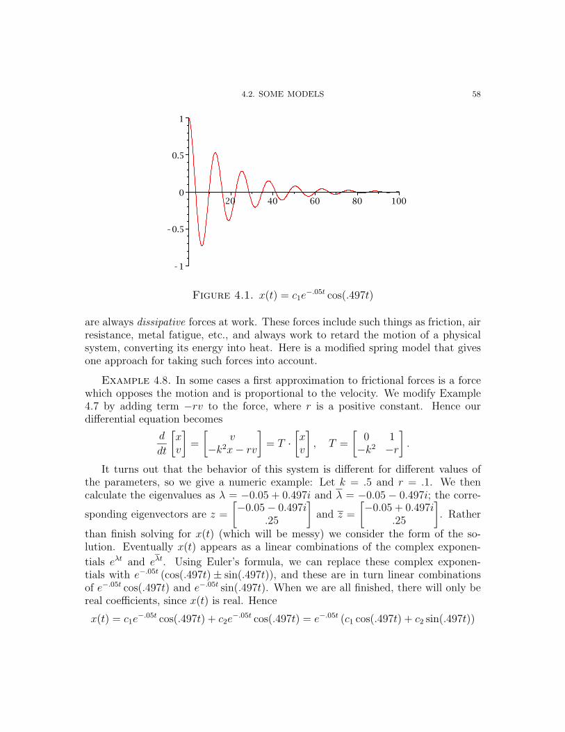
4.2. SOME MODELS 58
Figure 4.1. x(t) = c1e−.05t cos(.497t)
are always dissipative forces at work. These forces include such things as friction, airresistance, metal fatigue, etc., and always work to retard the motion of a physicalsystem, converting its energy into heat. Here is a modified spring model that givesone approach for taking such forces into account.
Example 4.8. In some cases a first approximation to frictional forces is a forcewhich opposes the motion and is proportional to the velocity. We modify Example4.7 by adding term −rv to the force, where r is a positive constant. Hence ourdifferential equation becomes
d
dt
[
xv
]
=
[
v−k2x− rv
]
= T ·[
xv
]
, T =
[
0 1−k2 −r
]
.
It turns out that the behavior of this system is different for different values ofthe parameters, so we give a numeric example: Let k = .5 and r = .1. We thencalculate the eigenvalues as λ = −0.05 + 0.497i and λ = −0.05 − 0.497i; the corre-
sponding eigenvectors are z =
[
−0.05 − 0.497i.25
]
and z =
[
−0.05 + 0.497i.25
]
. Rather
than finish solving for x(t) (which will be messy) we consider the form of the so-lution. Eventually x(t) appears as a linear combinations of the complex exponen-
tials eλt and eλt. Using Euler’s formula, we can replace these complex exponen-tials with e−.05t (cos(.497t) ± sin(.497t)), and these are in turn linear combinationsof e−.05t cos(.497t) and e−.05t sin(.497t). When we are all finished, there will only bereal coefficients, since x(t) is real. Hence
x(t) = c1e−.05t cos(.497t) + c2e
−.05t cos(.497t) = e−.05t (c1 cos(.497t) + c2 sin(.497t))
4.3. PHASE PORTRAITS 59
for some constants c1 and c2. The velocity v(t) will also have this general form; but
we can calculate it more quickly from x(t) by differentiating, since v =dx
dt.
We can now see how x(t) behaves as time increases: It is the product of a periodic
function, c1 cos(.497t) + c2 sin(.497t), with period2π
0.497, times an exponential e−.05t
which converges to 0 as t→ +∞. This system is an example of a damped harmonicoscillator : In each period x(t) comes back almost to its starting position, but witha smaller value. For large t the object is esentially stationary at the rest position ofthe spring. See Figure 4.1 for a sample.
4.3. Phase portraits
A graph like Figure 4.1 can help to visualize a dynamical system, but it showsonly a small part of the picture. Usually we can get considerable insight into theoverall behavior of a dynamical system by looking at another type of graph.
Suppose we have a vector differential equation fderivxt = f(x). This definesa flow F t as in the one-dimensional case: F t(x0) is equal to x(t) where x(t) isthe solution of the differential equation which satisfies the initial value conditionx(0) = x0. The existence of such a flow requires an m-dimensional version of theExistence and Uniqueness Theorem. We will postpone discussion of this until thenext chapter; it is valid for all systems that we will study. The analogs of Proposition2.2 and 2.5 are also true.
If x1 is a fixed state vector then we define the orbit or trajectory passing throughx1 to be the set of all points that are connected to x1 by the flow. That is, x2 is onthe orbit through x1 if F t1(x1) = x2 for some time value t1. We note some generalproperties of orbits:
Proposition 4.9. For any state vectors x1 and x2:
(a) x1 is on the orbit through x1.(b) If two orbits intersect then they are the same set.
Proof. x1 is on the orbit through x1, since F 0(x1) = x1.For the second part, suppose that the orbits through x1 and y1 have some state
in common – say z. Then if y2 is any point in the orbit through y1 then we can reachy2 from x1 as follows: Since z is on the orbit through x1 then F t(x1) = z for somet. Since z is on the orbit through y1 then F s(y1) = z for some s. Since y2 is on theorbit through y1 then F u(y1) = y2 for some u. Now use Proposition 2.2, twice:
F u−s+t(x1) = F u−s(F t(x1)) = F u−s(z) = F u−s(F s(y1)) = F u−s+s(y1) = F u(y1) = y2.
This means that y2 is on the orbit through x1. Since y2 was an arbitrary point ofthe orbit through y1 this means that the orbit through x1 contains the orbit through

4.3. PHASE PORTRAITS 60
y1. If we repeat this argument, starting with y1 , we see that the orbit through y1
contains the orbit through x1. So the two orbits are the same set.
Note: You may have seen this kind of argument before. It uses the relationx1 ∼ x2 defined by the condition that F t(x1) = x2 for some t. It follows fromProposition 2.2 that this relation is an equivalence relation, and the orbits are theequivalence classes.
In practical terms, all that Proposition 4.9 says is that the curves which aredescribed parametrically in state space by the solutions of the differential equationare the orbits. A description of all the orbits is called the phase portrait of thedynamical system.
We start with a simple example. Supposedx
dt= Hx where H =
[
1 00 −1
]
.
Then the solutions are given by x = etHx0, and, since H is diagonal, we have
etH =
[
et 00 e−t
]
. Hence, if x0 =
[
c1c2
]
, the solutions are given by
x1 = c1et, x2 = c2e
−t.
The orbit through (c1, c2) = (1, 1) is given parametrically as x1 = et, x2 = e−t.We can put this into a more recognizable form by eliminating t between the twoequations. If we multiply the equations together then the exponentials will cancel,leaving us with x1x2 = 1, which we recognize as a hyperbola, asymptotic to the x1
and x2 axes. Notice, though, that a hyperbola has two branches (in this case, in thefirst and fourth quadrants), but the orbit is just the branch of the hyperbola thatpasses through (1, 1).
We might ask for the orbit through the point (2, .5), but, since this is on thehyperbola through (1, 1), we do not expect a new orbit. To see this algebraically, notethat the orbit with (c1, c2) = (2, .5) is given parametrically as x1 = 2et, x2 = .5e−t,and if we eliminate t by multiplying the equations, we obtain x1x2 = 2 · .5 = 1, sowe still have the same hyperbola.
On the other hand, the orbit through (.5, .5) is given parametrically as x1 =.5et, x2 = .5e−t, and if we eliminate t between these equations we are left withx1x2 = .25, which is a different hyperbola. Again, the orbit is just the branch in thefirst quadrant.
These orbits are shown in Figure 4.2.In fact, three other orbits are shown in Figure 4.2.First, if the initial point is (c1, c2) = (0, 0) then the parametric equations become
x1 = 0·et = 0, x2 = 0·e−t, so x1(t) = 0, x2(t) = 0 for all t. That is, this orbit consistsonly of the point (0, 0). This is a special kind of orbit, called a stationary point (or

4.3. PHASE PORTRAITS 61
Figure 4.2. x′ = Hx, H =
[
1 00 −1
]
steady state, as in Chapter 2). When referring to the differential equationdx
dt= f(x)
such a point is usually called an equilibrium point. As in Chapter 2, any such pointscan be found by solving the equation f(x) = 0. In all our examples in this chapter,f(x) = Mx for some matrix M , so the origin will always be an equilibrium point.There may be other equilibrium points. In the next chapter we will look at systemswhere f(x) is more complicated than just multiplication be a matrix.
Another orbit shown in figure 4.2 is the positive x1 axis. This corresponds tothe initial condition (c1, c2) = (1, 0), which leads to the parametric equations x1 =et, x2 = 0 · e−t = 0. This represents the positive x1 axis since x2 is 0 for all t, whilex1 = et ranges over all positive real numbers as t ranges over (−∞,∞). Similarly,the positive x2 axis is an orbit.
The same kind of argument establishes the negative x1 and x2 axes as orbits.Note: These orbits along the axes do not contain the origin, since the origin is
another orbit and different orbits are disjoint.When we look at orbits we lose information about the time dependence of the
solutions. We can’t do much about this, but we can at least indicate in whichdirection the variable point (x1(t), x2(t)) moves along the orbit. This can be doneby differentiating the parametric equations for the orbit; the result, written as avector, points in the direction of motion of (x1(t), x2(t)). For example, the hyperbola

4.3. PHASE PORTRAITS 62
through (1, 1) has parametric equations x1 = et, x2 = e−t, and if we differentiate this
we obtaindx1
dt= et,
dx2
dt= −e−t. Then, for example, the point (1, 1) corresponds
to t = 0 and we have, this point, the vector (e0,−e−0) = (1,−1). Hence the point(x1(t), x2(t)) is moving along the hyperbola in this direction when t = 0. We concludethat the point (x1(t), x2(t)) moves from top to bottom (and left to right) along thehyperbola. This is true when t = 0, as we just calculated, and, more generally, forall t.
There is an easier way to see the direction of an orbit: We just calculated the
vector with coordinatesdx1
dtand
dx2
dt, working with a solution curve as it passes
through the point (x1, x2). But this is just, in vector terms,dx
dt. However, the
differential equation is in the formdx
dt= f(x), so we just need to calculate f(x)
to find the derivative vector of the solution curve through the point (x1, x2). Forexample, we could calculate the derivative at the point (1, 1) by this method, since
f
([
11
])
= H ·[
11
]
=
[
1−1
]
.
Using this method, it is easy to see that (x1, x2) moves along the second hyperbolain Figure 4.2 in the same direction, from top to bottom (and left to right). The motionalong the positive x1 axis is from left to right, and the motion along the positive x2
axis is from top to bottom. The origin is an equilibrium point, so it doesn’t move atall.
We can also see some limiting behavior. Points on the hyperbolic orbits in thefirst quadrant go to +∞, asymptotic to the x1 axis, as t → +∞, and to +∞,asymptotic to the x2 axis, as t → −∞. Points on the positive x2 asis converge to 0as t → +∞, and go to +∞ as t → −∞. The same kind of thing is true along thepositive x1 axis: points converge to the origin as t → −∞ and to +∞ as t → +∞.This is consistent with Proposition 2.5, which says that if a trajectory approaches alimit point in the domain of f then that limit point is an equilibrium point.
Before looking at some more examples we summarize a few facts about phase
portraits, in terms of the general equationdx
dt= f(x):
(1) Equilibrium points are orbits; they correspond to solutions of the algebraic equa-tion f(x) = 0.
(2) The vector f(x1) points in the direction of motion along the orbit passing throughthe ppoint x1.

4.3. PHASE PORTRAITS 63
Figure 4.3. x′ = Ax, A =
[
.01 .04
.02 −.01
]
(3) If a point on an orbit has a limit point x0 in the domain of f then x0 is an equilib-rium point (assuming the necessary conditions for the Existence and UniquenessTheorem at x0).
(4) Orbits are disjoint.
The next example is the “two cities” example (4.5). Several orbits, and thedirections of the vector field Ax, are shown in Figure 4.3. This is similar to thepicture in Figure 4.2, but the asymptotes of the hyperbolas are at an angle. Infact, the asymptotes are the lines through the eigenvectors v1 and v2. The originis an equilibrium point, since f(x) = Ax where A is a matrix, so f(0) = 0. Thehalf lines through the asymptotes are orbits. This is true true for any differential
equation of the formdx
dt= Mx, since, if v is an eigenvector of M corresponding to
the eigenvalue λ, then eλtv is a solution of the differential equation. Note that thisonly gives positive multiples of the eigenvector, so the orbit is a half-line. The otherhalf of the line through v is also an orbit, since −v is also an eigenvector, so the setof positivemultiples of −v is an orbit.

4.3. PHASE PORTRAITS 64
Figure 4.4. x′ = Bx, B =
[
−.02 .02.01 −.03
]
From Figure 4.3 we see that all population vectors in the first quadrant move to
be asymptotoc to the first eigenvector v1 =
[
21
]
as t→ +∞, as we discovered in our
earlier analysis of (4.5).
Equilibrium points that “look like” Figure 4.2 are called saddle points. We willexplain exactly what this means in the next chapter, but for now we can characterizethis picture by the condition that the eigenvalues are real, with one positive and onenegative.
The next example is our second “two cities” example, (4.6). Figure 4.4 showsthe equilibrium at the origin, and the straight line orbits along the half lines throughthe eigenvectors. In this example, all orbits converge to the origin as t → +∞,as we discovered in our earlier analysis of (4.6). As in that analysis, we see thatall population vectors in the first quadrant eventually turn and approach the origin
asymptotically to the positive line through the eigenvector v1 =
[
21
]
. In fact, all
orbits do this except the origin and the two straight line orbits corresponding to the
other eigenvector, v2 =
[
−11
]
.

4.3. PHASE PORTRAITS 65
Figure 4.5. x′ = Sx, S =
[
0 1−k2 0
]
, k = .5
In general, an equilibrium is called a sink or attractor if all near-by points con-verge to the equilibrium as t→ +∞. If we reverse the arrows in Figure 4.4 then wewill have an example of a source or repellor, in which all near-by points converge tothe equilibrium as t→ −∞.
The spring model, Example 4.7, has very different solutions from the populationmodels. The eigenvectors are purely imaginary, and the solutions are periodic. Thephase portrait is shown in Figure 4.5, with the parameter k = .5. The origin isstill an equilibrium, but there are no straight-line solutions, since the eigenvectorsare not real. If (x(t), v(t)) is a solution then both x(t) and v(t) are periodic, withperiod 2π/k = 4π. This means that the solution point (x(t), v(t)) will return toexactly its starting position after 4π time units; and then it will simply retrace itspath. In other words, the orbit is a closed curve. This is the only way a solutioncurve can ever intersect itself; if it did anything else than retrace its steps thenit would violate the uniqueness theorem. e previously calculated that the solutionwith initial condition x(0) = x0, v(0) = 0 is x(t) = x0 cos(kt) = x0 cos
(
12t)
, v(t) =
−kx0 sin(kt) = −12x0 sin
(
12t)
. Then
x2
x20
+v2
x20/4
= cos2(
12t)
+ sin2(
12t)
= 1.

4.3. PHASE PORTRAITS 66
Figure 4.6. x′ = Tx, T =
[
0 1−k2 −r
]
, k = .5, r = .1
In other words, the orbit through (x0, 0) is an ellipse, with semi-major axes |x0| and12|x0|.
An equilibrium is sometimes called a center if all nearby orbits are closed orbits.
Our last example is the damped oscillator of Example 4.8, with the parametersk = .5, r = .1. Again the origin is an equilibrium. In our previous analysis we sawthat all solutions converge to the origin as t → +∞, so this is another example ofa sink. However, the eigenvalues are not real, and this means that the solutions aregiven by periodic functions times an exponential factor which converges to 0. Thisforces the solutions to spiral around the origin as they converge to it, as shown inFigure 4.6.
In this example the origin is called a spiral sink. In general, for constant coefficientlinear systems, the origin is a sink if all the eigenvalues have negative real part (thisincludes real eigenvalues that are negative). In two dimensions it is called a spiralsink if, in addition, the eigenvalues are not real. In higher dimensions this spirallingbehavior is more complicated, and harder to visualize.

EXERCISES 67
Exercises
4.1. Calculate eA:
(a) A =
0 1 00 0 10 0 0
. Use the series.
(b) A =
a 1 00 a 10 0 a
. Use the fact that A = aI + A1 where A1 is the matrix in
part (a).
(c) A =
[
1 16 0
]
. Use eigenvalues and eigenvectors.
4.2. Derive (4.3) by following this outline:
(a) Let A =
[
a 00 a
]
and B =
[
0 −bb 0
]
. Show that eC = eA · eB.
(b) Show that eA = eaI.
(c) Let J =
[
0 −11 0
]
. The powers Jn follow a periodic pattern. What is it?
(d) Since B = bJ we have Bn = bnJn. Plug this into the series for eB anduse the same idea as in the proof of Euler’s formula to show that eB =[
cos(b) − sin(b)sin(b) cos(b)
]
.
(e) Finish.
4.3. This exercise demonstrates some of the borderline cases of phase portraits forlinear systems. For each of the following, prepare a sketch of the phase portrait
fordx
dt= Ax and indicate how it compares to the examples in Figures 4.3 – 4.6.
(a) Repeated eigenvalues: A =
[
−1 00 −1
]
. This doesn’t require Maple: analyze
the straight-line solutions.
(b) Zero eigenvalue: A =
[
−2 12 −1
]
. First find the equilibrium points.
(c) Repeated eigenvalues: A =
[
−3 4−1 1
]
. Use Maple.
(d) Repeated zero eigenvectors: A =
[
2 4−1 −2
]
.
EXERCISES 68
4.4. Let A =
[
a bc d
]
, T = trA = a+ d (the trace of A) and D = detA = ad− bc (the
determinant of A).(a) Check that the characteristic polynomial of A is λ2 − Tλ+D.(b) Use the quadratic formula to solve for the eigenvalues in terms of T and D.(c) If λ1 and λ2 are the eigenvalues then the characteristic equation factors as
(λ − λ1)(λ − λ2). Multiply this out and compare with the formula in (a) toconclude that T is the sum of the eigenvalues and D is their product. (Thisfact holds for m×m matrices, for any m.)
4.5. Using the results of Exercise 4.4, determine the conditions on T and D that leadto(a) Periodic orbits (eigenvalues purely imaginary, not 0).(b) A saddle (eigenvalues are real, one positive, one negative).(c) A sink (both eigenvalues have real part less than 0).(d) A spiral sink (a sink with non-real eigenvalues).
4.6. “Two city” population models like Example 4.5 have the formdx
dt= Ax, where
A is 2 × 2 and the terms off the diagonal (corresponding to migration) are non-negative.(a) Explain why such a system must have real eigenvalues. You might want to
use the results of Exercises 4.4 and/or 4.5.(b) This is harder: Explain why etA is a positive matrix for all t > 0.
4.7. In Example 4.8 the choice of k = .5 and r = 0 leads to a center, while k = .5 andr = .1 leads to a spiral sink. In the following, assume k = .5.(a) Find a formula for the eigenvalues of the system in terms of r.(b) Show that there is a sink at the origin for all r > 0.(c) There is a value rc so that there is a spiral sink for 0 < r < rc, and a non-spiral
sink for r ≥ rc. Find rc.(d) The solution, in case of a spiral sink, involves trig functions times exponential
functions. What is the period of the trig functions, as a function of r?

CHAPTER 5
Non-linear systems in two dimensions
5.1. A predator-prey model
Here is a further modification of the “rabbit island” models from chapter 2.We will use y to represent the number of rabbits on the island. Then a very simple
first approximation to modelling their population is the equationdy
dt= ry where r
is a positive parameter, representing the net growth rate of the rabbit population.This was covered in Example 2.1; we find that y(t) = erty0, so any positive initialpopulation will grow exponentially fast.
On similar grounds, suppose we represent the number of foxes on the island asx. If there is nothing edible on the island (except, perhaps, carrots) then we wouldexpect the foxes to die off. As a first approximation to this we can use a differential
equation likedx
dt= −sx where s is a positive parameter. Here −s represents the
net growth rate of the fox population, and it is negative since we expect that thedeath rate will be larger than the birth rate. Solving the differential equation leadsto x(t) = e−stx0, so any initial population of foxes will die off exponentially fast.
Now suppose both rabbits and foxes are present on the island. In this case weneed to model their interactions: foxes will now find something edible on the island,so we would expect the net growth rate for foxes to rise. Of course, at the same timewe would expect the net growth rate for rabbits to fall. More specifically, we replacethe net growth rate r for rabbits by r − βx where β is a positive constant. That is,the net growth rate for rabbits should decrease if foxes are present, and this decreaseshould be proportional to the number of foxes. On the other hand, we replace thenet growth rate −s for foxes by −s+ αx, where α is a positive constant, so the netgrowth rate for foxes will increase, and the amount of the increase is proportional tothe number of rabbits.
Putting everything together we have the following model. This model was firstproposed in the 1920’s (independently) by Volterra and Lotka, and this and similarmodels are known as Lotka-Volterra systems.
69

5.1. A PREDATOR-PREY MODEL 70
Example 5.1. Let z =
[
xy
]
. Then the predator-prey system is
dz
dt= f (z) =
[
(−s+ αy)x(r − βx)y
]
.
Here x and y represent populations of the predator (foxes) and the prey (rabbits);r,s,α,β are positive parameters.
It is not possible to solve this system of equations using elementary functions.We will instead try to find out as much as possible about the phase portrait of thesystem.
The first thing to do is to locate the equilibrium points. To do this we set f(z) = 0
and solve for z. Using z =
[
xy
]
and the definition of f(z) in Example 5.1, we get
(−s+ αy)x = 0
and
(r − βx)y = 0
which is equivalent to
x = 0 or y =s
αand
y = 0 or x =r
β
Since the combinations x = 0 with x =r
βand y = 0 with y =
s
αare impossible,
there are only two equilibrium points:
(0, 0) and
(
r
β,s
α
)
.
In fact, we can learn more from this calculation. Looking just at the x variable,
we haved
dtx(t) = (−s + αy(t))x(t). Then, by inspection, x(t) = 0 for all t is a
solution, and it doesn’t matter what y(t) is. In other words, if a solution startson the y axis (meaning x(0) = 0) then it will stay on the y axis (meaning x(t) =0) for all time. On the other hand, if x(t) = 0 for all t then the equation for y
becomesd
dty(t) = (r − αx(t))y(t) = ry(t), and this has the solution y(t) = y0e
rt.
So we have found the solutions that start on the y axis, (x(t), y(t)) = (0, y0ert).
Hence the positive and negative y semi-axes are trajectories, directed away from theorigin. Similarly, the solutions that start on the x axis stay there, and have the form(x(t), y(t)) = (x0e
−st, y), so the positive and negative x semi-axes are trajectories,directed toward the origin.
We have now found six trajectories of the system (the two equilibria and the foursemi-axes). It is always important to locate the equilibrium points, as we shall see,but the semi-axes are orbits only because of special features of this system. Namely,

5.1. A PREDATOR-PREY MODEL 71
we needed the fact that any orbit that starts on the y axis stays on the y axis, and
this was a consequence of the fact thatdx
dt= xg(x, y) where g(x, y) is a function
of x and y. We record this as a fact that is useful in some systems, especially inpopulation models.
Proposition 5.2. Ifdx
dt= f(x) is an m-dimensional differential equation and
the jth component of f(x) has xj as a factor then any solution that starts on thehyperplane defined by xj = 0 stays on that hyperplane for all time.
The pattern of straight line solutions through the origin is just like what we foundfor a saddle equilibrium, as in Figure 4.2. However, our predator-prey system is non-linear and we can’t expect the same phase portrait as for a linear system. In fact,we know that the phase portrait is different, since our system has two equilibria, buta linear hyperbolic system has only one equilibrium.
However, we can look at the equilibrium point at the origin as follows. First,rewrite f(z):
(5.1) f (z) =
[
(−s+ αy)x(r − βx)y
]
=
[
−sxry
]
+
[
αxy−βxy
]
=
[
−s 00 r
]
·[
xy
]
+
[
αxy−βxy
]
.
That is, we have written f(z) as the sum of two terms. The first has the form Az
where A is the constant matrix
[
−s 00 r
]
; it is called the linearization of f at the
origin. The second term involves only “higher powers” of x and y. If x and y are“small enough” then the entries in this second term, αxy and −βxy, will be muchsmaller than the entries −sx and ry in the linearization Az. In this case it is natural
to compare the solutions of the non-linear differential equationdz
dt= f(z) to the
solutions of the linearized equationdz
dt= Az. We will see, in the next section, a
general theorem which says, in case A is hyperbolic, that the solutions “near” anequilibrium of the non-linear system “look like” the solutions of the linearized systemnear the origin.
In our case the matrix A =
[
−s 00 r
]
has eigenvalues −s and r, so, since neither of
these has zero real part, the matrix is hyperbolic. So, near the origin, the trajectoriesof the predator-prey system are approximately the same as the trajectories of the
linearized systemdz
dt=
[
−s 00 r
]
· z near the origin, and this linear system has a
saddle equilibrium at the origin. Hence its trajectories consist of the origin, the x

5.1. A PREDATOR-PREY MODEL 72
and y semi-axes, and “hyperbola-like” curves asymptotic to the axes, similar to thetrajectories in Figure 4.2.
In Figure 4.2 the curves shown were true hyperbolas, and we verified this byeliminating t in the parametric equations for the orbits to obtain equations for theorbits in the form xy = C. We can do the same for our linearized system, but it ismore instructive to work as follows. Consider one trajectory; we know that it has theparametric form x = x(t), y = y(t) where (x(t), y(y)) is a solution of the differentialequation. In most cases we should be able to eliminate t between these equationsto obtain an equation y = h(x) for the trajectory. Using the chain rule we find adifferential equation for y as a function of x:
dy
dx· dxdt
=dy
dtchain rule
dy
dx=dy/dt
dx/dtdivision
dy
dx= −ry
sxsince
d
dt
[
xy
]
=
[
−s 00 r
] [
xy
]
, sodx
dt= −sx, dy
dt= ry.
Now we can solve the equationdy
dx= −ry
sxusing the method of Chapter 2. We will
modify this method slightly:
(1) Write in differential form: dy = −rysx
dx.
(2) Separate the variables:dy
ry= −dx
sx.
(3) Write the equation so that 0 is on the right hand side:dx
sx+dy
ry= 0.
(4) Integrate, putting the constant of integration on the right hand side, and simplifyto taste:
∫
dx
sx+
∫
dy
ry= C1
1
sln |x| + 1
rln |y| = C1
r ln |x| + s ln |y| = rsC1 = C2 multiply by rs
ln (absxr · absys) = C2 properties of the log
|x|r|y|s = eC2 = C exponentiate
We have left the equation in the form |x|r|y|s = C for several reasons.First, this is also satisfied by the origin, and by the x and y semi-axes, with
C = 0.

5.1. A PREDATOR-PREY MODEL 73
Second, this is recognizable as being “hyperbola-like”; in fact, if r = s then wecan take rth roots of both sides to get the form |x| |y| = C1/r = C0, which represents
the hyperbolas y = ±C0
x. If, for example, r = 2s then we would have curves like
y = ±C0
x2, which have the same general appearance as hyperbolas.
Third, we can see this as a special case of the form ϕ(x, y) = C, where ϕ(x, y), inthis case, is given by ϕ(x, y) = |x|r|y|s. Our analysis can be summarized as sayingthat the function ϕ is a conserved quantity or constant of the motion. This meansthat the value of ϕ(x(t), y(t)) is constant along any trajectory of the system, andthat is just what we found above. Conversely, if we have a constant of the motion ϕand ϕ(x0, y0) = c then phi(x(t), y(t)) = c holds for all t, if (x(t), y(t)) is a solution ofthe differential equation passing through (x0, y0). In other words, the orbit through(x0, y0) must lie in the level curve defined by ϕ(x, y) = c. It is not always possibleto find a useful constant of the motion, but if you do find one then you have a gooddescription of all the orbits of the system.
Let us try to apply the above technique to find a constant of the motion for thepredator-prey system:
dy
dx=dy/dt
dx/dt
=(r − βx)y
(−s+ αy)xsince
d
dt
[
xy
]
=
[
(−s+ αy)x(−s+ αy)x
]
dy =(r − βx)y
(−s+ αy)xdx write in differential form
−s+ αy
ydy =
r − βx
xdx separate variables
(
− r
x+ β
)
dx+
(
−sy
+ α
)
dy = 0 0 on the right
( r
x− β
)
dx+
(
s
y− α
)
dy = 0 multiply by − 1
r ln |x| − βx+ s ln |y| − αy = C1 integrate
er ln|x|−βx+s ln|y|−αy = eC1 = C exponentiate
er ln|x|e−βxes ln|y|e−αy = C properties of exponents
|x|re−βx|y|se−αy = C using ea ln b =(
eln b)a
= ba
So we have found a constant of the motion: ϕ(x, y) = |x|re−βx|y|se−αy.

5.1. A PREDATOR-PREY MODEL 74
Figure 5.1. Example 5.1 with r = .1, s = .2, α = .0001, β = .001.Time is measured in months.
The first thing we notice about ϕ is that it is zero exactly on the x and y axes, andwe have already seen that the origin and the 4 semi-axes are orbits. We concentrateon the first quadrant (which is all that is relevant in a population model). For x > 0the function xre−βx is non-negative; it approaches 0 as x → ∞; and it has only
one critical point, at x =r
β, where it has its maximum. The function yse−αy has a
similar description, with a maximum when y =s
α. The conserved quantity ϕ(x, y) is
the product of these two functions, so it has a strict maximum in the first quadrant
at
(
r
β,s
α
)
. If we write M for the maximum value of ϕ in the first quadrant then
we have just shown that the level set ϕ(x, y) = M is a single point, so this point is
an orbit of the dynamical system. Of course, we already knew this, since
(
r
β,s
α
)
is
the second equilibrium point.The rest of the first quadrant is covered by the level curves ϕ(x, y) = c with 0 <
c < M . It should be clear that these are closed curves surrounding the equilibrium
at
(
r
β,s
α
)
: Think of the graph of z = f(x, y); over the first quadrant this surface is
a “hill”, and our level curves ϕ(x, y) − c can be thought of as “slicing” this surfaceby a horizontal plane.

5.2. LINEARIZATION 75
The various features of the phase portrait in the first quadrant are illustrated inFigure 5.1. Since the orbits corresponding to ϕ(x, y) = c for 0 < c < M are closedorbits they correspond to periodic solutions. However, unlike the periodic orbits inthe linear case, Example 4.7, the periods depend on the orbit. It is easy to see thatthis must be so, since as c gets closer to 0 the orbit must pass very close to theorigin. However, the vectors f(x, y), for (x, y) near the origin, are very small, andso the point (x(t), y(t)) moves very slowly while it remains near the origin. Thereis no expression for the period in terms of c, but in the next section we shall see
some evidence that the period should be approximately2π√rs
for orbits close to the
equilibrium point
(
r
β,s
α
)
.
5.2. Linearization
The first step in analyzing a phase portrait is usually to find and classify theequilibrium points. Suppose the differential equation is written in the vector formdx
dt= f(x). It is relatively straightforward to find the critical points: we just write
f(x) =
[
f1(x, y)f2(x, y)
]
and solve the two equations f1(x, y) = 0, f2(x, y) = 0 simultane-
ously.Graphically, the equations f1(x, y) = 0 and f2(x, y) = 0 define curves in the xy
plane, and the equilibrium points are the intersections of these curves. These curvesare called nullclines and are often useful in understanding the geometry of the phaseportrait. The first, with equation f1(x, y) = 0, is the set of points where the thevector field f(x, y) has zero x coordinate; these are the points where the solutioncurves have a vertical tangent. Hence this is called the vertical nullcline. Similarly,f2(x, y) = 0 defines the set of points at which the solution curves have a horizontaltangent, so this set is called the horizontal nullcline. A more general type of curveis an isocline; this is a curve where the solution curves all have a given slope.
As an example of finding and classifying equilibria we start with a modification tothe predator-prey system of Example 5.1. In that system the rabbits population, inthe absence of predators, will grow exponentially. This is unrealistic, and we alreadysaw, in Example 2.4, a more reasonable one-species model, in which the populationgrowth is modified by a “crowding term”. We add this idea to our predator-preysystem, so that the net growth rate for the prey population is reduced not only by alinear term proportional to the number of foxes but also by a linear term proportionalto the number of rabbits:

5.2. LINEARIZATION 76
Example 5.3. Let z =
[
xy
]
. The modified predator-prey system is
dz
dt= f (z) =
[
(−s+ αy)x(r − βx− δy)y
]
.
Here x and y represent populations of the predator (foxes) and the prey (rabbits);r,s,α,β,δ are positive parameters.
We shall assume that
(5.2)r
δ− r
α> 0
Exercise 5.10 describes the situation when this condition is not satisfied.
We start our investigation of this system by drawing the nullclines. The verticalnullcline is defined by setting the x component of f(z) to zero, so (−s + αy)x = 0.Since the right hand side is 0 the only way that this can happen is if one of thefactors on the left is 0, and this leads to x = 0 or y = s/α. Thus the horizontalnullcline is the union of the two straight lines with these equations. Similarly thehorizontal nullcline is defined by (r − βx − δy)y = 0, so it is the union of the twostraight lines with equations y = 0 and βx+ δy = r.
We can find the equilibria by solving the equations for the nullclines simultane-ously, as we did for Example 5.1. There are four possibilities for solutions, sinceeach nullcline is the union of two straight lines. The pair of lines x = 0 and y = 0determines the equilibrium at the origin, O = (0, 0). If x = 0 and βx + δy = r we
find that y = r/δ, and this gives the second equilibrium, C =(
0,r
δ
)
. If we solve
y = s/α and βx + δy = r we find x = r/β − sδ/(αβ), so a third equilibrium is at
S =
(
r
β− sδ
αβ,s
α
)
. The x coordinate of S can be factored asδ
β·(r
δ− s
α
)
, and
this is positive by the condition (5.2). Hence S is in the first quadrant. The fourthcombination is y = 0 and y = s/α, and these lines do not intersect.
Figure 5.2 shows the nullclines and the equilibria, for a typical choice of param-eters. With these parameters C = (0, 5000) and S = (60, 2000). The point (0, 2000)is not an equilibrium point since it is not an intersection point of the two nullclines:it is on the vertical nullcline, but it is not on the horizontal nullcline. Similarly, thepoint (100, 0) is not an equilibrium point.
We have shown horizontal and vertical arrows along the nullclines. The directionsof the arrows are determined from the vector field f . For example, on the x axis,
which is part of the horizontal nullcline, we have y = 0 sodx
dt= (−s+ βy)x = −sx.
This is negative for x > 0 and positive for x < 0, so the field points to the leftfor x > 0 and to the right for x < 0. In general, along a nullcline the direction

5.2. LINEARIZATION 77
Figure 5.2. Nullclines for Example 5.3, with r = .1, s = .2, α =.0001, β = .001, δ = .0002.
of the arrows can only change at the equilibrium points. For example, along thehorizontal nullcline the direction of the vector field is determined by the sign ofits x component, and, by continuity, this sign can only change at points where thex component becomes 0. Hence, to determine the direction of the arrows along anullcline it is only necessary to divide it into pieces by cutting it at the equilibriumpoints, and then to check one point on each piece.
Warning: The nullclines are not, in general, solution curves. In Figure 5.2 thex and y axes are unions of trajectories, as is the equilibrium point S, but at otherpoints on the nullclines the solutions cross the nullclines.
Our next step in analyzing the phase portrait is to consider the linearization ofthe vector field near each equilibrium. We did this in the last section using equation(5.1), which exhibits f(z) as a linear function plus terms of “higher order”. We needa more systematic way of doing this. This is provided by the Linear ApproximationTheorem from multi-variable calculus; see Theorem A.6.
The procedure is as follows: For the vector differential equationdz
dt= f(z) we first
calculate the matrix derivative Df . Then, at each equilibrium point p we calculatethe eigenvalues of Df(p). Then we can apply the following two theorems, which willbe discussed later in this chapter.

5.2. LINEARIZATION 78
Theorem 5.4 (Hartman-Grobman). Suppose f is C1. If p is an equilibrium
point ofdz
dt= f(z) and A = Df(p) is hyperbolic then, for some positive r, there is
a change of variables w = h(p), defined for ‖v − p‖ < r, which transforms orbits ofthe system z′ = f(z) to orbits of the linearized system w′ = Aw.
Precisely, if z(t) is the solution of z′ = f(z) satisfying z(0) = z0 and w(t) isthe solution of w′ = Aw satisfying w(0) = h(z0) then w(t) = h(z(t)) as long as‖z(t) − p‖ < r.
Because of this theorem it is common to declare an equilibrium point p to be hy-perbolic if the derivative matrix Df(p) is hyperbolic. In two dimensions the theoremguarantees the following behavior of orbits near a hyperbolic equilibrium point.
(1) If all eigenvalues of Df(p) have negative real part then p is a sink. That is, if z0
is near enough to p then the solution z(t) of z′ = f(z), z(0) = z0 converges to pas t→ +∞, and, for some t < 0, it moves outside the disk of radius r around p.
(2) If all eigenvalues of Df(p) have positive real part then p is a source. That is, if z0
is near enough to p then the solution z(t) of z′ = f(z), z(0) = z0 converges to pas t→ −∞, and, for some t > 0, it moves outside the disk of radius r around p.
(3) If one eigenvalue is a positive real number and the other is negative then thereare two solutions starting near p which converge to p as t→ +∞, and there aretwo which converge to p as t → −∞. These are called the stable and unstablecurves at p. If z0 is near enough to p and is not equal to p and is not on a stableor unstable curve then then the solution z(t) of z′ = f(z), z(0) = z0 leaves thethe disk of radius r around p at some positive time and also at some negativetime. In this case the equilibrium is called a saddle point.
In the case of a sink or source we expect to see spiralling behavior if the eigenvaluesare non-real. In the case of a saddle point we expect that the stable and unstablecurves will have the same direction, at p, as the eigenspaces. These are both, in fact,true, but they do not follow from Theorem 5.4, since the change of variables h is, ingeneral, not differentiable at p. We will discuss this further in a later section.
We now apply the linearization procedure to the system of Example 5.3. We
first calculate Df . The first column of this matrix is∂f
∂xand the second is
∂f
∂y.
Differentiating
[
(−s+ αy)x(r − βx− δy)y
]
=
[
−sx+ αxyry − βxy − δy2
]
with respect to x and y gives
Df(x, y) =
[
−s+ αy αx−βy r − βx− 2δy
]
.
Next, we consider each equilibrium point:

5.2. LINEARIZATION 79
The first equilibrium is at the origin. Plugging (0, 0) into the formula for Df
gives Df(0, 0) =
[
−s 00 r
]
. This has eigenvalues −s and r, so this equilibrium point
is a hyperbolic saddle. The corresponding eigenvectors are
[
10
]
and
[
01
]
, so we expect
that the stable and unstable curves at the origin will be tangent to the x and y axes.In fact, we already know that the x and y axes are unions of orbits.
The second equilibrium is C = (0, r/δ), so
Df(C) = Df(
0,r
δ
)
=
[
−s+ α · r/δ 0β · r/δ r − 2r
]
=
[
−s+ α · r/δ 0−β · r/δ −r
]
.
The eigenvalues are λ1 = −s + α · rδ
= α(r
δ− s
α
)
and λ2 = −r. Condition (5.2)
implies that λ1 is positive, so C is another hyperbolic saddle. The second eigenvector
is v2 =
[
01
]
, and this is consistent with the fact that the y axis is a union of solutions.
The eigenvector corresponding to λ1 is messier: v1 =
[
1−rβ/ (rδ + (rα− sδ))
]
. It
follows from (5.2) that the slope of this vector is less than 0 and greater than −β/δ,which is the slope of the line βx + δy = r. Thus we expect the unstable curve at Cin the first quadrant to start at C at a negative slope, but greater than the slope ofthe horizontal nullcline passing through C.
The third equilibrium is S =
(
r
β− δs
αβ,s
α
)
, so
Df(S) =
[
−s+ α · s/α α (r/β − δs/(αβ))−β · s/α r − β (r/β − δs/(αβ)) − 2δ · s/α
]
=
[
0 (αr − δs)/β−βs/α −δs/α
]
The 1, 2 entry in this matrix may be written asαδ
β
(r
δ− s
α
)
, so, by condition (5.2), it
is positive. Hence this matrix has negative trace and positive determinant, and, usingexercise 4.5, we conclude that both eigenvalues have negative real part. Therefore Sis a hyperbolic sink. Further calculation shows that the sink is a spiral sink as long
asr
δ− s
α>
sδ
4α2.
Figure 5.3 shows the phase portrait in the first quadrant, with the same param-eters as in Figure 5.2; the scale has been changed to accommodate more orbits. Inthe figure the sink at S is obvious. The stable and unstable curves correspondingto the saddle at the origin lie on the x and y axes, and any orbit that passes close

5.2. LINEARIZATION 80
Figure 5.3. Example 5.3, with r = .1, s = .2, α = .0001, β =.001, δ = .0002. Time is measured in months.
to the origin has a “hyperbola-like” shape. For example, points starting in the firstquadrant near (100, 0) will move to the left, tracking the orbit on the stable curveon the x axis, and will slowly rise as they get near the origin. Eventually they willcome close enough to the y axis that they will begin to track the unstable curve onthe y axis. However, the curve will not continue to approach the y axis, since itwill eventually come under the influence of the sink or the saddle at C = (0, 5000).Points close to C will similarly track one of the stable curves at C, which converge toC along the y axis from above or below. When they get close enough to C they willstart moving away from C, tracking the unstable curve at C. This unstable curve isindicated on the Figure: It starts at C in the direction given by the eigenvector of thelinearized system which corresponds to the positive eigenvalue at C, and eventuallyit spirals toward the sink S.
The figure illustrates another feature of this example. Any orbit which starts inthe open first quadrant converges to the sink S as t → +∞. It requires some workto prove this, because it is necessary to explain why orbits that start with a largey coordinate will move far to the right, but will eventually move back towards theorigin with a y value less than the y value at the sink. Skipping this argument, weformalize this picture with a definition. If p is a sink of a dynamical system then wedefine the basin of attraction of p to be the set of all points (x, y) which approach p ast→ +∞. By the Hartman-Grobman Theorem we know that every point sufficiently

5.3. CONSERVATION OF ENERGY AND THE PENDULUM PROBLEM 81
Figure 5.4. The pendulum.
near p is in the basin, but the basin is usually much more extensive. In this case thebasin is the entire open first quadrant.
It is also interesting to ask where points came from. In this example, almost allpoints in the open first quadrant “go to ∞” as t→ −∞. In fact, in most cases theseorbits blow at a finite negative value of t. The only exceptions are the sink S, whichstays fixed for all t; and the points on the unstable curve of the saddle C, whichconverge to C as t→ −∞.
5.3. Conservation of energy and the pendulum problem
A classic physics problem is the simple pendulum. This system is confined to avertical plane. A mass m is attached to a massless, rigid rod of length L; the otherend of the rod is attached to a fixed point and is free to pivot about this point. Thereis no friction, and the only force acting on the mass is gravity. Then the mass isconstrained to move in a circle of radius L centered at the pivot point. See Figure5.4.
We use the angle x as the position variable, and notice that the tangential com-ponent of the gravitational force (0,−mg) has magnitude mg sin x. From this wederive, by a suitable variation of Newton’s Second Law, the following model:
Example 5.5. The ideal pendulum: The motion is governed by the equationd2x
dt2= −a2x where a2 =
g
L. The initial value problem for this equation is x(0) =

5.3. CONSERVATION OF ENERGY AND THE PENDULUM PROBLEM 82
x0,dx
dt(0) = v0 where x0 is the initial angular displacement and v0 is the initial
angular velocity.
As we did in the spring example 4.7, we replace this second order equation witha system of first order differential equations, by introducing the angular velocity
v =dx
dtas a second variable. Then
dv
dt=d2x
dt2= −a2 sin x, so the system version of
this model is
(5.3)dx
dt= v,
dv
dt= −a2 sinx.
It is not possible to find the solution curves of this system in terms of elementaryfunctions of t.
We start analyzing this system by examining its equilibrium points. Sincedx
dt= v
the vertical nullcline is defined by v = 0, so this is just the x axis. Sincedv
dt=
−a2 sin x the horizontal nullcline is defined by sin x = 0. This corresponds to infin-itely many vertical lines, defined by x = nπ where n is an integer. Hence the equi-libria are at the points (nπ, 0). When n = 0 this is just the origin, so x = 0, v = 0.This makes physical sense, since it corresponds to the pendulum hanging straightdown (the angle x is 0) and at rest (the angular velocity v is 0). The points (2kπ, 0)correspond to the same physical situation, since an angle of 2kπ also describes thependulum hanging straight down. The equilibria of the form ((2k + 1)π, 0) corre-spond to the physical situation where the pendulum is pointing straight up, and theangular velocity is 0. This makes some physical sense: remember that the shaft ofthe pendulum is rigid, so it is possible, although very unlikely, for it to balance inthis position and remain there for all time.
We can calculate the linearization of the system at these equilibria. Writing
f(x, v) =
[
v−a2 sin x
]
we obtain Df(x, v) =
[
0 1−a2 cosx 0
]
, so
Df(2kπ, 0) =
[
0 1−a2 0
]
, Df((2k + 1)π, 0) =
[
0 1a2 0
]
.
At the even multiples of π the eigenvalues are ±ai, with zero real part, so theseequilibria are not hyperbolic and the linearization process is not applicable. Accord-ing to ??? the solution curves near these equilibria must cycle around the origin,
approaching a rotation with period2π
a, but the linearization cannot tell us whether
the orbits are closed.

5.3. CONSERVATION OF ENERGY AND THE PENDULUM PROBLEM 83
At the odd multiples of π the eigenvalues are a and −a, so these equilibria are
saddles. The corresponding eigenvectors are
[
1a
]
and
[
1−a
]
, so the unstable curves
at these equilibria will have slope a, while the stable curves will have slope −a.We need more information before we can describe the behavior near the other
set of equilibria. In fact, we can get a full picture of the phase portrait by finding aconstant of the motion.
Most idealized models of simple physical systems have a particular constant ofthe motion, which is known in physics as the total energy of the system. In our casethis can be defined as ϕ(x, v) = 1
2v2 − a2 cosx. In physical terms this is the sum of
the kinetic energy K = 12v2 and the potential energy V = −a2 cosx, and these are
related to the differential equation bydx
dt=∂K
∂vand
dv
dt= −∂V
∂x. If we ignore the
physical meaning of these quantities we can simply verify
(5.4)dx
dt=∂ϕ
∂v,
dv
dt= −∂ϕ
∂x.
But these equations immediately imply that ϕ is a constant of the motion, since
d
dtϕ(x(t), v(t)) =
∂ϕ
∂x
dx
dt+∂ϕ
∂v
dv
dt=∂ϕ
∂x
∂ϕ
∂v+∂ϕ
∂v
(
−∂ϕ∂x
)
= 0.
So each orbit of the system lies in a single level curve, of the form ϕ(x, y) = c.To analyze these level curves, first note that − cosx ≥ −11 and v2 ≥ 0 so ϕ(x, v) =12v2 − a2 cosx ≥ 0 − a2(1) = −a2. So −a2 is a lower bound for ϕ; moreover, it is
the minimum value of ϕ since ϕ(2kπ, 0) = −a2 cos(2kπ) = −a2. Hence the level setdefined by ϕ = −a2 consists only of the points (2kπ, 0), so each of these points is asingle orbit. We already knew this, since each of these is an equilibrium point.
Since −a2 is the minimum value of ϕ the level sets ϕ = c for c < −a2 are empty.Suppose now that c > −a2. Then a2 cos(x) + c > 0 so the equation ϕ(x, y) =
12v2 − a2 cosx = c can be solved for v in terms of x, as
(∗) v = ±√
2a2 cos(x) + 2c.
If c > a2 then 2a2 cos(x) + 2c > 2a2(−1) + 2c > 0 for all values of x, so the levelcurve ϕ = c consists of two components, each defined for all x, one above the x axisand one below. Thus each of these components is an orbit.
If −a2 < c < a2 then the functions in (∗) are not defined for all x. To see this, letxc = cos−1
(
− ca2
)
. This is defined since |c/a2| < 1, and is in the interval (0, π). Since
the cosine function is even and is decreasing on (0, π) we have 2a2 cos(x) + 2c > 0for |x| < xc and 2a2 cos(x) + 2c < 0 for xc < |x| ≤ π. Then we can describe thelevel curve as follows. First, there is a closed loop which starts at (−xc, 0), followsthe graph of the positive function in (∗) until it hits the x axis again at (xc, 0), and

5.3. CONSERVATION OF ENERGY AND THE PENDULUM PROBLEM 84
Figure 5.5.dx
dt= v,
dv
dt= −a2 sin(x), with a = 2.
then returns to the point (−xc, 0) along the graph of the negative function in (∗). Byperiodicity, this same picture is repeated infinitely often, so there are closed loopssurrounding (2kπ, 0) for all k. Each of these closed loops is a closed orbit of thesystem.
There is one more case: c = a2. In this case we use the trig identity 1 + cosx =2 cos2(x/2) to simplify (∗):
v = ±√
2a2 (cos(x) + 1) = ±√
4a2 cos2(x
2
)
= ±2a∣
∣
∣cos(x
2
)∣
∣
∣.
The saddle points ((2k + 1)π, 0) are on this level set, since cos ((2k + 1)π/2) = 0. Ifwe cut the level set by taking out these points we are left with arcs of cos(x/2) and− cos(x/2) for x between consecutive odd multiples of π. Hence each such arc is anorbit of the system, and the orbit converges to saddle points as t→ ±∞. Hence eachsuch arcs represents, simultaneously, a stable curves of one saddle and an unstablecurve of another saddle. Curves which are simultaneously stable and unstable curvesof saddles (or of the same saddle) are called saddle connections.
All these features of the phase portrait are illustrated in Figure 5.5. The closedorbits correspond to the pendulum swinging back and forth periodically. The non-closed orbits, like the one through (0, 5), correspond to the pendulum swinging en-tirely around the pivot, and continuing periodically. The orbit through (0, 4) con-verges to (π, 0) in forward time, so it is one of the unstable curves for the saddle at(π, 0). In backward time is converges to (−π, 0) so it is one of the stable curves of

5.3. CONSERVATION OF ENERGY AND THE PENDULUM PROBLEM 85
the saddle at (−π, 0). The forward orbit starting at (0, 4) corresponds to the motionof the pendulum if it starts at its rest position, x = 0, with an angular velocityv = 4. This is exactly enough velocity so that the pendulum will approach (π, 0)as t → +∞. Physically, the pendulum swings counterclockwise, slowing down as itapproaches the balanced position where the shaft points straight up, with zero an-gular velocity. As t → −∞ the orbit approaches (−π, 0). This is the same physicalposition, but the pendulum is approaching it clockwise.
Notice how the stable and unstable curves separate the phase portrait into dif-ferent regions: Closed inside inside, non-closed outside. This is often true, and, forthis reason, a stable or unstable curve is often called a separatrix.
Like the spring model (Example 4.7), this model ignores any dissipative forces,like friction. As in Example 4.8 we can add a generic dissipative force which opposesthe action, so is in the direction opposite to v. This leads to:
Example 5.6. The pendulum model with friction: The modified equation of
motion isd2x
dt2= −a2x− rv where a2 =
g
Land r > 0.
As before, we treat this as a system of equations:
dx
dt= v,
dv
dt= −a2 sin(x) − rv.
For equilibrium points we need v = 0 and −a2 sin(x) − rv = 0. Plugging v = 0 intothe second equation leads to sin(x) = 0, so x = nπ, just as in the original model.
We now have f(x, v) =
[
v−a2 sin(x) − rv
]
, so Df(x, v) =
[
0 1−a2 cos(x) −r
]
. At the
equilibria this becomes
Df(2kπ, 0) =
[
0 1−a2 −r
]
, Df((2k + 1)π, 0) =
[
0 1a2 −r
]
.
At the odd multiples of π the derivative matrix has determinant −a2 < 0. Sincethe determinant is the product of the eigenvalues we must have one positive andone negative eigenvector. Thus the points ((2k + 1)π, 0) are still saddles. At theeven multiples of π the derivative matrix has determinant a2 > 0 and trace −r < 0.It follows from Exercise 4.5 that the points (2kπ, 0) are sinks. Further calculation
gives the eigenvalues as 12
(
−r ±√r2 − 4a2
)
. The eigenvalues are non-real if r < 2a,
so in this case the trajectories spiral toward the equilibrium point. For r ≥ 2a theeigenvalues are real, so the trajectories do not spiral.
Figure 5.6 shows a number of orbits for a choice of a and r for which the sinksshow spirals. Consider one orbit, for example the one passing near (0, 4). Here is aphysical interpretation of this orbit: The pendulum starts at its rest position, with

5.3. CONSERVATION OF ENERGY AND THE PENDULUM PROBLEM 86
Figure 5.6.dx
dt= v,
dv
dt= −a2 sin(x) − rv, with a = 2 and r = 0.7.
angular velocity v ≈ 4, so it starts moving counterclockwise. The pendulum neverreaches does not have enough velocity to carry it to, or beyond, the vertical positioncorresponding to the saddle at (π, 0). Instead it reaches approximately a horizontalposition with v = 0, then starts swinging clockwise. The pendulum will continue toswing back and forth, but, unlike in the idealized model, the motion does not repeat.It will, instead, oscillate around the rest position and steadily converge to the restposition.
A physical explanation for this decay of the motion is that the pendulum losesenergy. We can see this mathematically, using the energy function from the idealizedmodel, ϕ(x, v) = 1
2v2 − a2 cosx. We calculate the time derivative of ϕ along orbits
of the modified system to get
dϕ
dt=∂ϕ
∂x
dx
dt+∂ϕ
∂v
dv
dt= a2 sin(x) · v + v · (−a2 sin(x) − rv)
= −rv2
This is less than 0 if v 6= 0, so ϕ decreases as t increases, unless the orbit is one of theequilibrium points, where ϕ is constant. We therefore expect any orbit to convergeto one of the minima of ϕ, and these are the sinks (2kπ, 0). The only exceptions arethe equilibria and the stable curves that converge to the saddles.

5.4. LIMIT CYCLES 87
Figure 5.7. The separatrices in Figure 5.6.
In Figure 5.7 we show just the separatrices for a number of saddles, on a somewhatlarger scale. Notice that the stable curves form the boundaries of the basins ofattraction for the sinks. For example, the points on the Y axis between approximately(0,−5) and (0, 5) converge to the sink at (0, 0) as t → +∞. However, the pointsbetween approximately (0, 5) and (0, 10) converge to the sink at (0, 2π), and thosejust above this interval converge to the sink at (4π, 0).
Physically, an orbit starting at (0, 7) corresponds to the following physical motion:The pendulum starts at its rest position with an angular velocite v = 7. This isfast enough that the pendulum will swing counterclockwise through an entire circle,returning to its rest position, which is now represented by x = 2π, but with a smallerangular velocity. At this velocity it will not be energetic enough to complete anotherfull circle, so it will oscillate back and forth around its rest position, eventuallyconverging to the rest position. Similarly, an orbit starting at about (0, 12) willcorrespond to the pendulum being energetic enough to complete two full circlesbefore converging to its rest position, which is now represented by x = 4π.
5.4. Limit cycles
Here is a basic tool that is only available for analysing differential equations inR
2:
Theorem 5.7 (Poincare-Bendixson). Supposedx
dt= f(x) is a differential equa-
tion defined for x in some region of the plane R2. Suppose that S is a non-empty,

5.4. LIMIT CYCLES 88
bounded, closed, forward invariant subset of the domain of f . Then S contains anequilibrium point or a closed orbit.
The proof of this theorem requires some topology, and we will not attempt todescribe the proof. However, we need to explain the hypothesis, and then show howit is used.
A set S in Rk is bounded if the norms ‖x‖ for the elements of S have an upperbound; that is, there is a constant R so that ‖x‖ ≤ R for all x in S. Equivalently,the set S lies inside or on the circle of radius R around the origin. This condition isusually easy to check. For example, the square with vertices at (0, 0), (1, 0), (0, 1),and (1, 1) is bounded since it lies inside or on the circle centered at the origin ofradius
√2. (Draw a picture.)
A set S in Rk is closed if it contains all its limit points. This means that if xn
is a sequence of points in S which converges to a point x∗ in Rk then x∗ must liein S. An equivalent formulation is that if x is a point which is not in S then it isimpossible to find points of S arbitrarily close to x; in other words, for some positiveradius r there are no points of S within r of x. The value of r usually depends on x.
Most sets S that we will be interested in will be described by a finite numberof conditions which are equalities or “weak” inequalities (using ≤ or ≥ instead ofthe stronger versions, < or >). If these conditions involve only continuous functionsthen the set is closed. This is just because if a sequence of points xn satisfies suchconditions and xn → x∗ then functional values f(xn) converge to f(x∗) (since thefunctions involved are continuous) and equalities and weak inequalities are preservedby limits. For example, the set described by x2 + y2 ≤ 4 and xy ≥ 1 is closed.
There is an important topological property of sets called compactness, and asubset of Rk is compact if and only if it is both closed and bounded. We willoccasionally use the term “compact” instead of “closed and bounded”.
The last condition in the Poincare-Bendixson Theorem is that S must be “forwardinvariant”. This is only meaningful in terms of a particular differential equation,which determines the flow F t. Then we say that a set S is forward invariant if everypoint of S stays in S in future time: that is, if x0 is any point in S then F t(x0) lies in Sfor all t ≥ 0. We can also, of course, define backward invariant sets. The unmodifiedterm invariant sometimes means “forward invariant” and sometimes “forward andbackward invariant”, depending on the context.
It is sometimes difficult to verify that a set S is forward invariant. However,there is a common situation that is relatively easy to analyze. If we can determinethe “boundary” of a set S and we can verify that solutions that touch the boundarymust move into the interior of S, then no sloution can move out of S, so S is forwardinvariant. In this case we often say that the vector field f “points into” S. As ageneral procedure to check this, suppose that a part B of the boundary of S is defined

5.4. LIMIT CYCLES 89
by the level curve ϕ(x, y) = c, and the interior S lies on the side of the curve where
ϕ(x, y) < c. Then we calculatedϕ
dtat points of B. If this derivative is negative at a
point p of B then ϕ decreases along the solution curve that starts at p, at least for asmall range of positive t values. This means that the solution starts on the boundary,where ϕ = c, and moves into the interior, where ϕ < c. In other words, the set S
will be invariant ifdϕ
dt< 0 at all boundary points where ϕ = c and S satisfies ϕ ≤ c.
If one of the inequalities defining S has the form ψ ≥ c then you need to change the
sense of the inequality, so the condition becomesdϕ
dt> 0.
Note: It sometimes happens thatdϕ
dt= 0 at an isolated point p on the boundary,
butdϕ
dt< 0 at all nearby points of the boundary, so they move into S. If the
trajectory starting at p does not enter S then, by continuity of the flow, the samewould be true for the trajectories starting on the boundary at points close to p, acontradiction. Hence p must also move into S.
Here’s an example. Supposed
dt
[
xy
]
= f(x, y) =
[
−2x+ cos(y)−2y + sin(x)
]
, and let S be
the closed disk of radius 2 centered at the origin. Then S is closed and bounded. Itis also forward invariant. To see this, let ϕ(x, y) = x2 + y2. Then S is described byϕ(x, y) = x2 + y2 ≤ 4, and the boundary of S is the circle of radius 2 centered at theorigin, with equation ϕ(x, y) = x2 + y2 = 4. At points of the boundary,
dϕ
dt=
d
dt
(
x2 + y2)
dϕ
dt= 2x
dx
dt+ 2y
dy
dt= 2x (−2x+ cos(y)) + 2y (−2y + sin(x))
= −4(x2 + y2) + 2x cos(y) + 2y sin(x)
= −16 + 2x cos(y) + 2y sin(x) since x2 + y2 = 4
≤ −8 since 2x cos(y) ≤ 2 |x| ≤ 4
and 2y sin(x) ≤ 2 |y| ≤ 4
Hence the vector field points into S, so S is forward invariant. Then the Poincare-Bendixson Theorem guarantees that there is either an equilibrium point or a closedorbit (possibly both, and possibly more than one) in S. In fact, according to Theorem5.10 there is an equilibrium point in S. This equilibrium point can be found by solving

5.4. LIMIT CYCLES 90
f(x, y) = 0, but this cannot be solved without using numerical methods. Maple gives(x, y) ≈ (.486, 0.234).
The next example was discovered by van der Pol in 1920. He found it whileexperimenting with vacuum tubes; we do not give the derivation, which requiresknowledge of electrical circuits. It exhibits an isolated periodic orbit, so it is verydifferent qualitatively from the examples that we have seen so far. This feature hasmade the system useful in other applications, for example in an influential model ofneuron excitation due to FitzHugh and Nagumo in the early 1960’s.
Example 5.8. The van der Pol equation isd2x
dt2+ µ(x2 − 1)
dx
dt+ x = 0, where µ
is a positive parameter.
We can recast this as a system by introducing the variable v = fderivxt as inthe pendulum model; this leads to
dx
dt= v,
dv
dt= −µ(x2 − 1)v − x.
We shall study a different conversion, which is easier to analyze. We first introducethe auxiliary function F (x) = µ
(
13x3 − x
)
, which is an antiderivative of the factorµ(x2− 1) in van der Pol’s equation. In terms of this function we define a new variable
y =dx
dt+ F (x), so
dx
dt= y − F (x). Also,
dy
dt=
d
dt
(
dx
dt+ F (x)
)
=d2x
dt2+ F ′(x)
dx
dt=d2x
dt2+ µ(x2 − 1)
dx
dt,
which matches the first two terms in van der Pol’s equation. Hence van der Pol’s
equation becomesdy
dt+x = 0, or
dy
dt= −x. We summarize our convertied system as
(5.5)dx
dt= y − F (x),
dy
dt= −x, F (x) = µ
(
13x3 − x
)
.
We start analyzing this system by identifying the nullclines. The horizontalnullcline is given by −x = 0, so it is the y axis. The vertical nullcline is given byy − F (x) = 0, so it is the cubic curve with equation y = F (x) = µ
(
13x3 − x
)
.The cubic intersects the y axis only at the origin, so this is the only equilibrium
point. The derivative matrix for the vector field
[
y − F (x)−x
]
is
[
−F ′(x) 1−1 0
]
. Plug-
ging in the origin and remembering that F ′(x) = µ(x2 − 1), we get
[
µ 1−1 0
]
. The
eigenvalues of this matrix are 12
(
µ±√
µ2 − 4)
. These are non-real with positive real

5.4. LIMIT CYCLES 91
Figure 5.8. The invariant set S for the van der Pol system (5.5),with µ = 1.
part 12µ if 0 < µ < 2. If µ ≥ 2 then they are real and positive, since
√
µ2 − 4 < µ.Hence the origin is a source, and it spirals if µ < 2.
The general features of the phase portrait are similar for any positive value of µ.For convenience we fix µ = 1 for the rest of the analysis.
We shall apply the Poincare-Bendixson Theorem to the set S illustrated in Figure5.8. This set is bounded on the outsice by a hexagon and on the inside by the circleof radius
√3, centered at the origin. Precisely, the set S is defined by the inequality
x2 + y2 ≥ 3, together with inequalities corresponding to the six sides of the hexagon.In counterclockwise order these are:
x ≤ 4; y ≤ 4; y ≤ x+ 4; x ≥ −4; y ≥ −4; y ≥ x− 4.
Hence S is closed, and clearly it is bounded. We must show that it is forwardinvariant.
First we examine the circle x2 + y2 = 3. Define ϕ(x, y) = x2 + y2 and calculate
dϕ
dt=
d
dt
(
x2 + y2)
= 2xdx
dt+ 2y
dy
dt= 2x (y − F (x)) + 2y (−x) = 2xy − 2xF (x) − 2xy
= −2xF (x) = −2x(
13x3 − x
)
= −23x2(x2 − 3)

5.4. LIMIT CYCLES 92
Now on the circle x2 + y2 = 3 each coordinate, in absolute value, is no greater
than the radius,√
3. Hence x2 − 3 ≤ 0, sodϕ
dt≥ 0. At points where
dϕ
dt> 0 the
vector field points in the direction of increasing ϕ, so it points into S. The sameapplies to the two isolated points (0,±
√3) on the circle where the derivative of ϕ is
zero.Next we consider the sides of the hexagon:
On the side where x = 4 we havedx
dt= y − F (x). Since x = 4 and y ≤ 4, this
is y − F (4) = y −(
13· 64 − 4
)
≤ 4 − 52/3 = −40/3 < 0 so the vector field pointstoward decreasing x values, into S.
On the side where y = 4 we havedy
dt= −x and x ≥ 0. Hence
dy
dt< 0 and
the vector field points toward decreasing y values, into S. The same is true at the
isolated point (0, 4) wheredy
dt= 0.
On the side where y = x + 4 we have −4 ≤ x ≤ 0. Let ψ(x, y) = y − x, so this
side corresponds to ψ = 4. We computedψ
dt=dy
dt− dx
dt= −x − y + F (x). Plug in
y = x+ 4 and this becomesdψ
dt= −x− (x+ 4) +F (x) = 1
3x3 − 3x− 4. We need the
maximum value of this derivative, so we take its derivative with respect to x and setit equal to 0:
d
dx
(
13x3 − 3x− 4
)
= x2 − 3 = 0, so x = ±√
3.
So the maximum value ofdψ
dton the interval −4 ≤ x ≤ 0 occurs at x = −4 or at
x = −√
3 or at x = −0. The values ofdψ
dtat these three points are
x = −4dψ
dt=
1
3· (−64) − 3(−4) − 4 = −40
3< 0
x = −√
3dψ
dt=
1
3· (−3
√3) − 3(−
√3) + 4 = −2
√3 + 4 ≈ −.536 < 0
x = 0dψ
dt=
1
3· 0 − 3 · 0 − 4 = −4 < 0
Since the maximum value ofdψ
dt, for −4 ≤ x ≤ 0 is negative we conclude that
dψ
dtis negative at all points of the edge where y = x + 4, so the vector field is pointingtoward decreasing ψ values, into S.
The other three sides of S are handled similarly.
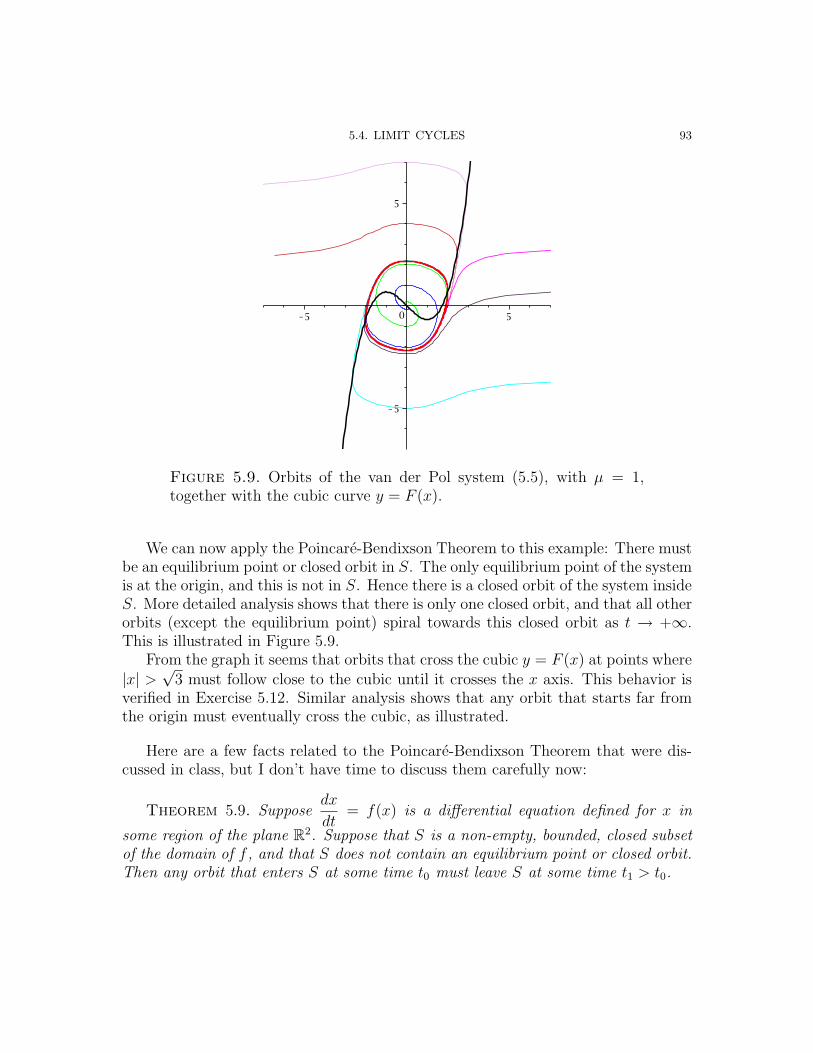
5.4. LIMIT CYCLES 93
Figure 5.9. Orbits of the van der Pol system (5.5), with µ = 1,together with the cubic curve y = F (x).
We can now apply the Poincare-Bendixson Theorem to this example: There mustbe an equilibrium point or closed orbit in S. The only equilibrium point of the systemis at the origin, and this is not in S. Hence there is a closed orbit of the system insideS. More detailed analysis shows that there is only one closed orbit, and that all otherorbits (except the equilibrium point) spiral towards this closed orbit as t → +∞.This is illustrated in Figure 5.9.
From the graph it seems that orbits that cross the cubic y = F (x) at points where|x| >
√3 must follow close to the cubic until it crosses the x axis. This behavior is
verified in Exercise 5.12. Similar analysis shows that any orbit that starts far fromthe origin must eventually cross the cubic, as illustrated.
Here are a few facts related to the Poincare-Bendixson Theorem that were dis-cussed in class, but I don’t have time to discuss them carefully now:
Theorem 5.9. Supposedx
dt= f(x) is a differential equation defined for x in
some region of the plane R2. Suppose that S is a non-empty, bounded, closed subsetof the domain of f , and that S does not contain an equilibrium point or closed orbit.Then any orbit that enters S at some time t0 must leave S at some time t1 > t0.

5.5. STABILITY 94
Theorem 5.10. Suppose thatdx
dt= f(x) is a differential equation defined for x
in some region of the plane R2. Suppose that S is a non-empty, bounded, closed,forward invariant subset of the domain of f , and that the boundary of S is a simpleclosed curve. Then S contains an equilibrium point.
A simple closed curve is a closed curve without self-intersections. Theorem 5.10applies in the special case that S consists of a closed orbit plus its interior.
5.5. Stability
There are several distinct notions of stability in dynamical systems. We will givetwo of them:
The first definitions refer to a fixed dynamical system. If C is a non-emptycompact invariant set we say that C is stable if all orbits that start near C stay nearC for all t ≥ 0, and we say that C is asymptotically stable if, in addition, all orbitsthat start near C converges to C as t→ +∞.
To make this precise, let F t be the flow of the system. Define dC(x) to be thedistance of a point x to the set C; this is the minimum distance from x1 to a pointin C. Then C is stable if there are two positive numbers δ and r so that if d(x1) < δthen d(F t(x1)) < r for all t ≥ 0. If, in addition, there is some positive number δ0 sothat lim
t→+∞dC(F t(x1)) = 0 whenever dC(x1) < δ0 then C is asymptotically stable.
If C consists of a single equilibrium point x0 then the definition of asymptoticallystable is the same as the definition of a sink. For an example of an equilibrium pointthat is stable, but not asymptotically stable, see the origin in the spring example,Figure 5.5.
If C consists of a single closed orbit then the definition of asymptotically stableis the same as the definition of two-sided limit cycle. On the other hand, each closedorbit surrounding the origin in Figure 5.5 is stable, but not asymptotically stable.
In higher dimensions we will see other examples of stable invariant sets.The main idea for this notion of stability is that perturbations of stable features
of the phase portrait stay near those features, or converge to them.
The second definition is concerned with the idea that features of the phase por-trait will persist when the dynamical system itself is perturbed. There is a formaldefinition for an entire dynamical system to be structurally stable, but we will in-stead concentrate on features of the phase portrait. We say that a dynamical systemis structurally stable near a compact invariant set C if every nearby system has acompact invariant set C ′ near C, and the orbits near and on C correspond to orbitsnear and on C ′. The precise definition requires a fair amount of analysis, so we willcontent ourselves with some simple special cases.

5.5. STABILITY 95
The main tool in almost all structural stability analysis is the following, which issimple enough that we can give a self-contained proof.
Theorem 5.11 (Banach Contraction Principle). Suppose that S is a non-emptyclosed subset of Rk and that the function F satisfies the following:
(a) S is F -invariant: If x ∈ S thwn F (x) ∈ S.(b) F is a contraction: There is a constant α so that 0 < α < 1 and ‖F (x) − F (y)‖ ≤
α ‖x− y‖ for all x and y in S.
Then there is a unique x∗ in S which is a fixed point for F , and, for any x0 in S,the iterates F n(x0) converge to x∗ as n→ +∞.
Proof. First we check that F cannot have more than one fixed point. Supposethat x1 and x2 are two different fixed points of F , so F (x1) = x1 and F (x2) = x2
and x1 6= x2. Then
‖x1 − x2‖ = ‖(x1) − F (x2)‖ ≤ α ‖x1 − x2‖ .
Subtracting α ‖x1 − x2‖ from both sides and simplifying gives (1−α) ‖x1 − x2‖ ≤ 0.But this is impossible since 1 − α > 0 and ‖x1 − x2‖ > 0. Thus it is impossible forF to have two different fixed points.
Next, notice that F is continuous. To see this, suppose that ε is a positive numberand define δ = ε. If ‖x1 − x2‖ < δ then
‖F (x1) − F (x2)‖ ≤ α ‖x1 − x2‖ < αδ = αε ≤ 1 · ε = ε,
using δ = ε and 0 < α < 1. This is the definition of continuity at the point x1 (andis also the definition of uniform continuity on all of S).
Suppose that x0 is in S. Then x1 = F (x0) is in S, so we can repeat to definex2 = F (x1) = F 2(x0). Continuing, we see that the sequence xn is well defined bythe rule xn = F (xn−1) and that xn is in S for all n; by iterating F we can also writexn = F n(x0). We need to see that the sequence xn has a limit. To do this we usea “telescoping series” trick to convert the limit of this sequence into the limit of aseries:
xn = (xn − xn−1) + (xn−1 − xn−2) + · · · + (x1 − x0) + x0

5.5. STABILITY 96
so xn =n∑
k=0
(xk − xk−1) + x0. Hence limn→∞
xn exists if and only if the infinite series
∞∑
k=0
(xk − xk−1) converges. To check this we first calculate
‖xk − xk−1‖ = ‖F (xk−1) − F (xk−2)‖ ≤ α ‖xk−1 − xk−2‖= α ‖F (xk−2) − F (xk−3)‖ ≤ α2 ‖xk−2 − xk−3‖. . .
≤ αk−1 ‖x1 − x0‖ .Now we can check that the series converges using the absolute convergence criterionand comparison to the geometric series:
∞∑
k=0
‖xk − xk−1‖ ≤∞∑
k=0
αk−1 ‖x1 − x0‖ =1
1 − α‖x1 − x0‖ <∞.
[This is an argument involving a series of vectors, but these calculations show thateach component of the series converses, since the absolute value of one componentof a vector is no greater than the length of the vector.]
Finally, since S is closed, the limit point x∗ is also in S. Using continuity of Fand the recursion relation F (xn) = xn+1,
F (x∗) = F(
limn→∞
xn
)
= limn→∞
F (xn) = limn→∞
xn+1 = limn→∞
xn = x∗.
Hence x∗ is a fixed point of F .
For applications we need a simple way to check that a function is a contraction.In the one dimensional case the Mean Value Inequality, Lemma 2.10, is very useful.This is also true in higher dimensions, but some definitions are required. First, weneed a way to measure the size of a matrix. There are many ways to do this, butthe most convenient is perhaps the hardest to calculate in practice. We define theoperator norm of a real matrix A by the rule
‖A‖ = the maximum value of ‖Ax‖ under the condition ‖x‖ = 1.
If A is an m× n matrix then x is a vector in Rn, so ‖x‖ is the usual length of an n
dimensional vector. Also, Ax is a vector in Rm, so ‖Ax‖ is the usual length of an mdimensional vector. What is new here is the definition of ‖A‖. Here are the basicproperties:
Proposition 5.12. Suppose A is a real m× n matrix. Then
(a) ‖Ax‖ ≤ ‖A‖ · ‖x‖ for any x in Rn.
(b) ‖AC‖ ≤ ‖A‖ · ‖C‖ for any m× p matrix C.

5.5. STABILITY 97
(c) The norm properties are satisfied:(i) ‖A‖ ≥ 0 and ‖A‖ = 0 if and only if A = 0.(ii) ‖cA‖ = |c| · ‖A‖ if c is a scalar.(iii) ‖A+B‖ ≤ ‖A‖ + ‖B‖ if B is also m× n.
There is a corresponding notion of norm for complex vectors and matrices, butwe will only consider the real case.
It is not easy to calculate ‖A‖ except in very simple cases. Here is one:
Lemma 5.13. If Λ is a real diagonal matrix with entries λk on the diagonal then‖Λ‖ = max |λk| .
Proof. Let r = max |λk| . Then, if ‖x‖ = 1, we have
‖Λx‖2 =n∑
k=1
λ2kx
2k ≤ r2
n∑
k=1
x2k = r2 ‖x‖2 = r2,
so ‖Λx‖ ≤ r. On the other hand, r = |λj| for some j and if x = ej is the correspondingunit vector then ‖x‖ = 1 so ‖Λ‖ ≥ ‖Λej‖ = ‖λjej‖ = |λj| = r. Putting theinequalities together gives ‖Λ‖ = r.
Most of the time the exact value of ‖A‖ is not needed. Here is a way to estimatethe size of a matrix which is close to a diagonal matrix:
Lemma 5.14. Suppose A and B are n×n real matrices and δ is a positive number.
(a) If |Bjk| < δ for all j, k then ‖B‖ < nδ.(b) If |Ajk| < δ for j 6= k and |Ajj| ≤ λ for all j then ‖A‖ ≤ λ+ nδ.
Proof. Part (a): Suppose ‖x‖ = 1. The Cauchy-Schwartz inequality, appliedto the vectors u = (1, 1, . . . , 1) and z = (|x1| , |x2| , . . . , |xn|), shows that
∑
k
|xk| =∑
k
ukzk ≤ ‖u‖ · ‖x‖ =√n · 1 =
√n.
Hence
|(Bx)j|2 ≤(
∑
k
|Bjkxj|)2
≤(
∑
k
δ |xk|)2
= δ2
(
∑
k
|xk|)2
≤ δ2(√
n)2
= nδ2.
Adding this up for the n components of Bx gives ‖Bx‖2 ≤ n · nδ2 = n2δ2, so
‖B‖ ≤√n2δ2 = nδ.
Part (b): Write A = Λ + B where Λ is diagonal with diagonal entries Ajj andB has the same entries as A off the diagonal and has zeros on the diagonal. Then,using Lemma 5.13:
‖A‖ = ‖Λ +B‖ ≤ ‖Λ‖ + ‖B‖ = max |Ajj| + ‖B‖ ≤ λ+ nδ.

5.5. STABILITY 98
Finally, here is the generalization of Lemma 2.10:
Theorem 5.15 (Mean Value Inequality). Suppose that F is a C1 function andthat K is a convex subset of the domain of F . Suppose that M is a constant and‖DF (x)‖ ≤M for all x in K. Then
‖F (x) − F (y)‖ ≤M · ‖x− y‖for all x and y in K.
Now, putting all these results together, we can give a simple criterion for theexistence of a sink:
Proposition 5.16. Suppose that G is a C1 discrete dynamical system definedon a subset of Rn. Suppose that x0 is a point, r is a positive number, and all pointswithin distance r of x0 are in the domain of G. Moreover, suppose that α is aconstant less than 1, and
(a) ‖DG(x)‖ ≤ α for all x with ‖x− x0‖ ≤ r.(b) ‖G(x0) − x0‖ ≤ (1 − α)r.
Then G has a unique fixed point x∗ satisfying ‖x∗ − x0‖ ≤ r, this fixed point is ahyperbolic sink, and and all points within distance r of x0 are in the basin of attractionof x∗.
Proof. Let B be the closed ball of radius r0 centered at x0: That is, B is definedby ‖x− x0‖ ≤ r0. This is a closed convex set. Hence the Mean Value Inequalityshows that ‖G(x) −G(y)‖ ≤ α ‖x− y‖ for all x, y in B. Now if x ∈ B then
‖G(x) − x0‖ = ‖G(x) −G(x0) +G(x0) − x0‖ since −G(x0) +G(x0) = 0
≤ ‖G(x) −G(x0)‖ + ‖G(x0) − x0‖ by the triangle inequality
≤ α ‖x− x0‖ + (1 − α)r since ‖G(x) −G(y)‖ ≤ α ‖x− y‖and ‖G(x0) − x0‖ ≤ (1 − α)r
≤ α · r + (1 − α)r = r since ‖x− x0‖ ≤ r
Thus G(x) ∈ B. Now the hypotheses of the Banach Contraction Principle aresatisfied, and this provides x∗ with the required properties.
We can now derive a prototype structural stability result for C1 discrete dy-namical systems. Suppose that x0 is a hyperbolic sink of F and DF (x0) is a realdiagonal matrix. Then α0 = ‖DF (x0)‖ is less than 1. Let δ0 = (1 − α0)/3. Thisis a positive number so, by continuity of DF , there is a positive number r so that‖DF (x)‖ ≤ α0 + δ0 whenever x is in the closed ball B of radius r centered at x0. Letα = α0 + 2δ0 and define δ to be the smaller of δ0 and (1−α)r. Notice that α < 1 soδ is positive.

5.6. BIFURCATIONS 99
Now supposeG is δ close to F onB in the C1 sense. This means that ‖F (x) −G(x)‖ ≤δ and ‖DF (x) −DG(x)‖ ≤ δ both hold, for all x ∈ B. We then have
‖DG(x)‖ ≤ ‖DF (x)‖ + ‖DF (x) −DG(x)‖ ≤ α0 + δ0 + δ ≤ α0 + 2δ0 = α,
and ‖G(x0) − x0‖ = ‖G(x0) − F (x0)‖ ≤ δ ≤ (1 − α)r
These are the hypotheses for Proposition 5.16, so G has a unique fixed point x∗ inB, and x∗ is a hyperbolic sink. This is exactly what is meant by structural stability.
We need to extend this argument. First we need to remove the restrictions thatDF (x0) is a real diagonal matrix; and then we need to consider other types of fixedpoints. For a discrete dynamical system defined by the transition rule F we say afixed point x0 is hyperbolic if all eigenvalues λ of the derivative matrix DF (x0) satisfy|λ| 6= 1. After considerably more work we find the following.
Theorem 5.17. Suppose F is an invertible C1 discrete dynamical system. Thenany hyperbolic fixed point of a C1 discrete dynamical system F is structurally stable.
Now we want the same kind of result for continuous dynamical systems. This isfacilitated by the following connection between equilibrium points of a differentialequation and fixed points of the flow:
Proposition 5.18. Suppose F t is the flow of the differential equationdx
dt= f(x).
If f is C2 then F t is C1. Moreover, if f(x0) = 0 then DF 1(x0) = eDf(x0).
It follows that the eigenvalues of DF 1(x0) are given by eλk where λk are theeigenvalues of Df(x0). Now
∣
∣ea+bi∣
∣ = |ea(cos(b) + i sin(b)| = ea√
cos2(b+ sin2(b)) = ea.
Hence the eigenvalue eλk of DF 1(x0) has absolute value equal to 1 if and only if theeigenvalue λk of Df(x0) has real part equal to 0. In other words, x0 is a hyperbolicequilibrium point of the differential equation if and only if x0 is a hyperbolic fixedpoint of F 1. Using this plus a little more analysis, we can convert Theorem 5.17 into
Theorem 5.19. Suppose f is C2. Then any hyperbolic equilibrium of the differ-
ential equationdx
dt= f(x) is structurally stable.
5.6. Bifurcations
Suppose a dynamical system depends on a parameter α. If the dynamical systemis structurally stable for some value of α, say α = α0, then small changes in α willcause only small changes in the phase portrait, and will not change the qualitativefeatures of the system. For example, suppose that x0 is a hyperbolic equilibrium

5.6. BIFURCATIONS 100
point for the system when α = α0. Then there will still be a unique hyperbolicequilibrium point near x0 when α is near α0, and this point will be of the same type(source, sink or saddle) as x0. Similarly, hyperbolic limit cycles (see the definition inthe next chapter) will persist.
On the other hand, the phase portrait may be different for other values of α. Forexample, when α = α1 the system might also be structurally stable, but there maybe a different number of equilibrium points than when α = α0 or their type (source,sink or saddle) might be different. In such a case there must be some value of theparameter, say α = α′, so that the phase portraits do not change qualitatively forα0 ≤ α < α′, but so that the phase portrait for α′ is different. Such a parametervalue is called a bifurcation value.
The system cannot be structurally stable for α = α′, since there are values ofα arbitrarily close to α′ for which the phase portrait is different from the phaseportrait for α = α′. In simple cases the phase portraits for α′ < α ≤ α1 willnot change qualitatively, so that the phase portrait for α = α′ represents the onlytransitional form between α = α0 and α = α1. However, the bifurcation picturecan be much more complicated, with many – possibly infinitely many – bifurcationvalues between α0 and α1.
Our next example is taken from a bio-engineering paper: T. Gardner, C. Cantor,J. Collins, Construction of a genetic toggle switch in Escherichia coli, Nature 403
(2000), 339–342.This system models the behavior of two genes, which we call GU and GV , inserted
via a plasmid in the bacterium Escherichia coli. These genes code for proteins, whichwe denote PU and PV , respectively. The protein PU is a repressor for the gene GV ;that is, the presence of PU in a cell inhibits the activity of gene GV . Similarly,PV is a repressor for the gene GU . This behavior can be manipulated externally,by controlling one of two chemicals called inducers. The inducer IU enhances theexpression of GU by interfering with the repressor PV . Similarly, IV is the inducerfor gene GV .
The paper describes experimental verification for behavior based on this basicmodel. The relative concentrations of the two repressors can be visually monitoredsince the expression of one of the genes also causes a green fluorescent protein to beproduced. Specifically, the authors used the following.
Example 5.20. There are two non-negative state variables, u and v, which arethe concentrations of the repressor proteins PU and PV . The simplified differentialequations for the concentrations are
du
dt= −u+
α
1 + vβ,
dv
dt= −v +
γ
1 + uδ

5.6. BIFURCATIONS 101
where α, β, γ and δ are positive parameters. The time scale has been adjusted sothat the coefficients of u and v in these equations are −1.
Here is a short explanation of the form of the equations. Consider the equation fordu
dt. The first term, −u, reflects the fact that the protein PU is rapidly broken down
within the cell, so that it will tend to disappear unless it is recreated. The second
term,α
1 + vβ, represents the production of the protein PU . This expression has a
maximum value of α when v is 0, and it decreases to 0 as v increases. This generalpicture is reasonable, since the presence of the protein PV represses the productionof the protein PU . The more precise form of this expression, including the meaningof the exponent β, is based on properties of specific bio-chemical reactions.
The effect of the inducer IU is incorporated in the parameter α. As the amount ofIU in the cell is increased the parameter α will increase, since a higher concentrationof IU makes it more likely that the gene GU will be able to produce the protein PU .
The equation fordv
dthas the same general interpretation.
The experiment showed that it is possible to make the gene GU “dominant” byadding the IU inducer, so that the concentration u of the protein PU became veryhigh and the concentration v of PV was almost 0. This situation persisted after theinducer was removed from the bacterial culture. It was then possible to switch thissituation, making the GV gene dominant, by adding the inducer IV to the system;again this configuration persisted after the inducer was removed. This explains thetitle of the article: The authors were able to turn their bacterial culture into a toggleswitch, which could be switched between the “GU dominant” and “GV dominant”states, and which would stay in one state until switched to the other.
The parameters used in the experimental model are quite specific, correspondingto known characteristics of the particular genes that were used; for example, β = 1,γ = 2.5. However, the qualitative picture does not depend on the actual values ofthe parameters, within a fairly broad range. In order to focus on the qualitativepicture we will simplify the situation, taking β = δ = 2 and restricting α and γ tovalues between 0 and 10.
We need to analyze the phase portrait for various values of the parameters αand γ. To find the equilibrium points we plot the nullclines and find the points ofintersection. The nullclines have the equations
(5.6) u =α
1 + v2, v =
γ
1 + u2
If we eliminate v between these equations we are left with a fifth degree polynomialequation for u, and each value of u is related to a single value of v by the second

5.6. BIFURCATIONS 102
(a) α = 4 (b) α = 5
(c) α = 5.796077291 (d) α = 7
Figure 5.10. Nullclines for Example 5.20. The curves are given by(5.6) with γ = 4 and α as shown. The dotted curve in plots (a) and(b) are the separatrices corresponding to the saddle points.
equation in (5.6). Hence there are at most 5 equilibrium points. In fact, there areat most 3 equilibrium points since two solutions of the fifth degree equation arenon-real. There are no closed orbits: see Exercise 5.18.
We start with Figure 5.10(a), showing the nullclines when α = 4 and γ = 4. Inthis case there are three equilibrium points. If we calculate the eigenvalues of thelinearizations we find that the equilibria near (4.0) and (0, 4), and these are sinks.The third equilibrium is on the line u = v and it is a saddle. If we consider only

5.6. BIFURCATIONS 103
points along the line u = v then the vector field f(u, v) becomes
f(u, u) =
(
−u+4
1 + u2, −u+
4
1 + u2
)
.
Hence the vector field, at all points on the line u = v, points in a direction parallelto the line u = v. That is, the line u = v is an invariant set, so it consists of orbits:the saddle point and the corresponding stable curves. Hence the line u = v is aseparatrix, dividing the plane into the basins of attraction for the two sinks. Thisseparatrix is also shown in the figure.
We interpret α = 4, γ = 4 as the “natural” state of the bacterial colony. Veryquickly, in each individual cell, the state vector (u, v) will converge to one of the twosinks. There will, of course, be some cells that are on, or very close to, the line u = v,but this will be a very small fraction of the total population. Hence we expect thatabout 50% of the cells will show “GU dominance”, so they will have a (u, v) valueclose to (4, 0), while the other 50% will show “GV dominance”, with a (u, v) valueclose to (0, 4).
We now consider what happens as the inducer IU is gradually added to theculture. This will have the net effect of increasing α. Since the system for α = 4 wasstructurally stable (the equilibria are hyperbolic) we expect that the phase portraitwill be qualitatively the same for α near 4. The nullclines for α = 5 are shown inFigure 5.10(b), and the general features are the same as for α = 4: There are twosinks and a saddle, and the stable curves of the saddle separate the plane into thetwo basins of attraction. It is not as easy to describe the separatrix, but, from thefigure, it has shifted upwards, so that somewhat more than 50% of the cells will findthemselves below the separatrix and hence attracted to the sink near (5, 0).
However, if α is increased enough then we see a different phase portrait: SeeFigure 5.10(d) for α = 7. The nullclines now have only one point of intersection,which is the sink near (7, 0). Thus we expect all cells to eventually converge to astate with a (u, v) value near (7, 0). That is, all cells will be “GU dominant”.
Since the systems for α = 4 and α = 7 are structurally stable, with different phaseportraits, there must be a bifurcation value for α between 4 and 7. Graphically, thisvalue of α is the value where the two nullclines have a transition from three pointsof intersection to one point of intersection. Increasing α has the effect of pulling the
nullcline v =α
1 + v2to the right, and the last α value for which there is an intersection
near the point (0, 4) occurs when the two nullclines have a point of tangency. Thisobservation gives a method for determining this value of α numerically: We needa point of intersection, so the two nullcline equations must be satisfied. Also, thenullclines must be tangent at the point of intersection, so we have a third equation,

5.6. BIFURCATIONS 104
expressing the fact that the two nullclines have the same slopes. This amounts tothe equation
d
du
(
4
1 + u2
)
=
[
d
dv
(
α
1 + v2
)]−1
.
Solving this equation together with the two nullcline equations (using Maple) givesthe bifurcation value α = 5.796077291, and this is shown in Figure 5.10(c). Theequilibrium point is at about (0.6238, 2.8794) and it is not hyperbolic; one of theeigennvalues is 0.
Graphically, the bifurcation occurs as the two equilibrium points on the leftcome closer together, then “coalesce” when the nullclines become tangent, and then“cancel out” as the nullclines pull apart. Calculations show that this movement ofthe equilibria is accompanied by a weakening of one of the eigenvalues at each point:at the sink the eigenvalues change from −.5, −1.5 to 0, −2, and at the saddle theychange from 0.3106, −2.3106 to 0, −2.
From these diagrams we can interpret the “toggle switch” behavior in the exper-iments. As indicated above, as the IU inducer is increased the bacterial populationwill move from a configuration evenly divided between GU dominant and GV domi-nant states to one in which essentially all bacteria show GU dominance. If the extraIU inducer is removed then the phase portrait will return from Figure 5.10(d) toFigure 5.10(a). However, since essentially all the bacteria are in a state very closeto the sink on the right, they will stay near that sink as α decreases. Hence, evenwhen the level of the IU inducer has fallen to its initial values, essentially all thebacteria will have (u, v) values near (4, 0), so they will show GU dominance. Thisinitially “sets” the toggle switch. It should then be clear that manipulating the otherinducer, IV , will push essentially all the bacteria to the sink near the v axis, andafter the extra inducer is removed the bacteria will mostly stay near this sink, so thebacteria will show GV dominance. This is how we switch the toggle between its twobasic configurations.

EXERCISES 105
Exercises
5.1. Using the same method as for the predator-prey equation, find a constant of themotion for each of the following:
(a)dx
dt= x2(y − 1),
dy
dt= xy.
(b)dx
dt= (x− 1)(y − 1),
dy
dt=
1
x+ 1.
(c)dx
dt= sinx cos y,
dy
dt= tanx.
5.2. Find a constant of the motion for the spring system, Example 4.7.
5.3. Section A.3 in the appendix reviews a method for solving an “exact differentialequation”. Use this method to find a constant of the motion for the following:
(a)dx
dt= y − 2x,
dy
dt= x2 + 2y.
(b)dx
dt= y − x2,
dy
dt= x(1 − x+ 2y).
5.4. Use Maple to determine the periods of several of the closed orbits in Figure 5.1.
5.5. This problem refers to the system of Figure 5.1. The island managers want toensure that there are always an adequate number of rabbits, since they make aliving by selling bunnies at Easter (this is reflected, of course, in the growth rater). You will need to use Maple to answer this completely, but you can get a firstapproximation by looking at the graph.(a) What are the maximum and minimum values for the rabbit population, if
initially there are 50 foxes and 2000 rabbits?(b) The island is in a nature preserve, but the managers have special permission to
arrange a one-time only reduction of 25 in the number of foxes. Why doesn’tit make sense to schedule this reduction when the foxes are at their minimumvalue?
(c) Approximately what is the optimum time to remove 25 foxes, in order to movethe system to a state with the greatest minimum number of rabbits?
(d) After this reduction, what will be the minimum number of rabbits?
5.6. Here is yet another Rabbit Island scenario. Instead of introducing predators(foxes) to the island we introduce competitors: woodchucks. Woodchucks andrabbits eat the same kind of thing (carrots?) so we expect that the net growthrate for rabbits will be reduced by an increased number of rabbits (because ofcrowding) and also by an increased number of woodchucks (competition). Ofcourse, the same thing holds from the woodchuck point of view.

EXERCISES 106
This leads to the following general model: We represent the rabbit populationby y and the woodchuck population by x, and we propose the following differentialequation:
d
dt
[
xy
]
=
[
(s− αx− βy)x(r − γx− δy)y
]
.
The parameters r, s, α, β, γ, δ are all positive.In this exercise, use the following values:
r = .1, s = .05, α = 0.0006, β = 0.0004, γ = 0.002, δ = 0.0004
You can use Maple, if you want, to prepare a phase portrait, but you don’treally need it. You might want to use Maple to calculate eigenvalues, but it’snot necessary.(a) There are four equilibrium points, all in the closed first quadrant. Sketch the
x and y nullclines and find the equilibrium points.(b) Describe the orbits on the x and y axes. Explain why an orbit can’t leave the
first quadrant.(c) The equilibrium points are all hyperbolic. Classify them. You should find 1
saddle, 1 source, 2 sinks. Is there any spiralling behavior?(d) What can you say about the basins of attraction for the sinks? You can ignore
all but the first quadrant.(e) What can you say about the stable and unstable curves starting at the saddle?(f) According to this model, can rabbits and woodchucks co-exist in the long run?
5.7. For each of the following, sketch the nullclines; find the equilibrium points; findthe linearizations at the equilibria; and classify the equilibria.
(a)dx
dt= 4y − y3,
dy
dt= x+ y.
(b)dx
dt= x2 − y2,
dy
dt= y + x2 − 2.
(c)dx
dt= xy + 6,
dy
dt= x2 − 7 − y.
5.8. Start with the second order differential equationd2x
dt2+ 2x3 = 0.
(a) Convert this to a system of differential equations, using x and y =dx
dtas the
variables.(b) This system has only one equilibrium, at the origin. Calculate the linearization
at the origin and verify that the system is not hyperbolic.(c) Show that ϕ(x, y) = x4 + y2 is a constant of the motion.(d) What can you say about the orbits?

EXERCISES 107
5.9. Start with the second order differential equation xd2x
dt2− dx
dt+ x2 − x3 = 0.
(a) Convert this to a vector differential equations in the formd
dt
[
xy
]
= f(x, y),
using x and y =dx
dtas the variables. What happens when x = 0?
(b) Here’s another way to convert the second order DE to a system: Divide the
equation by x2, notice that1
x
d2x
dt2− 1
x2
dx
dt=
d
dt
(
1
x
dx
dt
)
, and use the variables
x and z =1
x
dx
dt. Find the differential equations in terms of x and z.
(c) Part (b) produces a differential equation for x and z with one equilibrium.Find the equilibrium and classify it.
(d) What happens in the x-z system when x = 0?
5.10. Describe what happens in Example 5.3 when the condition (5.2) is replaced bythe condition
r/δ < r/α.
(The remaining case, when the inequality is replaced with an equality, involves anon-hyperbolic equilibrium, so it is not easy to analyse.)
5.11. Consider the following equations:
dx
dt= 4x− 3y − x(x2 + y2),
dy
dt= 3x+ 4y − y(x2 + y2).
(a) There are unique constants a and b so that a > 0 and x = a cos(bt), y =a sin(bt) is a solution of this system. Plug these formulas for x and y into thedifferential equations and determine a and b. Thus one orbit of this system isa circle of radius a, centered at the origin.
(b) Let ϕ(x, y) = x2 +y2 = r2. Calculatedϕ
dtand write it in the form r2(A−Br2)
for some constants A and B.(c) Use part (b) to explain why your solution from part (a) is a two-sided limit
cycle.(d) Sketch the phase portrait.

EXERCISES 108
5.12. This problem refers to the van der Pol system with µ = 1, and it explains whythe orbits which cross the cubic y = F (x) = 1
3x3 − x stay very close to the cubic
until they hit the x axis.Suppose y1 is any positive number. Define the region R to have the following
boundary curves:
top: y = y1
left: y = F (x)
right: y = F (x) − 2/3
bottom: y = 0
(a) Make a careful sketch of the region R; you can choose y1 = 4 (or any largervalue). The left and the right curves will be very close to each other.
(b) Check that the left and right curves intersect the x axis at x =√
3 and x = 2.
(c) Using the facts thatdy
dt= −x < 0 for x > 0 and
dx
dt= y − F (x) = 0 on the
cubic, check that solution curves enter R on its top and left boundaries, andexit on the bottom boundary.
(d) Let ψ(x, y) = y−F (x). Check thatdψ
dt= −x−F ′(x)ψ(x, y) along any solution
curve.
(e) Check thatdψ
dt≥ 0 on the right boundary of R. Explain why this implies
that solutions enter R on the right boundary. [Notice that the left boundarycorresponds to ψ = 0 and the right boundary corresponds to ψ = −2/3.]
(f) Usingdy
dt< 0, explain why R cannot contain any equilibrium points or closed
orbits.(g) Finally, explain why any solution curve which hits the cubic at any point
(x1, y1) where y1 > 0 must intersect the x axis between√
3 and 2.
5.13. Let F (x) =√
3 + x, and let S = [1,∞).
(a) Show that 0 < F ′(x) <1
2√
3for all x in S.
(b) Show that F and S satisfy the hypotheses of the Banach Contraction Principle.You should use the Mean Value Inequality (Theorem 5.15).
(c) Find the fixed point x∗ of F in S. That is, solve the equation F (x) = xalgebraically.
(d) Why does the sequence√
3,
√
3 +√
3,
√
3 +
√
3 +√
3, . . . converge to x∗?

EXERCISES 109
(e) Congratulations! You have now proved√
3 +
√
3 +
√
3 +√
3 + . . . = x∗
where x∗ was determined in part (c).
5.14. Let F (x) =1
3 + xand S = [0,∞). Follow the procedure of Exercise 5.13 to
determine x∗ and prove1
3 +1
3 +1
3 + · · ·
= x∗
5.15. Define the discrete dynamical system G by the rule
G(x1, x2) =
(
1
2x1 +
1
10sin(x2) −
1
100,
2
3x2 −
1
20ex1 +
1
10
)
.
(a) Suppose ‖x‖ ≤ 12. Show that the off-diagonal entries in DG(x) are less than 1
10
in absolute value. [Notice that |x1| ≤ 12
and e1/2 ≤ 2.]
(b) Use Lemma 5.14 to show that ‖DG(x)‖ ≤ 1315
if ‖x‖ ≤ 12.
(c) Show that ‖G(0, 0)‖ ≤ 115
.
(d) Now check that the hypotheses of Proposition 5.16 are satisfied, so that G hasa sink in the closed ball of radius 1
2centered at the origin.
5.16. Start with the differential equationsdx
dt= x2,
dy
dt= −y.
(a) This system has exactly one equilibrium point, at the origin. Show that thisis not a hyperbolic equilibrium by calculating the eigenvalues at the origin.
(b) Sketch the flow on the x axis.
(c) Now perturb the equations slightly, todx
dt= x2 + ε,
dy
dt= −y, where ε is a
small constant. Show that if ε is positive then the system has no equilibriumpoints.
(d) Show that, if ε is negative, say ε = −δ2, the system has two equilibriumpoints, both hyperbolic.
(e) Sketch the flow on the x axis for the perturbed system with negative ε.

EXERCISES 110
5.17. Start with the differential equationsdx
dt= x3,
dy
dt= −y.
(a) This system has exactly one equilibrium point, at the origin. Show that thisis not a hyperbolic equilibrium by calculating the eigenvalues at the origin.
(b) Sketch the flow on the x axis.
(c) Consider the perturbed systemdx
dt= x3 + εx,
dy
dt= −y, where ε is a small
constant. How many equilibrium points does the perturbed system have?Your answer will depend on the sign of ε.
(d) Any small perturbation of this system must have at least one equilibriumpoint. To show this, draw the square S with vertices (±1,±1), and showgraphically that the flow on the boundary of S always points into the square.This will still be true if the system is slightly perturbed Now cite a theoremin section 5.4.
5.18. The dynamical system of Example 5.20, with any choice of parameters, has noclosed orbits. Show this by contradiction: If there is a closed orbit, apply theDivergence Theorem to the vector field f(u, v) and the region enclosed by theclosed orbit. [The Divergence Theorem in two dimensions is also known as Green’sTheorem. There are two versions of Green’s Theorem – you need the one thatrelates the divergence of f to the normal component of f on the boundary curve.]
5.19. Here is another bifurcation in Example 5.20, with β = δ = 2. Suppose the inducersare simultaneously adjusted, so that α = γ remains true as α varies. The phaseportrait for α = γ = 4 was analyzed in the text; see Figure 5.10(a).(a) Find and analyze the equilibrium points when α = γ = 1.(b) There is a bifurcation when α = γ = α1 for some α1 between 1 and 4. Find
α1.(c) Find and analyze the equilibrium points at the bifurcation.

CHAPTER 6
Higher dimensions and chaos
6.1. The horseshoe
Chaos was discovered – and largely forgotten – several times. It was first describedby Poincare in about 1890 in his theoretical analysis of the “three body problem” ofclassical mechanics. It was rediscovered experimentally by van der Pol in the 1920’sin the “periodically forced” van der Pol equation, in his studies of vacuum tubes. Itwas analyzed by John Littlewood and Mary Cartwight in the 1940’s, who were ledto the periodically forced van der Pol equation while doing war-time radar research.They gave a complicated explanation of part of the very strange phase portrait thatunderlies van der Pol’s experiments, and Nathan Levinson gave a simpler explanationof these phenomena in the 1950’s.
But by about 1960 most of this work was unknown to almost all mathematicians,to the extent that Steve Smale published conjectures that, in effect, said that chaosdid not happen. Fortunately, Levinson told him about some of this history, andSmale disproved his own conjectures by creating the horseshoe map. Smale and hiscoworkers developed a very clear analysis, based on simple geometry, of this examplewhich illustrated many of the features that came to be codified under the heading of“chaotic dynamics”. This time the mathematical community embraced the notionof chaos, and since then there have been thousands of papers demonstrating chaos ina wide variety of dynamical systems. In almost all cases chaos has been establishedby detecting a copy of Smale’s horseshoe embedded in the phase portrait of thedynamical system.
The horseshoe system is easiest to explain as a discrete dynamical system in twovariables. We’ll discuss later how the horseshoe shows up in a three dimensionalsystem of differential equations.
We will not give formulas for all of the horseshoe system, since only some of thedetails are important for the analysis. We can describe the map as follows; referto Figure 6.1: Start with a rectangle in the plane, divided into three subrectangleslabeled V0, B and V1, with with two semi-circular endcaps, labeled A and C. Call thisfigure R. Imagine transforming this figure by the following sequence of operations:
(1) Shrink the rectangle vertically.
111

6.1. THE HORSESHOE 112
Figure 6.1. The horseshoe, showing the original region R and itsimage F (R).
(2) Shrink the endcaps horizontally, until they regain their semi-circular form.(3) Stretch the rectangles V0 and V1.(4) Bend the figure within the rectangle B so it forms a U -shaped figure, the “horse-
shoe”. The elongated rectangles V0 and V1, after this bending operation, arehorizontal.
With some care the horseshoe will now fit back inside the original figure R; the imagesof the caps A and C will be inside the original A, and the image of B will be insidethe cap C. The net effect is a function F which is defined on R. It can be extendedas a function defined on the entire plane, but we will not need this extension. It isan injection (a one-one function), so the inverse function F−1 is defined, at least onthe image F (R) of R. It is easy to construct F to be continuous, and, with somecare, it can be constructed to be C1 or, in fact, Ck for any k. We assume that thevertical shrinking and horizontal stretching on V0 and V1 are given by affine maps, so
F (x) =
[
λ 00 µ
]
x+ v0 if x ∈ V0,(6.1)
F (x) =
[
−λ 00 −µ
]
x+ v1 if x ∈ V1,(6.2)
where v0 and v1 are constant vectors and 0 < µ < 1 < λ. In the illustration µ < 12
and λ > 2. The matrix for F on V1 has negative entries since the map on V1 involvesrotation through 180 after the shrinking and stretching corresponding to µ and λ.

6.1. THE HORSESHOE 113
It is also easy to arrange that F will have a sink in A, so that all points in A arein the basin of attraction of this sink. Since F maps C into A, all points of C arealso in the basin of attraction of the sink. Since F maps B into C, all points in B arein the basin of attraction of the sink. This basin of attraction is not interesting inthe discussion of the chaotic behavior of F , and in general we will not be interestedin any points which leave V0 or V1 under any iterate F n. This leaves us with thefollowing set:
(6.3) Ω = x : F n(x) ∈ V0 ∪ V1 for all integers n .
This is a complicated set, and the action of F on points of Ω is also complicated.However, it can be represented in terms of an abstract encoding, and this encodingmakes it easy to describe the chaotic features of the horseshoe.
In this section we will describe the encoding and see how to use it, and in thenext section we’ll see how to construct it.
There are three ingredients in this encoding: A set of codes, a transformation onthese codes, and a way of measuring distance between codes.
First, the set Σ is the set of all bi-infinite sequences of 0’s and 1’s. In general,such a sequence can be written as σ =
⟨
σk : −∞ < k <∞⟩
. That is, there is a termσk corresponding to each integer, including negative integers. For example, we couldhave a sequence defined by σk = 0 for k ≤ 0 and σk = 1 for k ≥ 0. We would liketo write this sequence simply as . . . 0001111 . . . , but this representation cannot keeptrack of the subscript values. In particular, there is no way to tell whether the first 1in . . . 0001111 . . . is the 0th term of the sequence (as we intended), or the 5th term, orthe −17th term, etc. To make it possible to use this kind of notation we introduce adecimal point “.” which has no significance except as a separator between the termsof with negative subscripts and the terms with non-negative subscripts: the decimalpoint will always be written just before the term of index 0. With this conventionour example can now be written unambiguously as . . . 000 . 1111 . . . .
The second ingredient is a transformation of codes. This is a function sh (pro-nounced “shift”) defined on sequences in Σ by the rule
sh(σ) = σ′ where σ′k
= σk+1 for all k.
This is the formal definition, but it has a very simple interpretation. For example,the term in the 0th position in σ′ is σ′
0= σ0+1 = σ1. That is, the 1testst term in σ
becomes the 0th term in σ′. Continuing, we see that the 2nd term in σ becomes the1testst term in σ′, the 3rd term in σ becomes the 2nd term in σ′, and so on. This leadsto the following picture:
σ = . . . σ−3σ−2σ−1 . σ0σ1σ2σ3 . . . 7→ σ′ = . . . σ−3σ−2σ−1σ0 . σ1σ2σ3 . . .

6.1. THE HORSESHOE 114
We can describe this in two ways. Either we can think of the decimal point as fixed,and sh shifts the entire sequence σ one place to the left, or we can think of the termsof the sequence as fixed, and sh simply oves the decimal point one place to the right.We will prefer the second interpretation; it easily generalizes as:
Lemma 6.1. If k ≥ 0 then
(a) shk(σ) is obtained from σ by moving the decimal point k places to the right.(b) sh−k(σ) is obtained from σ by moving the decimal point k places to the left.
The third ingredient is a notion of distance between sequences in Σ. The idea isthat two sequences σ and τ should be close if they agree on a large range of subscriptscentered at the origin. Formally, we define the distance between σ and τ to be 0if σ = τ . Otherwise, we must have σn 6= τn for some integer n. We let N be thesmallest value of |n| for which σn 6= τn, and we define the distance between σ andtau to be
d(σ, τ) = 2−N .
In other words, N is the largest integer such that σn = τn for all n with |n| < N . Forexample, . . . 110 . 1001 . . . and . . . 101 . 0111 . . . differ in the 0th position, so N = 0and their distance is 20 = 1. For another example, let σ = . . . 1010101 . 001001001 . . .and τ = . . . 1010101 . 001000001 . . . The closest place to the center where these se-quences differ occurs at σ5 = 1, τ5 = 0, so N = 5 and the distance is d(σ, τ) = 1/32.
Now we have the ingredients for the main theorem.
Theorem 6.2. There is a function h from Ω to Σ so that
(a) h is a bijection.(b) For all integers k and all points p in Ω, h(F k(p)) = shk(h(p)).(c) Both h and h−1 are continuous.(d) σ = h(p) if and only if, all integers k, F k(p) lies in Vσ
k.
Here are some explanations of the different properties of h:
(a) A bijection is the same as a one-to-one correspondence. Thus each p in Ω corre-sponds to a unique sequence σ = h(p) in Σ, and each sequence σ in Σ correspondsto a unique point p = h−1(σ) in Ω.
(b) h(F k(p)) = shk(h(p)) means that the sequence corresponding to F k(p) is thesequence shk(σ), so the action of F k on Ω is “the same as” the action of shk
on Σ. In this context h is called a conjugacy from F k to shk.(c) The continuity condition means (in a precise ε-δ formulation) that two points in
Ω are close if and only if their corresponding sequences are close in Σ.(d) If p is in Ω then, by the definition of Ω, each iterate F k(p) lies in V0 ∪ V1, so we
can define a sequence σ by defining σk = 0 if F k(p) is in V0, and σk = 1 if F k(p)is in V1. Property (d) says that this rule is the definition of h(p).

6.1. THE HORSESHOE 115
This theorem will be proved in the next section. The following is a list of conse-quences:
Theorem 6.3. (a) F has sensitive dependence to initial conditions on Ω.(b) Ω contains infinitely many periodic points.(c) The periodic points are dense in Ω.(d) The homoclinic points of any periodic point are dense in Ω.(e) Ω contains a dense orbit.(f) F is topologically transitive on Ω.(g) F has positive entropy on Ω.(h) Ω is a fractal.(i) Ω is self-similar.
There are many studies of chaos and most of them use some or all of theseproperties of Ω as their definition of a chaotic system. We will explain some of theseproperties below.
Sensitive dependence on initial conditions: If we are in a system in whicha point p is attracted to a sink in forward time and to a source in backwards timethen nearby points stay close to p for all iterations. Technically, for any positive εthere is a positive δ so if q is within distance δ of p then F n(q) will be within distanceε of F n(p) for all integers n. “Sensitive dependence on initial conditions” says thatthis does not happen for any point in Ω. Technically, the condition is this: Thereis a positive constant d0 so that, if p and q are any two different points in Ω, thenfor some n the points F n(p) and F n(q) are at least distance d0 apart. This is one ofthe most striking properties of a chaotic system: Although the system is completelydeterministic, any difference in initial conditions will eventually be magnified to begreater than the fixed quantity d0. This means that, in a real system exhibitingsensitive dependence, precise long-term predictions are essentially impossible, sinceinitial conditions can only be specified with finite precision.
To prove that F shows sensitive dependence on initial conditions in Ω we translatethe question to Σ, where it is easy to answer: If σ and τ are different sequences thenthey differ in at least one term, so we can determine m so that σm 6= τm. We setn = −m, and notice that shn(σ) and shn(τ) differ in the 0th term, so their distanceis 1. Hence the function sh exhibits sensitive dependence on initial conditions withthe constant d0 = 1.
Let’s translate this back to F on Ω. If p and q are distinct points of Ω then theycorrespond to different sequences σ and τ as above. Then there is an integer n sothat shn(σ) and shn(tau) differ in the 0th term. These shifted sequences correspondto F n(p) and F n(q), and the 0th term in the shifted sequences specify the initialrectangles V0 or V1 which contain F n(p) and F n(q). Thus one of these points is in

6.1. THE HORSESHOE 116
V0 and one is in V1, and the definition of sensitive dependence is satisfied for F on Ωwith d0 being the distance between V0 and V1. Note that we can interpret sensitivedependence as follows: Unless we know p to “infinite precision” we cannot knowwhich rectangle, V0 or V1, will contain each iterate F n(p).
F has infinitely many periodic points: A point p is periodic with period kif k > 0 and F k(p) = p. Then the corresponding sequence σ is periodic under theshift, so shk(σ) = σ. Remembering that the nth term in shk(σ) is σn+k, we see thata sequence σ is periodic, with period k, if and only if
σn+k = σn
for all n. That is, the terms in the sequence σ are periodic with period k. If we knowthe terms σ0σ1 . . . σk−1 then all the terms of σ are determined by this periodicity: Todetermine σN then subtract a multiple of k from N (or add one) so that the result,r, is between 0 and k− 1. Then σN = σr. In other words, σ is obtained by repeatingthe block σ0σ1 . . . σk−1 forever, in positive and negative time. For example, if k = 4and σ0σ1σ2σ3 = 1000 then
σ = . . . 1000 1000 . 1000 1000 1000 . . .
is a periodic sequence of period 4. Clearly, we can specify infinitely many periodicsequences using this idea: For a sequence of period k we can choose the block 100 . . . 0,where there are k − 1 zeros.
We can be very precise about the periodic points in Ω by looking at the periodicsequences in Σ. We will use the notation πβ for the periodic sequence defined by afinite block β of 0’s and 1’s in this manner. That is, if β has length k then πβ has βin positions 0 through k − 1, and then this block is repeated forever. Here are thefirst few cases:
Period 1: We have π0 = . . . 000 . 000 . . . and π1 = . . . 111 . 111 . . . . These are thetwo fixed sequences.
Period 2: There are 4 blocks of length 4, so there are 4 sequences of period 4.However, π00 is the sequence . . . 0000 . 0000 . . . obtained by repeating 00, and thisis the same as the sequence π0. This is reasonable, since if σ is a fixed sequence,meaning sh(σ) = σ, then shk(σ) = shk−1(sh(σ)) = shk−1(σ), and a simple inductionshows that shk(σ) = σ for all k. Thus π00 and π11, although they have period 2, haveleast period 1. There are two sequences of least period 2, namely
π01 = . . . 10101 . 01010 . . . , π10 = . . . 01010 . 10101 . . .
Notice that sh(π01) = π10 and sh(π10) = π01. This illustrates another general fact: Ifσ is a periodic sequence of period k then shn(σ) is also periodic of period k. Moreover,the orbit of σ consists of the sequences σ, sh(σ), sh2(σ), . . . , shk−1(σ). This orbit hask elements if k is the least period of σ; otherwise this list of iterates has repetitions.

6.1. THE HORSESHOE 117
So we can summarize the period 2 situation: There are 4 sequences of period 2; thereare 2 sequences of least period 2; there are two orbits of size 1 and one orbit of size 2.
Period 3: There are 8 blocks of size 3. Thus we have the fixed sequencesπ000 = π0 and π111 = π1, corresponding to two orbits of size 1. The sequencesπ001, π010, π100 all have least period 3 and form a periodic orbit of size 3, and thesequences π011, π110, π101 form another such orbit.
Period 4: There are 16 = 24 blocks of size 4. As above, π0000 and π1111 are thefixed sequences. We also see that π0101 and π1010 are equal to the sequences π01 andπ10 of period 2, and this illustrates another general fact: If σ is a periodic sequenceof period k then σ is also a periodic sequence of period m where m is any positivemultiple of k. There are 12 blocks of size 4 that we have not yet considered, andthey define 12 periodic sequences of least period 4, grouped as 3 orbits of size 4.
Periodic points are dense: This means that, if p is any point in Ω and ε isany positive number then there is a periodic point within ε of p. We prove this bytranslating to Σ and then using Exercise 6.3.
The homoclinic points of any periodic orbit are dense: If p is a periodicpoint then a point q is called a homoclinic point of the orbit of p if q is not on thisorbit, and F n(p) converges to the orbit of p as n → +∞ and also as n → −∞.It is easy to find homoclinic points after we translate to Σ. The periodic point pcorresponds to a sequence σ consisting of an infinitely repeated block, β. We takea sequence τ which repeats β periodically in indices that are far away from 0; it isirrelevant what the terms in τ look like near 0. Schematically,
τ = . . . ββτ−M . . . τ−1 . τ1τ1 . . . τNββ . . .
If |K| is much larger than N or M then shK(τ) will have its decimal point in oneof the regions consisting of repetitions of the block β, and it will agree, for a largerange of indices centered at the origin, with a sequence of all β’s in a point in theorbit of σ. Thus the distance between shK(τ) and points in the orbit of σ will tendto 0 as |K| → ∞, so τ is homoclinic to the orbit of σ.
Saying that the homoclinic points of the orbit of p are dense means that, arbi-trarily close to any point r in Ω, we can find a point which is homoclinic to the orbitof p. To prove this we translate the problem to Σ. The point r corresponds to asequence ρ. Using the terminology above, we construct a homoclinic point τ withindistance 2−N−1 of ρ by defining τk = ρk for −N ≤ k ≤ N , and then filling in the restof τ with copies of β.
There is a dense orbit: This means that there is a single point p in Ω so that,for any other point q in Ω and any positive ε there is some n so that F n(p) is withinε of q. We translate this to Σ, where we need to define a sequence σ with the sameproperty. We define σ by stringing together all finite blocks of 0’s and 1’s. Here’s

6.1. THE HORSESHOE 118
how: In locations 1 and 2 we put 0 and 1, the two blocks of size 1. In the next 8locations we put 00, 01, 10, and 11, the 4 blocks of size 2. This is followed by the 8blocks of length 3, the 64 blocks of length 4, and so on. This process defines σk fork ≥ 1; the first 50 terms are
0 1 00 01 10 11 000 001 010 011 100 101 110 111 0000 0001 0010 0011
We define the terms with negative subscripts by reflection, so σ−k = σk. How wedefine σ0 is not important; for definiteness we set it to 0.
To see that the orbit of this sequence is dense, consider a sequence τ in Σ, andchoose N ≥ 0. Let βbe the block of terms in τ of length 2N + 1 centered at τ0, soβ = τ−N . . . τN . This block occurs in σ somewhere, since every finite block occurs
in σ. So there is some M so that σM−N . . . σM+N = β. So, if we write ρ = sh−M(σ),then the block of terms in ρ of length 2N + 1 centered at ρ0 is equal to β, which is
the corresponding block of τ . Hence the distance between ρ = sh−M(σ) and τ is nomore than 2N+1. This shows that we can find points on the orbit of σ as close asdesired to any given point τ in Σ, so the orbit of σ is dense.
Actually, this argument shows slightly more: Both the positive orbit and thenegative orbit or σ are dense, since we can choose M to be either positive or negative.
The remaining parts of Theorem 6.3 require more background, so we just giveshort descriptions.
F is topologically transitive: This is closely related to having a dense orbit;it says that any open set has a dense orbit.
F has positive entropy: There are several notions of entropy in dynamicalsystems. A system with positive entropy shows essentially random behavior on longtime scales.
Ω is a fractal: For most sets it is possible to define a number called the Hausdorffdimension. For simple sets this is the usual notion. For example, smooth curveshave Hausdorff dimension 1 and smooth surfaces have Hausdorff dimension 2. Setswith non-integral Hausdorff dimension are much more complicated; they are calledfractals. The Hausdorff dimension of Ω is bigger than 0 but less than 1.
Ω is self similar: A set is self-similar if small parts of the set are geometricallysimilar to each other. In effect, the fine structure of the set is the same at any scale.Ω has this property; for example, there is a linear map which transforms the part ofΩ which is inside V0 ∩ V1 onto all of Ω. Complicated sets – in particular, fractals –that are defined by iteration often show self-similarity.

6.2. ENCODING THE HORSESHOE 119
Figure 6.2. Six vertical segments a, b, . . . , f and their images.
6.2. Encoding the horseshoe
In this section we will give some of the details in the proof of Theorem 6.2. Wewill continue to use the notation of Figure 6.1 and of equations (6.1) and (6.2) todescribe the horseshoe map, and (6.3) to define Ω. The correspondence h betweenΩ and Σ is defined the condition in part (d) of Theorem 6.2. We need to see thath is a bijection, that h and h−1 are continuous, and that the conjugacy condition inpart (b) of Theorem 6.2 is satisfied.
We start by describing the images of vertical segments in V0∪V1 under F . Figure6.2 shows several vertical lines and their images. Consider the vertical segmentsa, b, c, d in V0. The image of each such segment is a vertical segment in the rectangleF (V0). This is just a consequence of the form (6.1) for F on V0, since both translationsand diagonal matrices transform vertical lines to vertical lines. Moreover, as we movevertical segments in V0 from left to right their images move continuously from leftto right in F (V0). So the left side of V0 is mapped into A, the segment a is mappedinto V0, b is mapped into B, c and d are mapped into V1, and the right side of V0
is mapped into C. Similarly, the vertical segments in V1 are mapped to verticalsegments in F (V1). As the segments in V1 move from left to right their images movefrom right to left, because of the negative entry −λ in the form (6.2).
Notice that the segments e and f map into the right and left sides of V0 respec-tively, so the subrectangle of V1 bounded by e and f maps into V0. Similarly, by

6.2. ENCODING THE HORSESHOE 120
Figure 6.3. The points which stay in V0 ∪ V1.
positioning vertical segments in V1 so that they map into the boundaries of V1 we willfind a subrectangle of V1 wich maps into V1. We can do the same in V0. We end withtwo subrectangles in each of V0 and V1 which map into either V0 or V1, as shown inFigure 6.3. Moreover, the points in V0∪V1 that are not in one of these subrectanglesmap into A∪B ∪C. In other words, the points in the four subrectangles are exactlythe points which stay in V0 ∪ V1.
We can repeat this process. Consider the subrectangle labeled V00. If p is a pointin V00 then F (p) is in V0. We next ask whether F 2(p) = F (F (p)) lies in V0 ∪ V1.Arguing as above, we see that each vertical segment in V00 maps under F 2 to a shortvertical segment, and these image segments range from A through V0 ∪ B ∪ V1 andinto C. Hence the points of V00 which map into V0 under F 2 form a vertical rectanglein V00, as do the points in V00 which map into V1 under F 2. The same picture holdsin the other three subrectangles V01, V10, V11, and we find that the points which stayin V0 ∪ V1 under both F and F 2 form eight thin vertical rectangles, as shown inFigure 6.4.
Here is the explanation of the numbering system for these rectangles: Look atV10. This is a subrectangle of V1, and consists of the points in V1 which are mappedinto V0. That is, a point p is in V10 if F 0(p) = p ∈ V1 and F (p) ∈ V0. The rectangleV100 is a subrectangle of V10 and consists of the points in V10 which map into V0

6.2. ENCODING THE HORSESHOE 121
Figure 6.4. The points which stay in V0 ∪ V1 for two iterations.
under F 2. That is, p is in V101 if F 0(p) = p ∈ V1, F1(p) ∈ V0, and F 2(p) ∈ V0. So
the subscript 100 of V100 tells where the image of V100 is under the iterates F 0, F 1,and F 2.
To generalize this picture we use finite sequences of 0’s and 1’s. The length of asequence σ is the number of terms σ, and it is written |σ|. For example, if σ = 010011then |σ| = 6. (There is a sequence of length zero, but we will not need to talk aboutit in this section.)
There is a way of combining two of these sequences, called concatenation, whichis defined by just pasting the two sequences together. For example, if σ = 010011and τ = 00100 then the concatenation of σ and τ , written στ , is the sequence010011 00100. Concatenation is not a commutative operation in general; in ourexample the concatenation of τ and σ in the opposite order is τσ = 00100 010011.
We will use the following related terminology: If a sequence ρ can be factored asρ = στ then we say that σ is a prefix of ρ and τ is a suffix of ρ. For example, ifρ = 001011 then 00 is a prefix of ρ, and 011 is a suffix.
We can refer to the individual terms in a sequence if we know where the numberingstarts or ends. For describing vertical rectangles we will use sequences that are num-bered starting at 0, so the terms of σ = 010011 will be labeled as σ = σ0σ1σ2 . . . σ5.

6.2. ENCODING THE HORSESHOE 122
Using this notation we define the generalized vertical rectangles by the condition
(6.4) p ∈ Vσ ⇐⇒ F k(p) ∈ Vσk
for 0 ≤ k ≤ n, where |σ| = n+ 1.
Note the similarity to the condition in Theorem 6.2(d).We summarize the properties of these sets:
Lemma 6.4. Suppose the rectangles V0 and V1 have width w and height h. Then
(a) Vσ is a vertical rectangle, of height h and width λn1w, where |σ| = n+ 1.(b) Vσ contains Vτ if σ is a prefix of τ .(c) Vσ and Vτ are disjoint unless σ is a prefix of τ or τ is a prefix of σ.(d) The image of Vσ
0σ1...σ
kunder F lies in Vσ
1σ2...σ
k.
(e) A point in V0∪V1 remains in V0∪V1 for n iterations if and only if it lies in someVσ where |σ| = n+ 1.
The proof just codifies the geometry discussed above. The formula for the widthof Vσ comes from the observation that each time F is applied to a rectangle in V0∪V1
the width of the rectangle is multiplied by λ; and, after n iterations, the rectanglestretches across either V0 or V1.
Now we need to consider the points that start in V0 ∪ V1 and remain there for allpositive iterates of F . To describe these we use infinite sequences σ = σ0σ1σ2 . . . .The prefix relation still makes sense when applied to a finite sequence and an infinitesequence.
If σ is such a sequence we can define Vσ by an obvious modification of (6.4): werequire F k(p) ∈ Vσ
kfor all k ≥ 0. Geometrically, these sets are rectangles of zero
width – that is:
Lemma 6.5. If σ is an infinite sequence of 0’s and 1’s then Vσ is a verticalsegment, and the analogs of the statements in Lemma 6.4 are still true.
Proof. The only real issue is whether Vσ is non-empty. In fact, it is defined bythe following limiting process. First, if τ is any finite prefix of σ, then Vσ is a subsetof Vτ . We write Ln and Rn for the left and right sides of Vτ , where τ is the prefixof σ of length n. These are vertical line segments and, as n increases, Ln moves tothe right and Rn moves to the left. We let ln be the x coordinate of Ln and we letrn be the x coordinate of Rn. Then ln is a non-decreasing bounded sequence of realnumbers, so it has a limit l∗. Similarly, rn has a limit r∗. Since the distance betweenln and rn is the width of Vτ and this width converges to 0 as n → +∞, we havel∗ = r∗. Then Vσ is the limit of the vertical segments Ln and Rn; that is, it is thevertical segment with x coordinate l∗ (or r∗).
This construction gives a lot of information about points that stay in V0 ∪ V1 forall positive iterations. We can specify an arbitrary future for a point, in the form

6.2. ENCODING THE HORSESHOE 123
Figure 6.5. Hσ for length of σ ≤ 3. The rectangles are identified bytheir subscripts.
of an infinite sequence σ, and we are guaranteed that there is a vertical segmentconsisting of points that have that future. For example, there is a vertical segmentconsisting of points that stay in V0 for all positive iterations: we just take σk = 0 forall k. Similarly, there is a vertical segment of points in V0 which has a future whichalternates between V1 and V0: we take σ = 010101 . . . .
To complete this picture we also need to analyze points that stay in V0 ∪ V1 forall negative iterations. We define sets Hσ using the analog of (6.4) for negative time:
(6.5) p ∈ Hσ ⇐⇒ F k(p) ∈ Vσk
for − n ≤ k ≤ −1 where n = |σ| .Notice that we are using negative indexes for the subscripts of the sets Hσ. Forexample, when we writeHσ with σ = 010011 then we understand that the entries in σare indexed as σ−6σ−5 . . . σ−1. Thus a point p in H010011 satisfies F−6(p) ∈ Vσ
−6= V0,
F−5(p) ∈ Vσ−5
= V1, . . . , F−1(p) ∈ Vσ−1
= V1.
Consider H0. According to the definition, this is the set of points p for whichF−1(p) ∈ V0. But the condition F−1(p) ∈ V0 is equivalent to the condition p ∈ F (V0).That is, H0 is just the image of V0 under F . This easily generalizes:
Lemma 6.6. Suppose σ is a sequence of length k. Then Hσ is the image of Vσ
under F k.

6.2. ENCODING THE HORSESHOE 124
For example, not only do we have H0 = F (V0) but H01 = F 2(V01), H011 =F 3(V011), and so on. Suppose that σ has length n. Then Vσ has width λ−n+1w andeach iteration of F multiplies horizontal lengths by λ, so F n(Vσ) = Hσ has lengthλn · λ−n+1w = λw. So all the horizontal rectangles Hσ have the same width as H0
and H1. Since Hσ lies in H0 or H1 we have the layout shown in Figure 6.5.The basic properties for these rectangles follow immediately from the correspond-
ing properties for the vertical rectangles, Lemma 6.4. Thus we have
Lemma 6.7. Suppose the rectangles V0 and V1 have width w and height h. Then
(a) Hσ is a horizontal rectangle, of height µnh and width λw, where n = |σ|.(b) Hσ contains Hτ if σ is a suffix of τ .(c) Hσ and Hτ are disjoint unless σ is a suffix of τ or τ is a suffix of σ.(d) The image of Hσ
−kσ−k+1
...σ−1
under F−1 lies in Hσ−k
σ−k+1
...σ−2
.
(e) A point is in V0 ∪ V1 for n iterations of F−1 if and only if it lies in some Hσ
where n = |σ|.Next, as we did for the sets Vσ, we extend the definition ofHσ to infinite sequences
σ. Now we have σ = . . . σ−3σ−2σ−1, and Hσ is defined by the condition that F−k(p) ∈Vσ
kfor all k ≤ −1. The analog of Lemma 6.5 is true, with a similar proof:
Lemma 6.8. If σ is an infinite sequence of 0’s and 1’s then Hσ is a horizontalsegment, and the analogs of the statements in Lemma 6.7 are still true.
We are now ready to put all this together. A point p is in Ω if and only if F k(p)is in V0 ∪ V1 for all integers k. This is equivalent to saying that F k(p) is in V0 ∪ V1
for all k ≥ 0, and also that F k(p) is in V0 ∪ V1 for all k < 0. By the infinite analogsof Lemma 6.4(e) and Lemma 6.7(e), this is in turn equivalent to the statement thatp lies in Vτ and also in Hρ, for some infinite sequences τ and ρ. That is, p is in theintersection Hρ ∩ Vτ . Moreover, any choice of infinite sequences ρ and τ determinesa unique point p in Ω, since Hρ and Vτ are horizontal and vertical line segments, sothey intersect in exactly one point.
We can concatenate the two infinite sequences ρ = . . . ρ−3ρ−2ρ−1 and τ =τ0τ1τ2 . . . to form a single bi-infinite sequence σ = ρ . τ . (We are using the deci-mal point as in Section 6.1 to mark the 0th term.)
Now we can show that the function h defined in Theorem 6.2(d) is a bijection.In fact, we have just described the inverse function: To each σ in Σ there is acorresponding point p = g(σ) in Ω, defined by
(6.6) g(σ) = p ⇐⇒ σ = ρ . τ and p is the intersection of Hρ and Vτ .
It is a simple matter to show that g is indeed a two-sided inverse of h, so h is abijection and h−1 = g.

6.3. TIME DEPENDENT SYSTEMS 125
We think of the sequence σ = h(p) as an encoding of the point p, and we thinkof the point p = h−1(σ) as the decoding of the sequence σ.
Now here is the encoding of the action of F , establishing the conjugacy conditionin Theorem 6.2(b):
Lemma 6.9. If p ∈ Ω corresponds to σ = h(p) ∈ Σ then, for any integer k, F k(p)corresponds to shk(σ).
Proof. Let F k(p) = q, and let τ = shk(σ). We need to show that the encodingof q is tau. From the definition of the encoding we have F n(p) ∈ Vσ
nfor all n. We
can replace the arbitrary integer n with n+ k to get F n+k(p) ∈ Vσn+k
for all n. But
F n+k(p) = F n(F k(p)) = F n(q), and σn+k = τn. So we have F n(q) ∈ Vτn
for all n.But then, by definition, the encoding of q is τ .
Finally, we demonstrate continuity for h and h−1.Suppose that p is in Ω and ε is a positive number. Choose N so that 2−N < ε.
Let d0 be the distance between V0 and V1. By continuity at p of the finitely manyfunctions F n for |n| < N , there is a positive number δso that, if q is within δ of pthen the distance from F n(q) and F n(p) is less than d0, for all n with |n| < N . Itfollows that, for each such n, F n(p) and F n(q) are in the same rectangle, V0 or V1.Hence the sequences h(p) and h(q) agree in all terms indexed by n with |n| < N ,so the distance from h(p) to h(q) in Σ is no more than 2−N < ε. This establishescontinuity of h.
Now suppose that σ is in Σ and ε is a positive number. Choose N large enoughthat
(6.7)
√
(µNh)2 + (λ−Nw)2 < ε
and let δ = 2−N−1. Let ρ = σ−Nσ−N+1 . . . σ−1 and τ = σ0σ1 . . . σN . If σ′ is a sequencewithin δ of σ then σ′ and σ agree in all terms indexed by n with |n| ≤ N . Henceboth h−1(σ) and h−1(σ′) lie in Hρ ∩Vτ . This is a rectangle, of height µNh and widthλ−Nw. The diameter of this rectangle, according to (6.7), is less than ε, so h−1(σ′)is within distance ε of h−1(σ). This establishes continuity of h−1 at σ.
6.3. Time dependent systems
So far we have concentrated on systems of differential equations of the formdx
dt= f(x) where, as indicated, the vector field f(x) depends only on the position
vector x. Such a system is called an autonomous or time indepentent system of
differential equations. A more general type of system has the formdx
dt= f(x, t)
where now the vector field f(x, t) depends explicitly on the time variable t. This

6.3. TIME DEPENDENT SYSTEMS 126
more general type of system is called a non-autonomous or time dependent system.All of our analysis so far has been concerned with autonomous systems. Some ofthe basic facts, like a suitable existence and uniqueness theorem, are still valid. Onthe other hand, our basic ideas of the flow, solution curves, and orbits all need to bemodified.
Here is a very simple example, which can be easily solved by integration:
(6.8)dx
dt= t,
dy
dt= x x(t0) = x0, y(t0) = y0.
To solve this, first separate variables in the first equation, to get dx = t dt, and then
integrate: x(t) =
∫
t dt = 12t2 + C. The constant is determined from the initial
conditions, so, plug in t = t0 and x(t0) = x0 and solve for C: x0 = 12t2 + C so
C = x0 − 12t20. Now plug this value of C into the formula for x(t):
x(t) = 12t2 + C = 1
2t2 + x0 − 1
2t20 = x0 + 1
2
(
t2 − t20)
.
Now do the same thing with the second differential equation to find y(t). First write
the equation in differential form and integrate: dy = x dx so y(t) =
∫
x(t) dt. In
more complicated systems of equations we would be stuck right here, since we needto know x(t) as a function of t in order to perform the integration. But this exampleis simple enough that we have already solved for x(t), so just plug in our formula:
y(t) =
∫
x(t) dx =
∫
(
x0 + 12t2 − 1
2t20)
dt = x0t+ 16t3 − 1
2t20t+ C.
Now plug in t = t0 and y(t0) = y0 and solve for C, and then rewrite the equation fory(t) with this value of C. After some algebra we find:
y(t) = y0 + x0(t− t0) + 16t3 − 1
2t20t+ 1
3t30.
Now that we have determined x(t) and y(t) we can define G(x0, y0, t) as thesolution with initial conditions x(0) = x0, y(0) = y0, just as we did for autonomous
systems. In vector terms, if we write z =
[
xy
]
and z0 =[
(]
x0
y0), we have
G(z0, t) =
[
x0 + 12t2
y0 + x0t+ 16t3
]
.
We do not write this as Gt(x0, y0) since G is not a flow. The defining condition for aflow is that GsGt = Gs+t. In our notation this would be G(G(z0, t), s) = G(z0, s+t),

6.3. TIME DEPENDENT SYSTEMS 127
Figure 6.6. Four solution curves of the system (6.8). The dottedparts of the curve correspond to negative time.
and this is not true. Gor example, suppose z0 =
[
00
]
, t = 1 and s = 1. Then
G
([
00
]
, 1
)
=
[
0 + 12· 12
0 + 0 · 1 + 16· 13
]
=
[
1216
]
G
(
G
([
00
]
, 1
)
, 1
)
= G
([
1216
]
, 1
)
=
[
12
+ 12· 12
16
+ 12· 1 + 1
6· 13
]
=
[
156
]
G
([
00
]
, 1 + 1
)
= G
([
00
]
, 2
)
=
[
0 + 12· 22
0 + 0 · 2 + 16· 23
]
=
[
243
]
,
so G(G(z0, t), s) 6= G(z0, s+ t).Not only do we not get a flow from the solution curves, but the solution curves
do not look like the solution curves of an autonomous system in a very fundamentalway: Different solution curves can intersect, and a single non-periodic solution curvecan have self-intersections. See Figure 6.6.
It should be clear that the notion of orbit is not supported by these solutioncurves. In particular, there are no equilibrium points of this system. If we setf(x, y, t) = 0 and solve we find t = 0, x = 0, and y is arbitrary. But this can’t

6.3. TIME DEPENDENT SYSTEMS 128
correspond to an equilibrium point, since every solution curve of (6.8) has x(t) = 12t2
plus a constant, so there are no solutions that are constant.
There is a simple way to reinterpret a time-dependent system as an autonomoussystem. We change t to a new variable, s, which corresponds to absolute time, asmeasured by a fixed clock. Now we are free to reuse the variable t, and we interpret itas relative time, giving the difference between s and the initial time s0, so s = s0 + t.This leads to an autonomous system of equations plus initial conditions, where theindependent variable is t and the independent variables are the original variables,plus the new variable s.
A solution to this reinterpreted system of equations will have the form x(t), s(t)where s(t) = t0 + t. Then the corresponding solution to the original time-dependentsystem is given by x(s− s0). Formally,
Theorem 6.10. X(s) is a solution of the time-dependent initial value problem
dX
ds= f(X, s), X(s0) = x0
if and only if X(s) = x(s−s0) where x(t), s(t) is a solution of the autonomous initialvalue problem
dx
dt= f(x, s),
ds
dt= 1, x(0) = x0, s(0) = s0.
The proof of this is very simple; it is essentially just a change of variables.
We apply this transformation to our example (6.8). Forst we change the t variableon the right hand side to the new independent variable s, and we replace the initial
value t0 with s0. Then we add the differential equationds
dt= 1, and we change
the initial conditions to indicate that the starting time is t = 0. This gives us theautonomous version
(6.9)dx
dt= s,
dy
dt= x,
ds
dt= 1 x(0) = x0, y(0) = y0, s(0) = s0.
The solution of this system is obtained by first solving for s, to get s = s0 + t, andthen proceeding as we did for the non-autonomous version. This produces
x(t) = x0 + s0t+ 12t2
y(t) = y0 + x0t+ 12s0t
2 + 16t3
s(t) = s0 + t

6.4. STRANGE ATTRACTORS 129
Figure 6.7. Solution curves of the autonomous version (6.9) of (6.8),using the same initial conditions as in Figure 6.6. The plane shown isthe xy plane, and the vertical line is the s axis.
Now, since we are working with an autonomous system, we cna use these solutioncurves to define a flow:
F t
x0
y0
s0
=
x0 + s0t+ 12t2
y0 + x0t+ 12s0t
2 + 16t3
s0 + t
.
Since we have a flow we know that the solution curves do not intersect, that they donot intersect each other unless they are periodic, and we can define orbits so we canthin about the phase portrait. However, the phase portrait is in three dimensions(x, y, s) rather than two. Figure 6.7 shows the same solution curves as in Figure 6.6,but interpreted in three dimensions.
6.4. Strange attractors

EXERCISES 130
Exercises
6.1. For the horseshoe map:(a) How many periodic points are there of period 6?(b) How many periodic points are there of least period 6?(c) How many periodic orbits are there of period 6? Give subtotals for the different
orbit sizes.
6.2. (a) Find a periodic sequence of distance at most 2−6 from . . . 000.111 . . . . Whatis its period?
(b) Suppose N is a positive integer and find a periodic sequence of distance atmost 2−N from . . . 000.111 . . . . What is its period?
6.3. Generalize Exercise 6.2 to show that, if σ is any sequence in Σ and N is arbitrarythen there is a periodic point within distance 2−N of σ.
6.4. There are many variations on the basic horseshoe picture. Here’s a “broken horse-shoe”:
(a) Draw the vertical rectangles that arise in this example. Specifically, show Vσ
and Hσ where σis a suitable string of 0’s and 1’s of length ≤ 4. This will notbe the same as in the full horseshoe. For example, V00 is empty since thereare no points that start in V0 and are in V0 after one iteration of F . [You donot need to draw the empty rectangles.]
(b) Draw the horizontal rectangles Hσ where σ has length ≤ 3.
6.5. Using the broken horseshoe of Exercise 6.4 we define the set Ω1 of points that liein V0 ∪ V1 under all iterations, and we encode x in Ω1 by the bi-infinite sequenceσ so that F n(x) lies in Vσn
for all n. Not all sequences can be obtained in thismanner; for example, the sequence . . . 000.0000 . . . corresponds to a point that
EXERCISES 131
ramains in V0 under all iterations, but no point in V0 remains in V0 for even oneiteration.
DefineΣ1 = σ : σ does not contain consecutive 0’s .
In other words, the condition for σ to be in Σ1 is that whenever σk = 0 thenσk+1 6= 0.
The following are three of the steps needed to show that sequences in Σ1 areexactly the encodings of points in Ω1. (The rest of the proof is the same as forthe full horseshoe.)(a) Suppose x is in Ω1; show that the encoding of x is in Σ1.(b) Suppose σ is a finite sequence so that 00 does not occur in σ. Show that Vσ
is non-empty.(c) For a finite sequence sequence as in part (b), show that Hσ is non-empty.
6.6. Using the definition of Σ1 in Exercise 6.5, find the number of periodic strings ofperiod p, for p ≤ 5 (at least). For p = 1, 2, 3 you should get 1, 3, 4. Do you seea pattern?
APPENDIX A
Review
A.1. Complex numbers
This section is a summary of practical algebra in the complex number system.Technically, a complex number is an ordered pair of real numbers; in other words,
the set C of complex numbers is the same as R2, the usual XY plane. Instead ofwriting a complex number z as (x, y) we will generally write it as x + iy. The realpart of z is x and the imaginary part of z is y.
Caution: The imaginary part of a complex number is a real number.Complex numbers of the form x + 0i = x are just real numbers, while complex
numbers of the form 0 + iy = iy, with y 6= 0, are called pure imaginary numbers.In this form the rules of algebra, for addition, subtraction, and multiplication can
be summarized as:
(1) Use the commutative, associative and distributive laws as for real numbers.(2) Remember that 0 and 1 are units for addition and multiplication, respectively.(3) Use i2 = −1 to reduce powers of i.
For example, i3 = i2 · i = −1 · i = −i. Also,
(2 + i)(3 − 2i) = 2 · 3 + 2 · (−2i) + i · 3 + i · (−2i)
= 6 − 4i+ 3i− 2i2 = 6 − i− 2 · (−1) = 8 − i.
There is an important operation for complex numbers called conjugation, whichis defined by “changing the sign of the imaginary part”. Specifically, if z = x + iythen z = x− iy. The main properties of congugation are:
(1) (z ± w) = z ± w.(2) z · w = z · w.(3) z = z.(4) z is real if and only if z = z.
(5) The real and imaginary parts of z are1
2(z + z) and
1
2i(z − z).
(6) z · z = x2 + y2. This is real and non-negative, and is 0 if and only if z = 0.
Using the conjugate we can calculate multiplicative inverses, so we can divide.The idea is to “rationalize the denominator” by multiplying top and bottom by the
132

A.1. COMPLEX NUMBERS 133
conjugate of the denominator. For example,
2 + i
3 + 2i=
(2 + i)(3 − 2i)
(3 + 2i)(3 − 2i)=
8 − i
32 − (2i)2=
8 − i
9 − (−4)=
8
13− i
13.
We can also use conjugation to define the absolute value or modulus of a complex
number as |z| =√z · z =
√
x2 + y2. For example, |3 + 2i| =√
9 + 4 =√
13.
Caution: The formula for |z| is√
x2 + y2, not√
x2 + (iy)2. Remember that yis real.
The absolute value has many of the same properties as the absolute value of realnumbers:
(1) |zw| = |z| · |w|.(2) |z| ≥ 0, and |z| = 0 if and only if z = 0.(3) |z + w| ≤ |z| + |w|.
Here are a few things to be careful about:
(1) |z|2 = z2 is true for real numbers, but is not generally true for complex numbers.(2) |z| = ±z is true for real numbers, but is not generally true for complex numbers.
There is no useful way to define an order relation for complex numbers; so z ≤ whas no meaning. All we can do is compare magnitudes, using absolute values.
Instead of using Cartesian coordinates, we can represent complex numbers usingpolar coordinates. The usual formulas relating Cartesian and polar coordinates are
x = r cos θ r =√
x2 + y2
y = r sin θ θ = arctan(y
x
)
Applying them to z = x + iy, we see that z = r cos θ + ir sin θ = r (cos θ + i sin θ),where r = |z|. The polar angle θ is called the argument of z. It can be any angle ifz = 0, and otherwise it is defined up to the addition of an integer multiple of 2π. Ifwe multiply two complex numbers in polar coordinates and remember the additionformulas for the sine and cosine, we are led to
r1 (cos θ1 + i sin θ1) · r2 (cos θ2 + i sin θ2) = r1r2 (cos(θ1 + θ2) + i sin(θ1 + θ2)) .
That is, when you multiply two complex numbers you multiply their absolute values,but you add their arguments. In geometric terms this means that multiplication ofpoints in the plane (i.e., complex numbers) by a fixed complex number z is thetransformation defined by a scale change of r = |z|, followed by a rotation aroundthe origin through the angle θ.
We can apply this to calculating zn. We write z = r cos θ + i sin θ in polarcoordinates. Then |zn| = |z|n = rn, and the argument of zn is obtained by adding n

A.2. PARTIAL DERIVATIVES 134
copies of the argument of z, to give nθ. So we have
(A.1) zn = (r(cos θ + i sin θ)) = rn (cos(nθ) + i sin(nθ)
This is known as De Moivre’s formula.Complex numbers were introduced to solve polynomial equations – indeed, the
quadratic equation often gives non-real solutions for quadratic equations. There aresimilar, but much more complicated, formulas for solving third and fourth degreepolynomial equations, and these also involve complex numbers. Mathematicianssuspected for many years that complex numbers were enough to solve all polynomialequations. This was first proved by Gauss in 1799, although there were some gapsin his proof; several different completely rigorous proofs have since appeared. It isimportant enough to be called the Fundamental Theorem of Algebra:
Theorem A.1 (Fundamental Theorem of Algebra). If P (z) is a polynomial ofdegree m > 0 with complex coefficients then P (z) has exactly m ccomplex rootsα1, α2, . . . , αm (listed with multiplicity). In other words, P (z) factors as c(z−α1)(z−α2) . . . (x− αm) where c is the coefficient of zm in P (z).
Even if the original polynomial has real coefficients there will probably be non-realroots. The following gives a way of organizing them.
Proposition A.2. If P (z) is a polynomial of degree m > 0 with real roots thenthe roots of P (z) can be listed as r1, r2, . . . , rp, c1, c1, c2, c2, . . . cq, cq (listed with mul-tiplicity) where p+2q = m, the roots ri are real, and the roots ci and ci are non-real.In other words, complex roots occur in conjugate pairs.
Proof. The key observation is that P (z) = P (z), which is true since conjugationpreserves sums and products and leaves the coefficients of P (z) unchanged, sincethese coefficients are real. From this we see that if P (z) = 0 then P (z) = 0. It isthen clear that each non-real root z is matched up with its conjugate z, and so wecan list the roots as in the proposition.
A.2. Partial derivatives
For a function f of two or more variables the partial derivatives are definedby differentiating with respect to one variable, while treating all other variables asconstants. For example, if f(x, y) = x2+y3−sin(3x+5y) then the partial derivativesare
∂f
∂x= 2x− 3 cos(3x+ 5y),
∂f
∂y= 3y2 − 5 cos(3x+ 5y).

A.2. PARTIAL DERIVATIVES 135
Higher order derivatives are defined by iterating this process. For example, for thisexample we have
∂2f
∂x2=
∂
∂x(2x− 3 cos(3x+ 5y)) = 2 + 9 sin(3x+ 5y)
∂2f
∂x∂y=
∂
∂x
(
3y2 − 5 cos(3x+ 5y))
= 15 sin(3x+ 5y)
∂2f
∂y2=
∂
∂y
(
3y2 − 5 cos(3x+ 5y))
= 6y + 25 sin(3x+ 5y)
∂2f
∂y∂x=
∂
∂y(2x− 3 cos(3x+ 5y)) = 15 sin(3x+ 5y)
In general, working with partial derivatives requires slightly stronger assumptionsthan in the corresponding single variable situations, and it is simplest to formulatethese extra assumptions in terms of continuity of the partial derivatives. We say afunction is a C1 function if it has first order partial derivatives with respect to all itsvariables, and these partials are continuous. We say a function is a C2 function if ithas continuous first and second order partials, and so on.
Also, working with partial derivatives, especially if the function f is a vectorfunction, leads to very cumbersome notation. We can often simplify this by usingthe matrix derivative, also known as the Jacobian matrix : Suppose f is a functionof n variables and its values are m-dimensional vectors, which we regard as column
vectors. If we calculate the partial derivative of f with respect to one of its variableswe will get a m dimensional vector. We can then form the m × n matrix that hasthese partial derivatives as its columns. This matrix is written as Df , or as Df(a)if the derivatives are all taken at the point a.
For example, if f(x, y) =
[
x2
xy + y2
]
then
∂f
∂x=
[
2xy
]
,∂f
∂y=
[
0x+ 2y
]
, Df =
[
2x 0y x+ 2y
]
, Df(−1, 3) =
[
−2 03 5
]
.
Here are some of the main facts about partial derivatives:
Theorem A.3. If f is C1 then f is continuous; if f is C2 then f is also C1.
Theorem A.4 (Equality of mixed partials). If f is C2 then the “mixed partials”
with respect to any two varialbes are equal. That is,∂2f
∂xi∂xj
=∂2f
∂xj∂xi
.
Theorem A.5 (Chain rule). If f and g are C1 functions then the compositionfg is C1. If a is in the domain of g and g(a) is in the domain of f then D(fg)(a) =Df(g(a))Dg(a).

A.3. EXACT DIFFERENTIAL EQUATIONS 136
Theorem A.6 (Linear approximation). If f is C1 and a is in the domain of fthen
f(x) = f(a) +Df(a)(x− a) +R(x)
where the remainder term R(x) satisfies
‖R(x)‖ = ε(x) ‖x− a‖ , limx→a
ε(x) = 0.
The condition on the remainder means that R(x) is very small in comparison tox− a, if x is near a.
A.3. Exact differential equations
Here is a technique for finding a constant of the motion for a system of equations
of the formd
dt
[
xy
]
= f(x, y). We are going to treat this as an “exact differential
equation”. A similar method is covered in Calc III, or in Physics courses, in termsof “finding a potential function for a conservative force field”.
Obtain an equation fordy
dx, and write it in the form P (x, y) dx+Q(x, y) dy = 0;
this equation is satisfied along the trajectories (x(t), y(t)) of the dynamical system. A
constant of the motion ϕ will satisfy dϕ =∂ϕ
∂xdx+
∂ϕ
∂ydy = 0 along these trajectories.
This suggests that we try to find a function ϕ satisfying dϕ = P dx+Qdy. If this is
possible then∂ϕ
∂x= P and
∂ϕ
∂y= Q, so
∂P
∂y=
∂
∂y
(
∂ϕ
∂x
)
=∂2ϕ
∂y∂x=
∂2ϕ
∂x∂y=
∂
∂x
(
∂ϕ
∂y
)
=∂Q
∂x.
Hence this method can’t work unless the integrability condition∂P
∂y=∂Q
∂xis satisfied.
Check this, and don’t bother to continue unless it is correct. However, you can tryto algebraically modify the equation P (x, y) dx + Q(x, y) dy = 0 to a different formP1(x, y) dx+Q1(x, y) dy = 0, and then you can try again. There are infinitely manyways to rewrite the equation, since you can multiply by any function of (x, y).
Now suppose the integrability condition is satisfied. Start with one of the equa-
tions, say∂ϕ
∂x= P (x, y), and integrate with respect to x. The result will be
ϕ(x, y), involving an arbitrary constant with respect to x. That is, the arbitraryconstant will in fact be a function of y, say g(y). Now plug this expression for ϕ,
including the unknown g(y), intodϕ
dy= Q(x, y). All x terms should cancel out from
this equation, leaving a differential equation for g(y) in terms of y. (If not, you made

A.3. EXACT DIFFERENTIAL EQUATIONS 137
a mistake; try again.) Solve this differential equation for g(y); you don’t need to keepthe constant of integration. Since you know c(y) you have now determined ϕ(x, y).Congratulations: This is a constant of the motion.
Here’s an example: Supposedx
dt= 2x− y2,
dy
dt= x− 2y. Then
dy
dx=dy/dt
dx/dt=
x− 2y
2x− y2.
Multiplying this out and gathering all terms on the left hand side produces
(∗) (2y − x) dx+ (2x− y2) dy = 0,
so the equations for ϕ are∂ϕ
∂x= P (x, y) = 2y − x,
∂ϕ
∂y= Q(x, y) = 2x − y2. The
integrability condition∂P
∂y=
∂Q
∂xis satisfied; both partials are equal to 2. If we
integrate∂ϕ
∂x= 2y − x with respect to x we find
ϕ =
∫
(2y − x) dx = 2xy − 12x2 + g(y)
where g(y), an unknown function of y, is a constant as long as we consider x to be
the variable. Now if we plug this expression for ϕ into the other equation,∂ϕ
∂y=
Q(x, y) = 2x− y2, we get
∂ϕ
∂y=
∂
∂y
(
2xy − 12x2 + g(y)
)
= 2x+ g′(y) = Q(x, y) = 2x− y2.
This simplifies to g′(y) = −y2, which integrates to g(y) = 13y3 (setting the constant
of integration to 0). So
ϕ(x, y) = 2xy − 12x2 + g(y) = 2x− 1
2x2 − 1
3y3.
Notice that we were fortunate in the way we wrote the differential equation (∗).We might have written it as
dy − x− 2y
2x− y2dx = 0, or
dx
2x− y2− dy
x− 2y= 0,
and neither of these satisfies the integrability condition.

APPENDIX B
Maple notes
This chapter contains some notes to help you get started using Maple. Thereare several styles for sending input to Maple, selected by the drop-down at the topof the worksheet. The default is “2D input”, so the input to raise 2 to the 100th
power appears as 2100. Since it is not always clear how to input things like fractions,exponents, differential equations, etc. I have represented input expressions as “Mapleinput”. This is a text-only input format, so it is clear which keystrokes are necessaryto indicate things like exponents, fractions, etc. For example, the input to raise 2 tothe 100th power, as Maple input, appears as 2^100.
You should be able to copy-and-paste from the input lines in this chapter to aMaple worksheet, even if the input mode in the worksheet is “2D input”.
Maple comes with an extensive help system, and these notes are not meant as areplacement. You can find help on a particular topic by searching for it: You canget a table of contents and a search box by opening “Maple help” on the Help menu.You can also enter help(DEplot), for example, to get help on the DEplot procedure.You can get the same effect if you position your cursor on a term in the worksheetand then hit the “F2” key or look under the “Help” menu.
B.1. Basic operations
B.2. Linear algebra
B.3. Differential equations
Here is an annotated Maple session which calculates and plots various quantitiesrelated to the system of differential equations
d
dt
[
xy
]
=
[
y−4x− .1y2
]
.
Load the DEtools package, and look at the help page:
> with(DEtools):
138

B.3. DIFFERENTIAL EQUATIONS 139
> help(DEtools);
You can define the system as a set (using ...) or as a list (using [...]) ofdifferential equations. It will be convenient to have a set later:
> DSys := diff(x(t),t) = y(t)-2*x(t), diff(y(t),t) = -x(t) +
.1*y(t)^3;
DSys :=
d
dtx (t) = y (t) − 2 x (t) ,
d
dty (t) = −x (t) + 0.1 (y (t))3
You can ask Maple for an analytic solution, but you won’t get anything useful:
> dsolve(DSys);[
x (t) = a where
[(
d
d ab ( a)
)
b ( a) − 3
50( b ( a))2 a + 1/5 b ( a)
+4 a − 1/10 ( b ( a))3 − 3
250b ( a) a2 − 1
1250a3 = 0
,
a = x (t) , b ( a) =d
dtx (t)
,
t =
∫
( b ( a))−1 d a + C1 , x (t) = a
]
,
y (t) =d
dtx (t) + 1/5 x (t)
]
Now we are going to draw some orbits in the phase portrait. We will need to specifyinitial conditions for the different solutions. This must be set up as a list or a set;we’ll use a list, because we might want to color the curves differently and in a list theorder is fixed. Each initial condition is specified as a list, containing initial valuesfor the variables.
These initial values were determined by experimentation: I specified one or two,looked at the graph, decided to put in a couple more or make adjustments, etc.
> Ics := [[x(0)=0,y(0)=2],[x(0)=2,y(0)=0],[x(0)=2,y(0)=2],
[x(0)=2,y(0)=3],[x(0)=-4,y(0)=0],[x(0)=4.3,y(0)=0],
[x(0)=4.4,y(0)=0]];
Ics := [[x (0) = 0, y (0) = 2], [x (0) = 2, y (0) = 0], [x (0) = 2, y (0) = 2],
[x (0) = 2, y (0) = 3], [x (0) = −4, y (0) = 0], [x (0) = 4.3, y (0) = 0],
[x (0) = 4.4, y (0) = 0]]
Now we ask for a plot. The DEplot procedure has several forms (look at the help);the form we are going to use requires that first six arguments, in order, are:

B.3. DIFFERENTIAL EQUATIONS 140
(1) The dynamical system.(2) The variables to plot; this is [x(t),y(t)].(3) The range for t, in the form t=firstT .. lastT.(4) The range for x, as above.(5) The range for y, as above.(6) The initial conditions.
There are also many options that can be specified after the first six arguments. We’lluse:
(1) color, the color of the arrows,(2) linecolor, the color of the trajectories.(3) thickness, the thickness of the trajectories.(4) numpoints, the number of points to plot per curve. Use a higher number if the
curves seem jagged. The default is 49.
Another useful option is obsrange, which indicates whether trajectories that leavethe plotting area should be redrawn if they re-enter. This is not necessary for thecurrent example. See help for DEplot, and for plot, for other options.
Here is the plot statement. The x, y and t ranges were determined by experimenta-tion. I also found the equilibrium points and made sure that they were included.
> DEplot(DSys,[x(t),y(t)],t=-5..10,x=-5..5,y=-5..5,Ics,color=gray,
linecolor=blue,thickness=1,numpoints=500);
From the graph it seemed that there was something interesting going on for orbitsthrough approximately (4.3, 0). To look more carefully at this I ran a different DEplotcommand, with three changes. First, I changed the initial conditions, since I onlywanted to look at two solutions. I just put the list of initial conditions in the plotstatement, rather than defining a new variable. Second, I wanted different colorsfor the two graphs, so the color option now specifies a list. (Search the help forcolornames for a list of the colors that Maple understands.) Third, I used the sceneoption to specify a graph of y versus t.
> DEplot(DSys,[x(t),y(t)],t=-5..10,x=-5..5,y=-5..5,
[[x(0)=4.4,y(0)=0],[x(0)=4.3,y(0)=0]],color=gray,
linecolor=[red,blue],thickness=1,numpoints=400,scene=[t,y]);
From this it seems that, as t → ∞, y(t) → 0 on one of the solutions but y → −∞on the other. It is hard to quantify this from the graph, but Maple will give us anumeric version of the solution. This uses the dsolve procedure as above, but witha numeric option. Since we are looking at only one solution curve it is necessary

B.3. DIFFERENTIAL EQUATIONS 141
to specify a single initial condition, and this version of dsolve requires that thedifferential equations and the initial conditions be specified in a single set. Wedefined DSys as a set of differential equations, so we just need to add the initialconditions to this set, which we do using the union operator:
> orb1 := dsolve(DSys union x(0)=4.4,y(0)=0, numeric, [x(t),y(t)]);
orb1 := proc (x rkf45 ) ... endproc
The result is a procedure, which we can use like a function to find points on thesolution curve. For example (after some experimentation):
> orb1(5);
[t = 5., x(t) = −1.34498191430922986, y(t) = −3.06222234749248834]
> orb1(5.6);
[t = 5.6, x(t) = −1.97384367918946269, y(t) = −7.27741244337618465]
> orb1(5.69);
[t = 5.69, x(t) = −2.60991725995272894, y(t) = −27.6725723616629864]
> orb1(5.696);
[t = 5.696, x(t) = −2.83579696162862049, y(t) = −96.8877322592397405]
> orb1(5.7);
Error, (in orb1) cannot evaluate the solution further right of 5.6965326,probably a singularity
It looks like the solution through (4.4, 0) blows up.
We can set up the solution through (4.3, 0) similarly:
> orb2 := dsolve(DSys union x(0)=4.3,y(0)=0, numeric, [x(t),y(t)]);
Then, after some experimentation, we see that x(10) ≈ −0.0161 and x(11) ≈−0.0069. If we want to determine t so that x(t) = −.01 then it appears that tis between 10 and 11. To find a better approximation to t we can try searchingfurther, but it is simpler to prepare a table of values. Rather than writing a loopto do this, we use another version of dsolve that computes a table of values. Aspart of the input we need to specify a sequence of t values to use, in the formatoutput = array([list of t values]). In the following we use Maple’s seq func-tion to fill in the t values. The seq function generates a sequence from a formula,
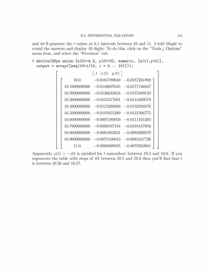
B.3. DIFFERENTIAL EQUATIONS 142
and we’ll generate the t values at 0.1 intervals between 10 and 11. I told Maple toround the answers and display 10 digits: To do this, click on the “Tools ¿ Options”menu item, and select the “Precision” tab.
> dsolve(DSys union x(0)=4.3, y(0)=0, numeric, [x(t),y(t)],
output = array([seq(10+i/10, i = 0 .. 10)]));
[
t x (t) y (t)]
10.0 −0.0161789040 −0.0187261898
10.1000000000 −0.0148697645 −0.0171746947
10.2000000000 −0.0136632824 −0.0157489123
10.3000000000 −0.0125517681 −0.0144389579
10.4000000000 −0.0115280660 −0.0132356876
10.5000000000 −0.0105855389 −0.0121306775
10.6000000000 −0.0097180050 −0.0111161205
10.7000000000 −0.0089197184 −0.0101847950
10.8000000000 −0.0081853621 −0.0093300578
10.9000000000 −0.0075100013 −0.0085457726
11.0 −0.0068890505 −0.0078262601
Apparently x(t) = −.01 is satisfied for t somewhere between 10.5 and 10.6. If youregenerate the table with steps of .01 between 10.5 and 10.6 then you’ll find that tis between 10.56 and 10.57.

APPENDIX C
Extra problems
C.1. Let F (x) = x2 − 2x+ 2. Find the steady states.
C.2. Let F (x) =x
2x+ 1, for x ≥ 0.
(a) Find the steady state. (There is only one; remember x ≥ 0.)(b) Calculate F t(1) for several values of t. You should see a pattern. Can you
write a non-recursive formula for F t(1)? What is limt→∞
F t(1)?
(c) Can you generalize part (b) by replacing 1 with any x > 0?
C.3. Let F (x) =x
x2 + 1, for any real x.
(a) Find the steady state. (There is only one.)(b) Show that F (x) < x for all x ≥ 0.(c) Why is lim
t→∞F t(x) = 0 for any x ≥ 0?
C.4. Find the flow defined by each of the following defferential equations:
(a)dx
dt= sec(x).
(b)dx
dt= eax, where a is a non-zero parameter.
(c)dx
dt=
√a2 − x2, where a is a positive parameter and |x| < a.
(d)dx
dt=
r
x− awhere r and a are non-zero parameters.
C.5. This question concerns the differential equationdx
dt= f(x) = (x− 1)2(x2 − 9).
In the following consider all possible initial values −∞ < x0 < ∞. Do not tryto solve the differential equation.(a) Find the steady state solutions.(b) Determine the intervals on which f(x) is positive or negative.(c) Sketch a number of solution curves using this information. Indicate the
steady state solutions, and indicate the limiting behavior of the other solu-tions.
143

C. EXTRA PROBLEMS 144
(d) Determine limt→∞
x(t) for all possible initial conditions. Your answer will de-
pend on different ranges of the initial conditions.
C.6. Radioactive isotopes decay according to the basic lawdx
dt= −rx where x is the
amount of the isotope and r is a constant. Here x is measured in grams and tin years. It is known that the most common isotope of radium has a half lifeof about 1600 years. This means that if x(t) is the solution of the differentialequation with initial condition x(0) = x0 then x(1600) = 1
2x0.
(a) Calculate r. [Solve the differential equation, then use logarithms. Give anumeric value for your answer.]
(b) Now suppose that, in an initially empty storage facility, 10 grams of thisisotope are deposited each year. Modify the differential equation to modelthis situation. Explain how you arrived at your modifications.
(c) The amount of radium in the storage facility has a finite limit as t → ∞.Find the limit.
(d) How long does it take until the amount of radium reaches 90% of its limit?
C.7. In each of the following, what restrictions are needed on the domain of x so thatany initial value problem with x0 in this domain will have a unique answer?Explain your answer.
(a)dx
dt= (1 − x2)1/3.
(b)dx
dt= (1 − x2)4/3.
(c)dx
dt= (1 − x2)−1/3.
C.8. A is a diagonalizable matrix. Using Maple, I calculated
A30 =
−11318 1617 8893−22582 3227 17743−11327 1618 8900
, A31 =
−14127 2018 11100−28309 4043 22242−14118 2017 11093
(rounded)
From this, determine an eigenvalue λ1 and corresponding eigenvector v1 for A.You should normalize v1 so that its third component is 1. You should be able todetermine λ1 to the nearest hundredth. (Do not use anything except a simplecalculator, for doing arithmetic.)
C.9. Let B =
[
2 1−1 0
]
.
(a) What are the eigenvalues and corresponding eigenvectors of B?(b) Is B diagonalizable?

C. EXTRA PROBLEMS 145
(c) Calculate a few powers of B. Do you see a pattern? Can you find a non-recursive formula for Bn?
C.10. There are three towns, North Apple, South Apple, Apple Core (abbreviated N,S, C). There is considerable migration between these towns. In each year
from N: 10% move to S, 10% move to C, and the rest stay in N;from S: 5% move to N, 15% move to C, and the rest stay in S;from C: 15% move to N, 20% move to S, and the rest stay in C.
This is a very simple model; we are ignoring births and deaths, and migrationfrom or to the outside.(a) Draw the network for this Markov chain, and write down the corresponding
matrix W . Follow the same scheme as in (3.5) and (3.6).(b) Find the limiting probability distribution p, using the fact that it is an
eigenvector of M = W T corresponding to the eigenvalue 1. Be sure thatthe entries in p sum to 1.
(c) Initially there are 1000000 people in each of the cities. What do you expectthe population in each city to be after many years?
C.11. Let A =
[
3 −21 0
]
. Find the solution todx
dt= Ax, x(0) = x0 =
[
a1
a2
]
by the
following method:(a) Find the eigenvalues and eigenvectors.(b) Find the change of basis matrix P and its inverse.(c) Find the matrix exponential etA by calculating PetΛP where Λ is the dia-
bonal matrix with the eigenvalues on the diagonal.
(d) Now calculate x(t) = etAx0 = etA ·[
a1
a2
]
C.12. Let A =
[
1 32 0
]
. Find the solution todx
dt= Ax, x(0) = x0 =
[
a1
a2
]
by the
following method:(a) Find the eigenvalues, λ1 and λ2, and the eigenvectors v1 and v2.
(b) x0 is a linear combination of v1 and v2, say x0 =
[
a1
a2
]
= c1v1 + c2v2. You
know the vectors v1 and v2, so this is a system of equations for the unknownsc1 and c2 in terms of the “known” constants a1 and a2. Solve for c1 and c2by row reduction or another method.
(c) Now x(t) = c1eλ1tv1+c2eλ2tv2. You know v1, v2, λ1, λ2 and you have formulas
for c1 and c2 in terms of a1 and a2. Put it all together.

C. EXTRA PROBLEMS 146
C.13. For each of the following differential equations, determine whether the equilib-rium at the origin is a saddle, a source, a sink, a center, or none of these. Incase it is a source or sink, determine whether it is a spiral source or sink.
(a)dx
dt= Ax, A =
[
3 −21 0
]
.
(b)dx
dt= Ax, A =
[
1 32 0
]
.
(c)dx
dt= Ax, A =
[
2 −51 0
]
.
(d)dx
dt= Ax, A =
[
2 −1−4 2
]
.
(e)dx
dt= Ax, A =
[
1 −52 −1
]
.


