Economics For Dummies®, 3rd Edition

Published by: John Wiley & Sons, Inc., 111 River Street, Hoboken, NJ07030-5774, www.wiley.com

Copyright © 2018 by John Wiley & Sons, Inc., Hoboken, New Jersey

Published simultaneously in Canada

No part of this publication may be reproduced, stored in a retrievalsystem or transmitted in any form or by any means, electronic,mechanical, photocopying, recording, scanning or otherwise, except aspermitted under Sections 107 or 108 of the 1976 United States CopyrightAct, without the prior written permission of the Publisher. Requests tothe Publisher for permission should be addressed to the PermissionsDepartment, John Wiley & Sons, Inc., 111 River Street, Hoboken, NJ07030, (201) 748-6011, fax (201) 748-6008, or online athttp://www.wiley.com/go/permissions.

Trademarks: Wiley, For Dummies, the Dummies Man logo,Dummies.com, Making Everything Easier, and related trade dress aretrademarks or registered trademarks of John Wiley & Sons, Inc., and maynot be used without written permission. All other trademarks are theproperty of their respective owners. John Wiley & Sons, Inc., is notassociated with any product or vendor mentioned in this book.

LIMIT OF LIABILITY/DISCLAIMER OF WARRANTY: WHILE THEPUBLISHER AND AUTHOR HAVE USED THEIR BEST EFFORTSIN PREPARING THIS BOOK, THEY MAKE NOREPRESENTATIONS OR WARRANTIES WITH RESPECT TO THEACCURACY OR COMPLETENESS OF THE CONTENTS OF THISBOOK AND SPECIFICALLY DISCLAIM ANY IMPLIEDWARRANTIES OF MERCHANTABILITY OR FITNESS FOR APARTICULAR PURPOSE. NO WARRANTY MAY BE CREATED OREXTENDED BY SALES REPRESENTATIVES OR WRITTEN SALESMATERIALS. THE ADVICE AND STRATEGIES CONTAINEDHEREIN MAY NOT BE SUITABLE FOR YOUR SITUATION. YOUSHOULD CONSULT WITH A PROFESSIONAL WHEREAPPROPRIATE. NEITHER THE PUBLISHER NOR THE AUTHORSHALL BE LIABLE FOR DAMAGES ARISING HEREFROM.

For general information on our other products and services, please

contact our Customer Care Department within the U.S. at 877-762-2974,outside the U.S. at 317-572-3993, or fax 317-572-4002. For technicalsupport, please visithttps://hub.wiley.com/community/support/dummies.

Wiley publishes in a variety of print and electronic formats and by print-on-demand. Some material included with standard print versions of thisbook may not be included in e-books or in print-on-demand. If this bookrefers to media such as a CD or DVD that is not included in the versionyou purchased, you may download this material athttp://booksupport.wiley.com. For more information about Wileyproducts, visit www.wiley.com.

Library of Congress Control Number: 2018937401

ISBN 978-1-119-47638-2 (pbk); ISBN 978-1-119-47627-6 (ebk); ISBN978-1-119-47632-0 (epdf)

Economics For Dummies®To view this book's Cheat Sheet, simply go towww.dummies.com and search for “Economics ForDummies Cheat Sheet” in the Search box.

Table of ContentsCoverIntroduction

About This BookFoolish AssumptionsIcons Used in This BookBeyond the BookWhere to Go from Here

Part 1: Economics: The Science of How People Deal withScarcity

Chapter 1: What Economics Is and Why You Should CareConsidering a Little Economic HistoryFraming Economics as the Science of ScarcitySending Microeconomics and Macroeconomics to SeparateCornersUnderstanding How Economists Use Models and Graphs

Chapter 2: Cookies or Ice Cream? Exploring ConsumerChoices

Describing Human Behavior with a Choice ModelPursuing Personal HappinessYou Can’t Have Everything: Examining LimitationsMaking Your Choice: Deciding What and How Much YouWantExploring Violations and Limitations of the Economist’sChoice Model

Chapter 3: Producing Stuff to Maximize HappinessFiguring Out What’s Possible to ProduceDeciding What to ProducePromoting Technology and Innovation

Part 2: Microeconomics: The Science of Consumer and FirmBehavior

Chapter 4: Supply and Demand Made EasyDeconstructing DemandSorting Out SupplyBringing Supply and Demand TogetherPrice Controls: Keeping Prices Away from MarketEquilibrium

Chapter 5: Introducing Homo Economicus, the Utility-Maximizing Consumer

Choosing by RankingGetting Less from More: Diminishing Marginal UtilityChoosing Among Many Options When Facing a LimitedBudgetDeriving Demand Curves from Diminishing Marginal Utility

Chapter 6: The Core of Capitalism: The Profit-Maximizing Firm

A Firm’s Goal: Maximizing ProfitsFacing CompetitionAnalyzing a Firm’s Cost StructureComparing Marginal Revenues with Marginal CostsPulling the Plug: When Producing Nothing Is Your Best Bet

Chapter 7: Why Economists Love Free Markets andCompetition

Ensuring That Benefits Exceed Costs: Competitive FreeMarketsWhen Free Markets Lose Their Freedom: Dealing withDeadweight LossesHallmarks of Perfect Competition: Zero Profits and LowestPossible Costs

Chapter 8: Monopolies: Bad Behavior withoutCompetition

Examining Profit-Maximizing MonopoliesComparing Monopolies with Competitive Firms

Considering Good MonopoliesRegulating Monopolies

Chapter 9: Oligopoly and Monopolistic Competition:Middle Grounds

Oligopolies: Looking at the Allure of Joining ForcesUnderstanding Incentives to Cheat the CartelRegulating OligopoliesStudying a Hybrid: Monopolistic Competition

Part 3: Applying the Theories of MicroeconomicsChapter 10: Property Rights and Wrongs

Allowing Markets to Reach Socially Optimal OutcomesExamining Externalities: The Costs and Benefits Others Feelfrom Your ActionsTragedy of the Commons: Overexploiting CommonlyOwned Resources

Chapter 11: Asymmetric Information and Public GoodsFacing Up to Asymmetric InformationProviding Public Goods

Chapter 12: Health Economics and Healthcare FinanceDefining Health Economics and Healthcare FinanceNoting the Limits of Health InsuranceComparing Healthcare InternationallyInflated Demand: Suffering from “Free” and Reduced-CostHealthcareInvestigating Singapore’s Secrets

Chapter 13: Behavioral Economics: InvestigatingIrrationality

Explaining the Need for Behavioral EconomicsComplementing Neo-Classical Economics with BehavioralEconomicsExamining our Amazing, Efficient, and Error-Prone BrainsSurveying Prospect Theory

Countering Myopia and Time InconsistencyGauging Fairness and Self-Interest

Part 4: Macroeconomics: The Science of Economic Growth andStability

Chapter 14: How Economists Measure the MacroeconomyGetting a Grip on the GDP (and Its Parts)Diving In to the GDP EquationMaking Sense of International Trade and Its Effect on theEconomy

Chapter 15: Inflation Frustration: Why More Money Isn’tAlways Good

Buying an Inflation: When Too Much Money Is a BadThingMeasuring InflationPricing the Future: Nominal and Real Interest Rates

Chapter 16: Understanding Why Recessions HappenIntroducing the Business CycleStriving for Full-Employment Output

Returning to Y*: The Natural Result of Price AdjustmentsResponding to Economic Shocks: Short-Run and Long-RunEffectsHeading toward Recession: Getting Stuck with Sticky PricesAchieving Equilibrium with Sticky Prices: The KeynesianModel

Chapter 17: Fighting Recessions with Monetary and FiscalPolicy

Stimulating Demand to End RecessionsGenerating Inflation: The Risk of Too Much StimulationFiguring Out Fiscal PolicyDissecting Monetary Policy

Chapter 18: Grasping Origins and Effects of FinancialCrises

Understanding How Debt-Driven Bubbles Develop

Seeing the Bubble BurstAfter the Crisis: Looking at Recovery

Part 5: The Part of TensChapter 19: Ten Seductive Economic Fallacies

The Lump of LaborThe World Is Facing OverpopulationSequence Indicates CausationProtectionism Is the Best Solution to Foreign CompetitionThe Fallacy of CompositionIf It’s Worth Doing, Do It 100 PercentFree Markets Are Dangerously UnstableLow Foreign Wages Mean That Rich Countries Can’tCompeteTax Rates Don’t Affect Work EffortForgetting Unintended Consequences

Chapter 20: Ten Economic Ideas to Hold DearSelf-Interest Can Improve SocietyFree Markets Require RegulationEconomic Growth Relies on InnovationFreedom and Democracy Make Us RicherEducation Raises Living StandardsIntellectual Property Boosts InnovationWeak Property Rights Cause All Environmental ProblemsInternational Trade Is a Good ThingGovernment Can Provide Public GoodsPreventing Inflation Is Easy

Chapter 21: Ten (Or So) Famous EconomistsAdam SmithDavid RicardoKarl MarxAlfred MarshallJohn Maynard Keynes

Kenneth Arrow and Gerard DebreuMilton FriedmanPaul SamuelsonRobert SolowGary BeckerRobert Lucas

Appendix: GlossaryAbout the AuthorAdvertisement PageConnect with DummiesIndexEnd User License Agreement

IntroductionEconomics is all about humanity’s struggle to achieve happiness in aworld full of constraints. There’s never enough time or money to doeverything people want, and things like curing cancer are still impossiblebecause the necessary technologies haven’t been developed yet. Butpeople are clever. They tinker and invent, ponder and innovate. Theylook at what they have and what they can do with it and take steps tomake sure that if they can’t have everything, they’ll at least have as muchas possible.

Having to choose is a fundamental part of everyday life. The science thatstudies how people choose — economics — is indispensable if youreally want to understand human beings both as individuals and asmembers of larger organizations. Sadly, though, economics has typicallybeen explained so badly that people either dismiss it as impenetrablegobbledygook or stand falsely in awe of it — after all, if it’s hard tounderstand, it must be important, right?

I wrote this book so you can quickly and easily understand economics forwhat it is — a serious science that studies a serious subject and hasdeveloped some seriously good ways of explaining human behavior outin the (very serious) real world. Economics touches on nearlyeverything, so the returns on reading this book are huge. You’llunderstand much more about people, the government, internationalrelations, business, and even environmental issues.

About This BookThe Scottish historian Thomas Carlyle called economics the “dismalscience,” but I’m going to do my best to make sure that you don’t come toagree with him. I’ve organized this book to try to get as much economicsinto you as quickly and effortlessly as possible. I’ve also done my best tokeep it lively and fun.

In this book, you find the most important economic theories, hypotheses,and discoveries without a zillion obscure details, outdated examples, orcomplicated mathematical “proofs.” Among the topics covered are

How the government fights recessions and unemploymentHow and why international trade is good for both individuals andnationsWhy poorly designed property rights are responsible forenvironmental problems such as global warming, pollution, andspecies extinctionsHow profits guide businesses to produce the goods and services youtake for grantedHow economic incentives affect healthcare costs, prices, andefficiencyWhy competitive firms are almost always better for society thanmonopoliesHow the Federal Reserve controls the money supply, interest rates,and inflation all at the same timeWhy government policies such as price controls and subsidies oftencause much more harm than goodHow the simple supply and demand model can explain the prices ofeverything from comic books to open-heart surgeries

You can read the chapters in any order, and you can immediately jump towhat you need to know without having to read a bunch of stuff that youcouldn’t care less about.

Economists like competition, so you shouldn’t be surprised that there are

a lot of competing views. Indeed, it’s only through vigorous debate andcareful review of the evidence that the profession improves itsunderstanding of how the world works. This book contains core ideasand concepts that economists agree are true and important — I try tosteer clear of fads or ideas that foster a lot of disagreement. (If you wantto be subjected to my opinions and pet theories, you’ll have to buy me adrink.)

Note: Economics is full of two things you may not find very appealing:jargon and algebra. To minimize confusion, whenever I introduce a newterm, I put it in italics and follow it closely with an easy-to-understanddefinition. Also, whenever I bring algebra into the discussion, I use thosehandy italics again to let you know that I’m referring to a mathematicalvariable. For instance, I is the abbreviation for investment, so you maysee a sentence like this one: I think that I is too big.

I try to keep equations to a minimum, but sometimes they help makethings clearer. In such instances, I sometimes have to use severalequations one after another. To avoid confusion about which equation I’mreferring to at any given time, I give each equation a number, which I putin parentheses. For example,

(1) (2)

Foolish AssumptionsI wrote this book assuming some things about you:

You’re sharp, thoughtful, and interested in how the world works.You’re a high school or college student trying to flesh out whatyou’re learning in class, or you’re a citizen of the world who realizesthat a good grounding in economics will help you understandeverything from business and politics to social issues like povertyand environmental degradation.You want to know some economics, but you’re also busy leading avery full life. Consequently, although you want the crucial facts, youdon’t want to have to read through a bunch of minutiae to find them.You’re not totally intimidated by numbers, facts, and figures. Indeed,you welcome them because you like to have things proven to youinstead of taking them on faith because some pinhead with a PhDsays so.You like learning why as well as what. That is, you want to knowwhy things happen and how they work instead of just memorizingfactoids.

Icons Used in This BookTo make this book easier to read and simpler to use, I include a fewicons that can help you find and fathom key ideas and information.

This icon alerts you that I’m explaining a fundamental economicconcept or fact that you would do well to stash away in yourmemory for later. It saves you the time and effort of marking thebook with a highlighter.

This icon tells you that the ideas and information that itaccompanies are a bit more technical or mathematical than othersections of the book. This information can be interesting andinformative, but I’ve designed the book so that you don’t need tounderstand it to get the big picture about what’s going on. Feel freeto skip this stuff.

This icon points out time and energy savers. I place this iconnext to suggestions for ways to do or think about things that can saveyou some effort.

This icon discusses any troublesome areas in economics youneed to know. Keep an eye open for them to alert you of potentialpitfalls.

Beyond the BookTo view this book’s Cheat Sheet, simply go to www.dummies.com andsearch for “Economics For Dummies Cheat Sheet” for a handy referenceguide that answers common questions about economics.

To gain access to the additional tests and practice online, all you have todo is register. Just follow these simple steps:

1. Find your PIN access code.Print-book users: If you purchased a print copy of this book, turn tothe inside front cover of the book to find your access code.E-book users: If you purchased this book as an e-book, you can getyour access code by registering your e-book atwww.dummies.com/go/getaccess. Go to that website and find yourbook. Click it and answer the security questions to verify yourpurchase. You’ll receive an email with your access code.

2. Go to Dummies.com and click Activate Now.3. Find your product (Economics For Dummies, 3rd Edition) and

then follow the on-screen prompts to activate your PIN.

Now you’re ready to go! You can come back to the program as often asyou want — simply log in with the username and password you createdduring your initial login. No need to enter the access code a second time.

For Technical Support, please visit http://wiley.custhelp.com orcall Wiley at 1-800-762-2974 (U.S.), +1-317-572-3994 (international).

Where to Go from HereThis book is set up so that you can understand what’s going on even ifyou skip around. The book is also divided into independent parts so thatyou can, for instance, read all about microeconomics without having toread anything about macroeconomics. The table of contents and indexcan help you find specific topics easily. But, hey, if you don’t knowwhere to begin, just do the old-fashioned thing and start at the beginning.

Part 1

Economics: The Science ofHow People Deal with Scarcity

IN THIS PART …Find out what economics is, what economists do, and why these thingsare important.

Decipher how people decide what brings them the most happiness.

Understand how goods and services are produced, how resources areallocated, and the roles of government and the market.

Chapter 1

What Economics Is and WhyYou Should Care

IN THIS CHAPTER Taking a quick peek at economic history Observing how people cope with scarcity Separating macroeconomics and microeconomics Getting a grip on the graphs and models that economists love to

use

Economics is the science that studies how people and societies makedecisions that allow them to get the most out of their limited resources.And because every country, every business, and every person has to dealwith constraints, economics is literally everywhere. For instance, youcould be doing something else right now besides reading this book. Youcould be exercising, watching a movie, or talking with a friend. Youshould only be reading this book if doing so is the best possible use ofyour very limited time. In the same way, you should hope that the paperand ink used to make this book have been put to their best use and thatevery last tax dollar that your government spends is being used in thebest way.

Economics gets to the heart of these issues, analyzing the behavior ofindividuals and firms, as well as social and political institutions, to seehow well they convert humanity’s limited resources into the goods andservices that best satisfy human wants and desires.

Considering a Little EconomicHistory

To better understand today’s economic situation and what sort of policyand institutional changes may promote the greatest improvements, youhave to look back on economic history to see how humanity got to whereit is now. Stick with me: I make this discussion as painless as possible.

Pondering just how nasty, brutish, and shortlife used to beFor most of human history, people didn’t manage to squeeze much out oftheir limited resources. Standards of living were quite low, and peoplelived poor, short, and rather painful lives. Consider the following facts,which didn’t change until just a few centuries ago:

Life expectancy at birth was about 25 years.More than 30 percent of newborns never made it to their fifthbirthdays.A woman had a one in ten chance of dying every time she gave birth.Most people had experienced horrible diseases and/or starvation.The standard of living was low and stayed low, generation aftergeneration. Except for the nobles, everybody lived at or nearsubsistence, century after century.

In the last 250 years or so, however, everything changed. For the firsttime in history, people figured out how to use electricity, engines,complicated machines, computers, radio, television, biotechnology,scientific agriculture, antibiotics, aviation, and a host of othertechnologies. Each has allowed people to do much more with the limitedamounts of air, water, soil, and sea they were given on planet Earth. Theresult has been an explosion in living standards, with life expectancy atbirth now over 70 years worldwide and with many people able to affordmuch better housing, clothing, and food than was imaginable a fewhundred years ago.

Of course, not everything is perfect. Grinding poverty is still a fact in alarge fraction of the world, and even the richest nations have to copewith pressing economic problems like unemployment and how totransition workers from dying industries to growing industries. But thefact remains that overall, the modern world is a much richer place thanits predecessor, and most nations now have sustained economic growth,which means that living standards rise year after year.

Identifying the institutions that raise livingstandardsThe obvious reason for higher living standards, which continue to rise, isthat human beings have recently figured out lots of new technologies, andpeople keep inventing more. But if you dig a little deeper, you have towonder why a technologically innovative society didn’t happen earlier.

The Ancient Greeks invented a simple steam engine and the coin-operated vending machine. They even developed the basic idea behindthe programmable computer. But they never quite got around to having anindustrial revolution and entering on a path of sustained economicgrowth.

And despite the fact that there have always been really smart people inevery society on earth, it wasn’t until the late 18th century, in England,that the Industrial Revolution actually got started and living standards inmany nations rose substantially and kept on rising, year after year.

So what factors combined in the late 18th century to so radicallyaccelerate economic growth? The short answer is that the followinginstitutions were in place:

Democracy: Because the common people outnumbered the nobles,the advent of democracy meant that for the first time, governmentsreflected the interests of a society at large. A major result was thecreation of government policy that favored merchants andmanufacturers rather than the nobility.The limited liability corporation: Under this business structure,investors could lose only the amount of their investment and not be

liable for any debts that the corporation couldn’t pay. Limitedliability greatly reduced the risks of investing in businesses and,consequently, led to much more investing.Patent rights to protect inventors: Before patents, inventorsusually saw their ideas stolen before they could make any money. Bygiving inventors the exclusive right to market and sell theirinventions, patents gave a financial incentive to produce lots ofinventions. Indeed, after patents came into existence, the world sawits first full-time inventors — people who made a living inventingthings.Widespread literacy and education: Without highly educatedinventors, new technologies don’t get invented. And without aneducated workforce, they can’t be mass-produced. Consequently, thedecision that many nations made to make primary and then secondaryeducation mandatory paved the way for rapid and sustainedeconomic growth.

Institutions and policies like these have given people a world of growthand opportunity and an abundance so unprecedented in world history thatthe greatest public health problem in many countries today is obesity.

Looking toward the futureThe challenge moving forward is to get even more of what people wantout of the world’s limited pool of resources. This challenge needs to befaced because problems like infant mortality, child labor, malnutrition,endemic disease, illiteracy, and unemployment are all alleviated byhigher living standards and an increased ability to pay for solutions tosuch problems.

Along those lines, it’s important to point out that many poverty-relatedproblems can be cured by extending to poorer nations the institutions thathave already been proven by already-rich countries to lead to risingliving standards. In addition, developing nations can also learn from themistakes that were made by already-rich countries back when they werein the process of figuring out how to raise living standards — mistakesrelated to promoting economic growth without causing massive amountsof pollution, numerous species extinctions, or widespread resourcedepletion.

Consequently, there are two related and very good reasons foryou to read this book and get a firm grasp about economics:

You can discover how modern economies function. Doing so cangive you an understanding not only of how they’ve so greatly raisedliving standards but also of where they need some improvement.By getting a thorough handle on fundamental economicprinciples, you can judge for yourself the economic policyproposals that politicians and others run around promoting. Afterreading this book, you’ll be much better able to sort the good fromthe bad.

Framing Economics as theScience of Scarcity

Scarcity is the fundamental and unavoidable phenomenon that creates aneed for the science of economics: There isn’t nearly enough time orstuff to satisfy all desires, so people have to make hard choices aboutwhat to produce and consume so that if they can’t have everything, they atleast have the best that was possible under the circumstances. Withoutscarcity of time, scarcity of resources, scarcity of information, scarcityof consumable goods, and scarcity of peace and goodwill on Earth,human beings would lack for nothing. Chapter 2 gets deep into scarcityand the tradeoffs that it forces people to make.

Economists analyze the decisions people make about how to bestmaximize human happiness in a world of scarcity. That process turns outto be intimately connected with a phenomenon known as diminishingreturns, which describes the sad fact that each additional amount of aresource that’s thrown at a production process brings forth successivelysmaller amounts of output.

Like scarcity, diminishing returns is unavoidable, and in Chapter 3, Iexplain how people very cleverly deal with this phenomenon in order toget the most out of humanity’s limited pool of resources.

Sending Microeconomics andMacroeconomics to SeparateCorners

The main organizing principle I use in this book is to divide economicsinto its two broad pieces, macroeconomics and microeconomics:

Microeconomics focuses on individual people and individualbusinesses. For individuals, it explains how they behave when facedwith decisions about where to spend their money or how to investtheir savings. For businesses, it explains how profit-maximizingfirms behave individually, as well as when competing against eachother in markets.Macroeconomics looks at the economy as an organic whole,concentrating on factors such as interest rates, inflation, andunemployment. It also encompasses the study of economic growthand the methods governments use to try to moderate the harm causedby recessions.

Underlying both microeconomics and macroeconomics are some basicprinciples such as scarcity and diminishing returns. Consequently, Ispend the rest of Part I explaining these fundamentals before diving in tomicroeconomics in Part II and macroeconomics in Part III. But first, thissection gives you an overview of microeconomics and macroeconomics.

Getting up close and personal:MicroeconomicsMicroeconomics gets down to the nitty gritty, studying the mostfundamental economic agents: individuals and firms. This section delvesdeeper into the micro side of economics, including info on supply anddemand, competition, property rights, problems with markets, and theeconomics of healthcare.

Balancing supply and demandIn a modern economy, individuals and firms produce and consume

everything that gets made. Supply and demand determine prices andoutput levels in competitive markets. Producers determine supply,consumers determine demand, and their interaction in markets determineswhat gets made and how much it costs. (See Chapter 4 for details.)

Individuals make economic decisions about how to get the mosthappiness out of their limited incomes. They do this by first assessinghow much utility, or satisfaction, each possible course of action wouldgive them. They then weigh costs and benefits to select the course ofaction that will yield the greatest amount of utility possible given theirlimited incomes. These decisions generate the demand curves that affectprices and output levels in markets. I cover these decisions and demandcurves in Chapter 5.

In a similar way, the profit-maximizing decisions of firms generate thesupply curves that affect markets. Every firm will decide what toproduce and how much to produce by comparing costs and revenues. Aunit of output will only be produced if doing so will increase its maker’sprofit. In particular, a firm will only produce a unit if the increase inrevenue from selling it exceeds the unit’s cost of production. Thisbehavior underpins the upward slope of supply curves and how theyaffect prices and output levels in markets, as I discuss in Chapter 6.

Considering why competition is so greatYou may not feel warm and fuzzy about profit-maximizing firms, buteconomists love them — just as long as they’re stuck in competitiveindustries. The reason is that firms that are forced to compete end upsatisfying two wonderful conditions:

They’re allocatively efficient, which simply means that they producethe goods and services that consumers most greatly desire toconsume.They’re productively efficient, which means that they produce thesegoods and services at the lowest possible cost.

The allocative and productive efficiency of competitive firmsare the basis of Adam Smith’s famous invisible hand — the idea

that when constrained by competition, each firm’s greed ends upcausing it to act in a socially optimal way, as if guided to do theright thing by an invisible hand. I discuss this idea, and much moreabout the benefits of competition, in Chapter 7.

Examining problems caused by lack of competitionUnfortunately, not every firm is constrained by competition. And whenthat happens, firms don’t end up acting in socially optimal ways. Themost extreme case is monopoly, a situation where there’s only one firmin an industry — meaning that it has absolutely no competition.Monopolies behave very badly, restricting output in order to drive upprices and inflate profits. These actions hurt consumers and may go onindefinitely unless the government intervenes.

A less-extreme case of lack of competition is oligopoly, a situation inwhich only a few firms are in an industry. In such situations, firms oftenmake deals not to compete against each other so that they can keep priceshigh and make bigger profits. However, these firms often have a hardtime keeping their agreements with each other. This fact means thatoligopoly firms often end up competing against each other despite theirbest efforts not to. Consequently, government regulation isn’t alwaysneeded. You can read more about monopolies in Chapter 8 andoligopolies in Chapter 9.

Reforming property rights

You can rely upon markets and competition to produce sociallybeneficial results only if society sets up a good system of propertyrights. A property right gives a person the exclusive authority todetermine how a productive resource can be used. Thus, forexample, a person who has the property right (ownership) over apiece of land can determine whether it will be used for farming, asan amusement park, or as a nature preserve. All pollution issues, aswell as all cases of species loss, are the direct result of poorlydesigned property rights generating perverse incentives to do badthings. Economists take this problem seriously and have done theirbest to reform property rights in order to alleviate pollution andeliminate species loss. I discuss these issues in detail in Chapter

10.

Dealing with other common market failuresMonopolies, oligopolies, and poorly designed property rights all lead towhat economists like to call market failures — situations in whichmarkets don’t deliver socially optimal outcomes. Two other commoncauses of market failure are asymmetric information and public goods:

Asymmetric information: Asymmetric information refers tosituations in which either the buyer or the seller knows more aboutthe quality of the good that he or she is negotiating over than does theother party. Because of the uneven playing field and the suspicions itcreates, a lot of potentially beneficial economic transactions neverget completed.Public goods: Public goods are goods or services that areimpossible to provide to just one person; if you provide them to oneperson, you have to provide them to everybody. (Think of an outdoorfireworks display, for example.) The problem is that most people tryto get the benefit without paying for it.

I discuss both these situations, and ways to deal with them, in Chapter11.

Diagnosing healthcare economicsAlmost everyone is deeply concerned about access to affordable, high-quality medical care — medical care delivered through government-runnational health systems, through employer-sponsored health insurance, orby direct payments made by consumers. Each system provides differentincentives that can affect efficiency, usage, and cost — sometimes quiteperversely. Chapter 12 gets you up to date on the incentives, regulations,and policies that determine how both coverage and affordability can beimproved from an economics standpoint.

Understanding behavioral economicsPeople aren’t always rational, and that matters because most ofeconomics was developed by asking what a rational person would do inone situation or another. Behavioral economics fills in the gaps bylooking at decision-making when people aren’t being rational. Fourbillion years of evolution has left us with brains that are prone to errors,

including being overconfident and too focused on the present, beingeasily confused by irrelevant information, and being unable to see thebigger picture when making financial decisions. I spend Chapter 13rationally explaining all this irrational behavior. It’s crazy fun.

Zooming out: Macroeconomics and the bigpictureMacroeconomics treats the economy as a unified whole. Studyingmacroeconomics is useful because certain factors, such as interest ratesand tax policy, have economy-wide effects and also because when theeconomy goes into a recession or a boom, every person and everybusiness is affected. This section gives you an overview ofmacroeconomics.

Measuring the economyEconomists measure gross domestic product (GDP), the value of allgoods and services produced in a nation’s economy in a given period oftime, usually a quarter or a year. Totaling up this number is vital becauseif you can’t measure how the economy is doing, you can’t tell whethergovernment polices intended to improve the economy are helping orhurting. Chapter 14 explains GDP in more depth.

Inflation measures how prices in the economy increase over time. Thistopic, inflation, is the focus of Chapter 15, and it is crucial because highrates of inflation usually accompany huge economic problems, includingdeep recessions and countries defaulting on their debts.

It’s also important to study inflation because poor government policy isthe sole culprit behind high rates of inflation — meaning thatgovernments are responsible when big inflations happen.

Looking at international tradeInternational trade occurs when consumers, firms, or governmentspurchase products or resources made in other countries. Becauseimported goods often compete with locally produced goods,international trade is the subject of endless political controversy andattempts to erect import duties or numerical quotas to keep foreign goodsout and thereby make life easier for domestic producers.

Those disputes are intensified by concerns about whether foreign

working conditions are humane, whether foreign producers are unfairlysubsidized by their governments, and whether currency exchange ratesare being manipulated by foreign governments to give their own firms acost advantage over firms in other countries. Chapter 14 explains howeconomists analyze these and other globalization issues.

Understanding and fighting recessions

A recession occurs when the total amount of goods and servicesproduced in an economy declines. Recessions are very painful fortwo reasons:

Less output means less consumption.Many workers lose their jobs because firms need fewer workers toproduce the reduced amount of output.

Recessions linger because institutional factors in the economy make itvery hard for prices in the economy to fall. If prices could fall quicklyand easily, recessions would quickly resolve themselves. But becauseprices can’t quickly and easily fall, economists have had to developantirecessionary policies to help get economies out of recessions asquickly as possible.

The man most responsible for developing antirecessionary policies wasthe English economist John Maynard Keynes, who in 1936 wrote the firstmacroeconomics book about fighting recessions. Chapter 16 introducesyou to his model of the economy and how it explicitly takes account ofthe fact that prices can’t quickly and easily fall to get you out ofrecessions. It serves as the perfect vehicle for illustrating the two thingsthat can help get you out of a recession.

Chapter 17 discusses two things governments can use to fight arecession:

Monetary policy: Monetary policy uses changes in the money supplyto change interest rates in order to stimulate economic activity. For

instance, if the government causes interest rates to fall, consumersborrow more money to buy things like houses and cars, therebystimulating economic activity and helping to get the economy movingfaster.Fiscal policy: Fiscal policy refers to using increased governmentspending or lower tax rates to help fight recessions. For instance, ifthe government buys more goods and services, economic activityincreases. In a similar fashion, if the government cuts tax rates,consumers end up with higher after-tax incomes, which, when spent,increase economic activity.

In the first decades after Keynes’s antirecessionary ideas were put intopractice, they seemed to work really well. However, they didn’t fare sowell during the 1970s, and it became apparent that although monetaryand fiscal policy were powerful antirecessionary tools, they had theirlimitations.

For this reason, Chapter 17 also covers how and why monetary andfiscal policy are constrained in their effectiveness. The key concept iscalled rational expectations. It explains how rational people very oftenchange their behavior in response to policy changes in ways that limit theeffectiveness of those changes. It’s a concept that you need to understandif you’re going to come up with informed opinions about currentmacroeconomic policy debates.

Financial crises are recessions triggered by the failure of importantfinancial institutions to keep their financial promises. Such failures oftenhappen after consumers or businesses take on too much debt and areunable to repay loans to banks. Sometimes they occur when a governmenttakes on too much debt and cannot repay its bondholders. Chapter 18discusses the causes and consequences of financial crises.

Understanding How EconomistsUse Models and Graphs

Economists like to be logical and precise, which is why they use a lot ofalgebra and other math. But they also like to present their ideas in easy-to-understand and highly intuitive ways, which is why they use so manygraphs.

The graphs economists use are almost always visual representations ofeconomic models. An economic model is a mathematical simplificationof reality that allows you to focus on what’s really important by ignoringlots of irrelevant details. For instance, the economist’s model ofconsumer demand focuses on how prices affect the amounts of goods andservices that people want to buy. Obviously, other things, such aschanging styles and tastes, affect consumer demand as well, but price iskey.

To avoid a graph-induced panic as you flip through the pages of thisbook, I spend a few pages helping you get acquainted with what youencounter in other chapters. Take a deep breath; I promise this won’thurt.

Introducing your first model: The demandcurveWhen economists look at demand, they simplify by concentrating onprices. Consider orange juice, for example. The price of orange juice isthe major thing that affects how much orange juice people are going tobuy. (I don’t care which dietary trend is in vogue — if orange juice cost$50 a gallon, you’d probably find another diet.) Therefore, it’s helpful toabstract from those other things and concentrate solely on how the priceof orange juice affects the quantity of orange juice that people want tobuy.

Suppose that economists go out and survey consumers, asking them howmany gallons of orange juice they would buy each month at threehypothetical prices: $10 per gallon, $5 per gallon, and $1 per gallon.The results are summarized in the following table:

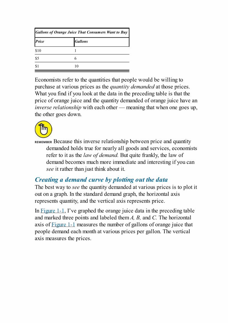
Gallons of Orange Juice That Consumers Want to Buy

Price Gallons

$10 1

$5 6

$1 10

Economists refer to the quantities that people would be willing topurchase at various prices as the quantity demanded at those prices.What you find if you look at the data in the preceding table is that theprice of orange juice and the quantity demanded of orange juice have aninverse relationship with each other — meaning that when one goes up,the other goes down.

Because this inverse relationship between price and quantitydemanded holds true for nearly all goods and services, economistsrefer to it as the law of demand. But quite frankly, the law ofdemand becomes much more immediate and interesting if you cansee it rather than just think about it.

Creating a demand curve by plotting out the dataThe best way to see the quantity demanded at various prices is to plot itout on a graph. In the standard demand graph, the horizontal axisrepresents quantity, and the vertical axis represents price.

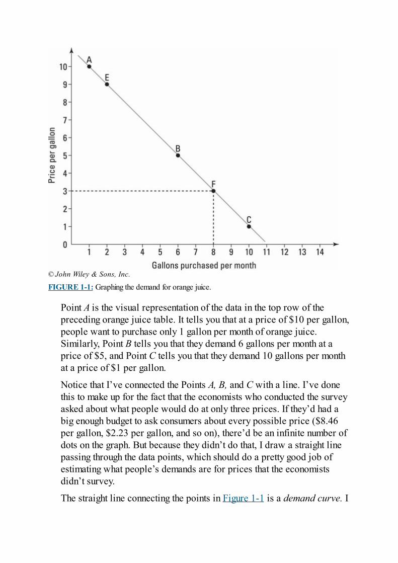
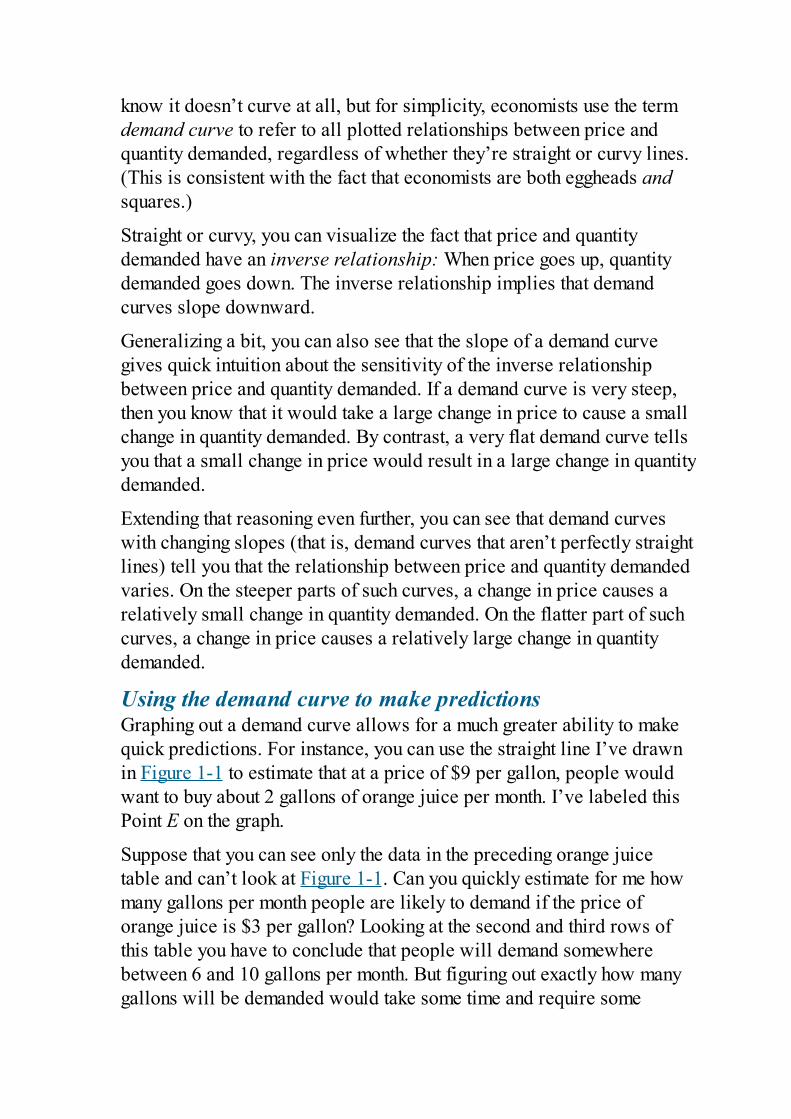
In Figure 1-1, I’ve graphed the orange juice data in the preceding tableand marked three points and labeled them A, B, and C. The horizontalaxis of Figure 1-1 measures the number of gallons of orange juice thatpeople demand each month at various prices per gallon. The verticalaxis measures the prices.

© John Wiley & Sons, Inc.

FIGURE 1-1: Graphing the demand for orange juice.

Point A is the visual representation of the data in the top row of thepreceding orange juice table. It tells you that at a price of $10 per gallon,people want to purchase only 1 gallon per month of orange juice.Similarly, Point B tells you that they demand 6 gallons per month at aprice of $5, and Point C tells you that they demand 10 gallons per monthat a price of $1 per gallon.

Notice that I’ve connected the Points A, B, and C with a line. I’ve donethis to make up for the fact that the economists who conducted the surveyasked about what people would do at only three prices. If they’d had abig enough budget to ask consumers about every possible price ($8.46per gallon, $2.23 per gallon, and so on), there’d be an infinite number ofdots on the graph. But because they didn’t do that, I draw a straight linepassing through the data points, which should do a pretty good job ofestimating what people’s demands are for prices that the economistsdidn’t survey.

The straight line connecting the points in Figure 1-1 is a demand curve. I

know it doesn’t curve at all, but for simplicity, economists use the termdemand curve to refer to all plotted relationships between price andquantity demanded, regardless of whether they’re straight or curvy lines.(This is consistent with the fact that economists are both eggheads andsquares.)

Straight or curvy, you can visualize the fact that price and quantitydemanded have an inverse relationship: When price goes up, quantitydemanded goes down. The inverse relationship implies that demandcurves slope downward.

Generalizing a bit, you can also see that the slope of a demand curvegives quick intuition about the sensitivity of the inverse relationshipbetween price and quantity demanded. If a demand curve is very steep,then you know that it would take a large change in price to cause a smallchange in quantity demanded. By contrast, a very flat demand curve tellsyou that a small change in price would result in a large change in quantitydemanded.

Extending that reasoning even further, you can see that demand curveswith changing slopes (that is, demand curves that aren’t perfectly straightlines) tell you that the relationship between price and quantity demandedvaries. On the steeper parts of such curves, a change in price causes arelatively small change in quantity demanded. On the flatter part of suchcurves, a change in price causes a relatively large change in quantitydemanded.

Using the demand curve to make predictionsGraphing out a demand curve allows for a much greater ability to makequick predictions. For instance, you can use the straight line I’ve drawnin Figure 1-1 to estimate that at a price of $9 per gallon, people wouldwant to buy about 2 gallons of orange juice per month. I’ve labeled thisPoint E on the graph.

Suppose that you can see only the data in the preceding orange juicetable and can’t look at Figure 1-1. Can you quickly estimate for me howmany gallons per month people are likely to demand if the price oforange juice is $3 per gallon? Looking at the second and third rows ofthis table you have to conclude that people will demand somewherebetween 6 and 10 gallons per month. But figuring out exactly how manygallons will be demanded would take some time and require some

annoying calculations.

By contrast, if you look at Figure 1-1, it’s easy to figure out how manygallons per month people would demand at $3 per gallon. You start at $3on the vertical axis, move sideways to the right until you hit the demandcurve at Point F, and drop down vertically until you get to the horizontalaxis, where you discover that you’re at 8 gallons per month. (To clarify,I’ve drawn in a dotted line that follows this path.) As you can see, usinga figure rather than a table makes coming up with model-basedpredictions much, much simpler.

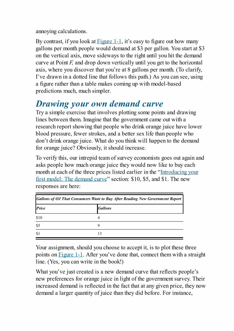
Drawing your own demand curveTry a simple exercise that involves plotting some points and drawinglines between them. Imagine that the government came out with aresearch report showing that people who drink orange juice have lowerblood pressure, fewer strokes, and a better sex life than people whodon’t drink orange juice. What do you think will happen to the demandfor orange juice? Obviously, it should increase.

To verify this, our intrepid team of survey economists goes out again andasks people how much orange juice they would now like to buy eachmonth at each of the three prices listed earlier in the “Introducing yourfirst model: The demand curve” section: $10, $5, and $1. The newresponses are here:

Gallons of OJ That Consumers Want to Buy After Reading New Government Report

Price Gallons

$10 4

$5 9

$1 13

Your assignment, should you choose to accept it, is to plot these threepoints on Figure 1-1. After you’ve done that, connect them with a straightline. (Yes, you can write in the book!)

What you’ve just created is a new demand curve that reflects people’snew preferences for orange juice in light of the government survey. Theirincreased demand is reflected in the fact that at any given price, they nowdemand a larger quantity of juice than they did before. For instance,

whereas before they wanted only 1 gallon per month at a price of $10,they now would be willing to buy 4 gallons per month at that price.

There is still, of course, an inverse relationship between price andquantity demanded, meaning that even though the health benefits oforange juice make people demand more orange juice, people are stillsensitive to higher orange juice prices. Higher prices still mean lowerquantities demanded, and your new demand curve still slopesdownward.

Use your new demand curve to figure out how many gallons per monthpeople are now going to want to buy at a price of $7 and at a price of $2.Figuring these things out from the data in the preceding table would behard, but figuring them out using your new demand curve should be easy.

Chapter 2

Cookies or Ice Cream?Exploring Consumer ChoicesIN THIS CHAPTER

Deciding what will bring the most happiness Cataloguing the constraints that limit choice Modeling choice behavior like an economist Evaluating the limitations of the choice model

Economics is all about how groups and individuals make choices andwhy they choose the things that they do. Economists have spent a greatdeal of time analyzing how groups make choices, but because groupchoice behavior usually turns out to be very similar to individual choicebehavior, my focus in this chapter is on individuals.

To keep things simple, my explanation of individual choice behaviorfocuses on consumer behavior because most of the choices people makeon a day-to-day basis involve which goods and services to consume.Human beings are constantly forced to choose because their wantsalmost always exceed their means. Limited resources, or scarcity, is atthe heart not only of economics but also of ecology and biology.Darwinian evolution is all about animals and plants competing overlimited resources to produce the greatest number of offspring. Economicsis about human beings choosing among limited options to maximizehappiness.

Describing Human Behaviorwith a Choice Model

Human beings may be complicated creatures with sometimes mystifyingbehavior, but most people are usually fairly predictable and consistentand behave pretty much like other people. You can gain a lot by studyingchoice behavior because if you can understand the choices people madein the past, you stand a good chance of understanding the choices they’llmake in the future.

Understanding (and even predicting) future choice behavior is veryimportant because major shifts in the economic environment are typicallythe result of millions of small individual decisions that add up to a majortrend. For instance, the circumstances under which millions ofindividuals choose to pursue work or school cumulate to major effectson the unemployment rate. And the choices these individuals make abouthow much of their paychecks to save or spend affect whether interestrates will be high or low and also whether gross domestic product(GDP) and overall economic output will increase or decrease. (I discussGDP in Chapter 14.)

In order to predict how self-interested individuals make theirchoices, economists have created a model of human behavior thatassumes that people are rational and able to calculate subtletradeoffs between possible choices. This model is a three-stageprocess:

1. Evaluate how happy each possible option can make you.2. Look at the constraints and tradeoffs limiting your options.3. Choose the option that will maximize your overall happiness.

Although not a complete description of human choice behavior, thismodel generally makes accurate predictions. However, many peoplequestion this explanation of human behavior. Here are three common

objections:

Are people really so self-interested? Aren’t people often motivatedby what’s best for others?Are people really aware at all times of all their options? How arethey supposed to rationally choose among new things that they’venever tried before?Are people really free to make decisions? Aren’t they constrained bylegal, moral, and social standards?

I spend the next few sections of this chapter expanding on the three-stepeconomic choice model and addressing the objections to it.

Pursuing Personal HappinessEconomists like to think of human beings as free agents with free wills.To economists, people are usually rational and, thus, normally capable ofmaking sensible decisions. But that begs the question of what motivatespeople and, in turn, of what sorts of things people will choose to dogiven their free wills.

In a nutshell, economists assume that the basic motivation driving mostpeople most of the time is a desire to be happy. This assumption impliesthat people make choices on the basis of whether or not those choiceswill make them as happy as they can be given their circumstances. Thissection examines how the pursuit of happiness affects consumerbehavior.

Using utility to measure happinessIf people make choices on the basis of which ones will bring them themost happiness, they need a way of comparing how much happiness eachpossible thing brings with it. Along these lines, economists assume thatpeople get a sense of satisfaction or pleasure from the things life offers.Sunsets are nice. Eating ice cream is nice. Friendship is nice. And Ihappen to like driving fast.

Economists suppose that you can compare all possible thingsthat you may experience with a common measure of happiness orsatisfaction that they call utility. Things you like a lot have highutility. Things that you like only a little have low utility. And thingsyou hate (like toxic waste or foods that cause you to have allergicreactions) have negative utility. Utility acts as a commondenominator that allows people to sensibly compare even radicallydifferent things.

The concept of utility is very broad. For a hedonist, utility may be thephysical gratification of experiencing sensual pleasures. But for amorally conscientious person, utility may be the sense of moralsatisfaction received when doing the right thing in a particular situation.

The important idea for economists is that people are able to sort out andcompare the utilities of various possible activities.

Taking “selfless” actions into accountEconomists take it as a given that people make their choices in life inorder to maximize their personal happiness. This viewpoint immediatelyraises objections because people are often willing to endure greatpersonal suffering in order to help others.

However, an economist can view altruism, helping others at one’s ownexpense, as a personal preference. The mother who doesn’t eat in orderto give what little food she has to her infant may be pursuing a goal(helping her child) that maximizes the mother’s own happiness. Thesame can be said about people who donate to charities. Most peopleconsider such generosity “selfless,” but it’s also consistent withassuming that people do things to make themselves happy. If people givebecause doing so makes them feel good, their selfless action is motivatedby selfish intention.

Because economists view human motivation as intrinsically self-interested economics is often accused of being immoral; however,economics is concerned with how people achieve their goals ratherthan with questioning the morality of those goals. For instance,some people like honey, but others do not. Economists make nodistinction between these two groups regarding the rightness orwrongness of their preferences. Rather, what interests economists ishow each group behaves given its preferences. Consequently,economics is amoral rather than immoral.

Economists are people, too, and they’re very concerned with things likesocial justice, climate change, and poverty. They just tend to interpret thedesire to pursue morality and equity as an individual goal that maximizesindividual happiness rather than as a group goal that should be pursuedin order to achieve some sort of collective good.

Self-interest can promote the common goodAdam Smith, one of the fathers of modern economics, believed that if

society was set up correctly, people chasing after their individualhappiness would provide for other people’s happiness as well. As hefamously pointed out in An Inquiry into the Nature and Causes of theWealth of Nations, published in 1776, “It is not from the benevolence ofthe butcher, the brewer, or the baker, that we can expect our dinner, butfrom their regard to their own interest.”

Put differently, the butcher, the brewer, and the baker make stufffor you not because they like you but because they want your money.Yet because they want your money, they end up producing for youeverything that you need to have a nice meal. When you trade themyour money for their goods, everyone is happier. You think that nothaving to prepare all that food is worth more to you than keepingyour money. And they think that getting your money is worth more tothem than the toil involved in preparing all that food.

Adam Smith expanded on this notion by saying that a person pursing hisown selfish interests may be “led by an invisible hand to promote an endwhich was no part of his intention.” Because economists recognize this“invisible hand,” they’re less concerned with intent than with outcomeand less concerned with what makes people happy than with how theypursue the things that make them happy.

You Can’t Have Everything:Examining Limitations

Life is full of limitations. Time, for instance, is always in limited supply,as are natural resources. The second stage of the economic choice modellooks at the constraints that force you to choose among your happyoptions.

For example, oil can be used to manufacture pharmaceuticals that cansave many lives. But it can also be used to make gasoline, which can beused to drive ambulances, which also save lives. Both pharmaceuticalsand gasoline are good uses for oil, so society has to come up with someway of deciding how much oil gets to each of these two good uses,knowing all the while that each gallon of oil that goes to one can’t beused for the other.

This section outlines the various constraints, as well as the unavoidablecost — opportunity cost — of getting what you want. For more on howmarkets use supply and demand to allocate resources in the face ofconstraints, please see Chapter 4.

Resource constraintsThe most obvious constraints on human happiness are the physicallimitations of nature. Not only are the supplies of oil, water, and fishlimited, but so are the radio frequencies on which to send signals and thehours of sunshine to drive solar-powered cars. There’s simply notenough of most natural resources for everyone to have as much as theywant.

The limited supply of natural resources is allocated in many differentways. In some cases, as with some endangered species, laws guaranteethat nobody can have any of the resource. With the electromagneticspectrum, national governments portion out the spectrum to broadcastersor mobile phone operators. But for the most part, private property andprices control the allocation of natural resources.

Under such a system, the use of the resource goes to the highest bidder.Although this system can discriminate against the poor because they

don’t have much to bid with, it does ensure that the limited supply of theresource at least goes to people who value it highly — in other words, tothose who have chosen this resource to maximize their happiness.

Technology constraintsYou have a much higher standard of living than your ancestors did. Youhave a cushier life because of improvements in the technology ofconverting raw resources into things people like to use. Yet technologyimproves less quickly than people would like, and as a result people’schoices are limited at any given moment by how advanced technology isright then. Therefore, it’s natural to think of technology as being aconstraint that limits choices.

As technology improves over time, people are able to producemore from the limited supply of resources on the planet. Or, putslightly differently, as technology improves, individuals have moreand better choices. In the last 200 years, people have figured outhow to immunize children against deadly diseases, how to useelectricity to provide light and mechanical power, how to build arocket capable of putting people on the moon, and how todramatically increase farm yields to feed more people. In just thelast 30 years, the Internet and cheap mobile phones haverevolutionized everything from entertainment to how governmentscommunicate with their citizens.

Time constraintsTime is a precious resource. Worse yet, time is a resource in fixedsupply. Therefore, the best that technology can do for people is to allowthem to produce more in the limited amount of time that they have or togrant them a few more years of life through better medical technology.

But even with a longer life span, you can only be in one place at a timeso that you only have a finite amount of time to work with. This meansyou must choose how to allocate your limited amount of time betweenleisure and labor, and between taking time to do things you like andselling your time to employers so that you can earn wages to pay forthings you like. This trade-off implies that time is a precious commodity

about which people must make serious choices.

Opportunity cost: The unavoidable costThe economic idea of opportunity cost is closely related to the idea oftime constraints. You can do only one thing at a time, which means that,inevitably, you’re always giving up a bunch of other things.

The opportunity cost of any activity is the value of the bestalternative thing you could’ve done instead. For instance, thismorning, I could’ve chatted on the phone with a friend, watched TV,or worked hard writing this chapter. I chose to chat with my friendbecause that made me happiest. (Don’t tell my editor!) Of the twothings that I didn’t choose, I consider working on the chapter to bebetter than watching TV. So the opportunity cost of chatting on thephone was not getting to spend the time working on this chapter.

Opportunity cost depends only on the value of the bestalternative option because you can always reduce a complicatedchoice with many options down to a simple choice between twothings: Option X versus the best alternative option out of all theother options you can choose from. It doesn’t matter whether youhave 3 alternative options or 3,000.

Simplifying a decision down to only two options makes choosing easy.You should go with option X (rather than the best alternative option) onlyif the pleasure you will receive from option X exceeds the opportunitycost of not getting to enjoy the best alternative option. And you shouldselect the best alternative option only if the opportunity cost of forgoingit exceeds the pleasure you would get from consuming option X.

Suppose that you can choose only one item from a selection of dessertsthat includes pecan ice cream, donuts, chocolate chip cookies, and peachcobbler. Select one of these at random — say, pecan ice cream. Then, outof all the other desserts, identify the one that you like best out of thatgroup. In my case, it’d be chocolate chip cookies.

My decision about which dessert to eat now comes down to simplycomparing how I feel about pecan ice cream and chocolate chip cookies.To select the ice cream means enduring the opportunity cost of not eatingthe cookies. I’ll do that only if the pleasure from eating the ice creamexceeds the opportunity cost of forgoing the chocolate chip cookies. AndI’ll opt for the chocolate chip cookies only if the opportunity cost offorgoing the chocolate chip cookies exceeds the pleasure I would getfrom eating the ice cream.

Making Your Choice: DecidingWhat and How Much You Want

At its most basic, the third stage of the economic choice model is nothingmore than cost-benefit analysis. In the third stage, you simply choose theoption for which the benefits outweigh the costs by the largest margin.

The cost-benefit model of how people make decisions is very powerfulin that it seems to correctly describe how most decisions are made. Butthis version of cost-benefit analysis can tell you only whether peoplechoose a given option. In other words, it’s only good at describing all-or-nothing decisions like whether or not to eat ice cream. A much morepowerful version of cost-benefit analysis uses the concept of marginalutility to tell you not just whether I’m going to eat ice cream but howmuch of it I will decide to eat.

To see how marginal utility works, recognize that the amount of utilitythat a given thing brings usually depends on how much of that given thinga person has already had. For instance, if you’ve been really hungry, thefirst slice of pizza that you eat brings you a lot of utility. The second sliceis also pleasant but not quite as good as the first because you’re nolonger starving. The third, in turn, brings less utility than the second. Andif you keep forcing yourself to eat, you may find that the 12th or 13thslice of pizza actually makes you sick and brings you negative utility.

Economists refer to this phenomenon as diminishing marginalutility. Each additional, or marginal, unit that is consumed bringsless utility than the previous unit so that the extra utility, ormarginal utility, brought by each successive unit diminishes as youconsume more and more units. Here, each successive slice of pizzabrings with it less additional, or marginal, utility than the previousslice.

To see how diminishing marginal utility predicts how people makedecisions about how much of something to consume, consider having $10to spend on $2 pizza slices or $2 baskets of fries. Economists presume

that the goal of people faced with a limited budget is to adjust thequantities of each possible thing they can consume to maximize theirtotal utility.

If I buy only four slices of pizza, then I free up $2 to spend on a basket offries. And because it’s my first basket of fries, eating it probably bringsme lots of marginal utility. Indeed, if the marginal utility gained from thatfirst basket of fries exceeds the marginal utility lost by giving up that fifthslice of pizza, I’ll definitely make the switch. I’ll keep adjusting thequantities of each food until I find the combination that maximizes howmuch total utility I can purchase using my $10.

Because different people have different preferences, the quantities ofeach good that will maximize each person’s total utility are usuallydifferent. Someone who detests fries will spend all his $10 on pizza. Aperson who can’t stand pizza will spend all her money on fries. And forpeople who choose to have some of each, the optimal quantities of eachdepend on their feelings about the two goods and how fast their marginalutilities decrease. Check out Chapter 5 for more detail on diminishingmarginal utility and how it causes demand curves to slope downward.

MARGINAL UTILITY IS FOR THEBIRDS!

Economists are very confident that cost-benefit analysis and diminishingmarginal utility are good descriptions of decision-making because there’s plentyof evidence that other species also behave in ways consistent with theseconcepts.

For instance, scientists can train birds to peck at one button in order to earnfood and another button to earn time on a treadmill. If scientists increase thecost of one of the options by increasing the number of clicks required to get it,the birds respond rationally by not clicking so much on the button for thatoption. But even more interesting is that they also switch to clicking more onthe button for the other option.

The birds seem to understand that they have only a limited number of clicksthey can make before they get exhausted, and they allocate these clicksbetween the two options to maximize their total utility. Consequently, when therelative costs and benefits of the options change, they change their behaviorquite rationally in response.

Most species also seem to be affected by diminishing marginal utility andbecome indifferent to marginal (that is, additional) units of something thatthey’ve recently enjoyed a lot of. So although economists’ models of humanbehavior may seem to ignore some relevant factors, they do take into accountsome very fundamental and universal behaviors.

Allowing for diminishing marginal utility makes this model of choicebehavior very powerful. It tells you not only what people will choose buthow much of each thing they will choose. It’s not perfect, however. Forexample, it assumes that people have a clear sense of the utility ofvarious things, a good idea of how fast marginal utilities diminish, andno trouble making comparisons. I discuss these substantial criticisms inthe next section.

Exploring Violations andLimitations of the Economist’sChoice Model

For simplicity, economists often assume that people are fully informedand totally rational when they make decisions. You may think that givespeople way too much credit, but models based on those assumptionswork surprisingly well much of the time.

However, in the real world, people aren’t always informed about thedecisions they need to make, and they aren’t always as reasonable aseconomists assume. In this section, I note some of the limitations of thechoice model and explain why they may not matter all that much in thelong run.

Understanding uninformed decision-makingWhen economists apply the choice model, they assume a situation inwhich a person knows all the possible options, knows how much utilityeach will bring, and knows the opportunity costs of each one. But howdo you evaluate whether it would be better to sit on top of Mount Everestfor five minutes or hang-glide over the Amazon for ten minutes? Becauseyou’ve never done either, you aren’t well-informed about the constraintsand costs of the choice and probably don’t even know what the utilitiesof the two options are.

Politicians touting novel new programs often ask voters to makesimilarly uninformed choices. They make their proposals sound as goodas possible, but in many cases, nobody really knows what they may begetting into.

Things are similarly murky with respect to choices involving luck oruncertainty. People buying lottery tickets in state lotteries have no ideaabout the eventual possible gain because the size of the prize depends onhow many tickets are sold before the drawing is made. The people whochoose to play lotteries also tend to have highly exaggerated“guesstimates” about their chances of winning.

Economists account for this reality by assuming that when faced withuninformed decisions, people make their best guesses about not onlyuncertain outcomes but also about how much they may like or dislikethings with which they have no previous experience. Although this mayseem like a fudge, because people in the real world are obviouslymaking decisions in such situations (they do, in fact, buy a whole lot oflottery tickets), the people in those situations must be fudging a bit aswell.

Whether people make good choices when they are uninformed is hard tosay. Obviously, people would prefer to be better informed beforechoosing. And some people do shy away from less certain options. Butoverall, the economist’s model of choice behavior seems quite capableof dealing with situations of incomplete information and uncertaintyabout random outcomes.

Making sense of irrationalityEven when people are fully informed about their options, they often makelogical errors in evaluating costs and benefits. I go through three of themost common errors in the following subsections. Don’t be alarmed ifyou find that you’ve made these errors yourself: After people have thesechoice errors explained to them, they typically stop making the errorsand start behaving in a manner consistent with rationally weighingmarginal benefits against marginal costs.

Sunk costs are sunk!

Economists refer to costs that have already been incurred andwhich should therefore not affect your current and future decision-making as sunk costs. Rationally speaking, you should consideronly the future, potential marginal costs and benefits of your currentoptions.

Suppose you just spent $15 to get into an all-you-can-eat sushi restaurant.How much should you eat? More specifically, when deciding how muchto eat, should you care about how much you paid to get into therestaurant? To an economist, the answer to the first question is “Eatexactly the amount of food that makes you most happy.” And the answer

to the second question is “How much it cost you to get in doesn’t matterbecause whether you eat 1 piece of sushi or 80 pieces of sushi; the costwas the same.”

Put differently, because the cost of getting into the restaurant is now inthe past, it should be completely unrelated to your current decision ofhow much to eat. After all, if you were suddenly offered $1,000 to leavethe sushi restaurant and eat next door at a competitor’s, would you refusesimply because you felt you had to eat a lot at the sushi restaurant inorder to get your money’s worth out of the $15 you spent? Of course not.

Unfortunately, most people tend to let sunk costs affect their decision-making until an economist points out to them that sunk costs areirrelevant — or, as economists never tire of saying, “Sunk costs aresunk!” (On the other hand, noneconomists quickly tire of hearing thisphrase.)

Mistaking a big percentage for a big dollar amountCosts and benefits are absolute, but people make the mistake of thinkingof the costs and benefits as percentages or proportions. Instead, youshould compare the total costs against the total benefits, because thebenefit of, say, driving to the next town to get a discount is the absolutedollar amount you save, not the percentage you save.

Suppose you decide to save 10 percent on a mobile phone by making aone-hour round trip to a store in another town. You plan to buy the phonefor only $90 instead of buying it at your local store for $100. Next, askyourself whether you’d also be willing to drive one hour in order to buya home theater system for $1,990 in the next town rather than for $2,000at your local store. You do the math, and because you would save only0.5 percent, you decide to buy the system for $2,000 at the local store.You may think you’re being smart, but you’ve just behaved in acolossally inconsistent and irrational way. In the first case, you werewilling to drive one hour to save $10. In the second, you were not.

Confusing marginal and averageSuppose your local government has recently built three bridges at a totalcost of $30 million. That’s an average cost of $10 million per bridge. Alocal economist does a study and estimates that the total benefits of thethree bridges to the local economy add up to $36 million, or an averageof $12 million per bridge.

A politician then starts trying to build a fourth bridge, arguing thatbecause bridges on average cost $10 million but on average bring $12million in benefits, it would be foolish not to build another bridge.Should you believe him? After all, if each bridge brings society a netgain of $2 million, you would want to keep building bridges forever.

What really matter in this decision are marginal costs andmarginal benefits, not average ones (see the earlier section“Making Your Choice: Deciding What and How Much You Want” toreview marginal utility). Who cares what costs and benefits all theprevious bridges brought with them? You have to compare the costsof that extra, marginal bridge with the benefits of that extra,marginal bridge. If the marginal benefits exceed the marginal costs,you should build the bridge. If the marginal costs exceed themarginal benefits, you should not.

For example, suppose that an independent watchdog group hires anengineer to estimate the cost of building one more bridge and aneconomist to estimate the benefits of building one more bridge. Theengineer finds that because the three shortest river crossings havealready been taken by the first three bridges, the fourth bridge will haveto be much longer. In fact, the extra length will raise the construction costto $15 million.

At the same time, the economist does a survey and finds that a fourthbridge isn’t really all that necessary. At best, it will bring with it only $8million in benefits. Consequently, this fourth bridge shouldn’t be builtbecause its marginal cost of $15 million exceeds its marginal benefit of$8 million. By telling voters only about the average costs and benefits ofpast bridges, the politician supporting the project is grossly misleadingthem. So watch out anytime somebody tries to sell you a bridge.

Chapter 3

Producing Stuff to MaximizeHappiness

IN THIS CHAPTER Determining your production possibilities Allocating resources in the face of diminishing returns Choosing outputs that maximize people’s happiness Understanding the role of government and markets in production

and distribution

Although it’s true that human beings face scarcity and can’t haveeverything they want (as I discuss in Chapter 2), it’s also true that theyhave a lot of options. Productive technology is now so advanced thatpeople can convert the planet’s limited supply of resources into anamazing variety of goods and services, including cars, computers,airplanes, cancer treatments, video games, and even totally awesome ForDummies books like this one.

In fact, thanks to advanced technologies, people are spoiled for choices.The huge variety of goods and services that can be produced means thatpeople must choose wisely if they want to convert the planet’s limitedresources into the goods and services that will provide the greatestpossible happiness when consumed.

This chapter explains how economists analyze the process by whichsocieties choose exactly what to produce in order to maximize humanhappiness. For every society, the process can be divided into two simplesteps:

1. Figure out all the possible combinations of goods and servicesthat it could produce given its limited resources and the currentlyavailable technology.

2. Choose one of these output combinations — presumably, thecombination that maximizes happiness.

Economists view success in each of the two steps in terms of twoparticular types of efficiency:

Productive efficiency: Producing any given good or service usingthe fewest possible resourcesAllocative efficiency: Allocating society’s limited supply ofresources to firms and industries so that they end up producing theproducts most wanted by consumers.

This chapter shows you how a society achieves both productive andallocative efficiency — that is, how a society can produce the things thatpeople most want at the lowest possible cost. I give you the lowdown ondiminishing returns, production possibilities frontier graphs (yeah,graphs!), and the interplay between markets and governments.

Figuring Out What’s Possible toProduce

In determining what’s possible to produce in an economy, economists listtwo major factors that affect both the maximum amounts and the types ofoutput that will be produced:

Limited resources: The first factor is obvious. If resources wereunlimited, goods and services would be as well.Diminishing returns: The more you make of something, the moreexpensive it becomes to produce. Even with mass production, aftersome level of output the cost of producing additional units will beginto rise. Eventually, the increasing cost exceeds the benefit ofproducing additional units. That of course limits how much of theproduct in question you will want to produce, even if it’s yourfavorite thing. In such situations, resources should be reallocated toproducing units of other products for which the benefits stilloutweigh the costs.A key result of diminishing returns is that societies are usually betteroff when they devote their limited resources to producing moderateamounts of many goods rather than producing a huge amount of justone thing.

This section gives you the lowdown on how limited resources anddiminishing returns determine production possibilities. It also shows youhow to represent these possibilities graphically.

Classifying resourcesYou can’t get output without inputs of resources. Economists traditionallydivide inputs, or factors of production, into four classes:

Land: Land isn’t just real estate but all naturally occurring resourcesthat can be used to produce things people want to consume. Landincludes the weather, plant and animal life, geothermal energy, andthe electromagnetic spectrum.

Labor: Labor is the work that people must do in order to producethings. A tree doesn’t become a house without human intervention.Capital: Capital is human-made machines, tools, and structures thataren’t directly consumed but are used to produce other things thatpeople do directly consume. For instance, a car that you drive forpleasure is a consumption good, but an identical car that you use tohaul around bricks for your construction business is capital. Capitalincludes factories, roads, sewers, electrical grids, the Internet, andso on.Entrepreneurial ability: The human resource, distinct from labor,that combines the other three factors of production (land, labor, andcapital) to produce new products or make innovations in theproduction of existing products. The difference between labor andentrepreneurial ability is that labor is simply work at a known task,whereas entrepreneurial ability is the skill of improving how wemake an existing product or the wherewithal to invent a completelynew product. Without entrepreneurial ability, we’d be stuck makingthe same things the same way, forever.

Clarifying human capitalWith respect to the factor of production known as labor, economists oftenspeak of human capital, which is the knowledge and skills that peopleuse to help them produce output. For instance, I have a lot of humancapital with regard to teaching economics, but I have extremely lowhuman capital with regard to painting and singing.

If you put a person to work at a job for which she has high human capital,she’ll produce much better or much more output than a person with lowhuman capital, even though they both supply the same amount of labor interms of hours worked. An important consequence is that skilled workers(high human capital) get paid more than unskilled workers (low humancapital). Therefore, a good way for societies to become richer is toimprove the skills of their workers through education and training. Ifsocieties can raise workers’ human capital levels, not only can theyproduce more with the same inputs of limited land, labor, and capital, buttheir workers will also be paid more and enjoy higher standards ofliving.

However, building up human capital is costly, and at any given instant,you should think of the level of human capital in a society as being fixed.Combined with limitations on the amount of land, labor, capital, andentrepreneurial ability, the limitation on human capital means that thesociety will be able to produce only a limited amount of output. Andalong these same lines, the decisions about where to best allocate theselimited resources become crucial because the resources must be used forproduction of the goods and services that will bring the greatest amountof happiness. (For more on limited resources and productionpossibilities, see the upcoming section “A little here, a little there:Allocating resources.”)

Diminishing returns

Diminishing returns is probably the most important economicfactor in determining exactly what to produce out of all the thingsthat could possibly be produced, given the limited supply ofresources. For virtually everything people make, the amount ofadditional output you get from each additional unit of inputdecreases as you use more and more of the input.

Diminishing returns is sometimes referred to as the low-hanging fruitprinciple. Imagine being sent into an apple orchard at harvest time topick apples. During the first hour, you pick a lot of apples because yougo for the low-hanging ones that are the easiest to reach. In the secondhour, however, you can’t pick as many because you have to start reachingawkwardly for fruit that is higher up. During the third hour you pick evenfewer apples; you now have to jump off the ground every time you try topick an apple because the only ones left are even farther away. Table 3-1demonstrates how your productivity — your output for a given amount ofinput — diminishes with each additional hour you work.

TABLE 3-1 Diminishing Returns to Apple Picking

Hour Worked Apples Picked Labor Cost per Apple

First 300 2 cents

Second 200 3 cents

Third 120 5 cents

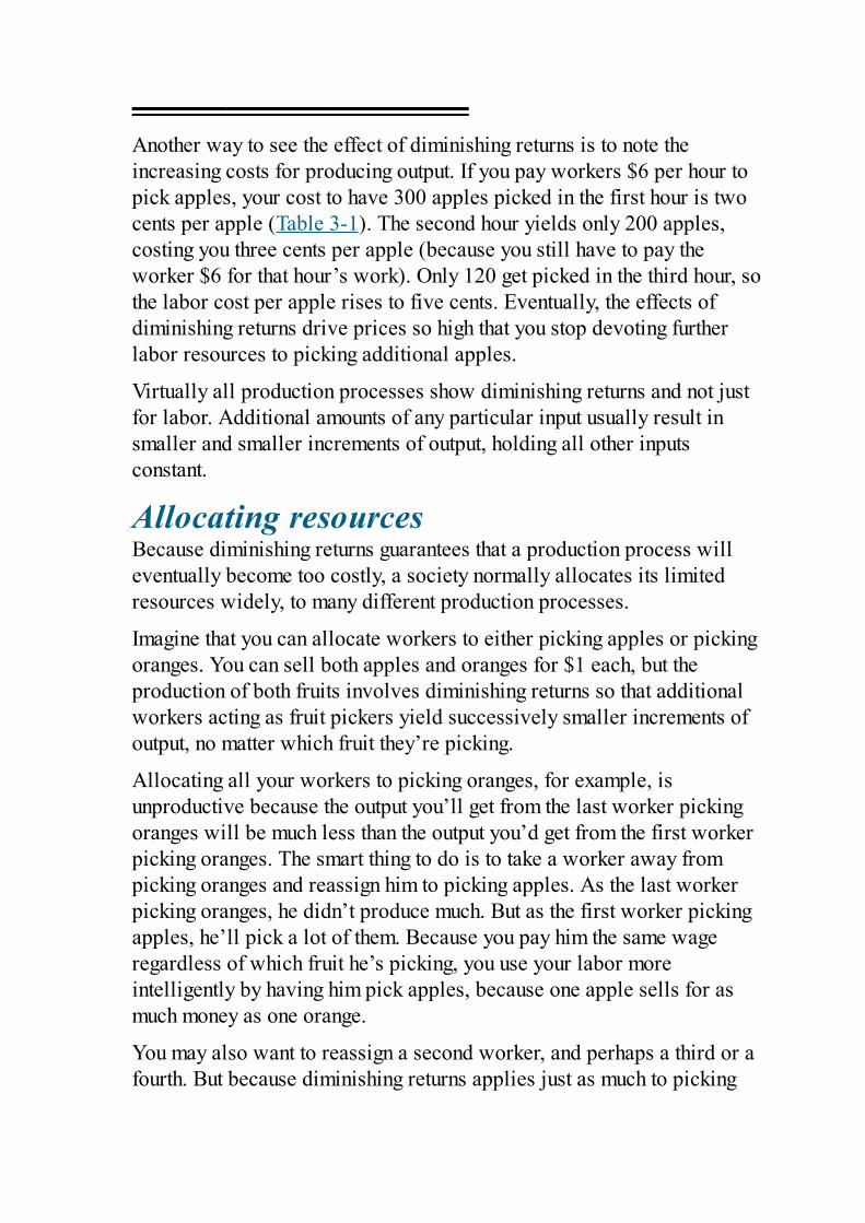
Another way to see the effect of diminishing returns is to note theincreasing costs for producing output. If you pay workers $6 per hour topick apples, your cost to have 300 apples picked in the first hour is twocents per apple (Table 3-1). The second hour yields only 200 apples,costing you three cents per apple (because you still have to pay theworker $6 for that hour’s work). Only 120 get picked in the third hour, sothe labor cost per apple rises to five cents. Eventually, the effects ofdiminishing returns drive prices so high that you stop devoting furtherlabor resources to picking additional apples.

Virtually all production processes show diminishing returns and not justfor labor. Additional amounts of any particular input usually result insmaller and smaller increments of output, holding all other inputsconstant.

Allocating resourcesBecause diminishing returns guarantees that a production process willeventually become too costly, a society normally allocates its limitedresources widely, to many different production processes.

Imagine that you can allocate workers to either picking apples or pickingoranges. You can sell both apples and oranges for $1 each, but theproduction of both fruits involves diminishing returns so that additionalworkers acting as fruit pickers yield successively smaller increments ofoutput, no matter which fruit they’re picking.

Allocating all your workers to picking oranges, for example, isunproductive because the output you’ll get from the last worker pickingoranges will be much less than the output you’d get from the first workerpicking oranges. The smart thing to do is to take a worker away frompicking oranges and reassign him to picking apples. As the last workerpicking oranges, he didn’t produce much. But as the first worker pickingapples, he’ll pick a lot of them. Because you pay him the same wageregardless of which fruit he’s picking, you use your labor moreintelligently by having him pick apples, because one apple sells for asmuch money as one orange.

You may also want to reassign a second worker, and perhaps a third or afourth. But because diminishing returns applies just as much to picking

apples as it does to picking oranges, you don’t want to reassign all theworkers. Each additional worker assigned to picking apples producesless than the previous worker picking apples. At some point, movingadditional workers from picking oranges to picking apples no longerbenefits you, and you’ve reached what economists refer to as an optimalallocation of your labor resource. As soon as you’ve found this sweetspot, you have no further incentive to move workers from picking onefruit to picking the other because no additional moving of workers willincrease total fruit picking. At this point, you’ve maximized your fruit-picking potential.

Graphing your production possibilitiesEconomists have a handy graph called the production possibilitiesfrontier (PPF) that lets you visualize the effect of diminishing returns andview the trade-offs you make when you reallocate inputs from producingone thing to producing another. The Production Possibilities Frontier,which is sometimes referred to as the production possibilities curve,also shows how limited resources constrain your ability to produceoutput. Figure 3-1 shows a PPF graph that corresponds to the data inTable 3-2.

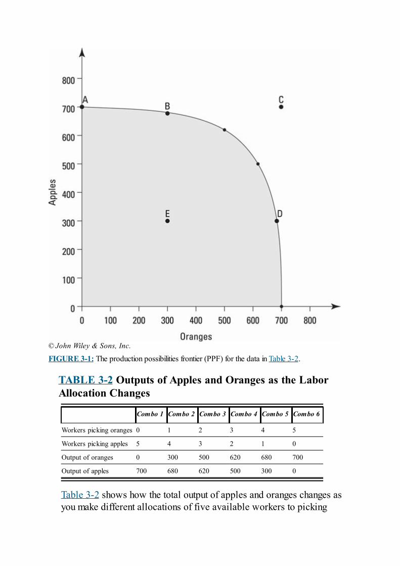
© John Wiley & Sons, Inc.

FIGURE 3-1: The production possibilities frontier (PPF) for the data in Table 3-2.

TABLE 3-2 Outputs of Apples and Oranges as the LaborAllocation Changes

Combo 1 Combo 2 Combo 3 Combo 4 Combo 5 Combo 6

Workers picking oranges 0 1 2 3 4 5

Workers picking apples 5 4 3 2 1 0

Output of oranges 0 300 500 620 680 700

Output of apples 700 680 620 500 300 0

Table 3-2 shows how the total output of apples and oranges changes asyou make different allocations of five available workers to picking

apples or oranges. For instance, if you put all five people to workpicking only apples for one whole day, you get 700 apples picked andzero oranges picked. If you move one worker to oranges (so fourworkers are picking apples and one worker is picking oranges), you get680 apples picked and 300 oranges picked. Because of diminishingreturns, taking one worker away from apples reduces apple output byonly 20. But moving that worker to oranges increases orange productionby 300 because that worker is the first one picking oranges and can getthe low-hanging fruit.

Graphing the combinationsYou can graph your production possibilities by plotting on a graph thevarious combinations of two output goods that can be produced as youvary the amount of a resource that is allocated between them. Figure 3-1plots the six output combinations that result from varying the allocationof workers in Table 3-2, thereby graphing all your productionpossibilities. Point A corresponds to putting all your workers to workpicking apples. Point B corresponds to the output you get from fourworkers picking apples and one worker picking oranges, and so on.

Note that each of the six points is attainable in the sense that you canactually produce the corresponding quantities of each fruit through someallocation of the five workers’ labor. On the other hand, a point like C isnot attainable. You can’t allocate your five workers in any way toproduce that many apples and oranges. Perhaps if you had more workersyou could produce such an output combination, but you’re limited to onlyfive workers.

Imagine that instead of allocating labor by worker, you allocate it bytime. The five workers each work for one day, so you have 5 worker-days of labor to allocate. You can now allocate, for instance, 3.2worker-days to apple-picking and 1.8 worker-days to orange-picking.This arrangement allows you to fill in the graph and draw a lineconnecting the six points that correspond to the output combinations thatyou get when allocating labor by worker.

A line passing through the points that represent various outputcombinations is called the production possibilities frontier, or PPF,

because it divides the area of the graph into two parts: Thecombinations of output that are possible to produce given yourlimited supply of labor are under the line in the shaded area, andthose that are not possible to produce are above it in the unshadedarea. In this way, the PPF graph captures the effect of scarceresources on production. Some output combinations are just notproducible given the limited supply of labor.

The PPF is a simplification of the real world, derived by allocating oneinput between just two outputs. The real world is, of course, morecomplicated, with many different resources allocated among manydifferent outputs. But the principles of limited resources and diminishingreturns that show up so clearly on the PPF graph also apply to the muchgreater variety of both inputs and outputs in the real world.

Interpreting the shape of the graphThe bowed-out curvature of the PPF graph illustrates the effects ofdiminishing returns. In Figure 3-1, the changing slope as you move alongthe frontier shows that the trade-off between apple production andorange production depends on where you start. If you’re at Point A,where you’re allocating all your resources to the production of apples,then you can, by reallocating resources, produce a lot more oranges atthe cost of giving up only a few apples. But if you start at Point D, whereyou’re already producing a lot of oranges, then you have to give up a lotof apples to get just a few more oranges.

In economic jargon, the changing slope of the PPF in the face ofdiminishing returns is due to the fact that the opportunity costs ofproduction vary depending on your current allocation of resources.(Check out Chapter 2 for more on opportunity cost, which is equal to thevalue of the best option you didn’t choose.) If you’re already producing alot of apples, the opportunity costs of devoting even more labor to moreapple production are very high because you’re giving up a lot ofpotential orange production. On the other hand, the opportunity costs ofdevoting that labor to orange production are very low because you haveto give up producing only a few apples. Clearly, you should devote thelabor to picking the fruit that has the lower opportunity costs because, inthis example, both fruits bring the same benefit: $1 per fruit sold.

Gauging efficiency

The PPF is very handy because any points that lie on the PPFitself (on the frontier) clearly show the output combinations you getwhen you’re productively efficient, or wasting none of yourresources.

In the example, you can’t increase the production of apples withoutreducing the production of oranges, and vice versa. For instance, if youstart at Point B, the only way to increase apple production is to slide upalong the frontier, which implies reducing orange production. You haveto make this tradeoff because you don’t have any wasted labor lyingaround with which you could get more apples without reducing theamount of labor already devoted to orange picking.

All the points below the line are productively inefficient. Consider PointE in Figure 3-1, which corresponds to producing 300 apples and 300oranges. You produce at a point like E only if you’re being productivelyinefficient. In fact, you can see from Table 3-2 that you can produce thesenumbers by sending only one worker to pick apples and another workerto pick oranges. You’re using just two of your five workers; the labor ofthe other three workers is either being wasted or not used at all.

In the real world, you end up at points like E because of inefficientproduction technology or poor management. For one reason or another,the resources that are available aren’t being used to produce as muchoutput as they could. Any manager who has five workers to allocate butproduces only output combination E should be fired!

Efficient economies should always be producing at some pointon their frontiers, because if they’re inside, they’re wasting theirlimited resources and aren’t maximizing the happiness that could begotten from them.

Reaching new frontiers with bettertechnologyOne simplification of the PPF is that other than the particular input you

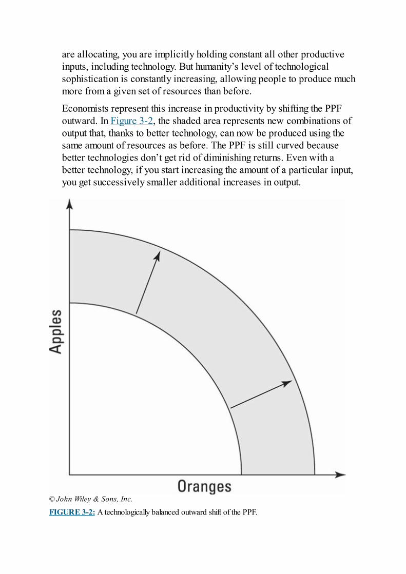
are allocating, you are implicitly holding constant all other productiveinputs, including technology. But humanity’s level of technologicalsophistication is constantly increasing, allowing people to produce muchmore from a given set of resources than before.

Economists represent this increase in productivity by shifting the PPFoutward. In Figure 3-2, the shaded area represents new combinations ofoutput that, thanks to better technology, can now be produced using thesame amount of resources as before. The PPF is still curved becausebetter technologies don’t get rid of diminishing returns. Even with abetter technology, if you start increasing the amount of a particular input,you get successively smaller additional increases in output.

© John Wiley & Sons, Inc.

FIGURE 3-2: A technologically balanced outward shift of the PPF.

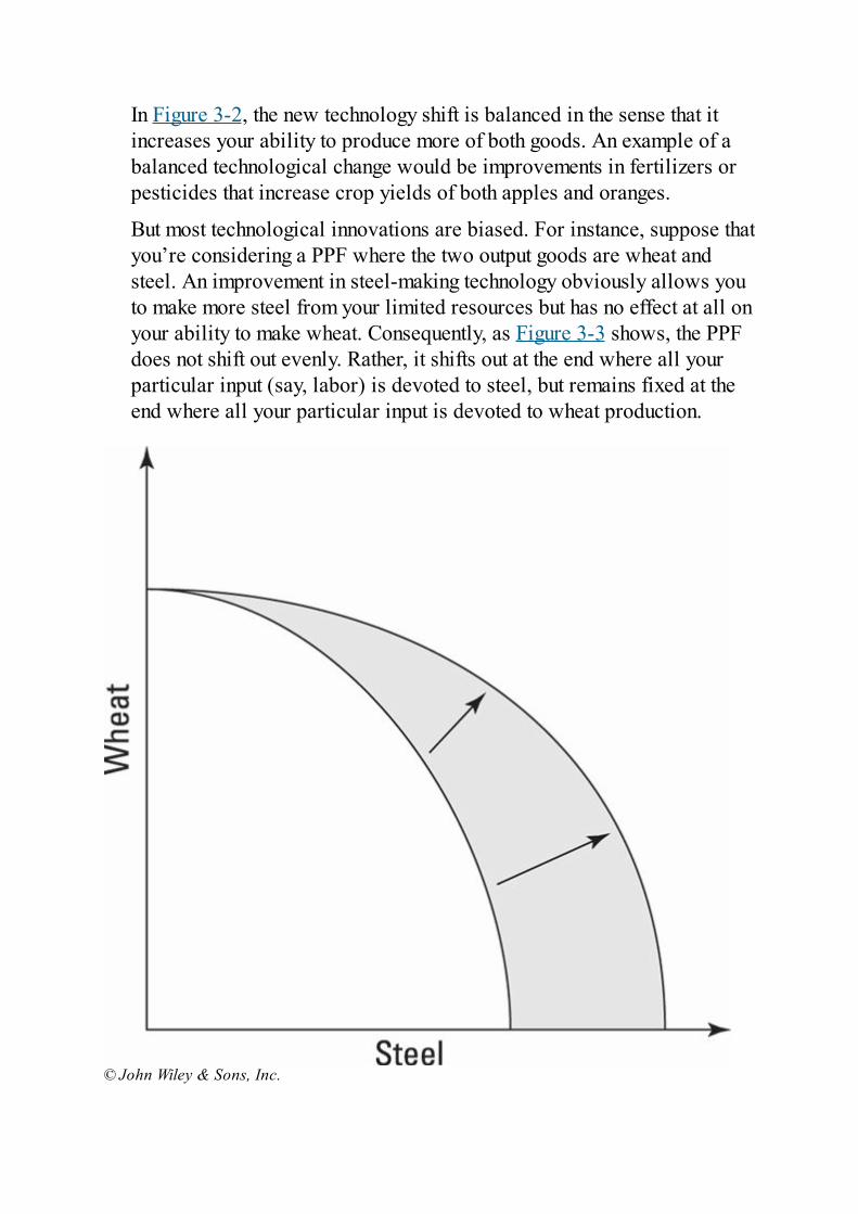
In Figure 3-2, the new technology shift is balanced in the sense that itincreases your ability to produce more of both goods. An example of abalanced technological change would be improvements in fertilizers orpesticides that increase crop yields of both apples and oranges.

But most technological innovations are biased. For instance, suppose thatyou’re considering a PPF where the two output goods are wheat andsteel. An improvement in steel-making technology obviously allows youto make more steel from your limited resources but has no effect at all onyour ability to make wheat. Consequently, as Figure 3-3 shows, the PPFdoes not shift out evenly. Rather, it shifts out at the end where all yourparticular input (say, labor) is devoted to steel, but remains fixed at theend where all your particular input is devoted to wheat production.

© John Wiley & Sons, Inc.

FIGURE 3-3: A technologically biased outward shift of the PPF.

Deciding What to ProduceAfter a society locates the frontier of efficient output combinations (seethe preceding sections), the next step is choosing the point along thefrontier that produces the combination of goods and services that makespeople most happy. Choosing only from among frontier combinationsguarantees productive efficiency. Choosing the single frontiercombination that maximizes happiness assures allocative efficiency.

Because determining where the frontier lies is mostly a matter ofengineering and applying current technology to available resources, itcreates little controversy. But deciding which particular combination ofoutputs a society as a whole should choose is much more complicated.People have preferences both as individuals and as groups about whichproducts make them happiest. An individual choosing a point along hisown personal PPF encounters no conflict; he just determines whatcombination of outputs makes him happiest and then he produces andconsumes it. The decision-making process becomes vastly morecomplicated when you consider an entire society’s PPF, in which caseyou’re sure to have vigorous disagreement about which combination ofoutputs to produce with the society’s limited resources.

For instance, your neighbor may not mind all the pollution produced bythe fact that he likes driving his SUV day and night. If he were living inhis own world, the pollution wouldn’t matter, but because you live nearhim, you’re affected by the pollution and object. Perhaps you’ll seekgovernment intervention that will limit what your neighbor is doing.Similarly, the government argues over what it should produce with itslimited resources: Some people favor farm subsidies while others favordefense spending or programs to aid the poor.

Because of competing priorities, some sort of decision-making processmust be established to determine what will actually get produced and to(try to) make sure that it pleases most of the people most of the time. Inmost modern economies, this process is the result of both private andpublic decisions acting through a combination of free markets andgovernment action. The process is not always smooth, but it hasdelivered the highest standards of living in world history.

In this section, I discuss the pros and cons of free markets andgovernment interventions and why it is that most nations have opted formixtures of the two rather than attempting to rely exclusively on one orthe other.

Comparing market results and governmentinterventionsWhen analyzing the ways in which modern economies and societiesselect a combination of goods and services to produce, realize thatcurrent laws and institutions are the result of conflicting pressures toeither

Leave markets to their own devices when turning resources intooutput.Use the power of government to intervene in markets in order tosecure a different set of outcomes.

Keep the following three factors in mind when considering the fightbetween leaving the markets alone and intervening:

Complexity: Modern economies are hugely complicated, withliterally millions of goods and services produced using limitedsupplies of land, labor, capital, and entrepreneurial ability. Marketshandle this complexity easily, but government interventions usuallydon’t — meaning that they often risk substantial reductions inproductive and allocative efficiency.Side effects: Some goods and services, such as cocaine and coal-burning power plants, have negative consequences that often fall on“third parties” who weren’t directly involved in either theproduction or the consumption of those products. These negativeconsequences bring forth substantial pressure for governmentintervention in the economy because markets, if left alone, willproduce a lot of these goods and services and, consequently, a lot ofnegative consequences for third parties.Inequality: Some people end up consuming a very large proportionof the goods and services produced, and others end up with verylittle. Such unequal distribution also brings forth a great deal of

pressure for government intervention in the economy in order toequalize living standards.

These factors are both a consequence and a cause of the fact that moderneconomies are largely a mix of market production and governmentintervention. For the most part, what to produce, how much of it toproduce, and who gets it are decided by voluntary transactions made byindividuals and businesses. But sometimes, the government uses itspowers to achieve outcomes that wouldn’t happen if individuals andbusinesses were left to their own devices.

In both cases, a huge apparatus of law and tradition governing economictransactions helps society produce a combination of output that is,hopefully, both productively efficient (so resources are not wasted) andallocatively efficient (so the economy is producing the things that peoplewant most). Next, I outline the benefits and the drawbacks that bothmarkets and governments bring to the economic table.

The magic of markets: Directing resources automaticallyMarket economies are simply collections of billions of small, face-to-face transactions between buyers and sellers. Economists use the termmarket production to capture what happens when one individual offers tomake or sell something to another individual at a price agreeable to both.

In markets, the allocation of resources is facilitated by the factthat each resource has a price, and whoever is willing to pay theprice gets the resource. In fact, market economies are often calledprice systems because prices serve as the signals that directresources. Holding supply constant, products in high demand havehigh prices, and products in low demand have low prices. Becausebusinesses like to make money, they follow the price signals andproduce more of what has a high price and less of what has a lowprice. In this way, markets tend to take limited resources and usethem to produce what people most want — or at least, what peopleare most willing to pay for.

For instance, the guy who sells you a TV at the local store has no ideaabout the total demand for TVs in the world, how many tons of steel or

plastic are needed to produce them, or how many other things weren’tproduced because the steel and plastic needed to make the TVs was usedfor TVs rather than other things. All he knows is that you’re willing topay him for a TV. And if he’s making a profit selling TVs, he orders moreTVs from the factory. The factory, in turn, increases production, takingresources away from the production of other things.

Markets have the benefit of figuring out, automatically, the things thatpeople want. To grasp why this is so amazing, consider that you live in aworld of more than 7 billion people. It would be very hard for any singleperson to gather enough information to figure out what each of them mostwants to buy. It would take several lifetimes to speak with each of them,even just to find out what they want for dinner, let alone all the otherthings they would most like to purchase on a typical day. But becauseproduction and distribution in modern economies aren’t centrallycontrolled (by a small number of government officials working togetherin a single place), nobody needs to know the big picture.

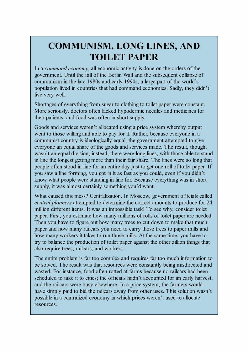
COMMUNISM, LONG LINES, ANDTOILET PAPER

In a command economy, all economic activity is done on the orders of thegovernment. Until the fall of the Berlin Wall and the subsequent collapse ofcommunism in the late 1980s and early 1990s, a large part of the world’spopulation lived in countries that had command economies. Sadly, they didn’tlive very well.

Shortages of everything from sugar to clothing to toilet paper were constant.More seriously, doctors often lacked hypodermic needles and medicines fortheir patients, and food was often in short supply.

Goods and services weren’t allocated using a price system whereby outputwent to those willing and able to pay for it. Rather, because everyone in acommunist country is ideologically equal, the government attempted to giveeveryone an equal share of the goods and services made. The result, though,wasn’t an equal division; instead, there were long lines, with those able to standin line the longest getting more than their fair share. The lines were so long thatpeople often stood in line for an entire day just to get one roll of toilet paper. Ifyou saw a line forming, you got in it as fast as you could, even if you didn’tknow what people were standing in line for. Because everything was in shortsupply, it was almost certainly something you’d want.

What caused this mess? Centralization. In Moscow, government officials calledcentral planners attempted to determine the correct amounts to produce for 24million different items. It was an impossible task! To see why, consider toiletpaper. First, you estimate how many millions of rolls of toilet paper are needed.Then you have to figure out how many trees to cut down to make that muchpaper and how many railcars you need to carry those trees to paper mills andhow many workers it takes to run those mills. At the same time, you have totry to balance the production of toilet paper against the other zillion things thatalso require trees, railcars, and workers.

The entire problem is far too complex and requires far too much information tobe solved. The result was that resources were constantly being misdirected andwasted. For instance, food often rotted at farms because no railcars had beenscheduled to take it to cities; the officials hadn’t accounted for an early harvest,and the railcars were busy elsewhere. In a price system, the farmers wouldhave simply paid to bid the railcars away from other uses. This solution wasn’tpossible in a centralized economy in which prices weren’t used to allocateresources.

In a competitive market, many sellers compete against each other toattract customers. Here are some of the advantages of competition:

Using resources efficiently and keeping prices low: A competitivemarket tends to guarantee productive efficiency because the best wayfor sellers to keep prices low is to make sure that they’re using alltheir resources efficiently, with nothing going to waste. Becausecompetition is ongoing, the pressure to be productively efficient isconstant.Sellers also have a big incentive to improve efficiency in order toundersell their rivals and steal their customers. Because every firmhas this incentive, prices tend to be driven so low that the businessescan just barely make a profit.Encouraging improvements in technology: In terms of the PPF(which I discuss in the earlier section “Graphing your productionpossibilities”), market production with a lot of competition tends toensure not only that economies produce along the frontier, but alsothat they have frontiers that are constantly being pushed outward asfirms improve productive efficiency thanks to the efforts ofentrepreneurs who supply the entrepreneurial ability that generatesinnovation and invention.

The misdeeds of markets: Ignoring morals and fairnessMarkets aren’t perfect. In particular, they suffer from two majorproblems:

Markets produce whatever people are willing to pay for, even ifthese things aren’t good for the people or the environment. As long asprofits are to be made, you can be pretty certain that a supply willarise to satisfy any demand. The fact that illegal drugs are widely andcheaply available — despite vigorous government programs to stoptheir production and distribution — is probably the best example ofthe robustness of markets. But although it’s nice that markets are sohell-bent on giving people what they’re willing to pay for, illegaldrugs are an excellent example of the fact that markets will deliverthings without caring about their social value or negativeconsequences such as drug addiction, broken families, and increasedcrime.

Along the same lines, producers sometimes utilize productionmethods that consumers don’t like. Child labor and sweatshop laborare primary examples. Often the government must intervene to changethese practices when the price system doesn’t provide enoughincentive for producers to reform such objectionable practices.Markets don’t in any way guarantee fairness or equity. The other bigproblem with markets is that they cater to those who have money tospend. The price system gives an incentive to produce only the thingsthat people are willing and able to pay for. If someone is very poor,he can’t give producers an incentive to provide him with even basicnecessities such as medicine and food.A related problem with markets is income and wealth inequality.Because market systems reward those who are best able to providegoods and services that people want to buy, some sellers end upbecoming very rich because they’re better at providing what peoplewant. This invariably leads to large inequalities in wealth that manypeople find offensive.

The case for government interventionMany societies use their governments to intervene and address theproblems that markets create or cannot fix. Government interventions inthe economy usually take one of three forms:

Penalties or bans on producing or consuming goods or servicesconsidered dangerous or immoral: These bans often work onlypartially because the market still has large incentives to provide suchgoods and services. For example, governments may ban drugs orimpose “sin taxes” on things like alcohol and tobacco, which, thoughlegal, are thought to be products whose use should be discouraged.Subsidies to encourage the production of goods and servicesconsidered desirable: For instance, most governments heavilysubsidize the education of children and the provision of medicalcare. They do so because of the fear that insufficient education andinadequate medical care will be provided without the subsidies.Education and medical care also often provide large spill-overbenefits to the wider public. Consider immunizations. They not onlyprotect those who are immunized but also those who aren’t becauseimmunization eliminates the possibility of the immunized infecting

the non-immunized.Taxes on the well-off to provide goods and services to the lessfortunate and to reduce inequalities in income and wealth: Thesetaxes are put toward things like good parks, clean air, and art, aswell as goods and services for the poor. Governments tax individualsand businesses in order to raise the money to provide such things.

In terms of the PPF graph, each of these government interventions causesthe economy to produce and allocate an output combination differentfrom the one that society would have ended up with if the markets hadmade all the production and allocation decisions.

Depending on the situation, the output combination produced by agovernment intervention may be better or worse than the marketcombination in terms of productive efficiency, allocative efficiency, orboth. Which combination is, in fact, better depends on the specifics ofeach case.

The case against government interventionGovernment intervention is a powerful force for redirecting economicactivity, but it doesn’t necessarily make the economy better. In fact, thereare at least three good reasons to worry that government interventionwill make things worse:

Special interests: Government programs are often the result ofspecial interest lobbying that persuades the legislature to put theinterests of a small group ahead of the interests of the general public.Inefficiency: Even when pursuing the common good, governmentprograms often deliver poor service because they have nocompetition to create incentives to produce government goods andservices efficiently.Inflexibility: Government interventions usually lack the flexibility ofthe price system, which is able to constantly redirect resources toaccommodate people’s changing willingness to pay for one goodrather than another. Government policies take years to pass, and lawsare usually written in a very precise manner that doesn’t allow forchanging circumstances and rapid innovation — things that the pricesystem handles with ease.

MO’ MONEY FOR MOHAIRMohair is extremely warm wool that grows on a special variety of goat. DuringWorld War II, the U.S. government decided that it needed mohair for the warmjackets worn by bomber pilots in their unheated cockpits. As a result, thegovernment started giving a large subsidy to encourage the production ofmohair. But planes have now been heated for nearly 70 years, and bomberjackets are nowadays made of synthetics. Yet the mohair subsidy remains, andmohair producers receive millions of dollars every year. Why? Because themohair producers lobby the U.S. government very hard each year to renew thesubsidy. For each producer, the subsidy is worth a lot of money. And becauseonly a fraction of one cent of the average tax bill goes to the mohair subsidy, noone protests it. Consequently, the mohair subsidy survives not because it doessociety any good but because lobbying pays off in a democracy. Many othergovernment programs are similarly deficient of widespread social benefits.

Although markets sometimes fail to deliver everything that society wants,government intervention isn’t a cure-all. Markets are very good atdelivering the vast majority of things that people want and can usually doso at the lowest possible cost. Consequently, government interventionshould be well thought out lest it make things worse rather than better.

Opting for a mixed economyIn the real world, few societies opt for an extreme type of economy, suchas one that is totally market-based or one that features constant andpervasive government intervention. Instead, most societies opt for somemixture of markets, government intervention, and what economists referto as traditional production. In their purest forms, these three types ofeconomy can be defined as follows:

Market: A market economy is one in which almost all economicactivity happens in markets with little or no interference by thegovernment. Because of the lack of government intervention, thissystem is also often referred to as laissez faire, which is French for“to allow to do” or “to leave alone.”Command: A command economy is one in which all economicactivity is directed by the government.Traditional: A traditional economy is one in which production and

distribution are handled along the lines of longstanding culturaltraditions. For instance, until the caste system was abolished in Indiaduring the last century, the production of nearly every good andservice could be done only by someone born into the appropriatecaste. Similarly, in medieval Europe, you couldn’t typically be partof the government or attain high military rank unless you were born anoble.

Because nearly every modern economy is a mixture of these three pureforms, most modern economies fall into the very inclusive categorycalled mixed economies. With the exception of a few isolated traditionalsocieties, however, the traditional economy part of the mixture hastended to decline in significance because most production has shifted tomarkets and because traditional economic restrictions with regard to ageand gender have become less important (and more illegal).

Mixed economies today are a mixture of the command economyand the market economy. The mixtures that you find in mostcountries typically feature governments that mostly allow markets todetermine what’s produced but that also mix in limited interventionsin an attempt to make improvements over what the market would doif left to its own devices.

The precise nature of the mixture depends on the country, with the UnitedStates and the United Kingdom featuring more emphasis on markets andFrance and Germany, for instance, featuring more emphasis ongovernment intervention. On the other hand, a few totalitarian states likeNorth Korea still persist in running pure command economies as part oftheir all-encompassing authoritarian regimes.

Noting the failure of command and the absence of laissezfaireCommand economies have historically been dismal failures (see thesidebar “Communism, long lines, and toilet paper” for details). Evenwell-intentioned governments can’t gather enough information aboutproduction and distribution to do a good job allocating resources. In fact,they do a much worse job than price systems do.

Consequently, the opposite extreme, absolutely no governmentintervention, can seem like an attractive option. Such laissez-fairesystems were first suggested by French economists several hundredyears ago in response to the habit of governments of that era to intervenevery heavily in economic activity. However, no pure laissez-faireeconomy has ever existed or probably could ever exist. The simple factis that properly functioning market economies that use price mechanismsto allocate resources require a huge amount of government support.

Among other things, market economies need governments to

Enforce property rights so people don’t stealProvide legal systems to write and enforce contracts so people canmake purchases and sales of goods and servicesEnforce standardized systems of weights and measures so peopleknow they aren’t being cheatedProvide a stable money supply that’s safe from counterfeitersEnforce patents and copyrights to encourage innovation andcreativity

Notice that all these things must be in place in order for markets tofunction. Consequently, a more moderate, more modern version oflaissez faire says that government should provide the institutionalframework necessary for market economies to function, and then itshould get out of the way and let people make and sell whatever isdemanded.

Deciding on the amount of government interventionBecause command economies don’t work very well and laissez-faireeconomies can’t really exist, most societies have opted for one form oranother of mixed economy in which governments and markets shareeconomic responsibilities. The precise nature of that mix varies fromcountry to country but all such mixtures feature some instances of directgovernmental command and control of economic activity interacting withmarkets that use a price system to allocate resources.

The vast majority of people want governments to do more than just set upthe institutions necessary for markets to function. They want governmentsto stop the production and sale of things like drugs or to subsidize theproduction of things that the market economy may not provide a lot of,like housing for the poor. They often also want to tax well-off citizens topay for government programs.

Many government programs are so commonplace that you don’t eventhink of them as being government interventions. For instance, free publicschools, safety features on cars, warning labels on medicine bottles,taxes on alcohol and tobacco, and mandatory contributions to retirementsystems are all government interventions in the economy.

The government interventions needed to implement such programs are, inmany cases, not efficient. But many people would argue that there’s quitea bit more to life than efficiency and that the inefficiencies caused bymany government interventions are well worth the benefits that theyproduce. For such people, the government interventions in questionincrease overall happiness despite the fact that they are, strictlyspeaking, inefficient.

At the end of the day, all government interventions — both goodand bad — are the result of a political process. In democracies, theamount of government intervention is, broadly speaking, a reflectionof the will of the people. Nations in which people have more trustin markets, like the United States and the United Kingdom, tend tofeature mixed economies with less government intervention thannations in which people are more suspicious of corporations andimpersonal market forces, like France and Germany.

Promoting Technology andInnovation

Technology is, in many ways, like any other good that can be provided bya market. If there’s a profit incentive to inventing a new technology,businesspeople will figure out a way to invent it, just as they figure outways to deliver all the other things that people are willing to pay for.However, unless government sets up the right set of laws and propertyrights, firms won’t find it profitable to innovate.

Thus, one of the most important jobs of government is helping to promotethe invention of new technologies so that people can enjoy higher livingstandards. Here are several ways in which government supportstechnology:

Funding research: Governments provide a good deal of directsupport through research grants and university subsidies.Protecting intellectual property rights: A crucial thing tounderstand about innovation is the indirect role that governments playnot by subsidizing new technology but by guarding it. In particular,the patents granted by governments provide a huge economicincentive for both individuals and businesses to innovate. A patentguarantees inventors of new products or business methods theexclusive right to profit from their innovations, usually for about 20years in most countries.

It’s not a coincidence that economic growth in the UnitedStates and Western Europe took off 200 years ago, right after patentsbecame widely enforced. For the first time in world history, therewas a secure financial incentive to use your brain to innovate. Beforethat time, innovating was extremely risky because after all your hardwork, others would simply copy your invention and sell it withoutyour permission.Copyrights for literary, musical, and cinematic works serve a similar

purpose. A great deal more art is produced when artists know thatthey can make a living. Along these lines, the easy duplication anddistribution of digital media on the Internet is a troublingdevelopment because it has weakened artists’ ability to charge for theart that they work so hard to produce.Encouraging education: You shouldn’t be surprised that every richcountry in the world has a policy of universal primary and secondaryeducation as well as strong universities. Smart new technologiesrequire well-educated researchers from good educational systems.Advanced economies also require smart, well-educated workers toimplement the new technologies. Consequently, it’s very importantthat education be available to everyone if an economy is to utilize theconstant flow of innovative new processes and tools that researchersdevelop.

POLITICAL SYSTEMS VERSUSECONOMIC SYSTEMS

The three categories used by economists to distinguish economic systems —market, command, and traditional — are only meant to convey informationabout a nation’s economic system. By contrast, terms like communism,capitalism, democracy, and socialism tend to either focus exclusively on anation’s political system or on how a nation’s political system is interwovenwith its economic system.

Consider the word democracy. It refers to a political system in which a nation’sgovernment is controlled by its citizens. Whether they direct the government toinstitute an economic system that is market, command, or traditional isn’tspecified by that fact that the country is run democratically. The fact that acountry is a democracy also says nothing by itself about whether thegovernment favors private ownership or government control of businesses.

In contrast, communist and socialist systems are supposed to featuredemocratic governments owning and operating all the businesses in an economyon behalf of the people. That is, both systems are by definition supposed toencompass both a nation’s political system as well as its economic system.

Please note, however, that actual communist and socialist governments havetended to fail in achieving their democratic political aspirations. Instead,communist and socialist nations like the old Soviet Union, North Korea, Cuba,and, recently, Venezuela, tend to feature non-democratic totalitariangovernments that use their almost total control over commerce as yet anothertool for suppressing their citizens.

Finally, understand that the term capitalism has many conflicting definitions.For some, it refers to economies featuring private property and free markets.To others, it’s defined by industrialization and the use of large amounts ofcapital equipment in the production process. Yet another group uses it todescribe a political-economic system in which the rich owners of largebusinesses use their power and influence over both commerce and thegovernment to exploit the poor. Because of these many conflicting (andcontroversial!) definitions, economists tend to avoid the term capitalism infavor of more precise descriptive terms like market-based economy.

Part 2

Microeconomics: The Scienceof Consumer and Firm

Behavior

IN THIS PART …Discover the relationships among prices, quantity supplied, and quantitydemanded and how changes in supply or demand affect marketequilibrium.

Understand how people maximize their happiness by navigating marginalutility, weighing alternatives, and choosing just the right amounts giventheir limited budgets.

Know how and why firms set output levels to maximize profits and whatthey do when they lose money.

Check out the social benefits of markets, how they can maximize totalsurplus, and what taxes and price controls do in a market setting.

Find out what monopolies are and how they behave.

Examine what collusion is and why some collusive oligopolies workwhile others don’t.

Chapter 4

Supply and Demand MadeEasy

IN THIS CHAPTER Understanding the relationship between prices and quantity

supplied or demanded Focusing on market equilibrium Understanding how shifts in demand or supply affect market

equilibrium Identifying policies that prevent market equilibrium

In the modern economy, most economic activity takes place in markets,places where buyers and sellers come together to trade money for a goodor service. A market doesn’t have to be an actual place, and manymarkets nowadays exist only in cyberspace. But no matter what sort ofinstitutional arrangement markets have, they all tend to behave in thesame way.

A very simple model called supply and demand does anexcellent job of describing how markets work, regardless of whichgood or service is being bought and sold. This model veryreasonably separates buyers from sellers and then summarizes eachgroup’s behavior with a single line on a graph. The buyers’behavior is captured by the demand curve, and the sellers’ behavioris captured by the supply curve. By putting these two curves on thesame graph, economists can show how buyers and sellers interact todetermine how much of any particular item will be sold, as well asthe price at which it will be sold.

The supply and demand model of markets is the economics profession’smost famous contribution to human understanding. It’s useful in so manyareas, shedding light on exactly how markets set prices and allocate

resources, as well as giving accurate predictions about how governmentpolicies will affect the behavior of markets. For instance, this model cantell you why the price of gas goes up during the summer and why theprice of wheat goes down after a good harvest. It can also predict —correctly — that agricultural price supports will cause anoverproduction of food and that rent control will lead to a shortage ofhousing.

I begin this chapter by explaining demand and supply separately andshowing you how to draw and manipulate supply curves and demandcurves; the demand curves capture the behavior of buyers, and the supplycurves capture the behavior of suppliers. The next step is to watch thecurves interact to see how markets function both when left to their owndevices and when subject to government regulation or intervention. Afterreading this chapter, you should have new insights on virtually everythingyou read about commerce, business, and politics.

Deconstructing DemandPeople want to buy things, and economists refer to that desire asdemand. When they say demand, economists aren’t referring to pie-in-the-sky dreams or to mere wishful thinking along the lines of, “I want abillion jillion scoops of ice cream!” Rather, when they say demand,economists mean how much of something people are both willing andable to pay for. So although I may want a billion jillion scoops of icecream (butter pecan, please!), that’s not my demand in the sense thateconomists use it. Rather, my demand is three scoops, because that’s howmuch I’m willing and able to buy at the price that my local ice creamshop charges.

To be precise, what I’ve actually just described is my quantitydemanded, which refers to how much I demand at a specific price,holding constant everything else in the world, including my income, mypreferences, and the prices of other goods and services. By contrast,when an economist uses the word demand, he means the whole range ofquantities that a person will demand while holding constant all otherpossible influencing factors.

In this section, I look at how a product’s own price determines a demandcurve’s slope and how changes in any other factor — includingpreferences and the prices of other products — can shift the position ofthe demand curve.

Prices and other stuff: Looking at whataffects quantity demandedEconomists divide everything that can possibly affect the quantitydemanded into two groups: the price and everything else. Here’s what“everything else” includes:

Tastes and preferences: Chief among the non-price things that affectquantity demanded are tastes and preferences. For instance, no matterhow low the price gets, I won’t buy even a single container ofcherry-and-chocolate ice cream, because I think it’s gross. At thesame time, however, lots of people love cherry-and-chocolate icecream so much that even if the price got very high, they’d still be

willing to buy quite a bit of it. No matter how much a container of acertain flavor costs, the people who love it will always have ahigher quantity demanded than I will. Because this is true for everypossible price, you can say that they have a higher demand than I do.Other prices: People’s demand for product X is affected not only bythe price of product X, but also by the prices of everything else theycan possibly buy. If, for example, the price of movie tickets rise,people are likely to not only go to the movies less often but to spendthe money they save by not going to the movies so often on otherentertainment activities, such as going to concerts. Thus, a change inthe price of movie tickets will affect their quantity demanded ofconcert tickets — even when the price of concert tickets hasn’tchanged.Income: As you get richer, you increase your quantity demanded ofcertain goods that you’ve always liked and can now afford to buymore of. These are called normal goods. On the other hand, youdecrease your quantity demanded of things that you were buying onlybecause you were too poor to get what you really wanted. These arecalled inferior goods. For example, new cars are normal goods, andreally old, poorly running used cars are inferior goods. Similarly,freshly made organic salads are normal goods, and three-day-old,discounted bread is an inferior good.

Given the complexity of variables such as preferences and income, whydo economists insist on dividing everything that could influence yourquantity demanded into only two groups, the price and everything else?First, they want to concentrate on prices. Second, when you translate theconcept of demand into a graph and create a demand curve, prices have avery different effect than do the other variables. Price changes move youalong a given demand curve, while the other variables determine wherethe curve is placed and how it’s shaped.

Graphing the demand curvePrices have an inverse relationship with the quantity demanded. In otherwords, the higher the price, the less quantity people demand (if all theother things that could possibly affect the quantity demanded are heldconstant). That’s why a demand curve slopes downward.

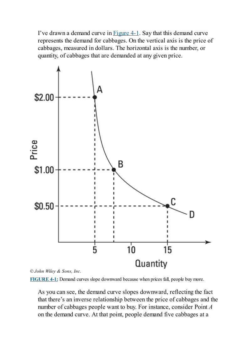
I’ve drawn a demand curve in Figure 4-1. Say that this demand curverepresents the demand for cabbages. On the vertical axis is the price ofcabbages, measured in dollars. The horizontal axis is the number, orquantity, of cabbages that are demanded at any given price.

© John Wiley & Sons, Inc.

FIGURE 4-1: Demand curves slope downward because when prices fall, people buy more.

As you can see, the demand curve slopes downward, reflecting the factthat there’s an inverse relationship between the price of cabbages and thenumber of cabbages people want to buy. For instance, consider Point Aon the demand curve. At that point, people demand five cabbages at a

price of $2 per cabbage. However, as you can see by looking at Point B,if the price drops to $1 per cabbage, people demand eight cabbages. Andif the price drops to only $0.50 per cabbage, they demand 15 cabbages.

Here’s how changes in price and other factors are reflected in thedemand curve:

Increases or decreases in price simply move you along the demandcurve.Nonprice factors (such as changes in people’s income or wealth andchanges in their tastes or preferences) determine where the demandcurve is located and how it’s shaped, so if any of these factorschanges, the demand curve shifts its location.

For instance, suppose that a government health study comes out sayingthat cabbages make people really attractive to members of the oppositesex. Naturally, this is going to increase the demand for cabbages.Geometrically, the effect is to shift the demand curve to the right. I’veillustrated this effect in Figure 4-2, where the demand curve before thestudy is announced is labeled D, and the demand curve after the study isannounced is labeled D'.

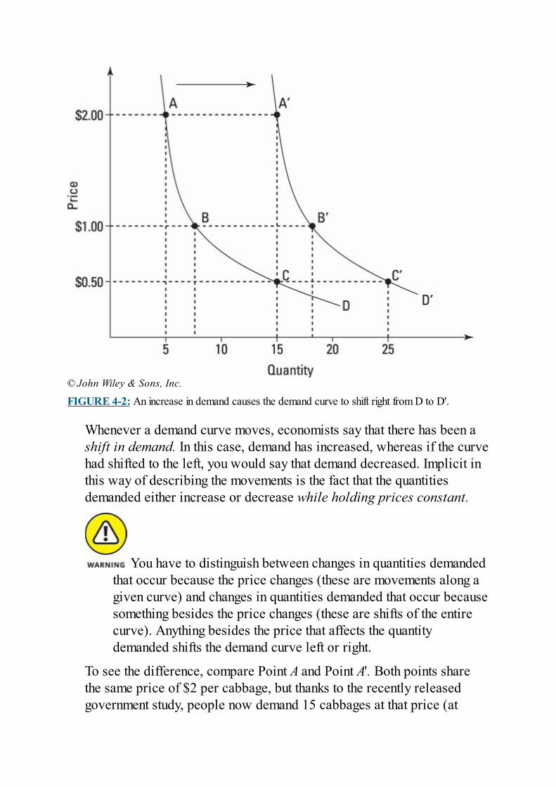
© John Wiley & Sons, Inc.

FIGURE 4-2: An increase in demand causes the demand curve to shift right from D to D'.

Whenever a demand curve moves, economists say that there has been ashift in demand. In this case, demand has increased, whereas if the curvehad shifted to the left, you would say that demand decreased. Implicit inthis way of describing the movements is the fact that the quantitiesdemanded either increase or decrease while holding prices constant.

You have to distinguish between changes in quantities demandedthat occur because the price changes (these are movements along agiven curve) and changes in quantities demanded that occur becausesomething besides the price changes (these are shifts of the entirecurve). Anything besides the price that affects the quantitydemanded shifts the demand curve left or right.

To see the difference, compare Point A and Point A'. Both points sharethe same price of $2 per cabbage, but thanks to the recently releasedgovernment study, people now demand 15 cabbages at that price (at

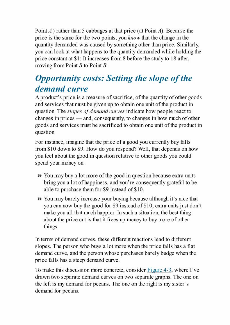
Point A') rather than 5 cabbages at that price (at Point A). Because theprice is the same for the two points, you know that the change in thequantity demanded was caused by something other than price. Similarly,you can look at what happens to the quantity demanded while holding theprice constant at $1: It increases from 8 before the study to 18 after,moving from Point B to Point B'.

Opportunity costs: Setting the slope of thedemand curveA product’s price is a measure of sacrifice, of the quantity of other goodsand services that must be given up to obtain one unit of the product inquestion. The slopes of demand curves indicate how people react tochanges in prices — and, consequently, to changes in how much of othergoods and services must be sacrificed to obtain one unit of the product inquestion.

For instance, imagine that the price of a good you currently buy fallsfrom $10 down to $9. How do you respond? Well, that depends on howyou feel about the good in question relative to other goods you couldspend your money on:

You may buy a lot more of the good in question because extra unitsbring you a lot of happiness, and you’re consequently grateful to beable to purchase them for $9 instead of $10.You may barely increase your buying because although it’s nice thatyou can now buy the good for $9 instead of $10, extra units just don’tmake you all that much happier. In such a situation, the best thingabout the price cut is that it frees up money to buy more of otherthings.

In terms of demand curves, these different reactions lead to differentslopes. The person who buys a lot more when the price falls has a flatdemand curve, and the person whose purchases barely budge when theprice falls has a steep demand curve.

To make this discussion more concrete, consider Figure 4-3, where I’vedrawn two separate demand curves on two separate graphs. The one onthe left is my demand for pecans. The one on the right is my sister’sdemand for pecans.

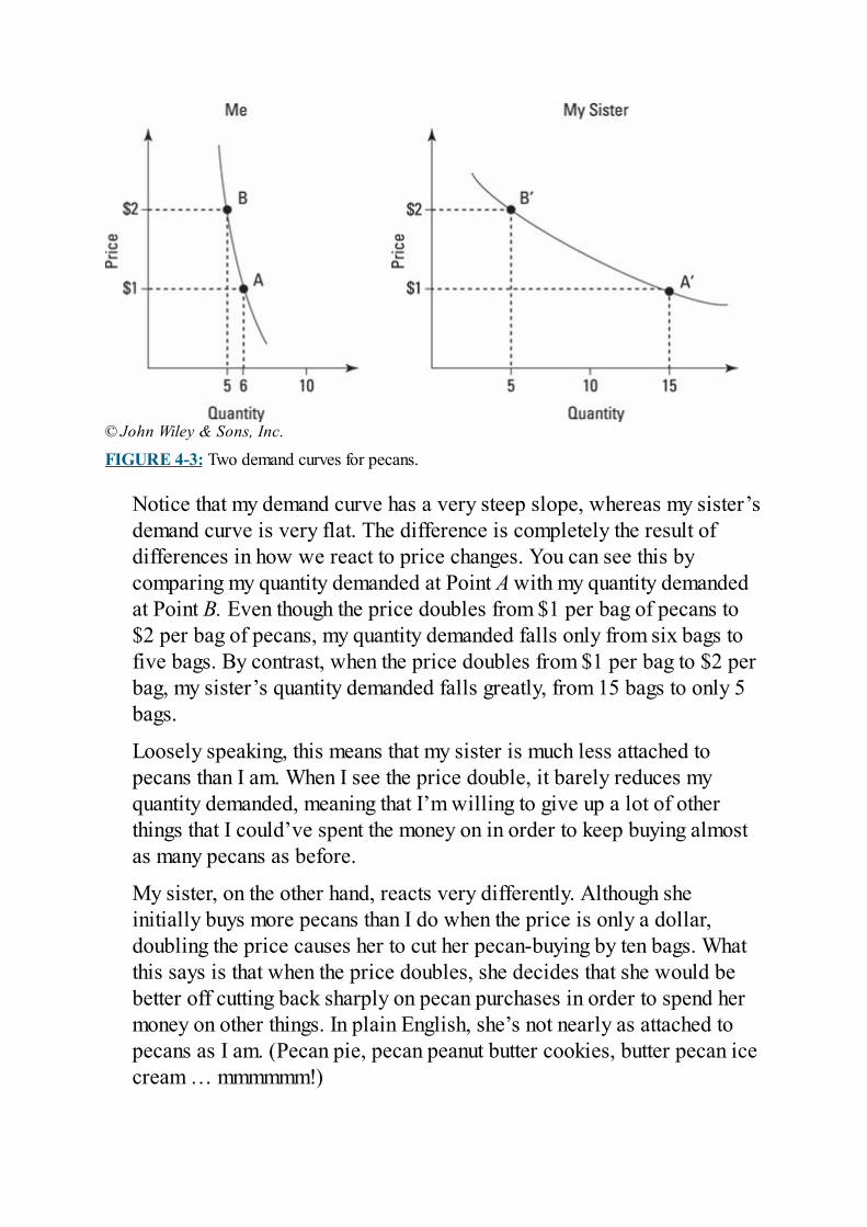
© John Wiley & Sons, Inc.

FIGURE 4-3: Two demand curves for pecans.

Notice that my demand curve has a very steep slope, whereas my sister’sdemand curve is very flat. The difference is completely the result ofdifferences in how we react to price changes. You can see this bycomparing my quantity demanded at Point A with my quantity demandedat Point B. Even though the price doubles from $1 per bag of pecans to$2 per bag of pecans, my quantity demanded falls only from six bags tofive bags. By contrast, when the price doubles from $1 per bag to $2 perbag, my sister’s quantity demanded falls greatly, from 15 bags to only 5bags.

Loosely speaking, this means that my sister is much less attached topecans than I am. When I see the price double, it barely reduces myquantity demanded, meaning that I’m willing to give up a lot of otherthings that I could’ve spent the money on in order to keep buying almostas many pecans as before.

My sister, on the other hand, reacts very differently. Although sheinitially buys more pecans than I do when the price is only a dollar,doubling the price causes her to cut her pecan-buying by ten bags. Whatthis says is that when the price doubles, she decides that she would bebetter off cutting back sharply on pecan purchases in order to spend hermoney on other things. In plain English, she’s not nearly as attached topecans as I am. (Pecan pie, pecan peanut butter cookies, butter pecan icecream … mmmmmm!)

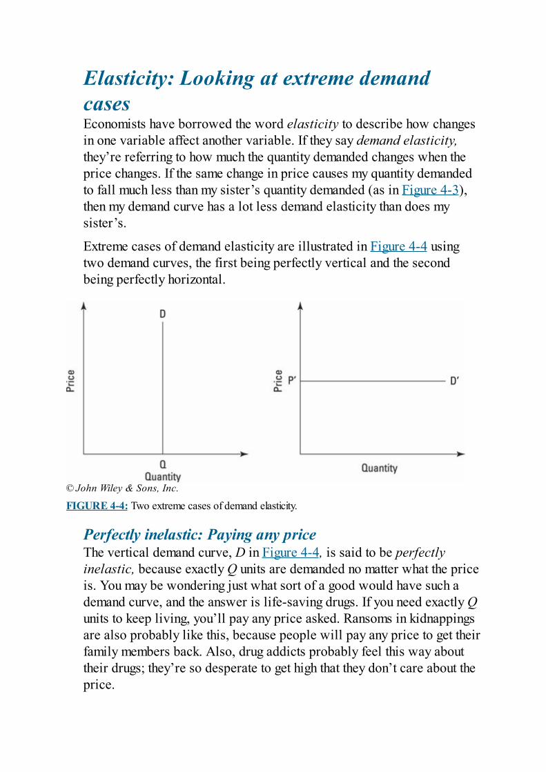
Elasticity: Looking at extreme demandcasesEconomists have borrowed the word elasticity to describe how changesin one variable affect another variable. If they say demand elasticity,they’re referring to how much the quantity demanded changes when theprice changes. If the same change in price causes my quantity demandedto fall much less than my sister’s quantity demanded (as in Figure 4-3),then my demand curve has a lot less demand elasticity than does mysister’s.

Extreme cases of demand elasticity are illustrated in Figure 4-4 usingtwo demand curves, the first being perfectly vertical and the secondbeing perfectly horizontal.

© John Wiley & Sons, Inc.

FIGURE 4-4: Two extreme cases of demand elasticity.

Perfectly inelastic: Paying any priceThe vertical demand curve, D in Figure 4-4, is said to be perfectlyinelastic, because exactly Q units are demanded no matter what the priceis. You may be wondering just what sort of a good would have such ademand curve, and the answer is life-saving drugs. If you need exactly Qunits to keep living, you’ll pay any price asked. Ransoms in kidnappingsare also probably like this, because people will pay any price to get theirfamily members back. Also, drug addicts probably feel this way abouttheir drugs; they’re so desperate to get high that they don’t care about theprice.

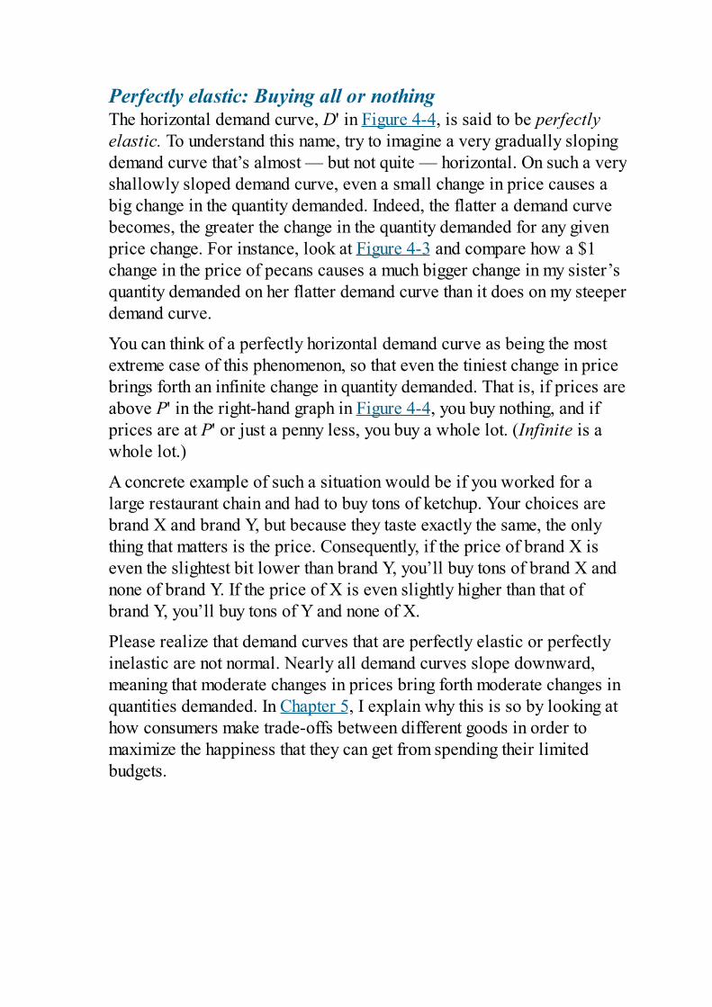
Perfectly elastic: Buying all or nothingThe horizontal demand curve, D' in Figure 4-4, is said to be perfectlyelastic. To understand this name, try to imagine a very gradually slopingdemand curve that’s almost — but not quite — horizontal. On such a veryshallowly sloped demand curve, even a small change in price causes abig change in the quantity demanded. Indeed, the flatter a demand curvebecomes, the greater the change in the quantity demanded for any givenprice change. For instance, look at Figure 4-3 and compare how a $1change in the price of pecans causes a much bigger change in my sister’squantity demanded on her flatter demand curve than it does on my steeperdemand curve.

You can think of a perfectly horizontal demand curve as being the mostextreme case of this phenomenon, so that even the tiniest change in pricebrings forth an infinite change in quantity demanded. That is, if prices areabove P' in the right-hand graph in Figure 4-4, you buy nothing, and ifprices are at P' or just a penny less, you buy a whole lot. (Infinite is awhole lot.)

A concrete example of such a situation would be if you worked for alarge restaurant chain and had to buy tons of ketchup. Your choices arebrand X and brand Y, but because they taste exactly the same, the onlything that matters is the price. Consequently, if the price of brand X iseven the slightest bit lower than brand Y, you’ll buy tons of brand X andnone of brand Y. If the price of X is even slightly higher than that ofbrand Y, you’ll buy tons of Y and none of X.

Please realize that demand curves that are perfectly elastic or perfectlyinelastic are not normal. Nearly all demand curves slope downward,meaning that moderate changes in prices bring forth moderate changes inquantities demanded. In Chapter 5, I explain why this is so by looking athow consumers make trade-offs between different goods in order tomaximize the happiness that they can get from spending their limitedbudgets.

Sorting Out SupplyIn the economist’s view of the supply of goods and services, the keyconcept is that supplying things is costly, and you have to pay people tosupply the things you want. Even more interesting, though, is the fact thatthe more you want them to supply, the higher their costs of supplyingeach additional unit. In other words, the first units tend to be relativelyinexpensive to produce, while later units become more and more costlyto produce. (In Chapter 6, I explain why this holds true.) If you wantproducers to make more and more, you have to pay them more and more.

In this section, I explain how rising costs cause supply curves to slopeupward and how entire supply curves can shift when the costs of inputschange.

Graphing the supply curveA supply curve shows the minimum prices at which someone is willingto sell various amounts of a good or service. Because production costsrise as people make more of something, suppliers insist on more moneyfor larger quantities. That’s why supply curves slope upward.

Imagine that a farmer named Babbage likes to grow cabbage. In Figure4-5, I graph Mr. Babbage’s supply of cabbages and label it S. (I wastempted to label it BS, for Babbage’s Supply, but I didn’t want you tellingyour friends that my book was full of BS.)

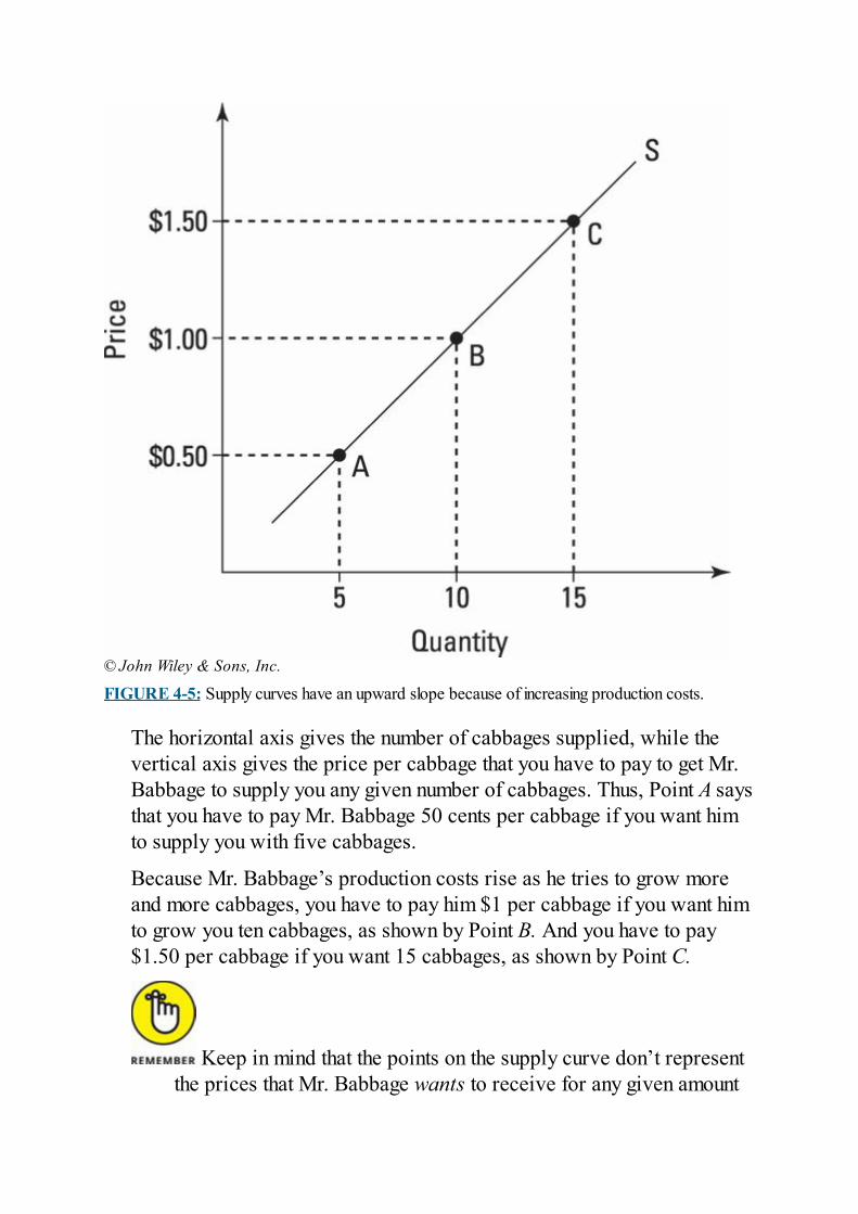
© John Wiley & Sons, Inc.

FIGURE 4-5: Supply curves have an upward slope because of increasing production costs.

The horizontal axis gives the number of cabbages supplied, while thevertical axis gives the price per cabbage that you have to pay to get Mr.Babbage to supply you any given number of cabbages. Thus, Point A saysthat you have to pay Mr. Babbage 50 cents per cabbage if you want himto supply you with five cabbages.

Because Mr. Babbage’s production costs rise as he tries to grow moreand more cabbages, you have to pay him $1 per cabbage if you want himto grow you ten cabbages, as shown by Point B. And you have to pay$1.50 per cabbage if you want 15 cabbages, as shown by Point C.

Keep in mind that the points on the supply curve don’t representthe prices that Mr. Babbage wants to receive for any given amount

of cabbages — obviously, he wants to receive a gazillion dollarsfor each one. Rather, what each dollar amount on a supply curverepresents is the minimum that you could pay him and still get himto produce the desired amount. At Point A, you can get him toproduce five cabbages if you pay him 50 cents per cabbage; if youoffer him 49 cents per cabbage, he won’t do it. Why not? Becausehe has costs, and he can cover them at 50 cents per cabbage but notat 49 cents per cabbage.

Separating sales price and production costEconomists split all the things that can affect the quantity supplied intotwo groups: the price and everything else. The things that go intoeverything else all relate to production costs — the costs of supplyingthe good in question.

When you see a particular supply curve, imagine that it derivesfrom a particular production technology used by the supplier.Because each possible technology creates its own uniquerelationship between output levels and costs, some technologiesgive rise to steeply sloped supply curves, while others generatefairly flat supply curves. (See Chapter 6 for all the details on firms’supply curves.)

Regardless of exactly how the curve is sloped or where it’s positioned,the fact that costs increase as output increases means that you need tooffer a higher and higher price to the supplier if you want to obtain moreunits. And that’s basically why prices move you along supply curves.

Price changes: Moving along the supply curveVarying the price of an item moves you along a given supply curvebecause the supply curve represents the minimum payment you need togive the supplier in order for him to supply the amount of output youwant.

Suppliers look at whatever price is being offered and make asmany units as are profitable but no more. Because costs rise with

each additional unit produced, the only way to get suppliers toproduce more is to offer them higher prices. Therefore, raising orlowering prices moves you along the supply curve as the suppliers’quantities supplied respond to changing prices.

To see how this works, consider what happens if you offer to pay Mr.Babbage $1 per cabbage, and then you let him choose how manycabbages he wants to produce. Given his supply curve in Figure 4-5,he’s going to want to produce exactly ten cabbages and no more. That’sbecause for cabbage number one through cabbage number nine, the costof production is less than what you’re paying him. For example, considerPoint A from Figure 4-5. At Point A, his production costs are 50 cents percabbage. That means that if you’re going to pay him $1 per cabbage,he’ll be making a nice profit. Similarly, because his cost per cabbage forproducing six cabbages is also less than $1 per cabbage, he’ll also wantto make number six. The same is true of cabbages seven, eight, and nine.

At ten cabbages, Mr. Babbage is indifferent, because his cost percabbage is $1 and you’re offering him $1. In such cases, economistsassume that he’ll produce the tenth just to keep the buyer happy. Butnotice that Mr. Babbage would not produce at Point C if you wereoffering him $1 per cabbage. That’s because his cost of production is$1.50 per cabbage, and he would lose money.

Cost changes: Shifting the supply curveBecause a supplier’s production costs determine where his supply curveis located and how it’s sloped, changes in production costs causechanges in the supply curve. Things that make production more costlywill shift the supply curve up, and things that lower costs will shift thesupply curve down.

Suppose Mr. Babbage’s production costs increase because thegovernment imposes a new organic farming law under which he’srequired to grow cabbages without using pesticides. In response, he hasto hire lots of extra workers to kill pests with tweezers instead of simplyspraying cheap chemicals.

Figure 4-6 shows the change in the supply curve. Because Mr. Babbage’sproduction costs have increased, the minimum you have to pay him toproduce any given level of output also goes up. Consequently, his supplycurve can be thought of as shifting upward vertically from So to S1.

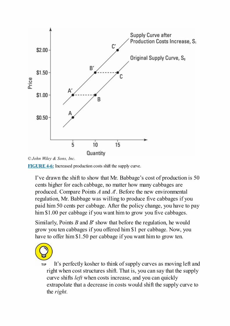
© John Wiley & Sons, Inc.

FIGURE 4-6: Increased production costs shift the supply curve.

I’ve drawn the shift to show that Mr. Babbage’s cost of production is 50cents higher for each cabbage, no matter how many cabbages areproduced. Compare Points A and A'. Before the new environmentalregulation, Mr. Babbage was willing to produce five cabbages if youpaid him 50 cents per cabbage. After the policy change, you have to payhim $1.00 per cabbage if you want him to grow you five cabbages.

Similarly, Points B and B' show that before the regulation, he wouldgrow you ten cabbages if you offered him $1 per cabbage. Now, youhave to offer him $1.50 per cabbage if you want him to grow ten.

It’s perfectly kosher to think of supply curves as moving left andright when cost structures shift. That is, you can say that the supplycurve shifts left when costs increase, and you can quicklyextrapolate that a decrease in costs would shift the supply curve tothe right.

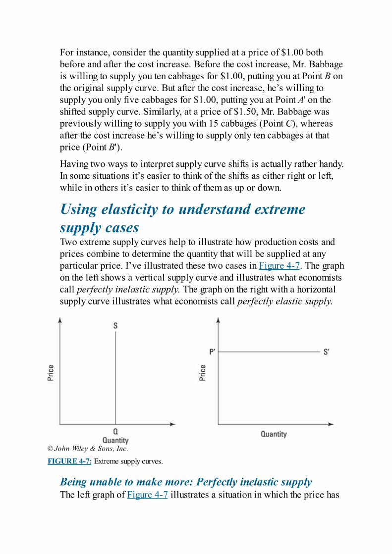
For instance, consider the quantity supplied at a price of $1.00 bothbefore and after the cost increase. Before the cost increase, Mr. Babbageis willing to supply you ten cabbages for $1.00, putting you at Point B onthe original supply curve. But after the cost increase, he’s willing tosupply you only five cabbages for $1.00, putting you at Point A' on theshifted supply curve. Similarly, at a price of $1.50, Mr. Babbage waspreviously willing to supply you with 15 cabbages (Point C), whereasafter the cost increase he’s willing to supply only ten cabbages at thatprice (Point B').

Having two ways to interpret supply curve shifts is actually rather handy.In some situations it’s easier to think of the shifts as either right or left,while in others it’s easier to think of them as up or down.

Using elasticity to understand extremesupply casesTwo extreme supply curves help to illustrate how production costs andprices combine to determine the quantity that will be supplied at anyparticular price. I’ve illustrated these two cases in Figure 4-7. The graphon the left shows a vertical supply curve and illustrates what economistscall perfectly inelastic supply. The graph on the right with a horizontalsupply curve illustrates what economists call perfectly elastic supply.

© John Wiley & Sons, Inc.

FIGURE 4-7: Extreme supply curves.

Being unable to make more: Perfectly inelastic supplyThe left graph of Figure 4-7 illustrates a situation in which the price has

no effect on the quantity supplied. As you can see in the graph, no matterhow low or how high the price, the quantity Q is supplied. Because thequantity supplied is completely unresponsive to the price, it is said to beperfectly inelastic, and supply situations that look like this are usuallyreferred to as situations of perfectly inelastic supply.

I expect you’re curious about what things have perfectly inelastic supplycurves. The answer is unique things that cannot be reproduced. Examplesinclude:

The Hope Diamond: Because it’s one of a kind — there’d still beonly one Hope Diamond, no matter how much anyone wanted to pay— its supply curve is vertical.Land: As comedian Will Rogers said back in the early 20th century,“Buy land. They ain’t making more of it.”The electromagnetic spectrum: There’s only one set of radiofrequencies, and everyone has to share because there’s no way tomake more.

An interesting thing about such situations is that there are no productioncosts. Because of this, offering the owner a price is not an incentive inthe way it is when you pay a producer enough to make something for you.Rather, the price serves solely to transfer the right of ownership andusage from one person to another.

Historically, the fact that the quantity of land supplied has nothing to dowith production costs has been the justification for property taxes. Theway governments see it, they can tax land as harshly as they wantbecause there’s no need to worry that the amount of land — and,consequently, the tax base — will ever decrease.

Producing however much you want: Perfectly elastic supplyThe right-hand graph in Figure 4-7 illustrates the case where the supplycurve is perfectly horizontal. The idea here is that the supplier isproducing something that has nonincreasing costs. No matter how manyunits you want her to produce, it always costs her only P' dollars to makea unit. Consequently, whether you want one unit produced or one jillionunits produced, you pay her P' dollars per unit.

In the real world, there probably aren’t any supply curves that are

perfectly elastic because production costs typically rise with outputlevels (as I explain in Chapter 6). But a few supply curves do comeclose. For instance, the supply curve for pencils looks nearly perfectlyelastic because pencil companies seem to be able to increase productionlevels by millions of units with only very small increases in costs.

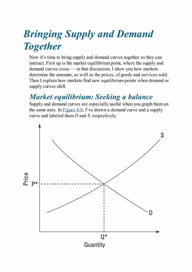
Bringing Supply and DemandTogether

Now it’s time to bring supply and demand curves together so they caninteract. First up is the market equilibrium point, where the supply anddemand curves cross — in that discussion, I show you how marketsdetermine the amounts, as well as the prices, of goods and services sold.Then I explain how markets find new equilibrium points when demand orsupply curves shift.

Market equilibrium: Seeking a balanceSupply and demand curves are especially useful when you graph them onthe same axes. In Figure 4-8, I’ve drawn a demand curve and a supplycurve and labeled them D and S, respectively.

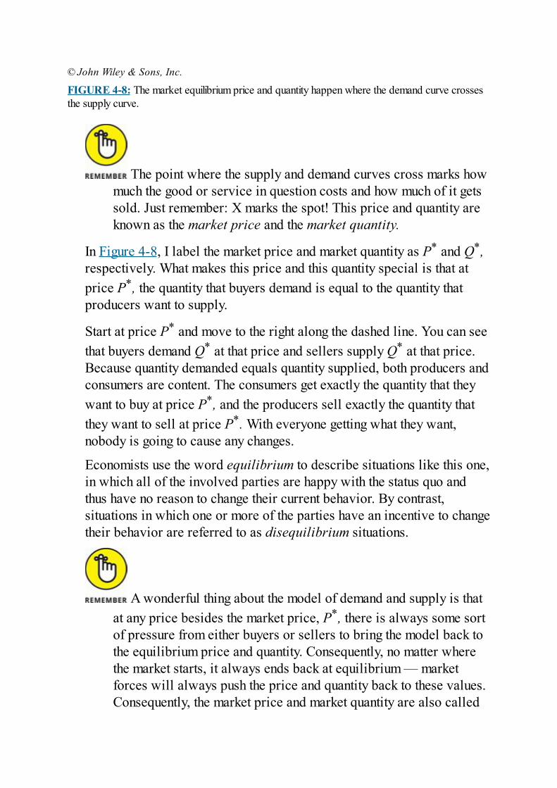
© John Wiley & Sons, Inc.

FIGURE 4-8: The market equilibrium price and quantity happen where the demand curve crossesthe supply curve.

The point where the supply and demand curves cross marks howmuch the good or service in question costs and how much of it getssold. Just remember: X marks the spot! This price and quantity areknown as the market price and the market quantity.

In Figure 4-8, I label the market price and market quantity as P* and Q*,respectively. What makes this price and this quantity special is that atprice P*, the quantity that buyers demand is equal to the quantity thatproducers want to supply.

Start at price P* and move to the right along the dashed line. You can seethat buyers demand Q* at that price and sellers supply Q* at that price.Because quantity demanded equals quantity supplied, both producers andconsumers are content. The consumers get exactly the quantity that theywant to buy at price P*, and the producers sell exactly the quantity thatthey want to sell at price P*. With everyone getting what they want,nobody is going to cause any changes.

Economists use the word equilibrium to describe situations like this one,in which all of the involved parties are happy with the status quo andthus have no reason to change their current behavior. By contrast,situations in which one or more of the parties have an incentive to changetheir behavior are referred to as disequilibrium situations.

A wonderful thing about the model of demand and supply is thatat any price besides the market price, P*, there is always some sortof pressure from either buyers or sellers to bring the model back tothe equilibrium price and quantity. Consequently, no matter wherethe market starts, it always ends back at equilibrium — marketforces will always push the price and quantity back to these values.Consequently, the market price and market quantity are also called

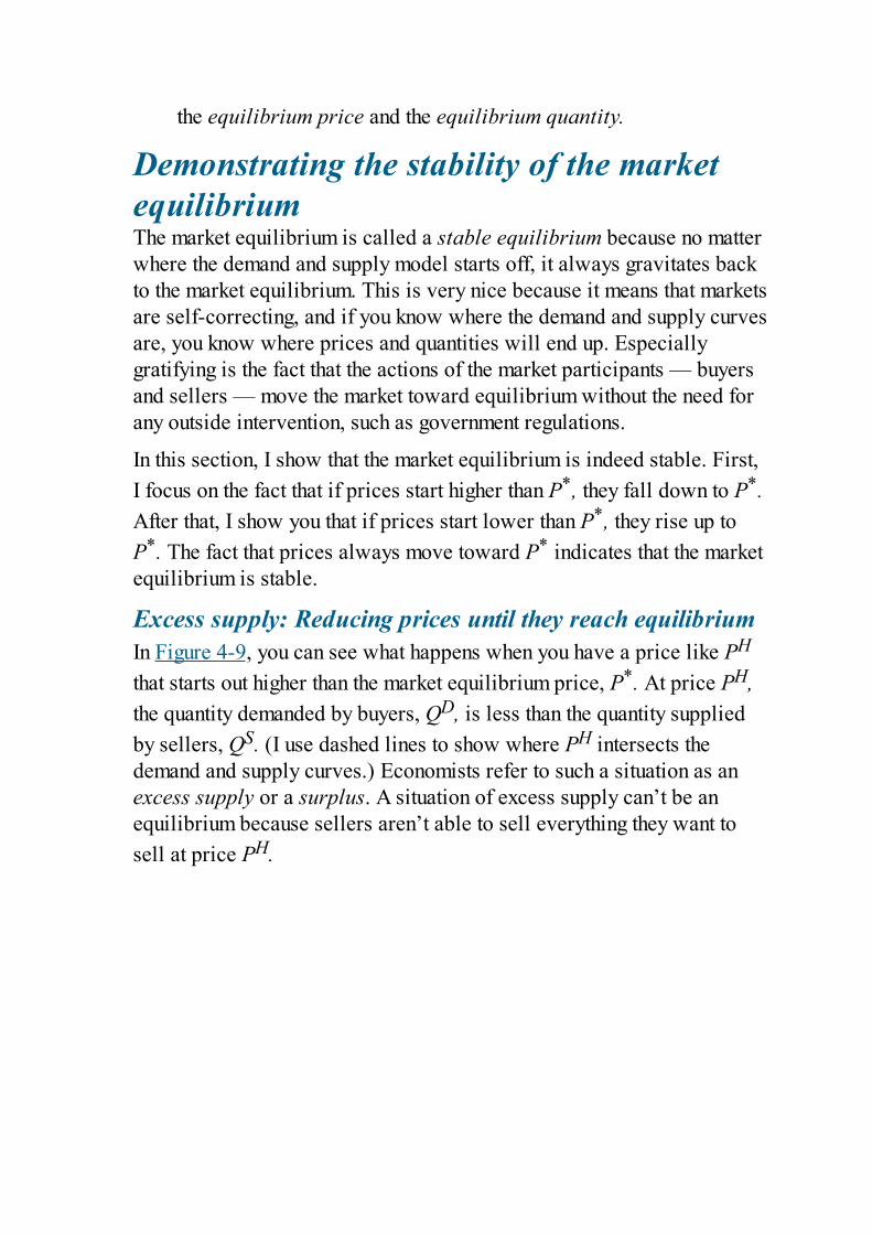
the equilibrium price and the equilibrium quantity.

Demonstrating the stability of the marketequilibriumThe market equilibrium is called a stable equilibrium because no matterwhere the demand and supply model starts off, it always gravitates backto the market equilibrium. This is very nice because it means that marketsare self-correcting, and if you know where the demand and supply curvesare, you know where prices and quantities will end up. Especiallygratifying is the fact that the actions of the market participants — buyersand sellers — move the market toward equilibrium without the need forany outside intervention, such as government regulations.

In this section, I show that the market equilibrium is indeed stable. First,I focus on the fact that if prices start higher than P*, they fall down to P*.After that, I show you that if prices start lower than P*, they rise up toP*. The fact that prices always move toward P* indicates that the marketequilibrium is stable.

Excess supply: Reducing prices until they reach equilibriumIn Figure 4-9, you can see what happens when you have a price like PH

that starts out higher than the market equilibrium price, P*. At price PH,the quantity demanded by buyers, QD, is less than the quantity suppliedby sellers, QS. (I use dashed lines to show where PH intersects thedemand and supply curves.) Economists refer to such a situation as anexcess supply or a surplus. A situation of excess supply can’t be anequilibrium because sellers aren’t able to sell everything they want tosell at price PH.

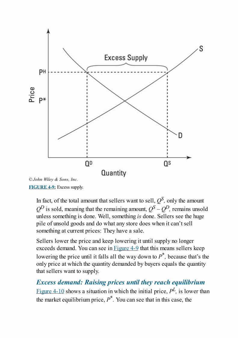
© John Wiley & Sons, Inc.

FIGURE 4-9: Excess supply.

In fact, of the total amount that sellers want to sell, QS, only the amountQD is sold, meaning that the remaining amount, QS – QD, remains unsoldunless something is done. Well, something is done. Sellers see the hugepile of unsold goods and do what any store does when it can’t sellsomething at current prices: They have a sale.

Sellers lower the price and keep lowering it until supply no longerexceeds demand. You can see in Figure 4-9 that this means sellers keeplowering the price until it falls all the way down to P*, because that’s theonly price at which the quantity demanded by buyers equals the quantitythat sellers want to supply.

Excess demand: Raising prices until they reach equilibriumFigure 4-10 shows a situation in which the initial price, PL, is lower thanthe market equilibrium price, P*. You can see that in this case, the

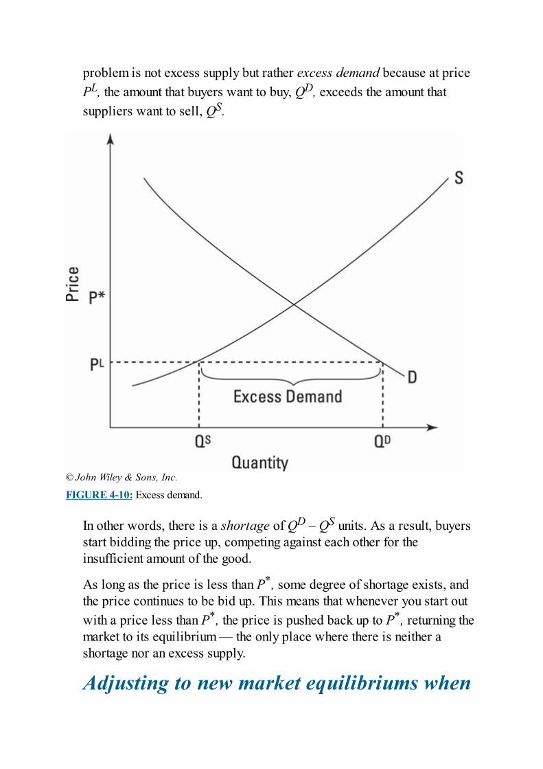
problem is not excess supply but rather excess demand because at pricePL, the amount that buyers want to buy, QD, exceeds the amount thatsuppliers want to sell, QS.

© John Wiley & Sons, Inc.

FIGURE 4-10: Excess demand.

In other words, there is a shortage of QD – QS units. As a result, buyersstart bidding the price up, competing against each other for theinsufficient amount of the good.

As long as the price is less than P*, some degree of shortage exists, andthe price continues to be bid up. This means that whenever you start outwith a price less than P*, the price is pushed back up to P*, returning themarket to its equilibrium — the only place where there is neither ashortage nor an excess supply.

Adjusting to new market equilibriums when

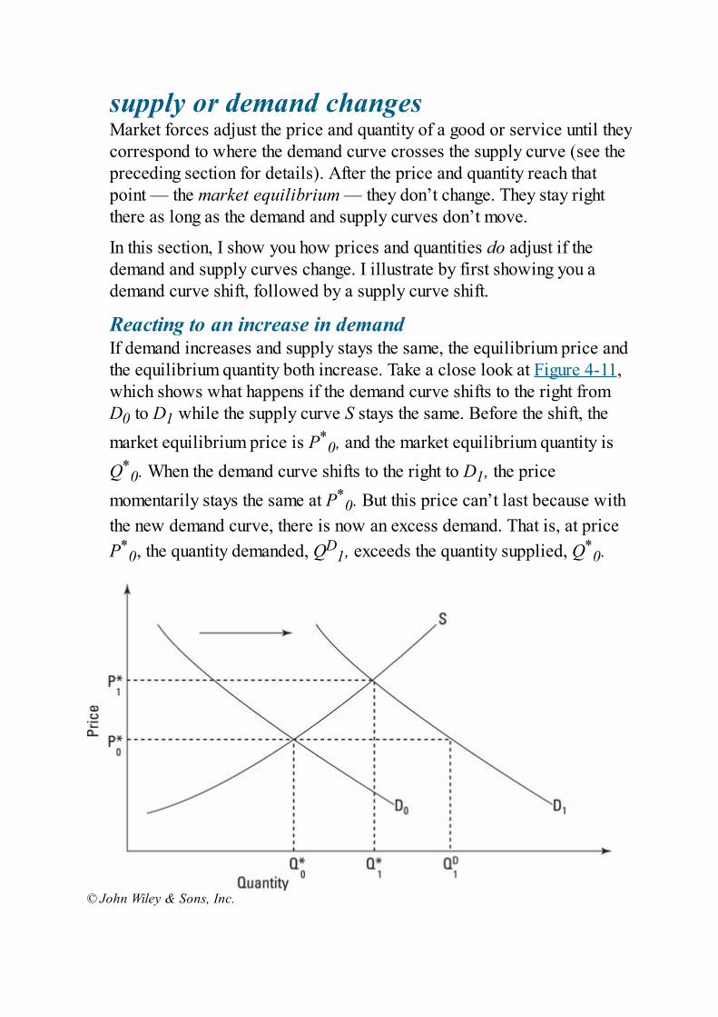
supply or demand changesMarket forces adjust the price and quantity of a good or service until theycorrespond to where the demand curve crosses the supply curve (see thepreceding section for details). After the price and quantity reach thatpoint — the market equilibrium — they don’t change. They stay rightthere as long as the demand and supply curves don’t move.

In this section, I show you how prices and quantities do adjust if thedemand and supply curves change. I illustrate by first showing you ademand curve shift, followed by a supply curve shift.

Reacting to an increase in demandIf demand increases and supply stays the same, the equilibrium price andthe equilibrium quantity both increase. Take a close look at Figure 4-11,which shows what happens if the demand curve shifts to the right fromD0 to D1 while the supply curve S stays the same. Before the shift, themarket equilibrium price is P*

0, and the market equilibrium quantity isQ*

0. When the demand curve shifts to the right to D1, the pricemomentarily stays the same at P*

0. But this price can’t last because withthe new demand curve, there is now an excess demand. That is, at priceP*

0, the quantity demanded, QD1, exceeds the quantity supplied, Q*

0.

© John Wiley & Sons, Inc.

FIGURE 4-11: A rightward shift of the demand curve.

Any such shortage causes buyers to bid up the price (see the earliersection “Excess demand: Raising prices until they reach equilibrium”).The result is that the price rises and continues to rise until it reaches P*

1,the price where demand curve D1 crosses supply curve S.

Note that when moving from the first equilibrium to the second, theequilibrium quantity increases from Q*

0 to Q*1. This result makes good

sense because if demand increases and buyers are willing to pay morefor something, you would expect more of it to be supplied. Also, theprice goes up from one equilibrium to the other because to get suppliersto supply more in a world of rising costs, you have to pay them more.

A much more subtle thing to realize, however, is that the slope of thesupply curve interacts with the demand curve to determine how big thechanges in price and quantity will be. Think of a vertical (perfectlyinelastic) supply curve, such as the one in the left-hand graph of Figure4-7. For such a supply curve, any increase in demand increases only theprice because the quantity can’t increase. On the other hand, if you aredealing with a horizontal (perfectly elastic) supply curve, as in the right-hand graph of Figure 4-7, a rightward shift in demand increases only thequantity, because the price is fixed at P'.

When you consider these two extreme cases, it hammers home the pointthat in a situation like Figure 4-11, neither demand nor supply is incomplete control. Their interaction jointly determines equilibrium pricesand quantities and how they change if the demand curve or the supplycurve shifts.

Reacting to a decrease in supplyIf supply decreases and demand stays the same, the equilibrium priceincreases, but the equilibrium quantity decreases. Consider Figure 4-12,in which the supply curve shifts from S0 to S1 because of an increase inproduction costs. (As I discuss in the earlier section “Cost changes:Shifting the supply curve,” this increase in costs can be considered toshift the supply curve either up or to the left. In Figure 4-12, I’ve drawn avertical arrow to indicate a vertical shift, but I could’ve just as correctlyput in a left arrow to indicate a leftward shift.)

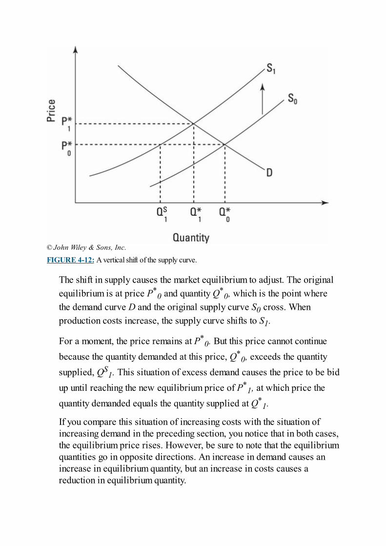
© John Wiley & Sons, Inc.

FIGURE 4-12: A vertical shift of the supply curve.

The shift in supply causes the market equilibrium to adjust. The originalequilibrium is at price P*

0 and quantity Q*0, which is the point where

the demand curve D and the original supply curve S0 cross. Whenproduction costs increase, the supply curve shifts to S1.

For a moment, the price remains at P*0. But this price cannot continue

because the quantity demanded at this price, Q*0, exceeds the quantity

supplied, QS1. This situation of excess demand causes the price to be bid

up until reaching the new equilibrium price of P*1, at which price the

quantity demanded equals the quantity supplied at Q*1.

If you compare this situation of increasing costs with the situation ofincreasing demand in the preceding section, you notice that in both cases,the equilibrium price rises. However, be sure to note that the equilibriumquantities go in opposite directions. An increase in demand causes anincrease in equilibrium quantity, but an increase in costs causes areduction in equilibrium quantity.

The equilibrium quantity falls when supply decreases becausethe increase in production costs doesn’t just affect the producer. Inorder to stay in business, the producer has to pass along the costincrease. But when he passes the increase along, it has a tendency todiscourage buyers. The result is that the equilibrium quantity fallsbecause some buyers are not willing to pay the higher prices. Thosewho still want to buy are willing to pay the higher prices — a factthat is reflected in the increased market price.

Price Controls: Keeping PricesAway from Market Equilibrium

Left to its own devices, a market always adjusts until the price andquantity are determined by where the demand and supply curves cross.The market equilibrium price has the very nice property that everyonewho wants to buy at that price can do so, and everyone who wants to sellat that price can also do so. In other words, the quantity demanded equalsthe quantity supplied.

However, the market price is not always the politically expedient price,and governments sometimes interfere in markets to prevent the marketequilibrium from being reached. Such interventions happen becausepolitically influential buyers think the market price is too high or becausepolitically influential sellers think the market price is too low.

Unfortunately, government intervention creates a whole new set ofproblems related to the misallocation of resources. In some cases,government intervention even hurts those whom the intervention isdesigned to help. In this section, I explain the effects of two kinds ofgovernment intervention: price ceilings and price floors. Price ceilingsprevent prices from rising to the market equilibrium, whereas pricefloors keep prices from falling to the market equilibrium. (Obviously,you use only one or the other!)

Setting upper limits with price ceilingsSometimes the government intervenes in a market to ensure that the pricestays below the market equilibrium price, P*. Such policies are calledprice ceilings because they prevent the price from rising as high as itwould if left alone. Prices hit the ceiling and then go no higher.

You may have heard about price ceilings on apartment rent. For instance,in an attempt to provide low-cost housing for the poor, city governmentsmay place price ceilings on how much a landlord can charge. Theproblem is that with prices artificially low, the quantity demanded isgreater than the quantity supplied, creating a shortage.

To see how this works, look at Figure 4-13, in which the price ceiling

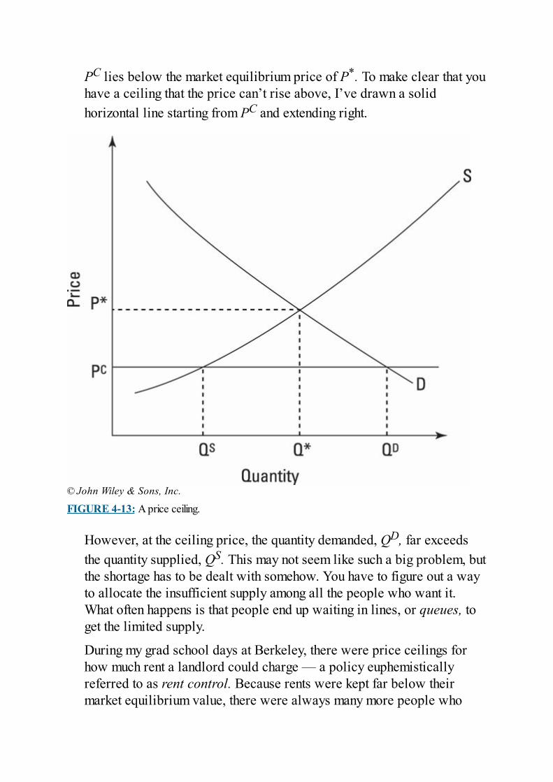
PC lies below the market equilibrium price of P*. To make clear that youhave a ceiling that the price can’t rise above, I’ve drawn a solidhorizontal line starting from PC and extending right.

© John Wiley & Sons, Inc.

FIGURE 4-13: A price ceiling.

However, at the ceiling price, the quantity demanded, QD, far exceedsthe quantity supplied, QS. This may not seem like such a big problem, butthe shortage has to be dealt with somehow. You have to figure out a wayto allocate the insufficient supply among all the people who want it.What often happens is that people end up waiting in lines, or queues, toget the limited supply.

During my grad school days at Berkeley, there were price ceilings forhow much rent a landlord could charge — a policy euphemisticallyreferred to as rent control. Because rents were kept far below theirmarket equilibrium value, there were always many more people who

wanted to rent apartments than there were apartments available. Theresult was that any time an apartment became available, you stood in linewith — literally — 200 people to fill out a rental application. With somany potential renters vying for one apartment, the landlord could takehis pick — hence, rental applications were often five to ten pages longand asked you everything. If you weren’t picked, you had to go get in thenext line for the next apartment that happened to come on the market.

FIRST WORLD SUPPORTS, THIRDWORLD SUFFERING

A perverse result of agricultural price supports in rich countries like the UnitedStates and the nations of the European Union is the great damage they inflict ondeveloping nations. For instance, the U.S. price of sugar is substantially higherthan the world price because the United States restricts imports of cheaperforeign sugar in order to help U.S. food production giants sell corn-basedsweeteners. The result is that thousands of poor Third World farmers whocould otherwise make a living selling sugar to Americans are left without alivelihood.

Even worse is what the United States does with some of the many tons ofexcess agricultural products that pile up due to its agricultural price supports.Not wanting to sell the excess in the United States and thereby depress U.S.prices, the government often sends the stuff free to developing countries asfood aid. That sounds nice and friendly, but when all that free wheat hitsNigeria, it puts Nigerian farmers out of business. That in turn ends up makingNigeria dependent on foreign food because it no longer has enough localfarmers to produce sufficient quantities of wheat to feed its own people.

Even worse, many of the newly bankrupted farmers move from thecountryside to cities in search of employment, worsening urban-overcrowdingproblems and themselves becoming dependent on free foreign wheat to survivewhen most of them can’t find employment. Thus, the U.S. government’sattempt to make its relatively very wealthy farmers a bit richer ends up causingcatastrophic harm to the truly very poor farmers of developing nations.

To avoid these problems, economists recommend that food aid from richcountries only be sent to poor countries during times of famine or droughtwhen local farmers are unable to produce enough to feed their country. Foodaid should be withdrawn as soon as a crisis ends so that it doesn’t permanentlyundercut local food prices and the ability of local farmers to make a living.

It didn’t matter if you had enough money to pay higher rent. It didn’tmatter if you were much more desperate than other potential renters.Because the government had created an excess demand, you had to waitin line and hope and pray that you’d get an apartment.

The main result of the policy was that thousands of people wasted tens ofthousands of hours each year waiting in line — and some of them stilldidn’t get apartments! Even worse was the fact that the policy actually

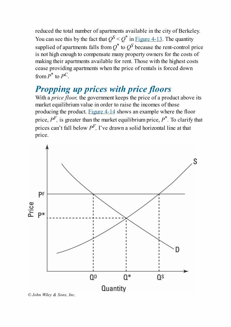
reduced the total number of apartments available in the city of Berkeley.You can see this by the fact that QS < Q* in Figure 4-13. The quantitysupplied of apartments falls from Q* to QS because the rent-control priceis not high enough to compensate many property owners for the costs ofmaking their apartments available for rent. Those with the highest costscease providing apartments when the price of rentals is forced downfrom P* to PC.

Propping up prices with price floorsWith a price floor, the government keeps the price of a product above itsmarket equilibrium value in order to raise the incomes of thoseproducing the product. Figure 4-14 shows an example where the floorprice, PF, is greater than the market equilibrium price, P*. To clarify thatprices can’t fall below PF, I’ve drawn a solid horizontal line at thatprice.

© John Wiley & Sons, Inc.

FIGURE 4-14: A price floor.

The problem here is that at price PF, the quantity supplied, QS, is muchbigger than the quantity demanded, QD. The normal response to such asituation of excess supply would be for the price to fall. The way thegovernment prevents this and keeps the price propped up is by steppingin and buying the excess supply.

In other words, of the total amount QS that’s supplied at price PF, regularconsumers demand and purchase QD. The remainder, QS – QD, must bepurchased by the government. That doesn’t sound so bad until you readabout price floors in agriculture, which are usually referred toeuphemistically as price supports (as in, “You poor thing! All you needis a little support!”).

Price supports generate huge piles of surplus farm output that nobodywants to buy. Consider the price support system for milk that the U.S.Department of Agriculture ran in the 1980s and 1990s. Each year, theDepartment of Agriculture had to buy up hundreds of thousands ofgallons of milk that nobody wanted to buy at the high price thegovernment was maintaining to help dairy farmers. What did thedepartment do with all of that milk? It turned it into cheese that itcouldn’t sell (because it was also supporting the price of cheese) andstored that surplus cheese in huge refrigerated warehouses —indefinitely! And yes, this was all done at the taxpayer’s expense.

Because many people have protested this sort of wastefulness, thegovernment switched policies for some crops. The government now paysmany farmers not to farm. That way, the farmers still get paid, but there’sno worry about an excess supply that has to be destroyed or given away(for concerns about food aid, go back to the earlier sidebar “First Worldsupports, Third Word suffering”). In terms of Figure 4-14, the goal ofthese policies is to shift the supply curve left until it intersects thedemand curve directly over quantity QD. If that can be done, there willbe no excess supply at price PF.

For both price ceilings and price floors, the message you should takeaway is that interfering with markets typically causes great mischief.(Yet, deep inside, I’m actually hoping that the government decides tosupport the salaries of academic economists. I’d love to end up getting

paid not to teach.)

Chapter 5

Introducing HomoEconomicus, the Utility-Maximizing Consumer

IN THIS CHAPTER Studying how people maximize their happiness Taking account of diminishing marginal utility Watching how people weigh alternatives Choosing exactly the right amounts within a limited budget

This chapter gets behind the demand curve (which I introduce in Chapter4) by showing you how people come to choose the things they choose.This decision-making process is very important because human wantsare what drive the economy. Firms don’t randomly produce goods andservices; they produce the things that people want to buy and arespending money on.

The thing that makes studying this process hard is the fact that peoplehave so many different things they can spend their money on. If aneconomist was asked to research how you would spend $100 in a storethat sold only blueberry muffins, his job wouldn’t be so hard. What’simpressive is that economists have come up with a way to explain howyou would spend $100 in a store that has hundreds or even thousands ofitems for sale.

Even more impressive is the fact that an economist can explain not onlywhich items you would buy but also how many of each you would buy. Inother words, economic theory can explain not just what you demand butalso the quantities you demand, which is where demand curves comefrom.

I start the chapter by discussing utility, which is how economistsmeasure human happiness. Economists assume that people act in waysthat maximize their happiness, but human actions are constrained,

especially by limited budgets. I explain how people navigate theseconstraints to get the most happiness possible given the limits involved.Finally, I show how these decisions underlie and explain the slope andposition of demand curves.

People must make choices because their means for satisfying their wantsare limited. There’s never enough money or time to do everything thatyou desire. Consequently, you need to choose wisely to get the mosthappiness out of the limited resources that you do have.

Economists and engineers refer to problems of this sort as constrainedoptimization problems because people are trying to optimize theirhappiness given the fact that they’re constrained by their limitedresources. The rest of this chapter shows you how economists model theway that people go about solving their everyday constrained optimizationproblem: deciding how to best spend their limited incomes on availablegoods and services — choosing not only which things to buy but alsohow much of each.

Choosing by RankingIn order for people to choose between the exceedingly different goodsand services available in the economy, they must have a way ofcomparing them. Comparing costs is pretty easy; you just compareprices. But how do you compare the benefits of various goods andservices? How do you assess whether it’s better to spend $20 on Swisschocolate bars or on a new plaid shirt? In what ways are chocolate andshirts even comparable?

Obviously, people do manage to make a comparison and rank thetwo choices. The way economists imagine that people do this is byassigning a common measure of happiness to each possible thingthey could buy and use. Economists call this common measure ofhappiness utility, and they imagine that if they could somehow getinside your brain and measure utility, they could do so using a unitthat they very uncreatively refer to as a util.

Given those assumptions, economists have come up with two alternativeways of thinking about how people make comparisons and choices:

Cardinal utility: Decision making under this system is based onassigning specific numbers of utils to different things — for instance,25 utils to the pleasure associated with eating a brownie or 75 utilsto the pleasure associated with watching a sunset. Making suchspecific assignments is called cardinal utility (like cardinalnumbers: 1, 2, 3 …). Some people object to cardinal utility becauseit’s not clear that people make such assessments — after all, howmany utils do you think you receive from a sunny day or an infant’ssmile?Ordinal utility: A much less objectionable thing to do is to think interms of ordinal utility, a system in which you simply rank things.For instance, instead of saying that the sunset has a utility of 75,which makes it preferred over the brownie with a utility of 25, youcan simply say that you prefer sunsets to brownies. This system has amuch more intuitive feeling for most people and eliminates the need

to try to measure things using the imaginary unit called the util.

It’s been proven mathematically that you can describe the same humanchoice behavior using ordinal utility that you can using cardinal utility,which means that economists don’t have to use cardinal utility. But I’mgoing to anyway! Why? Because explaining the crucial concept ofdiminishing marginal utility using the cardinal utility system is mucheasier. You can also explain diminishing marginal utility using theordinal system, but the math is so hard that it’s normally taught only toPhD students. So please forgive me if the cardinal utility system seems abit unrealistic, but it’s really the best way to convey this incrediblyimportant idea.

Getting Less from More:Diminishing Marginal Utility

People get bored even with things they like; they get tired of repetitionand sameness. Economists have to take account of this when studyinghow people choose to spend their money.

For instance, if I haven’t had any pizza in a long time, I’ll get a hugeamount of utility from eating a slice. The melted cheese, the basil andgarlic in the sauce, and the warmth in my mouth all make me very, veryhappy. But the thrill of pizza is dampened by eating that first slice so thatif I eat a second slice, it’s still very good, but not as good as the first.And if I have a third slice, it’s not as good as the second. And if I keepeating and eating and eating, the additional slices of pizza will soon getsickening and produce pain instead of pleasure if I eat them.

This phenomenon isn’t limited to pizza; it applies to nearly everything.Unless you’re addicted to something, you get tired of it as you have moreof it, and each additional unit brings you less happiness than the previousunit. To make this phenomenon clearer, look at Figure 5-1, which showsmy cumulative, total utility as I eat more and more slices of pizza. Forinstance, my total utility after eating one slice of pizza is 24 utils. Aftereating two slices, it’s 36 utils. And after three slices, it’s 46 utils.

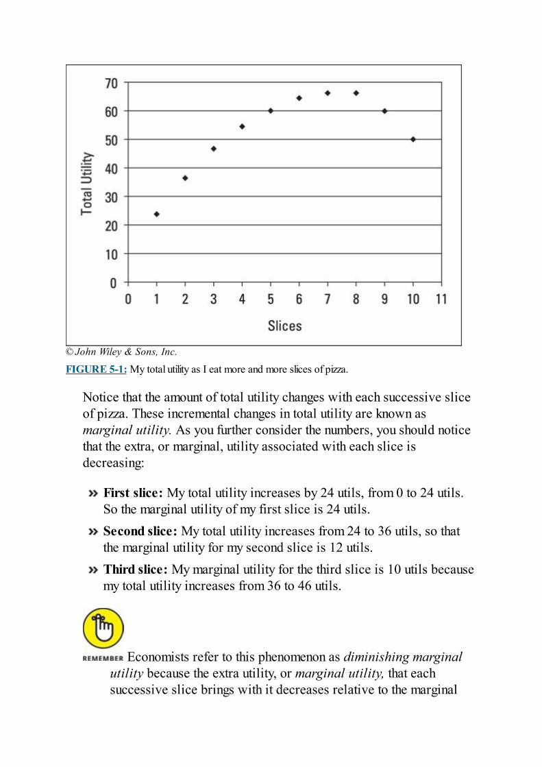
© John Wiley & Sons, Inc.

FIGURE 5-1: My total utility as I eat more and more slices of pizza.

Notice that the amount of total utility changes with each successive sliceof pizza. These incremental changes in total utility are known asmarginal utility. As you further consider the numbers, you should noticethat the extra, or marginal, utility associated with each slice isdecreasing:

First slice: My total utility increases by 24 utils, from 0 to 24 utils.So the marginal utility of my first slice is 24 utils.Second slice: My total utility increases from 24 to 36 utils, so thatthe marginal utility for my second slice is 12 utils.Third slice: My marginal utility for the third slice is 10 utils becausemy total utility increases from 36 to 46 utils.

Economists refer to this phenomenon as diminishing marginalutility because the extra utility, or marginal utility, that eachsuccessive slice brings with it decreases relative to the marginal

utility brought by the previous slice. Diminishing marginal utility issimply a reflection of the fact that people get fed up or bored withthings. Or, in the case of food and drink, their appetite decreaseswith each unit they consume.

Look at what happens in Figure 5-1 after slice number eight. My totalutility actually goes down, because slice number nine is making me alittle sick. And if I have slice number ten, I’m even sicker, so total utilityfalls again. What this decrease in total utility implies is that marginalutility must be negative for slices nine and ten. The data in Figure 5-1shows that although my total utility increases for slices one throughseven, it stalls at slice number eight and falls for slices nine and ten.

In Figure 5-2, I plot the marginal utility that I get for each slice of pizza. Ifeel diminishing marginal utility as I eat more and more slices of pizza,because the marginal utility that comes with each additional slice isalways less than that of the previous slice. Specifically, although mymarginal utility is 24 utils for the first slice, it falls to 0 utils for sliceeight and then actually becomes negative for slices nine and ten becauseeating them makes me ill. You can see quite clearly from the downwardslope of the points that my marginal utility diminishes as I eat more andmore slices of pizza.

© John Wiley & Sons, Inc.

FIGURE 5-2: The marginal utility I derive from each slice of pizza.

You have to be careful not to confuse diminishing marginalutility with negative marginal utility. As you see in Figure 5-2, thereis diminishing marginal utility for all slices of pizza starting withthe second, because each successive slice has a smaller marginalutility than the previous one. But the marginal utilities are stillpositive for all slices up to slice seven, and they become negativeonly for slices nine and ten.

That fact implies that you enjoy eating every slice up to and including theseventh slice because doing so brings you an increase in utility(happiness). So don’t think that just because marginal utility isdiminishing for a particular slice, you wouldn’t want to eat it. Marginalutility can be diminishing but still positive. The only slices you’lloutright want to avoid are the ninth and tenth.

Choosing Among Many OptionsWhen Facing a Limited Budget

The phenomenon of diminishing marginal utility makes studying humanchoices very interesting because preferences can’t be determined in theabstract. Rather, they depend on what you’ve already had.

If I haven’t had any ice cream for months and you ask me whether I wantchocolate or vanilla, I’ll say chocolate. But if you ask me whether I wantchocolate or vanilla after I’ve just eaten a gallon of chocolate, I’m goingto say vanilla because I’ve already more than satisfied my chocolatecravings.

So the answer to the question “Chocolate or vanilla?” isn’t asstraightforward as it seems. Your preferences exhibit diminishingmarginal utility, and even something that you normally like a lot won’tbring you much marginal utility (additional happiness) if you’ve justindulged in it a lot.

This fact ends up leading to a simple rule about how people makedecisions when faced with limited budgets. Essentially, people want tomaximize their total utility in buying a certain combination of goods —and to do that, the marginal utilities per dollar have to be equal for thefinal units of each good. I explain this process with a concrete examplein the next subsection before showing you the mathematical formula thatsummarizes the simple rule.

Trying to buy as much (marginal) utility asyou canA person interested in maximizing her utility will want to figure out howto best allocate any limited budget so as to purchase the combination ofgoods and services that will bring her the largest possible amount ofutility. But in doing so, she has to take account of the fact that eachproduct is subject to diminishing marginal utility, so that each successiveunit purchased and consumed brings less additional, or marginal, utilitythan the previous unit.

Suppose that I have $10 to spend and, because I’m going to the local

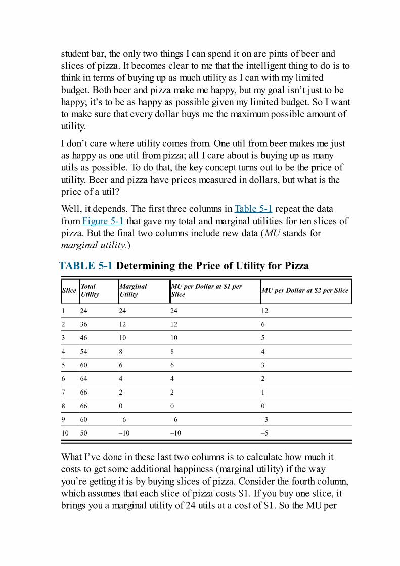
student bar, the only two things I can spend it on are pints of beer andslices of pizza. It becomes clear to me that the intelligent thing to do is tothink in terms of buying up as much utility as I can with my limitedbudget. Both beer and pizza make me happy, but my goal isn’t just to behappy; it’s to be as happy as possible given my limited budget. So I wantto make sure that every dollar buys me the maximum possible amount ofutility.

I don’t care where utility comes from. One util from beer makes me justas happy as one util from pizza; all I care about is buying up as manyutils as possible. To do that, the key concept turns out to be the price ofutility. Beer and pizza have prices measured in dollars, but what is theprice of a util?

Well, it depends. The first three columns in Table 5-1 repeat the datafrom Figure 5-1 that gave my total and marginal utilities for ten slices ofpizza. But the final two columns include new data (MU stands formarginal utility.)

TABLE 5-1 Determining the Price of Utility for Pizza

Slice TotalUtility

MarginalUtility

MU per Dollar at $1 perSlice MU per Dollar at $2 per Slice

1 24 24 24 12

2 36 12 12 6

3 46 10 10 5

4 54 8 8 4

5 60 6 6 3

6 64 4 4 2

7 66 2 2 1

8 66 0 0 0

9 60 –6 –6 –3

10 50 –10 –10 –5

What I’ve done in these last two columns is to calculate how much itcosts to get some additional happiness (marginal utility) if the wayyou’re getting it is by buying slices of pizza. Consider the fourth column,which assumes that each slice of pizza costs $1. If you buy one slice, itbrings you a marginal utility of 24 utils at a cost of $1. So the MU per

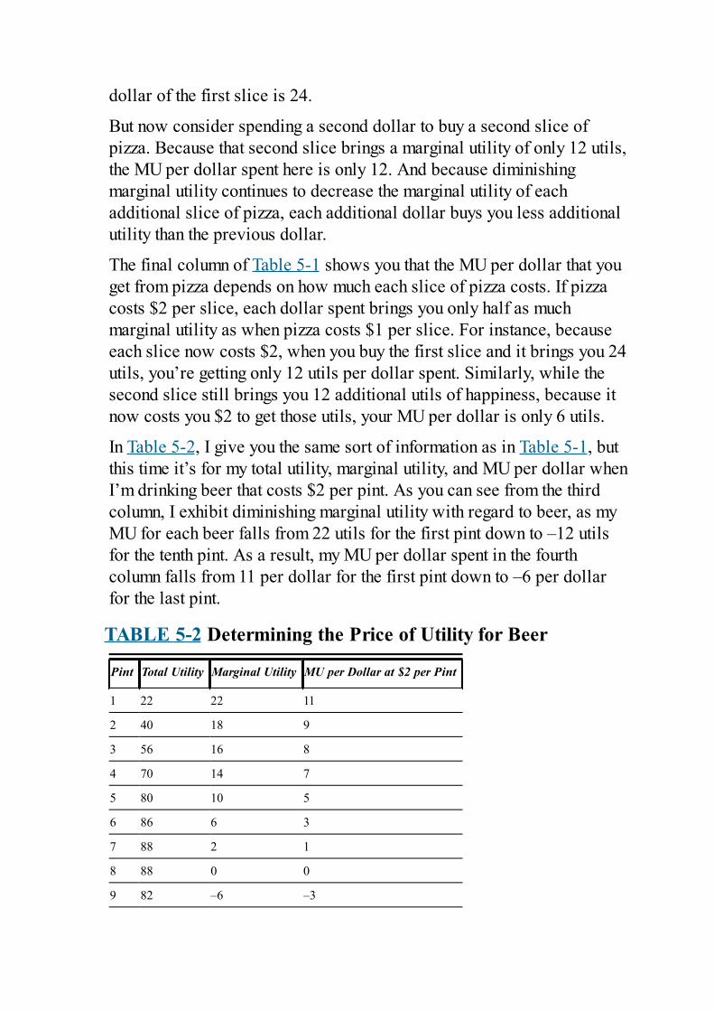
dollar of the first slice is 24.

But now consider spending a second dollar to buy a second slice ofpizza. Because that second slice brings a marginal utility of only 12 utils,the MU per dollar spent here is only 12. And because diminishingmarginal utility continues to decrease the marginal utility of eachadditional slice of pizza, each additional dollar buys you less additionalutility than the previous dollar.

The final column of Table 5-1 shows you that the MU per dollar that youget from pizza depends on how much each slice of pizza costs. If pizzacosts $2 per slice, each dollar spent brings you only half as muchmarginal utility as when pizza costs $1 per slice. For instance, becauseeach slice now costs $2, when you buy the first slice and it brings you 24utils, you’re getting only 12 utils per dollar spent. Similarly, while thesecond slice still brings you 12 additional utils of happiness, because itnow costs you $2 to get those utils, your MU per dollar is only 6 utils.

In Table 5-2, I give you the same sort of information as in Table 5-1, butthis time it’s for my total utility, marginal utility, and MU per dollar whenI’m drinking beer that costs $2 per pint. As you can see from the thirdcolumn, I exhibit diminishing marginal utility with regard to beer, as myMU for each beer falls from 22 utils for the first pint down to –12 utilsfor the tenth pint. As a result, my MU per dollar spent in the fourthcolumn falls from 11 per dollar for the first pint down to –6 per dollarfor the last pint.

TABLE 5-2 Determining the Price of Utility for Beer

Pint Total Utility Marginal Utility MU per Dollar at $2 per Pint

1 22 22 11

2 40 18 9

3 56 16 8

4 70 14 7

5 80 10 5

6 86 6 3

7 88 2 1

8 88 0 0

9 82 –6 –3

10 70 –12 –6

Purchasing the best combination of twogoods to maximize total utilityWhen facing a limited budget, the trick is to see how to allocatepurchases to get the most total utility. Tables 5-1 and 5-2 show you howmuch utility I can get by spending money on either pizza or beer. I have$10 to spend. As a first attempt, consider the two most extreme options:blowing all the money on pizza, or blowing all the money on beer. (Pizzacosts $1 per slice, and beer costs $2 per pint.)

If I spend all $10 on pizza, I can buy 10 slices of pizza, which wouldgive me a total utility of 50 utils. On the other hand, if I spend all $10 onbeer, I can buy 5 pints at $2 each and thereby get 80 total utils. If thesewere my only two options, I would clearly prefer to spend all my moneyon beer because it brings me more utils than does buying only pizza.

However, there’s a much better thing to do. I can get even more totalutility if I wisely mix up my consumption a bit and spend some of mymoney on beer and some of it on pizza.

The way I get the most utility possible out of my $10 is simple: Itake each of the ten dollars in turn and spend it on whichever goodbrings more utility. I don’t think of my task as buying slices of pizzaor pints of beer. Rather, my job is buying utility. For every dollarspent, I want to buy as much utility as possible, and I don’t carewhether that utility comes from beer or pizza.

The only thing complicating this process of spending each dollar onwhichever good will bring the most utility is the fact that I havediminishing marginal utility for both beer and pizza, meaning that theamount of utility I’ll be able to buy with each extra dollar spent willdepend on how much beer or pizza I’ve already bought. But given theinformation in Tables 5-1 and 5-2, I can figure out the best thing I shoulddo with each dollar:

Dollar 1: What should I do with the first dollar? From the fourth

column of Table 5-1, you can see that if I spend that dollar on pizza, Ican buy 24 utils of utility. On the other hand, the fourth column ofTable 5-2 tells you that if I spend that first dollar on beer (along witha second dollar because pints cost $2), I’ll get only 11 utils of utility.So, the obvious thing to do with the first dollar is to buy pizza ratherthan beer.Dollar 2: If I use my second dollar to buy a second slice of pizza, I’llget 12 utils of utility. If I buy beer with that second dollar (along witha third dollar because the price of a pint is $2), I’ll get only 11 utilsfor that second dollar because it will be spent on buying the first pint.So, it’s better to spend the second dollar on pizza rather than beer.Dollars 3 and 4: At dollar number three, everything changes. That’sbecause if I spend a third dollar on pizza, it will bring 10 utils. But ifI spend that third dollar (along with a fourth dollar since each pintcosts $2) on a pint, I get an MU per dollar of 11 utils (for eachdollar). So I should spend dollars three and four on buying the firstpint of beer.Dollar 5: I’ll want to spend the fifth dollar on pizza rather than beer,because I’ll get 10 utils of marginal utility if I use this dollar to buythe third slice of pizza but only 9 utils of marginal utility if I use thisdollar (along with a sixth dollar since pints cost $2 each) to purchasea second pint of beer.Dollars 6 and 7: I should spend dollars six and seven on beer,because I’ll get an MU per dollar of 9 utils for my second pint,whereas I’ll get only 8 utils if I spend the sixth dollar on a fourthslice of pizza.Dollars 8, 9, and 10: For dollar number eight, the MUs per dollarare tied. If I use this dollar to buy a fourth slice of pizza, I get 8 utils.I’ll get the same by spending that eighth dollar (plus the ninth dollar,because pints cost $2 each) on a third pint of beer. So I should spendmy last three dollars buying a fourth slice of pizza and a third pint ofbeer.

In Table 5-3, I list where I should spend each of my ten dollars. Noticethat the total utility I can purchase with my $10 is 110 utils. That’s muchbetter than the 50 utils I would get spending all the money on pizza or the80 utils I would get spending it all on beer. By spending each dollar in

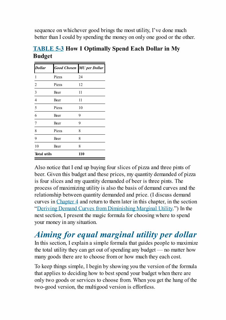
sequence on whichever good brings the most utility, I’ve done muchbetter than I could by spending the money on only one good or the other.

TABLE 5-3 How I Optimally Spend Each Dollar in MyBudget

Dollar Good Chosen MU per Dollar

1 Pizza 24

2 Pizza 12

3 Beer 11

4 Beer 11

5 Pizza 10

6 Beer 9

7 Beer 9

8 Pizza 8

9 Beer 8

10 Beer 8

Total utils 110

Also notice that I end up buying four slices of pizza and three pints ofbeer. Given this budget and these prices, my quantity demanded of pizzais four slices and my quantity demanded of beer is three pints. Theprocess of maximizing utility is also the basis of demand curves and therelationship between quantity demanded and price. (I discuss demandcurves in Chapter 4 and return to them later in this chapter, in the section“Deriving Demand Curves from Diminishing Marginal Utility.”) In thenext section, I present the magic formula for choosing where to spendyour money in any situation.

Aiming for equal marginal utility per dollarIn this section, I explain a simple formula that guides people to maximizethe total utility they can get out of spending any budget — no matter howmany goods there are to choose from or how much they each cost.

To keep things simple, I begin by showing you the version of the formulathat applies to deciding how to best spend your budget when there areonly two goods or services to choose from. When you get the hang of thetwo-good version, the multigood version is effortless.

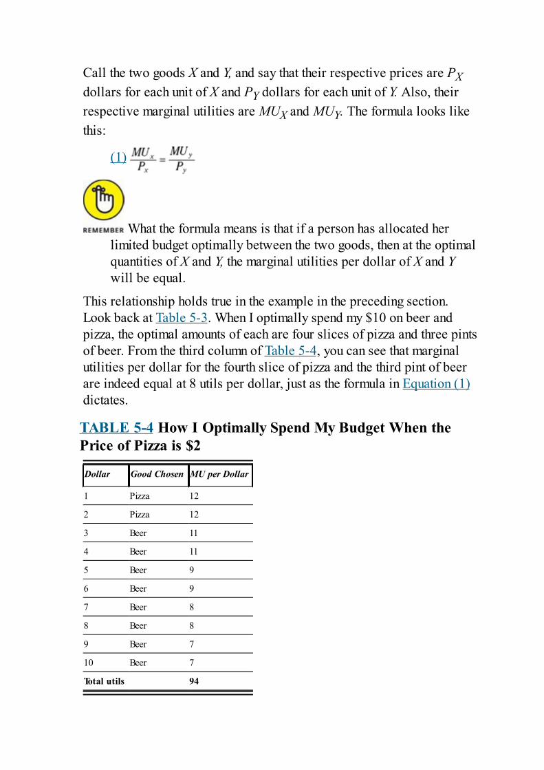
Call the two goods X and Y, and say that their respective prices are PXdollars for each unit of X and PY dollars for each unit of Y. Also, theirrespective marginal utilities are MUX and MUY. The formula looks likethis:

(1)

What the formula means is that if a person has allocated herlimited budget optimally between the two goods, then at the optimalquantities of X and Y, the marginal utilities per dollar of X and Ywill be equal.

This relationship holds true in the example in the preceding section.Look back at Table 5-3. When I optimally spend my $10 on beer andpizza, the optimal amounts of each are four slices of pizza and three pintsof beer. From the third column of Table 5-4, you can see that marginalutilities per dollar for the fourth slice of pizza and the third pint of beerare indeed equal at 8 utils per dollar, just as the formula in Equation (1)dictates.

TABLE 5-4 How I Optimally Spend My Budget When thePrice of Pizza is $2

Dollar Good Chosen MU per Dollar

1 Pizza 12

2 Pizza 12

3 Beer 11

4 Beer 11

5 Beer 9

6 Beer 9

7 Beer 8

8 Beer 8

9 Beer 7

10 Beer 7

Total utils 94

Seeing why the marginal utilities per dollar must be equalIf marginal utilities per dollar aren’t equal, you’ll want to keeprearranging your purchases until they are. In this section, I demonstratewhy marginal utilities per dollar have to be equal if you want tomaximize your utility when spending a limited budget.

HOW INFLATION AFFECTSPURCHASING COMBINATIONS

An interesting thing to notice when you stare at Equation (1) or Equation (3) inthis chapter is that if all the prices in the denominators were to suddenly go upby the same multiple, all the equalities would remain intact, meaning that peoplewould still choose to buy the same amounts of every good. For example, ifthere were suddenly an inflation that exactly doubled all prices, people wouldstill choose to buy exactly the same quantities of everything as they did before.

The idea behind this result is that if my income doubles at the same time thatthe prices of everything I buy double, nothing has really changed. I can stillpurchase exactly the same quantities of goods and services as I used topurchase before the inflation. And because those quantities were the ones thatwere maximizing my utility before, they’ll still be maximizing my utility now. Asa result, you may mistakenly conclude that inflation doesn’t matter.

But in Chapter 15, I tell you about the great horrors of inflation. These horrorsare caused by the fact that you never, in real life, see a perfect inflation like theone I just described in which the prices of all goods and services go up byexactly the same amount at exactly the same time.

Instead, what happens is that the prices of different goods and services go up atdifferent rates, so the fractions in Equations (1) and (3) are thrown completelyout of whack because their denominators change at different rates. When thathappens, people start drastically changing their quantities demanded in anattempt to reestablish equality between all their marginal utilities per dollar. Asthey do this, chaos results; some firms find demand suddenly falling for theirproducts, while others find it suddenly rising. So don’t let Equations (1) or (3)make you think that inflation doesn’t matter in the real world. It does.

First, imagine that I choose some other quantities of each good, so thatfor the final unit of X and the final unit of Y that I purchase,

(2)

Let pizza be X and beer be Y. From Tables 5-2 and 5-3, you can see thatif I purchase four pints of beer and two slices of pizza, the MU per dollarfor the fourth pint of beer is 7, and the MU per dollar for the second sliceof pizza is 16. Clearly, the MU per dollar of pizza is much bigger thanthe MU per dollar of beer if I spend my limited budget in this way.

But this way of spending my budget isn’t optimal. The reason is that themoney I’m spending on what is currently the final unit of X (pizza) buysmore marginal utility than the money I’m currently spending on the finalunit of Y (beer). If I can get more utility by spending a dollar on X than Ican on Y, I should take money away from spending on Y in order to spendit on X. And as long as the inequality in Equation (2) holds true, I shouldcontinue to take money away from Y in order to increase spending on X.

Applying the formula to multiple goods and servicesTo maximize total utility, you should rearrange your purchases so that forthe final units of each good, the marginal utilities per dollar are equal. Ifthat isn’t true, one of the goods offers you a higher amount of happinessfor each dollar spent, meaning that you want to rearrange your purchasesto spend more on that good. Only when Equation (1) (from earlier) holdswill you not want to rearrange any more, because neither good offers youmore happiness per dollar than the other.

Also realize that Equation (1) can be generalized to apply to manygoods. For example, in the case of three goods, you would arrange yourbuying so that for the last unit of each of the three goods X, Y, and Z:

(3)

If any of the three goods has a higher marginal utility per dollar than theothers, you’ll rearrange your purchases to buy less of the others and moreof that good. And you keep rearranging until Equation (3) holds true.

Deriving Demand Curves fromDiminishing Marginal Utility

Diminishing marginal utility is one reason demand curves slopedownward. You can get a hint of this from Figure 5-1, where you see thatthe marginal utility that comes with each successive slice of pizzadecreases. If your goal is to use your money to buy up as much utility aspossible in order to make yourself as happy as possible, you’d bewilling to pay less and less for each successive slice of pizza, becauseeach successive slice of pizza brings with it less utility than the previousslice.

However, Figure 5-1 is not a demand curve, for two reasons:

Price: It doesn’t take into account the effect prices have on thequantity demanded.Other goods: It looks at only one good in isolation, whereas thequantity demanded of a good is determined by finding the solution tothe more general problem of allocating a limited budget across allavailable goods in order to maximize total utility. In other words, youcan’t look at each good in isolation. How much of it you want to buydepends not only on its price but also on the prices of everything elseand how their marginal utilities vary as you buy more or less of them.

This section builds up demand curves from first principles, showing youhow changes in a good’s own price will cause movements along thatgood’s demand curve if you hold all other possible influencing factorsconstant. It also shows you how changes in any of those other possibleinfluencing factors — including the prices of other goods as well aschanges in preferences — can shift the entire demand curve to a newposition.

Seeing how price changes affect quantitiesdemandedPrice changes affect the quantity demanded of each good. As the pricesof different goods vary with respect to each other, so will the quantity

demanded of each good to obtain as much utility as possible given thenew prices.

In the example I’ve been using in this chapter, I’ve had to decide how tobest spend $10 when my choices are slices of pizza or pints of beer. Iwant to make one change to that example: Say that pizza now costs $2per slice rather than $1 per slice. What I want to show you is how thisprice change affects the quantity demanded of both pizza and beer.

The changes in quantities demanded result from the fact that the new,higher price of pizza reduces the marginal utility per dollar of pizza.Doubling the price of pizza means that the marginal utility per dollargenerated by each slice of pizza is exactly half of what it was before.You can see this by comparing the fourth and fifth columns of Table 5-2.Because the increase in price lowers the marginal utility that each dollarspent on pizza buys, it’s naturally going to affect where I spend mylimited budget of $10.

As you may expect, a higher price of pizza will lead me to eat less pizzaand drink more beer. You can prove this by spending, in order, each ofmy dollars so that I buy whichever good has the higher marginal utility.(The earlier section “Purchasing the best combination of two goods tomaximize total utility” walks you through the process.) The results aresummarized in Table 5-4.

By comparing Table 5-4 with Table 5-3, you can see that raising theprice of pizza from $1 to $2 has affected not only my quantity demandedof pizza but also my quantity demanded of beer. For pizza, my quantitydemanded has fallen from four slices down to only one. For beer, myquantity demanded has increased from three pints to four pints.

The increase in the price of pizza has also made me poorer in the onlysense that really matters: I’m less happy. Due to the price increase, thetotal number of utils that I can purchase with my $10 budget has fallenfrom 110 down to only 94. Despite rearranging my quantities consumedof beer and pizza to make the most of the new situation, the priceincrease still hurts me overall.

Graphing the price and quantity changes toform a demand curveYou can use information about how quantity demanded changes when

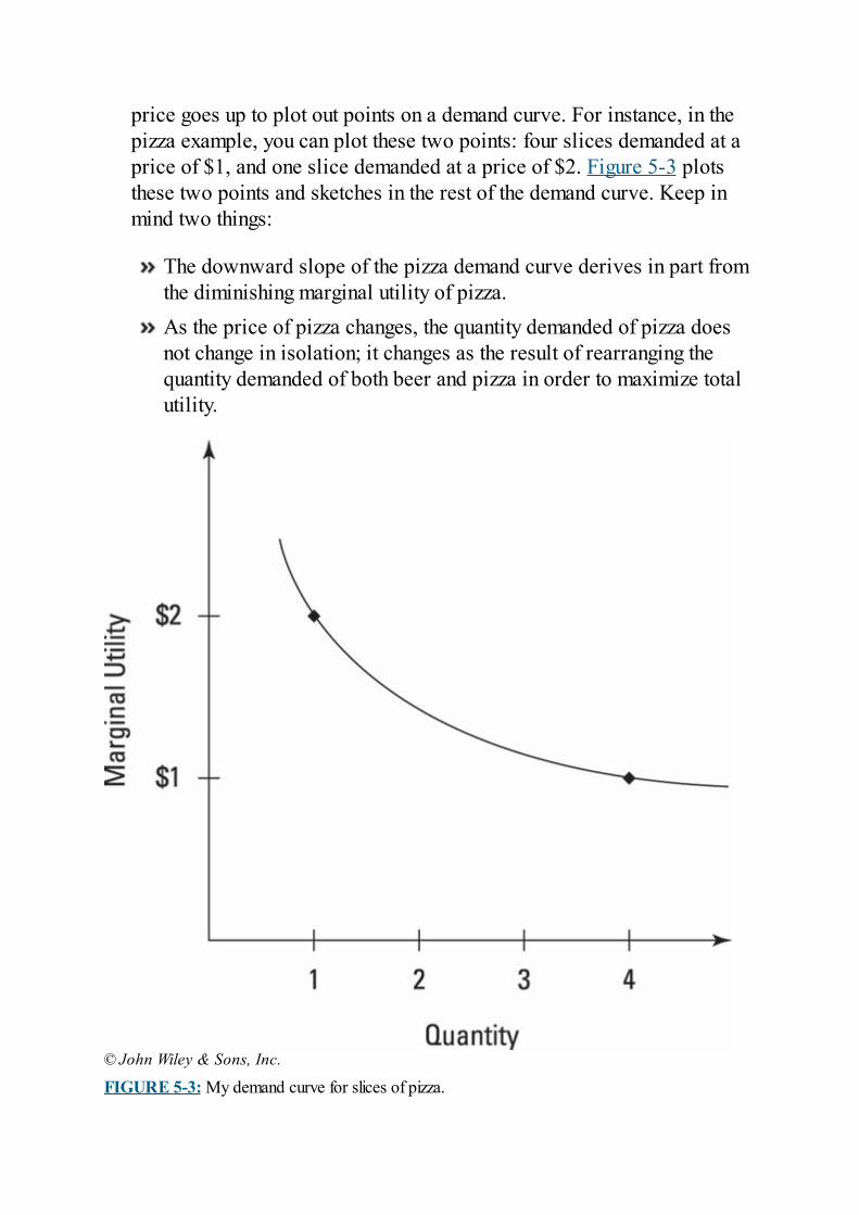
price goes up to plot out points on a demand curve. For instance, in thepizza example, you can plot these two points: four slices demanded at aprice of $1, and one slice demanded at a price of $2. Figure 5-3 plotsthese two points and sketches in the rest of the demand curve. Keep inmind two things:

The downward slope of the pizza demand curve derives in part fromthe diminishing marginal utility of pizza.As the price of pizza changes, the quantity demanded of pizza doesnot change in isolation; it changes as the result of rearranging thequantity demanded of both beer and pizza in order to maximize totalutility.

© John Wiley & Sons, Inc.

FIGURE 5-3: My demand curve for slices of pizza.

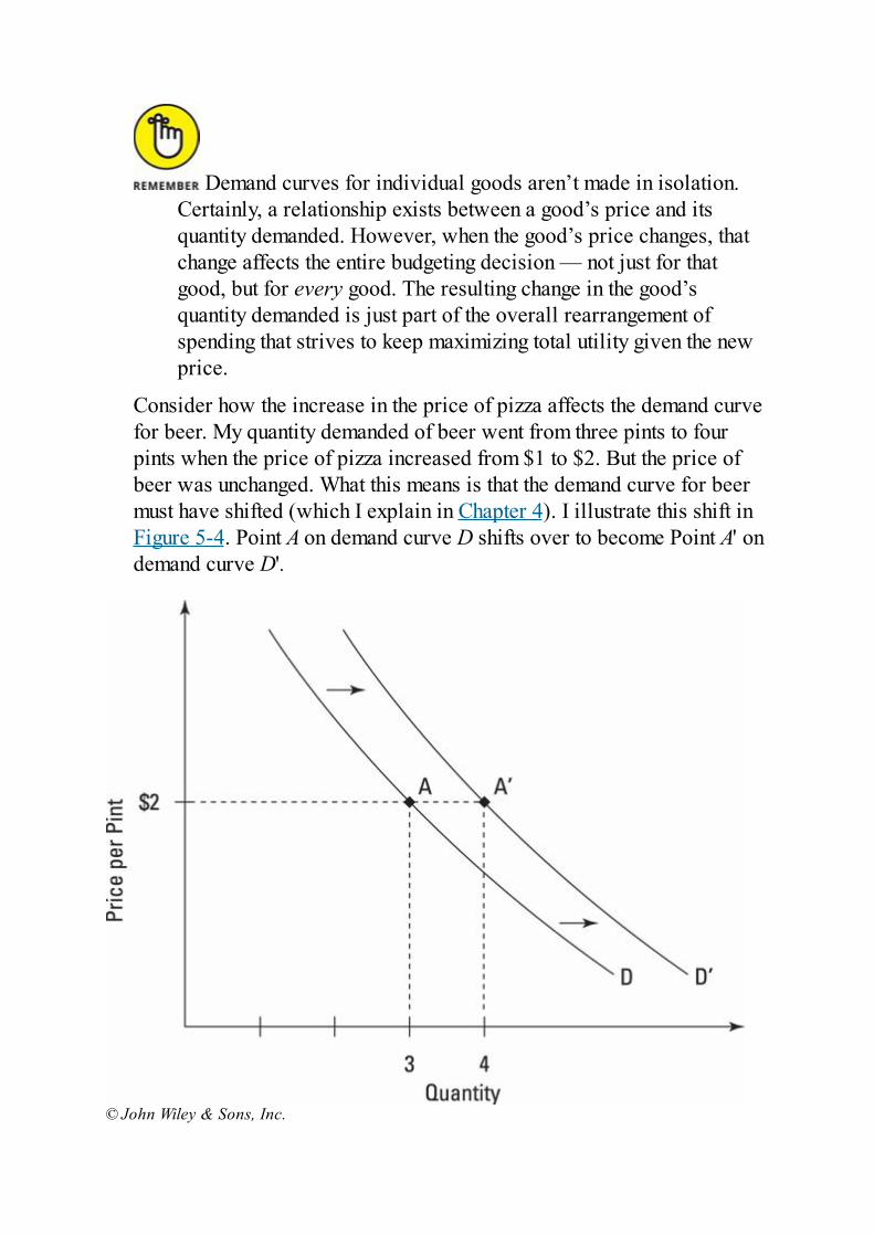
Demand curves for individual goods aren’t made in isolation.Certainly, a relationship exists between a good’s price and itsquantity demanded. However, when the good’s price changes, thatchange affects the entire budgeting decision — not just for thatgood, but for every good. The resulting change in the good’squantity demanded is just part of the overall rearrangement ofspending that strives to keep maximizing total utility given the newprice.

Consider how the increase in the price of pizza affects the demand curvefor beer. My quantity demanded of beer went from three pints to fourpints when the price of pizza increased from $1 to $2. But the price ofbeer was unchanged. What this means is that the demand curve for beermust have shifted (which I explain in Chapter 4). I illustrate this shift inFigure 5-4. Point A on demand curve D shifts over to become Point A' ondemand curve D'.

© John Wiley & Sons, Inc.

FIGURE 5-4: My demand curve for beer shifts to the right when the price of pizza increases.

Events where changes in the price of one good affect the quantitydemanded of another good are called cross-price effects. Bycontrast, when a change in a good’s own price affects its ownquantity demanded, you have own-price effects. Please note thatalthough cross-price effects cause demand curves to shift, own-price effects cause movements along given demand curves.

The direction of a cross-price effect depends on the situation. Inthis chapter, I allow consumers to purchase only two goods: beerand pizza. The result is that when the price of pizza goes up,consumers switch some of their purchasing power over to buyingbeer — or, as economists say, they substitute from one good to theother (see the sidebar “Examining complementary and substitutegoods”). That’s why when the price of pizza goes up, the demandcurve for beer in Figure 5-4 shifts to the right.

But in the real world, where many other consumption goods areavailable, the demand curve could very well shift the other direction.For instance, some people like drinking beer only when they eat pizza.For them, an increase in the price of pizza may decrease both the amountof pizza eaten and the amount of beer drunk.

Such people think of beer and pizza as a bundle. An increase in the priceof one member of the bundle increases the price of the entire bundle.These people would buy less of each member of the bundle in order tofree up money to spend on the many other consumption goods available.For consumers with these preferences and with the option of buyinggoods besides beer and pizza, when the price of pizza goes up, thedemand curve for beer would shift left.

EXAMINING COMPLEMENTARY ANDSUBSTITUTE GOODS

Some things just go together. Hot dogs and hot dog buns. Hamburgers andketchup. Shoes and shoelaces. In each of these pairs, the goods in question aremore useful or more pleasing when consumed along with the other member ofthe pair.

Because such goods complement each other, economists refer to them ascomplementary goods. An interesting thing about complementary goods is thatchanges in the price of one complement affect the other complement. Forinstance, if hot dogs go on sale, not only do people buy more hot dogs; theyalso buy more hot dog buns. And more mustard is sold, too.

By contrast, consider substitute goods — goods that serve similar functions sothat if the price of one goes up, people switch to the other one. For instance, ifthe price of train travel goes up, more people drive cars. And if the cost ofpostal mail goes up, more people use e-mail.

Both complementary goods and substitute goods are the result of cross-priceeffects. An increase in the price of a complement causes the quantity demandedof its pair to fall, while an increase in the price of a substitute causes thequantity demanded of its pair to rise.

As you look around the economy, make sure you think of it as one great bigorganic whole, where things don’t happen in isolation. When the price of onegood changes, it affects not just that good but also many other goods that areeither substitutes or complements. And if the prices of the substitutes orcomplements change, too, as a result of the initial price change, then all theirsubstitutes and complements are also affected. It’s like a gigantic ripple effect.

Chapter 6

The Core of Capitalism: TheProfit-Maximizing Firm

IN THIS CHAPTER Understanding why firms choose to maximize profits Deconstructing a firm’s cost structure Determining a firm’s profit-maximizing output level Seeing how costs determine a firm’s supply curve Understanding how firms react to losing money

In modern market economies like the one you live in, nearly everythingyou eat, drink, wear, drive, ride, fly, or use is made by some sort ofbusiness enterprise. So, naturally, economists devote a huge amount ofeffort to studying how businesses behave.

In this chapter, I show you how economists model a firm that’s a memberof a competitive industry, meaning a firm that’s just one of many firmscompeting against each other for your business. It’s important tounderstand how firms behave in competitive industries for two reasons:

Most firms in the real world face a lot of competition becausethey’re either members of perfectly competitive industries (which Italk about in this chapter) or monopolistically competitive industries(which I discuss in Chapter 9).All firms — even those that don’t face much competition — behavein remarkably similar ways.

Above all, firms like to maximize profits. And even more importantly, allfirms go about maximizing profits in the same way: by producing exactlythe level of output at which the cost of producing one more unit justequals the increase in revenue that the firm gets from selling that unit.

In this chapter, I show you why firms behave this way. When you knowthat, you’ll have a strong understanding of how all firms work, whether

they face strong competition from rivals or have no rivals at all.

A Firm’s Goal: MaximizingProfits

Firms are brought into existence by people in order to produce things.That statement should make you want to ask a fundamental question: Whydo people bother creating firms to make things? One reason could bealtruism. Another could be that making things is fun. Another could bethat the people who start a firm are bored doing other things. Buteconomists think the answer is much simpler.

Economists assume that the overriding goal of all corporations isto make as big a profit as possible. Economists make thisassumption for two reasons:

If you ask around, profit maximization is near the top of every firm’sto-do list.No matter what other goals a firm may have, it still wants tomaximize profits after taking steps to achieve those other goals.

For instance, a firm that wants to have a factory that emits no greenhousegases still, after it builds such a factory, wants to make as much money aspossible. After all, after it’s taken the steps necessary to protect theenvironment, why not make a nice big profit?

When the ice cream company Ben & Jerry’s started, it donated a largepercentage of its profits to charity. Given such a policy, the best way tohelp worthy causes was for Ben & Jerry’s to make as big a profit aspossible.

Many noneconomists object to people’s earning profits, but profitsensure that firms receive crucial inputs of entrepreneurial ability andrisk-taking. Think of someone who has the opportunity to start her ownbusiness. She could keep working for someone else and receive a steadywage. What is her incentive to strike out on her own and risk starting abusiness that may fail? The incentive is that she will receive the profits if

the business does well. Without potential profits, no one would riskleaving a safe job in order to innovate, and consumers as a whole wouldbe hurt because the supply of great new products and services wouldcome to a halt. (In Chapter 14, I explain in detail how entrepreneurialability receives profits in exchange for assuming the financial risksassociated with innovation and invention.)

Facing CompetitionFirms may or may not face a lot of competition from other firms. At oneextreme lies monopoly, in which a firm faces no competition because it’sthe only firm in its industry. At the other extreme lies what economistscall perfect competition, a situation in which a firm competes againstmany other firms in an industry in which they all produce an identicalgood. And in between the extremes lie two situations: oligopoly, wherethere are two, three, or (at most) a few firms in an industry; andimperfect (monopolistic) competition, in which there are manycompetitors, but each produces a slightly unique good. (See Chapters 8and 9 for details on monopolies, oligopolies, and monopolisticcompetition.)

In this chapter, you find out how firms behave under perfect competition,because in addition to explaining how important markets such as thestock market behave, this situation is also the simplest case tounderstand. It’s simple because when there are many competitors in anindustry in which every firm is producing identical products, none ofthem has any control over the prices they charge.

Listing the requirements for perfectcompetitionTo see why firms engaging in perfect competition have no control overthe prices they charge, you have to understand that perfect competitionassumes three things about the firms in an industry:

There are many of them.Each of them represents a very small part of the industry.They all sell identical or nearly identical products.

Wheat farming is an example of an industry that satisfies each of the threecriteria of perfect competition. There are literally tens of thousands ofwheat farmers in the United States. None of them produces more than asmall percentage of the total wheat produced each year, and all theirwheat is basically identical.

To see why these things together mean that individual farmers have nocontrol over the price of wheat, start with the fact that the farmers areproducing a nearly identical product. Because the wheat from one farmlooks like the wheat from any other farm, the only way a Kansas wheatfarmer can entice me to buy from him rather than from a Texas wheatfarmer is to offer me a lower price. Because all the wheat is identical,all I care about is price, meaning that farmers have to compete on priceand price alone.

With price jumping to the fore as the key factor in the wheat market, youcan use supply and demand analysis to figure out what the price will be.The price is determined by where the market demand curve for wheatcrosses the market supply curve for wheat (see Chapter 4 for details).How are these curves determined?

Market demand curve: Determined by adding up the individualdemand curves of all the people who want to buy wheatMarket supply curve: Comes from adding up the individual supplycurves of all the individual wheat farmers

This is where the first two assumptions of perfect competition come intoplay: Because there are so many wheat farmers, and because each ofthem produces such a very small part of the total supply of wheat, themarket supply curve for wheat is unaffected by the presence or absenceof any individual supply curve of any particular farmer. If a billionbushels of wheat are sold every year, the market price is unaffected bywhether a small farmer with only 1,000 bushels to sell bothers showingup to the market or not. He’s just too small a player to cause the marketprice to change.

If every player is too small to cause the market price to change, then eachone has to take as a given whatever price is generated by market demandinteracting with market supply.

Taking prices but setting quantitiesIf the three assumptions of perfect competition are met, they produce asituation in which individual firms have no control over the prices theycan charge. In fact, under perfect competition, economists refer to firmsas price takers because they have to take the price as given and deal

with it.

When you come right down to it, even the most powerful firmcan hope to control only two things: how much of its product tomake and what price to charge. Because firms have no control overtheir prices under perfect competition, that narrows the list to one:The only thing that price-taking firms can control is how much toproduce.

Firms choose to make whatever quantity maximizes their profits. Thisfact is mathematically convenient because the quantity of output that afirm chooses to produce controls each of the two things that determineprofits: total revenues and total costs.

To see this fact more clearly, you have to know that a firm’sprofit is simply defined as its total revenue minus its total costs. Putinto math, you get the following equation, where TR stands for totalrevenue and TC stands for total costs:

(1) For a competitive firm, its total revenue, TR, is simply the quantity, q, ofits output that it chooses to sell times the market price, p, that it can getfor each unit:

(2) For instance, if I can sell apples for $1 each and I sell 37 apples, mytotal revenue is $37 ($1 per apple × 37 apples = $37).

But notice that because the price at which I can sell (p) is out of myhands if I’m a price taker, the only way I can control my total revenue isby deciding how many apples to sell. So a firm can determine its totalrevenue by its decision about how big or small to make q.

Much of the rest of this chapter is devoted to showing you that the firm’stotal costs, TC, are also determined by how big or small q is. But theinteresting thing here is that although each extra unit of q sold brings in arevenue of p dollars, the cost of each unit of q manufactured depends on

how many units of q have already been made. Costs tend to increase asfirms produce more and more, so each successive unit costs more thanthe previous unit. This fact ends up limiting the number of units that afirm wants to produce.

Suppose that I can sell as many apples as I want for $1 each. The firstapple costs 10 cents to produce, the second one costs 20 cents, the thirdone costs 30 cents, and so on. In such a case, I’m willing to produce nomore than ten apples. Why? Because for each of the first nine apples, I’llmake a profit, but for apple ten (which costs $1 to produce), I’ll breakeven. If I produce any more apples, I’ll sustain a loss. (Apple number 11,for instance, would cost $1.10 to produce, but I’d get only $1 for sellingit.)

Consequently, you can see that both the TR and TC terms in profitequation (1) are determined by the firm’s choice of q. The only thing leftto figure out is exactly how big to make q in order to maximize profits. Itturns out that there’s a ridiculously simple formula that gives the solution.Pay attention, because you just may, uh, profit from reading this chapter.

Distinguishing between accounting profitsand economic profitsTo an economist, the terms profit and loss refer to whether the revenuefrom selling a firm’s output is bigger or smaller than the costs that mustbe incurred to produce that output. If the revenue exceeds the costs, thefirm is running a profit, whereas if the costs exceed the revenue, thefirm is running a loss. If the two are equal, the firm is breaking even.

Consider a business that sells lemonade. Both the accountant and theeconomist agree that the firm’s revenue is simply how much money thefirm makes from selling its product. However, they differ on what tocount as costs when calculating profit:

Accounting profit: The accountant considers costs to be only actualmonies spent in running the business: how much the firm pays itsworkers, how much it pays to buy supplies, and so on. Consider abusiness that sells lemonade. If the firm has revenues of $10,000 andit spends $9,000 to make those revenues, the accountant concludesthat the firm has a profit of $1,000. This number is the firm’saccounting profit — the type of profit that is reported every day in

financial statements and newspaper articles.

Economic profit: Economic profit takes into account not justthe money costs directly incurred by running a business but also theopportunity costs incurred. Think about the entrepreneur who startsthis lemonade business. After paying for his materials and for hisemployees’ wages, his accounting profits are $1,000. But is thatreally a good deal?Suppose that this person left a job as a computer programmer to openthe lemonade business, and in the same amount of time that it took thelemonade business to turn a $1,000 profit, he would have made$10,000 in wages if he had stayed at his old job. That is, he gave upthe opportunity to earn $10,000 in wages to open up a business thatmakes him only a $1,000 accounting profit. He actually sustains aneconomic loss of $9,000. When you know this fact, his decision toswitch careers doesn’t seem like such a good idea.

Economists like to concentrate on economic profits and losses ratherthan accounting profits or losses because the economic profits and lossesare what motivate people. By taking into account economic profits andlosses, you get directly at what motivates firms to produce not only thetypes of goods they choose to produce but the quantities of those goodsas well. In this example, you can imagine that when other computerprogrammers see what happened to this guy when he switched careers,they’re not going to follow him.

For the rest of the chapter, whenever you see any costs listed, assumethat they are economic costs; that is, they include not only money directlyspent operating a business but also the costs of other opportunitiesforgone in order to operate the business. Likewise, whenever you see aprofit or a loss, assume that it’s an economic profit or an economic loss— the factor that motivates entrepreneurs to want to do something or toavoid doing it.

The most important application of this concept is to determine how muchoutput a firm should produce. If producing the 12th unit of a productproduces an economic profit, obviously the firm wants to produce it. Butif increasing production to a 13th unit would result in an economic loss,

obviously the firm doesn’t want to produce it.

Analyzing a Firm’s CostStructure

To see how costs and revenues interact to determine economic profits orlosses, economists like to break up a firm’s total costs into twosubcategories:

Fixed costs: Fixed costs are costs that have to be paid even if thefirm isn’t producing anything. For instance, after a rent contract issigned for the firm’s headquarters, that rent must be paid whether thefirm produces anything or not. Similarly, if the firm has taken out aloan, it’s legally required to make its debt payments whether it’sproducing zero units of output or a billion.Variable costs: Variable costs are costs that vary with the amount ofoutput produced. For instance, if you are in the lemonade-makingbusiness and you choose to produce nothing, you obviously don’thave to buy any lemons. But the more lemonade you do produce, themore you spend buying lemons. Similarly, producing more lemonaderequires more workers, so your labor costs also vary with the amountof output you produce.

Fixed costs can be represented as FC and variable costs as VC.Together, they sum up to a firm’s total costs, or TC:

(3)

As you look at Equation (3), keep in mind that it deals with theeconomic costs facing the firm and therefore captures theopportunity costs of the firm’s expenditures on both fixed costs andvariable costs. (All expenditures, whether they’re fixed costs orvariable costs, involve opportunity costs — the other things yougave up buying in order to spend the money you spent on your fixedand variable costs.)

Focusing on costs per unit of output

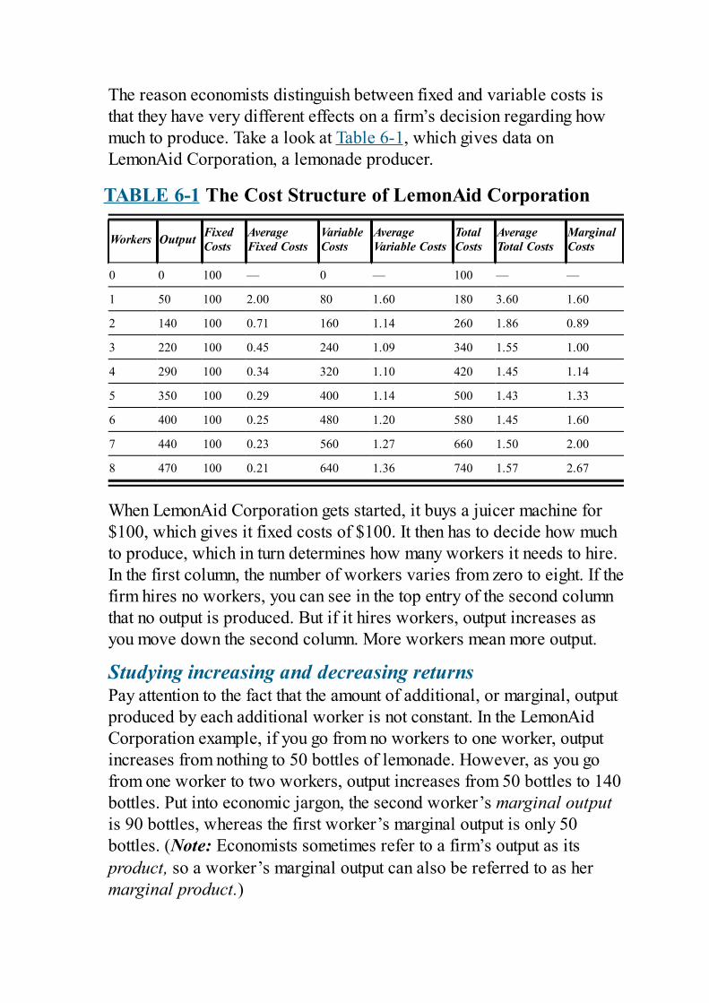
The reason economists distinguish between fixed and variable costs isthat they have very different effects on a firm’s decision regarding howmuch to produce. Take a look at Table 6-1, which gives data onLemonAid Corporation, a lemonade producer.

TABLE 6-1 The Cost Structure of LemonAid Corporation

Workers Output FixedCosts

AverageFixed Costs

VariableCosts

AverageVariable Costs

TotalCosts

AverageTotal Costs

MarginalCosts

0 0 100 — 0 — 100 — —

1 50 100 2.00 80 1.60 180 3.60 1.60

2 140 100 0.71 160 1.14 260 1.86 0.89

3 220 100 0.45 240 1.09 340 1.55 1.00

4 290 100 0.34 320 1.10 420 1.45 1.14

5 350 100 0.29 400 1.14 500 1.43 1.33

6 400 100 0.25 480 1.20 580 1.45 1.60

7 440 100 0.23 560 1.27 660 1.50 2.00

8 470 100 0.21 640 1.36 740 1.57 2.67

When LemonAid Corporation gets started, it buys a juicer machine for$100, which gives it fixed costs of $100. It then has to decide how muchto produce, which in turn determines how many workers it needs to hire.In the first column, the number of workers varies from zero to eight. If thefirm hires no workers, you can see in the top entry of the second columnthat no output is produced. But if it hires workers, output increases asyou move down the second column. More workers mean more output.

Studying increasing and decreasing returnsPay attention to the fact that the amount of additional, or marginal, outputproduced by each additional worker is not constant. In the LemonAidCorporation example, if you go from no workers to one worker, outputincreases from nothing to 50 bottles of lemonade. However, as you gofrom one worker to two workers, output increases from 50 bottles to 140bottles. Put into economic jargon, the second worker’s marginal outputis 90 bottles, whereas the first worker’s marginal output is only 50bottles. (Note: Economists sometimes refer to a firm’s output as itsproduct, so a worker’s marginal output can also be referred to as hermarginal product.)

Now look at these facts in terms of costs and benefits. If you have to payeach worker the same wage of $80 per day ($10 per hour for 8 hours ofwork), you’re going to like the fact that although the first workerproduces 50 bottles for his $80 pay, the second worker produces 90bottles for her $80 pay.

When the amount of return you get for a given amount of input(one more worker) increases as you add successive units of input,economists refer to the situation as increasing returns. Increasingreturns occur when a piece of productive capital is initiallyundermanned. Consider a sailboat that works optimally with a crewof ten. Could one person run the ship? Yes, but his productivitywould be very low as he would have to be running from one job tothe next and trying to do everything himself — raising sails,weighing anchor, calculating drift, steering the vessel, and so on. Insuch situations, efficiency is improved and increasing returns perworker result by increasing the number of workers toward theoptimal number of workers for that particular piece of productivecapital.

Increasing returns only happen, though, when a piece of productivecapital is undermanned. Thus, if you scan down the second column ofTable 6-1, you find that increasing returns don’t last forever. Indeed, inthe case of LemonAid Corporation, increasing returns end almostimmediately. Consider what happens to output when you add a thirdworker. Output does increase but only by 80 units, from 140 bottles to220 bottles. And things get successively worse with each additionalworker. Adding a fourth worker increases output by only 70 bottles.Adding a fifth increases output by only 60 bottles.

When each successive unit of an input, like labor, brings with ita smaller increase in output than the previous unit of input,economists call the situation diminishing returns.

Determining the cause of diminishing returns

I go into detail about what causes diminishing returns in Chapter 3, but Ibriefly explain here. What’s going on is that LemonAid Corporationbought only one juicer machine for squeezing the juice out of lemons.

The first worker can use the machine to squeeze enough juice for 50bottles by carrying lemons to the machine and then operating themachine. But it turns out that two workers together can do even better bydividing up the work: One brings lemons to the machine, and the otheroperates it. Working together, they can produce a total of 140 bottles —more than double the 50 bottles that one worker could produce workingalone.

However, a third worker doesn’t increase output nearly as much as asecond because the two major tasks — carrying and operating — havealready been taken care of. At best, he can just help the first two workersdo these tasks a little faster. The same holds true for all successiveworkers: Having them is helpful, but each one adds less to output thanthe previous one because things start getting crowded and there reallyisn’t much room left for improvement.

Examining average variable costsVariable costs are affected by the fact that additional workers first bringincreasing returns (when the firm’s capital is undermanned) but thendecreasing returns (when the capital is overmanned). In the case of theLemonAid Corporation example in Table 6-1, the variable costs are alllabor costs, with each worker having to be paid $80 per day. You cansee these variable costs increase as you move down the fifth column.

What’s much more interesting than looking at variable costs islooking at average variable costs (AVC), which are defined asvariable costs divided by quantity (VC/q). For instance, becauseone worker produces 50 bottles of output at a variable cost of $80,the average variable cost is per bottle. When twoworkers together cost $160 in variable costs but produce 140bottles, the average variable cost for two workers is only

per bottle.

The decrease in average variable costs is the result of increasing returns:

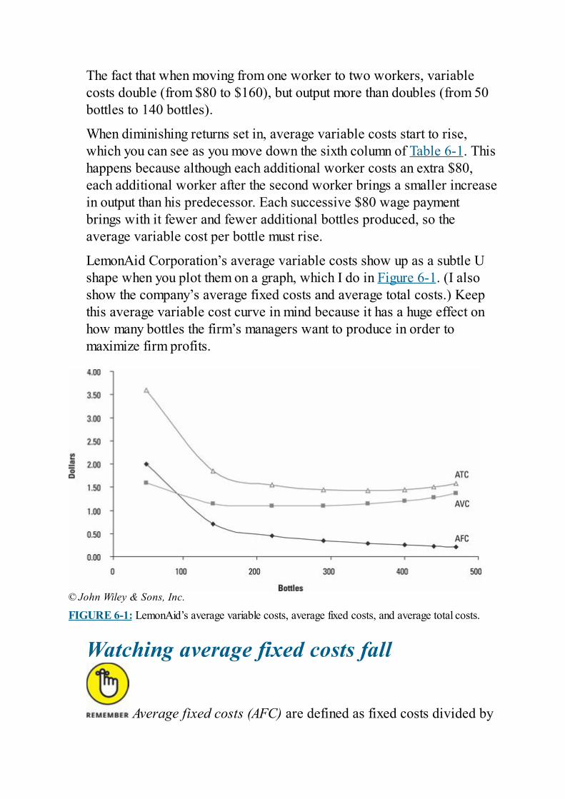
The fact that when moving from one worker to two workers, variablecosts double (from $80 to $160), but output more than doubles (from 50bottles to 140 bottles).

When diminishing returns set in, average variable costs start to rise,which you can see as you move down the sixth column of Table 6-1. Thishappens because although each additional worker costs an extra $80,each additional worker after the second worker brings a smaller increasein output than his predecessor. Each successive $80 wage paymentbrings with it fewer and fewer additional bottles produced, so theaverage variable cost per bottle must rise.

LemonAid Corporation’s average variable costs show up as a subtle Ushape when you plot them on a graph, which I do in Figure 6-1. (I alsoshow the company’s average fixed costs and average total costs.) Keepthis average variable cost curve in mind because it has a huge effect onhow many bottles the firm’s managers want to produce in order tomaximize firm profits.

© John Wiley & Sons, Inc.

FIGURE 6-1: LemonAid’s average variable costs, average fixed costs, and average total costs.

Watching average fixed costs fall

Average fixed costs (AFC) are defined as fixed costs divided by

quantity (FC/q). Average fixed costs always decline, because thesame fixed cost gets divided up over a greater and greater numberof units of output as output increases.

The fixed costs of LemonAid Corporation are always the $100 it paidfor the juicer machine, no matter what amount of output it produces. As aresult, the more lemonade it produces, the less average fixed costs are.That’s why AFC falls (see the fourth column of Table 6-1) from a valueof $2.00 per bottle when 50 bottles are produced using one worker downto only $0.21 per bottle when 470 bottles are produced using eightworkers. When you plot out average fixed costs per bottle, as in Figure6-1, you get a downward sloping AFC curve. Keep this fact in mindbecause it helps explain the shape of the average total costs (ATC) curve,as I explain in the next section.

Tracking the movement of average totalcostsAverage fixed costs always decline as output increases, while averagevariable costs first fall (due to increasing returns) and then rise (due todiminishing returns) — see the preceding sections for details. Becausetotal costs are the sum of fixed costs and variable costs, average totalcosts obviously depend on how average fixed costs and average variablecosts sum up.

Average total costs (ATC) are defined as total costs divided by quantity(TC/q). Now, take a look back at Equation (3) earlier in the chapter. Ifyou divide every term in Equation (3) by q, you get the following:

(4)

You can simplify this equation by realizing that average costs equal thevarious costs divided by the quantity, q. In other words, ,

, and . What you get is

(5) You can see clearly from this equation that average total costs depend onhow average fixed costs and average variable costs interact. There aretwo key points to understand here:

Average total costs (ATC) must always be greater than average

variable costs (AVC), because you have to add in average fixedcosts (AFC). Look at Figure 6-1, which shows that the ATC curve isabove the AVC curve. The vertical distance between them at anyparticular level of output is equal to the AFC at that output level. Asyou move from lower output levels to higher output levels, the ATCand AVC curves converge because AFC becomes smaller andsmaller. (In other words, the vertical distance between the ATC andAVC curves also gets smaller and smaller.)Average total costs (ATC) will reach a minimum value at a higherlevel of output than average variable costs (AVC). For instance,Table 6-1 shows that average variable costs reach their minimumvalue of $1.09 when three workers are hired and 220 bottles areproduced. Average total costs, however, reach their minimum of$1.43 when five workers are hired and 350 bottles are produced.The reason this happens is that average fixed costs are alwaysfalling, meaning that in Equation (5), the AFC part on the right-handside of the equation is always getting smaller and smaller. Thisconstant decline helps to temporarily offset the increases in averagevariable costs that happen when diminishing returns set in.Consequently, although average variable costs bottom out at threeworkers, average total costs don’t bottom out and start increasinguntil the fifth worker.

Focusing on marginal costsThe preceding sections demonstrate how the manager of a firm can useher data on total costs, fixed costs, and variable costs to calculate,respectively, average total costs, average fixed costs, and averagevariable costs. But what she really wants to know is what quantity, q, ofoutput she should produce in order to maximize profits. To solve thisproblem, she needs one more cost concept: marginal cost.

Marginal cost is how much total costs increase when youproduce one more unit of output. Crucially, the marginal cost of onemore unit of output depends on how much output has already beenproduced.

To see this, examine the total costs column of Table 6-1. Notice that totalcosts increase from $100 in the first row to $180 in the second row asoutput increases from 0 bottles to 50 bottles when the firm hires the firstworker. In other words, costs go up $80 while output goes up 50 bottles.So each of these extra, or marginal, 50 bottles on average increasescosts by each. The marginal cost per bottle, MC, isdefined as follows:

(6)

As you move down the marginal costs column of Table 6-1, you can seethat marginal costs first fall and then rise. This is yet another reflectionof the fact that LemonAid Corporation’s production process exhibitsincreasing returns followed by diminishing returns. Because the secondworker produces much more than the first worker but costs the same, themarginal cost falls when the second worker is added. For successiveworkers, costs keep increasing but marginal output keeps declining,which means marginal costs must rise.

Noticing where marginal cost equalsaverage cost

Here’s a fun fact that economists love: If you plot out marginalcosts to create a marginal cost (MC) curve, that curve will crossboth the average variable cost (AVC) curve and average total cost(ATC) curve at their minimum points — that is, at the bottom of theirrespective U shapes. (What, you don’t see the cause forcelebration?)

Look at Figure 6-2, where I plot the AVC, ATC, and MC curves you getby plotting out the data in Table 6-1. The MC curve goes through theminimum points of both the AVC and ATC curves. This happens becausethe marginal cost at each unit determines whether the AVC and ATCcurves are increasing or decreasing.

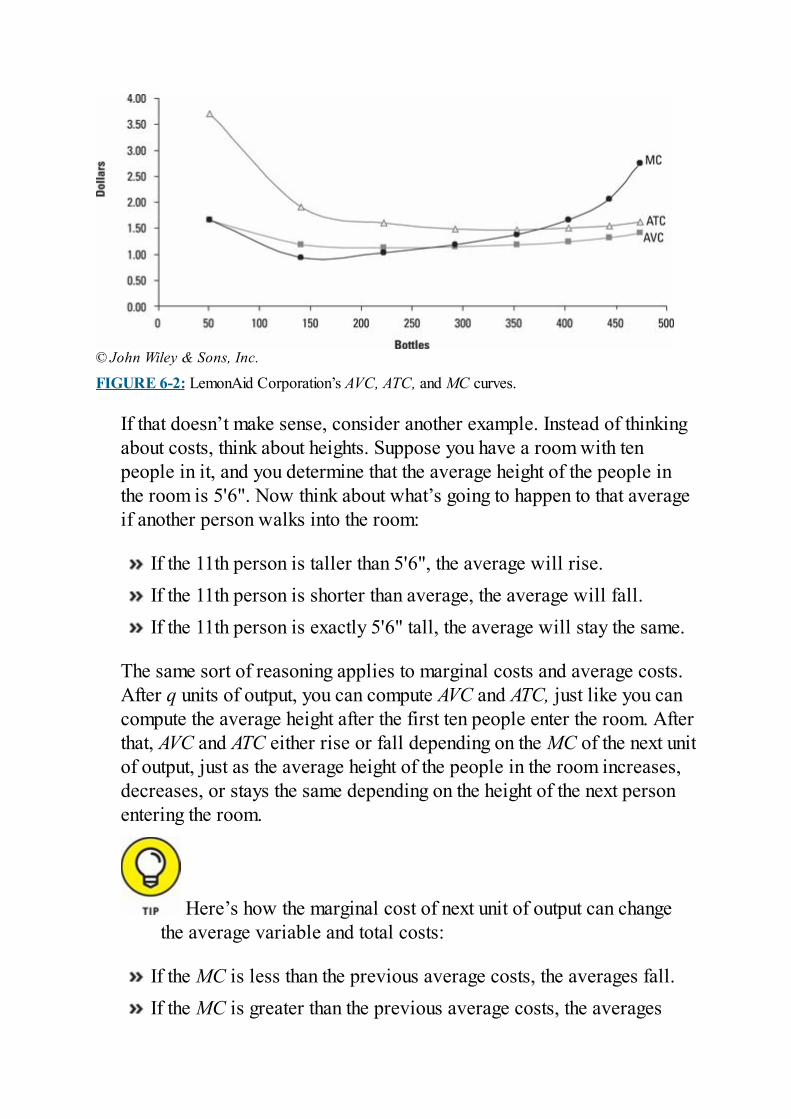
© John Wiley & Sons, Inc.

FIGURE 6-2: LemonAid Corporation’s AVC, ATC, and MC curves.

If that doesn’t make sense, consider another example. Instead of thinkingabout costs, think about heights. Suppose you have a room with tenpeople in it, and you determine that the average height of the people inthe room is 5'6". Now think about what’s going to happen to that averageif another person walks into the room:

If the 11th person is taller than 5'6", the average will rise.If the 11th person is shorter than average, the average will fall.If the 11th person is exactly 5'6" tall, the average will stay the same.

The same sort of reasoning applies to marginal costs and average costs.After q units of output, you can compute AVC and ATC, just like you cancompute the average height after the first ten people enter the room. Afterthat, AVC and ATC either rise or fall depending on the MC of the next unitof output, just as the average height of the people in the room increases,decreases, or stays the same depending on the height of the next personentering the room.

Here’s how the marginal cost of next unit of output can changethe average variable and total costs:

If the MC is less than the previous average costs, the averages fall.If the MC is greater than the previous average costs, the averages

rise.If the MC is exactly the same as the previous average costs, theaverages stay the same.

You can see these effects graphically by looking at various parts ofFigure 6-2. First, look at the output level of 140 bottles. At that outputlevel, the MC of producing one more bottle is less than both ATC andAVC, meaning that ATC and AVC will decrease if output is increased byone more bottle. That’s why the AVC curve and the ATC curve aredownward sloping at that output level. The average curves are beingpulled down by the low value of MC.

Next, look at the output level of 440 bottles. You can see that the MC atthat output level is higher than the ATC and the AVC. Consequently, bothAVC and ATC must be increasing. This increase is reflectedgeometrically by the upward slopes of both the AVC curve and the ATCcurve. The curves slope upward because the high value for MC ispulling them up.

Now, put some pieces together. Notice that the MC curve causes both theAVC curve and the ATC curve to be U-shaped (albeit subtly). On the leftside of Figure 6-2, the fact that MC is less than the average curves meansthat the average curves slope downward. On the figure’s right side, thefact that MC is greater than the average curves means the average curvesslope upward.

So you’ve come full circle to the fact that the MC curve has to cross thetwo average curves at their respective minimum points — at the bottomsof their respective U shapes. To the left of such a crossing point, theaverage must be falling because MC is less than the average. And to theright, the average must be rising because MC is larger than the average.But where the curves cross, the average curve is neither rising nor fallingbecause the MC of that unit of output is equal to the current average. (Inother words, a 5'6" person has walked into a room that already has a 5'6"average height, so the average doesn’t budge.)

Economists love to go on and on about this fact, but it’s really just areflection of the effect that increasing and then decreasing returns haveon cost curves. Costs first fall and then rise. And there’s some point inthe middle at which they momentarily stay the same, frozen for an instant

while transitioning from falling to rising. That point must be wheremarginal cost equals average cost, because only when MC equalsaverage cost can average cost be stationary.

Comparing Marginal Revenueswith Marginal Costs

Here’s a sad but true fact to keep in mind: Firms can’t always make aprofit. That’s because a firm in a perfectly competitive industry can’tcontrol the price at which its output sells, and sometimes that price is toolow for the firm to make a profit no matter what quantity it produces.When that happens, the best the firm can do is to minimize its losses andhope for the price to change. If the price drops low enough, the best thingto do may be to shut down production immediately, because that way thefirm will lose only its fixed costs. (I discuss the difference between fixedand variable costs in the earlier section “Analyzing a Firm’s CostStructure.”)

Later in the chapter, I discuss this sad situation in more detail. But first, Ifocus on a happier situation — one in which the market price is highenough that a firm wants to produce a positive amount of output. Thismay or may not mean that a firm is making a profit, but even if it isn’t, itslosses aren’t great enough to halt production.

Finding where marginal revenue equalsmarginal costIn the typical case where market prices are high enough that a firm wantsto make a positive amount of output, a ridiculously simple formula isused to determine the optimal quantity of output, q, that the firm shouldproduce. The firm wants to produce at the level of output where marginalrevenue equals marginal cost ( ).

Producing where does two things:

It minimizes the firm’s loss if it has to take a loss due to a low sellingprice for its output.It maximizes the firm’s profit if it’s able to make a profit because theselling price is high enough.

The idea behind basically comes down to a cost-benefit analysis. If producing and selling a bottle brings in morerevenue than it costs to make the bottle, then make it. If not, thendon’t make it. Easy, right?

Imagine that LemonAid Corporation can sell each bottle of lemonade thatit produces for $2. Economists like to say that the marginal revenue ofeach bottle is $2, because each and every bottle when sold brings in anextra $2. In terms of algebra, you can say that , where p is themarket price that this competitive firm must charge for each unit ofoutput.

What the firm’s managers must do is decide how much to produce basedon whether any given bottle will cost more or less than the $2 marginalrevenue that the firm would get by selling it.

Be very careful at this point. You have to remember that therelevant cost that the managers look at is an individual bottle’smarginal cost, MC. That’s because if they’re deciding on makingthat particular bottle, they need to isolate that bottle’s productioncost from the costs of all previously produced bottles in order tocompare it to the revenue that the bottle will bring if it’s producedand sold. MC does just that by ignoring all previous bottles andfocusing on what the next bottle will cost to make.

If the MC of that bottle is less than $2, obviously there is a gain to bemade by making it, and the managers will choose to make it. On the otherhand, if the MC is bigger than $2, producing the bottle would cause aloss, and the managers would choose not to produce it.

By looking at the MC of every possible bottle (the 1st, the 5th, the 97th,and so on) and comparing it with marginal revenue that the firm could getby selling it, the managers can determine exactly how many bottles toproduce. The necessary comparisons can be done by looking at a table ofcosts, such as Table 6-1, but it’s even easier to make the comparisonsgraphically.

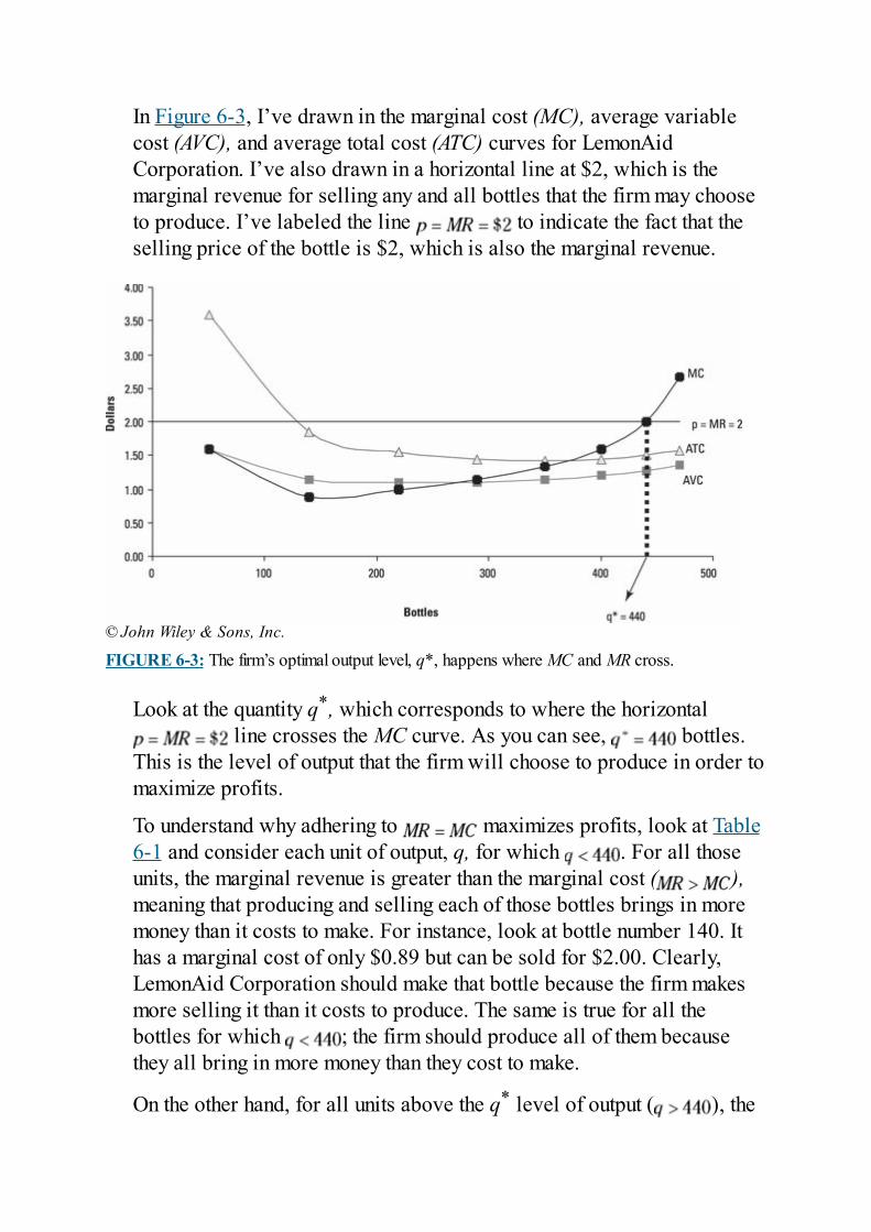
In Figure 6-3, I’ve drawn in the marginal cost (MC), average variablecost (AVC), and average total cost (ATC) curves for LemonAidCorporation. I’ve also drawn in a horizontal line at $2, which is themarginal revenue for selling any and all bottles that the firm may chooseto produce. I’ve labeled the line to indicate the fact that theselling price of the bottle is $2, which is also the marginal revenue.

© John Wiley & Sons, Inc.

FIGURE 6-3: The firm’s optimal output level, q*, happens where MC and MR cross.

Look at the quantity q*, which corresponds to where the horizontal line crosses the MC curve. As you can see, bottles.

This is the level of output that the firm will choose to produce in order tomaximize profits.

To understand why adhering to maximizes profits, look at Table6-1 and consider each unit of output, q, for which . For all thoseunits, the marginal revenue is greater than the marginal cost ( ),meaning that producing and selling each of those bottles brings in moremoney than it costs to make. For instance, look at bottle number 140. Ithas a marginal cost of only $0.89 but can be sold for $2.00. Clearly,LemonAid Corporation should make that bottle because the firm makesmore selling it than it costs to produce. The same is true for all thebottles for which ; the firm should produce all of them becausethey all bring in more money than they cost to make.

On the other hand, for all units above the q* level of output ( ), the

situation is reversed: The marginal revenue is less than the marginal cost( ). The firm would lose money if it produced and sold thosebottles. For instance, at an output level of 470 bottles, the MC is $2.67,but the MR is only $2.00. If the firm produced at that output level, itwould lose 67 cents on bottle number 470. Clearly, the company doesn’twant to do this.

By comparing the marginal revenues and marginal costs at all outputlevels, you can see that the managers of LemonAid Corporation want toproduce exactly units, the number of units where the MR and MClines cross.

Producing where doesn’t guarantee you a profit, but itdoes at least make sure that you produce only units that bring inmore money than they cost to make. The reason this formula byitself can’t guarantee a profit is that it doesn’t take account of thefixed costs you have to pay no matter what level of output you’reproducing. Even though you produce only units for which marginalrevenue is at least as great as marginal cost, you still may not makeenough of a gain from those units to pay off your fixed costs.

Visualizing profitsThere’s a quick and easy way to visually use the cost curves to determinewhether the firm is making a profit or a loss. The trick is to realize thatthe two components of profits, total revenue (TR) and total costs (TC),can each be represented by rectangles whose areas are equivalent totheir respective sizes. As a result, you can immediately tell whetherprofits are positive or negative by looking to see whether the TRrectangle is larger or smaller than the TC rectangle. If the TR rectangleexceeds the size of the TC rectangle, profits are positive. And if the TRrectangle is smaller than the TC rectangle, profits are negative — thefirm is running a loss.

To see how this works, look at Figure 6-4, where I’ve drawn ageneralized set of average total cost (ATC), average variable cost (AVC),and marginal cost (MC) curves, plus a horizontal line labeled toindicate that price equals marginal revenue for this competitive firm.Switching to this generalized set of curves will (I hope!) convince you

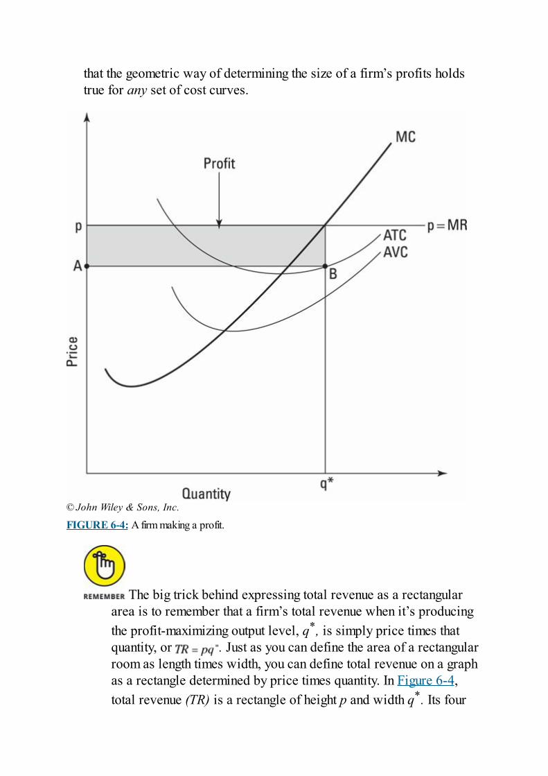
that the geometric way of determining the size of a firm’s profits holdstrue for any set of cost curves.

© John Wiley & Sons, Inc.

FIGURE 6-4: A firm making a profit.

The big trick behind expressing total revenue as a rectangulararea is to remember that a firm’s total revenue when it’s producingthe profit-maximizing output level, q*, is simply price times thatquantity, or . Just as you can define the area of a rectangularroom as length times width, you can define total revenue on a graphas a rectangle determined by price times quantity. In Figure 6-4,total revenue (TR) is a rectangle of height p and width q*. Its four

corners are located at the origin, at p, at the point where the line crosses the MC curve, and at q*.

You can also use a rectangle to represent the total costs that the firmincurs when producing q* units of output. To figure out where to drawthis rectangle, you have to use a little math trick to convert theinformation that the average total cost (ATC) curve gives you into whatyou want to graph, total costs (TC). To see how to apply this math trick,first look at Point B in Figure 6-4. It shows the average total cost (ATC)per unit when the firm is producing output level q*. The reason the trickis handy is because it shows that the rectangle whose width is q* andwhose height is given by the ATC at output level q* is actually equal tothe firm’s total costs. That is, TC is equal to the area of the rectanglewhose four corners are the origin, the point I’ve labeled A, the point I’velabeled B, and q*.

The heart of the math trick is realizing that when the firm isproducing at q*, . If you multiply both sides of thisequation by q*, you find that . This equation tells youthat TC (total cost) is indeed equal to the product of ATC (theaverage per-unit cost) and q* (the number of items), or to the areaof a rectangle of height ATC and width q* — exactly the rectanglethat I just showed you!

The firm’s profits, which are by definition equal to TR – TC, can also berepresented by the area of a specific rectangle. In fact, the profit is equalto the area of the shaded rectangle in Figure 6-4. That’s because profitsare simply the difference between TR and TC. Because the TR rectangleis larger than the TC rectangle in this case, the firm is making a profitwhose size is equivalent to the area of the shaded rectangle that’s definedby the area of the larger TR rectangle minus the area of the smaller TCrectangle.

Imagine what would happen if the price, p, increased. First,

notice that the optimal output, q*, would increase because the placewhere the horizontal line crosses the MC curve would moveup and to the right. Simultaneously, the total revenue rectanglewould increase in size, as would the total cost rectangle. But whichone grows faster? Do profits rise or fall?

Go ahead and draw in some lines to convince yourself that profits will infact increase — that is, the shaded profit rectangle will grow in size asthe price increases. As you’ll discover, a rising price increases thefirm’s profits.

You can prove that a rising price increases profits by noting thatas q* shifts right with increases in p, both the width and the heightof the profit rectangle get bigger. The width of the profit rectanglegets bigger with each increase in q* because the width of the profitrectangle is by definition exactly equal to q*. The height alsoincreases because as you move farther to the right, the distancebetween the MC curve and the ATC curve increases due to the factthat the slope of the MC curve is steeper than the slope of the ATCcurve. Thus, with both the width and the height of the profitrectangle increasing simultaneously, the area of the profit rectanglemust be increasing as well.

Visualizing lossesSo what happens if the price falls? This section explains how profits cango negative if the price falls far enough. Consider the situation illustratedin Figure 6-5, where the cost curves are the same as in Figure 6-4 but theprice (and therefore the marginal revenue [MR]) at which the firm cansell its product is much lower.

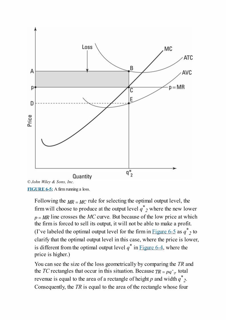
© John Wiley & Sons, Inc.

FIGURE 6-5: A firm running a loss.

Following the rule for selecting the optimal output level, thefirm will choose to produce at the output level q*

2 where the new lower line crosses the MC curve. But because of the low price at which

the firm is forced to sell its output, it will not be able to make a profit.(I’ve labeled the optimal output level for the firm in Figure 6-5 as q*

2 toclarify that the optimal output level in this case, where the price is lower,is different from the optimal output level q* in Figure 6-4, where theprice is higher.)

You can see the size of the loss geometrically by comparing the TR andthe TC rectangles that occur in this situation. Because , totalrevenue is equal to the area of a rectangle of height p and width q*

2.Consequently, the TR is equal to the area of the rectangle whose four

corners lie at the origin, at p, at C, and at q*2. It’s smaller than the TC

rectangle defined by the origin, Point A, Point B, and q*2. Because the

area of the total cost rectangle exceeds the area of the total revenuerectangle, the firm is running a loss equivalent to the size of the shadedarea in Figure 6-5.

Pulling the Plug: WhenProducing Nothing Is Your BestBet

You may wonder why a firm would stay in business if it’s running a lossrather than a profit. The usual answer is that it hopes that things will turnaround soon. Either it expects the price at which it can sell its productsto rise, or it expects that it can somehow reduce its costs of production.

Notice that those hopes are based upon outcomes that aren’t necessarilyunder the firm’s control. Indeed, you can best see the firm’s general lackof control over its destiny by the fact that as a competitive firm, it has totake the market price as given. That fact implies that the firm’s decisionabout whether to continue operating is in some sense out of its hands.

To see this, first note that if the price is high enough, the firm will bemaking a profit and should stay in business to keep collecting the profit.Graphically, this happens whenever the horizontal line crossesthe MC curve at a point above the bottom of the U-shaped ATC curve, asin Figure 6-4. If, however, the horizontal line crosses the MCcurve at a point below the bottom of the U-shaped ATC curve, the firmwill be making a loss, as in Figure 6-5. Naturally, the firm won’t want tokeep operating at a loss and will want to shut down if it expects that lowprice to persist.

However, the firm may be better off staying in business and continuing tooperate at a loss for a while. The existence of fixed costs implies thateven if a firm shuts down production, it’ll still operate at a loss (the firmmust still pay for its fixed costs, even though it won’t be generating anyrevenue after shutting down production). Whether it’s better to continueoperating for the time being or to shut down immediately depends onwhether the loss that the firm would incur by continuing to operate isbigger or smaller that the loss that the firm would incur if it shut downimmediately.

This section explains how the size of a firm’s fixed costs are the key tounderstanding whether a loss-making firm will want to shut down

immediately or continue operating until those fixed-cost commitmentsexpire.

Distinguishing between the short run andthe long run in microeconomics

In microeconomics, the short run is the period of time betweenthe present and when a firm’s fixed-cost contracts expire. It’s theperiod during which the continuing existence of fixed-costcommitments prevents the firm from being able to terminate itspurchases of productive inputs.

For example, consider a firm that has signed a rent contract for one year.Even if the firm is losing money and decides to fire all its employees andsell all its inventory, the firm will still have to pay rent until the contractexpires.

Thus, the existence of fixed-cost commitments implies that a loss-makingfirm can’t completely halt all its operations and exit its line of businessuntil all its fixed-cost contracts have expired. Because the particularlength of those fixed-cost commitments varies from firm to firm, there’sno set definition of how long the “short run” will last. For any particularfirm, it lasts until the firm’s fixed-cost commitments expire.

Extending that logic, the long run begins as soon as the short run ends.The start of the long run is important because it marks the moment whenthe firm’s fixed-cost commitments are completed and the firm is fullyable to end all business operations and exit its industry.

The short-run shutdown condition: Variablecosts exceed total revenues

A loss-making firm chooses to shut down productionimmediately if the size of the loss that it’d make by shutting downimmediately is less than the size of the loss that it’d make bycontinuing in operation and producing output until its fixed-cost

contracts expire. Economists call this situation the short-runshutdown condition.

Suppose you’re in charge of a firm that has a fixed-cost commitmentconsisting of a monthly rent of $1,000. That rent commitment implies thateven if you produce nothing, you’d sustain a loss of $1,000 per monthuntil the short run ends and you can get out of your rent commitment. Butthat potential loss doesn’t mean that you should definitely start producingstuff in order to try to make back some of the rent expenditure. Youshould choose to produce only if doing so results in either an outrightprofit or a loss of less than the $1,000 you stand to lose by doing nothing.

Consider Figure 6-6, where the price at which the firm can sell its outputis so low that the marginal revenue ( ) line and the marginal cost(MC) curve intersect at a point below the average variable cost (AVC)curve. What does this mean? Put simply, the total revenues in this caseare actually less than variable costs. (Total revenues are represented bythe rectangle whose four corners are at the origin and Points p, B, andq*

3, where q*3 represents the optimal output level at this price. Variable

costs are represented by the rectangle whose four corners are the originand Points C, D, and q*

3.)

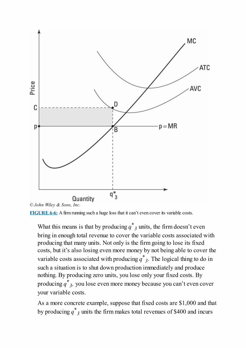
© John Wiley & Sons, Inc.

FIGURE 6-6: A firm running such a huge loss that it can’t even cover its variable costs.

What this means is that by producing q*3 units, the firm doesn’t even

bring in enough total revenue to cover the variable costs associated withproducing that many units. Not only is the firm going to lose its fixedcosts, but it’s also losing even more money by not being able to cover thevariable costs associated with producing q*

3. The logical thing to do insuch a situation is to shut down production immediately and producenothing. By producing zero units, you lose only your fixed costs. Byproducing q*

3, you lose even more money because you can’t even coveryour variable costs.

As a more concrete example, suppose that fixed costs are $1,000 and thatby producing q*

3 units the firm makes total revenues of $400 and incurs

variable costs of $500. Because total revenues cover only $400 of the$500 in variable costs, the firm loses $100 in variable costs byproducing. Add to that the $1,000 of fixed costs the firm will incur nomatter how much it produces, and the firm will lose a total of $1,100 byproducing q*

3 units of output. By contrast, if it shuts down and producesnothing, it loses only the $1,000 in fixed costs. Clearly, the firm shouldchoose to shut down production immediately (in the short run) instead ofwaiting until the long run when its fixed-cost commitment expires.

For the general case, the short-run shutdown condition works asfollows. If a firm’s total revenues at q*

3 are less than variablecosts, it’s better to shut down immediately (that is, in the short run).Graphically, this happens anytime the horizontal (marginalrevenue) line intersects the MC (marginal cost) curve at a pointbelow the U-shaped AVC (average variable cost) curve. In all suchsituations, total revenues will be less than variable costs —implying that it’s better to shut down immediately than to continue toproduce until the firm’s fixed-cost commitments have expired in thelong run.

The long-run shutdown condition: Totalcosts exceed total revenues

The long-run shutdown condition occurs when a loss-makingfirm is better off waiting until its fixed-cost commitments haveexpired before shutting down production. It’s better off waiting untilthe long run to shut down production if the firm’s total revenuescurrently exceed its variable costs but are less than its total costs.Graphically, this happens in any situation where the horizontal

(marginal revenue) line intersects the MC (marginal costs)curve at any point on the segment of the MC curve that lies abovethe bottom of the U-shaped AVC (average variable costs) curve butbelow the bottom of the U-shaped ATC (average total costs) curve,as in Figure 6-5.

In such a situation, the firm is guaranteed to lose money. But as long asthe firm is stuck with its current set of fixed cost commitments, the firm isbetter off producing rather than shutting down immediately. If itproduces, its total revenue will exceed its variable costs, meaning that itcan use the excess to pay off at least part of its fixed costs. On the otherhand, if it shuts down and produces nothing, it’ll lose all of its fixedcosts and thereby do worse.

Look at Figure 6-5. In this case, the firm is more than covering itsvariable costs because total revenues (represented by the box whose fourcorners are the origin and Points P, C, and q*

2) exceed variable costs(represented by the box whose four corners are the origin and Points D,E, and q*

2). Although this firm is losing money, it’s better off producingq*

2 rather than because total revenues exceed variable costs. Thefirm can take the extra money left over after paying variable costs anduse it to pay off some of its fixed costs.

As a more concrete example, suppose that the firm’s fixed costs are$1,000 and that when producing output level q*

2, it has a total revenue of$800 and variable costs of $700. The first $700 of the $800 in totalrevenues can go to paying off the variable costs, leaving $100 to pay offa portion of the $1,000 in fixed costs. The result is an overall loss of$900, rather than a $1,000 loss if the firm produces nothing. Thus, thisfirm should continue operating in the short run and wait until the long run— when its fixed-cost commitments have ended — before shutting downproduction and exiting its industry.

Chapter 7

Why Economists Love FreeMarkets and Competition

IN THIS CHAPTER Measuring the social benefits of different output levels Demonstrating that free markets maximize total surplus Reducing total surplus with taxes and price controls Producing at the lowest possible cost to society Adjusting to changes in supply and demand

Economists love competitive free markets — markets in whichnumerous buyers freely interact with numerous competitive firms.Indeed, economists firmly believe that when competitive free marketswork properly, they’re the very best way to convert society’s limitedresources into the goods and services that people want to buy. (Pleasenote that for brevity, I sometimes just say “free markets” or “markets” inthis chapter rather than writing “competitive free markets” each time. I’mtrying to maximize my resources here.)

Why do economists place such great confidence in competitive freemarkets? Because the interaction of supply and demand (which I discussin Chapter 4) leads to an outcome in which every unit of output that’sproduced satisfies two excellent conditions:

It’s produced at the minimum cost possible, meaning that there’s nowaste or inefficiency.Its benefits are always at least as big as its costs. That is,competitive free markets produce only output that makes the worldbetter off or at least no worse off.

Economists also love competitive free markets because they provide agold standard against which all other economic institutions can bejudged. In fact, economists refer to many economic problems as marketfailures precisely because they are instances where if markets could

function properly, the problems would quickly go away.

In this chapter, I show you that competitive free markets ensure thatbenefits exceed costs for all the output produced. I also show you thatcompetitive free markets produce the socially optimal quantity of output— the level that maximizes the benefits that society can get from itslimited supply of resources. Finally, I show you how competitiveindustries adjust to changes in supply and demand to ensure thateverything that’s being produced is produced at the lowest possible costto society.

Ensuring That Benefits ExceedCosts: Competitive Free Markets

Society has only a limited amount of land, labor, and capital out of whichto make things. Consequently, society must be very attentive whenfiguring out how to best convert its limited resources into the goods andservices that people most greatly desire.

Economists love competitive free markets because, if they areoperating properly, they make sure that resources are allocatedoptimally. In particular, such markets assure that resources gotoward producing only output for which the benefits exceed thecosts.

This point can be easily demonstrated using nothing more complicatedthan a supply and demand graph (such as the type I introduce in Chapter4). But first, this section explains the conditions under which competitivefree markets can function properly and thereby deliver such nice results.

Examining the traits of a properlyfunctioning market

Free markets guarantee optimal outcomes only if theseconditions are met:

Buyers and sellers all have access to the same full and completeinformation about the good or service in question. This guaranteesthat both parties will be willing to negotiate without having to worrythat the other guy has some secret information. (In Chapter 11, Iexplain how markets break down if one side or the other has moreinformation.)Property rights are set up so that the only way buyers can get

the good or service in question is by paying sellers for it. Thisensures that sellers have an incentive to produce output. As acounterexample, consider trying to sell tickets to an outdoorfireworks display: Because everyone knows that they can see thedisplay for free, nobody wants to pay for a ticket. And with nobodywilling to pay for a ticket, producers have no incentive to put on adisplay. (In Chapter 11, I discuss situations like these and howsociety must deal with them given that markets can’t.)Supply curves capture all the production costs associated withmaking the good or service in question. This requirement helpsensure that markets can make the proper cost-benefit calculations.For instance, if a steel factory can pollute for free, there’s no waythat the price of steel will incorporate the damage that the factory’spollution does to the environment. On the other hand, if thegovernment forces the factory to continuously pay for cleanup costs,these costs will be reflected in the market price, thereby allowingsociety to properly weigh the costs and benefits of the company’soutput. (Chapter 10 deals with ways to help markets along if supplyand demand curves don’t reflect all costs and benefits.)Demand curves capture all the benefits derived from the good orservice in question. This requirement also ensures proper cost-benefit analysis. If these first four conditions for free markets aremet, market forces can reach a social optimum — but only if they’refree from interference. Hence the need for two more conditions: onethat limits buyers and sellers, and another that constrains governmentintervention.There are both numerous buyers and numerous sellers, such thatnobody is big enough to affect the market price. This is oftencalled the price-taking assumption because everybody just has totake prices as given. This requirement eliminates problems such asmonopolies, in which individual buyers or sellers are so powerfulthat they can manipulate the market price in their own favor.The market price is completely free to adjust to equalize supplyand demand for the good or service in question. The sixthrequirement stipulates that supply and demand must be allowed tofreely determine the market price and market quantity unimpeded bygovernment-imposed price ceilings or floors. (In Chapter 4, I explain

the problems with price ceilings and floors and discuss how they hurtsociety.)

Basically, these six points accomplish two broad goals: They guaranteethat people will want to buy and sell in a market environment, and theyensure that markets will take into account all the costs and all thebenefits of producing and then consuming a given amount of output.

Analyzing the efficiency of free marketsEconomists use supply and demand curves to demonstrate that freemarkets produce socially optimal levels of output. But the simple insightbehind this result is that a unit of output can be socially beneficial toproduce and consume only if the benefits that people derive fromconsuming it exceed the costs of producing it.

This simple idea is, in fact, why demand curves and supply curves are souseful in analyzing the social optimum. Demand curves quantify thebenefits that people get from consumption by showing what they’d bewilling to pay to consume each and every particular unit of output (seeChapter 4 for details). Similarly, supply curves quantify the cost ofproducing each and every particular unit of output (see Chapter 6).

Using supply and demand to compare costs and benefitsBy drawing the demand and supply curves for a good or service on thesame graph, you can easily compare the benefits and costs of producingeach and every unit of output. To see how this is done, take a look atFigure 7-1, on which I’ve drawn a demand curve, D, and a supply curve,S.

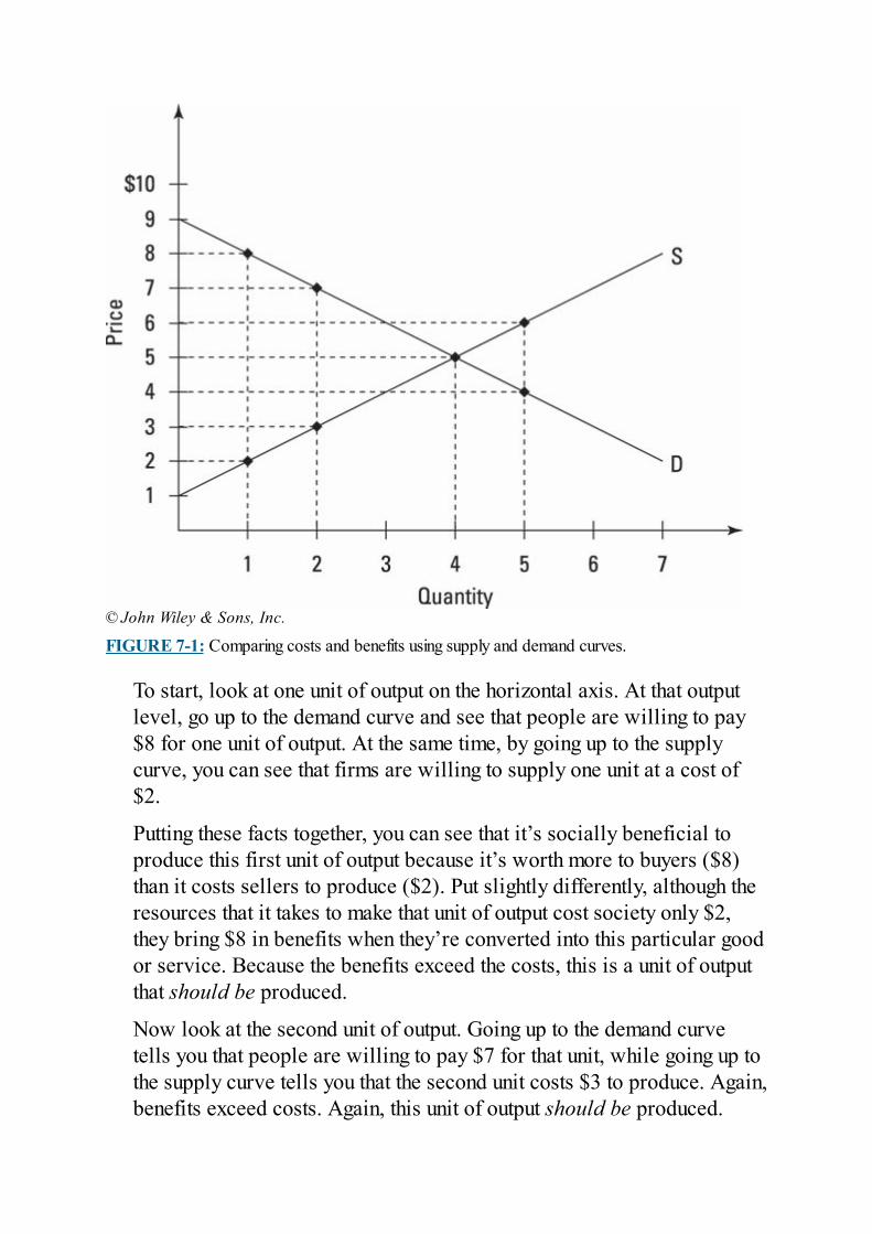
© John Wiley & Sons, Inc.

FIGURE 7-1: Comparing costs and benefits using supply and demand curves.

To start, look at one unit of output on the horizontal axis. At that outputlevel, go up to the demand curve and see that people are willing to pay$8 for one unit of output. At the same time, by going up to the supplycurve, you can see that firms are willing to supply one unit at a cost of$2.

Putting these facts together, you can see that it’s socially beneficial toproduce this first unit of output because it’s worth more to buyers ($8)than it costs sellers to produce ($2). Put slightly differently, although theresources that it takes to make that unit of output cost society only $2,they bring $8 in benefits when they’re converted into this particular goodor service. Because the benefits exceed the costs, this is a unit of outputthat should be produced.

Now look at the second unit of output. Going up to the demand curvetells you that people are willing to pay $7 for that unit, while going up tothe supply curve tells you that the second unit costs $3 to produce. Again,benefits exceed costs. Again, this unit of output should be produced.

By contrast, look at the fifth unit of output. You can see that the costs asgiven by the supply curve for producing the fifth unit are $6, while thebenefits as given by the demand curve are only $4. Because the costs ofproducing this unit exceed what anyone is willing to pay for it, this is aunit of output that shouldn’t be produced.

In other words, producing the fifth unit of output would destroy value.Why? Because making it involves converting $6 worth of resources intosomething that’s worth only $4 to consumers. Producing it would makethe world worse off. Better to redirect the resources that would benecessary to make a fifth unit of this product toward the production ofsomething that will generate net benefits to consumers.

Determining the socially optimal output levelA graph showing both the supply curve and the demand curve can tellyou precisely what quantity (q) of output should be produced. That’sbecause the supply and demand curves let you quickly compare costs andbenefits for every possible output level.

There are only three cost-benefit relationships:

Benefits exceed costs. In Figure 7-1, this occurs for every bit ofoutput such that .Benefits equal costs. This occurs at exactly units in the graph.Costs exceed benefits. This occurs for all output levels where .

Economists look at this and conclude that the socially optimal level ofoutput to produce is   units because for these units, benefits eitherexceed costs or at least are equal to costs. By producing the first fourunits of output, society either gains or at least isn’t made any worse off.

The socially optimal output level is always incredibly easy toidentify on any supply and demand graph: It’s just the quantityproduced where the demand and supply curves cross.

Economist Adam Smith’s big insight was to realize that

competitive free markets produce exactly the socially optimaloutput level on their own without anyone having to direct them to dothe right thing. This insight was the basis of Smith’s metaphor of aninvisible hand that seems to guide markets toward the sociallyoptimal output level, despite the fact that each individual in themarket may well be looking out only for his or her own interests.This result greatly simplifies life because it eliminates the need tohave a government official or any other sort of central plannerconstantly checking whether the right amount of output is beingproduced.

The proof of Smith’s assertion is almost trivial. All you have to do islook at Figure 7-1 and realize that the market equilibrium quantity —which happens when the market price is free to adjust so that the quantitysupplied by sellers equals the quantity demanded by buyers — isdetermined by where the supply and demand curves cross (to understandwhy, see Chapter 8). Thus, the market equilibrium quantity is exactlyequal to the number of units you’d want to produce if you were using thedemand and supply curves to compare benefits and costs.

Measuring everyone’s gains with totalsurplusEconomists use a concept called total surplus to add up the gains thatcome from producing the socially optimal output level. The gain, orsurplus, comes from the fact that benefits exceed costs for the units ofoutput that are produced.

The total surplus turns out to be divided between consumers andproducers. The part of the total surplus that goes to consumers is(naturally) called consumer surplus, and the part that goes to producersis called producer surplus.

In the subsections that follow, I tackle consumer surplus first and thenmove on to producer surplus. After I explain each separately, I add themtogether to explain total surplus. (And I hope that when you’re done withthis section, you feel like you’ve received at least a little consumersurplus.)

Measuring the consumer surplus of a discrete goodConsumer surplus is the gain people receive when they can buy things at

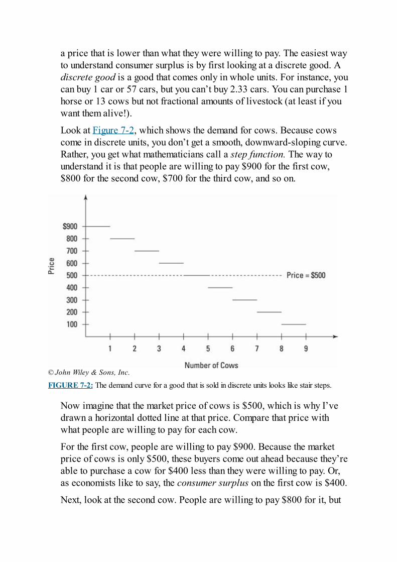
a price that is lower than what they were willing to pay. The easiest wayto understand consumer surplus is by first looking at a discrete good. Adiscrete good is a good that comes only in whole units. For instance, youcan buy 1 car or 57 cars, but you can’t buy 2.33 cars. You can purchase 1horse or 13 cows but not fractional amounts of livestock (at least if youwant them alive!).

Look at Figure 7-2, which shows the demand for cows. Because cowscome in discrete units, you don’t get a smooth, downward-sloping curve.Rather, you get what mathematicians call a step function. The way tounderstand it is that people are willing to pay $900 for the first cow,$800 for the second cow, $700 for the third cow, and so on.

© John Wiley & Sons, Inc.

FIGURE 7-2: The demand curve for a good that is sold in discrete units looks like stair steps.

Now imagine that the market price of cows is $500, which is why I’vedrawn a horizontal dotted line at that price. Compare that price withwhat people are willing to pay for each cow.

For the first cow, people are willing to pay $900. Because the marketprice of cows is only $500, these buyers come out ahead because they’reable to purchase a cow for $400 less than they were willing to pay. Or,as economists like to say, the consumer surplus on the first cow is $400.

Next, look at the second cow. People are willing to pay $800 for it, but

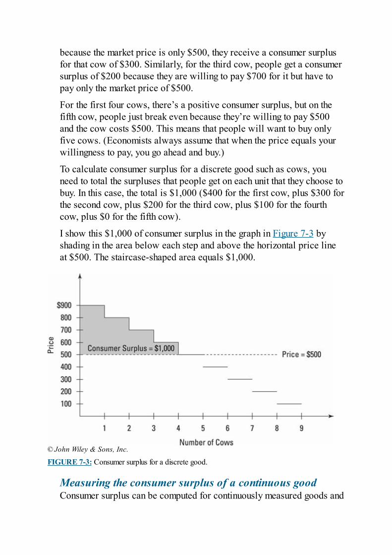
because the market price is only $500, they receive a consumer surplusfor that cow of $300. Similarly, for the third cow, people get a consumersurplus of $200 because they are willing to pay $700 for it but have topay only the market price of $500.

For the first four cows, there’s a positive consumer surplus, but on thefifth cow, people just break even because they’re willing to pay $500and the cow costs $500. This means that people will want to buy onlyfive cows. (Economists always assume that when the price equals yourwillingness to pay, you go ahead and buy.)

To calculate consumer surplus for a discrete good such as cows, youneed to total the surpluses that people get on each unit that they choose tobuy. In this case, the total is $1,000 ($400 for the first cow, plus $300 forthe second cow, plus $200 for the third cow, plus $100 for the fourthcow, plus $0 for the fifth cow).

I show this $1,000 of consumer surplus in the graph in Figure 7-3 byshading in the area below each step and above the horizontal price lineat $500. The staircase-shaped area equals $1,000.

© John Wiley & Sons, Inc.

FIGURE 7-3: Consumer surplus for a discrete good.

Measuring the consumer surplus of a continuous goodConsumer surplus can be computed for continuously measured goods and

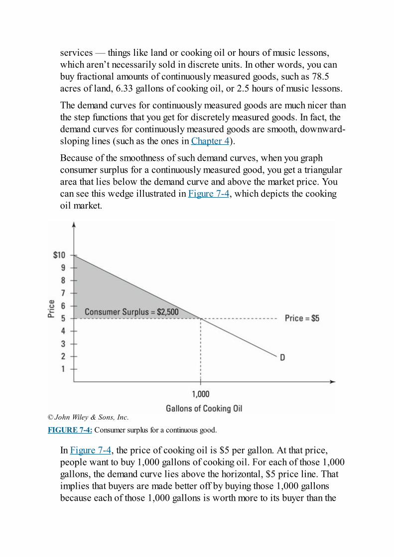
services — things like land or cooking oil or hours of music lessons,which aren’t necessarily sold in discrete units. In other words, you canbuy fractional amounts of continuously measured goods, such as 78.5acres of land, 6.33 gallons of cooking oil, or 2.5 hours of music lessons.

The demand curves for continuously measured goods are much nicer thanthe step functions that you get for discretely measured goods. In fact, thedemand curves for continuously measured goods are smooth, downward-sloping lines (such as the ones in Chapter 4).

Because of the smoothness of such demand curves, when you graphconsumer surplus for a continuously measured good, you get a triangulararea that lies below the demand curve and above the market price. Youcan see this wedge illustrated in Figure 7-4, which depicts the cookingoil market.

© John Wiley & Sons, Inc.

FIGURE 7-4: Consumer surplus for a continuous good.

In Figure 7-4, the price of cooking oil is $5 per gallon. At that price,people want to buy 1,000 gallons of cooking oil. For each of those 1,000gallons, the demand curve lies above the horizontal, $5 price line. Thatimplies that buyers are made better off by buying those 1,000 gallonsbecause each of those 1,000 gallons is worth more to its buyer than the

$5 per gallon that it costs to buy it.

To calculate consumer surplus for a continuous good, you totalup all the gains that people receive when buying for less money thanthey are willing to pay — just as you would do for a discrete good.But because you’re now dealing with a triangle, totaling up requiresa bit of geometry. Simply use the formula for the area of a triangle (

) to find the total surplus. In this case, youmultiply .

Measuring producer surplusProducer surplus measures the gain that firms receive when they can selltheir output for more than the minimum price that they would’ve beenwilling to accept. You can calculate producer surplus for both discreteand continuous goods, just as you can calculate consumer surplus foreach. In this section, I offer an example of calculating producer surplusfor a continuous good.

You can get a good handle on producer surplus by looking at Figure 7-5,which shows the supply curve, S, for cooking oil. This supply curve iscrucial for determining producer surplus because each point on thesupply curve tells you the minimum that you would have to pay suppliersfor them to give you the associated amount of output. By comparing eachminimum value with the higher market price that firms actually receivewhen they sell their output, you can compute producer surplus by findingthe area of a triangle. (For more on supply curves and how to interpretthem, see Chapter 4.)

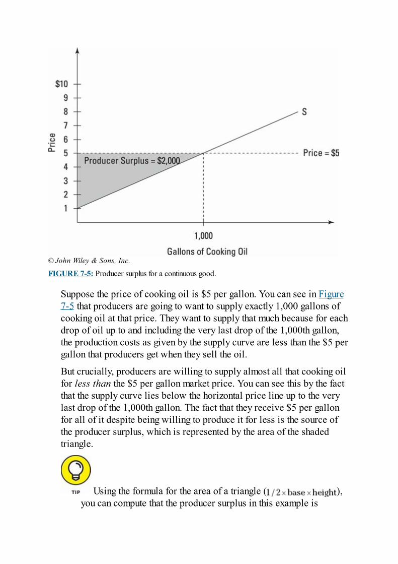
© John Wiley & Sons, Inc.

FIGURE 7-5: Producer surplus for a continuous good.

Suppose the price of cooking oil is $5 per gallon. You can see in Figure7-5 that producers are going to want to supply exactly 1,000 gallons ofcooking oil at that price. They want to supply that much because for eachdrop of oil up to and including the very last drop of the 1,000th gallon,the production costs as given by the supply curve are less than the $5 pergallon that producers get when they sell the oil.

But crucially, producers are willing to supply almost all that cooking oilfor less than the $5 per gallon market price. You can see this by the factthat the supply curve lies below the horizontal price line up to the verylast drop of the 1,000th gallon. The fact that they receive $5 per gallonfor all of it despite being willing to produce it for less is the source ofthe producer surplus, which is represented by the area of the shadedtriangle.

Using the formula for the area of a triangle ( ),you can compute that the producer surplus in this example is

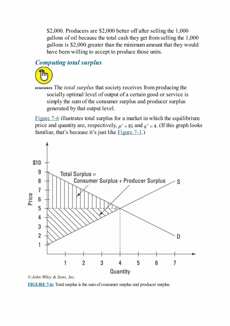
$2,000. Producers are $2,000 better off after selling the 1,000gallons of oil because the total cash they get from selling the 1,000gallons is $2,000 greater than the minimum amount that they wouldhave been willing to accept to produce those units.

Computing total surplus

The total surplus that society receives from producing thesocially optimal level of output of a certain good or service issimply the sum of the consumer surplus and producer surplusgenerated by that output level.

Figure 7-6 illustrates total surplus for a market in which the equilibriumprice and quantity are, respectively, and . (If this graph looksfamiliar, that’s because it’s just like Figure 7-1.)

© John Wiley & Sons, Inc.

FIGURE 7-6: Total surplus is the sum of consumer surplus and producer surplus.

I’ve drawn the total surplus area so you can clearly see that it’s made upof consumer surplus (the vertically striped area) plus producer surplus(the diagonally striped area). The two are separated by the horizontalline extending from the market equilibrium price ($5).

By again using the formula for the area of a triangle, you multiply to figure out that for this graph the total surplus is $16. The

total gain to society of producing at this output level is $16.

Contemplating total surplusTotal surplus is important because it puts a number on the gains that comefrom production and trade. Firms make things to make a profit. Peoplespend money on things because consuming those things makes themhappy. And total surplus tells you just how much better off bothconsumers and producers are after interacting with each other.

By putting a number on the gains made by their interaction, totalsurplus also provides a benchmark by which economists canmeasure the harm that comes from government policies that interferewith the market. It’s one thing to say that, for instance, pricesubsidies hurt consumers. It’s another thing to be able to say byexactly how many dollars consumers are harmed.

When Free Markets Lose TheirFreedom: Dealing withDeadweight Losses

Anything that interferes with the market’s ability to reach the marketequilibrium and produce the market quantity reduces total surplus.Economists refer to the amount by which total surplus is reduced usingthe colorful term deadweight loss.

In this section, I give you detailed examples of deadweight losses causedby price ceilings and taxes. These types of market interference are bothunder the government’s control, but you shouldn’t think that deadweightlosses are caused only by government policy. Anything that reducesoutput below the market quantity causes a deadweight loss. Monopoliesand oligopolies can be to blame, as can asymmetric information andpublic goods problems — all things that I discuss in the next fewchapters.

Coming up short: The deadweight loss froma price ceilingPrice ceilings are maximum prices at which sellers can legally sell theirproduct (see Chapter 4 for details). Generally, price ceilings areintended to help buyers obtain a low price, but they cause a lot of harm.As an example of a deadweight loss, look at Figure 7-7 in which thegovernment has imposed a price ceiling at PC.

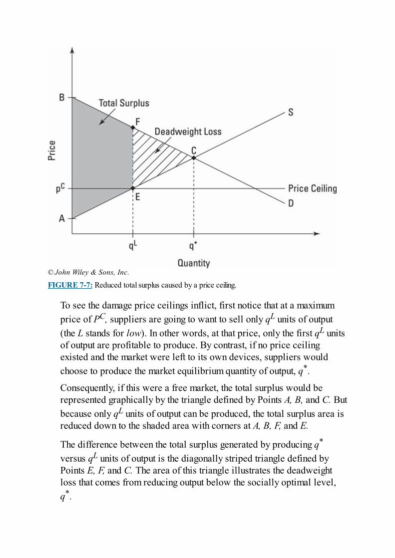
© John Wiley & Sons, Inc.

FIGURE 7-7: Reduced total surplus caused by a price ceiling.

To see the damage price ceilings inflict, first notice that at a maximumprice of PC, suppliers are going to want to sell only qL units of output(the L stands for low). In other words, at that price, only the first qL unitsof output are profitable to produce. By contrast, if no price ceilingexisted and the market were left to its own devices, suppliers wouldchoose to produce the market equilibrium quantity of output, q*.

Consequently, if this were a free market, the total surplus would berepresented graphically by the triangle defined by Points A, B, and C. Butbecause only qL units of output can be produced, the total surplus area isreduced down to the shaded area with corners at A, B, F, and E.

The difference between the total surplus generated by producing q*

versus qL units of output is the diagonally striped triangle defined byPoints E, F, and C. The area of this triangle illustrates the deadweightloss that comes from reducing output below the socially optimal level,q*.

The price ceiling is harmful because for all units between qL andq*, benefits exceed costs, meaning that such units should beproduced. By tallying up the gains that should’ve come fromproducing and consuming these units, the deadweight loss trianglecan precisely measure the harm that results from interfering with themarket.

Death and taxes: Finding the deadweightloss of a taxTaxes on goods and services can also cause deadweight losses. Thishappens because such taxes raise the costs of producing and consumingoutput. When these costs are artificially raised by the tax, peoplerespond by producing and consuming fewer units of output than they didbefore the tax was imposed. Because each unit that had been consumedbefore the tax was imposed was a unit for which benefits had exceededcosts, the reduction in output that results from the tax necessarily reducestotal surplus and causes a deadweight loss.

Seeing how taxes shift the supply curveTaxes on production shift supply curves upward. Why? Because to thefirms that are being taxed, taxes on production feel like increases inproduction costs. The firms know that the only way that they can at leastbreak even is if they pass the cost of the tax on to buyers — just as theyknow that they must pass on to buyers the costs of any labor, capital, orother resources. So just as any increase in input costs shifts supplycurves vertically, so does any production tax. Imposing a tax on sellersshifts the supply curve vertically by the amount of the tax.

Consider a concrete example — the supply of beef in a beef market inwhich the government is going to impose a tax of $1 per pound. Figure 7-8 shows two curves. (Well, actually they’re straight lines, but humor mehere.) The lower one, S, is the supply curve for beef. The higher one,labeled , is the supply curve after the tax is imposed. Theimportant thing to realize is that the curve is simply the originalsupply curve shifted up vertically by the amount of the tax, which in thiscase is $1.

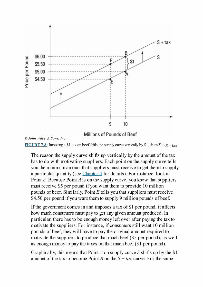
© John Wiley & Sons, Inc.

FIGURE 7-8: Imposing a $1 tax on beef shifts the supply curve vertically by $1, from S to .

The reason the supply curve shifts up vertically by the amount of the taxhas to do with motivating suppliers. Each point on the supply curve tellsyou the minimum amount that suppliers must receive to get them to supplya particular quantity (see Chapter 4 for details). For instance, look atPoint A. Because Point A is on the supply curve, you know that suppliersmust receive $5 per pound if you want them to provide 10 millionpounds of beef. Similarly, Point E tells you that suppliers must receive$4.50 per pound if you want them to supply 9 million pounds of beef.

If the government comes in and imposes a tax of $1 per pound, it affectshow much consumers must pay to get any given amount produced. Inparticular, there has to be enough money left over after paying the tax tomotivate the suppliers. For instance, if consumers still want 10 millionpounds of beef, they will have to pay the original amount required tomotivate the suppliers to produce that much beef ($5 per pound), as wellas enough money to pay the taxes on that much beef ($1 per pound).

Graphically, this means that Point A on supply curve S shifts up by the $1amount of the tax to become Point B on the S + tax curve. For the same

motivational reasons, Point E on the supply curve must shift up to Point Fon the S + tax curve. That is, if you have to pay suppliers $4.50 perpound to motivate them to give you 9 million pounds of beef in a worldin which $1 per pound must go to the government in taxes, you have tocollect a total of $5.50 per pound. And that’s exactly what happens atPoint F.

Every point on the supply curve, S, must shift up vertically in the sameway that Points A and E do, so the S + tax curve captures what the supplycurve looks like after the tax is imposed. With this shift in mind, you’reready to discover how this sort of taxation causes deadweight losses.

Seeing how taxes cause deadweight lossesDeadweight losses are called deadweight losses because you can’t say,“Your loss is my gain,” in this situation. You aren’t talking aboutsomething that passes from one person to another. Rather, deadweightlosses are losses in the sense of annihilation. The gains that would’veresulted if the market quantity of a good had been produced simplyvanish; they’re a weight that society is forced to bear as it strives tomaximize human happiness given limited resources.

Figure 7-9 adds a demand curve, D, to Figure 7-8 so you can see whathappens to total surplus when the government imposes a $1 per poundtax on the beef that’s sold in the beef market.

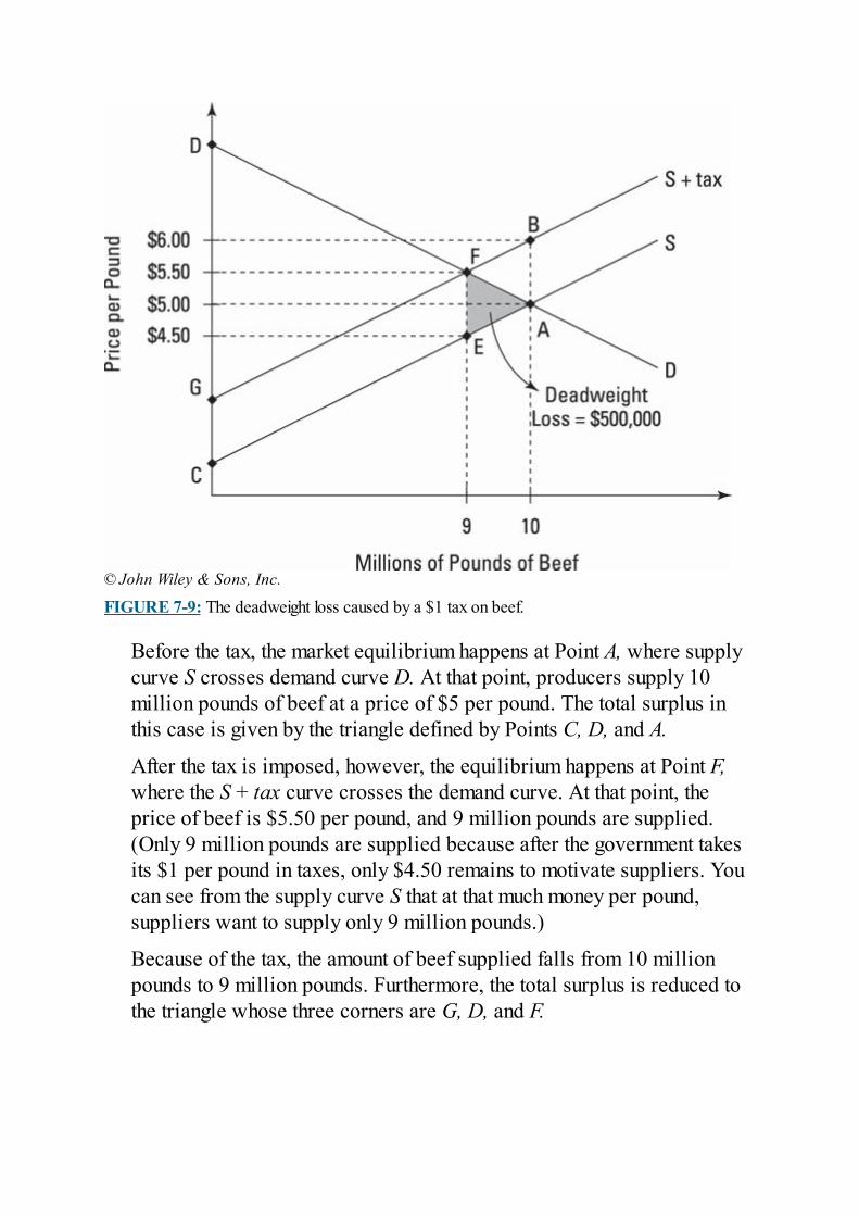
© John Wiley & Sons, Inc.

FIGURE 7-9: The deadweight loss caused by a $1 tax on beef.

Before the tax, the market equilibrium happens at Point A, where supplycurve S crosses demand curve D. At that point, producers supply 10million pounds of beef at a price of $5 per pound. The total surplus inthis case is given by the triangle defined by Points C, D, and A.

After the tax is imposed, however, the equilibrium happens at Point F,where the S + tax curve crosses the demand curve. At that point, theprice of beef is $5.50 per pound, and 9 million pounds are supplied.(Only 9 million pounds are supplied because after the government takesits $1 per pound in taxes, only $4.50 remains to motivate suppliers. Youcan see from the supply curve S that at that much money per pound,suppliers want to supply only 9 million pounds.)

Because of the tax, the amount of beef supplied falls from 10 millionpounds to 9 million pounds. Furthermore, the total surplus is reduced tothe triangle whose three corners are G, D, and F.

You can immediately see that this new total surplus is muchsmaller than the old total surplus. But before you start ranting aboutthe evils of government, you need to take account of the fact thattaxes are being collected. Taxes (theoretically, at least) benefitsociety, so you need to include this amount when calculating thetotal surplus of this good sold at this price. At the new equilibrium,$9 million in taxes will be collected because the 9 million poundsof beef sold will be taxed $1 each.

The $9 million in tax collections are represented graphically by theparallelogram whose corners are C, G, F, and E. This area waspreviously contained in the old total surplus triangle whose corners wereC, D, and A. Consequently, this area that used to be part of the old totalsurplus hasn’t been destroyed; it’s merely been transferred to thegovernment.

However, part of the old total surplus has been destroyed. This part isshown graphically by the shaded deadweight loss triangle (with cornersat E, F, and A). This area captures the fact that society has been madeworse off by the reduction in beef output from 10 million pounds to 9million pounds. (Okay, now you can start ranting about the evils ofgovernment.)

Measuring the size of the deadweight loss using the formula for the areaof a triangle ( ) tells you that the tax leads to adeadweight loss of $500,000. That’s a big number representing a hugereduction in total surplus deriving from the fact that for each of the 1million pounds of beef that are no longer being produced, benefits hadexceeded costs. All those gains are lost when the tax is imposed.

Note: In certain special cases, a tax can reduce (rather than cause) adeadweight loss. The intuition is that if a product is being inefficientlyoverproduced, then imposing a tax can make things better: By shifting thesupply curve upward, the tax causes production to decrease, therebyreducing the overproduction. I discuss these special cases in detail inChapter 10.

Hallmarks of PerfectCompetition: Zero Profits andLowest Possible Costs

A wonderful thing about free markets and competition is that output isproduced at the lowest possible cost. This fact is extremely importantbecause it means that free markets are as efficient as possible atconverting resources into the goods and services that people want to buy.

In addition, markets save society a lot of money because they produceefficiently without requiring human intervention. People don’t have topay big salaries to experts to make sure that markets run efficiently;markets do the job for free.

Understanding the causes and consequencesof perfect competition

To ensure that markets function efficiently, you need really strongcompetition among firms, a situation that economists refer to asperfect competition. Perfect competition exists when there aremany firms within a given industry that are all producing identical(or nearly identical) products (see Chapter 6 for details). Thefollowing things are also true when perfect competition exists:

Every firm is a price taker (meaning that the firm must accept themarket equilibrium price for what it produces) because its output is avery small fraction of the industry’s total output (see Chapter 6).Every firm has identical production technology.Firms are free to enter or leave the industry as they please.

When these requirements are met, perfect competition leads totwo very excellent outcomes:

Every firm in the industry makes zero economic profits. This ideadoes not mean that businesses earn no money above the costs ofdoing business; if that were true, no one would go into business.Firms must earn enough money to keep entrepreneurs motivated tostay in business (and to attract other entrepreneurs to open newfirms).So what does the first outcome mean? The economic profits earnedby a firm are any monies collected above and beyond what isrequired to keep an entrepreneur interested in continuing in business.So the fact that perfect competition leads to zero economic profitsmeans that managers just barely want to keep their current firmsoperating.It also means that nobody in the industry is getting filthy rich atanyone else’s expense. Rather, they’re doing just well enough to keepon supplying the output that society wants them to supply. Thissituation is great for society, because it’d be wasteful to payentrepreneurs more than necessary to get them to do what societywants.Every firm produces output at the minimum possible cost. Thisoutcome is good for society because it means that the least possibleamounts of resources are consumed while producing the output thatsociety wants.

Peering into the process of perfectcompetition

How does perfect competition actually work? The followingfour steps explain:

1. The market price of the output sold by every firm in the industry

is determined by the interaction of the industry’s overall supplyand demand curves.

2. Each firm takes the market price as given and produceswhatever quantity of output will maximize its own profit (orminimize its own loss if the price is so low that it’s not possible tomake a profit).

3. Because each firm has an identical production technology, eachwill choose to produce the same quantity and will consequentlymake the same profit or loss as every other firm in the industry.

4. Depending on whether firms in the industry are making profits orlosses, firms will either enter or leave the industry until themarket price adjusts to the level where all remaining firms aremaking zero economic profit.

The fourth point in this process — firm entry and exit — is veryimportant. To understand it clearly, I break it into two cases: one whereevery firm in the industry is making a profit because the market price ishigh and another where every firm in the industry is making a lossbecause the market price is low:

Attracting new firms by making profits: If every firm in an industryis making a profit, new firms are attracted to enter the industry, too,in hopes of sharing the profits. But when they enter, total industryoutput increases so much that the market price begins to fall. As theprice falls, profits fall, thereby lowering the incentive for furtherfirms to enter the industry.The process of new firms entering the industry continues until themarket price falls so low that profits drop to zero. When thathappens, the incentive to enter the industry disappears, and no morefirms enter.Losing existing firms when making losses: If every firm in anindustry starts out making losses because the market price is low,some of the existing firms exit the industry because they can’t standlosing money. When they do, total industry output falls. Thatreduction in total supply, in turn, causes the market price to rise. Andas the market price rises, firms’ losses decrease.The process of firms leaving and prices rising continues until the

remaining firms are no longer losing money.

The fact that firms can freely enter or leave the industry meansthat after all adjustments are made, firms always make a zeroeconomic profit. In other words, if there is perfect competition, youdon’t have to worry about firms exploiting anyone; they just barelymake enough money to stay in business.

The other important result of perfect competition — that competitivefirms produce at minimum cost — becomes apparent if you flesh out thefour-stage process of perfect competition by using cost curves. Iencourage you to take a look at Chapter 6 before moving on to the nextsection. If you haven’t read that chapter, this section may cause your eyesto cross (and you know what your mother said about the dangers ofcrossing your eyes).

Graphing how profits guide firm entry andexitIn this section, I use firm cost curves to demonstrate how market forcesautomatically cause firms to produce output at the lowest possible cost.To make this process clear, I present two cases. In the first, firms beginby making profits. In the second, firms begin by making losses. Eitherway, adjustments happen so that they end up making zero economicprofits and producing at minimum costs.

Visualizing firm entry when there are profitsTo see how an industry adjusts when it starts off making profits, look atFigure 7-10, which consists of two graphs. The one on the left gives themarket demand curve, D, and the initial market supply curve, So, fortennis balls. The one on the right gives the cost curves for one of themany identical firms that make tennis balls.

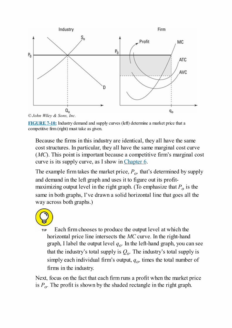
© John Wiley & Sons, Inc.

FIGURE 7-10: Industry demand and supply curves (left) determine a market price that acompetitive firm (right) must take as given.

Because the firms in this industry are identical, they all have the samecost structures. In particular, they all have the same marginal cost curve(MC). This point is important because a competitive firm’s marginal costcurve is its supply curve, as I show in Chapter 6.

The example firm takes the market price, Po, that’s determined by supplyand demand in the left graph and uses it to figure out its profit-maximizing output level in the right graph. (To emphasize that Po is thesame in both graphs, I’ve drawn a solid horizontal line that goes all theway across both graphs.)

Each firm chooses to produce the output level at which thehorizontal price line intersects the MC curve. In the right-handgraph, I label the output level qo. In the left-hand graph, you can seethat the industry’s total supply is Qo. The industry’s total supply issimply each individual firm’s output, qo, times the total number offirms in the industry.

Next, focus on the fact that each firm runs a profit when the market priceis Po. The profit is shown by the shaded rectangle in the right graph.

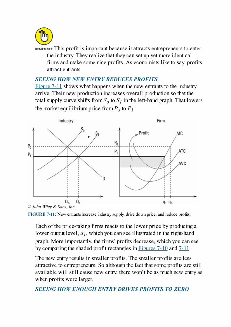
This profit is important because it attracts entrepreneurs to enterthe industry. They realize that they can set up yet more identicalfirms and make some nice profits. As economists like to say, profitsattract entrants.

SEEING HOW NEW ENTRY REDUCES PROFITSFigure 7-11 shows what happens when the new entrants to the industryarrive. Their new production increases overall production so that thetotal supply curve shifts from So to S1 in the left-hand graph. That lowersthe market equilibrium price from Po to P1.

© John Wiley & Sons, Inc.

FIGURE 7-11: New entrants increase industry supply, drive down price, and reduce profits.

Each of the price-taking firms reacts to the lower price by producing alower output level, q1, which you can see illustrated in the right-handgraph. More importantly, the firms’ profits decrease, which you can seeby comparing the shaded profit rectangles in Figures 7-10 and 7-11.

The new entry results in smaller profits. The smaller profits are lessattractive to entrepreneurs. So although the fact that some profits are stillavailable will still cause new entry, there won’t be as much new entry aswhen profits were larger.

SEEING HOW ENOUGH ENTRY DRIVES PROFITS TO ZERO

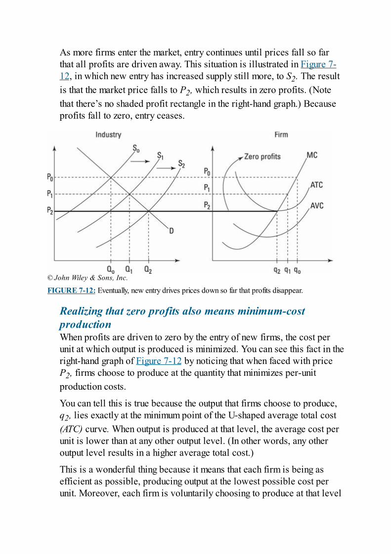
As more firms enter the market, entry continues until prices fall so farthat all profits are driven away. This situation is illustrated in Figure 7-12, in which new entry has increased supply still more, to S2. The resultis that the market price falls to P2, which results in zero profits. (Notethat there’s no shaded profit rectangle in the right-hand graph.) Becauseprofits fall to zero, entry ceases.

© John Wiley & Sons, Inc.

FIGURE 7-12: Eventually, new entry drives prices down so far that profits disappear.

Realizing that zero profits also means minimum-costproductionWhen profits are driven to zero by the entry of new firms, the cost perunit at which output is produced is minimized. You can see this fact in theright-hand graph of Figure 7-12 by noticing that when faced with priceP2, firms choose to produce at the quantity that minimizes per-unitproduction costs.

You can tell this is true because the output that firms choose to produce,q2, lies exactly at the minimum point of the U-shaped average total cost(ATC) curve. When output is produced at that level, the average cost perunit is lower than at any other output level. (In other words, any otheroutput level results in a higher average total cost.)

This is a wonderful thing because it means that each firm is being asefficient as possible, producing output at the lowest possible cost perunit. Moreover, each firm is voluntarily choosing to produce at that level

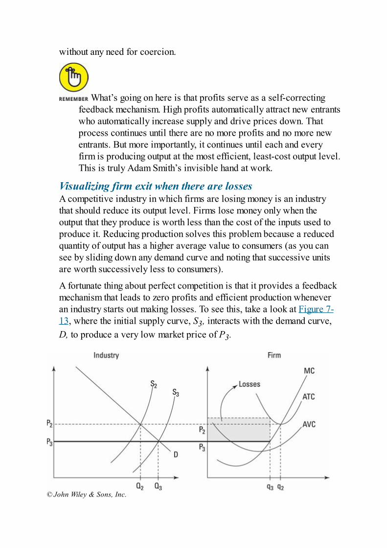
without any need for coercion.

What’s going on here is that profits serve as a self-correctingfeedback mechanism. High profits automatically attract new entrantswho automatically increase supply and drive prices down. Thatprocess continues until there are no more profits and no more newentrants. But more importantly, it continues until each and everyfirm is producing output at the most efficient, least-cost output level.This is truly Adam Smith’s invisible hand at work.

Visualizing firm exit when there are lossesA competitive industry in which firms are losing money is an industrythat should reduce its output level. Firms lose money only when theoutput that they produce is worth less than the cost of the inputs used toproduce it. Reducing production solves this problem because a reducedquantity of output has a higher average value to consumers (as you cansee by sliding down any demand curve and noting that successive unitsare worth successively less to consumers).

A fortunate thing about perfect competition is that it provides a feedbackmechanism that leads to zero profits and efficient production wheneveran industry starts out making losses. To see this, take a look at Figure 7-13, where the initial supply curve, S3, interacts with the demand curve,D, to produce a very low market price of P3.

© John Wiley & Sons, Inc.

FIGURE 7-13: Low market prices lead to losses and exiting firms.

At this market price, you can see in the right-hand graph that each firm inthe industry is making a loss, which is shown by the shaded rectangle.

This loss discourages all the firms in the industry, and those inthe weakest financial condition begin to exit. As that happens, theindustry supply curve in the left-hand graph shifts left (becausesupply decreases). That shift raises the market price and reduces thelosses made by firms remaining in the industry. But as long as thereare losses, firms continue to exit until the supply curve moves allthe way back to S2, at which point the market price is P2, and firmsare making zero profits as in Figure 7-12.

When the market price reaches P2 and firms are making zero profits, firmexits stop and, more importantly, each firm is producing at the least-costoutput level, q2.

Understanding that entry and exit don’t happen instantlyMarket pressures always push perfectly competitive firms to produce atthe lowest possible per-unit cost (see the preceding sections). Keep inmind that this nice result doesn’t happen overnight. When firms aremaking profits or sustaining losses, it takes time for new firms to enter (ifthere are profits) or for existing firms to leave (if there are losses).

Depending on the industry, these adjustment processes may takeanywhere from a few weeks to a few years. For example, setting up newpower plants takes a while because building a new power plant takes atleast a year. Similarly, even if agricultural prices fall and farmers aremaking losses, those farmers who drop out of the industry won’t do sountil the next growing season. On the other hand, if producing U.S. flagssuddenly becomes really profitable, you can be sure that scores of newfirms will pour into the industry within weeks.

The wonderful thing about perfect competition is that there are alwaysmarket forces acting to drive firms to produce at the minimum possiblecost. As I show you in the next few chapters, this lovely result falls apartwhen monopolies, oligopolies, public goods, and other problems prevent

perfect competition.

Chapter 8

Monopolies: Bad Behaviorwithout Competition

IN THIS CHAPTER Producing less and charging more than competitive firms Maximizing profit Benefiting society (in certain situations) Abiding by regulations

A firm that has no competitors in its industry is called a monopoly.Monopolies are much maligned because their profit incentive leads themto raise prices and lower output in order to squeeze more money out ofconsumers. As a result, governments typically go out of their way tobreak up monopolies and replace them with competitive industries thatgenerate lower prices and higher output.

At the same time, however, governments also very intentionally createmonopolies in other situations. For instance, governments issue patents,which give monopoly rights to inventors to sell and market theirinventions. Similarly, in many places, local services such as natural gasdelivery and trash collection are also monopolies created and enforcedby local government.

In this chapter, I explain why society forbids monopolies in somesituations and promotes them in others. First, I show you that profit-maximizing monopolies compare unfavorably with competitive firmsbecause they set higher prices and produce less output than competitivefirms. Then I explain how these problems may, in certain cases, beoutweighed by other factors — the need to promote innovation, forexample, and the odd fact that in some cases having a lot of competitorsis just too annoying.

Examining Profit-MaximizingMonopolies

Essentially, this chapter is one big exercise in cost-benefit analysis.Monopolies aren’t all evil. Neither are they utterly good. Whether youwant to have one in any particular instance depends on whether, in thatsituation, the benefits outweigh the costs. This section goes into detailabout the costs associated with monopolies.

Zeroing in on the problems monopoliescause

In an industry that has only one monopoly firm rather than lots ofsmall competitive firms, three socially harmful things occur:

The monopoly firm produces less output than a competitive industrywould.The monopoly firm sells its output at a higher price than the marketprice would be if the industry were competitive.The monopoly’s output is produced less efficiently and at a highercost than the output produced by a competitive industry.

Although all these things are harmful to consumers, keep in mind thatmonopolies don’t do these things to be jerks. Rather, these outcomes aresimply the result of monopolies’ acting to maximize their profits —which is, of course, the very same thing that competitive firms try to do.

The difference in outcomes between a competitive industry and amonopoly industry doesn’t have anything to do with bad intentions.Rather, it results from the fact that monopolies are free from thepressures that lead competitive industries to produce the sociallyoptimal output level (see Chapter 7 for info on these pressures).

Without these pressures, monopoly firms can increase prices andrestrict output to increase their profits — things that competitivefirms would also love to do but can’t.

The lack of competitive pressure also means that monopoly firms can getaway with costly, inefficient production. This is a real problem that youshould take seriously when considering whether the benefits of amonopoly outweigh its costs. I talk more about this issue later in thechapter.

Identifying the source of the problem:Decreasing marginal revenues

All the bad outcomes generated by a monopoly derive from thesame source: The monopolist faces a downward-sloping marginalrevenue curve. Marginal revenue is the increase in total revenuethat comes from selling each successive unit of a product. Thissimple fact causes monopolies to charge more, produce less, andproduce at higher costs than competitive firms.

How can one little curve cause such mayhem? A downward-slopingmarginal revenue curve implies that each additional unit that themonopoly sells brings less revenue than the previous unit. For instance,although the 10th unit sold may bring in $8, the 11th brings in only $3.Obviously, such a situation reduces the incentive to produce a lot ofoutput.

This situation stands in stark contrast to the marginal revenue situationfacing competitive firms (see Chapter 6). Competitive firms facehorizontal marginal revenue curves, meaning that whether they sell 11units or 11,000, each unit brings in the same amount of money. Naturally,that’s much more of an inducement to produce a lot of output.

Facing down demandWhy is there such a difference between the marginal revenue curvesfacing monopolists and competitive firms? A monopoly is free to choosethe price it wants to charge along the demand curve it faces for itsproduct. A competitive firm, on the other hand, has to take the market

price as given.

A monopoly firm can choose its price because as the only firm in itsindustry, it controls all the output in that industry. As a result, it cancreate a relatively high price by producing only a few units, or it caninduce a relatively low price by flooding the market. By contrast, eachfirm in a competitive industry is such a small part of its industry that itschoice of output makes too small a difference in total output to causeprice changes. (See Chapter 7 for more on why competitive firms can’taffect prices.)

The monopolist’s ability to control the price by altering itsoutput level means that the firm has to step back and consider whatoutput level to produce. The firm’s goal is profit maximization, so ithas to figure out what level of output will maximize its profits. Itturns out that a monopolist’s profit-maximizing output level isdefined by the same condition as that of a competitive firm: Produceat the output level where the marginal revenue curve crosses themarginal cost curve.

Deriving marginal revenue from the demand curve

For a monopoly, the marginal revenue of each successive unit ofoutput is less than the marginal revenue of the preceding unitbecause demand curves slope downward. The monopoly’s marginalrevenue curve has a precise relationship with the demand curve forthe monopoly’s output: If the demand curve is a straight line, theslope of the marginal revenue curve is twice as steep as the slope ofthe demand curve, meaning that marginal revenue falls quite quicklyas output increases.

To see how this works, take a look at Figure 8-1, which draws out ademand curve and its associated marginal revenue curve.

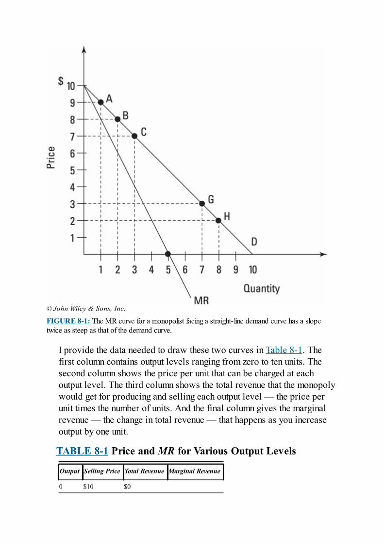
© John Wiley & Sons, Inc.

FIGURE 8-1: The MR curve for a monopolist facing a straight-line demand curve has a slopetwice as steep as that of the demand curve.

I provide the data needed to draw these two curves in Table 8-1. Thefirst column contains output levels ranging from zero to ten units. Thesecond column shows the price per unit that can be charged at eachoutput level. The third column shows the total revenue that the monopolywould get for producing and selling each output level — the price perunit times the number of units. And the final column gives the marginalrevenue — the change in total revenue — that happens as you increaseoutput by one unit.

TABLE 8-1 Price and MR for Various Output Levels

Output Selling Price Total Revenue Marginal Revenue

0 $10 $0

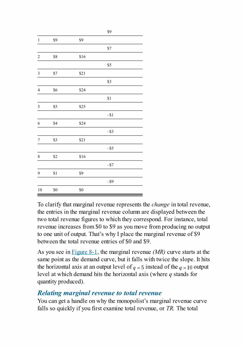
$9

1 $9 $9

$7

2 $8 $16

$5

3 $7 $21

$3

4 $6 $24

$1

5 $5 $25

–$1

6 $4 $24

–$3

7 $3 $21

–$5

8 $2 $16

–$7

9 $1 $9

–$9

10 $0 $0

To clarify that marginal revenue represents the change in total revenue,the entries in the marginal revenue column are displayed between thetwo total revenue figures to which they correspond. For instance, totalrevenue increases from $0 to $9 as you move from producing no outputto one unit of output. That’s why I place the marginal revenue of $9between the total revenue entries of $0 and $9.

As you see in Figure 8-1, the marginal revenue (MR) curve starts at thesame point as the demand curve, but it falls with twice the slope. It hitsthe horizontal axis at an output level of instead of the outputlevel at which demand hits the horizontal axis (where q stands forquantity produced).

Relating marginal revenue to total revenueYou can get a handle on why the monopolist’s marginal revenue curvefalls so quickly if you first examine total revenue, or TR. The total

revenue that the monopolist can get is simply the output it produces timesthe price at which it can sell its output. That is, . However, theprice at which a monopolist can sell depends on how much the firmproduces.

The relationship between output produced and the price at which theproduct can be sold depends on the demand curve. For instance, considerPoint A on the demand curve in Figure 8-1. At that point, one unit isbeing produced, and it can be sold for $9. Consequently, the totalrevenue at that point is $9. Next, look at Point B, at which two units ofoutput are being sold. At that output level, each unit can be sold for $8.Consequently, total revenue is . And at Point C, where threeunits can be sold for $7 each, total revenue is $21.

The important thing to notice is how total revenue changes as you movefrom A to B to C and output increases from one to two to three units.Total revenue goes from $9 to $16 to $21. Obviously, total revenueincreases. But look more deeply. Moving from A to B, TR increases by$7 (from $9 to $16). But moving from B to C, it increases by only $5(from $16 to $21). Each successive increase in total revenue is smallerthan the preceding increase. In other words, marginal revenue declinesas the monopoly increases production.

If you look at Table 8-1, you can see that marginal revenue continues tofall for each successive unit. In fact, it becomes negative for all unitsafter the fifth. You can see why by looking at Points G and H in Figure 8-1 as examples. At Point G, the monopolist can sell seven units of outputfor $3 each. That makes for a total revenue of $21. But if he increasesoutput to eight units at Point H, he can sell these units for only $2 each,implying a total revenue of $16.

Increasing output from seven units to eight units means decreasing totalrevenue from $21 to $16. That’s the same thing as saying that marginalrevenue is negative $5 as you move from seven to eight units of output.

Sliding down the demand curve: Higher output, lower pricesThe reason marginal revenue keeps declining and even becomes negativeis that the demand curve slopes downward, meaning that the only way toget people to buy more stuff is to offer them a lower price. You have tooffer them a lower price not just on additional units but on all previousunits as well. In other words, if the monopolist wants to sell only one

unit (see Point A), he can get $9 for it. But if the monopolist wants to selltwo units (see Point B), he has to lower the price down to $8 per unit forboth the first unit and the second unit.

Because total revenue equals price times quantity ( ), you cansee that the monopolist faces a trade-off as he increases production andslides down the demand curve. As he produces more, the quantity qobviously goes up, but the price p must fall. What happens to TR dependson whether the increases in q (output effects) are bigger than thedecreases in p (price effects).

You can see from Table 8-1 that as the monopoly increases productionthrough the first four units, total revenue keeps increasing, meaning thatthe gains from selling more units more than offset the declines fromgetting less money per unit. At an output of five units, the two effectscancel each other out. And for higher outputs, total revenue falls becausethe negative effect of less money per unit overwhelms the positive effectof selling more units.

Because marginal revenue (MR) tells you how total revenue(TR) changes as you increase output, the changes in TR caused byincreasing output show up in MR as well. If you look at Figure 8-1,you can see that MR is always declining. That’s because thenegative price effect of getting less per unit keeps getting strongerand stronger relative to the positive quantity effect of selling moreunits.

For straight-line demand curves (like the one you see in Figure8-1), the MR curve is a straight line that has twice as steep a slopeas the demand curve. If you know calculus, you can prove that theMR curve falls twice as fast as the demand curve: First take theequation of the demand curve shown in Figure 8-1, , andsubstitute it into the total revenue equation, . That gives you

. Then take the first derivative with respect tooutput, q. Because marginal revenue is dTR/dq, you find that

, meaning that MR has the same y-intercept as thedemand curve but twice as steep a slope.

When you understand the marginal revenue situation facing a monopolist,you can combine it with the firm’s marginal cost curve to figure out itsprofit-maximizing output level. As I show you in the next section, thislevel is less than that chosen by a competitive firm — a behavior thatleads to a social harm that can be quantified using the method ofdeadweight losses.

Choosing an output level to maximizeprofitsA monopoly is no different from a competitive firm when it comes to thecosts of producing output. Just like a competitive firm, a monopoly hasfixed costs, variable costs, and marginal costs (see Chapter 6). Moreimportantly, these costs all behave in exactly the same way, whether afirm is competitive or a monopoly. This means you can use costs to helpanalyze the decision-making process of a monopoly in the same way thatyou use them to analyze the decision-making process of competitivefirms.

The key difference, however, is that the monopoly faces a downward-sloping marginal revenue curve. In this section, you see how this factorcauses a profit-maximizing monopoly to produce less output than woulda profit-maximizing competitive firm.

Setting a monopoly’s marginal revenue equal to marginalcostThe monopoly goes about maximizing profits in much the same way as acompetitive firm. To see this, take a look at Figure 8-2, which draws amonopoly’s average total cost (ATC) and marginal cost (MC) curves onthe same graph as the monopoly’s demand curve and marginal revenue(MR) curve.

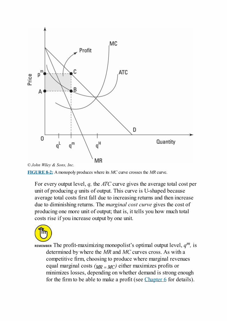
© John Wiley & Sons, Inc.

FIGURE 8-2: A monopoly produces where its MC curve crosses the MR curve.

For every output level, q, the ATC curve gives the average total cost perunit of producing q units of output. This curve is U-shaped becauseaverage total costs first fall due to increasing returns and then increasedue to diminishing returns. The marginal cost curve gives the cost ofproducing one more unit of output; that is, it tells you how much totalcosts rise if you increase output by one unit.

The profit-maximizing monopolist’s optimal output level, qm, isdetermined by where the MR and MC curves cross. As with acompetitive firm, choosing to produce where marginal revenuesequal marginal costs ( ) either maximizes profits orminimizes losses, depending on whether demand is strong enoughfor the firm to be able to make a profit (see Chapter 6 for details).

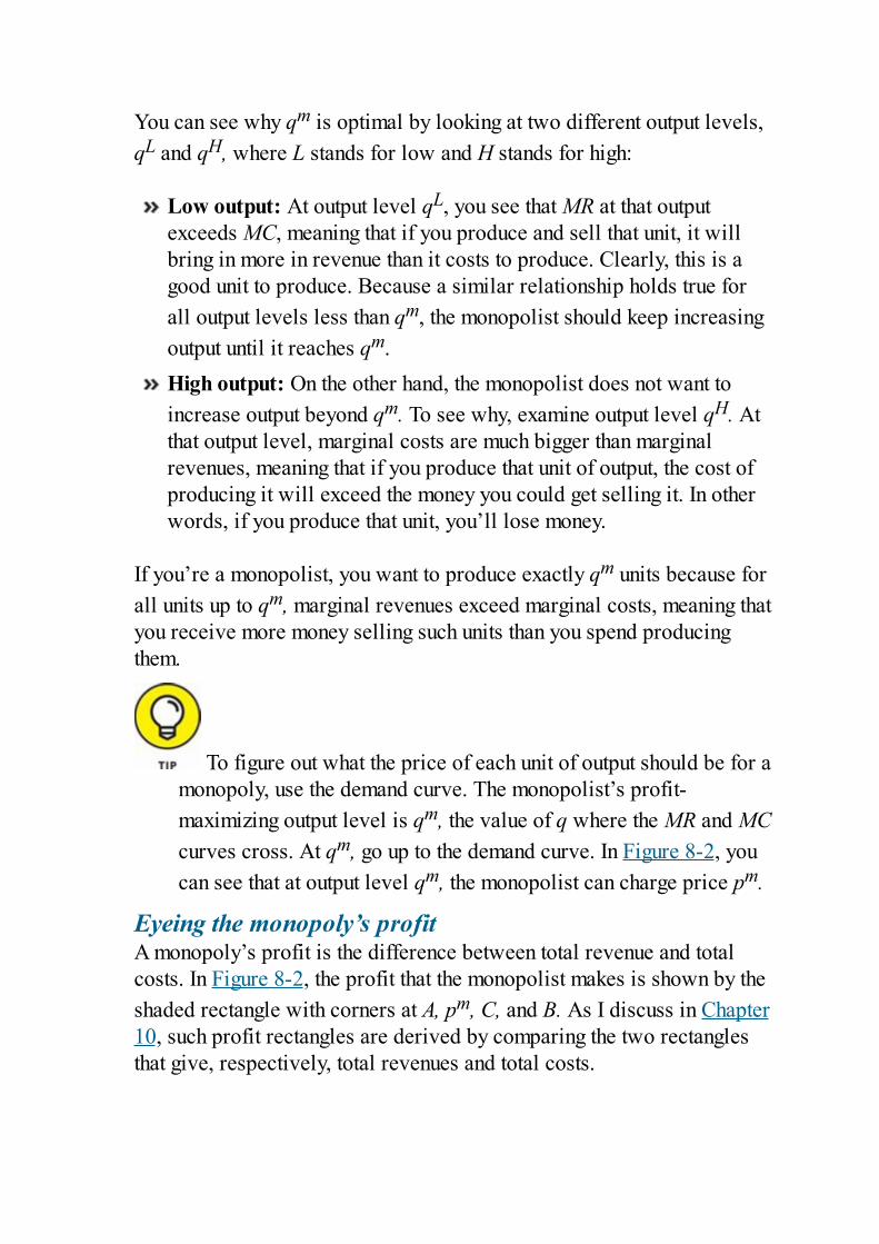
You can see why qm is optimal by looking at two different output levels,qL and qH, where L stands for low and H stands for high:

Low output: At output level qL, you see that MR at that outputexceeds MC, meaning that if you produce and sell that unit, it willbring in more in revenue than it costs to produce. Clearly, this is agood unit to produce. Because a similar relationship holds true forall output levels less than qm, the monopolist should keep increasingoutput until it reaches qm.High output: On the other hand, the monopolist does not want toincrease output beyond qm. To see why, examine output level qH. Atthat output level, marginal costs are much bigger than marginalrevenues, meaning that if you produce that unit of output, the cost ofproducing it will exceed the money you could get selling it. In otherwords, if you produce that unit, you’ll lose money.

If you’re a monopolist, you want to produce exactly qm units because forall units up to qm, marginal revenues exceed marginal costs, meaning thatyou receive more money selling such units than you spend producingthem.

To figure out what the price of each unit of output should be for amonopoly, use the demand curve. The monopolist’s profit-maximizing output level is qm, the value of q where the MR and MCcurves cross. At qm, go up to the demand curve. In Figure 8-2, youcan see that at output level qm, the monopolist can charge price pm.

Eyeing the monopoly’s profitA monopoly’s profit is the difference between total revenue and totalcosts. In Figure 8-2, the profit that the monopolist makes is shown by theshaded rectangle with corners at A, pm, C, and B. As I discuss in Chapter10, such profit rectangles are derived by comparing the two rectanglesthat give, respectively, total revenues and total costs.

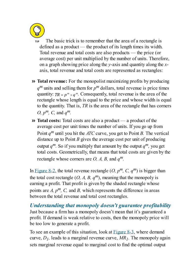
The basic trick is to remember that the area of a rectangle isdefined as a product — the product of its length times its width.Total revenue and total costs are also products — the price (oraverage cost) per unit multiplied by the number of units. Therefore,on a graph showing price along the y-axis and quantity along the x-axis, total revenue and total costs are represented as rectangles:

Total revenue: For the monopolist maximizing profits by producingqm units and selling them for pm dollars, total revenue is price timesquantity: . Consequently, total revenue is the area of therectangle whose length is equal to the price and whose width is equalto the quantity. That is, TR is the area of the rectangle that has cornersO, pm, C, and qm.Total costs: Total costs are also a product — a product of theaverage cost per unit times the number of units. If you go up fromPoint qm until you hit the ATC curve, you get to Point B. The verticaldistance up to Point B gives the average cost per unit of producingoutput qm. So if you multiply that amount by the output qm, you gettotal costs. Geometrically, that means that total costs are given by therectangle whose corners are O, A, B, and qm.

In Figure 8-2, the total revenue rectangle (O, pm, C, qm) is bigger thanthe total cost rectangle (O, A, B, qm), meaning that the monopoly isearning a profit. That profit is given by the shaded rectangle whosepoints are A, pm, C, and B, which represents the difference in areasbetween the total revenue and total cost rectangles.

Understanding that monopoly doesn’t guarantee profitabilityJust because a firm has a monopoly doesn’t mean that it’s guaranteed aprofit. If demand is weak relative to costs, then the monopoly price willbe too low to generate a profit.

To see an example of this situation, look at Figure 8-3, where demandcurve, D1, leads to a marginal revenue curve, MR1. The monopoly againsets marginal revenue equal to marginal cost to find the optimal output

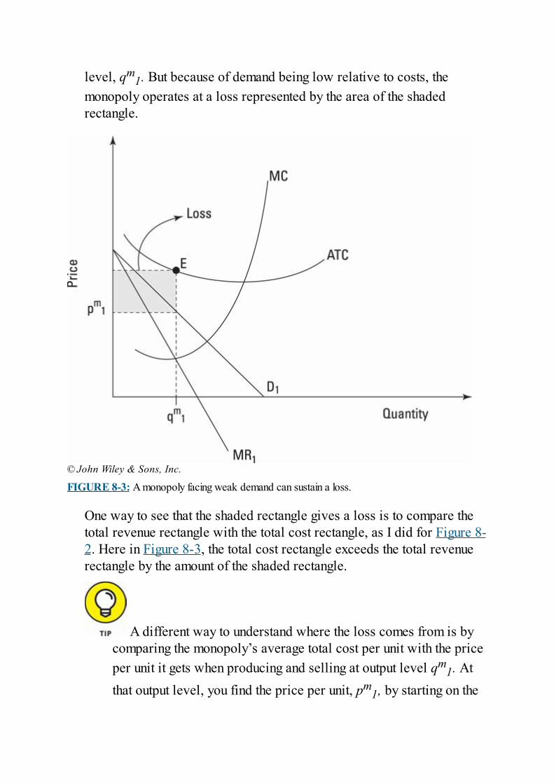
level, qm1. But because of demand being low relative to costs, the

monopoly operates at a loss represented by the area of the shadedrectangle.

© John Wiley & Sons, Inc.

FIGURE 8-3: A monopoly facing weak demand can sustain a loss.

One way to see that the shaded rectangle gives a loss is to compare thetotal revenue rectangle with the total cost rectangle, as I did for Figure 8-2. Here in Figure 8-3, the total cost rectangle exceeds the total revenuerectangle by the amount of the shaded rectangle.

A different way to understand where the loss comes from is bycomparing the monopoly’s average total cost per unit with the priceper unit it gets when producing and selling at output level qm

1. Atthat output level, you find the price per unit, pm

1, by starting on the

horizontal axis at qm1 and then going up to the demand curve. As

you can see, you have to go up even farther to get to the ATC curve,meaning that the average total cost per unit to make qm

1 unitsexceeds the price per unit you get from selling these units. This factimplies that the firm will lose money producing at output level qm

1.

As I show in Chapter 6, a firm in such a situation can’t do any better.That is, any other output level besides qm

1 would produce an evenbigger loss. If the monopoly can’t figure out a way to either reduce costsor increase demand, it will quickly go bankrupt.

Comparing Monopolies withCompetitive Firms

In this section, I compare a profit-maximizing monopoly with a profit-maximizing competitive firm. This comparison comes off very badly forthe monopoly because competitive firms deliver socially optimal outputlevels. Because monopolies always end up producing less thancompetitive firms, their output levels are always less than sociallyoptimal.

Looking at output and price levelsMonopolies produce less than competitive firms because they havedifferent marginal revenue curves. As I show earlier in the chapter,monopolies face downward-sloping marginal revenue curves. Bycontrast, competitive firms face horizontal marginal revenue curves.

You can see the comparison in Figure 8-4, where I’ve drawn in both thedownward-sloping marginal revenue curve of a monopoly, MRm, and thehorizontal marginal revenue curve of a competitive firm, MRC. Thegraph also has an average total cost curve, ATC, as well as a marginalcost curve, MC.

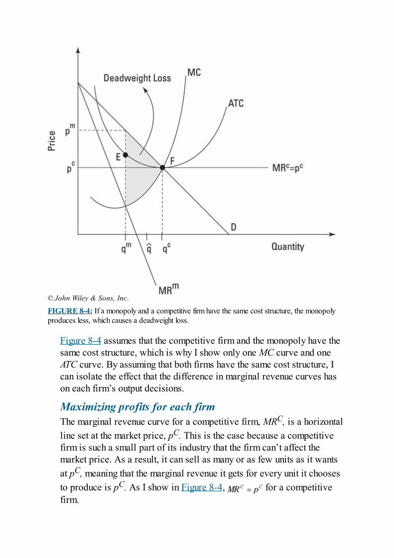
© John Wiley & Sons, Inc.

FIGURE 8-4: If a monopoly and a competitive firm have the same cost structure, the monopolyproduces less, which causes a deadweight loss.

Figure 8-4 assumes that the competitive firm and the monopoly have thesame cost structure, which is why I show only one MC curve and oneATC curve. By assuming that both firms have the same cost structure, Ican isolate the effect that the difference in marginal revenue curves hason each firm’s output decisions.

Maximizing profits for each firmThe marginal revenue curve for a competitive firm, MRC, is a horizontalline set at the market price, pC. This is the case because a competitivefirm is such a small part of its industry that the firm can’t affect themarket price. As a result, it can sell as many or as few units as it wantsat pC, meaning that the marginal revenue it gets for every unit it choosesto produce is pC. As I show in Figure 8-4, for a competitivefirm.

Market forces adjust supply and demand until the market price is equal tothe minimum average total cost at which a firm can produce.Geometrically, this means that the horizontal line just touchesthe bottom of the U-shaped ATC curve. (Refer to Chapter 7 for moreinformation.)

Monopolies and competitive firms follow the same basic rule tomaximize profits: They each produce where their marginal revenuecurve intersects their marginal cost curve. But because they havedifferent marginal revenue curves (as in Figure 8-4), they producedifferent outputs. The competitive firm produces qC, and themonopoly produces qm.

Understanding why the monopoly produces lessA competitive firm produces more than the monopolist because thecompetitive firm doesn’t have to worry about reducing its revenue perunit if it increases output. No matter how much it produces, it alwaysreceives on every unit sold because its output is too smallrelative to total output to affect the market price.

By contrast, the monopolist faces the market demand curve, meaning thatevery additional unit it sells lowers the price per unit that it receives onall units sold. Graphically, this appears as a downward-sloping MRm

curve that leads the monopoly to restrict output because it knows that themore it produces, the less money per unit it gets.

Because the monopoly restricts output compared to the competitive firm,the monopoly price, pm, is also higher than the competitive price, pC.This fact really irks consumers, but as I show you in the next section, thereal harm comes from the reduction in output.

Deadweight losses: Quantifying the harmcaused by monopoliesMonopolies cause harm because they reduce output below the sociallyoptimal level produced by competitive firms. Take a look at Figure 8-4and consider whether it would be good for society if all the units of

output between the monopoly output level, qm, and the competitive outputlevel, qC, were produced. For instance, look at unit q^. At that level ofoutput, the demand curve is above the marginal cost curve. That impliesthat people are willing to pay more for that unit of output than it costs tomake it. In other words, benefits exceed costs for that unit of output.Because this is true for all units between qm and qC, monopolies hurtsociety by failing to produce units of output for which benefits exceedcosts.

The harm caused to society when the monopoly fails to produce outputlevel q^ can be quantified as the vertical distance between the demandcurve and the marginal cost curve at output level q^. That verticaldistance is a dollar amount — the number of dollars by which benefitswould exceed costs for that unit if it was produced and consumed. If yougo through the same exercise for each and every unit between qm and qC,you can total up the harm caused by the failure of the monopoly toproduce all of those units. Graphically, the total harm measured indollars is equal to the area of the shaded deadweight loss region inFigure 8-4.

The deadweight loss region demonstrates that when monopolies restrictoutput in order to maximize their profits, they fail to produce units forwhich benefits exceed costs. That harms society.

Losing efficiencyAnother problem with monopolies is that they are not efficientproducers. You can see this in Figure 8-4. Competition leads competitivefirms to produce at qC, the output level that puts them at the bottom of theaverage total costs (ATC) curve. You can see this output level and cost asPoint F.

That output level minimizes production costs per unit of output,which you can see by comparing qC with any other output level.Whether you produce more or less than qC, average costs per unitwill be higher due to the U shape of the ATC curve.

In particular, look at the monopoly output level, qm. At that output level,you get to Point E on the ATC curve. Because the vertical distancebetween the horizontal axis and E is greater than the vertical distancebetween the horizontal axis and Point F, you know for certain that totalcosts per unit when producing the monopoly output level, qm, are higherthan those when producing the competitive output level, qC.Consequently, the monopoly is less efficient than the competitive firm —despite having identical costs.

This bad result is yet another example of monopolists facingdownward-sloping marginal revenue curves. The competitivefirm’s horizontal marginal revenue curve implies that it can sell asmany units as it wants at the competitive price pC. Consequently, thecompetitive firm has an incentive to increase output all the way toqC because doing so lowers per-unit production costs withoutreducing per-unit revenue. The same cost-reducing incentive existsfor a monopolist to increase its output; but the cost reduction ismore than offset by declining marginal revenue as the monopolymoves down along its downward-sloping marginal revenue curve.As a result, the monopolist’s profits are maximized at qm, eventhough qC is the lowest-cost output level.

Considering Good MonopoliesIn some cases, the benefits of monopolies actually outweigh their costs.This section takes a closer look at these instances, where the goal is toencourage innovation, cut redundancy, and keep costs low.

Encouraging innovation and investmentwith patentsThe most obvious place where monopolies do society a lot of good ispatents. Patents give inventors the exclusive right to market theirinventions for 20 years, after which time their inventions become publicproperty. That is, patents give inventors the right to run a monopoly for20 years.

Without patents, an inventor is unlikely to ever see any financialreward for her hard work because copycats will steal her idea andflood the market with rip-offs, thereby collapsing the price.Consequently, in a world without patents, far fewer people wouldbother to put in the time, effort, and money required to come up withnew inventions.

To remedy this situation, nations all over the world have establishedpatent offices to issue patents to inventors. The result is fasterinnovation, much more rapid economic growth, and much fasterincreases in living standards. Indeed, it’s hard to think of any moresocially beneficial monopolies than those that arise from patents.

Reducing annoyingly redundantcompetitorsSocieties have also stepped in to create monopolies in situations wherecompetition means annoying redundancies. Consider the followingexamples:

Trash hauling: Garbage trucks are extremely loud and annoying. Ifone company has a monopoly on hauling trash, you have to endure a

loud, annoying truck only once per week. But if, say, seven differenttrash-hauling companies compete, you may have to endure one eachday if you and six of your neighbors each choose to use a differentcompany that picks up on a different day of the week.Fiber-optic Internet access: If ten different companies offeringfiber-optic Internet access competed for your business,neighborhoods would have to have ten different sets of fiber-opticcables running through them — at much greater expense than runningjust one set of cables.Natural gas: Laying the pipes that deliver natural gas is expensive,and laying down multiple grids of gas pipe in one area would bewasteful.

Consequently, most towns and cities have decided that there will be onlyone trash-hauling company, one company laying fiber-optic cables, andone natural gas company. Each company is given a monopoly and is thenregulated to make sure that it doesn’t exploit customers. (See theupcoming “Regulating Monopolies” section.)

Keeping costs low with natural monopoliesAnother place where society may decide it’s better to have a monopolyrather than competition is in the case of what economists refer to asnatural monopoly industries, or natural monopolies. An industry is anatural monopoly if one large producer can produce output at a loweraverage cost per unit than many small producers. A good example iselectric power generation. Due to engineering constraints, a 10-megawattpower plant can produce energy at a far lower per-unit cost than a 1-megawatt power plant can.

To see how this leads to a natural monopoly, imagine that a town needing10 megawatts of power is initially served by ten of the small, 1-megawatt power plants. But then a big corporation comes along andbuilds a 10-megawatt power plant. Because the big plant can produce ata lower per-unit cost than the smaller, less efficient plants, the big plantoffers lower prices and steals all the customers — meaning that thesmaller plants quickly go bankrupt.

Such an industry is called a natural monopoly because it naturallybecomes dominated by a single, low-cost producer. The perplexing

problem here for policymakers is what to do with a natural monopoly.On one hand, everyone welcomes the fact that the big plant is much moreefficient: It burns less fuel and causes less environmental damage. Butbecause it has crushed all competition, people now have to worry thatthe new monopoly will charge high prices and produce less than thesocially optimal output level.

These conflicting good and bad points typically mean that governmentsallow the natural monopoly to stay in business as the only firm in itsindustry, but at the same time, they regulate it so that people don’t have toworry about high prices or low output levels. By doing so, society getsthe benefits brought by the most efficient production method withouthaving to worry about the problems that would otherwise result if themonopoly were left unregulated.

Regulating MonopoliesGovernments have to decide when to support and when to suppressmonopolies. For instance, patents support an inventor’s monopoly rightto produce and sell her invention for 20 years. After that, the productionand sale of the invention is thrown open to competition.

In other situations, various regulatory institutions have been developedeither to destroy a monopoly by breaking it apart or to regulate it afterdeciding to let it continue to be the only firm in its industry. In thissection, I present several of these regulatory schemes and explore whatthey do to improve the behavior of monopolies.

Subsidizing a monopoly to increase outputA profit-maximizing monopoly produces less than the socially optimallevel. In particular, a profit-maximizing monopoly produces where itsdownward-sloping marginal revenue curve, MRm, intersects its upward-sloping marginal cost curve, MC (see Figure 8-4). This output level, qm,is less than the socially optimal output level that would be produced by acompetitive firm, qC (for why, see “Comparing Monopolies withCompetitive Firms,” earlier).

One way to get the monopoly to produce more is to subsidize itsproduction costs so that the marginal cost curve in effect shiftsdown vertically. Doing so causes the marginal cost and marginalrevenue curves to meet at a higher level of output. And if thesubsidy is big enough, the monopoly can be induced to increaseoutput all the way to qC.

Some governments use this type of subsidy to get gas, electric, and phonecompanies to serve more people, especially poor people. If themonopoly firms’ costs of hooking up customers are subsidized, the firmsare willing to hook up more customers than they would without thesubsidy. Some people object to subsidizing a monopolist, so this sort ofsolution isn’t necessarily the most popular politically. But it is effectivein increasing output.

Imposing minimum output requirementsAnother way to get a monopoly to produce more is simply to order it toproduce more. For instance, in many areas telephone companies arerequired to provide land-line telephone service to everyone — even topeople who cannot pay for it themselves. (The idea is to make sure thateveryone is able to call for help if they have an emergency.) The same isoften true of companies that provide heating in the winter; in somejurisdictions, you can’t turn off someone’s heat for nonpayment of bills.

Minimum output requirements can force a monopoly to produce thesocially optimal output level. They are often very politically popularbecause many people think of monopolists as evil and exploitative anddon’t mind seeing them ordered to produce more.

Any forced increase in output also means a reduction in the monopoly’sprofit. Therefore, such programs are also popular because many peopleconsider a monopoly’s profits to be ill-gotten given the fact that the firmdoesn’t have to compete to earn them.

Regulators have to be careful, though, not to bankrupt the monopoliesthey are regulating. Depending on a monopoly’s cost curves, it’s quitepossible to force a monopoly to produce at an output level where it losesmoney. Because regulators don’t want to bankrupt monopolies and denyconsumers access to the products they produce, regulators are careful totake a monopoly’s cost structure into account when considering minimumoutput requirements.

Regulating monopoly pricingPerhaps the most common way to regulate a monopoly is to set the priceat which it can sell each and every unit of output that it produces. Thisapproach works because it changes the monopoly firm’s marginalrevenue curve from sloping downward to being horizontal. Therefore, iteliminates the monopoly’s usual problem that the more it sells, the less itcan charge per unit.

However, regulators have to pay close attention to a monopoly’s coststructure when choosing the regulated price so they don’t bankrupt themonopoly.

Marginal cost pricing: Benefit society but risk bankruptcy

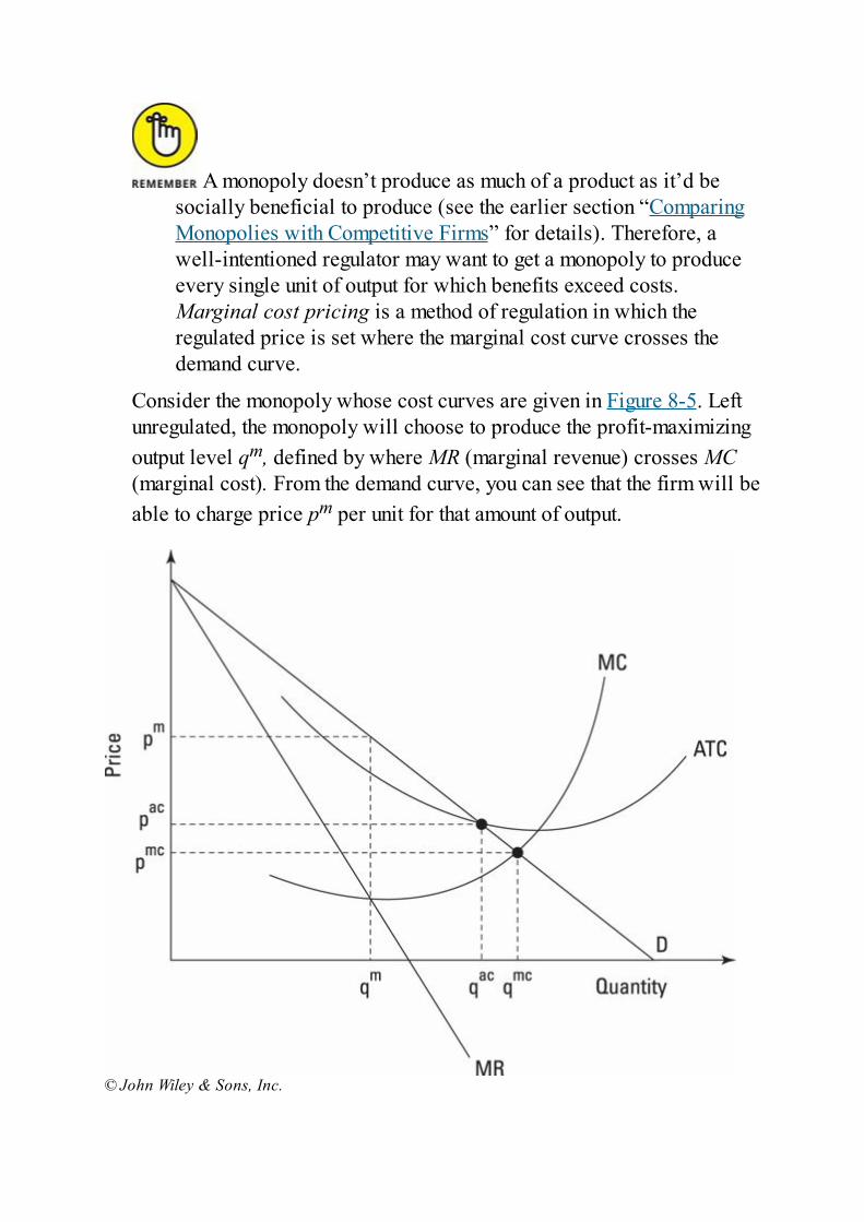
A monopoly doesn’t produce as much of a product as it’d besocially beneficial to produce (see the earlier section “ComparingMonopolies with Competitive Firms” for details). Therefore, awell-intentioned regulator may want to get a monopoly to produceevery single unit of output for which benefits exceed costs.Marginal cost pricing is a method of regulation in which theregulated price is set where the marginal cost curve crosses thedemand curve.

Consider the monopoly whose cost curves are given in Figure 8-5. Leftunregulated, the monopoly will choose to produce the profit-maximizingoutput level qm, defined by where MR (marginal revenue) crosses MC(marginal cost). From the demand curve, you can see that the firm will beable to charge price pm per unit for that amount of output.

© John Wiley & Sons, Inc.

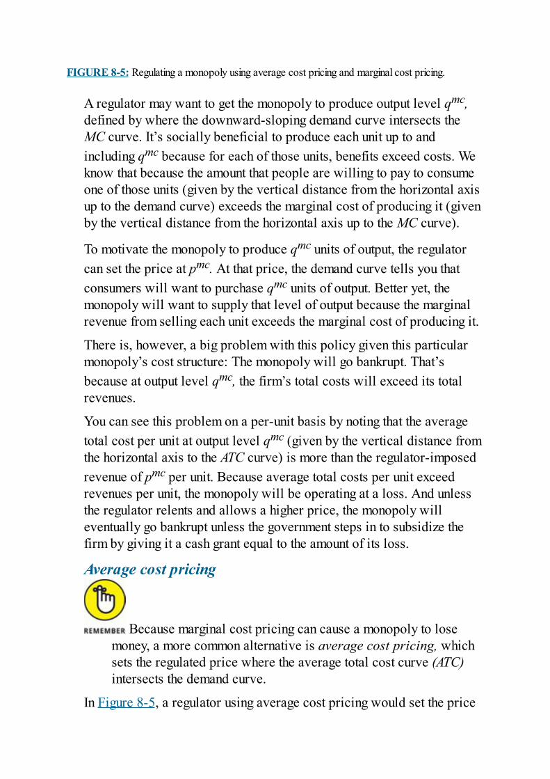
FIGURE 8-5: Regulating a monopoly using average cost pricing and marginal cost pricing.

A regulator may want to get the monopoly to produce output level qmc,defined by where the downward-sloping demand curve intersects theMC curve. It’s socially beneficial to produce each unit up to andincluding qmc because for each of those units, benefits exceed costs. Weknow that because the amount that people are willing to pay to consumeone of those units (given by the vertical distance from the horizontal axisup to the demand curve) exceeds the marginal cost of producing it (givenby the vertical distance from the horizontal axis up to the MC curve).

To motivate the monopoly to produce qmc units of output, the regulatorcan set the price at pmc. At that price, the demand curve tells you thatconsumers will want to purchase qmc units of output. Better yet, themonopoly will want to supply that level of output because the marginalrevenue from selling each unit exceeds the marginal cost of producing it.

There is, however, a big problem with this policy given this particularmonopoly’s cost structure: The monopoly will go bankrupt. That’sbecause at output level qmc, the firm’s total costs will exceed its totalrevenues.

You can see this problem on a per-unit basis by noting that the averagetotal cost per unit at output level qmc (given by the vertical distance fromthe horizontal axis to the ATC curve) is more than the regulator-imposedrevenue of pmc per unit. Because average total costs per unit exceedrevenues per unit, the monopoly will be operating at a loss. And unlessthe regulator relents and allows a higher price, the monopoly willeventually go bankrupt unless the government steps in to subsidize thefirm by giving it a cash grant equal to the amount of its loss.

Average cost pricing

Because marginal cost pricing can cause a monopoly to losemoney, a more common alternative is average cost pricing, whichsets the regulated price where the average total cost curve (ATC)intersects the demand curve.

In Figure 8-5, a regulator using average cost pricing would set the price

at pac. At that price, you can see from the demand curve that consumersdemand qac units of output. The monopoly is happy to supply that outputlevel because for each and every unit up to qac, marginal revenue (theregulated price per unit, pac) exceeds marginal cost — meaning that themonopoly gains financially by producing each and every one of theseunits.

The main benefit of this system is that you don’t have to worry about themonopoly’s going bankrupt (or where to get the money to subsidize amonopoly that would go bankrupt under marginal cost pricing). Averagecost pricing guarantees that the monopoly will break even.

You can see this fact by comparing the average total costs per unit atoutput level qac with the revenue per unit at that output level. You get theaverage total cost per unit by going up until you hit the average total costcurve. Because that vertical distance is equal to the regulated price perunit, pac, you know that the average total costs per unit are equal to theregulated price per unit — so the firm must be breaking even.

The downside to average cost pricing for this monopoly is that all thesocially beneficial units between qac and qmc don’t get produced. On theother hand, the only way to keep this monopoly in business to producethose units if you imposed marginal cost pricing would be to subsidize it.Using average cost pricing eliminates any worries associated withproviding subsidies. In particular, you don’t have to worry about anypotential harm that you may cause when raising the taxes that have to beimposed somewhere else in the economy in order to subsidize themonopoly.

Breaking up a monopoly into severalcompeting firmsOne solution to the problem of a monopoly is to destroy it by breaking itup into many competing firms. In the United States, the most famous caseof this solution was the division of American Telephone and TelegraphCorporation (AT&T) into a bunch of smaller competitors in 1984.

Before 1984, AT&T was a nationwide monopoly. If you wanted to makea telephone call anywhere in the United States, you had to use AT&Tbecause it was the only telephone company in the country. It was highly

regulated, with both quantity requirements to provide everyone a phoneand price requirements that encouraged it to provide a high quantity oftelecommunication services. But it was still a monopoly, and a judgeruled in 1984 that it should be broken up into numerous local firms inorder to foster competition.

The policy change worked extremely well. There was soon a verycompetitive market for telephone services between firms that had beenpart of AT&T. More recently, the telephone service industry has becomeeven more competitive due to the arrival of cellphone companies,Internet telephony companies, and even cable TV companies offeringphone services. This robust competition eliminates the problemsassociated with monopolies and ensures that telecommunication servicesare provided at low cost and in large quantity.

Creating competition is also a handy way to deal with a monopolybecause it eliminates the costs associated with having to continuallymonitor a regulated monopoly. Competition gets you to the sociallyoptimal output level without any sort of central control (for info on why,see Chapter 7). That stands in stark contrast to regulated monopolies,which typically require expensive bureaucracies to develop and enforcelaws and regulations.

Chapter 9

Oligopoly and MonopolisticCompetition: Middle

GroundsIN THIS CHAPTER

Deciding whether to compete or collude in an oligopoly Examining why some collusive pacts work and others don’t Regulating firms so they can’t collude Using product differentiation to elude perfect competition Limiting profits in monopolistic competition

The two most extreme forms that an industry can take are perfectcompetition (with many small competitive firms) and monopoly (wherethere’s only one firm and hence no competition). I cover those cases inChapters 6 and 8. This chapter concentrates on two interestingintermediate cases: oligopoly and monopolistic competition.

An oligopoly is an industry in which there are only a small number offirms — two, three, or a handful. The word itself is Greek for “fewsellers.” A diverse group of industries looks like this, including softdrinks and oil production. For instance, Coke and Pepsi dominate thesoft drink market, vastly outselling other carbonated beverages.Similarly, just four or five countries produce the majority of the world’soil.

Oligopoly industries are interesting because depending on specificcircumstances, the firms can either compete ruthlessly with each other orunite to behave almost exactly like a monopoly would. This means that insome cases, oligopolies can be left alone because competition ensuresthat they produce socially optimal output levels; in other cases,government regulation is needed to prevent them from acting likemonopolies and behaving in socially undesirable ways.

The second type of intermediate industry is monopolistic competition, asort of hybrid between perfect competition and monopoly. The key thingthat sets firms in this type of industry apart from firms in a perfectlycompetitive industry is product differentiation — the fact that each firmproduces a slightly different product than the others.

This chapter starts with a detailed look at oligopolies and the decisionsthat firms in this type of industry have to make. I then move on tomonopolistic competition and show why product differentiation doesn’tnecessarily translate into tidy profits.

Oligopolies: Looking at theAllure of Joining Forces

In industries where only a few firms operate, firms have a choice aboutwhether to compete or cooperate. This situation is very different fromperfect competition (which I discuss in Chapter 7). In perfectlycompetitive markets, there are so many firms, and each firm is such asmall part of the market, that their individual outputs don’t have anyeffect on the market price. As a result, competitive firms just take themarket price as given and adjust their output levels accordingly to makeas large a profit as possible.

However, in a market in which there are only a few sellers, each oneproduces enough of the total output to be able to affect the market price.Each company can increase output and lower its own price in an attemptto gain more customers at the expense of its rivals, or the firms can worktogether to limit production and keep prices high to maximize theircombined profits. This section explores the firms’ incentives to worktogether and the possible benefits of acting like a monopoly. Later, in“Understanding Incentives to Cheat the Cartel,” I explain why collusionusually doesn’t go as planned.

Sharing power over pricesWhen only a few firms are in an industry, the decisions that any one firmmakes about how much to produce or charge for its own output almostalways affect the outputs and prices of the other firms in its industry.

As an example, consider that only two major producers of cola-flavoredsodas operate in the United States: the Coca-Cola Company andPepsiCo. These two corporations produce such large fractions of thetotal output that if either one were to suddenly increase supply, themarket price of cola-flavored soda would drop dramatically. Onecompany’s increase in output causes the price to decrease for othercompanies in the market as well.

In other words, if Pepsi produces twice as much of its product andfloods the market, the price of Pepsi will drop dramatically. But mostpeople aren’t 100 percent loyal to one brand or the other, so if the price

of Pepsi drops dramatically, a lot of regular Coke drinkers are going toswitch brands and drink Pepsi. As a result of this decline in the demandfor Coke, the price of Coke will drop, too.

Cartel behavior: Trying to imitatemonopolists

When firms are involved in a situation where each of theirsupply decisions affects not only their own sales but those of theircompetitors as well, economists say the firms are in a strategicsituation because the firms involved have to decide which type ofstrategy to pursue. In particular, they have to decide whether tocompete or collude:

Compete: If they compete, they’ll both try to increase production toundercut each other on price and capture as many customers aspossible.Collude: If they collude, they’ll jointly cut back on production todrive up prices and increase their profits. For producers, collusion isbetter than competition because it leads to profits that last as long asthe firms keep colluding.

A group of firms that colludes and acts as a single coordinated whole isknown as a cartel. Because a cartel acts essentially as one gigantic firm,it effectively turns a bunch of individual firms into a single bigmonopoly.

This fact makes understanding the profit-maximizing behavior of a carteleasy, because it’s just like that of a monopoly. In fact, you can see what acartel wants to do by looking at the figures in Chapter 8, which illustratewhat a monopoly likes to do. In particular, a profit-maximizing cartelchooses to produce the monopoly’s profit-maximizing output level of qm

units (where marginal cost equals marginal revenue), as in Figure 8-2.Producing that output level maximizes the cartel’s collective profit. Andbetter yet for the cartel, that monopoly profit will persist as long as theparticipating companies keep cooperating and producing a combined

output of qm.

What’s really interesting, though, is that cartels often fail to maximizetheir collective profit because they can’t sustain the cooperation neededto keep their collective output at the monopoly output level qm.

Considering the criteria for coordinating acartelFor consumers, collusion is worse than competition because it leads tohigher prices and lower output. You may assume that governmentintervention is called for in order to protect consumers from collusion.But such intervention is needed only if firms actually collude.

A fascinating thing about the real world is that collusion doesn’t happenin a lot of industries where you might expect it to. For instance, Coke andPepsi are fierce competitors that spend billions of dollars a year onadvertising to try to steal each other’s customers. Similarly, most citieshave only a handful of competing cellphone networks. But instead ofcolluding, they compete so ruthlessly that many of them are constantlyflirting with bankruptcy. The same holds true for the airline industry,where bankruptcies are routine.

The big question that economists have to answer is “Why do wesee so little collusion in industries where you would expect more ofit?” The answer is that it’s often very difficult to get all the firms tocoordinate so they’re collectively producing the monopoly outputlevel, qm. To get the individual firms to cooperate and produceexactly qm units of combined output, you have to get them to agreeon two related things:

How to share the profits: Obviously, every firm wants as large ashare as possible.Output quotas: The firms must agree, and abide by, how much of thetotal output (qm) each firm will produce. Each firm will constantly betempted to produce more than its quota because doing so would bringhigher revenues.

Understanding Incentives toCheat the Cartel

To the extent that cartels work and create monopoly profits, they alsocreate temptations for cartel members to cheat. You can best understandthe behavior of cartels and their incentive to cheat using the insights ofgame theory.

Game theory is a branch of mathematics that studies how people behavein strategic situations — situations in which people take account ofothers’ actions or anticipated actions and then modify their own actionsaccordingly. For instance, chess and checkers are strategic situationsbecause what I do on my current move changes what my opponent doesin subsequent moves. Even more importantly, what I think my opponentwill do in response to each of the moves that I may make right now helpsme to choose the best thing to do.

Cartels are strategic situations because each firm has to take into accountwhat it thinks all the other firms are going to do before deciding what itshould do. Consequently, game theory models are probably the best wayto understand the motivations and temptations that guide the behavior ofcartel members. This section introduces a game theory model called thePrisoner’s Dilemma to explore decisions about whether to cheat. It thenapplies the model to the OPEC oil cartel.

Fleshing out the Prisoner’s DilemmaUnderstanding why cartels cheat is easy if you apply the Prisoner’sDilemma. The Prisoner’s Dilemma is a game theory model in which twocriminal partners have to individually decide whether to cheat on theirprevious agreement to not talk to the police.

It works in this way: Imagine Jesse and James have just robbed a bank.The police know this but don’t have any hard evidence against them.Rather, the only way of getting a conviction is to get one or both of thebank robbers to confess to the crime and give evidence against the other.Fortunately for the police, they do have some leverage because theymanaged to catch Jesse and James committing other unrelated, minorcrimes. These other crimes carry with them a one-year prison sentence.

The police are hoping to use the threat of a year in prison to get one orboth of the bank robbers to implicate his partner in exchange forimmunity from prosecution.

Jesse and James both swore to each other several days before that they’dnever rat on each other, but what happens when push comes to shove?

Comparing the payoffs of confessing or remaining silentFollowing standard procedure, the police separate Jesse and James,questioning them in separate interrogation rooms. The police offer eachof them the chance to give evidence against the other in exchange forimmunity.

The problem for each man is that what happens to him dependsnot only on what he does but on what his partner does as well. Eachman can trade a confession for immunity, but he gets the deal only ifhis partner doesn’t confess at the same time in the otherinterrogation room. Four outcomes are possible:

Both stay silent. If the men both keep their pact not to talk andneither confesses to robbing banks, each man gets only a year in jailfor the minor offense.Only Jesse confesses and gives evidence. If Jesse confesses andagrees to give evidence against James while James remains silent,Jesse goes free because he cooperated with police, but James getsten years for bank robbery.Only James confesses and gives evidence. If James gives evidencewhile Jesse remains silent, James goes free while Jesse goes toprison for ten years.Both confess and give evidence. If both men admit to the crime,both get five years in prison. Why five years each? If both confess,the police don’t need to make such a generous deal; they don’t needto give either man immunity in order to get evidence against the other.On the other hand, the police want to give each criminal an incentiveto confess, so they send each man to prison for only five yearsinstead of the ten years he’d get if he remained silent while hispartner gave evidence.

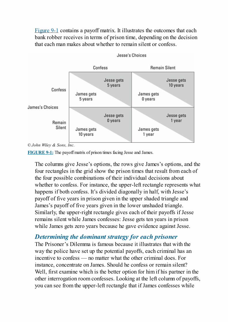
Figure 9-1 contains a payoff matrix. It illustrates the outcomes that eachbank robber receives in terms of prison time, depending on the decisionthat each man makes about whether to remain silent or confess.

© John Wiley & Sons, Inc.

FIGURE 9-1: The payoff matrix of prison times facing Jesse and James.

The columns give Jesse’s options, the rows give James’s options, and thefour rectangles in the grid show the prison times that result from each ofthe four possible combinations of their individual decisions aboutwhether to confess. For instance, the upper-left rectangle represents whathappens if both confess. It’s divided diagonally in half, with Jesse’spayoff of five years in prison given in the upper shaded triangle andJames’s payoff of five years given in the lower unshaded triangle.Similarly, the upper-right rectangle gives each of their payoffs if Jesseremains silent while James confesses: Jesse gets ten years in prisonwhile James gets zero years because he gave evidence against Jesse.

Determining the dominant strategy for each prisonerThe Prisoner’s Dilemma is famous because it illustrates that with theway the police have set up the potential payoffs, each criminal has anincentive to confess — no matter what the other criminal does. Forinstance, concentrate on James. Should he confess or remain silent?Well, first examine which is the better option for him if his partner in theother interrogation room confesses. Looking at the left column of payoffs,you can see from the upper-left rectangle that if James confesses while

Jesse confesses, James gets five years. On the other hand, the bottom-leftrectangle tells you that if James remains silent while Jesse confesses,James gets ten years.

Clearly, the best thing for James to do if Jesse confesses is to alsoconfess. But consider whether it’s better for James to confess or remainsilent when Jesse remains silent in the other interrogation room. Beginwith the upper-right rectangle, which shows that if James confesseswhile Jesse remains silent, James gets zero years in jail. By contrast, thebottom-right rectangle tells you that if James remains silent while Jesseis also silent, James gets one year in jail. Clearly, if Jesse remains silent,the best thing for James to do is confess and get zero years in jail ratherthan one year.

In other words, it’s always better for James to confess. If Jamesconfesses when Jesse confesses, James gets five years rather than ten.And if James confesses when Jesse remains silent, James gets zero yearsrather than one. So James should always confess no matter what Jesse issaying or not saying to the police in the other room. Because the payofffor confessing is always better for him than the payoff for not confessing,game theorists refer to confessing as James’s dominant strategy, bywhich they mean superior strategy.

If you go through the payoffs from Jesse’s perspective, you find thatconfessing is also Jesse’s dominant strategy, because no matter whatJames is doing, the payoffs to Jesse if he confesses are always betterthan those from remaining silent.

Confessing is thus a dominant strategy for both players — you shouldexpect both of them to separately confess. If they do so, they end up in theupper-left box of the payoff matrix, where they both get five years inprison.

Realizing that the dominant strategy leads to a lousyoutcome for both playersTypically, both men go with their dominant strategy and confess. Butbecause both separately decide to confess, they each end up getting fiveyears in prison — a much worse outcome than if they had both kept theirpromise to each other to remain silent. If they had both kept theirpromise, they each would’ve gone to jail for only one year. The logic ofthe dominant strategy is so compelling, though, that they each break the

agreement and end up going to prison for five years rather than one.

Cartel members also face a Prisoner’s Dilemma because theymust decide whether to obey the cartel agreement (to reduce outputto the monopoly level) or cheat and overproduce. The temptationfor cartel members to overproduce and break their cartel outputagreement is just as strong as the temptation for prisoners to confessand break their agreement not to talk to the police.

Enforcing the agreement: Resolving thedilemma with credible threats

One way to get a pair of criminals to stay quiet — or to get agroup of firms to stick to a cartel agreement — is to set up a strongthreat against cheaters.

Mafia movies illustrate a bloodthirsty but effective system that mobstersdeveloped to prevent people from confessing. The system is calledomerta, which is Sicilian for “silence.” Basically, what the mafia doesis change the payoffs to the Prisoner’s Dilemma so that the dominantstrategy switches from confessing to remaining silent. The mob does thisby explaining to their criminal members that if they talk to the police andconfess to anything or implicate anyone else, they’re going to die.

The mafia also makes sure that everyone knows that this threat iscredible and not just talk. Otherwise, the mafia’s members wouldn’t altertheir behavior.

The mafia’s credible death threat totally rearranges the payoffs to thePrisoner’s Dilemma. Instead of just comparing prison times, as in Figure9-1, prisoners now have to factor in death, as in Figure 9-2. In Figure 9-2, you find that the dominant strategy for both players is now to remainsilent because if either talks, the mafia will hunt him down and kill himno matter what the other guy does. The result is that both Jesse and Jameswill go to prison for only one year each because they’ll both keep theirmouths shut.

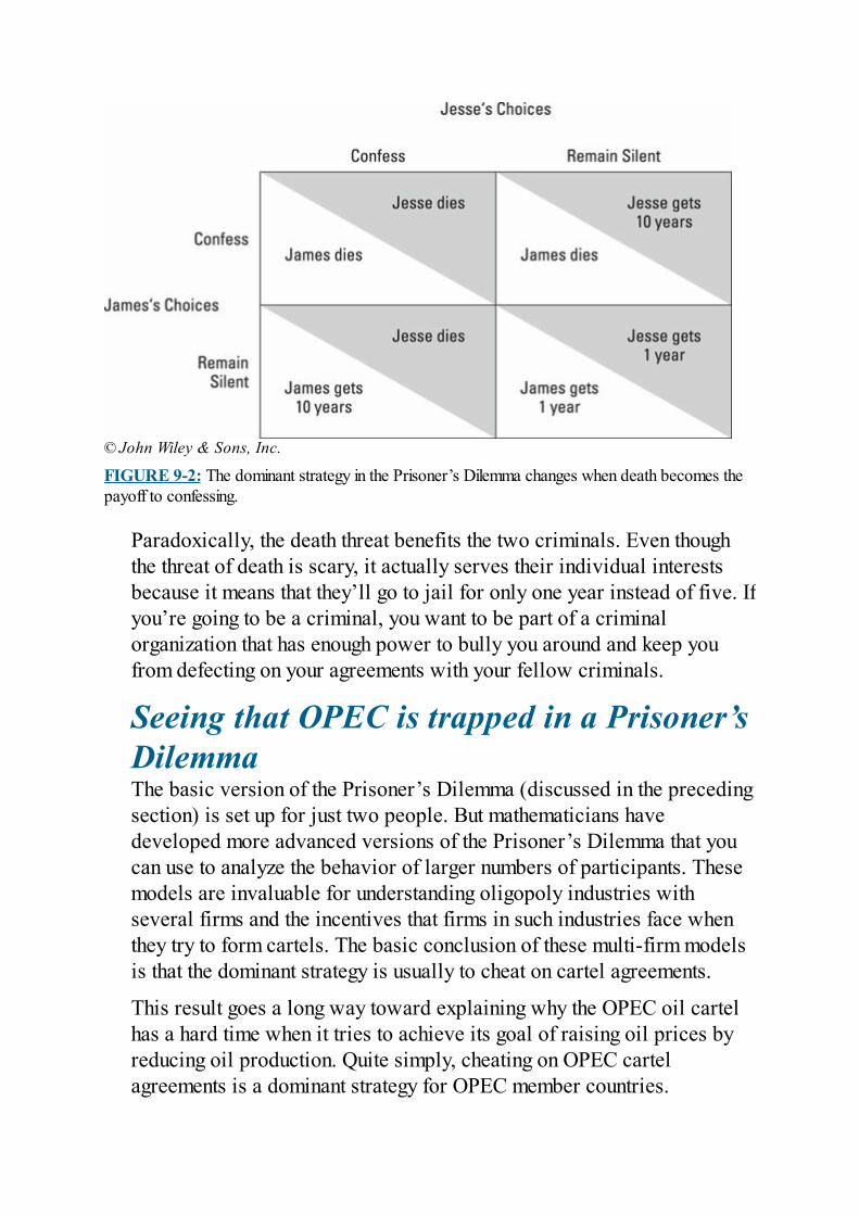
© John Wiley & Sons, Inc.

FIGURE 9-2: The dominant strategy in the Prisoner’s Dilemma changes when death becomes thepayoff to confessing.

Paradoxically, the death threat benefits the two criminals. Even thoughthe threat of death is scary, it actually serves their individual interestsbecause it means that they’ll go to jail for only one year instead of five. Ifyou’re going to be a criminal, you want to be part of a criminalorganization that has enough power to bully you around and keep youfrom defecting on your agreements with your fellow criminals.

Seeing that OPEC is trapped in a Prisoner’sDilemmaThe basic version of the Prisoner’s Dilemma (discussed in the precedingsection) is set up for just two people. But mathematicians havedeveloped more advanced versions of the Prisoner’s Dilemma that youcan use to analyze the behavior of larger numbers of participants. Thesemodels are invaluable for understanding oligopoly industries withseveral firms and the incentives that firms in such industries face whenthey try to form cartels. The basic conclusion of these multi-firm modelsis that the dominant strategy is usually to cheat on cartel agreements.

This result goes a long way toward explaining why the OPEC oil cartelhas a hard time when it tries to achieve its goal of raising oil prices byreducing oil production. Quite simply, cheating on OPEC cartelagreements is a dominant strategy for OPEC member countries.

OPEC stands for the Organization of Petroleum Exporting Countries.Although OPEC is a dull name, it represents a very lively group thatincludes Saudi Arabia, Iraq, Venezuela, Nigeria, Kuwait, Angola, andseveral other key oil-exporting nations. Together, these nations controlthe vast majority of the world’s oil reserves, meaning that they occupy anoligopoly industry with only a few firms. Because there are only a fewfirms, they have a chance to form a cartel and try to produce themonopoly output and make monopoly profits. Do they succeed?

On the whole, no. I say “on the whole” because although the nations donegotiate agreements about oil production, these agreements areconstantly broken. To see why that happens, you have to first understandthat OPEC has meetings where it decides how much total oil should beproduced and what fraction of that overall amount should be produced byeach country. At the meetings, each country is given a quota — amaximum amount that it’s supposed to produce. For instance, SaudiArabia may have a quota of 10 million barrels per day, whereas forVenezuela it’s 1 million barrels per day.

The problems start after the meetings when all the oil ministers go home.Each country realizes that producing more than its quota is the beststrategy. For instance, Venezuela is better off producing more than its 1million barrels a day quota no matter what the other countries do:

If the other countries obey their quotas, Venezuela is better offproducing more than its quota because it can sell lots of oil at a highprice. (The high price is caused by the fact that the other countriesare obeying their quotas.)If the other countries break their quotas and overproduce, the price ofoil will be low, meaning that Venezuela should also overproduce itsquota. There is no reason to obey the quota if prices are low due toeveryone else’s cheating.

Because each country faces the same temptation to overproduce itsquota, the OPEC cartel doesn’t typically work very well. Overproducingis a dominant strategy and is simply too tempting to resist given thepayoffs.

Using an enforcer to help OPEC members

stick to quotas

OPEC could benefit if it had some way of threatening itsmembers for violating their quotas. Because the member countriesare sovereign nations, death threats aren’t an option as they are inthe mafia. Rather, Saudi Arabia has sometimes tried to provide aneconomic threat against quota violators.

The economic threat comes in the form of super low oil prices. SaudiArabia is in the best position to make such a threat for two reasons:

It’s always been the world’s first or second largest oil producer.Saudi Arabia produces about 13 percent of the world’s oil, just a bitbehind the United States, which produces about 15 percent of theworld’s oil.It’s the world’s lowest-cost oil producer. Saudi Arabia can produceprofitably even if the price of oil falls down to $9 per barrel. (Oil istypically priced at between $40 and $100 per barrel, and most othercountries, including the United States, need a price of at least $20 perbarrel to break even.)

These two facts mean that if other countries cheat on their quotas, SaudiArabia could potentially increase its production so much that the price ofoil would fall very low. For instance, suppose the price fell to $9 perbarrel. Saudi Arabia would be the only OPEC member making a profit atthat price; everyone else would be losing money.

As a result, Saudi Arabia appears to be in a position to threaten otherOPEC members with bankruptcy if they violate their quotas.Unfortunately, the threat doesn’t work that well in the real world. Theproblem is that Saudi Arabia has limited pumping capacity. AlthoughSaudi Arabia may be able to produce an extra 10 or 20 percent more oilper day than it normally does, that much of an increase wouldn’t beenough to drive the price down to $9 per barrel and bankrupt the otherOPEC nations. Therefore, the Saudi Arabian threat isn’t nearly strongenough to switch the dominant strategy from cheating on the quota toobeying it. And because OPEC has never figured out a way to effectively

threaten quota violators, the cartel doesn’t work very well.

Regulating OligopoliesIn some industries, cartels are effective at reducing output and raisingprices. Typically, these are industries where one firm is large enough andpowerful enough to truly threaten other firms with bankruptcy.

In some cases, the industry will be broken up into even more firms topromote competition, but in others, regulations may be installed thatregulate the prices firms can charge or the quantities they can produce.The specific policy often depends intimately on the circumstances of thefirms in the industry and what policymakers think will best promote thegeneral welfare.

Breaking up dominant firmsOne important strategy for regulating an oligopoly is for the governmentto break it up into many smaller companies that will then compete witheach other. In the 19th century, cartels were called trusts — for example,the Sugar Trust, the Steel Trust, the Railroad Trust, and so on. Therefore,laws that broke up monopolies and cartels were called antitrust laws.The most famous of these in the United States was the Sherman Anti-Trust Act. Most countries have now passed similar legislation to breakup monopolies and cartels.

In U.S. history, the Standard Oil Company run by John D. Rockefellerduring the 19th century dominated an oligopoly industry. It controlledsomething like 90 percent of the oil sold in the United States, and if acompetitor didn’t do what Rockefeller wanted, he would simplybankrupt the other firm by offering oil at a ridiculously low price that thecompetitor couldn’t match.

Rockefeller would lose money temporarily while taking this action, butby bankrupting the competitors who disobeyed him, he was able toconvince the remaining firms to help him restrain output and make hugeprofits. Indeed, because Standard Oil exerted so much control, itsindustry was much more like a monopoly than an oligopoly.

Rockefeller’s effectiveness, however, soon brought a governmentalresponse. Standard Oil was broken up into dozens of smaller,independent oil companies, none of which was large enough and

powerful enough to dominate its industry and enforce collusion the waythat Standard Oil had.

Attempting to apply antitrust lawsA big problem with antitrust laws is deciding when to regulateoligopolies or break them up to promote competition. The first sign thatthere may potentially be a cartel is, of course, when you see only a fewfirms in an industry. But because of the Prisoner’s Dilemma, in somecases even a two-firm industry won’t be able to form an effective cartel.Consequently, prosecutors typically have to do more than just show thatthere aren’t many firms in an industry.

Typically, there has to be concrete proof of collusion. In otherwords, if one day every firm in an oligopoly industry decideswithout coordination to cut its output in half and thereby raiseprices, that may not be illegal. But if even a single text messagefrom a manager of one firm to a manager of another firm is foundsaying that the firms should enter into a cartel, that is illegal andenough for a prosecutor to hang a case on.

Studying a Hybrid: MonopolisticCompetition

An interesting form of competition that’s found in some industries has theodd name of monopolistic competition. In such industries, you findcharacteristics of both monopolies (see Chapter 8) and competitive firms(see Chapter 7). This section provides an overview of monopolisticcompetition.

Benefiting from product differentiationLike competitive firms operating in free markets, industries featuringmonopolistic competition have lots of firms competing against eachother. But unlike competitive free markets where all the firms sell anidentical product, in monopolistic competition each firm’s product isslightly different.

Think of the market for gasoline. Any large city has dozens, if nothundreds, of gas stations — all selling gasoline that is pretty much thesame. But if you look at each gas station with a little wider scope, younotice that each one sells a product that’s at least slightly different fromthe products sold by its competitors. For instance, some stations havemini-marts, and others have car washes or provide fuel with specialadditives designed to improve engine performance. And crucially, eachgas station is clearly differentiated from all the others because it has aunique location — something that’s very important to people who livenearby.

Economists use the term product differentiation to describe thethings that make each firm’s product a little bit different from itscompetitors’ products. The overall result of these differences is thatthey slightly decrease the intensity of competition. Your local gasstation, for instance, may be able to get away with charging you oneor two cents more per gallon than its competitors if it has nicefacilities and the next-closest competitor is several miles away.

On the other hand, there’s still a lot of competitive pressure in theindustry. Although your local station may be able to use its uniquecharacteristics to get away with charging you a little more, it couldn’tcharge you a lot more — if it tried to do that, you’d take your business toone of its competitors.

Similarly, all the restaurants in your neighborhood have to worry aboutwhat the other restaurants are charging, even if the others specialize incompletely different cuisines. Although you may be willing to pay 20percent more for something exotic, you wouldn’t likely be willing to pay90 percent more. Product differentiation lessens but does not eliminateprice competition.

Facing profit limitsYou may think that because monopolistically competitive firms can usetheir unique characteristics to raise prices, they’re guaranteed nice profitmargins. After all, in pure competition where firms all sell the sameproduct and have no way of differentiating themselves from theircompetitors, prices fall so low that firms end up earning zero economicprofits (see Chapter 7). If monopolistically competitive firms can raiseprices above the competitive price, it seems like a no-brainer that theyshould be guaranteed to make profits. Unfortunately for them, this isn’tthe case.

As pointed out by Cambridge economist Joan Robinson duringthe 1930s, monopolistically competitive firms still facecompetition. In particular, they face the prospect that if they’remaking tidy profits, those profits attract new entrants to theirindustry. When the new entrants begin producing, they take businessaway from the established firms and ruin their previously tidyprofits. In fact, new entrants continue to arrive until profits havebeen driven all the way back to zero.

Dealing with downward sloping demandJoan Robinson was able to show how this process works by slightlymodifying the monopoly model that I introduce in Chapter 8. To see whatshe did, look at Figure 9-3, which shows a single monopolistically

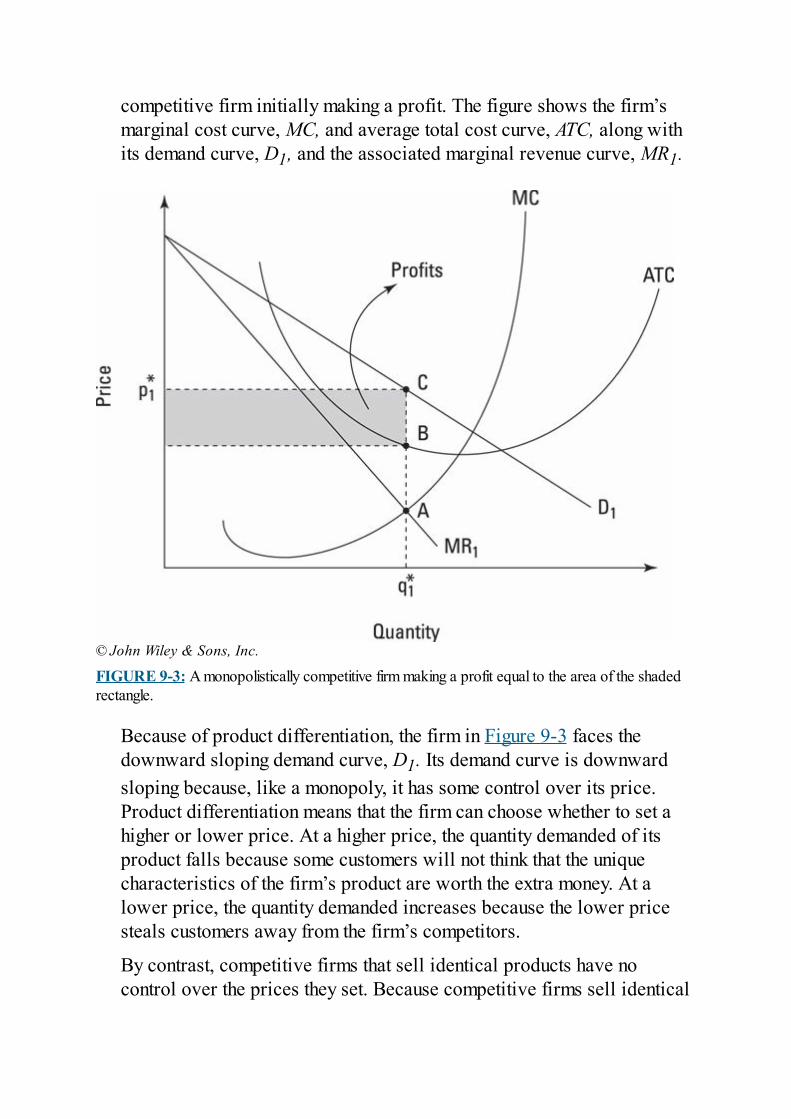
competitive firm initially making a profit. The figure shows the firm’smarginal cost curve, MC, and average total cost curve, ATC, along withits demand curve, D1, and the associated marginal revenue curve, MR1.

© John Wiley & Sons, Inc.

FIGURE 9-3: A monopolistically competitive firm making a profit equal to the area of the shadedrectangle.

Because of product differentiation, the firm in Figure 9-3 faces thedownward sloping demand curve, D1. Its demand curve is downwardsloping because, like a monopoly, it has some control over its price.Product differentiation means that the firm can choose whether to set ahigher or lower price. At a higher price, the quantity demanded of itsproduct falls because some customers will not think that the uniquecharacteristics of the firm’s product are worth the extra money. At alower price, the quantity demanded increases because the lower pricesteals customers away from the firm’s competitors.

By contrast, competitive firms that sell identical products have nocontrol over the prices they set. Because competitive firms sell identical

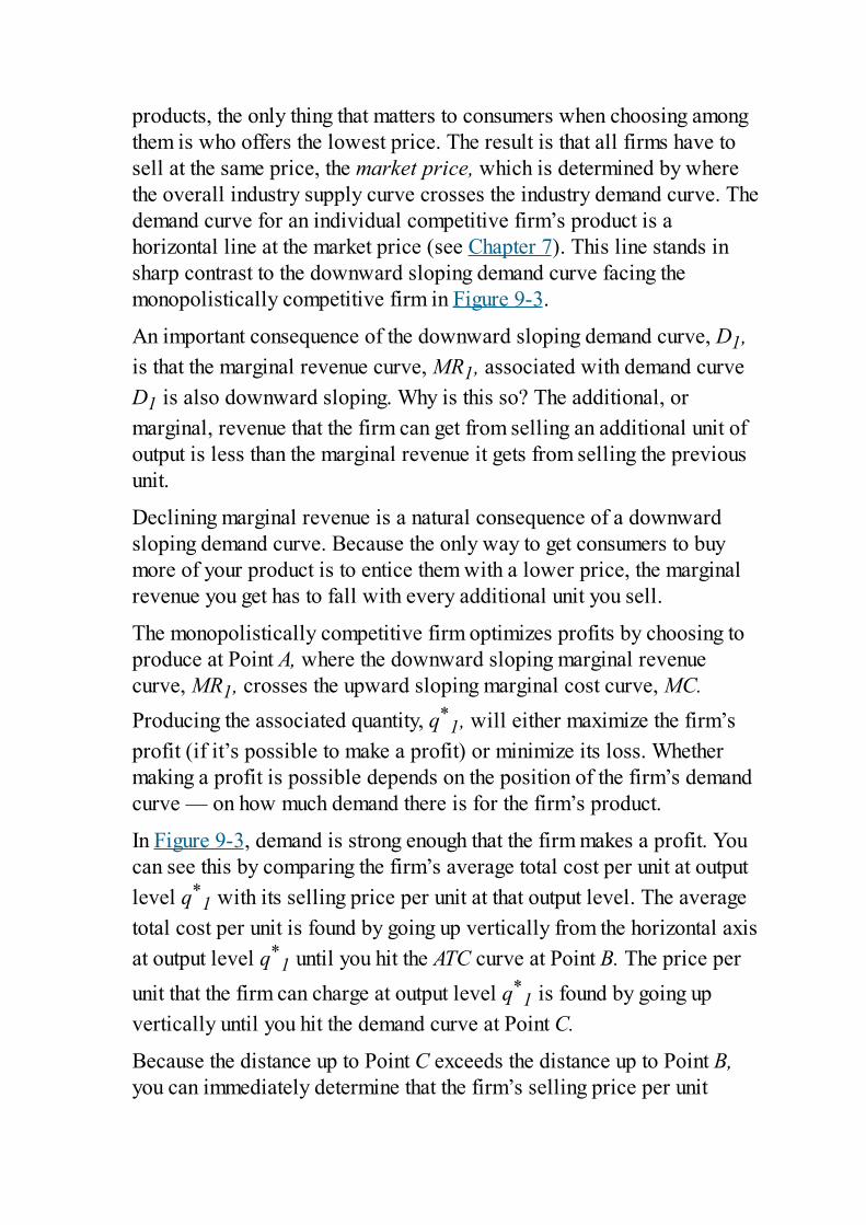
products, the only thing that matters to consumers when choosing amongthem is who offers the lowest price. The result is that all firms have tosell at the same price, the market price, which is determined by wherethe overall industry supply curve crosses the industry demand curve. Thedemand curve for an individual competitive firm’s product is ahorizontal line at the market price (see Chapter 7). This line stands insharp contrast to the downward sloping demand curve facing themonopolistically competitive firm in Figure 9-3.

An important consequence of the downward sloping demand curve, D1,is that the marginal revenue curve, MR1, associated with demand curveD1 is also downward sloping. Why is this so? The additional, ormarginal, revenue that the firm can get from selling an additional unit ofoutput is less than the marginal revenue it gets from selling the previousunit.

Declining marginal revenue is a natural consequence of a downwardsloping demand curve. Because the only way to get consumers to buymore of your product is to entice them with a lower price, the marginalrevenue you get has to fall with every additional unit you sell.

The monopolistically competitive firm optimizes profits by choosing toproduce at Point A, where the downward sloping marginal revenuecurve, MR1, crosses the upward sloping marginal cost curve, MC.Producing the associated quantity, q*

1, will either maximize the firm’sprofit (if it’s possible to make a profit) or minimize its loss. Whethermaking a profit is possible depends on the position of the firm’s demandcurve — on how much demand there is for the firm’s product.

In Figure 9-3, demand is strong enough that the firm makes a profit. Youcan see this by comparing the firm’s average total cost per unit at outputlevel q*

1 with its selling price per unit at that output level. The averagetotal cost per unit is found by going up vertically from the horizontal axisat output level q*

1 until you hit the ATC curve at Point B. The price perunit that the firm can charge at output level q*

1 is found by going upvertically until you hit the demand curve at Point C.

Because the distance up to Point C exceeds the distance up to Point B,you can immediately determine that the firm’s selling price per unit

exceeds the total cost of production per unit — meaning that the firmmust be making a profit on each unit sold. The size of the firm’s totalprofit on all units is the profit per unit times the total number of unitssold, so its total profit is equivalent to the area of the shaded rectangle inFigure 9-3. The area of the shaded rectangle is the width of q*

1 unitstimes the height of the profit per unit — the vertical distance betweenPoints B and C.

Finding equilibrium: Firm entry and exitWhat economist Joan Robinson realized was that profit attracts newentrants to the monopolistically competitive industry. Each new entrantsteals some business away from existing firms. Graphically, this meansthat the demand curve for any existing firm, like that of Figure 9-3, shiftsto the left. At each possible price that the firm may charge, it sells fewerunits than before because some of its old business has been stolen awayby new entrants.

Furthermore, new entrants continue to enter the industry and shiftdemand curves to the left until profits are driven all the way downto zero. Only then does the entry of new firms come to a halt.

You can see this sort of equilibrium in Figure 9-4. There, the demandcurve has shifted left all the way to D2, where it is just tangent to theATC curve at Point B. As the demand curve moves left, so does themarginal revenue curve, which now lies at MR2. Consequently, when thefirm optimizes its production level by producing where the MC curvecrosses MR2, it will produce at output level q*

2.

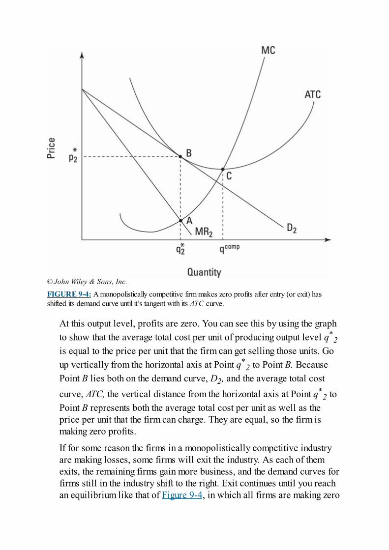
© John Wiley & Sons, Inc.

FIGURE 9-4: A monopolistically competitive firm makes zero profits after entry (or exit) hasshifted its demand curve until it’s tangent with its ATC curve.

At this output level, profits are zero. You can see this by using the graphto show that the average total cost per unit of producing output level q*

2is equal to the price per unit that the firm can get selling those units. Goup vertically from the horizontal axis at Point q*

2 to Point B. BecausePoint B lies both on the demand curve, D2, and the average total costcurve, ATC, the vertical distance from the horizontal axis at Point q*

2 toPoint B represents both the average total cost per unit as well as theprice per unit that the firm can charge. They are equal, so the firm ismaking zero profits.

If for some reason the firms in a monopolistically competitive industryare making losses, some firms will exit the industry. As each of themexits, the remaining firms gain more business, and the demand curves forfirms still in the industry shift to the right. Exit continues until you reachan equilibrium like that of Figure 9-4, in which all firms are making zero

profits.

Producing inefficientlyA key thing to notice about the equilibrium in Figure 9-4 is that it impliesthat each firm produces less efficiently than would firms in a competitiveindustry. The best way to see this fact is to compare the monopolisticallycompetitive firm’s output level when the industry is in equilibrium, q*

2  ,with the output level that would be produced by a firm with the samecost curves that was operating in a fully competitive industry in whichall firms sold an identical product. I’ve labeled this output level asqcomp in Figure 9-4.

In Chapter 7, I explain how market forces push competitive firms toproduce at qcomp, and why it ends up being exactly the level of output atwhich the ATC curve hits its minimum — that is, qcomp is the output levelat the bottom of the U-shaped ATC curve. The socially significantimplication of this fact is that competitive firms produce at the lowestpossible average total cost per unit. That makes them as efficient aspossible in terms of minimizing per-unit production costs.

By contrast, a monopolistically competitive firm operating in an industrywhere product differentiation allows it to have some control over theprices it charges will end up producing at a higher average total cost perunit. This is clearly the case in Figure 9-4 because the vertical distancefrom the horizontal axis up to Point B is longer than the vertical distancefrom the horizontal axis up to Point C. That fact implies that the firms ina monopolistically competitive industry are not as efficient as theywould be if they were in a perfectly competitive industry.

Some look at this result and conclude that society would be better off if itcould transform monopolistically competitive industries into competitiveindustries. But the cost savings might not be worth the loss of productdifferentiation. After all, variety is the spice of life. Would you reallywant every single restaurant to be identical in every way, to serve thesame food in the same type of room, under the same lights, with identicalfurniture? Probably not.

But you have to decide for yourself whether you think the higher costsassociated with variety are worthwhile — and in what situations.Although they may be worth it to you for restaurants, you may have a

different feeling about the product differentiation found among gasstations.

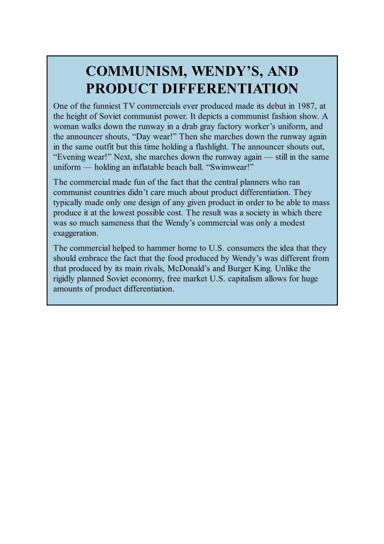
COMMUNISM, WENDY’S, ANDPRODUCT DIFFERENTIATION

One of the funniest TV commercials ever produced made its debut in 1987, atthe height of Soviet communist power. It depicts a communist fashion show. Awoman walks down the runway in a drab gray factory worker’s uniform, andthe announcer shouts, “Day wear!” Then she marches down the runway againin the same outfit but this time holding a flashlight. The announcer shouts out,“Evening wear!” Next, she marches down the runway again — still in the sameuniform — holding an inflatable beach ball. “Swimwear!”

The commercial made fun of the fact that the central planners who rancommunist countries didn’t care much about product differentiation. Theytypically made only one design of any given product in order to be able to massproduce it at the lowest possible cost. The result was a society in which therewas so much sameness that the Wendy’s commercial was only a modestexaggeration.

The commercial helped to hammer home to U.S. consumers the idea that theyshould embrace the fact that the food produced by Wendy’s was different fromthat produced by its main rivals, McDonald’s and Burger King. Unlike therigidly planned Soviet economy, free market U.S. capitalism allows for hugeamounts of product differentiation.

Part 3

Applying the Theories ofMicroeconomics

IN THIS PART …Explore how externalities create socially inefficient outcomes and howsocieties reckon with the Tragedy of the Commons.

Find out why markets depend on full disclosure, how secrets can ruin amarket, and why markets can’t always provide public goods.

Understand why health insurance faces special challenges and how out-of-pocket costs encourage healthy self-rationing.

Probe the fascinating area of behavioral economics, includingevolutionary irrationality, heuristics and cognitive biases, prospecttheory, myopia, framing effects, and altruism.

Chapter 10

Property Rights and WrongsIN THIS CHAPTER

Defining an ideal market Seeing how externalities create socially inefficient outcomes Taking steps to fix problems caused by externalities Exploiting and exhausting commonly owned resources

Economist Adam Smith came up with the invisible hand, the idea thateven though individuals pursue their own interests, the common good isachieved if you allow markets to allocate resources. Smith was quiteaware, however, that you achieve this nice result only if society’sproperty rights are set up correctly before people start to trade goods andservices in markets. In fact, he spent a good deal of his famous book, TheWealth of Nations, talking about how governments must properly defineproperty rights if they want markets to yield to socially beneficialoutcomes. (Chapter 7 discusses this idea in more depth.)

The gist of the problem is that if property rights are not set up correctly, aperson won’t fully take into account how his or her actions affect otherpeople. For instance, consider two pieces of land. One is privatelyowned, and the other is wilderness land that nobody owns and everyoneis free to use as they please. If you want to dump your trash on theprivately owned land, you have to pay the owner for the right to do so.(In other words, the owner is running a trash dump.) But like everyoneelse, you can dump trash for free on the wilderness land because nobodyhas the right to stop you.

Naturally, the difference in property rights with respect to the two piecesof land leads people to dump a lot more on the wilderness land becauseit’s less costly personally to do so. But the problem is that although it’sless costly personally, lots of costs are imposed on others. For example,what could’ve been a very nice park is now a heap of rotting garbage.Bad property rights lead to bad outcomes.

In this chapter, I talk about positive and negative externalities —

situations where one person’s behavior results in either benefits or coststo other people, but where the property rights are so badly defined thatthe costs and benefits aren’t properly accounted for. I also show you howmost cases of endangered or extinct species are the result of nonexistentproperty rights, and how redefining property rights can save speciesfrom oblivion.

Allowing Markets to ReachSocially Optimal Outcomes

For markets to achieve socially optimal outcomes, they must take intoaccount all the costs and benefits involved in any activity, regardless ofwho feels the effects of those costs and benefits. If markets do this, thedemand curve captures all benefits, the supply curve captures all costs,and the market equilibrium quantity ensures that only units of output forwhich benefits exceed costs are produced.

Look at Figure 10-1, which shows a demand curve and a supply curve.The market equilibrium quantity is q*, and the market equilibrium priceis P*. The important thing to realize is that it’s socially beneficial toproduce every unit up to and including q*. The reason for this can beseen by examining unit qo. You can see from the demand curve thatbuyers are willing to pay price Po for unit qo, but it costs suppliers onlyCo to produce unit qo.

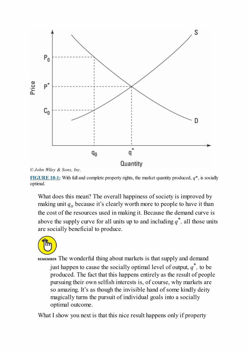
© John Wiley & Sons, Inc.

FIGURE 10-1: With full and complete property rights, the market quantity produced, q*, is sociallyoptimal.

What does this mean? The overall happiness of society is improved bymaking unit qo because it’s clearly worth more to people to have it thanthe cost of the resources used in making it. Because the demand curve isabove the supply curve for all units up to and including q*, all those unitsare socially beneficial to produce.

The wonderful thing about markets is that supply and demandjust happen to cause the socially optimal level of output, q*, to beproduced. The fact that this happens entirely as the result of peoplepursuing their own selfish interests is, of course, why markets areso amazing. It’s as though the invisible hand of some kindly deitymagically turns the pursuit of individual goals into a sociallyoptimal outcome.

What I show you next is that this nice result happens only if property

rights are full and complete, meaning that the demand curve captures allthe benefits that people are willing to pay for and the supply curvecaptures all the costs associated with production. As you’ll see, ifproperty rights aren’t full and complete, markets won’t generate sociallyoptimal output levels like q*. In such cases, the invisible hand turns outto be really invisible — it isn’t there!

Examining Externalities: TheCosts and Benefits Others Feelfrom Your Actions

Property rights give owners control over their property. For instance, Ican paint my car any color I want. I can modify the engine or the tailpipe.I can even install big, shiny 19-inch wheels to try to disguise the fact that,like most economists, I’m not actually very hip.

On the other hand, property rights aren’t unlimited. Society does restrictwhat I can do with my car. For instance, I can’t be a source of noisepollution by removing the muffler. I can’t drive it 90 miles per hour pastan elementary school. And it’s also illegal for me to play my 2,000-wattstereo at full volume late at night. I’m not legally allowed to do thesethings because I don’t live on an island by myself. Rather, I live in acommunity with many other people, and making lots of noise or drivingreally fast affects their quality of life. The way economists describe thissituation is by saying that my actions cause externalities.

An externality is a cost or a benefit that falls not on theperson(s) directly involved in an activity but on others.Externalities can be positive or negative:

Positive externality: A positive externality is a benefit that falls ona person not directly involved in an activity. Think of a beekeeper.She raises bees to sell the honey, but the bees also happen to flyaround pollinating flowers for local farmers, thereby increasing theircrop yields and providing them with a positive externality.Negative externality: A negative externality is a cost that falls on aperson not directly involved in an activity. Think of a steel mill that,as a byproduct of producing steel, puts out lots of soot and smoke.The pollution is a negative externality that causes smog and pollutesthe air breathed by everyone living near the factory.

This section takes a closer look at externalities.

Noting the effects of negative externalitiesGoods and services that impose negative externalities — that is, costs onthird parties — end up being overproduced. This happens becausenegative externalities and the costs that they impose on others aren’ttaken into account when people make decisions about how much toproduce.

For example, in the case of a polluting steel mill, the mill’s managerstake into account only their private costs of raw materials and running theplant.

If someone owned the atmosphere, the mill’s managers would have topay for the right to emit pollution. And if the atmosphere were owned bythe people who would have to breathe in the mill’s pollution, the firmwould be forced to pay those people for the right to pollute and would beforced to take into account the harm that the pollution causes them. Butbecause nobody owns the atmosphere, and firms don’t have to pay topollute into it, there’s no mechanism for making the mill’s managers takeinto account the costs of pollution that fall onto members of the broadercommunity. The result is that the firm overproduces steel.

The following subsections explain how negative externalities such aspollution cause overproduction by shifting supply curves. When theseshifted supply curves interact with demand curves, you can determineexactly how much overproduction will occur and how much harm resultsfrom each unit that is overproduced.

Looking at differences in private and social costsIn Chapter 6, I explain that a competitive firm’s supply curve is equal toits marginal cost curve. If a steel mill doesn’t take into account themarginal costs that its production of steel imposes on others, its marginalcost curve (its supply curve) is too low and leads to an overproductionof steel.

You can see this situation in Figure 10-2, where I’ve drawn in twosupply curves. The lower one is labeled Private MC because the firm’ssupply curve is its private marginal cost curve, which takes into accountonly the firm’s own costs of producing steel. The higher curve takes intoaccount not only the firm’s private costs but also the external pollution

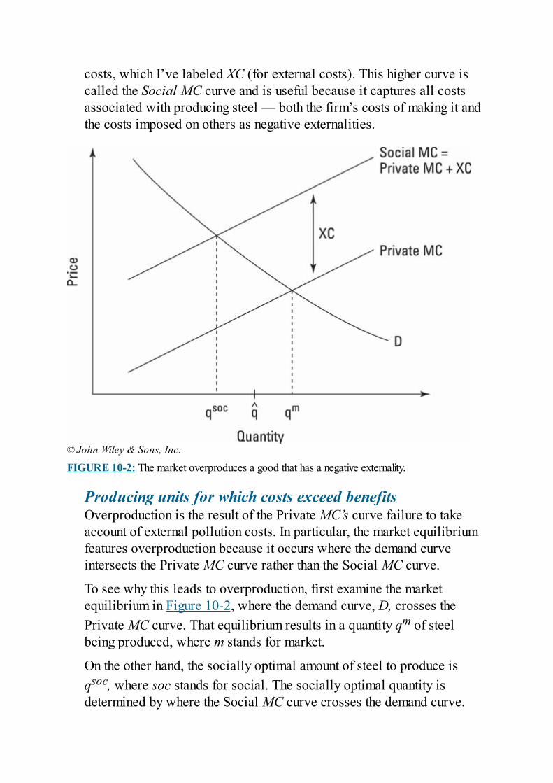
costs, which I’ve labeled XC (for external costs). This higher curve iscalled the Social MC curve and is useful because it captures all costsassociated with producing steel — both the firm’s costs of making it andthe costs imposed on others as negative externalities.

© John Wiley & Sons, Inc.

FIGURE 10-2: The market overproduces a good that has a negative externality.

Producing units for which costs exceed benefitsOverproduction is the result of the Private MC’s curve failure to takeaccount of external pollution costs. In particular, the market equilibriumfeatures overproduction because it occurs where the demand curveintersects the Private MC curve rather than the Social MC curve.

To see why this leads to overproduction, first examine the marketequilibrium in Figure 10-2, where the demand curve, D, crosses thePrivate MC curve. That equilibrium results in a quantity qm of steelbeing produced, where m stands for market.

On the other hand, the socially optimal amount of steel to produce isqsoc, where soc stands for social. The socially optimal quantity isdetermined by where the Social MC curve crosses the demand curve.

You can tell that qsoc is socially optimal because for every unit up to andincluding qsoc, the demand curve is above the Social MC curve, meaningthat the benefits of producing these units exceed the costs of producingthem. That’s true when taking into account not only private costs but theexternal costs that fall on third parties as well.

The problem with producing all the units from qsoc up to qm isthat although the benefits do exceed the firm’s private productioncosts, they don’t exceed the total costs when you take into accountXC, the cost of the negative externality.

For instance, look at output level q^, which lies between qsoc and qm.You can see by going up from q^ to the demand curve that the price thatpeople are willing to pay for that level of output does exceed the privatemarginal cost of producing it. (That is, the demand curve is above thePrivate MC curve at output level q^.) But if you go up even farther, yousee that what people are willing to pay for that level of output is actuallyless than the total, social cost of producing that much output. (That is, theSocial MC curve is higher than the demand curve at output level q^.)

Output level q^ shouldn’t be produced because the total cost ofproducing it exceeds what anyone is willing to pay for it. That’s why it’sunfortunate that output level qm is, in fact, produced in a marketeconomy. Every unit of output produced in excess of output level qsoc isa unit for which the total costs exceed the benefits.

Accepting positive amounts of negativeexternalities

A very important thing to realize is that the common reaction tonegative externalities — outlaw them! — is almost never sociallyoptimal. The goal isn’t to eliminate negative externalities. Rather,the goal is to ensure that when all costs and all benefits areweighed, the benefits from the units of output that are produced

outweigh the costs of producing them — including the costs of thenegative externalities.

In Figure 10-2, for all units of output up to and including qsoc, the totalbenefits are at least as great as the total costs, meaning that society as awhole benefits if these units are produced. Note in the figure that thesocially optimal output level qsoc is a positive number. That is, it’ssocially optimal to produce steel even though some pollution will beproduced along with it.

To understand the intuition behind this fact, think about automobiles. Carspollute. And the only way to totally get rid of their pollution is forsociety to totally ban cars. But do you really want to do that? Althoughit’s true that big, gas-guzzling cars produce prodigious amounts ofpollution without justifiable benefits, do you really want to get rid of allcars, including ambulances and fire trucks? Not at all, because althoughthese vehicles do emit pollution, the costs imposed on society by thepollution are more than compensated for by their social benefits — thelife-saving activities in which the vehicles are engaged.

The same holds true for the pollution being produced by the steel factoryat output level qsoc. The only way to totally eliminate the pollution fromthe steel factory is to shut it down. But that means removing from societyall the benefits that steel can provide, such as earthquake-proof buildingsand crash-resistant safety cages in automobiles.

The next thing to consider is how to make sure that only qsoc units areproduced when the market wants to overproduce goods with negativeexternalities.

Dealing with negative externalitiesThere are basically three ways to deal with negative externalities:

Pass laws banning or restricting activities that generate negativeexternalities. For instance, most cities now forbid you to dispose ofyour trash by burning it.Pass laws that directly target the negative externality itself(rather than the underlying activity that leads to the externality).For instance, steel mills are now required to install smokestackscrubbers that filter out most of the pollution before it goes into the

atmosphere.Impose costs, such as taxes, on people or firms generatingnegative externalities. For instance, governments can chargecompanies for each ton of pollution they emit. This solution isappealing to economists because it’s the one that is most likely tolead to the production of the socially optimal output level.You can see why economists like pollution taxes by looking back atFigure 10-2. Recall that XC is the external cost of the steel mill’spollution on others. If the government imposes a tax of XC dollars onevery unit of steel produced by the firm, the tax raises the firm’s costcurve up from Private MC to Social MC.

Setting the pollution tax at exactly XC dollars causes the firm’s marginalcost curve to lie exactly where the Social MC curve lies. Because afirm’s marginal cost curve is its supply curve, the result is that whendemand and supply now interact, the socially optimal output level qsoc isproduced. That is, by imposing exactly the right tax on steel, thegovernment can sit back and let the market do the rest. That makes thissort of pollution-reducing policy attractive compared to other potentialsolutions.

Compare this solution with a system where firms are ordered to installsmokestack scrubbers to reduce pollution. In such a system, you need tohire inspectors to constantly monitor factories to make sure they aren’tcheating. This sort of system is much more costly to implement thansimply imposing a tax on the mill’s easily measured steel output and thenletting supply and demand set the socially optimal output level. On theother hand, it may be difficult to figure out exactly how big the tax XCshould be, so the pollution tax solution isn’t without problems, either.

Calculating the consequences of positiveexternalities

Externalities can be positive as well as negative. The key thingto understand about positive externalities is that goods and servicesthat provide positive externalities to third parties end up being

underproduced.

Underproduction is typical for goods that generate positive externalities.Because property rights are set up in such a way that the recipients of thepositive externalities don’t have to pay for them, the producers of goodsthat generate positive externalities have no incentive to provide extraunits of output for the benefit of those receiving the positive externalities.

To see why goods that have positive externalities are underproduced,consider a beekeeper named Kate. Kate raises bees so she can sell thehoney and make some money. The people who buy her honey do sobecause the honey brings them utility when they eat it. But becauseKate’s bees go around pollinating the flowers of local farmers, thesefarmers also benefit from her beekeeping activities.

But — and here’s the crucial point — the farmers don’t pay Kate for thebenefits that her bees bring them; the bees just fly in and out of theirfields, and there’s no way to keep track of them. The result is that Kate isgoing to raise fewer hives of bees than she would if the farmers werepaying her for the benefits that her bees bring them.

You can see how this situation works in Figure 10-3. Kate’s supply curveis her marginal cost curve, and I’ve labeled it . I’ve labeled thedemand for her honey by the customers who pay for it as PrivateDemand. Where the supply curve and the Private Demand curve intersectgives the market equilibrium quantity of honey, qm.

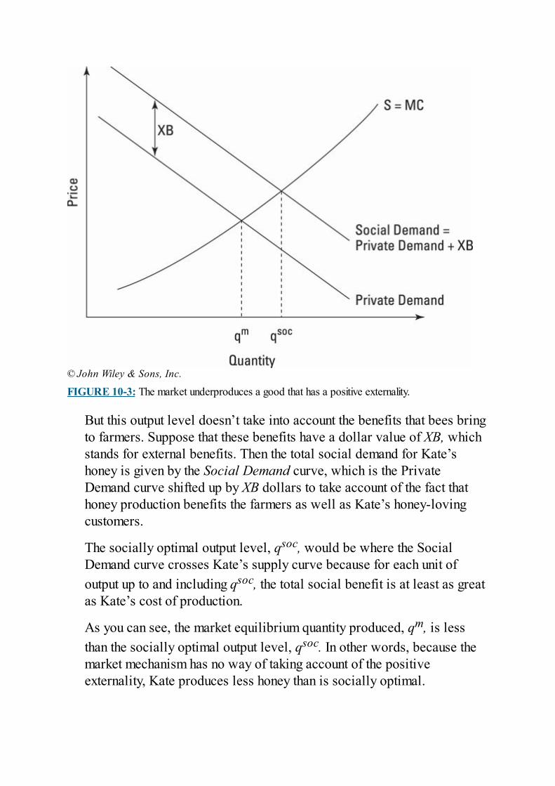
© John Wiley & Sons, Inc.

FIGURE 10-3: The market underproduces a good that has a positive externality.

But this output level doesn’t take into account the benefits that bees bringto farmers. Suppose that these benefits have a dollar value of XB, whichstands for external benefits. Then the total social demand for Kate’shoney is given by the Social Demand curve, which is the PrivateDemand curve shifted up by XB dollars to take account of the fact thathoney production benefits the farmers as well as Kate’s honey-lovingcustomers.

The socially optimal output level, qsoc, would be where the SocialDemand curve crosses Kate’s supply curve because for each unit ofoutput up to and including qsoc, the total social benefit is at least as greatas Kate’s cost of production.

As you can see, the market equilibrium quantity produced, qm, is lessthan the socially optimal output level, qsoc. In other words, because themarket mechanism has no way of taking account of the positiveexternality, Kate produces less honey than is socially optimal.

Subsidizing things that provide positiveexternalitiesBecause markets tend to underproduce goods and services that havepositive externalities, people have come up with ways to encouragehigher levels of production.

The most common way to encourage higher production of goodsthat generate positive externalities is with a subsidy, a payment ofmoney by a government to an individual or firm to encourage it toproduce more of a given type of output. Crucially, the governmentdoes not receive anything back from the recipient of the subsidy inreturn for the payment; the beneficiaries are the consumers whoreceive the additional output.

In the case of Kate’s beekeeping business, the government may pay her ahoney subsidy of, say, 20 cents per pound to encourage her to keep morehives. The result is more bees pollinating more flowers leading to higheroutput levels for the farmers. In fact, the government may even tax thefarmers to get the money to subsidize Kate’s honey. Doing so wouldmake the program pay for itself.

Similarly, governments also often subsidize the planting of trees in andaround cities. They must do so because many of the benefits of trees —shade, cooling, cleaner air, less soil erosion, and so on — are positiveexternalities that aren’t taken into account by the markets. Without thesubsidy, fewer trees would be planted than is socially optimal.

Tragedy of the Commons:Overexploiting CommonlyOwned Resources

An important economic problem that results from poorly definedproperty rights that don’t take account of negative externalities is calledthe Tragedy of the Commons. This section examines this problem indetail.

Overgrazing on a commonly owned fieldThe Tragedy of the Commons refers to a resource being overexploiteddue to the perverse incentives created by common ownership. Undercommon ownership, the resource is open for all to use as they please.These circumstances make rapid use and overexploitation likely becauseeach person has an incentive to use up as much of the resources aspossible before others can.

To understand the Tragedy of the Commons, think of a farming town inwhich most of the land is privately owned. However, there’s one largefield of common land where anyone can graze their cattle. In a privatefield, the owner has an incentive to limit the number of cattle that he putsout to graze. That’s because if he puts too many beasts in the field, theyquickly eat up all the grass and ruin the field for later grazers.Consequently, the owner of a private field puts only a few cattle out tograze. Doing so reduces his short-run profits (because he restricts thecurrent number of cows) but maximizes his long-run profits (because thefield stays in good shape, and he can keep grazing cattle well into thefuture).

With the commonly held field, however, everyone is going to put somecattle out there because the personal cost of doing so is nothing. Nobodyhas a personal incentive to preserve the field’s future usability. Theincentives are actually horribly perverse because if the common field iscurrently lush with grass, your incentive is to put as many of your cattleout there as quickly as possible to eat all the grass before the field isruined. Everyone else sees things the same way, so there is a mad rush to

put as many cattle out to graze as quickly as possible. The result, ofcourse, is that the field is rapidly ruined for everyone. So althoughthere’s no personal cost to putting a cow out to graze on a common field,there is a social cost. Each additional cow causes damage to the fieldthat reduces the future productivity of the field.

The difference between what happens to the private field versusthe common field is totally the result of the different property rightsgoverning the two types of land. In the case of privately ownedfields, farmers have an incentive to weigh the costs as well as thebenefits of putting more cattle out to graze. In particular, they takeinto account how much future profits will be reduced if currentovergrazing ruins the future usability of the field.

Extinctions and poor property rightsMany environmental problems are caused by Tragedy of the Commonssituations in which nobody owns the property rights to a given resource.Notably, most animal extinctions are the result of an absence of propertyrights.

For instance, think of tuna swimming in the open ocean. By internationaltreaty, nobody owns the open ocean. Hence nobody owns the tunaswimming in the open ocean. On the other hand, if you catch a tuna andpull it up onto your boat, you then have a property right over it and cansell it for money. That is, the only way to economically benefit from atuna is to kill it.

The result is that tuna and many other fish species are hugely overfished,with many near extinction. That’s because each fisherman has theincentive to harvest as many fish as quickly as possible before anyoneelse. This quickly leads to an extinct species, and fishermen are veryaware of the problem. But because of the way that property rights are setup in this case, no individual fisherman can do anything to prevent thecalamity. If one guy decides to hold back and take fewer fish in the hopethat by doing so the species will survive, someone else just comes in andcatches the fish that he spared. The species will go extinct anyway. As aresult, nobody has an incentive to hold back.

Avoiding the tragedy

When an economist sees a Tragedy of the Commons situation, hisfirst instinct is to change the property rights system governing theresource in question. Instead of commonly held property rights inwhich each person has an incentive to take as much of the resourceas possible before anyone else does, economists suggest privateownership so there will be an incentive to preserve the resource.Here are a couple of solutions:

Area-based property rights: In the case of overfishing, one solutionhas been to give fishermen private property rights to an entire fishingground — to all the fish in an area while they’re still alive. Thatgives the new owners the proper incentive to manage the stock on asustainable basis. Furthermore, because only one person has the rightto fish in a given area, there’s no longer a mad rush betweencompeting fishermen to harvest as many fish as possible beforeanyone else can get to them.Permits: For fish species that migrate freely between different areas,a different solution has been developed. In such cases, biologistsfirst determine the maximum number of fish that can be sustainablyharvested each year. The government then auctions off fishing permitsfor exactly that amount of fish. This method prevents the Tragedy ofthe Commons by creating a new sort of property right — the fishingpermit. It also has the nice benefit of creating a self-sufficientgovernment program. The money raised from auctioning off thefishing permits can be used to hire game wardens to preventunlicensed fishing, as well as for conservation and wildlifemanagement programs.Local collective management: Nobel Prize–winner Elinor Ostromstudied instances in which the resource-users in particular areaswere able to prevent the Tragedy of the Commons by developinglocal collective-management systems that restrained overuse.Herders sharing pastures in Africa and farmers sharing irrigationwater in Nepal have been able to avoid overexploitation by settingup systems in which outsiders can be excluded from exploiting the

resource, insiders can be monitored against overuse, mechanismsexist for punishing those who take more than their allotted shares,and collective-choice arrangements allow most insiders toparticipate in the decision-making that regulates the system.

Chapter 11

Asymmetric Informationand Public Goods

IN THIS CHAPTER Realizing how markets depend on full disclosure Seeing how secrets can ruin a market Examining the used car and insurance markets Understanding that markets can’t always provide public goods Getting public goods from governments and philanthropists

Markets provide nearly everything that people consume. But marketssometimes fail to provide certain products that people want, or marketsprovide either too much or too little of a particular good or service.Economists refer to such situations as cases of market failure, and in thischapter, I discuss two of the most interesting and common causes ofmarket failure:

Asymmetric information: This situation occurs when either thebuyer or the seller knows more about the thing he’s bargaining overthan the other party knows. The classic example is a high-qualityused car: The owner who’s trying to sell the vehicle knows all aboutthe car’s high quality and reliability, but the potential buyer can onlytake the owner’s word for it. Because the potential buyer has noreason to trust the seller’s assertions that the car is really good, heassumes the worst and offers a low price just in case the car turns outto be a low-quality “lemon.” But because the owner knows that thecar is of high quality, he rejects the low offer, and the car goes unsold— all because there’s no cheap and easy way to prove the car’s highquality to the potential buyer.Public goods: These kill off markets in a different way. That’sbecause the very nature of a public good makes it extremely difficultfor private sellers to charge users. The classic example is alighthouse. After it’s up and running, it benefits all nearby ships,

regardless of whether they pay for the service. That being the case,each and every ship owner tries to avoid paying for the service in thehope that somebody else will pay for it. But with no one paying, thelighthouse soon goes bankrupt, and society is denied a valuableservice.

In this chapter, I discuss these two causes of market failure further, showyou how pervasive they are, and describe some of the clever solutionsthat people have come up with to remedy them. So don’t expect anyasymmetric information here — I’ll make sure that you end up knowingeverything I do.

Please note that asymmetric information and public goods are not theonly things that can cause markets to fail. Market failures also result frommonopoly (Chapter 8), oligopoly (Chapter 9), and externalities (Chapter10).

Facing Up to AsymmetricInformation

In many real-life situations, buyers and sellers don’t share the sameinformation. Regardless of which party is better informed, economistsrefer to these situations as cases of asymmetric information because oneside has more information than the other.

For instance, sellers of used cars are much more knowledgeable aboutthe true quality of the vehicles than the buyers are. On the other hand, thebuyers of auto insurance policies are much better informed thaninsurance companies about whether or not the buyers are bad drivers.

In this section, I provide more in-depth information about asymmetricinformation.

Realizing that asymmetric informationlimits tradeAsymmetric information is very important in the real world because itlimits what goods and services can be successfully traded in markets.The fundamental reason is that if you know that the other guy is betterinformed, you’re afraid that he’ll use his information to take advantage ofyou.

In the case of used cars, buyers are afraid that sellers who know thattheir cars are bad will keep that fact to themselves and try to negotiatehigh prices, as if their cars were good. In the case of insurance,insurance companies are afraid that people who know they’re highinsurance risks will pretend to be low insurance risks so they can getlower rates.

Depending on how bad the asymmetric information gap is, markets mayeven collapse completely. That is, if you have huge worries that theseller of the used car is exaggerating the value of the vehicle he’s tryingto sell you, you probably won’t buy. That sounds like a reasonable thingto do, but that fear prevents the sale of good cars because everybody’sworried about bad cars. Similarly, if insurance companies can’t figureout a way to tell the good insurance risks from the bad ones, they may

charge high rates to everybody as though everyone were a high risk. Andthat, typically, causes the low-risk people not to buy insurance becausethey know they’re being overcharged.

In extreme cases, asymmetric information can lead to whateconomists call missing markets — situations in which there’s nomarket for a good or service. In these situations, markets are absentbecause many potential participants have been scared off by the factthat better-informed market participants may use their informationaladvantage to exploit less-informed market participants.

In less extreme cases, asymmetric information only hobbles but does notcompletely eliminate a market. I explore how this happens in the nextsection.

Souring on the lemons problem: The usedcar marketBerkeley economist George Akerlof got the Nobel Prize in Economics in2002 for a famous paper he wrote called “The Market for Lemons.” Thepaper, first published in 1970, is all about asymmetric information andmarket failure, and it was especially memorable because Akerlof usedthe market for used cars as his primary example. What Akerlof correctlyexplained was that poor-quality vehicles, or lemons, dominate the marketbecause asymmetric information drives away sellers who want to partwith high-quality used cars.

To make the intuition behind the result clear, imagine that there are onlythree kinds of used cars for sale: good, okay, and bad. They all look thesame on the outside and even test-drive pretty much the same, but theyhave major differences in terms of how much longer they’re going to lastbefore the engine gives out. Because of the difference in engine qualityand how long the cars are likely to last, the good cars are worth $15,000,the okay cars are worth $10,000, and the bad ones are worth $5,000.

The problem that leads to market failure is the asymmetric

information that exists between buyers and sellers. In particular,although each seller knows how good her own car’s engine is, thebuyers have no way of knowing.

Buyers could, of course, ask sellers to be truthful about the quality oftheir cars, and no doubt many sellers — probably most — would tell thetruth. But there’s no way to know whether they’re telling the truth.Consequently, when a particular seller tells you that her car is good,you’re still going to be nervous about being cheated.

As I show you in the following subsections, this very reasonable fearcauses nearly all good and okay cars to be withdrawn from the market.The result is a used car market that’s dominated by bad cars; as Akerlofput it, the used car market ends up becoming “a market for lemons.”

Seeing how quality used cars are driven from the marketImagine that you want to buy a used car, but you don’t want to overpayfor it. You know that there are only three types of cars: good, okay, andbad. In addition, you happen to know that one-third of all used cars onthe road are good, one-third are okay, and one-third are bad. How muchwould you be willing to pay for a used car?

Well, given the fact that good cars are worth $15,000, okay cars areworth $10,000, and bad cars are worth $5,000, and also given the factthat you don’t know which cars are which, imagine that you’d be willingto pay no more than $10,000. Why $10,000? Because that’s what theokay used car — the car of average quality — is worth.

Because sellers have no way of proving to you how good their cars are,a sensible thing to do when presented with a used car is to assume thatit’s of average quality and, therefore, worth $10,000. So you offer$10,000. And so do all the other buyers presented with used carsbecause they, like you, can’t tell the quality of used cars apart. Now lookat how different sellers react to the $10,000 offer depending on the truequality of their vehicles:

If a seller knows his car is bad and worth only $5,000, he happilyaccepts your offer.If a seller knows his car is okay, he also accepts because you’reoffering what the car’s actually worth.If a seller has a good car, he won’t accept unless he’s in some sort of

dire circumstance. He knows the car is worth $15,000, so he won’taccept your $10,000 offer unless he’s really desperate to raise cashin a hurry (perhaps to pay off some gambling debts).

The result is that nearly all the good cars on the market are withdrawn,leaving only bad and okay cars. Now consider how that situation changeswhat buyers are willing to offer. If all the good cars are withdrawn fromthe market, there’s now a 50/50 chance that a car is okay or bad. In sucha case, how much would you offer to pay if you were a buyer? Well, witha 50/50 chance of the car being worth either $10,000 or $5,000, you’llprobably offer the average of these two values: $7,500. But when youdo, the market becomes even more dysfunctional. After all, how are thesellers of okay cars going to react to being offered $7,500? They’regoing to reject the offer and withdraw their vehicles from the market,too.

The sad result is that with the good cars and then the okay carswithdrawn from the market, the only cars left are the bad ones, thelemons. Because of the asymmetric information problem, the used carmarket ends up being a market for lemons. Buyers know this, so theyoffer only $5,000 for any car on the market. And because only bad carsare offered, sellers accept the $5,000. So although it’s true that bad carsend up being priced correctly in the used car market, no market exists forgood or even okay used cars.

That’s a problem because people — both buyers and sellers — want totrade good and okay cars, and they would be much happier if they could.But unless some solution can be found to the asymmetric informationproblem, they’re all left out in the cold.

Making lemonade: Solutions to the lemons problemThe fundamental issue driving the lemons problem is that the sellers ofgood and okay cars have no way of convincing buyers that their cars areas good as the sellers know them to be. The whole problem could beresolved if sellers had some way to convince buyers that a good car is,in fact, a good car and an okay car is, in fact, an okay car.

In the next four subsections, I discuss ways to achieve this goal. Thesemethods don’t work perfectly, but because they offer some reassurance tobuyers, buyers are willing to offer enough to get sellers to part withhigher-quality automobiles.

BUYING INFORMATION FROM TRUSTED THIRD PARTIESSeveral companies now specialize in selling vehicle history reports topeople looking to purchase used cars. Potential buyers can enter thevehicle identification number (VIN) of the car they’re interested in andobtain a report that notes mileage, reported accidents, service and repairvisits, the number of owners the car has had, whether the car has everbeen leased, and so on.

Although these vehicle history reports aren’t guaranteed to be exhaustiveor perfectly accurate, they’re an inexpensive method by which potentialbuyers can help themselves identify problem vehicles. The reportsreduce the likelihood of market failure by helping make information moresymmetric between buyers and sellers.

OFFERING A WARRANTYOne way a seller can convince a buyer that she really has a good car isto offer the buyer a warranty. The seller knows that her good car won’tbreak down after she sells it, meaning that she’ll never have to pay forany repairs.

A warranty is convincing because only the seller of a good car would bewilling to offer a warranty. By contrast, the seller of a bad car wouldnever offer a warranty because he knows that his car will probably breakdown and that he’ll have to pay for the repairs. Consequently, if someoneis willing to offer you a warranty, she almost certainly has a good car.That’s why you see so many used car dealers offering warranties on thevehicles they sell. If they didn’t offer warranties, the lemons problemwould quickly take over, and prices would fall so low that only bad carswould be bought and sold on the used car market.

BUILDING A REPUTATIONAnother way to solve the lemons problem is to reassure buyers by settingup a market in such a way that sellers can build a reputation for honestyand fair dealing. This is why most good used cars are sold through usedcar dealers rather than directly between individuals.

Compare a used car dealership with an individual selling her used caronline. Who has more of an incentive to tell the truth about car quality?The used car dealer makes his living selling used cars, so if heovercharges one customer by pretending a bad car is good, he gets introuble. When that car starts to break down, the buyer becomes angry and

uses social media to tell all his friends that the dealer cheated him. Andthat loss of reputation cuts into the dealer’s future sales. In fact, he’llquickly go bankrupt if he develops a reputation for lying.

By contrast, an individual selling her used car doesn’t have to worryabout developing a reputation for lying. Her main source of income isn’tselling cars. If she cheats you and you get mad and tell all your friends, itwon’t affect her much because she’s not in the business of selling usedcars. The result is that she has much more of an incentive to lie than doesthe used car dealer, who has to worry about his reputation. As a result,many good used cars are sold through used car dealers. (But even at usedcar dealers, people still need some reassurance, which is why most usedcar dealers also offer warranties.)

GETTING AN EXPERT OPINIONBecause the heart of the lemons problem is asymmetric information,another method of resolving the problem is for skeptical buyers to hirean expert who can give them the information they need to distinguishgood, okay, and bad cars. Many car buyers employ this strategy whenthey have doubts about a seller’s honesty.

For a relatively small fee, a buyer can hire a disinterested third-partyexpert —for instance, a professional mechanic — to inspect the vehicleand make a list of repairs that will most likely be needed in the nearfuture. In this way, the buyer can get a better picture of the car’s qualityand what a fair price would be.

This method doesn’t fully resolve the asymmetric information problembecause the expert probably can’t discover everything that may bewrong with the car. To the extent that this is true, buyers may still besuspicious, and there may still be some potential for market failure.That’s why you often see buyer-initiated inspections used in conjunctionwith other methods of resolving asymmetric information, such aswarranties and sales by dealers who have a reputation to protect.

Issuing insurance when you can’t tellindividuals apartAn insurance company faces an asymmetric information problem of itsown. Its problem is that the people buying insurance know more than thecompany does about the risks they face.

Consider automobile insurance. Who needs it more: good drivers whohardly ever get into accidents or bad drivers who get into lots ofaccidents? Now, clearly, even good drivers want insurance becausethey’re sometimes involved in accidents for which they’re not to blame.But bad drivers want insurance even more to help pay for all theaccidents they know they’re going to cause because of their poor driving.

An asymmetric information problem faces the insurancecompanies because although individual drivers know whetherthey’re good or bad, the insurance companies can’t easily tell themapart. If they could tell them apart, insurance companies wouldsimply charge the good drivers a low rate for insurance and the baddrivers a high rate.

But because they can’t tell the good and bad drivers apart, the insurancecompanies run a serious risk of going bankrupt. To see why, imagine thatinsurance companies offered the same low rate to everyone, as thoughthey were all good drivers. This would soon lead to bankruptcy becausethe insurance companies wouldn’t be collecting enough in premiums topay off all the damage caused by the bad drivers.

To avoid bankruptcy, the insurance companies could go to the otherextreme, charging everyone as though they were bad drivers. But then thegood drivers wouldn’t bother buying insurance because for them itwould be overpriced. The result would be that only bad drivers wouldsign up for insurance.

This is a very poor result socially because you want everyone to be ableto buy insurance at a rate that fairly reflects their driving ability. Gooddrivers should be able to get insurance at a fair rate. And because gooddrivers make up most of the drivers in the real world, insurancecompanies lose out on lots of potential profits unless they can figure outa way to separate the good drivers from the bad drivers.

Grouping individuals to help tell them apartInsurance companies have come up with a paradoxical way of dealingwith the fact that they can’t tell whether an individual is a good or baddriver. Instead of focusing on the individual, they look for clues about theindividual based on the groups to which he or she belongs. Doing so

often gives the insurance companies a pretty good idea about whether theindividual is a good or bad driver.

For instance, government data indicates that males under 25 get intomany more serious accidents than females under 25 do. So if two peoplewalk into an insurance company and one of them is a 23-year-old maleand the other is a 22-year-old female, chances are that the male is aworse driver than the female. Consequently, you charge the male a higherinsurance rate.

This situation has the nice result of making sure that everybody can getinsurance at what is likely to be a fair price given the fact that, onaverage, males under 25 get into many more accidents than females under25.

In reality, this nice result isn’t the compelling reason behindinsurance companies’ decisions to infer as much as possible abouttheir customers by looking at which groups they belong to. Thesecompanies really have no choice; competition forces them to do so.

Why is this true? Consider two insurance companies, only one of whichuses group membership information to help set rates. The company thatdoesn’t use group information has to set very high rates because it’safraid that all its customers may be bad drivers. Doing so drives awaythe good drivers who don’t want to pay bad-driver rates for theirinsurance.

But the company that uses group information can offer multiple rates,such as high ones to young men and lower ones to young women. Doingso allows it to capture the business of many good drivers who don’t wantto deal with the first insurance company that sets only one high rate foreveryone. The result is that insurance companies are always looking forways to estimate an individual’s unknown risk profile based on the well-known risk profiles of the groups to which he or she belongs.

This process can lead to some rather unfair conclusions. The oddest isthat good-driving young males end up paying higher rates than good-driving young females because the only thing insurance companies haveto go on is gender. But such a system is still better than the even more

unfair alternative in which all good drivers would have to pay bad-driver rates, which is what would happen if insurance companies werebanned from using group membership information to try to distinguishtheir customers. The closer insurance companies can get to fullydistinguishing good and bad drivers using group membershipinformation, the fairer rates will be.

Keep in mind that the drivers for whom insurance companies have thegreatest need to use group membership information are new drivers.Because insurance companies don’t have any accident or violationrecords for new drivers, there’s a pressing need to try to separate thegood from the bad drivers using group membership information. Asdrivers get more experience, the insurance companies can getincreasingly accurate accident and violation information thatdistinguishes the good from the bad.

Avoiding adverse selectionUsing the groups to which a person belongs to estimate his or herindividual insurance risk goes only part of the way to resolving theasymmetric information problem that exists between insurancecompanies and their customers. Obviously, there’s still a lot ofindividual variation within any group. For instance, even if youngwomen are, on average, better drivers than young men, some youngwomen are bad drivers. This leads to a very difficult problem known asadverse selection.

If an insurance company sets a premium for young women on the basis ofhow often young women on average get into accidents, insurance will bemore attractive to young women who are really bad drivers than to youngwomen who are really good drivers.

As a result, young female bad drivers will be more prone to signup for insurance than young female good drivers. This tendency isknown as adverse selection because it’s as though the bad, oradverse, insurance risks self-select into buying insurance policies.The result is a customer pool that contains a disproportionately highnumber of bad drivers.

Adverse selection is a difficult problem because it feeds on itself. The

insurance company has to raise rates to take account of the fact that baddrivers are more likely to sign up than good drivers. But when it raisesrates, the problem just gets worse because the higher rates makeinsurance even less attractive to good drivers, meaning that the pool ofapplicants is going to be even more disproportionately dominated by baddrivers.

One solution to adverse selection is for an insurance company tooffer a large group of people one rate — on the condition thatnobody can opt out. For instance, at the school where I teach, ourhealth insurance company offers the school one low rate for everyemployee on the condition that every employee must be enrolled.By enrolling everyone, there’s no chance that the insurance pool isdominated by the sickly because all the healthy have declined to beenrolled.

Another solution is to force everyone to purchase insurance. Forexample, all 50 states now require drivers to buy auto insurance. Byforcing all drivers to purchase insurance, governments can relieveinsurance companies from having to worry about the adverse selectionproblem. On the other hand, many people consider these laws to becoercive because they force drivers to purchase insurance whether theywant to or not. In addition, good drivers may be forced to subsidize baddrivers because both may now be grouped together by insurancecompanies.

Mitigating moral hazardA big problem facing insurance companies is called moral hazard.Moral hazard arises because buying insurance tends to change people’sbehavior. For instance, if I didn’t have car insurance, I would drive muchmore carefully, knowing that I would have to use my own money to payfor any damage I cause. But because I do have insurance, I drive fasterand more recklessly knowing that if something goes wrong, the insurancecompany is going to be stuck with the bill. (Please know that when I say“I” in examples like this one, I don’t actually mean me. You see, I amabove moral hazard.)

The way car insurance companies deal with moral hazard is by offering

discounts in exchange for high deductibles. For instance, if I get into anaccident, the $1,000 deductible that I’ve chosen means that of any billsthat ensue from the accident, I have to pay the first $1,000.

The deductible serves as a strong inducement for me not to give in tomoral hazard and drive recklessly. And because the insurance companyknows that my high deductible gets rid of most of my moral hazardproblem, it’s willing to offer me insurance at a lower rate than if I’dopted for only a $100 deductible. Deductibles are a clever way ofreducing moral hazard problems and helping to make insurance moreaffordable for responsible drivers.

GROUP DISCRIMINATION,INDIVIDUAL IDENTIFICATION

The idea of grouping individuals to help sort them extends beyond insurance.For instance, companies want hard-working employees but can’t tell when youwalk in for an interview if you are, in fact, hard-working. So they try toestimate the chances that you are by seeing which groups you belong to.

For instance, nearly all straight-A students are hard-working. Therefore, ifyou’re a straight-A student, a company is going to be much more likely to hireyou. You may actually be lazy, but by seeing what group you belong to, thefirm improves its odds that you’re not.

The practice of using information about the groups to which an individualbelongs to try to figure out personal characteristics is referred to as statisticaldiscrimination. Although this practice typically improves economic outcomes,you have to decide for yourself whether — and in what cases — you think it’sfair or unfair.

Providing Public GoodsPublic goods are products that can’t be profitably produced by privatefirms because there’s no way to exclude nonpayers from using them. Theinability of private firms to profitably produce public goods derivesfrom the fact that they have two very special characteristics. Publicgoods are both nonrival and nonexcludable:

Nonrival: Nonrival means that one person’s using the good doesn’tdiminish another person’s ability to enjoy the good. Think of anoutdoor fireworks display, a statue in a park, or a television showbroadcast over the airwaves. Your consumption doesn’t in any waydiminish that of others. This stands in stark contrast to most goods,where if you consume more, less remains for others. (Think ofcookies.)Nonexcludable: Nonexcludable means that it’s hard to preventnonpayers from consuming a good or service. For instance, when youproduce an outdoor fireworks display, everyone in the vicinity getsto see it for free no matter how much you’d like to charge them for it.A more serious example is an army: When it’s in place to providenational defense, it provides national defense for everybody,including those who don’t want to contribute to the cost of the army’smaintenance.

The nonrival and nonexcludable characteristics of public goodsmake it very hard for private firms to make any money producingthem. Think about trying to get people to buy tickets to an outdoorfireworks display. Because people know that they’re going to beable to see it for free, they won’t buy tickets. Because they won’tbuy tickets, there’s no way to raise the money needed to put on thedisplay.

This sort of chicken-and-egg problem is frustrating, because althoughpeople don’t want to pay for something they can get for free, theyactually do like fireworks displays — meaning that they’re

fundamentally willing to pay something to see them. The problem isfiguring out how to get them to pay.

Taxing to provide public goodsThe most common solution to the problem of how to provide publicgoods has been for governments to step in and use tax money to pay forthem. In the case of fireworks, because nearly everybody likesfireworks, there’s no problem getting enough political support forspending tax money on displays. And after they’ve been funded by thetaxpayer, everyone can enjoy them.

National defense has historically been provided for by the governmentbecause it, too, is very much a nonexcludable, nonrival public good. Forinstance, because protection from foreign invaders is nonexcludable,there’s always a temptation to not help pay for it because you know thatif someone else does pay, you get to enjoy safety from foreign invadersfor free. And because national defense is nonrival, you know that thesafety you enjoy is of just as high a quality as the safety everyone elseenjoys. This fact, too, lessens your incentive to pay. As a result,governments force people to share the expense for national defense bylevying taxes.

Taxes and a good portion of government spending are often derided aswasteful (and often are wasteful), but keep in mind that in many cases,taxes are the only way to fund the wide variety of public goods youenjoy. Although nobody likes taxes, you probably wouldn’t want to tradea reduced tax burden for no public parks, no national army, no publicroads, no public sewers, and so on. Without the government’s ability toforce people to pay for these things, you’d likely not have them — atleast not in the quantity and variety that you currently enjoy.

Enlisting philanthropy to provide publicgoodsAlthough most public goods are paid for through taxation by thegovernment, some are paid for privately. So don’t think that governmentsare absolutely necessary to provide public goods. They aren’t. However,governments are a much more reliable way to provide public goodsbecause you don’t have to rely upon the philanthropic largesse of therich, who are under no obligation to spend their wealth on public rather

than private goods.

Don’t make the common mistake of thinking that public goodsare called public because they’re typically provided by thegovernment rather than the private sector. Economists call thempublic goods because private firms can’t profitably produce them,not because they have to be produced by the government. Privatephilanthropy can produce public goods without any help at all fromthe government.

For example, in the middle of Los Angeles, where I grew up, there’s ahuge and beautiful mountain park called Griffith Park. The land for itwas donated by a millionaire named Griffith J. Griffith. That is, heprovided a public good at personal expense.

The desire for fame or recognition may help encourage the philanthropicprovision of public goods. Rich people often trade million-dollardonations to hospitals, universities, and charities for having a buildingnamed after them. And corporations often sponsor cultural public goodssuch as fireworks displays, arts festivals, and parades in order to obtainname recognition and goodwill.

SUPPORTING FREE INFORMATIONWITH ADVERTISING

Google is currently the world’s largest and most popular Internet search engine.But when it first started in business, it lost money hand over fist. Its problemwas that it was providing Internet search results for free, as a public good.People went to google.com, typed in a search term, and got ranked resultswithout having to pay anything. This service was very helpful to users, butGoogle would’ve soon gone bankrupt if it hadn’t stumbled onto a way togenerate income from its services.

The solution was the same one that broadcast TV stations and newspapers hadlong used. Google would charge advertisers for the right to have their adsappear next to Google’s free search results. Thus, for instance, if a person wereusing Google to search for the word “dog,” the free search results would beaccompanied by ads paid for by companies selling products related to the worddog — for instance, hot dogs, dog food, and concert tickets for Snoop Dog.

Google’s search ads had an unintended casualty: They began to kill offnewspapers. This happened because Google’s targeted search ads were muchmore cost-effective for advertisers than newspaper print ads. For example, if acompany that wanted to sell dog collars took out a full-page ad in The NewYork Times, only a very small percentage of that paper’s readers would’ve hadany interest in that ad because the vast majority of them would’ve had nocurrent need to buy a dog collar. But if that same company placed its ads onlynext to Google search results that were generated for people who had beensearching for “dog collars,” then nearly every person who saw the ad might bein the market for a dog collar.

In the decade after Google introduced search ads, newspaper advertisingrevenues fell by more than half, and hundreds of newspapers went bankrupt orwere forced to merge with other newspapers to survive. Newspapers haveattempted to adjust to the Internet Age by publishing online and attempting tocapture online and mobile ad revenues. But because the news agencies’ adsaren’t as well targeted as those accompanying Google search results, they don’tcommand very high rates.

Providing a public good by selling a relatedprivate goodBroadcast radio is a public good. After a radio signal has been sent out

over the airways, it’s nonrival: My listening to a radio program doesn’treduce anyone else’s ability to tune in. It’s also nonexcludable: There’sno way to stop anyone with a radio from tuning in. So given that radioprogramming is very much a public good, how is it that so much radioprogramming is produced and broadcast every day by privately ownedand operated radio stations?

The answer is that the broadcast industry figured out that although radioitself is a public good, the commercials that they play on the radio arevery much private goods for which radio stations can charge a lot ofmoney. That is, if a car maker or beer maker or the publisher of arevolutionary new economics book with a yellow and black cover wantsan ad to to be broadcast to the millions of listeners who tune in for freeto the public good known as radio, the company has to pay forcommercial air time.

The trick behind broadcast radio is that the privately sold good calledadvertising pays for the freely provided public good called radio. To amore limited extent, many newspapers and magazines work the sameway. Although they raise some money from subscription fees or thenewsstand price, a substantial chunk of their revenue comes from theadvertising they sell.

Ranking new technology as a public goodYou live in an age of rapidly rising living standards. Why is this thecase? Because institutions are fostering the creation of new and bettertechnologies that allow people to produce more goods and services fromthe same old resources, or to produce entirely new goods and servicesthat were previously impossible to produce.

Technological progress is a public good. And because it is, society hashad to come up with ways to make sure that technological progresshappens given the fact that private individuals and firms have littleincentive to invent new technology.

Patenting to turn public goods into private goodsTo understand how new technologies are public goods, consider theinvention of the movable-type printing press by Johannes Gutenberg in1435. Before Gutenberg, books were copied by hand. But after heinvented the printing press, it was much cheaper to make new copies by

printing them. Furthermore, think about how simple the technology reallyis. The printing press is basically just a big version of the rubber stampsthat little kids like to play with. The invention was immediatelyunderstandable to anyone and everyone who heard about it, which meantthat they could make their own printing presses as soon as they heardabout it.

So how does this invention satisfy the characteristics of a public good?

It’s nonrival because my building and using a printing press doesn’tin any way lessen your ability to build and use a printing press.It’s basically nonexcludable because the cost of communicating thenew idea to another person is so low — just a short conversationdoes the trick.

The result is that unless society creates some sort of an institution toreward the creation of new ideas, there’s not going to be much of a profitincentive to go into the invention business. In fact, what happened toGutenberg was that everyone copied his idea and didn’t pay him for it.So unless you can come up with a way to financially reward the creationof new inventions, you’re not likely to get many of them.

The solution has been the creation of patents. By givinginventors the exclusive right to market and sell their inventions for20 years, patents provide a financial incentive to get people toinvest the time and energy necessary to come up with newtechnologies that benefit everyone. It’s no coincidence thateconomic growth took off after government-enforced patentsbecame widely available in Western Europe in the 18th century.

Subsidizing research into technologies that can’t be patentedNot every new innovation can be patented. That’s because you can patentonly something you invent, not something you discover. For instance, ifyou think up a chemical that’s never existed before and then synthesize it,you can patent it. But if you merely discover an existing chemical that’sbeen floating around the sea or lying in the soil, you can’t patent it.

This is a big problem for things like cancer research because many

potential cures are chemicals derived from plants and animals,chemicals that have existed in nature for eons. These chemicals havehuge potential benefits, but because they can’t be patented, nobody has astrong financial incentive to try to discover them.

As a result, the government and many private philanthropic groups fundresearch into areas of science where the public goods problem wouldotherwise limit research. This solution is very important to an economistbecause providing public goods is an economic problem that marketsand the invisible hand can’t fix. Other types of market failure, likeasymmetric information, have pretty decent private sector solutions (as Idiscuss in the section “Making lemonade: Solutions to the lemonsproblem,” earlier in the chapter).

Chapter 12

Health Economics andHealthcare Finance

IN THIS CHAPTER Understanding why health insurance has a hard time handling

preexisting conditions Comparing global healthcare expenditures Focusing on why out-of-pocket costs encourage good self-

rationing Understanding how Singapore delivers world-class care at

world-lowest cost

Of all the goods and services that modern science and technology canprovide, those that can extend someone’s lifespan, guard againstinfirmity, and repair the injuries caused by diseases and accidents areamong the most highly prized and intensely demanded. In addition, manypeople consider access to healthcare a basic human right. However,nothing is free. Any resources devoted to providing healthcare areresources that can’t be devoted to producing other products — includingpublic education and affordable housing, which many people alsoconsider basic human rights. Thus, scarcity applies to healthcare as muchas it does to any other good or service.

Because economics studies how people cope with scarcity, its insightsare useful when considering the trade-offs that governments andindividuals face. How can they best structure medical institutions toprovide the highest-quality care to the greatest number of people at thelowest possible cost? As I explain in this chapter, incentives matterprofoundly.

After defining health economics and health finance, this chapterintroduces the mechanics and limitations of health insurance beforeexamining which countries’ healthcare systems provide the best results atthe lowest costs. I then investigate the economic incentives that

Singapore’s healthcare system provides and how those incentivesunderpin its ability to provide top-quality care at extremely low costs. Iconclude with a discussion of how effective those incentive systemshave been when tried in other places.

Defining Health Economics andHealthcare Finance

Health economics is the study of how resources are allocated towardhealthcare. Thus, health economics investigates wide-ranging topics,including the best methods for funding medical research, whetherproviding medical care through central hospitals or local clinics is morecost-effective, how advertising for prescription drugs affects consumerbehavior, and how medical spending affects worker productivity.

A major focus of health economics is health finance, the study of howhealthcare is paid for. One method is for people to simply pay for itthemselves, directly with their own funds — as most people pay forfood, clothing, shelter, entertainment, and so on. But many medicalprocedures are both hard to plan for and extremely expensive — forinstance, life-saving emergency care after a serious car accident orcoronary bypass surgery to save an ailing heart. Both the high costs andunexpected nature of these types of procedures make them very difficultfor individuals to cope with individually.

One solution is health insurance, which helps people to pool resources tocope with these problems collectively. But health insurance is notwithout problems. In particular, both private health insurance andgovernment-provided health insurance create incentives for inefficiencyand artificially high demand that may be better handled by alternativemethods of health finance. I explore these problems with health insurancein the next section.

Noting the Limits of HealthInsurance

Health insurance can be great way of dealing with uncertain futurehealthcare costs — but only if you start off with a group of people whoare all currently healthy. In this scenario, the insurance company collectsmoney from a large number of healthy people who are exposed to a risk— for example, cancer —and stores that money away to compensate orreimburse the minority who will suffer that risk in the future. Becauseonly a few will eventually suffer the risk, the monthly premiums paid byeveryone purchasing insurance can be quite low. This is because thefuture costs of treating the few who will get cancer are spread across theentire group.

But people do get sick. As a result, you’re not going to find many groupsin which everybody is currently healthy. This is problematic because ahigh proportion of sick people can ruin the ability of health insurance todeal with future medical costs. The higher the proportion of unhealthypeople, the less functional health insurance becomes. Healthy peopledrop out when premiums are too high, and at some point, not enoughhealthy people are left in the group for their contributions to pay for thehigh future costs of the sickly.

This section explores the limits of health insurance. Recognizing thatinsurance has its limits is important because it helps you understand thedifficulties faced by both private companies and governments when theyattempt to use insurance as the primary means of funding healthcareexpenditures. In addition, you can immediately grasp that a big sellingpoint for other methods of funding healthcare is that they typicallysidestep the problems that beset health insurance. But don’t think thatavoiding insurance solves every problem related to funding healthcare;those other methods typically have some very serious problems of theirown.

Adverse selection: Looking at who buysinsurance

People who already have medical problems have preexistingconditions. Health insurance has difficulty coping with preexistingconditions due to adverse selection, which occurs when insurance isdisproportionately purchased by those who are more likely to needcostly reimbursements in the future. Adverse selection can drive upinsurance rates and even kill off an insurance market. (For details onadverse selection in auto insurance, see Chapter 11.)

To see how adverse selection wreaks havoc on health insurance markets,suppose an insurance company offers health insurance to a large group ofpeople — say, the population of Massachusetts. For those withpreexisting conditions, purchasing insurance is a no-brainer, becausethey’re certain that their future healthcare bills will be larger than theirinsurance premiums. But the money to pay for their future medical billshas to come from somewhere. With all the sick people purchasinginsurance, the insurance company knows that future treatment costs willbe high. The only way to cover those costs is to charge high premiums,getting enough money out of those without preexisting conditions to paythe expected costs.

Those without preexisting conditions will react the same way peoplereact to higher prices when considering any good or service: Some willstop buying the product. Their dropping out of the insurance marketmakes things even worse for the insurance company, because it’ll beforced to raise premiums even higher. But by raising insurancepremiums, even more healthy people will choose not to purchase healthinsurance, and premiums will go up again.

If this process is intense enough, all the healthy people will drop out, andthe insurance company will stop offering insurance — in which casenobody will have access to health insurance. It’s hard to get moreadverse than that!

Combating adverse selectionBoth the private and public sectors have taken on adverse selectionhead-on. This section highlights a few examples.

Charging different ratesAn important private-sector solution to the adverse-selection problem isfor insurance companies to charge different rates to different customers

based on their likely future health costs. Those without preexistingconditions get a lower rate, and those with preexisting conditions get arate that reflects their higher future health expenses. Unfortunately, thissolution can work only if insurance companies have the same informationabout health conditions as their customers and are legally allowed to setdifferent rates based on preexisting conditions. Here are some challengesthat arise:

Asymmetric information: Due to medical privacy laws, mostpatients have a better idea about their preexisting conditions than dotheir insurance companies (see Chapter 11, where I discussasymmetric information). Because of this, the strategy of settingdifferent insurance rates for the healthy and the sick can be difficultto implement, because those with preexisting conditions can simplypretend not to have them and apply for coverage at the lower rate.Fairness: Governments sometimes forbid insurance companies fromcharging different rates on the basis of preexisting conditions. Theseprohibitions are imposed for fairness reasons and assume that thosewith preexisting conditions are afflicted through no fault of theirown.However, this assumption is dubious for many diseases. Takediabetes. In most cases, obesity is a major factor contributing to Type2 diabetes, and obesity is in turn caused by overeating and not gettingenough exercise. For such diseases, critics argue that it would be fairto allow insurance companies to charge higher premiums becausepeople have these conditions as the result of lifestyle choices.Indeed, banning insurance companies from charging higher ratescould make people less healthy — if people know that theirinsurance rates won’t go up if they gain weight, they may be lesslikely to eat properly and exercise.However, many governments have imposed bans on charging higherrates to individuals with preexisting conditions. These bans make themultiple-rates solution to the adverse selection problem illegal andforce insurance companies to search for solutions, such as groupinsurance.

Offering group insuranceGroup insurance is a private-sector solution to the adverse selection

problem. It avoids the fairness issues that arise when charging higherprices to those with preexisting conditions. Under group insurance, aninsurance company offers insurance to a group whose members areselected for reasons other than whether they have any particular interestin obtaining health insurance.

For example, consider the employees of a large construction company.They were drawn to that employer because it offered jobs they liked.Thus, they probably consist of a fairly random mixture of healthy peopleand a few people with preexisting conditions. The group as a wholeprobably looks like the mixture of healthy and sick people found insociety at large.

The insurance company approaches the construction company and tellsits owners that they can buy health insurance for their employees but onlyif they purchase policies for all their employees. Doing so solves theadverse selection problem because if policies are bought for allemployees, then there will be plenty of healthy people to help pay for thehigh healthcare costs of those in the group who have costly preexistingconditions.

Insurance companies also offer group insurance deals to other groups,including trade unions, professional associations, and even large clubs.Any group will do just as long as its members contain plenty of healthypeople and everyone in the group is covered (so that the healthy cannotdrop out and thereby leave the insurance company with a smaller, sickergroup).

By mitigating the adverse selection problem, group insurance helpsprovide healthcare to tens of millions of people in the United States.Indeed, the large majority of Americans with private health insurancereceive it as part of plans paid for by their employers. Unfortunately,however, the availability of group insurance can make insurance harderto get for those who aren’t members of groups that can be easily solicitedby insurance companies.

Insurance companies may shy away from offering insurance toindividuals who aren’t already covered by a group insurance plan fortwo reasons:

Signing up individuals one at a time is substantially more expensive.

Insurance companies have to worry that people who apply forinsurance as individuals may be especially likely to have preexistingconditions.

This worry is not unfounded. Many people with costly preexistingconditions are too ill to hold down full-time jobs, so the fact that aperson is not already covered by an employer-based insurance planraises the likelihood that he or she has a costly preexisting condition.Therefore, some insurance companies charge high premiums to thoseseeking individual health insurance policies, and other insurancecompanies are reluctant to issue individual policies at all. Thus, theavailability of group insurance can make things worse rather than betterfor those who aren’t already members of insured groups.

Considering the public-sector responseThe public sector has also taken on adverse selection and sought to do soin ways that do not raise concerns about fairness. Canada and some othergovernments, for instance, have made the purchase of insurancemandatory. Because both the healthy and the sick must buy insurance,adverse selection can’t lead to either extremely high insurance premiumsor a total collapse of the health insurance market. And because everysingle person must buy insurance, there are no worries about fairness orunequal treatment.

Another government-imposed solution to the adverse selection problemis to eliminate health insurance altogether and have the governmentprovide all healthcare. This is how healthcare is provided in manycountries, including, most prominently, the United Kingdom. Thesehealthcare systems are owned and run by the government, cover everyresident, and are paid for out of general tax revenues. Because noinsurance is involved, adverse selection isn’t an issue. And becauseevery resident is covered, no problems with fairness arise with respectto coving those with preexisting conditions.

Both mandatory health insurance requirements and government-runhealthcare systems aren’t, however, without their problems. As I discussin the upcoming section “Inflated Demand: Suffering from ‘Free’ andReduced-Cost Healthcare,” both systems tend to lead to excessive andinefficient spending on healthcare that in turn necessitates cost-controlpolicies that are considered by many to be arbitrary, severe, and

ironically unfair.

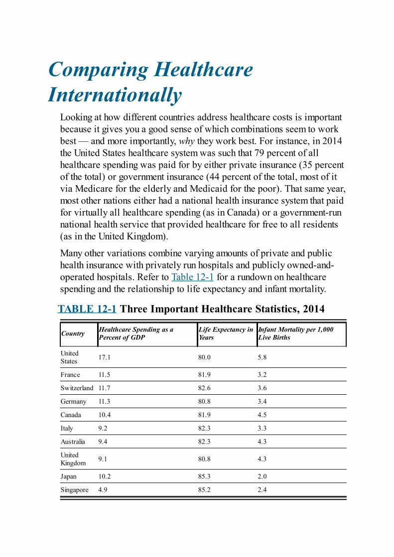
Comparing HealthcareInternationally

Looking at how different countries address healthcare costs is importantbecause it gives you a good sense of which combinations seem to workbest — and more importantly, why they work best. For instance, in 2014the United States healthcare system was such that 79 percent of allhealthcare spending was paid for by either private insurance (35 percentof the total) or government insurance (44 percent of the total, most of itvia Medicare for the elderly and Medicaid for the poor). That same year,most other nations either had a national health insurance system that paidfor virtually all healthcare spending (as in Canada) or a government-runnational health service that provided healthcare for free to all residents(as in the United Kingdom).

Many other variations combine varying amounts of private and publichealth insurance with privately run hospitals and publicly owned-and-operated hospitals. Refer to Table 12-1 for a rundown on healthcarespending and the relationship to life expectancy and infant mortality.

TABLE 12-1 Three Important Healthcare Statistics, 2014

Country Healthcare Spending as aPercent of GDP

Life Expectancy inYears

Infant Mortality per 1,000Live Births

UnitedStates 17.1 80.0 5.8

France 11.5 81.9 3.2

Switzerland 11.7 82.6 3.6

Germany 11.3 80.8 3.4

Canada 10.4 81.9 4.5

Italy 9.2 82.3 3.3

Australia 9.4 82.3 4.3

UnitedKingdom 9.1 80.8 4.3

Japan 10.2 85.3 2.0

Singapore 4.9 85.2 2.4

Source: CIA World Factbook, United States Central Intelligence Agency

The first column of Table 12-1 lists healthcare spending as a percent ofgross domestic product (GDP) for several developed countries in 2014.GDP is a measure of the total income earned within a country in a givenyear (see Chapter 13). Thus, the data in the first column tells how muchof each country’s total income was spent on healthcare. The numbersvary dramatically. The United States spent the most in 2014 at 17.1percent of its GDP. Most countries spent between 9 and 12 percent oftheir respective GDPs, and Singapore spent just 4.9 percent of its GDP.

The second and third columns of Table 12-1 give each country’s lifeexpectancy at birth and infant mortality rate. Although the United Statesspends substantially more than others on healthcare, it doesn’t achievethe best results on these two measures. In fact, it’s in last place on both!

In contrast, Singapore does best on both measures despite spending farless. Even more remarkable: In almost every health-quality categorymonitored by the World Health Organization, Singapore is either numberone in the world or near the top of the list. The natural conclusion is thatit’s possible to get very good healthcare without spending very muchmoney.

Inflated Demand: Suffering from“Free” and Reduced-CostHealthcare

The quantity demanded of any good or service — including healthcare— depends on the price faced by consumers. The lower the price, themore people want to buy. This relationship is called the law of demand,and it explains many of the cost and efficiency problems that result whenhealthcare is delivered with artificially low prices through eitherinsurance systems or national health systems. This section explores theproblems with an increased demand caused by artificially low prices.

Diverting funds to lower-value uses

People stop self-rationing when prices are set at artificially lowlevels. When healthcare has an artificially low price, some of itwill end up being devoted to lower-value uses, which reducesefficiency:

Treating minor problems: When visiting a doctor costs, say, $25,many people with minor problems will skip going to the doctorbecause they view their problems as not worth the cost of the officevisit. But if visits are free, many people with minor problems such ascolds and backaches will come in. This means that a large number ofpatients with very minor problems will be competing for the limitedsupply of medical services with people having more seriousproblems.Testing for uncommon diseases: For many diseases, preventivecare for a large number of people costs more than waiting for therelatively few people who will develop the disease to showsymptoms. Doctors don’t know who may be in danger, so they run thediagnostic tests on everyone — including those who wouldn’t haveended up suffering from the disease anyway. Diagnostic tests are

often quite expensive, so the costs of early detection often exceed themoney saved by avoiding the treatment of the disease in its advancedstages.Performing elective surgery: Artificially low pricing divertsresources to purely elective (rather than necessary) medicalprocedures. Consider knee surgery. At a price that reflects the fullcost of performing surgery, only a relative few will opt to pay forelective knee surgery. But with surgery available at an artificiallylow price, many more will opt for the procedure. The resourcesrequired to perform those surgeries —operating room space, the timeof doctors and nurses, anesthetics —could’ve been used to treatpatients with more life-threatening problems.Choosing expensive new treatments: Artificially low pricespromote the use of costly new medical procedures that are onlymarginally better than older procedures. Consider radiationtreatments for cancer. Old methods bombard tumors with X-rays;new methods bombard tumors with protons. Do protons work better?Nobody is sure. But artificially low prices make the two treatmentsappear to be about equally costly, so many patients and doctors optfor the costly new method.

The inefficiencies caused by artificially low healthcare prices aresystem-wide and lead to such massive increases in demand that severerationing systems have to be imposed to prevent spending from spiralingout of control.

Rationing healthcareSome government healthcare systems provide care free of charge toresidents, so the price of healthcare as seen from the viewpoint ofconsumers is zero. Applying the law of demand, you can immediatelyunderstand that people demand a lot more healthcare at the zero pricethan they would if they had to pay even a moderate price.

The government must cope with the high demand induced by “free”healthcare. The problem, of course, is that healthcare is not actually free.Hospitals must be built and maintained, doctors and nurses must be paid,and medicines must be purchased. Thus, the government developsmethods to limit the amount of healthcare supplied to a level that the

government can actually afford. Each method is a different form ofrationing. Here’s how these methods work for the United Kingdom’sNational Health Service:

Increased wait times: The simplest rationing method is waiting. In2017, patients in the United States waited an average of 3.5 weeks tosee a specialist. By comparison, the United Kingdom’s NationalHealth Service that year abandoned its previous goal of gettingpatients to specialists within 18 weeks. The NHS was forced toabandon that target because so many patients had been waiting evenlonger and because the NHS was struggling to even get patients togeneral practitioners quickly enough. The long waiting times for bothspecialists and general practitioners imposed a nonmonetary cost thathelped equalize the limited resources that the National HealthService could afford with the high quantity of services demanded bypatients who thought of healthcare as being “free.”Denial of service: Another tactic is denial of service based on costconsiderations. To that end, the National Health Service hasestablished the National Institute for Health and Clinical Excellence— or the NICE committee, as it’s better known. Just how nice is theNICE committee? Well that depends on your medical condition. TheNICE committee has decided on a general limit of £30,000(approximately $44,000) on the cost of extending a life for a year.Applying that rule to a specific situation, if an anti-cancer treatmentwould cost more than £30,000 to extend a cancer patient’s life for ayear, the National Health Service won’t pay for it. This cost rulekeeps a lid on expenditures, but it forces those with costly treatmentsto fund their own medical care.

Facing shortages and higher pricesHealth insurance isn’t free, because premiums must be paid byindividuals, firms, or government. But at the moment of use, the effect ofhealth insurance is to vastly increase the demand for healthcare bymaking healthcare look artificially inexpensive. This happens becausemost health insurance policies require only modest cost-sharing on thepart of consumers. For instance, a patient who’s prescribed a $1,000treatment of medication may only have to pay 10 percent of the cost, or$100, out of her own pocket because the insurance company pays for the

other 90 percent. The result is a stressed healthcare system that’soverwhelmed by the levels of demand.

Note that this is the case whether the insurance system is completelygovernment-run, as in Canada, or is largely in private hands, as in theUnited States. Increasing demand has two predictable effects:

Shortages: In government-run systems, where the government can fixprices, increases in demand cause shortages unless the governmentchooses to spend the money necessary to increase supply. TheCanadian government has been unwilling to do that and has insteadrelied on rationing. It employs both long waiting times for variousservices as well as other regulations that deny care (see thepreceding section). That said, Canada’s strategy of delaying ordenying care does limit spending. That’s why Table 12-1 shows thatCanada spent only 10.4 percent of its GDP on healthcare in 2014.Higher prices: In systems where healthcare prices are free to rise inresponse to increases in demand, prices rise. For instance, the UnitedStates spent 17.1 percent of its GDP on healthcare in 2014 becauseits prices could respond to the increases in demand caused by lowout-of-pocket costs. This dynamic has only gotten worse over timebecause the percentage of total healthcare spending that comesdirectly out of consumers’ pockets fell from almost 50 percent in1960 to only 11 percent in 2016. The lower the percentage falls, themore healthcare looks “free” at purchase. And the more it looks“free,” the more of it people demand (including expensive newtechnologies), driving up prices further.

Combatting inefficiency with bureaucracyWith artificially low prices, people do not engage in enough self-rationing (as they would if prices were higher). But rationing must stillhappen in some form or another because quantities demanded exceedquantities supplied. As a result, insurance companies and national healthsystems have attempted to develop bureaucratic systems that should,ideally, address those inefficiencies. Specifically, they allocate thelimited supply of care as efficiently as possible — that is, to the sickestand most deserving patients.

For example, one system forces patients to visit “gateway doctors”

before getting access to expensive specialists. The gateway doctors aretasked with saying no to most requests on the basis of preapprovedregulations. Unfortunately, these bureaucratic systems are oftenperceived as heartless, inflexible, and rule-bound by consumers whowould prefer that their doctors be free of preapproved regulations whensuggesting treatment options.

Even worse, the attempt to use a bureaucracy to allocate scarceresources efficiently appears to fail in most cases. (Check out the nearbysidebar on Gammon’s law, which explains that many medicalbureaucracies are so inefficient that allocating them more resourcesleads to reductions in measurable outputs of medical services!)

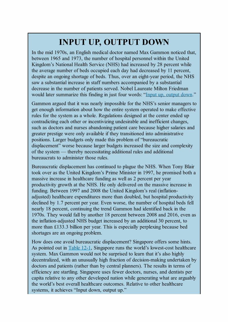
INPUT UP, OUTPUT DOWNIn the mid 1970s, an English medical doctor named Max Gammon noticed that,between 1965 and 1973, the number of hospital personnel within the UnitedKingdom’s National Health Service (NHS) had increased by 28 percent whilethe average number of beds occupied each day had decreased by 11 percent,despite an ongoing shortage of beds. Thus, over an eight-year period, the NHSsaw a substantial increase in staff numbers accompanied by a substantialdecrease in the number of patients served. Nobel Laureate Milton Friedmanwould later summarize this finding in just four words: “Input up, output down.”

Gammon argued that it was nearly impossible for the NHS’s senior managers toget enough information about how the entire system operated to make effectiverules for the system as a whole. Regulations designed at the center ended upcontradicting each other or incentivizing undesirable and inefficient changes,such as doctors and nurses abandoning patient care because higher salaries andgreater prestige were only available if they transitioned into administrativepositions. Larger budgets only made this problem of “bureaucraticdisplacement” worse because larger budgets increased the size and complexityof the system — thereby necessitating additional rules and additionalbureaucrats to administer those rules.

Bureaucratic displacement has continued to plague the NHS. When Tony Blairtook over as the United Kingdom’s Prime Minister in 1997, he promised both amassive increase in healthcare funding as well as 2 percent per yearproductivity growth at the NHS. He only delivered on the massive increase infunding. Between 1997 and 2008 the United Kingdom’s real (inflation-adjusted) healthcare expenditures more than doubled, but hospital productivitydeclined by 1.7 percent per year. Even worse, the number of hospital beds fellnearly 18 percent, continuing the trend Gammon had identified back in the1970s. They would fall by another 18 percent between 2008 and 2016, even asthe inflation-adjusted NHS budget increased by an additional 30 percent, tomore than £133.3 billion per year. This is especially perplexing because bedshortages are an ongoing problem.

How does one avoid bureaucratic displacement? Singapore offers some hints.As pointed out in Table 12-1, Singapore runs the world’s lowest-cost healthcaresystem. Max Gammon would not be surprised to learn that it’s also highlydecentralized, with an unusually high fraction of decision-making undertaken bydoctors and patients (rather than by central planners). The results in terms ofefficiency are startling. Singapore uses fewer doctors, nurses, and dentists percapita relative to any other developed nation while generating what are arguablythe world’s best overall healthcare outcomes. Relative to other healthcaresystems, it achieves “Input down, output up.”

Investigating Singapore’s SecretsOffering “free” healthcare, reduced-cost care, and health insurance allhave drawbacks (see the earlier sections in this chapter). However,Singapore has managed to create a set of medical institutions thatdelivers world-class healthcare while somehow spending 50 percentless than Canada and 70 percent less than the United States. This sectionexplains how.

Exploring cost-saving featuresThe secret to Singapore’s success has been a unique blend of private andpublic medical funding that keeps costs down by paradoxically makingpeople pay a lot of money out-of-pocket for their care. It also ensuresthat the poor will be cared for.

Singapore’s healthcare system has three main cost-savingfeatures:

Government mandates to encourage competition: Singaporeencourages competition by requiring hospitals to post prices for eachof their services on the Internet. Armed with this information,patients can shop around for the best deal. The government alsopublishes the track record of each hospital on each service so thatpatients can make informed decisions about quality as well as price.High out-of-pocket costs for consumers: Singapore insists uponhigh out-of-pocket costs to avoid the overconsumption and highprices that result when insurance policies pick up most of the pricefor medical procedures. Indeed, out-of-pocket spending representsabout 92 percent of all private healthcare spending in Singapore,compared to just 11 percent in the United States.Laws requiring people to save for future health expenditures:Having to pay for most medical spending out of pocket means thatSingapore’s citizens are faced with having to pay for most of theirhealthcare themselves. How can this be done without bankrupting theaverage citizen? The answer is mandatory health savings accounts.

Singapore’s citizens are required to save about 6 percent of theirincomes into MediSave accounts. MediSave deposits are privateproperty, so people have an incentive to spend the money in theiraccounts wisely. But the citizens of Singapore also know that theywon’t be left helpless if the money in their MediSave accounts runsout. The government subsidizes the healthcare of those who haveexhausted their MediSave accounts as well as the healthcare of thepoor and others who have not been able to accumulate much moneyin their MediSave accounts.

Singapore’s health ministry is still very much involved in policingdoctors and hospitals for safety and in providing healthcare to the poor.In fact, about one-third of all healthcare spending in Singapore is paidfor by the government on behalf of the poor. But Singapore restricts itsdirect management of the healthcare system by allowing high-out-of-pocket costs to ration care and direct the entrepreneurial efforts ofmedical researchers.

Weighing costs and benefits of medicalproceduresCrucially, the prices patients pay in Singapore are not artificially low.Unlike in the United Kingdom, where healthcare looks free, or the UnitedStates, where it looks artificially inexpensive due to insurance’s pickingup most of the bill, the residents of Singapore are faced with the fullprices of medical procedures. This causes them to self-ration,voluntarily choosing not to go to the hospital for minor problems. Thatfrees up resources for doctors and nurses to concentrate on treatingserious cases.

Singapore’s residents typically make very sensible decisions whenweighing the costs and benefits of various medical procedures. In fact,having to pay high out-of-pocket costs encourages good-decision makingbecause people who have to pay their own money for healthcaregenerally spend a lot more time educating themselves about their options.

Supporting cost-cutting innovationsSingapore’s system of individual self-rationing has meant that Singaporehas not had to set up a bureaucracy to ration care. The absence of such a

bureaucracy promotes innovation because instead of red tape, there areprofit incentives. These incentives are especially helpful in motivatingmedical entrepreneurs to figure out innovative methods for reducingcosts.

To see the power of profits, consider the fact that a medical doctor in theUnited Kingdom who comes up with an innovation will get no rewardfrom that country’s National Health Service. Indeed, her innovation willprobably never be implemented, because dozens of committees wouldhave to give their approval before her idea could be carried out. Bycontrast, a doctor with such an idea in Singapore could put it intopractice quickly.

Self-rationing affects the types of medical research in Singaporeversus in other countries. With individual self-rationing, moreresearch is devoted to reducing costs so that consumers can payless. Typically, that has nothing to do with inventing a new way oftreating a disease but rather with figuring out how to make aneffective older treatment less expensive. Thus, some hospitals inSingapore can do an open-heart surgery for only $20,000, versusabout $100,000 in the United States.

By contrast, the incentives facing medical researchers in the UnitedStates are very different. In the United States, most research is funded bythe government and directed toward developing new treatments. Successis measured by whether the new method works in the sense of curing thedisease or healing the wound; whether it does so substantially better thancurrently available methods when costs are taken into account is not ahigh priority.

The incentives facing the United States’ medical research system lead toa paradox: On one hand, they result in the United States having theworld’s most cutting-edge medical technologies. On the other hand, manyare hideously expensive and only marginally better than what wasavailable before. From a cost-benefit perspective, the development ofsuch technologies is wasteful.

Trying to copy Singapore’s success

No other country has copied all three of Singapore’s cost-reducingpolicies. But recent experiments suggest that huge savings can result fromimplementing just one: high out-of-pocket costs. A couple of examples,one a state government and one a private company, show some promise.

In 2007, Indiana introduced a new healthcare option for state employees.Any employee choosing this option received $2,750 in a health savingsaccount plus an insurance policy that covers 80 percent of any medicalexpenses between $2,750 and $8,000 and 100 percent of any expensesabove $8,000. Thus, any employee volunteering for the plan had to pay100 percent of all spending up to $2,750 from his or her health savingsaccounts.

These high-out-of-pocket expenses encourage prudence. Indeed, thosewho opted for the plan visited doctors and emergency rooms two-thirdsless often than they did before, were half as likely to be admitted to ahospital, and spent $18 less per prescription than state employees whoopted to stick with the state’s traditional health insurance option.

These changes in behavior led to a 35 percent decline in total healthcarespending for those who volunteered for the new plan versus those whostuck with the traditional option. An independent audit showed thatparticipants in the new plan weren’t cutting corners by skimping on cost-effective preventive care like annual physicals and annual mammogramscreenings. Thus, the savings appear to be permanent and sustainable.The program is also popular, with positive personal recommendationscausing voluntary participation to rise from 2 percent of state employeesin the program’s first year to 70 percent of state employees in theprogram’s second year.

Similar programs implemented by private companies like Whole FoodsMarket also show 30 to 40 percent cost reductions. Thus, it’s clear thatsubstantial costs savings can be achieved by simply confrontingconsumers with nonsubsidized prices that must be paid for with out-of-pocket spending.

Even greater savings can presumably be achieved by implementingSingapore’s two other cost-saving policies: encouraging competition andmandatory savings. Encouraging competition would likely lead toimproved services at lower costs, and mandatory health savings wouldpresumably make people even more cautious with out-of-pocket

spending because they would be aware that they were very muchspending their own money.

Widely implementing Singapore’s innovations may be difficult, however.Many individuals and firms do very well financially under the healthcaresystems currently in place. They may be reluctant to support innovations,as may the politicians who helped build the current systems.

Chapter 13

Behavioral Economics:Investigating Irrationality

IN THIS CHAPTER Defining irrationality as systematic error Explaining how evolution delivered a brain prone to systematic

error Understanding heuristics and cognitive biases Probing prospect theory Focusing in on myopia and time inconsistency Assessing the evidence for fairness and non-self-interested

behavior

Remember that Victorian-era historian, Thomas Carlyle? He was the onewho skewered economics as “the dismal science” in the late 19thcentury. Fortunately for everyone, behavioral economics popped onto thescene in the late 20th century. Within a few short years, a lot of thedismal became dazzling.

Explaining the Need forBehavioral Economics

Conventional 20th-century neoclassical economics makes many accuratepredictions about human choice behavior and how it responds tofinancial incentives and incrementally changing prices. But when thedecisions involve uncertainty and require the chooser to risk or commitor trust, neoclassical predictions often fail.

The key underlying problem is that real people are often irrational.That’s problematic for neoclassical economics because neoclassicaleconomics assumes that people are rational. Because rationality is at theheart of why neoclassical economics sometimes fails, let’s begin ourreview of behavioral economics by precisely defining rationality.

Rationality is defined by economists as decision-making thatavoids systematic errors.

A systematic error is an error that you do over and over, as if you cannever learn from your mistakes. A rational decision maker would not besubject to systematic errors. She would learn from her mistakes andfigure out how to get what she wants for the least cost and effort. Outsidefactors might still derail things, but anything that the rational decisionmaker could have done to maximize her chances of success would havebeen learned and applied.

If people were always rational, then standard, mid-20th centuryneoclassical economics would have always generated reliablepredictions about human decision-making. But people regularly andrepeatedly engage in behaviors that reduce their likelihood of achievingwhat they want. They engage in systematic errors. Behavioral economicsattempts to explain these systematic errors by combining insights fromeconomics, psychology, and biology. The goal is to develop theories thatcan deliver more accurate predictions about human choice behavior,including all the irrational stuff.

Decades of research have allowed behavioral economists to developtheories that can explain why our brains employ error-prone mentalshortcuts, why we don’t save enough for retirement, why we fall formarketing gimmicks, and why higher incomes rarely lead to permanenthappiness. Armed with those insights, behavioral economists have insome cases been able to develop beneficial correctives. And, leastdismally of all, behavioral economists have found extensive evidencethat people are not purely self-interested.

Complementing Neo-ClassicalEconomics with BehavioralEconomics

People aren’t always irrational. They are sometimes very rational, andas a result, neoclassical economic models often make very goodpredictions about decision-making. That’s why you should think ofbehavioral economics and neoclassical economics as complementarymethods for trying to explain why people make the choices that weobserve.

At the same time, it’s important to realize that the two sets of theories areoften radically different both in content and in what they imply about howwe should approach the world. In particular, they end up having verydifferent approaches to how we can help people to improve theirsituations.

In cases where people are being rational, a very simple way to help themis to offer them more options. After all, if they always act rationally andselect the best option from whatever is available, they can only be madebetter off by offering them more options. Thus, neoclassical economistsoften try to solve consumers’ problems by presenting them withadditional options.

But in situations where people are making systematic errors, addingmore options is unlikely to make things better. It may even worsen thesituation because a systematic error would now have more options toplay with. As just one example, if you have an impulse-eating problem,your life is not improved if your mom sends you a package of cookies inaddition to a package of brownies. That’s why behavioral economistsfocus on helping people make better choices from already availableoptions.

Behavioral economists also tend to assume that complex decision-making situations will tend to be best explained by a combination ofneoclassical economics and behavioral economics.

Let’s analyze how people shop at a supermarket:

Neoclassical economics tells us that incentives matter. Customerscare about prices. When prices go up, they buy less. When prices godown, they buy more.Behavioral economics gives us the additional understanding thatpeople tend to buy what they happen to see. This behavior is calledimpulse buying, and it falls outside of the neoclassicists’ notion thatthe consumer calculates marginal utilities and compares prices. Italso explains why grocery stores put the milk cooler at the back ofthe store — to force you to walk past lots of other items and thus bemore likely to see something tempting and make an impulse buy. Andit’s why they stock candy bars by the checkout lines — to tempt youwith an impulse buy just as you are probably quite hungry fromlooking at everything else in the store.

But how did we end up with brains that need both rational, neoclassicalmodels as well as irrational, behavioral models to explain? The answeris: four billion years of evolution.

Examining our Amazing,Efficient, and Error-ProneBrains

The most complex object in the known universe is the human brain,which has 100,000,0000,000 neurons sharing 10,000 times as manyconnections. This incredibly dense web of computing power allows us toobserve our environments, think creatively, and interact with people andobjects.

But despite all that processing power, the brain is quite prone to glitches.This is the result of four billion years of evolution having to deal withthe fact that the world was a very tough place for our ancestors. Evolvingbigger, smarter brains helped our ancestors survive, but bigger brainswere costly in terms of calories. The modern brain, for instance,represents just 5 percent of your body weight but consumes about 20percent of all your calories. So although there was evolutionary pressureto develop bigger brains, there was also a strong limiting factor in thatfinding enough calories to feed a bigger brain was very difficult beforeagriculture, fire, and modern hunting tools.

In response to the caloric constraint, evolution did two things: To theextent possible, it evolved a bigger (and hungrier!) brain. But it alsogenerated many low-energy mental shortcuts, or heuristics, to help getthe most decision-making power out of each ounce of brain tissue.

Deciphering heuristics

Because they’re shortcuts, heuristics aren’t the most accuratemental processing options. But in a world where calories were hardto come by, a low-energy “good enough” heuristic was better than a“perfect but costly” alternative. In economic terms, there werediminishing returns to deploying additional units of brain power.Heuristics developed because the opportunity cost of perfection

was too high.

The brain employs heuristics for nearly every type of action and decisionthat we make. Three examples will give you the general idea about howthese mental shortcuts help to economize on calories and calculations:

The gaze heuristic: You’re a centerfielder, and a baseball is hit inyour general direction. If you lock your eyes on the ball and run sothat the ball remains at the same angle above the horizon that it wasat when you first locked your eyes on the ball, then provided you’refast enough, you will end up running wherever you need to be tocatch the ball. This is the method actually used by people whencatching fly balls. They don’t use physics equations or an app topredict where to run to. They simply lock their gaze and run so as tokeep the angle constant. It’s a simple solution to a difficult problem.The steering heuristic: You’re riding a bicycle and movingforward. If you start to fall and you reflexively steer in the directionyou’re falling, you’ll generate enough centrifugal force to stay uprightlong enough to steady the bike. This is what novice bike riderssubconsciously learn to do: If falling to the right, steer right; if fallingto the left, steer left. Will this basic rule always work? Not on ice, itwon’t. And not if you’re standing still. But if you’re moving forward,it gets the job done very nicely indeed.The recognition heuristic: You’re asked to guesstimate whetherMunich or Stuttgart has the larger population. Most people don’tknow enough about Germany to give an informed answer to thisquestion. But they’ll often give the correct answer by choosing thecity with the more recognizable name. The recognition heuristic oftenworks because there’s a positive relationship between populationsize and how often cities are mentioned in books, conversation, andsocial media.

Heuristics help us make decisions rapidly and at low cost. But the factthat they’re hardwired means that expecting to avoid or unlearn themisn’t practical. For the most part, we’re stuck with them and prone to dowhatever they suggest.

This hardwiring can leave us vulnerable to being played bythose who understand heuristics and are willing to use them againstus. On the other hand, we can be helped by those who would like toplace us in situations in which heuristics tend toward desirableoutcomes. But if we cynically consider which of those twoalternatives is more likely, we can see the wisdom of shoring up ourdefenses with more information about how our brains are structuredand how their decision-making systems work.

Deconstructing brain modularityThe modern human brain has evolved with a modular structure, so thatspecific areas deal with specific sensations, activities, and emotionssuch as vision, breathing, and anger.

Located in the back of the head, adjacent to the entry of the spinal cordinto the skull, the older parts of the brain control subconscious activitieslike breathing and sweating as well as automatic emotional reactionssuch as fear and joy.

Located up front, near the forehead, are the newer parts of the brain thatallow creative thought, imagination about the future, and keeping track ofyour social network (Mark Zuckerwho?). These newer areas are largelyunder conscious control.

The differences between the older and newer brain modules allow us tothink about decision-making as being controlled by two interrelatedsystems that were given really creative names: System 1 and System 2.

System 1 is controlled by the older brain modules at the back of thehead. System 1 produces quick, unconscious reactions and “gutinstincts.”System 2 is controlled by the newer brain modules up front. System2 works more slowly, “thinks things over” deliberately, and deliversconscious calculations about how to handle various situations.

Some decisions are the result of your brain combining suggestions fromSystem 1 and System 2. But you need to keep in mind that a large body ofevidence suggests that the vast majority of decisions are probably either

fully or mostly the result of System 1. That’s very important becauseSystem 1 decision-making is prone to a wide variety of systematicerrors.

Cogitating on cognitive biases

Cognitive biases are the misperceptions or misunderstandingsthat produce systematic errors. Cognitive biases fall into twocategories:

Those resulting from faulty heuristics.Mental-processing errors that are the result of attempting to usebrains that evolved in much simpler times to solve modern problems.Our brains evolved before modern complexities such as calculus,computer science, and trying to figure out how to more “likes” onsocial media. So our brains simply haven’t developed the toolsnecessary to solve these problems very well.

Imagine a vicious underworld populated by thinking mistakes, and you’relooking at a line-up of “the usual suspects.” Do you see some familiarbad guys here (and can you give personal examples of each of thesebiases)?

Confirmation bias is the common human tendency to pay attentiononly to information that agrees with, or confirms, one’spreconceptions. This causes information that contradicts one’spreconceptions to be ignored completely or rationalized away, andthe incorrect opinion persists.Self-serving bias refers to people’s tendency to attribute theirsuccesses to personal effort or personal character traits but theirfailures to factors outside of their control. This bias makes it difficultfor people to learn from their mistakes.The overconfidence effect refers to people’s tendency to be overlyconfident about the correctness of their opinions and judgments andto act without taking time to verify their initial hunches.Hindsight bias occurs when people retroactively believe that they

were able to predict past events. A faulty “I-knew-it-all-along”perspective causes many people to overestimate their predictiveabilities.The availability heuristic causes people to base their estimatesabout the likelihood of an event not on objective facts but on whethermental images of similar events are quickly and readily brought tomind. Events that carry vivid and emotionally charged mental imagesare presumed to be much more common than events that bring to minddull or boring mental images. Shark attacks are in fact very rare, butthe mental image of being attacked by a shark is extremely vivid formost people.The planning fallacy refers to the tendency people have tosubstantially underestimate the time needed to complete a task. Whena student waits until 2 a.m. to start cramming for an 8 a.m. exam andwhen Congress waits until right before its August recess beforetrying to pass a long-awaited reform, both are up against the planningfallacy.Framing effects have to do with providing context, or framing, for adecision. Framing effects are in play when a change in context(frame) causes people to change their decision-making, and changesin context can cause extraordinary changes in behavior. Whenexperimenters tagged an area with graffiti and scattered trash around,ordinary people were twice as likely to litter, steal, and trespass.Upscale retail marketers play the opposite game, spending onexpensive packaging, displays, and even architecture to increase theperceived value of their merchandise — and, you guessed it, howmuch customers are willing to pay.

Surveying Prospect TheoryNeoclassical economics focuses much of its attention on consumer-choice situations in which people have to choose between different“goods,” as when selecting items at a supermarket. But in the real world,people have to make choices that involve the possibility of “bads” aswell — they have to deal with uncertainty and the possibility of badoutcomes as well as good ones.

Prospect theory makes predictions about how people will makedecisions when presented with both potential gains and potentiallosses. It’s based on three key factors that influence how peoplechoose in these situations:

People judge good things and bad things in relative terms, as gains orlosses relative to their current situation, or status quo.People experience both diminishing marginal utility for gains (eachsuccessive unit of gain feels good, but not as good as the previousunit) as well as diminishing marginal disutility for losses (eachsuccessive unit of loss hurts, but less painfully than the previousunit).People experience loss aversion, meaning that for losses and gainsnear the status quo, losses are felt much more intensely than gains —in fact, about 2.5 times more intensely.

In addition to shedding important light on how consumers weigh theirprospects, prospect theory also provides insights into how advertisersselect their tactics, how manufacturers decide on pricing, why peopletend to save too little for retirement, and why people often can’t stick toweight-loss programs.

To better see why psychologist Daniel Kahneman was awarded theNobel Prize in Economics for developing prospect theory, this sectionreviews instances of consumer behavior that would be hard to explainwithout it.

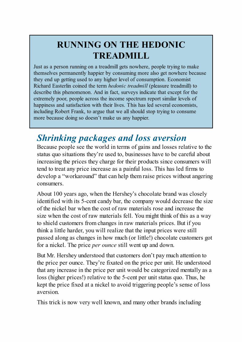
RUNNING ON THE HEDONICTREADMILL

Just as a person running on a treadmill gets nowhere, people trying to makethemselves permanently happier by consuming more also get nowhere becausethey end up getting used to any higher level of consumption. EconomistRichard Easterlin coined the term hedonic treadmill (pleasure treadmill) todescribe this phenomenon. And in fact, surveys indicate that except for theextremely poor, people across the income spectrum report similar levels ofhappiness and satisfaction with their lives. This has led several economists,including Robert Frank, to argue that we all should stop trying to consumemore because doing so doesn’t make us any happier.

Shrinking packages and loss aversionBecause people see the world in terms of gains and losses relative to thestatus quo situations they’re used to, businesses have to be careful aboutincreasing the prices they charge for their products since consumers willtend to treat any price increase as a painful loss. This has led firms todevelop a “workaround” that can help them raise prices without angeringconsumers.

About 100 years ago, when the Hershey’s chocolate brand was closelyidentified with its 5-cent candy bar, the company would decrease the sizeof the nickel bar when the cost of raw materials rose and increase thesize when the cost of raw materials fell. You might think of this as a wayto shield customers from changes in raw materials prices. But if youthink a little harder, you will realize that the input prices were stillpassed along as changes in how much (or little!) chocolate customers gotfor a nickel. The price per ounce still went up and down.

But Mr. Hershey understood that customers don’t pay much attention tothe price per ounce. They’re fixated on the price per unit. He understoodthat any increase in the price per unit would be categorized mentally as aloss (higher prices!) relative to the 5-cent per unit status quo. Thus, hekept the price fixed at a nickel to avoid triggering people’s sense of lossaversion.

This trick is now very well known, and many other brands including

Haagen-Dazs, Kraft, Tropicana, and Bounty have reacted to rising inputprices in recent years by reducing product sizes.

Framing effects and advertisingBecause people evaluate situations in terms of gains and losses, theirdecision-making can be very sensitive to the mental frame, or context,that they use to evaluate whether a possible outcome should be viewedas a gain or a loss. In terms of prospect theory, the framing informationdefines the status quo and thus our sense of whether any possibleoutcome will be perceived as a gain or as a loss.

Here are two examples of framing effects and how changing the framecan flip your perception of whether a possible outcome is to be viewedas a gain or as a loss:

You’re offered a salary of $100,000 per year. Nice! But what ifyou’re used to earning $140,000 per year? Not nice.You have a part-time job. Your boss walks in and says he’s going togive you a 10 percent raise. Sweet! But then he says all the otherpart-timers will be getting a 15 percent raise. Sour!

Advertisers know how important context is and go out of their way toframe their offers as gains rather than losses. Think about ads forhamburger meat. If they say “80 percent lean,” we think of the meat asoffering gains to health; but if they say “20 percent fat,” the same meatfeels like a potential coronary.

Any frame that alters gain-or-loss perceptions will affectpurchasing decisions. So sellers go out of their way to framepotential purchases as gains rather than losses.

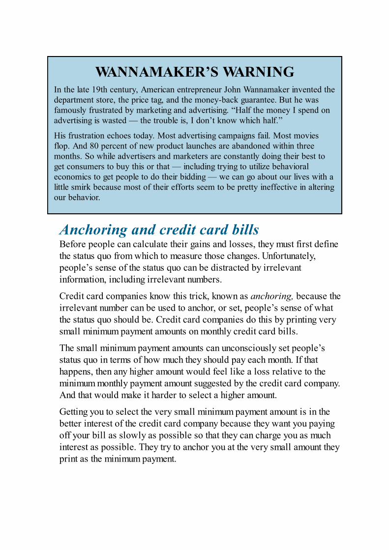
WANNAMAKER’S WARNINGIn the late 19th century, American entrepreneur John Wannamaker invented thedepartment store, the price tag, and the money-back guarantee. But he wasfamously frustrated by marketing and advertising. “Half the money I spend onadvertising is wasted — the trouble is, I don’t know which half.”

His frustration echoes today. Most advertising campaigns fail. Most moviesflop. And 80 percent of new product launches are abandoned within threemonths. So while advertisers and marketers are constantly doing their best toget consumers to buy this or that — including trying to utilize behavioraleconomics to get people to do their bidding — we can go about our lives with alittle smirk because most of their efforts seem to be pretty ineffective in alteringour behavior.

Anchoring and credit card billsBefore people can calculate their gains and losses, they must first definethe status quo from which to measure those changes. Unfortunately,people’s sense of the status quo can be distracted by irrelevantinformation, including irrelevant numbers.

Credit card companies know this trick, known as anchoring, because theirrelevant number can be used to anchor, or set, people’s sense of whatthe status quo should be. Credit card companies do this by printing verysmall minimum payment amounts on monthly credit card bills.

The small minimum payment amounts can unconsciously set people’sstatus quo in terms of how much they should pay each month. If thathappens, then any higher amount would feel like a loss relative to theminimum monthly payment amount suggested by the credit card company.And that would make it harder to select a higher amount.

Getting you to select the very small minimum payment amount is in thebetter interest of the credit card company because they want you payingoff your bill as slowly as possible so that they can charge you as muchinterest as possible. They try to anchor you at the very small amount theyprint as the minimum payment.

Here’s a pro tip: Decide how much you want to pay before yousee the bill. That way you can’t be influenced by any informationthat might anchor you into paying too little.

Examining the endowment effectIf you show a person a new mug and ask him to put a price on it, he mightsay $10. But if you gift that guy the mug and then ask him how much youwould have to pay him to buy it back, he will typically quote you asubstantially higher price, like $15.

What’s interesting is that the higher buy-back price isn’t the result of hisbluffing or attempting to drive a hard bargain. The way human brains arewired, people tend to put a higher valuation on anything that theycurrently possess, or are endowed with, than on identical items that theydon’t own but might purchase. This phenomenon is called the endowmenteffect. It shows up all over the place, including with home purchases.

It appears that loss aversion is the likely culprit behind the endowmenteffect. Once you possess something, having it becomes your new statusquo. And that means the prospect of parting with it would be perceivedas a potential loss relative to the status quo of retaining possession.Consequently, people demand more money to part with something theycurrently possess than they would to purchase the same item if theydidn’t own it yet.

That difference in perceived value can be a problem for negotiationsbetween buyers and sellers. The sellers will on average be demandingmore than the buyers are going to be willing to pay.

Stipulating status quo biasProspect theory also explains status quo bias, which is the tendencypeople have to favor any option that’s presented to them as being thedefault, or status quo, option.

The effect of status quo bias can be massive. Consider organ-donationprograms tied to driver’s license applications and renewals. In countrieswhere the default option is donating your organs if you die in a caraccident, nearly 100 percent of people are registered as donors. By

contrast, in countries where the default option is not donating if you diein a car accident, only about 10 percent of people are registered asdonors.

Both cases would require finding and filling out a form to switch theapplicant away from the default option. And in both cases, hardly anyonebothers to find and fill out the form. They just go with whatever optionwas presented as the default, or status quo.

Prospect theory explains such examples of status quo bias as acombination of the endowment effect and loss aversion. Put into a novelsituation, people will treat the default option as an endowment and willregard any other option as a prospect with the potential for loss. Lossaversion then kicks in and reinforces the appeal of the default option. Theresult is a bias toward the status quo and sticking with whatever thedefault option is.

Status quo bias was put to good use by researchers who wanted a simplemethod for increasing retirement savings. They made automaticenrollment into a savings program the default situation for thousands ofworkers. Those workers ended up saving far more than workers whosedefault option was to not be enrolled.

Such research leads to a more general point: Because people forthe most part tend to stick with whatever the status quo is, why notmake the status quo helpful or useful?

Countering Myopia and TimeInconsistency

Our distant forbears had to be almost entirely focused on the presentmoment — on how to avoid diseases and predatory animals andstarvation, for example, and on how to get through the next few weeks ormonths.

That’s why part of our genetic inheritance is our difficulty with long-runplanning and decisions that involve trade-offs between the present andthe future. Two of our major stumbling blocks are myopia and timeinconsistency.

Focusing on myopiaIn medicine, myopia means nearsightedness. People with myopia can seenearby objects clearly, but everything farther away looks blurry. Byanalogy, economists use myopia to refer to the fact that our brains have ahard time conceptualizing the future: It seems fuzzy, out of focus, andhard to see. That’s why we have great difficulty imagining, for example,the additional spending power that will be ours in 30 years if we beginsaving money now.

A primary consequence of decision-making myopia is that when aconsumer is forced to choose between one thing that will generatebenefits quickly and another thing that won’t yield benefits for a longtime, he will have a strong tendency to favor the more immediate optioneven if the long-run option would be well worth waiting for.

Consider having donuts today versus having an athletic figure down theline. Those donuts are close and warm and very tempting. You can smelland see them now. But the benefits of being in great shape in three or fouryears (washboard abs!) will seem relatively vague and far less pressing.Your brain will tell you to eat the donut — or two donuts — and thuslower the likelihood of your having a great physique in three years, evenif that’s something you genuinely want.

Tattling on time inconsistencyWe view the future myopically from the here and now. This leads to a

tendency to make bad predictions about what we’ll want to do atparticular points in the future.

Consider your 10 p.m. self setting an alarm for 6 a.m. the next morning,to get up and go to the gym. Your 10 p.m. self assumes that your 6 a.m.self will be on board with going to the gym once the alarm goes off.After all, it’s the same you. But when the alarm goes off at 6 a.m., your 6a.m. self doesn’t want to go — and even turns the alarm off, goes back tosleep, and never gets to the gym.

The underlying problem is that your 10 p.m. self myopically fails to seehow painful getting up and going to the gym is going to be. But when thatmoment arrives, your 6 a.m. self can see the pain very clearly. Thus, your6 a.m. self makes a decision in the moment that your 10 p.m. self did notcorrectly anticipate the night before.

Economists refer to situations like this as being examples of timeinconsistency. It happens whenever our current selves don’t understandwhat our future selves will want once the future becomes the present.

GETTING GREEN THE MYOPIC WAYMyopia causes consumers to focus too strongly on the up-front costs ofinstalling solar panels. They can’t see far enough into the future to appreciatethe massive long-run savings they could achieve if they paid for solar panelsnow in exchange for cheap electricity in the future.

A company called Solar City has figured out a way to work with, rather thanagainst, people’s myopia. It does so by offering leasing and financing optionsthat eliminate the need for consumers to pay for the up-front costs of installinga solar system. Instead, Solar City pays for the upfront costs and then makes itsmoney by splitting the resulting cost savings with consumers.

This arrangement actually benefits from myopia because consumers get tofocus on their share of the savings, which is immediately available. It’s a greatexample of working with, rather than against, a behavioral bias.

Beating self-control problems withprecommitmentsTime inconsistency is a major cause of self-control problems. Themisperceptions and misjudgments entailed by time inconsistency willsubtly encourage people to put themselves in temptation’s way. You cansay today that you’re going to spend three hours tomorrow working onyour tax return. But when tomorrow comes around, you binge watch yourfavorite show instead.

Fortunately, behavioral economists have developed some techniques tohelp us take actions today that can help control our rascally future selves.

One of the leading strategies for dealing with time inconsistencyis to make precommitments that aren’t easily reversed by yourfuture self. This strategy may include tactics such as setting multiplealarm clocks so that you can’t easily get back to sleep when you’resupposed to go to the gym; signing up for automatic payrolldeductions so you don’t have to decide every two weeks whether tosave for retirement or blow all the money on Pokémon cards; andjoining a weight-loss competition so that there will be ongoing

social pressure to help keep you committed to reaching yourweight-loss goals.

Gauging Fairness and Self-Interest

Neoclassical economics assumes that people are purely self-interested.Adam Smith, the founder of modern economics, put this idea into wordsin The Wealth of Nations in 1776: “It’s not from the benevolence of thebutcher, the brewer, or the baker that we expect our dinner, but from theirregard to their own interest. We address ourselves not to their humanitybut to their self-love, and never talk to them of our own necessities but oftheir advantage.”

Whoa, lighten up, Mr. Smith! That sounds like it could have been writtenby Ebenezer Scrooge or the Grinch.

Yet don’t judge Smith too quickly. He was a philosopher before he wasan economist, and in his other famous book, The Theory of MoralSentiments, Smith wrote, “How selfish soever man may be supposed,there are evidently some principles in his nature which interest him in thefortune of others and render their happiness necessary to him though hederives nothing from it except the pleasure of seeing it.”

Was Adam Smith an old softie from the get-go, despite his morefamously quoted statement on self-interest? It appears so. And itappears that he was right to feel that way. Behavioral economistshave amassed a pile of evidence that indicates that there is an ever-present human tendency toward altruism and caring about one’sfellow man. Although self-interest is also always present, mostpeople do care deeply about others and about the fairness of theirown behavior in interactions with other people. For that reason,economic transactions are heavily influenced by moral and ethicalfactors.

Defining fairness

In economics, fairness is a person’s sense of whether a price,wage, or allocation is considered morally or ethically acceptable.Any tendency toward pure self-interest is modified by people’ssense of fairness. In some cases, people go so far as to act preciselythe opposite of how you would expect a purely self-interestedperson to behave. Examples include giving anonymously to charity,obeying the law even when there is zero chance of getting caught,and being willing to pay a premium price to purchase a “fair-trade”product.

Examining the experimental evidence forfairnessIn recent decades, experimental games have been created to test people’sfeelings about fairness. One key feature is that the games are played forreal money, so that participants have a strong incentive to act in a self-interested manner so as to win as much money as possible.

Another key feature is that players interact anonymously via computerscreens. Economists provide that anonymity to give each player thechance to be a jerk without having to fear retaliation either during thegame or afterward. That freedom from retaliation liberates players to usewhatever strategies are most likely to maximize their own winningsduring the game. The question is whether players will use that freedom toact in a purely self-interested manner — or behave more nicely.

The dictator game and the ultimatum game are two of the most famous.Each game involves two players.

Dishing on the dictator gameThe experimental researcher who runs this game puts up a fixed amountof money, say $10, and designates one of the two players as the“dictator.” The dictator’s job is to determine the split — be it $10/$0 or$8.67/$1.33 or another division — between the dictator and the otherplayer. The dictator chooses the division. The researcher executes it,paying each player his or her share. And the game ends.

The dictator game has been played hundreds of thousands of times all

over the world. A review of the outcomes shows that roughly one-thirdof dictators keep all of the money for themselves. The other two-thirds ofdictators show generosity by allowing the other player some money —on average, $4.20. Seventeen percent of all dictators split the moneyevenly, and 5 percent of all dictators give the entire amount to the otherplayer.

From such experimental results, behavioral economists havecome to believe that some people are incredibly selfish, others areincredibly generous, and most of us are somewhere in between. Butthe most important thing to remember is that the most commonbehavior is to give a perfectly anonymous stranger a substantialshare of the money even though there are zero consequences forbeing entirely selfish.

Unraveling the ultimatum gameThis game is a bit more complex, represents a more realistic money-splitting situation, and is often played for higher stakes than $10. In thisreal-money, two-person game, there is no dictator who can unilaterallydecide what the split will be. Instead, both players must jointly agree onany proposed division of the money in order for the split to take place.

In real-world markets where buyers and sellers interact voluntarily, atransaction takes place only when a proposal made by one party isaccepted by the other. In the ultimatum game, one player is randomlyassigned to function as proposer and the other as responder — and bothface the possibility that if they can’t agree, both will forgo all possiblebenefits.

The proposer issues an offer (the ultimatum) in which she suggests a split— perhaps 70 percent for herself and 30 percent for the other player —and the responder gets to either accept it or reject it. If the responderaccepts the proposed split, the split is made, the game ends, and bothplayers go anonymously on their way. But if the responder rejects theproposer’s suggested split, neither player gets anything, and the gameends without anybody getting any money at all.

Here’s what typically happens: Almost no proposers suggest allocatingthe money perfectly unfairly, 100/0 percent in their own favor. The large

majority of proposers suggest either a perfectly equal 50/50 split orsomething close to it, like 55/45 percent.

The key thing to notice is that proposers in this ultimatum gameare even more considerate in their proposed splits than are dictatorsin the dictator game. That happens because the responders in theultimatum game can be active and reject, whereas the secondplayers in the dictator game must be passive and just take whateverthe dictator proposes. The ability of responders in the ultimatumgame to reject offers means proposers must be careful not to offendresponders, especially responders’ sense of fair treatment. Thatleads proposers toward suggesting very equal splits.

Digesting the experimental evidence onfairnessA good way to interpret the behavior we observe in the dictator andultimatum games is to notice that the two games support both the gentlerinstincts discussed in The Theory of Moral Sentiments and the power ofself-interest that features so prominently in The Wealth of Nations:

The fact that dictators who face no possibility of retaliationon average give quite a bit of the money to the other player in thedictator game is consistent with human beings having an intrinsicsense of fairness that causes them to help others even when there’snothing in it for themselves.The fact that splits become more equal when there’s a threat ofrejection in the ultimatum game shows that incentives for goodbehavior can make people behave even more fairly than they dowhen left completely to their own devices without any threat ofpunishment or retaliation.

The increased equality of splits that we see when both parties mustconsent to them gives us another way to understand Adam Smith’s

metaphor of the invisible hand. When people are constrained by havingto consider the needs and interests of others, they tend to behave in moremutually beneficial, socially optimal ways — as if guided to do the rightthing by an invisible hand.

That’s a powerful result from two simple games. And it’s yet anotherillustration of the dazzling insights that behavioral economics hasdelivered since it burst onto the scene back in the 1980s.

NUDGING PEOPLE TOWARDBETTER OUTCOMES

Behavioral economists have begun “nudging” people toward better decisions byusing gentle reminders or mild peer pressure. Many nudges can be implementedat extremely low cost. Here are some examples:

Weekly text-message reminders increased attendance at adult literacyclasses in England by 33 percent.Letters that told taxpayers in Guatemala that most of their neighborshad already paid their taxes tripled collections.Personal savings was increased by a factor of seven in the Philippinesby offering people commitment savings accounts which restrictedpeople from withdrawing money either until a specific date or until theaccount reached a specific dollar amount.Households slashed their electricity consumption substantially after anelectric company started printing sad-face icons like ☹ on the bills ofhigh-consumption households.

But before applauding these efforts too loudly, consider for yourself whethernudges are ethical. Would you be okay with being subconsciously manipulatedif the manipulation helped you get something you desired?

Part 4

Macroeconomics: The Scienceof Economic Growth and

Stability

IN THIS PART …Discover gross domestic product — the total value of goods andservices produced in a country.

Probe inflation, price indexes, and interest rates to see how inflation iscaused by printing too much money.

Explore the business cycle and why recessions happen.

Find out what government should or shouldn’t do to fight recessionsusing tools like stimulus spending and fiscal and monetary policy.

Understand that borrowing and debt drive price bubbles and financialcrises and why fiscal and monetary policy don’t work very well after afinancial crisis.

Chapter 14

How Economists Measurethe Macroeconomy

IN THIS CHAPTER Measuring gross domestic product: The total value of goods and

services Decomposing GDP into C+I+G+NX Understanding why free trade is good for you

Macroeconomics studies the economy as a whole. Seen from on high,either businesses or the government produces goods and services.Businesses produce the bulk of what people consume, but the governmentprovides many goods and services, including public safety, nationaldefense, and public goods such as roads and bridges. In addition, thegovernment provides the legal structure in which businesses operate andalso intervenes in the economy to regulate pollution, mandate safetyequipment, and redistribute income from the rich to the poor. (For moreon the division of tasks between private businesses and the government,see Chapter 3.)

To study production, distribution, and consumption with any realunderstanding, economists must keep track of exactly how much isproduced and where it all ends up. Consequently, economists havedeveloped a huge accounting apparatus, called National Income andProduct Accounts (NIPA), to measure economic activity. This systemproduces many useful statistics, including the famous gross domesticproduct (GDP), which measures the total quantity of goods and servicesproduced in a country in a given period of time.

The system can seem arcane, but knowing the accounting isindispensable — it’s the basis for all the mathematical models thateconomists use to understand and predict the business cycle, inflation,economic growth, and monetary and fiscal policy. (I present some ofthese models in Chapters 16 and 17.) So make sure to take, uh, properaccount of what I’m about to show you.

Getting a Grip on the GDP (andIts Parts)

Gross domestic product, or GDP, is a statistic that calculates thevalue of all goods and services produced in a given country in agiven period of time. In the United States, the Bureau of EconomicAnalysis at the Department of Commerce computes this statisticevery three months, giving an idea of how much economic activitytook place in the previous quarter. Add up the numbers for fourconsecutive quarters and you get GDP for a year.

GDP is very important because higher levels of output afford greateraccess not only to essentials like good food and quality healthcare, but toa wide variety of goods and services that bring people pleasure andenjoyment. I’m not saying that money is the only thing that matters, buteconomists evaluate economies by how successfully they maximizehappiness — and although money can’t buy you love, it can sure as heckbuy you a lot of other things that make you happy, such as food,education, and vacations. So, a high and quickly growing GDP ispreferable because it reflects lots of economic transactions that providepeople with the goods and services they desire. (To examine somereasons GDP may not always reflect increased happiness, see the latersection “Watching GDP rise with the good, the bad, and the ugly.”)

Chapters 2 and 3 discuss how people’s fundamental economic goal is tomaximize happiness given limited resources. Because people like toconsume goods and services, measuring GDP allows economists toquantify, in some sense, how well a country is doing at maximizing itscitizens’ happiness given the country’s limited resources. Rising GDPindicates that a country is figuring out ways to provide more goods andservices that make people happy.

In this section, I show how and why the economists who tabulate theNational Income and Product Accounts (NIPA) divide GDP into itsconstituent parts. Breaking up GDP lets you analyze each part separately

and get a good handle on the major factors that influence the productionof goods and services. But first, I give you a short explanation of whatGDP doesn’t take account of.

Leaving some things out of GDP

The GDP statistic counts only transactions that involve money,so if you do volunteer work for your parents or if a mother stayshome to take care of an infant, that economic activity — though veryproductive and socially beneficial — doesn’t get counted in GDP.

In economies like the United States’, GDP is very good at capturingnearly all output that’s produced because almost everything that’sproduced within the U.S. is subsequently sold. But in a largely rural andagrarian society of small farmers, most production is for consumptionwithin the household. Consequently, most of their output never makes itto the official GDP statistics.

As countries transition from rural agrarian economies with lotsof household production to market economies where nearlyeverything produced is sold for money, GDP appears to risebecause a lot of output is being counted for the first time. But thisapparent change may not be an increase in output. These limitationscan make comparing the GDPs of various countries misleading.

Tallying up what counts in GDPCounting sales where money trades hands can get a little tricky becauseboth a buyer and a seller are involved in every such transaction. Themoney that the buyer spends has to equal the money that the sellerreceives. Translated into economist lingo, income has to equalexpenditure. Consequently, you can measure GDP by totaling all theexpenditures in the economy or by counting up all the incomes in theeconomy. If your calculations are correct, both methods give you thesame value for GDP.

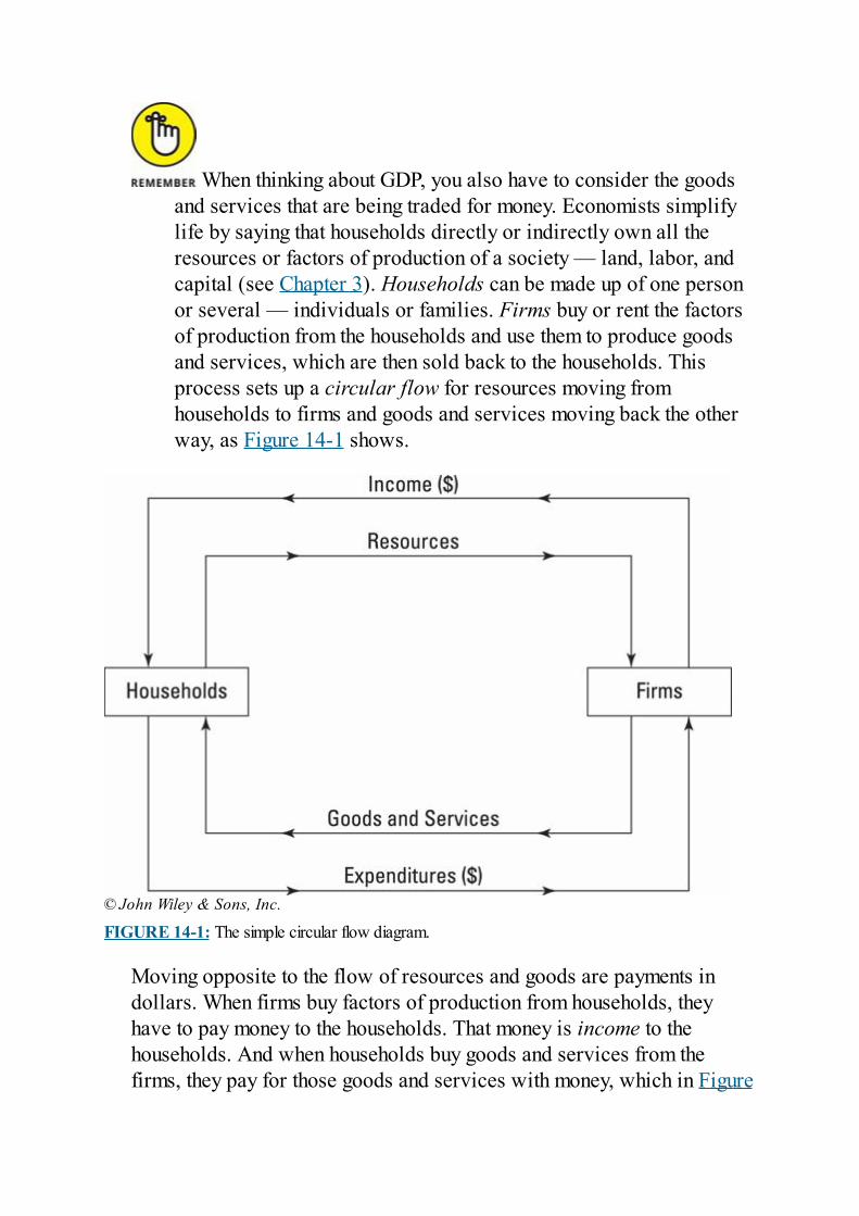
When thinking about GDP, you also have to consider the goodsand services that are being traded for money. Economists simplifylife by saying that households directly or indirectly own all theresources or factors of production of a society — land, labor, andcapital (see Chapter 3). Households can be made up of one personor several — individuals or families. Firms buy or rent the factorsof production from the households and use them to produce goodsand services, which are then sold back to the households. Thisprocess sets up a circular flow for resources moving fromhouseholds to firms and goods and services moving back the otherway, as Figure 14-1 shows.

© John Wiley & Sons, Inc.

FIGURE 14-1: The simple circular flow diagram.

Moving opposite to the flow of resources and goods are payments indollars. When firms buy factors of production from households, theyhave to pay money to the households. That money is income to thehouseholds. And when households buy goods and services from thefirms, they pay for those goods and services with money, which in Figure

14-1 are expenditures.

Households own firms; firms don’t exist on their own. As aresult, any money that a firm receives when it sells a good or aservice flows on as income to some individual or group ofindividuals. Because of this, incomes in Figure 14-1 have to equalexpenditures. Also, any resources that firms own — land, factories,mines, and so on — households also own because households ownall the firms in the economy. Thus, all income generated by sellingresources to produce goods and services flows directly orindirectly to households.

Accounting for streams of incomes, andassets

Although you can use either incomes or expenditures to measureGDP, economists prefer to use incomes because governments makeindividuals and businesses keep track of every penny of incomethey receive so that it can be taxed. This requirement providesextensive, accurate data about incomes.

Tracing the flow of incomeAll the income in the economy flows into one of four categories:

Labor receives wages.Land receives rent.Capital receives interest.Entrepreneurial ability receives profits.

Because you need land, labor, and capital to make things, you have topay for them. That’s why some of the income in the economy flows theirway. But in a dynamic, competitive economy, you also need individualswho are willing to bear business risks like going bankrupt and who arewilling to invest money in risky new technologies that may never catch

on. To get them to do so, you have to pay them, so some income must alsoflow as profits to risk-taking entrepreneurs to compensate them forproviding entrepreneurial ability.

Each of the four payments is a flow of money that compensates for a flowof services needed in production:

Wages: Workers charge wages for the labor services that theyprovide.Rent: Owners of buildings and land charge rents to tenants for theservices that real estate and physical structures provide.Interest: Firms wanting to obtain the services of capital, such asmachines and computers, must pay for them. This payment isconsidered interest because, for example, the cost of obtaining theservices of a $1,000 piece of capital equipment is the interestpayments that a firm must make on a $1,000 loan to buy that piece ofequipment.Profits: The firm’s profits must flow to the entrepreneurs and ownersof the firm, who risk that the firm may do badly or even go bankrupt.

Taking assets into considerationWhat happens to the flow of income if a firm buys land and office spacerather than rents it? Or if a firm owns its capital outright instead ofborrowing money to buy it? If a firm owns these things, it no longer hasto pay a flow of money to obtain a flow of services. Do expendituresstill equal incomes? Yes: Incomes still equal expenditures. But you haveto do some fancy accounting to see why. The key to this balancing act isunderstanding what an asset is.

An asset is something durable that isn’t directly consumed butthat gives off a flow of services that you do consume. A house is anasset because it provides shelter services. You don’t consume thehouse (just think of all the fiber!); you consume the services itprovides. Similarly, a car is an asset because although you don’tconsume the car itself, it provides transportation services.

You often have a choice between buying an asset outright and thereby

owning all the future services that the asset provides or letting someoneelse own the asset and sell you the services as they’re produced. Forexample, you can buy a house and thereby get all future shelter servicesthat the house provides, or you can rent the house and get those sameservices by paying for them each month. For this reason, an asset isconsidered to be a stock, and the services it provides are referred to as aflow.

For all assets that a firm owns, accountants put a dollar value onthe services that the assets provide based on what those sameservices would’ve cost if the firm had rented them. Accountants canthen divvy up the firm’s total income, calling some of it rent, someof it interest, and some of it profits, as though the owners of the firmwere getting three streams of income.

Because the firm’s owners provided the money to buy the firm’s assets,part of their income is compensation for providing these goods andservices, and the rest of their income is counted as compensation forproviding entrepreneurship and taking on risk. Consequently, all themoney expended on goods and services flows as income to somebodyfor providing land, labor, capital, or entrepreneurship (the four friendlyfactors of production). Under this methodology, incomes equalexpenditures even if firms own their own assets.

Following the funds, around and aroundThe simple circular flow diagram of Figure 14-1 captures the fact that anincome exists for every expenditure. However, because the diagramdivides the economy only into firms and households, it misses a lot of theaction that goes on in the real world. In Figure 14-2, you can see a muchmore realistic and detailed circular flow diagram that divides theeconomy into firms, households, and the government, with these entitiesmaking transactions in the following three markets:

Markets for factors of production: Money is exchanged topurchase or rent the land, labor, capital, and entrepreneurship used inproduction.Financial markets: People who want to lend money (savers) interact

with those who want to borrow money (borrowers). In these markets,the supply and demand for loans determine the interest rate, which isthe price you have to pay to get someone to lend you his money for awhile. Because most governments run deficits (in other words,they’re always in the hole) and have to borrow a lot of money,they’re major players in the financial markets.Markets for goods and services: People and the government buythe stuff that firms make.

© John Wiley & Sons, Inc.

FIGURE 14-2 The detailed circular flow diagram.

In Figure 14-2, arrows show the flows of dollars throughout theeconomy. Firms make factor payments — rent, wages, interest, andprofits — to households to obtain the factors of production — land,labor, capital, and entrepreneurial ability. (See the previous section“Accounting for the streams of incomes and assets” for details.)Households take the income they get from selling these factors and use itto pay for goods and services, to pay taxes, or to save. The government

buys goods and services using either the tax revenues it takes in or themoney it borrows in the financial markets. The financial markets alsoprovide dollars for corporations to make investments. These dollars addto those that firms get from selling goods and services to households andthe government.

Not all transactions in the financial markets are relevant to thecalculation of GDP. GDP measures currently produced output, andmost transactions in the financial markets are trading property rightsfor stuff produced long ago. For example, a house that was built 30years ago has nothing to do with current production, so the sale ofthe house doesn’t factor into this year’s GDP. Only the sales ofnewly constructed houses figure into this year’s GDP.

Counting stuff when it’s made, not when it’ssoldNewly produced output is counted as part of GDP as soon as it’sproduced, even before it gets sold. That makes keeping track of themoney associated with new production a little tricky.

For example, as soon as construction on a new house is completed, itsmarket value of $300,000 is estimated and counted as part of GDP rightthen, even though the house may not be sold for months. Supposeconstruction is completed on December 29, 2020, adding $300,000 tothe year 2020’s GDP. If the house is sold on February 21, 2021, itdoesn’t count in the year 2021’s GDP because double counting isn’tallowed.

When the house is sold, it’s considered old property and not newproduction. Economists just say that the property right to this now-oldhouse has changed hands from the builder to the new owner. Becausetrading old assets obviously involves no new production, it doesn’t countin GDP. Similarly, items such as used cars and used books don’t count inGDP, no matter how many times they’re bought and sold in resalemarkets.

This accounting convention applies to firms producing any sort of outputgood whatsoever. If Sony produces a TV on December 31, 2020, the

value of that TV is counted in the year 2020’s GDP, even though it won’tbe sold to a customer until the next year.

A handy way to think about this is to imagine that Sony builds theTV and then sells it to itself when putting the TV into inventory.This “sale” is what’s counted in GDP for the year 2020. When theTV is later sold out of inventory to a customer, the sale is just anexchange of assets (trading the TV for cash).

The fact that output is counted when it’s produced rather thanwhen it’s sold is a red flag when interpreting GDP statistics togauge the health of the economy. High GDP means only that a lot ofstuff is being produced and put into inventory. It doesn’t necessarilymean that firms are selling lots of stuff.

Economists who try to forecast where the economy is heading pay muchmore attention to inventory levels than they do to last quarter’s GDP.Why? Because it’s quite possible that although GDP is high, the economyis about to go into a recession because inventories are piling up andmanagers will soon cut back on production in order to get inventoriesback down to target levels.

Watching GDP rise with the good, the bad,and the uglyGenerally speaking, higher GDP is better than lower GDP because moreoutput produced means higher potential living standards, including betterhealthcare for the sick and more money to aid the needy. But higher GDPdoesn’t guarantee that happiness is increasing, because GDP often goesup when bad things happen. For instance, if a hurricane destroys a bigsection of a city, GDP goes up as reconstruction kicks into gear and lotsof new output is produced to replace what was destroyed. But wouldn’tit have been better not to have had the hurricane in the first place?

Similarly, higher GDP may be possible in certain situations only ifyou’re willing to tolerate more pollution or greater income inequality.

Countries experiencing the early stages of industrialization and quicklyrising living standards often also get dirtier environments and moresocial unrest because some people are getting richer much faster thanothers. The GDP number doesn’t reflect these negative outcomes.

GDP also doesn’t count the value of leisure. Many of my favorite timeshave been when I was neither producing nor consuming anything thatwould count in GDP — sitting on the beach, climbing a mountain, takinga walk, working out with friends. Moreover, an increase in GDP oftencomes at the price of sacrificing these leisure activities — meaning thatwhen you see an increase in GDP, overall well-being or happiness hasn’tnecessarily improved. So although policies that raise GDP are generallybeneficial for society, you must always examine the costs involved increating the rising output.

Diving In to the GDP EquationNow’s the time for you and GDP to make friends so you can understandall of GDP’s little secrets — in particular, its constituent parts and howthey behave. The discussion in this section is interesting by itself, but it’sdoubly useful because it makes the standard Keynesian macroeconomicmodel (which I introduce in Chapter 16) much easier to understand andmanipulate.

In the section “Tallying up what counts in GDP,” earlier in this chapter, Iexplain that you can measure GDP either by adding up all theexpenditures made on purchasing goods and services or by adding up allthe incomes that are derived from producing goods and services. Thetwo numbers have to be equal, so this switch to the expenditure methodof counting up GDP is totally kosher. (It’s also the perfect opportunity foryou to understand the economy from the point of view of where money isspent, as opposed to who gets to keep what’s earned.)

The expenditure equation for totaling up GDP adds together thefour traditional expenditure categories — consumption (C),investment (I), government spending (G), and net exports (NX).Their sum is abbreviated with the symbol Y and is equal to thevalue in dollars (or whatever currency a given country is using) ofall goods and services produced domestically in that country duringa given period of time (typically a quarter or a year). In terms ofalgebra, the GDP equation looks like this:

Here’s a quick look at the four expenditure variables that total up toGDP:

Consumption: C stands for consumption expenditures made byhouseholds on goods and services, whether produced domesticallyor abroad.Investment: I stands for investment expenditures that firms make onnew capital goods, including buildings, factories, and equipment. I

also contains changes in inventories, because any goods producedbut not sold during a period have to go into firms’ inventories and arecounted as inventory investments.Government expenditures: G stands for government expenditureson goods and services (they’ve got to buy paperclips for all thosegovernment documents).Net exports: NX stands for net exports, which are all a country’sexports (EX) minus all its imports (IM), or . EX is thenumber of dollars of your nation’s output that foreigners are buying.IM is the number of dollars of their output that your country isbuying.

These four expenditures make up the GDP because, as a group, they buyevery last bit of output produced in your country in a given period. Thefollowing subsections give more detail about each one.

“C” is for consumption (that’s good enoughfor me!)Household consumption spending accounts for about 70 percent of GDP— far more than the other three GDP components combined. Manyfactors affect how much income households decide to spend onconsumption and how much of it they decide to save for the future.

Microeconomists spend a lot of time studying the various factors thataffect such decisions, including expectations about whether the futurelooks bright or dark and how high or low the rates of return are onsavings. (See Part III of this book for info on microeconomics.)Macroeconomists, on the other hand, step back from these factorsbecause, when studying the economy as a whole, what matters is theamount of total consumption across the entire economy rather than theconsumption decisions of particular households or individuals.

Macroeconomists model consumption very simply, as a functionof people’s after-tax, or disposable, incomes. You can derivedisposable income algebraically using this handy three-stepprocess:

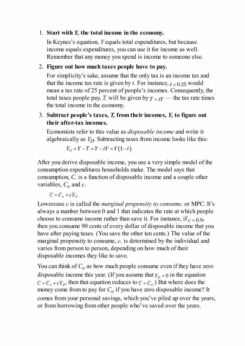
1. Start with Y, the total income in the economy.In Keynes’s equation, Y equals total expenditures, but becauseincome equals expenditures, you can use it for income as well.Remember that any money you spend is income to someone else.

2. Figure out how much taxes people have to pay.For simplicity’s sake, assume that the only tax is an income tax andthat the income tax rate is given by t. For instance, wouldmean a tax rate of 25 percent of people’s incomes. Consequently, thetotal taxes people pay, T, will be given by — the tax rate timesthe total income in the economy.

3. Subtract people’s taxes, T, from their incomes, Y, to figure outtheir after-tax incomes.Economists refer to this value as disposable income and write italgebraically as YD. Subtracting taxes from income looks like this:

After you derive disposable income, you use a very simple model of theconsumption expenditures households make. The model says thatconsumption, C, is a function of disposable income and a couple othervariables, Co and c.

Lowercase c is called the marginal propensity to consume, or MPC. It’salways a number between 0 and 1 that indicates the rate at which peoplechoose to consume income rather than save it. For instance, if ,then you consume 90 cents of every dollar of disposable income that youhave after paying taxes. (You save the other ten cents.) The value of themarginal propensity to consume, c, is determined by the individual andvaries from person to person, depending on how much of theirdisposable incomes they like to save.

You can think of Co as how much people consume even if they have zerodisposable income this year. (If you assume that in the equation

, then that equation reduces to .) But where does themoney come from to pay for Co if you have zero disposable income? Itcomes from your personal savings, which you’ve piled up over the years,or from borrowing from other people who’ve saved over the years.

What the overall equation says is that the totalconsumption expenditure in an economy is the amount peopleconsume even if they have no income (Co), plus a part of theirdisposable income (cYD).

For the rest of this book, I assume that the equation is agood-enough model of how consumption expenditures are determined inthe economy. It’s not perfectly realistic, but it does show that higher taxrates reduce consumption and that people make decisions about howmuch of their disposable incomes to save or consume. The equationallows you to analyze the effects of policies that change tax rates and theeffects of other policies that encourage people to spend higher or lowerfractions of their incomes.

“I” is for investment in capital stock

Investment is vital because the economy’s capacity to producedepends on how much capital is available to make output. Thecapital stock increases when firms purchase new tools, buildings,machines, computers, and so on to help produce consumptiongoods. Investment is a flow that increases the capital stock of theeconomy.

Of course, capital wears out as it’s used. Some of it rusts. Some of itbreaks down. Some of it’s thrown away when it becomes obsolete.Economists call all these flows that decrease the capital stockdepreciation.

Naturally, firms must make some investments just to replace the capitalthat has depreciated. But any investment in excess of depreciation causesthe overall size of the capital stock to increase, creating more potentialoutput for people to consume.

The flow of investment spending over any period of time

depends on the comparisons that firms make between the potentialbenefits and the costs of buying pieces of capital. The potentialbenefits are measured in terms of potential profits, and the costs ofbuying are measured by the interest rate, regardless of whether afirm takes out a loan to buy a given piece of capital.

Why does the interest rate matter so much? Naturally, if a firm needs totake out a loan to buy capital, higher interest rates make the firm lesslikely to borrow money because the loan repayment costs will be high.However, even if a firm has enough cash on hand to buy a given piece ofequipment, higher interest rates force the firm to decide between usingthe cash to buy the equipment and lending it to someone else. The higherthe interest rates, the more attractive loaning it out becomes.Consequently, higher interest rates discourage investment regardless ofwhether firms have to borrow to fund investment. (See Chapter 2 for whyhigher interest rates increase the opportunity cost of investing.)

Economists model the amount of investment expenditure that firms desireto make, I, as a function of the interest rate, r, which is given as apercentage. The equation that I use here is standard in introductory bookson macroeconomics (although notation does vary from book to book):

This equation is similar in spirit to the consumption equation in thepreceding section except for the minus sign, which indicates that whenthe interest rate rises, I falls.

The parameter Ir tells you how much I falls in an entire economy for anygiven increase in interest rates. For instance, suppose that r rises by 1percentage point. If Ir is, say, 10 billion, you know that each percentagepoint increase in interest rates will decrease investment by $10 billion.

The parameter Io tells you how much investment would occur if interestrates were zero. In truth, interest rates almost never fall all the way tozero, but suppose that they did. Then the second term in the equationwould be equal to zero, leaving you with .

The equation as a whole says that if interest rates were zero,investment expenditures would max out at Io. But as interest rates

rise above zero and keep on rising, investment falls more and more.In fact, rates could potentially rise so high that investment spendingwould fall to zero.

The relationship between interest rates and investment is onereason the government’s ability to set interest rates has greatbearing on the economy. By setting interest rates, the governmentcan determine how much businesses want to spend buyinginvestment goods. In particular, if the economy is in a recession, thegovernment can lower interest rates in order to raise firms’expenditures on investment and (hopefully) help improve theeconomy.

The big “G” (government, that is)In most countries, the government consumes a huge portion of GDP. In theUnited States, government at the local, state, and federal levels consumesabout 35 to 40 percent of the GDP. In many other countries, theproportion is even higher. In most of Europe, for instance, it’s closer to50 percent.

The government gets the money to buy all that output fromtaxation and borrowing. If a government’s tax revenues are exactlyequal to its expenditures, it has a balanced budget. If tax revenuesare greater than expenditures, it’s running a budget surplus. But ifthe government’s expenditures exceed its tax revenues (which thegovernment can arrange for by borrowing the difference on thefinancial markets), the government will be running a budget deficit.

Governments borrow by selling bonds. A typical bond says that inexchange for $10,000 right now, the government will give you back$10,000 in ten years and, in the meantime, pay you $1,000 per year foreach of the intervening years. If you accept the deal and buy the bond,you’re in effect lending the government $10,000 right now and getting a10 percent per-year return until the government gives you back your$10,000 in ten years.

A huge amount of political maneuvering goes into determining how mucha government is going to spend in a given year. Many groups lobby forspecial programs to benefit their hometown or their industry, and nomatter what, governments have to provide for essential governmentalfunctions such as national defense and law enforcement.

However, economists largely ignore the political machinations that gointo determining government expenditures because the economic effectsof government expenditure, G, depend on how big the expenditure turnsout to be — not on how it got to be that size. So, for the rest of this book,I make the simplifying assumption that government expenditures can bedenoted as

G is equal to some number, Go, that the political process determines. Gomay be high or low depending on politics, but in the end, you care onlyabout how big or small it turns out to be and can ignore where it camefrom.

G includes only government expenditures on newly producedgoods and services. It doesn’t include government expenditures thatmerely transfer money from one person to another. For instance,when the government taxes me and gives the money to a poorperson, that transaction has nothing to do with currently producedgoods and services and consequently doesn’t count as part of G. Soremember that when I talk about G, I’m talking about only thegovernment’s purchases of currently produced goods and services.

Measuring foreign trade with “NX”When your country sells domestically made goods and services tosomeone or some firm in another country, such sales are called exports,or EX. When someone in your country buys something produced abroad,such purchases are called imports, or IM. Net exports, or NX, is simplythe total value of all exports minus the total value of all imports during agiven period of time (mathematically, ). When using theexpenditure method for totaling up GDP, you add in net exports, NX. Butwhy add in only net exports?

The whole point of totaling up expenditures to get GDP is to figure outhow many total dollars were spent on products made in your owncountry. Most of that expenditure is made by locals, but foreigners canalso buy your products. That’s exactly what happens when they pay youfor the goods that you export to them. Consequently, you have to add inEX if you want to get a correct measure of expenditures made on stuffyou produce domestically.

You have to subtract imports of foreign goods to differentiate the totalexpenditures that domestic residents make on all goods and servicesfrom their expenditures on domestically made goods and services. Totalexpenditures on all goods and services, both domestic and foreign, are C(as covered earlier). To get just the part that’s spent on domesticallymade stuff, you subtract the value of imports, IM, because all moneyspent on imports is money that’s not spent on domestically made goodsand services. So C – IM gives the amount of money that domesticresidents spend on domestically produced output.

The result is that you can write your GDP expenditures equation thattotals up all expenditures made on domestically produced output asfollows:

But the equation normally puts the exports and imports next to each other:

Rearranging the GDP expenditures equation to include EX – IMquickly reveals your country’s trade balance. When EX – IM ispositive, you’re exporting more than you’re importing; when it’snegative, you’re importing more than you’re exporting. Economistslike to present the math in a way that tells a little story. Internationaltrade is hugely important, and you should understand not only whytrade balances can be positive or negative but also why youshouldn’t necessarily worry if it’s negative (covered next).

Making Sense of InternationalTrade and Its Effect on theEconomy

Modern countries do a huge amount of trading with other countries — sohuge, in fact, that for many countries, imports and exports equal morethan 50 percent of their GDPs. So now’s as good a time as any to focus alittle more deeply on the NX part of the GDP expenditure equation,

.

Understanding how international trade affects the economy isessential if you hope to have a complete understanding ofmacroeconomics. This understanding is also important becausepoliticians are constantly suggesting policies, such as tariffs andexchange rate controls, that are aimed squarely at international tradebut whose effects reverberate throughout the domestic economy.

This section explains why trade deficits (negative values of NX) aren’tnecessarily bad and why engaging in international trade — even when itmeans sustaining trade deficits — is typically hugely beneficial.

“Trade deficit” ain’t fightin’ wordsIf your exports exceed your imports, you have a trade surplus, and ifyour imports exceed your exports, you have a trade deficit.Unfortunately, the words surplus and deficit carry strong connotationsthat make surpluses sound like they’re necessarily better than deficits.That’s just not true, but you wouldn’t know it from the rhetoric thatpoliticians throw around. They make trade deficits sound as though theyonly lead to calamity.

To focus on whether a trade deficit or surplus exists is to miss

the point that international trade is a rearrangement of assets thatmakes everyone happier — even the country running the tradedeficit. As long as international trade is voluntary, all tradesenhance happiness, even if politicians say otherwise.

Consider two individuals who want to trade. Each person starts with$100 cash, and each produces a product for sale. The first guy grows andsells apples for $1 each. The second guy grows and sells oranges, alsofor $1 each. Each of them produces 50 pieces of fruit.

Next, suppose that the guy who grows apples really likes oranges andwants to buy 30 of them for $30, and suppose that the guy who growsoranges wants to buy 20 apples for $20. Each guy is happy to satisfy theother guy’s desires, so the apple grower spends $30 buying oranges fromthe orange grower, and the orange grower spends $20 buying applesfrom the apple grower.

Their trades shouldn’t cause any alarm bells to ring, but when peoplestart looking at their trades using the terms trade surplus and tradedeficit, they often come to the false conclusion that only one of the guysbenefits from the trades that, in reality, they both were quite eager tomake. To see where the confusion arises, notice that in the vocabulary ofinternational trade, the apple guy exports only $20 worth of apples butimports $30 worth of oranges. The orange guy exports $30 worth oforanges but imports only $20 worth of apples. So, you have a situation inwhich the apple guy is running a $10 trade deficit and the orange guy isrunning a $10 trade surplus.

Does this mean that the apple guy is worse off than the orange guy? No.Each person started with $150 worth of stuff: their respective $100 cashpiles plus $50 each worth of fruit. When they finish trading, they eachstill have $150 worth of stuff. The apple guy has $90 of cash plus $30worth of apples and $30 worth of oranges. The orange guy has $110 ofcash plus $20 worth of oranges and $20 worth of apples.

Saying that their trading has made either one poorer is way off the mark.In fact, both are happier with their arrangements of wealth after tradingthan they were before because their trades were voluntary. If the appleguy would’ve been happier keeping his initial $100 cash and 50 apples,he wouldn’t have traded for oranges — and the same goes for the orangeguy.

Considering assets — not just cashTo people who hate trade deficits, changes in cash holdings seemalarming. But when gauging whether trade is beneficial, you need toconsider the value of the traded assets, not just how much cash eachparty ends up with. For instance, the fact that the apple guy’s cash pile(see the preceding section) falls from $100 before the trade to only $90after the trade looks spooky to deficit-haters because they’re focused onthe fact that the apple guy is $10 poorer in terms of cash after tradingwith the orange guy. And they’re even more peeved because that $10ends up with the orange guy, giving him a commanding $110-to-$90advantage in terms of cash piles.

This perspective misses the fact that the apple guy’s overall wealth isstill $150 and he now has a distribution of assets that’s more pleasing tohim than what he had before. Deficit-haters respond to this by asking youwhat happens after the apple guy eats his 30 apples and 30 oranges andafter the orange guy eats his 20 apples and 20 oranges. In the end, all thatthe two guys have left are their cash piles. Because the apple guy has $20less cash than the orange guy, he must be worse off by running a tradedeficit.

Again, this reasoning misses the point that the apple guy was happiertrading and ending up with $90 of cash than he would’ve been not tradingand having $100 in cash. If not for trade, he would’ve had a boring dietof only apples.

Opponents of trade deficits really make things seem scary when they starttalking about land trading hands due to international trade. (“Oh no!” theysay. “The foreigners are taking over our country!”) To see their point,imagine that instead of starting with $100 each of cash, the fruit farmerseach start with 100 acres of land worth $1 per acre. The only way for theapple guy to come up with $10 of cash to pay for his trade deficit is byselling 10 acres of land to the orange guy. That is, the overall exchangethat they engage in is 20 apples plus 10 acres of land worth a combined$30 in exchange for 30 oranges worth $30. Because 10 of the apple guy’sacres of land now belong to the orange guy, deficit haters think the appleguy sold out his country — literally.

Such transfers of property do happen in real life. During the 1980s, theUnited States ran huge trade deficits with Japan. The result was that

Japanese corporations and individuals ended up owning many famousU.S. buildings and companies. This really spooked many jingoistic U.S.politicians, but they missed the point that all trading in life — be it withforeigners or fellow citizens — is designed to make both parties happy.After all, what good is keeping all your 100 acres of land if you’rehappier trading 10 of them for foreign-made goods? Or in the case of theUnited States during the 1980s, what good is continuing to own TimesSquare or Columbia Pictures if you’d rather trade them for HondaAccords and Sony VCRs? (The anti-Japanese hysteria at the time waseven sillier given that the largest group of foreign owners of U.S.property was, and still is, the British!)

Much to the chagrin of economists, the argument that the point of trade isto make you happier doesn’t always fly well. Many people view tradeas an antagonistic contest to dominate other countries by running tradesurpluses so that you eventually own all the other guy’s assets. Theyargue for restrictions on trade designed to rig trade relations so that theirown countries always run surpluses. But such policies inevitably failbecause anytime you put up a tariff barrier or an import tax to discourageimports and improve your trade balance, other countries can do the same.The result of such trade wars is that all the barriers, restrictions, andtaxes imposed by both sides reduce international trade to a trickle. Noone comes out ahead, and no one’s happy.

Consequently, for the last 70 years, national governments haveincreasingly pushed for fewer and fewer restrictions on internationaltrade. This free trade movement has resulted in hundreds of millions ofnew jobs and a vast improvement in living standards and happinessbecause people all over the world are free to trade and buy whatever itis that makes them happiest — even if that means buying from aforeigner.

Wielding a comparative advantageThe argument that even countries running trade deficits are better offbecause they get to consume a mix of goods and services they couldn’tget otherwise rests solely on the benefits of trading things that havealready been produced. But an even better argument for internationaltrade is that the trade actually increases the total amount of outputproduced in the world — meaning that there’s more output per person, so

overall living standards rise.

English economist David Ricardo developed this argument, known ascomparative advantage, in 1817 as a forceful rebuttal against the importtariffs known as the Corn Laws, which heavily taxed imports of foreign-grown grain. These laws kept the price of grain high, so the nobility thatowned the vast majority of farmland favored keeping them. Naturally, thepoor were opposed because the laws drove up the price of their basicfood supply: bread.

Ricardo pointed out that abolishing restrictions on international tradewould, in addition to helping England’s poor, actually make England andall the countries it traded with richer by encouraging them to specializein the production of goods and services that each of them could produceat the lowest possible opportunity cost (in terms of other goods andservices forgone). He demonstrated that this process of specializationwould increase total worldwide output and thereby raise livingstandards.

You can most easily understand the logic behind the comparativeadvantage argument by thinking in terms of people rather than countries.Consider a patent lawyer named Heather and her brother Adam, a bikemechanic. Heather is very good at filing patents for new discoveries andis also very good at repairing bicycles — in fact, she’s faster at that thanher brother. Adam is a smart guy and can file patents, too, although not asquickly as Heather can. Table 14-1 lists how many bike repairs andpatent filings each of them could do in one day if they put all their effortsinto only one of the activities.

TABLE 14-1 Productivity for Heather and Adam per Day

Person Patent Productivity Bike Repair Productivity

Heather 6 12

Adam 2 10

In one day’s work, Heather can produce 6 patents or repair 12 bikes;Adam can file 2 patents or repair 10 bikes. She is more efficient atproducing both patents and bike repairs because she can convert oneday’s labor into more of either good than Adam can. Heather has anabsolute advantage over Adam at producing both goods. She’s the more

efficient producer of both; with the same amount of labor input (oneworkday), she can produce more than her brother. Before David Ricardocame up with the idea of comparative advantage, the only thing anyoneknew to look at was absolute advantage. And when they saw situationslike that of Heather and Adam, they concluded (incorrectly) that becauseHeather is more efficient at both tasks, she has no need to trade with him.

In other words, people used to believe that because Heather is betterthan Adam at repairing bikes, not only should she work hard as a patentattorney filing lots of patents, but she should also fix her own bikewhenever it breaks down. Ricardo pointed out that this argument basedon absolute advantage is bogus and that Heather should, in fact, never fixbikes, despite the fact that she’s the most efficient bike repairpersonaround. The nifty thing Ricardo realized is that the world is better off ifeach person (and country) specializes.

Comparative advantage’s insight is that the measure of cost whenconsidering whether you should produce one good or another isn’thow many hours of labor input it takes you to produce each one(which is the logic behind absolute advantage). The true cost is theopportunity cost of how much of the production of one good youhave to give up to produce a unit of the other good.

To produce one patent, Heather must give up the chance to repair twobikes. To make one patent, Adam would have to give up the chance torepair five bikes. Heather is the lower-cost producer of patents andtherefore should specialize in filing patents. And Adam should specializein bike repairs because he’s the lower-cost producer of bike repairs. Ineconomic terminology, we say that Heather has a comparativeadvantage in the production of patents, whereas Adam has acomparative advantage in the production of bike repairs.

On a larger scale, countries should specialize in the production of goodsand services that they can deliver at lower opportunity costs than othercountries. If countries are free to do this, everything that’s producedcomes from the lowest-cost producer. Because this arrangement leads tothe most efficient possible production, total output increases, therebyraising living standards.

Politicians often argue that countries shouldn’t be “dependent” on othercountries for various goods and services. Any policy that takes thiswarning seriously by impeding trade and specialization increases costsand makes total output fall. Rather, by letting comparative advantageguide who makes what, free trade increases total world output andthereby raises living standards. In free trade, each country specializes inits area(s) of comparative advantage and trades with other countries forgoods and services it desires to consume.

Don’t be tricked by absolute advantage. Having an absoluteadvantage means you can make something at a lower cost asmeasured in inputs (Heather requires fewer hours of labor input tofile a patent than Adam does). But what matters in life are outputs— the things people actually want to consume. By focusing on costsas measured in terms of alternative types of output that must begiven up to produce a certain product, comparative advantageassures that you’re focusing on being efficient in terms of whatreally matters: output.

Chapter 15

Inflation Frustration: WhyMore Money Isn’t Always

GoodIN THIS CHAPTER

Risking inflation by printing too much money Measuring inflation with price indexes Adjusting interest rates to account for inflation

Inflation is the word economists use to describe a situation in which thegeneral level of prices in the economy is rising. Although some pricesmay stay the same and a few may fall, the large majority of prices rise.

Inflation is typically mild, with the overall level of prices rising only asmall percentage each year. But people dislike even mild inflationbecause — face it — who likes paying higher prices? Mild inflation alsocauses problems such as making retirement planning difficult. After all,if you don’t know how expensive things will be when you retire,calculating how much money you need to be saving right now is hard.

Things can go from bad to worse if inflation really gets out of controland prices begin rising 20 or 30 percent per month — something that hashappened in more than a few countries in the past century. Such situationsof hyperinflation usually accompany a major economic collapsefeaturing high unemployment and a major decrease in the production ofgoods and services. (For more on prices and how they affect theeconomy, see Chapter 16.)

The good news is that economists know exactly what causes inflationand how to stop it. The culprit is a money supply that grows too quickly,and the solution is to slow or halt the growth of the money supply.Unfortunately, some political pressure is always exerted in favor ofinflation so that simply knowing how to prevent inflation doesn’tnecessarily mean it won’t develop.

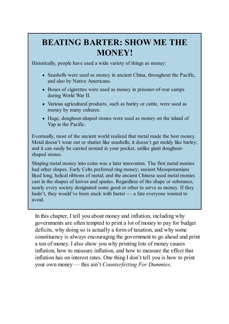
BEATING BARTER: SHOW ME THEMONEY!

Historically, people have used a wide variety of things as money:

Seashells were used as money in ancient China, throughout the Pacific,and also by Native Americans.Boxes of cigarettes were used as money in prisoner-of-war campsduring World War II.Various agricultural products, such as barley or cattle, were used asmoney by many cultures.Huge, doughnut-shaped stones were used as money on the island ofYap in the Pacific.

Eventually, most of the ancient world realized that metal made the best money.Metal doesn’t wear out or shatter like seashells; it doesn’t get moldy like barley;and it can easily be carried around in your pocket, unlike giant doughnut-shaped stones.

Shaping metal money into coins was a later innovation. The first metal monieshad other shapes. Early Celts preferred ring money; ancient Mesopotamiansliked long, helical ribbons of metal; and the ancient Chinese used metal moniescast in the shapes of knives and spades. Regardless of the shape or substance,nearly every society designated some good or other to serve as money. If theyhadn’t, they would’ve been stuck with barter — a fate everyone wanted toavoid.

In this chapter, I tell you about money and inflation, including whygovernments are often tempted to print a lot of money to pay for budgetdeficits, why doing so is actually a form of taxation, and why someconstituency is always encouraging the government to go ahead and printa ton of money. I also show you why printing lots of money causesinflation, how to measure inflation, and how to measure the effect thatinflation has on interest rates. One thing I don’t tell you is how to printyour own money — this ain’t Counterfeiting For Dummies.

Buying an Inflation: When TooMuch Money Is a Bad Thing

I don’t think I can overstate how important money is to the properfunctioning of the economy. Without it, you’d waste most of your timebartering, or arranging trades of one good for another — kind of like inkindergarten (“I’ll trade you my sandwich for your brownie”). Barteringworks well only in the rare circumstance that you run into somebody whohas what you want and who wants what you have.

In contrast, money provides a medium of exchange that allows you totrade for the brownie from the kid next to you, even if you don’t have asandwich. Money can be any good, object, or thing, but its definingcharacteristic is that it’s accepted as payment for all other goods andservices. In today’s economy, people pay for things using a wide varietyof monies, including government-issued coins and cash, checks drawn onprivate bank deposits, and electronic payments facilitated by debit cardsand so-called crypto currencies. Because money affects nearly everyeconomic transaction that takes place, money is at the heart ofmacroeconomics, the study of the economy as a whole.

As with everything in life, balance is essential. If a government prints toomuch money, prices go up, and you get inflation. If a government printstoo little, prices go down, and you get deflation. But how much money isthe right amount? And why does printing too much or too little causeinflation or deflation? In this section, I go into more detail about thesemoney matters.

Balancing money supply and demandBasically, money’s value is determined by supply and demand (which Idiscuss in detail in Chapter 4):

The supply of money is under government control, and thegovernment can very easily print more money anytime it wants to.The demand for money derives from its usefulness as a means ofpaying for things and from the fact that having money means nothaving to engage in barter.

For any given supply of money, supply and demand interact to set a valuefor each unit of money. If money is in short supply, each piece of moneyis very valuable; fewer pieces of money translate into fewer chances toavoid having to engage in barter. But if the government greatly increasesthe supply of money, then each individual unit of money loses valuebecause getting enough money together to avoid barter is easy.

Prices and the value of money are inversely related, meaningthat when the value of money goes up, prices go down (and viceversa). To see how this relationship works, suppose that money isin short supply and is consequently very valuable. Because it’s veryvaluable, it buys a lot of stuff. For instance, 1 dollar may buy 10pounds of coffee (that’s 10 cents per pound). But if money’s verycommon, then each unit isn’t very valuable. In this case, 1 dollarmay buy only 1 pound of coffee (that’s 1 dollar per pound). So thegreater the supply of money, the higher the prices.

CROESUS AND KUBLAI: THE KINGSOF MONEY

King Croesus of Lydia is usually given credit for solving the problem of bogusmetal money. In the sixth century BC, Croesus issued the first government-certified coins that guaranteed purity and weight.

Lydia was located in what is now western Turkey, and soon all the majortrading nations of the Mediterranean were using the new Lydian coins becausethey were by far the most trustworthy medium of exchange available. The newcoinage gave Lydian traders a major advantage, and the kingdom soon becamevery wealthy, so much so that Croesus was considered the richest man in theworld — even richer than King Midas (of Midas touch fame), whose goldCroesus minted into coins.

But coins are hard to carry around in large amounts, and it was up to theChinese emperor Kublai Khan to create the first paper money in the 13thcentury. This paper money was actually a kind of precious metal certificate;people holding one of these certificates could go to a government vault andredeem it for gold. Consequently, the pieces of paper were as good as gold, buta stack of paper was a whole lot easier to carry than a heavy bag of coins.

Paper money was such a radical innovation that when Marco Polo came backfrom China and told Europeans about it, they laughed, unable to conceive ofanything other than gold or silver coins serving as money. Their incredulity washard to overcome, and after paper money fell out of favor in China, it would becenturies before another government issued any again.

The demand for money tends to grow slowly over time. Growingeconomies produce more stuff, and consumers demand more money withwhich to buy the available stuff. Depending on how a government reactsto consumer demand for more money, three scenarios are possible:

The government increases the supply of money at the same rateas the growing demand for money. In this case, prices don’tchange. In other words, if supply and demand for money grow atequal rates, the relative value of money doesn’t change.The government increases the supply of money faster than thedemand for money grows. Here, inflation results as money becomesrelatively more plentiful and each piece of money becomes relatively

less valuable. With each piece of money possessing less value, youneed more pieces of money to buy any particular item — which is thesame as saying that the item’s price will rise.The government increases the supply of money slower than thedemand for money grows. In this case, deflation results becauseeach piece of money grows relatively more valuable. Buying anygiven good or service requires less money.

PREVENTING INFLATION WITH AGOLD STANDARD

Until the early 1970s, printing new bills was difficult because most of theworld’s paper currencies were backed by a valuable metal, such as gold. Underthis system, every piece of paper money circulating in the economy wasconvertible into a specific quantity of gold so that anyone holding cash couldredeem their cash for gold anytime they wanted. For instance, in the UnitedStates, you could bring $35 cash to the U.S. Treasury and get exactly 1 ounceof gold.

This gold standard made it difficult for the government to devalue the currencyby printing too much money because it first had to get more gold with which toback the new money. Because purchasing gold is expensive, governments wereeffectively restrained from increasing their money supplies.

But in 1971, President Nixon took the United States off the gold standard andon to the fiat system, in which paper currency isn’t backed by anything. Peoplejust have to accept the currency as though it has value. In fact, fiat is Latin for“Let it be!” So when you say fiat money, you’re basically referring to how agovernment creates money simply by ordering it into existence. The problemwith a fiat money system is that nothing limits the number of little pieces ofpaper that the government can print to pay its debts.

You may be wondering whether there’s any way to know exactlyhow much inflation you can expect from printing any given amountof extra money. You’re in luck! The quantity theory of money statesthat the overall level of prices in the economy is proportional to thequantity of money circulating in the economy. Proportional justmeans that things go up by equal ratios or proportions, so thequantity theory can also be stated this way: If you double the moneysupply, you double prices.

But why would any government want to cause inflation or deflation ofany size whatsoever? For the answer to that question, read on!

Giving in to the inflation temptationInflation is caused primarily by governments’ printing more paper money

or producing a large amount of cheap-metal coins, which vastlyincreases the supply of money and makes each piece of money lessprecious. As sellers demand higher prices to make up for the fact thateach piece of money is worth less, you get inflation.

So why in the world would governments ever opt to increases inthe money supply so fast that inflation will result? Good question.Historically, governments circulate more money in threecircumstances:

When governments can’t raise enough tax revenue to pay theirobligationsWhen governments feel pressure from debtors who want inflation sothey can repay their debts using less valuable moneyWhen governments want to try to stimulate the economy during arecession or depression

As you find out more about these three reasons for increasing the moneysupply, keep the following in mind: If the supply of money increasesfaster than the demand for money, inflation results. (For more on this, seethe earlier section “Balancing money supply and demand.”)Consequently, no matter what reason a government has for increasing thesupply of money, it runs the risk of inflation. And that’s true both forgood reasons, such as wanting to help the economy out of a recession,and for bad reasons, such as helping debtors repay their loans using lessvaluable money.

Paying bills by printing bills: HyperinflationGovernments almost always have debts, and printing extra money can bea tempting way to pay them. Quite often, a government may want to spendmore money than it’s collecting in tax revenue. One solution is to borrowthe shortfall, but another is to simply print new bills to cover thedifference.

The trouble with allowing a government to pay its debts and obligationsby printing money is that as soon as the newly printed money begins tocirculate, people spend it, drive up prices, and cause inflation. And if the

government prints successively more money, you end up with peopleoffering shopkeepers and producers successively more cash for the sameamount of goods and services. It’s like a giant auction where everybodybidding on items keeps getting more and more money to bid with.

If a government gets into the habit of rapidly printing new moneyto pay its bills, inflation can soon reach or even surpass 20 or 30percent per month, a situation referred to as a hyperinflation.Economists (and everyone else) hate hyperinflation because itgreatly disrupts daily life and ruins the investment climate.Hyperinflation does the following:

Causes people to waste huge amounts of time trying to avoid theeffects of rising prices: During the Weimar hyperinflation inGermany (which I discuss in the sidebar “Hyperinflation andHitler”), men working at factories were paid two or even three timesa day because money lost its value so quickly. Their wives waited atthe factories to immediately take the money to the nearest shops,trying to spend the pay before it lost most of its value. Shopping maybe fun, but not when you’re desperately racing against outrageouslyrising prices!Destroys the incentive to save: The only sensible thing to do withmoney during a hyperinflation is to spend it as quickly as you canbefore it loses even more of its value. People whose life savingswere in German marks during the Weimar hyperinflation soon foundthat what they had worked so hard to amass had become worthless.And people thinking about saving for the future were greatlydiscouraged because they knew that any money they saved wouldsoon lose all value.Harms businesses: The discouragement of saving causes majorbusiness problems because if people aren’t saving, then no money isavailable for businesses to borrow for new investments. And withoutnew investments, the economy can’t grow.

HYPERINFLATION AND HITLERHistory’s most infamous hyperinflation hit Germany in the 1920s, during theeconomically incompetent Weimar Republic. It so badly ruined the Germaneconomy that Germans would later vote Adolph Hitler into power because hepromised to fix things.

At the end of World War I, Germany faced the prospect of paying off massivedebts taken on during the conflict in addition to all the ongoing costs of runninga government. Most of its debts were in its own currency, the German mark.

Because the German government had the exclusive right to produce Germanmarks, the debt proved an irresistible temptation to begin printing money to payits bills. If the government owed a billion marks to a certain firm, it simplyprinted up a billion crisp, new mark bills and handed them over. If a bunch ofschoolteachers hadn’t been paid the previous month, the Weimar governmentsimply printed up enough new cash to pay them.

Soon, all the new money caused a wild hyperinflation. In fact, the rate ofinflation in Weimar Germany in 1922 was well over 100 percent per month —it reached nearly 6,000 percent by the end of year!

Then things really got out of control. Prices went up 1,300,000,000,000 times(this is not a misprint!) in 1923. That year, Germans paid 200,000 marks for aloaf of bread and 2 million marks for a pound of meat. Prices rose so rapidlythat waiters at restaurants had to pencil in new prices on menus several times aday. And if you ate slowly, you were sometimes charged twice what wasprinted on the menu because prices had gone up so much while you wereeating! In some places in Germany, people stopped bothering to take the timeto count out money. Instead, they tied paper bills into huge bricks and weighedthe bricks of cash. For instance, it may have cost 2 pounds of cash to buy achicken.

Feeling printing press pressures: Inflation politicsEven if the government isn’t trying to use inflation to increase taxrevenues (see the preceding section), a certain political constituency willalways pressure it to circulate more money. You may even be a memberof this group — they’re called borrowers. To understand the politics ofinflation, understand that one of the functions of money is to act as astandard of deferred payment. What does that mean?

Imagine that you borrow $1,000 to invest on your farm, promising to paythe bank back $1,200 next year. For the past several years, prices in the

economy have been stable, and, in particular, the pigs that you raise havesold for $100 each. Essentially, your loan lets you borrow the equivalentof 10 pigs with the promise to pay back 12 pigs next year.

But you’ve got an idea. You lobby your congressman to lobby thegovernment to print more money. All that new money causes inflation,after which the price of pigs rises to $200 each. Now you have to sellonly six pigs to pay back the $1,200 loan, leaving you with more pigs,you pig!

Lenders, of course, oppose the inflationary desires of borrowers. If youwere the bank, you would do everything in your power to stop theinflation. If it goes through, not only are your profits ruined, but you’re anoutright loser. In the first year, your loan of $1,000 is the equivalent often pigs. But after the inflation, you get paid back the equivalent of onlysix pigs. You take a 40 percent loss on the value of your loan. Too muchinflation, and a lender ends up being a pig in a poke.

As long as economies use money, lenders and borrowers will always belined up against each other, both trying to sway the government.

Stimulating the economy with inflation: Monetary policyA legitimate reason for governments to print more money has the veryrespectable name of monetary policy. Monetary policy refers to thedecisions a government makes about increasing or decreasing the moneysupply in order to stimulate or slow down the economy.

I go into monetary policy in detail in Chapter 17, but the basic idea isthat if the economy is in a recession, the government may print up somenew money and spend it. All the goods and services it buys with the newmoney stimulate the economy immediately. All those businesses thatreceived money from the government can now also go out and spend thatnew money themselves. And whoever receives the money from them willalso go out and spend it to buy things. In fact, this can theoretically go onforever and stimulate a lot of economic activity — enough to lift aneconomy out of a recession.

If this sounds too good to be true, it is. Why? Inflation. Whenpeople start spending all that new money, it drives up prices.

Eventually, the only effect of the government’s good intentions isthat prices rise and no additional goods are sold. For example, ifthe government doubles the money supply, businesses will doublethe prices they charge because each piece of money is worth half asmuch as before. Consequently, the total amount of goods andservices sold will be the same as before because although twice asmuch money is being spent, prices are also twice as high.

The sad upshot is that an increase in the money supply stimulates theeconomy only when it’s a surprise. If the government can print the moneyand start spending it before people can raise prices, you get an increasein the amount of goods and services sold. Eventually, of course, peoplefigure it out and raise prices, but until they do, the monetary stimulusworks.

Unfortunately, fooling people over and over is tough. You can surprisepeople once, but it’s much harder the second time and even harder thethird time. In fact, if the government keeps trying to surprise people,people begin to anticipate the government’s actions, and they raise priceseven before the government prints more money. Consequently, mostmodern governments have decided against using this sort of monetarystimulus and now strive for zero inflation or very low inflation.

Tallying up the effects of inflationIn the United States, prices rise only a small amount each year. However,even moderate inflation causes problems by cutting into the practicalbenefits of using money instead of barter. You can get a better sense ofthis fact by looking at the four functions that economists generally ascribeto money and the ways in which inflation screws up each of them:

Money is a store of value. If I sell a cow today for one gold coin, Ishould be able to turn around and trade that gold coin back for a cowtomorrow or next week or next month. When money retains its value,you can hold it instead of holding cows, or real estate, or any otherasset.Inflations weaken the use of money as a store of value because eachunit of currency is worth less and less as time passes.Money is a unit of account. When money is widely accepted in aneconomy, it often becomes the unit of account in which people write

contracts. People start using phrases like “$50 worth of lumber”rather than “50 square feet of lumber,” or “$1 million worth of shirtsin inventory” instead of “20,000 shirts in inventory.”This practice makes sense if money holds its value over time, but inthe presence of inflation, using money as a unit of account createsproblems because the value of money declines. For instance, if thevalue of money is falling fast, how much lumber, exactly, is “$50worth of lumber”?Money is a standard of deferred payment. If you want a cow, youprobably wouldn’t borrow a cow with the promise to repay twocows next year. Instead, you’d be much more likely to borrow andrepay in terms of money. That is, you’d borrow one gold coin and useit to buy a cow, after promising to pay back two gold coins next year.The progressive devaluing of money during a period of inflationmakes lenders reluctant to use money as a standard of deferredpayment. Suppose a friend asks to borrow $100, promising to payyou $120 in a year. That seems like a good deal — after all, it’s a 20percent interest rate. But if prices are rapidly rising and the value ofmoney is falling, how much will you be able to buy with that $120next year?Inflations make people reluctant to lend money. Potential lenders fearthat when the loans are repaid, the repayment cash won’t have thesame purchasing power as the cash that was lent. This uncertaintycan have a devastating effect on the development of new businesses,which rely heavily on loans to fund their operations.Money is a medium of exchange. Money is a medium (literallymeaning “something in the middle”) of trade between buyers andsellers because it can be directly exchanged for anything else, makingbuying and selling much easier. In a barter economy, an orangefarmer who wants to buy beer may have to first trade oranges forapples and then apples for beer because the guy selling the beerwants only apples. Money can eliminate this kind of hassle.But if inflation is bad enough, money is no longer an effectivemedium of exchange. During hyperinflations, economies often revertto barter so buyers and sellers don’t have to worry about the fallingvalue of money. For example, in a healthy economy, the orange sellercan first sell oranges for cash and then trade the cash for beer. But

during a hyperinflation, between the time he sells the oranges forcash and buys the beer, the price of beer may have skyrocketed sohigh that he can’t buy very much beer with the cash. During ahyperinflation, economies have to resort to cumbersome bartering.

Another effect of inflation is that it functions as a giant taxincrease. This seems strange because you normally think ofgovernments taxing by taking away chunks of people’s money, notby printing more money. But a tax is basically anything that transfersprivate property to the government. Debasing the currency orprinting more money can have this effect.

Suppose that the government wants to buy a $20,000 van for the postoffice. The honest way to go about this is to use $20,000 of tax revenuesto buy a van. But a sneakier way is to print $20,000 in new cash to buythe van. By printing and spending the new cash, the government hasconverted $20,000 of private property — the van — into publicproperty. So printing new cash works just like a tax. Because printingnew money ends up causing inflation, this type of taxation is oftenreferred to as an inflation tax.

Not only is the inflation tax sneaky, it unfairly targets the poor becausethey spend nearly all their incomes on goods and services, the prices ofwhich go up greatly during an inflation. By contrast, because the richhave the opportunity to save a lot of their incomes, proportionatelythey’re less affected by an inflation tax. By investing their savings inassets whose prices go up during an inflation (such as real estate), therich can insulate themselves from a great deal of the harm caused byinflation.

Measuring InflationInflation can cause lots of problems, so for the government to keepinflation under control, it needs a way to measure inflation accurately.

The value of money is determined by the interaction of the supply ofmoney with the demand for money (as I explain in the earlier section“Buying an Inflation: When Too Much Money Is a Bad Thing”). Thesupply of money is under the government’s control, but the governmentcan’t directly ascertain the demand for money; it has to look at howsupply and demand interact in order to determine how much to increaseor decrease the money supply:

If inflation is in effect, the government knows that the supply ofmoney is increasing faster than the demand for money. If it wants totame the inflation, it should reduce the supply of money.If deflation is in effect, the government knows that the demand formoney is increasing faster than the supply of money. If it wants to endthe deflation, it should increase the supply of money.

Because inflation is a general increase in the overall level ofprices, the best way to look for it is by seeing whether the cost ofbuying a large collection of many different goods and services risesover time. If, instead, you look at only one or two prices, you mayend up confusing a relative price increase for an increase in theoverall, general level of prices. (A relative price increase is whena single price increases when compared to other prices, whichremain unchanged or even fall.)

Economists arbitrarily define some large collection of goods andservices and refer to it as a market basket. They then measureinflation by finding out how much money it takes to buy this basketat various times. The best-known market basket is monitored by the

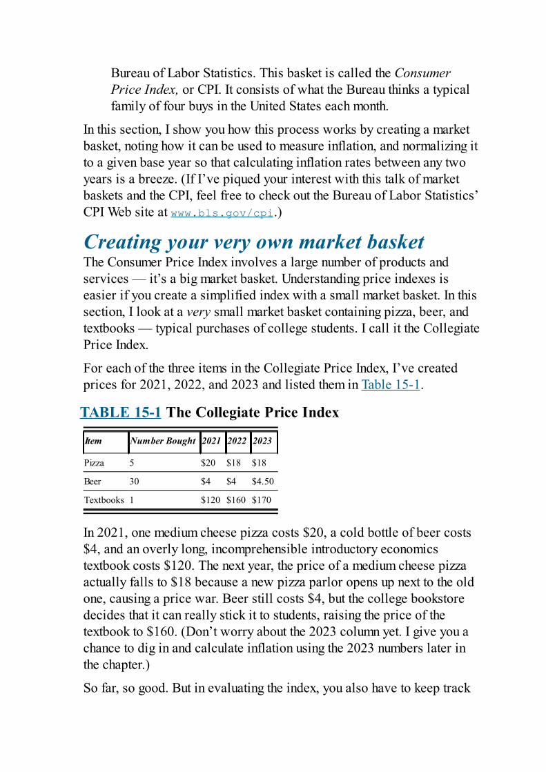
Bureau of Labor Statistics. This basket is called the ConsumerPrice Index, or CPI. It consists of what the Bureau thinks a typicalfamily of four buys in the United States each month.

In this section, I show you how this process works by creating a marketbasket, noting how it can be used to measure inflation, and normalizing itto a given base year so that calculating inflation rates between any twoyears is a breeze. (If I’ve piqued your interest with this talk of marketbaskets and the CPI, feel free to check out the Bureau of Labor Statistics’CPI Web site at www.bls.gov/cpi.)

Creating your very own market basketThe Consumer Price Index involves a large number of products andservices — it’s a big market basket. Understanding price indexes iseasier if you create a simplified index with a small market basket. In thissection, I look at a very small market basket containing pizza, beer, andtextbooks — typical purchases of college students. I call it the CollegiatePrice Index.

For each of the three items in the Collegiate Price Index, I’ve createdprices for 2021, 2022, and 2023 and listed them in Table 15-1.

TABLE 15-1 The Collegiate Price Index

Item Number Bought 2021 2022 2023

Pizza 5 $20 $18 $18

Beer 30 $4 $4 $4.50

Textbooks 1 $120 $160 $170

In 2021, one medium cheese pizza costs $20, a cold bottle of beer costs$4, and an overly long, incomprehensible introductory economicstextbook costs $120. The next year, the price of a medium cheese pizzaactually falls to $18 because a new pizza parlor opens up next to the oldone, causing a price war. Beer still costs $4, but the college bookstoredecides that it can really stick it to students, raising the price of thetextbook to $160. (Don’t worry about the 2023 column yet. I give you achance to dig in and calculate inflation using the 2023 numbers later inthe chapter.)

So far, so good. But in evaluating the index, you also have to keep track

of how many of each item is bought by the typical student each year. Forthe sake of simplicity, assume that a typical student buys 5 cheese pizzas,30 beers, and 1 economics textbook each year.

Calculating the inflation rateTo calculate how much inflation your college economy has (or deflation,if the price of this basket happens to go down), first total up how muchthe market basket costs each year using Table 15-1. In 2021, it costs$340: $100 on pizza (5 pizzas at $20 each), $120 on beer (30 beers at $4each), and $120 on economics textbooks (1 textbook at $120). The costof buying the same market basket in 2022 is $370, so the cost of buyingthe same market basket has gone up by $30.

Now that you’ve done the addition, you need some simple algebra.Economists use the capital letter P to denote how many dollars thedefined market basket costs. So in this case, P2021 means the cost ofbuying the market basket in 2021 and P2022 is the cost of buying themarket basket in 2022. Economics has a standard practice of denoting therate of inflation with the Greek letter π (pronounced “pie”).

To calculate the rate of inflation, you use a very simple formula:

(1) In the case of the Collegiate Price Index, the formula becomes:

(2) Substituting in and , you find that . Convertthis number into a percentage by multiplying by 100, and inflation in theCollegiate Price Index is 8.8 percent between 2021 and 2022. So on thebasis of this number, a student needs 8.8 percent more money in 2022 tobuy the simple market basket.

Setting up a price indexThe collegiate market basket (see Table 15-1) is a simple example.When government statisticians compute the Consumer Price Index, theybasically do the same thing, just using a lot more goods. They alsointroduce the concept of a price index (or price level index) to makecalculating and interpreting inflation rates over several years mucheasier. To set up a price index, statisticians first establish a base year, orindex year. Continuing the example from Table 15-1, suppose that 2021

is the base year for the Collegiate Price Index. You can then make ahandy mathematical transformation so that the price level in 2021 isfixed at the number 100 and the price levels of every other year are setup so that they’re relative to the 100 of the base year.

To make your base year, divide it by itself. That, ofcourse, gives you 1, which you then multiply by 100 to get 100 (

). This may seem like an idiotic thing to do until yourealize that if you do the same thing to the other years, you end upwith something very useful. Divide P2022 by P2021 and thenmultiply that quotient by 100 to get 108.8. This number is easy tointerpret: It’s 8.8 percent larger than 100. Or put differently, theprice level in 2022 is 8.8 percent larger than the price level in2021.

You can keep going, using the numbers for 2023 that appear in Table 15-1. For instance, . If you divide P2023 by P2021 and multiplyby 100, you get 116.2; the price level in 2023 is 16.2 percent bigger thanthe price level in 2021.

Figuring the rate of inflation between 2022 and 2023 using these indexnumbers is also easy. Because the price index level for 2022 is 108.8and the price index level for 2023 is 116.2, inflation is simply

, or 6.8 percent. (You’re using equation [1]here, but you’re inputting index numbers instead of the actual costs ofmarket baskets.)

Figure 15-1 charts the actual values of the Consumer Price Index from1983 to 2016. The index was set to a level of 100 using prices thatconsumers paid on average over the two-year period from 1982 to 1984.

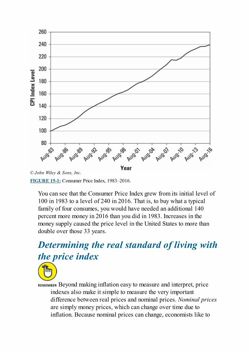
© John Wiley & Sons, Inc.

FIGURE 15-1: Consumer Price Index, 1983–2016.

You can see that the Consumer Price Index grew from its initial level of100 in 1983 to a level of 240 in 2016. That is, to buy what a typicalfamily of four consumes, you would have needed an additional 140percent more money in 2016 than you did in 1983. Increases in themoney supply caused the price level in the United States to more thandouble over those 33 years.

Determining the real standard of living withthe price index

Beyond making inflation easy to measure and interpret, priceindexes also make it simple to measure the very importantdifference between real prices and nominal prices. Nominal pricesare simply money prices, which can change over time due toinflation. Because nominal prices can change, economists like to

focus on real prices, which keep track of how much of one kind ofstuff you have to give up to get another kind of stuff, no matter whathappens to nominal prices.

For example, suppose that in 2021 you make $10 an hour working at ayouth camp and that the cost of a museum ticket is $20. The real cost of amuseum ticket to you is two hours of work. Suppose that the next year,the prices of all goods double. But your wages also double, so you’reearning $20 an hour, and a museum ticket costs $40. The result is that youstill have to work two hours to buy a museum ticket. So although thenominal price of a museum ticket has doubled, its real price in terms oflabor — how much labor you have to give up to get a museum ticket —hasn’t changed.

By constructing price indexes like the CPI, economists can tell how thereal standard of living changes for people from year to year. In theCollegiate Price Index example from preceding sections (using data fromTable 15-1), inflation is 8.8 percent between 2021 and 2022, meaningthat the cost of living of a typical college student went up 8.8 percent. Soif at the same time student incomes go up only 5 percent, students areactually worse off because costs have gone up faster than incomes. Realliving standards — measured in terms of how much stuff you can buywith your income — have fallen.

Identifying price index problemsUsing price indexes to track the cost of living isn’t a flawless system.Here are three big issues:

The market basket can never perfectly reflect family spending.The Bureau of Labor Statistics tries to keep track of what a typicalfamily of four purchases when calculating the Consumer Price Index(CPI). But families differ greatly, not only in terms of what they buybut also in terms of how many of each thing they buy.The market basket becomes outdated. The Bureau of LaborStatistics often waits way too long before including new types ofgoods in the market basket. For instance, the Bureau took years toinclude paid movie downloads from the Internet even while paiddownloads and streaming services were quickly replacing DVDmovie rentals. If the CPI fails to include popular new products, it’s

not fully capturing the price changes that matter to consumers.The market basket can’t account for quality. Price isn’t the onlything that matters to consumers. For example, what if a beer stays thesame price but improves in quality from one year to the next? You’regetting better beer for the same price, but this isn’t reflected in thedata. This problem is especially severe for things like computers,cellphones, and video games. For these products, quality improvesdramatically year after year while prices either stay the same or godown.

Each of these problems troubles government statisticians, who areconstantly coming up with better price indexes and statistical methods totry to overcome them. In the meantime, the Federal Reserve (thegovernment agency charged with regulating the money supply in theUnited States) has estimated that the CPI overstates inflation by 1 to 2percentage points per year. Most of the overstatement comes from thefailure of the CPI to account for new goods and quality improvements.

The main consequence of this overstatement is that the government isoverly generous with the cost-of-living increases it grants workers andretirees. Each year, government workers and retirees receive payincreases based upon increases in the CPI. These pay increases aredesigned to ensure that people’s real incomes aren’t eroded by inflation,but because the CPI is most likely overstating the rate of inflation eachyear, the cost-of-living increases are overly generous.

On the other hand, the rise of popular free Internet services has caused anopposite problem. Millions of people derive great enjoyment from theservices provided by Facebook, Google, and other Internet companies.But those services are provided free of charge. So it’s not at all clearhow one would be able to incorporate them into a price basket or keeptrack of how inflation in the overall economy affects the demand orsupply for these services — or how to account for quality improvementsto free online services.

Pricing the Future: Nominal andReal Interest Rates

Because inflation erodes the value of a loan repayment (see the earliersection “Tallying up the effects of inflation”), economists have todistinguish between nominal interest rates and real interest rates.Nominal interest rates are simply the normal, money interest rates thatyou’re used to dealing with; they measure the returns to a loan in terms ofmoney borrowed and money returned. Real interest rates, however,compensate for inflation by measuring the returns to a loan in terms ofunits of stuff lent and units of stuff returned. This distinction is importantbecause the real interest rate is what makes people want to save andinvest. After all, what lenders really care about isn’t how much moneythey get back but how much stuff they can buy with it.

Suppose that you borrow $1,000 with the promise to pay $1,100 to thelender in a year. Your nominal interest rate is 10 percent because you’repaying back an additional $100, or 10 percent more dollars than youborrowed. But if inflation occurs, the amount of stuff that $100 can buywill decrease over time.

Say a nice meal for two with a bottle of wine costs $100 right now butwill cost $105 next year. The lender is giving up 10 of these very goodmeals ($1,000 divided by $100 per meal) in order to give you the loan.Next year, when he gets repaid $1,100, he can buy 10.47 meals at theprice of $105. He is giving up 10 meals now in exchange for 10.47meals next year, meaning that the real rate of interest on the loan is 4.7percent. Because of inflation, the real interest rate on the loan issubstantially less than the nominal rate.

When lenders and borrowers negotiate a nominal interest rate ona loan, they both try to estimate what the inflation rate will be overthe period of the loan. This expected rate of inflation is denotedalgebraically as πe. (Don’t confuse expected inflation, πe, withactual inflation, π. Expected inflation is what people expect to

happen ahead of time, while actual inflation is what actually endsup happening.)

In this section, I show how to estimate and use the expected rate ofinflation.

Using the Fisher equationEconomist Irving Fisher came up with a simple formula that linksnominal and real interest rates. Here’s the Fisher equation, using i todenote the nominal interest rate and r to denote the real interest rate:

(3) This equation simply says that the nominal interest rate is the real interestrate plus the expected rate of inflation. This relationship is veryimportant to borrowers and lenders because although all loan contractsspecify a nominal rate of interest, their goal is to achieve a specific realrate of interest, even after any subsequent inflation reduces the value ofmoney. By using the Fisher equation, the borrowers and lenders candetermine what nominal interest to charge now to achieve a given realrate of return, taking into account the expected rate of inflation.

Suppose that a borrower and lender agree that 6 percent is a fair realrate of interest, and they also agree that inflation is likely to be 3.3percent over the course of one year. Using the Fisher equation, they writethe loan contract with a 9.3 percent nominal interest rate. A year later,when the borrower repays the lender 9.3 percent more money than wasborrowed, that money is expected to have only 6 percent morepurchasing power than the borrowed money, given the expected increasein prices.

Realizing that predictions aren’t perfectNegotiations like the one described in the preceding section dependcrucially on estimating the expected inflation rate, πe, and lots ofeconomists have job descriptions consisting primarily of trying topredict future inflation rates. Their predictions are widely reported in thebusiness media, but every person comes up with inflation forecasts in hisor her own way. Some listen to the experts, and others make estimatesbased on their own daily experiences.

During the period of low inflation starting in the early 1980s and

extending through the many years of recovery after the Great Recessionof 2007–2009, people’s inflation expectations were remarkablyaccurate. For example, consumers polled by researchers at theUniversity of Michigan each January were on average no more than acouple of percentage points off the actual rate of inflation over the next12 months. In addition, the vast majority of those polled had very similarpredictions about inflation. In that sort of an environment, people trustedtheir own inflation expectations and also tended to agree with otherpeople’s inflation expectations. Agreeing on the nominal interest rates tobe charged on particular loans was consequently relatively easy forborrowers and lenders.

But during periods of high inflation, actual rates of inflation tend to bequite unpredictable and volatile — with, say, a 35 percent rate one year,followed by a 15 percent rate the next year, and then a 45 percent rate theyear after. Thus, in periods of high inflation, individuals tend not to trusttheir own inflation forecasts or to agree with the inflation forecasts ofothers. In that sort of an environment, borrowers and lenders find itdifficult to agree on the nominal interest rates to be charged on particularloans. The resulting declines in lending and borrowing can reduceinvestment, and consequently, the economy’s ability to produce goodsand services.

Chapter 16

Understanding WhyRecessions Happen

IN THIS CHAPTER Visualizing the business cycle The ideal: Letting price adjustments eliminate recessions Reality: Coping with sticky prices and lingering recessions Linking slow price adjustments to slow wage adjustments Introducing the Keynesian model

Macroeconomists’ biggest task is to try to prevent — or at least shorten— recessions, those periods of time during which the economy’s outputof goods and services declines. Economists, politicians, and most otherpeople who work for a living despise recessions because of the toll theyexact in human suffering. That’s because when output falls, firms needfewer workers. The typical result is massive layoffs, which causesignificant increases in unemployment. In large countries such as theUnited States, millions of workers lose their jobs and their ability tosupport themselves and their families.

In this chapter, I use the aggregate supply/aggregate demand model toshow you how economists analyze recessions. Typically, recessionsbegin with what economists like to call shocks — unexpected bad eventssuch as terrorist attacks, natural disasters, the introduction of badgovernment policies, or sudden spikes in the cost of important naturalresources such as oil.

The first big lesson of this chapter is that if the prices of goods andservices in the economy were free to adjust to the changes in demand andsupply that shocks cause, the economy would typically be able torecover quite swiftly. Unfortunately, the second big lesson is that not allreal-world prices are free to adjust. Rather, some very important pricesare quite slow to adjust — they are, as economists like to say, sticky. Asa result, recessions can linger and cause a lot of harm unless the

government intervenes to help the economy recover more quickly. (InChapter 17, I discuss the best ways for governments to intervene.)

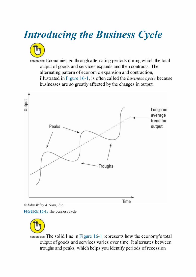
Introducing the Business Cycle

Economies go through alternating periods during which the totaloutput of goods and services expands and then contracts. Thealternating pattern of economic expansion and contraction,illustrated in Figure 16-1, is often called the business cycle becausebusinesses are so greatly affected by the changes in output.

© John Wiley & Sons, Inc.

FIGURE 16-1: The business cycle.

The solid line in Figure 16-1 represents how the economy’s totaloutput of goods and services varies over time. It alternates betweentroughs and peaks, which helps you identify periods of recession

and recovery. Here’s how you can distinguish between the two:

Recessions: Recessions, or contractions, are the periods of timeduring which output falls — that is, after a peak and before the nexttrough.Recoveries: Recoveries, or expansions, are the periods of timeduring which output increases — that is, after a trough and before thenext peak.

The dotted line in Figure 16-1 represents the long-run, average growthtrend for an economy’s total output of goods and services. I’ve drawnFigure 16-1 so that it has an upward-sloping average growth trend,capturing the fact that the economies of most countries now havesustained economic growth. In other words, on average, total outputtends to rise year after year. Because recessions still happen, however,the actual path given by the solid line fluctuates around the long-rungrowth path given by the dotted line.

In Figure 16-1, you can see that macroeconomic policy has two naturalgoals:

Make the long-run average growth line as steep as possible. Thesteeper it is, the faster (on average) total output and living standardsrise.Reduce the size of business cycle fluctuations around the long-run average growth line. Smaller distances between peaks andtroughs translate into fewer people suffering through bouts ofunemployment when output falls.

In Chapter 17, I explain the policies that economists think are best forachieving these two goals. But for Chapter 17 to make sense, I must firstexplain what causes the business cycle — especially recessions and thehigh rates of unemployment that accompany them. After all, if you don’tunderstand what’s wrong, you can’t sensibly fix it.

Striving for Full-EmploymentOutput

Before you can say whether an economy is doing well or doing poorly,you need some objective standard of what “doing well” is. Economistsuse the concept of full-employment output (which is represented by thesymbol Y*) as their measure of how well an economy should be doing.

The idea of full-employment output revolves around the conceptof full employment, by which economists mean a situation in whicheveryone who wants a full-time job can get one. Full-employmentoutput is the total amount of goods and services produced in theeconomy when there’s full employment in the labor market.

Please don’t confuse full-employment output with the economy’smaximum output, which is the larger amount of goods and servicesthat would be produced if everyone were forced to work as much ashumanly possible. Also, don’t assume that full employment is thesame thing as having a zero unemployment rate. Even wheneveryone who wants a job can get one, some unemployment willalways exist as people voluntarily quit one job to search for a betterone. For the duration of their job search, these people are countedas unemployed. Economists call this situation frictionalunemployment, as though the delay in finding a better job is due tosome sort of friction slowing the process down.

As technology improves, full-employment output (Y*) growsbecause better technology means that a fully employed labor forcecan produce more output. But to simplify their analyses, economistsusually ignore the long-term growth trend and look only at whether

actual output, Y, is currently above or below their best estimates ofY* at that particular moment. (I follow this convention, too, for therest of the chapter. You will find out how the economy adjusts tosituations in which output is either above or below potential outputat a given point in time.)

As I show you in this chapter, the economy naturally wants to adjust backto Y* anytime it deviates from Y*. If that adjustment process were rapidenough, you wouldn’t have to worry about business cycles, recessions,and unemployment. If the economy reverted back to Y* fast enough,recessions would be too brief to cause any serious negativeconsequences. Unfortunately, the natural adjustment process can be veryslow, and as a result, recessions can be quite lengthy and awful.

Returning to Y*: The NaturalResult of Price Adjustments

After an economic shock, such as a natural disaster or a spike in the costof natural resources, price adjustments tend to return an economy toproducing at full-employment output (Y*) (see “Striving for Full-Employment Output” earlier in this chapter for details on fullemployment). That’s right, I said price adjustments — not the president,and not the chairman of the Federal Reserve Board. Don’t believe me?Read on.

Consider a situation in which the overall demand for goods and servicesin the economy falls off: Individuals, firms, and the government demandand buy less than the economy is currently producing. The result is anexcess supply of output which, in turn, leads to lower prices. After all,what does any business do when it can’t sell off everything it’sproducing at the prices it’s currently charging? It has a sale. It lowersprices. The lower prices attract more buyers, and soon the business isable to sell off the rest of its output.

This process repeats itself all over the economy during aneconomic downturn. When aggregate demand falls off due to aneconomic shock, firms lower prices to make sure they sell off theiroutputs. This process eventually leads to two outcomes:

Prices all over the economy fall.

The economy again produces at full-employment output, Y*.

For this process to work well, prices must be able to change quickly; ifthey can, the economy very quickly returns to Y*. If, however, priceadjustments are slow, the economy may produce less output than Y* for asignificant amount of time. In other words, if prices don’t adjust quickly,you can get a recession. And until prices do adjust, the recession lingers.

Responding to Economic Shocks:Short-Run and Long-Run Effects

Economists like to break the time period after an economic shock intotwo parts, which they call the short run and the long run:

The short run: The period of time in which firms haven’t yet madeprice changes in response to an economic shockThe long run: The period of time after which firms have made allnecessary price changes in response to an economic shock

These definitions are intentionally vague because the speed at whichfirms adjust prices varies from shock to shock. In this section, I showyou the major differences between what happens in the short run and thelong run.

Defining some critical termsTo see the difference between an economy responding to a shock in theshort run versus the long run, begin by looking at Figure 16-2, which is amodel of the macroeconomy. The horizontal axis measures the dollarvalue of the output of goods and services sold in the economy (Y). Thisnumber is the same as a country’s gross domestic product (GDP), whichI discuss in Chapter 14. The vertical axis measures the overall pricelevel in the economy, P.

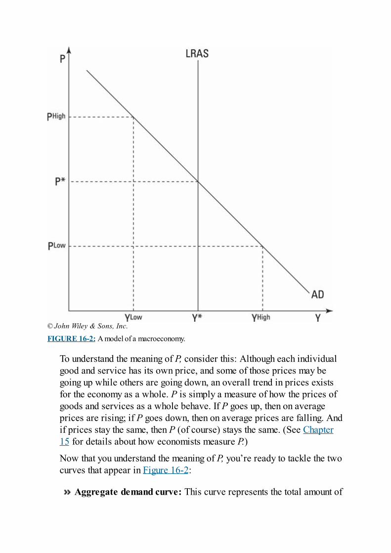
© John Wiley & Sons, Inc.

FIGURE 16-2: A model of a macroeconomy.

To understand the meaning of P, consider this: Although each individualgood and service has its own price, and some of those prices may begoing up while others are going down, an overall trend in prices existsfor the economy as a whole. P is simply a measure of how the prices ofgoods and services as a whole behave. If P goes up, then on averageprices are rising; if P goes down, then on average prices are falling. Andif prices stay the same, then P (of course) stays the same. (See Chapter15 for details about how economists measure P.)

Now that you understand the meaning of P, you’re ready to tackle the twocurves that appear in Figure 16-2:

Aggregate demand curve: This curve represents the total amount of

goods and services (Y) that people want to buy at any particular pricelevel P, holding all other factors constant.Notice that in Figure 16-2, the AD curve slopes downward. That’sbecause there’s an inverse relationship between the price level (P)and the amount of stuff that people want to buy (Y). Inverserelationship simply means that at the higher price level (P High),people want to buy a low level of output (Y Low). But if prices fall toP Low, people demand a much greater amount of output (Y High). Thedownward slope of the AD curve captures the fact that at lower pricelevels, people want to buy more.Long-run aggregate supply curve: This curve represents theamount of goods and services that an economy will produce whenprices have adjusted after an economic shock.In Figure 16-2, you can see that the LRAS is a vertical line — it isn’ta curve at all! (Do you feel cheated?) The LRAS is drawn above thepoint on the horizontal axis that represents the full-employment outputlevel, Y*. Why? Because in the long run, changes in prices alwaysreturn the economy to producing at the full-employment output level.

The tao of P: Looking at price adjustmentsin the long runIn Figure 16-2, P* represents the equilibrium level of prices in theeconomy. P* is determined by the intersection of the long-run aggregatesupply curve (LRAS) with the aggregate demand curve (AD). P* isboth the price level at which consumers demand exactly the amount offull-employment output (Y*) as well as the price level to which theeconomy will naturally return if the price level ever deviates from P*.

To see why the price level will always move back to P*, look at pricelevel PHigh and its corresponding aggregate demand level, YLow.Obviously, YLow is less than the economy’s full-employment level ofoutput (Y*). That’s important because firms would rather produce atoutput level Y*. In fact, they’ve invested in factories and equipmentthat’ll be wasted if they produce at lower levels of output. Consequently,their response is to cut prices in order to increase sales. And they

continue to cut prices until the overall price level in the economy fallsdown to P*, because that’s the price level at which consumers want tobuy exactly Y* worth of output.

Are you worried that all these price cuts will cause firms to lose money?Take heart: Firms don’t necessarily lose profits in this situation becausetheir costs are falling at the same time. That’s because when the economyis producing at less than Y*, there are a lot of unemployed workers and alot of unused productive inputs, such as iron and oil. Unemployment putsdownward pressure on wages; in other words, having lots ofunemployed labor readily available means you can hire people at lowerwages. And the larger the piles of unused productive inputs, the moretheir prices will fall, too.

Okay, so the lower prices attract more customers, increase sales, andcause firms to hire back unemployed workers. This process continuesuntil prices fall all the way to P*, at which point the economy isoperating at full employment again, meaning all workers who want full-time jobs can get them.

In a similar fashion, prices can’t remain below P* for long. At pricelevel PLow, people want to buy YHigh worth of output. But that’s morethan firms can produce at full employment. The only way to produce thatmuch output is if employees work more than the standard 40-hour workweek. The only way to get them to do so is to pay them more, and theonly way to give them higher wages is for firms to raise prices. So withdemand exceeding supply, prices are raised until they reach P*, at whichprice level the quantity demanded by consumers is exactly equal to thefull-employment output level, Y*.

As you can see, if prices have enough time to adjust, the economy alwaysreturns to producing at output level Y*. Because I’m calling the timerequired for prices to adjust the long run, it makes sense to call thevertical line above Y* the long-run aggregate supply curve because itshows how much output the economy will supply after prices have hadenough time to adjust to equalize the supply and demand for goods andservices. (For much more on supply and demand, see Chapter 4.)

A shock to the system: Adjusting to a shift in

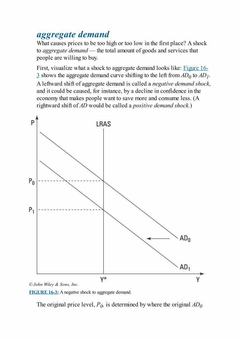
aggregate demandWhat causes prices to be too high or too low in the first place? A shockto aggregate demand — the total amount of goods and services thatpeople are willing to buy.

First, visualize what a shock to aggregate demand looks like: Figure 16-3 shows the aggregate demand curve shifting to the left from AD0 to AD1.A leftward shift of aggregate demand is called a negative demand shock,and it could be caused, for instance, by a decline in confidence in theeconomy that makes people want to save more and consume less. (Arightward shift of AD would be called a positive demand shock.)

© John Wiley & Sons, Inc.

FIGURE 16-3: A negative shock to aggregate demand.

The original price level, P0, is determined by where the original AD0

curve intersects the vertical LRAS curve. In the long run, after firmsadjust to the demand shock, the new price level, P1, will be where thenew AD1 curve intersects the vertical LRAS curve.

The new price level (P1) is less than the original price level(P0). Why? Because the demand for goods and services decreasesafter the negative demand shock. The only way to entice consumersto again purchase full-employment levels of output (Y*) is to lowerthe cost of buying that much output, so the price level has to fall.Firms may take a while to make the necessary price reductions, butwhen they do, the economy will again produce at Y* in the long run.

Dealing with fixed prices in the short runAfter an economic shock happens, prices eventually adjust to return theeconomy to full-employment output, Y* (see the preceding sections).However, this process may take a while because in the short run, pricesare essentially fixed. Even the managers of the most nimble firms needsome time to decide how much to cut prices. And some firms aren’t quiteas nimble.

Suppose that a firm has printed up catalogs listing the prices of the thingsit sells. This firm distributes catalogs only once a year, which means it’scommitted to selling to customers at these prices until the next catalog issent out. In such a situation, a firm adjusts its production to meetwhatever amount of demand happens to come along at these fixed prices.If a lot of people show up to buy at these prices, the firm increasesproduction, typically by hiring more employees. If very few people showup to buy, it reduces production, typically by hiring fewer employees.

Figure 16-4 depicts a situation in which firms have committed to a fixedset of prices and can respond to changes in demand only by adjustingtheir production levels. The figure shows the horizontal short-runaggregate supply curve (SRAS), which is actually a straight line. This“curve” corresponds to price level P0 because the firms, in the short run,can’t adjust their prices. Movements right and left along the SRAS curvecapture the increases and decreases in output that firms have to make as

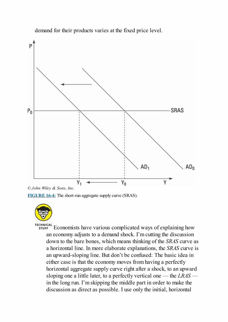
demand for their products varies at the fixed price level.

© John Wiley & Sons, Inc.

FIGURE 16-4: The short-run aggregate supply curve (SRAS).

Economists have various complicated ways of explaining howan economy adjusts to a demand shock. I’m cutting the discussiondown to the bare bones, which means thinking of the SRAS curve asa horizontal line. In more elaborate explanations, the SRAS curve isan upward-sloping line. But don’t be confused: The basic idea ineither case is that the economy moves from having a perfectlyhorizontal aggregate supply curve right after a shock, to an upwardsloping one a little later, to a perfectly vertical one — the LRAS —in the long run. I’m skipping the middle part in order to make thediscussion as direct as possible. I use only the initial, horizontal

curve and the final, vertical curve, calling the former the SRAS andthe latter the LRAS.

Figure 16-4 also has two aggregate demand curves, AD0 and AD1, thatagain show what happens when aggregate demand is reduced as theresult of a negative demand shock. The initial level of output that firmsproduce, Y0, is determined by the intersection of the original aggregatedemand curve, AD0, with the SRAS curve. In other words, at price levelP0, people demand output level Y0, and firms respond by supplying it.

When the negative demand shock strikes, it shifts aggregate demandleftward to AD1. Reduced demand means that at the fixed price level,customers are willing to buy less output. Because firms can’t changeprices, their only recourse is to reduce production down to match thedecrease in demand; this reduced level of output (Y1) appears on thegraph where the SRAS curve intersects AD1. Because lower output meansthat firms need fewer workers, you end up with a recession: Output falls,and unemployment rises.

ADJUSTING PRICES QUICKLY:WALMART AND Y*

The recessions of 1991 and 2001 were very mild — much milder, in fact, thanmost previous recessions in the United States. The exact reason for this isn’tclear, but many economists believe that one factor was that starting in the1980s, retailers got much better at quickly adjusting prices when supply didn’tequal demand.

The leader in this regard was Walmart, which developed the most sophisticatedinventory-management systems in the world. With these computerized systems,Walmart’s managers could tell minute-by-minute what was selling and what wasnot. As a result, the prices of slow-moving items could be cut very quickly sothat products didn’t go unsold for weeks or months, as was the case in decadespast when inventory was taken by hand once a month.

As a result of such innovations, prices could quickly adjust to equate supplyand demand. In fact, individual prices could fall much more rapidly, therebyhelping to get the economy back to producing at full-employment output (Y*)more quickly. Other things held equal, that means shorter, milder recessions.

This effect helped to moderate the severe recession of 2007–2009. Thatrecession occurred when aggregate demand declined substantially after acollapse in real estate prices. Thanks to sophisticated inventory-managementsystems, retailers like Walmart and Amazon were able to quickly identify andrespond to the decline in demand. They could ascertain which products wereno longer popular and thereby reduce orders for those products immediately.

Its inventory-management system prevented huge accumulations of unsoldproducts from building up in Walmart’s inventories. Thus, when the economybegan to finally grow again in 2009, Walmart and other retailers had toimmediately increase their factory orders to keep up with the increase indemand — something that they wouldn’t have chosen to do if large amounts ofunsold inventories had built up during the recession.

If you compare Figures 16-3 and 16-4, you can see that the leftward shiftin aggregate demand has very different effects in the short run and thelong run:

In the short run, when prices are fixed: Output falls andunemployment rises.

In the long run, when prices can fall: Output returns to the full-employment level.

Why the huge difference between the short run and the long run? Firmsaren’t forever stuck with their original catalog prices. Eventually, theyprint new catalogs with lower prices. The lower prices entice customersto purchase more, and soon the economy can return to producing at thefull-employment output level, Y*.

Putting together the long and short of itIf you have both long-run and short-run responses to an economic shocktucked under your belt, you’re ready to put the two very differentresponses together into one big picture. Figure 16-5 lets you see how aneconomy adapts to a negative demand shock both in the short run and inthe long run. The economy begins at point A, where the original aggregatedemand curve, AD0, intersects both the LRAS and the SRAS curves. AtPoint A, the economy is in equilibrium because at price level P0, theaggregate demand for output equals the full-employment level of output,Y*. There is neither a surplus nor a shortage that could cause prices tochange.

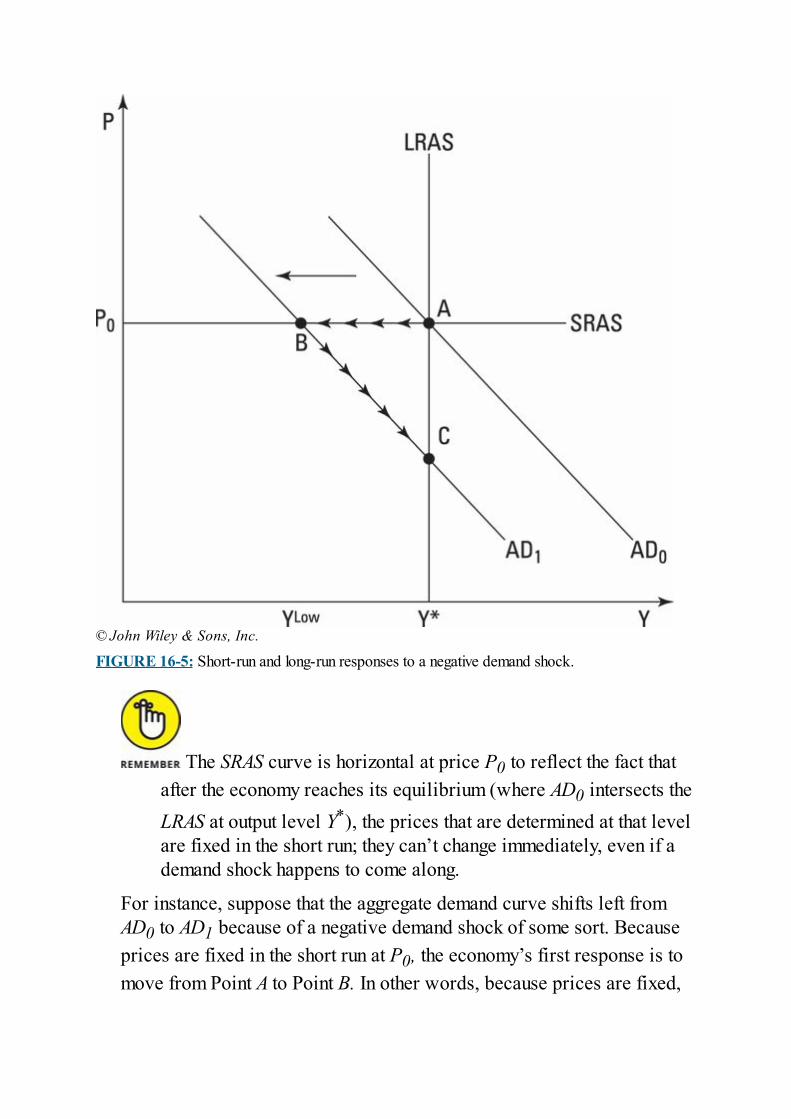
© John Wiley & Sons, Inc.

FIGURE 16-5: Short-run and long-run responses to a negative demand shock.

The SRAS curve is horizontal at price P0 to reflect the fact thatafter the economy reaches its equilibrium (where AD0 intersects theLRAS at output level Y*), the prices that are determined at that levelare fixed in the short run; they can’t change immediately, even if ademand shock happens to come along.

For instance, suppose that the aggregate demand curve shifts left fromAD0 to AD1 because of a negative demand shock of some sort. Becauseprices are fixed in the short run at P0, the economy’s first response is tomove from Point A to Point B. In other words, because prices are fixed,

production falls from Y* down to YLow as firms respond to decreaseddemand by cutting production. (Small arrows indicate the movement ofthe economy from Point A to Point B.)

At Point B, the economy is operating below full employment, implyingthat a lot of workers are unemployed. This high level of unemploymentcauses wages to fall. As wages fall, firms’ costs also fall, allowing themto cut prices in order to attract more customers.

Falling prices cause increased aggregate demand for goods and services,which eventually moves the economy all the way from Point B to Point C(arrows on the graph indicate this movement). When the economyreaches point C, it’s once again producing at full employment, Y*.

The short-run and long-run effects of a negative demand shockare basically total opposites of each other:

Short run: In the short run, prices are fixed while output decreases.

Long run: In the long run, prices decrease while output returns to Y*.

If prices don’t stay fixed for very long, the economy can quickly movefrom A to B to C. But if prices are slow to adjust to the negativeaggregate demand shock, the economy can take a very long time to getfrom A to B to C. In such cases, there’s a long-lasting recession duringwhich output remains below Y* and many people are unemployed.

Heading toward Recession:Getting Stuck with Sticky Prices

When the economy encounters a negative demand shock like the onedepicted in Figure 16-5, price flexibility (or lack of flexibility)determines both the severity and length of any recession that may result.If prices were infinitely flexible — if they could change within secondsor minutes after a shock — the economy would immediately move fromPoint A to Point C, and all would be right with the world. But if pricesare fixed for any period of time, the economy goes into a recession as itmoves from Point A to Point B before prices eventually fall and bring itback to full-employment output at Point C.

In the real world, prices are indeed somewhat slow to change, or aseconomists like to say, prices are sticky. Interestingly, prices tend to bestickier when going downward than upward, meaning that prices appearto have a harder time falling than rising.

The major culprit seems to be one particular price: wages. Wages are theprice employers must pay workers for their labor. Unlike other prices inthe economy, people are particularly emotionally attached to wages andhow they change over time.

Employees don’t like to see their wages cut. They have a strongsense of fairness concerning their wages and usually retaliateagainst any wage cut by working less hard. As a result, managerstypically find lowering wages to be counterproductive, even if afirm is losing money and needs to cut costs.

This section explains how firms’ worries about worker motivation leadto the sticky output prices that prevent the economy from rapidlyrecovering from recessions. When sales fall as a result of the recession,output prices can’t fall very much because firms choose to lay offworkers rather than cut wages.

Cutting wages or cutting workers

During a recession, you see a large increase in unemployment but littledecrease in wage rates. The fact that managers are unwilling to cutwages, however, has a nasty side effect: Not cutting wages makes it veryhard for firms to cut the prices of the goods and services they sell (formore on this topic, see the next section).

Suppose that a negative demand shock hits an economy and greatlyreduces sales at a particular company. The firm is losing money, somanagers need to figure out a way to cut costs. About 70 percent of thiscompany’s total costs are labor costs (wages and salaries). Naturally,labor costs are an obvious target for cuts.

But the managers of the firm realize that if they cut wages, employeeswill get angry and work less hard. In fact, their productivity may fall offso much that cutting wages may make the firm’s profit situation worse:Output may fall so much that sales revenues will decrease by more thanthe reduction in labor costs. Therefore, cutting wages isn’t really a goodoption.

So instead, the managers lay off a large chunk of their workforce in orderto reduce labor costs. For instance, if sales are down 40 percent, the firmmay lay off 40 percent of the workforce. However, any workers whoremain employed get to keep their old wages so that they aren’t angryand their productivity doesn’t fall.

Adding up the costs of wages and profitsObviously, firms need to turn a profit in order to stay in business. Andthat means making sure that the price per unit that they charge for theirproducts exceeds the cost per unit of making them.

During a recession, lower aggregate demand means that firms reduceproduction and sell fewer units. Wages are the largest component of mostfirms’ costs — in fact, they’re a full 70 percent of the average firm’scosts. If a firm can’t cut wages for fear of causing worker productivity todrop, it can’t reduce its per-unit production costs very much, either. Inturn, the firm can’t cut its prices very much because prices have to stayabove production costs if firms are to break even and stay in business.What does all this mean?

When demand drops off, prices are typically sticky. They stayhigh even though there’s less demand for output in the economy.That’s the reason behind the economy’s moving horizontally fromPoint A to Point B in Figure 16-5 after the negative demand shock.With prices sticky because firms can’t quickly or easily cut wages,the negative demand shock results in a recession, with output fallingand unemployment rising because so many workers get fired.

Worse yet, unless prices can somehow begin to fall, the economy won’tbe able to move from B to C to get back to producing at the full-employment output level (Y*). Prices do eventually fall, but this processcan take a long time, meaning that the negative demand shock can cause along-lasting recession.

One way around this slow adjustment process is for the government totry to offset the negative demand shock. The next section covers howsuch attempts may be able to speed recovery by avoiding the need forprices to adjust to bring the economy back to producing at the full-employment output level.

Returning to Y* with and withoutgovernment interventionIn Chapter 17, I explain in great detail how the government can usemonetary and fiscal stimuli to get around the sticky prices problem byboosting aggregate demand. Here, I want to give you a preview of howthat process works.

Imagine that after the negative demand shock depicted in Figure 16-5moves aggregate demand leftward from AD0 to AD1, the governmentdoesn’t hang around waiting for prices to fall. Instead, it stimulatesaggregate demand so that the aggregate demand curve shifts right andreturns to where it started, at AD0. Taking this action returns the economyto producing at full employment without having to wait for prices to fall.

What if the government doesn’t act to stimulate aggregate demand in thatfashion? What if the economy is at Point B and the government doesn’tintervene? In such cases, prices do eventually fall because firms’

production costs eventually fall.

Labor costs are very slow to fall because managers don’t want to riskalienating workers by cutting their wages (see the earlier section“Cutting wages or cutting workers” for details). But because so manyworkers are unemployed when the economy is at Point B, wageseventually decline. Some firms hire unemployed people at lower wages,which reduces the firms’ costs, meaning that they can undersell firms thatkeep wages high. Eventually, such competitive pressures mean that allfirms end up cutting wages.

Other costs also decline because during a recession, with output sodiminished, a significant portion of the economy’s productive capacity isunused. There are unused factories, unused trucks, unused train cars, andunused ships. There are also large amounts of unused lumber, iron, oil,and other productive inputs.

The owners of these unused inputs lower their prices to try to sell them.As their prices fall, production costs also fall, thereby allowing firms toreduce the selling prices of their output. And as these selling prices fall,the economy moves from Point B to Point C in Figure 16-5, restoring theeconomy to producing at the full-employment output level (Y*). See hownicely it all (eventually) works out?

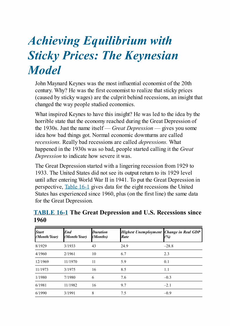
Achieving Equilibrium withSticky Prices: The KeynesianModel

John Maynard Keynes was the most influential economist of the 20thcentury. Why? He was the first economist to realize that sticky prices(caused by sticky wages) are the culprit behind recessions, an insight thatchanged the way people studied economies.

What inspired Keynes to have this insight? He was led to the idea by thehorrible state that the economy reached during the Great Depression ofthe 1930s. Just the name itself — Great Depression — gives you someidea how bad things got. Normal economic downturns are calledrecessions. Really bad recessions are called depressions. Whathappened in the 1930s was so bad, people started calling it the GreatDepression to indicate how severe it was.

The Great Depression started with a lingering recession from 1929 to1933. The United States did not see its output return to its 1929 leveluntil after entering World War II in 1941. To put the Great Depression inperspective, Table 16-1 gives data for the eight recessions the UnitedStates has experienced since 1960, plus (on the first line) the same datafor the Great Depression.

TABLE 16-1 The Great Depression and U.S. Recessions since1960

Start(Month/Year)

End(Month/Year)

Duration(Months)

Highest UnemploymentRate

Change in Real GDP(%)

8/1929 3/1933 43 24.9 –28.8

4/1960 2/1961 10 6.7 2.3

12/1969 11/1970 11 5.9 0.1

11/1973 3/1975 16 8.5 1.1

1/1980 7/1980 6 7.6 –0.3

6/1981 11/1982 16 9.7 –2.1

6/1990 3/1991 8 7.5 –0.9

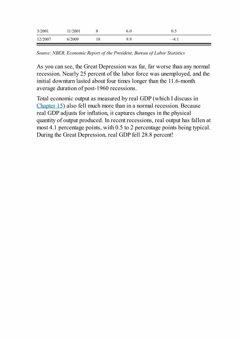
3/2001 11/2001 8 6.0 0.5

12/2007 6/2009 18 9.9 –4.1

Source: NBER, Economic Report of the President, Bureau of Labor Statistics

As you can see, the Great Depression was far, far worse than any normalrecession. Nearly 25 percent of the labor force was unemployed, and theinitial downturn lasted about four times longer than the 11.6-monthaverage duration of post-1960 recessions.

Total economic output as measured by real GDP (which I discuss inChapter 15) also fell much more than in a normal recession. Becausereal GDP adjusts for inflation, it captures changes in the physicalquantity of output produced. In recent recessions, real output has fallen atmost 4.1 percentage points, with 0.5 to 2 percentage points being typical.During the Great Depression, real GDP fell 28.8 percent!

WHAT MAKES A RECESSION ARECESSION?

I define a recession as a period of time during which output falls andunemployment rises. But this isn’t the only definition. For example, you mayread in a textbook or a newspaper article that an economy is in a recession ifreal GDP falls for two consecutive quarters. But if you look at Table 16-1, younotice that during certain recessions (such as the one that began in April 1960),real output actually went up rather than down. So why was that time periodlabeled a recession?

A lot of factors go into determining what gets labeled a recession. A group ofeconomists at the National Bureau of Economic Research (NBER) inCambridge, Massachusetts, gets to “officially” declare when recessions beginand end in the United States. This group has a long set of criteria that beginswith falling output and rising unemployment and includes lots of other things,such as how fast factories receive new orders. Sometimes these other factorscause the NBER to feel that the economy has passed a peak and has entered arecession, even if output isn’t falling.

Check out the NBER’s website at www.nber.org for more information aboutbusiness cycles and how the NBER goes about declaring recessions.

As a witness to the Great Depression, Keynes obviously wanted to figureout what could cause such a drastic economic downturn — and whatcould prevent such devastation from happening again. Keep reading formore on the Keynesian model.

Adjusting inventories instead of pricesNot only did Keynes figure out that sticky prices cause recessions, but healso developed a hugely influential model that’s still presented in manymacroeconomics textbooks. This model is a small part of a largerapproach to managing the macroeconomy that came to be calledKeynesianism — an approach that favored large governmentinterventions into the economy rather than the sort of laissez-fairepolicies of nonintervention preferred by other people. (For a discussionof the costs and benefits of having the government intervene in theeconomy, see Chapter 3.)

To be fair, I have to point out that Keynesianism has attracted a lot of

critics and is not the be-all-end-all of macroeconomics. But the part of itI present here is not controversial. It explains how an economy adjusts toequilibrium — a place where aggregate supply matches aggregatedemand — in the extreme short run after an economic shock, when pricescan’t change at all.

Look back at Figure 16-4 for a moment. The Keynesian model elaborateson exactly how an economy moves from producing at output level Y0 toproducing at output level Y1 when a shock to aggregate demand happensand prices are fixed at level P0.

Keynes’s model focuses your attention on firms’ inventories ofgoods that have been made but not yet sold. According to Keynes,changes in inventories guide firms to increase or decrease outputduring situations in which prices are sticky and can’t serve assignals of what to do.

To see the novelty of Keynes’s inventory idea, understand that if pricescould change, then prices (not inventories) would guide firm decisionsabout how much to produce:

If prices were rising, a firm would know that its product was popularand that it should increase output.If prices were falling, the firm would know that the product was notdoing well and that it should probably cut output (and maybe get intoanother line of business!).

In an economy with fixed prices, however, firms need some other way ofdeciding whether to increase or decrease production. Keynes realizedthat the guiding force would be changes in inventories, as you can see inthe following subsections.

Keeping an eye on target inventory levelsInventories are constantly turning over, with goods flowing both in andout. New production increases inventories, while new sales decreaseinventories. The two factors interact to determine if inventories arerising, falling, or staying the same. For instance, if new production

equals new sales, inventory levels stay constant. If new productionexceeds new sales, inventories rise.

The interaction of new production and new sales is importantbecause each firm has a target level of inventories that it likes tokeep on hand to meet situations in which sales temporarily runfaster than the firm can produce output. The costs and benefits ofhaving a bigger or smaller inventory on hand determine the targetlevel.

Having less inventory than the target level is dangerous because the firmmay not be able to keep up with sales spikes. Having more inventorythan the target level is wasteful because there’s no point in having stuffsitting around unsold, year after year. Each firm weighs these costs andbenefits to come up with its own target inventory level.

Target inventory levels may vary from year to year, depending onwhether firms are expecting strong or weak sales. If managers areexpecting strong sales, they may plan on increasing inventories, whereasif they’re expecting weak sales, they may plan on decreasing inventories.

Keynes realized that aggregate demand shocks (which are, bydefinition, unexpected) would show up as unexpected changes infirm inventories:

Unexpectedly low aggregate demand means that sales slow so much,inventories increase to levels higher than firms had planned on.Unexpectedly high aggregate demand means that sales increase somuch, inventories decrease and reach levels lower than firms hadplanned on.

Increasing or decreasing output as inventories fluctuateUnexpectedly large changes in inventories cause firms to change theiroutput levels as follows:

If inventories rise above target levels, firms respond by cutting

production. By reducing production rates to less than sales rates,inventories begin to fall down toward target levels.If inventories fall below target levels, firms respond by raisingproduction. By increasing production rates to more than sales rates,inventories begin to rise toward target levels.

The changes in output levels caused by changes in inventories are hugelyimportant because they determine not only whether output (Y) isincreasing or decreasing but also whether unemployment is rising orfalling. For instance, if firms increase production because inventorieshave fallen below target levels, they need to hire more workers, sounemployment falls. If, on the other hand, firms decrease productionbecause inventories rise above target levels, they need to lay offworkers, so unemployment rises.

Adjusting inventories based on planned and actualexpendituresThe Keynesian model differentiates between planned expenditures andactual expenditures as follows:

Planned expenditures: The amount of money that households,businesses, the government, and foreigners would like to spend ondomestically produced goods and services.Actual expenditures: What households, businesses, the government,and foreigners end up spending on domestically produced goods andservices. The sum total of all these actual expenditures is equal toGDP.

What happens when actual expenditures are different fromplanned expenditures? Inventories automatically change. Forinstance, if more money is spent on goods and services thanplanned, people are buying more output than is currently beingproduced. This situation is possible because firms sell (from theirinventories) goods that were produced in previous periods. On theflip side, if people spend less money on goods and services thanplanned, firms’ inventories rise because firms have to store all the

output that they can’t sell.

Keynes represented planned expenditures, PE, algebraically with thefollowing equation:

(1) What do all these letters mean? Here’s the short version (I discuss themin detail in Chapter 14):

C stands for the amount of output that consumers want to consume.

IP stands for the amount of output that firms plan to buy as investmentgoods, such as new factories and equipment, as well as any inventorychanges that firms plan to make.If, later on, firms have to increase or decrease inventories more thanthey planned, then actual investment, I, will not equal plannedinvestment, IP.G stands for how much output the government wants to spend onthings like building schools, paving roads, and ensuring an adequatesupply of paper for paperwork.NX stands for net exports — the value of a nation’s exports minus thevalue of its imports. NX tells you the net demand that the foreignsector of the economy has for stuff that your country makesdomestically.

For actual expenditures, Y, Keynes used the same equation that you use tocalculate gross domestic product (which I discuss in Chapter 14):

(2)

Why can you use the GDP equation to calculate actualexpenditures? Actual expenditures are equal to national incomebecause every cent of expenditure made in the economy is incometo somebody. Furthermore, actual expenditure is also equal to thedollar value of all goods and services produced in the economybecause every bit of output that’s produced is sold to someone.(Any output that a firm makes but can’t sell to customers is countedas being “sold” by the firm to itself as it’s placed into inventory.

These inventory changes are known as inventory investment andare totaled up in GDP as part of the total investment, I.)

Having three ways of looking at Y is very handy as you become familiarwith the Keynesian model. Sometimes understanding the model is easierif you think of Y as being actual expenditures; at other times,understanding is easier if you think of Y as being national income oroutput. I switch among these three definitions when doing so helps makeunderstanding the model easier.

The only difference between the right sides of Equations (1) and(2) is the investment variable, which is planned investment (IP) inthe first equation and actual investment (I) in the second. In otherwords, Y and PE differ only because of differences in investmentscaused by inventories’ increasing or decreasing unexpectedly whensales are more or less than planned.

Bringing some algebra into the mixYou knew it was coming: It’s time to get algebraic so you can identify theKeynesian model’s economic equilibrium, using mathematicalsuperpowers. (Now, where did I put those?)

First, you need to define a consumption function — a way to calculatetotal consumption — that you can substitute into Equation (1). In Chapter14, I present the following formula for calculating consumption:

(3)

For now, what you really need to know about this formula is that higherincome (Y) leads to higher consumption (C). If you substitute Equation(3) into Equation (1), you get the following:

(4)

If you look carefully, you can see that this equation shows that the totalplanned expenditures on goods and services in the economy (PE)depends on the total income in the economy (Y). The higher the totalincome, the more money people are going to plan to spend.

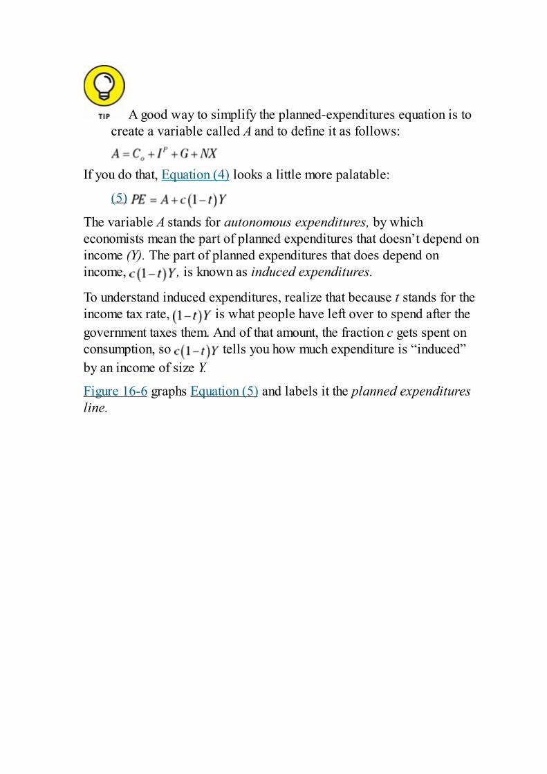
A good way to simplify the planned-expenditures equation is tocreate a variable called A and to define it as follows:

If you do that, Equation (4) looks a little more palatable:

(5)

The variable A stands for autonomous expenditures, by whicheconomists mean the part of planned expenditures that doesn’t depend onincome (Y). The part of planned expenditures that does depend onincome, , is known as induced expenditures.

To understand induced expenditures, realize that because t stands for theincome tax rate, is what people have left over to spend after thegovernment taxes them. And of that amount, the fraction c gets spent onconsumption, so tells you how much expenditure is “induced”by an income of size Y.

Figure 16-6 graphs Equation (5) and labels it the planned expendituresline.

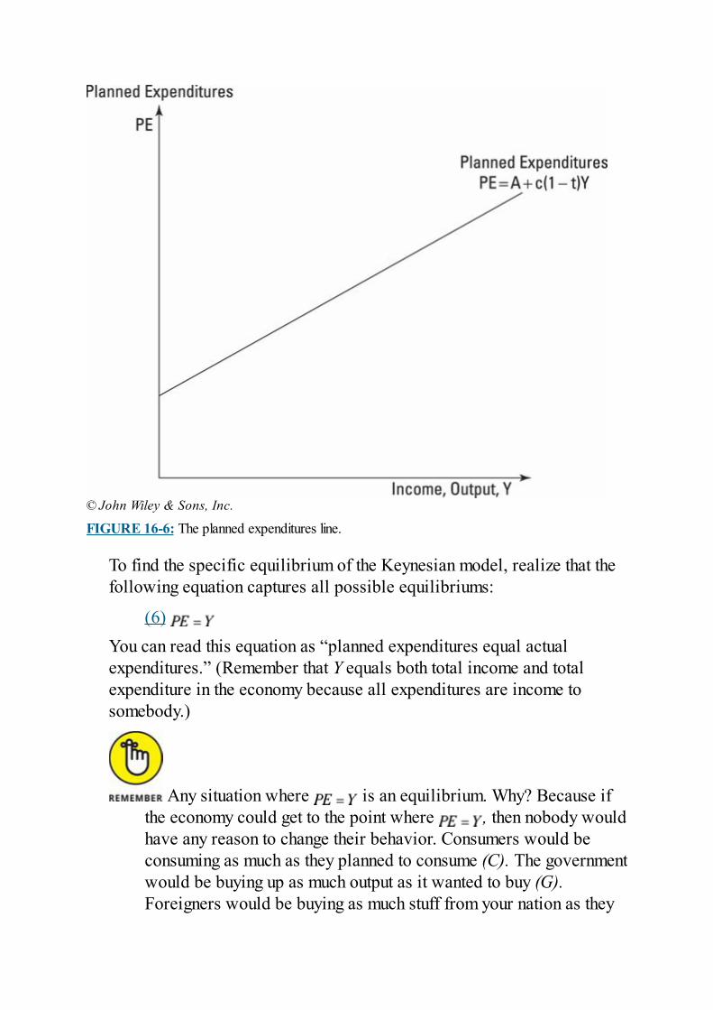
© John Wiley & Sons, Inc.

FIGURE 16-6: The planned expenditures line.

To find the specific equilibrium of the Keynesian model, realize that thefollowing equation captures all possible equilibriums:

(6) You can read this equation as “planned expenditures equal actualexpenditures.” (Remember that Y equals both total income and totalexpenditure in the economy because all expenditures are income tosomebody.)

Any situation where is an equilibrium. Why? Because ifthe economy could get to the point where , then nobody wouldhave any reason to change their behavior. Consumers would beconsuming as much as they planned to consume (C). The governmentwould be buying up as much output as it wanted to buy (G).Foreigners would be buying as much stuff from your nation as they

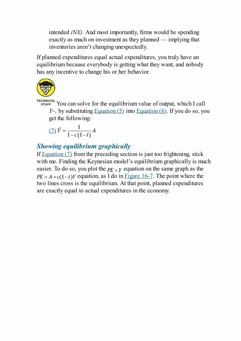
intended (NX). And most importantly, firms would be spendingexactly as much on investment as they planned — implying thatinventories aren’t changing unexpectedly.

If planned expenditures equal actual expenditures, you truly have anequilibrium because everybody is getting what they want, and nobodyhas any incentive to change his or her behavior.

You can solve for the equilibrium value of output, which I callY~, by substituting Equation (5) into Equation (6). If you do so, youget the following:

(7)

Showing equilibrium graphicallyIf Equation (7) from the preceding section is just too frightening, stickwith me. Finding the Keynesian model’s equilibrium graphically is mucheasier. To do so, you plot the equation on the same graph as the

equation, as I do in Figure 16-7. The point where thetwo lines cross is the equilibrium. At that point, planned expendituresare exactly equal to actual expenditures in the economy.

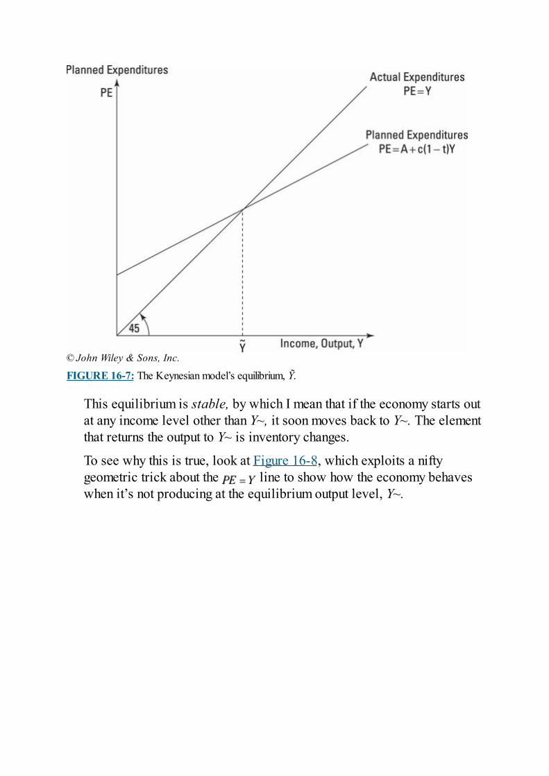
© John Wiley & Sons, Inc.

FIGURE 16-7: The Keynesian model’s equilibrium, Ỹ.

This equilibrium is stable, by which I mean that if the economy starts outat any income level other than Y~, it soon moves back to Y~. The elementthat returns the output to Y~ is inventory changes.

To see why this is true, look at Figure 16-8, which exploits a niftygeometric trick about the line to show how the economy behaveswhen it’s not producing at the equilibrium output level, Y~.

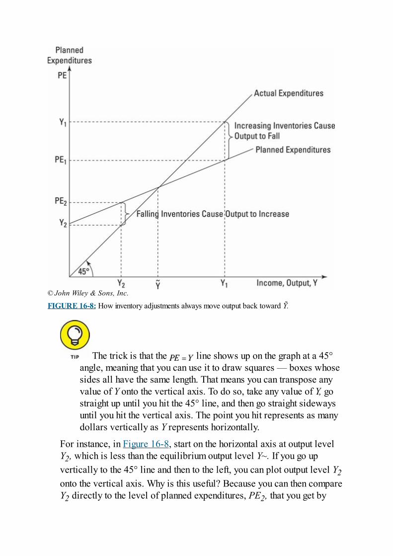
© John Wiley & Sons, Inc.

FIGURE 16-8: How inventory adjustments always move output back toward Ỹ.

The trick is that the line shows up on the graph at a 45°angle, meaning that you can use it to draw squares — boxes whosesides all have the same length. That means you can transpose anyvalue of Y onto the vertical axis. To do so, take any value of Y, gostraight up until you hit the 45° line, and then go straight sidewaysuntil you hit the vertical axis. The point you hit represents as manydollars vertically as Y represents horizontally.

For instance, in Figure 16-8, start on the horizontal axis at output levelY2, which is less than the equilibrium output level Y~. If you go upvertically to the 45° line and then to the left, you can plot output level Y2onto the vertical axis. Why is this useful? Because you can then compareY2 directly to the level of planned expenditures, PE2, that you get by

starting at output level Y2 on the horizontal axis.

As you can see, , meaning that planned expenditures exceedoutput in the economy. This means that inventories will unexpectedlydrop as firms sell part of their stockpiles of inventory to make up for thefact that people are buying up more stuff than firms are currentlyproducing. This drop in inventories will return the economy toequilibrium.

As inventories fall unexpectedly, firms increase production. As a result,Y increases. Furthermore, actual expenditures continue to increase until Yreaches Y~, because for any value of , planned expenditures willcontinue to exceed output, as you can see from the graph.

Inventory adjustments also return the economy to equilibrium if it startsout at an output level like Y1, which is greater than Y~. As you can see inFigure 16-8, by using the 45° line, actual output, Y1, exceeds plannedexpenditures, PE1. In other words, people are buying less (PE1) thanfirms are currently producing (Y1), so inventories will start to rise.

Firms respond to increases in inventories by reducing output. They layoff workers and cut production. As a result, Y falls. It continues to falluntil it reaches Y~ because for any value of , output will continue toexceed actual expenditures, as the graph shows.

Boosting GDP in the Keynesian modelKeynes didn’t just invent his model to explain how economies withsticky prices reach a stable equilibrium. What he really wanted to dowas to show what governments could do during a recession to makethings better.

For instance, consider Figure 16-8. Suppose that inventory adjustmentshave carried the economy to equilibrium income, Y~, but that Y~ is lessthan the economy’s full-employment output level, Y*. In such a case,Keynes asked, what — if anything — should governments do?

Governments could choose to do nothing. Eventually, because , prices will fall and the economy will return to full

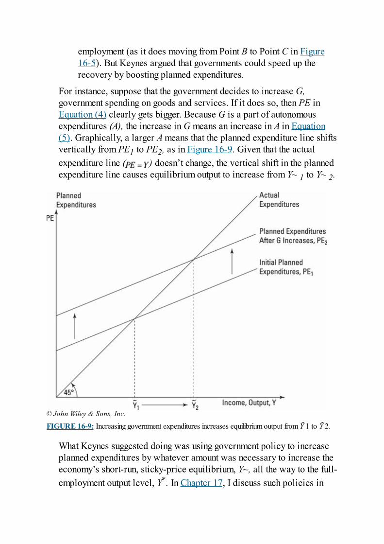
employment (as it does moving from Point B to Point C in Figure16-5). But Keynes argued that governments could speed up therecovery by boosting planned expenditures.

For instance, suppose that the government decides to increase G,government spending on goods and services. If it does so, then PE inEquation (4) clearly gets bigger. Because G is a part of autonomousexpenditures (A), the increase in G means an increase in A in Equation(5). Graphically, a larger A means that the planned expenditure line shiftsvertically from PE1 to PE2, as in Figure 16-9. Given that the actualexpenditure line ( ) doesn’t change, the vertical shift in the plannedexpenditure line causes equilibrium output to increase from Y~ 1 to Y~ 2.

© John Wiley & Sons, Inc.

FIGURE 16-9: Increasing government expenditures increases equilibrium output from Ỹ 1 to Ỹ 2.

What Keynes suggested doing was using government policy to increaseplanned expenditures by whatever amount was necessary to increase theeconomy’s short-run, sticky-price equilibrium, Y~, all the way to the full-employment output level, Y*. In Chapter 17, I discuss such policies in

greater detail, including why they don’t always work so well in practice.

Chapter 17

Fighting Recessions withMonetary and Fiscal Policy

IN THIS CHAPTER Using monetary and fiscal policy to stimulate the economy Facing the fact that too much stimulus causes inflation Realizing that rational expectations can frustrate monetary and

fiscal policy Getting the details behind monetary and fiscal policy

Monetary and fiscal policy are two of the most important functions ofmodern governments. Monetary policy focuses on increasing ordecreasing the money supply to influence the economy, and fiscal policyuses government spending and the tax code to influence the economy.

Thanks to the development of good economic theory, governments canuse monetary and fiscal policy to mitigate the duration and severity ofrecessions. This theory is hugely important because it gives governmentsthe chance to make a positive difference in the lives of billions ofpeople. Good economic policy can make a nation prosperous, but badeconomic policy can ruin it.

But monetary and fiscal policy are not without problems. In this chapter,I show you how well they can work in the best-case scenario and theirlimits and problems in the real world. By seeing the whole picture, youcan decide when and how governments should use monetary and fiscalpolicy.

The information in this chapter can put you two steps ahead of manypoliticians and help you judge when politically biased economists aretrying to pull a fast one. As Joan Robinson, one of the great economistsof the 20th century, said, “The purpose of studying economics is not toacquire a set of ready-made answers to economic questions but to learnhow to avoid being deceived by an economist.” I totally agree. But don’tworry, you can trust me.

If you haven’t read Chapter 16, I encourage you to do so before tacklingthis chapter. Although my goal with this book is to make each chapter itsown entity so that you can jump in and jump out wherever you need, Iintroduce and explain much of the terminology you encounter in thischapter in Chapter 16. You may find tackling monetary and fiscal policyeasier if you have a basic understanding of how recessions work, whichis the focus of that chapter.

Stimulating Demand to EndRecessions

Before looking at monetary and fiscal policy in detail, realize that thepurpose of both is to alter the aggregate demand for goods and services.(The aggregate demand is the total demand for goods and services in aneconomy.) In particular, both monetary and fiscal policy can increaseaggregate demand during a recession. This section explains this conceptmore in depth.

Aiming for full-employment outputThe ability to use monetary and fiscal policy to stimulate the economy isimportant because you always want to end a recession and return theeconomy to producing at the full-employment output level as quickly aspossible.

The full-employment output level, Y*, is the amount of output theeconomy produces at full employment, which occurs when every personwho wants a full-time job can get one. If the economy goes into recessionand produces less than Y* worth of output, millions of people lose theirjobs because firms need fewer workers to produce the smaller amount ofoutput.

Worse yet, the unemployment rate remains high until output returns to thefull-employment level. Monetary policy and fiscal policy are usefulprecisely because they can help return the economy to producing at Y* assoon as possible and shorten the frustration and misery the unemployedhave to endure.

Look at Figure 17-1, which shows how monetary and fiscal policy canstimulate aggregate demand and return an economy to producing at Y* asquickly as possible after the economy is hit with a negative demandshock. (Negative demand shocks [see Chapter 16] are events thatunexpectedly decrease aggregate demand, such as a drop in consumerconfidence.)

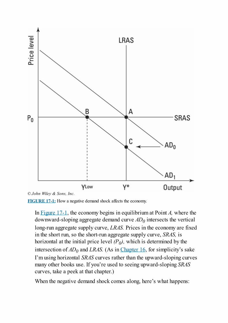
© John Wiley & Sons, Inc.

FIGURE 17-1: How a negative demand shock affects the economy.

In Figure 17-1, the economy begins in equilibrium at Point A, where thedownward-sloping aggregate demand curve AD0 intersects the verticallong-run aggregate supply curve, LRAS. Prices in the economy are fixedin the short run, so the short-run aggregate supply curve, SRAS, ishorizontal at the initial price level (P0), which is determined by theintersection of AD0 and LRAS. (As in Chapter 16, for simplicity’s sakeI’m using horizontal SRAS curves rather than the upward-sloping curvesmany other books use. If you’re used to seeing upward-sloping SRAScurves, take a peek at that chapter.)

When the negative demand shock comes along, here’s what happens:

The aggregate demand curve shifts left to AD1, reflecting thereduction in spending on goods and services.With prices fixed at P0 in the short run, the economy’s equilibriumshifts leftward from Point A to Point B, and output in the economyfalls from Y* down to YLow.As output falls, unemployment rises because firms don’t need asmany workers.

As you can see, the overall result of the demand shock is a recession: aperiod of declining output and increasing unemployment. Unfortunately, arecession can take a long time to resolve. If the government takes noaction to end a recession, the only way for the economy to return toproducing at the full-employment output level is for prices to drop so thatthe economy’s equilibrium can slide down the AD1 curve from Point B toPoint C. That process is typically very slow because of sticky (slow-to-change) prices, especially sticky wages. As a result, the economy hashigh unemployment and takes a long time to get back to producing at Y*

unless the government becomes involved. Refer to Chapter 16 for morein-depth information.

Back to work: Shifting the AD curve right

The trick that both monetary and fiscal policy accomplish is toincrease aggregate demand, which eliminates the need to endure theslow adjustment process that takes the economy from Point B toPoint C (see Figure 17-1). They do this by shifting the aggregatedemand curve to the right.

For instance, if the government were able to shift the aggregate demandcurve from AD1 back to AD0, the economy would jump back toequilibrium Point A. That’s very nice because it gets the economy back toproducing at Y* without having to go through the slow adjustment processneeded to get an economy to move from B to C. In human terms, thismeans that unemployment ends much sooner for millions of workers,who can once again find jobs and provide for themselves and theirfamilies. Unfortunately, implementing aggregate demand shifts to fight

recessions isn’t easy. Several problems can creep up involving inflationand people’s expectations about how increases in aggregate demandaffect prices.

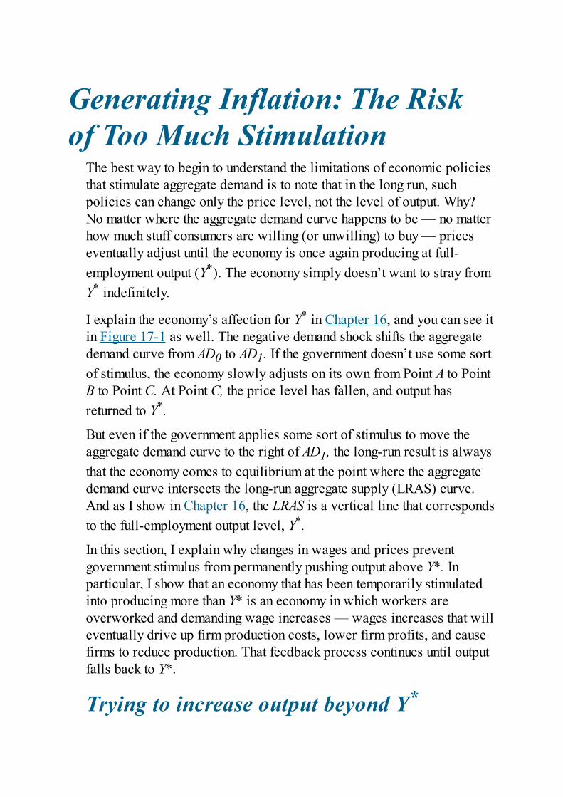
Generating Inflation: The Riskof Too Much Stimulation

The best way to begin to understand the limitations of economic policiesthat stimulate aggregate demand is to note that in the long run, suchpolicies can change only the price level, not the level of output. Why?No matter where the aggregate demand curve happens to be — no matterhow much stuff consumers are willing (or unwilling) to buy — priceseventually adjust until the economy is once again producing at full-employment output (Y*). The economy simply doesn’t want to stray fromY* indefinitely.

I explain the economy’s affection for Y* in Chapter 16, and you can see itin Figure 17-1 as well. The negative demand shock shifts the aggregatedemand curve from AD0 to AD1. If the government doesn’t use some sortof stimulus, the economy slowly adjusts on its own from Point A to PointB to Point C. At Point C, the price level has fallen, and output hasreturned to Y*.

But even if the government applies some sort of stimulus to move theaggregate demand curve to the right of AD1, the long-run result is alwaysthat the economy comes to equilibrium at the point where the aggregatedemand curve intersects the long-run aggregate supply (LRAS) curve.And as I show in Chapter 16, the LRAS is a vertical line that correspondsto the full-employment output level, Y*.

In this section, I explain why changes in wages and prices preventgovernment stimulus from permanently pushing output above Y*. Inparticular, I show that an economy that has been temporarily stimulatedinto producing more than Y* is an economy in which workers areoverworked and demanding wage increases — wages increases that willeventually drive up firm production costs, lower firm profits, and causefirms to reduce production. That feedback process continues until outputfalls back to Y*.

Trying to increase output beyond Y*

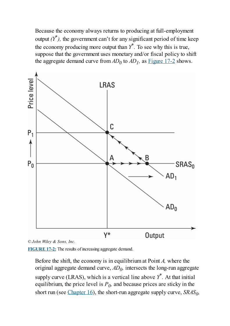
Because the economy always returns to producing at full-employmentoutput (Y*), the government can’t for any significant period of time keepthe economy producing more output than Y*. To see why this is true,suppose that the government uses monetary and/or fiscal policy to shiftthe aggregate demand curve from AD0 to AD1, as Figure 17-2 shows.

© John Wiley & Sons, Inc.

FIGURE 17-2: The results of increasing aggregate demand.

Before the shift, the economy is in equilibrium at Point A, where theoriginal aggregate demand curve, AD0, intersects the long-run aggregatesupply curve (LRAS), which is a vertical line above Y*. At that initialequilibrium, the price level is P0, and because prices are sticky in theshort run (see Chapter 16), the short-run aggregate supply curve, SRAS0,

is a horizontal line at P0.

When the government stimulates the economy and shifts the aggregatedemand curve to the right from AD0 to AD1, the economy initially shiftsfrom Point A to Point B. That is, because prices are fixed in the short run,the economy adjusts to a temporary equilibrium at B (where AD1intersects SRAS0).

The economy’s output level at Point B is greater than the full-employmentoutput level, Y*. Point B is only a temporary equilibrium because theonly way the economy can produce more than Y* is by using more laborthan is used at Y*. This can happen in only two ways, both of whichincrease wages:

Firms convince workers to work overtime. To get existing workersto consistently work overtime, firms must pay them high overtimewages.Firms increase the total number of workers by tempting peoplelike retirees, not normally in the labor force, to take jobs. Totempt people like retirees to join the workforce, firms must increasewages (because, obviously, these people weren’t tempted to work atthe old wages).

Either way, production costs rise. And as they do, firms pass them on toconsumers by raising the prices they charge for goods and services.That’s why the economy moves from Point B to Point C in Figure 17-2.As prices rise because wages are increasing, the economy moves up theAD1 curve (as the arrows indicate). Wages, and hence prices, continue torise until the economy is once again producing Y* worth of output atPoint C. At that point, there’s no need for further wage increases; theeconomy is once again producing at Y*, and firms don’t have to increasewages to try to produce more than that level.

Tracing the movement of real wagesIn the movement from A to B to C in Figure 17-2 caused by thegovernment’s stimulus, you can see that the only long-run consequence isan increase in the price level from P0 to P1. After a period of increasedproduction, the economy is back to producing at the full-employment

output level, Y*.

You can take two critical lessons away from this example:

The government can’t permanently keep output above Y*.The government can’t permanently keep more people employed thanthe number employed at Y*.

These two lessons are true because of real wages — measured not interms of money but by how much stuff workers can buy with the moneythey’re paid.

Real wages are crucial to understanding how governmentstimulus affects the economy because people don’t work hard formoney in and of itself — they work hard for the things money canbuy. This distinction is important because as the economy reacts tothe government’s shifting of the aggregate demand curve from AD0to AD1, real wages increase only temporarily. While they’re higher,workers supply more labor. But when wages fall back down to theiroriginal levels, workers go back to supplying their original amountof labor.

Raising nominal wages while prices are stuckTo see the importance of real wages, consider the situation of a banana-loving worker named Ralph. When the economy is at Point A in Figure17-2, Ralph is paid $10 per hour, and his favorite food, bananas, costs$1 per pound. This implies that his real wages — his wages measured interms of what they can buy — are 10 pounds of bananas per hour. At thatreal wage, Ralph is willing to work full-time.

When the government stimulates the economy and shifts the aggregatedemand curve from AD0 to AD1, workers like Ralph initially benefitbecause real wages initially rise. That’s because to produce more outputthan Y*, firms have to raise nominal wages (wages measured in money)in order to get workers to produce more. Because prices are initiallysticky at price level P0, the increase in nominal wages means an increasein real wages.

In Ralph’s case, suppose that the price of bananas remains at $1 perpound because of sticky prices, but Ralph’s nominal wage rises to $12per hour because the company he works for needs more labor. Ralph’sreal wage increases from 10 pounds of bananas per hour to 12 pounds ofbananas per hour.

This increase in real wages motivates workers to supply all the extralabor that’s required to produce higher levels of output. (In Figure 17-2,this is what’s going on at Point B.) Because nominal wages have gone upbut prices haven’t, the resulting increase in real wages causes workers tosupply more labor, which in turn allows firms to produce an output levelgreater than Y*.

Moving back to Y* and to original real wagesUnfortunately, as firms begin to pass on the costs of increased nominalwages as higher prices, real wages begin to fall. Suppose that because ofhigher labor costs, the price of bananas rises to $1.10 per pound. At thatprice, Ralph’s real wage falls from 12 pounds of bananas per hour downto 10.91 pounds of bananas per hour. (To get 10.91, divide Ralph’s $12-per-hour money wage by the $1.10-per-pound price of bananas.)

In Figure 17-2, the decrease in real wages happens as theeconomy moves along the aggregate demand curve from Point B toPoint C. As prices rise, real wages fall. Prices continue to rise untilreal wages return to where they were at Point A before thegovernment stimulated aggregate demand.

In Ralph’s case, the price of bananas continues to rise until they cost$1.20 per pound. Now his higher nominal wage of $12 per hour onceagain buys him 10 pounds of bananas per hour; his real wage is backwhere it started.

This boomerang effect in the real wage makes sense. Because theeconomy returns to producing at Y*, you only need to motivate workersto supply enough labor to produce Y*, not anything extra. Workers likeRalph were willing to supply that much labor at Point A for a real wageof 10 pounds of bananas per hour. After the economy has moved to PointC, these workers will once again be willing to supply that amount of

labor for the same real wage.

Not every worker is fixated on bananas like Ralph, but you get the idea:If both wages and prices rise by 20 percent, real wages remainunchanged, and consequently, the amount of labor that workers supplyends up unchanged.

Because the amount of labor reflects real wages, governmentstimulus policies that shift aggregate demand from AD0 to AD1 (asin Figure 17-2) can’t permanently increase the amount of laborfirms employ. Nor can these policies permanently increase workers’real wages. These effects are at best temporary; they last only aslong as the economy takes to adjust from A to B to C.

Failing to stimulate: What happens when astimulus is expectedUnfortunately, if people know about a stimulus ahead of time, theeconomy may adjust directly from A to C and eliminate the ability of theaggregate demand shift to stimulate the economy even temporarily. In thissection, I show you that prices may adjust so quickly that the stimulusmay fail to increase output at all, even temporarily.

Respecting the importance of price stickinessAs Figure 17-2 shows, any increase in output after aggregate demandshifts rightward from AD0 to AD1 depends on prices being sticky in theshort run. In other words, the economy moves from Point A to Point Balong the horizontal short-run aggregate supply curve, SRAS0, only if theprice level is fixed at P0 in the short run.

A lot of evidence shows that prices have a hard time falling during arecession (see Chapter 16 for details). In particular, firms don’t like tocut wages and insult their workers. The firms’ managers know that if theycut wages, workers will become angry and refuse to work hard, and theresulting decline in productivity will make the firm’s profit situationeven worse.

As a result, the economy has a lot of downward wage stickiness, which

means that nominal wages rarely decline. Downward wage stickinessleads to downward price stickiness, because firms can’t cut their pricesbelow production costs if they want to break even and stay in business.(Keep in mind that labor costs are, for most businesses, the largest partof production costs. If firms can’t cut wages, they can’t cut the price oftheir output.)

Realizing that prices aren’t very sticky upwardIn the preceding section, I talk only about downward stickiness; I don’tsay anything about prices or wages having trouble rising. In fact, thereseems to be very little in the economy that can cause upward wagestickiness or upward price stickiness.

HELPING EMPLOYMENT WITH ALITTLE INFLATION

Economists have thought a lot about the best way to use monetary policy.Many have concluded that it should always be just a little bit overstimulating sothat there’s always a modest 1 or 2 percent inflation rate. The idea is thatmodest inflation helps smooth out the labor market by giving firms a sneakyway to increase profits if they run into a temporary slowdown in sales.

Wages are typically sticky downward because if you cut workers’ wages, theyget mad and give less effort. The result is that when the demand for a firm’soutput slows and labor costs need to be cut to restore profitability, managersusually fire a portion of the workforce and keep the remaining workers at theirold wages instead of keeping all the workers on the job at lower wages.

The pressure to make such layoffs is lower in the presence of inflation, becauseinflation drives up the selling price of the firm’s output. If managers keepnominal wages fixed while that’s happening, profits improve and lessen theneed to fire anyone.

But workers’ real wages will fall, because while nominal (money) wages arefixed, the cost of living keeps rising due to the inflation. And because inflationhelps firm profits along, firms see less of a need to lay off workers. So althoughthe workers lose in some sense by their real wages falling, many still have jobs,whereas otherwise they would’ve been laid off.

Wages and prices seem quite free to rise if demand increases relative tosupply. Business and labor contracts may limit price and wage increasesfor a while, but as soon as these contracts expire, prices and wages arefree to rise.

Anticipating (and undermining) a stimulus

The lack of upward price stickiness implies two very importantideas for any government attempting to stimulate the economy intoproducing more than the full-employment output level (Y*):

If prices and wages can rise quickly, the economy will producemore than Y* only very briefly. That is, the economy will move

from A to B to C in Figure 17-2 very quickly — so quickly that thestimulus will cause output and employment to rise above Y* onlybriefly.If people see a stimulus coming, that stimulus (which attempts toincrease output beyond Y*) is likely to generate only inflationand no increase in output whatsoever. If people anticipate anincrease in aggregate demand, the economy may jump directly fromPoint A to Point C so that the price level rises without even atemporary increase in output.

This phenomenon is an example of rational expectations, a term thateconomists use to describe how people rationally change their currentbehavior in anticipation of future events. In this case, firms rationallydecide to raise prices immediately when they find out that thegovernment will be increasing aggregate demand from AD0 to AD1 in thefuture.

Indeed, firms’ only rational course of action is to raise pricesimmediately because if firms were to leave prices alone at P0, they’d bevolunteering for the decrease in profits that results when the economymoves from Point A to Point B (when nominal wages rise while pricesstay constant). By immediately raising prices and shifting the economydirectly from A to C, firms can avoid that situation altogether.

Rational expectations is one of the most important ideas inmacroeconomics because it tells you that there are strong limits onthe government’s ability to control the economy. People don’t justsit around like potted plants when the government announces apolicy change; they change their behavior. And sometimes theirbehavioral changes completely ruin the government’s ability tostimulate the economy — as is the case with firms’ immediatelyraising prices when the firms’ managers find out that the governmentis about to attempt a stimulus.

To see why this is true, suppose that the government preannounces a bigstimulus package that will shift aggregate demand from AD0 to AD1 in afew months’ time (see Figure 17-2). Because workers and businesses can

learn macroeconomics just as well as the politicians running thegovernment, workers and businesses realize that the only long-run effectof the upcoming stimulus will be for prices to rise from P0 to P1.

In addition, workers understand that real wages will remain unchangedin the long run because both their nominal wages and their cost of living(given by the price level) will increase by equal amounts. As a result,workers know that in the long run, the stimulus won’t help them at all.Indeed, their only hope for gains is based entirely upon the short run,when nominal wages should go up and the price level should stay thesame. In other words, they hope to benefit from the movement from A toB in Figure 17-2.

But firms aren’t stupid. They don’t want to have their profits reducedbecause wages are rising while prices are fixed, so firms simplyanticipate everything. Because prices eventually have to rise from P0 toP1 and wages eventually have to rise by an equal amount, firms getahead of the wage increases by raising prices as soon as they can.

Nothing prevents firms from raising prices because nothing in theeconomy causes upward price stickiness. So if firms can see the stimuluscoming ahead of time, they simply raise prices as soon as they can inorder to make sure that prices and wages are going up at the same pace.As a result, the price level jumps from P0 to P1.

Of course, at the same time, firms raise wages by an equal percentage inorder to keep real wages the same. They want to keep workers motivatedto supply the labor necessary to produce Y* worth of output.

As you can see, if a government tries to stimulate the economy pastproducing at Y*, and if everyone in the economy understands andanticipates the stimulus, it may not work at all. Prices and wages maysimply jump from Point A to Point C, meaning that the stimulus fails tostimulate because output stays constant at Y* while prices and wages goup simultaneously.

I explain monetary and fiscal policy in more detail in the rest of thechapter, where you can see other examples of rational expectationslimiting the effectiveness of government policy. Be sure to notice how, inevery case, changes in people’s behavior reduce the impact ofgovernment policy initiatives.

Figuring Out Fiscal PolicyFiscal policy concerns itself with how governments tax and spend. Itoverlaps macroeconomics because modern governments have manyopportunities to increase aggregate demand by making changes in fiscalpolicy. These changes fall into two main categories:

Indirect: Increasing aggregate demand indirectly by lowering taxesso that consumers have larger after-tax incomes to spend on buyingmore goods and servicesDirect: Increasing aggregate demand directly by buying more goodsand services

The first category involves decreasing government revenues, and thesecond involves increasing government spending. Because thegovernment’s budget deficit is defined as tax revenues minus spending,both types of fiscal policy are likely to increase government budgetdeficits. This idea is important because large and ongoing budget deficitsmay lead to many economic problems, including inflation. As a result,the fear of large budget deficits constrains the magnitude of fiscal policyinitiatives.

As you read about fiscal policy, keep the fear of large budgetdeficits in mind, because it limits the size of the aggregate demandshifts that a government can undertake. For instance, if you lookback at Figure 17-1, the government may want to use fiscal policyto shift aggregate demand rightward from AD0 to AD1, but if doingso would involve an overly large budget deficit, the governmentmay have to settle for a smaller shift that moves the economy onlypart of the way back to producing again at full-employment output(Y*).

Increasing government spending to help endrecessions

If an economy gets into trouble, one of the first things that politicians callfor is increased government spending. The idea is that if people areunemployed and unsold goods are sitting around gathering dust, thegovernment can come in with a lot of money and buy up a lot of unsoldproducts. The result is that the government generates so much demandthat businesses start hiring the unemployed in order to increase output tomeet all the new demand.

The hope is that this stimulus jump-starts further demand. When peoplewho were unemployed start getting paychecks again, they start spendingmore money, which means demand rises. When this happens, theeconomic recovery should be self-sustaining so the government doesn’tneed to continue to spend so much money.

Paying for increased government spendingPoliticians like suggesting increases in government spending becausesuch increases make politicians look good, especially if they can getsome of the new spending earmarked for their constituents. However,nothing in life is free.

The government can pay for increased spending in only threeways:

The government can print more money. Printing lots of new moneyto pay for increased government spending leads to large bouts ofinflation, which bring with them economic chaos and recession (seeChapter 15). Consequently, governments nowadays rarely resort toprinting money to pay for increased government purchases of goodsand services.The government can raise taxes. Raising taxes is problematicbecause if you’re trying to get out of a recession, you want consumersto spend as much as possible on goods and services. If you raisetaxes, consumers reduce their spending. You may offset some of thedecreased private spending by immediately turning around andspending all the tax revenue, but clearly this isn’t the way tostimulate aggregate demand in the long run. The government may aswell just let its citizens spend their money in the first place.

The government can borrow more money. To combat recessions,governments have to figure out a way to increase their spendingwithout decreasing private spending. The solution is borrowing.

Borrowing and spending: The most common solutionBy borrowing and spending money during a recession, the governmentcan increase its purchases of goods and services without decreasing theprivate sector’s purchases. Who does it borrow from? You and otherpeople like you.

At any given moment, people want to save a certain part of theirincomes. These people can use these savings to buy many different kindsof assets, including stocks and bonds issued by corporations, real estate,mutual funds, and annuities. But people can also use their savings to buygovernment bonds, which are, in essence, loans to the government.

By offering more bonds for sale, the government can redirectsome of the savings that people are making away from purchases ofother assets and into purchases of government-issued bonds. Byselling bonds, the government can get hold of lots of money that itcan spend on goods and services, thereby turning what otherwisewould’ve been private spending on assets into public spending ongoods and services.

Dealing with deficitsIncreasing government spending and financing it through borrowing isclearly a good way to increase the overall demand for goods andservices. But it has the potentially nasty side effect of creating a budgetdeficit, which is the dollar amount by which government spendingexceeds tax revenues during the current year. Any current budget deficitadds to the national debt, the cumulative total of all the money that thegovernment owes lenders.

The problem with budget deficits and the national debt is that they haveto be paid back someday. Consider a ten-year bond that pays a 6 percentrate of return. When you buy the bond from the government, you give it$1,000. In return, the government promises to do two things:

Give you back your $1,000 in ten yearsGive you $60 a year (a 6 percent return) until you get your $1,000back

So the government gets $1,000 now to spend on goods and services toboost the economy, but it has to figure out where to get $60 per year foryour interest payments and where to get $1,000 in ten years when thebond matures.

In this section, I explain how tax revenues and the government’s ability toprint money ensure that it should always be able to pay back its bonds.

Relying on the security of future tax revenuesObviously, the only reason people are willing to lend the government anymoney by buying bonds is that the buyers believe that the governmentwill eventually pay them back. They have confidence in repaymentbecause governments have the exclusive right to tax things. Essentially,all government borrowing is secured by future tax revenues.

But the link between taxes and bond repayments is not direct. Justbecause a government has a lot of bonds coming due, it doesn’tnecessarily have to raise taxes suddenly to get the money to pay off thebonds. That’s because governments often refinance the bonds that arecoming due by issuing new bonds to get enough cash to pay off the oldbonds. This process is referred to as rolling over the debt and isroutinely practiced by governments everywhere.

But don’t think that this is all just a huge scam to defer paying off the debtindefinitely. The only reason investors are willing to participate in arollover is that they have confidence that the government can always useits future tax revenues to pay off its debts. Investor confidence allowsgovernments to keep on borrowing, whether to fund new borrowing or toroll over old debt.

Paying the debt by printing money: A devastating choiceSometimes, investor confidence in the government turns out to have beenmisplaced. Governments have another (rather diabolical) way to pay offtheir bonds besides using tax revenues: They can print lots of money.

A $1,000 bond obligates the government to pay you back $1,000 worthof money. The bond doesn’t say where that $1,000 comes from. So the

government is free to print $1,000 worth of new bills and hand them toyou. This solution may seem okay at first, but when you and all the otherbond holders with newly printed cash go out into the economy and startspending that new money, you drive up prices and cause an inflation.

Big inflations destroy economic activity, as Chapter 15 explains. Priceslose much of their meaning, and people are much more mistrustful andreluctant to engage in long-term contracts or make long-term investmentsbecause they don’t know how much money will be worth in the future.

Knowing the potential horrors of inflation, people tend to worryanytime they see a government running large budget deficits orpiling up a very large debt. They worry that the government mayfind itself in a position in which it can’t raise taxes high enough topay off its obligations (or it isn’t willing to anger voters by raisingtaxes that high). Investors worry that if this situation occurs, thegovernment may resort to printing money to pay off its debts — anddoing so would ruin the economy.

Printing money to pay government debts would also badly hurt mostbondholders because most of them would get their cash after prices havegone up, meaning their cash won’t buy much stuff. Consequently, whenpeople really begin to worry that a government may start printing moneyto pay off its debts, finding anyone willing to buy government bonds getsharder. In such a situation, the only way for the government to get anyoneto buy its bonds is to offer higher and higher interest rates as acompensation for people’s worries that the money they’ll eventually getback won’t be worth much. These higher interest rates make thegovernment’s situation even more desperate because any debt rollovershave to be done at the higher interest rates.

Furthermore, because an inflation affects all bonds, not just the ones thegovernment issues, interest rates all across the economy rise if peoplefear inflation is coming. This situation can have bad economicconsequences immediately because higher interest rates dissuadeconsumers from borrowing money to buy things like cars and houses, andthe interest rates also discourage firms from borrowing money to buynew factories and equipment. Consequently, just the expectation that a

government may print money at some point in the future to pay off itsbonds can cause immediate harm to the economy. (This is anotherexample of rational expectations in action; see the section “Anticipating(and undermining) a stimulus,” earlier in the chapter, for details.)

Most governments try to keep their debt level and their deficits undercontrol so that no one seriously worries that the government will ever betempted to print money to pay off its bonds.

Dissecting Monetary PolicyMonetary policy is the manipulation of the money supply and interestrates in order to stabilize or stimulate the economy. In moderneconomies, monetary policy is regarded as the most powerful mechanismthat governments have at their disposal to fight recessions and reduceunemployment — even more powerful than fiscal policy.

Governments put monetary policy into practice by first changing thesupply of money in order to manipulate interest rates. Because interestrates affect everything from consumers’ demand for home mortgages tobusinesses’ demand for investment goods, interest rates have a huge andpervasive effect on stimulating or depressing economic activity.

To give you a complete picture of how monetary policy functions, I firstexplain what money is. I then show you that having too much money ispossible and how that idea is related to interest rates and inflation. That,in turn, gives you the insight necessary to understand how the governmentcan affect interest rates by changing the amount of money floating aroundin the economy.

Identifying the benefits of fiat money overthe gold standardMoney is an asset, meaning that it is a type of property that has value andwhich retains value over time. Other assets include real estate, preciousmetals such as gold, and financial assets such as stocks and bonds. Butmoney is unique because it’s the only asset that’s universally acceptableas a means of payment for goods and services.

Money makes an economy much more efficient because it eliminates theneed to engage in barter. But the need to verify the authenticity of money(so people are willing to accept it) means the responsibility forproducing money and suppressing counterfeits falls to governments. That,in turn, brings up potential problems, because governments always facethe temptation to print more money to pay off old debts or buy lots ofnewly produced goods and services.

Historically, one way to limit governments’ ability to print more moneyto pay bills was to put money on a metallic standard. Under such a

system, governments couldn’t print more bills without backing them witha precious metal, such as gold. For instance, the United States used tohave a gold standard under which people could redeem $35 for 1 ounceof gold. You could literally bring $35 of bills to the U.S. Treasury andexchange it for an ounce of gold.

What this meant for monetary policy was that the government couldn’tarbitrarily increase the supply of paper money because for every $35 ofnew bills it wanted to print, it had to buy an ounce of gold with which toback them. The high cost of buying gold limited the money supply. Such asystem is great for preventing big inflations because the only way youever get a big inflation is if the government prints a huge amount of newmoney. (When that new money begins circulating, it drives up prices.)

Preventing inflations is a good thing, but using a metallicstandard turns out to have some big drawbacks. That’s becauseusing a metallic standard causes the supply of money to be prettymuch fixed over time, meaning that even if the economy could use alittle bit more or a little bit less money to make it work better, thegovernment can’t do anything because the supply of money is fixedby the amount of gold the government has in its vaults.

In particular, the metallic standard means that you can’t use monetarypolicy to stimulate your economy if it gets into a recession. One of thereasons the Great Depression was so bad around the world was thatnearly every country was on a gold standard when the calamity began.This meant that governments were unable to increase their moneysupplies to help their economies. It also explains why the countries thatquit their gold standards earliest had the shortest and mildest recessions;after they quit, they were free to print new money to stimulate theireconomies. On the other hand, countries that stubbornly stuck to theirgold standards, such as the United States and England, had the mostprolonged and painful economic downturns.

Largely because of that experience and the desire to use monetary policyif needed, every country in the world has abandoned the gold standard infavor of fiat money. Under a fiat money system, the government simplyprints up as many bills as it likes, declares them to be money, and puts

them out in the economy. (Fiat means “let it be” in Latin.) The greatbenefit of this system is that the government can arbitrarily increase ordecrease the money supply in whatever way will best help to regulate theeconomy.

I use M to denote the total supply of money floating around theeconomy. For instance, “ ” means that the sum of theface values of all the bills and coins in the economy is $1.3 trillion.

Realizing you can have too much money!Monetary policy manipulates the supply of money in order to change theprice of borrowing money, the interest rate. The key to making monetarypolicy work is that the demand for money depends on the interest rate.

You have $1 million and can do whatever you want with it. Supposeyou’re frugal and decide to save every penny, at least for a year, becauseyou think that’ll be enough time to figure out how to best blow the money.My question to you is: Should you keep it all in cash? The correctanswer is “No!”

Holding wealth in cash is, to be blunt, not smart because it earns nointerest. Even if you put the money into a checking account at a bank,you’d get at least a tiny bit of interest. Even 1 percent of interest on amillion dollars is $10,000. Why would you give that up? Even better, ifyou use the cash to buy government bonds, you may get 5–6 percent innormal times. That’s $50,000 or $60,000 more than you’d get if you keptyour wealth in the form of cash.

Clearly, the higher the interest rate you can get on other assets, the moreincentive you have to convert your cash into other assets. In fact, the onlything preventing people from converting all their wealth to other assetsand never holding any cash is the fact that money lets them buy things.Beyond that function, money is not any better than any other asset; in fact,it’s worse in terms of its rate of return because the rate of return on cashis always zero.

Figure 17-3’s graph demonstrates how much money people demand tohold at any particular interest rate. I denote money demand as MD. Thenominal interest rate, i, is on the vertical axis. (For an explanation of

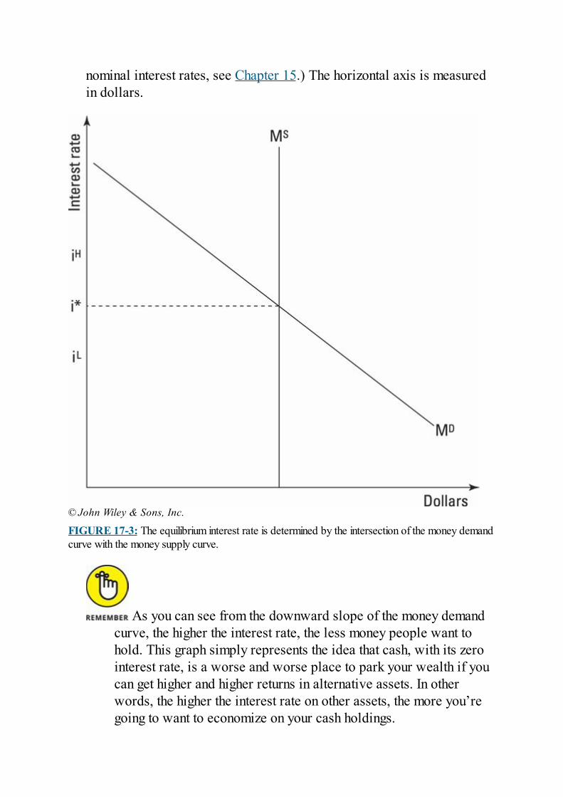
nominal interest rates, see Chapter 15.) The horizontal axis is measuredin dollars.

© John Wiley & Sons, Inc.

FIGURE 17-3: The equilibrium interest rate is determined by the intersection of the money demandcurve with the money supply curve.

As you can see from the downward slope of the money demandcurve, the higher the interest rate, the less money people want tohold. This graph simply represents the idea that cash, with its zerointerest rate, is a worse and worse place to park your wealth if youcan get higher and higher returns in alternative assets. In otherwords, the higher the interest rate on other assets, the more you’regoing to want to economize on your cash holdings.

Figure 17-3 also shows the vertical money supply curve, where MS

stands for money supply. This curve is vertical because the governmentcan decide how much money it wants to print and circulate withoutregard to the interest rate.

The MD and MS curves cross at interest rate i*. This interest rate is theequilibrium interest rate because it’s the only one at which the totalnumber of dollars of money that people want to hold is equal to the totalnumber of dollars that the government has circulated. More importantly,i* is a stable equilibrium, meaning that if interest rates ever deviatefrom it, they will be pushed back to i* by market forces.

Getting the basics about bondsThe best way to see why the equilibrium interest rate constitutes a stableequilibrium (see the preceding section) is to understand how interestrates are determined in the bond market. Pay close attention becausebond markets are the place where interest rates for the whole economyare determined. Bond markets have a huge effect on everything else thatgoes on in the economy.

A bond is a financial asset for which you pay a certain amount of moneyright now in exchange for a series of payments in the future. There aretwo kinds of payments, face value payments and coupon payments:

Face value payment: The face value is printed on the face of thebond certificate, and this payment comes on the date the bondexpires.Coupon payments: These payments are typically made twice peryear until the bond expires. They’re called coupon paymentsbecause before computerized recordkeeping, you’d literally clip acoupon off the bottom of the bond certificate and mail it in to receiveyour payment.

Typically, bonds expire after 1, 5, 10, or 20 years.

Bonds do not guarantee any sort of rate of return. They promiseonly to make the coupon and face value payments on time. The rate

of return depends on how much you pay for the right to receivethose payments.

If you think I’m speaking in tongues right now, bear with me. Imagine areally simple kind of bond called a zero-coupon bond (so namedbecause there are no coupon payments). The only payment this bond willever make is the face value payment that comes when the bond expires.And to make things really simple, suppose that this bond will pay itsowner exactly $100 exactly one year from now.

If you’re the bond owner, the rate of return the bond will pay depends onhow much you pay for it right now. Suppose that you were naive enoughto pay $100 for the bond right now. Your rate of return would be zeropercent because you paid $100 for something that will give you $100 ina year.

On the other hand, suppose you pay only $90 for the bond right now.Your rate of return will be about 11 percent because

, or 11.1 percent. If you could buy the bond foronly $50, your rate of return would be 100 percent because you’d doubleyour money in a year’s time.

The rate of return on a bond varies inversely with how much youpay for it. Because the amount of money you get in the future isalways fixed, the more you pay for it right now, the less is your rateof return. Higher bond prices imply lower rates of return.

Seeing the link between bond prices andinterest ratesThe fact that bond prices vary inversely with interest rates is the key tounderstanding why i* is a stable equilibrium in Figure 17-3. First,consider interest rates that are higher than i*, such as iH. When interestrates are higher than i*, the amount of money supplied exceeds theamount of money demanded. What this means is that people have beengiven more of the asset called money than they want to hold. So whatthey do is try to reallocate their portfolio of assets by using the excessmoney to buy other assets.

Another asset is bonds. But with all this new money being thrown at thelimited supply of bonds, the price of bonds rises. Now be careful. Whathappens to interest rates when bond prices rise? They fall. That’s why ifyou start out at an interest rate that’s higher than i*, interest rates will fallback toward i*. Excess money drives up the price of bonds, whichlowers interest rates.

On the other hand, for interest rates like iL that are lower than i*, theamount of money demanded exceeds the amount supplied. Becausepeople want more money than they have, they’re going to try to get it byselling noncash assets such as bonds in order to convert those assets intothe cash they want.

Imagine that everybody does this by trying to sell their bonds. With allthe selling, bond prices fall, meaning interest rates will rise. In fact,bond prices will continue to fall and interest rates rise until they’re backat i*, because that’s the only rate of interest at which people are satisfiedholding the amount of money MS that the government has decided tocirculate.

Movements back to the equilibrium interest rate, i*, are quick.Any excess money demand or excess money supply never lasts verylong because rapid adjustments in the price of bonds move theinterest rate to its equilibrium.

An important consequence of the fact that interest rates adjust so quicklyis that the government can print whatever amount of money it wants to,knowing that interest rates will adjust to get people to want to holdexactly that amount. This gives the government a very useful policy toolto manage the economy because it can think one step ahead and createwhatever interest rate it wants by printing the appropriate amount ofmoney.

Changing the money supply to changeinterest ratesMonetary policy works because governments know that interest ratesadjust in order to get people to hold whatever amount of money the

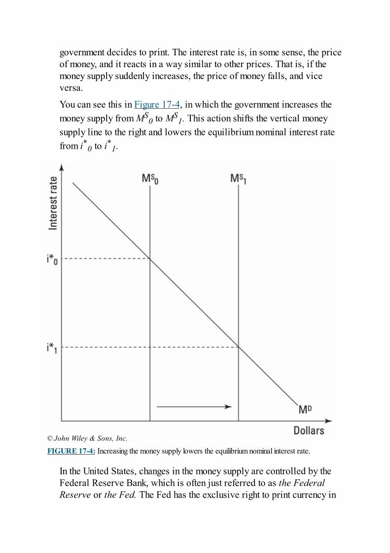
government decides to print. The interest rate is, in some sense, the priceof money, and it reacts in a way similar to other prices. That is, if themoney supply suddenly increases, the price of money falls, and viceversa.

You can see this in Figure 17-4, in which the government increases themoney supply from MS

0 to MS1. This action shifts the vertical money

supply line to the right and lowers the equilibrium nominal interest ratefrom i*0 to i*1.

© John Wiley & Sons, Inc.

FIGURE 17-4: Increasing the money supply lowers the equilibrium nominal interest rate.

In the United States, changes in the money supply are controlled by theFederal Reserve Bank, which is often just referred to as the FederalReserve or the Fed. The Fed has the exclusive right to print currency in

the United States, which means that it could make MS as big as it wantedto by printing more money and handing it out. However, the Fed actuallyrelies on a more subtle method for changing the money supply, a methodthat economists call open-market operations.

Open-market operations refers to the Fed’s buying and sellingof U.S. government bonds. That is, open-market operations aretransactions that take place in the public, or open, bond market.Depending on whether the Fed buys or sells bonds, the moneysupply out in circulation in the economy either increases ordecreases:

If the Fed wants to increase the money supply, it buys bonds. Tobuy bonds, the Fed must pay cash, which then circulates throughoutthe economy.If the Fed wants to decrease the money supply, it sells bonds. Thepeople to whom the Fed is selling the bonds have to give the Fedmoney, which the Fed then locks away in a vault so that it no longercirculates.

By buying or selling bonds in this way, the amount of money out incirculation (MS) can be very precisely controlled, meaning that the Fedcan, in turn, keep tight control over interest rates.

Lowering interest rates to stimulate theeconomyThe basic idea behind monetary policy is that lower interest rates causeboth more consumption and more investment, thereby shifting theaggregate demand curve to the right. Here’s how:

Consumption spending: Lower interest rates stimulate consumptionspending by increasing the attractiveness of taking out loans forbuying things such as automobiles and houses.Investment spending: Lower interest rates stimulate businesses’investment spending because at lower interest rates, a larger number

of potential investment projects become profitable. That is, if interestrates are 10 percent, businesses are only willing to borrow money toinvest in projects with rates of return of more than 10 percent. But ifinterest rates fall to 5 percent, all projects with rates of return higherthan 5 percent become viable, so firms take out more loans and startmore projects. (For more on how interest rates affect investment, seeChapter 14.)

When trying to remember how monetary policy works, keep inmind that it’s actually a very simple three-step process. When theFed wants to help increase output, it initiates the following chain ofevents:

1. It buys U.S. government bonds to increase the money supply.2. The increased money supply causes interest rates to fall because

the prices of bonds get bid up.3. Consumers and businesses respond to the lower interest rates by

taking out more loans and using the money to buy more goods.

The hard part is remembering that higher bond prices mean lowerinterest rates, which seems counterintuitive. But if you have a hard timeremembering that, don’t be embarrassed. Many economists get stuck onit, too.

Understanding how rational expectationscan limit monetary policyThe government’s ability to use increases in the money supply tostimulate the economy is limited by rational expectations and the fearsthat people have about inflation. Specifically, investors understand thatincreases in the money supply can cause inflation (as I discuss in Chapter15). Whenever the Federal Reserve increases the money supply to lowernominal interest rates, it has to do so with some moderation to avoidcausing inflationary fears that can offset the stimulatory effect ofincreasing the money supply.

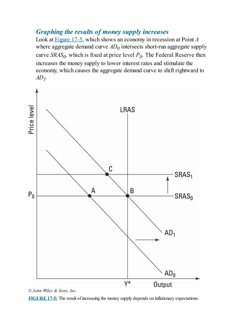
Graphing the results of money supply increasesLook at Figure 17-5, which shows an economy in recession at Point Awhere aggregate demand curve AD0 intersects short-run aggregate supplycurve SRAS0, which is fixed at price level P0. The Federal Reserve thenincreases the money supply to lower interest rates and stimulate theeconomy, which causes the aggregate demand curve to shift rightward toAD1.

© John Wiley & Sons, Inc.

FIGURE 17-5: The result of increasing the money supply depends on inflationary expectations.

At this point, two things can happen, depending on inflationaryexpectations:

If people believe that the price level will remain fixed at P0  , therightward shift in aggregate demand will move the economy’sequilibrium rightward along the SRAS0 curve from Point A to PointB.If people believe the price level will jump in response to theincrease in the money supply, the short-run aggregate supply curvewill shift up vertically by the amount that the price level is expectedto increase. That means that the economy’s equilibrium will movefrom A to C, where AD1 intersects the new short-run aggregatesupply curve, SRAS1.

Because output increases less if the economy moves from A to C than if itmoves from A to B, the Fed obviously has to be careful about inflationaryexpectations when trying to stimulate the economy by increasing themoney supply. If people expect inflation to occur, their actions can offsetsome of the stimulus that an increased money supply is expected to bringwith it.

Realizing how inflationary expectations affect interest rates

The underlying problem with monetary policy is that the Fed hasonly partial control over interest rates. In particular, it controlsmoney supply but not money demand. This is a problem because ifpeople think that an increase in the money supply will causeinflation, they increase their money demand because they’reexpecting to need more cash to buy things at higher prices.

So while the increase in the money supply tends to lower interest rates,as in Figure 17-4, the increase in money demand caused by inflationaryfears tends to increase interest rates. Because higher interest rates tend todecrease investment, any increase in interest rates caused by inflationaryfears works against the stimulus that the Fed is attempting to apply to theeconomy by increasing the money supply.

This decrease in the effectiveness of monetary stimulus is why the big

shift in aggregate demand in Figure 17-5 doesn’t shift the economy backto producing at Y*. With people expecting inflation, part of the stimulusends up causing inflation rather than stimulating the economy to producemore output.

Keeping inflationary expectations low to help monetarypolicy work wellSince the 1970s, most countries have been very cautious when usingmonetary policy. That’s because during the 1970s, countries learned thelesson that if people believe an increase in the money supply is going tocause inflation, an increase in the money supply may mostly end upcausing inflation rather than providing stimulus.

You can see an extreme case of this situation in Figure 17-6, whereoutput remains unchanged at the recessionary level YLow despite anincrease in the money supply that causes aggregate demand to shiftrightward from AD0 to AD1. The problem is that higher inflationaryexpectations cause the short-run aggregate supply curve to shift upvertically from SRAS0 to SRAS1, fully offsetting the increase in aggregatedemand. The short-run equilibrium shifts from A to B, but the only effectis a higher price level with no increase in output. Economists came torefer to the situation in Figure 17-6 as stagflation, in which the economyhas a stagnant output level coupled with inflation.

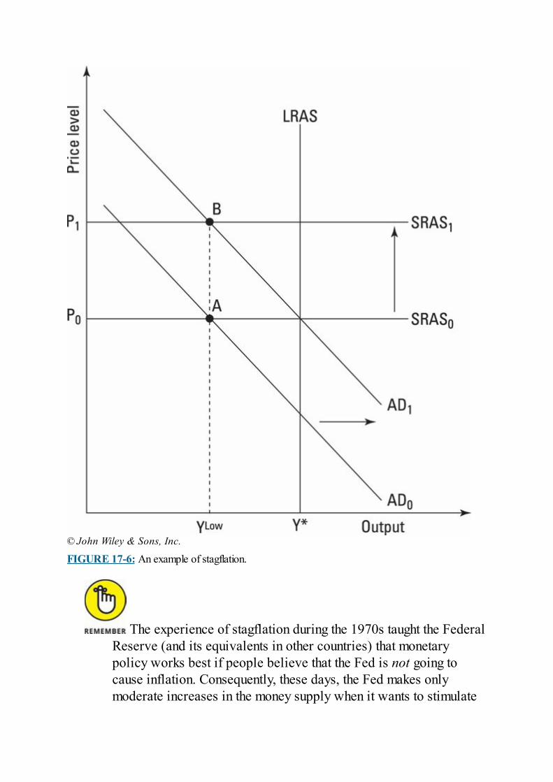
© John Wiley & Sons, Inc.

FIGURE 17-6: An example of stagflation.

The experience of stagflation during the 1970s taught the FederalReserve (and its equivalents in other countries) that monetarypolicy works best if people believe that the Fed is not going tocause inflation. Consequently, these days, the Fed makes onlymoderate increases in the money supply when it wants to stimulate

the economy. These increases end up being more effective thanlarger increases because they don’t trigger inflationary fears.

Examining quantitative easing and theGreat RecessionThe worldwide Great Recession of 2007–2009 began when a housingbubble in the United States popped in 2006. Trillions of dollars had beeninvested in the financial markets on the premise that residential housingprices would never decline significantly. As the bubble burst and homeprices began to plummet, dozens of large banks as well as manyhundreds of financial firms were threatened with bankruptcy.

Lending ceased not only for home mortgages but for business loans, andif it hadn’t been for aggressive interventions by governments and centralbanks, the entire worldwide financial system might have collapsed, suchthat nobody would have been able to obtain a loan for any purpose.Because the world economy is highly dependent on borrowed money tofinance everything from credit card purchases to factory construction,another Great Depression loomed just over the horizon.

To calm the immediate crisis, the Fed and other central banks becamelenders of last resort, ensuring that businesses could still obtain financingdirectly from the Fed even if banks were reluctant to loan. The Fed alsoprotected banks from banking panics by increasing the insurance limitsoffered to checking account depositors. These and other steps limited therecession to only being moderately severe.

That being said, the Great Recession was still much more severe thanyour typical recession. So it wasn’t surprising that the Fed and othercentral banks undertook innovative new monetary policy measures tostimulate the economy. These came to be known as unconventionalmonetary policy.

Under conventional monetary policy, central banks like the Fed useopen-market operations to purchase short-term (less than 1-yearmaturity) government bonds to increase the money supply and driveshort-term interest rates toward zero in order to stimulate the economy.(For more, see the earlier section “Lowering interest rates to stimulatethe economy.”)

But given the severity of the Great Recession, the Fed and other central

banks found that conventional monetary policy wasn’t going to be enoughto drive short-term interest rates to zero. Additional stimulus wasneeded. So the Fed and other central banks began to purchase trillions ofdollars worth of longer-term government bonds (with 5-year, 10-year,and 20-year maturities), private-sector bonds (including mortgage-backed securities), and even stocks. The goal in all cases was toincrease the quantity of money available to be loaned out. It was hopedthat more borrowing and lending would take place, thereby stimulatingboth consumption and investment.

These policies became known as quantitative easing (or QE), sincetheir goal was to ease the constraints on lending and borrowing byincreasing the quantity of money in circulation. By contrast, conventionalmonetary policy targets not the quantity of money in circulation but ratherthe price of money — the interest rate. Conventional monetary policyattempts to simulate the economy by lowering the price of loans.Unconventional monetary policy (quantitative easing) attempts toincrease the sheer volume of loans.

Another unconventional monetary policy was setting an explicit target forinflation, so that people would know how aggressive central banks weregoing to be with changes in the money supply. The inflation target wasset at 2 percent in the United States, which could only be met if the Fedwere increasing the money supply faster than any increase in moneydemand. By setting a 2 percent target, the Fed was committing itself tocontinually pushing the AD curve to the right and thus always attemptingto stimulate the economy. This commitment was intended to giveconsumers and businesses confidence that the Fed would stimulate aslong as necessary until the Great Recession was over and the economyhad fully recovered.

Chapter 18

Grasping Origins and Effectsof Financial Crises

IN THIS CHAPTER Understanding that borrowing and debt drive price bubbles and

financial crises Seeing how rising asset prices feed bubbles by increasing the

value of loan collateral Examining how popping bubbles can take down the banking

system Realizing that the post-bubble economy is hamstrung by high

debt levels Identifying why fiscal and monetary policy don’t work very well

after a financial crisis

A financial crisis is a period of economic instability triggered by thefailure of one or more major financial institutions to fulfill theirpromises. For instance, banking crises are triggered when banks fail tohonor their legal obligation to redeem deposits on demand. And currencycrises are triggered when national central banks break promises tomaintain fixed exchange rates.

Financial crises can cause recessions, periods of decline in the totaloutput of goods and services produced by the economy. Pleaseunderstand, though, that not every bank failure or broken promise aboutan exchange rate triggers a recession. A recession follows a financialcrisis only if previous events have led the economy into such aprecarious situation that bank failures or exchange-rate collapses make arecession almost inevitable. That happened in the United States andEurope in 2007, when the failure of many banks and investmentcompanies to repay money that they’d borrowed to invest in real estateled to the most severe recession in over 70 years.

So what sets the stage for a crisis? Massive amounts of debt.Financial crises are always preceded by economy-wide borrowingbinges that fuel unsustainable asset-price bubbles, typically instocks or real estate. These borrowing binges also fuel economicbooms because a great deal of the borrowed money is used topurchase not only stocks or real estate but also goods and services.

As a boom continues, people start thinking it’s permanent and that theirincomes will keep rising rapidly. This encourages them to take on evenmore debt, so when the bubble eventually bursts, they find themselveswith huge amounts of debt but much-lower-than-expected incomes. Theeconomy then goes into a recession as people retrench, directing more oftheir reduced incomes to paying down debt and less to buying goods andservices.

This chapter tells you how debt-driven bubbles develop, how they cancause misallocation of resources in the economy, and why recessions thatoccur after debt bubbles burst are so severe and hard for governments todeal with.

Understanding How Debt-DrivenBubbles Develop

Debt contracts, such as bonds and mortgages, are promises to repayparticular amounts of money. When negotiating such contracts, lendersnormally believe that those to whom they’re lending will be able torepay — or else lenders wouldn’t extend the loans. On the flip side,borrowers typically believe that they’ll be able to repay — or else theywouldn’t take out those loans.

However, a circular, self-reinforcing process can develop between thetotal amount of borrowing and the anticipated ability of borrowers torepay their loans. These situations drive asset-price bubbles, in whichspeculative purchases financed with borrowed money drive the price ofan asset (such as real estate) upward.

As long as the bubble continues to expand and prices continue to rise,nearly every loan gets paid off — leading both borrowers and lenders toerroneously conclude that lending and borrowing are very safe. Thatdrives the demand for even more borrowing and lending, further inflatingthe bubble. This continues until the bubble finally pops and pricescollapse. In this section, I give more detail on how bubbles get startedand expand, and I discuss price collapses later in “Seeing the BubbleBurst.”

Embracing borrowing in a boomingeconomy

During the periods preceding financial crises, the expectationsof both lenders and borrowers tend to be overly optimistic, usuallybecause the economy has enjoyed a period of sustained growth inoutput and living standards. With the demand for goods and serviceshigh, jobs are plentiful and wages tend to grow strongly. Thus, bothborrowers and lenders come to believe that the financial prospectsof borrowers are very strong — and therefore that to borrow or

lend successively larger amounts of money at successively lowerinterest rates wouldn’t be overly risky.

The problem is that the lending and borrowing facilitated by the initialoptimism can quickly become self-justifying, because when peoplespend borrowed money, that money stimulates the economy even moreand causes an even higher level of optimism that justifies making evenmore loans.

Firms use the loans to expand factories, and individuals use borrowedmoney to purchase houses, cars, and durable goods. All this economicactivity makes it easy for both borrowers and lenders to conclude that theboom will go on indefinitely and that paying back loans will always beeasy for borrowers.

Offering larger loans as collateral valuesriseThe sharp increase in lending and borrowing that precedes a financialcrisis is exacerbated by the fact that lending can drive up the value of theassets (such as real estate) that are used as collateral for loans.Collateral is property that a borrower pledges to a lender as security fora loan. People refer to the collateral as security because if the borrowerfails to repay the loan, the lender receives the collateral. Thus, thecollateral provides some financial security (safety) for the lender.

For instance, when a home buyer takes out a mortgage, the contract withthe bank from which she’s borrowing specifies that the house itselfserves as collateral for the mortgage loan. Thus, if the borrower defaultson the loan, the home will become the property of the bank, which canthen sell the home at auction to raise money to pay off the defaulted loan.

Having houses serve as their own collateral helps fuel housingbubbles. Because rising home prices imply rising collateral values,banks feel comfortable lending successively larger amounts ofmoney for home mortgage loans. But as loans become easier toobtain, more buyers take out loans, increase the demand for houses,and drive up home prices.

People then get into a self-reinforcing process as increased lending leadsto higher demand, which leads to higher prices, which leads to increasedlending because higher prices imply higher collateral values. This sort ofprocess drove the real estate bubble in Japan during the late 1980s aswell as the real estate bubbles in the United States, Ireland, and Spainfrom 2000 to 2006.

Relaxing lending standardsBeyond increasing collateral values, rising prices also cause lenders tobecome lax about their lending standards in an additional way. Duringnormal times, lenders verify that borrowers can pay off their loans withtheir labor income. If you have a low labor income, then you normallyaren’t allowed to borrow very much money because you won’t be able toafford large monthly loan payments.

This logic gets shunted aside during periods of rapidly rising real-estateprices. In fact, banks become increasingly willing to lend large amountsto anybody, including people with very low incomes, because rising realestate prices imply that borrowers should always be able to sell theirhouses for more than they paid for them.

For example, consider how willing a bank will be to give even a poorperson a loan of $200,000 to purchase a house if the price of the house isexpected to rise to $225,000 over the course of the next year. With themarket price of the house expected to rise by $25,000, the bank willassume that the chance that the borrower will default on the loan isvirtually zero because he’ll always be able to sell the house for moremoney than he borrowed. Thus, in situations where home prices areexpected to keep on rising, banks become willing to lend even to thosewith low incomes.

Borrowing more in hopes of profitThe willingness of banks to lend when home prices are expected to riseis matched by borrowers’ desire to take out loans in attempts to profitfrom the rising real estate prices. For instance, if home prices areexpected to rise from $200,000 to $225,000 over the next year, potentialborrowers will assume that they can easily repay a $200,000 mortgageloan by selling the house the next year for $225,000. In fact, they’llexpect to come out almost $25,000 ahead on the deal, even after

accounting for accumulated interest on the loan.

The risk is that the house prices won’t rise by as much as expected andmay even fall, but during a housing-price bubble, many people becomeso convinced that home prices will rise that they feel that they’re notreally taking on any risk when they borrow money to purchase realestate.

Indeed, because the potential $25,000 gain looks like free money, manymillions of people are tempted to take out loans to purchase houses thatthey’d otherwise have no reason to care about. Their goal isn’t to live inthose houses or to rent them out to tenants but rather to use borrowedmoney to “buy low and sell high,” hoping to profit if home pricescontinue to rise.

Watching the process gain momentumBoth borrowers and lenders are willing to participate in a real estatebubble. The lenders think that rising real estate prices almost certainlyguarantee that loans will be repaid, and borrowers think that rising realestate prices almost certainly guarantee that buyers can make money fornothing.

As soon as that process gains momentum, it can become temporarily self-sustaining. Lots of borrowed money drives up real estate prices, causingeven more people to think that price increases will be sustained, whichtempts both borrowers and lenders to increased borrowing and lending— thereby driving even further price increases. Sadly, though, there’s nosuch thing as a party that never ends — or a party for which nobody hasto pick up the tab.

Seeing the Bubble BurstDebt-driven asset-price bubbles eventually pop because at some point,borrowing enough money to keep prices rising becomes impossible.Imagine that home prices start off at $100,000. At that price, potentialbuyers must be able to borrow $100,000 each if they’re to purchase ahome. But if home prices are driven up over time to $300,000, then anynew potential buyers must get their hands on $300,000 of borrowedmoney to purchase a home. And if home prices rise to $500,000 perhouse, then potential buyers need loans of $500,000 each.

Given the limited amounts of money available for borrowing,buyers will at some point face the reality that they simply can’t findenough new money to borrow to drive prices up any higher. At thatpoint, prices will peak.

In this section, I explain why asset-price bubbles pop quickly rather thandeflate slowly. The end is rapid because the end of rising prices causesboth a massive increase in supply as well as a massive decrease indemand. With supply rising and demand falling, prices fall rapidly.

Deleveraging: Trying to ditch debt as pricesfallPeople who’ve borrowed money to purchase assets are in a leveragedposition, meaning that they’ve augmented (or in other words, leveraged)their own purchasing power with that of the money they’ve borrowed.

When a price bubble peaks, being in a leveraged position is extremelyprecarious. The problem is that if you’re a borrower, you probably don’thave enough labor income to pay off the loan. That’s because you tookout your loan in anticipation of future price increases. Your plan hadbeen to sell your house for more than you paid for it, thereby gettingenough money to pay off the mortgage loan while leaving any extramoney as profit.

With prices unable to rise any further (due to new borrowers’ being

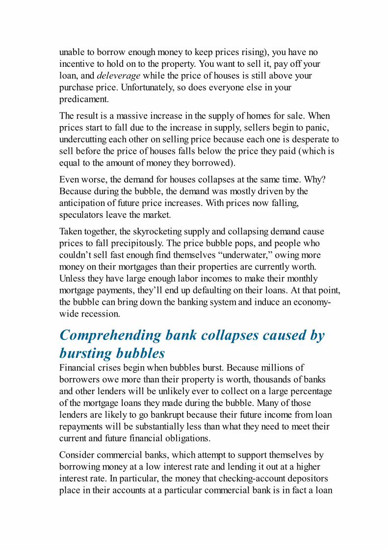
unable to borrow enough money to keep prices rising), you have noincentive to hold on to the property. You want to sell it, pay off yourloan, and deleverage while the price of houses is still above yourpurchase price. Unfortunately, so does everyone else in yourpredicament.

The result is a massive increase in the supply of homes for sale. Whenprices start to fall due to the increase in supply, sellers begin to panic,undercutting each other on selling price because each one is desperate tosell before the price of houses falls below the price they paid (which isequal to the amount of money they borrowed).

Even worse, the demand for houses collapses at the same time. Why?Because during the bubble, the demand was mostly driven by theanticipation of future price increases. With prices now falling,speculators leave the market.

Taken together, the skyrocketing supply and collapsing demand causeprices to fall precipitously. The price bubble pops, and people whocouldn’t sell fast enough find themselves “underwater,” owing moremoney on their mortgages than their properties are currently worth.Unless they have large enough labor incomes to make their monthlymortgage payments, they’ll end up defaulting on their loans. At that point,the bubble can bring down the banking system and induce an economy-wide recession.

Comprehending bank collapses caused bybursting bubblesFinancial crises begin when bubbles burst. Because millions ofborrowers owe more than their property is worth, thousands of banksand other lenders will be unlikely ever to collect on a large percentageof the mortgage loans they made during the bubble. Many of thoselenders are likely to go bankrupt because their future income from loanrepayments will be substantially less than what they need to meet theircurrent and future financial obligations.

Consider commercial banks, which attempt to support themselves byborrowing money at a low interest rate and lending it out at a higherinterest rate. In particular, the money that checking-account depositorsplace in their accounts at a particular commercial bank is in fact a loan

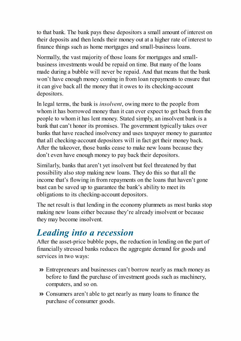
to that bank. The bank pays these depositors a small amount of interest ontheir deposits and then lends their money out at a higher rate of interest tofinance things such as home mortgages and small-business loans.

Normally, the vast majority of those loans for mortgages and small-business investments would be repaid on time. But many of the loansmade during a bubble will never be repaid. And that means that the bankwon’t have enough money coming in from loan repayments to ensure thatit can give back all the money that it owes to its checking-accountdepositors.

In legal terms, the bank is insolvent, owing more to the people fromwhom it has borrowed money than it can ever expect to get back from thepeople to whom it has lent money. Stated simply, an insolvent bank is abank that can’t honor its promises. The government typically takes overbanks that have reached insolvency and uses taxpayer money to guaranteethat all checking-account depositors will in fact get their money back.After the takeover, those banks cease to make new loans because theydon’t even have enough money to pay back their depositors.

Similarly, banks that aren’t yet insolvent but feel threatened by thatpossibility also stop making new loans. They do this so that all theincome that’s flowing in from repayments on the loans that haven’t gonebust can be saved up to guarantee the bank’s ability to meet itsobligations to its checking-account depositors.

The net result is that lending in the economy plummets as most banks stopmaking new loans either because they’re already insolvent or becausethey may become insolvent.

Leading into a recessionAfter the asset-price bubble pops, the reduction in lending on the part offinancially stressed banks reduces the aggregate demand for goods andservices in two ways:

Entrepreneurs and businesses can’t borrow nearly as much money asbefore to fund the purchase of investment goods such as machinery,computers, and so on.Consumers aren’t able to get nearly as many loans to finance thepurchase of consumer goods.

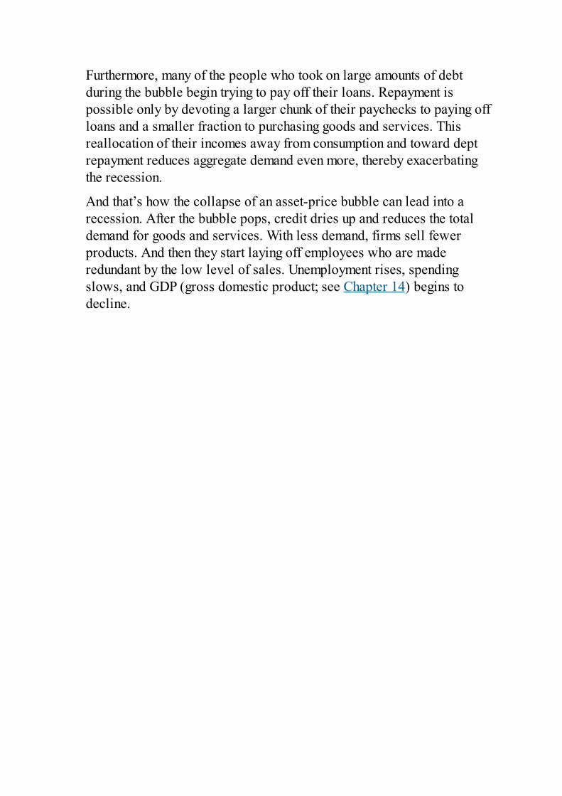
Furthermore, many of the people who took on large amounts of debtduring the bubble begin trying to pay off their loans. Repayment ispossible only by devoting a larger chunk of their paychecks to paying offloans and a smaller fraction to purchasing goods and services. Thisreallocation of their incomes away from consumption and toward deptrepayment reduces aggregate demand even more, thereby exacerbatingthe recession.

And that’s how the collapse of an asset-price bubble can lead into arecession. After the bubble pops, credit dries up and reduces the totaldemand for goods and services. With less demand, firms sell fewerproducts. And then they start laying off employees who are maderedundant by the low level of sales. Unemployment rises, spendingslows, and GDP (gross domestic product; see Chapter 14) begins todecline.

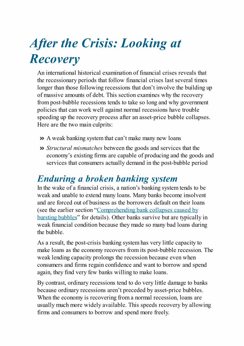
After the Crisis: Looking atRecovery

An international historical examination of financial crises reveals thatthe recessionary periods that follow financial crises last several timeslonger than those following recessions that don’t involve the building upof massive amounts of debt. This section examines why the recoveryfrom post-bubble recessions tends to take so long and why governmentpolicies that can work well against normal recessions have troublespeeding up the recovery process after an asset-price bubble collapses.Here are the two main culprits:

A weak banking system that can’t make many new loansStructural mismatches between the goods and services that theeconomy’s existing firms are capable of producing and the goods andservices that consumers actually demand in the post-bubble period

Enduring a broken banking systemIn the wake of a financial crisis, a nation’s banking system tends to beweak and unable to extend many loans. Many banks become insolventand are forced out of business as the borrowers default on their loans(see the earlier section “Comprehending bank collapses caused bybursting bubbles” for details). Other banks survive but are typically inweak financial condition because they made so many bad loans duringthe bubble.

As a result, the post-crisis banking system has very little capacity tomake loans as the economy recovers from its post-bubble recession. Theweak lending capacity prolongs the recession because even whenconsumers and firms regain confidence and want to borrow and spendagain, they find very few banks willing to make loans.

By contrast, ordinary recessions tend to do very little damage to banksbecause ordinary recessions aren’t preceded by asset-price bubbles.When the economy is recovering from a normal recession, loans areusually much more widely available. This speeds recovery by allowingfirms and consumers to borrow and spend more freely.

Struggling with structural mismatchesPost-bubble recessions tend to be longer and more severe than ordinaryrecessions partly because of structural mismatches. An economy has astructural mismatch between its production capacity and the productsconsumers demand if the mix of goods and services that the economy’sfirms are capable of producing differs from what consumers want topurchase and consume.

Post-crisis economies often feature structural mismatches because ofdistortions to productive capacity that occur while bubbles areexpanding. For example, consider the United States housing bubble of2000–2006 and the subsequent recession of 2007–2009.

The U.S. housing bubble of 2000–2006 was the largest real estate bubblein world history. During the expansionary phase of that bubble, creditwas easily available throughout the economy. This led to $2 trillion ofexcess housing being built and to many firms’ borrowing trillions ofdollars to fund new investment projects.

But even after the recession ended and the economy began to slowlygrow again in the summer of 2009, unemployment remained very highand businesses were producing at levels far below their capacity. Someexperts ascribed this to low aggregate demand caused by banks’ reducinglending and consumers’ reducing consumption in order to pay downdebts.

Other experts, however, feared that the U.S. economy was suffering froma structural mismatch. Their reasoning was that during the bubble, firmshad used their access to easy credit to build up lots of capacity toproduce things that were popular during the boom — large new houses,fancy malls, and plenty of SUVs and large trucks. After the bubblepopped, however, consumers didn’t want lots of new houses or newSUVs or additional large trucks. Instead, they wanted products such asiPads, better touch-screen cell phones, and smaller cars, as well as theability to do more of their shopping over the Internet instead of driving toshopping malls.

If that interpretation is correct, then recovering from the 2007–2009recession entailed a much slower recovery process than recovering froma plain-vanilla cyclical recession. The added difficulty came fromhaving to rejigger the economy’s production capacity from making the

products that were in demand while the bubble was expanding toproducing the different goods and services in demand after the bubbleburst.

Making that sort of a transition requires revamping old firms or startingnew firms, moving workers away from dying industries into newindustries, and undertaking the time and expense of retooling factoriesand restructuring supply chains. Making those adjustments all over theeconomy is not quick.

Noting the limits of government policyWhether a recession is preceded by a bubble or not, governments almostalways attempt to use both fiscal and monetary policy to increaseaggregate demand (see Chapter 17). However, government stimuluspolicies often appear unable to significantly speed up the recoveryprocess after a financial crisis. The policies are stymied by the debt thatremains after the bubble pops.

In particular, both fiscal and monetary policy are of limitedeffectiveness because post-bubble consumers want to deleverage,or get rid of their debt. Here’s how the desire to deleveragehampers both fiscal and monetary policy:

Fiscal policy: Post-crisis fiscal policy comes in the form of massiveincreases in government spending that are intended to stimulateaggregate demand by having the government purchase lots of goodsand services. The hope is that by increasing people’s incomes, thoseinitial purchases will spur further economic activity that willsnowball into robust economic growth as consumers return tospending confidently.But in the aftermath of a debt-driven bubble, fiscal policy’sstimulatory effects may be limited because people often useincreases in income to pay down debt (instead of using the money topurchase additional goods and services).Monetary policy: The government attempts to use monetary policyto stimulate demand by lowering interest rates to encourage bothconsumers and firms to borrow and spend more.

However, monetary policy fails to work very well after a debt-driven bubble because highly leveraged consumers are in no mood toborrow more money. They’re understandably more interested inpaying down their current debts than in taking on additional debts.

If this situation sounds very dismal, it is. Until the debt level in theeconomy falls so that people do not need to devote so much of theirincomes to paying off loans, economic growth is likely to remainstagnant, and government attempts at monetary and fiscal policy arelikely to prove ineffective.

Part 5

The Part of Tens

IN THIS PART …Discover ten common — but false — beliefs held about economics.

Get the scoop on ten valuable insights from economics.

Find out about some of the most famous economists who ever lived.

Chapter 19

Ten Seductive EconomicFallacies

IN THIS CHAPTER Avoiding logical fallacies that sucker intelligent people Steering clear of bad economic reasoning

In this short chapter, I outline the most attractive and compellingincorrect ideas in economics. Some are logical fallacies. A few aremyopic opinions that don’t take into account the big picture. And othersare poorly thought out examples of economic reasoning. All are to beavoided.

The Lump of LaborThe argument that there’s a fixed amount of work that you can divide upamong as many people as you want is often presented as a cure forunemployment. The idea goes that if you convert from a 40-hour workweek to a 20-hour work week, firms will have to hire twice as manyworkers. In 2000, for instance, France reduced its work week to only 35hours hoping that firms would hire more workers and cure the persistentunemployment problem.

It didn’t work; such policies have never worked. One problem is thathiring workers involves many fixed costs, including training costs andhealth insurance. So two 20-hour-per-week workers cost more to employthan one 40-hour-per-week worker. What’s more, two 20-hour-per-weekworkers don’t produce any more output than one 40-hour-per-weekworker.

So if laws were passed that forced firms to move from a 40-hour workweek to a 20-hour work week, firms wouldn’t double the size of theirworkforces. They’d hire fewer than twice as many workers becausecosts would go up.

In addition, even if cutting the work week in half actually did double thenumber of workers used, it would only hide the overall unemploymentproblem by spreading it around. If, for example, 100 percent of workersare working half-time, they are all 50 percent underemployed. In terms ofthe total amount of output that could be produced (and hence availablefor people to consume), that situation wouldn’t be any better than having50 percent of the population employed full-time and 50 percent totallyunemployed.

You really want a situation in which every worker who wants afull-time job is able to get one. Shortening the work week doesn’tachieve this goal.

The World Is FacingOverpopulation

Various versions of this myth have been floating around since the late18th century when Thomas Malthus first asserted it. He argued that livingstandards couldn’t permanently rise because higher living standardswould cause people to breed faster. He believed that population growthwould outpace our ability to grow more food, so we would be doomedto return to subsistence levels of nutrition and living standards.

Even when Malthus first published this idea, lots of evidence indicatedthat it was bunk. For generations, living standards had been rising whilebirth rates had been falling. And because that trend has continued up tothe present day, we’re not going to breed our way to subsistence. Indeed,many nations now face an underpopulation problem because birthrateshave fallen below the replacement rate necessary to keep the populationstable. The populations of Italy, Japan, and Russia, among others, havealready begun to shrink.

A related problem is that rapidly falling birth rates are wreaking havocon government-sponsored retirement systems because there aren’t enoughyoung workers to pay all the taxes needed to fund retirees’ pensions.

Sequence Indicates CausationPost hoc ergo propter hoc is a Latin phrase that translates roughly as,“Because you see one thing precede another, you think that it causes theother.” That is, if A happens before B, you assume that A causes B. Sucha deduction is false because A and B often don’t have any relationship.For instance, sometimes it rains in the morning, and I get a headache inthe afternoon. That doesn’t mean that the rain caused my headache.

Politicians try to pull this logical fallacy all the time when discussing theeconomy. For instance, suppose that politician A gets elected, and arecession begins a few months later. The two may have nothing to dowith each other, but you can be sure that during the next election,politician B — an opponent of politician A — will claim that therecession was the result of politician A’s policies. The only proofoffered is that one event happened before the other.

Protectionism Is the BestSolution to Foreign Competition

Many trade unions and politicians argue in favor of trade barriers andtaxes on imports on the grounds that these policies would benefit citizensand prevent jobs from being exported. The problem is that theirarguments consider only the benefits of protectionism. Trade barriers andtaxes on imports do protect the specific jobs that they’re intended toprotect. However, other jobs are often sacrificed in the process.

Another problem with protectionism is that citizens are consumers aswell as producers. For instance, if the government prevents theimportation of lower price, higher quality foreign automobiles, itpreserves jobs in the domestic auto industry. But costs for domesticconsumers rise as a result.

Protecting an unproductive industry that faces foreign competition onlyallows it to keep using resources that would otherwise be better used bymore vibrant industries. Workers who would otherwise move to jobs ininnovative, highly productive new industries instead get stuck in anindustry so unproductive that it can survive only by having thegovernment rig the economy in its favor.

Granted, the move from a dying industry to an innovative new industrycan be rough for an individual worker. But rather than avoid the need forchange by protecting unproductive industries, the government can helpdomestic workers more efficiently by providing retraining programs foremployees. (In the case of older workers who have only a few years ofemployment left, early retirement programs may be more viable thanretraining.)

The Fallacy of CompositionAssuming that what’s good for one person to do is good for everyone todo all at once is another common fallacy. For instance, if you’re at asold-out sporting event and want to get a better view, standing is a goodidea — but only if you’re the only one who stands up. If everyone elsealso stands up, everyone’s view is just as bad as when everyone wassitting down (but now everyone’s legs are getting tired). Consequently,what was good for you to do alone is actually bad for everyone to do atthe same time.

The fallacy of composition is false because some things in life have todo with relative position. For instance, if you start out as the lowest paidemployee at your firm but then get a 50 percent raise while nobody elsegets a raise, your relative position within the firm improves. However, ifeveryone gets a 50 percent raise at the same time, you’re still the lowestpaid person at the firm. If what matters to you is your relative standingwithin the firm, getting the same raise as everyone else doesn’t make youany happier. (On the other hand, if you are more interested in where youstand relative to people who work at other firms, getting a 50 percentraise is good even if everyone else at your firm gets it, too!)

If It’s Worth Doing, Do It 100Percent

We all value safety. But was a famous U.S. politician really beingsensible when he said that we should spend whatever money might benecessary to make flying on commercial airlines “as safe as possible”?Economists would say, “No!” The problem is that making commercialairline travel “as safe as possible” would mean making it prohibitivelyexpensive.

The politician failed to apply marginalism — the idea that the best wayto approach a problem is to compare marginal benefits with marginalcosts. The first few airline safety innovations (such as seatbelts andradar) are sensible to undertake because the extra, or marginal, benefitthat each brings is greater than the extra, or marginal, cost required topay for it. But after the first few safety innovations are implemented,successive innovations become more costly and less effective. At somepoint, additional innovations bring only small marginal increases insafety while running up high marginal costs.

When the costs for the extra safety innovations exceed theirbenefits, they shouldn’t be implemented. You should add safetyfeatures only as long as the marginal benefits exceed the marginalcosts — which means that you’ll usually stop adding safety featureslong before you get anywhere near making things “as safe aspossible.”

Free Markets Are DangerouslyUnstable

Free market prices and quantities often change extremely rapidly. Theydo so because supply and demand often change very quickly, causingrapid changes in equilibrium prices and quantities (which I discuss inChapter 4). But rapidly changing prices and quantities should not be seenas a problem in and of themselves. The responsiveness of markets isactually one of their great benefits. Unlike a government bureaucracy thatcan never react quickly to anything, markets can adjust to huge changes inworld events in only minutes.

The new equilibrium prices and quantities see to it that resources areallocated to their best uses and that society suffers from neither shortagesnor gluts. So don’t call markets unstable. Call them responsive.

Low Foreign Wages Mean ThatRich Countries Can’t Compete

Suppose that a U.S. factory pays its workers $20 per hour while acompeting factory in a developing country pays its workers $4 per hour.People mistakenly jump to the conclusion that because the foreignfactory’s labor costs are so much lower, it can easily undersell the U.S.factory. But this argument fails to take into account two things:

What actually matters is labor costs per unit, not labor costs perhour.Differences in productivity typically mean that labor costs per unitare often nearly identical despite huge differences in labor costs perhour.

To see what I mean, compare how productive the two factories are.Because the U.S. factory uses much more advanced technology, oneworker in one hour can produce 20 units of output. The U.S. worker getspaid $20 per hour, so the labor cost per unit of output is $1. The factoryin the developing country is much less productive; a worker thereproduces only 4 units in one hour. Given the foreign wage of $4 per hour,the labor cost per unit of output in the developing country is also $1.

Obviously, the developing country’s lower hourly wage rate per hourdoes not translate into lower labor costs per unit — meaning that itwon’t be able to undersell its U.S. competitor.

People who focus exclusively on the difference in labor costs per hournever mention the productivity differences that typically equalize laborcosts per unit. And don’t think that my example uses happy-happynumbers. Wage differences across countries really do tend to reflectproductivity differences.

Keep in mind that governments can seriously screw up whatwould otherwise be a near equality of labor costs per unit by fixing

artificially low exchange rates. For instance, if at an exchange rateof 8 Chinese yuan to 1 U.S. dollar labor costs per unit are equal, theChinese government could make labor costs per unit lookartificially low to U.S. consumers if it fixes its currency at, forinstance, 16 yuan to 1 dollar. In such situations, the inability of U.S.workers to compete with Chinese workers is due to the currencymanipulation, not to the lower wage rate per hour found in China.

Tax Rates Don’t Affect WorkEffort

Some politicians argue for raising income taxes as though the only effectof doing so will be to raise more money. But it’s been demonstrated overand over again that beyond a certain point, people respond to highertaxes by working less. And that reduction in labor denies society all thebenefits that would have come from the extra work. (Because peoplework less, the increased tax rate also doesn’t bring in nearly as muchrevenue as expected.)

So if you see a politician arguing for an increase in income taxes, lookinto the details to make sure that the disincentive effects of the tax hikedon’t cause more mischief than the benefits that will be derived fromspending the money raised by the tax increase.

Forgetting UnintendedConsequences

When evaluating a policy, people tend to concentrate on how the policywill fix some particular problem while ignoring or downplaying othereffects it may have. Economists often refer to this situation as The Law ofUnintended Consequences. For instance, suppose that you impose atariff on imported steel in order to protect the jobs of domesticsteelworkers. If you impose a high enough tariff, their jobs will indeedbe protected from competition by foreign steel companies. But anunintended consequence is that the jobs of some autoworkers will be lostto foreign competition. Why? The tariff that protects steelworkers raisesthe price of the steel that domestic automobile makers need to build theircars. As a result, domestic automobile manufacturers have to raise theprices of their cars, making them relatively less attractive than foreigncars. Raising prices tends to reduce domestic car sales, so somedomestic autoworkers lose their jobs.

Chapter 20

Ten Economic Ideas to HoldDear

IN THIS CHAPTER Understanding ten fundamental economic principles Arming yourself against the economic follies of politicians, the

media, and others

In this chapter, I list ten economic ideas that all informed people shouldunderstand and be ready to use to evaluate the policy proposals made bypoliticians, pundits, and the media. Some of these ideas aren’t true in allsituations, but because they’re usually correct, be wary if some guywants you to believe that they don’t apply to a particular situation.Chances are that he’s wrong.

Self-Interest Can ImproveSociety

The idea that self-interest can improve society is basically Adam Smith’sfamous invisible hand. If all economic transactions in a society arevoluntary on the parts of all parties involved, then the only transactionsthat will take place are those where all parties feel that they’re beingmade better off. This concept doesn’t mean that charitable acts are badfor society. Rather, it means that even philanthropy is generated by self-interest: People give because they enjoy helping others, so both giversand the people they help are better off. In addition, this conceptmotivates entrepreneurs to find ways to produce products you like atprices you like. Sellers must fear your power of choice — your right towalk away from any offer that you don’t consider advantageous.

Free Markets RequireRegulation

Economists firmly believe that voluntary transactions in free marketstend to work toward the common good. But they also believe that nearlyevery participant in the marketplace would love to rig the system in hisor her own favor. Adam Smith was quick to argue that for markets towork and serve the common good, the government has to fightmonopolies, collusion, and any other attempts to prevent a properlyfunctioning market in which firms vigorously compete against each otherto give consumers what they want at the lowest possible price.Government intervention may also be necessary to deal with asymmetricinformation, public goods, and externalities.

Economic Growth Relies onInnovation

The only way to have sustained economic growth and widespreadincreases in living standards is to invent more efficient technologies thatallow people to produce more from the limited supply of labor andphysical resources. To that end, societies should promote education andset up institutions such as patent rights, competitive markets, andcopyright laws to promote innovation and increases in efficiency.

Freedom and Democracy MakeUs Richer

Very good moral and ethical reasons exist for favoring freedom anddemocracy. But a more bottom-line reason is that because they promotethe free development and exchange of ideas, free societies have moreinnovation and, consequently, faster economic growth. And they attractforeign investment.

Education Raises LivingStandards

Not only do educated people produce more as workers — and get paidhigher salaries — they produce innovative new technologies. Sustainedeconomic growth and higher living standards are possible only if youeducate your citizens well. You have, of course, other good reasons forgetting an education, including the ability to appreciate high art andliterature. But if all you care about is rising living standards, work hardto promote education in science and engineering, sectors whererevolutionary technologies are created.

Intellectual Property BoostsInnovation

People need incentives to take risks. One of the biggest risks is leaving asecure job to start a new business or develop a great new idea.Intellectual property rights, such as patents and copyrights, guaranteethat you’ll be the only one making money off your hard, innovative work.Without this assurance, few would be willing to take the risks necessaryto provide new technologies and products.

Weak Property Rights Cause AllEnvironmental Problems

Environmental problems stem from poorly defined or nonexistentproperty rights that allow polluters to ignore the costs that they imposeon others. Therefore, economists favor the creation and enforcement ofproperty rights systems that force people to take all costs into account.People always need to do some polluting. After all, even if you don’twant gas-guzzling SUVs causing lots of pollution, you probably stillwant ambulances and fire trucks to operate even though they, too, pollutethe environment. The difference is that the benefits to society outweighthe costs of pollution in the case of the emergency vehicles. As I discussin Chapter 10, strong property rights are the key to ensuring that peopleweigh the complete costs and benefits of causing pollution. Propertyrights force people to take into account not only personal costs but alsothe costs that their actions impose on others.

International Trade Is a GoodThing

Opening your country to international trade means opening your countryto new ideas and innovations. Competition causes local businesses toinnovate to match the best offerings of companies from around the world.Throughout history, the richest and most dynamic societies have been theones open to international trade. Of course, what economists have inmind when they think of the benefits of international trade is free trade,where companies compete across borders to provide people with thebest goods and services at the lowest prices. Economists stronglycondemn the government subsidies and trade restrictions that impede freetrade and that try to rig the game in one country’s favor.

Government Can Provide PublicGoods

Economists view the existence of public goods as one of the mostimportant justifications for government intervention in the economy.Although private philanthropy can provide some public goods, many areso expensive that they can be provided only if the government uses taxesto fund them. Consequently, public goods are typically government-provided.

Private firms can provide goods and services only if they can at leastbreak even doing so. To break even (or make a profit), whatever a firmis selling has to be excludable, which means that only those paying forthe good or service receive it. As I explain in Chapter 11, some goodsand services are not excludable. For instance, a lighthouse provideswarning services to all ships in the vicinity regardless of whether theships’ captains pay the lighthouse keeper. The private lighthouse quicklygoes bankrupt because only a few captains are fair-minded enough to payfor the service. Goods and services that are not excludable are calledpublic goods because they’re essentially open to the public and can’t bekept private.

Because private firms can’t make a profit producing public goods, youtypically need governments to provide them. Governments can forcepeople to pay for public goods. They do this by levying taxes and usingthe tax revenues to pay for public goods, such as national defense, policedepartments, lighthouses, public fireworks displays, basic scientificresearch, and so on.

Preventing Inflation Is EasyHigh rates of inflation are caused by the government’s increasing themoney supply too rapidly. A growing economy always has a growingdemand for money because with more stuff to buy, you need more moneywith which to buy it. To keep the overall level of prices constant,increase the money supply at the same rate that demand is increasing. Ifthe supply of money increases faster than the demand, the value of moneyfalls, creating an inflation. In other words, you need more money to buythe same amount of stuff as before, so prices go up. The way to preventan inflation is to make sure that the government increases the moneysupply at the same rate that the demand for money increases. Moderncentral banks such as the Federal Reserve Bank in the United States cando this quite easily, so there’s no excuse for high rates of inflation.

Chapter 21

Ten (Or So) FamousEconomists

IN THIS CHAPTER Realizing that no economist works in isolation Singling out some amazing economists

This short chapter describes the ideas put forth by 12 of the best andmost influential economists. (Ten wasn’t enough.) Each either radicallychanged the way that economics conceptualizes the world or radicallychanged the way that politicians and government officials formulatepublic policy.

But don’t think these guys did it all on their own. As with any science, asingle person’s breakthrough is built on the hundreds of contributionsmade by scores of researchers. In other words, there are a whole lotmore than 10 — or even 12 — great economists. With any luck, this bookhas sparked your interest to learn more about economics, so you cancome to know the stellar ideas of the many great economists who didn’thappen to make this list.

Adam SmithAdam Smith (1723–1790) developed the intuition that as long as firmsare constrained by robust competition, their self-interested profit seekinginadvertently causes them to act in ways that are socially optimal — asthough they are guided by an invisible hand to do the right thing.

But Smith was not naive. He believed that businessmen prefer to colluderather than compete whenever possible, and that governments have avery important economic role to play in fostering the robust competitionneeded for the invisible hand to work its magic. He also believed thatgovernments must provide many essential public goods, like nationaldefense, that aren’t readily produced by the private sector.

David RicardoDavid Ricardo (1772–1823) discovered comparative advantage andargued correctly that international trade is a win-win situation for thecountries involved. Comparative advantage destroyed the intellectualrespectability of mercantilism, the mistaken theory behind colonialismthat viewed trade as being one-sided and consequently argued that tradeshould be set up to benefit the mother country at the expense of itscolony.

Ricardo correctly analyzed the economic phenomenon of diminishingreturns, which explains why costs tend to increase as you increaseproduction levels. He was also a strong early proponent of the quantitytheory of money, the idea that increasing the money supply will increaseprices.

Karl MarxKarl Marx (1818–1883) was the foremost economist among 19th-centurysocialists. None of his major economic theories is now believed to betrue, but because proponents of his Marxist ideas came to power indozens of countries during the 20th century, he is surely one of the mostinfluential economists who ever lived. (Marx gets the most space herenot because he’s the most important economist on this list, but because Ihave to take the time to explain his ideas before discrediting them. Theideas of the other economists on this list are already explained in detailin other places in this book.)

Marx’s most important intellectual contribution is his idea that capitalismis a historically unique form of social and productive organization. In hisbook Capital, he analyzed capitalism as a brand-new form of social andeconomic organization based on capital accumulation and factoryproduction. He called the owners of the factories “capitalists” andargued that they would be forced to exploit the workers who labored intheir factories.

In particular, he believed that the only capitalists who would survive andwhose businesses would grow were those who paid workers theminimum salaries necessary for the workers to survive. Thus, even asproductivity and output rose rapidly, workers would endure permanent,grinding poverty out of which they could never rise except by means of aviolent overthrow of the capitalists in which the workers would gaincontrol over the factories.

Marx argued that this violent overthrow would be facilitated by what hesaw as an inevitable tendency toward concentration and monopoly. Whenthere was only one monopoly firm in each industry, it would be mucheasier for the workers to revolt and take over the system.

With more than a century of hindsight, we know that Marx was wrong inhis economic thinking. In particular, workers’ wages do rise over time —in fact, they rise on average as fast as technological innovation increasesproductivity levels. That’s because capitalists compete over the limitedsupply of workers, and wages get bid up as quickly as productivityimprovements allow one capitalist to bid higher wages to steal workers

away from other capitalists. In addition, competition does not lead toeach industry being dominated by a single monopoly firm. Rather,competition remains robust in most industries and consequently deliversall the benefits of Adam Smith’s invisible hand.

Alfred MarshallAlfred Marshall (1842–1924) invented the supply-and-demand methodfor analyzing markets. Applying mathematics to economic theory, heclearly differentiated between shifts of demand and supply curves andmovements along demand and supply curves. In doing so, he cleared up2,000 years of faulty reasoning. He also made the revolutionaryprediction that the market price would be where the demand and supplycurves cross.

Marshall went one more step and realized that by comparing points alongdemand and supply curves with the market price, you could quantify thebenefits consumers and producers derive from market transactions: Thesum of consumer surplus and producer surplus is the total economicsurplus.

This method of quantifying the benefits of production and consumption isstill used today and forms the basis of welfare economics, which studiesthe costs and benefits of economic activities. This method also happensto illustrate the intuition behind Adam Smith’s invisible hand. The freemarket equilibrium, where demand and supply cross, is exactly the sameas what a benevolent social planner would choose to do to try tomaximize social welfare by maximizing total economic surplus. In otherwords, a free market does indeed act “as if moved by an invisible hand”to promote the common good.

John Maynard KeynesJohn Maynard Keynes (1883–1946) invented modern macroeconomicsand the idea of government-provided economic stimuli overcomingrecessions. Much of the rest of 20th-century macroeconomics was aresponse to his ideas.

His most famous ideas were developed in response to the long agony ofthe Great Depression of the 1930s. He first asserted that the GreatDepression was the result of a collapse in the expenditures being madeon goods and services. He then asserted that monetary policy had beenineffective in combating the decline in expenditures. And he finallyconcluded, given his dismay about monetary policy, that fiscal policywas the only remaining source of salvation. In particular, Keynesbelieved that the best way to increase expenditures in such direcircumstances was for the government to spend heavily to pay forprograms that would buy up lots of goods and services in order to get theeconomy moving again.

Keynes’s policy prescriptions were adopted during the Great Depressionin many countries, including the United States. And although many of hisideas about the cause of the Great Depression and the best policies fordealing with recessions are no longer embraced, his underlying idea thatgovernments are responsible for taming the business cycle remains verymuch with us today.

Kenneth Arrow and GerardDebreu

Kenneth Arrow (1921–2017) and Gerard Debreu (1921–2004)mathematically proved that Adam Smith’s intuition about the invisiblehand was, in fact, correct. Not only do competitive firms provide societywith the utility-maximizing combination of goods and services, they doso efficiently, at minimum cost. Since this proof came in the 1950s, itserved to disprove the assertions of totalitarians and communists thatcentrally planned economies were more productive or more efficientthan market economies.

Milton FriedmanMilton Friedman (1912–2006) convinced economists that the quantitytheory of money is, in fact, true: Sustained inflations are the result ofsustained increases in the money supply (printing too much money). Thisinsight put limits on using monetary policy to stimulate the economy.

Friedman also argued that the Great Depression was chiefly a monetarydisaster and that its severity was the result of a gruesomely tight moneysupply that kept real interest rates much too high. This diagnosis of thecause of the Great Depression is now the standard explanation, meaningthat the intellectual ammunition for Keynes’s solution to recessions —large increases in government spending — has lost much of the sway thatit once had. It has also led economists to conclude that monetary policyis more important than fiscal policy for regulating the economy andpreventing recessions.

Paul SamuelsonPaul Samuelson (1915–2009) has made many contributions. Perhaps themost important was crystallizing the idea that all economic behavior canbe thought of as consumers and firms maximizing either utility or profitssubject to a set of constraints. Constrained maximization has become thedominant paradigm that governs how economists conceive of economicbehavior.

Samuelson also developed a judicious blending of Keynesian andclassical ideas about the proper use of government intervention in theeconomy. Keynes argued for large government interventions to mitigaterecessions. Smith and Ricardo argued for minimal governmentinterventions, fearing that government interventions tend to make thingsworse. Samuelson’s neoclassical synthesis states that during recessionsthe government should be willing to make large interventions in theeconomy to get it moving, but when it’s operating at full potential, therole of government is to provide public goods and take care ofexternalities. Many economists embrace this view.

Robert SolowRobert Solow (b. 1924) has made huge contributions to theunderstanding of economic growth and rising living standards. Inaddition to developing innovative models of how economies grow, heshowed that the dominant long-run force propelling economic growth istechnological innovation.

Before Solow, the economic profession believed that increases in outputwere the result of increases in inputs. In particular, increases in outputwere solely the result of either using more workers or more capital (suchas bigger factories). What Solow demonstrated was that at most 50percent of the long-run growth of living standards can be explained byincreases in labor and capital. The rest has to be the result oftechnological innovation.

This created a huge paradigm shift among economists that has resulted inthe study of technological innovation and how it can be improved bygovernment policies like patents and copyrights. It also opens up therefreshing possibility that technological innovation will allow us toenjoy higher living standards without having to constantly increase use ofthe earth’s resources.

Gary BeckerGary Becker (1930–2014) has been hugely influential because he haspushed economics into areas that were previously immune to economicthinking. His first major contribution was to argue that free marketswould tend to work for equality and against racial and genderdiscrimination. The intuition is that firms that refuse to hire the bestqualified workers because of their race or gender put themselves at acompetitive disadvantage relative to nonbiased firms. Becker backed upthis intuition by showing that industries that are more competitive do, infact, employ more minorities and women.

Another significant contribution Becker made was to model families aseconomic units in which family members tend to act on the basis of cost–benefit analyses. As societies became richer and paid employmentbecame more plentiful (and better paying), Becker predicted that morewomen would choose to work rather than stay home. He provided aneconomic explanation for a huge change in the labor force that otherwisewould have been explained only in terms of sociological considerations(such as changing gender roles).

Similarly, he was the first to model criminal behavior in terms of howcriminals view the potential costs and benefits of committing a givencrime. If the expected benefits exceed the expected costs, the criminalwill most likely attempt the crime. This theory of criminal behavior isradically different from previous explanations, and it led Becker topropose the very influential idea that the best way to deter crime is toraise the costs relative to the benefits.

Robert LucasRobert Lucas (b. 1937) showed that people are sophisticated plannerswho constantly modify their optimal strategies in response to governmentpolicy. If you assume that people only very slowly change their behaviorin response to policy changes, you’ll overestimate the results of thosechanges.

Monetary policy loses most of its effectiveness if people rationally planfor it. Suppose the government announces that in three months it’s goingto double the money supply in an attempt to stimulate increasedpurchases of goods and services. If store owners keep prices the sameeven though more money is on the way, the economy will be stimulatedbecause people will buy more stuff with that new money. But if shopowners double their prices in anticipation of the doubling of the moneysupply, the policy change won’t result in any increase in the amount ofgoods and services sold. With prices twice as high, twice as muchmoney will only allow customers to buy as much as before.

Lucas’s idea came be known as rational expectations, and it broughtwith it a new humility about the extent to which government policy —monetary policy in particular — can influence the world.

Appendix

GlossaryThis glossary contains common economics terms. Words set in italictype are terms that are defined separately in this glossary.

absolute advantage:When a person or nation can produce more output from agiven amount of resource inputs than can another person ornation.

aggregate demand:Total demand for goods and services in an economy.

aggregate supply:The total supply of goods and services in an economy.

allocatively efficient:When an economy’s limited supply of resources is allocatedto the production of the goods and services that consumersmost greatly desire to consume.

anchoring:The tendency people have to anchor (base) the value thatthey assign an item on recently viewed, but logicallyirrelevant, information.

antitrust laws:Laws that regulate monopolies and cartels.

asset-price bubble:A situation in which the price of an asset rises above its truevalue; usually driven by speculative purchases financed withborrowed money.

asymmetric information:A situation in which either the buyer or the seller knowsmore about the quality of the good that he or she isnegotiating over than does the other party.

behavioral economics:The branch of economic theory that deals with irrational

decision making and systematic errors.capital:

Machines, factories, and infrastructure used to produceoutput.

cartel:A group of firms that colludes and acts as a singlecoordinated whole to restrict output and drive up prices;formerly called trusts.

collateral:An asset pledged to guarantee the repayment of a loan in theevent that the borrower fails to make his or her contractuallyobligated loan payments on schedule.

command economy:An economy in which all economic activity is directed bythe government.

comparative advantage:Occurs when a person or nation can produce a good orservice at a lower opportunity cost (in terms of other goodsand services that must be forgone) than another person ornation.

Consumer Price Index (CPI):The Bureau of Labor Statistics’ market basket (bundle ofgoods and services) used to measure changes in the pricesof goods and services bought by a typical family of four.

consumer surplus:The benefit consumers get when they can buy something forless than the maximum amount that they’re willing to payfor it.

deadweight loss:The amount by which total surplus (the sum of consumersurplus and producer surplus) is reduced whenever outputis less than the socially optimal output level.

deflation:When the overall level of prices in the economy is falling.

demand:The whole range of quantities that a person with a givenincome and preferences will demand at various possibleprices.

demand curve:A line on a graph that represents how much of a good orservice buyers will consume at various prices.

depreciation:A decrease in the economy’s stock of capital caused bywear and tear or obsolescence (when an older machine ortool, despite being in good working order, is no longerwanted because it’s been made outdated by newtechnologies).

dictator game:A behavioral economics game in which one person (thedictator) gets to anonymously split a sum of money with asecond player. Provides evidence of a human tendency forfairness because most dictators share at least some of themoney with the other player.

diminishing marginal utility:A situation in which each additional, or marginal, unit of agood or service that you consume brings less utility(happiness) than the previous unit.

diminishing returns:A situation in which each additional unit of a resource usedin a production process brings forth successively smalleramounts of output.

economic costs:Total costs, including money spent on production andopportunity cost (the value of the best alternative forgone).

economic profits:Any monies collected by a firm above and beyond what isrequired to keep an entrepreneur owner interested incontinuing in business.

economics:The study of how people allocate scarce resources amongalternative uses.

endowment effect:The tendency people have to put a higher dollar value onitems they possess as compared with identical items thatthey do not possess. Explained by prospect theory and lossaversion.

entrepreneur:Individuals who supply entrepreneurial ability to firms.

entrepreneurial ability:The human resource, distinct from labor, that combines theother three factors of production (land, labor, and capital)to produce new products or make innovations in theproduction of existing products. Without entrepreneurialability, we’d be stuck making the same things the same way,forever.

equilibrium:A situation where every party involved in an economicinteraction has no reason to change his or her currentbehavior.

externality:A cost or benefit that falls not on the person(s) directlyinvolved in an activity but on others; externalities can bepositive (benefits) or negative (costs).

factors of production:Inputs (resources) used to create goods and services,including land, labor, capital, and entrepreneurship.

financial markets:Markets in which either people trade the property rights toassets (such as real estate or stocks) or savers lend money toborrowers.

fiscal policy:A government’s policy on taxes and spending; increased

government spending and/or lower tax rates help to fightrecessions.

fixed costs:Costs that have to be paid even if a firm isn’t producinganything.

framing effects:Changes in decisions that are caused by making potentialoptions that were once viewed as losses look like gains, andvice versa. Explained by prospect theory.

full employment:When every worker who wants a full-time job can obtainone.

full-employment output (Y*):The quantity of output produced in the economy whenthere’s full employment in the labor market.

gross domestic product (GDP):The value of all goods and services produced in theeconomy in a given period of time, usually a quarter or ayear; the sum (denoted by the variable Y) of expenditures onconsumption, investment, government purchases, andexports less expenditures on imports, or Y = C + I + G +EX – IM.

human capital:The knowledge and skills that people use to help themproduce output.

hyperinflation:A very high rate of inflation; defined by some authors to bea rate of inflation in excess of 20 or 30 percent per month.

increasing returns:A situation in which each additional unit of a resource usedin a production process brings forth successively largeramounts of output.

inflation:When the overall level of prices in the economy is rising.

inflation rate:A measure of how the overall level of prices in the economychanges over time; if the inflation rate is positive, prices arerising; if the inflation rate is negative, prices are falling.

insolvent:Being unable to honor one’s financial obligations becauseone’s financial obligations exceed the combined value ofcurrent assets and future income.

interest rate:The price someone has to pay to borrow money.

investment:Spending to increase the economy’s stock of capital as wellas the value of any increases in inventories.

invisible hand:Adam Smith’s famous idea that when firms are constrainedby competition, each firm’s greed causes it to act in asocially optimal way, as if guided to do the right thing by aninvisible hand.

laissez faire:See market economy.

law of demand:The fact that for most goods and services, price and quantitydemanded have an inverse relationship (as one goes up, theother goes down).

long-run shutdown condition:A situation in which a firm’s total revenues exceed itsvariable costs but are less than its total costs; the firm willoperate until its fixed cost contracts expire (in the long run).

loss aversion:The tendency people have to avoid potential losses relativeto their current status quo situation. Explained by prospecttheory.

macroeconomics:The study of the economy as whole, concentrating on

economy-wide factors such as interest rates, inflation, andunemployment; macroeconomics also encompasses thestudy of economic growth and how governments usemonetary and fiscal policy to try to moderate the harmcaused by recessions.

marginal cost:How much total costs increase when you produce one moreunit of output.

marginal utility:The change in total utility (happiness) that results fromconsuming the next unit of a good or service; marginalutility can be positive or negative.

market basket:A bundle of goods and services selected to measureinflation; economists define a market basket, such as theConsumer Price Index, and then track how much money ittakes to buy this basket from one period to the next.

market economy:An economy in which the private decisions of consumers,resource suppliers, and firms determine how resources areallocated, with only limited interventions from thegovernment; often referred to as a laissez-faire (“to leavealone”) economic system.

market failures:Situations in which markets deliver nonoptimal socialoutcomes; common causes of market failure are asymmetricinformation, monopoly, externalities, and public goods.

microeconomics:The part of economics that studies individual people andindividual businesses; for people, microeconomics studieshow they behave when faced with decisions about where tospend their limited budgets; for businesses, it studies howprofit-maximizing firms behave individually and how theybehave when competing against each other in markets.

monetary policy:Using changes in the money supply to change interest ratesin order to stimulate or slow down economic activity.

monopolistic competition:A situation in which many firms with slightly differentproducts compete; production costs are above what couldbe achieved by perfectly competitive firms, but societybenefits from the product differentiation.

monopoly:A firm that has no competitors in its industry; it producesless output, has higher costs, generates a deadweight loss,and sells its output for a higher price than it would ifconstrained by competition; these negative outcomes usuallygenerate government regulation.

myopia:The human tendency to see near-term costs and benefitsclearly while giving relatively little thought to costs andbenefits that lie in the future. Leads to decisions that favorpresent options over future options.

natural monopoly:An industry in which one large producer can produceoutput at a lower cost than many small producers; itundersells its rivals and ends up as the only firm survivingin its industry.

nominal interest rates:Interest rates that measure the returns to a loan in terms ofmoney borrowed and money returned (as opposed to realinterest rates).

nominal prices:The price as it’s actually observed in current dollars;contrasts with real prices, which adjust for inflation.

nominal wages:Wages measured in current dollars; contrasts with realwages, which adjust for inflation.

oligopoly:An industry with only a few firms; if they collude, theyform a cartel to reduce output and drive up profits the waya monopoly does.

opportunity cost:The value of the best forgone alternative option; what yougive up in order to pursue a particular option.

perfect competition:A situation in which numerous small firms producingidentical products compete against each other in a givenindustry; perfect competition leads to firms’ producing thesocially optimal output level at the minimum possible costper unit.

price ceiling:A market intervention in which the government ensures thatthe price of a good or service stays below the free-marketprice.

price floor:A market intervention in which the government keeps theprice of a good or service above its free-market price.

Prisoner’s Dilemma:A situation in which a pair of prisoners (or firms) has todecide whether or not to cooperate; the dilemma is thatalthough the individual incentives favor not cooperating,both players would be better off if they could figure out away to cooperate.

producer surplus:The gain that producers receive when they can sell theiroutput at a price higher than the minimum amount forwhich they’re willing to make it

production possibilities frontier (PPF):A graph economists use to help them visualize the tradeoffsyou make when you efficiently reallocate inputs fromproducing one thing to producing another; sometimes

referred to as the production possibilities curve.productively efficient:

Producing a given good or service at the lowest possiblecost.

prospect theory:A behavioral economics theory of decision-making that hasthree main features: (1) people evaluate potential outcomesrelative to the status quo that they’re used to; (2) gains aresubject to diminishing marginal utility. whereas losses aresubject to diminishing marginal disutility; and (3) peoplefeel losses 2.5 times more intensely than gains.

public goods:Goods or services that can’t be profitably produced byprivate firms because the goods or services are impossibleto provide to just one person; if you provide them to oneperson, you have to provide them to everybody; because allconsumers hope somebody else will pay for public goods sothey can get them for free, usually nobody ends up paying.

quantity demanded:How much of a good or service a consumer will demand ata specific price, given his or her income and preferences.

quantity theory of money:The theory that the overall level of prices in the economy isproportional to the quantity of money circulating in theeconomy.

rational expectations:The theory that people will optimally change their behaviorin response to policy changes; depending on the situation,their behavioral changes can greatly limit the effectivenessof policy changes.

rationality:Behaviors and decisions that maximize a person’s likelihoodof achieving his or her goals.

real interest rates:

Interest rates that compensate for inflation by measuring thereturns to a loan in terms of units of stuff lent and units ofstuff returned (as opposed to nominal interest rates).

real prices:How much of one kind of thing (such as hours worked) youhave to give up to get a good or service, no matter whathappens to nominal prices.

real wages:Nominal wages adjusted for inflation; wages measured notin terms of current dollars (as nominal wages are) but ratherin terms of how much output can be purchased with thosecurrent dollars.

recession:A period of time during which an economy’s total outputfalls.

recovery:The period after a recession ends and during which aneconomy’s total output expands; continues until the nextrecession begins.

scarcity:The fact that people don’t have enough resources to satisfyall their wants; the phenomenon that creates the need foreconomics.

short-run shutdown condition:A situation in which a firm’s total revenues are less than itsvariable costs and the firm is better off shutting downimmediately and losing only its fixed costs.

socially optimal output level:The output level that maximizes the benefits that society canget from its limited supply of resources.

status quo:In prospect theory, the current situation against whichpeople evaluate potential gains and losses.

status quo bias:

The tendency people have to stick with default (status quo)situations rather than make changes. Explained by prospecttheory and loss aversion.

sticky prices:Prices that are slow to adjust to shocks; price stickiness cancause recessions to linger.

supply and demand:An economic model of markets that separates buyers fromsellers and then summarizes each group’s behavior with asingle line on a graph; the buyers’ behavior is captured bythe demand curve, and the sellers’ behavior is captured bythe supply curve; by putting these two curves on the samegraph, economists can show how buyers and sellers interactin markets to determine how much of any particular itemwill be sold, as well as the price at which it will be sold.

supply curve:A line on a graph that represents how much of a good orservice sellers will produce at various prices.

systematic errors:Sub-optimal choices that are made again and again as if aperson cannot learn from his mistakes.

time inconsistency:The human tendency to systematically misjudge at thepresent time what the future self will want to do. Caused bymyopia.

total surplus:The sum of producer surplus and consumer surplus.

Tragedy of the Commons:The idea that if a resource is open to public use, it typicallybecomes rapidly exhausted or ruined because each person’spersonal incentive is to use it up before anyone else can; thisproblem can be solved by private property rights, whichgive owners an incentive to conserve the resource andharvest it at sustainable rates.

ultimatum game:A behavioral economics game involving two players inwhich one gets to propose how to split a sum of money andthe other gets to accept or reject the proposal. If rejected,neither player gets anything. The game provides evidencethat the potential for rejection enhances fair behaviorbecause we observe that the splits offered in the ultimatumgame are more generous and more equal than the splitsmade by dictators in the dictator game.

utility:A measure of happiness that economists suppose people useto compare all possible things that they may experience.

variable costs:Costs that vary with the amount of output produced.

wealth:Anything that has value because it produces a flow ofdesirable goods and services or because it could produce aflow of desirable goods and services.

wages:The prices paid for the use or services of labor per unit oftime.

About the AuthorSean Masaki Flynn, Phd, is an associate professor of economics atScripps College in Claremont, California.

A recurring commentator on radio and television, Sean holds a BA ineconomics from the University of Southern California and a PhD ineconomics from UC Berkeley, where he completed his dissertation underthe supervision of Nobel Laureate George Akerlof.

As one of America’s leading economic educators, Sean is a coauthor,along with Campbell McConnell and Stanley Brue, of the world’s best-selling college economics textbook, Economics: Principles, Problems,and Policies (McGraw-Hill). The book’s popularity is such that it’s alsothe world’s best-selling college textbook on any subject.

Sean’s academic research focuses on the often puzzling and seeminglyirrational behavior of stock market investors, but he’s also investigatedtopics as wide-ranging as the factors that affect tipping behavior inrestaurants and why you see a lot of unionized workers only in certainindustries.

His recent focus has been on incorporating proven economic solutionsdirectly into law.

DedicationTo my mother, Lt. Cmdr. Mikiko Flynn, MD, who showed me first-handjust how much is possible for an immigrant if they get to move to acountry like ours that embraces education, hard work, and sensibleeconomic policies that lift all boats. I love you, Mom.

Author’s AcknowledgmentsI’d like to thank the many great economists who managed to get thingsinto my head despite my very thick skull.

Among my teachers, I can’t help but thank Caroline Betts, Tim Cason,Richard Ciccetti, Michael DePrano, Richard Easterlin, Robert Kalaba,Timur Kuran, Jeffrey Nugent, and Morton Shapiro for the excellenteducation I received as an undergraduate at the University of SouthernCalifornia.

I was equally blessed at UC Berkeley, where I got to complete adoctorate under the tutelage of some true intellectual giants, includingGeorge Akerlof, David Card, J. Bradford DeLong, Jan deVries, BarryEichengreen, Richard Gilbert, Daniel McFadden, Maurey Obstfeld,Matthew Rabin, David Romer, Christina Romer, and Janet Yellen. It wasespecially fun when Professors McFadden and Akerlof won theirrespective Nobel Prizes during my last two years at Cal.

However, my fellow economics students often did more than myprofessors to explain things to me when I wasn’t getting them, and theycontinue to educate me even now. So a very heartfelt thank you toCorinne Alexander, Lorenzo Blanco, Mark Carlson, Carlos Dobkin, TimDoede, Mike Enriquez, Fabio Ghironi, Petra Geraats, Aaron Green,Galina Hale, Alan Marco, Carolina Marquez, Marcelo Moreira, PetraMoser, Marc Muendler, Stefan Palmqvist, Doug Park, Raj Patel, StevePuller, Desiree Schaan, Doug Schwalm, Mark Stehr, Sam Thompson,Carla Tully, Jeff Weinstein, and Marta Wosinska.

I’ve also got to thank my current and former students at Scripps College,Vassar College, and UC Berkeley. Having to answer your many insightfulquestions made me a much better economist.

A big thank you to my literary agent Linda Roghaar and my old friendMike Jones for getting me this book deal. They heard Dummies andimmediately thought of me.

Lindsay Lefevere, Corbin Collins, and the entire production team atWiley also deserve huge praise. All their edits, suggestions, andformatting have turned out a book that’s far better than anything I couldhave come up with on my own.

I also have to deeply thank Dr. Robert B. Harris, the technical editor ofthis book. His comments and suggestions have made it far better than itwould have been otherwise.

Finally, many thanks to my parents for always making me do myhomework.

Publisher’s AcknowledgmentsSenior Acquisitions Editor: Lindsay Lefevere

Editor: Corbin Collins

Technical Editor: Robert B. Harris, PhD

Production Editor: Magesh Elangovan

Cover Photo: © af_istocker/iStockphoto

Take Dummies with youeverywhere you go!

Go to our Website

Like us on Facebook

Follow us on Twitter

Watch us on YouTube

Join us on LinkedIn

Pin us on Pinterest

Circle us on google+

Subscribe to our newsletter

Create your own Dummies book cover

Shop Online

Index

Aabsolute advantage, 275, 276, 383accounting profit, 106–107actual expenditures, 316–317, 318–320actual investment, 317adverse selection, 213–214, 223–226advertising, 217–218, 245–246AFC (average fixed costs), 111, 112aggregate demand (AD)

asset-price bubble bursting, effect of, 359–360defined, 326, 383fixed prices in short run, 306inflationary expectations, effect on, 348–349inventories, changes in caused by shocks, 315long-run and short-run responses to shock, 308–309in macroeconomy, 302shocks to, 304–305sticky prices problem, 309–312stimulus policies, limitations of, 328–336stimulus policies, overview, 326–328

aggregate supplydefined, 383long-run aggregate supply curve, 302, 303–304, 308–309,327, 329short-run aggregate supply curve, 305–306, 308–309, 327,329–330, 348–349

agricultural price supports, 79, 80–81Akerlof, George, 207, 208

algebra, in economics, 2allocation of resources, 37, 38–41, 45–46allocative efficiency, 12, 34, 42, 44, 383altruism, relation to happiness, 23–24American Telephone and Telegraph Corporation (AT&T), 171amoral nature of economics, 24anchoring, 246–247, 383animal extinctions, 203antirecessionary policies, 15–16. See also recessionsantitrust laws, 184, 383apartments, rent control for, 77–78area-based property rights, 204Arrow, Kenneth, 378asset-price bubbles

bursting of, 357–360defined, 354, 383development of, 354–357recovery after recessions caused by, 360–362

assetsin gross domestic product, 261–262in international trade, 273–274money as, 341

asymmetric informationin automobile insurance market, 211–214as cause of market failure, 13defined, 205, 383in health insurance market, 224as limiting trade, 206–207overview, 129, 206

statistical discrimination, 215used car market, 207–211

AT&T, 171automobile insurance industry, 211–214autonomous expenditures, 318, 322availability heuristic, 243average cost pricing, 169, 170average costs/benefits, irrational behavior related to, 31–32average fixed costs (AFC), 111, 112average total costs (ATC)

marginal cost equaling average cost, 113–115monopolies versus competitive firms, 164monopoly output level choices, 158–159profits, visualizing, 119tracking movement of, 111–112

average variable costs (AVC), 110–111, 112, 113–115

Bbalanced budget, 269banks, 284–285, 358–359, 360–361bans, government, 48bartering, 279, 287Becker, Gary, 380behavioral economics. See also consumer behavior

brain, research on, 240–243brain modularity, 242cognitive biases, 242–243complementing neo-classical economics with, 239–240defined, 383fairness and self-interest, gauging, 251–254heuristics, 240–241microeconomics, 14myopia, 248–249need for, 238nudging people toward better outcomes, 254overview, 237prospect theory, 244–248time inconsistency, 248, 249–250

benefits, irrational behavior related to, 31. See also cost-benefitanalysis; social benefits of free markets; socially optimal outputlevelbest alternative option, in opportunity cost, 26–27bias, 242–243, 247–248, 387Blair, Tony, 232bonds

budget deficits and national debt, 338–340defined, 344interest rates, link between prices and, 345open-market operations, 346, 351overview, 269, 344–345as paying for government spending, 338payment types, 344rate of return on, 344–345

borrowers, 283–285, 293–294, 295borrowing, 269, 337–338. See also asset-price bubblesbrain, research on, 240–243breaking even, 106breaking up monopolies, 171breaking up oligopolies, 184broadcast radio, as public good, 217–218budget, consumer behavior when facing limited, 88–95budget deficit, 269, 336, 338–340budget surplus, 269Bureau of Labor Statistics, 288. See also Consumer Price Indexbureaucracies, medical, 231, 232business cycle, 298–299businesses, in macroeconomics, 257. See also firms;microeconomicsbuyers. See consumer behavior; demand curve

Ccapital

defined, 383human, 35–36, 384investment in, 268–269as resource, 35

capitalism, 54, 376–377cardinal utility, 85Carlyle, Thomas, 237cartels. See also monopolies; oligopolies

criteria for coordinating, 176defined, 383incentives to cheat, 176–183overview, 175–176

cash holdings, relation to interest rate, 342–344causation, economic fallacy related to, 366–367ceilings, price, 77–78, 139–140, 386centralization, in command economies, 46choice behavior, individual. See consumer behavior; decision-making; economic choice model; microeconomicscircular flow diagram, 259–260, 262–263cognitive biases, 242–243coins, 278, 280collateral, 355–356, 383collective management of resources, 204Collegiate Price Index, 288–290collusion, 175, 184. See also cartels

command economy, 45–46, 50, 383commercial bank collapses, 359commercials, as paying for public good, 217–218commonly owned resources, overexploiting, 202–204communism, 45–46, 53–54, 190companies. See firms; microeconomicscomparative advantage, 274–276, 376, 383competition. See also monopolies; monopolistic competition; perfectcompetition

creating, dealing with monopolies by, 171firm behavior when facing, 101–102, 103–107foreign, protectionism in face of, 367in healthcare, 233, 236lack of, 12–13in market economies, 46–47Marxist view of, 377in microeconomics, 12–13redundant, eliminating, 165–166strategic situation, 175

competitive firms, versus monopolies, 161–164competitive free markets. See free markets; social benefits of freemarketscomplementary goods, 100composition, fallacy of, 368confirmation bias, 243constrained maximization, 379constrained optimization problems

choosing by ranking, 84–85demand curves, deriving, 95–99

diminishing marginal utility, 85–88, 95–99limited budget, facing, 88–95overview, 84

consumer behavior. See also behavioral economics; decision-makingchoosing by ranking, 84–85complementary and substitute goods, 100constraints, 25–27cost-benefit analysis, 27–28deriving demand curves, 95–99diminishing marginal utility, 85–88, 95–99economic choice model, 22inflation, effect on, 94irrationality, 30–32limitations of choice model, 29–32overview, 21, 83–84pursuit of happiness, 23–24uninformed decision-making, 29–30when facing limited budget, 88–95

Consumer Price Index (CPI), 288, 290–293, 383consumer surplus

of continuous good, 135–136defined, 383of discrete good, 133–134overview, 132–133in total surplus, 137, 138

consumptionin gross domestic product, 265, 266–267lower interest rates, effect on, 346–347in planned expenditures, 316

relation to happiness, 244consumption function, 318continuous good, consumer surplus of, 135–136contracts, debt, 354Corn Laws, 274cost-benefit analysis

by criminals, 380in economic choice model, 27–28in families, 380by firms regarding production, 116–117marginalism, 368research on bird behavior, 29in Singapore healthcare system, 234

cost-of-living increases, 293costs. See also average total costs; marginal costs; social benefits offree markets; socially optimal output level; total costs

average fixed, 111, 112average variable costs, 110–111, 112, 113–115categories of, 107diminishing returns, 36–37, 109–110economic, 106–107, 384increasing returns, 108–109, 110irrational behavior related to, 31monopoly output level choices, 158–161monopoly profitability, relation to, 160–161natural monopolies, effect on, 166negative externalities, 197–198, 199per unit of output, 108–110in perfect competition, 144, 146–150

production, 66–70, 75–76, 129Singapore healthcare system, 233–235when calculating profit, 106–107

coupon payments, for bonds, 344CPI (Consumer Price Index), 288, 290–293, 383credible threats, resolving Prisoner’s Dilemma with, 180–183credit card bills, anchoring on, 246–247criminals, cost–benefit analysis by, 380crises, financial. See financial crisesCroesus, 280cross-price effects, 99, 100currently produced output, in GDP, 263–264

Ddangerous goods, 47, 48deadweight losses

caused by monopolies, 163–164defined, 383overview, 138from price ceiling, 139–140from taxes, 140–143

dealerships, used car, 210Debreu, Gerard, 378debt contracts, 354debt-driven bubbles. See asset-price bubblesdebts

government, dealing with, 338–340increasing money supply to pay, 282–283

decision-making. See also consumer behavior; economic choicemodel

brain modularity, 242cognitive biases, 242–243heuristics, 240–241myopia in, 249, 250uninformed, 29–30

deductibles, 214deferred payment, money as standard of, 283–284, 286deficit

budget, 269, 336, 338–340trade, 272–273

deflation, 288, 384deleveraging, 358demand. See also aggregate demand

cost-benefit analysis based on, 130–132defined, 58, 384demand curve, 60–62elasticity, 63–65elements affecting, 59excess, 73–74, 77–78inflated, for low-cost healthcare, 228–231law of, 17, 228, 385market equilibrium, 70–76in microeconomics, 12for money, 279–282, 288opportunity costs, 62–63overview, 58perfectly elastic, 64–65positive externalities, effect on, 200–201price controls, 76–81in properly functioning market, 129–130weak, causing loss for monopoly, 160–161when asset-price bubbles burst, 358

demand curvecost-benefit analysis based on, 130–132defined, 19, 384deriving from diminishing marginal utility, 95–99drawing, 20graphing, 60–62market, 104

market equilibrium, 70–76monopolistic competition, 186–189monopoly marginal revenues, 154–157monopoly pricing, figuring out, 159negative externalities, 196–198opportunity costs, 62–63overview, 17, 57plotting out data for, 18–19predictions, making with, 19in properly functioning market, 129shifts in, 60–62, 74–75, 188–189slope of, 62–63socially optimal output level, 131–132, 194–195supply and demand, 12

demand elasticity, 63–65democracy, 9, 53, 372denial of service, when rationing healthcare, 230depreciation, 268, 384depressions, 312. See also Great Depressiondetailed circular flow diagram, 262–263developing nations, effect of price controls on, 79diagnostic tests, in low-cost healthcare systems, 229dictator game, 253, 384diminishing marginal utility

defined, 384deriving demand curves from, 95–99general discussion, 85–88overview, 28in prospect theory, 244

in research on birds, 29when facing limited budget, 88–90

diminishing returnscause of, determining, 109–110defined, 11, 384production possibilities frontier, 38–42role in production possibilities, 34, 36–37

discrete good, consumer surplus of, 133–134discrimination, in free markets, 380disequilibrium, 72disposable income, 266–267dominant strategy, Prisoner’s Dilemma, 179–180downward price stickiness, 333downward wage stickiness, 333

EEasterlin, Richard, 244economic choice model

constraints, 25–27cost-benefit analysis, 27–28irrationality, 30–32overview, 22pursuit of happiness, 23–24uninformed decision-making, 29–30violations and limitations of, 29–32

economic costs, 106–107, 384economic growth, 372, 379–380economic models, 16–20economic profits, 106–107, 144, 146, 188–189, 384economic shocks

causing recessions, 297changes in inventories caused by, 315combining long-run and short-run responses, 308–309fixed prices in short run, 305–307price adjustments in long run, 303–304responding to, 301–309shift in aggregate demand, 304–305

economic systems, versus political systems, 53–54economics. See also specific branches of economics; specificeconomic concepts

algebra in, 2assumption of rationality, 238

behavioral economics as complement to, 239defined, 7, 384history of, 8–10jargon in, 2models and graphs in, 16–20neoclassical, 238, 239, 251overview, 1–4as science of scarcity, 10–11

economy. See also specific economy typescircular flow diagram, 259–260detailed circular flow diagram, 262–263government and markets, role of, 43–49measuring, in macroeconomics, 14–15stimulating with inflation, 285

education, 9, 53, 372efficiency. See also productive efficiency

allocative, 12, 34, 42, 44, 383of free markets, 130–132of government intervention, 48, 52in low-cost healthcare systems, 228–229, 231monopolies as lacking in, 164monopolistic competition, 189–190of Singapore healthcare system, 232

elasticitydemand, 63–65supply, 69–70

elective surgery, 229endowment effect, 247, 248, 384entrepreneur, defined, 384

entrepreneurial ability, 35, 47, 102–103, 384entry, firm

graphing profits guiding, 146–150monopolistic competition, 188perfect competition, 145

environmental problems, 373equal marginal utility per dollar, 91–95equality, free markets as working for, 380equilibrium

defined, 384effect of negative demand shock on, 327–328invisible hand, relation to, 377in Keynesian model, 314, 317–322overview, 70–72price controls affecting, 76–81stable, 72–74, 320, 344supply or demand changes, 74–76

equilibrium (market) price, 71–72, 74–76equilibrium (market) quantity, 71–72, 74–76equilibrium interest rate, 343–344, 345equilibrium level of prices (P*), 303equity, markets as ignoring, 47evolution of brain, 240excess demand, 73–74, 77–78excess supply, 72–73, 79–81exchange rates, 370excludable goods, 374exit, firm

graphing profits guiding, 149–150

monopolistic competition, 188in perfect competition, 145

expected rate of inflation, 293–295expenditures, in GDP

consumption, 266–267government, 269–270investment, 268–269net exports, 270–271overview, 259–260, 265–266

expenditures, in Keynesian model, 316–323expert opinion, for lemons problem, 211exports, 266, 270–271, 317externalities

defined, 194, 384negative, 196–200overview, 195–196positive, 200–202

extinction, animal, 203

Fface value payments, for bonds, 344factors of production, 384fairness

defined, 251dictator game, 252experimental evidence for, 251–254of health insurance rates, 224–225markets as ignoring, 47overview, 251ultimatum game, 252–253

fallacy of composition, 368families, as economic units, 380farmers, price supports for, 80–81Federal Reserve Bank, 346–349, 351–352. See also monetary policyfiat system, 281, 342financial crises

debt-driven bubbles, 354–360defined, 353overview, 16, 353–354recovery, 360–362

financial markets, 262–263, 384firms. See also microeconomics; monopolies; monopolisticcompetition; oligopolies

breaking monopolies into several, 171circular flow for resources, 259–260, 262–263competition, facing, 103–107

competitive, versus monopolies, 161–164cost structure, 107–115long-run shutdown condition, 125losses, visualizing, 120–121loss-making, decision to stay in business, 121–125marginal revenues and marginal costs, 115–121overview, 101–102in perfect competition, 144–145price takers, 104–105profits, maximizing, 102–103profits, visualizing, 118–120profits guiding entry and exit, graphing, 146–150short-run shutdown condition, 123–124

fiscal policy. See also stimulus policiesafter financial crises, 362as antirecessionary policy, 16deficits, dealing with, 338–340defined, 325, 384increased government spending, 337–338inflation, generating, 328–336influence of Keynes on, 378limitations of, 362overview, 325–326, 336real wages, 331–332

Fisher equation, 294–295fishing, Tragedy of the Commons related to, 203, 204fixed costs

average, 111, 112in decision to operate at loss, 122

defined, 107, 384long-run shutdown condition, 125in production decisions, 108short-run shutdown condition, 123–124

fixed prices in short run, 305–307. See also Keynesian modelfood aid, 79foreign trade. See international tradeforeign wages, economic fallacies related to, 369–370framing effects, 243, 245–246, 384Frank, Robert, 244free healthcare, inflated demand for, 228–231free market equilibrium. See market equilibriumfree markets (market economies). See also social benefits of freemarkets

automatic direction of resources in, 44–45competition in, 46–47deadweight losses, 138–143defined, 49economic fallacies related to, 369economist confidence in, 127–128efficiency of, 130–132versus government interventions, 43–44misdeeds of, 47mixed economies, 49–52need for government in, 50–51perfect competition, 143–150as requiring regulation, 372traits of properly functioning, 129–130as working for equality, 380

free online services, in market basket, 293free trade, 274, 276, 373freedom, effect on economy, 372frictional unemployment, 299–300Friedman, Milton, 232, 378–379full and complete property rights, 194–195full employment, 299, 384full-employment output (Y*). See also Keynesian model; recessions

defined, 384economy’s affection for, 328–329long-run aggregate supply curve, 302monetary and fiscal policy, effect of, 326–328overview, 299–300price adjustments, 300–301price stickiness, 333–334real versus nominal wages, 331–332sticky prices problem, 311–312trying to increase output beyond, 329–330

Ggame theory, 176–177. See also Prisoner’s DilemmaGammon, Max, 232gateway doctors, 231gaze heuristic, 241GDP. See gross domestic productGermany, Weimar hyperinflation in, 283, 284gold standard, 281, 341–342Google, advertising on, 218government expenditures

in gross domestic product, 266, 269–270increasing to end recessions, 337–338in planned expenditures, 317

government intervention. See also fiscal policy; monetary policy;money supply

after financial crises, 359, 362case against, 48–49case for, 47–48command economies, 45–46deadweight losses from, 138–143deciding on amount of, 51–52influence of Keynes on, 378in Keynesian model, 322–323versus market production, 43–44in mixed economies, 50–52neoclassical synthesis, 379political systems versus economic systems, 53–54

price controls, 76–81rational expectations, 380–381for sticky prices, 311–312support of technology, 52–53

government-run healthcare systems, 231governments

adverse selection problem response, 226circular flow for resources, 262–263inflation, role in, 15in macroeconomics, 257public goods, providing, 216, 374recessions, fighting, 16in Singapore healthcare system, 233–234

graphs, in economics, 16–20. See also specific graphsGreat Depression, 312, 378, 379Great Recession, 350–352, 353–354, 361gross domestic product (GDP)

actual expenditures, relation to, 317assets, 261–262consumption, 266–267defined, 14, 257, 384equation for, 265–271government expenditures, 269–270healthcare spending as percent of, 227–228high, significance of, 258, 264–265income streams, 260–261information excluded from, 259information included in, 259–260investment expenditures, 268–269

Keynesian model, boosting in, 322–323markets, 262–263net exports, 270–271newly produced output, 263–264overview, 258during recessions and Great Depression, 312–313

group health insurance, 225–226grouping individuals, 212–215Gutenberg, Johannes, 219

Hhappiness. See also constrained optimization problems; utility

constraints on, 25–27consumption, relation to, 244deciding what to produce, role in, 42–43in economic choice model, 22GDP, relation to, 258, 264–265individual choice, role in, 84pursuit of, 23–24

health economicsdefined, 222inflated demand for low-cost care, 228–231internationally, 227–228limits of health insurance, 222–226overview, 14, 221–222in Singapore, 233–236

health finance, 222. See also health economicshealth insurance

adverse selection, 223–226group, 225–226multiple rates for, 224–225overview, 222–223

health savings accounts, 233hedonic treadmill, 244Hershey’s, 245heuristics, 240–241hindsight bias, 243

household consumption, in GDP, 266–267households, in circular flow diagram, 259–260housing market bubbles. See asset-price bubbleshuman capital, 35–36, 384hyperinflation

causes of, 282–283defined, 385effects of, 283overview, 277Weimar, in Germany, 283, 284

Iicons, explained, 3–4immoral goods, 47, 48imperfect competition. See monopolistic competitionimports, in GDP, 266, 270–271impulse buying, 239–240incentives, 239, 253income

circular flow for resources, 259–260in gross domestic product, 260–261inequality, 47, 48in quantity demanded, 59

increasing returns, 108–109, 110, 385Indiana, healthcare program in, 235–236individual choice behavior. See consumer behavior; microeconomicsinduced expenditures, 318inequality, 44, 47, 48inferior goods, 59inflation

consumer behavior, effect on, 94defined, 14, 385effects of, 286–287employment, impact on, 334expected rate of, 293–295explicit target for, 352gold standard as preventing, 281hyperinflation, 277, 282–284, 385

measuring, 287–293monetary policy, 285money supply and demand, balancing, 279–282overview, 14–15, 277–278prevention of, 374rational expectations regarding, 348–350when increasing money supply, 282–285, 339–340when stimulating aggregate demand, 328–336

inflation rate, 289–290, 293–295, 385inflation tax, 287information, access to, 129. See also asymmetric informationinnovation

cost-cutting, in healthcare, 234–235economic growth as reliant on, 372government support of, 52–53intellectual property rights, 373as propelling economic growth, 379–380

insolvent, 359, 385insurance market

asymmetric information in, 207, 211–214health, 222–226

intellectual property rights, 9, 52–53, 373interest, as income stream, 261interest rates

in bond markets, 344–345changing money supply to change, 346defined, 385equilibrium, 343–345inflationary expectations, effect on, 349

investment expenditure, role in, 268–269lowering, to stimulate economy, 346–348in monetary policy, 340, 345–348nominal, 293–294, 343, 386real, 293–294, 386relation to holding money in cash, 342–344when printing money to pay government debts, 340

international tradeassets, 273–274as beneficial, 373comparative advantage, 274–276, 376foreign wages, fallacies related to, 369–370in macroeconomics, 15overview, 271protectionism, 367trade deficit, 272–273

Internet services, in market basket, 293inventory investment, 317inventory levels

adjusting output to, 315–316in economic forecasting, 264equilibrium, relation to, 320–322in Keynesian model, overview, 314planned and actual expenditures, 316–317target level, 314–315

inventory-management systems, 307inverse relationship, defined, 17investment

defined, 385

in gross domestic product, 265–266, 268–269inventory, 317lower interest rates, effect on, 346–347in planned expenditures, 316–317

invisible handdefined, 12, 385fairness, research on, 254free market equilibrium, relation to, 377overview, 24perfect competition, 149proof of, 378property rights, 193, 194–195socially optimal output level, 132

irrational behavior, 30–32. See also behavioral economics

KKahneman, Daniel, 244Keynes, John Maynard, 15, 312–314, 378Keynesian model

adjusting output to inventory level, 315–316boosting GDP, 322–323equilibrium, 317–322overview, 312–314planned and actual expenditures, 316–317target level of inventories, 314–315

Keynesianism, 314King Croesus, 280Kublai Khan, 280

Llabor. See also human capital; wages

economic fallacies related to, 365–366as resource, 35

labor costs per unit, 369–370laissez faire economies. See market economiesland, as resource, 35law of demand, 17, 228, 385Law of Unintended Consequences, 370laws

antitrust, 184, 383negative externalities, dealing with, 199

lemons problem, used car market, 207–211lenders. See also asset-price bubbles

expected rate of inflation, 293–295opposition to inflation by, 284–286

lending standards, relaxing, 356leveraged position, 358limited budget, consumer behavior when facing, 88–95limited liability corporations, 9limited resources. See also scarcity

production possibilities frontier, 38–42role in production possibilities, 34, 35, 37

literacy. See educationliving standards

economic fallacies related to, 366education, effect on, 372

future, 10history of, 8institutions raising, 9real, determining, 291–292technological innovation, 379–380

lobbying, 48, 49local collective management of resources, 204long run

in microeconomics, 123price adjustments in, 303–304responses to economic shock in, 301, 307–308

long-run aggregate supply curve (LRAS)full-employment output, 329long-run and short-run responses to shock, 308–309in macroeconomy, 302negative demand shocks, 327price adjustments in long run, 303–304

long-run shutdown condition, 125, 385loss aversion

defined, 385endowment effect, 247in prospect theory, 244shrinking packages to avoid, 245status quo bias, 248

lossesdeadweight, 138–143defined, 106firm exit due to, graphing, 149–150framing effects, 245–246

monopolies running at, 160–161monopolistic competition, 188perfect competition, 145running a loss, 106, 121–125, 160–161staying in business despite of, 121–125visualizing, 120–121

low-cost healthcare, inflated demand for, 228–231low-hanging fruit principle, 36Lucas, Robert, 380–381Lydia, coins in, 280

Mmacroeconomics. See also gross domestic product; inflation;Keynesian model; recessions

defined, 11, 385household consumption, 266international trade, 15, 271–276measuring economy, 14–15money in, 279natural goals of, 299overview, 14, 257–258

mafia, Prisoner’s Dilemma resolution by, 180–181Malthus, Thomas, 366mandatory health insurance, 226mandatory health savings, 233, 236marginal cost curve, 159marginal cost pricing, 168–170marginal costs (MC)

comparing marginal revenues with, 115–121defined, 385equaling average cost, 113–115losses, visualizing, 120–121negative externalities, 197optimal output level, determining, 116–118overview, 112–113in perfect competition, 147positive externalities, 200–201profits, visualizing, 118–120

setting equal to marginal revenues, 158–159marginal output (marginal product), 108–109marginal propensity to consume (MPC), 267marginal revenues (MR)

comparing with marginal costs, 115–121losses, visualizing, 120–121of monopolies, decreasing, 153–157monopolies versus competitive firms, 162, 164monopolistic competition, 187optimal output level, determining, 116–118profits, visualizing, 118–120setting equal to marginal cost, 158–159

marginal utility. See also diminishing marginal utilitydefined, 86, 385irrational behavior related to, 31–32negative, 87–88overview, 27–28price changes and quantities demanded, 96–97research on bird behavior, 29when facing limited budget, 88–95

marginalism, 368market (equilibrium) price, 71–72, 74–76market (equilibrium) quantity, 71–72, 74–76market basket

calculating inflation rate, 289–290creating, 288–289defined, 288, 385issues with, 292–293price index, setting up, 290–291

market demand curve, 104market economies. See also social benefits of free markets

automatic direction of resources in, 44–45competition in, 46–47deadweight losses, 138–143defined, 49, 385economic fallacies related to, 369economist confidence in, 127–128efficiency of, 130–132versus government interventions, 43–44misdeeds of markets, 47mixed economies, 49–52need for government in, 50–51perfect competition, 143–150as requiring regulation, 372traits of properly functioning, 129–130as working for equality, 380

market equilibriumdefined, 384effect of negative demand shock on, 327–328invisible hand, relation to, 377in Keynesian model, 314, 317–322overview, 70–72price controls affecting, 76–81stable, 72–74, 320, 344supply or demand changes, 74–76

market equilibrium quantity, 132, 139market failures. See also asymmetric information; externalities;monopolies; oligopolies; public goods

defined, 385in microeconomics, 13overview, 128, 205–206

market price, 186. See also pricesmarket production, 44. See also market economies; productionmarket supply curve, 104markets. See also market economies

affecting gross domestic product, 262–263defined, 57financial, 262–263, 384missing, 207

Marshall, Alfred, 377Marx, Karl, 376–377maximization, constrained, 379maximum output, 299MC. See marginal costsmedical care economics. See health economicsmedical procedures, cost-benefit analysis of, 234MediSave accounts, Singapore, 233medium of exchange, money as, 279, 286–287mercantilism, 376metal monies, invention of, 278metallic standard, 341–342microeconomics. See also consumer behavior; firms; free markets;specific aspects of microeconomics

areas studied in, 11–14defined, 11, 385household consumption, 266long run, 123

short run, 122–123milk, price support system for, 80minimum output requirements, 167–168minimum possible cost, 144, 146, 148–149missing markets, 207mixed economies

amount of government intervention, 51–52as best option for most societies, 49–50versus other economy types, 50–51overview, 44

models, in economics, 16–20modularity, brain, 242mohair subsidy, 49monetary policy. See also stimulus policies

after financial crises, 362as antirecessionary policy, 16bonds in, 344–345defined, 325, 340, 385fiat money versus gold standard, 341–342during Great Recession, 350–352inflation, 285, 328–336interest rates, 342–348limitations of, 362overview, 325–326, 340–341rational expectations, 348–350, 380–381real wages, 331–332research on, 378–379unconventional, 351–352

money

as asset, 341defined, 279fiat system, 281, 342gold standard, 281, 341–342holding, relation to interest rate, 342–344inflation, effect on functions ascribed to, 286–287invention of, 278, 280as medium of exchange, 279, 286–287as standard of deferred payment, 283–284, 286as store of value, 286as unit of account, 286value of, relationship with prices, 280–281

money supply. See also monetary policychanging, to change interest rates, 346gold standard, 281increases, graphing results of, 348–349increasing, reasons for, 282–285, 337, 339–340inflation, relation to, 278supply and demand, balancing, 279–282

monopolies. See also cartelsbreaking up into competing firms, 171versus competitive firms, 161–164deadweight losses, 163–164decreasing marginal revenues, 153–157defined, 12–13, 103, 385efficiency, lack of, 164good, 165–166natural, 166output level, choice of, 152, 158–161

overview, 151–152price, ability to control, 153–154problems caused by, 152–153profits of, 159–161regulating, 167–171

monopolistic competitiondefined, 103, 385overview, 174, 185product differentiation, 185profit limits, 186–190

moral hazard, in insurance industry, 214morals, markets as ignoring, 47MPC (marginal propensity to consume), 267MR. See marginal revenuesmultiple-rates solution, adverse selection problem, 224–225myopia, 248–250, 386

Nnational debt, 338–340National Health Service (NHS), UK, 229–230, 232National Income and Product Accounts (NIPA), 257–258National Institute for Health and Clinical Excellence (NICEcommittee), UK, 230natural monopoly, 166, 386natural resources, limited supply of, 25. See also resourcesnegative demand shock

changes in inventories caused by, 315defined, 327fixed prices in short run, 305–307full-employment output, effect on, 327–328long-run and short-run responses, 308–309overview, 304–305sticky prices, 309–312

negative externalitiesaccepting positive amounts of, 198–199dealing with, 199–200defined, 196overproduction, 196–198overview, 196private and social costs, 197

negative marginal utility, 87–88neoclassical economics. See also economics

assumption of rationality in, 238behavioral economics as complementary method, 239

self-interest in, 251neoclassical synthesis, 379net exports

in gross domestic product, 266, 270–271in planned expenditures, 317

new technologiesas public good, 219–220shifting PPF outward, 41–42

newly produced output, in GDP, 263–264newspaper advertising, 218NHS (National Health Service), UK, 229–230, 232NICE committee (National Institute for Health and ClinicalExcellence), UK, 230NIPA (National Income and Product Accounts), 257–258nominal interest rates, 293–294, 343, 386nominal prices, 291, 386nominal wages, 331–332, 386nonexcludable public goods, 215, 374. See also public goodsnonrival public goods, 215normal goods, 59

Ooligopolies

antitrust laws, 184breaking up dominant firms, 184cartel behavior, 175–176criteria for coordinating cartel, 176defined, 13, 103, 386incentives to cheat cartel, 176–183overview, 173–174regulating, 183–184sharing power over prices, 174–175

omerta system, 180–181online resources, for book, 4online services, in market basket, 293OPEC (Organization of Petroleum Exporting Countries) oil cartel,181–183open-market operations, 346, 351opportunity costs

in comparative advantage concept, 274–276defined, 386in economic choice model, 26–27economic profit, 106production possibilities frontier, 40slopes of demand curves, 62–63total costs, 107

optimal output level, determining, 116–118optimization problems. See constrained optimization problems

ordinal utility, 85Ostrom, Elinor, 204out-of-pocket costs, in healthcare, 233–236output levels. See production; socially optimal output leveloutput quotas

for cartels, 176OPEC oil cartel, 182–183

overconfidence effect, 243overexploitation of commonly owned resources, 202–204overfishing, 203, 204overpopulation, 366overproduction, 196–198own-price effects, 99

PP* (equilibrium level of prices), 303package sizes, shrinking, 245paper money, invention of, 280. See also money supplypatent rights

good monopolies, 165government protection of, 52–53role in raised living standards, 9turning public goods into private goods, 219

payments, for bonds, 344payoff matrix, Prisoner’s Dilemma, 177–179penalties, government, 48percentages, irrational behavior related to, 31perfect competition. See also monopolies

causes and consequences of, 144defined, 103, 386overview, 143–144process of, 145–146profits guiding firm entry and exit, graphing, 146–150requirements for, 103–104

perfectly elastic demand, 64–65perfectly elastic supply, 69, 70perfectly inelastic demand, 64perfectly inelastic supply, 69–70permits, for Tragedy of the Commons prevention, 204philanthropy, providing public goods through, 216–217planned expenditures, 316–317, 318–321, 322–323

planned investment, 316–317planning fallacy, 243political systems, 53–54politics

behind increased money supply, 283–285government interventions as result of, 52role in government expenditures, 270

population growth, economic fallacies related to, 366positive demand shock, 304positive externalities

consequences of, 200–201defined, 196subsidizing things providing, 201–202

post hoc ergo propter hoc, 366–367PPF. See production possibilities frontierprecommitments, 250preexisting conditions, in health insurance market, 223–226preferences

diminishing marginal utility, 88role in quantity demanded, 59

price adjustmentsin long run, 303–304natural result of, 300–301

price ceilings, 77–78, 139–140, 386price controls

overview, 76–77price ceilings, 77–78price floors, 79–81in rich countries, effect on poor countries, 79

price floors, 79–81, 386price index. See also Consumer Price Index

issues with, 292–293real standard of living, determining with, 291–292setting up, 290–291

price supports, 79, 80–81price systems, 45. See also market economiesprice takers, 104–105, 144prices. See also asset-price bubbles; inflation

aggregate demand shock, effect on, 304–305cross-price effects, 99, 100on demand curve, 17–20, 60–62, 96–99demand elasticity, 63–65diminishing returns, 36–37equilibrium level of, 303fixed, in short run, 305–307hyperinflation, effect of, 283long-run and short-run responses to shock, 308–309losses, visualizing, 120–121in low-cost healthcare systems, 230–231in macroeconomy, 301–302market, 71–72, 74–76market equilibrium, 70–76monopolistic competition, 186monopoly, regulating, 168–170monopoly ability to control, 153–154monopoly marginal revenues, 153–157monopoly profitability, relation to, 161nominal, 291, 386

oligopolies as sharing power over, 174–175own-price effects, 99per unit of output, for monopoly, 159in perfect competition, 103–104product differentiation, relation to, 185production cost, relation to, 66–67profits, visualizing, 120in properly functioning market, 129–130quantity demanded, relationship with, 59, 60, 96–97real, 291, 387retailer responses to recessions, 307shrinking packages when raising, 245slopes of demand curves, 62–63sticky, 297–298, 309–312, 333, 387stimulation of aggregate demand, 328–332stimulus policies, effect on, 334–336on supply curve, 65–67supply elasticity, 69–70in total revenue, 118–119of utility, determining, 89–90value of money, inverse relationship with, 280–281

price-taking assumption, 129printing money. See money supplyprinting press, as public good, 219Prisoner’s Dilemma

credible threats, resolving with, 180–181defined, 386dominant strategy, determining, 179–180dominant strategy outcome, 180

OPEC oil cartel, 181–183overview, 177payoff matrix, 177–179

private demand, 200–201private goods, selling to provide public goods, 217–218private marginal cost, 197producer surplus, 132–133, 136–138, 386product differentiation, 174, 185, 186, 189–190production. See also gross domestic product; Keynesian model;recessions; socially optimal output level

allocating resources, 37comparing marginal revenues with marginal costs, 115–121decision-making behind, overview, 42–43diminishing returns, 36–37firm control over, 104–105government and markets, role of, 43–49human capital, 35–36market, 44mixed economies, 49–52monopolies versus competitive firms, 162–164monopolistic competition, 189–190monopoly marginal revenues, 153–157monopoly output level choices, 158–161negative externalities, effects of, 196–198overview, 33–34political systems versus economic systems, 53–54positive externalities, effect on, 200–202possibilities for, determining, 34–42production possibilities frontier, 38–42

resources, classifying, 35subsidies for monopolies to increase, 167taxes on, as shifting supply curve, 140–141technology, support of, 52–53

production costsmarket equilibrium, 75–76in properly functioning market, 129sales price, relation to, 66–67on supply curve, 67–69supply elasticity, 69–70

production possibilities frontier (PPF)defined, 386efficiency, gauging, 40–41government intervention, 48graphing production possibilities, 38–40interpreting shape of graph, 40overview, 38technology, effect of new, 41–42

productive efficiencycompetition, relation to, 46defined, 34, 386government and markets, role of, 44overview, 12production possibilities frontier, 40–41

profit-maximizing cartels. See cartelsprofit-maximizing decisions by firms, 12, 102–103. See also firms;microeconomicsprofit-maximizing monopolies

versus competitive firms, 161–164

deadweight losses, 163–164decreasing marginal revenues, 153–157efficiency, lack of, 164output level, choice of, 152, 158–161overview, 152price, ability to control, 153–154problems caused by, 152–153subsidies for, 167

profitsaccounting versus economic, 106–107borrowing more in hopes of, 356–357economic, 106–107, 144, 146, 188–189, 384guiding firm entry and exit, graphing, 146–150as income stream, 261of monopolies, 159–161monopolies versus competitive firms, 162–163monopolistic competition, 186–190in perfect competition, 144–149relation to marginal revenues and marginal costs, 118running a profit, 106sharing of, in cartels, 176sticky prices problem, 310–311total revenues and total costs in, 105visualizing, 118–120

property, international transfer of, 273–274property rights

environmental problems caused by weak, 373externalities overview, 195–196in microeconomics, 13

negative externalities, 196–200overview, 193–194positive externalities, 200–202in properly functioning market, 129socially optimal output level, 194–195Tragedy of the Commons, 202–204

property taxes, justification for, 70proportions, irrational behavior related to, 31proposer, in ultimatum game, 253prospect theory

anchoring and credit card bills, 246–247defined, 386endowment effect, 247framing effects and advertising, 245–246overview, 244shrinking packages and loss aversion, 245status quo bias, 247–248

protectionism, 367public goods

as cause of market failure, 13defined, 206, 386enlisting philanthropy to provide, 216–217government role in providing, 216, 374overview, 215–216ranking new technology as, 219–220selling related private good to provide, 217–218taxing to provide, 216

public sector, adverse selection response from, 226purchasing behavior. See consumer behavior

Qquantitative easing (QE), 350–352quantity demanded. See also demand

defined, 17, 58, 386on demand curve, 18–20, 60–62, 97–99effect of price on, 96–97elements affecting, 59inverse relationship with prices, 60

quantity supplied. See supply and demand; supply curvequantity theory of money, 281, 376, 378, 386

Rradio, as public good, 217–218ranking, choosing by, 84–85rational expectations

defined, 386fiscal policy, relation to, 340as limiting monetary policy, 348–350overview, 16, 380–381stimulus policies, effect on, 334–336

rationalitydefined, 238, 386in neoclassical economics, 239

rationing healthcare, 229–231real estate bubbles. See asset-price bubblesreal GDP, during recessions and Great Depression, 312–313real interest rates, 293–294, 386real prices, 291, 387real wages, 331–332, 334, 387recessions. See also fiscal policy; Keynesian model; monetarypolicy; stimulus policies

after financial crises, 353–354business cycle, 298–299defined, 15, 297, 298, 328, 387full-employment output, 299–300government intervention, 322–323Great Recession, 350–352inflation, generating, 328–336

in macroeconomics, 15–16overview, 15–16, 297–298post-bubble, overview, 359–360post-bubble, recovery from, 360–362price adjustments, 300–301real GDP during, 312–313real wages, 331–332responding to economic shocks, 297, 301–309sticky prices, 297–298, 309–312

recognition heuristic, 241recovery

defined, 298, 387from post-bubble recessions, 360–362

redundant competitors, monopolies as eliminating, 165–166regulation

of free markets, need for, 372of monopolies, 167–171of oligopolies, 183–184

relative price increase, 288Remember icon, explained, 3rent, as income stream, 261rent control, 77–78reputation, role in used car market, 210research

government funding of, 52medical, effect of self-rationing on, 234–235

resources. See also property rightsallocating, 37–41, 45–46automatic direction of, in free markets, 44–45

circular flow for, 259–260, 262–263classifying, 35competition, relation to use of, 46constraints on, in economic choice model, 25production possibilities frontier, 38–42role in production possibilities, 34, 35, 37scarcity of, 10–11, 21, 387

responder, in ultimatum game, 253retailers, response to recessions, 307retirement savings, 248revenues. See marginal revenues; total revenueRicardo, David, 274–275, 376rich countries, price controls in, 79Robinson, Joan, 186, 188, 326Rockefeller, John D., 184rolling over the debt, 339running a loss, 106, 121–125, 160–161running a profit, 106

Ssafety features, marginalism related to, 368sales price. See pricesSamuelson, Paul, 379Saudi Arabia, capacity to threaten OPEC, 183savings

effect of hyperinflation on, 283as paying for increased government spending, 338retirement, effect of status quo bias on, 248in Singapore healthcare system, 233

scarcitydefined, 387economics as science of, 10–11, 21

security, collateral as, 355self-control problems, 250self-interest

behavioral economic research on, 251–254in economic choice model, 23–24as improving society, 371in neoclassical economics, 251

selfless actions, 23–24self-rationing, in healthcare, 234–235self-serving bias, 243sequence indicates causation fallacy, 366–367shocks. See economic shocksshort run

fixed prices in, 305–307

in microeconomics, 122–123responses to economic shock in, 301, 307–308

shortagesin low-cost healthcare systems, 230–231price controls for, 77–78in stable equilibrium, 73–74

short-run aggregate supply curve (SRAS)fixed prices in short run, 305–306full-employment output, 329–330inflationary expectations, 348–349long-run and short-run responses to shock, 308–309negative demand shocks, 327

short-run shutdown condition, 123–124, 387shrinking package sizes, 245Singapore, healthcare in, 228, 232–236Smith, Adam, 12, 24, 132, 193, 251, 375–376social benefits of free markets. See also socially optimal output level

efficiency of free markets, 130–132overview, 128total surplus, 132–138traits of properly functioning market, 129–130

social demand, 201social marginal cost, 197socialism, 53–54socially optimal output level

defined, 387determining, 131–132minimum output requirements, 167–168monopolies as free from pressure of, 152

monopolies versus competitive firms, 163–164negative externalities, 198overview, 128property rights, relation to, 194–195

society, self-interest as improving, 371Solar City, 250solar panels, myopic decision-making regarding, 250Solow, Robert, 379–380special interests, in government intervention, 48, 49specialization, in comparative advantage concept, 274–276SRAS. See short-run aggregate supply curvestable equilibrium, 72–74, 320, 344stagflation, 350standard of deferred payment, money as, 283–284, 286standard of living. See living standardsStandard Oil Company, 184statistical discrimination, 215status quo

anchoring, 246–247defined, 387framing effects, 245–246in prospect theory, 244

status quo bias, 247–248, 387steering heuristic, 241step function, 133sticky prices. See also Keynesian model

defined, 387overview, 297–298reasons for, 309–312

role in effect of stimulus policies, 333stimulus policies

aggregate demand, increasing, 326–328inflation, 285limitations of, 328–336, 362lowering interest rates, 346–348price stickiness, 333–334rational expectations, effect on, 333–336, 348–350real wages, 331–332trying to increase output beyond Y*, 329–330

stocks, assets as, 261store of value, money as, 286strategic situation, 175. See also cartels; oligopoliesstructural mismatches, in recovery process, 360, 361–362subsidies

for goods with positive externalities, 201–202government intervention through, 48, 49for monopolies, 167for technologies that can’t be patented, 220

substitute goods, 100sunk costs, irrational behavior related to, 30–31supply and demand. See also aggregate supply; money supply

cost-benefit analysis based on, 130–132defined, 387demand, understanding, 58–65elasticity, 69–70excess supply, 72–73, 79–81market equilibrium, 70–76in Marshall's research, 377

in microeconomics, 12overview, 57–58perfectly elastic supply, 69, 70perfectly inelastic supply, 69–70price controls, 76–81in properly functioning market, 129–130supply, understanding, 65–70supply curve, graphing, 65–69when asset-price bubbles burst, 358

supply curvecost changes, 67–69cost-benefit analysis based on, 130–132defined, 387graphing, 65–69long-run aggregate, 302–304, 308–309, 327, 329market, 104in market equilibrium, 70–76negative externalities, 196–198overview, 57positive externalities, 200–201price and production cost, 66–67price changes, 67in properly functioning market, 129shifts in, 67–69, 75–76, 140–141short-run aggregate, 305–306, 308–309, 327, 329–330, 348–349socially optimal output level, 131–132, 194–195supply and demand, 12taxes, effect on, 140–141

supply elasticity, 69–70surplus. See also consumer surplus; total surplus

budget, 269price controls for, 79–81producer, 132–133, 136–138, 386in stable equilibrium, 72–73trade, 272

System 1 decision-making, 242System 2 decision-making, 242systematic errors

brain modularity, 242cognitive biases, 242–243defined, 238, 387offering more options in cases of, 239

Ttarget level of inventories, 314–315tastes, role in quantity demanded, 59taxes

deadweight losses from, 140–143in disposable income calculation, 267economic fallacies related to, 370government budget, role in, 269as government intervention, 48inflation functioning as, 287negative externalities, dealing with, 199–200paying for increased government spending, 337property, justification for, 70public goods, providing through, 216revenues from, as securing government borrowing, 339

TC. See average total costs; total costsTechnical Stuff icon, explained, 3technology

competition as encouraging improvements, 46–47in economic choice model, 25–26government support of, 52–53innovation as propelling economic growth, 379–380new, as public good, 219–220new, shifting PPF outward for, 41–42

Third World, effect of price controls on, 79threats, resolving Prisoner’s Dilemma with, 180–183time constraints, in economic choice model, 26

time inconsistency, 248–250, 387Tip icon, explained, 3total consumption, calculating, 318total costs (TC). See also average total costs

defined, 107long-run shutdown condition, 125monopoly profits, 159–160role in profit, 105, 118–120

total revenue (TR)long-run shutdown condition, 125monopoly marginal revenues, 153–157monopoly profits, 159–160role in profit, 105, 118–120short-run shutdown condition, 123–124

total surpluscomputing, 137, 138consumer surplus of continuous good, 135–136consumer surplus of discrete good, 133–134deadweight losses, 138–143defined, 387importance of, 137–138in Marshall's research, 377overview, 132–133producer surplus, 136–137

total utilitydiminishing marginal utility, 28marginal utility, relation to, 86–87maximizing, when facing limited budget, 91–95

trade, asymmetric information as limiting, 206–207. See also

international tradetrade balance, 271trade deficit, 272–273trade surplus, 272traditional economy, 50Tragedy of the Commons, 202–204, 387trusted third parties, buying information from, 209–210trusts, 184. See also cartels

Uultimatum game, 252–253, 387unconventional monetary policy, 351–352underproduction, 200–202unemployment. See also full-employment output

economic fallacies related to, 365–366frictional, 299–300price adjustments in long run, 303relation to inventory levels, 316sticky prices problem, 310, 311

uninformed decision-making, 29–30unintended consequences, 370unit of account, money as, 286unit of output, costs per, 108–110United Kingdom, NHS in, 229–230, 232United States

Federal Reserve, 346–349, 351–352foreign property ownership in, 273–274healthcare in, 227, 228housing bubble in, 361medical research in, 235price controls in, 78–81

upward price stickiness, lack of, 333used car market, asymmetric information in, 205, 207–211utility. See also consumer behavior; diminishing marginal utility;marginal utility

cardinal, 85

defined, 84, 387marginal, 27–29measuring happiness with, 23ordinal, 85overview, 12total, 28, 86–87, 91–95

Vvalue, money as store of, 286variable costs

average, 110–115defined, 107, 387role in production decisions, 108short-run shutdown condition, 123–124

vehicle history reports, 209–210

Wwages

defined, 387downward stickiness, 333foreign, economic fallacies related to, 369–370government stimulus policies, relation to, 329–332as income stream, 261inflation, impact on, 334Marxist view of, 376–377nominal, 331–332, 386real, 331–332, 334, 387sticky prices problem, 309–311stimulus policies, effect on, 334–336

wait times, when rationing healthcare, 230Walmart, 307Wannamaker, John, 246Warning icon, explained, 4warranties, in used car market, 210wealth, defined, 387wealth inequality, 47, 48Weimar hyperinflation, Germany, 283, 284welfare economics, 377Wendy’s, 190

YY*. See full-employment output; Keynesian model; recessions

Zzero economic profits, 144, 146, 188–189zero-coupon bonds, 344

WILEY END USERLICENSE AGREEMENT

Go to www.wiley.com/go/eula to access Wiley’s ebook EULA.