Eo

Sa

b

a

ARRAA

KSCSE

1

lt

oshttcs(nepea

0d

Analytica Chimica Acta 631 (2009) 142–152

Contents lists available at ScienceDirect

Analytica Chimica Acta

journa l homepage: www.e lsev ier .com/ locate /aca

cotoxicity and chemical sediment data classification by the usef self-organising maps

tefan Tsakovskia, Blazej Kudlakb,∗, Vasil Simeonova, Lidia Wolskab, Jacek Namiesnikb

Faculty of Chemistry, University of Sofia “St. Kl. Okhridski”, 1164 Sofia, 1, J. Bourchier Blvd., BulgariaDepartment of Analytical Chemistry, Chemical Faculty, Gdansk University of Technology, 11/12 Naturowicza, 80-952 Gdansk, Poland

r t i c l e i n f o

rticle history:eceived 27 May 2008eceived in revised form 15 October 2008ccepted 16 October 2008vailable online 31 October 2008

eywords:elf-organising maps

a b s t r a c t

The present paper deals with the presentation in a new interpretation of sediment quality assessment. Thisoriginal approach studies the relationship between ecotoxicity parameters (acute and chronic toxicity)and chemical components (polluting species like polychlorinated biphenyls (PCBs), pesticides, polycyclicaromatic hydrocarbons (PAH), heavy metals) of lake sediments samples from Turawa Lake, Poland by anapplication of self-organising maps (SOMs) to the monitoring dataset (59 samples × 44 parameters) inorder to obtain visual images of the components distributed at each sampling site when all componentsare included in the classification and data projection procedure. From the SOMs obtained, it is possible to

hemometricsedimentscotoxicity

select groups of similar ecotoxicity (either acute or chronic) and to analyse within each one of them therelationship of the other chemicals to the toxicity determining parameters (EC50 and mortality). Studieshave shown, convincingly, that different regions from the Turawa Lake bottom indicate different patternsof ecotoxicity related to various chemical pollutants, such as the “heptachlor-B” pattern, “pesticide andPAH” pattern, “structural” pattern or “PCB congeners” pattern. Thus, an easy way of multivariate analysis ofsmall datasets with ecotoxicity parameters involved becomes possible. Additionally, a distinction betweenthe effects of pollution on acute and chronic toxicity seems reasonable.

wtc

idRafici

mdt

. Introduction

Careful environmental monitoring requires data collection fromake and river bottom sediments, as they reveal important charac-eristics of aquatic ecosystems.

Sediments can serve both as reservoirs and as potential sourcesf contaminants to the water column, and can adversely affectediment-dwelling organisms, aquatic-dependent wildlife anduman health [1]. Effective risk assessment requires finding a rela-ionship between sediment chemistry and toxicity endpoints. Inhe present state of art one common approach is linking chemi-al concentrations to toxicity data [2]. This is a typical univariatetrategy which produces traditional Sediment Quality GuidelinesSQG). The problems of the SQG estimation procedure are con-ected with the bioavailability of sediment contaminants and the

ffects of covarying chemicals and chemical mixtures. The “mixturearadox” is somehow resolved by “grouping” contaminants, usingmpirically derived SQG’s [3]. However, it is our conviction that thebove-mentioned problems can be solved, to a large extent, simply

∗ Corresponding author. Tel.: +48 583471356.E-mail address: blaizek@gmail.com (B. Kudlak).

Tdythadt

003-2670/$ – see front matter © 2008 Elsevier B.V. All rights reserved.oi:10.1016/j.aca.2008.10.053

© 2008 Elsevier B.V. All rights reserved.

ith the application of multivariate statistical methods. Moreover,hese methods could be applied even to smaller data sets (usuallyollected during short-term monitoring).

Assessment of the impact of pollution on biological diversityn water bodies requires not only good quality bottom sedimentatasets, but also a complete multivariate statistical data analysis.ecently, many studies have been performed using chemometricpproaches for monitoring datasets as the best way for classi-cation, modeling and interpretation of various environmentalompartments, just to cite a limited number of personal case stud-es [4–13].

In a previous study on sediment-quality assessment, effort wasade to gain specific information about the relationship between

ifferent chemical and ecotoxicity parameters measured in bot-om sediment samples [14]. Using a relatively large dataset fromurawa Lake – an artificial reservoir – treated with intelligentata analysis projection and classification methods (cluster anal-sis, principal components analysis with multiple regression on

he identified principal components), several general conclusionsave been reached. These studies have proven that sedimentss a representative biomonitoring system should be consideredependent not only on their chemical composition but also onheir ecotoxicity properties. Further, a significant linkage between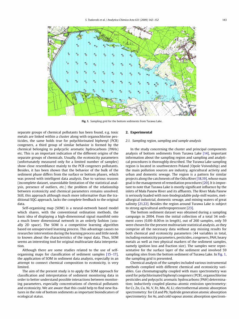

S. Tsakovski et al. / Analytica Chimica Acta 631 (2009) 142–152 143

ttom

smtcces(sBsw(ybSdd

wbaabrtst

otal

coiate

2

2

aicrtupgtiiast

cmwcbimnsst

mau

Fig. 1. Sampling grid for the bo

eparate groups of chemical pollutants has been found, e.g. toxicetals are linked within a cluster along with organochlorine pes-

icides, the same holds true for polychlorinated biphenyl (PCB)ongeners, a third group of similar behavior is formed by thehemical belonging to polycyclic aromatic hydrocarbons (PAHs)tc. This is an important indication of the different origins of theeparate groups of chemicals. Usually, the ecotoxicity parametersunfortunately measured only for a limited number of samples)how close resemblance mainly to the PCB congeners pollutants.esides, it has been shown that the behavior of the bulk of theediment phase differs from the surface or bottom phases, whichas proved with intelligent data analysis. Due to various reasons

incomplete dataset, unavoidable limitation of the statistical anal-sis, presence of outliers, etc.) the problem of the relationshipetween ecotoxicity and chemical parameters remains unsolved.till, this approach although much more informative than the tra-itional SQG approach, lacks the complete feedback to the originalata.

Self-organising map (SOM) is a neural-network based modelhich shares, with the conventional ordination methods, the

asic idea of displaying a high-dimensional signal manifold ontomuch lower dimensional network in an orderly fashion (usu-

lly 2D space). The SOM is a competitive learning algorithmased on unsupervised learning process. This advantage causes noesearcher intervention during the learning process and little needso known about the characteristics of the input data. Thus, SOMeems an interesting tool for original multivariate data interpreta-ion.

Although there are some studies related to the use of self-rganising maps for classification of sediment samples [15–17],he application of SOM in sediment data analysis, especially in anttempt to connect chemical composition to ecotoxicity, is veryimited.

The aim of the present study is to apply the SOM approach forlassification and interpretation of sediment monitoring data in

rder to better understand possible interactions between monitor-ng parameters, especially concentrations of chemical pollutantsnd ecotoxicity. We are aware that this could help to find new fea-ures in the role of bottom sediments as important bioindicators ofcological status.

ptfss

sediments from Turawa Lake.

. Experimental

.1. Sampling region, sampling and sample analysis

In the study concerning the cluster and principal componentsnalysis of bottom sediments from Turawa Lake [14], importantnformation about the sampling region and sampling and analyti-al procedures is thoroughly described. The Turawa Lake samplingegion is located in southwestern Poland (Opole Voivodship) andhe main pollution sources are industry, agricultural activity andrban and domestic sewage. The region is a pattern for similarrojects along the catchments of the Odra River [18,19], whose mainoal is the management of remediation procedures [20]. It is impor-ant to note that Turawa Lake is mostly significant influence by thenlets of Mała Panew River and its affluents. The River Mała Panews seriously loaded with non-biodegradable pulp-mill wastes, met-llurgical industrial, domestic sewage, and mining waters of greatalinity [21,22]. Besides the region around Turawa Lake is subjecto strong agricultural anthropopressure [23].

The bottom sediment dataset was obtained during a samplingampaign in 2004. From the initial collection of a total 34 sedi-ent cores (0.00–8.00 m in length), out of 260 samples, only 59ere chosen for the present multivariate statistical analysis, as they

omprise all the necessary data without any missing results foroth chemical and ecotoxicity parameters (44 variables in total,

ncluding exotoxicity parameters, pesticides, congeners, PAH, heavyetals as well as two physical markers of the sediment samples,

amely ignition loss and fraction size). The samples were repre-entative for the surface layer of the sediment and involved 59ampling sites from the bottom sediment of Turawa Lake. In Fig. 1,he sampling grid is presented.

Chemical analysis of the samples included various instrumentalethods complied with different chemical and ecotoxicity vari-

bles. Gas chromatography coupled with mass spectrometry wassed for polychlorinated biphenyl congeners (PCB), organochlorine

esticides and polycyclic aromatic hydrocarbons (PAH) determina-ion; inductively coupled plasma–atomic emission spectrometry:or Cr, Zn, Cu, Ni, V, Fe, Mn, Al, Li; electrothermal atomic absorptionpectrometry: for Cd and Pb; hydride generation atomic absorptionpectrometry: for As, and cold vapour atomic absorption spectrom-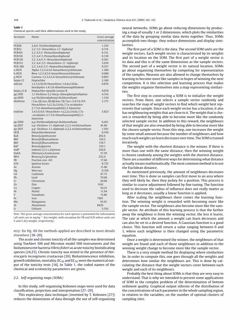

144 S. Tsakovski et al. / Analytica Chimi

Table 1Chemical species and their abbreviations used in the study.

Acronym Name Gross averageconcentration

PCB28 2,4,4′-Trichlorobiphenyl 1.219PCB52 2,2′ ,5,5′-Tetrachloro-1,1′-biphenyl 0.174PCB101 2,2′ ,4,5,5′-Pentachlorobiphenyl 0.115PCB118 2,3′ ,4,4′ ,5-Pentachlorobiphenyl 0.130PCB138 2,2′ ,3,4,4′ ,5′-Hexachlorobiphenyl 0.561PCB153 2,2′ ,4,4′ ,5,5′-Hexachloro-1,1′-biphenyl 3.076PCB 180 2,2′ ,3,4,4′ ,5,5′-Heptachlorobiphenyl 0.357a HCH Alpha-1,2,3,4,5,6-hexachlorocyclohexane 1.384b HCH Beta-1,2,3,4,5,6-hexachlorocyclohexane 0.686g HCH Gamma-1,2,3,4,5,6-hexachlorocyclohexane 0.863hepta Cl Heptachlor 2.169aldrine 1,2,3,4,10,10-Hexachloro-1,4,4a,5,8,8a-

hexahydro-1,4:5,8-dimethanonaphthalene0.876

hepta Cl B Heptachlor epoxide isomer B 0.070pp DDE 1,1-Dichloro-2,2-bis(p-chlorophenyl)ethylene 4.314op DDD o,p-Dichlorodiphenyl dichloroethane 1.334dieldrine (1a�,2�,2a�,3�,6�,6a�,7�,7a�)-3,4,5,6-9,9-

Hexachloro-1a,2,2a,3,6,6a,7,7a-octahydro-2,7:3,6-dimethanonaphth[2,3-b]oxirene

2.175

endrine 3,4,5,6,9,9,-Hexachloro-1a,2,2a,3,6,6a,7,7a--octahydro-2,7:3,6-Dimethanonaphth[2,3-b]oxirene

5.823

pp DDD p,p-Dichlorodiphenyl dichloroethane 6.451op DDT o,p′-Dichloro-1,1-diphenyl-2,2,2-trichloroethane 41.06pp DDT p,p′-Dichloro-1,1-diphenyl-2,2,2-trichloroethane 1.591HCB Hexachlorobenzene 0.556BaA Benzo[a]anthracene 202.6BbF Benzo[b]fluoranthene 319.5BkF Benzo[k]fluoranthene 178.7BaP Benzo[a]pyrene 319.1IndP Indeno(1,2,3-c,d)pirene 320.6DahA Dibenzo(a,h)antracene 37.59BPer Benzo(g,h,i)perylene 232.4FR Fraction size <63 17.66IGN Ignition losses 8.735As Arsenic 11.06Hg Mercury 0.156Cd Cadmium 47.75Pb Lead 79.66Cr Chromium 20.06Zn Zinc 1142Cu Copper 34.22Ni Nickel 11.94V Vanadium 15.86Fe Iron 7901Mn Manganese 95.91Al Aluminium 8426Li Lithium 5.516

N(%

ee

ubsegpc

2

c

r

nioal

waiTgolctt

vsrhssotbmi

miTat

otsul

ttpaTcc1e

ww

ldcw

u

ote: The gross average concentration for each species is presented for informationall units are in mg kg−1 dry weight, with exception for FR and IGN where units areand % dry weight, respectively).

try: for Hg. All the methods applied are described in more detailslsewhere [18–20].

The acute and chronic toxicity of all the samples was determinedsing ToxAlert 100 and Microtox model 500 instruments and theioluminescent bacteria Vibrio fisheri as acute toxicity bioindicatingpecies [24,25]. Chronic toxicity was tested in the presence of Het-rocypris incongruens crustacean [26]. Bioluminescence inhibition,rowth inhibition, mortality, EC20 and EC50 were the numerical out-ut of the toxicity tests [14]. In Table 1, the coded names of thehemical and ecotoxicity parameters are given.

.2. Self-organising maps (SOMs)

In this study, self-organising Kohonen maps were used for datalassification, projection and interpretation [27–29].

This exploratory data technique (invented by T. Kohonen [27])educes the dimensions of data through the use of self-organising

ostis

ca Acta 631 (2009) 142–152

eural networks. SOMs go about reducing dimensions by produc-ng a map of usually 1 or 2 dimensions, which plots the similaritiesf the data by grouping similar data items together. Thus, SOMsccomplish two things: they reduce dimensions and display simi-arities.

The first part of a SOM is the data. The second SOM units are theeight vectors. Each weight vector is characterized by its weights

nd its location on the SOM. The first part of a weight vector ists data and this is of the same dimensions as the sample vectors.he second part of a weight vector is its natural location. SOMso about organising themselves by competing for representationf the samples. Neurons are also allowed to change themselves byearning to become more like samples in hopes of winning the nextompetition. It is this selection and learning process that makeshe weights organise themselves into a map representing similari-ies.

The first step in constructing a SOM is to initialize the weightectors. From there, one selects a sample vector randomly andearches the map of weight vectors to find which weight best rep-esents that sample. Since each weight vector has a location, it alsoas neighbouring weights that are close to it. The weight that is cho-en is rewarded by being able to become more like the randomlyelected sample vector. In addition to this reward, the neighboursf that weight are also rewarded by being able to become more likehe chosen sample vector. From this step, one increases the weighty some small amount because the number of neighbours and howuch each weight can learn decreases over time. The SOM is trained

teratively.The weight with the shortest distance is the winner. If there is

ore than one with the same distance, then the winning weights chosen randomly among the weights with the shortest distance.here are a number of different ways for determining what distancectually means mathematically. The most common method is to usehe Euclidean distance.

As mentioned previously, the amount of neighbours decreasesver time. This is done so samples can first move to an area wherehey will likely be, then they jockey for a position. This process isimilar to coarse adjustment followed by fine tuning. The functionsed to decrease the radius of influence does not really matter as

ong as it decreases, usually a linear function is applied.After scaling the neighbours there comes the learning func-

ion. The winning weight is rewarded with becoming more likehe sample vector. The neighbours also become more like the sam-le vector. An attribute of this learning process is that the fartherway the neighbour is from the winning vector, the less it learns.he rate at which the amount a weight can learn decreases andan also be set to a desired function. A Gaussian function is a goodhoice. This function will return a value ranging between 0 and, where each neighbour is then changed using the parametricquation.

Once a weight is determined the winner, the neighbours of thateight are found and each of those neighbours in addition to theinning weight change to become more like the sample vector.

There is a very simple method for displaying where similaritiesie. In order to compute this, one goes through all the weights andetermines how similar the neighbours are. This is done by cal-ulating the distance that the weight vectors cover between eacheight and each of its neighbours.

Probably the best thing about SOMs is that they are very easy tonderstand. That is why we intended to present some applications

f SOM in the complex problem of the determination of bottomediment quality. Graphical output informs of the distribution ofhe concentrations of each parameter in the whole sampling region,n relation to the variables, on the number of optimal clusters ofampling sites.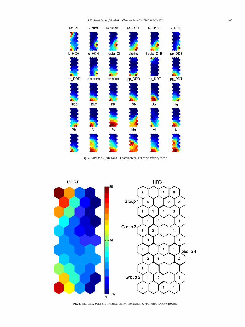

S. Tsakovski et al. / Analytica Chimica Acta 631 (2009) 142–152 145

Fig. 2. SOM for all sites and 30 parameters in chronic toxicity mode.

Fig. 3. Mortality SOM and hits diagram for the identified 4 chronic toxicity groups.

146 S. Tsakovski et al. / Analytica Chimi

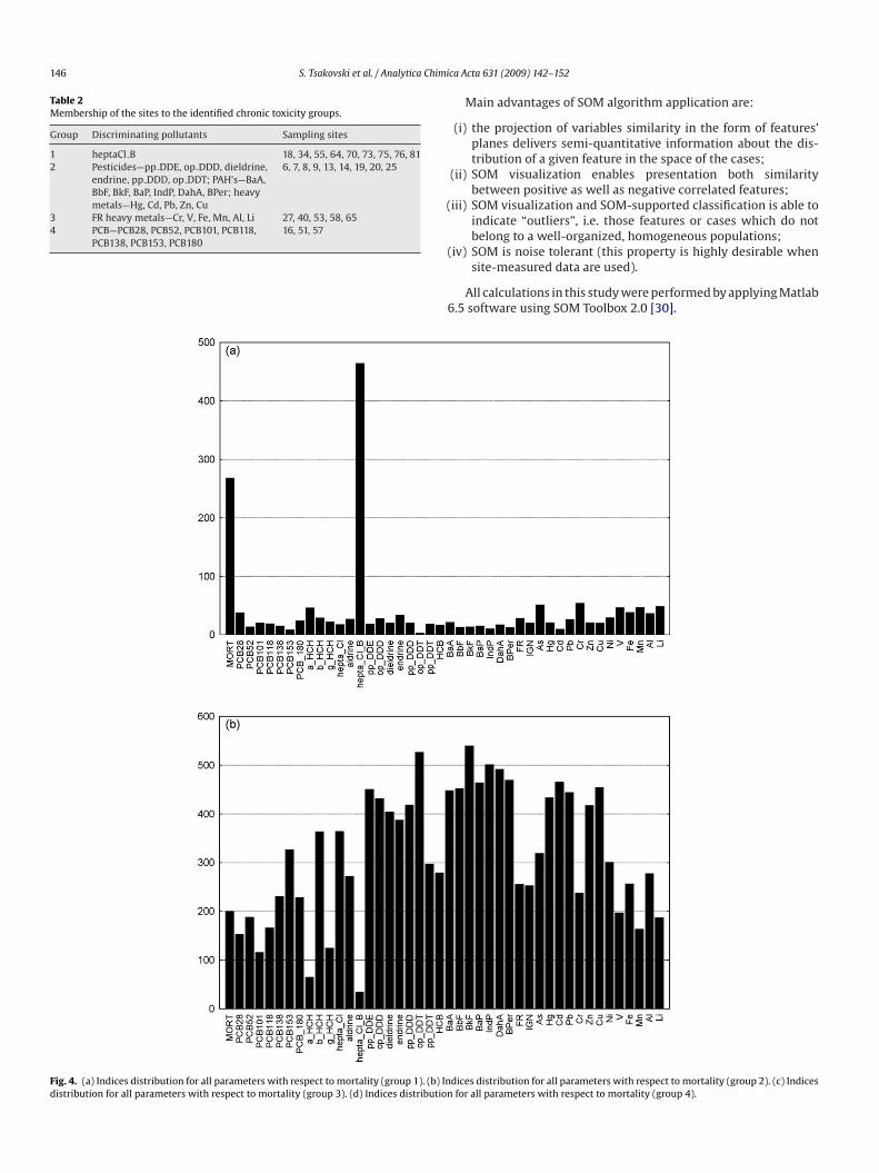
Table 2Membership of the sites to the identified chronic toxicity groups.

Group Discriminating pollutants Sampling sites

1 heptaCl B 18, 34, 55, 64, 70, 73, 75, 76, 812 Pesticides—pp DDE, op DDD, dieldrine,

endrine, pp DDD, op DDT; PAH’s—BaA,BbF, BkF, BaP, IndP, DahA, BPer; heavymetals—Hg, Cd, Pb, Zn, Cu

6, 7, 8, 9, 13, 14, 19, 20, 25

3 FR heavy metals—Cr, V, Fe, Mn, Al, Li 27, 40, 53, 58, 654 PCB—PCB28, PCB52, PCB101, PCB118, 16, 51, 57

(

Fd

PCB138, PCB153, PCB180(

6

ig. 4. (a) Indices distribution for all parameters with respect to mortality (group 1). (b) Inistribution for all parameters with respect to mortality (group 3). (d) Indices distribution

ca Acta 631 (2009) 142–152

Main advantages of SOM algorithm application are:

(i) the projection of variables similarity in the form of features’planes delivers semi-quantitative information about the dis-tribution of a given feature in the space of the cases;

(ii) SOM visualization enables presentation both similaritybetween positive as well as negative correlated features;

iii) SOM visualization and SOM-supported classification is able toindicate “outliers”, i.e. those features or cases which do notbelong to a well-organized, homogeneous populations;

iv) SOM is noise tolerant (this property is highly desirable whensite-measured data are used).

All calculations in this study were performed by applying Matlab.5 software using SOM Toolbox 2.0 [30].

dices distribution for all parameters with respect to mortality (group 2). (c) Indicesfor all parameters with respect to mortality (group 4).

S. Tsakovski et al. / Analytica Chimica Acta 631 (2009) 142–152 147

(Conti

3

ti5co3ttm

fm

mic

3

ctc

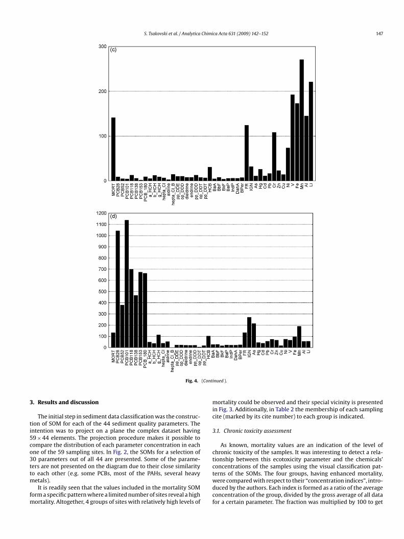
Fig. 4.

. Results and discussion

The initial step in sediment data classification was the construc-ion of SOM for each of the 44 sediment quality parameters. Thentention was to project on a plane the complex dataset having9 × 44 elements. The projection procedure makes it possible toompare the distribution of each parameter concentration in eachne of the 59 sampling sites. In Fig. 2, the SOMs for a selection of0 parameters out of all 44 are presented. Some of the parame-ers are not presented on the diagram due to their close similarity

o each other (e.g. some PCBs, most of the PAHs, several heavy

etals).It is readily seen that the values included in the mortality SOM

orm a specific pattern where a limited number of sites reveal a highortality. Altogether, 4 groups of sites with relatively high levels of

twdcf

nued ).

ortality could be observed and their special vicinity is presentedn Fig. 3. Additionally, in Table 2 the membership of each samplingite (marked by its cite number) to each group is indicated.

.1. Chronic toxicity assessment

As known, mortality values are an indication of the level ofhronic toxicity of the samples. It was interesting to detect a rela-ionship between this ecotoxicity parameter and the chemicals’oncentrations of the samples using the visual classification pat-

erns of the SOMs. The four groups, having enhanced mortality,ere compared with respect to their “concentration indices”, intro-uced by the authors. Each index is formed as a ratio of the averageoncentration of the group, divided by the gross average of all dataor a certain parameter. The fraction was multiplied by 100 to get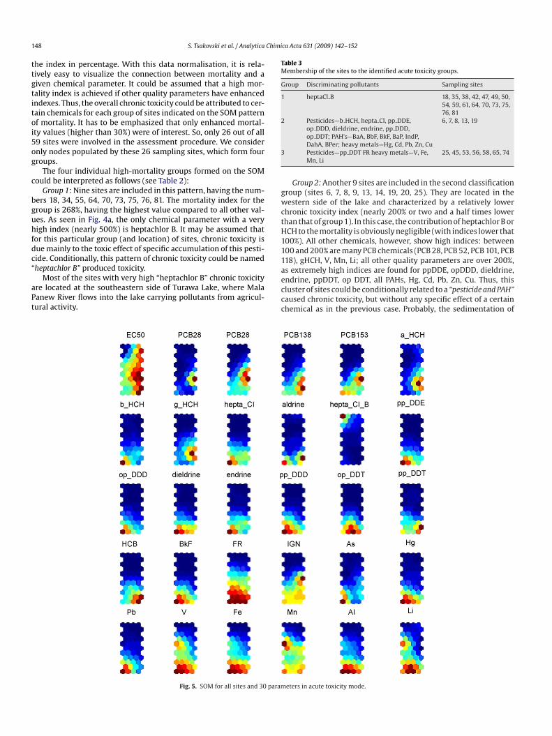

1 Chimica Acta 631 (2009) 142–152

ttgtitoi5og

c

bguhfdc“

aPt

Table 3Membership of the sites to the identified acute toxicity groups.

Group Discriminating pollutants Sampling sites

1 heptaCl B 18, 35, 38, 42, 47, 49, 50,54, 59, 61, 64, 70, 73, 75,76, 81

2 Pesticides—b HCH, hepta Cl, pp DDE,op DDD, dieldrine, endrine, pp DDD,

6, 7, 8, 13, 19

3

gwctH111

48 S. Tsakovski et al. / Analytica

he index in percentage. With this data normalisation, it is rela-ively easy to visualize the connection between mortality and aiven chemical parameter. It could be assumed that a high mor-ality index is achieved if other quality parameters have enhancedndexes. Thus, the overall chronic toxicity could be attributed to cer-ain chemicals for each group of sites indicated on the SOM patternf mortality. It has to be emphasized that only enhanced mortal-ty values (higher than 30%) were of interest. So, only 26 out of all9 sites were involved in the assessment procedure. We considernly nodes populated by these 26 sampling sites, which form fourroups.

The four individual high-mortality groups formed on the SOMould be interpreted as follows (see Table 2):

Group 1: Nine sites are included in this pattern, having the num-ers 18, 34, 55, 64, 70, 73, 75, 76, 81. The mortality index for theroup is 268%, having the highest value compared to all other val-es. As seen in Fig. 4a, the only chemical parameter with a veryigh index (nearly 500%) is heptachlor B. It may be assumed that

or this particular group (and location) of sites, chronic toxicity isue mainly to the toxic effect of specific accumulation of this pesti-ide. Conditionally, this pattern of chronic toxicity could be named

heptachlor B” produced toxicity.

Most of the sites with very high “heptachlor B” chronic toxicityre located at the southeastern side of Turawa Lake, where Malaanew River flows into the lake carrying pollutants from agricul-ural activity.

aeccc

Fig. 5. SOM for all sites and 30 param

op DDT; PAH’s—BaA, BbF, BkF, BaP, IndP,DahA, BPer; heavy metals—Hg, Cd, Pb, Zn, CuPesticides—pp DDT FR heavy metals—V, Fe,Mn, Li

25, 45, 53, 56, 58, 65, 74

Group 2: Another 9 sites are included in the second classificationroup (sites 6, 7, 8, 9, 13, 14, 19, 20, 25). They are located in theestern side of the lake and characterized by a relatively lower

hronic toxicity index (nearly 200% or two and a half times lowerhan that of group 1). In this case, the contribution of heptachlor B orCH to the mortality is obviously negligible (with indices lower that00%). All other chemicals, however, show high indices: between00 and 200% are many PCB chemicals (PCB 28, PCB 52, PCB 101, PCB18), gHCH, V, Mn, Li; all other quality parameters are over 200%,

s extremely high indices are found for ppDDE, opDDD, dieldrine,ndrine, ppDDT, op DDT, all PAHs, Hg, Cd, Pb, Zn, Cu. Thus, thisluster of sites could be conditionally related to a “pesticide and PAH”aused chronic toxicity, but without any specific effect of a certainhemical as in the previous case. Probably, the sedimentation of

eters in acute toxicity mode.

S. Tsakovski et al. / Analytica Chimica Acta 631 (2009) 142–152 149

or the

dir

sa

t(mslmtonotapptr

toiPcsF

a

tccfs

3

siocp

ait

tcsv

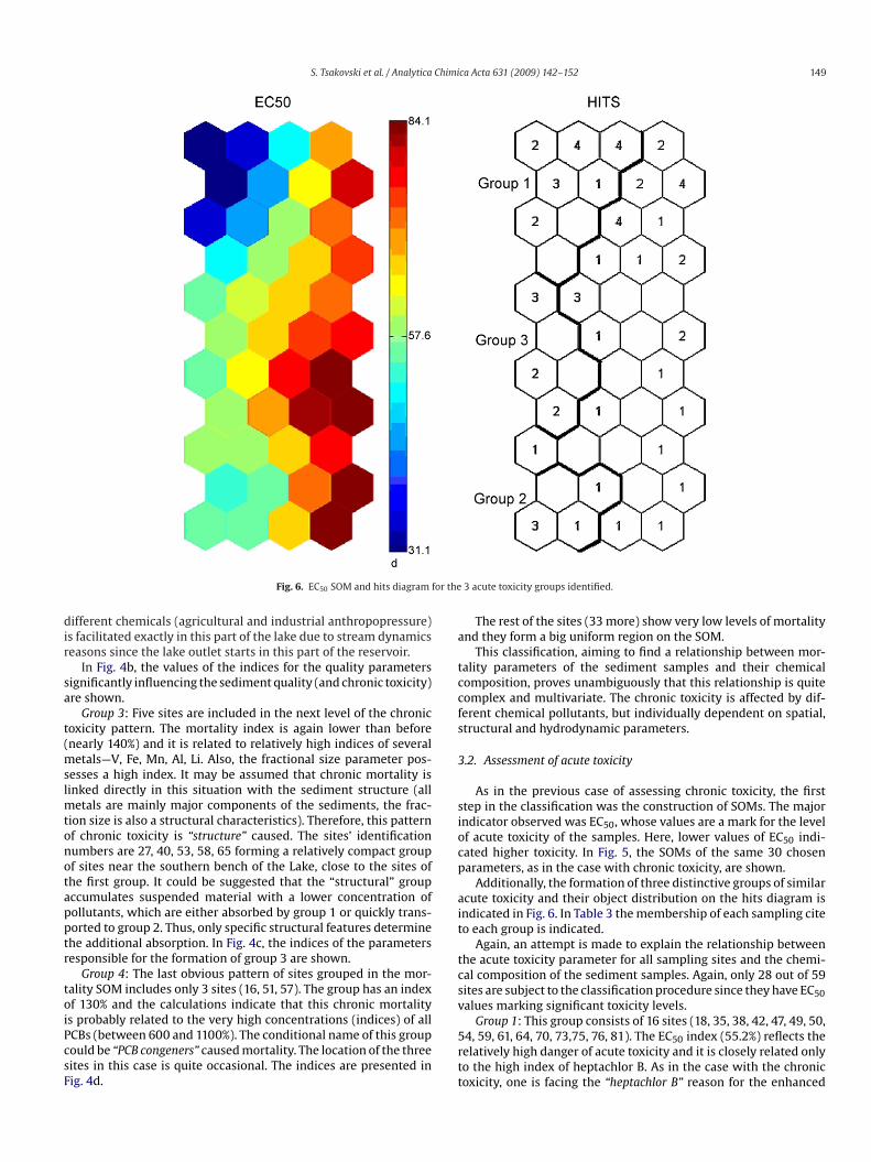
Fig. 6. EC50 SOM and hits diagram f

ifferent chemicals (agricultural and industrial anthropopressure)s facilitated exactly in this part of the lake due to stream dynamicseasons since the lake outlet starts in this part of the reservoir.

In Fig. 4b, the values of the indices for the quality parametersignificantly influencing the sediment quality (and chronic toxicity)re shown.

Group 3: Five sites are included in the next level of the chronicoxicity pattern. The mortality index is again lower than beforenearly 140%) and it is related to relatively high indices of several

etals—V, Fe, Mn, Al, Li. Also, the fractional size parameter pos-esses a high index. It may be assumed that chronic mortality isinked directly in this situation with the sediment structure (all

etals are mainly major components of the sediments, the frac-ion size is also a structural characteristics). Therefore, this patternf chronic toxicity is “structure” caused. The sites’ identificationumbers are 27, 40, 53, 58, 65 forming a relatively compact groupf sites near the southern bench of the Lake, close to the sites ofhe first group. It could be suggested that the “structural” groupccumulates suspended material with a lower concentration ofollutants, which are either absorbed by group 1 or quickly trans-orted to group 2. Thus, only specific structural features determinehe additional absorption. In Fig. 4c, the indices of the parametersesponsible for the formation of group 3 are shown.

Group 4: The last obvious pattern of sites grouped in the mor-ality SOM includes only 3 sites (16, 51, 57). The group has an indexf 130% and the calculations indicate that this chronic mortality

s probably related to the very high concentrations (indices) of allCBs (between 600 and 1100%). The conditional name of this groupould be “PCB congeners” caused mortality. The location of the threeites in this case is quite occasional. The indices are presented inig. 4d.

5rtt

3 acute toxicity groups identified.

The rest of the sites (33 more) show very low levels of mortalitynd they form a big uniform region on the SOM.

This classification, aiming to find a relationship between mor-ality parameters of the sediment samples and their chemicalomposition, proves unambiguously that this relationship is quiteomplex and multivariate. The chronic toxicity is affected by dif-erent chemical pollutants, but individually dependent on spatial,tructural and hydrodynamic parameters.

.2. Assessment of acute toxicity

As in the previous case of assessing chronic toxicity, the firsttep in the classification was the construction of SOMs. The majorndicator observed was EC50, whose values are a mark for the levelf acute toxicity of the samples. Here, lower values of EC50 indi-ated higher toxicity. In Fig. 5, the SOMs of the same 30 chosenarameters, as in the case with chronic toxicity, are shown.

Additionally, the formation of three distinctive groups of similarcute toxicity and their object distribution on the hits diagram isndicated in Fig. 6. In Table 3 the membership of each sampling citeo each group is indicated.

Again, an attempt is made to explain the relationship betweenhe acute toxicity parameter for all sampling sites and the chemi-al composition of the sediment samples. Again, only 28 out of 59ites are subject to the classification procedure since they have EC50alues marking significant toxicity levels.

Group 1: This group consists of 16 sites (18, 35, 38, 42, 47, 49, 50,4, 59, 61, 64, 70, 73,75, 76, 81). The EC50 index (55.2%) reflects theelatively high danger of acute toxicity and it is closely related onlyo the high index of heptachlor B. As in the case with the chronicoxicity, one is facing the “heptachlor B” reason for the enhanced

1 Chimi

eto“g

ficiHf

ii

aoinc“

Ft

Ff

50 S. Tsakovski et al. / Analytica

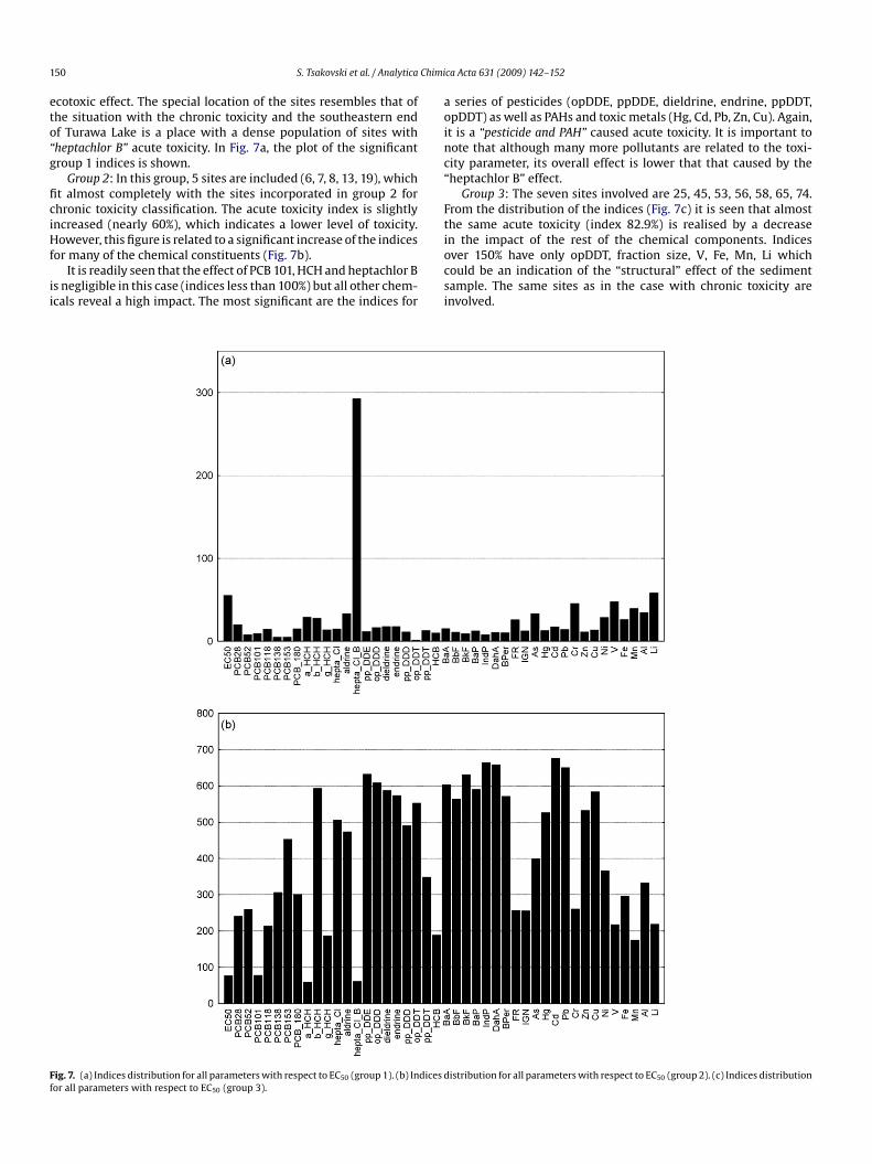
cotoxic effect. The special location of the sites resembles that ofhe situation with the chronic toxicity and the southeastern endf Turawa Lake is a place with a dense population of sites withheptachlor B” acute toxicity. In Fig. 7a, the plot of the significantroup 1 indices is shown.

Group 2: In this group, 5 sites are included (6, 7, 8, 13, 19), whicht almost completely with the sites incorporated in group 2 forhronic toxicity classification. The acute toxicity index is slightlyncreased (nearly 60%), which indicates a lower level of toxicity.

owever, this figure is related to a significant increase of the indices

or many of the chemical constituents (Fig. 7b).It is readily seen that the effect of PCB 101, HCH and heptachlor B

s negligible in this case (indices less than 100%) but all other chem-cals reveal a high impact. The most significant are the indices for

iocsi

ig. 7. (a) Indices distribution for all parameters with respect to EC50 (group 1). (b) Indices dor all parameters with respect to EC50 (group 3).

ca Acta 631 (2009) 142–152

series of pesticides (opDDE, ppDDE, dieldrine, endrine, ppDDT,pDDT) as well as PAHs and toxic metals (Hg, Cd, Pb, Zn, Cu). Again,t is a “pesticide and PAH” caused acute toxicity. It is important toote that although many more pollutants are related to the toxi-ity parameter, its overall effect is lower that that caused by theheptachlor B” effect.

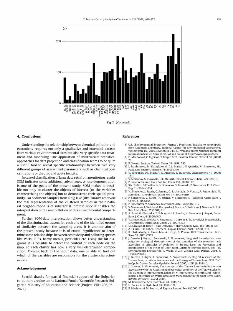
Group 3: The seven sites involved are 25, 45, 53, 56, 58, 65, 74.rom the distribution of the indices (Fig. 7c) it is seen that almosthe same acute toxicity (index 82.9%) is realised by a decrease

n the impact of the rest of the chemical components. Indicesver 150% have only opDDT, fraction size, V, Fe, Mn, Li whichould be an indication of the “structural” effect of the sedimentample. The same sites as in the case with chronic toxicity arenvolved.

istribution for all parameters with respect to EC50 (group 2). (c) Indices distribution

S. Tsakovski et al. / Analytica Chimica Acta 631 (2009) 142–152 151

(Conti

4

efmaadc

Sibcitrim

ootmlgmswz

A

cg2

R

[

[[

[

[

[[[

[

[

[

Fig. 7.

. Conclusions

Understanding the relationship between chemical pollution andcotoxicity requires not only a qualitative and extended datasetrom various environmental sites but also very specific data treat-

ent and modelling. The application of multivariate statisticalpproaches for data projection and classification seems to be quiteuseful tool to reveal specific relationships between two very

ifferent groups of assessment parameters such as chemical con-entrations or chronic and acute toxicity.

In case of classification of large data sets from monitoring resultsOM indicates some additional advantages, whose demonstrations one of the goals of the present study. SOM makes it possi-le not only to cluster the objects of interest (or the variablesharacterizing the objects) but to demonstrate their spatial prox-mity. For sediment samples from a big lake (like Turawa reservoirhe real representation of the clustered samples in their natu-al neighbourhood is of substantial interest since it enables thenterpretation of the real pollution of this environmental compart-

ent.Further, SOM data interpretation allows better understanding

f the discriminating tracers for each one of the identified groupsf similarity between the sampling areas. It is another aim ofhe present study because it is of crucial significance to deter-

ine some relationships between ecotoxicity and polluting speciesike PAHs, PCBs, heavy metals, pesticides etc. Using the hit dia-rams it is possible to detect the content of each node on theap, so each cluster has now a very well-determined compo-

ition. Coming back to the input data, one is able to find outhich of the variables are responsible for the cluster characteri-

ation.

cknowledgement

Special thanks for partial financial support of the Bulgariano-authors are due to the National Fund of Scientific Research, Bul-arian Ministry of Education and Science (Project VUH 206/06 –472).

[[[

nued ).

eferences

[1] U.S. (Environmental Protection Agency), Predicting Toxicity to Amphipodsfrom Sediment Chemistry, National Center for Environmental Assessment,Washington, DC, 2005, EPA/600/R-04/030. Available from: National TechnicalInformation Service, Springfield, VA and online at http://www.epa.gov/ncea.

[2] D. MacDonald, C. Ingersoll, T. Berger, Arch. Environ. Contam. Toxicol. 39 (2000)20.

[3] R. Swartz, Environ. Toxicol. Chem. 18 (1999) 780.[4] I. Stanimirova, M. Daszykowski, D.L. Massart, F. Questier, V. Simeonov, H.J.

Puxbaum, Environ. Manage. 74 (2005) 349.[5] V. Simeonov, D.L. Massart, G. Andreev, S. Tsakovski, Chemosphere 41 (2000)

1411.[6] V. Simeonov, S. Tsakovski, D.L. Massart, Toxicol. Environ. Chem. 72 (1999) 81.[7] P. Simeonova, Ann. Univ. Sof. Fac. Chem 100 (2008) 177.[8] S.N. Eddins, D.F. Williams, V. Simeonov, S. Tsakovski, P. Simeonova, Ecol. Chem.

Eng. 11 (2004) 1024.[9] V. Simeonov, J. Stratis, C. Samara, G. Zachariadis, D. Voutsa, A. Anthemidis, M.

Sofoniou, Th. Kouimtzis, Water Res. 37 (2003) 4119.10] P. Simeonova, C. Sarbu, Th. Spanos, V. Simeonov, S. Tsakovski, Centr. Euro. J.

Chem. 4 (2006) 68.11] P. Simeonova, V. Simeonov, Microchim. Acta 156 (2007) 315.12] V. Simeonov, L. Wolska, A. Kuczynska, J. Gurwin, S. Tsakovski, J. Namiesnik, Crit.

Rev. Anal. Chem. 37 (2007) 81.13] A. Astel, G. Glosinska, T. Sobczynski, L. Boszke, V. Simeonov, J. Siepak, Centr.

Euro. J. Chem. 4 (2006) 543.14] V. Simeonov, L. Wolska, A. Kuczynska, J. Gurwin, S. Tsakovski, M. Protasowicki,

J. Namiesnik, Trends Anal. Chem. 26 (2007) 323.15] J.P. Lacassie, B. Roser, J. Ruiz Del Solar, F. Herve, Sedim. Geol. 165 (2004) 175.16] A.P. Clare, D.R. Cohen, Geochem.: Explor. Environ. Anal. 1 (2001) 119.17] B. Chakraborty, R. Kaustubha, A. Hedge, A. Pereira, IEEE Trans. Geosci. Rem.

Sens. 39 (2001) 2722.18] J. Gurwin, J. Kryza, I. Poprawski, A. Skowronek, Integrated investigative cam-

paign for ecological determination of the condition of the retention tankaccording to principles of evolution in Turawa Lake, in: Protection andRecultivation of the Fields of Oder Basin, Scientific Exercise Books, vol. 131,Environmental Engineering 12 Wydz. U. Ziel. Zielona Gora, Poland, 2004, p.133 (in Polish).

19] J. Gurwin, J. Kryza, I. Poprawski, A. Skowronek, Geological research of theTurawa Lake, in: Water Resources and the Ecology of Turawa Lake, NOT FSNTin Opole. Opole - Strzelce Opolskie, Poland, 2005, p. 211 (in Polish).

20] J. Gurwin, A. Skowronek, The concept of the Turawa Lake revitalization—inaccordance with the Assessment of ecological condition of the Turawa Lake for

the planning of improvement action, in: XI International Scientific and Techno-logical Conference on Water Resources Management in the Oder River Basin,RWMB, Wroclaw, Poland, 2006.

21] M. Bombowna, Acta Hydrobiol. 28 (1986) 55.22] H. Bucka, Acta Hydrobiol. 28 (1986) 121.23] R. Machowski, M. Ruman, M. Rzetała, Limnol. Rev. 6 (2006) 179.

1 Chimi

[[[

52 S. Tsakovski et al. / Analytica

24] Merck, ToxAlert 100 Operating Manual Version 0.09, Merck, Germany, 1999.25] Tigret, Microtox Analyzer Manual, Tigret, Poland, 2006.26] Ostracodtoxkit F, Chronic “Direct Contact” Toxicity Test for Freshwater

Sediments”, Standard Operational Procedure, MicroBioTests Inc., Belgium,2005.

[

[[[

ca Acta 631 (2009) 142–152

27] T. Kohonen, Self-Organizing and Associative Memory, 3rd edition, SpringerVerlag, New York, 1989.

28] A.J. Mukherjee, Comp. Civil Eng. 11 (1997) 74.29] S.A. Mingoti, J.O. Lima, Eur. J. Oper. Res. 174 (2006) 1742.30] SOM Toolbox 2.0, Available at http://www.cis.hut.fi/projects/somtoolbox/.