Effects of Fluid Motions in Liquid Tanks on Vessel Motions Using a Simple Panel Method

1 Copyright © 2009 by ASME

Proceedings of the 28th International Conference on Offshore Mechanics and Arctic Engineering (Symposium 6 Ocean Engineering)

OMAE2009 May 31 - June 5, 2009, Honolulu, Hawaii, USA

OMAE2009-80071

EFFECTS OF FLUID MOTIONS IN LIQUID TANKS ON VESSEL MOTIONS USING A SIMPLE PANEL METHOD

Yusong Cao/Keppel Offshore & Marine USA, Inc.Fuwei Zhang / Marintek USA, Inc.

ABSTRACT

This paper presents a simple and fast panel method to include the effect of liquid tanks of a vessel in the prediction of the natural frequencies of the vessel motions. The effects are expressed in terms of modifications to the added mass and stiffness matrices of the vessels with the liquids in the tanks assumed being rigid. An application example for a vessel with two internal liquid tanks is demonstrated. INTRODUCTION

Fluid motion in a liquid tank (particularly when the tank is partially filled during loading and unloading) can have a significant effect on the motion of the vessel carrying the liquid. It is important to consider these effects in the early design stage of a liquid carrying vessel in order to achieve a good motion performance. The motion of the fluid in a liquid tank undergoing arbitrary 6DOF motions can be very complicated and violet and it remains a great challenge to accurately predict the liquid flow and the hydrodynamic load on the tank which affects the motion of the vessel. Although significant progress has been made recently in experimental techniques and advanced computational methods (such as CFD), it is still not feasible to use these approaches to study the performance at the early stage of the vessel design because the cost and time required are very high.

As known, avoiding the motion natural frequencies of a vessel being close the frequencies of the environmental conditions is an effective way to improve the vessel’s motion performance. An accurate and fast method to predict the natural frequencies of the vessel with the effect of the liquid tanks is very helpful at the early design stage.

Linear wave theories based on potential flow assumption have been used to study the sloshing of liquid in a tank and its effect on the vessel’s motion (Molin et al 2002; Malenica et al

2003; Newman 2005; Zalar et al, 2007). Although the linear wave theories are based on small wave amplitude assumption and are not accurate for violet motions of the liquid in the tank, it is adequate to use them for the study of the natural frequencies of the system (vessel + liquid tanks) since the study concerns the initial stability of the system in which the motions of the vessel, as well as the motion of the liquid in the tanks, is assumed small.

WAMIT (WAMIT, Inc.) and HydroStar (BVeritas Software) are two most widely used software commercially available for calculation of hydrodynamic loads on a vessel and the motions of the vessel in waves based on the diffraction and radiation wave theory. Both software were initially developed for the external wave loads on the vessel. The features of the software have recently (Newman 2005, Lee 2007, Chen et al 2007, and Zalar et al 2007) been extended to include the effects of the liquid motions in the internal liquid tanks of the vessel.

Because of the same linear free surface boundary condition used in the boundary value problem of the internal liquid motions and in that for the external radiated waves, a unified approach has been employed to solve the coupled tank/vessel motions. In this approach, the interior wetted surfaces of the tanks are included as an extension of the conventional computational domain defined by the exterior wetted surface of the vessel hull. The interior flows and the exterior flow are not hydrodynamically coupled. This physical condition is enforced in the unified approach by setting equal to zero all elements of the left-hand-side of the linear system where the singularity and field points are in different fluid domains, resulting in a block-diagonal linear system. The same free-surface Green function is used for each domain. The main advantage of this approach is that the computer code can be extended to include the internal tanks with relatively few modifications to the code and input data preparation. The unified approach, however, has some

https://www.researchgate.net/publication/237212809_Wave_eects_on_vessels_with_internal_tanks?el=1_x_8&enrichId=rgreq-784545f211045ac68481ccbb064afea8&enrichSource=Y292ZXJQYWdlOzI2NzYwNTQ3MjtBUzoyMTkwMTUxMzQ4Nzk3NDRAMTQyOTIyODY4NTY0NA==


https://www.researchgate.net/publication/265187824_Sloshing_Effects_Accounting_for_Dynamic_Coupling_Between_Vessel_and_Tank_Liquid_Motion?el=1_x_8&enrichId=rgreq-784545f211045ac68481ccbb064afea8&enrichSource=Y292ZXJQYWdlOzI2NzYwNTQ3MjtBUzoyMTkwMTUxMzQ4Nzk3NDRAMTQyOTIyODY4NTY0NA==



drawbacks. The main drawback is the computational efficiency, as mentioned in Newman (2005), due to 1) the need to solve a larger system of linear equations and 2) the need to re-run the complete interior/exterior analysis whenever there is a change to any of the interior domains.

There is a need in the marine and offshore industries for a more computationally efficient approach and computer code to include the effects of the liquid motions in the internal tanks, especially for quickly estimating the system’s natural frequencies. There are a few reasons for the need:

1) In the early design stage of the vessel with liquid tanks, there are situations in which the hull geometry and draft are fixed and the effect of the changes in the positions of the tanks and the percentages of tank fillings need to be examined. The hydrodynamic coefficients for the exterior flow need not to be re-calculated every time when a parameter for the tanks changes. The saving would be very significant since a large number of changes may need to be examined.

2) Many existing diffraction/radiation codes still do not have the capability to include effects of the liquid tanks. An effective and efficient independent code to include the liquid tanks effect is very desirable.

3) In a coupled analysis of an offshore floating system with mooring and risers (such as SEMI, SPAR, TLP, etc.), the hydrodynamic coefficients of the vessel are used as input to the code to calculate the wave loads and the vessel motion. An independent code to generate the hydrodynamic coefficients as input to the motion code to include the liquid tank effects without re-running the exterior flow solver, which should make the use of the codes more flexible and efficient.

It is also worth pointing out that since the interior flow in a tank does not need to satisfy the far-field radiation condition, it is computationally inefficient to use the free-surface Green function to solve for the interior flow. Although the free-surface Green function satisfies the far-field radiation condition in addition to the linearized free surface, it is much more costly to evaluate. Since the interior flow is independent from the exterior flow, it can be solved using the Rankine-source Green function more efficiently even through the interior free surface needs to be discretized.

This paper presents a simple and fast panel method to include the effects of liquid tanks. The interior flow for each tank is solved independently. A desingularized boundary integral equation (DBIE) with Rankine-source Green function is used to solve the interior flow problem (Cao et al 1991). The effects from all the tanks are expressed in terms of modifications to the added mass and hydrostatic stiffness matrices of the vessels with the liquids in the tanks assumed being rigid. The modified added mass and stiffness matrices can be used by any motion code as usually used. More details are given in the following sections. An application example for a vessel with two internal liquid tanks will be demonstrated.

PROBLEM FORMULATION The motions of the liquid in tanks of arbitrary shape mounted on a vessel are considered. The tanks are partially filled so that there is a free surface in each tank. The liquid motions are caused by the motion of the tanks moving with the vessel. Since the flow in a tank is hydrodynamically uncoupled with those in other tanks, the flow in each tank can be solved separately. The flow and the pressure of the fluid (static and dynamic) in a tank are to be sought. Once the pressure on the tank is obtained, the force and moment by the liquid on the tank (thus the vessel) can be calculated by integrating the pressure over the wet wall surface. Assumptions Some assumptions are needed in order to linearize the problem formulation: 1) The liquid in the tank is incompressible and has a

constant density. 2) The viscous effect of the fluid is negligible and the flow

is irrotational so that the potential flow model is used to describe the fluid motion.

3) The motion of the vessel, thus the motion of the tank, is sufficiently small so that the fluid motion is also small.

4) The motion of the free surface is thus small and the linear free surface conditions are applicable.

5) The tank wall is rigid and the fluid does not penetrate the wall.

6) The linearized equations of motion for the vessel can be used because of the small motion assumption 3).

7) Linear superposition is applicable because of the above assumptions 3) and 4) and the frequency-domain approach can be used.

When the effect of the tank liquid on the vessel motion is considered, it is also assumed that liquid tank is fixed onto the vessel. In other words, there is no relative movement between the tank and the vessel. Coordinate Systems Six coordinate system frames are employed to describe the motions of the vessel and the tank, and the flow in the tank: 1) global coordinate frameOXYZ . The origin of OXYZ is on the calm water surface of the exterior fluid domain. The Z-axis points upward vertically and the OXY plane coincides with the horizontal water surface. 2) vessel-fixed frameOxyz . This frame is fixed to the vessel and moves with the vessel. There is no relative motion between the vessel and this frame. This frame coincides with the global frame when the vessel (including the tanks in it) is in the static equilibrium. 3) vessel-attached frame vvv zyOx . The origin of this frame coincides with the origin of the vessel-fixed frame all the time. This frame moves with the vessel but does not rotate. The three axes of this frame are parallel to the corresponding axes of the global frame.

https://www.researchgate.net/publication/30850952_Three-dimensional_desingularised_boundary_integral_method_for_potential_problems?el=1_x_8&enrichId=rgreq-784545f211045ac68481ccbb064afea8&enrichSource=Y292ZXJQYWdlOzI2NzYwNTQ3MjtBUzoyMTkwMTUxMzQ4Nzk3NDRAMTQyOTIyODY4NTY0NA==



4) tank-fixed frame ttt zyxO . This frame is fixed to a tank. The origin of this frame is fixed in the vessel-fixed frame. The three axes of the frame are parallel to the respective axes of the vessel-fixed frame. 5) tank-attached frame tvtvtv zyxO . The origin of this frame coincides with the origin of the tank-fixed frame all the time. This frame moves with the tank but does not rotate. The three axes of this frame are parallel to the respective axes of the global frame OXYZ . 6) tank global frame ttt ZYOX . The origin of this frame is fixed in a point in the global frame OXYZ . This fixed point coincides with the origin of the tank-attached frame

tvtvtv zyxO when the system is in the static equilibrium. The axes of ttt ZYOX are parallel to the respective axes of the global frame. The translational motion of the vessel is described by the position of the origin of the vessel-attached frame in the global system. The rotational motion of the vessel is described by the orientation of the vessel-fixed frame relative to the vessel-attached frame. Similarly, the translational motion of the tank is described by the position of the origin of the tank-attached frame in the tank global frame. The rotational motion of the tank is described by the orientation of the tank-fixed frame relative to the tank-attached frame. The positions and the orientations of these coordinate frames are chosen such that the mean positions, the mean rotations of the motions of the vessel and the tank are zero, which is also the static equilibrium of the vessel system. The vertical position of the origin of the tank global frame should also be on the mean of the free surface of the liquid in the tank. Motion of Liquid in a Tank The flow in a tank will be solved first in the tank global frame. The flow is described using a velocity potential

),,,( tzyx tttΦ which is governed by the Laplace equation 0),,,(2 =Φ∇ tzyx ttt (in D) (1) in the fluid domain D. Boundary conditions are needed on the free surface of the liquid and on the wall of the tank. Because of the linearity, the linear free surface boundary condition is imposed on the mean free surface Sf and the no-penetration condition is imposed on the mean surface of the tank wall Sb,

02

2

=∂Φ∂

+∂Φ∂

xg

t (on Sf: z=0) (2)

and bVnn

rrr⋅=Φ∇⋅ (on Sb) (3)

where bVr

is the velocity of the points on the tank wall. nr is the normal vector of the tank wall pointing out from the liquid. For simplicity of notation, the subscript t in ),,( ttt zyx has been omitted and are omitted hereafter.

Once the velocity potential is solved, the free surface elevation and the linearized dynamic pressure on the tank surface can be calculated using,

tg

tyx∂Φ∂

−=1),,(η (on z=0) (4)

ttzyxp

∂Φ∂

−= ρ),,,( (on Sb) (5)

where g is the gravitational acceleration and ρ is the density of the liquid. The force and moment on the tank by the liquid can be calculated,

∫∫=bS

dsntzyxpF vv),,,( (6)

∫∫ ×=bS

dsrntzyxpM )(),,,( vvr (7)

where rv is the position vector of a point on the tank wall. The velocity of the point on the tank wall velocity, bV

r, can

be expressed as, )( rVV obrrrr

×Ω+= (8)

where oVr

is the translation velocity of the origin of the tank-

attached frame and Ωr

is the rotational velocity of the tank (the tank-fixed frame) relative to the tank-attached frame). With use of matrix/vector notation, the motion of the tank can be expressed as { }Ttxtxtxtxtxtxt )(),(),(),(),(),()( 654321=x

where )(txi )3~1( =i are the translations in x, y, and z

directions (surge, sway and heave) and )(txi )5~4( =i the rotation angles of the tank about x, y, z axes (roll, pitch and yaw), respectively. For a single frequency harmonic motion of the tank with small amplitudes, the motion can be expressed as,

{ }{ } titiT

T

eeXXXXXX

txtxtxtxtxtxtωω X

x

==

=

654321

654321

,,,,,

)(),(),(),(),(),()( (9)

and the velocity of the tank can then be expressed as,

{ } ( ) tiTo eitV ωω Xx ==Ω )(, &rr

(10) Substituting Eq. (10) into (8), then to (3), and combining Eqs. (1) and (2), we have the boundary value problem (BVP) for ),,,( tzyxΦ ,

{ }⎪⎪⎪

⎩

⎪⎪⎪

⎨

⎧

=Φ∇⋅

==∂Φ∂

+∂Φ∂

=Φ∇

∑=

6

1

2

2

2

)()(

)0(0

)(0),,,(

jb

tijj SoneMiXn

zonx

gt

Dintzyx

ωωr

(11)

Since BVP (11) is linear, ),,,( tzyxΦ can be decomposed into,

{ }∑=

=Φ6

1),,()(),,,(

j

tij ezyxXitzyx ωϕω (12)


where ),,( zyxjϕ satisfy the following BVP,

⎪⎪⎩

⎪⎪⎨

⎧

=∇⋅

==+−

=∇

)(

)0(0

)(0),,(2

2

bjj

zjj

j

SonMn

zong

Dinzyx

ϕ

ϕϕω

ϕ

r

(13)

and

⎪⎩

⎪⎨⎧

=+−+−+−

=

=

)6~4(),,(

)3~1(),,(

jxnynznxnynzn

jnnn

M

yxxzzy

zyx

j

Once BVP (13) are solved, the flow is known and the force and moment on the tank can be calculated. This solution approach follows a similar path to solve the exterior flow. BVP (13) is similar to that for the exterior flow. The main difference is that the fluid domain is finite for the interior flow problem and there is no far-field radiation condition to satisfy. Another difference is that in the exterior flow problem, the spatial mean free surface elevation can remain unchanged at z=0 for all time due to any motion of the vessel because of the infinite fluid domain. For the interior flow problem, this may not be true for all type of the tank motions. For most of the tank geometries in application, this is true for the flows due to surge, sway, roll, pitch and yaw. For the flow due to heave, however, the spatial mean of the free surface changes with time in the tank global frame. The free surface condition in BVP (13) is not valid for ),,(3 zyxϕ . Fortunately, the flow due to a pure heave motion is actually very simple. In fact, if one stays in the tank-fixed frame, he should see no flow motion because the body forces acting on the liquid are the gravity and the inertial force due to the heave acceleration which are all in line with the z-axis. The liquid moves with the tank like a rigid body. The force and moment on the tank by the liquid can be easily determined using Newton’s third law. Numerical Solution Method A desingularized boundary integral method (DBIM) using the Rankine-type Green function is used to solve BVP (13) for

),,( zyxjϕ except ),,(3 zyxϕ . The direct version of DBIM can

be derived from the Green’s theorem (Cao et al, 1991). For any harmonic function ),,( zyxjϕ , the Green’s theorem states,

∫∫ ⎟⎟⎠

⎞⎜⎜⎝

⎛

∂

∂−⎟

⎠⎞

⎜⎝⎛

∂∂

=S q

qj

qqjpj ds

Rnx

Rnxx 1)(1)()(

rrr ϕ

ϕαϕ (14)

where

⎪⎩

⎪⎨

⎧

=

)(0

);(

)(4

Ddomainfluidtheoutsideisxif

Sboundarydomaintheonisxif

Ddomainfluidtheinsideisxif

p

p

p

r

r

r

γ

π

α

and γ is the solid angle of the boundary, qp xxR rr−= is the

distance between the field point pxr and the integration

point qxr . The DBIM places the field pxr outside the fluid

domain, resulting in the desingularized boundary integral equation (DBIE),

01)(1)( =⎟⎟⎠

⎞⎜⎜⎝

⎛

∂

∂−⎟

⎠⎞

⎜⎝⎛

∂∂

∫∫S q

qj

qqj ds

Rnx

Rnx

rr ϕ

ϕ (15)

Replacing the boundary integral on the left-hand-side of Eq. (15) with the sum of the integrals over the free surface Sf and the tank wall Sb, and applying the free surface and tank wall boundary conditions, we arrive at the DBIE for jϕ ,

∫∫∫∫

∫∫

=⎟⎟⎠

⎞⎜⎜⎝

⎛−⎟

⎠⎞

⎜⎝⎛

∂∂

+

⎟⎠⎞

⎜⎝⎛

∂∂

bf

b

Sj

S qqj

S qqj

dsR

MdsRgRn

x

dsRn

x

111)(

1)(

2ωϕ

ϕ

r

r

(16)

To obtain a numerical solution, the boundary surfaces Sf and Sb are discretized into N flat quadrilateral or triangular panels. The potential jϕ is approximated with a constant

distribution on each panel. The surface integrals in Eq. (16) are approximated with the sum of integrals over the panels. The DBIE is collocated at N field points, resulting in a system of N linear algebraic equation. To ensure a converged numerical solution, the N field points are placed at a distance from the centroids of the panels. The distance is proportional to the square root of the area of the corresponding panel (Cao et al, 1991). Hydrodynamic Force and Moment on Tank and Added Mass Once jϕ is solved, the hydrodynamic pressure, Eq.(5), on

the panels can be evaluated,

ti

jjj ezyxXtzyxp ωϕρω

⎭⎬⎫

⎩⎨⎧

−−= ∑=

6

1

2 )),,((),,,( (17)

The force on the tank and the moment about the axes of the tank-attached frame are,

ti

j Sjj

S

edsnzyxXdsntzyxpFbb

ωϕρω⎪⎭

⎪⎬⎫

⎪⎩

⎪⎨⎧

⎟⎟⎠

⎞⎜⎜⎝

⎛−−== ∑ ∫∫∫∫

=

6

1

2 )),,((),,,( vvv

(18)

( )

( ) ti

j Sjj

S

edsrnzyxX

dsrntzyxpM

b

b

ωϕρω⎪⎭

⎪⎬⎫

⎪⎩

⎪⎨⎧

⎟⎟⎠

⎞⎜⎜⎝

⎛×−−=

×=

∑ ∫∫

∫∫

=

6

1

2 )),,((

),,,(

rv

vr

(19)

Combining the force and moment into a load vector, ( )( )Tzyxzyx

T

MMMFFF

FFFFFF

,,,,,

,,,,, 654321

=

=F (20)

we can write it in matrix form, tie ωωω XaF )(2−= (21)





where )(ωa is the added mass matrix (similar to the added mass of the exterior flow) whose elements can be calculated with,

( )⎪⎪⎭

⎪⎪⎬

⎫

⎪⎪⎩

⎪⎪⎨

⎧

=×−⋅

=−⋅

=∫∫

∫∫

− )6~4()),,((

)3~1()(

)(3 kfordsrnzyxi

kfordsni

a

b

b

Sjk

Sjk

kj rvr

rr

ϕρ

ϕρ

ω (22)

As mentioned earlier, BVP (13) does not reflect the liquid motion due to the heave motion correctly. The liquid moves with the tank like a rigid body. Therefore, the elements in the third column of added mass )(ωa calculated using Eq. (22) should be replaced with the values calculated with the liquid treated as the rigid body. Let a be the mass matrix of the liquid treated as a rigid body. The difference between )(ωa and a represents the effect of the liquid motion in the tank,

aaa ˆ)()(~ −= ωω (23) Clearly, the elements in the third column of )(~ ωa are zero. Effect of Liquid in Tank on Hydrostatic Stiffness Let vector ( )Tcococococococo FFFFFF 654321 ,,,,,=F represent the hydrostatic load on the tank when the tank is in the static equilibrium. coF is measured in the tank-attached frame.

cococo FFF 321 ,, are the forces in the x, y, and z directions,

respectively. cococo FFF 654 ,, are the moments about the x, y, and z axes, respectively. Obviously, we have,

0;;

;;0;0

654

321

==−=

−===co

cgco

cgco

cococo

FxwFywF

wFFF (24)

where w is the weight of the liquid. ( cgx , cgy , cgz ) is the

center of gravity of the liquid volume. Let vector ( )Tc

jcj

cj

cj

cj

cj

cj FFFFFF 654321 ,,,,,=F represent the

hydrostatic load on the tank measure in the tank-attached frame when the tank has undergone a displacement jXδ in the jth

mode of motion. The hydrostatic effect of the liquid can be represented by the hydrostatic stiffness matrix c whose elements are defined as,

⎪⎭

⎪⎬⎫

⎪⎩

⎪⎨⎧ −

= →j

cokj

ckj

Xkj XFF

cj δδ 0lim (25)

For a tank of arbitrary shape, we have

0;;;;0;0

0;;;;0;0

0;;;;0;0

0;;;;0;0

0;;;;0;0

0;;;;0;0

66656646362616

65555545352515

64454444342414

635343332313

625242322212

615141312111

==−=−===

==−=−===

==−=−===

==−=−===

==−=−===

==−=−===

ccg

ccg

cccc

ccg

ccg

cccc

ccg

ccg

cccc

ccg

ccg

cccc

ccg

ccg

cccc

ccg

ccg

cccc

FwxFywFwFFF

FwxFywFwFFF

FwxFywFwFFF

FwxFywFwFFF

FwxFywFwFFF

FwxFywFwFFF

(26)

where ),( 44 cgcg yx , ),( 55 cgcg yx and ),( 66 cgcg yx are the centers

of gravity of the liquid volume after the tank undergoes the displacement jXδ (j=4~6), respectively. Substituting Eqs (24)

and (26) into Eq. (25), one see that most of the elements of c are zero,

⎟⎟⎟⎟⎟⎟⎟⎟

⎠

⎞

⎜⎜⎜⎜⎜⎜⎜⎜

⎝

⎛

=

000000000000

000000000000000000

565554

464544

cccccc

c

The center of gravity, ),( 66 cgcg yx , can be easily found,

)sin(),cos( 6666 XRyXRx oocgoocg δαδα +=+= (27)

where oocgoocgcgcgo RyRxyxR αα sin,cos,22 ==+= (28)

Substituting (27) and (28) into (25), we have,

cgcg wycxwc −=−= 5646 , (29)

For a tank of certain simple shape, ),( 44 cgcg yx and ),( 55 cgcg yx

can be found analytically. For a tank of arbitrary shape, they,

thus ⎟⎟⎠

⎞⎜⎜⎝

⎛

5554

4544

cccc

, have to be calculated numerically based on

the definition, Eq.(25). It is interesting to notice that the vertical restoring force coefficient 33c is zero. This is because the weight/volume of the liquid in the tank does not change with the movement of the tank. While the hydrostatic vertical restoring force on the vessel from the exterior water is very significant because the displaced water volume (buoyancy) changes with the heave of the vessel. Vessel’s Equation of Motion Let vector ( )Tvvvvvvv XXXXXX 654321 ,,,,,=X represent the complex amplitudes of the vessel’s surge, sway, heave, roll, pitch and yaw. The motion amplitudes of a tank mounted on the vessel is related to the vessel motion, the motion of the kth tank can be expressed in terms of vX ,

vk

k Q XX =)( (30) where kQ is the coordinate transformation matrix depending on the location of the origin of the tank-fixed frame in the global frame. The dynamic and the static loads on the vessel due to the liquid in the tank can be expressed in terms of the vessel’s motion,

( )tiv

kktiv

kk

tivkkk

td

eQeQ

eQωω

ω

ωωω

ωω

XaXa

XaF

)(~ˆ

)(22

2

−−=

−= (31)

( ) tivkk

cokk

ts eQ ωXcFF += (32)


The loads in Eqs. (31) and (32) are measured in the local tank-attached frame. They need to be transferred to the vessel-attached frame before they are put into the equation of motion of the vessel in which the forces/moments should be measure in the vessel-attached frame. The total loads are obtained by Summing the contributions from all K tanks gives the total loads on the vessel and can be expressed as,

tivt

tivt

vd eAeA ωω ωω XXF ~ˆ 22 −−= (33)

tivcovs eC ωXFF ~

+= (34)

where

⎪⎪⎩

⎪⎪⎨

⎧

==

==

∑∑

∑∑

==

==

K

k

cokk

coK

kkkkt

K

kkkkt

K

kkkkt

PQPC

QPAQPA

11

11

;~

)(~)(~;ˆˆ

FFc

aa ωω (35)

The coordinate transformation matrix kQ and the force

transformation matrix kP are as follows,

⎟⎟⎟⎟⎟⎟⎟⎟

⎠

⎞

⎜⎜⎜⎜⎜⎜⎜⎜

⎝

⎛

−−

−

=

1000000100000010000~~100

~0~010

~~0001

kk

kk

kk

k

xyxzyz

Q

⎟⎟⎟⎟⎟⎟⎟⎟

⎠

⎞

⎜⎜⎜⎜⎜⎜⎜⎜

⎝

⎛

−−

−=

1000~~010~0~001~~0000100000010000001

,

kk

kk

kkk

xyxzyz

P

(36) where )~,~,~( kkk zyx are the coordinates of the origin of the tank-fixed frame in the vessel’s global frame for the kth tank. The equation of motion for the vessel including the effects of the interior liquid tanks is

( )evtvtvt

vevvvv

CAA

CCBiAM

FXXX

X

=+−−

++−−−~)(~ˆ

~)()(22

22

ωωω

ωωωωω (37)

where vM is the mass matrix of the vessel excluding the

masses of the liquids in the tanks. )(ωvA , )(ωvB and vC are the added mass, radiation damping and hydrostatic stiffness matrices from the exterior flow.

eC~ is the exterior stiffness matrix representing the restoring effects from other connection to the vessel, such as mooring and risers. eF is the external

loads on the vessel (wave diffraction, wind, etc.). tv AMM ˆ+= is the mass matrix including the effects of the liquids treated as rigid bodies in some conventional analyses. )(~ ωtA and tC~ can be considered as the modifications accounting for the liquid motions to the mass and stiffness matrices in the conventional analyses. No radiation damping results from the liquid motion because no waves radiate out from the tanks. Viscous damping from the liquid motion has been considered by some researchers (e.g. Malenica et al, 2003) with the aid of an artificial dissipation term in the body boundary condition. However, the resulting damping coefficients need to be calibrated with experimental test data. Since the natural

frequencies of the system is largely dependent on the mass and stiffness of the system, inclusion of the viscous damping in the tanks, as well as the viscous damping from the exterior flow, may not be critical, and thus is omitted in our study. Finally, the equation of motion is expressed as,

( )( ) evtevvtv CCCBiAAM FX =+++−++−~~)()(~)(2 ωωωωω

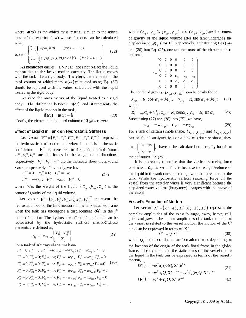
(38) Once the )(~ ωtA and tC~ are calculated, they are used to modify the added mass and the stiffness matrices and the Eq. (38) can be solved with the existing solver in the conventional analyses. AN APPLICATION EXAMPLE Application of the present method is demonstrated with a vessel with internal tanks. The example is the vessel with two tanks used in TEST22 from the WAMIT manual. The vessel has a length of 20 m, breath of 4.4 m and draft of 1.2 m. Both tanks are rectangular and have the same length tl (2 m), breath

tb (4.2 m) and height (>1.0m). Both tanks are filled with the same water with a depth td of 1.0 m. The aft side of tank 1 and the forward side of tank 2 are in the same plane x=0. The bottom of tank 1 is at z=0 and the bottom of tank 2 is at z = -1.0 m. Figure 1 shows the wetted part of the vessel and the two liquid tanks. The origin of the local tank frames for a tank is placed on the center of the liquid free surface. Therefore, we have, )0,0,1()~,~,~();1,0,1()~,~,~( 222111 −== zyxzyx .

Also, 0),( 66 =cgcg yx , thus 05646 == cc , for both tanks.

For the rectangular tanks, it can be shown that,

⎟⎟⎠

⎞⎜⎜⎝

⎛+

⎟⎟⎟⎟

⎠

⎞

⎜⎜⎜⎜

⎝

⎛

−

−=⎟⎟

⎠

⎞⎜⎜⎝

⎛1001

)2

(

120

012)(

3

3

5554

4544 tttt

tt

tt

tdlbd

lb

bl

dcccc

ρρ (39)

It should be pointed out that, based on definition of c , Eq. (25), the stiffness matrix vC in Eqs. (37) and (38) should be evaluated only using the weight of the vessel and the center of gravity of the vessel without accounting for the liquids in the tanks. The second term in Eq. (39) represents the restoring force due to the weight of the liquids treated as rigid bodies. Should vC be evaluated using the total weight (vessel and liquids in tanks) and the center of gravity with the weight of the liquids included, the second term in Eq. (39) shall be dropped. The added mass of the tank liquid in the local frames. Then the motion RAOs are examined to see the effect of the liquid sloshing on the natural frequencies of the vessel motions.


Figure 1. The vessel with two internal liquid tanks

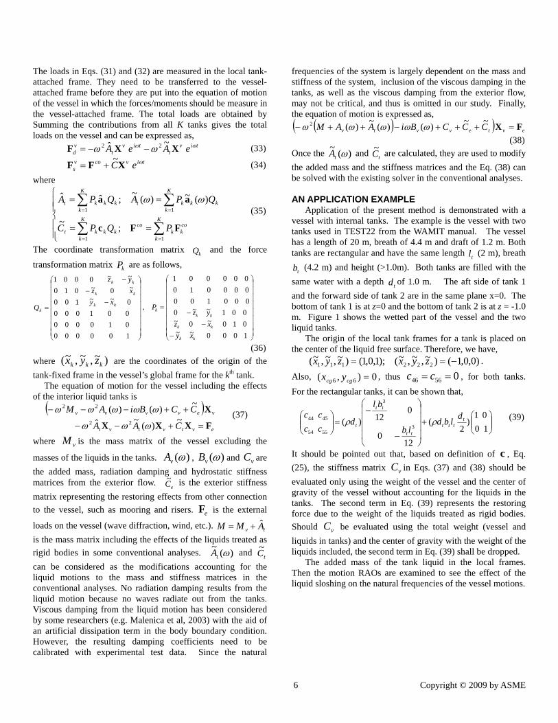
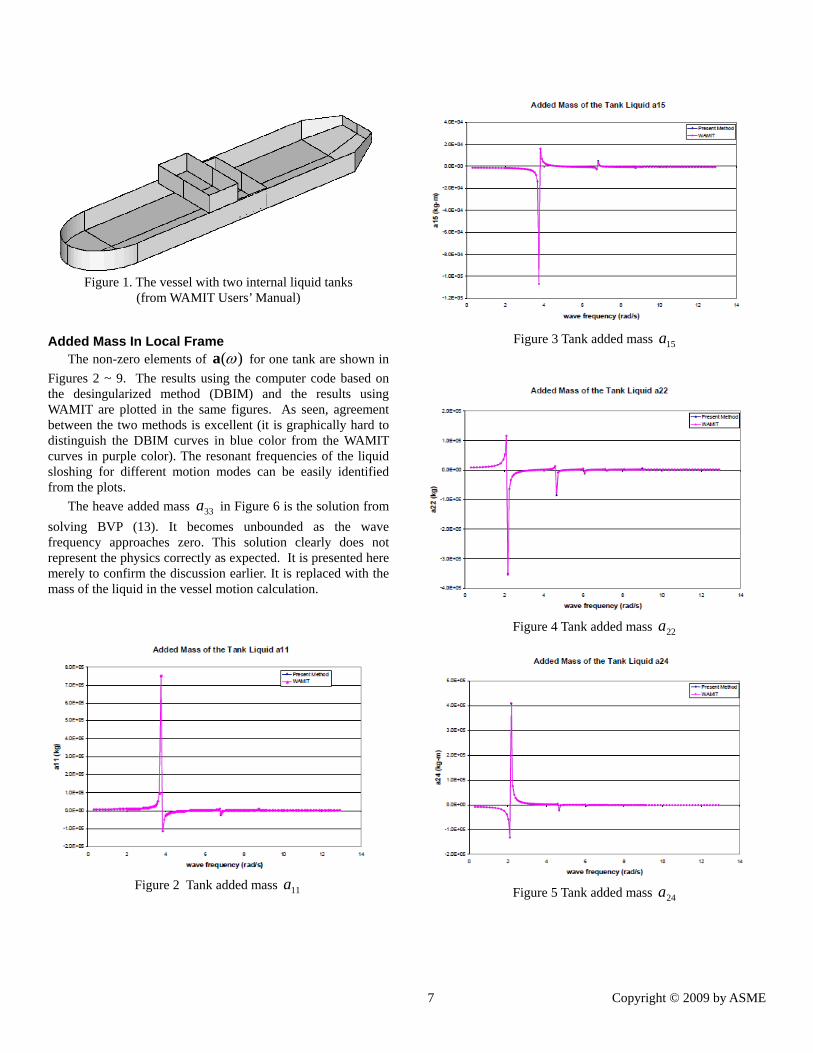
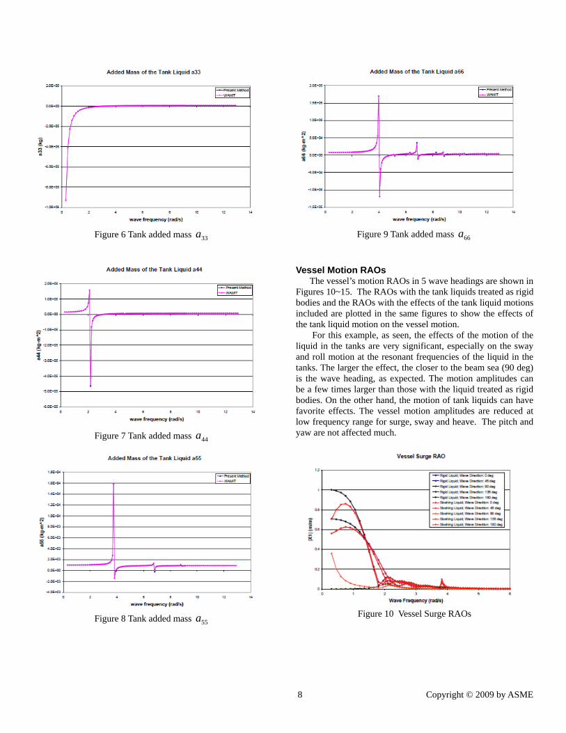
(from WAMIT Users’ Manual) Added Mass In Local Frame The non-zero elements of )(ωa for one tank are shown in Figures 2 ~ 9. The results using the computer code based on the desingularized method (DBIM) and the results using WAMIT are plotted in the same figures. As seen, agreement between the two methods is excellent (it is graphically hard to distinguish the DBIM curves in blue color from the WAMIT curves in purple color). The resonant frequencies of the liquid sloshing for different motion modes can be easily identified from the plots. The heave added mass 33a in Figure 6 is the solution from solving BVP (13). It becomes unbounded as the wave frequency approaches zero. This solution clearly does not represent the physics correctly as expected. It is presented here merely to confirm the discussion earlier. It is replaced with the mass of the liquid in the vessel motion calculation.

Figure 2 Tank added mass 11a









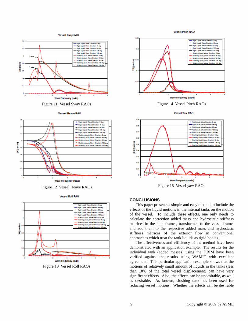
Vessel Motion RAOs The vessel’s motion RAOs in 5 wave headings are shown in Figures 10~15. The RAOs with the tank liquids treated as rigid bodies and the RAOs with the effects of the tank liquid motions included are plotted in the same figures to show the effects of the tank liquid motion on the vessel motion. For this example, as seen, the effects of the motion of the liquid in the tanks are very significant, especially on the sway and roll motion at the resonant frequencies of the liquid in the tanks. The larger the effect, the closer to the beam sea (90 deg) is the wave heading, as expected. The motion amplitudes can be a few times larger than those with the liquid treated as rigid bodies. On the other hand, the motion of tank liquids can have favorite effects. The vessel motion amplitudes are reduced at low frequency range for surge, sway and heave. The pitch and yaw are not affected much.

Figure 10 Vessel Surge RAOs


Figure 11 Vessel Sway RAOs

Figure 12 Vessel Heave RAOs

Figure 13 Vessel Roll RAOs

Figure 14 Vessel Pitch RAOs

Figure 15 Vessel yaw RAOs

CONCLUSIONS This paper presents a simple and easy method to include the effects of the liquid motions in the internal tanks on the motion of the vessel. To include these effects, one only needs to calculate the correction added mass and hydrostatic stiffness matrices in the tank frames, transformed to the vessel frame, and add them to the respective added mass and hydrostatic stiffness matrices of the exterior flow in conventional approaches which treat the tank liquids as rigid bodies. The effectiveness and efficiency of the method have been demonstrated with an application example. The results for the individual tank (added masses) using the DBIM have been verified against the results using WAMIT with excellent agreement. This particular application example shows that the motions of relatively small amount of liquids in the tanks (less than 18% of the total vessel displacement) can have very significant effects. Also, the effects can be undesirable, as well as desirable. As known, sloshing tank has been used for reducing vessel motions. Whether the effects can be desirable


or undesirable depends on many parameters such as the number of tanks, tank shape, amount of liquid in the tanks, the locations of the tanks, the dominant direction of the environment, interaction of the tanks and the vessel, etc. A comprehensive parameter study is very important to gain a good understanding of the effects and prediction of the performance. It is believed that the method presented in this paper would be a very effective and useful tool for engineers/designers who need to deal with the liquid motion in tanks.

REFERENCES 1) M. Zalar, L. Diebold, E. Baudin, J. Henry, and X.B. Chen,

(2007), “Sloshing Effects Accounting for Dynamic Coupling Between Vessel and Tank Liquid Motion”, Proceedings of 26th Inter. Conf. on Offshore Mechanics and Arctic Engin., June 10-15, San Diego, California, USA.

2) Malenica S., Zalar M., Chen X.B. (2003), “Dynamic Coupling of Seakeeping and Sloshing”, Paper No. 2003-JSC-267, ISOPE.

3) Molin, B., Remy, F., Rigaud, S., & de Jouette, Ch., 2002, ‘LNG-FPSO’s: frequency domain, coupled analysis of support and liquid cargo motions,’ Proceedings IMAM Conf., Rethymnon, Greece.

4) Newman, J. N., 2005, “Wave Effects on Vessels with Internal Tanks”, 20th WWWFB, Spitsbergen, May 29 –June 1, 2005.

5) C.H. Lee, (2007) “WAMIT Users’ Manual Version 6.3”. 6) Chen, X-B, et al, (2007) “HydroStar Users’ Manual ”. 7) Y. Cao, W.W. Schultz and R.F. Beck, “Three-dimensional

desingularized boundary integral methods for potential problems’’, International Journal for Numerical Methods in Fluids, Vol.12, 1991.


















Documents

Effects of Fluid Motions in Liquid Tanks on Vessel Motions Using a Simple Panel Method