Journal of Ecology

2007

95

, 1084–1097

© 2007 The AuthorsJournal compilation© 2007 British Ecological Society

Blackwell Publishing Ltd

Effects of size, competition and altitude on tree growth

DAVID A. COOMES*†‡ and ROBERT B. ALLEN‡

†

Conservation and Community Ecology Group, Department of Plant Sciences, University of Cambridge, Downing Street, Cambridge CB2 3EA, UK,

‡

Landcare Research, PO Box 40, Lincoln 7640, New Zealand

Summary

1.

Understanding the factors influencing tree growth is central to forest ecology becauseof the significance of growth to forest structure and biomass. One of the simplest, yetmost controversial growth models, proposed by Enquist and colleagues, predicts thatstem-diameter growth scales as the one-third power of stem diameter. Recent analysesof large-scale data sets have challenged the generality of this theory and highlighted theinfluence of resource competition on the scaling of growth with size.

2.

Here we explore the factors regulating the diameter growth of 3334 trees of mountainbeech (

Nothofagus solandri

var.

cliffortioides

) growing in natural single-species forests inNew Zealand. Maximum-likelihood modelling was used to quantify the influencesof tree size, altitude, the basal area of taller neighbours (

B

L

) and the basal area of allneighbours (

B

T

) on growth. Our interpretation of the models assumed that tallerneighbours compete for light whereas all neighbours compete for nutrients.

3.

The regression analyses indicate that competition for light has a strong influence onthe growth of small trees, whereas competition for nutrients affects trees of all sizes.These findings are consistent with experimental manipulation studies showing thatcompetition for light and nutrients inhibits the growth of small mountain beech trees,and fertilizer application studies showing that nitrogen limits the growth of large trees.

4.

Tree growth declined with altitude. The regression analyses suggest that the intensityof light competition also declines with altitude, when trees with similar

B

T

and

B

L

valueswere compared along the gradient. These results are consistent with observations thattrees become stunted and have more open canopies at high altitudes.

5.

Our study is the first to build the effects of competition and environment intoEnquist’s model of tree growth. We show that competitive interactions alter the scaling ofmean growth rate with size, whereas altitude does not influence the scaling of potentialgrowth rate with size.

Key-words

: Boltzmann–Arrhenius function, competition, elevation, facilitation, metabolictheory, non-linear mixed-effects model, quantile regression, temperature, Tilman vs.Grime debate, WBE theory

Journal of Ecology

(2007)

95

, 1084–1097doi: 10.1111/j.1365-2745.2007.01280.x

Introduction

Trees in natural populations usually exhibit largevariation in growth (e.g. Harper 1977). Understandingthis variation in growth is central to forest ecologybecause of its significance to forest structure and bio-mass. One approach to understanding variation in treegrowth is to derive mechanistic explanations for thepotential maximum growth rate of trees and then

determine why and how the growth of individuals fallsbelow this potential constraint. Enquist (2002) arguedthat because trees have an efficient transport systemthen whole-tree photosynthetic rate is simply related tothe number of leaves on a tree, and so is mechanisticallyrelated to size by an invariant power law. Based uponthis relationship, Enquist

et al

. (1999) argued that stemdiameter growth

dD/dt

scales as

D

1/3

(henceforth referredto as the Enquist growth model). Clearly the assumptionthat photosynthetic rate is only dependent upon leafnumber, or size, is suspect because it is, of course, alsolimited by many other factors including the supply ofwater, light and nutrients (Coomes 2006; Reich

et al

.

*Author to whom correspondence should be addressed:David A. Coomes. Tel.:

+

44 1223 333911. Fax:

+

44 1223 332418.E-mail: dac18@cam.ac.uk.

1085

Effects on growth of size, competition and altitude

© 2007 The AuthorsJournal compilation © 2007 British Ecological Society,

Journal of Ecology

95

, 1084–1097

2006; Muller-Landau

et al.

2006). In a recent paper,Muller-Landau

et al

. (2006) fitted growth curves todata from 1.7 million trees in 10 tropical forests. Theyshowed that the scaling of mean diameter growth withsize varied considerably among the forests, and was notdescribed by a power law with slope of 1/3. They arguedthat the changing supply of light with size exerted astrong influence on the scaling of growth: small treeswere shaded by taller neighbours and grew slowly asa consequence, while larger trees were less affected byshading (see Weiner 1990). Therefore the Enquist growthmodel needs to be reconsidered, with the control ofcompetition made more explicit (Coomes 2006).

Here we build upon these ideas using a data set of3334 mountain beech trees (

Nothofagus solandri

var.

cliffortioides

) growing along an altitudinal gradient inNew Zealand’s Southern Alps. Our work exploresthree avenues not investigated by Muller-Landau

et al

.(2006) in their important tropical study. First, weconsider whether the Enquist growth model representsan upper boundary relationship that occurs whennothing else is limiting except flow through the vascularnetwork. The supply of resources to trees is spatiallyheterogeneous because gaps created by the death oflarge trees allow light to penetrate to the forest floor andsometimes result in the release of nutrients (Coomes& Grubb 2000), so tree growth in natural forests isimmensely variable (Canham

et al

. 2004). We hypo-thesized that the diameter growth of trees uninhibitedby competition scales with D

1/3

, as the Enquist growthmodel predicts. We investigate this hypothesis by usingquantile regression to fit an upper boundary curveto the size–growth distribution (Thomson

et al

. 1996;Cade

et al

. 1999; Cade & Guo 2000) and testing howsimilar it was to the curve predicted by the Enquistgrowth model.

Second, we use neighbourhood modelling to explorethe ways in which competition for light and nutrientsvaries with tree size (Freckleton & Watkinson 2001;

Canham

et al

. 2004; Uriarte

et al

. 2004). The generalform of our model is

G

=

λ

D

α

l

(

B

L

)

n

(

B

T

), where

G

isstem-diameter growth,

B

L

and

B

T

are the basal areas oflarger neighbours and all neighbours, respectively, and

l

(

B

L

) and

n

(

B

T

) are functions that describe the compe-titive effect of such neighbours on growth. The function

l

(

B

L

) is often regarded as defining the effect of com-petition for light because only taller neighbours areable to intercept light before it reaches the focal tree(Vanclay 1995; cf Schwinning & Weiner 1998). By similarreasoning,

n

(

B

T

) describes the effect of below-groundcompetition because nutrient-uptake by a plant dependsupon the extent to which the fine roots of neighbouringplants have depleted the pool of available nutrients, andthe roots of all neighbours compete for resources, notjust the taller neighbours (Schwinning & Weiner 1998).Our hypothesis was that competition affects the growthof all trees, but that competition shifts from being mainlyfor light when the focal tree is small to being mainly fornutrients when the tree reaches maturity (Fig. 1).

Third, we examine the ways in which potentialgrowth rate and competitive intensity vary with altitude.Grime (1977) has argued that competition is intense inproductive sites, where the potential for rapid growthallows rapid pre-emption of resources, but decreases inintensity and importance in less productive (‘stressed’)sites. In contrast, Tilman (1988) has argued that plantsrespond plastically to changing rates of resourcesupply (Bloom

et al

. 1985; Gleeson & Tilman 1992), andconsequently compete for light in nutrient-rich sitesand for below-ground resources in nutrient-depletedsites. These contrasting views form the basis for oneof the longest running debates in ecology (Craine2005). Numerous authors have quantified changes incompetitive intensity along environmental gradientsusing short-term removal experiments in herbaceouscommunities (Goldberg

et al

. 1999; Callaway

et al

. 2002;Maestre

et al

. 2005) but there have been remarkablyfew studies using long-lived individuals in forest

Fig. 1. A conceptual model of the ways in which growth varies with tree size, as a result of changes in competition with neighbours:(a) As the stem diameter D of a tree increases, there is a decrease in the basal area of taller neighbours (BL) while the basal area(BT) of all neighbours remains relatively constant; (b) the intensity of competition for light (. . . .) decreases with size because treesare less likely to be overshadowed by taller neighbours, whereas the intensity of competition for nutrients (- - -) remains constant;(c) the difference between potential growth rate (no competitors · - · - ·) and mean growth rate (with competitors —) is greatest forsmall trees because the overall intensity of competition is greatest for small trees.

1086

D. A. Coomes & R. B. Allen

© 2007 The AuthorsJournal compilation © 2007 British Ecological Society,

Journal of Ecology

95

, 1084–1097

communities, and only one that has explicitly factoredsize into their design (Canham

et al

. 2004). As well astesting for how light competition varies with altitudewe evaluate the Enquist growth model prediction thatthe size-dependence of growth, as defined by the scalingexponent

α

, does not vary with environment.We examine diameter growth in mountain beech

trees found in unmanaged stands which form naturallysingle-species forests on the eastern slopes of NewZealand’s Southern Alps (Wardle 1984). Data collectedfrom 246 permanent plots, spanning a 780-m altitudinalgradient, were used to evaluate the ways in which size,competition for light, and altitude interact to affect anindividual’s diameter growth. These monospecificforests are uniquely suitable for testing such relationshipswithout the confounding effects of species turnover.Specifically we test the following hypotheses.

1.

The Enquist growth model defines the upper rate ofgrowth that occurs when competition is not limiting;

2.

there is a shift in relative importance of competitionfor light and nutrients with ontogeny;

3.

Trees are slower growing and less influenced bycompetition for light in high altitude forests, but thescaling exponent is unaffected by altitude.

Methods

The 200-km

2

study area (43

°

10

′

S, 171

°

35

′

E) has amountainous terrain with peaks over 2000 m a.s.l. andvalley bottoms down to 600 m a.s.l altitude. Mountainbeech (

Nothofagus solandri

var.

cliffortioides

; Notho-fagaceae) is a light-demanding species and a member ofone of the few ectomycorrhizal genera in New Zealandforests (Wardle 1984). The mountain beech forest in thestudy area is spatially heterogeneous because storms,earthquakes and pathogen outbreaks have patchilydisturbed the stands over recent decades (Wardle &Allen 1983; Harcombe

et al

. 1998; Allen

et al

. 1999). Thisheterogeneity was beneficial for our neighbourhoodmodelling because it provided a wide range of neigh-bourhood basal area values. While the mean basalarea of mountain beech trees per plot increases withaltitude (Harcombe

et al

. 1998), the trees get shorter,and there is a substantial reduction in biomass per plotas a result (Harcombe

et al

. 1998). A weather station at914 m altitude on the eastern edge of the study areahas recorded a mean annual temperature of 8.0

°

C,precipitation of 1447 mm year

–1

, and irradiance of4745 MJ m

–2

year

–1

(McCracken 1980). Monthly meandaily temperature is greatest in February (13.9

°

C)and least in July (2.0

°

C). Air temperature decreasesby 0.71

°

C, and rainfall increases by 21.9 mm year

–1

,for every 100-m rise in altitude (based on 13 years ofdata; McCracken 1980). Rainfall increases fromabout 1200 mm year

–1

in the east to 2500 mm year

–1

inwestern parts of the study area (Griffiths & McSaveney1983), and there is no evidence to suggest that rainfall

limits growth within the study area (Wardle 1984).There is compelling evidence from fertilizer and root-trenching experiments that nitrogen limits tree growthin our mountain beech forest (Davis

et al

. 2004; Platt

et al

. 2004), so we regard below-ground competitionand competition for nutrients as being synonymous inthis paper.

We utilized plots sampling 9000 ha of forest thatincluded stands up to the natural tree line at 1400 ma.s.l. A total of 246 plots were established systematicallyalong 98 compass lines in the mountain beech forestover the austral summers of 1970–71 and 1972–73 (allen1993; Allen

et al

. 1999; Coomes & Allen 2007). Theorigins of lines were randomly located points alongstream channels (30–1000 m apart), and their compassdirections were also chosen at random. Plots were thenlocated at 200-m intervals along each line until the treeline was reached, giving rise to lines containing betweenone and eight plots (mean

=

2.6). The altitude of a plotwas based upon field measurements using a barometricaltimeter. Each plot was 0.04 ha (20

×

20 m), anddivided into 16 subplots (5

×

5 m). Within each plot, thediameter at breast height (d.b.h.) of each tree stem

>

30 mm, and the subplot in which it was located, wererecorded. Plots were re-enumerated during the australsummers that started in 1974 and 1993. All tree stemswere tagged in 1974, and new recruits (

>

30 mm d.b.h.)tagged in 1993. Hereafter, we refer to the nominal datefor plot establishment as 1974, and utilize the survivingindividuals in 1993 to characterize stem diametergrowth. Trees that died between 1974 and 1993 tendedto have slower growth rates than trees that survived(D.A. Coomes & R. B. Allen, unpublished data), so ourapproach overestimates the average growth rate ofthe population; this issue is not considered further inthis paper. The vast majority of trees are single-stemmedand resprouting is uncommon.

Growth analyses were focused on the 3334 individualsin the four central 5

×

5 m subplots of the 246 plots. Asthe data set contained information about which squaresubplot a tree was located in, our competition indiceswere based upon summing basal areas within setsubplots (Freckleton & Watkinson 2001). Given the closecorrelation (

r

2

=

0.74) between stem diameter andheight in mountain beech forests (Harcombe

et al

. 1998),taller trees are taken to be those with larger diameters.We calculated

B

L

by summing the basal area of stemsthat had diameters larger than the initial diameter of atarget tree within a 15

×

15 m area centred upon the5

×

5 m subplot containing the target tree. Values of

B

L

were calculated from diameter data collected in1974 and 1993, expressed in standard units (cm

2

m

–2

)and averaged. We chose to use the mean of the 1974 and1993 values because it is more representative of theneighbourhood conditions experienced by a tree overthe course of the study than the value at either the start

1087

Effects on growth of size, competition and altitude

© 2007 The AuthorsJournal compilation © 2007 British Ecological Society,

Journal of Ecology

95

, 1084–1097

or end of the study. The basal area of all neighbours

B

T

was calculated in the same way. Neighbourhood areasof 25 m

2

and 400 m

2

were also tried, but regressionmodels had weaker explanatory power than ones basedon an area of 225 m

2

.

The Enquist growth model suggests stem diametergrowth

dD/dt

is defined by the following power function:

dD/dt

= λ0 Dα, eqn 1

where D is the diameter at breast height, λ0 is thescaling coefficient and α is the scaling exponent. Ourfirst hypothesis, that the Enquist growth model definesa potential growth curve rather the mean growth curve,was tested by using non-linear quantile regression(nlrq routine in the quantreg package of R) to fit theintergrated form of the power function to our data set:

eqn 2

where D0 is the initial diameter at breast height, Dt isdiameter recorded at the second enumeration, t is thetime between measurements (19 years), λ 0 is the scalingcoefficient and α is the scaling exponent. We used theintegrated form of the power function because instan-taneous growth rate (dD/dt) varies continuously andnon-linearly with size (Muller-Landau et al. 2006).Quantile regression allowed us to fit curves through themiddle of the data set by weighting regression on the50th quantile, and to the ‘upper boundary’ (Cade &Guo 2000); the choice to define the upper boundary isarbitrary so we used the 95th and the 99th quantiles.

Our second hypothesis, that mountain beech treescompete mainly for light as juveniles and for nutrientsas adults, was tested by fitting alternative competitionfunctions to the data (e.g. Canham et al. 2004; Uriarteet al. 2004). The effect of competition for light wasmodelled using the function:

eqn 3

where D is the stem diameter, BL is the basal area oftaller neighbours, and λ2 and λ3 define the competitiveeffect of taller neighbours on growth. BL was theaverage of the values calculated from the 1974 and1993 surveys. Note that λ1 D

α/(1 + λ1/λ2) is the potentialgrowth rate attained when trees are not subjected tocompetition. The logic behind this choice of functionis explained in Appendix S1 (see SupplementaryMaterial). Briefly, we assume that the amount of light

reaching a tree is determined non-linearly by the leafarea index (LAI) of taller trees around it (the Beer–Lambert law is used), and that the assimilation rate ofthe plant depends non-linearly on light availability(the Michealis–Menten function is used). Based onthese assumptions, λ3 quantifies the amount of shadecast by taller neighbours (it is directly proportional tothe light-extinction coefficient) while λ2 quantifies theresponse of the target tree to light (it is the slope of thegrowth-light curve at zero light). The model containsfour parameters to be estimated by regression analysis(α, λ1, λ2, λ3).

We decided against developing a complex mech-anistic model to describe the effects of below-groundcompetition because much remains obscure about theprocesses involved in taking up and retaining nutrients(e.g. Schwinning & Weiner 1998; Högberg & Read 2006;Reich et al. 2006). Instead, the effects of competitionfor below-ground resources were modelled using thefollowing simple function:

eqn 4

where BT is the total basal area of all trees within aspecified area around a target stem, and λ4 and α areparameters to be estimated by regression. BT was theaverage of the values calculated from the 1974 and1993 surveys. This is a basic density-dependencefunction which predicts that growth declines towardszero with increasing BT. An important distinctionfrom the light model is that it assumes that the abilityof a plant to capture nutrient depends on the total basalarea of neighbours, rather than on the basal area oftaller neighbours. Note that we tried increasing theflexibility of the response curve by including an extraparameter to raise BT to a power, but these models failedto converge. When we fixed the exponent at differentvalues and allowed the likelihood estimator to find theoptimal value for the other parameters, we found thatthe models converged and the AICs of the models wereworse, or very similar to, the AIC value of the modelgiven (i.e. exponent set at 1).

Finally, the combined model of competition for lightand nutrient that we chose, after extensive explorationof alternative models, was:

eqn 5

This model can only be fitted when trees of a wide rangeof sizes are considered because BT is closely correlatedwith BL for small trees (by definition BT = BL for the smallesttree in the plot), but the two metrics are much lessclosely related for big trees (see Appendices S3 and S4).

The parameters in equations 1, 3, 4 and 5 wereestimated by maximum likelihood methods (Canhamet al. 2004). The integrated forms of the models werefitted using non-linear mixed-effects modelling (the nlmeroutine in R), which accommodated the covariance

D D tt [ ( ) ] ,/( )= + −− −01

01 11α αλ α

dDdt

D

e BL

,=+

λλλ

α

λ

1

1

2

1 3

dDdt

DBT

( )

=+λ

λ

α1

41

dD dt D e BBT

L/ /[( / )( )]= + +λ λ λ λα λ1 1 2 41 13

1088D. A. Coomes & R. B. Allen

© 2007 The AuthorsJournal compilation © 2007 British Ecological Society, Journal of Ecology 95, 1084–1097

associated with non-independent sampling (trees withinplots) as a random intercept term (R Foundation2006). For example, parameters λ0 and α in equation 1were estimated by fitting as:

eqn 6

where D0 and Dt are stem diameters in 1974 and 1993,∆t is the time interval, εi is a plot-level random term andε is the residual error. Both random terms wereassumed to be normally distributed, and analyses ofresiduals indicated that this assumption was valid.

The relative strength of alternative models (equations1, 3, 4 and 5) were compared by their Akaike InformationCriteria (AICs). AIC is defined as the –2 log(maximumlikelihood) + 2 (number of parameters), and providesa quantitative measure that can be used to rankalternative models; the model with the smallest AICis taken to be the ‘best’ of the set under consideration(Burnham & Anderson 2002). AICs were used to makethese comparisons because the models are not nested.

Growth rates may decline with altitude because ofreduced air and soil temperatures (an adiabatic effect),shorter growing seasons, increased exposure to wind,and reduced supply of nutrients. The effect of altitudeon the potential growth rate parameter was ascertainedby allowing λ1 to become a quadratic function of altitude(A):

λ1 = λ1A + λ1B A + λ1C A2. eqn 7

The significance of altitude terms was tested by like-lihood ratio tests, and by examination of standard errorestimates (i.e. testing whether the parameter differedfrom zero by more than two times the standard error).Having incorporated the effects of altitude on potentialgrowth rate, we proceeded to explore whether thescaling exponent or competition terms (i.e. α, λ2, λ3, orλ4) varied with altitude. Each of these terms was madeinto a quadratic function of altitude, the models wererefitted, and the statistical significance of addingaltitude terms was tested using log-likelihood ratio tests.The change in AIC associated with adding the altitudeterms is also given, for consistency.

If the fall in mean temperature with altitude isthe main determinant of changes in growth rate (e.g.Benecke & Nordmeyer 1982; Richardson et al. 2005)then the Enquist growth model theory predicts thatthe Boltzmann–Arrhenius function provides a mech-anistic explanation for changes in potential growth(Enquist et al. 2003):

λ1 = λ8 exp(–E/kT ) eqn 8

where T is absolute temperature in Kelvin based on alapse rate of 0.71 °C per 100 m altitude, E is the average

activation energy (c. 0.65 eV), and k is the Boltzmannconstant (8.62 × 10–5 eV K–1). The goodness of fit ofthe Boltzmann–Arrhenius function vs. the quadraticfunction of altitude was assessed by comparing AICs.

Several indices of competition intensity have beenproposed in the literature, of which we selected to usethe log-transformed performance ratio:

ln RR = ln(GP/GC), eqn 9

where GP is the potential growth of a plant growingwithout competitors and GC is growth in the presenceof competitors (Goldberg et al. 1999). Most studies ofcompetition have involved inserting herbaceous plantsinto natural communities and comparing their growthwith paired controls growing in isolation from com-petitors. In our study, it is the regression model thatprovides the mean and potential growth rates usedto calculate ln RR. The general form of the growthmodel is GC = λDαl(BL)n(BT), where l(BL) and n(BT)are functions that describe the effects of competitionfor light and nutrients, respectively, and the potentialgrowth rate is GC = λl(0)n(0)Dα. Entering these growthfunctions into equation 9 we get:

ln RR = ln l(0)/l(BL) – ln n(0)/n(BT). eqn 10

We define ln l(0)/l(BL) and ln n(0)/n(BT) as being com-petition intensities for light and nutrients, respectively(henceforth ICL and ICN). The advantage of using lnRR is that it is simply the sum of ICL and ICN.

In order to explore how the mean ICL varied withaltitude, we plotted ICL against A for all 3334 trees inthe data and then fitted a smooth curve through thedata using generalized additive models (the gamfunction in R, selecting the smoothing spline optionwith 6 d.f., and otherwise using default settings).This approach was also used to explore the ways inwhich mean ICL, ICN and ln RR varied withaltitude and tree size. All curves fitted by gams weresignificantly different from flat-line relationships(P < 0.00001) unless otherwise stated. Note thatsimply inserting the mean value of BL or BT intoICN or ICL would give an incorrect estimate of themean intensity of competition because of Jensen’sInequality (the function of a mean is not equal to themean of a function).

Results

Growth of mountain beech trees was significantlycorrelated with tree size (r = 0.41, P < 0.00001),

D D tt i [ ( ) ] ,/( )= + − + +− −01

01 11α αλ α ε ε∆

1089Effects on growth of size, competition and altitude

© 2007 The AuthorsJournal compilation © 2007 British Ecological Society, Journal of Ecology 95, 1084–1097

although growth rates were immensely variable amongindividual trees of the same size (Fig. 2a). Quantileregression provides an indication of this variability.The average growth curve was estimated to be dD/dt = 0.037D 0.68, using quantile regression weighted onthe 50th quantile of the data set (i.e. τ = 0.50). The 95%confidence interval for the scaling exponent, 0.63–0.73,did not overlap with the value of 0.33 predicted by theEnquist growth model. The scaling exponent of theupper boundary was 0.40 (95% CI = 0.29–0.51) whenτ = 0.95, and was 0.25 (95% CI = 0.16–0.35) whenτ = 0.99 (Fig. 2b). Clearly, the scaling exponent of theupper boundary was highly dependent on the value ofτ chosen.

The influence of size on growth was also evident frommaximum likelihood modelling. The power functionwas dD/dt = 0.114D0.52, and was a better fit to the datathan the null model (∆AIC = 178, P < 0.00001). Thescaling exponent was significantly different from thatpredicted by the Enquist growth model (0.52 ± 0.023vs. 1/3, t = 8.29, P < 0.00001).

The growth function which included BL and BT wasfound to be the best fitting of all the models that wecompared (i.e. it had the lowest AIC; Table 1). In otherwords, the regression analyses suggest that competitionfor both light and nutrients suppress the growth of treesin mountain beech forests. To illustrate the extent towhich growth was reduced by competition for lightand nutrients, we calculated the mean growth rate ofsmall, medium and large trees for which BL was lessthan 20 cm2 m–2, between 20 and 40 cm2 m–2, and greaterthan 40 cm2 m–2 (upper row of Fig. 3), and for which BT

was less than 20 cm2 m–2, between 20 and 40 cm2 m–2, andgreater than 40 cm2 m–2 (lower row of Fig. 3). It can be seenthat growth was strongly suppressed by neighbours inall size classes (Fig. 3); differences between classes wereall statistically significant (t-tests, P < 0.0001).

The intensity of competition for light is given byICL = ln(1 + 0.068 exp(0.048BL)). Tall trees have fewtaller neighbours, so the mean value of BL decreases

Fig. 2. (a) Diameter growth rate of individual trees, calculated as (Dt – D0)/∆t and plotted as a function of initial stem diameter(D0). The diameter size-classes used in subsequent regression analyses (‘small’ < 150 mm, ‘medium’ 150–250 mm and‘large’ > 250 mm) are shown; (b) the same data presented as mean growth rates (�) within 15 size classes (± 1 SEM), and scalingrelationships fitted by quantile regression through the centre of the dataset (τ = 0.50), and to the ‘upper boundary’ of the data set(τ = 0.95 and 0.99). The scaling exponent (α) is also given for each of these regression relationships.

Table 1. Parameter estimates and standard errors for five models of stem diameter growth (dD/dt) for 3334 mountain beech trees.Models were fitted using maximum likelihood methods and the last column gives the Akaike Information Criteria (AICs) relativeto the model with the lowest AIC (the final one). Burnham & Anderson (2002) state that models that differ by more than 10 fromthe best model are poorly supported

Model Growth function Parameter estimates (± SE) AIC

Null λ 0 λ0 = 1.11 ± 0.030 477

Power λ0 Dα λ0 = 1.11 ± 0.016, α = 0.52 ± 0.023 299

+ Light λ1 = 0.94 ± 0.19, λ2 = 8.70 ± 2.61, λ3 = 0.042 ± 0.0050, α = 0.19 ± 0.029 10

+ Nutrients λ1Dα/(1 + λ4BT) λ1 = 0.23 ± 0.035, λ4 = 0.013 ± 0.0026, α = 0.48 ± 0.022 183

+ Light

+ Nutrients

λ1 = 1.01 ± 0.19, λ2 = 15.0 ± 5.54, λ3 = 0.048 ± 0.0062,

λ4 = 0.0055 ± 0.0017, α = 0.20 ± 0.0300

λ λ λα λ1 1 21 3D e BL/( / )+

λλ λ λ

α

λ1

1 2 41 13

D

e BBT

L[( / )( )]+ +

1090D. A. Coomes & R. B. Allen

© 2007 The AuthorsJournal compilation © 2007 British Ecological Society, Journal of Ecology 95, 1084–1097

with size (Fig. 4a), and this results in a decrease in meanICL with size (Fig. 4b). The intensity of competitionfor nutrients is given by ICN = ln(1 + 0.0055 BT).Mean ICN remains virtually constant with size becauseBT varies little with size (Fig. 4a,b). The overall inten-

sity of competition (ln RR = ICN + ICL) decreaseswith size as a result of the decreases in ICL (Fig. 4b).Finally, the mean growth curve is given by ln GC =exp(ln GP – ICL – ICP). The mean and potential growthcurves are shown in Fig. 4(c). Note that the difference

Fig. 3. Influences of taller neighbours (BL) and all neighbours (BT) on the diameter growth (mean ± 1 SEM) of small (30–150 mm), medium (151–250 mm) and large (> 251 mm) diameter trees. BL and BT were separated into three classes (darkgrey < 20, mid-grey 20–40 and light grey > 40 cm2 m–2). The percentage of trees within a size class that experience each level ofcompetition is given above the bar.

Fig. 4. Changes with tree diameter in (a) mean BL (. . . .) and BT (- - -); (b) mean ICL (. . . .), ICN (---) and ln RR (—) and (c) meandiameter growth (—) and potential diameter growth rate (· - · - ·). The curves in panels (a) and (b) were obtained by fittinggeneralized additive models.

1091Effects on growth of size, competition and altitude

© 2007 The AuthorsJournal compilation © 2007 British Ecological Society, Journal of Ecology 95, 1084–1097

between potential and mean growth curves decreaseswith increasing size because competition for light isdiminishing, resulting in the average growth curvehaving a steeper slope than the potential growth curve.

As a check on the validity of our regression model-ling, we estimated the light extinction coefficient ofmountain beech stands from parameter λ 3 in the best-supported model. As explained in the Appendix S1,λ3 = vBi /Ai where v is the light extinction coefficient, Bi

is its stem basal area and Ai is the leaf area of a tree. Formountain beech trees growing at mid-altitude, therelationship between leaf biomass ML (g) and basal areaBi (cm2) is given by ML = 15.2 Bi (Osawa & Allen 1993),and the relationship between leaf biomass (g) and leafarea (cm–2) is given by ML = 176 A (Hollinger 1989), fromwhich it follows that Bi /Ai = 176/15.2. The estimatedvalue of λ3 is 0.048 ± 0.0061 (Table 1), so we estimateν to be 0.048 × 176/15.2 = 0.56, which is within the rangeof coefficients measured directly in several forest types(0.28–0.62; in Jarvis & Leverenz 1983).

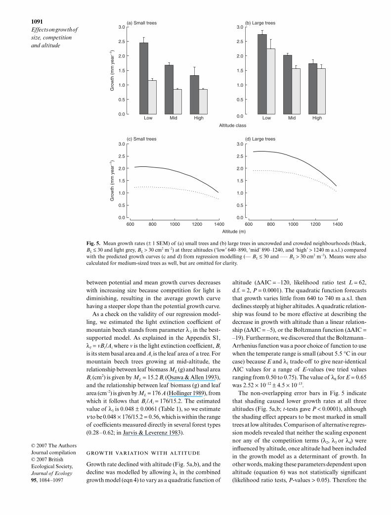
Growth rate declined with altitude (Fig. 5a,b), and thedecline was modelled by allowing λ1 in the combinedgrowth model (eqn 4) to vary as a quadratic function of

altitude (∆AIC = –120, likelihood ratio test L = 62,d.f. = 2, P = 0.0001). The quadratic function forecaststhat growth varies little from 640 to 740 m a.s.l. thendeclines steeply at higher altitudes. A quadratic relation-ship was found to be more effective at describing thedecrease in growth with altitude than a linear relation-ship (∆AIC = –5), or the Boltzmann function (∆AIC =–19). Furthermore, we discovered that the Boltzmann–Arrhenius function was a poor choice of function to usewhen the temperate range is small (about 5.5 °C in ourcase) because E and λ1 trade-off to give near-identicalAIC values for a range of E-values (we tried valuesranging from 0.50 to 0.75). The value of λ8 for E = 0.65was 2.52 × 10–12 ± 4.5 × 10–13.

The non-overlapping error bars in Fig. 5 indicatethat shading caused lower growth rates at all threealtitudes (Fig. 5a,b; t-tests gave P < 0.0001), althoughthe shading effect appears to be most marked in smalltrees at low altitudes. Comparison of alternative regres-sion models revealed that neither the scaling exponentnor any of the competition terms (λ2, λ3 or λ4) wereinfluenced by altitude, once altitude had been includedin the growth model as a determinant of growth. Inother words, making these parameters dependent uponaltitude (equation 6) was not statistically significant(likelihood ratio tests, P-values > 0.05). Therefore the

Fig. 5. Mean growth rates (± 1 SEM) of (a) small trees and (b) large trees in uncrowded and crowded neighbourhoods (black,BL ≤ 30 and light grey, BL > 30 cm2 m–2) at three altitudes (‘low’ 640–890, ‘mid’ 890–1240, and ‘high’ > 1240 m a.s.l.) comparedwith the predicted growth curves (c and d) from regression modelling (— BL ≤ 30 and . . . . BL > 30 cm2 m–2). Means were alsocalculated for medium-sized trees as well, but are omitted for clarity.

1092D. A. Coomes & R. B. Allen

© 2007 The AuthorsJournal compilation © 2007 British Ecological Society, Journal of Ecology 95, 1084–1097

most strongly supported growth function that includedthe effects of size, altitude and competition was:

eqn 11

where A1 = 0 for the lowest altitude plot in the studyarea (i.e. A1 = A – 640). The quadratic λ1 functionchanges little from 640 to 800 m altitude (peaking atA1 = 729 m) then decreases rapidly towards higheraltitudes. However, λ2 remains greater than zero at thetree line, so there is no indication of a switch fromcompetition to facilitation. The means and standarderrors of the parameter estimate were λ1A = 0.982 ±0.206, λ1B = 2.17 × 10–4 ± 0.412 × 10–4, λ1C = –1.21 × 10–6

± 5.4 × 10–7, λ2 = 15.9 ± 5.67, λ3 = 0.052 ± 0.0063, λ4 =0.0025 ± 0.0013, and α = 0.22 ± 0.030. The predictedchanges in growth with altitude and crowding for smalltrees (D = 100 mm) and large trees (D = 300 mm) arebroadly consistent with the empirical data (Fig. 5d).

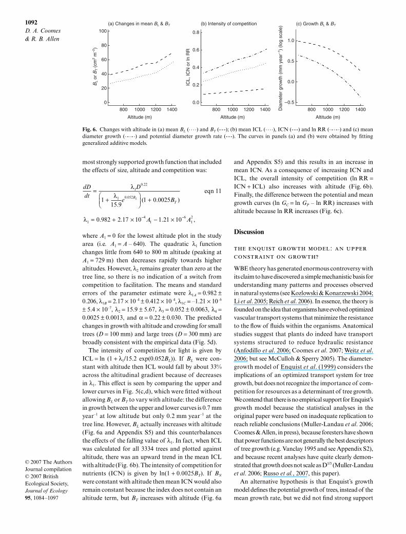
The intensity of competition for light is given byICL = ln (1 + λ1/15.2 exp(0.052BL)). If BL were con-stant with altitude then ICL would fall by about 33%across the altitudinal gradient because of decreasesin λ1. This effect is seen by comparing the upper andlower curves in Fig. 5(c,d), which were fitted withoutallowing BL or BT to vary with altitude: the differencein growth between the upper and lower curves is 0.7 mmyear–1 at low altitude but only 0.2 mm year–1 at thetree line. However, BL actually increases with altitude(Fig. 6a and Appendix S5) and this counterbalancesthe effects of the falling value of λ1. In fact, when ICLwas calculated for all 3334 trees and plotted againstaltitude, there was an upward trend in the mean ICLwith altitude (Fig. 6b). The intensity of competition fornutrients (ICN) is given by ln(1 + 0.0025BT). If BN

were constant with altitude then mean ICN would alsoremain constant because the index does not contain analtitude term, but BT increases with altitude (Fig. 6a

and Appendix S5) and this results in an increase inmean ICN. As a consequence of increasing ICN andICL, the overall intensity of competition (ln RR =ICN + ICL) also increases with altitude (Fig. 6b).Finally, the difference between the potential and meangrowth curves (ln GC = ln GP – ln RR) increases withaltitude because ln RR increases (Fig. 6c).

Discussion

:

WBE theory has generated enormous controversy withits claim to have discovered a simple mechanistic basis forunderstanding many patterns and processes observedin natural systems (see Kozlowski & Konarzewski 2004;Li et al. 2005; Reich et al. 2006). In essence, the theory isfounded on the idea that organisms have evolved optimizedvascular transport systems that minimize the resistanceto the flow of fluids within the organisms. Anatomicalstudies suggest that plants do indeed have transportsystems structured to reduce hydraulic resistance(Anfodillo et al. 2006; Coomes et al. 2007; Weitz et al.2006; but see McCulloh & Sperry 2005). The diameter-growth model of Enquist et al. (1999) considers theimplications of an optimized transport system for treegrowth, but does not recognize the importance of com-petition for resources as a determinant of tree growth.We contend that there is no empirical support for Enquist’sgrowth model because the statistical analyses in theoriginal paper were based on inadequate replication toreach reliable conclusions (Muller-Landau et al. 2006;Coomes & Allen, in press), because foresters have shownthat power functions are not generally the best descriptorsof tree growth (e.g. Vanclay 1995 and see Appendix S2),and because recent analyses have quite clearly demon-strated that growth does not scale as D1/3 (Muller-Landauet al. 2006; Russo et al., 2007, this paper).

An alternative hypothesis is that Enquist’s growthmodel defines the potential growth of trees, instead of themean growth rate, but we did not find strong support

dDdt

D

e BBT

L

.

( . )

.

.

=+

+

λλ

10 22

1 0 052115 9

1 0 0025

λ14

16

120 982 2 17 10 1 21 10 . . . ,= + × − ×− −A A

Fig. 6. Changes with altitude in (a) mean BL (. . . .) and BT (- - -); (b) mean ICL (. . . .), ICN (---) and ln RR (· - · - ·) and (c) meandiameter growth (· - · - ·) and potential diameter growth rate (- - -). The curves in panels (a) and (b) were obtained by fittinggeneralized additive models.

1093Effects on growth of size, competition and altitude

© 2007 The AuthorsJournal compilation © 2007 British Ecological Society, Journal of Ecology 95, 1084–1097

for this hypothesis in the case for mountain beech trees(Fig. 1b and Table 1). The reality was that tree growthwas immensely variable (Fig. 2a). The upper boundarywas diffuse, and this uncertainty meant that the upperpotential curve was ill-defined: for instance, simplychoosing the 95th rather than the 99th quantile in thequantile regression analysis resulted in α changingfrom 0.25 to 0.40 (Fig. 2b). Also, the values of α esti-mated by the regression analyses depended greatly on thechoice of function (Table 1). However, the alternativehypothesis cannot be rejected using evidence from justone species: further analyses may reveal that thescaling exponent is about 1/3 when averaged acrossspecies. Considerable differences among species are tobe expected, not least because the scaling of mass todiameter varies between species (Niklas 2004). Forexample, the conclusion that dD/dt ∝ D1/3 is based onan assumption that M ∝ D8/3 but empirical studies showthat species often deviate from this allometric relation-ship. Specifically, the mass-diameter relationships of 15North American tree species have exponents rangingfrom 2.15 to 2.74, with an average of 2.48 (recalculatedfrom Ter-Mikaelian & Korzukhin 1997). Thus, thegrowth curves of these species could have exponentsthat ranged from 0.26 to 0.85 even before other sourcesof uncertainty are considered (Li et al. 2005 and Russoet al. 2007). Some of these differences may result fromviolations of some assumptions of the branching modelsthat are fundamental to WBE theory (Enquist et al.2007). Therefore the potential growth rate curves of alarge number of species need to be estimated before anyconclusions can be reached about the generality of thealternative scaling theory.

Forest ecologists universally appreciate the importanceof light as a limiting factor for tree growth (e.g. Pacalaet al. 1996; Smith et al. 1997; Herwitz et al. 2000;Canham et al. 2004; Uriarte et al. 2004; Wyckoff & Clark2005). The light extinction coefficient of mountainbeech was estimated to be 0.53. This equates with about4% of light being transmitted through a canopy with aleaf area index of six, which is typical for mountainbeech (Hollinger 1989). This diminution of light by thecanopy is less than that commonly observed in manytropical and temperate forests (Coomes & Grubb 2000),but is still likely to have strong effects on the growthof subordinates, especially as mountain beech is alight-demanding species (Wardle 1984). Competitionfor light alters the shape of the growth curve becauseshorter trees are more deeply shaded, on average, thantaller trees, and so are particularly strongly affected bylight competition (Weiner 1990; Muller-Landau et al.2006). This situation is likely to be universal in naturalforests (e.g. Wyckoff & Clark 2005; Sheil et al. 2006), soa systematic deviation of the mean growth curve fromdD/dt ∝ D1/3 will be observed generally (Coomes 2006).

The huge variability in growth rate observed in thisstudy (Fig. 2) is typical of that reported elsewhere (e.g.Van Mantgem & Stephenson 2005), and reflects theability of trees to alter metabolic rates in response toresource supply (Harper 1977; Grubb 1992; Reich et al.2006). The ontogenetic growth of any particular tree ina natural population is unlikely to bear much resem-blance to a scaling function because trees may spendlong periods of time suppressed in deep shade followedby relatively brief interludes of fast growth in high lightwhen openings are created above them by tree-fallevents (e.g. Uhl & Murphy 1981; Wright et al. 2000).

Growth was also affected by competition for nutrients,and intense competition for nitrogen is known tooccur in mountain beech forests: substantial increasesin growth rate have been reported when trenches are cutaround seedlings to isolate them from root competitionwith established trees (Platt et al. 2004), and nitrogenaddition results in large increases in fine root and seedproduction (Davis et al. 2004). More generally, Coomes& Grubb (2000) have reported that root trenchingresults in increased growth rates in many forest types,and particularly when the seedlings are growing inrelatively well illuminated forest understoreys. Manymodels of tree growth include sophisticated functionsof light interception by neighbours (e.g. Pacala et al.1996), but very few attempt to include competition forbelow-ground resources (Canham et al. 2004). Furtherprogress will require the development of a mechanisticunderstanding of root competition and nutrient reten-tion. We were not able to derive a mechanistic modelwithout being speculative about the ways in which fineroots compete for nutrients, and plants recycle andstore nutrients (Reich et al. 2006), and we are awarethat competitive intensity may not be related to BT inthe way we have supposed (Weiner 1990; Schwinning& Weiner 1998). A mixture of experimentation andmodelling is required to make further progress (Tilmanet al. 2004).

Diameter growth rates declined with altitude, and thiswas associated with a shortening of growing seasonand reduction in mean summer temperatures (Wardle1984). Physiological studies have also reported sub-stantial losses of productivity with altitude in mountainbeech stands, resulting from falls in both photo-synthetic and respiration rates (Table 2). However, theBoltzmann–Arrhenius function did not adequatelyrepresent the fall in growth rate; the decline in growthrate above 1100 m was greater than predicted. Perhapsthe Boltzmann–Arrhenius function adequately modelsthe decline in growth with altitude that result fromfalling temperatures, but fails to capture the negativeeffects of mineral nutrient shortage or strong winds.For example, phosphorus availability is known todecline with altitude across our 246 mountain beechplots (r = –0.29, P < 0.0001; R. B. Allen, unpublished

1094D. A. Coomes & R. B. Allen

© 2007 The AuthorsJournal compilation © 2007 British Ecological Society, Journal of Ecology 95, 1084–1097

data), and may contribute to slow growth at highaltitudes. Alternatively, it may be that the metabolicresponse of plants to temperature variation is morecomplex than that encapsulated by the thermodynamicsformula (Clarke 2004). Enquist et al. (1999) has sug-gested wood density variation might also contribute tochanging growth rates. The wood density of mountainbeech increase by 13% from the lowest to the highestelevation sites in the study area (0.47–0.53 g cm–3;Jenkins 2005), which is much less than the change indiameter growth rate.

The debate on changes in competition intensity withenvironmental gradients is one of the most protractedin plant community ecology (e.g. Grime 1977; Tilman1988; Grace 1991; Goldberg et al. 1999; Craine 2005).Our analyses indicate that competition intensityincreased with altitude, but this is exactly opposite tothe trend we had expected. Previous studies of light-demanding Nothofagus species in Chile have indicatedthat competition has its strongest influence on standdynamics at low altitudes (Pollman & Veblen 2004).Mountain-beech trees produce only about half as muchwood and leaf biomass at high altitude than at mid-altitude, whilst producing a similar amount of rootbiomass (Table 2; Benecke & Nordmeyer 1982). As aresult, high altitude trees are stunted, have opencanopies, and allow more light to be transmitted to theforest floor (D.A. Coomes, unpublished data). Thus,while we anticipated that the intensity of competitionfor light would diminish with altitude, the analysessuggest the opposite. Why did our findings differ somarkedly from our expectations?

Understanding why basal area increases withaltitude may hold the key to resolving this paradox.The only reason that competition intensity increaseswith altitude is because mean basal area increaseswith altitude (Fig. 6); had basal area been invariantof altitude then our analyses would have predicted adecline in competition intensity with altitude (Fig. 5c,d).So why does basal area increase with altitude? One

possibility is that spatial variation in disturbance hascreated the observed pattern: many trees at low andmid-altitudes died after being damaged by snow stormsin 1968 and 1972, whereas trees at high altitude weremuch less affected, and we know that the forest is indisequilibrium as a result of temporal variation in distur-bance frequency (Wardle & Allen 1983; Allen et al. 1999;Coomes & Allen 2007). If differences in disturbance historyare responsible for the observed increases in basal areawith altitude, then resurveying the plots in, say, 100 yearstime might give the opposite trend! From this perspectiveit seems more logical to calculate competitive intensitieswith basal area kept constant. When this is done, theregression analyses are consistent with expectations:ICL declines with altitude whereas ICN stays constant,so competition for light is most intense at low altitude andcompetition for nutrients is most intense at the tree line.This fits with the idea that trees respond plastically tochanging rates of resource supply by allocating morecarbon to above-ground tissues when below-groundresources are relatively abundant, and allocating morecarbon to roots when nutrients are scarce (Bloom et al.1985; Tilman 1988; Gleeson & Tilman 1992). The keyquestion is whether disturbance history really is the driverof the basal area trend, or whether it is underpinned byphysiological processes. Further investigation is requiredinto this issue.

Irrespective of whether competition intensity in-creases or decreases with altitude, when expressed inabsolute terms, the effect of competition on growth wasgreatest at low altitude (Grace 1991): shading reducedthe growth of small trees by about 7 mm year–1 at 640 maltitude but by only 2 mm year–1 at the tree line(Fig. 5c). These findings are broadly consistent withthe theory of Grime (1977), that plants associated withproductive habitats are inherently fast growing andtheir fast growth rates allow pre-emptive capture ofresources from neighbours, while plants associatedwith ‘stressed’ sites have traits that allow them to surviveharsh conditions, but also result in slow growth rate.

Table 2. Estimated annual C balance (T C ha–1 year–1) for montane (1000 m a.s.l.) and subalpine (1320 m a.s.l.) mountain beechstands in the study area (adapted from data in Benecke & Nordmeyer 1982). Subalpine values are given as a proportion ofmontane values.

Altitude (m)

Proportion1000 1320

Whole plantPhotosynthesis 37.1 15.7 0.42Respiration 20.3 6.7 0.33Net growth 16.8 9.0 0.54

Growth allocationFoliage 4.7 2.6 0.55Branch 4.9 1.7 0.35Stemwood 4.4 2.2 0.50Coarse roots 0.8 0.7 0.88Fine roots 2.0 1.8 0.90Total growth 16.8 9.0 0.54

1095Effects on growth of size, competition and altitude

© 2007 The AuthorsJournal compilation © 2007 British Ecological Society, Journal of Ecology 95, 1084–1097

The fact that growth rates are slow in ‘stressed’ habitatsmeans that competition may go undetected unlessstudies are well replicated and monitored over long timeframes. This may explain why most studies in stressedhabitats do not detect competitive interactions. Severalrecent experiments have reported that competitiveinteractions give way to facilitation interactions athigh altitude (Callaway 1995; Brooker & Callaghan1998; Callaway et al. 2002), and have brought to atten-tion the hitherto neglected importance of facilitationin plant community dynamics. However, our study didnot unearth fresh evidence of facilitation. We hadanticipated that facilitation might be important inhigh-altitude forests of mountain beech because treesexperience similar conditions to those in Callaway’sstudy (Wardle 1984), but no evidence was found despiteour analyses being based on high numbers of replicates.Given the nature of plastic above- and below-groundgrowth responses by tree species along gradients, wesuggest resolving differences among studies may requirecomprehensive data on allocation patterns in trees. Forexample, reduced diameter growth near the tree line, uponthe loss of neighbours, may reflect increased allocationof growth below-ground to capture soil resources.

Finally, the potential growth rate had the samescaling exponent at all altitudes (α = 0.22). If potentialgrowth rate is controlled by the design of the internaltransport systems, then this finding suggests that theevolutionary design of the transport system is similaracross the sequence. A recent study of the wood anat-omy of mountain beech trees sampled at three altitudesshowed that the vascular systems were all remarkablysimilar in structure, and that the scaling of vessel sizeswithin the trees was broadly consistent with the designthat WBE theory predicts would minimize resistanceto hydraulic flow (Coomes et al. 2006). Therefore ouranalyses support some aspects of scaling theoy (Westet al. 1997), but not Enquist’s theory of tree growth.

Conclusions

Our study is the first to build the effects of competitionand environment into Enquist’s model of tree growth.We show that competitive interactions alter the scalingof mean growth rate with size, whereas altitude doesnot influence the scaling of potential growth ratewith size. Ecologists need to include the effects ofcompetition for light and nutrients and various types ofdisturbance into models of size-dependent processes, asthese factors swamp out the potentially real effects thatWBE theory might encapsulate (Tilman et al. 2004).

Acknowledgements

We thank John Wardle for his foresight in establishingthe plot network in the early 1970s, the many fieldcrews that have collected data over the years, and theNational Vegetation Survey Databank for making thedata available. We are particularly grateful to Larry

Burrows and Kevin Platt for fieldwork and checkingthe data. Lawren Sack provided helpful comments onthe manuscript. The work was supported by UK-NERC,the former New Zealand Forest Service, Departmentof Conservation and the New Zealand Foundation forResearch, Science and Technology (Contract C09X0502).The research benefited from discussions as part of theAustralian Research Council – New Zealand networkon Vegetation Function and Futures.

ReferencesAllen, R.B. (1993) A Permanent Plot Method for Monitoring

Changes in Indigenous Forests Manaaki Whenua – LandcareResearch New Zealand Ltd, Christchurch, New Zealand.

Allen, R.B., Bellingham, P.J. & Wiser, S.K. (1999) Immediatedamage by an earthquake to a temperate montane forest.Ecology, 80, 708–714.

Anfodillo, T., Carraro, V., Carrer, M., Fior, C. & Rossi, S.(2006) Converging tapering of xylem conduits in differentwoody species. New Phytologist, 169, 279–290.

Benecke, U. & Nordmeyer, A.H. (1982) Carbon uptake andallocation by Nothofagus Solandri var. cliffortioides (Hook. f.)Poole and Pinus contorta Douglas ex Loudon ssp. contortaat montane and subalpine altitudes. Carbon Uptake andAllocation in Subalpine Ecosystems as a Key to Management(ed. R.H. Waring), pp. 9–21. Forest Research Laboratory,Oregon State University, Corvallis.

Bloom, A.J., Chapin, F.S. & Mooney, H.A. (1985) Resourcelimitation in plants. An economic analogy. Annual Reviewof Ecology and Systematics, 16, 363–392.

Brooker, R.W. & Callaghan, T.V. (1998) The balance betweenpositive and negative plant interactions and its relationshipto environmental gradients: a model. Oikos, 81, 196–207.

Burnham, K.P. & Anderson, D.R. (2002) Model Selection andMultimodel Inference: A Practical Information–TheoreticalApproach, 2nd edn. Springer-Verlag, New York, NY.

Cade, B.S. & Guo, Q. (2000) Estimating effects of constraintson plant performance with regression quantiles. Oikos, 91,245–254.

Cade, B.S., Terrell, J.W. & Schroeder, R.L. (1999) Estimatingeffects of limiting factors with regression quantiles. Ecology,80, 311–323.

Callaway, R.M. (1995) Positive interactions among plants.Botanical Reviews, 61, 306–349.

Callaway, R.M., Brooker, R.W., Choler, P., Kikvidze, Z.,Lortie, C.J., Michalet, R., Paolini, L., Pugnaire, F.I.,Newingham, B., Aschehoug, E.T., Armas, C., Kikodze, D.& Cook, B.J. (2002) Positive interactions among alpineplants increase with stress. Nature, 417, 844–848.

Canham, C.D., LePage, P.T. & Coates, K.D. (2004) A neigh-bourhood analysis of canopy tree competition: effectsof shading versus crowding. Canadian Journal of ForestResearch, 34, 778–787.

Clarke, A. (2004) Is there a universal temperature dependenceof metabolism? Functional Ecology, 18, 252–256.

Coomes, D.A. (2006) Challenges to the generality of WBEtheory. Trends in Ecology and Evolution, 21, 593–596.

Coomes, D.A. & Allen, R.B. (2007) Mortality and tree-sizedistributions in natural mixed-age forests. Journal of Ecology,95, 27–40.

Coomes, D.A. & Allen, R.B. (in press) The statistical basic ofscaling theories. Journal of Ecology.

Coomes, D.A., Jenkins, K.L. & Cole, L. (2007) Scaling of treevascular transport systems along gradients of nutrientsupply and altitude. Biology Letters, 3, 86–89.

Coomes, D.A. & Grubb, P.J. (2000) Impacts of root competi-tion in forests and woodlands: a theoretical framework andreview of experiments. Ecological Monographs, 70, 171–207.

1096D. A. Coomes & R. B. Allen

© 2007 The AuthorsJournal compilation © 2007 British Ecological Society, Journal of Ecology 95, 1084–1097

Craine, J.M. (2005) Reconciling plant strategy theories ofGrime and Tilman. Journal of Ecology, 93, 1041–1052.

Davis, M.R., Allen, R.B. & Clinton, P.W. (2004) The influenceof N addition on nutrient content, leaf carbon isotope ratio,and productivity in a Nothofagus forest during standdevelopment. Canadian Journal of Forest Research, 34,2037–2048.

Enquist, B.J. (2002) Universal scaling in tree vascular plantallometry: toward a general quantitative theory linking formand functions from cells to ecosystems. Tree Physiology, 22,1045–1064.

Enquist, B.J., Allen, A.P., Brown, J.H., Gillooly, J.F., Kerkhoff, A.J.,Niklas, K.J., Price, C.A. & West, G.B. (2007) Does theexception prove the rule? Nature, 445, E9–E10.

Enquist, B.J., Economo, E.P., Huxman, T.E., Allen, A.P.,Ignace, D.D. & Gillooly, J.F. (2003) Scaling metabolismfrom organisms to ecosystems. Nature, 423, 639–642.

Enquist, B.J., West, G.B., Charnov, E.L. & Brown, J.H. (1999)Allometric scaling of production and life-history variationin vascular plants. Nature, 401, 907–911.

R Foundation (2006) The R project for statistical computing.http://www.r-project.org.

Freckleton, R.P. & Watkinson, A.R. (2001) Nonmanipulativedetermination of plant community dynamics. Trends inEcology and Evolution, 16, 301–307.

Gleeson, S.K. & Tilman, D. (1992) Plant allocation and themultiple limitation hypothesis. American Naturalist, 139,1322–1343.

Goldberg, D.E., Rajaniemi, T., Gurevitch, J. & Stewart-Oaten, A. (1999) Empirical approaches to quantifyinginteraction intensity: competition and facilitation alongproductivity gradients. Ecology, 80, 1118–1131.

Grace, J.B. (1991) A clarification of the debate between Grimeand Tilman. Functional Ecology, 5, 583–587.

Griffiths, G.A. & McSaveney, M.J. (1983) Distribution of meanannual precipitation across some steepland regions of NewZealand. New Zealand Journal of Science, 26, 197–210.

Grime, J.P. (1977) Plant Strategies and Vegetation Processes.John Wiley, Chichester.

Grubb, P.J. (1992) A positive distrust in simplicity-lessonsfrom plant defences and from competition among plantsand among animals. Journal of Ecology, 80, 585–610.

Harcombe, P.A., Allen, R.B., Wardle, J.A. & Platt, K.H.(1998) Spatial and temporal patterns in stand structure,biomass, growth and mortality in a monospecificNothofagus solandri var. cliffortioides (Hook. f.) Pooleforests in New Zealand. Journal of Sustainable Forestry, 6,313–345.

Harper, J.L. (1977) Population Biology of Plants. Academic Press.Herwitz, S.R., Slye, R.E. & Turton, S.M. (2000) Long-term

survivorship and crown area dynamics of tropical rainforest canopy trees. Ecology, 81, 585–597.

Högberg, P. & Read, D.J. (2006) Towards a more plant physio-logical perspective on soil ecology. Trends in Ecology andEvolution, 21, 548–554.

Hollinger, D.Y. (1989) Canopy organization and foliage photo-synthetic capacity in a broad-leaved evergreen montaneforest. Functional Ecology, 3, 53–62.

Jarvis, P.G. & Leverenz, J.W. (1983) Productivity of temperate,deciduous and evergreen forests. Encyclopedia of PlantPhysiology: Productivity and Ecosystem Processes, pp. 234–280. Springer-Verlag, Berlin.

Jenkins, K.L. (2005) Some properties of New Zealand woods.Unpublished M.Phil. Thesis, University of Cambridge.

Kozlowski, J. & Konarzewski, M. (2004) Is West, Brown andEnquist’s model of allometric scaling mathematicallycorrect and biologically relevant? Functional Ecology, 18,283–289.

Li, H.T., Han, X.G. & Wu, J.G. (2005) Lack of evidence for3/4 scaling of metabolism in terrestrial plants. Journal ofIntegrative Plant Biology, 47, 1173–1183.

Maestre, F.T., Valladares, F. & Reynolds, J.F. (2005) Is thechange of plant–plant interactions with abiotic stresspredictable? A meta-analysis of field results in arid environ-ments. Journal of Ecology, 93, 748–757.

McCracken, I.J. (1980) Mountain climate in the CraigieburnRange, New Zealand. Mountain Environments and SubalpineTree Growth (eds U. Benecke & M.R. Davis), pp. 41–59.Forest Research Institute Bulletin, 70, Christchurch, NewZealand.

McCulloh, K. & Sperry, J. (2005) Patters in hydraulicarchitecture and their implications for transport efficiency.Tree Physiology, 25, 257–267.

Muller-Landau, H.C. & 42 others (2006) Comparing tropicalforest tree size distributions with the predictions of metabolicecology and equilibrium models. Ecology Letters, 9, 589–602.

Niklas, K.J. (2004) Plant allometry: is there a grand unifyingtheory? Biology Reviews, 79, 871–889.

Osawa, A. & Allen, R.B. (1993) Allometric theory explainsself-thinning relationships of mountain beech and red pine.Ecology, 74, 1020–1032.

Pacala, S.W., Canham, C.D., Saponara, J., Silander, J.A.,Kobe, R.K. & Ribbens, E. (1996) Forest models defined byfield measurements. II. Estimation, error analysis anddynamics. Ecological Monographs, 66, 1–43.

Platt, K.H., Allen, R.B., Coomes, D.A. & Wiser, S.K. (2004)Mountain beech seedling responses to removal of below-ground competition and fertiliser. New Zealand Journal ofEcology, 28, 289–293.

Pollmann, W. & Veblen, T.T. (2004) Nothofagus regenerationdynamics in south-central Chile: a test of a general model.Ecological Monographs, 74, 615–634.

Reich, R.B., Tjoelker, M.G., Machado, J.L. & Oleksyn, J.(2006) Universal scaling of respiratory metabolism, sizeand nitrogen in plants. Nature, 439, 457–461.

Richardson, S.J., Allen, R.B., Whitehead, D., Carswell, F.E.,Ruscoe, W.A. & Platt, K.H. (2005) Climate and net carbonavailability both determine seed production in a temperatetree species. Ecology, 86, 972–981.

Russo, S., Wiser, S.W. & Coomes, D.A. (2007) Growth-sizescaling relationships of woody plant species differ frompredictions of the Metabolic Ecology Model. Ecology Letters,doi: 10.1111/j.1461-0248.2007.01079.x.

Schwinning, S. & Weiner, J. (1998) Mechanisms determiningthe degree of size asymmetry in competition among plants.Oecologia, 113, 447–455.

Sheil, D., Salim, A., Chave, J., Vanclay, J. & Hawthorn, W.D.(2006) Illumination-size relationships of 109 coexistingtropical forest tree species. Journal of Ecology, 94, 494–507.

Smith, D.M., Larson, B.C., Kelty, M.J. & Ashton, P.M.S.(1997) The Practice of Silviculture: Applied Forest Ecology.John Wiley, New York, NY.

Ter-Mikaelian, M.T. & Korzukhin, M.D. (1997) Biomassequations for sixty-five North American tree species. ForestEcology and Management, 97, 1–24.

Thomson, J.D., Weiblen, G., Thomson, B.A., Alfaro, S. &Legendre, P. (1996) Untangling multiple factors in spatialdistributions: lilies, gophers, and rocks. Ecology, 77, 1698–1715.

Tilman, D. (1988) Plant Strategies and the Dynamics and Structureof Plant Communities. Princeton University Press, NJ.

Tilman, D., Hille Ris Lambers, J., Harpole, S., Dybzinski, R.,Fargione, J., Clark, C. & Lehman, C. (2004) Does metabolictheory apply to community ecology? It’s a matter of scale.Ecology, 85, 1797–1799.

Uhl, C. & Murphy, P.G. (1981) Composition, structure, andregeneration of tierra firme forest in the Amazon Basin ofVenezuela. Tropical Ecology, 22, 219–237.

Uriarte, M., Canham, C.D., Thompson, J. & Zimmerman,J.K. (2004) A neighborhood analysis of tree growth andsurvival in a hurricane-driven tropical forest. EcologicalMonographs, 74, 591–614.

1097Effects on growth of size, competition and altitude

© 2007 The AuthorsJournal compilation © 2007 British Ecological Society, Journal of Ecology 95, 1084–1097

Van Mantgem, P.J. & Stephenson, N.L. (2005) The accuracyof matrix population model projections for coniferous treesin the Sierra Nevada, California. Journal of Ecology, 93,737–747.

Vanclay, J.K. (1995) Growth models for tropical forests:a synthesis of models and methods. Forest Science, 41, 7–42.

Wardle, J.A. (1984) The New Zealand Beeches. New ZealandForest Service, Christchurch, New Zealand.

Wardle, J.A. & Allen, R.B. (1983) Dieback in New ZealandNothofagus forests. Pacific Science, 37, 397–404.

Weiner, J. (1990) Asymmetric competition in plant populations.Trends in Ecology and Evolution, 5, 360–364.

Weitz, J.S., Ogle, K. & Horn, H.S. (2006) Ontogenetically stablehydraulic design in woody plants. Functional Ecology, 20,191–199.

West, G.B., Brown, J.H. & Enquist, B.J. (1997) A generalmodel for the origin of allometric scaling laws in biology.Science, 276, 122–126.

Wright, E.F., Canham, C.D. & Coates, K.D. (2000)Effects of suppression and release on sapling growthfor 11 tree species of northern, interior BritishColumbia. Canadian Journal of Forest Research, 30, 1571–1580.

Wyckoff, P.H. & Clark, J.S. (2005) Tree growth predictionusing size and exposed crown area. Canadian Journal ofForest Research, 35, 13–20.

Received 20 February 2007; accepted 30 May 2007Handling Editor: Susan Schwinning

Supplementary material

The following supplementary material is available forthis article:

Appendix S1. Biological basis for the light competi-tion function.

Appendix S2. Alternative growth models notdescribed in main body of paper.

Appendix S3. Correlations between BT and BL.

Appendix S4. Changes in BT and BL with size.

Appendix S5. Increases in BT and BL with altitude.

This material is available as part of the online articlefrom http://www.blackwell-synergy.com/doi/abs/10.1111/j.1365-2745.2007.01280.x

Please note: Blackwell Publishing is not responsiblefor the content or functionality of any supplementarymaterials supplied by the authors. Any queries (otherthan missing material) should be directed to the cor-responding author of the article.