Embed Size (px)
Citation preview

Journal of Statistical Planning and Inference 27 (1991) 105-123
North-Holland
105
Efficient estimation of the stationary distribution for exponentially ergodic Markov chains
Spiridon Penev *
Institute of Applied Mathematics & Informatics, 1000 Sofia, Bulgaria
Received 4 April 1989; revised manuscript received 21 September 1989
Recommended by J. Pfanzagl
Abstract: In a classical paper by Dvoretsky, Kiefer and Wolfowitz the asymptotic minimaxity of the em-
pirical distribution function in case of i.i.d. observations X1,X,, . . ..X. of the random variable X has
been shown. If X,,X,, . . . ,X,,, . . . is only a stationary sequence we still could use the empirical distribu-
tion function as an estimator of the (continuous) stationary distribution F. But the question of its asymp-
totic efficiency arises in this case. Under some additional assumptions (stationary homogeneous
exponentially ergodic Markov sequence) we show that the empirical distribution function is an efficient
estimator in a local asymptotic minimax sense.
Using the bounded subconvex loss function g(sup, fi IF,,(t)-F(t)J) with g-bounded, increasing, the
local asymptotic minimax bound equals Eg(sup IY(t)l) w h ere Y(t) is a certain Gaussian process.
AMS Subject Classification: Primary 62G20, 62M05; secondary 62605, 62G30.
Key words and phrases: Local asymptotic minimaxity; empirical distribution function; Markov
sequences; stability.
1. Introduction
The problem of asymptotic minimaxity of the empirical distribution function
(EDF) has attracted the attention of many statisticians. In a pioneering paper of
Dvoretsky, Kiefer and Wolfowitz (1956) it was shown that in case of i.i.d. observa-
tions the EDF is asymptotically minimax among the collection of all continuous
distributions. As Millar (1979) notes, “This paper has stood for over 20 years as one
of the pivotal achievements of nonparametric decision theory”.
One direction for generalizing this result was to show the asymptotic minimax
character of the EDF in case i.i.d. among smaller classes of DF’s (such as the class
of the concave distributions, the distributions having a decreasing density with
respect to Lebesgue measure, the IFR-distributions and so on).
* Research partially supported by the Ministry of Culture, Science and Education in Bulgaria; Con-
tract 1035.
0378-3758/91/$03.50 0 1991-Elsevier Science Publishers B.V. (North-Holland)

106 S. Penev / Efficient estimation of the stationary distribution
Kiefer and Wolfowitz (1976) proved the asymptotic minimaxity of the EDF in the
class of all concave distributions. In the papers Millar (1979, 1983), using the
modern technique of convergence of experiments and the general formulation of the
asymptotic minimax theorem of Le Cam (1972), the asymptotic minimaxity of the
EDF among each of the above mentioned (and also other) classes was shown.
On the other hand it was natural to try to generalize the results of Dvoretsky,
Kiefer and Wolfowitz in another direction - namely to avoid the i.i.d. assumption.
Indeed this makes the problem harder, but there exists a result of Billingsley (1968)
in the literature, showing the existence of a limit distribution for the EDF of a sta-
tionary q-mixing sequence of observations. This bolstered our feeling that it could
be done similarly for weakly dependent observations. Also there was the book of
Roussas (1972), showing the possibility to prove local asymptotic minimax optimali-
ty of estimators and tests in parametric situations also in case of observations arising
from stationary ergodic Markov sequences. As far as we know, not much has been
done in applying this in nonparametric situations.
Our contribution here is, using the theory of convergence of experiments, to show
that the (piecewise linear and continuous version of the) EDF for a special class of
stationary ergodic Markov sequences possesses a local asymptotic minimax (LAM)
optimality property.
We do not strive for the utmost generality in the assumptions because this would
make the proofs more involved. Also the discussion will be heuristic in some part.
Let us start with a concise outline of the probabilistic setting we deal with.
We consider a homogeneous Markov chain X= (Xn)nkO taking values in (E, %).
Here E = [0, l] and YI3 its Bore1 a-field. The chain has a regular transition probability
kernel P(x,A),xe [0, l],A E % and (to begin with) arbitrary initial distribution
g(xo). We assume that the following condition holds:
Condition (A). Existence of bounded density, i.e. a bounded function p(y 1 x) on
the unit square such that
P(x,A) = i
P(Y 1 xl dy A
for all A E S& VXE [0, 11 and, moreover, inf, p(y 1 x)26>0 for all Y in a set S with
positive Lebesgue measure h(s) > 0.
This condition has important consequences:
(i) Doeblin’s condition holds.
(ii) There is a uniquely defined invariant probability measure rr for P( . , . ) and
moreover exponential convergence holds, i.e. there exist qe (0, l),a>O such that
;trr ;;g IP”(x,B)--rc(B)I 5aqn for all n.

S. Penev / Efficient estimation of the stationary distribution 107
(Loeve (1960, Chapter VII, 27.3), Doob (1956, p. 197)). Here P”(. , .) denotes the
n-step transition probability kernel.
(iii) If 9(X0) := n then the sequence X= (X,,)nZo is stationary and v-mixing with
v(n) =aq”. Here we use the definition of p-mixing sequence given in Billingsley
(1968, Chapter 20, 20.2).
(iv) 7reA lE. Th’ f 11 is o ows easily from the equality n=nP and the fact that
p( . , . ) is bounded.
Additionally to Condition (A) we assume:
Condition (B). Z- 2 lE.
After these probabilistic preliminaries let us introduce the statistical model we
consider. Suppose we have weakly dependent observations x0, xi, x2, . . . ,x, from a
stationary Markov chain X with (unknown) transition probability kernel P( . , - ) and initial law 9(X0)= 71 satisfying Conditions (A) and (B). The problem is to
estimate the stationary distribution function F. Of course we still could use the EDF
as we would certainly do (relying on the result of Dvoretsky, Kiefer and Wolfowitz)
if the observations were i.i.d. But now the question of the asymptotic efficiency of
this estimator arises. We shall see (Theorem 5.1 and Corollary 5.1) that the
(piecewise linear and continuous version of the) EDF preserves its optimality in a
local asymptotic minimax sense.
2. Perturbations and stability
Now we would like to discuss the difficulties which arise when we try to describe
LAM lower bounds in non-i.i.d. situations. The complexity here is of qualitative
nature. Let us explain it in some words. In order to describe LAM lower bounds
one has to consider perturbations of a given probability structure in a neighborhood of this structure. Now in the i.i.d. case describing such neighborhoods is an easy
job because once perturbed the density for one observation, one has already per-
turbed the whole (product-density) structure. In case of dependency there are much
more possibilities for perturbance. But they also can not be too much because one
has to preserve the main properties of the structure (e.g. stationarity, ergodicity)
after the perturbation. That means that the structure has to possess some kind of
stability.
To describe this property we have first to define the perturbations of the chain
in a suitable form.
Let H be the set of all measurable functions h(x,y) on the unit square with
E h2(Xo,X,)< 03, E(h(X,,X,) 1 X0) = 0 almost surely. H is a Hilbert space with
respect to the scalar product
(hi,&) = Eh,Wo,X,MXo,X,).
108 S. Penev / Efficient estimation of the stationary distribution
Let p( . ) denote the density of n with respect to A IE.
We denote the corresponding norm by
llhll ?f = jj h2(x>y)p(_v 1 x)&4 dy h.
Let HO be the subset of all bounded (sup-norm) h E H. Then H, is dense in H
which follows for example from Strasser (1985, Lemma 75.5). For h E HO and suf-
ficiently large n define the (perturbed) transition kernel P,,,\ii; by:
ph/di (XT A ) = c P(Y I-9(1 + W,Wfi) dy = s Ph,dY 1 X> dy. A A
Now we shall see that under small perturbations of the kernel P( . , a) of the form
prescribed the chain X remains geometrically ergodic with invariant probability
=h/di - Tt.
It is obvious that Condition (A) remains valid under small perturbations using
kernels Ph/fi if h E HO and n is large enough for it will exist a positive constant
6, I 6 such that
infph/fi(y 1 x)>dl>o if inf& ) x)z6>0. x x
For n large enough we get transition probability kernels Ph,\i;2(. , . ) satisfying
Condition (A) for all h E H,,. Hence (cf. (ii)- after Condition (A)), a unique in-
variant probability zh,,&, (. ) for Ph/fi(. , . ) exists with nh/j, 4 il for all h E HO.
The following lemma is true:
Lemma 2.1. For n large enough, under the Conditions (A) and (B) it holds
7th/fi -A IEfor all hEHo.
This lemma shows that also Condition (B) remains valid under the small perturba-
tions we consider.
Corollary 2.1. For n large enough, zh/\i;; - rc for all h E HO.
Our next step is to see that not only remain Conditions (A) and (B) valid for the
small perturbations described, but also a kind of stability property is true. To
describe it let us denote by m the set of finite signed measures on [0, l] endowed with
the variation norm 11 . I/ (which makes it a Banach space). The kernel P( . , -) defines
a linear mapping m + m by fiP( .) = 1 p(dx)P(x, . ) for p E m. The norm II . 11 defines
in a natural way a norm in the space of linear bounded operators B : m + m by
IIBII =sup( IIiuBII: lliull% 1). Let us fix some arbitrary d>O. Denote
Kd = h EH: sup lh(x,y)j cd .
X,Y I

S. Penev / Efficient estimation of the stationary distribution 109
The stability property means that for all h E Kd and all n 1 n,(d) a constant C(P)
exists such that
/I n- =h/\in 11 i c(p> 11 ph/\l;l - p 11. (2.1)
In a more general framework and for general norms such stability requirements
are studied in Kartashov (1981) and Kartashov (1984) who considers the so-called
strongly stable Markov chains. For the variation norm we consider it was shown in
Neveu (1964, Chapter V.3.2) (cf. also Kartashov (1981)) that strong stability and in
particular (2.1) is ensured by Doeblin’s condition. Hence (cf. (i) after Condition
(A)), (2.1) holds in our case.
For a given h EH~ and n large enough nh,,,$ --71. Write the density (dn(h,\i,)/
drc)(x) in the form l+&(x). If SUP~,~ lh(x,y))~C, and sup,,,p(y/x)~C,, C=
C, . C,, then: supll~~l c 1 11 pPh,& - P)ll4 I?&%. Hence:
IIPh,fi - PI/ i c/hi. (2.2)
Finally using (2.1) we get:
fill 7r - nh/vs 11 = V%Z " ~h_(x)~(x)~ dKdic(P)lIPh,vi;-P 11 Ice.
1 (2.3)
0
Write P#,x for the law of X0, Xi,. . . ,X,, under Ph/\ii2( . ) and 9(X0) = nh/&. Denote
by pi;,( .) the density with respect to A lE of the measure ?rh&.
Lemma 2.2. Under conditions (A) and (B) it holds
loi3 dP/$& - (X0, x, 3 . . . >
dP,j”’ X,) =&h-i llhll~+o~,y(l)
where An,h s N(0, I( hll$) under PF’.
3. The construction of the mapping z
Now we want to introduce the main steps in finding the LAM bound for the
estimators or the stationary distribution of the chain. We are going to follow Millar
(1983, Chapter VIII).
Fix some h E Ho. Write v, for zh/“;l and Q,( . , . ) for Ph,dx(. , . ).
Let us consider F J&(u) = 10” pg,(X) dX. It holds:
-iI F,,du) = Fe(u) +
I h-WPW dx.
I; 0
Here, of course, F,(u) = F(u) = jt p(x) d_x = x([O, u]). We have:
&(F,,~(u) -F(U)) = fi [” h-,(x)p(x) ti = G(~, - rr)[~, 4. -0
(3.1)

110 S. Penev / Efficient estimation of the stationary distribution
Crucial in the sequel is the following presentation given in Kartashov (1981) and
Kartashov (1984):
v, = rt(Z- (Q, - P)R)-’ (valid for large n).
Here R = (Z- P+ZZ-' =ZZ+ CT=*=, (P'-ZZ) and ZZ= 1 on is the stationary projector
of the transition kernel P, i.e. ZZ(x, dy) = n[O, 11. rr(dy). By Z we denote the identity
mapping I: m + m and by QP: QP(x,A) = j Q(x, dy)P(y,A). The operator R is
bounded because of the strong stability property (Kartashov (1981, Theorem 1)).
For large n we can present v, as a convergent sum:
v,= ~[Z+(Q,-P)R+((Q,-P)R)2+~~~]
= n(Z+(Q,-P)R)+o(IIQ,-PII)=n(Z+(Q,-P)R)+o(l/fi)
For the last equality (2.2) has also been used.
Hence
fi(v, - n)
=&T(Q~-P)R+o(I)=&(Q,-P) ZZ+[!~(P~-n)]+o(l). L
In view of the obvious equality (Q, - P)Zi'= 0 we have:
fi(P,,&-F(u)) =\/;;n(Q,-P,.~~~(P’-n)lo,u)+o(l). (3.2)
Let us denote by #)(y 1 x) the k-step transition density. Then (3.2) may be writ-
ten in the form
fi(Ph,fi(~) -P(u))
111 1 =
I .I’ W, Y)P(Y 1 X)P(X) dx dy
0 0
+kE,
U I
1i.i
I ZG,Y)P(Y 1 x)~(x)P’% 1~) kdydz+o(l).
0.0 0
This gives rise to the following definition of the mapping tl : H+B (B - the
Banach space of continuous functions x in [0, 11,x(O) =x(l) = 0, endowed with the
supremum norm):
U 1
rlh(z.4) =
s I h(x,y)P(y 1 X)P(X) tidy
0 0
+ j,
” 1
552
1
Z&Y)P(Y I x)P(x)P(% I u) dx dy dz. (3.3) 0 0 0
This mapping could be used for construction of an abstract Wiener space (Millar
(1983)). But at this point we have to overcome some additional difficulties. The

S. Penev / Efficient estimation of the stationary distribution 111
problem is that the mapping ~1: H -+ B lacks the desirable one-to-one property
(many kernel densities ph(y 1 x) with essentially different functions h will yield the
same stationary density pb(x)). In order to make the mapping one-to-one, we
decompose the space H in a direct sum of ker ~~ and its orthogonal complement
H,:H=kerr,@H,.
Now if hi, h2 E H and hl = hiker + hlkerl, h2 = hzker + hzkerl are their corresponding
decompositions, then rlhl = s,h, iff h, - h2 E ker rl almost surely and this means
h Iker~ = hzkerL almost surely.
Hence if we consider the rather narrower parametrization, using only the
subspace HI instead of the space H, then the mapping T : Hl -+ B (T - restriction of
T, on the space H,) will be one-to-one.
4. The dual mapping T* : B* --+ H:
The closure of TH, in sup-norm gives the space B. The dual space B* coincides
with the set of finite signed measures on [0, 11. Denote by ( . , 1 jB the duality rela-
tion between the elements of B* and B. For a finite signed measure m on [0, l] and
for arbitrary h E Hl we can write
(m, ThjB = (T*m, h) = s*m(s, i’)h(s, t)p(t 1 @p(s) dt ds. (4.1)
Now we remember that the functions h EH satisfy the property
E(h(&,X,) ( X0) = 0 almost surely. Hence for any functions c(s), c~(s)~>~ not
depending on t we can write:
(m, r&n
- c(s)Ms, OP@ j S)P(S) dt b m(du)
U,, u,(d - ~dW+~‘(r ] t) drl
. m(du)W, OPU 1 @P(S) dt h 1 -1
= 1 i1 m[t,l]--E(s)+ f
CO .o s
1
(m [r, 11 - P&)p(@(r ( t) dr k=l o 1
. h(s, t)p(f 1 S)P(S) dt ds (4.2)

112 S. Penev / Efficient estimation of the stationary distribution
We have denoted by E(s), Sk(s)kzl the results of the integration with respect to m of
c(s), C!&)k> 1.
The functions S(s) and ?&) should be chosen so that r*m(s, t) EH~ cH, i.e.
j 7*m(s, f)p(t ) s) dt = 0 for all s.
This will be true if E(s) = j F(b 1 s)m(db) and
&(s) = F@+‘)(b 1 s)m(db), k = 1,2, . . .
where
Fck)(t ) s) = .i ’ p’“‘(b ) s) db 0
(here we have used Fubini’s theorem and the integration-by-parts formula). Com-
paring (4.1) and (4.2) we get:
T*m(s, C) = m [t, l] - d
’ l F(b
0
+,t,
1 si m [r, 0
s)m W
]_ 1f7(k+I) s (a ( s)m(da) 0 1
pCk)(r 1 t) dr
s)m(db)+ E 1
(F’k’(r 1 t) -Fck+ ‘)(r 1 s))m(dr) k=l s 0
(again we have used Fubini and integration by parts). Hence
~,o,.,(t) -F(u 1s) + kgl (Fck)(u j t) -Fck+‘)(u j s))] m(du).
Now we have to prove that not only T*m(s, t) E H, but even T*m(s, t) EH~. At
first we note that if Qn,h, =(I +hi/v%)p(y 1 x), i= 1,2, then r,h, -T~Iz~=O means
in view of (3.2) that fi~(Q,,~,- Qn,JR =O. Because of the one-to-one property
of the mapping I-P+I7=R-‘:m -+m (Kartashov (1981)) it follows then that
rQ,,h, = nQ,,tzz. Hence if h E ker TV, then essentially # h(s, t)p(t 1 s)p(s) ds=O for
all t E [0, l] and 1: h(s, t)p(t I s) dt = 0 for all SE [0, l] hold. In view of these
equalities one can easily see that the equality
1 1
r i T*m(.s, t)h(s, t)p(t 1 s)p(s) ds dt = 0
LO .o
holds, which means s*m E H,.
Proposition 4.1. It holds
Il7*ll?f= [I !” { E(Y(u)Y(o)))m(du)m(du), -0 0
where Y(t), t E [0, l] is the ‘Billingsfeyprocess’ (Biflingsley (1968, Theorem 22. l)), i.e.

S. Penev / Efficient estimation of the stationary distribution 113
the Gaussian stochastic process with a.s. continuous paths, E Y(u) = 0, P(Y(O)= Y(l)=O)=l,
E{ Y(u)Y(u)} = F(min(u, u))-P’(u)F(o)
+ j, 1.i’ 1
zp, u)w-% I 0 @To - Wu)F(u) 0 I
$1 ii’ 1 Z[O, o)(t)F’k’(U I 0 two - F(u)F(u) I * (4.3)
0
Remark 4.1. Formula (4.3) is just another version of the formula 22.12 for the
covariance function in Billingsley (1968).
5. The local asymptotic information hound
Assume the chain satisfies the Conditions (A) and (B). The expansion of
log(dP&/dP&@) in Lemma 2.2 and the first lemma of Le Cam (1972) show that
the measures Pi;k and P,$“’ are contiguous. Denote by
A n,h = & :$i h(xi*xi+ 1).
The Cramer-Wold device, combined with Theorem 20.1 of Billingsley (1968), shows
that the vector dn,h,,dn,h *,..., dn,hk converges to multivariate normal with mean
vector zero and covariance matrix
z= (oc)i,i=r,2 ,_,_, k, oi,j= (hi,hj).
If & is the canonical normal cylinder measure on HI, then its characteristic func-
tion is Q(h) = exp( - + llhll;) for all h E HI”= H,. The crucial fact is that the image
R of this cylinder measure by the mapping r has characteristic function (Millar
(1983, Chapter V.l, (1.7))):
1 1
exp{ -9 IIr*mll’,} = exp -3 L i’.r
E[Y(u)Y(u)]m(du)m(du) . 0 0 I
i.e. R (on C[O, 11) is the law of the process Y of Proposition 4.1.
The process Y(t), te [0, l] possesses continuous trajectories a.s. and R is a
a-additive measure on the space B. Denote by Kid (d>O) the set Kid =
{h EHI 1 SUP~,~ (h(x,y)/ <d). Ho, = IJ,,, K,, is dense in HI.
All the above mentioned ensures for every fixed d>O the convergence of the ex-
periments {Pi;k : h eKld} to the limit experiment t%, the Gaussian shift for the
abstract Wiener space (r,H,,B) (see also Millar (1983, Chapters 11.2.3, V.2)). We
have proved also that fi(Ph,,&(u) --F(u)) = th(u) + o(l). Hence
&(y-F/& = fi(y-F,)+fi(F,-F,,& =y’-sh+o(l).

114 S. Penev / Efficient estimation of the stationary distribution
Here Y’ = fi(Y -F,) will be considered as an estimator of the ‘local parameter’
rh if Y is an estimator of the ‘global parameter’ Fe.
Let g be a bounded increasing function defined on [O,oo) and I(x) =
g(sup, Ix(t)]), where x is a real continuous function on [0, 11. If F is the continuous distribution function of X0 then the loss when estimating
F by the function x will be defined to be equal to l(fi(x-F)). Then the same
arguments as in Millar (1983, Theorem 1.10.(a)) or in Strasser (1985, Chapter 83)
lead to the following theorem:
Theorem 5.1. Denote by b any Markov kernel in the decision space. Then under the Conditions (A) and (B) it holds
lim lim inf inf sup d-m b hcK,d 13
1(~(Y_Fh,J;;))b(x,dY)~~~(dx)2E ~(Y,,(P,). “+L=
Here Y,,(,, denotes the ‘Billingsley process’ with F= F,, Fck)(u 1 t) = Pk(t, [0, v)), FO(t) = n [0, t).
Note that in Millar’s theorem the inf is taken over the so-called generalized pro-
cedures (which are a little bit more than the Markov kernels). But taking inf only
over the Markov kernels we preserve, of course, the sign of the inequality.
Corollary 5.1. Let now Kd= {h EH ) SUP~,~ 1 h(x, y) I< d}. Then under Conditions (A) and (B) it holds
lim lim inf inf sup d’03
I(~(Y-F,,~))b(x,dY)P~,;~(dx)lEz(Y,,(,,). n-03 b hcKd
This is of course true, because we have enlarged the set over which the supremum
has to be taken.
6. The asymptotic efficiency of the EDF
Now we want to show that the lower bound in Corollary 5.1 can actually be
attained and that the efficient estimator attaining it is the (piecewise linear and con-
tinuous version of the) EDF (see e.g. Billingsley (1968, Chapter 11.13)). In fact we
would like to have the ‘standard’ EDF
but there is a problem because it does not belong to the class of decision functions
we consider. Note however that asymptotically it does not matter if we take the
‘standard’ EDF or its continuous version. Abusing notation we shall denote both

S. Penev / Efficient estimation of the stationary distribution 115
of them in the same way. Alternatively one could try to extend Millar’s results for
the case of D-spaces instead of separable Banach spaces but we do not make such
an effort here.
We have to show
(6.1)
Our loss function 1 is bounded. The discussion in Millar (1984) shows then that
in order to show (6.1) it suffices to show that for every fixed d>O under I’$&,
9 fi@-Ft,,/d - yFo,(P)
for an arbitrary sequence hr, h,, . . . , h,, . . . in Kd.
So we have to prove a uniform (in shrinking neighbourhoods) variant of Theorem
22.1 of Billingsley (1968). The whole proof is tedious. We skip the details and
illustrate only some steps in the proof.
To make a start, we introduce the following notations: Eh,,,x( .) will denote the
expected value under Pr>h; n
e(u) = EoUI,o,.,Wo) -FoW)U,o,,,(&)-Fo(u))l;
&,~,/d~) = Ewd(~,o,u~(Xo) -Fh,/,~(u))(I[o,u)(xk) -Fh,,/fi(@)b
02w = @o(u) + 2 E @k,O@). k=l
We have already seen that the v-mixing property, the uniqueness of the stationary
distribution and the exponential speed of convergence remain valid for small pertur-
bations of the transition kernel. Now we want to show some uniformity of this
validity when h := h,/fi, h, E I&d>0 fixed. First of all, we show the following
lemma:
Lemma 6.1. Under the Conditions (A) and (B):
hsz; suP sip IP;Jvrn(X,A) - %,J,dA)l 5 4” n d x
for sufficiently large n (here P&G denotes the n-step transition probability corre- sponding to the kernel Ph,/&(x, A) = jA ph,/fi(y 1 x) dy and nh”,,& iS the stationary probability distribution, corresponding to the same kernel; q E (0,1)).
Corollary 6.1. For large n it holds:
hs~g f i2v5GXl<w n d i=l
dzere vh,/di) = suPx sup,4 jp&,,&,A) - n,,,,&(A)\.

116 S. Penev / Efficient estimation of the stationary distribution
Lemma 6.2.
uniformly in 1.4 and in h,eKd.
Analogous tedious calculations like in the proof of Lemma 6.2 show that corre-
sponding uniform (in shrinking neighbourhoods) variants of Lemma 4 (Chapter 20),
Theorem 20.1 and Lemma 1 (Chapter 22) in Billingsley (1968) hold. This shows the
convergence of the finite dimensional distributions in Theorem 22.1 (Billingsley
(1968)) is uniform. Now it remains to show that for large n, for all E > 0, q > 0 and
6 E (0,l) and for all h, E Kd the inequality
P~~~~(W(r,,h,/\,6)r&)rSrl (6.2)
holds, where
Y n, h,/&i = fi@n - Fh,/d ~(x.6)=,t~~P6 IW-W)l.
lnequalrty (6.2) means some kind of ‘uniform tightness’ for all h, E Kd. This can
be proved in analogous way as in the proof of Theorem 22.1, using on the corre-
sponding places the uniform variants of Lemma 4 (Chapter 20) and Lemma 1
(Chapter 22).
Remark 6.1. The condition of boundedness of the loss function 1 can easily be
weakened. The most trivial way to do this is to replace 1 by min(a, 1) and then to
let a--+00. Also other loss functions like I,,F(~) =g(n{ (x(t) - F(t))2F(dt) with g
bounded, increasing and uniformly continuous could alternatively be used.
Remark 6.2. We consider in this paper the state space E= [0, 11. In fact this is not
a severe restriction. It is not difficult to see that Theorem 22.1 of Billingsley can be
reformulated for the case that the state space is R’ by conveniently defining the
function gt(o) there. Correspondingly our optimality result can be reformulated to
cover this case.
7. Appendix
This appendix contains the proofs of the main statements in the paper.
Proof of Lemma 2.1. For large n the kernels ph/fi(. , .) satisfy Condition (A) if
h E HO and hence (cf. (iv)) zh/fi 9A for n large enough. In view of Condition (B)
it suffices to show that n Q rr,,,\i;; for n large enough. We shall see even more. In-
stead of ‘shrinking’ functions h/fi +O let us consider ‘fixed’ functions h but in
suitably small neighbourhood (sup-norm) of 0. Of course if h E HO then h/fi will

S. Penev / Efficient estimation of the stationary distribution 117
belong to any fixed neighbourhood of 0 for n large enough. Denote by Kd=
{~EH: su~x,~ lh(x,y)l <d} f or some d> 0. We shall see that there exists 6 E (0,l)
such that if h E K8 then n + nh. At first note that under Condition (A) there exist
r~(0, 1) and 6’>0 such that
for n large enough (cf. Loke (1960, p. 369) or study carefully the proof of Lemma
6.1 below). Now take 6 E (0, min(d’, 1 -r)). Assume there exists A E!J~ such that
n(A) > 0 but r&I) = 0 for some h E K6. Then
r”zP,“(x,A)r (
1 -sup lh(x,y)I ‘PN(x,A)Z(l -6)“n(A)/2 &Y >
for all n large enough. Hence (1 - d)n/rn 5 2/r&4). But (l-&)/r> 1 and we get
contradiction if n is large enough.
Proof of Lemma 2.2. It holds:
for a realization x0, x1, . . . , x,, of the random variables X0(o), X,(o), . . . ,X,(o).
Here pr;,( . ) denotes the density with respect to A lE of the invariant measure nh,&.
Let us denote
then l;lo,yll,...,v,,... is p-mixing with p(n) = 2a. q” ~ ‘, a> 0, q E (0,l). This is a con-
sequence of the exponential convergence (cf. (ii) and (iii) after Condition (A) or
rbragimov and Linnik (1965, Chapter XIX)). Then it holds: C,“=, n’j/$($<m. Moreover E Iii = 0 and under P$‘),
(Theorem 20.1 of Billingsley (1968)). But using the definition of 17i, we have easily
Eqol;lk=O for k= 1,2, . . . . Hence under Pp),
Because of the stationarity it holds also
a.s.

118 S. Penev / Efficient estimation of the stationary distribution
Proof of Proposition 4.1. Using Fubini’s theorem, we get the following expression
for llr*m1];:
. ( z,o,“)(t)-F(v Is)+ i (F’k’(v ( t)-F(k+‘) k=l
. F(dt 1 s)F(ds) 1 m(du)m(do)
Let US fix some natural number N. Then
s 0 1 i 0 1 (ILO, u,(f) - F(u 1 d)(Jo, u,(t) - F(u 1 s))F(dt 1 s)F(ds)
= F(min(u, 0)) - s
’ F(v I s)F(u 1 s)F(ds), 0
Z,o,U~(t)[F(k)(v 1 t)-Fck+‘)(v 1 s)]F(dt 1 s)F(ds)
(7.1)
Z,o,U)(f)F(k)(v I t)F(dt) - F(u)F(v) I + NF(u)F(o)
_ F(u I s)Fck+ ‘)(v I s)F(ds). (7.2)
(7.3) -analogous to (7.2) with ‘exchanged roles’ of u and v.
Using the equality
“1
! Fck)(u 1 t)p(t 1 S) dt = Ftk+ l)(u / s),
0
we get:
1 to i
‘1 i 0
F(u 1 s). ; (F(‘)(o 1 t) - Fck+‘)(u 1 s))F(dt 1 s)F(ds) = 0, (7.4) k=l
1
.I’ I ‘1
F(o 1 S) . f (Fck’(u 1 t) - Fck+ ‘)(u 1 s))F(dt 1 s)F(ds) = 0. (7.5) 0 0 k=l
It is easy to check the following equality:
$1
LO i
1
5 0 (F’k’(~ 1 t) - Fck+ ‘) (u 1 s))(F(‘)(o 1 t) - F(‘+ ‘)(v ) s)) . F(dt 1 s)F(dt)
‘1 1
= F’k’(~ 1 t)F(‘)(o 1 t)F(dt) - Fck+ “(u / s)F(‘+ ‘)(v 1 s)F(ds). 0 0
S. Penev / Efficient estimation of the stationary distribution 119
Using this result, one has:
j, j, i; 1: (F’@(u 1 t) -Fck+ ‘)(u / s))(F(‘)(u ) t) -F”+ ‘)(u 1 s))F(dt 1 s)F(ds)
1 1
= F(u 1 t). f F(‘)(u 1 t)F(dt) 0
1 t)F(u 1 t)F(dt) + s F(u 0 I=2
+ s ’ F(u I t). f F(k)(~ I i’)F(dt) +
s
I FcN+ “(u 1 s)FcN+ “(u 1 s)F(ds)
0 k=2 0
5
1
_
0
FcN+ ‘)(u ) s) . ,fl F(‘+ ‘)(u 1 s)F(ds)
s
1
-
0
FcN+ ‘)(u 1 s) . ki, Fck+ ‘)(u 1 s)F(ds).
Using (7.1)-(7.5) and the last equality, we deduce:
1 1
AN= i i[ 0 0
Z,o,Uj(t) - F(u 1 s) + ,E, (F’k’(~ 1 t) -Fck+ ‘) (u I s))]
Zro,,,(t)-F(u 1 s)+ 2 (Fck’(u 1 t)-Ftk+‘) k=l
(u ( s))] . F(dt j s)F(ds)
= F(min(u, u)) + : ii
ILo, uj(OF(k)(u / OF(W - F(u)F(u) k=l 1
+k!, Ir;
Zlo,uj(W(k)(u ) W(W - F(u)F(o)
1
+ F(N+ l)(u 1 s)~(N+ 1) (u 1 s)F(ds) -
s F(u 1 t)FcN+ ‘)(u 1 t)F(dt)
_ s F(u 1 t)FcN+ ‘)(u ) t)F(dt) I
+ (u I s) . ,;, F”+ “(u 1 s)F(ds) 1
+ NF(u)F(o) - FcN+ ‘)(u 1 s). f Fck+ ‘)(u 1 s)F(ds) . k=l 1
Because of the uniform and exponentially fast convergence, the expression in the
third brackets on the right side tends uniformly in u and u to -F(u)F(u) as N+ m.
Due to the same reason:
NF(u)F(u) - i ’ FcN+ ‘) (u 1 s) . ,!I F”+ ‘)(u 1 s)F(ds)
I IF(u) - FcN+ ‘) (u 1 s) I . ,il F(‘+ ‘)(u 1 GF(ds)

120 S. Penev / Efficient estimation of the stationary distribution
sNeaoqN+‘-+O as N--*03
uniformly in u and v. Hence
lim A,-,, = F(min(u, v)) -F(u)F(v) N-CC
+ j, 1s 1
Jo, u)w~(k)(v 0
+ k!, is 1 Z[O, V)Wk)(U
0
Therefore
I 0 fl(O - F(u)F(v) I I 0 fl(O -F(uF(v) I *
IIT*di = 1; 1; (E(Y(u)Y(v)))m(du)m(do).
Proof of Lemma 6.1. Denote by
Then
A h,/di = sup sup {P~,/\~;;(x~,A)-P~,,\~;;(x*,A)). XI,XZ A
A h&i = SUP SUP XI,XZ A 1
{P(Y I Xl) A
. (I+ n-“2h,(x~,~))-~(~ 1 x2)(1 + n-1’2Mx2,~HI dy
5sup sup s
(P(Y j XI)-P(Y j~2W~+2C2d/fi xl,xz A A
(we used that p( y 1 x) is bounded and h, E K,J.
But the condition (A) ensures that
sup sup s
(P(YI~,)-P(YI~~))~YI~-~ XI,XZ A A
(consult for this inequality Loeve (1960, Chapter VII.27.3)).
Hence there exists (for large n) a constant q< 1 such that independently of
h, E Kd the inequality Ah,,&< q holds.
Now using Loke (1960, Chapter VII.27.3.B) we have
Proof of Lemma 6.2. Obviously
Eh,/\i;l{~(~(u)-Fh,,~(u))}2
= Eh,/fi(z[O, u)(~O) - Fh,/6i(@)2
+ 2 i (l - (k/n))E,“,~~{(z,O,u)(XO) -Fh,,du)) k=l
’ cz[O, .)(xk) - Fh,/vd~)))~
S. Penev / Efficient estimation of the stationary distribution 121
We want to evaluate from above the difference
lb204 -e?,,dmElw -4?“/d~))1*1
5 leow-eo,h,/d~)l +zkEn l@,(U)1
n-1 n-1 n-1
+ 2 kg, @k(U) - k;, @k,h,/dK@) + E, Wn)Qk,hn/\lJ2@) . (7.6)
Now we use Corollary 7.1 of Ibragimov and Linnik (1965, Chapter XIX) and in- equality (20.35) of Billingsley (1968) to verify that the series I,“=, ek and C,“=, Q~,~,/G are absolutely convergent uniformly in h, E Kd, u E [0, 11. Hence
,tn l&r +O as n-+oo, (7.7)
; 1:; ,r; I@k,h,/dK +o as n-too (7.8)
and the convergence is uniform in h, E K,,, u E [0, 11. But from (7.6) it follows:
Ia*(U)-Eh./\lJI{~(~n(U)-Fh~,~(U))}*l
5 I@&+@0,h,/fi04 +g le,(u)l
n-1 co n-l + WEE Fi l@/&/d~)I +2 k;, k+r(~) -ek,h,/dA~)) *
Apparently, in order to complete the proof, we have only to show the uniform convergence of Cil: (ek(u)-@k,h,,~(z.4)) to zero. It is easy to see that
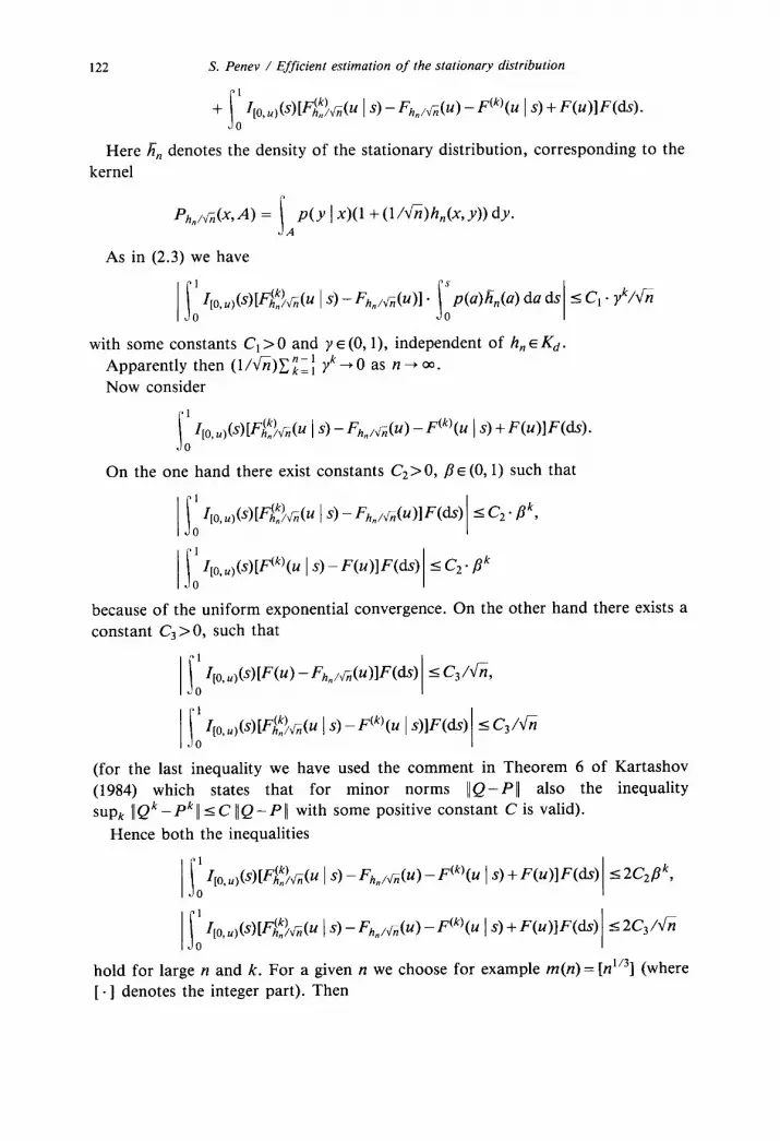
122 S. Penev / Efficient estimation of the stationary distribution
+ s
I ~ro,u,W~~ki;;c~ 1s) -Ft,,,\l;;@) -F(% 14 +F@WXW.
0
Here h;, denotes the density of the stationary distribution, corresponding to the
kernel
P/,,\l;;(x, -4) = s PLY 1 x)(1 +W%Lw9) dy. A
As in (2.3) we have
I!
1 s
~~o,u~W[F&x(~ 14 -F/,,,d~)l . ~(42;,(4 dads 5 G . yk/fi 0 0
with some constants Ct > 0 and y E (0, l), independent of h, E Kd.
Apparently then (l/fi)Ciii yk+O as n+oc.
Now consider
.I’
1
I[o, .,CW&z@ 19 - F/z,,,\l;;@) - Fck)@ ) 4 + F@W’(W. 0
On the one hand there exist constants Cz> 0, /3~ (0,l) such that
15
I ~,o,u,(W&i@ 14 - F/zn/fi@M’W 5 G. Bk,
0
Ii
1
~[o,&)[F(~)(~ 1s) -F(u)lF(W 5 C2. Pk
0
because of the uniform exponential convergence. On the other hand there exists a
constant C,>O, such that
(for the last inequality we have used the comment in Theorem 6 of Kartashov
(1984) which states that for minor norms I/Q-P 11 also the inequality
sup, 11 Qk - Pk 11 I C IIQ - P I( with some positive constant C is valid).
Hence both the inequalities
IS 1
~~o,u~W~%d~ 14 -4z,,d~)-F(~)(~ 1 ~)+F(u)lF(ds) r2C2pk, 0
hold for large n and k. For a given n we choose for example m(n) = [n1’3] (where
[. ] denotes the integer part). Then

S. Penev / Efficient estimation of the stationary distribution 123
The expression on the right side of the last inequality can be made arbitrarily
small for large n. This completes the proof.
Acknowledgement
The author is indebted to the referee for critical reading of earlier version leading
to substantial improvement of both the style and presentation of this article.
References
Billingsley, P. (1968). Convergence of Probability Measures. Cambridge University Press, Cambridge.
Dvoretsky, A., J. Kiefer and J. Wolfowitz (1956). Asymptotic minimax character of the sample distribu-
tion function and the classical multinomial estimator. Ann. Math. Statist. 27, 642-669. Doob, J.L. (1956). Stochastic Processes. Wiley, New York.
Ibragimov, I.A. and Yu.V. Linnik (1965). Independent and Stationary Sequences (in Russian). Nauka,
Moscow.
Kartashov, N.V. (1981). Strongly stable Markov chains. In: V.M. Zolotarev and V.V. Kalishnikov, Eds.,
Stability Problems for Stochastic Models, Proceedings of Seminar. The Institute for Systems Studies,
Moscow, 54-59.
Kartashov, N.V. (1984). Criteria for uniform ergodicity and strong stability of Markov chains with
general phase state. Theory Probab. Math. Statist. 30, 65-81. Kiefer, J. and J. Wolfowitz (1976). Asymptotically minimax estimation of concave and convex distribu-
tion functions. Z. Wahrsch. Verw. Gebiete 34, 73-85. LeCam, L.M. (1972). Limits of experiments. In: Proceedings of the Sixfh Berkeley Symposium on
Mathematical Statistics and Probability. University of California Press, Berkeley-Los Angeles,
245-261.
Loeve, M. (1960). Probability Theory, 2nd ed. D. van Nostrand, Princeton, NJ.
Millar, P.W. (1979). Asymptotic minimax theorems for the sample distribution function. Z. Wahrsch. Verw. Gebiete 48, 233-252.
Millar, P.W. (1983). The Minimax Principle in Asymptotic Statistical Theory. Ecole d’Ete de Pro-
babilites de Saint-Fluor X1-1981. Lecture Notes in Mathematics, Vol. 976. Springer-Verlag, Berlin,
76-265.
Millar, P.W. (1984). A general approach to the optimality of minimum distance estimators. Trans. Amer. Math. Sot. 286 (l), 377-418.
Neveu, J. (1964). Bases MathPmatiques du Calcul des ProbabilitB. Masson, Paris.
Roussas, G. (1972). Contiguity of Probability Measures. Cambridge University Press, Cambridge.
Strasser, H. (1985). Mathematical Theorey of Statistics. W. de Gruyter, Berlin-New York.