Efficient Strongly Relational Polyhedral Analysis

Sriram Sankaranarayanan1,3, Michael A. Colon2, Henny Sipma3, Zohar Manna3

1 NEC Laboratories America, Princeton, NJsrirams@nec-labs.com

2 Center for High Assurance Computer Systems, Naval Research Laboratory,colon@itd.nrl.navy.mil

3 Computer Science Department, Stanford University, Stanford, CA 94305-9045(sipma,zm)@theory.stanford.edu ⋆

Abstract. Polyhedral analysis infers invariant linear equalities and in-equalities of imperative programs. However, the exponential complex-ity of polyhedral operations such as image computation and convex hulllimits the applicability of polyhedral analysis. Weakly relational domainssuch as intervals and octagons address the scalability issue by consideringpolyhedra whose constraints are drawn from a restricted, user-specifiedclass. On the other hand, these domains rely solely on candidate expres-sions provided by the user. Therefore, they often fail to produce stronginvariants.We propose a polynomial time approach to strongly relational analysis.We provide efficient implementations of join and post condition opera-tions, achieving a trade off between performance and accuracy. We haveimplemented a strongly relational polyhedral analyzer for a subset ofthe C language. Initial experimental results on benchmark examples areencouraging.

1 Introduction

Polyhedral analysis seeks to discover invariant linear equality and inequality re-lationships among the variables of an imperative program. The computed invari-ants are used to establish safety properties such as freedom from buffer overflows.The standard approach to polyhedral analysis is through a fixed point iterationin the domain of convex polyhedra [9]. Complexity considerations, however, re-strict its application to small systems. Libraries such as NewPolka [13] andPPL [2] have made strides towards addressing some of these tractability issues,but still the approach remains impractical for large systems.

At the heart of this intractability lies the need to repeatedly convert be-tween constraint and generator representations of polyhedra. Efficient analysistechniques work on restricted forms of polyhedra wherein such a conversion canbe avoided. Weakly relational domains such as octagons [17], intervals [7], oc-tahedra [6] and the TCM domain [18], avoid these conversions by considering

⋆ This research was supported in part by NSF grants CCR-01-21403, CCR-02-20134,CCR-02-09237, CNS-0411363 and CCF-0430102, by ARO grant DAAD 19-01-1-0723and by NAVY/ONR contract N00014-03-1-0939 and the Office of Naval Research.

polyhedra whose constraints are fixed a priori. The abstract domain of Simonet al. [19] considers polyhedra with at most two variables per constraint. Usingthese syntactic restrictions, the analysis can be carried out efficiently. However,the main drawback of such syntactic restrictions is the inability of the analysisto infer invariants that require expressions of an arbitrary form. Thus, in manycases, such domains may fail to prove the property of interest.

In this paper, we provide an efficient strongly relational polyhedral domainby drawing on ideas from both weak and strong relational analysis. We presentalternatives to the join and post condition operations. In particular, we providea new join algorithm, called inversion join, that works in polynomial time inthe size of the input polyhedra, as opposed to the exponential space polyhedraljoin. We make use of linear programming to implement an efficient join and postcondition operators, along with efficient inclusion checks and widening operators.

On the other hand, our domain operations are weaker than the conventionalpolyhedral domain operations, potentially yielding weaker invariants. Using aprototype implementation of our techniques, we have analyzed several sortingand string handling routines for buffer overflows. Our initial results are promis-ing; our analysis performs better than the standard approaches while computinginvariants that are sufficiently strong in practice.

Outline. Section 2 discusses the preliminary notions of polyhedra, transitionsystems and invariants. Section 3 discusses algorithms for domain operationsneeded for polyhedral analysis. Section 4 discusses the implementation and theresults obtained on benchmark examples.

2 Preliminaries

We recall some standard results on polyhedra, followed by a brief description ofsystem models and abstract interpretation. Throughout the paper, let R repre-sent the set of reals and R+ = R∪{±∞} represent the extended real numbers.

Definition 1 (Linear Assertions). A linear expression e is of the form a1x1+· · · + anxn + b, wherein each ai ∈ R and b ∈ R+. The expression is said to behomogeneous if b = 0. A linear constraint is of the form a1x1+· · ·+anxn+b ⊲⊳ 0,with ⊲⊳ ∈ {≥, =}. A linear assertion is a finite conjunction of linear inequalities.

Note that the linear inequality e+∞ ≥ 0 represents the assertion true, whereasthe inequality e − ∞ ≥ 0 represents false . Since each equality e = 0 can berepresented as a conjunction of two inequalities, an assertion can be written inmatrix form as Ax+ b ≥ 0, where A is a m×n matrix, while x and b are n andm-dimensional vectors, respectively. The set of points in Rn satisfying a linearassertion is called a polyhedron.

The representation of a polyhedron by a linear assertion is known as its con-straint representation. Alternatively, a polyhedron may be represented explicitlyby a finite set of vertices and rays, known as the generator representation. Eachrepresentation may be exponentially larger than the other. For instance, the n

dimensional hypercube is represented by 2n constraints and 2n generators. Ef-ficient libraries of conversion algorithms such as the new PolKa [12] and theParma Polyhedral Library (PPL) [2] have made significant improvements to thesize of the polyhedra for which the conversion is possible. Nevertheless, this con-version still remains intractable for large polyhedra involving 100s of variablesand constraints.

A Template Constraint Matrix (TCM) T is a finite set of homogeneous linearexpressions over x. Given an assertion ϕ, its expressions induce a TCM T whichwe shall denote as Ineqs (ϕ). If ϕ is represented as Ax+b ≥ 0 then Ineqs (ϕ) : Ax.

Linear Programming We briefly describe the theory of linear programming.Details may be found in standard textbooks [5].

Definition 2 (Linear Programming). A canonical instance of the linear pro-gramming (LP) problem is of the form

minimize e subject to ϕ ,

for assertion ϕ and a linear expression e, called the objective function.

The goal is to determine the solution of ϕ for which e is minimal. A LPproblem can have one of three results: (1) an optimal solution; (2) −∞, i.e, e isunbounded from below in ϕ; (3) +∞, i.e, ϕ has no solutions.

It is well-known that an optimal solution, if it exists, is realized at a vertexof the polyhedron. Therefore, the optimal solution can be found by evaluatinge at each of the vertices. Enumerating all the vertices is very inefficient becausethe number of generators is worst-case exponential in the number of constraints.The popular simplex algorithm (due to Danzig [10]) employs a sophisticatedhill climbing strategy that converges on an optimal vertex without necessarilyenumerating all vertices. In theory, the technique is worst-case exponential. Thesimplex method is efficient over most problems. Interior point methods such asKarmarkar’s algorithm and other techniques based on ellipsoidal approximationsare guaranteed to solve linear programs in polynomial time. Using an open-sourceimplementation of simplex such as glpk [15], massive LP instances involvingtens of thousands (104 and beyond) of variables and constraints can be solvedefficiently.

Programs and Invariants

We assume programs over real valued variables without any function calls. Theprogram is represented by a linear transition system also known as a control flowgraph.

Definition 3 (Linear Transition Systems). A linear transition system (LTS)Π : 〈L, T , ℓ0, Θ〉 over a set of variables V consists of

– L: a set of locations (cutpoints);

– T : a set of transitions (edges), where each transition τ : 〈ℓi, ℓj , ρτ 〉 consistsof a pre-location ℓi, a post-location ℓj, and a transition relation ρτ , repre-sented as a linear assertion over V ∪ V ′, where V denotes the values of thevariables in the current state, and V ′ their values in the next state;

– ℓ0 ∈ L: the initial location;– Θ: a linear assertion over V specifying the initial condition.

A run of a LTS is a sequence 〈m0, s0〉 , 〈m1, s1〉 , . . ., with mi ∈ L and si avaluation of V , also called a state, such that

– Initiation: m0 = ℓ0, and s0 |= Θ

– Consecution: for all i ≥ 0 there exists a transition τ : 〈ℓj , ℓk, ρτ 〉 such thatmi = ℓj , mi+1 = ℓk, and 〈si, si+1〉 |= ρτ .

A state s is reachable at location ℓ if 〈ℓ, s〉 appears in some run.A given linear assertion ψ is a linear invariant of a linear transition system

(LTS) at a location ℓ iff it is satisfied by every state reachable at ℓ. An assertionmap associates each location of a LTS to a linear assertion. An assertion mapη is invariant if η(ℓ) is an invariant, for each ℓ ∈ L. In order to prove a givenassertion map invariant, we use the inductive assertions method due to Floyd(see [16]).

Definition 4 (Inductive Assertion Maps). An assertion map η is inductiveiff it satisfies the following conditions:

Initiation: Θ |= η(ℓ0),Consecution: For each transition τ : 〈ℓi, ℓj, ρτ 〉, (η(ℓi) ∧ ρτ ) |= η(ℓj)

′. Notethat η(ℓj)

′ refers to η(ℓj)[V |V ′] with variables in V substituted by their cor-responding primed variables in V ′.

It is well known that any inductive assertion map is invariant. However, theconverse need not be true. The standard technique for proving an assertioninvariant is to find an inductive assertion that strengthens it.

Linear Relations Analysis

Linear relation analysis seeks an inductive assertion map for the input program,labeling each location with a linear assertion. Analysis techniques are basedon the theory of Abstract Interpretation [8] and specialized for linear relationsby Cousot and Halbwachs [9]. The technique starts with an initial assertionmap, and weakens it iteratively using the post, join and the widening operators.When the iteration converges, the resulting map is guaranteed to be inductive,and hence invariant. Termination is guaranteed by the design of the wideningoperator.

The post condition operator takes an assertion ϕ and a transition τ , andcomputes the set of states reachable by τ from a state satisfying ϕ. It can beexpressed as

post(ϕ, τ) : (∃V0)(ϕ(V0) ∧ ρτ (V0, V ))

Standard polyhedral operations can be used to compute post. However, moreefficient strategies for computing post exist when ρτ has a special structure.Given assertions ϕ{1,2} such that ϕ1 |= ϕ2, the standard widening ϕ1∇ϕ2 is anassertion ϕ that contains all the inequalities in ϕ1 that are satisfied by ϕ2. Thedetails along with key mathematical properties of widening are described in [9,8], and enhanced versions appear in [12, 4, 1]. As mentioned earlier, the analysisbegins with an initial assertion map defined by η0(ℓ0) = Θ, and η0(ℓ) = false forℓ 6= ℓ0. At each step, the map ηi is updated to map ηi+1 as follows:

ηi+1(ℓ) = ηi(ℓ) 〈op〉

ηi(ℓ)⊔

τj≡〈ℓj ,ℓ,ρ〉

(post(ηi(ℓj), τj))

,

where op is the join (⊔) operator for a propagation step, and the widening (∇)operator for a widening step. The overall algorithm requires a predefined itera-tion strategy. A typical strategy carries out a fixed number of initial propagationsteps, followed by widening steps until termination.

Linear Assertion Domains

Linear relation analysis is performed using a forward propagation wherein poly-hedra are used to represent sets of states. Depending on the family of polyhedraconsidered, such domains are classified as weakly relational or strongly relational.

Let T = {e1, . . . , em} be a TCM. The weakly relational domain induced byT consists of assertions

∧

ei∈T ei + bi ≥ 0 for bi ∈ R+. TCMs and their inducedweakly relational domain are formalized in our earlier work [18]. Given a weaklyrelational domain defined by a TCM T and a linear transition system Π , weseek an inductive assertion map η such that η(ℓ) belongs to the domain of T foreach location ℓ. Many weakly relational domains have been studied: Intervals,octagons and octahedra are classical examples.

Example 1 (Weakly Relational Analysis). Let X be the set of system variables.The interval domain is defined by the TCM consisting of expressions TX ={±xi | xi ∈ X}. Thus, any polyhedron belonging to the domain is an intervalexpression of the form

∧

(xi + ai ≥ 0 ∧ −xi + bi ≥ 0) . The goal of intervalanalysis is to discover the coefficients ai, bi ∈ R+ representing the bounds foreach variable xi at each location of the program [7].

The octagon domain of Mine subsumes the interval domain by consideringadditional expressions of the form ±xi ± xj such that xi, xj ∈ X [17]. Theoctahedron domain due to Clariso and Cortadella considers expressions of theform

∑

i aixi such that ai ∈ {−1, 0, 1} [6].

It is possible to carry out the analysis in any weakly relational domain effi-ciently [18].

Theorem 1. Given a TCM T and a linear system Π, all the domain opera-tions for the weakly relational analysis of Π in the domain induced by T can beperformed in time polynomial in |T | and |Π |.

integer x,y where (x = 1 ∧ x ≥ y)ℓ0 : while true do

if (x ≥ y) then(x, y) := (x + 2, y + 1)

else(x, y) := (x + 2, y + 3)

end ifend while

Fig. 1. An example program.

Weakly relational domains are appealing since the analysis in these domainsis scalable to large systems. On the other hand, the invariants they produce areoften imprecise. For instance, even if ei + ai ≥ 0 is invariant for some expressionei in the TCM, its proof may require an inductive strengthening ej + aj ≥ 0,where ej is not in the TCM.

A strongly relational analysis does not syntactically restrict the polyhedraconsidered. The polyhedral domain is not restricted in its choice of invariantexpressions, and is potentially more precise than a weakly relational domain.The main drawback, however, is the high complexity of the domain operations.Each domain operation requires conversions from the constraint to the generatorrepresentation and back. Popular implementations of strongly relational analysisrequire worst case exponential space due to repeated representation conversions.

Example 2. Consider the system in Figure 1. Interval and octagon domains bothdiscover the invariant ∞ ≥ x ≥ 1 at location ℓ0. A strongly relational analysissuch as polyhedral analysis discovers the invariant x ≥ 1 ∧ 3x−2y ≥ 1, as doesthe technique that we present.

3 Domain Operations

The theory of Abstract Interpretation provides a framework for the design ofprogram analyses. A sound program analysis can be designed by constructingan abstract domain with the following domain operations:

Join (union) Given two assertions ϕ1, ϕ2 in the domain, we seek an assertionϕ such that ϕ1 |= ϕ and ϕ2 |= ϕ. In many domains, it is possible to find thestrongest possible ϕ satisfying this condition. The operation of computingsuch an assertion is called the strong join.

Post Condition Given an assertion ϕ, and a transition relation ρτ , we seekan assertion ψ such that ϕ[V ] ∧ ρτ [V, V ′] |= ψ[V ′]. A strong post con-dition operator computes the strongest possible assertion ψ satisfying thiscondition.

Widening Widening ensures the termination of the fixed point iteration.

Additionally, inclusion tests between assertions are important for detectingthe termination of an iteration. Feasibility tests and redundancy elimination

are also frequently used to speed up the analysis. We present several differentjoin and post condition operations, each achieving a different trade off betweenefficiency and precision.

Join

Given two linear assertions ϕ1 and ϕ2 over a vector x of system variables, weseek a linear assertion ϕ, such that both ϕ1 |= ϕ and ϕ2 |= ϕ.

Strong Join. The strong join seeks the strongest assertion ϕ (denoted ϕ1 ⊔s

ϕ2) subsuming both ϕ1 and ϕ2. In the domain of convex polyhedra, this isknown as the polyhedral convex hull and is obtained by computing the generatorrepresentations of ϕ1 and ϕ2. The set of generators of ϕ is the union of thoseof ϕ1 and ϕ2. This representation is then converted back into the constraintrepresentation. Due to the repeated representation conversions, the strong joinis worst-case exponential space in the size of the input assertions.

Example 3. Consider the assertions

ϕ1 : x− y ≤ 5 ∧ y + x ≤ 10 ∧ −10 ≤ x ≤ 5ϕ2 : x− y ≤ 9 ∧ y + x ≤ 5 ∧ −9 ≤ x ≤ 6

Their strong join ϕ1 ⊔s ϕ2, generated by the union of their vertices, is

ϕ : 6x+ y ≤ 35 ∧ y+ 3x+ 45 ≥ 0 ∧ x− y ≤ 9 ∧ x+ y ≤ 10 ∧ −10 ≤ x ≤ 6 .

Weak Join. The weak join operation is inspired by the join used in weaklyrelational domains.

Definition 5 (Weak Join). The weak join of two polyhedra ϕ1, ϕ2 is computedas follows:1. Let TCM T = Ineqs (ϕ1) ∪ Ineqs (ϕ2) be the set of inequality expressions thatoccur in either of ϕ{1,2}. Recall that each equality in ϕ1 or ϕ2 is represented bytwo inequalities in T .2. For each expression ei in T , we compute the values ai and bi using linearprogramming, as follows:

ai = minimize ei subject to ϕ1

bi = minimize ei subject to ϕ2

It follows that ϕ1 |= (ei ≥ ai) and ϕ2 |= (ei ≥ bi).3. Let ci = min(ai, bi). Therefore, both ϕ1, ϕ2 |= (ei ≥ min(ai, bi) ≡ ci).

The weak join ϕ1 ⊔w ϕ2 is given by the assertion∧

ei∈T ei ≥ ci.

The advantage of the weak join is its efficiency: it can be computed using LPqueries, where both the number of such queries and the size of each individualquery is polynomial in the input size. On the other hand, the weak join does notdiscover any new relations. It is weaker than the strong join, as shown by theargument above (and strictly so, as shown by the following Example).

Example 4. Consider the assertions ϕ1, ϕ2 from Example 3 above. The TCM T

and the ai, bi values are shown in the table below:

T :

# Relation ai(ϕ1) bi(ϕ2)1 y − x ≥ −5 −92 −y − x ≥ −10 −53 x ≥ −10 −94 −x ≥ −5 −6

The weak join is given by

ϕw : (y − x ≥ −9 ∧ −y − x ≥ −10 ∧ x ≥ −10 ∧ −x ≥ −6) .

This result is strictly weaker than the strong join computed in Example 3.

Restricted Joins. The weak join shown above is more efficient than the strongjoin. However, this efficiency comes at the cost of precision. We therefore seekefficient alternatives to strong and weak join. The k-restricted join (denoted ⊔k)improves upon the weak join as follows:

1. Choose a subset of inequalities from ϕ1, ϕ2, each of cardinality at most k. Letψ1 and ψ2 be the assertions formed by the chosen inequalities. In general,ψ1, ψ2 may contain different sets of inequalities, even different cardinalities.Note that ϕi |= ψi for i = 1, 2.

2. Compute the strong join ψ1 ⊔s ψ2 in isolation. Conjoin the results with theweak join ϕ1 ⊔w ϕ2.

3. Repeat step 1 for a different set of choices of ψ{1,2}, while conjoining eachsuch join to the weak join.

Since ϕi |= ψi, for i = 1, 2, it follows by the monotonicity of the strong joinoperation that ϕ1 ⊔s ϕ2 |= ψ1 ⊔s ψ2. Thus ϕ1 ⊔s ϕ2 |= ϕ1 ⊔k ϕ2 for each k ≥ 0.

Let ϕ1, ϕ2 have at most m constraints. The k-restricted join requires vertexenumeration for O((m

k )2) polyhedra with at most k constraints. As such, this

join is efficient only if k is a small constant. We shall now provide an efficientO(m2) algorithm based on ⊔2, to improve the weak join.

Inversion Join. The inversion join is based on the 2-restricted join. Let T bethe TCM and ai, bi be the values computed for the weak join as in Definition 5.Consider pairs of expressions ei, ej ∈ T yielding the assertions

ψ1 : ei ≥ ai ∧ ej ≥ aj

ψ2 : ei ≥ bi ∧ ej ≥ bj

We use the structure of the assertions ψ1, ψ2 to perform their strong join ana-lytically. The key notion is that of an inversion.

Definition 6 (Inversion). Expressions ei, ej ∈ T and corresponding coeffi-cients ai, aj , bi, bj form an inversion iff the following conditions hold:

ei ≥ ai

ej≥

aj

ei ≥ bi

ej≥

b j

(a) (b)

H

(c)

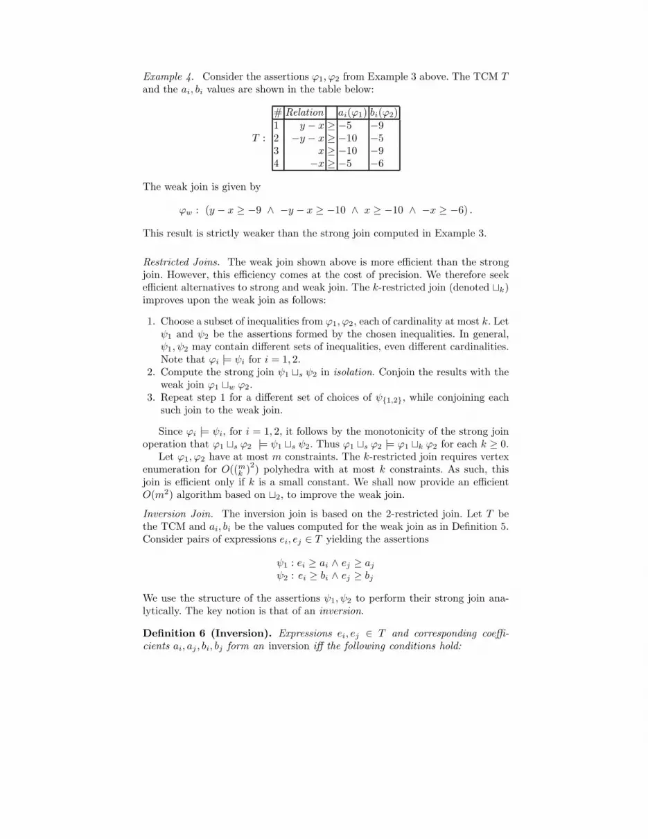
Fig. 2. (a) ai > bi, aj < bj , (b) Weak join is strictly weaker than strong join, (c)ai > bi, aj > bj : Weak join is the same as strong join.

1. ai, aj, bi, bj ∈ R, i.e, none of them is ±∞.2. ei 6= λej for λ ∈ R, i.e, ei, ej are linearly independent.3. ai < bi and bj < aj (or vice-versa).

Example 5. Consider two “wedges” ψ1 : ei ≥ ai ∧ ej ≥ aj and ψ2 : ei ≥bi ∧ ej ≥ bj . Depending on the values of ai, aj , bi, bj , two cases arise as depictedin Figures 2(a,b,c). Figures 2(a,b) form an inversion. When this happens, theweak join (a) is strictly weaker than the strong join (b). Figure 2(c) does notform an inversion. The weak and strong joins coincide in this case.

Therefore, a strong join of polyhedra that form an inversion gives rise to a halfspace that is not discovered by the weak join. We now derive this “missinghalf-space” H analytically.

The half space subsumes both ψ1 and ψ2. A half-space that is a consequenceof ψ1 : ei ≥ ai ∧ ej ≥ aj is of the form H : ei + λijej ≥ ai + λijaj , forsome λij ≥ 0. Similarly for ψ2, we obtain H : ei + λijej ≥ bi + λijbj . Equatingcoefficients, yields the equation ai +λijaj = bi +λijbj . The required value of λij

is

λij =ai − bi

bj − aj

.

Note that requiring λij > 0 yields ai < bi and bj < aj . Therefore, ψ1, ψ2 containa non trivial common half-space iff they form an inversion.

Definition 7 (Inversion Join). Given ϕ1, ϕ2 the inversion join ϕ1 ⊔inv ϕ2 iscomputed as follows:

1. Compute the TCM T = Ineqs (ϕ1) ∪ Ineqs (ϕ2).2. For each ei ∈ T compute ai, bi as defined in Definition 5 using linear pro-

gramming. At this point ϕ1 |= ei ≥ ai and ϕ2 |= ei ≥ bi. Let ϕw = ϕ1 ⊔w ϕ2

be the weak join.3. For each pair ei, ej, consider the expression ei +λijej ≥ ai +λijaj, with λij

as defined above.4. The inversion join is the conjunction of ϕw and all the inversion expressions

generated in Step 3. Optionally, simplify the result by removing redundantinequalities.

(a)

(b)

(c)

y

x

Fig. 3. Inversion join over two polyhedra (a), (b) and (c) are the newly discoveredrelations.

Example 6. Figure 3 shows the result of an inversion join over two input poly-hedra ϕ1, ϕ2 used in Example 3. Example 4 shows the TCM T and the ai, bivalues. There are three inversions

# Expressions Subsuming Half-Space(a) 〈1, 3〉 y + 3x+ 45 ≥ 0(b) 〈2, 4〉 −y − 6x+ 35 ≥ 0(c) 〈1, 2〉 y − 9x+ 65 ≥ 0

The “expressions” column in the table above refers to expressions by their rownumbers in the table of Example 4. From Figure 3, note that (c) is redundant.Therefore the result of the join may require redundancy elimination (algorithmprovided later in this section). This result is equivalent to the result of the strongjoin in Example 3.

Theorem 2. Let ϕ1, ϕ2 be two polyhedra. It follows that

ϕ1 ⊔s ϕ2 |= ϕ1 ⊔inv ϕ2 |= ϕ1 ⊔w ϕ2 .

The inversion join requires as many LP queries as the weak join and ad-ditional O(m2n) arithmetic operations to compute inversions, where m is thenumber of inequalities in T and n, the dimensionality.

Note. The descriptions of the weak and inversion join treat each equality astwo inequalities. The resulting join could be made more precise if additionally,the equality join defined by Karr’s analysis [14] is computed and conjoined tothe result. This can be achieved in time that is polynomial in the number ofequalities.

Post Condition

The post condition computes the image of an assertion ϕ under a transitionrelation of the form ξ ∧ x

′ = Ax + b. This is equivalent to the image ofϕ∧ ξ under the affine transformation x

′ = Ax + b. If the matrix A is invertible,then this image is easily computed by substituting x = A−1(x′ − b) [9]. On theother hand, it is frequently the case that A is not invertible. We present threealternatives, the strong, weak and restricted post conditions.

Strong Post. The strong post is computed by first enumerating the generators ofϕ∧ ξ. Each generator is transformed under the operation Ax + b. The resultingpolyhedron is generated by these images. Conversion back to the constraintrepresentation completes the computation.

Weak Post. Weak post requires a TCM T ′ labeling the post location of thetransition. Alternatively, this TCM may be derived from Ineqs (η(ℓ′)) where η(ℓ′)labels the post-location. Given the existence of such a TCM, we may use thepost operation defined for TCMs [18] to compute the weak post.

Note. The post condition computation for equalities can be performed separatelyusing the image operation defined for Karr’s analysis. This can be added to theresult, thus strengthening the weak post.

k-Restricted Post The k-restricted post condition improves upon the weak postby using the monotonicity of the strong post operation (see [8]) similar to the k-restricted join algorithm. Therefore, considering a subset of up to k inequalitiesψ, we may compute the strong post of ψ and add the result conjunctively to theweak post. The results improve upon the precision of weak post. As is the casefor join, it is possible to treat the cases for k = 1, 2 efficiently.

Example 7. Consider the polyhedron ϕ : x− y ≥ 0 ∧ x ≤ 0 ∧ x + y + 3 ≤ 0and the transformation x := x + 3, y := 0. Consider the TCM T = {x − y, x+y, y− x,−x− y}. The weak post of ϕ w.r.t T is computed by finding bounds foreach expression. For instance the bound for x− y is discovered by solving:

minimize x′ − y′ s.t. ϕ ∧ x′ = x+ 3 ∧ y′ = 0

The overall weak post is obtained by solving 4 LPs, one for each element of T ,

ϕw : 3 ≥ x− y ≥ 1.5 ∧ 3 ≥ x+ y ≥ 1.5 .

This is strictly weaker than the strong post ϕs : 3 ≥ x ≥ 1.5 ∧ y = 0. The1-restricted post computes the post condition of each half-space in ϕ separately.This yields the result y = 0 for all the three half-spaces. Conjoining the 1-restricted post with the weak post yields the same result as the strong post inthis example.

Note. The projection operation, an important primitive for interprocedural anal-ysis, can be implemented along the same lines as the post condition operation,yielding the strong, weak and restricted projection operations.

Feasibility, Inclusion Check and Redundancy Elimination

There exist polynomial time algorithms that are efficient in practice for checkingfeasibility of a polyhedron and inclusion between two polyhedra.

Feasibility. The simplex method can be used to check feasibility of a givenlinear inequality assertion ϕ. In practice, we solve the optimization problemminimize 0 subject to ϕ. An answer of +∞ indicates the infeasibility of ϕ.

Inclusion Check. As a primitive, consider the problem of checking whether agiven inequality e ≥ 0 is entailed by ϕ, posing the LP: minimize e subject to ϕ.If the optimal solution is a, it follows from the definition of a LP problem thatϕ |= e ≥ a. Thus subsumption holds iff a ≥ 0. In order to decide if ϕ |=Ax + b ≥ 0, we decide if the entailment holds for each half-space Aix + bi ≥ 0.

Redundancy Elimination (Simplification). Each inequality is checked for sub-sumption by the remaining inequalities using the inclusion check primitive.

Widening

The standard widening of Cousot and Halbwachs may be implemented efficientlyusing linear programming. Let ϕ1, ϕ2 be two polyhedra such that ϕ1 |= ϕ2.

Let us assume that ϕ1, ϕ2 are both satisfiable. We seek to drop any constraintei ≥ 0 in ϕ1 that is not a consequence of ϕ2. This can be achieved by the inclusiontest primitive described above.

Definition 8 (Standard Widening). The standard widening of two polyhedraϕ1 |= ϕ2, denoted ϕ = ϕ1∇ϕ2 is computed as follows,

1. Check satisfiability of ϕ1, ϕ2. If either one is unsatisfiable, widening reducesto their join.

2. Otherwise, for each ei ∈ Ineqs (ϕ1), compute bi = minimize ei subject to ϕ2.If bi < 0 then drop the constraint ei ≥ 0 from ϕ1.

This operator is identical to the widening defined by Cousot and Halb-wachs [9]. The operator may be improved by additionally computing the joinof the equalities in both polyhedra. The work of Bagnara et al. [1] presentsseveral approaches to improving the precision of widening operators.

4 Performance

We have implemented many of the ideas in this paper in the form of an ab-stract domain library written in Ocaml. Our library uses GLPK [15] to solveLP queries, and PPL [2] to convert between the constraint and generator rep-resentations of polyhedra. Such conversions are used to implement the strongjoin and post condition. Communication between the different libraries is imple-mented using Unix pipes. As a result, the communication overhead is significantfor small examples.

Choosing Domain Operations. We have provided several options for the joinand the post condition operations. In practice, one can envision many strategiesfor choosing among these operations. Our implementation chooses between thestrong and the weak versions based on the sizes of the input polyhedra. Strongpost condition and joins are used for smaller polyhedra (40 variables+constraints).On the other hand, the inversion join is used for polyhedra with roughly 100sof variables+constraints, while the weak versions are used for larger polyhedra.

Name (#vars) #trans Strong+Weak Purely Strong ±time mem time mem

req-grant(11) 8 3.14 5.7 0.1 4.1 +csm(13) 8 6.21 5.9 0.1 4.2 6=c-pJava(18) 14 11.2 6.0 0.1 4.1 6=multipool(18) 21 10.0 6.0 2.1 9.2 +

incdec(32) 28 39.12 6.8 8.7 10.4 6=mesh2x2(32) 32 33.8 6.4 18.53 66.2 6=bigjava(44) 37 46.9 7.2 256.2 55.3 6=mesh3x2(52) 54 122 8.1 > 1h+ > 800+ +

Table 1. Performance on Benchmark Examples. All times are in seconds and memoryutilization in Mbs.

We observe empirically that the use of strong operations does not improve theresult once the widening phase is started. Therefore, we resort to weak join andpost condition for the widening phase of the analysis.

4.1 Benchmark Examples

We supplied our library to generate invariants for a few benchmark system mod-els drawn from related projects such as FAST [3] and our previous work [18].Table 1 shows the complexity of each system in terms of number of variables(#vars) along with the performance of our technique of mixed strong, weakand inversion domain operations as compared with the purely strong join/postoperations implemented directly in C++ using the PPL library. We comparethe running time and memory utilization of both implementations. Results weremeasured on an Intel Xeon II processor with 1GB RAM. The last column com-pares the invariants generated. A “+” indicates that our technique discoversstrictly stronger invariants whereas a “ 6=” denotes that the invariants are in-comparable.

Also, for small polyhedra, strong operations frequently outperform weak do-main operations in terms of time. However, their memory consumption seemsasymptotically exponential. Therefore, weak domain operations yield a drasticperformance improvement when the size of the benchmark examples increasesbeyond the physical memory capacity of the system. Comparing the invariantsgenerated, it is interesting to note that the invariants produced by both tech-niques are, for the most part, incomparable. While inversion join is weaker thanstrong join, the non-monotonicity of the widening operation and its dependenceon the syntactic representation of the polyhedra cause the two versions to com-pute different invariants.

Analysis of πVC Programs. We applied our abstract domain library to analyzea subset of the C language called πVC , consisting of imperative programs overintegers with function calls. The language features dynamically allocated arrays,

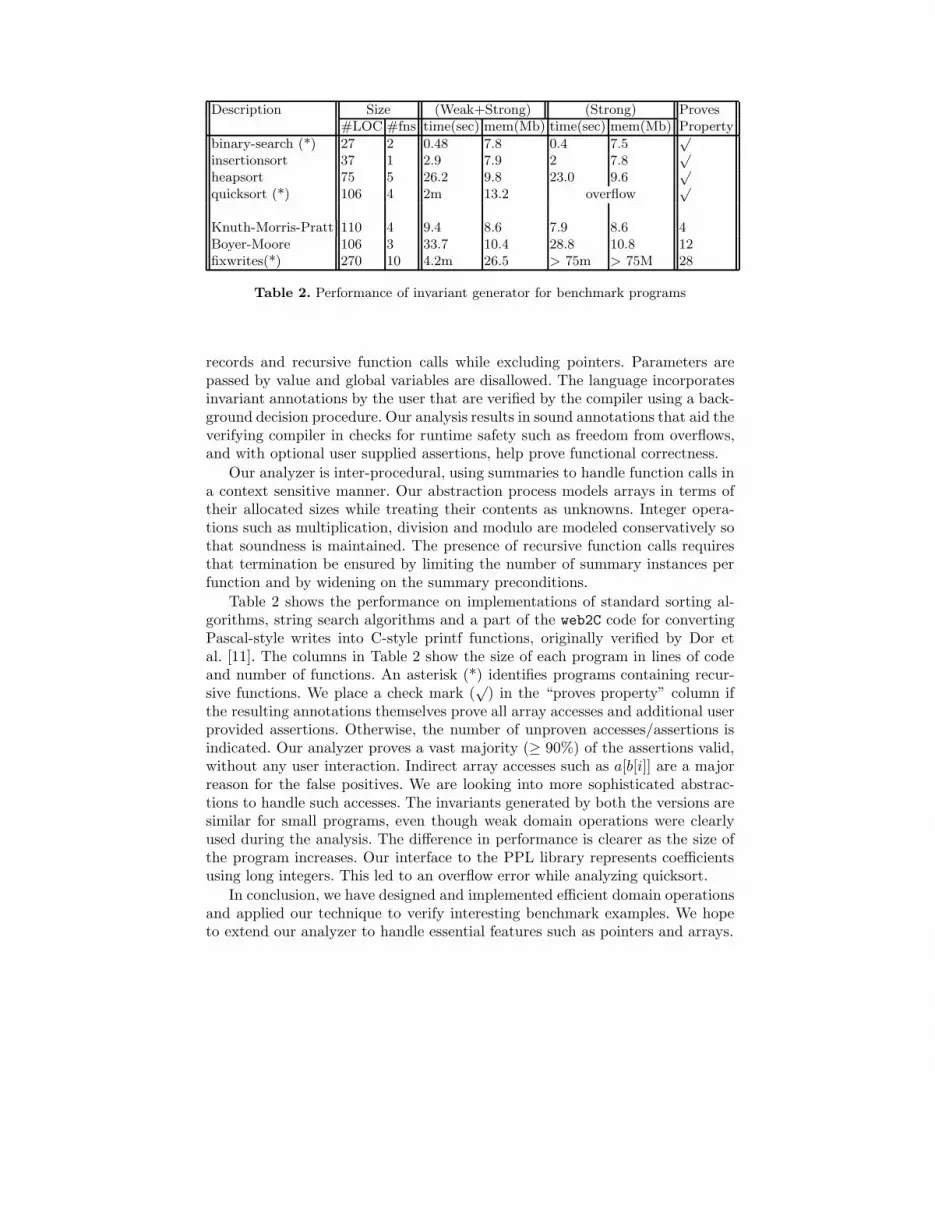
Description Size (Weak+Strong) (Strong) Proves#LOC #fns time(sec) mem(Mb) time(sec) mem(Mb) Property

binary-search (*) 27 2 0.48 7.8 0.4 7.5√

insertionsort 37 1 2.9 7.9 2 7.8√

heapsort 75 5 26.2 9.8 23.0 9.6√

quicksort (*) 106 4 2m 13.2 overflow√

Knuth-Morris-Pratt 110 4 9.4 8.6 7.9 8.6 4Boyer-Moore 106 3 33.7 10.4 28.8 10.8 12fixwrites(*) 270 10 4.2m 26.5 > 75m > 75M 28

Table 2. Performance of invariant generator for benchmark programs

records and recursive function calls while excluding pointers. Parameters arepassed by value and global variables are disallowed. The language incorporatesinvariant annotations by the user that are verified by the compiler using a back-ground decision procedure. Our analysis results in sound annotations that aid theverifying compiler in checks for runtime safety such as freedom from overflows,and with optional user supplied assertions, help prove functional correctness.

Our analyzer is inter-procedural, using summaries to handle function calls ina context sensitive manner. Our abstraction process models arrays in terms oftheir allocated sizes while treating their contents as unknowns. Integer opera-tions such as multiplication, division and modulo are modeled conservatively sothat soundness is maintained. The presence of recursive function calls requiresthat termination be ensured by limiting the number of summary instances perfunction and by widening on the summary preconditions.

Table 2 shows the performance on implementations of standard sorting al-gorithms, string search algorithms and a part of the web2C code for convertingPascal-style writes into C-style printf functions, originally verified by Dor etal. [11]. The columns in Table 2 show the size of each program in lines of codeand number of functions. An asterisk (*) identifies programs containing recur-sive functions. We place a check mark (

√) in the “proves property” column if

the resulting annotations themselves prove all array accesses and additional userprovided assertions. Otherwise, the number of unproven accesses/assertions isindicated. Our analyzer proves a vast majority (≥ 90%) of the assertions valid,without any user interaction. Indirect array accesses such as a[b[i]] are a majorreason for the false positives. We are looking into more sophisticated abstrac-tions to handle such accesses. The invariants generated by both the versions aresimilar for small programs, even though weak domain operations were clearlyused during the analysis. The difference in performance is clearer as the size ofthe program increases. Our interface to the PPL library represents coefficientsusing long integers. This led to an overflow error while analyzing quicksort.

In conclusion, we have designed and implemented efficient domain operationsand applied our technique to verify interesting benchmark examples. We hopeto extend our analyzer to handle essential features such as pointers and arrays.

Acknowledgments. Many thanks to Mr. Aaron Bradley for implementing theπVC front end, the reviewers for their incisive comments and to the developersof the PPL [2] and GLPK [15] libraries.

References

1. Bagnara, R., Hill, P. M., Ricci, E., and Zaffanella, E. Precise wideningoperators for convex polyhedra. In Static Analysis Symposium (2003), vol. 2694 ofLNCS, Springer–Verlag, pp. 337–354.

2. Bagnara, R., Ricci, E., Zaffanella, E., and Hill, P. M. Possibly not closedconvex polyhedra and the Parma Polyhedra Library. In SAS (2002), vol. 2477 ofLNCS, Springer–Verlag, pp. 213–229.

3. Bardin, S., Finkel, A., Leroux, J., and Petrucci, L. FAST: Fast accel-ereation of symbolic transition systems. In Computer-aided Verification (July2003), vol. 2725 of LNCS, Springer–Verlag.

4. Besson, F., Jensen, T., and Talpin, J.-P. Polyhedral analysis of synchronouslanguages. In Static Analysis Symposium (1999), vol. 1694 of LNCS, pp. 51–69.

5. Chvatal, V. Linear Programming. Freeman, 1983.6. Clariso, R., and Cortadella, J. The octahedron abstract domain. In Static

Analysis Symposium (2004), vol. 3148 of LNCS, Springer–Verlag, pp. 312–327.7. Cousot, P., and Cousot, R. Static determination of dynamic properties of

programs. In Proceedings of the Second International Symposium on Programming(1976), Dunod, Paris, France, pp. 106–130.

8. Cousot, P., and Cousot, R. Abstract Interpretation: A unified lattice modelfor static analysis of programs by construction or approximation of fixpoints. InACM Principles of Programming Languages (1977), pp. 238–252.

9. Cousot, P., and Halbwachs, N. Automatic discovery of linear restraints amongthe variables of a program. In ACM POPL (Jan. 1978), pp. 84–97.

10. Dantzig, G. B. Programming in Linear Structures. USAF, 1948.11. Dor, N., Rodeh, M., and Sagiv, M. CSSV: Towards a realistic tool for statically

detecting all buffer overflows in C. In Proc. PLDI’03 (2003), ACM Press.12. Halbwachs, N., Proy, Y., and Roumanoff, P. Verification of real-time systems

using linear relation analysis. Formal Methods in System Design 11 (1997), 157–185.

13. Jeannet, B. The convex polyhedra library New Polka. Available online fromhttp://www.irisa.fr/prive/Bertrand.Jeannet/newpolka.html.

14. Karr, M. Affine relationships among variables of a program. Acta Inf. 6 (1976),133–151.

15. Makhorin, A. The GNU Linear Programming Kit (GLPK), 2000. Availableonline from http://www.gnu.org/software/glpk/glpk.html.

16. Manna, Z. Mathematical Theory of Computation. McGraw-Hill, 1974.17. Mine, A. A new numerical abstract domain based on difference-bound matrices.

In PADO II (May 2001), vol. 2053 of LNCS, Springer–Verlag, pp. 155–172.18. Sankaranarayanan, S., Sipma, H. B., and Manna, Z. Scalable analysis of

linear systems using mathematical programming. In Verification, Model-Checkingand Abstract-Interpretation (VMCAI 2005) (January 2005), vol. 3385 of LNCS.

19. Simon, A., King, A., and Howe, J. M. Two variables per linear inequality asan abstract domain. In LOPSTR (2003), vol. 2664 of Lecture Notes in ComputerScience, Springer, pp. 71–89.