Embed Size (px)
Citation preview

Copyr
ELECTRIC POWER DISTRIBUTIONEQUIPMENT AND SYSTEMS
ight © 2006 Taylor & Francis Group, LLC

Copyr
A CRC title, part of the Taylor & Francis imprint, a member of theTaylor & Francis Group, the academic division of T&F Informa plc.
Boca Raton London New York
EPRI Solutions, Inc.Schenectady, NY
T. A. Short
ELECTRIC POWER DISTRIBUTIONEQUIPMENT AND SYSTEMS
ight © 2006 Taylor & Francis Group, LLC

9576_Discl.fm Page 1 Monday, October 10, 2005 1:27 PM
Copyr
The material was previously published in Electric Power Distribution Handbook © CRC Press LLC 2004.
Published in 2006 byCRC PressTaylor & Francis Group 6000 Broken Sound Parkway NW, Suite 300Boca Raton, FL 33487-2742
© 2006 by Taylor & Francis Group, LLCCRC Press is an imprint of Taylor & Francis Group
No claim to original U.S. Government worksPrinted in the United States of America on acid-free paper10 9 8 7 6 5 4 3 2 1
International Standard Book Number-10: 0-8493-9576-3 (Hardcover) International Standard Book Number-13: 978-0-8493-9576-5 (Hardcover) Library of Congress Card Number 2005052135
This book contains information obtained from authentic and highly regarded sources. Reprinted material isquoted with permission, and sources are indicated. A wide variety of references are listed. Reasonable effortshave been made to publish reliable data and information, but the author and the publisher cannot assumeresponsibility for the validity of all materials or for the consequences of their use.
No part of this book may be reprinted, reproduced, transmitted, or utilized in any form by any electronic,mechanical, or other means, now known or hereafter invented, including photocopying, microfilming, andrecording, or in any information storage or retrieval system, without written permission from the publishers.
For permission to photocopy or use material electronically from this work, please access www.copyright.com(http://www.copyright.com/) or contact the Copyright Clearance Center, Inc. (CCC) 222 Rosewood Drive,Danvers, MA 01923, 978-750-8400. CCC is a not-for-profit organization that provides licenses and registrationfor a variety of users. For organizations that have been granted a photocopy license by the CCC, a separatesystem of payment has been arranged.
Trademark Notice: Product or corporate names may be trademarks or registered trademarks, and are used onlyfor identification and explanation without intent to infringe.
Library of Congress Cataloging-in-Publication Data
Short, T.A. (Tom A.), 1966-Electric power distribution equipment and systems / Thomas Allen Short.
p. cm.Includes bibliographical references and index.ISBN 0-8493-9576-3 (alk. paper)1. Electric power distribution--Equipment and supplies. I. Title.
TK3091.S466 2005621.319--dc22 2005052135
Visit the Taylor & Francis Web site at http://www.taylorandfrancis.com
and the CRC Press Web site at http://www.crcpress.com
Taylor & Francis Group is the Academic Division of Informa plc.
ight © 2006 Taylor & Francis Group, LLC

9576_C00.fm Page 5 Friday, October 14, 2005 9:00 AM
Copyr
Dedication
To the future. To Jared. To Logan.
ight © 2006 Taylor & Francis Group, LLC

9576_C00.fm Page 7 Tuesday, November 1, 2005 7:02 AM
Copyr
Preface
In industrialized countries, distribution systems deliver electricity literallyeverywhere, taking power generated at many locations and delivering it toend users. Generation, transmission, and distribution—of the big three com-ponents of the electricity infrastructure, the distribution system gets the leastattention. Yet, it is often the most critical component in terms of its effect onreliability and quality of service, cost of electricity, and aesthetic (mainlyvisual) impacts on society.
Like much of the electric utility industry, several political, economic, andtechnical changes are pressuring the way distribution systems are built andoperated. Deregulation has increased pressures on electric power utilities tocut costs and has focused emphasis on reliability and quality of electricservice. The great fear of deregulation is that service will suffer because ofcost cutting. Regulators and utility consumers are paying considerable atten-tion to reliability and quality. Customers are pressing for lower costs andbetter reliability and power quality. The performance of the distributionsystem determines greater than 90% of the reliability of service to customers(the high-voltage transmission and generation system determines the rest).If performance is increased, it will have to be done on the distribution system.Utilities are looking for the most cost-effective and efficient management oftheir distribution assets.
This book is a spinoff from the Electric Power Distribution Handbook (2004)that includes the portions of that handbook that target equipment and appli-cations of equipment. It includes overhead designs, underground issues andapplications, and voltage regulation and capacitor applications. Managingthese assets is key to controlling costs, regulating voltage, controlling main-tenance, and managing failures. Proper specification, application, and main-tenance will improve equipment reliability, which will help reduce costs,improve safety, and improve customer reliability.
I hope you find useful information in this book. If it’s not in here, hopefully,one of the many bibliographic references will lead you to what you’re lookingfor. Please feel free to e-mail me feedback on this book including errors,comments, opinions, or new sources of information—I’d like to hear fromyou. Also, if you need my help with any interesting consulting or researchopportunities, I’d love to hear from you.
Tom ShortEPRI Solutions, Inc.
Schenectady, [email protected]
ight © 2006 Taylor & Francis Group, LLC

9576_C00.fm Page 9 Friday, October 14, 2005 9:00 AM
Copyr
Acknowledgments
First and foremost, I’d like to thank my wife Kristin—thank you for yourstrength, thank you for your help, thank you for your patience, and thankyou for your love. My play buddies, Logan and Jared, energized me andmade me laugh. My family was a source of inspiration. I’d like to thank myparents, Bob and Sandy, for their influence and education over the years.
EPRI Solutions, Inc. (formerly EPRI PEAC) provided a great deal of sup-port on this project. I’d like to recognize the reviews, ideas, and support ofPhil Barker and Dave Crudele here in Schenectady, New York, and alsoArshad Mansoor, Mike Howard, Charles Perry, Arindam Maitra, and therest of the energetic crew in Knoxville, Tennessee.
Many other people reviewed portions of the draft and provided input andsuggestions including Dave Smith (Power Technologies, Inc.), Dan Ward(Dominion Virginia Power), Jim Stewart (Consultant, Scotia, NY), ConradSt. Pierre (Electric Power Consultants), Karl Fender (Cooper Power Systems),John Leach (Hi-Tech Fuses, Inc.), and Rusty Bascom (Power Delivery Con-sultants, LLC).
Thanks to Power Technologies, Inc. for opportunities and mentoring dur-ing my early career with the help of several talented, helpful engineers,including Jim Burke, Phil Barker, Dave Smith, Jim Stewart, and John Ander-son. Over the years, several clients have also educated me in many ways;two that stand out include Ron Ammon (Keyspan, retired) and Clay Burns(National Grid).
EPRI has been supportive of this project, including a review by LutherDow. EPRI has also sponsored a number of interesting distribution researchprojects that I’ve been fortunate enough to be involved with, and EPRI hasallowed me to share some of those efforts here.
As a side-note, I’d like to recognize the efforts of linemen in the electricpower industry. These folks do the real work of building the lines andkeeping the power on. As a tribute to them, a trailer at the end of eachchapter reveals a bit of the lineman’s character and point of view.
ight © 2006 Taylor & Francis Group, LLC

9576_C00.fm Page 11 Friday, October 14, 2005 9:00 AM
Copyr
About the Author
Mr. Short has spent most of his career working on projects helping utilitiesimprove their reliability and power quality. He performed lightning protec-tion, reliability, and power quality studies for many utility distribution sys-tems while at Power Technologies, Inc. from 1990 through 2000. He has doneextensive digital simulations of T&D systems using various software toolsincluding EMTP to model lightning surges on overhead lines and under-ground cables, distributed generators, ferroresonance, faults and voltagesags, and capacitor switching. Since joining EPRI PEAC in 2000 (now EPRISolutions, Inc.), Mr. Short has led a variety of distribution research projectsfor EPRI, including a capacitor reliability initiative, a power quality hand-book for distribution companies, a distributed generation workbook, and aseries of projects directed at improving distribution reliability and powerquality.
As chair of the IEEE Working Group on the Lightning Performance ofDistribution Lines, he led the development of IEEE Std. 1410-1997, Improvingthe Lightning Performance of Electric Power Overhead Distribution Lines. He wasawarded the 2002 Technical Committee Distinguished Service Award by theIEEE Power Engineering Society for this effort.
Mr. Short has also performed a variety of other studies including railroadimpacts on a utility (flicker, unbalance and harmonics), load flow analysis,capacitor application, loss evaluation, and conductor burndown. Mr. Shorthas taught courses on reliability, power quality, lightning protection, over-current protection, harmonics, voltage regulation, capacitor application, anddistribution planning.
Mr. Short developed the Rpad engineering analysis interface(www.Rpad.org) that EPRI Solutions, Inc. is using to offer engineering, infor-mation, mapping, and database solutions to electric utilities. Rpad is aninteractive, web-based analysis program. Rpad pages are interactive work-book-type sheets based on R, an open-source implementation of the S lan-guage (used to make many of the graphs in this book). Rpad is an analysispackage, a web-page designer, and a gui designer all wrapped in one. Rpadmakes it easy to develop powerful data-analysis applications that can beeasily shared on a company intranet.
Mr. Short graduated with a master’s degree in electrical engineering fromMontana State University in 1990 after receiving a bachelor’s degree in 1988.
ight © 2006 Taylor & Francis Group, LLC

9576_C00.fm Page 13 Friday, October 14, 2005 9:00 AM
Copyr
Contents
1 Fundamentals of Distribution Systems ....................................... 11.1 Primary Distribution Configurations .......................................................41.2 Urban Networks...........................................................................................91.3 Primary Voltage Levels .............................................................................121.4 Distribution Substations ...........................................................................171.5 Subtransmission Systems .........................................................................201.6 Differences between European and North American Systems..........221.7 Loads............................................................................................................261.8 The Past and the Future ...........................................................................28References...............................................................................................................30
2 Overhead Lines ............................................................................. 332.1 Typical Constructions................................................................................332.2 Conductor Data..........................................................................................382.3 Line Impedances ........................................................................................432.4 Simplified Line Impedance Calculations ...............................................512.5 Line Impedance Tables..............................................................................572.6 Conductor Sizing .......................................................................................572.7 Ampacities...................................................................................................61
2.7.1 Neutral Conductor Sizing .........................................................712.8 Secondaries .................................................................................................732.9 Fault Withstand Capability ......................................................................74
2.9.1 Conductor Annealing.................................................................752.9.2 Burndowns...................................................................................77
2.10 Other Overhead Issues..............................................................................832.10.1 Connectors and Splices..............................................................832.10.2 Radio Frequency Interference...................................................86
References...............................................................................................................88
3 Underground Distribution........................................................... 913.1 Applications................................................................................................91
3.1.1 Underground Residential Distribution (URD) ......................923.1.2 Main Feeders ...............................................................................943.1.3 Urban Systems.............................................................................943.1.4 Overhead vs. Underground ......................................................95
3.2 Cables...........................................................................................................983.2.1 Cable Insulation ..........................................................................993.2.2 Conductors.................................................................................104
ight © 2006 Taylor & Francis Group, LLC

9576_C00.fm Page 14 Friday, October 14, 2005 9:00 AM
Copyr
3.2.3 Neutral or Shield ......................................................................1043.2.4 Semiconducting Shields...........................................................1063.2.5 Jacket ...........................................................................................107
3.3 Installations and Configurations ...........................................................1083.4 Impedances ............................................................................................... 111
3.4.1 Resistance ................................................................................... 1113.4.2 Impedance Formulas................................................................ 1143.4.3 Impedance Tables......................................................................1213.4.4 Capacitance ................................................................................121
3.5 Ampacity ...................................................................................................1233.6 Fault Withstand Capability ....................................................................1363.7 Cable Reliability .......................................................................................139
3.7.1 Water Trees.................................................................................1393.7.2 Other Failure Modes ................................................................1423.7.3 Failure Statistics ........................................................................144
3.8 Cable Testing ............................................................................................1473.9 Fault Location...........................................................................................148References.............................................................................................................153
4 Transformers ................................................................................ 1594.1 Basics..........................................................................................................1594.2 Distribution Transformers ......................................................................1644.3 Single-Phase Transformers .....................................................................1664.4 Three-Phase Transformers ......................................................................174
4.4.1 Grounded Wye – Grounded Wye ..........................................1794.4.2 Delta – Grounded Wye ............................................................1834.4.3 Floating Wye – Delta................................................................1834.4.4 Other Common Connections ..................................................185
4.4.4.1 Delta – Delta ............................................................1854.4.4.2 Open Wye – Open Delta........................................1864.4.4.3 Other Suitable Connections ..................................189
4.4.5 Neutral Stability with a Floating Wye ..................................1894.4.6 Sequence Connections of Three-Phase Transformers .........191
4.5 Loadings ....................................................................................................1914.6 Losses .........................................................................................................1974.7 Network Transformers ............................................................................2014.8 Substation Transformers .........................................................................2024.9 Special Transformers ...............................................................................206
4.9.1 Autotransformers......................................................................2064.9.2 Grounding Transformers .........................................................207
4.10 Special Problems ......................................................................................2104.10.1 Paralleling ..................................................................................2104.10.2 Ferroresonance .......................................................................... 2114.10.3 Switching Floating Wye – Delta Banks.................................2204.10.4 Backfeeds....................................................................................223
ight © 2006 Taylor & Francis Group, LLC

9576_C00.fm Page 15 Friday, October 14, 2005 9:00 AM
Copyr
4.10.5 Inrush..........................................................................................226References.............................................................................................................229
5 Voltage Regulation...................................................................... 2335.1 Voltage Standards ....................................................................................2335.2 Voltage Drop.............................................................................................2365.3 Regulation Techniques ............................................................................238
5.3.1 Voltage Drop Allocation and Primary Voltage Limits........2385.3.2 Load Flow Models....................................................................2405.3.3 Voltage Problems ......................................................................2425.3.4 Voltage Reduction.....................................................................243
5.4 Regulators .................................................................................................2455.4.1 Line-Drop Compensation ........................................................249
5.4.1.1 Load-Center Compensation ..................................2505.4.1.2 Voltage-Spread Compensation .............................2535.4.1.3 Effects of Regulator Connections .........................257
5.4.2 Voltage Override .......................................................................2585.4.3 Regulator Placement ................................................................2585.4.4 Other Regulator Issues.............................................................259
5.5 Station Regulation....................................................................................2605.5.1 Parallel Operation.....................................................................2615.5.2 Bus Regulation Settings ...........................................................262
5.6 Line Loss and Voltage Drop Relationships .........................................262References.............................................................................................................266
6 Capacitor Application ................................................................ 2696.1 Capacitor Ratings.....................................................................................2736.2 Released Capacity....................................................................................2766.3 Voltage Support........................................................................................2776.4 Reducing Line Losses..............................................................................280
6.4.1 Energy Losses ............................................................................2836.5 Switched Banks ........................................................................................2846.6 Local Controls...........................................................................................2866.7 Automated Controls ................................................................................2886.8 Reliability ..................................................................................................2906.9 Failure Modes and Case Ruptures........................................................2916.10 Fusing and Protection .............................................................................2956.11 Grounding.................................................................................................307References.............................................................................................................309
ight © 2006 Taylor & Francis Group, LLC

9576_C00.fm Page 17 Friday, October 14, 2005 9:00 AM
Copyr
Credits
Tables 4.3 to 4.7 and 4.13 are reprinted with permission from IEEE Std.C57.12.00-2000. IEEE Standard General Requirements for Liquid-Immersed Dis-tribution, Power, and Regulating Transformers. Copyright 2000 by IEEE.
Figure 4.17 is reprinted with permission from ANSI/IEEE Std. C57.105-1978. IEEE Guide for Application of Transformer Connections in Three-PhaseDistribution Systems. Copyright 1978 by IEEE.
Tables 6.2, 6.4, and 6.5 are reprinted with permission from IEEE Std. 18-2002. IEEE Standard for Shunt Power Capacitors. Copyright 2002 by IEEE.
Table 6.3 is reprinted with permission from ANSI/IEEE Std. 18-1992. IEEEStandard for Shunt Power Capacitors. Copyright 1993 by IEEE.
ight © 2006 Taylor & Francis Group, LLC

1
1
Fundamentals of Distribution Systems
Electrification in the early 20th century dramatically improved productivityand increased the well-being of the industrialized world. No longer a luxury— now a necessity — electricity powers the machinery, the computers, thehealth-care systems, and the entertainment of modern society. Given itsbenefits, electricity is inexpensive, and its price continues to slowly decline(after adjusting for inflation — see Figure 1.1).
Electric power distribution is the portion of the power delivery infrastruc-ture that takes the electricity from the highly meshed, high-voltage trans-mission circuits and delivers it to customers. Primary distribution lines are“medium-voltage” circuits, normally thought of as 600 V to 35 kV. At adistribution substation, a substation transformer takes the incoming trans-mission-level voltage (35 to 230 kV) and steps it down to several distributionprimary circuits, which fan out from the substation. Close to each end user,a distribution transformer takes the primary-distribution voltage and stepsit down to a low-voltage secondary circuit (commonly 120/240 V; otherutilization voltages are used as well). From the distribution transformer, thesecondary distribution circuits connect to the end user where the connectionis made at the service entrance. Figure 1.2 shows an overview of the powergeneration and delivery infrastructure and where distribution fits in. Func-tionally, distribution circuits are those that feed customers (this is how theterm is used in this book, regardless of voltage or configuration). Some alsothink of distribution as anything that is radial or anything that is below 35 kV.
The distribution infrastructure is extensive; after all, electricity has to bedelivered to customers concentrated in cities, customers in the suburbs, andcustomers in very remote regions; few places in the industrialized world donot have electricity from a distribution system readily available. Distributioncircuits are found along most secondary roads and streets. Urban construc-tion is mainly underground; rural construction is mainly overhead. Subur-ban structures are a mix, with a good deal of new construction goingunderground.
A mainly urban utility may have less than 50 ft of distribution circuit for eachcustomer. A rural utility can have over 300 ft of primary circuit per customer.
Several entities may own distribution systems: municipal governments,state agencies, federal agencies, rural cooperatives, or investor-owned utili-
9576_C01.fm Page 1 Friday, October 14, 2005 9:04 AM
Copyright © 2006 Taylor & Francis Group, LLC

2
Electric Power Distribution Equipment and Systems
ties. In addition, large industrial facilities often need their own distributionsystems. While there are some differences in approaches by each of thesetypes of entities, the engineering issues are similar for all.
For all of the action regarding deregulation, the distribution infrastructureremains a natural monopoly. As with water delivery or sewers or otherutilities, it is difficult to imagine duplicating systems to provide true com-petition, so it will likely remain highly regulated.
Because of the extensive infrastructure, distribution systems are capital-intensive businesses. An Electric Power Research Institute (EPRI) surveyfound that the distribution plant asset carrying cost averages 49.5% of thetotal distribution resource (EPRI TR-109178, 1998). The next largest compo-nent is labor at 21.8%, followed by materials at 12.9%. Utility annual distri-bution budgets average about 10% of the capital investment in thedistribution system. On a kilowatt-hour basis, utility distribution budgetsaverage 0.89 cents per kilowatt-hour (see Table 1.1 for budgets shown relativeto other benchmarks).
Low cost, simplification, and standardization are all important designcharacteristics of distribution systems. Few components and/or installationsare individually engineered on a distribution circuit. Standardized equip-ment and standardized designs are used wherever possible. “Cookbook”engineering methods are used for much of distribution planning, design,and operations.
Distribution planning is the study of future power delivery needs. Plan-ning goals are to provide service at low cost and high reliability. Planningrequires a mix of geographic, engineering, and economic analysis skills.New circuits (or other solutions) must be integrated into the existing distri-bution system within a variety of economic, political, environmental, elec-trical, and geographic constraints. The planner needs estimates of load
FIGURE 1.1
Cost of U.S. electricity adjusted for inflation to year 2000 U.S. dollars. (Data from U.S. cityaverage electricity costs from the U.S. Bureau of Labor Statistics.)
1920 1940 1960 1980 2000 0
20
40
Cos
t of
elec
tric
ityC
ents
per
kilo
wat
t-ho
ur
9576_C01.fm Page 2 Friday, October 14, 2005 9:04 AM
Copyright © 2006 Taylor & Francis Group, LLC

Fundamentals of Distribution Systems
3
FIGURE 1.2
Overview of the electricity infrastructure.
TABLE 1.1
Surveyed Annual Utility Distribution Budgets in
U.S. Dollars
Average Range
Per dollar of distribution asset 0.098 0.0916–0.15Per customer 195 147–237Per thousand kWH 8.9 3.9–14.1Per mile of circuit 9,400 4,800–15,200Per substation 880,000 620,000–1,250,000
Source:
EPRI TR-109178,
Distribution Cost Structure — Methodol-ogy and Generic Data
, Electric Power Research Institute, Palo Alto,CA, 1998.
Large GenerationStations
G G G
Bulk Transmission230-750 kV
Subtransmission69-169 kV
Primary Distribution4-35 kV
Secondary Distribution120/240 V
9576_C01.fm Page 3 Friday, October 14, 2005 9:04 AM
Copyright © 2006 Taylor & Francis Group, LLC

4
Electric Power Distribution Equipment and Systems
growth, knowledge of when and where development is occurring, and localdevelopment regulations and procedures. While this book has some materialthat should help distribution planners, many of the tasks of a planner, likeload forecasting, are not discussed. For more information on distributionplanning, see Willis’s
Power Distribution Planning Reference Book
(1997),IEEE’s
Power Distribution Planning
tutorial (1992), and the
CEA DistributionPlanner’s Manual
(1982).
1.1 Primary Distribution Configurations
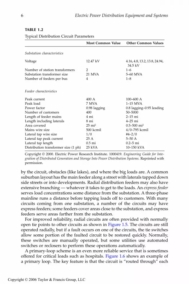
Distribution circuits come in many different configurations and circuitlengths. Most share many common characteristics. Figure 1.3 shows a “typ-ical” distribution circuit, and Table 1.2 shows typical parameters of a distri-bution circuit. A
feeder
is one of the circuits out of the substation. The mainfeeder is the three-phase backbone of the circuit, which is often called the
mains
or
mainline
. The mainline is normally a modestly large conductor suchas a 500- or 750-kcmil aluminum conductor. Utilities often design the mainfeeder for 400 A and often allow an emergency rating of 600 A. Branchingfrom the mains are one or more
laterals
, which are also called taps, lateraltaps, branches, or branch lines. These laterals may be single-phase, two-phase, or three-phase. The laterals normally have fuses to separate themfrom the mainline if they are faulted.
The most common distribution primaries are four-wire, multigroundedsystems: three-phase conductors plus a multigrounded neutral. Single-phaseloads are served by transformers connected between one phase and theneutral. The neutral acts as a return conductor and as an equipment safetyground (it is grounded periodically and at all equipment). A single-phaseline has one phase conductor and the neutral, and a two-phase line has twophases and the neutral. Some distribution primaries are three-wire systems(with no neutral). On these, single-phase loads are connected phase to phase,and single-phase lines have two of the three phases.
There are several configurations of distribution systems. Most distributioncircuits are radial (both primary and secondary). Radial circuits have manyadvantages over networked circuits including
• Easier fault current protection• Lower fault currents over most of the circuit• Easier voltage control• Easier prediction and control of power flows• Lower cost
Distribution primary systems come in a variety of shapes and sizes (Figure1.4). Arrangements depend on street layouts, the shape of the area covered
9576_C01.fm Page 4 Friday, October 14, 2005 9:04 AM
Copyright © 2006 Taylor & Francis Group, LLC

Fundamentals of Distribution Systems
5
FIGURE 1.3
Typical distribution substation with one of several feeders shown (many lateral taps are leftoff). (Copyright © 2000. Electric Power Research Institute. 1000419.
Engineering Guide for Inte-gration of Distributed Generation and Storage Into Power Distribution Systems.
Reprinted withpermission.)
R
Single-phase lateral
Three-phase lateral
Recloser
Circuit breakeror recloser
100 Kfuse
65 Kfuse
21/28/35 MVA Z=9%
Load Tap Changing (LTC)transformer
400-A peak600-A emergency
feeder rating3-phase, 4-wiremultigrounded
circuit
Normallyopen tie
12.47 kV
138 kV
Normally openbus tie
Three-phasemains
9576_C01.fm Page 5 Friday, October 14, 2005 9:04 AM
Copyright © 2006 Taylor & Francis Group, LLC
6
Electric Power Distribution Equipment and Systems
by the circuit, obstacles (like lakes), and where the big loads are. A commonsuburban layout has the main feeder along a street with laterals tapped downside streets or into developments. Radial distribution feeders may also haveextensive branching — whatever it takes to get to the loads. An
express feeder
serves load concentrations some distance from the substation. A three-phasemainline runs a distance before tapping loads off to customers. With manycircuits coming from one substation, a number of the circuits may haveexpress feeders; some feeders cover areas close to the substation, and expressfeeders serve areas farther from the substation.
For improved reliability, radial circuits are often provided with normallyopen tie points to other circuits as shown in Figure 1.5. The circuits are stilloperated radially, but if a fault occurs on one of the circuits, the tie switchesallow some portion of the faulted circuit to be restored quickly. Normally,these switches are manually operated, but some utilities use automatedswitches or reclosers to perform these operations automatically.
A primary-loop scheme is an even more reliable service that is sometimesoffered for critical loads such as hospitals. Figure 1.6 shows an example ofa primary loop. The key feature is that the circuit is “routed through” each
TABLE 1.2
Typical Distribution Circuit Parameters
Most Common Value Other Common Values
Substation characteristics
Voltage 12.47 kV 4.16, 4.8, 13.2, 13.8, 24.94, 34.5 kV
Number of station transformers 2 1–6Substation transformer size 21 MVA 5–60 MVANumber of feeders per bus 4 1–8
Feeder characteristics
Peak current 400 A 100–600 APeak load 7 MVA 1–15 MVAPower factor 0.98 lagging 0.8 lagging–0.95 leadingNumber of customers 400 50–5000Length of feeder mains 4 mi 2–15 miLength including laterals 8 mi 4–25 miArea covered 25 mi
2
0.5–500 mi
2
Mains wire size 500 kcmil 4/0–795 kcmilLateral tap wire size 1/0 #4–2/0Lateral tap peak current 25 A 5–50 ALateral tap length 0.5 mi 0.2–5 miDistribution transformer size (1 ph) 25 kVA 10–150 kVA
Copyright © 2000. Electric Power Research Institute. 1000419.
Engineering Guide for Inte-gration of Distributed Generation and Storage Into Power Distribution Systems.
Reprinted withpermission.
9576_C01.fm Page 6 Friday, October 14, 2005 9:04 AM
Copyright © 2006 Taylor & Francis Group, LLC

Fundamentals of Distribution Systems
7
critical customer transformer. If any part of the primary circuit is faulted, allcritical customers can still be fed by reconfiguring the transformer switches.
Primary-loop systems are sometimes used on distribution systems forareas needing high reliability (meaning limited long-duration interrup-tions). In the open-loop design where the loop is left normally open at somepoint, primary-loop systems have almost no benefits for momentary inter-ruptions or voltage sags. They are rarely operated in a closed loop. A widelyreported installation of a sophisticated
closed
system has been installed inOrlando, FL, by Florida Power Corporation (Pagel, 2000). An example ofthis type of closed-loop primary system is shown in Figure 1.7. Faults onany of the cables in the loop are cleared in less than six cycles, which reducesthe duration of the voltage sag during the fault (enough to help manycomputers). Advanced relaying similar to transmission-line protection isnecessary to coordinate the protection and operation of the switchgear inthe looped system. The relaying scheme uses a transfer trip with permissiveover-reaching (the relays at each end of the cable must agree there is a fault
FIGURE 1.4
Common distribution primary arrangements.
Express feederSingle mainline
Branched mainline Very branched mainline
9576_C01.fm Page 7 Friday, October 14, 2005 9:04 AM
Copyright © 2006 Taylor & Francis Group, LLC

8
Electric Power Distribution Equipment and Systems
between them with communications done on fiberoptic lines). A backupscheme uses directional relays, which will trip for a fault in a certain direc-tion unless a blocking signal is received from the remote end (again overthe fiberoptic lines).
Critical customers have two more choices for more reliable service wheretwo primary feeds are available. Primary selective and secondary selectiveschemes both are normally fed from one circuit (see Figure 1.8). So, thecircuits are still radial. In the event of a fault on the primary circuit, theservice is switched to the backup circuit. In the primary selective scheme,the switching occurs on the primary, and in the secondary selectivescheme, the switching occurs on the secondary. The switching can be donemanually or automatically, and there are even static transfer switches thatcan switch in less than a half cycle to reduce momentary interruptions andvoltage sags.
Today, the primary selective scheme is preferred mainly because of thecost associated with the extra transformer in a secondary selective scheme.The normally closed switch on the primary-side transfer switch opens after
FIGURE 1.5
Two radial circuits with normally open ties to each other. (Copyright © 2000. Electric PowerResearch Institute. 1000419.
Engineering Guide for Integration of Distributed Generation and StorageInto Power Distribution Systems.
Reprinted with permission.)
Normally open tie
9576_C01.fm Page 8 Friday, October 14, 2005 9:04 AM
Copyright © 2006 Taylor & Francis Group, LLC

Fundamentals of Distribution Systems
9
sensing a loss of voltage. It normally has a time delay on the order of seconds— enough to ride through the distribution circuit’s normal reclosing cycle.The opening of the switch is blocked if there is an overcurrent in the switch(the switch doesn’t have fault interrupting capability). Transfer is also dis-abled if the alternate feed does not have proper voltage. The switch canreturn to normal through either an open or a closed transition; in a closedtransition, both distribution circuits are temporarily paralleled.
1.2 Urban Networks
Some distribution circuits are not radial. The most common are the grid andspot secondary networks. In these systems, the secondary is networkedtogether and has feeds from several primary distribution circuits. The spot
FIGURE 1.6
Primary loop distribution arrangement. (Copyright © 2000. Electric Power Research Institute.1000419.
Engineering Guide for Integration of Distributed Generation and Storage Into Power Distri-bution Systems.
Reprinted with permission.)
N.C.
N.C.
N.C.N.O.
9576_C01.fm Page 9 Friday, October 14, 2005 9:04 AM
Copyright © 2006 Taylor & Francis Group, LLC

10
Electric Power Distribution Equipment and Systems
network feeds one load such as a high-rise building. The grid network feedsseveral loads at different points in an area. Secondary networks are veryreliable; if any of the primary distribution circuits fail, the others will carrythe load without causing an outage for any customers.
The spot network generally is fed by three to five primary feeders (seeFigure 1.9). The circuits are generally sized to be able to carry all of the loadwith the loss of either one or two of the primary circuits. Secondary networkshave network protectors between the primary and the secondary network.A network protector is a low-voltage circuit breaker that will open whenthere is reverse power through it. When a fault occurs on a primary circuit,fault current backfeeds from the secondary network(s) to the fault. Whenthis occurs, the network protectors will trip on reverse power. A spot networkoperates at 480Y/277 V or 208Y/120 V in the U.S.
Secondary grid networks are distribution systems that are used in mostmajor cities. The secondary network is usually 208Y/120 V in the U.S. Fiveto ten primary distribution circuits (e.g., 12.47-kV circuits) feed the secondarynetwork at multiple locations. Figure 1.10 shows a small part of a secondarynetwork. As with a spot network, network protectors provide protection forfaults on the primary circuits. Secondary grid networks can have peak loads
FIGURE 1.7
Example of a closed-loop distribution system.
R
R
R
R
RRR
R
R
R
To loads
R
R
9576_C01.fm Page 10 Friday, October 14, 2005 9:04 AM
Copyright © 2006 Taylor & Francis Group, LLC

Fundamentals of Distribution Systems
11
of 5 to 50 MVA. Most utilities limit networks to about 50 MVA, but somenetworks are over 250 MVA. Loads are fed by tapping into the secondarynetworks at various points. Grid networks (also called street networks) cansupply residential or commercial loads, either single or three phase. Forsingle-phase loads, three-wire service is provided to give 120 V and 208 V(rather than the standard three-wire residential service, which supplies 120V and 240 V).
Networks are normally fed by feeders originating from one substation bus.Having one source reduces circulating current and gives better load divisionand distribution among circuits. It also reduces the chance that networkprotectors stay open under light load (circulating current can trip the pro-tectors). Given these difficulties, it is still possible to feed grid or spot net-works from different substations or electrically separate buses.
The network protector is the key to automatic isolation and continuedoperation. The network protector is a three-phase low-voltage air circuitbreaker with controls and relaying. The network protector is mounted onthe network transformer or on a vault wall. Standard units are available withcontinuous ratings from 800 to 5000 A. Smaller units can interrupt 30 kAsymmetrical, and larger units have interrupt ratings of 60 kA (IEEE Std.
FIGURE 1.8
Primary and secondary selective schemes. (Copyright © 2000. Electric Power Research Institute.1000419.
Engineering Guide for Integration of Distributed Generation and Storage Into Power Distri-bution Systems.
Reprinted with permission.)
N.C.
N.O.
N.O.
N.C.
N.C.
PrimarySelectiveScheme
SecondarySelectiveScheme
N.O. = Normally openN.C. = Normally closed
9576_C01.fm Page 11 Friday, October 14, 2005 9:04 AM
Copyright © 2006 Taylor & Francis Group, LLC

12
Electric Power Distribution Equipment and Systems
C57.12.44–2000). A network protector senses and operates for reverse powerflow (it does not have forward-looking protection). Protectors are availablefor either 480Y/277 V or 216Y/125 V.
The tripping current on network protectors can be changed, with low,nominal, and high settings, which are normally 0.05 to 0.1%, 0.15 to 0.20%,and 3 to 5% of the network protector rating. For example, a 2000-A networkprotector has a low setting of 1 A, a nominal setting of 4 A, and a high settingof 100 A (IEEE Std. C57.12.44–2000). Network protectors also have fuses thatprovide backup in case the network protector fails to operate, and as asecondary benefit, provide protection to the network protector and trans-former against faults in the secondary network that are close.
The closing voltages are also adjustable: a 216Y/125-V protector has low,medium, and high closing voltages of 1 V, 1.5 V, and 2 V, respectively; a480Y/277-V protector has low, medium, and high closing voltages of 2.2 V,3.3 V, and 4.4 V, respectively.
1.3 Primary Voltage Levels
Most distribution voltages are between 4 and 35 kV. In this book, unlessotherwise specified, voltages are given as line-to-line voltages; this followsnormal industry practice, but it is sometimes a source of confusion. The four
FIGURE 1.9
Spot network. (Copyright © 2000. Electric Power Research Institute. 1000419.
Engineering Guidefor Integration of Distributed Generation and Storage Into Power Distribution Systems.
Reprintedwith permission.)
Networktransformer
Network protector
208Y/120 V or 480Y/277 V spot network
or
9576_C01.fm Page 12 Friday, October 14, 2005 9:04 AM
Copyright © 2006 Taylor & Francis Group, LLC

Fundamentals of Distribution Systems
13
major voltage classes are 5, 15, 25, and 35 kV. A voltage class is a term appliedto a set of distribution voltages and the equipment common to them; it isnot the actual system voltage. For example, a 15-kV insulator is suitable forapplication on any 15-kV class voltage, including 12.47 kV, 13.2 kV, and 13.8kV. Cables, terminations, insulators, bushings, reclosers, and cutouts all havea voltage class rating. Only voltage-sensitive equipment like surge arresters,capacitors, and transformers have voltage ratings dependent on the actualsystem voltage.
FIGURE 1.10
Portion of a grid network. (Copyright © 2000. Electric Power Research Institute. 1000419.
Engineering Guide for Integration of Distributed Generation and Storage Into Power DistributionSystems.
Reprinted with permission.)
Network transformer
Network protector
or
208Y/120-Vnetwork
Primaryfeeders
9576_C01.fm Page 13 Friday, October 14, 2005 9:04 AM
Copyright © 2006 Taylor & Francis Group, LLC

14
Electric Power Distribution Equipment and Systems
Utilities most widely use the 15-kV voltages as shown by the survey resultsof North American utilities in Figure 1.11. The most common 15-kV voltageis 12.47 kV, which has a line-to-ground voltage of 7.2 kV.
The dividing line between distribution and subtransmission is often gray.Some lines act as both subtransmission and distribution circuits. A 34.5-kVcircuit may feed a few 12.5-kV distribution substations, but it may also servesome load directly. Some utilities would refer to this as subtransmission,others as distribution.
The last half of the 20th century saw a move to higher voltage primarydistribution systems. Higher-voltage distribution systems have advantagesand disadvantages (see Table 1.3 for a summary). The great advantage ofhigher voltage systems is that they carry more power for a given current(Table 1.4 shows maximum power levels typically supplied by various dis-tribution voltages). Less current means lower voltage drop, fewer losses, andmore power-carrying capability. Higher voltage systems need fewer voltage
FIGURE 1.11
Usage of different distribution voltage classes (n = 107). (Data from [IEEE Working Group onDistribution Protection, 1995].)
TABLE 1.3
Advantages and Disadvantages of Higher Voltage Distribution
Advantages Disadvantages
Voltage drop
— A higher-voltage circuit has less voltage drop for a given power flow.
Capacity
— A higher-voltage system can carry more power for a given ampacity.
Losses
— For a given level of power flow, a higher-voltage system has fewer line losses.
Reach
— With less voltage drop and more capacity, higher voltage circuits can cover a much wider area.
Fewer substations
— Because of longer reach, higher-voltage distribution systems need fewer substations.
Reliability
— An important disadvantage of higher voltages: longer circuits mean more customer interruptions.
Crew safety and acceptance
— Crews do not like working on higher-voltage distribution systems.
Equipment cost
— From transformers to cable to insulators, higher-voltage equipment costs more.
Percentage using each voltage class
35 kV
25 kV
15 kV
5 kV
0 20 40 60 80
Portion of total load
0 20 40 60 80
By number of utilities
9576_C01.fm Page 14 Friday, October 14, 2005 9:04 AM
Copyright © 2006 Taylor & Francis Group, LLC

Fundamentals of Distribution Systems
15
regulators and capacitors for voltage support. Utilities can use smaller con-ductors on a higher voltage system or carry more power on the same sizeconductor. Utilities can run much longer distribution circuits at a higherprimary voltage, which means fewer distribution substations. Some funda-mental relationships are:
•
Power
— For the same current, power changes linearly with voltage.
when
I
2
= I
1
•
Current
— For the same power, increasing the voltage decreasescurrent linearly.
when
P
2
= P
1
•
Voltage drop
— For the same power delivered, the percentage voltagedrop changes as the ratio of voltages squared. A 12.47-kV circuit hasfour times the percentage voltage drop as a 24.94-kV circuit carryingthe same load.
when
P
2
= P
1
•
Area coverage
— For the same load density, the area covered increaseslinearly with voltage: A 24.94-kV system can cover twice the area ofa 12.47-kV system; a 34.5-kV system can cover 2.8 times the area ofa 12.47-kV system.
TABLE 1.4
Power Supplied by Each Distribution
Voltage for a Current of 400 A
System Voltage(kV)
Total Power(MVA)
4.8 3.312.47 8.622.9 15.934.5 23.9
PVV
P21
11=
IVV
I21
21=
VVV
V% %21
2
2
1=⎛
⎝⎜
⎞
⎠⎟
9576_C01.fm Page 15 Friday, October 14, 2005 9:04 AM
Copyright © 2006 Taylor & Francis Group, LLC

16
Electric Power Distribution Equipment and Systems
where
V
1
,
V
2
= voltage on circuits 1 and 2
P
1
,
P
2
= power on circuits 1 and 2
I
1
,
I
2
= current on circuits 1 and 2
V
%1
,
V
%2
= voltage drop per unit length in percent on circuits 1 and 2
A
1
,
A
2
= area covered by circuits 1 and 2
The squaring effect on voltage drop is significant. It means that doublingthe system voltage quadruples the load that can be supplied over the samedistance (with equal percentage voltage drop); or, twice the load can besupplied over twice the distance; or, the same load can be supplied over fourtimes the distance.
Resistive line losses are also lower on higher-voltage systems, especiallyin a voltage-limited circuit. Thermally limited systems have more equallosses, but even in this case higher voltage systems have fewer losses.
Line crews do not like higher voltage distribution systems as much. Inaddition to the widespread perception that they are not as safe, gloves arethicker, and procedures are generally more stringent. Some utilities will notglove 25- or 35-kV voltages and only use hotsticks.
The main disadvantage of higher-voltage systems is reduced reliability.Higher voltages mean longer lines and more exposure to lightning, wind,dig-ins, car crashes, and other fault causes. A 34.5-kV, 30-mi mainline is goingto have many more interruptions than a 12.5-kV system with an 8-mi main-line. To maintain the same reliability as a lower-voltage distribution system,a higher-voltage primary must have more switches, more automation, moretree trimming, or other reliability improvements. Higher voltage systemsalso have more voltage sags and momentary interruptions. More exposurecauses more momentary interruptions. Higher voltage systems have morevoltage sags because faults further from the substation can pull down thestation’s voltage (on a higher voltage system the line impedance is lowerrelative to the source impedance).
Cost comparison between circuits is difficult (see Table 1.5 for one utility’scost comparison). Higher voltage equipment costs more — cables, insulators,transformers, arresters, cutouts, and so on. But higher voltage circuits canuse smaller conductors. The main savings of higher-voltage distribution isfewer substations. Higher voltage systems also have lower annual costs fromlosses. As far as ongoing maintenance, higher voltage systems require lesssubstation maintenance, but higher voltage systems should have more treetrimming and inspections to maintain reliability.
Conversion to a higher voltage is an option for providing additional capacityin an area. Conversion to higher voltages is most beneficial when substation
AVV
A22
11=
9576_C01.fm Page 16 Friday, October 14, 2005 9:04 AM
Copyright © 2006 Taylor & Francis Group, LLC

Fundamentals of Distribution Systems 17
space is hard to find and load growth is high. If the existing subtransmissionvoltage is 34.5 kV, then using that voltage for distribution is attractive; addi-tional capacity can be met by adding customers to existing 34.5-kV lines (aneutral may need to be added to the 34.5-kV subtransmission line).
Higher voltage systems are also more prone to ferroresonance. Radio inter-ference is also more common at higher voltages.
Overall, the 15-kV class voltages provide a good balance between cost,reliability, safety, and reach. Although a 15-kV circuit does not naturallyprovide long reach, with voltage regulators and feeder capacitors it can bestretched to reach 20 mi or more. That said, higher voltages have advantages,especially for rural lines and for high-load areas, particularly where substa-tion space is expensive.
Many utilities have multiple voltages (as shown by the survey data inFigure 1.11). Even one circuit may have multiple voltages. For example, autility may install a 12.47-kV circuit in an area presently served by 4.16 kV.Some of the circuit may be converted to 12.47 kV, but much of it can be leftas is and coupled through 12.47/4.16-kV step-down transformer banks.
1.4 Distribution Substations
Distribution substations come in many sizes and configurations. A small ruralsubstation may have a nominal rating of 5 MVA while an urban station maybe over 200 MVA. Figure 1.12 through Figure 1.14 show examples of small,medium, and large substations. As much as possible, many utilities have stan-dardized substation layouts, transformer sizes, relaying systems, and automa-tion and SCADA (supervisory control and data acquisition) facilities. Mostdistribution substation bus configurations are simple with limited redundancy.
Transformers smaller than 10 MVA are normally protected with fuses, butfuses are also used for transformers to 20 or 30 MVA. Fuses are inexpensiveand simple; they don’t need control power and take up little space. Fusesare not particularly sensitive, especially for evolving internal faults. Largertransformers normally have relay protection that operates a circuit switcher
TABLE 1.5
Costs of 34.5 kV Relative to 12.5 kV
Item Underground Overhead
Subdivision without bulk feeders 1.25 1.13Subdivision with bulk feeders 1.00 0.85Bulk feeders 0.55 0.55Commercial areas 1.05–1.25 1.05–1.25
Source: Jones, A.I., Smith, B.E., and Ward, D.J., “Considerationsfor Higher Voltage Distribution,” IEEE Transactions on Power De-livery, vol. 7, no. 2, pp. 782–8, April 1992.
9576_C01.fm Page 17 Friday, October 14, 2005 9:04 AM
Copyright © 2006 Taylor & Francis Group, LLC

18 Electric Power Distribution Equipment and Systems
or a circuit breaker. Relays often include differential protection, sudden-pressure relays, and overcurrent relays. Both the differential protection andthe sudden-pressure relays are sensitive enough to detect internal failuresand clear the circuit to limit additional damage to the transformer. Occasion-ally, relays operate a high-side grounding switch instead of an interrupter.When the grounding switch engages, it creates a bolted fault that is clearedby an upstream device or devices.
The feeder interrupting devices are normally relayed circuit breakers,either free-standing units or metal-enclosed switchgear. Many utilities alsouse reclosers instead of breakers, especially at smaller substations.
Station transformers are normally protected by differential relays whichtrip if the current into the transformer is not very close to the current outof the transformer. Relaying may also include pressure sensors. The high-side protective device is often a circuit switcher but may also be fuses or acircuit breaker.
Two-bank stations are very common (Figure 1.13); these are the standarddesign for many utilities. Normally, utilities size the transformers so that ifeither transformer fails, the remaining unit can carry the entire substation’sload. Utility practices vary on how much safety margin is built into thiscalculation, and load growth can eat into the redundancy.
FIGURE 1.12Example rural distribution substation.
FIGURE 1.13Example suburban distribution substation.
10/13/17 MVA Z=7%
Load Tap Changing (LTC)transformer
24.94 kV
115 kV
LTC21/28/35 MVA
Z=9%
12.47 kV
138 kV
Normally openbus-tie breaker
9576_C01.fm Page 18 Friday, October 14, 2005 9:04 AM
Copyright © 2006 Taylor & Francis Group, LLC

Fundamentals of Distribution Systems 19
Most utilities normally use a split bus: a bus tie between the two buses isnormally left open in distribution substations. The advantages of a split bus are:
• Lower fault current — This is the main reason that bus ties are open.For a two-bank station with equal transformers, opening the bus tiecuts fault current in half.
• Circulating current — With a split bus, current cannot circulatethrough both transformers.
• Bus regulation — Bus voltage regulation is also simpler with a splitbus. With the tie closed, control of paralleled tap changers is moredifficult.
Having the bus tie closed has some advantages, and many utilities useclosed ties under some circumstances. A closed bus tie is better for
• Secondary networks — When feeders from each bus supply either spotor grid secondary networks, closed bus ties help prevent circulatingcurrent through the secondary networks.
FIGURE 1.14Example urban distribution substation.
LTC30/40/50 MVA
Z=16%
12.47 kV
138 kV
12.47 kV
138 kV
12.47 kV
138 kV
12.47 kV
138 kV
50 Mvar
9576_C01.fm Page 19 Friday, October 14, 2005 9:04 AM
Copyright © 2006 Taylor & Francis Group, LLC

20 Electric Power Distribution Equipment and Systems
• Unequal loading — A closed bus tie helps balance the loading on thetransformers. If the set of feeders on one bus has significantly dif-ferent loading patterns (either seasonal or daily), then a closed bustie helps even out the loading (and aging) of the two transformers.
Whether the bus tie is open or closed has little impact on reliability. In theuncommon event that one transformer fails, both designs allow the stationto be reconfigured so that one transformer supplies both bus feeders. Theclosed-tie scenario is somewhat better in that an automated system canreconfigure the ties without total loss of voltage to customers (customers dosee a very large voltage sag). In general, both designs perform about thesame for voltage sags.
Urban substations are more likely to have more complicated bus arrange-ments. These could include ring buses or breaker-and-a-half schemes. Figure1.14 shows an example of a large urban substation with feeders supplyingsecondary networks. If feeders are supplying secondary networks, it is notcritical to maintain continuity to each feeder, but it is important to preventloss of any one bus section or piece of equipment from shutting down thenetwork (an N-1 design).
For more information on distribution substations, see (RUS 1724E-300,2001; Westinghouse Electric Corporation, 1965).
1.5 Subtransmission Systems
Subtransmission systems are those circuits that supply distribution substa-tions. Several different subtransmission systems can supply distribution sub-stations. Common subtransmission voltages include 34.5, 69, 115, and 138kV. Higher voltage subtransmission lines can carry more power with lesslosses over greater distances. Distribution circuits are occasionally suppliedby high-voltage transmission lines such as 230 kV; such high voltages makefor expensive high-side equipment in a substation. Subtransmission circuitsare normally supplied by bulk transmission lines at subtransmission substa-tions. For some utilities, one transmission system serves as both the sub-transmission function (feeding distribution substations) and thetransmission function (distributing power from bulk generators). There ismuch crossover in functionality and voltage. One utility may have a 23-kVsubtransmission system supplying 4-kV distribution substations. Anotherutility right next door may have a 34.5-kV distribution system fed by a 138-kV subtransmission system. And within utilities, one can find a variety ofdifferent voltage combinations.
Of all of the subtransmission circuit arrangements, a radial configurationis the simplest and least expensive (see Figure 1.15). But radial circuitsprovide the most unreliable supply; a fault on the subtransmission circuit
9576_C01.fm Page 20 Friday, October 14, 2005 9:04 AM
Copyright © 2006 Taylor & Francis Group, LLC

Fundamentals of Distribution Systems 21
can force an interruption of several distribution substations and service tomany customers. A variety of redundant subtransmission circuits are avail-able, including dual circuits and looped or meshed circuits (see Figure 1.16).The design (and evolution) of subtransmission configurations depends onhow the circuit developed, where the load is needed now and in the future,what the distribution circuit voltages are, where bulk transmission is avail-able, where rights-of-way are available, and, of course, economic factors.
Most subtransmission circuits are overhead. Many are built right alongroads and streets just like distribution lines. Some — especially higher volt-age subtransmission circuits — use a private right-of-way such as bulktransmission lines use. Some new subtransmission lines are put under-ground, as development of solid-insulation cables has made costs morereasonable.
FIGURE 1.15Radial subtransmission systems.
N.C.
N.O.
Dual-sourcesubtransmission
N.O.
N.C.
Single-source, radialsubtransmission
Least reliable: Faults on theradial subtransmission circuitcan cause interruptions to multiple substations.
More reliable: Faults on one of the radial subtransmission circuits should not cause interruptions to substations.Double-circuit faults can cause multiple stationinterruptions.
Bulk transmission source
Distributionsubstation
9576_C01.fm Page 21 Friday, October 14, 2005 9:04 AM
Copyright © 2006 Taylor & Francis Group, LLC

22 Electric Power Distribution Equipment and Systems
Lower voltage subtransmission lines (69, 34.5, and 23 kV) tend to bedesigned and operated as are distribution lines, with radial or simple looparrangements, using wood-pole construction along roads, with reclosers andregulators, often without a shield wire, and with time-overcurrent protection.Higher voltage transmission lines (115, 138, and 230 kV) tend to be designedand operated like bulk transmission lines, with loop or mesh arrangements,tower configurations on a private right-of-way, a shield wire or wires forlightning protection, and directional or pilot-wire relaying from two ends.Generators may or may not interface at the subtransmission level (whichcan affect protection practices).
1.6 Differences between European and North American Systems
Distribution systems around the world have evolved into different forms.The two main designs are North American and European. This book dealsmainly with North American distribution practices; for more information onEuropean systems, see Lakervi and Holmes (1995). For both forms, hardwareis much the same: conductors, cables, insulators, arresters, regulators, andtransformers are very similar. Both systems are radial, and voltages andpower carrying capabilities are similar. The main differences are in layouts,configurations, and applications.
FIGURE 1.16Looped subtransmission system.
If either source segment is lost,one transformer can supply both
distribution buses.
Bulk transmission source
Can continue tosupply load if either transmissionsegment is lost.
Cannot supply load if the bottom
transmission segment is lost.
9576_C01.fm Page 22 Friday, October 14, 2005 9:04 AM
Copyright © 2006 Taylor & Francis Group, LLC

Fundamentals of Distribution Systems 23
Figure 1.17 compares the two systems. Relative to North American designs,European systems have larger transformers and more customers per trans-former. Most European transformers are three-phase and on the order of 300to 1000 kVA, much larger than typical North American 25- or 50-kVA single-phase units.
Secondary voltages have motivated many of the differences in distributionsystems. North America has standardized on a 120/240-V secondary system;on these, voltage drop constrains how far utilities can run secondaries,typically no more than 250 ft. In European designs, higher secondary volt-ages allow secondaries to stretch to almost 1 mi. European secondaries arelargely three-phase and most European countries have a standard secondaryvoltage of 220, 230, or 240 V, twice the North American standard. With twicethe voltage, a circuit feeding the same load can reach four times the distance.And because three-phase secondaries can reach over twice the length of asingle-phase secondary, overall, a European secondary can reach eight timesthe length of an American secondary for a given load and voltage drop.Although it is rare, some European utilities supply rural areas with single-
FIGURE 1.17North American versus European distribution layouts.
Single-phase laterals
3-phase, 4-wiremultigrounded
primary
12.47 kV
North American Layout
4-wire, 3-phase secondaries
3-phaseprimary
11 kV
European Layout
120/240 V
220/380 V or230/400 V or240/416 V
240/480 V
May be grounded with a resistor or reactor
9576_C01.fm Page 23 Friday, October 14, 2005 9:04 AM
Copyright © 2006 Taylor & Francis Group, LLC

24 Electric Power Distribution Equipment and Systems
phase taps made of two phases with single-phase transformers connectedphase to phase.
In the European design, secondaries are used much like primary lateralsin the North American design. In European designs, the primary is nottapped frequently, and primary-level fuses are not used as much. Euro-pean utilities also do not use reclosing as religiously as North Americanutilities.
Some of the differences in designs center around the differences in loadsand infrastructure. In Europe, the roads and buildings were already in placewhen the electrical system was developed, so the design had to “fit in.”Secondary is often attached to buildings. In North America, many of theroads and electrical circuits were developed at the same time. Also, in Europehouses are packed together more and are smaller than houses in America.
Each type of system has its advantages. Some of the major differencesbetween systems are the following (see also Carr and McCall, 1992;Meliopoulos et al., 1998; Nguyen et al., 2000):
• Cost — The European system is generally more expensive than theNorth American system, but there are so many variables that it ishard to compare them on a one-to-one basis. For the types of loadsand layouts in Europe, the European system fits quite well. Europeanprimary equipment is generally more expensive, especially for areasthat can be served by single-phase circuits.
• Flexibility — The North American system has a more flexible primarydesign, and the European system has a more flexible secondarydesign. For urban systems, the European system can take advantageof the flexible secondary; for example, transformers can be sitedmore conveniently. For rural systems and areas where load is spreadout, the North American primary system is more flexible. The NorthAmerican primary is slightly better suited for picking up new loadand for circuit upgrades and extensions.
• Safety — The multigrounded neutral of the North American primarysystem provides many safety benefits; protection can more reliablyclear faults, and the neutral acts as a physical barrier, as well ashelping to prevent dangerous touch voltages during faults. TheEuropean system has the advantage that high-impedance faults areeasier to detect.
• Reliability — Generally, North American designs result in fewercustomer interruptions. Nguyen et al. (2000) simulated the perfor-mance of the two designs for a hypothetical area and found that theaverage frequency of interruptions was over 35% higher on theEuropean system. Although European systems have less primary,almost all of it is on the main feeder backbone; loss of the mainfeeder results in an interruption for all customers on the circuit.
9576_C01.fm Page 24 Friday, October 14, 2005 9:04 AM
Copyright © 2006 Taylor & Francis Group, LLC

Fundamentals of Distribution Systems 25
European systems need more switches and other gear to maintainthe same level of reliability.
• Power quality — Generally, European systems have fewer voltagesags and momentary interruptions. On a European system, lessprimary exposure should translate into fewer momentary interrup-tions compared to a North American system that uses fuse saving.The three-wire European system helps protect against sags fromline-to-ground faults. A squirrel across a bushing (from line toground) causes a relatively high impedance fault path that does notsag the voltage much compared to a bolted fault on a well-groundedsystem. Even if a phase conductor faults to a low-impedance returnpath (such as a well-grounded secondary neutral), the delta – wyecustomer transformers provide better immunity to voltage sags,especially if the substation transformer is grounded through a resis-tor or reactor.
• Aesthetics — Having less primary, the European system has an aes-thetic advantage: the secondary is easier to underground or to blendin. For underground systems, fewer transformer locations andlonger secondary reach make siting easier.
• Theft — The flexibility of the European secondary system makespower much easier to steal. Developing countries especially havethis problem. Secondaries are often strung along or on top of build-ings; this easy access does not require great skill to attach into.
Outside of Europe and North America, both systems are used, and usagetypically follows colonial patterns with European practices being morewidely used. Some regions of the world have mixed distribution systems,using bits of North American and bits of European practices. The worstmixture is 120-V secondaries with European-style primaries; the low-voltagesecondary has limited reach along with the more expensive European pri-mary arrangement.
Higher secondary voltages have been explored (but not implemented tomy knowledge) for North American systems to gain flexibility. Highersecondary voltages allow extensive use of secondary, which makes under-grounding easier and reduces costs. Westinghouse engineers contended thatboth 240/480-V three-wire single-phase and 265/460-V four-wire three-phase secondaries provide cost advantages over a similar 120/240-V three-wire secondary (Lawrence and Griscom, 1956; Lokay and Zimmerman,1956). Higher secondary voltages do not force higher utilization voltages;a small transformer at each house converts 240 or 265 V to 120 V for lightingand standard outlet use (air conditioners and major appliances can beserved directly without the extra transformation). More recently, Bergeronet al. (2000) outline a vision of a distribution system where primary-leveldistribution voltage is stepped down to an extensive 600-V, three-phase
9576_C01.fm Page 25 Friday, October 14, 2005 9:04 AM
Copyright © 2006 Taylor & Francis Group, LLC

26 Electric Power Distribution Equipment and Systems
secondary system. At each house, an electronic transformer converts 600 Vto 120/240 V.
1.7 Loads
Distribution systems obviously exist to supply electricity to end users, soloads and their characteristics are important. Utilities supply a broad rangeof loads, from rural areas with load densities of 10 kVA/mi2 to urban areaswith 300 MVA/mi2. A utility may feed houses with a 10- to 20-kVA peakload on the same circuit as an industrial customer peaking at 5 MW. Theelectrical load on a feeder is the sum of all individual customer loads. Andthe electrical load of a customer is the sum of the load drawn by the cus-tomer’s individual appliances. Customer loads have many common charac-teristics. Load levels vary through the day, peaking in the afternoon or earlyevening. Several definitions are used to quantify load characteristics at agiven location on a circuit:
• Demand — The load average over a specified time period, often 15,20, or 30 min. Demand can be used to characterize real power,reactive power, total power, or current. Peak demand over someperiod of time is the most common way utilities quantify a circuit’sload. In substations, it is common to track the current demand.
• Load factor — The ratio of the average load over the peak load. Peakload is normally the maximum demand but may be the instanta-neous peak. The load factor is between zero and one. A load factorclose to 1.0 indicates that the load runs almost constantly. A low loadfactor indicates a more widely varying load. From the utility pointof view, it is better to have high load-factor loads. Load factor isnormally found from the total energy used (kilowatt-hours) as:
whereLF = load factor
kWh = energy use in kilowatt-hoursdkW = peak demand in kilowatts
h = number of hours during the time period• Coincident factor — The ratio of the peak demand of a whole system
to the sum of the individual peak demands within that system. The
LFkWh
d hkW
=×
9576_C01.fm Page 26 Friday, October 14, 2005 9:04 AM
Copyright © 2006 Taylor & Francis Group, LLC

Fundamentals of Distribution Systems 27
peak demand of the whole system is referred to as the peak diversifieddemand or as the peak coincident demand. The individual peakdemands are the noncoincident demands. The coincident factor is lessthan or equal to one. Normally, the coincident factor is much lessthan one because each of the individual loads do not hit their peakat the same time (they are not coincident).
• Diversity factor — The ratio of the sum of the individual peakdemands in a system to the peak demand of the whole system. Thediversity factor is greater than or equal to one and is the reciprocalof the coincident factor.
• Responsibility factor — The ratio of a load’s demand at the time ofthe system peak to its peak demand. A load with a responsibilityfactor of one peaks at the same time as the overall system. Theresponsibility factor can be applied to individual customers, cus-tomer classes, or circuit sections.
The loads of certain customer classes tend to vary in similar patterns.Commercial loads are highest from 8 a.m. to 6 p.m. Residential loads peakin the evening. Weather significantly changes loading levels. On hot summerdays, air conditioning increases the demand and reduces the diversity amongloads. At the transformer level, load factors of 0.4 to 0.6 are typical (Gangeland Propst, 1965).
Several groups have evaluated coincidence factors as a function of thenumber of customers. Nickel and Braunstein (1981) determined that onecurve fell roughly in the middle of several curves evaluated. Used by Arkan-sas Power and Light, this curve fits the following:
where n is the number of customers (see Figure 1.18).At the substation level, coincidence is also apparent. A transformer with
four feeders, each peaking at 100 A, will peak at less than 400 A because ofdiversity between feeders. The coincident factor between four feeders isnormally higher than coincident factors at the individual customer level.Expect coincident factors to be above 0.9. Each feeder is already highlydiversified, so not much more is gained by grouping more customerstogether if the sets of customers are similar. If the customer mix on eachfeeder is different, then multiple feeders can have significant differences. Ifsome feeders are mainly residential and others are commercial, the peak loadof the feeders together can be significantly lower than the sum of the peaks.For distribution transformers, the peak responsibility factor ranges from 0.5to 0.9 with 0.75 being typical (Nickel and Braunstein, 1981).
Different customer classes have different characteristics (see Figure 1.19for an example). Residential loads peak more in the evening and have a
Fnco = +
+⎛⎝
⎞⎠
12
15
2 3
9576_C01.fm Page 27 Friday, October 14, 2005 9:04 AM
Copyright © 2006 Taylor & Francis Group, LLC

28 Electric Power Distribution Equipment and Systems
relatively low load factor. Commercial loads tend to be more 8 a.m. to 6 p.m.,and the industrial loads tend to run continuously and, as a class, they havea higher load factor.
1.8 The Past and the Future
Looking at Seelye’s Electrical Distribution Engineering book (1930), we findmore similarities to than differences from present-day distribution systems.The basic layout and operations of distribution infrastructure at the start ofthe 21st century are much the same as in the middle of the 20th century.Equipment has undergone steady improvements; transformers are moreefficient; cables are much less expensive and easier to use; and protectionequipment is better (see Figure 1.20 for some development milestones).Utilities operate more distribution circuits at higher voltages and use moreunderground circuits. But the concepts are much the same: ac, three-phasesystems, radial circuits, fused laterals, overcurrent relays, etc. Advances incomputer technology have opened up possibilities for more automation andmore effective protection.
How will future distribution systems evolve? Given the fact that distribu-tion systems of the year 2000 look much the same as distribution systems in1950, a good guess is that the distribution system of 2050 (or at least 2025)will look much like today’s systems. More and more of the electrical infra-structure will be placed underground. Designs and equipment will continue
FIGURE 1.18Coincident factor average curve for utilities.
0.0
0.2
0.4
0.6
0.8
1.0
Number of customers
Coi
ncid
ent f
acto
r
1 5 10 15 20
9576_C01.fm Page 28 Friday, October 14, 2005 9:04 AM
Copyright © 2006 Taylor & Francis Group, LLC
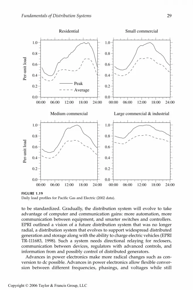
Fundamentals of Distribution Systems 29
to be standardized. Gradually, the distribution system will evolve to takeadvantage of computer and communication gains: more automation, morecommunication between equipment, and smarter switches and controllers.EPRI outlined a vision of a future distribution system that was no longerradial, a distribution system that evolves to support widespread distributedgeneration and storage along with the ability to charge electric vehicles (EPRITR-111683, 1998). Such a system needs directional relaying for reclosers,communication between devices, regulators with advanced controls, andinformation from and possibly control of distributed generators.
Advances in power electronics make more radical changes such as con-version to dc possible. Advances in power electronics allow flexible conver-sion between different frequencies, phasings, and voltages while still
FIGURE 1.19Daily load profiles for Pacific Gas and Electric (2002 data).
00:00 06:00 12:00 18:00 24:000.0
0.2
0.4
0.6
0.8
1.0
00:00 06:00 12:00 18:00 24:000.0
0.2
0.4
0.6
0.8
1.0
00:00 06:00 12:00 18:00 24:000.0
0.2
0.4
0.6
0.8
1.0
00:00 06:00 12:00 18:00 24:000.0
0.2
0.4
0.6
0.8
1.0
Per-
unit
load
Residential
Peak
Average
Small commercial
Medium commercial
Per-
unit
load
Large commercial & industrial
9576_C01.fm Page 29 Friday, October 14, 2005 9:04 AM
Copyright © 2006 Taylor & Francis Group, LLC

30 Electric Power Distribution Equipment and Systems
producing ac voltage to the end user at the proper voltage. While possible,radical changes are unlikely, given the advantages to evolving an existingsystem rather than replacing it. Whatever the approach, the future has chal-lenges; utilities will be expected to deliver more reliable power with minimalpollution while keeping the distribution system hidden from view and caus-ing the least disruption possible. And of course, costs are expected to staythe same or go down.
References
Bergeron, R., Slimani, K., Lamarche, L., and Cantin, B., “New Architecture of theDistribution System Using Electronic Transformer,” ESMO-2000, Panel on Dis-tribution Transformer, Breakers, Switches and Arresters, 2000.
Carr, J. and McCall, L.V., “Divergent Evolution and Resulting Characteristics Amongthe World’s Distribution Systems,” IEEE Transactions on Power Delivery, vol. 7,no. 3, pp. 1601–9, July 1992.
CEA, CEA Distribution Planner’s Manual, Canadian Electrical Association, 1982.EPRI 1000419, Engineering Guide for Integration of Distributed Generation and Storage
Into Power Distribution Systems, Electric Power Research Institute, Palo Alto,CA, 2000.
FIGURE 1.20Electric power distribution development timeline.
1890
1900
1910
1920
1930
1940
1880
1950
1960
1970
1980
1990
2000
CSP transformersMetal-clad switchgear
Autoreclosing circuit breakers
Hydraulic reclosers
TR-XLPE cablesAmorphous core distribution transformers
Metal-oxide riser pole arresters
XLPE cablesEPR cables
Westinghouse’s ac distribution systems
Distribution systems feeding arc lamps
Edison’s dc network in New York City
Paper insulated underground cables
Secondary grid network in NY with network protectors with autoreclosing
US peak load = 10 GW
US peak load = 100 GW
US peak load = 400 GW
Emergence of actechnology assuperior to dc
Rapid load growthand rise of 25 and35 kV distribution
Oil embargo and focus on energy efficiencyIncrease in underground
residential distribution
Growth of 15-kV distribution; move to multigrounded neutral systems
US Rural ElectrificationAssociation established
Mainly 2 and 4 kVdistribution
Increased load sensitivities(computers, digital clocks).Emergence of distribution-scalegeneration technologies.
Padmounted transformers
9576_C01.fm Page 30 Friday, October 14, 2005 9:04 AM
Copyright © 2006 Taylor & Francis Group, LLC
Fundamentals of Distribution Systems 31
EPRI TR-109178, Distribution Cost Structure — Methodology and Generic Data, ElectricPower Research Institute, Palo Alto, CA, 1998.
EPRI TR-111683, Distribution Systems Redesign, Electric Power Research Institute, PaloAlto, CA, 1998.
Gangel, M.W. and Propst, R.F., “Distribution Transformer Load Characteristics,” IEEETransactions on Power Apparatus and Systems, vol. 84, pp. 671–84, August 1965.
IEEE Std. C57.12.44–2000, IEEE Standard Requirements for Secondary Network Pro-tectors.
IEEE Tutorial Course, Power Distribution Planning, 1992. Course text 92 EHO 361–6-PWR.
IEEE Working Group on Distribution Protection, “Distribution Line Protection Prac-tices Industry Survey Results,” IEEE Transactions on Power Delivery, vol. 10, no.1, pp. 176–86, January 1995.
Jones, A.I., Smith, B.E., and Ward, D.J., “Considerations for Higher Voltage Distribu-tion,” IEEE Transactions on Power Delivery, vol. 7, no. 2, pp. 782–8, April 1992.
Lakervi, E. and Holmes, E.J., Electricity Distribution Network Design, IEE Power Engi-neering Series 21, Peter Peregrinius, 1995.
Lawrence, R.F. and Griscom, S.B., “Residential Distribution — An Analysis of Systemsto Serve Expanding Loads,” AIEE Transactions, Part III, vol. 75, pp. 533–42, 1956.
Lokay, H.E. and Zimmerman, R.A., “Economic Comparison of Secondary Voltages:Single and Three Phase Distribution for Residential Areas,” AIEE Transactions,Part III, vol. 75, pp. 542–52, 1956.
Meliopoulos, A.P. S., Kennedy, J., Nucci, C.A., Borghetti, A., and Contaxis, G., “PowerDistribution Practices in USA and Europe: Impact on Power Quality,” 8thInternational Conference on Harmonics and Quality of Power, 1998.
Nguyen, H.V., Burke, J.J., and Benchluch, S., “Rural Distribution System DesignComparison,” IEEE Power Engineering Society Winter Meeting, 2000.
Nickel, D.L. and Braunstein, H.R., “Distribution. Transformer Loss Evaluation. II.Load Characteristics and System Cost Parameters,” IEEE Transactions on PowerApparatus and Systems, vol. PAS-100, no. 2, pp. 798–811, February 1981.
Pagel, B., “Energizing International Drive,” Transmission & Distribution World, April2000.
RUS 1724E-300, Design Guide for Rural Substations, United States Department of Ag-riculture, Rural Utilities Service, 2001.
Seelye, H.P., Electrical Distribution Engineering, McGraw-Hill New York, 1930.Westinghouse Electric Corporation, Distribution Systems, vol. 3, 1965.Willis, H.L., Power Distribution Planning Reference Book, Marcel Dekker, New York,
1997.
No matter how long you’ve been a Power Lineman, you still notice it whenpeople refer to your poles as “telephone poles.”
Powerlineman law #46, By CD Thayer and other Power Linemen,http://www.cdthayer.com/lineman.htm
9576_C01.fm Page 31 Friday, October 14, 2005 9:04 AM
Copyright © 2006 Taylor & Francis Group, LLC

33
2
Overhead Lines
Along streets, alleys, through woods, and in backyards, many of the dis-tribution lines that feed customers are overhead structures. Because over-head lines are exposed to trees and animals, to wind and lightning, and tocars and kites, they are a critical component in the reliability of distributioncircuits. This chapter discusses many of the key electrical considerationsof overhead lines: conductor characteristics, impedances, ampacity, andother issues.
2.1 Typical Constructions
Overhead constructions come in a variety of configurations (see Figure 2.1).Normally one primary circuit is used per pole, but utilities sometimes runmore than one circuit per structure. For a three-phase circuit, the most com-mon structure is a horizontal layout with an 8- or 10-ft wood crossarm on apole (see Figure 2.2). Armless constructions are also widely found wherefiberglass insulator standoffs or post insulators are used in a tighter config-uration. Utilities normally use 30- to 45-ft poles, set 6 to 8 ft deep. Verticalconstruction is also occasionally used. Span lengths vary from 100 to 150 ftin suburban areas to as much as 300 or 400 ft in rural areas.
Distribution circuits normally have an underbuilt neutral — the neutralacts as a safety ground for equipment and provides a return path forunbalanced loads and for line-to-ground faults. The neutral is 3 to 5 ft belowthe phase conductors. Utilities in very high lightning areas may run theneutral wire above the phase conductors to act as a shield wire. Someutilities also run the neutral on the crossarm. Secondary circuits are oftenrun under the primary. The primary and the secondary may share theneutral, or they may each have their own neutral. Many electric utilitiesshare their space with other utilities; telephone or cable television cablesmay run under the electric secondary.
9576_C02.fm Page 33 Monday, October 17, 2005 7:15 AM
Copyright © 2006 Taylor & Francis Group, LLC

34
Electric Power Distribution Equipment and Systems
(a)
FIGURE 2.1
Example overhead distribution structures. (a) Three-phase 34.5-kV armless construction withcovered wire.
9576_C02.fm Page 34 Monday, October 17, 2005 7:15 AM
Copyright © 2006 Taylor & Francis Group, LLC

Overhead Lines
35
(b)
FIGURE 2.1
Continued. (b) Single-phase circuit, 7.2 kV line-to-ground.
9576_C02.fm Page 35 Monday, October 17, 2005 7:15 AM
Copyright © 2006 Taylor & Francis Group, LLC
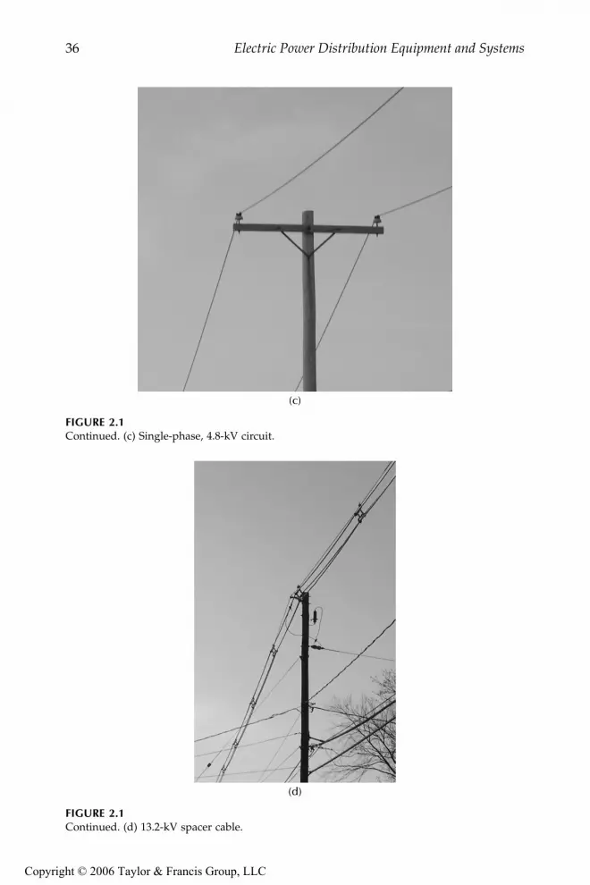
36
Electric Power Distribution Equipment and Systems
(c)
FIGURE 2.1
Continued. (c) Single-phase, 4.8-kV circuit.
(d)
FIGURE 2.1
Continued. (d) 13.2-kV spacer cable.
9576_C02.fm Page 36 Monday, October 17, 2005 7:15 AM
Copyright © 2006 Taylor & Francis Group, LLC

Overhead Lines
37
Wood is the main pole material, although steel, concrete, and fiberglassare also used. Treated wood lasts a long time, is easy to climb and attachequipment to, and also augments the insulation between the energized con-ductors and ground. Conductors are primarily aluminum. Insulators are pintype, post type, or suspension, either porcelain or polymer.
The National Electrical Safety Code (IEEE C2-2000) governs many of thesafety issues that play important roles in overhead design issues. Poles musthave space for crews to climb them and work safely in the air. All equipmentmust have sufficient strength to stand up to “normal” operations. Conduc-tors must carry their weight, the weight of any accumulated ice, plus with-stand the wind pressure exerted on the wire. We are not going to discussmechanical and structural issues in this book. For more information, see the
Lineman’s and Cableman’s Handbook
(Kurtz et al., 1997), the
Mechanical DesignManual for Overhead Distribution Lines
(RUS 160-2, 1982), the
NESC
(IEEE C2-2000), and the
NESC Handbook
(Clapp, 1997).Overhead construction can cost $10,000/mi to $250,000/mi, depending on
the circumstances. Some of the major variables are labor costs, how devel-oped the land is, natural objects (including rocks in the ground and trees inthe way), whether the circuit is single or three phase, and how big theconductors are. Suburban three-phase mains are typically about $60,000 to$150,000/mi; single-phase laterals are often in the $40,000 to $75,000/mirange. Construction is normally less expensive in rural areas; in urban areas,crews must deal with traffic and set poles in concrete. As Willis (1997) notes,upgrading a circuit normally costs more than building a new line. Typicallythis work is done live: the old conductor has to be moved to standoff bracketswhile the new conductor is strung, and the poles may have to be reinforcedto handle heavier conductors.
FIGURE 2.2
Example crossarm construction. (From [RUS 1728F-803, 1998].)
3′ −8′′4′′ 4′′3′ −8′′
4′′
8′′
NeutralPosition of guy
9′′2′ −0′′
1′ −6′′
9576_C02.fm Page 37 Monday, October 17, 2005 7:15 AM
Copyright © 2006 Taylor & Francis Group, LLC

38
Electric Power Distribution Equipment and Systems
2.2 Conductor Data
A
wire
is metal drawn or rolled to long lengths, normally understood to be asolid wire. Wires may or may not be insulated. A
conductor
is one or morewires suitable for carrying electric current. Often the term
wire
is used to meanconductor. Table 2.1 shows some characteristics of common conductor metals.
Most conductors are either aluminum or copper. Utilities use aluminumfor almost all new overhead installations. Aluminum is lighter and lessexpensive for a given current-carrying capability. Copper was installedmore in the past, so significant lengths of copper are still in service onoverhead circuits.
Aluminum for power conductors is alloy 1350, which is 99.5% pure andhas a minimum conductivity of 61.0% IACS [for more complete character-istics, see the
Aluminum Electrical Conductor Handbook
(Aluminum Associa-tion, 1989)]. Pure aluminum melts at 660
°
C. Aluminum starts to anneal
TABLE 2.1
Nominal or Minimum Properties of Conductor Wire Materials
Property
International Annealed
Copper Standard
Commercial Hard-Drawn Copper Wire
Standard 1350-H19
Aluminum Wire
Standard 6201-T81
Aluminum Wire
Galvanized Steel Core
WireAluminum Clad Steel
Conductivity,% IACS at 20
°
C100.0 97.0 61.2 52.5 8.0 20.3
Resistivity at 20
°
C,
Ω⋅
in.
2
/1000 ft
0.008145 0.008397 0.013310 0.015515 0.101819 0.04007
Ratio of weight for equal dc resistance and length
1.00 1.03 0.50 0.58 9.1 3.65
Temp. coefficient of resistance, per
°
C at 20
°
C
0.00393 0.00381 0.00404 0.00347 0.00327 0.00360
Density at 20
°
C, lb/in.
3
0.3212 0.3212 0.0977 0.0972 0.2811 0.2381
Coefficient of linear expansion,10
-6
per
°
C
16.9 16.9 23.0 23.0 11.5 13.0
Modulus of elasticity,10
6
psi
17 17 10 10 29 23.5
Specific heat at 20
°
C,cal/gm-
°
C
0.0921 0.0921 0.214 0.214 0.107 0.112
Tensile strength,10
3
psi
62.0 62.0 24.0 46.0 185 175
Minimum elongation,%
1.1 1.1 1.5 3.0 3.5 1.5
Source:
Southwire Company,
Overhead Conductor Manual
, 1994.
9576_C02.fm Page 38 Monday, October 17, 2005 7:15 AM
Copyright © 2006 Taylor & Francis Group, LLC

Overhead Lines
39
(soften and lose strength) above 100
°
C. It has good corrosion resistance;when exposed to the atmosphere, aluminum oxidizes, and this thin, invisiblefilm of aluminum oxide protects against most chemicals, weathering condi-tions, and even acids. Aluminum can corrode quickly through electricalcontact with copper or steel. This galvanic corrosion (dissimilar metals cor-rosion) accelerates in the presence of salts.
Several variations of aluminum conductors are available:
•
AAC — all-aluminum conductor
— Aluminum grade 1350-H19 AAChas the highest conductivity-to-weight ratio of all overhead conduc-tors. See Table 2.2 for characteristics.
•
ACSR — aluminum conductor, steel reinforced
— Because of its highmechanical strength-to-weight ratio, ACSR has equivalent or higherampacity for the same size conductor (the kcmil size designationis determined by the cross-sectional area of the aluminum; the steelis neglected). The steel adds extra weight, normally 11 to 18% ofthe weight of the conductor. Several different strandings are avail-able to provide different strength levels. Common distribution sizesof ACSR have twice the breaking strength of AAC. High strengthmeans the conductor can withstand higher ice and wind loads.Also, trees are less likely to break this conductor. See Table 2.3 forcharacteristics.
•
AAAC — all-aluminum alloy conductor
— This alloy of aluminum, the6201-T81 alloy, has high strength and equivalent ampacities of AACor ACSR. AAAC finds good use in coastal areas where use of ACSRis prohibited because of excessive corrosion.
•
ACAR — aluminum conductor, alloy reinforced
— Strands of aluminum6201-T81 alloy are used along with standard 1350 aluminum. Thealloy strands increase the strength of the conductor. The strands ofboth are the same diameter, so they can be arranged in a variety ofconfigurations.
For most urban and suburban applications, AAC has sufficient strengthand has good thermal characteristics for a given weight. In rural areas,utilities can use smaller conductors and longer pole spans, so ACSR oranother of the higher-strength conductors is more appropriate.
Copper has very low resistivity and is widely used as a power conductor,although use as an overhead conductor has become rare because copper isheavier and more expensive than aluminum. It has significantly lower resis-tance than aluminum by volume — a copper conductor has equivalentampacity (resistance) of an aluminum conductor that is two AWG sizeslarger. Copper has very good resistance to corrosion. It melts at 1083
°
C, startsto anneal at about 100
°
C, and anneals most rapidly between 200 and 325
°
C(this range depends on the presence of impurities and amount of hardening).When copper anneals, it softens and loses tensile strength.
9576_C02.fm Page 39 Monday, October 17, 2005 7:15 AM
Copyright © 2006 Taylor & Francis Group, LLC

40
Electric Power Distribution Equipment and Systems
Different sizes of conductors are specified with gage numbers or area incircular mils. Smaller wires are normally referred to using the American wiregage (AWG) system. The gage is a numbering scheme that progresses geo-metrically. A number 36 solid wire has a defined diameter of 0.005 in. (0.0127
TABLE 2.2
Characteristics of All-Aluminum Conductor (AAC)
AWG kcmil StrandsDiameter,
in.GMR,
ft
Resistance,
ΩΩΩΩ
/1000 ftBreaking.Strength,
lbWeight,
lb/1000 ft
dc
60-Hz ac
20
°°°°
C 25
°°°°
C 50
°°°°
C 75
°°°°
C
6 26.24 7 0.184 0.0056 0.6593 0.6725 0.7392 0.8059 563 24.64 41.74 7 0.232 0.0070 0.4144 0.4227 0.4645 0.5064 881 39.12 66.36 7 0.292 0.0088 0.2602 0.2655 0.2929 0.3182 1350 62.21 83.69 7 0.328 0.0099 0.2066 0.2110 0.2318 0.2527 1640 78.4
1/0 105.6 7 0.368 0.0111 0.1638 0.1671 0.1837 0.2002 1990 98.92/0 133.1 7 0.414 0.0125 0.1299 0.1326 0.1456 0.1587 2510 124.83/0 167.8 7 0.464 0.0140 0.1031 0.1053 0.1157 0.1259 3040 157.24/0 211.6 7 0.522 0.0158 0.0817 0.0835 0.0917 0.1000 3830 198.4
250 7 0.567 0.0171 0.0691 0.0706 0.0777 0.0847 4520 234.4 250 19 0.574 0.0181 0.0693 0.0706 0.0777 0.0847 4660 234.3 266.8 7 0.586 0.0177 0.0647 0.0663 0.0727 0.0794 4830 250.2 266.8 19 0.593 0.0187 0.0648 0.0663 0.0727 0.0794 4970 250.1 300 19 0.629 0.0198 0.0575 0.0589 0.0648 0.0705 5480 281.4 336.4 19 0.666 0.0210 0.0513 0.0527 0.0578 0.0629 6150 315.5 350 19 0.679 0.0214 0.0494 0.0506 0.0557 0.0606 6390 327.9 397.5 19 0.724 0.0228 0.0435 0.0445 0.0489 0.0534 7110 372.9 450 19 0.769 0.0243 0.0384 0.0394 0.0434 0.0472 7890 421.8 477 19 0.792 0.0250 0.0363 0.0373 0.0409 0.0445 8360 446.8 477 37 0.795 0.0254 0.0363 0.0373 0.0409 0.0445 8690 446.8 500 19 0.811 0.0256 0.0346 0.0356 0.0390 0.0426 8760 468.5
500 37 0.813 0.0260 0.0346 0.0356 0.0390 0.0426 9110 468.3 556.5 19 0.856 0.0270 0.0311 0.0320 0.0352 0.0383 9750 521.4 556.5 37 0.858 0.0275 0.0311 0.0320 0.0352 0.0383 9940 521.3 600 37 0.891 0.0285 0.0288 0.0297 0.0326 0.0356 10700 562.0 636 37 0.918 0.0294 0.0272 0.0282 0.0309 0.0335 11400 596.0 650 37 0.928 0.0297 0.0266 0.0275 0.0301 0.0324 11600 609.8 700 37 0.963 0.0308 0.0247 0.0256 0.0280 0.0305 12500 655.7
700 61 0.964 0.0310 0.0247 0.0256 0.0280 0.0305 12900 655.8 715.5 37 0.974 0.0312 0.0242 0.0250 0.0275 0.0299 12800 671.0 715.5 61 0.975 0.0314 0.0242 0.0252 0.0275 0.0299 13100 671.0 750 37 0.997 0.0319 0.0230 0.0251 0.0263 0.0286 13100 703.2
750 61 0.998 0.0321 0.0230 0.0251 0.0263 0.0286 13500 703.2 795 37 1.026 0.0328 0.0217 0.0227 0.0248 0.0269 13900 745.3 795 61 1.028 0.0331 0.0217 0.0227 0.0248 0.0269 14300 745.7 874.5 37 1.077 0.0344 0.0198 0.0206 0.0227 0.0246 15000 820.3 874.5 61 1.078 0.0347 0.0198 0.0206 0.0227 0.0246 15800 820.6 900 37 1.092 0.0349 0.0192 0.0201 0.0220 0.0239 15400 844.0
900 61 1.094 0.0352 0.0192 0.0201 0.0220 0.0239 15900 844.0 954 37 1.124 0.0360 0.0181 0.0191 0.0208 0.0227 16400 894.5 954 61 1.126 0.0362 0.0181 0.0191 0.0208 0.0225 16900 894.8 1000 37 1.151 0.0368 0.0173 0.0182 0.0199 0.0216 17200 937.3
1000 61 1.152 0.0371 0.0173 0.0182 0.0199 0.0216 17700 936.8
Source:
Aluminum Association,
Aluminum Electrical Conductor Handbook
, 1989; Southwire Company,
OverheadConductor Manual
, 1994.
9576_C02.fm Page 40 Monday, October 17, 2005 7:15 AM
Copyright © 2006 Taylor & Francis Group, LLC

Overhead Lines
41
cm), and the largest size, a number 0000 (referred to as 4/0 and pronounced“four-ought”) solid wire has a 0.46-in. (1.17-cm) diameter. The larger gagesizes in sequence of increasing conductor size are: 4, 3, 2, 1, 0 (1/0), 00 (2/0), 000 (3/0), 0000 (4/0). Going to the next bigger size (smaller gage number)increases the diameter by 1.1229. Some other useful rules are:
• An increase of three gage sizes doubles the area and weight andhalves the dc resistance.
• An increase of six gage sizes doubles the diameter.
Larger conductors are specified in circular mils of cross-sectional area. Onecircular mil is the area of a circle with a diameter of one mil (one mil is one-thousandth of an inch). Conductor sizes are often given in kcmil, thousands
TABLE 2.3
Characteristics of Aluminum Conductor, Steel Reinforced (ACSR)
AWG kcmil StrandsDiameter,
in.GMR,
ft
Resistance,
ΩΩΩΩ
/1000 ftBreaking.Strength,
lbWeight,
lb/1000 ft
dc
60-Hz ac
20
°°°°
C 25
°°°°
C 50
°°°°
C 75
°°°°
C
6 26.24 6/1 0.198 0.0024 0.6419 0.6553 0.7500 0.8159 1190 36.04 41.74 6/1 0.250 0.0033 0.4032 0.4119 0.4794 0.5218 1860 57.44 41.74 7/1 0.257 0.0045 0.3989 0.4072 0.4633 0.5165 2360 67.02 66.36 6/1 0.316 0.0046 0.2534 0.2591 0.3080 0.3360 2850 91.22 66.36 7/1 0.325 0.0060 0.2506 0.2563 0.2966 0.3297 3640 1021 83.69 6/1 0.355 0.0056 0.2011 0.2059 0.2474 0.2703 3550 115
1/0 105.6 6/1 0.398 0.0071 0.1593 0.1633 0.1972 0.2161 4380 1452/0 133.1 6/1 0.447 0.0077 0.1265 0.1301 0.1616 0.1760 5300 1833/0 167.8 6/1 0.502 0.0090 0.1003 0.1034 0.1208 0.1445 6620 2304/0 211.6 6/1 0.563 0.0105 0.0795 0.0822 0.1066 0.1157 8350 291
266.8 18/1 0.609 0.0197 0.0644 0.0657 0.0723 0.0788 6880 289 266.8 26/7 0.642 0.0217 0.0637 0.0652 0.0714 0.0778 11300 366 336.4 18/1 0.684 0.0221 0.0510 0.0523 0.0574 0.0625 8700 365 336.4 26/7 0.721 0.0244 0.0506 0.0517 0.0568 0.0619 14100 462 336.4 30/7 0.741 0.0255 0.0502 0.0513 0.0563 0.0614 17300 526 397.5 18/1 0.743 0.0240 0.0432 0.0443 0.0487 0.0528 9900 431 397.5 26/7 0.783 0.0265 0.0428 0.0438 0.0481 0.0525 16300 546 477 18/1 0.814 0.0263 0.0360 0.0369 0.0405 0.0441 11800 517 477 24/7 0.846 0.0283 0.0358 0.0367 0.0403 0.0439 17200 614 477 26/7 0.858 0.0290 0.0357 0.0366 0.0402 0.0438 19500 655 477 30/7 0.883 0.0304 0.0354 0.0362 0.0389 0.0434 23800 746 556.5 18/1 0.879 0.0284 0.0309 0.0318 0.0348 0.0379 13700 603 556.5 24/7 0.914 0.0306 0.0307 0.0314 0.0347 0.0377 19800 716 556.5 26/7 0.927 0.0313 0.0305 0.0314 0.0345 0.0375 22600 765 636 24/7 0.977 0.0327 0.0268 0.0277 0.0300 0.0330 22600 818 636 26/7 0.990 0.0335 0.0267 0.0275 0.0301 0.0328 25200 873 795 45/7 1.063 0.0352 0.0216 0.0225 0.0246 0.0267 22100 895 795 26/7 1.108 0.0375 0.0214 0.0222 0.0242 0.0263 31500 1093 954 45/7 1.165 0.0385 0.0180 0.0188 0.0206 0.0223 25900 1075 954 54/7 1.196 0.0404 0.0179 0.0186 0.0205 0.0222 33800 1228 1033.5 45/7 1.213 0.0401 0.0167 0.0175 0.0191 0.0208 27700 1163
Sources
: Aluminum Association,
Aluminum Electrical Conductor Handbook
, 1989; Southwire Company,
OverheadConductor Manual
, 1994.
9576_C02.fm Page 41 Monday, October 17, 2005 7:15 AM
Copyright © 2006 Taylor & Francis Group, LLC

42
Electric Power Distribution Equipment and Systems
of circular mils. In the past, the abbreviation MCM was used, which alsomeans thousands of circular mils (M is thousands, not mega, in this case).By definition, a solid 1000-kcmil wire has a diameter of 1 in. The diameterof a solid wire in mils is related to the area in circular mils by .
Outside of America, most conductors are specified in mm
2
. Some usefulconversion relationships are:
1 kcmil = 1000 cmil = 785.4
×
10
–6
in
2
= 0.5067 mm
2
Stranded conductors increase flexibility. A two-layer arrangement hasseven wires; a three-layer arrangement has 19 wires, and a four-layerarrangement has 37 wires. The cross-sectional area of a stranded conductoris the cross-sectional area of the metal, so a stranded conductor has a largerdiameter than a solid conductor of the same area.
The area of an ACSR conductor is defined by the area of the aluminum inthe conductor.
Utilities with heavy tree cover often use covered conductors — conductorswith a thin insulation covering. The covering is not rated for full conductorline-to-ground voltage, but it is thick enough to reduce the chance of flash-over when a tree branch falls between conductors. Covered conductor is alsocalled
tree wire
or weatherproof wire. Tree wire also helps with animal faultsand allows utilities to use armless or candlestick designs or other tightconfigurations. Tree wire is available with a variety of covering types. Theinsulation materials polyethylene, XLPE, and EPR are common. Insulationthicknesses typically range from 30 to 150 mils (1 mil = 0.001 in. = 0.00254cm); see Table 2.4 for typical thicknesses. From a design and operatingviewpoint, covered conductors must be treated as bare conductors accordingto the National Electrical Safety Code (NESC) (IEEE C2-2000), with the onlydifference that tighter conductor spacings are allowed. It is also used inAustralia to reduce the threat of bush fires (Barber, 1999).
While covered wire helps with trees, it has some drawbacks comparedwith bare conductors. Covered wire is much more susceptible to burndownscaused by fault arcs. Covered-wire systems increase the installed cost some-what. Covered conductors are heavier and have a larger diameter, so the iceand wind loading is higher than a comparable bare conductor. The coveringmay be susceptible to degradation due to ultraviolet radiation, tracking, andmechanical effects that cause cracking. Covered conductors are more sus-ceptible to corrosion, primarily from water. If water penetrates the covering,it settles at the low points and causes corrosion (it cannot evaporate). Onbare conductors, corrosion is rare; rain washes bare conductors periodically,and evaporation takes care of moisture. The Australian experience has beenthat complete corrosion can occur with covered wires in 15 to 20 years ofoperation (Barber, 1999). Water enters the conductor at pinholes caused bylightning strikes, at cover damage caused by abrasion or erosion, and atholes pierced by connectors. Temperature changes then cause water to be
d A=
9576_C02.fm Page 42 Monday, October 17, 2005 7:15 AM
Copyright © 2006 Taylor & Francis Group, LLC

Overhead Lines
43
pumped into the conductor. Because of corrosion concerns, water-blockedconductors are better.
Spacer cables and aerial cables are also alternatives that perform well intreed areas. Spacer cables are a bundled configuration using a messengerwire holding up three phase wires that use covered wire. Because the spacercable has significantly smaller spacings than normal overhead constructions,its reactive impedance is smaller.
Guy wires, messenger wires, and other wires that require mechanicalstrength but not current-carrying capability are often made of steel. Steel hashigh strength (see Table 2.5). Steel corrodes quickly, so most applications usegalvanized steel to slow down the corrosion. Because steel is a magneticmaterial, steel conductors also suffer hysteresis losses. Steel conductors havemuch higher resistances than copper or aluminum. For some applicationsrequiring strength and conductivity, steel wires coated with copper or alu-minum are available. A copperweld conductor has copper-coated steelstrands, and an alumoweld conductor aluminum-coated steel strands. Bothhave better corrosion protection than galvanized steel.
2.3 Line Impedances
Overhead lines have resistance and reactance that impedes the flow of cur-rent. These impedance values are necessary for voltage drop, power flow,short circuit, and line-loss calculations.
TABLE 2.4
Typical Covering Thicknesses of Covered All-Aluminum
Conductor
Size AWGor kcmil Strands
Cover Thickness,mil
Diameter, in.Bare Covered
6 7 30 0.184 0.2394 7 30 0.232 0.2852 7 45 0.292 0.3731 7 45 0.328 0.410
1/0 7 60 0.368 0.4802/0 7 60 0.414 0.5243/0 7 60 0.464 0.5744/0 7 60 0.522 0.629
266.8 19 60 0.593 0.695336.4 19 60 0.666 0.766397.5 19 80 0.724 0.857477 37 80 0.795 0.926556.5 37 80 0.858 0.988636 61 95 0.918 1.082795 61 95 1.028 1.187
9576_C02.fm Page 43 Monday, October 17, 2005 7:15 AM
Copyright © 2006 Taylor & Francis Group, LLC

44
Electric Power Distribution Equipment and Systems
The dc resistance is inversely proportional to the area of a conductor;doubling the area halves the resistance. Several units are used to describe aconductor’s resistance. Conductivity is often given as %IACS, the percentconductivity relative to the International Annealed Copper Standard, whichhas the following volume resistivities:
0.08145
Ω
-in.
2
/1000 ft = 17.241
Ω
-mm
2
/km = 10.37
Ω
-cmil/ft
And with a defined density of 8.89 g/cm
3
at 20
°
C, the copper standard hasthe following weight resistivities:
875.2
Ω
-lb/mi
2
= 0.15328
Ω
-g/m
2
Hard-drawn copper has 97.3%IACS. Aluminum varies, depending on type;alloy 1350-H19 has 61.2% conductivity.
Temperature and frequency — these change the resistance of a conductor.A hotter conductor provides more resistance to the flow of current. A higher
TABLE 2.5
Characteristics of Steel Conductors
SizeDiameter,
in.ConductorArea, in.
2
Weight,lb/1000 ft
Strength,lb
Resistance,
ΩΩΩΩ
/1000 ft
dc25˚C
60-Hz ac at thegiven current level
10A 40A 70A 100A
High-Strength Steel — Class A Galvanizing
5/8 0.621 0.2356 813 29,600 0.41 0.42 0.43 0.46 0.491/2 0.495 0.1497 517 18,800 0.65 0.66 0.68 0.73 0.77
7/16 0.435 0.1156 399 14,500 0.84 0.85 0.88 0.94 1.003/8 0.360 0.0792 273 10,800 1.23 1.25 1.28 1.38 1.46
Utilities Grade Steel
7/16 0.435 0.1156 399 18,000 0.87 0.88 0.90 0.95 1.023/8 0.380 0.0882 273 11,500 1.23 1.25 1.28 1.38 1.46
Extra-High-Strength Steel — Class A Galvanizing
5/8 0.621 0.2356 813 42,400 0.43 0.43 0.44 0.47 0.501/2 0.495 0.1497 517 26,900 0.67 0.68 0.69 0.73 0.78
7/16 0.435 0.1156 399 20,800 0.87 0.88 0.90 0.95 1.023/8 0.360 0.0792 273 15,400 1.28 1.29 1.31 1.39 1.48
Extra-High-Strength Steel — Class C Galvanizing
7/16 0.435 0.1156 399 20,800 0.70 0.70 0.71 0.713/8 0.360 0.0792 273 15,400 1.03 1.03 1.03 1.04
5/16 0.312 0.0595 205 11,200 1.20 1.30 1.30 1.30
Source:
EPRI,
Transmission Line Reference Book: 345 kV and Above
, 2nd ed., Electric PowerResearch Institute, Palo Alto, CA, 1982.
9576_C02.fm Page 44 Monday, October 17, 2005 7:15 AM
Copyright © 2006 Taylor & Francis Group, LLC

Overhead Lines
45
frequency increases the internal magnetic fields. Current has a difficult timeflowing in the center of a conductor at high frequency, as it is being opposedby the magnetic field generated by current flowing on all sides of it. Currentflows more easily near the edges. This
skin effect
forces the current to flowin a smaller area of the conductor.
Resistance changes with temperature as
where
R
t
2
= resistance at temperature
t
2
given in
°
C
R
t
1
= resistance at temperature
t
1
given in
°
C
M
= a temperature coefficient for the given material = 228.1 for aluminum = 241.5 for annealed hard-drawn copper
For a wide range of temperatures, resistance rises almost linearly withtemperature for both aluminum and copper. The effect of temperature issimplified as a linear equation as
where
α
= a temperature coefficient of resistance = 0.00404 for 61.2% IACS aluminum at 20
°
C = 0.00347 for 6201-T81 aluminum alloy at 20
°
C = 0.00383 for hard-drawn copper at 20
°
C = 0.0036 for aluminum-clad steel at 20
°
C
So, the resistance of aluminum with a 61.2% conductivity rises 4% for every10
°
C rise in temperature.We can also linearly interpolate using resistances provided at two different
temperatures as
where
R
(
T
c
) = conductor resistance at temperature
T
c
R
(
T
high
) = resistance at the higher temperature
T
high
R
(Tlow) = resistance at the lower temperature Tlow
R RM tM tt t2 1
2
1
=++
R R t tt t2 1 2 11= + −[ ( )]α
R T R TR T R T
T TT Tc low
high low
high lowc low( ) ( )
( ) ( )( )= +
−−
−
9576_C02.fm Page 45 Monday, October 17, 2005 7:15 AM
Copyright © 2006 Taylor & Francis Group, LLC

46 Electric Power Distribution Equipment and Systems
With alternating current, skin effects raise the resistance of a conductorrelative to its dc resistance. At 60 Hz, the resistance of a conductor is veryclose to its dc resistance except for very large conductors. Skin effects aremuch more important for high-frequency analysis such as switching surgesand power-line carrier problems. They play a larger role in larger conductors.
The internal resistance of a solid round conductor including skin effectsis [for details, see Stevenson (1962)]:
where
x =
f = frequency in Hzµ = relative permeability = 1 for nonmagnetic conductors (including alu-
minum and copper)Rdc = dc resistance of the conductor in ohms/1000 ft
ber, bei, ber′, and bei′ = real and imaginary modified Bessel functions andtheir derivatives (also called Kelvin functions)
For x greater than 3 (frequencies in the kilohertz range), the resistanceincreases linearly with x (Clarke, 1950) approximately as
So, for higher frequencies, the ac resistance increases as the square root ofthe frequency. For most distribution power-frequency applications, we canignore skin effects (and they are included in ac resistance tables).
For most cases, we can model a stranded conductor as a solid conductorwith the same cross-sectional area. ACSR with a steel core is slightly different.Just as in a transformer, the steel center conductor has losses due to hysteresisand eddy currents. If an ACSR conductor has an even number of layers, theaxial magnetic field produced by one layer tends to cancel that produced bythe next layer. We can model these as a tubular conductor for calculatingskin effect. For odd numbers of layers, especially single-layered conductorslike 6/1 or 7/1, the 60-Hz/dc ratio is higher than normal, especially at highcurrent densities. These effects are reflected in the resistances included intables (such as Table 2.3).
The reactance part of the impedance usually dominates the impedanceson overhead circuit for larger conductors; below 4/0, resistance plays moreof a role. For all-aluminum conductors on a 10-ft crossarm, the resistance
RR
x x x x xx x
ac
dc
= ′ − ′′ + ′2 2 2
ber bei bei berbei ber
( ) ( ) ( ) ( )( ( )) ( ( ))
0 02768.f
Rdc
µ
RR
x fR
ac
dc dc
= + = +2 2
14
0 009786 0 25. .µ
9576_C02.fm Page 46 Monday, October 17, 2005 7:15 AM
Copyright © 2006 Taylor & Francis Group, LLC

Overhead Lines 47
approximately equals the reactance for a 2/0 conductor. Reactance is pro-portional to inductance; and inductance causes a voltage that opposes thechange in the flow of current. Alternating current is always changing, so areactance always creates a voltage due to current flow.
Distance between conductors determines the external component of reac-tance. Inductance is based on the area enclosed by a loop of current; a largerarea (more separation between conductors) has more inductance. On over-head circuits, reactance of the line is primarily based on the separationsbetween conductors — not the size of the conductor, not the type of metalin the conductor, not the stranding of the conductor.
The reactance between two parallel conductors in ohms per mile is:
wheref = frequency in hertzdab = distance between the conductorsGMR = geometric mean radius of both conductors
dab and GMR must have the same units, normally feet. More separation —a bigger loop — gives larger impedances.
The geometric mean radius (GMR) quantifies a conductor’s internal induc-tance — by definition, the GMR is the radius of an infinitely thin tube havingthe same internal inductance as the conductor out to a one-foot radius. TheGMR is normally given in feet to ease calculations with distances measuredin feet. GMR is less than the actual conductor radius. Many conductor tablesprovide xa, the inductive reactance due to flux in the conductor and outsidethe conductor out to a one-foot radius. The GMR in feet at 60 Hz relates toxa as:
where GMR is in feet, and xa is in ohms/mile.For a solid, round, nonmagnetic conductor, the relationship between the
actual radius and the GMR is
For stranded conductors, the GMR is
Xf d
GMRabab= 0 2794
60 10. log
xGMRa = 0 2794
110. log
GMRr
e= =−1 4 0 779/ .
GMR k r= ⋅
9576_C02.fm Page 47 Monday, October 17, 2005 7:15 AM
Copyright © 2006 Taylor & Francis Group, LLC
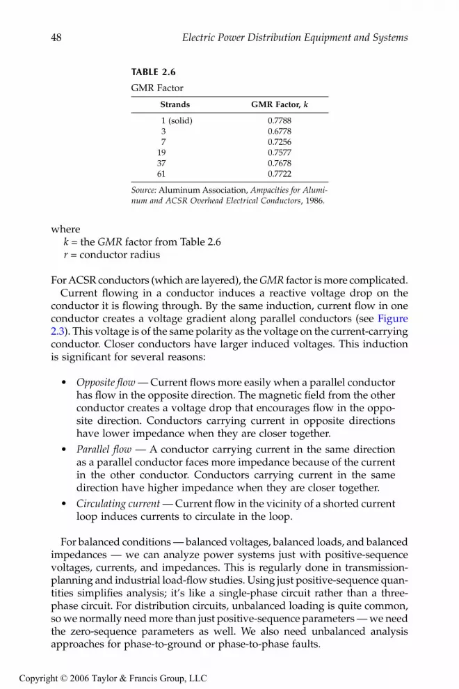
48 Electric Power Distribution Equipment and Systems
wherek = the GMR factor from Table 2.6r = conductor radius
For ACSR conductors (which are layered), the GMR factor is more complicated.Current flowing in a conductor induces a reactive voltage drop on the
conductor it is flowing through. By the same induction, current flow in oneconductor creates a voltage gradient along parallel conductors (see Figure2.3). This voltage is of the same polarity as the voltage on the current-carryingconductor. Closer conductors have larger induced voltages. This inductionis significant for several reasons:
• Opposite flow — Current flows more easily when a parallel conductorhas flow in the opposite direction. The magnetic field from the otherconductor creates a voltage drop that encourages flow in the oppo-site direction. Conductors carrying current in opposite directionshave lower impedance when they are closer together.
• Parallel flow — A conductor carrying current in the same directionas a parallel conductor faces more impedance because of the currentin the other conductor. Conductors carrying current in the samedirection have higher impedance when they are closer together.
• Circulating current — Current flow in the vicinity of a shorted currentloop induces currents to circulate in the loop.
For balanced conditions — balanced voltages, balanced loads, and balancedimpedances — we can analyze power systems just with positive-sequencevoltages, currents, and impedances. This is regularly done in transmission-planning and industrial load-flow studies. Using just positive-sequence quan-tities simplifies analysis; it’s like a single-phase circuit rather than a three-phase circuit. For distribution circuits, unbalanced loading is quite common,so we normally need more than just positive-sequence parameters — we needthe zero-sequence parameters as well. We also need unbalanced analysisapproaches for phase-to-ground or phase-to-phase faults.
TABLE 2.6
GMR Factor
Strands GMR Factor, k
1 (solid) 0.77883 0.67787 0.7256
19 0.757737 0.767861 0.7722
Source: Aluminum Association, Ampacities for Alumi-num and ACSR Overhead Electrical Conductors, 1986.
9576_C02.fm Page 48 Monday, October 17, 2005 7:15 AM
Copyright © 2006 Taylor & Francis Group, LLC

Overhead Lines 49
With symmetrical components, the phasors of circuit quantities on eachof the three phases resolve to three sets of phasors. For voltage, the symmet-rical components relate to the phase voltages as:
Va = V0 + V1 + V2 V0 = 1/3 (Va + Vb + Vc)
Vb = V0 + a2V1 + aV2 and V1 = 1/3 (Va + aVb + a2Vc)
Vc = V0 + aV1 + a2V2 V2 = 1/3 (Va + a2Vb + aVc)
where
These phase-to-symmetrical conversions apply for phase-to-ground as wellas phase-to-phase voltages. The same conversions apply for converting linecurrents to sequence currents:
Ia = I0 + I1 + I2 I0 = 1/3 (Ia + Ib + Ic)
Ib = I0 + a2I1 + aI2 and I1 = 1/3 (Ia + aIb + a2Ic)
Ic = I0 + aI1 + a2I2 I2 = 1/3 (Ia + a2Ib + aIc)
FIGURE 2.3Mutual induction.
Closer spacing increases impedanceI I
I
Closer spacing reduces impedance
I
I
-+
Effects of induction:
Mutual induction: IA
IB 0
VB ZABIA
a a= ∠ ° = ∠ °1 120 1 2402 and .
9576_C02.fm Page 49 Monday, October 17, 2005 7:15 AM
Copyright © 2006 Taylor & Francis Group, LLC

50 Electric Power Distribution Equipment and Systems
The voltage drop along each of the phase conductors depends on thecurrents in each of the phase conductors and the self impedances (such asZaa) and the mutual impedances (such as Zab) as
Va = ZaaIa + ZabIb + ZacIc
Vb = ZbaIa + ZbbIb + ZbcIc
Vc = ZcaIa + ZcbIb + ZccIc
Likewise, when we use sequence components, we have voltage drops ofeach sequence in terms of the sequence currents and sequence impedances:
V0 = Z00I0 + Z01I1 + Z02I2
V1 = Z10I0 + Z11I1 + Z12I2
V2 = Z20I0 + Z21I1 + Z22I2
This is not much of a simplification until we assume that all of the self-impedance terms are equal (ZS = Zaa = Zbb = Zcc) and all of the mutualimpedances are equal (ZM = Zab = Zac = Zbc = Zba = Zca = Zcb). With thisassumption, the sequence impedances decouple; the mutual terms of thezero-sequence matrix (such as Z12) become zero. Zero-sequence current onlycauses a zero-sequence voltage drop. This is a good enough approximationfor many distribution problems and greatly simplifies hand and computercalculations. Now, the sequence voltage drop equations are:
V0 = Z00I0 = (ZS + 2ZM)I0
V1 = Z11I1 = (ZS – ZM)I1
V2 = Z22I2 = (ZS – ZM)I2
Now, we have the sequence terms as
Z0 = ZS + 2ZM
Z1 = Z2 = ZS – ZM
And likewise,
ZS = (Z0 + 2Z1)/3
ZM = (Z0 – Z1)/3
9576_C02.fm Page 50 Monday, October 17, 2005 7:15 AM
Copyright © 2006 Taylor & Francis Group, LLC

Overhead Lines 51
Note ZS, the self-impedance term. ZS is also the “loop impedance” — theimpedance to current through one phase wire and returning through theground return path. This loop impedance is important because it is theimpedance for single-phase lines and the impedance for single line-to-ground faults.
Engineers normally use three methods to find impedances of circuits. Inorder of least to most accurate, these are:
• Table lookup• Hand calculations• Computer calculations
This book provides data necessary for the first two approaches. Tablelookups are quite common. Even though table lookup is not the most accu-rate approach, its accuracy is good enough for analyzing most commondistribution problems. Computer calculations are quite accessible and alloweasier analysis of more complicated problems.
2.4 Simplified Line Impedance Calculations
The positive-sequence impedance of overhead lines is
whereRφ = resistance of the phase conductor in Ω/distancek1 = 0.2794f/60 for outputs in Ω/mi
= 0.0529f/60 for outputs in Ω/1000 ftf = frequency in hertzGMRφ = geometric mean radius of the phase conductor in ftGMDφ = geometric mean distance between the phase conductors in ftGMDφ = for three-phase linesGMDφ = 1.26 dAB for a three-phase line with flat configuration, either hor-
izontal or vertical, where dAB = dBC = 0.5dCA
GMDφ = dAB for two-phase lines*
* The two-phase circuit has two out of the three phases; the single-phase circuit has one phaseconductor with a neutral return. While it may seem odd to look at the positive-sequence imped-ance of a one- or two-phase circuit, the analysis approach is useful. This approach uses fictitiousconductors for the missing phases to model the one- or two-phase circuit as an equivalent three-phase circuit (no current flows on these fictitious phases).
Z R jkGMD
GMR1 1 10= +φφ
φ
log
d d dAB BC CA3
9576_C02.fm Page 51 Monday, October 17, 2005 7:15 AM
Copyright © 2006 Taylor & Francis Group, LLC

52 Electric Power Distribution Equipment and Systems
GMDφ = dAN for single-phase lines*dij = distance between the center of conductor i and the center of con-
ductor j, in feet
For 60 Hz and output units of Ω/1000 ft, this is
Zero-sequence impedance calculations are more complicated than posi-tive-sequence calculations. Carson’s equations are the most common way toaccount for the ground return path in impedance calculations of overheadcircuits. Carson (1926) derived an expression including the earth return path.We’ll use a simplification of Carson’s equations; it includes the followingassumptions (Smith, 1980)
• Since distribution lines are relatively short, the height-dependentterms in Carson’s full model are small, so we neglect them.
• The multigrounded neutral is perfectly coupled to the earth (this hassome drawbacks for certain calculations as discussed in Chapter 13).
• End effects are neglected.• The current at the sending end equals that at the receiving end (no
leakage currents).• All phase conductors have the same size conductor.• The ground is infinite and has uniform resistivity.
Consider the circuit in Figure 2.4; current flows in conductor a and returnsthrough the earth. The voltage on conductor a equals the current times Zaa,which is the self-impedance with an earth return path. The current in con-ductor a induces a voltage drop along conductor b equaling the phase-acurrent times Zab, which is the mutual impedance with an earth return path.These two impedances are found (Smith, 1980) with
whereRe = resistance of the earth return path
= 0.0954f/60 Ω/mi = 0.01807f/60 Ω/1000 ft
Z R jGMD
GMR1 100 0529= +φφ
φ
. log
Z R R jkD
GMR
Z R jkDd
aa ee
ab ee
ab
= + +
= +
φφ
1 10
1 10
log
log
9576_C02.fm Page 52 Monday, October 17, 2005 7:15 AM
Copyright © 2006 Taylor & Francis Group, LLC

Overhead Lines 53
De = = equivalent depth of the earth return current in ftρ = earth resistivity in Ω-mdab = distance between the centers of conductors a and b
For 60 Hz and output units of Ω/1000 ft,
These equations lead to different formulations for the zero-sequenceimpedance of circuits depending on the grounding configuration. They arealso useful in their own right in many circumstances. Single-phase circuitswith a phase and a neutral are often easier to analyze using these equationsrather than using sequence components. Consider a single-phase circuit thatis perfectly grounded with a current of IA in the phase conductor. As Figure2.5 shows, we can find the neutral current as a function of the mutualimpedance between the two conductors divided by the self-impedance ofthe neutral conductor.
Now, let’s look at the zero-sequence impedances — these change depend-ing on grounding configuration. Figure 2.6 shows the configurations that wewill consider.
A three-wire overhead line has a zero-sequence impedance of (Smith, 1980):
FIGURE 2.4Depiction of Carson’s impedances with earth return.
Mutually coupled parallel conductors
Earth
Ia Ib 0
Va ZaaIa
Vb ZabIa
dab
2160 ρ / f
Z R jGMR
Z jd
aa
abab
= + +
= +
φφ
ρ
ρ
0 01807 0 0529278 9
0 01807 0 0529278 9
10
10
. . log.
. . log.
Z R R j kD
GMR GMDe
e0 1 10 23
3 3= + +⋅
φφ φ
log
9576_C02.fm Page 53 Monday, October 17, 2005 7:15 AM
Copyright © 2006 Taylor & Francis Group, LLC

54 Electric Power Distribution Equipment and Systems
For a four-wire multigrounded system, the zero-sequence self-impedanceis:
where ZNN is the self-impedance of the neutral conductor with an earthreturn, and ZφN is the mutual impedance between the phase conductors asa group and the neutral. For 60 Hz and output units of Ω/1000 ft, the zero-sequence self-impedance is
whereGMRN = geometric mean radius of the neutral conductor in ftGMDφN = geometric mean distance between the phase conductors as a
group and the neutral in ftGMDφN = for three-phase linesGMDφN = for two-phase linesGMDφN = dAN for single-phase lines
A special case is for a four-wire unigrounded circuit where the returncurrent stays in the neutral, which has a zero-sequence impedance of (Enderet al., 1960)
FIGURE 2.5Current flow in a neutral conductor based on self-impedances and mutual impedances.
IA
IN
Ie IA IN
VN 0
VN 0 ZANIA ZNNIN
So, INZAN
ZNNIA
Z R R j kD
GMR GMD
Z
Zee N
NN0 1 10 23
2
3 3 3= + +⋅
−φφ φ
φlog
Z R jGMR GMD
Z
ZN
NN0 10 23
2
0 0542 0 1587278 9
3= + +⋅
−φφ φ
φρ. . log
.
Z R jGMRNN N
N
= + +0 01807 0 0529278 9
10. . log. ρ
Z jGMDN
Nφ
φ
ρ= +0 01807 0 0529
278 910. . log
.
d d dAN BN CN3
d dAN BN
9576_C02.fm Page 54 Monday, October 17, 2005 7:15 AM
Copyright © 2006 Taylor & Francis Group, LLC
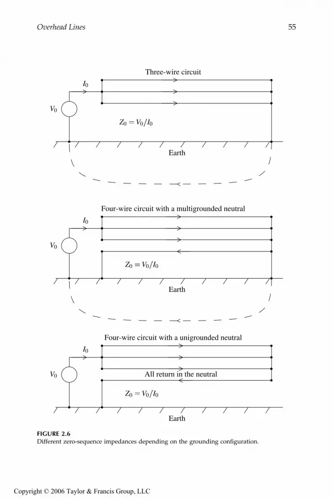
Overhead Lines 55
FIGURE 2.6Different zero-sequence impedances depending on the grounding configuration.
Three-wire circuit
Earth
Four-wire circuit with a multigrounded neutral
Earth
Four-wire circuit with a unigrounded neutral
Earth
All return in the neutral
I0
I0
I0
V0
V0
V0
Z0 V0 I0
Z0 V0 I0
Z0 V0 I0
9576_C02.fm Page 55 Monday, October 17, 2005 7:15 AM
Copyright © 2006 Taylor & Francis Group, LLC

56 Electric Power Distribution Equipment and Systems
This is for a four-wire unigrounded circuit where there are no connectionsbetween the neutral conductor and earth. We can also use this as an approx-imation for a multigrounded neutral line that is very poorly grounded.Remember that the equation given above for a multigrounded circuitassumes perfect grounding. For some calculations, that is not accurate. Thisis the opposite extreme, which is appropriate for some calculations. Lat(1990) used this as one approach to estimating the worst-case overvoltageon unfaulted phases during a line-to-ground fault.
So, what does all of this mean? Some of the major effects are:
• Conductor size — Mainly affects resistance — larger conductors havelower positive-sequence resistance. Positive-sequence reactance alsolowers with larger conductor size, but since it changes with thelogarithm of conductor radius, changes are small.
• Conductor spacings — Increasing spacing (higher GMDφ) increases Z1.Increasing spacing reduces Z0. Both of these changes with spacingare modest given the logarithmic effect.
• Neutral — Adding the neutral always reduces the total zero-sequenceimpedance, |Z0|. Adding a neutral always reduces the reactive por-tion of this impedance. But adding a neutral may increase or maydecrease the resistive portion of Z0. Adding a small neutral with highresistance increases the resistance component of Z0.
• Neutral spacing — Moving the neutral closer to the phase conductorsreduces the zero-sequence impedance (but may increase the resistiveportion, depending on the size of the neutral).
• Earth resistivity — The earth resistivity does not change the earthreturn resistance (Re only depends on frequency). The currentspreads to wider areas of the earth in high-resistivity soil. Earthresistivity does change the reactance. Higher earth resistivities forcecurrent deeper into the ground (larger De), raising the reactance.
• Grounding — The positive-sequence impedance Z1 stays the sameregardless of the grounding, whether four-wire multigrounded,ungrounded, or unigrounded.
• Negative sequence — Equals the positive-sequence impedance.
Figure 2.7 and Figure 2.8 show the effects of various parameters on thepositive and zero-sequence impedances. Many of the outputs are not par-ticularly sensitive to changes in the inputs. Since many parameters are func-tions of the logarithm of the variable, major changes induce only smallchanges in the impedance.
Z R R jR j kGMD
GMR GMR GMDn n
N
N
0 1 10 23 3
2= + + +
⋅φ
φ
φ φ
log33
9576_C02.fm Page 56 Monday, October 17, 2005 7:15 AM
Copyright © 2006 Taylor & Francis Group, LLC

Overhead Lines 57
When do we need more accuracy or more sophistication? For power flows,fault calculations, voltage flicker calculations, and voltage sag analysis, wenormally don’t need more sophistication. For switching surges, lightning,or other higher frequency transient analysis, we normally need more sophis-ticated line models.
Most unbalanced calculations can be done with this approach, but somecases require more sophistication. Distribution lines and most lower-voltagesubtransmission lines are not transposed. On some long circuits, even withbalanced loading, the unbalanced impedances between phases creates volt-age unbalance.
2.5 Line Impedance Tables
This section has several tables of impedances for all-aluminum, ACSR, andcopper constructions. All are based on the equations in the previous sectionand assume GMD = 4.8 ft, conductor temperature = 50°C, GMDφN = 6.3 ft,and earth resistivity = 100 Ω-m. All zero-sequence values are for a four-wiremultigrounded neutral circuit.
2.6 Conductor Sizing
We have an amazing variety of sizes and types of conductors. Several elec-trical, mechanical, and economic characteristics affect conductor selection:
FIGURE 2.7Effect of spacings and conductor size on the positive-sequence impedance with 500-kcmil AACphases (GMR = 0.0256 ft) and GMDφ=5 ft.
Resistance
Reactance
2 4 6 80.00
0.05
0.10
0.15
0.20
200 400 600 800 10000.00
0.05
0.10
0.15
0.20
Phase wire GMD, feet
R0
& X
0, Ω
/100
0 fe
et
Phase wire kcmil
9576_C02.fm Page 57 Monday, October 17, 2005 7:15 AM
Copyright © 2006 Taylor & Francis Group, LLC
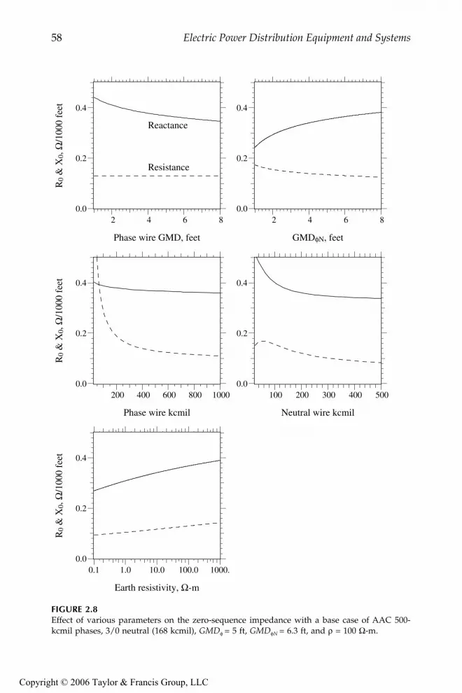
58 Electric Power Distribution Equipment and Systems
FIGURE 2.8Effect of various parameters on the zero-sequence impedance with a base case of AAC 500-kcmil phases, 3/0 neutral (168 kcmil), GMDφ = 5 ft, GMDφN = 6.3 ft, and ρ = 100 Ω-m.
Reactance
Resistance
2 4 6 80.0
0.2
0.4
200 400 600 800 10000.0
0.2
0.4
0.1 1.0 10.0 100.0 1000.0.0
0.2
0.4
2 4 6 80.0
0.2
0.4
100 200 300 400 5000.0
0.2
0.4
Phase wire GMD, feet
R0
& X
0, Ω
/100
0 fe
et
Phase wire kcmil
R0
& X
0, Ω
/100
0 fe
et
Earth resistivity, Ω-m
R0
& X
0, Ω
/100
0 fe
et
GMDφN, feet
Neutral wire kcmil
9576_C02.fm Page 58 Monday, October 17, 2005 7:15 AM
Copyright © 2006 Taylor & Francis Group, LLC

Overhead Lines 59
• Ampacity — The peak current-carrying capability of a conductorlimits the current (and power) carrying capability.
• Economics — Often we will use a conductor that normally operateswell below its ampacity rating. The cost of the extra aluminum paysfor itself with lower I2R losses; the conductor runs cooler. This alsoleaves room for expansion.
• Mechanical strength — Especially on rural lines with long spanlengths, mechanical strength plays an important role in size and typeof conductor. Stronger conductors like ACSR are used more often.Ice and wind loadings must be considered.
• Corrosion — While not usually a problem, corrosion sometimes limitscertain types of conductors in certain applications.
As with many aspects of distribution operations, many utilities standard-ize on a set of conductors. For example, a utility may use 500-kcmil AAC
TABLE 2.7
Positive-Sequence Impedances of All-Aluminum Conductor
Phase Size Strands R1 X1 Z1
6 7 0.7405 0.1553 0.75664 7 0.4654 0.1500 0.48902 7 0.2923 0.1447 0.32621 7 0.2323 0.1420 0.2723
1/0 7 0.1839 0.1394 0.23082/0 7 0.1460 0.1367 0.20003/0 7 0.1159 0.1341 0.17724/0 7 0.0920 0.1314 0.1604250 7 0.0778 0.1293 0.1509266.8 7 0.0730 0.1286 0.1478300 19 0.0649 0.1261 0.1418336.4 19 0.0580 0.1248 0.1376350 19 0.0557 0.1242 0.1361397.5 19 0.0490 0.1229 0.1323450 19 0.0434 0.1214 0.1289477 19 0.0411 0.1208 0.1276500 19 0.0392 0.1202 0.1265556.5 19 0.0352 0.1189 0.1240700 37 0.0282 0.1159 0.1192715.5 37 0.0277 0.1157 0.1190750 37 0.0265 0.1151 0.1181795 37 0.0250 0.1146 0.1173874.5 37 0.0227 0.1134 0.1157900 37 0.0221 0.1130 0.1152954 37 0.0211 0.1123 0.1142
1000 37 0.0201 0.1119 0.1137
Note: Impedances, Ω/1000 ft (× 5.28 for Ω/mi or × 3.28for Ω/km). GMD = 4.8 ft, Conductor temp. = 50°C.
9576_C02.fm Page 59 Monday, October 17, 2005 7:15 AM
Copyright © 2006 Taylor & Francis Group, LLC

60 Electric Power Distribution Equipment and Systems
TABLE 2.8
AAC Zero-Sequence, Z0, and Ground-Return Loop Impedances,ZS = (2Z1 + Z0)/3
PhaseSize
NeutralSize R0 X0 Z0 RS XS ZS
6 6 0.8536 0.5507 1.0158 0.7782 0.2871 0.82942 6 0.4055 0.5401 0.6754 0.3301 0.2765 0.43062 2 0.4213 0.4646 0.6272 0.3353 0.2513 0.41901 6 0.3454 0.5374 0.6389 0.2700 0.2738 0.38451 1 0.3558 0.4405 0.5662 0.2734 0.2415 0.3648
1/0 6 0.2971 0.5348 0.6117 0.2216 0.2712 0.35021/0 1/0 0.2981 0.4183 0.5136 0.2220 0.2323 0.32132/0 6 0.2591 0.5321 0.5919 0.1837 0.2685 0.32532/0 2/0 0.2487 0.3994 0.4705 0.1802 0.2243 0.28773/0 2 0.2449 0.4540 0.5158 0.1589 0.2407 0.28843/0 3/0 0.2063 0.3840 0.4359 0.1461 0.2174 0.26194/0 1 0.2154 0.4299 0.4809 0.1331 0.2309 0.26654/0 4/0 0.1702 0.3716 0.4088 0.1180 0.2115 0.2422250 2/0 0.1805 0.3920 0.4316 0.1120 0.2169 0.2441250 250 0.1479 0.3640 0.3929 0.1012 0.2075 0.2309266.8 2/0 0.1757 0.3913 0.4289 0.1072 0.2161 0.2413266.8 266.8 0.1402 0.3614 0.3877 0.0954 0.2062 0.2272300 2/0 0.1675 0.3888 0.4234 0.0991 0.2137 0.2355300 300 0.1272 0.3552 0.3773 0.0856 0.2025 0.2198336.4 2/0 0.1607 0.3875 0.4195 0.0922 0.2123 0.2315336.4 336.4 0.1157 0.3514 0.3699 0.0772 0.2003 0.2147350 2/0 0.1584 0.3869 0.4181 0.0899 0.2118 0.2301350 350 0.1119 0.3499 0.3674 0.0744 0.1994 0.2129397.5 2/0 0.1517 0.3856 0.4143 0.0832 0.2105 0.2263397.5 397.5 0.1005 0.3463 0.3606 0.0662 0.1974 0.2082450 2/0 0.1461 0.3841 0.4109 0.0776 0.2089 0.2229450 450 0.0908 0.3427 0.3545 0.0592 0.1951 0.2039477 2/0 0.1438 0.3835 0.4096 0.0753 0.2084 0.2216477 477 0.0868 0.3414 0.3522 0.0563 0.1943 0.2023500 4/0 0.1175 0.3605 0.3791 0.0653 0.2003 0.2107500 500 0.0835 0.3401 0.3502 0.0540 0.1935 0.2009556.5 4/0 0.1135 0.3591 0.3766 0.0613 0.1990 0.2082556.5 556.5 0.0766 0.3372 0.3458 0.0490 0.1917 0.1978700 4/0 0.1064 0.3561 0.3717 0.0542 0.1960 0.2033700 700 0.0639 0.3310 0.3371 0.0401 0.1876 0.1918715.5 4/0 0.1060 0.3559 0.3714 0.0538 0.1958 0.2030715.5 715.5 0.0632 0.3306 0.3366 0.0395 0.1873 0.1915750 4/0 0.1047 0.3553 0.3705 0.0526 0.1952 0.2022750 750 0.0609 0.3295 0.3351 0.0380 0.1866 0.1904795 4/0 0.1033 0.3548 0.3695 0.0511 0.1946 0.2012795 795 0.0582 0.3283 0.3335 0.0361 0.1858 0.1893874.5 4/0 0.1010 0.3536 0.3678 0.0488 0.1935 0.1996874.5 874.5 0.0540 0.3261 0.3305 0.0332 0.1843 0.1873900 4/0 0.1004 0.3533 0.3672 0.0482 0.1931 0.1990900 900 0.0529 0.3254 0.3296 0.0324 0.1838 0.1866954 4/0 0.0993 0.3525 0.3662 0.0471 0.1924 0.1981
9576_C02.fm Page 60 Monday, October 17, 2005 7:15 AM
Copyright © 2006 Taylor & Francis Group, LLC

Overhead Lines 61
for all mainline spans and 1/0 AAC for all laterals. While many circuitlocations are overdesigned, the utility saves from reduced stocking, fewertools, and standardized connectors. While many utilities have more than justtwo conductors, most use just a handful of standard conductors; four to sixeconomically covers the needs of most utilities.
2.7 Ampacities
The ampacity is the maximum designed current of a conductor. This currentcarrying capacity is normally given in amperes. A given conductor has
954 954 0.0510 0.3239 0.3279 0.0310 0.1828 0.18541000 4/0 0.0983 0.3521 0.3656 0.0462 0.1920 0.19751000 1000 0.0491 0.3232 0.3269 0.0298 0.1823 0.1847
Note: Impedances, Ω/1000 ft (× 5.28 for Ω/mi or × 3.28 for Ω/km). GMD =4.8 ft, GMDφN = 6.3 ft, Conductor temp. = 50°C, Earth resistivity = 100Ω-m.
TABLE 2.9
Positive-Sequence Impedances of ACSR
Phase Size Strands R1 X1 Z1
6 6/1 0.7500 0.1746 0.77004 6/1 0.4794 0.1673 0.50772 6/1 0.3080 0.1596 0.34691 6/1 0.2474 0.1551 0.2920
1/0 6/1 0.1972 0.1496 0.24762/0 6/1 0.1616 0.1478 0.21903/0 6/1 0.1208 0.1442 0.18814/0 6/1 0.1066 0.1407 0.1765
266.8 18/1 0.0723 0.1262 0.1454336.4 18/1 0.0574 0.1236 0.1362397.5 18/1 0.0487 0.1217 0.1311477 18/1 0.0405 0.1196 0.1262556.5 18/1 0.0348 0.1178 0.1228636 18/1 0.0306 0.1165 0.1204795 36/1 0.0247 0.1140 0.1167
Note: Impedances, Ω/1000 ft (× 5.28 for Ω/mi or ×3.28 for Ω/km). GMD = 4.8 ft, Conductortemp. = 50°C.
TABLE 2.8 (Continued)
AAC Zero-Sequence, Z0, and Ground-Return Loop Impedances,ZS = (2Z1 + Z0)/3
PhaseSize
NeutralSize R0 X0 Z0 RS XS ZS
9576_C02.fm Page 61 Monday, October 17, 2005 7:15 AM
Copyright © 2006 Taylor & Francis Group, LLC

62 Electric Power Distribution Equipment and Systems
TABLE 2.10
ACSR Zero-Sequence, Z0, and Ground-Return Loop Impedances,ZS = (2Z1 + Z0)/3
PhaseSize
NeutralSize R0 X0 Z0 RS XS ZS
4 4 0.6030 0.5319 0.8040 0.5206 0.2888 0.59532 4 0.4316 0.5242 0.6790 0.3492 0.2812 0.44832 2 0.4333 0.4853 0.6505 0.3498 0.2682 0.44071 4 0.3710 0.5197 0.6385 0.2886 0.2766 0.39981 1 0.3684 0.4610 0.5901 0.2877 0.2571 0.3858
1/0 4 0.3208 0.5143 0.6061 0.2384 0.2712 0.36111/0 1/0 0.3108 0.4364 0.5357 0.2351 0.2452 0.33972/0 2 0.2869 0.4734 0.5536 0.2034 0.2563 0.32722/0 2/0 0.2657 0.4205 0.4974 0.1963 0.2387 0.30903/0 2 0.2461 0.4698 0.5304 0.1626 0.2527 0.30053/0 3/0 0.2099 0.4008 0.4524 0.1505 0.2297 0.27464/0 1 0.2276 0.4465 0.5012 0.1469 0.2426 0.28364/0 4/0 0.1899 0.3907 0.4344 0.1344 0.2240 0.2612
266.8 2/0 0.1764 0.3990 0.4362 0.1070 0.2171 0.2421266.8 266.8 0.1397 0.3573 0.3836 0.0948 0.2032 0.2242336.4 2/0 0.1615 0.3963 0.4280 0.0921 0.2145 0.2334336.4 336.4 0.1150 0.3492 0.3676 0.0766 0.1988 0.2130397.5 2/0 0.1528 0.3944 0.4230 0.0834 0.2126 0.2284397.5 397.5 0.1002 0.3441 0.3584 0.0659 0.1958 0.2066477 2/0 0.1446 0.3923 0.4181 0.0752 0.2105 0.2235477 477 0.0860 0.3391 0.3498 0.0557 0.1927 0.2006556.5 2/0 0.1389 0.3906 0.4145 0.0695 0.2087 0.2200556.5 556.5 0.0759 0.3351 0.3436 0.0485 0.1902 0.1963
Note: Impedances, Ω/1000 ft (× 5.28 for Ω/mi or × 3.28 for Ω/km). GMD = 4.8ft, GMDφN = 6.3 ft, Conductor temp. = 50°C, Earth resistivity = 100 Ω-m.
TABLE 2.11
Positive-Sequence Impedances of Hard-Drawn Copper
Phase Size Strands R1 X1 Z1
4 3 0.2875 0.1494 0.32402 3 0.1809 0.1441 0.23131 7 0.1449 0.1420 0.2029
1/0 7 0.1150 0.1393 0.18072/0 7 0.0911 0.1366 0.16423/0 12 0.0723 0.1316 0.15014/0 12 0.0574 0.1289 0.1411250 12 0.0487 0.1270 0.1360300 12 0.0407 0.1250 0.1314350 19 0.0349 0.1243 0.1291400 19 0.0307 0.1227 0.1265450 19 0.0273 0.1214 0.1244500 19 0.0247 0.1202 0.1227
Note: Impedances, Ω/1000 ft (× 5.28 for Ω/mi or × 3.28 for Ω/km). GMD = 4.8 ft, Conductor temp. = 50°C.
9576_C02.fm Page 62 Monday, October 17, 2005 7:15 AM
Copyright © 2006 Taylor & Francis Group, LLC

Overhead Lines 63
several ampacities, depending on its application and the assumptions used.House and Tuttle (1958) derive the ampacity calculations described below,which are used in IEEE Std. 738-1993 and most other published ampacitytables (Aluminum Association, 1986; Southwire Company, 1994).
Sun, wind, and ambient temperature change a conductor’s ampacity. Aconductor’s temperature depends on the thermal balance of heat inputs andlosses. Current driven through a conductor’s resistance creates heat (I2R).The sun is another source of heat into the conductor. Heat escapes from theconductor through radiation and from convection. Considering the balanceof inputs and outputs, the ampacity of a conductor is
TABLE 2.12
Copper Zero-Sequence, Z0, and Ground-Return Loop Impedances,ZS = (2Z1 + Z0)/3
PhaseSize
NeutralSize R0 X0 Z0 RS XS ZS
3 3 0.3515 0.4459 0.5678 0.2707 0.2468 0.36633 3 0.3515 0.4459 0.5678 0.2707 0.2468 0.36636 6 0.5830 0.5157 0.7784 0.4986 0.2751 0.56956 6 0.5830 0.5157 0.7784 0.4986 0.2751 0.56954 6 0.4141 0.5104 0.6572 0.3297 0.2697 0.42604 4 0.4146 0.4681 0.6253 0.3299 0.2556 0.41732 6 0.3075 0.5051 0.5913 0.2231 0.2644 0.34602 2 0.2924 0.4232 0.5143 0.2181 0.2371 0.32211 4 0.2720 0.4606 0.5349 0.1873 0.2482 0.31091 1 0.2451 0.4063 0.4745 0.1783 0.2301 0.2911
1/0 4 0.2421 0.4580 0.5180 0.1574 0.2455 0.29161/0 1/0 0.2030 0.3915 0.4410 0.1443 0.2234 0.26602/0 3 0.2123 0.4352 0.4842 0.1315 0.2362 0.27032/0 2/0 0.1672 0.3796 0.4148 0.1165 0.2176 0.24683/0 2 0.1838 0.4106 0.4498 0.1095 0.2246 0.24983/0 3/0 0.1383 0.3662 0.3915 0.0943 0.2098 0.23004/0 2 0.1689 0.4080 0.4415 0.0946 0.2219 0.24124/0 4/0 0.1139 0.3584 0.3760 0.0762 0.2054 0.2191250 1 0.1489 0.3913 0.4187 0.0821 0.2151 0.2303250 250 0.0993 0.3535 0.3671 0.0656 0.2025 0.2128300 1 0.1409 0.3893 0.4140 0.0741 0.2131 0.2256300 300 0.0856 0.3487 0.3590 0.0557 0.1995 0.2071350 1 0.1351 0.3886 0.4115 0.0683 0.2124 0.2231350 350 0.0754 0.3468 0.3549 0.0484 0.1985 0.2043400 1 0.1309 0.3871 0.4086 0.0641 0.2109 0.2204400 400 0.0680 0.3437 0.3503 0.0431 0.1964 0.2011450 1/0 0.1153 0.3736 0.3910 0.0566 0.2055 0.2131450 450 0.0620 0.3410 0.3466 0.0389 0.1946 0.1984500 1/0 0.1127 0.3724 0.3891 0.0540 0.2043 0.2113500 500 0.0573 0.3387 0.3435 0.0356 0.1930 0.1963
Note: Impedances, Ω/1000 ft (× 5.28 for Ω/mi or × 3.28 for Ω/km). GMD = 4.8ft, GMDφN = 6.3 ft, Conductor temp. = 50°C, Earth resistivity = 100 Ω-m.
9576_C02.fm Page 63 Monday, October 17, 2005 7:15 AM
Copyright © 2006 Taylor & Francis Group, LLC

64 Electric Power Distribution Equipment and Systems
whereqc = convected heat loss, W/ftqr = radiated heat loss, W/ftqs = solar heat gain, W/ft
Rac = Nominal ac resistance at operating temperature t, Ω/ft
The convected heat loss with no wind is
Wind increases convection losses. The losses vary based on wind speed.The IEEE method uses the maximum qc from the following two equations:
whereD = conductor diameter, in.tc = conductor operating temperature, °Cta = ambient temperature, °Ctf = (tc + tc)/2V = air velocity, ft/hρf = air density at tf, lb/ft3
µf = absolute viscosity of air at tf, lb/h-ftKf = thermal conductivity of air at tf, W/ft2/°C
The density, viscosity, and thermal conductivity of air all depend on tem-perature (actually the film temperature Tf near the surface of the conductor,which is taken as the average of the conductor and ambient temperatures).Tables of these are available in the references (IEEE Std. 738-1993; SouthwireCompany, 1994). We may also use the following polynomial approximations(IEEE Std. 738-1993):
Iq q q
Rc r s
ac
=+ −
q D t tc f c a= −0 283 0 75 1 25. ( ). .ρ
qD V
K t t
qD V
K t t
cf
ff c a
cf
ff c a
1
0 52
2
0 6
1 01 0 371
0 1695
= +
−
=
−
. . ( )
. ( )
.
.
ρµ
ρµ
ρ fc c
f
H HT
=− × + ×
+
− −0 080695 0 2901 10 0 37 101 0 00367
5 10 2. ( . ) ( . ).
9576_C02.fm Page 64 Monday, October 17, 2005 7:15 AM
Copyright © 2006 Taylor & Francis Group, LLC

Overhead Lines 65
where Hc is the altitude above sea level in feet.
A conductor radiates heat as the absolute temperature to the fourthpower as
whereD = conductor diameter, in.
ε = emissivity (normally 0.23 to 0.91 for bare wires)Tc = conductor temperature, °CTa = ambient temperature, °C
A conductor absorbs heat from the sun as
whereα = solar absorptivity
Qs = total solar heat in W/ft2
θ = effective angle of incidence of the sun’s raysD = conductor diameter, in.
The angles and total solar heat depend on the time of day and the latitude.Since the solar input term does not change the output significantly, we canuse some default values. For a latitude of 30°N at 11 a.m. in clear atmosphere,Qs = 95.2 W/ft,2 and θ = 78.6°.
Emissivity (ε) is the ability of a conductor to radiate heat into the air.Absorptivity (α) quantifies how much heat a conductor can absorb. Emis-sivity and absorptivity are interrelated; a nice shiny conductor reflects awaymuch of the sun’s heat but does not radiate heat well. Commonly, both areassumed to be 0.5 for bare wire. More conservative assumptions, possiblyoverconservative, are 0.7 for emissivity and 0.9 for absorptivity.
Some of the main factors impacting ampacity are
• Allowable conductor temperature — Ampacity increases significantlywith higher allowed temperatures.
k T T
T T T
f f f
f f f f
= + × − ×
= + × − × + ×
− −
− − −
0 007388 2 27889 10 1 34328 10
0 0415 1 2034 10 1 1442 10 1 9416 10
5 9 2
4 7 2 10 3
. . .
. . . .µ
q DT T
rc a=
+
−
+
0 138
273100
273100
4 4
. ε
q QD
s s= α θ12
sin
9576_C02.fm Page 65 Monday, October 17, 2005 7:15 AM
Copyright © 2006 Taylor & Francis Group, LLC

66 Electric Power Distribution Equipment and Systems
• Ambient temperature — Ampacity increases about 1% for each 1°Cdecrease in ambient temperature.
• Wind speed — Even a small wind helps cool conductors significantly.With no wind, ampacities are significantly lower than with a 2-ft/sec crosswind.
Table 2.13 through Table 2.15 show ampacities of all-aluminum, ACSR,and copper conductors. All assume the following:
TABLE 2.13
Ampacities of All-Aluminum Conductor
Conductor Stranding
Conductor Temp. = 75°°°°C Conductor Temp. = 100°°°°C
Ambient = 25°°°°C Ambient = 40°°°°C Ambient = 25°°°°C Ambient = 40°°°°C
No Wind Wind No Wind Wind No Wind Wind No Wind Wind
6 7 60 103 46 85 77 124 67 1114 7 83 138 63 114 107 166 92 1482 7 114 185 86 152 148 223 128 1991 7 134 214 101 175 174 258 150 230
1/0 7 157 247 118 203 204 299 176 2662/0 7 184 286 139 234 240 347 207 3093/0 7 216 331 162 271 283 402 243 3584/0 7 254 383 190 313 332 466 286 414250 7 285 425 213 347 373 518 321 460250 19 286 427 214 348 375 519 322 462266.8 7 298 443 223 361 390 539 335 479266.8 19 299 444 224 362 392 541 337 481300 19 325 479 243 390 426 584 367 519336.4 19 351 515 262 419 461 628 397 559350 19 361 527 269 428 474 644 408 572397.5 19 394 571 293 464 517 697 445 619450 19 429 617 319 501 564 755 485 671477 19 447 640 332 519 588 784 506 697477 37 447 641 333 520 589 785 507 697500 19 461 658 342 534 606 805 521 716556.5 19 496 704 368 571 654 864 562 767556.5 37 496 705 369 571 654 864 563 768600 37 522 738 388 598 688 905 592 804636 37 545 767 404 621 720 943 619 838650 37 556 782 413 633 737 965 634 857700 37 581 814 431 658 767 1000 660 888715.5 37 590 825 437 667 779 1014 670 901715.5 61 590 825 437 667 780 1014 671 901750 37 609 848 451 686 804 1044 692 927795 37 634 881 470 712 840 1086 722 964795 61 635 882 470 713 840 1087 723 965800 37 636 884 471 714 841 1087 723 965874.5 61 676 933 500 754 896 1152 770 1023874.5 61 676 934 500 754 896 1152 771 1023900 37 689 950 510 767 913 1172 785 1041954 37 715 983 529 793 946 1210 813 1074954 61 719 988 532 797 954 1221 821 1084
1000.0 37 740 1014 547 818 981 1252 844 1111
9576_C02.fm Page 66 Monday, October 17, 2005 7:15 AM
Copyright © 2006 Taylor & Francis Group, LLC

Overhead Lines 67
• Emissivity = 0.5, absorptivity = 0.5• 30°N at 11 a.m. in clear atmosphere• Wind speed = 2 ft/sec• Elevation = sea level
The solar heating input has modest impacts on the results. With no sun,the ampacity increases only a few percent.
Some simplifying equations help for evaluating some of the significantimpacts on ampacity. We can estimate changes in ambient and allowabletemperature variations (Black and Rehberg, 1985; Southwire Company,1994) with
TABLE 2.14
Ampacities of ACSR
Conductor Stranding
Conductor Temp. = 75°°°°C Conductor Temp. = 100°°°°C
Ambient = 25°°°°C Ambient = 40°°°°C Ambient = 25°°°°C Ambient = 40°°°°C
No Wind Wind No Wind Wind No Wind Wind No Wind Wind
6 6/1 61 105 47 86 79 126 68 1124 6/1 84 139 63 114 109 167 94 1494 7/1 85 141 64 116 109 168 94 1492 6/1 114 184 86 151 148 222 128 1972 7/1 117 187 88 153 150 224 129 1991 6/1 133 211 100 173 173 255 149 227
1/0 6/1 156 243 117 199 202 294 174 2612/0 6/1 180 277 135 227 235 337 203 3003/0 6/1 208 315 156 258 262 370 226 3294/0 6/1 243 363 182 296 319 443 274 394266.8 18/1 303 449 227 366 398 547 342 487266.8 26/7 312 458 233 373 409 559 352 497336.4 18/1 356 520 266 423 468 635 403 564336.4 26/7 365 530 272 430 480 647 413 575336.4 30/7 371 536 276 435 487 655 419 582397.5 18/1 400 578 298 469 527 708 453 629397.5 26/7 409 588 305 477 538 719 463 639477 18/1 453 648 337 525 597 793 513 705477 24/7 461 656 343 532 607 804 523 714477 26/7 464 659 345 534 611 808 526 718477 30/7 471 667 350 540 615 810 529 720556.5 18/1 504 713 374 578 664 874 571 777556.5 24/7 513 722 380 585 677 887 582 788556.5 26/7 517 727 383 588 682 893 587 793636 24/7 562 785 417 635 739 962 636 854636 26/7 567 791 420 639 748 972 644 863795 45/7 645 893 478 721 855 1101 735 977795 26/7 661 910 489 734 875 1122 753 996954 45/7 732 1001 541 807 971 1238 835 1099954 54/7 741 1010 547 814 983 1250 846 1109
1033.5 45/7 769 1048 568 844 1019 1294 877 1148
I IT T
T Tnew oldc new a new
c old a old
=−−
, ,
, ,
9576_C02.fm Page 67 Monday, October 17, 2005 7:15 AM
Copyright © 2006 Taylor & Francis Group, LLC

68 Electric Power Distribution Equipment and Systems
where Inew is the new ampacity based on a new conductor limit Tc,new and anew ambient temperature Ta,new. Likewise, Iold is the original ampacity basedon a conductor limit Tc,old and an ambient temperature Ta,old.
This approach neglects solar heating and the change in conductor resis-tance with temperature (both have small impacts). Doing this simplifies theampacity calculation to a constant (dependent on weather and conductorcharacteristics) times the difference between the conductor temperature andthe ambient temperature: I2 = K(Tc – Ta). We do not use this simplificationfor the original ampacity calculation, but it helps us evaluate changes intemperatures or currents.
We use this approach in Figure 2.9 to show the variation in ampacity withambient conductor assumptions along with two conductor operating limits.
TABLE 2.15
Ampacities of Copper Conductors
Conductor Stranding
Conductor Temp. = 75°°°°C Conductor Temp. = 100°°°°CAmbient = 25°°°°C Ambient = 40°°°°C Ambient = 25°°°°C Ambient = 40°°°°CNo Wind Wind No Wind Wind No Wind Wind No Wind Wind
6 3 83 140 63 116 107 169 92 1506 1 76 134 58 110 98 160 85 1435 3 97 162 73 134 125 195 108 1745 1 90 155 68 127 115 185 99 1654 3 114 188 86 154 147 226 127 2014 1 105 179 80 147 136 214 117 1913 7 128 211 97 174 166 254 143 2263 3 133 217 101 178 173 262 149 2333 1 123 206 93 170 159 248 137 2212 7 150 244 114 201 195 294 168 2622 3 157 251 118 206 203 303 175 2702 1 145 239 110 196 187 287 161 2561 3 184 291 138 238 239 351 206 3131 7 177 282 133 232 229 340 197 303
1/0 7 207 326 156 267 269 394 232 3512/0 7 243 378 183 309 317 457 273 4073/0 12 292 444 219 362 381 539 328 4793/0 7 285 437 214 357 373 530 321 4724/0 19 337 507 252 414 440 617 379 5494/0 12 342 513 256 418 448 624 386 5554/0 7 335 506 251 413 438 615 377 547250 19 377 563 282 459 493 684 424 608250 12 384 569 287 464 502 692 432 615300 19 427 630 319 513 559 767 481 682300 12 435 637 324 519 569 776 490 690350 19 475 694 355 565 624 847 537 753350 12 484 702 360 571 635 858 546 763400 19 520 753 387 612 682 920 587 817450 19 564 811 420 659 742 993 639 883500 37 606 865 450 702 798 1061 686 942500 19 605 865 450 701 797 1059 685 941600 37 685 968 509 784 905 1190 779 1057700 37 759 1062 563 860 1003 1308 863 1161750 37 794 1107 588 895 1051 1364 904 1211800 37 826 1147 612 927 1092 1412 939 1253900 37 894 1233 662 995 1189 1527 1023 1356
1000 37 973 1333 719 1075 1313 1676 1129 1488
9576_C02.fm Page 68 Monday, October 17, 2005 7:15 AM
Copyright © 2006 Taylor & Francis Group, LLC

Overhead Lines 69
Also, Figure 2.10 shows the conductor temperature vs. loading for severalAAC conductors. This graph highlights the major impact of operating tem-perature on ampacity. If we are overly conservative on a conductor limit, weend up with an overly restrictive ampacity.
We can also use the simplified ampacity equation to estimate the conductortemperature at a current higher or lower than the rated ampacity as (and ata different ambient temperature if we wish):
When examining a line’s ampacity, always remember that the overheadwire may not be the weakest link; substation exit cables, terminations, reclos-ers, or other gear may limit a circuit’s current before the conductors do. Also,with currents near a conductor’s rating, voltage drop is high.
FIGURE 2.9AAC ampacity with ambient temperature variations, using adjustments from base ampacitydata in Table 2.13 (2 ft/sec wind, with sun).
42
1/02/03/04/0
266.8
336.4
477
556.5
636
795
0 20 40 0
200
400
600
800
1000
1200
4
2
1/02/03/0
4/0
266.8
336.4
477
556.5
636
795
0 20 40 0
200
400
600
800
1000
1200
App
roxi
mat
e am
paci
ty, A
75C Operating Temperature 100C Operating Temperature
Ambient temperature, degrees Celsius
T TII
T Tc new a newnew
oldc old a old, , , ,( )= +
−2
9576_C02.fm Page 69 Monday, October 17, 2005 7:15 AM
Copyright © 2006 Taylor & Francis Group, LLC

70 Electric Power Distribution Equipment and Systems
The maximum operating temperature is an important consideration.Higher designed operating temperatures allow higher currents. But at highertemperatures, we have a higher risk of damage to the conductors. Aluminumstrands are strain hardened during manufacturing (the H19 in aluminum’s1350-H19 designation means “extra hard”). Heating relaxes the strands —the aluminum elongates and weakens. This damage is called annealing. Asaluminum anneals, it reverts back to its natural, softer state: fully annealed1350 aluminum wire elongates by 30% and loses 58% of its strength (10,000psi vs. 24,000 psi fully hardened). Even fully annealed, failure may not beimmediate; the next ice load or heavy winds may break a conductor. Slowannealing begins near 100°C. Aluminum anneals rapidly above 200°C.Annealing damage is permanent and accumulates over time. Remainingstrength for AAC conductors varies with conductor temperature and dura-tion of exposure as approximately (Harvey, 1971)
whereRS = remaining strength, percent of initial strength
FIGURE 2.10Conductor temperatures based on the given currents for selected AAC conductors, usingadjustments from base ampacity data in Table 2.13 (2 ft/sec wind).
4
2
1/0
2/03/0
4/0
266.8
336.4477
556.5
636
79525C Ambient
50 100 150 200100.0
1000.
200.
2000.
500.
4
2
1/0
2/0
3/0
4/0
266.8
336.4477
556.5
636
79540C Ambient
50 100 150 200
Conductor temperature, degrees Celsius
Cur
rent
, A
R k tSTd c= − −
10 001 0 0950 1. ( . . )
9576_C02.fm Page 70 Monday, October 17, 2005 7:15 AM
Copyright © 2006 Taylor & Francis Group, LLC

Overhead Lines 71
d = strand diameter, in.t = exposure time, h
Tc = conductor temperature, °Ck1 = (–0.24Tc + 135), but if k1>100, use k1 = 100
Figure 2.11 shows the loss of strength with time for high-temperatureoperation using this approximation.
ACSR may be loaded higher than the same size AAC conductor. As thealuminum loses strength, the steel carries more of the tension. The steel doesnot lose strength until reaching higher temperatures.
Covered conductors are darker, so they absorb more heat from the sun butradiate heat better; the Aluminum Association (1986) uses 0.91 for both theemissivity and the absorptivity of covered wire. Table 2.16 shows ampacitiesof covered wire. Covered conductors have ampacities that are close to bare-conductor ampacities. The most significant difference is that covered con-ductors have less ability to withstand higher temperatures; the insulationdegrades. Polyethylene is especially prone to damage, so it should not beoperated above 75°C. EPR and XLPE may be operated up to 90°C.
Some utilities use two ratings, a “normal” ampacity with a 75°C designtemperature and an “emergency” ampacity with a 90 or 100°C design. Con-ductors are selected for the normal rating, but operation is allowed to theemergency rating. Overhead circuits have considerable capability for over-load, especially during cooler weather. We do not use relaying to trip “over-loaded” circuits. At higher temperatures, conductors age more quickly butdo not usually fail immediately.
2.7.1 Neutral Conductor Sizing
Because the neutral conductor carries less current than the phase conductors,utilities can use smaller neutral conductors. On three-phase circuits with
FIGURE 2.11Loss of strength of all-aluminum conductors due to exposure to high temperatures.
110C
125C
150C
0 10 20 3010+0
10+1
10+2
10+3
10+4
Percent of original strength lost
Exp
osur
e tim
e, h
ours
9576_C02.fm Page 71 Monday, October 17, 2005 7:15 AM
Copyright © 2006 Taylor & Francis Group, LLC

72 Electric Power Distribution Equipment and Systems
balanced loading, the neutral carries almost no current. On single-phasecircuits with a multigrounded neutral, the neutral normally carries 40 to 60%of the current (the earth carries the remainder).
On single-phase circuits, some utilities use fully rated neutrals, where theneutral and the phase are the same size. Some use reduced neutrals. Theresistance of the neutral should be no more than twice the resistance of thephase conductor, and we are safer with a resistance less than 1.5 times thephase conductor, which is a conductivity or cross-sectional area of 2/3 thephase conductor. Common practice is to drop one to three gage sizes for theneutral: a 4/0 phase has a 2/0 neutral, or a 1/0 phase has a number 2 neutral.Dropping three gage sizes doubles the resistance, so we do not want to goany smaller than that.
On three-phase circuits, most utilities use reduced neutrals, dropping thearea to about 25 to 70% of the phase conductor (and multiplying the resis-tance by 1.4 to 4).
Several other factors besides ampacity play a role in how small neutralconductors are:
• Grounding — A reduced neutral increases the overvoltages on theunfaulted phases during single line-to-ground faults (see Chapter13). It also increases stray voltages.
TABLE 2.16
Ampacities of All-Aluminum Conductor Covered with PE, XLPE, or EPR
AWG orkcmil Stranding
CoverThickness
(mil)
Conductor Temp. = 75˚C Conductor Temp. = 90˚C25˚C
Ambient40˚C
Ambient25˚C
Ambient40˚C
Ambient
6 7 30 105 85 120 1054 7 30 140 110 160 1352 7 45 185 145 210 1801 7 45 210 170 245 210
1/0 7 60 240 195 280 2402/0 7 60 280 225 325 2803/0 7 60 320 255 375 3204/0 7 60 370 295 430 3704/0 19 60 375 295 430 370266.8 19 60 430 340 500 430336.4 19 60 500 395 580 495397.5 19 80 545 430 635 545477 37 80 615 480 715 610556.5 37 80 675 530 785 675636 61 95 725 570 850 725795 61 95 835 650 980 835
1033.5 61 95 980 760 1150 985
Note: Emissivity = 0.91, absorptivity = 0.91; 30°N at 12 noon in clear atmosphere; wind speed= 2 ft/sec; elevation = sea level.
Source: Aluminum Association, Ampacities for Aluminum and ACSR Overhead Electrical Conduc-tors, 1986.
9576_C02.fm Page 72 Monday, October 17, 2005 7:15 AM
Copyright © 2006 Taylor & Francis Group, LLC

Overhead Lines 73
• Faults — A reduced neutral reduces the fault current for single line-to-ground faults, which makes it more difficult to detect faults at fardistances. Also, the reduced neutral is subjected to the same faultcurrent as the phase, so impacts on burning down the neutral shouldbe considered for smaller neutrals.
• Secondary — If the primary and secondary neutral are shared, theneutral must handle the primary and secondary unbalanced current(and have the mechanical strength to hold up the secondary phaseconductors in triplex or quadraplex construction).
• Mechanical — On longer spans, the sag of the neutral should coor-dinate with the sag of the phases and the minimum ground clear-ances to ensure that spacing rules are not violated.
2.8 Secondaries
Utilities most commonly install triplex secondaries for overhead service tosingle-phase customers, where two insulated phase conductors are wrappedaround the neutral. The neutral supports the weight of the conductors. Phaseconductors are normally all-aluminum, and the neutral is all-aluminum,aluminum-alloy, or ACSR, depending on strength needs. Insulation is nor-mally polyethylene, high-molecular weight polyethylene, or cross-linkedpolyethylene with thickness ranging from 30 to 80 mils (1.1 to 2 mm) ratedfor 600 V. Similarly for three-phase customers, quadraplex has three insu-lated phase conductors wrapped around a bare neutral. Table 2.17 showscharacteristics of polyethylene triplex with an AAC neutral.
Triplex secondary ampacities depend on the temperature capability of theinsulation. Polyethylene can operate up to 75°C. Cross-linked polyethyleneand EPR can operate higher, up to 90°C. Table 2.18 shows ampacities fortriplex when operated to each of these maximum temperatures. Quadraplexhas ampacities that are 10 to 15% less than triplex of the same size conductor.Ampacities for open-wire secondary are the same as that for bare primaryconductors.
Table 2.19 shows impedances of triplex. Two impedances are given: onefor the 120-V loop and another for a 240-V loop. The 240-V loop impedanceis the impedance to current flowing down one hot conductor and returningon the other. The 120-V loop impedance is the impedance to current downone hot conductor and returning in the neutral (and assuming no currentreturns through the earth). If the phase conductor and the neutral conductorare the same size, these impedances are the same. With a reduced neutral,the 120-V loop impedance is higher. Table 2.19 shows impedances for thereduced neutral size given; for a fully-rated neutral, use the 240-V impedancefor the 120-V impedance.
9576_C02.fm Page 73 Monday, October 17, 2005 7:15 AM
Copyright © 2006 Taylor & Francis Group, LLC

74 Electric Power Distribution Equipment and Systems
2.9 Fault Withstand Capability
When a distribution line short circuits, very large currents can flow for ashort time until a fuse or breaker or other interrupter breaks the circuit. Oneimportant aspect of overcurrent protection is to ensure that the fault arc andfault currents do not cause further, possibly more permanent, damage. Thetwo main considerations are:
TABLE 2.17
Typical Characteristics of Polyethylene-Covered AAC Triplex
Phase Conductor
Neutral Options (Bare)
ACSRNeutral Messenger
Reduced ACSRNeutral Messenger
AACNeutral Messenger
Size(Stranding)
InsulationThickness,
milSize
(Stranding)
RatedStrength,
lbSize
(Stranding)
RatedStrength,
lbSize
(Stranding)
RatedStrength,
lb
6 (1) 45 6 (6/1) 11906 (7) 45 6 (6/1) 11904 (1) 45 4 (6/1) 1860 6 (6/1) 1190 6 (7) 5634 (7) 45 4 (6/1) 1860 6 (6/1) 1190 4 (7) 8812 (7) 45 2 (6/1) 2850 4 (6/1) 1860 2 (7) 1350
1/0 (7) 60 1/0 (6/1) 4380 2 (6/1) 2853 1/0 (7) 19901/0 (19) 60 1/0 (6/1) 4380 2 (6/1) 2853 1/0 (7) 19902/0 (7) 60 2/0 (6/1) 5310 1 (6/1) 3550 2/0 (7) 25102/0 (19) 60 2/0 (6/1) 5310 1 (6/1) 35503/0 (19) 60 3/0 (6/1) 6620 1/0 (6/1) 4380 3/0 (19) 33104/0 (19) 60 4/1 (6/1) 8350 2/0 (6/1) 5310 4/0 (19) 4020
336.4 (19) 80 336.4 (18/1) 8680 4/0 (6/1) 8350 336.4 (19) 6146
TABLE 2.18
Ampacities of All-Aluminum Triplex
Phase ConductorAWG Strands
Conductor temp = 75˚C Conductor temp = 90˚C25˚C
Ambient40˚C
Ambient25˚C
Ambient40˚C
Ambient
6 7 85 70 100 854 7 115 90 130 1152 7 150 120 175 150
1/0 7 200 160 235 2002/0 7 230 180 270 2303/0 7 265 210 310 2654/0 7 310 240 360 310
Note: Emissivity = 0.91, absorptivity = 0.91; 30°N at 12 noon in clear atmosphere;wind speed = 2 ft/sec; elevation = sea level.
Source: Aluminum Association, Ampacities for Aluminum and ACSR Overhead ElectricalConductors, 1986.
9576_C02.fm Page 74 Monday, October 17, 2005 7:15 AM
Copyright © 2006 Taylor & Francis Group, LLC

Overhead Lines 75
• Conductor annealing — From the substation to the fault location, allconductors in the fault-current path must withstand the heat gener-ated by the short-circuit current. If the relaying or fuse does not clearthe fault in time, the conductor anneals and loses strength.
• Burndowns — Right at the fault location, the hot fault arc can burnthe conductor. If a circuit interrupter does not clear the fault in time,the arc will melt the conductor until it breaks apart.
For both annealing and arcing damage, we should design protection toclear faults before more damage is done. To do this, make sure that the time-current characteristics of the relay or fuse are faster than the time-currentdamage characteristics. Characteristics of annealing and arcing damage areincluded in the next two sections.
2.9.1 Conductor Annealing
During high currents from faults, conductors can withstand significant tem-peratures for a few seconds without losing strength. For all-aluminum con-ductors, assuming a maximum temperature of 340°C during faults iscommon. ACSR conductors can withstand even higher temperatures becauseshort-duration high temperature does not affect the steel core. An upperlimit of 645°C, the melting temperature of aluminum, is often assumed. Forshort-duration events, we ignore convection and radiation heat losses andassume that all heat stays in the conductor. With all heat staying in theconductor, the temperature is a function of the specific heat of the conductormaterial. Specific heat is the heat per unit mass required to raise the tem-perature by one degree Celsius (the specific heat of aluminum is 0.214 cal/g-°C). Considering the heat inputs and the conductor characteristics, the
TABLE 2.19
Typical Impedances of All-Aluminum Triplex Secondaries, ΩΩΩΩ/1000 ft
Phase Neutral 120-V Loop Impedance* 240-V Loop ImpedanceSize Strands Size Strands RS1 XS1 RS XS
2 7 4 7 0.691 0.0652 0.534 0.06331 19 3 7 0.547 0.0659 0.424 0.0659
1/0 19 2 7 0.435 0.0628 0.335 0.06162/0 19 1 19 0.345 0.0629 0.266 0.05963/0 19 1/0 19 0.273 0.0604 0.211 0.05894/0 19 2/0 19 0.217 0.0588 0.167 0.0576250 37 3/0 19 0.177 0.0583 0.142 0.0574350 37 4/0 19 0.134 0.0570 0.102 0.0558500 37 300 37 0.095 0.0547 0.072 0.0530
* With a full-sized neutral, the 120-V loop impedance is equal to the 240-V loop impedance.
Source: ABB Inc., Distribution Transformer Guide, 1995.
9576_C02.fm Page 75 Monday, October 17, 2005 7:15 AM
Copyright © 2006 Taylor & Francis Group, LLC

76 Electric Power Distribution Equipment and Systems
conductor temperature during a fault is related to the current (SouthwireCompany, 1994) as
whereI = fault current, At = fault duration, sec
A = cross-sectional area of the conductor, kcmilT2 = conductor temperature from the fault, °CT1 = conductor temperature before the fault, °CK = constant depending on the conductor, which includes the conduc-
tor’s resistivity, density, and specific heat (see Table 2.20)λ = inferred temperature of zero resistance, °C below zero (see Table 2.20)
If we set T2 to the maximum allowable conductor temperature, we canfind the maximum allowable I2t characteristic for a given conductor. For all-aluminum conductors, with a maximum temperature, T2 = 340°C, and anambient of 40°C, the maximum allowable time-current characteristic for agiven conductor size (Southwire Company, 1994) is
For ACSR with a maximum temperature of 640˚C, the maximum allowabletime-current characteristic for a given conductor size (Southwire Company,1994) is
Covered conductors have more limited short-circuit capability because theinsulation is damaged at lower temperatures. Thermoplastic insulations likepolyethylene have a maximum short-duration temperature of 150°C. Thethermoset insulations EPR and XLPE have a maximum short-duration tem-
TABLE 2.20
Conductor Thermal Data for Short-Circuit Limits
Conductor Material λλλλ, °°°°C K
Copper (97%) 234.0 0.0289Aluminum (61.2%) 228.1 0.01266201 (52.5%) 228.1 0.0107Steel 180.0 0.00327
Source: Southwire Company, Overhead Conductor Manual, 1994.
IA
t KTT1000
2
102
1
=
++
logλλ
I t A2 267 1= ( . )
I t A2 286 2= ( . )
9576_C02.fm Page 76 Monday, October 17, 2005 7:15 AM
Copyright © 2006 Taylor & Francis Group, LLC

Overhead Lines 77
perature of 250°C. With these upper temperature limits (and T1 = 40°C), theallowable time-current characteristics of aluminum conductors are:
Figure 2.12 compares short-circuit damage curves for various conductors.
2.9.2 Burndowns
Fault-current arcs can damage overhead conductors. The arc itself generatestremendous heat, and where an arc attaches to a conductor, it can weakenor burn conductor strands. On distribution circuits, two problem areasstand out:
FIGURE 2.12Annealing curves of bare AAC, ACSR, and covered AAC.
6
4
2
1/0
2/0
3/0
4/0
266.8
336.4
397.5
477
556.5
636
795
1000
Tlim=340C
1.0 10.00.01
0.1
1.0
10.0
100.0
1000.
6
4
2
1/0
2/0
3/0
4/0
266.8
336.4
397.5
477
556.5
636
795
954
Tlim=645C
1.0 10.0
6
4
2
1/0
2/0
3/0
4/0
266.8
336.4
397.5
477
556.5
636
795
1000
Tlim=250C
1.0 10.0
Current, kA
Tim
e, s
BareAAC
Current, kA
BareACSR
Current, kA
XLPE-CoveredAAC
Polyethylene:
XLPE or EPR:
I t A
I t A
2 2
2 2
43
56
=
=
( )
( )
9576_C02.fm Page 77 Monday, October 17, 2005 7:15 AM
Copyright © 2006 Taylor & Francis Group, LLC

78 Electric Power Distribution Equipment and Systems
1. Covered conductor — Covered conductor (also called tree wire orweatherproof wire) holds an arc stationary. Because the arc cannotmove, burndowns happen faster than with bare conductors.
2. Small bare wire on the mains — Small bare wire (less than 2/0) is alsosusceptible to wire burndowns, especially if laterals are not fused.
Covered conductors are widely used to limit tree faults. Several utilitieshave had burndowns of covered conductor circuits when the instantaneoustrip was not used or was improperly applied (Barker and Short, 1996; Shortand Ammon, 1997). If a burndown on the main line occurs, all customerson the circuit will have a long interruption. In addition, it is a safety hazard.After the conductor breaks and falls to the ground, the substation breakermay reclose. After the reclosure, the conductor on the ground will probablynot draw enough fault current to trip the station breaker again. This is ahigh-impedance fault that is difficult to detect.
A covered conductor is susceptible to burndowns because when a faultcurrent arc develops, the covering prevents the arc from moving. The heatfrom the arc is what causes the damage. Although ionized air is a fairly goodconductor, it is not as good as the conductor itself, so the arc gets very hot.On bare conductors, the arc is free to move, and the magnetic forces fromthe fault cause the arc to move (in the direction away from the substation;this is called motoring). The covering constricts the arc to one location, so theheating and melting is concentrated on one part of the conductor. If thecovering is stripped at the insulators and a fault arcs across an insulator, thearc motors until it reaches the covering, stops, and burns the conductor apartat the junction. A party balloon, lightning, a tree branch, a squirrel — anyof these can initiate the arc that burns the conductor down. Burndowns aremost associated with lightning-caused faults, but it is the fault current arc,not the lightning, that burns most of the conductor.
Conductor damage is a function of the duration of the fault and the currentmagnitude. Burndown damage occurs much more quickly than conductorannealing that was analyzed in the previous section.
Although they are not as susceptible as covered conductors, bare conduc-tors can also have burndowns. In tests of smaller bare conductors, FloridaPower & Light Co. (FP&L) found that the hot gases from the arc anneal theconductor (Lasseter, 1956). They found surprisingly little burning from thearc; in fact, arcs could seriously degrade conductor strength even when thereis no visible damage. Objects like insulators or tie wires absorb heat fromthe ionized gases and reduce the heat to the conductor.
What we would like to do is plot the arc damage characteristic as a functionof time and current along with the time-current characteristics of the pro-tective device (whether it be a fuse or a recloser or a breaker). Doing this,we can check that the protective device will clear the fault before the con-ductor is damaged. Figure 2.13 shows burndown damage characteristics forsmall bare ACSR conductors along with a 100 K lateral fuse element and atypical ground relay element. The fuse protects the conductors shown, but
9576_C02.fm Page 78 Monday, October 17, 2005 7:15 AM
Copyright © 2006 Taylor & Francis Group, LLC

Overhead Lines 79
the ground relay does not provide adequate protection against damage forthese conductors. These damage curves are based on FP&L’s tests, whereLasseter reported that the threshold-of-damage was 25 to 50% of the averageburndown time (see Table 2.21).
Such arc damage data for different conductor sizes as a function of timeand current is limited. Table 2.22 summarizes burndown characteristics ofsome bare and covered conductors based on tests by Baltimore Gas & Electric(Goode and Gaertner, 1965). Figure 2.14 shows this same data on time-current plots along with a 100 K fuse total clearing characteristic. For con-ductor sizes not given, take the closest size given in Table 2.22, and scale theburndown time by the ratio of the given conductor area to the area of thedesired conductor.
FIGURE 2.13Bare-conductor ACSR threshold-of-damage curves along with the 100-K lateral fuse total clear-ing time and a ground relay characteristic. (Damage curves from [Lasseter, 1956].)
100 K
Ground relay: CO-11, TD=5.0, pickup=300A
#2
#4
10+2 10+3 10+40.01
0.1
1.0
10.0
100.0
Current, A
Tim
e, s
econ
ds
9576_C02.fm Page 79 Monday, October 17, 2005 7:15 AM
Copyright © 2006 Taylor & Francis Group, LLC

80 Electric Power Distribution Equipment and Systems
If covered conductor is used, consider the following options to limit burn-downs:
• Fuse saving — Using a fuse blowing scheme can increase burndownsbecause the fault duration is much longer on the time-delay relayelements than on the instantaneous element. With fuse saving, theinstantaneous relay element trips the circuit faster and reduces con-ductor damage.
• Arc protective devices (APDs) — These sacrificial masses of metalattach to the ends where the covering is stripped (Lee et al., 1980).The arc end attaches to the mass of metal, which has a large enoughvolume to withstand much more arcing than the conductor itself.
• Fuse all taps — Leaving smaller covered conductors unprotected isa sure way of burning down conductors.
• Tighter fusing — Not all fuses protect some of the conductor sizesused on taps. Faster fuses reduce the chance of burndowns.
• Bigger conductors — Bigger conductors take longer to burn down.Doubling the conductor cross-sectional area approximately doublesthe time it takes to burn the conductor down.
Larger bare conductors are fairly immune to burndown. Smaller conduc-tors used on taps are normally safe if protected by a fuse. The solutions forsmall bare conductors are
• Fuse all taps — This is the best option.
TABLE 2.21
The Burndown Characteristics of Several Small Bare Conductors
Conductor Threshold of Damage Average Burndown Time
#4 AAAC
#4 ACSR
#2 ACSR
#6 Cu
#4 Cu
Note: I = rms fault current, A; t = fault duration, sec.
Source: Lasseter, J.A., “Burndown Tests on Bare Conductor,” ElectricLight and Power, pp. 94–100, December 1956.
tI
= 43751 235. t
I= 17500
1 235.
tI
= 8000 973. t
I= 3350
0 973.
tI
= 16000 973. t
I= 3550
0 973.
tI
= 4100 909. t
I= 1440
0 909.
tI
= 5000 909. t
I= 1960
0 909.
9576_C02.fm Page 80 Monday, October 17, 2005 7:15 AM
Copyright © 2006 Taylor & Francis Group, LLC

Overhead Lines 81
• Fuse saving — The time-delay relay element may not protect smallertap conductors. Faults cleared by an instantaneous element with fusesaving will not damage bare conductors. If fuse blowing is used,consider an alternative such as a high-set instantaneous or a delayedinstantaneous (see Chapter 8 for more information).
FIGURE 2.14Burndown characteristics of various conductors. The dashed line is the total clearing time fora 100-K fuse. (Data from [Goode and Gaertner, 1965].)
Current, kA
Tim
e, s
econ
ds
350
500
0.1
1.0
0.1 1 10
AAC Bare
336.44/0
0.1 1 10
ACAR Bare
#23/0336.4
4/0
0.1
1.0
ACSR Bare
#2
3/0
ACSR Covered
#4 1/0
0.1
1.0
Copper Bare
#4
#6
1/0
Copper Covered
9576_C02.fm Page 81 Monday, October 17, 2005 7:15 AM
Copyright © 2006 Taylor & Francis Group, LLC

82 Electric Power Distribution Equipment and Systems
TABLE 2.22
Burndown Characteristics of Various Conductors
Current, ADuration, 60-Hz Cycles
CurvefitMin Max Other
#6 Cu covered 100 48.5 55.5 51 t = 858/I1.51
200 20.5 24.5 22360 3.5 4.5 4.5
1140 1.5 1.5 1.5#4 Cu covered 200 26.5 36.5 28 t = 56.4/I0.92
360 11 12.5 121400 4.5 5.5 5.54900 1 1.5 1.5
#4 Cu bare 380 24.5 32.5 28.5 t = 641/I1.25
780 6 9 81300 3.5 7 4.54600 1 1.5 1
#2 ACSR covered 750 8 9 14 t = 15.3/I0.65
1400 10 9 144750 3.5 4.5 49800 2 2 NA
#2 ACSR bare 1350 38 39 40 t = 6718/I1.26
4800 10 11.5 109600 4.5 5 6
15750 1 1.5 NA1/0 Cu covered 480 13.5 20 18 t = 16.6/I0.65
1300 7 15.5 94800 4 5 4.59600 2 2.5 2.5
1/0 Cu bare 1400 20.5 29.5 22.5 t = 91/I0.78
4800 3.5 7 4.59600 4 6 6
15000 3 4 3.53/0 ACSR covered 1400 35 38 37 t = 642600/I1.92
1900 16 17 16.53300 10 12 114800 2 3 3
3/0 ACSR bare 4550 26 30.5 28.5 t = 1460/I0.95
9100 14 16 1515500 8 9.5 818600 7 9 7
4/0 ACAR bare 2100 24 29 28 t = 80.3/I0.68
4800 16 18 17.59200 8 9.5 8.5
15250 8 8 NA4/0 ACSR bare 4450 53 66 62 t = 68810/I1.33
8580 21 26 2515250 10 14 NA18700 8 10 8.5
336.4-kcmil ACAR bare 4900 33 38.5 33 t = 6610/I1.10
9360 12 17.5 1715800 8 8.5 818000 7 14 7.5
9576_C02.fm Page 82 Monday, October 17, 2005 7:15 AM
Copyright © 2006 Taylor & Francis Group, LLC

Overhead Lines 83
2.10 Other Overhead Issues
2.10.1 Connectors and Splices
Connectors and splices are often weak links in the overhead system, eitherdue to hostile environment or bad designs or, most commonly, poor instal-lation. Utilities have had problems with connectors, especially with higherloadings (Jondahl et al., 1991).
Most primary connectors use some sort of compression to join conductors(see Figure 2.15 for common connectors). Compression splices join two con-ductors together — two conductors are inserted in each end of the sleeve,and a compression tool is used to tighten the sleeve around the conductors.For conductors under tension, automatic splices are also available. Crewsjust insert the conductors in each end, and serrated clamps within the splicegrip the conductor; with higher tension, the wedging action holds tighter.
For tapping a smaller conductor off of a larger conductor, many optionsare available. Hot-line clamps use a threaded bolt to hold the conductorstogether. Wedge connectors have a wedge driven between conductors heldby a C-shaped body. Compression connectors (commonly called squeeze-ons) use dies and compression tools to squeeze together two conductorsand the connector.
Good cleaning is essential to making a good contact between connectorsurfaces. Both copper and aluminum develop a hard oxide layer on thesurface when exposed to air. While very beneficial in preventing corrosion,the oxide layer has high electrical resistance. Copper is relatively easy tobrush clean. Aluminum is tougher; crews need to work at it harder, and a
336.4-kcmil ACSR bare 8425 25 26 26 t = 2690/I0.97
15200 10 15 1418800 12 13 12
350-kcmil AAC bare 4800 29 21 20 t = 448/I0.84
9600 11.5 13.5 1215200 8 9 8.518200 8 7.5 7.5
500-kcmil AAC bare 4800 42 43 42.5 t = 2776/I0.98
8800 22.5 23 2215400 13 14.5 1418400 11 12 10.5
Source: Goode, W.B. and Gaertner, G.H., “Burndown Tests and Their Effect on Distri-bution Design,” EEI T&D Meeting, Clearwater, FL, Oct. 14–15, 1965.
TABLE 2.22 (Continued)
Burndown Characteristics of Various Conductors
Current, ADuration, 60-Hz Cycles
CurvefitMin Max Other
9576_C02.fm Page 83 Monday, October 17, 2005 7:15 AM
Copyright © 2006 Taylor & Francis Group, LLC

84 Electric Power Distribution Equipment and Systems
shiny surface is no guarantee of a good contact. Aluminum oxidizes quickly,so crews should clean conductors just before attaching the connector. Withoutgood cleaning, the temperatures developed at the hotspot can anneal theconductor, possibly leading to failure. Joint compounds are important; theyinhibit oxidation and help maintain a good contact between joint surfaces.
Corrosion at interfaces can prematurely fail connectors and splices. Gal-vanic corrosion can occur quickly between dissimilar metals. For this reason,aluminum connectors are used to join aluminum conductors. Waterproofjoint compounds protect conductors and joints from corrosion.
Aluminum expands and contracts with temperature, so swings in conduc-tor temperature cause the conductor to creep with respect to the connector.This can loosen connectors and allow oxidation to develop between theconnector and conductor. ANSI specifies a standard for connectors to with-stand thermal cycling and mechanical stress (ANSI C119.4-1998).
Poor quality work leads to failures. Not using joint compound (or notusing enough), inadequate conductor cleaning, misalignments, not fully
FIGURE 2.15Common distribution connectors. 1 Reprinted with the permission of Cooper Industries, Inc.2 Reprinted with the permission of Hubbell Power Systems, Inc. 3 Reprinted with the permissionof Tyco Electronics Corporation.
9576_C02.fm Page 84 Monday, October 17, 2005 7:15 AM
Copyright © 2006 Taylor & Francis Group, LLC

Overhead Lines 85
inserting the conductor prior to compression, or using the wrong dies —any of these mistakes can cause a joint to fail prematurely.
Infrared thermography is the primary way utilities spot bad connectors.A bad connection with a high contact resistance operates at significantlyhigher temperatures than the surrounding conductor. While infrared inspec-tions are easy for crews to do, they are not foolproof; they can miss badconnectors and falsely target good conductors. Infrared measurements arevery sensitive to sunlight, line currents, and background colors. Temperaturedifferences are most useful (but still not perfect indicators). Experience andvisual checks of the connector can help identify false readings (such as glaredue to sunlight reflection). A bad connector can become hot enough to meltthe conductor, but often the conductor can resolidify, temporarily at a lowerresistance. Infrared inspections can miss these bad connectors if they are inthe resolidified stage. For compression splices, EPRI laboratory tests andfield inspections found high success rates using hotstick-mounted resistancemeasuring devices that measure the resistance across a short section of theconductor (EPRI 1001913, 2001).
Short-circuit current can also damage inline connectors. Mechanicalstresses and high currents can damage some splices and connectors. If aninline connector does not make solid contact at its interfaces to the conductor,hotspots can weaken and possibly break the connector or conductor. If thecontact is poor enough to cause arcing, the arcing can quickly eat the con-nection away. Mechanical forces can also break an already weakened orcorroded connector.
Hot-line clamps are popular connectors that crews can easily apply withhot-line tools. Threaded bolts provide compression between conductors.Hot-line clamps can become loose, especially if not installed correctly. Util-ities have had problems with hot-line clamps attached directly to primaryconductors, especially in series with the circuit (rather than tapped for ajumper to equipment) where they are subjected to the heat and mechanicalforces of fault currents. Loose or high-resistance hot-line clamps can arcacross the interface, quickly burning away the primary conductor.
Stirrups are widely used between the main conductor and a jumper to atransformer or capacitor bank. A stirrup is a bail or loop of wire attached tothe main conductor with one or two compression connectors or hot-lineconnectors. Crews can quickly make a connection to the stirrup with hot-line clamps. The main reason for using the stirrup is to protect the mainconductor from burndown. If tied directly to the main conductor, arcingacross a poor connection can burn the main conductor down. If a poor hot-line clamp is connected to a stirrup, the stirrup may burn down, but themain line is protected. Also, any arcing when crews attach or detach theconnector does not damage the main conductor, so stirrups are especiallyuseful where jumpers may be put on and taken off several times. Usingstirrups is reliable; a survey by the National Rural Electric CooperativeAssociation (NRECA) found that less than 10% of utilities have annual failure
9576_C02.fm Page 85 Monday, October 17, 2005 7:15 AM
Copyright © 2006 Taylor & Francis Group, LLC

86 Electric Power Distribution Equipment and Systems
rates between 1 and 5%, and almost all of the remainder have failure ratesless than 1% (RUS, 1996).
2.10.2 Radio Frequency Interference
Distribution line hardware can generate radio-frequency interference (RFI).Such interference can impact the AM and FM bands as well as VHF televisionbroadcasts. Ham radio frequencies are also affected.
Most power-line noise is from arcs — arcs across gaps on the order of 1mm, usually at poor contacts. These arcs can occur between many metallicjunctions on power-line equipment. Consider two metal objects in closeproximity but not quite touching. The capacitive voltage divider betweenthe conducting parts determines the voltage differences between them. Thevoltage difference between two metallic pieces can cause an arc across asmall gap. After arcing across, the gap can clear easily, and after the capac-itive voltage builds back up, it can spark over again. These sparkovers radiateradio-frequency noise. Stronger radio-frequency interference is more likelyfrom hardware closer to the primary conductors.
Arcing generates broadband radio-frequency noise from several kilohertzto over 1000 MHz. Above about 50 MHz, the magnitude of arcing RFI dropsoff. Power-line interference affects lower frequency broadcasts more thanhigher frequencies. The most common from low to high frequency are: AMradio (0.54 to 1.71 MHz), low-band VHF TV (channels 2 to 6, 54 to 88 MHz),FM radio (88.1 to 107.9 MHz), and high-band VHF TV (channels 7 to 13, 174to 216 MHz). UHF (ultra-high frequencies, about 500 MHz) are only createdright near the sparking source.
On an oscilloscope, arcing interference looks like a series of noise spikesclustered around the peaks of the sinusoidal power-frequency driving volt-age (see Figure 2.16). Often power-line noise causes a raspy sound, usuallywith a 120-Hz characteristic. The “sound” of power-line noise varies depend-ing on the length of the arcing gap, so interference cannot always be iden-tified by a specific characteristic sound (Loftness, 1997).
FIGURE 2.16Arcing source creating radio-frequency interference.
Voltage
9576_C02.fm Page 86 Monday, October 17, 2005 7:15 AM
Copyright © 2006 Taylor & Francis Group, LLC

Overhead Lines 87
Arcing across small gaps accounts for almost all radio-frequency interfer-ence created by utility equipment on distribution circuits. Arcing fromcorona can also cause interference, but distribution circuit voltages are toolow for corona to cause significant interference. Radio interference is morecommon at higher distribution voltages.
Some common sources and solutions include [for more detail, see (Loft-ness, 1996; NRECA 90-30, 1992)]:
• Loose or corroded hot-line clamps — Replace the connector. After clean-ing the conductor and applying fresh inhibitor replace the clampwith a new hot-line clamp or a wedge connector or a squeeze-onconnector.
• Loose nut and washer on a through bolt — Commonly a problem ondouble-arming bolts between two crossarms; use lock washers andtighten.
• Loose or broken insulator tie wire or incorrect tie wire — Loose tie wirescan cause arcing, and conducting ties on covered conductors gener-ate interference; in either case, replace the tie wire.
• Loose dead-end insulator units — Replace, preferably with single-unittypes. Semiconductive grease provides a short-term solution.
• Loose metal staples on bonding or ground wires, especially near the top —Replace with insulated staples (hammering in existing staples mayonly help for the short term).
• Loose crossarm lag screw — Replace with a larger lag screw or with athrough bolt and lock washers.
• Bonding conductors touching or nearly touching other metal hardware —Separate by at least 1 in. (2.54 cm).
• Broken or contaminated insulators — Clean or replace.• Defective lightning arresters, especially gapped units — Replace.
Most of these problems have a common characteristic: gaps between met-als, often from loose hardware. Crews can fix most problems by tighteningconnections, separating metal hardware by at least 1 in., or bonding hard-ware together. Metal-to-wood interfaces are less likely to cause interference;a tree branch touching a conductor usually does not generate radio-fre-quency interference.
While interference is often associated with overhead circuits, undergroundlines can also generate interference. Again, look for loose connections, eitherprimary or secondary such as in load-break elbows.
Interference from an arcing source can propagate in several ways: radia-tion, induction, and conduction. RFI can radiate from the arcing source justlike a radio transmitter. It can conduct along a conductor and also coupleinductively from one conductor to parallel conductors. Lower frequenciespropagate farther; AM radio is affected over larger distances. Interference is
9576_C02.fm Page 87 Monday, October 17, 2005 7:15 AM
Copyright © 2006 Taylor & Francis Group, LLC

88 Electric Power Distribution Equipment and Systems
roughly in inverse proportion to frequency at more than a few poles fromthe source.
Many different interference detectors are available; most are radios withdirectional antennas. Closer to the source, instruments can detect radio-frequency noise at higher and higher frequencies, so higher frequencies canhelp pinpoint sources. As you get closer to the source, follow the highestfrequency that you can receive. (If you cannot detect interference at higherand higher frequencies as you drive along the line, you are probably goingin the wrong direction.) Once a problem pole is identified, an ultrasonicdetector with a parabolic dish can zero in on problem areas to identify wherethe arcing is coming from. Ultrasonic detectors measure ultra-high frequencysound waves (about 20 to 100 kHz) and give accurate direction to the source.Ultrasonic detectors almost require line-of-sight to the arcing source, so theydo not help if the arcing is hidden. In such cases, the sparking may be internalto an enclosed device, or the RF could be conducted to the pole by a sec-ondary conductor or riser pole. For even more precise location, crews canuse hot-stick mounted detectors to identify exactly what’s arcing.
Note that many other nonutility sources of radio-frequency interferenceexist. Many of these also involve intermittent arcing. Common power-fre-quency type sources include fans, light dimmers, fluorescent lights, loosewiring within the home or facility, and electrical tools such as drills. Othersources include defective antennas, amateur or CB radios, spark-plug ignitionsfrom vehicles or lawn mowers, home computers, and garage door openers.
References
ABB, Distribution Transformer Guide, 1995.Aluminum Association, Ampacities for Aluminum and ACSR Overhead Electrical Con-
ductors, 1986.Aluminum Association, Aluminum Electrical Conductor Handbook, 1989.ANSI C119.4-1998, Electric Connectors for Use Between Aluminum-to-Aluminum or Alu-
minum-to-Copper Bare Overhead Conductors.Barber, K., “Improvements in the Performance and Reliability of Covered Conductor
Distribution Systems,” International Covered Conductor Conference, Cheshire,U.K., January 1999.
Barker, P.P. and Short, T.A., “Findings of Recent Experiments Involving Natural andTriggered Lightning,” IEEE/PES Transmission and Distribution Conference,Los Angeles, CA, 1996.
Black, W.Z. and Rehberg, R.L., “Simplified Model for Steady State and Real-TimeAmpacity of Overhead Conductors,” IEEE Transactions on Power Apparatus andSystems, vol. 104, pp. 29–42, October 1985.
Carson, J.R., “Wave Propagation in Overhead Wires with Ground Return,” Bell Sys-tem Technical Journal, vol. 5, pp. 539–54, 1926.
Clapp, A.L., National Electrical Safety Code Handbook, The Institute of Electrical andElectronics Engineers, Inc., 1997.
9576_C02.fm Page 88 Monday, October 17, 2005 7:15 AM
Copyright © 2006 Taylor & Francis Group, LLC

Overhead Lines 89
Clarke, E., Circuit Analysis of AC Power Systems, II, General Electric Company, 1950.Ender, R.C., Auer, G.G., and Wylie, R.A., “Digital Calculation of Sequence Imped-
ances and Fault Currents for Radial Primary Distribution Circuits,” AIEE Trans-actions on Power Apparatus and Systems, vol. 79, pp. 1264–77, 1960.
EPRI 1001913, Electrical, Mechanical, and Thermal Performance of Conductor Connections,Electric Power Research Institute, Palo Alto, CA, 2001.
EPRI, Transmission Line Reference Book: 345 kV and Above, 2nd ed., Electric PowerResearch Institute, Palo Alto, CA, 1982.
Goode, W.B. and Gaertner, G.H., “Burndown Tests and Their Effect on DistributionDesign,” EEI T&D Meeting, Clearwater, FL, Oct. 14–15, 1965.
Harvey, J.R., “Effect of Elevated Temperature Operation on the Strength of AluminumConductors,” IEEE/PES Winter Power Meeting Paper T 72 189–4, 1971. Ascited by Southwire (1994).
House, H.E. and Tuttle, P.D., “Current Carrying Capacity of ACSR,” IEEE Transactionson Power Apparatus and Systems, pp. 1169–78, February 1958.
IEEE C2-2000, National Electrical Safety Code Handbook, The Institute of Electrical andElectronics Engineers, Inc.
IEEE Std. 738-1993, IEEE Standard for Calculating the Current-Temperature Relationshipof Bare Overhead Conductors.
Jondahl, D.W., Rockfield, L.M., and Cupp, G.M., “Connector Performance of Newvs. Service Aged Conductor,” IEEE/PES Transmission and Distribution Con-ference, 1991.
Kurtz, E.B., Shoemaker, T.M., and Mack, J.E., The Lineman’s and Cableman’s Handbook,McGraw Hill, New York, 1997.
Lasseter, J.A., “Burndown Tests on Bare Conductor,” Electric Light & Power, pp.94–100, December 1956.
Lat, M.V., “Determining Temporary Overvoltage Levels for Application of MetalOxide Surge Arresters on Multigrounded Distribution Systems,” IEEE Trans-actions on Power Delivery, vol. 5, no. 2, pp. 936–46, April 1990.
Lee, R.E., Fritz, D.E., Stiller, P.H., Kilar, L.A., and Shankle, D.F., “Prevention of Cov-ered Conductor Burndown on Distribution Circuits,” American Power Confer-ence, 1980.
Loftness, M.O., AC Power Interference Field Manual, Percival Publishing, Tumwater,WA, 1996.
Loftness, M.O., “Power Line RF Interference — Sounds, Patterns, and Myths,” IEEETransactions on Power Delivery, vol. 12, no. 2, pp. 934–40, April 1997.
NRECA 90-30, Power Line Interference: A Practical Handbook, National Rural ElectricCooperative Association, 1992.
RUS 160-2, Mechanical Design Manual for Overhead Distribution Lines, United StatesDepartment of Agriculture, Rural Utilities Service, 1982.
RUS 1728F-803, Specifications and Drawings for 24.9/14.4 kV Line Construction, UnitedStates Department of Agriculture, Rural Utilities Service, 1998.
RUS, “Summary of Items of Engineering Interest,” United States Department ofAgriculture, Rural Utilities Service, 1996.
Short, T.A. and Ammon, R.A., “Instantaneous Trip Relay: Examining Its Role,” Trans-mission and Distribution World, vol. 49, no. 2, 1997.
Smith, D.R., “System Considerations — Impedance and Fault Current Calculations,”IEEE Tutorial Course on Application and Coordination of Reclosers, Sectionalizers,and Fuses, 1980. Publication 80 EHO157-8-PWR.
Southwire Company, Overhead Conductor Manual, 1994.
9576_C02.fm Page 89 Monday, October 17, 2005 7:15 AM
Copyright © 2006 Taylor & Francis Group, LLC

90 Electric Power Distribution Equipment and Systems
Stevenson, W.D., Elements of Power System Analysis, 2nd ed., McGraw Hill, New York,1962.
Willis, H.L., Power Distribution Planning Reference Book, Marcel Dekker, New York,1997.
Saying “You can’t do that” to a Lineman is the same as saying “Hey, how abouta contest?”
Powerlineman law #23, By CD Thayer and other Power Linemen,http://www.cdthayer.com/lineman.htm
9576_C02.fm Page 90 Monday, October 17, 2005 7:15 AM
Copyright © 2006 Taylor & Francis Group, LLC

91
3
Underground Distribution
Much new distribution is underground. Underground distribution is muchmore hidden from view than overhead circuits, and is more reliable. Cables,connectors, and installation equipment have advanced considerably in thelast quarter of the 20th century, making underground distribution installa-tions faster and less expensive.
3.1 Applications
One of the main applications of underground circuits is for undergroundresidential distribution (URD), underground branches or loops supplyingresidential neighborhoods. Utilities also use underground construction forsubstation exits and drops to padmounted transformers serving industrialor commercial customers. Other uses are crossings: river crossings, highwaycrossings, or transmission line crossings. All-underground construction —widely used for decades in cities — now appears in more places.
Underground construction is expensive, and costs vary widely. Table 3.1shows extracts from one survey of costs done by the CEA; the two utilitieshighlighted differ by a factor of ten. The main factors that influence under-ground costs are:
•
Degree of development —
Roads, driveways, sidewalks, and water pipes— these and other obstacles slow construction and increase costs.
•
Soil condition —
Rocks and frozen ground increase overtime pay forcable crews.
•
Urban, suburban, or rural —
Urban construction is more difficult notonly because of concrete, but also because of traffic. Rural construc-tion is generally the least expensive per length, but lengths are long.
•
Conduit —
Concrete-encased ducts cost more than direct-buried con-duits, which cost more than preassembled flexible conduit, whichcost more than directly buried cable with no conduits.
9576_C03.fm Page 91 Monday, October 17, 2005 8:12 AM
Copyright © 2006 Taylor & Francis Group, LLC
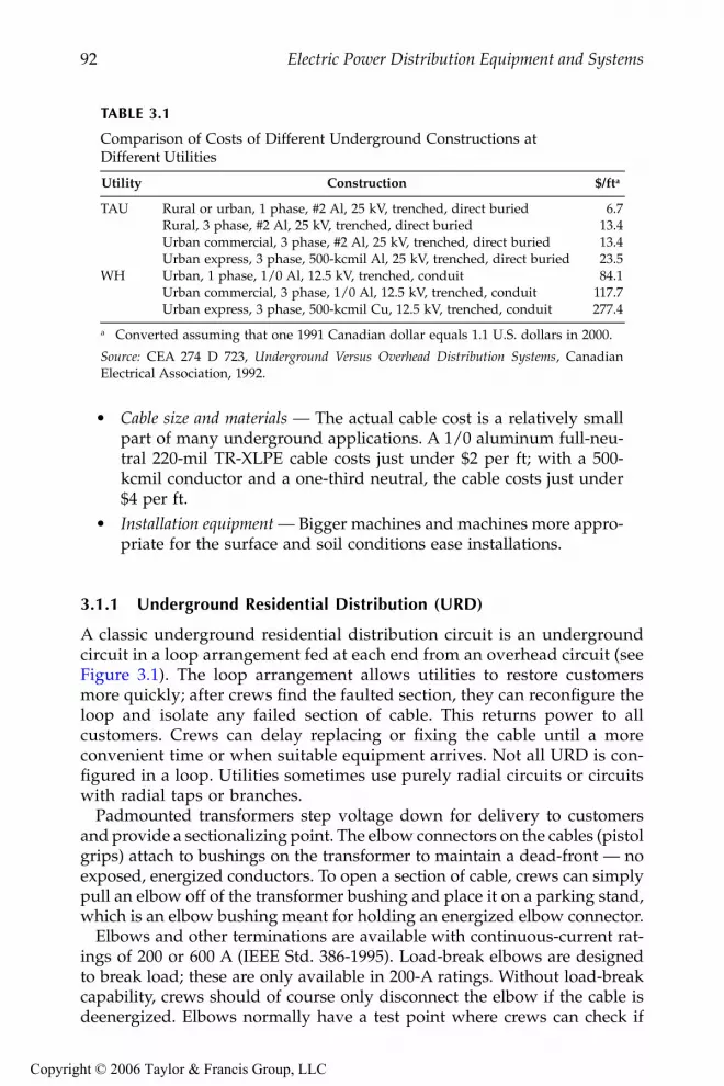
92
Electric Power Distribution Equipment and Systems
•
Cable size and materials —
The actual cable cost is a relatively smallpart of many underground applications. A 1/0 aluminum full-neu-tral 220-mil TR-XLPE cable costs just under $2 per ft; with a 500-kcmil conductor and a one-third neutral, the cable costs just under$4 per ft.
•
Installation equipment —
Bigger machines and machines more appro-priate for the surface and soil conditions ease installations.
3.1.1 Underground Residential Distribution (URD)
A classic underground residential distribution circuit is an undergroundcircuit in a loop arrangement fed at each end from an overhead circuit (seeFigure 3.1). The loop arrangement allows utilities to restore customersmore quickly; after crews find the faulted section, they can reconfigure theloop and isolate any failed section of cable. This returns power to allcustomers. Crews can delay replacing or fixing the cable until a moreconvenient time or when suitable equipment arrives. Not all URD is con-figured in a loop. Utilities sometimes use purely radial circuits or circuitswith radial taps or branches.
Padmounted transformers step voltage down for delivery to customersand provide a sectionalizing point. The elbow connectors on the cables (pistolgrips) attach to bushings on the transformer to maintain a dead-front — noexposed, energized conductors. To open a section of cable, crews can simplypull an elbow off of the transformer bushing and place it on a parking stand,which is an elbow bushing meant for holding an energized elbow connector.
Elbows and other terminations are available with continuous-current rat-ings of 200 or 600 A (IEEE Std. 386-1995). Load-break elbows are designedto break load; these are only available in 200-A ratings. Without load-breakcapability, crews should of course only disconnect the elbow if the cable isdeenergized. Elbows normally have a test point where crews can check if
TABLE 3.1
Comparison of Costs of Different Underground Constructions at
Different Utilities
Utility Construction $/ft
a
TAU Rural or urban, 1 phase, #2 Al, 25 kV, trenched, direct buried 6.7Rural, 3 phase, #2 Al, 25 kV, trenched, direct buried 13.4Urban commercial, 3 phase, #2 Al, 25 kV, trenched, direct buried 13.4Urban express, 3 phase, 500-kcmil Al, 25 kV, trenched, direct buried 23.5
WH Urban, 1 phase, 1/0 Al, 12.5 kV, trenched, conduit 84.1Urban commercial, 3 phase, 1/0 Al, 12.5 kV, trenched, conduit 117.7Urban express, 3 phase, 500-kcmil Cu, 12.5 kV, trenched, conduit 277.4
a
Converted assuming that one 1991 Canadian dollar equals 1.1 U.S. dollars in 2000.
Source:
CEA 274 D 723,
Underground Versus Overhead Distribution Systems
, CanadianElectrical Association, 1992.
9576_C03.fm Page 92 Monday, October 17, 2005 8:12 AM
Copyright © 2006 Taylor & Francis Group, LLC

Underground Distribution
93
the cable is live. Elbows are also tested to withstand ten cycles of faultcurrent, with 200-A elbows tested at 10 kA and 600-A elbows tested at 25kA (IEEE Std. 386-1995).
The interface between the overhead circuit and the URD circuit is the riserpole. At the riser pole (or a dip pole or simply a dip), cable terminationsprovide the interface between the insulated cable and the bare overheadconductors. These pothead terminations grade the insulation to preventexcessive electrical stress on the insulation. Potheads also keep water fromentering the cable, which is critical for cable reliability. Also at the riser poleare expulsion fuses, normally in cutouts. Areas with high short-circuit cur-rent may also have current-limiting fuses. To keep lightning surges fromdamaging the cable, the riser pole should have arresters right across thepothead with as little lead length as possible.
Underground designs for residential developments expanded dramati-cally in the 1970s. Political pressure coupled with technology improvementswere the driving forces behind underground distribution. The main devel-opments — direct-buried cables and padmounted transformers having load-break elbows — dramatically reduced the cost of underground distributionto close to that of overhead construction. In addition to improving the visuallandscape, underground construction improves reliability. Underground res-
FIGURE 3.1
An example front-lot underground residential distribution (URD) system.
Riserpoles
Padmounted transformerPrimarySecondary
Openpoint
9576_C03.fm Page 93 Monday, October 17, 2005 8:12 AM
Copyright © 2006 Taylor & Francis Group, LLC

94
Electric Power Distribution Equipment and Systems
idential distribution has had difficulties, especially high cable failure rates.In the late 1960s and early 1970s, given the durability of plastics, the poly-ethylene cables installed at that time were thought to have a life of at least50 years. In practice, cables failed at a much higher rate than expected,enough so that many utilities had to replace large amounts of this cable.
According to Boucher (1991), 72% of utilities use front-lot designs for URD.With easier access and fewer trees and brush to clear, crews can more easilyinstall cables along streets in the front of yards. Customers prefer rear-lotservice, which hides padmounted transformers from view. Back-lot place-ment can ease siting issues and may be more economical if lots share rearproperty lines. But with rear-lot design, utility crews have more difficultyaccessing cables and transformers for fault location, sectionalizing, and repair.
Of those utilities surveyed by Boucher (1991), 85% charge for undergroundresidential service, ranging from $200 to $1200 per lot (1991 dollars). Someutilities charge by length, which ranges from $5.80 to $35.00 per ft.
3.1.2 Main Feeders
Whether urban, suburban, or even rural, all parts of a distribution circuitcan be underground, including the main feeder. For reliability, utilities oftenconfigure an underground main feeder as a looped system with one or moretie points to other sources. Switching cabinets or junction boxes serve as tiepoints for tapping off lateral taps or branches to customers. These can be inhandholes, padmounted enclosures, or pedestals above ground. Three-phasecircuits can also be arranged much like URD with sections of cable runbetween three-phase padmounted transformers. As with URD, the pad-mounted transformers serve as switching stations.
Although short, many feeders have an important underground section— the substation exit. Underground substation exits make substations eas-ier to design and improve the aesthetics of the substation. Because they areat the substation, the source of a radial circuit, substation exits are criticalfor reliability. In addition, the loading on the circuit is higher at the sub-station exit than anywhere else; the substation exit may limit the entirecircuit’s ampacity. Substation exits are not the place to cut corners. Somestrategies to reduce the risks of failures or to speed recovery are: concrete-enclosed ducts to help protect cables, spare cables, overrated cables, andgood surge protection.
While not as critical as substation exits, utilities use similar three-phaseunderground dips to cross large highways or rivers or other obstacles. Theseare designed in much the same way as substation exits.
3.1.3 Urban Systems
Underground distribution has reliably supplied urban systems since theearly 1900s. Cables are normally installed in concrete-encased duct banks
9576_C03.fm Page 94 Monday, October 17, 2005 8:12 AM
Copyright © 2006 Taylor & Francis Group, LLC

Underground Distribution
95
beneath streets, sidewalks, or alleys. A duct bank is a group of parallel ducts,usually with four to nine ducts but often many more. Ducts may be precastconcrete sections or PVC encased in concrete. Duct banks carry both primaryand secondary cables. Manholes every few hundred feet provide access tocables. Transformers are in vaults or in the basements of large buildings.
Paper-insulated lead-covered (PILC) cables dominated urban applicationsuntil the late 20th century. Although a few utilities still install PILC, mostuse extruded cable for underground applications. In urban applications,copper is more widely used than in suburban applications. Whether feedingsecondary networks or other distribution configurations, urban circuits maybe subjected to heavy loads.
“Vertical” distribution systems are necessary in very tall buildings.Medium-voltage cable strung up many floors feed transformers within abuilding. Submarine cables are good for this application since their protec-tive armor wire provides support when a cable is suspended for hundredsof feet.
3.1.4 Overhead vs. Underground
Overhead or underground? The debate continues. Both designs have advan-tages (see Table 3.2). The major advantage of overhead circuits is cost; anunderground circuit typically costs anywhere from 1 to 2.5 times the equiv-alent overhead circuit (see Table 3.3). But the cost differences vary wildly,and it’s often difficult to define “equivalent” systems in terms of perfor-mance. Under the right conditions, some estimates of cost report that cableinstallations can be less expensive than overhead lines. If the soil is easy todig, if the soil has few rocks, if the ground has no other obstacles like waterpipes or telephone wires, then crews may be able to plow in cable faster andfor less cost than an overhead circuit. In urban areas, underground is almostthe only choice; too many circuits are needed, and above-ground space istoo expensive or just not available. But urban duct-bank construction isexpensive on a per-length basis (fortunately, circuits are short in urban appli-
TABLE 3.2
Overhead vs. Underground: Advantages of Each
Overhead Underground
Cost
— Overhead’s number one advantage. Significantly less cost, especially initial cost.
Longer life
— 30 to 50 years vs. 20 to 40 for new underground works.
Reliability
— Shorter outage durations because of faster fault finding and faster repair.
Loading
— Overhead circuits can more readily withstand overloads.
Aesthetics
— Underground’s number one advantage. Much less visual clutter.
Safety
— Less chance for public contact.
Reliability
— Significantly fewer short and long-duration interruptions.
O&M
— Notably lower maintenance costs (no tree trimming).
Longer reach
— Less voltage drop because reactance is lower.
9576_C03.fm Page 95 Monday, October 17, 2005 8:12 AM
Copyright © 2006 Taylor & Francis Group, LLC

96
Electric Power Distribution Equipment and Systems
cations). On many rural applications, the cost of underground circuits isdifficult to justify, especially on long, lightly loaded circuits, given the smallnumber of customers that these circuits feed.
Aesthetics is the main driver towards underground circuits. Especially inresidential areas, parks, wildlife areas, and scenic areas, visual impact isimportant. Undergrounding removes a significant amount of visual clutter.Overhead circuits are ugly. It is possible to make overhead circuits less uglywith tidy construction practices, fiberglass poles instead of wood, keepingpoles straight, tight conductor configurations, joint use of poles to reducethe number of poles, and so on. Even the best though, are still ugly, andmany older circuits look awful (weathered poles tipped at odd angles,crooked crossarms, rusted transformer tanks, etc.).
Underground circuits get rid of all that mess, with no visual impacts inthe air. Trees replace wires, and trees don’t have to be trimmed. At groundlevel, instead of poles every 150 ft (many having one or more guy wires)urban construction has no obstacles, and URD-style construction has just
TABLE 3.3
Comparison of Underground Construction Costs with Overhead Costs
Utility Construction $/ft
a
Undergroundto overhead
ratio
Single-Phase Lateral Comparisons
NP Overhead 1/0 AA, 12.5 kV, phase and neutral 8.4NP Underground 1/0 AA, 12.5 kV, trenched, in conduit 10.9 1.3APL Overhead Urban, #4 ACSR, 14.4 kV 2.8APL Underground Urban, #1 AA, 14.4 kV, trenched, direct
buried6.6 2.4
Three-Phase Mainline Comparisons
NP Overhead Rural, 4/0 AA, 12.5 kV 10.3NP Underground Rural, 1/0 AA, 12.5 kV, trenched, in
conduit17.8 1.7
NP Overhead Urban, 4/0 AA, 12.5 kV 10.9NP Underground Urban, 4/0 AA, 12.5 kV, trenched, in
conduit17.8 1.6
APL Overhead Urban, 25 kV, 1/0 ACSR 8.5APL Underground Urban, 25 kV, #1 AA, trenched, direct
buried18.8 2.2
EP Overhead Urban, 336 ACSR, 13.8 kV 8.7EP Underground Urban residential, 350 AA, 13.8 kV,
trenched, direct buried53.2 6.1
EP Underground Urban commercial, 350 AA, 13.8 kV, trenched, direct buried
66.8 7.6
a
Converted assuming that one 1991 Canadian dollar equals 1.1 U.S. dollars in 2000.
Source:
CEA 274 D 723,
Underground Versus Overhead Distribution Systems
, Canadian ElectricalAssociation, 1992.
9576_C03.fm Page 96 Monday, October 17, 2005 8:12 AM
Copyright © 2006 Taylor & Francis Group, LLC

Underground Distribution
97
padmounted transformers spaced much less frequently. Of course, for max-imum benefit, all utilities must be underground. There is little improvementto undergrounding electric circuits if phone and cable television are stillstrung on poles (i.e., if the telephone wires are overhead, you might as wellhave the electric lines there, too).
While underground circuits are certainly more appealing when finished,during installation construction is messier than overhead installation. Lawns,gardens, sidewalks, and driveways are dug up; construction lasts longer;and the installation “wounds” take time to heal. These factors don’t mattermuch when installing circuits into land that is being developed, but it canbe upsetting to customers in an existing, settled community.
Underground circuits are more reliable. Overhead circuits typically faultabout 90 times/100 mi/year; underground circuits fail less than 10 times/100 mi/year. Because overhead circuits have more faults, they cause morevoltage sags, more momentary interruptions, and more long-duration inter-ruptions. Even accounting for the fact that most overhead faults are tempo-rary, overhead circuits have more permanent faults that lead to long-durationcircuit interruptions. The one disadvantage of underground circuits is thatwhen they do fail, finding the failure is harder, and fixing the damage orreplacing the equipment takes longer. This can partially be avoided by usingloops capable of serving customers from two directions, by using conduitsfor faster replacement, and by using better fault location techniques. Under-ground circuits are much less prone to the elements. A major hurricane maydrain an overhead utility’s resources, crews are completely tied up, customeroutages become very long, and cleanup costs are a major cost to utilities.However, underground circuits are not totally immune from the elements.In “heat storms,” underground circuits are prone to rashes of failures. Under-ground circuits have less overload capability than overhead circuits; failuresincrease with operating temperature.
In addition to less storm cleanup, underground circuits require less peri-odic maintenance. Underground circuits don’t require tree trimming, easilythe largest fraction of most distribution operations and maintenance budgets.The CEA (1992) estimated that underground system maintenance averaged2% of system plant investment whereas overhead systems averaged 3 to 4%,or as much as twice that of underground systems.
Underground circuits are safer to the public than overhead circuits. Over-head circuits are more exposed to the public. Kites, ladders, downed wires,truck booms — despite the best public awareness campaigns, these stillexpose the public to electrocution from overhead lines. Don’t misunderstand;underground circuits still have dangers, but they’re much less than on over-head circuits. For the public, dig-ins are the most likely source of contact.For utility crews, both overhead and underground circuits offer dangers thatproper work practices must address to minimize risks.
We cannot assume that underground infrastructure will last as long asoverhead circuits. Early URD systems failed at a much higher rate thanexpected. While most experts believe that modern underground equipment
9576_C03.fm Page 97 Monday, October 17, 2005 8:12 AM
Copyright © 2006 Taylor & Francis Group, LLC

98
Electric Power Distribution Equipment and Systems
is more reliable, it is still prudent to believe that an overhead circuit will last40 years, while an underground circuit will only last 30 years.
Overhead vs. underground is not an all or nothing proposition. Manysystems are hybrids; some schemes are:
•
Overhead mainline with underground taps —
The larger, high-currentconductors are overhead. If the mains are routed along major roads,they have less visual impact. Lateral taps down side roads and intoresidential areas, parks, and shopping areas are underground.Larger primary equipment like regulators, reclosers, capacitorbanks, and automated switches are installed where they are moreeconomical — on the overhead mains. Because the mainline is amajor contributor to reliability, this system is still less reliable thanan all-underground system.
•
Overhead primary with underground secondary —
Underground sec-ondary eliminates some of the clutter associated with overhead con-struction. Eliminating much of the street and yard crossings keepsthe clutter to the pole-line corridor. Costs are reasonable because theprimary-level equipment is still all overhead.
Converting from overhead to underground is costly, yet there are locationsand situations where it is appropriate for utilities and their customers. Circuitextensions, circuit enhancements to carry more load, and road-rebuildingprojects — all are opportunities for utilities and communities to upgrade tounderground service.
3.2 Cables
At the center of a cable is the phase conductor, then comes a semiconductingconductor shield, the insulation, a semiconducting insulation shield, theneutral or shield, and finally a covering jacket. Most distribution cables aresingle conductor. Two main types of cable are available: concentric-neutralcable and power cable. Concentric-neutral cable normally has an aluminumconductor, an extruded insulation, and a concentric neutral (Figure 3.2 showsa typical construction). A concentric neutral is made from several copperwires wound concentrically around the insulation; the concentric neutral isa true neutral, meaning it can carry return current on a grounded system.Underground residential distribution normally has concentric-neutralcables; concentric-neutral cables are also used for three-phase mainline appli-cations and three-phase power delivery to commercial and industrial cus-tomers. Because of their widespread use in URD, concentric-neutral cablesare often called URD cables. Power cable has a copper or aluminum phase
9576_C03.fm Page 98 Monday, October 17, 2005 8:12 AM
Copyright © 2006 Taylor & Francis Group, LLC

Underground Distribution
99
conductor, an extruded insulation, and normally a thin copper tape shield.On utility distribution circuits, power cables are typically used for mainlinefeeder applications, network feeders, and other high current, three-phaseapplications. Many other types of medium-voltage cable are available. Theseare sometimes appropriate for distribution circuit application: three-conduc-tor power cables, armored cables, aerial cables, fire-resistant cables, extraflexible cables, and submarine cables.
3.2.1 Cable Insulation
A cable’s insulation holds back the electrons; the insulation allows cableswith a small overall diameter to support a conductor at significant voltage.A 0.175-in. (4.5-mm) thick polymer cable is designed to support just over 8kV continuously; that’s an average stress of just under 50 kV per in. (20 kV/cm). In addition to handling significant voltage stress, insulation must with-stand high temperatures during heavy loading and during short circuits andmust be flexible enough to work with. For much of the 20th century, paperinsulation dominated underground application, particularly PILC cables.The last 30 years of the 20th century saw the rise of polymer-insulated cables,polyethylene-based insulations starting with high-molecular weight poly-ethylene (HMWPE), then cross-linked polyethylene (XLPE), then tree-retar-dant XLPE and also ethylene-propylene rubber (EPR) compounds.
Table 3.4 compares properties of TR-XLPE, EPR, and other insulation mate-rials. Some of the key properties of cable insulation are:
•
Dielectric constant
(
ε
, also called permittivity) — This determines thecable’s capacitance: the dielectric constant is the ratio of the capac-itance with the insulation material to the capacitance of the same
FIGURE 3.2
A concentric neutral cable, typically used for underground residential power delivery.
9576_C03.fm Page 99 Monday, October 17, 2005 8:12 AM
Copyright © 2006 Taylor & Francis Group, LLC

100
Electric Power Distribution Equipment and Systems
configuration in free space. Cables with higher capacitance drawmore charging current.
•
Volume resistivity —
Current leakage through the insulation is afunction of the insulation’s dc resistivity. Resistivity decreases astemperature increases. Modern insulation has such high resistivitythat very little resistive current passes from the conductor throughthe insulation.
•
Dielectric losses —
Like a capacitor, a cable has dielectric losses. Theselosses are due to dipole movements within the polymer or by themovement of charge carriers within the insulation. Dielectric lossescontribute to a cable’s resistive leakage current. Dielectric lossesincrease with frequency and temperature and with operating voltage.
•
Dissipation factor
(also referred to as the loss angle, loss tangent, tan
δ
, and approximate power factor) — The dissipation factor is theratio of the resistive current drawn by the cable to the capacitivecurrent drawn (
I
R
/
I
X
). Because the leakage current is normally low,the dissipation factor is approximately the same as the power factor:
Paper-Insulated Lead-Covered (PILC) Cables.
Paper-insulated cables have pro-vided reliable underground power delivery for decades. Paper-insulatedlead-sheathed cable has been the dominant cable configuration, used mainlyin urban areas. PILC cables have kraft-paper tapes wound around the con-ductor that are dried and impregnated with insulating oil. A lead sheath isone of the best moisture blocks: it keeps the oil in and keeps water out. Papercables are normally rated to 85
°
C with an emergency rating up to 105
°
C(EPRI TR-105502, 1995). PILC cables have held up astonishingly well; many50-year-old cables are still in service with almost new insulation capability.While PILC has had very good reliability, some utilities are concerned about
TABLE 3.4
Properties of Cable Insulations
DielectricConstant
20
°
C
Loss AngleTan
δ
at 20
°
C
VolumeResistivity
Ω
-m
AnnualDielectric
Loss
a
W/1000 ft
UnagedImpulseStrength
V/mil
WaterAbsorption
ppm
PILC 3.6 0.003 10
11
N/A 1000–2000 25PE 2.3 0.0002 10
14
N/A 100XLPE 2.3 0.0003 10
14
8 3300 350TR-XLPE 2.4 0.001 10
14
10 3000 <300EPR 2.7–3.3 0.005–0.008 10
13
–10
14
28–599 1200–2000 1150–3200
a
For a typical 1/0 15-kV cable.
Copyright © 2001. Electric Power Research Institute. 1001894.
EPRI Power Cable MaterialsSelection Guide
. Reprinted with permission.
pf dissipation factor= = + ≈ =I I I I I I IR R R X R X/ / /2 2
9576_C03.fm Page 100 Monday, October 17, 2005 8:12 AM
Copyright © 2006 Taylor & Francis Group, LLC
Underground Distribution
101
its present day failure, not because of bad design or application, but becausethe in-service stock is so old. Moisture ingress, loss of oil, and thermal stresses— these are the three main causes of PILC failure (EPRI 1000741, 2000). Waterdecreases the dielectric strength (especially when the cable is hot) andincreases the dielectric losses (further heating the cable). Heat degrades theinsulating capability of the paper, and if oil is lost, the paper’s insulatingcapability declines. PILC use has declined but still not disappeared. Someutilities continue to use it, especially to supply urban networks. Utilities useless PILC because of its high cost, work difficulties, and environmentalconcerns. Splicing also requires significant skill, and working with the leadsheath requires environmental and health precautions.
Polyethylene (PE).
Most modern cables have polymer insulation extrudedaround the conductor — either polyethylene derivatives or ethylene-propy-lene properties. Polyethylene is a tough, inexpensive polymer with goodelectrical properties. Most distribution cables made since 1970 are based onsome variation of polyethylene. Polyethylene is an ethylene polymer, a longstring or chain of connected molecules. In polyethylene, some of the polymerchains align in crystalline regions, which give strength and moisture resis-tance to the material. Other regions have nonaligned polymer chains — theseamorphous regions give the material flexibility but are permeable to gas andmoisture and are where impurities locate. Polyethylene is a thermoplastic.When heated and softened, the polymer chains break apart (becoming com-pletely amorphous); as it cools, the crystalline regions reform, and the mate-rial returns to its original state. Polyethylene naturally has high density andexcellent electrical properties with a volume resistivity of greater than 10
14
Ω
-m and an impulse insulation strength of over 2700 V/mil.
High-Molecular Weight Polyethylene (HMWPE).
High-molecular weightpolyethylene is polyethylene that is stiffer, stronger, and more resistant tochemical attack than standard polyethylene. Insulations with higher molec-ular weights (longer polymer chains) generally have better electrical prop-erties. As with standard polyethylene, HMWPE insulation is a thermoplasticrated to 75
°
C. Polyethylene softens considerably as temperature increases.Since plastics are stable and seem to last forever, when utilities first installedHMWPE in the late 1960s and early 1970s, utilities and manufacturersexpected long life for polyethylene cables. In practice, failure rates increaseddramatically after as little as 5 years of service. The electrical insulatingstrength (the dielectric strength) of HMWPE was degraded by water treeing,an electrochemical degradation driven by the presence of water and voltage.Polyethylene also degrades quickly under partial discharges; once partialdischarges start, they can quickly eat away the insulation. Because of highfailure rates, HMWPE insulation is off the market now, but utilities still havemany miles of this cable in the ground.
Cross-Linked Polyethylene (XLPE).
Cross-linking agents are added that formbonds between polymer chains. The cross-linking bonds interconnect thechains and make XLPE semi-crystalline and add stiffness. XLPE is a ther-moset: the material is vulcanized (also called “cured”), irreversibly creating
9576_C03.fm Page 101 Monday, October 17, 2005 8:12 AM
Copyright © 2006 Taylor & Francis Group, LLC

102
Electric Power Distribution Equipment and Systems
the cross-linking that sets when the insulation cools. XLPE has about thesame insulation strengths as polyethylene, is more rigid, and resists watertreeing better than polyethylene. Although not as bad as HMWPE, pre-1980sXLPE has proven susceptible to premature failures because of water treeing.XLPE has higher temperature ratings than HWMPE; cables are rated to 90
°
Cunder normal conditions and 130
°
C for emergency conditions.
Tree-Retardant Cross-Linked Polyethylene (TR-XLPE).
This has adders toXLPE that slow the growth of water trees. Tree-retardant versions of XLPEhave almost totally displaced XLPE in medium-voltage cables. Various com-pounds when added to XLPE reduce its tendency to grow water trees undervoltage. These additives tend to slightly reduce XLPE’s electrical properties,slightly increase dielectric losses, and slightly lower initial insulationstrength (but much better insulation strength when aged). While there is nostandard industry definition of TR-XLPE, different manufacturers offer XLPEcompounds with various adders that reduce tree growth. The oldest andmost widely used formulation was developed by Union Carbide (now Dow);their HFDA 4202 tree-retardant XLPE maintains its insulation strength betterin accelerated aging tests (EPRI TR-108405-V1, 1997) and in field service(Katz and Walker, 1998) than standard XLPE.
Ethylene-Propylene Rubber (EPR).
EPR compounds are polymers made fromethylene and propylene. Manufacturers offer different ethylene-propyleneformulations, which collectively are referred to as EPR. EPR compounds arethermoset, normally with a high-temperature steam curing process that setscross-linking agents. EPR compounds have high concentrations of clay fillersthat provide its stiffness. EPR is very flexible and rubbery. When new, EPRonly has half of the insulation strength as XLPE, but as it ages, its insulationstrength does not decrease nearly as much as that of XLPE. EPR is naturallyquite resistant to water trees, and EPR has a proven reliable record in thefield. EPR has very good high-temperature performance. Although soft, itdeforms less at high temperature than XLPE and maintains its insulationstrength well at high temperature (Brown, 1983). Most new EPR cables arerated to 105
°
C under normal conditions and to 140
°
C for emergency condi-tions, the MV-105 designation per UL Standard 1072. (Historically, both XLPEand EPR cables were rated to 90
°
C normal and 130
°
C emergency.) In additionto its use as cable insulation, most splices and joints are made of EPR com-pounds. EPR has higher dielectric losses than XLPE; depending on the par-ticular formulation, EPR can have two to three times the losses of XLPE toover ten times the losses of XLPE. These losses increase the cost of operationover its lifetime. While not as common or as widely used as XLPE in theutility market, EPR dominates for medium-voltage industrial applications.
TR-XLPE vs. EPR: which to use? Of the largest investor-owned utilities56% specify TR-XLPE cables, 24% specify EPR, and the remainder specify amix (Dudas and Cochran, 1999). Trends are similar at rural cooperatives. Ina survey of the co-ops with the largest installed base of underground cable,42% specify TR-XLPE, 34% specify EPR, and the rest specify both (Dudasand Rodgers, 1999). When utilities specify both EPR and TR-XLPE, com-
9576_C03.fm Page 102 Monday, October 17, 2005 8:12 AM
Copyright © 2006 Taylor & Francis Group, LLC

Underground Distribution
103
monly EPR is used for 600-A three-phase circuits, and TR-XLPE is used for200-A applications like URD. Each cable type has advocates. TR-XLPE is lessexpensive and has lower losses. EPR’s main feature is its long history ofreliability and water-tree resistance. EPR is also softer (easier to handle) andhas a higher temperature rating (higher ampacity). Boggs and Xu (2001)show how EPR and TR-XLPE are becoming more similar: EPR compoundsare being designed that have fewer losses; tree-retardant additives to XLPEmake the cable more tree resistant at the expense of increasing its waterabsorption and slightly increasing losses.
Cables have a voltage rating based on the line-to-line voltage. Standardvoltage ratings are 5, 8, 15, 25, and 35 kV. A single-phase circuit with anominal voltage of 7.2 kV from line to ground must use a 15-kV cable, notan 8-kV cable (because the line-to-line voltage is 12.47 kV).
Within each voltage rating, more than one insulation thickness is available.Standards specify three levels of cable insulation based on how the cablesare applied. The main factor is grounding and ability to clear line-to-groundfaults in order to limit the overvoltage on the unfaulted phases. The standardlevels are (AEIC CS5-94, 1994):
•
100 percent level —
Allowed where line-to-ground faults can becleared quickly (at least within one minute); normally appropriatefor grounded circuits
•
133 percent level —
Where line-to-ground faults can be cleared withinone hour; normally can be used on ungrounded circuits
Standards also define a 173% level for situations where faults cannot becleared within one hour, but manufacturers typically offer the 100 and 133%levels as standard cables; higher insulation needs can be met by a customorder or going to a higher voltage rating. Table 3.5 shows standard insulationthicknesses for XLPE and EPR for each voltage level. In addition to protectingagainst temporary overvoltages, thicker insulations provide higher insula-tion to lightning and other overvoltages and reduce the chance of failurefrom water tree growth. For 15-kV class cables, Boucher (1991) reported that59% of utilities surveyed in North America use 100% insulation (175-mil).
TABLE 3.5
Usual Insulation Thicknesses for XLPE or EPR
Cables Based on Voltage and Insulation Level
Voltage Rating,kV
Insulation Thickness, Mil
(1 mil = 0.001 in. = 0.00254 cm)100% Level 133% Level
8 115 14015 175 22025 260 32035 345 420
9576_C03.fm Page 103 Monday, October 17, 2005 8:12 AM
Copyright © 2006 Taylor & Francis Group, LLC

104
Electric Power Distribution Equipment and Systems
At 25 and 35 kV, the surveyed utilities more universally use 100% insulation(88 and 99%, respectively). Dudas and Cochran (1999) report similar trendsin a survey of practices of the 45 largest investor-owned utilities: at 15 kV,69% of utilities specified 100% insulation; at 25 and 35 kV, over 99% of utilitiesspecified 100% insulation.
3.2.2 Conductors
For underground residential distribution (URD) applications, utilities nor-mally use aluminum conductors; Boucher (1991) reported that 80% of utili-ties use aluminum (alloy 1350); the remainder, copper (annealed, soft).Copper is more prevalent in urban duct construction and in industrial appli-cations. Copper has lower resistivity and higher ampacity for a given size;aluminum is less expensive and lighter. Cables are often stranded to increasetheir flexibility (solid conductor cables are available for less than 2/0). ASTMclass B stranding is the standard stranding. Class C has more strands forapplications requiring more flexibility. Each layer of strands is wound in anopposite direction. Table 3.6 shows diameters of available conductors.
3.2.3 Neutral or Shield
A cable’s shield, the metallic barrier that surrounds the cable insulation,holds the outside of the cable at (or near) ground potential. It also providesa path for return current and for fault current. The shield also protects thecable from lightning strikes and from current from other fault sources. Themetallic shield is also called the
sheath
.A concentric neutral — a shield capable of carrying unbalanced current
— has copper wires wound helically around the insulation shield. The con-centric neutral is expected to carry much of the unbalanced load current,with the earth carrying the rest. For single-phase cables, utilities normallyuse a “full neutral,” meaning that the resistance of the neutral equals thatof the phase conductor. Also common is a “one-third neutral,” which has aresistance that is three times that of the phase conductor. In a survey ofunderground distribution practices, Boucher (1991) reported that full neu-trals dominated for residential application, and reduced neutrals are usedmore for commercial and feeder applications (see Figure 3.3).
Power cables commonly have 5-mil thick copper tape shields. These arewrapped helically around the cable with some overlap. In a tape-shield cable,the shield is not normally expected to carry unbalanced load current. As wewill see, there is an advantage to having a higher resistance shield: the cableampacity can be higher because there is less circulating current. Shields arealso available that are helically wound wires (like a concentric neutral butwith smaller wires).
Whether wires or tapes, cable shields and neutrals are copper. Aluminumcorrodes too quickly to perform well in this function. Early unjacketed cables
9576_C03.fm Page 104 Monday, October 17, 2005 8:12 AM
Copyright © 2006 Taylor & Francis Group, LLC

Underground Distribution
105
normally had a coating of lead-tin alloy to prevent corrosion. Cable neutralsstill corroded. Dudas (1994) reports that in 1993, 84% of utilities specified abare copper neutral rather than a coated neutral.
The longitudinally corrugated (LC) shield improves performance for faultcurrents and slows down water entry. The folds of a corrugated copper tapeare overlapped over the cable core. The overlapping design allows move-ment and shifting while also slowing down water entry. The design performsbetter for faults because it is thicker than a tape shield, so it has less resis-tance, and it tends to distribute current throughout the shield rather thankeeping it in a few strands.
TABLE 3.6
Conductor Diameters
Size
Solid
Class B strandingDiameter, in. Strands Diameter, in.
24 0.0201 7 0.02322 0.0253 7 0.02920 0.032 7 0.03619 0.035 7 0.04118 0.0403 7 0.04616 0.0508 7 0.05814 0.0641 7 0.07312 0.0808 7 0.09210 0.1019 7 0.116
9 0.1144 7 0.138 0.1285 7 0.1467 0.1443 7 0.1646 0.162 7 0.1845 0.1819 7 0.2064 0.2043 7 0.2323 0.2294 7 0.262 0.2576 7 0.2921 0.2893 19 0.332
1/0 0.3249 19 0.3732/0 0.3648 19 0.4193/0 0.4096 19 0.474/0 0.46 19 0.528250 37 0.575300 37 0.63350 37 0.681400 37 0.728500 37 0.813600 61 0.893750 61 0.998
1000 61 1.1521250 91 1.2891500 91 1.4121750 127 1.5262000 127 1.6322500 127 1.824
9576_C03.fm Page 105 Monday, October 17, 2005 8:12 AM
Copyright © 2006 Taylor & Francis Group, LLC

106
Electric Power Distribution Equipment and Systems
3.2.4 Semiconducting Shields
In this application, semiconducting means “somewhat conducting”: thematerial has some resistance (limited to a volume resistivity of 500
Ω
-m[ANSI/ICEA S-94-649-2000, 2000; ANSI/ICEA S-97-682-2000, 2000]), morethan the conductor and less than the insulation. Semiconducting does notrefer to nonlinear resistive materials like silicon or metal oxide; the resistanceis fixed; it does not vary with voltage. Also called screens or semicons, thesesemiconducting shields are normally less than 80 mil. The resistive materialevens out the electric field at the interface between the phase conductor andthe insulation and between the insulation and the neutral or shield. Withoutthe shields, the electric field gradient would concentrate at the closest inter-faces between a wire and the insulation; the increased localized stress couldbreak down the insulation. The shields are made by adding carbon to anormally insulating polymer like EPR or polyethylene or cross-linked poly-ethylene. The conductor shield is normally about 20 to 40 mil thick; theinsulation shield is normally about 40 to 80 mil thick. Thicker shields areused on larger diameter cables.
Semiconducting shields are important for smoothing out the electric field,but they also play a critical role in the formation of water trees. The mostdangerous water trees are vented trees, those that start at the interfacebetween the insulation and the semiconducting shield. Treeing starts at voidsand impurities at this boundary. “Supersmooth” shield formulations havebeen developed to reduce vented trees (Burns, 1990). These mixtures usefiner carbon particles to smooth out the interface. Under accelerated agingtests, cables with supersmooth semiconducting shields outperformed cableswith standard semiconducting shields.
Modern manufacturing techniques can extrude the semiconducting con-ductor shield, the insulation, and the semiconducting insulation shield inone pass. Using this
triple
extrusion provides cleaner, smoother contactbetween layers than extruding each layer in a separate pass.
FIGURE 3.3
Surveyed utility use of cable neutral configurations for residential, commercial, and feederapplications. (Data from [Boucher, 1991].)
Percent
CorrugatedTape shield
Reduced neutralFull neutral
0 20 40 60 80
Residentialn=139
Commercialn=145
0 20 40 60 80
0 20 40 60 80
Feedern=130
9576_C03.fm Page 106 Monday, October 17, 2005 8:12 AM
Copyright © 2006 Taylor & Francis Group, LLC

Underground Distribution
107
A note on terminology: a
shield
is the conductive layer surrounding anotherpart of the cable. The conductor shield surrounds the conductor; the insula-tion shield surrounds the insulation. Used generically, shield refers to themetallic shield (the sheath). Commonly, the metallic shield is called theneutral, the shield, or the sheath. Sometimes, the sheath is used to mean theouter part of the cable, whether conducting or not conducting.
3.2.5 Jacket
Almost all new cables are jacketed, and the most common jacket is anencapsulating jacket (it is extruded between and over the neutral wires). Thejacket provides some (but not complete) protection against water entry. Italso provides mechanical protection for the neutral. Common LLDPE jacketsare 50 to 80 mil thick.
Bare cable, used frequently in the 1970s, had a relatively high failure rate(Dedman and Bowles, 1990). Neutral corrosion was often cited as the mainreason for the higher failure rate. At sections with a corroded neutral, theground return current can heat spots missing neutral strands. Dielectricfailure, not neutral corrosion, is still the dominant failure mode (Gurniak,1996). Without the jacket, water enters easily and accelerates water treeing,which leads to premature dielectric failure.
Several materials are used for jackets. Polyvinyl chloride (PVC) was oneof the earliest jacketing materials and is still common. The most commonjacket material is made from linear low-density polyethylene (LLDPE). PVChas good jacketing properties, but LLDPE is even better in most regards:mechanical properties, temperature limits, and water entry. Moisture passesthrough PVC jacketing more than ten times faster than it passes throughLLDPE. LLDPE starts to melt at 100
°
C; PVC is usually more limited,depending on composition. Low-density polyethylene resists abrasion bet-ter and also has a lower coefficient of friction, which makes it easier to pullthrough conduit.
Semiconducting jackets are also available. Semiconducting jackets providethe grounding advantages of unjacketed cable, while also blocking moistureand physically protecting the cable. When direct buried, an exposed neutralprovides an excellent grounding conductor. The neutral in contact with thesoil helps improve equipment grounding and improves protection againstsurges. A semiconducting jacket has a resistivity equivalent to most soils(less than 100
Ω
-m), so it transfers current to the ground the same as anunjacketed cable. NRECA (1993) recommends not using a semiconductingjacket for two reasons. First, semiconducting jackets let more water passthrough than LLDPE jackets. Second, the semiconducting jacket could con-tribute to corrosion. The carbon in the jacket (which makes the jacket semi-conducting) is galvanic to the neutral and other nearby metals; especiallywith water in the cable, the carbon accelerates neutral corrosion. Othernearby objects in the ground such as ground rods or pipes can also corrodemore rapidly from the carbon in the jacket.
9576_C03.fm Page 107 Monday, October 17, 2005 8:12 AM
Copyright © 2006 Taylor & Francis Group, LLC

108
Electric Power Distribution Equipment and Systems
3.3 Installations and Configurations
Just as there are many different soil types and underground applications,utilities have many ways to install underground cable. Some common instal-lation methods include [see NRECA RER Project 90-8 (1993) for more details]:
•
Trenching —
This is the most common way to install cables, eitherdirect-buried or cables in conduit. After a trench is dug, cable isinstalled, backfill is added and tamped, and the surface is restored.A trenching machine with different cutting chains is available foruse on different soils. Backhoes also help with trenching.
•
Plowing —
A cable plow blade breaks up and lifts the earth as itfeeds a cable into the furrow. Plowing eliminates backfilling anddisturbs the surface less than trenching. NRECA reports that plow-ing is 30 to 50% less expensive than trenching (NRECA RER Project90-8, 1993). Plowed cables may have lower ampacity because of airpockets between the cable and the loose soil around the cable. Heatcannot transfer as effectively from the cable to the surrounding earth.
•
Boring — A number of tunneling technologies are available to drillunder roads or even over much longer distances with guided, fluid-assisted drill heads.
Utilities also have a number of installation options, each with tradeoffs:
• Direct buried — Cables are buried directly in the earth. This is thefastest and least expensive installation option. Its major disadvan-tage is that cable replacement or repair is difficult.
• Conduit — Using conduit allows for quicker replacement or repair.Rigid PVC conduit is the most common conduit material; steel andHDPE and fiberglass are also used. Cables in conduit have lessampacity than direct-buried cables.
• Direct buried with a spare conduit — Burying a cable with a spareconduit provides provisions for repair or upgrades. Crews can pullanother cable through the spare conduit to increase capacity or, ifthe cable fails, run a replacement cable through the spare conduitand abandon the failed cable. Normally, when the cable is plowedin, the conduit is coilable polyethylene.
• Concrete-encased conduit — Most often used in urban construction,conduit is encased in concrete. Concrete protects the conduit, resist-ing collapse due to shifting earth. The concrete also helps preventdig-ins.
• Preassembled cable in conduit — Cable with flexible conduit can bepurchased on reels, which crews can plow into the ground together.
9576_C03.fm Page 108 Monday, October 17, 2005 8:12 AM
Copyright © 2006 Taylor & Francis Group, LLC
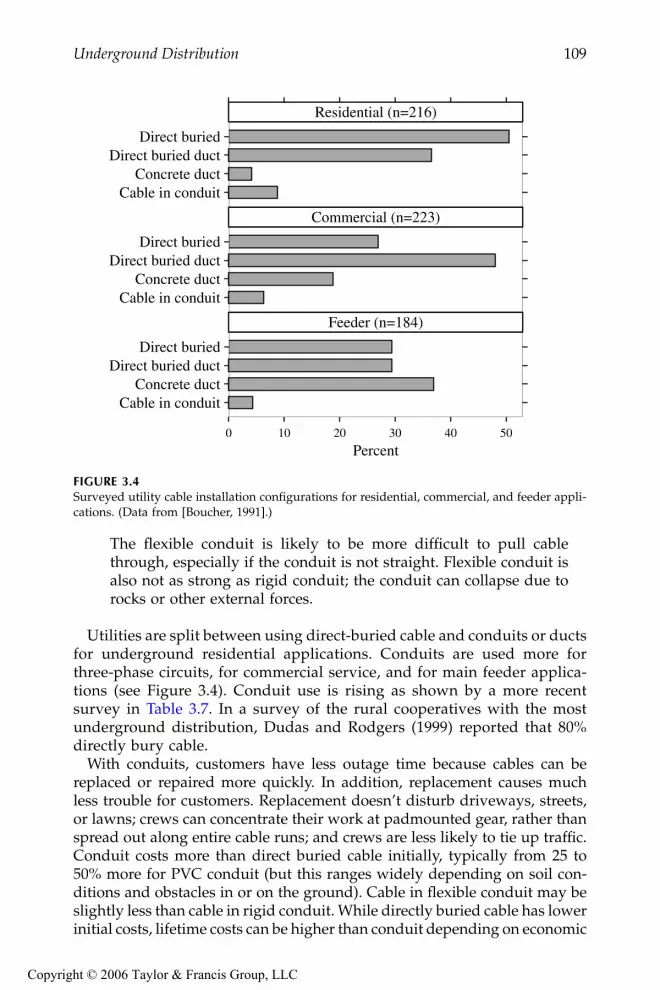
Underground Distribution 109
The flexible conduit is likely to be more difficult to pull cablethrough, especially if the conduit is not straight. Flexible conduit isalso not as strong as rigid conduit; the conduit can collapse due torocks or other external forces.
Utilities are split between using direct-buried cable and conduits or ductsfor underground residential applications. Conduits are used more forthree-phase circuits, for commercial service, and for main feeder applica-tions (see Figure 3.4). Conduit use is rising as shown by a more recentsurvey in Table 3.7. In a survey of the rural cooperatives with the mostunderground distribution, Dudas and Rodgers (1999) reported that 80%directly bury cable.
With conduits, customers have less outage time because cables can bereplaced or repaired more quickly. In addition, replacement causes muchless trouble for customers. Replacement doesn’t disturb driveways, streets,or lawns; crews can concentrate their work at padmounted gear, rather thanspread out along entire cable runs; and crews are less likely to tie up traffic.Conduit costs more than direct buried cable initially, typically from 25 to50% more for PVC conduit (but this ranges widely depending on soil con-ditions and obstacles in or on the ground). Cable in flexible conduit may beslightly less than cable in rigid conduit. While directly buried cable has lowerinitial costs, lifetime costs can be higher than conduit depending on economic
FIGURE 3.4Surveyed utility cable installation configurations for residential, commercial, and feeder appli-cations. (Data from [Boucher, 1991].)
Percent
Cable in conduitConcrete duct
Direct buried ductDirect buried
0 10 20 30 40 50
Feeder (n=184)
Cable in conduitConcrete duct
Direct buried ductDirect buried
Commercial (n=223)
Cable in conduitConcrete duct
Direct buried ductDirect buried
Residential (n=216)
9576_C03.fm Page 109 Monday, October 17, 2005 8:12 AM
Copyright © 2006 Taylor & Francis Group, LLC

110 Electric Power Distribution Equipment and Systems
assumptions and assumptions on how long cables will last or if they willneed to be upgraded. Some utilities use a combination approach; most cableis direct buried, but ducts are used for road crossings and other obstacles.
The National Electrical Safety Code requires that direct-buried cable haveat least 30 in. (0.75 m) of cover (IEEE C2-1997). Typically, trench depths areat least 36 in.
If communication cables are buried with primary power cables, extra rulesapply. For direct-buried cable with an insulating jacket, the NESC requiresthat the neutral must have at least one half of the conductivity of the phaseconductor (IEEE C2-1997) (it must be a one-half neutral or a full neutral).
Some urban applications are constrained by small ducts: 3, 3.5, or 4-in.diameters. These ducts were designed to hold three-conductor paper-insu-lated lead-sheathed cables which have conductors squashed in a sector shapefor a more compact arrangement. Insulation cannot be extruded over theseshapes, so obtaining an equivalent replacement cable with extruded insula-tion is difficult. Manufacturers offer thinner cables to meet these applications.For triplex cable, the equivalent outside diameter is 2.155 times the diameterof an individual cable. So, to fit in a 3-in. duct, an individual cable must beless than 1.16 in. in diameter to leave a 1/2-in. space (see Table 3.8 for otherduct sizes). Some cable offered as “thin-wall” cable has slightly reducedinsulation. For 15-kV cable, the smallest insulation thicknesses rangebetween 150 and 165 mil as compared to the standard 175 mil (EPRI 1001734,2002) (the ICEA allows 100% 15-kV cable insulation to range from 165 to 205
TABLE 3.7
Surveyed Utility Use of Cable Duct Installations
Percent of Cable Miles with Each Configuration1998 Installed Planned for the Future
Direct buried 64.6 46.9Installed in conduit sections 25.5 37.9Preassembled cable in conduit 7.1 11.7Direct buried with a spare conduit 1.1 0.5Continuous lengths of PE tubing 1.7 3.0
Source: Tyner, J. T., “Getting to the Bottom of UG Practices,” Transmission & DistributionWorld, vol. 50, no. 7, pp. 44–56, July 1998.
TABLE 3.8
Maximum Cable Diameters for Small Conduits Using PILC or Triplexed Cables that Leave 1/2-in. Pulling Room
Duct Size, in.
Largest Three-Conductor
15-kV PILC
Maximum CableDiameter for Triplex
Construction, in.
Largest StandardConstruction Triplexed 15-kV
Copper Cable
3.0 350 kcmil 1.16 3/03.5 750 kcmil 1.39 350 kcmil4.0 1000 kcmil 1.62 500 kcmil
9576_C03.fm Page 110 Monday, October 17, 2005 8:12 AM
Copyright © 2006 Taylor & Francis Group, LLC

Underground Distribution 111
mil (ANSI/ICEA S-97-682-2000, 2000)). One manufacturer has proposedreduced insulation thicknesses based on the fact that larger conductors havelower peak voltage stress on the insulation than smaller conductors (Cinque-mani et al., 1997), for example, 110-mil insulation at 15 kV for 4/0 through750 kcmil. The maximum electric field (EPRI 1001734, 2002) is given by
whereEmax = maximum electric field, V/mil (or other distance unit)
V = operating or rated voltage to neutral, Vd = inside diameter of the insulation, mil (or other distance unit)
D = outside diameter of the insulation in the same units as d
So, a 750-kcmil cable with 140-mil insulation has about the same maximumvoltage stress as a 1/0 cable with 175-mil insulation at the same voltage.Nevertheless, most manufacturers are reluctant to trim the primary insula-tion too much, fearing premature failure due to water treeing. In additionto slightly reduced insulation, thin-wall cables are normally compressedcopper and have thinner jackets and thinner semiconducting shields aroundthe conductor and insulation. EPRI has also investigated other polymers foruse in thin-wall cables (EPRI TR-111888, 2000). Their investigations foundpromising results with novel polymer blends that could achieve insulationstrengths that are 30 to 40% higher than XLPE. These tests suggest promise,but more work must be done to improve the extrusion of these materials.
3.4 Impedances
3.4.1 Resistance
Cable conductor resistance is an important part of impedance that is usedfor fault studies and load flow studies. Resistance also greatly impacts acable’s ampacity. The major variable that affects resistance is the conductor’stemperature; resistance rises with temperature. Magnetic fields from alter-nating currents also reduce a conductor’s resistance relative to its dc resis-tance. At power frequencies, skin effect is only apparent for large conductorsand proximity effect only occurs for conductors in very tight configurations.The starting point for resistance calculations is the dc resistance. From there,we can adjust for temperature and for frequency effects. Table 3.9 shows thedc resistances of several common conductors used for cables.
Resistance increases with temperature as
EV
d D dmax = 2ln( / )
9576_C03.fm Page 111 Monday, October 17, 2005 8:12 AM
Copyright © 2006 Taylor & Francis Group, LLC

112 Electric Power Distribution Equipment and Systems
whereRt2 = resistance at temperature t2 given, °CRt1 = resistance at temperature t1 given, °CM = a temperature coefficient for the given material
= 228.1 for aluminum = 234.5 for soft-drawn copper
TABLE 3.9
dc Resistance at 25°°°°C in ΩΩΩΩ/1000 ft
Size
Aluminum Uncoated Copper Coated Copper
SolidClass-B
Stranded SolidClass-B
Stranded SolidClass-B
Stranded
24 26.2 27.322 16.5 17.220 10.3 10.5 10.7 11.219 8.21 8.5318 6.51 6.64 6.77 7.0516 4.1 4.18 4.26 4.4414 4.22 2.57 2.62 2.68 2.7312 2.66 2.7 1.62 1.65 1.68 1.7210 1.67 1.7 1.02 1.04 1.06 1.08
9 1.32 1.35 0.808 0.824 0.831 0.8578 1.05 1.07 0.641 0.654 0.659 0.6797 0.833 0.85 0.508 0.518 0.523 0.5396 0.661 0.674 0.403 0.41 0.415 0.4275 0.524 0.535 0.319 0.326 0.329 0.3394 0.415 0.424 0.253 0.259 0.261 0.2693 0.33 0.336 0.201 0.205 0.207 0.2132 0.261 0.267 0.159 0.162 0.164 0.1691 0.207 0.211 0.126 0.129 0.13 0.134
1/0 0.164 0.168 0.1 0.102 0.103 0.1062/0 0.13 0.133 0.0795 0.0811 0.0814 0.08433/0 0.103 0.105 0.063 0.0642 0.0645 0.06684/0 0.082 0.0836 0.05 0.0509 0.0512 0.0525250 0.0708 0.0431 0.0449300 0.059 0.036 0.0374350 0.0505 0.0308 0.032400 0.0442 0.027 0.0278500 0.0354 0.0216 0.0222600 0.0295 0.018 0.0187750 0.0236 0.0144 0.0148
1000 0.0177 0.0108 0.01111250 0.0142 0.00863 0.008881500 0.0118 0.00719 0.00741750 0.0101 0.00616 0.006342000 0.00885 0.00539 0.005552500 0.00715 0.00436 0.00448
Note: × 5.28 for Ω/mi or × 3.28 for Ω/km.
R RM tM tt t2 1
2
1
=++
9576_C03.fm Page 112 Monday, October 17, 2005 8:12 AM
Copyright © 2006 Taylor & Francis Group, LLC

Underground Distribution 113
Both copper and aluminum change resistivity at about the same rate asshown in Figure 3.5.
The ac resistance of a conductor is the dc resistance increased by a skineffect factor and a proximity effect factor
whereRdc = dc resistance at the desired operating temperature, Ω/1000 ftYcs = skin-effect factorYcp = proximity effect factor
The skin-effect factor is a complex function involving Bessel functionsolutions. The following polynomial approximates the skin-effect factor(Anders, 1998):
where
xs =
f = frequency, Hz
FIGURE 3.5Resistance change with temperature.
AlCu
0 50 100 150
1.0
1.2
1.4
Temperature, degrees Celsius
Res
ista
nce
rela
tive
to th
at a
t 25C
R R Y Ydc cs cp= + +( )1
Yx
xx
Y x x x
Yx
x
css
ss
cs s s s
css
s
=+
≤
= − − + < ≤
= − <
4
4
2
192 0 82 8
0 136 0 0177 0 0563 2 8 3 8
2 21115
3 8
..
. . . . .
.
for
for
for
0 02768.f kR
s
dc
⋅
9576_C03.fm Page 113 Monday, October 17, 2005 8:12 AM
Copyright © 2006 Taylor & Francis Group, LLC

114 Electric Power Distribution Equipment and Systems
ks = skin effect constant = 1 for typical conductors in extruded cables, may be less than one for paper cables that are dried and impregnated and especially those with round segmental conductors [see Neher and McGrath (1957) or IEC (1982)].
Rdc = dc resistance at the desired operating temperature, Ω/1000 ft
For virtually all applications at power frequency, xs is < 2.8.With a conductor in close proximity to another current-carrying conductor,
the magnetic fields from the adjacent conductor force current to flow in theportions of the conductor most distant from the adjacent conductor (withboth conductors carrying current in the same direction). This magnetic fieldeffect increases the effective ac resistance. The proximity effect factor isapproximately (Anders, 1998; IEC 287, 1982):
where
a =
xp =
dc = conductor diameters = distance between conductor centers
kp = proximity effect constant = 1 for typical conductors in extruded cables; may be < 1 for paper cables that are dried and impregnated and espe-cially those with round segmental conductors [see Neher and McGrath (1957) or IEC (1982)].
At power frequencies, we can ignore proximity effect if the spacing exceedsten times the conductor diameter (the effect is less than 1%).
Table 3.10 and Table 3.11 show characteristics of common cable conductors.
3.4.2 Impedance Formulas
Smith and Barger (1972) showed that we can treat a multi-wire concentricneutral as a uniform sheath; further work by Lewis and Allen (1978) and byLewis, Allen, and Wang (1978) simplified the calculation of the representa-tion of the concentric neutral. Following the procedure and nomenclature ofSmith (1980) and Lewis and Allen (1978), we can find a cable’s sequenceimpedances from the self and mutual impedances of the cable phase andneutral conductors as
Y ay yacp = +
+
2 20 3121 18
0 27.
..
x
xy
ds
p
p
c4
4192 0 8+=
.,
0 02768.f k
Rp
dc
⋅
9576_C03.fm Page 114 Monday, October 17, 2005 8:12 AM
Copyright © 2006 Taylor & Francis Group, LLC

Underground Distribution 115
The self and mutual impedances in the sequence equations are found with
TABLE 3.10
Characteristics of Aluminum Cable Conductors
Conductor Stranding GMR, in.
ac/dcResistance
Ratio
Resistances, Ω/1000 ft
dc at 25°C ac at 25°C ac at 90°C
2 7 0.105 1 0.2660 0.2660 0.33281 19 0.124 1 0.2110 0.2110 0.2640
1/0 19 0.139 1 0.1680 0.1680 0.21022/0 19 0.156 1 0.1330 0.1330 0.16643/0 19 0.175 1 0.1050 0.1050 0.13144/0 19 0.197 1 0.0836 0.0836 0.1046250 37 0.216 1.01 0.0707 0.0714 0.0893350 37 0.256 1.01 0.0505 0.0510 0.0638500 37 0.305 1.02 0.0354 0.0361 0.0452750 61 0.377 1.05 0.0236 0.0248 0.0310
1000 61 0.435 1.09 0.0177 0.0193 0.0241
TABLE 3.11
Characteristics of Copper Cable Conductors
Conductor Stranding GMR, in.
ac/dcResistance
Ratio
Resistances, Ω/1000 ft
dc at 25°C ac at 25°C ac at 90°C
2 7 0.105 1 0.1620 0.1620 0.20271 19 0.124 1 0.1290 0.1290 0.1614
1/0 19 0.139 1 0.1020 0.1020 0.12762/0 19 0.156 1.01 0.0810 0.0818 0.10233/0 19 0.175 1.01 0.0642 0.0648 0.08114/0 19 0.197 1.01 0.0510 0.0515 0.0644250 37 0.216 1.01 0.0431 0.0435 0.0545350 37 0.256 1.03 0.0308 0.0317 0.0397500 37 0.305 1.06 0.0216 0.0229 0.0286750 61 0.377 1.13 0.0144 0.0163 0.0204
1000 61 0.435 1.22 0.0108 0.0132 0.0165
Z Z ZZ ZZ Z
Z Z ZZ ZZ Z
aa abax ab
xx ab
aa abax ab
xx ab
11
2
00
2
222
= − −−−
= + −++
( )
( )
Z R R jkD
GMRaa ee= + +φ
φ1 10log
9576_C03.fm Page 115 Monday, October 17, 2005 8:12 AM
Copyright © 2006 Taylor & Francis Group, LLC

116 Electric Power Distribution Equipment and Systems
where the self and mutual impedances with earth return are:Zaa = self impedance of each phase conductorZab = the mutual impedance between two conductors (between two
phases, between two neutral, or between a phase and a neutral)Zax = the mutual impedance between a phase conductor and its concentric
neutral (or sheath)Zxx = self impedance of each concentric neutral (or shield)
andRφ = resistance of the phase conductor, Ω/distanceRN = resistance of the neutral (or shield), Ω/distancek1 = 0.2794f/60 for outputs in Ω/mi
= 0.0529f/60 for outputs in Ω/1000 ftf = frequency, Hz
GMRφ = geometric mean radius of the phase conductor, in. (see Table 3.12)GMDφ = geometric mean distance between the phase conductors, in.
=
= 1.26 dAB for a three-phase line with flat configuration, either hori-zontal or vertical, when dAB = dBC = 0.5dCA
= the cable’s outside diameter for triplex cables = 1.15 times the cable’s outside diameter for cables cradled in a
ductdij = distance between the center of conductor i and the center of con-
ductor j, in. (see Figure 3.6)Re = resistance of the earth return path
= 0.0954(f/60)Ω/mi = 0.01807(f/60)Ω/1000 ft
De = = equivalent depth of the earth return current, in.ρ = earth resistivity, Ω-m
GMRN = geometric mean radius of the sheath or neutral. For single-con-ductor cables with tape or lead sheaths, set GMRN equal to the average radius of the sheath. For cables with a multi-wire con-
centric neutral, use GMRN = where n is the
number of neutrals and rn is the radius of each neutral, in.
Z R jkD
GMD
Z R R jkD
GMR
Z R jkD
DN
ab ee
xx N ee
N
ax ee
= +
= + +
= +
φ1 10
1 10
1 10 2
log
log
log
d d dAB BC CA3
25920 ρ f
0 7788 2 1. ( )nDN rnn
n −
9576_C03.fm Page 116 Monday, October 17, 2005 8:12 AM
Copyright © 2006 Taylor & Francis Group, LLC
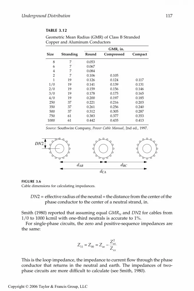
Underground Distribution 117
DN2 = effective radius of the neutral = the distance from the center of the phase conductor to the center of a neutral strand, in.
Smith (1980) reported that assuming equal GMRN and DN2 for cables from1/0 to 1000 kcmil with one-third neutrals is accurate to 1%.
For single-phase circuits, the zero and positive-sequence impedances arethe same:
This is the loop impedance, the impedance to current flow through the phaseconductor that returns in the neutral and earth. The impedances of two-phase circuits are more difficult to calculate (see Smith, 1980).
TABLE 3.12
Geometric Mean Radius (GMR) of Class B Stranded Copper and Aluminum Conductors
Size StrandingGMR, in.
Round Compressed Compact
8 7 0.0536 7 0.0674 7 0.0842 7 0.106 0.1051 19 0.126 0.124 0.117
1/0 19 0.141 0.139 0.1312/0 19 0.159 0.156 0.1463/0 19 0.178 0.175 0.1654/0 19 0.200 0.197 0.185250 37 0.221 0.216 0.203350 37 0.261 0.256 0.240500 37 0.312 0.305 0.287750 61 0.383 0.377 0.353
1000 61 0.442 0.435 0.413
Source: Southwire Company, Power Cable Manual, 2nd ed., 1997.
FIGURE 3.6Cable dimensions for calculating impedances.
dAB
DN2
dBC
dCA
Z Z ZZZaa
ax
xx11 00
2
= = −
9576_C03.fm Page 117 Monday, October 17, 2005 8:12 AM
Copyright © 2006 Taylor & Francis Group, LLC

118 Electric Power Distribution Equipment and Systems
The sheath resistances depend on whether it is a concentric neutral, a tapeshield, or some other configuration. For a concentric neutral, the resistanceis approximately (ignoring the lay of the neutral):
whereRstrand = resistance of one strand, in Ω/unit distance
n = number of strands
A tape shield’s resistance (Southwire Company, 1997) is
whereρc = resistivity of the tape shield, Ω-cmil/ft = 10.575 for uncoated copper
at 25°CAs = effective area of the shield in circular mil
As =
b = thickness of the tape, mildm = mean diameter outside of the metallic shield, milL = lap of the tape shield in percent (normally 10 to 25%)
Normally, we can use dc resistance as the ac resistance for tape shieldsor concentric neutrals. The skin effect is very small because the shieldconductors are thin (skin effect just impacts larger conductors). We shouldadjust the sheath resistance for temperature; for copper conductors, theadjustment is:
whereRt2 = resistance at temperature t2 given in °CRt1 = resistance at temperature t1 given in °C
These calculations are simplifications. More advanced models, normallyrequiring a computer, can accurately find each element in the full impedancematrix. For most load-flow calculations, this accuracy is not needed, thoughaccess to user-friendly computer models allows quicker results than calcu-
RR
nneutralstrand=
RAshield
c
s
=ρ
450
100b d
Lm⋅ ⋅−
R Rttt t2 1
2
1
234 5234 5
=++
.
.
9576_C03.fm Page 118 Monday, October 17, 2005 8:12 AM
Copyright © 2006 Taylor & Francis Group, LLC

Underground Distribution 119
lating the equations shown here. For evaluating switching transients andsome ampacity problems or configurations with several cables, we some-times need more sophisticated models [see Amateni (1980) or Dommel (1986)for analytical details].
In a cable, the neutral tightly couples with the phase. Phase current inducesneutral voltages that force circulating current in the neutrals. With balanced,positive-sequence current in the three phases and with symmetrical conduc-tors, the neutral current (Lewis and Allen, 1978; Smith and Barger, 1972) is
which is
Since DN2 and GMRN are almost equal, if RN is near zero, the neutral (orshield) current (IX1) almost equals the phase current (Ia). Higher neutralresistances actually reduce positive-sequence resistances.
Significant effects on positive and zero-sequence impedances include:
• Cable separation — Larger separations increase Z1; spacing doesnot affect Z0. Triplex cables have the lowest positive-sequenceimpedance.
• Conductor size — Larger conductors have much less resistance; reac-tance drops somewhat with increasing size.
• Neutral/shield resistance — Increasing the neutral resistance increasesthe reactive portion of the positive and zero-sequence impedances.Beyond a certain point, increasing neutral resistances decreases theresistive portion of Z1 and Z0.
• Other cables or ground wires — Adding another grounded wire nearbyhas similar impacts to lowering sheath resistances. Zero-sequenceresistance and reactance usually drop. Positive-sequence reactanceis likely to decrease, but positive-sequence resistance may increase.
Figure 3.7 and Figure 3.8 show the impact of the most significant variableson impedances for three-phase and single-phase circuits. None of the fol-lowing significantly impacts either the positive or zero-sequence imped-ances: insulation thickness, insulation type, depth of burial, and earthresistivity.
IZ ZZ Z
IXax ab
xx aba1 = −
−−
Ij
dDN
R jd
GMR
IX
ab
Nab
N
a1
10
10
0 05292
0 0529= −
+
. log
. log
9576_C03.fm Page 119 Monday, October 17, 2005 8:12 AM
Copyright © 2006 Taylor & Francis Group, LLC

120 Electric Power Distribution Equipment and Systems
FIGURE 3.7Effect of various parameters on the positive-sequence (top row) and zero-sequence impedances(bottom row) with a base case having 500-kcmil aluminum cables with 1/3 neutrals, 220-milinsulation, a horizontal configuration with 7.5 in. between cables, and ρ = 100 Ω-m.
FIGURE 3.8Resistance and reactance of a single-phase cable (R = R0 = R1 and X = X0 = X1) as the size of thecable and neutral varies with a base case having a 4/0 aluminum cable with a full neutral, 220-mil insulation, and ρ = 100 Ω-m.
5 10 15 200.00
0.05
0.10
Resistance
Reactance
5 10 15 200.0
0.1
0.2
0.3
0.4
0.5
200 400 600 800 1000
200 400 600 800 1000
0.0 0.5 1.0
0.0 0.5 1.0
Cable separation, inches
R0
and
X0,
Ω/1
000
feet
Phase wire kcmil Neutral or shield resistanceΩ/1000 feet
Cable separation, inches
R1
and
X1,
Ω/1
000
feet
Phase wire kcmil Neutral or shield resistanceΩ/1000 feet
Resistance
Reactance
200 400 600 800 10000.00
0.05
0.10
0.15
0.20
0.25
0.0 0.5 1.0
Phase wire kcmil
R a
nd X
, Ω/1
000
feet
Neutral or shield resistanceΩ/1000 feet
9576_C03.fm Page 120 Monday, October 17, 2005 8:12 AM
Copyright © 2006 Taylor & Francis Group, LLC

Underground Distribution 121
3.4.3 Impedance Tables
This section contains tables of several common cable configurations foundon distribution circuits. All values are for a multigrounded circuit. Manyother cable configurations are possible, with widely varying impedances.For PILC cables, refer to impedances in the Westinghouse (1950) T&D book.For additional three-phase power cable configurations, refer to the IEEE RedBook (IEEE Std. 141-1993), St. Pierre (2001), or Southwire Company (1997).
3.4.4 Capacitance
Cables have significant capacitance, much more than overhead lines. A sin-gle-conductor cable has a capacitance given by:
whereC = capacitance, µF/1000 ftε = dielectric constant (2.3 for XLPE, 3 for EPR, see Table 3.4 for others)d = inside diameter of the insulation, mil (or other distance unit)
D = outside diameter of the insulation in the same units as d
TABLE 3.13
Loop Impedances of Single-Phase Concentric-Neutral Aluminum Cables
ConductorSize
Full Neutral 1/3 NeutralNeutral R X Neutral R X
2 10#14 0.4608 0.18571 13#14 0.3932 0.1517
1/0 16#14 0.3342 0.1259 6#14 0.3154 0.22952/0 13#12 0.2793 0.0974 7#14 0.2784 0.21483/0 16#12 0.2342 0.0779 9#14 0.2537 0.18844/0 13#10 0.1931 0.0613 11#14 0.2305 0.1645250 16#10 0.1638 0.0493 13#14 0.2143 0.1444350 20#10 0.1245 0.0387 18#14 0.1818 0.1092500 16#12 0.1447 0.0726750 15#10 0.1067 0.0462
1000 20#10 0.0831 0.0343
Note: Impedances, Ω/1000 ft (× 5.28 for Ω/mi or × 3.28 for Ω/km). Con-ductor temperature = 90°C, neutral temperature = 80°C, 15-kV class,220-mil insulation, ρ = 100 Ω-m. For the neutral, 10#14 means 10strands of 14-gage wire.
CDd
=
0 00736
10
.
log
ε
9576_C03.fm Page 121 Monday, October 17, 2005 8:12 AM
Copyright © 2006 Taylor & Francis Group, LLC

122 Electric Power Distribution Equipment and Systems
The vars provided by cable are
whereQvar = var/1000 ft/phase
f = frequency, HzC = capacitance, µF/1000 ft
VLG,kV = line-to-ground voltage, kV
Table 3.17 shows capacitance values and reactive power produced bycables for typical cables. The table results are for XLPE cable with a dielectricconstant (ε) of 2.3. For other insulation, both the capacitance and the reactivepower scale linearly. For example, for EPR with ε = 3, multiply the valuesin Table 3.17 by 1.3 (3/2.3 = 1.3).
TABLE 3.14
Impedances of Three-Phase Circuits Made of Three Single-Conductor Concentric-Neutral Aluminum Cables
Conductor Size Neutral Size R1 X1 R0 X0 RS XS
Full Neutral
2 10#14 0.3478 0.1005 0.5899 0.1642 0.4285 0.12171 13#14 0.2820 0.0950 0.4814 0.1166 0.3484 0.1022
1/0 16#14 0.2297 0.0906 0.3956 0.0895 0.2850 0.09022/0 13#12 0.1891 0.0848 0.3158 0.0660 0.2314 0.07853/0 16#12 0.1578 0.0789 0.2573 0.0523 0.1910 0.07014/0 13#10 0.1331 0.0720 0.2066 0.0423 0.1576 0.0621250 16#10 0.1186 0.0651 0.1716 0.0356 0.1363 0.0553350 20#10 0.0930 0.0560 0.1287 0.0294 0.1049 0.0471
1/3 Neutral
1/0 6#14 0.2180 0.0959 0.5193 0.2854 0.3185 0.15912/0 7#14 0.1751 0.0930 0.4638 0.2415 0.2713 0.14253/0 9#14 0.1432 0.0896 0.4012 0.1787 0.2292 0.11934/0 11#14 0.1180 0.0861 0.3457 0.1375 0.1939 0.1032250 13#14 0.1034 0.0833 0.3045 0.1103 0.1704 0.0923350 18#14 0.0805 0.0774 0.2353 0.0740 0.1321 0.0762500 16#12 0.0656 0.0693 0.1689 0.0468 0.1000 0.0618750 15#10 0.0547 0.0584 0.1160 0.0312 0.0752 0.0494
1000 20#10 0.0478 0.0502 0.0876 0.0248 0.0611 0.0417
Note: Impedances, Ω/1000 ft (× 5.28 for Ω/mi or × 3.28 for Ω/km). Resistances for aconductor temperature = 90°C and a neutral temperature = 80°C, 220-mil insulation(15 kV), ρ = 100 Ω-m. Flat spacing with a 7.5-in. separation between cables. For theneutral, 10#14 means 10 strands of 14-gage wire.
Q f C Vvar LG kV= ⋅ ⋅ ⋅2 2π ,
9576_C03.fm Page 122 Monday, October 17, 2005 8:12 AM
Copyright © 2006 Taylor & Francis Group, LLC

Underground Distribution 123
3.5 Ampacity
A cable’s ampacity is the maximum continuous current rating of the cable.We should realize that while we may derive one number, say 480 A, forampacity during normal operations for a given conductor, there is nothingmagic about 480 A. The cable will not burst into flames at 481 A; the 480 Ais simply a design number. We don’t want to exceed that current duringnormal operations.
The insulation temperature is normally the limiting factor. By operatingbelow the ampacity of a given cable, we keep the cable insulation below its
TABLE 3.15
Impedances of Single-Conductor Aluminum Power Cables with Copper Tape Shields
Conductor Size R1 X1 R0 X0 RS XS
Flat spacing with a 7.5-in. separation
2 0.3399 0.1029 0.6484 0.4088 0.4427 0.20491 0.2710 0.0990 0.5808 0.3931 0.3743 0.1971
1/0 0.2161 0.0964 0.5268 0.3790 0.3196 0.19062/0 0.1721 0.0937 0.4833 0.3653 0.2759 0.18423/0 0.1382 0.0911 0.4494 0.3493 0.2419 0.17714/0 0.1113 0.0883 0.4217 0.3314 0.2148 0.1693250 0.0955 0.0861 0.4037 0.3103 0.1982 0.1609350 0.0696 0.0822 0.3734 0.2827 0.1709 0.1490500 0.0508 0.0781 0.3483 0.2557 0.1499 0.1373750 0.0369 0.0732 0.3220 0.2185 0.1319 0.1216
1000 0.0290 0.0698 0.3018 0.1915 0.1200 0.1104
Triplex
2 0.3345 0.0531 0.7027 0.4244 0.4573 0.17691 0.2655 0.0501 0.6330 0.4060 0.3880 0.1687
1/0 0.2105 0.0483 0.5767 0.3893 0.3326 0.16202/0 0.1666 0.0465 0.5310 0.3734 0.2880 0.15543/0 0.1326 0.0448 0.4944 0.3550 0.2532 0.14824/0 0.1056 0.0432 0.4636 0.3346 0.2249 0.1403250 0.0896 0.0424 0.4418 0.3109 0.2070 0.1319350 0.0637 0.0403 0.4067 0.2807 0.1780 0.1204500 0.0447 0.0381 0.3769 0.2518 0.1554 0.1093750 0.0308 0.0359 0.3443 0.2129 0.1353 0.0949
1000 0.0228 0.0348 0.3197 0.1853 0.1218 0.0850
Note: Impedances, Ω/1000 ft (× 5.28 for Ω/mi or × 3.28 for Ω/km). Resis-tances for a conductor temperature = 90°C and a shield temperature= 50°C, 220-mil insulation (15 kV), ρ = 100 Ω-m, 5-mil copper tapeshield with a lap of 20%.
9576_C03.fm Page 123 Monday, October 17, 2005 8:12 AM
Copyright © 2006 Taylor & Francis Group, LLC

124 Electric Power Distribution Equipment and Systems
TABLE 3.16
Impedances of Single-Conductor Copper Power Cables
Conductor Size R1 X1 R0 X0 RS XS
Flat spacing with a 7.5-in. separation
2 0.2083 0.1029 0.5108 0.4401 0.3092 0.21531 0.1671 0.0991 0.4718 0.4267 0.2687 0.2083
1/0 0.1334 0.0965 0.4405 0.4115 0.2358 0.20152/0 0.1082 0.0938 0.4171 0.3967 0.2112 0.19483/0 0.0871 0.0911 0.3975 0.3794 0.1906 0.18724/0 0.0705 0.0884 0.3816 0.3626 0.1742 0.1798250 0.0607 0.0862 0.3719 0.3471 0.1644 0.1732350 0.0461 0.0823 0.3558 0.3181 0.1493 0.1609500 0.0352 0.0782 0.3411 0.2891 0.1372 0.1485750 0.0272 0.0732 0.3241 0.2490 0.1261 0.1318
1000 0.0234 0.0699 0.3104 0.2196 0.1191 0.1198
Triplex
2 0.2032 0.0508 0.5707 0.4642 0.3257 0.18861 0.1619 0.0477 0.5301 0.4480 0.2846 0.1811
1/0 0.1281 0.0460 0.4966 0.4295 0.2509 0.17382/0 0.1028 0.0442 0.4709 0.4116 0.2255 0.16673/0 0.0816 0.0426 0.4485 0.3910 0.2039 0.15874/0 0.0649 0.0409 0.4299 0.3713 0.1866 0.1510250 0.0551 0.0398 0.4175 0.3532 0.1759 0.1442350 0.0403 0.0377 0.3962 0.3202 0.1589 0.1319500 0.0292 0.0355 0.3765 0.2882 0.1450 0.1197750 0.0211 0.0333 0.3524 0.2450 0.1315 0.1039
1000 0.0173 0.0322 0.3336 0.2142 0.1227 0.0929
Note: Impedances, Ω/1000 ft (× 5.28 for Ω/mi or × 3.28 for Ω/km). Resis-tances for a conductor temperature = 90°C and a shield temperature= 50°C, 220-mil insulation (15 kV), ρ = 100 Ω-m, 5-mil copper tapeshield with a lap of 20%.
TABLE 3.17
Cable Capacitance for Common Cable Sizes and Voltages
Size
Capacitance, µF/1000 ft Reactive power, kvar/1000 ft
175 mil 220 mil 260 mil 345 mil12.5 kV175 mil
12.5 kV220 mil
25 kV260 mil
34.5 kV345 mil
2 0.0516 0.0441 0.0396 0.0333 1.01 0.862 3.09 4.981 0.0562 0.0479 0.0428 0.0358 1.1 0.936 3.35 5.35
1/0 0.0609 0.0516 0.046 0.0383 1.19 1.01 3.6 5.722/0 0.0655 0.0553 0.0492 0.0407 1.28 1.08 3.84 6.093/0 0.0712 0.0599 0.0531 0.0437 1.39 1.17 4.15 6.544/0 0.078 0.0654 0.0578 0.0473 1.52 1.28 4.52 7.08250 0.0871 0.0727 0.064 0.0521 1.7 1.42 5.00 7.79350 0.0995 0.0826 0.0725 0.0586 1.94 1.61 5.67 8.76500 0.113 0.0934 0.0817 0.0656 2.21 1.83 6.38 9.81750 0.135 0.111 0.0969 0.0772 2.65 2.18 7.57 11.5
1000 0.156 0.127 0.111 0.0875 3.04 2.49 8.64 13.1
Note: For XLPE cable with ε = 2.3.
9576_C03.fm Page 124 Monday, October 17, 2005 8:12 AM
Copyright © 2006 Taylor & Francis Group, LLC
Underground Distribution 125
recommended maximum temperature. Cross-linked polyethylene cables arerated for a maximum operating temperature of 90°C during normal opera-tions. Operating cables above their ampacity increases the likelihood ofpremature failures: water trees may grow faster, thermal runaway-failuresare more likely, and insulation strength may decrease. In addition to absolutetemperature, thermal cycling also ages cable more quickly.
Ampacity most often limits the loading on a cable; rarely, voltage drop orflicker limits loadings. Relative to overhead lines, cables of a given size havelower impedance and lower ampacities. So cable circuits are much less likelythan overhead circuits to be voltage-drop limited. Only very long cable runson circuits with low primary voltages are voltage-drop limited. Ampacity isnot the only consideration for cable selection; losses and stocking consider-ations should also factor into cable selection. Choosing the smallest cablethat meets ampacity requirements has the lowest initial cost, but since thecable is running hotter, the cost over its life may not be optimal because ofthe losses. Also allow for load growth when selecting cables.
Ampacity calculations follow simple principles: the temperature at theconductor is a function of the heat generated in a cable (I2R) and the amountof heat conducted away from the cable. We can model the thermal perfor-mance with a thermal circuit analogous to an electric circuit: heat is analo-gous to current; temperature to voltage; and thermal resistance to electricalresistance. Heat flow through a thermal resistance raises the temperaturebetween the two sides of the thermal material. Higher resistance soils orinsulations trap the heat and cause higher temperatures. Using the thermalequivalent of Ohm’s law, the temperature difference is:
whereTC = conductor temperature, °CTA = ambient earth temperature, °C
RTH = total thermal resistance between the cable conductor and the air, thermal Ω-ft
H = heat generated in the cable, W ( = I2R)I = electric current in the conductor, A
R = electric resistance of the conductor, Ω/ft
Most ampacity tables and computer calculation routines are based on theclassic paper by Neher and McGrath (1957). The original paper is an excellentreference. Ander’s book (1998) provides a detailed discussion of cableampacity calculations, including the Neher–McGrath method along withIEC’s method that is very similar (IEC 287, 1982). Hand calculations orspreadsheet calculations of the Neher–McGrath equations are possible, buttiresome; while straightforward in principle, the calculations are verydetailed. A review of the Neher–McGrath procedure — the inputs, the tech-
∆T T T R H R I RC A TH TH= − = = ( )2
9576_C03.fm Page 125 Monday, October 17, 2005 8:12 AM
Copyright © 2006 Taylor & Francis Group, LLC
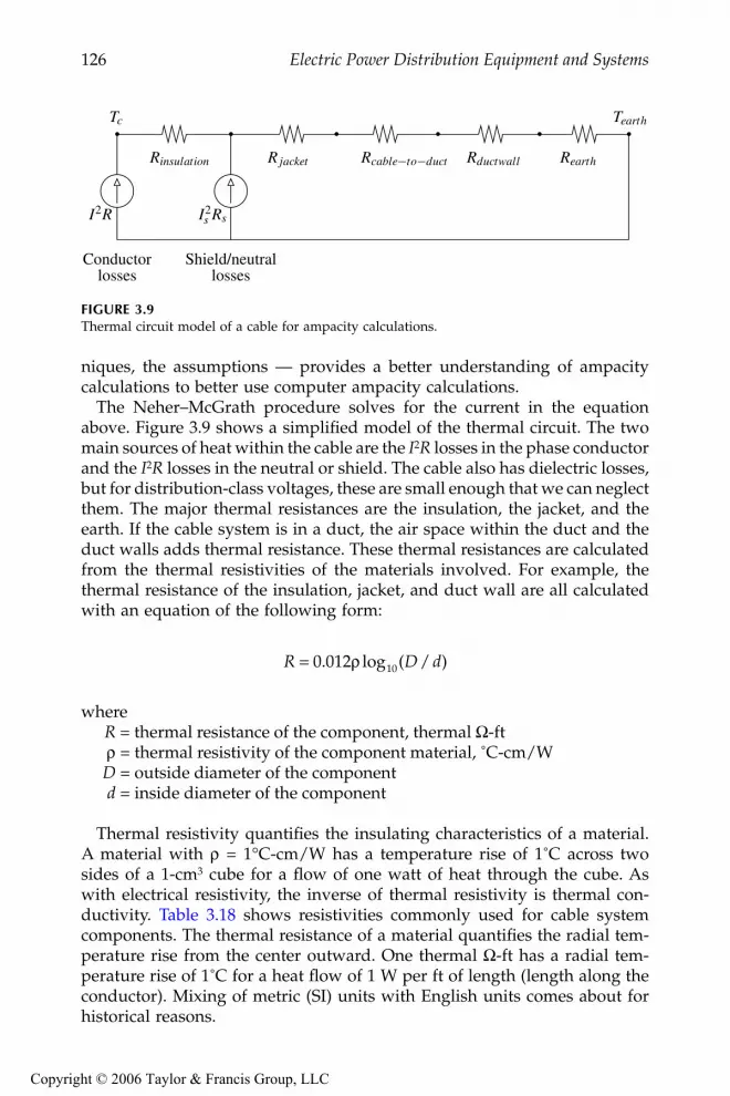
126 Electric Power Distribution Equipment and Systems
niques, the assumptions — provides a better understanding of ampacitycalculations to better use computer ampacity calculations.
The Neher–McGrath procedure solves for the current in the equationabove. Figure 3.9 shows a simplified model of the thermal circuit. The twomain sources of heat within the cable are the I2R losses in the phase conductorand the I2R losses in the neutral or shield. The cable also has dielectric losses,but for distribution-class voltages, these are small enough that we can neglectthem. The major thermal resistances are the insulation, the jacket, and theearth. If the cable system is in a duct, the air space within the duct and theduct walls adds thermal resistance. These thermal resistances are calculatedfrom the thermal resistivities of the materials involved. For example, thethermal resistance of the insulation, jacket, and duct wall are all calculatedwith an equation of the following form:
whereR = thermal resistance of the component, thermal Ω-ftρ = thermal resistivity of the component material, ˚C-cm/WD = outside diameter of the componentd = inside diameter of the component
Thermal resistivity quantifies the insulating characteristics of a material.A material with ρ = 1°C-cm/W has a temperature rise of 1˚C across twosides of a 1-cm3 cube for a flow of one watt of heat through the cube. Aswith electrical resistivity, the inverse of thermal resistivity is thermal con-ductivity. Table 3.18 shows resistivities commonly used for cable systemcomponents. The thermal resistance of a material quantifies the radial tem-perature rise from the center outward. One thermal Ω-ft has a radial tem-perature rise of 1˚C for a heat flow of 1 W per ft of length (length along theconductor). Mixing of metric (SI) units with English units comes about forhistorical reasons.
FIGURE 3.9Thermal circuit model of a cable for ampacity calculations.
Conductorlosses
Shield/neutrallosses
Tc Tearth
Rinsulation R jacket Rcable to duct Rductwall Rearth
I2R I2s Rs
R D d= 0 012 10. log ( / )ρ
9576_C03.fm Page 126 Monday, October 17, 2005 8:12 AM
Copyright © 2006 Taylor & Francis Group, LLC

Underground Distribution 127
The Neher–McGrath calculations also account for multiple cables, cableswith cyclic daily load cycles, external heat sources, duct arrangements, andshield resistance and grounding variations.
Often, the easiest way to find ampacities for a given application is withampacity tables. Table 3.19 and Table 3.20 show ampacities for commondistribution configurations. Of the many sources of ampacity tables, the IEEEpublishes the most exhaustive set of tables (IEEE Std. 835-1994). The NationalElectrical Code (NFPA 70, 1999) and manufacturer’s publications (Okonite,1990; Southwire Company, 1997) are also useful. Ampacity tables provide a
TABLE 3.18
Thermal Resistivities of Common Components
ComponentThermal Resistivity,
°°°°C-cm/W
XLPE insulation 350EPR insulation 500Paper insulation 700PE jackets 350PVC jackets 500Plastic ducts 480Concrete 85Thermal fill 60Soil 90Water 160Air 4000
Sources: IEC 287, Calculation of the Continuous CurrentRating of Cables (100% Load Factor), 2nd ed., Interna-tional Electrical Commission (IEC), 1982; Neher, J. H.and McGrath, M. H., “The Calculation of the Temper-ature Rise and Load Capability of Cable Systems,”AIEE Transactions, vol. 76, pp. 752–64, October 1957.
TABLE 3.19
Ampacities of Single-Phase Circuits of Full-Neutral Aluminum Conductor Cables
Size
Direct BuriedLoad Factor
In ConduitLoad Factor
100% 75% 100% 75%
2 187 201 146 1531 209 225 162 170
1/0 233 252 180 1882/0 260 282 200 2103/0 290 316 223 2344/0 325 356 249 262250 359 395 276 291350 424 469 326 345
Note: 90˚C conductor temperature, 25˚C ambi-ent earth temperature, ρ = 90°C-cm/W.
9576_C03.fm Page 127 Monday, October 17, 2005 8:12 AM
Copyright © 2006 Taylor & Francis Group, LLC

128 Electric Power Distribution Equipment and Systems
good starting point for determining the ampacity of a specific cable appli-cation. When using tables, be careful that the assumptions match your par-ticular situation; if not, ampacity results can be much different than expected.
Conductor temperature limits, sheath resistance, thermal resistivity of thesoil — these are some of the variables that most impact ampacity (see Figure3.10). These and other effects are discussed in the next few paragraphs [seealso (CEA, 1982; NRECA RER Project 90-8, 1993) for more discussions].
Sheath resistance — On a three-phase circuit, the resistance of the sheath(or shield or neutral) plays an important role in ampacity calculations.Because a cable’s phase conductor and sheath couple so tightly, currentthrough the phase induces a large voltage along the sheath. With the cablesheath grounded periodically, circulating current flows to counter theinduced voltage. The circulating current is a function of the resistance of thesheath. This circulating current leads to something counterintuitive: sheathswith higher resistance have more ampacity. Higher resistance sheaths reducethe circulating current and reduce the I2R losses in the sheath. This effect is
TABLE 3.20
Ampacities of Three-Phase Circuits Made of Single-Conductor, One-Third Neutral Aluminum Cables
Size
Direct BuriedLoad factor
In ConduitLoad factor
100% 75% 100% 75%
Flat spacing (7.5-in. separation)
1/0 216 244 183 1992/0 244 277 207 2263/0 274 312 233 2554/0 308 352 262 287250 336 386 285 315350 392 455 334 370500 448 525 382 426750 508 601 435 489
1000 556 664 478 541
Triplex
1/0 193 224 158 1732/0 220 255 180 1973/0 249 290 204 2254/0 283 330 232 256250 312 365 257 284350 375 442 310 345500 452 535 375 419750 547 653 457 514
1000 630 756 529 598
Note: 90˚C conductor temperature, 25˚C ambi-ent earth temperature, ρ = 90°C-cm/W.
9576_C03.fm Page 128 Monday, October 17, 2005 8:12 AM
Copyright © 2006 Taylor & Francis Group, LLC

Underground Distribution 129
most pronounced in larger conductors. Many ampacity tables assume thatcable sheaths are open circuited, this eliminates the sheath losses andincreases the ampacity. The open-circuit sheath values can be approximatelycorrected to account for circulating currents (Okonite, 1990) by
FIGURE 3.10Effect of variables on ampacity for an example cable.
Am
paci
ty, a
mpe
res
0.5 0.7 0.9
300
400
500
Loss factor2 4 6 8 10
Shield resistance in multiples of phase resistance
Spacing, inches5 10 15 20
80 100 120 140
300
400
500
Conductor temp.°C
Am
paci
ty, a
mpe
res
Soil temp.°C
15 20 25 30 50 100 150 200Earth thermal resistivity
°C-cm W
500 kcmil aluminum, 15-kV, 220-mil insulation1/3 neutral, direct buried, jacketed, load factor = 1ρearth = 90C-cm/W, ρinsulation = ρ jacket = 400C-cm/WTc = 90C, Tearth = 25C 7.5 in
36 in
kI R
I R I RS S
=+
2
2 2
9576_C03.fm Page 129 Monday, October 17, 2005 8:12 AM
Copyright © 2006 Taylor & Francis Group, LLC

130 Electric Power Distribution Equipment and Systems
wherek = ampacity multiplier to account for sheath losses, i.e., Igrounded sheath =
k · Iopen sheath
I = phase conductor current, AIS = sheath current, A
I2R = phase conductor losses, W/unit of lengthIS
2RS = sheath losses, W/unit of length
The sheath losses are a function of the resistance of the sheath and themutual inductance between the sheath and other conductors. For a triangularconfiguration like triplex, the shield losses are
where
andXM = mutual inductance of the sheath and another conductor, mΩ/1000 ftRS = resistance of the sheath, mΩ/1000 ft
f = frequency, HzS = spacing between the phase conductors, in.
dS = mean diameter of the sheath, in.
For configurations other than triplex, see Southwire Company (1997) orOkonite (1990). Figure 3.11 shows how sheath losses vary with conductorsize and with spacing. Spacing has a pronounced effect. Steel ducts cansignificantly increase heating from circulating currents. In fact, even nearbysteel pipes can significantly reduce ampacity.
Spacings — Separating cables separates the heat sources. But at largerspacings, circulating currents are higher. Optimal spacings involve balancingthese effects. For smaller cables, separating cables provides the best ampacity.For larger cables (with larger circulating currents), triplex or other tightspacing improves ampacity. For one-third neutral, aluminum cables, NRECA(1993) shows that a flat spacing with 7.5 in. between cables has better ampac-ity than triplex for conductors 500 kcmil and smaller. For copper cables, thethreshold is lower: conductors larger than 4/0 have better ampacity with atriplex configuration.
Conductor temperature — If we allow a higher conductor temperature, wecan operate a cable at higher current. If we know the ampacity for a givenconductor temperature, at a different conductor temperature we can find theampacity with the following approximation:
I R I RX
R XS S SM
S M
2 22
2 2=+
X f S dM S= 2 0 1404 210π ( . ) log ( / )
9576_C03.fm Page 130 Monday, October 17, 2005 8:12 AM
Copyright © 2006 Taylor & Francis Group, LLC

Underground Distribution 131
whereI' = ampacity at a conductor temperature of TC′ and an ambient earth tem-
perature TA′I = ampacity at a conductor temperature of TC and an ambient earth tem-
perature TA (all temperatures are in °C)
We can use these equations to find emergency ampacity ratings of cables.In an emergency, XLPE can be operated to 130°C. Some EPR cables can beoperated to 140°C (MV-105 cables). ICEA standards allow emergency over-load for 100 hours per year with five such periods over the life of the cable.Polyethylene cables, including HMWPE, have little overload capability.Their maximum recommended emergency temperature is 95°C. Table 3.21shows common ampacity multipliers; these are valid for both copper andaluminum conductors within the accuracy shown. We can also use the
FIGURE 3.11Shield losses as a function of shield resistance for aluminum cables (triplex configuration).
2 4 6 8
020
4060
8010
0
A
B
CD
EF
ABCDEF
::::::
1000 kcmil750 kcmil500 kcmil350 kcmil250 kcmil1/0
Shield resistance in multiples of phase resistance
Shie
ld lo
sses
in p
erce
nt o
f ph
ase
loss
estriplex spacing
2 4 6 8
020
4060
8010
0 A
B
C
D
E
F
Shield resistance in multiples of phase resistance
7.5-inch spacing
2 4 6 8
′ =′ − ′
−++ ′
′ =′ − ′
−++ ′
I IT TT T
TT
I IT TT T
TT
C A
C A
C
C
C A
C A
C
C
228 1228 1
234 5234 5
.
.
.
.(
(Aluminum conductor)
Copper conductor)
9576_C03.fm Page 131 Monday, October 17, 2005 8:12 AM
Copyright © 2006 Taylor & Francis Group, LLC

132 Electric Power Distribution Equipment and Systems
appropriate temperature-adjustment equation to adjust for different ambientearth temperatures.
Loss factor — The earth has a high thermal storage capability; it takesconsiderable time to heat (or cool) the soil surrounding the cable. Close tothe cable, the peak heat generated in the cable determines the temperaturedrop; farther out, the average heat generated in the cable determines thetemperature drop. As discussed in Chapter 5, we normally account forlosses using the loss factor, which is the average losses divided by the peaklosses. Since this number is not normally available, we find the loss factorfrom the load factor (the load factor is the average load divided by the peakload). Assuming a 100% load factor (continuous current) is most conserva-tive but can lead to a cable that is larger than necessary. We should try toerr on the high side when estimating the load factor. A 75% load factor iscommonly used.
Conduits — The air space in conduits or ducts significantly reduces ampac-ity. The air insulation barrier traps more heat in the cable. Direct-buriedcables may have 10 to 25% higher ampacities. Although the less air the better,there is little practical difference in the thermal performance between thesizes of ducts commonly used. Concrete duct banks have roughly the samethermal performance as direct-buried conduits (concrete is more consistentand less prone to moisture fluctuations).
Soil thermal resistivity and temperature — Soils with lower thermal resistivitymore readily conduct heat away from cables. Moisture is an importantcomponent, moist soil has lower thermal resistivity (see Figure 3.12). Densesoil normally has better conductivity. More so than any other single factor,soil resistivity impacts the conductor’s temperature and the cable’s ampac-ity. A resistivity of 90°C-cm/W is often assumed for ampacity calculations.This number is conservative enough for many areas, but if soil resistivitiesare higher, cable temperatures can be much higher than expected. For com-mon soils, Table 3.22 shows typical ranges of thermal resistivities. At typicalinstallation depths, resistivity varies significantly with season as moisturecontent changes. Unfortunately in many locations, just when we needampacity the most — during peak load in the summer — the soil is closeto its hottest and driest. Seasonal changes can be significant, but daily
TABLE 3.21
Common Ampacity Rating Conversions (with TA = 25°°°°C)
Original Temperature,°C
New Temperature,°C Ampacity Multiplier
75 95 1.1590 75 0.9090 105 1.0890 130 1.20
105 140 1.14
9576_C03.fm Page 132 Monday, October 17, 2005 8:12 AM
Copyright © 2006 Taylor & Francis Group, LLC

Underground Distribution 133
changes are not; soil temperature changes lag air temperature changes by 2to 4 weeks.
The depth of burial can affect ampacity. With a constant resistivity andsoil temperature, deeper burial decreases ampacity. But deeper, the soil tendsto have lower temperature, more moisture, and soil is more stable seasonally.To go deep enough to take advantage of this is not cost effective though.
For areas with poor soil (high clay content in a dry area, for example),one of several thermal backfills can give good performance, with stable
FIGURE 3.12Effect of moisture on the thermal resistivity of various soils. (Copyright © 1997. Electric PowerResearch Institute. TR-108919. Soil Thermal Properties Manual for Underground Power Transmission.Reprinted with permission.)
0
50
100
150
200
250
300
350
400
0 5 10 15 20 25 30Moisture Content (% by dry weight)
Th
erm
al R
esis
tivi
ty (o
C-c
m/W
)
Soft Organic Clay
Clay
Silt
Silty Sand with Gravel
Uniform Sand
Stone Screenings
FTB
9576_C03.fm Page 133 Monday, October 17, 2005 8:12 AM
Copyright © 2006 Taylor & Francis Group, LLC
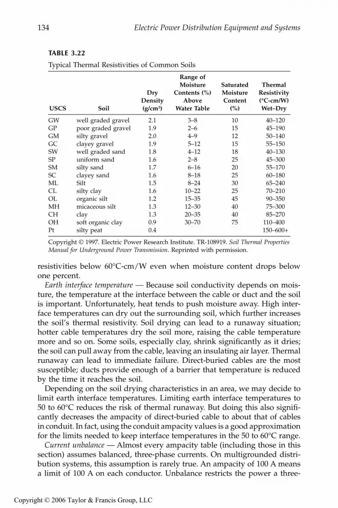
134 Electric Power Distribution Equipment and Systems
resistivities below 60°C-cm/W even when moisture content drops belowone percent.
Earth interface temperature — Because soil conductivity depends on mois-ture, the temperature at the interface between the cable or duct and the soilis important. Unfortunately, heat tends to push moisture away. High inter-face temperatures can dry out the surrounding soil, which further increasesthe soil’s thermal resistivity. Soil drying can lead to a runaway situation;hotter cable temperatures dry the soil more, raising the cable temperaturemore and so on. Some soils, especially clay, shrink significantly as it dries;the soil can pull away from the cable, leaving an insulating air layer. Thermalrunaway can lead to immediate failure. Direct-buried cables are the mostsusceptible; ducts provide enough of a barrier that temperature is reducedby the time it reaches the soil.
Depending on the soil drying characteristics in an area, we may decide tolimit earth interface temperatures. Limiting earth interface temperatures to50 to 60°C reduces the risk of thermal runaway. But doing this also signifi-cantly decreases the ampacity of direct-buried cable to about that of cablesin conduit. In fact, using the conduit ampacity values is a good approximationfor the limits needed to keep interface temperatures in the 50 to 60°C range.
Current unbalance — Almost every ampacity table (including those in thissection) assumes balanced, three-phase currents. On multigrounded distri-bution systems, this assumption is rarely true. An ampacity of 100 A meansa limit of 100 A on each conductor. Unbalance restricts the power a three-
TABLE 3.22
Typical Thermal Resistivities of Common Soils
USCS Soil
DryDensity(g/cm3)
Range ofMoisture
Contents (%)Above
Water Table
SaturatedMoistureContent
(%)
ThermalResistivity(°C-cm/W)Wet–Dry
GW well graded gravel 2.1 3–8 10 40–120GP poor graded gravel 1.9 2–6 15 45–190GM silty gravel 2.0 4–9 12 50–140GC clayey gravel 1.9 5–12 15 55–150SW well graded sand 1.8 4–12 18 40–130SP uniform sand 1.6 2–8 25 45–300SM silty sand 1.7 6–16 20 55–170SC clayey sand 1.6 8–18 25 60–180ML Silt 1.5 8–24 30 65–240CL silty clay 1.6 10–22 25 70–210OL organic silt 1.2 15–35 45 90–350MH micaceous silt 1.3 12–30 40 75–300CH clay 1.3 20–35 40 85–270OH soft organic clay 0.9 30–70 75 110–400Pt silty peat 0.4 150–600+
Copyright © 1997. Electric Power Research Institute. TR-108919. Soil Thermal PropertiesManual for Underground Power Transmission. Reprinted with permission.
9576_C03.fm Page 134 Monday, October 17, 2005 8:12 AM
Copyright © 2006 Taylor & Francis Group, LLC

Underground Distribution 135
phase cable circuit can carry (IA = IB = IC = 100 A carries more power thanIA = 100 A, IB = IC = 70 A). In addition, the unbalanced return current mayincrease the heating in the cable carrying the highest current. It may or itmay not; it depends on phase relationships and the phase angle of theunbalanced current. If the unbalances are just right, the unbalanced returncurrent can significantly increase the neutral current on the most heavilyloaded phases. Unbalance also depends on the placement of the cables. Ina flat configuration, the middle cable is the most limiting because the outertwo cables heat the middle cable.
Just as higher sheath resistances reduce circulating currents, higher sheathresistances reduce unbalance currents in the sheath. Higher sheath resis-tances force more of the unbalanced current to return in the earth. The heatgenerated in the sheath from unbalance current also decreases with increas-ing sheath resistance (except for very low sheath resistances, where thesheath has less resistance than the phase conductor).
System voltage and insulation thickness — Neither significantly impacts theampacity of distribution cables. Ampacity stays constant with voltage; 5-kVcables have roughly the same ampacity as 35-kV cables. At higher voltages,insulation is thicker, but this rise in the thermal resistance of the insulationreduces the ampacity just slightly. Higher operating voltages also causehigher dielectric losses, but again, the effect is small (it is more noticeablewith EPR cable).
Number of cables — Cables in parallel heat each other, which restricts ampac-ity. Figure 3.13 shows an example for triplex power cables in duct banks.
Cable crossings and other hotspots — Tests have found that cable crossingscan produce significant hotspots (Koch, 2001). Other hotspots can occur inlocations where cables are paralleled for a short distance like taps to pad-mounted transformers or other gear. Differences in surface covering (suchas asphalt roads) can also produce hot spots. Anders and Brakelmann (1999a,1999b) provide an extension to the Neher–McGrath model that includes theeffects of cable crossings at different angles. They conclude: “the derating of
FIGURE 3.13Ampacity reduction with multiple cable circuits in a duct bank (15 kV, aluminum, 500 kcmil,tape shield power cables, triplex configuration).
2 4 6 8
7080
9010
0
Number of circuits
Am
paci
ty, p
erce
nt
2 4 6 8
7080
9010
0
9576_C03.fm Page 135 Monday, October 17, 2005 8:12 AM
Copyright © 2006 Taylor & Francis Group, LLC

136 Electric Power Distribution Equipment and Systems
3 to 5% used by some utilities may be insufficient, especially for cables withsmaller conductors.”
Riser poles — Cables on a riser pole require special attention. The protectivevertical conduit traps air, and the sun adds external heating. Hartlein andBlack (1983) tested a specific riser configuration and developed an analyticalmodel. They concluded that the size of the riser and the amount of ventingwere important. Large diameter risers vented at both ends are the best. Withthree cables in one riser, they found that the riser portion of the circuit limitsthe ampacity. This is especially important in substation exit cables and theirriser poles. In a riser pole application, ampacity does not increase for lowerload factors; a cable heats up much faster in the air than when buried in theground (the air has little thermal storage). NRECA (1993) concluded thatproperly vented risers do not need to be derated, given that venting canincrease ampacity between 10 and 25%. If risers are not vented, then theriser becomes the limiting factor. Additional work in this area has been doneby Cress (1991) (tests and modeling for submarine cables in riser poles) andAnders (1996) (an updated analytical model).
3.6 Fault Withstand Capability
Short-circuit currents through a conductor’s resistance generates tremen-dous heat. All cable between the source and the fault is subjected to the samephase current. For cables, the weakest link is the insulation; both XLPE andEPR have a short-duration upper temperature limit of 250°C. The short-circuit current injects energy as a function of the fault duration multipliedby the square of the current.
For aluminum conductors and XLPE or EPR insulation, the maximumallowable time-current characteristic is given by
whereI = fault current, At = fault duration, sec
A = cross-sectional area of the conductor, kcmil
This assumes an upper temperature limit of 250°C and a 90°C startingtemperature. For copper, the upper limit is defined by
I t A2 248 4= ( ).
I t A2 272 2= ( ).
9576_C03.fm Page 136 Monday, October 17, 2005 8:12 AM
Copyright © 2006 Taylor & Francis Group, LLC

Underground Distribution 137
We can plot these curves along with the time-current characteristics of theprotecting relay, fuse, or recloser to ensure that the protective devices protectour cables.
Damage to the shield or the neutral is more likely than damage to thephase conductor. During a ground fault, the sheath may conduct almost asmuch current as the phase conductor, and the sheath is normally smaller.With a one-third neutral, the cable neutral’s I2t withstand is approximately2.5 times less than the values for the phase conductor indicated in Figure3.14 (this assumes a 65°C starting temperature). Having more resistance, atape shield is even more vulnerable. A tape shield has a limiting time-currentcharacteristic of
where z is 79.1 for sheaths of copper, 58.2 for bronze, 39.2 for zinc, 23.7 forcopper-nickel, and 15 for lead [with a 65°C starting temperature and an
FIGURE 3.14Short-circuit limit of cables with EPR or XLPE insulation.
2
1/0
2/0
3/0
4/0
250
350
500
750
1000
1.0 10.00.01
0.1
1.0
10.0
100.0
1000.
2
1/0
2/0
3/0
4/0
250
350
500
750
1000
1.0 10.0
Current, kA
Tim
e, s
Aluminumconductor
Current, kA
Copperconductor
I t z A2 2= ⋅( )
9576_C03.fm Page 137 Monday, October 17, 2005 8:12 AM
Copyright © 2006 Taylor & Francis Group, LLC

138 Electric Power Distribution Equipment and Systems
upper limit of 250°C; using data from (Kerite Company)]. Figure 3.15 showswithstand characteristics for a 5-mil copper tape shield. The characteristicchanges with cable size because larger diameter cables have a shield with alarger circumference and more cross-sectional area. If a given fault currentlasts longer than five times the insulation withstand characteristic (at 250°C),the shield reaches its melting point.
In the vicinity of the fault, the fault current can cause considerably moredamage to the shield or neutral. With a concentric neutral, the fault currentmay only flow on a few strands of the conductor until the cable has agrounding point where the strands are tied together. Excessive temperaturescan damage the insulation shield, the insulation, and the jacket. In addition,the temperature may reach levels that melt the neutral strands. A tape shieldcan suffer similar effects: where tape layers overlap, oxidation can build upbetween tape layers, which insulate the layers from each other. This canrestrict the fault current to a smaller portion of the shield. Additionally, wherethe fault arc attaches, the arc injects considerable heat into the shield orneutral, causing further damage at the failure point. Some additional damageat the fault location must be tolerated, but the arc can burn one or moreneutral strands several feet back toward the source.
Martin et al. (1974) reported that longitudinally corrugated sheaths per-form better than wire or tape shields for high fault currents. They alsoreported that a semiconducting jacket helped spread the fault current to thesheaths of other cables (the semiconducting material breaks down).
Pay special attention to substation exit cables in areas with high faultcurrents (especially since exit cables are critical for circuit reliability). During
FIGURE 3.15Short-circuit insulation limit of copper tape shields based on outside diameter (starting tem-perature is 65°C, final temperature is 250°C, 20% lap on the shield).
0.51
1.5
2
2.5
3
Outsidediameterof the shieldin inches
1.0 10.00.01
0.1
1.0
10.0
Current, kA
Tim
e, s
9576_C03.fm Page 138 Monday, October 17, 2005 8:12 AM
Copyright © 2006 Taylor & Francis Group, LLC

Underground Distribution 139
a close fault, where currents are high, a reduced neutral or tape shield ismost prone to damage.
3.7 Cable Reliability
3.7.1 Water Trees
The most common failure cause of solid-dielectric cables has been watertreeing. Water trees develop over a period of many years and accelerate thefailure of solid dielectric cables. Excessive treeing has led to the prematurefailure of many polyethylene cables. Cable insulation can tree two ways:
• Electrical trees — These hollow tubes develop from high electricalstress; this stress creates partial discharges that eat away at theinsulation. Once initiated, electrical trees can grow fast, failing cablewithin hours or days.
• Water trees — Water trees are small discrete voids separated byinsulation. Water trees develop slowly, growing over a period ofmonths or years. Much less electrical stress is needed to cause watertrees. Water trees actually look more like fans, blooms, or busheswhereas electrical trees look more like jagged branched trees. As itsname indicates, water trees need moisture to grow; water that entersthe dielectric accumulates in specific areas (noncrystalline regions)and causes localized degradation. Voids, contaminants, temperature,and voltage stress — all influence the rate of growth.
The formation of water trees does not necessarily mean the cable will fail.A water tree can even bridge the entire dielectric without immediate failure.Failure occurs when a water tree converts to an electrical tree. One explana-tion of the initiation of electrical trees is from charges trapped in the cableinsulation. In Thue’s words (1999), “they can literally bore a tunnel from onevoid or contaminant to the next.” Impulses and dc voltage (in a hi-pot test)can trigger electrical treeing in a cable that is heavily water treed.
The growth rate of water trees tends to reduce with time; as trees fan out,the electrical stress on the tree reduces. Trees that grow from contaminantsnear the boundary of the conductor shield are most likely to keep growing.These are “vented” trees. Bow-tie trees (those that originate inside the cable)tend to grow to a critical length and then stop growing.
The electrical breakdown strength of aged cable has variation, a variationthat has a skewed probability distribution. Weibull or lognormal distribu-tions are often used to characterize this probability and predict futurefailure probabilities.
9576_C03.fm Page 139 Monday, October 17, 2005 8:12 AM
Copyright © 2006 Taylor & Francis Group, LLC

140 Electric Power Distribution Equipment and Systems
Polyethylene insulation systems have been plagued by early failurescaused by water trees. Early XLPE and especially HMWPE had increasingfailure rates that have led utilities to replace large quantities of cable. Bymost accounts, polyethylene-based insulation systems have become muchmore resistant to water treeing and more reliable for many reasons (Dudas,1994; EPRI 1001894, 2001; Thue, 1999):
• Extruded semiconducting shields — Rather than taped conductor andinsulation shields, manufacturers extrude both semiconductingshields as they are extruding the insulation. This one-pass extrusionprovides a continuous, smooth interface. The most dangerous watertrees are those that initiate from imperfections at the interfacebetween the insulation and the semiconducting shield. Reducingthese imperfections reduces treeing.
• Cleaner insulation — AEIC specifications for the allowable numberand size of contaminants and protrusions have steadily improved.Both XLPE compound manufacturers and cable manufacturers havereduced contaminants by improving their production and handlingprocesses.
• Fewer voids — Dry curing reduces the number and size of voids inthe cable. Steam-cured cables pass through a long vulcanizing tubefilled with 205°C steam pressurized at 20 atm. Cables cured withsteam have sizeable voids in the insulation. Instead of steam, drycuring uses nitrogen gas pressurized to 10 atm; an electrically heatedtube radiates infrared energy that heats the cable. Dry curing hasvoids, but these voids have volumes 10 to 100 times less than withsteam curing.
• Tree-retardant formulations — Tree-retardant formulations of XLPEperform much better in accelerated aging tests, tests of field-agedcables, and also in field experience.
EPR insulation has proven to be naturally water tree resistant; EPR cableshave performed well in service since the 1970s. EPR insulation can and doeshave water trees, but they tend to be smaller. EPR cable systems have alsoimproved by having cleaner insulation compounds, jackets, and extrudedsemiconductor shields.
Several accelerated aging tests have been devised to predict the perfor-mance of insulation systems. The tests use one of two main methods toquantify performance: (1) loss of insulation strength or (2) time to failure. Inaccelerated aging, testers normally submerge cables in water, operate thecables at a continuous overvoltage, and possibly subject the cables to thermalcycling. The accelerated water treeing test (AWTT) is a protocol that mea-sures the loss of insulation strength of a set of samples during one year oftesting (ANSI/ICEA S-94-649-2000, 2000). The wet aging as part of this testincludes application of three times rated voltage and current sufficient to
9576_C03.fm Page 140 Monday, October 17, 2005 8:12 AM
Copyright © 2006 Taylor & Francis Group, LLC

Underground Distribution 141
heat the water to 60°C. In another common test protocol, the acceleratedcable life test (ACLT), cables are submerged in water, water is injected intothe conductor strands, cables are operated to (commonly) four times nominalvoltage, and cables are brought to 90°C for eight hours each day. The cablesare operated to failure. Brown (1991) reported that under such a test, XLPEand TR-XLPE cables had geometric mean failure times of 53 and 161 days,respectively. Two EPR constructions did not fail after 597 days of testing.Because EPR and XLPE age differently depending on the type of stress, EPRcan come out better or worse than TR-XLPE, depending on the test condi-tions. There is no consensus on the best accelerated-aging test. Normallysuch tests are used to compare two types of cable constructions. Bernsteinconcludes, “… there is still no acceptable means of relating service andlaboratory aging to ‘remaining life’ ” (EPRI 1000273, 2000).
Even without voltage, XLPE cable left outdoors can age. EPRI found thatXLPE cables left in the Texas sun for 10 years lost over 25% of their acinsulation strength (EPRI 1001389, 2002). These researchers speculate thatheating from the sun led to a loss of peroxide decomposition by-products,which is known to result in loss of insulation strength.
Since water promotes water treeing, a few utilities use different forms ofwater blocking (Powers, 1993). Water trees grow faster when water entersthe insulation from both sides: into the conductor strands and through thecable sheath. The most common water-protection method is a filled strandconductor; moisture movement or migration is minimized by the filling,which can be a semiconducting or an insulating filler. Another variationuses water absorbing powders; as the powder absorbs water it turns to agel that blocks further water movement. An industry standard water block-ing test is provided (ICEA Publication T-31-610, 1994; ICEA Publication T-34-664, 1996). In addition to reducing the growth and initiation of watertrees, a strand-blocked conductor reduces corrosion of aluminum phaseconductors. We can also use solid conductors to achieve the same effect (onsmaller cables).
Another approach to dealing with water entry and treeing in existing cableis to use a silicone injection treatment (Nannery et al., 1989). After injectioninto the stranded conductor, the silicone diffuses out through the conductorshield and into the insulation. The silicone fills water-tree voids and reactswith water such that it dries the cable. This increases the dielectric strengthand helps prevent further treeing and loss of life.
Another way to increase the reliability is to increase the insulation thick-ness. As an example, the maximum electrical stress in a cable with an insu-lation thickness of 220 mil (1 mil = 0.001 in. = 0.00254 cm) is 14% lower thana 175-mil cable (Mackevich, 1988).
Utilities and manufacturers have taken steps to reduce the likelihood ofcable degradation. Table 3.23 shows trends in cable specifications for under-ground residential cable. Tree-retardant insulation and smooth semiconduc-tor shields, jackets and filled conductors, and dry curing and triple extrusionare features specified by utilities to improve reliability.
9576_C03.fm Page 141 Monday, October 17, 2005 8:12 AM
Copyright © 2006 Taylor & Francis Group, LLC

142 Electric Power Distribution Equipment and Systems
Good lightning protection also reduces cable faults. This requires surgearresters at the riser pole and possibly arresters at the cable open point(depending on the voltage). Keep arrester lead lengths as short as possible.Surges are a known cause of dielectric failures. Surges that do not fail theinsulation may cause aging. Accelerated aging tests have found that 15-kVXLPE cables tested with periodic surges applied with magnitudes of 40, 70,and 120 kV failed more often and earlier than samples that were notsurged (EPRI EL-6902, 1990; EPRI TR-108405-V1, 1997; Hartlein et al., 1989;Hartlein et al., 1994). Very few of the failures occurred during the applicationof a surge; this follows industry observations that cables often fail after athunderstorm, not during the storm.
Rather than continue patching, many utilities regularly replace cable. Pro-gram policies are done based on the number of failures (the most commonapproach), cable inspection, customer complaints, or cable testing. High-molecular weight polyethylene and older XLPE are the most likely candi-dates for replacement. Most commonly, utilities replace cable after two orthree electrical failures within a given time period (see Table 3.24).
3.7.2 Other Failure Modes
Cable faults can be caused by several events including:
TABLE 3.23
Trends in URD Cable Specifications
Characteristic 1983 1988 1993 1998
XLPE insulation 84 52 20 0TR-XLPE insulation 36 52 68EPR insulation 12 12 28 32Protective jacket 64 80 92 93a
Filled strand conductor 4 32 60 68Dry cure for XLPE and TR-XLPE 24 56 52Triple extrusion 44 64 67a
Supersmooth semicon shields 0 44 56Bare copper neutrals 72 84
Note: Percentage of the 25 largest investor-owned utilities in theU.S. that specify the given characteristic.
a Somewhat different data set: percentages from the top 45 largestinvestor-owned utilities.
Sources: Dudas, J. H., “Technical Trends in Medium Voltage URDCable Specifications,” IEEE Electrical Insulation Magazine, vol. 10,no. 2, pp. 7–16, March/April 1994; Dudas, J. H. and Cochran, W.H., “Technical Advances in the Underground Medium-Voltage Ca-ble Specification of the Largest Investor-Owned Utilities in theU.S.,” IEEE Electrical Insulation Magazine, vol. 15, no. 6, pp. 29–36,November/December 1999.
9576_C03.fm Page 142 Monday, October 17, 2005 8:12 AM
Copyright © 2006 Taylor & Francis Group, LLC

Underground Distribution 143
• Dig-ins• Cable failures• Cable equipment failures — splices, elbows, terminations
Better public communications reduces dig-ins into cables. The most com-mon way is with one phone number that can be used to coordinate markingof underground facilities before digging is done. Physical methods of reduc-ing dig-ins include marker tape, surface markings, or concrete covers.Marker tape identifies cable. A few utilities use surface marking to perma-nently identify the location of underground facilities. Concrete covers aboveunderground facilities physically block dig-ins.
Temporary faults are unusual in underground facilities. Faults are nor-mally bolted, permanent short circuits. Reclosing will just do additionaldamage to the cable. Occasionally, animals or water will temporarily fault apiece of live-front equipment. Recurring temporary faults like these can bevery difficult to find.
Another type of temporary, self-clearing fault can occur on a cable splice(Stringer and Kojovic, 2001). Figure 3.16 shows a typical waveform of animpending splice failure. This type of fault has some distinguishing charac-teristics: it self-clears in 1/4 cycle, the frequency of occurrence increases withtime, and faults occur near the peak of the voltage. The author has observedthis type of fault during monitoring (but never identified the culprit). Thistype of fault can occur in a cable splice following penetration of water intothe splice. The water breaks down the insulation, then the arc energy meltsthe water and creates vapor at high pressure. Finally, the high-pressure vaporextinguishes the arc. The process can repeat when enough water accumulatesagain until the failure is permanent. This type of self-clearing fault can gounnoticed until it finally fails. The downside is that it causes a short-durationvoltage sag that may affect sensitive equipment. Another problem, the faultmay have enough current to blow a fuse; but since the fault self-clears, itcan be much harder to find. Crews may just replace the fuse (successfully)and leave without replacing the damaged equipment.
TABLE 3.24
Typical Cable Replacement Criteria
Replacement Criteria Responses (n = 51)
One failure 2%Two failures 31%Three failures 41%Four failures 4%Five failures 6%Based on evaluation procedures 16%
Source: Tyner, J. T., “Getting to the Bottom of UG Prac-tices,” Transmission & Distribution World, vol. 50, no. 7,pp. 44–56, July 1998.
9576_C03.fm Page 143 Monday, October 17, 2005 8:12 AM
Copyright © 2006 Taylor & Francis Group, LLC

144 Electric Power Distribution Equipment and Systems
3.7.3 Failure Statistics
The annual failures of cables is on the order of 6 to 7 failures per 100 mi peryear (3.7 to 4.3 failures per 100 km per year) according to survey data fromthe Association of Edison Illuminating Companies from 1965 through 1991(Thue, 1999). Figure 3.17 shows cable failure data from a variety of sources;experience varies widely. Application, age, and type of cable markedlychange the results. Utilities have experienced high failures of HMWPE,especially those that installed in the early 1970s. An EPRI database of 15utilities showed a marked increase in failure rates for HMWPE cables withtime (Stember et al., 1985). XLPE also shows a rise in failure rates with time,but not as dramatic (see Figure 3.18). The EPRI data showed failure ratesincreased faster with a higher voltage gradient on the dielectric for bothHMWPE and XLPE.
Much of the failure data in Figure 3.17 is dominated by earlier polyethyl-ene-based cable insulation technologies. Not as much data is available onthe most commonly used insulation materials: TR-XLPE and EPR. The AEICsurvey reported results in 1991 — both had fewer than 0.5 failures per 100cable mi during that year. TR-XLPE results were better (0.2 vs. 0.4 failures/100 mi/year for EPR), but the installed base of TR-XLPE would have beennewer than EPR at that time. Jacketed cable has had fewer failures thanunjacketed cable as shown in Table 3.25.
Another consideration for underground circuits is the performance ofconnectors and other cable accessories. 200-A elbows have failed at highrates (and they tend to fail when switching under load) (Champion, 1986).
FIGURE 3.16Self-clearing fault signature on an incipient cable-splice failure. (From Stringer, N. T. andKojovic, L. A., “Prevention of Underground Cable Splice Failures,” IEEE Trans. Industry App.,37(1), 230-9, Jan./Feb. 2001. With permission. ©2001 IEEE.)
-2
-1
0
1
2
3
4
5
6
0 20 40 60 80 100Time [mS]
Cur
rent
[kA
]
August 06, 1995 at 09:38:33
Phase B
9576_C03.fm Page 144 Monday, October 17, 2005 8:12 AM
Copyright © 2006 Taylor & Francis Group, LLC
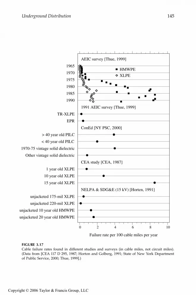
Underground Distribution 145
FIGURE 3.17Cable failure rates found in different studies and surveys (in cable miles, not circuit miles).(Data from [CEA 117 D 295, 1987; Horton and Golberg, 1991; State of New York Departmentof Public Service, 2000; Thue, 1999].)
0 2 4 6 8 10
1965
1970
1975
1980
1985
1990
TR-XLPE
EPR
> 40 year old PILC
< 40 year old PILC
1970-75 vintage solid dielectric
Other vintage solid dielectric
1 year old XLPE
10 year old XLPE
15 year old XLPE
unjacketed 175-mil XLPE
unjacketed 220-mil XLPE
unjacketed 10 year old HMWPE
unjacketed 20 year old HMWPE
AEIC survey [Thue, 1999]
1991 AEIC survey [Thue, 1999]
ConEd [NY PSC, 2000]
CEA study [CEA, 1987]
NELPA & SDG&E (15 kV) [Horten, 1991]
HMWPE
XLPE
Failure rate per 100 cable miles per year
9576_C03.fm Page 145 Monday, October 17, 2005 8:12 AM
Copyright © 2006 Taylor & Francis Group, LLC

146 Electric Power Distribution Equipment and Systems
One important factor is that the type of splice should be correctly matchedwith the type of cable (Mackevich, 1988). Table 3.26 shows annual failurerates for some common underground components that were developedbased on data from the Northwest Underground Distribution Committee ofthe Northwest Electric Light and Power Association (Horton and Golberg,1990; Horton and Golberg, 1991). Table 3.27 shows failure rates of splices forNew York City.
An EPRI review of separable connector reliability found mixed results(EPRI 1001732, 2002). Most utilities do not track these failures. One utilitythat did keep records found that failure rates of separable connectors ranged
FIGURE 3.18Cumulative service-time failure rates for HMWPE and XLPE cable. (From Stember, L. H.,Epstein, M. M., Gaines, G. V., Derringer, G. C., and Thomas, R. E., “Analysis of Field FailureData on HMWPE- and XLPE-Insulated High-Voltage Distribution Cable,” IEEE Trans. PowerApparatus Sy., PAS-104(8), 1979-85, August 1985. With permission. ©1985 IEEE.)
TABLE 3.25
Comparison of the Median of the Average Yearly Failure Rates of XLPE Found by AEIC from 1983 to 1991
Configuration Failures per 100 Cable miles/year
No jacket 3.1Jacketed 0.2Direct buried 2.6Duct 0.2
Source: Thue, W. A., Electrical Power Cable Engineering,Marcel Dekker, New York, 1999.
HMWPE
XLPE
70 72 74 76 78 80 0
1
2
3
Year
Failu
res
per
100
mile
-yea
rs
9576_C03.fm Page 146 Monday, October 17, 2005 8:12 AM
Copyright © 2006 Taylor & Francis Group, LLC

Underground Distribution 147
from 0.1 to 0.4% annually. Of these failures, an estimated 3 to 20% are fromoverheating. They also suggested that thermal monitoring is a good practice,but effectiveness is limited because the monitoring is often done when theloadings and temperatures are well below their peak.
3.8 Cable Testing
A common approach to test cable and determine insulation integrity is touse a hi-pot test. In a hi-pot test, a dc voltage is applied for 5 to 15 min.IEEE-400 specifies that the hi-pot voltage for a 15-kV class cable is 56 kV foran acceptance test and 46 kV for a maintenance test (ANSI/IEEE Std. 400-1980). Other industry standard tests are given in (AEIC CS5-94, 1994; AEICCS6-96, 1996; ICEA S-66-524, 1988). High-pot testing is a brute-force test;imminent failures are detected, but the amount of deterioration due to agingis not quantified (it is a go/no–go test).
The dc test is controversial — some evidence has shown that hi-pot testingmay damage XLPE cable (Mercier and Ticker, 1998). EPRI work has shown
TABLE 3.26
Annual Underground-Component Failure Rates
Component Annual Failure Rate, %
Load-break elbows 0.009t15-kV molded rubber splices 0.3125-kV molded rubber splices 0.1835-kV molded rubber splices 0.25Single-phase padmounted transformers 0.3
Note: t is the age of the elbow in years.
Sources: Horton, W. F. and Golberg, S., “The Failure Rates of Under-ground Distribution System Components,” Proceedings of the Twen-ty-Second Annual North American Power Symposium, 1990;Horton, W. F. and Golberg, S., “Determination of Failure Rates ofUnderground Distribution System Components from Historical Da-ta,” IEEE/PES Transmission and Distribution Conference, 1991.
TABLE 3.27
Underground Network Component Failure Rates in New York City(Con Edison)
Component Annual Failure Rate, %
Splices connecting paper to solid cables (stop joints) 1.20Splices connecting similar cables (straight joints) 0.51Network transformers 0.58
Source: State of New York Department of Public Service, “A Report on Consoli-dated Edison’s July 1999 System Outages,” March 2000.
9576_C03.fm Page 147 Monday, October 17, 2005 8:12 AM
Copyright © 2006 Taylor & Francis Group, LLC

148 Electric Power Distribution Equipment and Systems
that dc testing accelerates treeing (EPRI TR-101245, 1993; EPRI TR-101245-V2, 1995). For hi-pot testing of 15-kV, 100% insulation (175-mil, 4.445-mm)XLPE cable, EPRI recommended:
• Do not do testing at 40 kV (228 V/mil) on cables that are aged(especially those that failed once in service and then are spliced).Above 300 V/mil, deterioration was predominant.
• New cable can be tested at the factory at 70 kV. No effect on cablelife was observed for testing of new cable.
• New cable can be tested at 55 kV in the field prior to energizationif aged cable has not been spliced in.
• Testing at lower dc voltages (such as 200 V/mil) will not pick outbad sections of cable.
Another option for testing cable integrity: ac testing does not degrade soliddielectric insulation (or at least degrades it more slowly). The use of verylow frequency ac testing (at about 0.1 Hz) may cause less damage to agedcable than dc testing (Eager et al., 1997) (but utilities have reported that it isnot totally benign, and ac testing has not gained widespread usage). Thelow frequency has the advantage that the equipment is much smaller than60-Hz ac testing equipment.
3.9 Fault Location
Utilities use a variety of tools and techniques to locate underground faults.Several are described in the next few paragraphs [see also EPRI TR-105502(1995)].
Divide and conquer — On a radial tap where the fuse has blown, crewsnarrow down the faulted section by opening the cable at locations. Crewsstart by opening the cable near the center, then they replace the fuse. If thefuse blows, the fault is upstream; if it doesn’t blow, the fault is downstream.Crews then open the cable near the center of the remaining portion andcontinue bisecting the circuit at appropriate sectionalizing points (usuallypadmounted transformers). Of course, each time the cable faults, more dam-age is done at the fault location, and the rest of the system has the stress ofcarrying the fault currents. Using current-limiting fuses reduces the fault-current stress but increases the cost.
Fault indicators — Faulted circuit indicators (FCIs) are small devicesclamped around a cable that measure current and signal the passage of faultcurrent. Normally, these are applied at padmounted transformers. Faultedcircuit indicators do not pinpoint the fault; they identify the fault to a cablesection. After identifying the failed section, crews must use another method
9576_C03.fm Page 148 Monday, October 17, 2005 8:12 AM
Copyright © 2006 Taylor & Francis Group, LLC

Underground Distribution 149
such as the thumper to precisely identify the fault. If the entire section is inconduit, crews don’t need to pinpoint the location; they can just pull thecable and replace it (or repair it if the faulted portion is visible from theoutside). Cables in conduit require less precise fault location; a crew onlyneeds to identify the fault to a given conduit section.
Utilities’ main justification for faulted circuit indicators is reducing thelength of customer interruptions. Faulted circuit indicators can significantlydecrease the fault-finding stage relative to the divide-and-conquer method.Models that make an audible noise or have an external indicator decreasethe time needed to open cabinets.
Utilities use most fault indicators on URD loops. With one fault indicatorper transformer (see Figure 3.19), a crew can identify the failed section andimmediately reconfigure the loop to restore power to all customers. The crewcan then proceed to pinpoint the fault and repair it (or even delay the repairfor a more convenient time). For larger residential subdivisions or for circuitsthrough commercial areas, location is more complicated. In addition to trans-formers, fault indicators should be placed at each sectionalizing or junctionbox. On three-phase circuits, either a three-phase fault indicator or threesingle-phase indicators are available; single-phase indicators identify thefaulted phase (a significant advantage). Other useful locations for fault indi-cators are on either end of cable sections of overhead circuits, which arecommon at river crossings or under major highways. These sections are notfused, but fault indicators will show patrolling crews whether the cablesection has failed.
Fault indicators may be reset in a variety of ways. On manual reset units,crews must reset the devices once they trip. These units are less likely toreliably indicate faults. Self-resetting devices are more likely to be accurateas they automatically reset based on current, voltage, or time. Current-resetis most common; after tripping, if the unit senses current above a threshold,it resets [standard values are 3, 1.5, and 0.1 A (NRECA RER Project 90-8,1993)]. With current reset, the minimum circuit load at that point must beabove the threshold, or the unit will never reset. On URD loops, whenapplying current-reset indicators, consider that the open point might change.This changes the current that the fault indicator sees. Again, make sure the
FIGURE 3.19Typical URD fault indicator application.
Riser pole Riser poleNormally open point
Fault indicators
9576_C03.fm Page 149 Monday, October 17, 2005 8:12 AM
Copyright © 2006 Taylor & Francis Group, LLC

150 Electric Power Distribution Equipment and Systems
circuit load is enough to reset the fault indicator. Voltage reset models pro-vide a voltage sensor; when the voltage exceeds some value (the voltagesensor senses at secondary voltage or at an elbow’s capacitive test point).Time-reset units simply reset after a given length of time.
Fault indicators should only operate for faults — not for load, not forinrush, not for lightning, and not for backfeed currents. False readings cansend crews on wild chases looking for faults. Reclose operations also causeloads and transformers to draw inrush, which can falsely trip a fault indi-cator. An inrush restraint feature disables tripping for up to one secondfollowing energization. On single-phase taps, inrush restraint is really onlyneeded for manually-reset fault indicators (the faulted phase with the blownfuse will not have inrush that affects downstream fault indicators). Faults inadjacent cables can also falsely trip indicators; the magnetic fields coupleinto the pickup coil. Shielding can help prevent this. Several scenarios causebackfeed that can trip fault indicators. Downstream of a fault, the storedcharge in the cable will rush into the fault, possibly tripping fault indicators.McNulty (1994) reported that 2000 ft of 15-kV cable created an oscillatorycurrent transient that peaked at 100 A and decayed in 0.15 msec. Nearbycapacitor banks on the overhead system can make outrush worse. Motorsand other rotating equipment can also backfeed faults. To avoid false trips,use a high set point. Equipment with filtering that reduces the indicator’ssensitivity to transient currents also helps, but too much filtering may leavethe faulted-circuit indicator unable to detect faults cleared rapidly by current-limiting fuses.
Self-resetting fault indicators can also falsely reset. Backfeed currents andvoltages can reset fault indicators. On a three-phase circuit with one phasetripped, the faulted phase can backfeed through three-phase transformerconnections (see Chapter 4), providing enough current or enough voltage toreset faulted-circuit indicators. On single-phase circuits, these are not a prob-lem. In general, single-phase application is much easier; we do not havebackfeed problems or problems with indicators tripping from faults on nearbycables. For single-phase application guidelines, see (IEEE Std 1216-2000).
Fault indicators may have a threshold-type trip characteristic like aninstantaneous relay (any current above the set point trips the flag), or theymay have a time-overcurrent characteristic which trips faster for highercurrents. Those units with time-overcurrent characteristics should be coor-dinated with minimum clearing curves of current-limiting fuses to ensurethat they operate. Another type of fault indicator uses an adaptive settingthat trips based on a sudden increase in current followed by a loss of current.
Set the trip level on fault indicators to less than 50% of the available faultcurrent or 500 A, whichever is less (IEEE P1610/D03, 2002). This trip thresh-old should be at least two to three times the load on the circuit to minimizefalse indications. These two conditions will almost never conflict, only at theend of a very long feeder (low fault currents) on a cable that is heavily loaded.
Normally, fault indicators are fixed equipment, but they can be used fortargeted fault location. When crews arrive at a faulted and isolated section,
9576_C03.fm Page 150 Monday, October 17, 2005 8:12 AM
Copyright © 2006 Taylor & Francis Group, LLC

Underground Distribution 151
they first apply fault indicators between sections (normally at padmountedtransformers). Crews reenergize the failed portion and then check the faultindicators to identify the faulted section. Only one extra fault is applied tothe circuit, not multiple faults as with the divide and conquer method.
Section testing — Crews isolate a section of cable and apply a dc hi-potvoltage. If the cable holds the hi-pot voltage, crews proceed to the nextsection and repeat until finding a cable that cannot hold the hi-pot voltage.Because the voltage is dc, the cable must be isolated from the transformer.In a faster variation of this, high-voltage sticks are available that use the acline voltage to apply a dc voltage to the isolated cable section.
Thumper — The thumper applies a pulsed dc voltage to the cable. As itsname implies, at the fault the thumper discharges sound like a thumpingnoise as the gap at the failure point repeatedly sparks over. The thumpercharges a capacitor and uses a triggered gap to discharge the capacitor’scharge into the cable. Crews can find the fault by listening for the thumpingnoise. Acoustic enhancement devices can help crews locate weak thumpingnoises; antennas that pick up the radio-frequency interference from the arcdischarge also help pinpoint the fault. Thumpers are good for finding theexact fault location so that crews can start digging. On a 15-kV class system,utilities typically thump with voltages from 10 to 15 kV, but utilities some-times use voltages to 25 kV.
While pulsed discharges are thought to be less damaging to cable than asteady dc voltage, utilities have concern that thumping can damage theunfailed sections of cable. When a thumper pulse breaks down the cable,the incoming surge shoots past the fault. When it reaches the open point,the voltage doubles, then the voltage pulse bounces back and forth betweenthe open point and the fault, switching from +2 to –2E (where E is thethumper pulse voltage). In tests, EPRI research found that thumping canreduce the life of aged cable (EPRI EL-6902, 1990; EPRI TR-108405-V1, 1997;Hartlein et al., 1989; Hartlein et al., 1994). The thumping discharges at thefailure point can also increase the damage at the fault point. Most utilitiestry to limit the voltage or discharge energy, and a few don’t use a thumperfor fear of additional damage to cables and components (Tyner, 1998). A fewutilities also disconnect transformers from the system during thumping toprotect the transformer and prevent surges from propagating through thetransformer (these surges should be small). If the fault has no gap, and ifthe fault is a solid short circuit, then no arc forms, and the thumper will notcreate its characteristic thump (fortunately, solid short circuits are rare incable faults). Some crews keep thumping in an effort to burn the short circuitapart enough to start arcing. With cable in conduit, the thumping may belouder near the conduit ends than at the fault location. Generally, crewsshould start with the voltage low and increase as needed. A dc hi-pot voltagecan help determine how much voltage the thumper needs.
Radar — Also called time-domain reflectometry (TDR), a radar set injectsa very short-duration current pulse into the cable. At discontinuities, a por-tion of the pulse will reflect back to the set; knowing the velocity of wave
9576_C03.fm Page 151 Monday, October 17, 2005 8:12 AM
Copyright © 2006 Taylor & Francis Group, LLC

152 Electric Power Distribution Equipment and Systems
propagation along cable gives us an estimate of the distance to the fault.Depending on the test set and settings, radar pulses can be from 5 ns to 5µs wide. Narrower pulses give higher resolution, so users can better differ-entiate between faults and reflections from splices and other discontinuities(Banker et al., 1994).
Radar does not give pinpoint accuracy; its main use is to narrow the faultto a certain section. Then, crews can use a thumper or other pinpoint tech-nique to find the failure. Taking a radar pulse from either end of a cable andaveraging the results can lead to an improved estimate of the location. Radarlocation on circuits with taps can be complicated, especially those withmultiple taps; the pulse will reflect off the taps, and the reflection from theactual fault will be less than it otherwise would be. Technology has beendeveloped to use above-ground antennas to sense and pinpoint faults basedon the radar signals.
Radar and thumper — After a fuse or other circuit interrupter clears a faultin a cable, the area around the fault point recovers some insulation strength.Checking the cable with an ohm meter would show an open circuit. Likewise,the radar pulse passes right by the fault, so the radar set alone cannot detectthe fault. Using radar with a thumper solves this problem. A thumper pulsebreaks down the gap, and the radar superimposes a pulse that reflects offthe fault arc. The risetime of the thumper waveshape is on the order of afew microseconds; the radar pulse total width may be less than 0.05 µsec.Another less attractive approach is to use a thumper to continually burn thecable until the fault resistance becomes low enough to get a reading on aradar set (this is less attractive because it subjects the cable to many morethumps, especially if crews use high voltages).
Boucher (1991) reported that fault indicators were the most popular faultlocating approach, but most utilities use a variety of techniques (see Figure3.20). Depending on the type of circuit, the circuit layout, and the equipmentavailable, different approaches are sometimes better.
FIGURE 3.20Utility use of fault-locating techniques (204 utilities surveyed, multiple responses allowed).(Data from [Boucher, 1991].)
Number of responses
Other
Manual reset fault indicators
Thumper
Radar
Divide and conquer
Self reset fault indicators
0 20 40 60 80 100
Single-phase circuits Three-phase circuits
0 20 40 60 80 100
9576_C03.fm Page 152 Monday, October 17, 2005 8:12 AM
Copyright © 2006 Taylor & Francis Group, LLC

Underground Distribution 153
When applying test voltages to cables, crews must be mindful that cablescan hold significant charge. Cables have significant capacitance, and cablescan maintain charge for days.
References
AEIC CS5-94, Specification for Cross-Linked Polyethylene Insulated, Shielded Power CablesRated 5 through 46 kV, Association of Edison Illuminating Companies, 1994.
AEIC CS6-96, Specification for Ethylene Propylene Rubber Shielded Power Cables Rated5–69 kV, Association of Edison Illuminating Companies, 1996.
Ametani, A., “A General Formulation of Impedance and Admittance of Cables,” IEEETransactions on Power Apparatus and Systems, vol. PAS-99, no. 3, pp. 902–10,May/June 1980.
Anders, G. and Brakelmann, H., “Cable Crossings-Derating Considerations. I. Deri-vation of Derating Equations,” IEEE Transactions on Power Delivery, vol. 14, no.3, pp. 709–14, July 1999a.
Anders, G. and Brakelmann, H., “Cable Crossings-Derating Considerations. II. Ex-ample of Derivation of Derating Curves,” IEEE Transactions on Power Delivery,vol. 14, no. 3, pp. 715–20, July 1999b.
Anders, G. J., “Rating of Cables on Riser Poles, in Trays, in Tunnels and Shafts — AReview,” IEEE Transactions on Power Delivery, vol. 11, no. 1, pp. 3–11, January1996.
Anders, G. J., Rating of Electric Power Cables: Ampacity Computations for Transmission,Distribution, and Industrial Applications, IEEE Press, McGraw-Hill, New York,1998.
ANSI/ICEA S-94-649-2000, Standard for Concentric Neutral Cables Rated 5 through 46kV, Insulated Cable Engineers Association, 2000.
ANSI/ICEA S-97-682-2000, Standard for Utility Shielded Power Cables Rated 5 through46 kV, Insulated Cable Engineers Association, 2000.
ANSI/IEEE Std. 400-1980, IEEE Guide for Making High-Direct-Voltage Tests on PowerCable Systems in the Field.
Banker, W. A., Nannery, P. R., Tarpey, J. W., Meyer, D. F., and Piesinger, G. H.,“Application of High Resolution Radar to Provide Non-destructive Test Tech-niques for Locating URD Cable Faults and Splices,” IEEE Transactions on PowerDelivery, vol. 9, no. 3, pp. 1187–94, July 1994.
Boggs, S. and Xu, J. J., “Water Treeing — Filled vs. Unfilled Cable Insulation,” IEEEElectrical Insulation Magazine, vol. 17, no. 1, pp. 23–9, January/February 2001.
Boucher, R., “A Summary Of The Regional Underground Distribution Practices For1991,” Regional Underground Distribution Practices (IEEE paper 91 TH0398-8-PWR), 1991.
Brown, M., “EPR Insulation Cuts Treeing and Cable Failures,” Electrical World, vol.197, no. 1, pp. 105–6, January 1983.
Brown, M., “Accelerated Life Testing of EPR-Insulated Underground Cable,” IEEEElectrical Insulation Magazine, vol. 7, no. 4, pp. 21–6, July/August 1991.
Burns, N. M., Jr., “Performance of Supersmooth Extra Clean Semiconductive Shieldsin XLPE Insulated Power Cables,” IEEE International Symposium on ElectricalInsulation, 1990.
9576_C03.fm Page 153 Monday, October 17, 2005 8:12 AM
Copyright © 2006 Taylor & Francis Group, LLC

154 Electric Power Distribution Equipment and Systems
CEA 117 D 295, Survey of Experience with Polymer Insulated Power Cable in UndergroundService, Canadian Electrical Association, 1987.
CEA 274 D 723, Underground Versus Overhead Distribution Systems, Canadian ElectricalAssociation, 1992.
CEA, CEA Distribution Planner’s Manual, Canadian Electrical Association, 1982.Champion, T., “Elbow Failures Cast Doubt on Reliability,” Electrical World, vol. 200,
no. 6, pp. 71–3, June 1986.Cinquemani, P. L., Yingli, W., Kuchta, F. L., and Doench, C., “Performance of Reduced
Wall EPR Insulated Medium Voltage Power Cables. I. Electrical Characteris-tics,” IEEE Transactions on Power Delivery, vol. 12, no. 2, pp. 571–8, April 1997.
Cress, S. L. and Motlis, H., “Temperature Rise of Submarine Cable on Riser Poles,”IEEE Transactions on Power Delivery, vol. 6, no. 1, pp. 25–33, January 1991.
Dedman, J. C. and Bowles, H. L., “A Survey of URD Cable Installed on Rural ElectricSystems and Failures of That Cable,” IEEE Rural Electric Power Conference, 1990.
Dommel, H. W., “Electromagnetic Transients Program Reference Manual (EMTPTheory Book),” prepared for Bonneville Power Administration, 1986.
Dudas, J. H., “Technical Trends in Medium Voltage URD Cable Specifications,” IEEEElectrical Insulation Magazine, vol. 10, no. 2, pp. 7–16, March/April 1994.
Dudas, J. H. and Cochran, W. H., “Technical Advances in the Underground Medium-Voltage Cable Specification of the Largest Investor-Owned Utilities in the U.S.,”IEEE Electrical Insulation Magazine, vol. 15, no. 6, pp. 29–36, November/Decem-ber 1999.
Dudas, J. H. and Rodgers, J. R., “Underground Cable Technical Trends for the LargestRural Electric Co-ops,” IEEE Transactions on Industry Applications, vol. 35, no.2, pp. 324–31, March/April 1999.
Eager, G. S., Katz, C., Fryszczyn, B., Densley, J., and Bernstein, B. S., “High VoltageVLF Testing of Power Cables,” IEEE Transactions on Power Delivery, vol. 12, no.2, pp. 565–70, April 1997.
EPRI 1000273, Estimation of Remaining Life of XLPE-Insulated Cables, Electric PowerResearch Institute, Palo Alto, CA, 2000.
EPRI 1000741, Condition Assessment of Distribution PILC Cable Assets, Electric PowerResearch Institute, Palo Alto, CA, 2000.
EPRI 1001389, Aging of Extruded Dielectric Distribution Cable: Phase 2 Service Aging,Electric Power Research Institute, Palo Alto, CA, 2002.
EPRI 1001732, Thermal Issues and Ratings of Separable Insulated Connectors, ElectricPower Research Institute, Palo Alto, CA, 2002.
EPRI 1001734, State of the Art of Thin Wall Cables Including Industry Survey, ElectricPower Research Institute, Palo Alto, CA, 2002.
EPRI 1001894, EPRI Power Cable Materials Selection Guide, EPRI, Palo Alto, CA, 2001.EPRI EL-6902, Effects of Voltage Surges on Solid-Dielectric Cable Life, Electric Power
Research Institute, Palo Alto, CA, 1990.EPRI TR-101245, Effect of DC Testing on Extruded Cross-Linked Polyethylene Insulated
Cables, Electric Power Research Institute, Palo Alto, CA, 1993.EPRI TR-101245-V2, Effect of DC Testing on Extruded Cross-Linked Polyethylene Insulated
Cables — Phase II, Electric Power Research Institute, Palo Alto, CA, 1995.EPRI TR-105502, Underground Cable Fault Location Reference Manual, Electric Power
Research Institute, Palo Alto, CA, 1995.EPRI TR-108405-V1, Aging Study of Distribution Cables at Ambient Temperatures with
Surges, Electric Power Research Institute, Palo Alto, CA, 1997.
9576_C03.fm Page 154 Monday, October 17, 2005 8:12 AM
Copyright © 2006 Taylor & Francis Group, LLC
Underground Distribution 155
EPRI TR-108919, Soil Thermal Properties Manual for Underground Power Transmission,Electric Power Research Institute, Palo Alto, CA, 1997.
EPRI TR-111888, High-Ampacity, Thin-Wall, Novel Polymer Cable, Electric Power Re-search Institute, Palo Alto, CA, 2000.
Gurniak, B., “Neutral Corrosion Problem Overstated,” Transmission & DistributionWorld, pp. 152–8, August 1996.
Hartlein, R. A. and Black, W. Z., “Ampacity of Electric Power Cables in VerticalProtective Risers,” IEEE Transactions on Power Apparatus and Systems, vol. PAS-102, no. 6, pp. 1678–86, June 1983.
Hartlein, R. A., Harper, V. S., and Ng, H. W., “Effects of Voltage Impulses on ExtrudedDielectric Cable Life,” IEEE Transactions on Power Delivery, vol. 4, no. 2, pp.829–41, April 1989.
Hartlein, R. A., Harper, V. S., and Ng, H. W., “Effects of Voltage Surges on ExtrudedDielectric Cable Life Project Update,” IEEE Transactions on Power Delivery, vol.9, no. 2, pp. 611–9, April 1994.
Horton, W. F. and Golberg, S., “The Failure Rates of Underground DistributionSystem Components,” Proceedings of the Twenty-Second Annual North Amer-ican Power Symposium, 1990.
Horton, W. F. and Golberg, S., “Determination of Failure Rates of UndergroundDistribution System Components from Historical Data,” IEEE/PES Transmis-sion and Distribution Conference, 1991.
ICEA Publication T-31-610, Guide for Conducting a Longitudinal Water Penetration Re-sistance Test for Sealed Conductor, Insulated Cable Engineers Association, 1994.
ICEA Publication T-34-664, Conducting Longitudinal Water Penetration Resistance Testson Cable, Insulated Cable Engineers Association, 1996.
ICEA S-66-524, Cross-Linked Thermosetting Polyethylene Insulated Wire and Cable forTransmission and Distribution of Electrical Energy, Insulated Cable Engineers As-sociation, 1988.
IEC 287, Calculation of the Continuous Current Rating of Cables (100% Load Factor), 2nded., International Electrical Commission (IEC), 1982.
IEEE C2-1997, National Electrical Safety Code.IEEE P1610/D03, Draft Guide for the Application of Faulted Circuit Indicators for 200/600
A, Three-Phase Underground Distribution, 2002.IEEE Std 1216-2000, IEEE Guide for the Application of Faulted Circuit Indicators for 200
A, Single-Phase Underground Residential Distribution (URD).IEEE Std. 141-1993, IEEE Recommended Practice for Electric Power Distribution for In-
dustrial Plants.IEEE Std. 386-1995, IEEE Standard for Separable Insulated Connector Systems for Power
Distribution Systems Above 600 V.IEEE Std. 835-1994, IEEE Standard Power Cable Ampacities.Katz, C. and Walker, M., “Evaluation of Service Aged 35 kV TR-XLPE URD Cables,”
IEEE Transactions on Power Delivery, vol. 13, no. 1, pp. 1–6, January 1998.Kerite Company, “Technical Application Support Data.” Downloaded from www.ker-
ite.com, June 2002.Koch, B., “Underground Lines: Different Problems, Practical Solutions,” Electrical
World T&D, March/April 2001.Lewis, W. A. and Allen, G. D., “Symmetrical Component Circuit Constants and
Neutral Circulating Currents for Concentric Neutral Underground DistributionCables,” IEEE Transactions on Power Apparatus and Systems, vol. PAS-97, no. 1,pp. 191–9, January/February 1978.
9576_C03.fm Page 155 Monday, October 17, 2005 8:12 AM
Copyright © 2006 Taylor & Francis Group, LLC

156 Electric Power Distribution Equipment and Systems
Lewis, W. A., Allen, G. D., and Wang, J. C., “Circuit Constants for Concentric NeutralUnderground Distribution Cables on a Phase Basis,” IEEE Transactions on PowerApparatus and Systems, vol. PAS-97, no. 1, pp. 200–7, January/February 1978.
Mackevich, J. P., “Trends in Underground Residential Cable Systems,” IEEE RuralElectric Power Conference, 1988.
Martin, M. A., Silver, D. A., Lukac, R. G., and Suarez, R., “Normal and Short CircuitOperating Characteristics of Metallic Shielding Solid Dielectric Power Cable,”IEEE Transactions on Power Apparatus and Systems, vol. PAS-93, no. 2, pp. 601–13,March/April 1974.
McNulty, W. J., “False Tripping of Faulted Circuit Indicators,” IEEE/PES Transmis-sion and Distribution Conference, 1994.
Mercier, C. D. and Ticker, S., “DC Field Test for Medium-Voltage Cables: Why CanNo One Agree?,” IEEE Transactions on Industry Applications, vol. 34, no. 6, pp.1366–70, November/December 1998.
Nannery, P. R., Tarpey, J. W., Lacenere, J. S., Meyer, D. F., and Bertini, G., “Extendingthe Service Life of 15 kV Polyethylene URD Cable Using Silicone Liquid,” IEEETransactions on Power Delivery, vol. 4, no. 4, pp. 1991–6, October 1989.
Neher, J. H. and McGrath, M. H., “The Calculation of the Temperature Rise and LoadCapability of Cable Systems,” AIEE Transactions, vol. 76, pp. 752–64, October1957.
NFPA 70, National Electrical Code, National Fire Protection Association, 1999.NRECA RER Project 90-8, Underground Distribution System Design and Installation
Guide, National Rural Electric Cooperative Association, 1993.Okonite, Engineering Data for Copper and Aluminum Conductor Electrical Tables, Okonite
Company, publication EHB-90, 1990.Powers, W. F., “An Overview of Water-Resistant Cable Designs,” IEEE Transactions
on Industry Applications, vol. 29, no. 5, 1993.Smith, D. R., “System Considerations — Impedance and Fault Current Calculations,”
IEEE Tutorial Course on Application and Coordination of Reclosers, Section-alizers, and Fuses, 1980. Publication 80 EHO157-8-PWR.
Smith, D. R. and Barger, J. V., “Impedance and Circulating Current Calculations forUD Multi-Wire Concentric Neutral Circuits,” IEEE Transactions on Power Appa-ratus and Systems, vol. PAS-91, no. 3, pp. 992–1006, May/June 1972.
Southwire Company, Power Cable Manual, 2nd ed, 1997.St. Pierre, C., A Practical Guide to Short-Circuit Calculations, Electric Power Consultants,
Schenectady, NY, 2001.State of New York Department of Public Service, “A Report on Consolidated Edison’s
July 1999 System Outages,” March 2000.Stember, L. H., Epstein, M. M., Gaines, G. V., Derringer, G. C., and Thomas, R. E.,
“Analysis of Field Failure Data on HMWPE- and XLPE-Insulated High-VoltageDistribution Cable,” IEEE Transactions on Power Apparatus and Systems, vol. PAS-104, no. 8, pp. 1979–85, August 1985.
Stringer, N. T. and Kojovic, L. A., “Prevention of Underground Cable Splice Failures,”IEEE Transactions on Industry Applications, vol. 37, no. 1, pp. 230–9, January/February 2001.
Thue, W. A., Electrical Power Cable Engineering, Marcel Dekker, New York, 1999.Tyner, J. T., “Getting to the Bottom of UG Practices,” Transmission & Distribution World,
vol. 50, no. 7, pp. 44–56, July 1998.Westinghouse Electric Corporation, Electrical Transmission and Distribution Reference
Book, 1950.
9576_C03.fm Page 156 Monday, October 17, 2005 8:12 AM
Copyright © 2006 Taylor & Francis Group, LLC

Underground Distribution 157
I was down in the hole and pulled on one of the splices thinking that I mightfind the faulted one by pulling it apart, well you can only guess what happensnext! KA-BOOOM, I was really pissed off at that point and still am. BUT YOUKNOW SOMETHING, IT’S MY FAULT FOR TAKING SOME OTHERHALF ASS LINEMAN’S WORD FOR IT BEING DEAD AND NOTCHECKING IT OUT FOR MY SELF!
Anonymous poster, about beginning work after another lineman toldhim that the cables were disconnected at the source end.
www.powerlineman.com
9576_C03.fm Page 157 Monday, October 17, 2005 8:12 AM
Copyright © 2006 Taylor & Francis Group, LLC

159
4
Transformers
Ac transformers are one of the keys to allowing widespread distribution ofelectric power as we see it today. Transformers efficiently convert electricityto higher voltage for long distance transmission and back down to lowvoltages suitable for customer usage. The distribution transformer normallyserves as the final transition to the customer and often provides a localgrounding reference. Most distribution circuits have hundreds of distribu-tion transformers. Distribution feeders may also have other transformers:voltage regulators, feeder step banks to interface circuits of different volt-ages, and grounding banks.
4.1 Basics
A transformer efficiently converts electric power from one voltage level toanother. A transformer is two sets of coils coupled together through a mag-netic field. The magnetic field transfers all of the energy (except in anautotransformer). In an ideal transformer, the voltages on the input and theoutput are related by the turns ratio of the transformer:
where
N
1
and
N
2
are the number of turns and
V
1
and
V
2
are the voltage onwindings 1 and 2.
In a real transformer, not all of the flux couples between windings. This
leakage
flux creates a voltage drop between windings, so the voltage is moreaccurately described by
V NN
V11
22=
V NN
V X IL11
22 1= −
9576_C04.fm Page 159 Monday, October 17, 2005 9:12 AM
Copyright © 2006 Taylor & Francis Group, LLC

160
Electric Power Distribution Equipment and Systems
where
X
L
is the leakage reactance in ohms as seen from winding 1, and
I
1
isthe current out of winding 1.
The current also transforms by the turns ratio, opposite of the voltage as
The “ampere-turns” stay constant at ; this fundamental rela-tionship holds well for power and distribution transformers.
A transformer has a magnetic core that can carry large magnetic fields.The cold-rolled, grain-oriented steels used in cores have permeabilities ofover 1000 times that of air. The steel provides a very low-reluctance path formagnetic fields created by current through the windings.
Consider voltage applied to the
primary
side (source side, high-voltageside) with no load on the
secondary
side (load side, low-voltage side). Thewinding draws
exciting
current from the system that sets up a sinusoidalmagnetic field in the core. The flux in turn creates a back emf in the coil thatlimits the current drawn into the transformer. A transformer with no loadon the secondary draws very little current, just the exciting current, whichis normally less than 0.5% of the transformer’s full-load current. On theunloaded secondary, the sinusoidal flux creates an open-circuit voltage equalto the primary-side voltage times the turns ratio.
When we add load to the secondary of the transformer, the load pullscurrent through the secondary winding. The magnetic coupling of the sec-ondary current pulls current through the primary winding, keeping constantampere-turns. Normally in an inductive circuit, higher current creates moreflux, but not in a transformer (except for the leakage flux). The increasingforce from current in one winding is countered by the decreasing force fromcurrent through the other winding (see Figure 4.1). The flux in the core ona loaded transformer is the same as that on an unloaded transformer, eventhough the current is much higher.
The voltage on the primary winding determines the flux in the transformer(the flux is proportional to the time integral of voltage). The flux in the coredetermines the voltage on the output-side of the transformer (the voltage isproportional to the time derivative of the flux).
Figure 4.2 shows models with the significant impedances in a transformer.The detailed model shows the series impedances, the resistances and thereactances. The series resistance is mainly the resistance of the wires in eachwinding. The series reactance is the leakage impedance. The shunt branchis the magnetizing branch, current that flows to magnetize the core. Most ofthe magnetizing current is reactive power, but it includes a real powercomponent. Power is lost in the core through:
•
Hysteresis
— As the magnetic dipoles change direction, the core heatsup from the friction of the molecules.
I NN
I N I N I12
12 1 1 2 2= = or
N I N I1 1 2 2=
9576_C04.fm Page 160 Monday, October 17, 2005 9:12 AM
Copyright © 2006 Taylor & Francis Group, LLC

Transformers
161
FIGURE 4.1
Transformer basic function.
FIGURE 4.2
Transformer models.
Magnetic equivalent circuit Electric circuit
φcore
φcore
φL1 φL2
R 0
I1 I2
V1 V2E1 E2
E1N1N2
E2
N1I1 N2I2
L1 L2
L1 and L2 are from the leakage fluxes, φL1 and φL2Since R 0, N1I1 N2I2
Magnetizingbranch
Detailed transformer model
Simplified model
Idealtransformer
9576_C04.fm Page 161 Monday, October 17, 2005 9:12 AM
Copyright © 2006 Taylor & Francis Group, LLC

162
Electric Power Distribution Equipment and Systems
•
Eddy currents
— Eddy currents in the core material cause resistivelosses. The core flux induces the eddy currents tending to opposethe change in flux density.
The magnetizing branch impedance is normally above 5,000% on a trans-former’s base, so we can neglect it in many cases. The core losses are oftenreferred to as iron losses or no-load losses. The load losses are frequentlycalled the wire losses or copper losses. The various parameters of transform-ers scale with size differently as summarized in Table 4.1.
The simplified transformer model in Figure 4.2 with series resistance andreactance is sufficient for most calculations including load flows, short-circuitcalculations, motor starting, or unbalance. Small distribution transformershave low leakage reactances, some less than 1% on the transformer rating,and
X/R
ratios of 0.5 to 5. Larger power transformers used in distributionsubstations have higher impedances, usually on the order of 7 to 10% with
X/R
ratios between 10 and 40.The leakage reactance causes voltage drop on a loaded transformer. The
voltage is from flux that doesn’t couple from the primary to the secondarywinding. Blume et al. (1951) describes leakage reactance well. In a realtransformer, the windings are wound around a core; the high- and low-voltage windings are adjacent to each other. Figure 4.3 shows a configuration;each winding contains a number of turns of wire. The sum of the current ineach wire of the high-voltage winding equals the sum of the currents in the
TABLE 4.1
Common Scaling Ratios in Transformers
QuantityRelativeto kVA
Relative to a ReferenceDimension,
l
Rating kVA
l
4
Weight K kVA
3/4
K
l
3
Cost K KVA
3/4
K (% Total Loss)
–3
Length K kVA
1/4
K
l
Width K kVA
1/4
K
l
Height K kVA
1/4
K
l
Total losses K kVA
3/4
K
l
3
No-load losses K kVA
3/4
K
l
3
Exciting current K kVA
3/4
K
l
3
% Total loss K kVA
–1/4
K
l
–1
% No-load loss K kVA
–1/4
K
l
–1
% Exciting current K kVA
–1/4
K
l
–1
% R K kVA
–1/4
K
l
–1
% X K kVA
1/4
K
l
Volts/turn K kVA
1/2
K
l
2
Source:
Arthur D. Little, “Distribution Transformer Rulemak-ing Engineering Analysis Update,” Report to U.S. Depart-ment of Energy Office of Building Technology, State, andCommunity Programs. Draft. December 17, 2001.
9576_C04.fm Page 162 Monday, October 17, 2005 9:12 AM
Copyright © 2006 Taylor & Francis Group, LLC

Transformers
163
low-voltage winding (
N
1
I
1
= N
2
I
2
), so each winding is equivalent to a busbar.Each busbar carries equal current, but in opposite directions. The opposingcurrents create flux in the gap between the windings (this is called
leakageflux
). Now, looking at the two windings from the top, we see that the wind-ings are equivalent to current flowing in a loop encompassing a given area.This area determines the leakage inductance.
The leakage reactance in percent is based on the coil parameters andseparations (Blume et al., 1951) as follows:
where
f
= system frequency, Hz
N
= number of turns on one winding
I
= full load current on the winding, A
r
= radius to the windings, in.
w
= width between windings, in.
h
= height of the windings, in.
S
kVA
= transformer rating, kVA
FIGURE 4.3
Leakage reactance.
Equivalent Circuit
Top View of Windings
w
Insulation between the primary and secondary windings
Current ina loop
Area determinesleakage inductance
Side View of Windings
h
r
w
Current
Xf NI rw
hSkVA% = ( )126
10
2
11
9576_C04.fm Page 163 Monday, October 17, 2005 9:12 AM
Copyright © 2006 Taylor & Francis Group, LLC
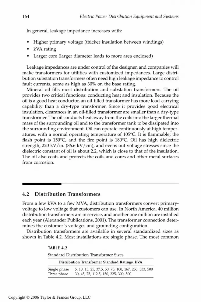
164
Electric Power Distribution Equipment and Systems
In general, leakage impedance increases with:
• Higher primary voltage (thicker insulation between windings)• kVA rating• Larger core (larger diameter leads to more area enclosed)
Leakage impedances are under control of the designer, and companies willmake transformers for utilities with customized impedances. Large distri-bution substation transformers often need high leakage impedance to controlfault currents, some as high as 30% on the base rating.
Mineral oil fills most distribution and substation transformers. The oilprovides two critical functions: conducting heat and insulation. Because theoil is a good heat conductor, an oil-filled transformer has more load-carryingcapability than a dry-type transformer. Since it provides good electricalinsulation, clearances in an oil-filled transformer are smaller than a dry-typetransformer. The oil conducts heat away from the coils into the larger thermalmass of the surrounding oil and to the transformer tank to be dissipated intothe surrounding environment. Oil can operate continuously at high temper-atures, with a normal operating temperature of 105
°
C. It is flammable; theflash point is 150
°
C, and the fire point is 180
°
C. Oil has high dielectricstrength, 220 kV/in. (86.6 kV/cm), and evens out voltage stresses since thedielectric constant of oil is about 2.2, which is close to that of the insulation.The oil also coats and protects the coils and cores and other metal surfacesfrom corrosion.
4.2 Distribution Transformers
From a few kVA to a few MVA, distribution transformers convert primary-voltage to low voltage that customers can use. In North America, 40 milliondistribution transformers are in service, and another one million are installedeach year (Alexander Publications, 2001). The transformer connection deter-mines the customer’s voltages and grounding configuration.
Distribution transformers are available in several standardized sizes asshown in Table 4.2. Most installations are single phase. The most common
TABLE 4.2
Standard Distribution Transformer Sizes
Distribution Transformer Standard Ratings, kVA
Single phase 5, 10, 15, 25, 37.5, 50, 75, 100, 167, 250, 333, 500Three phase 30, 45, 75, 112.5, 150, 225, 300, 500
9576_C04.fm Page 164 Monday, October 17, 2005 9:12 AM
Copyright © 2006 Taylor & Francis Group, LLC

Transformers
165
overhead transformer is the 25-kVA unit; padmounted transformers tend tobe slightly larger where the 50-kVA unit is the most common.
Distribution transformer impedances are rather low. Units under 50 kVAhave impedances less than 2%. Three-phase underground transformers inthe range of 750 to 2500 kVA normally have a 5.75% impedance as specifiedin (ANSI/IEEE C57.12.24-1988). Lower impedance transformers provide bet-ter voltage regulation and less voltage flicker for motor starting or otherfluctuating loads. But lower impedance transformers increase fault currentson the secondary, and secondary faults impact the primary side more (deepervoltage sags and more fault current on the primary).
Standards specify the insulation capabilities of distribution transformerwindings (see Table 4.3). The low-frequency test is a power-frequency (60Hz) test applied for one minute. The basic lightning impulse insulation level(BIL) is a fast impulse transient. The front-of-wave impulse levels are evenshorter-duration impulses.
The through-fault capability of distribution transformers is also given inIEEE C57.12.00-2000 (see Table 4.4). The duration in seconds of the short-circuit capability is:
where
I
is the symmetrical current in multiples of the normal base currentfrom Table 4.4.
Overhead and padmounted transformer tanks are normally made of mildcarbon steel. Corrosion is one of the main concerns, especially for anythingon the ground or in the ground. Padmounted transformers tend to corrode
TABLE 4.3
Insulation Levels for Distribution Transformers
Low-FrequencyTest Level,
kV rms
Basic LightningImpulse Insulation Level,
kV Crest
Chopped-Wave Impulse Levels
Minimum Voltage,kV Crest
MinimumTime to
Flashover,
µ
s
10 30 36 1.015 45 54 1.519 60 69 1.526 75 88 1.634 95 110 1.840 125 145 2.2550 150 175 3.070 200 230 3.095 250 290 3.0
140 350 400 3.0
Source
: IEEE Std. C57.12.00-2000. Copyright 2000 IEEE. All rights reserved.
tI
= 12502
9576_C04.fm Page 165 Monday, October 17, 2005 9:12 AM
Copyright © 2006 Taylor & Francis Group, LLC

166
Electric Power Distribution Equipment and Systems
near the base (where moisture and dirt and other debris may collect). Sub-mersible units, being highly susceptible to corrosion, are often stainless steel.
Distribution transformers are “self cooled”; they do not have extra coolingcapability like power transformers. They only have one kVA rating. Becausethey are small and because customer peak loadings are relatively shortduration, overhead and padmounted distribution transformers have signif-icant overload capability. Utilities regularly size them to have peak loadsexceeding 150% of the nameplate rating.
Transformers in underground vaults are often used in cities, especially fornetwork transformers (feeding secondary grid networks). In this application,heat can be effectively dissipated (but not as well as with an overhead orpadmounted transformer).
Subsurface transformers are installed in an enclosure just big enough tohouse the transformer with a grate covering the top. A “submersible” trans-former is normally used, one which can be submerged in water for anextended period (ANSI/IEEE C57.12.80-1978). Heat is dissipated throughthe grate at the top. Dirt and debris in the enclosure can accelerate corrosion.Debris blocking the grates or vents can overheat the transformer.
Direct-buried transformers have been attempted over the years. The mainproblems have been overheating and corrosion. In soils with high electricaland thermal resistivity, overheating is the main concern. In soils with lowelectrical and thermal resistivity, overheating is not as much of a concern,but corrosion becomes a problem. Thermal conductivity in a direct-buriedtransformer depends on the thermal conductivity of the soil. The buriedtransformer generates enough heat to dry out the surrounding soil; the driedsoil shrinks and creates air gaps. These air gaps act as insulating layers thatfurther trap heat in the transformer.
4.3 Single-Phase Transformers
Single-phase transformers supply single-phase service; we can use two orthree single-phase units in a variety of configurations to supply three-phase
TABLE 4.4
Through-Fault Capability of Distribution Transformers
Single-Phase Rating, kVA Three-Phase Rating, kVA
Withstand Capability in per Unit of Base Current
(Symmetrical)
5–25 15–75 4037.5–110 112.5–300 35167–500 500 25
Source
: IEEE Std. C57.12.00-2000,
IEEE Standard General Requirements for Liquid-Immersed Distri-bution, Power, and Regulating Transformers
.
9576_C04.fm Page 166 Monday, October 17, 2005 9:12 AM
Copyright © 2006 Taylor & Francis Group, LLC

Transformers
167
service. A transformer’s nameplate gives the kVA ratings, the voltage ratings,percent impedance, polarity, weight, connection diagram, and cooling class.Figure 4.4 shows a cutaway view of a single-phase transformer.
For a single-phase transformer supplying single-phase service, the load-full current in amperes is
where
S
kVA
= Transformer kVA rating
V
kV
= Line-to-ground voltage rating in kV
FIGURE 4.4
Single-phase distribution transformer. (Photo courtesy of ABB, Inc. With permission.)
ISV
kVA
kV
=
9576_C04.fm Page 167 Monday, October 17, 2005 9:12 AM
Copyright © 2006 Taylor & Francis Group, LLC

168
Electric Power Distribution Equipment and Systems
So, a single-phase 50-kVA transformer with a high-voltage winding of12470GrdY/7200 V has a full-load current of 6.94 A on the primary. On a 240/120-V secondary, the full-load current across the 240-V winding is 208.3 A.
Table 4.5 and Table 4.6 show the standard single-phase winding connec-tions for primary and secondary windings. High-voltage bushings arelabeled H*, starting with H1 and then H2 and so forth. Similarly, the low-voltage bushings are labeled X1, X2, X3, and so on.
The standard North American single-phase transformer connection isshown in Figure 4.5. The standard secondary load service is a 120/240-Vthree-wire service. This configuration has two secondary windings in serieswith the midpoint grounded. The secondary terminals are labeled X1, X2,and X3 where the voltage X1-X2 and X2-X3 are each 120 V. X1-X3 is 240 V.
Power and distribution transformers are assigned polarity dots accordingto the terminal markings. Current entering H1 results in current leaving X1.The voltage from H1 to H2 is in phase with the voltage from X1 to X3.
On overhead distribution transformers, the high-voltage terminal H1 isalways on the left (when looking into the low-voltage terminals; the termi-nals are not marked). On the low-voltage side, the terminal locations aredifferent, depending on size. If X1 is on the right, it is referred to as
additivepolarity
(if X3 is on the right, it is
subtractive polarity
). Polarity is additive ifthe voltages add when the two windings are connected in series around thetransformer (see Figure 4.6). Industry standards specify the polarity of a
TABLE 4.5
Winding Designations for Single-Phase Primary and Secondary Transformer
Windings with One Winding
Nomenclature Examples Description
E 13800 E shall indicate a winding of E volts that is suitable for
∆
connection on an E volt system.
E/E
1
Y 2400/4160Y E/E
1
Y shall indicate a winding of E volts that is suitable for
∆
connection on an E volt system or for Y connection on an E
1
volt system.
E/E
1
GrdY 7200/12470GrdY E/E
1
GrdY shall indicate a winding of E volts having reduced insulation that is suitable for
∆
connection on an E volt system or Y connection on an E
1
volt system, transformer, neutral effectively grounded.
E
1
GrdY/E 12470GrdY/7200480GrdY/277
E
1
GrdY/E shall indicate a winding of E volts with reduced insulation at the neutral end. The neutral end may be connected directly to the tank for Y or for single-phase operation on an E
1
volt system, provided the neutral end of the winding is effectively grounded.
E
1
= E
Note
: E is line-to-neutral voltage of a Y winding, or line-to-line voltage of a
∆
winding.
Source
: IEEE Std. C57.12.00-2000. Copyright 2000 IEEE. All rights reserved.
3
9576_C04.fm Page 168 Monday, October 17, 2005 9:12 AM
Copyright © 2006 Taylor & Francis Group, LLC

Transformers 169
TABLE 4.6
Two-Winding Transformer Designations for Single-Phase Primaries and Secondaries
Nomenclature Examples Description
E/2E 120/240240/280
E/2E shall indicate a winding, the sections of which can be connected in parallel for operation at E volts, or which can be connected in series for operation at 2E volts, or connected in series with a center terminal for three-wire operation at 2E volts between the extreme terminals and E volts between the center terminal and each of the extreme terminals.
2E/E 240/120 2E/E shall indicate a winding for 2E volts, two-wire full kilovoltamperes between extreme terminals, or for 2E/E volts three-wire service with 1/2 kVA available only, from midpoint to each extreme terminal.
E × 2E 240 × 480 E × 2E shall indicate a winding for parallel or series operation only but not suitable for three-wire service.
Source: IEEE Std. C57.12.00-2000. Copyright 2000 IEEE. All rights reserved.
FIGURE 4.5Single-phase distribution transformer diagram.
FIGURE 4.6Additive and subtractive polarity.
X1X2X3X4
X1X2X3
X1X2X3X4
120 V
120 V
240 V
X1
X3
X2
H1
H1Additive:
H2
X1 if additiveX1 if subtractive
Subtractive:(>200kVA or >8660V)
V1
V2
V2 V1
V1 V2
9576_C04.fm Page 169 Monday, October 17, 2005 9:12 AM
Copyright © 2006 Taylor & Francis Group, LLC

170 Electric Power Distribution Equipment and Systems
transformer, which depends on the size and the high-voltage winding. Sin-gle-phase transformers have additive polarity if (IEEE C57.12.00-2000):
kVA ≤ 200 and V ≤ 8660
All other distribution transformers have subtractive polarity. The reasonfor the division is that originally all distribution transformers had additivepolarity and all power transformers had subtractive polarity. Increasing sizesof distribution transformers caused overlap between “distribution” and“power” transformers, so larger distribution transformers were made withsubtractive polarity for consistency. Polarity is important when connectingsingle-phase units in three-phase banks and for paralleling units.
Manufacturers make single-phase transformers as either shell form or coreform (see Figure 4.7). Core-form designs prevailed prior to the 1960s; now,both shell- and core-form designs are available. Single-phase core-formtransformers must have interlaced secondary windings (the low-high-lowdesign). Every secondary leg has two coils, one wrapped around each legof the core. The balanced configuration of the interlaced design allowsunbalanced loadings on each secondary leg. Without interlacing, unbal-anced secondary loads excessively heat the tank. An unbalanced secondaryload creates an unbalanced flux in the iron core. The core-form constructiondoes not have a return path for the unbalanced flux, so the flux returnsoutside of the iron core (in contrast, the shell-form construction has a returnpath for such flux). Some of the stray flux loops through the transformertank and heats the tank.
The shell-form design does not need to have interlaced windings, so thenoninterlaced configuration is normally used on shell-form transformers sinceit is simpler. The noninterlaced secondary has two to four times the reactance:the secondary windings are separated by the high-voltage winding and theinsulation between them. Interlacing reduces the reactance since the low-voltage windings are right next to each other.
Using a transformer’s impedance magnitude and load losses, we can findthe real and reactive impedance in percent as
whereSkVA = transformer rating, kVAWCU = WTOT – WNL = load loss at rated load, W
WTOT = total losses at rated load, WWNL = no-load losses, W
Z = nameplate impedance magnitude, %
RW
SCU
kVA
=10
X Z R= −2 2
9576_C04.fm Page 170 Monday, October 17, 2005 9:12 AM
Copyright © 2006 Taylor & Francis Group, LLC
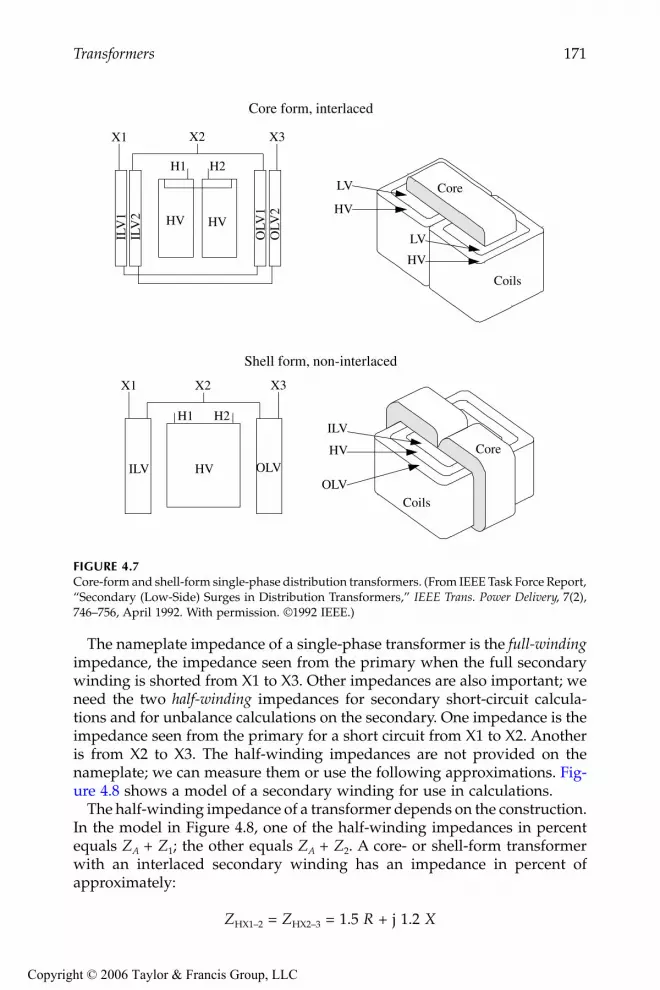
Transformers 171
The nameplate impedance of a single-phase transformer is the full-windingimpedance, the impedance seen from the primary when the full secondarywinding is shorted from X1 to X3. Other impedances are also important; weneed the two half-winding impedances for secondary short-circuit calcula-tions and for unbalance calculations on the secondary. One impedance is theimpedance seen from the primary for a short circuit from X1 to X2. Anotheris from X2 to X3. The half-winding impedances are not provided on thenameplate; we can measure them or use the following approximations. Fig-ure 4.8 shows a model of a secondary winding for use in calculations.
The half-winding impedance of a transformer depends on the construction.In the model in Figure 4.8, one of the half-winding impedances in percentequals ZA + Z1; the other equals ZA + Z2. A core- or shell-form transformerwith an interlaced secondary winding has an impedance in percent ofapproximately:
ZHX1–2 = ZHX2–3 = 1.5 R + j 1.2 X
FIGURE 4.7Core-form and shell-form single-phase distribution transformers. (From IEEE Task Force Report,“Secondary (Low-Side) Surges in Distribution Transformers,” IEEE Trans. Power Delivery, 7(2),746–756, April 1992. With permission. ©1992 IEEE.)
H1 H2
X2
Core
ILV
HV
OLVCoils
ILV OLVHV
X1 X3
H1 H2
Shell form, non-interlaced
Core
Coils
Core form, interlaced
LV
HV
LV
HV
X2X1 X3
HV HV
ILV
1IL
V2
OLV
1O
LV2
9576_C04.fm Page 171 Monday, October 17, 2005 9:12 AM
Copyright © 2006 Taylor & Francis Group, LLC

172 Electric Power Distribution Equipment and Systems
where R and X are the real and reactive components of the full-windingimpedance (H1 to H2 and X1 to X3) in percent. A noninterlaced shell-formtransformer has an impedance in percent of approximately:
ZHX1–2 = ZHX2–3 = 1.75 R + j 2.5 X
In a noninterlaced transformer, the two half-winding impedances are notidentical; the impedance to the inner low-voltage winding is less than theimpedance to the outer winding (the radius to the gap between the outersecondary winding and the primary winding is larger, so the gap betweenwindings has more area).
A secondary fault across one 120-V winding at the terminals of a nonin-terlaced transformer has current about equal to the current for a fault acrossthe 240-V winding. On an interlaced transformer, the lower relative imped-ance causes higher currents for the 120-V fault.
Consider a 50-kVA transformer with Z = 2%, 655 W of total losses, no-loadlosses of 106 W, and a noninterlaced 120/240-V secondary winding. Thistranslates into a full-winding percent impedance of 1.1 + j1.67. For a faultacross the 240-V winding, the current is found as
For a fault across the 120-V winding on this noninterlaced transformer, thecurrent is found as
FIGURE 4.8Model of a 120/240-V secondary winding with all impedances in percent. (Impedance datafrom [Hopkinson, 1976].)
ZA Z1
Z2
Full-winding impedance = R jXInterlaced secondary windingZA 0 5R j0 8XZ1 Z2 R j0 4XNoninterlaced secondary windingZA 0 25R j0 6XZ1 1 5R j3 3XZ2 1 5R j3 1X (inner winding)
Z R jXS
j jkVA
Ω Ω,
.. .
.. .240
2 210 0 241 1 1 67
10 0 2450
0 013 0 019V
kV kVkVA
= +( ) ( ) = +( ) ( ) = +
IZ240
240
0 2410 4V
V
kVkA= =.
.,Ω
9576_C04.fm Page 172 Monday, October 17, 2005 9:12 AM
Copyright © 2006 Taylor & Francis Group, LLC

Transformers 173
Consider the same transformer characteristics on a transformer with aninterlaced secondary and Z = 1.4%. The 240-V and 120-V short-circuit cur-rents are found as
The fault current for a 120-V fault is significantly higher than the 240-Vcurrent.
Completely self-protected transformers (CSPs) are a widely used single-phase distribution transformer with several built-in features (see Figure 4.9):
• Tank-mounted arrester• Internal “weak-link” fuse• Secondary breaker
CSPs do not need a primary-side cutout with a fuse. The internal primaryfuse protects against an internal failure in the transformer. The weak linkhas less fault-clearing capability than a fuse in a cutout, so they need externalcurrent-limiting fuses where fault currents are high.
Z R j XS
j
j
kVAΩ
Ω
, . ..
. ..
. .
120
2 2
1 75 2 510 0 12
1 93 4 1810 0 12
50
0 0055 0 0120
V
kV kVkVA
= +( ) ( ) = +( ) ( )
= +
IZ120
120
0 129 06V
V
kVkA= =.
.,Ω
Z R jXS
j jkVA
Ω Ω,
.. .
.. .240
2 210 0 241 1 0 87
10 0 2450
0 013 0 01V
kV kVkVA
= +( ) ( ) = +( ) ( ) = +
IZ240
240
0 2414 9V
V
kVkA= =.
.,Ω
Z R j XS
j
j
kVAΩ
Ω
, . ..
. ..
. .
120
2 2
1 5 1 210 0 12
1 65 1 0410 0 12
50
0 0048 0 003
V
kV kVkVA
= +( ) ( ) = +( ) ( )
= +
IZ120
120
0 1221 4V
V
kVkA= =.
.,Ω
9576_C04.fm Page 173 Monday, October 17, 2005 9:12 AM
Copyright © 2006 Taylor & Francis Group, LLC

174 Electric Power Distribution Equipment and Systems
Secondary breakers provide protection against overloads and secondaryfaults. The breaker responds to current and oil temperature. Tripping iscontrolled by deflection of bimetallic elements in series. The oil temperatureand current through the bimetallic strips heat the bimetal. Past a criticaltemperature, the bimetallic strips deflect enough to operate the breaker.Figure 4.10 shows trip characteristics for secondary breakers inside two sizetransformers. The secondary breaker has an emergency position to allowextra overload without tripping (to allow crews time to replace the unit).Crews can also use the breaker to drop the secondary load.
Some CSPs have overload-indicating lights that signal an overload. Theindicator light doesn’t go off until line crews reset the breaker. The indicatorlights are not ordered as often (and crews often disable them in the field)because they generate a fair number of nuisance phone calls from curious/helpful customers.
4.4 Three-Phase Transformers
Three-phase overhead transformer services are normally constructed fromthree single-phase units. Three-phase transformers for underground service(either padmounted, direct buried, or in a vault or building or manhole) arenormally single units, usually on a three- or five-legged core. Three-phasedistribution transformers are usually core construction (see Figure 4.11), with
FIGURE 4.9Completely self-protected transformer.
X1X2X3
H1
weaklinkfuse
9576_C04.fm Page 174 Monday, October 17, 2005 9:12 AM
Copyright © 2006 Taylor & Francis Group, LLC
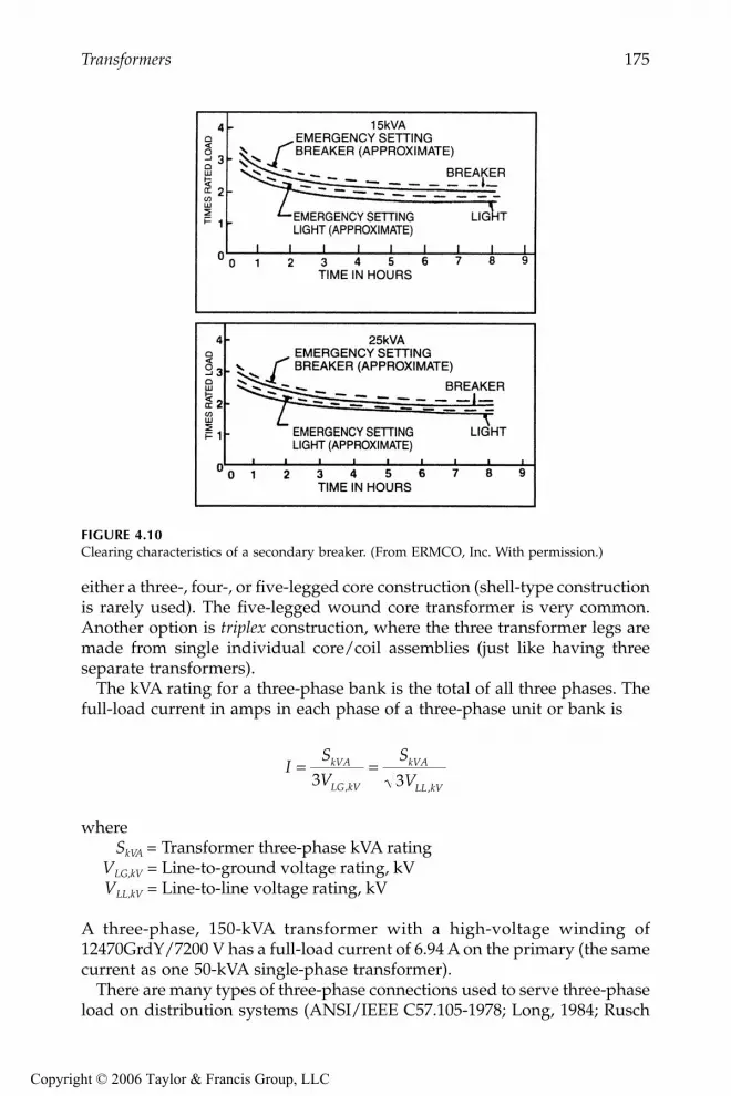
Transformers 175
either a three-, four-, or five-legged core construction (shell-type constructionis rarely used). The five-legged wound core transformer is very common.Another option is triplex construction, where the three transformer legs aremade from single individual core/coil assemblies (just like having threeseparate transformers).
The kVA rating for a three-phase bank is the total of all three phases. Thefull-load current in amps in each phase of a three-phase unit or bank is
whereSkVA = Transformer three-phase kVA rating
VLG,kV = Line-to-ground voltage rating, kVVLL,kV = Line-to-line voltage rating, kV
A three-phase, 150-kVA transformer with a high-voltage winding of12470GrdY/7200 V has a full-load current of 6.94 A on the primary (the samecurrent as one 50-kVA single-phase transformer).
There are many types of three-phase connections used to serve three-phaseload on distribution systems (ANSI/IEEE C57.105-1978; Long, 1984; Rusch
FIGURE 4.10Clearing characteristics of a secondary breaker. (From ERMCO, Inc. With permission.)
ISV
S
VkVA
LG kV
kVA
LL kV
= =3 3, ,
9576_C04.fm Page 175 Monday, October 17, 2005 9:12 AM
Copyright © 2006 Taylor & Francis Group, LLC

176 Electric Power Distribution Equipment and Systems
and Good, 1989). Both the primary and secondary windings may be con-nected in different ways: delta, floating wye, or grounded wye. This notationdescribes the connection of the transformer windings, not the configurationof the supply system. A “wye” primary winding may be applied on a “delta”distribution system. On the primary side of three-phase distribution trans-formers, utilities have a choice between grounded and ungrounded windingconnections. The tradeoffs are:
• Ungrounded primary — The delta and floating-wye primary connec-tions are suitable for ungrounded and grounded distribution sys-tems. Ferroresonance is more likely with ungrounded primary
FIGURE 4.11Three-phase core constructions.
Five-legged wound core
Four-legged stacked core
Three-legged stacked core
9576_C04.fm Page 176 Monday, October 17, 2005 9:12 AM
Copyright © 2006 Taylor & Francis Group, LLC

Transformers 177
connections. Ungrounded primary connections do not supplyground fault current to the primary distribution system.
• Grounded primary — The grounded-wye primary connection is onlysuitable on four-wire grounded systems (either multigrounded orunigrounded). It is not for use on ungrounded systems. Grounded-wye primaries may provide an unwanted source for ground faultcurrent.
Customer needs play a role in the selection of the secondary configura-tion. The delta configuration and the grounded-wye configuration are thetwo most common secondary configurations. Each has advantages anddisadvantages:
• Grounded-wye secondary — Figure 4.12 shows the most commonlyused transformers with a grounded-wye secondary winding:grounded wye – grounded wye and the delta – grounded wye. The
FIGURE 4.12Three-phase distribution transformer connections with a grounded-wye secondary.
480 or 208 V
277 or 120 V
480 or 208 V
277 or 120 V
Grounded Wye -- Grounded Wye
Delta -- Grounded Wye
9576_C04.fm Page 177 Monday, October 17, 2005 9:12 AM
Copyright © 2006 Taylor & Francis Group, LLC

178 Electric Power Distribution Equipment and Systems
standard secondary voltages are 480Y/277 V and 208Y/120 V. The480Y/277-V connection is suitable for driving larger motors; lightingand other 120-V loads are normally supplied by dry-type transform-ers. A grounded-wye secondary adeptly handles single-phase loadson any of the three phases with less concerns about unbalances.
• Delta secondary — An ungrounded secondary system like the deltacan supply three-wire ungrounded service. Some industrial facilitiesprefer an ungrounded system, so they can continue to operate withline-to-ground faults. With one leg of the delta grounded at themidpoint of the winding, the utility can supply 240/120-V service.End-users can use more standard 230-V motors (without worryingabout reduced performance when run at 208 V) and still run lightingand other single-phase loads. This tapped leg is often called thelighting leg (the other two legs are the power legs). Figure 4.13 showsthe most commonly used connections with a delta secondary wind-ings. This is commonly supplied with overhead transformers.
Many utilities offer a variety of three-phase service options and, of course,most have a variety of existing transformer connections. Some utilities restrictchoices in an effort to increase consistency and reduce inventory. A restrictiveutility may only offer three choices: 480Y/277-V and 208Y/120-V four-wire,three-phase services, and 120/240-V three-wire single-phase service.
For supplying customers requiring an ungrounded secondary voltage,either a three-wire service or a four-wire service with 120 and 240 V, thefollowing provides the best connection:
• Floating wye – delta
For customers with a four-wire service, either of the following are normallyused:
• Grounded wye – grounded wye• Delta – grounded wye
Choice of preferred connection is often based on past practices and equip-ment availability.
A wye – delta transformer connection shifts the phase-to-phase voltagesby 30° with the direction dependent on how the connection is wired. Thephase angle difference between the high-side and low-side voltage on delta– wye and wye – delta transformers is 30°; by industry definition, the lowvoltage lags the high voltage (IEEE C57.12.00-2000). Figure 4.14 showswiring diagrams to ensure proper phase connections of popular three-phaseconnections.
Table 4.7 shows the standard winding designations shown on the name-plate of three-phase units.
9576_C04.fm Page 178 Monday, October 17, 2005 9:12 AM
Copyright © 2006 Taylor & Francis Group, LLC

Transformers 179
4.4.1 Grounded Wye – Grounded Wye
The most common three-phase transformer supply connection is thegrounded wye – grounded wye connection. Its main characteristics are:
• Supply — Must be a grounded 4-wire system• Service
• Supplies grounded-wye service, normally either 480Y/277 V or208Y/120 V.
FIGURE 4.13Common three-phase distribution transformer connections with a delta-connected secondary.
240 V
120 V
Delta -- Delta
Floating Wye -- Delta
Open Wye -- Open Delta
240 V
120 V
240 V
120 V
Common delta secondary connections: 240-V 3-wire 480-V 3-wire 240/120-V 4-wire (shown)
9576_C04.fm Page 179 Monday, October 17, 2005 9:12 AM
Copyright © 2006 Taylor & Francis Group, LLC

180 Electric Power Distribution Equipment and Systems
• Cannot supply 120 and 240 V.• Does not supply ungrounded service. (But a grounded wye –
floating wye connection can.)• Tank heating — Probable with three-legged core construction; less
likely, but possible under severe unbalance with five-legged coreconstruction. Impossible if made from three single-phase units.
• Zero sequence — All zero-sequence currents — harmonics, unbalance,and ground faults — transfer to the primary. It also acts as a high-impedance ground source to the primary.
• Ferroresonance — No chance of ferroresonance with a bank of single-phase units or triplex construction; some chance with a four- or five-legged core construction.
FIGURE 4.14Wiring diagrams for common transformer connections with additive units. Subtractive unitshave the same secondary connections, but the physical positions of X1 and * are reversed onthe transformer.
X1*
H1 H2
X1*
H1 H2
X1*
H1 H2
A B C
a b c
X1*
H1 H2
X1*
H1 H2
X1*
H1 H2
A B C
a b c
n
X1*
H1 H2
X1*
H1 H2
X1*
H1 H2
A B C
a b cn
N
* is the opposite winding to X1, either X2, X3, or X4 depending on the transformer
9576_C04.fm Page 180 Monday, October 17, 2005 9:12 AM
Copyright © 2006 Taylor & Francis Group, LLC

Transformers 181
• Coordination — Because ground faults pass through to the primary,larger transformer services and local protective devices should becoordinated with utility ground relays.
The grounded wye – grounded wye connection has become the mostcommon three-phase transformer connection. Reduced ferroresonance is themain reason for the shift from the delta – grounded wye to the groundedwye – grounded wye.
TABLE 4.7
Three-Phase Transformer Designations
Nomenclature Examples Description
E 2400 E shall indicate a winding that is permanently ∆ connected for operation on an E volt system.
E1Y 4160Y E1Y shall indicate a winding that is permanently Y connected without a neutral brought out (isolated) for operation on an E1 volt system.
E1Y/E 4160Y/2400 E1Y/E shall indicate a winding that is permanently Y connected with a fully insulated neutral brought out for operation on an E1 volt system, with E volts available from line to neutral.
E/E1Y 2400/4160Y E/E1Y shall indicate a winding that may be ∆ connected for operation on an E volt system, or may be Y connected without a neutral brought out (isolated) for operation on an E1 volt system.
E/E1Y/E 2400/4160Y/2400 E/E1Y/E shall indicate a winding that may be ∆ connected for operation on an E volt system or may be Y connected with a fully insulated neutral brought out for operation on an E1 volt system with E volts available from line to neutral.
E1GrdY/E 12470GrdY/7200 E1GrdY/E shall indicate a winding with reduced insulation and permanently Y connected, with a neutral brought out and effectively grounded for operation on an E1 volt system with E volts available from line to neutral.
E/E1GrdY/E 7200/12470GrdY/7200 E/E1GrdY/E shall indicate a winding, having reduced insulation, which may be ∆ connected for operation on an E volt system or may be connected Y with a neutral brought out and effectively grounded for operation on an E1 volt system with E volts available from line to neutral.
V × V1 7200 × 14400 V × V1 shall indicate a winding, the sections of which may be connected in parallel to obtain one of the voltage ratings (as defined in a–g) of V, or may be connected in series to obtain one of the voltage ratings (as defined in a–g) of V1. Winding are permanently ∆ or Y connected.
Source: IEEE Std. C57.12.00-2000. Copyright 2000 IEEE. All rights reserved.
9576_C04.fm Page 181 Monday, October 17, 2005 9:12 AM
Copyright © 2006 Taylor & Francis Group, LLC
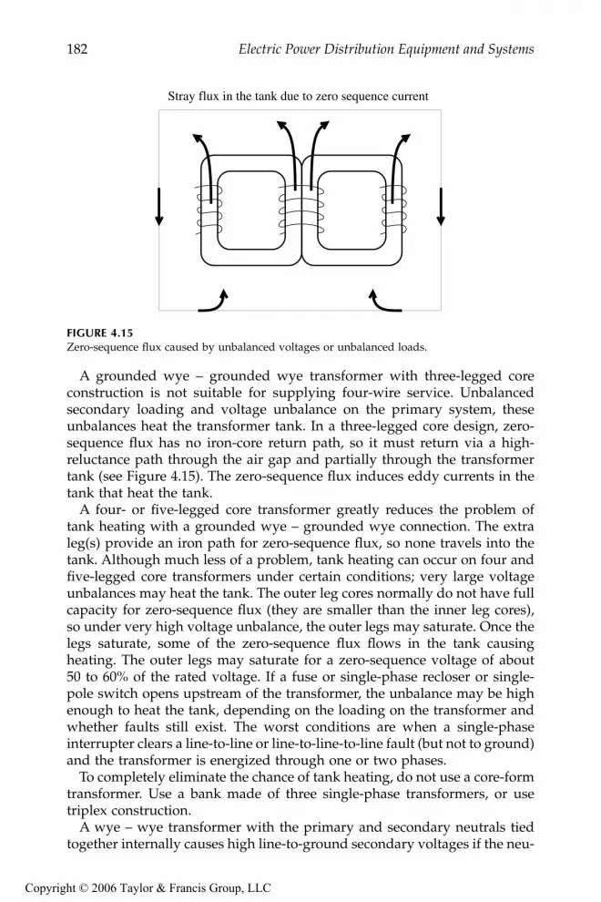
182 Electric Power Distribution Equipment and Systems
A grounded wye – grounded wye transformer with three-legged coreconstruction is not suitable for supplying four-wire service. Unbalancedsecondary loading and voltage unbalance on the primary system, theseunbalances heat the transformer tank. In a three-legged core design, zero-sequence flux has no iron-core return path, so it must return via a high-reluctance path through the air gap and partially through the transformertank (see Figure 4.15). The zero-sequence flux induces eddy currents in thetank that heat the tank.
A four- or five-legged core transformer greatly reduces the problem oftank heating with a grounded wye – grounded wye connection. The extraleg(s) provide an iron path for zero-sequence flux, so none travels into thetank. Although much less of a problem, tank heating can occur on four andfive-legged core transformers under certain conditions; very large voltageunbalances may heat the tank. The outer leg cores normally do not have fullcapacity for zero-sequence flux (they are smaller than the inner leg cores),so under very high voltage unbalance, the outer legs may saturate. Once thelegs saturate, some of the zero-sequence flux flows in the tank causingheating. The outer legs may saturate for a zero-sequence voltage of about50 to 60% of the rated voltage. If a fuse or single-phase recloser or single-pole switch opens upstream of the transformer, the unbalance may be highenough to heat the tank, depending on the loading on the transformer andwhether faults still exist. The worst conditions are when a single-phaseinterrupter clears a line-to-line or line-to-line-to-line fault (but not to ground)and the transformer is energized through one or two phases.
To completely eliminate the chance of tank heating, do not use a core-formtransformer. Use a bank made of three single-phase transformers, or usetriplex construction.
A wye – wye transformer with the primary and secondary neutrals tiedtogether internally causes high line-to-ground secondary voltages if the neu-
FIGURE 4.15Zero-sequence flux caused by unbalanced voltages or unbalanced loads.
Stray flux in the tank due to zero sequence current
9576_C04.fm Page 182 Monday, October 17, 2005 9:12 AM
Copyright © 2006 Taylor & Francis Group, LLC

Transformers 183
tral is not grounded. This connection cannot supply three-wire ungroundedservice. Three-phase padmounted transformers with an H0X0 bushing havethe neutrals bonded internally. If the H0X0 bushing is floated, high voltagescan occur from phase to ground on the secondary.
To supply ungrounded secondary service with a grounded-wye primary,use a grounded wye – floating wye connection: the secondary should befloating wye with no connection between the primary and secondary neu-tral points.
4.4.2 Delta – Grounded Wye
The delta – grounded wye connection has several interesting features, manyrelated to its delta winding, which establishes a local grounding referenceand blocks zero-sequence currents from entering the primary.
• Supply — 3-wire or 4-wire system.• Service
• Supplies grounded-wye service, normally either 480Y/277 V or208Y/120 V.
• Cannot supply both 120 and 240 V.• Does not supply ungrounded service.
• Ground faults — This connection blocks zero sequence, so upstreamground relays are isolated from line-to-ground faults on the second-ary of the customer transformer.
• Harmonics — The delta winding isolates the primary from zero-sequence harmonics created on the secondary. Third harmonics andother zero-sequence harmonics cannot get through to the primary(they circulate in the delta winding).
• No primary ground source — For line-to-ground faults on the primary,the delta – grounded wye connection cannot act as a groundingsource.
• Secondary ground source — Provides a grounding source for the sec-ondary, independent of the primary-side grounding configuration.
• No tank heating — The delta connection ensures that zero-sequenceflux will not flow in the transformer’s core. We can safely use a three-legged core transformer.
• Ferroresonance — Highly susceptible.
4.4.3 Floating Wye – Delta
The floating-wye – delta connection is popular for supplying ungroundedservice and 120/240-V service. This type of connection may be used from
9576_C04.fm Page 183 Monday, October 17, 2005 9:12 AM
Copyright © 2006 Taylor & Francis Group, LLC

184 Electric Power Distribution Equipment and Systems
either a grounded or ungrounded distribution primary. The main character-istics of this supply are:
• Supply — 3-wire or 4-wire system.• Service
• Can supply ungrounded service.• Can supply four-wire service with 240/120-V on one leg with a
midtapped ground.• Cannot supply grounded-wye four-wire service.
• Unit failure — Can continue to operate if one unit fails if it is rewiredas an open wye – open delta.
• Voltage unbalance — Secondary-side unbalances are more likely thanwith a wye secondary connection.
• Ferroresonance — Highly susceptible.
Do not use single-phase transformers with secondary breakers (CSPs) inthis connection. If one secondary breaker opens, it breaks the delta on thesecondary. Now, the primary neutral can shift wildly. The transformer maybe severely overloaded by load unbalance or single phasing on the primary.
Facilities should ensure that single-phase loads only connect to the lightingleg; any miswired loads have overvoltages. The phase-to-neutral connectionfrom the neutral to the opposite phase (where both power legs cometogether) is 208 V on a 240/120-V system.
The floating wye – delta is best used when supplying mainly three-phaseload with a smaller amount of single-phase load. If the single-phase load islarge, the three transformers making up the connection are not used asefficiently, and voltage unbalances can be high on the secondary.
In a conservative loading guideline, size the lighting transformer to supplyall of the single-phase load plus 1/3 of the three-phase load (ANSI/IEEEC57.105-1978). Size each power leg to carry 1/3 of the three-phase load plus1/3 of the single-phase load. ABB (1995) describes more accurate loadingequations:
Lighting leg loading in kVA:
Lagging power leg loading in kVA:
Leading power leg loading in kVA:
kVA k k k kbc = + +13
4 432
12
3 1 cosα
kVA k k k kca = + − ° +( )13
2 12032
12
3 1 cos α
9576_C04.fm Page 184 Monday, October 17, 2005 9:12 AM
Copyright © 2006 Taylor & Francis Group, LLC

Transformers 185
wherek1 = single-phase load, kVAk3 = balanced three-phase load, kVAα = θ3 – θ1
θ3 = phase angle in degrees for the three-phase loadθ1 = phase angle in degrees for the single-phase load
For wye – delta connections, the wye on the primary is normally inten-tionally ungrounded. If it is grounded, it creates a grounding bank. This isnormally undesirable because it may disrupt the feeder protection schemesand cause excessive circulating current in the delta winding. Utilities some-times use this connection as a grounding source or for other unusual reasons.
Delta secondary windings are more prone to voltage unbalance problemsthan a wye secondary winding (Smith et al., 1988). A balanced three-phaseload can cause voltage unbalance if the impedances of each leg are different.With the normal practice of using a larger lighting leg, the lighting leg hasa lower impedance. Voltage unbalance is worse with longer secondaries andhigher impedance transformers. High levels of single-phase load also aggra-vate unbalances.
4.4.4 Other Common Connections
4.4.4.1 Delta – Delta
The main features and drawbacks of the delta – delta supply are:
• Supply — 3-wire or 4-wire system.• Service
• Can supply ungrounded service.• Can supply four-wire service with 240/120-V on one leg with a
midtapped ground.• Cannot supply grounded-wye four-wire service.
• Ferroresonance — Highly susceptible.• Unit failure — Can continue to operate if one unit fails (as an open
delta – open delta).• Circulating current — Has high circulating current if the turns ratios
of each unit are not equal.
A delta – delta transformer may have high circulating current if any of thethree legs has unbalance in the voltage ratio. A delta winding forms a series
kVA k k k kab = + − ° −( )13
2 12032
12
3 1 cos α
9576_C04.fm Page 185 Monday, October 17, 2005 9:12 AM
Copyright © 2006 Taylor & Francis Group, LLC

186 Electric Power Distribution Equipment and Systems
loop. Two windings are enough to fix the three phase-to-phase voltage vec-tors. If the third winding does not have the same voltage as that created bythe series sum of the other two windings, large circulating currents flow tooffset the voltage imbalance. ANSI/IEEE C57.105-1978 provides an examplewhere the three phase-to-phase voltages summed to 1.5% of nominal asmeasured at the open corner of the delta winding (this voltage should bezero for no circulating current). With a 5% transformer impedance, a currentequal to 10% of the transformer rating circulates in the delta when the opencorner is connected. The voltage sees an impedance equal to the three wind-ing impedances in series, resulting in a circulating current of 100% × 1.5%/ (3×5%) = 10%. This circulating current directly adds to one of the threewindings, possibly overloading the transformer.
Single-phase units with secondary breakers (CSPs) should not be used forthe lighting leg. If the secondary breaker on the lighting leg opens, the loadloses its neutral reference, but the phase-to-phase voltages are maintainedby the other two legs (like an open delta – open delta connection). As withthe loss of the neutral connection to a single-phase 120/240-V customer,unbalanced single-phase loads shift the neutral and create low voltages onone leg and high voltages on the lightly loaded leg.
4.4.4.2 Open Wye – Open Delta
The main advantage of the open wye – open delta transformer configurationis that it can supply three-phase load from a two-phase supply (but thesupply must have a neutral).
The main features and drawbacks of the open wye – delta supply are:
• Supply — 2 phases and the neutral of a 4-wire grounded system.• Service
• Can supply ungrounded service.• Can supply four-wire service with 240/120-V on one leg with a
midtapped ground.• Cannot supply grounded-wye four-wire service.
• Ferroresonance — Immune.• Voltage unbalance — May have high secondary voltage unbalance.• Primary ground current — Creates high primary-side current unbal-
ance. Even with balanced loading, high currents are forced into theprimary neutral.
Open wye – open delta connections are most efficiently applied when theload is predominantly single phase with some three-phase load, using onelarge lighting-leg transformer and another smaller unit. This connection iseasily upgraded if the customer’s three-phase load grows by adding a secondpower-leg transformer.
9576_C04.fm Page 186 Monday, October 17, 2005 9:12 AM
Copyright © 2006 Taylor & Francis Group, LLC

Transformers 187
For sizing each bank, size the power leg for 1/ = 0.577 times thebalanced three-phase load, and size the lighting leg for all of the single-phaseload plus 0.577 times the three-phase load (ANSI/IEEE C57.105-1978). Thefollowing equations more accurately describe the split in loading on the twotransformers (ABB, 1995). The load on the lighting leg in kVA is
for a leading lighting leg
for a lagging lighting leg
The power leg loading in kVA is:
wherek1 = single-phase load, kVAk3 = balanced three-phase load, kVAα = θ3 – θ1
θ3 = phase angle in degrees for the three-phase loadθ1 = phase angle in degrees for the single-phase load
The lighting leg may be on the leading or lagging leg. In the open wye –open delta connection shown in Figure 4.13, the single-phase load is on theleading leg. For a lagging connection, switch the lighting and the power leg.Having the lighting connection on the leading leg reduces the loading onthe lighting leg. Normally, the power factor of the three-phase load is lessthan that of the single-phase load, so α is positive, which reduces the loadingon the lighting leg.
On the primary side, it is important that the two high-voltage primaryconnections are not made to the same primary phase. If this is accidentallydone, the phase-to-phase voltage across the open secondary is two times thenormal phase-to-phase voltage.
The open wye – open delta connection injects significant current into theneutral on the four-wire primary. Even with a balanced three-phase load,significant current is forced into the ground as shown in Figure 4.16. Theextra unbalanced current can cause primary-side voltage unbalance and maytrigger ground relays.
Open-delta secondary windings are very prone to voltage unbalance,which can cause excessive heating in end-use motors (Smith et al., 1988).Even balanced three-phase loads significantly unbalance the voltages. Volt-age unbalance is less with lower-impedance transformers. Voltage unbalance
3
kVAk
kk k
L = + + + °( )32
12 3 1
32
330cos α
kVAk
kk k
L = + + − °( )32
12 3 1
32
330cos α
kVAk
L = 3
3
9576_C04.fm Page 187 Monday, October 17, 2005 9:12 AM
Copyright © 2006 Taylor & Francis Group, LLC

188 Electric Power Distribution Equipment and Systems
reduces significantly if the connection is upgraded to a floating wye – closeddelta connection. In addition, the component of the negative-sequence volt-age on the primary (which is what really causes motor heating) can add tothat caused by the transformer configuration to sometimes cause a negative-sequence voltage above 5% (which is a level that significantly increasesheating in a three-phase induction motor).
While an unusual connection, it is possible to supply a balanced, groundedfour-wire service from an open-wye primary. This connection (open wye –partial zig-zag) can be used to supply 208Y/120-V service from a two-phaseline. One of the 120/240-V transformers must have four bushings; X2 andX3 are not tied together but connected as shown in Figure 4.17. Each of thetransformers must be sized to supply 2/3 of the balanced three-phase load.If four-bushing transformers are not available, this connection can be madewith three single-phase transformers. Instead of the four-bushing trans-former, two single-phase transformers are placed in parallel on the primary,and the secondary terminals of each are configured to give the arrangementin Figure 4.17.
FIGURE 4.16Current flow in an open wye – open delta transformer with balanced three-phase load.
FIGURE 4.17Quasiphasor diagram of an open-wye primary connection supplying a wye four-wire neutralservice such as 208Y/120 V. (From ANSI/IEEE Std. C57.105-1978. Copyright 1978 IEEE. Allrights reserved.)
1 pu
1 pu
1 pu
1.73 pu
3 pu
1.73 pu
Neutral
H1 H1
H2
X1 X1
X3X4
X2
9576_C04.fm Page 188 Monday, October 17, 2005 9:12 AM
Copyright © 2006 Taylor & Francis Group, LLC

Transformers 189
4.4.4.3 Other Suitable Connections
While not as common, several other three-phase connections are used attimes:
• Open delta – Open delta — Can supply a three-wire ungroundedservice or a four-wire 120/240-V service with a midtapped groundon one leg of the transformer. The ungrounded high-side connectionis susceptible to ferroresonance. Only two transformers are needed,but it requires all three primary phases. This connection is less effi-cient for supplying balanced three-phase loads; the two units musttotal 115% of the connected load. This connection is most efficientlyapplied when the load is predominantly single phase with somethree-phase load, using one large lighting-leg transformer andanother smaller unit.
• Delta – Floating wye — Suitable for supplying a three-wireungrounded service. The ungrounded high-side connection is sus-ceptible to ferroresonance.
• Grounded wye – Floating wye — Suitable for supplying a three-wireungrounded service from a multigrounded primary system. Thegrounded primary-side connection reduces the possibility of fer-roresonance.
4.4.5 Neutral Stability with a Floating Wye
Some connections with a floating-wye winding have an unstable neutral,which we should avoid. Unbalanced single-phase loads on the secondary,unequal magnetizing currents, and suppression of third harmonics — allcan shift the neutral.
Consider a floating wye – grounded wye connection. In a wye – wye trans-former, the primary and secondary voltages have the same vector relation-ships. The problem is that the neutral point does not have a groundingsource; it is free to float. Unbalanced loads or magnetizing currents can shiftthe neutral and create high neutral-to-earth voltages and overvoltages onthe phases with less loading. The reverse connection with a grounded wye– floating wye works because the primary-side neutral is connected to thesystem neutral, which has a grounding source. The grounding source fixesthe neutral voltage.
In a floating wye, current in one branch is dependent on the currents in theother two branches. What flows in one branch must flow out the other twobranches. This creates conditions that shift the neutral (Blume et al., 1951):
• Unbalanced loads — Unequal single-phase loads shift the neutralpoint. Zero-sequence current has no path to flow (again, the groundsource is missing). Loading one phase drops the voltage on that
9576_C04.fm Page 189 Monday, October 17, 2005 9:12 AM
Copyright © 2006 Taylor & Francis Group, LLC

190 Electric Power Distribution Equipment and Systems
phase and raises the voltage on the other two phases. Even a smallunbalance significantly shifts the neutral.
• Unequal magnetizing currents — Just like unequal loads, differencesin the amount of magnetizing current each leg needs can shift thefloating neutral. In a four- or five-legged core, the asymmetry of thecore causes unequal magnetizing requirements on each phase.
• Suppression of third harmonics — Magnetizing currents contain sig-nificant third harmonics that are zero sequence. But, the floating wyeconnection has no ground source to absorb the zero-sequence cur-rents, so they are suppressed. The suppression of the zero-sequencecurrents generates a significant third-harmonic voltage in each wind-ing, about 50% of the phase voltage on each leg according to Blumeet al. (1951). With the neutral grounded in the floating wye –grounded wye, a significant third-harmonic voltage adds to eachphase-to-ground load. If the neutral is floating (on the wye–wyetransformer with the neutrals tied together), the third-harmonic volt-age appears between the neutral and ground.
In addition to the floating wye – grounded wye, avoid these problemconnections that have an unstable neutral:
• Grounded wye – grounded wye on a three-wire system — The grounded-wye on the primary does not have an effective grounding source,so it acts the same as a floating-wye – grounded-wye.
• A wye – wye transformer with the primary and secondary neutrals tiedtogether internally (the H0X0 bushing) but with the neutral left floating —Again, the neutral point can float. Unbalanced loading is not a prob-lem, but magnetizing currents and suppression of third harmonicsare. These can generate large voltages between the neutral point andground (and between the phase wires and ground). If the secondaryneutral is isolated from the primary neutral, each neutral settles to adifferent value. But when the secondary neutral is locked into theprimary neutral, the secondary neutral follows the neutral shift of theprimary and shifts the secondary phases relative to ground.
Another poor connection is the floating wye – floating wye. Although notas bad as the floating-wye – grounded-wye connection, the neutral can shiftif the connection is made of three units of different magnetizing character-istics. The neutral shift can lead to an overvoltage across one of the windings.Also, high harmonic voltage appears on the primary-side neutral (which isokay if the neutral is properly insulated from the tank).
Three-legged core transformers avoid some of the problems with a floatingwye. The phantom tertiary acts as a mini ground source, stabilizes theneutral, and even allows some unbalance of single-phase loads. But as itstabilizes the neutral, the unbalances heat the tank. Given that, it is best to
9576_C04.fm Page 190 Monday, October 17, 2005 9:12 AM
Copyright © 2006 Taylor & Francis Group, LLC

Transformers 191
avoid these transformer connections. They provide no features or advantagesover other transformer connections.
4.4.6 Sequence Connections of Three-Phase Transformers
The connection determines the effect on zero sequence, which impacts unbal-ances and response to line-to-ground faults and zero-sequence harmonics.Figure 4.18 shows how to derive sequence connections along with commonexamples. In general, three-phase transformers may affect the zero-sequencecircuit as follows:
• Isolation — A floating wye – delta connection isolates the primaryfrom the secondary in the zero sequence.
• Pass through — The grounding of the grounded wye – grounded wyeconnection is determined by the grounding upstream of the trans-former.
• Ground source — A delta – grounded wye connection provides aground source on the secondary. (And, the delta – grounded wyeconnection also isolates the primary from the secondary.)
4.5 Loadings
Distribution transformers are output rated; they can deliver their rated kVAwithout exceeding temperature rise limits when the following conditions apply:
• The secondary voltage and the voltage/frequency do not exceed105% of rating. So, a transformer is a constant kVA device for avoltage from 100 to 105% (the standards are unclear below that, sotreat them as constant current devices).
• The load power factor ≥ 80%.• Frequency ≥ 95% of rating.
The transformer loading and sizing guidelines of many utilities are basedon ANSI/IEEE C57.91-1981.
Modern distribution transformers are 65°C rise units, meaning they havenormal life expectancy when operated with an average winding temperaturerise above ambient of not more than 65°C and a hottest spot winding tem-perature rise of not more than 80°C. Some older units are 55°C rise units,which have less overloading capability.
At an ambient temperature of 30°C, the 80°C hottest-spot rise for 65°C riseunits gives a hottest-spot winding temperature of 110°C. The hot-spot tem-
9576_C04.fm Page 191 Monday, October 17, 2005 9:12 AM
Copyright © 2006 Taylor & Francis Group, LLC

192 Electric Power Distribution Equipment and Systems
FIGURE 4.18Zero-sequence connections of various three-phase transformer connections.
H winding L winding
Common connections Zero-sequence diagram
H
T
3-legged core (acts as a high-impedance tertiary)
Tertiary winding
Zero-sequence diagram
ZH
ZH
ZH
ZH
ZH
ZH
ZH
ZL
ZL
ZL
ZL
ZL
ZL
ZL
ZT
ZG
3ZG
5 ZH ZL
Shorted for a grounded-wye winding
Impedance of 3ZG for for a wye winding grounded through an impedance ZG
Open for a floating-wye winding
Open with a short to ground on the inside point for a delta winding
L
9576_C04.fm Page 192 Monday, October 17, 2005 9:12 AM
Copyright © 2006 Taylor & Francis Group, LLC

Transformers 193
perature on the winding is critical; that’s where insulation degrades. Theinsulation’s life exponentially relates to hot-spot winding temperature asshown in Figure 4.19. At 110°C, the normal life expectancy is 20 years.Because of daily and seasonal load cycles, most of the time temperatures arenowhere near these values. Most of the time, temperatures are low enoughnot to do any significant insulation degradation. We can even run at tem-peratures above 110°C for short periods. For the most economic operationof distribution transformers, they are normally sized to operate at significantoverloads for short periods of the year.
We can load distribution transformers much more heavily when it is cold.Locations with winter-peaking loads can have smaller transformers for agiven loading level. The transformer’s kVA rating is based on an ambienttemperature of 30°C. For other temperatures, ANSI/IEEE C57.91-1981 sug-gests the following adjustments to loading capability:
• > 30°C: decrease loading capability by 1.5% of rated kVA for each°C above 30°C.
• < 30°C: increase loading capability by 1% of rated kVA for each °Cabove 30°C.
Ambient temperature estimates for a given region can be found usinghistorical weather data. For loads with normal life expectancy, ANSI/IEEEC57.91-1981 recommends the following estimate of ambient temperature:
• Average daily temperature for the month involved — As an approxima-tion, the average can be approximated as the average of the dailyhighs and the daily lows.
FIGURE 4.19Transformer life as a function of the hottest-spot winding temperature.
80 100 120
10.0
100.0
T Hottest-spot temperature, C
l=
Nor
mal
life
expe
ctan
cy,y
ears
l106328 8 T 273 11 269
8766
9576_C04.fm Page 193 Monday, October 17, 2005 9:12 AM
Copyright © 2006 Taylor & Francis Group, LLC

194 Electric Power Distribution Equipment and Systems
For short-time loads where we are designing for a moderate sacrifice oflife, use:
• Maximum daily temperature
In either case, the values should be averaged over several years for the monthinvolved. C57.91-1981 also suggests adding 5°C to be conservative. Thesevalues are for outdoor overhead or padmounted units. Transformersinstalled in vaults or other cases with limited air flow may require someadjustments.
Transformers should also be derated for altitudes above 3300 ft (1000 m).At higher altitudes, the decreased air density reduces the heat conductedaway from the transformer. ANSI/IEEE C57.91-1981 recommends deratingby 0.4% for each 330 ft (100 m) that the altitude is above 3300 ft (1000 m).
Load cycles play an important role in determining loading. ANSI/IEEEC57.91-1981 derives an equivalent load cycle with two levels: the peak loadand the initial load. The equivalent two-step load cycle may be derived froma more detailed load cycle. The guide finds a continuous load and a short-duration peak load. Both are found using the equivalent load value from amore complicated load cycle:
whereL = equivalent load in percent, per unit, or actual kVAL1, L2, …, = The load steps in percent, per unit, or actual kVAt1, t2, …, = The corresponding load durations
The continuous load is the equivalent load found using the equation abovefor 12 h preceding and 12 h following the peak and choosing the higher ofthese two values. The guide suggests using 1-h time blocks. The peak is theequivalent load from the equation above where the irregular peak exists.
The C57.91 guide has loading guidelines based on the peak duration andcontinuous load prior to the peak. Table 4.8 shows that significant overloadsare allowed depending on the preload and the duration of the peak.
Because a region’s temperature and loading patterns vary significantly,there is no universal transformer application guideline. Coming up withstandardized tables for initial loading is based on a prediction of peak load,which for residential service normally factors in the number of houses, aver-age size (square footage), central air conditioner size, and whether electricheat is used. Once the peak load is estimated, it is common to pick a trans-former with a kVA rating equal to or greater than the peak load kVA estimate.With this arrangement, some transformers may operate significantly abovetheir ratings for short periods of the year. Load growth can push the peak
LL t L t L t L t
t t t tn n
n
=+ + + +
+ + + +12
1 22
2 32
32
1 2 3
L
L
9576_C04.fm Page 194 Monday, October 17, 2005 9:12 AM
Copyright © 2006 Taylor & Francis Group, LLC
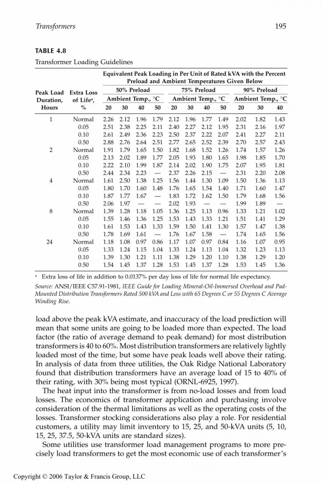
Transformers 195
load above the peak kVA estimate, and inaccuracy of the load prediction willmean that some units are going to be loaded more than expected. The loadfactor (the ratio of average demand to peak demand) for most distributiontransformers is 40 to 60%. Most distribution transformers are relatively lightlyloaded most of the time, but some have peak loads well above their rating.In analysis of data from three utilities, the Oak Ridge National Laboratoryfound that distribution transformers have an average load of 15 to 40% oftheir rating, with 30% being most typical (ORNL-6925, 1997).
The heat input into the transformer is from no-load losses and from loadlosses. The economics of transformer application and purchasing involveconsideration of the thermal limitations as well as the operating costs of thelosses. Transformer stocking considerations also play a role. For residentialcustomers, a utility may limit inventory to 15, 25, and 50-kVA units (5, 10,15, 25, 37.5, 50-kVA units are standard sizes).
Some utilities use transformer load management programs to more pre-cisely load transformers to get the most economic use of each transformer’s
TABLE 4.8
Transformer Loading Guidelines
Peak LoadDuration,
Hours
Extra Lossof Lifea,
%
Equivalent Peak Loading in Per Unit of Rated kVA with the Percent Preload and Ambient Temperatures Given Below
50% Preload 75% Preload 90% PreloadAmbient Temp., °C Ambient Temp., °C Ambient Temp., °C20 30 40 50 20 30 40 50 20 30 40
1 Normal 2.26 2.12 1.96 1.79 2.12 1.96 1.77 1.49 2.02 1.82 1.430.05 2.51 2.38 2.25 2.11 2.40 2.27 2.12 1.95 2.31 2.16 1.970.10 2.61 2.49 2.36 2.23 2.50 2.37 2.22 2.07 2.41 2.27 2.110.50 2.88 2.76 2.64 2.51 2.77 2.65 2.52 2.39 2.70 2.57 2.43
2 Normal 1.91 1.79 1.65 1.50 1.82 1.68 1.52 1.26 1.74 1.57 1.260.05 2.13 2.02 1.89 1.77 2.05 1.93 1.80 1.65 1.98 1.85 1.700.10 2.22 2.10 1.99 1.87 2.14 2.02 1.90 1.75 2.07 1.95 1.810.50 2.44 2.34 2.23 — 2.37 2.26 2.15 — 2.31 2.20 2.08
4 Normal 1.61 2.50 1.38 1.25 1.56 1.44 1.30 1.09 1.50 1.36 1.130.05 1.80 1.70 1.60 1.48 1.76 1.65 1.54 1.40 1.71 1.60 1.470.10 1.87 1.77 1.67 — 1.83 1.72 1.62 1.50 1.79 1.68 1.560.50 2.06 1.97 — — 2.02 1.93 — — 1.99 1.89 —
8 Normal 1.39 1.28 1.18 1.05 1.36 1.25 1.13 0.96 1.33 1.21 1.020.05 1.55 1.46 1.36 1.25 1.53 1.43 1.33 1.21 1.51 1.41 1.290.10 1.61 1.53 1.43 1.33 1.59 1.50 1.41 1.30 1.57 1.47 1.380.50 1.78 1.69 1.61 — 1.76 1.67 1.58 — 1.74 1.65 1.56
24 Normal 1.18 1.08 0.97 0.86 1.17 1.07 0.97 0.84 1.16 1.07 0.950.05 1.33 1.24 1.15 1.04 1.33 1.24 1.13 1.04 1.32 1.23 1.130.10 1.39 1.30 1.21 1.11 1.38 1.29 1.20 1.10 1.38 1.29 1.200.50 1.54 1.45 1.37 1.28 1.53 1.45 1.37 1.28 1.53 1.45 1.36
a Extra loss of life in addition to 0.0137% per day loss of life for normal life expectancy.
Source: ANSI/IEEE C57.91-1981, IEEE Guide for Loading Mineral-Oil-Immersed Overhead and Pad-Mounted Distribution Transformers Rated 500 kVA and Less with 65 Degrees C or 55 Degrees C AverageWinding Rise.
9576_C04.fm Page 195 Monday, October 17, 2005 9:12 AM
Copyright © 2006 Taylor & Francis Group, LLC

196 Electric Power Distribution Equipment and Systems
life. These programs take billing data for the loads from each transformerto estimate that transformer’s loading. These programs allow the utility tomore aggressively load transformers because those needing changeout canbe targeted more precisely. Load management programs require data setupand maintenance. Most important, each meter must be tied to a giventransformer (many utilities have this information infrastructure, but somedo not).
Transformer loadings vary considerably. Figure 4.20 shows the distribu-tion of average loadings on two sizes of transformers at one typical utility.Most transformers are not heavily loaded: in this case, 85% of units haveaverage loadings less than the nameplate. Many units are very lightlyloaded, and 10% are quite heavily loaded. Smaller units have more spreadin their loading.
Seevers (1995) demonstrates a simple approach to determining trans-former loading. Their customers (in the southern U.S.) had 1 kW of demandfor every 400 kWh’s, regardless of whether the loads peaked in the winteror summer. Seevers derived the ratio by comparing substation demand withkWh totals for all customers fed from the substation (after removing pri-mary-metered customers and other large loads). To estimate the load on agiven transformer, sum the kWh for the month of highest usage for allcustomers connected to the transformer and convert to peak demand, in thiscase by dividing by 400 kWh per kW-demand. While simple, this methodidentifies grossly undersized or oversized transformers. Table 4.9 showsguidelines for replacement of underloaded transformers.
Transformers with an internal secondary breaker (CSPs) are a poor-man’sform of transformer load management. If the breaker trips from overload,replace the transformer (unless there are extraordinary weather and loadingconditions that are unlikely to be repeated).
FIGURE 4.20Distributions of average loadings of two transformer sizes at one utility. (From [ORNL-6927,1998])
0.0 0.5 1.0 1.5
25 kVA 100 kVA
0
25
50
75
100
Average loading, per unit
Perc
ent o
f tr
ansf
orm
ers
exce
edin
g th
e x-
axis
val
ue
9576_C04.fm Page 196 Monday, October 17, 2005 9:12 AM
Copyright © 2006 Taylor & Francis Group, LLC

Transformers 197
Especially in high-lightning areas, consider the implications of reductionof insulation capability. At hottest-spot temperatures above 140°C, the solidinsulation and the oil may release gasses. While not permanently reducinginsulation, the short-term loss of insulation strength can make the trans-former susceptible to damage from lightning-caused voltage surges. Thethermal time constant of the winding is very short, 5 to 15 min. On this timescale, loads on distribution transformers are quite erratic with large, short-duration overloads (well above the 20- or 30-min demand loadings). Theseloads can push the winding hottest-spot temperature above 140°C.
Padmounted transformers have a special concern related to loading: casetemperatures. Under heavy loading on a hot day, case temperatures canbecome hot. ABB measured absolute case temperatures of 185 to 200°F (85to 95°C) and case temperature rises above ambient of 50 to 60°C on 25 and37.5-kVA transformers at 180% loadings and on a 50-kVA transformer at150% continuous load (NRECA RER Project 90-8, 1993). The hottest temper-atures were on the sides of the case where the oil was in contact with thecase (the top of the case was significantly cooler). While these temperaturessound quite high, a person’s pain-withdrawal reflexes will normally protectagainst burns for normal loadings that would be encountered. Reflexes willprotect against blistering and burning for case temperatures below 300°F(149°C). Skin contacts must be quite long before blistering occurs. For a casetemperature of 239°F (115°C), NRECA reported that the skin-contact time toblister is 6.5 sec (which is more than enough time to pull away). At 190°F(88°C), the contact time to blister is 19 sec.
4.6 Losses
Transformer losses are an important purchase criteria and make up an appre-ciable portion of a utility’s overall losses. The Oak Ridge National Laboratoryestimates that distribution transformers account for 26% of transmission and
TABLE 4.9
One Approach to a Transformer Replacement Program
Existing Transformer kVA Loading Estimate in kVA Recommended Size in kVA
25 10 or less 1037.5 15 or less 1050 20 or less 1575 37.5 or less 37.5
100 50 or less 50167 100 or less 100
75 or less 75 or 50
Source: Seevers, O. C., Management of Transmission and Distribution Systems, Penn WellPublishing Company, Tulsa, OK, 1995.
9576_C04.fm Page 197 Monday, October 17, 2005 9:12 AM
Copyright © 2006 Taylor & Francis Group, LLC

198 Electric Power Distribution Equipment and Systems
distribution losses and 41% of distribution and subtransmission losses(ORNL-6804/R1, 1995). At one utility, Grainger and Kendrew (1989) esti-mated that distribution transformers were 55% of distribution losses and2.14% of electricity sales; of the two main contributors to losses, 86% wereno-load losses, and 14% were load losses.
Load losses are also called copper or wire or winding losses. Load lossesare from current through the transformer’s windings generating heatthrough the winding resistance as I2R.
No-load losses are the continuous losses of a transformer, regardless ofload. No-load losses for modern silicon-steel-core transformers averageabout 0.2% of the transformer rating (a typical 50-kVA transformer has no-load losses of 100 W), but designs vary from 0.15 to 0.4% depending on theneeds of the utility. No-load losses are also called iron or core losses becausethey are mainly a function of the core materials. The two main componentsof no-load losses are eddy currents and hysteresis. Hysteresis describes thememory of a magnetic material. More force is necessary to demagnetizemagnetic material than it takes to magnetize it; the magnetic domains in thematerial resist realignment. Eddy current losses are small circulating cur-rents in the core material. The steel core is a conductor that carries analternating magnetic field, which induces circulating currents in the core.These currents through the resistive conductor generate heat and losses.Cores are typically made from cold-rolled, grain-oriented silicon steel lam-inations. Manufacturers limit eddy currents by laminating the steel core in9- to 14-mil thick layers, each insulated from the other. Core losses increasewith steady-state voltage.
Hysteresis losses are a function of the volume of the core, the frequency,and the maximum flux density (Sankaran, 2000):
whereVe = volume of the core
f = frequencyB = maximum flux density
The eddy-current losses are a function of core volume, frequency, fluxdensity, lamination thicknesses, and resistivity of the core material (Sanka-ran, 2000):
wheret = thickness of the laminationsr = resistivity of the core material
P V f B h e.∝ 1 6
P V B f t re e ∝ 2 2 2
9576_C04.fm Page 198 Monday, October 17, 2005 9:12 AM
Copyright © 2006 Taylor & Francis Group, LLC
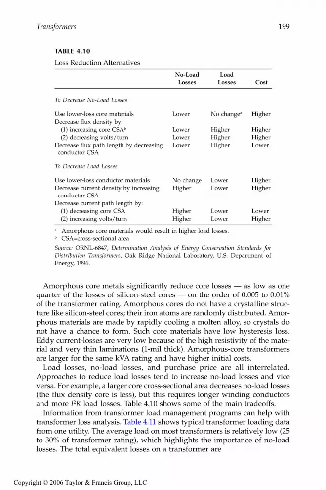
Transformers 199
Amorphous core metals significantly reduce core losses — as low as onequarter of the losses of silicon-steel cores — on the order of 0.005 to 0.01%of the transformer rating. Amorphous cores do not have a crystalline struc-ture like silicon-steel cores; their iron atoms are randomly distributed. Amor-phous materials are made by rapidly cooling a molten alloy, so crystals donot have a chance to form. Such core materials have low hysteresis loss.Eddy current-losses are very low because of the high resistivity of the mate-rial and very thin laminations (1-mil thick). Amorphous-core transformersare larger for the same kVA rating and have higher initial costs.
Load losses, no-load losses, and purchase price are all interrelated.Approaches to reduce load losses tend to increase no-load losses and viceversa. For example, a larger core cross-sectional area decreases no-load losses(the flux density core is less), but this requires longer winding conductorsand more I2R load losses. Table 4.10 shows some of the main tradeoffs.
Information from transformer load management programs can help withtransformer loss analysis. Table 4.11 shows typical transformer loading datafrom one utility. The average load on most transformers is relatively low (25to 30% of transformer rating), which highlights the importance of no-loadlosses. The total equivalent losses on a transformer are
TABLE 4.10
Loss Reduction Alternatives
No-LoadLosses
LoadLosses Cost
To Decrease No-Load Losses
Use lower-loss core materials Lower No changea HigherDecrease flux density by:
(1) increasing core CSAb Lower Higher Higher(2) decreasing volts/turn Lower Higher Higher
Decrease flux path length by decreasingconductor CSA
Lower Higher Lower
To Decrease Load Losses
Use lower-loss conductor materials No change Lower HigherDecrease current density by increasing conductor CSA
Higher Lower Higher
Decrease current path length by:(1) decreasing core CSA Higher Lower Lower(2) increasing volts/turn Higher Lower Higher
a Amorphous core materials would result in higher load losses.b CSA=cross-sectional area
Source: ORNL-6847, Determination Analysis of Energy Conservation Standards forDistribution Transformers, Oak Ridge National Laboratory, U.S. Department ofEnergy, 1996.
9576_C04.fm Page 199 Monday, October 17, 2005 9:12 AM
Copyright © 2006 Taylor & Francis Group, LLC

200 Electric Power Distribution Equipment and Systems
whereLtotal = average losses, kW (multiply this by 8760 to find the annual kilo-
watt-hours)P = peak transformer load, per unit
Fls = loss factor, per unitLno-load = rated no-load losses, kW
Lload = rated load losses, kW
Many utilities evaluate the total life-cycle cost of distribution transformers,accounting for the initial purchase price and the cost of losses over the lifeof the transformer (the total owning cost or TOC). The classic work done byGangel and Propst (1965) on transformer loads and loss evaluation providesthe foundation for much of the later work. Many utilities follow the EdisonElectric Association’s economic evaluation guidelines (EEI, 1981). To evalu-ate the total owning cost, the utility’s cost of losses are evaluated usingtransformer loading assumptions, including load factor, coincident factor,and responsibility factor. Utilities typically assign an equivalent presentvalue for the costs of no-load losses and another for the cost of load losses.Loss values typically range from $2 to $4/W of no-load losses and $0.50 to$1.50/W of load losses (ORNL-6847, 1996). Utilities that evaluate the lifecosts of transformers purchase lower-loss transformers. For example, a 50-
TABLE 4.11
Summary of the Loading of One Utility’s Single-Phase Pole-Mounted Distribution Transformers
Size(kVA)
No. ofInstalled
TransformersMWh/
TransformerAnnual PUAvg. Load
Annual PULoad Factor
CalculatedLoss Factor
10 59,793 21 0.267 0.405 0.20015 106,476 34 0.292 0.430 0.22125 118,584 60 0.309 0.444 0.23437 77,076 96 0.329 0.445 0.23550 50,580 121 0.308 0.430 0.22275 24,682 166 0.281 0.434 0.225
100 8,457 220 0.280 0.463 0.252167 3,820 372 0.283 0.516 0.304250 592 631 0.320 0.568 0.360333 284 869 0.331 0.609 0.407500 231 1,200 0.304 0.598 0.394667 9 1,666 0.317 0.476 0.264833 51 2,187 0.333 0.629 0.431
Note: PU = per unit
Source: ORNL-6925, Supplement to the “Determination Analysis” (ORNL-6847) and Anal-ysis of the NEMA Efficiency Standard for Distribution Transformers, Oak Ridge NationalLaboratory, U.S. Department of Energy, 1997.
L P F L Ltotal ls load no load= + −2
9576_C04.fm Page 200 Monday, October 17, 2005 9:12 AM
Copyright © 2006 Taylor & Francis Group, LLC

Transformers 201
kVA single-phase, non-loss-evaluated transformer would have approxi-mately 150 W of no-load losses and 675 W of load losses; the same loss-evaluated transformer would have approximately 100 W of no-load lossesand 540 W of load losses (ORNL-6925, 1997). Nickel (1981) describes aneconomic approach in detail and compares it to the EEI method. The IEEEhas developed a more recent guide (C57.12.33).
4.7 Network Transformers
Network transformers, the distribution transformers that serve grid and spotnetworks, are large three-phase units. Network units are normally vault-types or subway types, which are defined as (ANSI C57.12.40-1982):
• Vault-type transformers — Suitable for occasional submergedoperation
• Subway-type transformers — Suitable for frequent or continuous sub-merged operation
Network transformers are often housed in vaults. Vaults are undergroundrooms accessed through manholes that house transformers and other equip-ment. Vaults may have sump pumps to remove water, air venting systems,and even forced-air circulation systems. Network transformers are also usedin buildings, usually in the basement. In these, vault-type transformers maybe used (as long as the room is properly built and secured for such use).Utilities may also use dry-type units and units with less flammable insulat-ing oils.
A network transformer has a three-phase, primary-side switch that canopen, close, or short the primary-side connection to ground. The standardsecondary voltages are 216Y/125 V and 480Y/277 V. Table 4.12 shows stan-dard sizes. Transformers up to 1000 kVA have a 5% impedance; above 1000kVA, 7% is standard. X/R ratios are generally between 3 and 12. Lowerimpedance transformers (say 4%) have lower voltage drop and higher sec-ondary fault currents. (Higher secondary fault currents help on a networkto burn clear faults.) Lower impedance has a price though — higher circu-lating currents and less load balance between transformers. Network trans-
TABLE 4.12
Standard Network Transformer Sizes
Standard Ratings, kVA
216Y/125 V 300, 500, 750, 1000480Y/277 V 500, 750, 1000, 1500, 2000, 2500
9576_C04.fm Page 201 Monday, October 17, 2005 9:12 AM
Copyright © 2006 Taylor & Francis Group, LLC

202 Electric Power Distribution Equipment and Systems
formers may also be made out of standard single-phase distributiontransformers, but caution is warranted if the units have very low leakageimpedances (which could cause very high circulating currents and secondaryfault levels higher than network protector ratings).
Most network transformers are connected delta – grounded wye. By block-ing zero sequence, this connection keeps ground currents low on the primarycables. Then, we can use a very sensitive ground-fault relay on the substationbreaker. Blocking zero sequence also reduces the current on cable neutralsand cable sheaths, including zero-sequence harmonics, mainly the thirdharmonic. One disadvantage of this connection is with combination feeders— those that feed network loads as well as radial loads. For a primary line-to-ground fault, the feeder breaker opens, but the network transformers willcontinue to backfeed the fault until all of the network protectors operate(and some may stick). Now, the network transformers backfeed the primaryfeeder as an ungrounded circuit. An ungrounded circuit with a single line-to-ground fault on one phase causes a neutral shift that raises the line-to-neutral voltage on the unfaulted phases to line-to-line voltage. The non-network load connected phase-to-neutral is subjected to this overvoltage.
Some networks use grounded wye – grounded wye connections. Thisconnection fits better for combination feeders. For a primary line-to-groundfault, the feeder breaker opens. Backfeeds to the primary through the net-work still have a grounding reference with the wye – wye connection, sochances of overvoltages are limited. The grounded wye – grounded wyeconnection also reduces the change of ferroresonance in cases where a trans-former has single-pole switching.
Most network transformers are core type, either a three- or five-leggedcore. The three-legged core, either with a stacked or wound core, is suitablefor a delta – grounded wye connection (but not a grounded wye – groundedwye connection because of tank heating). A five-legged core transformer issuitable for either connection type.
4.8 Substation Transformers
In a distribution substation, power-class transformers provide the conver-sion from subtransmission circuits to the distribution primary. Most areconnected delta – grounded wye to provide a ground source for the distri-bution neutral and to isolate the distribution ground system from the sub-transmission system.
Station transformers can range from 5 MVA in smaller rural substations toover 80 MVA at urban stations (base ratings). Stations with two banks, eachabout 20 MVA, are common. Such a station can serve about six to eight feeders.
Power transformers have multiple ratings, depending on cooling methods.The base rating is the self-cooled rating, just due to the natural flow to the
9576_C04.fm Page 202 Monday, October 17, 2005 9:12 AM
Copyright © 2006 Taylor & Francis Group, LLC

Transformers 203
surrounding air through radiators. The transformer can supply more loadwith extra cooling turned on. Normally, fans blow air across the radiatorsand/or oil circulating pumps. Station transformers are commonly suppliedwith OA/FA/FOA ratings. The OA is open air, FA is forced air cooling, andFOA is forced air cooling plus oil circulating pumps.
The ANSI ratings were revised in the year 2000 to make them more con-sistent with IEC designations. This system has a four-letter code that indi-cates the cooling (IEEE C57.12.00-2000):
• First letter — Internal cooling medium in contact with the windings:• O mineral oil or synthetic insulating liquid with fire point = 300˚C
• K insulating liquid with fire point > 300˚C
• L insulating liquid with no measurable fire point
• Second letter — Circulation mechanism for internal cooling medium:
• N natural convection flow through cooling equipment and inwindings
• F forced circulation through cooling equipment (i.e., coolantpumps); natural convection flow in windings (also called nondi-rected flow)
• D forced circulation through cooling equipment, directed fromthe cooling equipment into at least the main windings
• Third letter — External cooling medium:
• A air
• W water
• Fourth letter — Circulation mechanism for external cooling medium:
• N natural convection
• F forced circulation: fans (air cooling), pumps (water cooling)
So, OA/FA/FOA is equivalent to ONAN/ONAF/OFAF. Each coolinglevel typically provides an extra one-third capability: 21/28/35 MVA. Table4.13 shows equivalent cooling classes in the old and new naming schemes.
Utilities do not overload substation transformers as much as distributiontransformers, but they do run them hot at times. As with distribution trans-formers, the tradeoff is loss of life versus the immediate replacement cost ofthe transformer. Ambient conditions also affect loading. Summer peaks aremuch worse than winter peaks. IEEE Std. C57.91-1995 provides detailedloading guidelines and also suggests an approximate adjustment of 1% ofthe maximum nameplate rating for every degree C above or below 30°C.The hottest spot conductor temperature is the critical point where insulationdegrades. Above a hot-spot conductor temperature of 110°C, life expectancydecreases exponentially. The life halves for every 8°C increase in operatingtemperature. Most of the time, the hottest temperatures are nowhere near
9576_C04.fm Page 203 Monday, October 17, 2005 9:12 AM
Copyright © 2006 Taylor & Francis Group, LLC

204 Electric Power Distribution Equipment and Systems
this. Tillman (2001) provides the loading guide for station transformersshown in Table 4.14.
The impedance of station transformers is normally about 7 to 10%. Thisis the impedance on the base rating, the self-cooled rating (OA or ONAN).The impedance is normally higher for voltages on the high-side of the trans-former that are higher (like 230 kV). Transformer impedance can be specifiedwhen ordering. Large stations with 50 plus MVA transformers are normallyprovided with extra impedance to control fault currents, some as high as30% on the transformer’s base rating.
The positive and zero-sequence impedances are the same for a shell-typetransformer, so the bolted fault currents on the secondary of the transformerare the same for a three-phase fault and for a line-to-ground fault (providedthat both are fed from an infinite bus). In a three-legged core type trans-former, the zero-sequence impedance is lower than the positive-sequenceimpedance (typically ), so ground faults can cause higher cur-rents. With a three-legged core transformer design, there is no path for zero-sequence flux. Therefore, zero-sequence current will meet a lower-imped-ance branch. This makes the core-type transformer act as if it had a delta-connected tertiary winding. This is the magnetizing branch (from line toground), and this effectively reduces the zero-sequence impedance. In ashell-type transformer, there is a path through the iron for flux to flow, sothe excitation impedance to zero sequence is high.
Because most distribution circuits are radial, the substation transformer isa critical component. Power transformers normally have a failure ratebetween 1 to 2% annually (CEA 485 T 1049, 1996; CIGRE working group12.05, 1983; IEEE Std. 493-1997). Many distribution stations are originallydesigned with two transformers, where each is able to serve all of the sub-station’s feeders if one of the transformers fails. Load growth in some areashas severely reduced the ability of one transformer to supply the wholestation. To ensure transformer reliability, use good lightning protection andthermal management. Do not use reduced-BIL designs (BIL is the basiclightning impulse insulation level). Also, reclosing and relaying practicesshould ensure that excessive through faults do not damage transformers.
TABLE 4.13
Equivalent Cooling Classes
Year 2000 DesignationsDesignations Prior
to Year 2000
ONAN OAONAF FAONAN/ONAF/ONAF OA/FA/FAONAN/ONAF/OFAF OA/FA/FOAOFAF FOAOFWF FOW
Source: IEEE Std. C57.12.00-2000. Copyright2000 IEEE. All rights reserved.
Z Z0 10 85 = .
9576_C04.fm Page 204 Monday, October 17, 2005 9:12 AM
Copyright © 2006 Taylor & Francis Group, LLC

Transformers 205
TABLE 4.14
Example Substation Transformer Loading Guide
Type of Load
FA (ONAF) NDFOA (OFAF)
Max% Load
Max TopOil Temp
(˚C)
Max TopOil Temp
(˚C)
MaxWinding Temp
(˚C)
Normal summer load 105 95 135 130Normal winter load 80 70 115 140Emergency summer load 115 105 150 140Emergency winter load 90 80 130 150Non-cyclical load 95 85 115 110
FA NDFOAAlarm Settings 65˚C Rise 65˚C Rise
Top Oil 105˚C 95˚CHot Spot 135˚C 135˚CLoad Amps 130% 130%
Notes: (1) The normal summer loading accounts for periods when temperatures areabnormally high. These might occur every 3 to 5 years. For every degree C thatthe normal ambient temperature during the hottest month of the year exceeds30˚C, de-rate the transformer 1% (i.e., 129% loading for 31˚C average ambient).(2) The % load is given on the basis of the current rating. For MVA loading,multiply by the per unit output voltage. If the output voltage is 0.92 per unit,the recommended normal summer MVA loading is 120%. (3) Exercise cautionif the load power factor is less than 0.95 lagging. If the power factor is less than0.92 lagging, then lower the recommended loading by 10% (i.e., 130 to 120%).(4) Verify that cooling fans and pumps are in good working order and oil levelsare correct. (5) Verify that the soil condition is good: moisture is less than 1.5%(1.0% preferred) by dry weight, oxygen is less than 2%, acidity is less than 0.5,and CO gas increases after heavy load seasons are not excessive. (6) Verify thatthe gauges are reading correctly when transformer loads are heavy. If correctfield measurements differ from manufacturer’s test report data, then investigatefurther before loading past nameplate criteria. (7) Verify with infrared cameraor RTD during heavy load periods that the LTC top oil temperature relative tothe main tank top oil temperature is correct. For normal LTC operation, theLTC top oil is cooler than the main tank top oil. A significant deviation fromthis indicates LTC abnormalities. (8) If the load current exceeds the bushingrating, do not exceed 110˚C top oil temperature (IEEE, 1995). If bushing size isnot known, perform an infrared scan of the bushing terminal during heavyload periods. Investigate further if the temperature of the top terminal cap isexcessive. (9) Use winding power factor tests as a measure to confirm theintegrity of a transformer’s insulation system. This gives an indication of mois-ture and other contaminants in the system. High BIL transformers require lowwinding power factors (<0.5%), while low BIL transformers can tolerate higherwinding power factors (<1.5%). (10) If the transformer is extremely dry (lessthan 0.5% by dry weight) and the load power factor is extremely good (0.99lag to 0.99 lead), then add 10% to the above recommendations.
Source: Tillman, R. F., Jr, “Loading Power Transformers,” in The Electric Power Engi-neering Handbook, L. L. Grigsby, Ed.: CRC Press, Boca Raton, FL, 2001.
9576_C04.fm Page 205 Monday, October 17, 2005 9:12 AM
Copyright © 2006 Taylor & Francis Group, LLC

206 Electric Power Distribution Equipment and Systems
4.9 Special Transformers
4.9.1 Autotransformers
An autotransformer is a winding on a core with a tap off the winding thatprovides voltage boost or buck. This is equivalent to a transformer with onewinding in series with another (see Figure 4.21).
For small voltage changes, autotransformers are smaller and less costlythan standard transformers. An autotransformer transfers much of the powerdirectly through a wire connection. Most of the current passes through thelower-voltage series winding at the top, and considerably less current flowsthrough the shunt winding.
Autotransformers have two main applications on distribution systems:
• Voltage regulators — A regulator is an autotransformer with adjust-able taps that is normally capable of adjusting the voltage by ±10%.
• Step banks — Autotransformers are often used instead of traditionaltransformers on step banks and even substation transformers where
FIGURE 4.21Autotransformer with an equivalent circuit.
Load
Autotransformer
Equivalent model
n1
n2I1
I2n1
n1 n2I1
I1
b
n2
n1I2
V1
V2 V1n2
n1V1 bV1
n2
n1V1
Zautob 1
b
2
Z
1 : b
bn1 n2
n1
n2
n1b 1
where Z is the impedance across the entire winding
9576_C04.fm Page 206 Monday, October 17, 2005 9:12 AM
Copyright © 2006 Taylor & Francis Group, LLC

Transformers 207
the relative voltage change is moderate. This is normally voltagechanges of less than a factor of three such as a 24.94Y/14.4kV–12.47Y/7.2 kV bank.
The required rating of an autotransformer depends on the voltage changebetween the primary and secondary. The rating of each winding as a per-centage of the load is
whereb = voltage change ratio, per unit
To obtain a 10% voltage change (b = 1.1), an autotransformer only has tobe rated at 9% of the load kVA. For a 2:1 voltage change (b = 2), an autotrans-former has to be rated at 50% of the load kVA. By comparison, a standardtransformer must have a kVA rating equal to the load kVA.
The series impedance of autotransformers is less than an equivalent stan-dard transformer. The equivalent series impedance of the autotransformer is
where Z is the impedance across the entire winding. A 5%, 100-kVA conven-tional transformer has an impedance of 25.9 Ω at 7.2 kV line to ground. A2:1 autotransformer (b = 2) with a load-carrying capability of 100 kVA anda winding rating of 50 kVA and also a 5% winding impedance has animpedance of 6.5 Ω, one-fourth that of a conventional transformer.
For three-phase applications on grounded systems, autotransformers areoften connected in a grounded wye. Other possibilities are delta (each wind-ing is phase to phase), open delta (same as a delta, but without one leg), andopen wye. Because of the direct connection, it is not possible to provideground isolation between the high- and low-voltage windings.
4.9.2 Grounding Transformers
Grounding transformers are sometimes used on distribution systems. Agrounding transformer provides a source for zero-sequence current.Grounding transformers are sometimes used to convert a three-wire,ungrounded circuit into a four-wire, grounded circuit. Figure 4.22 showsthe two most common grounding transformers. The zig-zag connection isthe most widely used grounding transformer. Figure 4.23 shows how agrounding bank supplies current to a ground fault. Grounding transformers
Sb
b= − 1
Zb
bZauto = −
1 2
9576_C04.fm Page 207 Monday, October 17, 2005 9:12 AM
Copyright © 2006 Taylor & Francis Group, LLC

208 Electric Power Distribution Equipment and Systems
FIGURE 4.22Grounding transformer connections.
FIGURE 4.23A grounding transformer feeding a ground fault.
primary neutral
Grounded Wye -- Delta Zig-Zag Grounding Bank
primary neutral
Substation
Sequence Equivalent
I
I
I
I
IIIIF
IF 3
3I
IA
IA 2I
XT0
9576_C04.fm Page 208 Monday, October 17, 2005 9:12 AM
Copyright © 2006 Taylor & Francis Group, LLC

Transformers 209
used as the only ground source to a distribution circuit should be in servicewhenever the three-phase power source is in service. If the grounding trans-former is lost, a line-to-ground causes high phase-to-neutral voltages on theunfaulted phases, and load unbalances can also cause neutral shifts andovervoltages.
A grounding transformer must handle the unbalanced load on the circuitas well as the duty during line-to-ground faults. If the circuit has minimalunbalance, then we can drastically reduce the rating of the transformer. Itonly has to be rated to carry short-duration (but high-magnitude) faults,normally a 10-sec or 1-min rating is used. We can also select the impedanceof the grounding transformer to limit ground-fault currents.
Each leg of a grounding transformer carries one-third of the neutral currentand has line-to-neutral voltage. So in a grounded wye – delta transformer,the total power rating including all three phases is the neutral current timesthe line-to-ground voltage:
A zig-zag transformer is more efficient than a grounded wye – delta trans-former. In a zig-zag, each winding has less than the line-to-ground voltage,by a factor of , so the bank may be rated lower:
ANSI/IEEE Std. 32-1972 requires a continuous rating of 3% for a 10-secrated unit (which means the short-time rating is 33 times the continuousrating). A 1-min rated bank has a continuous current rating of 7%. On a12.47-kV system supplying a ground-fault current of 6000 A, a zig-zag wouldneed a 24.9-MVA rating. We will size the bank to handle the 24.9 MVA for10 sec, which is equivalent to a 0.75-MVA continuous rating, so this bankcould handle 180 A of neutral current continuously.
For both the zig-zag and the grounded wye – delta, the zero-sequenceimpedance equals the impedance between one transformer primary and itssecondary.
Another application of grounding transformers is in cases of telephoneinterference due to current flow in the neutral/ground. By placing a ground-ing bank closer to the source of the neutral current, the grounding bank shiftssome of the current from the neutral to the phase conductors to lower theneutral current that interferes with the telecommunication wires.
Grounding transformers are also used where utilities need a ground sourceduring abnormal conditions. One such application is for a combinationfeeder that feeds secondary network loads and other non-network line-to-ground connected loads. If the network transformers are delta – groundedwye connected, the network will backfeed the circuit during a line-to-groundfault. If that happens while the main feeder breaker is open, the single-phase
S V ILG N=
3
S V ILG N= 3
9576_C04.fm Page 209 Monday, October 17, 2005 9:12 AM
Copyright © 2006 Taylor & Francis Group, LLC

210 Electric Power Distribution Equipment and Systems
load on the unfaulted phases will see an overvoltage because the circuit isbeing back fed through the network loads as an ungrounded system. Agrounding bank installed on the feeder prevents the overvoltage duringbackfeed conditions. Another similar application is found when applyingdistributed generators. A grounded wye – delta transformer is often specifiedas the interconnection transformer to prevent overvoltages if the generatordrives an island that is separated from the utility source.
Even if a grounding bank is not the only ground source, it must be sizedto carry the voltage unbalance. The zero-sequence current drawn by a bankis the zero-sequence voltage divided by the zero-sequence impedance:
Severe voltage unbalance can result when one phase voltage is openedupstream (usually from a blown fuse or a tripped single-phase recloser). Inthis case, the zero-sequence voltage equals the line-to-neutral voltage. Thegrounding bank will try to hold up the voltage on the opened phase andsupply all of the load on that phase, which could severely overload thetransformer.
4.10 Special Problems
4.10.1 Paralleling
Occasionally, crews must install distribution transformers, either at achangeover or for extra capacity. If a larger bank is being installed to replacean existing unit, paralleling the banks during the changeover eliminates thecustomer interruption. In order to parallel transformer banks, several criteriashould be met:
• Phasing — The high and low-voltage connections must have thesame phasing relationship. On three-phase units, banks of differentconnection types can be paralleled as long as they have compatibleoutputs: a delta – grounded wye may be paralleled with a groundedwye – grounded wye.
• Polarity — If the units have different polarity, they should be wiredaccordingly. (Flip one of the secondary connections.)
• Voltage — The phase-to-phase and phase-to-ground voltages on theoutputs should be equal. Differences in turns ratios between thetransformers will cause circulating current to flow through the trans-formers (continuously, even with zero load).
I V Z0 0 0=
9576_C04.fm Page 210 Monday, October 17, 2005 9:12 AM
Copyright © 2006 Taylor & Francis Group, LLC

Transformers 211
Before connecting the second transformer, crews should ensure that thesecondary voltages are all zero or very close to zero (phase A to phase A, Bto B, C to C, and the neutral to neutral).
If the percent impedances of the transformers are unequal, the load willnot split in the same proportion between the two units. Note that this is thepercent impedance, not the impedance in ohms. The unit with the lowerpercent impedance takes more of the current relative to its rating. Forunequal impedances, the total bank must be derated (ABB, 1995) as
whereK1 = Capacity of the unit or bank with the larger percent impedanceK2 = Capacity of the unit or bank with the smaller percent impedanceZ1 = Percent impedance of unit or bank 1Z2 = Percent impedance of unit or bank 2
4.10.2 Ferroresonance
Ferroresonance is a special form of series resonance between the magnetizingreactance of a transformer and the system capacitance. A common form offerroresonance occurs during single phasing of three-phase distributiontransformers (Hopkinson, 1967). This most commonly happens on cable-fedtransformers because of the high capacitance of the cables. The transformerconnection is also critical for ferroresonance. An ungrounded primary con-nection (see Figure 4.24) leads to the highest magnitude ferroresonance.During single phasing (usually when line crews energize or deenergize thetransformer with single-phase cutouts at the cable riser pole) a ferroresonantcircuit between the cable capacitance and the transformer’s magnetizing
FIGURE 4.24Ferroresonant circuit with a cable-fed transformer with an ungrounded high-side connection.
d
ZZ
K K
K K=
+
+
2
11 2
1 2
9576_C04.fm Page 211 Monday, October 17, 2005 9:12 AM
Copyright © 2006 Taylor & Francis Group, LLC

212 Electric Power Distribution Equipment and Systems
reactance drives voltages to as high as five per unit on the open legs of thetransformer. The voltage waveform is normally distorted and often chaotic(see Figure 4.25).
Ferroresonance drove utilities to use three-phase transformer connectionswith a grounded-wye primary, especially on underground systems.
The chance of ferroresonance is determined by the capacitance (cablelength) and by the core losses and other resistive load on the transformer(Walling et al., 1993). The core losses are an important part of the ferroreso-nant circuit.
Walling (1994) breaks down ferroresonance in a way that highlights severalimportant aspects of this complicated phenomenon. Consider the simplifiedferroresonant circuit in Figure 4.26. The transformer magnetizing branch hasthe core-loss resistance in parallel with a switched inductor. When the trans-
(A)
(B)
FIGURE 4.25Examples of ferroresonance. (A) From Walling, R. A., Hartana, R. K., and Ros, W. J., “Self-Generated Overvoltages Due to Open-Phasing of Ungrounded-Wye Delta Transformer Banks,”IEEE Trans. Power Delivery, 10(1), 526-533, January 1995. With permission. ©1995 IEEE. (B) Smith,D. R., Swanson, S. R., and Borst, J. D., “Overvoltages with Remotely-Switched Cable-FedGrounded Wye-Wye Transformers,” IEEE Trans. Power Apparatus Sys., PAS-94(5), 1843-1853,1975. With permission. ©1975 IEEE.
9576_C04.fm Page 212 Monday, October 17, 2005 9:12 AM
Copyright © 2006 Taylor & Francis Group, LLC

Transformers 213
former is unsaturated, the switched inductance is open, and the only con-nection between the capacitance and the system is through the core-lossresistance. When the core saturates, the capacitive charge dumps into thesystem (the switch in Figure 4.26 closes). The voltage overshoots and, as thecore comes out of saturation, charge is again trapped on the capacitor (butof opposite polarity). This happens every half cycle (see Figure 4.27 forwaveforms). If the core loss is large enough (or the resistive load on thetransformer is large enough), the charge on the capacitor drains off beforethe next half cycle, and ferroresonance does not occur. The transformer coredoes not stay saturated long during each half cycle, just long enough to
FIGURE 4.26Simplified equivalent circuit of ferroresonance on a transformer with an ungrounded high-sideconnection.
FIGURE 4.27Voltages, currents and transformer flux during ferroresonance. (Adapted from Walling, R. A.,“Ferroresonant Overvoltages in Today's Loss-Evaluated Distribution Transformers,” IEEE/PESTransmission and Distribution Conference, 1994. With permission of the General ElectricCompany.)
cablecapacitance
transformermagnetizingreactance
25
-1.5Transformer Voltage (pu) 0.2 Capacitor Current (pu)
-0.2
0.0
Source and Capacitor Voltages (pu) Transformer Flux (pu)
2
-2
0
2
-2
0
1.5
0.0
Time (ms)0
Time (ms)0 25
Flux builds untilthe core saturates
Slowlydropped byno-load losses
9576_C04.fm Page 213 Monday, October 17, 2005 9:12 AM
Copyright © 2006 Taylor & Francis Group, LLC

214 Electric Power Distribution Equipment and Systems
release the trapped charge on the capacitor. If the cable susceptance or evenjust the transformer susceptance is greater than the transformer core lossconductance, then ferroresonant overvoltages may occur.
In modern silicon-steel distribution transformers, the flux density at ratedvoltage is typically between 1.3 and 1.6 T. These operating flux densitiesslightly saturate the core (magnetic steel fully saturates at about 2 T). Becausethe core is operated near saturation, a small transient (such as switching) isenough to saturate the core. Once started, the ferroresonance self-sustains.The resonance repeatedly saturates the transformer every half cycle.
Table 4.15 shows what types of transformer connections are susceptible toferroresonance. To avoid ferroresonance on floating wye – delta transform-ers, some utilities temporarily ground the wye on the primary side of floatingwye – delta connections during switching operations.
Ferroresonance can occur on transformers with a grounded primary con-nection if the windings are on a common core such as the five-legged coretransformer [the magnetic coupling between phases completes the ferrores-onant circuit (Smith et al., 1975)]. The five-legged core transformer connectedas a grounded wye – grounded wye is the most common undergroundtransformer configuration. Ferroresonant overvoltages involving five-leggedcore transformers normally do not exceed two per unit.
Ferroresonance is a function of the cable capacitance and the transformerno-load losses. The lower the losses relative to the capacitance, the higherthe ferroresonant overvoltage can be. For transformer configurations that aresusceptible to ferroresonance, ferroresonance can occur approximately when
BC ≥ PNL
whereBC = capacitive reactive power per phase, vars
PNL = core loss per phase, W
The capacitive reactive power on one phase in vars depends on the voltageand the capacitance as
TABLE 4.15
Transformer Primary Connections Susceptible to Ferroresonance
Susceptible Connections Not Susceptible
Floating wyeDeltaGrounded wye with 3, 4, or 5-legged core construction
Line-to-line connected single-phase units
Grounded wye made of three individual units or units of triplex construction
Open wye – open deltaLine-to-ground connected single-phase units
BV
fCCkV=2
32π
9576_C04.fm Page 214 Monday, October 17, 2005 9:12 AM
Copyright © 2006 Taylor & Francis Group, LLC

Transformers 215
whereVkV = rated line-to-line voltage, kV
f = frequency, HzC = capacitance from one phase to ground, µF
Normally, ferroresonance occurs without equipment failure if the crewfinishes the switching operation in a timely manner. The loud banging,rumbling, and rattling of the transformer during ferroresonance may alarmline crews. Occasionally, ferroresonance is severe enough to fail a trans-former. The overvoltage stresses the transformer insulation, and the repeatedsaturation may cause tank heating as flux leaves the core (although manymodes of ferroresonance barely saturate the transformer and do not causesignificant tank heating). Surge arresters are the most likely equipment casu-alty. In attempting to limit the ferroresonant overvoltage, an arrester mayabsorb more current than it can handle and thermally run away. Gappedsilicon-carbide arresters were particularly prone to failure, as the gap couldnot reseal the repeated sparkovers from a long-duration overvoltage. Gaplessmetal-oxide arresters are much more resistant to failure from ferroresonanceand help hold down the overvoltages. Ferroresonant overvoltages may alsofail customer’s equipment from high secondary voltages. Small end-usearresters are particularly susceptible to damage.
Ferroresonance is more likely with
• Unloaded transformers — Ferroresonance disappears with load aslittle as a few percent of the transformer rating.
• Higher primary voltages — Shorter cable lengths are required forferroresonance. Resonance is more likely even without cables, justdue to the internal capacitance of the transformer. With higher volt-ages, the capacitances do not change significantly (cable capacitanceincreases just slightly because of thicker insulation), but vars aremuch higher for the same capacitance.
• Smaller transformers — Smaller no-load losses.• Low-loss transformers — Smaller no-load losses.
Severe ferroresonance with voltages reaching peaks of 4 or 5 per unitoccurs on three-phase transformers with an ungrounded high-voltage wind-ing during single-pole switching. If the transformer is fed by undergroundcables and crews switch the transformer remotely, ferroresonance is likely.
On overhead circuits, ferroresonance is common with ungrounded primaryconnections on 25- and 35-kV distribution systems. At these voltages, theinternal capacitance of most transformers is enough to ferroresonate. The useof low-loss transformers has caused ferroresonance to appear on overhead15-kV distribution systems as well. Amorphous core and low-loss silicon-steel core transformers have much lower core losses than previous designs.With less core losses, ferroresonance happens with lower amounts of capac-
9576_C04.fm Page 215 Monday, October 17, 2005 9:12 AM
Copyright © 2006 Taylor & Francis Group, LLC

216 Electric Power Distribution Equipment and Systems
itance. Tests by the Southern California Edison Company on three-phasetransformers with ungrounded primary connections found that ferroreso-nance occurred when the capacitive power per phase exceeded the trans-former’s no-load losses per phase by the following relationship (Jufer, 1994):
The phase-to-ground capacitance of overhead transformers is primarilydue to the capacitance between the primary and secondary windings (thesecondary windings are almost at zero potential). A typical 25-kVA trans-former has a phase-to-ground capacitance of about 2 nF (Walling et al., 1995).For a 7.2-kV line-to-ground voltage, 0.002 µF is 39 vars. So, if the no-loadlosses are less than 39 vars/1.27 = 30.7 W per phase, the transformer mayferroresonate under single-pole switching.
Normally, ferroresonance occurs on three-phase transformers, but ferrores-onance can occur on single-phase transformers if they are connected phase tophase, and one of the phases is opened either remotely or at the transformer.Jufer (1994) found that small single-phase padmounted transformers con-nected phase to phase ferroresonate when remotely switched with relativelyshort cable lengths. Their tests of silicon-steel core transformers found that a25-kVA transformer resonated with 50 ft (15 m) of 1/0 XLPE cable at 12 kV.A 50-kVA transformer resonated with 100 ft of cable, and a 75-kVA unitresonated with 150 ft of the cable. Peak primary voltages reached 3 to 4 perunit. Secondary-side peaks were all under 2 per unit. Longer cables producedslightly higher voltages during ferroresonance. Jufer found that ferroresonancedidn’t occur if the resistive load in watts per phase (including the transformer’sno-load losses and the resistive load on the secondary) exceeded 1.15 timesthe capacitive vars per phase (PNL + PL > 1.15BC). Bohmann et al. (1991)describes a feeder where single-phase loads were switched to a phase-to-phaseconfiguration, and the reconfiguration caused a higher-than-normal arresterfailure rate that was attributed to ferroresonant conditions on the circuit.
It is widely believed that a grounded-wye primary connection eliminatesferroresonance. This is not true if the three-phase transformer has windingson a common core. The most common underground three-phase distributiontransformer has a five-legged wound core. The common core couples thephases. With the center phase energized and the outer phases open, thecoupling induces 50% voltage in the outer phases. Any load on the outertwo phases is effectively in series with the voltage induced on the centerphase. Because the coupling is indirect and the open phase capacitance is inparallel with a transformer winding to ground, this type of ferroresonanceis not as severe as ferroresonance on configurations with an ungroundedprimary winding. Overvoltages rarely exceed 2.5 per unit.
Five-legged core ferroresonance also depends on the core losses of thetransformer and the phase-to-ground capacitance. If the capacitive varsexceed the resistive load in watts, ferroresonance may occur. Higher capac-
B PC NL≥ 1 27.
9576_C04.fm Page 216 Monday, October 17, 2005 9:12 AM
Copyright © 2006 Taylor & Francis Group, LLC

Transformers 217
itances — longer cable lengths — generally cause higher voltages (see Figure4.28). To limit peak voltages to below 1.25 per unit, the capacitive powermust be limited such that [equivalent to that proposed by Walling (1992)]:
with BC in vars and PNL in watts; both are per phase.Ferroresonance can occur with five-legged core transformers, even when
switching at the transformer terminals, due to the transformer’s internal line-to-ground capacitance. On 34.5-kV systems, transformers smaller than 500kVA may ferroresonate if single-pole switched right at the transformer ter-minals. Even on 15-kV class systems where crews can safely switch all butthe smallest 5-legged core transformers at the terminals, we should includethe transformer’s capacitance in any cable length calculation; the trans-former’s capacitance is equivalent to several feet (meters) of cable. Thecapacitance from line-to-ground is mainly due to the capacitance betweenthe small paper-filled layers of the high-voltage winding. This capacitanceis very difficult to measure since it is in parallel with the coil. Walling (1992)derived an empirical equation to estimate the line-to-ground transformercapacitance per phase in µF:
FIGURE 4.28Five-legged core ferroresonance as a function of no-load losses and line-to-ground capacitance.(Adapted from Walling, R. A., Barker, K. D., Compton, T. M., and Zimmerman, L. E., “Ferrores-onant Overvoltages in Grounded Wye-Wye Padmount Transformers with Low-Loss SiliconSteel Cores,” IEEE Trans. Power Delivery, 8(3), 1647-60, July 1993. With permission. ©1993 IEEE.)
0 5 101.0
1.5
2.0
2.5
Susceptance/Core loss (%/%)
Max
imum
ove
rvol
tage
, per
uni
t
B PC NL≤ 1 86.
CS
VkVA
kV
=0 000469 0 4
0 25
. .
.
9576_C04.fm Page 217 Monday, October 17, 2005 9:12 AM
Copyright © 2006 Taylor & Francis Group, LLC

218 Electric Power Distribution Equipment and Systems
whereSkVA = transformer three-phase kVA ratingVkV = rated line-to-line voltage in kV
In vars, this is
where f is the system frequency, Hz.To determine whether the transformer no-load losses exceed the capacitive
power, the transformer’s datasheet data is most accurate. For coming upwith generalized guidelines, using such data is not realistic since so manydifferent transformer makes and models are ordered. Walling (1992) offeredthe following approximation between the three-phase transformer rating andthe no-load losses in watts per phase:
Walling (1992) used his approximations of transformer no-load losses andtransformer capacitance to find cable length criteria for remote single-poleswitching. Consider a 75-kVA 3-phase 5-legged core transformer at 12.47 kV.Using these approximations, the no-load losses are 60.5 W per phase, andthe transformer’s capacitance is 27.4 vars per phase. To keep the voltageunder 1.25 per unit, the total vars allowed per phase is 1.86(60.5W) = 111.9vars. So, the cable can add another 84.5 vars before we exceed the limit. At12.47 kV, a 4/0 175-mil XLPE cable has a capacitance of 0.412 µF/mi, whichis 1.52 vars per foot. For this cable, 56 ft is the maximum length that weshould switch remotely. Beyond that, we may have ferroresonance above1.25 per unit. Table 4.16 shows similar criteria for several three-phase trans-formers and voltages. The table shows critical lengths for 4/0 cables; smallercables have less capacitance, so somewhat longer lengths are permissible.At 34.5 kV, crews should only remotely switch larger banks.
Another situation that can cause ferroresonance is when a secondary hasungrounded power factor correction capacitors. Resonance can even occuron a grounded wye – grounded wye connection with three separate trans-formers. With one phase open on the utility side, the ungrounded capacitorbank forms a series resonance with the magnetizing reactance of the openleg of the grounded-wye transformer.
Ferroresonance most commonly happens when switching an unloadedtransformer. It also usually happens with manual switching; ferroresonancecan occur because a fault clears a single-phase protective device, but this ismuch less common. The main reason that ferroresonance is unlikely for mostsituations using a single-phase protective device is that either the fault orthe existing load on the transformer prevents ferroresonance.
B fV SC kV kVA= 0 000982 1 75 0 4. . .
P S SNL kVA kVA= − ( )( )4 54 1 13 310. . log
9576_C04.fm Page 218 Monday, October 17, 2005 9:12 AM
Copyright © 2006 Taylor & Francis Group, LLC

Transformers 219
If the fuse is a tap fuse and several customers are on a section, the trans-formers will have somewhat different characteristics, which lowers the prob-ability of ferroresonance (and ferroresonance is less likely with largertransformers).
Solutions to ferroresonance include
• Using a higher-loss transformer• Using a three-phase switching device instead of a single-phase
device• Switching right at the transformer rather than at the riser pole• Using a transformer connection not susceptible to ferroresonance• Limiting remote switching of transformers to cases where the capac-
itive vars of the cable are less than the transformer’s no load losses
Arrester application on transformer connections susceptible to ferroreso-nance brings up several interesting points. Ferroresonance can slowly heatarresters until failure. Ferroresonance is a weak source; even though the per-unit magnitudes are high, the voltage collapses when the arrester starts toconduct (we cannot use the arresters time-overvoltage curve [TOV] to predictfailure). Normally, extended ferroresonance of several minutes can occurbefore arresters are heated enough to enter thermal runaway. The mostvulnerable arresters are those that are tightly applied relative to the voltagerating. Tests by the DSTAR group for ferroresonance on 5-legged core trans-formers in a grounded wye – grounded wye connection (Lunsford, 1994;Walling et al., 1994) found
TABLE 4.16
Cable Length Limits in Feet for Remote Single-Pole Switching to Limit Ferroresonant Overvoltages to Less than 1.25 per Unit
TransformerRating
kVA
Critical Cable Lengths, ft12.47 kV4/0 XLPE175 mil
0.412 µF/mi1.52 vars/ft
24.94 kV4/0 XLPE260 mil
0.261 µF/mi4.52 vars/ft
34.5 kV4/0 XLPE345 mil
0.261 µF/mi7.08 vars/ft
75 56 5 0112.5 81 10 0150 103 16 0225 144 26 1300 181 36 6500 265 59 16750 349 82 27
1000 417 100 361500 520 128 492000 592 146 56
9576_C04.fm Page 219 Monday, October 17, 2005 9:12 AM
Copyright © 2006 Taylor & Francis Group, LLC

220 Electric Power Distribution Equipment and Systems
• Arrester currents were always less than 2 A.• Under-oil arresters, which have superior thermal characteristics,
reached thermal stability and did not fail.• Porcelain-housed arresters showed slow heating — sometimes
enough to fail, sometimes not, depending on the transformer type,cable lengths, and arrester type. Elbow arresters showed slow heat-ing — slower than the riser-pole arresters. Failure times for eithertype were typically longer than 30 min.
With normal switching times of less than one minute, arresters do not haveenough time to heat and fail. Crews should be able to safely switch trans-formers under most circumstances. Load — even 5% of the transformerrating — prevents ferroresonance in most cases. The most danger is withunloaded transformers. If an arrester fails, the failure may not operate thedisconnect, which can lead to a dangerous scenario. When a line workerrecloses the switch, the stiff power-frequency source will fail the arrester.The disconnect should operate and draw an arc. On occasion, the arrestermay violently shatter.
One option to limit the exposure of the arresters is to put the arrestersupstream of the switch. At a cable riser pole this is very difficult to do withoutseriously compromising the lead length of the arrester.
4.10.3 Switching Floating Wye – Delta Banks
Floating wye – delta banks present special concerns. As well as being proneto ferroresonance, single-pole switching can cause overvoltages due to aneutral shift. On a floating wye – delta, the secondary delta connection fixesthe transformer’s primary neutral close to ground potential. After one phaseof the primary wye is opened, the neutral can float far from ground. Thiscauses overvoltages, both on the secondary side and the primary side. Theseverity depends on the balance of the load.
When crews open one of the power-leg phases, if there is no three-phaseload and only the single-phase load on the lighting leg of the transformer,the open primary voltage Vopen reaches 2.65 times normal as shown in Figure4.29. The voltage across the open switch also sees high voltage. The voltagefrom B to B′ in Figure 4.29 can reach over 2.75 per unit. Secondary line-to-line voltages on the power legs can reach 1.73 per unit. The secondary deltaforces the sum of the three primary line-to-neutral voltages to be equal. Withsingle-phase load on phase C and no other load, the neutral shifts to the C-phase voltage. The delta winding forces VB′N to be equal to –VAN, significantlyshifting the potential of point B′.
The line-to-ground voltage on the primary-side of the transformer on theopen phase is a function of the load unbalance on the secondary. Given theratio of the single-phase load to the three-phase load, this voltage is [assuming
9576_C04.fm Page 220 Monday, October 17, 2005 9:12 AM
Copyright © 2006 Taylor & Francis Group, LLC

Transformers 221
passive loads and that the power factor of the three-phase load equals thatof the single-phase load (Walling et al., 1995)]
where
On the secondary side, the worst of the two line-to-line voltages acrossthe power legs have the following overvoltages depending on loading bal-ance (PTI, 1999):
Figure 4.30 shows these voltages as a function of the ratio K.Contrary to a widespread belief, transformer saturation does not signifi-
cantly reduce the overvoltage. Walling et al.’s (1995) EMTP simulationsshowed that saturation did not significantly reduce the peak voltage mag-nitude. Saturation does distort the waveforms significantly and reduces theenergy into a primary arrester.
Some ways to avoid these problems are
• Use another connection — The best way to avoid problems with thisconnection is to use some other connection. Some utilities do not
FIGURE 4.29Neutral-shift overvoltages on a floating wye – delta transformer during single-pole switching.
1 phase
3-phasebalanced
load
Vectors for single-phase loadconnected to the transformerand no three-phase load
N = C
G
NB’
C
A
AB
B’
G
B
Vopen
Vs
VB N 173%
VB G 265%
VAN 173%
VK KKopen = + +
+7 1
2
2
K =Single-phase load
Balanced three-phase load
VKKs = +
+3
12
9576_C04.fm Page 221 Monday, October 17, 2005 9:12 AM
Copyright © 2006 Taylor & Francis Group, LLC

222 Electric Power Distribution Equipment and Systems
offer an open wye – delta connection and instead move customersto grounded-wye connections.
• Neutral grounding — Ground the primary-wye neutral duringswitching operations, either with a temporary grounding jumper orinstall a cutout. This prevents the neutral-shift and ferroresonantovervoltage. The ground-source effects during the short-time switch-ing are not a problem. The line crew must remove the neutral jumperafter switching. Extended operation as a grounding bank can over-heat the transformer and interfere with a circuit’s ground-fault pro-tection schemes.
• Switching order — Neutral shifts (but not ferroresonance) are elimi-nated by always switching in the lighting leg last and taking it out first.
Arrester placement is a sticky situation. If the arrester is upstream of theswitch, it does not see the neutral-shift/ferroresonant overvoltage. But thetransformer is not protected against the overvoltages. Arresters downstreamof the switch protect the transformer but may fail. One would rather havean arrester failure than a transformer failure, unless the failure is near a linecrew (since an arrester is smaller, it is more likely than a transformer toexplode violently — especially porcelain-housed arresters). Another concernwas reported by Walling (2000): during switching operations, 10-per-unitovervoltage bursts for 1/4 cycle ringing at about 2 kHz when closing in thesecond phase. These were found in measurements during full-scale tests andalso in simulations. This transient repeats every cycle with a declining peakmagnitude for more than one second. If arresters are downstream from theswitches, they can easily control the overvoltage. But if they are upstreamof the switches, this high voltage stresses the transformer insulation.
FIGURE 4.30Neutral-shift overvoltages as a function of the load unbalance.
0 5 10 15 200.5
1.0
1.5
2.0V
olta
ge, p
er u
nit
Vopen primary phase-to-groundvoltage on the open phase
Vs secondary phase-to-phase voltage
K, ratio of single-phase load to three-phase load
9576_C04.fm Page 222 Monday, October 17, 2005 9:12 AM
Copyright © 2006 Taylor & Francis Group, LLC
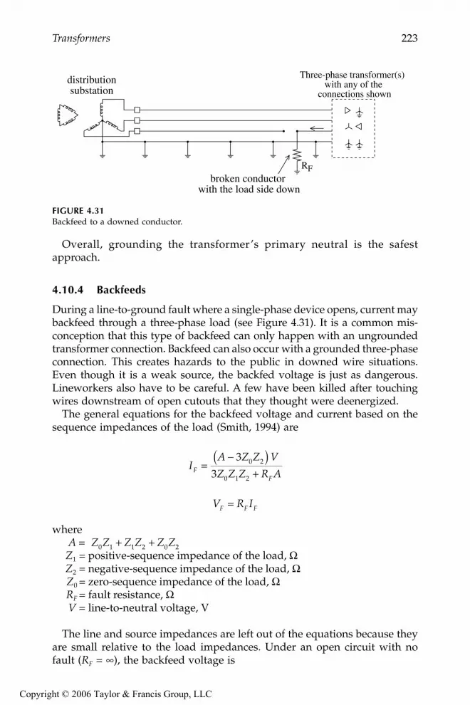
Transformers 223
Overall, grounding the transformer’s primary neutral is the safestapproach.
4.10.4 Backfeeds
During a line-to-ground fault where a single-phase device opens, current maybackfeed through a three-phase load (see Figure 4.31). It is a common mis-conception that this type of backfeed can only happen with an ungroundedtransformer connection. Backfeed can also occur with a grounded three-phaseconnection. This creates hazards to the public in downed wire situations.Even though it is a weak source, the backfed voltage is just as dangerous.Lineworkers also have to be careful. A few have been killed after touchingwires downstream of open cutouts that they thought were deenergized.
The general equations for the backfeed voltage and current based on thesequence impedances of the load (Smith, 1994) are
whereA =
Z1 = positive-sequence impedance of the load, ΩZ2 = negative-sequence impedance of the load, ΩZ0 = zero-sequence impedance of the load, ΩRF = fault resistance, ΩV = line-to-neutral voltage, V
The line and source impedances are left out of the equations because theyare small relative to the load impedances. Under an open circuit with nofault (RF = ∞), the backfeed voltage is
FIGURE 4.31Backfeed to a downed conductor.
Three-phase transformer(s) with any of the
connections shown
RF
distributionsubstation
broken conductor with the load side down
IA Z Z V
Z Z Z R AFF
=−( )
+3
30 2
0 1 2
V R IF F F=
Z Z Z Z Z Z0 1 1 2 0 2+ +
9576_C04.fm Page 223 Monday, October 17, 2005 9:12 AM
Copyright © 2006 Taylor & Francis Group, LLC

224 Electric Power Distribution Equipment and Systems
For an ungrounded transformer connection (Z0 = ∞), the backfeed current is
The backfeed differs depending on the transformer connection and theload:
• Grounded wye – grounded wye transformer connection• Will not backfeed the fault when the transformer is unloaded or
has balanced line-to-ground loads (no motors). It will backfeedthe fault with line-to-line connected load (especially motors).
• Ungrounded primary transformer• Will backfeed the fault under no load. It may not be able to
provide much current with no load, but there can be significantvoltage on the conductor. Motor load will increase the backfeedcurrent available.
Whether it is a grounded or ungrounded transformer, the available back-feed current depends primarily on the connected motor load. Motors dom-inate since they have much lower negative-sequence impedance; typicallyit is equal to the locked-rotor impedance or about 15 to 20%. With no faultimpedance (RF = 0), the backfeed current is approximately:
where MkVA is the three-phase motor power rating in kVA (and we can makethe common assumption that 1 hp = 1 kVA), VLG,kV is the line-to-groundvoltage in kV, and Z2,pu is the per-unit negative-sequence (or locked-rotor)impedance of the motor(s). Figure 4.32 shows the variation in backfeedcurrent versus motor kVA on the transformer for a 12.47-kV system (assum-ing Z2,pu = 0.15).
The voltage on the open phases depends on the type of transformer con-nection and the portion of the load that is motors. Figure 4.33 shows thebackfeed voltage for an open circuit and for a typical high-impedance fault(RF = 200 Ω).
As discussed in Chapter 7, the maximum sustainable arc length in inchesis roughly where I is the rms current in amperes, and V is the
VA Z Z V
AF =−( )3 0 2
IZ Z V
Z Z R Z ZFF
=−( )
+ +( )1 2
1 2 1 2
2
3
IM
V ZFkVA
LG kV pu
=⋅9 2, ,
l I V= ⋅
9576_C04.fm Page 224 Monday, October 17, 2005 9:12 AM
Copyright © 2006 Taylor & Francis Group, LLC
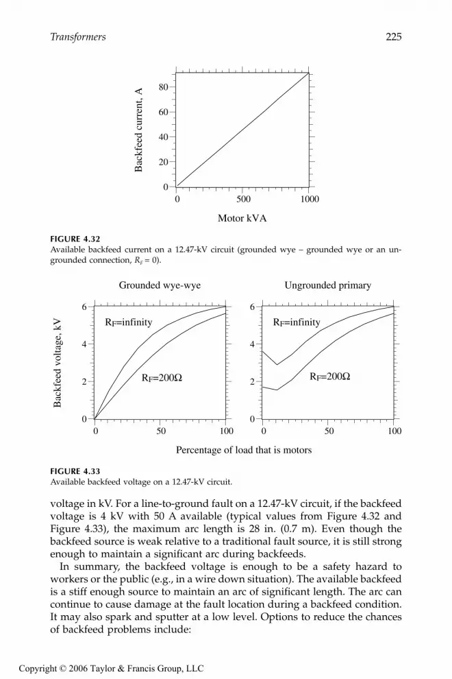
Transformers 225
voltage in kV. For a line-to-ground fault on a 12.47-kV circuit, if the backfeedvoltage is 4 kV with 50 A available (typical values from Figure 4.32 andFigure 4.33), the maximum arc length is 28 in. (0.7 m). Even though thebackfeed source is weak relative to a traditional fault source, it is still strongenough to maintain a significant arc during backfeeds.
In summary, the backfeed voltage is enough to be a safety hazard toworkers or the public (e.g., in a wire down situation). The available backfeedis a stiff enough source to maintain an arc of significant length. The arc cancontinue to cause damage at the fault location during a backfeed condition.It may also spark and sputter at a low level. Options to reduce the chancesof backfeed problems include:
FIGURE 4.32Available backfeed current on a 12.47-kV circuit (grounded wye – grounded wye or an un-grounded connection, RF = 0).
FIGURE 4.33Available backfeed voltage on a 12.47-kV circuit.
0 500 1000 0
20
40
60
80
Motor kVA
Bac
kfee
d cu
rren
t, A
RF=200Ω
RF=infinity
0 50 100 0
2
4
6
RF=200Ω
RF=infinity
0 50 100 0
2
4
6
Grounded wye-wye Ungrounded primary
Percentage of load that is motors
Bac
kfee
d vo
ltage
, kV
9576_C04.fm Page 225 Monday, October 17, 2005 9:12 AM
Copyright © 2006 Taylor & Francis Group, LLC

226 Electric Power Distribution Equipment and Systems
• Make sure crews follow safety procedures (if it is not grounded, itis not dead).
• Follow standard practices regarding downed conductors includingproper line designs and maintenance, public education, and workertraining.
Another option is to avoid single-pole protective devices (switches, fuses,or single-phase reclosers) upstream of three-phase transformer banks. Mostutilities have found that backfeeding problems are not severe enough towarrant not using single-pole protective devices.
To analyze more complicated arrangements, use a steady-state circuitanalysis program (EMTP has this capability). Most distribution fault analysisprograms cannot handle this type of complex arrangement.
4.10.5 Inrush
When a transformer is first energized or reenergized after a short interrup-tion, the transformer may draw inrush current from the system due to thecore magnetization being out of sync with the voltage. The inrush currentmay approach short-circuit levels, as much as 40 times the transformer’sfull-load current. Inrush may cause fuses, reclosers, or relays to falsely oper-ate. It may also falsely operate faulted-circuit indicators or cause sectional-izers to misoperate.
When the transformer is switched in, if the system voltage and the trans-former core magnetization are not in sync, a magnetic transient occurs. Thetransient drives the core into saturation and draws a large amount of currentinto the transformer.
The worst inrush occurs with residual flux left on the transformer core.Consider Figure 4.34 and Figure 4.35, which shows the worst-case scenario.A transformer is deenergized near the peak core flux density (Bmax), whenthe voltage is near zero. The flux decays to about 70% of the maximum andholds there (the residual flux, Br). Some time later, the transformer is reen-ergized at a point in time when the flux would have been at its negativepeak; the system voltage is crossing through zero and rising positively. Thepositive voltage creates positive flux that adds to the residual flux alreadyon the transformer core (remember, flux is the time integral of the voltage).This quickly saturates the core; the effective magnetizing branch drops tothe air-core impedance of the transformer.
The air core impedance is roughly the same magnitude as the trans-former’s leakage impedance. Flux controls the effective impedance, so whenthe core saturates, the small impedance pulls high-magnitude current fromthe system. The core saturates in one direction, so the transformer drawspulses of inrush every other half cycle with a heavy dc component. The dcoffset introduced by the switching decays away relatively quickly.
9576_C04.fm Page 226 Monday, October 17, 2005 9:12 AM
Copyright © 2006 Taylor & Francis Group, LLC
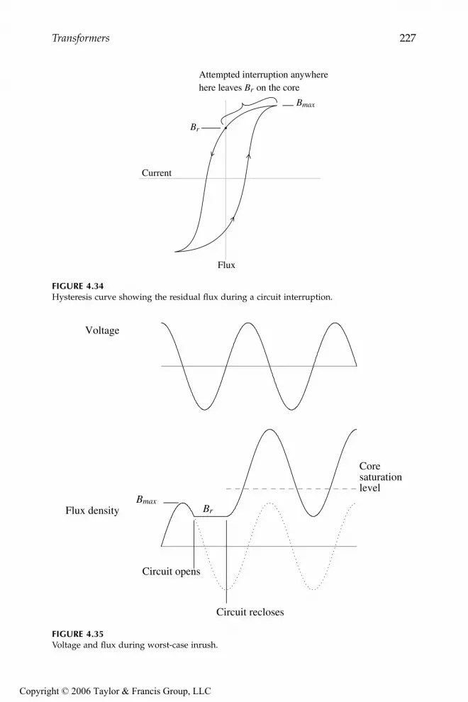
Transformers 227
FIGURE 4.34Hysteresis curve showing the residual flux during a circuit interruption.
FIGURE 4.35Voltage and flux during worst-case inrush.
Flux
Current
Bmax
Br
Attempted interruption anywherehere leaves Br on the core
Br
Voltage
Flux densityBmax
Circuit opens
Circuit recloses
Coresaturationlevel
9576_C04.fm Page 227 Monday, October 17, 2005 9:12 AM
Copyright © 2006 Taylor & Francis Group, LLC

228 Electric Power Distribution Equipment and Systems
Figure 4.36 shows an example of inrush following a reclose operation mea-sured at the distribution substation breaker.
Several factors significantly impact inrush:
• Closing point — The point where the circuit closes back in determineshow close the core flux can get to its theoretical maximum. The worstcase is when the flux is near its peak. Fortunately, this is also whenthe voltage is near zero, and switches tend to engage closer to avoltage peak (an arc tends to jump the gap).
• Design flux — A transformer that is designed to operate lower onthe saturation curve draws less inrush. Because there is more mar-gin between the saturation point and the normal operating region,the extra flux during switching is less likely to push the core intosaturation.
• Transformer size — Larger transformers draw more inrush. Theirsaturated impedances are smaller. But, on a per-unit basis relativeto their full-load capability, smaller transformers draw more inrush.The inrush into smaller transformers dies out more quickly.
• Source impedance — Higher source impedance relative to the trans-former size limits the current that the transformer can pull from thesystem. The peak inrush with significant source impedance (West-inghouse Electric Corporation, 1950) is
FIGURE 4.36Example inrush current measured at a substation (many distribution transformers together).(Copyright © 1996. Electric Power Research Institute. TR-106294-V3. An Assessment of Distribu-tion System Power Quality: Volume 3: Library of Distribution System Power Quality Monitoring CaseStudies. Reprinted with permission.)
0 7
Amps
iii Xpeak =
+0
01
9576_C04.fm Page 228 Monday, October 17, 2005 9:12 AM
Copyright © 2006 Taylor & Francis Group, LLC

Transformers 229
wherei0 = peak inrush without source impedance in per unit of the transformer
rated currentX = source impedance in per unit on the transformer kVA base
Other factors have less significance. The load on the transformer does notsignificantly change the inrush. For most typical loading conditions, thecurrent into the transformer will interrupt at points that still leave about 70%of the peak flux on the core.
While interruptions generally cause the most severe inrush, other voltagedisturbances may cause inrush into a transformer. Voltage transients andespecially voltage with a dc component can saturate the transformer andcause inrush. Some examples are:
• Voltage sags — Upon recovery from a voltage sag from a nearby fault,the sudden rise in voltage can drive a transformer into saturation.
• Sympathetic inrush — Energizing a transformer can cause a nearbytransformer to also draw inrush. The inrush into the switched trans-former has a significant dc component that causes a dc voltage drop.The dc voltage can push the other transformer into saturation anddraw inrush.
• Lightning — A flash to the line near the transformer can push thetransformer into saturation.
References
ABB, Distribution Transformer Guide, 1995.Alexander Publications, Distribution Transformer Handbook, 2001.ANSI C57.12.40-1982, American National Standard Requirements for Secondary Network
Transformers, Subway and Vault Types (Liquid Immersed).ANSI/IEEE C57.12.24-1988, American National Standard Underground-type Three-Phase
Distribution Transformers, 2500 kVA and Smaller; High Voltage 34 500 GrdY/19 200V and Below; Low Voltage 480 V and Below — Requirements.
ANSI/IEEE C57.12.80-1978, IEEE Standard Terminology for Power and DistributionTransformers.
ANSI/IEEE C57.91-1981, IEEE Guide for Loading Mineral-Oil-Immersed Overhead andPad-Mounted Distribution Transformers Rated 500 kVA and Less with 65 Degrees COr 55 Degrees C Average Winding Rise.
ANSI/IEEE C57.105-1978, IEEE Guide for Application of Transformer Connections inThree-Phase Distribution Systems.
ANSI/IEEE Std. 32-1972, IEEE Standard Requirements, Terminology, and Test Procedurefor Neutral Grounding Devices.
Blume, L. F., Boyajian, A., Camilli, G., Lennox, T. C., Minneci, S., and Montsinger, V.M., Transformer Engineering, Wiley, New York, 1951.
9576_C04.fm Page 229 Monday, October 17, 2005 9:12 AM
Copyright © 2006 Taylor & Francis Group, LLC

230 Electric Power Distribution Equipment and Systems
Bohmann, L. J., McDaniel, J., and Stanek, E. K., “Lightning Arrester Failures andFerroresonance on a Distribution System,” IEEE Rural Electric Power Confer-ence, 1991.
CEA 485 T 1049, On-line Condition Monitoring of Substation Power Equipment UtilityNeeds, Canadian Electrical Association, 1996.
CIGRE working group 12.05, “An International Survey on Failure in Large PowerTransformer Service,” Electra, no. 88, pp. 21–48, 1983.
EEI, “A Method for Economic Evaluation of Distribution Transformers,” March,28–31, 1981.
EPRI TR-106294-V3, An Assessment of Distribution System Power Quality: Volume 3:Library of Distribution System Power Quality Monitoring Case Studies, ElectricPower Research Institute, Palo Alto, CA, 1996.
Gangel, M. W. and Propst, R. F., “Distribution Transformer Load Characteristics,” IEEETransactions on Power Apparatus and Systems, vol. 84, pp. 671–84, August 1965.
Grainger, J. J. and Kendrew, T. J., “Evaluation of Technical Losses on Electric Distri-bution Systems,” CIRED, 1989.
Hopkinson, F. H., “Approximate Distribution Transformer Impedances,” GeneralElectric Internal Memorandum, 1976. As cited by Kersting, W. H. and Phillips,W. H., “Modeling and Analysis of Unsymmetrical Transformer Banks ServingUnbalanced Loads,” Rural Electric Power Conference, 1995.
Hopkinson, R. H., “Ferroresonant Overvoltage Control Based on TNA Tests on Three-Phase Delta-Wye Transformer Banks,” IEEE Transactions on Power Apparatusand Systems, vol. 86, pp. 1258–65, October 1967.
IEEE C57.12.00-2000, IEEE Standard General Requirements for Liquid-Immersed Distri-bution, Power, and Regulating Transformers.
IEEE Std. 493-1997, IEEE Recommended Practice for the Design of Reliable Industrial andCommercial Power Systems (Gold Book).
IEEE Std. C57.91-1995, IEEE Guide for Loading Mineral-Oil-Immersed Transformers.IEEE Task Force Report, “Secondary (Low-Side) Surges in Distribution Transform-
ers,” IEEE Transactions on Power Delivery, vol. 7, no. 2, pp. 746–56, April 1992.Jufer, N. W., “Southern California Edison Co. Ferroresonance Testing of Distribution
Transformers,” IEEE/PES Transmission and Distribution Conference, 1994.Long, L. W., “Transformer Connections in Three-Phase Distribution Systems,” in
Power Transformer Considerations of Current Interest to the Utility Engineer,1984. IEEE Tutorial Course, 84 EHO 209-7-PWR.
Lunsford, J., “MOV Arrester Performance During the Presence of FerroresonantVoltages,” IEEE/PES Transmission and Distribution Conference, 1994.
Nickel, D. L., “Distribution Transformer Loss Evaluation. I. Proposed Techniques,”IEEE Transactions on Power Apparatus and Systems, vol. PAS-100, no. 2, pp.788–97, February 1981.
NRECA RER Project 90-8, Underground Distribution System Design and InstallationGuide, National Rural Electric Cooperative Association, 1993.
ORNL-6804/R1, The Feasibility of Replacing or Upgrading Utility Distribution Transform-ers During Routine Maintenance, Oak Ridge National Laboratory, U.S. Depart-ment of Energy, 1995.
ORNL-6847, Determination Analysis of Energy Conservation Standards for DistributionTransformers, Oak Ridge National Laboratory, U.S. Department of Energy, 1996.
ORNL-6925, Supplement to the “Determination Analysis” (ORNL-6847) and Analysis ofthe NEMA Efficiency Standard for Distribution Transformers, Oak Ridge NationalLaboratory, U.S. Department of Energy, 1997.
9576_C04.fm Page 230 Monday, October 17, 2005 9:12 AM
Copyright © 2006 Taylor & Francis Group, LLC

Transformers 231
ORNL-6927, Economic Analysis of Efficient Distribution Transformer Trends, Oak RidgeNational Laboratory, U.S. Department of Energy, 1998.
PTI, “Distribution Transformer Application Course Notes,” Power Technologies, Inc.,Schenectady, NY, 1999.
Rusch, R. J. and Good, M. L., “Wyes and Wye Nots of Three-Phase DistributionTransformer Connections,” IEEE Rural Electric Power Conference, 1989.
Sankaran, C., “Transformers,“ in The Electrical Engineering Handbook, R. C. Dorf, Ed.:CRC Press, Boca Raton, FL, 2000.
Seevers, O. C., Management of Transmission & Distribution Systems, PennWell Publish-ing Company, Tulsa, OK, 1995.
Smith, D. R., “Impact of Distribution Transformer Connections on Feeder ProtectionIssues,” Texas A&M Annual Conference for Protective Relay Engineers, March1994.
Smith, D. R., Braunstein, H. R., and Borst, J. D., “Voltage Unbalance in 3- and 4-WireDelta Secondary Systems,” IEEE Transactions on Power Delivery, vol. 3, no. 2,pp. 733–41, April 1988.
Smith, D. R., Swanson, S. R., and Borst, J. D., “Overvoltages with Remotely-SwitchedCable-Fed Grounded Wye-Wye Transformers,” IEEE Transactions on Power Ap-paratus and Systems, vol. PAS-94, no. 5, pp. 1843–53, 1975.
Tillman, R. F., Jr, “Loading Power Transformers,” in The Electric Power EngineeringHandbook, L. L. Grigsby, Ed.: CRC Press, Boca Raton, FL, 2001.
Walling, R. A., “Ferroresonance Guidelines for Modern Transformer Applications,” inFinal Report to the Distribution Systems Testing, Application, and Research(DSTAR) Consortium: General Electric, Industrial and Power Systems, PowerSystems Engineering Department, 1992. As cited in NRECA RER Project 90-8,1993.
Walling, R. A., “Ferroresonant Overvoltages in Today’s Loss-Evaluated DistributionTransformers,” IEEE/PES Transmission and Distribution Conference, 1994.
Walling, R. A., 2000. Verbal report at the fall IEEE Surge Protective Devices CommitteeMeeting.
Walling, R. A., Barker, K. D., Compton, T. M., and Zimmerman, L. E., “FerroresonantOvervoltages in Grounded Wye-Wye Padmount Transformers with Low-LossSilicon Steel Cores,” IEEE Transactions on Power Delivery, vol. 8, no. 3, pp.1647–60, July 1993.
Walling, R. A., Hartana, R. K., Reckard, R. M., Sampat, M. P., and Balgie, T. R.,“Performance of Metal-Oxide Arresters Exposed to Ferroresonance in Pad-mount Transformers,“ IEEE Transactions on Power Delivery, vol. 9, no. 2, pp.788–95, April 1994.
Walling, R. A., Hartana, R. K., and Ros, W. J., “Self-Generated Overvoltages Due toOpen-Phasing of Ungrounded-Wye Delta Transformer Banks,“ IEEE Transac-tions on Power Delivery, vol. 10, no. 1, pp. 526–33, January 1995.
Westinghouse Electric Corporation, Electrical Transmission and Distribution ReferenceBook, 1950.
9576_C04.fm Page 231 Monday, October 17, 2005 9:12 AM
Copyright © 2006 Taylor & Francis Group, LLC

232 Electric Power Distribution Equipment and Systems
All hell broke loose, we had a ball of fire that went phase to phase shooting fireout the xfmer vents like a flame thrower showering slag on the linemen and sentthe monster galloping down the line doing the Jacobs ladder effect for 2 spansbefore it broke …
The next time you’re closing in on that new shiny xfmer out of the shop, thinkabout the night we got a lemon.
anonymous posterwww.powerlineman.com
9576_C04.fm Page 232 Monday, October 17, 2005 9:12 AM
Copyright © 2006 Taylor & Francis Group, LLC

233
5
Voltage Regulation
One of a utility’s core responsibilities is to deliver voltage to customerswithin a suitable range, so utilities must regulate the voltage. On distributioncircuits, voltage drops due to current flowing through the line impedances.Primary and secondary voltage drop can be allocated as necessary along thecircuit to provide end users with suitable voltage. Voltage regulators — inthe substation or on feeders — can adjust primary voltage. This chapterdiscusses voltage regulators and regulation standards and techniques.
5.1 Voltage Standards
Most regulatory bodies and most utilities in America follow the ANSI voltagestandards (ANSI C84.1-1995). This standard specifies acceptable operationalranges at two locations on electric power systems:
•
Service voltage
— The service voltage is the point where the electricalsystems of the supplier and the user are interconnected. This isnormally at the meter. Maintaining acceptable voltage at the serviceentrance is the
utility’s
responsibility.•
Utilization voltage
— The voltage at the line terminals of utilizationequipment. This voltage is the
facility’s
responsibility. Equipmentmanufacturers should design equipment which operates satisfacto-rily within the given limits.
The standard allows for some voltage drop within a facility, so servicevoltage requirements are tighter than utilization requirements.
The standard also defines two ranges of voltage:
•
Range A —
Most service voltages are within these limits, and utilitiesshould design electric systems to provide service voltages within
9576_C05.fm Page 233 Friday, October 14, 2005 9:20 AM
Copyright © 2006 Taylor & Francis Group, LLC

234
Electric Power Distribution Equipment and Systems
these limits. As the standard says, voltage excursions “should beinfrequent.”
•
Range B —
These requirements are more relaxed than Range A limits.According to the standard: “Although such conditions are a part ofpractical operations, they shall be limited in extent, frequency, andduration. When they occur, corrective measures shall be undertakenwithin a reasonable time to improve voltages to meet Range Arequirements.” Utilization equipment should give acceptable per-formance when operating within the Range B utilization limits,“insofar as practical” according to the standard.
These limits only apply to sustained voltage levels and not to momentaryexcursions, sags, switching surges, or short-duration interruptions.
Table 5.1 shows the most important limits, the limits on low-voltage sys-tems. The table is given on a 120-V base; it applies at 120 V but also to anylow-voltage system up to and including 600 V. The main target for utilitiesis the Range A service voltage, 114 to 126 V.
ANSI C84.1 defines three voltage classes: low voltage (1 kV or less),medium voltage (greater than 1 kV and less than 100 kV), and high voltage(greater than or equal to 100 kV). Within these classes, ANSI provides stan-dard nominal system voltages along with the voltage ranges. A more detailedsummary of the ANSI voltages is shown in Table 5.2 and Table 5.3.
For low-voltage classes, two nominal voltages are given — one for theelectric system and a second, somewhat lower, nominal for the utilizationequipment (for low-voltage motors and controls; other utilization equipmentmay have different nominal voltages). In addition, the standard gives com-mon nameplate voltage ratings of equipment as well as information on whatnominal system voltages the equipment is applicable to. As the standardpoints out, there are many inconsistencies between equipment voltage rat-ings and system nominal voltages.
For medium-voltage systems, ANSI C84.1 gives tighter limits for RangesA and B. Range A is –2.5 to +5%, and Range B is –5 to +5.8%. However, mostutilities do not follow these as limits for their primary distribution systems(utilities use the ANSI service voltage guidelines and set their primary volt-age limits to meet the service voltage guidelines based on their practices).The three-wire voltages of 4,160, 6,900, and 13,800 V are mainly suited forindustrial customers with large motors. Industrial facilities use motors onthese systems with ratings of 4,000, 6,600, and 13,200 V, respectively.
TABLE 5.1
ANSI C84.1 Voltage Ranges for 120 V
Service Voltage
Utilization VoltageMinimum Maximum Minimum Maximum
Range A 114 (–5%) 126 (+5%) 110 (–8.3%) 125 (+4.2%)Range B 110 (–8.3%) 127 (+5.8%) 106 (–11.7%) 127 (+5.8%)
9576_C05.fm Page 234 Friday, October 14, 2005 9:20 AM
Copyright © 2006 Taylor & Francis Group, LLC

Voltage Regulation
235
Improper voltage regulation can cause many problems for end users. Sus-tained overvoltages or undervoltages can cause the following end-useimpacts:
•
Improper or less-efficient equipment operation
— For example, lightsmay give incorrect illumination or a machine may run fast or slow.
•
Tripping of sensitive loads
— For example, an uninterruptible powersupply (UPS) may revert to battery storage during high or lowvoltage. This may drain the UPS batteries and cause an outage tocritical equipment.
In addition, undervoltages can cause
•
Overheating of induction motors
— For lower voltage, an inductionmotor draws higher current. Operating at 90% of nominal, the full-load current is 10 to 50% higher, and the temperature rises by 10 to15%. With less voltage, the motor has reduced motor starting torque.
TABLE 5.2
ANSI Standard Nominal System Voltages and Voltage Ranges for
Low-Voltage Systems
NominalSystemVoltage
NominalUtilization
Voltage
Range A
Range B
Maximum
Minimum
Maximum
MinimumUtilizationand Service
Voltage
a
ServiceVoltage
UtilizationVoltage
Utilizationand Service
VoltageServiceVoltage
UtilizationVoltage
Two Wire, Single Phase
120 115 126 114 110 127 110 106
Three Wire, Single Phase
120/240 115/230 126/252 114/228 110/220 127/254 110/220 106/212
Four Wire, Three Phase
208Y/120 200 218/126 197/114 191/110 220/127 191/110 184/106240/120 230/115 252/126 228/114 220/110 254/127 220/110 212/106
480Y/277 460 504/291 456/263 440/254 508/293 440/254 424/245
Three Wire, Three Phase
240 230 252 228 220 254 220 212
480 460 504 456 440 508 440 424
600 575 630 570 550 635 550 530
Note:
Bold entries show preferred system voltages.
a
The maximum utilization voltage for Range A is 125 V or the equivalent (+4.2%) for othernominal voltages through 600 V.
9576_C05.fm Page 235 Friday, October 14, 2005 9:20 AM
Copyright © 2006 Taylor & Francis Group, LLC

236
Electric Power Distribution Equipment and Systems
Also, overvoltages can cause
•
Equipment damage or failure
— Equipment can suffer insulation dam-age. Incandescent light bulbs wear out much faster at higher volt-ages.
•
Higher no-load losses in transformers
— Magnetizing currents arehigher at higher voltages.
5.2 Voltage Drop
We can approximate the voltage drop along a circuit as
V
drop
= |V
s
| – |V
r
|
≈
I
R
·R + I
X
·X
TABLE 5.3
ANSI Standard Nominal System Voltages and Voltage Ranges for
Medium-Voltage Systems
NominalSystemVoltage
Range A
Range B
Maximum
Minimum
Maximum
MinimumUtilizationand Service
VoltageServiceVoltage
UtilizationVoltage
Utilizationand Service
VoltageServiceVoltage
UtilizationVoltage
Four Wire, Three Phase
4160Y/2400 4370/2520 4050/2340 3740/2160 4400/2540 3950/2280 3600/20808320Y/4800 8730/5040 8110/4680 8800/5080 7900/4560
12000Y/6930 12600/7270 11700/6760 12700/7330 11400/6580
12470Y/7200 13090/7560 12160/7020 13200/7620 11850/684013200Y/7620 13860/8000 12870/7430 13970/8070 12504/7240
13800Y/7970 14490/8370 13460/7770 14520/8380 13110/757020780Y/1200 21820/12600 20260/11700 22000/12700 19740/11400
22860Y/13200 24000/13860 22290/12870 24200/13970 21720/12540
24940Y/14400 26190/15120 24320/14040 26400/15240 23690/1368034500Y/19920 36230/20920 33640/19420 36510/21080 32780/18930
Three Wire, Three Phase
2400 2520 2340 2160 2540 2280 2080
4160 4370 4050 3740 4400 3950 3600
4800 5040 4680 4320 5080 4560 41606900 7240 6730 6210 7260 6560 5940
13800 14490 13460 12420 14520 13110 11880
23000 24150 22430 24340 2185034500 36230 33640 36510 32780
Notes:
Bold entries show preferred system voltages. Some utilization voltages are blank becauseutilization equipment normally does not operate directly at these voltages.
9576_C05.fm Page 236 Friday, October 14, 2005 9:20 AM
Copyright © 2006 Taylor & Francis Group, LLC

Voltage Regulation
237
where
V
drop
= voltage drop along the feeder, V
R
= line resistance,
Ω
X
= line reactance,
Ω
I
R
= line current due to real power flow (in phase with the voltage), A
I
X
= line current due to reactive power flow (90
°
out of phase with the voltage), A
In terms of the load power factor,
pf
, the real and reactive line currents are
where
I =
magnitude of the line current, A
pf
= load power factor
qf
= load reactive power factor = sin(cos
–1
(
pf
))
θ
= angle between the voltage and the current
While just an approximation, Brice (1982) showed that
I
R
·R + I
X
·X
is quiteaccurate for most distribution situations. The largest error occurs underheavy current and leading power factor. The approximation has an error lessthan 1% for an angle between the sending and receiving end voltages up to8
°
(which is unlikely on a distribution circuit). Most distribution programsuse the full complex phasor calculations, so the error is mainly a consider-ation for hand calculations.
This approximation highlights two important aspects about voltage drop:
•
Resistive load
— At high power factors, the voltage drop stronglydepends on the resistance of the conductors. At a power factor of0.95, the reactive power factor (
qf
) is 0.31; so even though the resis-tance is normally smaller than the reactance, the resistance plays amajor role.
•
Reactive load
— At moderate to low power factors, the voltage dropdepends mainly on the reactance of the conductors. At a power factorof 0.8, the reactive power factor is 0.6, and because the reactance isusually larger than the resistance, the reactive load causes most of thevoltage drop. Poor power factor significantly increases voltage drop.
Voltage drop is higher with lower voltage distribution systems, poor powerfactor, single-phase circuits, and unbalanced circuits. The main ways toreduce voltage drop are to:
• Increase power factor (add capacitors)• Reconductor with a larger size
I I pf I
I I qf I I pf
R
X
= ⋅ =
= ⋅ = = −
cos
sin sin(cos ( ))
θ
θ 1
9576_C05.fm Page 237 Friday, October 14, 2005 9:20 AM
Copyright © 2006 Taylor & Francis Group, LLC

238
Electric Power Distribution Equipment and Systems
• Balance circuits• Convert single-phase sections to three-phase sections• Reduce load• Reduce length
In many cases, we can live with significant voltage drop as long as wehave enough voltage regulation equipment to adjust for the voltage drop onthe circuit.
5.3 Regulation Techniques
Distribution utilities have several ways to control steady-state voltage. Themost popular regulation methods include:
• Substation load tap-changing transformers (LTCs)• Substation feeder or bus voltage regulators• Line voltage regulators• Fixed and switched capacitors
Most utilities use LTCs to regulate the substation bus and supplementaryfeeder regulators and/or switched capacitor banks where needed.
Taps on distribution transformers are another tool to provide proper volt-age to customers. Distribution transformers are available with and withoutno-load taps (meaning the taps are to be changed without load) with stan-dard taps of
±
2.5 and
±
5%. Utilities can use this feature to provide a fixedboost for customers on a circuit with low primary voltage. This also allowsthe primary voltage to go lower than most utilities would normally allow.Remember, the service entrance voltage is most important. Most distributiontransformers are sold without taps, so this practice is not widespread. It alsorequires consistency; an area of low primary voltage may have several trans-formers to adjust — if one is left out, the customers fed by that transformercould receive low voltage.
5.3.1 Voltage Drop Allocation and Primary Voltage Limits
Most utilities use the ANSI C84.1 ranges for the service entrance, 114 to 126V. How they control voltage and allocate voltage drop varies. Consider thevoltage profile along the circuit in Figure 5.1. The substation LTC or busregulator controls the voltage at the source. Voltage drops along the primaryline, the distribution transformer, and the secondary. We must consider thecustomers at the start and end of the circuit:
9576_C05.fm Page 238 Friday, October 14, 2005 9:20 AM
Copyright © 2006 Taylor & Francis Group, LLC

Voltage Regulation
239
•
End — Heavily loaded
— Low voltages are a concern, so we considera heavily loaded transformer and secondary. The allocation acrossthe secondary depends on the utility’s design practices as far asallowable secondary lengths and conductor sizes are concerned.
•
Source — Lightly loaded
— Near the source, we can operate the pri-mary above 126 V, but we must ensure that the first customer doesnot have overvoltages when that customer is lightly loaded. Com-monly, utilities assume that the secondary and transformer drop tothis lightly loaded customer is 1 V. With that, the upper primaryvoltage limit is 127 V.
In the voltage drop along the primary, we must consider the regulatorbandwidth (and bandwidths for capacitors if they are switched based onvoltage). Voltage regulators allow the voltage to deviate by half the band-width in either direction. So, if we have a 2-V bandwidth and a desiredrange of 7 V of primary drop, subtracting the 2-V bandwidth only leaves5 V of actual drop (see Figure 5.1). Likewise, if we choose 127 V as ourupper limit on the primary, our maximum set voltage is 126 V with a 2-Vregulator bandwidth.
Normally, utilities use standardized practices to allocate voltage drop.Deviations from the standard are possible but often not worth the effort.
If we have an express feeder at the start of a circuit, we can regulate thevoltage much higher than 126 V as long as the voltage drops enough by thetime the circuit reaches the first customer.
Primary voltage allocation affects secondary allocation and vice versa. Arural utility may have to allow a wide primary voltage range to run long
FIGURE 5.1
Voltage drop along a radial circuit with no capacitors or line regulators.
115
120
125
ANSI C84 Upper Limit
ANSI C84 Lower Limit
Lightly loaded first customer
Heavily loaded customer at the end
Transformer voltage drop
Secondary voltage drop
Regulatorbandwidth
Vol
tage
,Von
a12
0-V
base
9576_C05.fm Page 239 Friday, October 14, 2005 9:20 AM
Copyright © 2006 Taylor & Francis Group, LLC

240
Electric Power Distribution Equipment and Systems
circuits, which leaves little voltage drop left for the transformer and second-ary. Since rural loads are typically each fed by their own transformer, ruralutilities can run the primary almost right to the service entrance. Using low-impedance distribution transformers and larger-than-usual transformersalso helps reduce the voltage drop beyond the primary. For the secondaryconductors, triplex instead of open wire and larger size conductors helpreduce secondary drop. Utilities that allow less primary voltage drop canrun longer secondaries.
Utility practices on voltage limits on the primary range widely, as shownin Table 5.4. The upper range is more consistent — most are from 125 to 127V — unless the utility uses voltage reduction (for energy conservation orpeak shaving). The lower range is more variable, anywhere from 112 to 123V. Obviously, the utility that uses a 112-V lower limit is not required to abideby the ANSI C84.1 limits.
5.3.2 Load Flow Models
Load flows provide voltage profiles that help when planning new distribu-tion circuits, adding customers, and tracking down and fixing voltage prob-lems. Most distribution load-flow programs offer a function to plot thevoltage as a function of distance from the source.
We can model a distribution circuit at many levels of detail. Many utilitiesare modeling more of their systems in more detail. For most load flows,
TABLE 5.4
Primary Voltage Ranges at Several Utilities
Service Area Type Minimum MaximumPercentRange
Dense urban area 120 127 5.4Dense urban area 117 126 7.5Urban/suburban 114 126 10.0Urban/suburban 115 125 8.3Urban/suburban
No conservation reduction 119 126 5.8With conservation reduction 119 123 3.3
Multi-state area 117 126 7.5Multi-state area
Urban standard 123 127 3.3Rural standard 119 127 6.6
Suburban and rural 113 125 10.0Suburban and rural
Urban standard 116 125 7.5Rural standard 112 125 10.8
Urban and rural 115 127 10.0Rural, mountainous 116 126 8.3Rural, mountainous 113 127 11.7
Source:
Willis, H. L.,
Power Distribution Planning Reference Book
, MarcelDekker, New York, 1997b, with additional utilities added.
9576_C05.fm Page 240 Friday, October 14, 2005 9:20 AM
Copyright © 2006 Taylor & Francis Group, LLC

Voltage Regulation
241
utilities normally just model the primary. Modeling the secondary is occa-sionally useful for modeling specific problems at a customer. We can stillhave very good models with simplifications. Modeling long laterals orbranches is normally a good idea, but we can lump most laterals togetheras a load where they tie into the main line. Modeling each transformer as aload is rarely worth the effort; we can combine loads together and maintainaccuracy with some common sense. Most mainline circuits can be accuratelymodeled if broken into 10 to 20 sections with load lumped with each section.Of course, accurate models of capacitors and line regulators are a good idea.
Correctly modeling load phasing provides a better voltage profile on eachphase. Unbalanced loads cause more voltage drop because of:
•
Higher loop impedance
— The impedance seen by unbalanced loads,the loop impedance including the zero-sequence impedance, ishigher than the positive-sequence impedance seen by balancedloads.
•
Higher current on the loaded phases
— If the current splits unevenlyby phases, the more heavily loaded phases see more voltage drop.
Utilities often do not keep accurate phasing information, but it helpsimprove load-flow results. We do not need the phasing on every transformer,but we will have better accuracy if we know the phasing of large single-phase taps.
Of the data entered into the load flow model, the load allocation is thetrickiest. Most commonly, loads are entered in proportion to the transformerkVA. If a circuit has a peak load equal to the sum of the kVA of all of theconnected transformers divided by 2.5, then each load is modeled as thegiven transformer size in kVA divided by 2.5. Incorporating metering datais another more sophisticated way to allocate load. If a utility has a trans-former load management system or other system that ties metered kilowatt-hour usage to a transformer to estimate loadings, feeding this data to theload flow can yield a more precise result. In most cases, all of the loads aregiven the same power factor, usually what is measured at the substation.Additional measurements could be used to fine-tune the allocation of powerfactor. Some utilities also assign power factor by customer class.
Most distribution load flow programs offer several load types, normallyconstant power, constant current, and constant impedance:
•
Constant power load
— The real and reactive power stays constant asthe voltage changes. As voltage decreases, this load draws morecurrent, which increases the voltage drop. A constant power modelis good for induction motors.
•
Constant current load —
The current stays constant as the voltagechanges, and the power increases with voltage. As voltage decreases,the current draw stays the same, so the voltage drop does not change.
9576_C05.fm Page 241 Friday, October 14, 2005 9:20 AM
Copyright © 2006 Taylor & Francis Group, LLC

242
Electric Power Distribution Equipment and Systems
•
Constant impedance load
— The impedance is constant as the voltagechanges, and the power increases as the square of the voltage. Asvoltage decreases, the current draw drops off linearly; so the voltagedrop decreases. The constant impedance model is good for incan-descent lights and other resistive loads.
Normally, we can model most circuits as something like 40 to 60% constantpower and 40 to 60% constant impedance (see Table 5.5 for one set ofrecommendations). Modeling all loads as constant current is a good approx-imation for many circuits. Modeling all loads as constant power is conser-vative for voltage drop.
5.3.3 Voltage Problems
Voltage complaints (normally undervoltages) are regular trouble calls forutilities. Some are easy to fix; others are not. First, check the secondary. Beforetackling the primary, confirm that the voltage problem is not isolated to thecustomers on the secondary. If secondary voltage drop is occurring, checkloadings, make sure the transformer is not overloaded, and check for a loosesecondary neutral.
If the problem is on the primary, some things to look for include:
•
Excessive unbalance
— Balancing currents helps reduce voltage drop.•
Capacitors
— Look for blown fuses, incorrect time clock settings,other incorrect control settings, or switch malfunctions.
•
Regulators
— Check settings. See if more aggressive settings canimprove the voltage profile enough: a higher set voltage, more linedrop compensation, and/or a tighter bandwidth.
These problems are relatively easy to fix. If it is not these, and if there istoo much load for the given amount of impedance, we will have to addequipment to fix the problem. Measure the primary voltage (and if possiblethe loadings) at several points along the circuit. An easy way to measure the
TABLE 5.5
Load Modeling Approximations Recommended by Willis (1997a)
Feeder TypePercent
Constant PowerPercent
Constant Impedance
Residential and commercial, summer peaking 67 33Residential and commercial, winter peaking 40 60Urban 50 50Industrial 100 0Developing countries 25 75
Source:
Willis, H. L., “Characteristics of Distribution Loads,” in
Electrical Transmission andDistribution Reference Book
. Raleigh, NC, ABB Power T&D Company, 1997.
9576_C05.fm Page 242 Friday, October 14, 2005 9:20 AM
Copyright © 2006 Taylor & Francis Group, LLC

Voltage Regulation
243
primary voltage is to find a lightly loaded distribution transformer andmeasure the secondary voltage. Measure the power factor at the substation.A poor power factor greatly increases the voltage drop.
Load flows are a good tool to try out different options to improve voltageon a circuit. If possible, match voltage profiles with measurements on thecircuit. Measurements provide a good sanity check. Try to measure duringpeak load conditions. Regulator and capacitor controllers can provide extrainformation if they have data logging capability. Normally, we allocate theload for the model equally by transformer kVA. This may not always beright, and measurements can help “tweak” the model. A load flow can helpdetermine the best course of action. Where do we need a supplementary lineregulator? How many? Can fixed capacitors do the job? Do we need switchedcapacitors? Circuits with poor power factor are the best candidates for capac-itors as they will help reduce line losses as well as improve voltage.
In addition to extra regulating equipment, consider other options. Some-times, we can move one or more circuit sections to a different feeder toreduce the loading on the circuit. If transformers have taps, investigatechanging the transformer taps. Though it is expensive, we can also buildnew circuits, upgrade to a higher voltage, or reconductor.
5.3.4 Voltage Reduction
Utilities can use voltage adjustments as a way to manage system load.Voltage reduction can reduce energy consumption and/or reduce peakdemand. Several studies have shown roughly a linear response relationshipbetween voltage and energy use — a 1% reduction in voltage reduces energyusage by 1% (or just under 1%, depending on the study). Kirshner andGiorsetto (1984) analyzed trials of conservation voltage reduction (CVR) atseveral utilities. While results varied significantly, most test circuits hadenergy savings of between 0.5 and 1% for each 1% voltage reduction. Theirregression analysis of the feeders found that residential energy savings were0.76% for each 1% reduction in voltage, while commercial and industrialloads had reductions of 0.99% and 0.41% (but the correlations between loadclass and energy reduction were fairly small).
Voltage reduction works best with resistive loads because the power drawnby a resistive load decreases with the voltage squared. Lighting and resistiveheating loads are the dominant resistive loads; these are not ideal resistiveloads. For example, the power on incandescent lights varies as the voltageto the power of about 1.6, which is not quite to the power of 2 but close.Residential and commercial loads have higher percentages of resistive load.For water heaters and other devices that regulate to a temperature, reducingvoltage does not reduce overall energy usage; the devices just run more often.
Voltage reduction to reduce demand has even more impact than that onenergy reduction. The most reduction occurs right when the voltage isreduced, and then some of the reduction is lost as some loads keep running
9576_C05.fm Page 243 Friday, October 14, 2005 9:20 AM
Copyright © 2006 Taylor & Francis Group, LLC

244
Electric Power Distribution Equipment and Systems
longer than normal to compensate for lower voltage. For example, Priessand Warnock (1978) found that during a 4-h, 5% voltage reduction, thedemand on one typical residential circuit dropped by 4% initially and dimin-ished to a 3% drop by the end of the 4-h period.
Voltage reduction works best on short feeders — those that do not havemuch voltage drop. On these, we can control reduction just through adjust-ments of the station LTC regulator settings. It is straightforward to set up asystem where operators can change the station set voltage through SCADA.On longer circuits, we need extra measures. Some strategies include:
•
Extra regulators — Extra regulators can help flatten the voltage profilealong the circuit. Each regulator is set with a set voltage and com-pensation settings appropriate for a tighter voltage range. Thisapproach is most appropriate for energy conservation. Controllingthe regulators to provide peak shaving is difficult; the communica-tions and controls add significantly to the cost.
• Feeder capacitors — The vars injected by capacitors help flatten thevoltage profile and allow a lower set voltage on the station LTC. Onmany circuits, just fixed capacitors can flatten the profile enough toreduce the station set voltage. McCarthy (2000) reported how Geor-gia Power used this strategy to reduce peak loads by 500 kW oncircuits averaging approximately 18 MW.
• Tighter bandwidth — With a smaller regulator bandwidth, the voltagespread on the circuit is smaller. A smaller bandwidth requires morefrequent regulator or LTC maintenance (the regulator changes tapsmore often) but not drastic differences. Kirshner (1990) reported thatreducing the bandwidth from 3 to 1.5 V doubled the number ofregulator tap changes.
• Aggressive line drop compensation — An aggressive line-drop com-pensation scheme can try to keep the voltage at the low end (say,at 114 V) for the last customer at all times. The set voltage in thestation may be 115 to 117 V, depending on the circuit voltage profile.Aggressive compensation boosts the voltage during heavy loads,while trying to keep voltages low at the ends of circuits. Duringlight loads, the station voltage may drop to well under 120 V. Thisstrategy helps the least at heavy load periods, so it is more usefulfor energy conservation than for peak shaving. Aggressive com-pensation makes low voltages more likely at the end of circuits. Ifany of the planning assumptions are wrong, especially power fac-tor and load placement, customers at the end of circuits can havelow voltages.
• Others — Other voltage profile improvement options help whenimplementing a voltage reduction program, although some of theseoptions, such as reconductoring, undergrounding, load balancing,and increasing primary voltage levels, are quite expensive.
9576_C05.fm Page 244 Friday, October 14, 2005 9:20 AM
Copyright © 2006 Taylor & Francis Group, LLC

Voltage Regulation 245
5.4 Regulators
Voltage regulators are autotransformers with automatically adjusting taps.Commonly, regulators provide a range from –10 to +10% with 32 steps. Eachstep is 5/8%, which is 0.75 V on a 120-V scale.
A single-phase regulator has three bushings: the source (S), the load (L),and the source-load (SL). The series winding is between S and L. Figure 5.2shows a straight regulator (ANSI type A) with the taps on the load side. AnANSI type B, the inverted design, has the taps on the source bushing. Theregulator controller measures current with a CT at the L bushing and mea-sures the voltage with a PT between L and SL. Regulators have a reversingswitch that can flip the series winding around to change back and forthbetween the boost and the buck connection.
Regulators are rated on current (IEEE Std. C57.15-1999). Regulators alsohave a kVA rating which is the two-winding transformer rating and not theload-carrying capability. A regulator at 7.62 kV line to ground with a ±10%range and a load current rating of 100 A has a kVA rating of 0.1(7.62kV)(100A) = 76 kVA. The load-carrying capability is ten times the regulator’skVA rating.
By reducing the range of regulation, we can extend the rating of theregulator. Reducing the range from ±10 to ±5% increases the rating by 60%(see Figure 5.3).
The impedance is the two-winding impedance times a base value aboutten times as large. Because the impedance is so small, we can normallyneglect it.
Three-phase regulators, often used in stations, are used on wye or deltasystems. A three-phase regulator controls all three phases simultaneously.These are normally larger units. The normal connection internally is a wyeconnection with the neutral point floating.
Commonly, utilities use single-phase units, even for regulating three-phasecircuits. We can connect single-phase regulators in several ways [see Figure5.4 and (Bishop et al., 1996)]:
FIGURE 5.2ANSI type A single-phase regulator, meaning taps on the load bushing.
Boost connection
SL
SL
Buck connection
SL
SL
9576_C05.fm Page 245 Friday, October 14, 2005 9:20 AM
Copyright © 2006 Taylor & Francis Group, LLC
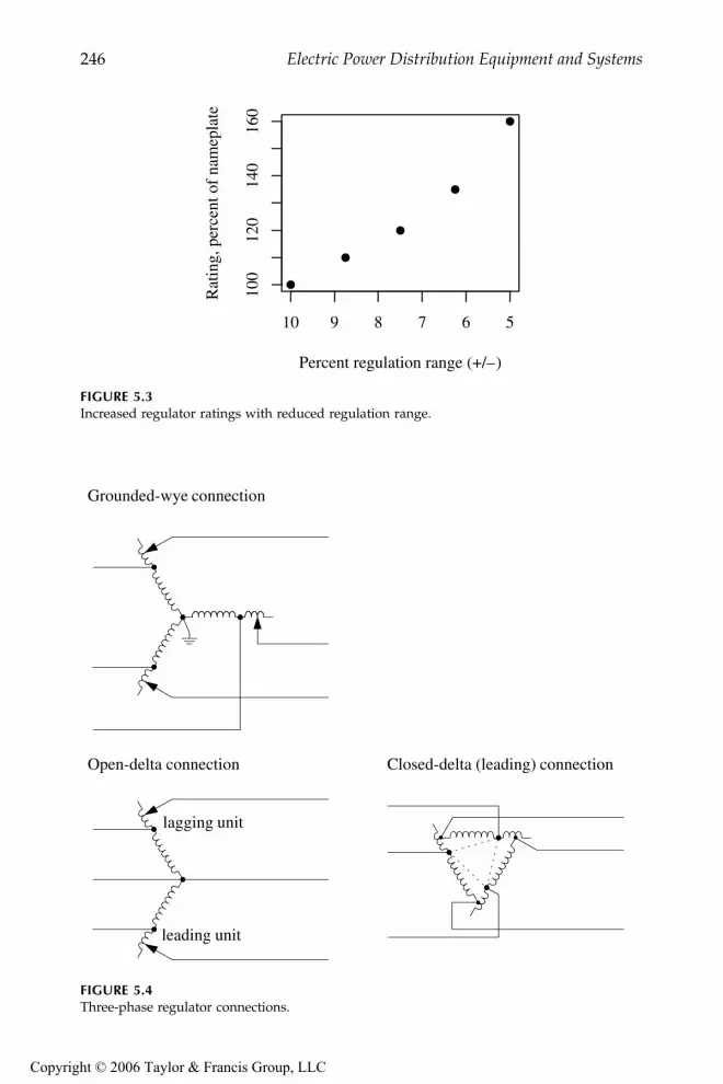
246 Electric Power Distribution Equipment and Systems
FIGURE 5.3Increased regulator ratings with reduced regulation range.
FIGURE 5.4Three-phase regulator connections.
Percent regulation range (+/–)
Rat
ing,
per
cent
of
nam
epla
te
10 9 8 7 6 5
100
120
140
160
Grounded-wye connection
Open-delta connection Closed-delta (leading) connection
lagging unit
leading unit
9576_C05.fm Page 246 Friday, October 14, 2005 9:20 AM
Copyright © 2006 Taylor & Francis Group, LLC

Voltage Regulation 247
• Line to neutral — On four-wire systems, three-phase circuits normallyhave three single-phase regulators connected line to neutral. Line-to-neutral connections are also appropriate for single-phase and two-phase circuits. Each regulator independently controls voltage, whichhelps control voltage unbalance as well as steady-state voltage.
• Open delta — Only two single-phase regulators are needed, eachconnected phase to phase.
• Closed delta — Three regulators are connected phase to phase. Usingthe closed delta extends the regulation range by 50%, from ±10 to±15%.
In both of the delta connections, the regulators see a current phase-shiftedrelative to the voltage. In the leading connection with unity power factorloads, the line current through the regulator leads the line-to-line voltage by30°. The lagging connection has the current reversed: for a unit power factorload, the line current lags the line-to-line voltage by 30°. In the open-deltaconfiguration, one of the units is leading and the other is lagging. In theclosed-delta arrangement, all three units are either leading or all three arelagging. Although uncommon, both of the delta connections can be appliedon four-wire systems.
Regulators have a voltage regulating relay that controls tap changes. Thisrelay has three basic settings that control tap changes (see Figure 5.5):
• Set voltage — Also called the set point or bandcenter, the set voltageis the desired output of the regulator.
• Bandwidth — Voltage regulator controls monitor the differencebetween the measured voltage and the set voltage. Only when thedifference exceeds one half of the bandwidth will a tap change start.Use a bandwidth of at least two times the step size, 1.5 V for ±10%,32-step regulators. Settings of 2 and 2.5 V are common.
• Time delay — This is the waiting time between the time when thevoltage goes out of band and when the controller initiates a tap
FIGURE 5.5Regulator tap controls based on the set voltage, bandwidth, and time delay.
BandwidthSet voltage
Time delay
Tap change
9576_C05.fm Page 247 Friday, October 14, 2005 9:20 AM
Copyright © 2006 Taylor & Francis Group, LLC

248 Electric Power Distribution Equipment and Systems
change. Longer time delays reduce the number of tap changes. Typ-ical time delays are 30 to 60 sec.
If the voltage is still out of bounds after a tap change, the controller makesadditional tap changes until the voltage is brought within bounds. The exactdetails vary by controller, and some provide programmable modes. In somemodes, controllers make one tap change at a time. In other modes, thecontroller may initiate the number of tap changes it estimates are needed tobring the voltage back within bounds. The time delay relay resets if thevoltage is within bounds for a certain amount of time.
A larger bandwidth reduces the number of tap changes, but at a cost. Withlarger bandwidth, the circuit is not as tightly regulated. We should includethe bandwidth in voltage profile calculations to ensure that customers arenot given over or under voltages. Voltage that was used for bandwidth canbe used for voltage drop along the circuit. With a higher bandwidth we mayneed more regulators on a given line. So, use at least two times the step size,but do not use excessively high bandwidths such as 3 or 3.5 V.
In addition to these basics, regulator controllers also have line-drop com-pensation to boost voltages more during heavy load. Controllers also mayhave high and low voltage limits to prevent regulation outside of a desiredrange of voltages. In addition to the regulator and control application infor-mation provided here, see Beckwith (1998), Cooper Power Systems (1978),General Electric (1979), and Westinghouse (1965).
Many regulators are bi-directional units; they can regulate in either direc-tion, depending on the direction of power flow. A bi-directional regulatormeasures voltage on the source side using an extra PT or derives an estimatefrom the current. If the regulator senses reverse power flow, it switches toregulating the side that is normally the source side. We need reverse modefor a regulator on circuits that could be fed by an alternate source in thereverse direction. Without a reverse mode, the regulator can cause voltageproblems during backfeeds. If a unidirectional regulator is fed “backwards,”the regulator PT is now on the side of the source. Now, if the voltage drops,the regulator initiates a tap raise. However, the voltage the PT sees does notchange because it is on the source side (very stiff). What happened was thevoltage on the load side went down (but the regulator controller does notknow that because it is not measuring that side). The controller still seeslow voltage, so it initiates another tap raise which again lowers the voltageon the other side of the regulator. The controller keeps trying to raise thevoltage until it reaches the end of its regulation range. So, we have an alreadylow voltage that got dropped by an extra 10% by the unidirectional regulator.If the controller initially sees a voltage above its set voltage, it ratchets allthe way to the high end causing a 10% overvoltage. Also, if the incomingvoltage varies above and below the bandwidth, the regulator can run backand forth between extremes. A bi-directional regulator prevents these run-aways. Depending on its mode, under reverse power, a bi-directional reg-ulator can regulate in the reverse direction, halt tap changes, or move to the
9576_C05.fm Page 248 Friday, October 14, 2005 9:20 AM
Copyright © 2006 Taylor & Francis Group, LLC

Voltage Regulation 249
neutral point (these last two do not require PTs on both sides but just powerdirection sensing).
Regulators also have an operations counter. The counter helps identifywhen a regulator is due for refurbishment. Regulators are designed to per-form many tap changes, often over one million tap changes over the life ofa regulator. A regulator might change taps 70 times per day, which is 25,000times per year (Sen and Larson, 1994). A regulator counter also provides agood warning indicator; excessive operations suggest that something iswrong, such as wrong line drop compensation settings, a bandwidth or timedelay that is too small, or widely fluctuating primary voltages.
Regulators have “drag hands” — markers on the tap position indicatorthat show the maximum and minimum tap positions since the drag handswere last reset. The drag hands are good indicators of voltage problems. Ifmaintenance reviews continually show the drag upper hand pegging out at+10%, the upstream voltage is probably too low. More work is needed tocorrect the circuit’s voltage profile. Advanced controllers record much moreinformation, including tap change records and demand metering to profilevoltages, currents, and power factors.
5.4.1 Line-Drop Compensation
LTC transformer and regulator controls can be augmented with line-dropcompensation. During heavy load, the controller boosts voltage the most,and during light load, voltage is boosted the least. The line-drop compen-sator uses an internal model of the impedance of the distribution line tomatch the line impedance. The user can set the R and X values in thecompensator to adjust the compensation. The controller adjusts taps basedon the voltage at the voltage regulating relay, which is the PT voltage plusthe voltage across the line-drop compensator circuit (see Figure 5.6). Withno compensation, the voltage regulating relay adjusts the taps based on thePT voltage.
Since load on a typical distribution line is distributed, R and X compen-sator settings are chosen so that the maximum desired boost is obtained
FIGURE 5.6Line drop compensator circuit.
PT
CT Regulation point
Voltage Regulating
Relay
R XR X
I
I/ct
V/pt (R+jX)(I/ct)
9576_C05.fm Page 249 Friday, October 14, 2005 9:20 AM
Copyright © 2006 Taylor & Francis Group, LLC
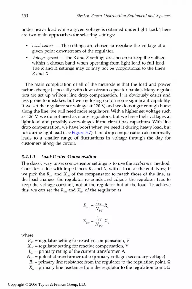
250 Electric Power Distribution Equipment and Systems
under heavy load while a given voltage is obtained under light load. Thereare two main approaches for selecting settings:
• Load center — The settings are chosen to regulate the voltage at agiven point downstream of the regulator.
• Voltage spread — The R and X settings are chosen to keep the voltagewithin a chosen band when operating from light load to full load.The R and X settings may or may not be proportional to the line’sR and X.
The main complication of all of the methods is that the load and powerfactors change (especially with downstream capacitor banks). Many regula-tors are set up without line drop compensation. It is obviously easier andless prone to mistakes, but we are losing out on some significant capability.If we set the regulator set voltage at 120 V, and we do not get enough boostalong the line, we will need more regulators. With a higher set voltage suchas 126 V, we do not need as many regulators, but we have high voltages atlight load and possibly overvoltages if the circuit has capacitors. With linedrop compensation, we have boost when we need it during heavy load, butnot during light load (see Figure 5.7). Line-drop compensation also normallyleads to a smaller range of fluctuations in voltage through the day forcustomers along the circuit.
5.4.1.1 Load-Center Compensation
The classic way to set compensator settings is to use the load-center method.Consider a line with impedances RL and XL with a load at the end. Now, ifwe pick the Rset and Xset of the compensator to match those of the line, asthe load changes the regulator responds and adjusts the regulator taps tokeep the voltage constant, not at the regulator but at the load. To achievethis, we can set the Rset and Xset of the regulator as
whereRset = regulator setting for resistive compensation, VXset = regulator setting for reactive compensation, VICT = primary rating of the current transformer, A
NPT = potential transformer ratio (primary voltage/secondary voltage)RL = primary line resistance from the regulator to the regulation point, ΩXL = primary line reactance from the regulator to the regulation point, Ω
RIN
R
XIN
X
setCT
PTL
setCT
PTL
=
=
9576_C05.fm Page 250 Friday, October 14, 2005 9:20 AM
Copyright © 2006 Taylor & Francis Group, LLC

Voltage Regulation 251
A regulator’s R and X compensator settings are in units of volts. By usingvolts as units, we can directly see the impact of the regulator on a 120-Vscale. Consider an example where the set voltage is 120 V. With a current atunity power factor and Rset = 6 V (Xset does not matter at unity power factor),the controller regulates the voltage to 120 + 6 = 126 V when the current isat the peak CT rating. If the current is at half of the CT rating, the controllerregulates to the set voltage plus 3 or 123 V. Available compensator settingsare normally from –24 to +24 V.
Note that the primary CT rating is an important part of the conversion tocompensator settings. The CT rating may be the same as the regulator ratingor it may be higher. The CT rating is given on the nameplate. Table 5.6 showsthe regulator ratings and primary CT current rating for one manufacturer.Regulators may be applied where the nameplate voltage does not match thesystem voltage if they are close enough to still allow the desired regulationrange at the given location. Also, some regulators have taps that allow themto be used at several voltages. Make sure to use the appropriate PT ratio forthe tap setting selected.
FIGURE 5.7Voltage profiles on a circuit with various forms of regulation.
Vset=120 V, No line drop compensation
114
118
122
126
Vset=126 V, No line drop compensation
Vol
tage
114
118
122
126
Line drop compensation
Source End114
118
122
126
Full loadLight load
9576_C05.fm Page 251 Friday, October 14, 2005 9:20 AM
Copyright © 2006 Taylor & Francis Group, LLC

252 Electric Power Distribution Equipment and Systems
When specifying impedances for the line-drop compensator, use the cor-rect line impedances. For a three-phase circuit, use the positive-sequenceimpedance. For a single-phase line, use the loop impedance ZS which isabout twice the positive-sequence impedance.
On a delta regulator, either an open delta or a closed delta, divide the PTratio by . On a delta regulator the PT connects from phase to phase, butthe internal circuit model of the line-drop compensator is phase to ground,so we need the factor to correct the voltage.
Line-drop compensation works perfectly for one load at the end of a line,but how do we set it for loads distributed along a line? If loads are uniformlydistributed along a circuit that has uniform impedance, we can hold thevoltage constant at the midpoint of the section by using:
• 3/8 rule — For a uniformly distributed load, a regulator can holdthe voltage constant at the midpoint of the circuit if we use line-dropcompensation settings based on 3/8 of the total line impedance. Acircuit with a uniformly distributed load has a voltage drop to theend of the circuit of one half of the drop had all of the loads beenlumped into one load at the end of the circuit. Three-fourths of thisdrop is on the first half of the circuit, so (1/2)(3/4) = 3/8 is theequivalent voltage drop on a uniformly distributed load.
Make sure not to allow excessive voltages. We can only safely compensatea certain amount, and we will have overvoltages just downstream of theregulator if we compensate too much. Check the voltage to the voltageregulating relay to ensure that it is not over limits. The maximum voltage is
Vmax = Vset + (pf ⋅Rset + qf ⋅Xset) Imax
TABLE 5.6
Regulator and Primary CT Ratings in Amperes
Regulator CurrentRatings
CTPrimary Current
25 2550 5075 75100 100150 150167, 200 200219, 231, 250 250289, 300 300328, 334, 347, 400 400418, 438, 463, 500 500548, 578, 656, 668 600833, 875, 1000, 1093 10001332, 1665 1600
3
3
9576_C05.fm Page 252 Friday, October 14, 2005 9:20 AM
Copyright © 2006 Taylor & Francis Group, LLC

Voltage Regulation 253
whereVset = regulator set voltageRset = resistive setting for compensation, VXset = reactive setting for compensation, V
pf = load power factorqf = load reactive power factor = sin(cos–1(pf))
Imax = maximum load current in per unit relative to the regulator CT rating
If V is more than what you desired, reduce Rset and Xset appropriately to meetyour desired limit.
5.4.1.2 Voltage-Spread Compensation
In another method, the voltage-spread method, we find compensator settingsby specifying the band over which the load-side voltage should operate. Forexample, we might want the regulator to regulate to 122 V at light load and126 V at full load. If we know or can estimate the light-load and full-loadcurrent, we can find R and X compensator settings to keep the regulatedvoltage within the proper range. If we want the regulator to operate over agiven compensation range C, we can choose settings to satisfy the following:
C = V – Vset = pf ⋅Rset + qf ⋅Xset
whereRset = resistive setting for compensation, VXset = reactive setting for compensation, V
pf = load power factorqf = load reactive power factor = sin(cos–1(pf))C = total desired compensation voltage, V
Vset = regulator set voltage, VV = voltage that the controller will try to adjust the regulator to, V
With line current operating to the regulator CT rating limit (which is oftenthe regulator size) and the current at the given power factor, these settingswill boost the regulator by C volts on a 120-V scale. Any number of settingsfor Rset and Xset are possible to satisfy this equation. If we take where the X/R ratio is selectable, the settings are
X RsetXR set=
RC
pf qf
XC
pf qfR
set XR
set
XR
XR
XR set
=+
=+
=
9576_C05.fm Page 253 Friday, October 14, 2005 9:20 AM
Copyright © 2006 Taylor & Francis Group, LLC

254 Electric Power Distribution Equipment and Systems
where = X/R ratio of the compensator settings
Note that C must be given as seen on the regulator PT secondaries, on a120-V base. As an example, if the feeder voltage should be not more than126 V at the limit of the regulator, and the desired voltage at no load is 122 V,set the regulator set voltage at 122 V and find Rset and Xset to give C = 4 V.For a power factor of 0.85 and = 3, the equations above give Rset = 1.64V and Xset = 4.94 V.
To control the voltage range for a light load other than zero and for a peakload other than the regulator CT rating, we can use the following to find thevoltage swing from light load to full load as
Vmax – Vmin = (pf ⋅Rset + qf ⋅Xset)Imax – (pf ⋅Rset + qf ⋅Xset)Imin
whereVmax = desired voltage at the maximum load current on a 120-V base, VVmin = desired voltage at the minimum load current on a 120-V base, VImax = maximum load current in per-unit relative to the regulator CT ratingImin = minimum load current in per-unit relative to the regulator CT rating
Now, the R and X settings are
And, the regulator set voltage is
With a compensator X/R ratio equal to the line X/R ratio, these equationsmove the effective load center based on the choice of voltage and currentminimums and maximums.
Just like we can choose to have the compensator X/R ratio equal the lineX/R ratio, we can choose other values as well. There are good reasons whywe might want to use other ratios; this is done mainly to reduce the sensi-tivity to power factor changes. The zero reactance method of selecting com-pensator makes Xset = 0 (and the compensator X/R = 0) but otherwise usesthe same equations as the voltage spread method (General Electric, 1979).
XR
XR
RV
pf qf I I
X R
set XR
setXR set
=−
+ −
=
max min
max min
V( )( )
V V pf R qf X Iset set set= − ⋅ + ⋅ = −−
−min min minmax min
max minminV
V VI I
I( )
9576_C05.fm Page 254 Friday, October 14, 2005 9:20 AM
Copyright © 2006 Taylor & Francis Group, LLC

Voltage Regulation 255
By making Xset zero, the compensator is not sensitive to variations in powerfactor caused by switched capacitors or load variation; only real powerchanges cause regulator movement. This method also simplifies applicationof regulators. The equations become
And, the regulator set voltage is
Vset = Vmin – (pf ⋅Rset)Imin
The equations simplify more if we assume that Imin = 0 (our error with thisis that voltages run on the high side during light load). A further simplifi-cation is to assume that the power factor is one. If the power factor is lessthan that at full load, the regulator will not boost the voltage quite as much.Often, we do not know the power factor at the regulator location anyway.
This method is useful with switched capacitor banks close to the regulator.It does not perform well for low power factors if we have assumed a powerfactor near unity. With this control, the regulator will not provide enoughboost with poor power-factor load.
Another option is to take X/R = 0.6, which weights the real power flowmore than the reactive power flow, but not as extremely as the zero reactancecompensation method. So, although the controller is somewhat desensitizedto changes in power factor, the regulator provides some action based onreactive power. Figure 5.8 shows several X/R compensator settings chosento provide an operating band from 121 V at light load to 127 V at full load.The settings were chosen based on a power factor of 0.9, and the curvesshow the voltage as the power factor varies. The middle graph with X/R =0.6 performs well over a wide range of power factors. The graph on the left,where X/R = 3 which is the line X/R ratio, has the most variation with changesin power factor. If power factor is lower than we expected, the compensatorwill cause high voltages.
With X/R = 0.6 and pf = 0.9, the voltage spread equations are
And, the regulator set voltage is
R
X
set
set
=−
−
=
V Vpf(I I )
max min
max min
0
R
X R
set
set set
=−
−
=
0 86
0 6
.
.
V V(I I )
max min
max min
9576_C05.fm Page 255 Friday, October 14, 2005 9:20 AM
Copyright © 2006 Taylor & Francis Group, LLC

256 Electric Power Distribution Equipment and Systems
The universal compensator method fixes compensation at Rset = 5 V and Xset
= 3 V to give a 6-V compensation range with current ranging up to theregulator CT rating (General Electric, 1979). For other voltage ranges andmaximum currents, we can use:
And we assume that Imin = 0, so the regulator set voltage is
Vset = Vmin
To make this even more “cookbook,” we can standardize on values of Vmax
and Vmin, for example, values of 126 V and 120 V. If the full-load is the CT
FIGURE 5.8Regulated voltage based on different compensator settings and power factors with the percent-age loadings given on the graph. All settings are chosen to operate from 121 V at light load(33%) to 127 V at full load (100% of the primary CT ratio) at a power factor of 0.9.
R=4.1V, X=12.2VVset=118.0V
25%
50%
75%
100%
0.7 0.8 0.9 1.0
120
125
130R=7.7V, X=4.6V
Vset=118.0V
25%
50%
75%
100%
0.7 0.8 0.9 1.0
R=10.0V, X=0.0VVset=118.0V
25%
50%
75%
100%
0.7 0.8 0.9 1.0
Power factor
V VV VI I
Iset minmax min
max minmin= −
−
−
RI
XI
set
set
=−
=−
56
36
max
max min
max
max min
V V
V V
( )
( )
9576_C05.fm Page 256 Friday, October 14, 2005 9:20 AM
Copyright © 2006 Taylor & Francis Group, LLC

Voltage Regulation 257
rating (which we might want in order to be conservative), the default settingsbecome Rset = 5 V and Xset = 3 V. The universal compensation method is easyyet relatively robust.
With any of the voltage-spread methods of setting the R and X line-dropcompensation, the peak current is an important parameter. If we underesti-mate the load current, the regulator can overcompensate and cause high volt-ages (if we do not have a voltage override limiter or if it is disabled). Checkregulator loadings regularly to ensure that the compensation is appropriate.
5.4.1.3 Effects of Regulator Connections
On an open-delta regulator, one regulator is connected leading, and the otherlagging. We need to adjust the compensator settings to account for the 30°phase shift. On the leading regulator, the current leads the voltage by 30°;so we need to subtract 30° from the compensator settings, which is the sameas multiplying by 1∠30° or (cos 30° – j sin 30°). Modify the settings for theleading regulator (Cooper Power Systems, 1978; Westinghouse Electric Cor-poration, 1965) with
R′set = 0.866 Rset + 0.5Xset
X′set = 0.866 Xset – 0.5Rset
And for the lagging regulator we need to add 30°, which gives
R′set = 0.866 Rset – 0.5Xset
X′set = 0.866 Xset + 0.5Rset
For an X/R ratio above 1.67, R′set is negative on the lagging regulator; andfor a ratio below 0.58, X′set is negative on the leading regulator. Most con-trollers allow negative compensation.
In the field, how do we tell between the leading and the lagging regulator?Newer regulator controllers can tell us which is which from phase anglemeasurements. For older controllers, we can modify the compensator set-tings to find out (Lokay and Custard, 1954). Set the resistance value on bothregulators to zero, and set the reactance setting on both to the same nonzerovalue. The unit that moves up the most number of tap positions is the laggingunit (with balanced voltages, this is the unit that goes to the highest raiseposition). If the initial reactance setting is not enough, raise the reactancesettings until the leading and lagging units respond differently.
With a closed-delta regulator, all three regulators are connected eitherleading or lagging. All three regulators have the same set of compensatorsettings; adjust them all with either the leading or the lagging equationsdescribed for the open-delta regulator.
9576_C05.fm Page 257 Friday, October 14, 2005 9:20 AM
Copyright © 2006 Taylor & Francis Group, LLC

258 Electric Power Distribution Equipment and Systems
On a three-phase regulator, even on a delta system, the compensator set-tings do not need adjustment. The controller accounts for any phase shiftthat might occur inside the regulator.
5.4.2 Voltage Override
Use the voltage override feature on the regulator controller. No matter howwe select the line-drop compensation settings, an important feature is anupper voltage limit on the regulation action. The regulator keeps the regu-lated voltage below this limit regardless of the line-drop compensation set-tings. Always use this feature to protect against overvoltages caused byincorrect line-drop compensation settings or unusually high loadings. Thisupper voltage limiter is also called “first house protection,” as it is the firstfew customers downstream that could have overvoltages due to regulatoraction. With a voltage limit, we can set line-drop compensator settings moreaggressively and not worry about causing overvoltages to customers. On aregulator without an upper limit (normally older units), increase estimatedpeak loadings when calculating line-drop compensation settings in order toreduce the risk of creating overvoltages. Voltage override functions usuallyhave a deadband type setting on the voltage limit to prevent repeated tapchanges. For example, we might set a 126-V upper limit with a deadbandof an extra 2 V. Above 128 V the controller immediately taps the regulatordown to 126 V, and between 126 and 128 V the controller prohibits tap raises(different controllers implement this function somewhat differently; someinclude time delays). Even without line-drop compensation, the voltageoverride function helps protect against sudden changes in upstream voltages(the out-of-limit response is normally faster than normal time-delay settingsprogrammed into regulators).
5.4.3 Regulator Placement
With no feeder regulators, the entire voltage drop on a circuit must be withinthe allowed primary voltage range. One feeder regulator can cover primaryvoltage drops up to twice the allowed voltage variation. Similarly, two sup-plementary regulators can cover primary voltage drops up to three timesthe allowed variation. For a uniformly distributed load, optimum locationsfor two regulators are at distances from the station of approximately 20% ofthe feeder length for one and 50% for the other. For one feeder regulator, theoptimum location for a uniformly distributed load is at 3/8 of the line lengthfrom the station.
When placing regulators and choosing compensator settings, allow forsome load growth on the circuit. If a regulator is applied where the load isright near its rating, it may not be able to withstand the load growth. How-ever, it is more than just concern about the regulator’s capability. If we wantto keep the primary voltage above 118 V, and we add a regulator to a circuit
9576_C05.fm Page 258 Friday, October 14, 2005 9:20 AM
Copyright © 2006 Taylor & Francis Group, LLC

Voltage Regulation 259
right at the point where the primary voltage falls to 118 V, that will correctthe voltage profile along the circuit with present loadings. If loadingsincrease in the future, the voltage upstream of the regulator will drop below118 V. As previously discussed, when setting line-drop compensator settings,the maximum load on the regulator should allow room for load growth toreduce the chance that the regulator boosts the voltage too much.
Several regulators can be strung together on a circuit. Though this canmeet the steady-state voltage requirements of customers, it will create a veryweak source for them. Flicker problems from motors and other fluctuatingloads are more likely.
Also consider the effect of dropped load on regulators. A common case isa recloser downstream of a line regulator. If the regulator is tapped upbecause of heavy load and the recloser suddenly drops a significant portionof the load, the voltage downstream of the regulator will pop up until theregulator controller shifts the taps back down.
5.4.4 Other Regulator Issues
Normally, voltage regulators help with voltage unbalance as each regulatorindependently controls its phase. If we aggressively compensate, the line-dropcompensation can cause voltage unbalance. Consider a regulator set to operatebetween 120 V at no load and 126 V at full load. If one phase is at 50% loadand the other two are at 0% load, the line-drop compensator will tap to 123 Von the loaded phase and to 120 V on the unloaded phases. Depending oncustomer placements, this may be fine if the voltages correct themselves alongthe line. But if the unbalance is due to a large tapped lateral just downstreamof the regulator, the regulator needlessly unbalances the voltages.
Capacitor banks pose special coordination issues with regulators. A fixedcapacitor bank creates a constant voltage rise on the circuit and a constantreactive contribution to the current. Either fixed or switched, capacitorsupstream of a regulator do not interfere with the regulator’s control action.Downstream capacitors pose the problem. A capacitor just downstream ofa regulator affects the current that the regulator sees, but it does not mea-surably change the shape of the voltage profile beyond the regulator. In thiscase, we would like the line-drop compensation to ignore the capacitor. Thevoltage-spread compensation with a low compensator X/R or the zero-reac-tance compensator settings work well because they ignore or almost ignorethe reactive current, so it works with fixed or switched banks downstreamof the regulator. The load-center approach is more difficult to get to workwith capacitors.
We do not want to ignore the capacitor at the end of a circuit section weare regulating because the capacitor significantly alters the profile along thecircuit. In this case, we do not want zero-reactance compensation; we wantsome X to compensate for the capacitive current.
Switched capacitors can interact with the tap-changing controls on regu-lators upstream of the capacitors. This sort of interaction is rare but can
9576_C05.fm Page 259 Friday, October 14, 2005 9:20 AM
Copyright © 2006 Taylor & Francis Group, LLC

260 Electric Power Distribution Equipment and Systems
happen if the capacitor is controlled by voltage (not radio, not time of day,not vars). A regulator may respond to an upstream or downstream capacitorswitching, but that does not add up to many extra tap changes since thecapacitor switches infrequently. Normally, the capacitor cannot cycle backand forth against the regulator. The only case might be if the regulator hasnegative settings for the reactive line-drop compensation.
With several regulators in series, adjustments to the time delay settingsare the proper way to coordinate operations between units. Set the down-stream regulator with the longest time delay so it does not change tapsexcessively. For multiple regulators, increase the time delay with increasingdistance from the source. Tap changes by a downstream regulator do notchange the voltage upstream, but tap changes by an upstream regulatoraffect all downstream regulators. If a downstream regulator acts before theupstream regulator, the downstream regulator may have to tap again to meetits set voltage. Making the downstream regulator wait longer prevents itfrom tapping unnecessarily. Separate the time delays by at least 10 to 15 secto allow the upstream unit to complete tap change operations.
5.5 Station Regulation
Utilities most commonly use load tap changing transformers (LTCs) to con-trol distribution feeder voltages at the substation. In many cases (short, urban,thermally limited feeders) an LTC is all the voltage support a circuit needs.
An LTC or a stand-alone voltage regulator must compensate for the voltagechange on the subtransmission circuit as well as the voltage drop throughthe transformer. Of these, the voltage drop through the transformer is nor-mally the largest. Normally, the standard ±10% regulator can accomplishthis. A regulator can hit the end of its range if the load has especially poorpower factor. The voltage drop across a transformer follows:
Vdrop = IR · R + IX ·X
Since a transformer’s X/R ratio is so high, the reactive portion of the loadcreates the most voltage drop across the transformer. Consider a 10% imped-ance transformer at full load with a load power factor of 0.8, which meansthe reactive power factor is 0.6. In this case, the voltage drop across thetransformer is 6%. If the subtransmission voltage is 120 V (on a 120-V scale),the maximum that the regulator can boost the voltage to is 124 V. If thisexample had a transformer loaded to more than its base open-air rating(OA or ONAN), the regulator would be more limited in range. In mostcases, we do not run into this problem as power factors are normally muchbetter than these.
9576_C05.fm Page 260 Friday, October 14, 2005 9:20 AM
Copyright © 2006 Taylor & Francis Group, LLC

Voltage Regulation 261
In most cases, bus regulation suffices. For cases where circuits have sig-nificant voltage drop, individual feeder regulation can be better. Individualfeeder regulation also performs better on circuits with different load cycles.If commercial feeders are on the same bus as residential feeders, it is lesslikely that a bus regulator can keep voltages in line on all circuits. Normally,we handle this by using bus regulation and supplementary line regulators.In some cases, individual feeder regulation in the station is more appropriate.
The voltage on feeders serving secondary networks is controlled at theprimary substation with LTC transformers. These circuits are short enoughthat feeder regulators are unnecessary. Network feeders are often suppliedby parallel station transformers; paralleling LTC units raises several issuesthat are discussed in the next section.
5.5.1 Parallel Operation
With care, we can parallel regulators. The most common situation is in asubstation where a utility wants to parallel two LTC transformers. If twoparalleled transformers do not have the same turns ratio, current will circu-late to balance the voltages. The circulating current is purely reactive, but itadds extra loading on the transformer.
Some of the methods to operate LTC transformers in parallel (Jauch, 2001;Westinghouse Electric Corporation, 1965) include
• Negative-reactance control — The reactance setting in the line-dropcompensator is set to a negative value, so higher reactive currentforces the control to lower taps. The transformer with the higher taphas more reactive current, and the transformer with the lower tapis absorbing this reactive current (it looks capacitive to this trans-former). So, a negative-reactance setting forces the transformer withthe highest tap (and most reactive current) to lower its taps andbring it into alignment with the other unit. This method limits theuse of line-drop compensation and can lead to lower bus voltages.
• Master-follower — One controller, the master, regulates the voltageand signals the other tap changers (the followers) to match the tapsetting. The master control normally gets feedback from the follow-ers to confirm their operation.
• Var balancing — The controller adjusts taps as required to equalizethe vars flowing in parallel transformers. Auxiliary circuitry isrequired. This method has the advantage that it works with trans-formers fed from separate transmission sources.
• Circulating current method — This is the most common control. Aux-iliary circuitry is added to separate the load current through eachtransformer from the circulating current. Each transformer LTC con-trol is fed the load current. The controller adjusts taps to minimize
9576_C05.fm Page 261 Friday, October 14, 2005 9:20 AM
Copyright © 2006 Taylor & Francis Group, LLC

262 Electric Power Distribution Equipment and Systems
the difference in current between parallel units. Removing a unitdoes not require changing controller settings.
The complications associated with paralleling regulators are another rea-son utilities normally avoid closed bus ties in distribution substations.
5.5.2 Bus Regulation Settings
Although too often left unused, bus regulators (whether stand-alone regu-lators or load tap changing transformers) can use line-drop compensation.The concept of a load center rarely has good meaning for a bus supportingseveral circuits, but the voltage spread methods allow the regulator to boostvoltage under heavy load.
The voltage-spread equations assume that the power factor at full load isthe same as the power factor at light load. If the power factor is different atlight and peak loads, we can use this information to provide more precisesettings. We could solve the following to find new R and X settings withdifferent power factors
Vmax – Vmin = (pfmax ⋅ Rset + qfmax ⋅ Xset)Imax – (pfmin ⋅ Rset + qfmin ⋅ Xset)Imin
However, it is easier to use the equations in Section 5.4.1.2 and use theaverage of the power factor at peak load and the power factor at light load.With line-drop compensation for bus regulation, the voltage-override featurehelps to ensure that the LTC or regulator does not cause excessive voltages.
Individual substation feeder regulators are set the same as line feederregulators. We can tune controller settings more precisely based on theindividual characteristics of a given feeder. If the first part of the feeder isan express feeder with no load on it, we could boost the voltage higher thannormal, especially if the circuit is voltage limited. Our main constraint ismaking sure that the first customer does not have high voltage.
5.6 Line Loss and Voltage Drop Relationships
Line losses are from the line current flowing through the resistance of theconductors. After distribution transformer losses, primary line losses are thelargest cause of losses on the distribution system. Like any resistive losses,line losses are a function of the current squared multiplied by the resistance(I2R). Ways to reduce line losses include
• Use a higher system voltage• Balance circuits
9576_C05.fm Page 262 Friday, October 14, 2005 9:20 AM
Copyright © 2006 Taylor & Francis Group, LLC
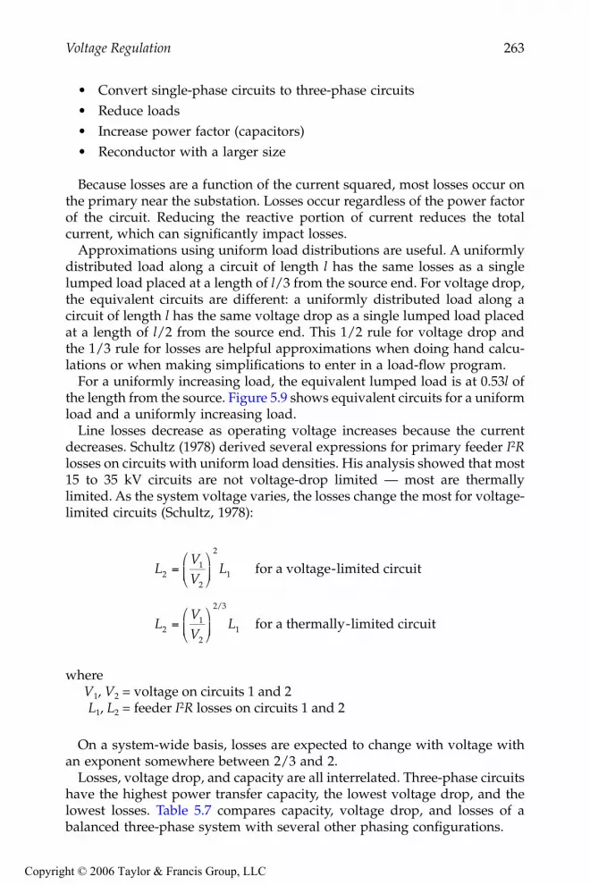
Voltage Regulation 263
• Convert single-phase circuits to three-phase circuits• Reduce loads• Increase power factor (capacitors)• Reconductor with a larger size
Because losses are a function of the current squared, most losses occur onthe primary near the substation. Losses occur regardless of the power factorof the circuit. Reducing the reactive portion of current reduces the totalcurrent, which can significantly impact losses.
Approximations using uniform load distributions are useful. A uniformlydistributed load along a circuit of length l has the same losses as a singlelumped load placed at a length of l/3 from the source end. For voltage drop,the equivalent circuits are different: a uniformly distributed load along acircuit of length l has the same voltage drop as a single lumped load placedat a length of l/2 from the source end. This 1/2 rule for voltage drop andthe 1/3 rule for losses are helpful approximations when doing hand calcu-lations or when making simplifications to enter in a load-flow program.
For a uniformly increasing load, the equivalent lumped load is at 0.53l ofthe length from the source. Figure 5.9 shows equivalent circuits for a uniformload and a uniformly increasing load.
Line losses decrease as operating voltage increases because the currentdecreases. Schultz (1978) derived several expressions for primary feeder I2Rlosses on circuits with uniform load densities. His analysis showed that most15 to 35 kV circuits are not voltage-drop limited — most are thermallylimited. As the system voltage varies, the losses change the most for voltage-limited circuits (Schultz, 1978):
whereV1, V2 = voltage on circuits 1 and 2L1, L2 = feeder I2R losses on circuits 1 and 2
On a system-wide basis, losses are expected to change with voltage withan exponent somewhere between 2/3 and 2.
Losses, voltage drop, and capacity are all interrelated. Three-phase circuitshave the highest power transfer capacity, the lowest voltage drop, and thelowest losses. Table 5.7 compares capacity, voltage drop, and losses of abalanced three-phase system with several other phasing configurations.
LVV
L
LVV
L
21
2
2
1
21
2
2 3
1
=⎛
⎝⎜
⎞
⎠⎟
=⎛
⎝⎜
⎞
⎠⎟
for a voltage-limited circuit
for a thermally-limited circuit/
9576_C05.fm Page 263 Friday, October 14, 2005 9:20 AM
Copyright © 2006 Taylor & Francis Group, LLC

264 Electric Power Distribution Equipment and Systems
FIGURE 5.9Equivalent circuits of uniform loads.
Uniform load Uniformly increasing load
0
I
0
I2
0
l0
I
l0
l0 l0
I
I2
I
I
I
Equivalent circuits with one lumped load
Equivalent voltage drop
Equivalent line losses
12 l
13 l
Equivalent voltage drop12 l
I
I
Equivalent voltage drop23 l
815 l
Equivalent line losses
Line currents
Line currents squared
0
9576_C05.fm Page 264 Friday, October 14, 2005 9:20 AM
Copyright © 2006 Taylor & Francis Group, LLC
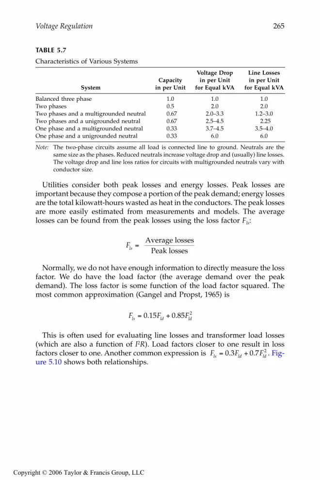
Voltage Regulation 265
Utilities consider both peak losses and energy losses. Peak losses areimportant because they compose a portion of the peak demand; energy lossesare the total kilowatt-hours wasted as heat in the conductors. The peak lossesare more easily estimated from measurements and models. The averagelosses can be found from the peak losses using the loss factor Fls:
Normally, we do not have enough information to directly measure the lossfactor. We do have the load factor (the average demand over the peakdemand). The loss factor is some function of the load factor squared. Themost common approximation (Gangel and Propst, 1965) is
This is often used for evaluating line losses and transformer load losses(which are also a function of I2R). Load factors closer to one result in lossfactors closer to one. Another common expression is . Fig-ure 5.10 shows both relationships.
TABLE 5.7
Characteristics of Various Systems
SystemCapacity
in per Unit
Voltage Dropin per Unit
for Equal kVA
Line Lossesin per Unit
for Equal kVA
Balanced three phase 1.0 1.0 1.0Two phases 0.5 2.0 2.0Two phases and a multigrounded neutral 0.67 2.0–3.3 1.2–3.0Two phases and a unigrounded neutral 0.67 2.5–4.5 2.25One phase and a multigrounded neutral 0.33 3.7–4.5 3.5–4.0One phase and a unigrounded neutral 0.33 6.0 6.0
Note: The two-phase circuits assume all load is connected line to ground. Neutrals are thesame size as the phases. Reduced neutrals increase voltage drop and (usually) line losses.The voltage drop and line loss ratios for circuits with multigrounded neutrals vary withconductor size.
Fls = Average losses
Peak losses
F F Fls ld ld= +0 15 0 85 2. .
F F Fls ld ld= +0 3 0 7 2. .
9576_C05.fm Page 265 Friday, October 14, 2005 9:20 AM
Copyright © 2006 Taylor & Francis Group, LLC

266 Electric Power Distribution Equipment and Systems
References
ANSI C84.1-1995, American National Standards for Electric Power Systems and Equipment— Voltage Ratings (60 Hz).
Beckwith, Basic Considerations for the Application of LTC Transformers and AssociatedControls, Beckwith Electric Company, Application Note #17, 1998.
Bishop, M. T., Foster, J. D., and Down, D. A., “The Application of Single-Phase VoltageRegulators on Three-Phase Distribution Systems,” IEEE Industry ApplicationsMagazine, pp. 38–44, July/August 1996.
Brice, C. W., “Comparison of Approximate and Exact Voltage Drop Calculations forDistribution Lines,” IEEE Transactions on Power Apparatus and Systems, vol. PAS-101, no. 11, pp. 4428–31, November, 1982.
Cooper Power Systems, “Determination of Regulator Compensator Settings,” 1978.Publication R225-10-1.
Gangel, M. W. and Propst, R. F., “Distribution Transformer Load Characteristics,”IEEE Transactions on Power Apparatus and Systems, vol. 84, pp. 671–84, August1965.
General Electric, Omnitext, 1979. GET-3537B.IEEE Std. C57.15-1999, IEEE Standard Requirements, Terminology, and Test Code for Step-
Voltage Regulators.Jauch, E. T., “Advanced Transformer Paralleling,” IEEE/PES Transmission and Dis-
tribution Conference and Exposition, 2001.Kirshner, D., “Implementation of Conservation Voltage Reduction at Commonwealth
Edison,” IEEE Transactions on Power Systems, vol. 5, no. 4, pp. 1178–82, Novem-ber 1990.
FIGURE 5.10Relationship between load factor and loss factor.
0.0 0.5 1.00.0
0.2
0.4
0.6
0.8
1.0
Load factor
Los
s fa
ctor
Fls 0 3Fld 0 7F2ld
Fls 0 15Fld 0 85F 2ld
9576_C05.fm Page 266 Friday, October 14, 2005 9:20 AM
Copyright © 2006 Taylor & Francis Group, LLC

Voltage Regulation 267
Kirshner, D. and Giorsetto, P., “Statistical Tests of Energy Savings Due to VoltageReduction,” IEEE Transactions on Power Apparatus and Systems, vol. PAS-103,no. 6, pp. 1205–10, June 1984.
Lokay, H. E. and Custard, R. L., “A Field Method for Determining the Leading andLagging Regulator in an Open-Delta Connection,” AIEE Transactions, vol. 73,Part III, pp. 1684–6, 1954.
McCarthy, C., “CAPS — Choosing the Feeders, Part I,” in Systems Engineering Tech-nical Update: Cooper Power Systems, 2000.
Priess, R. F. and Warnock, V. J., “Impact of Voltage Reduction on Energy and De-mand,” IEEE Transactions on Power Apparatus and Systems, vol. PAS-97, no. 5,pp. 1665–71, Sept/Oct 1978.
Schultz, N. R., “Distribution Primary Feeder I2R Losses,” IEEE Transactions on PowerApparatus and Systems, vol. PAS-97, no. 2, pp. 603–9, March–April 1978.
Sen, P. K. and Larson, S. L., “Fundamental Concepts of Regulating DistributionSystem Voltages,” IEEE Rural Electric Power Conference, Department of Elec-trical Engineering, Colorado University, Denver, CO, 1994.
Westinghouse Electric Corporation, Distribution Systems, vol. 3, 1965.Willis, H. L., “Characteristics of Distribution Loads,” in Electrical Transmission and
Distribution Reference Book. Raleigh, NC: ABB Power T&D Company, 1997a.Willis, H. L., Power Distribution Planning Reference Book, Marcel Dekker, New York,
1997b.
Regs? Treat them with respect. They are a transformer. Anyone who has droppedload with a tx knows that you can build a fire if you don’t take the load intoconsideration. The difference with regs is that the load is the feeder. Get it?
anonymous postwww.powerlineman.com
9576_C05.fm Page 267 Friday, October 14, 2005 9:20 AM
Copyright © 2006 Taylor & Francis Group, LLC

269
6
Capacitor Application
Capacitors provide tremendous benefits to distribution system performance.Most noticeably, capacitors reduce losses, free up capacity, and reduce volt-age drop:
•
Losses; Capacity
—
By canceling the reactive power to motors andother loads with low power factor, capacitors decrease the line cur-rent. Reduced current frees up capacity; the same circuit can servemore load. Reduced current also significantly lowers the
I
2
R
linelosses.
•
Voltage drop
—
Capacitors provide a voltage boost, which cancelspart of the drop caused by system loads. Switched capacitors canregulate voltage on a circuit.
If applied properly and controlled, capacitors can significantly improvethe performance of distribution circuits. But if not properly applied or con-trolled, the reactive power from capacitor banks can create losses and highvoltages. The greatest danger of overvoltages occurs under light load. Goodplanning helps ensure that capacitors are sited properly. More sophisticatedcontrollers (like two-way radios with monitoring) reduce the risk of improp-erly controlling capacitors, compared to simple controllers (like a time clock).
Capacitors work their magic by storing energy. Capacitors are simpledevices: two metal plates sandwiched around an insulating dielectric. Whencharged to a given voltage, opposing charges fill the plates on either side ofthe dielectric. The strong attraction of the charges across the very shortdistance separating them makes a tank of energy. Capacitors oppose changesin voltage; it takes time to fill up the plates with charge, and once charged,it takes time to discharge the voltage.
On ac power systems, capacitors do not store their energy very long —just one-half cycle. Each half cycle, a capacitor charges up and then dis-charges its stored energy back into the system. The net real power transferis zero. Capacitors provide power just when reactive loads need it. Just whena motor with low power factor needs power from the system, the capacitoris there to provide it. Then in the next half cycle, the motor releases its excessenergy, and the capacitor is there to absorb it. Capacitors and reactive loads
9576_C06.fm Page 269 Friday, October 14, 2005 9:21 AM
Copyright © 2006 Taylor & Francis Group, LLC

270
Electric Power Distribution Equipment and Systems
exchange this reactive power back and forth. This benefits the systembecause that reactive power (and extra current) does not have to be trans-mitted from the generators all the way through many transformers and manymiles of lines; the capacitors can provide the reactive power locally. Thisfrees up the lines to carry real power, power that actually does work.
Capacitor units are made of series and parallel combinations of capacitorpacks or elements put together as shown in Figure 6.1. Capacitor elementshave sheets of polypropylene film, less than one mil thick, sandwichedbetween aluminum foil sheets. Capacitor dielectrics must withstand on theorder of 2000 V/mil (78 kV/mm). No other medium-voltage equipment hassuch high voltage stress. An underground cable for a 12.47-kV system hasinsulation that is at least 0.175 in. (4.4 mm) thick. A capacitor on the samesystem has an insulation separation of only 0.004 in. (0.1 mm).
Utilities often install substation capacitors and capacitors at points ondistribution feeders. Most feeder capacitor banks are pole mounted, the leastexpensive way to install distribution capacitors. Pole-mounted capacitorsnormally provide 300 to 3600 kvar at each installation. Many capacitors areswitched, either based on a local controller or from a centralized controllerthrough a communication medium. A line capacitor installation has thecapacitor units as well as other components, possibly including arresters,fuses, a control power transformer, switches, and a controller (see Figure 6.2for an example).
FIGURE 6.1
Capacitor components. (From General Electric Company. With permission.)
Bushing
Discharge resistor
Capacitor elements
9576_C06.fm Page 270 Friday, October 14, 2005 9:21 AM
Copyright © 2006 Taylor & Francis Group, LLC

Capacitor Application
271
While most capacitors are pole mounted, some manufacturers providepadmounted capacitors. As more circuits are put underground, the need forpadmounted capacitors will grow. Padmounted capacitors contain capacitorcans, switches, and fusing in a deadfront package following standard pad-mounted-enclosure integrity requirements (ANSI C57.12.28-1998). Theseunits are much larger than padmounted transformers, so they must be sitedmore carefully to avoid complaints due to aesthetics. The biggest obstaclesare cost and aesthetics. The main complaint is that padmounted capacitorsare large. Customers complain about the intrusion and the aesthetics of sucha large structure (see Figure 6.3).
FIGURE 6.2
Overhead line capacitor installation. (From Cooper Power Systems, Inc. With permission.)
FIGURE 6.3
Example padmounted capacitor. (From Northeast Power Systems, Inc. With permission.)
Vacuumswitch
Control powertransformer
Capacitor unit
9576_C06.fm Page 271 Friday, October 14, 2005 9:21 AM
Copyright © 2006 Taylor & Francis Group, LLC

272
Electric Power Distribution Equipment and Systems
Substation capacitors are normally offered as open-air racks. Normallyelevated to reduce the hazard, individual capacitor units are stacked in rowsto provide large quantities of reactive power. All equipment is exposed. Stackracks require a large substation footprint and are normally engineered forthe given substation. Manufacturers also offer metal-enclosed capacitors,where capacitors, switches, and fuses (normally current-limiting) are allenclosed in a metal housing.
Substation capacitors and feeder capacitors both have their uses. Feedercapacitors are closer to the loads — capacitors closer to loads more effectivelyrelease capacity, improve voltage profiles, and reduce line losses. This isespecially true on long feeders that have considerable line losses and voltagedrop. Table 6.1 highlights some of the differences between feeder and stationcapacitors. Substation capacitors are better when more precise control isneeded. System operators can easily control substation capacitors wired intoa SCADA system to dispatch vars as needed. Modern communication andcontrol technologies applied to feeder capacitors have reduced this advan-tage. Operators can control feeder banks with communications just likestation banks, although some utilities have found the reliability of switchedfeeder banks to be less than desired, and the best times for switching in varsneeded by the system may not correspond to the best time to switch thecapacitor in for the circuit it is located on.
Substation capacitors may also be desirable if a leading power factor isneeded for voltage support. If the power factor is leading, moving this capac-itor out on the feeder increases losses. Substation capacitors cost more thanfeeder capacitors. This may seem surprising, but we must individually engi-neer station capacitors, and the space they take up in a station is often valuablereal estate. Pole-mounted capacitor installations are more standardized.
Utilities normally apply capacitors on three-phase sections. Applicationson single-phase lines are done but less common. Application of three-phasebanks downstream of single-phase protectors is normally not done because
TABLE 6.1
Substation vs. Feeder Capacitors
Advantages Disadvantages
Feeder Capacitors
Reduces line lossesReduces voltage drop along the feederFrees up feeder capacityLower cost
More difficult to control reliablySize and placement important
Substation Capacitors
Better controlBest placement if leading vars are needed for system voltage support
No reduction in line lossesNo reduction in feeder voltage dropHigher cost
9576_C06.fm Page 272 Friday, October 14, 2005 9:21 AM
Copyright © 2006 Taylor & Francis Group, LLC

Capacitor Application
273
of ferroresonance concerns. Most three-phase banks are connectedgrounded-wye on four-wire multigrounded circuits. Some are connected infloating wye. On three-wire circuits, banks are normally connected as afloating wye.
Most utilities also include arresters and fuses on capacitor installations.Arresters protect capacitor banks from lightning-overvoltages. Fuses isolatefailed capacitor units from the system and clear the fault before the capacitorfails violently. In high fault-current areas, utilities may use current-limitingfuses. Switched capacitor units normally have oil or vacuum switches inaddition to a controller. Depending on the type of control, the installationmay include a control power transformer for power and voltage sensing andpossibly a current sensor. Because a capacitor bank has a number of compo-nents, capacitors normally are not applied on poles with other equipment.
Properly applied capacitors return their investment very quickly. Capaci-tors save significant amounts of money in reduced losses. In some cases,reduced loadings and extra capacity can also delay building more distribu-tion infrastructure.
6.1 Capacitor Ratings
Capacitor units rated from 50 to over 500 kvar are available; Table 6.2 showscommon capacitor unit ratings. A capacitor’s rated kvar is the kvar at ratedvoltage. Three-phase capacitor banks are normally referred to by the totalkvar on all three phases. Distribution feeder banks normally have one ortwo or (more rarely) three units per phase. Many common size banks onlyhave one capacitor unit per phase.
IEEE Std. 18 defines standards for capacitors and provides applicationguidelines. Capacitors should not be applied when any of the followinglimits are exceeded (IEEE Std. 18-2002):
• 135% of nameplate kvar• 110% of rated rms voltage, and crest voltage not exceeding 1.2
of rated rms voltage, including harmonics but excluding transients• 135% of nominal rms current based on rated kvar and rated voltage
Capacitor dielectrics must withstand high voltage stresses during normaloperation — on the order of 2000 V/mil. Capacitors are designed to with-stand overvoltages for short periods of time. IEEE Std. 18-1992 allows up to300 power-frequency overvoltages within the time durations in Table 6.3(without transients or harmonic content). New capacitors are tested with atleast a 10-sec overvoltage, either a dc-test voltage of 4.3 times rated rms oran ac voltage of twice the rated rms voltage (IEEE Std. 18-2002).
2
9576_C06.fm Page 273 Friday, October 14, 2005 9:21 AM
Copyright © 2006 Taylor & Francis Group, LLC

274
Electric Power Distribution Equipment and Systems
Capacitors should withstand various peak voltage and current transients;the allowable peak depends on the number of transients expected per year(see Table 6.4).
The capacitance of a unit in microfarads is
TABLE 6.2
Common Capacitor Unit Ratings
Volts, rms(Terminal-to-Terminal) kvar
Numberof Phases BIL, kV
216 5, 7 1/2, 13 1/3, 20, and 25
1 and 3 30
240 2.5, 5, 7 1/2, 10, 15, 20, 25, and 50
1 and 3 30
480, 600 5, 10, 15, 20, 25, 35, 50, 60, and 100
1 and 3 30
2400 50, 100, 150, 200, 300, and 400
1 and 3 75, 95, 125, 150, and 200
2770 50, 100, 150, 200, 300, 400, and 500
1 and 3 75, 95, 125, 150, and 200
4160, 4800 50, 100, 150, 200, 300, 400, 500, 600, 700, and 800
1 and 3 75, 95, 125, 150, and 200
6640, 7200, 7620, 7960, 8320, 9540, 9960, 11,400, 12,470, 13,280, 13,800, 14,400
50, 100, 150, 200, 300, 400, 500, 600, 700, and 800
1 95, 125, 150, and 200
15,125 50, 100, 150, 200, 300, 400, 500, 600, 700, and 800
1 125, 150, and 200
19,920 100, 150, 200, 300, 400, 500, 600, 700, and 800
1 125, 150, and 200
20,800, 21,600, 22,800, 23,800, 24,940
100, 150, 200, 300, 400, 500, 600, 700, and 800
1 150 and 200
Source:
IEEE Std. 18-2002. Copyright 2002 IEEE. All rights reserved.
TABLE 6.3
Maximum Permissible Power-Frequency Voltages
Duration
Maximum Permissible Voltage(multiplying factor to be applied
to rated voltage rms)
6 cycles 2.2015 cycles 2.001 sec 1.7015 sec 1.401 min 1.3030 min 1.25Continuous 1.10
Note:
This is not in IEEE Std. 18-2002 but it will be addressedin IEEE’s updated capacitor application guide.
Source:
ANSI/IEEE Std. 18-1992. Copyright 1993 IEEE. Allrights reserved.
9576_C06.fm Page 274 Friday, October 14, 2005 9:21 AM
Copyright © 2006 Taylor & Francis Group, LLC

Capacitor Application
275
where
V
kV
= capacitor voltage rating, kV
Q
kvar
= unit reactive power rating, kvar
Capacitors are made within a given tolerance. The IEEE standard allowsreactive power to range between 100 and 110% when applied at rated sinu-soidal voltage and frequency (at 25˚C case and internal temperature) (IEEEStd. 18-2002). Older units were allowed to range up to 115% (ANSI/IEEEStd. 18-1992). Therefore, the capacitance also must be between 100 and 110%of the value calculated at rated kvar and voltage. In practice, most units arefrom +0.5 to +4.0%, and a given batch is normally very uniform.
Capacitor losses are typically on the order of 0.07 to 0.15 W/kvar atnominal frequency. Losses include resistive losses in the foil, dielectric losses,and losses in the internal discharge resistor.
Capacitors must have an internal resistor that discharges a capacitor to 50V or less within 5 min when the capacitor is charged to the peak of its ratedvoltage . This resistor is the major component of losses within acapacitor. The resistor must be low enough such that the
RC
time constantcauses it to decay in 300 sec as
where
V
= capacitor voltage rating, V
R
= discharge resistance,
Ω
C
= capacitance, F
TABLE 6.4
Expected Transient Overcurrent and Overvoltage Capability
Probable Numberof Transients
per year
Permissible Peak TransientCurrent (multiplying factor to be
applied to rated rms current)
Permissible Peak Transient Voltage(multiplying factor to be applied to
rated rms voltage)
4 1500 5.040 1150 4.0
400 800 3.44000 400 2.9
Note
: This is not in IEEE Std. 18-2002, but it will be addressed in IEEE’s updated capacitorapplication guide.
Source:
ANSI/IEEE Std. 18-1992. Copyright 1993 IEEE. All rights reserved.
CQ
VuFkvar
kV
=2 65
2
.
( )2Vrms
502
300
Ve RC≤ − /
9576_C06.fm Page 275 Friday, October 14, 2005 9:21 AM
Copyright © 2006 Taylor & Francis Group, LLC

276
Electric Power Distribution Equipment and Systems
So, the discharge resistor must continually dissipate at least the followingpower in watts:
where
Q
kvar
is the capacitor rating (single or three phase). For 7.2-kV capac-itors, the lower bound on losses is 0.047 W/kvar.
Some utilities use a shorting bar across the terminals of capacitors duringshipping and in storage. The standard recommends waiting for 5 min toallow the capacitor to discharge through the internal resistor.
Capacitors have very low losses, so they run very cool. But capacitors arevery sensitive to temperature and are rated for lower temperatures thanother power system equipment such as cables or transformers. Capacitorsdo not have load cycles like transformers; they are always at full load. Also,capacitors are designed to operate at high dielectric stresses, so they haveless margin for degraded insulation. Standards specify an upper limit forapplication of 40 or 46
°
C depending on arrangement (see Table 6.5). Theselimits assume unrestricted ventilation and direct sunlight. At the lower end,IEEE standard 18 specifies that capacitors shall be able to operate continu-ously in a –40˚C ambient.
6.2 Released Capacity
In addition to reducing losses and improving voltage, capacitors releasecapacity. Improving the power factor increases the amount of real-powerload the circuit can supply. Using capacitors to supply reactive powerreduces the amount of current in the line, so a line of a given ampacity can
TABLE 6.5
Maximum Ambient Temperatures for Capacitor Application
Mounting Arrangement
Ambient Air Temperature
(˚C)4-h Average
a
Isolated capacitor 46Single row of capacitors 46Multiple rows and tiers of capacitors 40Metal-enclosed or -housed equipments 40
a
The arithmetic average of the four consecutive highest hourly read-ings during the hottest day expected at that location.
Source:
IEEE Std. 18-2002. Copyright 2002 IEEE. All rights reserved.
PQ
Vwattskvar= − ⎛
⎝⎜
⎞⎠⎟
113 235 36
.ln
.
9576_C06.fm Page 276 Friday, October 14, 2005 9:21 AM
Copyright © 2006 Taylor & Francis Group, LLC

Capacitor Application
277
carry more load. Figure 6.4 shows that capacitors release significant capacity,especially if the original power factor is low. Figure 6.5 shows another wayto view the extra capacity, as a function of the size of capacitor added.
6.3 Voltage Support
Capacitors are constant-impedance devices. At higher voltages, capacitorsdraw more current and produce more reactive power as
I
=
I
rated
V
pu
and
Q
kvar
=
Q
rated
V
pu
2
where
V
pu
is the voltage in per unit of the capacitor’s voltage rating. Capac-itors applied at voltages other than their rating provide vars in proportionto the per-unit voltage squared.
Capacitors provide almost a fixed voltage rise. The reactive currentthrough the system impedance causes a voltage rise in percent of
FIGURE 6.4
Released capacity with improved power factor.
0.60
0.70
0.80
0.90
0.95
1.00 Corrected power factor
0.5 0.6 0.7 0.8 0.9 1.0 0
20
40
60
Original power factor
Ext
ra c
apac
ity, p
erce
nt o
f th
e or
igin
al lo
ad
VQ X
Vrisekvar L
kV l l
= -10 2
,
9576_C06.fm Page 277 Friday, October 14, 2005 9:21 AM
Copyright © 2006 Taylor & Francis Group, LLC

278
Electric Power Distribution Equipment and Systems
where
X
L
= positive-sequence system impedance from the source to the capac-itor,
Ω
V
kV, l-l
= line-to-line system voltage, kV
Q
kvar
= three-phase bank rating, kvar
While this equation is very good for most applications, it is not exactlyright because the capacitive current changes in proportion to voltage. At ahigher operating voltage, a capacitor creates more voltage rise than theequation predicts.
Since the amount of voltage rise is dependent on the impedance upstreamof the bank, to get the voltage boost along the entire circuit, put the capacitorat the end of the circuit. The best location for voltage support depends onwhere the voltage support is needed. Figure 6.6 shows how a capacitorchanges the voltage profile along a circuit. Unlike a regulator, a capacitorchanges the voltage profile upstream of the bank.
Table 6.6 shows the percentage voltage rise from capacitors for commonconductors at different voltages. This table excludes the station transformer
FIGURE 6.5
Extra capacity as a function of capacitor size.
0.6
0.7
0.8
0.9
Original power factor
0 50 1000.6
0.7
0.8
0.9
1.0
0.6
0.7
0.8
0.9
Original power factor:
0 50 100 0
20
40
60
Capacitor kvar in percent of original load kVA
New
pow
er f
acto
rE
xtra
cap
acity
inpe
rcen
t of
the
orig
inal
load
9576_C06.fm Page 278 Friday, October 14, 2005 9:21 AM
Copyright © 2006 Taylor & Francis Group, LLC

Capacitor Application
279
FIGURE 6.6
Voltage profiles after addition of a capacitor bank. (Copyright © 2002. Electric Power ResearchInstitute. 1001691.
Improved Reliability of Switched Capacitor Banks and Capacitor Technology.
Re-printed with permission.)
TABLE 6.6
Percent Voltage Rise for Various Conductors and Voltage Levels
Conductor Size
X
L
ΩΩΩΩ
/mi
Percent Voltage Rise per Mile with 100 kvar per Phase
Line-to-Line System Voltage, kV4.8 12.47 24.9 34.5
4 0.792 1.031 0.153 0.038 0.0202 0.764 0.995 0.147 0.037 0.019
1/0 0.736 0.958 0.142 0.036 0.0194/0 0.694 0.903 0.134 0.034 0.017350 0.656 0.854 0.127 0.032 0.017500 0.635 0.826 0.122 0.031 0.016750 0.608 0.791 0.117 0.029 0.015
Note:
Impedance are for all-aluminum conductors with GMD=4.8 ft.
Voltage rise from the capacitor
Voltage profile with the capacitor
Voltage profile without the capacitor
100
102
104
96
98
100
With no load
With load
Voltage profile without the capacitor
Feed
ervo
ltage
,per
cent
9576_C06.fm Page 279 Friday, October 14, 2005 9:21 AM
Copyright © 2006 Taylor & Francis Group, LLC

280
Electric Power Distribution Equipment and Systems
impedance but still provides a useful approximation. Inductance does notchange much with conductor size; the voltage change stays the same overa wide range of conductor sizes. For 15-kV class systems, capacitors increasethe voltage by about 0.12% per mi per 100 kvar per phase.
On switched capacitor banks, the voltage change constrains the size ofbanks at some locations. Normally, utilities limit the voltage change to 3 to4%. On a 12.47-kV circuit, a three-phase 1200-kvar bank boosts the voltage4% at about 8 mi from the substation. To keep within a 4% limit, 1200-kvarbanks must only be used within the first 8 mi of the station.
6.4 Reducing Line Losses
One of the main benefits of applying capacitors is that they can reducedistribution line losses. Losses come from current through the resistance ofconductors. Some of that current transmits real power, but some flows tosupply reactive power. Reactive power provides magnetizing for motors andother inductive loads. Reactive power does not spin kWh meters and per-forms no useful work, but it must be supplied. Using capacitors to supplyreactive power reduces the amount of current in the line. Since line lossesare a function of the current squared,
I
2
R
, reducing reactive power flow onlines significantly reduces losses.
Engineers widely use the “2/3 rule” for sizing and placing capacitors tooptimally reduce losses. Neagle and Samson (1956) developed a capacitorplacement approach for uniformly distributed lines and showed that theoptimal capacitor location is the point on the circuit where the reactive powerflow equals half of the capacitor var rating. From this, they developed the2/3 rule for selecting and placing capacitors. For a uniformly distributedload, the optimal size capacitor is 2/3 of the var requirements of the circuit.The optimal placement of this capacitor is 2/3 of the distance from thesubstation to the end of the line. For this optimal placement for a uniformlydistributed load, the substation source provides vars for the first 1/3 of thecircuit, and the capacitor provides vars for the last 2/3 of the circuit (seeFigure 6.7).
A generalization of the 2/3 rule for applying
n
capacitors to a circuit is tosize each one to 2/(2
n
+1) of the circuit var requirements. Apply them equallyspaced, starting at a distance of 2/(2
n
+1) of the total line length from thesubstation and adding the rest of the units at intervals of 2/(2
n
+1) of thetotal line length. The total vars supplied by the capacitors is 2
n
/(2
n
+1) ofthe circuit’s var requirements. So to apply three capacitors, size each to 2/7of the total vars needed, and locate them at per unit distances of 2/7, 4/7,and 6/7 of the line length from the substation.
Grainger and Lee (1981) provide an optimal yet simple method for placingfixed capacitors on a circuit with any load profile, not just a uniformly
9576_C06.fm Page 280 Friday, October 14, 2005 9:21 AM
Copyright © 2006 Taylor & Francis Group, LLC

Capacitor Application
281
distributed load. With the Grainger/Lee method, we use the reactive loadprofile of a circuit to place capacitors. The basic idea is again to locate banksat points on the circuit where the reactive power equals one half of thecapacitor var rating. With this 1/2
-kvar rule
, the capacitor supplies half of itsvars downstream, and half are sent upstream. The basic steps of thisapproach are:
1.
Pick a size —
Choose a standard size capacitor. Common sizes rangefrom 300 to 1200 kvar, with some sized up to 2400 kvar. If the banksize is 2/3 of the feeder requirement, we only need one bank. If thesize is 1/6 of the feeder requirement, we need five capacitor banks.
2.
Locate the first bank
— Start from the end of the circuit. Locate thefirst bank at the point on the circuit where var flows on the line areequal to half of the capacitor var rating.
3.
Locate subsequent banks
— After a bank is placed, reevaluate the varprofile. Move upstream until the next point where the var flowequals half of the capacitor rating. Continue placing banks in thismanner until no more locations meet the criteria.
There is no reason we have to stick with the same size of banks. We couldplace a 300-kvar bank where the var flow equals 150 kvar, then apply a 600-
FIGURE 6.7
Optimal capacitor loss reduction using the two-thirds rule. (Copyright © 2002. Electric PowerResearch Institute. 1001691.
Improved Reliability of Switched Capacitor Banks and Capacitor Tech-nology.
Reprinted with permission.)
0
2
0
2reactive lineflowMvar
Uniform load—2/3’s rule for placing one capacitor
Substation Feeder end
0
2
0
2reactive lineflowMvar
Without capacitors
2-Mvar bank
Without capacitors
With one capacitor
9576_C06.fm Page 281 Friday, October 14, 2005 9:21 AM
Copyright © 2006 Taylor & Francis Group, LLC

282
Electric Power Distribution Equipment and Systems
kvar bank where the var flow equals 300 kvar, and finally apply a 450-kvarbank where the var flow equals 225 kvar. Normally, it is more efficient touse standardized bank sizes, but different size banks at different portions ofthe feeder might help with voltage profiles.
The 1/2-kvar method works for any section of line. If a line has majorbranches, we can apply capacitors along the branches using the samemethod. Start at the end, move upstream, and apply capacitors at pointswhere the line’s kvar flow equals half of the kvar rating of the capacitor. Italso works for lines that already have capacitors (it does not optimize theplacement of all of the banks, but it optimizes placement of new banks). Forlarge industrial loads, the best location is often going to be right at the load.
Figure 6.8 shows the optimal placement of 1200-kvar banks on an examplecircuit. Since the end of the circuit has reactive load above the 600-kvarthreshold for sizing 1200-kvar banks, we apply the first capacitor at the end
FIGURE 6.8
Placement of 1200-kvar banks using the 1/2-kvar method.
0
2
0
2reactive lineflowMvar
Substation Feeder end
0
2
0
2reactive lineflowMvar
Without capacitors
1200 kvar
After the first capacitor placement
0
2
0
2
1200 kvar
After the second capacitor placement
1200 kvar1200 kvar
reactive lineflowMvar
9576_C06.fm Page 282 Friday, October 14, 2005 9:21 AM
Copyright © 2006 Taylor & Francis Group, LLC

Capacitor Application
283
of the circuit. (The circuit at the end of the line could be one large customeror branches off the main line.) The second bank goes near the middle. Thecircuit has an express feeder near the start. Another 1200-kvar bank couldgo in just after the express feeder, but that does not buy us anything. Thetwo capacitors total 2400 kvar, and the feeder load is 3000 kvar. We reallyneed another 600-kvar capacitor to zero out the var flow before it gets to theexpress feeder.
Fortunately, capacitor placement and sizing does not have to be exact.Quite good loss reduction occurs even if sizing and placement are not exactlyoptimum. Figure 6.9 shows the loss reduction for one fixed capacitor on acircuit with a uniform load. The 2/3 rule specifies that the optimum distanceis 2/3 of the distance from the substation and 2/3 of the circuit’s var require-ment. As long as the size and location are somewhat close (within 10%), thenot-quite-optimal capacitor placement provides almost as much loss reduc-tion as the optimal placement.
Consider the voltage impacts of capacitors. Under light load, check thatthe capacitors have not raised the voltages above allowable standards. Ifvoltage limits are exceeded, reduce the size of the capacitor banks or thenumber of capacitor banks until voltage limits are not exceeded. If additionalloss reduction is desired, consider switched banks as discussed below.
6.4.1 Energy Losses
Use the average reactive loading profile to optimally size and place capaci-tors for energy losses. If we use the peak-load case, the 1/2-kvar method
FIGURE 6.9
Sensitivity to losses of sizing and placing one capacitor on a circuit with a uniform load. (Thecircles mark the optimum location for each of the sizes shown.)
506775
85
Capacitor size as a percentageof the feeder’s reactive load
0 20 40 60 80 100 0
20
40
60
80
Capacitor location, percent of the total line length
Los
s re
duct
ion
in p
erce
ntof
the
tota
l los
ses
due
to r
eact
ive
pow
er
9576_C06.fm Page 283 Friday, October 14, 2005 9:21 AM
Copyright © 2006 Taylor & Francis Group, LLC

284
Electric Power Distribution Equipment and Systems
optimizes losses during the peak load. If we have a load-flow case with theaverage reactive load, the 1/2-kvar method or the 2/3 rule optimizes energylosses. This leads to more separation between banks and less kvars appliedthan if we optimize for peak losses.
If an average system case is not available, then we can estimate it by scalingthe peak load case by the reactive load factor,
RLF
:
The reactive load factor is similar to the traditional load factor except thatit only considers the reactive portion of the load. If we have no informationon the reactive load factor, use the total load factor. Normally, the reactiveload factor is higher than the total load factor. Figure 6.10 shows an exampleof power profiles; the real power (kW) fluctuates significantly more than thereactive power (kvar).
6.5 Switched Banks
Switched banks provide benefits under the following situations:
•
More loss reduction
— As the reactive loading on the circuit changes,we reduce losses by switching banks on and off to track thesechanges.
•
Voltage limits
— If optimally applied banks under the average load-ing scenario cause excessive voltage under light load, then useswitched banks.
In addition, automated capacitors — those with communications — havethe flexibility to also use distribution vars for transmission support.
Fixed banks are relatively easy to site and size optimally. Switched banksare more difficult. Optimally sizing capacitors, placing them, and decidingwhen to switch them are difficult tasks. Several software packages are avail-able that can optimize this solution. This is an intensely studied area, andtechnical literature documents several approaches (among these Carlisle andEl-Keib, 2000; Grainger and Civanlar, 1985; Shyh, 2000).
To place switched capacitors using the 1/2-kvar method, again place thebanks at the location where the line kvar equals half the bank rating. Butinstead of using the average reactive load profile (the rule for fixed banks),use the average reactive flow during the time the capacitor is on. With time-switched banks and information on load profiles (or typical load profiles),
RLF = Average kvar Demand
Peak kvar Demand
9576_C06.fm Page 284 Friday, October 14, 2005 9:21 AM
Copyright © 2006 Taylor & Francis Group, LLC

Capacitor Application
285
we can pick the on time and the off time and determine the proper sizingbased on the average reactive flow between the on and off times. Or, we canplace a bank and pick the on and off times such that the average reactiveline flow while the bank is switched on equals half of the bank rating. Inthese cases, we have specified the size and either the placement or switchingtime. To more generally optimize — including sizing, placement, number ofbanks, and switching time — we must use a computer, which iterates to finda solution [see Lee and Grainger (1981) for one example].
Combinations of fixed and switched banks are more difficult. The fol-lowing approach is not optimal but gives reasonable results. Apply fixedbanks to the circuit with the 1/2-kvar rule based on the light-load case.Check voltages. If there are undervoltages, increase the size of capacitors,use more capacitor banks, or add regulators. Now, look for locations suit-able for switched banks. Again, use the average reactive line flows for thetime when the capacitor is on (with the already-placed fixed capacitors inthe circuit model). When applying switched capacitors, check the light-load case for possible overvoltages, and check the peak-load case for under-voltages.
FIGURE 6.10Example of real and reactive power profiles on a residential feeder on a peak summer day with95% air conditioning. (Data from East Central Oklahoma Electric Cooperative, Inc. [RUS 1724D-112, 2001].)
kVA
kW
kvar
00:00 06:00 12:00 18:00 24:00
40
60
80
100
00:00 06:00 12:00 18:00 24:00 70
80
90
Perc
ent o
f th
e da
ily k
VA
pea
kT
empe
ratu
re, d
egF
9576_C06.fm Page 285 Friday, October 14, 2005 9:21 AM
Copyright © 2006 Taylor & Francis Group, LLC

286 Electric Power Distribution Equipment and Systems
6.6 Local Controls
Several options for controls are available for capacitor banks:
• Time clock — The simplest scheme: the controller switches capacitorson and off based on the time of day. The on time and the off timeare programmable. Modern controllers allow settings for weekendsand holidays. This control is the cheapest but also the most suscep-tible to energizing the capacitor at the wrong time (due to loadsbeing different from those expected, to holidays or other unexpectedlight periods, and especially to mistakenly set or inaccurate clocks).Time clock control is predictable; capacitors switch on and off atknown times and the controller limits the number of switching oper-ations (one energization and one deenergization per day).
• Temperature — Another simple control; the controller switches thecapacitor bank on or off depending on temperature. Normally thesemight be set to turn the capacitors on in the range of 85 and 90°Fand turn them off at temperatures somewhere between 75 and 80°F.
• Voltage — The capacitor switches on and off, based on voltage. Theuser provides the threshold minimum and maximum voltages aswell as time delays and bandwidths to prevent excessive operations.Voltage control is most appropriate when the primary role of acapacitor is voltage support and regulation.
• Vars — The capacitor uses var measurements to determine switch-ing. This is the most accurate method of ensuring that the capacitoris on at the appropriate times for maximum reduction of losses.
• Power factor — Similar to var control, the controller switches capac-itors on and off based on the measured power factor. This is rarelyused by utilities.
• Current — The capacitor switches on and off based on the line current(as measured downstream of the capacitor). While not as effectiveas var control, current control does engage the capacitor duringheavy loads, which usually corresponds to the highest needs for vars.
Many controllers offer many or all of these possibilities. Many are usablein combination; turn capacitors on for low voltage or for high temperature.
Var, power factor, voltage, or current controllers require voltage or currentsensing or both. To minimize cost and complexity, controllers often switchall three phases using sensors on just one phase. A control power transformeris often also used to sense voltage. While unusual, Alabama Power switcheseach phase independently depending on the var requirements of each phase(Clark, 2001); this optimizes loss reduction and helps reduce unbalance.Because capacitor structures are rather busy, some utilities like to use voltage
9576_C06.fm Page 286 Friday, October 14, 2005 9:21 AM
Copyright © 2006 Taylor & Francis Group, LLC
Capacitor Application 287
and/or current-sensing insulators. Meter-grade accuracy is not needed forcontrolling capacitors.
To coordinate more than one capacitor with switched var controls, set themost-distant unit to have the shortest time delay. Increase the time delay onsuccessive units progressing back to the substation. This leaves the unitclosest to the substation with the longest time delay. The most distant unitswitches first. Upstream units see the change and do not need to respond.This strategy is the opposite of that used for coordinating multiple linevoltage regulators.
For var-controlled banks, locate the current sensor on the source (substa-tion) side of the bank. Then, the controller can detect the reactive powerchange when the capacitor switches. To properly calculate vars, the wiringfor the CT and PT must provide correct polarities to the controller.
One manufacturer provides the following rules of thumb for setting varcontrol trip and close settings (Fisher Pierce, 2000):
• Close setpoint: 2/3 × capacitor bank size (in kvar), lagging.• Trip setpoint: Close set point – 1.25 × bank size, will be leading. (This
assumes that the CT is on the source side of the bank.)
For a 600-kvar bank application, this yields
Close setpoint: 2/3 × 600 = +400 kvar (lagging)Trip setpoint: 400 – 1.25 × 600 = –350 kvar (leading)
For this example, the unit trips when the load kvar drops below +250 kvar(lagging). This effectively gives a bandwidth wide enough (+400 to +250kvar) to prevent excessive switching operations in most cases.
Voltage-controlled capacitor banks have bandwidths. Normally, we wantthe bandwidth to be at least 1.5 times the expected voltage change due tothe capacitor bank. Ensure that the bandwidth is at least 3 or 4 V (on a 120-V scale). Set the trip setting below the normal light-load voltage (or the bankwill never switch off).
If a switched capacitor is located on a circuit that can be operated fromeither direction, make sure the controller mode can handle operation withpower flow in either direction. Time-of-day, temperature, and voltage controlare not affected by reverse power flow; var, current, and power factor controlare affected. Some controllers can sense reverse power and shift controlmodes. One model provides several options if it detects reverse power:switch to voltage mode, calculate var control while accounting for the effectof the capacitor bank, inhibit switching, trip and lock out the bank, or closeand hold the bank in. If a circuit has distributed generation, we do not wantto shift modes based on reverse power flow; the controller should shiftmodes only for a change in direction to the system source.
9576_C06.fm Page 287 Friday, October 14, 2005 9:21 AM
Copyright © 2006 Taylor & Francis Group, LLC

288 Electric Power Distribution Equipment and Systems
Capacitor controllers normally have counters to record the number ofoperations. The counters help identify when to perform maintenance andcan identify control-setting problems. For installations that are excessivelyswitching, modify control settings, time delays, or bandwidths to reduceswitching. Some controllers can limit the number of switch operations withina given time period to reduce wear on capacitor switches.
Voltage control provides extra safety to prevent capacitors from causingovervoltages. Some controllers offer types of voltage override control; theprimary control may be current, vars, temperature, or time of day, but thecontroller trips the bank if it detects excessive voltage. A controller may alsorestrain from switching in if the extra voltage rise from the bank would pushthe voltage above a given limit.
6.7 Automated Controls
Riding the tide of lower-cost wireless communication technologies, manyutilities have automated capacitor banks. Many of the cost reductions andfeature improvements in communication systems have resulted from theproliferation of cellular phones, pagers, and other wireless technologies usedby consumers and by industry. Controlling capacitors requires little band-width, so high-speed connections are unnecessary. This technology changesquickly. The most common communications systems for distribution linecapacitors are 900-MHz radio systems, pager systems, cellular phone sys-tems, cellular telemetric systems, and VHF radio. Some of the commonfeatures of each are
• 900-MHz radio — Very common. Several spread-spectrum dataradios are available that cover 902–928 MHz applications. A privatenetwork requires an infrastructure of transmission towers.
• Pager systems — Mostly one-way, but some two-way, communica-tions. Pagers offer inexpensive communications options, especiallyfor infrequent usage. One-way communication coverage is wide-spread; two-way coverage is more limited (clustered around majorcities). Many of the commercial paging networks are suitable forcapacitor switching applications.
• Cellular phone systems — These use one of the cellular networks toprovide two-way communications. Many vendors offer cellularmodems for use with several cellular networks. Coverage is typicallyvery good.
• Cellular telemetric systems — These use the unused data componentof cellular signals that are licensed on existing cellular networks.They allow only very small messages to be sent — enough, though,
9576_C06.fm Page 288 Friday, October 14, 2005 9:21 AM
Copyright © 2006 Taylor & Francis Group, LLC

Capacitor Application 289
to perform basic capacitor automation needs. Coverage is typicallyvery good, the same as regular cellular coverage.
• VHF radio — Inexpensive one-way communications are possiblewith VHF radio communication. VHF radio bands are available fortelemetry uses such as this. Another option is a simulcast FM signalthat uses extra bandwidth available in the commercial FM band.
Standard communication protocols help ease the building of automatedinfrastructures. Equipment and databases are more easily interfaced with stan-dard protocols. Common communication protocols used today for SCADAapplications and utility control systems include DNP3, IEC 870, and Modbus.
DNP 3.0 (Distributed Network Protocol) is the most widely used standardprotocol for capacitor controllers (DNP Users Group, 2000). It originated inthe electric industry in America with Harris Distributed Automation Prod-ucts and was based on drafts of the IEC870-5 SCADA protocol standards(now known as IEC 60870-5). DNP supports master–slave and peer-to-peercommunication architectures. The protocol allows extensions while still pro-viding interoperability. Data objects can be added to the protocol withoutaffecting the way that devices interoperate. DNP3 was designed for trans-mitting data acquisition information and control commands from one com-puter to another. (It is not a general purpose protocol for hypertext,multimedia, or huge files.)
One-way or two-way — we can remotely control capacitors either way.Two-way communication has several advantages:
• Feedback — A local controller can confirm that a capacitor switchedon or off successfully. Utilities can use the feedback from two-waycommunications to dispatch crews to fix capacitor banks with blownfuses, stuck switches, misoperating controllers, or other problems.
• Voltage/var information — Local information on line var flows andline voltages allows the control to more optimally switch capacitorbanks to reduce losses and keep voltages within limits.
• Load flows — Voltage, current, and power flow information frompole-mounted capacitor banks can be used to update and verifyload-flow models of a system. The information can also help whentracking down customer voltage, stray voltage, or other power qual-ity problems. Loading data helps utilities monitor load growth andplan for future upgrades. One utility even uses capacitor controllersto capture fault location information helping crews to locate faults.
When a controller only has one-way communications, a local voltage over-ride control feature is often used. The controller blocks energizing a capacitorbank if doing so would push the voltage over limits set by the user.
Several schemes and combinations of schemes are used to control capac-itors remotely:
9576_C06.fm Page 289 Friday, October 14, 2005 9:21 AM
Copyright © 2006 Taylor & Francis Group, LLC

290 Electric Power Distribution Equipment and Systems
• Operator dispatch — Most schemes allow operators to dispatch dis-tribution capacitors. This feature is one of the key reasons utilitiesautomate capacitor banks. Operators can dispatch distributioncapacitors just like large station banks. If vars are needed for trans-mission support, large numbers of distribution banks can beswitched on. This control scheme is usually used in conjunction withother controls.
• Time scheduling — Capacitors can be remotely switched, based onthe time of day and possibly the season or temperature. While thismay seem like an expensive time control, it still allows operators tooverride the schedule and dispatch vars as needed.
• Substation var measurement — A common way to control feedercapacitors is to dispatch based on var/power factor measurementsin the substation. If a feeder has three capacitor banks, they areswitched on or off in some specified order based on the power factoron the feeder measured in the substation.
• Others — More advanced (and complicated) algorithms can dispatchcapacitors based on a combination of local var measurements andvoltage measurements along with substation var measurements.
6.8 Reliability
Several problems contribute to the overall reliability or unreliability of capac-itor banks. In a detailed analysis of Kansas City Power & Light’s automatedcapacitor banks, Goeckeler (1999) reported that blown fuses are KCP&L’sbiggest problem, but several other problems exist (Table 6.7). Their automa-
TABLE 6.7
Maintenance Needs Identified by Kansas City Power & Light’s Capacitor Automation System Based on Two Years of Data
ProblemAnnual Percent
Failures
Primary fuse to capacitor blown (nuisance fuse operation) 9.1Failed oil switches 8.1Hardware accidentally set to “Local” or “Manual” 4.2Defective capacitor unit 3.5Miscellaneous 2.4Control power transformer 1.5TOTAL 28.8
Source: Goeckeler, C., “Progressive Capacitor Automation Yields Economic andPractical Benefits at KCPL,” Utility Automation, October 1999.
9576_C06.fm Page 290 Friday, October 14, 2005 9:21 AM
Copyright © 2006 Taylor & Francis Group, LLC

Capacitor Application 291
tion with two-way communications allowed them to readily identify bankfailures. The failure rates in Table 6.7 are high, much higher than mostdistribution equipment. Capacitor banks are complicated; they have a lot ofequipment to fail; yet, failure rates should be significantly better than this.
An EPRI survey on capacitor reliability found wide differences in utilities’experience with capacitors (EPRI 1001691, 2002). Roughly one-third of sur-vey responses found feeder capacitors “very good,” another one-thirdfound them “typical of line equipment,” and the final third found them“problematic.” The survey along with follow-up contacts highlighted sev-eral issues:
• Misoperation of capacitor fuses — Many utilities have operations offuses where the capacitor bank is unharmed. This can unbalancecircuit voltages and reduce the number of capacitors available forvar support. Review fusing practices to reduce this problem.
• Controllers — Controllers were found “problematic” by a significantnumber of utilities. Some utilities had problems with switches andwith the controllers themselves.
• Lightning and faults — In high-lightning areas, controllers can failfrom lightning. Controllers are quite exposed to lightning andpower-supply overvoltages during faults. Review surge protectionpractices and powering and grounding of controllers.
• Human element — Many controllers are set up incorrectly. Somecontrollers are hard to program. And, field crews often do not havethe skills or proper attitudes toward capacitors and their controls.At some utilities, crews often manually switch off nearby capacitors(and often forget to turn them back on after finishing their work).To reduce these problems, properly train crews and drive home theneed to have capacitors available when needed.
6.9 Failure Modes and Case Ruptures
Capacitors can fail in two modes:
• Low current, progressive failure — The dielectric fails in one of theelements within the capacitor (see Figure 6.11). With one elementshorted, the remaining elements in the series string have increasedvoltage and higher current (because the total capacitive impedanceis lower). With more stress, another element may short out. Failurescan cascade until the whole string shorts out. In this scenario, thecurrent builds up slowly as elements successively fail.
9576_C06.fm Page 291 Friday, October 14, 2005 9:21 AM
Copyright © 2006 Taylor & Francis Group, LLC

292 Electric Power Distribution Equipment and Systems
• High current — A low-impedance failure develops across the capac-itor terminals or from a phase terminal to ground. A broken connec-tor could cause such a fault.
Most failures are progressive. Sudden jumps to high current are rare. Todetect progressive failures quickly, fusing must be very sensitive. Film-foilcapacitors have few case ruptures — much less than older paper units. AnEPRI survey of utilities (EPRI 1001691, 2002) found that film-foil capacitorruptures were rare to nonexistent. This contrasts sharply with paper capac-itors, where Newcomb (1980) reported that film/paper capacitors rupturedin 25% of failures.
Paper and paper-film capacitors have an insulating layer of paper betweensheets of foil. When a breakdown in a pack occurs, the arc burns the paperand generates gas. In progressive failures, even though the current is onlysomewhat higher than normal load current, the sustained arcing can createenough gas to rupture the enclosure. Before 1975, capacitors predominantlyused polychlorinated biphenyls (PCB) as the insulating liquid. Environmen-tal regulations on PCB greatly increased the costs of cleanup if these unitsruptured (U.S. Environmental Protection Agency 40 CFR Part 761 Polychlo-rinated Biphenyls (PCBs) Manufacturing, Processing, Distribution in Com-merce, and Use Prohibitions). The environmental issues and safety concernsled utilities to tighten up capacitor fusing.
In modern film-foil capacitors, sheets of polypropylene film dielectric sep-arate layers of aluminum foil. When the dielectric breaks down, the heatfrom the arc melts the film; the film draws back; and the aluminum sheetsweld together. With a solid weld, a single element can fail and not createany gas (the current is still relatively low). In film-foil capacitors, the pro-gressive failure mode is much less likely to rupture the case. When all of the
FIGURE 6.11Capacitor unit with a failed element.
Individual element
Failed element
Series section
9576_C06.fm Page 292 Friday, October 14, 2005 9:21 AM
Copyright © 2006 Taylor & Francis Group, LLC

Capacitor Application 293
packs in series fail, high current flows through the capacitor. This can gen-erate enough heat and gas to rupture the capacitor if it is not cleared quickly.
Figure 6.12 shows capacitor-rupture curves from several sources. Mostcase-rupture curves are based on tests of prefailed capacitors. The capacitorsare failed by applying excessive voltage until the whole capacitor is brokendown. The failed capacitor is then subjected to a high-current short-circuit
FIGURE 6.12Capacitor rupture curves. (Data from [ANSI/IEEE Std. 18-1992; Cooper Power Systems, 1990;General Electric, 2001].)
1
2
3
4
1: Cooper2: GE, 300 kvar and above3: NEMA film/foil4: NEMA paper-film
10+2 10+3 10+40.01
0.1
1.0
10.0
100.0
Current, amperes
Tim
e, s
econ
ds
9576_C06.fm Page 293 Friday, October 14, 2005 9:21 AM
Copyright © 2006 Taylor & Francis Group, LLC

294 Electric Power Distribution Equipment and Systems
source of known amperage for a given time. Several such samples are testedto develop a case-rupture curve.
The case-rupture curves do not represent all failure modes. Such curvesdo not show the performance during the most common failures: low-currentand progressive element failures (before all elements are punctured).Although, thankfully, rare, high-current faults more severe than those testedfor the rupture curves are possible. An arc through the insulating dielectricfluid can generate considerable pressure. Pratt et al. (1977) performed testson film/foil capacitor units with arc lengths up to 3 in. (7.6 cm) in length.They chose 3 in. as the maximum realistic arc length in a capacitor as thegap spacing between internal series section terminals. Under these condi-tions, they damaged or ruptured several units for currents and times wellbelow the capacitor rupture curves in Figure 6.12.
Also consider other equipment at a capacitor bank installation. Capacitorswitches, especially oil switches, are vulnerable to violent failure. This typeof failure has not received nearly the attention that capacitor ruptures ordistribution transformer failures have. Potential transformers, currenttransformers, controller power-supply transformers, and arresters: thesetoo can fail violently. Any failure in which an arc develops inside a smallenclosure can rupture or explode. In areas with high fault current, considerapplying current-limiting fuses. These will help protect against violentfailures of capacitor units, switches, and other accessories in areas withhigh fault current.
When one element fails and shorts out, the other series sections have highervoltage, and they draw more current. Capacitor packs are designed with apolypropylene film layer less than one mil thick (0.001 in. or 0.025 mm),which is designed to hold a voltage of 2000 V. Table 6.8 shows the numberof series sections for several capacitors as reported by Thomas (1990). Morerecent designs could have even fewer groups. One manufacturer uses threeseries sections for 7.2 to 7.96 kV units and six series sections for 12.47 to 14.4kV units. As series sections fail, the remaining elements must hold increasingvoltage, and the capacitor draws more current in the same proportion. Figure
TABLE 6.8
Number of Series Sections in Different Voltage Ratings
Unit Voltage, VManufacturer
A B C
2,400 2 2 27,200 4 4 47,620 5 5 4
13,280 8 8 713,800 8 8 —14,400 8 8 8
Source: Thomas, E. S., “Determination of Neutral Trip Settingsfor Distribution Capacitor Banks,” IEEE Rural Electric PowerConference, 1990. With permission. ©1990 IEEE.
9576_C06.fm Page 294 Friday, October 14, 2005 9:21 AM
Copyright © 2006 Taylor & Francis Group, LLC

Capacitor Application 295
6.13 shows the effect on the per-unit current drawn by a failing unit and theper-unit voltage on the remaining series sections.
If a capacitor bank has multiple units on one phase and all units areprotected by one fuse (group fusing), the total bank current should be con-sidered. Consider a bank with two capacitor units. If one unit loses half ofits series sections, that unit will draw twice its nominal current. The group— the two units together — will draw 1.5 times the nominal bank load. (Thisis the current that the fuse sees.)
6.10 Fusing and Protection
The main purpose of the fuse on a capacitor bank is to clear a fault if acapacitor unit or any of the accessories fail. The fuse must clear the faultquickly to prevent any of the equipment from failing violently. Ruptures ofcapacitors have historically been problematic, so fusing is normally tight.Fuses must be sized to withstand normal currents, including harmonics.
A significant number of utilities have problems with nuisance fuse oper-ations on capacitor banks. A fuse is blown, but the capacitors themselves arestill functional. These blown fuses may stay on the system for quite sometime before they are noticed (see Figure 6.14). Capacitors with blown fusesincrease voltage unbalance, can increase stray voltages, and increase losses.Even if the capacitor controller identifies blown fuses, replacement addsextra maintenance that crews must do.
FIGURE 6.13Per-unit current drawn by a failing bank depending on the portion of the bank that is failed(assuming an infinite bus). This is also the per-unit voltage applied on the series sections stillremaining.
0 20 40 60 1
2
3
4
Percent of the series packs shorted out
Per-
unit
curr
ent a
nd v
olta
ge
9576_C06.fm Page 295 Friday, October 14, 2005 9:21 AM
Copyright © 2006 Taylor & Francis Group, LLC

296 Electric Power Distribution Equipment and Systems
IEEE guides suggest selecting a fuse capable of handling 1.25 to 1.35 timesthe nominal capacitor current (IEEE Std. C37.48-1997); a 1.35 factor is mostcommon. Three factors can contribute to higher than expected current:
• Overvoltage — Capacitive current increases linearly with voltage, andthe reactive vars increase as the square of the voltage. When esti-mating maximum currents, an upper voltage limit of 110% is nor-mally assumed.
• Harmonics — Capacitors can act as a sink for harmonics. This canincrease the peak and the rms of the current through the capacitor.Additionally, grounded three-phase banks absorb zero-sequenceharmonics from the system.
• Capacitor tolerance — Capacitors were allowed to have a tolerance to+15% above their rating (which would increase the current by 15%).
Most fusing practices are based on fusing as tightly as possible to preventcase rupture. So, the overload capability of fuse links is included in fusesizing. This effectively allows a tighter fusing ratio. K and T tin links can beoverloaded to 150%, so for these links with a 1.35 safety factor, the smallestsize fuse that can be used is
FIGURE 6.14Capacitor bank with a blown fuse. (Copyright © 2002. Electric Power Research Institute. 1001691.Improved Reliability of Switched Capacitor Banks and Capacitor Technology. Reprinted with permission.)
9576_C06.fm Page 296 Friday, October 14, 2005 9:21 AM
Copyright © 2006 Taylor & Francis Group, LLC

Capacitor Application 297
whereImin = minimum fuse rating, A
I1 = capacitor bank current, A
Table 6.9 shows one manufacturer’s recommendations based on this tight-fusing approach.
With this tight-fusing strategy, fuses must be used consistently. If silverlinks are used instead of tin links, the silver fuses can blow from expectedlevels of current because silver links have no overload capability.
Prior to the 1970s, a fusing factor of 1.65 was more common. Due toconcerns about case ruptures and PCBs, the industry went to tighter fusingfactors, 1.35 being the most common. Because of the good performance ofall-film capacitors and problems with nuisance fuse operations, consider a
TABLE 6.9
Fusing Recommendations for ANSI Tin Links from One Manufacturer
3-Phase Bankkvar
System Line-to-Line Voltage, kV4.2 4.8 12.5 13.2 13.8 22.9 24.9 34.5
Recommended Fuse Link
150 20T 20T 8T 6T 6T 300 40K 40K 15T 12T 12T 8T 8T 5T450 65K 50K 20T 20T 20T 10T 10T 8T600 80K 65K 25T 25T 25T 15T 15T 10T900 100K 40K 40K 40K 20T 20T 15T
1200 50K 50K 50K 30T 25T 20T1800 80K 80K 80K 40K 40K 30K2400 100K 100K 100K 65K 50K 40K
Fusing Ratio for the Recommended Link (Link Rating/Nominal Current)
150 0.96 1.11 1.15 0.91 0.96 300 0.96 1.11 1.08 0.91 0.96 1.06 1.15 1.00450 1.04 0.92 0.96 1.02 1.06 0.88 0.96 1.06600 0.96 0.90 0.90 0.95 1.00 0.99 1.08 1.00900 0.92 0.96 1.02 1.06 0.88 0.96 1.00
1200 0.90 0.95 1.00 0.99 0.90 1.001800 0.96 1.02 1.06 0.88 0.96 1.002400 0.90 0.95 1.00 1.07 0.90 1.00
Note: This is not the manufacturer’s most up-to-date fusing recommendation.It is provided mainly as an example of a commonly applied fusingcriteria for capacitors.
Source: Cooper Power Systems, Electrical Distribution — System Protection, 3rded., 1990.
II
Imin = =1 35
1 50 91
1
..
.
9576_C06.fm Page 297 Friday, October 14, 2005 9:21 AM
Copyright © 2006 Taylor & Francis Group, LLC

298 Electric Power Distribution Equipment and Systems
looser fusing factor, possibly returning to the 1.65 factor. Slower fuses shouldalso have fewer nuisance fuse operations.
Capacitors are rated to withstand 180% of rated rms current, includingfundamental and harmonic currents. Fusing is normally not based on thislimit, and is normally much tighter than this, usually from 125 to 165% ofrated rms current. Occasionally, fuses in excess of 180% are used. In severeharmonic environments (usually in commercial or industrial applications),normally fuses blow before capacitors fail, but sometimes capacitors failbefore the fuse operates. This depends on the fusing strategy.
If a capacitor bank has a blown fuse, crews should test the capacitors beforere-fusing. A handheld digital capacitance meter is the most commonapproach and is accurate. Good multimeters also can measure a capacitancehigh enough to measure the capacitance on medium-voltage units. There isa chance that capacitance-testers may miss some internal failures requiringhigh voltage to break down the insulation at the failure. Measuring thecapacitance on all three phases helps identify units that may have partialfailures. Partial failures show up as a change in capacitance. In a partialfailure, one of several series capacitor packs short out; the remaining packsappear as a lower impedance (higher capacitance). As with any equipmentabout to be energized, crews should visually check the condition of thecapacitor unit and make sure there are no bulges, burn marks, or other signsthat the unit may have suffered damage.
Some utilities have problems with nuisance fuse operations on distributiontransformers. Some of the causes of capacitor fuse operations could be thesame as transformer fuse operations, but some differences are apparent:
• Capacitor fuses see almost continuous full load (when the capacitoris switched in).
• Capacitor fuses tend to be bigger. The most common transformersizes are 25 and 50 kVA, usually with less than a 15 A fuse. Typicalcapacitor sizes are 300 to 1200 kvar with 15 to 65 A fuses.
• Both have inrush; a capacitor’s is quicker.• Transformers have secondary faults and core saturation that can
contribute to nuisance fuse operations; capacitors have neither.
Some possible causes of nuisance fuse operations are
• Lightning — Capacitors are a low impedance to the high-frequencylightning surge, so they naturally attract lightning current, whichcan blow the fuse. Smaller, faster fuses are most prone to lightning.Given that the standard rule of thumb that a fuse at least as big asa 20K or a 15T should prevent nuisance operations, it is hard to seehow lightning itself could cause a significant number of fuse oper-ations (as most capacitor bank fuses are larger than this).
9576_C06.fm Page 298 Friday, October 14, 2005 9:21 AM
Copyright © 2006 Taylor & Francis Group, LLC

Capacitor Application 299
• Outrush to nearby faults — If a capacitor dumps its stored chargeinto a nearby fault, the fuse can blow. Capacitor banks also haveinrush every time they are switched in, but this is well below themelt point of the fuse.
• Severe harmonics — Harmonics increase the current through the fuse.• Animal or other bushing faults — A fault across a bushing due to an
animal, contamination on the bushing, or tree contact can blow afuse. By the time anyone notices the blown fuse, the squirrel orbranch has disappeared. Use animal guards and covered jumpers toreduce these.
• Mechanical damage and deterioration — Corrosion and vibration canweaken fuse links. On fuse links collected from the field on trans-formers, Ontario Hydro found that 3% had broken strain wires (CEA288 D 747, 1998). Another 15% had braids that were brittle and hadbroken strands. Larger fuses used in capacitors should not have asmuch of a problem.
• Installation errors — Fuses are more likely to blow if crews put in thewrong size fuse or wrong type fuse or do not properly tighten thebraid on the fuse.
Outrush is highlighted as a possible failure mode that has been neglectedby the industry. Outrush is sometimes considered for station banks to cal-culate the probability of a fuse operation from a failure of an adjacent parallelunit. But for distribution fuses, nearby faults have not been considered inregard to the effects on fuse operations.
The energy input into the fuse during outrush depends on the line resis-tance between the capacitor and the fault (see Figure 6.15). The capacitor hasstored energy; when the fault occurs, the capacitor discharges its energy intothe resistance between the capacitor and the fault. Closer faults cause moreenergy to go into the fuse. The I2t that the fuse suffers during outrush to aline-to-ground fault is
FIGURE 6.15Outrush from a capacitor to a nearby fault.
Storedcharge
Fault
Line resistance
9576_C06.fm Page 299 Friday, October 14, 2005 9:21 AM
Copyright © 2006 Taylor & Francis Group, LLC

300 Electric Power Distribution Equipment and Systems
whereC = capacitance of one unit, μF
Vpk = peak voltage on the capacitor at the instant of the fault, kVR = resistance between the capacitor and the fault, Ω
Qkvar = single-phase reactive power, kvarVpu = voltage at the instant of the fault in per unit of the capacitor’s rated
voltage
Table 6.10 shows several sources of fuse operations and the I2t that theygenerate for a 900-kvar bank at 12.47 kV. The nominal load current is 41.7A. Utilities commonly use 40 or 50-A fuses for this bank. The table showsthe minimum melt I2t of common fuses. Outrush to nearby faults produceshigh enough energy to blow common fuses, especially the K links. Of theother possible causes of fuse operation, none are particularly high except fora lightning first stroke. The lightning data is misleading because much ofthe first stroke will go elsewhere — usually, the line flashes over, and muchof the lightning current diverts to the fault.
Use Figure 6.16 to find outrush I2t for other cases. Two factors makeoutrush worse:
• Higher system voltages — The outrush I2t stays the same withincreases in voltage for the same size capacitor bank. The line imped-ance stays the same for different voltages. But higher-voltage capac-
TABLE 6.10
Comparison of I2t of Events that Might Blow a Fuse to the Capability of Common Fuses for a Three-Phase, 900-kvar Bank at 12.47 kV (Iload = 41.7 A)
Source I2t, A2-sec
Lightning, median 1st stroke 57,000Lightning, median subsequent stroke 5,500Inrush at nominal voltage (ISC=5 kA, X/R=8) 4,455Inrush at 105% voltage 4,911Outrush to a fault 500-ft away (500-kcmil AAC) 20,280Outrush to a fault 250-ft away (500-kcmil AAC) 40,560Outrush to a fault 250-ft away with an arc restrikea 162,24040K fuse, minimum melt I2t 36,20050K fuse, minimum melt I2t 58,70040T fuse, minimum melt I2t 107,000
a Assumes that the arc transient leaves a voltage of 2 per unit onthe capacitor before the arc restrikes.
I tCV
RQR
Vpk
kvarpu
2
2
2
12 2 65
= =.
9576_C06.fm Page 300 Friday, October 14, 2005 9:21 AM
Copyright © 2006 Taylor & Francis Group, LLC

Capacitor Application 301
itor banks use smaller fuses, with less I2t capability. So, a 25-kVcapacitor installation is more likely to have nuisance fuse operationsthan a 12.5-kV system.
• Larger conductors — Lower resistance.
Consider a 1200-kvar bank with 500-kcmil conductors. At 12.47 kV (Iload =55.6 A) with a 65K fuse, the fuse exceeds its minimum melt I2t for faults upto 150 ft away. At 24.94 kV (Iload = 27.8 A) with a 30K fuse, the fuse may meltfor faults up to 650 ft away. At 34.5 kV (Iload = 20.1 A) with a 25 K fuse, the
FIGURE 6.16Outrush as a function of the resistance to the fault for various size capacitor banks (the sizesgiven are three-phase kvar; the resistance is the resistance around the loop, out and back; thedistances are to the fault).
300 kvar
600 kvar
900 kvar1200 kvar
0.00 0.02 0.04 0.06
10.0
100.0
20.
200.
5.
50.
0 500 1000
0 200 400 600
0 100 200 300
15K
20K
25K
30K
40K
50K
65K
80K
100K
10T
12T
15T
20T
25T
30T
40T
50T
65T
Resistance, ohms
I2 t, A
2 -s
x 1
03
Feet of 795-kcmil aluminum
Feet of 500-kcmil aluminum
Feet of 4/0 aluminum
Fuseminimum melt
I2t
9576_C06.fm Page 301 Friday, October 14, 2005 9:21 AM
Copyright © 2006 Taylor & Francis Group, LLC

302 Electric Power Distribution Equipment and Systems
location is off of the chart (it is about 950 ft). Note that the distance scalesin Figure 6.16 do not include two important resistances: the capacitor’sinternal resistance and the fuse’s resistance. Both will help reduce the I2t.Also, the minimum melt I2t values of the fuses in Figure 6.16 are the 60-Hzvalues. For high-frequency currents like an outrush discharge, the minimummelt I2t of expulsion fuses is 30 to 70% of the 60-Hz I2t (Burrage, 1981).
As an estimate of how much outrush contributes to nuisance fuse opera-tions, consider a 900-kvar bank at 12.47 kV with 40K fuses. We will estimatethat the fuse may blow or be severely damaged for faults within 250 ft (76m). Using a typical fault rate on distribution lines of 90 faults/100 mi/year(56 faults/100 km/year), faults within 250 ft (75 m) of a capacitor occur atthe rate of 0.085 per year. This translates into 8.5% fuse operations percapacitor bank per year, a substantial number.
The stored energy on the fault depends on the timing of the fault relativeto the point on the voltage wave. Unfortunately, most faults occur at or nearthe peak of the sinusoid.
Several system scenarios could make individual instances worse; most aresituations that leave more than normal voltage on the capacitor before itdischarges into the fault:
• Regulation overvoltages — Voltages above nominal increase the out-rush energy by the voltage squared.
• Voltage swells — If a line-to-ground fault on one phase causes avoltage swell on another and the fault jumps to the “swelled” phase,higher-than-normal outrush flows through the fuse.
• Arc restrikes — If a nearby arc is not solid but sputters, arc restrikes,much like restrikes of switches, can impress more voltage on thecapacitor and subject the fuse to more energy, possibly much largervoltage depending on the severity. (I know of no evidence that thisoccurs regularly; most arcs are solid, and the system stays faultedonce the arc bridges the gap.)
• Lightning — A nearby lightning strike to the line can charge up thecapacitor (and start the fuse heating). In most cases, the lightningwill cause a nearby flashover, and the capacitor’s charge will dumpright back through the fuse.
• Multiple-phase faults — Line-to-line and three-phase faults are moresevere for two reasons: the voltage is higher, and the resistance islower. For example, on a line-to-line fault, the voltage is the line-to-line voltage, and the resistance is the resistance of the phase wires(rather than the resistance of a phase wire and the neutral in series).
These estimates are conservative in that they do not consider skin effects,which have considerable effect at high frequencies. Skin effects increase theconductor’s resistance. The transients oscillate in the single-digit kilohertzrange. At these frequencies, conductor resistance increases by a factor of two
9576_C06.fm Page 302 Friday, October 14, 2005 9:21 AM
Copyright © 2006 Taylor & Francis Group, LLC
Capacitor Application 303
to three. On the negative side, the fuse element is impacted by skin effects,too — higher frequency transients cause the fuse to melt more quickly.
Capacitors also have inrush every time they are energized. Inrush intogrounded banks has a peak current (IEEE Std. 1036-1992) of
whereIpk = peak value of inrush current, AISC = available three-phase fault current, AI1 = capacitor bank current, A
The energy into a fuse from inrush is normally very small. It subjects thecapacitor fuse to an I2t (in A2-s) (Brown, 1979) of
wherek = X/R ratio at the bank location
Inrush is much worse if a capacitor is switching into a system with a nearbycapacitor. The outrush from the already-energized bank dumps into thecapacitor coming on line. Fuses at both banks see this transient. In substationapplications, this back-to-back switching is a major design consideration, oftenrequiring insertion of reactors between banks. For distribution feeder capac-itors, the design constraints are not as large. A few hundred feet of separationis enough to prevent inrush/outrush problems. For back-to-back switching,the I2t is almost the same as that for outrush:
The only difference is that the capacitance is the series combination of thetwo capacitances: C=C1C2/(C1+C2), and Qkvar=Q1Q2/(Q1+Q2). For the samesize banks, C=C1/2, and Qkvar=Q1/2. Figure 6.16 applies if we double the kvarvalues on the curves. In most situations, maintaining a separation of 500 ftbetween capacitor banks prevents fuse operations from this inrush/outrush.Separate capacitor banks by 500 ft (150 m) on 15-kV class circuits to avoidinrush problems. Large capacitor banks on higher voltage distribution sys-tems may require modestly larger separations.
Preventing case ruptures is a primary goal of fusing. The fuse should clearbefore capacitor cases fail. Figure 6.17 shows capacitor rupture curves com-pared against fuse clearing curves. The graph shows that there is consider-
I I Ipk SC= 1 41 1.
I t k I ISC2 2
12 65 1 1000= +. /
I tCV
RQR
Vpk
kvarpu
2
2
2
12 2 65
= =.
9576_C06.fm Page 303 Friday, October 14, 2005 9:21 AM
Copyright © 2006 Taylor & Francis Group, LLC

304 Electric Power Distribution Equipment and Systems
able margin between fuse curves and rupture curves. Consider a 12.47-kV,900-kvar bank of three 300-kvar units, which has a nominal current of 41.7A. Utilities commonly use a 40 or 50 K fuse for this bank. Larger fuses forthis bank are possible, while still maintaining levels below case rupturecurves. An EPRI survey found that case ruptures on modern film-foil capac-itors are rare (EPRI 1001691, 2002). This gives us confidence that we canloosen fusing practices without having rupture problems.
FIGURE 6.17Fuse curves with capacitor rupture curves.
Capacitor rupture curves
Fuse total clear curves
40
50
65
80
10+2 10+3 10+40.01
0.1
1.0
10.0
100.0
Cooper
GE, 300 kvar and above
Current, amperes
Tim
e, s
econ
ds
T links
K links
9576_C06.fm Page 304 Friday, October 14, 2005 9:21 AM
Copyright © 2006 Taylor & Francis Group, LLC

Capacitor Application 305
In areas of high fault current, current-limiting fuses provide extra safety.Either a backup current-limiting fuse in series with an expulsion link or afull-range current-limiting fuse is an appropriate protection scheme in highfault-current areas. While it may seem that expulsion fuses provide adequateprotection even to 8 kA (depending on which rupture curve we use), current-limiting fuses provide protection for those less frequent faults with longerinternal arcs. They also provide protection against failures in the capacitorswitches and other capacitor-bank accessories. Utilities that apply current-limiting fuses on capacitors normally do so for areas with fault currentsabove 3 to 5 kA.
With backup current-limiting fuses, it is important that crews check thebackup fuse whenever the expulsion link operates. On transformers, crewscan get away with replacing the expulsion link. If the transformer still doesnot have voltage, they will quickly know that they have to replace thebackup link. But, on capacitors, there is no quick indication that the backup-fuse has operated. Crews must check the voltage on the cutout to see if thebackup fuse is operational; or crews should check the capacitor neutralcurrent after replacing the expulsion link to make sure it is close to zero (ifall three phases are operational, the balanced currents cancel in the neutral).In addition to not fixing the problem, failing to replace a blown backup fusecould cause future problems. The backup fuse is not designed to hold systemvoltage continuously — they are not an insulator. Eventually, they will trackand arc over.
Because of utility problems with nuisance fuse operations, some looseningof fusing practices is in order. For most of the possible causes of nuisance-fuse operations, increasing the fuse size will decrease the number of falseoperations. Going to a slower fuse, especially, helps with outrush and otherfast transients. If you have nuisance fuse operation problems, consider usingT links and/or increase the fuse size one or two sizes. Treat these recom-mendations as tentative; as of this writing, these fusing issues are the subjectof ongoing EPRI research, which should provide more definitive recommen-dations.
Neutral monitoring (Figure 6.18) is another protection feature that somecapacitor controllers offer. Neutral monitoring can detect several problems:
• Blown fuse — When one capacitor fuse blows, the neutral currentjumps to a value equal to the phase current.
• Failing capacitor unit — As a capacitor fails, internal groups of seriespacks short out. Prior to complete failure, the unit will draw morecurrent than normal. Figure 6.19 shows how the neutral currentchanges when a certain portion of the capacitor shorts out. Capaci-tors rated from 7.2 to 7.96 kV normally have three or four seriessections, so failure of one element causes neutral currents of 25%(for four in series) or 34% (for three in series) of the phase current.
9576_C06.fm Page 305 Friday, October 14, 2005 9:21 AM
Copyright © 2006 Taylor & Francis Group, LLC

306 Electric Power Distribution Equipment and Systems
Failure of more than half of the series sections causes more than thecapacitor’s rated current in the neutral.
• High harmonic current — Excessive neutral current may also indicatehigh harmonic currents.
Neutral monitoring is common in substation banks, and many controllersfor switched pole-mounted banks have neutral-monitoring capability. Neu-tral-current monitors for fixed banks are also available, either with a localwarning light or a wireless link to a centralized location.
Neutral monitoring can help reduce operations and maintenance by elim-inating regular capacitor patrols and field checks. Quicker replacement ofblown fuses also reduces the time that excessive unbalance is present (and
FIGURE 6.18Neutral monitoring of a capacitor bank.
FIGURE 6.19Neutral current drawn by a failing grounded-wye bank depending on the portion of the bankthat is failed (the neutral current is in per-unit of the nominal capacitor current).
Neutral monitoring CT
0 20 40 60 0
1
2
3
Percent of the series packs shorted out
Per-
unit
neut
ral c
urre
nt
9576_C06.fm Page 306 Friday, October 14, 2005 9:21 AM
Copyright © 2006 Taylor & Francis Group, LLC

Capacitor Application 307
the extra losses and possibility of stray voltage). This can lead to more reliablevar regulation, and even reduce the number of capacitor banks needed.
6.11 Grounding
Three-phase capacitors can be grounded in a wye configuration orungrounded, either in a floating-wye or a delta. For multigrounded distri-bution systems, a grounded-wye capacitor bank offers advantages and dis-advantages:
• Unit failure and fault current — If a unit fails, the faulted phase drawsfull fault current. This allows the fuse to blow quickly, but requiresfuses to be rated for the full fault current.
• Harmonics — The grounded-wye bank can attract zero-sequenceharmonics (balanced 3rd, 9th, 15th, …). This problem is often foundin telephone interference cases.
Advantages and disadvantages of the floating-wye, ungrounded banksinclude
• Unit failure — The collapse of voltage across a failed unit pulls thefloating neutral to phase voltage. Now, the neutral shift stresses theremaining capacitors with line-to-line voltage, 173% of the capaci-tor’s rating.
• Fault current — When one unit fails, the circuit does not draw fullfault current — it is a high-impedance fault. This is an advantage insome capacitor applications.
• Harmonics — Less chance of harmonic problems because theungrounded, zero-sequence harmonics (balanced 3rd, 9th, 15th, …)cannot flow to ground through the capacitor.
The response of the floating-wye configuration deserves more analysis.During a progressive failure, when one series section shorts out, the shift ofthe neutral relieves the voltage stress on the remaining series sections. In theexample in Figure 6.20, for a floating-wye bank with half of the series sectionsshorted, the line-to-neutral voltage becomes 0.75 per unit. The remainingelements normally see 50% of the line-to-neutral voltage, but now they see75% (1.5 per unit, so the current is also 1.5 times normal). The reduction involtage stress due to the neutral shift prolongs the failure — not what wewant. The excess heating at the failure point increases the risk of gas gener-ation and case rupture. When one element fails, we really want the fuse (orother protection) to trip quickly. The neutral shift also increases the voltagestress on the units on the other phases.
9576_C06.fm Page 307 Friday, October 14, 2005 9:21 AM
Copyright © 2006 Taylor & Francis Group, LLC

308 Electric Power Distribution Equipment and Systems
Floating-wye configurations are best applied with neutral detection — apotential transformer measuring voltage between the floating neutral andground can detect a failure of one unit. When one unit fails, a relay moni-toring the neutral PT should trip the capacitor’s oil or vacuum switch (obvi-ously, this only works on switched banks).
Standard utility practice is to ground banks on multigrounded systems.Over 80% of the respondents to an EPRI survey used grounded-wye capac-itor connections (EPRI 1001691, 2002). On three-wire systems, utilities useboth ungrounded-wye and delta configurations.
Most utilities use two-bushing capacitors, even though most also use agrounded neutral. Having two bushings allows crews to convert capacitorbanks to a floating neutral configuration if telephone interference is a problem.
Utilities universally ground capacitor cases on pole-mounted capacitors(even though it is not strictly required by the National Electrical Safety Code[IEEE C2-1997]). In rare cases, banks with single-bushing capacitors arefloated when it becomes necessary to convert a bank to a floating-wye. Avoidthis if possible.
FIGURE 6.20Comparison of grounded-wye and ungrounded-wye banks during a partial and full failure ofone unit. (Copyright © 2002. Electric Power Research Institute. 1001691. Improved Reliability ofSwitched Capacitor Banks and Capacitor Technology. Reprinted with permission.)
Partial failure:Half of a unit’sseries sectionsshort out.
Grounded wye Ungrounded wye
V = 1 puI = 2 pu
V = 0.75 puI = 1.5 pu
V = 1.15 puI = 1.15 pu
V = 1.15 puI = 1.15 pu
V = 0 puI =bolted fault current
V = 1 puI = 1 pu
V = 1 puI = 1 pu
V = 0 puI = 3 pu
V = 1.73 puI = 1.73 pu
V = 1.73 puI = 1.73 pu
Full failure
V = 1 puI = 1 pu
V = 1 puI = 1 pu
9576_C06.fm Page 308 Friday, October 14, 2005 9:21 AM
Copyright © 2006 Taylor & Francis Group, LLC
Capacitor Application 309
References
ANSI C57.12.28-1998, Pad-Mounted Equipment Enclosure Integrity.ANSI/IEEE Std. 18-1992, IEEE Standard for Shunt Power Capacitors.Brown, R. A., “Capacitor Fusing,” IEEE/PES Transmission and Distribution Confer-
ence and Expo, April 1–6, 1979.Burrage, L. M., “High Frequency Characteristics of Capacitors and Fuses — Applied
in High-Voltage Shunt Banks,” IEEE/PES Transmission and Distribution Con-ference, 1981.
Carlisle, J. C. and El-Keib, A. A., “A Graph Search Algorithm for Optimal Placementof Fixed and Switched Capacitors on Radial Distribution Systems,” IEEE Trans-actions on Power Delivery, vol. 15, no. 1, pp. 423–8, January 2000.
CEA 288 D 747, Application Guide for Distribution Fusing, Canadian Electrical Associ-ation, 1998.
Clark, G. L., “Development of the Switched Capacitor Bank Controller for Indepen-dent Phase Switching on the Electric Distribution System,” Distributech 2001,San Diego, CA, 2001.
Cooper Power Systems, Electrical Distribution — System Protection, 3rd ed., 1990.DNP Users Group, “A DNP3 Protocol Primer,” 2000. www.dnp.org.EPRI 1001691, Improved Reliability of Switched Capacitor Banks and Capacitor Technology,
Electric Power Research Institute, Palo Alto, CA, 2002.Fisher Pierce, “POWERFLEX 4400 and 4500 Series Instruction Manual,” 2000.General Electric, “Case Rupture Curves,” 2001. Downloaded from http://www.gein-
dustrial.com.Goeckeler, C., “Progressive Capacitor Automation Yields Economic and Practical
Benefits at KCPL,” Utility Automation, October 1999.Grainger, J. J. and Civanlar, S., “Volt/VAr Control on Distribution Systems with
Lateral Branches Using Shunt Capacitors and Voltage Regulators. I. The overallproblem,” IEEE Transactions on Power Apparatus and Systems, vol. PAS-104, no.11, pp. 3278–83, November 1985.
Grainger, J. J. and Lee, S. H., “Optimum Size and Location of Shunt Capacitors forReduction of Losses on Distribution Feeders,” IEEE Transactions on Power Ap-paratus and Systems, vol. PAS-100, no. 3, pp. 1005–18, March 1981.
IEEE C2-1997, National Electrical Safety Code.IEEE Std. 18-2002, IEEE Standard for Shunt Power Capacitors.IEEE Std. 1036-1992, IEEE Guide for Application of Shunt Power Capacitors.IEEE Std. C37.48-1997, IEEE Guide for the Application, Operation, and Maintenance of
High-Voltage Fuses, Distribution Enclosed Single-pole Air Switches, Fuse Discon-necting Switches, and Accessories.
Lee, S. H. and Grainger, J. J., “Optimum Placement of Fixed and Switched Capacitorson Primary Distribution Feeders,” IEEE Transactions on Power Apparatus andSystems, vol. PAS-100, no. 1, pp. 345–52, January 1981.
Neagle, N. M. and Samson, D. R., “Loss Reduction from Capacitors Installed onPrimary Feeders,” AIEE Transactions, vol. 75, pp. 950–9, Part III, October 1956.
Newcomb, G. R., “Film/Foil Power Capacitor,” IEEE International Symposium onElectrical Insulation, Boston, MA, 1980.
9576_C06.fm Page 309 Friday, October 14, 2005 9:21 AM
Copyright © 2006 Taylor & Francis Group, LLC

310 Electric Power Distribution Equipment and Systems
Pratt, R. A., Olive, W. W. J., Whitman, B. D., and Brown, R. W., “Capacitor CaseRupture Withstand Capability and Fuse Protection Considerations,” EEI T&DConference, Chicago, IL, May 5-6, 1977.
RUS 1724D-112, The Application of Capacitors on Rural Electric Systems, United StatesDepartment of Agriculture, Rural Utilities Service, 2001.
Shyh, J. H., “An Immune-Based Optimization Method to Capacitor Placement in aRadial Distribution System,” IEEE Transactions on Power Delivery, vol. 15, no. 2,pp. 744–9, April 2000.
Thomas, E. S., “Determination of Neutral Trip Settings for Distribution CapacitorBanks,” IEEE Rural Electric Power Conference, 1990.
They quit respecting us when we got soft and started using bucket trucks andnow anybody can become a lineman, it is sick.
In response to: Do linemen feel they are respected by management andcoworkers for the jobs they are doing, do management and coworkersunderstand what you do?
www.powerlineman.com
9576_C06.fm Page 310 Friday, October 14, 2005 9:21 AM
Copyright © 2006 Taylor & Francis Group, LLC


