Electron density distribution and solar plasma correction of radio signals using MGS, MEX, and VEX spacecraft navigation data and its application to planetary ephemerides

arX

iv:1

206.

5667

v2 [

phys

ics.

spac

e-ph

] 7

Jan

2013

Astronomy & Astrophysicsmanuscript no. arXive January 8, 2013(DOI: will be inserted by hand later)

Electron density distribution and solar plasma correctionof radio signals using MGS, MEX and VEX spacecraft navigation

data and its application to planetary ephemerides

A. K. Verma1,2, A. Fienga1,3, J. Laskar3, K. Issautier4, H. Manche3, and M. Gastineau3

1 Observatoire de Besancon, CNRS UMR6213, 41bis Av. de l’Observatoire, 25000 Besancon, France2 CNES, Toulouse, France3 Astronomie et Systemes Dynamiques, IMCCE-CNRS UMR8028, 77 Av. Denfert-Rochereau, 75014 Paris, France4 LESIA, Observatoire de Paris,CNRS, UPMC, Universite Paris Diderot, 5 Place Jules Janssen, 92195 Meudon, France

January 8, 2013

Abstract. The Mars Global Surveyor (MGS), Mars Express (MEX), and Venus Express (VEX) experienced several superiorsolar conjunctions. These conjunctions cause severe degradations of radio signals when the line of sight between the Earth andthe spacecraft passes near to the solar corona region. The primary objective of this work is to deduce a solar corona modelfrom the spacecraft navigation data acquired at the time of solar conjunctions and to estimate its average electron density. Thecorrected or improved data are then used to fit the dynamical modeling of the planet motions, called planetary ephemerides.We analyzed the radio science raw data of the MGS spacecraft using the orbit determination software GINS. The range bias,obtained from GINS and provided by ESA for MEX and VEX, are then used to derive the electron density profile. Theseprofiles are obtained for different intervals of solar distances: from 12R⊙ to 215R⊙ for MGS, 6R⊙ to 152R⊙ for MEX, andform 12R⊙ to 154R⊙ for VEX. They are acquired for each spacecraft individually, for ingress and egress phases separatelyand both phases together, for different types of solar winds (fast, slow), and for solar activity phases (minimum, maximum).We compared our results with the previous estimations that were based onin situ measurements, and on solar type III radioand radio science studies made at different phases of solar activity and at different solar wind states. Our results are consistentwith estimations obtained by these different methods. Moreover, fitting the planetary ephemeridesincluding complementarydata that were corrected for the solar corona perturbations, noticeably improves the extrapolation capability of the planetaryephemerides and the estimation of the asteroids masses.

Key words. solar corona - celestial mechanics - ephemerides

1. Introduction

The solar corona and the solar wind contain primarily ionizedhydrogen ions, helium ions, and electrons. These ionized par-ticles are ejected radially from the Sun. The solar wind pa-rameters, the velocity, and the electron density are changingwith time, radial distances (outward from Sun), and the so-lar cycles (Schwenn & Marsch 1990, 1991). The strongly tur-bulent and ionized gases within the corona severely degradethe radio wave signals that propagate between spacecraft andEarth tracking stations. These degradations cause a delay anda greater dispersion of the radio signals. The group and phasedelays induced by the Sun activity are directly proportional tothe total electron contents along the LOS and inversely propor-tional with the square of carrier radio wave frequency.

By analyzing spacecraft radio waves facing a solar con-junction (when the Sun directly intercepts the radio signalsbetween the spacecraft and the Earth), it is possible to study

Send offprint requests to: A. Verma, [email protected]

Table 1: Previous models based onin situ and radio sciencemeasurements (see text for detailed descriptions).

Spacecraft Data type AuthorMariner 6 and 7 radio science Muhleman et al.(1977)Voyager 2 radio science Anderson et al.(1987)Ulysses radio science Bird et al.(1994)Helios land 2 in situ Bougeret et al.(1984)Ulysses in situ Issautier et al.(1998)Skylab Coronagraph Guhathakurta et al.(1996)Wind solar radio Leblanc et al.(1998)

burst III

the electron content and to better understand the Sun. Anaccurate determination of the electron density profile in thesolar corona and in the solar wind is indeed essential forunderstanding the energy transport in collision-less plasma,which is still an open question (Cranmer 2002). Nowadays,

http://arxiv.org/abs/1206.5667v2

2 Verma et al: Electron density distribution from MGS, MEX and VEX

mainly radio scintillation and white-light coronagraph mea-surements can provide an estimation of the electron densityprofile in the corona (Guhathakurta & Holzer 1994; Bird et al.1994; Guhathakurta et al. 1996, 1999; Woo & Habbal 1999).However, the solar wind acceleration and the corona heatingtake place between 1 to 10 R⊙ wherein situ observations arenot possible. Several density profiles of solar corona modelbased on different types of data are described in the literature(Table1). The two viable methods that are generally used to de-rive these profiles are (Muhleman & Anderson 1981) (1) directin situ measurements of the electron density, speed, and ener-gies of the electron and photons, and (2) an analysis of single-and dual-frequency time delay data acquired from interplane-tary spacecraft.

We performed such estimations using MGS, MEX, andVEX navigation data obtained from 2002 to 2011. These space-craft experienced several superior solar conjunctions. This hap-pened for MGS in 2002 (solar activity maximum), for MEX in2006, 2008, 2010, and 2011 (solar activity minimum), and forVEX in 2006, 2008 (solar activity minimum). The influencesof these conjunctions on a spacecraft orbit are severely noticedin the post-fit range and can be seen in the Doppler residualsobtained from the orbit determination software (see Figure1).

In section 2, we use Doppler- and range-tracking observa-tions to compute the MGS orbits. From these orbit determi-nations, we obtained range systematic effects induced by theplanetary ephemeris uncertainties, which is also called rangebias. For the MEX and VEX spacecraft, these range biasesare provided by the ESA (Fienga et al. 2009). These range bi-ases are used in the planetary ephemerides to fit the dynamicalmodeling of the planet motions. For the three spacecraft, solarcorona corrections were not applied in the computation of thespacecraft orbits. Neither the conjunction periods included inthe computation of the planetary orbits.

In section 3, we introduce the solar corona modeling andthe fitting techniques that were applied to the range bias data.In section 4, the results are presented and discussed. In partic-ular, we discuss the new fitted parameters, the obtained aver-age electron density, and the comparisons with the estimationsfound in the literature. The impact of these results on plane-tary ephemerides and new estimates of the asteroid masses arealso discussed in this section. The conclusions of this workaregiven in section 5.

2. Data analysis of MGS, MEX, and VEX spacecraft

2.1. Overview of the MGS mission

The MGS began its Mars orbit insertion on 12 September 1997.After almost sixteen months of orbit insertion, the aerobrak-ing event converted the elliptical orbit into an almost circulartwo-hour polar orbit with an average altitude of 378 km. TheMGS started its mapping phase in March 1999 and lost com-munication with the ground station on 2 November 2006. Theradio science data collected by the DSN consist of one-wayDoppler, 2/3 way ramped Doppler and two-way range obser-vations. The radio science instrument used for these data setsconsists of an ultra-stable oscillator and the normal MGS trans-

mitter and receiver. The oscillator provides the referencefre-quency for the radio science experiments and operates on theX-band 7164.624 MHz uplink and 8416.368 MHz downlinkfrequency. Detailed information of observables and referencefrequency are given inMoyer (2003).

2.1.1. MGS data analysis with GINS

The radio science data used for MGS are available on theNASA PDS Geoscience website1. These observations were an-alyzed with the help of the GINS (Geodesie par IntegrationsNumeriques Simultanees) software provided by the CNES(Centre National d’Etudes Spatiales). GINS numerically inte-grates the equations of motion and the associated variationalequations. It simultaneously retrieves the physical parametersof the force model using an iterative least-squares technique.Gravitational and non-gravitational forces acting on the space-craft are taken into account. The representation of the MGSspacecraftmacro-model and the dynamic modeling of the orbitused in the GINS software are described inMarty et al.(2009).

For the orbit computation, the simulation was performedby choosing two day data-arcs with two hours (approx. oneorbital period of MGS) of overlapping period. From the over-lapping period, we were then able to estimate the quality ofthe spacecraft orbit determination by taking orbit overlapdif-ferences between two successive data-arcs. The least-squaresfit was performed on the complete set of Doppler- and range-tracking data-arcs corresponding to the orbital phase of the mis-sion using the DE405 ephemeris (Standish 1998). To initializethe iteration, the initial position and velocity vectors ofMGSwere taken from the SPICE NAIF kernels2.

The parameters that were estimated during the orbit fit-ting are (1) the initial position and velocity state vectorsof thespacecraft, (2) the scale factors FD and FS for drag accelerationand solar radiation pressure, (3) the Doppler- and range resid-uals per data-arc, (4) the DSN station bias per data arc, and(5) the overall range bias per data-arc to account the geometricpositions error between the Earth and the Mars.

2.1.2. Results obtained during the orbit computation

In Figure1, we plot the root mean square (rms) values of theDoppler- and range post-fit residuals estimated for each data-arc. These post-fit residuals represent the accuracy of the or-bit determination. To plot realistic points, we did not consider19% of the data-arcs during which the rms value of the post-fitDoppler residuals are above 15 mHz, the range residuals areabove 7 m, and the drag coefficients and solar radiation pres-sures have unrealistic values. In Figure1, the peaks and thegaps in the post-fit residuals correspond to solar conjunctionperiods. The average value of the post-fit Doppler- and two-way range residuals are less than 5mHz and 1m, which ex-cludes the residuals at the time of solar conjunctions.

1 http://geo.pds.nasa.gov/missions/ mgs/rsraw.html2 http://naif.jpl.nasa.gov/naif/

Verma et al: Electron density distribution from MGS, MEX andVEX 3

Fig. 1: Doppler- and range rms of post-fit residuals of MGS foreach two day data-arc. The residuals show the accuracy of theorbit determinations. The peaks and gaps in residuals correspond to solar conjunction periods of MGS.

2.2. MEX and VEX data analysis

The MEX and VEX radiometric data were analyzed doneby the ESA navigation team. These data consist of two-wayDoppler- and range measurements. These data sets were usedfor the orbit computations of MEX and VEX. However, de-spite their insignificant contribution to the accuracy of the orbitcomputation, range measurements are mainly used for the pur-pose of analyzing errors in the planetary ephemerides. Thesecomputations are performed with the DE405 (Standish 1998)ephemeris. The range bias obtained from these computationsis provided by ESA, and we compared them to light-time de-lays computed with the planetary ephemerides (INPOP), ver-sion 10b, (Fienga et al. 2011b), and the DE421 (Folkner et al.2008) ephemerides. For more details, seeFienga et al.(2009).

2.2.1. MEX: orbit and its accuracy

Mars Express is the first ESA planetary mission for Mars,launched on 2 June 2003. It was inserted into Mars orbit on25 December 2003. The orbital period of MEX is roughly 6.72hours and the low polar orbit attitude ranges from 250 km (peri-center) to 11500 km (apocenter).

The MEX orbit computations were made using 5-7-daytrack data-arcs with an overlapping period of two days betweensuccessive arcs. The differences in the range residuals com-puted from overlapping periods are less than 3 m, which rep-resents the accuracy of the orbit determination. As describedin Fienga et al.(2009), there are some factors that have limitedthe MEX orbit determination accuracy, such as the imperfectcalibrations of thrusting and the off-loading of the accumulated


Fig. 2: Systematic error (range bias) in the Earth-Mars and the Earth-Venus distances obtained from the INPOP10b ephemeris:(Top panel) range bias corresponding to the MGS obtained foreach two day data-arc; (middle and bottom panels) range biascorresponding to the MEX and the VEX.

angular momentum of the reaction wheels and the inaccuratemodeling of solar radiation pressure forces.

2.2.2. VEX: orbit and its accuracy

Venus Express is the first ESA planetary mission for Venus,launched on 9 November 2005. It was inserted into Venus orbiton 11 April 2006. The average orbital period of VEX is roughly24 hours and its highly elliptical polar orbit attitude rangesfrom 185km (pericenter) to 66500km (apocenter). However,data were almost never acquired during the descending leg oforbit, nor around periapsis (Fienga et al. 2009).

The orbit was computed in the same manner as the MEX.The computed orbit accuracy is more degraded than MEX

(Fienga et al. 2009). This can be explained by the unfavorablepatterns of tracking data-arcs, the imperfect calibrationof thewheel off-loadings, the inaccurate modeling of solar radiationpressure forces, and the characteristics of the orbit itself. Thedifferences in the range residuals computed from overlappingperiods are from a few meters to ten meters, even away fromthe solar conjunction periods.

2.3. Solar conjunction: MGS, MEX, VEX

The MGS, MEX, and VEX experienced several superior so-lar conjunctions. In June 2002, when the solar activity wasmaximum, the MGS SEP angle (see Figure3) remained be-low 10◦ for two months and went at minimum to 3.325◦ ac-


cording to available data. For MEX, the SEP angle remainedbelow 10◦ for two months and was at minimum three times: inOctober 2006, December 2008, and February 2011. Similarly,the VEX SEP angle remained below 8◦ for two months andwas at minimum in October 2006 and June 2008. The MEXand VEX superior conjunctions happened during solar min-ima. The influences of the solar plasma on radio signals duringsolar conjunction periods have been noticed through post-fitrange and Doppler residuals, obtained during the orbit com-putations. Owing to insufficient modeling of the solar coronaperturbations within the orbit determination software, nocor-rection was applied during the computations of the spacecraftorbit and range rate residuals. The peaks and gaps shown inFigure 2 demonstrate the effect of the solar conjunction onthe range bias. The effect of the solar plasma during the MEXand VEX conjunctions on the radiometric data are described inFienga et al.(2009), and for the MGS it is shown in Figure1.The range bias (Figure2) during solar conjunctions is used forderiving the electron density profiles of a solar corona model.These profiles are derived separately from the orbit determina-tion.

3. Solar corona model

3.1. Model profile

As described in section 1, propagations of radio waves throughthe solar corona cause a travel-time delay between the Earthstation and the spacecraft. These time delays can be modeledbyintegrating the entire ray path (Figure3) from the Earth station(LEarths/n) to the spacecraft (Ls/c) at a given epoch. This modelis defined as

∆τ =1

2cncri( f )×

∫ Ls/c

LEarths/n

Ne(l) dL (1)

ncri( f ) = 1.240× 104

(

f1 MHz

)2

cm−3 ,

wherec is the speed of light,ncri is the critical plasma den-sity for the radio carrier frequencyf , and Ne is an electrondensity in the unit of electrons per cm3 and is expressed as(Bird et al. 1996)

Ne(l, θ) = B

(

lR⊙

)−ǫ

F(θ) cm−3 , (2)

whereB and ǫ are the real positive parameters to be de-termined from the data. R⊙ andl are the solar radius and radialdistance in AU. F(θ) is the heliolatitude dependency of the elec-tron density (Bird et al. 1996), whereθ represents the heliolat-itude location of a point along the LOS at a given epoch. Themaximum contribution in the electron density occurs whenlequals the MDLOS,p (see Figure3 ), from the Sun. At a givenepoch, MDLOS is estimated from the planetary and spacecraftephemerides. The ratio of the MDLOS and the solar radii (R⊙)is given byr, which is also called the impact factor:(

pR⊙

)

= r .

The electron density profile presented byBird et al.(1996)is valid for MDLOS greater than 4R⊙. Below this limit, turbu-lences and irregularities are very high and non-negligible. Thesolar plasma is therefore considered as inhomogeneous and ad-ditional terms (suchr−6 andr−16) could be added to Equation2 (Muhleman et al. 1977; Bird et al. 1994). However, becauseof the very high uncertainties in the spacecraft orbit and rangebias measurements within these inner regions, we did not in-clude these terms in our solar corona corrections.

At a given epoch, the MGS, MEX, and VEX MDLOS al-ways remain in the ecliptic plane. The latitudinal variations inthe coverage of data are hence negligible compared to the vari-ation in the MDLOS. These data sets are thus less appropriatefor the analysis of the electron density as a function of heliolat-itude (Bird et al. 1996). Equation 2 can therefore be expressedas a function of the single-power-law (ǫ) of radial distance onlyand be reduced to

Ne(l) = B

(

lR⊙

)−ǫ

cm−3 . (3)

On the other hand, at a given interval of the MDLOS inthe ecliptic plane,Guhathakurta et al.(1996) andLeblanc et al.(1998) added one or more terms to Equation 3, that is

Ne(l) = A

(

lR⊙

)−c

+ B

(

lR⊙

)−d

cm−3 (4)

with c≃ 4 and d= 2.To estimate the travel-time delay, we analytically integrated

the LOS (Equation 1) from the Earth station to the spacecraft,using Equation 3 and Equation 4 individually. The analyticalsolutions of these integrations are given in Appendix A.

In general, the parameters of the electron density profilesdiffer from one model to another. These parameters may varywith the type of observations, with the solar activity, or with thesolar wind state. In contrast, the primary difference between theseveral models postulated for the electron density (r >4) is theparameterǫ (Equation 3), which can vary from 2.0 to 3.0.

For example, the density profile parameters obtained byMuhleman et al.(1977) using theMariner-7 radio science datafor the range of the MDLOS from 5R⊙ to 100R⊙ at the time ofmaximum solar cycle phase are

Ne =(1.3± 0.9)× 108

r6+

(0.66± 0.53)× 106

r2.08±0.23cm−3 .

The electron density profile derived byLeblanc et al.(1998) using the data obtained by theWind radio and plasmawave investigation instrument, for the range of the MDLOSfrom about 1.3R⊙ to 215R⊙ at the solar cycle minimum is

Ne =0.8× 108

r6+

0.41× 107

r4+

0.33× 106

r2cm−3 .

Furthermore, based onin situ measurements, such as thoseobtained with theHelios 1 and 2 spacecraft,Bougeret et al.(1984) gave an electronic profile as a function of the MDLOSfrom 64.5R⊙ to 215R⊙ as follows

Ne =6.14p2.10

cm−3 .


Similarly, Issautier et al.(1998) analyzedin situ measure-ments of the solar wind electron density as a function of helio-latitude during a solar minimum. The deduced electron densityprofile at high latitude (>40◦) is given as

Ne =2.65

p2.003±0.015cm−3 .

This Ulysses high-latitude data set is a representative sampleof the stationary high-speed wind. This offered the opportu-nity to study thein situ solar wind structure during the minimalvariations in the solar activity. As presented inIssautier et al.(1998), electronic profiles deduced from other observations innumerous studies were obtained either during different phasesof solar activity (minimum or maximum), different solar windstates (fast or slow-wind), using data in the ecliptic plane(lowlatitudes). These conditions may introduce some bias in thees-timation of electronic profiles of density.

Comparisons of the described profiles with the results ob-tained in this study are presented in section 4.2 and are plottedin Figure 9.

Fig. 3: Geometric relation between Earth-Sun-Probe. Whereβ

is the Earth-Sun-Probe (ESP) angle andα is the Sun-Earth-Probe (SEP) angle.

3.2. Solar wind identification of LOS and data fitting

As described inSchwenn(2006), the electronic profiles arevery different in slow- and fast-wind regions. In slow-wind re-gions, one expects a higher electronic density close to the MNLof the solar corona magnetic field at low latitudes (You et al.2007). It is then necessary to identify if the region of the LOS iseither affected by the slow-wind or by the fast-wind. To investi-gate that question, we computed the projection of the MDLOS

on the Sun surface. We then located the MDLOS heliographiclongitudes and latitudes with the maps of the solar corona mag-netic field as provided by the WSO3. This magnetic field is cal-culated from photospheric field observations with a potentialfield model4.

However, zones of slow-wind are variable and not pre-cisely determined (Mancuso & Spangler 2000; Tokumaru et al.2010). As proposed inYou et al. (2007, 2012), we took lim-its of the slow solar wind regions as a belt of 20◦ above andbelow the MNL during the solar minima. For the 2002 solarmaximum, this hypothesis is not valid, the slow-wind regionbeing wider than during solar minima.Tokumaru et al.(2010)showed the dominating role of the slow-wind for this entire pe-riod and for latitudes lower than±70◦ degrees.

An example of the MDLOS projection on the Sun′s sur-face with the maps of solar corona magnetic field is shown inFigure4. These magnetic field maps correspond to the meanepoch of the ingress and egress phases of the solar conjunc-tion at 20R⊙. The dark solid line represents the MNL and thebelt of the slow-wind region is presented by dashed lines. Thetwo marked points give the projected locations of the MDLOS,ingress (N) and egress (H) at 20R⊙. For the entire MDLOS, thisdistribution of the slow- or fast-wind regions in the ingress andegress phases of solar conjunctions are shown in Figure5. Theblack (white) bars in Figure5 present the count of data setsdistributed in the slow- (fast-) wind region.

After separating the MDLOS into slow- and fast-wind re-gions as defined in Figure5, the parameters of Equations 3 and4 are then calculated using least-squares techniques. These pa-rameters are obtained for various ranges of the MDLOS, from12R⊙ to 215R⊙ for MGS, 6R⊙ to 152R⊙ for MEX, and from12R⊙ to 154R⊙ for VEX. The adjustments were performed, forall available data acquired at the time of the solar conjunctions,for each spacecraft individually, and separately for fast-andslow-wind regions (see Table2).

To estimate the robustness of the electronic profile deter-minations, adjustments on ingress and egress phases were per-formed separately. The differences between these two estima-tions and the one obtained on the whole data set give the sen-sitivity of the profile fit to the distribution of the data, butalsoto the solar wind states. These differences are thus taken as theuncertainty in the estimations and are given as error bars intheTable2.

4. Results and discussions

4.1. Estimated model parameters and electron density

As described in section 3.2, we estimated the model parametersand the electron density separately for each conjunction oftheMGS, MEX, and VEX. A summary of these results is presentedin Table2. The MDLOS in the unit of solar radii (R⊙) men-tioned in this table (column 5) represents the interval of avail-able data used for calculating the electronic profiles of den-sity. These profiles were then used for extrapolating the average

3 http://wso.stanford.edu/4 http://wso.stanford.edu/synsourcel.html

Verm

aetal:E

lectrondensity

distributionfrom

MG

S,M

EX

andV

EX

7

Table 2: Solar corona model parameters and electron densities estimated from two different models using the MGS, MEX, and VEX range bias. The electron density out fromthe interval of the MDLOS is extrapolated from the given model parameters.

S/C Year S.C1 S.W.S2 MDLOS 3Ne = Br−ǫ Ne =Ar−4 + Br−2

B (× 106) ǫ Ne @20R⊙ Ne @215R⊙* B (×106) A (× 108) Ne @20R⊙ Ne @215R⊙*

MGS Aug 2002 MaxS.W 12-215 0.51±0.06 2.00±0.01 1275±150 11±1.5 0.52±0.04 0 1300±100 11±1

F.W - - - - - - - - -

MEX Oct 2006 MinS.W - - - - - - - - -

F.W 6-40 1.90±0.50 2.54±0.07 942±189 2.3±0.9 0.30±0.10 0.16±0.02 850±263 6±1

MEX Dec 2008 MinS.W 6-71 0.89±0.42 2.40±0.16 673±72 2.3±1.3 0.22±0.04 0.10±0.02 615±90 5±1

F.W - - - - - - - - -

MEX Feb 2011 MinS.W 40-152 0.52±0.10 2** 1300±25* 11±1 0.52±0.10 0 1300±25* 11±1

F.W 6-60 1.70±0.10 2.44±0.01 1138±31 3.5±0.5 0.33±0.02 0.24±0.04 975±60 7±1

VEX Oct 2006 MinS.W 12-154 0.52±0.30 2.10±0.10 964±600 7±4 0.40±0.28 0 1000±600 9±6

F.W 12-130 1.35±1.10 2.33±0.30 1256±649 5±2 0.44±0.15 0 1087±480 9±4

VEX Jun 2008 MinS.W 12-154 1.70±1.50 2.50±0.50 950±625 3±2 0.31±0.20 0 775±450 7±4

F.W 41-96 0.10±0.01 2** 250±25* 2±1 0.10±0.01 0 250±25* 2±1

1 S.C: Solar cycle2 S.W.S: Solar wind state (F.W: fast-wind, S.W: slow-wind)3 MDLOS: Minimum distance of the line of sight in the unit of solar radii (R⊙)* Extrapolated value** Fixed


Fig. 4: Solar corona magnetic field maps extracted from WSO atthe mean epoch of 20R⊙ ingress and egress. The dark solid linerepresents the magnetic neutral line. The dashed red lines correspond to the belt of the slow-wind region. The two markedpointsgive the projected locations of the ingress (N) and egress (H) minimal distances at 20R⊙. For the MGS 2002 solar conjunction,the hypothesis of a±20◦ belt is not relevant (see section 4.1.1)

electron density at 215R⊙ (1AU). The period of the solar con-junctions, solar activities, and solar wind states are alsogiven incolumns 2, 3, and 4. Table2 also contains the estimated param-eters of two different models: the first model fromBird et al.(1996) corresponds to Equation 3, whereas the second model isbased onGuhathakurta et al.(1996) andLeblanc et al.(1998)and follows Equation 4 with c=4. Estimated model parametersfor the slow- and fast-wind regions are presented in columns6and 7.

4.1.1. Mars superior conjunction

The MGS experienced its superior conjunction in 2002 whenthe solar activity was maximum and the slow-wind region wasspread at about±70◦ of heliolatitude (Tokumaru et al. 2010).Figure6 represents the projection of the MGS MDLOS on thesolar surface (black dots) superimposed with the 2002 synop-tic source surface map of solar wind speeds derived from STELIPS observations extracted fromTokumaru et al.(2010). It sug-gests that, the MDLOS of the MGS exclusively remains in theslow-wind region. Respective estimates of the model parame-ters and of the electron densities are given in Table2. From thistable one can see that the estimates of the electron density fromboth models are very similar. Parameterǫ of Equation 3 is then


Fig. 5: Distribution of the latitudinal differences between MDLOS and MNL in the slow- and fast-wind regions during the ingressand egress phases of solar conjunctions. The black (white) bars present the slow- (fast-) wind regions as defined by±20◦ (>±20◦)along the MNL during solar minima.

estimated as 2.00±0.01, which represents a radially symmetri-cal behavior of the solar wind and hence validates the assump-tion of a spherically symmetrical behavior of the slow-windduring solar maxima (Guhathakurta et al. 1996). Whereas forEquation 4, the contribution of ther−4 term at large heliocen-tric distances (r> 12R⊙) is negligible compared to ther−2 term.Thus, the parameterA for these large heliocentric distances isfixed to zero and consequently gave similar results to Equation3, as shown in Table2.

In contrast, MEX experienced its superior conjunctions in2006, 2008, and 2011 during solar minima. The distributionof data during these conjunctions with respect to MDLOS areshown in Figure7. From this figure, one can see that the MEX2006 (2008) conjunction corresponds to the fast- (slow-) windregion, whereas 2011 conjunction is a mixture of slow- andfast-winds. The estimated parameters of these conjunctions aregiven in Table2. An example of the comparison between twomodels (Equation 3 and 4) is shown in Figure8. This figurecompares the electron density profiles obtained from the twomodels during the MEX 2008 conjunction. These profiles areextrapolated from 1R⊙ to 6R⊙ and from 71R⊙ to 215R⊙. Theupper triangles in Figure8 indicate electronic densities ob-tained at 20R⊙ and at the extrapolated distance of 215R⊙ (1AU)

with error bars obtained as described in section 3.2. As one seesin that figure, electronic profiles are quite similar over thecom-putation interval till 71R⊙ and become significantly differentafter this limit. This suggests that the estimated parameters forboth models are valid for the range of MDLOS given in Table2. Finally, for the MEX 2011 conjunction, as shown in Figures5 and7, the data are mainly distributed in the slow-wind (63%)during ingress phase and in the fast-wind (100%) during egressphase. Owing to the unavailability of slow-wind data near theSun (MDLOS< 40R⊙), we fixedǫ to 2 for Equation 3 (seeTable2). Moreover, the average electron density estimated forthis conjunction is higher for the slow-wind than for the fast-wind and it is consistent withTokumaru et al.(2010), whichsuggests that near the MNL, the electron content is higher thanin the fast-wind regions.

4.1.2. Venus superior conjunction

The VEX 2006 and 2008 conjunctions exhibit a mixture ofslow- and fast-wind (Figure7). These conjunctions occurredapproximately at the same time as the MEX superior conjunc-tions. However, the limitations in the VEX orbit determinationintroduced bias in the estimation of the model parameters and


Fig. 6: 2002 synoptic source surface map of solar wind speedsderived from STEL IPS observations extracted fromTokumaru et al.(2010). The black dots represent the MGS MDLOS during the 2002 conjunction period for the range of 12R⊙ to120R⊙.

Fig. 7: Distribution of the MGS, MEX, and VEX data in the slow (black) and fast (white) wind with respect to MDLOS in unitsof solar radii (R⊙). Negative (positive) MDLOS represents the distribution in the ingress (egress) phase.

the electron densities. This can be verified from the discrep-ancies presented in Table2 for the VEX 2006 and 2008 con-junctions. Despite these high uncertainties, post-fit range biascorrected for the solar corona allows one to add complemen-tary data in the construction of the planetary ephemerides (seesection 4.5).

4.2. Comparison with other models

Table 3 represents the estimated electron densities at 20R⊙

and 215R⊙ (1AU) from the various models. These models arerepresentative of radio science measurements (Muhleman et al.1977; Anderson et al. 1987; Bird et al. 1994, 1996), in situmeasurements (Bougeret et al. 1984; Issautier et al. 1997), andsolar type III radio emission (Leblanc et al. 1998) measure-ments (Table1). Table3 and Figure9 allow us to compare the


Table 3: Electron densities estimated from different models at 20R⊙ and at 215R⊙ (1AU).

Authors Spacecraft Solar MDLOS Ne @ 20R⊙ Ne @ 215R⊙

activity (el. cm−3) (el. cm−3)

Leblanc et al.(1998) Wind Min 1.3-215 847 7.2

Bougeret et al.(1984) Helios 1 and 2 Min/Max 65-215 890 6.14

Issautier et al.(1998) Ulysses Min 327-497 307* 2.65±0.5*

Muhleman et al.(1977) Mariner 6 and 7 Max. 5-100 1231± 64 9±3

Bird et al.(1994) Ulysses Max 5-42 1700± 100 4.7±0.415

Anderson et al.(1987) Voyager 2 Max 10-88 6650± 850 38±4

* Mean electron density corresponds to latitude≥40◦

Fig. 9: Comparison of different electron density profiles at different phases of the solar cycle from 1R⊙ to 215R⊙ (1AU).

average electron density, obtained from different observations,made approximately during the same solar activity cycle.

Figure 9 illustrates the comparisons of different electrondensity profiles, extrapolated from 1R⊙ to 215R⊙. From thisfigure it can be seen that approximately all electron densityprofiles follow similar trends (∝ r−ǫ , ǫ varying from 2 to 3)until 10R⊙ (panelB), whereas the dispersions in the profilesbelow 10R⊙ (panelA) are due to the contribution of higher or-der terms, such asr−4, r−6 or r−16.

In Table 3, we also provide the average electron densityat 20R⊙ and 215R⊙, based on the corresponding models (ifnot given by the authors). The two individual electron den-

sity profiles for ingress and egress phases have been given byAnderson et al.(1987) andBird et al.(1994). To compare theirestimates with ours, we took the mean values of both phases.Similarly, Muhleman et al.(1977) gave the mean electron den-sity at 215R⊙ estimated from round-trip propagation time de-lays of theMariner 6 and 7 spacecraft.

Table3 shows a wide range of the average electron den-sities, estimated at 20R⊙ and 215R⊙ during different phasesof solar activity. Our estimates of the average electron densityshown in Table2 are very close to the previous estimates, es-pecially during solar minimum. The widest variations betweenour results and the earlier estimates were found during solar


Fig. 8: Example of the comparison between electron densitymodels given in Equations 3 and 4. The electron density pro-files are plotted from 1R⊙ to 215R⊙ (1AU) for the MEX 2008conjunction using the model parameters given in Table2. Theerror bars plotted in the figure correspond to the electron den-sity obtained at 20R⊙ and 215R⊙ (see Table2).

Table 4: Statistics of the range bias before and after solarcorona corrections.

S/CPre-fit Post-fit

mean (m) σ (m) mean (m) σ (m)

MGS, 2002 6.02 10.10 -0.16 2.89

MEX, 2006 42.03 39.30 0.85 9.06

MEX, 2008 16.00 20.35 -0.10 4.28

MEX, 2011 15.44 19.20 0.11 6.48

VEX, 2006 5.47 11.48 -0.74 6.72

VEX, 2008 3.48 11.48 -0.87 7.97

maxima and can be explained from the high variability of thesolar corona during these periods.

4.3. Post-fit residuals

One of the objectives of this study is to minimize the effectof the solar corona on the range bias. These post-fit range bi-ases can then be used to improves the planetary ephemeris(INPOP). The pre-fit range bias represents the systematic er-ror in the planetary ephemerides during the solar conjunctionperiods. Figure10shows the pre-fit residuals over plotted withthe simulated time delay (in units of distance), obtained fromthe solar corona model based on Equation 3. In contrast, thepost-fit range bias represents the error in the ephemerides aftercorrection for solar corona perturbations.

From Figure10one can see that the systematic trend of thesolar corona perturbations is almost removed from the rangebias. The post-fit range bias of the VEX at low solar radii (es-

pecially during the egress phase) is not as good as the MGSand MEX. This can be explained by the degraded quality of theVEX orbit determination (see section 2.2.2). The dispersion inthe pre-fit and post-fit range bias is given in Table4. The es-timated dispersions in the post-fit range bias are one order ofmagnitude lower than the dispersions in the pre-fit range bias.It shows a good agreement between the model estimates andthe radiometric data. The corrected range bias (post-fit) isthenused to improve the planetary ephemerides (see section 4.5).

4.4. Model parameter dependency on theephemerides.

The range bias data are usually very important for constructingthe planetary ephemerides (Folkner et al. 2008; Fienga et al.2011b). These measurements correspond to at least 57% ofthe total amount of data used for the INPOP construction(Fienga et al. 2009). Range bias data at the time of the solarconjunctions are not taken into account due to very high un-certainties (see Figure2). Equations 3 and Figure3 show thedependency of the density profile over geometric positions ofthe spacecraft (orbiting a planet) relative to the Earth andtheSun. The range bias used for this study includes the error inthe geometric distance of Mars and Venus relative to the Earth.These errors are varying from one ephemeris to another andimpact directly on the estimates of the mean electron density.

Figure 11 illustrates the electron density estimatedat 20R⊙ for MGS, MEX and VEX using DE421 andINPOP10b ephemerides. The dashed (DE421) and dotted-dashed (INPOP10b) lines present the time limit up to whichthese ephemerides are fitted over range bias data. The curverepresents the differences between INPOP10b and DE421 esti-mations of Mars-Earth geometric distances.

In particular, the Mars orbit is affected by the belt of aster-oids. The asteroid masses may cause a degradation in the esti-mates of the Mars orbit. Therefore, as one can see in Figure11,the geometric differences between the INPOP10b and DE421estimates of the Mars-Earth geometric distances are magni-fied from the extrapolation period onward. Hence, the electrondensities estimated using DE421and INPOP10b are consistentwith each other within the error bars before the extrapolationperiod, whereas after this period, the DE421and INPOP10b es-timates of the electron densities are quite different from eachother. The sensitivity of the solar corona parameters and theelectron densities, deduced from the analysis of the range bias,is then low as long as the computation is included in the timeinterval of the fit of the planetary ephemerides. However, outfrom the fitting time, the quality of these computations canbe degraded by the extrapolation capability of the planetaryephemerides. Conversely, by fitting the planetary ephemerides(INPOP) including data corrected for the solar corona pertur-bations, some noticeable improvement can appear in the ex-trapolation capability of the planetary ephemerides and intheestimates of the asteroid masses (see section 4.5).


Fig. 10: Left panel: model-estimated solar corona over-plotted on the pre-fit residuals. Right panel: post-fit residuals after coronacorrections. Top, middle, and bottom panels correspond to the MGS 2002, MEX 2008, and VEX 2006 conjunctions.

4.5. Impact on planetary ephemerides.

As one can see in Figure10, correct the effects inducedby the solar corona on the observed Mars-Earth distancesis significant over some specific periods of time (during so-lar conjunctions). We aim to estimate the impact of this im-portant but time-limited improvement of the measurementsof interplanetary distances on the construction of the plane-tary ephemerides. To evaluate any possible improvement, weproduced two ephemerides, INPOP10c and INPOP10d, bothfitted over the same data set as was used for the construc-tion of INPOP10b (Fienga et al. 2011b). This data set con-tains all planetary observations commonly used for INPOP(seeFienga et al.(2009, 2011a)), including the MGS data ob-tained in section 2.1.1 and the MEX and VEX range bias pro-vided by ESA. These newly built ephemerides are based on the

same dynamical modeling as described inFienga et al.(2009,2011a). However, INPOP10c is estimated without any solarcorona corrections on the MGS, MEX and VEX range bias,and INPOP10d includes the solar corona corrections evalu-ated in the previous sections. The selection of the fitted aster-oid masses and the adjustment method (bounded value least-squares associated with a priori sigmas) are the same for thetwo cases. The weighting schema are also identical. The differ-ences remain in the quality and the quantity of the range biasused for the fit (one corrected for solar plasma and one not) andin the procedure selecting the data actually used in the fit.

For INPOP10c, about 119901 observations were selected.Of these, 57% are MGS, MEX, and VEX range bias data thatare not corrected for solar corona effects. Based on a veryconservative procedure, observations obtained two monthsbe-


Fig. 11: Variation of the average electron density at 20R⊙ and 215R⊙ using the DE421 and INPOP10b ephemeris. The dotted-dashed (INPOP) and dashed (DE421) vertical lines present the starting time of extrapolation. The plain line shows the differencesin the Mars-Earth geometric distances estimated with INPOP10b and DE421

fore and after the conjunctions were removed from the fitteddata sample. This strategy leads to removal of about 7% ofthe whole data set, which represents 14% of the MGS, MEX,and VEX observations. For INPOP10d, thanks to the solarcorona corrections, only observations of SEP smaller than 1.8degrees were removed from the data sample. This representsless than 1% of the whole data sample. The estimated accuracyof the measurements corrected for the solar plasma is 2.4 me-ters when observations not affected by the solar conjunctionshave an accuracy of about 1.7 meters. By keeping more obser-vations during solar conjunction intervals, the number of datawith a good accuracy is then significantly increased.

Adjustments of planet initial conditions, mass of the sun,sun oblateness, mass of an asteroid ring, and the masses of 289asteroids were then performed in the same fitting conditionsasINPOP10b.

No significant differences were noted for the evaluated pa-rameters except for the asteroid masses.

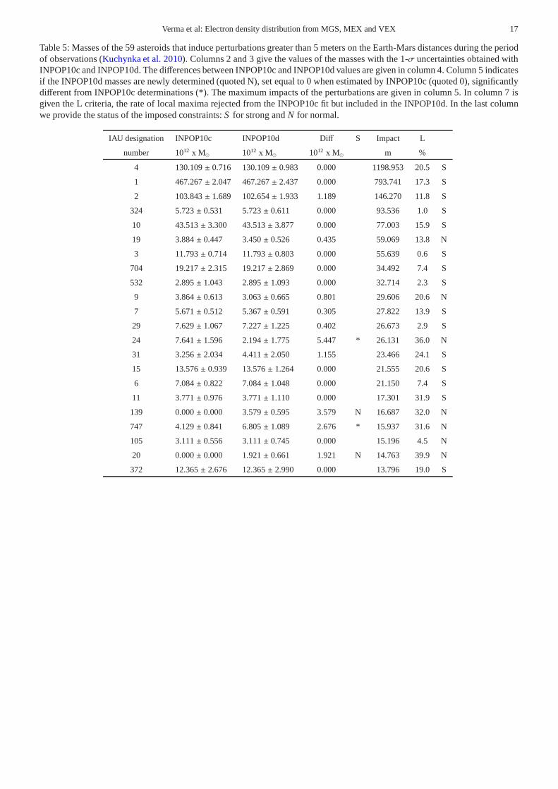
For the masses estimated both in INPOP10c andINPOP10d, 20% induce perturbations bigger than 5 meters onthe Earth-Mars distances during the observation period. Themasses of these 59 objects are presented in Tables5, 6, and7. Within the 1-σ uncertainties deduced from the fit, we no-tice 10 (17%) significant differences in masses obtained with

INPOP10c and INPOP10d, quoted with a “*” in column 5 ofthe two tables, 7 (12%) new estimates made with INPOP10d,noted N in column 5, and 6 (10%) masses put to 0 in INPOP10dwhen estimated in INPOP10c, marked with 0 in the fifth col-umn.

Table8 lists masses found in the literature compared withthe quoted values of Tables5, 6, and7. In this table, 80% ofthe INPOP10d estimates have a better consistency with thevalues obtained by close encounters than the one obtainedwith INPOP10c. Of these, the new estimates obtained withINPOP10d for (20), (139) and (27) agree well with the valuesfound in the literature. For (45) Eugenia, the INPOP10c valueis closer to the mass deduced from the motion of its satellite(Marchis et al. 2008) even if the INPOP10d value is still com-patible at 2-σ. For (130) Elektra, the INPOP10c and INPOP10destimated values are certainly under evaluated. Finally, one cannote the systematic bigger uncertainties of the INPOP10d es-timates. The supplementary data sample collected during thesolar conjunctions that has 30% more noise than the data col-lected beyond the conjunction can explain the degradation ofthe uncertainties for the INPOP10d determinations comparedto INPOP10c.


By correcting the range bias for the solar corona effects, weadded more informations related to the perturbations inducedby the asteroids during the conjunction intervals.

In principal, during the least-squares estimation of the as-teroid masses, the general trend of the gravitational perturba-tion induced by the asteroid on the planet orbits should be de-scribed the most completely by the observable (the Earth-Marsdistances) without any lack of information. In particular,foran optimized estimation, the data sets used for the fit shouldinclude local maxima of the perturbation.

However, it could happen that some of the local maximaoccur during the solar conjunction intervals. One can then ex-pect a degradation of the least-squares estimation of the per-turber mass if no solar corrections are applied or if these in-tervals are not taken into account during the fit. To estimatewhich mass determination can be more degraded than anotherby thiswindow effect, we estimatedL, the percentage of localmaxima rejected from the INPOP10c fit in comparison with theINPOP10d adjustment including all data sets corrected for so-lar plasma.L will give the loss of information induced by therejection of the solar conjunction intervals in terms of highestperturbations.

The L criteria are given in column 7 of Tables5, 6, and7. As an example, for (24) Themis one notes in Table8 thegood agreement between the close encounter estimates and theINPOP10d mass determination compared with INPOP10c. Onthe other hand, based on theL criteria, 36% of the local max-ima happen near solar conjunctions. By neglecting the solarconjunction intervals, more than a third of the biggest perturba-tions are missing in the adjustment. This can explain the morerealistic INPOP10d estimates compared with INPOP10c.

We also indicate in Tables5, 6, and 7 if important con-straints were added in the fit (column 8). In these cases, evenif new observations are added to the fit (during the solar con-junction periods), there is a high probability to obtain a sta-ble estimates of the constrained masses as for the biggest per-turbers of Table5. For the other mass determinations, one cannote a consistency between high values of theL criteria andthe non-negligible mass differences between INPOP10c andINPOP10d.

Fig. 12: MEX extrapolated residuals estimated with INPOP10d(light dots) and INPOP10c (dark dots).

By improving the range bias residuals during the solar con-junction periods, we then slightly improved the asteroid massdeterminations.

Estimates of residuals for data samples not used in theINPOP fit and dated after or before the end of the fitting intervalare currently made to evaluate the real accuracy of the planetaryephemerides (Fienga et al. 2011a, 2009). To estimate if the useof the solar corona corrections induces a global improvementof the planetary ephemerides, the MEX extrapolated residualswere computed with INPOP10c and INPOP10d. As one cansee in Figure12, the INPOP10d MEX extrapolated residualsshow a better long-term behavior compared with INPOP10cwith 30% less degraded residuals after two years of extrapola-tion.

Supplementary data of the MEX and VEX obtained dur-ing the first six months of 2012 would confirm the long-termevolutions of the INPOP10d, INPOP10c and INPOP10b.

This improvement can be explained by the more realisticadjustment of the ephemerides with denser data sets (7%) andmore consistent asteroid mass fitting.

5. Conclusion

We analyzed the navigation data of the MGS, MEX, and VEXspacecraft acquired during solar conjunction periods. We esti-mated new characteristics of solar corona models and electrondensities at different phases of solar activity (maximum andminimum) and at different solar wind states (slow and fast).Good agreement was found between the solar corona modelestimates and the radiometric data. We compared our estimatesof electron densities with earlier results obtained with differ-ent methods. These estimates were found to be consistent dur-ing the same solar activities. During solar minima, the elec-tron densities obtained byin situ measurements and solar radioburst III are within the error bars of the MEX and VEX es-timates. However, during the solar maxima, electron densitiesobtained with different methods or different spacecraft showweaker consistencies. These discrepancies need to be investi-gated in more detail, which requires a deeper analysis of dataacquired at the time of solar maxima.

The MGS, MEX, and VEX solar conjunctions data allowsus to analyze the large-scale structure of the corona electrondensity. These analyses provide individual electron density pro-files for slow- and fast-wind regions during solar maxima andminima activities.

In the future, planetary missions such as MESSENGERwill also provide an opportunity to analyze the radio-sciencedata, especially at the time of maximum solar cycle.

We tested the variability caused by the planetaryephemerides on the electron density parameters deduced fromthe analysis of the range bias. This variability is smaller thanthe 1-σ uncertainties of the time-fitting interval of the plan-etary ephemerides but becomes wider beyond this interval.Furthermore, data corrected for solar corona perturbations wereused for constructing of the INPOP ephemerides. Thanks tothese supplementary data, an improvement in the estimationofthe asteroid masses and a better behavior of the ephemerideswere achieved.


6. Acknowledgments

A. K. Verma is the research fellow of CNES and RegionFranche-Comte and thanks CNES and Region Franche-Comtefor financial support. Part of this work was made using theGINS software; we would like to acknowledge CNES, whoprovided us access to this software. We are also grateful toJ.C Marty (CNES) and P. Rosenbatt (Royal Observatory ofBelgium) for their support in handling the GINS software. TheAuthors are grateful to the anonymous referee for helpful com-ments, which improved the manuscript.

References

Anderson, J. D., Krisher, T. P., Borutzki, S. E., et al. 1987,TheAstrophysical Journal, 323, L141

Baer, J., Chesley, S. R., & Matson, R. 2011, AJ, in pressBird, M. K., Paetzold, M., Edenhofer, P., Asmar, S. W., &

McElrath, T. P. 1996, A&A, 316, 441Bird, M. K., Volland, H., Paetzold, M., et al. 1994, The

Astrophysical Journal, 426, 373Bougeret, J.-L., King, J. H., & Schwenn, R. 1984, Solar

Physics, 90, 401Cranmer, S. R. 2002, Space Sci. Rev., 101, 229Fienga, A., Kuchynka, P., Laskar, J., et al. 2011b, in EPSC-DPS

Join Meeting 2011, 1879Fienga, A., Laskar, J., Manche, H., et al. 2011a, Celestial

Mechanics and Dynamical AstronomyFienga, A., Laskar, J., Morley, T., et al. 2009, A&A, 507, 1675Folkner, W. M., Williams, J. G., & Boggs, D. H. 2008, IOM

343R-08-003Guhathakurta, M., Fludra, A., Gibson, S. E., Biesecker, D.,&

Fisher, R. 1999, J. Geophys. Res., 104, 9801Guhathakurta, M. & Holzer, T. E. 1994, ApJ, 426, 782Guhathakurta, M., Holzer, T. E., & MacQueen, R. M. 1996,

ApJ, 458, 817Issautier, K., Meyer-Vernet, N., Moncuquet, M., & Hoang, S.

1997, Solar Physics, 172, 335Issautier, K., Meyer-Vernet, N., Moncuquet, M., & Hoang, S.

1998, J. Geophys. Res., 103, 1969Kuchynka, P., Laskar, J., Fienga, A., & Manche, H. 2010,

A&A, 514, A96Leblanc, Y., Dulk, G. A., & Bougeret, J.-L. 1998, Solar

Physics, 183, 165Mancuso, S. & Spangler, S. R. 2000, ApJ, 539, 480Marchis, F., Descamps, P., Baek, M., et al. 2008, icarus, 196,

97Marty, J. C., Balmino, G., Duron, J., et al. 2009, Planetary and

Space Science, 57, 350Moyer, T. D. 2003, Formulation for Observed and Computed

Values of Deep Space Network Data Types for Navigation,Vol. 2 (John Wiley & Sons)

Muhleman, D. O. & Anderson, J. D. 1981, The AstrophysicalJournal, 247, 1093

Muhleman, D. O., Esposito, P. B., & Anderson, J. D. 1977,Astrophysics Journalj, 211, 943

Schwenn, R. 2006, Space Sci. Rev., 124, 51

Schwenn, R. & Marsch, E., eds. 1990, Physics and Chemistryin Space, Vol. 20, Physics of the Inner Heliosphere, Vol. I:Large-Scale Phenomena (Springer)

Schwenn, R. & Marsch, E., eds. 1991, Physics and Chemistryin Space, Vol. 21, Physics of the Inner Heliosphere, Vol. II:Particles, Waves and Turbulence (Springer)

Standish, E. M. 1998, IOM 312F-98-483Tokumaru, M., Kojima, M., & Fujiki, K. 2010, Journal of

Geophysical Research (Space Physics), 115, 4102Woo, R. & Habbal, S. R. 1999, Geophys. Res. Lett., 26, 1793You, X. P., Coles, W. A., Hobbs, G. B., & Manchester, R. N.

2012, MNRAS, 422, 1160You, X. P., Hobbs, G. B., Coles, W. A., Manchester, R. N., &

Han, J. L. 2007, ApJ, 671, 907Zielenbach, W. 2011, The Astronomical Journal, 142, 120


Table 5: Masses of the 59 asteroids that induce perturbations greater than 5 meters on the Earth-Mars distances during the periodof observations (Kuchynka et al. 2010). Columns 2 and 3 give the values of the masses with the 1-σ uncertainties obtained withINPOP10c and INPOP10d. The differences between INPOP10c and INPOP10d values are given in column 4. Column 5 indicatesif the INPOP10d masses are newly determined (quoted N), set equal to 0 when estimated by INPOP10c (quoted 0), significantlydifferent from INPOP10c determinations (*). The maximum impacts of the perturbations are given in column 5. In column 7 isgiven the L criteria, the rate of local maxima rejected from the INPOP10c fit but included in the INPOP10d. In the last columnwe provide the status of the imposed constraints:S for strong andN for normal.

IAU designation INPOP10c INPOP10d Diff S Impact L

number 1012 x M⊙ 1012 x M⊙ 1012 x M⊙ m %

4 130.109± 0.716 130.109± 0.983 0.000 1198.953 20.5 S

1 467.267± 2.047 467.267± 2.437 0.000 793.741 17.3 S

2 103.843± 1.689 102.654± 1.933 1.189 146.270 11.8 S

324 5.723± 0.531 5.723± 0.611 0.000 93.536 1.0 S

10 43.513± 3.300 43.513± 3.877 0.000 77.003 15.9 S

19 3.884± 0.447 3.450± 0.526 0.435 59.069 13.8 N

3 11.793± 0.714 11.793± 0.803 0.000 55.639 0.6 S

704 19.217± 2.315 19.217± 2.869 0.000 34.492 7.4 S

532 2.895± 1.043 2.895± 1.093 0.000 32.714 2.3 S

9 3.864± 0.613 3.063± 0.665 0.801 29.606 20.6 N

7 5.671± 0.512 5.367± 0.591 0.305 27.822 13.9 S

29 7.629± 1.067 7.227± 1.225 0.402 26.673 2.9 S

24 7.641± 1.596 2.194± 1.775 5.447 * 26.131 36.0 N

31 3.256± 2.034 4.411± 2.050 1.155 23.466 24.1 S

15 13.576± 0.939 13.576± 1.264 0.000 21.555 20.6 S

6 7.084± 0.822 7.084± 1.048 0.000 21.150 7.4 S

11 3.771± 0.976 3.771± 1.110 0.000 17.301 31.9 S

139 0.000± 0.000 3.579± 0.595 3.579 N 16.687 32.0 N

747 4.129± 0.841 6.805± 1.089 2.676 * 15.937 31.6 N

105 3.111± 0.556 3.111± 0.745 0.000 15.196 4.5 N

20 0.000± 0.000 1.921± 0.661 1.921 N 14.763 39.9 N

372 12.365± 2.676 12.365± 2.990 0.000 13.796 19.0 S


Table 6: Same as Table5


number 1012 x M⊙ 1012 x M⊙ 1012 x M⊙ m %

8 3.165± 0.353 3.325± 0.365 0.159 12.664 17.7 S

45 3.523± 0.819 1.518± 0.962 2.005 * 11.790 21.0 N

41 3.836± 0.721 2.773± 0.977 1.063 11.568 15.2 N

405 0.005± 0.003 0.006± 0.003 0.001 11.378 21.2 N

511 9.125± 2.796 9.125± 3.138 0.000 10.248 20.5 S

52 8.990± 2.781 8.990± 3.231 0.000 9.841 3.0 S

16 12.613± 2.286 12.613± 2.746 0.000 9.701 8.9 S

419 1.185± 0.461 0.425± 0.398 0.760 9.585 10.2 N

78 0.026± 0.016 0.024± 0.016 0.002 9.389 9.8 N

259 0.092± 0.002 0.006± 0.003 0.086 9.222 31.4 N

27 0.000± 0.000 1.511± 0.982 1.511 N 9.146 29.5 N

23 0.000± 0.000 0.093± 0.156 0.093 N 9.067 31.1 N

488 3.338± 1.850 0.000± 0.000 3.338 0 8.614 2.8 N

230 0.000± 0.000 0.263± 0.169 0.263 N 7.620 27.0 N

409 0.002± 0.001 0.002± 0.001 0.000 0 7.574 2.2 N

94 1.572± 1.097 7.631± 2.488 6.058 * 7.466 28.5 N

344 2.701± 0.497 2.088± 0.515 0.613 7.465 15.3 N

130 0.099± 0.047 0.221± 0.069 0.122 * 7.054 31.7 N

111 1.002± 0.323 0.000± 0.000 1.002 0 6.985 11.4 N

109 0.495± 0.322 1.318± 0.852 0.823 6.865 18.7 N

42 1.144± 0.362 0.083± 0.389 1.061 * 6.829 0.6 N

63 0.000± 0.000 0.424± 0.143 0.424 N 6.451 17.4 N

12 2.297± 0.319 1.505± 0.331 0.792 * 6.159 21.7 N

469 0.088± 0.073 0.000± 0.000 0.088 0 6.107 18.1 N

144 0.176± 0.297 0.751± 0.361 0.575 6.087 22.8 N

Table 7: Same as Table5


number 1012 x M⊙ 1012 x M⊙ 1012 x M⊙ m %

356 4.173± 0.868 4.173± 0.902 0.000 5.759 2.2 N

712 0.000± 0.000 1.228± 0.267 1.228 N 5.745 2.2 N

88 1.340± 0.866 0.000± 0.000 1.340 0 5.742 1.4 N

60 0.402± 0.221 0.282± 0.268 0.120 5.733 3.8 N

50 0.686± 0.187 1.031± 0.566 0.345 5.702 2.0 N

128 4.699± 1.522 0.000± 0.000 4.677 0 5.624 3.0 N

5 0.448± 0.165 0.913± 0.220 0.466 * 5.533 15.8 N

59 4.332± 0.607 1.364± 1.097 2.968 * 5.325 12.1 N

98 1.414± 0.603 2.100± 0.705 0.686 5.195 15.1 N

194 6.387± 0.701 4.380± 0.819 2.007 * 5.145 2.9 N

51 3.546± 0.748 3.639± 0.937 0.093 5.109 15.6 N

156 3.263± 0.438 3.089± 0.576 0.174 5.103 19.3 N


Table 8: Asteroid masses found in the recent literature compared with the values estimated in INPOP10c and INPOP10d. Theuncertainties are given at 1 published sigma.

IAU designation INPOP10c Close-encounters Refs INPOP10d

number 1012 x M⊙ 1012 x M⊙ 1012 x M⊙ %

5 0.448± 0.165 1.705± 0.348 Zielenbach(2011) 0.913± 0.220 15.8

12 2.297± 0.319 2.256± 1.910 Zielenbach(2011) 1.505± 0.331 21.7

20 0.000± 0.000 1.680± 0.350 Baer et al.(2011) 1.921± 0.661 39.9

24 7.6± 1.6 2.639± 1.117 Zielenbach(2011) 2.2± 1.7 36.0

27 0.000± 0.000 1.104± 0.732 Zielenbach(2011) 1.511± 0.982 29.5

45 3.523± 0.819 2.860± 0.060 Marchis et al.(2008) 1.518± 0.962 21.0

59 4.332± 0.607 1.448± 0.0187 Zielenbach(2011) 1.364± 1.097 12.1

94 1.572± 1.097 7.878± 4.016 Zielenbach(2011) 7.631± 2.488 28.5

130 0.099± 0.047 3.320± 0.200 Marchis et al.(2008) 0.221± 0.069 31.7

139 0.000± 0.000 3.953± 2.429 Zielenbach(2011) 3.579± 0.595 32.0


Appendix A: Analytical solution

This section presents the analytical solutions of Equation1.Let, I1 and I2 be the integral solutions of Equation 1 usingEquation 3 and 4i.e. ,

I1 =

∫ Ls/c

LEarths/n

B

(

lR⊙

)−ǫ

dL (A.1)

and

I2 =

∫ Ls/c

LEarths/n

[

A

(

lR⊙

)−4

+ B

(

lR⊙

)−2]

dL . (A.2)

From the geometry (Figure 3) we define

P = RS/E sin α ,

LDC = RE/S C − RS/E cos α ,

L2DE = l2 − P2 ,

l2 = L2 + R2S/E − 2 L RS/E cos α ,

whereα andβ are the angle between the Sun-Earth-Probe(SEP) and the Earth-Sun-Probe (ESP).P is the MDLOS fromthe Sun. With these expressions,I1 can be written as

I1 =

∫ Ls/c

LEarths/n

B Rǫ⊙

(

dL

(L2 + R2S/E − 2 L RS/E cos α)ǫ/2

)

s

= B Rǫ⊙

∫ Ls/c

LEarths/n

(

dL

([L − RS/E cos α]2 + R2S/E sin2 α)ǫ/2

)

.

Assuming,

x = L − RS/E cos α ,

a = RS/E sin α ,

dx = dL ,

with L = 0 at the Earth station (LEarths/n ) andL = RE/S C atthe spacecraft (Ls/c). Then the integralI1 can be written as

I1 = B Rǫ⊙

∫ RE/S C−RS/E cos α

−RS/E cos α

dx

(x2 + a2)ǫ/2

=B Rǫ

⊙

aǫ

∫ RE/S C−RS/E cos α

−RS/E cos α

dx

(1+ x2

a2 )ǫ/2.

Now letxa= tan θ ,

and

dx = a sec2 θ dθ .

Therefore,

I1 =B Rǫ

⊙

aǫ

∫ arctan(RE/S C −RS/E cos α)

a

arctan(−RS/E cos α)

a

a sec2 θ

(tan2 θ + 1)ǫ/2dθ . (A.3)

From the geometry of Figure 3, the lower limit of EquationA.3 can be written as

arctan

(

−RS/E cos α

a

)

= arctan

(

−RS/E cos α

RS/E sin α

)

= arctan

(

− cot α

)

,

with

cot α = tan

(

π

2− α

)

.

Hence,

arctan

(

−RS/E cos α

a

)

= α −π

2.

Similarly, the upper limit of Equation A.3 can be written as

arctan

(

RE/S C − RS/E cos α

a

)

= arctan

(


RS/E sin α

)

,

with

RE/S C − RS/E cos α = RS/E sin α

[

tan

(

β −

{

π

2− α

} ) ]

.

Hence,

arctan

(


a

)

= β + α −π

2.

Now Equation A.3 is given by

I1 =B Rǫ

⊙

aǫ

∫ β+α− π2

α− π2

a sec2 θ

(tan2 θ + 1)ǫ/2dθ .

with

sec2 θ = tan2 θ + 1 ,

and

cos θ =1

sec θ.

Therefore, the integralI1 can be written as

I1 =B Rǫ

⊙

aǫ−1

∫ β+α− π2

α− π2

(cos θ)ǫ−2 dθ . (A.4)

The maximum contribution of the integral occurs atθ = 0.To solve this integral, Taylor series expansion was used andforθ near zero, it can be given as

f (θ) = f (0) + θ

(

d fdθ

)

+θ2

2!

(

d2 fdθ2

)

+θ3

3!

(

d3 fdθ3

)

+θ4

4!

(

d4 fdθ4

)

.......... + θ (θn) , (A.5)

with

f (θ) = (cos θ)ǫ−2 .


Then

f (0) = 1(

d fdθ

)

= −(ǫ − 2) (sin θ) (cos θ)(ǫ−3) ,

(

d fdθ

)

θ=0

= 0 ,

(

d2 fdθ2

)

= (ǫ − 2) (ǫ − 3) (sin2 θ) (cos θ)(ǫ−4)

−(ǫ − 2) (cos θ)(ǫ−2) ,

(

d2 fdθ2

)

θ=0

= −(ǫ − 2) ,

(

d3 fdθ3

)

= −(ǫ − 2) (ǫ − 3) (ǫ − 4) (sin3 θ) (cos θ)(ǫ−5)

+(ǫ − 2) (3ǫ − 8) (sin θ) (cos θ)(ǫ−3) ,

(

d3 fdθ3

)

θ=0

= 0 ,

(

d4 fdθ4

)

= (ǫ − 2) (ǫ − 3) (ǫ − 4) (ǫ − 5) (sin4 θ) (cos θ)(ǫ−6)

−(ǫ − 2) (ǫ − 3) (6ǫ − 20) (sin2 θ) (cos θ)(ǫ−4)

+(ǫ − 2) (3ǫ − 8) (cos θ)(ǫ−2) ,

(

d4 fdθ4

)

θ=0

= (ǫ − 2) (3ǫ − 8) .

Now, Equation A.5 can be written as

(cos θ)(ǫ−2) = 1− (ǫ − 2)θ2

2!+ (ǫ − 2) (3ǫ − 8)

θ4

4!+ .... θ (θn)

= 1−ǫ − 2

2θ2 +

3ǫ2 − 14ǫ + 1624

θ4 + .... θ (θn) .

By neglecting the higher order terms, the integral (EquationA.4) can be written as

I1 =B Rǫ

⊙

aǫ−1

∫ β+α− π2

α− π2

(

1−ǫ − 2

2θ2 +

3ǫ2 − 14ǫ + 1624

θ4)

dθ

=B Rǫ

⊙

aǫ−1

[

θ −ǫ − 2

6θ3 +

3ǫ2 − 14ǫ + 16120

θ5]β+α− π2

α− π2

=B Rǫ

⊙

aǫ−1

[

β −ǫ − 2

6

(

(β + α − π/2)3 − (α − π/2)3)

+3ǫ2 − 14ǫ + 16

120

(

(β + α − π/2)5 − (α − π/2)5)]

.

By substituting the value ofa, we can write the integralI1

as

I1 =B Rǫ

⊙

(RS/E sinα)ǫ−1

[

β −ǫ − 2

6

(

(β + α − π/2)3 − (α − π/2)3)

+3ǫ2 − 14ǫ + 16

120

(

(β + α − π/2)5 − (α − π/2)5)]

. (A.6)

Now, Equation A.2 can be written asI2= I2a + I2b where,

I2a =

∫ Ls/c

LEarths/n

A

(

lR⊙

)−4

dL , (A.7)

and

I2b =

∫ Ls/c

LEarths/n

B

(

lR⊙

)−2

dL . (A.8)

Using a similar approach to the previous integral, one canwrite

I2a =A R4

⊙

a3

∫ β+α− π2

α− π2

cos2 θ dθ

=A R4

⊙

a3

[

14

(2 θ + sin 2θ)

]β+α− π2

α− π2

=A R4

⊙

4 a3

[

(2 β − sin 2(α + β) + sin 2α)

]

=A R4

⊙

4 R3S/E sin3α

[

(2 β − sin 2(α + β) + sin 2α)

]

.

Similarly, Equation A.8 can be written as

I2b =B R2

⊙

a

∫ β+α− π2

α− π2

dθ

=B R2

⊙

a

[

θ

]β+α− π2

α− π2

=B R2

⊙

RS/E sin αβ .

Now by usingI2a andI2b, expressionI2 can be written as

I2 =A R4

⊙

4 R3S/E sin3α

[

(2 β − sin 2(α + β) + sin 2α)

]

+B R2

⊙

RS/E sin αβ .

(A.9)

Documents

Electron density distribution and solar plasma correction of radio signals using MGS, MEX, and VEX spacecraft navigation data and its application to planetary ephemerides