Embed Size (px)
Citation preview
Degree project in Materials Science and Engineering
Second cycle, 30 credits
Embedding Carbon Nanotubes Sensors into Carbon Fiber Laminates
RICCARDO ANDOLFI
Stockholm, Sweden 2022
Abstract
The use of Fibre Reinforced Polymer (FRP) composite materials in structural
applications has increased in the past decades in highperformance sectors, such
as in the automotive and aeronautic industries, for weight reduction purposes.
However, FRP composite materials can offer more significant innovation potential.
The application of CNTs in conjunction with composite material can allow the creation
of multifunctional materials, relying on FRP for the structural side and CNT for the
sensing ability. In this master thesis, the embedment of a Vertical Aligned Carbon
Nanotube (VACNT) layer into the interlaminar region of Carbon Fibre (CF) laminates
to provide polyvalent sensing ability to thematerial was investigated. In order to obtain
accurate results, the sensor had to be isolated from the rest of the laminate. For this
reason, the main problem to be solved in this project was the electrical isolation on the
CNT layer and its contacts from the layers of CF laminate. This study aims to find a
suitable isolation technique in order to apply the CNT sensor technology, developed in
previous studies, into CF laminate. Although thought for aerospace applications, these
sensors could be applied to different structural components in various fields.1
Keywords
Multifunctional Materials, Sensing Abilities, Carbon Nanotubes, Carbon Fibers,
Analytical Modelling, Finite Element Modelling
1This abstract was generated by the AI syntax algorithm kindly offered by the JDaily company. Forthis I personally thank Sarti Riccardo and all his colleagues. For more information visit www.jdaily.it
i
Sammanfattning
Användningen av fiberförstärkta polymerer (FRP)kompositmaterial i strukturella
applikationer har ökat under de senaste decennierna i högpresterande sektorer, såsom
i fordons och flygindustrin, för viktminskningsändamål. FRPkompositmaterial kan
dock erbjuda mer betydande innovationspotential. Användningen av CNTs i
kombination med kompositmaterial kan möjliggöra skapandet av multifunktionella
material, beroende på FRP för den strukturella sidan och CNT för
avkänningsförmågan. I denna masteruppsats undersöktes inbäddningen av ett
Vertical Aligned Carbon Nanotube (VACNT) lager i den interlaminära regionen av
Carbon Fiber (CF) laminat för att ge polyvalent avkänningsförmåga till materialet.
För att få exakta resultat måste sensorn isoleras från resten av laminatet. Av
denna anledning var huvudproblemet som skulle lösas i detta projekt den elektriska
isoleringen på CNTlagret och dess kontakter från lagren av CFlaminat. Denna studie
syftar till att hitta en lämplig isoleringsteknik för att tillämpa CNTsensorteknologin,
utvecklad i tidigare studier, i CFlaminat. Även om de är tänkta för flygtillämpningar,
kan dessa sensorer appliceras på olika strukturella komponenter inom olika
områden.
Nyckelord
Multifunktionella Material, Avkänningsförmåga, Kolnanorör, Kolfibrer, Analytisk
Modellering, Finita Elementmodellering
ii

Acronyms
FRP Fibre Reinforced Polymer
CFRP Carbon Fibres Reinforced Polymers
CF Carbon Fibre
GF Glass Fibre
CNT Carbon Nanotube
VACNT Vertical Aligned Carbon Nanotube
SWCNT SingleWalled Carbon Nanotube
MWCNT MultiWalled Carbon Nanotube
CVD Chemical Vapour Deposition
RTM Resin Transfer Moulding
VIM Vacuum Infusion Moulding
RIM Resin Injection Moulding
CM Compression Moulding
IM Injection Moulding
ILSS Interlaminar Shear Strength
UTM Universal Testing Machine
RH Relative Humidity
QI Quasi Isotropic
ROM Rule Of Mixture
BC Boundary Condition
CFD Computational Fluid Dynamics
FEM Finite Element Modelling
FE Finite Element
DSC Differential Scanning Calorimetry
TMA Thermomechanical Analysis
CTE Coefficient of Thermal Expansion
iii

FITC Fluctuation Induced Tunnelling Conduction
CVD Chemical Vapour Deposition
iv
Contents
1 Introduction 11.1 Problem . . . . . . . . . . . . . . . . . . . . . . . . . . . . . . . . . . . . 2
1.2 Aim . . . . . . . . . . . . . . . . . . . . . . . . . . . . . . . . . . . . . . 2
1.3 Research Questions . . . . . . . . . . . . . . . . . . . . . . . . . . . . . 2
1.4 Background of the Project . . . . . . . . . . . . . . . . . . . . . . . . . . 3
1.5 Benefits, Ethics and Sustainability . . . . . . . . . . . . . . . . . . . . . 3
1.6 Delimitations . . . . . . . . . . . . . . . . . . . . . . . . . . . . . . . . . 3
2 Theoretical Background 42.1 Composite Materials . . . . . . . . . . . . . . . . . . . . . . . . . . . . . 4
2.1.1 Production . . . . . . . . . . . . . . . . . . . . . . . . . . . . . . 5
2.1.2 Characteristics . . . . . . . . . . . . . . . . . . . . . . . . . . . . 5
2.1.3 Properties . . . . . . . . . . . . . . . . . . . . . . . . . . . . . . 7
2.2 Carbon Nanotubes . . . . . . . . . . . . . . . . . . . . . . . . . . . . . . 8
2.2.1 Synthesis . . . . . . . . . . . . . . . . . . . . . . . . . . . . . . . 8
2.2.2 Structure . . . . . . . . . . . . . . . . . . . . . . . . . . . . . . . 10
2.2.3 Properties . . . . . . . . . . . . . . . . . . . . . . . . . . . . . . 12
2.3 Modelling . . . . . . . . . . . . . . . . . . . . . . . . . . . . . . . . . . . 14
2.3.1 The steps for an effective modelling process . . . . . . . . . . . 14
2.3.2 Types of models . . . . . . . . . . . . . . . . . . . . . . . . . . . 16
3 The work 17
4 Methodologies and Methods 204.1 Microscopy . . . . . . . . . . . . . . . . . . . . . . . . . . . . . . . . . . 20
4.2 Impregnation method 1 . . . . . . . . . . . . . . . . . . . . . . . . . . . 20
4.3 Impregnation method 2 . . . . . . . . . . . . . . . . . . . . . . . . . . . 20
v
CONTENTS
4.4 Samples layout . . . . . . . . . . . . . . . . . . . . . . . . . . . . . . . . 21
4.5 IV measurements . . . . . . . . . . . . . . . . . . . . . . . . . . . . . . 22
4.6 COMSOL model . . . . . . . . . . . . . . . . . . . . . . . . . . . . . . . 22
4.7 MATLAB model . . . . . . . . . . . . . . . . . . . . . . . . . . . . . . . . 23
4.8 Through the thickness resistance measure . . . . . . . . . . . . . . . . 24
4.9 Curing method and monitoring . . . . . . . . . . . . . . . . . . . . . . . 26
4.10 Temperature sensing . . . . . . . . . . . . . . . . . . . . . . . . . . . . 26
4.11 Thermal expansion evaluation . . . . . . . . . . . . . . . . . . . . . . . 27
4.12 Contact Resistance Measurement . . . . . . . . . . . . . . . . . . . . . 27
4.13 Evaluation of the minimum amount of carbon fibre filaments for contactpurpose . . . . . . . . . . . . . . . . . . . . . . . . . . . . . . . . . . . . 28
4.14 Short beam threepoint bending test . . . . . . . . . . . . . . . . . . . . 28
5 Result 305.1 Microscopy . . . . . . . . . . . . . . . . . . . . . . . . . . . . . . . . . . 30
5.2 IV measurements . . . . . . . . . . . . . . . . . . . . . . . . . . . . . . 36
5.3 Through the thickness resistance measure . . . . . . . . . . . . . . . . 37
5.4 COMSOL model . . . . . . . . . . . . . . . . . . . . . . . . . . . . . . . 40
5.5 Matlab model . . . . . . . . . . . . . . . . . . . . . . . . . . . . . . . . . 42
5.6 Curing monitoring . . . . . . . . . . . . . . . . . . . . . . . . . . . . . . 43
5.7 Thermal expansion evaluation . . . . . . . . . . . . . . . . . . . . . . . 44
5.8 Temperature sensing . . . . . . . . . . . . . . . . . . . . . . . . . . . . 46
5.9 Contact resistance . . . . . . . . . . . . . . . . . . . . . . . . . . . . . . 49
5.10 Evaluation of minimum amount of carbon fiber filaments for contactpurpose . . . . . . . . . . . . . . . . . . . . . . . . . . . . . . . . . . . . 49
5.11 Short beam threepoint bending test . . . . . . . . . . . . . . . . . . . . 50
6 Discussion of Results 516.1 Microscopy . . . . . . . . . . . . . . . . . . . . . . . . . . . . . . . . . . 51
6.2 IV measurements . . . . . . . . . . . . . . . . . . . . . . . . . . . . . . 52
6.3 Through the thickness resistance measure . . . . . . . . . . . . . . . . 53
6.4 COMSOL model . . . . . . . . . . . . . . . . . . . . . . . . . . . . . . . 53
6.5 Matlab model . . . . . . . . . . . . . . . . . . . . . . . . . . . . . . . . . 55
6.6 Curing monitoring . . . . . . . . . . . . . . . . . . . . . . . . . . . . . . 56
6.7 Thermal expansion evaluation . . . . . . . . . . . . . . . . . . . . . . . 57
vi

CONTENTS
6.8 Temperature sensing . . . . . . . . . . . . . . . . . . . . . . . . . . . . 586.9 Contact resistance . . . . . . . . . . . . . . . . . . . . . . . . . . . . . . 626.10 Evaluation of the minimum amount of carbon fibre filaments for contact
purpose . . . . . . . . . . . . . . . . . . . . . . . . . . . . . . . . . . . . 636.11 Short beam threepoint bending test . . . . . . . . . . . . . . . . . . . . 64
7 Conclusions 657.1 Comment by Scuderia Ferrari F1 team . . . . . . . . . . . . . . . . . . 67
7.1.1 Applications . . . . . . . . . . . . . . . . . . . . . . . . . . . . . 677.1.2 Advantages . . . . . . . . . . . . . . . . . . . . . . . . . . . . . . 687.1.3 Disadvantages . . . . . . . . . . . . . . . . . . . . . . . . . . . . 687.1.4 Must Have . . . . . . . . . . . . . . . . . . . . . . . . . . . . . . 69
7.2 Future Work . . . . . . . . . . . . . . . . . . . . . . . . . . . . . . . . . 70
8 Acknowledgements 71
9 References 73
vii
Chapter 1
Introduction
The use of Fibre Reinforced Polymer (FRP) composite materials in structural
applications has increased in the past decades in highperformance sectors, such
as in the automotive and aeronautic industries, for weight reduction purposes.
Today, most composite materials are limited to the structural area and are replacing
traditional metallic materials in the aeronautics and automotive industries [1].
However FRP composite materials can offer more significant innovation potential.
Excellent mechanical performance and considerable versatility in composition and
microstructure make fibre composite materials a particularly attractive platform for
developing multifunctional systems [2]. Multifunctionality is achieved by combining
one or more conventionally separated functions into a single material or structure [3],
including load carrying, structural health monitoring, morphing, selfhealing, energy
storage, and other functions [4]. Multifunctional materials and structures are pivotal
for future innovations. Many established institutions have recognised this potential.
For instance, NASA regards multifunctionality as a critical attribute for future deep
space missions [5].
During the past years, nanotechnology in material science has undergone tremendous
innovations regarding materials such as Graphene and Carbon Nanotube (CNT). The
application of CNT in conjunction with composite material can allow the creation
of multifunctional materials, relying on FRP for the structural side and CNT for the
sensing ability.
1
CHAPTER 1. INTRODUCTION
In this master thesis, the integration of a NAWAStich® Vertical Aligned Carbon
Nanotube (VACNT) layer into the interlaminar region of Carbon Fibre (CF) laminates
in order to provide polyvalent sensing ability to thematerialwas investigated. Different
isolation techniques have been explored, and the most suitable one was proposed.
Finite elements and an analytical model were built to support the results. Both the
models were derived using, as a base, experimental data.
1.1 Problem
Since the carbon fibres are electrically conductive, the CF prepreg’s layers are
electrically conductive too, both in the longitudinal, transverse and outofplane
directions [6]. Although the CF layers are less conductive in the transverse than in
the longitudinal and outofplane directions due to the conduction method, which is
by contact between transverse fibres [7], in this study they are still more conductive
than the CNT layer. In order to obtain accurate results, the sensor has to be isolated
from the rest of the laminate. For this reason, the main problem in this project is the
electrical isolation on the CNT sensor and its contacts from the layers of CF laminate.
The secondary problem is to succeed in the electrical isolationwithout adding excessive
thickness that would decrease the material’s mechanical properties.
1.2 Aim
This study aims to find a suitable isolation technique in order to apply the CNT sensor
technology developed in previous studies into CF laminate.
1.3 Research Questions
• How can we isolate the sensor from the CF laminate?
• Canwepredict how thin the isolationmembrane has to be in order to be effective?
• Does the sensor with the proposed isolation technique works as a temperature
sensor?
• Does the sensor with the proposed isolation technique works as a curing sensor?
• Does the introduction of the sensor reduce the laminate’smechanical properties?
2
CHAPTER 1. INTRODUCTION
1.4 Background of the Project
This thesis project is part of the course MH202X Degree Project in Materials and
Process Design, the final course of the Master’s Programme of Engineering Materials
Science (TTMVM) at KTH Royal Insitute of Technology in Stockholm. The thesis
project was conducted during the second semester of the academic year 2020/2021 by
the Lightweight Structure Laboratory at KTH in collaboration with SAAB Aeronautics
in Linköping. Professor Malin Åkermo from the Engineering Mechanics department
at KTH and Per Hallander, Technical Fellow Composites technology &Manufacturing
Processes at Saab Aeronautics, has supervised the project.
1.5 Benefits, Ethics and Sustainability
Been able to insert this kind of sensor inside CF components would be a great benefit,
especially in the aerospace industry. Continuous monitoring of temperature and
strain state of critical components could reduce the maintenance costs and allow
the designers to adopt a more radical approach, reducing the applied safety factor.
Allowing amore radical design approach, these sensors could help reduce the material
usage, which translates into lighter vehicles with lower fuel consumption.
Although thought for aerospace applications, these sensors could be applied to
different structural components. Aerodynamic components in race cars, composite
moulds, tools, gas tanks and many other components could benefit significantly from
continuous stress and temperature monitoring.
1.6 Delimitations
This thesis project is focused on the method to effectively embed the CNT layer inside
a CF laminate. SAAB Aerospace provided both the CNT layer and the CF prepreg. The
technique used to produce the sensing material will not be discussed in this project.
Moreover, the sensing ability will be tested only to validate the isolation method,
comparing the outcomes with results obtained in other studies.
3
Chapter 2
Theoretical Background
2.1 Composite Materials
Composite materials are defined as ”A macroscopic combination of two or more
distinct materials into one with the intent of suppressing undesirable properties of
the constituent materials in favour of desirable properties” [8].
In more general terms, the term composite materials applies to any material system
made of two or more distinctly different constituents. Among this broad class
of materials, the Fiber Reinforced Polymers (FRP) are the more recent and most
requested by the industry thanks to their excellent weighttostrength ratio and the
possibility to tailor the material properties to suit the particular application. In
these materials, a fibrous reinforcement is embedded into a polymeric matrix. The
reinforcements most widely used are carbon, glass and aramid fibres. Fibrous
reinforcement can be embedded inside the polymeric matrix in different ways. For
less demanding applications, short fibres arranged randomly in the three dimensions
are usually used. In applications where the performances are the limiting factor, long
bundles of aligned fibres are used. As matrix materials, thermosets are usually used
for highend applications requiring high performances, such as aircraft or race cars.
On the other hand, thermoplastic matrices are more common in the massproduction
industry for their low price and ease of usage.
4
CHAPTER 2. THEORETICAL BACKGROUND
2.1.1 Production
FRP production methods vary substantially depending on the material system desired
and on the final component’s topology. In the case of long fibres reinforcement
and thermosets matrices, various layers of fibres must be superimposed to form a
laminate to obtain a threedimensional product with a consistent thickness. Each
layer, usually thick from 0.1 up to several mm, can consist of socalled prepreg where
the polymericmatrix, commonly epoxy resin, has been impregnated before lamination
or by dry fibres, which will have to be impregnated with a polymeric material during
the lamination process. Prepregs, widely used in the aerospace industry, once stacked
into a laminate, require a curing cycle in an autoclave, where temperature and pressure
are applied in order to promote the curing process and remove any possible trapped air
bubble. Dryfibers based processes, such as Resin Transfer Moulding (RTM), Vacuum
Infusion Moulding (VIM) and Resin Injection Moulding (RIM), are more commonly
used in the automotive industry and rely on the base principle of forming the dry fibres’
cloth into a mould before impregnate and cure them.
On the other hand, in the case of short random reinforcement with thermoset or
thermoplastic matrices, the desired shape can be obtained directly without laminating
several layers. CompressionMoulding (CM) and InjectionMoulding (IM) are themost
common manufacturing techniques.
2.1.2 Characteristics
One typical characteristic of continuous long fibre reinforced polymers is that they
show different properties depending on the orientation. Already at the singlelayer
level, the mechanical, thermal and electrical properties are different in the fibres’
longitudinal and transverse directions. Once stacked into a laminate, the properties in
the outofplane direction are different from the inplane ones. This difference arises
from the fact that fibrous reinforcement and matrix have very dissimilar properties.
Themost commonway to describe the lamina’s properties knowing the basematerial’s
properties is to use the Rule Of Mixture (ROM) under the assumptions [8] that:
• The matrix is homogeneous, linearly elastic and isotropic
• The fibres are homogeneous, linearly elastic, isotropic (or transversely isotropic),
5
CHAPTER 2. THEORETICAL BACKGROUND
perfectly aligned and regularly spaced
• Fibre and matrix are free of voids, there is complete bonding and no transitional
region between them
• The lamina ismacroscopically homogeneous and orthotropic, linearly elastic and
initially stressfree.
In particular, in order to describe the lamina’s properties in the direction longitudinal
to the fibers, the Voigt Model [8] shown in Eq.2.1, is widely used.
E1 =∑i
Eiνi (2.1)
WhereE1 is Young’s modulus of the lamina, Ei is Young’s modulus of each component
and νi its volume fraction.
On the other hand, to describe the properties in the transverse and occasionally out
ofplane directions, the Reuss Model [8] shown in Eq.2.2, is used.
1
E2
=∑i
νiEi
(2.2)
Although developed to model laminas’ mechanical properties, the presented models
can be applied to estimate laminas’ thermal and electrical properties too.
Laminas’ orthotropicity can be exploited on a macroscopic level to obtain the desired
macroscopic properties. By tuning the orientation of the laminas with respect to each
other, it is possible to obtain macroscopic components with orthotropic properties or
balance the differences between the different laminas to obtain an almost isotropic
final component. In order to do so, the Generalised Hooke’s Law for orthotropic
materials needs to be used. In this law, the relation between the stresses and strains
is described by a stiffness tensor. This tensorial law gives the possibility of using the
socalled transformation matrix, which allows translating stresses and strains applied
in a global coordinate system at the laminate’s level to local stresses and strains in the
lamina’s level.
6
CHAPTER 2. THEORETICAL BACKGROUND
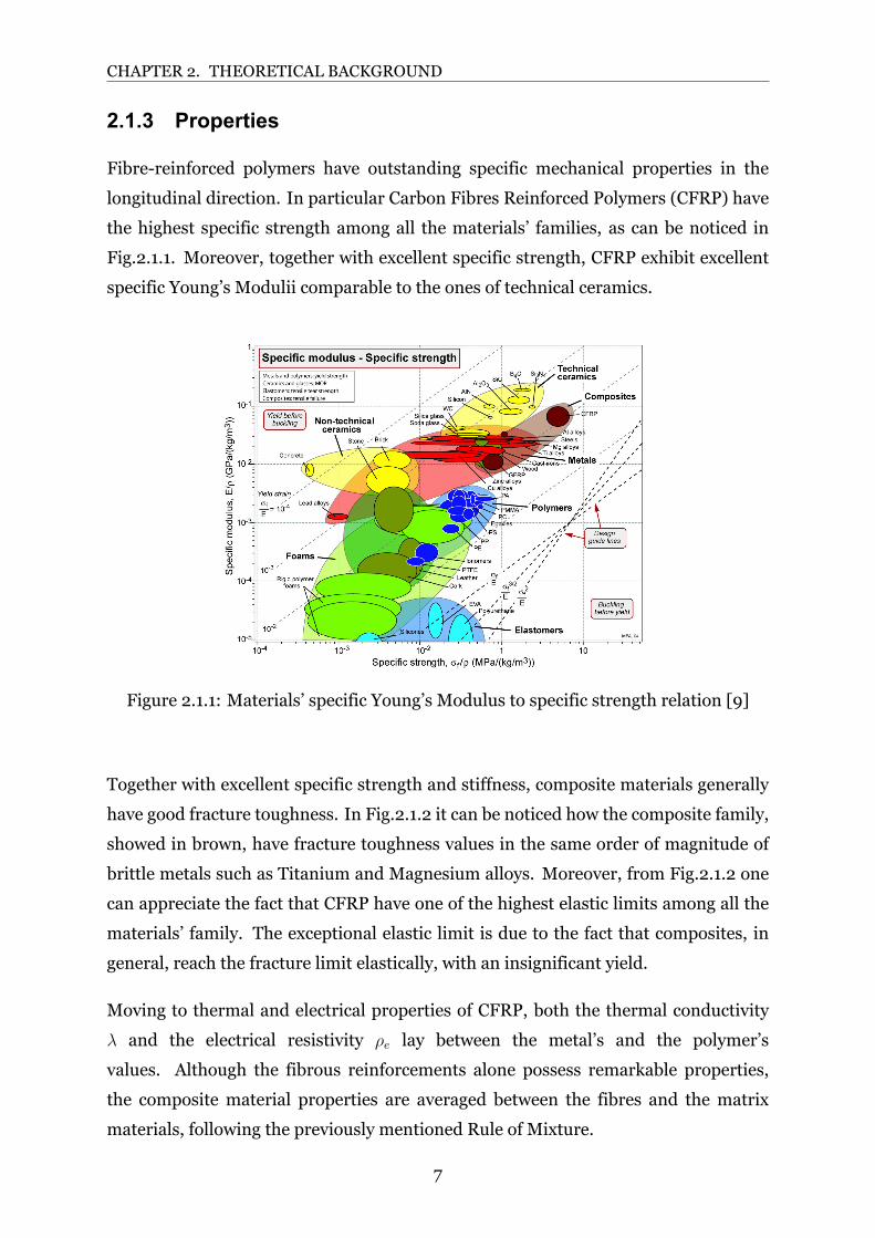
2.1.3 Properties
Fibrereinforced polymers have outstanding specific mechanical properties in the
longitudinal direction. In particular Carbon Fibres Reinforced Polymers (CFRP) have
the highest specific strength among all the materials’ families, as can be noticed in
Fig.2.1.1. Moreover, together with excellent specific strength, CFRP exhibit excellent
specific Young’s Modulii comparable to the ones of technical ceramics.
Figure 2.1.1: Materials’ specific Young’s Modulus to specific strength relation [9]
Together with excellent specific strength and stiffness, composite materials generally
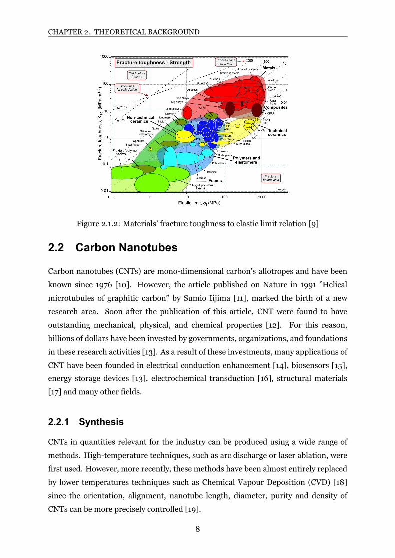
have good fracture toughness. In Fig.2.1.2 it can be noticed how the composite family,
showed in brown, have fracture toughness values in the same order of magnitude of
brittle metals such as Titanium and Magnesium alloys. Moreover, from Fig.2.1.2 one
can appreciate the fact that CFRP have one of the highest elastic limits among all the
materials’ family. The exceptional elastic limit is due to the fact that composites, in
general, reach the fracture limit elastically, with an insignificant yield.
Moving to thermal and electrical properties of CFRP, both the thermal conductivity
λ and the electrical resistivity ρe lay between the metal’s and the polymer’s
values. Although the fibrous reinforcements alone possess remarkable properties,
the composite material properties are averaged between the fibres and the matrix
materials, following the previously mentioned Rule of Mixture.
7
CHAPTER 2. THEORETICAL BACKGROUND
Figure 2.1.2: Materials’ fracture toughness to elastic limit relation [9]
2.2 Carbon Nanotubes
Carbon nanotubes (CNTs) are monodimensional carbon’s allotropes and have been
known since 1976 [10]. However, the article published on Nature in 1991 ”Helical
microtubules of graphitic carbon” by Sumio Iijima [11], marked the birth of a new
research area. Soon after the publication of this article, CNT were found to have
outstanding mechanical, physical, and chemical properties [12]. For this reason,
billions of dollars have been invested by governments, organizations, and foundations
in these research activities [13]. As a result of these investments, many applications of
CNT have been founded in electrical conduction enhancement [14], biosensors [15],
energy storage devices [13], electrochemical transduction [16], structural materials
[17] and many other fields.
2.2.1 Synthesis
CNTs in quantities relevant for the industry can be produced using a wide range of
methods. Hightemperature techniques, such as arc discharge or laser ablation, were
first used. However, more recently, these methods have been almost entirely replaced
by lower temperatures techniques such as Chemical Vapour Deposition (CVD) [18]
since the orientation, alignment, nanotube length, diameter, purity and density of
CNTs can be more precisely controlled [19].
8
CHAPTER 2. THEORETICAL BACKGROUND
Electric arc discharge
The CNT synthesis is performed in a reaction chamber filled with inert gas. Usually,
heliumor argon are used [20]. A difference of potential is applied between two graphite
electrodes which are gradually approached until the gap between them is small enough
to trigger an electric arc breakdown. The graphite is sublimated by the plasma created
by the electric arc between the two electrodes where temperatures can reach 6000
°C [20]. During the sublimation, atoms migrate towards colder zones within the
chamber, allowing a nanotube deposit to accumulate onto the graphitic cathode. The
type of nanotube that is formed depends crucially upon the composition of the anode
[20].
Laser Ablation
Developed initially to recreate the conditions of interstellar dust formation around
stars by Kroto, Smalley and coworkers [21], this technique led to the discovery of C60
Buckminsterfullerene in 1985. Since then, this technique has been used to produce not
only fullerenes but also carbon nanotubes.
In this process, a graphite pellet is placed inside a quartz tube, filled with an inert gas
flow, within an oven at a controlled temperature around 1000–1200°C. A high power
laser beam is focused on the pellet and vaporizes graphite by scanning its surface. The
carbon sublimated from the graphite pellet is displaced by the gas flow, coalesces to
CNTs in the gas phase, and finally deposits on a cooled copper collector [20].
Chemical Vapour Deposition
In this synthesis technique, a precursor of metal catalyst is introduced into a reactor
chamber, and the catalyst particles are formed insitu from the gas phase [20].
The most frequently used catalyst precursors are organometallic compounds both in
gaseous, liquid or solid states. Catalyst precursors can also be dissolved in organic
solvents that will also serve as carbon precursors such as benzene, nhexane, xylene, or
toluene [22]. One commonCVDmethod used formass production of CNTs is the high
pressure carbon monoxide (HiPco) process that employs iron pentacarbonyl Fe(CO)5
as a catalyst precursor and carbonmonoxide as a carbon precursor in a pressure range
of 1–10 atm and synthesis temperatures of 800–1200 °C [20].
9
CHAPTER 2. THEORETICAL BACKGROUND
2.2.2 Structure
Carbon nanotubes are tubular structures that look like rolledup graphene sheets
with carbon atoms are arranged in a hexagonal structure [23] and in the sp2 bonding
state. Although this tubular structure develop in the threedimensional space, usually
the tubule diameters are small enough to exhibit the effects of onedimensional (1D)
periodicity [24].
Depending on the process for CNT fabrication illustrated in the previous section, there
are two types of CNTs: SingleWalled Carbon Nanotube (SWCNT) and MultiWalled
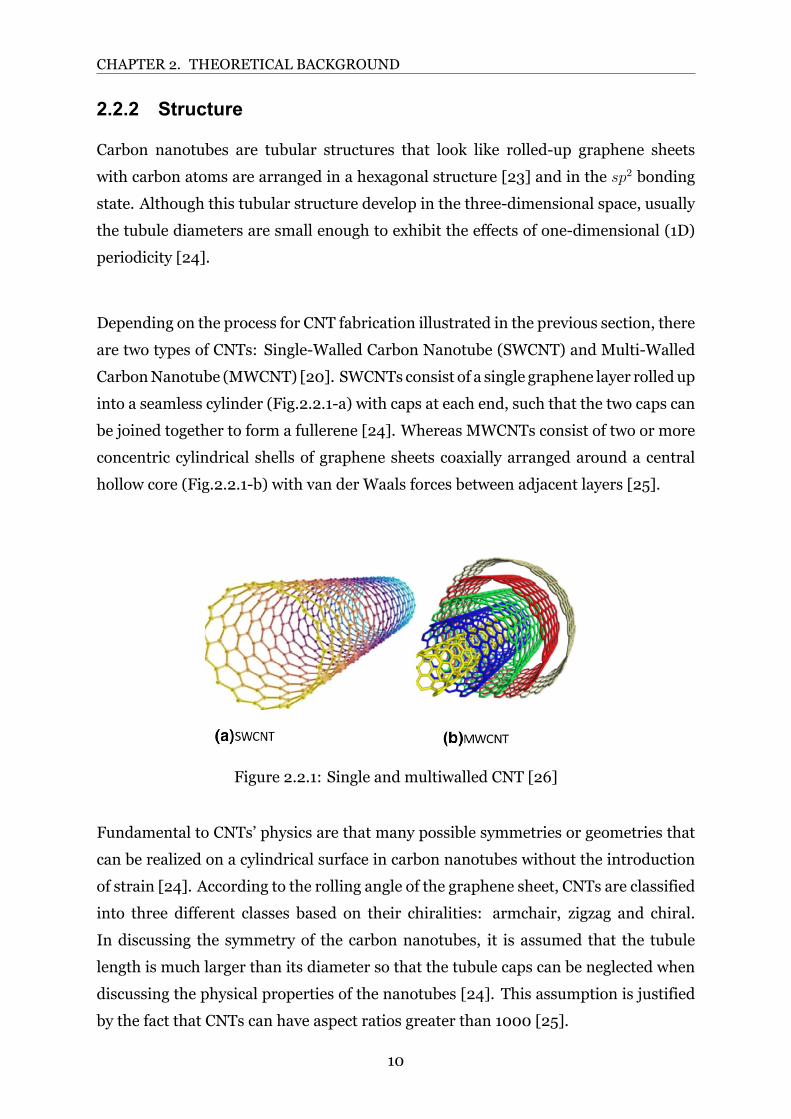
CarbonNanotube (MWCNT) [20]. SWCNTs consist of a single graphene layer rolled up
into a seamless cylinder (Fig.2.2.1a) with caps at each end, such that the two caps can
be joined together to form a fullerene [24]. Whereas MWCNTs consist of two or more
concentric cylindrical shells of graphene sheets coaxially arranged around a central
hollow core (Fig.2.2.1b) with van der Waals forces between adjacent layers [25].
Figure 2.2.1: Single and multiwalled CNT [26]
Fundamental to CNTs’ physics are that many possible symmetries or geometries that
can be realized on a cylindrical surface in carbon nanotubes without the introduction
of strain [24]. According to the rolling angle of the graphene sheet, CNTs are classified
into three different classes based on their chiralities: armchair, zigzag and chiral.
In discussing the symmetry of the carbon nanotubes, it is assumed that the tubule
length is much larger than its diameter so that the tubule caps can be neglected when
discussing the physical properties of the nanotubes [24]. This assumption is justified
by the fact that CNTs can have aspect ratios greater than 1000 [25].
10
CHAPTER 2. THEORETICAL BACKGROUND
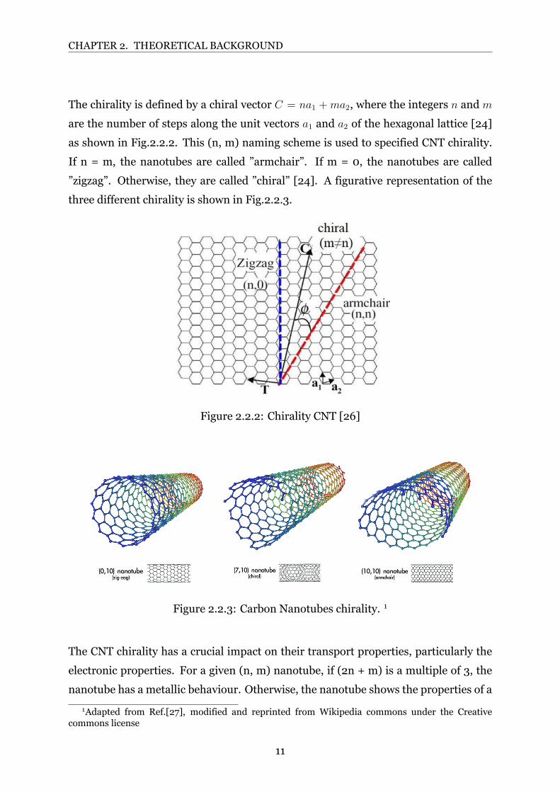
The chirality is defined by a chiral vector C = na1 +ma2, where the integers n and m
are the number of steps along the unit vectors a1 and a2 of the hexagonal lattice [24]
as shown in Fig.2.2.2. This (n, m) naming scheme is used to specified CNT chirality.
If n = m, the nanotubes are called ”armchair”. If m = 0, the nanotubes are called
”zigzag”. Otherwise, they are called ”chiral” [24]. A figurative representation of the
three different chirality is shown in Fig.2.2.3.
Figure 2.2.2: Chirality CNT [26]
Figure 2.2.3: Carbon Nanotubes chirality. 1
The CNT chirality has a crucial impact on their transport properties, particularly the
electronic properties. For a given (n, m) nanotube, if (2n + m) is a multiple of 3, the
nanotube has a metallic behaviour. Otherwise, the nanotube shows the properties of a
1Adapted from Ref.[27], modified and reprinted from Wikipedia commons under the Creativecommons license
11
CHAPTER 2. THEORETICAL BACKGROUND
semiconductor [25]. The abovementioned classification applies to SWCNT; however,
each MWCNT contains several coaxial graphene tubes where each layer can have
different chiralities, so the prediction of its physical properties is more complicated
than that of SWCNT.
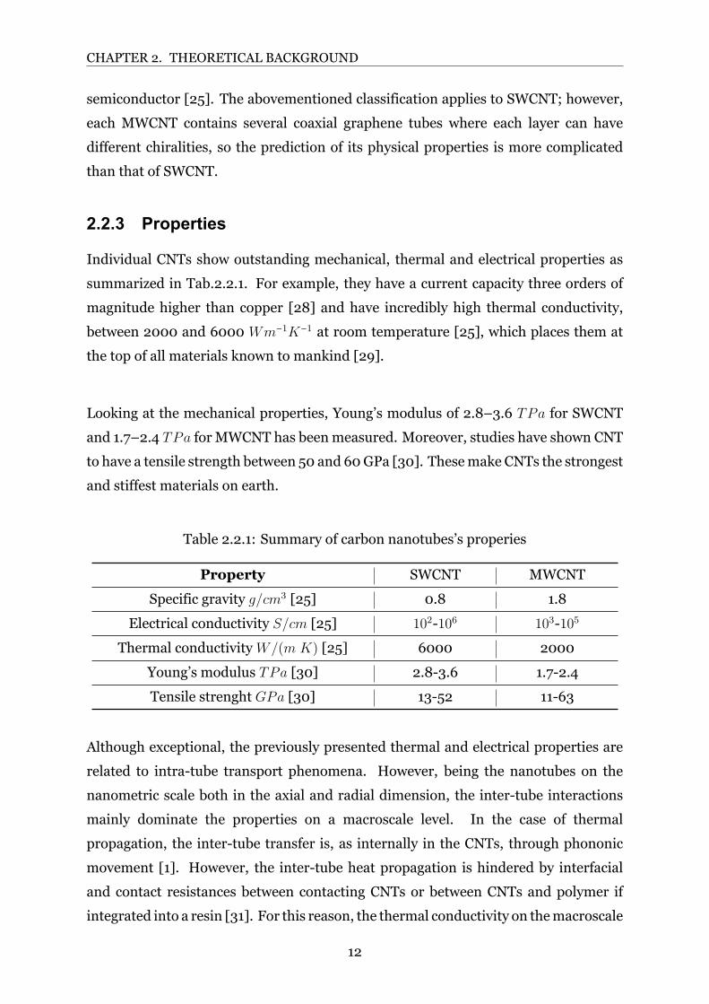
2.2.3 Properties
Individual CNTs show outstanding mechanical, thermal and electrical properties as
summarized in Tab.2.2.1. For example, they have a current capacity three orders of
magnitude higher than copper [28] and have incredibly high thermal conductivity,
between 2000 and 6000 Wm−1K−1 at room temperature [25], which places them at
the top of all materials known to mankind [29].
Looking at the mechanical properties, Young’s modulus of 2.8–3.6 TPa for SWCNT
and 1.7–2.4 TPa for MWCNT has beenmeasured. Moreover, studies have shown CNT
to have a tensile strength between 50 and 60GPa [30]. Thesemake CNTs the strongest
and stiffest materials on earth.
Table 2.2.1: Summary of carbon nanotubes’s properies
Property SWCNT MWCNT
Specific gravity g/cm3 [25] 0.8 1.8
Electrical conductivity S/cm [25] 102106 103105
Thermal conductivityW/(m K) [25] 6000 2000
Young’s modulus TPa [30] 2.83.6 1.72.4
Tensile strenght GPa [30] 1352 1163
Although exceptional, the previously presented thermal and electrical properties are
related to intratube transport phenomena. However, being the nanotubes on the
nanometric scale both in the axial and radial dimension, the intertube interactions
mainly dominate the properties on a macroscale level. In the case of thermal
propagation, the intertube transfer is, as internally in the CNTs, through phononic
movement [1]. However, the intertube heat propagation is hindered by interfacial
and contact resistances between contacting CNTs or between CNTs and polymer if
integrated into a resin [31]. For this reason, the thermal conductivity on themacroscale
12
CHAPTER 2. THEORETICAL BACKGROUND
level will result much lower and, so far, no adequate method of exploiting the excellent
thermal properties to their full extent has been found [1].
Similarly to thermal conduction properties, the electrical conduction properties are
also reduced when the CNTs are applied on a macroscale level, especially if the
CNT are integrated into a polymeric matrix. While the electrical resistance of each
individual CNT through the axial direction depends only on the atomic structure
and the tube’s chirality (see Sec.2.2.1), in a VACNT forest infiltrated by a polymeric
matrix, the intertube electric conduction is dominated by two main two mechanisms:
mechanical contact between conductive particles and electron tunnelling effects due
to an insulating film of matrix material between crossing nanotubes [32]. The total
resistance of a polymer infiltrated VACNT forest on a macroscopic level can be
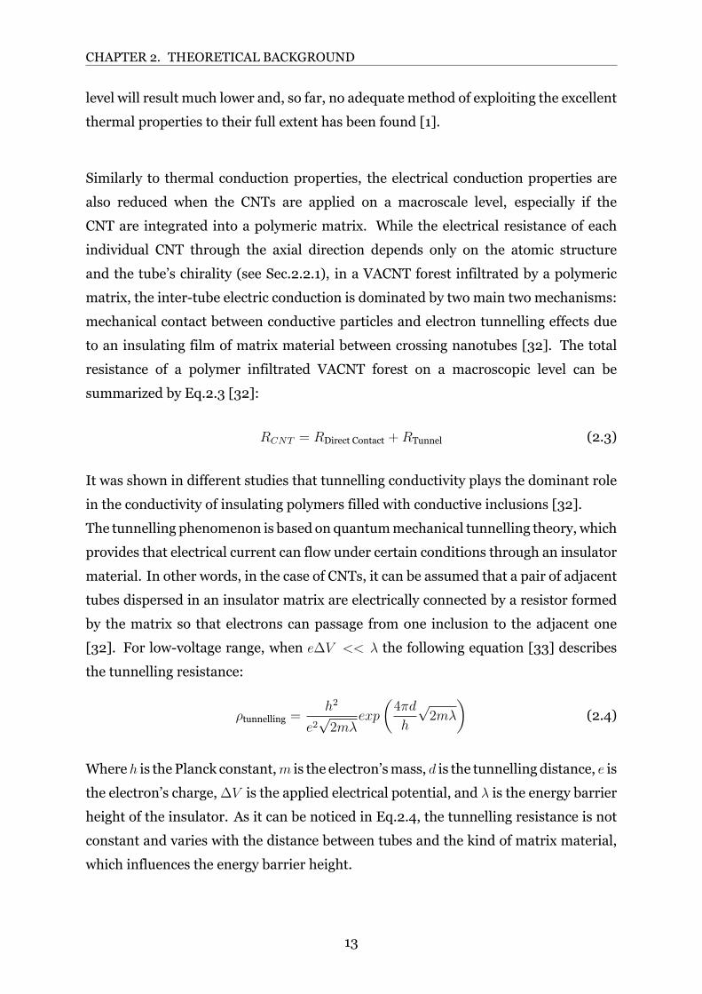
summarized by Eq.2.3 [32]:
RCNT = RDirect Contact +RTunnel (2.3)
It was shown in different studies that tunnelling conductivity plays the dominant role
in the conductivity of insulating polymers filled with conductive inclusions [32].
The tunnelling phenomenon is based on quantummechanical tunnelling theory, which
provides that electrical current can flow under certain conditions through an insulator
material. In other words, in the case of CNTs, it can be assumed that a pair of adjacent
tubes dispersed in an insulator matrix are electrically connected by a resistor formed
by the matrix so that electrons can passage from one inclusion to the adjacent one
[32]. For lowvoltage range, when e∆V << λ the following equation [33] describes
the tunnelling resistance:
ρtunnelling =h2
e2√2mλ
exp
(4πd
h
√2mλ
)(2.4)
Whereh is the Planck constant,m is the electron’smass, d is the tunnelling distance, e is
the electron’s charge,∆V is the applied electrical potential, and λ is the energy barrier
height of the insulator. As it can be noticed in Eq.2.4, the tunnelling resistance is not
constant and varies with the distance between tubes and the kind of matrix material,
which influences the energy barrier height.
13
CHAPTER 2. THEORETICAL BACKGROUND
2.3 Modelling
Oxford Academic English dictionary defines scientific modelling as ”The work of
making a simple description of a system or a process that can be used to explain it,
predict results, etc” [34].
Reducing the complexity of the interested systems through assumptions, models allow
to understand, define, quantify, visualize or simulate phenomena by referencing it
to existing and usually commonly accepted laws of physics. Although modelling is a
crucial component of modern science, scientific models at best are approximations of
the objects and systems that they represent and, for this reason, scientists constantly
areworking to improve and refinemodels as newknowledge or data are available.
2.3.1 The steps for an effective modelling process
In order to create a valid model that approximates the system or process of interest
in an effective way, seven steps should be followed. First of all, the researcher should
identify the fundamental law of nature behind the system. Examples of fundamental
physics’ laws are the conservation of energy in the case of heat transfer phenomenon
or Maxwell’s laws of electromagnetism. In general, fundamental laws of physics are
general equations that describe a physical phenomenon independently of the material
system on which they are applied.
The next step in the modelling process is to look for constitutive laws, mechanistic or
phenomenological, that allow applying fundamental laws of physics to a givenmaterial
system, taking into consideration the material properties. Examples of constitutive
laws are the Fourier laws for thermal conduction or Ohm’s law of electrical conduction.
A common thread among all constitutive laws is the presence of a parameter, such as
thermal conductivity or electrical resistivity, representing the material response to a
particular physical phenomenon.
After finding the Fundamental laws of physics and introducing the constitutive laws,
boundary conditions have to be used to specify the characteristics of the interested
phenomenon at the boundary of the study domain. Boundary conditions can prescribe
either a fixed value for a study variable, such as voltage in case of electric conduction,
14
CHAPTER 2. THEORETICAL BACKGROUND
or the mechanism by which the parameter under analysis varies at the edges of the
study domain, such as convection or radiation in heat transfer problem.
Once all the boundary conditions are set, assumptions on constitutive laws, boundary
conditions and the system’s geometry can be made. In order to do so, geometrical
symmetries of the system can be exploited. This is the most delicate of all the steps
since wrong assumptions can compromise the model’s validity. After making explicit
all the assumptions, the researcher should decide which type of model suits him the
best. We will discuss different types of models in the next section (Sec.2.3.2).
After this step, the model is set up and ready to be used to gain pieces of information
on a system or predict its behaviour. However, even though the model setup phase
is completed, the outputs must be verified and validated to have a valid model.
The verification and validation step focuses on comparing the model outputs with
experimental results and fundamental physics to find any possible discrepancy.
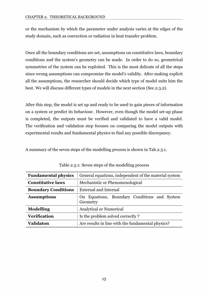
A summary of the seven steps of the modelling process is shown in Tab.2.3.1.
Table 2.3.1: Seven steps of the modelling process
Fundamental physics General equations, independent of the material system
Constitutive laws Mechanistic or Phenomenological
Boundary Conditions External and Internal
Assumptions On Equations, Boundary Conditions and SystemGeometry
Modelling Analytical or Numerical
Verification Is the problem solved correctly ?
Validaton Are results in line with the fundamental physics?
15
CHAPTER 2. THEORETICAL BACKGROUND
2.3.2 Types of models
Scientific models can be of three main different typology :
• Analytical
• Numerical
• SemiAnalytic
Analytical models represent a closedform mathematical solution to the system’s
governing equation subject to the initial and boundary conditions [35]. This variety of
models is usually applied to systems where the governing equations are well defined,
and the solution method is known. For example, electrical systems can be modelled as
equivalent circuits that can be solved using the well known Kirchhoff’s law.
Numerical models are based on a numerical procedure such as finite difference or
finite element method [35] and are used when the governing equations are extremely
difficult or even impossible to solve analytically. Applications of this kind ofmodels are
found in Computational Fluid Dynamics (CFD) software and structural Finite Element
Modelling (FEM).
In between the previous model’s type, SemiAnalytical models can be found. This
variety of models combine both closedform and numerical procedures in solving the
governing equation [35].
16
Chapter 3
The work
This thesis work started with the idea of using the already commercially available
HexPly® M21 prepreg, exploiting the fact that on its surface, thermoplastic particles
were deposited. The idea was to take advantage of the increased interlaminar region’s
thickness to create an isolating layer without adding any more material. First of all,
the Nylon particles have been characterized. Then their behaviour in the interlaminar
region once cured in a laminate was investigated. The next step was to try to embed
the CNT layer and measure the resistance to check if the particles created an effective
isolation method. As it will be shown in the next section, this isolation solution was
not effective, and another method was proposed.
The second isolation method took inspiration from W. Johannisson PhD thesis [36].
In this thesis, the author uses a 23 µm polyester film charged with ceramic particles to
create an electrical barrier in order to separate two sides of a laminate and be able to
electrically charge only one side to give the laminate morphing properties. This film
was tested for our purpose too. In the first iteration, the Freudenberg 301123 filmwas
applied dry on both sides of the CNT layer and CF veil. Ten samples were produced
with this isolation solution, but only two of them showed resistance in the order of kΩ,
as expected for conduction through the CNT layer, while the remaining eight exhibit
resistances in the order of hundreds of Ohms, revealing conduction through the fibre
bed. This variance was studied, and a possible cause was found in the film’s porosity.
For this reason, it was decided to try to fill the porosity impregnating the film with
epoxy resin.
17
CHAPTER 3. THEWORK
The first attempt of filling the film’s porosity was carried on trying to impregnate the
separator with HexPly® 6376 epoxy film, gelled before being used in the laminate.
This decision was motivated by the fact that this epoxy film was the same matrix used
in the CF prepreg. Although this solution gave more consistent resistance values in
the samples, solving the variance problem, an excess of epoxy resin was found during
a microscopy observation. With this impregnation method, the insulating barrier was
found to be thicker than desirable. In order to reduce the excess matrix accumulated
during the impregnation process, liquid impregnation was tried. Furthermore, to ease
the process, a resin thinner (Ethanol) was used to reduce the matrix viscosity. This
solution has proven itself very effective in creating an isolating barrier without adding
any thickness to the polyester film.
Once an effective method to electrically insulate the CNT layer from the fibre beds was
found, the focus shifted towards the modelling side. The primary purpose was to find,
through simulation, the minimum required thickness for the impregnated separator.
While experimentally we had the limit of the material existing and available on the
market, with the models, we were detached from this limit, and we could find, ideally,
what could be the thickness of a separator that would still serve its purpose of electrical
insulation while affecting the least possible the properties of the final laminate.
Initially, a COMSOL Multiphysics model was built, and the electrical conduction was
simulated using a Finite Element Method. Although very useful and illustrative, this
method started to show weaknesses once the separator’s thickness was simulated
below 5 µm. The problems arose from the mesh skewness, which could only be solved
by tremendously decreasing the size of the mesh elements, which would have required
computational power unavailable for this study.
In order to overcome the abovementioned issue, an analytical model was developed
in Matlab. This model was built from an equivalent circuit describing the CNT layer
embedded into a CF laminate. Kirchhoff and Ohm’s laws were used to calculate the
equivalent resistance of different paths that the current could take from the terminal
to the ground. With this model, thicknesses up to 10 nm were simulated.
18
CHAPTER 3. THEWORK
For both the Finite Element (FE) and Analytical models, material data had to
be measured in order to build complete, representative and accurate models. In
particular, laminate’s longitudinal, transverse and outofplane resistivities were
critical. While the first two were relatively simple to measure, having laminated the
necessary samples, the last one required a more complex setup that will be explained
in Sec.4.8.
Once an effective solution to electrically insulate the CNT from the fibre beds was
found, and both the FE and Analytical models were developed, the attention moved
toward the validation of the proposed solution. We tested whether the usage of a
separator filmhindered thematerial’s functionality as a curing sensor and temperature
sensor. Both tests, implying strain, contribute to validate the material’s ability as
a strain sensor implicitly. In order to have a benchmark, the results obtained from
these tests were compared to the ones found in studies conducted by Karlsson in Glass
Fibre (GF) laminates.
Once the isolation solution was validated, we tried to see whether the insertion of the
CNT and separator layers inside the CF laminate reduced the mechanical properties
of the latter. Since the embedding implies a localized increase in thickness of the
interlaminar region, the Interlaminar Shear Strength (ILSS) was reputed to be the
most easily affected and was studied. Using a standardized short beam threepoint
bending test, as explained in Sec.4.14, the effect of the insertion of the CNT on the
ILSS was studied. Different contact solutions were explored since the contact material
was identified from this test as the most harmful.
Finally, a suitable combination of a separator membrane and a contact solution was
found. This combination has proved to be the best within the limits of this study,
although it leaves room for substantial improvements in the future.
19
Chapter 4
Methodologies and Methods
4.1 Microscopy
To observe the laminate’s crosssection, the samples were mounted using Buehler’s
VariDur 200 epoxy resin. After the curing, the mounted samples were polished using
Buehler’s Phoenix Beta polishingmachine set at 300 rpm and 30N of load. For optical
analysis, the samples were polished with sandpaper, increasing grit until the 4000 grit
was reached. After the polishing, the samples were observed with an Olympus BX53M
microscope.
4.2 Impregnation method 1
To impregnate the Freudenberg FS 301123 separator, we have used aHexply 6376 film
with an areal weight of 36 gm2 , corresponding to a thickness of 27 µm. To impregnate
the membrane, the epoxy film has been applied to the polyester film and put under
vacuum for 10 min at 40°C. After this period, the impregnated separator was placed in
the oven for 1 h at 100°C in order to reach the gel point.
4.3 Impregnation method 2
To reduce the resin excess shown in the separator membrane impregnate with method
1, a liquid impregnation has been chosen. To a mixture of liquid epoxy resin Araldite
LY8615 and 50 %wt Araldur hardener, 20 %wt Ethanol has been added to reduce the
20
CHAPTER 4. METHODOLOGIES ANDMETHODS
viscosity of the solution and improve the impregnation. To impregnate a 120x40 mm
membrane, 1 ml of the aforementioned solution has been used. Once the desired
volume was spread using a syringe, a layer each of bleeder and breather fabric was
placed on top of the membrane. To absorb the excess resin, the vacuum was applied
for 5min. After this period, themembranewas kept under vacuum for 20min at 100°C
in order to reach gel point, as specified by the manufacturer [37].
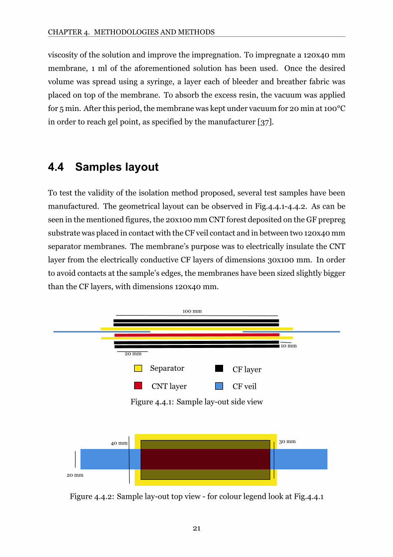
4.4 Samples layout
To test the validity of the isolation method proposed, several test samples have been
manufactured. The geometrical layout can be observed in Fig.4.4.14.4.2. As can be
seen in thementioned figures, the 20x100mmCNT forest deposited on the GF prepreg
substratewas placed in contact with the CF veil contact and in between two 120x40mm
separator membranes. The membrane’s purpose was to electrically insulate the CNT
layer from the electrically conductive CF layers of dimensions 30x100 mm. In order
to avoid contacts at the sample’s edges, the membranes have been sized slightly bigger
than the CF layers, with dimensions 120x40 mm.
CNT layer CF veil
Separator CF layer
20 mm
100 mm
10 mm
Figure 4.4.1: Sample layout side view
40 mm
20 mm
30 mm
Figure 4.4.2: Sample layout top view for colour legend look at Fig.4.4.1
21
CHAPTER 4. METHODOLOGIES ANDMETHODS
4.5 IV measurements
IV measurements were performed to control if the electrical potential is in a linear
relationship with the electrical current applied (Ohm’s law). An electrical potential
sweep from 0 to 9 V was performed using a BioLogic SP50 potentiostat with crocodile
jaws, while the electrical potential needed to supply the prescribed current was
recorded.
4.6 COMSOL model
The Electric Current (ec) module of COMSOL Multiphysics has been used to model
the sensor behaviour inside the laminate. Since the sensor system showed symmetry
along the direction between the contacts, a 2D model approach was chosen. Reducing
themodel froma 3D to a 2D case reduces the computational timewithout losing crucial
information about the sensor’s behaviour. The geometry modelled in the software
represented a CNT layer, surrounded by two separator membranes, one 90° CF layer
and one 0° CF layer for each side. The heights of the CF and CNT rectangular domains,
representing the thickness on the layers, were set to be equal to the ones measured
using optical micrography. In particular, the CF layers were modelled to be 100 µm
high while the CNT layer 10 µm. On the other hand, the height of the separator’s
domain and the length of all domains were parametrized. The parameterization was
used in a linear sweep afterwards.
Once the geometry was built, an Electric Insulation Boundary Condition (BC) was
applied to all the external boundaries. After that, a Ground BC was applied to one
edge of the sensor domain, and a Terminal BC of 0.1 V was applied to the opposite one.
To model the electrical anisotropicity of both the CF layers, two Current Conservation
BCs were applied to the two different layers. This BC makes it possible for the user
to fill the electrical conductivity matrix manually. An isotropic electrical conductivity
was used for the remaining two domains (CNT and separator).
To mesh the domains, a free triangular mesh was used. Depending on the domain,
a different maximum element size was used. For the CNT layer, the maximum size
was chosen to be onefifth of the separator’s thickness. For the separator’s domain, a
22
CHAPTER 4. METHODOLOGIES ANDMETHODS
maximum size of half of the CNT layer’s thickness was used. For the CF layers’ domain,
a softwarecontrolled element size was chosen, setting the mesh to be calibrated for
general physics and extremely fine. Moreover, during the computation, the software
was allowed to compute an error estimate on the mesh and adapt it to reduce the error
for amaximum of 2 refinements. The error estimationmethod was chosen to be the L2
norm of error squared. The software was also allowed to coarsen the mesh if needed,
with a maximum coarsening factor of 5.
Two parametric sweep studies were performed to investigate the effect of different
separator thicknesses on different sensor lengths. In the first one, the separator’s
thickness was set to be 5, 10 and 23 µm. In the second one, the sample’s length was
set to be 10, 20 and 50 mm. After the stationary study was computed, the results were
plotted both as a current density surface plot and as a 1Dplot of current density through
the sample’s thickness. Three thicknesses were investigated: at the edge close to the
voltage source, middle and end of the sample.
4.7 MATLAB model
The longitudinal ρ0 and transverse ρ90 fibre resistivity derived from measured
resistance on specific samples. CNT layer’s resistivity ρCNT was derived from
measured resistance on an unembedded sensor. Separator’s conductivity was derived
theoretically using the ROM [38] :
σimpregnated separator = σseparator · (1− V fepoxy) + σepoxy · V fepoxy (4.1)
Where the epoxy’s volume fraction V fepoxy was set equal to the theoretical separator’s
porosity of 55%. From the obtained conductivity, the resistivity ρsep has been obtained
as :
ρimpregnated separator =1
σimpregnated separator(4.2)
The interlaminar resistivity ρinter has been calculated following the method explained
in the following section.
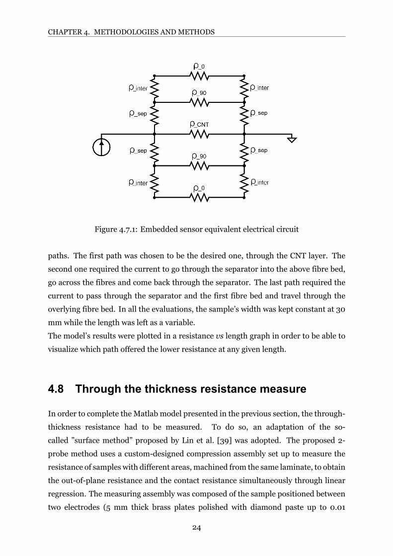
After measuring all the required resistivity, we built the equivalent electrical circuit
shown in Fig.4.7.1, in order to evaluate the equivalent resistivity of three different
23
CHAPTER 4. METHODOLOGIES ANDMETHODS
Figure 4.7.1: Embedded sensor equivalent electrical circuit
paths. The first path was chosen to be the desired one, through the CNT layer. The
second one required the current to go through the separator into the above fibre bed,
go across the fibres and come back through the separator. The last path required the
current to pass through the separator and the first fibre bed and travel through the
overlying fibre bed. In all the evaluations, the sample’s width was kept constant at 30
mm while the length was left as a variable.
The model’s results were plotted in a resistance vs length graph in order to be able to
visualize which path offered the lower resistance at any given length.
4.8 Through the thickness resistance measure
In order to complete the Matlab model presented in the previous section, the through
thickness resistance had to be measured. To do so, an adaptation of the so
called ”surface method” proposed by Lin et al. [39] was adopted. The proposed 2
probe method uses a customdesigned compression assembly set up to measure the
resistance of samples with different areas, machined from the same laminate, to obtain
the outofplane resistance and the contact resistance simultaneously through linear
regression. The measuring assembly was composed of the sample positioned between
two electrodes (5 mm thick brass plates polished with diamond paste up to 0.01
24
CHAPTER 4. METHODOLOGIES ANDMETHODS
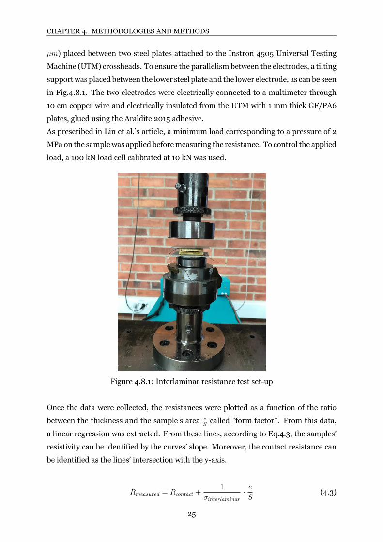
µm) placed between two steel plates attached to the Instron 4505 Universal Testing
Machine (UTM) crossheads. To ensure the parallelism between the electrodes, a tilting
supportwas placed between the lower steel plate and the lower electrode, as can be seen
in Fig.4.8.1. The two electrodes were electrically connected to a multimeter through
10 cm copper wire and electrically insulated from the UTM with 1 mm thick GF/PA6
plates, glued using the Araldite 2015 adhesive.
As prescribed in Lin et al.’s article, a minimum load corresponding to a pressure of 2
MPa on the samplewas applied beforemeasuring the resistance. To control the applied
load, a 100 kN load cell calibrated at 10 kN was used.
Figure 4.8.1: Interlaminar resistance test setup
Once the data were collected, the resistances were plotted as a function of the ratio
between the thickness and the sample’s area eScalled ”form factor”. From this data,
a linear regression was extracted. From these lines, according to Eq.4.3, the samples’
resistivity can be identified by the curves’ slope. Moreover, the contact resistance can
be identified as the lines’ intersection with the yaxis.
Rmeasured = Rcontact +1
σinterlaminar
· eS
(4.3)
25
CHAPTER 4. METHODOLOGIES ANDMETHODS
4.9 Curing method and monitoring
The prepreg used in this study is a HexPly® 6376 from Hexcel, a UD carbon fibre
impregnated with a 6376 epoxy matrix. The recommended curing cycle is 180°C for
2 h under 1 bar vacuum. The plateau temperature is reached with a heating rate
of 2°C/min as prescribed by the producer datasheet [40]. In order to monitor the
sample’s resistance during curing, a BioLogic SP50 potentiostat was connected with
crocodile jaws to brass plates placed in contact with the sample’s carbon fibre veil
contacts. Using the provided ECLab software, a constant electrical current of 50 µA
was used as input. The electrical potential required to let the prescribed electrical
current flow has been measured. Dividing the measured electrical potential by the
input electrical current, the electrical resistance has been obtained. A 1 mm thick glass
fibre plate has been used to electrically isolate the sample from the metal backplate.
The same samples’ matrix system has been used.
To monitor the temperature during curing, two thermocouples embedded into a CF
laminate with the same material and thickness of the tested samples have been used.
The thermocouples’ terminals have been connected to a National Instrument NI 9212
module and analyzed using a Labview script.
4.10 Temperature sensing
To reproduce different temperature condition, an ACS FM340C climate chamber has
been used. The temperature cycle has been programmed to start at 20°C, cool down the
samples to 70°C with a cooling rate of 3°C/min, stabilize the temperature for 30 min,
then heat the sample to 180 °C with a heat rate of 4°C/min, stabilize the temperature
for 30min and finally cool down the sample to room temperature with a cooling rate of
3.8 °C/min. The change in samples’ resistancewith temperature has beenmeasured by
connecting the carbon fibre veil to a BioLogic SP50 potentiostat with crocodile jaws.
Similarly to the curing monitoring, a constant electric current of 50 µA has been used
as input and the electrical potential was measured in order to calculate the resistance.
After applying a lowpass filter to remove the noise, the percentile change in resistance
with respect to the initial value at 20 °C have been calculated in order to be able to
compare the samples with different initial resistance. The lowpass filter used is the
26
CHAPTER 4. METHODOLOGIES ANDMETHODS
builtin Matlab function filtfilt which apply a Butterworth filter of order 15, with a
normalized 3dB frequency of 0.01π rad/sample. Similarly to the curing monitoring
case, a 1 mm glass fibre plate was used to isolate the sample from the metal backplate.
The same thermocouples used during the curing monitoring have been used to keep
track of the temperature profile. The thermocouples’ terminals have been connected
to a National Instrument NI 9212 module and analyzed using a Labview script.
4.11 Thermal expansion evaluation
To evaluate thermal expansion, Thermomechanical Analysis (TMA) was chosen. TMA
is a technique that measures a materials’ dimensional changes under controlled
conditions of force, atmosphere, time, and temperature [41]. Analysis were performed
by TA Instrument® at their headquarter on CF [0]6 and [90]6 laminates using a
Discovery TMA 450 testing machine. Analysis was conducted for each sample in both
the longitudinal, transverse, and outofplane directions. Both samples were tested
from 70°C to 180°Cwith a heating rate of 5°C/min. The samples’ dimensions followed
the specifications of the measuring instrument manufacturer of 20 mm in length, 4.3
mm in width, and 0.6mm in thickness.
4.12 Contact Resistance Measurement
Different contact solutions have been evaluated. A 450 µm diameter copper wire, a
200 µm diameter NiCrNi wire with a 250 µm GF insulation [42] from a Roth+Co K
Type Thermocouple, Toray T800HB CF yarn and a 8 g/m2 Ni coated CF veil have been
used.
To assess the quality of different contact methodology, the contact resistance of each
contact solution has been evaluated. In order to do so, samples with four contacts,
two per side and perpendicular to the samples’ longitudinal direction, were laminated.
For this evaluation, the composite layers used had 120 x 40mm dimensions, while the
sensormaterial was chosen to be 100x 30mm. The contact resistancewas calculated as
the difference between the resistance value between the two inner contacts measured
with a two probe method and a fourprobe method. In the two probe method, a
multimeter was used to evaluate the sample’s resistance directly. In the fourprobe
27
CHAPTER 4. METHODOLOGIES ANDMETHODS
method, a current of 100 µA was applied to the external contacts while measuring the
voltage between the two inner contactswith a voltmeter. Voltmeters typically have high
electrical impedance to prevent them from affecting the circuit being measured, so no
current will flow through the inner two probes. Only the voltage is measured between
the inner probes, meaning that the probes resistances and the contact resistances do
not contribute to themeasurement [43]. Any difference in resistance between the two
probes and fourprobes measurements will therefore arise entirely from the contact
resistance.
2 ·Rcontact =
(R2−probe −
V4−probe
Iapplied
)(4.4)
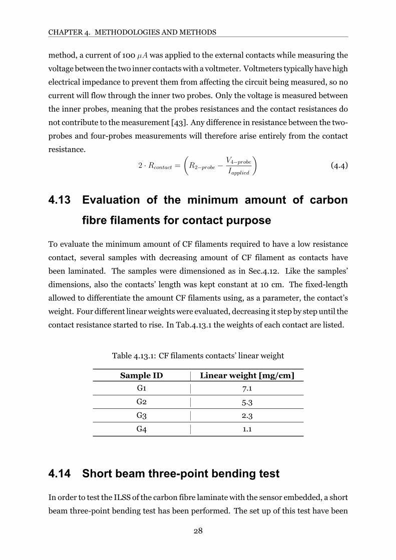
4.13 Evaluation of the minimum amount of carbon
fibre filaments for contact purpose
To evaluate the minimum amount of CF filaments required to have a low resistance
contact, several samples with decreasing amount of CF filament as contacts have
been laminated. The samples were dimensioned as in Sec.4.12. Like the samples’
dimensions, also the contacts’ length was kept constant at 10 cm. The fixedlength
allowed to differentiate the amount CF filaments using, as a parameter, the contact’s
weight. Four different linearweightswere evaluated, decreasing it step by step until the
contact resistance started to rise. In Tab.4.13.1 the weights of each contact are listed.
Table 4.13.1: CF filaments contacts’ linear weight
Sample ID Linear weight [mg/cm]
G1 7.1
G2 5.3
G3 2.3
G4 1.1
4.14 Short beam threepoint bending test
In order to test the ILSS of the carbon fibre laminate with the sensor embedded, a short
beam threepoint bending test has been performed. The set up of this test have been
28
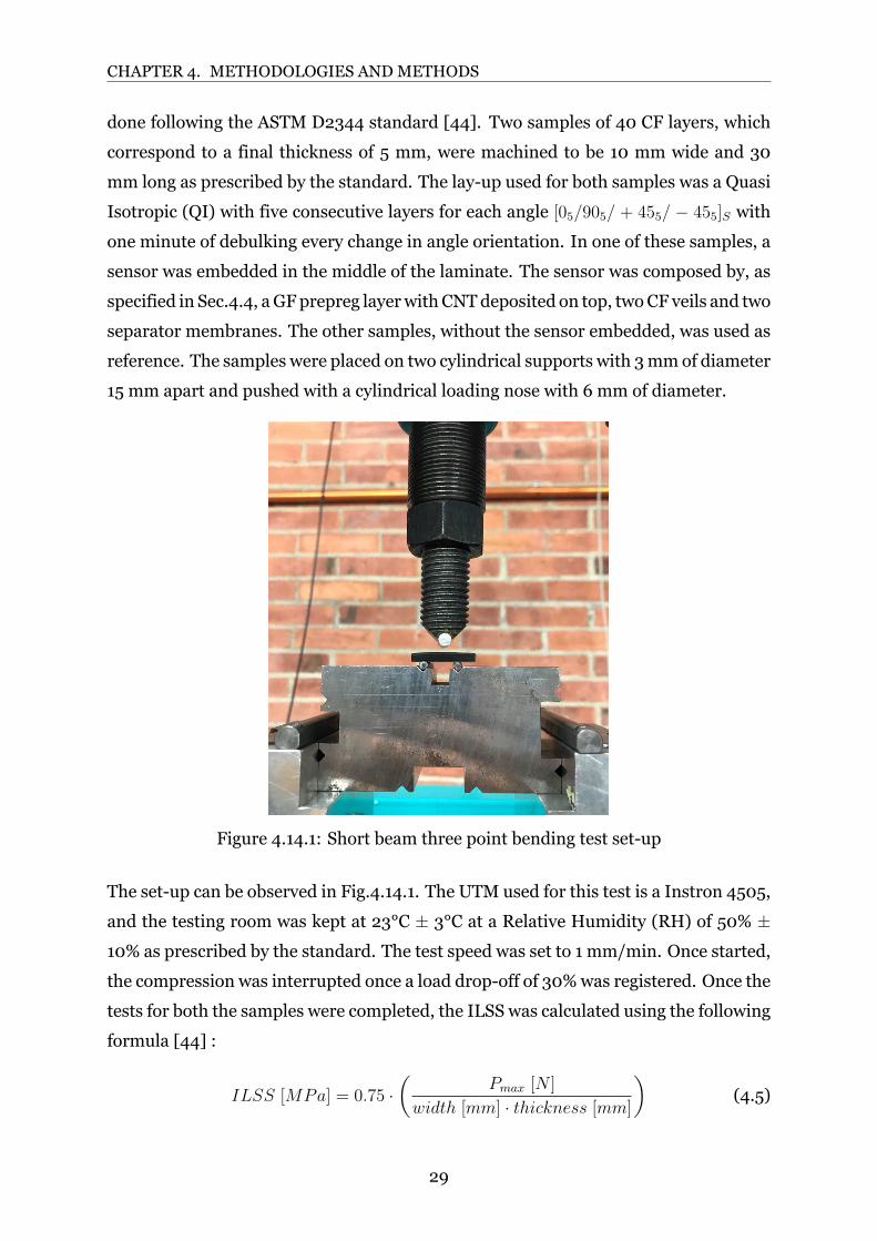
CHAPTER 4. METHODOLOGIES ANDMETHODS
done following the ASTM D2344 standard [44]. Two samples of 40 CF layers, which
correspond to a final thickness of 5 mm, were machined to be 10 mm wide and 30
mm long as prescribed by the standard. The layup used for both samples was a Quasi
Isotropic (QI) with five consecutive layers for each angle [05/905/ + 455/ − 455]S with
one minute of debulking every change in angle orientation. In one of these samples, a
sensor was embedded in the middle of the laminate. The sensor was composed by, as
specified in Sec.4.4, aGFprepreg layerwithCNTdeposited on top, twoCF veils and two
separator membranes. The other samples, without the sensor embedded, was used as
reference. The samples were placed on two cylindrical supports with 3mmof diameter
15 mm apart and pushed with a cylindrical loading nose with 6 mm of diameter.
Figure 4.14.1: Short beam three point bending test setup
The setup can be observed in Fig.4.14.1. The UTM used for this test is a Instron 4505,
and the testing room was kept at 23°C ± 3°C at a Relative Humidity (RH) of 50% ±10% as prescribed by the standard. The test speed was set to 1 mm/min. Once started,
the compression was interrupted once a load dropoff of 30%was registered. Once the
tests for both the samples were completed, the ILSS was calculated using the following
formula [44] :
ILSS [MPa] = 0.75 ·(
Pmax [N ]
width [mm] · thickness [mm]
)(4.5)
29
Chapter 5
Result
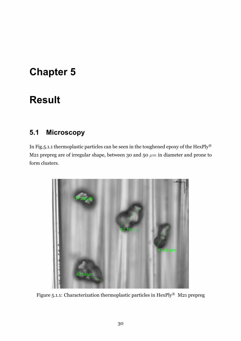
5.1 Microscopy
In Fig.5.1.1 thermoplastic particles can be seen in the toughened epoxy of the HexPly®
M21 prepreg are of irregular shape, between 30 and 50 µm in diameter and prone to
form clusters.
Figure 5.1.1: Characterization thermoplastic particles in HexPly® M21 prepreg
30
CHAPTER 5. RESULT
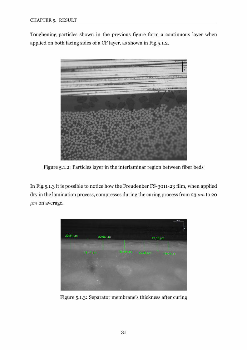
Toughening particles shown in the previous figure form a continuous layer when
applied on both facing sides of a CF layer, as shown in Fig.5.1.2.
Figure 5.1.2: Particles layer in the interlaminar region between fiber beds
In Fig.5.1.3 it is possible to notice how the Freudenber FS301123 film, when applied
dry in the lamination process, compresses during the curing process from 23 µm to 20
µm on average.
Figure 5.1.3: Separator membrane’s thickness after curing
31
CHAPTER 5. RESULT
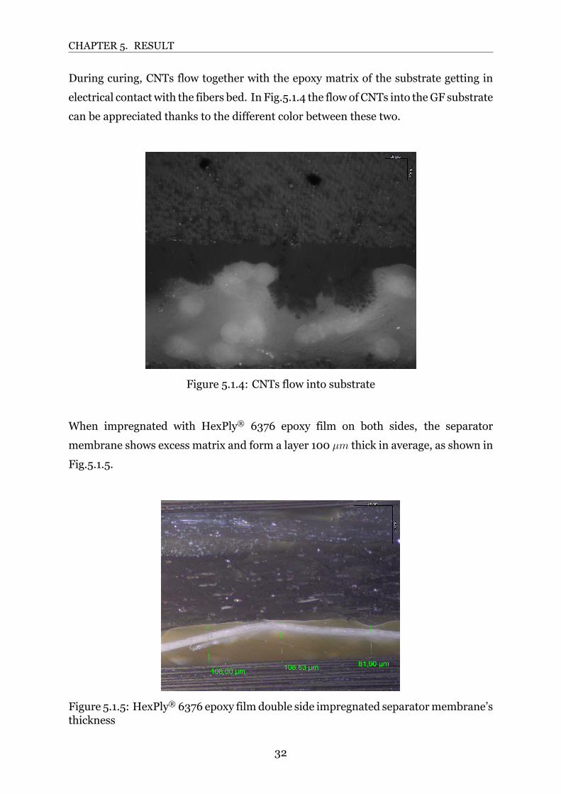
During curing, CNTs flow together with the epoxy matrix of the substrate getting in
electrical contact with the fibers bed. In Fig.5.1.4 the flow of CNTs into theGF substrate
can be appreciated thanks to the different color between these two.
Figure 5.1.4: CNTs flow into substrate
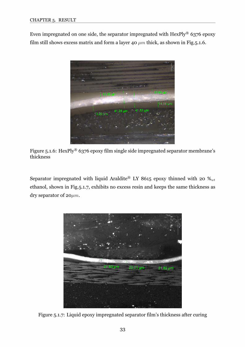
When impregnated with HexPly® 6376 epoxy film on both sides, the separator
membrane shows excess matrix and form a layer 100 µm thick in average, as shown in
Fig.5.1.5.
Figure 5.1.5: HexPly® 6376 epoxy film double side impregnated separatormembrane’sthickness
32
CHAPTER 5. RESULT
Even impregnated on one side, the separator impregnated with HexPly® 6376 epoxy
film still shows excess matrix and form a layer 40 µm thick, as shown in Fig.5.1.6.
Figure 5.1.6: HexPly® 6376 epoxy film single side impregnated separator membrane’sthickness
Separator impregnated with liquid Araldite® LY 8615 epoxy thinned with 20 %wt
ethanol, shown in Fig.5.1.7, exhibits no excess resin and keeps the same thickness as
dry separator of 20µm.
Figure 5.1.7: Liquid epoxy impregnated separator film’s thickness after curing
33
CHAPTER 5. RESULT
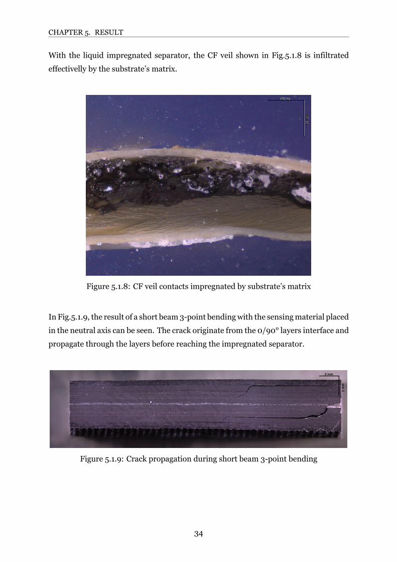
With the liquid impregnated separator, the CF veil shown in Fig.5.1.8 is infiltrated
effectivelly by the substrate’s matrix.
Figure 5.1.8: CF veil contacts impregnated by substrate’s matrix
In Fig.5.1.9, the result of a short beam3point bendingwith the sensingmaterial placed
in the neutral axis can be seen. The crack originate from the 0/90° layers interface and
propagate through the layers before reaching the impregnated separator.
Figure 5.1.9: Crack propagation during short beam 3point bending
34
CHAPTER 5. RESULT
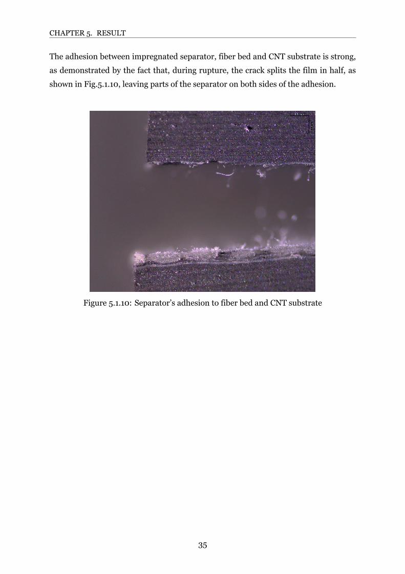
The adhesion between impregnated separator, fiber bed and CNT substrate is strong,
as demonstrated by the fact that, during rupture, the crack splits the film in half, as
shown in Fig.5.1.10, leaving parts of the separator on both sides of the adhesion.
Figure 5.1.10: Separator’s adhesion to fiber bed and CNT substrate
35
CHAPTER 5. RESULT
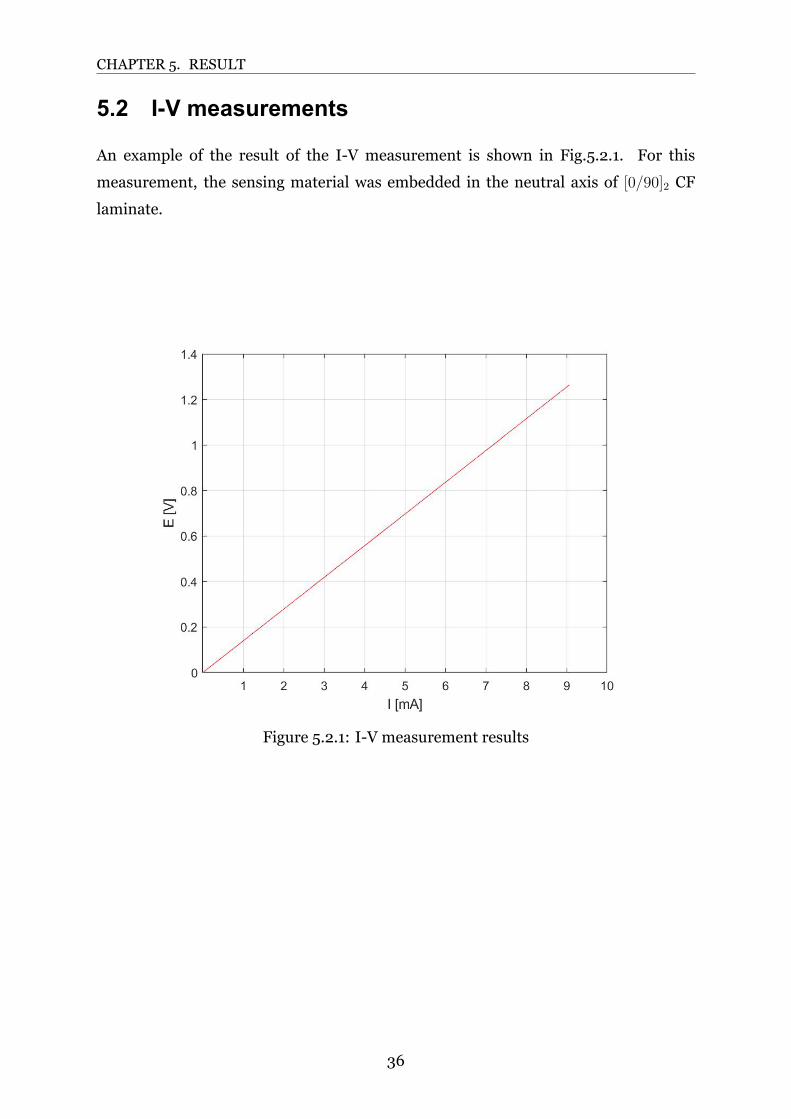
5.2 IV measurements
An example of the result of the IV measurement is shown in Fig.5.2.1. For this
measurement, the sensing material was embedded in the neutral axis of [0/90]2 CF
laminate.
Figure 5.2.1: IV measurement results
36
CHAPTER 5. RESULT
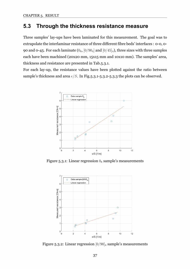
5.3 Through the thickness resistance measure
Three samples’ layups have been laminated for this measurement. The goal was to
extrapolate the interlaminar resistance of three different fibre beds’ interfaces : 00, 0
90 and 045. For each laminate (08, [0/904] and [0/45]4), three sizes with three samples
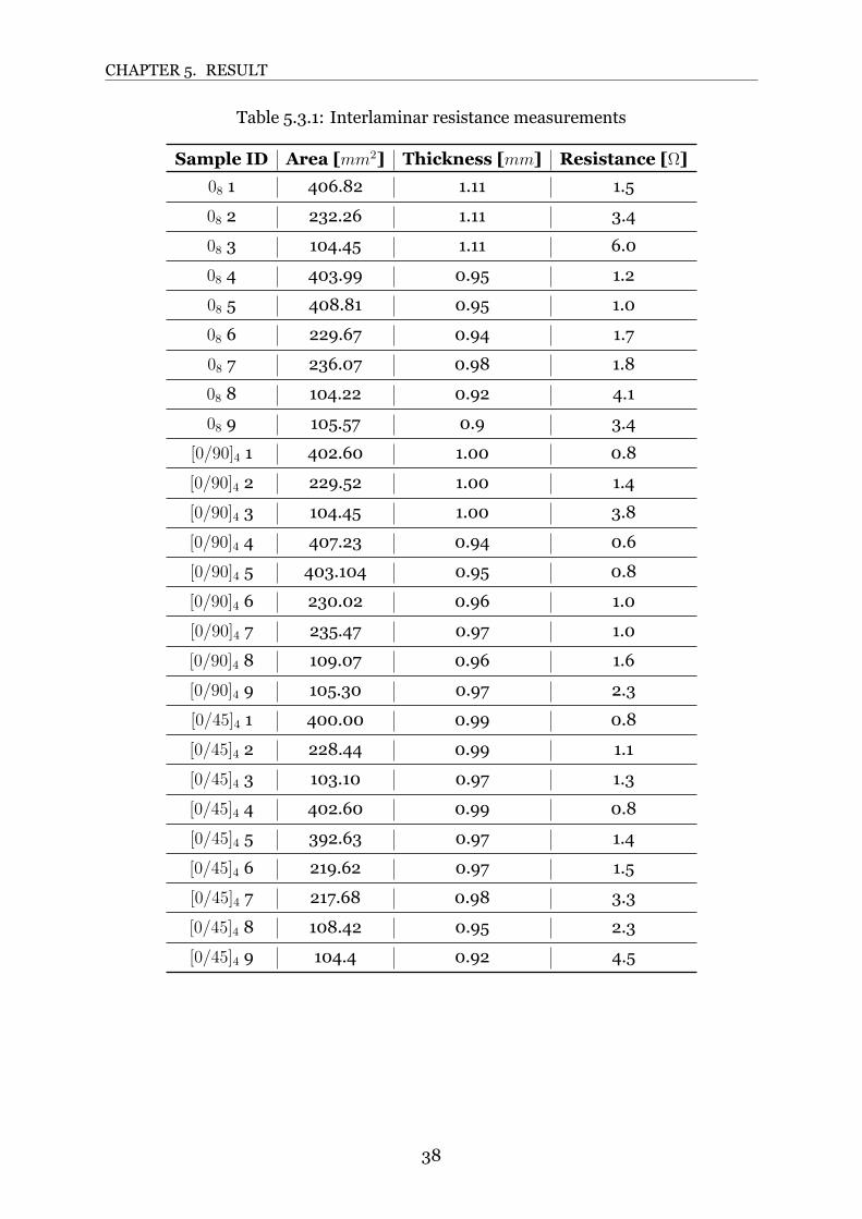
each have been machined (20x20 mm, 15x15 mm and 10x10 mm). The samples’ area,
thickness and resistance are presented in Tab.5.3.1.
For each layup, the resistance values have been plotted against the ratio between
sample’s thickness and area e/S. In Fig.5.3.15.3.25.3.3 the plots can be observed.
Figure 5.3.1: Linear regression 08 sample’s measurements
Figure 5.3.2: Linear regression [0/90]4 sample’s measurements
37
CHAPTER 5. RESULT
Table 5.3.1: Interlaminar resistance measurements
Sample ID Area [mm2] Thickness [mm] Resistance [Ω]
08 1 406.82 1.11 1.5
08 2 232.26 1.11 3.4
08 3 104.45 1.11 6.0
08 4 403.99 0.95 1.2
08 5 408.81 0.95 1.0
08 6 229.67 0.94 1.7
08 7 236.07 0.98 1.8
08 8 104.22 0.92 4.1
08 9 105.57 0.9 3.4
[0/90]4 1 402.60 1.00 0.8
[0/90]4 2 229.52 1.00 1.4
[0/90]4 3 104.45 1.00 3.8
[0/90]4 4 407.23 0.94 0.6
[0/90]4 5 403.104 0.95 0.8
[0/90]4 6 230.02 0.96 1.0
[0/90]4 7 235.47 0.97 1.0
[0/90]4 8 109.07 0.96 1.6
[0/90]4 9 105.30 0.97 2.3
[0/45]4 1 400.00 0.99 0.8
[0/45]4 2 228.44 0.99 1.1
[0/45]4 3 103.10 0.97 1.3
[0/45]4 4 402.60 0.99 0.8
[0/45]4 5 392.63 0.97 1.4
[0/45]4 6 219.62 0.97 1.5
[0/45]4 7 217.68 0.98 3.3
[0/45]4 8 108.42 0.95 2.3
[0/45]4 9 104.4 0.92 4.5
38
CHAPTER 5. RESULT
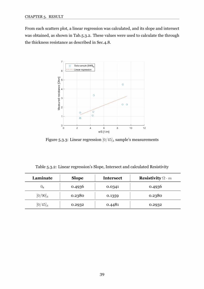
From each scatters plot, a linear regression was calculated, and its slope and intersect
was obtained, as shown in Tab.5.3.2. These values were used to calculate the through
the thickness resistance as described in Sec.4.8.
Figure 5.3.3: Linear regression [0/45]4 sample’s measurements
Table 5.3.2: Linear regression’s Slope, Intersect and calculated Resistivity
Laminate Slope Intersect Resistivity Ω ·m
08 0.4936 0.0341 0.4936
[0/90]4 0.2380 0.1359 0.2380
[0/45]4 0.2932 0.4481 0.2932
39
CHAPTER 5. RESULT
5.4 COMSOL model
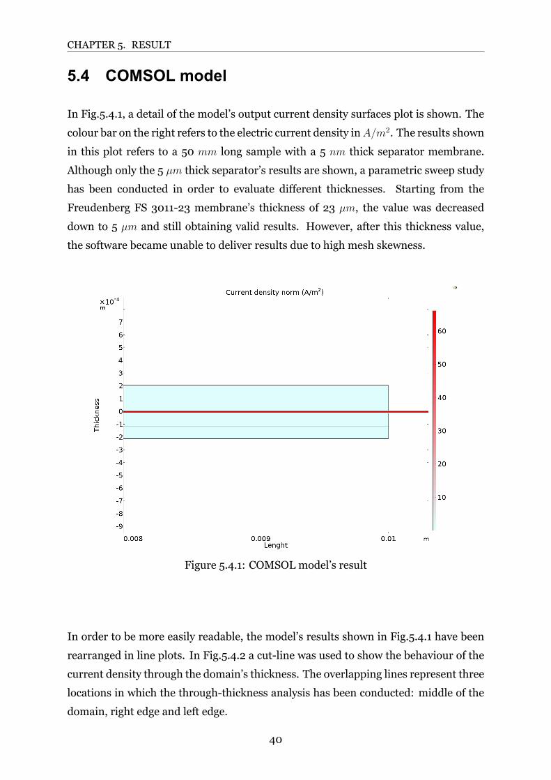
In Fig.5.4.1, a detail of the model’s output current density surfaces plot is shown. The
colour bar on the right refers to the electric current density inA/m2. The results shown
in this plot refers to a 50 mm long sample with a 5 nm thick separator membrane.
Although only the 5 µm thick separator’s results are shown, a parametric sweep study
has been conducted in order to evaluate different thicknesses. Starting from the
Freudenberg FS 301123 membrane’s thickness of 23 µm, the value was decreased
down to 5 µm and still obtaining valid results. However, after this thickness value,
the software became unable to deliver results due to high mesh skewness.
Figure 5.4.1: COMSOL model’s result
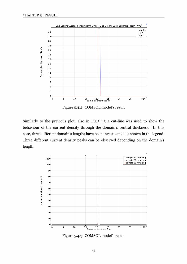
In order to be more easily readable, the model’s results shown in Fig.5.4.1 have been
rearranged in line plots. In Fig.5.4.2 a cutline was used to show the behaviour of the
current density through the domain’s thickness. The overlapping lines represent three
locations in which the throughthickness analysis has been conducted: middle of the
domain, right edge and left edge.
40
CHAPTER 5. RESULT
Figure 5.4.2: COMSOL model’s result
Similarly to the previous plot, also in Fig.5.4.3 a cutline was used to show the
behaviour of the current density through the domain’s central thickness. In this
case, three different domain’s lengths have been investigated, as shown in the legend.
Three different current density peaks can be observed depending on the domain’s
length.
Figure 5.4.3: COMSOL model’s result
41
CHAPTER 5. RESULT
5.5 Matlab model
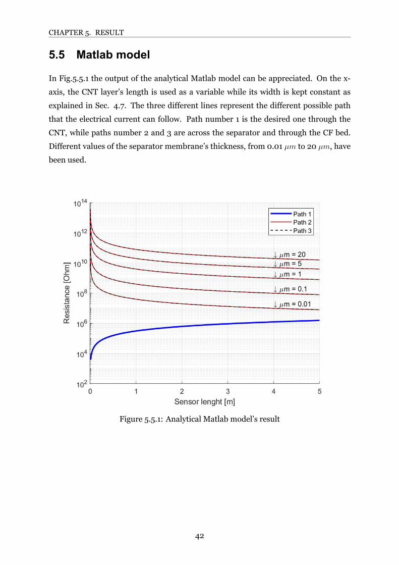
In Fig.5.5.1 the output of the analytical Matlab model can be appreciated. On the x
axis, the CNT layer’s length is used as a variable while its width is kept constant as
explained in Sec. 4.7. The three different lines represent the different possible path
that the electrical current can follow. Path number 1 is the desired one through the
CNT, while paths number 2 and 3 are across the separator and through the CF bed.
Different values of the separator membrane’s thickness, from 0.01 µm to 20 µm, have
been used.
Figure 5.5.1: Analytical Matlab model’s result
42
CHAPTER 5. RESULT
5.6 Curing monitoring
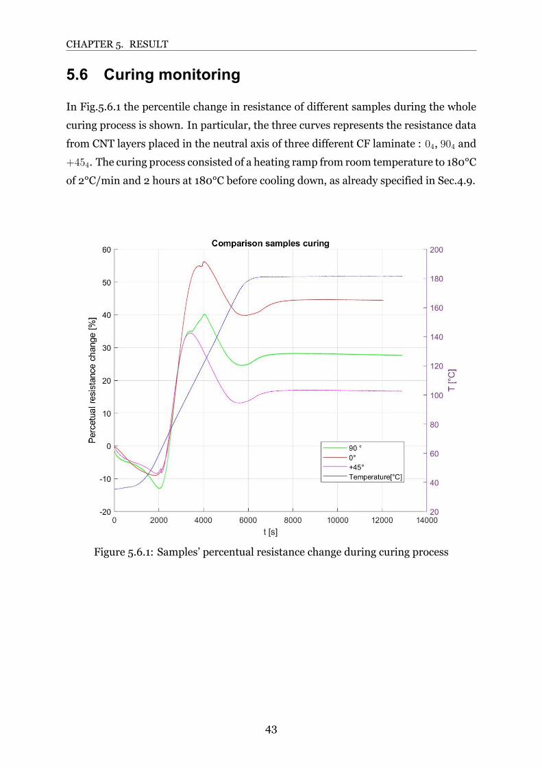
In Fig.5.6.1 the percentile change in resistance of different samples during the whole
curing process is shown. In particular, the three curves represents the resistance data
from CNT layers placed in the neutral axis of three different CF laminate : 04, 904 and
+454. The curing process consisted of a heating ramp from room temperature to 180°C
of 2°C/min and 2 hours at 180°C before cooling down, as already specified in Sec.4.9.
Figure 5.6.1: Samples’ percentual resistance change during curing process
43
CHAPTER 5. RESULT
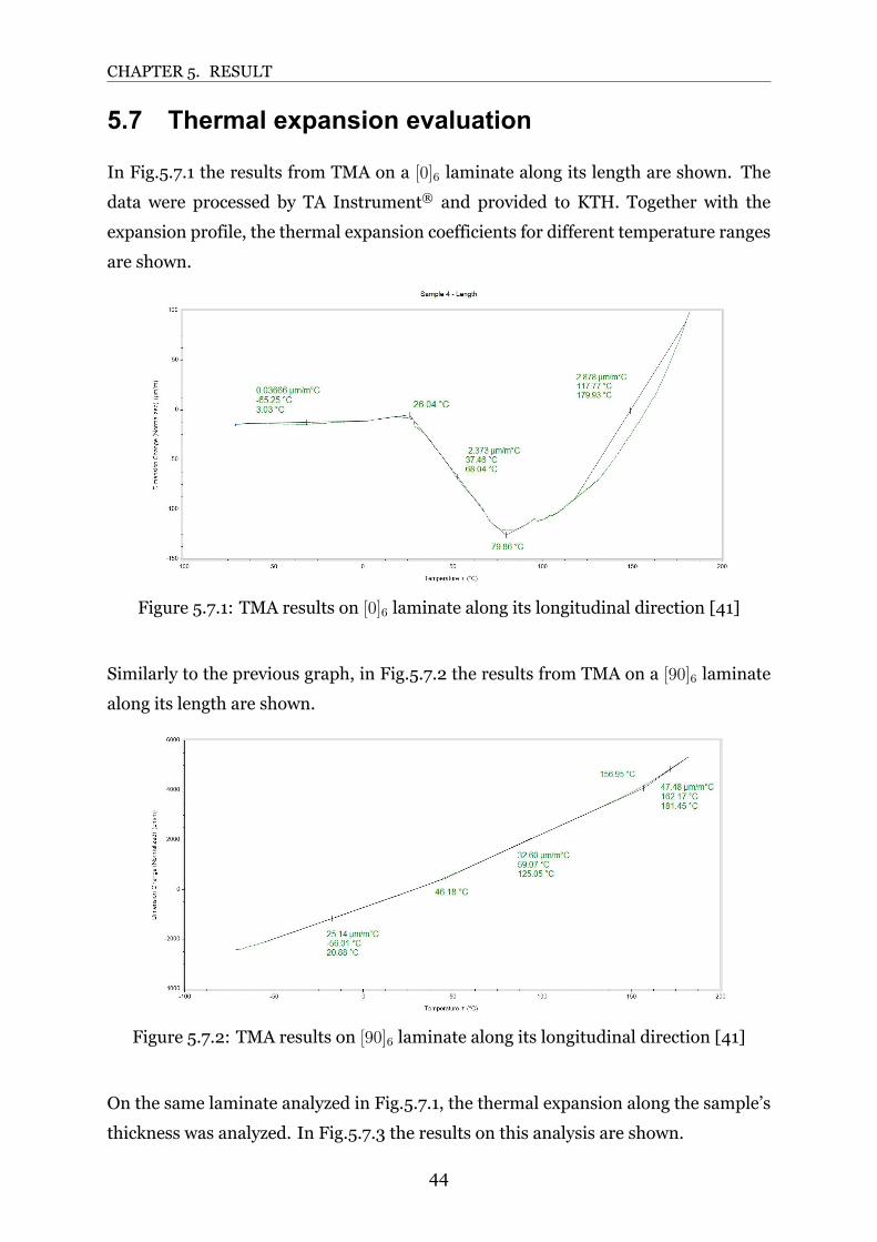
5.7 Thermal expansion evaluation
In Fig.5.7.1 the results from TMA on a [0]6 laminate along its length are shown. The
data were processed by TA Instrument® and provided to KTH. Together with the
expansion profile, the thermal expansion coefficients for different temperature ranges
are shown.
Figure 5.7.1: TMA results on [0]6 laminate along its longitudinal direction [41]
Similarly to the previous graph, in Fig.5.7.2 the results from TMA on a [90]6 laminate
along its length are shown.
Figure 5.7.2: TMA results on [90]6 laminate along its longitudinal direction [41]
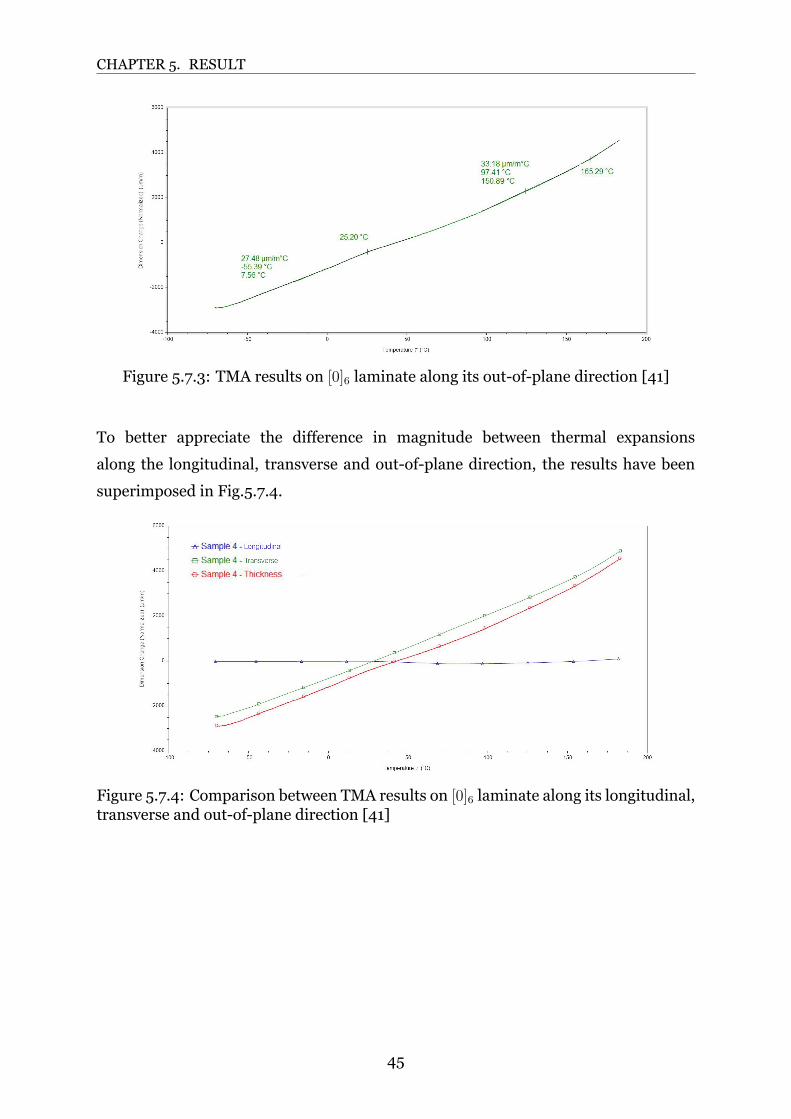
On the same laminate analyzed in Fig.5.7.1, the thermal expansion along the sample’s
thickness was analyzed. In Fig.5.7.3 the results on this analysis are shown.
44
CHAPTER 5. RESULT
Figure 5.7.3: TMA results on [0]6 laminate along its outofplane direction [41]
To better appreciate the difference in magnitude between thermal expansions
along the longitudinal, transverse and outofplane direction, the results have been
superimposed in Fig.5.7.4.
Figure 5.7.4: Comparison between TMA results on [0]6 laminate along its longitudinal,transverse and outofplane direction [41]
45
CHAPTER 5. RESULT
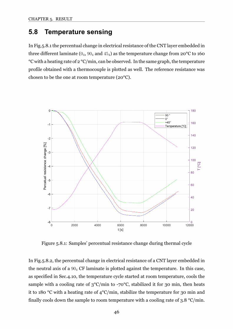
5.8 Temperature sensing
In Fig.5.8.1 the percentual change in electrical resistance of the CNT layer embedded in
three different laminate (04, 904 and 454) as the temperature change from 20°C to 160
°Cwith a heating rate of 2 °C/min, can be observed. In the same graph, the temperature
profile obtained with a thermocouple is plotted as well. The reference resistance was
chosen to be the one at room temperature (20°C).
Figure 5.8.1: Samples’ percentual resistance change during thermal cycle
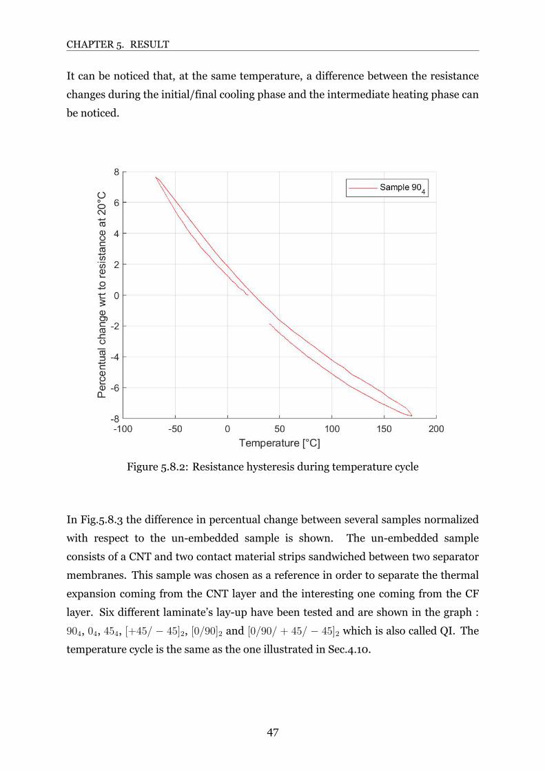
In Fig.5.8.2, the percentual change in electrical resistance of a CNT layer embedded in
the neutral axis of a 904 CF laminate is plotted against the temperature. In this case,
as specified in Sec.4.10, the temperature cycle started at room temperature, cools the
sample with a cooling rate of 3°C/min to 70°C, stabilized it for 30 min, then heats
it to 180 °C with a heating rate of 4°C/min, stabilize the temperature for 30 min and
finally cools down the sample to room temperature with a cooling rate of 3.8 °C/min.
46
CHAPTER 5. RESULT
It can be noticed that, at the same temperature, a difference between the resistance
changes during the initial/final cooling phase and the intermediate heating phase can
be noticed.
Figure 5.8.2: Resistance hysteresis during temperature cycle
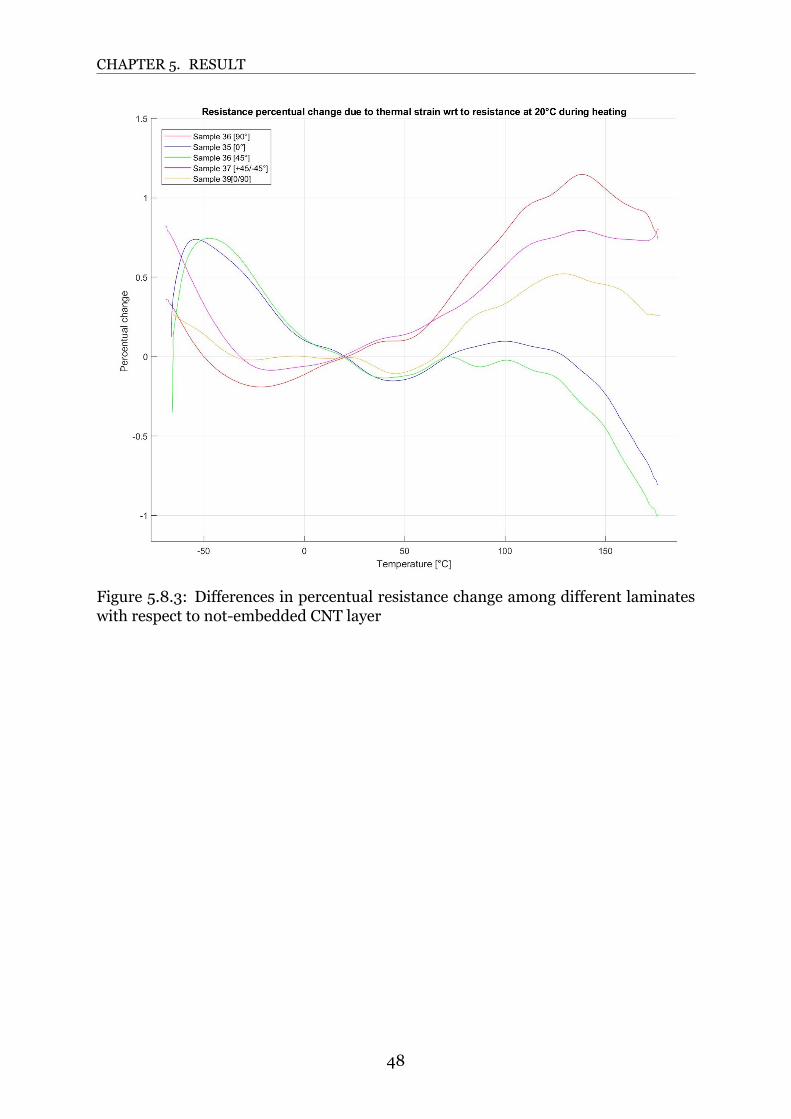
In Fig.5.8.3 the difference in percentual change between several samples normalized
with respect to the unembedded sample is shown. The unembedded sample
consists of a CNT and two contact material strips sandwiched between two separator
membranes. This sample was chosen as a reference in order to separate the thermal
expansion coming from the CNT layer and the interesting one coming from the CF
layer. Six different laminate’s layup have been tested and are shown in the graph :
904, 04, 454, [+45/ − 45]2, [0/90]2 and [0/90/ + 45/ − 45]2 which is also called QI. The
temperature cycle is the same as the one illustrated in Sec.4.10.
47
CHAPTER 5. RESULT
Figure 5.8.3: Differences in percentual resistance change among different laminateswith respect to notembedded CNT layer
48
CHAPTER 5. RESULT
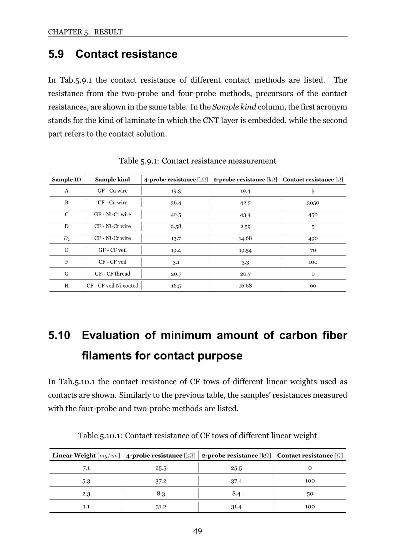
5.9 Contact resistance
In Tab.5.9.1 the contact resistance of different contact methods are listed. The
resistance from the twoprobe and fourprobe methods, precursors of the contact
resistances, are shown in the same table. In the Sample kind column, the first acronym
stands for the kind of laminate in which the CNT layer is embedded, while the second
part refers to the contact solution.
Table 5.9.1: Contact resistance measurement
Sample ID Sample kind 4probe resistance [kΩ] 2probe resistance [kΩ] Contact resistance [Ω]
A GF Cu wire 19.3 19.4 5
B CF Cu wire 36.4 42.5 3050
C GF NiCr wire 42.5 43.4 450
D CF NiCr wire 2.58 2.59 5
D2 CF NiCr wire 13.7 14.68 490
E GF CF veil 19.4 19.54 70
F CF CF veil 3.1 3.3 100
G GF CF thread 20.7 20.7 0
H CF CF veil Ni coated 16.5 16.68 90
5.10 Evaluation of minimum amount of carbon fiber
filaments for contact purpose
In Tab.5.10.1 the contact resistance of CF tows of different linear weights used as
contacts are shown. Similarly to the previous table, the samples’ resistances measured
with the fourprobe and twoprobe methods are listed.
Table 5.10.1: Contact resistance of CF tows of different linear weight
Linear Weight [mg/cm] 4probe resistance [kΩ] 2probe resistance [kΩ] Contact resistance [Ω]
7.1 25.5 25.5 0
5.3 37.2 37.4 100
2.3 8.3 8.4 50
1.1 31.2 31.4 100
49
CHAPTER 5. RESULT
5.11 Short beam threepoint bending test
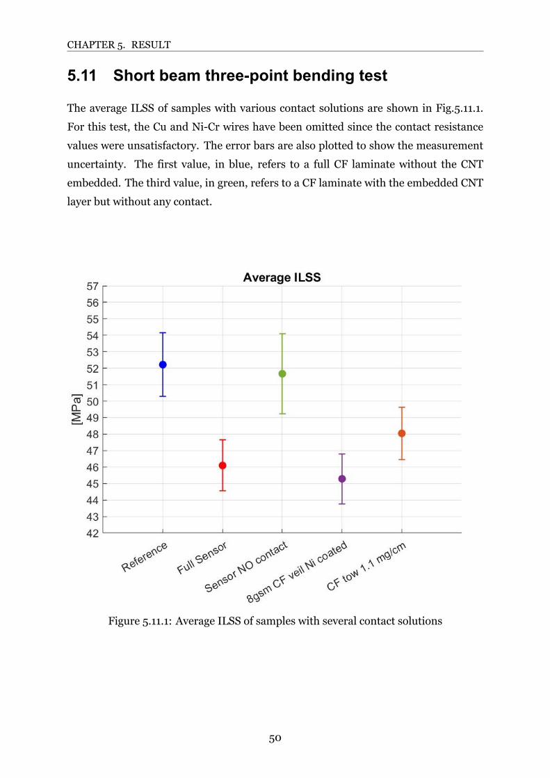
The average ILSS of samples with various contact solutions are shown in Fig.5.11.1.
For this test, the Cu and NiCr wires have been omitted since the contact resistance
values were unsatisfactory. The error bars are also plotted to show the measurement
uncertainty. The first value, in blue, refers to a full CF laminate without the CNT
embedded. The third value, in green, refers to a CF laminate with the embedded CNT
layer but without any contact.
Figure 5.11.1: Average ILSS of samples with several contact solutions
50
Chapter 6
Discussion of Results
6.1 Microscopy
With the microscopic analysis, we analyzed the nylon particles present on the surface
of the HexPlay M21® CF prepreg. We were able to observe their irregular shape and
their average diameter, which assess between 30 and 50 µm. From Fig.5.1.2 it was also
possible to observe that the thermoplastic particles create a constant and continuous
layer that divides fibres beds after curing. Unfortunately, this interlaminar layer is
unable to electrically separate CNT from the CF beds, and therefore the possibility of
using this material as the insulating barrier was discarded from the study.
A 20 µm Freudenberg separator filmwas used to create a consistent separating barrier.
Unfortunately, this membrane, when laminated dry in the sample, was not able to
isolate the CNT barrier from the CF beds. The problem with the dry membrane was
identified in its porosity which allowed CNT to get dragged the flow of epoxy matrix
in the substrate and diffuse through the separator membrane, as it can be observed in
Fig.5.1.4. To fill the porosity, the separator was impregnated with an epoxy film of the
same kind as the one present in the CF prepreg. The separator impregnated with this
technique worked as an insulating barrier. However, as it is noticeable in Fig.5.1.5,
the microscopy analysis showed a layer of excess matrix on both membrane’s sides,
reaching an impregnated thickness of 100 µm.
51
CHAPTER 6. DISCUSSION OF RESULTS
To remove the excess matrix and fill the separator’s porosity without increasing its
thickness, we have used a liquid impregnation method, switching from an epoxy film
to a thinned liquid epoxy. As it is possible to observe in Fig.5.1.7, this change allowed
to have a 20 µm impregnated separator. This liquid impregnation technique proved to
be very effective in creating an electrical barrier between CNT and CF.
Moreover, since the impregnated and gelled separator formed an impermeable barrier,
it was unsure whether the epoxy resin present in the CNT’s GF prepreg substrate
would be enough to impregnate the 32 gsm CF veil contact material effectively during
the curing process. From the microscopy analysis, we were able to check that the
matrix in the GF prepreg substrate is enough to impregnate without any problems
the contact material, as notable in Fig.5.1.8. Furthermore, since smaller and thinner
contact solutions were successfully tested, the contact material’s impregnation was no
longer considered a problem.
Finally, the failure mechanism during a short beam 3point bending was investigated
with a microscopic analysis of the sample section and after failure. Observing various
samples, it was possible to reconstruct the crack initiation at the 0/90 interface at
halflength from the sample, where the force was applied. From this point, the crack
propagated through the sample before reaching the impregnated separator. From
Fig.5.1.10 it is possible to appreciate the strong adhesion between the membrane and
the CF beds. In fact, during the rupture, the crack splits the separator in half, leaving
parts of the membrane on both sides of the adhesion.
6.2 IV measurements
From the graph shown in Sec.5.2, a linear relationship between voltage and current
can be appreciated. The linearity between these two physical quantities means that the
MWCNT forest does not behave as a semiconductor but as a metal, following Ohm’s
law [45]. The confirmation that theMWCNT forest behaves in a metallic way is crucial
to exploiting the material’s sensing ability using low voltages.
52
CHAPTER 6. DISCUSSION OF RESULTS
The application of low potentials allows to have minimal currents, which translate to
low heating power generated through Joule’s effect [46]:
P = R · I2 (6.1)
Where P is the power dissipated in Watts, R the resistance in Ohms, and I the current
in Ampere. The low heat dissipations allow us to consider negligible the increase in
temperature, which will not affect in a significant way the measurements.
6.3 Through the thickness resistance measure
Since the linear regression’s slopes shown in Tab.5.3.2 represent the samples’
conductivity in the outofplane direction, from the inverse of these data, it is possible
to obtain the throughthickness electrical resistivity of 0/0, 0/90 and 0/45 interfaces.
It can be noticed that, although all three laminates show low resistivity values, among
them, the 08 laminate shows the higher value. On the other hand, the [0/90]4 and [0/45]4
laminate show a similar value, almost half of the previous one. Moreover, between
these last two laminates, the [0/45]4 laminate shows a slighter higher value than the
[0/90]4 one. Although the amount of data are not sufficient to draw any conclusion, the
hypothesis that a higher angle between fibres of adjacent layers increases the contact
points between fibres, reducing the outofplane resistivity can be formulated. Even
so, considering the typical thicknesses of composite components that are usually in
the order of mm, the throughthickness resistance in CF laminates will not play a
significant role either their conduction method or in their modelling.
6.4 COMSOL model
From the surface plot in Fig. 5.4.2 it is possible to notice that the only red area,
representing a high value of current density, is located in themiddle domain. This peak
signifies that the current is flowing exclusively through the CNT layer in the middle of
the laminate.
Although quite illustrative, this representation method does not allow a deeper and
more precise quantitative analysis. To do that, we changed the kind of model’s output
towards a line graph. In this kind of graph, we show the current density distribution
53
CHAPTER 6. DISCUSSION OF RESULTS
along three crosssections: left, middle and right domain’s edge. From the spike in
Fig.5.4.1 it is clear that all the current density is localized in the CNT layer, between
205 and 215 µm.
Furthermore, since we parametrized all the domain’s length, we tested whether the
domain’s length would have affected the current density distribution with such a thin
insulation barrier. While keeping the separator domain’s height fixed at 5 µm, the
domain’s length was varied from 10 to 20 and 50mm and looked at themiddle section.
From this sweep’s result, it is possible to hypothesize that the sample’s length, at least
for small changes, does not influence the current flow path but only the intensity of
the current density. This hypothesis is also supported by the results obtained with the
analytical model, which will be discussed in the next section.
Due to its nature of simplified representation of reality, any model carries several
approximations and limitations with it. Looking at the approximations introduced
in this model, the biggest one is to consider both the CNT, the separator and the CF
layers as made of a homogeneousmaterial with conductivity values either measured in
the case of the CNT and CF layers or estimated in case of the separator. While for the
impregnated separator, this assumption can be considered as robust, for the CNT layer
it could be a source of error. However, the approximation was reputed acceptable in
both cases since themagnitude of the possible error caused by treating the CNT layer as
a homogeneousmaterial was considered negligible. Another important approximation
introduced in this model is to exclude the contact material from the simulation and
consider the contact between them and the CNT layer as ideal, therefore with zero
contact resistance. This approximation is supported by the fact that the contact
resistances, measured and reported in Sec.5.9, are at least two orders of magnitude
lower than the rest of the system and therefore, their exclusion from themodel does not
imply a significant error. Finally, a very evident approximation is the reduction of the
problem to a 2D model. This approximation is justified by the fact that the geometry
chosen to be represented is symmetrical along its length. For other geometries, this
assumption should be reconsidered carefully.
On the other hand, themajor limitations of thismodel are related to the intrinsic nature
of a FEMmodel. Since with this approach, themodel is subdivided into finite elements
54
CHAPTER 6. DISCUSSION OF RESULTS
through a mesh, it is inevitable to reach a bottleneck once the domain’s ratio between
height and length gets smaller. Although the bottleneck could be delayed using more
computational power during the simulation, the software will eventually reach a limit
point where the mesh skewness will not be allowed to simulation to keep running, and
the simulation will fail.
6.5 Matlab model
From the graph in Fig.5.5.1 it is possible to notice that with this analytical model, we
managed to simulate extremely thin separator membranes for a wide range of sensor
lengths. It is possible to observe that, even with a 5 m long sample, the difference in
resistance between the path through the CNT layer and the ones through the CF beds
is around one order of magnitude with the 0.01 µm separator membrane. However, if
we consider that the span of the sensory region would be in the order of 1meter inmost
future applications, we can realize that evenwith a 0.01µm film, the alreadymentioned
difference in resistance hovers around two orders of magnitude. A conclusion that we
can draw from this model’s results is that the separator’s thickness and material are
not the limiting factors in the CNT layer’s isolation. The main limiting factor is the
technological challenge of producing a continuum and poreless film with submicron
thickness. Techniques such as CVD with insitu polymerization [47] could allow the
formation of such ultrathin layer over the surface of either the CNT layer or the CF
bed, although more studies are needed in this direction
In comparison with the previous FEM model, this model does not set any limitation
on the separator’s thickness or aspect ratio (length/width). Even though the domain’s
width has been fixed in this particular model, it is possible to leave that parameter
as a variable, obtaining surface plots instead of line plots. The only limitation of
this model is its inability to simulate domains with complex shapes, although, with
few assumptions, it is possible to reconduct these to simpler domains suitable for
this model. On the other hand, the primary assumption is, similarly to the previous
model, to consider both the CNT, the separator and the CF layers as made of a
homogeneous material with conductivity values either measured in the case of the
CNT and CF layers or estimated in case of the separator. As explained in the previous
section, the approximation was reputed acceptable in both cases since the magnitude
55
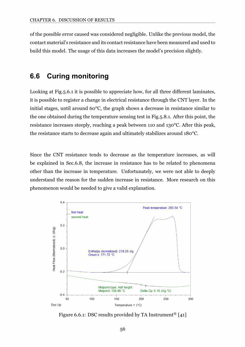
CHAPTER 6. DISCUSSION OF RESULTS
of the possible error caused was considered negligible. Unlike the previous model, the
contactmaterial’s resistance and its contact resistance have beenmeasured and used to
build this model. The usage of this data increases the model’s precision slightly.
6.6 Curing monitoring
Looking at Fig.5.6.1 it is possible to appreciate how, for all three different laminates,
it is possible to register a change in electrical resistance through the CNT layer. In the
initial stages, until around 60°C, the graph shows a decrease in resistance similar to
the one obtained during the temperature sensing test in Fig.5.8.1. After this point, the
resistance increases steeply, reaching a peak between 110 and 130°C. After this peak,
the resistance starts to decrease again and ultimately stabilizes around 180°C.
Since the CNT resistance tends to decrease as the temperature increases, as will
be explained in Sec.6.8, the increase in resistance has to be related to phenomena
other than the increase in temperature. Unfortunately, we were not able to deeply
understand the reason for the sudden increase in resistance. More research on this
phenomenon would be needed to give a valid explanation.
Figure 6.6.1: DSC results provided by TA Instrument® [41]
56
CHAPTER 6. DISCUSSION OF RESULTS
Although not deeply understood, the results are auspicious toward the possibility of
following the curing process from inside the laminate stepbystep. Following live
the curing process would allow the possibility of designing curing cycles for a specific
matrix curing degree, which is crucial in process cycles that include postcuring steps.
Although the initial results are very encouraging, more research has to be done on this
topic since, so far, the onset and peak temperature registered during these tests do not
match with the data obtained from a Differential Scanning Calorimetry (DSC) analysis
on the same matrix. The mismatch can be noticed comparing the DSC results in
Fig.6.6.1 where, for example, the temperature of crosslinking onset is found at 171.72°C
with the one in Fig.5.6.1 where it could be identified around 60°C.
6.7 Thermal expansion evaluation
Looking at the results from the TMA we can obtain some helpful information. First
of all, we can notice how the thermal expansion coefficient in the fibres’ direction
is not constant and changes three times in the temperature range from 70°C
to 180°C. Moreover, we can see how, in the lowtemperature range, the thermal
expansion coefficient is extremely low and almost constant below 26°C. After this
temperature, the coefficient becomes negative, meaning that the material shrinks as
the temperature increases. Finally, for temperatures higher than 79°C, the thermal
expansion coefficient changes sign again and becomes positive, meaning that the
material expands as temperature increases.
The thermal expansion behaviour in the longitudinal direction can be explained by the
fact that in this direction, the principal component is the fibrous reinforcement which
alone has a negative Coefficient of Thermal Expansion (CTE), usually between 9 and 0
µm/m°C [48]. However, being embedded into a polymericmaterial, the fibres interact
with the matrix and, after 79°C, the matrix expansion overcome the fibre’s tendency to
contract, and the whole laminate expands slightly.
On the other hand, looking at the expansion profile of a sample in the transverse
direction, we can see how the thermal expansion coefficient remains almost constant
throughout the temperature range, increasing slightly as the temperature increases.
Similarly, the thermal expansion coefficient in the outofplane direction remains
almost constant throughout the temperature range, with values similar to those in the
transverse direction. The thermal expansion behaviour, both in the transverse and
57
CHAPTER 6. DISCUSSION OF RESULTS
outofplane direction, can be explained by the fact that in these two directions the
prevailing component is the matrix which, as cast without any reinforcement, has a
positive CTE usually between 45 and 65 µm/m°C [49].
Moreover, it is noticeable that the coefficient in this direction is one order ofmagnitude
higher than the one along the fibre’s direction, meaning that the material will expand
much more in the transverse direction than in the longitudinal one. This difference
in magnitude is also clearly noticeable in Fig.5.7.4, where the expansion profile in the
longitudinal, transverse and outofplane directions are overlapped.
6.8 Temperature sensing
From Fig.5.8.1 it is possible to see how the CNT layer changes resistance with the
temperature change. The profiles of the percentual change in resistance closely follow
the inverse of the thermocouple’s profile. While the induced electromotive force
measured in the thermocouple raises as the temperature increases (Seebeck Effect),
the resistance of the CNT layer decreases as the temperature increases.
The relation between change in temperature and resistance can be explained by
looking at the conduction mechanism of the CNT layer. As explained in Sec.2.2.3,
the total resistance of a CNT forest on a macroscopical level is composed of contact
resistance and tunnelling resistance. While the first component is considered as
constant, the second one varies with multiple parameters such as tunnelling distance
or applied potential, as shown in Eq.2.4. This equation, however, does not represent
the behaviour of CNT in a temperature changing environment since all the parameters
are temperature invariant. To analyze the thermal response of the electrical properties
ofMWCNT networks, we need to consider the fact that the electric field seen by a CNT
CNT junction is not only the one externally applied. Since every tunnel junction in the
CNT forest is situated in a thermal bath, there will inevitably be thermal fluctuations
leading to a voltage difference across each junction [50]. In fact, the RootMean Square
(RMS) of the thermal fluctuation voltage of a junction is given by the equation [51]:
RMS(VT ) =
…kb T
C(6.2)
Where kb is Boltzmann’s constant and C is the capacitance of the junction. When C
58
CHAPTER 6. DISCUSSION OF RESULTS
is small, which is the case for the CNTCNT tunnel junctions, the thermalinduced
voltage fluctuations can be appreciable [50]. Based on this thermalinduced voltage
fluctuation, amodel called the Fluctuation Induced Tunnelling Conduction (FITC) had
been built. With thismodel, the temperaturedependent resistance of a CNT forest can
be expressed as [52]:R(T )
R(T0)= βe
(Tb
T+Ts
)(6.3)
Where T0 is the reference temperature, Tb is the tunnelling activation energy divided
by the Boltzmann’s constant, Ts is the temperature at which thermal activation occurs,
and β is a scaling factor.
This model can explain the resistance behaviour observed in Fig.5.8.1 where the
fluctuation induced tunnelling dictates the CNT forest’s resistance. Since the epoxy
resin’s thermal expansion coefficient is relatively low, the increase in resistance due
to the increase in tunnelling distance caused by thermal expansion is negligible with
respect to the FITC, which is dominant. Although this applies to an epoxy matrix, the
relation between these twomechanisms can vary depending on thematrix in which the
CNT forest is embedded.
In Fig.5.8.2 it can be noticed a degree of hysteresis in the CNT layer’s resistance
during a thermal cycle going from 20°C to 70°C, then to 180°C and back to 20°C.
It is noticeable that the percentual change in resistance with respect to the resistance
measured at room temperature does not come back to zero when the sample is in the
heating phase from 70°C to 180°C. One possible explanation for this phenomenon
is that this sample’s configuration with a single layer of CNT is sensible to different
heating/cooling rates. As explained in Sec.4.10 the thermal cycle has three different
heating/cooling rates. The climate chamber is set to cool from 20°C to 70°C with a
cooling rate of 3°C/min, heat up to 180°C with a rate of 4°C/min and cool down to
room temperature with a rate of 3.8 °C/min. This difference in rates may cause the
mismatch in resistance at the same temperature showed in Fig.5.8.2, although more
studies have to be performed to confirm this correlation.
59
CHAPTER 6. DISCUSSION OF RESULTS
Moving on to Fig.5.8.3, we can appreciate the effect of laminates’ thermal expansion.
Since all the results are normalized at 20°C with respect to a notembedded CNT layer,
the shown changes in resistance are only due to the CF laminate’s thermal expansion.
Immediately we can notice some disturbance at the temperature scale’s boundaries.
For both frigid and scorching temperatures, the signal became very noisy and, even
after a low pass filter was applied, it remained not very representative of the physical
phenomenon. However, apart from these boundary effects, the presented graph
shows, in the interval around 50°C/150°C, the ability of the material system to detect
thermal expansions of laminates with different layers’ orientations, in accordance with
the data of thermal expansion coefficient, obtained with TMA.
From the TMA results, we know that the 90° laminate has a positive CTE which
increases slightly at higher temperatures. Moreover, we also know that the fibre’s
longitudinal direction CTE is very small and negative between room temperature
and around 80°C. Knowing this, we can explain the behaviour of the 90° sample
in Fig.5.8.3, shown with a red line in the graph. We can notice how the resistance
increases as the temperature increases since the sample expands in the sample’s length
and slightly contracts in the sample’s width. Looking at the constitutive equation of the
resistance of a uniform crosssection conductor:
R =ρ · lA
(6.4)
Where ρ is the resistivity, l is the length and A = l · w is the crosssectional area, it is
clear that an expansion along l and aminimal contraction along w will lead towards an
increase in the sample’s resistance.
On the other hand, the 0° laminate sample shown in Fig.5.8.3 as the blue line decreases
its resistance as the temperature increases from subzero to around 80°C. As it can be
seen in Fig.5.7.1, CF longitudinal CTE is positive, although very close to zero, until
26°C. For this reason, until the material reaches room temperature, the sample is
expanding slightly in its length. At the same time though, the material is expanding in
the fibre’s transverse direction, substantially expanding the sample’s width, reducing
the overall electrical resistance. After room temperature, the fibres start to contract
while they keep expanding in the transverse direction. This combination of effects
60
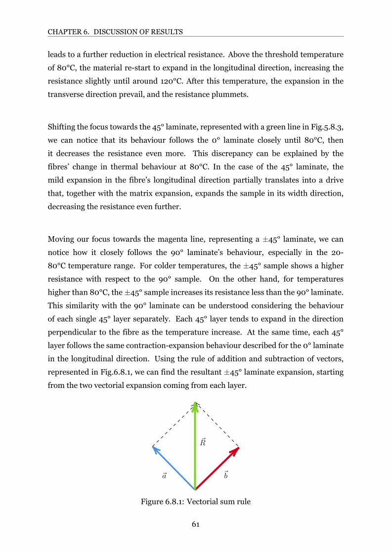
CHAPTER 6. DISCUSSION OF RESULTS
leads to a further reduction in electrical resistance. Above the threshold temperature
of 80°C, the material restart to expand in the longitudinal direction, increasing the
resistance slightly until around 120°C. After this temperature, the expansion in the
transverse direction prevail, and the resistance plummets.
Shifting the focus towards the 45° laminate, represented with a green line in Fig.5.8.3,
we can notice that its behaviour follows the 0° laminate closely until 80°C, then
it decreases the resistance even more. This discrepancy can be explained by the
fibres’ change in thermal behaviour at 80°C. In the case of the 45° laminate, the
mild expansion in the fibre’s longitudinal direction partially translates into a drive
that, together with the matrix expansion, expands the sample in its width direction,
decreasing the resistance even further.
Moving our focus towards the magenta line, representing a ±45° laminate, we cannotice how it closely follows the 90° laminate’s behaviour, especially in the 20
80°C temperature range. For colder temperatures, the ±45° sample shows a higherresistance with respect to the 90° sample. On the other hand, for temperatures
higher than 80°C, the±45° sample increases its resistance less than the 90° laminate.This similarity with the 90° laminate can be understood considering the behaviour
of each single 45° layer separately. Each 45° layer tends to expand in the direction
perpendicular to the fibre as the temperature increase. At the same time, each 45°
layer follows the same contractionexpansion behaviour described for the 0° laminate
in the longitudinal direction. Using the rule of addition and subtraction of vectors,
represented in Fig.6.8.1, we can find the resultant ±45° laminate expansion, startingfrom the two vectorial expansion coming from each layer.
ba
R
Figure 6.8.1: Vectorial sum rule
61
CHAPTER 6. DISCUSSION OF RESULTS
Suppose we consider a to be the expansion in the transverse direction of the 45°
layer and b to be the one of the 45° layer, the resultant R can be considered as
the expansion parallel to the sample’s length. Similarly, the expansion/contraction
coming from the longitudinal direction of each 45° layer translates into a resultant
expansion/contraction parallel to the ±45° sample’s width.For this reason, the±45° laminate behaves similarly to the 90°laminate, althoughwithlower percentual changes.
Similarly to the±45° laminate, in the crossply laminate, each layer wants to expand ina different direction, and the resultant expansion/contraction needs to be calculated,
like previously, using the rule of addition and subtraction of vectors. Unlike the
previous case, the major expansions coming from the fibre’s transverse direction
combine into a resultant diagonal to the sample. The resultant diagonal expansion
can be decomposed in a longitudinal and a transverse sample expansion. The first
component drives towards the increase in resistance and the second towards the
resistance reduction, balancing each other out. For this reason, we can notice that
the yellow line, representing the [0/90] laminate in Fig.5.8.3, remain very close to the
zeroline from 50°C to 80°C. Once 80°C are reached, the fibres start to expand in the
longitudinal direction, and the resistance slightly increases. During the whole interval
80150°C, the crossply laminate’s resistance remains much higher than the 0° ones
since, unlike in the 0° sample, in the [0/90] case the expansion in the sample’s width
direction is limited and controlled by the fibre’s expansion in that direction, which is
one order of magnitude smaller than the matrix expansion.
6.9 Contact resistance
The goal of analyzing different contact solutions was to find a preferable alternative
with lower contact resistance. The benchmark in this investigation was the 32 g/m2
CF veil with a contact resistance between 70 and 100Ω. The first idea was to substitute
the 32 g/m2 CF veil with a thinner 8 g/m2 Nicoated CF veil. This solution kept the
contact resistance value in the same order as the benchmark, being thinner, lighter
and less intrusive in the laminate.
62
CHAPTER 6. DISCUSSION OF RESULTS
The second idea was to change from a veil to wires, first metallic and then CF tows.
The contact resistances with both Cu and NiCr wires were very high and fickle. Since
the wire’s contact surface is minimal, the contact resistance is highly dependent on the
wire’s position and whether or not it gets in direct contact with the CNTs. On the other
hand, the CF tow shows excellent contact resistance, even lower than the measuring
tool’s sensibility. The reason is that, with this contact solution, we have a significant
increase in the contact surface between the CNT and CF tow, being the CF tow made
of thousands of CF threads and not a single wire like in the previous case.
6.10 Evaluation of the minimum amount of carbon
fibre filaments for contact purpose
It can be seen from Tab.4.13.1 that, below the initial linear weight, the contact
resistance starts to increase. However, even though the thinner tows shows higher
contact resistance than the thickest, it is still in the same range as the reference value,
or even lower. Although there is not a significant reduction in contact resistance from
the reference, the CF tows should be preferred as contact solution for twomain reasons.
Firstly, they demonstrated to be less intrusive, as can be seen in the next section,
affecting less the laminate’s ILSS. Secondly, the CF tows are smaller and easier to
handle without breaking them, which makes it possible, in principle, to extract them
from the laminate through the outofplane direction, provided the proper isolation.
This contact configuration wouldmake it possible to have sensing ability on a localized
area of a component without having contacts going through thewhole component until
the edges.
63
CHAPTER 6. DISCUSSION OF RESULTS
6.11 Short beam threepoint bending test
From Fig.5.11.1 we can immediately notice how the ILSS average value of the reference
laminate and the laminate with CNT layer embedded without contact material are,
inside measurement’s errors, equal. This equivalency signifies that, in this material
property, the contact material has a critical impact. Moreover, it is possible to make
some considerations about the impact of each contact solution on the laminate’s
interlaminar shear strength.
It is noticeable how the 32 g/m2 CF veil reduces the average ILSS by around 6MPa,
which represents an 11% reduction, both with respect to the reference CF laminate and
the laminate with the CNT layer embedded without contact material.
Moreover, the 8 g/m2 Nicoated CF veil show an ILSS reduction comparable to one
caused by the 32 g/m2 CF veil. Although the average value is slightly lower for the Ni
coated veil, considering the error bars, we can conclude that these two contact solutions
have a very similar effect on this material property.
Finally, looking at the CF tow with a linear density of 1.1mg/cm, we can notice how it
has a slightly lower effect on thematerial’s interlaminar shear strength, with an average
ILSS value that falls within the reference and the 32 g/m2 CF veil’s values.
It is essential to underline that, for this test, the CNT and contact layers have been
placed in the laminate’s neutral axis. For this reason, this test’s results represent the
bestcase scenario where the insertion of a contactmaterial should affect thematerial’s
properties in a lesser way.
64
Chapter 7
Conclusions
The thesis work carried out led to exciting and promising results regarding the
embedment and insulation of CNTs within carbon laminates with the aim of creating
a multifunctional material with sensing abilities. Various insulation techniques have
been proposed, studied, and tested. Among the different techniques proposed, the
solution of adopting a 23 µm polyester film impregnatedwith liquid epoxy resin proved
to be the most effective. Using this film, it was possible to obtain stable and replicable
resistance results, so it was chosen as the best solution among the options available.
Having obtained an effective electrical isolation technique experimentally, we
wondered if the introduction of this film inside the laminate would interfere with the
sensory abilities of the CNT layer. To do this, we tested the temperature and curing
sensing abilities. In both cases, the results obtained were in line with those deriving
from studies previously conducted on GF laminates. The likeness between the results
in laminated CF and GF indicates the fact that the insulating layer did not interfere
with the sensory properties of the material.
In addition, we also wondered if the introduction of the polyester film could reduce
the mechanical properties of the laminate, in particular its ILSS, and if the adhesion
between CF bed and the film was strong enough not to be the site of crack initiation.
To test this, we carried out various short beam 3 point bending tests, and the results
showed an insignificant reduction in ILLS in the order of 11 %. Furthermore, from
the failure analysis, we could see that when the crack reaches the insulating film, it
proceeds inside it and not at the bonding interface.
65
CHAPTER 7. CONCLUSIONS
After having obtained an efficient insulation technique, we proceeded to create a
model to be able to understand, freeing ourselves from the technological andmaterial’s
availability limits, what could be the minimum thickness required to have adequate
electrical insulation between CNT and CF. We started with a twodimensional finite
element model using COMSOL Multiphysics software. Using this model, we began to
understand that the thickness required for the insulating layer could be well below the
23 µm used experimentally. Unfortunately, a major limitation was found in the FEM
model for which it was not possible to simulate thicknesses of less than 5 µm. The
reason for this limitation is related to the relationship between the width and height of
themodel’s domain. When this ratio becomes too small, as in the domain representing
the insulating filmwith a thickness of less than 5µm, the individual elements thatmake
up the domain mesh become too distorted, and the model is no longer able to provide
results. An analytical model was built using Matlab software based on the electrical
circuit equivalent to the physical system to circumvent this problem. Using thismodel,
it was possible to simulate insulation thicknesses of a fewnanometers. From the results
obtained with this model, it was possible to understand that insulating films with the
same electrical properties as the polyester and epoxy film used experimentally can
effectively isolate CNT layers longer than one meter with thicknesses lower than 50
nm.
Having found promising results towards the birth of multifunctional composite
materials with sensing opens the door to numerous exciting possibilities in various
industrial sectors. In aerospace applications, this technology could reveal extremely
helpful in constantly controlling the mechanical and thermal stresses to which critical
parts are subjected and reducing the number and frequency of visual inspections
and Non Destructive Tests (NDT). The reduced number and frequency of controls
would lead to a massive reduction in operating costs, making passenger flights more
affordable.
In addition to aerospace, this technology can bring benefits in numerous other areas.
In motorsport, for example, it could be very beneficial in the testing phase, both in
the wind tunnel to punctually record the downforce generated by the aerodynamic
66
CHAPTER 7. CONCLUSIONS
devices and in track tests to verify that, for elements such as the front wing, the
deformations predicted by the simulations are in agreement with those obtained on
track. Furthermore, the possibility of constantly monitoring the temperature can be
critical on the race car for temperature profiles of critical parts, replacing today’s
thermosensitive adhesives in the composite parts. In addition, even in the mass
automotive field, stressmonitoring could reduce the safety factor used by the designers
and notify independently if any component has been damaged in use and requires a
check. The reduction of the safety factor would lead to the design of more optimized
and therefore lighter components which, in the transport world, translates into lower
emissions for ICE vehicles and a more extended range for electric vehicles.
7.1 Comment by Scuderia Ferrari F1 team
While writing the report for the thesis project, I worked at the Ferrari F1 team and had
the opportunity to talk with Senior Eng.Claudio Silenzi and his collegues of the sensors
department’s senior designers Eng.Christos Karpis and about this project. During our
conversation, wediscussed the potential applications, advantages anddisadvantages of
the technology studied in this thesis applied to the motorsport industry. Moreover, we
also discuss the requirements that this sensing technology should fulfil to be applicable
to the F1 world.
7.1.1 Applications
From our conversation emerged that, usually in F1, if a sensing technology is ready to
be used, meaning that it has a high Technology Readiness Level (TRL), an application
can be found since there is always a need for improvement in sensors in motorsport.
Rarely though the sensing technology is developed in house at Ferrari F1, they usually
take existing and consolidated technology to adapt it to their needs. However,
the company can sometimes collaborate with research centres to develop a sensing
technology if they repute the technology interesting enough.
In the past, they have already tried to work with optical fibres, embedding Fibre
Bragg Grating (FBG) inside CF laminate in order to gain sensing ability. However,
this kind of technology proved extremely difficult to work with, especially in double
curved surfaces and small bending radius such as the car’s aero component. For this
67
CHAPTER 7. CONCLUSIONS
reason, this technology was abandoned. From our initial study, the application of CNT
layer inside components with complex shapes and small bending radius should not
represent an issue, and it could be an advantage over the FBR technology.
Moreover, from the conversation, it turned out that pressure sensing ability would be
very beneficial to the aerodynamic team in order to be able to map the aerodynamic
pressure (downforce) all over the car. The current pressure sensors are only able to
measure pressure difference spotwise. It would be interesting and valuable to be able
to make a distributed analysis, for example, with stripes or a grid of CNT layers.
Temperature sensing could be helpful too for components close to the engine, such as
the engine bulkhead or gearbox casing. However, being able to record a temperature
profile is a feature that is not very interesting for them since the engine engineers are
usually more interested in the maximum temperature reached, and there are simpler
and cheaper solutions to do that, such as thermal tapes or thermocouples. Moreover,
components that are usually subjected to very high temperatures are made of metal
and not composite.
7.1.2 Advantages
The area which could benefit the most from the introduction of this technology in
the motorsport industry would be the Aerodynamic department. At the actual state,
this technology would be able to measure strain on mounting points of aerodynamic
devices, which can be translated into downforce, without disturbing the surface shape
and profile of the mounting itself. Moreover, in the future, it could be even more
effective to directly measuring the pressure applied on the aerodynamic surfaces
without modifying the wings’ surface or profile at all.
Furthermore, the possibility of being able to have a distributed analysis and mapping
the pressure level all around the car in realtime could be highly beneficial, especially
during the aeropackage development and validation.
7.1.3 Disadvantages
The main disadvantage with this technology is the impossibility of substitute the
sensing layer in case of failures or problems. Being embedded inside the CF laminate,
68
CHAPTER 7. CONCLUSIONS
the CNT layer and the contacts are not replaceable in case of problems. Moreover,
during the conversation, we identified the system’s weak link to be the contacts. In case
of contact break up, thewhole component has to be replaced, which is not economically
nor practically feasible even for a high budget industry such as F1 .
Moreover, it is impossible to use this sensing technology only during development or
testing and remove it after. The sensing material would have to remains inside the
laminate and, although it does not add much weight by itself, if we consider the whole
wiring and CU, it is still useless weight.
7.1.4 Must Have
• Datasheet with an extensive report of the property of the material system is
required.
• Installationmanualwith detailed instructions on how to install, wire and use the
material system is required.
• Contacts with connectors or connections ready to be plugged into the Central
Unit (CU) logging the data are needed.
• Qualification: Homologation tests might be required depending on the final
application. If the material system is used for a wind tunnel model, functional
tests are sufficient. However, if the material will be applied to the race car,
no formal homologation is required, but tests like vibration tests, maximum
operation Temperature tests, Humidity tests, Acceleration tests, maximum
Voltage tests, minimum Voltage are needed. Furthermore, if the material will
be applied on mass production cars, a full spectrum of homologation tests are
required. In any case, exhaustive proofs of design andmanufacturing robustness
are required.
• Affidability test: high degree of reliability and repeatability is crucial to be able
to apply this technology in F1.
• Sensibility: the sensing ability has to be very sensible. Deformations in the F1
aero package are very low.
• Robustness: the insertion of the CNT layer can not reduce the robustness, or any
other mechanical properties, of the material in which it is embedded.
69
CHAPTER 7. CONCLUSIONS
7.2 Future Work
The future work regarding the presented technology should be focused on four main
points. Firstly we should investigate further the potential of the curing sensing ability
of this material system, trying to interpret and understand the results we obtained so
far. Secondly, we should focus on the possibility of having pressure sensing ability
which, as the senior engineers at Ferrari F1 suggested, is very innovative and desired.
Thirdly, a solid effort should be put in trying to make the manufacturing process
more robust and less manual, with the main focus on finding a suitable strong contact
material, which was found to be the weakest link. Finally, more research and work
should be put into reducing the thickness of the separator membrane. Now that the
proof of concept works and the models show the potential for improvements, more
techniques have to be found in order to manufacture membranes that will not reduce
the material system’s robustness and strength.
Alongside these four research areas, studies towards a better understanding of the CNT
interaction with the CF laminate should continue as well as all the efforts towards the
system’s validation and the design robustness.
70

Chapter 8
Acknowledgements
First of all, I would like to thank allmy familywhohave always supportedme, especially
in these two years away from home. Their love and support was essential to be able to
make my goal a reality. The hard moments were a few but thanks to their love, I have
always managed to overcome them. I thank from the bottom of my heart my father
and my mother who have never stopped believing in me even for a second in the last
25 years and I wish my two sisters to know how to shine like the stars that they are.
It is to all of them that I dedicate this important milestone, waiting for new goals to
become reality: ad maiora semper.
In addition to my family I would like to thank Professor Malin Åkermo, from the
Engineering Mechanics department at KTH, for the availability, kindness and trust
shown in me. It has been a real pleasure to have her as a supervisor and I hope that in
a not that far future we will have the opportunity to work together again. Furthermore,
I thank from the bottom of my heart Tobias Karlsson who, in addition to following me
day after day in my thesis path, has proved to be a great friend. I keep his friendship
in the album of the best things that have happened to me. I wish him the best for his
PhD and for his future in general which, being the brilliant person that he is, I’m sure
will be bright.
Secondly, I would like to thank Per Hallander and all SAAB Aerospace for supporting
the project within which my thesis took place. It was a pleasure to collaborate with a
company of such a high calibre andwith such a deep knowledge of compositematerials.
71

CHAPTER 8. ACKNOWLEDGEMENTS
I hope that our greeting was not a farewell but a goodbye and that in the future I will
be able to collaborate with them again.
Last but not least, I would like to thank my closest friends who, despite being far
away and scattered around the world, never stop to feel close one another. We’ve
been through a lot together and I am truly a lucky man to be able to regard these
wonderful people as my best friends. Whatever the future might hold for us I wish
we’ll be able to celebrate more achievements like this in the future and to cheer for
each other successes. I love you all from the bottom of my heart.
72
Chapter 9
References
[1] Karlsson, Tobias. Study on the impact
of CNT or graphene reinforced interlaminar region in composites. Backup
Publisher: Luleå University of Technology, Department of Engineering Sciences
and Mathematics. Luleå University of Technology, Department of Engineering
Sciences and Mathematics, 2019.
[2] Johannisson, Wilhelm, Nguyen, Sang, Lindbergh, Göran, Zenkert, Dan,
Greenhalgh, Emile S, Shaffer, Milo S P, and Kucernak, Anthony R J. “A
residual performance methodology to evaluate multifunctional systems”. eng.
In:Multifunctional Materials 3.2 (2020). Publisher: IOP Publishing, p. 25002.
ISSN: 23997532.
[3] González, C., Vilatela, J. J., MolinaAldareguía, J. M., Lopes, C. S., and LLorca,
J. “Structural composites for multifunctional applications: Current challenges
and future trends”. In: Progress in Materials Science 89 (2017), pp. 194–251.
ISSN: 00796425. DOI: https : / / doi . org / 10 . 1016 / j . pmatsci . 2017 .
04 . 005. URL: https : / / www . sciencedirect . com / science / article / pii /
S0079642517300415.
[4] Gibson, Ronald F. “A review of recent research onmechanics of multifunctional
composite materials and structures”. In: Composite Structures 92.12 (2010),
pp. 2793–2810. ISSN: 02638223. DOI: https : / / doi . org / 10 . 1016 / j .
compstruct.2010.05.003. URL: https://www.sciencedirect.com/science/
article/pii/S0263822310001583.
73
CHAPTER 9. REFERENCES
[5] NASA. SBIR Phase I Solicitation. 2015. URL: https://sbir.nasa.gov/SBIR/
abstracts/15-1.html (visited on 05/12/2021).
[6] Hirano, Yoshiyasu, Yamane, Takuya, and Todoroki, Akira. “Throughthickness
electric conductivity of toughened carbonfibrereinforced polymer laminates
with resinrich layers”. In:Composites Science and Technology 122 (Jan. 2016),
pp. 67–72. ISSN: 02663538. DOI: 10 . 1016 / j . compscitech . 2015 . 11 .
018. URL: http : / / www . sciencedirect . com / science / article / pii /
S026635381530138X.
[7] Louis, M, Joshi, S.P, and Brockmann, W. “An experimental investigation of
throughthickness electrical resistivity of CFRP laminates”. In: Composites
Science and Technology 61.6 (May 2001), pp. 911–919. ISSN: 02663538. DOI:
10.1016/S0266-3538(00)00177-9. URL: https://www.sciencedirect.com/
science/article/pii/S0266353800001779.
[8] Zenkert, Dan and Battley, Mark. Foundations of fibre composites. KTH,
Stockholm, 2003.
[9] Ashby, Mike. Ansys GRANTA Education Hub, Teaching resources. URL:
https : / / www . grantadesign . com / education / teachingresources/ (visited
on 05/28/2021).
[10] Oberlin, A., Endo, M., and Koyama, T. “Filamentous growth of carbon through
benzene decomposition”. In: Journal of Crystal Growth 32.3 (1976), pp. 335–
349. ISSN: 00220248. DOI: https : / / doi . org / 10 . 1016 / 0022 - 0248(76 )
90115- 9. URL: https://www.sciencedirect.com/science/article/pii/
0022024876901159.
[11] Iijima, Sumio. “Helical microtubules of graphitic carbon”. eng. In: Nature
(London) 354.6348 (1991). Place: LONDONPublisher: NATUREPUBLISHING
GROUP, pp. 56–58. ISSN: 00280836.
[12] Gogotsi, Yury.
“Carbon Nanotube Science: Synthesis, Properties and Applications, Peter J.F.
Harris. Cambridge University Press (2009). Hardback, Price 45 GBP (US$81),
ISBN: 9780521828956”. eng. In: Carbon 47.15 (2009). Publisher: Elsevier
Ltd, pp. 3585–3586. ISSN: 00086223.
74
CHAPTER 9. REFERENCES
[13] Su, Dang Sheng. “20 Years of Carbon Nanotubes”. eng. In: ChemSusChem 4.7
(2011). Place: Weinheim Publisher: WILEYVCH Verlag, pp. 811–813. ISSN:
18645631.
[14] Hirano, Yoshiyasu, Katsumata, Shingo, Iwahori, Yutaka, and Todoroki,
Akira. “Artificial lightning testing on graphite/epoxy composite laminate”. In:
Composites Part A: Applied Science and Manufacturing 41.10 (Oct. 2010),
pp. 1461–1470. ISSN: 1359835X. DOI: 10 . 1016 / j . compositesa . 2010 .
06 . 008. URL: http : / / www . sciencedirect . com / science / article / pii /
S1359835X10001752.
[15] Trojanowicz, Marek. “Analytical applications of carbon nanotubes: a review”.
In: TrAC Trends in Analytical Chemistry 25.5 (2006), pp. 480–489. ISSN:
01659936. DOI: https : / / doi . org / 10 . 1016 / j . trac . 2005 . 11 .
008. URL: https : / / www . sciencedirect . com / science / article / pii /
S0165993605002591.
[16] Pujadó, Mercè Pacios. Carbon Nanotubes as Platforms for Biosensors with
Electrochemical and Electronic Transduction. eng. 1. Aufl. Vol. 7374. Springer
Theses. Berlin, Heidelberg: SpringerVerlag, 2012. ISBN: 9783642314209.
[17] Guzman de Villoria, R, Hallander, P, Ydrefors, L, Nordin, P, and Wardle,
B.L. “Inplane strength enhancement of laminated composites via aligned
carbon nanotube interlaminar reinforcement”. eng. In: Composites science and
technology 133 (2016). Publisher: Elsevier Ltd, pp. 33–39. ISSN: 02663538.
[18] Prasek, Jan, Drbohlavova, Jana, Chomoucka, Jana, Hubalek, Jaromir, Jasek,
Ondrej, Adam, Vojtech, and Kizek, Rene. “Methods for carbon nanotubes
synthesis Review”. eng. In: Journal ofmaterials chemistry 21.40 (2011). Place:
CAMBRIDGE Publisher: ROYAL SOC CHEMISTRY, pp. 15872–15884. ISSN:
09599428.
[19] He, Z.B., Maurice, JeanLuc, Lee, Chang Seok, Cojocaru, Costel, and Pribat,
Didier. “Growth mechanisms of carbon nanotrees with branched carbon
nanofibers synthesized by plasmaenhanced chemical vapour deposition”. In:
CrystEngComm 16 (2014), pp. –. DOI: 10.1039/C3CE42241K.
[20] Journet, Catherine, Picher,Matthieu, and Jourdain, Vincent. “Carbon nanotube
synthesis: from largescale production to atombyatom growth”. eng. In:
75
CHAPTER 9. REFERENCES
Nanotechnology 23.14 (2012). Place: BRISTOL Publisher: IOP Publishing,
pp. 142001–142001. ISSN: 09574484.
[21] Kroto, H. W., Heath, J. R., O’Brien, S. C., Curl, R. F., and Smalley, R. E. “C60:
Buckminsterfullerene”. In: Nature 318.6042 (Nov. 1985), pp. 162–163. ISSN:
14764687. DOI: 10 . 1038 / 318162a0. URL: https : / / doi . org / 10 . 1038 /
318162a0.
[22] Saito, Takeshi, Xu, WeiChun, Ohshima, Satoshi, Ago, Hiroki, Yumura, Motoo,
and Iijima, Sumio. “Supramolecular Catalysts for the Gasphase Synthesis of
Singlewalled Carbon Nanotubes”. In: The Journal of Physical Chemistry B
110.12 (Mar. 2006). Publisher: American Chemical Society, pp. 5849–5853.
ISSN: 15206106. DOI: 10 . 1021 / jp057513i. URL: https : / / doi . org / 10 .
1021/jp057513i.
[23] Iijima, Sumio. “Helical microtubules of graphitic carbon”. eng. In: Nature
(London) 354.6348 (1991). Place: LONDONPublisher: NATUREPUBLISHING
GROUP, pp. 56–58. ISSN: 00280836.
[24] Dresselhaus,M. S., Dresselhaus,G., andSaito, R. “Physics of carbonnanotubes”.
In: Carbon 33.7 (1995), pp. 883–891. ISSN: 00086223. DOI: https://doi.
org/10.1016/0008-6223(95)00017-8. URL: https://www.sciencedirect.
com/science/article/pii/0008622395000178.
[25] Ma, PengCheng, Siddiqui, Naveed A, Marom, Gad, and Kim, JangKyo.
“Dispersion and functionalization of carbon nanotubes for polymerbased
nanocomposites: A review”. eng. In: Composites. Part A, Applied science and
manufacturing41.10 (2010). Place:OXFORDPublisher: Elsevier Ltd, pp. 1345–
1367. ISSN: 1359835X.
[26] Devi, Rekha and Gill, Sandeep Singh.
“A squared bossed diaphragm piezoresistive pressure sensor based on CNTs for
low pressure range with enhanced sensitivity”. In: Microsystem Technologies
(Jan. 2021). ISSN: 14321858. DOI: 10 . 1007 / s00542 - 020 - 05208 - 7. URL:
https://doi.org/10.1007/s00542-020-05208-7.
[27] Mstroeck, User. A diagram showing the types of carbon nanotubes. URL:
https://sv.m.wikipedia.org/wiki/Fil:Types_of_Carbon_Nanotubes.png.
76
CHAPTER 9. REFERENCES
[28] Hong, Seunghun andMyung, Sung. “A flexible approach tomobility”. In:Nature
Nanotechnology 2.4 (Apr. 2007), pp. 207–208. ISSN: 17483395. DOI: 10 .
1038/nnano.2007.89. URL: https://doi.org/10.1038/nnano.2007.89.
[29] Janas, D and Koziol, K. K. “A review of production methods of carbon nanotube
and graphene thin films for electrothermal applications”. eng. In: Nanoscale
6.6 (2014). Place: CAMBRIDGEPublisher: ROYAL SOCCHEMISTRY, pp. 337–
345. ISSN: 20403364.
[30] Qian,
Dong,Wagner, Liu,Wing Kam, Yu,MinFeng, andRuoff, Rodney S. “Mechanics
of carbon nanotubes”. In: Applied Mechanics Reviews 55.6 (2002). _eprint:
https://asmedigitalcollection.asme.org/appliedmechanicsreviews/article
pdf/55/6/495/5439523/495_1.pdf, pp. 495–533. ISSN: 00036900. DOI: 10.
1115/1.1490129. URL: https://doi.org/10.1115/1.1490129.
[31] Bozlar, Michael, He, Delong, Bai, Jinbo, Chalopin, Yann, Mingo, Natalio, and
Volz, Sebastian. “Carbon Nanotube Microarchitectures for Enhanced Thermal
Conduction at Ultra low Mass Fraction in Polymer Composites”. eng. In:
Advanced materials (Weinheim) 22.14 (2010). Place: WEINHEIM Publisher:
WILEYV C H VERLAG GMBH, p. 1654. ISSN: 09359648.
[32] Li, Chunyu, Thostenson, Erik T, and Chou, TsuWei. “Dominant role of
tunneling resistance in the electrical conductivity of carbon nanotubebased
composites”. eng. In: Applied physics letters 91.22 (2007). Place: MELVILLE
Publisher: AMER INST PHYSICS, p. 223114. ISSN: 00036951.
[33] Oskouyi, Amir, Sundararaj, Uttandaraman,
andMertiny, Pierre. “TunnelingConductivity andPiezoresistivity of Composites
Containing Randomly Dispersed Conductive NanoPlatelets”. In: Materials 7
(2014), pp. 2501–2521. DOI: 10.3390/ma7042501.
[34] Oxford Learners
Dictionaries. eng. URL: https : / / www . oxfordlearnersdictionaries . com /
definition/academic/modelling?q=modelling (visited on 06/02/2021).
[35] Estabragh, A. R., Pereshkafti, M. R. S., and Javadi, A. A. “Comparison Between
Analytical and Numerical Methods in Evaluating the Pollution Transport in
Porous Media”. In: Geotechnical and Geological Engineering 31.1 (Feb. 2013),
77
CHAPTER 9. REFERENCES
pp. 93–101. ISSN: 15731529. DOI: 10.1007/s10706-012-9566-6. URL: https:
//doi.org/10.1007/s10706-012-9566-6.
[36] Asp, Leif E., Bouton, Karl, Carlstedt, David, Duan, Shanghong, Harnden, Ross,
Johannisson, Wilhelm, Johansen, Marcus, Johansson, Mats K. G., Lindbergh,
Göran, Liu, Fang, Peuvot, Kevin, Schneider, Lynn M., Xu, Johanna, and
Zenkert, Dan. “A Structural Battery and its Multifunctional Performance”.
In: Advanced Energy and Sustainability Research n/a.n/a (). _eprint:
https://onlinelibrary.wiley.com/doi/pdf/10.1002/aesr.202000093,
p. 2000093. DOI: https://doi.org/10.1002/aesr.202000093. URL: https:
//onlinelibrary.wiley.com/doi/abs/10.1002/aesr.202000093.
[37] Huntsman, Corporation. Advanced Materials, Araldite® LY 8615 / Aradur®
8615 / Hardener XB 5173 Datasheet. eng. Dec. 2012. URL: https://samaro.
fr/pdf/FT/Araldite_FT_LY_8615_Aradur_8615_Hardener_XB5173_EN.pdf.
[38] Åström, B. Tomas.Modeling of Polymer Composite Manufacturing. eng. 1999.
[39] Lin, Yueguo, Gigliotti, Marco, LafarieFrenot, Marie Christine, Bai, Jinbo,
Marchand, Damien, andMellier, David. “Experimental study to assess the effect
of carbon nanotube addition on the throughthickness electrical conductivity
of CFRP laminates for aircraft applications”. eng. In: Composites. Part B,
Engineering 76.3137 (2015). Publisher: Elsevier Ltd, pp. 31–37. ISSN: 1359
8368.
[40] Corporation, Hexcel. HexPly® 6376 Product Data Sheet. eng. URL: https :
/ / www . hexcel . com / user _ area / content _ media / raw / HexPly _ 6376 _ eu _
DataSheet.pdf.
[41] TA, Instrument.TMA450EM–Composite SampleAnalysis forKTH. eng. June
2021.
[42] ThermocoupleWire 9.103T.610.02X020 Datasheet. eng, ger, fre. URL: https:
//www.elfa.se/Web/Downloads/_m/ul/thermoleitungen_tds_mul.pdf.
[43] Miccoli, I, Edler, F, Pfnür, H, and Tegenkamp, C. “The 100th anniversary of
the fourpoint probe technique: the role of probe geometries in isotropic and
anisotropic systems”. eng. In: Journal of physics. Condensed matter 27.22
(2015). Place: BRISTOL Publisher: IOP Publishing, p. 223201. ISSN: 0953
8984.
78
CHAPTER 9. REFERENCES
[44] International, ASTM. D2344/D2344M16 Standard Test Method for Short
Beam Strength of Polymer Matrix Composite Materials and Their Laminates.
eng. Tech. rep. West Conshohocken, PA: ASTM International, 2016.
[45] Chen, S. “Asymmetrical IV curves from a symmetrical devices structure of
Organic Photovoltaics”. In: 2014.
[46] Joule, James Prescott. “On the production of heat by voltaic electricity”. eng.
In: Abstracts of the papers printed in the Philosophical transactions of the
Royal Society of London 4 (1843). Place: London Publisher: The Royal Society,
pp. 280–282. ISSN: 03655695.
[47] Asatekin, Ayse, Barr, Miles C., Baxamusa, Salmaan H., Lau, Kenneth K. S.,
Tenhaeff, Wyatt, Xu, Jingjing, and Gleason, Karen K. “Designing polymer
surfaces via vapor deposition”. In: Materials Today 13.5 (2010), pp. 26–33.
ISSN: 13697021. DOI: https : / / doi . org / 10 . 1016 / S1369 - 7021(10 )
70081- X. URL: https://www.sciencedirect.com/science/article/pii/
S136970211070081X.
[48] Nanni, A. “Guide for the Design and Construction of Concrete Reinforced with
FRP Bars (ACI 440.1R03)”. eng. In: Structures Congress 2005. 2005, pp. 1–6.
ISBN: 9780784407530.
[49] ToolBox, Engineering. Coefficients of Linear Thermal Expansion. 2003. URL:
https://www.engineeringtoolbox.com/linear-expansion-coefficients-
d_95.html.
[50] Sheng, Ping, Sichel, E. K, and Gittleman, J. I. “FluctuationInduced Tunneling
Conduction in CarbonPolyvinylchloride Composites”. eng. In: Physical review
letters 40.18 (1978), pp. 1197–1200. ISSN: 00319007.
[51] Van Kampen, N.G. “Nonlinear thermal fluctuations in a diode”. eng. In:
Physica 26.8 (1960). Publisher: Elsevier B.V, pp. 585–604. ISSN: 00318914.
[52] Lee, Jeonyoon, Stein, Itai Y,Devoe,Mackenzie E, Lewis,Diana J, Lachman,Noa,
Kessler, Seth S, Buschhorn, Samuel T, and Wardle, Brian L. “Impact of carbon
nanotube length on electron transport in aligned carbon nanotube networks”.
eng. In: Applied physics letters 106.5 (2015). Place: United States, p. 53110.
ISSN: 00036951.
79