NBER WORKING PAPER SERIES

EMPLOYEE RESPONSE TOCOMPULSORY SHORT-TIME WORK

Victor R. Fuchs

Joyce P. Jacobsen

Working Paper No. 2089

NATIONAL BUREAU OF ECONOMIC RESEARCH1050 Massachusetts Avenue

Cambridge, MA 02138December 1986

This study was supported in part by funds provided by the Alfred P.Sloan and Rockefeller Foundations to the National Bureau ofEconomic Research for the project "Women's Quest for EconomicEquality." We are indebted to the "ABC" corporation and itspersonnel managers for their help in planning and executing thesurvey, and to the employees of the company for their cooperation.Seymour Martin Lipset provided valuable advice concerning thewording and order of the survey questions, and Claire Gilchrist didan excellent job of producing and processing the survey. We arealso grateful to Takeshi Amemiya and Tom MaCurdy for adviceconcerning the econometric issues, and to Ellen Jones for herhelpful research assistance. The research reported here is part ofthe NBER's research program in Labor Studies. Any opinionsexpressed are those of the authors and not those of the NationalBureau of Economic Research.

NBER Working Paper #2089December 1986

Employee Response to Compulsory Short-Time Work

ABSTPCT

This paper reports the results of a survey of over 1500 employees who

faced compulsory reductions of 10 percent in hours of work and earnings during

the second half of 1985. The workers were asked how they used the free time

and how they viewed the program, and their answers were analyzed in relation

to their economic and social characteristics. On average, the workers spent 12

percent of the free time in uncompensated work for the company; 43 percent in

other work (mostly housework, childcare, and other nonmarket chores), and 45

percent in leisure-time activities such as resting, reading, and hobbies.

Ceceris paribus, education and income were positively related to percentage of

time spent in company work, and age was negatively related. Time spent in

other work rose with the presence of children, especially for women. Employee

reaction to the program was generally favorable; married women were most

positive and married men least positive. Workers 45 years of age and over were

significantly more positive than those 35-44. There was a strong connection

between time use and reaction to the program; workers who spent more of their

free time working without pay at the company or in home production were much

less positive than those who spent more time in leisure activities.

Victor R. Fud'.s Joyce acobsenNBER NBER204 Junipero Serra BOUleVaXd 204 Junipero Serra BoulevardStanford, CA 94305 Stanford, CA 94305

EMPLOYEE RESPONSE TO COMPULSORY SHORT-TIME WORK

by

Victor R. Fuchs and Joyce P. Jacobsen

1. Introduction

When a firm experiences a decline in demand, it can respond in a

variety of ways. If the decline is expected to be temporary, one

frequently pursued strategy is to maintain price and cut back on output

and inputs, especially labor. This reduction usually takes the form of

layoffs for a portion of the workforce, but sometimes the firm shortens

the hours of work for all or virtually all of the employees. Such short-

time compensation (STC), or work-sharing, is alleged to have numerous

advantages as compared with conventional layoffs (Best and Mattesich 1980,

Best 1985), but very little is known about employee response to STC.

The initiation by a major manufacturing company (called ABC in this

paper) of a six-month, company-wide program of STC in the second half of

1985 provided an excellent opportunity to gather systematic data

concerning employee response to short-time work. How do employees spend

the additional time off? Do they work more hours at norimarket production,

or do they enjoy true leisure? Do some employees come in to work anyway,

even though they are not paid? What do workers think of STC after having

direct experience with it? How does it affect them personally? Does

employee use of time and their reaction to the program vary systematically

with sex, marital status, or other characteristics?

1

This paper reports the results of a survey of a sample of over 1,500

ABC employees taken a few months after the STC program ended. First we

present a brief review of the literature on STC, followed by a description

of the ABC company and the survey. The employees' use of the time off and

their reactions to the program are subjects of the multivariate analysis

reported in sections 4 and 5. The paper concludes with a discussion of the

implications of the findings for policy and future research.

2. Review of Literature

Much of the literature on STC (used synonymously with worksharing) is

exhortatory rather than descriptive or analytical. Numerous social

benefits are claimed for STC, including less disruption associated with

unemployment (e.g., crime, poor health) and less need for redistributive

programs such as public assistance or public service jobs. The Federal

Republic of Germany makes more extensive use of worksharing than does any

other country, partly because the unemployment rate is seen as a "foreign

policy issue"- -"an immediate and meaningful reflection of the 'score' of

the continuing East-West political and economic competition" [Meisel 1984].

In the United States there were extensive efforts to promote

worksharing by both Presidents Hoover and Roosevelt during the Great

Depression but the practice fell into disuse until the mid-1970s [Nemirow

1984]. By 1986 there were 11 states that provided unemployment insurance

benefits for workers who face compulsory short workweeks, but only two

states, California and Arizona, had more than 10,000 workers drawing such

benefits in 1985. Even in California, the state that has led the way for

STC, less than one percent of total unemployment benefits are paid to

workers who are on short time [Business Week 1986].

2

Employers are said to like STC because it improves employee morale,

lowers administrative costs, eliminates future costs of hiring and

training new workers, and provides greater flexibility [MaCoy and Morand

l984J. A survey of 292 California firms who used STC reported 50 percent

as highly or extremely satisfied and only 2 percent as highly or extremely

dissatisfied. Comparable figures for a Canadian survey involving 296

respondents were 38 and 4 percent, respectively [Reid and Meltz 1984].

Less is known about employee response to STC. Workers are said to

benefit from continued job attachment and continued fringe benefit

protection. A 1980 survey of workers elicited 953 answers to a

hypothetical question concerning preferences for STC as an alternative to

layoffs.1' A substantial majority (64 percent) said they would favor STC;

19 percent said they would prefer a layoff program; and the balance were

neutral [Best 1981]. Women were more likely than men to indicate a

preference for STC (69 vs. 61 percent), but the difference was not

statistically significant. In general there was very little systematic

relation between socioeconomic characteristics and attitudes toward STC.

A Canadian study attempted to infer employee attitudes toward

worksharing by looking at the incidence of such provisions in collective

bargaining agreements in Ontario in August 1978 [Meltz, Reed and Swartz

1981]. Out of 2,163 agreements covering 816,000 employees, 6.2 percent of

the agreements covering 7.6 percent of the employees provided for

worksharing. The investigators ran regressions across industries with the

share of the employees covered by a worksharing provision as the dependent

variable2' The independent variables were average weekly earnings,

percentage of employees female, percentage of employees part-time, and

percentage of employees ages 25-54. The coefficient for percent female was

3

consistently significantly different from zero and indicates that for

every increase of one percentage point in that variable there was an

increase of almost one percentage point in the incidence of worksharing.

The wage and age variables were not significantly different from zero; the

coefficient for the percent part-time has a significant negative

coefficient.

The California Employment Development Department surveyed (by

telephone) approximately 450 workers who experienced STC during 1978-80

[State of California 1982]. In response to a question about time use, 60

percent of the respondents mentioned "work around the house," and the

second most frequently mentioned use (23 percent) was "time with family."

All other possible uses (e.g., "traveled," "looked for a new job," "read

or studied") were mentioned by 71 percent of the respondents. The total

exceeds 100 percent because many workers mentioned more than one use; the

amount of time spent in each one was not asked. About 40 percent of the

respondents said they put a "high value" on the additional free time; 33

percent said "moderate value," and 27 percent "little or no value." A

great majority favored repeated use of the program (as an alternative to

layoffs) and only five percent were opposed to future use.

There is, apparently, no study of employee response to an actual STC

program that relates time use and opinion to socioeconomic characteristics

in a multivariate framework or that explores whether workers' use of time

affects their opinion of the program. The survey and analysis presented in

this paper help to fill that gap.

4

3. Description of Survey

This section provides some background on ABC and its implementation

of the short-time program. This is followed by a description of how the

survey was formulated and carried out. Finally, there is a discussion of

the representatjveness of the responses relative to the sample population.

ABC is a large manufacturing firm with multiple product lines and

worldwide sales and production. It has a reputation for maintaining good

employee relations; it offers a competitive and varied benefit package,

and has, since its inception, been committed to a no-layoff philosophy.

The standard workweek is normally 40 hours, but the company allows flex-

time for all employees. ABC is less accommodating with respect to working

fewer than 40 hours per week, but there are some permanent part-time

employees and a few shared positions. All in all, less than 5 percent of

the employees normally work fewer than 40 hours per week.

In 1985, ABC began to experience a slowdown in business. As layoffs

were ruled out and worksharing was a strategy that had worked for the firm

twice before in the 1970s, it was a natural policy choice now that the

firm needed to cut costs. In July 1985 management decided to try a Friday

off without pay. This experiment was deemed a success, and in August the

program was put into full swing. All employees were subject to a program

of working 90 percent of their previous formal hours for 90 percent of

their previous monthly pay..' In California, the employees who had to take

days off were eligible for compensation from the state unemployment

insurance fund. Compensation was based on salary level up to a maximum of

$32 per day off for workers earning more than $5,533 in their highest

quarter. Information on the California worksharing program was made

available by the firm (stacks of applications and samples of completed

5

forms were prominently displayed at the workplace), and ABC personnel

managers estimate that over 75 percent of the workforce received insurance

benefits.

The program was presented as a short-term measure, scheduled to end

by January 1986. On January 1 it was replaced by a program of a 5 percent

reduction in both pay and hours. In March a new policy was announced,

effective April 1, which allowed each division to set its own rules

regarding STC. Some divisions returned to full-time (including two of the

three divisions covered in this study), some did not, and some had

different policies for different workers. This continuation of a short-

time schedule beyond the period originally expected may have led to

different answers about employee reactions than would have occurred

otherwise, even though the survey asked specifically about the earlier,

uniform policy.

In November 1985 we approached ABC with a proposal for a survey and

were told to delay the request until after the program was scheduled to

end. In January we again expressed our interest in surveying part of their

workforce, preferably only workers in one general area, so as to control

for factors which might vary geographically. In late March, ABC granted

access to three California divisions whose heads had agreed to cooperate

in distributing the survey. A short questionnaire was developed, tested on

two focus groups of workers at a division which was not included in the

survey sample, and then distributed along with the regular paycheck

distribution to all workers in the three divisions in early April, 1986.

Anonymity and confidentiality was stressed and postpaid envelopes were

included so that the questionnaires could be mailed directly to us. The

questionnaire was short- -and age, education, and income questions were

6

phrased in ranges, so as to elicit a high response rate. The appendix

Contains a facsimile of the questionnaire.

Out of an estimated sample population of 3,553, 1,911 questionnaires

were returned, yielding a response rate of 53.8 percent. Of these 1,911

questionnaires, 123 (6.4 percent) were not used due to incomplete or

unclear information about time use and/or opinion of the program./'

Another 265 questionnaires (13.9 percent) were not used due to missing

information on one or more independent variables. However, those

questionnaires missing only occupation were kept, and this fact noted.

Thus the detailed analysis is based on 1,523 observations, 42.9 percent of

the sample popu1ation.I

How representative are these observations of the underlying

distribution of workers? Table 1 shows a simple comparison- -the breakdown

of the sample population by sex, age, race, pay, and job type, provided by

the firm. These one-way frequencies are compared to those of the 1,523

usable responses. Women and whites, younger workers, and workers in the

middle and lowest salary ranges are slightly over-represented.

4. Results: Use of Time

Five categories were originally specified that people might divide

their time among in percentage terms. The percent of time spent in the

categories of volunteering, paid work, and other (usually schoolwork or

illness) was quite small.W It was decided that these miscellaneous

responses were best incorporated into a three-category system, for

analytical and explicative ease. These categories are: 1) ABC Work--time

spent working either at the firm or on company projects at home;

2) Leisure- - time spent resting, traveling, socializing, or doing hobbies

7

Table 1. Comparison of the distribution of usable responses to that of

the sample population.

WomenMen

Own Income ($1,000s)

< 1515-2525-3535-4545-60> 60

Percent offull population

(N—3,553)

45.654.4

2.536.129.218.410.43.4

Percent ofusable responses

(N—l,523)

52.147.9

4.027.833.921.311.21.7

Job Type*

ManagementOther exemptNonexemp t

< 252 5-34

35-4445-5455-64> 65

White (non-Hispanic)Other

17.736.745.6

9.042.925.214.77.70.5

68 . 831.2

21.338.739.9

9.547 . 323.214.25.40.5

76.024.0

Sex

Age

Race

*lJsable responses number 1,402; sample population figures are out of3,865 individuals, as data were not available for the same period.

8

or sports; 3) Other Work- -time spent mostly on nonmarket production,

including housework, childcare, running errands, and volunteer work, but

also including other market work and investment (schoolwork, looking for

another job).2'

Originally the study was partially geared towards studying changes

in how time was used over the course of the program. Therefore, the

workers were asked to try to recall how they allocated their time both in

the first month of the program (August 1985) and in the last month that

all divisions were subject to the program (December 1985). For most

workers, there were negligible changes in how time was allocated between

the two months. Therefore, the average of the two months is used in the

following analysis. Use of the simple mean rather than using the time

allocation of one or the other month also has the feature of averaging the

two types of time-off which the workers experienced: in August, September

and October the days off were scheduled for alternate Fridays so the

workers had three-day weekends; in November and December the days off were

bunched together with scheduled holidays and vacation days so that the

workers had an extended holiday period.

Table 2 shows the mean values for percent of time spent in the

three categories for the set of usable responses, stratified by personal

characteristics. The overall means are: 45.3 percent of time devoted to

Leisure, 11.8 percent to ABC Work, and 42.9 percent spent on Other Work.

Married persons spend less time in Leisure and more time in Other Work

than unmarried people do. When both sex and marital status are taken into

account, a pattern emerges that married women spend the most time in Other

Work, followed by married men, unmarried women, and unmarried men.

Employees with children spend much more time in Other Work than people

without children, cutting down on both ABC Work and Leisure. ABC Work

9

Table 2. Employee time use on days off by socioeconomic characteristics.ABC Work Leisure Other Work N

All 11.8 45.3 42.9 1,523

By sexWomen 8.8 44.1 47.1 794

Men 15.0 46.6 38.4 729

By marital statusMarried 11.6 40.3 48.1 816

Not married 12.0 51.0 37.0 707

By sex & marital statusMarried women 8.3 40.8 50.9 417

Married men 15.0 39.8 45.2 399

Not-married women 9.4 47.8 42.8 377

Not-married men 15.0 54.8 30.2 330

By childrenNo child 12.4 49.6 38.0 1,033

Child < 6 8.3 35.4 56.3 205

Child, not < 6 11.9 36.6 51.5 285

By educationNot beyond high school 3.4 41.7 54.9 193

Some college 6.3 44.6 49.1 489

College graduate 12.0 49.3 38.7 452

Some graduate work 17.7 46.2 36.1 129

Graduate degree 25.0 41.6 33.4 260

By own income ($l,000s)< 15 6.2 34.9 58.9 61

15-25 2.8 44.3 52.9 424

25-35 10.4 49.6 40.0 517

35-45 18.0 44.2 37.8 325

> 45 26.0 41.0 33.0 196

By job typeManagement 25.4 41.3 33.3 299

Other exempt 12.8 48.4 38.8 543

Nonexempt 3.7 44.3 52.0 560

Job type missing 10.4 45.8 43.8 121

By age< 35 13.5 47.1 39.4 864

35-44 12.2 41.3 46.5 354

> 45 6.4 44.7 48.9 305

By raceWhite (non-Hispanic) 12.6 46.3 41.1 1,157

Other 9.3 41.8 48.9 366

By inclusionUsable sample 11.8 45.3 42.9 1,523

Dropped observations 13.9 40.4 45.7 261

10

rises sharply with education, while Other Work drops to offset it. A

similar pattern is found as salary level rises. In the occupation groups

managers do more ABC Work; other exempt workers (norimanagerial persons who

are on salaries with no overtime pay) are slightly over the mean on ABC

Work, but spend more time than the managers in both Leisure and Other

Work. Nonexempt workers (those who can collect overtime pay) spend

significantly less time in ABC Work and a much higher amount of time in

Other Work. Younger people spend less time in Other Work, but more time on

ABC Work than older people. Finally, with regard to race, non-Hispanic

whites spend more time in both Leisure and ABC Work than all other groups.

The last two lines of Table 2 compare the mean time use and opinions

of persons in the usable sample to the responses of those persons who were

deleted due to their not providing full information about their personal

characteristics. The deleted respondents spent less time in leisure

activities and more time in both market and nonmarket work. These

differences, however, are not large.

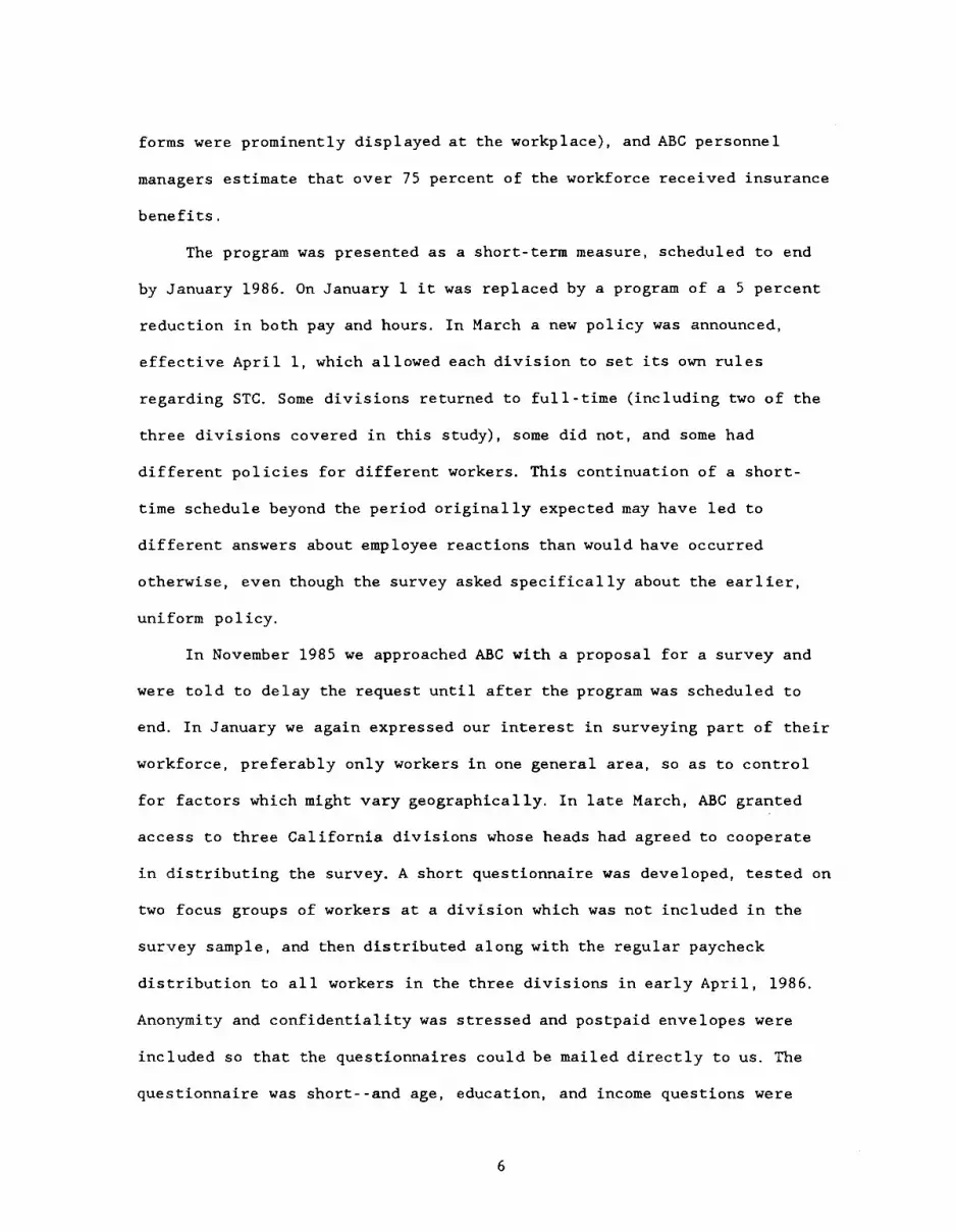
An examination of the means, however, does not do full justice to the

data. A smoothed distribution of all respondents for each of the three

categories of time use is shown in Figure 1. While responses are distri-

buted fairly normally for Leisure and Other Work, there is evidence of

bunching at the endpoints, and 68 percent of the respondents did no ABC

Work. This bunching means that modeling time use using a conventional set

of demand equations and estimating this system using ordinary least

squares will lead to inconsistent parameter estimates [Wales and Woodland

1983]. In an attempt to remedy these problems, a model of sequential

decisiorunaking, involving correction for the upper and lower bunching of

the data and a partial satisfaction of the adding-up constraint, has been

used.

11

% of r.spoes

0

30

25

20

%ofresponses 15

10

5

%ofresponses

0O 10 20 30 40 50 60 70 80 90 100

% of tine spent ws Leisure

0 10 20 30 40 50 60 70 80 90 100%oftinespeMb0ther York

Figure 1. Distribution of responses by percent of time spentin various activities.

12

70

60

50

40

30

20

10

0 10 20 30 40 50 60 70 80 90 100%oftbnespenti ABCYork

25

20

15

In this model, the person faced with how to spend his time makes two

sequential decisions. First, the worker makes the decision about whether

or not he will do ABC Work and how much time to spend doing it. This

decision is assumed to come first because for a large number of respond-

ents, there was no choice in this matter. Most hourly employees needed a

special pass in order to enter the plant on the days off and their work

was not of a type which could be undertaken off the premises: these

employees only had to decide how to divide their time between Leisure and

Other Work. On the other end of the spectrum, some salaried workers,

especially managers, felt compelled to do ABC Work; certainly some of the

written comments on the survey forms indicated that they felt this was not

a choice for them./ After the decision as to how much time to spend doing

ABC Work has been made, the worker allocates the remaining time between

Leisure and Other Work.2! Finally, his opinion of the program is hypothe-

sized to depend, in part, on how he allocates his time. Opinion is not

hypothesized to affect time use.

Operationally, this model of time use and opinion consists of four

equations. First, the percentage of time devoted to ABC Work as a function

of independent variables is estimated using a two-limit tobit specifica-

tion where the truncation points are 0 and 100 percent of time. Then, two

equations with percent of time spent on Leisure and Other Work as the

dependent variables are estimated using the same independent variables,

again using a double-truncated tobit, where the bottom limit is again 0,

but here the upper limit varies for each worker: it is set to 100 percent

minus the amount of ABC Work performed.iQ' Finally, as discussed in sec-

tion 5 of this paper, an equation is run with opinion as the dependent

variable, using the technique of ordered probit, and using the same

independent variables as listed below plus the percentages of time spent

13

in ABC Work and Leisure.

Formally, estimation of the time use part of the model involves

maximizing functions (A) and (B) below.

The basic tobit model postulates the existence of a latent variable

= 3'x +

where Y is the latent variable for person i, i=l n

X is a set of explanatory variables for i, and

is the residual for i.

However, Y is observed rather than Y, where:

*

IL.iIY.L

Ii 1 ii* *

—. Y. iIL.<Y <L.1 1 ii 1 2i

L*

L. f Y. � L.2i 1

and the likelihood function is given by:

L(p,I Y, X, L1, L2) =

I I

L.-X. Y.-3X. _____fI 1 1

1)]Y.=L. yy YL21

1 11 1 1

In the case of = W the desired amount of ABC Work and = W

the observed amount of ABC Work,

(L11=O-, '- foralliL2= 100 J

14

and

(A) L(,aIw,x)=

—py w—px. 100—px.

fltt( a fJ[i_t( 1)]wi=o wi=wi wi=100

While for desired Leisure, L4,

L11=O 1for all i

L2.=(100—W.)

And

(B) L(p,oILE,x,L2)=

—X. LE.-X. 1OO—W.—3X.

1I''( a 1)[T11t(1 ________

LE1= 0 LB. =LB1 LE= L23

Function (B) can then be reestimated substituting in observed and

desired Other Work for Leisure to yield a set of parameters relating the

independent variables to Other Work. By assumption, ABC Work does not

enter (B) as an explanatory variable.

The parameters of the likelihood functions were estimated using the

ML procedure in TSP 4.1. Standard errors were calculated using Newtonian

analytic second derivatives.

15

The matrix of independent variables includes education (EDUC); dummy

variables to indicate the presence of at least one child under the age of

six in the worker's household (YNGKID) and the presence of no young child,

but at least one child over five years of age (OLDKID); race (NONWHITE);

own salary (OWNINC); and spouse's salary (SPOUSINC). Three job dummies are

included, indicating, in order, managers (MGT), other exempt workers

(OTHEX), and nonexempt workers (NONEX). The omitted class are those

observations where occupation is coded as missing. Two age dummies are

also included, to signify those under 35 (< 35) and those 45 and over

(> 45). In order to expose structural differences, the tobit equations are

estimated separately for married and unmarried individuals, in which case

a dummy variable to indicate sex is included (WOMAN); and also separately

by sex, in which case a marital status dummy is included (MARRIED). As

noted in section 3, education, and salary variables are measured with

error, as they are set at the midpoints of the indicated ranges and

subject to upper and lower truncation.

There are two problems with using this model to predict how a person

will allocate time among the three uses. First, since within-equation

variance is not fully accounted for by the included variables, each use of

time is predicted with error. Second, the model is not constrained to make

the three predicted uses of time sum to 100 for each person. An

alternative method which satisfies the adding-up constraint, but which

yields higher prediction error for each time component, is to estimate

only two of the three equations (ABC Work, by hypothesis, is estimated

first, and then either Leisure or Other Work). The predicted values are

calculated from these two equations, checked to make sure each is between

o and 100 (higher and lower values are set at these values), and then

16

subtracted from 100 to yield an estimate for the percent of time spent in

the third area. This estimate is also constrained to be between 0 and 100.

To compare the results of these two methods, the mean absolute error

for each time use component under each method was calculated. In general,

the differences were not large. For example, for married persons, using

direct estimation of function (B) for Other Work yields a prediction error

of 22.3 percent. Calculating Other Work as the corrected residual time use

has an error of 23.8 percent. For the model as a whole, for married

persons, the three separately-calculated estimates of the time use

components sum to 9 percent more or less, on average, than 100 percent.

Prediction is slightly better for women and not-married persons and

slightly worse for men. Since the problem of not meeting the overall

constraint appears to be small relative to regular prediction error, all

twelve estimated equations are reported.

Table 3 shows the results of these estimations. For married

individuals, EDUC, OWNINC, and < 35 have a positive effect on percent of

time spent doing ABC Work, while the dummy variables YNGKID and N0NHITE

exert negative influences. The percent of time spent in Leisure for

marrieds is negatively related to YNOKID and OLDKID and positively related

to SPOUSINC; the opposite pattern appears for Other Work. Not-married

individuals also increase time spent in ABC Work with EDUC, OWNINC, and <

35, and spend less time if they are in the group with dummy NONEX. They

increase the percent of time devoted to Leisure only if < 35, and decrease

it in response to the presence of YNGKID, OLDKID, or WOMAN. Again, Other

Work exhibits the opposite pattern to that of Leisure.

Many variables are significant in the equations for women: EDUC,

OWNING, and < 35 are again positively related to ABC Work, and YNGKID is

significantly negative. In the Leisure equation, only SPOUSINC is

17

Table 3. Results of tobit estimations, percent of time spent in ABC Work,Leisure, and Other Work (standard errors in parentheses).

Married Not married

(N—816) (N—707)ABC Work Leisure Other Work ABC Work Leisure Other Work

WOMAN -2.60 -3.68 4.94 -0.20 -6.88* 7.27**

(6.66) (3.31) (3.26) (4.69) (2.75) (2.62)

MARRI ED

YNGKID l7.57* -l0.47** 15.28** -8.38 -17.22** 15.60*

(7.01) (3.39) (3.35) (14.75) (6.66) (6.38)

OLDKID 3.32 -lO.44** 8.68** 3.17 -18.95** 18.OO**

(6.80) (3.28) (3.24) (8.07) (4.30) (4.12)

SPOUSINC -0.16 0.24* -0.24*

(0.20) (0.10) (0.10)

EDUC 6.83** -1.00 -0.80 3.26* 0.35 -1.07

(1.50) (0.73) (0.73) (1.38) (0.80) (0.76)

OWNINC l.44** 0.02 -O.46** O.85** 0.08 -0.32

(0.31) (0.15) (0.15) (0.30) (0.18) (0.17)

MCT 1.50 0.77 -3.86 13.74 -6.26 -2.49

(10.72) (5.40) (5.34) (9.56) (5.89) (5.62)

OTHEX -19.04 3.33 4.31 -4.97 -1.83 3.54

(10.32) (5.06) (5.00) (8.73) (5.19) (4.95)

NONEX -18.70 -2.21 6.03 -28.00** 1.61 4.68(10.61) (4.86) (4.80) (9.70) (5.23) (4.99)

< 35 15.67* -3.34 -0.62 19.29** 8.45* -11.5O**

(6.97) (3.39) (3.36) (6.90) (3.68) (3.52)

> 45 -12.42 -0.77 3.52 -8.81 3.89 -0.34

(7.73) (3.62) (3.58) (9.04) (4.55) (4.35)

NONWHITE -13.35* -0.69 4.07 3.18 -5.60 2.69

(6.45) (2.98) (2.95) (5.55) (3.14) (3.00)

CONSTANT 166.4O** 55.16** 71.14** -102.29** 47.12** 60.24**

(24.41) (11.09) (10.94) (23.33) (12.66) (12.09)

Log oflikelihood -1462 -3289 -3280 -1451 -2880 -2862

** denotes p < .01; * denotes p < .05. CONTINUED

18

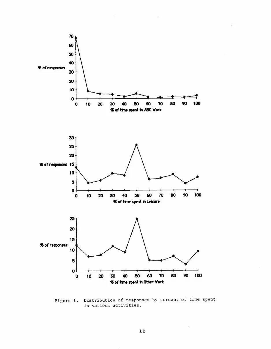
Table 3 (Concluded)

Men Women(N—729) (N—794)

ABC Work Leisure Other Work ABC Work Leisure Other Work

WOMAN

MARRIED -2.85 -19.81** 20.78** 8.96 -12.55* l3.48**(8.30) (4.91) (4.80) (10.90) (5.01) (4.93)

YNGKID -14.17 -6.60 12.1l** -19.91* -l802** 20.89**(7.90) (4.43) (4.35) (8.92) (3.84) (3.76)

OLDKID 4.88 -6.04 3.07 2.60 -16.12** 16.08**(7.55) (4.33) (4.23) (7.04) (3.19) (3.15)

SPOUSING 0.22 0.18 -0.30 -0.31 0.25* -0.25*(0.26) (0.16) (0.16) (0.26) (0.12) (0.12)

EDUC 5.23** -1.26 -0.50 5.05** 0.21 -1.25(1.43) (0.85) (0.83) (1.44) (0.68) (0.66)

OWNINC 1.04** -0.02 -0.39* 1.20** 0.16 -0.37*(0.28) (0.17) (0.16) (0.36) (0.17) (0.17)

MGT 0.36 6.63 -7.28 22.32 -12.90* -0.18(9.08) (5.64) (5.52) (11.93) (5.61) (5.51)

OTHEX -12.64 1.14 5.17 -5.94 1.46 0.36(8.56) (5.21) (5.10) (11.16) (5.05) (4.96)

NONEX -46.29** 4.43 3.82 -2.34 -5.03 5.51(10.56) (5.49) (5.37) (10.97) (4.67) (4.59)

< 35 12.54 4.15 -6.50 22.52** -0.74 -4.18(6.97) (3.94) (3.86) (6.86) (3.12) (3.07)

> 45 -11.67 2.54 3.88 -7.04 -1.31 1.72(7.65) (4.36) (4.27) (8.85) (3.66) (3.59)

NONWHITE -7.09 -1.11 3.87 -0.37 -5.58* 359(5.85) (3.33) (3.26) (6.21) (2.80) (2.75)

CONSTANT -126.78** 73.36** 50.08** -156.47** 49.11* 67.03**(23.24) (13.28) (13.00) (25.61) (10.63) (10.44)

Log oflikelihood -1638 -2889 -2884 -1273 -3268 -3256

** denotes < .01; * denotes p < .05.

19

significantly positive, while YNGKID, OLDKID, NONWHITE, MARRIED, and MGT

are all negative and significant. The equations run separately for men

have fewer significant variables. In the ABC Work equation, EDUC and

OWNINC are positively related and NONEX is significantly negative. In the

Leisure equation, only MARRIED is significant, and it exhibits a large

negative influence. Other Work again displays essentially the same

significant variables as in Leisure, but with the opposite sign.

How should these results be interpreted? These equations do not show

how a person allocates all of his or her time from scratch. Instead, the

equations are applicable to the special case in which a person subject to

a constraint on how much time may be spent working at a certain job for

pay suddenly find's this constraint to be changed so that 16 hours a month

must be reallocated away from paid work at ABC into other areas.

It may be tempting to extrapolate from this story and argue that if a

person were given yet another hour of free time, that this equation would

predict how he would, on average, spend that hour. But these equations

should be treated only as descriptive of the case for which they are

estimated. If a person were given nine hours off instead of eight, his

constraint would be different, and how he allocates time on the margin may

be different from the percentage split found in these data.

These equations can, however, demonstrate how members of a population

of workers, when faced with a worksharing program of this type, may vary

in their time allocation behavior when various easily observed personal

characteristics are taken into account. First, examine the ABC Work

equations. On average, the younger, better-educated, and higher-paid

members of the workforce are more likely to spend a significant amount of

time working at their primary job without pay. Perhaps this is because

they look at the time as an investment in human capital and are the most

20

willing to take on such an investment as they have the highest

expectations of future returns. In contrast, those workers with lower

income or a young child in their household prefer to invest their time in

Other Work, presumably including childcare.

Upon observing the coefficients on the job-type dummies, it appears

that exempt workers vary little in their time allocation. Nonexempt

workers exhibit a negative relationship in two of the four ABC Work

equations and are never positively related to time spent working- -this had

been expected, given that their access to the firm was restricted on the

days off. It is somewhat surprising that the MGT dummy did not enter with

positive significance, as managers were hypothesized to feel obligated

to work anyway. Perhaps this obligation is tied more to these persons'

other characteristics, such as high salary and education levels, rather

than to their job status.

Turning to the use of time as leisure, it is harder to see patterns,

except that time spent in Leisure decreases for those persons with

children and for married people. The nonleisure time is apparently spent

in Other Work rather than in ABC Work.

5. Results: Employee Reaction to STC

In order to determine employee reaction to the STC program the sample

respondents were asked to indicate how the practice of unpaid days off

affected them personally. They responded by placing a mark on a nine-point

line that was labeled "very negative" at one end, "very positive" at the

other end, and "neutral" in the middle.11' Separate questions were asked

21

about the employee's reaction in August 1985 and December 1985. For most

employees the responses were very similar for both months; therefore an

average of the two was used in all subsequent analysis.

The distribution of responses, grouped into the nine categories, is

shown in Figure 2. We see that positive reactions tend to outnumber the

negative ones, and that there is a central tendency around "neutral." We

also see a tendency for women to react more positively than men. In order

to lessen the arbitrary nature of the scaling, all responses were classified

into three categories: "positive," "negative," or "neutral," according to

whether the mean score for the two months was above 5.5, below 4.5, or

between or equal to those two values. Table 4 shows the distribution of

responses in these three categories by sex and by other socioeconomic

characteristics.

Overall, approximately one-half of the employees reacted positively

to the program, 29 percent were neutral, and 22 percent were negative.1-"

Women were more likely to be positive than men, but this sex difference

was evident only for married persons. Because married women tended to

react very positively to the program while married men were the least

positive, there was no overall difference between married and not-married

employees. The multivariate analysis described below takes account of this

important sex-marital status interaction and possible other interactions

with these variables.

The partial relation between employee reaction and socioeconomic

characteristics was investigated by running ordered probit regressions

with the dependent variable showing whether the response was positive,

neutral, or negative. Operationally, the underlying function for opinion

about the short-time policy is specified as

22

% of rpons.s

25

20

15

10

5

01 2

vsrv—

Figure 2. Distribution of responses by opinion of program, by sex.

23

3 4 5 6 7 8 9neutral Yerv positivT

Table 4. Employee reaction to STC by socioeconomic characteristics.

Percent of employeesPositive Neutral Negative

All 49.1 28.8 22.1

By sexWomen 53.6 27.2 19.1Men 44.2 30.4 25.4

By marital statusMarried 49.4 27.9 22.7Not married 48.8 29.7 21.5

By sex and marital statusMarried women 57.3 27.1 15.6Married men 41.1 28.8 30.1Not-married women 49.6 27.3 23.1Not-married men 47.8 32.4 19.7

By childrenNo child 50.3 29.3 20.3Child < 6 44.9 26.3 28.8Child, not < 6 47.7 28.4 23.9

By educationNot beyond high school 40.9 33.2 25.9

Some college 52.2 24.5 23.3

College graduate 51.1 27.0 21.9Some graduate work 58.1 32.6 9.3Graduate degree 41.5 34.6 23.8

By own income ($1,000)< 15 50.8 23.0 26.215-25 45.3 30.9 23.825-35 52.8 26.3 20.935-45 50.5 29.5 20.0> 45 44.9 31.1 24.0

By job typeManagement 47.5 30.1 22.4

Other exempt 50.3 30.9 18.8

Non-exempt 49.8 25.9 24.3

Job type missing 44.6 28.9 26.4

By age< 35 47.6 30.6 21.9

35-44 47.5 25.4 27.1> 45 55.4 27.5 17.0

By raceWhite (non-Hispanic) 50.6 27.9 21.5Other 44.5 31.4 24.0

24

*Yi — 'Xi + u

where is the response of person i, i—l,2, .. . ,n

is a set of explanatory variables for i, and

u is the residual.

Instead of observing Y, the following are observed:

fi1 if person reports negatv rewlion0 othervise

1 if person reports a ri.eutcsl rescilorL2 , o othervise

1 if person reports a positve retionC) Othelvise

Y is assumed to be distributed along the standard normal, and the

following likelihood function is used to estimate the vector :

L( ,oc( X.,6,6,S) =

6 6 6

{ [ i)('[ 1( — px.) — 4( —px.)

2[i — — p'x.) ] }

a., the dividing point between positive and nonpositive opinion, is

estimated as well, while the dividing point between negative and

nonnegative opinion is normalized to zero.

25

The sample was partitioned by marital status or by sex, and in each

case two equations were estimated. The first included only the

socioeconomic characteristics as right-hand-side variables; the second

added two variables describing the employee's use of time.

The results, presented in Table 5, show that the difference between

married women and married men is highly significant even after controlling

for the other variables. One way to interpret these coefficients is to

multiply them by the standard normal density function evaluated at a

particular set of X's (e.g., the means of the independent variables). This

yields the derivatives of the probabilities with respect to each

independent variable, e.g.

d tt)( p'x1) -f = =(t1A.h i' k

where is the kth element of the parameter vector 3. These are evaluated

for significant k' using the vector of the means of X (X) for each

sample group (married/not married, or men/women). They are evaluated in

the regions of both the upper and lower dividing points:

upper - - -= cc-p x) .

1oier ,.

k _.4i(...p )With this method, the coefficient .408 in the first regression can be

interpreted as indicating that women were 16 percentage points more likely

to be positive than men (holding constant the other characteristics), and

26

WOMAN

Table 5. Results of ordered probit regressions, probability of being positive,neutral, or negative about STC (standard errors in parentheses).

.408** •454**(.11) (.11)

Married (N=816) Not married (N=707) Men (N=729) Women (N=794)

.058

(.09)

.093

(.10)

MARRIED - .298*(.15)

-.206

(.16)

-.083

(.18)

.032

(.18)

YNGKID .065

(.11)

.137

(.11)

- .370(.22)

-.280

(.23)

.043

(.14)

.069

(.14)

- .150(.14)

- .017(.14)

OLDKID .035

(.11)

.108

(.11)

- .297*(.14)

-.199

(.15)

.064

(.14)

.090

(.14)

- .169(.11)

- .035(.12)

SPOUSING .006

(.003)

.005

(.003).000

(.005)

.000

(.005)

.010*

(.004).008

(.004)

EDUC - .003(.02)

.014

(.02)

.024

(.03)

.025

(.03)

.015

(.03)

.031

(.03)

.005

(.02)

.007

(.02)

OWNING .000

(.01)

.002

(.01)

.003

(.01)

.004

(.01)

- .002(.01)

.000

(.01)

.002

(.01)

- .003(.01)

MGT -.015

(.18).005

(.18)

.221

(.20)

.320

(.20)

.256

(.18)

.257

(.18)

-.122

(.20)

.051

(.21)

OTHEX .098

(.17)

.054

(.17).307

(.18)

.318

(.18)

.269

(.16)

.256

(.17)

.098

(.18)

.082

(.19)

NONEX - .043(.16)

- .028(.16)

.271

(.18)

.234

(.18).121

(.17)

.079

(.17).010

(.17)

.050

(.17)

< 35 -.161

(.11)

-.123

(.11)

.278*

(.13)

.259*

(.13)-.091

(.12)

-.097

(.12)

.114

(.11)

.152

(.11)

> 45 .229

(.12)

.231

(.12)

.478**

(.16)

.458**

(.16)

.229

(.14)

.204

(.14)

.300*

(.13)

.322*

(.14)

NONWHITE - .055(.10)

-.070

(.10)

-.158

(.11)

-.127

(.11)

-.124

(.10)

-.135

(.10)

- .053(.10)

- .007(.10)

AgCWORK - . 014**(.002)

- . 011**(.002)

- . 011**(.002)

- . 015**(.002)

OTHWORK - . 010**(.002)

- oo7**(.002)

- . 008**(.002)

- . 011**(.002)

CONSTANT .438

(.36)

.778*

(.38)

- .132(.44)

.217

(.45)

.482

(.41)

.600

(.42)

.533

(.38)

1.02**

(.40)

aLog oflikelihood

.796

-825

.837

-796

.842

-722

.866

-706

.825

-770

.853

-752

.802

-783

.844

-754

** denotes p < .01; * denotes p < .05.

27

that they were 12 percentage points less likely to be negative. The sex-

marital status interaction shows up as well in the regression for men

where the coefficient - .298 translates into married men having 12

percentage points less probability of being positive and 8 percentage

points more likely to be negative than not-married men. In the regressions

limited to women a statistically significant relationship is found for

spouse's income. The higher the spouse's income the more likely a woman is

to react positively. The coefficient for marital status in the women's

regression is not statistically significant, suggesting that fo: women the

amount of money the husband makes is more important than marital status

per

The presence of children produces a more positive response for

married persons and for men, and a more negative response for not-married

persons and women, but only one coefficient is statistically significant.

Age is significant in several specifications. In general, those employees

who were 45 and over were much more positive about the program than those

between 35 and 45. In the case of not-married employees, for instance, the

coefficient of .478 (when evaluated at the means of the variables) implies

that employees 45 and over were 19 percentage points more likely to be

positive than the 35-44 age group, and 13 percentage points less likely to

be negative. Among the not-married, younger workers (under 35) tended to

be more positive about the program than those 35-44, but this was not true

for married employees. The coefficients for education, own income, job

type, and race are not statistically significant.

One of the strongest and most consistent results is the relation

between time use and reaction to the program. The more time an employee

spent in ABC Work or Other Work, the more likely was the reaction to be

28

negative, and this was true regardless of marital status or sex. The

coefficient of - .010 for married employees, for instance, implies that,

ceteris paribus, an employee who spent all his or her time in Other Work

was 40 percentage points less likely to be positive about the program and

30 percentage points more likely to be negative than an employee whose

time was devoted entirely to leisure. Employees who spent their time at

ABC Work were least likely to be positive about the program; the

difference between the ABC Work and Other Work coefficients typically come

close to but do not quite reach the .05 level of significance.

Respondents were invited to supplement their replies to the survey

with written comments, and one-fourth of the employees did so. About 57

percent of the comments amplified reactions to the program; the other

comments clarified answers regarding socioeconomic characteristices, gave

opinions about the study, or described feelings (mostly negative) about

the employment and wage policies instituted by ABC after the end of the

STC program.

Of the detailed comments that concerned reaction to the program, 65

percent were positive, 10 percent negative, and 25 percent were mixed

(included both positive and negative reactions). Thus the employees who

felt strongly enough about the program to provide written comments tended

to be more positive than the sample as a whole. The difference between

women and men that was noted in the survey responses was also present in

the comments: the number of positive/negative comments was 64/7 for

married women, 36/11 for married men, and 53/6 and 33/5 for not-married

women and not-married men, respectively.

A detailed reading of positive comments revealed two primary themes.

Some employees liked the STC program because they preferred it to a

program of 1ayoffs.i/ Other employees reacted positively because they

29

actually preferred the shorter work time, albeit with lower pay.i1 The

negative comments stressed the financial hardship of adjusting to 10

percent less income and the difficulty of making the best possible use of

the days off. Some of the negative comments indicated that the workload

did not decrease at their job; thus they felt they had to work harder on

the days that they were employed.

6. Discussion

This survey of California workers who experienced 10 percent

reductions in hours and pay for six months in 1985 shows that use of the

time off and opinion of the program varied systematically with

socioeconomic characteristics. Ceteris paribus, the propensity to come in

to work anyway rose with education and income, and fell with age. The

presence of children (especially under age 6) resulted in an appreciable

increase in the percentage of time devoted to Other Work (mostly home

production), especially for women. Employee reaction to the program was

most positive among married women and least positive among married men.

Age was also related to reaction, with older workers (45+) feeling most

positive and those ages 35-44 feeling least positive. One of the strongest

and most consistent results was a positive association between percentage

of time spent in Leisure and reaction to the program.

The strong relationship between time use and opinion of the program

suggests that for many workers the time off was not truly "free time." The

use that they made of it was constrained in ways that affected their

opinion of the program. For instance, some employees apparently felt

obliged to come in to work anyway on an unpaid basis. Similarly, some

30

employees must have felt constrained to do other work (such as household

chores), and the more they did the less likely they were to think

positively of the program.

The results indicate that differences in sex roles are important,

even among a sample of persons all of whom hold regular full-time jobs.

The effect of sex on opinion of the program varies with marital status,

and the effect of children on time use varies with sex. An interaction

between age and sex also appears in the propensity to come in to work on

the day off. Women under age 35 were much more likely to do so than those

35 and over.

The generally positive reaction to the program suggests that other

firms might give serious consideration to compulsory short-time work as an

alternative to layoffs. From a public policy perspective there seems to be

little reason to provide unemployment insurance compensation for layoffs,

but not for compulsory short time. To be sure, these results are based on

employees in only one company, and one needs to be careful about

generalizing to the employed population as a whole. Moreover, the basis

for the generally positive reaction to the program is ambiguous. Some

employees were positive because they preferred it to layoff, whereas

others actually preferred STC to a full-time, full-pay schedule. Whether

they would have done so in the absence of the unemployment insurance

subsidy is not known.

These results should be interpreted with caution and qualifications,

but they do have the virtue of arising from a real situation, not a

hypothetical question, and they do cover a fairly large sample of workers.

The implications for gender roles, age, and presence of children on hours

of work and use of unpaid time seem important and worthy of further

investigation.

31

FOOTNOTES

1. The hypothetical question indicated that workers on STC would

receive one-half of their pre-tax hourly wage for each hour lost from

their regular workweek.

2. Eight industries with zero worksharing were eliminated from the

analysis to avoid clustering. This reason is not persuasive.

3. An exception was made for two small groups who were working on

projects that were deemed vital to the future profitability of Jie

company. One of these groups, which was not located in a division that was

surveyed, worked on its usual schedule. The other group, which was located

in a surveyed division, was put on a 110 percent time for 100 percent pay

program, in which they were expected to come in on alternate Saturdays for

a full day.

4. Some of these were from people who were not covered by the

program, either because they were on leave in one or both of the months

referred to on the questionnaire, or because they were not working at the

firm at that time. Others were from people who were incorrectly included

in our sample who were actually on the schedule of working extra weekend

hours without pay.

5. Examination revealed that there were not significant differences

by division with respect to time use and opinion, so the divisions were

pooled for the subsequent analysis.

6. In the sample of 1,523 persons used in the following statistical

analysis, the mean amount of time spent in volunteer work was 1.0 percent;

in paid work, 2.4 percent. Even among those people who reported spending a

positive amount of time in one or the other category the amount of time

32

was not substantial- -83 persons did volunteer work, for an average of 17.8

percent of their time; 105 persons spent an average of 35.4 percent of

their time in paid work.

7. Some problems were encountered in the course of coding the

answers to this question. Occasionally the time use figures did not add up

to 100 percent; in these cases the figures were summed and renormalized by

their total. Several people were not sure where to classify their holiday

shopping- - they would either place it in the "other" category or indicate

in a comment by their placement of it in either the leisure or chores

category that they were making a somewhat arbitrary decision as to how to

categorize this activity. Such time use was split 50-50 between the

Leisure and Other Work categories.

8. As one manager commented, "Given that my job requires 50+ hours

per week (60-70 hours per week during the program), telling me I should

take a day off was ridiculous."

9. To check for specification error, the model was rerun under the

two alternative specifications of decision order. There are no cases in

which a significant sign reversal occurs, but some magnitudes become up to

twice as large and some parameters become significant which are not

significant in the reported equations.

10. Raising the top constraint on either Other Work or Leisure from

(100 - ABC Work) to 100 does not significantly change the parameter

estimates from those reported here.

11. See the appendix.

12. The 261 replies that were excluded from the analysis because of

missing data showed a slightly less favorable reaction: 43 percent

positive, 30 percent neutral, and 27 percent negative.

33

13. If SPOUSINC is deleted from the equation, the coefficient for

MARRIED is positive and significant at p < .01.

14. E.g., "My personal feelings about the unpaid time off was quite

positive due to my appreciation for ABC's philosophy"; "I very much

appreciated having a lob and now am very willing to share losses as well

as profits."15. E.g., "The time off meant more to me than the pay for one day";

"Thoroughly enjoyed the time off- -would love to continue it. Allowed me to

spend time with my child."

34

REFERENCES

Best, Fred. 1985. "Short-Time Compensation in North America: Trends and

Prospects," Personnel (January), pp. 34-41.

Best, Fred. 1981. Work Sharing, Kalamazoo, Michigan, W. E. Upjohn

Institute for Employment Research, pp. 108-109.

Best, Fred, and James Mattesich. 1980. "Short-Time Compensation Systems in

California and Europe," Monthly Labor Review (July), pp. 13-22.

Blyton, Paul. 1985. "Short-Time Working," Changes in Working Time: An

International Review, pp. 89-100.

Business Week. 1986. "Shorter Workweeks: An Alternative to Layoffs" (April

14), pp. 77-78.

McCoy, Ramelle, and Martin J. Morand. 1984. "Short-Time Compensation: The

Implications for Management," in Ramelle MaCoy and Martin J. Morand,

eds., Short-Time Compensation: A Formula for Work Sharing, New York:

Pergamon Press. (pp. 14-35)

Meisel, Harry. 1984. "The Pioneers: STC in the Federal Republic of

Germany," in Ramelle MaCoy and Martin J. Morand, eds., Short-Time

Compensation: A Formula for Work Sharing, New York: Pergamon Press,

(pp. 53-60)

Meltz, Noah M., Frank Reid, and Gerald S. Swartz, Sharing the Work: An

Analysis of the Issues in Worksharing and Jobsharing, Toronto,

University of Toronto Press, 1981.

Nemirow, Martin. 1984. "Work-Sharing Approaches: Past and Present,"

Monthly Labor Review (September), pp. 34-39.

Reid, Frank, and Noah M. Meltz. 1984. "Canada's STC: A Comparison with the

California Version," in Ramelle MaCoy and Martin J. Morand, eds.,

35

Short Time Compensation, A Formula for Work Sharing, New York,

Pergamon Press, p. 108.

State of California. 1982. California Shared Work Unemployment Insurance

Evaluation, Employment Development Department, Health and Welfare

Agency, Sacramento, CA (March).

Wales, T. J., and A. D. Woodland. 1983. "Estimation of Consumer Demand

Systems with Binding Non-Negativity Constraints," Journal of

Econometrics (April), pp. 263-285.

36

APPENDIX

Hello: We are two Stanford researchers conducting a study of people's attitudes towards work schedules. With ABC'S help,we are conducting this voluntary survey in several divisions. If you could spend a few minutes tilling out this shortannvnus questionnaire, we'd appreciate your help. Feel tree to contact us at (415) 326—7639 if you have any questionsor cocinents about this survey. Please write any cocinents or amplifications you nay have on the back and returnthis surveyto us in the attached postage—paid envelope.

Naturally, we will share the overall results of our study with ABC though not the Individual data. Many thanks foryour help.Sincerely,

Victor 8. Fuchs, Professor of EconomicsJoyce Jacobsen, graduate student

1. ABC began a series of unpaid days off last stiTmer. We are interested In how You snent this time. esoecially In arychan2ea over this oeriod. Please estimate the percent of this time that you spent in each category:

a) In August. 1985 b) In Decmnber. 1985

1) Did hobbies, sports, travel,or rested

2) Did housework, chores, errands,or child care

3) Performed volunteer work

4) Came to work at ABC anyway

5) Performed other work for pay

6) Other (please specify): _______ Other: ____________

TOTAL: 100% 100%

2. How did ARC'S practice of unnaid davs off affect you personally? (Please place a mark on the line at the pointwhich corresponds to the effect on you, as best you can remember.)

very negative neutral very positivea) In August. 1985: I I I I I

1 2 3 4 5 6 7 8 9

very negative neutral very positive

b)InDeeprther.1g85: I I I I I I1 2 3 4 5 6 7 8 9

3. What is your lob at ABC? ______________________________________________________PLEA CIRCLE AJI1ERS FOR TIE RD1AIHI OHESTIONS.

4 • What is your sex? Hale / Female

5. What is Your agØ under 25 / 25—34 / 35—44 / 45—54 I 55—64 / over 64

6. What is your race? White (Non_Hispanic) / Black (Non—Hispanic) / Hispanic I Asian or Pacific Islander / Other7. What is the ranae of your anoual saar?

under $15,000 / *15,000—25,000 / $25,001—$35,000 / $35,001—$45,000 / *45001—160,000 / over $60,0008. What is your hiehest level of sohoo1Ig?

Less than high school grad / High school grad / Some college / College grad / Some grad work / Graduate degree9. a) Bow many children under eec 6 live in your household? None / 1 / 2 / 3 / ii or ure

b) Now many thildr beta,'een aecs 6 and 18? None / 1 / 2 / 3 / 4 or emre10. a) Does your snouse work for pay? Don't have one / No / Yes—part—time / Yes—full—time

b) If Yes, what Is the ranee of Your a annual sal cry?

under $15,000 / *15,000—25,000 / *25,001—35,000 / *35,001—45,000 / $'35,001—60,000 / over $60,000

Again, cornents on the back of this sheet are welcome. Thank you (or your participation.

37