Energetics of Winter Troughs Entering South America

Energetics of Winter Troughs Entering South America

EVERSON DAL PIVA

Universidade Federal de Santa Maria, Santa Maria, Brazil

MANOEL A. GAN AND V. BRAHMANANDA RAO

Centro de Previsao de Tempo e Estudos Climaticos, Instituto Nacional de Pesquisas Espaciais,

Sao Jose dos Campos, Brazil

(Manuscript received 11 February 2009, in final form 15 October 2009)

ABSTRACT

The energetics and behavior of midtropospheric troughs over the Southern Hemisphere and their re-

lationship with South America surface cyclogenesis were studied during the winters of 1999–2003. All surface

cyclogenesis situations over Uruguay and adjacent areas associated with 500-hPa troughs were analyzed. The

atmospheric circulation associated with type-B and type-C cyclones form the basis for two composites:

composite B (with 25 cases) and composite C (with 13 cases). The results showed that the midtropospheric

troughs were more intense in composite C than in composite B before the surface cyclogenesis and that the

opposite occurred during the surface cyclogenesis. The baroclinic conversion was dominant in both com-

posites. In composite B, the ageostrophic flux convergence (AFC) contributed positively to the intensification

of the surface cyclone since it imported energy into the area before the cyclogenesis started. But in composite

C, the AFC served as a sink because it exported energy. Based on these results, it can be concluded that (i) the

trough was crucial for the cyclogenesis; (ii) the variables in the mid- and upper levels did not differ signifi-

cantly from one composite to another; (iii) the northerly heat and moisture flow acted as a preconditioning for

the cyclogenesis, mainly for composite C; (iv) the baroclinic conversion dominated the energetics; and (v) the

AFC had only a secondary role, contributing negatively to the development of the cyclone in composite C and

positively to the initial development in composite B.

1. Introduction

A characteristics feature of the mid- and upper-

tropospheric flow is the continuous presence of synoptic-

scale waves. These waves have an important role in both

the heat and momentum budget, and can induce surface

cyclogenesis. Following the Petterssen and Smebye (1971)

study, the extratropical cyclones can be classified into

types A or B, depending on the configuration of the

upper- and lower-level circulation. In type A, the sur-

face cyclone initially develops in lower levels, and the

upper-level trough develops during the evolution of the

cyclone associated with temperature advection. In type B,

the surface cyclogenesis happens when the preexisting

upper-level trough is located over an area favorable to

cyclogenesis, such as the presence of warm advection in

lower levels.

In the 1980s, Radinovic (1986) proposed the exis-

tence of another cyclone development called type C,

which would be associated with orographic effects, known

as lee cyclogenesis. More recently, Plant et al. (2003)

proposed another cyclone category, whose initial devel-

opment is similar to type B, but with subsequent de-

velopments strongly dependent on latent heat release

at midlevels. It can be noted that with the exception of

type A, all other cyclone categories have the upper-level

trough as a precursor. Sanders (1986, 1988) suggested

that all type-A cyclones should be classified as type B,

because they form predominantly over the oceans where

there is not enough upper-level information to observe

the trough precursor.

Studies of South American cyclogenesis have shown

that mid- and upper-level troughs are present in all cases

analyzed by Gan and Rao (1996), Innocentini and

Caetano Neto (1996), Marengo et al. (1997), Seluchi and

Corresponding author address: Everson Dal Piva, Universidade

Federal de Santa Maria, P.O. Box 5021, Santa Maria, RS 97110-

970, Brazil.

E-mail: [email protected]

1084 M O N T H L Y W E A T H E R R E V I E W VOLUME 138

DOI: 10.1175/2009MWR2970.1

� 2010 American Meteorological Society

Saulo (1998), Vera et al. (2002), and Funatsu et al. (2004).

The synoptic conditions associated with South American

cyclogenesis were studied by Seluchi (1995) in 54 cases

from 1980 to 1984. The results showed that the distur-

bance triggering the surface cyclogenesis can be identified

5 days before the surface cyclogenesis when a long-wave

midtropospheric trough, over an area of enhanced baro-

clinicity near to 358S is present.

Since the mid- and upper-level troughs are crucial for

the development of surface cyclogenesis, several studies

were made with the objective of identifying preferential

areas of formation, dissipation, and displacement of the

troughs in the Northern (Sanders 1988; Lefevre and

Nielsen-Gammon 1995; Dean and Bosart 1996) and

Southern (Keable et al. 2002; Fuenzalida et al. 2005; Piva

et al. 2008a) Hemispheres.

The classic normal-mode baroclinic instability, the

nonmodal instability, and the downstream development

(DSD) are the main theories, or conceptual models used

to explain the upper-level mobile trough genesis (Nielsen-

Gammon 1995). From a baroclinic view, the energy

exchange happens between eddies and basic-state flow

through the heat and momentum fluxes. Randel and

Stanford (1985a,b) showed that the energy exchange be-

tween wave and steady-state flow is a valid concept in the

Southern Hemisphere. Also, the medium-scale Rossby

wave (with a wavenumber between 4 and 7) presented

a well-defined life cycle, with baroclinic growth, matu-

rity, and barotropic decay. However, the ageostrophic

fluxes vanish because their calculations are integrated

over a latitude belt encompassing all 3608 longitudes.

Nonetheless, when we compute the energetics using a

regional rather than a zonal average, it is possible to

notice that the eddy kinetic energy (EKE) is transported

downstream through the ageostrophic geopotential fluxes.

The mechanism associated with DSD is the wave en-

ergy dispersion. In the case of Rossby waves, the westerly

group velocity results in a DSD sequence of the troughs

and ridges show time and spatial scales that agree with

the observed conditions. Studying the life cycle of the

troughs in the Southern Hemisphere for the 1984–85

summer, Chang (2000) found that, except for the first

wave, the majority of the waves that develop later are

associated with wave packets dominated by ageostrophic

energy fluxes and not by baroclinic–barotropic conver-

sion. The DSD mechanism was also identified in the

subtropical and polar jets in the Southern Hemisphere,

particularly in the first one because of the smaller baro-

clinicity (Berbery and Vera 1996; Rao et al. 2002).

The downstream baroclinic development (DSBD)

proposed by Orlanski and Sheldon (1995) associates the

DSD to baroclinic instability. In this theory, the initial

EKE growth occurs by ageostrophic flux convergence

and is maintained by baroclinic conversion. They suggest

is that the eddy generated by upper-level ageostrophic

fluxes can induce circulation at lower levels, allowing the

eddy to use the baroclinicity available locally.

South America near 358S is an important region for

surface cyclogenesis (Gan and Rao 1991; Sinclair 1994,

1995; Simmonds and Keay 2000). This region becomes

more prominent if only the more intense systems are

considered (Sinclair 1995). These intense systems can

lead to explosive cyclogenesis as a theme of increasing

interest (Seluchi and Saulo 1998; Piva et al. 2008b).

Despite this, the energetics of the surface cyclogenesis

in this region still have not been studied. In other regions

of the world, the extratropical cyclone kinetic energy

budget has been the subject of several studies (Eddy

1965; Smith 1973; Chen and Bosart 1977; Kung 1977;

Smith 1980; Dare and Smith 1984; Masters and Kung

1986; Lackmann et al. 1999; Decker and Martin 2005;

Danielson et al. 2006a,b), using different datasets and

methodologies. Most of them considered the ageostrophic

flux convergence and the baroclinic conversion (vertical

velocity and temperature correlation) terms in the same

mechanism called cross-isobaric flow (a good discussion

about this can be found in Orlanski and Katzfey 1991). As

a consequence, the DSD is not emphasized. The studies

that considered both terms separately (emphasizing the

DSD) were applied to kinetic energy budget of the upper-

level troughs (Orlanski and Katzfey 1991; Orlanski and

Sheldon 1993; Chang 2000) and no attention was given to

surface cyclones.

Therefore, the kinetic energy budget applied to the

coupled trough–cyclone system, emphasizing the energy

transport due to ageostrophic fluxes in the cyclogenesis

cases over South America have not been studied yet,

and this is the objective of this article.

2. Data and methodology

The datasets used were the 6-hourly gridded data from

the National Centers for Environmental Prediction–

National Center for Atmospheric Research (NCEP–

NCAR) reanalysis (Kalnay et al. 1996) for the 1999–2003

winters. The intercomparison between the NCEP–NCAR

and NCEP–Department of Energy (DOE) reanalysis

showed that the latter is more active (considering the

track density and mean intensity) in the South Hemi-

sphere storm track region than the first one, mainly in

the cyclonic relative vorticity at 850 mb and in the mean

sea level pressure (SLP) field (Hodges et al. 2003). The

intercomparison between the NCEP–NCAR and the

40-yr European Centre for Medium-Range Weather

Forecasts (ECMWF) Re-Analysis (ERA-40) showed

that the latter presents greater strong-cyclone activity

APRIL 2010 P I V A E T A L . 1085

and less weak-cyclone activity over most areas of the

austral extratropical ocean than the NCEP–NCAR

(Wang et al. 2006). Opposite trends in the mean SLP

cyclone frequency were identified in previous studies.

In the NCEP–NCAR and NCEP–DOE datasets the

trends were negative (Simmonds and Keay 2000; Lim

2005), but in the ERA-40 the trends were positive (Lim

and Simmonds 2007). The comparison of annual mean

atmospheric energetics was carried out with NCEP–

NCAR and ERA-40 by Marques et al. (2009). No appre-

ciable difference was found between the two reanalyses,

although the energetics from NCEP–NCAR was, in gen-

eral, slightly smaller than those from ERA-40. Such small

differences were found mainly in the South Hemisphere.

Thus, some differences between our results and other

studies using another reanalysis dataset can be expected.

Based on the previous studies, it seems that the energy

conversions terms may be more intense in the ERA-40

than in the NCEP–DOE dataset; and more intense in

the latter than in the NCEP–NCAR dataset.

Only the winter (June–August) was considered when

selecting the cases because this season has the highest

frequency of surface cyclogenesis over Uruguay and

adjacent areas (area between 608–458W longitude and

37.58–27.58S latitude, represented by the box over the

east coast of South America in Fig. 2) according to pub-

lished studies (Gan and Rao 1991; Sinclair 1994, 1995).

Another reason for this choice was to avoid features

absent in winter but present in the other seasons (such

as the Bolivian high or diurnal convection over south-

east Brazil), which disturb the composites. Only 5 yr

were considered because there were enough cases to

make the composites during this period. All the situations

with a midtropospheric (500 hPa) trough that generated

surface cyclogenesis were analyzed, and the center of

the surface cyclone was located over Uruguay and ad-

jacent areas. Thus, we did not consider situations such

as (i) when the midtropospheric troughs were very

weak, which induced just a light reduction of sea level

pressure; or (ii) when midtropospheric troughs gener-

ated a surface cyclone in an area very far from the area

of interest (e.g., near the Andes or south of 408S).

Based on these criteria, 38 cases were separated in two

composites indicated as B (with 25 cases) and C (with

13 cases). Letters B and C were chosen because the

synoptic characteristics of the cases are similar to the

type-B cyclone according to the Petterssen and Smebye

(1971) and type-C cyclone following the Radinovic (1986)

criteria, respectively. Composite C had three character-

istics of the type-C cyclone: (i) a preexistent surface cy-

clone over the southeast Pacific Ocean, (ii) a cold air block

west of the Andes, and (iii) the southward incursion of

warm air over South America east of the Andes. The

cyclones with different characteristics were grouped in

composite B. Although the separation of cases into B

and C composites would appear to be qualitative and

somewhat subjective, it should be emphasized that the

categorization was based on the experience and regional

knowledge of the authors. Results in papers published

by other authors (Seluchi 1995; Innocentini and Caetano

Neto 1996; Funatsu et al. 2004; Mendes et al. 2007) were

also considered. The cyclone was considered formed when

there was a closed isobar in the sea level pressure field with

a 2-hPa contour interval, as used by Gan and Rao (1991).

The semistationary and persistent closed pressure centers

over Paraguay and northwestern Argentina were not

considered because they are not transient systems. The

midtropospheric troughs were defined with the associ-

ation of the 3 variables at 500 hPa: (i) the geopotential

height every 60 m, (ii) the Eulerian centripetal acceler-

ation (proposed by Lefevre and Nielsen-Gammon 1995),

and (iii) the meridional wind component. The lifetime of

the trough began when the geopotential height presented

cyclonic curvature, and the Eulerian centripetal acceler-

ation became positive. During the trough development,

the Eulerian centripetal acceleration and the geopotential

cyclonic curvature increased (both in area and magni-

tude). The zero isoline of the meridional wind compo-

nent placed on the maximum of the Eulerian centripetal

acceleration made the trough identification and tracking

easier.

The wavelength and amplitude of the troughs were

obtained from the Hovmoller diagram of geopotential

height deviation averaged in the latitudinal belt. The

geopotential height deviation was calculated subtracting

the geopotential height zonal mean, and averaging this

value over the 308–408S latitude belt for most of the cases.

The trough wavelength corresponds to the distance (in

degrees longitude) between two isolines with zero de-

viation, one west of the trough and the other east of the

downstream ridge. The trough meridional tilt was de-

termined from the horizontal tilt of the null meridional

wind component isoline.

The trough energetics was calculated by the EKE

equation (Orlanski and Katzfey 1991):

›K

›t5�$ � (VK)�$ � (V9

af9)�v9a9�V9 � (V9

3�$

3)V

1V9 � (V39 �$

3)V9� ›vK

›p� ›v9f9

›p1RES.

(1)

Here, K is the EKE per unit mass, V is the horizontal

wind velocity, v is the vertical velocity in pressure co-

ordinates, f is the geopotential, a is the specific volume,

and p is the pressure. The overbar denotes time mean


and primed quantities denote deviation from time mean,

which include the months of June, July, and August (as

used by Lackmann et al. 1999; Chang 2000). The vectors

and gradient operators with the subscript ‘‘3’’ represent

three-dimensional vectors, while those without the sub-

script contain the horizontal components only. The sub-

script a represents the horizontal ageostrophic wind

components with most of the nondivergent part removed

by defining the geostrophic wind with a constant Coriolis

parameter (Orlanski and Sheldon 1993).

The meaning of the right-hand terms of Eq. (1) was

discussed by Orlanski and Katzfey (1991) and Chang

(2000). The first term is called EKE flux convergence

(KFC) and represents the advective energy flux. It is

responsible for displacing the EKE maximum. The sec-

ond term is the ageostrophic flux convergence (AFC),

which represents the radiative energy transport, and is

associated with the dispersive nature of the waves. The

third term represents the baroclinic (BRC) conversion.

The fourth and fifth terms represent Reynolds and mean

stresses, respectively, and, since they are associated with

horizontal shear, they might be regarded as barotropic

(BRT) conversion. The sixth and seventh terms are the

vertical advection and energy flux, respectively. The last

term is the budget residue (RES) that is obtained from

the difference between observed kinetic energy ten-

dency (OKT) and calculated kinetic energy tendency

(CKT). The OKT is obtained by the difference of the

two EKE field with a 12-h interval and the CKT is the

sum of all terms on the right-hand side of Eq. (1), except

for the RES term. So, the RES contains mechanisms

that are not explained by Eq. (1), such as the friction,

diabatic, and subgrid effects; besides errors due to the

numerical methods such as the interpolation and taking

derivatives.

The terms in the EKE tendency equation are pre-

sented in the vertically averaged form, which is de-

fined as

A 51

(PB� P

T)

ðPB

PT

a dp.

Here A is the vertically averaged variable, a is the var-

iable given in several pressure levels, and PT is the

pressure at the top (100 mb) of the data. At the bottom

(PB), the pressure depends on the orography that was

obtained by reanalysis data. However, the lowest level

was the 1000-hPa pressure surface.

The advantage of Eq. (1) is that it contains the three

dominant processes of trough formation and dissipation,

such as the baroclinic instability (BRC term), the baro-

tropic instability (BRT term) and the DSD (AFC term).

This equation can be integrated over a volume, resulting

in Eq. (2) (Chang 2000):

›hKi›t

5�h$ � (VK)i � h$ � (V9a

f9)i � hv9a9i � hV9 � (V93� $

3)V 1 V9 � (V9

3� $

3)V9i � [vK]j

B

1 [vK]jT 1 [v9f9]jB 1 [v9f9]jT 1 hRESi1 h$ �VyKi1

›ps

›t1 V

y� $p

s

� �K

� ��B

. (2)

Here, the hi and [] symbols represent the volume and

surface integral, respectively. The last symbol can be at

the top (subscript T, taken at the 100-hPa level) or at the

bottom (subscript B, taken at the surface pressure) of

the volume. The subscripts y and s represent the velocity

of the volume and the surface level, respectively.

The terms of Eq. (2) have the same interpretation as

those in Eq. (1), except for the two vertical transport terms

in Eq. (1) (sixth and seventh terms) that were transformed

into a surface integral and can be interpreted as the ver-

tical energy fluxes through the lower [bottom (B)] and

upper [top (T)] boundaries (from sixth to ninth terms).

The tenth term represents the energy flux due to the

volume integration displacement, while the last term

represents the change of energy due to the variation of

the mass in the volume. Here, the volume is kept fixed,

so, the terms (tenth and part of the last term), which

involve the volume displacement, vanish.

Equation (2) requires the setting of the volume dimen-

sions. (For both composites, the area used is represented

by dashed lines in Figs. 7a and 12a.) The latitudinal

boundaries are from 508 to 208S, and 308 wide longitude.

In the vertical the levels from the surface to 100 hPa were

used. Over high orography areas, the integration at lower

levels depends on the mountain height given by reanalysis

data. The volume-averaged approach introduces compli-

cations arising from the need to define a volume of inte-

gration. Boundary flux terms and more than one feature

within the control volume are some examples. Further

discussions about this can be found in McGinley (1982),

Dare and Smith (1984), and Lackmann et al. (1999).

3. Results

Figure 1 shows some characteristics of the midtro-

pospheric (500 hPa) troughs of composites B and C,

APRIL 2010 P I V A E T A L . 1087

respectively. The trough amplitude ranged from 2206

(2217) m to 28 (229) m and the amplitude average was

288 (2118) m for composite B (C), indicating that the

troughs in composite C might be more intense than in

the case of B (Fig. 1a). The difference in the amplitude

between the composites is statistically significant at the

level of 90% (according to the Student’s t test). The

average wavelength was 648 longitude (wavenumber

K 5 5–6) and 768 longitude (K 5 4–5) for composites B

and C, respectively (Fig. 1b). The average lifetime was

128 h (160 h) and the traveled distance was 698 (818)

longitude for composite-B (-C) troughs (Figs. 1c,d). The

meridional tilt of the troughs was northwest–southeast

(or positive tilt) for most of the troughs in composite B

and northeast–southwest (or negative tilt), followed by

northwest–southeast in composite C (Fig. 1e). This in-

dicates poleward and equatorward eddy momentum

transport for composites B and C, respectively (Holton

1992, p. 336). Many composite-C troughs are formed in

remote regions of South America, as shown in Figs. 1f

and 2. Figure 1 shows that there is a wide variety of trough

configurations that generate cyclones in South America.

In this figure, we can see composite-C troughs are more

intense, have a longer wavelength, and that their genesis

is more distant from South America.

Figures 3 and 4 show the SLP and 500-hPa geopo-

tential height for composites B and C, respectively.

Initially we observed that there is a small-scale trough

with north–south horizontal tilt at 808W (Fig. 3a). The

southern part of the trough, south of 308S, moves east at

FIG. 1. Trough characteristics for the composites B and C: (a) amplitude (m), (b) wavelength (8 lon), (c) lifetime (h), (d) displacement

(8 lon), (e) meridional tilting during cyclone formation time, and (f) genesis area as indicated in Fig. 2.


the same time its amplitude increases and changes its

meridional tilt to northwest–southeast (Figs. 3b–d). At

0 h, the formation of the surface cyclone, whose center is

identified in Fig. 3c with a closed isobar, occurs. After

24 h, an indication of trough division is observed, with the

presence of two troughs, one with a strong northwest–

southeast meridional tilt with axis passing through 308S,

758W and another with northeast–southwest tilt over the

South Atlantic Ocean. The SLP field for composite B

shows two subtropical anticyclones, one over the South

Pacific Ocean and another over the South Atlantic, plus

a region of low pressure over South America (Fig. 3a). At

224 h, there was an inverted trough structure over Para-

guay, northern Argentina, and southern Brazil (Fig. 3b).

This surface trough extends southeast for the following

24 h, when the formation of the surface cyclone over

Uruguay with central pressure of 1012 hPa occurs (Fig. 3c).

The cyclone intensifies and moves southeast with a central

pressure of 1008 hPa at 124 h (Fig. 3d). Figure 3 also

shows the intensification of subtropical anticyclones over

FIG. 2. Positions of trough formation for composites B and C. Genesis areas are the Indian Ocean (IND), Australia–

New Zealand (ANZ), Pacific South Center (PSC), Pacific Southeast (PSE), and Circumpolar 1, 2, and 3 (CP1, CP2,

and CP3), respectively. The box over the east coast of South America indicates the region where the surface cyclones

must be stationed to be considered in the composites. Topography (km, thick isoline, label omitted) over South

America corresponds to 1.5, 3, and 4.5 km.

FIG. 3. (a)–(d) SLP [solid line, contour interval (CI) 2 hPa] and 500-hPa geopotential height (dashed line, CI 6 dam, shaded regions are

statistically significant at level of 95%) of composite B. In (a), the box with dashed lines indicates the area where the spatial average of the

heat and moisture flux shown in Fig. 5c were made. In (c), the box with solid lines shows the area where the spatial average of the variables

shown in Figs. 5a,b and 6 were made. The time in the upper-right corners refers to the formation of the surface cyclone.

APRIL 2010 P I V A E T A L . 1089

the oceans and the intrusion of a transient anticyclone

over the South American continent, even though the

transient anticyclone is not well defined.

The geopotential height evolution for composite C

confirms that the trough had higher amplitude and

wavelength than in composite B (Fig. 4). This result is

expected, since the cases chosen for composite C had a

preexisting surface cyclone over the Pacific Ocean (from

248 to 212 h) as observed in Figs. 4a,b. At midlevels

the trough moves toward South America and becomes

less defined than in composite B. At 124 h there is an

indication of two troughs, one over the Andes and an-

other short wave over southeastern Brazil and the South

Atlantic Ocean (Fig. 4d). Two processes might explain

the presence of the two troughs. One is the trough di-

vision that happened in composite B, while the other is

linked to the fact that some cyclones over the South-

eastern Pacific maintain their structures for a longer

period. This keeps the trough over the region while the

other trough continues its propagation. The SLP com-

posite C (Fig. 4) shows that at 248 h there was a cyclone

in the southeastern Pacific Ocean, an anticyclone over

the South Atlantic Ocean, and an area of low pressure

over South America (Fig. 4a). The cyclone over the

South Pacific moves to north, reducing its horizontal

scale and weakening until it disappears at 0 h (Figs. 4a–c).

The transient cyclone develops at 0 h over southern

Brazil and Uruguay with 1006-hPa central pressure

(Fig. 4c). The cyclone that formed over southern Brazil

and Uruguay moves southeast and becomes more in-

tense, reaching a central pressure of 1002 hPa after

24 h (Figs. 4c,d). The dissipation of the surface cyclone

over the southeast Pacific and the formation of a new

cyclone to the northeast of the preexisting one over

South America is a typical feature of lee cyclogenesis

(Buzzi and Tibaldi 1978; McGinley 1982; Gan and Rao

1994).

The variation of the geopotential height and the SLP

fields in composite B (Fig. 3) and C (Fig. 4) show a typ-

ical pattern of cyclone occurrence of type B and type C,

respectively, usually observed over Uruguay and adja-

cent areas.

The surface cold front present in both composites has

a different behavior in each case. In composite B, the

cold front shows a rapid displacement to the northeast

(Fig. 3c) over southern Brazil, with a meridional exten-

sion around 488W at 124 h (Fig. 3d). In composite C, the

cold front shows a slow movement (Fig. 4c) and extension

to the northwest from the South Atlantic Ocean (358S,

458W) to Paraguay around 208S, 558W (Fig. 4d). Another

difference between the two composites refers to the

surface winds within the warm sector of the cyclone

during the period from 212 to 0 h (Figs. 3c and 4c). Based

on SLP fields, we can deduce that in composite B the flow

FIG. 4. As in Fig. 3, but for composite C.


is northerly with a small zonal component (Fig. 3c), while

in composite C the flow is northwesterly (Fig. 4c). These

differences are linked to the fact that in composite C, the

surface cyclone forms farther north than in composite B,

and is directly related to the transport of heat and mois-

ture from the Amazon region toward the cyclone.

The time evolution of some variables averaged in the

area is shown in Fig. 5. The temperature gradient and

the Eady growth rate were calculated in the area in-

dicated in Fig. 3c (composite B) and Fig. 4c (composite

C). The area used for the calculation of the meridional

equivalent potential temperature flux in the two com-

posites is indicated in Fig. 3a. The horizontal temperature

gradient shows the same behavior for both compos-

ites, but for composite C the gradient is slightly higher

(Fig. 5a). The temperature gradient increases from

4.58C (500 km)21 at 248 h to 5.68C (500 km)21 in

composite B, and to 5.88C (500 km)21 in composite C at

0 h (surface cyclone formation time). The larger dif-

ference between these composites is found at the end of

the period (from 16 to 124 h), when the temperature

gradient decreases rapidly in composite B; however, in

composite C the temperature gradient remains constant.

This difference also appears in the Eady growth rate.

Until the formation of the cyclone (0 h), the growth rate

remains practically the same in both composites. There

is an increase until 0 h, after that there is a decrease in

composite B, while the increase in composite C con-

tinues (Fig. 5b). This behavior might be associated to the

surface cold front, because in composite C (Figs. 4c,d)

the front moves more slowly northeast than in composite

B (Figs. 3c,d). Unlike the temperature gradient, the Eady

growth rate in composite B was slightly higher than in

composite C for the period from 230 to 13 h. This ap-

pears to be a contradictory result because of the geo-

strophic relationship between the horizontal temperature

gradient and vertical wind shear. However, this is ex-

plained by the fact that we used the more general form as

given in Simmonds and Lim (2009). The explanation for

this contradiction may be due to the fact that in addition

to thermal wind, the Eady growth rate involves static

stability through the Brunt–Vaisala frequency. However,

FIG. 5. Spatial average for the (a) horizontal temperature

gradient [8C (500 km)21], (b) Eady growth rate (day21), and

(c) meridional equivalent potential temperature flux (K m s21)

for composites B (open circle) and C (closed circle) at 850 hPa.

APRIL 2010 P I V A E T A L . 1091

thermal stability does not seem to explain this contradic-

tion, because, as shown in Fig. 5c, the meridional heat and

moisture flow from the Amazon region is greater in com-

posite C than in composite B, suggesting that the thermal

stability is smaller in composite C than in composite B. The

warm and wet air transport toward the south of the con-

tinent reaches its maximum at 212 h, suggesting that this

transport is important for cyclogenesis preconditioning

(Mendes et al. 2007). This agrees with the formation

mechanism of the type-B and type-C cyclone, in which an

upper-level trough is necessary over the warm advection

region (Petterssen and Smebye 1971; Radinovic 1986).

The evolution of the relative vorticity advection, di-

vergence, wind speed at 300 hPa, and vertical velocity

at 500 hPa in composites B and C are shown in Fig. 6.

The relative vorticity advection shows negative values

for approximately 24 h before the surface cyclogenesis

(between 224 and 0 h). This confirms the importance

of troughs at high levels during the cyclone formation

period, as separated for type-B and type-C cyclones

(Fig. 6a). We can see this in the divergence (Fig. 6b) and

vertical velocity (Fig. 6d) fields, which display the in-

crease of the divergence and upward vertical motion

until the cyclogenesis starts in composite B (at 0 h) or

until 6 h before the cyclogenesis in composite C (26 h).

We can see that the wind magnitude presents almost the

same behavior in both composites until 16 h. Up to this

time the wind remains constant in composite B, around

37 m s21, but continues to intensify in composite C until

it reaches 40 m s21. The analysis of the wind field at high

levels is important because it is a source of kinetic en-

ergy for the development of both cyclone types as indi-

cated by Radinovic (1986). In type-B cyclones, the energy

is advected into the cyclone domain, mainly in the jet

stream region, while in type C, the energy increases by

baroclinic conversion through the decrease in local baro-

clinicity and the redistribution of the kinetic energy of the

zonal flow (Radinovic 1986).

FIG. 6. As in Fig. 5, but for (a) relative vorticity advection (31029 s22), (b) divergence (31025 s21), (c) wind magnitude (m s21) at

300 hPa, and (d) vertical velocity (310 Pa s21) at 500 hPa.


4. Kinetic energy budget of composites

a. Composite B

The evolution of both geopotential height at 500 hPa

and vertically averaged EKE are shown in Fig. 7. At the

beginning (248 h), EKE was around 150 m2 s22 over

the South Atlantic Ocean (Fig. 7a). The energy of the

center upstream of the trough started to increase after

236 h, reaching the maximum of 180 m2 s22 over the

Andes at 0 h (Figs. 7b,c). The energy center downstream

of the trough reached the value of 150 m2 s22 at 212 h

over South America, with the maximum of 240 m2 s22

over the South Atlantic Ocean at 24 h (Figs. 7c,d). In

energy conversion terms the emphasis will be given on

the growth and decay phase of the maximum EKE

centers west and east of the trough.

The BRC term (Fig. 8) is positive in almost over the

entire domain except in an area close to the Andes

(approximately 708W at 224 h). Associated with the

EKE maximum center upstream of the trough, there is

an area of BRC conversion on the southeast Pacific at

224 h and over the Andes at the 0 h (Figs. 8b,c). On the

east coast of South America (south of Brazil, Uruguay,

and the South Atlantic Ocean), where the surface cy-

clogenesis occurred, the BRC term remained positive

and varied between 60 and 120 m2 s22 day21 until 0 h

when it started to increase. It then reached the maxi-

mum of 300 m2 s22 day21 over the South Atlantic at

124 h (Fig. 8d). The highest baroclinic conversion oc-

curred in the warm zone of the cyclone and was associ-

ated with the EKE center development downstream of

the trough.

The vertically averaged AFC and ageostrophic flux

vector indicate the regions where the energy was exported

(negative values) or imported (positive values; Fig. 9).

In Fig. 9, we note that there are three main areas where

the ageostrophic flux transfers energy from one region

to another. These regions are 1) the Southeast Pacific

Ocean between 408–258S and 908–808W; 2) the South-

east Pacific Ocean between 608–58S and 1008–808W; and

3) the South Atlantic between 458–308S and 508–308W.

In the first region, the fluxes transfer energy from the

Pacific Ocean region to the Andes during the initial 36 h

(Figs. 9a,b); after this period (at 0 h) the fluxes start to

transfer energy from the Pacific–Andes to the region near

the surface cyclogenesis region (Fig. 9c). These fluxes

occur at the trough axis and follow its eastward displace-

ment, losing their intensity after the 112 h (figure not

shown) when the trough is less defined than it was before.

The trough axis is a preferential region for transport

FIG. 7. (a)–(d) 500-hPa geopotential heights (CI 60 m) and vertically averaged EKE (CI 30 m2 s22, values below 150 m2 s22 omitted) for

composite B. In (a), the box with dashed lines represents the area where the volume average shown in Fig. 11 were made.

APRIL 2010 P I V A E T A L . 1093

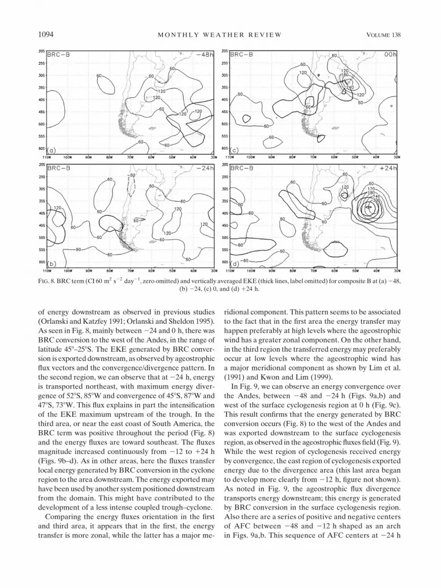
of energy downstream as observed in previous studies

(Orlanski and Katzfey 1991; Orlanski and Sheldon 1995).

As seen in Fig. 8, mainly between 224 and 0 h, there was

BRC conversion to the west of the Andes, in the range of

latitude 458–258S. The EKE generated by BRC conver-

sion is exported downstream, as observed by ageostrophic

flux vectors and the convergence/divergence pattern. In

the second region, we can observe that at 224 h, energy

is transported northeast, with maximum energy diver-

gence of 528S, 858W and convergence of 458S, 878W and

478S, 738W. This flux explains in part the intensification

of the EKE maximum upstream of the trough. In the

third area, or near the east coast of South America, the

BRC term was positive throughout the period (Fig. 8)

and the energy fluxes are toward southeast. The fluxes

magnitude increased continuously from 212 to 124 h

(Figs. 9b–d). As in other areas, here the fluxes transfer

local energy generated by BRC conversion in the cyclone

region to the area downstream. The energy exported may

have been used by another system positioned downstream

from the domain. This might have contributed to the

development of a less intense coupled trough–cyclone.

Comparing the energy fluxes orientation in the first

and third area, it appears that in the first, the energy

transfer is more zonal, while the latter has a major me-

ridional component. This pattern seems to be associated

to the fact that in the first area the energy transfer may

happen preferably at high levels where the ageostrophic

wind has a greater zonal component. On the other hand,

in the third region the transferred energy may preferably

occur at low levels where the ageostrophic wind has

a major meridional component as shown by Lim et al.

(1991) and Kwon and Lim (1999).

In Fig. 9, we can observe an energy convergence over

the Andes, between 248 and 224 h (Figs. 9a,b) and

west of the surface cyclogenesis region at 0 h (Fig. 9c).

This result confirms that the energy generated by BRC

conversion occurs (Fig. 8) to the west of the Andes and

was exported downstream to the surface cyclogenesis

region, as observed in the ageostrophic fluxes field (Fig. 9).

While the west region of cyclogenesis received energy

by convergence, the east region of cyclogenesis exported

energy due to the divergence area (this last area began

to develop more clearly from 212 h, figure not shown).

As noted in Fig. 9, the ageostrophic flux divergence

transports energy downstream; this energy is generated

by BRC conversion in the surface cyclogenesis region.

Also there are a series of positive and negative centers

of AFC between 248 and 212 h shaped as an arch

in Figs. 9a,b. This sequence of AFC centers at 224 h

FIG. 8. BRC term (CI 60 m2 s22 day21, zero omitted) and vertically averaged EKE (thick lines, label omitted) for composite B at (a) 248,

(b) 224, (c) 0, and (d) 124 h.


(Fig. 9b) begins with a divergence at 428S, 1058W and

ends also in divergence at 458S, 508W. This sequence

suggests that there is a transport of energy from the

Pacific (at 428S, 1058W) to the surface cyclogenesis

region. It is also interesting to note that the DSBD mech-

anism proposed by Orlanski and Sheldon (1995), pre-

viously discussed, may be related to the development of

the EKE center east of the trough. It grows initially by

AFC and then by BRC (baroclinic instability), decaying

later by AFC. The same mechanism seems to occur at

0 h (Fig. 9c) when the EKE center at 378S, 558W grows

by AFC (and lightly by BRC conversion, Fig. 8c) and at

124 h the BRC when conversion is dominant (Fig. 8d).

Thus, there is evidence of the DSBD in composite B and

it must be remembered that the DSBD presents a ‘‘se-

quence of events characterizing type-B cyclogenesis, but

expressed in terms of eddy kinetic energy’’ as noted by

Orlanski and Sheldon (1995, p.613).

Figure 10 presents the BRT, KFC, and RES terms at

0 h. The BRT term had a different role for each EKE

maximum west and east of the trough. Negative values

of BRT in the EKE center to the west of the trough show

that it decays by barotropic stability. On the other hand,

positive values in the eastern energy center indicate that

it grows by barotropic instability. It is important to

emphasize that in the Lackmann et al. (1999) study, the

Reynolds stress was the dominant term during the EKE

increase associated with a jet streak in upper levels and it

was the precursor of a rapidly intensifying cyclone in the

western Atlantic. However, Lackmann et al. (1999) used

a different budget equation, where the Reynolds stress is

included in the BRT term used in our study. In the

western center of trough EKE, the KFC term presents

negative values from the center to the northwest, and

positive values from the center to the east. This shows its

role in moving only the energy center, without influ-

encing the EKE increase or decrease (Orlanski and

Katzfey 1991; Chang 2000). The RES term was generally

negative and has considerable magnitude over South

America and the Atlantic Ocean. Since this term also

includes physical processes that are not explained by

Eq. (2), the negative values indicate that some physical

processes should be included in the equation to reduce

the CKT. In this case, the most important process is the

EKE dissipation by friction, mainly because the RES

had higher values around the region where the surface

cyclone developed and it was at its maximum over the

continent, where the friction is normally greater.

FIG. 9. As in Fig. 8, but for the AFC (CI 60 m2 s22 day21, zero omitted) term and ageostrophic flux vectors (m3 s23).

APRIL 2010 P I V A E T A L . 1095

The evolution of the main conversion terms and the

EKE evolution and its tendencies (OKT and CKT) are

shown in Fig. 11. Only the four conversion terms (BRC,

AFC, KFC, and BRT) are shown because they are the

dominant processes in the EKE budget. The RES term

is averaged in the volume [Eq. (2)] for the area rep-

resented by the dashed line in Fig. 7a, also shown in

Fig. 11. The EKE starts with values above 100 m2 s22 at

248 h, decreases to values close to 80 m2 s22 at 218 h,

and increases at the end of the period with 105 m2 s22 at

124 h (Fig. 11a). The CKT was overestimated by ap-

proximately 20 m2 s22 day21 when compared with OKT.

Despite the CKT not showing negative tendency between

248 and 224 h as with OKT, there is a reduction in its

magnitude. This shows a behavior similar to OKT during

the analyzed period (Fig. 11a). The overestimated values

of CKT are represented by negative RES values, which

remained close to 220 m2 s22 day21 through the pe-

riod. The analysis of the energy conversion terms shows

that the BRC term dominated the entire period, reach-

ing a maximum of 75 m2 s22 day21 at 118 h, while the

other three terms did not exceed 30 m2 s22 day21 in

absolute values (Fig. 11b). The BRT term was the low-

est, it did not reach the values of 210 m2 s22 day21. The

AFC term showed three distinct phases. The former

between 248 and 218 h (Figs. 9a,b and 11b) when this

term was negative showing that the ageostrophic fluxes

were exporting energy out of the region. This energy was

exported south from latitude 508S between longitudes

608 and 408W; and east along longitude 358W between

latitudes 408 and 508S. The second phase of the AFC

occurs between 218 and 112 h (Figs. 9c and 11b) when

the ageostrophic fluxes are being imported energy into

the volume. This energy originated at the upstream re-

gion of the Pacific/Andes (see Fig. 9). The last phase of

the AFC happens in the last 12 h of the period when it

presents negative values, reflecting the downstream

energy propagation that occurs in the eastern boundary

of the volume. As the AFC term did not dominate the

EKE conversion at any time of the period, the de-

velopment of the cyclone was not associated with the

DSBD. But it is necessary to emphasize that the AFC

had a secondary importance in the EKE growth because

it only occurred when the AFC became positive (i.e.,

when the flow stopped exporting energy out of the re-

gion). Another important point is that the cyclone only

began developing when the AFC reached its maximum

at 0 h (Figs. 11a,b). Even with the BRC conversion in-

creasing fairly and dominating the energy conversions

after the cyclone development, it is balanced by the in-

crease of divergent fluxes (AFC negative). This con-

tributes to the initiation of the decay phase as observed

by Orlanski and Katzfey (1991), Lackmann et al. (1999),

Chang (2000), and McLay and Martin (2002). A similar

FIG. 10. As in Fig. 8, but for the (a) BRT (CI 30 m2 s22 day21,

zero omitted), (b) KFC (CI 60 m2 s22 day21, zero omitted), and

(c) RES (CI 60 m2 s22 day21, zero omitted) term at 0 h.


result was obtained by Chen and Bosart (1977) when

they studied the energy of cyclone and anticyclone

composites in North America. These authors found that

after cyclogenesis initiation, the EKE generation in the

region became more important than the energy flux going

away.

b. Composite C

The vertically averaged EKE for composite C (Fig. 12)

shows two major differences in relation to composite B

(Fig. 7). The first one refers to the energy maximum to the

west of the trough on the southeast Pacific. In this case,

FIG. 11. Temporal evolution of volume-averaged EKE budget for composite B: (a) EKE (solid line), OKT (line with closed circle), CKT

(dotted–dashed line), and RES (dotted line) evolution; (b) the evolution of KFC (dotted line), AFC (line with closed circle), BRC (solid

line), and BRT (dotted–dashed line). Units are m2 s22 day21, except for the EKE unit which is m2 s22.


APRIL 2010 P I V A E T A L . 1097

the EKE reached values above 210 m2 s22 (Fig. 12)

while in composite B, the EKE remained less than

180 m2 s22 (Figs. 7a–d). This difference in the magnitude

of energy reflects the different configurations associated

with each composite. In composite C, the trough seemed

more amplified than in composite B and a surface cy-

clone was present over the Pacific Ocean in composite C

(Figs. 3–4). The second main difference refers to the

magnitude of energy of the center located on the east

side of the trough over the cyclogenesis region. It reached

a maximum value of 210 m2 s22 at 124 h in a small area

(Fig. 12d), unlike composite B where the energy reached

a maximum of 240 m2 s22 (Fig. 7d). Despite the fact that

the surface cyclone intensity is higher in composite C, the

trough in upper levels of South America was seen to be

less defined. As the winds were more intense in the upper

levels than in the lower, the highest level of energy was

found at these levels, which explains why the EKE center

is weaker in composite C than in composite B during the

surface cyclogenesis (Figs. 12c,d).

Despite the presence of a surface cyclone over the

southeast Pacific, the BRC conversion in the region was

very weak. The reduced positive conversion area, which

exceeded 60 m2 s22 day21 (Fig. 13), was lower than the

BRC conversion observed in composite B (Fig. 8). This

result is due to the fact that the cyclones in the southeast

Pacific Ocean are already in the mature or decay stage.

But in the surface cyclogenesis region over Uruguay and

southern Brazil, the situation was different, and the

BRC conversion was higher in composite C than in B.

For example, at 0 h the BRC maximum conversion was

360 m2 s22 day21 on the border of Uruguay and south-

ern Brazil (Fig. 13c), while in composite B the maximum

was 240 m2 s22 day21 (Fig. 8c). At 112 h, the maximum

values of BRC conversion in composite B were observed

to be around 420 m2 s22 day21 over the South Atlantic,

however in composite C the BRC conversion was

540 m2 s22 day21 (figure not shown). The difference in

magnitude of the baroclinic conversion is associated

with the intensity of the surface cyclone (stronger SLP

decrease). It can also be associated with higher latent

heat released (stronger meridional equivalent potential

temperature flux) in composite C than in B. However, in

the upper (relative vorticity advection and divergence)

and middle (vertical motion) levels the forcing was not

stronger in composite C when compared to composite B

(Fig. 6).

The ageostrophic fluxes as well as the convergence/

divergence patterns became more intense in composite

C than in B (Figs. 9 and 14). In this case, three areas

of intense fluxes were also observed as in composite

B, over 1) the Pacific–Andes between 308 and 408S, 2) the



southeast Pacific, and 3) the Uruguay and South Atlantic.

The main difference between both composites is the

presence of cyclonic circulation in composite C cen-

tered at approximately 608S, 858W at 224 h (Fig. 14b),

which propagates slowly east. This circulation exported

energy out of the region to the south of South America

and the Malvinas Islands, and distributed it south and

southwest toward the southeast Pacific and west of the

Antarctic Peninsula. In composite B, the flow in the area

of the Pacific–Andes generated positive AFC over the

Andes from 248 to 224 h, and over the cyclogenesis

region at 0 h (Fig. 9). Meanwhile in composite C, the

positive AFC area is located 108 farther west than in

composite B, centered over the Andes only at 224 h

(Fig. 14b). In the cyclogenesis region, the flow from the

Pacific–Andes did not show a positive AFC region at

any time (i.e., the increase of the EKE in the cyclogen-

esis region did not occur by energy flux from the wave

located upstream on the Pacific–Andes). Above the cy-

clogenesis region, negative AFC values formed ac-

companying the cyclone in its southeast displacement

(Figs. 14c,d). This divergence was also observed in com-

posite B, but with lower intensity (Figs. 9c,d). The di-

vergence at the beginning of cyclogenesis reached values

of 2420 m2 s22 day21 (Fig. 14c) while in composite B

the maximum magnitude was of 2240 m2 s22 day21

(Fig. 9c). The negative AFC increased up to the end of

the studied period, reaching 2540 m2 s22 day21 around

37.58S, 408W at 124 h (Fig. 14d). Meanwhile, in com-

posite B, the negative AFC near the cyclone reached the

maximum of 2360 m2 s22 day21 at 112 h (figure not

shown), decreasing later. The negative AFC values in

the region between southern South America and around

the Malvinas Islands were due to the cyclonic circula-

tion (recirculation) centered at 608S, 858W commented

on earlier. This recirculation has been observed in

previous studies (Orlanski and Katzfey 1991; Orlanski

and Sheldon 1995). And, as Decker and Martin (2005)

mentioned, it can be associated to the lifetime increase

of the EKE maximum because the recirculation delays

the decay that would occur through divergence of the

ageostrophic geopotential flux.

The BRT term was negative in most of the domain,

similar to composite B, but the Antarctic Peninsula

showed elevated negative values (Fig. 15). The negative

values of BRT probably can be interpreted as Rossby

wave radiation forced by Antarctic topography, however,

further studies are necessary to confirm this interpretation


APRIL 2010 P I V A E T A L . 1099

because in composite B the BRT conversion was weak in

this area. As in composite B, the EKE center in the cy-

clogenesis region gains energy from the mean flow

through the BRT positive term, but the mean flow also

takes eddy kinetic energy by BRT conversion in the

northern portion of the EKE center over the cyclogen-

esis region between 112 and 124 h (figure not shown).

The KFC term shows the northward displacement of the

energy center west of the trough and the eastward dis-

placement of the energy center on the east side of the

trough over South America (Fig. 15b). As for composite

B, the RES term was generally negative, but there are

high positive values in the Antarctica region (Fig. 15c).

The volume-averaged EKE (Fig. 16) shows that the

EKE decreased slightly during the first 24 h (from 248

to 224 h), reaching a minimum of 80 m2 s22 at 224 h.

After that, a linear growth phase began up the end of the

period (Fig. 16a). As in composite B, the OKT was lower




than CKT as indicated by the RES term (around of

230 m2 s22 day21), but both terms show a similar be-

havior with time. We cannot determine which mechanism

explains the initial phase with negative OKT because

CKT remained positive throughout the period. In this

period, the dominant conversion term was the BRC as

was observed in composite B (Figs. 11b and 16b). Its

values remained under 60 m2 s22 day21 until 6 h before

the formation of the cyclone (26 h), when a rapid growth

phase began, reaching around 100 m2 s22 day21 at the

end of the period (124 h). The BRT term remained

smaller (in absolute values) than 10 m2 s22 day21, and

did not play an important role in the development/decay

of EKE. The convergence terms (KFC and AFC) showed

negative values during most of the period. The KFC term

presented positive values during 18 h (between 224 and

26 h), but with a magnitude lower than 10 m2 s22 day21.

The AFC was always negative, exporting energy out

of the volume from the south (508S) and east (358W)

boundaries at different periods (Fig. 14). Before the

cyclone formation, the energy was exported upstream

from the southern boundary of the volume as discussed

previously when the recirculation in the ageostrophic

fluxes and AFC were analyzed (Figs. 14a,b). After the

formation of the cyclone, the energy is exported down-

stream to southeast through the east boundary as ob-

served near 358S, 408W (Figs. 14c,d). Unlike composite

B, AFC did not appear to play an important role in the

volume-averaged energetics.

5. Conclusions

For five winter periods from 1999 to 2003, we analyzed

all cases in which a 500-hPa trough crossed South

America and triggered surface cyclogenesis in Uruguay

or the adjacent areas. A total of 38 cases were divided

into two composites named composite B (with 25 cases)

and composite C (with 13 cases).

A comparative study of the two composites showed

that the trough over the South Pacific Ocean was less

intense in composite B than in composite C, but became

more intense after crossing the Andes. The midtropo-

sphere trough identified in both composites showed that

the trough was less (more) intense on the South Pacific

Ocean (crossing the Andes) in composite B (C) before

(during) surface cyclogenesis phase. From the variables

analyzed in the lower, middle, and upper troposphere,

only the meridional equivalent potential temperature

flux showed differences, its magnitude being higher in

composite C than in B. The results also show that the

meridional heat and moisture fluxes in lower levels had

a crucial role in surface cyclogenesis. As previous studies

have shown, this meridional flow serves as precondi-

tioning to the formation of the cyclone (i.e., its effect

occurs in the phase prior to the onset of the cyclogene-

sis). The analysis of composites B and C shows that the

heat and moisture flow was intense at 48 h prior to cy-

clogenesis, attaining the maximum at 12 h before it.

Although the flow was important for both composites, it

was more intense in composite C. This shows the role of

mountains in blocking the propagation of cold air from

the South Pacific Ocean, and allowing the intensification

of the warm air advection on the lee side of the Andes, as

observed in the formation of the lee cyclogenesis in the

Alps by Radinovic (1986).

The baroclinic conversion was higher in composite

C than in B, reflecting the more intense surface cyclo-

genesis in composite C, despite the higher kinetic energy

in composite B. This contradiction appears because ki-

netic energy was higher at upper levels where the winds

are more intense in composite B. The ageostrophic en-

ergy flux, responsible for downstream development, was

more intense in composite C. This flux is important in

energy export and import upstream and downstream of

the cyclogenesis region, respectively.

The conversion terms averaged in the volume showed

that there are some differences in the energetics of the

two composites. The baroclinic conversion was dominant

in the two composites, but more intense in composite C.

In composite B, the AFC contributed positively to the

intensification of the surface cyclone because it imported

energy into the domain before the beginning of the cy-

clogenesis. On the other hand, in composite C the AFC

served as a sink because it exported energy out of the

domain.

Based on these results, it is possible to conclude that for

both composites 1) the trough was crucial for the cyclo-

genesis; 2) the variables in lower, middle, and upper levels

did not differ from one composite to another; 3) the

northerly heat and moisture flow acted as a precondi-

tioning for the cyclogenesis, mainly for composite-C;

4) the baroclinic conversion dominated the energetics;

and 5) the ageostrophic flux convergence had a second-

ary role. It contributed negatively to the development of

the cyclone in composite C and positively to the initial

development of the cyclone in composite B.

The surface cyclones in composites B and C seem to

develop in the middle and in the upstream edge of the

wavepackets, respectively. This conjecture was based on

the Decker and Martin (2005) study, which analyzed two

cyclogenesis events. During the first one, the associated

EKE center developed before the surface cyclone, the

AFC term was negative, and the cyclogenesis happened

upstream from the wave packet. During the second cy-

clogenesis event, the associated EKE center developed

together with the surface cyclone, the AFC term was

APRIL 2010 P I V A E T A L . 1101

near zero, and the cyclogenesis happened in the midst of

the wave packet. Here, in the composite C, the associated

EKE center developed 24 h before the surface cyclone

and the AFC term was negative. In the composite B, the

associated EKE center developed 12 h before the surface

cyclone and the AFC term was positive. Thus, it seems

that composite C is more dispersive than composite B and

the surface cyclogenesis seems to happen in a different

position in relation to the wave packet.

Acknowledgments. This paper is part of the Ph.D.

thesis of the first author. Thanks are due to the Conselho

Nacional de Desenvolvimento Cientıfico e Tecnologico

(CNPq, Project 381246/2007-8) and Coordenacxao de

Aperfeicxoamento de Pessoal de Nıvel Superior (CAPES)

for the first author’s Ph.D. scholarship. The authors also

thank Dr. E. J. M. Chang for his help.

REFERENCES

Berbery, E. H., and C. S. Vera, 1996: Characteristics of the Southern

Hemisphere winter winter storm tracks with filtered and un-

filtered data. J. Atmos. Sci., 53, 468–481.

Buzzi, A., and S. Tibaldi, 1978: Cyclogenesis in the lee of the Alps:

A case study. Quart. J. Roy. Meteor. Soc., 104, 271–287.

Chang, E. K. M., 2000: Wave packets and life cycles of troughs

in the upper troposphere: Examples from the Southern

Hemisphere summer season of 1984/85. Mon. Wea. Rev., 128,

25–50.

Chen, T.-J., and L. F. Bosart, 1977: Quasi-Lagrangian kinetic energy

budget of composite–cyclone–anticyclone couplets. J. Atmos.

Sci., 34, 452–464.

Danielson, R. E., J. R. Gyakum, and D. N. Straub, 2006a: A case

study of downstream baroclinic development over the North

Pacific Ocean. Part I: Dynamical impacts. Mon. Wea. Rev., 134,

1534–1548.

——, ——, and ——, 2006b: A case study of downstream baroclinic

development over the North Pacific Ocean. Part II: Diagnoses

of eddy energy and wave activity. Mon. Wea. Rev., 134, 1549–

1567.

Dare, P. M., and P. J. Smith, 1984: A comparison of observed and

model energy balance for an extratropical cyclone system.

Mon. Wea. Rev., 112, 1289–1308.

Dean, D. B., and L. F. Bosart, 1996: Northern Hemisphere 500-hPa

trough merger and fracture: A climatology and case study.

Mon. Wea. Rev., 124, 2644–2671.

Decker, S. G., and J. E. Martin, 2005: A local energetics analysis of

the life cycle differences between consecutive, explosively deep-

ening, continental cyclones. Mon. Wea. Rev., 133, 295–316.

Eddy, A., 1965: Kinetic energy production in a mid-latitude storm.

J. Appl. Meteor., 4, 569–575.

Fuenzalida, H. A., R. Sanchez, and R. Garreaud, 2005: A clima-

tology of cutoff lows in the Southern Hemisphere. J. Geophys.

Res., 110, D18101, doi:10.1029/2005JD005934.

Funatsu, B. M., M. A. Gan, and E. Caetano Neto, 2004: A case

study of orographic cyclogenesis over South America. At-

mosfera, 17, 91–113.

Gan, M. A., and V. B. Rao, 1991: Surface cyclogenesis over South

America. Mon. Wea. Rev., 119, 1293–1302.

——, and ——, 1994: The influence of the Andes Cordillera on

transient disturbances. Mon. Wea. Rev., 122, 1142–1157.

——, and ——, 1996: Case studies of cyclogenesis over South

America. Meteor. Appl., 3, 359–369.

Hodges, K. I., B. J. Hoskins, J. Boyle, and C. Thorncroft, 2003: A

comparison of recent reanalysis datasets using objective fea-

ture tracking: Storm tracks and tropical easterly waves. Mon.

Wea. Rev., 131, 2012–2037.

Holton, J. R., 1992: An Introduction to Dynamic Meteorology.

International Geophysics Series, Vol. 48, Academic Press,

350 pp.

Innocentini, V., and E. Caetano Neto, 1996: A case study of the

9 August 1988 South Atlantic storm: Numerical simulations of

the wave activity. Wea. Forecasting, 11, 78–88.

Kalnay, E., and Coauthors, 1996: The NCEP/NCAR 40-Year

Reanalysis Project. Bull. Amer. Meteor. Soc., 77, 437–471.

Keable, M., I. Simmonds, and K. Keay, 2002: Distribution and

temporal variability of 500-hPa cyclone characteristics in the

Southern Hemisphere. Int. J. Climatol., 22, 131–150.

Kung, E. C., 1977: Energy sources in middle-latitude synoptic-scale

disturbances. J. Atmos. Sci., 34, 1352–1365.

Kwon, H. J., and G. H. Lim, 1999: Reexamination of the structure

of the ageostrophic wind in baroclinic waves. J. Atmos. Sci., 56,

2513–2521.

Lackmann, G. M., D. Keyser, and L. F. Bosart, 1999: Energetics of

an intensifying jet streak during the Experiment on Rapidly

Intensifying Cyclones over the Atlantic (ERICA). Mon. Wea.

Rev., 127, 2777–2795.

Lefevre, R. J., and J. W. Nielsen-Gammon, 1995: An objective

climatology of mobile troughs in the Northern Hemisphere.

Tellus, 47A, 638–655.

Lim, E. P., 2005: Global changes in synoptic activity with increasing

CO2. Ph.D. thesis, The University of Melbourne, Victoria,

Australia, 381 pp.

——, and I. Simmonds, 2007: Southern Hemisphere winter extra-

tropical cyclone characteristics and vertical organization ob-

served with the ERA-40 data in 1979–2001. J. Climate, 20,

2675–2690.

Lim, G. H., J. R. Holton, and J. M. Wallace, 1991: The structure of

the ageostrophic wind field in baroclinic waves. J. Atmos. Sci.,

48, 1733–1745.

Marengo, J., A. Cornejo, P. Satyamurty, and C. Nobre, 1997: Cold

surges in tropical and extratropical South America: The strong

event in June 1994. Mon. Wea. Rev., 125, 2759–2786.

Marques, C. A. F., A. Rocha, J. Corte-Real, J. M. Castanheira,

J. Ferreira, and P. Melo-Goncxalves, 2009: Global atmospheric

energetics from NCEP-Reanalysis 2 and ECMWF-ERA-40

Reanalysis. Int. J. Climatol., 29, 159–174, doi:10.1002/joc.1704.

Masters, S. E., and E. C. Kung, 1986: An energetics analysis of

cyclonic development in the Asian winter monsoon. J. Meteor.

Soc. Japan, 64, 35–51.

McGinley, J. A., 1982: A diagnosis of Alpine lee cyclogenesis. Mon.

Wea. Rev., 110, 1271–1287.

McLay, J. G., and J. E. Martin, 2002: Surface cyclolysis in the

North Pacific Ocean. Part III: Composite local energetics of

tropospheric-deep cyclone decay associated with rapid sur-

face cyclolysis. Mon. Wea. Rev., 130, 2507–2529.

Mendes, D., E. P. Souza, I. F. Trigo, and P. M. A. Miranda, 2007:

On precursors of South American Cyclogenesis. Tellus, 59A,

114–121.

Nielsen-Gammon, J. W., 1995: Dynamical conceptual models of

upper-level mobile trough formation: Comparison and appli-

cation. Tellus, 47A, 705–721.


Orlanski, I., and J. Katzfey, 1991: The life cycle of cyclone wave in

the Southern Hemisphere. Part I: Eddy energy budget. J. At-

mos. Sci., 48, 1972–1998.

——, and J. P. Sheldon, 1993: A case of downstream baroclinic

development over western North America. Mon. Wea. Rev.,

121, 2929–2950.

——, and ——, 1995: Stages in the energetics of baroclinic systems.

Tellus, 47A, 605–628.

Petterssen, S., and S. J. Smebye, 1971: On the development of ex-

tratropical cyclones. Quart. J. Roy. Meteor. Soc., 97, 457–482.

Piva, E. D., M. A. Gan, and V. B. Rao, 2008a: An objective study of

500-hPa moving troughs in the Southern Hemisphere. Mon.

Wea. Rev., 136, 2186–2200.

——, M. C. L. Moscati, and M. A. Gan, 2008b: Papel dos fluxos de

calor latente e sensıvel em superfıcie associado a um caso

de ciclogenese na costa leste da America do Sul (Role of

surface latent and sensible heat fluxes associated to a South

America east coast cyclogenesis case). Brazilian J. Meteor.,

23, 450–476.

Plant, R. S., G. C. Craig, and S. L. Gray, 2003: On the threefold

classification of extratropical cyclogenesis. Quart. J. Roy. Me-

teor. Soc., 129, 2989–3012.

Radinovic, D., 1986: On the development of orographic cyclones.

Quart. J. Roy. Meteor. Soc., 112, 927–951.

Randel, W. J., and J. L. Stanford, 1985a: An observational study of

medium-scale wave dynamics in the Southern Hemisphere

summer. Part I: Wave structure and energetics. J. Atmos. Sci.,

42, 1172–1188.

——, and ——, 1985b: An observational study of medium-scale

wave dynamics in the Southern Hemisphere summer. Part II:

Stationary-transient wave interference. J. Atmos. Sci., 42,

1189–1197.

Rao, V. B., A. M. C. do Carmo, and S. H. Franchito, 2002: Seasonal

variations in the Southern Hemisphere storm tracks and as-

sociated wave propagation. J. Atmos. Sci., 59, 1029–1040.

Sanders, F., 1986: Explosive cyclogenesis in the west-central North

Atlantic Ocean, 1981–1984. Part I: Composite structure and

mean behavior. Mon. Wea. Rev., 114, 1781–1794.

——, 1988: Life history of mobile troughs in the upper westerlies.

Mon. Wea. Rev., 116, 2759–2786.

Seluchi, M. E., 1995: Diagnostico y pronostico de situaciones si-

nopticas conducentes a ciclogenesis sobre el este de Sudamerica

(Diagnostic and prognostic of the synoptic situations tigger-

ing to cyclogenesis on the South America). Geophys. Int., 34,

171–186.

——, and A. C. Saulo, 1998: Possible mechanisms yielding an ex-

plosive coastal cyclogenesis over South America: Experiment

using a limited area model. Aust. Meteor. Mag., 47, 309–320.

Simmonds, I., and K. Keay, 2000: Mean Southern Hemisphere

extratropical cyclone behavior in the 40-Yr NCEP–NCAR

reanalysis. J. Climate, 13, 873–885.

——, and E.-P. Lim, 2009: Biases in the calculation of Southern

Hemisphere mean baroclinic eddy growth rate. Geophys. Res.

Lett., 36, L01707, doi:10.1029/2008GL036320.

Sinclair, M. R., 1994: An objective cyclone climatology for the

Southern Hemisphere. Mon. Wea. Rev., 122, 2239–2256.

——, 1995: A climatology of cyclogenesis for the Southern Hemi-

sphere. Mon. Wea. Rev., 123, 1601–1619.

Smith, P. J., 1973: The kinetic energy budget over North America

during a period of major cyclone development. Tellus, 25,

411–423.

——, 1980: The energetics of extratropical cyclones. Rev. Geophys.

Space Phys., 18, 378–386.

Vera, C. S., P. K. Vigliarolo, and E. H. Berbery, 2002: Cold season

synoptic-scale waves over subtropical South America. Mon.

Wea. Rev., 130, 684–699.

Wang, X. L., V. R. Swail, and F. W. Zwiers, 2006: Climatology and

changes of extratropical cyclone activity: Comparison of

ERA-40 with NCEP–NCAR reanalysis for 1958–2001. J. Cli-

mate, 19, 3145–3166.

APRIL 2010 P I V A E T A L . 1103

Documents

Energetics of Winter Troughs Entering South America