Embed Size (px)
Citation preview

The end of 200 unrepeatable yearsCarles Riba Romeva
Energy resources and crisis


The end of 200 unrepeatable yearsCarles Riba Romeva
Energy resources and crisis
Translation: Maria Martínez Odriozola

First edition: July 2011Second edition: September 2011Traslation: April 2012
© Carles Riba Romeva, 2011
© Iniciativa Digital Politècnica, 2011Oficina de Publicacions Acadèmiques Digitals de la UPCJordi Girona Salgado 31, Edifici Torre Girona, D-203, 08034 BarcelonaTel.: 934 015 885 Fax: 934 054 101
www.upc.edu/idpE-mail: [email protected]
Cobert dessign: Ernest Castelltort

Carles Riba Romeva, Energy resources and crisis. The end of 200 unrepeatable years, 2012 5
Acknowledgements
This text is the result of my increasing interest towards the issues of energy and envi-ronment in relation to which I have been stimulated by many people in many ambits.
One of them is the university/company collaboration ambit by means of the Centre de Disseny d’Equips Industrials from the Universitat Politècnica de Catalunya (CDEI-UPC) where I have been accompanied by the collaborators and, specially, by Carles Domènech, Sònia Llorens, Huáscar Paz, Elena Blanco, Andreu Presas and Sònia Mestre, to which I am very grateful. The innovation projects that have been carried out with companies, such as Girbau, Ros Roca, Lloveras, Industrias Puigjaner, Comexi, Matachana, Reverté or Automat, together with the Center’s new strategic positioning have supplied me with many reflection elements when writing this text.
I have also been stimulated by the interest of many teachers and students from the Escola Tècnica Superior d’Enginyeria Industrial de Barcelona (ETSEIB), from which I am a teacher, as well as doctorate students and assistants to the professional Master in Mechanical Engineering and Industrial Equipment. I would like to specially mention the Institute of Sustainability of UPC and its responsible team, who have taken in this publication and the diffusion of this project.
Another ambit that has helped me in my reflection process has been the world of the local studies to which I am bonded through the Centre d’Estudis Comarcals del Baix Llobregat (CECBLL) and the Coordinadora de Centres d’Estudi de Parla Catalana (CCEPC), from which I am the president and the vicepresident, correspondingly. They are an ambit of direct perception of the reality where people work with hope, generosity and sensibility, and where very intense human relationships are developed.
I am also grateful to many people who, being familiar with my work, have given me valuable remarks, have made me reach to information or have asked me to participate in interventions and conferences. Even at the risk of forgetting some people, I would like to mention: José Luís Atienza Ferrero, Rafael Boronat, Jaume Bosch Mestres, Marta Bosch, Roser Busquets, Miquel Serarols, Daniel Clos, Judit Coll, Joaquim Co-rominas, Felip Fenollosa, Rosendo Fernández, Dídac Ferrer, Narcís Figueras, Josep Fontana, Gabriel Garcia Acosta, Pere Girbau Bover, Joan Ramon Gomà, Esther Ha-chuel, Eusebi Jarauta, Maria del Carme Jiménez, Joan Ramon Laporte, Jordi Martínez Miralles, Heriberto Maury, Josep Lluís Moner, Belén Pascual, Miquel Peiró, Agustí Pé-rez, Ramon Plandiura, Lourdes Plans, Reies Presas, Ricard Presas, Josep Puig Boix, Marta Pujadas, Carme Renom, Pau Riba, Valeriano Ruiz, Josep Santesmases, Miquel Sararols, Jaume Seda, Jaume Serrasolses, Jordi Sicart, Toni Sudrià, Enric Tello, Car-me Torras, Eva Torrents, Enric Velo, Francesc Viso and Joan Vivancos.
I would like to mention Ramon Sans Rovira in a special way, peer engineer and friend since we were students, with whom I have collaborated many years when he was technical director at Girbau, for his constant following and support during this entire process and for his determined will to start the debate at the companies. Furthermore, I would like to mention Elisa Pulla, who has created a series of magnificent documents to present the book’s contents.
Finally, I wish to express that I would not have been able to carry out all of this work if I hadn’t had my family’s support: from my wife Mercè Renom Pulit, historian with a re-markable sensibility towards social phenomena, who has helped me understand many things about human behavior and from my children, Martina, Nolasc and Joana, who, together with his partner Miquel Ardèvol, are the parents of my first grandson. They have always, since they were young, followed my thoughts and they have supplied me with new elements.

6 Carles Riba Romeva, Energy resources and crisis. The end of 200 unrepeatable years, 2012

Carles Riba Romeva, Energy resources and crisis. The end of 200 unrepeatable years, 2012 7
Index
Part 1 – Primary energy resources
1. Introduction 1.1 Motivation and point of view 1.2 Basic concepts about energy 1.3 Sources of information
1.4 Measurement units 1.5 New energetic accounting
2. Evolution of the worldwide energy consumption 2.1 Energy consumption of primary sources 2.2 Energy consumption by regions
2.3 Population and energy per capita
3. Non renewable energies’ reserves 3.1 Evaluation of the energy reserves 3.2 Analysis of the oil and natural gas reserves 3.3 Analysis of the coal reserves
4. Growth and projection 4.1 Divorce between growth projection and reserves 4.2 Vision from ultimate recovery 4.3 Peak production of fuels
Part 2 – Secondary (or intermediate) energies
5. Commercial fuels 5.1 From primary to secondary energies
5.2 Fuels from oil, gas and coal and their uses 5.3 Oil, strategic resource
6. Electricity 6.1 The electric system 6.2 Production and consumption of electricity
6.3 Characteristics and limitations of the electricity 6.4 New electric technologies
Part 3 – Alternative sources of energy
7. Unconventional fuels 7.1 Origin of fossil fuels
7.2 Increasing difficulty in the obtaining 7.3 Unconventional oils 7.4 Unconventional natural gas
7.5 Fuels obtained by transformation
8. The uncertain nuclear alternative 8.1 From military uses to civil uses 8.2 Evolution of nuclear energy production 8.3 Evaluation of uranium resources 8.4 Consumptions and impacts of nuclear energy
8.5 New nuclear technologies

8 Carles Riba Romeva, Energy resources and crisis. The end of 200 unrepeatable years, 2012
9. New sources of renewable energy 9.1 Natural renewable resources
9.2 Solar energy 9.3 Hydroelectric energy 9.4 Wind energy 9.5 Geothermal energy 9.6 Energy from oceans 9.7 Biofuels
Part 4 – The resources of the Earth
10. The resources of the biosphere 10.1 Agriculture, livestock, fishing and forests 10.2 Ecological footprint and energy
11. The atmosphere and the climate change 11.1 CO2 Emissions 11.2 The carbon cycle
12.3 Carbon, oxygen and life
12. Final reflections 12.1 Summary of the main tendencies 12.2 To change the development paradigm 12.3 The future of Europe: to lead the energy decrease
Bibliography
Main consulted information sources

Carles Riba Romeva, Energy resources and crisis. The end of 200 unrepeatable years, 2012 9
People say that human civilization do as well as they can with the information that they dispose of. I would qualify that they do as well as they can with the knowledge that they have.
For Lluc, my first grandson, who was born recently

10 Carles Riba Romeva, Energy resources and crisis. The end of 200 unrepeatable years, 2012

Carles Riba Romeva, Energy resources and crisis. The end of 200 unrepeatable years, 2012 11
Part 1
Primary energy resources
After introducing the author’s motivation to write this book and making several conceptual remarks, this first part analyzes the recent and galloping evolution of the world’s primary en-ergy consumption. In other words, it deal with the consumption of those natural resources that we can transform into useful energy, for the human race.
Each of the before mentioned resources has its own nature. Firstly, we have fossil fuels (namely, carbon, oil and natural gas), in different natural states (solid, liquid and gas, re-spectively) and with different densities, energy contents and transformation, manipulation and transport forms. There is also another combustible, uranium, which has a non-renewable character and whose exploitation is highly differentiated to that of the previous fuels. Finally, there are numerous (but not so available) sources of renewable energy (hy-draulic, wind, marine, bio-mass and, last but not least, solar power). With a much minor im-portance, we also have access to geothermal energy, which proceeds from the Earth’s core; and to tidal power, which is derived from the gravitational system Earth-Moon.
Therefore, in order to be able to evaluate the consumption and reserves of these resources, as well as to establish projections for the future (which is the objective of three chapters of this part of the book), it becomes necessary to adopt a common measurement standard. In this sense, it is customary to use the potential primary thermal energy as main magnitude. When a source of energy does not experience a thermal transformation (for example, hy-droelectric, wind or photovoltaic energy), then it is measured considering the primary ther-mal energy that would have been needed in order to produce the same effect, in terms of the world average.
This first part, which is based on data obtained from the most important energy agencies, shows the enormous growth of the worldwide energy consumption and evidences that any possible future forecasts contradict the finite character of the Earth’s resources.
In the first chapter, the book’s motivations are introduced together with the points of view that have been adopted by the author. Moreover, a brief display about concepts related to energy is exposed as well as a clarification related to the units and the conversion factors that have been used throughout the book.
Chapter 2 studies the evolution of the worldwide primary energy consumption (or its thermal equivalent) during the last decades. It constitutes a first warning about the volume and ten-dency of this demand.
Chapter 3 analyzes the non-renewable primary energy reserves (well-known oil, natural gas, carbon and uranium resources that can be considered as obtainable).
And, finally, in the last chapter of this section, several consumption evolution and fossil fuel exhaustion dynamic hypothesis are analyzed.

12 Carles Riba Romeva, Energy resources and crisis. The end of 200 unrepeatable years, 2012
1. Introduction
1.1. Motivation and point of view
Motivation
In this introductory chapter, I make my motivation to write this book about energy resources and the crisis in which we are living explicit.
In 2006, I received an invitation from the Universidad del Norte (Barranquilla, Colombia) to lecture a conference about eco-design. It was the first time that I prepared a public disserta-tion with environmental thematic and this obliged me to get my ideas and reflections straight in a text entitled “Principios de ecodiseño. Como proteger nuestro entorno” <http://www.uninorte.edu.co/divisiones/Ingenierias/IDS/secciones.asp?ID=15>.
As I advanced in my reflection, I realized that it would be difficult to go beyond a trivial and standard vision if I didn’t understand our energy system at a higher level. From a scientific point of view, Physics establish that energy cannot be lost, only transformed, but also that in every transformation it is degraded. From a human point of view, we shall evaluate the per-sonal and social levels of satisfaction that are obtained with the use of energy. And; finally, from the point of view of nature and its resources, the Earth’s capacity to sustain the devel-opment in which we have embarked on, is set out. How can all of these aspects be joined?
Subsequently, in January 2010, I wrote an urgent article titled “Recursos energètics i crisi. Canvi de paradigma de desenvolupament” which, at the end, was not published but, any-way, it can be found on the Internet, <http://www.pelcanvi.org/?q=agoradecreixdoc>. Since then, I have carried out several lectures in politic and academic ambits together with social organizations that have made me perceive the public’s sensibility about this matter.
With time, my investigations and reflections took shape until I decided to convert them into the book that you are currently holding. In addition, I have the enormous satisfaction that it has been received by the UPC’s Sustainability Institute.
Point of view
My professional activities (engineering professor at UPC and director of one of its research centres, the CDEI -Industrial Equipment Design Centre-, through which I have collaborated with numerous companies in the development of equipment goods) have leaded me to pro-gressively reflect on several aspects of energy consumption and the environmental impact that is generated by services’ production and provision, as well as the consequences that they have over the climate change.
Nowadays, the most relevant problems (lack of energy, overpopulation and climate change) have become more global, so they should be analyzed together. However, the dominant way of thinking, which is always immediatist and hurried, analyzes them in a partial and iso-lated way. Consequently, with the passing of time, the sensation that many of the official truths are not very consistent, has been invading me.
The previous ascertainment has driven me to establish my own analysis of the situation. I have based it on information coming from recognized sources (EIA-govUSA, IEA-OECD, FAO-NU, IAEA-NU, WEC, amongst others), but introducing two unusual premises:
a) On one hand, I express the reflection for the world as a whole, establishing interrelations between different aspects and considering sufficiently significant time periods. Reflec-tions about partial matters in restricted territorial ambits and in very limited time periods (for example, the last terms, as many economical analysis usually do) often lead to mis-

Carles Riba Romeva, Energy resources and crisis. The end of 200 unrepeatable years, 2012 13
taken conclusions and, usually, do not provide orientations about the attitudes and deci-sions to be taken in the future.
b) Besides, I base my analysis in numeric evaluations of different parameters and tenden-cies and I give priority to physical measures over monetary values. This decision has been taken because, monetary measurements depend on speculations, market condi-tioning factors and on the different states’ and corporations’ political interest which nota-bly distort the reality’s perception.
The project’s first result has been to state that our globalized world’s tendencies contradict the dominant media discourse. Indeed, we are quickly advancing towards the exhaustion of non-renewable energy resources (most of the responsibility still belongs to the developed countries, which currently include China and other emerging powers such as India, Brazil or Russia) having no feasible alternatives in the actual development coordinates. At the same time, we are contributing on a climate change with unknown and unpredictable conse-quences and with no way back at a human race time scale.
Simultaneously, the worldwide population is growing at a very high speed (especially in the poorest countries). This fact, together with the first world’s countries’ voracity, establishes an ecologic footprint that is no longer sustainable. Therefore, the reflection of poor societies following the development guidelines of the richer societies will no longer be a reality for everybody.
The climate change has a more uncertain and distant perception, even though, probably, it will become the main problem in the future. On the contrary, the non-renewable energy re-sources’ decline is very immediate and it will be clearly perceptible this decade (if it is not already the underlying cause of the crisis in which we are installed). This decline will have a very important impact on the most developed societies (the most gluttonous): With an ab-sence of abundant and cheap energy, the actual development model, which is based on continuous “growth”, is no longer possible. For this reason, a progressive “economic” im-poverishment will take place in the richest societies.
Consequently, the first challenge to be faced in many developed countries is the energy de-cline (conclusion which has also been reached by Aleklett in 2007 [Ale-2007]) and, in the poorest countries, the overpopulation (factors which are still in continuous growth), problems which will not find a solution unless there is a change in the development paradigm that takes the fact that the Earth is limited into consideration. If an adequate response to the en-ergy challenge is found, the climate change (which, from the “bad conscience” and selfish-ness of the wealthy societies, has become, nowadays, little more than a media concern) will start to find real solution procedures in the new development coordinates which will neces-sarily have to be adopted.
Moreover, it will be difficult to articulate serious and efficient alternative policies (and posi-tively make headway to the new challenges that are to arrive) if it is not done from the knowledge and comprehension of the big tendencies and consequences of the use of ener-gy, of natural resources and the population’s evolution at a worldwide scale. This is one of the main objectives of this book.
1.2. Basic concepts about energy
The concept of energy is complex. The most generic definition is: “capacity to work, to pro-duce an effect”. This definition is applied, not only on living organisms and people, but also on the natural phenomena and the technical systems, and it includes both quantitative and qualitative aspects. Common language qualifies a person as energetic if he or she is charac-terized by his or her decisiveness, somebody who knows what he wants, even if he/she is minute and physically weak: we are talking about the dimension of quality. Sometimes, we refer to the enormous force of the wind or the sea’s energy: in these cases we are talking about the dimension of quantity.

14 Carles Riba Romeva, Energy resources and crisis. The end of 200 unrepeatable years, 2012
The most classic definition of energy, which is dealt with by physicians, is the: “capacity to carry out work”. This is understood as the effect of displacing the application points of a re-sistive force. This definition is adequate when the result of the transformation is mechanic energy, but it becomes much more indirect when it is applied to other fields in Physics.
In the physical world, transformations between phenomena from different natures (mechani-cal, electromagnetic, thermal, chemical, nuclear, biochemistry, a.s.o.) continuously take place in constant relations, and energy is the parameter that makes it possible to measure the equivalences between them. There are energies that appear in the form of stock, nor-mally as potential energies: chemical linkage energy and energy of the nuclear forces (fuels, fissile materials), gravitational energy (hydraulic dams, etc.). However, other energies show themselves as a flow: amongst them, the energy that is associated to the movement of bod-ies, electricity, heat, air and water currents, and so on.
In the international system (SI), energy is expressed in Joules (J, and its multiples); in day a day life, which is highly linked to electricity, it is preferred to use the technical measurement unit of kilowatt hour (kWh), whilst, in primary energy evaluations, the most frequent unit is the tonne of oil equivalent or tonne of oil equivalent (TPE or TOE). Finally, in particle phys-ics, the electronvolt (eV) is the most common measurement unit.
Different related realities are analyzed when considering energy:
- energy in the sense of sciences related to physics - human energy, physiological and psychological phenomenon - energy that is used by human societies
In this text, we will focus on the third point of view. Previously, though, we will carry out a brief review on the main laws that rule the energy in physic systems.
Energy in sciences and techniques
The laws that rule energy transformations are:
First principle (law of conservation of energy)
This principle establishes that energy may neither be created nor destroyed, it is only trans-formed. In the physical world, phenomena take place in defined proportions and, in any transformation (for example, from electric to mechanic energy, with a small thermal dissipa-tion), the “amounts of energy found before and after the process takes place, sum up the same value.
Einstein generalized the law of conservation of energy and the sum of the energy and the mass by means of his very well-known equation E = m·c2 (c is the speed of light). Transfor-mations between mass and energy are usually found in the nuclear phenomena in which small mass variations imply enormous quantities of energy.
The diversity of physical phenomena and the plurality of associated energy manifestations have favoured the use of a big amount of energy units (they are studied later on in the text).
Second principle (law of degradation of energy)
It establishes that all natural processes tend to states with a higher level of disorder, in which energy disperses and degrades. The physical magnitude that measures disorder is entropy.
Real processes are irreversible and they always go in the direction that is driven by the deg-radation of energy: heat flows from a hot source to a cold one, but not the other way round; liquid water goes down, it never goes up; firewood burns, but combustion gas doesn’t spon-taneously reconstruct the wood, and so on.
In certain circumstances, there are subsystems that increase the order, but always at the expense of other subsystems that acquire an equal or superior level of disorder. For exam-ple, the development of living beings or the functioning of machines are subsystems in which order increases (entropy diminishes); but in order to ensure that organisms don’t die

Carles Riba Romeva, Energy resources and crisis. The end of 200 unrepeatable years, 2012 15
or that machines don’t stop, a continuous flow that suffers degradation will be necessary. This flow, will basically come from, as a last resort, solar radiation.
Note that, the more irreversible the processes are (they find themselves more far away from reversibility), the quicker they are. However, the energy degradation also increases (entropy increases) and; therefore, efficiency decreases. In modern life, “time is gold” (economical), but hurries are also an “energy (and environmental) inefficiency”.
Exergy and quality
Exergy is defined as the maximum amount of energy that, in theoretic reversibility condi-tions, it can be transformed into work when it interacts with its environment, which is as-sumed to be constant. The remaining amount of energy, which does not have any practical use as to what work is referred, is called anergy and is related to entropy.
In the same way that energy always remains constant (first principle), exergy keeps destroy-ing itself throughout any physical process. It is for this reason that sources of energy con-sume themselves (they destroy exergy while they supply work or equivalent energies).
Not all of the different forms of energy have the same capacity to transform themselves into other energies with high efficiency rates. In general, conversions from thermal energy (com-bustion, nuclear, geothermal, solar, and so on) to mechanic or electric energy have low effi-ciencies, whilst the opposite conversions have higher efficiencies, in the same way as con-versions between mechanic and electric energy also do. Energies that have a high conver-sion, normally are also versatile.
Then, we are talking about high quality energies (mechanic and electric energy beyond them) and low quality energies (mainly, thermal energies). In the first ones, almost all of the energy can be converted into exergy, whilst, in the second ones, only a small amount of ex-ergy can be obtained from the total amount of available energy.
The economic and social use of energy
Physics’ laws are invulnerable and, because of this, any transformation is always submitted to them. In the same way, the human use of energy, not only in the personal dimension but also in the economic and social ones, adds considerations and dynamics that re-comment the adoption of specific concepts in these fields.
From an economic and social point of view, four different stages can be distinguished in re-lation to energy and its use: 1. Primary energy; 2. Secondary energy (or intermediate); 3. Energy’s final use; 4. Satisfaction in the use of energy. They are described below.
1. Primary energies
We name all of those natural resources (which have not been transformed or adapted by technical systems) that have a potential capacity to supply useful energy to human beings, as primary energies. They are, amongst others, oil, natural gas, coal, uranium, biomass, hydraulic energy, tidal power (from waves, marine currents, from tides) and, the most abun-dant, solar energy. Without the adequate transformation or adaptation, they may not be di-rectly used [Rui-2006].
In relation to primary energies, we can distinguish between resources and reserves [USGS-1980]:
Resources. They are solid, liquid or gas materials with a natural origin. They are present in the Earth’s crust, in the adequate form, quantity and concentration for the economic ex-traction (or potentially feasible in the future) of a material or a sub-product to be carried out.
Reserves. It is the known quantity of a recoverable and exploitable energy resource with the actual (or from the moment that is being considered) technical and economical condi-tions.
With the technologic evolutions and the modifications in the economic conditions, some re-sources may become exploitable reserves in the future.

16 Carles Riba Romeva, Energy resources and crisis. The end of 200 unrepeatable years, 2012
2. Secondary energies (or intermediate)
They are energy forms that are obtained by transformation or adaption of primary energies, which, in this way, become easily accessible, easy to handle and controllable for their spe-cific application. When they are conveniently transformed into final energy they make it pos-sible to obtain effects to satisfy human necessities. The two basic forms of secondary ener-gies are: commercialized fuels (gasoline, gasoil, kerosene propane and butane) and the electricity that is available in electric connections [Rui-2006].
3. Final use of energy
They are the energy manifestations in the form of effects that satisfy human necessities: mechanical energy in the shape of a traveller or a merchandise’s displacement, or to manu-facture products; thermal energy in the form of heating, or for industrial processes; electro-magnetic radiations in the shape of artificial illumination, screen viewers or long distance transmitters; electric energy transformed to communication or information by means of com-puting; chemical energy to obtain food, substances and materials, and so on. [Rui-2006].
Up to here we can establish the energy efficiency indexes: from the primary energy it is transformed into useful energy in order to satisfy the human needs that we have just de-scribed. From now on, simple quantitative evaluations no longer make sense and qualitative evaluations become relevant.
4. Satisfaction in the use of energy
It is the perceived satisfaction of needs arising from the use of energy, aspect no linked with technical management but with the social use of resources. For example, a private car can have exemplary technical management on energy and environmental issues and provide low social returns, while a fleet of polluting and energy-inefficient buses can have large so-cial returns.
This last step is very important. It is more social and experiential than technical. In the actual context where energy is still abundant, we pay little attention to this step: to evaluate the utility of the energy investment. We can ask ourselves: has this journey been useful? This artificial light, this communication? Has it been addressed to the most adequate user? Could they be obtained in another way? Could they have been avoided? And many more.
In the dominant conception of the economically developed world, talking about the problem with energy directly implies looking for the solutions in how to find new ways to generate more energy, when in the future we can find ourselves with a forced decline due to the ex-haustion of fossil fuels. Precisely, the improvement in the social profitability of the uses of energy may be one of the most efficient orientations in order to solve the resources’ crisis, and, to be more specific, the energy ones.
Schemes of the economical and social stages of energy
An schematic representation of the stages of energy and its use is found below. In the first transformations, the efficiencies and the energy profitability indexes are indicated; in the last stage, the evaluation is, necessarily, qualitative.
People’s mobility
Starting from a primary energy, 100 energy units of crude oil, which is transformed (ap-proximate efficiency of 0,85) into a commercialized intermediate energy, oil combustible, by means of extraction, distillation and transport until it reaches the user.
From this point onwards, a energy converter (a vehicle with an efficiency of a 0,23) will be used in order to transform the petrol’s chemical energy into mechanical energy at the wheel (19,5 energy units from the 100 corresponding to the initial oil). Furthermore, only part of the wheel’s energy actually transports the traveller (70 kg from the total of 1.350 kg) and, after carrying out a series of calculus, only 1,01 from the 100 primary energy units actually reach the traveller.

Carles Riba Romeva, Energy resources and crisis. The end of 200 unrepeatable years, 2012 17
Another (not less important) thing is the personal and social satisfaction which this jour-ney has produced, which may no longer be evaluated in terms of energy.
Sanitary hot water
Starting from solar radiation (primary energy) over a thermal solar collector. As it is a di-rect collection and an autoconsumption system, there is no need of a previous adapta-tion of primary energy in order to create an intermediate energy.
The thermal solar collector itself, generates sanitary hot water at the temperature that it is going to be used and with an efficiency that may be of the order of 0,6 of the incident solar radiation.
Analogously to the previous case, a different thing is the personal and social satisfaction that this sanitary hot water has provoked.
These schemes make it more easy to view the successive energy transformations as well as making it possible to detect where the system can be improved. Further on, they are used to evaluate the use of several electric systems.
To advance in energy’s technical and social efficiency
Since early man until about two centuries, forced by necessity, man had been very careful to optimize the energy obtained. Since the Industrial Revolution, developed societies have dis-posed of increasing amounts of energy (a gift from nature that, since not long ago, has seemed to be unlimited to us). This circumstance has made us forget, in a progressive way, our worries about the energy uses.
Oil that is found underground is not the same as the distilled fuel that we can find in the nearest petrol station to home. Uranium mineral is not the same as the electricity that we have in our home’s plugs. Between these stages, there are processes that increase ener-gy’s availability and/or its quality but that imply high inefficiencies that are not actually seen by the final user.
From the perspective of the future fossil energy decline, it becomes necessary to become conscious of the hidden processes that make it possible for us to dispose of resources at home. This is the path that has been started by the European automobile industry when sig-nalling the process which is known as WTT, well-to-tank. Following the second principle, the law of degradation of energy, part of the primary energy is lost (degraded) so as to favour that another part increases its quality (gasoil, electricity). In general, energy is degraded.
Primary Intermediate Final use Satisfaction 100 85,0 1,01 (qualitative) 0,85 0,23·(70/1350)
oil well adaptation petrol vehicle
person’s
mobility social use ?
Solar radiation Final use Satisfaction 100 60,0 0,60
Solar radiation Thermal solar collector
Hot water Social use ?

18 Carles Riba Romeva, Energy resources and crisis. The end of 200 unrepeatable years, 2012
On the other hand, the fuel that is found in the petrol station is not the same as the transfor-mation into the vehicle’s displacement: a converter (the automobile) intervenes so as to trans-form the fuel into energy at the wheel which will displace the vehicle. Analogously, the electric-ity that is gained from a domestic plug is not the same as the illumination of a lamp or the functioning of a radio. In this stage, energy is transformed into something that is technically useful (a journey, light, sound), but its efficiency as an energy disappears, it exhausts itself.
This new vision is, undoubtedly, an important step forward. Moreover, the energy crisis that is approaching us will oblige us to go beyond this stage, to consider the final use of energy (not for the wheel, but for the traveller) and its social profitability (has the travel been useful?).
1.3. Sources of information
Productions and consumptions
For the productions and the consumptions we have started from the data from the Energy Information Administration, energy agency from the Energy Department of the United States (EIA-govUSA) <http://www.eia.gov/cfapps/ipdbproject/IEDIndex3.cfm>.
The EIA offers series of data from 1980 to 2008 (in February 2011, some data correspond-ing to 2009 were available) from countries found worldwide and from the seven regions in which the planet is divided: North America (with Mexico), South and Central America, Eu-rope, Eurasia (countries that used to belong to the URSS), Middle East (Oriental Mediterra-nean and Persian Gulf), Africa, and Asia and Oceania (which includes the rest of the coun-tries belonging to Asia and Oceania) (figure 1.1).
Figure 1.1 World’s regions as established by the Regions EIA-govUSA and which have been adopted in the present text. These are: North America (with Mexico), South and Central Amer-ica, Europe (with Turkey), Eurasia (countries that used to belong to the URSS), Middle East (Oriental Mediterranean and Persian Gulf), Africa and Asia (remaining) and Oceania. Source: EIA-govUSA
The energies that are analyzed by the EIA-govUSA are, oil (and liquid fuels), natural gas, coal and electricity. Amongst the electric energy, we distinguish between the conventional thermal generation, nuclear generation, hydraulic generation and the generation with new sources of renewable energy, grouped in geothermal, wind, solar, tidal, biomass and waste energies (all of them being commercialized energies).
Africa Asia &Oceania
Middle East
Eurasia Europe
South and C. America
North America

Carles Riba Romeva, Energy resources and crisis. The end of 200 unrepeatable years, 2012 19
The information has been completed with data about the traditional biomass (firewood, charcoal, cultivation residuals, animal residuals) which has been indirectly supplied by the International Energy Agency (AIE/IEA-OECD, <http://www.iea.org/stats/index.asp>). Tradi-tional biomass (which is not considered by the EIA-govUSA because it is not commercial-ized) is the only one with which a 38% of the worldwide population cooks and heats (more than 2.600 millions of people from Africa, from the South-East Asia and from South and Central America), value that the IEA-OECD foresees will increase in the next twenty years.
Even though the fact that the International Energy Agency (IEA-OECD) includes traditional biomass in its energy accounts is a very important step, the fact that it has chosen to group it with renewable fuels and energy of waste (combustible renewables and waste, CR&W) is, from my point of view, an inconvenient that does not make it possible to delimit realities that have opposite signs. Biofuels and the valorisation of waste are technologies of advanced societies that are aimed at the environment, whilst traditional biomass is the subsistence resource from the poorest societies and countries.
In most cases, if we know the countries’ socio-economical realities, we can assign the IEA values in this epigraph to one of the two types of resource (traditional biomass, or biofuels and assessment of residuals). However, in some cases, such as Brazil, with significant val-ues of traditional biomass and an important biofuel production, we may not know which part corresponds to each type.
It is a shame that we do not dispose of a good estimation of traditional biomass (from which more than one third of the world’s population is living from) that is made by an important inter-national agency, especially when the IEA itself, during 1998’s World Energy Outlook edition, included an excellent chapter about biomass that has not been continued (WEO-1998, chap-ter 10, p. 157-171, <http://www.manicore.com/fichiers/world_energy_outlook_1998.pdf>).
Reserves
In relation to the sources of information about non-renewable energy resources’ reserves, I have mainly followed the criteria from the EIA-govUSA.
For the reserves of oil and natural gas, I have used the evaluations that are annually carried out by the Oil and Gas Journal (the last of them refers to year 2007).
For coal, I have used the evaluations of the reserves that are carried out by the World Ener-gy Council, normally, every two years. In the section that is dedicated to reserves (chapter 3), the estimations at the end of year 2007, that are contained in the Survey of Energy Re-sources, Interim Update 2009, are summarized. While the projects are being done, the Sur-vey of Energy Resources 2010 have appeared with estimations at the end of 2008 that have not very significant differences in relation to the previous year’s estimations (except for the case of Germany). This country, after an unexplainable decrease from 66.000 Tg (tera-grams, or millions of tonnes) in its reserves in 1999 to 6.700 Tg in 2002, in this last report (end of 2008) has been attributed again with 40.699 Tg (always of lignite, the coal that has the lowest energy content). As the worldwide count increases from 826.001 to 860.938 Tg, with a difference that almost coincides with the one corresponding to Germany, in the text the data belonging to 2007 have been maintained.
In relation to uranium reserves, the series of evaluations that have been supplied by the In-ternational Atomic Energy Agency (IAEA) have been used as a reference. This agency is an organism that depends on the United Nations and it has a worldwide prestige in its ambit.
Cumulative consumptions
Another aspect that we have considered to be especially relevant in order to evaluate the world’s energy situation is the cumulative consumption of energy resources. This is an indi-cator of the maximum level of consumption that has been achieved by the different countries

20 Carles Riba Romeva, Energy resources and crisis. The end of 200 unrepeatable years, 2012
and regions that are being analyzed, the original reserves (before the consumption begins) and also of the responsibility that each of these countries has on the CO2 emissions that have been accumulated until now.
The Oil and Gas Journal supplies data about the cumulative consumption of oil and natural gas, and the IAEA supplies information about the uranium that has already been consumed.
We have not found any direct sources of information about the cumulative consumptions of coal yet (it is the most important resource as well as the first one to begin its exploitation process. However, we have been able to indirectly evaluate them with the aid of the histori-cal CO2 emission data (by countries, years and origin) that have been supplied by the CDIAC (Carbon Dioxide Information Analysis Centre), American organism that counts with governmental support.
Projections on future consumptions and the decline of reserves
For the future projections about energy’s evolution, we have based ourselves on the last editions (years 2008, 2009 and 2010) of the prospective documents from the International Energy Outlook from the EIA-govUSA (<http://www.eia.doe.gov/oiaf/ieo/>) and the World Energy Outlook from the IEA-OECD (<http://www.worldenergyoutlook.org/>), which repre-sent the most optimistic official visions.
We have also used more critical studies, specially those from the Energy Watch Group (<http:// www.energywatchgroup.org/>), and from members of the ASPO (Association for the Study of Peak Oil&Gas, <http://www.peakoil.net/>). Amongst them, I would like to highlight the contribution of the retired French engineer J. Laherrère (<http://aspofrance.viabloga.com/texts/documents>).
Data about productions and natural resources
From the beginning, it has seemed to us that the energy crisis will finally affect on the most important products: those that are destined to human diet and to the maintenance of the cli-matic conditions that make life possible. Therefore, in the last part of this book, we wanted to carry out an assessment of the biosphere’s natural resources.
The data and statistics that have been supplied by the United Nation’s Food and Alimentation Organization (FAO) by means of their database (<http://www.fao.org/corp/statistics/es/>), es-pecially FAOSTAT, has been of an invaluable utility.
In the evaluation of biomass, the projects that have been carried out by the scientific net of the Scientific Committee on Problems of the Environment (SCOPE; <http://www.icsu-scope.org/>) have been useful. We would like to specially remark documents SCOPE-13 and SCOPE-21.
The work that has been carried out by the Intergovernmental Panel on Climate Change (IPCC, <http://www.ipcc.ch/>) have helped in order to establish carbon cycle schemes.
Data about emissions and the environment
We have obtained the data corresponding to the emissions of CO2 from the EIA-govUSA, be-ing coherent with the fossil combustible consumptions (<http://www.eia.gov/cfapps/ipdbpro ject/IEDIndex3.cfm>). The EIA supplies the information about the emissions’ evolution during the period that is ranged from 1980 to 2009, for different countries and regions, depending on each of the fossil fuels.
This data could also have been obtained from the CDIAC starting at much previous periods (almost since the beginning of the significant use of fossil fuels in each country) up to year 2007. Moreover, the CDIAC also gives information about the amount of CO2 that is emitted during the production of cement (which is much minor than that of fossil fuels). However, as we have previously mentioned, we have only used the data provided by the CDIAC when evaluating the historical consumption of coal.
Finally, the stabilization scenarios of the CO2 emissions which have been provided by the de IPCC have allowed us to establish a reference frame for the consequences of the green-house effect gases’ cumulative emissions.

Carles Riba Romeva, Energy resources and crisis. The end of 200 unrepeatable years, 2012 21
1.4. Measurement units
Documentary databases normally employ different and not coherent measurement units with the different sources of energy (oil, natural gas, coal, nuclear energy, hydraulic energy, renew-able fuels and energies). This fact makes the comparative analysis between productions, con-sumptions and reserves that correspond to each one of them much more difficult.
If the aim is to carry out a general analysis, it is necessary to adopt reference measurement units to express any type of energy and at all levels. This is done to provide an idea of the orders of magnitude and be able to make comparisons.
We need measurement units for two basic different magnitudes: energy and power (energy per unit time or energy flow per unit time). The magnitude of energy is appropriate for meas-uring the energy resources available: in economical terms, it would be equivalent to capital. On the other hand, the magnitude of power is suitable for measuring energy flows, produc-tions, consumptions, exchanges (in general we talk about energy per day or per year): in economical terms, they would be the monetary flows, receipts, payments and transfers.
Therefore, the most adequate energy unit to measure flows (productions, consumptions, ex-changes) is the Watt (W = J/s, one watt is equal to one Joule per second) and its multiples kW (kilowatt = 1.000 W), MW (megawatt = 1.000.000 W), GW (gigawatt = 1.000.000.000 W) and TW (terawatt = 1.000.000.000.000 W), this last one is useful in order to measure the power or the energy flows at a worldwide scale. When we use calories per day (kcal/d), megawatts hour per month (MWh/m) or millions of tonnes of oil equivalent per year (GTOE/a), then, we are talking about powers (or energy flows) which can be expressed as multiples of watts.
In order to measure the cumulative energies (or non-renewable reserves) at a worldwide scale, our preference is to use the terawatt-year (TWa; “a” from latin annus), energy that a source of one TW generates during one year (1 TWa = 0,7532 GTOE, Thousands of millions of tonnes of oil equivalent). It is an enormous value, of the order of the total energy that is generated by the 437 existing nuclear plants during an entire year. It has the advantage that, dividing the reserves in TWa by the consumption in TW, we can directly obtain the number of years of reserves that are left if our consumption rate remains constant.
A table of power orders of magnitude is given below:
Table 1.1. Power Orders of Magnitude
10 We: low consumption light bulb (equivalent to 30 Wt) 100 Wt: endogenous consumption of a sedentary person (approx. 2.065 kcal/d) 1.000 We = 1 kWe: average electric heater (equivalent to about 3.000 Wt) 10.000 We = 10 kWe: 125 to 150 cc motorcycle (13,6 CV) 100.000 We = 100 kWe: 2.000 cc big automobile (136 CV) 1.000.000 We = 1 MWe: medium-big wind turbine (currently, they reach 5 MWe) 1.000.000.000 We = 1 GWe: big power plant (equivalent to approximately 3 GWt) 1.000.000.000.000 Wt = 1 TWt: the worldwide energy consumption is ~18 TWt
Developed by: Carles Riba Romeva
We must distinguish between TWt (thermal terawatt) and TWe (electric terawatt); the first one corresponds to a thermal power and the second one to an electric or a mechanic one. Due to the fact that any transformation from thermal energy to electric or mechanic energy has a very low efficiency (from 20 to 50%), the equivalence relation of 1 TWe = 3 TWt is usually used. This relation is the approximate worldwide average in the generation of elec-tricity by means of thermal processes.
The EIA-govUSA uses the value of 2,90 for thermal plants (which it applies to electric ener-gies that come from hydroelectric, wind and solar sources), variable values for nuclear elec-tricity depending on the country which is being studied (values ranged from 2,95 to 3,31) and a double value (6,16) for geothermal energy (scarcely representative at a worldwide scale).

22 Carles Riba Romeva, Energy resources and crisis. The end of 200 unrepeatable years, 2012
Measurement units’ diversity
One of the greatest difficulties that we have to face when trying to picture the implications of actual worldwide energy consumptions is, beside the great values that are difficult to compare with references to everyday life, the remarkable disparity between the measurement units that have been generated in the different energy sectors, which do not facilitate comparisons.
Oil With time, two different measurement units in the oil sector have been established: the oil bar-rel (b) and the tonne of oil equivalent (TOE). In addition, these two units are not energy units: the barrel is a volume unit which is equivalent to 159 litres; and the tonne is a unit of mass, which is equivalent to 1.000 kg. The different oils that are found in the Earth do have neither the same density nor the same heat of combustion. Therefore, the relations between these units change depending on the location. With the objective to establish a reference, it has been agreed that the equivalence between a TOE and energy is of 1 TOE = 10.000 Mcal = 41,868 GJ. Similarly, a conventional relation has been established between a TOE and a barrel (1 TOE = 6,84 b), which assumes that oil’s density is of 0,9195 Mg/m3. In some parts of the book we used the relationship between barrel and energy that derives from the real world average.
Natural Gas In a similar way, two different volume measurement units are used to measure the energy ca-pacity of natural gas: the cubic meter (m3) and the cubic foot (cf or ft3), and the relation found between them is of 1 m3 = 35,315 cf (EIA). In the case of gases, the relation between volume and energy, as well as not being constant for all of the different natural gas deposits, it has to precise the pressure and temperature at which the measurements have been taken (standard conditions are 1 atmosphere and 20ºC). The conventional relation between natural gas’ energy and volume is of 34,7 GJ/m3. In some parts of this text we have also used the relation between natural gas volume and energy that is obtained from the real worldwide average.
Coal It is usually measured in tonnes (Mg), which are also known as metric tonnes; Americans use the short ton, which is equivalent to 2000 pounds or to 0.9072 metric tonnes (EIA). Different types of coals have very different heats of combustion. For this reason, has been established a conventional relation between coal’s mass and its energy: 1 tonne of coal equivalent (TCE) = 0,7 TOE = 29,308 GJ/Mg. In this case, the real relation between mass and energy has also been used, in many countries studying it for every country, as the differences between loca-tions are highly remarkable. For example, in order to estimate the reserves in coal energy, we have started from data corresponding to each of the different categories of coal’s reserves, in tonnes. These categories are: bituminous, subbituminous and lignite.
Uranium It is normally measured in tonnes of natural uranium, that is to say, an isotopes composition with a 99,3% of U238 uranium (non fissile) and a 0,7% of U235 uranium (fissile). The data that has been published about the real efficiency of a natural tonne of uranium is very scarce and, predictably, it also depends on the type of technology that has been used and on the plant’s management system. In the statistics that are provided by the EIA, the produced thermal en-ergy and the generated electricity are directly supplied, but not in tonnes of consumed natural uranium. For this reason it is not possible to establish a relation between the combustible’s mass and its associated energy. The following relation has been adopted according to a gen-eral convention: 1 tonne of natural uranium 1(tUnat) = 10.000 TOE = 418,68 TJ.
Electricity The previous sections were about the measurement units that were employed when dealing with primary energy resources. On the contrary, in this section, we will deal with measure-ment units of a transformed energy: electricity. The most frequent measurement unit is the electric kilowatt-hour (kWeh, in the domestic ambit as well as in small industries) and some of its multiples: the megawatt hour (MWeh, in big industries), the gigawatt-hour (GWh, in big power plants) and the terawatt hour (TWeh, in the different countries’ energy accounting as well as the worldwide energy count).

Carles Riba Romeva, Energy resources and crisis. The end of 200 unrepeatable years, 2012 23
On one hand, table 1.2 establishes the main equivalences between energy units in different sectors and energy ambits. On the other hand, table 1.3 establishes the equivalence be-tween energy flow measurement units in relation to an average time or energy power.
Table 1.2. Equivalences between different energy measurement units
TWa EJ GTOE Gb Tcf Tm3 MtU PWh Ecal PBTU
TWa 1 31,5360 0,7532 5,4275 32,0481 0,9075 0,0753 8,7600 7,5322 29,8891
EJ 0,0317 1 0,0239 0,1721 1,0162 0,0288 0,0024 0,2778 0,2388 0,9478
GTOE 1,3276 41,8680 1 7,2056 42,5479 1,2048 0,1000 11,6300 10,0000 39,6815
Gb 0,1842 5,8104 0,1388 1 5,9048 0,1672 0,0139 1,6140 1,3878 5,5070
Tcf 0,0312 0,9840 0,0235 0,1691 1 0,0283 0,0024 0,2733 0,2350 0,9326
Tm3 1,1019 34,7504 0,8300 5,9807 35,3148 1 0,0830 9,6529 8,3000 32,9357
MtU 13,2763 418,6800 10,0000 72,0565 425,4793 12,0482 1 116,3000 100,0000 396,8155
PWh 0,1142 3,6000 0,0860 0,6196 3,6585 0,1036 0,0086 1 0,8598 3,4120
Ecal 0,1328 4,1868 0,1000 0,7206 4,2548 0,1205 0,0100 1,1630 1 3,9682
PBTU 0,0335 1,0551 0,0252 0,1816 1,0722 0,0304 0,0025 0,2931 0,2520 1
Prefixes of unit multiples: k (kilo) = 103; M (mega) = 10
6; G (giga) = 10
9; T (tera) = 10
12; P (peta) = 10
15; E (exa) =
1018
. Units: J (joule); Wa (watt·year); TOE (tonne of oil equivalent); tUnat (tonne of natural uranium); cal (calorie); BTU (British Thermal Unity). Conventional equivalences: 1 TOE = 10 Gcal; 1 TCE (tonne of coal equivalent) = 0,7·TOE; 1 tUnat = 10.000 TOE; 1 BTU = 1.055,06 J; 1 cal = 4,1868 J (SI); 1 TOE = 6,84 b (oil barrel); 1 therm = 1 Mcal; 1 kWh = 3,6 MJ. Sources: SI (International System), EIA-govUSA, IEA-OECD, [Rui-2006]; Developed by: Carles Riba Romeva
Table 1.3. Equivalences between different power units (or of average energy flow)
TW EJ/a GTOE/a Mb/d Tcf/a Tm3/a ktU/a PWh/a Ecal/a PBTU/a
TW 1 31,5360 0,7532 14,8698 32,0481 0,9075 0,0753 8,7600 7,5322 29,8891
EJ/a 0,0317 1 0,0239 0,4715 1,0162 0,0288 0,0024 0,2778 0,2388 0,9478
GTOE/a 1,3276 41,8680 1 19,7415 42,5479 1,2048 0,1000 11,6300 10,0000 39,6815
Mb/d 0,0673 2,1208 0,0507 1 2,1553 0,0610 0,0051 0,5891 0,5065 2,0101
Tcf/a 0,0312 0,9840 0,0235 0,4640 1 0,0283 0,0024 0,2733 0,2350 0,9326
Tm3/a 1,1019 34,7504 0,8300 16,3854 35,3148 1 0,0830 9,6529 8,3000 32,9357
ktU/a 13,2763 418,6800 10,0000 197,4150 425,4793 12,0482 1 116,3000 100,0000 396,8155
PWh/a 0,1142 3,6000 0,0860 1,6975 3,6585 0,1036 0,0086 1 0,8598 3,4120
Ecal/a 0,1328 4,1868 0,1000 1,9742 4,2548 0,1205 0,0100 1,1630 1 3,9682
PBTU/a 0,0335 1,0551 0,0252 0,4975 1,0722 0,0304 0,0025 0,2931 0,2520 1
a = year, d = day. Prefixes of unit multiples and conventional equivalences between units Table 1.2. Sources: [Rui-2006], EIA-govUSA, IEA-OECD; Developed by: Carles Riba Romeva.
1.5. New energy accounting
In this section, I would like to emphasize the fact that, in order to be able to be aware of the enormous energy consumption that is taking place in the developed countries, beyond the economic assessment, new energy accounting tools are necessary. These new tools have to consider the nature laws’ limitations and they have to supply us with options in order cor-rect our attitudes and decisions.
Amongst these new tools, we would like to introduce the reader to two of them: 1) energy return on investment (EROI) so as to understand certain limits in the obtaining process and transformation of primary energy, and 2) embodied energy which, during the manufacture and use stages, is an interesting tool that makes it possible to evaluate the efficiency of dif-ferent options in relation to energy.

24 Carles Riba Romeva, Energy resources and crisis. The end of 200 unrepeatable years, 2012
Energy return on investment (EROI)
The EROI is the quotient between the useful energy that an energy resource supplies and the energy spend in the process of it being obtained, adapted and/or transformed. A lower EROI that 1 means that the resource supplies less energy than the one that is being consumed dur-ing its obtaining, adaptation and/or transformation (that is to say, energy is lost).
Therefore, in a context of energy shortage, it only makes sense to exploit those resources whose EROI is clearly greater than 1 (several authors recommend the minimum EROI to be ranged between the values of 3 and 5 so as to make it possible to carry out a viable exploi-tation of the resource).
Table 1.4. Values of EROI supplied by different authors
Year EROI Reference
Non renewable
Oil and gas (discovered)
Coal (at the mine’s exit)
Oil and gas (discovered)
Oil ad gas (production) Coal (at the mine’s exit) Oil and gas Natural gas Oil shale
1940 1950 1970 1970 1970
1984 2005 2005
>100 80 8 23 30
11 ÷ 18 10
5,2 ÷ 5,8
Cleveland et al. 1984 Cleveland et al. 1984 Cleveland et al. 1984 Cleveland et al. 1984 Cleveland et al. 1984, Hall et al. 1986
Cleveland 2005 Button and Sell, 2005
Herweyer i Gupta, 2008
Nuclear (water) 4 Cleveland et al. 1984
Renewable
Hydroelectric Wind
1984 2008
11,2 19,8
Cleveland et al. 1984 Kubiszewski and Cleveland, 2008
Solar collector Concentration collector Photovoltaic Photovoltaic
1984 1984 1984 2009
1,9 1,6
1,7÷10 6,56
Cleveland et al. 1984, Hall et al. 1986 Cleveland et al. 1984, Hall et al. 1986 Cleveland et al. 1984 Kubiszewski and Cleveland 2009
Ethanol (sugar cane) Ethanol (corn) Methanol (wood) Biodiesel
1984 1984 1984
0,8 ÷1,7 1,3 2,6
1 ÷ 3
Cleveland et al. 1984, Hall et al. 1986 Cleveland et al. 1984 Cleveland et al. 1984 Hall, Powers et al.
Geothermal 1984 4 Cleveland et al. 1984
Sources: [Cle-1984], [Cle-2005], [Hal-1986], [Her-2005], [Kub-2008], [Kub-2009]. Developed by: Carles Riba Romeva
This aspect limits the economic view that forecasts that, when prices rise, market reacts and offers more products. In the case of energy resources, this is true when the EROI is clearly greater than 1. If this does not happen, its exploitation will only be feasible if the energy re-source is subsidized (by means of public investment) with other energy resources that have a superior value (this is the case of several biofuels).
This concept explains the fact that many deposits with resources that are still very important have been abandoned. If the energy exploitation cost is greater than (or of the same order as) the efficiency of the resource that is extracted from it, the activity is abandoned. These deposits will only be able to be exploited for some time more if new technologies that require a minor consumption of energy are developed.
This principle has several exceptions when the obtained energy has a higher quality than the initial energy. In this way, the use of more energy than the one that will be used becomes justi-fied. This is the case of the generation of electricity from thermal energy sources, or of the transformation of coal into liquid fuel, which is so highly necessary in transport systems.

Carles Riba Romeva, Energy resources and crisis. The end of 200 unrepeatable years, 2012 25
Embodied energy
Embodied energy is an environmental accounting concept that is measured by means of the commercialized primary energy that has been consumed in all of the stages of a product, a service or a material’s life cycle until the stage that is being considered. For further compre-hension:
- The extraction, transformation and transport of raw materials - The conception and the design of the product or service - The product’s manufacture or the service’s preparation - The product or the service’s commercialization - The use or the application of the product or the provision of a service - The scrapping of the product or service and the withdrawal of the waste materials - The reuse of components, materials’ recycling and energy exploitation
It is a useful concept as an indicator of the environmental efficiency when several equivalent alternatives are being compared in order to obtain the same product or to provision the same service. It also allows us to analyze the energy effects in each of the life cycle’s differ-ent stages.
Table 1.5. Values of the most common materials’ embodied energy
Materials Densities
First obtaining Recycling
Input material in the process
Specific energy
Volumetric energy
Specific energy
Mg/m3 GJ/Mg GJ/m3 GJ/Mg
Meta
ls Iron 7,85 35,3 275,3 9,5 Iron ore
Aluminium 2,70 218,0 590 28,8 Bauxite
Copper 8,94 70,0 625 17,5 to 50 Chalcopyrite
Poly
mers
Polyethylene (LDPE) 0,92 78,1 71,8 Oil
Polyamide 6.6 1,14 138,6 158,0 Oil
Rubber 0,93 101,7 91,5 Latex
Constr
uct Cement 1,50 4,6 6,9 Calcium and clay
Concrete 2,30 0,95 2,2 Cement and others
Glass 2,50 15,0 37,5 Silicon
Sources: values of first obtaining and recycling specific energy: [Ham-2008]; metal and polymer densities: [Rib-2007]; the rest: Internet. Developed by: Carles Riba Romeva
Embodied energy allows us to view the volume of energy that we deal with and to notice that we are usually quite careless as to what adequate energy administration is referred.
Example: the aluminium can
A simple aluminium can used to contain drinks has a mass of about 25 g. If the aluminium is a first obtaining material, the container’s simple material (without taking the manufacturing process into account) has employed an energy investment (embodied energy) of 5,45 MJ.
If this energy is applied to move a bus, with a mass of de 15.000 kg, through a horizontal plane, with a propellant system’s global efficiency of a 20% and an rolling coefficient of a 0,025, it could make the vehicle move forward for approximately 300 meters.
Trying to avoid the loss of invested energy is one of the main reasons to justify materials’ recycling process. If the previous can were recycled, the difference between the first obtain-ing energy (5,45 MJ) and the recycling energy (0,72 MJ) would be preserved. That is, 4,73 MJ would be saved/recovered for every can.

26 Carles Riba Romeva, Energy resources and crisis. The end of 200 unrepeatable years, 2012
Evaluation of the energy consumptions and the greenhouse effect gases’ emissions
The Centre de Disseny d’Equips Industrials de la Universitat Politècnica de Catalunya (CDEI-UPC), which I personally manage, is carrying out studies about embodied energy and the CO2 emissions that are implied in industrial activities and, amongst them, the manufacture of indus-trial equipment goods and analogous products.
The first studies prove that, due to their obsession towards the market sale price, most of the times we are not conscious of neither the consumptions nor the emissions that are im-plied in the use of durable apparatus and goods and in the provision of services.
The evaluations that have been carried out up to the present moment make it possible to es-tablish the following relations: For domestic equipment, if the embodied energy and the emis-sions that are linked to its manufacture are 1, the energy consumption and the posterior emis-sions during its use (and, eventually, its elimination) are comprised between the values of 1 and 10 (for example, in a domestic washing machine or a particular automobile, they are usu-ally of 2,5). Furthermore, in industrial equipment goods, that work at a much more intensive rate, the consumptions and the emissions during their use are much higher than in the domes-tic case and they find themselves between the values of 10 and 100 (in the machines that have been analyzed by the CDEI-UPC values comprised between 30 and 80 have been found).
Considering the energy crisis that is being forecasted (see the evolution of the energy con-sumptions, the available reserves and the provisions; chapters 2, 3 and 4), the price (which only reflects the manufacturing consumptions and emissions) is a poor indicator of energy and environment issues. It becomes necessary to change the concept and to analyze the lifecy-cle’s consumptions and emissions, mainly, of those corresponding to the usage stage, which is the most decisive one.
In this sense, the CDEI-UPC, with the support from the Govern de la Generalitat de Catalu-nya, is developing methods and databases in order to establish energy and environment evaluations during the conceptual design stage of equipment goods, where decisions have a maximum relevance.
In order to obtain good information and, at the same time, to display the maximum amount of innovation potentials, the evaluation is established by considering together the equipment and the operative process during the entire lifecycle, from the stages in which the equipment is originated (definition, design and manufacture) to the destination stages (use, mainte-nance, eventual reconfigurations, end-of-life), and in all of the elements and aspects that act as coadjutants in the process.

Carles Riba Romeva, Energy resources and crisis. The end of 200 unrepeatable years, 2012 27
2. Evolution of the worldwide energy consumption
2.1. Energy consumption of primary sources
In this chapter, the worldwide primary energy consumption’s evolution is studied according to the different primary sources of energy and the different regions in the world. As it can be ob-served, the absolute growth during the period from 1980 to 2008 (period from which the EIA-govUSA offers its data) is very important and it is based, mainly, on fossil fuels.
In order to complete this vision, it is convenient to analyze the primary energy consumption per capita at a worldwide scale and in the world’s different regions. With this objective, we have briefly reviewed the population’s growth in the whole world and in its different regions throughout this same period.
For big ambits (the world, the regions) and long periods (one year or more) the production or consumption of energy may be considered as an average continuous flow. Energy per unit of time is a power that is measured in W (watts) or in any of its multiples.
At a worldwide scale, the production or consumption measurement unit that has been cho-sen is the TW (T = tera = 1012; 1 TW = 1 million of millions of watts). Those energies that are from a different nature have been reduced to equivalent thermal energy (Wt, thermal watts).
A table with the consumptions (thermal energy) of the main sources of primary energy from 1980 to 2008 is shown below. This table has been developed using the data from the EIA-govUSA, and complementing it with the values of the Combustible Renewables and Waste’ (CR&W, mainly, traditional biomass) consumption. These complementary values are obtained from the data that is supplied by the International Energy Agency (IEA-OECD).
Table 2.1. Worldwide primary sources’ energy consumption (TWt)
1980 % 1985 1990 1995 2000 2005 2008 %
Oil 4,383 42,23 4,117 4,570 4,772 5,203 5,686 5,720 32,02
Natural Gas 1,802 17,36 2,120 2,521 2,714 3,043 3,527 3,809 21,32
Coal 2,338 22,53 2,755 2,981 2,940 3,090 4,098 4,572 25,59
Nuclear energy 0,253 2,44 0,512 0,681 0,778 0,858 0,921 0,908 5,08
Non-renewable 8,777 84,56 9,504 10,753 11,204 12,194 14,233 15,009 84,01 1980=100 100,00 108,28 122,51 127,66 138,93 162,16 171,00
Increase by periods 0,727 1,249 0,451 0,990 2,039 0,776
Hydroelectric energy 0,599 5,77 0,682 0,746 0,846 0,894 0,967 1,028 5,76
Other renew. electr. 1 0,016 0,15 0,027 0,056 0,072 0,100 0,145 0,195 1,09
Renewable fuels 2 0,988 9,52 1,109 1,211 1,302 1,393 1,543 1,634 9,14
Renewable 1,602 15,44 1,818 2,014 2,220 2,387 2,655 2,858 15,99 1980=100 100,00 113,47 125,68 138,56 148,96 165,72 178,35
Increase by periods 0,216 0,196 0,206 0,167 0,268 0,203
Total 10,379 100,00 11,322 12,767 13,424 14,581 16,888 17,867 100,00
1980=100 100,00 109,10 123,04 129,40 140,55 162,80 172,23 Increase by periods 0,943 1,445 0,657 1,157 2,307 0,979
1 All of the renewable electric energies, except for hydroelectric energy (wind, photovoltaic, thermosolar, tidal, renewable fuels to generate electricity).
2 Combustible renewables and waste: traditional biomass, biofuels, urban and industrial waste.
Sources: EIA-govUSA: oil, natural gas, coal, nuclear, hydroelectric and non-hydraulic renewable energies; IEA-OECD: renewable fuels and waste. Developed by: Carles Riba Romeva
In order to show the worldwide energy consumption throughout these 28 years, the data cor-responding to table 2.1 has been graphically represented. The graph of figure 2.1 (scale from

28 Carles Riba Romeva, Energy resources and crisis. The end of 200 unrepeatable years, 2012
0 to 18 TWt) shows the global evolution and the distribution between renewable and non-renewable energies. On the other hand, the graph that of figure 2.2 (scale from 0 to 6 TWt) shows the individual evolution of each of different sources of energy.
World consumption of primary energy (TWt)
0,0
2,0
4,0
6,0
8,0
10,0
12,0
14,0
16,0
18,0
1980 1985 1990 1995 2000 2005
Renewables
Non renewables
Total consumption
Figure 2.1. Evolution of the worldwide energy consumption during the period ranged from 1980 to 2008, as well as the distribution between renewable and non-renewable energies. Scale 0-18 TWt. Source: EIA-govUSA, IEA-OECD. Developed by: Carles Riba Romeva
Worldwide consumption of primary energies (TWt)
0,0
1,0
2,0
3,0
4,0
5,0
6,0
1980 1985 1990 1995 2000 2005
Oil
Natural gas
Coal
Nuclear
CR&W
Hydroelectric
Other renew. electr.
Figure 2.2. Evolution of each type of energy’s consumption from 1980 to 2008. Source: EIA-govUSA and IEA-OECD. Developed by: Carles Riba Romeva
Worldwide energy consumption of primary sources (TWt)
Worldwide primary energy consumption (TWt)

Carles Riba Romeva, Energy resources and crisis. The end of 200 unrepeatable years, 2012 29
Table 2.1 and figures 2.1 and 2.2 deserve the following general comments to be stated:
Very important Increase in the consumption of primary energy
1. The consumption of energy around the world keeps increasing. Specifically, a 72,23% during the period from 1980 to 2008, with an absolute global increase of 7,488 TWt.
2. The energy consumption increases are not moderate; they have been intensified during the latest years. After having had absolute increases of 2,387 TWt during the decade from 1980 to 1990 and of 1,814 TWt for the following decade (1990-2000), the last eight years from this period (2000-2008), an increase of 3,285 TWt has been registered, even though during the last three years the crisis is already noticeable.
Most of the increase comes from non renewable energies
3. When analyzing the distribution of the absolute increase (7,488 TWt), the outlook be-comes deceiving from an environmental point of view. The consumption of non renewa-ble sources increases in 6,232 TWt, whilst the increase of fossil fuels is of 5,577 TWt.
4. Furthermore, renewable energies only absorb 1,258 TWt of this increase, being the most important components those that correspond to renewable fuels (0,649 TWt, majorly, traditional biomass and not biofuels) and hydraulic energy (0,429 TWt).
5. The new sources of renewable energy (solar, wind, tidal, geothermal, our only hope!), even though they have multiplied themselves by twelve during the studied period, they have only experimented a modest increase of a 0,179 TWt.
6. The absolute difference between non-renewable and renewable energies does not stop increasing. It goes from 7,184 TWt in 1980 to 13,158 TWt in 2008.
The percentages of renewable/non-renewable energies do not vary
7. The percentage of non-renewable sources of energy almost does not decrease during the 28 years that are being studied in this period: It drops from 84,56% to 84,01%. Oil loses importance (-10,21%) in relation to natural gas (+3,96%) and coal (+3,06%). In general, fossil fuels decrease (from an 82,20% to a 78,96%), percentage which is almost recovered by the fourth non-renewable combustible, uranium (+2,64%). Note that, the last years, non-renewable fuels gain importance whilst uranium decreases in importance.
8. Renewable sources of energy gain a small percentage weight (0,55%, which corresponds to what non-renewable energies lose) but they still represent a scarce 15,96% out from the total. Hydroelectric energy almost maintains itself constant and renewable fuels and waste (mainly traditional biomass) lose a 0,38%, that is compensated for by the new renewable electric sources in a 0,94% which, anyway, only reaches the value of a 1,09% in 2008.
Renewable sources of energy and conventional biomass
9. Even though renewable energies are growing, most of this increase is due to traditional biomass (the only energy that 2600 millions of inhabitants actually dispose of, a 38% of the total humanity, in poorly developed countries from Africa, Asia and Latin America; from which we will talk about further on in the text) and to hydroelectric energy.
10. The new renewable sources of electric energy are still a lost residual. Even though they have had a spectacular relative increase (they have multiplied themselves by 12,5), their incidence in the global energy supply has just exceeded the value of a 1% in 2008 (spe-cifically, a 1,095%) (see the detail in figure 2.3).
New sources of renewable energy
There is a perception in the media that some new sources of energy (especially wind and solar and biofuels) are progressing at a very high speed and that soon they will be able to substitute fossil fuels. But, what is actually true from this point of view?

30 Carles Riba Romeva, Energy resources and crisis. The end of 200 unrepeatable years, 2012
This statement is only partly true. On one hand, it is true that these energies are being de-veloped at very high speeds (in some countries), but it is also true that their importance at a worldwide scale is almost irrelevant in comparison to the increases found in other compo-nents of the energy palette (specially, natural gas and coal).
In order to show this fact, table 2.2 breaks down the evolution of the new renewable electric sources of energy (geothermal, wind power, solar and tidal, or renewable fuels that are used to produce electricity) and also the evolution of the two main biofuels (ethanol and biodiesel, which are included in table 2.1, in the section corresponding to renewable fuels).
Table 2.2. Evolution of renewable sources of energies and biofuels (TWt)
1980 % world 1985 1990 1995 2000 2005 2008 % world
Geothermal 0,0094 0,0913 0,0159 0,0246 0,0259 0,0345 0,0379 0,0412 0,2280
Wind power 0,0000 0,0000 0,0000 0,0012 0,0026 0,0102 0,0333 0,0684 0,3789
Solar and tidal 0,0002 0,0016 0,0002 0,0003 0,0004 0,0004 0,0009 0,0028 0,0154
CR&W 0,0059 0,0569 0,0109 0,0310 0,0430 0,0546 0,0727 0,0829 0,4588
Total oth. ren. elect. 0,0156 0,1498 0,0271 0,0562 0,0719 0,1001 0,1448 0,1953 1,0813
Ethanol – – – – 0,0133 0,0260 0,0540 0,2988
Biodiesel – – – – 0,0010 0,0049 0,0189 0,1047
Total biofuels – – – – 0,0143 0,0309 0,0739 0,4035
Source: EIA-govUSA. Developed by Carles Riba Romeva
And, again, these values are also graphically represented (figure 2.3). Even though both the generation and the consumption have had a spectacular evolution during the last few years, none of the new sources of energy exceeds the value of 0,09 TWt in 2008 (that is to say, 1/200 of the primary energy that is consumed worldwide). Except for biofuels (an almost im-perceptible part of the renewable combustibles and waste which also includes traditional biomass; orange line in figure 2.2), the addition of all of them corresponds to other sources of renewable electric energy (inferior green line in figure 2.2).
Consum mundial de noves energies renovables (TWt)
0,000
0,015
0,030
0,045
0,060
0,075
0,090
1980 1985 1990 1995 2000 2005
Geothermal
Wind
Solar, waves and tindal
CR&W
Bioethanol
Biodiesel
Figure 2.3. Evolution of the consumption of other renewable electric sources of energy from 1980 to 2008 (scale from 0 to 0,09 TWt). Source: EIA-govUSA. Developed by: Carles Riba Romeva
New renewable energy worldwide consumption (TWt)

Carles Riba Romeva, Energy resources and crisis. The end of 200 unrepeatable years, 2012 31
Other renewable electrical sources of energy
The EIA-govUSA supplies data since 1980. The most important renewable generation comes from combustible renewables and waste (0,0829 TWt in 2008) with a sustainable growth. The second most important electric generation comes from wind power, developed more recently but with a very quickly grown (0,0684 TWt in 2008). Geothermal energy has been used for a long time now, but its growth has always been moderate (0,0412 TWt in 2008). Finally, solar energy (which includes photovoltaic energy and thermo solar power plants), together with the energy that is generated by tides and waves, even though it is experimenting a certain pro-gress, it is not perceptible at a worldwide scale (0,0028 TWt in 2008).
Biofuels
The EIA-govUSA supplies data about biofuels since 2000. Bioethanol (which is mainly pro-duced in the United States, Brazil and in certain areas in Asia) is the main biofuel (in 2000 there was already some production of it). The use of bioethanol has grown very quickly (0,0540 TWt in 2008). Biodiesel (which is mainly produced in Europe), was almost nonexist-ent in year 2000 and, even though it has progressed very quickly, it has a much minor global importance (0,0189 TWt in 2008). In the same way, both biofuels become insignificant when compared to the consumption of oil.
False expectations
There are news that induce to false expectations.
Spain and wind power For example, the fact that in Spain “wind power exceeds for the first time the value of nu-clear energy” has been highlighted (La Vanguardia, 2-12-2009). Certainly, Spain is one of the wind power’ worldwide leaders. However, its annual production (not its punctual one in the early morning in a specially windy day), only represented a 13% of the total electric energy produced in 2009 and a 5,5% of the de total consumed energy, whilst the percent-age corresponding to non-renewable fuels is still worth more than an 85%.
China and its leadership in renewable energies Not long after China deactivated the Conference in Copenhaguen about Climate Change together with the United states, it announced that it “planned that one third of its energy shall be renewable in 2050” (El Mundo, 7-12-2009). But, China consumed 0,886 TWt of coal in 2000 (28,5% of the world) and it increased this value until a 1,868 TWt in 2008 (42,58% of the world; an increase of a 110,8% in 8 years). Nevertheless, in 2008, the set of the new renewable energies (mainly thermal solar collectors used to heat water in build-ings, in which China is a worldwide remarkable leader) summed up a total of 0,035 TWt
(less than a 1,5% of their primary energy consumption), but with a tendency to increase.
This does not mean that these objectives are not important in the matter of renewable ener-gies, but or either they are more scarce than what they are insinuating, or they are unattainable or, even, contradictory when compared with other aspects of countries’ energy policies.
Traditional biomass
It is appropriate to carry out a series of considerations about traditional biomass (included in the section named “Combustible renewables and waste”; table 2.1 and figure 2.2) here; spe-cially due to the importance that it has in many countries and in the less favoured populations.
Traditional biomass (wood from the forest, charcoal, crop residuals and animal residuals) is the energy of the poor and, as it doesn’t usually form part of the commercial energy circuits, the big information agencies have margined it (amongst them, the EIA-govUSA).
The first time that it became the object of an official recognition was in the IEA-OECD’s an-nual report from the 1998 edition, World Energy Outlook [WEO-1998], in chapter 10, which was in fact titled «Biomass». The obtained sensation is that the authors become aware of the importance of this source of energy and they treat it in a sincere and delicate way. The beginning of this chapter is as follows:

32 Carles Riba Romeva, Energy resources and crisis. The end of 200 unrepeatable years, 2012
«Biomass energy currently (in 1998) represents approximately 14% of world final energy consumption, a higher share than that of coal (12%) and comparable to those of gas (15%) and electricity (14%). In developing countries, in which three-quarters of the world’s popula-tion live, biomass energy (firewood, charcoal, crop residues and animal wastes) accounts, on average, for one-third of total final energy consumption and for nearly 75% of the energy used in households. For large portions of the rural populations of these countries, and for the poorest sections of urban populations, biomass is often the only available and affordable source of energy for basic needs such as cooking and heating…». Nowadays, traditional biomass has decreased in percentage due to the superior increase in other energy sources. However, in general terms, its consumption has increased.
The WEO also carried out some first numerical evaluations of the traditional biomass in 1995 and a projection towards year 2020, which is reproduced below (IEA-OECD gives its values in MTOE, millions of tonnes of oil equivalent; here we have changed these magnitudes to TWt as it had a greater coherence):
Table 2.3. Evaluation of the traditional biomass (TWt) according to IEA
Countries and regions 1995 Projection 2020
Biomass Convent. Total % biom. Biomass Convent. Total % biom.
China 0,273 1,147 1,421 19,2 0,297 2,789 3,087 9,6 East Asia 0,155 0,616 0,771 20,1 0,181 1,693 1,873 9,6
South Asia 0,324 0,377 0,701 46,2 0,409 1,077 1,486 27,5 Latin America 0,110 0,600 0,710 15,5 0,126 1,309 1,435 8,8 Africa 0,299 0,300 0,599 49,9 0,601 0,574 1,175 51,2
Developing Countries 1,162 3,040 4,202 27,7 1,614 7,441 9,056 17,8
Other no-OECD 0,037 1,924 1,961 1,9 0,040 2,958 2,998 1,3 OECD 0,189 5,749 5,937 3,2 0,228 7,348 7,577 3,0
Worldwide total 1,387 10,713 12,100 11,5 1,883 17,748 19,630 9,6
The original values in MTOE’s have been translated to TWt. Source: World Energy Outlook 1998 [WEO-2008], chapter 10 (IEA-OECD). Developed by: Carles Riba Romeva
The IEA-OECD has incorporated traditional biomass in its accounting but, as it has done it inside the section named as “Combustible Renewables and Waste” (where there are also bio-fuels and industrial and urban waste), it rests importance to this aspect which is so important for an increasing amount of people in the Earth, even though it has progressed a lot.
Posterior analysis from the IEA-OECD [WEO-2006] highlights other aspects of biomass’ use, such as the diseases caused by the inhalation of smoke or the deterioration of forests, and they propose policies to eliminate the use of traditional biomass (non-commercialized).
Figure 2.4 shows the energy profile’s evolution corresponding to three significant countries that includes de traditional biomass consumption.
Nigeria, even though it has important oil and natural gas reserves, which it mainly exports abroad, is a very representative country of the sub-Saharan region. Its almost 160 millions of inhabitants (Germany and France together) subsist basing themselves on traditional bio-mass (almost an 80% of the consumed energy). Specifically, their consumption has in-creased from 27 to 84 MTOE/a during the period 1971-2007 (from 0,037 to 0,111 TWt), with an increase that is almost proportional to the population.
The case of India may seem completely different, but it is not. Traditional biomass, which represents a bit more than a 27% of the energy consumption, is, in absolute terms, of 165 MTOE/a in 2007 (0,219 TWt). And, in Brazil, where it is difficult to differentiate between tradi-tional biomass and the production of biofuels, the total value is of 71 MTOE/a (0,094 TWt).
Maybe an enormous marginalized error is being committed or, maybe, this reality is being hided.
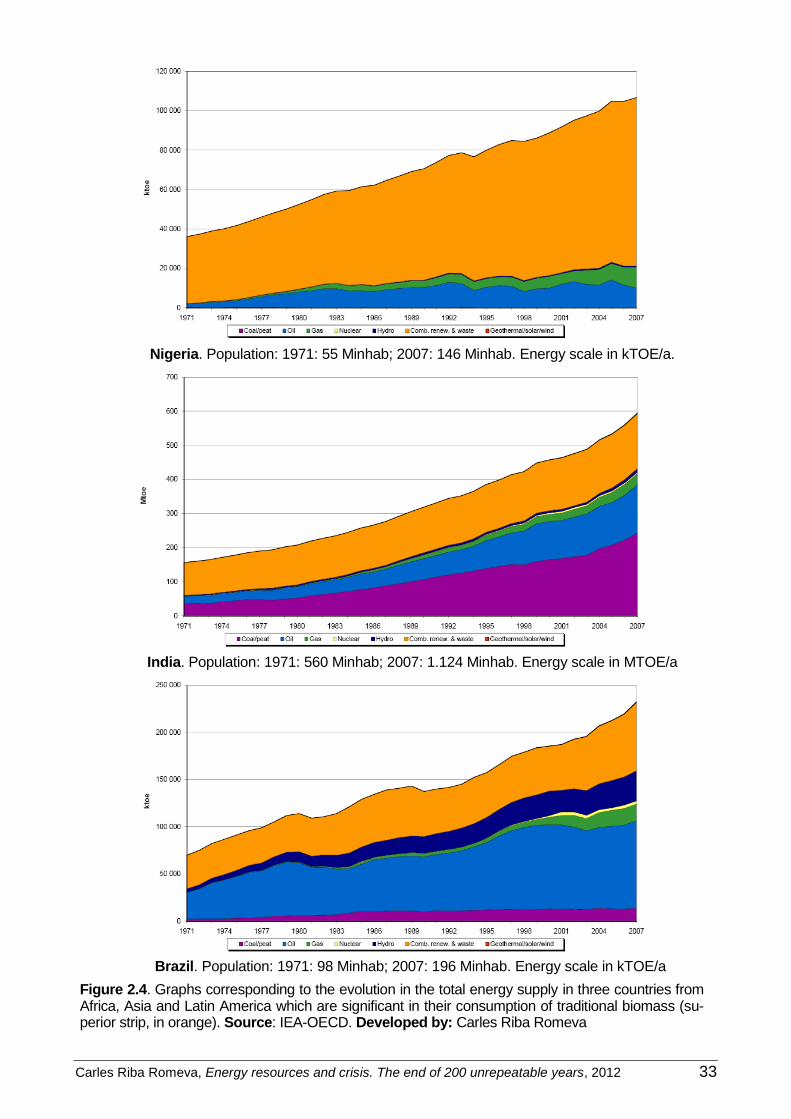
Carles Riba Romeva, Energy resources and crisis. The end of 200 unrepeatable years, 2012 33
Nigeria. Population: 1971: 55 Minhab; 2007: 146 Minhab. Energy scale in kTOE/a.
India. Population: 1971: 560 Minhab; 2007: 1.124 Minhab. Energy scale in MTOE/a
Brazil. Population: 1971: 98 Minhab; 2007: 196 Minhab. Energy scale in kTOE/a
Figure 2.4. Graphs corresponding to the evolution in the total energy supply in three countries from Africa, Asia and Latin America which are significant in their consumption of traditional biomass (su-perior strip, in orange). Source: IEA-OECD. Developed by: Carles Riba Romeva

34 Carles Riba Romeva, Energy resources and crisis. The end of 200 unrepeatable years, 2012
2.2. Energy consumption by regions
Table 2.4 and its graphical representation in figure 2.5 make it possible to analyze the evolu-tion of primary energy consumption in the worldwide regions that have been previously es-tablished.
Table 2.4. Worldwide energy consumption (TWt), by regions
1980 % 1985 1990 1995 2000 2005 2008 %
North America 3,068 29,56 3,048 3,399 3,673 3,998 4,106 4,039 22,61
Cnt. and S. America 0,481 4,64 0,524 0,595 0,700 0,809 0,912 0,990 5,54
Europe 2,440 23,51 2,492 2,612 2,644 2,813 2,993 3,012 16,86
Eurasia 1,575 15,17 1,875 2,051 1,420 1,356 1,494 1,562 8,74
Middle East 0,196 1,89 0,287 0,376 0,463 0,581 0,764 0,875 4,90
Africa 0,428 4,12 0,514 0,580 0,655 0,742 0,875 0,930 5,21
Asia and Oceania 2,191 21,11 2,582 3,152 3,870 4,282 5,744 6,458 36,15
Total 10,379 100,0 11,322 12,766 13,424 14,581 16,888 17,866 100,0
Index 1980=100
North America 100,00 99,35 110,81 119,72 130,32 133,83 131,66 C. and S. America 100,00 108,96 123,69 145,36 168,05 189,45 205,66 Europe 100,00 102,12 107,04 108,36 115,27 122,65 123,45 Eurasia 100,00 119,05 130,26 90,15 86,14 94,89 99,20 Middle East 100,00 146,41 191,90 236,09 296,32 389,62 446,35 Africa 100,00 120,09 135,53 153,09 173,42 204,55 217,35 Asia and Oceania 100,00 117,84 143,86 176,63 195,40 262,14 294,71
Sources: EIA-govUSA: oil, natural gas, coal, nuclear, hydraulic and new renewable sources of energy. IEA-OECD: combustible renewables and waste. Developed by: Carles Riba Romeva
Worldwide primary energy consumption, by regions (TWt)
0,0
1,0
2,0
3,0
4,0
5,0
6,0
7,0
1980 1985 1990 1995 2000 2005
North Amèrica
Cent. and South America
Europe
Eurasia
Middle East
Africa
Asia and Oceania
Figure 2.5. Primary energy consumption’s evolution by regions during the period 1980-2008 (scale from 0 to 7 TWt). Source: EIA-govUSA. Devel-oped by: Carles Riba Romeva
Worldwide primary energy consumption, by regions (TWt)

Carles Riba Romeva, Energy resources and crisis. The end of 200 unrepeatable years, 2012 35
Table 2.4 and figure 2.5 suggest the following comments:
Absolute increases. Asia, the maximum increase
1. Asia and Oceania is the region that registers the main increase in its energy consump-tion during the period comprised between 1980 and 2008 (+4,267 TWt, a 56,99% of the worldwide total of +7,487 TWt). This region is followed, at a very large distance, by North America (+0,971 TWt, a 12,97% of the worldwide’s total value).
2. The following four regions (South and Central America, Europe, Middle East and Africa) have increases that are ranged between the values of 0,500 and 0,680 TWt (from a 6,7 to a 9,1% at a worldwide scale). Finally, Eurasia, globally experiments a slight decrease of -0,013 TWt.
Percentage increases. Middle East and Asia and Oceania, maximum increases.
3. Middle East heads the list with a consumption increase of a +346,35% during the considered period. This region is followed by Asia and Oceania, which had an increase of a +194,71%.
4. Two more regions show important increases (which are quite significantly compensated for by the population’s increase): Africa, with an increase of a +117,35%, and South and Central America, with a +105,66%.
5. In North America and Europe, the increase has been much more moderate (+31,66% and 23,45%), whilst Eurasia does not have any increase.
Change in the relative weight. Asia and Oceania reaches the first position
6. According to their energy consumption, the way in which regions were ordered in 1980 was: North America, Europe, Asia and Oceania and Eurasia and, at a remarkable dis-tance, South and Central America, Africa and Middle East.
7. At the end of the studied period (2008), Asia and Oceania had placed itself in the first position, after exceeding North America and Europe. The other regions follow the same order as in 1980.
Change in the relative weight. First world regions decrease.
8. The most developed regions in 1980 lose weight in 2008: North America (-6,95%), Eu-rope (-6,65%) and Eurasia (-6,43%, it reflects the soviet union’s overthrow).
9. There are two regions that increase their weight in a very moderate manner: South and Central America (+0,90%) and Africa (+1,09%).
10. Finally, there are two regions that increase their weight in a spectacular way: Asia and Oceania (+15,04%; from a 21,11% of the worldwide total to a 36,15%), as a reflection of China’s dynamics and, in a less significant way, of India. And Middle East (+3,01%, but with a low population), with an increase that is induced by their availability of energy.
The connection between economy and energy
11. In a general way, the most dynamic economies (Asia and Oceania, Middle East) are linked to important energy consumption increases.
12. In this sense, the case of Eurasia is paradigmatic: after increasing the energy consump-tion in a 30,26% until 1990, the political and economical collapse of the soviet union in-duces an energy consumption reduction of a 17,80% from 1990 to 1998, which finally overcomes this reduction up to a -0,82% in 2008.
In the next few pages (section 2.3), from the data of table 2.6 and figure 2.6, and the knowledge about the worldwide and regional population’s evolution (table 2.8), we can ana-lyse the interesting question of primary energy consumed per capita for each of these areas as well as its evolution over time.
This is one of the most basic aspects that must be understood from the geostrategic situa-tions of each of the different countries in order to be able to correctly direct the actions that must be carried out.
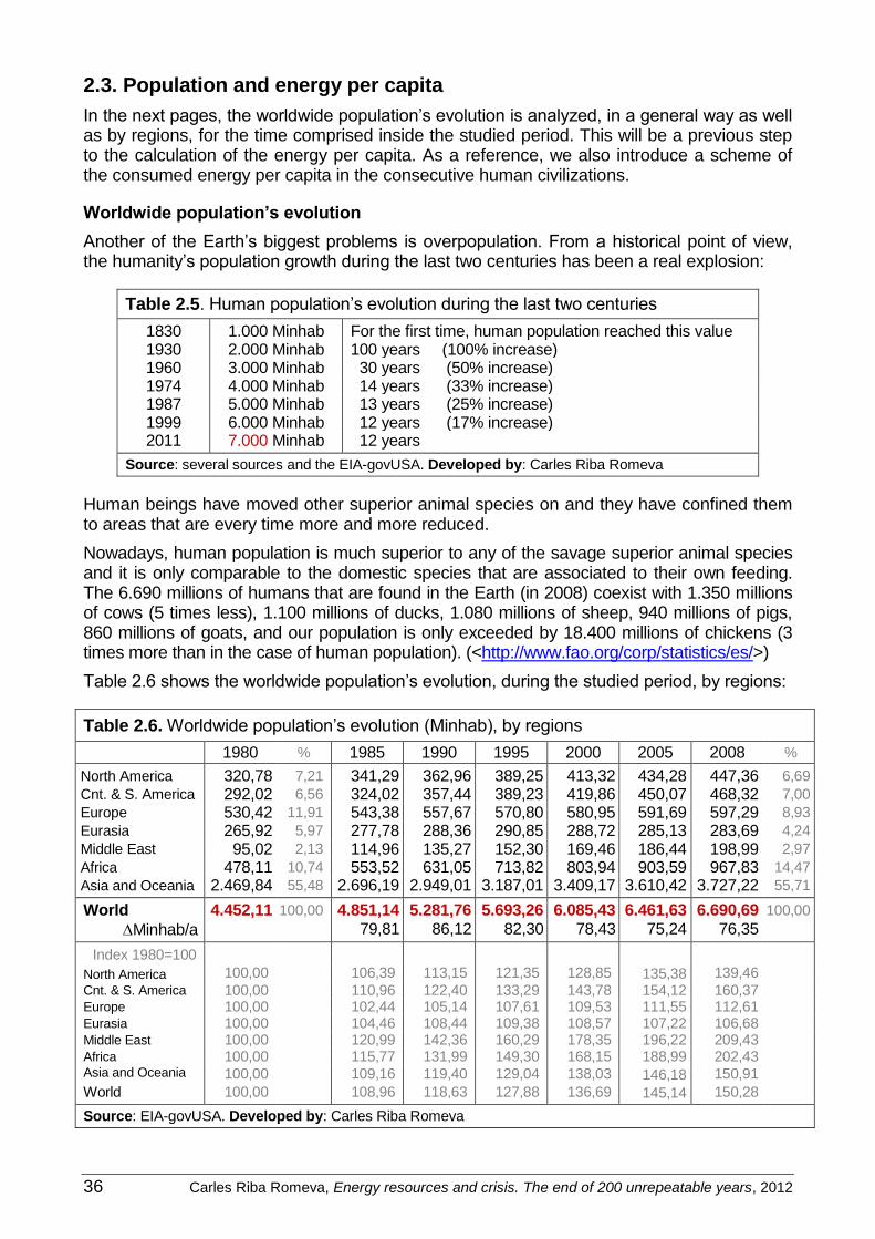
36 Carles Riba Romeva, Energy resources and crisis. The end of 200 unrepeatable years, 2012
2.3. Population and energy per capita
In the next pages, the worldwide population’s evolution is analyzed, in a general way as well as by regions, for the time comprised inside the studied period. This will be a previous step to the calculation of the energy per capita. As a reference, we also introduce a scheme of the consumed energy per capita in the consecutive human civilizations.
Worldwide population’s evolution
Another of the Earth’s biggest problems is overpopulation. From a historical point of view, the humanity’s population growth during the last two centuries has been a real explosion:
Table 2.5. Human population’s evolution during the last two centuries
1830 1.000 Minhab For the first time, human population reached this value 1930 2.000 Minhab 100 years (100% increase) 1960 3.000 Minhab 30 years (50% increase) 1974 4.000 Minhab 14 years (33% increase) 1987 5.000 Minhab 13 years (25% increase) 1999 6.000 Minhab 12 years (17% increase) 2011 7.000 Minhab 12 years
Source: several sources and the EIA-govUSA. Developed by: Carles Riba Romeva
Human beings have moved other superior animal species on and they have confined them to areas that are every time more and more reduced.
Nowadays, human population is much superior to any of the savage superior animal species and it is only comparable to the domestic species that are associated to their own feeding. The 6.690 millions of humans that are found in the Earth (in 2008) coexist with 1.350 millions of cows (5 times less), 1.100 millions of ducks, 1.080 millions of sheep, 940 millions of pigs, 860 millions of goats, and our population is only exceeded by 18.400 millions of chickens (3 times more than in the case of human population). (<http://www.fao.org/corp/statistics/es/>)
Table 2.6 shows the worldwide population’s evolution, during the studied period, by regions:
Table 2.6. Worldwide population’s evolution (Minhab), by regions
1980 % 1985 1990 1995 2000 2005 2008 %
North America 320,78 7,21 341,29 362,96 389,25 413,32 434,28 447,36 6,69
Cnt. & S. America 292,02 6,56 324,02 357,44 389,23 419,86 450,07 468,32 7,00
Europe 530,42 11,91 543,38 557,67 570,80 580,95 591,69 597,29 8,93
Eurasia 265,92 5,97 277,78 288,36 290,85 288,72 285,13 283,69 4,24
Middle East 95,02 2,13 114,96 135,27 152,30 169,46 186,44 198,99 2,97
Africa 478,11 10,74 553,52 631,05 713,82 803,94 903,59 967,83 14,47
Asia and Oceania 2.469,84 55,48 2.696,19 2.949,01 3.187,01 3.409,17 3.610,42 3.727,22 55,71
World 4.452,11 100,00 4.851,14 5.281,76 5.693,26 6.085,43 6.461,63 6.690,69 100,00
Minhab/a 79,81 86,12 82,30 78,43 75,24 76,35
Index 1980=100 North America 100,00 106,39 113,15 121,35 128,85 135,38 139,46 Cnt. & S. America 100,00 110,96 122,40 133,29 143,78 154,12 160,37 Europe 100,00 102,44 105,14 107,61 109,53 111,55 112,61 Eurasia 100,00 104,46 108,44 109,38 108,57 107,22 106,68 Middle East 100,00 120,99 142,36 160,29 178,35 196,22 209,43 Africa 100,00 115,77 131,99 149,30 168,15 188,99 202,43 Asia and Oceania 100,00 109,16 119,40 129,04 138,03 146,18 150,91
World 100,00 108,96 118,63 127,88 136,69 145,14 150,28
Source: EIA-govUSA. Developed by: Carles Riba Romeva

Carles Riba Romeva, Energy resources and crisis. The end of 200 unrepeatable years, 2012 37
Població segons regions (Mhab)
0
500
1.000
1.500
2.000
2.500
3.000
3.500
4.000
1980 1985 1990 1995 2000 2005
North America
Cent. and South America
Europe
Eurasia
Middle East
Africa
Asia and Oceania
Figure 2.6. Population’s evolution, by regions, during the period 1980-2008 (scale from 0 to 4.000 Minhab). Sources: EIA. Developed by: Carles Riba Romeva
Table 2.6 and its representation in figure 2.6, suggest the following comments:
The worldwide population is in a continuous growth
1. During the period comprised between 1980 and 2008 (one generation, approximately), the worldwide population grew in 2.238,58 Minhab (millions of inhabitants). This fact im-plies an increase of a 50,28%.
2. The increases seem to slow down with the passing of time. However, previsions locate the worldwide population’s maximum value between 8.500 and 10.000 Minhab towards half way XXI century. For this reason, in not much more than 200 years (since 1830), the planet’s human population will have been multiplied by almost ten.
The regions’ absolute increase
3. All of the regions, except for Eurasia the last few years, grow. Nevertheless, the biggest absolute increases are given in the case of Asia and Oceania (1.257,84 Minhab, almost the value of China’s actual population) and Africa (489,72 Minhab, more than the present population in North America).
4. The five remaining regions have a collective growth of 491,48 Minhab: South and Central America, 176,30 Minhab; North America, 127,58 Minhab; Middle East, 103,97 Minhab; Europe, 66,87 Minhab; and Eurasia, 17,77 Minhab.
The region’s relative increases
5. There are two regions that double their population during this period: Middle East (increase of a 109,43%), rich in energy resources, and Africa (102,43%), the poorest region.
6. Three more regions grow proportionally, not too far away, from the worldwide average growth: South and Central America, ten points above it (60,37%); Asia and Oceania, al-most at the worldwide average value (50,91%), and North America, more than 10 points below it (39,46%).
7. Finally, there are two regions that experience small relative growths: Europe (12,61%) and Eurasia (6,68%).
Population, by regions (Minhab)

38 Carles Riba Romeva, Energy resources and crisis. The end of 200 unrepeatable years, 2012
Civilizations and energy consumption
Human civilizations’ development has been associated to a progressive increase in the en-ergy consumption per capita (figure 2.7). In order to show this relationship, it is very visual to use the endosomatic energy consumption as a measurement unit (basal energy + activity’s energy) per day for an average active person, which may be translated into an approximate average thermal power of 120 Wt.
According to Cook (figure 2.7), since primitive agricultural civilizations that consumed about 4,8 times the human body’s endosomatic energy (576 Wt/inhab; which is still the situation of an important part of Africa and Asia), we are evolving towards industrial civilizations, which consume 31 times their endosomatic energy (3.720 Wt/inhab; situation which is a bit inferior to that of Europe or Eurasia) and towards post-industrial societies that reach a consumption level which is 92,7 times the endosomatic energy (11.124 Wt/inhab; approximate situation of the United States)
Human civilization's energy consumption
0
10
20
30
40
50
60
70
80
90
100
primitive hunter primitive
agricultural
advanced
agricultural
industrial technological
Transport
Agricultural and industry
Home and commece
Food
Figure 2.7. Graphical representation of the daily energy consumption per capita for different civi-lizations: primitive humans (1.000.000 years ago), European hunters (100.000 years), first agri-cultural civilizations (5.000 years ago); European advanced agricultural societies (XV century); industrial society (XIX century) and advanced technological societies (end of the XX century). In-stead of measuring it in kcal/day, the endosomatic energy consumption of an actual active per-son (120 Wt) has been used. Source: Cook [Coo-1971]. Developed by: Carles Riba Romeva
In any case, in nowadays’ human civilization there is a correlation between energy consump-tion and societies peaks and declines. For example, in several states from the ex-soviet union, as well as in Cuba or North Korea, the economical decline that took place after Berlin’s Wall was torn down are clearly reflected in the energy consumption curves.
One of the future challenges will be to find new human development forms in a context of fos-sil fuel resources’ decline. Will it be necessary to look for alternative sources of energy in order to substitute them? It is the path that seems to be implicitly followed, even though I have not been capable to identify them. Or, shall we think of a new development type which is not re-lated to the increase (or even, associated to the decrease) of the energy resources?
0,8 0 0 0
0,8
10,4 0,4 2,8 4,8 2,4
92,7 25,4 36,7 26,6 4,0
4,8 0
1,6 1,6 1,6
2,0 0 0
0,8 1,2
31,0 5,6 9,7 12,9 2,8
Human civilizations’ energy consumption Unit: active person’s endosomatic energy’s consumption, 120 Wt

Carles Riba Romeva, Energy resources and crisis. The end of 200 unrepeatable years, 2012 39
Consumed energy per capita’s evolution
The previous data about worldwide energy consumption at a general scale and by regions (table 2.4), combined with the population’s data which is obtained in table 2.6, make it possi-ble to establish the values of the energy consumption per capita (table 2.7). The measure-ment unit that has been used is the Wt/inhab.
Table 2.7. Consumed primary energy per capita (Wt/inhab), by regions
1980 Món=100 1985 1990 1995 2000 2005 2008 world=100
North America 9.563 410,22 8.930 9.365 9.435 9.672 9.454 9.028 338,09
C. & S. America 1.648 70,69 1.619 1.666 1.797 1.926 2.026 2.113 79,15
Traditional biomass1
327 345 309 286 268 290 302
Europe 4.600 197,33 4.586 4.684 4.632 4.841 5.058 5.043 188,87
Eurasia 5.922 254,00 6.748 7.133 4.881 4.698 5.240 5.506 206,20
Middle East 2.063 88,50 2.497 2.781 3.039 3.428 4.097 4.397 164,67
Africa 895 38,40 929 919 918 923 969 961 35,99
Traditional biomass1 420 414 417 419 423 432 435
Asia and Oceania 887 38,06 958 1.069 1.214 1.256 1.591 1.733 64,89
Traditional biomass1 224 224 223 216 211 214 215
World 2.331 100,00 2.334 2.417 2.358 2.396 2.614 2.670 100,00
Traditional biomass1 222 229 229 229 229 239 244
1980=100 100,0 100,11 103,68 101,14 102,78 112,11 114,54 1
The traditional biomass consumption per capita is included in the consumption of primary energy of the corre-sponding geographical area (the immediately superior row).
Sources: EIA-govUSA and IEA-OECD (traditional biomass). Developed by: Carles Riba Romeva
Figure 2.8 is the graphical representation of the data corresponding to table 2.7:
Energy per capita, by regions (Wt/inhab)
0
1.000
2.000
3.000
4.000
5.000
6.000
7.000
8.000
9.000
10.000
1980 1985 1990 1995 2000 2005
North America
Cent. and S. Amèrica
Europe
Eurasia
Middle East
Africa
Asia and Oceania
World
Figure 2.8. Evolution of the consumed energy per capita in the world’s different regions during the period comprised from 1980 to 2008 (scale from 0 to 10.000 Wt/inhab). Source: EIA-govUSA (energy and population). Developed by: Carles Riba Romeva
The data from both table 2.7 and its graphical representation in figure 2.8 suggest the follow-ing comments:
Energy per capita, by regions (Wt/inhab)

40 Carles Riba Romeva, Energy resources and crisis. The end of 200 unrepeatable years, 2012
The worldwide energy consumption per capita has remained almost constant
1. The consumption per capita has remained constant (approximately 2.400 Wt/inhab, about 20 times the average endosomatic energy of a human being) during the period from 1980 to 2000, and it only increased slightly at the beginnings of the XXI century, when it reached the value of 2.670 Wt/inhab in 2008, just before the economical crisis began.
2. The last increase in the world energy consumption per capita coincides with the latest fi-nancial and real estate bubbles and economic getaway from China and other emergent countries. Won’t the explosion of the actual economical crisis be a symptom of the exhaus-tion of the Earth’s capacity to supply us with resources beyond the actual consumption?
The rich and the poor are differentiated by their energy consumption per capita
3. In 2008, the average energy consumption per capita in the world is of 2.670 Wt/inhab.
4. Four regions (North America, Europe, Eurasia and Middle East) which sum up a total of 1.527 millions of inhabitants (23% of the world’s total population) consumed a power of 9,488 TWt (53% of the world’s total consumption), with an average consumption per cap-ita of 6.212 Wt/inhab (between 9.028 and 4.397 Wt/inhab).
5. Three more regions (Central and South America, Asia and Oceania and Africa), with a population of 5.163 millions of inhabitants (77% of the world’s total population), con-sumed 8,378 TWt (47% of the world’s total consumption), with an average consumption per capita of 1.627 Wt/inhab (between 2.113 and 961 Wt/inhab). The worse situation cor-responds to Africa (36, taking 100 as the worldwide consumption per capita).
Spectacular differences between regions
6. There are enormous regional differences in the energy consumption per capita: North America (includes Mexico) consumes 9.028 Wt/inhab (decreasing), whilst Africa con-sumes approximately ten times less (961 Wt/inhab; and almost half of this value corre-sponds to traditional biomass).
7. The United States of America is the economical power which has the maximum con-sumption per capita: during this whole period it has maintained itself over the 11.000 Wt/inhab and it reached a maximum consumption of 12.000 Wt/inhab in 2000.
Evolution of the energy consumption per capita
8. Two regions almost double their primary energy consumption per capita during the peri-od elapsed from 1980-2008: Middle East, with an increase of a 113,13% and a con-sumption of 4.397 Wt/inhab at the end of the period, and Asia and Oceania, with an in-crease of a 95,29% and a consumption of 1.733 Wt/inhab in 2008 (but the absolute value is below the worldwide average value).
9. North America, Africa and also Europe (5.086 Wt/inhab), Eurasia (5.506 Wt/inhab) and South and Central America (2.113 Wt/inhab) have very slight variations in their energy consumption per capita.
10. It is interesting to observe the variations in Eurasia’s energy consumption per capita. First, it increases until more than 7.100 Wt/inhab and, after the soviet regime’s fall, in 1995, it decreases until a value below the one corresponding to Europe (approximately 4.500 Wt/inhab); subsequently, with the revaluation of its energy resources, it increases again at the end of the period (approximately 5.500 Wt/inhab in 2008). It is another verifica-tion of the connection between economy and energy.
The consumption of traditional biomass
11. The consumption per capita of combustible renewables and waste in the world increases slightly during the studied period from 222 to 244 Wt/inhab. From these, an 83,7% corre-spond to the regions of Africa, Asia and Oceania and South and Central America.
12. In three regions of the world there is an important consumption of combustible renewables and waste, which, almost exclusively, can be attributed to traditional biomass (they are shown in colour in table 2.7.): Africa (435 Wt/inhab), Asia and Oceania (215 Wt/inhab) and South and Central America (302 Wt/inhab). In Africa, this consumption per capita slightly increases, whilst in the other two remaining regions, it slightly decreases.

Carles Riba Romeva, Energy resources and crisis. The end of 200 unrepeatable years, 2012 41
3. Non-renewable energies’ reserves
3.1. Evaluation of the energy reserves
Fossil fuels and Uranium are non-renewable sources of energy which, nowadays, cover most part of the energy supply for developed societies and developing societies (an 84,00% of the total production and a 84,12% of the worldwide consumptions). Moreover, these per-centages have scarcely been modified throughout the 28 years that have been studied.
Therefore, in any analysis of the energy supply’s evolution that is carried out, it is very im-portant to evaluate the reserves of each of these resources.
The reserve is an energy resource that is technically and economically recoverable, concept which, strictly speaking, only applies to non-renewable resources (oil, natural gas, coal and uranium). Each of these resources is usually measured with different measurement units (bar-rels, b; cubic feet, cf; tonnes, Tg; Natural uranium kilotonnes, ktUnat or GgUnat). In this text we have made an effort to translate these quantities to a common measurement unit: the thermal terawatt year: TWta.
The assessment of reserves has caused controversy, many of them with enough solid grounds for make us think that, in many cases, they have been overestimated. However, in order to avoid arguments, we have used the evaluations that have been carried out or ap-proved by some of the main international agencies and associations. We have used the fol-lowing sources of information for the values of energy reserves: oil and natural gas: Oil & Gas Journal (data collected by the EIA-govUSA); coal: WEC (collected by the EIA-govUSA, except for the data according to the USA); uranium: NEA-IAEA (from the Red Book 2007). The ob-tained results are given in tables 3.1 (by regions) and 3.2 (by countries).
Table 3.1. Worldwide fuels’ reserves (TWty), by regions
Oil Nat. Gas Coal Uranium Total Populat.
Information sources Oil&Gas J. Oil&Gas J. WEC NEA-IAEA several EIA
2007 2007 2007 2007 2007 2007
Wo
rld
Physical Units Gb1 Tcf1 Tg1 ktU1
Physical Measurem. 1.316,7 6.189,4 826.002 5.468,8
Conversion factors TWta/Gb TWta/Tcf TWta/Mst TWta/ktU Worldwide average 0,19639
2 0,03480
2 0,000698 2 0,013751
2
Energy unit TWta TWta TWta TWta TWta % world Minhab World 258,577 215,383 577,032 75,200 1.126,191 100,00 6.614,13
% of the resources 22,96 19,12 51,24 6,68 100,00
2 North America 41,385 9,743 186,043 10,506 247,676 21,99 443,06 6 S. and C. America 20,946 9,125 10,252 4,054 44,376 3,94 462,28 7 Europe 3,030 5,964 16,065 1,566 26,626 2,36 595,51 1 Eurasia 19,452 68,352 152,503 23,010 263,316 23,38 284,12 3 Middle East 145,268 90,164 1,188 1,559 238,180 21,15 194,96 5 Africa 22,014 17,375 25,108 14,365 78,863 7,00 945,91 4 Asia and Oceania 6,483 14,661 185,873 20,139 227,155 20,17 3.688,28
1 Gb (giga) = 109 barrels; Tcf (tera) = 10
12 cubic feet; Tg = (tera) = 10
6 tonnes (of all of coal’s categories); ktU
(kilo) = 103 natural uranium tonnes.
2 The calculations have been done using the following basic values: oil, average worldwide value, 43,02 GJ/Mg
(minimum value of 37,89 in comparison to a maximum of 44,89); natural gas: average value, 38,76 kJ/m3 (min-
imum of 29,96 and maximum of 48,84); coal: from the base of different countries and average values of the en-ergy efficiency for each type of coal (table 3.5); average value: 22,03 GJ/Mg (minimum value of, 5,26 and max-imum of 32,09); uranium: average worldwide value, 433,64 TJ/MgUnat.
Sources: Oil & Gas Journal (data collected by the EIA-govUSA): oil and natural gas reserves; WEC, World Energy Council: coal reserves (also collected by the EIA-govUSA in MST); NEA-IAEA (Red Book 2007): urani-um reserves. Developed by: Carles Riba Romeva

42 Carles Riba Romeva, Energy resources and crisis. The end of 200 unrepeatable years, 2012
Table 3.2. Different fuels’ reserves around the world (TWty), by countries (2007)
Oil Nat. Gas Coal Uranium Total Populat.
World Measurement Unit TWta TWta TWta TWta TWta % world Minhab
World 258,577 215,383 577,032 75,200 1.126,191 100,00 6.614,13 % of the reserves 22,96 19,12 51,24 6,68 100,00
1 United States 4,069 7,259 180,049 4,661 196,039 17,41 301,29
2 Russia 11,803 56,708 106,858 7,502 182,871 16,24 141,38 3 China 3,147 2,797 85,056 0,934 91,933 8,16 1.321,85 4 Australia 0,297 1,105 58,051 17,092 76,546 6,80 20,75 5 Iran 26,842 34,409 1,188 0,022 62,461 5,95 65,40 6 Saudi Arabia 51,860 8,406 60,266 5,35 27,59 7 Canada 34,832 1,983 5,092 5,819 47,727 4,24 32,94 8 Kazakhstan 5,901 3,503 19,182 11,238 39,824 3,54 15,28 9 India 1,078 1,313 35,521 1,002 38,915 3,46 1.124,13 10 Qatar 2,939 31,891 34,830 3,09 0,81
11 South Africa 0,003 23,732 5,983 29,717 2,64 48,37 12 Ukraine 0,078 1,366 24,594 2,743 28,781 2,56 46,30 13 United Arab Emirates 18,937 7,510 26,447 2,35 4,44 14 Iraq 22,391 3,923 26,314 2,34 27,50 15 Venezuela 16,422 6,071 0,487 22,980 2,04 26,02
16 Kuwait 20,105 1,926 22,032 1,96 2,51 17 Nigeria 7,125 6,371 0,159 13,655 1,21 143,31 19 Libya 8,011 1,844 9,855 0,88 6,05 18 Brazil 2,328 0,376 3,038 3,828 9,570 0,85 193,92 20 Algeria 2,280 6,098 0,052 0,268 8,699 0,77 33,36 21 Indonesia 0,826 3,566 3,669 0,080 8,140 0,72 234,69 22 Colombia 0,293 0,124 6,174 6,591 0,59 42,60 23 Uzbekistan 0,117 2,211 1,464 1,526 5,318 0,47 27,08 24 Poland 0,019 0,157 4,268 4,443 0,39 38,52 25 Norway 1,476 2,947 0,005 4,413 0,39 4,64 26 Serbia & Montenegro 4,112 4,112 0,37 9,92 27 Namibia 0,077 3,781 3,858 0,34 2,07 28 Nigeria 0,060 3,768 3,828 0,34 14,21 29 Mexico 2,483 0,500 0,782 0,025 3,791 0,34 108,70 30 Turkmenistan 0,118 3,503 3,621 0,32 38,50
32 Germany 0,073 0,269 3,046 0,096 3,485 0,31 82,40 33 Egypt 0,733 2,049 0,018 2,800 0,25 75,68
35 Pakistan 0,056 0,816 1,291 2,163 0,19 169,12 42 United Kingdom 0,752 0,606 0,119 1,477 0,13 60,78 44 Thailand 0,061 0,482 0,547 1,091 0,097 65,15
45 Sudan 0,850 0,104 0,955 0,085 39,38 54 Turkey 0,060 0,010 0,559 0,100 0,729 0,065 74,77 57 Vietnam 0,121 0,236 0,110 0,088 0,555 0,049 86,52 60 Japan 0,012 0,056 0,314 0,091 0,473 0,042 127,43 67 Italy 0,124 0,198 0,009 0,084 0,415 0,037 58,18 68 Spain 0,029 0,205 0,155 0,393 0,035 40,45 69 Burma 0,010 0,353 0,001 0,364 0,032 47,37 70 Philippines 0,027 0,120 0,211 0,358 0,032 94,16 77 France 0,024 0,012 0,161 0,197 0,017 63,71 79 Bangladesh 0,005 0,164 0,169 0,015 152,03 86 Congo (Kinshasa) 0,035 0,074 0,037 0,146 0,013 64,39
93 South Korea 0,083 0,083 0,007 48,25 121 Ethiopia 0,000 0,000 79,94
Sources: Oil and natural gas: Oil & Gas Journal (data collected by the EIA-govUSA): coal reserves: WEC; uranium reserves: IAEA-NEA (Red Book 2007). Developed by: Carles Riba Romeva

Carles Riba Romeva, Energy resources and crisis. The end of 200 unrepeatable years, 2012 43
Another interesting table (table 3.3) is the one that shows the first countries in each energy resource reserves and the global average for this resource.
Table 3.3. Leading countries in each of the non-renewable energy resources’ reserves
Countries Oil
Countries Natural gas
TWta % % acum TWta % % acum
1 Saudi Arabia 51,860 20,06 20,06 1 Russia 56,708 26,33 26,33
2 Canada 34,832 13,47 33,53 2 Iran 34,409 15,98 42,30
3 Iran 26,842 10,38 43,91 3 Qatar 31,891 14,81 57,11
4 Iraq 22,391 8,66 52,57 4 Saudi Arabia 8,406 3,90 61,01
5 Kuwait 20,105 7,78 60,34 5 United Arab Em. 7,510 3,49 64,50
6 United Arab Em. 18,937 7,32 67,67 6 USA 7,259 3,37 67,87
7 Venezuela 16,422 6,35 74,02 7 Nigeria 6,371 2,96 70,83
8 Russia 11,803 4,56 78,58 8 Algeria 6,098 2,83 73,66
9 Libya 8,011 3,10 81,68 9 Venezuela 6,071 2,82 76,48
10 Nigeria 7,125 2,76 84,43 10 Iraq 3,923 1,82 78,30
Countries Coal
Countries Uranium
TWta % % acum TWta % % acum
1 USA 180,049 31,13 31,13 1 Australia 17,092 22,73 22,73
2 Russia 106,858 18,47 49,60 2 Kazakhstan 11,238 14,94 37,67
3 China 85,056 14,70 64,30 3 Russia 7,502 9,98 47,65
5 Australia 58,051 10,04 74,34 4 South Africa 5,983 7,96 55,61
4 India 35,521 6,14 80,48 5 Canada 5,819 7,74 63,34
8 Ukraine 24,594 4,25 84,73 6 USA 4,661 6,20 69,54
6 South Africa 23,732 4,10 88,84 7 Brazil 3,828 5,09 74,63
7 Kazakhstan 19,182 3,32 92,15 8 Namibia 3,781 5,03 79,66
9 Columbia 6,174 1,07 93,22 9 Nigeria 3,768 5,01 84,67
10 Canada 5,092 0,88 94,10 10 Ukraine 2,743 3,65 88,32
Sources: Oil and natural gas reserves: Oil & Gas Journal (data collected by the EIA-govUSA): coal reserves: WEC; uranium reserves: NEA-IAEA (Red Book 2007). Developed by: Carles Riba Romeva
Tables 3.1, 3.2 and 3.3 lead us to make the following comments:
Finite reserves
1) The estimated reserves of non-renewable fuels in the world sum up to the value of 1.126,191 TWta. Considering the actual consumption rate of these fuels, 15,009 TWt (table 2.1), there are only enough resources for the next 75 years. The new discovering, con-sumptions and exhaustion policies will be analyzed further on in the text.
2) It is frequent to analyze the relation (R/P, reserves/production) for each of the different sources of energy. The obtained results were: oil: 258,577/5,720 = 45,2 years; natural gas: 215,383/3,809 = 56,5 years; coal: 577,032/4,572 = 126,2 years; uranium: 75,200/0,908 = 82,8 years. Therefore, from this point of view, it seems that we still have a certain temporal margin in order to react. More realistic simulations will be carried on later.
Concentrated and not evenly distributed
3) Non-renewable sources of energy are very badly geographically distributed. Two countries (Russia and the United States) share out, almost evenly, more than a 33% of reserves with only a 6,7% of the worldwide population. The first ten countries (the two countries mentioned and China, Iran, Saudi Arabia, Australia, India, Canada, Kazakhstan and Qatar) sum up a total of 831,4 TWta. This value is a 73,7% of the total worldwide reserves.
4) The first ten countries’ analysis hides an imbalance. If we separate China and India, the remaining 8 countries have a total of 700,6 TWta in reserves (62,1% of the world) for a population of 605,4 millions of inhabitants (a 9,2% of the world), whilst the two countries mencioned dispose of energy reserves for the value of 130,8 TWta (11,6%) for a popula-tion of 2.446,0 millions of inhabitants (a 37,0% of the world population).

44 Carles Riba Romeva, Energy resources and crisis. The end of 200 unrepeatable years, 2012
5) In all energy sources (oil, natural gas, coal and uranium), four countries sum up more than a 50% of the world’s reserves (60% in the case of natural gas and coal) and, ten countries sum up more than an 80% (except for the case of natural gas, which is nearby).
Imbalance that favours coal (the most polluting fuel)
6) The most important reserves in the world are coal reserves (the fuel that has the highest impact on the climate change), a 51,2%. On the contrary to what many people think, coal is the most concentrated resource. Eight countries (USA, Russia, China, Australia, India, Ukraine, South Africa and Kazakhstan) have a total of 533,0 TWta (a 92,1% of the worldwide reserves). Several of these countries have not committed to Kyoto’s protocol.
7) The second most relevant reserves are those of oil (closest to exhaustion), the 22,96% of the total, and they are also concentrated. Eight countries (Saudi Arabia, Canada, Iran, Iraq, Kuwait, the United Arab Emirates, Venezuela and Russia) sum up a total value of 203,19 TWta (a 78,6% of the worldwide reserves). All of these countries, except for Can-ada and Russia, belong to the OPEC.
8) Natural gas reserves (the less pollutant fossil fuel) are a bit minor than oil reserves (19,12%) and they are concentrated in three different countries: Russia, Iran and Qatar, which sum up a total of 123,01 TWta (a 57,1% of the global worldwide reserves). These countries are followed by a set of six countries (Saudi Arabia, the United Arab Emirates, USA, Nigeria, Algeria and Venezuela) with a total of 41,72 TWta more, which make an accumulated total of a 76,5% of the worldwide reserves.
9) Finally, the minor reserves (by far) are uranium ones (6,68%), and they are also concen-trated in a small number of countries. The three first countries (Australia, Kazakhstan and Russia) have a total of 35,83 TWta, a 47,7% of the worl, and the next six countries (South Africa, Canada, USA, Brazil, Namibia and Nigeria) sum up a total of 27,84 TWta more, which make an cumulative percentage of a 84,7% of the world’s total uranium reserves.
Reserves’ distribution by regions and strategic aspects
10) Four of the world’s different regions (Eurasia, North America, Middle East and Asia and Oceania) have, each one, between a 20,0 and a 23,4% of the worldwide energy reserves. In three of them, the main reserves are coal (North America, Asia and Oceania and Eura-sia), whilst in the Middle East are oil and natural gas. Eurasia is the most balanced (apart of coal, it has the most important uranium reserves in the world and the second in natural gas). North America also has the second most important oil reserves in the world (a bit more deceitful, as they are mainly Canada’s oil sands); and Asia and Oceania (specifical-ly, Australia) has the second most important uranium reserves in the world.
11) The remaining three regions are more scarce in energy resources: Africa has a 7,0% of the world reserves, quite equilibrated; South and Central America counts has a 3,9% of it, diversified, but with little uranium; finally, Europe, in the utmost last, has a scarce 2,36% of the worldwide reserves, mainly of low-quality coal.
12) Coal is strategic for some big countries that have scarce alternative resources in relation to their consumption or needs. Specifically, the USA, the country’s largest consumer in the world in absolute terms and per capita (3,49 TWt and 11.584 Wt/inhab, in 2007); China, the most populated country in the world (1.321,8 Minhab in 2007) and the second largest energy consumer (2,91 TWt, in 2007), and India, the second most populated country in the world (1.124,1 Minhab, in 2007). It is difficult for them to relinquish it. Japan, South Korea, Australia (which supplies the two previous countries) and South Africa, which burns a 93% of the coal consumed in Africa, find themselves in the same coal-dependency situation.
13) There are developed countries, with high energy consumptions per capita, that almost do not dispose of reserves. Some of the most populated ones are: South Korea (48,3 Min-hab and 0,083 TWty of reserves), France (63,7 and 0,197), Spain (40,5 and 0,393), Italy (58,2 and 0,415) or Japan (127,4 and 0,509). And, in slightly better conditions, the United Kingdom (60,8 and 1,477) and Germany (82,4 and 2,829).

Carles Riba Romeva, Energy resources and crisis. The end of 200 unrepeatable years, 2012 45
14) There are other highly populated countries that will struggle to develop because of the great shortage of energy resources. Some of the most populated ones are: Ethiopia (79,9 Minhab, with no known reserves), Congo Kinasha (64,4 Minhab and 0,146 TWty); Bangla-desh (152,0 and 0,169), the Philippines (94,2 and 0,358), Burma (47,4 and 0,364), Vi-etnam (86,5 and 0,555). And, in slightly better conditions: Thailand (65,2 and 1,091), Paki-stan (169,1 and 2,163), Egypt (75,7 and 2,800) and Mexico (108,7 and 3,791).
3.2. Analysis of the oil and natural gas reserves
There are several sources of information that, periodically, supply data about oil and natural gas reserves. Amongst the most well-known there is: the BP oil company, the magazines: Oil & Gas Journal and World Oil, the Organization of the Oil Exporting Countries (OPEC) and the International Cedigaz association. Not all of the information coincides, but the ap-proximation degree is considered to be acceptable (table 3.4).
Table 3.4. Different estimations of oil and natural gas reserves
Oil Natural Gas
Regions
BP 1 O&G J. 2 W. Oil 3 OPEC 4 BP 1 CEDIGAZ O&G J. 2 W.Oil 3 end 2007 end 2007 end 2007 End 2007 end 2007 end 2008 end 2009 end 2007
Gb Gb Gb Gb Tcf Tcf Tcf Tcf
North America 70,31 209,91 57,54 25,94 308,29 308,46 308,79 314,06 S. & C. America 111,21 122,69 104,79 134,69 272,84 260,09 266,54 246,98 Europe 15,57 13,66 13,80 15,11 207,65 218,13 169,09 168,98 Eurasia 128,15 98,89 126,00 129,05 1.890,89 1.900,26 1.993,80 2.104,00 Middle East 755,32 746,00 727,31 741,57 2.585,35 2.609,32 2.591,65 2.570,22 Africa 117,48 117,06 114,72 119,57 514,92 514,33 494,08 504,21 Asia & Oceania 40,85 34,01 40,05 38,28 510,69 531,81 430,41 527,58
World 1.238,89 1.342,21 1.184,21 1.204,18 6.290,64 6.342,41 6.254,36 6.436,03 1
BP, Statistical Review of World Energy, june 2008. 2 Oil & Gas Journal, vol. 106.48 (22nd December 2008), PennWell Corporation.
3 Word Oil, vol. 229 Num. 9 (September 2008), Gulf Publishing Company.
4 OPEC, Organization of the Oil Exporting Countries, Annual Statistical Bulletin, 2007.
5 CEDIGAZ, Centre International d'Information sur le Gaz Naturel et tous les Hydrocarbures Gazeux), Natural
Gas in the World, July 2008. Sources: The ones that have been mentioned. Developed by: Carles Riba Romeva
This project uses the assessments that were collected by the EIA-gov USA and published in the Oil & Gas Journal as a reference. This choice has two advantages: 1. the level of break-down by countries is higher than when using other sources. 2. It makes the coherence with the rest of the data from the EIA much easier.
In order to establish comparisons, it becomes necessary to transform the physical data (b, oil barrels; cf, cubic feet of natural gas) into energy data (TWta, thermal terawatts year), but not all of the oils or natural gases from different origins have the same energy quality. The conversion factor has been established, for each country, using the gross heat content (in BTU/barrel, or BTU/cf) which is supplied by the EIA as a reference, both for oil and natural gas. We have considered that reserves will not be of a better quality than those that were extracted from the Earth in 2007.
Evolution of the oil reserves’ estimations
A very important aspect that is used to evaluate the oil reserves’ estimations is to know how they have evolved with the passing of time (see figure 3.1. which has been made using the successive historical data assessments carried out by the Oil & Gas Journal).
The first observation is that reserves have always increased (in theory, due to new discover-ies), instead of diminishing as a consequence of their consumption.

46 Carles Riba Romeva, Energy resources and crisis. The end of 200 unrepeatable years, 2012
Evolution of oil reserves (TWta)
0
50
100
150
200
250
300
1980 1985 1990 1995 2000 2005
North America
S. & C. America
Europe
Eurasia
Middle East
Africa
Asia & Oceania
World
Figure 3.1. Evolution of global oil reserves (according to the Oil &Gas Journal), trans-lated to TWta. Source: EIA (Oil & Gas Journal). Developed by: Carles Riba Romeva
The fact that the increases in the oil reserves have been greater than oil’s consumption has lead optimistic people and oil companies to state that this resource is almost inexhaustible and that the new oil extractions are only a monetary issue.
However, the two discontinuities that have originated the main increases in the latest years’ reserves must be analyzed: years 1987-1990 and 2002-2003 (figure 3.1).
The first discontinuity (from 1987 to 1990) has a recognized explanation which has even been accepted the International Energy Agency (World Energy Outlook 2008, [WEO-2008]). Since 1982, and with the objective to control the International market’s prices, the OPEC decides to establish production quotes that depend, amongst others, on each country’s reserves.
The historical data sequence shows that, in few years, countries that belonged to the OPEC revised their oil reserves increasing their value; however, no significant new oilfield discover-ies were registered: in 1985, Kuwait increased them from 66,8 to 92,7 Gb (G = giga, 109 bar-rels); in 1988, the United Arab Emirates (from 33,1 to 98,1 Gb), Iran (from 48,8 to 92,9 Gb), Iraq (from 47,1 to 100,0 Gb) and Venezuela (from 25,0 to 56,3 Gb) also increased their re-serves, and, two years later, in 1990, Saudi Arabia did the same (from 172,6 to 257,6 Mb). These increases registered a total increase due to revision of 304,0 Gb. This phenomenon is what the Energy Watch Group [EWG-2008] call «political reserves».
The second discontinuity (from 2002 to 2003) is due to the acceptance of a substantial amount of the oil sands that are located in Athabasca (Canada) as oil (conventional oil) re-serves. This acceptance was carried out by the Oil&Gas Journal. In this way, Athabasca’s (Canada) oil sands, a sort of sand with tar, become the second most important oil reserves in the world (from 4,9 Gb to 180,0 Gb). A nice 175,1 Gb increase.
For one reason, «political reserves», or for another, «unconventional oils», we can doubt of the efficiency of 479,1 Gb of the total oil reserves, a 36,4% of the total 1.316,7 Gb of world-wide oil reserves in 2007.
In the same way, it is convenient to contrast the previous reserves’ estimation sequence with the new oil well discoveries (figure 3.2), according to J. Laherrère, retired engineer from the French oil company Total [Lah-2008].
Evolution of global oil reserves (TWta)

Carles Riba Romeva, Energy resources and crisis. The end of 200 unrepeatable years, 2012 47
Figure 3.2. World crude oil annual discoveries (in green), production (in purple) and forecasts (in discontinuous lines). Source: J. Laherrère and J. L. Wingert [Lar-2008]
Figure 3.2 shows that the amount of new crude-oil discoveries abruptly decrease since 1975, whilst the production (and consumption) keep growing, even though they do it in a more mod-erate way since the oil crisis that took place from 1973 to 1979. The new discoveries do not justify the crude oil estimations’ increases that were published in the Oil & Gas Journal.
Figure 3.2 also shows peak oil. This issue will be tackled further on in the text.
Evolution of natural gas reserves’ estimations
Analogously, natural gas reserves’ estimations have also increased with the passing of time (they doubled their value and even continued increasing during the period comprised be-tween 1980 and 2008, figure 3.3) and they also have some discontinuities in their evolution, accordingly with the discovery of new gas fields.
Natural gas reserves' evolution (TWta)
0
50
100
150
200
1980 1985 1990 1995 2000 2005
North America
S. & C. America
Europe
Eurasia
Middle East
Africa
Asia & Oceania
World
Figure 3.3. Evolution of global natural gas reserves, translated to TWta. Source: Oil & Gas Journal (EIA-govUSA). Developed by: Carles Riba Romeva
Evolution of global natural gas reserves (TWta)

48 Carles Riba Romeva, Energy resources and crisis. The end of 200 unrepeatable years, 2012
Laherrère also supplies a graph with the new natural gas discoveries, comparing them with the evolution found in production (and consumption).
Figure 3.4. In red: world conventional natural gas annual discovery; in blue: reinjected gas; in purple: consumed gas; in green: unconventional gas; in black: losses; in yellow: gas burners found in wells (detected with the aid of a satellite); in light blue: production-consumption forecast; in fine black (several lines): International Energy Outlook fore-casts (IEO-2008, EIA-govUSA). Source: J. Laherrère and J. L. Wingert [Lar-2008]
Figure 3.4 shows that, although in recent years there have been some important discoveries of natural gas, the trend is downward. Therefore, data from Figures 3.3 and 3.4 for natural gas are more concordant. Nevertheless, it could be interesting to carry out a further investi-gation on the 1992 and 2003 discontinuities observed in Figure 3.3.
In any case, the figure 3.4 also indicates (with some delay with respect to oil), natural gas peak between the years 2015 to 2020.
3.3. Analysis of the coal reserves
Coal is the most abundant fossil fuel as well as being the one that has the highest and most important local (pollution due to emissions), regional (acid rain) and worldwide (CO2 emissions to the atmosphere). Therefore, coal reserve’s assessment has a remarkable relevance.
Coal was the fuel with which it developed the Industrial Revolution in the late eighteenth and throughout the nineteenth century in Europe and the United States. It was also the basis for the development of the countries of the Soviet bloc and, today, remains the main energy base in many countries (China, India, USA, Japan, South Korea, Australia, South Africa)
Recently, since oil started to become scarce in comparison to its demand (as demonstrated by the maximum price of all time of 140 $/barrel in 2007, immediately before the financial crisis began), some big economical powers (specially China and the United States) have increased its consumption, fact that has had a bearing on the worldwide consumption.
The World Energy Council (WEC), International Organization, founded in 1923 which has its headquarters in London, leader in energy studies since 1924, periodically supplies estimations of the resources and coal reserves that are a reference in this issue. Table 3.5 shows the data

Carles Riba Romeva, Energy resources and crisis. The end of 200 unrepeatable years, 2012 49
from the last seven estimated coal reserves of major producing countries and the whole world (which have a major global coherence then the previous ones).
Table 3.5. Evolution of the coal reserves’ estimations (Tg, or millions of tonnes)1
Countries 1990 2 1993? 2 1996 2 1999 2 2002 2 2005 2 2007 2 (1992) (1995) (1998) (2001) (2004) (2007) (2009)
United States 240.561 240.558 246.643 249.994 246.643 242.721 238.308 URSS 241.000 241.000 Russia URSS URSS 157.010 157.010 157.010 157.010 157.010 China 114.500 114.500 114.500 114.500 114.500 114.500 114.500 India 62.548 69.947 74.733 84.396 92.445 59.498 58.600 Australia 90.940 90.940 90.400 82.090 78.500 76.600 76.200 South Africa 55.333 55.333 55.333 49.520 48.750 48.000 30.408 Kazakhstan URSS URSS 34.000 34.000 31.279 31.300 31.300 Ukraine URSS URSS 34.356 34.153 34.153 33.873 33.873 Germany 80.069 67.300 67.000 66.000 6.739 6.708 6.708 Poland 41.200 42.100 14.309 22.160 14.000 7.502 7.502 United Kingdom 7.148 2.500 1.500 1.500 220 155 155 Indonesia 32.063 32.063 5.220 5.370 4.968 4.328 4.328 Serbia i Mont. 16.570 16.570 16.472 16.256 16.591 13.885 13.885 Brazil 2.359 2.845 11.950 11.929 10.113 7.088 7.059 Columbia 4.539 4.539 6.749 6.648 6.611 6.959 6.814 Rest of the world 73.821 75.369 89.207 83.760 79.857 65.293 67.109
World 1.039.183 1.031.610 984.211 984.453 909.064 847.488 826.001 1
The temporal series starts in 1924 and there are 8 estimations before the one in 1992. Nevertheless, the first ones have not been reproduced due to the omission of certain countries or the greater incoherence of the data.
2 Reserves at the end of the year (in parenthesis, the publication date).
Source: Survey of Energy Resources del WEC (World Energy Council), collected by the EIA-govUSA (ex-cept for the data from the USA). Developed by: Carles Riba Romeva
Not very precise estimations of the coal reserves
As it was noted by the Energy Watch Group in their study about coal [EWG-2007], the data from the World Energy Council «are of a poor quality». Probably, this is due to the fact that the WEC collects information from different countries with non-uniform accounting criteria.
1. In the considered period (1990-2007, table 3.5), the reserves decrease in a continuous way (not like the reserves of oil, natural gas, and as we will see further on in chapter 8, of uranium). Specifically, they decrease in 213.182 Tg, whilst, according to the EIA, the worldwide coal production during these 16 years has been of 80.413 Tg. Therefore, there is a global revision with a tendency towards decrease in the coal reserves of 122.769 Tg, which cannot be justified by consumption.
2. There are several countries with significant resources in which the coal reserves have di-minished in an unjustified manner. The estimation of India reserves, after increasing up to 92.455 Tg in 2002, drops abruptly to 58.600 Tg in 2007; South Africa drops from 55.333 Tg in 1999 to 30.408 Tg in 2007; Indonesia, without relevant reserves in 1989, first in-creases until a value of 32.063 Tg in 1990 but then it drops to 5.220 Tg in 1996; similarly, Brazil goes from 2.845 to 11.950 Tg in 1996 and then this value drops to 7.088 in 2005.
3. However, the most downward spectacular revisions of reserves are given in European countries that find themselves in an advanced exploitation state (or in the final phase): Germany, with an estimated amount of reserves of 80.069 Tg in 1990, reduces them ab-ruptly ten years later (2002) to 6.739 Tg; the United kingdom, which had recognized 45.000 Tg in 1980 (not in table 3.5), nowadays has residual coal reserves (155 Tg), or Po-land, with recognized reserves for the value of 41.200 Tg in 1990, have experimented suc-cessive decreases and oscillations and currently find themselves in the value of 7.502 Tg.

50 Carles Riba Romeva, Energy resources and crisis. The end of 200 unrepeatable years, 2012
Coals’ qualities
4. Coals have much more diverse qualities than oil or natural gas (table 3.6). In this way, in order to quantify the importance of the reserves, we must translate the tonnes of coal to energy resources. A tonne of anthracite (about 32 GJ/Mg) is not the same as a tonne of bi-tuminous coal (more than 23,865 GJ/Mg, according to the IEA), than a tonne of sub-bituminous coal (between 17,435 and 23,865 GJ/Mg, according to IEA) and a tonne of lig-nite (less than 17,435 GJ/Mg), which can reach the value of 5,5 GJ/Mg in poor quality lig-nites. By countries, the extreme coal quality values are Venezuela (32,087 GJ/Mg) and Greece (5,261 GJ/Mg).
Table 3.6. Coal reserves by regions according to their type (2007) and energy equivalent
Regions
Type of coal1 Primary Energy
Anthr./bitum Sub-bitum. Lignite Total Total2 A.E. Eff.3
Tg Tg Tg Tg TWty GJ/Mg
North America 113.281 100.473 32.526 246.280 186,043 23,823 S. and C. America 6.964 8.019 24 15.007 10,252 21,545 Europe 8.433 3.567 34.068 46.068 16,065 10,997 Eurasia 93.609 114.049 18.337 225.995 152,503 20,698 Middle East 1.386 0 0 1.386 1,188 27,033 Africa 31.839 171 3 32.013 25,108 24,734 Asia and Oceania 155.809 38.540 64.904 259.253 185,873 22,610
World 411.321 264.819 149.862 826.002 577,032 22,031 1
Anthracite/bituminous; sub-bituminous; lignite. 2 Energy values obtained from the tonnes of coal reserves that were estimated in 2007 (source: WEC) and average energy efficiency for each region (in GJ/Mg) in 2007.
3 Average energy efficiency obtained from the values of the total tonnage and the primary energy extracted from the coals of every country in 2007 (source: EIA-gov USA). It has been assumed that the reserves are not of a better quality than the coal that is currently being produced; anyway, they will tend to give a minor energy efficiency with the progressive exhaustion of the higher quality resources.
Sources: Survey of Energy Resources 2009, of the WEC (World Energy Council), collected by the EIA (ex-cept for the data of the USA); IEA-OECD; EIA-govUSA. Developed by: Carles Riba Romeva
5. The big carboniferous regions (Asia and Oceania, North America and Eurasia) distribute their reserves between high quality coals (anthracites and bituminous) and low quality coals (sub-bituminous and lignites). Europe, which comes next, has more than 80% of the low quality coals (mainly, lignites) and from an energy point of view, it comes after Af-rica, which has a lower tonnage but its reserves are almost exclusively of high quality coals. South America, with a lower tonnage (half the amount of Africa and one third of that of Europe), has both low and high quality coals. And, finally, the Middle East has al-most testimonial coal reserves, but the ones that it does have are of a high quality.
6. The countries that have the greater amount of reserves (more than 4.000 Tg) are located in the following coal quality groups: a) more than a 90% of high quality coals: South Africa (100,0%), Columbia (94,4%), India (92,2%), Kazakhstan (90,0%) and Poland (80,1%); b) between 40 and a 60%: China (54,3%), Canada (52,8%), Australia (48,3%), USA (45,7%) and Ukraine (45,3%); c) between a 20 and a 40%: Indonesia (39,8%), Czech Republic (37,2%) and Russia (31,3%); d) less than a 20%: Germany (2,3%), Brazil (0,0%) and Ser-bia and Montenegro (0,0%).
Therefore, (and as the Energy Watch Group stated in their analysis about coal [EWG-2007]), these observations make us think that, probably, there are less coal reserves than what we presume of. And, moreover, as the better coals are extracted, the remaining ones have a decreasing level of quality.

Carles Riba Romeva, Energy resources and crisis. The end of 200 unrepeatable years, 2012 51
4. Growth and projections
4.1. Divorce between growth projections and reserves
In this chapter, the growth projections of the predicted energy consumptions by the energy agencies (EIA, Energy Information Administration, of the USA Government and the IEA, In-ternational Energy Agency, of the OECD), are contrasted with the nowadays accepted re-serves of the energy resources. This supposition entails a constant growth until, approxi-mately in 2060, the coal reserves are used up and; therefore, the actual technologic and economic system collapses.
This rather pessimistic vision is contrasted by the defenders of the current growth society that affirm that energy resources are much higher than reserves (which is true) and that their extraction is only an issue of technology and price. Therefore, technologic development and the market provide the necessary resources for future generations, in such a way that we do not have to worry.
The previous «anthropocentric view» of reality is falsely optimist and further on (chapter 5) is contrasted by a «ecospheric view» [Gar-2010], in which a more realistic analysis of the re-source exploitation boundaries imposed by nature and that, for the first time, affect the whole humanity: the production zenith phenomenon and the need of an energy return on investment (EROI) significantly higher than 1.
For some time already, energy agencies (EIA-govUSA and IEA-OECD) make growth projec-tions of the energy consumption for the following 20 or 25 years. Specifically, the annual EIA report, International Energy Outlook 2010 [IEO-2010], predicts that consumption of non-renewable resources of energy (oil, natural gas, coal and uranium) will increase from an an-nual 1,313% (following a geometric progression) from 14,562 to 19,915 TWt during the peri-od 2006-2030, and the annual IEA report, the World Energy Overlook 2009 [WEO-2009], predicts an increase of from 13,564 to 19,367 TWt, for the same period.
From this data and from the total reserves of non-renewable energy resources of 2007 (1.126,191 TWta, chapter 3), the process of depletion of these resources has been projected based on the following three assumptions:
a) The annual consumption of non-renewable energies increases according to the annual ge-ometric growth calculated from values of year 2006 and 2030 (table 4.1). It gives remarka-bly coincident projections for both information sources considered.
b) All of the energy resources (oil, natural gas, coal and uranium) participate jointly, that is, when a resource is exhausted, the consumption of other resources increases in order to cover the total energy consumption projections.
c) The reserves of energy resources do not increase. Although this assumption is not true for some resources (specially, natural gas), it is not so in the two more plentiful resources: coal reserves have decreased in previous years and new discoveries of oil wells can be easily compensated by the false «political reserves» (chapter 3).
Like it is shown below (table 4.1), extrapolating the increases predicted by the EIA-govUSA and the IEA-OECD (that reflect the actual consumption trends, without considering the limits of reserves), non-renewable fuels will become exhausted in year 2060 or 2061 (that is, in 50 years!).

52 Carles Riba Romeva, Energy resources and crisis. The end of 200 unrepeatable years, 2012
Table 4.1. Growth projections of the EIA-govUSA and the IAE-OECD1
Non-renewable energies (oil, natural gas, coal and uranium) jointly
Source Units World consumption Reserves
2006 1 2030 1 % annual2
2007 Exhaust. year
EIA-govUSA TWt 14,562 19,915
1,313
2060 PBTU 435,3 595,3
IEA-OECD TWt 13,564 19,367
1,495
2061 MTOE 10.217 14.588
Evaluation C. Riba TWta 1.126,191 1 The values from 2006 and the provisions for 2030 have been adopted as they coincided for both
sources of information (EIA and IEA). 1 Annual growth percentage (geometric) during the period elapsed from 2006-2030.
Sources: EIA-govUSA, IEA-OECD, the project itself. Developed by: Carles Riba Romeva
The analysis below uses data and projections of the EIA-govUSA (very similar to those of the IEA-OECD). If the hypothesis or joint participation of the different resources in the pro-jected consumption is followed, situation explained below, is given:
Oil reserves (258,490 TWta in 2007) are the first to become exhausted in 2046 (in 36 years!). Once oil has become exhausted (until that moment the main energy resource), if the con-sumption predictions by the EIA-govUSA are maintained, consumptions will be shared by the rest of the non-renewable resources, and so on.
Then, exhaustions will hasten in chain during the following 15 years: 3 years later (2049), the world natural gas reserves will become exhausted (215,164 TWta in 2006); 3 years later (2052), world uranium reserves will become exhausted (72,564 TWta in 2006); finally, 9 years later (2060) the remaining reserves of coal will also become exhausted (577,032 TWta in 2007). Figure 4.1 shows this sequence.
Exhaustion of non-renewable reserves
0
100
200
300
400
500
600
700
800
900
1.000
1.100
1.200
2007 2012 2017 2022 2027 2032 2037 2042 2047 2052 2057
Oil
Natural gas
Uranium
Coal
Figure 4.1. Progressive exhaustion of the non-renewable resources’ reserves (oil, natural gas, uranium and coal) assuming that they act jointly covering the consumption projections that have been carried out by the EIA. Source: EIA-govUSA. Developed by: Carles Riba Romeva
Exhaustion of non-renewable energy

Carles Riba Romeva, Energy resources and crisis. The end of 200 unrepeatable years, 2012 53
When fossil resources start to decline, a «domino effect» is produced. After the exhaustion of oil and natural gas around 2049, we will still have approximately half of the coal reserves (about 310 TWta), but then, coal almost by itself (uranium is residual) only can sustain con-sumption required little more than 10 years. This makes us realise that it is not correct to analyse the energy system considering each of the resources separately, like the indexes R/P (reserves/production), to be discussed below.
The misleading R/P (reserves/production) relations
Large information agencies, oil companies and governments frequently use R/P (re-serves/production) relations of each individual resource in order to evaluate the remaining time before their exhaustion. These R/P indexes lead to mistakes due to:
1. They do not predict future evolution of the consumption, only the actual consumption. In effect, new demands tend to increase while eventual discoveries tend to decrease (para-bolic form of figure 4.1).
2. They do not consider the need to share the exhausted consumption between those that are still being exploited. For example, the large reserves of coal by itself only cover few years of the world’s energy demand.
3. They do not predict certain unfavourable effects like that, once oil is exhausted, growing amounts of natural gas and coal will be transformed into liquid fuels destined for transport. These transformations have very low performances and significantly decrease the energy capacity of the original resources.
All of this is in this way if we consider the growth predictions carried out by the EIA-govUSA and the IEA-OECD, that are also claimed and desired by most governments and corpora-tions, and are implicitly accepted by large sections of society, without precise information about energy limits.
However, the limits imposed by nature (mainly the peak of production, section 4.3, and the EROI, section 1.5), will make things different and the lack of resources will become more apparent earlier, if the actual crisis is not already a sign.
Reserves and resources
The EIA or International Energy Agency’s World Energy Outlook report, in a general manner and concretely in the 2008 edition ([WEO-2008], page 41), calms worldwide public opinion affirming that «The world is not running short of oil or gas just yet». And it continues saying: «Estimates of remaining proven reserves of oil and NGLs range from about 1.2 to 1.3 trillion barrels (including about 0.2 trillion barrels of non-conventional oil)» (amount that coincides with the given value in this book; trillion = tera), although it admits that «most of the increase in reserves has come from revisions made in the 1980s in OPEC countries rather than from new discoveries…». Later on, WEO-2008 (page 42) adds: «Ultimately recoverable conventional oil resources, which include initial proven and probable reserves from discovered fields, reserves growth and oil that has yet to be found, are estimated at 3.5 trillion barrels. Only a third of this total, or 1.1 trillion barrels, has been produced up to now». And it continues affirming that «The total long-term potentially recoverable oil-resource base, including extra-heavy oil, oil sands and oil shales (another largely undeveloped, though costly resource), is estimated at around 6.5 trillion barrels. Adding coal-to-liquids and gas-to-liquids increases this potential to about 9 trillion barrels». That is between 5 and 7 times the proven oil reserves!
When it comes to natural gas, WEO-2008 (page 42), after affirming that the « Remaining proven reserves amount to 180 tcm» (Tm3, about 6.350 Tft3, amount slightly higher than the one given in this book), it affirms that «Ultimately recoverable remaining resources of con-ventional natural gas, including remaining proven reserves, reserves growth and undiscov-

54 Carles Riba Romeva, Energy resources and crisis. The end of 200 unrepeatable years, 2012
ered resources, could amount to well over 400 tcm» and still adds that «Nonconventional gas resources –including coalbed methane, tight gas sands and gas shales– are much larg-er, amounting perhaps to over 900 tcm». That is 5 times the proven natural gas reserves!
These amounts given by the EIA (that aim to calm down the economical world) give more importance to a generic resource estimation than to a serious evaluation of reserves. The exploitation of many of the reported resources is, in practice, very limited, due to the conse-quences of the production zenith and the energy return on investment.
However, the following year’s edition [WEO-2009] ignores the oil reserves issue and reduc-es those of the gas, while it makes a warning about the urgent need of energy investments in order to maintain the energy availability.
But, in any way, if it were possible to extract all of the resources that are described in the WEO-2008 (supposing that the owners would allow total exploitation), then, the climate change would definitely have no solution (chapter 9).
4.2. Vision from ultimate recovery
When we talk about a resource’s reserves, we refer to the amount of this resource that can still be extracted. Ultimate recovery refer to the total amount of resources which have been already extracted or that can be extracted, as if we were placed at the beginning of the ex-traction process. In each historical moment, the ultimate recovery is shared between two addends: the cumulative production, or the already consumed resources, and the reserves, or the recoverable resources in the future.
Seeing resources under the perspective of the ultimate recovery helps us to be aware of the initial energy patrimony and of the rhythm of consumption.
The rhythms of production and the amount of reserves have been previously analysed (chapters 2 and 3), being the obtaining of data for this analysis relatively easy. However, the cumulative production starting from the extraction of the resource has additional difficulties due to the lower interest that it has (it belongs to the past, it does not solve the actual or fu-ture problems) and the difficulty to evaluate more fragmented and less reliable data.
Cumulative productions
The procedures followed for obtaining of the cumulative productions are explained below. For oil, natural gas and uranium (the most recently extracted non-renewable energy resources) data is obtained from published estimations of recognized organization. On the other hand, for coal’s cumulative production (with a history of above 200 years), we have had to resort to more complex indirect evaluations.
Oil and natural gas
In the case of oil and natural gas, the procedure has been as follows. The USGS (United States Geological Survey), in its report 98-468 (Identified Reserves, Undiscovered Resources and Futures, <http://pubs.usgs.gov/of/1998/of98-468/>) provides a series of estimations on cumulative oil (Gb) and natural gas (Tcf) production until 1st of January of 1993 for the differ-ent regions of the world and the main countries that hold these resources. The rest of the cu-mulative production (1993-2007) has been obtained summing up the values given by the EIA-govUSA annual productions of these two resources.
Coal
The evaluation of coal’s cumulative production has been more complex, due to the fact that we have not found any source of information that directly supplies the needed data. Table 4.2 has been developed (we think that with a sufficient and contrasted approximation) from:

Carles Riba Romeva, Energy resources and crisis. The end of 200 unrepeatable years, 2012 55
a) Carbon emissions to the atmosphere due to coal combustion
The CDIAC [Bod-2010], American centre that relies on the support of the Department of Energy (DOE) of the United States Government, supplies values corresponding to the amounts of carbon emissions that are due to different causes (among them, coal com-bustion) for different countries, in a period that covers the beginning of the significant use of each fossil fuel in each country (in some cases, from 1751), to year 2007.
Due to the fact that carbon emissions are related to the coal cumulative consumption, these amounts have been turned into consumed energy, and have been rescaled with the imports and exports to transform them into cumulative production of coal primary energy.
b) Import-export estimations
The EIA-govUSA supplies us with data about imports and exports of coal between 1980 and 2007 (in fact, until 2008). Due to the fact that the coal markets were relatively smaller before year 1980, parting from previous data and information about the import-export his-tory in different areas of the world, the corresponding extrapolations have been carried out in order to evaluate the volume of previous exchanges.
Results are shown in table 4.2
Table 4.2. Estimation of the cumulative production and ultimate recovery of coal
Regions
CDIAC Translation EIA Total Futures Ultimate
emissions to consumpt. import-exp. production reserves recovery
Tg C 1
TWta TWta TWta TWta TWta
prev. 2007 prev. 2007 prev. 2007 prev. 2007 post. 2007 before 1750
North America 45.475,4 59,011 3,529 62,540 186,043 248,583 S. & C. America 985,3 1,279 0,288 1,567 10,252 11,819 Europe 56,565,0 73,401 -5,206 68,195 16,065 84,260 Eurasia 18,255,0 23,689 0,853 24,542 152,503 177,045 Middle East 177,0 0,230 -0,192 0,038 1,188 1,226 Africa 4.287,3 5,563 1,399 6,962 25,108 32,070 Asia & Oceania 45.053,2 58,463 -0,670 57,793 185,873 243,666
World 71,965 221,636 0,000 221,636 577,032 798,669 1 The transformation of carbon emissions (C) into energies is based on a conversion of 89,6 gCO2/MJ (=
24,44 gC/MJ = 0,00129765 TgC/TWta) which is the average of the different types of coals (the relationship between the CO2 emissions and the primary energy scarcely differs depending on the type of coal.
Sources: CDIAC, for the cumulative carbon emissions by coal combustion until 2007; EIA-govUSA, for the import-export estimations from 1980-2007; EIA-govUSA and other sources, to evaluate the previous imports and exports. Developed by: Carles Riba Romeva
Uranium
The evaluation of uranium’s cumulative production is easy to obtain, as the Red Book sup-plies us with this information. Specifically, the Red Book from 2007 estimates the uranium cumulative production until the end of year 2007 (see chapter 8).
Ultimate recovery’s summary
In table 4.3 we can see the summary of the ultimate recovery of non-renewable energy re-sources (oil, natural gas, coal, uranium) in each of the world’s regions (North America, South America, Eurasia, Middle East, Africa, Asia and Oceania), divided into its two components (cumulative production and future reserves) for year 2007. It also includes several percent-ages and the population reference for each of the regions.

56 Carles Riba Romeva, Energy resources and crisis. The end of 200 unrepeatable years, 2012
Table 4.3. Cumulative production, future reserves and ultimate recovery (TWta)
Regions Oil 1
Natural gas 1 Coal 1
cum. prod fut. res. ult. recov. cum. prod fut. res. ult. recov. cum. prod fut. res. ult. recov.
pre. 2007 post. 2007 pre. 1750 pre. 2007 post. 2007 Pre. 1750 pre. 2007 post. 2007 pre. 1750
N. America 52,1 41,4 93,5 40,3 9,7 50,1 62,5 186,0 248,5 S.&C.America 18,7 20,9 39,6 2,9 9,1 12,0 1,6 10,3 11,9 Europe 12,1 3,0 15,1 10,0 6,0 16,0 68,2 16,1 84,3 Eurasia 31,1 19,5 50,5 25,1 68,4 93,5 24,6 152,5 177,1 Middle East 56,7 145,3 202,0 5,3 90,2 95,4 0,0 1,2 1,2 Africa 18,9 22,0 40,9 3,0 17,4 20,4 6,9 25,1 32,0 Asia&Oceania 16,6 6,5 23,1 7,0 14,7 21,7 57,8 185,9 243,7
World 206,1 258,6 464,7 93,7 215,4 309,1 221,6 577,1 798,7 44,4% 55,6% 100,0% 30,3% 69,7% 100,0% 27,75% 72,25% 100,00%
Regions Uranium 1 Non-renewable energies 1
cum. prod fut. res. ult. recov. cum. prod fut. res. ult. recov. ult. recov Exhaust. Population
pre. 2007 post. 2007 pre. 1750 pre. 2007 post. 2007 pre. 1750 % % Minhab
N. America 10,7 10,5 21,2 164,4 247,7 412,1 24,6 40,1 443,1 S.&C.America 0,1 4,1 4,1 23,1 44,4 67,5 4,0 34,4 462,3 Europe 6,5 1,6 8,1 95,2 26,6 121,8 7,3 78,4 595,5 Eurasia 5,8 23,0 28,8 86,3 263,3 349,6 20,8 24,7 284,1 Middle East 0,0 1,6 1,6 62,0 238,2 300,1 17,9 20,7 194,9 Africa 5,6 14,4 19,9 33,6 78,9 112,5 6,7 30,4 945,9 Asia&Oceania 2,6 20,1 22,7 76,7 227,2 303,9 18,5 27,0 3.688,3
World 31,3 75,2 106,5 541,3 1.126,2 1.667,5 100,0 32,9 6.614,1 29,4% 70,6% 100,0% 32,5% 67,5% 100,0% 1 For each resource there are three columns: Cumulative production previous to 2007; Future reserves (poste-rior to 2007) and ultimate recovery, previous to the massive consumption (symbolically, before 1750).
Sources: EIA-govUSA, CDIAC, Red Book 2007. Developed by: Carles Riba Romeva
The analysis parting from the ultimate recovery gives us a much more complete image of the situation. In fact, it shows the past use of the resources (cumulative production) and the future possibilities of energy resources’ use.
In this way, Europe’s situation is particularly instructive. When it comes to the ultimate re-covery, Europe is not in the worst of situations but, on the other hand, the historical use of resources in the world energy context places Europe in the last positions. Europe, that was the region that headed the fossil fuel energy consumption industrial development, also needs to head the goal of learning to develop in the actual decreasing energy context.
Two sequences of graphic representations are established below.
The first one (figures 4.2 to 4.6) shows us the current status (year 2007) regarding the cu-mulative production and the future reserves of each resource and of the total non-renewable resources for the different regions of the world and for the world as a whole.
The second one (figures from 4.7 to 4.13) reproduces the same exhaustion sequence of the non-renewable resources of figure 4.1, but as ultimate recovery divided into cumulative pro-duction and future reserves.
In all of these figures, the vertical line 0 represents the actual moment for each date (2007 is the most recent date in which we dispose of estimated reserves and productions). In the left hand side, we can find the cumulative production (consumed resources, in pink), and in the right hand side, we can find the future reserves, divided into the reserves that are predicted to be consumed in the following 5 years (according to the EIA-govUSA or the IAE-OECD predic-tions, that are almost the same, in red) and the rest of the future reserves (in purple).
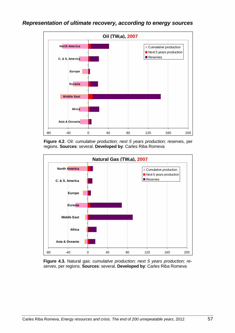
Carles Riba Romeva, Energy resources and crisis. The end of 200 unrepeatable years, 2012 57
Representation of ultimate recovery, according to energy sources
Petroleum (TWta), 2007
-80 -40 0 40 80 120 160 200
Asia & Oceania
Africa
Middle East
Eurasia
Europe
C. & S. America
North America Cumulative production
Next 5 years production
Reserves
Figure 4.2. Oil: cumulative production; next 5 years production; reserves, per regions. Sources: several. Developed by: Carles Riba Romeva
Natural gas (TWta), 2007
-80 -40 0 40 80 120 160 200
Asia & Oceania
Africa
Middle East
Eurasia
Europe
C. & S. America
North America Cumulative production
Next 5 years production
Reserves
Figure 4.3. Natural gas: cumulative production; next 5 years production; re-serves, per regions. Sources: several. Developed by: Carles Riba Romeva
Oil (TWta), 2007
Natural Gas (TWta), 2007

58 Carles Riba Romeva, Energy resources and crisis. The end of 200 unrepeatable years, 2012
Coal (TWta), 2007
-80 -40 0 40 80 120 160 200
Asia & Oceania
Africa
Middle East
Eurasia
Europe
C. & S. America
North America
Cumulative production
Next 5 years production
Reserves
Figure 4.4. Coal: cumulative production; next 5 years production; reserves, per regions. Sources: several. Developed by: Carles Riba Romeva
Uranium (TWta), 2007
-80 -40 0 40 80 120 160 200
Asia & Oceania
Africa
Middle East
Eurasia
Europe
C. & S. America
North America Cumulative production
Next 5 years production
Reserves
Figure 4.5. Uranium: cumulative production; next 5 years production; reserves, per regions. Sources: several. Developed by: Carles Riba Romeva
It is necessary to highlight that, in the four previous representations (figures from 4.2 to 4.5), the same scale has been maintained in order to make the perception of the importance of each of the resources in relationship to the others easier.
In the representation shown in figure 4.6, for the set of non-renewable energy resources, the scale has had to be enlarged.
Coal (TWta), 2007
Uranium (TWta), 2007

Carles Riba Romeva, Energy resources and crisis. The end of 200 unrepeatable years, 2012 59
Non-renewable energies (TWta), 2007
-200 -160 -120 -80 -40 0 40 80 120 160 200 240 280
Asia & Oceania
Africa
Middle East
Eurasia
Europe
C. & S. America
North America
Cumulative production
Next 5 years prodution
Reserves
Figure 4.6. Non-renewable energies: cumulative production; next 5 years produc-tion; reserves, per regions. Sources: several. Developed by: Carles Riba Romeva
Comments on the results of the cumulative production estimations, the future reserves and the ultimate recovery (table 4.3 and figures from 4.2 to 4.6).
Cumulative productions
1) The cumulative production of non-renewable sources of energy up to year 2007 (552,7 TWta) are, approximately, 1/3 of nowadays’ estimated ultimate recovery.
2) Oil’s cumulative production in relative terms is the most important among non-renewable sources of energy (206,1 TWta and the 44,4%); if the «political reserves» of oil are elimi-nated (OPEC increases during the 80s; inclusion of Canada’s oil sands; 479,1 of the 1.316,7 Mb, mega barrels, of year 2007), this percentage rises up to 54,8%. This would mean that we have already gone beyond peak oil.
3) The other three non-renewable fuel’s cumulative production is between the 26,7% and the 30,3% of the ultimate recovery, that is, an important part of the recoverable resources have already been consumed. The lowest percentage is that belonging to coal.
Resources exhaustion, by regions
4) Europe’s resources exhaustion clearly stands out. Of the European ultimate recovery of non-renewable energy sources (123,4 TWta, superior to those of Africa and South and Central America), almost 4/5 have already been exhausted (78,4%). And this is so in al-most all of the resources: oil (80,1%), coal (80,9%) and uranium (80,2%), and only natu-ral gas is excluded (62,5%).
5) In this sense, Europe is at the forefront of the world: the need of coal-free politics will be due to the lack of fossil fuels. At the moment, we keep consuming fuels from other regions: oil from the Middle East, natural gas from Russia and coal from Africa, but, as the world energy situation becomes more critical, Europe’s traditional economy will suffer.
6) In second place, North America stands out as it has consumed 2/5 parts of its ultimate reserves (40,1%). Although it has the highest ultimate reserves (413,3 TWta, almost 1/4 of the world, a 24,6%, for a population of a 6,7%), the non-renewable fuels cumulative production is of almost 1/3 of the world (30,0%; followed by Europe, with a 17,5%). It has exhausted a 85,1% of the conventional oil (eliminating the misleading non-conventional “oil sands” of Canada), 80,4% of natural gas and 50,5% of the uranium (in spite of Can-
Non-renewable energies (TWta), 2007

60 Carles Riba Romeva, Energy resources and crisis. The end of 200 unrepeatable years, 2012
ada’s excellent reserves). Only 74,8% of coal is left, even though almost the same amount than in Europe has been consumed (62,5 TWta).
7) Noteworthy cases are South & Central America and Africa: In spite of being quite unde-veloped regions having few ultimate reserves (67,7 and 113,3 TWta, a 4,0 and the 6,7% of the world’s total value, very much lower than their populations), have consumed im-portant amounts of their ultimate reserves (a 34,4 and a 30,4%), mainly for the profit of North America and Europe.
8) Asia and Oceania have important originated resources (311,2 TWta, and a18,5% of the world’s total amount), poorly spread for the profit of the low populated and rich Australia, that will hardly be able to cover the development needs of the 55,7% of the world’s popu-lation of this region. Almost all of the resources are of coal (81,8%). The level of exhaus-tion is of a 71,9% for oil, a 32,3% for natural gas, only a 23,7% for coal (ultimate recovery of 236,3 TWta), and a 11,4% for uranium (mainly in Australia).
9) Finally, in this unequally distribution of energy resources in the world, two regions (Mid-dle East and Eurasia) accumulate a 38,7% of the ultimate recovery of energy, with a 7,2% of the world’s total population. Also, they have the more strategic fuels: the 54,4% of the total amount of oil (202,0 TWta in the Middle East and 50,5 in Eurasia) and 61,1% of natural gas (95,4 TWta in the Middle East and 93,5 in Eurasia). Eurasia also has sig-nificant resources of coal and the first worldwide resources of uranium (27,1%). These two regions also have the worldwide lower exhaustion levels (a 20,7% in the Middle East and a 24,7% in Eurasia).
Non-renewable energy exhaustion’s sequences
Below you can see the worldwide energy resources exhaustion sequence which has been done following the assumptions of figure 4.1 (increases of consumption predicted by the EIA-govUSA). But now we include the cumulative productions.
Non-renewable energy in the world: cumulative production,
next 5 years production, and future reserves (TWtA), 2007
-1800 -1600 -1400 -1200 -1000 -800 -600 -400 -200 0 200 400 600 800 1000 1200
Uranium
Coal
Natural gas
Oil
Non-renewables
Cumulative production
Next 5 year production
Reserves
Figure 4.7. Non-renewable energies in the world, 2007: cumulative production, next 5 year production and reserves. Sources: several. Developed by: Carles Riba Romeva
Non-renewable energy in the world: cumulative production,
next 5 years production and future reserves (TWta) 2007

Carles Riba Romeva, Energy resources and crisis. The end of 200 unrepeatable years, 2012 61
Non-renewable energy in the world: cumulative production,
next 5 years production, and future reserves (TWta), 2017
-1800 -1600 -1400 -1200 -1000 -800 -600 -400 -200 0 200 400 600 800 1000 1200
Uranium
Coal
Natural gas
Oil
Non-renewables
Cumulative production
Next 5 years production
Reserves
Figure 4.8. Non-renewable energies in the world, 2017: cumulative production, next 5 year production and reserves. Sources: several. Developed by: Carles Riba Romeva
Non-renewable energy in the world: cumulative production,
next 5 years production, and future reserves (TWta), 2027
-1800 -1600 -1400 -1200 -1000 -800 -600 -400 -200 0 200 400 600 800 1000 1200
Uranium
Coal
Natural gas
Oil
Non-renewables
Cumulative production
Next 5 years production
Reserves
Figure 4.9. Non-renewable energies in the world, 2027: cumulative production, next 5 year production and reserves. Sources: several. Developed by: Carles Riba Romeva
Non-renewable energy in the world: cumulative production, next 5 years production and future reserves (TWta) 2017
Non-renewable energy in the world: cumulative production, next 5 years production and future reserves (TWta) 2027

62 Carles Riba Romeva, Energy resources and crisis. The end of 200 unrepeatable years, 2012
Non-renewable energy in the world: cumulative production,
next 5 years production, and future reserves (TWta), 2037
-1800 -1600 -1400 -1200 -1000 -800 -600 -400 -200 0 200 400 600 800 1000 1200
Uranium
Coal
Natural gas
Oil
Non-renewables
Cumulative production
Next 5 years production
Reserves
Figure 4.10. Non-renewable energies in the world, 2037: cumulative production, next 5 year production and reserves. Sources: several. Developed by: Carles Riba Romeva
Non-renewable energy in the world: cumulative production,
next 5 years production, and future reserves (TWta), 2047
-1800 -1600 -1400 -1200 -1000 -800 -600 -400 -200 0 200 400 600 800 1000 1200
Uranium
Coal
Natural gas
Oil
Non-renewables
Cumulative production
Next 5 years production
Reserves
Figure 4.11. Non-renewable energies in the world, 2047: cumulative production, next 5 year production and reserves. Oil will be exhausted (2046) and are ready to do natural gas and uranium. Sources: several. Developed by: Carles Riba Romeva
Non-renewable energy in the world: cumulative production, next 5 years production and future reserves (TWta), 2037
Non-renewable energy in the world: cumulative production, next 5 years production and future reserves (TWta), 2047
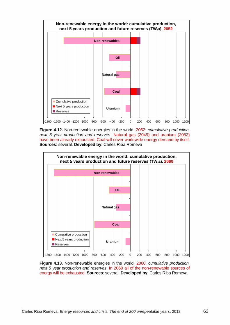
Carles Riba Romeva, Energy resources and crisis. The end of 200 unrepeatable years, 2012 63
Non-renewable energy in the world: cumulative production,
next 5 years production, and future reserves (TWta), 2052
-1800 -1600 -1400 -1200 -1000 -800 -600 -400 -200 0 200 400 600 800 1000 1200
Uranium
Coal
Natural gas
Oil
Non-renewables
Cumulative production
Next 5 years production
Reserves
Figure 4.12. Non-renewable energies in the world, 2052: cumulative production, next 5 year production and reserves. Natural gas (2049) and uranium (2052) have been already exhausted. Coal will cover worldwide energy demand by itself. Sources: several. Developed by: Carles Riba Romeva
PNon-renewable energy in the world: cumulative production,
next 5 years production, and future reserves (TWta), 2060
-1800 -1600 -1400 -1200 -1000 -800 -600 -400 -200 0 200 400 600 800 1000 1200
Uranium
Coal
Natural gas
Oil
Non-renewables
Cumulative production
Next 5 years production
Reserves
Figure 4.13. Non-renewable energies in the world, 2060: cumulative production, next 5 year production and reserves. In 2060 all of the non-renewable sources of energy will be exhausted. Sources: several. Developed by: Carles Riba Romeva
Non-renewable energy in the world: cumulative production, next 5 years production and future reserves (TWta), 2052
Non-renewable energy in the world: cumulative production, next 5 years production and future reserves (TWta), 2060

64 Carles Riba Romeva, Energy resources and crisis. The end of 200 unrepeatable years, 2012
4.3. Peak production of fuels
Indeed, technology and economy can have influence on the obtaining of energy resources, but not in the determinant way that both the economical conceptions and the anthropocen-tric view presuppose.
Nature has its own laws, and if we do not bear them in mind, it ends up reminding them to us in some way or another. There have been many civilizations in Earth that have declined or disappeared due to the exhaustion of the resources in their environment. Until now, they have moved or have been replaced by other civilizations in other places with new resources to be exploited.
The problem that we have nowadays is that humanity is exceeding the capacity of the Earth’s resources, which becomes apparent in many ways (ecological footprint, declining of resources, climate change).
There are different limits in relation to non-renewable energy resources, among which we can find the production peak and the decrease of the energy return on investment (EROI) below a certain threshold.
Then, we focus on the first one.
The problem of “energy security” (in short term) is not only the exhaustion of reserves, but also the limit of the production rhythm. And here is where the Hubbert’s peak theory comes into play.
In 1956, M.K. Hubbert, a worldwide recognized geophysicist and Shell oil company consult-ant, predicted that oil production in the United States would reach its maximum value (peak or zenith) around 1970 and that afterwards it would start to decline. With time this prediction has proven to be of a remarkable exactitude.
Figure 4.14. Correlation between Hubbert’s predictions and oil production in USA. Source: Wikipedia (Hubbert peak theory)
Hubbert’s peak theory, which was initially developed to predict oil production in the United States, establishes that the extraction of oil (or of a resource of similar nature) in a geo-graphical area which is of the appropriate dimensions, follows a curve in the form of a sym-

Carles Riba Romeva, Energy resources and crisis. The end of 200 unrepeatable years, 2012 65
metric bell, that has its maximum peak when half of the reserves have been extracted. From this moment, the production starts to decline until it becomes exhausted.
This theory has a growing acceptance and has originated the international association ASPO (Association for the Study of Peak Oil & Gas), with important national organizations in more than 25 countries of all continents and that, among others, incorporates well-known scien-tists and retired technicians belonging to the main oil companies.
In March 1998, Colin Campbell, a retired geologist of the BP (British Petroleum) oil company, and Jean Laherrère, a retired oil engineer of Total, a French oil company (which is an actual member of the ASPO) published a scientific report in the Scientific American under the title of “The End of Cheap Oil” (<http://dieoff.org/page140.pdf>, [Cam-1998]) where, among others, they argued that new discoveries are more and more less frequent and that they tend to an asymptotic value which is not very much higher than actual reserves.
The estimation of the ultimate recovery
One of the arguments of main hydrocarbon companies in order to calm the public opinion down on the theme of energy resources is that there are still many reserves to be discov-ered [WEO-2009].
The ultimate recovery (that include the resources extracted from the beginning of the extrac-tion, the current reserves and the future discoveries until the exhaustion of the resource), in which Hubbert theory is based, are not easy to evaluate. Probably, who has most and better worked in order to solve this question (where new evaluation criteria is needed) is J. Laher-rère, the energy consultant and retired engineer of the French oil company Total.
Figure 4.15. Cumulative discoveries (1860-2007), except USA and Canada. It ex-cludes USA and Canada due to the huge amount of oil wells (the ownership is linked to the property of the land) that do not make these countries comparable with the situation of the rest of the world. Source: J. H. Laherrère [Lah-2009]
Initially, he based his method on the creaming curves, developed by the oil company Shell during the 80s, based on the New Field Wildcat (NFW). However, dealing with the difficulty of obtaining information from the historical oil wells, Laherrère established a relationship be-

66 Carles Riba Romeva, Energy resources and crisis. The end of 200 unrepeatable years, 2012
tween the cumulative discoveries (of crude oil or natural gas) and the number of fields of these fuels (figure 4.15).
The resulting curves tend towards a series of limits from which Laherrère [Lah-2009] infers the value of the last oil and natural gas ultimate recovery (that is to say, the set formed by the extracted resources and those that can be extracted during the fields’ entire life cycle). In figure 4.15 it is shown that these amounts are of 1.750 Gb (109 barrels) for oil and of 8.700 Tcf (1012 cubic feet) for natural gas, to which we must add 65 Gb and 180 Tcf belonging to USA and Canada.
Estimation of the different fuels’ peak oil
Oil and liquid fuels’ peak
J. Laherrère has published several studies about the evolution of energy resources’ produc-tion, specially oil and liquid fuels. A good summary of his estimations and conclusions was the work that he presented with J-L. Wingert during the VII ASPO annual Conference in Barcelo-na [Lah-2008].
Figure 4.16. Previsions made by J. Laherrère [Lah-2008] about the peak oil. An-nual liquid fuel production with logistic models for ultimate recovery of 2,7 Tb, 3 Tb and 4Tb (Tb = 1012 barrels), considering reasonable restrictions without social ten-sions and without important and fast price increases (no above ground con-
straints). Source: J. Laherrère, JL. Wingert [Lah-2008]
Figure 4.16 summarises Laherrère’s estimations and predictions for liquid fuels, for which it is necessary to evaluate the corresponding ultimate recovery (including the already con-sumed oil, the discovered reserves and the ones that are still to be discovered) of all of the different types of liquid fuels, both natural and synthetic. Laherrère distinguishes between:
Cheap oil:
Conventional oil (green line), without extra-heavy oil (EH). The thick line is the already consumed oil and the thin line is the production’s previsions. According to Lahèrrere, the peak oil took place in year 2006, with 71 Mb/d for ultimate reserves of 2 Tb. The decline will force, around 2060, conventional oil to be residual.

Carles Riba Romeva, Energy resources and crisis. The end of 200 unrepeatable years, 2012 67
Natural gas plant liquids (NGPL), mainly propane and butane (gases that are extract-ed with natural gas, easily liquefiable at low pressures). The inferior thick line (purple) shows consumption until the present time. The blue superior thick line shows the consumption of conventional oil and NGPL, with a maximum amount of 85 b/d around 2009 (according to the figure, it is almost the peak oil). The previsions for the whole of the liquid fuels (continuation of the blue curve) are studied later on.
Expensive oils: as we reach the peak oil, it is desired to substitute conventional oil with other unconventional liquid fuels. Mainly:
Extra-heavy oil, extracted from Canada and Venezuela, with last resources of 0,5 Tb.
Synthetic oils: biomass-to-liquid (BTL), gas-to-liquids (GTL) and coal-to-liquid (CTL) trans-formations.
As well as the conventional oil ultimate recovery (2 Tb), Laherrère establishes three sce-narios with different unconventional oils ultimate recovery values: the minimum one with 0,7 additional Tb; the medium one with 1 additional Tb and the superior one with 2 addi-tional Tb. Unconventional oils need more investments and their exploitation is slower than that of conventional oils (evolution according to the inferior bell curves in red colour, 0,7 Gb; purple, 1 Gb and orange, 2 Gb).
It could seem that the different scenarios of ultimate recovery (2,7 3 and 4 Tb) would make the peak oil vary considerably. However, if the evolution of conventional and un-conventional oils’ production is added up, we obtain very similar peaks (in value and date) and the only variations are given at the posterior evolution at the beginning of the declining process (decreasing superior curves, continuation of the thick blue curve).
A model without unusual restrictions (such an economic crisis) places the peak of liquid fuels (conventional and unconventional) between years 2010 and 2015 with a value that is close to 85 Mb/d. We will need to be aware of the worldwide production evolution. In the last five years, it has been of: 84,59 Mb/d (2005); 84,65 Mb/d (2006); 84,52 Mb/d (2007); 85,45 Mb/d (2008); 84,37 Mb/d (2009).
The estimations of main energy agencies (EIA-govUSA and IEA-OECD), always growing (black lines in figure 4.16), come into flagrant contradiction with Hubbert’s model and Lahèrrere’s estimations (and of many other authors who have carried out similar stud-ies), and it seems that they will never be possible.
Demand pressure, technological improvements and investment effort can modify, within limits, the value and the moment of peak oil, but its declining process will inevitably take place, and the fall will be more sudden if we have forced it beyond its natural limit.
The peak oil and its posterior declining process will have important economical conse-quences. Due to the fact that liquid fuels are the basis of transport and have a very diff i-cult substitution (see chapter 5), it will not be possible to maintain the globalization based on the segmentation of productions in faraway places and that allows well-being socie-ties to enjoy of products coming from many parts of the world at any time. Therefore, it represents a ceiling to economy’s generalized growth in the way that it is growing nowa-days.
Nowadays, declining of oil is a reality in many countries of the world. As well as USA, many other countries have gone beyond the peak oil: Venezuela (1970), Libya, (1970), Canada (1974), Indonesia (1977), Egypt (1993), India (1995), Syria (1995), Argentina (1998), the United Kingdom (1999), Australia (2000), Norway (2001) and Mexico (2004). The main Persian Gulf’s countries situation is not well known, but it is thought that their peak oil is not far.

68 Carles Riba Romeva, Energy resources and crisis. The end of 200 unrepeatable years, 2012
Peak gas (or peak natural gas)
In a similar way to oil and liquid fuels, J. Laherrère also makes an estimation of the peak gas, or natural gas production’s peak (figure 4.17).
Figure 4.17. As a result of J. Laherrère’s estimation of peak gas for ultimate re-covery of 10.000 Tcf where, in addition to consumption, he considers natural gas’ reinjection in crude oil wells, non-conventional gases and losses (included losses from burners). Source: ASPO-France [Lah-2008]
According to this estimation done by J. Laherrère, the world peak gas will take place in 2020 for a production of 135 Tcf/a (1012 cubic feet per year). Only in ten years! As a reference, the worldwide productions of the previous years, according to the EIA, are: 100,08 Tcf/a (2005), 103,42 Tcf/a (2006), 105,77 Tcf/a (2007), 109,79 Tcf/a (2008) and 106,47 Tcf/a (2009).
It is interesting to state, again, that the growth previsions that have been carried out by the large energy agencies (EIA-govUSA and IEA-OECD) for natural gas during the following years (black lines of figure 4.17) do not seem to reflect the reality.
Diminishing new discoveries
Some of the new deposits that have been recently discovered seem to confirm these trends:
Tupi (Brazil). In 2006 Brazil discovers, at 265 km from the coast, the large deposit of Tupi, with reserves of between 5 and 8 Gb (millions of millions of barrels) that require a drilling at more than 2.000 meters of depth, and a very complicated commercial exploitation. Tak-ing the highest value of this estimation, it represents the 0,61% of the worldwide oil re-serves, that is, 94 days of this fuel’s consumption (around 3 months).
Repsol (Venezuela). In 2009, Repsol finds large natural gas deposits in Venezuela, with reserves of between 190.000 and 226.000 Mm3 (millions of cubic meters). The highest value of this estimation represents the 0,11% of the worldwide natural gas reserves, that is, 25 days of this fuel’s consumption (less than a month).

Carles Riba Romeva, Energy resources and crisis. The end of 200 unrepeatable years, 2012 69
Truly, these resources are of great importance for the countries where they are found and for the exploitation companies, but they represent a negligible contribution to the supply at a worldwide scale.
Peak coal
Although Laherrère also does an estimation of the peak of the worldwide coal production, we have chosen to reproduce that one made by the Energy Watch Group [WEG-2007], more in line with the sources used in our study for this fuel (figure 4.18).
Figure 4.18. It shows an estimation of the evolution of the global production of coal and its peak, realized by Energy Watch Group. At the same time, it also shows the evolution of the main producing countries where the coal is separated into bitumi-nous and sub-bituminous. Source: WEG [WEG-2007]
This estimation is done in tones of oil equivalent (TOE). The production peak is found ap-proximately between 2025 and 2030 for a maximum production of 3.650 TOE/a (4,85 TWt). According to the EIA, coal production in the previous years (turned into energy) have been of 4,116 TWt (2005), 4,269 TWt (2006), 4,440 TWt (2007) and 4,572 TWt (2008). As in the previous cases, the estimates carried out by the IEA-OECD [WEO-2006] following the actual consumption trend (black superior line of figure 4.18) will not be able to reflect reality.
Therefore, although coal reserves are the most important, the peak production will come relatively soon and at a value that is not much higher than the current production. However, the declining process will be softer and more prolonged than in the case of liquid fuels. This estimate is in line with the perception that the WEC (World Energy Council) reserves are overblown.
It is interesting to observe that the worldwide peak coal will be preceded by the peak coal in China; in this case, with a quite quick declining process. Therefore, the miracle of the Chi-nese growth (based on a 75% in coal energy produced in this country) has a relatively close expiration date.

70 Carles Riba Romeva, Energy resources and crisis. The end of 200 unrepeatable years, 2012
Peak of uranium
The cumulative production of uranium in 2007 was of 2.194 millions of tones of natural urani-um (ktUnat = GgUnat), while the reserves estimated by the Red Book 2007 (NEA-IAEA) were of 5.468 GgUnat for that same year.
The Watch Energy Group [WEG-2006] presents a projection of the future evolution of the natural uranium production (figure 4.19) where the peak of natural uranium is shown.
Figure 4.19. Watch Energy Group estimate of the past and future evolution of worldwide natural uranium’s production and its peak, where the influence of con-sidering several types of reserves according to their cost is shown. The measure-ment unit that has been used is the kilo tonnes of natural uranium (ktUnat). Source: WEG [WEG-2006]
The historical evolution of uranium’s production has already shown two peaks, approximate-ly during the 60s and the 80s. It is necessary to bear in mind the influence of the production of fissile material for atomic bombs during the Cold War.
However, the most important is the peak of uranium related to the future depletion of that resource. According to the WEG estimations, for reserves of RAR+IR <130 $/kg (see chap-ter 8), this would take place between years 2030 and 2035 for a maximum production of 82 MgUnat/a (or ktUnat/a; figure 4.19).
As a reference, according to the World Nuclear Association (WNA), the production in the previous years has been of: 41,72 GgUnat/a (2005), 39,44 GgUnat/a (2006), 41,28 GgUnat/a (2007), 43,85 GgUnat/a (2008) and 50,77 GgUnat/a (2009). Although this is the most favoura-ble zenith, it is also the resource that less influences in covering the current consumptions.
General comment on peaks
The peak phenomenon does not mean that the resources will run out (like it was assumed in chapter 4, about projections and exhaustions). The peak production of the different fuels simply strangles the growth. It is a serious warning that will oblige us to change the para-digm of developing (from energy growth to energy decrease), but also extends the time for the inevitable restructuring.

Carles Riba Romeva, Energy resources and crisis. The end of 200 unrepeatable years, 2012 7
Index
Part 1 – Primary energy resources
1. Introduction 1.1 Motivation and point of view 1.2 Basic concepts about energy 1.3 Sources of information
1.4 Measurement units 1.5 New energetic accounting
2. Evolution of the worldwide energy consumption 2.1 Energy consumption of primary sources 2.2 Energy consumption by regions
2.3 Population and energy per capita
3. Non renewable energies’ reserves 3.1 Evaluation of the energy reserves 3.2 Analysis of the oil and natural gas reserves 3.3 Analysis of the coal reserves
4. Growth and projection 4.1 Divorce between growth projection and reserves 4.2 Vision from ultimate recovery 4.3 Peak production of fuels
Part 2 – Secondary (or intermediate) energies
5. Commercial fuels 5.1 From primary to secondary energies
5.2 Fuels from oil, gas and coal and their uses 5.3 Oil, strategic resource
6. Electricity 6.1 The electric system 6.2 Production and consumption of electricity
6.3 Characteristics and limitations of the electricity 6.4 New electric technologies
Part 3 – Alternative sources of energy
7. Unconventional fuels 7.1 Origin of fossil fuels
7.2 Increasing difficulty in the obtaining 7.3 Unconventional oils 7.4 Unconventional natural gas
7.5 Fuels obtained by transformation
8. The uncertain nuclear alternative 8.1 From military uses to civil uses 8.2 Evolution of nuclear energy production 8.3 Evaluation of uranium resources 8.4 Consumptions and impacts of nuclear energy
8.5 New nuclear technologies

Carles Riba Romeva, Energetic resources and crisis. The end of 200 unrepeatable years, 2012 71
Part 2
Secondary (or intermediate) energies
In previous chapters we have studied primary energies, that is, those energies that we ob-tain from nature. They are oil, natural gas, coal and uranium, which are found in the earth’s crust, but they also are geothermal energy, tidal power, solar power, and, indirectly, wind power, waterfalls, sea waves and biomass.
Primary energies cannot be used directly, they need to be transformed into useful (manipu-latable and controllable) secondary (or intermediate) energies in order to satisfy human needs. The main secondary energies are fuels and electricity.
It is necessary to distinguish between oil (primary energy) with its derivatives (petrol, gasoil, kerosene, propane, butane), or natural gas (primary energy which is bordered with rocks) with transformed gas products (compressed natural gas, CNG; liquefied natural gas, LNG), or sed-imentary coal rocks (primary energy) with solid transformed fuels (granulated of anthracite, coal, lignite, coke or briquettes of peat) which are used in the power station industries or at homes, or uranium ores (primary energy), with uranium fuel with which nuclear power stations obtain their energy.
In each of the previous cases more or less important transformations are needed in order to make sure energy use is effective. These processes are not free and many times imply en-ergy expenses and emissions of gases that affect climate. Therefore, energy that is involved in secondary sources is composed of two addends: useful energy that the resource provides and energy that is consumed in its obtaining. And, in a similar way, secondary source emis-sions are also composed of two addends: emissions in order to make energy effective (that normally refers to combustion) and emissions that are generated due to its obtaining.
There are two main secondary energy systems which are fuels and electricity.
Fuels form a big secondary (or intermediate) energy system. Normally they are oil, natural gas or coal products, but they can also come from biomass or waste materials. They are used in transport (especially the liquid ones), in heating and industrial processes.
Electricity is another secondary (or intermediate) energy, which is obtained by the trans-formation of different primary sources (fossil fuels, nuclear power, hydraulic energy, wind energy, solar energy, geothermal energy or biomass). It is a very versatile energy and one of the main means with which we can connect primary sources with a large diversity of needs: light, heat and cold, computer and information systems, activation of electrical ap-pliances and machines, industrial processes, and so on.
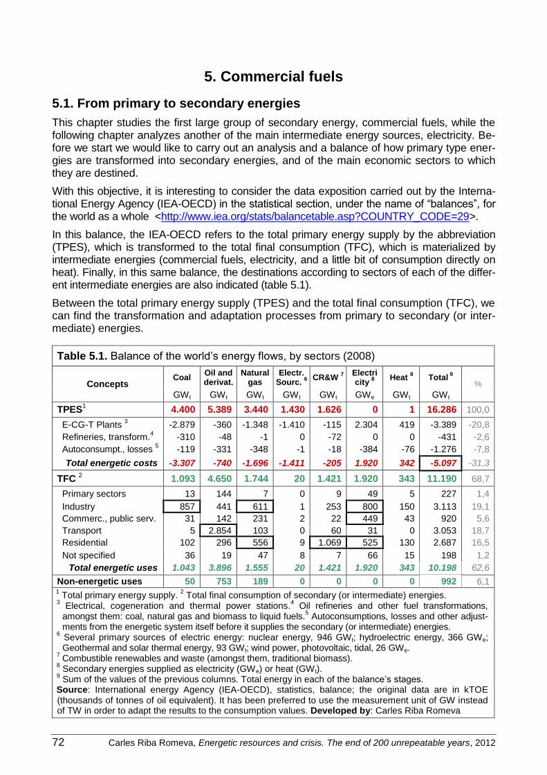
72 Carles Riba Romeva, Energetic resources and crisis. The end of 200 unrepeatable years, 2012
5. Commercial fuels
5.1. From primary to secondary energies
This chapter studies the first large group of secondary energy, commercial fuels, while the following chapter analyzes another of the main intermediate energy sources, electricity. Be-fore we start we would like to carry out an analysis and a balance of how primary type ener-gies are transformed into secondary energies, and of the main economic sectors to which they are destined.
With this objective, it is interesting to consider the data exposition carried out by the Interna-tional Energy Agency (IEA-OECD) in the statistical section, under the name of “balances”, for the world as a whole <http://www.iea.org/stats/balancetable.asp?COUNTRY_CODE=29>.
In this balance, the IEA-OECD refers to the total primary energy supply by the abbreviation (TPES), which is transformed to the total final consumption (TFC), which is materialized by intermediate energies (commercial fuels, electricity, and a little bit of consumption directly on heat). Finally, in this same balance, the destinations according to sectors of each of the differ-ent intermediate energies are also indicated (table 5.1).
Between the total primary energy supply (TPES) and the total final consumption (TFC), we can find the transformation and adaptation processes from primary to secondary (or inter-mediate) energies.
Table 5.1. Balance of the world’s energy flows, by sectors (2008)
Concepts Coal
Oil and derivat.
Natural gas
Electr. Sourc.
6 CR&W 7 Electri
city 8 Heat
8 Total
9
%
GWt GWt GWt GWt GWt GWe GWt GWt
TPES1
4.400 5.389 3.440 1.430 1.626 0 1 16.286 100,0
E-CG-T Plants 3
-2.879 -360 -1.348 -1.410 -115 2.304 419 -3.389 -20,8
Refineries, transform.4
-310 -48 -1 0 -72 0 0 -431 -2,6
Autoconsumpt., losses 5
-119 -331 -348 -1 -18 -384 -76 -1.276 -7,8
Total energetic costs -3.307 -740 -1.696 -1.411 -205 1.920 342 -5.097 -31,3
TFC 2
1.093 4.650 1.744 20 1.421 1.920 343 11.190 68,7
Primary sectors 13 144 7 0 9 49 5 227 1,4
Industry 857 441 611 1 253 800 150 3.113 19,1
Commerc., public serv. 31 142 231 2 22 449 43 920 5,6
Transport 5 2.854 103 0 60 31 0 3.053 18,7
Residential 102 296 556 9 1.069 525 130 2.687 16,5
Not specified 36 19 47 8 7 66 15 198 1,2
Total energetic uses 1.043 3.896 1.555 20 1.421 1.920 343 10.198 62,6
Non-energetic uses 50 753 189 0 0 0 0 992 6,1 1 Total primary energy supply.
2 Total final consumption of secondary (or intermediate) energies.
3 Electrical, cogeneration and thermal power stations.
4 Oil refineries and other fuel transformations,
amongst them: coal, natural gas and biomass to liquid fuels.5 Autoconsumptions, losses and other adjust-
ments from the energetic system itself before it supplies the secondary (or intermediate) energies. 6 Several primary sources of electric energy: nuclear energy, 946 GWt; hydroelectric energy, 366 GWe; Geothermal and solar thermal energy, 93 GWt; wind power, photovoltaic, tidal, 26 GWe.
7 Combustible renewables and waste (amongst them, traditional biomass).
8 Secondary energies supplied as electricity (GWe) or heat (GWt).
9 Sum of the values of the previous columns. Total energy in each of the balance’s stages.
Source: International energy Agency (IEA-OECD), statistics, balance; the original data are in kTOE (thousands of tonnes of oil equivalent). It has been preferred to use the measurement unit of GW instead of TW in order to adapt the results to the consumption values. Developed by: Carles Riba Romeva

Carles Riba Romeva, Energetic resources and crisis. The end of 200 unrepeatable years, 2012 73
The conversion from primary to secondary energies is what the automobile industry has called WTT (well-to-tank), that entails important processes and costs, both of resources and of energy.
Nevertheless, it is so easy to fill up the fuel tank in the gas station just around the corner, or, even more, switch an electric appliance or turn the heat on, that people belonging to devel-oped countries have tendency to ignore or underestimate these resources.
Comparison between table 5.1 and 2.1
The data from table 5.1 (IEA-OECD, in GW), and from table 2.1 (EIA-govUSA, in TW), has been obtained from different sources of information and apply non coincident accounting criteria. Therefore, the studied values are not the same, and there is an overall global differ-ence of 1.581 GWt out of the total of 17.876 GWt (- 8,85% according to IEA-OECD’s data).
This disparity is in a 50% due to the different criteria used by the IEA-OECD and the EIA-govUSA. The first agency adds up the thermal primary energies (from fuel, natural gas, coal, uranium, geothermal, solar thermal and residuals), with electric energies (already trans-formed, and, therefore, secondary) that come from primary hydraulic sources and other re-newable electric sources (wind, photovoltaic and tidal power).
If, as it is done by the EIA-govUSA, we had counted the non-thermal electric energies as equivalent primary energy (thermal energy that would have been necessary in order to pro-duce them; by a factor of three), the IEA-OECD’s hydroelectric primary energy would be modified from 366,3 GWe (remark 6 in table 5.1) to 1.098,8 GWt, with an increase of de 732,5 GWt, and wind power, photovoltaic energy and tidal power would be modifies from 26,4 GWe (remark 6 in table 5.1) to 79,1 GWt with an increase of 52,7 GWt. In total, an ap-proximation of 785,2 GWt.
The other half of the disparity is due to the IEA-OECD’s lower evaluations of fossil fuels, of which I do not know the cause: -331 GWt in oil; -369 GWt in natural gas, and -172 GWt in coal.
Data Analysis of table 5.1
Table 5.1 provides us with a lot of information about the world energetic system. Some of the most outstanding observations are:
Secondary energies’ generation
1. Electricity has very high generation costs. If we deduct 392 GWt that are obtained from non-thermal sources (a 17% of the total; table 5.1, remark 6), thermal losses in the gen-eration (3.389 GWt) are much higher than the generated electrical energy (2.304 - 392 = 1.912 GWe). If we also add the part related to autoconsumptions and losses (inseparable considering the data available in table 5.1), we get closer to the formula 1 We = 3 Wt.
2. Combustible adaptation (extraction, washing, distillation, transport, transformation, liqua-tion and compression, depending on the fuels) has a direct energetic cost which is much lower than that belonging to electricity (about 431 GWt in total). But then we have to add the corresponding part in relationship to autoconsumption and losses.
3. Generally transformation from primary to intermediate energies (WTT, according to car industry) has a very high cost of 5.097 GWt. (31,3% of primary energy). The main cause is electrical generation.
4. 3.307 GWt of coal (75% of the source) and 1.696 GWt of natural gas (49,3% of the source) is destined to electricity generation and primary fuels’ adaptation and transformation. Also 740 GWt of oil (13,7% of the source) and 205 GWt of combustible renewables and waste (12,6% of the source) are destined to these transformations.

74 Carles Riba Romeva, Energetic resources and crisis. The end of 200 unrepeatable years, 2012
Final energy consumption
5. In final consumptions, the use of liquid fuels in transportation is highlighted (2.854 GWt, a 61,4% of the consumed resource, a 93,5% of transport consumption). This use, which in-creases with time, is dispersed in space and it does not allow CO2 sequestration.
6. In second place, the consumption of traditional biomass in undeveloped countries’ homes (1.069 GWt, a 75,2% of the final renewable fuels and residuals’ consumptions), is also to be considered. This amount highlights the importance of firewood, coal and farming and animal residues, specially for undeveloped countries and their more than 2.600 million in-habitants.
7. Residual coal from electrical production is used mainly in industry (857 GWt, a 82,2% of coal for final uses). On the other hand, the amount of natural gas that is destined to final uses is higher (1.744 GWt), but it has a more disperse distribution in which industrial uses (611 GWt), residential uses (556 GWt) and commercial and service uses (231 GWt),are the most remarkable ones, whilst only 103 GWt are destined to transportation.
8. Even though the amount of electricity (1.920 GWe) is lower than that of the liquid fuels that are obtained from oil (4.650 GWt), as it is a high quality energy that needs about three times more primary energy during its obtaining, it is the intermediate energy that needs of a higher effort. We can find the highest electrical consumption in industries (800 GWe, equivalent to approximately 2.400 GWt), followed by domestic use (525 GWe, equivalent to approximately 1.575 GWt), and commercial and service use (449 GWe, equivalent to approximately 1.337 GWt).
9. It is important to highlight that primary economic sectors (and, specially, agriculture) origin quite small direct energy consumptions worldwide (227 GWt, which corresponds to a 1,3% of primary energies and a 2,0% of secondary energies). Nevertheless, fertilizers and pesti-cides produce other consumptions that must also be considered, which are the energy spent in industrial processes and in raw materials.
10. Finally, non-energetic uses of fossil fuels are relatively important (992 GWt, 6,1% of prima-ry sources), and those based on oil and its products clearly stand-out from the rest (753 GWt, the 75,9% of these sources).
5.2. Fuels from crude oil, gas and coal and their uses
Fossil fuels (crude oil, natural gas and coal) are the world’s actual economical basic ener-getic sources. According to the EIA-govUSA (table 2.1), they, all together, represented al-most a 80% (78,93%) of the primary energy that was consumed in 2008. Of this percentage, 32,02% corresponds to oil (which has decreased in value), while 21,32% belongs to natural gas and 25,59% to coal (both of them have increased in value).
All the other primary energy sources together at a worldwide scale (that is, hydroelectric power, nuclear power, traditional biomass, biofuels, energy from residues and new renewa-ble energy sources) sum up 21,07%, value which is a little bit lower than that of natural gas, which is the less consumed fossil fuel.
And this tendency has not changed significantly during the last 30 years (almost), in which fossil fuel use has gone from 82,12% in 1980 to 78,93% in 2008 (a decrease of -3,195, that is almost recovered by nuclear power +2,64%).
What has significantly changed during this period is the distribution between the fossil fuels: crude oil decreases more than ten percentage points (-10,21%), while natural gas increases almost four points (+3,96), and coal increases approximately three points (+3,06%, with an accelerated increase during the last years).

Carles Riba Romeva, Energetic resources and crisis. The end of 200 unrepeatable years, 2012 75
As it has been seen in the previous section, fossil fuels are used in almost all economic sec-tors, out of which we would like to highlight two remarkable uses:
- Crude oil products are used massively and almost exclusively in different means of transport (by road, by air, by sea and in less proportion, by railway). This will be ana-lyzed in the following section.
- Coal, and natural gas (with increasing values in the previous years), are some of the principal bases of electric generation.
Crude oil products
Crude oil, as it is taken from oil well, has impurities and volatile elements, which make it un-suitable even for burning in boilers. But, on the other hand, it is formed by a mixture of high value hydrocarbons, that when conveniently separated and refined, provide fuels for differ-ent internal combustion engines, and also raw material for petrochemical processes that are used in the manufacture of plastics, elastomers, lubricants, solvents, detergents, textile fi-bers, fertilizers, pesticides, etc.
Different types of crude oil are classified according to their density in ºAPI (American Petro-leum Institute). Light oils (> 31,1º API) and with low content of sulphur are the easiest to re-fine (like for example Brent in the North Sea, or WTI, West Texas Intermediate). Medium-weight crude oils have API gravities of between 22,3 and 31,1 °API; heavy crude oils of be-tween 10 and 22,3 °API; and extra-heavy crude oils have lower gravities than 10°API.
Fractional distillation
It is used to separate different hydrocarbons of oil. It is a physical separation process that uses heat and consists of evaporation of crude oil (mixture of liquids with different but similar boiling points) in an oven, to make it pass through a distillation tower with crosswise plates at different heights with pass-through holes. While the steam goes up the tower it becomes cooler, and fractions with decreasing boiling points start condensing and liquids are decant-ed in each of the plates. Many times a second distillation tower is used, with a pressure that is lower than atmospheric pressure, in order to achieve better refining.
Figure 5.2 is a scheme of fractional distillation. It shows principal fractions (hydrocarbon groups with similar chain length and boiling points), with ranks of temperatures and of chain lengths, and an estimation of the obtained percentages, as well as the main uses of each one of them.
Table 5.2. Fractional distillation and oil products
Fraction Temp. ºC Chain % 1
Applications
Liquefied gases 20 to 40 C1 to C5 7 Gas cylinders
Naphta 70 to 120 C5 to C9 10 Chemistry
Petrol 120 to 160 C5 to C10 40 Automobiles
Kerosene 160 to 250 C10 to C16 8 Aviation
Diesel 260 to 330 C14 to C20 24 Automobiles
Lubricants 300 to 370 C20 to C50 1 Lubrication
Heavy oils 360 to 400 C20 to C70 4 Boats, Power plants
Asphalts, residues > 400 > C50 6 Roads
1 These proportions vary a lot depending on the cracking process and the posterior reformation process.
Sources: Figure from the Wikipedia; other sources. Developed by: Carles Riba Romeva
crude oil
oven

76 Carles Riba Romeva, Energetic resources and crisis. The end of 200 unrepeatable years, 2012
Before entering the unit of distillation, there normally is an elimination of mineral salts, and after the distillation different processes can take place like for example:
Cracking
The fraction of fuel that is obtained from the simple distillation of fuel is normally lower than the demand, while in other longer chain fractions the contrary phenomenon occurs. The cracking process has been developed in order to avoid this kind of imbalances. It is based on high-temperature heating of hydrocarbons under pressure, normally using a catalyst, and some-times in hydrogen atmosphere, in such a way that long chains are fractioned into shorter chains that are similar to those found in petrol.
Catalytic reformation
It is an additional chemical treatment that uses temperature, pressure and different catalysts, and that has the objective to break lineal hydrocarbon chain links and convert them into branched out chains (for example isooctane, that provides higher efficiency in internal com-bustion engines, higher octane rating), or create alkenes (double-link hydrocarbons), which are used in the manufacture of plastics for polymerization, or in the creation of aromatic com-pounds, which are the raw material of many petrochemical products.
Refining
In all distilled products, it is necessary to eliminate impurities in order to obtain quality prod-ucts, fit for consumption.
Natural gas
It is a primary energy resource consisting of a mixture of light gases in which methane prevails (normally more than 80%, sometimes it can reach 95%), but it also contains other gases in different proportions, which normally are useless or pollutant, like for example nitrogen, heli-um, carbon dioxide (CO2), and hydrogen sulphide (H2S).
Natural gas is found in many ways in deposits: a) as associated gas in oil wells, either in the upper layer or dissolved in liquid; b) as non-associated gas when there is almost no oil in oil wells. In this last case, there are: the only natural gas oil wells (dry gas), and the oil wells that combine natural gas with low molecular weight hydrocarbons, which can be condensed (called condensed of natural gas).
Conditioning
Natural gas is not used directly as it leaves the well, it undergoes many purification processes. Some of the components of the gas that is obtained from the well are separated from the mix-ture, either because they don’t have energetic capacity (nitrogen and CO2) or because they can make its use difficult (CO2 would interfere in the cryogenic liquation process).
On the other hand, hydrocarbons with larger molecular weight (propane, butane) are separat-ed, condensed and commercialized separately, due to the fact that their presence could be dangerous during the natural gas combustion process. At high pressures and close to atmos-pheric temperatures, methane hydrates can block the conductions; therefore, water vapour is also eliminated. Finally, sulphur compounds are reduced to very low levels, in order to avoid corrosion in facilities, and to prevent acid rain effects.
To alert families in case of gas leaks, traces of compounds of mercaptans, with a characteris-tic smell, are added to the mixture.
Storage and transport
In environmental conditions, natural gas occupies very large volumes, which is the main diffi-culty for its storage and transport.

Carles Riba Romeva, Energetic resources and crisis. The end of 200 unrepeatable years, 2012 77
The two main ways in which natural gas is transported at a long-distance are: gas pipelines and conversion to liquefied natural gas. Both ways need complex facilities and important en-ergetic expenses, this fact makes natural gas less appealing.
On the other hand, a percentage of gas leaks are normally unavoidable during its transport and manipulation. This fact considerably decreases the advantage of the lower natural gas CO2 emissions during combustion (we must remember that methane’s greenhouse effect is 25 times larger than that of CO2, which is why in oilfields or oil rigs in which natural gas can not be reused, it is burned).
Vehicle propulsion application
Natural gas’ application as vehicle’s fuel has the disadvantage that it occupies a large volume in atmospheric conditions. It must either be compressed at a high pressure or liquefied in cry-ogenic conditions. This adds complexity and important masses in storage systems that make natural gas less attractive in comparison to liquid fuels.
Coals
As it will be seen later on (chapter 7), this resource is formed mainly because of the burial of large masses of vegetable matter which origins layers of coal inserted into layers of mineral sediments. These layers have kept their original localizations (without migrations like oil or natural gas), but they can have suffered a posterior process of folding or other geological modifications.
There are two main types of coal deposits: those in which layers of coal come to the surface, and give way to open pit mines, and those that are deeper in and origin underground mines.
Open pit mines
In these deposits, where giant excavators pull off the superior layers of land where the veins of coal and the layers of sterile material are found, the exploitation is distributed in descending steps with a maximum depth of 400 meters and it progressively grows in extension. Opencast exploitations have the following characteristics as main advantages: their quick implementa-tion, their high resource recuperation (up to the 90%, in comparison to a maximum 50% in underground mines), their more moderate exploitation cost and their less dangerous working conditions, but also their higher environmental and landscape impact.
Figure 5.1. Open pit mine in Latrobe Valley, Australia, with an excavator. Source: http://www.theage.com.au/environment/brumbys-dirty-secret-coal-for-export-20091013-gvnp.html

78 Carles Riba Romeva, Energetic resources and crisis. The end of 200 unrepeatable years, 2012
Open pit mines are becoming more frequent, especially in the United States, Canada, Austral-ia, and in less importance, Eurasia and South Africa, which, comparatively, make less efficient subterranean exploitations.
Underground mines
Nowadays it is still the most frequent exploitation method. In all facilities there is a main well with an elevator for mineworkers and another one for materials, and a second ventilation well in order to renew the air and avoid the accumulation of explosive gases (the much feared fire-damp).
In the inferior part of the mine, there is system of transversal galleries, at different levels, which are vertically connected between them, that allows access to the veins of the mineral and communicate them with the main well where coal will be extracted. To avoid the galleries from collapsing, pillars are left in each layer, which limits maximum extraction of coal to the 50%. Transport of materials in the inside of the mine is normally done using wagons, and in more modern facilities, also with conveyor belts.
With depth, exploitation difficulties and costs increase: temperature increases (at 1000 meters, approximately 30ºC), and firedamp elimination (in fact, methane) is becoming more expen-sive. Exploitation limit is of 1.500 meters, but most mines work in lower depths, between 100 and 500 meters. The proportion of coal in geological formation, and the width and inclination of the veins, are factors that affect costs. Modern technical exploitation methods increase the advantages of the most favourable mines in comparison with the less favourable mines.
Commercialized coals
Coal is always mixed with materials that decrease its quality and make its use difficult. There-fore, once the material is extracted from the mine, and before it is commercialized, physical crushing and washing processes have to be followed.
There are three types of coal (chapter 7): a) bituminous coals, with high heating values, like for example coal and coke coal (anthracite is also included); b) subbituminous coals, with moderate heating values, and higher moisture and ash content; c) lignite, which are the less developed coals, with low heating values and with more moisture and ash content.
But coals that are pulled off from the earth’s core are also distinguished by the conditions and the quality of the presentation [Mer-2007]. There are four commercial categories of noble coals (<10% in ashes) according to the grain size: 1) with a dimension ranged between 20 and 120 mm; 2) with a dimension ranged between 6 and 20 mm; 3) fine grain coals, with par-ticles from 1 to 10mm big; and 4) powdered form coals, with particles that can even be 100
m small. Other classifications such as: coals without grain size, which contain from powder to big chunks; mixed coals, with a 20-30% in ashes; crude coal, as it is extracted from the mine; secondary coals, proceeding from cleaning processes and containing a 40% in ashes; or, re-covered coals, coming from decantation ponds or previous residues; are also used.
Main secondary fuels’ characteristics
Table 5.3 shows the main characteristics of commercialized secondary fuels. It gives us the following information:
1) Density
2) Mass energy, both the energy consumed in its obtaining and the energy that is propor-tioned during its combustion (LHV, lower heating value, subtracting the heat of evapo-ration of water vapour), or in the fuel’s entire lifecycle
3) Volumetric energy, as in the previous point (MJ/litre o MJ/m3)
4) Emissions of CO2, both during its obtaining and during the combustion, or in the whole lifecycle.

Carles Riba Romeva, Energetic resources and crisis. The end of 200 unrepeatable years, 2012 79
Table 5.3. Main characteristics of commercialized secondary fuels
Fuel Density Volum. Energy
Massic energy 1 Emissions (CO2 equivalent) 2
obtaining LHV lifecycle obtaining LHV lifecycle
Liquid kg/litre 1
MJt/litre MJt/kg MJt/kg 2 MJt/kg gCO2/MJt gCO2/MJt gCO2/MJt
Petrol 0,745 32,2 6,0 43,2 49,2 12,5 73,4 85,9 Diesel 0,832 35,9 6,9 43,1 50,0 14,2 73,2 87,5 Kerosene (aviation) 0,720 31,5 4,8 43,7 48,5 9,8 71,2 81,0 LPG (propane, butane) 0,550 24,8 5,4 45,1 50,5 7,9 65,7 73,6 Biodiesel (soy) 0,890 32,8 43,8 36,8 80,6 -28,9 76,2 47,3 Ethanol (sugar cane) 0,794 21,3 48,0 26,8 74,8 -60,9 71,4 10,5 Ethanol (beetroot) 0,794 21,3 34,8 26,8 61,6 -41,7 71,4 29,7 Ethanol (corn) 0,794 21,3 34,8 26,8 61,6 -20,8 71,4 50,6 LGN (liquid) 0,428 19,3 14,0 45,1 59,1 19,9 56,2 76,1 Liquid hydrogen (NG) 0,071 8,5 135,7 120,1 255,8 126,3 0,0 126,3
Gas kg/m 3 MJt/litre MJt/kg MJt/kg
2 MJt/kg gCO2/MJt gCO2/MJt gCO2/MJt
Hydrogen (NG) 0,090 0,0108 119,3 120,1 262,2 104,7 0,0 104,7 Hydrogen (of coal) 0,090 0,0108 198,8 120,1 340,8 232,8 0,0 232,8 Hydrogen (electrolysis) 0,090 0,0108 342,2 120,1 482,4 203,8 0,0 203,8 Natural gas (EU-mix) 0,777 0,0350 6,0 45,1 56,2 8,4 56,2 64,6 Natural gas (Siberia) 0,777 0,0350 15,1 45,1 65,3 21,7 56,2 77,9
Solid Mg/m 4 MJt/litre MJt/kg MJt/kg MJt/kg gCO2/MJt gCO2/MJt gCO2/MJt
Anthracite 1,105 32,6 2,8 29,5 32,3 15,8 96,8 112,6 Bituminous 0,833 23,2 2,6 27,8 30,4 15,8 87,3 103,1 Subbituminous 0,816 16,2 2,4 19,9 22,3 15,8 90,3 106,1 Lignite 0,801 11,9 2,4 14,9 17,3 15,8 91,6 107,4 Pit 0,350 4,6 1,0 13,0 14,0 10,0 106,0 116,0 Firewood 0,425 6,0 1,1 14,0 15,1 -85,0 93,0 8,0 Charcoal 0,250 7,4 26,5 29,5 56,0 640,0 145,0 785,0 1
The values of the LHV (lower heating value) corresponding to liquid and gas fuels have been obtained from [WTW-WTT1-2007] and those from solid fuels from the IPCC (coals) and FAO (pit, firewood and charcoal). The energy that is consumed in the obtaining of these fuels has been calculated from [WTW-WTT2-2007].
2 The emissions of the liquid and gas fuels’ combustion have been obtained from [WTW-WTT2-2007]and those from solid fuels, from [IPCC-2005], annex 1, page 398 (except for charcoal). The emissions that are generated in the obtaining of liquid and gas fuels have been obtained from [WTW-WTT2-2007]; and those that correspond to solid fuels have been estimated by the author using the data from [WTW-WTT2-2007].
3 The values for the liquid fuels’ densities have been obtained from [WTW-WTT2-2007].
4 The values from solid fuels’ densities have been obtained from the IPCC.
Sources: [WTW-WTT1-2007], [WTW-WTT2-2007], [IPCC-2005], FAO. Developed by: Carles Riba Romeva
Energy converters and efficiency
One of the main aspects of current developed societies is the development of a great variety and diversity of energy convertors in order to transform primary energy into a useful form of energy, mainly into electricity (electric generators) and into mechanic energy (different types of motors).
Sometimes transformation chains are complex. For example, mechanic energy used in an elevator uses energy from an electric motor that obtains energy from electricity generated by the mechanical energy produced by a turbine that transforms thermodynamical energy from water vapour that has received energy from a combustion energy reaction from the energy from the chemical links of a fuel. And, in each one of these steps, energy expenses reduce the process’ efficiency.
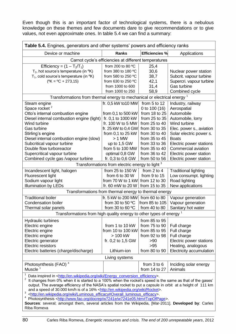
80 Carles Riba Romeva, Energetic resources and crisis. The end of 200 unrepeatable years, 2012
Even though this is an important factor of technological systems, there is a nebulous knowledge on these themes and few documents dare to give recommendations or to give values, not even approximate ones. In table 5.4 we can find a summary:
Table 5.4. Engines, generators and other systems’ powers and efficiency ranks
Device or machine Ranks Efficiencies % Applications
Carnot cycle’s efficiencies at different temperatures
Efficiency = (1 – T2/T1) from 200 to 80 ºC 25,4 T2, hot source’s temperature (in ºK) from 380 to 180 ºC 30,6 Nuclear power station T1, cold source’s temperature (in ºK) from 580 to 250 ºC 38,7 Subcrit. vapour turbine
(ºK = ºC + 273,15) from 630 to 250 ºC 42,1 Supercri. vapour turbine from 1000 to 600 31,4 Gas turbine from 1000 to 250 58,9 Combined cycle
Transformations from thermal energy to mechanical or electrical energy 1
Steam engine fr. 0,5 kW to10 MW from 5 to 12 Industry, railway Space rocket 2
0 to 100 (16) Aerospatial Otto’s internal combustion engine from 0,1 to 500 kW from 18 to 25 Automobile Diesel internal combustion engine (light) fr. 0,1 to 1000 kW from 25 to 35 Automobile, lorry Wind turbine fr. 100 W to 5 MW from 25 to 40 Wind turbine Gas turbine fr. 25 kW to 0,4 GW from 30 to 35 Elec. power s., aviation Stirling’s engine from 0,1 to 25 kW from 30 to 40 Solar electric power s. Diesel internal combustion engine (slow) > 1 MW from 35 to 45 Boats Subcritical vapour turbine up to 1,5 GW from 33 to 36 Electric power stations Double flow turboreactor from 5 to 100 MW from 35 to 40 Commercial aviation Supercritical vapour turbine optimal 0,8 GW from 36 to 42 Electric power station Combined cycle gas /vapour turbine fr. 0,3 to 0,6 GW from 50 to 56 Electric power station
Transformations from electric energy to light 3
Incandescent light, halogen from 25 to 150 W from 2 to 4 Traditional lighting Fluorescent light from 6 to 30 W from 9 to 15 Low consumpt. lighting Sodium vapour light from 70 W to 1 kW from 12 to 30 Road lighting Illumination by LEDs fr. 60 mW to 20 W from 15 to 35 New applications
Transformations from thermal energy to thermal energy
Traditional boiler fr. 5 kW to 200 MW from 60 to 80 Vapour generation Condensation boiler from 30 to 50 ºC from 85 to 105 Vapour generation Thermal solar panels from 30 to 60 ºC from 40 to 80 Sanitary hot water
Transformations from high quality energy to other types of energy 1
Hydraulic turbines from 85 to 95 Electric engine from 1 to 10 kW from 75 to 90 Full charge Electric engine from 10 to 100 kW from 85 to 95 Full charge Electric engine > 100 kW from 92 to 98 Full charge Electric generator fr. 0,2 to 1,5 GW >90 Electric power stations Electric resistors >95 Heating, analogous Electric batteries (charge/discharge) Lithium-ion from 80 to 90 Electricity accumulation
Living systems
Photosynthesis (FAO) 4 from 3 to 6 Inciding solar energy Muscle 1 from 14 to 27 Animals 1 Data inspired in <http://en.wikipedia.org/wiki/Energy_conversion_efficiency>.
2 It changes from 0% when it is started to a 100% when the rocket’s speed is the same as that of the gases’
output. The average efficiency of the NASA’s spatial rocket to put a capsule in orbit at a height of 111 km and a speed of 30.000 km/h is of a 16% <http://en.wikipedia.org/wiki/Rocket>.
3 <http://en.wikipedia.org/wiki/Luminous_efficacy#Overall_luminous_efficacy>.
4 Photosynthesis <http://www.fao.org/docrep/w7241e/w7241e05.htm#TopOfPage>.
Sources: several; amongst them, several articles from the Wikipedia, [Mar-2011]. Developed by: Carles Riba Romeva

Carles Riba Romeva, Energetic resources and crisis. The end of 200 unrepeatable years, 2012 81
Comments on table 5.4:
1. Carnot’s cycle (thermal cycle in reversibility conditions that is based on the temperature of the hot and cold sources, T1 and T2 in ºK) gives energetic efficiencies which are not much higher than those of real machines, which means that, in general, they are techni-cally well optimized, with a high energetic efficiency (the exergy would be the maximum theoretical mechanical energy that could be obtained).
2. All machines that convert thermal energy (or from a compressible gas) into mechanical energy have low efficiency: internal combustion engines, gas and vapour turbines, turbo-jets, and also wind turbines.
3. Transformations between mechanical and electrical energy normally have high efficiency and losses are usually determined by auxiliary elements. Therefore, electric generators (from mechanic to electrical energy) and electric engines (from electrical to mechanic energy) normally have efficiencies that are superior than 80%, that increase with the ma-chine’s dimensions and the regularity of the velocities and the charges in relationship to the nominal working point.
5.3. Oil, a strategic resource
When we compare oil (liquid) with the other fossil fuels, either gas (natural gas), or solid (coal), we can clearly see the advantage of oil, especially when it comes to transport.
Conventional oil (45,3 MJ/kg and 38,87 MJ/litre, density of 0,858 kg/litre), its products (pet-rol, gasoil, kerosene), and liquid oil gases (LPG, mainly propane and butane) are high ener-getic fossil fuels that, due to their liquid nature, are easy to transport, manipulate and store in quite safe conditions.
Green house effect gas emissions, 68,0 gCO2/MJ, are found between natural gas, less pol-lutant, and coal, more pollutant.
These advantages of liquid fuels have made their market be a global worldwide one (export-import fuel relationships are approximately, half of the production), and has made oil be-come our main energetic reference (it has become frequent to reduce the measures that are made in other energetic sources to TOEs, tonnes of oil equivalent).
Table 5.5. Characteristics of the main primary fossil fuels
Fuels Density Energetic content Greenhouse effect gases
Mg/m3 MJ/kg MJ/litre kgCO2/kg kgCO2/MJ
Natural gas gas 0,00072 48,3 0,0348 2,250 0,0502 liquid 0,45 48,3 21,7 2,250 0,0502
Crude Oil global 0,82 44,8 36,76 2,800 0,0620 conventional 0,858 45,3 38,87 3,100 0,0680 Liquidized gas 0,55 50,0 27,25 3,000 0,0600
Coal global 1,32 21,92 28,9 1,950 0,0896
Remark: the values that are in bold have been obtained calculating them from the data given in the EIA-govUSA’s tables. Sources: EIA-govUSA and others. Developed by: Carles Riba Romeva
In a simplified manner, conventional ratios are established between the measurements of vol-ume and mass of some fuels and their energetic content. For example: 1 TOE (tonne of oil equivalent) = 10.000 Mcal = 41,868 GJ; 1 TCE (tonne of coal equivalent) = 0,7 TOE = 7.000 Mcal = 29,308 GJ; or also 1 tUnat (tonne of natural uranium) = 10.000 TEP = 418,68 TJ.

82 Carles Riba Romeva, Energetic resources and crisis. The end of 200 unrepeatable years, 2012
In table 5.5 the values that have been obtained as a worldwide average, in 2008, of the cor-responding fuels (EIA-govUSA) have been marked in bold. That is to say, they are meas-ured values (or estimated from measures).
High energetic density
Below, you can see different examples that show the great energetic density of oil, that nor-mally passes unnoticed:
Example 1 (how could we substitute oil?)
Ramon Sans Rovira, a good friend and engineer peer, let me know that he had considered (and, due to the results, discarded), the following energy accumulation system:
It was based in a tower that was adjacent to a building (of, for example, 20 meters) with a big similar to a tower clock weight. Photovoltaic panels would produce energy during the day, and, using a little engine, the weight would be elevated. Then, the engine, working as a generator, would give electric energy as the weight would go down. It is a conceptually very interesting idea, but numbers need to be calculated.
They are the following: 1 litter of petrol contains a technical primary energy of 32,2 MJt (ta-ble 5.3) that, when transformed to mechanical energy (with an efficiency of the 25% of a thermal engine), gives 8,05 MJ (8.050.000 J). If the weight of the tower has a mass of 1.000 kg (equivalent to the mass of a small automobile, 9.800 N), this energy would allow the elevation of the mass-automobile up to 821,4 meters of height! And a deposit, of 40 li-tres of gasoline, would allow to elevate it up to the stratosphere, 32.857,1 meters! Imagine an automobile that has been elevated 821 meters with only 1 litre of gasoline: how could we substitute gasoline?
Exemple 2 (accumulate and transport energy)
We have got used to the autonomy that conventional thermal motor automobiles give us, as well as the simplicity and speed at which we fill up the gas tank.
Indeed, an automobile with a full gas tank (40 litres, or 29,8 kg of gasoline, and a thermal energy of 1.288 MJt, table 5.3) can cover a distance of 600 km and obtain a mechanic en-ergy on the wheel of 75 kWh. Then, with this same energy on the wheel, with an electric propulsion system (efficiency battery-road of 0,75), batteries of 100,0 kWh would be need-ed. Lead-acid batteries (0,035 kWh/kg) would weigh 2.857,1 kg and those of lithium-ion (0,150 kWh/kg), about 666,7 kg, instead of 29,8 kg of gasoline.
On the other hand, the time needed to refuel (approximately 120 seconds for each 40 litres of gasoline) represents a thermal power of 1.288 MJt/120 s = 10,62 MWt that, in terms of electric power (with a reduction factor of 1/3) would be of 3,54 MWe. That is a huge power, about 1.000 times higher than that of a family home (3,5 kWe)! Therefore, the battery re-charge of an electric automobile is not only a technical matter of the batteries, but also and mainly of the electric supply.
Also, it is important to remember that behind the plug there is an electric system that, in a big proportion (electrical mix), the only thing that it does is use, in a remote way, the large amount of thermal energy that mainly comes from fossil fuels.
Example 3 (feed people or automobiles?)
An adult person’s average consumption of food is of 3.000 kcal/d, which is equivalent to 12.558 MJt/d; therefore, the energy of one litre of gasoline would energetically feed three persons during one day.
The World’s liquid fuel consumption is of 85 Mb/d (million barrel per day; 1 barrel = 159 li-tres), that would be equivalent to the food consumption of a population of 40.500 million inhabitants, that is, almost 6 times the total worldwide population of about 6.800 million in-habitants.

Carles Riba Romeva, Energetic resources and crisis. The end of 200 unrepeatable years, 2012 83
Oil versus all the other fossil fuels
Alternative fuels to oil, natural gas and coal, have several disadvantages that are analyzed below:
Natural gas versus oil
Natural gas has a very low energetic density (0,0348 MJt/litre, about 1.000 times lower than that of oil). This involves expensive and voluminous treatment, manipulation and transport facilities.
Natural gas transport is either done by bulky and vulnerable gas pipelines, or if not it needs to be liquidized. This last alternative entails, firstly, the need to eliminate some impurities, and then, cool natural gas up to -161 ºC at little above atmospheric pressure (cryogenic tanks at origin and destination points, cryogenic ships for transport). And, in spite of it all, the resulting energetic density of liquid natural gas (LNG) is a 60% of that of oil (21,7 MJt/litre).
All of this makes the worldwide natural gas market be much more reduced than that of oil. This low energetic density also makes its application to vehicles and transport difficult. How-ever, it produces low CO2 emissions (0,0502 kgCO2/MJt), which boosts its application in co-generation and combined cycles.
Coal versus oil
Coal, which had been the main fuel at the beginnings of the industrial era, is now becoming more prominent due to the decline of oil, especially in those countries with important stocks (China, India and the USA).
Coals also have serious disadvantages. Their energetic density is inferior to that of oil (the average amount of coal produced in the world is between 22 MJt/kg and 29 MJt/litre), and, due to the fact that it is not liquid, the extraction, manipulation and transport are less effi-cient. Furthermore, it is not only the fossil fuel that produces more greenhouse effect gases (0,0896 kgCO2/MJt), it is also the one that produces the most dangerous local pollution (emissions, acid rain).
Oil and transport alternatives
These characteristics have as a consequence that oil and its byproducts (gasoline, kero-sene, gasoil) are very difficult to replace in all transport systems, both for passengers and merchandise transportation systems (automobiles, buses, trucks, vans, planes, boats and in a lower proportion, railways).
If we ever run out of oil, how will we make cars run? How will boats do their long-distance travels? How will airplanes take off? When we don’t have enough oil, how will we hold global economy firm?
The decline of oil will put our society in a very difficult situation and will make our working system end in a crisis. Oil is the base of transport (automobiles, trucks, planes, boats), and of alimentation (tractors and agriculture machinery, fertilizers, pesticides, fodder, agriculture and cattle products’ transport, posterior transformations, containers), as well as the main part of other activities.
Alternatives are very complex. As it will be seen in part 3, one of them is to prolong the ac-tual liquid fuel era: it is the non-conventional fuel strategy (extra-heavy fuels, oil sands, oil shale) and the liquid transformation strategy, (CTL or coal to liquid; GTL or gas to liquid), but these strategies will also be living in borrowed time. And the liquid biofuel strategy (BTL or biomass to liquids) is clearly not enough to maintain our actual lifestyle.
Other strategies need important social and technological transformations, like reorientation in front of new non-renewable energies.

84 Carles Riba Romeva, Energetic resources and crisis. The end of 200 unrepeatable years, 2012
6. Electricity
6.1. The electric system
Apart from little isolated autonomous systems, almost all of the generated and used electric energy is transmitted through large geographical zones by interconnected electrical nets (at a country scale, or in a lower scale, regionally and internationally).
Different generation centres provide the energy that they produce (power stations and nuclear power stations, hydroelectric power stations, wind farms, solar energy farms and, lately, a lot of small industrial and private generators), in the same time that different users take energy when needed (they turn on the light, connect electrical appliances, communication systems and computer appliances, make machines and other industrial processes work).
Unlike fuels, electric energy has several determinant particularities that are mentioned be-low. Later on, after analyzing electrical consumption’s evolution in the last 28 years, we will stop to analyze its significance and consequences, in detail.
These particularities are:
1. Energy may not be accumulated
Electricity is consumed (it has to be consumed) in the same moment that it is generated, and is mainly non-accumulative. Because of this, one of the main problems in the man-agement of the electrical net is to make sure that important demand changes (second to second) coincide with the generation system as a whole.
2. It participates in a mix
Interconnection through a net makes it impossible to distinguish the origin of electric en-ergy. Consumption participates in a mix that combines the different generation systems (thermal, nuclear, hydroelectric, wind, photovoltaic, geothermal), and it is necessary to count the average efficiency and emissions of CO2 of the system as a whole.
3. Low generation efficiencies
Most of the world’s electricity (81%) is obtained from thermal power (fossil fuels, nuclear power, renewable fuels and geothermal energy), with an average efficiency, that, with distribution expenses, is below 1/3. This is not a consequence of a poor management, but of the majorly used technologies (vapour turbines) and the rules that thermodynamic cycles follow.
4. High quality energy
It is a high quality energy because it can be transformed with high efficiency rates (nor-mally higher than a 80%) and it is also very versatile. Mechanical energy is also of a very high quality, while those that act as thermal energy (chemical, nuclear, solar and ther-mal) are considered to be low quality energies. Therefore, low efficiency rates of global electric energy obtaining processes must be considered.
6.2. Production and consumption of electricity
Table 6.1 is a summary of the world’s electric system’s components.
Firstly, the primary energy that is consumed to produce electricity in its thermal equivalent is indicated. Then, the generated electrical energy is indicated (as it leaves the power station) and its components: coming from conventional thermal energy (fossil fuels), from nuclear power stations, from hydroelectric power stations, from non-hydroelectric renewable systems (geothermal, wind, photovoltaic solar, solar power stations, of waves and tides, and so on).

Carles Riba Romeva, Energetic resources and crisis. The end of 200 unrepeatable years, 2012 85
Later on, losses due to distribution in electric lines are indicated and, finally, the electric con-sumption is shown (the plug at home or in the industry). It is necessary to highlight the low global efficiency of electric systems (last lines of table 6.1): generation efficiency (B/A) and global efficiency (D/A, consumed energy/primary energy).
Table 6.1. Evolution of the worldwide electric system, according to the primary sources
Energy 1980 % 1985 1990 1995 2000 2005 2008 %
Primary equiv. (TWt) A 2,807 3,328 3,966 4,382 5,018 5,863 6,387
Generation (TWe) B 0,915 100,00 1,080 1,289 1,438 1,663 1,980 2,181 100,00
Conventional thermal 0,638 69,71 0,690 0,815 0,889 1,060 1,308 1,469 67,38
Nuclear 0,078 8,54 0,163 0,218 0,252 0,280 0,301 0,297 13,62
Hydroelectric 0,197 21,49 0,223 0,245 0,280 0,299 0,330 0,356 16,33
Renewable not hydr. 0,004 0,38 0,006 0,014 0,019 0,027 0,043 0,061 2,80 Hydraulic pumping -0,001 -0,12 -0,001 -0,002 -0,002 -0,003 -0,003 -0,003 -0,13
Distrib. losses (TWe) C 0,079 0,091 0,104 0,128 0,158 0,183 0,189 Consumption (TWe) D 0,836 0,988 1,186 1,310 1,506 1,797 1,991
1980=100 100,0 118,2 141,8 156,7 180,0 214,9 238,2
Efficiency B/A (We/Wt) 0,326 0,324 0,325 0,328 0,331 0,338 0,341
Efficiency D/A (We/Wt) 0,298 0,297 0,299 0,299 0,300 0,306 0,312
% losses (C/B)·100 8,60 8,45 8,06 8,88 9,49 9,25 8,68
Source: EIA-govUSA. Developed by: Carles Riba Romeva
Figure 6.1 graphically represents the main data from the previous table. The evolution of the used primary energy, the generated electricity (as it leaves the power station), the consumed electricity (user’s plug) and, amongst the generated electricity, the renewable part and the negligible part that corresponds to not hydraulic renewable energies; are represented accord-ing to their corresponding values.
Worldwide elesctric system (TWt and TWe)
0,0
1,0
2,0
3,0
4,0
5,0
6,0
7,0
1980 1985 1990 1995 2000 2005
Used primary energy (TWt)
Produced electricity (TWe)
Consumed electricity (TWe)
Produced renewable electricity (TWe)
Prod. renew. non-hydraulic electr. (TWe)
Figure 6.1. Electric system’s evolution. Relationship between the used primary energy (or equivalent), the generated electricity and the consumed electricity (the difference corresponds to the distribution losses). It also shows the generated electricity from re-newable sources, and from new non-hydroelectric renewable sources. Source: EIA-govUSA. Developed by: Carles Riba Romeva.
Worldwide electric system (TWt and TWe)
86 Carles Riba Romeva, Energetic resources and crisis. The end of 200 unrepeatable years, 2012
To make table 6.1 and figure 6.1, and add the electricity productions from different origins (thermal, nuclear, wind, photovoltaic, geothermal), they have all been turned to equivalent thermal primary energy (criterion adopted by the EIA-govUSA, but not by the IEA-OECD).
Many electrical power stations use thermal energy (coal, natural gas, nuclear energy, geo-thermal, waste combustion, biomass) to generate electricity, and, then, it is not difficult to add energy as primary fuel energy. But, when it is wanted to add electricity from hydroelec-tric, wind or photovoltaic systems, where there is no thermal energy involved, we don’t have a common measurement unit.
An example of the food market can illustrate this aspect very well: everybody knows that it is not the same to purchase 1kg of chicken breast (in our case, the electricity), that to buy the full animal (in our case, the primary energy). The equivalence is on the price (out of the total animal, we obtain a fraction: the chicken breast).
In the same way, for the electricity obtained from non-thermal primary sources, it is conven-tionally established that 1 unit of electric energy is equivalent to 3 units of thermal energy (global efficiency of electric generation thermal power stations). This is the reason why, in the data from the EIA-govUSA, the world hydroelectric (in primary equivalent) and nuclear energy are of the same order of magnitude (16,35% and 13,67%, respectively) while, in data from the IEA-OECD, hydroelectric energy (in We) is about three times lower than nuclear energy (in Wt).
In this book the first criteria of equivalent energies has been adopted.
Data from table 6.1 and the graphical representation in figure 6.1 allow us to comment the following:
1) The most important aspect of the world’s electric system is that the efficiency be-tween the electric energy as it leaves the power station and the primary thermal en-ergy as it enters the system is of a 34,1% (a 65,9% of the primary energy is lost, mainly as thermal energy), efficiency which has improved during the last 28 years (from 32,6 to 34,1%).
2) The electric energy that the user receives is still lower due to the losses in the electric distribution lines (at a worldwide scale, a 8,68% of the electric energy as it is leaves the generation stations). Therefore, average world efficiency of electric energy at home’s plug or at the factory is of a 31,2%.
3) Therefore, the use of electric energy implies a very low generation efficiency, even though the posterior electric energy use can be very efficient. Specifically, the use of electrical energy to generate heat (electric heating, water heaters, kitchens, vapour generators) normally implies one of our energetic system’s biggest inefficiencies, as it starts from a global thermal-electric energy efficiency of the 31,2%, to later on give heat again.
4) Most of the world’s electricity is obtained from non-renewable fuels (81,00%) and is majorly obtained from fossil fuels (67,38%) and, the rest, from nuclear energy (13,62%), as well as renewable energies in a smaller amount (biomass, residues...). This is the main reason of the system’s low efficiency. At least the 67,38% of the world’s electric energy is associated to intense CO2 emissions, due to the combustion of fossil fuels (at a high proportion, coal).
5) The amount of electricity that is obtained from renewable energies is of a 19,13%, mainly from hydroelectric energy (16,35%). Even though they have quickly increased, new renewable electric energy sources (wind, geothermal, thermal solar, photovoltaic solar, wave and tidal power) only generated 2,80% of the world’s total electricity gen-eration in 2008.

Carles Riba Romeva, Energetic resources and crisis. The end of 200 unrepeatable years, 2012 87
6) It is necessary to negatively highlight that, during the studied 28 years, renewable energies have lost importance in the electric system (from 21,87% in 1980 to 19,13% in 2008, which represents a decrease of the 2,76%). The increase of new renewable energies (our greatest hope) has not made up for the loss of importance of hydroe-lectric energy (-5,16%).
Worldwide consumption’s evolution and regional distribution
The production and consumption of electricity has a faster evolution than that of the total energy consumptions. We would only like to record this fact and its regional distribution, in order to analyze its consequences later on in the book. Table 6.2 shows the production and consumption evolution of electricity, by regions.
Table 6.2. Evolution of the electric consumptions, by regions
1980 % 1985 1990 1995 2000 2005 2008 %
Electric consumptions in GWeh/a
North America 2.461,0 33,6 2.779,0 3.371,6 3.753,1 4.257,9 4.544,7 4.658,7 26,7
S. & C. America 269,8 3,7 350,0 420,6 523,0 649,1 767,1 873,5 5,0
Europe 2.006,0 27,4 2.280,2 2.526,3 2.640,4 2.941,9 3.230,5 3.361,3 19,3
Eurasia 1.168,6 16,0 1.382,5 1.460,9 1.074,4 1.031,9 1.139,3 1.244,9 7,1
Middle East 84,5 1,2 150,1 204,6 285,2 385,1 520,7 629,7 3,6
Africa 170,4 2,3 222,3 277,6 317,1 367,3 472,9 525,2 3,0
Asia & Oceania 1.162,8 15,9 1.494,4 2.123,6 2.882,7 3.551,4 5.063,4 6.151,5 35,3
World 7.323,1 100,0 8.658,4 10.385,2 11.476,0 13.184,7 15.738,7 17.444,8 100,0
Electric consumptions in TWe
North America 0,281 33,61 0,317 0,385 0,428 0,486 0,519 0,532 26,71
S. & C. America 0,031 3,68 0,040 0,048 0,060 0,074 0,088 0,100 5,01
Europe 0,229 27,39 0,260 0,288 0,301 0,336 0,369 0,384 19,27
Eurasia 0,133 15,96 0,158 0,167 0,123 0,118 0,130 0,142 7,14
Middle East 0,010 1,15 0,017 0,023 0,033 0,044 0,059 0,072 3,61
Africa 0,019 2,33 0,025 0,032 0,036 0,042 0,054 0,060 3,01
Asia & Oceania 0,133 15,88 0,171 0,242 0,329 0,405 0,578 0,702 35,26
World 0,836 100,00 0,988 1,186 1,310 1,505 1,797 1,991 100,00
Electric consumptions: growth indexes (1980=100)
North America 100,0 112,9 137,0 152,5 173,0 184,7 189,3
S. & C. America 100,0 129,8 155,9 193,9 240,6 284,4 323,8
Europe 100,0 113,7 125,9 131,6 146,7 161,0 167,6
Eurasia 100,0 118,3 125,0 91,9 88,3 97,5 106,5
Middle East 100,0 177,6 242,1 337,5 455,7 616,2 745,2
Africa 100,0 130,4 162,9 186,0 215,5 277,5 308,1
Asia & Oceania 100,0 128,5 182,6 247,9 305,4 435,4 529,0
World 100,0 118,2 141,8 156,7 180,0 214,9 238,2
Source: EIA-govUSA; Developed by: Carles Riba Romeva
In the first place, it is important to comment the significantly larger increase of electric con-sumption in relation to the general energy consumption (index of 238,2 instead of 172,2).
But if the individual increases of each of the world’s regions is analyzed, some of them are outstanding and affect some of the most populated areas of the planet. Middle East’s grow-ing factor is of 745,2; that of Asia and Oceania is of 529,0; that of South and Central Ameri-ca is of 323,8 and that of Africa is of 308,1. All of these regions more than triple their electric consumption.

88 Carles Riba Romeva, Energetic resources and crisis. The end of 200 unrepeatable years, 2012
Truly, access to electricity is one of the main developing indexes of any society and there is still a very important part of humanity that does not have access to it. Specifically, 1.441 mil-lions of people, a 21,1% of the world’s population, according to the data supplied by the IEA (WEO 2010, or <http://www.iea.org/weo/electricity.asp>), territorially distributed as follows:
Table 6.3. Inhabitants with no access to electricity
Minhab % population1
Latin America 31 6,6 Middle East 22 10,5 Sub-Samarian Africa 585 69,5 China and Eastern Asia 186 9,2 Southern Asia 612 37,8 Rest of the World 5
World 1.441 21,1 1 Percentage over the population of each of the different geographic ambits.
Source: IEA-OECD, International Energy Agency (WEO 2010)
Considering the near decline of energetic fossil resources, several questions are brought up in relationship to electricity: how can we provide electricity to this 21,1% of the world’s popu-lation (1,5 times the population of developed countries) that still does not have it? Will the “everything-electric” tendency of developed countries be sustainable? Up to what point are developing countries (especially China) doing it correctly when it comes to electricity? Later on we will retake some of these questions.
6.3. Characteristics and limitations of the electricity
Below we will analyze some of the electrical system’s characteristics (already stated in the introduction) and their implications, more specifically.
1. Non-accumulative energy
Electricity is produced at the same time that it is consumed. The accumulation systems by means of reversible hydraulic dams or, most recently, the prevision of accumulation in batteries of the future electric automobile farm, require highly considerable investments, and they can only accumulate a small amount of the total generated energy.
Effectively, worldwide hydraulic pumping represented a 0,13% in 2008 (table 6.1); the transformation of a 10% of the Spanish automobile park of 2008 into electric (2,2 million units) with a circulation of 15.000 km/a, would accumulate the 2,3% of the electric energy generated in Spain.
For this reason, one of the main problems in the management of the electric net is to make important demand variations coincide (minute to minute) with the generation sys-tems as a whole. Nuclear power energy, due to its scarce flexibility, and wind and photo-voltaic energy, due to their variability, are the energies that give more difficulties.
In order to illustrate the management of the electric net, evolution of the electricity gener-ation structure in Spain is shown. This is in real time and is granted by the Spanish Elec-tric Net (REE).
Two dates have been chosen: the 5th of May of 2010, very windy, with the coal thermal power stations almost not functioning, and combined cycle natural gas power plants working at mid power adjusting themselves to the demand; and the 14th of September of 2010, not at all windy (specially in late hours of the day when demand is higher), in which thermal coal power stations and combined cycle stations were put into operation.
Note that:
a) Nuclear electricity generation is practically constant and is prioritized in front of other thermal power stations. This lack of flexibility makes nuclear energy to keep away from

Carles Riba Romeva, Energetic resources and crisis. The end of 200 unrepeatable years, 2012 89
the generation and demand adjustment process at the same time as it moves the ineffi-ciencies towards other components of the system.
b) Wind energy is totally variable and has to be exploited when it is produced.
c) Thermal power stations (especially those of combined cycle) are the main resource that the electric system counts with in order to adjust the generation to the demand.
Figure 6.2. Structure of the real time electric generation, according to the REE (<https://demanda.ree.es/generacion_acumulada.html>, on the 5th may 2010), spe-cially windy day (44,8% of wind power generation at 3.00 h). Source: REE (5/5/2010).
Figure 6.3. Structure of the real time electric generation, according o the REE (<https://demanda.ree.es/generacion_acumulada.html>), on the 14th September 2010, scarcely windy day (3,1%, at 20.50 h). Source: REE (14/09/2010)

90 Carles Riba Romeva, Energetic resources and crisis. The end of 200 unrepeatable years, 2012
2. It participates in a mix
The interconnection through an electric net makes the electrical energy be of an un-known origin. Both electric energy generators and electric consumers supply or remove energy from the net, where it is impossible to know the origin or destination of each kWh. Therefore, final consumers cannot say that they are consuming wind energy or any other specific source of energy, but they have to count the average efficiency and the system’s CO2 emissions.
Below, in table 6.4, the different origins of electricity and the different efficiencies in dif-ferent parts of the world are shown. Data from other three countries which we have found interesting is also included (USA, China and Spain), according to the EIA (none of these regions or countries that exchange more that a 1,5% of their electrical production, except for Spain, that does so in a 3,75%). The electric mix is the combination of the dif-ferent electric generation systems (thermal, nuclear, hydroelectric, wind, photovoltaic, geothermal...), and it is directly linked to CO2 emissions.
Table 6.4. Origin of electric energy, by regions (mix from 2008, in %)
Regions and countries
thermal nuclear hydroe-lectric
renew. not-hydr.
net effi-ciency
distribut. losses
total effi-ciency
% % % % We/Wt % We/Wt
North America 65,43 18,10 13,45 3,15 0,339 6,79 0,316 S. and C. America 31,02 2,01 63,90 3,09 0,344 16,14 0,289 Europe 52,91 25,13 15,64 6,68 0,340 7,18 0,317 Eurasia 65,99 17,49 16,36 0,24 0,339 11,56 0,295 Middle East 98,77 0,00 1,18 0,06 0,345 13,18 0,299 Africa 81,62 1,93 16,12 0,53 0,345 11.81 0,309 Asia and Oceania 77,90 7,57 13,13 1,45 0,343 8,35 0,315
World 67,38 13,62 16,33 2,80 0,341 8,68 0,312
Spain 60,70 19,09 7,93 12,66 0,344 5,11 0,314 USA 71,05 19,57 6,19 3,35 0,339 5,97 0,322 China 81,29 2,03 16,22 0,46 0,345 5,96 0,323
First four columns: percentage of primary energies, according to their origin (they sum up a 100%); fifth column: net efficiency, relation between the produced electric energy and the primary energy that has been used; sixth column: percentage of distribution losses (electric net) over the energy that is pro-duced by the power plant; seventh column: global efficiency from the primary energy until the user’s electric plug. Source: EIA-govUSA. Developed by: Carles Riba Romeva
Note that:
a) In different regions or countries of the world, the electric mix has different composi-tions. The electric interconnection between different countries is still relatively small, and interconnections between regions are practically residual.
b) The efficiencies of the different regions and countries are quite low but also uniform between each other, regardless of the mix.
c) On the other hand, greenhouse effect gas emissions (specially, CO2) are very differ-ent between countries, due to the different mix composition. This aspect will be ana-lyzed in the following section.
3. Electric consumptions’ efficiency and CO2 emissions.
There is an extended wrong idea that electricity consumes low quantities of energy and that it does not emit greenhouse effect gases. Furthermore, if the use of the electric ve-hicle was to become widespread, the substitution of fuels (gasoline, diesel, with high im-

Carles Riba Romeva, Energetic resources and crisis. The end of 200 unrepeatable years, 2012 91
positive charges) by electricity (with quite lower taxes), would make the administration loose one of its principal taxes.
The electric automobile paradox
Misleading advertising carried out by many electric automobile industries that defend the new electric automobile investments (which are subsidized) and the serious irresponsibil-ity of governments which have not corrected or specified these lies, has clearly contrib-uted to expand these erroneous ideas about the electric automobile.
Figure 6.4. It has become a common practice to use adver-tisement slogans such as «zero emission» in electric auto-mobile’s advertising launches. Source: press (19/09/2010)
Previous statements reflect the ignorance in relation to the lifecycle concept.
It is true that electric automobiles’ engines have a very high efficiency and that they do not emit greenhouse effect gases during the transformation of energy from the battery to the wheels of the vehicle. But it is false if we consider the lifecycle that goes from the primary source to the energy of the wheels, as the generation of electric energy, that de-pends on the mix of each country or region, is normally very pollutant.
Apart from South and Central America, in which fossil fuels have a low participation in the generation of electricity (30,75%), in the rest of regions this participation is over the 50%, and in more populated regions (Africa, Asia and Oceania), it is around a 80%, reaching a 95% in the Middle East.
Which are, then, the comparative consumptions of primary energy and CO2 emissions between a thermal and a net-connected electric automobile? To find out, the CO2 emis-sions in relation to the electric mixes are analyzed for the world and for three countries: Spain (representative of Europe), USA and China (table 6.5).
Table 6.5. CO2 emissions of different electric mixes (2008)
Contribution of the primary energy sources in each electric mix
Liquids Natural gas Coals Nuclear Renewable Total
gCO2/MJt gCO2/MJt gCO2/MJt gCO2/MJt gCO2/MJt
87,6 67,6 114,1 25,0 8,0
Ambits % % % % % %
World 5,58 20,64 41,16 13,62 19,13 100,00 Spain 6,06 30,28 24,35 19,07 20,59 100,00 USA 1,79 20,89 48,37 19,57 9,54 100,00 China 1,01 0,91 79,37 2,03 16,68 100,00
Ambits gCO2/MJt gCO2/MJt gCO2/MJt gCO2/MJt gCO2/MJt gCO2/MJt
World 4,89 13,95 46,96 3,41 1,53 70,74 Spain 5,31 20,47 27,79 4,77 1,65 59,98 USA 1,56 14,12 55,19 4,89 0,76 76,53 China 0,88 0,62 90,56 0,51 1,33 93,90 1 The small differences between the additions are due to pumping in hydroelectric power plants.
Sources: Values of the emissions, table 5.3; electric mix, according to each country’s official sources of information. Developed by: Carles Riba Romeva
X
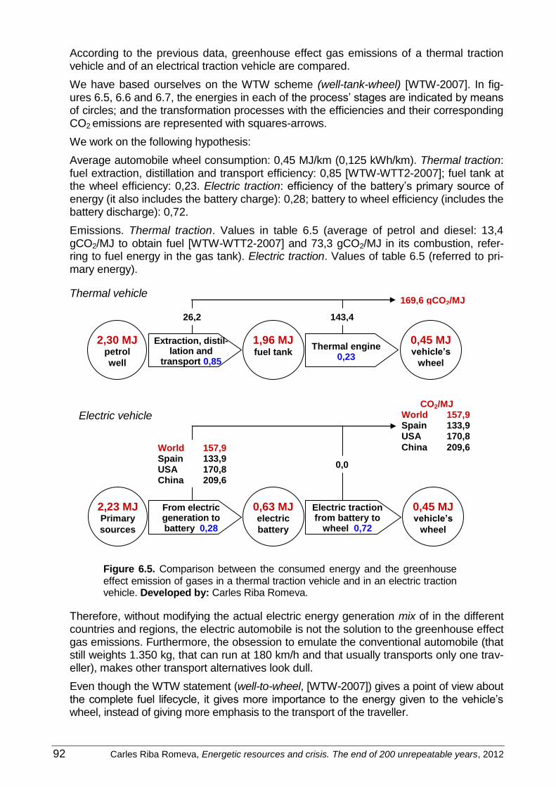
92 Carles Riba Romeva, Energetic resources and crisis. The end of 200 unrepeatable years, 2012
According to the previous data, greenhouse effect gas emissions of a thermal traction vehicle and of an electrical traction vehicle are compared.
We have based ourselves on the WTW scheme (well-tank-wheel) [WTW-2007]. In fig-ures 6.5, 6.6 and 6.7, the energies in each of the process’ stages are indicated by means of circles; and the transformation processes with the efficiencies and their corresponding CO2 emissions are represented with squares-arrows.
We work on the following hypothesis:
Average automobile wheel consumption: 0,45 MJ/km (0,125 kWh/km). Thermal traction: fuel extraction, distillation and transport efficiency: 0,85 [WTW-WTT2-2007]; fuel tank at the wheel efficiency: 0,23. Electric traction: efficiency of the battery’s primary source of energy (it also includes the battery charge): 0,28; battery to wheel efficiency (includes the battery discharge): 0,72.
Emissions. Thermal traction. Values in table 6.5 (average of petrol and diesel: 13,4 gCO2/MJ to obtain fuel [WTW-WTT2-2007] and 73,3 gCO2/MJ in its combustion, refer-ring to fuel energy in the gas tank). Electric traction. Values of table 6.5 (referred to pri-mary energy).
Thermal vehicle
Electric vehicle
Figure 6.5. Comparison between the consumed energy and the greenhouse effect emission of gases in a thermal traction vehicle and in an electric traction vehicle. Developed by: Carles Riba Romeva.
Therefore, without modifying the actual electric energy generation mix of in the different countries and regions, the electric automobile is not the solution to the greenhouse effect gas emissions. Furthermore, the obsession to emulate the conventional automobile (that still weights 1.350 kg, that can run at 180 km/h and that usually transports only one trav-eller), makes other transport alternatives look dull.
Even though the WTW statement (well-to-wheel, [WTW-2007]) gives a point of view about the complete fuel lifecycle, it gives more importance to the energy given to the vehicle’s wheel, instead of giving more emphasis to the transport of the traveller.
Extraction, distil-lation and
transport 0,85
0,45 MJ vehicle’s
wheel
Thermal engine 0,23
1,96 MJ fuel tank
2,30 MJ
petrol
well
26,2 143,4
169,6 gCO2/MJ
From electric generation to battery 0,28
0,45 MJ vehicle’s
wheel
Electric traction from battery to
wheel 0,72
0,63 MJ electric
battery
2,23 MJ
Primary
sources
World 157,9 Spain 133,9 USA 170,8 China 209,6
0,0
CO2/MJ World 157,9 Spain 133,9 USA 170,8
China 209,6

Carles Riba Romeva, Energetic resources and crisis. The end of 200 unrepeatable years, 2012 93
Mobility alternatives
Apart from the reflection that we will have to do in the near future about the need of cer-tain trips (business trips, weekend’s tourism, sports events, many times unnecessary),
the simple fact of giving more importance to the passenger than to the wheel sheds light on the transport alternatives.
Below there is an analysis of how different types of transports transform 100 MJ of wheel
energy into the traveller’s movement. Only the mass ratio has been considered, but the analysis could also be enriched with other parameters, such as speed and air resistance
or the different rolling types (tire, wheel-lane).
Figure 6.6. Energetic efficiency of different transporta-
tion alternatives. Developed by: Carles Riba Romeva.
4. High-quality energy
As it has already been said, an energy is considered to be of a high-quality when it can be transformed to any other type of energy at a high efficiency (normally, >80%). Electricity (and also mechanical energy) are high-quality energies, whilst those that show themselves
as thermal energies (chemical, nuclear, thermal solar) are low-quality energies.
It is important to keep in mind that, in order to obtain electric energy (it is not directly available in nature), generation processes from primary sources, generally with very low
transformation efficiencies (a 31,2% of the worldwide average at the domestic or indus-trial plug; table 6.1), are necessary.
In this aspect, an observation that has been done by the American electric engineer Richard Duncan, in his well-known project World Energy Production, Population Growth, and the Road to the Olduvai Gorge [Dun-2001], says that without the crucial cybernetic
C3 functions (communication, computing and control), the actual industrial civilization would remain mutilated.
And he adds that (and this observation is also of great interest) these crucial functions C3 also need of a 15% of the total consumed electric energy. The rest of the electric en-ergy is consumed in other uses, being most of them, basically, thermal.
Maybe Duncan’s vision is too schematic. We should add, lighting (of which we clearly abuse! You just need to look at the photographs of the earth taken at night from space), electric drive (of which we also abuse! Just look at the high amount of appliances that
have always been turned on manually and that now it is done with little electric engines),
100 MJ vehicle’s
wheel
Automobile 1.350 kg
1 passenger
5,3 MJ traveler’s
transport
Electric bicycle 25 kg
1 passenger
75,0 MJ traveler’s
transport
Bus 12.000 kg
50 passengers
23,8 MJ traveler’s
transport

94 Carles Riba Romeva, Energetic resources and crisis. The end of 200 unrepeatable years, 2012
and certain industrial processes that are closely related to electricity (like for example
electrolysis) to the three C3 main functions. But the previous statement does not take that we should carefully think if it makes sense to consume a very important part of the
electric energy (which is so expensive to obtain) in purely thermal uses (heating, kitch-ens...), whose only advantage is the “everything electric” comfort.
Electric heating’s efficiency
To illustrate this aspect, the electric efficiency and the CO2 emissions both for a gas heat-ing and for a domestic electric heating are compared below. The obtaining of 3,6 MJ of
comfort, which would be the comfort given by 1kWh of electric heating, is taken as a refer-ence. The process is as follows (figure 6.6):
Electric heating
Gas heating
Figure 6.7. Comparison between the consumed primary energy
and the greenhouse effect gas emissions by an electric and a gas heating system. Developed by: Carles Riba Romeva.
Definitively, with the mix values in electricity and gas, electric heating consumes 70%
more primary energy and emits a 110% more greenhouse effect gases than natural gas heating.
6.4. New electric technologies
Nowadays, a big effort is being done in order to improve the generation of electricity in sev-
eral ways. Firstly, conventional thermal power stations are trying to be improved (mainly those of natural gas and coal) in order to obtain higher efficiencies. Secondly, one of the
areas with more activity is the one that tries to obtain energy from renewable sources of en-ergy (mainly wind, solar, but also of waves and tides). However, as it will be seen in chapter 9, although these energies have quickly grown in the previous years, they represent an ex-
tremely low part of the worldwide production.
Probably, with the decline of fossils fuels it will be necessary to limit the use of electric energy.
The “everything electric” tendency (as Duncan warned), will have to be limited. But the electric system will also have to be transformed at a low scale and in favour of the distributed produc-tion as, as well as having to use each time more rare resources, it will have educational ef-
fects that will have to be applied during the following years.
Electric gen.
(world’s mix) 0,312
3,60 MJ home
comfort
Electric heating 1,00
3,60 MJ housing
plugs
11,5 MJ
Primary
sources
817 0
817 gCO2
Nat. gas obtain-ing (world’s mix)
0,85
3,60 MJ home
comfort
Natural gas heating
0,60
6,00 MJ natural
gas
6,74 MJ
natural
gas well
50 337
388 gCO2

Carles Riba Romeva, Energetic resources and crisis. The end of 200 unrepeatable years, 2012 95
Conventional electric production improvements
The main types of new electric power stations with improved efficiencies are:
a) Cogeneration systems and stations (CHP, combined heat and power). It is a simple idea: reuse thermal energy of residual combustion gases of a conventional electric generation system for other processes in which heat is required. In this way, a global efficiency that can be of more than an 80% is achieved, although the efficiency from thermal to electric energy remains as always (35%), and the rest (up to an additional 40%) corresponds to an efficiency from thermal to thermal energy.
b) Combined cycle gas turbine (CCGT), it uses fuel in more than one thermodynamic cycle successively. Initially, combustion gas at high temperatures (normally between 1.100 and 1.300ºC) propels a gas turbine which is similar to those of aviation engines. Afterwards, leak gases are used to produce water vapour (between 450 i 650ºC), which propels a conventional vapour turbine. Global efficiencies (from thermal to electric energy) of be-tween the 50 and the 60% are obtained (between 20 and 25% larger than those of con-ventional thermal power stations). The same principle is applied to sea engines, (COGAS, combined gas and steam). At the same time, it is possible to reuse the residual heat of the combined cycle following the cogeneration principle.
Cogeneration can use any fuel, whilst combined cycle has more specific requisites as to the fuel that has to be used initially in the gas turbine. In combined cycle power stations natural gas is the most frequently used fuel, as well as other liquid fuels that are atomized. As well as improving the efficiency, the use of natural gas in combined cycles also has as an ad-vantage, the substantial reduction of CO2 emissions per unit of generated energy.
Another technology that is used in those countries that dispose of large amounts of coal (spe-cially USA), is the integrated gasification combined cycle (IGCC), in which the first process in the power station is the transformation from coal to a synthetic gas (syngas). In this case, it is not sure that the benefits of this technology compensate the expenses of the transformation of coal into gas (global efficiency, CO2 emissions per unit of generated energy).
On the other hand, new intelligent systems are being developed that will make it possible to manage the consumptions’ connections in the most appropriate moments (late hours at night, moments in which a lot of wind energy is being produced...) in order to improve the global electric system efficiency (but, breaking with the principle that is based in using ener-gy at any time and at any intensity!).
In chapter 9 we will analyze the new alternatives in electric energy generation from renewa-ble sources of energy.

96 Carles Riba Romeva, Energetic resources and crisis. The end of 200 unrepeatable years, 2012

Carles Riba Romeva, Energetic resources and crisis. The end of 200 unrepeatable years, 2012 97
Part 3
Alternative sources of energy
The limit of fossil energetic resources is becoming more and more evident everyday, due to the first production zenith symptoms and the danger of their decline. Furthermore, current economic and politic leaders continue pledging their commitment to a development that is based on the constant growth in the consumption of energy and material resources.
Post-industrial societies (mainly those belonging to the OECD) consume between 50 and 100 times their endosomatic power of a person (the one that it needs as a living being), ten-dency that has been followed by the leading sectors of developing countries (China, India, Brazil, among others). On the other hand, most of Sub-Saharian Africa, large zones of the Southeast Asia and also some areas of Latin America consume from 5 to 10 times their en-dosomatic power, mainly as traditional biomass.
It is often thought that cybernetic society requires less energy. But as it is shown in data from important agencies (EIA-govUSA and IEA-OECD), the use of fossil fuel energy has kept increasing, and only a crisis such as the one that we are living now (and that we are managing so badly) has been able to origin a slight decrease. The prevailing way of thinking defends that we must leave this crisis with an economical growth and this can be done in any way, without stopping to think if nature disposes of the necessary resources to do so.
There are three delusions that make us ignore the background reflections about energy:
1. From time to time, the press publishes news about new fossil fuel discoveries (which are becoming more inaccessible and expensive) that give the impression that it will be long be-fore they run out. But when new oilfields are evaluated at a global context, it is stated that they only cover a global energetic consumption of days, or, at most, months.
2. New endless energy sources are proclaimed (third generation nuclear reactors, nuclear fusion...) but it is not said that, even if these projects were successful (which is not assured) the first power stations would not be ready until after 2030, when the decline of fossil fuels would be a deep reality.
3. Finally, many people who defend sustainable options think that it is only necessary to re-place fossils fuels with new carbon-free renewable sources of energy. However, these alter-native energies will never be able to provide the large amount of energy that we currently still dispose of thanks to fossil fuels (and specially, petroleum).
When future predictions related to alternative sources of energy are done, it is important to consider:
a) The coherence with the world and regional supply according to the considered energetic resources and the population’s evolution.
b) The necessary alternative energy establishment time and investment costs.
c) Different phenomena’s interdependence. Once the decline of a certain fossil fuel has started (for example, petroleum), the problem will not be how to fill up the gas tank, but how to transform the production system and how to feed people.
Part 3 of this book analyzes other sources of energy: unconventional fuels, nuclear alterna-tives and new renewable sources of energy. As we will see, neither of them guarantees the current energy consumption expenses and, even less, the future increases that energy agen-cies predict. Today, the only effective alternative is the new renewable sources of energy (as they were already in the past), although they will force us to drastically reduce energy con-sumption in developed countries and to introduce important social and technologic changes.

98 Carles Riba Romeva, Energetic resources and crisis. The end of 200 unrepeatable years, 2012
7. Unconventional fuels
7.1. Origin of fossil fuels
Fossil fuels are, basically, petroleum and natural gas, which are mainly composed of hydro-carbons (carbon and hydrogen) and coals, composed mainly by the carbon element.
Both of them have been formed during million of years from organic remains of living beings, the first ones principally from microorganisms (plankton, seaweeds and bacteria) present in masses of water (oceans and lakes) and the second ones, from superior vegetable remains (trunks, leaves, roots), and, in some cases, from spores.
These energetic resources are the result of a long process that begins with the formation of sediments, with a significant content in organic matter, that afterwards suffer different trans-formations under particular circumstances. Without certain biological, chemical and geologi-cal processes (anaerobic decomposition, pyrolisis, tectonic movements), of long length in time (up to hundreds of millions of years), the diffuse organic matter, trapped in the sedi-mentary stratum would not have been transformed or concentrated, and, nowadays, we would not have fossil fuels as we currently know them.
Hydrocarbons’ formation
Hydrocarbon-based fuels are, mainly, liquid (crude petroleum), and gas (natural gas), alt-hough there are also solid hydrocarbons (extraheavy petroleum, oil sand and bitominous shales).
The main stages in the formation of liquid and gas fossil fuels are:
Sedimentation In the upper layers of the Earth, in aqueous mediums (wetlands, lakes and oceans) a lot of living organisms have died. Most of this biomass has recycled its materials through respira-tion and decomposition, but a small amount has been trapped in sediments, where it has been mixed with mud and sand. This process, which is still present, is almost imperceptible at a human scale, but it has great importance at a geological scale (from millions to hun-dreds of millions of years).
Formation of Kerogen After sedimentation, organic fraction, diffused in small fillets (in very low proportions, often of about a 1%), goes through an anaerobic process caused by bacteria, and is transformed to a solid insoluble substance called kerogen, that remains fossilized. Kerogen, which is very scattered, is difficult to use as a fuel, but at a worldwide scale it represents a mass of 10.000.000 Pg of carbon (Pg = 1015 grams) [SCOPE13-1979], amount that is about 1.000 times higher than the reserves of coal, and between 2.000 and 3.000 times higher than the reserves of petroleum or gas.
Pyrolysis Starting from plaque tectonics, the sedimentary layers slowly sink (between hundreds and thousands of meters) and temperature and pressure increases. Initially, CO2 and salt water is separated but, as depth increases, the organic matter (kerogen), which is inserted in the sediment, suffers a slow chemical fragmentation process (pyrolysis) that origins hydrocar-bons and that can last between tens and hundreds of millions of years.
Formation of petroleum and natural gas Kerogen pyrolysis at moderate depths (temperatures between 60º and 120ºC) origins, pre-ponderantly, liquid hydrocarbons (long chains). But, if the rock that contains the kerogen sinks into deeper layers and achieves higher temperatures (>120ºC), then pyrolysis is inten-

Carles Riba Romeva, Energetic resources and crisis. The end of 200 unrepeatable years, 2012 99
storage rock (porous and permeable)
storage rock (porous and permeable)
Extra-heavy petroleum
oil sands
secondary
migration
secondary
migration
degradation
oil
gas
gas
water
trap
trap
sedimentation
oil shales
bedrock (mainly liquids)
bedrock (mainly gasses)
seas and lakes
maturing (pyrolysis 60 to 120ºC)
maturing
(pyrolysis > 120ºC)
kerogen
formation
primary
migration
primary
migration
sified and gas hydrocarbons are produced (shorter chains), leaving a bituminous residue. All of the components that result from this process (water, CO2, liquid hydrocarbons and bitu-men) remain inserted in the small interstices of the sedimentary rock (called bedrock), which normally has a low permeability, in substitution of kerogen.
Migration and traps The increase in pressure can end up overcoming the impermeability of the bedrock, and ex-pel the liquid and gas hydrocarbons (primary migration) to other more permeable stratums (storage rock). In its ascending movement due to low density (secondary migration), these hydrocarbons can be trapped by some trap, like an anticlinal fold or an impermeable stratum fault (clay, salt) and form an accumulation (deposit). Petroleum and natural gas normally go together. In deposits with lower depths, petroleum normally dominates (many times with a layer of water at the bottom) and, in deposits with more depth it is natural gas that dominates. They can be extracted by simple decompression (the fluid flows by itself) or by pumping.
Figure 7.1. Scheme of the fossil fuel formation process (petroleum and natural gas). It is necessary to highlight the position of the oil shales at the end of the process, as immature still not formed oils, and oil sands at the end of the process, as degraded oils that have lost most of their volatile components. Source: several. Developed by: Carles Riba Romeva.
atmosphere

100 Carles Riba Romeva, Energetic resources and crisis. The end of 200 unrepeatable years, 2012
Other evolutions of kerogen
Oil shales
They are sedimentary rocks that contain kerogen that has not been pyrolysed yet (before petroleum and natural gas is formed), with a solid consistency similar to that of lignites, but with a content in organic matter much lower than that of forming carbons. To transform them into petroleum, an artificial pyrolysis process needs to be done at high temperature (at 500ºC in order to accelerate a process that normally takes millions of years). Even though worldwide oil shale resources are enormous (2,83 Tb, more than the double of petroleum’s reserves), the energetic balance for kerogen’s obtaining and its transformation to petroleum is not efficient.
Extra heavy crude oils and oil sands or tar sands
If, after the primary migration, the petroleum that has been formed by kerogen’s pyrolysis does not find a trap in which to form a deposit, it ends up reaching the surface, where the volatile components escape and the liquid components are decomposed by bacteria and transformed into bitumen (mixture of high viscosity organic components and inorganic mat-ter). The world’s most important deposits are the extra heavy crude oils in the Orinoco Belt (Venezuela), and the oil sands in Athabasca (Canada). Worldwide resources are enormous, (2,48 Tb and 3,27 Tb, respectively, that are about four times the conventional oil reserves), but their obtaining presents many difficulties and only 0,31 Tb are counted as reserves.
Coals’ formation
Coals also come from a variety of kerogen that is formed from organic matter. But, unlike petroleum and natural gas, they are the result of large vegetable masses from continental zones that origin a sediment where there is majorly organic matter. This has as a result that, in the posterior process of lithification and diagenesis (transformation into a rock) the ele-ment carbon becomes majoritary and hydrocarbons are found in a minor proportion.
Origin and transformation of coal
Although coals have been formed in all geological eras, since plants were formed almost 400 million years ago, it was during the superior carboniferous and the Permian periods (from 310 to 230 million years ago) that the suitable circumstances for its formation were given: growth of large masses of lush vegetable, with giant plants in a tropical climate; low ocean depth, with sudden changes in sea level combined with intense rain periods, where marshes and floodplains periodically buried big volumes of vegetation (the future coal beds); appearance of trees with woody crust (lignified) when microorganisms that were capable of decomposing it were still not present.
By means of a progressive sinking process that has taken place during millions of years, with increasing pressures and temperatures, these layers of dense vegetable matter pro-gressively fossilized, eliminating humidity and volatile components (light hydrocarbons, CO2) and increasing the %C (carbon) in such a way that they were transforming themselves into increasingly evolved coals: from peat to lignite, to sub-bituminous coal, to black coal (bitumi-nous coal) and to anthracite.
Being coals solid matters, they don’t migrate like fluid hydrocarbons (petroleum and natural gas) do, and, for this reason, they are found in the same place where they were formed. Coal beds, however, suffer important deformations due to tectonic movements and folds.
Coal characterization The main technologic parameters that are used in order to characterize coals are: their composition, their moisture content, their volatile element proportion, their ash content, and above all, their heat of combustion. Table 7.1 shows ranks of values for each of the different coal types.

Carles Riba Romeva, Energetic resources and crisis. The end of 200 unrepeatable years, 2012 101
Chemical composition. Dry carbons (without humidity) have a hydrogen content (4 to 6%) which is approximately half of that of petroleums, and a high content in carbon (C) that var-ies from >50% in peat and >90% in anthracites.
Humidity. Free water that can be eliminated by evaporation in hot air at 105ºC. It is a non-combustible component of coal that increases its deadweight, consumes heat and weak-ens the physical structure. It goes from >75% in peat to <10% in anthracite.
Volatile elements. Gases that are adsorbed during the process of coal formation, essentially CO2 and methane (CH4). Their content tends to decrease with the evolution degree of the studied coal. They are released when coal is distilled at temperatures of about 1.000ºC, with an absence of air.
Ashes. Inorganic solid mineral matter that is a residue of combustion. Some coals contain sulphur (S) or nitrogen compounds that, during combustion, give corrosive acids that are responsible of acid rain.
Heat of combustion (HC). Energy that is provided by the combustion of dry coal (without humidity). The heat of combustion of volatile elements is normally lower than that of coal. The coke carbon obtained by distillation of low ash and sulphur content bituminous coal in a oxygen-free oven at 1.000ºC, where the volatile elements are disposed of, has a higher heat of combustion than the coal that origins it, and is used in the iron industry.
Figure 7.2. Scheme of coal’s formation process. As vegetable mass sinks, it progressively turns to peat, lignite, sub-bituminous coal, bituminous coal and anthracite. They loose humidity and volatile elements and gain carbon content and heat of combustion. Sources: several. Developed by: Carles Riba Romeva.
Peat
Lignite
Sub-bituminous
Coal (bituminous)
Anthracite
Volatile comp.: 15 a 40% HC: from 23,8 to 31 MJ/kg
Volatile comp.: <10% HC: from 30 to 35 MJ/kg
Volatile comp.: <70% HC: from 6 to 9 MJ/kg
Volatile comp.: 50 a 75% HC: from 8 to 17 MJ/kg
Volatile comp.: 25 a 50% HC: from 17,4 to 23,8 MJ/kg
Sinkage and transformation
Atmosphere
mars i llacs

102 Carles Riba Romeva, Energetic resources and crisis. The end of 200 unrepeatable years, 2012
Peat Fibrous structure sediment, of brown or black colour, that results from the compaction and transformation of wetland vegetation in anaerobic conditions. It is the first geologic step in the formation of coal. With a spongy aspect, still with free cellulose and with perceptible to the eye vegetable traces, peat has low heat of combustion and high relative humidity. Upon drying, it can be used as a fuel. Since the appearance of superior plants, near 400 million years ago, peat has been in con-tinuous formation. Peatlands cover around 3 million km2 (six times Spain’s surface, a 2% of the Earth’s emerged surface) and have high carbon content.
Lignite It is the first type of coal, but also the one that is considered to have a lowest quality level. Lignite can have a lumpy consistence, and, in some cases, it contains traces of vegetable matter, but it does not contain free cellulose. It is normally brown (often referred to as brown coal) or black, it has a high inherent moisture content (but lower than that of peat) and a high content of volatile matter. It is used almost exclusively as a steam and electricity generation fuel, although it many times contains significant amounts of sulphur that cause acid rain.
Subbituminous coal Category of coal that normally doesn’t appear in Europe’s classifications, whose properties range from those of lignite to those of bituminous coal, it is dark brown or soft black and it has a lumpy consistence (it can be considered better quality lignite). It is used primarily as fuel for steam and electric power generation.
Bituminous coal Dense, hard, black, fragile and stratified coal, with an important content of bitumen hydro-carbons, with low moisture content and high heat of combustion. It is the most abundant and consumed coal at a worldwide scale, and it is primarily used as a fuel for electric generation, in industrial combustion processes and in the obtaining of coke fuel. Coke fuel is derived from distillation of bituminous coal at high temperatures in an airless furnace in order to eliminate the volatile content (very pollutant process). Obtained gases are normally industrially useful and the solid that is obtained (coke coal, light porous and with high heat of combustion), is used in the iron and steal manufacturing processes (dues to the low impurities) and it is harvested as a domestic fuel (little smoke and low pollution).
Anthracite It is the type of coal that has been formed at deeper deposits gaining the highest quality coals as a result. It is hard, black and shiny, but also difficult to extract, with the high-est carbon content and the fewest volatile matter and moisture content. Its calorific content is one of the highest, although it ignites with difficulty. Anthracite is relatively not abundant in nature and it is mainly used in industrial processes and in domestic heating.
Table 7.1. Types of coals and their characteristics
Coals Density Carbon (C) Humidity Volatiles Ashes Heat of comb.
Mg/M3 (dry) % 1 % (dry) % (dry) % (dry) MJ/kg
Peat (dry) <1 40 to 60 >50 >75 50 6 to 9 Lignite 1,1 to 1,3 60 to 75 25 to 50 50 to 75 30 to 50 9 to 17,4 Subbituminous 1,2 to 1,4 70 to 80 15 to 25 25 to 50 20 to 30 17,4 to 23,8 Bituminous 1,2 to 1,5 75 to 90 5 to 15 15 to 40 10 to 20 23,8 to 31 Anthracite 1,4 to 1,8 >90 1 to 6 <10 0 to 10 30 to 35 1 The carbon content in coals is distributed in free carbon and the carbon that forms part of hydrocarbons. Only in the case of anthracite is the %C close enough to the total free carbon content.
Sources: several. Developed by: Carles Riba Romeva

Carles Riba Romeva, Energetic resources and crisis. The end of 200 unrepeatable years, 2012 103
7.2. Increasingly difficulty in the obtaining
Fossil fuels are usually defined as those fuels that are directly obtained from nature, in rela-tively simple extraction conditions in relatively accessible areas and that need processes that consume not large amounts of energy in order to make them suitable for consumption. They are: a) liquid fuels obtained from solid ground oil wells and at wells that are at low-depth waters; b) natural gas obtained from not very deep wells in concentrated deposits and near to the consumption point; c) high quality coals that obtained from open-pit mines or easily accessible underground mines.
However, the Earth’s crust stores a much greater amount of organic matter as a result of multiple plant and animal biological cycles, the burial of dead organic matter together with the sediments, its sinkage and its transformation into different grades during hundreds of million of years. As it has already been said (section 7.1), sediments contain 10.000.000 Pg of C, mostly as low-concentrated kerogen, or as transformed organic matter which is highly diffused in rocks or in very inaccessible places where exploitation is not possible.
The transformation of an extremely low part of this organic matter into useful fossil fuels for our energetic needs (called resources, that contain about 6.000 Pg of C) is the result of very particular circumstances and is a nature’s gift. Furthermore, only a fraction of these fossil fuels have the correct concentration and accessibility for their exploitation (called reserves: 1.316,7 Gb of petroleum, 6.189,4 Tcf of natural gas and 826.002 million tons of coal; see table 3.1), that contain 675,55 Pg of C, a little more than 1/10 of the resources.
The fact that there is a large amount of organic matter spread out in the Earth’s crust many times leads us to confuse it with reserves. Certainly, with new technological developments some complementary resources will be exploited and transformed, like unconventional oils, and unconventional natural gas. But, as we will see further on, we will only be able to exploit a little part of these resources (most of it is currently counted as reserves) and at a very slow rhythm, that will not be able to compensate de decline of conventional fossil fuels.
Unconventional resources
In order to avoid or delay the effects of the decline and exhaustion of conventional fossil fuels (easy to put into value), the oil companies, many governments and an important part of civilized country’s citizens have their hopes pinned on unconventional fossil fuels, that have different ways to obtain new liquid and gas fuels with increasing extraction and/or transfor-mation difficulties.
These new strategies are:
a) To exploit oilfields and conventional gas deposits found in deep waters (at more than 500 meters) and in locations with a difficult accessibility (for example the Arctic Ocean).
b) To extract and transform decomposed oils (oil sands, extraheavy crude oils) and still not formed oils (oil shales’ kerogene).
c) To obtain different types of difficult access unconventional gases (tight gas, coalbed gas or shale gas).
d) To try to energetically exploit methane hydrates (or methane clathrates), of the continen-tal margins and of the permafrost.
e) To turn natural gas and coal into suitable for transport liquid fuels (GTL, gas-to-liquid, and CTL, coal-to-liquid) or to convert biomass to fuel (BTL, biomass-to-liquid, parting from farming land, seaweed or forest biomass).

104 Carles Riba Romeva, Energetic resources and crisis. The end of 200 unrepeatable years, 2012
The only thing that all of these strategies (except some biofuels of which we will talk in sec-tion 9.7) do is prolong fossil fuels’ era with everyday more expensive and difficult to obtain resources. Resources’ exploitation will suffer important limitations:
1) Energy return on investment (EROI) will tend to decrease, due to their obtaining, until values that are less than or equal to 1 are reached. Then, fuel obtaining will need as much or more energy as the energy that the fuel provides, and the exploitation will be no longer profitable.
2) Time and costs (both energetic and economic) of the needed investments will progres-sively increase and loose efficiency, in such a way that efficiency will have to be valued. In any way, they will hardly be there on time to mitigate the declining of conventional oil.
3) For the same energy efficiency, the use of unconventional oil increases the environmen-tal impact and the emissions of CO2. The environmental impact will grow every time more and more when trying to obtain the same amount of energy.
4) Natural gas and coal conversion to liquid fuels will rush the exhaustion of these reserves to an earlier date than the one that was expected due to low energetic efficiencies of GTL transformation and, even worse, CTL transformation.
5) Finally, in the off-chance that new exploitable petroleum or natural gas deposits were found, the good news would be masked by the environmental impact that its obtaining and use would produce.
Effectively, carbon-based energy and the climate change are part of the same equation. If we want to solve the climate change problem, we will have to learn to resign to fossil fuel exploitation (this is similar to the battle that Equator is currently fighting in order to preserve the unrepeatable forests of the natural park in Yasuni and resign the exploitation of 0,9Gb of crude oil that are found in its subsoil, less than 1/1000 of the worldwide reserves).
From an environmental point of view, new deposit discoveries (Brazil, Gabon...) are bad news. The strategy of solving the declinine of fossil fuels by systematically exploiting uncon-ventional oil with decreasing energetic efficiencies and increasing emissions leads us to a totally wrong path that will make human civilization be unlikely and scarcely feasible in the near future.
7.3. Unconventional oils
In this section, liquid fuels that don’t come from conventional oil or gas deposits are ana-lysed. They are primary sources that until now have had difficult accessibility or extraction processes, and have had a complex valuation; specifically:
Hard-to-reach oils (deepwater oils, Arctic...).
Extra-heavy crude oils
Oil sand or tar sand
Oil shale
In section 7.4 unconventional gases are analysed, while in section 7.5 liquid fuels for transport obtained by other primary fossil fuels’ transformation (mainly coal, CTL, natural gas and GTL) are analysed. Finally, in chapter 9, which is about renewable sources of ener-gy, a range of fuels which are derived from biomass, or biofuels, will be analyzed.
From conventional to unconventional oils
Conventional oil is found in accessible solid ground or near the coast zones, at less than 500 meters of depth and it has properties that allow it to be processed in conventional refin-eries. Previous years’ production (about 66 Mb/d, or million barrels per day, the 78% of the 85 Mb/d of global liquid production) has reached its zenith and starts to show declining

Carles Riba Romeva, Energetic resources and crisis. The end of 200 unrepeatable years, 2012 105
symptoms. 7,7 Mb/d (the 9%) need to be added, which are the result of liquefying gas fuels that go with petroleum or natural gas (specifically, butane and propane).
Unconventional oils are the result of the exploitation of deposits that are less accessible and efficient than conventional ones. Nowadays, they have a global production of 11,3 Mb/d (a 13% of the global production) and they are distributed as follows: 3,9 Mb/d (a 4,5%) are oils from Canada’s oil sands, Venezuela and other countries’ heavy and extra heavy crude oils, and of oil from oil shales; 6,5 Mb/d (a 7,6%) are oils extracted from deep waters of more than 500 meters of depth (Gulf of Mexico, Gulf of Guinea and, in the future the Santos oilfield, in front of the Brazilian coast), and 0,9 Mb/d (a 1%) correspond to the Arctic region [Pri-2008].
Stages of Conventional Deposits
The successive oil deposit exploitation stages are:
Primary oil recovery. In a first stage, petroleum emerges from the oil well due to natural rea-sons (associated or dissolved gas pressure, water hydrostatic pressures or drainage in suit-able areas); primary recovery, that only needs a valve system to be managed, allows the obtaining of between a 12 and a 15% (recuperation factor) of the initial deposit’s petroleum, percentage which is higher in light oils and lower in heavy oils. The obtaining energetic and economical costs are very low.
Secondary oil recovery. From a given exploitation grade, pressure decreases and petroleum does not flow into the surface; then, it needs to be boosted by floods with water (quite cheap process) or by injection with gases that displace petroleum; with these methods, more ex-pensive than those of the primary recovery, additional recuperation factors of between a 15 and a 20% are achieved, which gives global recuperation factors in relationship to the initial petroleum of from a 25 to a 35%.
Enhanced oil recovery (EOR). In other cases, due to the compactness of rocks or to the high viscosity of oils (heavy oils), crude oil needs to be fluidized in order to make it be able to cir-culate towards the surface easier. Generally, this is achieved by carrying out different pro-cedures: injecting water vapour into the oil well, burning part of the fuel in situ or using chemical products (detergents) in order to decrease its viscosity. With enhanced oil recovery techniques, exploitations that were no longer efficient often can produce again, although due to the process’ cost, the price of the fuels rise. These methods allow an increase of the re-cuperation factor of the deposit from 5 to 15% to place it between a 40 and a 50%, although costs and emissions considerably increase.
Deep water platforms
For some time, we have been drilling oil and gas wells under the surface of the sea. These wells are gaining an increasing importance with the passing of time. The report [IEA-ETSAP-P01-2010] affirms that the potential of these deposits is between 150 and 200 Gb, from which an important part is already counted as reserves.
The first oil platforms were drilled near to the coast in quite shallow waters, with the towers fixed on the ocean floor (for example deposits in Maracaibo, Venezuela). As solid ground deposits exhaust, exploitations in growing distances from the coast and at larger depths (up to 3.000 meters) increase. The previously mentioned ETSAP report estimates that a 70% of the deep water resources are found in high seas, with a depth ranging from 2.000 to 4.000 meters.
The development of oilfields in high seas requires important investments, and only those that dispose of optimal conditions can be exploited. We have passed from fixed to the floor oil rigs (with depths of up to 500 meters) to floating oil rigs and, separation and transport to the coast technologies on the sea floor are being currently developed.

106 Carles Riba Romeva, Energetic resources and crisis. The end of 200 unrepeatable years, 2012
The paradigm of this technology limit at very deep waters is the giant deposit in Tupi (from 5 to 8 Gb), which was recently discovered (2006) at 250 km from the Brazilian coast at a depth of more than 2.000 meters. From the ocean’s floor, an imbalanced layer of sand of 2.000 meters has been drilled and other deeper layers of rocks of 2.000 more meters have also been drilled (in total, more than 6.000 meters). The commercial exploitation is predicted to be started in 2013. The depth makes it impossible for the rig to be fixed to the ocean floor, so it is subjected to wind and drafts, which implies constant energy expenses to make sure the drill stays in a vertical position. As well, the oil has to be taken to the surface by a series of tubes that have to undergo extreme pressure and temperature conditions, as well as the corrosive effects and the instability (layer of salt, movement of the oil rig) that can produce important amounts of incidents during the exploitation process. It is predicted that the pro-duction at a constant regime will be of 0,5 Mb/d (1/170 of the worldwide production). The recently (2008) discovered oilfield in Carioca, also in the submarine basin of Santos (Brazil), has the same characteristics as the one in Tupi.
On the other hand, the recent accident (2010) of the semisubmersible oil rig, Deep water Horizon (rented to Transocean by BP) while it was drilling a 1.500 meters deep well in the Gulf of Mexico highlights the risks and limits of this technology, in the same way that the Chernobyl disaster did with nuclear power in 1986. In effect, at the end of the drilling pro-cess, the 20th of April of 2010 there was a gas leak and an explosion in the tower, followed by fire in the facilities. Even though several ships gave aid trying to put out the fire, the oil rig sank two days later producing eleven casualties. Do to the accident, petroleum leaked to the sea during 106 days until, the 5th of August, BP announced that it had been sealed. Trans-ocean came into conflict with BP in the following days accusing BP of having reduced ex-penses increasing therefore the risk of leaks.
Figure 7.3. Deepwater Horizon oil rig fire the 20th of April of 2010 in the Gulf of Mexico. Source: newspaper El País
According to experts from the University of Colombia [Cro-2010], this accident has poured approximately 5,2 million barrels into the sea, out of which 0,8 have been recovered. The worst oil tanker wreck was the one of the Amoco Cadiz in the French coasts in year 1978, in which less than a third part of the oil was spilled, and the worst disaster of these characteris-tics was Iraq’s deliberate pour during the Persic Gulf war in 1991, in which the double was spilled. Latest information indicates that the oil in the Gulf of Mexico, as well as having a vis-ible impact in the south coasts of the United States, is depositing itself in large areas of the ocean floor, posing a serious threat to marine life.
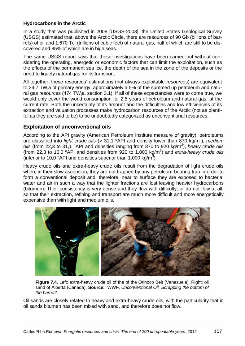
Carles Riba Romeva, Energetic resources and crisis. The end of 200 unrepeatable years, 2012 107
Hydrocarbons in the Arctic
In a study that was published in 2008 [USGS-2008], the United States Geological Survey (USGS) estimated that, above the Arctic Circle, there are resources of 90 Gb (billions of bar-rels) of oil and 1.670 Tcf (trillions of cubic feet) of natural gas, half of which are still to be dis-covered and 85% of which are in high seas.
The same USGS report says that these investigations have been carried out without con-sidering the operating, energetic or economic factors that can limit the exploitation, such as the effects of the permanent sea ice, the depth of the sea in the zone of the deposits or the need to liquefy natural gas for its transport.
All together, these resources’ estimations (not always exploitable resources) are equivalent to 24,7 TWta of primary energy, approximately a 5% of the summed up petroleum and natu-ral gas resources (474 TWta, section 3.1). If all of these expectancies were to come true, we would only cover the world consumption for 2,5 years of petroleum and natural gas, at the current rate. Both the uncertainty of its amount and the difficulties and low efficiencies of its extraction and valuation processes make hydrocarbon resources of the Arctic (not as plenti-ful as they are said to be) to be undoubtedly categorized as unconventional resources.
Exploitation of unconventional oils
According to the API gravity (American Petroleum Institute measure of gravity), petroleums are classified into light crude oils (> 31,1 ºAPI and density lower than 870 kg/m3), medium oils (from 22,3 to 31,1 °API and densities ranging from 870 to 920 kg/m3), heavy crude oils (from 22,3 to 10,0 ºAPI and densities from 920 to 1.000 kg/m3) and extra-heavy crude oils (inferior to 10,0 °API and densities superior than 1.000 kg/m3).
Heavy crude oils and extra-heavy crude oils result from the degradation of light crude oils when, in their slow ascension, they are not trapped by any petroleum-bearing trap in order to form a conventional deposit and; therefore, near to surface they are exposed to bacteria, water and air in such a way that the lighter fractions are lost leaving heavier hydrocarbons (bitumen). Their consistency is very dense and they flow with difficulty, or do not flow at all, so that their extraction, refining and transport are much more difficult and more energetically expensive than with light and medium oils.
Figure 7.4. Left: extra-heavy crude oil of the of the Orinoco Belt (Venezuela). Right: oil sand of Alberta (Canada). Source: WWF, Unconventional Oil, Scrapping the bottom of the barrel?
Oil sands are closely related to heavy and extra-heavy crude oils, with the particularity that in oil sands bitumen has been mixed with sand, and therefore does not flow.

108 Carles Riba Romeva, Energetic resources and crisis. The end of 200 unrepeatable years, 2012
Extra-heavy crude oil
We know of the existence of 162 reservoirs in 21 countries, 13 of which are at the sea [WEC-2010]. However, the Orinoco Belt (Venezuela) contains almost all of the world’s resources (2.111 Gb, billions of barrels, of a total of 2.150 Gb), as well as almost the totality of the known
reserves. The accumulated world production is of 17,1 Gb (out of which 14,8 is in the Orinoco Belt). The Venezuelan oil company (PDVA) estimates reserves (that can be extracted) of
heavy oils of 235 Gb, in which the report [WEC-2010] only accepts 57,9 Gb (of a total of 59,1 Gb that exists worldwide) (see table 7.2).
Extra-heavy crude oils and oil sands are modified hydrocarbons that differ in the degree by
which they have been degraded by bacteria and erosion from the original crude oil. Venezuela’s extra-heavy crude oils are less degraded than oil sands in Canada, and are found at higher temperatures (>50ºC, in comparison to the cold weather in North Canada), which
makes extraction easier; but they are still too heavy to be transported by pipeline and
processed in conventional refineries.
In spite of these favorable circumstances, the fact that they dispose of abundant light oil and the difficulty to access First World’s technology and capital have not estimulated Venezuela in the development of these resources in the same way as in the case of Canada. In the
1980, the Venezuelan oil company PDVA developed the emulsion known as orimulsion (70% extra heavy crude oil, 30% water), that allows transport through pipelines.
Nowadays, extra heavy crude oils from Venezuela ara extracted by means of multilateral horizontal wells in combination with submersible pumps, but very low recuperation factors are obtained (from an 8 to a 12%). North-East Venezuela treatment plants reuse solvents,
extracting sulfur and nitrogen, and with an efficiency ranging from a 87 to a 95%, transforming heavy oils into a synthetic petroleum.
Recently, with the PDVA and international company’s tender, the Venezuelan government
has given a boost to a development plan for the Orinoco Belt. The exploitation area is of 11.593 km² (1/3 of Catalonia), divided into four large areas (Boyaca, Junin, Ayacucho and
Carabobo), with a potential production of 1,2 Mb/d (million barrels per day) and reserves of 25,5 Gb, according to official Venezuelan sources.
Oil sands
They consist in degraded oil that is trapped in a complex mixture of sand, water and clay. Bitumen, an extremely viscous hydrocarbon with a large carbon content, is found in a pro-
portion that ranges from 1 to 20% in oils sands.
598 diposits have been reported in 23 countries [WEC-2010] and there is no notice of sea deposits. In particular, oil sands are found in extremely large quantities in Athabasca (Canada),
with an amount of 2.434 Gb from the global value of 3.228 Gb. Of these resources, 243,2 are considered as reserves (a 7,5%), most of which are in Canada (179,4 Gb, already counted as
reserves in this country).
Apart from Canada, other large oil sand reserves are located in Kazakhstan (420,7 Gb) and Russia (346,8 Gb), with unexploited reserves of 42,0 and 28,4 Gb respectivelly. Resources in
the United States (53,5 Gb), Nigeria (38,3 Gb) and Madagascar (16 Gb) can hardly be considered as reserves (table 7.2).
This resource is only exploited in Alberta, Canada (1,30 Mb/d, millions barrels per day),
where oil sands, with an aproximate bitumen content of a 10%, are covered by 140.000 km2 of boreal forests in the regions of Athabasca, Peace River and Cold Lake.

Carles Riba Romeva, Energetic resources and crisis. The end of 200 unrepeatable years, 2012 109
Up to a depth of 80 meters, oil sands are extracted using open pit mining techniques (some
of the ones that are used in Athabasca are visible from the space). Oil sands are transported by enormous trucks to a plant where bitumen is separated from oil sands by hot water and
chemical products up to a proportion of a 90%. In open pit mines 2 tons of mineral has to be manipulated in order to obtain one barrel of petroleum (159 litres).
In the mining industry, upon injecting steam in situ (without physically extracting the mineral)
bitumen can flow and, therefore, it can be extracted. The in situ technique which is most commonly used in Canada is the Cycle Steam Simulator (CSS), where steam is injected
through a vertical well and the mixture of bitumen is extracted through the same shaft in a cyclic way; this way recuperation factors of from a 25 to a 30% are achieved. Another very promising in situ technique is the Steam Assisted Gravity Drainage (SAGD), where steam is
injected through horizontal wells (they start being vertical but at a certain depth they curve and become horizontal), and the mixture of bitumen is picked by another horizontal shaft that is found below. This method is applied to deeper deposits and it requires less energy and
achieves recuperation factors of up to a 50%.
In both of the previous cases, by removing carbon (firing) or adding hydrogen (hydrocracking),
the bitumen is transformed into synthetic petroleum, and it is finally distilled to obtain derived products.
Oil shales
They are sedimentary rocks containing a high proportion of solid organic matter, in the form of kerogen (organic matter that has not totally decomposed), out of which liquid fuels (or synthetic oils) can be extracted by a pyrolysis process at about 500ºC.
With efficiencies below 100 to 125 litres per tonne, it is not viable to turn oil shales into liquid fuels, as processes require important energy consumptions and emit large amounts of greenhouse effect gases. It is also directly used as a low heating value fuel for electric
generation, in the manufacture of cement or for other industrial uses. In this case, efficiency is better.
Most oil shales exploitation methods involve open pit mining, although in situ pyrolysis
processes are being experimented. They consist in heating the shale underground using different procedures (amongst which the electric procedure is found) in order to pump the
resulting liquid to the surface afterwards. This process also creates important environmental impacts (generated fluid leaks, energy consumptions and emissions).
It is estimated that oil shale resources, if they were to be viable, have the potential to provide 4.876 Gb (thousands of millions of barrels) of liquid fuel (about four times the amount of conventional petroleum’s reserves). Deposits in the United Stattes constitute ¾ of the world’s
resources, but they have still not been commercially exploited (apart from millitary pilot experiments). However, oil shales served for oil production in other countries like Scotland
from the 19th century to 1940, Fushum (China) from 1930 to recent years (petroleum production), and, above all, Estonia, that, during the last decades, has leaded oil shale’s exploitation, using it as a source of energy to produce electricity.
Energetic consumption and unconventional fuel emissions
Due to the expensive and complex obtaining and processing processes, energy consumption and greenhouse effect gases emissions of unconventional fuels are considerably higher than
those of conventional fuels. Furthermore, they all consume large amounts of water: in oil sands, up to 2 or 3 barrels of water are consumed for each barrel of bitumen.

110 Carles Riba Romeva, Energetic resources and crisis. The end of 200 unrepeatable years, 2012
In relationship to the energetic consumption, the obtaining of synthetic petroleum from extra-
heavy crude oils (Orinoco Belt) requires up to a 20 or a 25% of the energy content that the fuel can provide (energy return on investment, EROI, from 3 to 3,5, already in the limit of en-
ergy’s viability). In oil shales, it depends on the transformation process: if they are directly used as fuels, they are similar to lignite; their transformation into liquid fuels through pyrolysis presents many unknown viability factors that have limited their production to residual values.
This makes us think that the energy return on investment factor is not much superior to 1 (some authors estimate it inferior to 1).
When it comes to greenhouse effect gas emissions, there are huge disparities between dif-ferent estimations. To the petroleum combustion emissions obtained from 74 gCO2/MJ (TTW process), according to the well-documented report of the NDRC [Mui-2010], we must add the
increase of emissions in the obtaining (WTT process) of 32 gCO2/MJ for open pit exploited oil sands, of 34 to 42 gCO2/MJ for the obtaining in situ, and of 80 to 102 gCO2/MJ for oil shales
(values that would verify the lack of viability of the exploitation process). It does not explicitly
cite extra-heavy crude oils, but they would have to be placed as lower-grade oil sands.
Resources, reserves and production
Table 7.2 shows these aspects:
Table 7.2. Resources,reserves and production of unconventional liquids crude fuels. 1
Type Resources Reserves CuPr 2 Production Gb % Gb % TWty Gb Mb/d TWt
Extraheavy petroleum 2.150 100,00 59,1 100,00 11,61 17,09 0,67 0,048 Venezuela 2.111 98,19 58,0 98,14 11,39 14,78 0,58 0,042
United Kingdom 12 0,56 0,08 0,14 0,02 1,01 China 9 0,42 0,75 1,27 0,15 0,14
Azerbaijan 9 0,42 0,125 0,21 0,02 0,76
Oil sands 3.329 100,00 243,2 100,00 47,76 6,46 1,30 0,093 Canada 2.434 73,12 170,4 70,07 33,46 6,40 1,30 0,093
Kazakhstan 421 12,65 42,4 17,43 8,33 0 Russia 347 10,42 28,4 11,68 5,58 0,014
USA 53 1,59 0 0,00 0,00 0,024
Nigeria 38 1,14 0,6 0,25 0,12 0
Oil shales 4.876 100,00 ? ? 0,005 0,0177 0,0026 USA 3.707 76,03 0 0
China 354 7,26 0,0076
Russia 248 5,09 0 0
D.R. Congo 100 2,05 0 0
Brazil 82 1,68 0,0038
Italy 73 1,50 0 0
Jordania 34 0,70 0 0
Australia 32 0,66 0 0
Latvia 16 0,33 0,0063 0
Unconventional petroleum 10.265 302,3 59,37 23,56 1,99 0,142 % conventional 27,9 2,36 2,27
Conventional petroleum 1.084,0 199,67 1.000,0 83,12 5,590 1 The data procede from the IEA-ESTAP-P02A. The measures in TWt and TWta are assessed by the author.
2 Cumulative production.
Source: Meyer, R.F. USGS; Dyni, J.R. USGS; IEA-ETSAP-P02-2010 ; Developed by: Carles Riba Romeva

Carles Riba Romeva, Energetic resources and crisis. The end of 200 unrepeatable years, 2012 111
Comments on table 7.2:
1. The volume of resources of each of the unconventional fuels outweighs (doubles, triples or quadruples) the conventional petroleum resources by far. This could make us think that
it will be long until the exhaustion of fossil fuels takes place.
2. However, when it comes to reserves, previous amounts are drastically reduced. Extra-heavy crude oil reserves are only a 2,7% of the resources; oil sand reserves are a 7,3%
of the reserves, and there are no recorded oil shale reserves.
3. It has been confirmed that unconventional resources, which are much more abundant
than petroleum (10.265 Gb), have a current production of only 2 Mb/d, when the rest of the liquid fuel’s production is of 83 Mb/d, with reserves of not much more than 1.300 Gb. This low exploitation is verified by the stocked production.
4. Oil shales’ exploitation as a source of primary liquid fuels seems unlikely and scarcely fea-
sible, both at present and in the future. Figure 7.5 shows the evolution of previous years’ weak exploitation, with a global production peak in 1980. Furthermore, main use has been
in direct combustion, not in the transformation into liquid fuels.
Figure 7.5. Worldwide oil shales production evolution, with a production
zenith in 1980, with 46 million tons (almost 4 days of conventional petroleum production). Source: [Dyn-2006], US Geological Survey
Extra-heavy crude oils and oil sands have future exploitation possibilities, although this is bad
news environmentally speaking. Indeed, energy is not fully exploited (other resources are con-sumed, like natural gas or part of the obtained petroleum), with an important environmental cost due to higher amount of CO2 emissions.
Furthermore, the main agencies (IEA-OECD, EIA-govUSA), in their projections, do not pre-dict large increases in the production of unconventional liquid fuels. Specifically, projections of the EIA-govUSA for 2030 on the evolution of these unconventional liquid fuels (Interna-tional Energy Outlook 2009, page 22) are very moderate. Production of oil sands is predicted
to go from 1,9 Mb/d (millions of barrels per day) in 2010 to 4,2 Mb/d in 2030, while extra-
heavy crude oils are predicted to increase from the current value of 0,7 Mb/d to 1,2 Mb/d in 2030 and oil shales, which nowadays do not have a perceptible production, are predicted to reach 0,2 Mb/d in 2030. Summing up, 6,6 Mb/d in 2030, considering that global liquid fuel
production is currently of about 85 Mb/d.
Also, in order to achieve these productions, we need to predict considerable investments in
facilities and needed equipments, as well as long implementation periods.

112 Carles Riba Romeva, Energetic resources and crisis. The end of 200 unrepeatable years, 2012
7.4. Unconventional natural gas
There are several sources of natural gas that function as primary energy resources. These sources of natural gas are difficult to exploit because they are difficult to access. These can be divided into two groups:
a) Natural gas fields which are far away from the consumption area, they are difficult to ex-ploit due to the incidence of transport’s extremely low energetic density. Canalization though long-distance pipelines (many thousands of kilometres) or transportation as lique-fied natural gas (GNL) can be some of the alternatives for this problem.
b) Unconventional natural gas deposits, they are either low concentration sources of this resource or resources that are difficult to access within the Earth’s crust and which need special extraction methods. Main types are: tight gas, shale gas, coalbed methane and gas hydrates.
The transport alternatives of conventional natural gas deposits which are found far from the consumption point do not increase the accounted reserves of this resource, but make exploi-tation and commercialization easier. They will, however, produce a faster exhaustion of the reserves with higher energetic and environmental costs.
Unconventional natural gas deposits are, in a small amount, already accounted as reserves, and in its major part, are regarded as simple future expectancies. In some cases (coalbed methane), they have similar to conventional natural gas environmental effects but, in others (tight gas and shale gas) they can produce much more negative environmental effects as well as pollution of aquifers. Finally, as to methane hydrates, due to their global volume and the lack of control that the climate change can generate, more than as a resource, we should consider them as a danger.
Large pipelines and liquefied gas transport
Due to the low density at environmental pressure and temperature (0,00072 Mg/m3) and the consequently low energetic density (0,0348 GJ/m3), natural gas does not have the same transport and storage easiness than conventional crude oil (with a density of 0,858 Mg/m3 and an energetic density of 38,87 GJ/m3, about 1.000 times superior) (table 5.5). This makes worldwide natural gas (and other gas fuels) commercialization much minor than that of petroleum (and other liquid fuels).
Therefore, natural gas deposits which are far away from the main consumption points have the difficulty of transport for their commercialization. The two main natural gas transport sys-tems are pipelines (expensive and relatively vulnerable facilities) and liquefaction (that re-quires expensive facilities and consumption of significant amounts of energy). There is a third option, which is the transformation of natural gas into a liquid fuel for its consumption, but it also needs a relatively important energetic cost.
The pipeline solution has been used by producers such as Algeria or Eurasian countries regarding consumer countries in Europe, and by Canada regarding the United States. Other producing countries (Qatar, Nigeria) choose to avoid the exploitation of this energetic re-source, or to burn the produced natural gas with petroleum, in order to avoid the much larger greenhouse effect of methane in comparison to CO2 (about 25 times), or to start to choose other strategies such as liquefaction.
Liquefied natural gas (LNG)
Liquefied natural gas (LNG) significantly reduces its volume. For this reason, energetic den-sity spectacularly increases, making transport and storage easier and increasing worldwide commercialization.

Carles Riba Romeva, Energetic resources and crisis. The end of 200 unrepeatable years, 2012 113
Nevertheless, this process requires important investments and energetic consumptions, that reduce the energy return on investment (EROI) of this fuel and increase the greenhouse ef-fect gas emissions.
Figure 7.6. Vaixell metaner
Figure 7.6. Methane tanker
Liquefied gas transport entails different processes:
Conditioning: All of the substances that can make the cooling process difficult, like for example carbon dioxide and sulphydric acid must be eliminated, as well as water. Impurities also need to be eliminated. This makes liquefied natural gas be of a very high quality.
Cooling. Afterwards, natural gas cools until it transforms itself into liquid at a temperature of -161ºC. The volume is reduced 632 times with regard to the volume at atmospheric pressure.
Storage. Liquefied natural gas is stored at slightly above atmospheric pressure conditions, in cryogenic double-wall (the interior wall made out of nickel-plated steel) tanks that are con-stantly cooled and that have very strict security rules.
Transport. Liquefied natural gas is transported in special boats, called methane tankers, that have a double hull and include several constantly cooled tanks. Typical methane tanks can transport between 75.000 and 260.000 m3 of liquefied natural gas, which is equivalent to between 47,4 and 164,3 Mm3 (millions of cubic meters), at atmospheric pressure.
Regasification. Once it has reached its destination, natural gas is pumped out of the methane tank into storage cryogenic deposits. In order to transform it into gas again, it expands using heat exchangers that use water or sea water. Once the gas state is accomplished, the pressure of the gas that enters the gas pipelines or the distribution network, is regulated.
According to the Well-to-Wheels Report [WTW-2007], in order to supply natural gas as liq-uefied natural gas (LNG) through transport it is necessary to consume 31 MJ for each 100 MJ of final energy that is available in the gas (131 MJ of primary energy are needed to ex-ploit 100 MJ of the supplied gas).
Out of the 31 MJ that are consumed during the supply, 9 MJ account for liquefaction, 9 MJ more for cryogenic transport and 3 MJ for reception and regasification. The consumption in the other stages (10 MJ between extraction and conditioning, distribution and compression) is almost the same as other natural gas supply methods.
Efficiency decreases from 89% for the European mix to 76% for LNG, and the energy return on investment (EROI) is reduced from 8,3 to 3,2 (reduced to less than a half; see table 7.3).
In the stage that involves transportation to the final consumer (liquefaction + methane tanker ship + reception and evaporation), the CO2 emissions are many times higher than the supply by the European mix, which results in a emission increase of 11,4 gCO2/MJf (table 7.3).

114 Carles Riba Romeva, Energetic resources and crisis. The end of 200 unrepeatable years, 2012
Table 7.3. Energetic efficiencies and emissions during natural gas’ commercialization
Valuation stages of the energetic resource
GN (mix-EU) GN (7.000 km) 1 GNL (liquefied)
MJ/MJf 2 gCO2/MJf
2 MJ/MJf
2 gCO2/MJf
2 MJ/MJf
2 gCO2/MJf
2
1 Extraction and conditioning 0,02 3,2 0,03 3,6 0,03 3,3 2 Transformation (in the origin) 0,09 5,7 3 Transport to the market 3 0,02 1,9 0,19 14,6 0,09+0,03 5,6+1,8 4 Transform. (near market) 5 Distribution and compression 0,01+0,06 0,6+2,8 0,01+0,06 0,6+2,8 0,01+0,06 0,6+2,8
A Total 0,12 8,5 0,30 21,7 0,31 19,9
B Efficiency 4 = 1/(1+A) 0,89 0,77 0,76
C EROI 5 = 1/A 8,3 3,3 3,2
D Total emissions per MJf 6 64,7 77,9 76,1
1 Transport in 7000 km gas pipeline
2 Energy consumption (in MJ) and equivalent greenhouse effect gases emissions (in gCO2) per energy of
the final natural gas fuel (in MJf) 3 In the case of liquefied natural gas (LNG), transport my methane tanker + reception and regasification at
the destination point 4 Efficiency defined as fuel’s final energy in relation to the primary energy
5 Energy return on investment (EROI)
6 The emission of equivalent greenhouse effect gases in the combustion of natural gas is of 56,2 gCO2/MJf
Source: Well-to-Wheel Report [WTW-2007]. Developed by: Carles Riba Romeva
Predictable LNG evolution
The first gas liquefying plant was built in 1941 in Cleveland (USA), and the first sea transport was done in 1959. Since then, this means of transport has been generalised, reaching the value of 172,6 Tg (million tonnes) of liquefied natural gas transported in 2008, out of the 2.524,3 Tg of worldwide natural gas consumption (6,8%). It all points at a rapid increase in this proportion in the near future.
At the beginning of 2009, there were 25 operating liquefaction plants worldwide. These plants were located in 15 different countries, and 5 more were under construction, as well as 65 regasification plants which were operative in 19 countries, and 16 more which were un-der construction. The methane-carrying ship fleet reaches almost 300 units, with a global capacity of 40 million m3, and 125 more are currently being built, which will increase the effi-ciency in a 50%.
All of these facilities and investments make up a situation that eases the exploitation in re-mote locations (when geographical conditions do not allow transport by gas pipeline). On the other hand, as the Well-to-Wheel Report [WTW-2007] European report shows, a gas pipe-line transport with a length of 7.000 km has similar energetic costs and environmental im-pact to those of liquefied natural gas.
Unconventional natural gas
Unconventional natural gas is known as the one that cannot be extracted following usual procedures in conventional oil wells. Tight gas, shale gas and coalbed methane or CBM are unconventional natural gases. Methane hydrates (or methane clathrates), which are current-ly not commercially useful (and that, as we will say further on, we hope that they will be) are also included.
The United States is the only country with a significant unconventional natural gas produc-tion (almost a 40% of their production), and this resource will possibly lead to a considerable energetic development during some transition years.
However, as other energetically limited resources, techniques used in the extraction of un-conventional natural gas (hydraulic fracturing, net of horizontal wells) bring up important environmental problems, that need to be closely evaluated.

Carles Riba Romeva, Energetic resources and crisis. The end of 200 unrepeatable years, 2012 115
Tight gas and shale gas
Natural gas (consisting primarily of methane) is originated, in less or more proportion, in all the rocks that contain organic matter in the petroleum and coal formation cycles. Often,
rocks where natural gas is found have a low permeability, and therefore gas does not easily flow and its extraction is difficult. When this gas is found in rocks with dispersed petroleum, it is called tight gas, and when it is found in oil shales, it is called shale gas.
Due to the compactness and impermeability of the environment, and low flow rates, gas is trapped in the rock’s interstices and it is not usually efficient to obtain it with the use of verti-cal oil wells. Its production needs either the hydraulic fracturing technique (also called hydrofracking, or fracking) or the horizontal wells’ deployment.
Hydraulic fracturing is done by pumping the fracturing fluid into the wellbore at high pres-
sures, with the objective of breaking up or fracturing the shale, sometimes up to depths of 8.000 meters. High-permeability sand is added to the injected liquid in order to keep the fractures in the shale open. Gas flows through the fractured rocks and into the surface
through the oil well.
Horizontal wells represent another technique to achieve a larger surface area with the de-
posit, allowing a more efficient gas transfer. This technique is only to be applied in solid ground, and achieves maximum recovery rates of a 20%.
Hydraulic fracturing has been used for more than sixty years in order to increase the efficiency
of conventional hydrocarbon wells. Due to the rise in the price of fuels, it has lately had a fast expansion as an unconventional natural gas extracting method of oil shales.
Coalbed methane (CBM)
The structures of coal deposits generate and store important amounts of gases with a high content in methane. If the site is so rich in methane and operated, the gas releases during
the extraction process. Recent practices are aimed at extracting the gas not only for security and environmental reasons, but also for its economic value.
But if the reserve is not worthwhile due to its deepness or to the poor quality of the coal, the
methane or coalbed methane (CBM), stays trapped in a low permeability (that decreases with depth) medium. Like in other unconventional natural gas exploitations, in order to make
extraction possible we need to carry out an hydraulic fracturing process or to create horizon-tal wells. But as water at high pressures traps de gas, it has to be extracted to make the pumping off of the methane easier.
Nowadays, techniques based on the injection of CO2 are being developed. CO2 is rapidly absorbed by coal and helps the flowing of methane (double function: geologic storage of
CO2 and natural gas obtaining).
Resources, reserves and production
Reports about natural gas normally do not distinguish between the conventional or unconventional origin of the fuel. In any case, the EIA-govUSA (International Energy Outlook 2009, page 40) projections vaguely mention the case of the United States, in which it is
highlighted that in this country the unconventional natural gas production will go from a 47% of the global gas production in 2006 to a 56% in 2030.
Table 7.4 summarises these aspects using data from the IEA-ETSAP-P02 document:

116 Carles Riba Romeva, Energetic resources and crisis. The end of 200 unrepeatable years, 2012
Table 7.4. Resources,reserves and production of unconventional natural gas1
Type Resources Reserves2 Production of 20053
Tm3 % TWty Tm
3 TWty Tm
3/a TWt
Tight gas 210 22,8 231,4 100 110,2 North America (ex. Mexico) 39 4,2 43,0 0,161 0,177 South America (and Mexico) 37 4,0 40,8 Africa 55 6,0 60,6 Asia and Oceania 51 5,5 56,2
Coalbed gas 256 27,8 282,1 180 198,3 North America (ex. Mexico) 85 9,2 93,7 0,051 0,056 Eurasia 112 12,1 123,4 Asia and Oceania 49 5,3 54,0
Shale gas 456 49,5 502,5 380 418,7 North America (ex. Mexico) 109 11,8 120,1 0,008 0,009 South America (and Mexico) 60 6,5 66,1 Africa 80 8,7 88,1 Asia and Oceania 174 18,9 191,7
Unconvent. Natural gas 922 100,0 1.016 660 727,3 0,220 0,242 % over conventional 337,6 7,08
Convent. Natural gas 175 215,4 3,108 3,809 1 The data procede from the IEA-ESTAP-P02A. The measures in TWt and TWta are assessed by the author.
2 For the case of conventional natural gass, they are the reserves themselves; for unconventional natural gas, they are very generous estimations (in %) from the source of information (IEA-ETSAP-02, 2010).
3 The values correspond to the unconventional natural gas production of the USA, the most significative production in the world, which represents a 40% of the total amount of natural gas that is produced in that country.
Source: IEA-ETSAP-P02, 2010. Developed by: Carles Riba Romeva
Comments on table 7.4:
1. Estimated unconventional natural gas resources, in their different forms, are huge and, as occurs with liquid fuels, are much higher than conventional natural gas resources. This can make us believe that we have enough natural gas resources for many decades.
2. In this case, and due to the high recovery rate that conventional natural gas deposits normally have (up to 80% of the resource), the IEA-ETSAP has predicted similar recovery rates that will not be given in unconventional gases. In fact, in order to achieve this, a lot of land in a lot of different countries would have to be drilled.
3. In relationship to production, the only country that significantly extracts unconventional gas resources is the United States, that currently makes up for a 40% of the total gas produced by the country. As experience shows, oil wells will rapidly become exhausted, and we will need to drill in other places, in a continuous territorial pilgrimage.
Exploitation and impacts of unconventional gas
Unconventional gas is found in low permeability rocks where gas does not flow. With hy-draulic fracturing and horizontal well techniques, the substratum increases in permeability which allows us to get nearer to where the gas is.
However, all of these techniques have a big territorial impact of which we still do not know the consequences (see figure 7.7).
On the other hand, these techniques consume large amounts of water and use potentially toxic substances, with a high risk of polluting the aquifers. Even though most of these diposits are at higher depths than aquifers, the toxic water that enters and exits the oilwells crosses them.
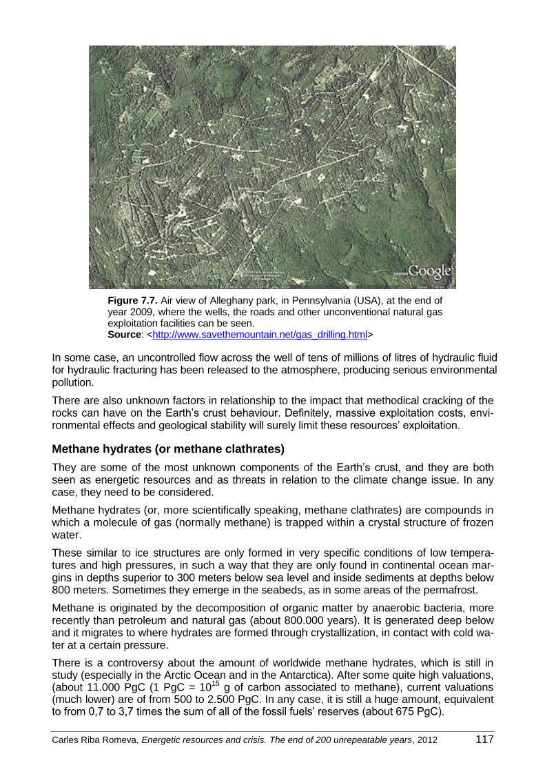
Carles Riba Romeva, Energetic resources and crisis. The end of 200 unrepeatable years, 2012 117
Figure 7.7. Air view of Alleghany park, in Pennsylvania (USA), at the end of year 2009, where the wells, the roads and other unconventional natural gas exploitation facilities can be seen. Source: <http://www.savethemountain.net/gas_drilling.html>
In some case, an uncontrolled flow across the well of tens of millions of litres of hydraulic fluid for hydraulic fracturing has been released to the atmosphere, producing serious environmental pollution.
There are also unknown factors in relationship to the impact that methodical cracking of the rocks can have on the Earth’s crust behaviour. Definitely, massive exploitation costs, envi-ronmental effects and geological stability will surely limit these resources’ exploitation.
Methane hydrates (or methane clathrates)
They are some of the most unknown components of the Earth’s crust, and they are both seen as energetic resources and as threats in relation to the climate change issue. In any case, they need to be considered.
Methane hydrates (or, more scientifically speaking, methane clathrates) are compounds in which a molecule of gas (normally methane) is trapped within a crystal structure of frozen water.
These similar to ice structures are only formed in very specific conditions of low tempera-tures and high pressures, in such a way that they are only found in continental ocean mar-gins in depths superior to 300 meters below sea level and inside sediments at depths below 800 meters. Sometimes they emerge in the seabeds, as in some areas of the permafrost.
Methane is originated by the decomposition of organic matter by anaerobic bacteria, more recently than petroleum and natural gas (about 800.000 years). It is generated deep below and it migrates to where hydrates are formed through crystallization, in contact with cold wa-ter at a certain pressure.
There is a controversy about the amount of worldwide methane hydrates, which is still in study (especially in the Arctic Ocean and in the Antarctica). After some quite high valuations, (about 11.000 PgC (1 PgC = 1015 g of carbon associated to methane), current valuations (much lower) are of from 500 to 2.500 PgC. In any case, it is still a huge amount, equivalent to from 0,7 to 3,7 times the sum of all of the fossil fuels’ reserves (about 675 PgC).

118 Carles Riba Romeva, Energetic resources and crisis. The end of 200 unrepeatable years, 2012
Figure 7.8. Methane hydrates. Left: combustion of a methane hydrate. Right: zones of
the planet’s continental rigs where methane hydrates are found; the USGS classifies them as energetic resources. Source: map of the US Geological Survey.
In atmospheric conditions, this white compound melts and releases methane that can be
burned. This has made us consider its use as an energetic source, and many projects have been initiated, but the geographical dispersion and the compound’s instability have made the
commercial exploitation not possible.
Due to either changes in sea level or increases of temperature in deep water, methane hy-drates can lose their stability conditions and dissociate, releasing the gas to the sediments,
which finally reach the atmosphere. Due to methane’s important greenhouse effect, a mas-sive release of methane can cause a sudden change in climate with catastrophic conse-
quences. There is the hypothesis that this was the cause of one of the massive extinctions.
Therefore, more than a resource, methane hydrates (quite unknown to most of us), can rep-resent a risk. Even more, the climatic change can, within its perverse and catastrophic ef-
fects, produce the destabilization of these reservoirs.
7.5. Fuels obtained by transformation
Liquid fuels based on petroleum (gasoline, gasoil, kerosene) are the basis of transport in modern developed societies (automobile, truck, boat; the only mean of transport to which
this cannot totally be applied is the railway, when it is electrically powered).
But, at the same time, petroleum is the first energetic resource that threatens to go short,
while other less vital for transport fuels (natural gas and, above all, coal) have a larger amount of reserves. This is where the interest to transform coal into liquid fuel derives from.
The main transformations are:
Gasification (coal, biomass, residues)
From natural gas to liquid fuel (GTL, gas-to-liquid)
From coal to liquid fuel (CTL, coal-to-liquid)
Biofuels (or BTL transformation, biomass-to-liquid)
Biofuels, together with renewable sources of energy, are discussed in chapter 9. Below we
will analyse the GTL and CTL transformations.

Carles Riba Romeva, Energetic resources and crisis. The end of 200 unrepeatable years, 2012 119
There is finally another fuel that many people mistake with a primary energy source while it
is only an energy carrier, a way in which the use of energy can be facilitated.
From different energetic sources to hydrogen
It is important not to confuse fuels obtained by transformation with primary energy sources. These energy carriers do not increase the availability of energy; they decrease it (because these transformations make efficiencies decrease).
In any case, these transformations provide more appropriate fuels for certain applications (for example liquid fuels for transport), or avoid local pollution or bad conscience (for exam-ple, hydrogen that does not produce CO2 during the combustion process, but it does during the manufacture process).
Gasification (coal and other organic matter)
Coal (and others like biomass or certain residues) gasification consists in its partial and controlled combustion (with lack of oxygen) in order to obtain a synthetic gas with combustion properties (syngas, mixture of H2, CO and CO2), obtained in different types of gasifiers (fluidized bed reactor, entrained flow gasifier, etc.).
The synthetic gas (syngas) has a great variety of uses: a) as an integrated gasification combined cycle (IGCC) fuel in an electrical station; b) as a gas that can be turned into a synthetic natural gas (SNG); c) as a gas that can produce hydrogen (H2); d) as a gas that can be transformed into a synthetic petroleum by means of the Fischer-Tropsch synthesis process; e) as raw material in the manufacture of certain chemical products. Polygeneration is the simultaneous manufacture of fuels, electricity and chemical products.
Gasification, which was initially developed to produce town gas at the end of the 18th century, favours a very versitile group of processes and applications that make the global energetic system more flexible. Also, on the basis of very spread and cheap resources, like biomass and residues, it is a technology that can provide developing countries with energetic resources.
In 2007 there were 144 registered gas plants worldwide and 427 working reactors, with a global heat capacity of 56 GWt, out of which 31GWt accounts to coal’s gasification. There are projections that there will be an increase of up to 155 GWt in 2015, which will specially affect Africa and the Middle West (64%), being more moderate in Asia and Oceania (27%), even lower in Europe (9%), and negligible in the United States [IEA-ETSAP-S01-2010].
However, energetic efficiencies of gasification processes are low and greenhouse effect gas emissions high (see table 7.5).
Transformation of coal and liquid fuels (CTL and GTL)
Considering the zenith of conventional petroleum and its future decline, one of the most promising alternatives is the transformation of coal (plentiful and relatively cheap) and natural gas (hard to render profitable when the resource is away from the consumption) into liquid fuels, like gasoline or synthetic diesel (CTL, coal-to-liquid and GTL, gas-to-liquid processes).
In this way, countries with large reserves of coal and limited reserves of petroleum (USA, China, India, Australia, South Africa) consider the CTL transformation the way to guarantee the supply of liquid fuels, which is so necessary for transport. Other countries with large re-serves of not consumed natural gas (Qatar, Nigeria) contemplate GTL processes like the way to commercialize this fuel. However, the low energetic efficiencies of these transfor-mations, as well as the considerable greenhouse effect gas emissions and the high invest-ments on facilities, impose serious limitations to their generalization.

120 Carles Riba Romeva, Energetic resources and crisis. The end of 200 unrepeatable years, 2012
The transformation of coal into synthetic petroleum (CTL) has a long history, that began in 1913 with F. Bergius’ direct coal liquefaction (DCL) and in 1923 with F. Fischer and H. Tropsch’s (FT process) indirect coal liquefaction (ICL). During the Second World War, Germany (with important coal and poor petroleum reserves) used direct liquefaction and during the isolation due to the apartheid, South Africa (also with important coal and poor petroleum reserves) started to carry out de indirect liquefaction process in 1955, which it is currently still carring out competitively.
Direct liquefaction (DCL), based on pyrolysis and hydrogenation, is simple and has a good thermal efficiency (>60%), but the quantity and quality of the obtained product is low. Indirect liquefaction is more complex (previous coal gasification is required) and the thermal efficien-cy is lower (from 50 to 55%), but the quantity and quality of the final product is better. Gas to liquid transformation (GTL) is based in either the direct conversion or in the Fischer-Tropsch process application to the synthetic gas.
These processes are not free: they have more unfavourable energetic efficiencies and emissions than those of the initial fuels (see table 7.5). Furthermore, if their use is wide-spread, they will precipitate the exhaustion of coal and natural gas reserves.
As the EIA-govUSA projections (International Energy Outlook 2009, page 22) predict for 2030, the productions that can be obtained are limited. They predict that the 0,2 Mb/d (mil-lions of barrels per day) of fuel obtained by the CTL process will increase to 1,2 Mb/d in 2030, and that the almost negligent production of fuel obtained by the GTL process that we currently have will become of 0,3 Mb/d in 2030. Remember that the current production and consumption of petroleum is of 85 Mb/d.
Finally, the establishment of these processes requires important investments. Industrial plants are like a combination of a power station and a refinery, and its investment cost ranges from 25.000 to 35.000 Euros per barrel/day of capacity. The scale benefits stop from the 17.000 b/d, and then the facilities need to be replicated.
Data from Sasol Chemicals Industry (South Africa)
The South-African company Sasol, worldwide leader in the transformation of coal to liquid, with more than 50 years of experience, gives the following data about the process [SAS-2009]:
- Thermal efficiency: ranging from a 38 to a 42% (depending on the coal and on the pro-cess)
- Emissions: 1.000 kgCO2/barrel (approximately, 163 gCO2/MJ)
In the production of liquid fuel, the CTL process emits 163 gCO2/MJ, and when it is burned it emits around 74 gCO2/MJ more (similar to other liquid fuels). Therefore, the total process (CTL + combustion of the liquid) entails total emissions of approximately 105 gCO2/MJ.
Figure 7.9. Panoramic view of the CTL plant in Sasol, Sagunta (South Africa)

Carles Riba Romeva, Energetic resources and crisis. The end of 200 unrepeatable years, 2012 121
Hydrogen
Energy carrier, not primary energy source
Frequently, when we refer to hydrogen, we mistake it with a new primary energy source. This is incorrect, as: hydrogen is not plentifully found in nature (if it was, it would escape from the Earth to the space as it is not trapped by gravity). For this reason, it has to be obtained from the transformation of other primary sources.
Hydrogen is simply an energy carrier. It only makes sense to produce it if it has advantages in its use in comparison to the sources where it comes from.
Hydrogen’s obtaining
It can be obtained from fossil fuels (and renewable fuels) or by means of water electrolysis. It is used to feed both internal combustion engines and fuel cell vehicles (FCV).
The cheapest way to obtain hydrogen (H2) is by natural gas transformation or by coal gasifi-cation. However, these processes emit large amounts of CO2 (see table 7.5) and, therefore, the production of hydrogen on a large scale only makes sense if it is combined with carbon capture and sequestration techniques.
The adaptation of internal combustion engines to hydrogen is a mature technology, relatively easy and not expensive to implant and efficiencies are slightly higher. Fuel cells are still on an experimental stage and costs are off-market, but they point at higher efficiencies. The problem, however, is the obtaining, storage and manipulation of hydrogen.
Extremely low volumetric heat of combustion
In the combustion (or oxidation) of a fuel, we refer to mass heating value as the amount of energy that is released during the combustion of a unit of mass, and it is measured in units of MJ/kg or kWh/kg and volumetric heat combustion as the amount of energy that it can pro-vide per unity of volume, it is normally measured in MJ/m3 (gases) or MJ/litre (liquids).
Therefore, fuels used for transport require high mass heating values to decrease the deadweight. In this way, liquid fuels have advantage over electric batteries, but gas fuels still seem to have more advantages, and, above all, hydrogen, as it has a mass heating value almost three times higher than gasoline (120,1 MJ/kg, instead of 43,2 MJ/kg).
Nevertheless, in order to avoid occupying too much space, fuels used for transport also need high volumetric heat combustion and, in relationship to this, gas fuels are much inferior to liquids. In effect, hydrogen in environmental conditions (neither compressed nor liquefied) supplies almost 3.000 times less energy than gasoline for the same volume (0,0108 MJ/litre, instead of 32,2 MJ/litre).
Cryogenic temperatures, high pressures and chemical absortion.
They are alternatives for the manipulation and storage of hydrogen. However, special facilities and high expenses are needed to achieve the appropriate pressures and temperatures.
Liquefied hydrogen (at -252,9ºC) has a density of 0,071 kg/l (that is, 71 grams per litre) while 1 litre of gasoline contains more hydrogen (116 grams, a 64% more) being the rest of the mass (around 730 grams) majorly carbon that also contributes to the energy of combustion. Cool temperature facilities and important insulators are needed.
In order to achieve compressed hydrogen densities of similar values to those of the liquid, the gas has to be compressed at extremely high pressures (between 350 and 700 bar), with an energy consumption that can range from a 11 to a 15% of the fuel’s energy. The deposit is much more voluminous and heavy than that of a liquid fuel.
A lot of investigation has been done on the topic of hydrogen storage by absortion in metal hydrates or other substances, but none of the results are even close to having similar volumetric energetic densities to those of liquid hydrocarbons.

122 Carles Riba Romeva, Energetic resources and crisis. The end of 200 unrepeatable years, 2012
The vehicle’s tank
To cover a distance of 500 km, considering the best engine efficiency, a standard automobile needs 9,5 kg of hydrogen (using the fuel cell it is reduced to 6,1 kg). If we choose the
liquefaction process, the deposit will hold 135 litres; if the compression is at 350 bar it will hold 300 litres; and if the compression is at 700 bars, it will hold 150 litres.
Summarizing
Remember again that hydrogen is not a primary energy source, but a simple energy carrier. Therefore, it will consume the energies (that are normally high) of the necessary transfor-
mations in order for it to be obtained, and it will emit the greenhouse effect gases that these transformations have origined (that are also normally quite high) (see table 7.5).
For this reason, hydrogen is not a carbon-free type of energy, as it is commonly said. Like
electricity, hydrogen in its use is carbon-free, but it is very pollutant when it comes to its obtaining. The whole life cycle has to be considered.
The so called hydrogen economy has serious technical and economical difficulties, that are
currently still far from being solved. Apart from appeasing our bad consience on the climatic change, we still don’t know the advantages that it will bring.
Table 7.5. Energetic efficiencies, emissions and costs of different transformations
Transformations Energy Emissions Investment
Eff. % TRE gCO2/MJ €/GJ (installed)
Synthetic gas (syngas) 1 fr. 73 to 75 2,85 55 from 10,4 to 13,2 Synthetic gas + hydrogen 1 fr. 73 to 75 2,85 55 from 10,8 to 14,1
Natural synthetic gas (NSG) 1 60 1,50 78 from 15,5 to 20,9 Coal to liquid (CTL) 2 48 0,92 120 from 9,8 to 13,5
Gas to liquid (GTL) 2 56 1,27 27 from 3,8 to 4,6
Compressed hydrogen (from coal) 3 42 0,71 233 Compressed hydrogen (fr. natural gas) 3 54 1,19 105
Compressed hydrogen (electr. mixEU) 3 22 0,28 208 Compressed hydrogen (wind electr) 3 56 1,26 9
Liquid hydrogen (nat gas 4.000 km) 3 43 0,88 126 1 Data obtained from the document: ETSAP-S01-2010, Syngas production from coal
2 Data obtained from the document: ETSAP-S02-2010, Liquid fuels production from coal & gas
3 Data obtained from the document: Well-to-Tank Report, version 2c, March 2007, WTT Appendix 2,
Description and detailed energy and GHG balance of individual pathways. Sources: [IEA-ETSAP-S01-2009], [IEA-ETSAP-S02-2009] and [WTW-WTT2-2007]; Developed by:
Carles Riba Romeva
CO2 sequestration or biosequestration
Throughout the geologic eras, nature and life have generated an enormous sequestration of CO2, which is reflected in the carbon cycle (see figure 11.10). Biosphere, land, organic matter
dissolved in ocean water, sedimens and kerogene (of which fossil fuels are a negligible part) are the result of the CO2 sequestration of an arcaic Earth atmosphere that contained this gas
in large amounts.
Nowadays, after almost two centuries of fossil fuel exploitation and with the accelerated consumption of the last fifty years, developed societies can no longer hide the imbalances
that they produce. It is like wanting to fix something that we break everyday, without having the intention of ceasing to break it.
Commonly, carbon sequestration is the excuse that allows us to insist in the need to change
things. As this problem will someday be solved, this allows me to keep working with

Carles Riba Romeva, Energetic resources and crisis. The end of 200 unrepeatable years, 2012 123
technologies that are only justified if the important volume sequestration is efficient. And, as
some technologies are only justified by sequestration, it is worth to keep investigating although solutions are doubtfull. A vicious circle.
We are talking about a technical sequestration, disconnected from nature and that manipu-lates the biosphere. There is another cooperative sequestration that aims to collaborate with nature and biosphere in order to re-establish the balance. But it needs a total change in mentality. In the first place, we would need to stop exploitating fossil fuels (main cause of the imbalance) and, afterwards, we would have to do a big effort to be ecologically friendly, understanding the complex natural phenomenons.
Types of technical sequestration
It is worth to analyse the technical sequestrations of CO2 with which we are working.
The so called Carbon Capture and Storage (CCS) is the collection of technical proposals with the aim of removing CO2 from the atmosphere or avoiding its arrival to it. In the environmental evalution of the processes (for example, those included in the document WTW of the European Union [WTW-2007]), the final CCS annotation appears, that presupposes that the process is acompanied by CO2.. Obviously, the emissions are lower, but the truth about CO2
sequestration is still being analysed in pilot plants.
It is necessary to warn the reader that all of the technical sequestration options are applied when CO2 is generated as a concentrate (as electric power stations, cement industry, iron and steel sector industries, petrochemical industries). It is assumed that a large part of the CO2
emissions that are generated in a disperse way (as vehicles, airships, ships, farm machinery and of public works, domestic heating, isolated consumptions) will never be sequestrated.
Reuse
It is not, stictly speaking, a type of sequestration, but a means of optimizing the resource. It is based on the capture of the residual CO2 of many processes, in order to use it as an input substance in other processes that need it. It would avoid generating more CO2 for these processes.
Chemical sequestration
Normally, combustion is done in order to fully exploit the energy from the fuels’ chemical bonds. To invert the process means that, together with the CO2, the energy that had been previously obtained has to be sequestrated again. Therefore, it is not viable, unless carbon is incorporated into other compounds that can be deposited as residues.
Injections in geological formations
It consists in injecting CO2 into geological formations that are capable of absorving it. Due to the fact that the atmosphere’s CO2 concentration is an issue that began to worry us quite recently, although injection in geological formation techniques have been known for long, the long-term geological sequestration of CO2 is a new concept.
The first commercial experience in relationship to the sequestration of CO2 began in year 2000 in Weyburn (Canada), and the first pilot experience of a power station with integrated CCS system was first done in Vattenfall (Germany), with the objective of analysing its feasibility.
Real CO2 emissions
EIA-govUSA statistical data about CO2 do not even include the sequestration of CO2 (CCS techniques). On the other hand, it is stated that during the 2000-2008 period, the greenhuse effect emissions to the atmosphere increased at a rhythm of 3% per year, while world population did so at a 2,5 times lower rhythm.
124 Carles Riba Romeva, Energetic resources and crisis. The end of 200 unrepeatable years, 2012
8. The uncertain nuclear alternative
8.1. From military uses to civil uses
Most of the Earth’s physical phenomena are related to the gravitational or electromagnetic forces. On the other hand, most significant nuclear phenomena are found in stars and at the interior of our planet, in far from atmosphere places; that are why they have been the latest area of physics to be discovered.
It is a quite unknown source of energy and discussions about nuclear power are normally unfounded. Below we will analyse if nuclear power could be a possible alternative source of energy.
The reactions that take place in the atomic nucleus put into play energies which are millions of times superior to those of the chemical links for a same amount of mass. In effect, fission of one atom of uranium U235 (only fissile isotope that is found in nature) releases an energy of around 200 MeV (millions of electro-volts), 40.000.000 times superior to most energetic chemical reactions (amongst them, those of fossil fuels). When, at the end of 1939, the German physicist Lise Meitner and her nephew, also a physicist, Otto Frisch discovered nu-clear fission by interpreting different experiments carried out by previous scientists, they im-mediately guessed the terrible consequences that this energy could unleash.
The first nuclear energy use was the military one (its “original sin”), through the large-scale deployment of the Manhattan American project (which began in 1940) and with the unjustifi-able attacks of the United States to the civil population of Hiroshima and Nagasaki the 6th and the 9th of August of 1945 with two atomic fission bombs (or A bombs), of enriched ura-nium and plutonium, respectively. Instead of being the end of Second World War, these at-tacks were the beginning of the Cold War and of the arms race. In effect, the Soviet Union did their first nuclear experiment four years later, in 1949, to which the United Kingdom in 1953, France in 1960, China in 1964 and later on other countries (India, Pakistan, Israel, and South Africa) followed. Meanwhile, in 1952, the United States made the first hydrogen bomb (or H bomb) explode. This type of bomb combines fusion and fission, with hundreds of times superior power, context in which the agreements of nuclear non-proliferation are rati-fied (1968).
But, also a tonne of natural uranium (1 tUnat) provides a primary thermal energy of approxi-mately 450 TJt (tera, or 1012 thermal joules), that, transformed to electric energy, generates 40,2 GWeh (or millions of kWeh; the Red Book 2007 points out a worldwide production of 2.675 TWeh with an uranium consumption of 66.500 tUnat). It is a huge amount of energy, equivalent to the amount of energy that 10.500 tonnes of petroleum or 15.000 of coal provide.
It was not until 1954 (nine years after the Hiroshima and Nagasaki explosions), that the USSR set up the first nuclear reactor of electrical production in Obninsk. Two years later (1956), the United Kingdom set up the Calder Hall nuclear power station and, the following year (1957), the United States inaugurated their nuclear station of Shippingport. However, few months before the start of the first soviet power station, in 1953, United States president Eisenhower anticipated with his well-known media speech in the ONU Meeting, called “at-oms for peace”, where he supported the civil uses of nuclear energy. Its more evident con-sequence was the creation, in 1957, of the International Atomic Energy Agency (IAEA).
The new nuclear hope
From there on, 565 nuclear power stations have been built in 33 countries. At the end of 2009, 123 had been removed, 5 of them were out of order for long time and 437 were in working conditions. In the same moment, there were 55 nuclear power stations under con-struction, 40 of them in China, Russia, South Korea and India, and there were also 61 of them planned (IAEA, Nuclear Power Reactors in the World, 2010).

Carles Riba Romeva, Energetic resources and crisis. The end of 200 unrepeatable years, 2012 125
In the previous decades (1990-2010), after the progressive decline of the new nuclear con-structions beginning in 1975 (see figure 8.2), probably due to the lack of economic profitabil-ity [Cod-2008], the never able to be solved problem regarding radioactive residues and the large public opinion impact after the Harrisburg (1979) and Chernobyl (1986) accidents, nu-clear power has been facing times of stagnation.
Lately, due to the increasing concern regarding the lack of petroleum and the climate change threat, a campaign has been re-launched (a first effect is the revival of previous five years 2005-2010 nuclear stations) that proposes nuclear energy as an alternative with the two following premises:
a) It is a source of energy which will difficultly become exhausted. b) It does not produce greenhouse effect gas emissions.
In this way, nuclear energy claims to be the solution to the two main problems that humanity is currently facing. With the text already closed, a new and serious nuclear accident has tak-en place in the BMR nuclear power stations in Fukushima (Japan) for natural reasons (grade 9,1 earth tremor and posterior tsunami, the 11th of March 2011), which, before it was controlled, had already been considered to be a nuclear accident as serious as the one in Chernobyl. This fact will surely make nuclear expectations be decreasingly revised.
The first of the two given premises can seem a paradox in relationship to data in chapter 4 according to which uranium reserves, in 2007, where only the 6,68% of the whole of unre-newable energetic resources together with petroleum, natural gas and coal. The nuclear system is very complex and not well-known by the public (even by many politicians), and it is important to analyse it carefully. However, as it will be seen later on, the nuclear power al-ternative as the future energetic source finds important uncertainties and impracticabilities.
The statement that nuclear resources represent an interminable source of energy is based on the following considerations:
1) The resources of natural uranium are almost unlimited. It is only a question of price.
Certainly, worldwide uranium resources are very much higher than the 5,47 millions of tones that were consigned as reserves in 2007 (that is to say, amount of uranium that is capable of being extracted with the current economic technologies and parameters).
Natural uranium is spread, in small proportions, in rocks and very plentiful media (phos-phates, granites, sea water) in such a way that there is enough amount to cover humani-ty’s energetic needs for hundreds of years.
Due to the low economic incidence of nuclear fuel in the generated electricity, it would be a matter of assuming natural uranium growing costs in order to exploit every time less favourable but more plentiful deposits.
2) Breeder reactors will multiply the use of nuclear resources (uranium, thorium).
According to its cosmic origin, natural uranium from the Earth’s crust is composed by a 0,71% of the fissile uranium isotope U235 (the one that makes nuclear reactors and atom-ic bombs work) and a the 99,28% of the non-fissile uranium isotope U238 (nowadays, ra-dioactive waste). Nevertheless, by bombing uranium U238 with neutrons, this is transmut-ed into the plutonium isotope Pu239, which is not present in nature, but is highly fissile (it has already been used in Nagasaki’s atomic bomb in 1945) and which is suitable as a nu-clear combustible.
The breeder reactors’ technology, which was started more than fifty years ago, would transform the isotope U238 (which is known as fertile) into plutonium Pu239 (fissile) and this would increase the load expectations of natural uranium in about 140 times.
Analogously, the isotope of thorium Th232 (three times more plentiful in nature than fis-sile uranium), also fertile, bombed with neutrons is transmuted into the isotope of urani-um U233, which is also fissile, and this would increase future capacities of the nuclear energetic system even more.

126 Carles Riba Romeva, Energetic resources and crisis. The end of 200 unrepeatable years, 2012
3) Nuclear fusion, the great energetic hope for the future
Finally, the tuning of the techniques to control nuclear fusion (reaction that takes place in stars and in the Sun), consisting in the union of light nuclei (deuterium and tritium), to ob-tain a heavier nucleus of helium together with an enormous energy release, would allow us to dispose of a new, almost inexhaustible, source of energy.
This is the challenge of the worldwide multilateral ITER project. Up to the moment, fusion energy had only been used to manufacture the hydrogen bomb (H bomb).
It is not necessary to say that the treatment of radioactive waste that is originated in each of the phases of the nuclear cycle is a large concern that is still not fully solved. Security and nuclear accidents are not minor concerns either, as well as the precautions and limitations that need to be taken in order to avoid military uses of nuclear resources.
However, we find it necessary to distinguish if the three claimed paths to go beyond the cur-rent uranium reserves (the 6,68% of the unrenewable sources of energy) are technically and economically feasible and if they can be implemented in an adequate margin of time in order to save the effects of the decline of petroleum and other fossil fuels (section 8.3).
It is also important to know if nuclear energy has an adequate energy return on investment (EROI) tax and if it does or does not emit greenhouse effect gases, and in case that it did, to what extent it emits them (section 8.4). Before we do so, however, we briefly present the main information regarding the nuclear system evolution.
8.2. Evolution of nuclear energy production
In this section, information is given on the theme of the evolution of worldwide nuclear power stations, where two historical eras are clearly distinguished, with an inflection point around year 1990. Its distribution according to regions and countries will also be analysed.
Evolució de les centrals nuclears en el món
0
50
100
150
200
250
300
350
400
450
500
19
54
19
57
19
60
19
63
19
66
19
69
19
72
19
75
19
78
19
81
19
84
19
87
19
90
19
93
19
96
19
99
20
02
20
05
20
08
Nombre (unitats)
Potència (GWe)
Figure 8.1. Evolution of the worldwide nuclear power stations’ park. The first column repre-sents the number of power stations and, the second one, the global installed power (GWe). After a fast growth, since 1990 the number of nuclear power stations remains almost con-stant, but the substitution of the old installations by the new ones makes the installed power (and the production, which has not been represented) increase slightly. Source: IAEA, Nu-clear Reactor Power in the World, 2010 Edition. Developed by: Carles Riba Romeva
Evolution of worldwide nuclear power stations
Number (units)
Power (GWe)

Carles Riba Romeva, Energetic resources and crisis. The end of 200 unrepeatable years, 2012 127
Most of nuclear power stations were built before 1990: 486 units, out of which 416 were in working conditions. Nuclear stations that were built later on, between 1990 and 2009 (79 units), cover little above the retired facilities (58 units) and the park only increases in 21 nu-clear power stations (figure 8.1).
In the previously mentioned period (1990-2009), the installed power capacity and the elec-tricity generation increase due to the fact that the new reactors are more efficient than the removed ones (67,25 GWe of the new installed power capacity in relationship to the 14,80 GWe of removed power) and the average power of the facilities increases from 0,765 GWe, in 1990, to 0,848 GWe, in 2009.
However, the influence of nuclear energy in the worldwide electric system decreases from its maximum value of 17,7% in 1996, to a 13,7% in 2008 (4 percentage points in 12 years).
Centrals nuclears iniciades en el món
0
5
10
15
20
25
30
35
40
45
19
54
19
57
19
60
19
63
19
66
19
69
19
72
19
75
19
78
19
81
19
84
19
87
19
90
19
93
19
96
19
99
20
02
20
05
20
08
Centrals (unitats)
Potència (GWe)
Figure 8.2. Evolution of the number of nuclear power stations that were started every year: number of units (first column) and global power in GWe (second column). Until 1965, the power stations that had been opened were of a relatively low power. The most important amount of new nuclear station constructions was given between 1967 and 1985. After the stop that took place between 1990 and 2005, certain recuperation is started. Source: IAEA, Nuclear Reactor Power in the World, 2010. Developed by: Carles Riba Romeva
Summing up, at the end of 2009 there were 437 nuclear power stations worldwide, in working conditions, (according to the EIA) and, after some years of stagnation of new initiatives (de-cline from 1977 to 1990 and stagnation since then, figure 8.2), in the last years it seems that there has been a moderate resumption of new constructions (55 units at the end of 2009).
Another aspect that makes it easier to have a clearer view of the nuclear system and that at the same times provides information about the effective nuclear energy trends is the analy-sis of the nuclear power stations age spectrum.
Figure 8.3 shows that younger nuclear power stations, with higher future exploitation capaci-ties (below 20 years of age) are only 78 (the 17,8% of the current park) while the average of the world park is above 25 natural years, amount that is not far from the 24,6 years of func-tioning at whole power that Storm grants as maximum life [Sto-2007], belonging to thirty natural years.
Also, most of the old nuclear power stations are found in developed countries, while new nuclear power stations are found in developing countries.
Number (units)
Power (GWe)
Nuclear power stations that have started every year in the world
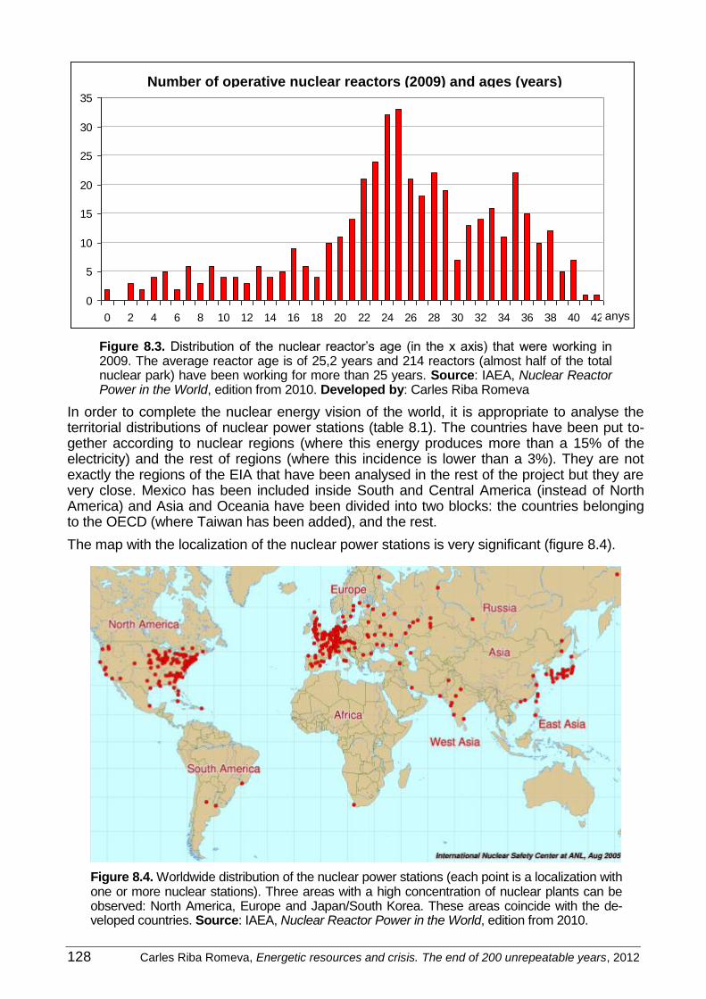
128 Carles Riba Romeva, Energetic resources and crisis. The end of 200 unrepeatable years, 2012
Nombre de reactors en funcionament (2009) i edats (anys)
0
5
10
15
20
25
30
35
0 2 4 6 8 10 12 14 16 18 20 22 24 26 28 30 32 34 36 38 40 42
Figure 8.3. Distribution of the nuclear reactor’s age (in the x axis) that were working in 2009. The average reactor age is of 25,2 years and 214 reactors (almost half of the total nuclear park) have been working for more than 25 years. Source: IAEA, Nuclear Reactor Power in the World, edition from 2010. Developed by: Carles Riba Romeva
In order to complete the nuclear energy vision of the world, it is appropriate to analyse the territorial distributions of nuclear power stations (table 8.1). The countries have been put to-gether according to nuclear regions (where this energy produces more than a 15% of the electricity) and the rest of regions (where this incidence is lower than a 3%). They are not exactly the regions of the EIA that have been analysed in the rest of the project but they are very close. Mexico has been included inside South and Central America (instead of North America) and Asia and Oceania have been divided into two blocks: the countries belonging to the OECD (where Taiwan has been added), and the rest.
The map with the localization of the nuclear power stations is very significant (figure 8.4).
Figure 8.4. Worldwide distribution of the nuclear power stations (each point is a localization with one or more nuclear stations). Three areas with a high concentration of nuclear plants can be observed: North America, Europe and Japan/South Korea. These areas coincide with the de-veloped countries. Source: IAEA, Nuclear Reactor Power in the World, edition from 2010.
anys
Number of operative nuclear reactors (2009) and ages (years)

Carles Riba Romeva, Energetic resources and crisis. The end of 200 unrepeatable years, 2012 129
Table 8.1. Nuclear power stations, nuclear electric production and population (2009)
World and regions
In operation In construction Produced energy Population
N 1
GWe2 % N
1 GWe
2 % TWeh
3 % %PE
4 Min-
hab5
%
World 437 370,7 100,0 55 54,3 100,0 2.558 100,0 13,6 6.614 100,0
Nuclear regions 398 351,9 94,9 27 27,8 51,1 2.433 95,1 21,1 1.414 21,4
America (Can+USA) 122 113,3 30,6 1 1,2 2,3 882 34,5 18,7 334 5,1 Europe 149 133,9 36,1 6 6,3 11,5 874 34,2 25,3 595 9,0
Eurasia 47 35,2 9,5 11 9,5 17,5 233 9,1 17,6 284 4,3
Asia and Oceania 6
80 69,5 18,8 9 10,8 19,8 444 17,3 21,6 201 3,0
Other regions 39 18,8 5,1 28 26,6 48,9 124,6 4,9 1,7 5.200 78,6
America (the rest) 6 4,1 1,1 1 0,8 1,4 29,9 1,2 1,9 571 8,6
Middle East 0 0,0 0,0 1 1,0 1,8 0,0 0,0 0,0 195 3,0
Africa 2 1,8 0,5 0 0,0 0,0 11,6 0,5 2,0 946 14,3 Asia Oceania (the rest) 31 12,9 3,5 26 24,8 45,7 83,1 3,2 1,8 3.488 52,7
Main countries7
1 USA 104 100,7 27,2 1 1,2 2,2 796,9 31,2 20,2 301 4,7
2 France 59 63,3 17,1 1 1,7 3,0 391,8 15,3 75,2 64 1,0
3 Japan 54 46,8 12,6 1 1,4 2,5 263,1 10,3 28,9 127 2,0 4 Russia 31 21,7 5,9 9 7,5 13,8 152,8 6,0 17,8 141 2,2
5 South Korea 20 17,7 4,8 6 6,8 12,5 141,1 5,5 34,8 48 0,7
6 Germany 17 21,5 5,5 127,7 5,0 26,1 82 1,3
7 Canada 18 12,6 3,4 85,1 3,3 14,8 33 0,5
8 Ukraine 15 13,1 3,5 2 2,0 3,7 77,9 3,0 48,6 46 0,7 9 China 11 8,4 2,3 20 21,6 39,7 62,9 2,6 1,9 1.322 20,6
10 United Kingdom 19 10,1 2,7 62,9 2,5 17,9 61 0,9
11 Spain 8 7,5 2,0 50,6 2,0 17,5 41 0,6 12 Sweden 10 9,0 2,4 50,0 2,0 37,4 9 0,14
13 Belgium 7 5,9 1,6 45,0 1,8 51,7 10 0,16
14 Taiwan 6 5,0 1,3 2 2,6 4,8 39,9 1,6 17,1 23 0,4
15 Switzerland 5 3,2 0,9 26,3 1,0 39,5 8 0,12
16 Czech Republic 6 3,7 1,0 25,7 1,0 33,8 10 0,16 17 Finland 4 2,7 0,7 1 1,7 3,2 22,6 0,9 32,9 5 0,08
18 India 18 4,0 1,1 5 2,9 5,4 14,8 0,6 2,2 1.141 17,1
19 Hungary 4 1,9 0,5 14,3 0,6 43,0 10 0,16
20 Bulgaria 2 1,9 0,5 2 2,0 3,7 14,2 0,6 35,9 7 0,11 21 Slovakia 4 1,8 0,5 2 0,9 1,6 13,1 0,5 53,5 5 0,08
22 Brazil 2 1,9 0,5 12,2 0,5 2,9 193 3,0
23 South Africa 2 1,8 0,5 11,6 0,5 4,8 48 0,7
24 Romania 2 1,3 0,3 10,8 0,4 20,6 22 0,3
25 Mexico 2 1,3 0,4 10,1 0,4 4,1 109 1,7 26 Latvia
7 10,0 0,4 76,2 4 0,05
27
Argentina 2 0,9 0,3 1 0,7 1,4 7,6 0,3 7,0 40 0,6 1
Number of nuclear power stations, at the end of 2009 (IAEA, Nuclear Power Reactors in the World, 2010)
2 Nuclear power station’s installed power at the end of 2009, in GWe (10
9 electric Watts), according to the IAEA
3 Total amount of electric energy, with a nuclear origin, that was produced in 2009, in TWeh (10
12 electric
Wattshour), according to the IAEA
4 Nuclear energy’s participation rate (in percentage) in the total electric production. World and regions: data from the EIA 2007. Countries: data from 2009, according to the IAEA, Nuclear Power Reactors in the World, 2010
5 Population in 2007, in Minhab (millions of inhabitants), according to the EIA
6 Japan, South Korea, Australia and New Zealand (Asia and Oceania, OECD), the two latter with no nuclear power stations, to which Taiwan has also been added.
7 There are 33 countries that have (or have had) nuclear power stations. The list continues with Slovenia (1 cen-tral), Holland (1), Pakistan (2) and Armenia (1) Italy (4) and Kazakhstan (1) as they had closed their nuclear power plants before 2009, and Lithuania has closed them during 2009. Furthermore, Iran is currently building its first nuclear plant.
Source: IAEA, EIA-govUSA;. Developed by: Carles Riba Romeva

130 Carles Riba Romeva, Energetic resources and crisis. The end of 200 unrepeatable years, 2012
Comments on Current nuclear energy situations and their evolutions:
1. In spite of the fast development that took place during the first decades, nuclear en-ergy has been stalled since 1990, when the new constructions had replaced only slightly more than the retired constructions.
2. The rhythm of new station’s construction (in spite of the resurgence) will not replace the current worldwide park. The prolonged average building time of a nuclear power station (7,8 years in the last decade) implies that the 55 nuclear power stations that are at the moment under construction only represent 7 new stations per year. On the other hand, there are 127 nuclear power stations around the world that have been functioning for more than 30 years (the average age of nuclear power plants have been removed so far has been 25 years).
3. In 2009, nuclear energy supplied a13,7% of the total electric energy worldwide (or a 5,08% of the primary energy). During the previous twenty years, the nuclear system has lost weight (in 1996 it supplied a 17,7% of the electric energy, which is equiva-lent to a 5,33% of the primary energy).
4. Nuclear energy supplies developed countries (a 95,1% supplies developed countries and Eurasia with a 21,4% of the world population, and supplies a 21,1% of the total electricity they consume), while it is residual in developing countries (a 4,9% of the generated nuclear electricity for a 78,6% of the total world population and it supplies only a 1,7% of the total electricity that they consume).
5. The new nuclear power stations which are under construction (55 units, out of which 20 are in China, 9 in Russia, 6 in South Korea and 5 in India), and the ones that are planned to be built (61, out of which 38 will be in China, 11 in Japan before the Fu-kushima accident, and 5 in Russia) announce an important decrease of nuclear en-ergy in Europe and North America, due to the predicted future closure of the power stations without having planned their replacement.
6. Future predictions highlight that nuclear energy will keep being almost absent in Af-rica, South America and large areas of Asia and Oceania.
8.3. Evaluation of uranium resources
The starting point of this critical analysis is the data given by the biennial publishing of the IAEA (International Agency of Atomic Energy, under the authority of the United Nations) and the NEA (Nuclear Energy Agency, of the OECD) titled Uranium Resources, Production and Demand, also known as the Red Book, which was first edited in 1965 and is known as the worldwide uranium reference <http://www.nea.fr/pub/ret.cgi?id=new>.
These official documents (specially the latest year’s editions, belonging to year 2007 and 2009) declare that there are enough uranium resources to cover plenty of years, and there-fore, we do not need to worry. The NEA press release that took place the 3rd of June 2008, in Paris, during the presentation of the 2007 Red Book, states, in relationship to uranium:
«Over the base of electric energy generation with a nuclear origin in 2006 and of the ac-tual state of the available technology, the identified resources are enough for 100 years.»
The German-origin study group EWG (Energy Watch Group), formed by a group of scien-tists and experts, with the objective of investigating the concept of sustainability in the global energy supply, devotes its first project to the nuclear theme [EWG-2006]. In appendixes 1 and 2, it reviews the different uranium reserves definitions of the IAEA-NEA, and the histori-cal evaluations that have been made in the Red Book since 1965.
The mostly used scheme is that of the IAEA-NEA, that distinguishes between “known re-sources” and “not discovered resources”. It divides the first ones into “reasonably assured re-sources” (RAR) and “inferred resources” (IR), previously known as “estimated additional re-
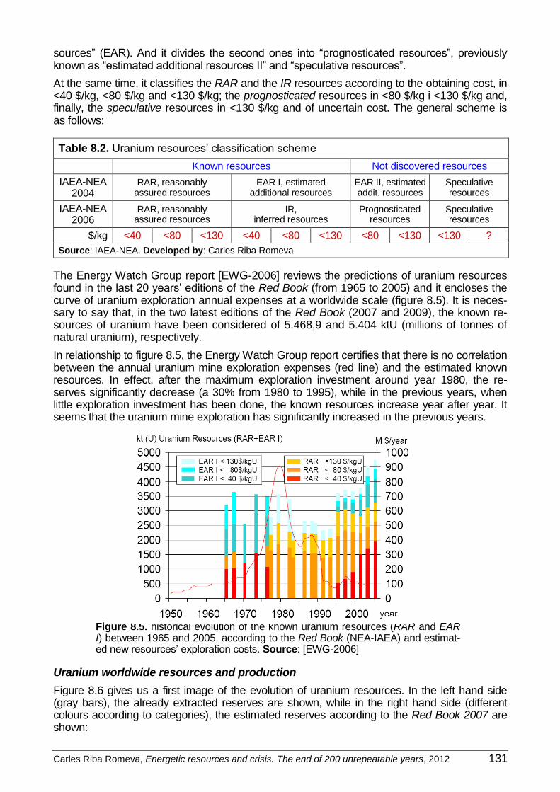
Carles Riba Romeva, Energetic resources and crisis. The end of 200 unrepeatable years, 2012 131
sources” (EAR). And it divides the second ones into “prognosticated resources”, previously known as “estimated additional resources II” and “speculative resources”.
At the same time, it classifies the RAR and the IR resources according to the obtaining cost, in <40 $/kg, <80 $/kg and <130 $/kg; the prognosticated resources in <80 $/kg i <130 $/kg and, finally, the speculative resources in <130 $/kg and of uncertain cost. The general scheme is as follows:
Table 8.2. Uranium resources’ classification scheme
Known resources Not discovered resources
IAEA-NEA 2004
RAR, reasonably assured resources
EAR I, estimated additional resources
EAR II, estimated addit. resources
Speculative resources
IAEA-NEA 2006
RAR, reasonably assured resources
IR, inferred resources
Prognosticated resources
Speculative resources
$/kg <40 <80 <130 <40 <80 <130 <80 <130 <130 ?
Source: IAEA-NEA. Developed by: Carles Riba Romeva
The Energy Watch Group report [EWG-2006] reviews the predictions of uranium resources found in the last 20 years’ editions of the Red Book (from 1965 to 2005) and it encloses the curve of uranium exploration annual expenses at a worldwide scale (figure 8.5). It is neces-sary to say that, in the two latest editions of the Red Book (2007 and 2009), the known re-sources of uranium have been considered of 5.468,9 and 5.404 ktU (millions of tonnes of natural uranium), respectively.
In relationship to figure 8.5, the Energy Watch Group report certifies that there is no correlation between the annual uranium mine exploration expenses (red line) and the estimated known resources. In effect, after the maximum exploration investment around year 1980, the re-serves significantly decrease (a 30% from 1980 to 1995), while in the previous years, when little exploration investment has been done, the known resources increase year after year. It seems that the uranium mine exploration has significantly increased in the previous years.
Figure 8.5. historical evolution of the known uranium resources (RAR and EAR I) between 1965 and 2005, according to the Red Book (NEA-IAEA) and estimat-ed new resources’ exploration costs. Source: [EWG-2006]
Uranium worldwide resources and production
Figure 8.6 gives us a first image of the evolution of uranium resources. In the left hand side (gray bars), the already extracted reserves are shown, while in the right hand side (different colours according to categories), the estimated reserves according to the Red Book 2007 are shown:

132 Carles Riba Romeva, Energetic resources and crisis. The end of 200 unrepeatable years, 2012
-450 -300 -150 0 150 300 450 600 750 900 1050 1200 1350
Extrets fi 2006
RAR <40 $/kg
RAR 40-80 $/kg
RAR 80-130 $/kg
IR <40 $/kg
IR 40-80 $/kg
IR 80-130 $/kg
Canadà
Estats Units
Alemanya
Àfrica del Sud
Rússia
Austràlia
República Txeca
Kazakhstan
Níger
Namíbia
França
Xina
Uzbekistan
Gabon
Rep. Dem. Congo
Hongria
Romania
Bulgària
Ucraïna
Índia
Espanya
Brasil
Mongòlia
Dinamarca
Jordània
Figure 8.6. Representation of the stocked production (extracted resources) at the end of 2006 (left) and of the different resources RAR and IR for the main uranium producing countries (past, present and future). Source: Red Book 2007. Developed by: Carles Riba Romeva.
Table 8.3 gives information about resources, production, demand and accumulated produc-tion of uranium. In the Red Book 2009 a slight decrease of the “known resources” is stated in relationship to the Red Book 2007, as well as some surprising variations (on top: Austral-ia, China and Canada, on the bottom: Kazakhstan, South Africa, USA and Ukraine).
Both in table 8.3 and in figure 8.6, it is stated that many countries have exhausted their ura-nium reserves, without having almost any resources left (Germany, Czech republic, France, Gabon, Democratic Republic of Congo, Hungary, Romania, Bulgaria and Spain). The United States are in a declining production situation (1.453 tUnat/a in 2009, when they had reached 20.000 tUnat/a) and they only have low-quality resources left.
Current uranium production (2009) is fundamentally based on three first level countries (Ka-zakhstan, 14.020 tUnat/a; Canada, 10.173, and Australia, 7.982) and in four second-level coun-tries (Namibia, 4.626 tUnat/a; Russia, 3.564; Niger, 3.243, and Uzbekistan, 2.429). Depending on the known resources (RAR+IR <130 $/kg), in the future South Africa (295.000 tUnat), Brazil (279.000), China (171.000), Jordan (112.000) and Ukraine (105.000) could gain importance.
We will need to see if, as uranium is extracted, the resources assigned by the IAEA-NEA in each country will not fit to the fall, as has occurred with France and the United States (it will be seen later on). In any case, it seems scarcely realistic to count on the “undiscovered resources” (prognosticated and speculative), that, according to the Red Book 2007, add up 10.540,1 ktUnat, almost the double of the “known resources”. The IAEA-NEA does not consider them reserves.
ktUnat
Canada
EUA
Germany
South Africa
Russia
Australia
Czech Republic
Kazakhstan
Niger
Namibia
France
China
Uzbekistan
Gabon
Congo, R.D.
Hungary
Romania
Bulgaria
Ukraine
India
Spain
Brazil
Mongolia
Denmark
Jordan

Carles Riba Romeva, Energetic resources and crisis. The end of 200 unrepeatable years, 2012 133
Table 8.3. Reserves, production, consumption and stocked production of natural uranium
Countries RAR+IR
<130 $/kg, Red B. 2009
RAR+IR <130 $/kg,
Red B. 2007
Production Red Book
2009
Production Red Book
2007
Demand Red Book
2007
Stocked production end of 2006
Countries ordered by production volume (tUnat) 1
1 Australia 1.673.000 1.243.000 7.982 9.516 0 130.414
2 Kazakhstan 651.000 817.300 14.020 4.357 0 108.045
3 Canada 485.000 423.200 10.173 11.628 1.900 396.597
4 Russia 373.300 545.600 3.564 3.431 4.100 129.729
5 South Africa 295.000 435.100 563 674 290 154.461
6 Namibia 284.000 275.000 4.626 3.147 0 84.950
7 Brazil 279.000 278.400 345 110 450 1.899
8 Niger 272.000 274.000 3.243 3.093 0 100.664
9 United States 207.000 339.000 1.453 1.039 22.825 359.193
10 China 171.000 67.900 750 750 1.500 29.189
11 Jordan 112.000 111.800 0 0 0 0
12 Uzbekistan 111.000 111.000 2.429 2.300 0 28.242
13 Ukraine 105.000 199.500 840 800 2.480 11.500
14 India 80.000 72.900 290 230 445 8.370
15 Mongolia 49.000 62.000 0 0 0 535
Rest of the countries ordered by volume of demand (tUnat) 1
1 France n.d. 2 11.700 8 7 9.000 75.977
2 Japan n.d. 6.600 n.d. 0 8.790 84
3 Germany n.d. 7.000 n.d. 94 3.490 219.399
4 South Korea n.d. 0 n.d. 0 3.200 0
5 United King-dom n.d. 0 n.d. 0 1.900 0
6 Sweden n.d. 10.000 n.d. 0 1.600 200
7 Spain n.d. 11.300 n.d. 0 1.310 5.028
8 Belgium n.d. 0 n.d. 0 1.065 686
9 Czech Rep. n.d. 700 n.d. 409 740 109.433
10 Bulgaria n.d. n.d. n.d. 0 505 16.357
11 Hungary n.d. n.d. n.d. 3 380 21.048
12 Romania n.d. 6.700 75 90 200 18.169
13 Gabon n.d. 5.800 n.d. 0 0 25.403
14 Congo, D. R. n.d. 2.700 n.d. 0 0 25.600
World 5.404.000 5.468.900 50.772 41.719 69.110 2.193.512
Coverage of the Uranium requirements 73,5% 65% 1 tUnat = tonnes of natural uranium (isotope composition: 99,28% of U238; 0,71% of U235).
2 No data
Source: Red Book 2007 and Red Book 2009. Developed by: Carles Riba Romeva
French and American uranium mines history
The Energy Watch Group report gives interesting information on the evolution of the French and American mines according to the estimated resources [EWG-2006].
French mining
The uranium mining process started very early in France in order to cover both military and electricity needs (it is the second worldwide country when it comes to nuclear energy, more than a 15% of the world, and the first when it comes to nuclear energy production, with more than a 75%). The production gradually increased up to 3.300 tUnat/a, in year 1980 it rapidly decreased until it became residual in year 2001 (figure 8.7). Including the stored production and the inferred resources (11.700 tUnat), accepted uranium resources (past and present) in France are of 87.700 tUnat.

134 Carles Riba Romeva, Energetic resources and crisis. The end of 200 unrepeatable years, 2012
However, between 1970 and 1990, and during the full summit of the French uranium mining industry the estimation of various Red Book (IAEA-NEA) editions placed French resources (RR+EAR <80 $/kg) between 120.000 and 130.000 tUnat, between a 38 and a 48% above the currently accepted reality, with resources that were almost exhausted and a practically stopped production. United States
France
Evolution of the natural uranium production
Stocked production and estimations of the reserves
Figure 8.7. Evolution of the uranium extraction in France and the United States with the passing of time together with the forecasts of Uranium resources of the succes-sive Red Book from the IAEA-NEA editions. The strong correlation between the pro-duction’s decline and the forecast’s decline can be observed. Source: [EWG-2006]
United States’ American mining
Commercial uranium production started in 1947 and it rapidly grew until it reached a peak of 15.000 tUnat/a in 1960. In the following years (1960-1980), uranium production, almost al-ways greater than 10.000 tUnat/a, reached a second peak of 20.000 tUnat/a in 1980. From then on, a noticeable decline started, reaching amounts of up to 1.000 tUnat/a starting from year 2000 (figure 8.7), although lately a small increase has been insinuated.
According to the Energy Watch Group [EWG-2006], at the end of 2005 the United States had extracted approximately 420.000 tUnat (according to the Red Book 2007, 360.000 tUnat).
During years with full productive summit (years 1965-1980), the IAEA-NEA overestimated the Uranium resources. In 1977, when 200.000 tUnat had been extracted from American mines, resources of 1.360.000 tUnat were estimated (RAR+EAR I <80 $/kg) or 1.800.000 tUnat (RAR+EAR I <130$/kg).
Since the production decline that took place in the 80’s, the IAEA-NEA reduced United States’ expectancies in more than 1.000.000 tUnat. The Red Book 2007, with 361.000 tUnat that had already been extracted, places the resources RAR+IR<130 $/kg of the United States in 339.000 tUnat, and the Red Book 2009 reduces them to 207.000 tUnat.

Carles Riba Romeva, Energetic resources and crisis. The end of 200 unrepeatable years, 2012 135
8.4. Consumptions and impacts of nuclear energy
The Dutch physicochemical J.W. Storm van Leeuwen and the American nuclear physicist P.B. Smith published an extense and well documented study, called Nuclear Power: the En-ergy Balance [Sto-2007], that analyses nuclear energy’s life cycle (that has currently become a reference), where the energetic costs and the greenhouse effect emissions of the nuclear cycle as a whole are analysed.
Table 8.4. Invested energy and CO2 emissions in a random nuclear power station1
Concepts2 Invested energy CO2 emissions
PJ/life kJ/kWeh Tg/life g/kWeh
1 Power station’s construction3 80,00 371,25 5,00 23,20
2 Mining + grinding (G =0,15%, soft rock)3 9,60 44,55 0,64 2,95
3 Combustible preparation (front-end) 33,61 155,95 1,26 5,83
4 Operation and maintenance 84,60 392,59 5,25 24,37
Production operations (1+2+3+4) 207,81 964,34 12,14 56,34
5 Mining claim (environment restitution)4 17,25 80,05 1,15 5,35
6 Combustible preparation residues (front-end) 20,19 93,71 1,54 7,15
7 Treatment of used combustible (back-end) 13,93 64,65 1,05 4,85
8 Power station’s dismantling3 120,00 556,87 7,50 34,80
Restitution operations (5+6+7+8) 171,38 795,28 11,24 52,16
Total 379,18 1.759,62 23,38 108,50 1 The parameters of a reference nuclear power station, according to Storm & Smith, are: power, 1 GWe;
time working at full power: 24,6 years (the station’s physical life is longer than that); total amount of pro-duced electric energy: 215,5 TWeh (or 775,8 PJ); consumed Uranium: 5.212 tUnat (42,35 MWeh/MgUnat)
2 The sections that do not have a remark are considered to be constant
3 These values have a big variability. Storm and Smith show the following range: for construction: 40-120
PJ/life and 2,5-7,5 Tg/life, and for dismantling: 80-140 PJ/life and 7,5-17,5 Tg/life.
4 The consumed energy and the CO2 emissions strongly depend on the grade of the ore and on the type
of rock (soft or hard). In hard rocks with a G=0,013% grade, it would reach the value of 519 PJ/life and 13,6 Tg/life in the mining and grinding section and 349 PJ/life and 26,2 Tg/life in the environment restitu-tion section.
Source: Storm & Smith [Sto-2007]. Developed by: Carles Riba Romeva
Certainly, Storm & Smith’s study is an analysis of the life cycle of nuclear energy with a rigor that we would like to have with other energetic sources and activities. But, as the authors themselves admit, a lot of the information, that the nuclear system should provide, is missing.
In any case, it leads to the following observations:
1. Nuclear energy is not exempt from CO2 emissions (108,5 gCO2/kWeh), although they are lower than in gas (450 gCO2/kWeh) or coal (900 gCO2/kWeh) stations.
2. Considering only the energy of the production operations, the energy return on investment (EROI) tax is of 775,8/207,8 = 3,75 (quite low).
3. If the restitution operations are also included, the invested energy and the CO2 emissions almost double. The EROI is reduced to 775,8/379,2 = 2,05 (to the limit of utility).
4. The uranium ore grade and the type of rock can be decisive for the viability of the mining operations, grinding and restitution of the environment, as every time poorer uranium re-sources are exploited (see energy cliff in the following section).
Uranium mining’s limitations
Natural uranium is found spread in many rocks of the Earth’s crust, as well as in sea water. All of this uranium would supply resources for all of the world’s nuclear power stations during thousands of years.

136 Carles Riba Romeva, Energetic resources and crisis. The end of 200 unrepeatable years, 2012
Table 8.5 shows the typical uranium concentrations in different environments, according to the WNA document Supply of Uranium 2010, <http://www.world-nuclear.org/info/inf75.html>. We have completed it with the calculus of the mineral mass that needs to be processed in each case in order to obtain the annual charge of a nuclear reactor of 1 GWe (around 180 tUnat per natural year), considering a decreasing extraction performance as the concentra-tion of the resource in the different environments decreases.
Table 8.5. Uranium concentrations in different environments and materials
Type of environment ppm1 of Unat
Extraction’s efficiency
Tonnes of processed ore 2
Very high grade ore (Canada), 20% 200.000 99% 910
High grade ore, 2% 20.000 98% 9.200
Low grade ore, 0,1% 1,000 91% 198.000
Very low grade ore (Namibia), 0,01% 100 50% 3 3.600.000
Granite 4 a 5 50% 3 80.000.000
Sedimentary rocks 2 50% 3 180.000.000
Earth’s continental crust (average) 2,8 50% 3 128.600.000
Sea water 0,00334 50% 3 108.000.000.000 1 ppm = parts per million = 0,0001%.
2 For the obtaining of 180 tUnat, necessary combustible to make a combustible 1GWe work for one year.
3 Probably, for the indicated concentrations, the efficiencies are minor than those that have been established.
Sources: WNA [WNA-2010] and Storm & Smith [Sto-2007], part D. Developed by: Carles Riba Romeva
The extraction of uranium from the Earth’s crust until the yellow cake (concentrated uranium oxide U3O8) is obtained, needs a sequence of mechanic and chemical processes that con-sume important amounts of energy and resources, and emit important volumes of green-house effect gases (table 8.4). The yellow cake is the base of the posterior enrichment pro-cesses and of nuclear fuel fabrication.
In subterranean galleries and open-pit mines, the rock containing uranium needs to be dug, and transported to the mill where it is crushed and grinded until it turns to powder. From this moment, uranium components are dissolved with sulphuric acid and other chemical products in order to separate it from the rest of useless materials. Afterwards, the solution needs to be processed in order to recover the uranium and eliminate the remaining products until the yel-low cake is finally obtained. In these processes, a large volume of residual material is pro-duced (rocks and remaining lands, solvents), with different grades of radioactive contamina-tion that needs to be processed.
In some mines, found in porous areas, uranium is extracted through a process called ISL, in-situ leaching; from a 22% of the world production in 1990, to a 37% in 2009. It consists in the injection into the land of certain chemical products (diluted sulphuric acid, hydrogen peroxide) and, after a residence time of several years, the solution with uranium is pumped through pro-duction wells. From this moment on, a concentration and a precipitation process is followed that gives place to the yellow cake. The ISL process avoids the extraction and grinding of the rocks, but it has serious environmental consequences, especially when it comes to land, un-derground waters, rivers and lakes.
Unlike posterior processes, the profitability of the uranium mine strongly depends on the type and the ore grade from which we part from, especially due to the volume of the materials to be processed and of the used products. Not without having many difficulties (due to the disper-sion of official data), Storm and Smith established a correlation between the uranium ore grades and the energetic costs and the emissions of its life cycle ([Sto-2006]; [Sto-2007], part D), showing that, below a certain threshold concentration, or grade (between 0,015 or, at the limit, 0,010%), of the uranium ore, a sudden fall of the net energy is produced (energy cliff) by the whole process of obtaining nuclear electricity, that may reach zero.

Carles Riba Romeva, Energetic resources and crisis. The end of 200 unrepeatable years, 2012 137
Figure 8.8. Energy cliff. The bar diagram shows the known uranium resources’ distribution according to the grade (or richness) of the ore and the type of rock (soft, mixed or hard). The width of every bar depends on the grade interval that has been considered and the height corresponds to the amount of known re-source (left hand side scale: 1 TgUnat = 1.000.000 tUnat). On top, the energetic ef-ficiency’s representative lines have been superimposed (TJ/Mg = electric energy obtained by unit of mass of used Unat; scale at the right). The yellow lines (on top) indicate the efficiency once the production operation energies have been sub-tracted (partial debt); the red lines (inferior ones) are the ones that have been calculated once the restitution operations have been considered (full debt). The splitting of these lines correspond to soft ores (superior) and hard ores (inferior). The superior blue straight line corresponds to the nominal electric energy that is generated by 1 Mg d’Unat (without debts) Source: Storm & Smith [Sto-2006].
Figure 8.8 comes from a summarised project carried out by Storm van Leeuwen, which was published by the Oxford Research Group [Sto-2006]. In this figure, it is seen that the influ-ence of the ore grade in the energy balance (and also in the CO2 emissions) is almost con-stant for values superior that are greater than a 0,1%. But, for lower values, the incidence of the mine progressively grows, to the extent that the efficiency of the nuclear system is can-celled for ore grades of between 0,02 and 0,01% (depending on the cases), almost inde-pendently of if we consider the partial or full debt.
The Red Book classifies the different uranium resources according to the needed monetary costs for their obtaining, and it assumes that, with successive price increases, new resources can be obtained, regardless the ore grade. This economic vision avoids the fact that the ener-gy return over investment (EROI) tax of any energetic resource (not subsidized) has to be higher than 1, that is, that the energy that the resource supplies has to be superior to the en-ergy that has been invested in its obtaining.
Certainly, a favourable technology change can move this limit, and, this will undoubtedly occur in the future. But the “energy cliff” is so abrupt that the displacement will difficultly be very sig-nificant. On the other hand, Storm & Smith observe that the “energy cliff” establishes, approx-imately, the frontier of the Red Book’s “known resources”
Some examples can illustrate the previous vision:
a) Extraction of uranium from granite. As it is shown in table 8.5, it is necessary to turn over and process, at least, approximately 80 million tonnes of hard granite rock in order to obtain
145 TJ/Mg
theoretically produced electricity
138 Carles Riba Romeva, Energetic resources and crisis. The end of 200 unrepeatable years, 2012
approximately 180 tonnes of natural uranium to make a nuclear power station of 1 GWe run during one year. With a granite density of 2,7 Mg/m3, as Storm & Smith indicate [Sto-2007], part D, it corresponds to a volume of rock of 100 x 100 meters of width and height of almost 3 km of longitude.
b) Extraction of uranium from sea water. In the same table 8.5 it is shown that, at least it would be needed to extract uranium from 108.000 Hm3 of sea water in order to obtain 180 tonnes of natural uranium to make a nuclear power station of 1 GWe work during one year. As a com-parison term, the world year supply of a metropolis like Barcelona is of around 400 Hm3/a. However, we must consider that the 1.370.000.000 Hm3 of sea water from oceans could sup-ply 4.575.000 tUnat, an amount which is close to the RAR + IR resources that are recorded in the Red Book.
The same energy would be obtained with 2,8 million tonnes of coal!
Comments on uranium resources and their impacts
1. Following the current consumption rhythm (approximately 65.000 tUnat/a), the 5.470.000 tUnat of “known resources” supply us with combustible for 84 years, but they only cover a 5.08% of the primary energy.
2. Historically, the Red Book adjusts the different countries’ “known reserves” downwards when the exhaustion of their mines is near. That is the case of France and of the United States.
3. Apart from the mines that are found in Canada (with close to a 8% of the world’s re-serves), almost all of the worldwide uranium’s “known resources” (RAR+ IR) are found in ores with a lower grade than 0,5%
4. The evaluation of the uranium’s “known resources” according to economic parameters, leads to false expectations. If the limit of the reserves is posed according to the EROI tax, it is established in the ores whose grades are found between the values of 0’01 and 0,02%. It is the conclusion that Storm & Smith present as the “energy cliff”.
5. The complete analysis of nuclear energy’s life cycle shows that nuclear energy is not ex-empt of CO2 emissions (nominally, around 108 gCO2/kWeh), although they are clearly lower than in the case of coal or thermal power stations. In any case, if every time poorer ores are exploited, in the “energy cliff” limit, emissions can increase until they rank equally to a gas electric station.
6. If the production operations are only considered (partial debt), the energy return on in-vestment (EROI) tax is of 3,75 (very low) and, if we also include the restitution operations (total debt), it is of 2,05 (at the limit of utility).
8.5. New nuclear technologies
Nuclear technology is very complex and quite misunderstood. Therefore, it is positive to summarize its main aspects and phenomena before we evaluate the totally dissenting affir-mations of the defenders and detractors of the new alternatives.
Nuclear transformations
Generally speaking, the nucleus of heavy atoms (beyond lead, whose atomic number is 82) are unstable and, through radioactivity or nuclear fission, tend to progressively transform themselves into smaller and more stable nuclei. On the other hand, small atomic nuclei (hy-drogen, helium and lithium) in extreme excitation conditions join together and give place to larger nuclei (nuclear fusion). There are also other nuclear transformations which are in-duced by the collision of particles, especially neutrons.

Carles Riba Romeva, Energetic resources and crisis. The end of 200 unrepeatable years, 2012 139
The most frequent transformations that have incidence in nuclear energy are:
Radioactivity (or radioactive disintegration)
It is a spontaneous transformation of certain substances (radioisotopes) into more stable
atomic nuclei, emitting energy and mass as particles (helium nucleus), particles (elec-
trons or positrons) and particles (very high energy electromagnetic radiations).
The effects of radioactivity in living beings are complex and varied, and they are measured with a weighted unit of measurement called sievert. Radioactivity exponentially decays in time, and its persistence is measured with the use of the half-life, that is, the time that half of the radioactive nuclei take to disintegrate.
and radiations are relatively not very dangerous when they are out of living beings, but they are extremely dangerous when they are inhaled in the form of radioactive particles (for example, the ingestion of only one milligram of plutonium turns out to be lethal, and the half-
life time is of 24.220 years). radiations are difficult to neutralize and are always pernicious.
Both the combustible and the different residues of the nuclear cycle are radioactive, and they are classified according to several categories:
1. High-level waste (HLW): spent nuclear fuel, reprocessing waste, irradiated material de-rived from the fabrication of bombs. They contain fission products and transuranium ele-ments, which accumulate a 95% of the radioactivity of the nuclear cycle, and are very diffi-cult to eliminate. As the study [MIT-2003] affirms, «today, more than forty years after the first commercial nuclear power plant entered service, no country has yet succeeded in disposing of high-level nuclear waste…».
2. Intermediate-level waste (ILW), and 3. Low-level waste (LLW). These two categories, with imprecise profiles, reach a 95% of the volume of the residues of the nuclear cycle (waste of the mines, remains of the grinding, depleted uranium of the enrichment, pollutant materials of the plant or of its dismantling) and also need an adequate processing.
Transmutation by neutron absorption
Certain atomic nuclei, when they are bombarded by a neutron, are transmuted into other elements. This is the case of some non fissile isotopes (uranium U238 and thorium Th232, said to be fertile), that are transmuted into fissile isotopes (plutonium Pu239 and uranium U233, respectively).
These reactions have a controversial influence on the future of nuclear energy through the breeder reactors’ technology.
Nuclear fission
It is a nuclear reaction that is originated by the collision of a neutron on an unstable heavy atomic nucleus (fissile), which normally divides into two more light nuclei emitting other by-
products (usually 2 to 3 neutrons and and radiation) and releases a large amount of en-ergy (close to 200 MeV per atom).
Basic reactions that take place in nuclear reactors are fission of uranium U235; to a lesser extent that of plutonium Pu239, and eventually, also that of uranium U233.
Nuclear fusion
It is a nuclear reaction that takes place between two light atomic nuclei (for example, deuter-ium and tritium) in order to form a heavier and more stable nucleus (for example, helium). The fusion reaction is accompanied by the emission of particles (one neutron) and of a huge amount of energy.
It is the nuclear reaction that is characteristic of stars and of the Sun and of the future fusion nuclear energy.
140 Carles Riba Romeva, Energetic resources and crisis. The end of 200 unrepeatable years, 2012
Thermal reactors and breeder reactors
The objective of nuclear reactors is to carry out a controlled fission chain reaction and use the heat to generate electricity. In order to accomplish this, the two approaches that are explained below have been considered. Even though almost all of the nuclear power stations that we currently have belong to the first approach, the second one has been postulated as a solution for the future.
Burner reactors. They use uranium U235 (natural or slightly enriched up to from a 3 to a 5%) only one time in an open cycle (or once through fuel cycle). After some time, parts of it are renewed (the spare parts). Most of the current reactors are of the burner type and use uranium U235 as a fuel (PWR, BWR, PHWR, CGR and LWGR). Slow neutrons (thermal neutrons) make this fission reaction much more efficient. Therefore, a neutron moderator is needed in order to decrease the speed of fast neutrons that come from the fission reac-tion. They can also burn recycled fuels (MOX, see later on).
Breeder reactors. They are nuclear reactors that, at the same time, generate heat from fis-sion of fissile isotopes (uranium U235, plutonium Pu239, uranium U233 or mixtures of them) and use remaining fission neutrons to transform part of the fertile U238 uranium into fissile Pu239 plutonium (that this way turns into a new fuel), or natural fertile Th232 thori-um into fissile U233 uranium. This is why they are called breeders. The transmutation from U238 to Pu239 (the most frequent case) is more efficient if fast neutrons are used (directly from fission, without being moderated). They are the fast breeder reactors which are con-sidered as one of the future’s hopes.
In order to avoid the “critical mass” effect (that could unleash an uncontrolled nuclear chain reaction), the fuel (natural uranium, enriched uranium or MOX) is disposed in the reactor in the form of multiple parallel bars which are spaced out (in some cases in the form of ball overcrowding), amongst which the moderator and the control bars are situated, at the same time as the working fluid circulates through the system (the coolant). The most common moderators are light water, heavy water (deuterium D, instead of hydrogen H) and graphite; the working fluids are normally the light or heavy water itself and, in other cases, a gas (generally CO2); in breeder reactors, certain liquid metals are used (normally, liquid sodium; and more rarely, liquid lead) which have good thermal properties but do not have a moderat-ing effect. The control bars are normally made out of cadmium or steel with boron.
In nuclear reactor technology it is quite frequent to talk about generations. First generation reactors, which were built in the decades from 1950 to 1960, were low power prototypes. Second generation reactors were built between 1970 and 1990, and they correspond to most of the commercial reactors that are currently operative (PWR and BWR, CANDU, LWGR). The third generation reactors correspond to present nuclear reactors and to those that will be developed in the near future. These third generation nuclear reactors have im-proved designs in comparison to second generation reactors. Further on in the text we will also talk about fourth generation reactors and the promoting GIF group.
Nuclear combustible open cycle. Burner reactors
Nowadays, most of the operative nuclear power stations work at an open cycle, that is to say, they use the nuclear combustible once through, in such a way that, once it has been burned, the consumed combustible is considered to be a residue.
When the consumed combustible is extracted from the reactor, it is introduced into a series of pools that are attached to the power station itself, where it is cooled and where its radio-activity progressively decreases for several years. An important part of the consumed com-bustible is still stored in the pools, waiting for an adequate treatment and for a definitive elim-ination. Precisely, the problems that are encountered when trying to eliminate consumed combustible materials with a high radioactive activity, together with the options of recovering part of the remaining combustible, are the main reprocessing strategies’ motivations.

Carles Riba Romeva, Energetic resources and crisis. The end of 200 unrepeatable years, 2012 141
Table 8.6. Nuclear reactors, characteristics and names
Type of nuclear reactor
Characteristics PWR1
(VVER) BWR2
(ABWR) PHWR3 (Candu)
GCR/AGR4 (Magnox)
LWGR5 (RBMK)
FBR6
Fuel Enriched uranium
Enriched uranium
Natural uranium
Natural or enriched uran.
Enriched uranium
PuO2/UO2
Coolant
Steam generation
H2O indirect
H2O direct
DO2 indirect
CO2 indirect
H2O direct
Liquid Na indirect
Moderator H2O H2O DO2 graphite graphite No
Worldwide park IAEA, 2009: 437 operative parks, 55 under construction, 125 retired1
Operative 265 92 45 18 15 2
Under construction 46 3 3 0 1 2
Retired 34 23 5 42 9 7
Total 343 120 58 60 25 11
Main countries USA, France, Japan, South Korea, Russia
USA, Japan,
Sweden
Canada, India
United Kingdom
Russia Japan, Russia
1 Type of reactor with an American origin, It is the most frequent type of reactor: USA (69), France (58), Japan (24), South Korea (16), Russia (15), Ukraine (15), Germany (11), China (9), Belgium (7), Spain (6), Czech Republic (6). And, also, the type of most of the new constructions: China (20), Russia (7), South Korea (6).
2 Second most common type of reactor: USA (35), Japan (30), Sweden (7) and Germany (6). But not many new constructions are started (3).
3 Canadian technology reactor type. They are concentrated in Canada (22) and also in India (17).
4 Type of reactor that has concentrated itself in the United Kingdom (18). 42 of them have been retired: United Kingdom (24), France (9).
5 Russian technology reactor type (15). The ones that were closed in Chernobyl, Ukraine (4) and Latvia (2) were from this type.
6 Fast electrons’ breeder reactor. There are only 2 active reactors of this type (Beloyarski-3, in Russia, which is still operative, and Monju, in Japan, it has been stopped for a long time; there are two more under construc-tion (Beloyarski-4, in Russia; PFBR in India) and seven retired reactors (1 in Germany, 1 in the USA, 2 in France, 1 in Kazakhstan and 2 in the United Kingdom).
7 Amongst the retired reactors, there are three that don’t form part of the before mentioned classifications.
Source: IAEA, Nuclear Power Reactors in the World, 2010. Developed by: Carles Riba Romeva
Main types of nuclear burner reactors:
Light water reactor (LWR). Nuclear burner reactors that use light water (H2O), both as a mod-erator and a cooler, and enriched uranium at from a 3 to a 5% of U235 as a combustible. There are two main types (PWR and BWR) and they constitute most of the operating reac-tors and reactors under construction.
Pressurised water reactor (PWR, VVER in the soviet version). Light water reactors, where water is kept liquid in the vessel at a temperature of 325 ºC thanks to its high pressure (more than 150 bar) which is maintained by pumps. The primary circuit’s heat (polluted water coming from the reactor’s vessel) is transferred to a secondary circuit by means of an exchanger, where the steam that moves the turbines is generated. They imply high construction costs, but their maintenance is simple and secure. The accident in Three Miles Island, in the United States in 1979, partially melted the PWR reactor’s core, but with no severe external consequences. They are the most common nuclear reactors.
Boiling water reactors (BWR). Light water reactors at a more moderate pressure (approxi-mately 75 bar). The water from the reactor vessel directly generates the steam that moves the turbines. The construction process is cheaper (minor pressure, only one water circuit) and a higher thermal efficiency is obtained from it, but security is minor and maintenance is more delicate, as the turbines’ steam is polluted. It is the second most common nuclear reactor. The ones in Fikushima are of this type.

142 Carles Riba Romeva, Energetic resources and crisis. The end of 200 unrepeatable years, 2012
Pressurized heavy water reactor, PHWR, or CANDU, Canadian-deuterium-uranium. Burner nuclear reactors that are based on a Canadian technology in which the bars of combustible are disposed in horizontal pressurized tubes. These tubes have a double wall and are indi-vidually cooled by means of pressurized heavy water (D2O, deuterium substitutes hydro-gen). The tubes containing the combustible and coolant are set in the core of big deposit which is named Calandria. This deposit is also full of heavy water. Due to the fact that heavy water moderates at the same rate as light water but it absorbs less neutrons, these reactors can burn natural uranium directly (avoiding the expensive enrichment process, even though heavy water is more expensive to obtain than light water) and they make a better use of the consumed fuel. They are characterized by the fact that can be recharged without stopping the reactor. They are the type of nuclear reactors that make up Canada and India’s nuclear parks, amongst others.
Gas cooled reactor (GCR) and advanced gas cooled reactor (AGR). These burner nuclear reactors use CO2 at 40 bars and 500ºC as a coolant, and graphite as a moderator. The use of graphite (it absorbs fewer neutrons than light water) makes it possible to burn natural uranium (in GCR) and poorly enriched uranium (AGR), but it is less secure. The steel ves-sel is very big as the core’s power density is very low and, it is subjected to high pressures. This technology is mainly used in the United Kingdom (for example, in the Magnox reactors).
Light water graphite reactor (LWGR, also known as RBMK). Soviet burner reactors with a double technology: military and civil. The enriched uranium combustible is found inside a series of vertical pressurized tubes through which there is a flow of boiling light water, the coolant. These tubes find themselves in the core of a mass of graphite that acts as a mod-erator. This disposition makes the frequent access to each bar of combustible easier and avoids the need of stopping the reactor when extracting the plutonium before it is polluted. They have the same defects as the reactors that use graphite as a moderator and, as well, they do not dispose of a concrete container. This is the type of reactor that experienced the tragic accident at Chernobyl in 1986, with the explosion of the nucleus (of chemical nature, not nuclear) and the expulsion of uncontrolled radioactive material. The expulsion caused many deaths due to radiation and a serious environmental pollution that has forced to main-tain completely evacuate a big amount of surface. This type of reactors has been retired from Ukraine (4) and Lithuania (2), but there are still 15 that are operative in Russia.
All of the nuclear reactor’s cores are subjected to internal neutron bombarding and at an extremely high radioactivity during their entire operative period. This fact origins material ageing and the embrittlement of the steel in the vassel or in the pressurized tubes through which the coolant (water, heavy water or gas) flows, that are subject to high pressures and temperatures. For this reason, nuclear power stations have an expiration date. With the passing of time, repairs become more and more frequent, the installation’s efficiency drops and the risk of leaks or breakages (even catastrophic ones) increases.
On the other hand, in those nuclear stations where water, or light water, work both as a moderator and a coolant, if the coolant fails (leaks, formation of bubbles, defective pump-ing), temperature may occasionally rise to temperatures that are high enough to melt the core, but the nuclear reaction immediately declines as the moderator also fails. This case corresponds to the accident that took place in Three Mile Island (PWR type reactor).
The same does not occur with those reactors in which graphite is the moderator as, in case that the coolant failed, it usually stays. If the coolant that is failing is light water (which is a neutron absorbent), reactivity can even increase as more neutrons remain. Furthermore, the big mass of graphite has a potential fire danger, as it happened in the disaster of Chernobyl (LWGR type).
Nuclear fuel closed cycle. Reprocessing and reproduction
There are several reasons that lead us to set out closed cycle strategies, that is to say, to con-sider the treatment and/or reuse of consumed nuclear combustible, of impoverished uranium (residue from the enrichment process) or of fissile materials from military and civil arsenals.

Carles Riba Romeva, Energetic resources and crisis. The end of 200 unrepeatable years, 2012 143
A) To increase nuclear resources’ efficiency
1. By using residual U235 uranium (<1%) and generated Pu239 plutonium (slightly > 1%) which are present in spent combustible (strategy and reprocessing).
2. By making use of the big amounts of fertile uranium U238 (currently a residue) that we dispose of, which is present both in the used combustible and in impoverished urani-um, transmuting it into fissile plutonium Pu239 (fast neutrons reproducing strategy).
3. Making use of fertile thorium Th232, which is relatively abundant in nature, transmut-ing it into fissile uranium U233 (slow, or thermal, neutrons reproducing strategy).
B) To collaborate in the treatment of high activity nuclear residues
The spent fuel of nuclear reactors contains an approximate amount of a 3% in fission products (highly radioactive but with a relatively short average life, of hundreds of years) and a small fraction of transuranium elements (with a slightly lower radioactivity, but much more persistent in time, tens of thousands of years).
Future fast reactors (fast neutron reactors) could “burn”, together with the nuclear fuel, an important part of the persistent transuranium elements.
C) To collaborate diminishing the military and civil arsenals
After the frenzied weapon race that took place during the first years of the Cold War, in 1987 the USA and the USSR signed the first dismantling agreement by which they committed to reduce their military arsenals in a 80%.
Based on the Red Book 2007, and crossing the data with other sources of information (WNA, amongst them), Dittmar [Dit-2009] does the following balance of uranium resources produced and consumed since they were started to be exploited, as well as the existence of civil and military uranium stocks in 2008 (in equivalent tonnes of natural uranium):
Table 8.7. Global balance of nuclear fuels in 2008
Produced Urani-um (until 2008)
Consumed Ura-nium (until 2008)
Civil stocks (2008)
Military stocks & weapons (2008)
equiv. tUnat equiv. tUnat equiv. tUnat equiv. tUnat
World 2.410.000 1 1.820.000 1 50.000 540.000
Countries of the OECD (USA, U. Kingdom, France) 27.000 230.000
Countries of the old USSR 23.000 310.000 1 The values have been rounded up so as to make them sum up. Source: M. Dittmar [Dit-2009]
As is known, the uranium needs in order to supply the worldwide nuclear power stations (from 65.000 to 70.000 tUnat/a) have come from, in the last years, in 2/3 from mining and in 1/3 from civil and military stocks, especially from the old USSR.
Reprocessing
In a nuclear reactor it is necessary to renew the combustible (the recharges) periodically due to the increasing presence of fissile products that absorb neutrons (amongst them Xenon Xe135), that would end up stopping the chain reaction even without the control bars. But de-spite being a non-desired waste, spent fuel still contains fissile uranium U235 (from a 0,3 to a 0,8%) and plutonium resulting from the transmutation of uranium U238 (just over 1%).
The primary objective of reprocessing is to make a profit of these fissile materials, which may supply up to a 25% of supplementary energy. Amongst the reprocessing strategies, the most highlighted ones are: PUREX (plutonium uranium extraction, the most commonly used in re-processing plants), where uranium and plutonium are extracted separately, or UREX (uranium extraction), where the plutonium that remains in the residual is not suitable for military uses.
The most common way to use reprocessed materials is to transform them into MOX (mixed oxides, a mix of uranium oxide and plutonium oxide). Some 40 reactors in the entire world

144 Carles Riba Romeva, Energetic resources and crisis. The end of 200 unrepeatable years, 2012
(less than a 10%; amongst them, Fukoshima’s reactor 3) have the license to operate with this fuel. The production of MOX (scarcely a 2% of the worldwide nuclear fuel production) is concen-trated in France and its consumption is mainly concentrated in France and Germany (table 8.8).
Table 8.8. Worldwide MOX production and consumption
Year Production Consumption
2004 2005 2006
2007 (prev.)
1.211 1 equivalent tonnes of Unat
1.171 1 equivalent tonnes of Unat
1.188 1 equivalent tonnes of Unat
1.180 1 equivalent tonnes of Unat
1.323 2 equivalent tonnes of Unat
620 3 equivalent tonnes of Unat
513 3 equivalent tonnes of Unat
269 3 equivalent tonnes of Unat 1 France’s production ranges from 1.110 to 1.160 equivalent tonnes of Unat.
2 The consumptions of Germany and France are from 480 to 800 equivalent tonnes of Unat.
3 France’s consumption is missing (in 2004 it had been of 800 equivalent tonnes of Unat)
Source: IAEA-NEA, Red Book 2007 [IAEA-RB-2007]
Breeder reactors
The objective of breeder reactors is to, after certain operating time, reproduce (by transmu-tation) the double amount to that of the spent fuel (reproducing effect), either from uranium U238 or thorium Th232 (not fissile but plentiful). In this way, the worldwide availability of fis-sile nuclear combustible would be lengthened for several thousands of years.
Fissile material (U235, Pu239, U233, or combinations of them, depending on the cases) is disposed in the reactor’s core and it irradiates the blanket that surrounds it, formed by fertile material (U238 in the shape of impoverished uranium or Th232). It is necessary to extract the blanket periodically and reprocess it in special plants in order to obtain the plutonium Pu239 or uranium U233 that will be used as a new fuel.
The breeder function is measured by the duplication time (operation time to duplicate the initial fuel). This would allow the reactor to continue working as well as starting the operation of a new one. However, duplication has never been achieved in any reactor and, extrapolating the experimental results, times of between 25 and 40 years have been estimated.
We must consider that all burner reactors produce a certain “breeder effect” as they trans-form a small amount of uranium U238 into Pu239 which, partly, fissions and supplies up to a 30% of thermal energy that is used by the reactor to produce electricity. Some breeder reac-tors (for example, the Russian BN-600) work burning more combustible than the one that they actually generate, but they improve its efficiency.
Fast breeder reactors (FBR).
Transmutation of fertile uranium U238 into fissile plutonium Pu239 is much more efficient with fast electrons (not moderate), but the fission reaction becomes more difficult. With an equivalence in power, it has the inconvenient that it requires a much larger amount of adequate combustible (plutonium Pu239 and/or enriched uranium U235 at a 20%) and it creates a high energetic density in the core which needs of a very efficient cooler.
Therefore, water is excluded as a cooler (moderator effect and low thermal efficiency). The most common cooler in this type of reactors is liquid sodium, which is highly efficient at a thermal level (from 500 to 550ºC when operating at very low pressures), but it has the serious inconvenient that it reacts violently with water and that it catches fire when it is in contact with air. I fact, most of the numerous accidents and the low availability of these reactors is due to the problems that are encountered with sodium.
The leading countries in nuclear technology (USA, United Kingdom, USSR, France, Germany) have, for a long time already, been dedicating very important economical re-sources to develop the technology of fast breeder reactors [Dit-2009]. Nevertheless, they have found themselves with many technical and economical difficulties (accidents with sodium, material corrosion, high costs, low availability, scarce generation of fissile mate-rial), both in experimental reactors and in commercial reactors that have been referred to in table 8.9. This has made them give up in their investigations of these technologies.

Carles Riba Romeva, Energetic resources and crisis. The end of 200 unrepeatable years, 2012 145
Table 8.9. History of fast breeder reactors FBR
Reactor Country Power (MWe)
Connection (years in construction)
Disconnection (operating years)
Retired Dounreay DFR Enrico Fermi I BN-350 Phénix Dounreay PFR KNK II Superphénix
United Kingdom USA Kazakhstan (USSR) France United Kingdom Germany France
11 61 52 130 234 17
1.200
1962 (7)
1966 (10) 1973 (9) 1973 (5) 1975 (9) 1978 (5) 1986 (10)
1977 (15)
1972 (6) 1999 (26) 2009 (36) 1994 (19) 1991 (13) 1998 (12)
Active BN-600 Monju1
Russia Japan
560 246
1980 (11)
1986 (10)
(2010?)
Under construction BN-800 BN-800
India Russia
470 804
20xx? (>6?)
2013? (5?)
(?) (?)
1 Reactor that finds itself out of order since 1995, after it had an accident with sodium. Its reconnection
has been forecasted for 2009.
Source: IAEA, Nuclear Power Reactors in the World, 2010. Developed by: Carles Riba Romeva
Slow breeder reactors
Fertile thorium Th232 transmutation into fissile uranium U233 has a greater efficiency with slow neutrons (moderate). This fact eases the use of conventional reactors (with several adaptations) in order to test this technology.
In 1977, the American reactor Shippingport (from the PWR type) carried out its first ex-periment related to thorium’s cycle. Five years later, it had increased by a factor of 1,013 (far from reproduction).
India, which disposes of scarce uranium resources and plentiful thorium resources, has focused on the development of thorium’s cycle using heavy water reactors of the PHWR type (or CANDU) and a centre that reprocesses combustibles that are derived from tho-rium. It will be necessary to see how these tests evolution with the passing of time.
GIF (Generation IV International Forum)
In year 2000, the group that promotes the fourth generation nuclear reactors named Generation IV International Forum (GIF) was formed, where there are ten participant countries (South Africa, Argentina, Brazil, Canada, South Korea, USA, France, Japan, United Kingdom and Switzerland), as well as the European Union. Its objective is to promote a new generation of nuclear technology and, specifically, to develop the nuclear reactors that will be built and used from 2010 to 2030.
In 2003, the GIG selected six types of future nuclear reactors (many of them were not supported by experimental prototypes), with common objectives: to reuse nuclear com-bustible, to generate less high activity nuclear residues, to increase the level of passive safety and to diminish the construction time. These are: three different types of fast reac-tors, of sodium (sodium-cooled fast reactor, SFR), lead (lead-cooled fast reactor, LFR) and gas (gas-cooled fast reactor, GFR); the supercritical-water reactor (SCWR); the mol-ten salt reactor (MSR) and the very-high-temperature reactor (VHTR).
When it was formally constituted (2002), and in the most optimistic scenario, the GIF forecasted that none of these technologies would be operative before 2030. In the eight years that have elapsed since then, it seems that no substantial advance has been pro-duced.

146 Carles Riba Romeva, Energetic resources and crisis. The end of 200 unrepeatable years, 2012
Hope on nuclear fusion
The large future hope (or illusion) of nuclear energy is the development of nuclear fusion or the union of light nuclei in order to form a larger nucleus. Specifically, the union of hydrogen deuterium and tritium isotopes, to form helium with the emission of a neutron, releasing an enormous amount of energy (17,5 eV for an initial atomic mass of 5, near four times more than fission). Until now, this type of energy which is typical of stars and Sun energy, had only been used in the manufacture of the H bomb (or thermonuclear bomb that combines fission with fusion), very much more powerful than the fission A bombs.
The control of nuclear fusion is much more difficult than nuclear fission, due to the fact that a temperature of 15 million ºC is needed to overcome the existing electromagnetic repulsion between the nuclei in order to trigger the nuclear reaction. The problems that nuclear fusion needs to solve, in order to become a commercial energy, are huge. Among them there is the initialisation and maintenance of the fusion reaction, the confinement of the radioactive me-dia at very high temperatures, the development of adequate materials for the infrastructure’s construction, the extraction of heat and the supply and manipulation of tritium. Thus, growing amounts of scientists conclude that commercial fusion energy will never be a reality.
However, thanks to a colossal economic effort, the development of the nuclear fusion ener-gy is canalized by means of the ITER project (International thermonuclear experimental re-actor) in which the European Union, the United States, China, India, Japan, Russia and Ko-rea jointly participate, and that aims at proving the scientific and technological feasibility of nuclear fusion reactors at a large scale.
After a hardly-fought international competition, a pilot power station of the type of tokamak in Cadarache (France), is being built and it is expected that the project ends by 2017. But as the ITER web (http://www.iter.org/PROJ/Pages/ITERAndBeyond.aspx) very well explains, this construction is not an objective on its own, but the bridge towards the first demonstration plant to test the large scale generation of electric energy and the production of tritium as a fuel. Its conceptual design will end by 2017 and its construction would drive the industrial era of nucle-ar fusion to the 2030 decade. In case that it were successful, electric energy obtained by nu-clear fusion could be a reality in the net from the following decade (2040) onwards.
Even if this happened, it would still be too late! The decline of petroleum will have started too long ago and the energetic and development paradigm will need to be changed.
Comments on nuclear technologies and exploitation of resources
1. The civil and military nuclear fuel stocks can keep covering a part of the world’s consump-tion (during the previous year it has decreased to a 25%). However, they are of the order of 1/10 of the natural uranium reserves and they are subjugated to the uncertainties of the geopolitical relationships. They can be a transitory solution, especially for the countries that claim to have most of the stocks: the United States and Russia.
2. The production of the reprocessed fuel is less than a 2% of the world consumption. The reprocessing process is expensive; it needs time and it origins residues.
3. Neither uranium U238 nor thorium Th232 are fissile and, therefore, they cannot put a nu-clear power station into work: before they need to be transmuted into plutonium Pu239 and uranium U233, but the strategy of the breeder reactors has still not worked. The obtained results do not justify the high expenses, the lack of security and the low level of availability.
4. If it were successful, the IV generation reactors will not start to be operative until after two decades. And nuclear fission, if it is viable, will not be useful, at least, until after three dec-ades. It will be long after the declining of petroleum and the consequent energetic lack of supply.

Carles Riba Romeva, Energetic resources and crisis. The end of 200 unrepeatable years, 2012 147
9. New sources of renewable energy
9.1. Natural renewable resources
They are primary sources (obtained directly from nature) that are continually supplied or that can be rapidly replaced by natural processes in a short period in comparison to human life. In the case of renewable energies, they are solar radiation, biomass, animal or human force, wind, rain and rivers, ocean waves, ocean currents, geothermal and tidal energy. Apart from the last two, the rest of them directly or indirectly come from the sun.
Until the end of the 18th century, before fossil fuels’ exploitation, human civilizations had only used renewable sources of energy. And, when any of them consumed its resources more rapidly than its generation (especially when it comes to land and biomass), civilizations disappeared or emigrated to other most favourable or unexploited areas.
Current situation is totally different. Humanity, with a total population of about 7.000 million habitants, exploits the Earth’s resources (specially the energetic ones) in a rhythm that is much greater than its sustainability, and humans can no longer search for virgin lands to move into, as new resources do not longer exist. In any case, only small privileged commu-nities will be able to do so, but not all humans.
The ecological footprint analysis measures the level of sustainability of a society. It represents the amount of biologically productive land and sea area necessary to supply the resources that a human population consumes, and to assimilate associated waste with the capacity of the biosphere to regenerate it. It is measured in hectares of land per habitant (ha/inhab). The ecologic footprint varies a lot from one country to the other, but the most significant aspect is that, at a global scale, we have exceeded the Earth’s total load and in 2006. 1,4 Earths would have been necessary in order to supply us with the resources that we consumed.
The energy that we receive from the sun
The surface of the Earth, where we live in, constantly receives energy, basically from three sources that, considering the duration of human civilization, are almost inexorable and are considered renewable. The main renewable source of energy comes from the sun’s radiation (just by observing the difference in light and heat that there is between day and night), which is the result of atomic fusion reactions that take place in the nucleus of the star. But in lower proportions we also receive energy from nuclear disintegration in the nucleus of the Earth, in the form of geothermal energy, and the energy derived from the gravitational effects between the Earth and the Moon, that causes the tides and the ocean currents associated (figure 9.1).
The side of the Earth that is exposed to sunlight varies, but the exposed section (and, there-fore, the received energy) is always the same. After a series of reflections, absorptions and emissions in different mediums (atmosphere, clouds, solid ground, woods, oceans, sea and continental ices), the Earth emits energy to the Space and the final balance is negligible (the Earth receives and emits the same amount of energy).
This does not happen exactly in the way that has been previously explained. There are (and there have been) small imbalances in the energy balance, in such a way that the Earth cools or heats, as it has occurred through the different geological eras. The study of the Paleocli-mate (the climate’s evolution in earlier geological times) shows continuous changes in the Earth’s atmosphere and climate, which help us understand our planet’s evolution. In fact, the current climatic change is a consequence of an imbalance induced by humanity that pro-duces an excessive absorption of energy.

148 Carles Riba Romeva, Energetic resources and crisis. The end of 200 unrepeatable years, 2012
A first question that we could ask ourselves is if the irradiation power that the Earth receives from the Sun is higher or lower than the primary energy that we consume. Figure 9.1 helps us answer this question.
The Sun constantly irradiates 380·1012 TW out of which 174.400 TW (2.2 thousand millionth parts) come in contact with the Earth. Human primary energy consumption in 2008 was of 17,9 TW (chapter 2), that is, about 10.000 times lower (0,01%) than the power that the Earth receives from the Sun. If we also included the solar energy captured by agriculture, live-stock, ocean and woods that we use (about two times more), we would only reach a 0,03%.
Figure 9.1. Energy flow balance (in TW) that intervene in the Earth and come from the Sun, the interaction with the Moon and the planet’s interior nuclear reactions, together with the reflection, absorption and emission flows of the different media and the Space’s emissions. Sources: Ener-gy Resources, report developed by the National Research Council – National Academy of Sci-ences, under the management of M. K. Hubbert a requirement of the president of the United States J. F. Kennedy [Hub-1962]; Resources of the Earth: Origin, Use and Environmental Impact [Cra-2001]; Earth's Annual Global Mean Energy Budget, project published by Kiehl & Trenberth al Bulletin of the American Meteorology Society [Kie-1997]. Developed by: Carles Riba Romeva
In principle, this is good news.
Earth and
oceans (E+O) Geothermal Flow (nuclear disintegration)
32,3 TW
Submarine volcanoes
11 TW
SUN radiates E+O absorbs
85.700 TW
A+C radiates E+O absorbs 165.300 TW
Atmosphere and clouds
(A+C)
Evaporation transpiration
39.800 TW
Thermal energy
12.200 TW
E+O radiates, A+C absorbs 178.500 TW
Greenhouse
effect
SUN emits, A+C absorbs
34.200 TW
A+C emitted to space 9.500 TW
Long wavelength radiation
119.900 TW
E+O radiated to space
20.400 TW
A+C reflected to Space
39.200 TW
E reflected to Space
15.300 TW
Short radiation 54.500 TW
SUN emits (nuclear fusion)
174.400 TW
Tides 2,7 TW
MOON (gravi-tational force)
2,7 TW
Winds, ocean currents, waves
350 TW
Volcanoes and thermal
sources 0,3 TW
Thermal con-
duction 21 TW
Photo- synthesis
40 TW

Carles Riba Romeva, Energetic resources and crisis. The end of 200 unrepeatable years, 2012 149
The other sources of energy, even though they are quite important at a human scale, are almost negligible in relationship to solar energy: the geothermal energy is of 32,3 TW and the energy from the sea waves and the ocean currents associated is of 2,7 TW.
Before starting to analyse the Earth’s energetic balance, it is necessary to make the follow-ing aspects clear:
Irradiation power. It is the irradiation energy that is received by a surface per unit of time. The Earth receives an irradiation power of 174.400 TW from the Sun (previously mentioned value).
Irradiance. It is the power per unit of surface. The irradiance that the Earth receives from the Sun (over its diametrical section and before it crosses the atmosphere) is of 1.368 W/m2, which also receives the name of solar constant. If the irradiance is evenly distributed over the globe (four times the diametrical section), it gives the value of 342 W/m2, which consid-ers the average between night and day.
Irradiation. It is the total irradiation energy received by a surface during a determined time pe-riod. For example, solar irradiation over a photovoltaic panel with an area of 1,5 m2 which is located in Barcelona, at a fix angle of 30º from the horizontal and looking towards the South, for half a year, is of 4.698 MJ (value calculated using the PVGIS software; see Figure 9.3)
Earth’s energetic balance
The following Earth energetic balance (illustrated in figure 9.1) is based on data provided by Kiehl & Trenberth [Kie-1997] in relationship to an average irradiance in the Earth’s entire surface of 342 W/m2 that we have preferred to turn into global irradiation powers over the planet basing ourselves on a total incident power of 174.400 TW.
A quite important part of the solar energy is reflected by the atmosphere and the clouds (39.200 TW, a 22,5%), and by the surface of the continents and oceans (15.300 TW, a 8,8%), and is emitted to space as short wave radiation (in total, 54.500 TW, a 31,3%). An-other significant part is absorbed by the atmosphere and clouds (34.200 TW, the 19,6%), in such a way that only 85.700 TW (a 49,1% of the solar radiation) reaches and is absorbed by the surface of continents and oceans. Of these, 40 TW do so through photosynthesis.
Between the Earth’s surface and the atmosphere a very important mutual radiation loop is created (greenhouse effect): the continents and oceans emit 178.500 TW and the atmos-phere and clouds return 165.300 TW, both flows of the same magnitude as the incident ra-diation from the Sun on the Earth. There is also a lower flow of direct radiation from the Earth’s surface to Space (20.400 TW, the 11,7%).
Another important flow of energy goes from the Earth’s surface to the atmosphere through thermal conduction, water evaporation and transpiration (cloud formation) that, all together, accounts for 52.000 TW (a 29,8% of the incident energy). These processes origin wind, ocean currents, and waves, that all together sum up a total of 350 TW.
The other important energetic balance is the one that takes place between the atmosphere and the clouds. This system receives 34.200 TW by direct absorption of the Sun; 178.500 TW of continent and ocean radiation; 52.000 TW of thermal conduction, convection, evapo-ration and transpiration energy. In total, 264.700 TW (a 151,7% of the incident energy) that is shared between the radiated energy to the surface of continents and oceans (165.300 TW) and the energy which is emitted to the Space as short-wave radiation (99.500 TW, the 57,0% of the incident energy).
Finally, the power emitted to Space as long-wave radiation from continents and oceans (20.400 TW) and from atmosphere and clouds (99.500 TW) is of 119.900 TW. If we add it to the power of the Sun’s radiation reflected as short-waves by atmosphere and clouds (39.300 TW) and by continents and oceans (15.300 TW), it gives a power of 174.400 TW, that is the one that the Sun had initially given. Therefore, the balance is negligible, at short-term.

150 Carles Riba Romeva, Energetic resources and crisis. The end of 200 unrepeatable years, 2012
Table 9.1. Balance of the Sun’s energy in the Earth’s biggest systems (in TW)
Coming from the Sun (174.400) Emitted to Space (174.400)
Reflected radiation 54.500 Reflected radiation (short wavelength) 54.500 By the atmosphere and the clouds 39.200 By the atmosphere and the clouds 39.200 By continents and oceans 15.300 By continents and oceans 15.300
Absorbed radiation 119.900 Emitted radiation (long wavelength) 119.900 By the atmosphere and the clouds 34.200 By the atmosphere and the clouds 99.500 By continents and oceans 85.700 By continents and oceans 20.400
Continents and oceans Atmosphere and Clouds
Absorbed radiation 251.000 Absorbed radiation and energy 264.700 From the Sun 85.700 From the Sun 5.34.200 From the atmosphere and the clouds 165.300 From continents and oceans 178.500
Radiated and transmitted energy1 251.000 By conduction and transmission 12.200
Radiated to Space 20.400 By evaporation and transmission 39.800
Radiat. tow. the atmosphere and clouds 178.500 Emitted radiation1 264.700 By conduction and convection 12.200 Towards continents and oceans 165.300 By evaporation and transpiration 39.800 To Space 99.500 1 Additions are not exact due to rounding ups
Source: Kiehl & Trenberth [Kie-1997]. Developed by: Carles Riba Romeva
The other two sources of energy (geothermal and gravitational) have not been considered in this balance, being their value of several magnitude orders lower than the rest of the cases.
Flow energies and stock energies
Humanity collects a small amount of the huge quantity of energy that nature provides. Main-ly came from photosynthesis (a small amount of the 40 TW) through biomass (crops, pas-tures, forests, livestock, fisheries, aquiculture, wood); from wind, waves and water currents (a very small part of the 350 TW of energy involved in these phenomena), from geothermal sources (an extremely low part of the 32 TW through geothermal power stations), and from Earth-Moon gravitational system (some tidal power facilities).
Probably humanity needs to make it up with nature and learn to cooperate in order to obtain larger amounts of these energies in a sustainable and respectful way. In this chapter, the opportunities that renewable sources of energy offer are analysed.
In renewable energies, limits are posed in different terms than those of unrenewable energies. The main limit of the last ones is the available stocks that we can consume more or less rapid-ly. On the other hand, the limit of many renewable sources is the maximum energy flow that nature provides us with, without time limit. Biomass is in the borderline between renewable and unrenewable sources, as poor management can destroy the capital (the biomass).
Mainly, unrenewable energies are stock resources, with a high availability and easy man-agement, as its use can be modulated according to human demands. But they are limited in its total amount and in time.
On the other hand, renewable energies are flow resources. In general, they have a more difficult management and are not always adaptable to demand. At a human time scale, however, they do not have limitations due to exhaustion, as long as the energy that they offer to nature is accepted.
Some renewable sources are at the same time of stock and of flow (hydroelectric energy with reservoirs, biomass from woods and crops), which requires a correct management of the demand within the limits that are established by nature.

Carles Riba Romeva, Energetic resources and crisis. The end of 200 unrepeatable years, 2012 151
Load factor in renewable energies
One of the characteristics of renewable energies is their fluctuation in time. Not only the so-lar energy but also rain and wind vary with time and are normally unpredictable. Therefore, the obtained energy is fluctuating.
The level of establishment of these new sources of energy is normally measured in terms of installed power capacity, that is, the nominal power that facilities can provide. But, according to the geographical situation and the climate conditions, they provide considerably lower useful energy than they would provide in optimal conditions.
After a year, a wind turbine, a solar panel or a concentrated solar power station generate an equivalent energy to the functioning at nominal power of a determined fraction of functioning hours (named load factor). This value is normally ranged between 0,2 and 0,3. Hydroelec-tric energy supplies load factors that double the previous ones in value and geothermal en-ergy triples them. For this reason, the installed power evaluations must be corrected by means of the load factor with the objective to gain the effective generated energy. This pa-rameter is also applicable to non-renewable energies, but it is not so significant as its value (at least at a power level) is closer to 1 (in general from 0,8 to 0,95).
Consumptions, emissions and investment in new facilities
Renewable energies are based on continuous flows and on natural cycles. For this reason, usually accumulated little waste, and above all, do not emit greenhouse effect gases to the atmosphere, as fossil fuels do. Biofuels, although they generate CO2 emissions when they are burned, these emissions are offset, due to the process of photosynthesis carried out by plants, as long as the process is well managed and plant biomass is maintained.
It is also important to highlight that, not all our activities, even those based on renewable sources and processes are polluted by the dominant system based on unrenewable energies, which has a special incidence in relationship to investment in new facilities. For example, a wind turbine is manufactured with steel obtained in blast furnace (that consumes fossil fuels and emit CO2); is manufactured in conventional workshops that use energy (generated in a mix where fossil fuels and CO2 emissions are present at high proportions), and is transported and installed with the help of machinery that consumes petroleum.
Unfortunately, almost all of the available investment data is given in monetary units (normal-ly dollars, less frequently in euros), and not in primary energy consumptions or in green-house effect emissions. This fact makes many people not consider the physical impacts of emissions. However, some time ago I ascertained that, in constructions and manufactures in which large amounts of materials are used (and fewer labour), like the building industry, public works and the manufacture of machinery and equipment industry, the relationship cost/primary energy consumption is almost constant and approximately of 0,033 US$/MJ or 0,025 €/MJ. The very coincident relation cost/energy (€/MJ) of steel and cement has re-markably influenced on this result.
This fact, as well as the data from the EIA on global CO2 emissions (30.314 Tg/a, or millions of tonnes per year in 2008) and the global primary energy consumption (518,70 EJ/a, or 1018 J/a, or millions of millions of MJ/a), allows us to establish an average relationship between the emitted CO2 and the worldwide consumed primary energy (of all kinds): 58,4 gCO2/MJ.
Consumed energy Emitted CO2 Monetary investment
1,00 MJ 58,4 gCO2 0,033 $ or 0,025 €
We normally think in terms of consumption, but we will have to start to evaluate reserves in terms of needed energy for new facilities investment.

152 Carles Riba Romeva, Energetic resources and crisis. The end of 200 unrepeatable years, 2012
Use of renewable energies
Firstly, we consider it useful to analyse the current use (2008) of renewable energies, in the context of general consumption (table 9.2).
Table 9.2. Worldwide renewable energies (2008)
Breakdown of the renewable thermal energies (in GWt) 1
Tradition. Biomass
Residues & biogas
Biofuels Geother-
mal Solar
thermal TOTAL thermal
Electric non thermal
TOTAL renewable
Primary supply 1.488,1 76,3 91,2 77,5 14,6 1.747,8 1.163,6 2 2.911,4
Transform. and ind. use 189,1 51,0 2,6 72,3 0,3 315,3 Electricity GWt 53,8 33,3 1,1 45,4 0,3 134,0
Electricity TWeh 162,8 100,8 3,4 64,6 0,9 332,5
Other transformations 117,4 17,4 1,5 26,8 0,0 163,1 Own use of energy ind. 17,9 0,3 0,0 0,0 0,0 18,2
Final consumption 1.299,0 25,3 88,5 5,3 14,4 1.432,5 Agric., fish. and forests 9,2 0,1 0,0 0,2 0,0 9,6
Industry 232,6 12,3 1,5 0,4 0,2 246,9 Commerce, public serv. 17,5 3,0 0,0 1,2 0,4 22,1 Transport 0,0 0,0 87,0 0,0 0,0 87,0 Residential 1.032,8 9,9 0,0 3,2 6,1 1.052,0 Others 6,8 0,0 0,0 0,3 7,8 14,8
Breakdown of the renewable electric energies
Hydroelec-tric
Wind Solar
photov. Tidal
TOTAL electric
Primary equivalent 1.087,2 72,3 4,0 0,2 1.163,6 GWt
Electricity 3.287,6 218,5 12,0 0,5 3.518,6 TWeh
Comparison between the different sources of energy
GWt % total TWeh GWt % renew.
Total 17.920 100,0 Total renewable 2.911,4 100,00
Total non-renewable 15.009 83,8 Thermal renewable 1.613,7 55,43
Petroleum 5.720 31,9 Traditional biomass 1.434,2 49,26 Natural gas 3.809 21,3 Biofuels 90,0 3,09 Coal 4.572 25,5 Urban residues and biogas 43,0 1,48 Uranium 908 5,1 Geothermal 32,1 1,10
Total renewable 2.911 16,2 Solar thermal energy 14,3 0,49
Thermal renewable 1.614 9,0 Renewable electric 3.851,2 1.297,7 44,57
Traditional biomass 1.434 8,0 Hydroelectric 3.287,6 1.087,2 37,34 Other renew. thermal 180 1,0 Wind 218,5 72,3 2,48
Renewable electric 1.298 7,2 Primary biomass 162,8 53,8 1,85 Hydroelectric 1.087 6,1 Urban residues and biogas 100,8 33,3 1,14 Elec origin non ther.
3 76 0,4 Geothermal 64,6 45,4 1,56
Elec origin thermal 134 0,7 Solar Photovoltaic E. 12,0 4,0 0,14
Others 4,9 1,6 0,06 1 The data come from the IEA-OECD (given in GWeh/a and TJ/a), except for those that correspond to non-renewable sources of energy, which proceed from the EIA-govEEUU. In order to continue with the text’s gen-eral approach, the values have been translated to power (in GWt instead of TWt, in order to adjust them to the renewable energies’ dimensions).
2 Equivalent primary energy of the renewable electric energy sources with a non-thermal origin (hydroelectric, wind, photovoltaic, tidal). The translations from electric energies to primary energies has been done basing ourselves on the conversion factors that are deduced from the data in the EIA-govEEUU.
3 Sources: renewable electric energy except for hydroelectric energy and energies with a thermal origin.
Sources: IEA-OECD and EIA-govEEUU. Developed by: Carles Riba Romeva
Comments on table 9.2:
1. In the first place, it is verified again that renewable sources provide about a 16% of the total consumed energies. The small differences that are observed in relationship to data

Carles Riba Romeva, Energetic resources and crisis. The end of 200 unrepeatable years, 2012 153
from Chapter 2 (Part 1) are due to more precise renewable energy data (16,2% instead of 15,99%).
2. There are two traditional sources that supply most of the renewable energy:
a) Hydroelectric energy (evaluated as primary energy), accounts for a 6,1% of the world-wide energy and a 37,3% of the renewable energies.
b) Traditional biomass represents a 8,0% of the primary energy and a 49,3% of the worldwide renewable energies. Most part (1.032,8 GWt, domestic use) is the main cooking and heating means for the poorest societies of the Earth (37% of the total world population)
3. The rest of the renewable energies (evaluated as primary energies) only add up a 2,1% of the worldwide primary energy. The renewable sources that provide electricity (except for hydroelectric) add up a 1,1%, and those that provide heat (except traditional bio-mass), including biofuels and solar thermal collectors, another 1,0%.
4. Amongst these last ones, and considering both electric and thermal uses, there is almost an equilibrium between four sources: biofuels (3,13% of the renewable energies), geo-thermal energy (2,66%), urban and industrial residues, and biogas (2,62%) and wind en-ergy (2,47%, only electric).
5. Solar thermal energy (0,49% of the renewable energies), photovoltaic solar energy (0,14%) and the different ways of reusing sea energy (waves, currents, tides, 0,01%) almost do not have a bearing on the global computation.
Future use of renewable energies
It is necessary to analyse, in detail, the current contribution that each of the renewable sources has. As we have previously seen, the current outlook is not very promising and only traditional renewable energies supply important amounts of energy, but at the same time they are the ones that have lower increase potential. Hydroelectric energy would at the most dou-ble and, when it comes to woods, their excessive exploitation should rather be slowed down.
It is not easy to work with renewable sources of energy. The production of 3,13% of the re-newable energies in the form of biofuels (that correspond to only a 1,57% of the liquid fuels that we consume) has already produced important imbalances in the food market and has accelerated the deforestation process. And the wind parks and solar energy farms almost do not make a difference in the world’s energy accounting.
However, renewable energies (biomass, solar thermal and photovoltaic energy, wind, geo-thermal, waves) have enough potential to theoretically cover humanity’s needs. But this en-ergy reaches us in a diffuse way, sporadically and not always with the intensity and availabil-ity to which fossil fuels have got us used to.
Renewable energies are the basic energetic resources thanks to which humanity will be able to subsist in the future. Also, the return to the use of renewable energies will be done in much better conditions than in previous historical stages, due to our better knowledge of the resources, of the dynamics of current phenomena, of the new facilities to properly manage the demands and of the new communication media.
But their use will need a radical change in conceptions and mentalities, a change in the en-ergetic paradigm. It will be necessary for us to treat natural systems with a respectful and collaborative spirit, instead of the current dominant and exploitation attitude. This will require a much more complex management of resources, not forcing the rhythms of nature and sac-rificing comfort and carefree.
In the last chapter of the book we will analyse these considerations more precisely.

154 Carles Riba Romeva, Energetic resources and crisis. The end of 200 unrepeatable years, 2012
9.2. Solar energy
Energy obtained directly from the Sun by technical processes is not currently the most im-portant of the renewable energies. When it comes to amounts, hydroelectric energy, energy from biomass, wind energy and geothermal energy have much more importance. But solar energy does not only have a very high potential, but it is the energy from which most of the other renewable sources of energy derive from, which is why we analyse it first.
Solar radiation resources
As it has already been seen, the power of solar radiation on Earth is of 174.400 TW. The solar constant (or irradiance on the diametrical section) is of 1.368 W/m2 and the average irradiance on the Earth’s surface (four times higher than the diametrical section) is of 342 W/m2.
Figure 9.2. Insolation map (in en kWh/m2/d) for the different areas in the Earth averaged in the period elapsed from July 1983 to June 2005 (22 years). Table 9.3 shows the equiva-lences between measurements that have been made in different measurement units. Source: Surface Meteorology and Solar Energy (NASA/SSE): Global/Regional Data.
http://www.eso.org/gen-fac/pubs/astclim/espas/world/ION/ion-pwv.html
Table 9.3. Equivalences between different insolation measurements
kWh/m2/d 1,0 2,0 3,0 4,0 5,0 6,0 7,0 8,0
kWh/m2/a 365 730 1.095 1.460 1.825 2.190 2.555 2.920
W/m2 41,67 83,33 125,00 166,67 208,33 250,00 291,67 333,33
Insolation is the direct solar energy that intercepts one unit of the Earth’s surface per unit of time, it depends on factors such as the angle of ray incidence, the exposition time and the previous reflection and absorption phenomena (atmosphere, clouds) that decrease part of the solar irradiance. This causes that only an average of a 49,1% of the solar energy comes into contact with the Earth’s surface, which is equivalent to 167,9 W/m2.
The map of the NASA/SSE shows that insulations go from 8 kWh/m2/d (333 W/m2) in more
insulated areas to 2 kWh/m2/d (83 W/m2) in less insulated areas, being the average value of
3,9401 kWh/m2/d (1.438 kWh/m2
/a, or 164,2 W/m2, slightly minor than the previously given value) (figure 9.2).

Carles Riba Romeva, Energetic resources and crisis. The end of 200 unrepeatable years, 2012 155
Solar energy is quite well distributed through all of the Earth’s surface, and the average re-ceived energy per 1 m2 during a year is of 5,3 GJ equivalent to 0,9 barrels of petroleum, 180 kg of coal or 150 m3 of natural gas. With average human consumption, and using a 16% of the solar energy (which is possible), each of the Earth’s inhabitants would need a surface of about 100 m2.
Below three ways in which solar energy can be used are analysed: a) photovoltaic systems (PV); concentrated solar power (CSP) stations; c) solar heating and cooling (SHC) systems.
Photovoltaic energy
It is the electric power obtained directly from the Sun’s energy using semiconductor devices (photovoltaic cells) that, when stimulated by light cause a small electric potential difference between its ends. Several photovoltaic cells connected in series, which form a photovoltaic panel, allow the obtaining of usable voltages and currents.
The use of photovoltaic power can be done following two strategies: a) in places where there is a power grid, photovoltaic energy is transformed into alternating current and is introduced into the grid; b) in isolated places where it is not economically viable to access the power grid (isolated farms, rural refugees, meteorological or communication stations), photovoltaic cells are connected to batteries that allow the regulation of their use.
Photovoltaic cells are characterized by the peak power, or power generated in standard condi-tions (insulation of 1.000 W/m² and cell temperature of 25ºC, not environmental temperature).
Figure 9.3. Relationship between insolation, peak power of the photovoltaic cell and the obtained electric power (if the panel’s temperature is kept at 25ºC)
Photovoltaic cells
Nowadays, more than 85% of the photovoltaic cells (the energy collectors of the photovoltaic panels) are made out of layers of crystalline silicon (c-Si) and it seems they will continue dominating during the current decade. It is a mature and tested technology, which is based on a plentiful resource, with an acceptable durability (annual loss of efficiency of a 1%) and a controllable functioning (due to the decrease of efficiency with temperature). In the last years, costs have significantly decreased.
According to the manufacturing process, cells can be monocrystalline silicon (sc-Si, single) or polycrystalline silicon (mc-Si, multi). The maximum efficiency (percentage of incident ra-diation that turns to electricity) of monocrystalline silicon cells can reach the 25%, and close to a 20% in polycrystalline silicon, amounts that have doubled since 1990. But, due to the fact that the global efficiency of a photovoltaic panel is of a 75%, this is translated into an habitual peak power (or nominal) of from 135 to 185 Wp/m
2 in the first ones and from 120 to 150 Wp/m
2 in the second ones.
Photovoltaic panel 200 Wp
Insolation 1.000 W/m2
200 We
Photovoltaic panel 200 Wp
Insolation 1.200 W/m2
(1.200/1.000)·200 = 240 We

156 Carles Riba Romeva, Energetic resources and crisis. The end of 200 unrepeatable years, 2012
Recently, thin film solar cells have been developed (width measured in microns,m), they are deposited in a pane (glass, metal, rigid or flexible plastic). The first cells have used amorphous silicon (a-Si), but other materials such as cadmium telluride (CdTe) or copper indium gallium selenide (CIGS) have been developed.
The main advantages of thin film solar cells are their low material and energy consumption (and, therefore, low costs and environmental impacts), the greater ease of manufacture, the better integration in buildings and the lower thermal sensibility. But they also reduce the cell’s efficiency up to a maximum of a 16%, which produces a peak power of from 100 to 120 Wp/m
2. Nowadays, CdTe is the most used of the thin solar cells.
Many hopes have been settled in the development of new materials for photovoltaic cells, based both in organic and inorganic compounds. Some thin films applied to aerospatiale systems have efficiencies ranging from a 28 to a 30%, but their cost is high and some labor-atory developments have reached efficiencies of more than a 40%. Depending on the price, the application must be associated to concentration systems.
Table 9.4. Main parameters of photovoltaic systems
Type of photo-voltaic cell
Peak efficiency 1 Manufacturing consumptions and emissions Cost 3
Rank 3 Typical
2 Energy consump. 2 CO2 emissions 2
gCO2/MJ 4 €/Wp Wp/m
2 Wp/m
2 MJ/m
2 MJ/Wp kgCO2/m
2 kgCO2/Wp
Si monocrystal. 135 a 165 140 1.900 12,80 250 1,78 138,8 2,8 a 3,5 Si multicrystal. 120 a 140 132 1.530 11,60 220 1,65 143,0 2,3 a 3,0 Si amorf 100 a 120 112 1.170 10,20 175 1,53 150,4 1 We name the peak power per unit of surface (Wp/m
2) as peak efficiency.
2 Values given by or deduced from the data supplied in the article [Als-2006].
3 Values obtained by the author from commercial websites (December 2010).
4 CO2 deduced from the data from [Als-2006]. They are 2,5 times more intense than the global average.
Source: [Als-2006] and commercial data (December 2010). Developed by: Carles Riba Romeva
Data in table 9.4 shows that the manufacture of photovoltaic cells consumes a lot of primary energy and emits lots of greenhouse effect gases, about 2,5 times more than the worldwide average.
According to Alsema and others [Als-2006], the energy payback time (or time in which the device generates the desired energy) of fix support photovoltaic systems ranges from 1,6 years (amorphous silicon) to 2,1 years (monocrystalline silicon) for South European solar irradiation, and between 2,9 and 3,6 years for Central European solar irradiation. This study also predicts that, due to a future technologic evolution, there will be a decrease of the ener-gy return time and of the emissions.
Evaluation of the electric generation with photovoltaic systems
With the interactive map PVGIS (Photovoltaic Geographical Information System of the Joint Research Centre, JRC–European Commission, http://re.jrc.ec.europa.eu/pvgis/apps4/pvest. php), the photovoltaic exploitation that could be obtained with a photovoltaic panel of 125 Wp (watts peak) and a surface of 1 m2 has been analysed, considering different latitudes, specif-ically those of Tunisia (North Africa), Barcelona (South Europe), Paris (Central Europe) and Oslo (North Europe).
It has been considered that the panel is assembled on a fix support, with the optimal inclina-tion according to the case, or over a double-axis solar tracker. Results are shown in table 9.5.

Carles Riba Romeva, Energetic resources and crisis. The end of 200 unrepeatable years, 2012 157
Table 9.5. Solar energy’s exploitation in a photovoltaic panel (125 Wp, 1 m2)1
(monthly values of the fix support)
Barcelona (fix at 36º and 2 axis tracker) Paris (fix at 34º and 2 axis tracker)
Insolation. Generation Load factor Gen/Ins
2 Insolation. Generation
Load factor Gen/Ins
2
kWh/m2 kWh/m
2 % % kWh/m
2 kWh/m
2 % %
January 99,5 9,9 10,66 9,96 38,3 3,9 4,19 10,18
February 105,0 10,3 12,26 9,81 62,2 6,3 7,54 10,18
March 153,0 14,6 15,70 9,54 103,0 10,1 10,86 9,81
April 158,0 14,9 16,56 9,43 134,0 12,7 14,11 9,48
May 175,0 16,2 17,42 9,26 148,0 13,8 14,84 9,32
June 181,0 16,4 18,22 9,06 153,0 13,9 15,44 9,08
July 193,0 17,3 18,60 8,96 170,0 15,3 16,45 9,00
August 186,0 16,6 17,85 8,92 156,0 14,2 15,27 9,10
September 163,0 14,9 16,56 9,14 122,0 11,4 12,67 9,34
October 137,0 12,8 13,76 9,34 88,1 8,5 9,17 9,68
November 98,4 9,6 10,66 9,75 52,2 5,3 5,89 10,15
December 92,7 9,2 9,90 9,94 30,5 3,1 3,34 10,20
Annual (fix) 1.741,6 162,7 14,86 9,34 1.257,3 118,6 10,83 9,43
Annual (tracker) 2.297,0 214,9 19,63 9,36 1.587,6 150,2 13,72 9,46
Tunis (fix at 30º and 2 axis tracker) Oslo (fix at 40º and 2 axis tracker)
Annual (fix) 1.897,0 173,9 15,88 9,17 1.003,0 97,4 8,89 9,71
Annual (tracker) 2.508,0 229,9 21,00 9,17 1.321,6 129,8 11,85 9,82 1
These values correspond to a photovoltaic panel with an area of 1 m
2 and a peak power of 125 Wp. A more
efficient panel (for example, one with a peak power of 150 Wp/m2) would have generated 258,0 kWh in one
year over a 2 axis tracker in Barcelona (instead of 214,9 kWh), with an load factor of 23,56% and an inso-lation efficiency of an 11,23%.
2 Efficiency of the generated energy over the insolation.
Source: Calculations carried out by means of the interactive map from the PVGIS (JRC-European Union). Developed by: Carles Riba Romeva
Comments on table 9.5:
1. Considering the variability of the isolation and using modules of 125 Wp/m2, the average
load factor (remember, over m2 of the installed panel) is of between 8,89 and 15,88 (from Oslo to Tunisia) if the panel is fix, and between 11,85 and 21,00 if it is installed on a double-axis solar tracker.
2. The exploitation of insolation (percentage that is transformed into electricity) is of be-tween a 9,7 and a 9,17% (from Oslo to Tunisia) if the panel is fix, and between a 9,82 and a 9,17 if it is installed on a double-axis solar tracker (quite similar between them). The loss of exploitation in Tunis is due to the negative effect of the increase in tempera-ture of photovoltaic cells. Panels which are against building walls also have a lower effi-ciency as the refrigeration is also lower.
3. The differences in efficiency at different latitudes, although they are important, allow the use of photovoltaic solar energy in almost all of the inhabited latitudes. In Oslo, with a double-axis solar tracker and cells of 125 Wp/m
2, 129,8 kWh/a are obtained, and if photo-voltaic cells are of 150 Wp/m
2, 155,8 kWh/a are obtained, with a load factor of 14,23 and an exploitation of insulation of 11,79%.
Worldwide installed photovoltaic power
The American agency EIA gives values for solar energy (photovoltaic and thermal solar), energy from the sea and tidal power. But we consider that it is necessary to distinguish the evolution and, inside solar energy, the one of each one of its components.

158 Carles Riba Romeva, Energetic resources and crisis. The end of 200 unrepeatable years, 2012
It is not easy to find well-organized public data on the theme of photovoltaic energy, due to the fact that most part of the regional or national world organizations centre their attention on technology, business and markets.
Table 9.5 is based on a study of the Observ’ER association [Obs-2010] about the worldwide production of electricity parting from renewable energies. We have adapted ourselves to the information that these tables gives us. The installed power capacity has been obtained from different sources.
Table 9.6. Photovoltaic solar energy production (GWeh/a) and installed power (MWp)
Regions Production (GWeh/a) PI1 (MWp) LU2
1999 2006 2007 2008 2009 % (2009) 2.008 2009 %
North America 143 657 826 1.132 1.635 8,0 1.290 1.920 11,63
S.and C.America 16 29 33 37 41 0,2 30 35 14,40
Europe 116 2.514 3.795 7.451 14.600 71,7 10.945 16.850 11,99
Eurasia 0 0 0 0 0 0,0 0 0
Middle East 1 2 2 3 19 0,1 5 25 14,46
Africa 19 70 73 82 90 0,4 65 73 14,89
Asia and Oceania 205 2.240 2.471 3.034 3.977 19,5 3.340 3.975 12,41
World 500 1.478 5,512 7.200 11.739 100,0 15.675 22.878 12,06
Index 2006=100 9,1 100,0 130,6 213,0 369,4 Inst. Power MWp 1.150 6.956 9.550 15.675 22.878
1 Germany 60 2.220 3.075 4.420 6.200 30,4 6.019 9.830 8,93
2 Spain2 18 119 501 2.562 6.036 33,9 3.421 3.520 19,85
3 Japan 124 1.900 2.000 2.300 2.900 14,2 2.149 2.633 13,85
4 USA 120 607 800 1.099 1.546 7,6 1.168 1.643 12,56
5 Italy 18 35 39 193 750 3,7 458 1.032 11,49
6 South Korea 4 31 71 281 480 2,4 357 455 13,50
7 France - 73 88 115 225 1,1 130 305 11,81
8 China 38 114 121 145 183 0,9 104 289 12,49
9 Belgium - 2 6 42 164 0,8 71 363 8,63
11 Australia 33 105 123 156 152 0,7 105 187 11,88 1 Installed photovoltaic power (peak power, or nominal in MWp)
2 Load factor, or equivalent operating percentage at the peak or nominal power. Due to the fast increase in the installed power in many countries and regions, the load factor has been calculated with an average peak power value (the semisum of the power at the end of the year and at the beginning of the year –or at the end of the previous year).
3 On the basis of the data from the Comisión Nacional de Energía, the spanish photovoltaic production in 2009 gives an unusually high load factor (19,85). The two previous years, 2007 and 2008, the load factor resulted to be of, approximately, 14,4 from January to September 2010 (which includes the hottest months) and then it acquired the value of 16,2.
Sources: for the productions, [Obs-2010]; for the installed powers, [WEC-2010] and several sources of infor-mation and articles. Developed by: Carles Riba Romeva
Comments on table 9.6:
1. The production of photovoltaic electricity has had an important increase in the past years. The decreases of photovoltaic cell’s prices and the promotion policies that have been carried out by many countries have a bearing on this respect.
2. However, it still represents a negligible part of the produced and consumed primary en-ergy (0,023%) as well as a much reduced part of the worldwide generated and produced electric energy (0,139%).
3. Most of the production of photovoltaic energy is done in Europe (more than a 70%) and in the countries belonging to the OECD of Asia. China, and even at a lower proportion, India, still have not developed all of their potential in this area. China has only done so with the hot water collectors.

Carles Riba Romeva, Energetic resources and crisis. The end of 200 unrepeatable years, 2012 159
4. Photovoltaic energy’s load factors are among the lowest and represent exactly between a 8,5% (central Europe countries) and a 15% (Africa, Middle East). In this respect, isola-tion is obviously involved, but an increase in the photovoltaic cell’s efficiency will have a global improvement effect that, without any doubt, will make this energy more attractive.
Ways of using photovoltaic solar energy
Off-grid connected systems
Like all of the solar energy systems, photovoltaic panels only work during sunshine hours (direct or indirect sunlight), which makes energy availability difficult in isolated facilities (off-grid). In these cases, three alternatives can be taken: a) limit consumption to only sunshine hours; b) establish hybrid systems with other methods of energy generation (for example, with an generating group); c) install electricity accumulators (for example, with batteries). Off-grid systems are more frequent in developing countries and in isolated areas.
Grid connected systems
In grid connected photovoltaic systems, consumption is laid out between different users and, during no-sunshine hours, other sources of energy can cover the demand. But a system used to transform direct current into alternating current is needed (inverter). When a unit is at the same time generating and consuming energy, the differences between the emitted and the absorbed energy of the grid are accounted. Grid connected systems are common in developed countries and in densely populated areas.
Thermal solar energy
The thermal exploitation of solar energy has generated different strategies and has found many application fields. In some cases, applications search the direct use of thermal energy and in others, the direct transformation to electricity; in some of them sunlight is directly ex-ploited, while in others solar rays are concentrated in order to achieve higher temperatures. The concentration is measured with the number of suns.
The main fields of application are:
Architecture
Solar energy has influenced building design since the beginning of architectural history due to our effort to achieve a welcoming atmosphere (orientation relative to the Sun, door and window placement, ventilation, wall width). Nowadays, domestic heating and, in less propor-tion, climatization (domestic heating and air conditioning) are used in order to obtain hot wa-ter, as well as in illumination.
Agriculture, stockbreeder and aquiculture
In these fields, low temperature solar energy can be used for greenhouses, processes, farm heating, tempering of aquiculture installations, drying and other similar processes.
Industrial processes
Apart from climatization of buildings and industrial facilities, many other processes also re-quire hot water or thermal energy in general (drying, distillation, etc.). With concentrating systems, very high temperatures (that could cover almost any kind of industrial process), can be achieved
Electricity generation
Finally, as it has already been said, one of the applications of solar thermal energy that will gain importance in the future is electricity generation, normally in limited dimension values (for low power levels, photovoltaic energy is more efficient).
Below two of the main solar thermal energy applications and their technologies are analysed:
a) hot water solar collectors, which are destined to the thermal exploitation of solar energy, and b) thermal solar power stations, whose main objective is to generate electricity.

160 Carles Riba Romeva, Energetic resources and crisis. The end of 200 unrepeatable years, 2012
Hot water solar thermal collectors
Solar thermal collectors are devices that have been designed to collect heat by absorbing sunlight. Amongst them, we can find all of those that are used in solar thermal power sta-tions with concentrating systems (see below); now we want to analyse simple solar collec-tors, used in the heating of a fluid (normally water).
Flat plate collectors
The simplest ones are flat plate collectors. They have a flat box with a crystal cover which is exposed to sunlight, by the interior of which a channelled fluid moves and heats itself while it moves; generally the system is completed by a hot water exterior accumulator.
There is a simpler type of flat plate collector in which a flat solar collector, without the crystal cover, is used. It has many uses (for example in swimming pools’ heating). But a more so-phisticated type also exists, in which the surface of the pipe that receives the solar energy is insulated by a second exterior pipe that creates a vacuum (vacuum pipes).
Efficiency and performance
The performance of a solar collector can reach a 75% of the incident radiation; and, there-fore, with the Earth’s average insolation (3,94 kWh/m2/d; figure 9.2), and considering water’s temperature difference to be of 40ºC, each square meter of solar collector could heat 350 litres of water per day. That’s not bad at all! Due to the dimensions of solar thermal collec-tors, family needs are covered with few units. Inconvenients are shown when there is an extremely cold weather or when there is no sunlight, but, in any way, there is an important saving of other sources of energy (estimations of around a 70% have been made).
Figure 9.4. Hot water solar col-lectors in a Chinese city’s roof
Installed power capacity and evolution
The hot water solar thermal collectors have expanded in the last years and significantly con-tribute in the production of hot water in many countries.
We could ask ourselves if this energy represents an important amount (it does not appear in the EIA-govUSA statistics as it is not a commercialized energy), due to that, in comparison with other renewable energies, it is not the less important. In fact, if we compare the average installed thermal power capacity of the worldwide solar thermal collectors with the primary installed capacity of a nuclear station of 1 GWe, the obtained result is surprising.
Considering an load factor of a 0,9 (a 90% of the time at nominal power), the average prima-ry power of a nuclear station is of 1GWe x 3 GWt/GWe x 0,9 = 2,7 GWt; while the average power of the worldwide hot water solar collectors in 2008 was of 26,2 GWt (table 9.7), that is, an amount equivalent to 9,7 nuclear stations, out of which 6,8, were located in China.

Carles Riba Romeva, Energetic resources and crisis. The end of 200 unrepeatable years, 2012 161
Table 9.7. Solar collector’s surface and energetic equivalent
Country or region
2008 Increase 2008
Installed surface 1 Produced
power2
Over consum.
3
New installed surface
1
Mm2 % GWt
% Mm
2 %
World 212,9 100,0 26,21 0,16 40,0 100,0
1 China 150,1 70,5 18,48 0,65 31,0 77,5
2 Europe Union 26,2 12,3 3,22 0,12 4,7 11,8
3 Turkey 10,6 5,0 1,31 0,91 1,0 2,5
4 Japan 6,0 2,8 0,73 0,10 0,3 0,7
5 Israel 3,6 1,7 0,45 1,55 0,3 0,7
6 Brazil 3,4 1,6 0,42 0,12 0,6 1,4
7 USA 2,8 1,3 0,34 0,01 0,3 0,7
8 India 2,6 1,2 0,31 0,05 0,4 1,1
9 Australia 1,9 0,9 0,24 0,12 0,3 0,7
10 South Korea 1,5 0,7 0,18 0,06
Other countries 4,3 2,0 0,52 0,01 0,7 1,8 1 [REN21-2010] gives the installed capacity of the solar collectors in thermal power (GWt)
and in surface (m2). We have preferred to use these last values. The absolute values have
been estimated from the percentage values. 2 This produced thermal energy has been calculated assuming that the collectors are capa-
ble of using a 70% of the average insolation on the Earth’s surface (Figure 9.2). 3 Percentage that represents the amount of thermal power that has been produced by the
solar collectors over the country or the region’s total power consumption. Source: [REN21-2010]. Developed by: Carles Riba Romeva
Comments on table 9.7:
1. Even though only in Israel it represents a 1% of the consumed energy, the volume of solar thermal collectors (in m2) and the average power they supply us with (in GWt), make us consider the solar thermal collectors as one of the renewable energies of the fu-ture. In order to carry out a comparison, they produce around 100 times more energy than the worldwide solar power stations.
2. China is the leader country in this technology, having more than a 70% of the world’s total amount of solar thermal collectors. It is also its main manufacturer. However, it only represents a 0,65% of the total energy consumption in China.
3. The diffusion of this technology increases rapidly. The amount of solar energy collectors increased in an 18,8% during 2008, and China still increases its participation quota.
Finally, it is important to highlight that this energy is obtained from the environment, without intermediates, and that it helps to increase people’s welfare. Also, it is very efficient as it di-rectly heats buildings or sanitary water that we use with almost no transformations.
It is a solution with a low complexity level, a low cost and a high efficiency. For this reason it is necessary to promote its generalised use around the world, especially in new buildings.
Thermal solar power stations
They are facilities that are arranged in large areas of land in order to capture solar thermal energy, concentrate it at high temperatures (normally between around 350 and 550ºC) and transform it into electric energy.
It is a concentrated form of energy generation that requires important facilities and important technical resources.

162 Carles Riba Romeva, Energetic resources and crisis. The end of 200 unrepeatable years, 2012
Figure 9.5. Solar thermal power stations. Left: Andasol I thermosolar park (Spain), with parabolic cylinder collectors and a thermal accumulation system by melted salts. Right: solar power tower plants, PS01, first, and PS02, second, with their corresponding heliostats (Spain)
Amongst the several different types of thermal solar power plants, the ones that are most highly consolidated are the following:
Parabolic cylinder concentrating power plants- Parabolic trough systems
They are ones that are most commonly used, nowadays. They consist of long parallel rows of solar cylindrical-parabolic collectors (normally positioned in East-West direction), that re-flect and concentrate the solar radiation onto an absorber pipe located along the focal line of the collector. This way, the sunlight is tracked by rotation on one axis (horizontal) and with few reflected energy loss in the ends. The solar heat transfer increases the temperature of the liquid that flows through collector’s tube (in the case of oil, temperature has a limit of 400ºC) and, by means of an exchanger, produces steam that moves the turbines that gen-erate electricity. The global efficiency of the concentration system at the electric net is of a 15% (similar to that of photovoltaic energy).
The Solar Energy Generating Systems (SEGS) project, in the desert of Mojave (USA), that has developed nine plants with a total capacity of 342 MWe, has been of reference in the theme of parabolic trough systems.
Nowadays, Spain is the leader of this technology (almost a 70% of the world), with 9 built power plants and 32 more under construction, each one of them of a nominal power of around 50 MWe, with a reflecting surface of 250.000 m2 (facilities occupy around 5 to 10 times more), which are predicted to produce 105 GWeh/a, with an load factor of a 0,24. The cost of the previous installations is of 200 M€, that is, around 4 €/We of nominal power.
The World Bank highlights the importance of the integration of solar and integrated solar combined cycle (ISCC) power stations, to cover both the flows in the demand and a reduc-tion of emissions, while the European Commission prefers the strictly solar power stations. Nowadays, the trend of countries like Egypt, Algeria and Morocco has been towards ISCC power stations. In the future we will have to keep its effective use in mind.
Andasol, the Spanish solar power station, has an innovative thermal energy accumulation system for 7,5 hours of functioning through 28.500 tons of molten sands. The solar field is bigger than in other solar power stations without accumulation systems, but it allows the regulation of the power independently of the solar radiation (day/night, demand variations, etc.), and gives place to a load factor that is greater than 0,40, although the energy produc-tion cost is a 10% higher.
Heliostat and tower power plants
It consists of a tower that resides in the centre of a heliostat field (hundreds of solar tracking mirrors). The heliostats focus concentrated sunlight on a receiver which sits on top of the

Carles Riba Romeva, Energetic resources and crisis. The end of 200 unrepeatable years, 2012 163
tower that heats molten sand to over 550 º C. The sand flows into a thermal storage tank, and is pumped into a steam generator. The steam drives a turbine to generate electricity (the last stages are the same as in a conventional coal-fired power plant).
Heliostat power plants have many advantages in relationship to parabolic trough power plants: it reaches higher temperatures and, therefore, the thermodynamic conversion is more efficient; it has a thermal storage device that makes the energy management easier; it has less need to flatten the area. The disadvantage is the system’s complexity (dual-axis tracker in each heliostat), and the associated cost.
Solar One, the American pilot solar-thermal project built in the Mojave Desert, successfully produced energy from 1982 to 1988, with water/steam as a thermal fluid. It was later rede-veloped by adding a molten salt accumulation system, and made into Solar Two, producing 10 MWe from 1996 to 1999, when it was closed.
Nowadays the most important examples of this type of solar power stations are the PS01 and the PS02 near Sevilla (Spain), with a power of 11 and 20 MWe correspondingly.
It is important to mention the Invanpah Solar Power Facility, an enormous American project with a total power of 370 MWe between three different localizations in California that is pre-dicted to be built between 2009 and 2012. It has the particularity that it uses gas boilers when there is not enough sunlight.
Parabolic dish systems
It has a reflective parabolic dish on a dual-axis tracker that focuses all the sunlight that strikes the dish onto a focal point where the receiver, and sometimes also the conversion system (frequently a Stirling engine, but also other systems like water/steam engines) are found.
The parabolic geometry properties and the dual-axis tracking give these system excellent benefits when it comes to concentration capacity and efficiency (it can reach a 30%). How-ever, the configuration also limits the maximum power to from 10 to 25 kWe.
It is an ideal for off-grid systems (not connected to the electricity distribution network) with not very high power (in some cases, parabolic dishes are connected in series). In the most energetically efficient case of the collector and the conversion system, there is no possibility to store energy and, therefore, the management of the system is not very flexible.
Table 9.9. Main worldwide thermal solar energy power plants in 2010 (>10 MWe)
Solar power plant Country Pow.
Type Units Start Area Prod.
LF1
MWe year Mm2 GWeh
1. Solar Energy G.S. USA 354 Parab. Cyl. 9 1984-90 2,290 654,5 0,21 2. Solnova 1, 3 i 4 Spain 150 Parab. Cyl. 3 2010 3. Andasol 1 i 3 Spain 100 Parab. Cyl 2 2008-09 0,510 363,6 0,41 4. Nevada Solar One USA 64 Parab. Cyl. 2007 134,0 0,24 5. Ibersol Ciud. Real Spain 50 Parab. Cyl. 1 2009 0,288 103,0 0,23 6. Alvarado 1 Spain 50 Parab. Cyl. 1 2009 105,2 0,24 7. Extresol 1 Spain 50 Parab. Cyl. 1 2010 0,255 8. La Florida Spain 50 Parab. Cyl. 1 2010 9. PS20 solar p.t. Spain 20 Tower & h. 1 2009 0,150 10. Yzard (CC) Iran 17 Parab. Cyl. 1 11. PS10 solar p.t. Spain 11 Tower & h. 1 2006 0,075
Total 940 1 Load factor, time fraction in which it would have been working at its nominal power
Source: List of solar thermal power stations – Wikipedia (04-11-2011). Developed by: Carles Riba Romeva

164 Carles Riba Romeva, Energetic resources and crisis. The end of 200 unrepeatable years, 2012
Solar energy characteristics
Advantages
In the first place, it is important to say that solar radiation carries a huge amount of energy that is spread around the world, although intensity decreases with latitude.
It is endless, renewable and cheap, and has always been the energy of the poor. In its direct form it is available for everybody; there is no need for authorizations or concessions.
It is also very versatile. From solar energy we can obtain heat (domestic heating, solar water heaters, and solar cooking devices) and, in a more complex way, we can also obtain air-conditioning. We can obtain electricity, either in a more centralized and efficient way with thermal solar power stations or with photovoltaic systems in more reduced and spread facili-ties. Finally, we must not forget that we also obtain indirect energy from the Sun through crops and woods.
Also, it is ecologically friendly and does not produce pollution. In any case, environmental impacts can derive from investments in equipment.
Disadvantages
The main disadvantage is that we cannot obtain solar energy whenever we want (like we have got used to with fossil fuels). There is night and day, a continuous change in the incidence angle, different seasons, clouds and climate. This makes load factors normally quite low.
Another disadvantage in its exploitation is dispersion. We must obtain energy from large surface areas (very extensive facilities) in order to obtain an amount of energy that satisfies our needs. The use of solar energy will in the future oblige us to find less intensive applica-tions in energy consumption.
And the last aspect we must consider is the transformation of the current system, based on the use of fossil fuels, into several renewable energy systems (solar energy is among them), and the investments and implantation times that this will entail.
9.3. Hydroelectric energy
Hydroelectric energy is currently the most important of all of the commercialized renewable sources of energy and, according to the EIA, it generates 3.119 TWeh/a (2008), equivalent to a 16,33% of the worldwide electricity and to a 5,76% of all of the primary energy. With an installed electric power capacity of 857 GWe (18,8% of the total), hydroelectric power sta-tions supply more than a 50% of the electricity of 43 countries (mainly in South and Central America, Africa, Asia and Oceania).
Hydroelectric power stations work from three basic configurations: a) waterfalls that are creat-ed by the water that is collected in reservoirs; b) using the river currents; c) double reservoir systems that find themselves at different levels with a reversible pumping system (with a glob-al efficiency of a 80%). Waterfalls with a large volume of flow but a low height use hydraulic Kaplan turbines; whilst those that have an outstanding height but a low volume of flow (in mountain areas) use Pelton turbines and intermediate situations use Francis turbines.
Hydraulic reservoirs can store enormous amounts of energy: this makes it much easier to have a flexible management that varies depending on the demand’s fluctuations, as well as the optimization of the electric production and the use of other non-accumulative sources of energy (photovoltaic solar energy and wind power), that would be lost if it weren’t for the double reservoir systems with different levels and a reversible pumping system).
Furthermore, reservoirs supply us with other key services for the community, such as flood control, irrigation or drinkable water reserves.

Carles Riba Romeva, Energetic resources and crisis. The end of 200 unrepeatable years, 2012 165
Hydroelectric production’s evolution
In table 9.9 the recent evolution of hydroelectric production is shown, at a worldwide level, by regions and also by countries. Like in other tables about renewable energies, the in-stalled power and the load factor, that is the proportion of equivalent time that the system would work at its nominal power, is also shown.
Table 9.9. hydroelectric energy’s evolution
Regions Hydroelectric energy production (TWeh/a) IP1 (GWe) LF2
1990 1995 2000 2005 2008 % (2008) 2008 2008
North America 610,0 670,6 663,3 657,7 672,3 21,6 163,76 46,9
S. and C. America 362,6 460,4 545,9 611,9 664,1 21,3 136,66 55,5
Europe 474,5 540,3 585,2 540,7 564,5 18,1 167,11 38,6
Eurasia 230,7 235,6 226,0 245,2 234,0 7,5 69,66 38,4
Middle East 9,6 11,0 7,9 20,9 8,5 0,3 11,99 8,1
Africa 54,9 59,1 74,5 89,3 94,5 3,0 22,11 48,8
Asia and Oceania 402,3 475,8 516,7 728,3 881,1 28,2 285,96 35,2
World 2.144,5 2.452,8 2.619,6 2.893,9 3.119,0 100,0 857,25 41,5 Index 1990=100 100,0 114,4 122,2 134,9 145,4
Eq. TWt 3 0,746 0,846 0,894 0,968 1,028
1 China 125,1 184,9 220,2 393,0 522,4 16,7 171,50 34,8
2 Canada 293,9 332,6 354,9 360,0 378,6 12,1 74,44 58,1
3 Brazil 204,6 251,4 301,4 334,1 365,9 11,7 78,29 53,3
4 USA 292,9 310,8 275,6 270,3 254,8 8,2 77,93 37,3
5 Russia 0,0 173,7 162,4 171,0 163,1 5,2 47,00 39,6
6 Norway 119,9 120,1 137,5 134,3 138,2 4,4 28,25 55,8
7 India 70,9 71,9 73,7 100,7 113,2 3,6 39,31 32,9
8 Venezuela 36,6 50,9 62,2 74,3 86,7 2,8 14,57 67,9
9 Japan 88,4 81,3 86,4 75,7 75,5 2,4 21,85 39,4
10 Sweden 71,8 67,4 77,8 72,1 68,4 2,2 16,35 47,7
11 France 52,8 72,2 66,5 51,2 63,1 2,0 20,87 34,5
12 Paraguay 27,2 41,7 53,0 50,7 54,9 1,8 8,13 77,1
13 Colombia 27,2 31,8 31,8 39,4 43,1 1,4 8,90 55,3
14 Italy 31,3 37,4 43,8 35,7 41,2 1,3 13,73 34,3
15 Mexico 23,2 27,3 32,8 27,4 38,8 1,2 11,39 38,9
16 Austria 31,2 36,7 41,4 35,9 37,6 1,2 8,22 52,2
17 Switzerland 29,5 34,8 36,5 30,9 35,7 1,1 13,48 30,2
18 Turkey 22,9 35,2 30,6 39,2 32,9 1,1 13,83 27,2
19 Argentina 17,7 26,6 28,5 33,7 30,0 1,0 9,02 37,9
20 Pakistan 16,8 23,0 17,0 30,6 27,5 0,9 6,46 48,6 1 Nominal hydroelectric installed power.
2 Load factor, or equivalent functioning percentage at the nominal power.
3 Energy flow’s equivalent primary power.
Source: EIA-govUSA. Developed by: Carles Riba Romeva
Comments on table 9.9:
1. The worldwide hydroelectric energy is, by far, the most important renewable energy sys-tem (apart from traditional biomass), and in the past 18 years it has moderately in-creased (45,4%).
2. There are regions in which this energy has been scarcely developed (North America with an increase of a 10,2%, and Europe, with a 19,0%) and others where it has been a great evolution (South and Central America, with an increase of a 83,1%, and Asia and Oce-ania with a 119,0%).

166 Carles Riba Romeva, Energetic resources and crisis. The end of 200 unrepeatable years, 2012
3. The global load factor is intermediate (a 41,5%, almost the double of wind and solar ener-gies and half of that of geothermal energy). Two aspects are related to this; first, the droughts, which can be a limiting factor, and second, being a cumulative energy, it is used to compensate consumption imbalances.
Hydroelectric energy characteristics
Hydroelectric energy currently has a great generation capacity, that covers a 5,76% of the worldwide primary energy consumption, and that will continue being important. Its main char-acteristics are:
Growth potential Hydroelectric energy’s gross potential in the entire planet could reach the value of 40.000 TWeh/a, from which 16.000 TWeh/a are technically exploitable [WEC-2010] and approxi-mately 6.000 TWeh/a are economically feasible [IEA-ETSAP-E12-2010], that is to say, a value that doubles current production can be reached. Most of the new hydraulic resources that may be developed find themselves in Africa, Asia and Latin America. It is estimated that the small hydroelectric installations (from 1 to 10 MWe) can cope with a joint power of from150 to 200 GWe, from which only a 20% is being exploited [IEA-ETSAP-E12-2010].
Scarce waste Hydroelectric energy does not generate CO2 emissions as there is no combustion process implied and, in general, it does not provoke an important environmental impact, In any case, the main emissions derive from the construction of the reservoirs and of the power stations, whose costs range between the values of 2.800 and 3.800 €/kWe. Hydroelectric installations with reservoirs may have important territorial impacts that are derived from the loss of culti-vation lands or of forests that become buried.
Continuity in the generation In stable water courses, the water flow is constant and, in the reservoirs, the capacity may be limited by climate effects. However, it is an almost constant energy flow (there are coun-tries that have a load factor that is greater than a 75%), easy to control, and that offers a astonishing capacity to adapt itself to the demand or to compensate for any imbalances that are created by other nodes in the net.
Low consumption Hydroelectric energy has minimum operating consumption levels and a low maintenance cost. If the climate change does not produce important disruptions in the precipitation re-gime, this will be one of the most sustainable sources of energy.
9.4. Wind energy
Wind energy has been used by humanity for millions of years, through sail boats, and more recently, through windmills. At first, it provided mechanical energy directly, but in the last thirty years it has been successfully used to provide electricity.
Wind is almost everywhere (including oceans), although its intensity significantly varies from one place to another. The potential of the wind source is enormous, and an estimation done by Cole [WEC-2010] suggests that it is of 1.000 TW for all the Earth. Only if a 1% were used, it would cover many times the current consumption of electricity.
It is a currently viable and mature alternative to produce electricity, but, as it also happens with other renewable sources of energy, it depends on the quirks of nature and the produced energy (although being very valuable) is much lower in amount than the energy provided by fossil fuels.
General options
Wind energy systems have increased since the first 25 kWe models that were used thirty years ago, to the biggest wind turbines that currently exist, of 6 MWe (equivalent to 18 MWt),

Carles Riba Romeva, Energetic resources and crisis. The end of 200 unrepeatable years, 2012 167
with a 120 meters tall tower and a rotor of 126 meters of diameter. Its load factor is approxi-mately of a 25%.
The main reason for this increase in dimensions is that power increases with the blade’s swept area and that costs decrease with the scale factor. Another factor that also collabo-rates with this evolution is that power increases with the cube of wind speed. At higher heights of the rotor, wind speed is also higher (the land effect is avoided) and, therefore, power rapidly increases. This is achieved building very tall towers or installing them at the top of mountains.
A very outstanding alternative is to place wind turbines at the sea (off-shore) due to that, not having obstacles, wind blows with more force and is also more constant than in solid ground. This, as well as avoiding increasing affectations in solid ground, can compensate the higher investments that building above sea produces (anchored in the bottom of the sea or floating) and the maintenance cost overruns. It is in off-shore facilities that the largest wind turbines are used.
Figure 9.6. Offshore wind farm near Copenhagen (Denmark). Source: http://en.wikipedia.org/wiki/Offshore_wind_power
On-grid wind farms
It is current to have a certain amount of wind turbines in a same place (or at sea) in order to create a wind farm that shares the control elements and the transmission method with elec-tric energy. In this way, wind farms have a more operative dimension. It is interesting to compare the energetic dimension of large wind turbines with those of a typical 1 GWe power nuclear station. Considering the usual load factors, (25% for the wind turbine, over a 80% in nuclear power stations), 640 large wind turbines of 5 MWe would be necessary if we wanted to replace the nuclear power station. Also, considering that the major part of the installed wind turbines worldwide is very much smaller, this relationship would even be larger.
Off-grid isolated wind turbines
Even though large wind turbines have cached our attention, there is a wide range of smaller dimension wind turbines (from 25 kWe to hundreds of We) that many times work off-grid. In combination with a group of batteries, they can supply energy to a place or to a farm, or they can pump water.
Wind energy, like solar energy, is well spread throughout the planet and is at everybody’s dis-posal (at home, attached spaces), with practically no investments or affectations. In a lacking of future energy, local use of wind energy will allow many families and communities to obtain energetic autonomy. It is already so in some rural houses, farms or isolated facilities in devel-oped countries, while in developing countries, wind energy starts to be a support for communi-ties which are out of supplies.

168 Carles Riba Romeva, Energetic resources and crisis. The end of 200 unrepeatable years, 2012
Technological aspects
Wind energy’s characteristics
The nominal speed of the wind turbine is chosen in order to make use of the more frequent winds, and because it is normally much lower than that of the electric generator, a multiply-ing gear is needed. If the wind is too weak, the rotor does not start, but if it is high wind, there is danger of damage and it needs to be stopped. The most frequent way of controlling the speed and the power of the rotor is changing the inclination of the blades (that can spin around them). In the case of high winds, in an active or passive way, blades turn until they are perpendicular to the wind current.
Synchronization or accumulation
On-grid wind turbines need a control system in order to synchronise the generated current with the grid’s frequency. You can choose to synchronous or asynchronous generators, and direct or indirect connection to the network. In indirect connection, the current generated by wind power goes through electronic devices in order to adjust the frequency of the grid. With an asynchronous generator, this takes place automatically.
In off-grid systems, the current has to be transformed to direct current in order to feed a sys-tem of batteries.
Evolution of wind energy production
The use of wind energy on a large scale is a relatively modern fact. In 1990, wind facilities where symbolic, while in 2008 electrical production accounted for almost a 2,5% of the re-newable energies and a 0,4% of all primary energies. Increases are considerable (a 31,0% in 2009) with a total of 157,9 GWe installed at the end of this year.
Table 9.10. Evolution of the wind energy production at a worldwide scale, by regions and by countries (main producing countries)
Regions Wind energy production (TWeh/a) IP1 (GWe) UF2
1990 1995 2000 2005 2008 % (2008) 2008 2008
North America 2,79 3,23 5,86 19,23 59,25 28,2 27,106 25,0
S. and C. America 0,00 0,00 0,20 0,46 0,90 0,4 0,628 16,3
Europe 0,67 3,88 21,20 67,40 114,22 54,4 65,026 20,1
Eurasia 0,00 0,00 0,01 0,14 0,36 0,2 0,259 15,8
Middle East 0,00 0,00 0,00 0,08 0,20 0,1 0,089 25,2
Africa 0,00 0,00 0,21 0,80 1,24 0,6 0,460 30,8
Asia and Oceania 0,03 0,54 2,48 11,52 33,75 16,1 26,978 14,3
World 3,50 7,64 29,97 99,62 209,92 100,0 120.547 19,9 Index 1990=100 100,0 218,7 857,3 2.849,9 6.005,0 Index 2000=100 100,0 332,4 700,4
Eq. TWt 3 0,0012 0,0026 0,0102 0,0333 0,0694
1 USA 2,79 3,16 5,59 17,81 55,36 26,4 24,651 25,6
2 Germany 0,03 1,63 8,88 25,87 38,55 18,4 23,895 18,4
3 Spain 0,01 0,26 4,49 20,12 30,59 14,6 16,546 21,1
4 India 0,03 0,47 1,60 6,27 13,05 6,2 10,243 14,5
5 China 0,00 0,06 0,58 1,93 12,43 5,9 12,170 11,7
6 Utd.Kingdom 0,01 0,37 0,90 2,76 6,74 3,2 3,406 22,6
7 Denmark 0,58 1,12 4,03 6,28 6,58 3,1 3,163 23,8
8 Portugal 0,00 0,02 0,16 1,68 5,47 2,6 2,857 21,9
9 France 0,00 0,01 0,07 0,91 5,40 2,6 3,422 18,0 10 Italy 0,00 0,01 0,54 2,23 4,62 2,2 3,525 15,0 1 Nominal installed wind power.
2 Load factor, or equivalent operating % at the nominal power.
3 Equivalent primary power to the energy flow.
Sources: Produced energy: EIA; installed power; World Wind Energy Association (WWEA), [WWEA-2009]. Developed by: Carles Riba Romeva

Carles Riba Romeva, Energetic resources and crisis. The end of 200 unrepeatable years, 2012 169
Comments on table 9.9:
1. The first consideration is that wind energy quickly develops at a worldwide scale. Taking year 2000 as a reference, in eight years the total produced energy (as well as the in-stalled power capacity) has multiplied by 7.
2. Another important consideration is that, at the moment, its use is reduced to a small amount of countries (more than 70% in the first five countries), which are mostly found in Europe and North America. It seems that China, that has more than doubled the installed power capacity in 2009, is beginning to climb up in this list.
3. Although it is not seen in table 9.10, the off-shore installed power capacity, that in Octo-ber 2010 was already of 3,16 GWe, is beginning to become visible.
Wind energy’s characteristics
Advantages
Wind is a renewable, inexhaustible source of energy that can be used by everybody (nobody can prohibit its use) and normally it can coexist with other uses of the land. It is highly spread and normally adequate locations are near to the consumers.
Wind technology is easy to access (in comparison with other energetic systems) and it makes it possible to modulate the system’s dimensions, at the same time that it provides new activities.
In small facilities it allows the decentralized implementation in familiar or small community units, both if it is an autonomous regime or if it exchanges with the grid. It can be a very in-teresting education tool for the management and saving of energy.
In large facilities, despite being a young technology with large innovation possibilities, wind energy is competitive in front of other energy resources. The implantation does not require a long time (from 6 months to a year) and the return on investment is fast (according to Ku-biszewski, the energy returned on energy invested tax (EROI) is approximately of 20 [Kub-2010]).
The running of the wind turbines does not produce emission or polluting residues. It can have minor disadvantages, like the landscape impact, interference with birds or noise pollution.
Disadvantages
Like in all of the renewable energy alternatives, the amount of obtained energy is limited in comparison to the energy that fossil fuels supply.
Wind energy is not only not available at all times, but also it is not always available in the amounts that we desire. Therefore, we have to either plan accumulation systems or adminis-ter the demand according to its availability (and not the other way around). This is a disad-vantage that traditional electric companies find, but that will have to be adequately solved.
The accumulation of wind energy in on-grid systems could be combined with the use of double reservoirs and reversible pumping hydroelectric power stations. It would consist in the full exploitation of the wind resources at our disposal, pumping water to the superior res-ervoir and afterwards administering this energy through the hydraulic turbine according to the demand. The double reservoir option has a global efficiency of a 80%.
Other proposals predict accumulation of wind energy in future electric automobile’s batteries. The following example highlights the difficulty to put this solution into practice: a) In 2009 Spain produced 36,99 wind TWeh/a (13,2% of the electricity, according to REE, Red Eléctrica Española); b) a standard electric automobile that runs 15.000 km/a, consumes about 3.375 kWeh/a as it exits the wind turbine (equivalent to 180 Weh/km at the battery); c) If it is predicted that a 25% of the generated wind energy accumulates in batteries at nights, 2.740.00 electric vehicles are needed in Spain (a 13% of the Current park). But we are hardly selling some hundreds of electric vehicles per year.

170 Carles Riba Romeva, Energetic resources and crisis. The end of 200 unrepeatable years, 2012
9.5. Geothermal energy
Geothermal energy comes from the heat produced in the Earth’s interior due to the disinte-gration of radioactive isotopes such as uranium, thorium and potassium (87%), as well as from the heat originated during the planet’s formation and from the solar energy absorbed by the Earth’s crust.
The Earth’s crust is the external thin layer of the Earth, with a solid consistence (it is made out of granite and it is often covered with sedimentary stratum), with a thickness of from 20 to 60 km in continental zones (average radius of the Earth is of 6.371 km), and a much lower thick-ness in the bottom of the sea (from 5 to 15 km). Near the surface, Earth’s crust temperature is very low (from 15 to 20ºC), but quickly increases with depth reaching values ranging from 500º to 1.000ºC as it contacts the mantle. Afterwards the Earth’s temperature increases in a slower rate towards the centre of the planet, reaching 5.000ºC in the nucleus.
The planet’s enormous interior energy (equivalent to 350.000.000 times the summed up non-renewable energetic resources) origins a flow of energy towards the surface of the Earth, that, in average, ranges from 0,063 W/m2 [Cra-2001] to 0,082 W/m2 [WEC-2010] and globally rep-resents a power of from 32,1 to 41,8 TWt (about two times the value of the total power that is consumed by humanity).
This flow of energy is reflected in all of the Earth’s crust by a 2 to 3ºC increase of temperature with every 100 meters of depth (geothermal gradient). But also there are places with very much higher gradients (geothermal fields) due to geologic particularities such as: a) intrusion of melted rock (magma) into the Earth’s crust; b) slimming of the Earth’s crust; c) rising of sub-terranean waters that have been in contact with very hot rocks at many kilometres of depth; d) thermal insulation of deep rocks by superior layers (like shales) with low thermal conductivity, and e) unusual heating of not very deep rocks due to radioactive elements.
Medium and high temperature geothermal energy applications
The most attractive applications of geothermal energy are those in which medium or high temperature geothermal energy sources are used in favourable places, allowing the obtaining of electricity and the realisation of processes with a higher added value. It is mainly used to produce electricity and industrial heat, like for example: heating and sanitary water of large buildings and urban districts, certain industrial processes, greenhouses, livestock, aquiculture.
Nowadays, the high and medium temperature geothermal energy worldwide capacity is of 9,3 GWe of installed electric power capacity, that generates 60 TWeh/a (the 0,32% of the world’s electric energy), and about 18 GWt in installed thermal power capacity, that produce 63 TWth/a of heat. Therefore, locations are limited.
According to the level of temperature, the following types of geothermal resources are dis-tinguished:
a) Systems in which steam dominates. They are not very common in the world (geysers in North California, Larderello in Italy and Masukawa in Japan) and they allow the direct move-ment of a special turbine in order to produce electricity; in some cases, a previous separation process is needed to obtain vapour while the condensate is reinjected to the well.
b) High temperature geothermal energy (>100ºC). It operates in very hot or very deep geo-thermal wells where water is injected to the rocks at high pressures. This geothermal energy is mainly useful in the obtaining of electricity and it is normally subdivided into:
High temperature geothermal energy (greater than 150ºC). It allows the production of electricity through the vapour that flows with enough pressure to feed a turbine.
Average temperature geothermal energy (from 100ºC to 150ºC). It uses a fluid medium to produce electricity.

Carles Riba Romeva, Energetic resources and crisis. The end of 200 unrepeatable years, 2012 171
c) Low temperature geothermal energy (from 30ºC to 100ºC). Geothermal hot water depos-its found at depths ranging from a few hundred to several thousand meters. It is mainly used for collective heating networks.
d) Very low temperature geothermal energy (from 10ºC to 30ºC). Also known as geothermal heat pump, it is mainly used in heating and air conditioning systems. It requires electric feed-ing and it supplies a many times superior thermal energy.
Geothermal energy for the production of electricity
The American agency EIA-govUSA gives us information about the evolution of the electricity produced by geothermal energy (table 9.11).
Table 9.11. Evolution of the electric production using geothermal energy
Regions Electricity production (TWeh/a) IP1 (GWe) LF2
1990 1995 2000 2005 2008 % (2008) 2008 2008
North America 20,30 18,76 19,70 21,63 21,65 35,8 3,221 76,7
S. and C. America 0,77 1,16 1,80 2,35 2,82 4,7 0,467 69,1
Europe 3,43 3,66 5,87 6,76 10,09 16,7 1,309 88,0
Eurasia 0,03 0,03 0,06 0,39 0,44 0,7 0,082 61,6
Middle East 0,00 0,00 0,00 0,00 0,00 0,0 0,000 --
Africa4 0,32 0,37 0,41 0,95 1,13 1,9 0,122 ?
Asia and Oceania 10,02 13,01 21,63 21,75 24,30 40,2 4,066 68,2
World 34,86 36,99 49,47 53,82 60,44 100,0 9,267 74,4 Index 1990=100 100,0 106,1 141,9 154,4 173,4
Eq. TWt 3 0,0246 0,0259 0,0348 0,0378 0,0425
1 USA 15,43 13,38 14,09 14,69 14,95 24,7 2,256 75,6
2 Philippines 5,19 5,83 11,05 9,41 9,81 16,2 1,958 57,2
3 Indonesia 1,07 2,10 4,63 6,27 7,88 13,0 0,933 96,5
4 Mexico 4,87 5,39 5,61 6,93 6,70 11,1 0,965 79,3
5 Italy 3,06 3,26 4,47 5,06 5,24 8,7 0,671 89,2
6 New Zealand 2,10 2,06 2,78 3,00 3,99 6,6 0,585 77,9
7 Iceland 0,29 0,28 1,26 1,58 3,84 6,3 0,575 76,2
8 Japan 1,65 3,01 3,18 3,06 2,61 4,3 0,532 56,1
9 Salvador 0,40 0,42 0,75 1,00 1,44 2,4 0,204 80,6
10 Kenya4 0,32 0,37 0,41 0,95 1,12 1,9 0,115 ? 1 Nominal geothermal installed power.
2 Load factor, or equivalent operating percentage at the nominal power.
3 Equivalent primary power to the energy flow.
4 In the data from the EIA; there is an incongruity between the generated power and the installed power (load factor is greater than 1)
Sources: Produced energy: EIA. Developed by: Carles Riba Romeva
Comments on table 9.11:
1. The electric power that is generated from geothermal energy is almost negligible at a worldwide scale (0,32% of the produced electric energy, and 0,24% of the primary ener-gy); the EIA indicates that the thermoelectric efficiency of geothermal stations is lower than the one of conventional thermal stations: 6,16 TWt/TWe.
2. On the other hand, geothermal energy’s load factor is of a 74,4% at a worldwide scale, much more favourable than for other renewable energies (thermal solar, photovoltaic or wind). This implies that a reduced installed power capacity of geothermal stations (9,27 GWe) produce near 1/3 of the electric energy that is produced by the wind installed power capacity (121,05 GWe).
3. Favourable locations for geothermal energy are relatively limited, which in the future will not allow the expansion of this source of energy.
172 Carles Riba Romeva, Energetic resources and crisis. The end of 200 unrepeatable years, 2012
Low temperature geothermal energy applications
Recently, technologies based on the use of geothermal energy have had more and more dif-fusion. This energy, although it is limited to applications where very low temperatures and re-
duced energetic intensities are required, as it is associated to the Earth’s entire surface, is very attractive and available for everybody.
The outer layer of the Earth heats and cools with the atmosphere but, at a certain depth (few
meters), the subsoil’s temperature keeps constant throughout the year, staying at the approx-imate local average temperature (from 10º to 15ºC in most of warm climate countries). With
depth, temperature increases.
One of the most interesting applications is geothermal climatization (heating in winter and cooling in summer), and the obtaining of sanitary quality waters in low population area build-
ings. Two systems that imply different investments and energetic consumptions can be con-sidered: a) without a geothermal heat pump; b) with a geothermal heat pump.
Climatization without a geothermal heat pump
It is a simple system with a low energetic cost when functioning, but it entails relatively high investments. Land has to be drilled until the desired subsoil temperature is found (comfort
temperature, from 20 to 22ºC; from 50 to 300 meters of depth). Hot or cold temperatures are obtained by pumping a liquid to the surface that acquires the subsoil’s temperature, at winter hotter than environmental temperature and at summer cooler. The underground heating op-
tion in a building is very effective and the hydraulic pump’s consumption is much reduced in relationship to the energy that would be used in a conventional heating or cooling system. It
requires little surface extension.
Climatization with a geothermal heat pump
Even at low depths (from 50 cm to few meters), the soil’s temperature is quite constant in time
and is similar to the average temperature of its location. If this temperature is lower than the comfort temperature, which is common in warm climate countries (immediate subsoil tem-peratures ranging from 8 to 15ºC), then a system to cover the temperature jump is needed.
The heat pump, which works in a similar way as air conditioning: at winter it pumps heat from the subsoil to the building, and at summer it does the same but the other way around. The
energetic balance of geothermal heaters with heat pumps is around 4 kWth of heat energy per 1 kWeh of consumed electric energy, which apparently represents a saving of a 75%; howev-er, it is not said that in the electric mix of most of the world’s regions and countries, the gener-
ation of 1 kWeh implies, approximately, the consumption of 3 kWth of primary energy (and the corresponding CO2 emissions according to the mix), in such a way that the real saving is pos-
sibly lower than 25%. In the horizontal pipes layout, a surface of land from one to two times the surface of the land to be climatized is recommended, while with vertical pipes (from 50 to
70 meters of depth), the needed amount of land is much lower.
Geothermal energy’s characteristics
Geothermal energy can at the same time imply limitations and opportunities. Its constancy in
time is one of its main advantages. Its territorial distribution is more complex and it depends on the level of temperature of the geothermal sources.
Local source of energy. The location of the facilities needs to be local. If electricity is gener-
ated, it is possible to transmit it at distance, but if heat is produced, then its use also has to be local. Therefore, it is an energetic source that does not allow outsourcing and that avoids its dependence.
Few residues. In principle, it does not generate CO2 and it has low environmental impacts.
However, certain geothermal deposits emit hydrogen sulphide that can be lethal at high

Carles Riba Romeva, Energetic resources and crisis. The end of 200 unrepeatable years, 2012 173
quantities and can be detected by its strong smell. In other geothermal resources, steam is
emitted to the surface mixed up with or polluted with substances such as arsenic or ammo-niac. In certain facilities, thermal pollution or landscape degradation are produced.
Constant production. It offers a constant energy flow in time, regardless of day and night, sea-
sons, rains, winds, river flow or other climate factors. This is reflected in a high load factor, normally superior than 0,70. It also avoids some of the destructive climatic extreme incidents
(hurricane winds, sea storms) to which other energetic systems can be subjected.
Low energy consumption. In high temperature systems it produces net energy with a very low
consumption of other sources of energy. In low temperature geothermal systems for climatiza-tion of buildings, the use of heat pumps can make the energetic benefits significantly de-crease; on the other hand, the use of deeper wells with simple hydraulic pumps can give ac-
ceptable efficiencies.
9.6. Energy from oceans
As we have already seen, energy that we currently obtain from oceans is the lowest in amount in comparison with other energies (0,5 TWeh/a in 2008, a 0,007% of the renewable energies
and a 0,001% of all the energies), although its theoretical potential is huge.
And, although there have been facilities at sea for many years (like the tidal power station of
La Rance, France, since 1967), technologies to make profit of the ocean’s energy are still at an experimental stage.
Oceans can supply energy through many sources and technologies: a) exploiting the wave’s
energy; b) exploiting the ocean’s currents; c) exploiting the tides, either through a dam or through the currents that they produce; d) turning the ocean’s thermal gradient into energy (OTEC, Ocean Thermal Energy Conversion), or e) exploiting the saline gradient [IEA-OES-
2009].
Even though the economical potential of exploitable energy from oceans is very big in rela-
tionship to the current use (about 500 TWeh/a from waves and about 100 TWeh/a from tides [IEA-ETSAP-E13-2010]), it is very moderate in relationship to the almost 19.100 TWeh that were generated during year 2008 at a worldwide scale. Other methods to obtain energy
from the sea are difficult to evaluate in the current technologic development situation.
Ocean’s energetic effects on climate
In any case, oceans already indirectly supply us with enormous energetic benefits through marine circulation.
Indeed, the Sun influences on the sea in two ways: creating winds that by friction move the
superficial layers (maximum around 100 meters of depth), and altering its density by tem-perature and/or by salinity changes. The differences in density, together with the Earth’s ro-
tation effects, give rise to thermohaline circulation (determined by thermal and salt content effects) that give place to linked superficial and deep currents, covering all oceans, and have great importance in the configuration of different climates and marine life, due to the supply
of oxygen and nutrients.
The Gulf Stream is a part of the superficial termohaline circulation that moves large amounts of warm water from the Gulf of Mexico to the North European coasts. At this point, under the
effects of the Earth’s rotation, Gulf Stream turns towards Greenland and water, which be-comes saltier due to cooling and progressive evaporation effects, sinks and returns as a
deep cold current (between 2.000 and 4.000 meters) that moves in a north-south direction. This sinking in front of the Greenland coasts (and in lower intensity, in the Labrador Sea) is precisely one of the main termohaline circulation driving forces.

174 Carles Riba Romeva, Energetic resources and crisis. The end of 200 unrepeatable years, 2012
Figure 9.7. Termohaline circulation with hot superficial currents in orange and deep cold currents in blue. Source: IPCC, corrected by the Woods Hole Oceanographic Institution
Gulf current’s dimension is enormous: it has around 100 km of width and a depth of between 800 and 1200 meters, with a speed that reaches 2,5 m/s at the surface, and carries a power of around 1.400 TWt in the form of heat (almost 80 times the human consumption).
Therefore, the Gulf current is strong and, together with draughts of air that have the same sign, supplies West Europe with a countless amount of heat that makes it have a much warmer climate than what it would correspond. Indeed, it is only necessary to observe that Barcelona’s latitude (41,23º north, a city found in the South of Europe with a hot climate) is superior to that of New York (40,78º, a city in the North of the United States), Peking (39,92º, a city found in the North of China), and that the latitude of Copenhagen (55,66º, a city found in the North of Europe with a temperate climate) can only be compared with that of Moscow (55,77º) and with that of South Alaska (54,66º).
Even though it is still under discussion, it seems that one of the climate change effects will be the thaw of enormous amounts of fresh water in the Greenland coasts, which will slow the Gulf current down producing a decrease of temperatures in Europe, against the global warming effect. If this takes place, in Europe we will have lost a lot more energy than the one we can gain with big efforts in other areas.
9.7. Biofuels
In the broadest sense, biofuels are solid, liquid or gas substances provided by nature and that are used to obtain energy by combustion (heat, electricity, vehicle drive). They derive, directly or indirectly, from any type of biomass, that is, from plants (cultivated or from woods), from animal and microorganism residues as well as from organic waste material. Fossil hydrocarbons (petroleum, natural gas) and fossil coals (including peat) are excluded.
Due to the fact that all of these substances can be regenerated in periods that are compara-ble to human life (and many times quite inferior), they can be classified as renewable ener-gies; but a poor management of these resources can also lead us to consume or waste the capital (deforestation of woods, ground’s exhaustion, extinction of species) giving place to an irreversible loss of resources (at least for a very large period of time) as it occurs with fossil fuels.

Carles Riba Romeva, Energetic resources and crisis. The end of 200 unrepeatable years, 2012 175
Biofuels include, among others: a) traditional biomass (firewood, charcoal, plant residues and animal residues); b) normally liquid biofuels that differ from the rest because they can be used in internal combustion engines (Otto and diesel cycles), and c) biogas, obtained by organic matter’s decomposition.
Biofuel’s evolution
As it has already been seen in section 5.3, due to their high energetic density and to their easy manipulation, liquid fuels are ideal for most part of the transport systems, which is why big efforts are being done to obtain them from biomass (BTL, biomass-to-liquid). The most known biofuels (and the ones that are most commonly used) are bioethanol and biodiesel. There are different generations of biofuels, as can be seen below:
First generation biofuels
Their name is due to the fact that they are obtained from seeds, grains or full plants of crops that had been initially destined for human use or forage. Therefore, its production clashes with human feeding. The transformation of these crops gives place to two energetic products with mature technologies: bioethanol, based on sugar crops (Currently a 80% of the energy produced by biofuels), and biodiesel, based on oil crops (almost the rest of the production). Bioethanol is obtained from sugar beets, sugar canes or from cereals (corn, wheat) and is used in conventional engines mixed with gasoline (from a 5 to a 10%) and in adapted en-gines (in higher percentages), or previously converted into ETBE (ethyl tert-butyl ether) and mixed with gasoline (from a 5 to a15%) in order to increase the octane index and to elimi-nate the use of additives with lead. Biodiesel is obtained from the transformation of vegeta-ble oils (soy, palm, rape, sunflower) and is used either directly on adapted engines or mixed in relatively low proportions with oil, in conventional diesel engines.
Second generation biofuels
The second generation of biofuels aims to reuse and give value to other biomass forms that do not clash with human feeding, like not food plants (for example, the jartropha), crops’ res-idues (straw, stubble field), or biomass from the woods. In order to transform the biomass that contains cellulose (wood, agriculture residues) a complex process that still does not have an economically feasible industrial translation is needed: lignin is separated from cellu-lose with the help of enzymes, afterwards the cellulose molecules are broken by hydrolysis obtaining carbohydrates that, following a fermentation and a distillation process, are turned into bioethanol. Although these new perspectives enormously increase the volume of bio-mass and usable residues, most of the technologies to produce second generation biofuels are still under development.
New generation biofuels
Third generation biofuels are those in which algae are used as raw materials for the obtaining of biodiesel. Actually, microscopic algae theoretically have many advantages (fast growth in inhospitable locations and conditions, functioning as an important CO2 sewer, generation of multiple by-products that can make the process more efficient), but this technology still has to overcome many pitfalls before it is economically viable at a large scale.
Moreover, we are also starting to think about new generations of biofuels created from ad-vanced biochemical processes or from solar-to-fuel technologies. But neither of these solu-tions is predicted to be commercialized before two or three decades, and we will have to see if they will be able to produce biofuels in significant amounts.
Biofuel’s production
Although second and third generation biofuels can lead to a hopeful solution, it is positive to consider the current production of biofuels and its evolution in time (table 9.12).
Similarly to other renewable sources, they have had a spectacular increase, but their pro-duction is still symbolic at a worldwide scale.
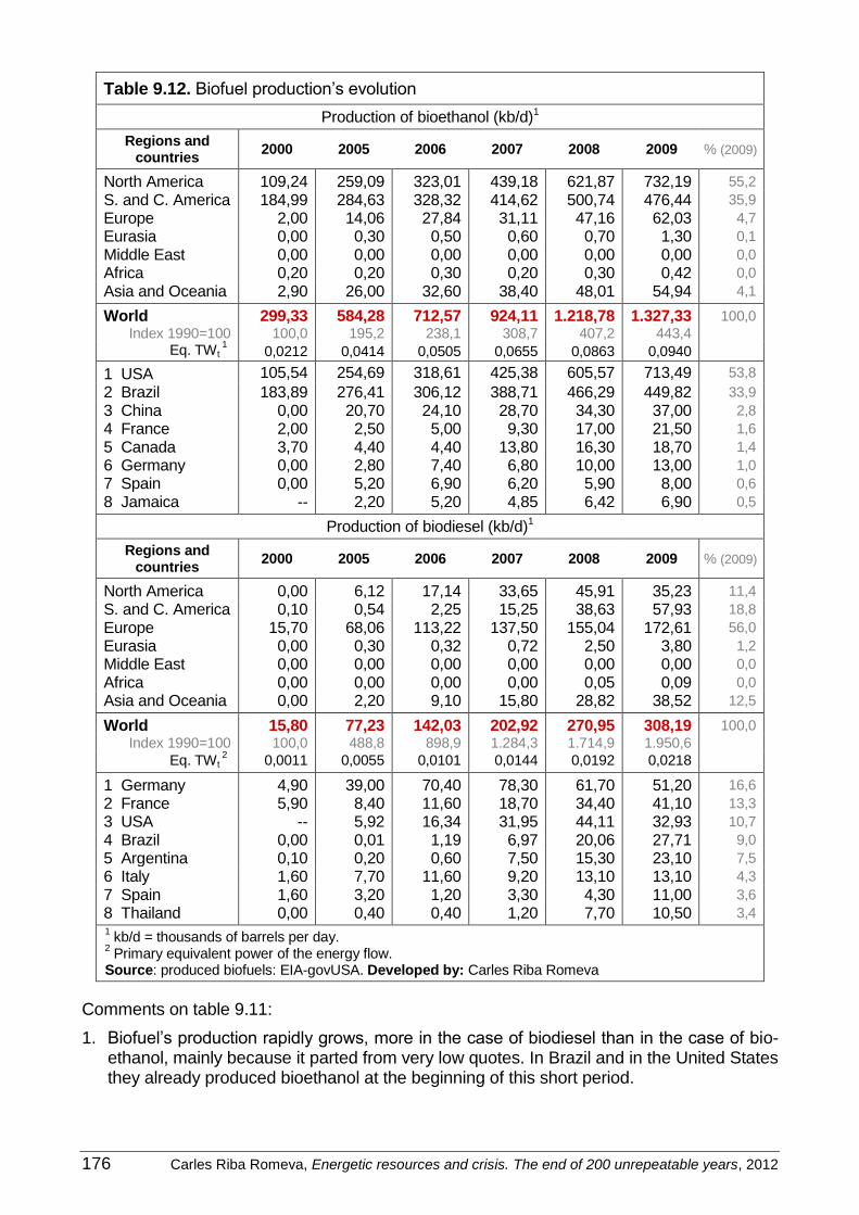
176 Carles Riba Romeva, Energetic resources and crisis. The end of 200 unrepeatable years, 2012
Table 9.12. Biofuel production’s evolution
Production of bioethanol (kb/d)1
Regions and countries
2000 2005 2006 2007 2008 2009 % (2009)
North America 109,24 259,09 323,01 439,18 621,87 732,19 55,2
S. and C. America 184,99 284,63 328,32 414,62 500,74 476,44 35,9
Europe 2,00 14,06 27,84 31,11 47,16 62,03 4,7
Eurasia 0,00 0,30 0,50 0,60 0,70 1,30 0,1
Middle East 0,00 0,00 0,00 0,00 0,00 0,00 0,0
Africa 0,20 0,20 0,30 0,20 0,30 0,42 0,0
Asia and Oceania 2,90 26,00 32,60 38,40 48,01 54,94 4,1
World 299,33 584,28 712,57 924,11 1.218,78 1.327,33 100,0
Index 1990=100 100,0 195,2 238,1 308,7 407,2 443,4 Eq. TWt
1 0,0212 0,0414 0,0505 0,0655 0,0863 0,0940
1 USA 105,54 254,69 318,61 425,38 605,57 713,49 53,8
2 Brazil 183,89 276,41 306,12 388,71 466,29 449,82 33,9
3 China 0,00 20,70 24,10 28,70 34,30 37,00 2,8
4 France 2,00 2,50 5,00 9,30 17,00 21,50 1,6
5 Canada 3,70 4,40 4,40 13,80 16,30 18,70 1,4
6 Germany 0,00 2,80 7,40 6,80 10,00 13,00 1,0
7 Spain 0,00 5,20 6,90 6,20 5,90 8,00 0,6
8 Jamaica -- 2,20 5,20 4,85 6,42 6,90 0,5
Production of biodiesel (kb/d)1
Regions and countries
2000 2005 2006 2007 2008 2009 % (2009)
North America 0,00 6,12 17,14 33,65 45,91 35,23 11,4
S. and C. America 0,10 0,54 2,25 15,25 38,63 57,93 18,8
Europe 15,70 68,06 113,22 137,50 155,04 172,61 56,0
Eurasia 0,00 0,30 0,32 0,72 2,50 3,80 1,2
Middle East 0,00 0,00 0,00 0,00 0,00 0,00 0,0
Africa 0,00 0,00 0,00 0,00 0,05 0,09 0,0
Asia and Oceania 0,00 2,20 9,10 15,80 28,82 38,52 12,5
World 15,80 77,23 142,03 202,92 270,95 308,19 100,0
Index 1990=100 100,0 488,8 898,9 1.284,3 1.714,9 1.950,6
Eq. TWt 2 0,0011 0,0055 0,0101 0,0144 0,0192 0,0218
1 Germany 4,90 39,00 70,40 78,30 61,70 51,20 16,6
2 France 5,90 8,40 11,60 18,70 34,40 41,10 13,3
3 USA -- 5,92 16,34 31,95 44,11 32,93 10,7
4 Brazil 0,00 0,01 1,19 6,97 20,06 27,71 9,0
5 Argentina 0,10 0,20 0,60 7,50 15,30 23,10 7,5
6 Italy 1,60 7,70 11,60 9,20 13,10 13,10 4,3
7 Spain 1,60 3,20 1,20 3,30 4,30 11,00 3,6
8 Thailand 0,00 0,40 0,40 1,20 7,70 10,50 3,4 1 kb/d = thousands of barrels per day.
2 Primary equivalent power of the energy flow.
Source: produced biofuels: EIA-govUSA. Developed by: Carles Riba Romeva
Comments on table 9.11:
1. Biofuel’s production rapidly grows, more in the case of biodiesel than in the case of bio-ethanol, mainly because it parted from very low quotes. In Brazil and in the United States they already produced bioethanol at the beginning of this short period.

Carles Riba Romeva, Energetic resources and crisis. The end of 200 unrepeatable years, 2012 177
2. The summed up amounts of both biofuels (1,64 Mb/d, millions of barrels per day) barely
represent a 2% of the worldwide production and consumption of petroleum and liquid fuels in the last years (approximately 85 Mb/d).
3. In the previous table (obtained from EIA-govUSA data) we consider those countries that transform biofuels, not those that produce the initial crops as producers. This fact hides some severe imbalances such as the Tortillas conflict, in Mexico, the deforestations in the
Asiatic south-east (specially Malaysia and Indonesia) or the substitution of traditional feed-ing crops by the monocultivation of energetic crops in Africa and South America (specially
in Argentina and Brazil).
First generation biofuels’ limitations
Biofuels (mainly ethanol and biodiesel), obtained from different crops, seem to be the great-
est hope to substitute petroleum. However, two important aspects need to be analysed: the
energy returned on investment (EROI) and the incidence on agriculture and feeding.
Biofuels’ substitutive capacity
A key issue is the analysis of the Earth’s crops capacity to produce biofuels in substitution of petroleum. The amount of ethanol that could be produced if the main world crops (mainly
cereals and sugar crops) were destined to its production has been evaluated. Results are given in table 9.13.
Table 9.13. Agriculture and biofuels (crops efficiencies for ethanol)
Year 2007 Cultivated
surface Crops’
production Ethanol’s efficiency
Total ethanol
Equivalent petroleum
Equivalent petroleum
Mha Tg/a litres/ha Glitres/a 1 Glitres/a 1 Mb/d 1
Wheat 222,8 683,4 952 212,1 142,1 2,45
Rice 159,3 685,9 1.806 287,7 192,8 3,32
Corn 161,1 826,2 1.960 315,8 211,6 3,65
Sorghum 44,9 65,5 494 22,2 14,9 0,26
Sugar cane 24,3 1.736,3 4.550 110,6 74,1 1,28
Sugar beet 4,3 222,0 5.060 21,8 14,6 0,25
Worldwide total 617,7 4.219,3 970,1 649,9 11,20
Worldwide (all crops) 1.447,9 10.249,0 Worldwide (petroleum) 85,00
% world 42,6% 2
41,2% 2 % world 13,2% 3
1 Glitres/a = thousands of millions of litres per year; Mb/d = millions of barrels per day.
2 Percentage in relation to the worldwide surface and production of all crops, including forage.
3 Percentage in relation to recent years’ worldwide petroleum production, approximately 85 Mb/d.
Sources: cultivated surfaces and agricultural productions: [FAOSTAT-2011]; each type of crop’s different
ethanol production efficiencies (litres/ha) and equivalence: 0,67 litres of petroleum equivalent for every litre of ethanol: [FAO-2008], page 21. Developed by: Carles Riba Romeva.
Definitely, if we entirely dedicated a 42,6% of the world’s total cultivation land (a surface which
is almost the double than that of India), and a 41,2% of the production in tonnage, we would obtain 11,2 Mb/d (millions of barrels per day) of petroleum, that would represent only a 13,2%
of the current liquid fuel production (about 85 Mb/d).
Therefore, first generation biofuels cannot, in any way, be considered a petroleum substitu-tive source, while on the other hand, they can be considered as a frontal collision with the
food supply.

178 Carles Riba Romeva, Energetic resources and crisis. The end of 200 unrepeatable years, 2012
Efficiency and emissions
In relationship to this issue, there has been controversy on if they produce more energy than they consume and in what proportion. Many evaluations place biofuels’ efficiency, measured as EROI (energy returned on investment = used energy, divided by the consumed energy in order to obtain it), between 0,7 and 1,8 (table 1.4). This means that, depending on the type of crop and the level of mechanization, it is possible that some biofuels consume more en-ergy (through machinery, fertilizers, pesticides, transport and transformation) than the one that they supply (EROI lower than 1). Then, it would be useless to manufacture them, even if its production is subsidized.
When EROI is considerably superior than 1, its production makes sense, but, according to the origin of the energy used for its production, it is not free of emissions; although in gen-eral emissions are lower than those of petroleum (for example, 60%).
Deforestation
Biofuels do not only put world’s feeding at risk (they have already originated many conflicts), but in many cases they are the excuse to carry out deforestation processes that as well as providing wood are a very large source of CO2 emissions that will not be recovered by bio-fuels for many years to come (if the crops are finally cultivated). Al Gore [Gor-2009] says that, «ironically, a North American tax which was thought for the promotion of biofuels has been a significant factor of virgin forest’s elimination in order to plant palm oil».
Biofuels based on algae
Those that defend algae farming for the obtaining of biofuels argue, among others that: They are a type of biomass that reproduces every few days allowing many crops per year. They produce an amount of biomass per unit of surface that is much larger than that of traditional crops. They allow the use of marginal and sterile land, as well as residual and salt waters. They consume CO2 being therefore a drain of greenhouse effect gases. Once the oil is ex-tracted, useful by-products for cattle feeding and aquiculture, as well as raw materials for many industrial processes (pigments, cosmetic products, fibres for paper) remain. Algae can also be used to clean sedimentation tanks or residual waters.
Figure 9.8. Pilot microscopic algae farms. Sources: Left: artificial open lake systems, <http://www.makebiofuel.co.uk/biofuel-from-algae>. Right: photobioreactor system, <http://www.enn.com/energy/article/37961>.
The two technologies that are currently most frequently tested are those of the open lake and of the closed circuit photobioreactors (figure 9.8). The first one has the advantage that it has relatively lower exploitation costs, but productivity is quite low and evaporation entails

Carles Riba Romeva, Energetic resources and crisis. The end of 200 unrepeatable years, 2012 179
very high water consumption. The second option is more productive, however, it has higher process costs (nutrient’s circulation, CO2 injection) that make it a less economically viable option, and that can make it produce more CO2 than it absorbs.
Even though algae biofuels have a large theoretical potential, they are not a current mature solution that is capable of displacing petroleum or of competing with other renewable ener-getic sources (wind, solar thermal, geothermal or first generation biofuels). Although several economical sectors (among them some oil and aviation companies) have pinned their hopes on algae biofuels as the only viable alternative to substitute fossil fuels, important investiga-tion and innovation efforts need to be done in the following years in order to convert these concepts into operative realities.
Some scientists show confidence in the capacity of algae fuels to significantly contribute in the coverage of future fossil fuel demands, but others are sceptic. In any case, it will be nec-essary to consider the advantages and disadvantages of these options bearing the energet-ic and environmental aspects in mind, as well as the efficiency derived from the eventual by-products.

180 Carles Riba Romeva, Energetic resources and crisis. The end of 200 unrepeatable years, 2012

Carles Riba Romeva, Energetic resources and crisis. The end of 200 unrepeatable years , 2012 181
Part 4
The resources of the Earths
In this fourth part, I would like to carry out a brief review of the Earth’s resources, which are the ones that have always sustained us and that still do, as the living animal beings that we are.
We have called this book Energetic resources and crisis, the end of 200 unrepeatable years. We evidently refer to the crisis that is produced by the decline in fossil energetic resources, with a finite stock in time, at a human civilization scale. But it is not a crisis due to the ex-haustion of the energetic sources that have sustained life for 3.500 million years and hu-mans for almost 150 years. We still have the Sun, which is the original source of almost all of the energies that we have, as well as geothermal and tidal energy.
On the other hand, we can exhaust or damage natural capital, such as forests, biodiversity, agricultural land, water or the atmosphere. In this last part of the book, we would like to re-view how humans are treating these resources and, amongst all, this civilization with an an-nounced end, which is based on fossil fuels. Energy is not a compound of nature or of our activity as humans: energy crosses everything; it is what makes everything (both biologically alive or inert) move. Animals and plants subsist on energy, climate is energy, the very slow Earth movements are energy, and Solar energy is the main energy that makes the whole planet keep working.
Chapter 10 is about the biosphere’s resources; especially agriculture, livestock, fishing and aquiculture, and of forest resources. In one of its sections, the ecologic footprint view is ana-lysed.
Chapter 11 is about atmosphere and climate change: the first section analyses the evolution of CO2 emissions; the second one studies the carbon cycle with its sinks and flows, and the third section examines carbon, oxygen and life. In this last part, the evaluation reports car-ried out by the Intergovernmental Panel on Climate Change (IPCC) is analysed, in order to advance the consequences of the climate change.
In chapter 12, the last chapter of the book, conclusions can be found. It starts with a sum-mary of the main analysed trends, it then carries out a reflection on the necessary change in the development paradigm, and some of the elements that will make it possible, and finally it proposes a strategy for Europe to carry out.

182 Carles Riba Romeva, Energetic resources and crisis. The end of 200 unrepeatable years , 2012
10. The resources of the biosphere
10.1. Agriculture, livestock, fishing and forests
Energy is present in all of the biological processes and humans, that are not absent of it, are found at the top of the life chain. We are, without any doubt, the more complex and interest-ing living beings, but also the ones that have a greater dependence on the rest.
According to the Gaia hypothesis that was developed by James Lovelock [Lov-1988], since there is life on Earth (approximately 3.500 million years), there is an interaction with the at-mosphere, the oceans and the lithosphere, in such a way that the system behaves as a self-regulated complex system, that maintains the Earth with the most profitable conditions for life. But, humans belonging to post-industrial societies, with their obsession to make econo-my grow, seem to have forgotten this.
In this section, the evolution of several aspects related to the biosphere’s resources, which are our main material means of sustenance as living beings, are analysed.
In the first place, the different types of surfaces of the planet are studied, as well as the main uses that humans do of each of these areas. Afterwards, the evolution of the agricultural, livestock, fishing and aquiculture productions are separately analysed. Later on, the evolu-tion of forests and the products that are extracted from them are briefly analysed. Finally, a global balance of the products that the biosphere supplies us with is done.
Use of the Earth
One first question of interest is to learn about the use that humanity does of each of the Earth’s surfaces, that, even though it changes with time, it has a relatively slow variation. We have used data from the FAO on this theme.
The surface of the Earth’s globe is of 510,07 Mkm2 (106 km2, millions of square kilometres), out of which only 149,90 (a 29,1%, that is, less than one third) correspond to solid ground and the rest are seas and oceans.
The emerged lands have a different consideration for humans and for the FAO in the follow-ing classification: a) agricultural surface, that is distributed between arable lands, permanent crops and meadows; b) forest surface; c) other types of land (including deserts, permanent snows and other unproductive surfaces; d) interior water (rivers and lakes). See table 10.1.
If we leave the tiny surface of the interior waters behind, the surface of the continents is broadly speaking divided into three relatively similar parts: agricultural surface (49,32 Mkm2 the most extense one, that includes the meadows of pasture), the unproductive lands (43,15 Mkm2; if the Antartida is included, it becomes the largest one of the three, with 56,88 Mkm2) and the forest surface (39,37 Mkm2, the least extense one).
But, when we analyse the components of the agricultural surface, we can see that the major part belongs to meadows (33,78 Mkm2, a surface which is slightly superior than that of Afri-ca), while crop lands (arable lands and permanent crops) only occupy 15,54 Mkm2 (a 10,4% of the emerged land surface).
Although these surfaces have small changes in time, some variations are significant. There-fore, from 1990 to 2007 the interior waters have increase in +0,37 Mkm2 (probably due to new reservoirs); crop lands, in +0,67 Mkm2; meadows almost do not vary (+0,07 Mkm2), and the unproductive lands have also grown (+0,25 Mkm2). In the negative side, it is needed to regret the decrease of -1,40 Mkm2 of forests (a surface of 82.000 km2 annually, equivalent to 2,5 times the surface of Catalonia or almost that of Portugal), that feeds the increases of other surfaces.
The FAO (FAOSTAT, <http://faostat.fao.org/site/377/default.aspx#ancor>) gives data on the surface and the uses of the Earth, which are summarized in table 10.1.

Carles Riba Romeva, Energetic resources and crisis. The end of 200 unrepeatable years , 2012 183
Table 10.1. Surface and uses of land, according to regions (2007)
Agricultural surface
Arable lands
Permanent crops
Meadows Forest surface
Other lands
Interior waters
Surface of the region
Regions A=B+C+D B C D E F G A+E+F+G
Surface absolute values (en Mkm2)
North America 5,858 2,400 0,122 3,336 6,773 9,735 1,382 23,747 S. & C. America 6,115 1,243 0,169 4,702 8,509 3,711 0,259 18,593 Europe 2,404 1,345 0,158 0,901 1,793 1,294 0,182 5,673 Eurasia 5,649 1,985 0,042 3,621 8,499 7,320 0,840 22,307 Middle East 2,738 0,324 0,040 2,374 0,164 2,575 0,120 5,597 Africa 11,575 2,192 0,273 9,110 6,273 11,796 0,671 30,315 Asia 10,581 4,165 0,607 5,809 5,308 4,688 0,809 21,386 Oceania 4,400 0,456 0,014 3,930 2,055 2,036 0,070 8,561
World 49,319 14,111 1,426 33,782 39,373 43,155 4,334 136,180
Antartida 0 0 0 0 0 13,720 0 13,720
World 49,319 14,111 1,426 33,782 39,373 56,875 4,334 149,900 % 32,9 (9,4) (1,0) (22,5) 26,3 37,9 2,9 100,0
Surface values per inhabitant (ha/inhab)
North America 1,32 0,54 0,03 0,75 1,53 2,20 0,31 5,36 S. & C. America 1,32 0,27 0,04 1,01 1,84 0,80 0,06 4,01 Europe 0,41 0,23 0,03 0,15 0,31 0,22 0,03 0,97 Eurasia 1,99 0,70 0,01 1,27 2,99 2,58 0,30 7,85 Middle East 1,40 0,17 0,02 1,22 0,08 1,32 0,06 2,87 Africa 1,22 0,23 0,03 0,96 0,66 1,25 0,07 3,20 Asia 0,29 0,11 0,02 0,16 0,15 0,13 0,02 0,59 Oceania 12,57 1,30 0,04 11,23 5,87 5,82 0,20 24,47
World 0,75 0,21 0,02 0,51 0,60 0,86 0,07 2,27
Distribution of the Earth’s uses in each region (horizontal sums = 100%) Density
(inhab/km2)
North America 24,7 10,1 0,5 14,0 28,5 41,0 5,8 18,7
S. & C. America 32,9 6,7 0,9 25,3 45,8 20,0 1,4 24,9 Europe 42,4 23,7 2,8 15,9 31,6 22,8 3,2 103,2 Eurasia 25,3 8,9 0,2 16,2 38,1 32,8 3,8 12,7 Middle East 48,9 5,8 0,7 42,4 2,9 46,0 2,1 34,8 Africa 38,2 7,2 0,9 30,0 20,7 38,9 2,2 31,2 Asia 49,5 19,5 2,8 27,2 24,8 21,9 3,8 170,8 Oceania 51,4 5,3 0,2 45,9 24,0 23,8 0,8 4,1
World 32,9 9,4 1,0 22,5 26,3 37,9 2,9 49,1
Source: FAOSTAT, <http://faostat.fao.org/site/377/default.aspx#ancor> (FAO, United Nations). Developed by: Carles Riba Romeva
Comments on table 10.1:
1. Africa is the most extense region in the world (30 Mkm2), four regions have little above 20 Mkm2 (Noth America, Eurasia, Asia and South America), another one (Oceania, which is considered separately) has approximately 8,5 Mkm2, and two more (Europe and the Mid-dle East) have an extension which is almost four times inferior (around 5,5 Mkm2).
2. Europe and Asia, which are more populated (103,2 and 170,8 inhab/km2), destine a higher proportion of their surface to worked lands and permanent crops (a 26,5% and a 22,3% respectively) that the rest of the regions (densities <35 inhab/km2).
3. When it comes to worked surface lands per inhabitant, the large surplus regions of Oce-ania, Eurasia and North America (1,30, 0,70 and 0,54 ha/inhab, respectively) clearly stand out from the rest.
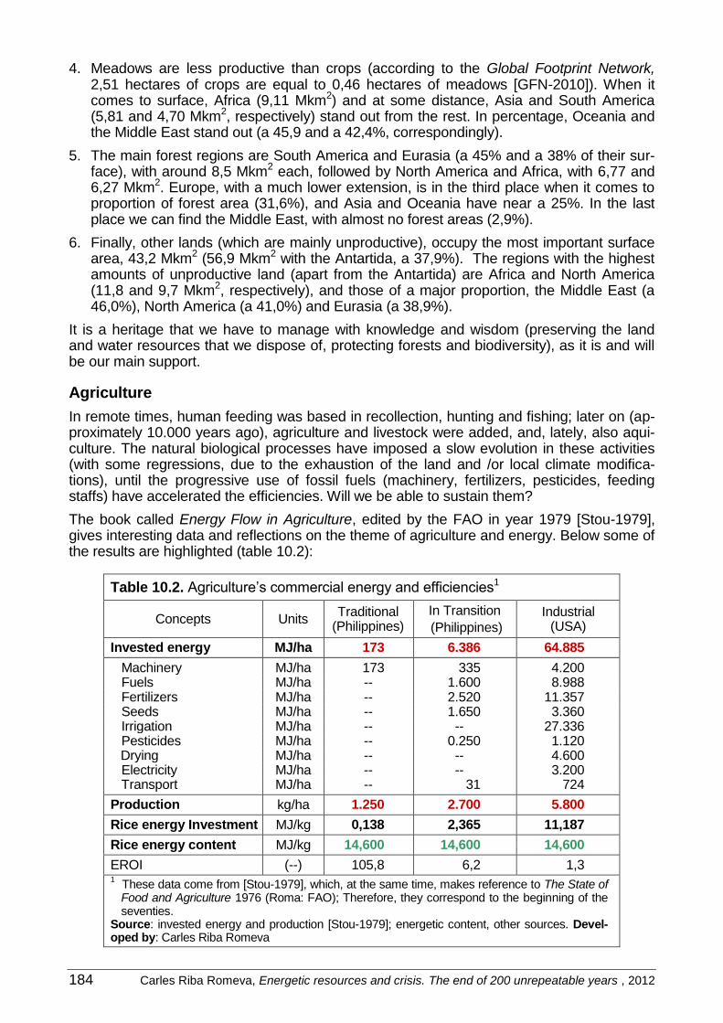
184 Carles Riba Romeva, Energetic resources and crisis. The end of 200 unrepeatable years , 2012
4. Meadows are less productive than crops (according to the Global Footprint Network, 2,51 hectares of crops are equal to 0,46 hectares of meadows [GFN-2010]). When it comes to surface, Africa (9,11 Mkm2) and at some distance, Asia and South America (5,81 and 4,70 Mkm2, respectively) stand out from the rest. In percentage, Oceania and the Middle East stand out (a 45,9 and a 42,4%, correspondingly).
5. The main forest regions are South America and Eurasia (a 45% and a 38% of their sur-face), with around 8,5 Mkm2 each, followed by North America and Africa, with 6,77 and 6,27 Mkm2. Europe, with a much lower extension, is in the third place when it comes to proportion of forest area (31,6%), and Asia and Oceania have near a 25%. In the last place we can find the Middle East, with almost no forest areas (2,9%).
6. Finally, other lands (which are mainly unproductive), occupy the most important surface area, 43,2 Mkm2 (56,9 Mkm2 with the Antartida, a 37,9%). The regions with the highest amounts of unproductive land (apart from the Antartida) are Africa and North America (11,8 and 9,7 Mkm2, respectively), and those of a major proportion, the Middle East (a 46,0%), North America (a 41,0%) and Eurasia (a 38,9%).
It is a heritage that we have to manage with knowledge and wisdom (preserving the land and water resources that we dispose of, protecting forests and biodiversity), as it is and will be our main support.
Agriculture
In remote times, human feeding was based in recollection, hunting and fishing; later on (ap-proximately 10.000 years ago), agriculture and livestock were added, and, lately, also aqui-culture. The natural biological processes have imposed a slow evolution in these activities (with some regressions, due to the exhaustion of the land and /or local climate modifica-tions), until the progressive use of fossil fuels (machinery, fertilizers, pesticides, feeding staffs) have accelerated the efficiencies. Will we be able to sustain them?
The book called Energy Flow in Agriculture, edited by the FAO in year 1979 [Stou-1979], gives interesting data and reflections on the theme of agriculture and energy. Below some of the results are highlighted (table 10.2):
Table 10.2. Agriculture’s commercial energy and efficiencies1
Concepts Units Traditional
(Philippines)
In Transition
(Philippines)
Industrial (USA)
Invested energy MJ/ha 173 6.386 64.885
Machinery MJ/ha 173 335 4.200 Fuels MJ/ha -- 1.600 8.988 Fertilizers MJ/ha -- 2.520 11.357 Seeds MJ/ha -- 1.650 3.360 Irrigation MJ/ha -- -- 27.336 Pesticides MJ/ha -- 0.250 1.120
Drying MJ/ha -- -- 4.600 Electricity MJ/ha -- -- 3.200 Transport MJ/ha -- 31 724
Production kg/ha 1.250 2.700 5.800
Rice energy Investment MJ/kg 0,138 2,365 11,187
Rice energy content MJ/kg 14,600 14,600 14,600
EROI (--) 105,8 6,2 1,3 1 These data come from [Stou-1979], which, at the same time, makes reference to The State of Food and Agriculture 1976 (Roma: FAO); Therefore, they correspond to the beginning of the seventies.
Source: invested energy and production [Stou-1979]; energetic content, other sources. Devel-oped by: Carles Riba Romeva

Carles Riba Romeva, Energetic resources and crisis. The end of 200 unrepeatable years , 2012 185
Even though this book was written many years ago (more than 30), it is still a reference work that allows us to reflect on the scope and the consequences of the transition from traditional to industrial agriculture (the text calls it «modern»), in a moment where many of these trans-formations were being conceived.
Data in table 10.2 lead us to make the following reflections:
1. As it is very well indicated in the original text (and the table), it is a commercial energy, not of total energy. With all security, if solar energy that makes plants grow were account-ed, the balances would be more evenly matched.
2. However, the commercial energies that have been used in industrial agriculture are al-most exclusively unrenewable sources of energy that produce greenhouse effect gases. Therefore, industrial agriculture is not sustainable.
3. Due to the fact that the energetic value of rice is of 14,6 MJ/kg, traditional agriculture has an energy return on investment (EROI) tax in relationship to unrenewable sources of en-ergy of 105,8, while in industrial agriculture the value of the EROI tax decreases to 1,1 (value that is not admissible as a raw material for the production of energy).
It is necessary to analyse a minimum of three different efficiencies: a) production per hectare (Mg/ha); b) production per farmer (Mg/farmer); c) energetic efficiency, or the energy that the agricultural or livestock product contains in relationship to the energy that has been invested in its production (MJprod/MJcons).
In the previous hundred years, where agriculture has been mechanized, the successful re-sults of the two first efficiencies have been spectacular (increases of from 2 to 4 times in the efficiencies per hectare, and from 5 to 20 times in the efficiency per farmer). On the other hand, the energetic efficiency has spectacularly decreased, that has gone unnoticed until the arrival of biofuels, that only make sense with a minimum energy return on investment tax (EROI > 4).
Crops, productions and efficiencies
Tables 10.3 and 10.5 contain data about crops, productions and agricultural efficiencies, and have been obtained from the FAOSTAT (<http://faostat.fao.org/site/567/default.aspx#ancor>, FAO, United Nations). They provide the values of the cultivated surfaces, the productions and the efficiencies of the main groups of agricultural products from 1961 to 2008. Table 10.3 groups the data according to the function of the different types of crops, while table 10.4 groups the data according to regions.
From a global point of view, the analysis of the data suggests the following comments:
1. The use of the world’s cultivation land has gone from 1.064 Mha in 1961 (a surface a little above than the surface of the United States) to 1.448 Mha in 2008, with a relatively moderate increase of a 36,1%. Most of the more suitable lands for crops in the world are already being exploited and the new lands that are going to be exploited require growing energetic and working costs for their production and maintenance [Stou-1979].
2. The cultivated land has grown much less than the world population, which, in this same period, has gone from 3.072,8 Minhab in 1961 to 6.750,1 Minhab in 2008, which is equiva-lent to a growth of a119,7% (it has more than doubled). Therefore, this means that the cul-tivated surface per inhabitant has decreased in a 38% during this period, as it has gone from 0,345 ha/inhab in 1961 to 0,214 ha/inhab in 2008 (table 10.5). This is one of the main components of the ecological footprint (section 10.2).
3. On the other hand, the overall crop productions have almost tripled, due to the fact that they has gone from 3.453 Tg/a (millions of tonnes per year) in 1961 to 10.249 Tg/a in 2008 (increase of a 196,8%). Therefore, the most substantial part of this increase can be claimed to the improvement in the efficiency per cultivated surface.

186 Carles Riba Romeva, Energetic resources and crisis. The end of 200 unrepeatable years , 2012
Table 10.3. Agriculture. Cultivated surface, production and efficiency (by crops)
Cultivated surfaces (Mha, million hectares)
Crops 1961 % 1970 1980 1990 2000 2008 % Incr. 1
Cereals 648,0 60,9 675,5 717,2 708,5 672,7 712,2 49,2 109,9
Vegetables 21,1 2,0 20,3 23,1 28,2 40,7 48,7 3,4 231,2
Fruits 24,6 2,3 28,9 32,9 41,1 49,1 55,0 3,8 223,3
Roots and tubers 47,6 4,5 48,2 45,9 46,0 53,2 52,9 3,7 111,1
Pulses 64,0 6,0 64,4 61,3 68,8 64,9 71,8 5,0 112,2
Oleaginous crops 81,6 7,7 97,7 127,5 151,3 189,7 228,1 15,8 279,6
Sugar crops 16,0 1,5 18,9 22,3 25,9 25,5 28,7 2,0 179,6
Forage crops 92,5 8,7 91,5 96,8 205,8 169,4 161,7 11,2 174,8
Primary fiber crops 38,6 3,6 40,7 40,5 37,6 35,0 34,1 2,4 88,4
Other crops 27,0 2,5 28,9 33,3 40,8 46,1 49,7 3,4 183,8
Total in the world 1.063,6 100,0 1.117,1 1.203,3 1.356,9 1.350,4 1.447,9 100,0 136,1
Productions (Tg/a, millions of tonnes per year)
Crops 1961 % 1970 1980 1990 2000 2008 % Incr. 1
Cereals 877 25,4 1.193 1.550 1.952 2.060 2.521 24,6 287,5
Vegetables 197 5,7 224 289 415 651 806 7,9 409,2
Fruits 200 5,8 266 339 402 569 706 6,9 353,2
Roots and tubers 455 13,2 560 523 574 699 738 7,2 162,1
Pulses 41 1,2 44 41 59 55 61 0,6 150,8
Oleaginous crops 105 3,0 138 204 302 460 661 6,4 631,8
Sugar crops 609 17,6 834 1.003 1.363 1.508 1.959 19,1 321,6
Forage crops 919 26,6 1.073 1.389 3.672 2.809 2.671 26,1 290,7
Primary fibers crops 33 1,0 41 47 59 58 70 0,7 213,6
Other crops 18 0,5 21 25 34 44 56 0,5 313,3
Total in the world 3.453 100,0 4.393 5.410 8.832 8.914 10.249 100,0 296,8
1 Corn 205 5,9 266 397 483 593 826 8,1 403,0
2 Rice, paddy 216 6,2 316 397 519 599 686 6,7 318,1
3 Wheat 222 6,4 311 440 592 586 683 6,7 307,3
4 Potatoes, papes 271 7,8 298 241 267 327 326 3,2 120,3
5 Yucca 71 2,1 99 124 153 177 233 2,3 326,2
1 Sugar cane 448 13,0 609 735 1.053 1.258 1.736 16,9 387,6
2 Soy 267 0,8 44 81 109 161 231 2,3 857,7
3 Sugar beet 161 4,7 224 268 309 250 222 2,2 138,3
4 Palm nut 14 0,4 15 30 61 120 207 2,0 1.517,
Efficiencies per unit of surface (Mg/ha, tonnes per hectare)
Crops 1961 % 1970 1980 1990 2000 2008 % Incr. 1
Cereals 1,35 41,7 1,77 2,16 2,76 3,06 3,54 50,0 261,5
Vegetables 9,34 287,7 11,05 12,54 14,70 16,00 16,53 233,6 177,0
Fruits 7,34 226,2 8,54 9,56 9,10 10,70 11,77 166,3 160,3
Roots and tubers 9,57 294,7 11,62 11,39 12,47 13,14 13,96 197,3 145,9
Pulses 0,64 19,6 0,68 0,67 0,86 0,86 0,86 12,1 134,4
Oleaginous crops 1,28 39,5 1,41 1,60 2,00 2,42 2,90 40,9 226,0
Sugar crops 38,16 1.175, 44,19 45,07 52,70 59,06 68,35 965,6 179,1
Forage crops 9,93 306,0 11,72 14,35 17,84 16,59 16,52 233,3 166,3
Primary fibers crops 0,85 26,3 1,00 1,15 1,58 1,64 2,06 29,1 241,8
Other crops 0,66 20,4 0,72 0,75 0,83 0,95 1,13 16,0 170,4
Total in the world 3,25 100,0 3,93 4,50 6,51 6,60 7,08 100,0 218,0 1 1961-2008 increase (1961=100)
Source: FAOSTAT (FAO, United Nations). Developed by: Carles Riba Romeva

Carles Riba Romeva, Energetic resources and crisis. The end of 200 unrepeatable years , 2012 187
Table 10.4. Agriculture. Cultivated surface, production and efficiency (by regions)
Cultivated surfaces (Mha, millions of hectares)
Regions 1961 % 1970 1980 1990 2000 2008 % Incr. 1
North America 155,4 14,6 154,3 184,6 184,9 187,8 192,1 13,3 123,6
S. and C. America 71,6 6,7 84,6 99,4 108,3 112,2 136,1 9,4 190,2
Europe 140,9 13,3 136,7 142,7 155,2 148,2 143,9 9,9 102,1
Eurasia 173,8 16,3 167,8 172,9 209,7 148,9 147,8 10,2 85,1
Middle East 14,8 1,4 18,0 19,9 26,2 23,3 24,1 1,7 162,8
Africa 105,1 9,9 130,1 126,5 154,2 183,2 218,6 15,1 207,9
Asia and Oceania 402,1 37,8 425,6 457,4 518,3 546,7 585,3 40,4 145,6
World 1.063,6 100,0 1.117,1 1.203,3 1.356,9 1.350,4 1.447,9 100,0 136,1
Productions (Tg/a, millions of tonnes per year)
Regions 1961 % 1970 1980 1990 2000 2008 % Incr. 1
North America 542 15,7 678 855 1.577 1.702 1.695 16,5 312,5
S. and C. America 410 11,9 532 646 911 1.033 1.493 14,6 364,3
Europe 697 20,2 873 1.148 1.534 1.522 1.503 14,7 215,5
Eurasia 623 18,1 648 693 1.522 660 677 6,6 108,7
Middle East 27 0,8 38 57 101 119 131 1,3 486,1
Africa 204 5,9 334 396 490 613 761 7,4 373,8
Asia and Oceania 950 27,5 1.290 1.614 2.696 3.265 3.988 38,9 420,0
World 3.453 100,0 4.393 5.410 8.832 8.914 10.249 100,0 296,8
Efficiencies per unit of surface (Mg/(ha·y), tons per hectare and year)
Regions 1961 World =100 1970 1980 1990 2000 2008
World =100 Incr.
1
North America 3,49 107,5 4,39 4,63 8,53 9,06 8,82 124,6 252,8
S. and C. America 5,73 176,4 6,28 6,51 8,41 9,20 10,97 155,0 191,5
Europe 4,95 152,4 6,38 8,05 9,89 10,27 10,45 147,6 211,1
Eurasia 3,59 110,5 3,86 4,01 7,26 4,43 4,58 64,7 127,7
Middle East 1,83 56,2 2,12 2,88 3,84 5,11 5,45 77,0 298,5
Africa 1,94 59,7 2,57 3,13 3,18 3,35 3,48 49,2 179,8
Asia and Oceania 2,36 72,7 3,03 3,53 5,20 5,97 6,81 96,3 288,5
World 3,25 100,0 3,93 4,50 6,51 6,60 7,08 100,0 218,0 1 1961-2008 increase (1961=100)
Source: FAOSTAT (FAO, United Nations). Developed by: Carles Riba Romeva
4. Effectively, the average efficiency of the worldwide crops has gone from 3,25 Mg/ha (tonnes per hectare) in 1961 to 7.08 Mg/ha in 2008, with an increase of a 117,8%. This improvement would difficultly have been accomplished without the mechanization of agri-culture and, above all, without the investment in growing amounts of facilities, fertilizers and pesticides, which consume important amounts of fossil fuel energetic resources.
5. The production in tonnes of the worldwide crops is divided into four parts that are relatively balanced: cereals, 2.521 Tg/a (millions of tonnes per year); HFTL (vegetables, fruits, tu-bers and legumes), 2.331 Tg/a; crops for biofuels, 2.396 Tg/a, and crops for forages (for animal feeding), 2.671 Tg/a. A series of crops with minor productions are left (the oleagi-nous for human consumption, the dry fruits, spices, primary fibers, rubber and tobacco), that sum up a total approximate amount of 340 Tg/a.
6. The efficiencies per hectare of the different crops are very different. It is important to re-member that in sugar cane and in most forages the whole plant is recollected. Amongst feeding crops, cereals have relatively low efficiencies per hectare (although they are the ones that have improved more), and green vegetables, vegetables and potatoes, have higher efficiencies.

188 Carles Riba Romeva, Energetic resources and crisis. The end of 200 unrepeatable years , 2012
Table 10.5. Agriculture. Productions per capita (by regions)
Population (Minhab, millions of inhabitants)1
Regions 1961 % 1970 1980 1990 2000 2008 % Incr. 2
North America 247 8,0 283 323 366 418 454 6,7 183,9
S. and C. America 187 6,1 235 294 359 422 468 6,9 250,4
Europe 458 14,9 496 530 556 577 599 8,9 130,8
Eurasia 218 7,1 243 265 289 288 284 4,2 130,2
Middle East 52 1,7 68 95 136 174 207 3,1 399,6
Africa 292 9,5 367 482 639 819 987 14,6 338,0
Asia and Oceania 1.628 52,8 1.995 2.448 2.947 3.417 3.753 55,6 230,5
World 3.081 100,0 3.686 4.438 5.290 6.115 6.750 100,0 219,1
Surface per inhabitant (ha/inhab, hectares per inhabitant)
Regions 1961 % 1970 1980 1990 2000 2008 % Incr. 2
North America 0,630 182,4 0,545 0,572 0,505 0,449 0,423 197,4 67,2
S. and C. America 0,383 111,0 0,361 0,338 0,302 0,266 0,291 135,7 76,0
Europe 0,308 89,2 0,276 0,269 0,279 0,257 0,240 112,0 78,1
Eurasia 0,798 231,0 0,691 0,651 0,726 0,517 0,521 242,9 65,3
Middle East 0,286 82,9 0,266 0,210 0,193 0,134 0,117 54,4 40,7
Africa 0,360 104,3 0,355 0,262 0,241 0,224 0,221 103,2 61,5
Asia and Oceania 0,247 71,5 0,213 0,187 0,176 0,160 0,156 72,7 63,2
World 0,345 100,0 0,303 0,271 0,256 0,221 0,214 100,0 62,1
Efficiencies per inhabitant and per year (Mg/(hab·y), tonnes per inhabitant and per year)
Regions 1961 % 1970 1980 1990 2000 2008 % Incr. 2
North America 2,20 67,7 2,39 2,65 4,31 4,07 3,74 52,8 170,0
S. and C. America 2,20 67,6 2,27 2,20 2,54 2,45 3,19 45,1 145,5
Europe 1,52 46,9 1,76 2,17 2,76 2,64 2,51 35,5 164,8
Eurasia 2,86 88,1 2,67 2,61 5,27 2,29 2,39 33,7 83,4
Middle East 0,52 16,1 0,56 0,60 0,74 0,69 0,64 9,0 121,6
Africa 0,70 21,5 0,91 0,82 0,77 0,75 0,77 10,9 110,6
Asia and Oceania 0,58 18,0 0,65 0,66 0,91 0,96 1,06 15,0 182,2
World 1,12 34,5 1,19 1,22 1,67 1,46 1,52 21,4 135,5 1 Population according to data from the FAO;
2 Increase between 1961 and 2008 (1961=100)
Source: FAOSTAT (FAO, United Nations). Developed by: Carles Riba Romeva
Crops and energy consumption
The preface of the before mentioned FAO study Energy for World Agriculture [Stou-1979], states that (with the perspective of the moment in which it was written) agriculture con-sumes, approximately, a 3,5% of the worldwide energy, a 2,9% of which belongs to devel-oped countries and a 0,6% to developing countries.
It also highlights that efficiency increase that is expected with the application of the “green revolution” technologies in developing countries depends, in a great measure, on very inten-sive energy inputs, such as fertilizers, machinery and pesticides.
In chapter 2 of the same project, on the theme of «energy flow on agriculture», he insists on saying that, although many developing countries have reserves of unused lands that are potentially productive, they will not be able to cover the increasing demands of food unless it is with increases of productivity, that is to say, with fossil fuel energy.
From a current point of view, these increases of productivity that need the massive use of resources based on fossil fuels (fertilizers, machinery and pesticides) can have an opposite effect when their decline begins. It is another element that must be considered.

Carles Riba Romeva, Energetic resources and crisis. The end of 200 unrepeatable years , 2012 189
Analysis of the main productive countries
In a simplistic form, below we will consider, among food products cereals; vegetables, fruits, roots, tubers and legumes. Certainly, they are the basis of human nutrition, but some cere-als are also used in the feeding of animals or in the manufacture of biofuels. And, vice versa, some of the sugar crops or oleaginous are also used for human nutrition. However, at a large scale, this simplification does not alter the global scenario.
From the crop’s point of view (table 10.3), the following comments come up:
1. Cereals cover a 49,2% of the worldwide cultivated lands (in 1961, production was even higher with a 60,9%), and the absolute surface has slightly increased up to 712,2 Mha. Production has almost triplicates (from 877 Tg/a, or millions of tonnes per year, to 2.525 Tg/a). The efficiency per hectare is one of the lowest, but it has increased from 1,35 Mg/ha (tonnes per hectare) in 1961 to 3,54 Mg/ha in 2008 (increase of the 161,5%).
2. Cereal production is almost ¼ of the worldwide agricultural productions and one of the main basis of human nutrition. It is divided into three relatively evenly divided parts be-longing to the most important cereals: corn, 826 Tg/a in 2008; rice, 686 Tg/a, and wheat, 683 Tg/a; the rest of the summed-up cereals give the value of 325 Tg/a.
3. Vegetable and fruits double the extension of the cultivated land (131,2% and 123,3% of increase, respectively) and quadruple the productions (309,2% and 253,2% of increase). These crops, very intense when it comes to work force, have quite high efficiencies (15,5 and 11,8 Mg/ha, correspondingly) and, together with roots and tubers (with also high effi-ciencies, 13,96 Mg/ha) and legumes, add up almost the same value as cereals (2.311 Tg/a) and they make up for almost the other half of human nutrition.
4. The main energetic crops are sugar cane (1.736 Tg/a in 2008, in the whole plant) and, af-terwards, almost at a fifty-fifty ratio, soy (231 Tg/a, oleaginous), sugar beet (222 Tg/a) and palm (207 Tg/a oleaginous). The rest are oleaginous crops that together sum up 224 Tg/a: they are mainly coconut, 61 Tg/a; rape, 58 Tg/a; peanut, 38 Tg/a and sunflower, 35 Tg/a.
5. Finally, we can find forage crops, in which we must highlight: true grasses and leguminous (1.264 Tg/a in 2008, the second crop when it comes to production); alfalfa (463 Tg/a); for-age corn (374 Tg/a); unspecified forage products (256 Tg/a) and clover (90 Tg/a).
6. The rest of the feeding and not feeding crops are much more minoritary. We only high-light (in Tg/a) cotton (65,4), dried fruits (12,2), rubber (10,6), coffee (8,2), tobacco (6,7) and tea (3,9).
Definitely, nowadays, almost half of the crops are destined to human nutrition, and, from the other half, approximately a 25% is used for animal feeding (forage products), and another 25% is destined to feed thermal engines (biofuels).
And the analysis of the producer countries (tables 10.6 and 10.7), brings about the following comments:
1. The population’s weight is stated in the production of feeding crops, although large dif-ferences are observed (for example, between China and India).
2. It is also stated that in developing countries the relative weight of vegetables, fruits, roots and tubers is higher in relation to cereals.
3. The major net exporters in the cereal market in 2008 are (there is no table) the United States +89,6 Tg/a; Argentina, +28,1 Tg/a; France, +26,8 Tg/a; Canada, +18,2 Tg/a; Ukraine, +16,4 Tg/a; Russia, +13,1 Tg/a; and Australia, +12,2 Tg/a. And the major net importer countries are: Japan, -25,2 Tg/a; Mexico, -13,3 Tg/a; South Korea, -12,2 Tg/a; Egypt, -12,1 Tg/a; Spain, -11,2 Tg/a; Saudi Arabia, -10,9 Tg/a; and Iran, -10,6 Tg/a. It is stated that the two most populated countries of the world almost auto supply themselves: China, -5,1 Tg/a, and India, +6,5 Tg/a (eating less).

190 Carles Riba Romeva, Energetic resources and crisis. The end of 200 unrepeatable years , 2012
Table 10.6. Main countries producing feeding crops in 2008
Main countries producing cereals
Countries Cereals Corn Rice Wheat Barley
Tg/a %
world Tg/a % world Tg/a
% world Tg/a % world Tg/a % world
World 2.520,7 100,0 826,2 100,0 685,9 100,0 683,4 100,0 155,1 100,0
1 China 480,1 19,0 166,0 20,1 193,4 28,2 112,5 16,5 3,1 2,0
2 USA 403,5 16,0 307,1 37,2 9,2 1,3 68,0 10,0 5,2 3,4
3 India 267,0 10,6 19,7 2,4 148,3 21,6 78,6 11,5 1,2 0,8
4 Russia 106,4 4,2 6,7 0,8 0,7 0,1 63,8 9,3 23,1 14,9
5 Brazil 79,7 3,2 58,9 7,1 12,1 1,8 6,0 0,9 0,2 0,2
6 Indonesia 76,6 3,0 16,3 2,0 60,3 8,8 0,0 0,0 0,0 0,0
7 France 70,1 2,8 15,8 1,9 0,1 0,0 39,0 5,7 12,2 7,8
8 Canada 56,0 2,2 10,6 1,3 0,0 0,0 28,6 4,2 11,8 7,6
9 Ukraine 52,7 2,1 11,4 1,4 0,1 0,0 25,9 3,8 12,6 8,1
10 Germany 50,1 2,0 5,1 0,6 0,0 0,0 26,0 3,8 12,0 7,7
11 Bangladesh 49,1 1,9 1,3 0,2 46,9 6,8 0,8 0,1 0,0 0,0
12 Vietnam 43,3 1,7 4,5 0,5 38,7 5,6 0,0 0,0 0,0 0,0
13 Argentina 36,8 1,5 22,0 2,7 1,2 0,2 8,5 1,2 1,7 1,1
14 Mexico 36,1 1,4 24,3 2,9 0,2 0,0 4,0 0,6 0,8 0,5
15 Thailand 36,1 1,4 4,2 0,5 31,7 4,6 0,0 0,0 0,0 0,0
16 Pakistan 35,5 1,4 3,6 0,4 10,4 1,5 21,0 3,1 0,1 0,1
17 Australia 35,4 1,4 0,4 0,0 0,2 0,0 21,4 3,1 8,0 5,2
18 Myanmar 32,0 1,3 1,1 0,1 30,5 4,4 0,2 0,0 0,0 0,0
19 Nigeria 30,2 1,2 7,5 0,9 4,2 0,6 0,1 0,0 0,0 0,0
20 Turkey 29,3 1,2 4,3 0,5 0,8 0,1 17,8 2,6 5,9 3,8
Main countries producing vegetables, fruits, roots/tubers and legumes (VFRL)
Countries VFRL Vegetables Fruits Roots/Tubers Legumes
Tg/a %
world Tg/a % world Tg/a
% world Tg/a % world Tg/a % world
World 2.311,4 100,0 805,8 100,0 706,0 100,0 738,1 100,0 61,5 100,0
1 China 727,7 31,5 376,3 46,7 191,1 27,1 155,3 21,0 4,9 8,0
2 India 216,4 9,4 89,2 11,1 68,1 9,6 44,8 6,1 14,2 23,2
3 Nigeria 112,7 4,9 10,8 1,3 9,5 1,3 89,4 12,1 3,0 4,8
4 USA 86,6 3,7 34,4 4,3 30,6 4,3 19,7 2,7 1,9 3,1
5 Brazil 83,4 3,6 7,7 1,0 41,0 5,8 31,2 4,2 3,5 5,7
6 Indonesia 50,0 2,2 8,4 1,0 16,4 2,3 24,9 3,4 0,3 0,5
7 Russia 47,8 2,1 13,0 1,6 4,2 0,6 28,9 3,9 1,8 2,9
8 Turkey 45,2 2,0 21,4 2,7 18,6 2,6 4,2 0,6 1,0 1,6
9 Thailand 37,9 1,6 3,3 0,4 9,1 1,3 25,4 3,4 0,2 0,3
10 Iran 33,3 1,4 11,2 1,4 17,0 2,4 4,7 0,6 0,4 0,6
11 Egypt 33,1 1,4 16,9 2,1 11,8 1,7 4,0 0,5 0,4 0,6
12 Italy 33,1 1,4 12,6 1,6 18,7 2,7 1,6 0,2 0,2 0,3
13 Spain 31,6 1,4 10,9 1,4 18,0 2,6 2,4 0,3 0,3 0,4
14 Mexico 31,6 1,4 10,3 1,3 17,9 2,5 1,9 0,3 1,4 2,3
15 Ukraine 30,5 1,3 8,0 1,0 2,4 0,3 19,5 2,6 0,6 0,9
16 Vietnam 25,1 1,1 7,6 0,9 6,1 0,9 11,1 1,5 0,3 0,4
17 Philippines 23,9 1,0 5,2 0,6 15,7 2,2 2,8 0,4 0,1 0,1
18 Ghana 22,7 1,0 0,6 0,1 4,0 0,6 18,0 2,4 0,0 0,0
19 France 21,3 0,9 5,0 0,6 8,8 1,2 6,8 0,9 0,8 1,3
20 Poland 20,0 0,9 5,4 0,7 3,9 0,5 10,5 1,4 0,2 0,4
Source: FAOSTAT (FAO, United Nations). Developed by: Carles Riba Romeva

Carles Riba Romeva, Energetic resources and crisis. The end of 200 unrepeatable years , 2012 191
Table 10.7. Main countries in the production of forage and biofuel products
Main countries in the production of forage products
Countries Forage Grasses Alfalfa Forage corn For. products1
Tg/a %
world Tg/a
% world Tg/a
% world Tg/a
% world Tg/a
% world
World 2.670,7 100,0 1.264,6 100,0 462,8 100,0 374,5 100,0 256,0 100,0
1 USA 697,8 26,1 311,1 24,6 263,5 56,9 101,3 27,0 0,0 0,0
2 Australia 312,0 11,7 307,0 24,3 5,0 1,1 0,0 0,0 0,0 0,0
3 Germany 165,9 6,2 0,0 0,0 1,0 0,2 71,0 18,9 8,2 3,2
4 Russia 133,6 5,0 91,0 7,2 0,0 0,0 23,5 6,3 17,0 6,6
5 France 120,2 4,5 67,4 5,3 13,5 2,9 13,8 3,7 0,0 0,0
6 Argentina 118,4 4,4 48,0 3,8 39,0 8,4 17,2 4,6 0,0 0,0
7 Canada 102,8 3,9 94,0 7,4 0,0 0,0 8,8 2,4 0,0 0,0
8 India 94,0 3,5 0,0 0,0 0,0 0,0 0,0 0,0 94,0 36,7
9 Italy 71,1 2,7 17,0 1,3 24,5 5,3 14,0 3,7 10,0 3,9
10 Unit. Kingdom 60,6 2,3 55,0 4,3 0,0 0,0 3,8 1,0 0,0 0,0
11 China 58,5 2,2 0,0 0,0 0,0 0,0 0,0 0,0 58,5 22,8
12 Egypt 52,0 1,9 0,0 0,0 0,0 0,0 0,0 0,0 0,0 0,0
13 Mexico 51,3 1,9 2,9 0,2 28,9 6,2 12,8 3,4 0,5 0,2
14 Ukraine 37,6 1,4 20,0 1,6 0,0 0,0 9,2 2,4 0,4 0,2
15 Japan 37,3 1,4 31,0 2,5 0,0 0,0 4,9 1,3 0,0 0,0
16 Paraguay 35,8 1,3 0,0 0,0 0,1 0,0 0,0 0,0 35,7 14,0
17 Poland 35,6 1,3 0,0 0,0 0,9 0,2 17,1 4,6 0,0 0,0
18 Spain 34,7 1,3 15,2 1,2 12,4 2,7 3,9 1,0 0,4 0,1
19 Sweden 30,5 1,1 30,5 2,4 0,0 0,0 0,0 0,0 0,0 0,0
20 Romania 25,6 1,0 7,8 0,6 5,5 1,2 0,8 0,2 0,0 0,0
Main countries in the production of fuel crops2
Countries Fuel crops Sugar cane Sugar beet Soy Palm
Tg/a %
world Tg/a
% world Tg/a
% world Tg/a
% world Tg/a
% world
World 2.395,9 100,0 1.736,3 100,0 222,0 100,0 230,6 100,0 207,0 100,0
1 Brazil 705,2 28,5 645,3 37,2 0,0 0,0 59,2 25,7 0,7 0,3
2 India 358,1 14,2 348,2 20,1 0,0 0,0 9,9 4,3 0,0 0,0
3 China 151,2 6,1 124,9 7,2 10,0 4,5 15,5 6,7 0,7 0,3
4 USA 130,2 6,2 25,0 1,4 24,4 11,0 80,7 35,0 0,0 0,0
5 Indonesia 111,8 5,7 26,0 1,5 0,0 0,0 0,8 0,3 85,0 41,1
6 Malaysia 83,7 4,6 0,7 0,0 0,0 0,0 0,0 0,0 83,0 40,1
7 Thailand 83,0 3,4 73,5 4,2 0,0 0,0 0,2 0,1 9,3 4,5
8 Argentina 76,2 3,6 30,0 1,7 0,0 0,0 46,2 20,1 0,0 0,0
9 Pakistan 64,0 2,5 63,9 3,7 0,1 0,0 0,0 0,0 0,0 0,0
10 Mexico 51,6 2,0 51,1 2,9 0,0 0,0 0,2 0,1 0,3 0,1
11 Colombia 41,8 1,7 38,5 2,2 0,0 0,0 0,1 0,0 3,2 1,5
12 Australia 32,7 1,3 32,6 1,9 0,0 0,0 0,0 0,0 0,0 0,0
13 France 30,4 1,1 0,0 0,0 30,3 13,7 0,1 0,0 0,0 0,0
14 Russia 29,7 1,1 0,0 0,0 29,0 13,1 0,7 0,3 0,0 0,0
15 Philippines 26,9 1,1 26,6 1,5 0,0 0,0 0,0 0,0 0,3 0,1
16 Guatemala 26,7 1,1 25,4 1,5 0,0 0,0 0,0 0,0 1,2 0,6
17 Germany 23,0 0,9 0,0 0,0 23,0 10,4 0,0 0,0 0,0 0,0
18 Egypt 21,6 0,8 16,5 0,9 5,1 2,3 0,0 0,0 0,0 0,0
19 South Africa 20,8 0,8 20,5 1,2 0,0 0,0 0,3 0,1 0,0 0,0
20 Vietnam 16,4 0,6 16,1 0,9 0,0 0,0 0,3 0,1 0,0 0,0 1 Not specified forage products
2 Oleaginous products for human consumption have been separated.
Source: FAOSTAT (FAO, United Nations). Developed by: Carles Riba Romeva

192 Carles Riba Romeva, Energetic resources and crisis. The end of 200 unrepeatable years , 2012
Imbalances and the food crisis
Parting from information found in the Wikipedia (<http://en.wikipedia.org/wiki/Maize>, 2011), based on data obtained from the USDA (United States Department of Agriculture), the des-tination of the huge corn production in the United States (307,1 Tg/a in 2008, a 37,2% of the world’s production) can be detached. Specifically, a 43,4% (133,2 Tg/a) is destined to ani-mal feeding; a 30,2% (92,6 Tg/a) to the manufacture of bioethanol; a 15,3% (47,0 Tg/a), to exportation, and a 7,8% (23,9 Tg/a) to the manufacture of starch and other products, and only 2,7% (8,3 Tg/a), to human consumption.
The neighbouring country, Mexico, that has corn as a basic alimentary product (and the «tor-tas»), only produces 24,3 Tg/a (three times more that the human consumption of the United States, but 5,5 times less than what this country destines to animal feeding, 3,8 times less than what is transformed to bioethanol and 1,9 times less than what is destined to exporta-tion). This explains, at a considerable extent, the large increase in the price of corn during the period elapsed from 2006 to 2008 (a 120% according to the World Bank), which, since 2997, has been the cause of the “tortilla” conflict (Mexico imported 9,1 Tg/a of corn in 2008).
Livestock productions
The FAO also supplies us with very interesting data on the theme of livestock and the asso-ciated productions to different countries and regions of the world. This information is sum-marized below.
In the first place, values are given corresponding to in production or sacrificed heads of cattle followed by the annual productions, in Tg/a (or millions of tonnes per year). The number of caps under production corresponds to poultry that give eggs or mammals that produce milk; the number of sacrificed heads refers to the amount of animals that have been sacrificed in order to supply us with meat.
In some species, the number of heads that there are in a certain moment is lower than the number of sacrificed animals (several generations are sacrificed each year). That is the case of chickens: in 2008 there were 18.139 millions, out of which 6.385 millions were laying hens, and at the same time 52.887 millions of chickens were sacrificed. In other species, the inverse situation is given. In the case of the beef stockbreeder: in 2008 there were 1.373 millions of heads, out of which 247 millions were dairy cows that produced milk, and there were 298 sac-rificed animals.
Table 10.8 on the theme of livestock invites us to carry out the following reflections:
1. In these previous almost fifty years (1961-2008), worldwide livestock and its main by-products have intensely increased, almost always at a much higher rate than that of the population, that has multiplied itself by 2,19 in the same period.
2. The production of poultry and of rodents has been multiplied by 9,77 (chicken by 10,34), and that of mammals has been multiplied by 3,02. The production of eggs has multiplied itself by 4,33 and only milk production has grown a little bit below the population growth (it has been multiplied by 2.01).
3. The production of poultry and rodent meat is of 91,53 Tg/a (millions of tonnes per year) in 2008. Chickens provide a 85,7% of the meat, followed by turkeys with a 6,1% and ducks with a 4,0%, while rabbits and rodents only represent a 1,61% of the production. The effi-ciency per animal has increased from 1,271 kg/head in 1961 to 1,628 kg/head in 2008.
4. The meat production of large mammals is more than the double than before, 184,60 Tg/a in 2008, but its increase has been much lower. Pork meat stands out (56,3% of the pro-duction), with an increase that is above the average (251,3%), and that of cows (33,4% of the production), with a more moderate increase (69,9%). The other meats of this group have more moderate participations. The efficiency per animal has also increased from 61,5 kg/head in 1961 to 72,0 kg/head in 2008.

Carles Riba Romeva, Energetic resources and crisis. The end of 200 unrepeatable years , 2012 193
Table 10.8. Livestock in the world. Livestock heads, production and efficiencies
Animals 1961 % 1970 1980 1990 2000 2008 % Aug.1
Livestock that is destined to meat (millions of heads/a in production or being sacrificed)
Chicken 6.584 89,3 11.054 18.382 27.013 40.890 51.171 91,0 777
Turkey 142 1,9 194 350 562 667 663 1,2 467
Ducks 227 3,1 337 479 803 1.946 2.534 4,5 1.118
Rabbits and rodents 350 4,8 413 578 712 957 1.183 2,1 337
Other birds 68 0,9 88 98 227 537 658 1,2 963
Poultry and rodents 7.372 100,0 12.086 19.888 29.317 44.997 56.208 100,0 763
Pigs 376 37,8 537 756 922 1.156 1.321 51,5 351
Cows 173 17,4 211 235 254 275 294 11,5 170
Sheep 331 33,2 368 384 465 487 523 20,4 158
Goats 103 10,3 119 156 228 315 392 15,3 381
Others1 13 1,3 15 17 22 30 34 1,3 271
Big mammals 996 100,0 1.249 1.549 1.892 2.262 2.565 100,0 258
Livestock that is destined to eggs and milk (millions of heads)
Poultry (egg-laying)2 1.955 100,0 2.544 3.013 3.706 5.120 6.384 100,0 326
Cows 177 45,6 185 210 223 222 246 35,5 139
Sheep 116 29,9 126 150 171 191 205 29,6 177
Goats 74 19,0 76 93 125 152 179 25,8 243
Other (buffalos, camels) 21 5,5 24 31 43 51 64 9,2 300
Dairy mammals 389 100,0 411 484 563 616 694 100,0 179
Meat production and efficiencies (Tg/a, millions of tonnes per year)
Chickens 7,56 80,6 13,14 22,90 35,35 58,31 78,16 85,4 1.034
Turkeys 0,90 9,6 1,22 2,05 3,72 5,07 5,60 6,1 622
Ducks 0,34 3,6 0,50 0,71 1,23 2,87 3,71 4,0 1.103
Rabbits and rodents 0,42 4,5 0,51 0,75 0,96 1,31 1,61 1,8 386
Other poultry 0,16 1,7 0,24 0,29 0,64 1,95 2,45 2,7 1.533
Poultry and rodents 9,37 100,0 15,61 26,70 41,89 69,51 91,53 100,0 977 Kg/head 1,271 1,292 1,342 1,429 1,545 1,628
Pork meat 24,80 40,5 35,84 52,70 69,92 89,79 103,98 56,3 419
Veal meat 27,68 45,2 38,35 45,57 53,05 56,27 61,67 33,4 223
Sheep meet 4,93 8,1 5,54 5,65 7,03 7,66 8,25 4,5 167
Goat meet 1,10 1,8 1,29 1,69 2,66 3,77 4,87 2,6 442
Other meats 2,68 4,4 3,08 3,32 3,97 4,85 5,83 3,2 217
Big mammals 61,20 100,0 84,10 108,93 136,63 162,34 184,60 100,0 302 Kg/head 61,5 67,4 70,3 72,2 71,8 72,0
Egg and milk productions and efficiencies (Tg/a, millions of tonnes per year)
Eggs (Tg/a) 15,13 100,0 20,41 27,42 37,55 55,17 66,10 100,0 437 Kg/(head·a) 7,74 8,02 9,10 10,13 10,78 10,35
Cow milk 313,63 91,1 359,28 422,35 479,03 490,13 578,70 83,4 185
Sheep milk 5,10 1,5 5,50 6,82 7,98 8,03 9,07 1,3 178
Goat milk 6,97 2,0 6,49 7,74 9,98 12,65 15,24 2,2 219
Other milks 18,49 5,4 20,56 28,75 45,43 67,94 91,23 13,1 494
Total milk (Tg/a) 344,18 100,0 391,82 465,66 542,42 578,76 694,24 100,0 202 Kg/(head·a) 885,9 953,7 961,1 963,9 940,0 1.000,3
1 Buffalos, horses, camels, donkeys, mules and others
2 Hens > 97%.
Source: FAOSTAT (FAO, United Nations). Developed by: Carles Riba Romeva

194 Carles Riba Romeva, Energetic resources and crisis. The end of 200 unrepeatable years , 2012
Table 10.9. Main meat, egg and milk producing countries
Main countries producing meat from poultry, rodents and eggs
Countries
Poultry and rodent meat
Chicken Other poul-try’s meat
Rodent meat Eggs
Tg/a %
world Tg/a % world Tg/a
% world Tg/a % world Tg/a % world
World 91,529 100,0 78,155 100,0 11,759 100,0 1,614 100,0 66,103 100,0
1 USA 19,881 21,7 16,994 21,7 2,886 24,5 0,000 0,0 5,339 8,1
2 China 16,475 18,0 11,055 14,1 4,760 40,5 0,660 40,9 26,734 40,4
3 Brazil 10,663 11,6 10,216 13,1 0,446 3,8 0,002 0,1 1,939 2,9
4 Mexico 2,629 2,9 2,581 3,3 0,044 0,4 0,004 0,3 2,337 3,5
5 Russia 2,055 2,2 2,001 2,6 0,043 0,4 0,011 0,7 2,135 3,2
6 France 1,662 1,8 0,932 1,2 0,678 5,8 0,051 3,2 0,947 1,4
7 Iran 1,578 1,7 1,566 2,0 0,012 0,1 0,000 0,0 0,727 1,1
8 Unit. Kingdom 1,430 1,6 1,259 1,6 0,170 1,4 0,000 0,0 0,613 0,9
9 Indonesia 1,381 1,5 1,350 1,7 0,031 0,3 0,000 0,0 1,324 2,0
10 Japan 1,369 1,5 1,369 1,8 0,000 0,0 0,000 0,0 2,554 3,9
11 Italy 1,358 1,5 0,790 1,0 0,327 2,8 0,240 14,9 0,724 1,1
12 Germany 1,308 1,4 0,764 1,0 0,510 4,3 0,034 2,1 0,790 1,2
13 Canada 1,230 1,3 1,041 1,3 0,188 1,6 0,000 0,0 0,419 0,6
14 Argentina 1,211 1,3 1,160 1,5 0,044 0,4 0,007 0,4 0,480 0,7
15 Spain 1,176 1,3 1,082 1,4 0,025 0,2 0,069 4,3 0,802 1,2
16 Thailand 1,105 1,2 1,019 1,3 0,086 0,7 0,000 0,0 0,872 1,3
17 Turkey 1,102 1,2 1,088 1,4 0,015 0,1 0,000 0,0 0,824 1,2
18 Venezuela 1,046 1,1 0,802 1,0 0,000 0,0 0,244 15,1 0,158 0,2
19 Malaysia 1,042 1,1 0,931 1,2 0,111 0,9 0,000 0,0 0,476 0,7 20 Colombia 1,015 1,1 1,011 1,3 0,000 0,0 0,004 0,2 0,542 0,8
30 India 0,695 0,8 0,649 0,8 0,046 0,4 0,000 0,0 3,060 4,6
Main countries producing meat from big mammals and milk
Countries
Meat from big mammals
Pork meat Bovine meat Sheep and goat meat
Milk
Tg/a % world Tg/a % world Tg/a % world Tg/a % world Tg/a % world
World 184,597 100,0 103,983 100,0 61,670 100,0 13,119 100,0 694,235 100,0
1 China 58,029 31,4 47,190 45,4 5,841 9,5 3,806 29,0 40,180 5,8
2 USA 22,569 12,2 10,599 10,2 11,839 19,2 0,104 0,8 86,160 12,4
3 Brazil 12,169 6,6 3,015 2,9 9,024 14,6 0,109 0,8 27,716 4,0
4 Germany 6,349 3,4 5,111 4,9 1,210 2,0 0,025 0,2 28,691 4,1
5 Spain 4,316 2,3 3,484 3,4 0,658 1,1 0,166 1,3 7,374 1,1
6 Russia 4,081 2,2 2,042 2,0 1,769 2,9 0,174 1,3 32,346 4,7
7 France 3,849 2,1 2,029 2,0 1,518 2,5 0,097 0,7 25,348 3,7
8 India 3,658 2,0 0,479 0,5 0,896 1,5 0,715 5,4 109,000 15,7
9 Australia 3,268 1,8 0,377 0,4 2,155 3,5 0,710 5,4 9,223 1,3
10 Canada 3,265 1,8 1,941 1,9 1,288 2,1 0,016 0,1 8,140 1,2
11 Argentina 3,179 1,7 0,230 0,2 2,830 4,6 0,062 0,5 10,325 1,5
12 Mexico 3,002 1,6 1,161 1,1 1,667 2,7 0,094 0,7 10,931 1,6
13 Vietnam 2,800 1,5 2,470 2,4 0,194 0,3 0,011 0,1 0,294 0,0
14 Italy 2,777 1,5 1,606 1,5 1,057 1,7 0,060 0,5 12,116 1,7
15 Poland 2,317 1,3 1,920 1,8 0,393 0,6 0,001 0,0 12,445 1,8
16 Philippines 1,952 1,1 1,606 1,5 0,180 0,3 0,053 0,4 0,014 0,0
17 Unit. Kingdom 1,932 1,0 0,740 0,7 0,862 1,4 0,326 2,5 13,719 2,0
18 Denmark 1,838 1,0 1,707 1,6 0,129 0,2 0,002 0,0 4,720 0,7
19 Pakistan 1,819 1,0 0,000 0,0 0,680 1,1 0,415 3,2 33,270 4,8
20 Japan 1,779 1,0 1,249 1,2 0,520 0,8 0,000 0,0 7,982 1,1
Source: FAOSTAT (FAO, United Nations). Developed by: Carles Riba Romeva

Carles Riba Romeva, Energetic resources and crisis. The end of 200 unrepeatable years , 2012 195
5. Egg production (more than 92% from hens) is important. In weight, it is 2/3 of the poultry and rodent meat (66,10 Tg/a). Here also the efficiency of the laying hen has increased from 7,74 kg/(head·a) in 1961 to 10,35 kg/(head·a) in 2008.
6. Finally, milk, that is, with difference, the production with more tonnage (694,24 Tg/a in 2008, a 67,0% of all of the animal products), although its increase has been more mod-erate (it has been multiplied by 2,02), and it has lost weight since 1961, in which it repre-sented a 80,1% of all of the animal products.
In relation to producer countries (table 10.9), we must comment on the following:
1. The United States are the first producer country of poultry and rodents (a 21,7% of the world’s total production), even above China, that is the second producer country (18,0%), and Brazil (11,6%), that is the third one. It is needed to review that India is found in the 30th place, with a consumption of a worldwide 0,8%, although it has a 1/6 of the population.
2. On the other hand, in relationship to eggs, China has a 40,4% of the worldwide production, almost the double of the weight of their country. Here, India occupies the third worldwide position (after USA), with a 4,6% of the production (in any case, it is less than 1/3 of its population weight).
3. In the theme of large mammal meat production, China is found in the first place, with a 31,4% of the world production and a 45,5% of the production of pork meat. USA and Brazil are found in the second and third position (12,2% and 6,6%, respectively), with a high bovine meat production (a 19,2% and a 14,6%). Some European countries stand out (a 4rth position for Germany, a 5th for Spain and a 7th for France) and Russia (6th). Here, India has a more advanced position (the 8th), although it does not even represent a 2,0% of the worldwide total.
4. Finally, when it comes to milk production, India is at the top of the list, with a 15,7% of the world’s production (almost its population weight), closely followed by the United States (12,4%) and, at a larger distance, by China (5,8%), Pakistan (4,8%) and Russia (4,7%).
It is important to highlight that livestock is not a secondary actor when it comes to consump-tion of resources and the world energy. In fact:
a) It uses 33,78 Mkm2 in form of meadows, more than the double of the cultivated surface (specifically, 2,17 times the 15,54 Mkm2 of arable lands and permanent crops).
b) It consumes a 26,1% of the agricultural production as forage (although the cultivated sur-face is only of a 11,2%).
c) It transforms an every time higher proportion of cereals and other human nutrition com-pounds into order to manufacture forage. As we have already seen, in the United States they destined 133,2 Tg/a of corn in 2008 (16,1% of the world) to forage, where cereals occupy almost half of the cultivated surface of the world, a 49,2%.
Therefore, the intensification of human diets in meat and other livestock by-products has direct consequences on the consumption of energy and on environmental effects.
Table 10.10 shows the production per capita of meat, eggs, milk and of the whole of livestock products, in Tg/(inhab·a), for the whole of the world and for the most populated countries of the Earth. Even though the global sum of these productions goes from the 429,9 Tg/a in 1961 to 1.036,5 Tg/a in 2008, the world production (and the consumption) per capita has progressed in a much slower way: from 139,5 kg/(inhab·a) in 1961 to 153,5 kg/(inhab·a) in 2008.
The differences between the most populated countries of the world are abysmal. From France, Germany or the United States, with 512,7, 451,4 and 429,8 kg/(inhab·a) of livestock products, respectively, to Bangladesh, Indonesia, Nigeria or the Democratic republic of Congo, with 24,5, 21,5, 14,5 or 2,2 kg/(inhab·a), correspondingly. The differences are of twenty times more.

196 Carles Riba Romeva, Energetic resources and crisis. The end of 200 unrepeatable years , 2012
Table 10.10. Production per capita of products that are derived from livestock
Pobl. Meat PR1 Eggs Meat BM2 Milk Total
2008 1961 2008 1961 2008 1961 2008 1961 2008 2008 Minhab Kg/(inhab·a) Kg/(inhab·a) Kg/(inhab·a) Kg/(inhab·a)
3 4
World 6.750 3,0 13,6 4,9 9,8 19,9 27,3 111,7 102,8 153,5 100,0
1 China 1.345 1,1 12,2 2,3 19,9 2,8 43,1 2,8 29,9 105,1 68,5
2 India 1.181 0,2 0,6 0,4 2,6 3,5 3,1 44,5 92,3 98,5 64,2
3 USA 312 17,5 63,8 19,5 17,1 68,7 72,4 301,4 276,4 429,8 279,9
4 Indonesia 227 0,6 6,1 0,6 5,8 3,0 5,2 2,1 4,4 21,5 14,0
5 Brazil 192 1,8 55,5 2,9 10,1 26,5 63,4 70,6 144,4 273,4 178,1
6 Pakistan 177 0,2 3,4 0,2 2,9 7,2 10,3 120,6 188,0 204,6 133,3
7 Bangladesh 160 0,3 1,1 0,4 1,7 2,7 2,6 16,5 19,1 24,5 15,9
8 Nigeria 151 0,7 1,6 1,6 3,7 4,1 6,1 3,1 3,1 14,5 9,4
9 Russia 141 14,5 15,1 28,9 228,8 287,3 187,1
10 Japan 127 1,4 10,8 9,5 20,1 5,9 14,0 22,5 62,7 107,5 70,0
11 Mexico 109 3,5 24,2 3,6 21,5 22,2 27,7 63,9 100,7 174,1 113,4
12 Philippines 90 2,2 8,4 3,0 6,9 9,7 21,6 0,7 0,2 37,0 24,1
13 Vietnam 87 1,6 6,1 1,6 2,8 9,3 32,1 0,5 3,4 44,4 28,9
14 Germany 82 2,5 15,9 9,2 9,6 55,0 77,2 343,9 348,8 451,4 294,0
15 Egypt 82 2,9 9,8 1,2 3,6 7,5 8,9 40,5 73,1 95,5 62,2
16 Ethiopia 81 1,7 0,6 2,3 0,5 16,2 6,7 26,0 20,3 28,1 18,3
17 Turkey 74 2,3 14,9 2,3 11,2 14,2 9,4 224,6 165,6 201,1 131,0
18 Iran 73 1,9 21,5 2,7 9,9 11,9 11,9 70,9 104,2 147,5 96,1
19 Thailand 67 3,3 16,4 10,4 12,9 11,4 17,3 0,1 11,7 58,3 38,0
20 D.R. Congo 64 0,3 0,2 0,3 0,1 5,2 1,8 0,4 0,1 2,2 1,4
21 France 62 15,3 26,8 11,2 15,3 64,5 62,0 419,4 408,6 512,7 333,9
22 Un. Kingdom 61 6,1 23,3 14,3 10,0 35,4 31,4 227,0 223,2 287,9 187,5
23 Italy 60 6,3 22,8 7,7 12,1 23,3 46,6 212,9 203,3 284,8 185,5
24 South Africa 50 2,0 19,7 3,6 9,5 32,1 24,3 143,3 64,4 118,0 76,8
25 Myanmar 50 0,9 16,2 0,7 5,0 4,0 13,4 5,4 24,5 59,1 38,5
26 South Korea 48 0,8 11,3 1,5 12,3 3,3 27,1 0,2 45,8 96,6 62,9
27 Ukraine 46 17,5 18,9 23,9 255,7 316,1 205,8
28 Colombia 45 1,9 22,5 4,0 12,0 24,9 24,6 106,9 165,1 224,3 146,1
29 Spain 44 3,3 26,4 8,3 18,0 17,8 97,0 115,5 165,8 307,2 200,1
30 Tanzania 42 0,6 1,1 1,1 0,9 9,8 7,1 27,0 22,5 31,5 20,5 1 Meat from poultry and rodents.
2 Meat from big mammals
3 kg/(inhab/a).
4 2008=100 for the average value of kg/(inhab/a) in the world
Source: FAOSTAT (FAO, United Nations). Developed by: Carles Riba Romeva
It is interesting to comment on data found in table 10.10 (countries > 42 Minhab):
1. China, that in 2008 has an intermediate livestock products production (a 68,5% of the world average), has done an spectacular progression during this period: from 9,0 kg/(inhab·a) in 1961 to 105,01 kg/(inhab·a) in 2008 (it has been multiplied by almost 12). Pork meat and eggs stand out (a 45% and a 40,4% of the world’s total value, respectively).
2. India, that in 2008 has a slightly lower production per capita (a 64,2% of the world aver-age) and has not done such an spectacular progression: from 48,6 kg/(inhab·a) in 1961 has gone to 96,5 kg(inhab·a) in 2008. Their diet almost does not include meat or eggs and it is mainly based on milk (a 15,7%, it is the first worldwide producer).
3. The United Stated and Brazil stand out for a high production of poultry and rodents (mainly chicken: a 63,8 and a total value of 55,5 kg/(hab·a) in 2008), at a very large distance from the countries that follow. Some of the main European countries, together with the United States and Brazil, have important productions per capita of meat of large mammals. Spain stands out when it comes to pork meat, and the rest stands out for beef.

Carles Riba Romeva, Energetic resources and crisis. The end of 200 unrepeatable years , 2012 197
Table 10.11. Fishing and aquiculture in the world. Production
1961 % 1970 1980 1990 2000 2007 %
World production (Tg/a, millions of tonnes per year)
Total 37,170 100,0 59,753 65,636 102,311 136,165 159,090 100,0 Index 1961=100 100,0 160,8 176,6 275,2 366,3 428,0
Continental waters 3,480 9,4 5,181 6,883 14,514 27,883 43,175 27,1 Sea waters 33,691 90,6 54,572 58,753 87,796 108,282 115,915 72,9
Captures 35,285 94,9 56,306 58,447 85,485 94,493 90,741 57,0 Index 1961=100 100,0 159,6 165,6 242,3 267,8 257,2
Continental waters 2,699 7,3 3,851 4,461 6,441 8,578 10,221 6,4 Sea waters 32,586 87,7 52,455 53,986 79,044 85,915 80,520 50,6
Aquiculture 1,886 5,1 3,447 7,189 16,826 41,673 68,349 43,0 Index 1961=100 100,0 182,8 381,2 892,3 2.209,9 3.624,6
Continental waters 0,781 2,1 1,331 2,422 8,073 19,305 32,954 20,7 Sea waters 1,105 3,0 2,117 4,767 8,752 22,367 35,395 22,2
Production per regions (C = captures; A = aquiculture) (Tg/a, millions of tonnes per year)
North America (C) 4,167 11,2 4,618 6,470 8,898 7,309 7,140 4,5
(A) 0,106 0,3 0,173 0,181 0,379 0,638 0,795 0,5
South and Cen-tral America
(C) 6,326 17,0 15,064 8,382 14,771 18,766 14,752 9,3
(A) 0,000 0,0 0,001 0,020 0,207 0,819 1,638 1,0
Europe (C) 8,217 22,1 11,901 12,640 10,992 12,384 9,530 6,0
(A) 0,297 0,8 0,498 0,760 1,245 2,019 2,353 1,5
Eurasia (C) -- -- -- 9,688 4,823 4,142 2,6
(A) -- -- -- 0,420 0,126 0,151 0,1
Middle East (C) 0,168 0,5 0,268 0,400 0,629 0,840 0,911 0,6
(A) 0,010 0,0 0,013 0,028 0,050 0,075 0,241 0,2
Africa (C) 2,464 6,6 3,742 3,667 5,104 6,815 7,268 4,6
(A) 0,008 0,0 0,010 0,026 0,082 0,406 0,955 0,6
Asia and Oceania (C) 13,944 37,5 20,712 26,889 35,402 43,557 46,997 29,5
(A) 1,465 3,9 2,752 6,174 14,443 37,591 62,216 39,1
Countries with major fishing productions (Tg/a, millions de tonnes per year)
1 China 3,086 8,30 3,784 5,807 14,667 43,284 57,827 36,35
2 Indonesia 0,915 2,46 1,257 1,878 3,243 5,118 8,815 5,54
3 India 0,961 2,59 1,759 2,445 3,880 5,669 7,584 4,77
4 Peru 5,217 14,03 12,484 2,710 6,874 10,665 7,420 4,66
5 Japan 6,687 17,99 9,333 11,133 11,136 6,467 5,542 3,48
6 Philippines 0,477 1,28 1,104 1,716 2,504 3,000 4,972 3,13
7 USA 2,955 7,95 2,963 3,872 5,936 5,216 4,857 3,05
8 Chile 0,441 1,19 1,231 2,893 5,424 4,973 4,810 3,02
9 Vietnam 0,474 1,28 0,618 0,560 0,941 2,137 4,585 2,88
10 Thailand 0,316 0,85 1,438 1,800 2,790 3,735 3,831 2,41
11 Russia 0,000 0,00 0,000 0,000 7,659 4,105 3,510 2,21
12 South Korea 0,425 1,14 0,876 2,408 3,285 2,506 3,353 2,11
13 Norway 1,527 4,11 2,983 2,536 1,951 3,383 3,275 2,06
14 Myanmar 0,360 0,97 0,432 0,580 0,744 1,192 3,169 1,99
15 Bangladesh 0,451 1,21 0,690 0,647 0,846 1,661 2,563 1,61
16 Malaysia 0,168 0,45 0,343 0,740 1,010 1,461 1,754 1,10
17 Mexico 0,225 0,61 0,385 1,285 1,447 1,404 1,745 1,10
18 Taiwan 0,315 0,85 0,613 0,935 1,455 1,350 1,347 0,85
19 Iceland 0,734 1,97 0,749 1,525 1,524 2,004 1,312 0,82
20 Spain 0,979 2,63 1,562 1,376 1,335 1,381 1,166 0,73
Source: Fisheries STAT (FAO, United Nations). Developed by: Carles Riba Romeva

198 Carles Riba Romeva, Energetic resources and crisis. The end of 200 unrepeatable years , 2012
Fishing and aquiculture
Another of humans’ ancestral activities is fishing. The history of the activities of humanity that are destined to the obtaining of products from the biosphere (vegetables and animals) has gone through two fundamental stages: a) the first one is the harvest of fruits from the forests and the hunting or fishing of animals; b) the second one is vegetable cultivation and animals breeding in order to obtain the needed products.
It is surprising to state that fishing (still majority in the obtaining of sea animals) belongs to the harvest stage, while hunting has almost extinguished with commercial ends and the con-trary attitude has emerged, in favour of the preservation of species. Probably, this is due to the immensity of the sea and the higher difficulty to perceive the consequences of bad prac-tices and over exploitation. However, this is significantly changing, not so much because of a change of mind in relationship to the conservation movement but more for the very quick growth of aquiculture.
Below, the evolution of these activities, related with products of the aquatic biota, are ana-lysed, on the basis of the evolution shown in table 10.11. Data found in this table drives us to do the following comments:
1. A first verification is that both fishing and aquiculture production have increased in a very intense way in the analysed period (from 1961 to 2008): it has gone from 37,2 Tg/a (mil-lions of tonnes per year) to 159,9 Tg/a. Therefore, in the last 47 years it has more than quadrupled, with an increase of a 328%, while human population has little above dou-bled in the same period (from 3.081 to 6.750 Minhab, with an increase of a 119,1%). In consequence, the consumption of fishing and aquiculture products has gone from 12,1 kg/(inhab·a), at the beginning of the period, to 23,7 kg/(inhab·a), at the end.
2. A second verification is that aquiculture grows with much more intensity than in the case of fishing; from 1,9 Tg/a in 1961 to 68,3 Tg/a in 2008, an increase of a 3.525% (it multi-plies by 36), while fishing goes from 35,3 Tg/a to 90,7 Tg/a (it increases in a 157%). Each time more, aquiculture productions (almost evenly divided between sea waters and continental waters) and fishing (majorly at sea) tend to become equal. Even though over-fishing can exhaust natural biological resources that should be renewable, aquiculture has to feed animals, and this activity consumes large amounts of energy and resources, as livestock does.
3. And a third verification is that the fishing and aquiculture production is focused in Asia and Oceania (109,2 Tg/a, the 68,3% of the world), both in fishing and in aquiculture. And, in Asia, China stands out (57,8 Tg/a, the 36,1% of the world), followed by Indone-sia, India, Japan (in recession), the Philippines, Vietnam and Thailand, among the first ten positions. Other countries that stand out from the rest are Peru (fluctuating), Chile, the United States and Russia.
Definitely, aquatic products have a very high growth, mainly induced by aquiculture, one of the primary activities that consumes higher amounts of energy.
Resources from forests
Forests are one of the biosphere’s resources that supply us with more important benefits for human life, even though we often seem to forget it.
Without any doubt, the main function of forest masses is the transformation of CO2 from the atmosphere into organic matter through the chlorophyllous function (around 120 Pg/a of carbon, or 440 Pg/a of CO2, half of which returns by the respiration of plants, see section 11.3). Without this process, the carbon cycle would not be possible and living matter would keep consuming itself (through respiration) until its total degradation.

Carles Riba Romeva, Energetic resources and crisis. The end of 200 unrepeatable years , 2012 199
Table 10.12. Forests and forest products in the world
Evolution of forest surfaces (ResourceSTAT)
Regions and countries 1990 1995 2000 2005 2008 1990-00 2000-08 Mkm
2 Mkm
2 Mkm2 Mkm
2 Mkm2 % km
2/a km
2/a
North America 6,768 6,769 6,771 6,778 6,785 16,8 320 1.778
S. and C. America 9,775 9,548 9,321 9,091 8,984 22,2 -45.337 -42.222
Europe 1,658 1,697 1,737 1,772 1,795 4,4 7.896 7.242
Eurasia 8,494 8,501 8,509 8,508 8,513 21,0 1.428 16
Middle East 0,134 0,135 0,136 0,136 0,136 0,3 162 84
Africa 7,492 7,289 7,086 6,915 6,812 16,8 -40.674 -34.157
Asia and Oceania 7,357 7,322 7,287 7,402 7,417 18,3 -7.025 16.320
World1 41,678 41,262 40,846 40,604 40,442 100,0 -83.231 -50.439
Index 1961=100 100,0 99,0 98,0 97,4 97,0
1 Russia -- 8,091 8,093 8,088 8,090 20,00 2
-373
2 Brazil 5,748 5,604 5,459 5,305 5,239 12,95 -28.896 -27.540
3 Canada 3,101 3,101 3,101 3,101 3,101 7,67 0 0
4 USA 2,963 2,983 3,002 3,021 3,033 7,50 3.860 3.827
5 China 1,603 1,671 1,770 1,930 2,013 4,98 19.860 30.417
6 D.R. Congo 1,571 1,588 1,572 1,557 1,548 3,83 -3.114 -3.114
7 Australia 1,545 1,547 1,549 1,539 1,511 3,74 420 -4.715
8 Indonesia 1,185 1,090 994 979 958 2,37 -19.136 -4.509
9 Sudan 763 734 705 702 701 1,73 -5.890 -542
10 Peru 701 697 692 687 683 1,69 -943 -1.151
11 India 639 647 654 677 681 1,68 1.451 3.443
12 Mexico 702 685 668 656 651 1,61 -3.540 -2.048
13 Colombia 625 620 615 610 607 1,50 -1.010 -1.010
14 Angola 609 604 597 591 587 1,45 -1.248 -1.248
15 Bolivia 628 614 601 587 578 1,43 -2.704 -2.850
16 Zambia 528 520 511 503 498 1,23 -1.666 -1.666
17 Venezuela 520 506 492 477 469 1,16 -2.875 -2.876
18 Mozambique 433 423 412 401 394 0,98 -2.190 -2.179
19 Tanzania 415 395 375 354 342 0,85 -4.033 -4.034
20 Myanmar 392 370 349 333 324 0,80 -4.350 -3.095
Roundwood production (millions de m3) (ForesSTAT)
Regions 1961 % 1970 1980 1990 2000 2008 %
North America 409,6 16,3 501,7 589,7 713,4 714,1 560,6 16,4
S. and C. America 176,5 7,0 197,7 267,4 314,6 379,3 437,6 12,8
Europe 317,0 12,6 334,5 332,0 411,6 417,1 433,0 12,7
Eurasia 351,0 14,0 385,0 356,6 386,4 200,6 225,4 6,6
Middle East 6,6 0,3 6,3 5,2 1,7 1,6 1,5 0,0
Africa 276,9 11,0 338,9 404,1 495,5 594,9 687,8 20,2
Asia and Oceania 978,2 38,9 1.050,9 1.168,1 1.180,1 1.122,6 1.064,6 31,2
World 2.515,8 100,0 2.814,9 3.123,1 3.503,2 3.430,1 3.410,5 100,0 Index 1961=100 100,0 111,9 124,1 139,2 136,3 135,6
Roundwood’s destination (millions de m3) (ForesSTAT)
Firewood, charcoal3 1.498,0 59,5 1.538,5 1.677,0 1.810,5 1.825,9 1.868,1 54,8
Index 1961=100 100,0 102,7 111,9 120,9 121,9 124,7
Wood, industrial roll 1.017,8 40,5 1.276,4 1.446,1 1.692,7 1.604,2 1.542,4 45,2 Index 1961=100 100,0 125,4 142,1 166,3 157,6 151,5
Carpentry uses4 636,7 25,3 759,7 874,0 1043,5 972,1 883,1 25,9
Wood pulp, particles 213,7 8,5 314,3 370,3 422,2 489,0 515,2 15,1
Other industrial uses 167,5 6,7 202,4 201,9 227,1 143,0 144,1 4,2 1 The data from the FAO differ when they deal with the types of uses of land or when they deal with forests.
2 It formed part of the USSR.
3 6 m
3 of firewood per tonne of coal.
4 Pieces, serrated wood and wood panels.
Source: ResourceSTAT and ForesSTAT (FAO, United Nations). Developed by: Carles Riba Romeva
200 Carles Riba Romeva, Energetic resources and crisis. The end of 200 unrepeatable years , 2012
But, unfortunately, often forests are only considered regarding their commercial value (their more visible facet), in the form of cut trunks and land clearance (roundwood, measured in m3), that can have the following two main uses:
a) Fuels. Majorly firewood, but also wood transformed into charcoal in an approximate rela-tion of 1 Tg (tonne) of charcoal per 6 m3 of roundwood. Firewood and, in less proportion, charcoal, have historically been the main fuels of human civilization, and they still are for approximately 2.600 millions of the Earth’s inhabitants (important parts of Subsaharian Afri-ca, South and East Asia and South and Central America). It is also used in the production of electricity in industrial processes.
b) Industrial uses. The more direct use is the production of wood (planks, beams, strips, laminated woods and conglomerates), mainly used in the building and furniture industry, but also to produce wood pulp to manufacture paper, cardboard and its by-products. Round-wood is also used, in less proportion, in other industrial processes.
Being the functions and the products that are obtained from forests so important, it is neces-sary to treat this resource correctly, although the real and effective management of this re-source is normally far from this purpose.
Data in table 10.12 on the theme of wood resources and the activities that are related to them suggest the following comments and reflections:
1. The forest’s surface of the planet is still very important, with 40,44 Mkm2 (millions of square kilometres), superior to the surface of meadows and more than the double of the cultivated surface. South America, Eurasia, Asia and Oceania, North America and Africa have forest surfaces (in decreasing order) of from 9,0 Mkm2 to 6,8 Mkm2. Europe, with a much lower surface, only has 1,8 Mkm2 and the Middle East’s forest surface is almost residual (0,13 Mkm2).
2. The management of forests is very different according to regions. There are countries in which the surface of forests increases (with every time lower increases in China, India, the United States, Turkey, Spain and Sweden), while in other areas the forest surface is de-stroyed. Unfortunately, however, the global balance is negative and worrying: during the decade from 1991-2000, the world lost 83.200 km2/a of forest surface (larger area than the Benelux), and during the following decade it decreased to losses of 50.400 km2/a.
3. There are three areas of the world in which a lot of forests are destroyed: South America (specially the Amazon), Sub-Saharan Africa and the South-East of Asia. The country with more responsibilities is Brazil, with more than 27.000 km2/a of forest loss (almost the surface of Catalonia); Indonesia, the second country in which more forests are de-stroyed, has lately moderated this trend (to 4.500 km2/a of losses), and Sudan, that was the third country, has moderated the losses up to 540 km2/a; on the other hand, Austral-ia, that preserves its forests, has began a very negative tendency (4.700 km2/a).
4. There are many countries in which forests significantly decrease, some of which are not found in table 10.12, with surface of forests of less than 320.000 km2. In decreasing losses order (period 2000-2008), the following countries stand out from the rest: Nigeria, 4.100 km2/a; Tanzania, 4.000 km2/a; Zimbabwe, 3.300 km2/a; the Democratic Republic of Con-go, 3.100 km2/a; Myanmar, 3.100 km2/a (decreasing); Venezuela, 2.900 km2/a; Bolivia, 2.800 km2/a; Argentina, 2.500 km2/a; the Republic of Cameroon, 2.200 km2/a; Mozam-bique, 2.180 km2/a; Mexico, 2.000 km2/a (decreasing) and the Republic of Ecuador, 2.000 km2/a. It is important to keep in mind that 2.000 km2 is four times Andorra’s surface.
5. We must not only worry for the absolute losses (a 3% in the last 17 years), but specially for the quality of the forests that are destroyed, mainly tropical ones, with a great biodi-versity but with also a very fragile structure, that is often unrecoverable.
6. The surface of forests has been lost for many reasons: a) clear-cut logging of trees in order to obtain roundwood; b) firewood or vegetable coal (in areas (with) powerful demo-graphic pressure); c) new fertile lands (also due to demographic pressure); d) crops for

Carles Riba Romeva, Energetic resources and crisis. The end of 200 unrepeatable years , 2012 201
biofuels (specially, palm in the South-East of Asia); e) fires (many of them provoked to make the change of use effective).
Even though the loss of forests is quite small, compared to the existing forests (at the actual rhythm, they will become exhausted in approximately 800 years), in general it represents a significant transfer of carbon to the atmosphere and a loss on the capacity to regenerate CO2 through the chlorophyllous function. Therefore, we are losing a fundamental heritage of vital cycles, which, at a certain moment, can generate a difficult to revert imbalance.
Forest products
Table 10.12 shows that, in spite of the loss of forest land (a 3% in the period 1990-2008, according to data from ResourceSTAT), the pressure to extract resources from forests has increased in a 35,6% in the previous 47 years (ForeSTAT, 1961-2008).
The increase of the firewood and of the fuels (that are currently still the most exploited re-sources) has been more moderate (a 24,7% increase), while the pressure to exploit the roundwood of forests has increased in a much more important way (the 51,5%).
The industrial destination of the products from forests (roundwood) has been reinforced in time and has gone from a 40,5% in 1961 to a 45,2% in 2008. In this last date, a 25,9% was destined to carpentry, a 15,1% to the manufacture of paper pulp and a 4,2% to other indus-trial uses.
Summary: the Earth’s resources
In this last section, we would like to summarize all of the previous sections on the theme of the Earth’s resources and the products that are obtained from it. Specifically, agriculture, livestock, fishing, aquiculture and forest resources.
They are obviously different products, due to their values, consumptions and to the emis-sions that they origin (for example, 1 kg of beef is not the same that 1 kg of firewood). But it is interesting to compare them in order to establish the general relationships and orders of magnitude, and verify their evolution in time. At the same time, the Earth’s resources (in the disposable surface, except for the sea) in the worldwide populations of each moment have reproduced in order to establish relationships product/surface and product/inhabitant.
One first difficulty that has risen in the establishment of these comparisons has been to re-late forest products with the rest; indeed, firewood and roundwood are given in m3 (cubic meters), instead of Mg (tonnes). It is important to know the average density of wood, and the FAOSTAT does not give this information. Here (at the risk of being wrong) we have consid-ered an average density of 0,5 kg/m3, and we would like to make it clear that the comparison that is carried out below only has value when it comes to orders of magnitude.
Data in table 10.13 for the evolution of the biosphere’s resources and its by-products invite us to do the following observations:
1. The most important production Tg/a (millions of tonnes per year) is, without any doubt, agriculture, that has almost tripled its production in the analysed period. From 3.453 Tg/a in 1961, it has increased up to a total of 10.249 Tg/a in 2008.
2. The second most important production in Tg/a are forest products, that slowly progress and have only increased in a 35,6% in the analysed period.
3. However, livestock surely surpasses them when it comes to the value of the product: from 429 Tg/a in 1961, it has achieved the value of 1.038 Tg/a in 2008, with an increase of a 141,9%. Probably, out of all of the analysed activities, it is the one that generates more consumption and environmental impacts.
4. Finally, fishing and aquiculture (specially the last one), the smaller exploitation, are the ones that have increased most: from 37 Tg/a in 1961 to 159 Tg/a in 2008, with an in-crease of a 328,0%.

202 Carles Riba Romeva, Energetic resources and crisis. The end of 200 unrepeatable years , 2012
Table 10.13. Biosphere products in the world (Tg/a)
1961 % 1970 1980 1990 2000 2008 % Índex1
Productions (Tg/a, millions de tonnes per year)
Agriculture 3.453 66,7 4.393 5.410 8.832 8.914 10.249 77,9 296,8
Livestock 429 8,3 512 629 759 867 1.038 7,9 241,9
Fishing and aquicult. 37 0,7 60 66 102 136 159 1,2 428,0
Forests2 1.258 24,3 1.408 1.562 1.752 1.715 1.706 13,0 135,6
Total 5.177 100,0 6.373 7.667 11.445 11.632 13.152 100,0 254,0
Surfaces (Mha, millions of hectares)
Cultivated lands 1.368 1.422 1.450 1.520 1.514 1.527 17,1 111,6
Meadows 3.087 3.139 3.213 3.335 3.427 3.357 37,6 108,7
Forests 4.168 4.085 4.044 45,3 97,0
Total 9.022 9.026 8.928 100,0 99,0
Efficiencies per surface (Mg/(ha·a), tonnes per hectare and per year)
Agriculture 2,52 3,09 3,73 5,81 5,89 6,71 265,9
Livestock 0,14 0,16 0,20 0,23 0,25 0,31 222,5
Forests2 0,42 0,42 0,42
Total 1,27 1,29 1,47
Population (Minhab, millions of inhabitants)
Population 3.072,8 3.677,1 4.428,1 5.280,3 6.115,4 6.750,1 219,7
Productions per capita (kg/(inhab·a), kilograms per inhabitant and per year)
Agriculture 1.123,7 66,7 1.194,7 1.221,7 1.672,6 1.457,6 1.518,4 77,9 135,1
Livestock 139,6 8,3 139,2 142,0 143,7 141,8 153,8 7,9 110,1
Fishing and aquicult. 12,0 0,7 16,3 14,9 19,3 22,2 23,6 1,2 195,6
Forests2 818,8 48,6 765,6 705,3 663,4 560,9 505,3 25,9 61,7
Total 1.684,8 100,0 1.733,0 1.731,3 2.167,4 1.902,1 1.948,4 100,0 115,6
1 Increase in the period 1961-2008. We have used 1961=100 as a reference.
2 FAOSTAT gives its values in Mm
3/a (millions of cubic meters per year, Table 10.11). in order to make it
easier to compare it with other values, the values have been translated to Tg/a (millions of tonnes per year), considering an average wood density of 0,5 Mg/m
3.
Source: Data from the FAOSTAT (FAO, United Nations). Developed by: Carles Riba Romeva
Finally, in relationship to the product/surface and product/inhabitant efficiencies, the follow-ing remarks must be done:
5. The amount of surface resources that are destined to these activities have kept almost constant due to the decrease of forests (a 3% in the period 1990-2008). From 1961 to 2008, the cultivation surface has increased in a 11,6%, and the one of meadows, in a 8,7%.
6. Agricultural productions per hectare have gone from 2,52 Tg/ha in 1961 to 6,71 Tg/ha in 2008, with an increase in efficiency of a 165,7%. This would not have been possible without the increasing use of machinery resources, fertilizers and pesticides which are very intensive in the consumption of fossil fuels.
7. The comparison with livestock productions is not so immediate, as they consume forage and fodder which come from agriculture. However, referring it to meadows, it has gone from 0,14 Mg/ha in 1961 to 0,31 Mg/ha in 2008 (increase of a 112,5%).
8. An important reflection appears when the evolutions of the productions per capita, highly influenced by the population growth, are analysed, that as a whole increase in a 15,6% in the period 1961-2008. The agricultural products per capita increase in a 35,1%, while livestock per capita does so in a 10,1%, and only fishing and aquiculture per capita sig-nificantly increase (specially the last one), in a 95,6%. On the other hand, forest products per capita decrease in a 39,3% (evidence of pressure on forests).
Carles Riba Romeva, Energetic resources and crisis. The end of 200 unrepeatable years , 2012 203
10.2. Ecological footprint and energy
The ecological footprint is another way of analysing the unsustainability of the current life-style, based on fossil fuels, in terms of biocapacity of the Earth’s natural systems to sustain human activities.
This concept is part of the dynamics that were started by the Club of Rome (The limits to growth, or Meadows report, published in 1972), but it is not until the Rio Conference in 1992 (the “Earth summit”) that W. E. Rees, Economy teacher at the University of the British Co-lumbia (Canada), formulates it in a project titled Ecological Footprints and Appropriated Car-rying Capacity: What Urban Economics Leaves Out [Ree-1992]. Between 1990 and 1994, Swiss Mathis Wackernagel developed the concept and the calculus in his doctoral thesis, supervised by Rees, and, later on, Wackernagel and Rees published the results in the book Our Ecological Footprint: Reducing Human Impact on the Earth [Wac-1996].
In 2003, Mathis Wackernagel and Susan Burns founded the Global Footprint Network, an independent organization with headquarters in the United States, Belgium and Switzerland, that has the creation of a future in which human beings can live well with the Earth’s re-sources as an objective. The network includes more than 200 associated organizations, among which we can find the WWF and the New Economics Foundation. Every year, the Global Footprint Network publishes a detailed Ecological Footprint Atlas of each country (Ecological Footprint Atlas 2010 [GFN-2010a]).
The footprint concept has progressively acquired general recognition, specially due to the WWF Foundation (World Wide Fund for Nature, important worldwide independent ecologist organization, created in 1961), that sees them as a powerful means of communication with the general public. Among the publications of the WWF, there is a biennial report, Living Planet Report, that, among others, spreads data of the ecological footprint [WWF-2010].
On the other hand, the recollection and the integration of the needed official data in order to establish the ecological footprint has not been an easy task, in a context where economy prevails over the environment. Already in 1993, the United Nations (UN) published the Man-ual of National Accounting: System of integrated Environmental and Economic Accounting (SEEA), which was the result of the debate between the United Nations Environmental Pro-gram (UNEP) and the World Bank in an international meeting. After many vicissitudes, the creation of the United Nations Committee of Experts on Environmental-Economic Account-ing (UNCEEA) has been an important milestone to implement these new criteria and estab-lish an international statistical rule in order to harmonize the national compatibilities of the different countries’ ecological footprint. The Global Footprint Network association actively takes part in these tasks.
Concept and definitions
The ecological footprint is a measure of the amount of biologically productive land and water that a person or a certain community needs in order to produce the resources that they con-sume and to absorb the residues that they generate, using the habitual technologies and practices.
This methodology calculates and compares two indicators: a) the ecological footprint, that measures the human demand of the resources of the biosphere (demand indicator), and b) the biocapacity, that measures the capacity of the ecosystems to produce useful biological materials and to absorb the residues generated by human beings, both at a local and at a global scale.

204 Carles Riba Romeva, Energetic resources and crisis. The end of 200 unrepeatable years , 2012
The limit of sustainability is given when the ecological footprint exceeds the biocapacity; this case is scientifically known as overshoot.
Ecological footprint, EF
For a certain land, it is calculated over the base of the human requirement in 6 different types of areas, expressed in surface average efficiency units (gha, global hectares): a) of crops (vegetable foods and other resources, like for example fibres or biofuels); b) of pas-tures (food for cattle) c) of fisheries (fish); d) of forests (wood and paper among others); e) built areas (houses, workplaces, facilities); f) of carbon footprint (mainly forests and seas, in order to absorb the energetic consumption emissions).
The consumption ecological footprint, EFC, is of interest in order to avoid attributing a country with the impacts of the resources or productions that are consumed in another country. Therefore, it is necessary to add the ecological footprint, EFP, the imports ecologi-cal footprint, EFI, and subtract the exports ecological footprint, EFE: (EFC = EFP + EFI – EFE) to the production. In the world, the production and consumption ecological footprints coincide: EFC = EFP.
Biocapacity, BC
For a certain land, it is calculated as the sum of the areas (A) with different types of aver-aged efficiency (of crops, pastures, fish factories forest and built) that it disposes of, multi-plied by the yield factor (YF) and the equivalence factor (EQF), according to the following expression: BC = A·YF·EQF.
Overshoot
If at a local scale the ecological footprint exceeds the biocapacity (overshoot), it implies that the country or region import biocapacity or count with foreign natural resources. But the overshoot in the Earth as a whole is a very serious problem, as the import of bio-capacity is not possible. This fact can be seen by the Earth Overshoot Day which is a day of a certain year in which humanity will have already consumed all of the resources that nature can provide during that year. The first Earth Overshoot Day was in 1977.
Evolution of the ecological footprint
The web of the Global Footprint Network gives us interesting information and data to ana-lyse the evolution of the ecological footprint and the biocapacity of the Earth during the last few years, and distribute it according to regions and countries. We have used data from 2007, found in the documents Ecological Footprint Atlas 2010 i 2010_NFA_data_tables.xls: <http://www.footprintnetwork.org/en/index.php/GFN/page/ecological_footprint_atlas_2008/> and <http://www.footprintnetwork.org/images/uploads/2010_NFA_data_tables.xls>.
Attention! There are differences between the data of the world as a whole and the sum of data from countries and regions, as it is shown below:
Ggha (billions gha) TOTAL Crops Pastures Forests Fishing Industry
Built C foot-
Ecological footprint
World 17.995,6 3.903,3 1.394,9 1.909,9 725,8 426,3 9.634,4
Sum of countries 16.314,9 3.975,2 1.040,6 1.898,4 828,2 511,1 8.061,3
Biocapacity World 11.894,6 3.904,9 1.551,8 4.962,5 1.049,3 426,3
Sum of countries 12.012,2 3.906,2 1.516,9 4.934,4 1.143,8 511,1
The Global Footprint Network should explain this difference and/or solve the error. However, we have used their data, due to the meaning and the importance that it has. The series of global data from around the world (from 1961 to 2007) has allowed the study of humanity’s ecological footprint evolution (table 10.14 and figures 10.1, 10.2 and 10.3), while the data by countries (grouped according to the EIA-govUSA regions that have been used in the rest of the book) have made the analysis of the geographical distribution of the ecological footprint and of the biocapacities possible.

Carles Riba Romeva, Energetic resources and crisis. The end of 200 unrepeatable years , 2012 205
Worldwide ecological footprint and overshoot
Figure 10.1 shows the humanity global ecological footprint according to the different compo-nents (crops, pastures, forests, fisheries, built areas and carbon footprint), taking the Earth’s biocapacity as a unit.
Table 10.14. Evolution of the ecological footprint and the biocapacity in the world (gha/inhab)1
1961 1965 1970 1975 1980 1985 1990 1995 2000 2005 2007
Population (Ginhab) 3,07 3,32 3,68 4,05 4,43 4,84 5,28 5,71 6,12 6,51 6,67
1961=100 100,0 108,2 119,7 131,9 144,1 157,4 171,8 185,9 199,0 211,9 217,1
Ecological footprint and world biocapacity (Ggha, thousands of millions of global hectares)
Ecol. Footprint (EF) 7,24 8,38 10,14 11,22 12,33 12,57 14,02 14,85 15,49 17,29 17,99
1961=100 100,0 115,8 140,1 155,0 170,3 173,7 193,7 205,1 213,9 238,9 248,6
Crops 3,49 3,54 3,65 3,69 3,75 3,84 3,90 3,85 3,87 3,91 3,90
Pastures 1,20 1,29 1,28 1,38 1,32 1,11 1,27 1,40 1,38 1,40 1,39 Fisheries 1,23 1,32 1,41 1,44 1,59 1,68 1,81 1,73 1,82 1,90 1,91 Forests 0,28 0,32 0,37 0,39 0,41 0,46 0,53 0,65 0,67 0,72 0,73 Built areas 0,20 0,22 0,24 0,26 0,29 0,31 0,34 0,37 0,39 0,42 0,43
Carbon footprint 0,84 1,70 3,19 4,05 4,97 5,17 6,17 6,85 7,36 8,94 9,63
Biocapacity (BC)2 11,48 11,51 11,56 11,60 11,65 11,74 11,89 11,97 11,96 11,92 11,89
1961=100 100,0 100,3 100,7 101,1 101,5 102,3 103,6 104,3 104,2 103,9 103,6
World ecological footprint and biocapacity per capita (gha/inhab, global hectare per inhabitant)
EF per capita 2,36 2,52 2,76 2,77 2,78 2,60 2,65 2,60 2,53 2,66 2,70
1961=100 100,0 107,1 117,1 117,5 118,2 110,3 112,7 110,3 107,5 112,7 114,5
Crops 1,13 1,07 0,99 0,91 0,85 0,79 0,74 0,67 0,63 0,60 0,59 Pastures 0,39 0,39 0,35 0,34 0,30 0,23 0,24 0,24 0,22 0,22 0,22 Fisheries 0,09 0,10 0,10 0,10 0,09 0,09 0,10 0,11 0,11 0,11 0,11 Forests 0,40 0,40 0,38 0,36 0,36 0,35 0,34 0,30 0,30 0,29 0,29 Built areas 0,06 0,06 0,07 0,07 0,07 0,07 0,07 0,06 0,06 0,06 0,06
Carbon footprint 0.27 0,51 0,87 1,00 1,12 1,07 1,17 1,20 1,20 1,37 1,44
BC per capita 2 3,73 3,46 3,14 2,86 2,63 2,43 2,25 2,09 1,96 1,83 1,78
1961=100 100,0 92,7 84,2 76,7 70,5 65,0 60,3 56,1 52,4 49,0 47,7
EF/BC3 0,631 0,728 0,877 0,967 1,058 1,071 1,179 1,241 1,295 1,451 1,513
Overshoot day No No No No 11 De 6 De 5 No 21 Oc 8 Oc 8 Se 29 Ag 1 Global hectare (standardized) per inhabitant (there is an erroneous indication in the original).
2 Biocapacity per capita (in gha/inhab) diminishes with the passing of years due to the increase in population.
3 When the quotient between the ecological footprint and the biocapacity is minor than one (EF/BC < 1, in green), the situation is sustainable; otherwise (in red), there is overshooting. Due to the existing discrepan-cies between the data from the Global Footprint Network for the entire world and for the world, by countries, the overshoot corresponding to 2007 is greater in this table (1,513) than in table 10.7 (1,358).
Source: Global Footprint Network. Developed by: Carles Riba Romeva <http://www.footprintnetwork.org/images/uploads/2010_NFA_data_tables.xls>
Table 10.14 is graphically represented in figures 10.1, 10.2 and 10.3 and its data suggests the following comments:
1. The determinant component of the ecological footprint is carbon footprint. Although the fossil fuels era started at the end of the 18th century, it has been in the previous fifty years when the ecological effects have turned out to be determinant.
2. Table 10.1 and figure 10.1 show that the increase in the ecological footprint basically falls on that of carbon (from 0,84 Ggha in 1961 to 9,63 Ggha in 2005, with an increase of a 1.044%); the rest of the summed up footprints go from 6,40 Ggha in 1961 (at the moment, the bulk of the footprint) to a minority value of a 8,36 Ggha in 2005 (increase of a 31%).

206 Carles Riba Romeva, Energetic resources and crisis. The end of 200 unrepeatable years , 2012
Figure 10.1. Evolution of the human ecological footprint (EF), that is, the natural re-sources required in Ggha (billions of global hectares). Source: Global Footprint Net-work [GFN-2010]. Developed by: Carles Riba Romeva
Huella ecológica mundial por cápita (gha/hab)
0,0
0,5
1,0
1,5
2,0
2,5
3,0
1961 1965 1970 1975 1980 1985 1990 1995 2000 2005 2007
Construcción
Pesquerías
Bosques
Pastos
Cultivos
Huella CO2
Figure 10.2. Evolution of the world ecological footprint (EF) per capita (in gha/inhab). Source: Global Footprint Network [GFN-2010]. Developed by: Carles Riba Romeva
3. Thus, the area of the carbon footprint goes from just little more than a 10% of the ecolog-ical footprint in 1961 to more than a 50% in 2005. And, measured in Earth’s biocapacity, it goes from a 7,3% in 1961 to more than a 80% in 2005.
4. As a corollary of the previous point, it can be said that, without the environmental impact of fossil fuels, humanity’s ecological footprint would be environmentally sustainable (there would not be an overshoot). However, developed societies (or developing socie-ties), as we currently know them, would not be economically viable.
5. When it comes to footprint per capita (gha/inhab, table 10.1 and figure 10.2), apart from a small increase at the beginning of the period, total values are kept practically constant.
Worldwide ecological footprint (Ggha)
0,0
3,0
6,0
9,0
12,0
15,0
18,0
1961 1965 1970 1975 1980 1985 1990 1995 2000 2005 2007
Built areas
Fisheries
Forests
Pastures
Crops
CO2 footp.
Built areas
Fisheries
Forests
Pastures
Crops
CO2 footp.
Built areas
Fisheries
Forests
Pastures
Crops
CO2 footp.
Worldwide ecological footprint (Ggha)
World ecological footprint per capita (gha/inhab)

Carles Riba Romeva, Energetic resources and crisis. The end of 200 unrepeatable years , 2012 207
The relative increase of the carbon footprint (from 0,27 gha/inhab in 1961 to 1,44 gha/inhab in 2005) is compensated for by the decrease of the rest of the footprints (from 2,09 gha/inhab in 1961 to 1,26 gha/inhab in 2005). The biological footprint has been re-placed by the fossil footprint.
Petjada ecològica i biocapacitat per càpita (gha/hab)
-1,5
-1,0
-0,5
0,0
0,5
1,0
1,5
2,0
2,5
3,0
1961 1966 1971 1976 1981 1986 1991 1996 2001 2006
EF romanent
EF coberta per la BC
EF no coberta per la BC
Figure 10.3. Evolution of the worldwide ecological footprint (EF) minus the biocapacity (BC) per capita (in gha/inhab). The darker part shows the overshoot. Source: Global Footprint Network [GFN-2010]. Developed by: Carles Riba Romeva
6. The Earth’s biocapacity has kept almost constant in absolute terms during all of the stud-ied period (from 11,48 Ggha in 1961 to 11,89 Ggha in 2007), but the increase in popula-tion during this period has made the biocapacity per capita decrease to less than the half: from 3,73 gha/inhab in 1961 to 1,78 gha/inhab in 2005.
7. The ecological footprint per capita (table 10.14) grows during the first years from 2,36 gha/inhab to 2,78 gha/inhab in 1980, afterwards it decreases up to 2,60 gha/inhab in 1995 and it increases again up to 2,70 gha/inhab in 2007. During the last 27 years, therefore, it has slightly decreased.
8. The biocapacity per capita, however, has constantly decreased, due to the fact that the Earth’s resources are practically the same, while, in the considered period (1961-2007), population has more than doubled (increase of a 117,1%), and this trend will continue as world population grows.
9. As a consequence of the previous trends (maintenance of the ecological footprint per capita, constant decrease of the biocapacity per capita), in 1977 the Earth’s biocapacity overshooted for the first time. Since then, the overshoot has kept increasing, and accord-ing to global data, in 2007 it had reached 1,51 times the Earth.
Therefore, the world analysis of the ecological footprint and of the biocapacity gives the im-age of a civilization that consumes the capital on which it is sustained. In a general way, we are substituting the biocapacity that is associated to the Earth by the energy obtained from fossil fuels (pesticides, machinery, fertilizers), which increases the apparent efficiency of the biologic systems (mainly, crops).
However, when this contribution (gift of nature) lacks, it will be difficult to think that the Earth’s biocapacity will be able to sustain the vital needs of a humanity that has both a consumption and a population above sustainability.
Ecological footprint and biocapacity per capita (gha/inhab)
Remaining EF
EF covered by BC
EF not covered by BC

208 Carles Riba Romeva, Energetic resources and crisis. The end of 200 unrepeatable years , 2012
There are different types of countries regarding the evolution of the ecological capacity and biocapacity. Figure 10.4 shows some of the characteristic profiles:
Figure 10.4. Evolution (1961-2007) of the ecological footprint and the biocapacity (gha/inhab) in different types of countries (each graph has its own scale): a) Afghanistan: lives of its own biocapac-ity (also in Cambodia); b) Pakistan: its biocapacity decreases more than the ecological footprint (al-so in India, Bangladesh, Nigeria, and Morocco); c) Brazil: the large biocapacity is decreasing (also in Canada, the Democratic Republic of Congo, Indonesia, Myanmar, the countries of Andes); d) Ger-many: the ecological footprint is much superior to its biocapacity but the distance does not increase (also in the United Kingdom, Ethiopia, Cuba); e) China: increasing ecological footprint, that surpass-es its biocapacity (also in USA, Mexico, Algeria, Saudi Arabia, Iran, Thailand); f) Spain: country which has an ecological footprint which is superior to its biocapacity and that keeps growing (also France, Italy, Egypt, Japan, South Korea). Source: Global Footprint Network; Developed by: Carles Riba Romeva <http://www.footprintnetwork.org/en/index.php/GFN/page/trends/afghanistan/>
Spain
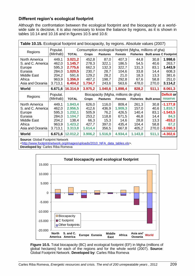
Carles Riba Romeva, Energetic resources and crisis. The end of 200 unrepeatable years , 2012 209
Different region’s ecological footprint
Although the confrontation between the ecological footprint and the biocapacity at a world-wide sale is decisive, it is also necessary to know the balance by regions, as it is shown in tables 10.14 and 10.16 and in figures 10.5 and 10.6:
Table 10.15. Ecological footprint and biocapacity, by regions. Absolute values (2007)
Regions Populat. (Minhab)
Consumption ecological footprint (Mgha, millions of gha) TOTAL Crops Pastures Forests Fisheries Built areas C Footprint
North America 449,1 3.021,2 452,8 87,0 407,3 44,8 30,8 1.998,6 S. and C. America 462,0 1.145,7 278,3 322,1 186,5 54,5 40,6 263,7 Europe 595,3 2.775,6 662,3 132,3 322,7 131,3 83,1 1.443,9 Eurasia 284,0 1.020,5 230,7 28,7 104,6 33,8 14,4 608,3 Middle East 204,2 591,6 129,2 28,2 21,0 18,3 13,3 381,6 Africa 963,9 1.356,0 487,2 198,7 292,8 67,6 58,8 251,0 Asia and Oceania 3.713,1 6.404,2 1.734,7 243,6 563,6 478,0 270,0 3.114,2
World 6.671,6 16.314,9 3.975,2 1.040,6 1.898,4 828,2 511,1 8.061,3
Regions Populat. (Minhab)
Biocapacity (Mgha, millions de gha) Deficit or reserve TOTAL Crops Pastures Forests Fisheries Built areas
North America 449,1 1.843,4 626,0 116,0 809,4 261,3 30,8 -1.177,8 S. and C. America 462,0 2.956,5 412,6 436,9 1.909,3 157,0 40,6 1.810,7 Europe 595,3 1.232,1 505,9 76,2 426,5 140,4 83,1 -1.543,5 Eurasia 284,0 1.104,7 253,2 118,8 671,5 46,8 14,4 84,3 Middle East 204,2 138,4 66,3 15,3 14,6 28,8 13,3 -453,2 Africa 963,9 1.423,2 427,7 397,0 435,4 104,4 58,8 67,2 Asia and Oceania 3.713,1 3.313,8 1.614,4 356,5 667,8 405,2 270,0 -3.090,3
World 6.671,6 12.012,2 3.906,2 1.516,9 4.934,4 1.143,8 511,1 -4.302,6
Source: Global Footprint Network <http://www.footprintnetwork.org/images/uploads/2010_NFA_data_tables.xls>. Developed by: Carles Riba Romeva
Biocapacitat i Petjada ecològica total (Ggha)
-20.000
-15.000
-10.000
-5.000
0
5.000
10.000
15.000
Biocapacitat
Petjada de C
Altres Petjades
Amèrica Nord
Amèrica Sud i C.
Europa Euràsia Orient Mitjà
Àfrica Àsia i
Oceania Món
Figure 10.5. Total biocapacity (BC) and ecological footprint (EF) in Mgha (millions of global hectares) for each of the regions and for the whole world (2007). Source: Global Footprint Network. Developed by: Carles Riba Romeva
Total biocapacity and ecological footprint (Mgha)
Biocapacity
C footprint
Other footprints
North America
Middle East
Africa Asia and Oceania
World Eurasia S. and C. America America
Europe

210 Carles Riba Romeva, Energetic resources and crisis. The end of 200 unrepeatable years , 2012
Table 10.16. Ecological footprint and biocapacity per regions. Amounts per capita (2007)
Regions Populat. (Minhab)
Consumption ecological footprint per inhabitant (gha/inhab) TOTAL Crops Pastures Forests Fisheries Built areas C footpr.
North America 449,1 6,73 1,01 0,19 0,91 0,10 0,07 4,45 S. and C. America 462,0 2,48 0,60 0,70 0,40 0,12 0,09 0,57 Europe 595,3 4,66 1,11 0,22 0,54 0,22 0,14 2,43 Eurasia 284,0 3,59 0,81 0,10 0,37 0,12 0,05 2,14 Middle East 204,2 2,90 0,63 0,14 0,10 0,09 0,07 1,87 Africa 963,9 1,41 0,51 0,21 0,30 0,07 0,06 0,26 Asia and Oceania 3.713,1 1,72 0,47 0,07 0,15 0,13 0,07 0,84
World 6.671,6 2,45 0,60 0,16 0,28 0,12 0,08 1,21
Regions Populat. (Minhab)
Biocapacity per inhabitant (gha/inhab) Deficit or reserve TOTAL Crops Pastures Forests Fisheries Built areas
North America 449,1 4,10 1,39 0,26 1,80 0,58 0,07 -2,63 S. and C. America 462,0 6,40 0,89 0,95 4,13 0,34 0,09 3,92 Europe 595,3 2,07 0,85 0,13 0,72 0,24 0,14 -2,59 Eurasia 284,0 3,89 0,89 0,42 2,36 0,16 0,05 0,30 Middle East 204,2 0,68 0,32 0,08 0,07 0,14 0,07 -2,22 Africa 963,9 1,48 0,44 0,41 0,45 0,11 0,06 0,07 Asia and Oceania 3.713,1 0,89 0,43 0,10 0,18 0,11 0,07 -0,83
World 6.671,6 1,80 0,59 0,23 0,74 0,17 0,08 -0,64
Source: Global Footprint Network <http://www.footprintnetwork.org/images/uploads/2010_NFA_data_tables.xls>. Developed by: Carles Riba Romeva
Biocapacitat i Petjada ecològica per càpita (gha/hab)
-8,00
-6,00
-4,00
-2,00
0,00
2,00
4,00
6,00
8,00
Biocapacitat
Petjada de C
Altres petjades
Amèrica Nord
Amèrica Sud i C.
Europa Euràsia Orient Mitjà
Àfrica Àsia i
Oceania Món
Figure 10.6. Biocapacity (BC) and ecological footprint (EF), per capita (in gha/inhab, global hectares per inhabitant), for each region and for the world (2007). Source: Global Footprint Network. Developed by: Carles Riba Romeva
The different regions of the world are very different when it comes to population and re-sources and, therefore, the game of imports and exports of the ecological footprint and of the biocapacities will take part (directly or indirectly) every time more in the worldwide geo-strategic game.
Biocapacity
C footprint
Other footpr.
North America
Middle East
Africa Asia and Oceania
World Eurasia S. and C. America America
Europe

Carles Riba Romeva, Energetic resources and crisis. The end of 200 unrepeatable years , 2012 211
Comments:
1. The most important matter is that the world’s ecological footprint (EF) is higher than its biocapacity (BC) (16.314,9, against 12.012,2 Mgha; an overshoot of a 35,8%). As it has been previously said, the higher values that the Global Footprint Network takes for the Earth as a whole (17.995,6 and 11.894,6 Mgha, with an overshoot of a 51,3%) are not coherent with the sum of the data for each country.
2. The second noteworthy aspect is the importance of the carbon ecological footprint (EFC), that is related to the use of fossil fuels: 8.061,3 Mgha, a 49,4% of the global eco-logical footprint. The result is still impressive if the carbon footprint is compared with the Earth biocapacity, due to the fact that it absorbs a 67,1% (8.061,2, against 12.012,2 Mgha). As it has been mentioned before, if this footprint was to be eliminated, humanity would still be sustainable.
4. There are three regions in the world that have a positive balance between biocapacity and ecological footprint, but only the net balance of South and Central America has a significant value (1.810,7 Ggha), while in the others it is testimonial (Eurasia, 84,3 Mgha, and Africa 67,2 Mgha).
5. The rest of the regions have a strongly negative balance. The worst of all is Asia and Oceania (-4.302,6 Mgha, mostly due to their high population); afterwards comes Europe (-1.543,2 Mgha), North America (-1.177,8 Mgha) and the Middle East (-453,2 Mgha).
Different countries’ ecological footprint
Table 10.17 shows three lists of countries, all of them referred to the more than 20 Minhab: a) the 8 countries with a higher ecological footprint (in fact, they are the most populated countries, which consume most); b) the 8 countries with more biocapacity (mainly those countries with higher surface area and with more productive land); c) finally, the 19 countries with extreme values of ecological footprint (the worldwide average biocapacity per capita BCm = 100 is taken as a unit of measurement), and some intermediate significant countries.
The following observations can be made:
1. The countries with the highest ecological footprint sum up a 51,8% of the population and a 55,2% of the ecological footprint, while the 8 countries which have a higher biocapacity sum up a 51,3% of the population but only a 41,2% of the biocapacity. Therefore, the ecological footprint is more concentrated than the biocapacity.
2. There are large differences between the ecological footprints of the different countries. The value per capita referred to the world average biocapacity per capita (BCm = 1) is, on one hand, of EF/BCm = 4,44 (3,44 times unsustainable) in the United States and, on the other hand, of 0,35 (with a margin of the 0,65 in relationship to sustainability) in Bangladesh. However, unsustainable countries prevail, being Spain’s fourth position surprising.
3. The carbon footprint per capita in relationship to world average per capita biocapacity ranges from EFC/BCm = 3,09 in the United States to very near to zero values in Afghani-stan, Mozambique, Congo D.R., Ethiopia or Tanzania. But the ecological footprint, sub-tracted from the carbon footprint (EF-EFC)/BCm, has much less extreme values (from 2,07 in Australia to 0,27 in Bangladesh).
4. The participation of the carbon footprint (EFC) in the ecological footprint (EF) is very im-portant. In the 14 countries with the highest ecological footprint (the first six are shown in table 10.17) the carbon footprint is greater than 1,2 times the average Earth biocapacity (BCm), while in the 14 countries with a minor ecological footprint (the six last ones in ta-ble 10.17), the carbon footprint is minor than 0,2 times the BCm.
Summing up, the different countries’ ecological footprint due to consumption is highly related to their wealth. And the higher it is, the more participation the carbon footprint has. With the decline of fossil fuels, a geopolitical disorder, that will mainly affect the most developed countries, can be forecasted.

212 Carles Riba Romeva, Energetic resources and crisis. The end of 200 unrepeatable years , 2012
Table 10.17. Ecological footprint and biocapacity by regions and by countries (2007)
Ecological footprint and biocapacity of the regions 1
Regions Population EF total BC total BC-EF total EF/inhab BC/inhab EF/BCm EFC/BCm
(Minhab) Mgha Mgha Mgha gha/inhab gha/inhab -- --
North America 449,1 3.021,2 1.843,4 -1.177,8 6,73 4,10 3,74 2,47 S. and C. Ameri-ca. 462,0 1.145,7 2.956,5 1.810,7 2,48 6,40 1,38 0,32 Europe 595,3 2.775,6 1.232,1 -1.543,5 4,66 2,07 2,59 1,35 Eurasia 284,0 1.020,5 1.104,7 84,3 3,59 3,89 2,00 1,19 Middle East 204,2 591,6 138,4 -453,2 2,90 0,68 1,61 1,04 Africa 963,9 1.356,0 1.423,2 67,2 1,41 1,48 0,78 0,14 Asia and Oce-ania 3.713,1 6.404,2 3.313,8 -3.090,3 1,72 0,89 0,96 0,47
World 6.671,6 16.314,9 12.012,2 -4.302,6 2,45 1,80 1,36 0,67
Countries with larger total ecological footprint 2
1 China 1.336,6 2.959,2 1.307,2 -1.652,0 2,21 0,98 1,23 0,67 2 USA 308,7 2.468,1 1.193,9 -1.274,1 8,00 3,87 4,44 3,09 3 India 1.164,7 1.063,4 594,3 -469,0 0,91 0,51 0,51 0,18 4 Russia 141,9 625,8 815,8 190,1 4,41 5,75 2,45 1,51 5 Japan 127,4 602,4 76,3 -526,1 4,73 0,60 2,63 1,74 6 Brazil 190,1 552,4 1.707,7 1.155,2 2,91 8,98 1,61 0,24 7 Germany 82,3 418,5 158,5 -260,0 5,08 1,92 2,82 1,50 8 Mexico 107,5 322,1 158,0 -164,1 3,00 1,47 1,66 0,76
Countries with larger biocapacity 2
1 Brazil 190,1 552,4 1.707,7 1.155,2 2,91 8,98 1,61 0,24 2 China 1.336,6 2.959,2 1.307,2 -1.652,0 2,21 0,98 1,23 0,67 3 USA 308,7 2.468,1 1.193,9 -1.274,1 8,00 3,87 4,44 3,09 4 Russia 141,9 625,8 815,8 190,1 4,41 5,75 2,45 1,51 5 India 1.164,7 1.063,4 594,3 -469,0 0,91 0,51 0,51 0,18 6 Canada 32,9 231,1 491,5 260,5 7,01 14,92 3,90 2,24 7 Australia 20,9 142,6 306,8 164,2 6,84 14,71 3,80 1,73 8 Indonesia 224,7 272,6 303,9 31,3 1,21 1,35 0,67 0,19
Countries with major and minor ecological footprint measured in average biocapacity (BCm = 1)2
1 USA 308,7 2.468,1 1.193,9 -1.274,1 8,00 3,87 4,44 3,09 2 Canada 32,9 231,1 491,5 260,5 7,01 14,92 3,90 2,24 3 Australia 20,9 142,6 306,8 164,2 6,84 14,71 3,80 1,73 4 Spain 44,1 238,8 71,1 -167,7 5,42 1,61 3,01 1,52 5 Saudi Arabia 24,7 126,7 20,7 -106,0 5,13 0,84 2,85 1,94 6 Germany 82,3 418,5 158,5 -260,0 5,08 1,92 2,82 1,50 13 Russia 141,9 625,8 815,8 190,1 4,41 5,75 2,45 1,51 17 Brazil 190,1 552,4 1.707,7 1.155,2 2,91 8,98 1,61 0,24 26 China 1.336,6 2.959,2 1.307,2 -1.652,0 2,21 0,98 1,23 0,67 37 Nigeria 147,7 212,2 165,0 -47,2 1,44 1,12 0,80 0,09 44 Indonesia 224,7 272,6 303,9 31,3 1,21 1,35 0,67 0,19 50 India 1.164,7 1.063,4 594,3 -469,0 0,91 0,51 0,51 0,18 51 Mozambique 21,9 16,9 41,4 24,5 0,77 1,89 0,43 0,02 52 Pakistan 173,2 132,8 74,1 -58,7 0,77 0,43 0,43 0,14 53 R. D. Congo 62,5 47,1 172,7 125,6 0,75 2,76 0,42 0,02 54 Afghanistan 26,3 16,4 14,3 -2,1 0,62 0,54 0,35 0,02 55 Bangladesh 157,8 98,0 59,2 -38,8 0,62 0,38 0,35 0,07 1 The symbols used in this table are: EF=ecological footprint (of consumption); EFC=carbon footprint;
BC=biocapacity; BCm=average world biocapacity. The units are: gha=global hectare; Mgha =millions of global hectares; hab=inhabitants; Minhab=millions of inhabitants
2 Amongst the 55 countries in the world with more than 20 million inhabitants
Source: Global Footprint Network. Developed by: Carles Riba Romeva

Carles Riba Romeva, Energetic resources and crisis. The end of 200 unrepeatable years , 2012 213
11. The atmosphere and the climate change
11.1. CO2 emissions
Introduction
At the beginning we said that, in this book, we would give more importance to the exhaus-tion of unrenewable sources of energy than to CO2 emissions and to climate change. We argued that this was due to the fact that, probably, the consequences of the decline of fossil fuel energetic resources would come first in our everyday lives and, also, in the higher po-tential that this fact can have in moving people’s consciences and wills.
But, at a longer term, the most serious and decisive problem that humanity will face (and that can put our survival at risk) is a unfavourable climate change, that, has ended up being the cause of the five massive extinctions that have taken place throughout the different geo-logical eras.
The climate change is not a secondary element of our lives it is a very important fact that can condition, in a decisive way, future human civilizations and the existence of life. Howev-er, the world as we currently know it, marked by the immediate economical worries, under-stands everything that has price much better (that is, it has been monetized), as well as the impact on our economies, than the complex equilibriums and the dynamics of the processes and the nature’s resources.
When giving an “economic” price to the CO2 emissions, the Kyoto protocol invites us to count them and to consider them in our balances. Although that, if we see it from this per-spective, we do not face the underlying problem, it has the advantage that it has become a “mediatic” theme which helps us to become aware of the limits of natural resources and of the impacts that derive from its use.
Once the dimension and the recent evolution of the CO2 emissions (and of other green-house effect gases), are understood, and being conscious of the climatic effects that they currently generate, we ask ourselves about the balance of the current carbon cycle, in com-parison to the preindustrial situation:
- Which are the different carbon sinks that are found in nature and their magnitudes? - Which are the carbon flows and their intensities, and in which deposits do they take place?
Finally, we analyse the most important aspect and, probably, the one that we know less of. It is about our relationship with nature and our try to predict the future consequences of the CO2 emissions and of the climate change.
In this context, we make some brushstrokes on the past (paleoclimate), and, at the same time, we closely analyse the conclusions of the Intergovernmental Panel on Climate Change (IPCC) and their last evaluation report (AR4, 2007) on the perspectives and future projections.
Therefore, the different sections of this chapter will carry out a tour from the current CO2 emissions to the projections of the future climate change:
- CO2 emissions (section 11.1) - Carbon cycle (section 11.2) - Carbon, oxygen and life (section 11.3)
In the same way that we have to be aware of our day to day development in relationship to the use of energetic resources and the emissions that derive from them, we also have to follow the indications of the climate change experts with a lot of attention in order to know the predictions. Will we be able to correct our collective behaviour?

214 Carles Riba Romeva, Energetic resources and crisis. The end of 200 unrepeatable years , 2012
CO2 emissions in the previous years
In the previous 150 years (and specially, in the last 50), the use of fossil fuels has produced a very important increase of CO2 and other greenhouse effect gases to the atmosphere, which has been the main cause of the climate change (section 11.3).
During this period (long at an economical perspective, but very short at a geological scale), below we analyse data on the CO2 emissions which is offered by the Energy Information Administration (EIA) of the United States Government.
Table 11.1. Evolution of the fossil fuel emissions (TgCO2/a)1
1980 % 1985 1990 1995 2000 2005 2008 %
Petroleum 8.825,2 47,9 8.333,0 9.118,0 9.421,7 10.174,2 11.125,7 11.170,8 36,6
Natural gas 3.086,3 16,7 3.507,0 4.147,2 4.488,1 4.974,3 5.748,3 6.273,4 20,6
Coal 6.522,4 35,4 7.702,1 8.350,8 8.240,3 8.655,2 11.492,2 13.049,0 42,8
Foss. fuels 18.433,9 100,0 19.542,1 21.616,0 22.150,1 23.803,6 28.366,2 30.493,2 100,0
Petroleum 100,0 94,4 103,3 106,8 115,3 126,1 126,6
Natural gas 100,0 113,6 134,4 145,4 161,2 186,2 203,3
Coal 100,0 118,1 128,0 126,3 132,7 176,2 200,1
Fossil fuels 100,0 106,0 117,3 120,2 129,1 153,9 165,4 1 Tg (teragrams = 10
12 grams = millions of tonnes).
Source: EIA-govUSA. Developed by: Carles Riba Romeva
It is interesting to graphically reproduce the evolution of these emissions (see figure 11.1, where we have also included data from 2009, recently included by the EIA).
Emissions segons combustible (TgCO2/any)
0
4.000
8.000
12.000
16.000
20.000
24.000
28.000
32.000
1980 1985 1990 1995 2000 2005
Petroli
Gas natural
Carbó
Combustibles fòssils
Figure 11.1. Evolution of the world’s CO2 emissions during the 1980-2009 peri-od, according to the fuels that origin the emission. It is observed that global emissions slow down, for the first time, in 2009 (30.451,6 TgCO2/a), due to a decrease in the petroleum emissions (second consecutive year) and of the nat-ural gas emissions (for the first time), while emissions from coal keep increas-ing. Source: EIA. Developed by: Carles Riba Romeva
Emissions by fuels (TgCO2/a)
Oil
Natural gas
Coal
Fossil fuels

Carles Riba Romeva, Energetic resources and crisis. The end of 200 unrepeatable years , 2012 215
It is also interesting to analyse the evolution of the CO2 emissions according to regions and countries:
Table 11.2. Evolution of the emissions by regions (TgCO2/a)
1980 % 1985 1990 1995 2000 2005 2009 %
North America 5.475,0 29,7 5.329,8 5.814,7 6.151,1 6.819,3 7.014,0 6.410,5 21,1
S. & C. America 627,4 3,4 624,6 716,3 857,6 991,8 1.104,0 1.273,0 4,2
Europe 4.680,3 25,4 4.553,8 4.545,7 4.309,0 4.457,8 4.676,7 4.310,3 14,2
Eurasia 3.081,9 16,7 3.535,7 3.820,8 2.467,5 2.327,5 2.519,2 2.358,0 7,7
Middle East 490,7 2,7 579,2 729,9 901,3 1.093,9 1.449,2 1.714,1 5,6
Africa 537,1 2,9 640,9 725,7 825,7 887,3 1.056,9 1.121,6 3,7
Asia & Oceania 3.541,5 19,2 4.278,0 5.262,9 6.637,8 7.226,1 10.546,1 13.264,1 43,6
World 18.433,9 100,00 19.542,1 21.616,0 22.150,1 23.803,6 28.366,2 30.451,6 100,00
North America 100,0 97,3 106,2 112,3 124,6 128,1 117,1
S. and C. America 100,0 99,6 114,2 136,7 158,1 176,0 202,9
Europe 100,0 97,3 97,1 92,1 95,2 99,9 92,1
Eurasia 100,0 114,7 124,0 80,1 75,5 81,7 76,5
Middle East 100,0 118,0 148,7 183,7 222,9 295,3 349,3
Africa 100,0 119,3 135,1 153,7 165,2 196,8 208,8
Asia and Oceania 100,0 120,8 148,6 187,4 204,0 297,8 374,5
World 100,0 106,0 117,3 120,2 129,1 153,9 165,2
Evolution of the emissions by countries (TgCO2/a)
1 China 1.448,5 7,86 1.857,8 2.269,7 2.861,7 2.849,7 5.512,7 7.710,5 25,32
2 USA 4.776,6 25,91 4.604,8 5.041,0 5.319,9 5.861,8 5.991,5 5.424,5 17,81
3 India 291,2 1,58 447,4 578,6 870,2 1.003,0 1.183,3 1.602,1 5,26
4 Russia - - - 1.603,1 1.556,1 1.652,7 1.572,1 5,16
5 Japan 947,0 5,14 926,2 1.047,0 1.116,2 1.201,4 1.241,3 1.098,0 3,61
6 Germany 1.056,0 5,73 1.014,2 990,6 890,8 854,7 847,4 765,6 2,51
7 Canada 457,4 2,48 443,7 470,6 508,7 573,3 623,4 541,0 1,78
8 S. Korea 131,7 0,71 172,3 242,1 381,4 438,8 493,8 528,1 1,73
9 Iran 116,8 0,63 159,9 202,1 262,2 320,6 449,2 527,2 1,73
10 U. Kingdom 613,6 3,33 589,3 601,8 560,1 560,3 583,1 519,9 1,71
11 S. Arabia 176,9 0,96 179,2 208,0 235,3 290,5 405,5 470,0 1,54
12 S. Africa 235,0 1,27 302,0 298,0 347,5 386,0 432,5 450,4 1,48
13 Mexico 240,3 1,30 280,7 302,2 321,4 383,0 397,8 443,6 1,46
14 Brazil 185,7 1,01 192,7 237,3 289,1 344,4 369,7 420,2 1,38
15 Australia 198,8 1,08 237,7 267,6 289,1 356,3 397,2 417,7 1,37
16 Indonesia 85,8 0,47 101,4 156,0 214,8 266,3 330,6 413,3 1,36
17 Italy 371,8 2,02 365,7 415,4 431,4 447,7 471,9 407,9 1,34
18 France 488,9 2,65 396,8 367,7 372,5 401,7 414,0 396,7 1,30
19 Spain 195,0 1,06 205,0 224,1 243,4 317,5 382,9 329,9 1,08
20 Taiwan 70,6 0,38 81,6 118,3 182,4 256,1 288,8 290,9 0,96
Note: Data from the EIA only includes the greenhouse effect gases that come from fossil fuels (petroleum, natural gas and coal), but they do not include other emissions (for example, methane) or other sources (for example, the concrete industry, the burning of residues or the crops or livestock exploitations) Source: EIA-govUSA. Developed by: Carles Riba Romeva
Analogously to table 11.1, the evolution of the emissions according to regions and countries is better perceived if it is shown with a graphical representation (see figure 11.2, for regions; figures 11.3 and 11.4, for countries). Figure 11.4 reproduces the inferior part of figure 11.3 (limited scale to 2.000 TgCO2/a) in order to show the evolution of the countries that go after China and the United States better.

216 Carles Riba Romeva, Energetic resources and crisis. The end of 200 unrepeatable years , 2012
Emissions, segons regions (TgCO2/any)
0
2.000
4.000
6.000
8.000
10.000
12.000
14.000
1980 1985 1990 1995 2000 2005
North America
S. & C. America
Europe
Eurasia
Middle East
Africa
Asia & Oceania
Figure 11.2. Evolution of the CO2 emissions in the 1980-2009 period, per re-gions. As North America, Europe and Eurasia slowed down the emissions in the last years of the crisis, the other four regions keep increasing. The enormous in-crease of the emissions in Asia and Oceania stands out. Source: EIA-govUSA. Developed by: Carles Riba Romeva
Emissions en els principals països (TgCO2/any)
0
1.000
2.000
3.000
4.000
5.000
6.000
7.000
8.000
1980 1985 1990 1995 2000 2005
China
USA
India
URSS-Russia
Japan
Germany
Canada
South Korea
Iran
United Kingdom
Figure 11.3. Evolution of the CO2 emissions in the 1980-2009 period, by coun-tries. We highlight the increase of China at the beginning of the decrease of the United States. The emissions of the USSR-Russia correspond to the USSR up to year 1992 and to Russia right from this moment. Source: EIA-govUSA. De-veloped by: Carles Riba Romeva
Emissions in the main countries (TgCO2/a)
Emissions, by regions (TgCO2/a)

Carles Riba Romeva, Energetic resources and crisis. The end of 200 unrepeatable years , 2012 217
Emissions en els principals països (TgCO2/any)
0
500
1.000
1.500
2.000
1980 1985 1990 1995 2000 2005
China
USA
India
URSS-Russia
Japan
Germany
Canada
South Korea
Iran
United Kingdom
Figure 11.4. The beginning of China, the collapse of the USSR-Russia in the previous years, while the United States exceed it, can be seen. On the other hand, the strong increases that have been experimented by India and Iran, the moderate increases of Japan and South Korea and the moderate decreases of Germany and the United Kingdom stand out. Source: EIA-govUSA. Developed by: Carles Riba Romeva
The analysis of tables 11.1, 11.2 and figures 11.1, 11.2, 11.3 and 11.4 drive us to make the following reflections and comments:
General
1. It is not true that, as sometimes some news seem to say, that the emissions are being reduced. At a worldwide scale, between 1980 and 2008, they have grown from 18.434 to 30.493 TgCO2/a, with an increase of a 65,4%.
2. As figure 11.1 very well shows, there is a change in the composition of the emissions. At the beginning of the period the emissions derived from petroleum combustion were dom-inant (47,9%) while at the end of the period weight has shifted to the derived from coal emissions (42,8%). This means that, as petroleum reaches its zenith, coal, which is the most pollutant fuel when it comes to emissions, takes over.
According to regions
3. The increase in Asia and Oceania’s emissions stands out (from 3.541 to 12.338 TgCO2/a between 1980 and 2008, with an increase of a 248,4%), that goes from a 19,2% to a 40,5% of the total world emissions. The increase of the Middle East also stands out (238%). Two other regions almost double their emissions in the same period: Africa, with an increase of a 115%, and South and Central America, with a 95,8%.
4. North America increases in a 25,8% (first it grows in absolute emissions until 2007 and then it slightly decreases) and in 1980 it becomes the country which emits more CO2 emissions, and in 2008 it has a distanced second place. Europe starts as the second CO2 emitter in 1980 and it ends being the third in 2008, without varying much in absolute terms, at the same time that it decreases the participation in worldwide emissions in a 10%. Finally, Eurasia, which is in fourth place, reaches its maximum amount in 1990, with 3.821 TgCO2/a, and drops to a minimum of 2.328 TgCO2/a in 2000.
Emissions in the main countries (TgCO2/a)

218 Carles Riba Romeva, Energetic resources and crisis. The end of 200 unrepeatable years , 2012
Changes in emissions (1980-2009),
by regions (TgCO2/any)
-1.000
0
1.000
2.000
3.000
4.000
5.000
6.000
7.000
8.000
9.000
10.000
11.000
12.000
13.000
14.000
Àsia i
Oceania
Amèrica
del Nord
Europe Euràsia Orient Mitjà Amèrica
Sud i C.
Àfrica
Emissions 1980
Emissions 2009
Increase 1980-2009
Figure 11.5. Evolution of the CO2 emissions in the period from 1980 to 2009, according to the studied regions, which have been set in a decreasing order for 2009. The only two regions that experiment a fall are Europe and Eurasia. Source: EIA. Developed by: Carles Riba Romeva
According to countries
5. According to countries, China stands out: in 1980 it emitted 1.448 TgCO2/a, in 2007 it surpassed the United States and in 2008 it places itself in 6.804 TgCO2/a; without mod-erating its growth with the crisis, it jumps to 7.710 TgCO2/a in 2009 (increase of 906 TgCO2 in one year, amount which is superior to Germany’s current emissions, which is the 4th worldwide economy). The global increase in the 1980-2009 period is of 6.262 TgCO2/a, +432% (figure 11.3). In 2009, China emitted a 25,3% of the worldwide CO2
emissions, which is above the weight of its population (a 19,9%).
6. In absolute increase amounts, India follows China: in 1980 it emitted 291,2 TgCO2/a and in 2009 it moved to the third place (1.602,1 TgCO2/a; increase of 1.310 TgCO2/a, +450,1%); but its emissions (a 5,3% of the world) are far from its demographic weight (a 17,1%).
7. The United States, first worldwide CO2 emitter in 1980 (the 25,9%), ends up being the second one (a 19,1% in 2009). However, emissions increase (third higher absolute in-crease, +648,0 TgCO2/a, a 13,6%), although with the crisis it suffers a slight decline.
8. Except for in some European countries and in Eurasia (as it will be commented later on), almost all of the countries increase their CO2 emissions during this period, some of them with very high increases (see table 11.3). Many of the most important absolute increases are found in countries from the South-East of Asia and in the Middle East.
10. In Europe, emissions almost do not vary during this period. But, while some occidental countries and countries from eastern Europe reduce their emissions due to the decrease in the use or coal or to the effects of the fall of Berlin’s Wall (Germany, Poland, United Kingdom, France, Romania), the Mediterranean countries and some others compensate for these decreases with increases (Turkey, Spain, Greece, Portugal, Ireland).
11. The evolution of Eurasia (for the first years we do not have the breakdown regarding the actual countries) is very complex. In the first decade (1980-1998), these countries increase their emissions +738,9 TgCO2/a; with the dissolving of the USSR (1990-1998), their emis-sions decrease in -1.609,3 TgCO2/a; with the new century (1998-2008), partially recovers with +384,4 TgCO2/a. And, in the previous year, a new decrease has started.
Changes in the emissions (1980-2009),
by regions (TgCO2/a)
Asia and Oceania
North America
Europe S. and C. America
Africa Middle East
America
Eurasia
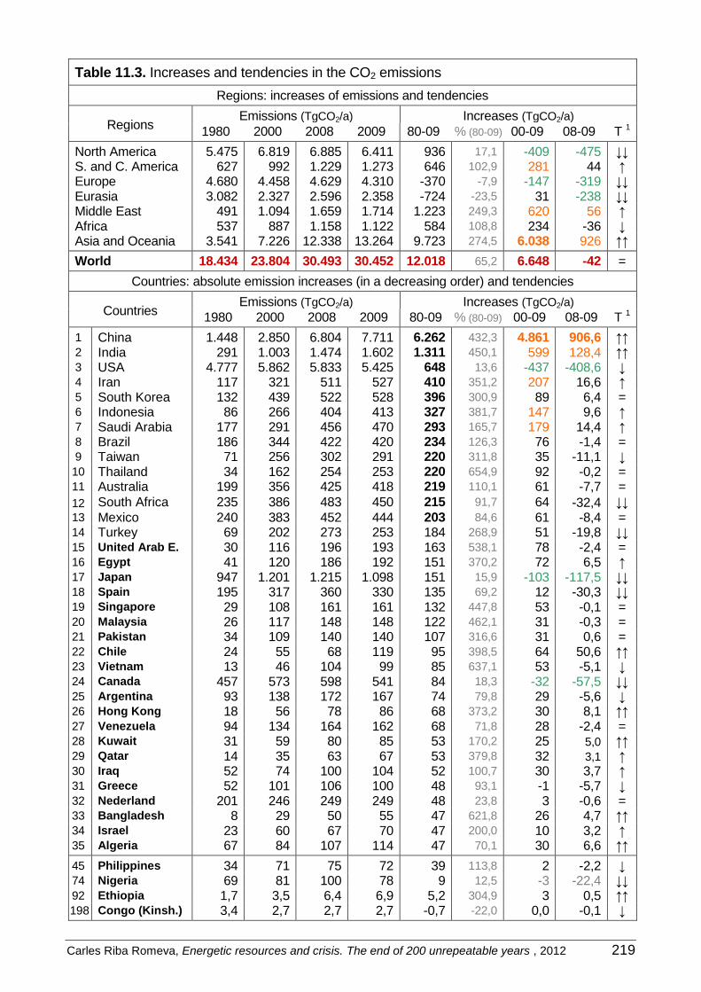
Carles Riba Romeva, Energetic resources and crisis. The end of 200 unrepeatable years , 2012 219
Table 11.3. Increases and tendencies in the CO2 emissions
Regions: increases of emissions and tendencies
Regions Emissions (TgCO2/a) Increases (TgCO2/a)
1980 2000 2008 2009 80-09 % (80-09) 00-09 08-09 T 1
North America 5.475 6.819 6.885 6.411 936 17,1 -409 -475 ↓↓ S. and C. America 627 992 1.229 1.273 646 102,9 281 44 ↑ Europe 4.680 4.458 4.629 4.310 -370 -7,9 -147 -319 ↓↓ Eurasia 3.082 2.327 2.596 2.358 -724 -23,5 31 -238 ↓↓ Middle East 491 1.094 1.659 1.714 1.223 249,3 620 56 ↑ Africa 537 887 1.158 1.122 584 108,8 234 -36 ↓ Asia and Oceania 3.541 7.226 12.338 13.264 9.723 274,5 6.038 926 ↑↑
World 18.434 23.804 30.493 30.452 12.018 65,2 6.648 -42 =
Countries: absolute emission increases (in a decreasing order) and tendencies
Countries Emissions (TgCO2/a) Increases (TgCO2/a)
1980 2000 2008 2009 80-09 % (80-09) 00-09 08-09 T 1
1 China 1.448 2.850 6.804 7.711 6.262 432,3 4.861 906,6 ↑↑ 2 India 291 1.003 1.474 1.602 1.311 450,1 599 128,4 ↑↑ 3 USA 4.777 5.862 5.833 5.425 648 13,6 -437 -408,6 ↓ 4 Iran 117 321 511 527 410 351,2 207 16,6 ↑ 5 South Korea 132 439 522 528 396 300,9 89 6,4 = 6 Indonesia 86 266 404 413 327 381,7 147 9,6 ↑ 7 Saudi Arabia 177 291 456 470 293 165,7 179 14,4 ↑ 8 Brazil 186 344 422 420 234 126,3 76 -1,4 = 9 Taiwan 71 256 302 291 220 311,8 35 -11,1 ↓ 10 Thailand 34 162 254 253 220 654,9 92 -0,2 = 11 Australia 199 356 425 418 219 110,1 61 -7,7 =
12 South Africa 235 386 483 450 215 91,7 64 -32,4 ↓↓ 13 Mexico 240 383 452 444 203 84,6 61 -8,4 = 14 Turkey 69 202 273 253 184 268,9 51 -19,8 ↓↓ 15 United Arab E. 30 116 196 193 163 538,1 78 -2,4 = 16 Egypt 41 120 186 192 151 370,2 72 6,5 ↑ 17 Japan 947 1.201 1.215 1.098 151 15,9 -103 -117,5 ↓↓ 18 Spain 195 317 360 330 135 69,2 12 -30,3 ↓↓ 19 Singapore 29 108 161 161 132 447,8 53 -0,1 = 20 Malaysia 26 117 148 148 122 462,1 31 -0,3 = 21 Pakistan 34 109 140 140 107 316,6 31 0,6 = 22 Chile 24 55 68 119 95 398,5 64 50,6 ↑↑ 23 Vietnam 13 46 104 99 85 637,1 53 -5,1 ↓ 24 Canada 457 573 598 541 84 18,3 -32 -57,5 ↓↓ 25 Argentina 93 138 172 167 74 79,8 29 -5,6 ↓ 26 Hong Kong 18 56 78 86 68 373,2 30 8,1 ↑↑ 27 Venezuela 94 134 164 162 68 71,8 28 -2,4 = 28 Kuwait 31 59 80 85 53 170,2 25 5,0 ↑↑ 29 Qatar 14 35 63 67 53 379,8 32 3,1 ↑ 30 Iraq 52 74 100 104 52 100,7 30 3,7 ↑ 31 Greece 52 101 106 100 48 93,1 -1 -5,7 ↓ 32 Nederland 201 246 249 249 48 23,8 3 -0,6 = 33 Bangladesh 8 29 50 55 47 621,8 26 4,7 ↑↑ 34 Israel 23 60 67 70 47 200,0 10 3,2 ↑ 35 Algeria 67 84 107 114 47 70,1 30 6,6 ↑↑
45 Philippines 34 71 75 72 39 113,8 2 -2,2 ↓ 74 Nigeria 69 81 100 78 9 12,5 -3 -22,4 ↓↓ 92 Ethiopia 1,7 3,5 6,4 6,9 5,2 304,9 3 0,5 ↑↑ 198 Congo (Kinsh.) 3,4 2,7 2,7 2,7 -0,7 -22,0 0,0 -0,1 ↓

220 Carles Riba Romeva, Energetic resources and crisis. The end of 200 unrepeatable years , 2012
Countries: absolute emission decreases (in a decreasing order) and tendencies
Countries Emissions (TgCO2/a) Decreases (TgCO2/a)
1980 2000 2008 2009 80-09 % (80-09) 00-09 08-09 T 1
208 Denmark 65 54 54 50 -15 -23,7 -5 -4,7 ↓↓ 209 North Korea 111 69 70 80 -31 -28,0 10 10,0 ↑↑ 210 Sweden 82 61 55 51 -32 -38,6 -10 -4,2 ↓↓ 211 Hungary 84 55 56 50 -34 -40,3 -5 -6,0 ↓↓ 212 Bulgaria 89 49 50 44 -44 -49,8 -5 -6,0 ↓↓ 213 Romania 171 93 97 81 -90 -52,9 -13 -16,0 ↓↓ 214 France 489 402 429 397 -92 -18,9 -5 -31,9 ↓↓ 215 United Kingdom 614 560 564 520 -94 -15,3 -40 -43,9 ↓↓ 216 Poland 429 293 295 286 -143 -33,4 -7 -9,0 ↓ 217 Germany 1.056 855 823 766 -290 -27,5 -89 -57,5 ↓↓
Countries from Eurasia
3.082 2.327 2.596 2.358 -724 -23,5 31 -238,0 ↓↓
1 Tendency from 2008 to 2009: = (between +2 and -2%); ↑ (between +2 and + 6%); ↑↑ (> 6%); ↓ (between -2
and -6%); ↓↓ (< -6%). Source: EIA-govUSA. Developed by: Carles Riba Romeva
Changes in emissions (1980-2009),
by counties (TgCO2/any)
-1.000
0
1.000
2.000
3.000
4.000
5.000
6.000
7.000
8.000
Xina Índia EUA Iran França Regne
Unit
Polònia Alemanya
Emissions 1980
Emissions 2009
Increase 1980-2009
Figure 11.6. Evolution of the CO2 emissions in the 1980-2009 period, by countries: the four that have increased more and the four that have decreased more (changes in red). Source: EIA-govUSA. Developed by: Carles Riba Romeva
As it can be seen in the previous tables and figures, the issue of curbing greenhouse gas emissions (concretely, CO2), and to the effects of the climate change has taken a global di-mension and it is not possible to solve it without involving the newly emerging powers and, specially, China and India, due to the trends that they suggest.
CO2 emissions and fossil fuels energy take part in the same equation. In the dominant eco-nomic paradigm, development is synonymous to fossil fuel energy consumption, and this is translated directly to CO2 emissions to the atmosphere.
The analysis of the different countries’ emissions to the atmosphere supplies us with a snap-shot of its development state. In the current energetically-based crisis, the interpretation of the emissions’ fluctuations and their tendencies has become an essential aspect.
Changes in the emissions (1980-2009),
by extreme countries (TgCO2/a)
China India USA Iran France UK Poland Germany
Carles Riba Romeva, Energetic resources and crisis. The end of 200 unrepeatable years , 2012 221
In effect, Europe starts the decline with the stagnation of the emissions. China, India and other countries belonging to the South-East of Asia and the Middle East accompany their spectacu-lar economical growths with emissions of the same order. The Eurasian economy has fluctu-ated according to its emissions. The United States achieve the summit of their hegemony and, at the same time, the summit of their consumption and emissions. South America progresses in a moderate way, as well as their emissions, and countries belonging to Sub-Saharan Africa almost do not appear in the emission map (apart from South Africa, which has important coal resources).
Therefore, it does not make any sense to analyse the CO2 emissions and the climate change without studying, at the same time, the theme of energy and development.
CO2 emissions per capita
In the previous sections, we have paid more attention on the increases and decreases of the global CO2 emissions than on their distribution according to population. In fact, in the world balance, it is the absolute values that are important.
But, in order to complete the vision on the theme of emissions, it is also necessary to ana-lyse the evolution of the CO2 emissions per inhabitant (or per capita) of the different regions and countries through time (table 11.4). Certainly, it is not desirable to have high emissions per capita, but large differences in this parameter imply that there is a very poor distribution of the Earth’s resources.
The analysis of table 11.4 invites us to do the following comments:
General
1. In the first place, it is needed to point out that, at a worldwide scale, the emission per capi-ta does not undergo many changes in time. In 1980 they were of 4,14 MgCO2/(inhab·a) (tonne per inhabitant and year), then they decreased up to 3,88 (from 1994 to 2001) and in 2008 they increased up to the value of 4,55, but insinuated a decline the following year. Therefore, the large increase of emissions in the previous years is partly made up for by the growth of the world population.
According to regions
2. A tendency of the regions to become equal in this aspect is perceived (figure 11.7). The three regions that had higher emissions per capita in 1980 have reduced them (North America, from 17,09 to 14,19 MgCO2/(inhab·a), to -17,0%; Eurasia, from 11,59 to 8,32, a -28,2%, and Europe, from 8,84 to 7,14, a -19,3%). Two regions with inferior emissions per capita than the world average have increased, (Asia and Oceania spectacularly, from 1,43 to 3,53, a +145,9%, and South and Central America, moderately, from 2,14 to 2,68, a 25,3%). The Middle East, although in 1980 was already above the world average, in-creases a 57,2% and in 2009 is placed in second place, tied with Eurasia.
3. Africa is kept in the last place and it almost does not increase (from 1,12 to 1,13 MgCO2/ (inhab·a)). Only South Africa, that still does not bear a 5% of the continent’s population, generates more than a 40% of the CO2 emissions. The rest of Africa, therefore, only generates 0,71 MgCO2/(inhab·a).
4. A similar situation is given in Asia. If the four countries with a singular dynamic economy are considered separately (China, Japan, South Korea and Australia), a 59,6% of the remaining population (2.241,7 Minhab) emits, in average, only 1,57 MgCO2/(inhab·a).
By countries
5. Among the countries with more than 20 million inhabitants (table 11.5), the ones that emit more emissions are Australia and Saudi Arabia, with values near to 20 MgCO2/(inhab·a), and with important increases during the analysed period (1980-2009). On the other hand, the countries that follow them, the United States and Canada, have slightly decreased their emissions per capita.

222 Carles Riba Romeva, Energetic resources and crisis. The end of 200 unrepeatable years , 2012
6. Among the first CO2 emitters per capita (>8,8 MgCO2/(inhab·a), which is the double than the world average), apart from many countries belonging to the OECD (America, Europe and Asia), countries with important energetic resources, either of petroleum (among them, Saudi Arabia), of coal (Kazakhstan, Turkmenistan, South Africa) or of combined resources (Russia) are found.
7. In an intermediate position, China stands out, with 5,8 MgCO2/(inhab·a), slightly superior to the world average and with a spectacular increase in the considered period. The rest of the countries with a population that is greater than 80 million inhabitants (Mexico, Egypt, Brazil, Indonesia, India, Vietnam, Pakistan, Philippines, Nigeria, Bangladesh and Ethiopia) have emissions which are below the world average, and those of the last six is inferior than a 25% of this value. Ethiopia, like many other African countries, almost does not emit CO2.
Table 11.4. Emissions per capita, by regions and by countries (TgCO2/(inhab·a))
Evolution of the emissions per capita, by regions
1980 Wor.=100 1985 1990 1995 2000 2005 2009 Wor.=100 1980=100
North America 17,09 412,8 15,64 16,04 15,81 16,50 16,14 14,19 315,7 83,0
S. & C. America 2,14 51,7 1,92 2,00 2,19 2,35 2,45 2,68 59,7 125,3
Europe 8,84 213,4 8,40 8,17 7,57 7,69 7,88 7,14 158,8 80,7
Eurasia 11,59 279,9 12,73 13,25 8,48 8,06 8,84 8,32 185,2 71,8
Middle East 5,23 126,3 5,09 5,40 5,92 6,32 7,59 8,22 183,0 157,2
Africa 1,12 27,1 1,16 1,15 1,16 1,10 1,17 1,13 25,1 100,8
Asia & Oceania 1,43 34,6 1,58 1,78 2,08 2,12 2,92 3,53 78,5 245,9
World 4,14 100,00 4,02 4,09 3,89 3,91 4,38 4,49 100,0 108,5
Evolution of the emissions per capita, by countries1
1980 Wor.=100 1985 1990 1995 2000 2005 2009 Wor.=100 1980=100
1 Australia 13,60 328,5 15,14 15,78 16,08 18,70 19,63 19,64 437,2 144,4
2 S. Arabia 17,65 426,3 13,44 12,95 12,55 13,63 17,15 18,56 413,0 105,1
3 USA 21,02 507,6 19,35 20,19 19,98 20,77 20,26 17,67 393,2 84,1
4 Canada 18,60 449,2 17,10 16,93 17,13 18,43 19,25 16,15 359,5 86,8
5 Taiwan 3,96 95,6 4,22 5,83 8,57 11,55 12,72 12,66 281,8 319,9
6 Russia -- -- -- 10,80 10,61 11,58 11,23 249,8
7 S. Korea 3,46 83,4 4,22 5,65 8,46 9,37 10,29 10,89 242,3 315,1
8 Germany 13,49 325,8 13,06 12,48 10,91 10,40 10,28 9,30 206,9 74,1
9 S. Africa 7,75 187,2 8,52 7,74 8,23 8,57 9,11 9,18 204,4 118,4
10 Japan 8,11 195,8 7,67 8,48 8,91 9,48 9,73 8,64 192,3 106,6
11 U. Kingdom 10,86 262,1 10,37 10,44 9,59 9,44 9,60 8,35 185,9 76,9
12 Poland 12,06 291,1 11,34 8,76 7,98 7,57 7,46 7,43 165,3 61,6
13 Spain 5,70 125,6 6,12 7,82 8,76 7,84 6,12 7,13 158,6 137,0
18 China 1,47 35,5 1,76 1,98 2,35 2,26 4,25 5,83 129,6 396,0
23 Mexico 3,52 84,9 3,66 3,56 3,46 3,83 3,75 3,99 88,8 113,4
31 Egypt 0,96 23,2 1,51 1,69 1,68 1,84 2,22 2,44 54,2 254,2
32 Brazil 1,51 36,4 1,40 1,57 1,77 1,95 1,96 2,11 47,1 140,1
33 Indonesia 0,57 13,7 0,61 0,85 1,08 1,24 1,44 1,72 38,3 302,8
35 India 0,43 10,3 0,59 0,69 0,95 1,00 1,08 1,38 30,8 325,7
38 Vietnam 0,25 6,0 0,28 0,25 0,41 0,58 0,90 1,12 24,8 447,0
40 Pakistan 0,40 9,5 0,46 0,56 0,65 0,72 0,69 0,77 17,2 195,7
41 Philippines 0,66 16,1 0,47 0,64 0,80 0,87 0,84 0,74 16,4 111,1
43 Nigeria 0,92 22,3 0,72 0,85 0,91 0,66 0,78 0,52 11,6 56,4
44 Bangladesh 0,09 2,1 0,10 0,13 0,19 0,22 0,28 0,36 8,0 413,0
54 Ethiopia 0,04 1,1 0,06 0,06 0,04 0,05 0,06 0,08 1,8 183,4 1 The position of each country is related to the 57 countries that, in 2009, had a greater population than 20Minhab.
Source: EIA-govUSA. Developed by: Carles Riba Romeva

Carles Riba Romeva, Energetic resources and crisis. The end of 200 unrepeatable years , 2012 223
Variacions de les emissions (1980-2009) segons països
(MgCO2/(hab·any))
0
2
4
6
8
10
12
14
16
18
20
Amèrica
del Nord
Amèrica
Sud i C.
Europa Euràsia Orient Mitjà Àfrica Àsia i
Oceania
Món
Emissions 1980
Emissions 2000
Emissions 2009
Figure 11.7. Evolution of the CO2 emissions (1980, 2000 and 2009), by regions and in the world. Source: EIA-govUSA. Developed by: Carles Riba Romeva
8. Europe countries tend to converge in the emissions of CO2. Those of occidental North Europe (Germany, United Kingdom, France, Nordic countries) and of oriental Europe (Po-land, Romania, Hungary, Czech Republic), part from relatively high emissions per capita in 1980, normally between 7 and 15 MgCO2/(inhab·a), and tend to decrease them up to an interval of between 5 to 10 in 2009. On the other hand, Mediterranean European coun-tries (Spain, Italy, Greece, Portugal) part from inferior values in 1980, normally between 3 and 7, and tend to increase them up to 5 to 9 in 2009. It is necessary to highlight several specific cases: Holland and Belgium maintain their emissions between 13 and 15 MgCO2/(inhab·a) with almost no variations; Iceland and Ireland have a similar to Mediter-ranean countries behaviour, that, parting from moderate values, increase their emissions; Turkey increases from 1,5 to 3,3, and Albania follows the reverse way and decreases from 3,3 to 1,5.
Stocked emissions
Data from the EIA only includes the CO2 that is emitted to the atmosphere from fossil fuels: petroleum and other liquid fuels; natural gas, including the one that is burned (flaring) in or-der to avoid the emission of the gas with a higher greenhouse effect, methane; and coals. It does not include other sources of greenhouse effect gases, like the cement industry, or cer-tain crops or livestock exploitations.
Furthermore, the greenhouse effect gas emissions origin other discussions (which I consider appropriate) between developed and developing countries on the theme of if the current emissions have to be taken into reference, or on the other hand if we have to consider the accumulated emissions from the beginning of the fossil fuel and other related activity’s use. As well as the debate on the hidden transfers of emissions through the exportation of prod-ucts that are manufactured in one country and consumed in another.
This aspect modifies the vision of the theme. When, in some countries that currently have relatively low, declining emissions in a worldwide context (for example Germany, United Kingdom or France, in the process of exhausting their reserves, especially those of coal),
Oceans >100 m (37.100 Pg) 37.200 Pg (+100)
Evolution of the CO2 emissions per capita,
by regions (MgCO2/(inhab·a))
North America
S. and C. America
Asia and Oceania
Middle East
Europe Eurasia Africa World

224 Carles Riba Romeva, Energetic resources and crisis. The end of 200 unrepeatable years , 2012
the accumulated emissions in the past are accounted, and their historical responsibility then appears with all clarity. But, in order to carry out this analysis, the data that is needed some-times belongs to the 18th century.
The CDIAC (Carbon Dioxide Information Analysis Centre, Oak Ridge National Laboratory, TE, USA) is an American centre that supplies data on the theme of greenhouse effect gases and on the climate change expenses to the Department of Energy (DOE) of the North Amer-ican Government. Like other American institutions of this type, it makes an important part of its information public.
Evolution of the world CO2 emissions (TgC)
0
1000
2000
3000
4000
5000
6000
7000
8000
9000
1751 1801 1851 1901 1951 2001
Coal
Petroleum
Natural gas
Cement
Figure 11.8. Evolution of the world ‘s stocked CO2 emissions (in TgC, millions of tonnes of C) caused by the different fossil fuels and cement in the 1751-2007 period (values of the accumulated components). Source: CDIAC. Developed by: Carles Riba Romeva
Figure 11.8 shows (parting from data of the CDIAC) the worldwide accumulated CO2 emis-sions associated to the consumption of fossil fuels and to the manufacture of cement. It can be observed that, almost until after the Second World War, the CO2 emissions (and the con-sumption of fossil fuels) were relatively small. After a large growth in the period 1945-1975 (basically, associated to petroleum) and a certain moderation in the following years (1975-2000, specially in European countries), emissions associated to coal register a strong re-covery in the last few years (2000-2008) as a consequence of the massive growth of the consumption of this fuel in China, and in less proportion, in India.
Table 11.5, with the accumulated CO2 emissions according to their origin, the dates and the localizations, according to data from the CDIAC, suggests the following comments:
1. The first part of the table numerically shows the worldwide CO2 emissions in several dates. In 2007 (last date of the CDIAC), it is of 330.092 TgC (only the mass of the car-bon element). To translate it into TgCO2, it is needed to multiply it by the stoichiometric ratio (C=12; O=16; CO2/C = 44/12 = 3,667), that gives us 1.210.336 TgCO2 emitted to the atmosphere. This is equivalent to almost forty years of the current emissions (30.493 TgCO2/a in 2008, almost equal to those of 2009).
2. The second part of the table shows the distribution of the accumulated emissions in 2007 in the different regions. North America and Europe, with a 31,7% and a 27,2% respec-tively, of these emissions, stand out. The third place, which belongs to Asia and Oceania (a 21,1% with much inferior accumulated emissions per capita), and the fourth place, Eurasia (a 12,5%).
Evolution of the world’s stocked CO2 emissions (TgC)

Carles Riba Romeva, Energetic resources and crisis. The end of 200 unrepeatable years , 2012 225
Table 11.5. Accumulated CO2 emissions, by dates, origin and localization
Coal Petroleum NG NG Flame Concrete Total Indexes1
Worldwide accumulated emissions with the passing of time (in TgC, millions of tonnes of carbon)2
1900 11.972 221 40 0 0 12.234 3,7
1950 53.942 6.857 1.322 20 231 62.371 19,9
1980 97.772 46.411 13.019 1.689 2.175 161.066 49,0
2000 143.967 93.597 33.194 2.586 5.497 278.841 84,5
2007 164.104 112.206 43.213 2.957 7.611 330.092 100,0
Accumulated emissions in the whole world and by regions until 2007 (in TgC, millions of tonnes of C)2
North America 44.320 39.787 18.001 434 830 103.372 31,3
S. & C. America 934 6.043 1.371 452 372 9.172 2,8
Europe 56.153 24.394 7.451 91 1.836 89.926 27,2
Eurasia 17.868 12.568 9.960 194 646 41.236 12,5
Middle East 174 4.940 2.191 1.019 269 8.592 2,6
Africa 3.921 2.730 685 465 280 8.081 2,4
Asia & Oceania 40.734 21.744 3.554 303 3.378 69.714 21,1
World 164.104 112.206 43.213 2.957 7.611 330.092 100,0
The same title (in TgCO2, millions of tonnes of carbon dioxide)2
North America 162.506 145.886 66.005 1.590 3.044 379.030 31,3
S. & C. America 3.423 22.158 5.026 1.658 1.364 33.630 2,8
Europe 205.895 89.443 27.321 335 6.734 329.729 27,2
Eurasia 65.514 46.084 36.520 710 2.369 151.198 12,5
Middle East 638 18.112 8.032 3.736 985 31.503 2,6
Africa 14.378 10.011 2.510 1.703 1.027 29.630 2,4
Asia & Oceania 149.358 79.728 13.033 1.110 12.387 255.616 21,1
World 601.713 411.423 158.449 10.843 27.908 1.210.336 100,0
The same title (in TWty, millions of millions of thermal watts year)3
2.817,7 3
1.987,8 3 1.579,3
3 1.579,3
3
North America 57,673 73,392 41,793 1,007 173,865 32,9
S. & C. America 1,215 11,147 3,183 1,050 16,595 3,1
Europe 73,072 44,997 17,299 0,212 135,580 25,7
Eurasia 23,251 23,184 23,124 0,450 70,009 13,3
Middle East 0,227 9,112 5,086 2,366 16,790 3,2
Africa 5,103 5,036 1,589 1,078 12,807 2,4
Asia & Oceania 53,007 40,110 8,252 0,703 102,072 19,3
World 213,547 206,979 100,326 6,866 527,718 100,0
Countries with the biggest amount of accumulated emissions in 2007 (in TgC, millions of tonnes of C)1
1 USA 42.842 35.432 16.529 272 650 95.724 29,0 (29,0)
2 USSR-Russia 16.830 11.922 8.825 191 610 38.378 11,6 (40,6)
3 China 25.664 5.112 515 8 2.223 33.521 10,2 (50,8)
4 Germany 16.381 4.576 1.410 13 313 22.692 6,9 (57,7) 5 U: Kingdom 15.228 3.367 1.394 54 130 20.173 6,1 (63,8)
6 Japan 5.103 7.861 1.043 0 493 14.500 4,4 (68,2)
7 India 6.928 2.098 261 40 367 9.694 2,9 (71,1) 8 France 4.994 3.472 707 13 186 9.373 2,8 (73,9)
9 Canada 2.390 3.149 1.579 60 79 7.257 2,2 (76,1)
10 Poland 5.634 573 230 0 104 6.542 2,0 (78,1) 11 Italy 1.084 3.175 1.017 0 263 5.539 1,7 (79,8) 12 South Africa 3.742 517 22 0 56 4.337 1,3 (81,2) 1 1st part: 2007=100; 2nd, 3rd and 4th: % in the world; 5th: % in the world (accumulated).
2 CDIAC gives its emis-
sion values in gC (carbon); in the 2nd part, it has been translated to gCO2 (C=12; O=16; CO2/C=44/12).
3 In order to obtain the values of energy (TWty) from the values of the CO2 emissions the average values that have been obtained from the EIA (energy and emissions for each fuel) have been used.
Sources: CDIAC and EIA-govUSA. Developed by: Carles Riba Romeva

226 Carles Riba Romeva, Energetic resources and crisis. The end of 200 unrepeatable years , 2012
3. The other three regions (South and Central America, Middle East and Africa) accumulate much lower emissions, with percentages of from a 2,8 to a 2,4%. This is, at the same time, an indicator of the little use that they have done of fossil fuels.
4. In relation to the accumulated emissions per fuel, the most important ones are those of coal (164.104 TgC, a 49,7%); followed by those of petroleum (112.206 TgC, a 34,0%), natural gas, including the burning or flaring (45.970 TgC, a 13,0%), and cement (7.611 TgC, a 2,3%). If the measurement is done in energetic terms, due to the fact that the dif-ferent fuels have different energy/emission ratios (note 3 of table 11.5), more favourable to natural gas and petroleum, things are more equal. Coal: 213,5 TWta, a 40,5%; petro-leum: 207,0 TWta, a 39,2%; natural gas, that looses the energy from the flaring (100,3 TWta, a 19,0%).
5. The 12 countries with a higher accumulated coal consumption before 2007 and, there-fore, with a higher historical greenhouse effect incidence due to fuels are, in the first place, and clearly standing out from the rest, the United States (95.724 TgC, a 29,0% of the world); in the second place, at a distance USSR-Russia (38.378 TgC, a 11,6%); in the third place in accumulated emissions, China (33.521 TgC, a 10,2%); followed by Germany (22.692 TgC, a 6,9%), the United Kingdom (20.173 TgC, a 6,1%) and Japan (14.500 TgC, a 4,4%); the seventh place belongs to India (9.694 TgC, a 2,9%) followed by France (9.373 TgC, a 2,8%), Canada (7.257 TgC, a 2,2%), Poland (6.542 TgC, a 2,0%), Italy (5.539 TgC, a 1,7%) and South Africa (4.337 TgC, a 1,3%). Between them they accumulate more than a 80% of the historical emissions.
6. They are followed by, in the following order, Mexico, Australia, the Czech Republic, Spain, South Korea, Belgium, Iran, Brazil, Holland, Saudi Arabia, Indonesia and Romania, having all of them accumulated more than 2.000 TgC.
Therefore, in the currently changing world, the responsibilities of the CO2 emissions and the climate change turn into an increasingly shared issue. Although it is true that North America and Europe (and also Eurasia) have accumulated proportionally higher emissions in rela-tionship to their population, and due to their history, it is also true that the irruption of new very-populated countries, with very quick developments, can make currently accumulated emissions play a secondary role.
Figure 11.9. CO2 emissions’ flows, reflected in commerce (TgCO2/a). Source: Carbon Budget 2009, from the Global Carbon Project (CDIAC). <http://www.globalcarbonproject.org/carbonbudget/09/files/GCP2010_CarbonBudget2009.pdf>

Carles Riba Romeva, Energetic resources and crisis. The end of 200 unrepeatable years , 2012 227
11.2. The carbon cycle
This cycle studies the exchange of carbon (C) between the components that are present in the different environments of our planet. The carbon deposits are measured in Pg (peta grams = 1015 g = 1 Gt = 1 gigatonne = 109 tonnes) and the flows, in Pg/a (or peta grams per year).
It is one of nature’s most complex cycles and it intervenes in a decisive way in three deter-minant aspects for humans: life, climate and energy.
The complexity of the carbon cycle is due to, among others, the following aspects:
1. The carbon compounds are found in the Earth’s four superficial spheres:
- the biosphere (which is divided into the terrestrial and the marine biosphere) - the atmosphere (CO2 and methane) - the hydrosphere (dissolved CO2, dissolved organic matter and particulate organic matter) - the lithosphere (carbonate rocks, carbons and hydrocarbons, kerogene)
Each one of them has one or more carbon sinks of a different nature, and between them different intensity flows are established.
2. The carbon cycle has a biogeochemical nature, with great complexity and biological criti-cism, chemical and physical reactions, that take place in all of the Earth’s environments. Carbon is present in two types of compounds:
- Organic compounds, characterized by the C-C and C-H links, that are the basis of living beings, dead beings, decomposed beings and also of hydrocarbons.
- Inorganic compounds, mainly CO2 in the atmosphere and dissolved in oceans, and cal-cium carbonate CaCO3 of the carbonated rocks.
3. The flows are very different in intensity and in the carbon permanency time in the different environments. It is important to distinguish between two types of subcycles:
Short cycles, where the flows are established between the atmosphere and the terrestrial biota (around 120 Pg/a in both senses), and between the atmosphere and the surface oceans (approximately 90 Pg/a in both senses). Considering the values of the flows and the dimension of the sinks (820 Pg in the atmosphere), the carbon permanency time in the different environments is of few years.
Long cycles, where the flows are much smaller (inferior than 1 Pg/a), and much larger sinks take part (the lithosphere and the CO2 which is dissolved in oceans); therefore, the carbon permanency time is much higher (between 104 and millions of years, Ma).
4. Carbon (C) is the essential element of the biological production, all known life sources contain carbon compounds.
Since the appearance of life on Earth, approximately 3.500 million years ago, the carbon cy-cle has had a crucial role in biological processes due to photosynthesis, from which organic matter is obtained, and also due to respiration, with its consequent obtaining of energy.
5. Carbon takes part in climate regulation by means of the two main greenhouse effect gas-es: carbon dioxide (CO2) and methane (CH4).
Due to the interaction between living beings and the atmosphere its composition has evolved from being majorly composed of CO2, approximately 3.500 Ma ago, to its current composition.
In any case, the variations in these gases’ percentages in the atmosphere may be the cause of climate changes, as in the case of current increases of these gases.
6. Finally, carbon (C) is the main element of fossil fuels (carbons and hydrocarbons), that constitutes the energetic basis of our human civilization
With the accelerated burning of fossil fuels, a new carbon flow has been introduced from the lithosphere to the atmosphere, and it seems that it will substantially alter the climate.
This fact, combined with the exhaustion of fossil fuels, are the two main challenges that humanity is currently facing.

228 Carles Riba Romeva, Energetic resources and crisis. The end of 200 unrepeatable years , 2012
Sinks and flows of the carbon cycle (table 11.6 and figure 11.10)
What at a short term regulates life and climate are the so called short carbon cycles, that take place between the biosphere, the atmosphere and the hydrosphere, where the sinks are small and the flows are big, while climatic conditions are regulated in long term by the long carbon cycles, where the lithosphere also takes part and where the sinks are large and the flows are very small.
The burning of fossil fuels upsets de balance of long carbon cycles.
Organic matter is divided into biota (or living matter), composed by living microorganisms, animals and plants, and necrosphere (or dead organic matter), formed by decomposed or-ganic matter from living beings, which is found in terrestrial soils, dissolved in oceans’ organ-ic matter and in marine sediments.
At the same time, it is possible to distinguish between terrestrial biota (microorganisms, plants, fungi and terrestrial animals), and marine biota (microorganisms, algae and marine animals). Each one of them has its own dynamics and flows.
Sinks in the atmosphere
They are mainly two greenhouse effect gases:
Carbon dioxide (CO2)
It is a relatively small sink with huge importance for life and for climate control by means of the greenhouse effect. Before the industrial era, its volume was of around 595 PgC (correspond-ing to around 280 ppm, parts per million). This volume has kept increasing, due to the burning of fossil fuels, up to 750 PgC (355 ppm) around 1990 (value that is recorded by most of the schemes on the carbon cycle) and, nowadays (2010), it is of around 820 PgC (390 ppm).
The carbon flows between the atmosphere and the terrestrial biota (of around 120 PgC/a, 1015 grams of carbon per year), and between the atmosphere and the oceans (of around 90 PgC/a), corresponding to the short carbon cycles, are some of the most intense ones and make carbon’s permanency time in the atmosphere be of around four years.
Methane (CH4)
Methane, with a greenhouse effect that is approximately 25 times more powerful than that of CO2, is unstable in the atmosphere and oxidizes after approximately ten years, transforming itself into CO2 and water. Therefore, its presence implies a continuous emission, mainly with an anthropogenic origin (crops, livestock, and natural gas leaks). In 1990, this sink was of around 10 PgC.
Sinks in the hydrosphere
The hydrosphere contains three types of carbon sinks:
Dissolved inorganic carbon (DIC)
It is the third most plentiful carbon sink in nature and it is found majorly in oceans as CO2 and carbonate ions. In superficial waters (up to 100 meters, where most marine life takes place), there are 918 Pg of inorganic carbon, while in deep waters there are around 37.350 PgC, with a permanency time of 2.000 years. It is a much superior sink than carbon from living beings and from the atmosphere. The flows between the surface of the sea and the atmosphere are important (around 90 Pg/a in both senses).
Dissolved organic carbon (DOC)
It is organic matter in a practically colloidal state, that does not allow the identification of the living beings’ structures from which it comes from. In oceans, its value is of approximately 40 PgC in surface waters and around 700 PgC in deep waters, with a permanency time of 5.000 years.

Carles Riba Romeva, Energetic resources and crisis. The end of 200 unrepeatable years , 2012 229
Particulate organic carbon (POC)
Dead organic matter (or necrosphere) where the structures of living beings from where it comes from can still be recognized. In surface waters, there is a mass of 5 PgC, with a rela-tively short permanency time, and in deep waters, there are from 20 to 30 PgC, with a per-manency time of between 10 and 100 years.
Sinks in the lithosphere
Carbonate sedimentary rocks
The largest carbon sink in the Earth is formed by carbonate sedimentary rocks (mainly, car-bonates), that are part of the geologic sinks and constitute almost a 80% of the carbon that is found in the Earth’s crust. The estimations are less precise (between 20.000.000 and 100.000.000 PgC) and in figure 11.10 we have used the value of 60.000.000 PgC [Reeb-1997]. The flows in this type of sink are very small (<0,2 Pg/a) and the carbon permanency time is very long (>100 My, millions of years).
Fossil organic matter
Nature’s second largest carbon sink is formed by fossil organic matter (also called kero-gene), of which there are also many discrepancies in the estimations (from 5.000.000 to 15.000.000 PgC). In the scheme, an average value of 10.000.000 PgC has been adopted. The flows in this type of sinks are also very small and the permanency time is very long.
The transformation of a fraction of kerogene has given place to fossil fuels (coal, petroleum and natural gas, approximately 3.500 PgC) out of which only a small part constitute the re-serves (675 PgC all together).
Methane hydrates
Methane hydrates (or clathrates) are found in the continental margins of oceans, in sedi-ments at depths of more than 300 meters and in permafrost areas. Recent evaluations (de-creasing) are between 500 and 2.500 PgC, from 1 to 4 times the overall reserves of fossil fuels, and between 4 to 20 times the natural gas reserves.
It has been thought to use them as an energetic source, but their dispersion and instability have not allowed it yet. The most serious danger, however, would be the destabilization of these sinks due to climatic reasons and the massive release of methane to the atmosphere.
Biosphere and necrosphere sinks
We will distinguish between terrestrial biosphere and marine biosphere. At the same time we associate the two alive organic matter sinks to the dead organic matter sink (necrosphere), buried or in phase of decomposition: the soils at the terrestrial biota and the marine sedi-ments in the marine biota.
Terrestrial biosphere
It is the most important biota in volume, with estimations that range from 520 to 680 PgC. According to the [SCOPE13-1979], it is of 519,3 PgC, out of which 515,0 PgC correspond to trees and plants; 3,1 PgC, to bacteria and fungi, and not much more than 1,16 PgC, to ani-mals. This last amount is divided into 1,02 PgC corresponding to invertebrate animals and 0,14 PgC to vertebrate animals, where human (0,045 PgC) and domestic animal biomass is currently a majority.
The carbon flows in which the terrestrial biota takes part are plant photosynthesis, that trans-forms 120 PgC/a of CO2 from the atmosphere to organic matter, and animals and plants’ res-piration, that returns approximately 60 PgC/a as CO2. This imbalance is compensated for by dead matter (mainly vegetable, fallen leaves, detritus), that is transferred to soils (around 60 PgC/a), and the decomposition of an equivalent amount, that returns to the atmosphere as CO2 and methane. Carbon permanency time in the terrestrial biota is of 50 years.

230 Carles Riba Romeva, Energetic resources and crisis. The end of 200 unrepeatable years , 2012
Figure 11.10. Carbon cycle according to the Intergovernmental Panel on Climate Change. The blue boxes correspond to sinks (PgC) and the remarks that do not have a box, to flows (PgC/a). The numbers in black correspond to preindustrial sinks or flows, while the numbers in red corre-spond to sinks and flows of 1990 (in the text some aspects of the posterior evolution are com-mented); in parenthesis and in colour, the increases from the preindustrial era to 1990. Source: IPPC [IPCC-AR4-GWI-C7-2007]. Developed by: Carles Riba Romeva
Soils
On the contrary to what many people think, soils have large amounts of carbon (around 1.780 PgC), that almost triple alive air matter. Among this organic matter, there are approx-imately 360 PgC of peat, with a permanency time that is greater than 1.000 years, and from 250 to 500 PgC of particulate organic matter (POC), with a greater permanency time than 10 years. The rest has superior permanency times.
This enormous amount of dead organic matter coexists with 3,1 PgC of decomposers (bacteria and fungi), that, as we have already seen, origin a carbon flow to the atmosphere of around 60 PgC in the shape of CO2 and methane that balances photosynthesis and respiration.
Marine biota
The amount of algae biomass (that carries out photosynthesis), bacteria and the rest of plank-ton is of 2,8 PgC, while the other vertebrate and invertebrate animals add up a total of 0,47 PgC. The marine biota is quite similar to that of terrestrial animals, but there is no vegetation.
Terrestrial biota, detritus & soils
(2.300 Pg) 2.261 Pg (+101,-140)
Fossil fuels
(3.700 Pg) 3.456 Pg (-244)
Rivers
0,8 Pg/a
Atmosphere
597 Pg, 762 Pg (+165)
119,6 Pg/a 120,0 Pg/a 122,6 Pg/a
(+2,6)
1,6 Pg/a
6,4 Pg/a
Meteorization
0,2 Pg/a
Rocks 60.000.000 Pg Kerogen 15.000.000 Pg Methane hydrates 2.500 Pg
Marine biota
(3 Pg)
Superficial sediments
(150 Pg)
90,2 Pg/a 91,8 Pg/a
(+1,6)
Oceans <100 m
(900 Pg) 918 Pg (+18)
101 Pg/a 11 Pg/a
70,6 Pg/a 90,6 Pg/a
(+20,0)
70,0 Pg/a 92,2 Pg/a
(+22,2)
50 Pg/a 39 Pg/a
0,2 Pg/a
Oceans > 100 m (37.000 Pg) 37.200 Pg (+100)
(150 Pg)

Carles Riba Romeva, Energetic resources and crisis. The end of 200 unrepeatable years , 2012 231
The marine biota has the characteristic that it reproduces at a very high speed (several times per year). Therefore, the photosynthetic reproduction is high (table 11.8), although the bio-mass is quite reduced. Consequently, the average carbon permanency time in the marine biota is very low (less than a year).
Marine sediments
At the seabed and the ocean floor there are accumulated organic matter sediments (approxi-mately 150 PgC), out of which 120 PgC correspond to the continental shelves and around 30 PgC to the seabed. Sedimentation flows are very low (approximately 0,2 PgC/a) and carbon permanency time in these sinks is between few and 1.000 years.
Table 11.6. Carbon mass in the different sinks (PgC)
Earth’s ambits Total < 100 m > 100 m %
Atmosphere 760 0,01
Carbon dioxide, CO2 750
Methane, CH4 10
Terrestrial systems 2.300 0,003
Terrestrial biota 520
Terrestrial plants (primary producers) 518,8
Terrestrial animals 1,2
Soils and detritus 1.780
Dead organic matter 1.776,9
Decomposers 3,1
Marine systems 38.268 918 37.350 0,051
Dissolved inorganic carbon (DIC) 37.343 870 36.473
Dissolved organic carbon (DOC) 740 40 700
Particulate organic carbon (POC) 32 5 27
Living beings 3 3
Marine sediments 150 150
Lithosphere 75.000.000 99,945
Rocks containing carbon 60.000.000 79,956
Kerogene and by-products 15.000.000 19,989
Fossil fuels 3.456 Reserves (can be extracted) 675 Methane hydrates ~2.500
Sources: The global data from the atmosphere’s sinks, from terrestrial and marine systems and from fossil fuels have been obtained from carbon’s cycle from the IPCC [IPCC-AR4-WGI-C7-2007]; in order to determine the rest of the data, the following documents have been used as a reference: [SCOPE13-1979], [SCOPE21-1983] and [Reeb-1997], amongst others. The author has adjusted the values in order to make them coherent. Developed by: Carles Riba Romeva
It is interesting to analyse, comparing the preindustrial era and recent times (1990), the varia-tions that have been produced in the sinks and the carbon flows, due to anthropogenic causes.
In the first place, the amount of carbon in the atmosphere has considerably increased (+165 PgC in 1990); and it is currently above 820 PgC, with an increase of more than +220 PgC.
Carbon found in oceans has also increased (+118 PgC), which entails an acidification that starts to have consequences in some systems. The overall terrestrial vegetation and the soils have experienced a double effect: on one hand, photosynthesis’ positive reaction due to a greater concentration of CO2 in the atmosphere (+101 PgC). On the other hand, a decrease in the soils due to changes in their use (-140 PgC, caused by deforestation and fires). The over-all result that is gained from these two effects is negative and has the value of -39 PgC.
Flows have imbalanced in such a way that not only terrestrial vegetation but also oceans are acting as a drain. Furthermore, the increase in the atmosphere-oceans’ flow must be high-lighted.

232 Carles Riba Romeva, Energetic resources and crisis. The end of 200 unrepeatable years , 2012
Biomass’ distribution
Table 11.7, which is based on data from the SCOPE 13 document and the FAOSTAT, shows biomass’ distribution among the different types of living beings:
Table 11.7. Carbon mass in living beings (Pg)1
Terrestrial Marine Total %
Moneras, protozoae and fungi 3,07 2,80 5,87 1,12
Plankton2 1,08 1,08 0,21
Bacteria 2,17 0,35 2,52 0,48
Algae 1,37 1,37 0,26
Fungi 0,90 0,90 0,17
Plants 515,00 515,00 98,57
Invertebrate animals 1,02 0,15 1,16 0,22
Annelid 0,41 0,09 0,50 0,10
Arthropod 0,38 0,0004 0,38 0,07
Other invertebrates 0,23 0,06 0,29 0,06
Wild vertebrate animals 0,004 0,318 0,322 0,06
Fish 0,293 0,293 0,06
Birds 0,00007 0,00007 0,00
Mammals 0,004 0,025 0,029 0,01
Men and domestic vertebrates 0,137 0,137 0,03
Domestic birds 0,002 0,002 0,00
Domestic mammals 0,090 0,090 0,02
Men 0,045 0,045 0,01
Total 519,231 3,268 522.489 100,00 1 General data has been obtained from table 5.10 from the document [SCOPE13-1979], from
estimated values by Bower in1966 and with the attribution of the habitat (terrestrial, marine, soil). The value transformation from DM (dry matter) to PgC has been carried out by the au-thor considering the following ratio 1 gDM = 0,45 gC. The values for men and domestic an-imals have been evaluated from the data that was supplied by the FAO in 2007.
2 Plankton is not a species, it is a set of small living beings that include bacteria, algae and
several invertebrate animals. Table 10.5 from the following document [SCOPE13-1979], not only specifies the bacteria, algae and invertebrate animals that are present in plankton, but it also shows plankton as a separate group and it attributes it a biomass value that is added to the others.
Sources: general data: [SCOPE13-1979]; men and domestic animals: FAOSTAT. Developed by: Carles Riba Romeva
Comments on table 11.7:
1. In the first place it is important to state that the determinant weight of the terrestrial vegeta-tion in the terrestrial biota is of 515 PgC, more than a 98,5%, while the rest of the living be-ings (both the simplest and the animal kingdoms) share out a scarce 1,5%.
2. When it comes to importance, the second group are moneras (living beings with no differ-entiated nucleus), protozoa and fungi (as a whole, 5,87 PgC, a 1,12%), where bacteria prevail (2,52 PgC). These groups form a very important part of marine plankton and of soil decomposers.
3. Animals make up a much smaller biomass (1,62 PgC). In the first place, there are inverte-brate animals (1,16 PgC, headed by annelids, 0,50 PgC, and arthropods 0,38 PgC), fol-lowed by vertebrates (0,47 PgC, where fish dominate, 0,293 PgC).
4. Amongst terrestrial vertebrates (birds and mammals, 0,141 PgC), men and domestic ani-mals already constitute the biomass’ bulk (0,137 PgC), while wild animals’ biomass is al-most residual.
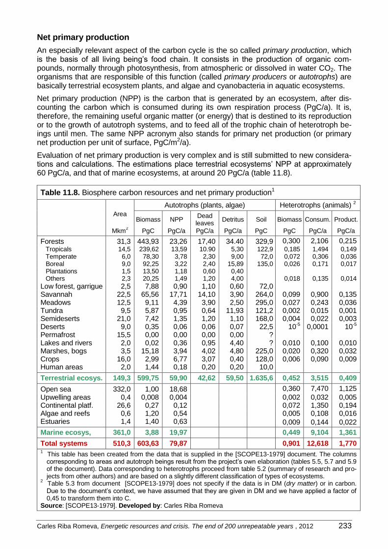
Carles Riba Romeva, Energetic resources and crisis. The end of 200 unrepeatable years , 2012 233
Net primary production
An especially relevant aspect of the carbon cycle is the so called primary production, which is the basis of all living being’s food chain. It consists in the production of organic com-pounds, normally through photosynthesis, from atmospheric or dissolved in water CO2. The organisms that are responsible of this function (called primary producers or autotrophs) are basically terrestrial ecosystem plants, and algae and cyanobacteria in aquatic ecosystems.
Net primary production (NPP) is the carbon that is generated by an ecosystem, after dis-counting the carbon which is consumed during its own respiration process (PgC/a). It is, therefore, the remaining useful organic matter (or energy) that is destined to its reproduction or to the growth of autotroph systems, and to feed all of the trophic chain of heterotroph be-ings until men. The same NPP acronym also stands for primary net production (or primary net production per unit of surface, PgC/m2/a).
Evaluation of net primary production is very complex and is still submitted to new considera-tions and calculations. The estimations place terrestrial ecosystems’ NPP at approximately 60 PgC/a, and that of marine ecosystems, at around 20 PgC/a (table 11.8).
Table 11.8. Biosphere carbon resources and net primary production1
Area
Autotrophs (plants, algae) Heterotrophs (animals) 2
Biomass NPP Dead leaves
Detritus Soil Biomass Consum. Product.
Mkm2 PgC PgC/a PgC/a PgC/a PgC PgC PgC/a PgC/a
Forests 31,3 443,93 23,26 17,40 34.40 329,9 0,300 2,106 0,215 Tropicals 14,5 239,62 13,59 10.90 5,30 122,9 0,185 1,494 0,149 Temperate 6,0 78,30 3,78 2,30 9,00 72,0 0,072 0,306 0,036 Boreal 9,0 92,25 3,22 2,40 15,89 135,0 0,026 0,171 0,017 Plantations 1,5 13,50 1,18 0,60 0,40 Others 2,3 20,25 1,49 1,20 4,00 0,018 0,135 0,014
Low forest, garrigue 2,5 7,88 0,90 1,10 0,60 72,0 Savannah 22,5 65,56 17,71 14,10 3,90 264,0 0,099 0,900 0,135 Meadows 12,5 9,11 4,39 3,90 2,50 295,0 0,027 0,243 0,036 Tundra 9,5 5,87 0,95 0,64 11,93 121,2 0,002 0,015 0,001 Semideserts 21,0 7,42 1,35 1,20 1,10 168,0 0,004 0,022 0,003 Deserts 9,0 0,35 0,06 0,06 0,07 22,5 10-5 0,0001 10-5 Permafrost 15,5 0,00 0,00 0,00 0,00 ? Lakes and rivers 2,0 0,02 0,36 0,95 4,40 ? 0,010 0,100 0,010 Marshes, bogs 3,5 15,18 3,94 4,02 4,80 225,0 0,020 0,320 0,032 Crops 16,0 2,99 6,77 3,07 0,40 128,0 0,006 0,090 0,009 Human areas 2,0 1,44 0,18 0,20 0,20 10,0
Terrestrial ecosys. 149,3 599,75 59,90 42,62 59,50 1.635,6 0,452 3,515 0,409
Open sea 332,0 1,00 18,68 0,360 7,470 1,125
Upwelling areas 0,4 0,008 0,004 0,002 0,032 0,005 Continental platf. 26,6 0,27 0,12 0,072 1,350 0,194 Algae and reefs 0,6 1,20 0,54 0,005 0,108 0,016 Estuaries 1,4 1,40 0,63 0,009 0,144 0,022
Marine ecosys, 361,0 3,88 19,97 0,449 9,104 1,361
Total systems 510,3 603,63 79,87 0,901 12,618 1,770 1 This table has been created from the data that is supplied in the [SCOPE13-1979] document. The columns
corresponding to areas and autotroph beings result from the project’s own elaboration (tables 5.5, 5.7 and 5.9 of the document). Data corresponding to heterotrophs proceed from table 5.2 (summary of research and pro-jects from other authors) and are based on a slightly different classification of types of ecosystems.
2 Table 5.3 from document [SCOPE13-1979] does not specify if the data is in DM (dry matter) or in carbon.
Due to the document’s context, we have assumed that they are given in DM and we have applied a factor of 0,45 to transform them into C.
Source: [SCOPE13-1979]. Developed by: Carles Riba Romeva
234 Carles Riba Romeva, Energetic resources and crisis. The end of 200 unrepeatable years , 2012
11.3. Carbon, oxygen and life
Life in our planet exists thanks to the maintenance, within narrow limits, of a series of pa-rameters. The atmosphere’s composition or the existence of a liquid layer in the shape of seas or oceans, facts that seem so natural to us, do not happen quite by chance, they are due to self-regulated processes between living and lifeless beings.
When the NASA requested the collaboration of J. Lovelock [Lov-1988] to study if there was life on Mars, he said that it was not necessary to go there, as analysing the composition of the atmosphere was enough. If there is life on a planet, traces can be found in its atmosphere.
Venus, which is closer to the Sun than the Earth, has a dense atmosphere (90 bar), most of which is composed of CO2 (a 96,5%), and an intense greenhouse effect is produced making the temperature of its surface be of around 450ºC. On the other hand, Mars, with a very light atmosphere (0,0064 bar), also majorly made out of CO2 (the 95,3%), has a very weak greenhouse effect (approximately 5ºC), which places the average surface temperature at around -60ºC.
The Earth’s atmosphere is totally different: it is majorly composed of nitrogen (a 78%) and oxygen (a 21%), while CO2 is only residually found (a 0,28% or 280 ppm, parts per million, during the preindustrial era, and a 0,39% or 390 ppm, nowadays).
The percentage of CO2 is a key aspect to regulate the Earth’s temperature by means of the greenhouse effect. Relatively small changes of concentration can produce variations in tem-perature and climate that can be significant enough to unbalance the conditions that make life possible. At the same time, CO2 (of the atmosphere or dissolved in water) is also an es-sential compound from which life is fed through photosynthesis, plant and algae’s synthesiz-ing function, as well as a by-product of all living beings’ respiration.
Water steam has an even more powerful greenhouse effect than CO2, but evaporation and precipitations very quickly regulate the cycle (that is why climate has very intense local varia-tions); in fact, it is an aspect that is still not well-known and is being currently studied ([IPCC-AR4-SR-2007], page 73). On the other hand, CO2 is accumulated and remains in the at-mosphere in a much longer cycle at a geological scale and, therefore, it has a higher long-term incidence on temperature and climate.
For this reason, although climate change is usually perceived in a very confusing way by means of the variable climate in each moment and place, global climatic conditions are being generated that will become very different (and probably, more adverse) for future generations.
A glance backward
To establish some references to the possible consequences of climate change, it is interest-ing to go back in time and learn about the previous eras’ climate (or paleoclimate).
On the contrary to what many people think, the primitive terrestrial atmosphere consisted mainly of CO2 (like the one in Venus and Mars). But, approximately 3.800 Ma (Ma = millions of years) ago, around 750 Ma after the planet’s formation, the first life forms appeared. They were anaerobic cyan bacteria, which gradually transformed this atmosphere by fixing the carbon as organic matter or calcareous rocks and releasing oxygen to the atmosphere.
It was not until much later (around 2.400 Ma), that the atmosphere acquired a nitrogen and oxygen composition, which was relatively similar to the one that we currently have. As a re-sult, and due to the decrease of greenhouse effect gases, first CO2 and then methane, the first large glaciation age was produced. However, oxygenic photosynthesis, which is more efficient, promoted the evolution and development of new aerobic life forms (which, nowa-days, are a majority).
The prokaryote mats of unicellular beings without a differentiated nucleus (amongst them, cy-anobacteria) dominated the Earth for more than 2.000 Ma, until the appearance of the eukar-

Carles Riba Romeva, Energetic resources and crisis. The end of 200 unrepeatable years , 2012 235
yotes, with a differentiated nucleus. The first multicellular beings are more recent (between -850 Ma and -650 Ma), but it is not until the paleozoic (or primary, from -542 to -251 Ma) and the mesozoic (or secondary, from -251 to -65 Ma) eras that a remarkable evolution of the fau-na and the vegetation (first, marine and afterwards, terrestrial) is produced, with big bursts of life but also with remarkable extinctions (five of them, massive), period that ends with the dis-appearance of dinosaurs (-65 Ma). Then the cenozoic (or tertiary, from -65 Ma to the current day) era starts, in which mammals prevail and grass and meadows appear as new forms of vegetation. The hominids don’t appear until the last 4,5 Ma and the Homo sapiens strictly speaking corresponds to the last 130.000 years (0,130 Ma). Human civilizations start with ag-riculture and livestock after the last glaciation, 10.000 years (0,010 Ma) ago.
Climate and life have had an intertwined existence. The first climatic wide scope phenomena of which we have knowledge are major glaciations, that occurred between -2.500 and -2.300 Ma, presumably due to a failure in the greenhouse effect. Later on, at the end of the prote-rozoic era (from -800 to -600 Ma), new massive, possibly the most severe, glaciations or “snowball Earth” were produced, that almost completely extinguished life. However, at the beginning of the paleozoic era (-542 Ma), several continental plates’ movements towards the Equator and a strong volcanic activity reverted the glaciation and new, more developed, life forms were created, leaving an important fossil record.
CO2 en l'atmosfera (RCO2 = vegades CO2 actual)
0
5
10
15
20
25
30
-570 -520 -470 -420 -370 -320 -270 -220 -170 -120 -70 -20
RCO2
Figure 11.11. CO2 emissions’ model from the Palaeozoic era up to the present time (RCO2: proportion of CO2 in the atmosphere in relationship to the propor-tion of pre-industrial CO2). It can be observed that there have always been much higher values of CO2 (up to 26 times the current ones). At the beginning of the Palaeozoic era, the Sun shined a 6% less than what it currently does. Source: [GEOCARB III-2002]
The climatic conditions that made the life bursts and the extinction episodes during the Pal-aeozoic, Mesozoic and the first part of the Cenozoic era (-570 to -2,5 Ma) possible, are not fully known. It seems that several different aspects were involved, such as tectonic move-ments, volcanism, changes in ocean currents, asteroid collisions or the conditions caused by living beings’ atmospheric changes. In any case, current knowledge does not allow the es-tablishment of an univocal correlation between the level of CO2 in the atmosphere estimated
CO2 en l’atmosfera (RCO2 = vegades CO2 preindustrial)
CO2 in the atmosphere (RCO2 = times of preindustrial CO2)

236 Carles Riba Romeva, Energetic resources and crisis. The end of 200 unrepeatable years , 2012
by the models [GEOCARB III-2002] and the life evolution conditions during these eras (fig-ure 11.1).
The quaternary era started 2,5 Ma ago, after a long period of approximately 200.000 years where there were almost no glaciations. Several conditions, like the new continental configu-ration and the decrease of the amount of CO2 in the atmosphere, lead to a progressive cool-ing of the climate, where oscillations between glaciations and interglaciations, related to as-tronomical phenomena, started to appear.
These oscillations result from the combination of the eccentricity change of the Earth’s orbit around the Sun (of almost circular at 155 Mkm (millions of kilometres), to an eccentricity of 5 Mkm, in cycles of around 100.000 years); the change in the inclination of the Earth’s axis (between 22,2º and 24,5º; currently, 23,5º, in cycles of around 41.000 years), and the pre-cession (or change in the direction of the inclination) of the Earth’s axis in cycles of around 21.000 years. In the first part of the period (from -2,5 to 0,9 Ma), oscillations every 40.000 years prevailed, and later on (between -0,9 and -0,010 Ma), the major glaciations were re-peated every 100.000 years.
Figure 11.12. Variations of deuterium (δD) in the Antarctic permafrost (temperature indica-tor) and atmospheric concentrations of greenhouse effect gases, carbon dioxide (CO2), methane (CH4) and nitrous oxide (N2O) in the air that is trapped inside the ice cores. The data cover a total of 650.000 years and the shaded bands show warm interglacial periods. In red the recent anthropogenic CO2 variations are shown. Source: IPCC, AR4, Working Group I, Technical summary, page 24 [IPCC-AR4-WGI-TS-2007]
There is a remarkable correlation between the temperatures of the glacial and interglacial cycles in the previous 650.000 years and the records of the CO2 concentration in the atmos-phere, that have varied in amounts ranging from 180 to 300 ppm (parts per million). But we have already stated that there is a great scientific consensus that the primary cause of these temperature variations in the previous glacial and interglacial cycles are the Earth’s orbit cycle changes (or Milanković cycles).
Although the atmospheric variations follow these cycles, with a positive feedback effect (they reinforce both the cooling and the warming), its explanation is still one of climate’s main un-solved aspects, as it is evidenced in the paleoclimate chapter ([IPCC-AR4-WGI-C6-2007], page 446).

Carles Riba Romeva, Energetic resources and crisis. The end of 200 unrepeatable years , 2012 237
In the same chapter of the IPCC document (page 449) it is stated that global climate is deter-mined by the planet’s radiation balance, that can be modified in three main ways: 1) changing the incident solar radiation (for example, changes in the Earth’s orbit or in the intensity of the Sun radiation); 2) changing the fraction of reflected solar radiation (or albedo; for example, changes of clouds, of aerosol presence in the atmosphere or of type of soil coverage); and 3) changing the greenhouse effect by the return of the longwave radiated energy from the Earth surface (for example, changes in greenhouse effect gases’ concentration). Local climate also depends on the effects of wind and ocean currents. They are all factors that play a role in pre-sent and past climate changes.
To affirm that climate variations that have taken place during the previous hundreds of years depend on CO2 concentrations (as Al Gore’s An Inconvenient Truth, could make us believe) does not correspond with the current scientific consensus. This affirmation has been widely criticized. In effect, the continuation of the Milanković cycles would have leaded to a new gla-ciation. However, the very fast CO2 anthropogenic growth during the last two centuries (and specially, the previous fifty years), which currently already reaches the value of 390 ppm and that is mainly originated by the burning of fossil fuels, seems to be the main cause of an unu-sual climate warming that breaks with the natural trend.
The climatologist W. Ruddiman [Rud-2005] goes further on and states that, without the CO2 emissions derived from deforestation in order to create crops and meadows, since the be-ginning of human civilizations, the Earth’s climate would have already entered a new glacia-tion stage. According to his evaluations, the agricultural and livestock climatic impacts in the previous 10.000 years are of the same order of magnitude than the impacts of industrial emissions of the last 150 years.
The 2007 IPPC report and climate change
The Intergovernmental Panel on Climate Change (IPCC) is an organization that was created in 1988, within the framework of the United Nations and with its headquarters in Geneve (Switzerland), whose main objective is the study of the climate change.
Nowadays, it groups around 2.000 scientists from more than a hundred countries and it has published four assessment reports: the First Assessment Report (FAR), published in 1990, in which the scientific evidences that raise concerns about climate change were confirmed; the Second Assessment Report (SAR), published in 1997, which provided the basis for ne-gotiations of the Kyoto Protocol; the Third Assessment Report (TAR), in 2001, that dealed with several scientific questions and useful techniques for the design of climate change re-lated policies; finally the Fourth Assessment Report (AR4), from 2007, unequivocally con-firmed the anthropogenic origins of global warming and evaluated their consequences.
The latest documents (TAR and AR4) establish the main conclusions of the IPCC on the climate change issue, which are worth commenting. The fourth document (AR4-2007), con-firms the conclusions of the third document (TAR-2001) and, in many subjects, alerts that new knowledge predicts more serious consequences than what it had been said in the pre-vious document.
When we try to summarize the conclusions of the 2007 AR4 document, we face a contradic-tory state of mind. There is a dramatic warning on the severity of the situation, but it is writ-ten in a “very polite” language, with many “nuances” to avoid hurting anyone’s feelings, in such a way that the text is cryptic and tedious, supplying sceptical and not well informed readers with “alibis” to allow them to argue to the contrary or dilatory.
This aspect has made me reflect a lot. The IPCC is an “intergovernmental” commission, which means that it reports to the governments of the different countries of the world. In spite of the importance of its existence and the effort that it has carried out, its voice remains subdued. I have the impression that a situation like the one of the “The Emperor’s New Clothes” tale is given. A lot of people see it, but no one dares saying anything, until a little child cries out, "But he isn't wearing anything at all!"

238 Carles Riba Romeva, Energetic resources and crisis. The end of 200 unrepeatable years , 2012
If we remove precautions and reiterative technicalities, our summary of the Fourth Assess-ment report (AR4 2007) is as follows:
1. “Five reasons to worry”:
Risks for singular systems. The increase of temperature makes certain singular fields especially vulnerable, like polar and high mountain ecosystems, coral reefs and places with a lot of biodiversity, with a high risk of species’ extinction.
Risks of extreme meteorological phenomena. In many regions, both of developed and of developing countries, droughts, heat waves and floods are predicted to increase, having adverse impacts that will imply an increase of the water stress and of the frequency of uncontrolled fires, with negative effects on food production, health and facilities.
Distribution of impacts and vulnerabilities. Often, the economically weaker regions or popu-lations will be the most vulnerable to suffer damages related to climate: dry areas, large deltas and small islands and in general, poor and elderly people. Africa is one of the most vulnerable continents, due to the significant impact diversity, many stress factors and their limited adaptive capacity.
Totalized impact. In comparison with previous reports from the IPCC, climate change’s benefits would be minor than the ones that had been previously forecasted, whilst the damages would be greater and would negatively affect hundreds of millions of people due the decrease in the water supply, the increase in malnutrition and a higher impact over hu-man health.
Large scale singularities’ risks. As well as a bigger sea water expansion than the one that had been initially foreseen, Greenland’s thaw and, possibly that of part of the Antarctica, could have very important large scale effects. A complete thaw of Greenland’s mantle of ice would make the sea’s level rise in 7 meters, which could be irreversible.
2. What shall we do? Stabilize greenhouse effect gases? Mitigation and adaptation?
This is a key section of the document, but I believe that the argument has not been well exposed. Let’s start with the AR4 report essential warning:
The more time we spend before we reduce the greenhouse effect gas emissions, the more difficult it will be to achieve low stabilization values (maximum value that CO2 will reach in the atmosphere, in ppm). And, the higher the CO2 stabilization value, the more serious and irreversible the climate change’s impacts and consequences will be.
Due to the lack of mitigation measures, it is possible that the climate change, at a large term, overwhelms the capacity of adaptation of natural and human-managed systems (impacts in coast areas due to the several meters increase of the sea level, disappear-ance of the mountain glaciers that have an irreplaceable role as water reservoirs, loss of basic for human sustenance ecosystems).
The AR4 report encloses these affirmations with the following warnings:
The mitigation measures’ benefits (in terms of avoided climate change) will take several decades to be evident. But these measures will avoid us to be anchored in carbon-dependent facilities and developing paths, whose consequences are even worse. Between lines, the IPCC report asks us for a change in the development paradigm.
Neither mitigation nor adaptation can avoid all of the climate change impacts by them-selves, but adaptation will be needed even in the most modest stabilization scenarios. On the other hand, once the greenhouse effect gas concentrations are stabilized, tempera-ture will keep increasing during many decades and will tend to stabilize, although it will be centuries before this is accomplished.

Carles Riba Romeva, Energetic resources and crisis. The end of 200 unrepeatable years , 2012 239
3. Stabilization scenarios
The Fourth Assessment Report of the IPCC establishes several CO2 and other greenhouse effect gas emissions stabilization scenarios [IPCC-AR4-SR-2007], that are summarized in table 11.9.
Table 11.9. Characteristics of the stabilization scenarios1
Category CO2 CO2eq
2 Max. emiss.3 CO2 20504 temper.5 sea level6
ppm ppm years ºC Meters
I 350 – 400 445 – 490 2000 – 2015 -85 a -50 2,0 – 2,4 0,4 – 1,4 II 400 – 440 490 – 535 2000 – 2020 -60 a -30 2,4 – 2,8 0,5 – 1,7 III 440 – 485 535 – 590 2010 – 2030 -30 a +5 2,8 – 3,2 0,6 – 1,9 IV 485 – 570 590 – 710 2020 – 2060 +10 a +60 3,2 – 4,0 0,6 – 2,4 V 570 – 660 710 – 885 2050 – 2080 +25 a +85 4,0 – 4,9 0,8 – 2,9 VI 660 – 790 885 – 1130 2060 – 2090 +90 a +140 4,9 – 6,1 1,0 – 3,7
1 Stabilization is the maintenance, at a constant level, of the greenhouse effect gases’ atmospheric concen-
trations. 2 CO2eq also includes the effects of the other greenhouse effect gases.
3 Year intervals with the maximum amount of CO2 emissions.
4 Worldwide variation of the CO2 emissions in relation to those of year 2000.
5 Increase in temperature over the preindustrial levels in equilibrium conditions.
6 Increase in the sea’s level over the preindustrial level, in equilibrium conditions, by thermal expansion.
Source: IPCC [IPCC-AR4-WGI-TS-2007], page 67. Developed by–summary: Carles Riba Romeva
From the exposition of these scenarios, the synthesis report of the Fourth assessment re-port enters a series of technical terms and treatises that make it very difficult to distinguish which of these scenarios are we talking about. Further on a reasoning path has been pro-posed in order to answer this highly important matter.
4. Technical measures? Or development paradigm change?
When it comes to the last aspect of the report [IPCC-AR4-SR-2007], I have to state that I am openly in disagreement with it. Below I literally transcribe the introduction of the 5.5 section of this report:
“There is high agreement and much evidence that all stabilisation levels assessed can be achieved by deployment of a portfolio of technologies that are either currently available or expected to be commercialised in coming decades, assuming appropriate and effective incentives are in place for development, acquisition, deployment and diffusion of technol-ogies and addressing related barriers.”
The message seems to be: world citizens, we can keep doing what we have always done, it is not necessary to modify or to resign anything! The climate change problem will be simply solved with technical means.
From my point of view, the message is totally wrong (I would even say it is coward), dic-tated by political and not scientific authorities. Maybe this imprudent optimism can be ex-plained (but not justified) by the fact that the AR4 was written during the collective eupho-ria-madness (2007), from which the current economical crisis started.
Probably, before five years, the first petroleum decline symptoms will make us realise that our economy is lacking natural resources in which to sustain. And we will also discover that we are pretending to be “sorcerers’ apprentices” with climate, which is the basis of the resources that will have to sustain us again in the future.

240 Carles Riba Romeva, Energetic resources and crisis. The end of 200 unrepeatable years , 2012
Climate consequences derived from the burning of fossil fuels
The current dominating economic and political speech is contradictory, if not schizophrenic.
On one hand, we start to be conscious of the lack of energy and, therefore, any new discovery or exploitation of fossil fuel deposits seems to be great news (recently, BP and some Russian oil companies are aiming to exploit the Arctic). And, on the other hand, the sustainability poli-cies that propose (but do not accomplish) an economy which is more carbon-free are gaining acceptance.
We have to be clearly aware of the fact that fossil energy and climate change belong to the same equation. The two previous conceptions are, therefore, totally incompatible due to the fact that the more fossil fuel reserves are discovered and used, the more unquestionable the climate change will be.
In order to illustrate this issue I propose the following argument thread. We ask ourselves:
In the current political context, are there any countries with important reserves of fossil fuels (petroleum, natural gas, coal) not willing to use them for environmental responsibility reasons? The United States? Russia and Central Asia countries? China? India? The Persic Gulf coun-tries? Australia? South Africa? Venezuela? Brazil? (By the way, it would be necessary to care-fully follow the case of the petroleum reserves of the national Yasuni Park, in the Ecuador, a small experience that goes in the sense of resignation and that is a paradigmatic case of bio-diversity preservation, with a very powerful defence). And following this same argument thread: the expensive investments aimed to find new limit sources of fossil fuels (unconven-tional oils and gases) are not to use them later on? Unfortunately, the answers are negative.
If we are not willing to stop using fossil fuels’ reserves, the sustainability policies will be able to prolong climate change in time, but they will difficultly be able to cancel the global and cumulative effects.
Having this into consideration, it is worthy to analyse the global impacts that the combustion of actual fossil fuels reserves will have on the atmosphere’s CO2 concentration. In order to carry out this estimation, we have considered the following aspects:
1. Nowadays (2010), in the atmosphere, there are around 3.000 Pg (1015 grams = millions of millions of tonnes) of CO2, that correspond to around 820 PgC (calculated using the molecular weight ratio: C=12; O = 16; CO2 = 12+16+16 = 44).
2. In 2010, the amount of CO2 in the atmosphere is, approximately, of 389 ppm (parts per million, or fraction of 0,000389, a 0,0389%) in volume in relationship to the overall atmos-phere gases, having increased, during the past ten years, an average of near 2 ppm/a (Earth System Research Laboratory, <http://www.esrl.noaa.gov/gmd/ccgg/trends/>).
4. In order to transform the fuel reserves into amount of CO2 due to combustion, the rela-tionships found in table 5.5 are used: natural gas (average of 0,0502 kgCO2/MJ), petro-leum (average of 0,0620 kgCO2/MJ), coal (average of 0,0896 kgCO2/MJ).
In relationship to the greenhouse effect gases, nature provides us with two large sinks when the atmospheric CO2 concentration increases: absorption increases due to plant photosyn-thesis and solution increases in the surface layers of oceans. These trends compensate an important part of the atmospheric CO2 anthropogenic increase.
The Intergovernmental Panel on Climate Change (IPCC) estimates the atmosphere-ocean and atmosphere-Earth flows, as well as the global CO2 balance for 1980 and 1990, and for the period 2000-2005 [IPCC-AR4-WGI-TS-2007], page 26. See table 11.10.

Carles Riba Romeva, Energetic resources and crisis. The end of 200 unrepeatable years , 2012 241
Table 11.10. Global CO2 balance between the atmosphere, the oceans and the biosphere
(flows in Pg/a) Years 1980 Years 1990 2000-2005
Atmospheric increase 3,3 ± 0,1 3,2 ± 0,1 4,1 ± 0,1
Emissions (fossil fuel, cement) 5,4 ± 0,3 6,4 ± 0,4 7,2 ± 0,3
Oceans–atmosphere flux -1,8 ± 0,8 -2,2 ± 0,4 -2,2 ± 0,5
Land–atmosphere flux -0,3 ± 0,9 -1,0 ± 0,6 -0,9 ± 0,6
Land use change 1,4 (0,4 a 2,3) 1,6 (0,5 a 2,7) Not available
Residual terrestrial sink -1,7 (-3,4 a 0,2) -2,6 (-4,3 a -0,9) Not available
Source: [IPCC-AR4-WGI-TS-2007], page 26
This implies that the fraction of emitted CO2 that is absorbed by natural systems (land + oceans) has been the following: in the 80’s, 2,1/5,4 (Pg/Pg) = 0,389; in the 90’s, 3,1/6,4 = 0,484; from 2000 to 2005, 3,1/7,2 = 0,431. In front of these natural flows draining, the amount of carbon capture and storage (CCS) that is carried out by men is practically residu-al: with the capacity of a few operating plants and of the ones that are projected for the fol-lowing years, we will be far from the capture of 1/1000 of emitted CO2 (< 0,1%).
Table 11.1 explores the level of stabilization of the emissions that would result from the total combustion of fossil fuels. They are evaluated according to the fraction of CO2 (from 0,6 to 0,3) that they are capable of absorbing in natural sinks (terrestrial vegetation and oceans).
Table 11.11. Global estimations of the amount of CO2 emitted due to the fossil fuels
Evaluation of the amount of emitted CO2 due to the combustion of fossil fuels
Fossil fuel Reserves Impact CO2 emissions
TWta EJ (1018 J) kgCO2/MJ PgCO2 PgC
Petroleum 258,577 8.154,5 0,0620 505,58 137,88 Natural 215,383 6.792,3 0,0502 340,97 92,99 Coal 577,032 18.197,3 0,0896 1.630,48 444,68
Total 1.050,992 33.144,1 2.477,03 675,55
Evaluation of the increases of CO2 in the atmosphere (en ppm)
2009 Emissions due to the fossil fuels Absorption Increase Final
ppm CO2 PgC ppm CO2 fraction PgCO2 ppm CO2
389,0 675,55 320,47 0,60 128,2 517,2 389,0 675,55 320,47 0,55 144,2 533,2 389,0 675,55 320,47 0,50 160,2 549,2 389,0 675,55 320,47 0,45 176,3 565,3 389,0 675,55 320,47 0,40 192,3 581,3 389,0 675,55 320,47 0,35 208,3 597,3 389,0 675,55 320,47 0,30 224,3 613,3
Sources: Petroleum and gas reserves: Oil&Gas Journal; of coal: World Energy Council (WEC); emissions: Earth System Research Laboratory (Mauna Loa, CO2), <http://www.esrl.noaa.gov/gmd/ccgg/trends/>. Devel-oped by: Carles Riba Romeva
The summary section of the AR4 report says that, as the global warming is produced, it is expected that the coupling between climate and carbon increase the fraction of anthropo-genic emissions that persists in the atmosphere ([IPCC-AR4-SR-2007], page 67). Therefore, it seems prudent to adopt a value for the absorbed fraction which is not superior than 0,45.
This would situate CO2 stabilization in approximately 565 ppm, in the superior limit of the IV stabilization scenario (table 11.9), with a temperature increase of close to 4ºC and a sea water level increase (by expansion, without considering thaws) of approximately 2 meters. Everything makes us think that nobody will be able to avoid this scenario unless there is a change in our way of thinking.

242 Carles Riba Romeva, Energetic resources and crisis. The end of 200 unrepeatable years , 2012
12. Final reflections
12.1. Summary of the main trends
The main trends that have been analysed in previous chapters are summarized below:
1. Continuously increasing energy consumption The worldwide energy consumption increases more and more quickly everyday. But, at the same time, the increase in population has made the energy consumption per capita constant in the previous decades (1980-2008), apart from a small increase in the years before the 2007 crisis.
2. Important significant inequalities between societies There is an important inequality in the energy consumption distribution among the re-gions of the world, between the different countries (up to ten times of difference) and within the countries, both in absolute terms and per capita. Until now, the energy con-sumption was strongly related to countries’ wealth to their development’s evolution.
3. Limited non-renewable fuels’ reserves The (proven) worldwide non-renewable reserves of energy are limited, and their evalua-tion involves many uncertainties (new deposits to be discovered, but also oversized re-serves). If the worldwide current growth rhythm continues (both economic and of popula-tion), it is predicted that they will totally become exhausted near year 2060.
4. Petroleum zenith’s impact on development According to the zenith of petroleum theory (and the posterior zenith of other non-renewable sources), it is very possible that the current economic model, based on increas-ing fossil energy consumptions, experience a widespread imbalance that will take place much before this date (probably the actual crisis is its beginning).
5. Unconventional fossil fuels are not the solution Unconventional fossil fuels can difficultly mitigate the decline of conventional fuels and, in any case, they entail slower extractions and superior investments in facilities and envi-ronmental costs.
6. The nuclear alternative is uncertain and remote At the moment, nuclear energy is based in the consumption (combustion) of U235 urani-um, which is very scarce in nature. The breeding reactor alternative or the fusion energy (at the moment, very uncertain) will not be available until after thirty years or more, when the decline of fossil fuels will have disrupted the current model of development.
7. Renewable sources of energy will be more limited Alternative renewable sources of energy (biofuels, hydroelectric energy, solar, wind, geo-thermal and tidal) will not allow the maintenance of the current consumption and they will not be so easily available. In any case they will be the energies that will sustain us in the future.
8. Abuse of the biosphere’s resources The evolution of agriculture, livestock, fishing, aquiculture and the exploitation of forests has rather followed the economy’s dictation than a management that preserves these re-sources and adapts itself to their rhythms. In most cases, the large productivity increases are due to the use of enormous amounts of fossil fuels.
9. Consequences of climate change Climate change and the consumption of fossil fuels make part of the same equation. As the exploitation of the deposits increases, fossil fuels’ efficiency decreases and emis-sions grow. At the same time, we face a serious lack of energy and a climate change that has unpredictable consequences. In any case, however, everything makes us pre-dict that future sustainable capacities will decrease (IPCC reports).

Carles Riba Romeva, Energetic resources and crisis. The end of 200 unrepeatable years , 2012 243
10. Need of a change in the development paradigm The energetic and climate crisis can be solved in two ways: with a new perception of our relationship with nature and its resources that generates a change in the development paradigm (with a minor consumption, more sustainable and more egalitarian), or with fights (economic and military) in order to hoard the last resources. It is in our hands (in the hands of humanity) to choose one option or the other.
Table 12.1. Summary of the main data of the study
Chapte
r 1
Consumption of primary energy
1980 2008 Increase
Total 10,379 TWt 17,867 TWt 72,23 %
Petroleum 4,383 TWt 5,720 TWt 30,50 %
Natural Gas 1,802 TWt 3,809 TWt 111,37 %
Coal 2,223 TWt 4,572 TWt 105,67 %
Uranium 0,353 TWt 0,908 TWt 287,35 %
Unrenewable 84,56 % 84,01% 71,00 %
Hydroelectric 0,599 TWt 1,028 TWt 71,62 %
Other electr. renew. 0,016 TWt 0,195 TWt 1.218,75 %
Renew. fuels 0,988 TWt 1,634 TWt 65,38 %
Renewable 15,44 % 15,99 % 78,35 %
Chapte
r 2
Consumption of primary energy per capita
1980 2008 Increase
World 2.331 Wt/inhab 2.670 Wt/inhab 14,54 %
North America 9.563 Wt/inhab 9.028 Wt/inhab -5,59 %
Africa 895 Wt/inhab 961 Wt/inhab 7,37 %
Asia and Oceania 887 Wt/inhab 1.733 Wt/inhab 95,38 %
Chapte
r 3
Non-renewable energy reserves (world, 2007)
Physical units Energy units % reserves
Total 1.126,191 TWta 100,00 %
Petroleum 1.316,7 Gb 258,577 TWta 22,96 %
Natural gas 6.189,4 Tcf 215,383 TWta 19,12 %
Coal 826.002,0 Tg 577,032 TWta 51,24 %
Uranium 5.468,8 ktU 75,200 TWta 6,68 %
Chapte
r 8
Biological systems’ productions
1980 2008 Increase
Total 5.177 Tg/a 13.153 Tg/a 154,07 %
Agriculture 3.454 Tg/a 10.249 Tg/a 196,73 %
Livestock 429 Tg/a 1.038 Tg/a 141,96 %
Fishing & aquiculture 37 Tg/a 159 Tg/a 329,73 %
Forest products 1.258 Tg/a 1.706 Tg/a 35,61 %
Chapte
r 9
CO2 emissions to the atmosphere
1980 2008 Increase
Total 18.443,9 TgCO2/a 30.493,2 TgCO2/a 65,33 %
Petroleum 8.825,2 TgCO2/a 11.170,8 TgCO2/a 26,58 %
Natural gas 3.086,3 TgCO2/a 6.273,4 TgCO2/a 103,27 %
Coal 6.522,4 TgCO2/a 13.049,0 TgCO2/a 100,06 %
Developed by: Carles Riba Romeva

244 Carles Riba Romeva, Energetic resources and crisis. The end of 200 unrepeatable years , 2012
12.2. To change the development paradigm
The disposal of easy and plentiful energy has allowed the development of advanced indus-trial societies, with an unprecedented deployment of social knowledge and wellbeing. But this easiness has induced wasteful practices in which the high energetic capacity of fossil fuels has been used to obtain wealth, not to insure a balanced welfare between people and countries.
But fossil energy is finite and the limits are already starting to insinuate themselves. Still more than half of the initial total fossil energy is left, but at the current consumption and growing rhythms it will run out in 50 years, due to the fact that the production zeniths will be reached in the decade that has just begun. Furthermore, we are inducing an unpredictable climate change with serious consequences. They will be 200 unrepeatable years (from 1830 to 2030) that some of us will have lived with an unusual abundance, but the actual crisis an-nounces the beginning of the end.
What shall we do considering the new energetic and climatic perspective that we will soon be facing?
In first place, we have to avoid burying our heads in the sand. Even though the knowledge of this limit contains a message that we don’t like, the opinion makers and the governments shall explain it to citizens. It gets us nowhere to continue telling the whole world that to over-come the crisis we only need to promote the indiscriminate consumption again (these rules belong to the past); due to that, without the support of a plentiful and cheap source of ener-gy, the new “green shoots” will only feedback the worst consequences of the energetic and climatic crisis.
Certainly, fossil fuels will not suddenly run out, from one day to another. But the fact that we have already reached the zenith of petroleum, which is the most determinant energetic re-source, will change all of the developing parameters in which we have relied on until now.
Worldwide energy consumption is huge, nowadays, and the social and technological alter-natives are not improvised. When, in some decades, the decline of fossil fuels is in a more advanced stage, our civilization will be extremely vulnerable if we have not done the neces-sary things in order to adapt ourselves to the change. And, the richer and more urban the societies, the consequences will be more tough and the adaptation more difficult.
How will we maintain the current system without economically growing? How will civilization sustain with a progressive reduction of transport? How will we feed the impressive population increases in Third World Countries? How will we do the transition towards renewable sources of energy if we waste the for-
midable fossil resources of energy in trivial consumptions? Does it make sense to promote agrarian societies towards fossil fuel based economies,
now that this resource is starting to decline?
But in order to build the still unknown alternative to the actual systemic crisis, some essential changes in our mentality and behaviour are needed. I will assay a first approximation by means of the following questions:
Is the improvement of energetic efficiency enough? Can technology solve the energetic problem? Are renewable sources of energy enough? Reflection on wealth and autonomy Willingness to build the alternative
Developed societies citizens’ mentality is installed in a carefree comfort and believes that society will be able to supply enough energetic resources forever, at any time and in the re-quired amount. This will soon no longer be possible. The reflection on the previous points has made me hint at some of the elements that we will need in order to be able to positively overcome en the actual crisis.

Carles Riba Romeva, Energetic resources and crisis. The end of 200 unrepeatable years , 2012 245
Is energetic efficiency enough? Jevons’ paradox
Many people trust that the energy problem can be solved by simply improving the energetic efficiency of our technical systems. The decrease in the consumption of energy to obtain the same result allows consumption energy saving (for example, low-energy light-bulbs, that supply the same amount of light but with less than 20% of electricity).
However, this attitude is not aware of the paradox that was stated, in 1865, by the British economist, W.S. Jevons, in his work titled The Coal Question. According to Jevons, the im-provement of a system’s efficiency decreases the temporary consumption of the considered resource, but, given that promotes its use, it induces a global increase in the long-term con-sumption (for example, every time more efficient engines promote the increase in vehicles’ fleet, which, as a consequence, increases the global fuel consumption).
In Economy, well-known analogous dynamics are given: when we reduce the price of a product, market expands in such a way that the business’ volume increases above the re-cruitment level that was caused by the price reduction. Jevons’ paradox is a consequence that is applied to energetic consumptions.
From the point of view of monetary wealth, this market expansion has a positive effect. But when it is related to an energy that is threatening to become scarce, the increase in consump-tion turns out to be a problem. It is the situation that will be given in the near future: economies based on non-renewable fossil fuels will be strangled by the decline of these resources.
Can technology save the energetic problem?
Apart from efficiency, it is also trusted that technology will be able to solve the energetic problem, even if the global consumption of energy increases. It is said that «technologies are there; in any case we just have to apply them». And then the problem refers to economi-cal constraints about monetary resources and the necessary time for investments.
Analysing the evolution of human societies and, above all, of previous 150 years’ industrial and technologic societies, the answer seems to be affirmative. The increasing evolution of human societies has been accompanied by progressively higher energetic consumptions (figure 2.1) at the same time that, at a smaller scale, a coupling between economical pro-gresses and regressions of certain countries (old USSR, Cuba, North Korea, the current crisis in advanced societies) and energetic consumptions, can be observed.
However, nowadays, a decisive new element appears: we start to have a global vision of the Earth, and we are aware that, with the evolution of consumption and population, non-renewable energetic resources will soon become scarce. After a spectacular growth due to the exponential consumption of fossil fuels (created by nature during millions of years), for the first time we perceive their limits and we are on the threshold of their decline and poste-rior exhaustion.
How can we evolve without the collaboration of these exceptional sources of energy?
This represents a change of paradigm in the evolution of humanity that we can not solve blindly delegating it to technologies and economy. In any case, we must remember that be-hind the technological and economical solutions, there are also people that impose their points of view and opinions.
Therefore, we are entering a new stage in which, in order to solve the energetic and envi-ronmental crisis, we can no longer keep trusting economy and technology dynamics. We need to invert the terms: depending on the new situation, we will have to establish post-carbon developing agreements and align economy and technology with these objectives.
And this will imply changes of mentality, sacrifices and renunciations.

246 Carles Riba Romeva, Energetic resources and crisis. The end of 200 unrepeatable years , 2012
Are renewable energies enough?
In front of the predictable decline of non-renewable sources of energy (including unconven-tional fuels and uranium) and the uncertainty and the remoteness of the nuclear fusion alter-native, it is pertinent to consider if renewable energies are enough.
The answer is affirmative: renewable sources of energy (thermal solar and photovoltaic, wind, hydraulic, geothermal, biomass) have enough potential to cover humanity’s current basic energetic needs. Thanks to them, in the future humanity will be able to sustain, but their exploitation and management require a drastic change of mentality, a change in the energetic paradigm.
The return to the use of renewable energies will be done in much better conditions than in previous historical stages, as we currently have (or can have) much more precise knowledge on resources, natural phenomena and on the capacity to manage the demand; but this will require an adaptation to the dynamics that these resources need. However, as we have seen in the third part of this book, technologies based on renewable sources of energy will not be able to provide, in any way, neither the availability nor the intensity of fossil energy, to which we have got used to.
We will have to migrate from the idea of «the client rules» (anthropocentric vision) to the con-cept of «nature offers» (ecospheric vision) [Gar-2010]. For many developed society citizens, this «apparent regression» can be perceived as a civilization setback, but it is not so. After we change, we will discover that the extreme lack of concern and comfort in which developed societies had installed themselves also implied important personal and social renunciations.
Renewable energies are much more widely distributed than non-renewable fuels (fossils and nuclear), they are more scalable and putting them into value requires lower investments. But a larger human intervention will be needed in its management, often at a more local scale. It is crucial to consider the use of time and must learn to not consume everything we have and create reserves (make savings) for less favourable times.
Wealth and autonomy
The wealth and poverty debate is normally established according to the income per capita, mediatised index by economy and policies, that does not make it possible to grasp or cor-rectly manage the people development. This debate, in my opinion, needs to be comple-mented with the consideration of people, families and communities’ autonomy and depend-ence, (the reflection could also be done referring to possession or dispossession).
A person (a family or a village) is poor when it barely has what it needs to live; it can control the means of survival but, due to several reasons (low-efficiency resources, knowledge or techniques which are not efficient), it needs to make a large effort in order to be able to sus-tain. On the other hand, a person (or a family or a village) is dependent (not autonomous or deprived) when it does not have the control on the means of subsistence; it can be a rich person if it has subsidies or if with not much work it obtains enough resources, but it does not control the resources or the knowledge or the capacities that sustain it. Under the per-spective of the energetic and climate crisis’ autonomy/dependence dimension can have as much importance as wealth/poverty.
Often, the help that is given by rich countries to poor ones imposes organizational and tech-nological structures that dispossess the poor communities and make them be dependant (or in some cases, subsidized, in order to compensate for the dispossession).
A notorious case was the green revolution that took place from 1960 to 1990. With the sponsorship of several American foundations and with the agreement of some national gov-ernments (Mexico, India, Pakistan, Philippines) and the FAO, technological and economical criteria were applied (single-crop farming, transgenic variants, fertilizers and pesticides), that

Carles Riba Romeva, Energetic resources and crisis. The end of 200 unrepeatable years , 2012 247
allowed the increase of some agricultural productions (especially those of cereals). Howev-er, in the negative side there is the loss of an important part of the agricultural and livestock biodiversity, the impacts of fertilizers and pesticides on the environment, a huge increase in the cost of fossil fuel energy and water per unit of production and another effect that is nor-mally not known: the dispossession of millions of farmers from their lands and traditional knowledge. As FAO today admits, «poor farmers who did not have these resources were excluded from the green revolution becoming many of them even poorer» <http://www.fao.org/kids/es/revolution.html>.
Another form of dependence is the concentration of the population in large cities, especially in poor countries as, in a energetic shortage context, life in large cities will be more vulnera-ble than rural life. In the report State of Mundial Population 2007, el United Nations Popula-tion Fund (UNFPA) estimates that, in 2008, urban population (3.300 million people) for the first time exceeds the value of rural population, and predicts that in 2030 urban population will be of almost 5.000 millions, many of them poor <http://www.unfpa.org/help/sitemap/index.html>.
In a collaboration project between the Centre de Disseny d’Equips Industrials (CDEI-UPC), which I direct, and Nepal, I learned many things about autonomy attitudes. It was about try-ing to improve the cable-car transport system (replicated in several places) in order to facil-ityate the arrival of agricultural products which were produced in the mountain slopes to the road-market at the end of the valley (figure 12.1). The responsible Nepalese had chosen to use an autonomous system, that was driven by gravity, with a quite more complex man-agement than a motorized one, but totally to their reach. And, at the same time, they estab-lished that the design of all of its parts could be built in Nepal as a condition, except for ca-bles and bearings, critical elements that they accepted to import. This is an attitude which is autonomy oriented and that will avoid these systems to be affected by the energetic crisis.
Figure 12.1. Cable-car transport system based on gravity, in Nepal, in which the Centre de Disseny d’Equips Industrials de la Universitat Politècnica de Catalunya (Carles Domènech, dressed in red) participated during its improvement process. One of the conditions that was established by the Nepalese project responsible was that all of the component parts should be able to be constructed in their country (autonomy condition), except for cables and bear-ings. Source: CDEI-UPC
Natural resources’ traditional knowledge, had until few generations ago had been the main sustenance of families and collectives, are currently unknown by many parts of the society. Under the perspective of a necessary transition towards a new post-coal energetic paradigm (not of an increase in the classic economical sense), a re-education towards autonomy is needed, both for physical resources and for knowledge and capacities.

248 Carles Riba Romeva, Energetic resources and crisis. The end of 200 unrepeatable years , 2012
Building the alternative
As mechanization with the growth premise develops, cheap man labour is substituted by so-phisticated technology, eager of energy. It is the contradiction of economy: every time more people are marginalized, instead of integrated, and each time more energy and resources are consumed instead of saving them. However, some economical and social sectors are en-riched and generate outrageous imbalances. And this also occurs between countries.
The dominant conception insists in the fact that economy and technology are unavoidable realities, beyond the desires and wills of people and of communities. But, behind the economy and the technology, there are people with key information and power that make their decisions according to their own interests. There are not, therefore, absolute truths but options based on certain assumptions, that can be modified by collective agreements. On the basis of these agreements, economy and technology can become wonderful tools to carry them out.
In order to overcome the current energetic and climate crisis, we require a change in the de-velopment paradigm, as the growth that has been registered during the previous years in de-veloped countries is not extendable to the rest of the countries. We do not have enough natu-ral resources, or enough Earth (see information on the ecological footprint in section 10.2).
If efforts are made only to substitute current technologies with others which are more efficient or that have less environmental impact, we will only encourage the consumption of an unwor-ried society (Jevons paradox), that will be catastrophically cut off with the decline of fossil re-sources. At the same time, we will have wasted fossil energy with expendable objectives with-out having established the basis to impulse the development towards a post coal society.
We need to be aware of the limits of nature’s resources and also generate new attitudes in the population (specially in more developed countries) in order for them to abandon privileg-es such as avoiding to take the responsibility or the excessive convenience in aspects such as the consumption of out of season products, the continuous use of cars, the comfort of the costly everything-electric or the lack of concern in relation to the primary resources that sus-tain us.
This implies not only a change in attitude in relation to consumption, but also another way of giving value to investments in relation to the new paradigm:
- New oil prospecting or investments in renewable sources of energy? - More automobile facilities or public transport facilities? - Investments in aviation, or investment in public telecommunication systems?
We have to try to build the alternative without giving up to the best cultural, social and tech-nologic progresses of our industrial society. But one thing is that the engine of humanity’s activity (of the economy) is an avid market to get richness, that does not want to know any-thing about resources’ limits, and another thing is that the social engines are activities that give solutions to people’s needs considering equality, autonomy and commitment with future sustainability.
We need to be reconciled with the rest of living beings in the biosphere, working in coopera-tion. We have to stop the acceleration of our work and respect nature’s times, as many of the energetic inefficiencies are due to hurries. We have to be respectful with biodiversity and with human cultural diversity.
In this new perspective, a symbiosis between traditional and new technologies is needed, as well as between traditional cultures (normally well-established in their natural environment) and more developed cultures, which, at the same time, need to favour the harsh and difficult adaptation to the energetic decrease stage, but that will probably make us discover new so-cial values making people more happy. We have to re-learn the most efficient processes from poorer countries, from the energetic and the ecological point of view.
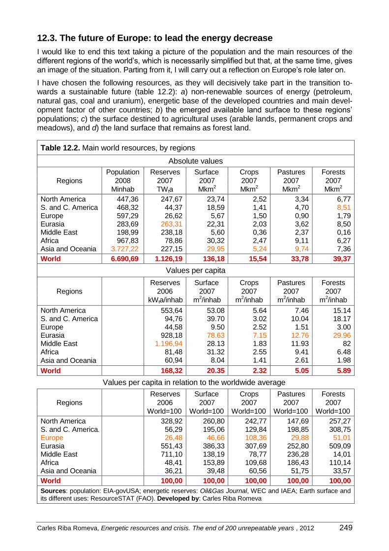
Carles Riba Romeva, Energetic resources and crisis. The end of 200 unrepeatable years , 2012 249
12.3. The future of Europe: to lead the energy decrease
I would like to end this text taking a picture of the population and the main resources of the different regions of the world’s, which is necessarily simplified but that, at the same time, gives an image of the situation. Parting from it, I will carry out a reflection on Europe’s role later on.
I have chosen the following resources, as they will decisively take part in the transition to-wards a sustainable future (table 12.2): a) non-renewable sources of energy (petroleum, natural gas, coal and uranium), energetic base of the developed countries and main devel-opment factor of other countries; b) the emerged available land surface to these regions’ populations; c) the surface destined to agricultural uses (arable lands, permanent crops and meadows), and d) the land surface that remains as forest land.
Table 12.2. Main world resources, by regions
Absolute values
Regions
Population Reserves Surface Crops Pastures Forests
2008 2007 2007 2007 2007 2007
Minhab TWta Mkm2 Mkm2 Mkm2 Mkm2
North America 447,36 247,67 23,74 2,52 3,34 6,77 S. and C. America 468,32 44,37 18,59 1,41 4,70 8,51 Europe 597,29 26,62 5,67 1,50 0,90 1,79 Eurasia 283,69 263,31 22,31 2,03 3,62 8,50 Middle East 198,99 238,18 5,60 0,36 2,37 0,16 Africa 967,83 78,86 30,32 2,47 9,11 6,27 Asia and Oceania 3.727,22 227,15 29,95 5,24 9,74 7,36
World 6.690,69 1.126,19 136,18 15,54 33,78 39,37
Values per capita
Regions
Reserves Surface Crops Pastures Forests
2006 2007 2007 2007 2007
kWta/inhab m2/inhab m2/inhab m2/inhab m2/inhab
North America 553,64 53.08 5.64 7.46 15.14 S. and C. America 94,76 39.70 3.02 10.04 18.17 Europe 44,58 9.50 2.52 1.51 3.00 Eurasia 928,18 78.63 7.15 12.76 29.96 Middle East 1.196,94 28.13 1.83 11.93 82 Africa 81,48 31.32 2.55 9.41 6.48
Asia and Oceania 60,94 8.04 1.41 2.61 1.98
World 168,32 20.35 2.32 5.05 5.89
Values per capita in relation to the worldwide average
Regions
Reserves Surface Crops Pastures Forests
2006 2007 2007 2007 2007
World=100 World=100 World=100 World=100 World=100
North America 328,92 260,80 242,77 147,69 257,27 S. and C. America. 56,29 195,06 129,84 198,85 308,75 Europe 26,48 46,66 108,36 29,88 51,01 Eurasia 551,43 386,33 307,69 252,80 509,09 Middle East 711,10 138,19 78,77 236,28 14,01 Africa 48,41 153,89 109,68 186,43 110,14 Asia and Oceania 36,21 39,48 60,56 51,75 33,57
World 100,00 100,00 100,00 100,00 100,00
Sources: population: EIA-govUSA; energetic reserves: Oil&Gas Journal, WEC and IAEA; Earth surface and its different uses: ResourceSTAT (FAO). Developed by: Carles Riba Romeva

250 Carles Riba Romeva, Energetic resources and crisis. The end of 200 unrepeatable years , 2012
The results from table 12.2 are graphically shown in figures 12.2 and 12.3, where the differ-ences in population and in resources between the different regions can be observed.
Population and resources, by regions (% world)
0
10
20
30
40
50
60
Asia &
Oceania
Africa Europe North
America
S.& C.
America
Eurasia Middle East
Population
Reserves
Agricultural area
Forestal area
Figure 12.2. Graphical representation, by regions, of the population, non-renewable en-ergy reserves, agricultural land (arable lands, permanent crops and meadows) and forest land, given in percentage over the total value of the world. The regions have been set ac-cording to a decreasing population percentage order. Sources: population: EIA-govUSA; energetic resources: Oil&Gas Journal, WEC and IAEA; Earth surface and its different us-es: ResourceSTAT (FAO). Developed by: Carles Riba Romeva
Resources per capita, by regions (world=100)
0
100
200
300
400
500
600
700
800
Middle Est Eurasia North
America
S.& C.
America
Africa Asia &
Oceania
Europe
Reserves
Country area
Agricultural area
Forest areal
Figure 12.2. Graphical representation of certain resources per capita, by regions: non-renewable energy reserves, country surface, agricultural land (arable lands, permanent crops and meadows) and forest surface, taking the world as a reference = 100. The re-serves have been set according to their decreasing reserves per capita of non-renew-able energy order. Sources: population: EIA-govUSA; energetic resources: Oil&Gas Journal, WEC and IAEA; Earth surface and its different uses: ResourceSTAT (FAO). Developed by: Carles Riba Romeva
Population and resources, by regions (% of the world)
Resources per capita, by regions (world = 100)
World = 100
Carles Riba Romeva, Energetic resources and crisis. The end of 200 unrepeatable years , 2012 251
Comments on table 12.2 and on figures 12.2 and 12.3:
1. There are four regions (Asia and Oceania, Africa, Europe, and South and Central Ameri-ca) that have a higher amount of population than of non-renewable energetic reserves, while there are three regions (North America, Eurasia and the Middle East) in which this relationship is the other way round (as it can be clearly seen in figure 12.2).
2. Asia and Oceania, and Europe have all of the values of the resources per capita (not only of non-renewable energy reserves, but also of country, agricultural and forest area) much minor than the worldwide average (Europe is queued as to what energy reserves is referred, little above a 25% of the world average). The rest of the regions have agricul-tural and forest area per capita that exceed the world’s average, except for the amount of forests in the Middle East (figure 12.3).
Europe
For better or for worse, Europe has a historic responsibility in relationship to the development method that has been adopted by humanity. Europe was the first region of the world that be-gan the based on fossil fuels (mainly coal in the 19th century and the first half of the 20th cen-tury) industrial development, colonizing other regions of the world in order to exploit their re-sources in its own benefit, as well as exploiting their own fossil resources (mainly coal) until it almost exhausted them.
Europe has consequently acquired a high standard of living and of development, and has been the spearhead of the current world civilization (regrettably, it has also been where the two World Wars have taken place). But, nowadays, it has the weakest basis of energetic and other related to the Earth resources among the different regions of the world, and, for this rea-son, even though it has an enviable level of wealth and wellbeing, a decline due to the lack of resources is becoming apparent.
During the second half of the 20th century, after the Second World War, the Anglo-Saxon North America has relieved Europe in the world leadership, and currently it seems that we are at a transition phase towards China’s leadership (as long as it has coal resources), as well as other Asian countries.
Which can be Europe’s role in the world?
The economical, technological and control of the natural resources through colonization leadership is long gone. Nowadays, being fossil fuel energy reserves almost exhausted, and with biosphere resources limited in relationship to the population, Europe is reluctantly found, in the spearhead of a difficult and non attractive change: it has to lead the “energetic decrease” trying to maintain, as much as possible, the better values of its culture, which is still worldwide recognized.
When we talk about leadership we refer to the following: other regions of the world (Eurasia, Middle East, and in less proportion, South America, Asia and Africa) still have fossil energet-ic resources in which to base the improvement of the poor life conditions of their population. And, therefore, they will surely exploit their resources until a limit situation in which they be-come exhausted is given. It will be then that these countries will be forced to change.
However, progressively (and starting with Asia, that is the region that has more adjusted resources according to its population) all the regions will have to be aimed at the coordina-tion of new sustainable energetic facilities, adapted to decreasing consumptions, following the same path that Europe will have already started.
Anglo-Saxon North America, Eurasia and the Middle East are the regions with more non-renewable sources of energy in relationship to their population, and, therefore, the ones that will be less forced to start the path towards sustainability.
Paradoxically, the worldwide lack of fossil resources (that governments ignore) can be the best climate change solution.

252 Carles Riba Romeva, Energetic resources and crisis. The end of 200 unrepeatable years , 2012
Bibliography
ALEKLETT, K. [Ale-2007], “Reserve Driven Forecast for Oil, Gas & Coal and Limits in Carbon Dioxide Emissions. Peak oil, peak gas, peak coal and peak CO2”, Discussion Paper No. 2007-18, organized by the Joint Transport Research Centre (OECD) and the Interna-tional Transport Forum (IEA), Paris, December 2007.
ALSEMA, E.A.; WILD-SCHOLTEN, M.J. DE; DTHENAKIS, V.M. [Als-2006], “Environment Impacts of the PV Electricity Generation. A critical comparison of energy supply options”, 21st Euro-pean Photovoltaic Solar Energy Conference, Dresden, 4th-8th September 2006.
BECKER, M.; MEINECKE, W.; GEYER, M.; TRIEB, F.; BLANCO, M.; ROMERO, M.; FERRIÈRE, A. [Bec-2000], “Solar Thermal Power Plants”. EUREC-Agency, May 2000.
BODEN, T.; MARLAND,G. (CDIAC) [Bod-2010], “Emissions from Fossil-Fuel Burning, Cement Manufacture, and Gas Flaring: 1751-2007”, CDIAC (Carbon Dioxide Information Analysis Centre, Oak Ridge National Laboratory (USA), <http://cdiac.ornl.gov/ftp/ndp030 /global. 1751_2007.ems>, 2010.
CAMPBELL, C.J.; LAHERRÈRE, J.H. [Cam-1998], “The End of Cheap Oil”, Scientific American, March 1988, p. 78-83, <http://dieoff.org/page140.pdf>.
CLEVELAND, C.J.; COSTANZA, R.; HALL, C.A.S.; KAUFMANN, R. [Cle-1984], “Energy and the U.S. Economy: A Biophysical Perspective”, Science, 225, p. 890-897, 1984.
CLEVELAND, C.J. [Cle-2005], “Net Energy from the Extraction of Oil and Gas in the United States”, Energy, The International Journal, 30(5), p. 769-782, 2005.
COCHRAN, B., et. al. [Coc-2010], “Fast Breeder Reactor Programs: History and Status”, Re-port of the International Panel on Fissile Materials (IPFM), 2010.
CODERCH, M.; ALMIRON, N. [Cod-2008], “El espejismo nuclear”, Editorial Los Libros del Lince, Barcelona, 2008.
COOK, E. [Coo-1971], “The Flow of Energy in an Industrial Society”, Scientific American, September 1971.
CRAIG, J.R.; VAUGHAN, D.J.; SKINNER, B.J. [Cra-2001], “Resources of the Earth: Origin, Use and Environmental Impact”, Parson Education Inc., New Jersey, 2001.
CRONE, T.J.; TOLSTOY, M. [Cro-2010], “Magnitude of the 2010 Gulf of Mexico Oil Leak”, Sci-ence, vol. 330, num. 6004, p. 634, October 2010.
DITTMAR, M. [Dit-2009], “The Future of Nuclear Energy: Facts and Fiction”: Chapter I: “Nuclear Fission Energy Today” (<http://arxiv.org/PS_cache/arxiv/pdf/0908/0908.0627v1.pdf>, arXiv: 0908.0627, August 2009); Chapter II: “What is known about Secondary Uranium Re-sources?” (<http://arxiv.org/PS_cache/arxiv/pdf/0908/0908.3075v1.pdf>, arXiv:0908.3075v1, August 2009); Chapter III: “How (un)reliable are the Red Book Uranium Resource Data?” (<http://arxiv.org/PS_cache/arxiv/pdf/0909/0909.1421v1.pdf>, arxiv.org/abs/0909. 1421, Sep-tember 2009) Chapter IV: “Energy from Breeder Reactors and from Fusion?” (<http:// arxiv.org/PS_cache/arxiv/pdf/0911/0911.2628v1.pdf>, arXiv:0911.2628v1, November 2009).
DUARTE, C. M.(coord.) [Dua-2009], “Cambio global. Impacto de la actividad humana sobre el sistema Tierra”, CSIC, Madrid, 2009.
DUCH GUILLOT, G.; FERNÁNDEZ SUCH, F. [Duc-2010], “L’agroindústria sota sospita”, Quaderns de Cristianisme i Justícia, 171. Barcelona, 2010. <http://www.fespinal.com/espinal/llib/ct171.pdf>.
DUNCAN, R. [Dun-2001], “World Energy Production, Population Growth, and the Road to the Olduvai Gorge”, Population and Environment, vol. 22, num. 5. Palo Alto (USA), 2001.

Carles Riba Romeva, Energetic resources and crisis. The end of 200 unrepeatable years , 2012 253
DYNI, J.R. [Dyn-2006], “Geology and Resources of Some World Oil-Shale Deposits”, Scien-tific Investigations Report 2005–5294, USGS, Reston (Virginia, USA), 2006.
<http://pubs.usgs.gov/sir/2005/5294/pdf/sir5294_508.pdf>.
EWG, ENERGY WATCH GROUP (ZITTEL, W.; SCHINDLER, J.) [EWG-2006], “Uranium Resources and Nuclear Energy”, EWG-Paper No 1/06, December 2006. <http://www.energywatchgroup.org/Topics.55+M5d637b1e38d.0.html>.
EWG, ENERGY WATCH GROUP (ZITTEL, W.; SCHINDLER, J.) [EWG-2007], “Coal: Resources and Future Production”, EWG-Paper No 1/07, March 2007. <http://www.energywatchgroup.org/Topics.55+M5d637b1e38d.0.html>.
EWG, ENERGY WATCH GROUP (SCHINDLER, J.; ZITTEL, W.) [EWG-2008], “Crude Oil: The Sup-ply Outlook”, Energy Watch Group, 2008/02/11 LBST. <http://www.energywatchgroup.org/Topics.55+M5d637b1e38d.0.html>.
FAO (WIEBE, K., coord.) [FAO-2008], “The State of Food and Agriculture. Biofuels: Pro-spects, risks and opportunities”. FAO, Rome, 2008.
<ftp://ftp.fao.org/docrep/fao/011/i0100e/i0100e.pdf>.
FAO (IERSEL, S. VAN; FLAMMINI, A., coord.) [FAO-2010], “Algae-Based Biofuels: Applications and co-products”. Environment and Natural Resources Management, Working Paper 44. FAO, Rome, 2010.
FAOSTAT [FAOSTAT-2011], FAO, Roma 2011. FAOSTAT <http://faostat.fao.org/site/339/default.aspx>: crops (surface and production), livestock (heads and production), amongst others. PopSTAT <http://faostat.fao.org/site/452/default.aspx>: population, men and women, ur-ban and rural population, economically active and agriculturally economically active pop-ulation. ResourceSTAT <http://faostat.fao.org/site/405/default.aspx>: data on the Earth; also: wa-ter, fertilizers, plaguicides, machinery, labor. ForestSTAT <http://faostat.fao.org/site/630/default.aspx>: forest productions.
GARCÍA ACOSTA, G.; RIBA ROMEVA, C. [Gar-2010], “From Anthropocentric Design to Eco-spheric Design: Questioning Desing Epicentre”, 11th International Design Conference. p. 29-37. The Design Society, Dubrovnik 2010.
GEOCARB III (BERNER, R.A.) [GEOCARB III-2002], “GEOCARB III: A Revised Model of At-mospheric CO2 over Phanerozoic Time”. World Data Center for Paleoclimatology, Boul-der, and NOAA Paleoclimatology Program. <ftp://ftp.ncdc.noaa.gov/pub/data/paleo/climate_forcing/trace_gases/phanerozoic_co2.txt> Original refference: BERNER, R.A.; KOTHAVALA, Z., “GEOCARB III: A Revised Model of Atmospheric CO2 over Phanerozoic Time”, American Journal of Science, vol. 301, p.182-204, February 2001.
GFN (GLOBAL FOOTPRINT NETWORK) [GFN-2010], “Harmonizing the National Footprint Ac-counts with the System of Integrated Environmental and Economic Accounting”, 5th UNCEEA meeting, New York, 23rd-25 th June 2010.
<http://unstats.un.org/unsd/envaccounting/ceea/meetings/UNCEEA-5-11.pdf>.
GORE, AL [Gor-2009], “La nostra opció. Un pla per resoldre la crisi climàtica”, Edition 62 and Editorial Gedisa S.A., 2010. (original title “Our Choice. A Plan to Solve the Climate Crisis”).
GREET, [GREET-2008], “Transportation Fuel Cycle Analysis Model, GREET 1.8b” (pub-lished on the 5th September 2008), Argonne National Laboratory, Argonne, 2008, <http://www.transportation.anl.gov/modeling_simulation/GREET/index.html>.
HALL, C., CLEVELAND, C.J. AND KAUFMANN, R. [Hal-1986], “Energy and Resource Quality”, Wiley-Interscience, New York, 1986 (second edition, University Press of Colorado, 1992).

254 Carles Riba Romeva, Energetic resources and crisis. The end of 200 unrepeatable years , 2012
HAMMOND, G.; JONES, C. [Ham-2008], “Inventory of Carbon & Energy” (ICE), version 1.6a. Sustainable Energy Research Team (SERT), Department of Mechanical Energy, Univer-sity of Bath, United Kingdom, 2008. <http://people.bath.ac.uk/cj219/>.
HERWEYER, M.C.; GUPTA, A. [Her-2008], “Unconventional Oil: Tar Sands and Shale Oil, Ap-pendix D”: The Oil Drum, 2008, <http://www.theoildrum.com/node/3839>.
HIRSCH, H., et. al. [Hir-2007], “Los peligros de la energía nuclear”, Greenpeace, 2007.
HÖÖK, M.; ALEKLETT, K. [Höö-2009], “A review on coal-to-liquid fuels and its coal consump-tion”, International Journal of Energy Research, John Wiley & Sons, Ltd., 1099-114X, 0363-907X, <http://dx.doi.org/10.1002/er.1596>.
HUBBERT, M.K. (dir.), et. al. [Hub-1962], “Energy Resources. A report to the Committee on Natural Resources”, Publication 1000-D, National Research Council – National Academy of Sciences, Washington, D.C., 1962.
IAEA [IAEA-2010], “Nuclear Power Reactors In The World, Edition 2010” (Reference Data Series No 2), published by the International Atomic Energy Agency, 2008. <http://www-pub.iaea.org/MTCD/publications/PDF/iaea-rds-2-30_web.pdf>
IAEA [IAEA-RB- 2007], “Uranium 2007: Resources, Production and Demand”, (also known as “Red Book 2007”), Joint report from the NEA-IAEA (Nuclear Energy Agency-OECD and the International Atomic Energy Agency -UN) and published by the IAEA, 2008.
IEA-ETSAP [IEA-ETSAP-XXX-2009], XXX=: P01, “Conventional oil and gas production”; P02, “Non-conventional oil and gas production”; E01, “Coal fired power”; E02, “Gas-Fired Power”; E03, “Nuclear Power”; E04, “Combined Head and Power”; E05, “Biomass for Heat and Power”; E06, “Geothermal Heat and Power”; E07, “Hydropower”; E08, “Marine Energy”; E14, “CO2 Capture and Storage (CCS)”; S01, “Synthetic Production of Gas from Coal”; S02, “Liquids Fuel Production from Coal and Gas”. International Energy Agency (Energy Technology Systems Analysis Program - ETSAP), 2010. <http://www.etsap.org/index.asp>.
IEA-OES [IEA-OES-2009], “Implementing Agreement on Ocean Energy Systems” (OES-IA). Annual Report 2009. International Energy Agency. <http://www.iea-oceans.org/>.
IEA [IEA-WEO-1998], “World Energy Outlook”, 1998 edition. International Energy Agency (IEA-AIE). <http://www.manicore.com/fichiers/world_energy_outlook_1998.pdf>. (<http://www.iea.org/textbase/nppdf/free/1990/weo1998.pdf>, 2009).
IEA [IEA-WEO-2006], “World Energy Outlook”, 2006 edition. International Energy Agency (IEA-AIE). < http://www.iea.org/textbase/nppdf/free/2006/weo2006.pdf>.
IEA [IEA-WEO-2008], “World Energy Outlook”, 2008 edition. International Energy Agency (IEA-AIE). < http://www.iea.org/textbase/nppdf/free/2008/weo2008.pdf>.
IEA [IEA-WEO-2009], “World Energy Outlook”, 2009 edition. International Energy Agency (IEA-AIE). < http://www.iea.org/textbase/nppdf/free/2009/weo2009.pdf>.
IEA [IEA-WEO-2010], “World Energy Outlook”, 2010 edition. International Energy Agency (IEA-AIE). < http://www.worldenergyoutlook.org/2010.asp>.
IPCC (METZ, B.; DAVIDSON, O.; DE CONINCK, H.; editors) [IPCC-2005], “IPCC Special Report On Carbon Dioxide Capture And Storage, Annex I. Properties of CO2 and carbon-based fuels”, IPCC, 2005. <http://www.ipcc-wg3.de/publications/special-reports/special-report-on-carbon-dioxide-capture-and-storage>.
IPCC (SOLOMON, S.; QIN, D.; MANNING, M., et al.) [IPCC-AR4-WGI-TS-2007], “Technical Summary. A: Climate Change 2007: The Physical Science Basis”. Contribution of Work-ing Group I to the Fourth Assessment Report of the Intergovernmental Panel on Climate

Carles Riba Romeva, Energetic resources and crisis. The end of 200 unrepeatable years , 2012 255
Change [SALOMON, S., et al.]. Cambridge University Press, Cambridge, United Kingdom and New York, USA, 2007. <http://www.ipcc.ch/publications_and_data/ar4/wg1/en/ts.html>.
IPCC (JENSEN, E.; OVERPECK, J., et al.) [IPCC-AR4-WGI-C6-2007], “Paleoclimate” (chapter 6) A: Climate Change 2007: The Physical Science Basis. Contribution of Working Group I to the Fourth Assessment Report of the Intergovernmental Panel on Climate Change [SALOMON, S., et al.]. Cambridge University Press, Cambridge, United Kingdom and New York, USA, 2007.<http://www.ipcc.ch/publications_and_data/ar4/wg1/en/ch6.html>.
IPCC (DENMAN, K.L.; BRASSEUR, G., et al.) [IPCC-AR4-WGI-C7-2007], “Couplings between Changes in the Climate System and Biogeochemistry” (chapter 7). IPCC Fourth As-sessment Report: Climate Change 2007 (AR4). Contribution of Working Group I to the Fourth Assessment Report of the Intergovernmental Panel on Climate Change, 2007. <http://www.ipcc.ch/publications_and_data/ar4/wg1/en/ch7.html>.
IPCC (PACHAURI, R.K.; REISINGER, A. (ed.)) [IPCC-AR4-SR-2007], “Climate Change 2007: Synthesis Report”, Contribution of Working Groups I, II and III to the Fourth Assessment Report of the Intergovernmental Panel on Climate Change. IPCC, Geneva, Switzerland, page 104 <http://www.ipcc.ch/publications_and_data/ar4/syr/en/contents.html>.
KENWARD, M. [Ken-1976], “Potential Energy: An Analysis of World Energy Technology”. Cambridge University Press, Cambridge, 2008.
KIEHL, J. T.; TRENBERTH, K. E. [Kie-1997], “Earth's Annual Global Mean Energy Budget”, Bul-letin of the American Meteorology Society, num. 78, p.197-208, Boston, 1997.
KLARE, M.T. [Kla-2008], “Planeta sediento, recursos menguantes. La nueva geopolítica de la energía”, Ediciones Urano S.A., Barcelona, 2008.
KUBISZEWSKI, I.; CLEVELAND, C.J. [Kub-2008], “Energy return on investment (EROI) for wind energy”, The Encyclopaedia of Earth, <http://www.eoearth.org/article/Energy_return_ on_investment_(EROI)_for_photovoltaic_energy>.
KUBISZEWSKI, I.; CLEVELAND, C.J. [Kub- 2009], “Energy return on investment (EROI) for pho-tovoltaic energy”, The Encyclopaedia of Earth. <http://www.eoearth.org/article/Energy_return_on_investment_(EROI)_for_photovoltaic_energy>.
KUBISZEWSKI, I.; CLEVELAND, C.J.; ENDERS P.K. [Kub-2010], “Meta-analysis of net energy re-turn for wind power systems”, Renewable Energy No 35 pp. 218–225, 2010.
LAHERRÈRE, J. H. [Lah-2008], “Essai de perspectives energetiques”, Seminar TOTAL Mar-keting, Deauville (France), 2008.
<http://aspofrance.viabloga.com/files/JL_Deauville_2008.pdf>.
LAHERRÈRE, J. H. [Lah-2009], “Creaming Curves & Cumulative Discovery at End 2007 by Continents”, ASPO (France) 2009. <http://aspofrance.viabloga.com/files/JL_cream_end2007.pdf>.
LÓPEZ BERMÚDEZ, F. [Lop-2002], “Erosión y desertificación. Heridas de la Tierra”, Nivola Li-bros y Ediciones S.L., Tres Cantos (Madrid), 2002.
LOVELOCK, J. E. [Lov-1988], “The Ages of Gaia”. Oxford University Press, 1988. (Spanish version: “Las edades de Gaia. Una biografía de nuestro planeta vivo” (4th edition, 2007), Tusquets Editores S.A., Barcelona, 1993).
LOZANO LEYVA, M. [Loz-2010], “Nucleares, ¿por qué no? Cómo afrontar el futuro de la ener-gía”. Ed. Debolsillo, Barcelona, 2010.
MARTÍNEZ, I. [Mar-2011], “Termodinámica: básica y aplicada”. Editorial Dossat S.A., Madrid, 1992 (exhausted). There is an updated edition, translated to English with the title “Isidoro

256 Carles Riba Romeva, Energetic resources and crisis. The end of 200 unrepeatable years , 2012
Martínez' lectures on Thermodynamics” (chapter 17: “Thermodynamics of power genera-tion”) a: <http://webserver.dmt.upm.es/~isidoro/bk3/index.html>, 2011.
MCNEILL, J.R. [Mcn-2003], “Algo nuevo bajo el sol. Historia medioambiental del mundo en el siglo XX”, Alianza Editorial S.A., Madrid, 2003.
MÉRENNE-SCHOUMAKER, B. [Mer-2007], “Géographie de l’énergie. Acteurs, lieux et enjeux », Éditions Belin, París. 2007.
MIT (director executiu: BECKJORD, E.S.) [MIT-2003], “The Future of Nuclear Power (An Inter-disciplinary MIT Study)”, Massachusetts Institute of Technology, Boston, 2003.
MUI, S.; TONACHEL, L.; MCENANEY, B.; SHOPE, E. [Mui-2010], “GHG Emission Factors for High Carbon Intensity Crude Oil”, Natural Resources Defense Council, NRDC, June 2010. <http://www.circleofblue.org/waternews/wp-content/uploads/2010/08/NRDC-ghg-emissions-report-from-unconventional.pdf>.
OBSERV’ER; [Obs-2010], “Worldwide electricity production from renewable energy sources Twelfth Inventory - Edition 2010”, Observ’ER (association with headquarters in Paris that informs about and promotes renewable energies), <http://www.energies-renouvelables .org/observ-er/html/ inventaire/Eng/conclusion.asp>.
PRIETO, P. [Pri-2008], “La última gran esperanza negra (El yacimiento petrolífero Carioca en las costas de Brasil a la luz de la desinformación mediática y la especulación bursátil)”, Rebelión, 18th April 2008. <http://www.rebelion.org/noticia.php?id=66169>.
REEBURG, W.S. [Reeb-1997], “Figures Summarizing the Global Cycles of Biologically Active Elements”. <http://www.ess.uci.edu/~reeburgh/figures.html>, 2011.
REES, W.E. [Ree-1992], “Ecological Footprints and Appropriated Carrying Capacity: What Ur-ban Economics Leaves Out”, Environment and Urbanization, vol. 4, num. 2, October 1992. <http://phobos.ramapo.edu/~vasishth/Readings/Rees-Ecol_Footprints+Carrying_Capacity .pdf>.
REN21 [REN21-2010], “Renewables 2010, Global Status Report”, REN21 (Renewable En-ergy Policy Network for the 21st Century), 2010. <http://www.ren21.net/Portals/97/ documents /GSR/REN21_GSR_2010_full_revised%20Sept2010.pdf>.
RIBA ROMEVA, C. [Rib-2007], “Disseny de màquines IV. Selecció de materials”. Edicions UPC, Col·lecció TEM (Temes d’Enginyeria Mecànica), num. 20, Barcelona, 2007.
RODRÍGUEZ MARTÍNEZ, J. [Rod-2010], “Ecología” (2nd ed.), Ediciones Pirámide, Madrid, 2010.
RUDDIMAN, W.F. [Rud-2005], “Los tres jinetes del cambio climático. Una historia milenaria del hombre y el clima” (original title: “Plows, Plagues and Petroleum. How Humans Took Control of Climate)”, Turner Publicaciones S.L., Madrid, 2005.
RUIZ, VALERIANO [Rui-2006], “El reto energético. Opciones de futuro para la energía”, Edito-rial Almuzara S.L., 2006.
SAMARAS, C.; MEISTERLING, K. [Sam-2008], “Life Cycle Assessment of Greenhouse Gas Emission from Plug-in Hybrid Vehicles: Implications for Policy”, Environmental Science & Technology, vol. 42, num. 9, p. 3179-3176, University of Iowa (USA).
SASOL (MULDER, H.) [SAS-2009], “Coal-to-Liquid: can CO2 emissions be significantly reduced?” (PowerPoint presentation), South African SASOL company Technology Ltd., 2009. <http://www.engr2.pitt.edu/pcc/2009/2009%20Plenary%20Presentations/Mulder.Presentation.pdf>.
SCOPE (BOLIN, B., et. al.) [SCOPE13-1979], “The Global Carbon Cycle, Life Cycle”, Scien-tific Committee on Problems of the Environment (SCOPE 13), Wiley, 1979. <http://www.icsu-scope.org/downloadpubs/scope13/index.html>.

Carles Riba Romeva, Energetic resources and crisis. The end of 200 unrepeatable years , 2012 257
SCOPE (BOLIN, B.; COOK, R.B.) [SCOPE21-1983], “The Major Biogeochemical Cycles and Their Interactions”, Scientific Committee on Problems of the Environment (SCOPE 21), Wiley, 1983. <http://www.icsu-scope.org/downloadpubs/scope21/index.html>.
SOVACOOL, B.K.; [Sov-2008], “Valuing the greenhouse gas emissions from nuclear power: A critical survey”, Energy Policy, 36, 2008, page 2940-2953.
<http://www.nirs.org/climate/background/sovacool_nuclear_ghg.pdf>.
STORM VAN LEEUWEN, J.W. [Sto-2006], “Energy from Uranium”, published by the Oxford Re-search Group, 2006. <http://www.stormsmith.nl/>
STORM VAN LEEUWEN, J.W. [Sto-2007], “Nuclear Power – The Energy Balance”. Part A: “Nu-clear power in its global context” (October 2007). Part B: “The reference reactor” (October 2007). Part C: “Energy analysis – The method” (October 2007). Part D: “Uranium” (Octo-ber 2007). Part E: “Energy analysis – Process data” (October 2007). Part F: “Reactor: construction, operation, maintenance and refurbishments, decommissioning and disman-tling” (December 2007). Part G “Energy analysis – Results” (January 2008); Part H: “The future of nuclear power” (February 2008). Original work by J.W. Storm van Leeuwen and Philip Smith, August 2005, <http://www.stormsmith.nl/>.
STOUT, B.A.; MYERS, C.A.; HURARS, A.; FAIDLEY, L.W. [Stou-1979], Energy for World Agricul-ture, FAO, 1979.
ŠÚRI, M.; HULD, T.A.; DUNLOP, E.D.; OSSENBRINK, H.A. [Sur-2007], “Potential of solar electrici-ty generation in the European Union member states and candidate countries”. Solar En-ergy, 81, 1295-1305. <http://dx.doi.org/10.1016/j.solener.2006.12.007>.
USGS [USGS-1980], “Principles of a Resource/Reserve Classification for Minerals”. United States Geological Survey, USGS Circular 831, edited in 1980. <http://www.jorc.org/pdf/1980 usgs-usbm circular 831.pdf>.
USGS [USGS-2008], “Circum-Arctic Resource Appraisal: Estimates of Undiscovered Oil and Gas North of the Arctic Circle”. United States Geological Survey, USGS Fact Sheet 2008-3049, <http://pubs.usgs.gov/fs/2008/3049/fs2008-3049.pdf>.
WACKERNAGEL, M.; REES, W.E. [Wac-1996], “Our Ecological Footprint: Reducing Human Im-pact on the Earth”; New Society Publishers, Canada, 1996.
WEC [WEC-2007], “Survey of Energy Resources”. World Energy Council, 2007. <http://www.worldenergy.org/documents/ser2007_final_online_version_1.pdf>.
WEC [WEC-2010], “Survey of Energy Resources”. World Energy Council, 2010. <http://www.worldenergy.org/documents/ser_2010_report.pdf>.
WNA [WNA-2010], “Supply of Uranium”, World Nuclear Association. <http://www.world-nuclear.org/info/inf75.html> (updated in December 2010).
WTW [WTW-2007], “Well-to-wheels analysis of future automotive fuels and powertrains in the european context. WELL-to-WHEELS Report”, version 2c, March 2007, JRC/IES-EU, CONCAVE, EUCAR. <http://ies.jrc.ec.europa.eu/jec-research-collaboration/downloads-jec.html>.
WTW [WTW-TTW-2007], “Well-to-wheels analysis of future automotive fuels and power-trains in the european context. TANK-to-WHEELS Report”, version 2c, March 2007, JRC/IES-EU, CONCAVE, EUCAR. <http://ies.jrc.ec.europa.eu/jec-research-collaboration/downloads-jec.html>.
WTW [WTW-WTT-2007], “Well-to-wheels analysis of future automotive fuels and power-trains in the european context. WELL-to-TANK Report”, Version 2c, March 2007, JRC/IES-EU, CONCAVE, EUCAR. <http://ies.jrc.ec.europa.eu/jec-research-collaboration/downloads-jec.html>.

258 Carles Riba Romeva, Energetic resources and crisis. The end of 200 unrepeatable years , 2012
WTW [WTW-WTT1-2007], “Well-to-wheels analysis of future automotive fuels and power-trains in the european context. WELL-to-TANK Report; Appendix 1, Description of indi-vidual processes and detailed input data”, version 2c, March 2007, JRC/IES-EU, CON-CAVE, EUCAR. <http://ies.jrc.ec.europa.eu/jec-research-collaboration/downloads-jec.html>.
WTW [WTW-WTT2-2007], “Well-to-wheels analysis of future automotive fuels and power-trains in the european context. WELL-to-TANK Report; Appendix 2, Description and de-tailed energy and GHG balance of individual pathways”, version 2c, March 2007, JRC/IES-EU, CONCAVE, EUCAR. <http://ies.jrc.ec.europa.eu/jec-research-collaboration/downloads-jec.html>.
WWEA, World Wind Energy Association [WWEA-2009], “La energía eólica en el mundo. Informe 2008”, WWEA, Bonn (Germany), February 2009. <http://www.wwindea.org/home/images/stories/worldwindenergyreport2008_es.pdf>.
WWF (WORLD WIDE FUND FOR NATURE) [WWF-2010], “Living Planet Report 2010. Biodiversi-ty, biocapacity and development”. WWF org., Switzerland, 2010. <http://assets.panda.org/downloads/lpr2010.pdf>.

Carles Riba Romeva, Energetic resources and crisis. The end of 200 unrepeatable years , 2012 259
Main consulted information sources
CDIAC (CARBON DIOXIDE INFORMATION ANALYSIS CENTRE, Oak Ridge National Laborato-ry, Tennessee, USA)
It is an American centre that counts with the support of the Department of Energy of the United States Government and it supplies data on greenhouse effect gases and on the climate change. As other American institutions of the same kind, it makes its information public.
In order to estimate the past emissions and the already used fuels, its database on the CO2 emissions in time has been very useful (annual data that in some cases belongs to up to 1751), according to countries and to causes that origin them. Specifically, coal, pe-troleum and natural gas combustion, concrete production and the burning of unused nat-ural gas (flaring).
<http://cdiac.ornl.gov/>
The information supplied by the CDIAC on the carbon cycle (carbon budget) is also in-teresting, as well as its recent modifications.
<http://www.globalcarbonproject.org/carbonbudget/09/data.htm>
EARTH SYSTEM RESEARCH LABORATORY
Commerce Department of the United States Government / National Oceanic & Atmos-pheric Administration / NOAA Research.
It supplies updated information on the monthly evolutions of the CO2 emissions to the atmosphere (in ppm) at the Mauna Loa Observatory (Hawaii) and also average values in different points of the marine surface. At the same time, it supplies the annual increase in ppm for these two evaluations.
<http://www.esrl.noaa.gov/gmd/ccgg/trends/>
EIA, ENERGY INFORMATION ADMINISTRATION
Department of Energy (DOE) of the United States Government. It has as a subtitle: “In-dependent Statistics and Analysis”.
It supplies very complete information on themes related to the United States energy, as well as for the world as a whole (it is the source of information that has been mainly used in this project).
<http://www.eia.gov/>
This source of information has the two following advantages: 1) Its basic statistical data has a free access (very complete series from 1980 to 2008). 2) It adopts the criteria of establishing the thermal equivalency for electric energies of non-thermal origins (electro-hydraulic and new renewable non-hydraulic electric energies). However, it has two dis-advantages: 1) It does not give data in International System units: petroleum in barrels (b), natural gas, in cubic feet (cf); coal, in short tones (st or sht); thermal energy, in British thermal units (BTU); this has obliged us to present tables of units and measurement equivalencies. 2) It does not provide data on traditional biomass (only for the USA).
It presents the production or the generation of energies according to types, regions and countries, and the energetic content of the different sources, the CO2 emissions generat-ed by the different sources and the population according to countries and regions. Data from the EIA has been the basis of this study.
<http://www.eia.gov/cfapps/ipdbproject/IEDIndex3.cfm>

260 Carles Riba Romeva, Energetic resources and crisis. The end of 200 unrepeatable years , 2012
Among other applications, it annually publishes the International Energy Outlook (IEO-year), where, among other information, it establishes the projections on the theme of the evolution of the production and the energy consumptions in a period of twenty years or more.
<http://www.eia.doe.gov/oiaf/ieo/>
FAO, FOOD AND AGRICULTURE ORGANIZATION (Food and Agriculture Organization of the United Nations, UN)
The FAO, which was founded in 1945 and has its headquarters in Rome, carries out in-ternational actions with the aim to eradicate hunger. It acts as a neutral forum in all coun-tries (developed and developing) where they meet in order to negotiate agreements and debate policies, giving special attention to rural areas and poor countries.
<http://www.fao.org/index_es.htm>
The FAO has many statistical databases of great interest at a worldwide scale: FAOSTAT, having agricultural, nutrition, fishing products, forest products, food help, land exploitation and population statistics; AQUASTAT, global information system on the use of water in ag-riculture and in rural environments; TERRASTAT, information of the main limitations of soils and the effects of man’s actions.
FAO databases supply very interesting data in order to evaluate the uses of soil, the ag-ricultural and livestock productions, the agricultural actives and the mechanization, the dynamics and the uses of forests or the availability of waters. Data from the FAO has been used in many chapters of this project.
<http://faostat.fao.org/DesktopDefault.aspx?PageID=291&lang=es>
IAEA, INTERNATIONAL ATOMIC ENERGY AGENCY, UN
Specialized United Nations organization with headquarters in Vienna, currently with 144 member states, that has the «acceleration and increase of the atomic energy contribu-tion for peace, health and wealth in the world» as an objective. Its statute was approved in October 1956 by 81 countries and it is in force since July 1957.
<http://www.iaea.org/>
Since 1965, the Nuclear Energy Agency, NEA, created in 1958 by the OCDE, carries out periodic reviews, together with the IAEA and in collaboration with the member states, of the resources, the production and the demand of uranium (1965, 1967, 1970, 1973, 1976, 1977, 1979, 1982, 1983, 1986, 1988, 1989, and, lately every two years: 1991, 1993, 1995, 1997, 1999, 2001, 2003, 2005, 2007 and 2009), in a report known as the Red Book.
<http://www.oecdbookshop.org/>
IEA-AIE, INTERNATIONAL ENERGY AGENCY, OCDE
Intergovernmental association with headquarters in Paris, founded due to the petroleum 1973-1974 crisis, that acts as an assessor in energetic policies for its 28 member coun-tries (Germany, Australia, Austria, Belgium, Canada, South Korea, Denmark, Slovakia, Spain, United States of America, Finland, France, Greece, Holland, Hungary, Ireland, Ita-ly, Japan, Luxembourg, Norway, New Zealand, Poland, Portugal, United Kingdom, Czech Republic, Sweden, Switzerland and Turkey). Its initial function was to «coordinate measures in emergency times in the supply of petroleum», that was extended with new activities related to «energetic security, economic development and environmental pro-tection».
The IEA-AIE is one the main sources of information that we have on the theme of ener-gy. However, it has two disadvantages: 1) The documentation and the data, especially when it comes to historical series, are sold at prices which may not be paid by individu-als. 2) It adds up the thermal power (Wt) and the electric power (We), which is a criterion

Carles Riba Romeva, Energetic resources and crisis. The end of 200 unrepeatable years , 2012 261
that we do not share as it highly decreases the real effect of energies such as hydroelec-tric, wind and photovoltaic.
On the other hand, it is the only important source of information that supplies data on traditional biomass. The first consistent study that we have found on the theme is on chapter 10 (“Biomass”) of the World Energy Overlook 1998. In this chapter, it is high-lighted that biomass represents a 14% of the worlds energy consumption (more than coal and natural gas, and comparable to electricity). And that, in developing countries (where a 75% of the total humanity lives), biomass (firewood, charcoal, crop and animal residues) covers, in average, 1/3 of the total energy consumption and near 3/4 parts of the energy used in homes for cooking and heating.
In a certain moment of this chapter (page 158) it is said: «In spite of its significance at world level and its vital importance for developing countries, biomass is often treated as a footnote item by most sources of global energy statistics. This exclusion is usually justi-fied on the grounds that data on traditional biomass are too scarce and unreliable to be presented alongside commercial energy». And later on (page 161) it adds: « For the first time, the IEA has prepared a database for biomass energy use in non-OECD countries. Data are included for more than 100 non-OECD countries».
However, later on, the IEA-AIE incorporates in this same section, called CR&W (com-bustible renewables & waste), both traditional biomass like biofuels and the energy from industrial and urban waste, which newly makes it difficult to distinguish each of these values, if it is not by countries or regions. In any case, it is necessary to look for more de-tailed information that has to be acquired at high prices.
<http://www.iea.org/>
IEA-ETSAP (ENERGY TECHNOLOGY SYSTEMS ANALYSIS PROGRAMME) It is a program that was established by the International Energy Agency (IEA) in 1976 that has the objective to analyse the capacities of the different energy systems, from the economic, environmental and technologic point of view, at a multinational scale. It func-tions as a cooperation consortium between the teams of the different member countries, in which other groups or persons are invited, in order to obtain a consistent analysis on energetic realities.
<http://www.etsap.org/E-techDS/>
IPCC, INTERGOVERNMENTAL PANEL ON CLIMATE CHANGE, UN
Founded in 1989, with headquarters in Geneva (Switzerland) it is the assessment body for the climate change of the United Nations Environment Programme (UNEP:) and the World Meteorological Organization (WMO), aiming to supply the world with a clear and scientific vision of the climate state and its potential environmental and socioeconomic consequences.
The main documents of the IPCC are the assessment reports. Four of them have been emitted: IPCC First Assessment Report 1990 (FAR); IPCC Second Assessment Re-port: Climate Change 1995 (SAR); IPCC Third Assessment Report: Climate Change 2001 (TAR), and IPCC Fourth Assessment Report: Climate Change 2007 (AR4). The scenarios that have been reproduced in this book have been extracted from the last report (AR4).
<http://www.ipcc.ch/>

262 Carles Riba Romeva, Energetic resources and crisis. The end of 200 unrepeatable years , 2012
JOINT RESEARCH CENTRE – CONCAWE – EUCAR
The Joint Research Centre (JRC) is a general direction of the European Commission that has the objective of providing specific technical and scientific support for the concep-tion, development, implementation and control of the European Union’s policies.
The Institute for Environment and Sustainability is one of the seven institutes that form part of the JRC and it is aimed at policies for the protection and sustainable development of the environment in Europe and at a worldwide scale. It was created in 2001, it has more than 400 employees and a budget of 45 M€/a, and its headquarters are in Ispra (Lake Maggiore, Italy).
It is based on seven activity fields: 1) Sustainable use of natural resources: water, soil and forests. 2) Sustainable agriculture and rural development. 3) Mitigation and adaptation to the climate change. 4) Environmental risks and natural dangers. 5) Sustainable transport and air quality. 6) Environmental dimension of the cooperation for development. 7) Envi-ronmental monitoring and information systems: GMES (Global Monitoring for Environment and Security) and INSPIRE (Infrastructure for Spatial Information in Europe).
<http://ec.europa.eu/dgs/jrc/index.cfm>
Well-to-Wheels Report
EUCAR (European Council for Automotive R&D, association of the main European car manufacturers, with headquarters in Brussels), and CONCAWE (leader oil companies association that operate in Europe, created in 1963), together with the IES-JRC (Euro-pean Commission), they evaluate the energy and the greenhouse effect gas emissions in automobiles’ life cycle (WTW, well-to-wheels) for a large variety of fuels and of current driving systems with a future application potential.
The first version of the report was published in 2003; the second, in 2007, and currently the third edition is being finished.
<http://ies.jrc.ec.europa.eu/jec-research-collaboration/downloads-jec.html>
PVGIS (Photovoltaic Geographical Information System)
It includes an inventory, with a cartographic basis, of the solar energy resources and the evaluation of the generation of electricity from photovoltaic systems in Europe, Africa and the South-East of Asia. It is a part of the SOLAREC action, that contributes to apply the renewable energies in the European Union as a source of sustainable energy at long-term. This system has interactive maps that make it possible to carry out evaluations.
<http://re.jrc.ec.europa.eu/pvgis/apps4/pvest.php#>
NASA. NATIONAL AERONAUTICS AND SPACE ADMINISTRATION
United States of America (USA) governmental association, founded in1958 and that is responsible of the research, space exploration and civil aeronautic programmes. In Feb-ruary 2006, the NASA described its mission as follows: «To advance itself to the future of spatial exploration, in the scientific discovery and in aeronautic investigation».
In its trajectory, the NASA has leaded the efforts of the United States in space explora-tion, with the missions of the Moon of the Apollo, the Skylab space station and, later on, the space shuttle. Currently the NASA supports the International Space Station and has developed a manned space ship, Orion.
On the other hand, the scientific developments of the NASA focus on knowing the Earth better through the Earth Observing System, especially in heliophysics, as well as explor-ing the Solar System and carry out research in the theme of astrophysics. The NASA shares data with the different national and international organizations, like the green-house effect gases observation satellite.
<http://www.nasa.gov/>

Carles Riba Romeva, Energetic resources and crisis. The end of 200 unrepeatable years , 2012 263
The NASA’s database, Surface Meteorology and Solar Energy (NASA/SEE), contains parameters that are aimed at evaluating and designing renewable energy systems in all the regions of the world. The set of data of the SSE is formulated parting from the meas-urements obtained by the NASA’s satellites and their posterior elaboration. They com-prise the period from July 22nd 1983 to June 2005 and the results are given using a mesh of 1º in latitude and 1º in length. Average values are also given.
<http://www.eso.org/gen-fac/pubs/astclim/espas/world/ION/ion-pwv.html>
REN21. RENEWABLE ENERGY POLICY NETWORK FOR THE 21ST CENTURY
Global policy net that offers an international leadership forum in the theme of renewable energy. It is open to all of the interested parts and aims to establish contact with govern-ments, international institutions, and non-governmental organizations, industrial organi-zations and other associations and initiatives. Its objective is to boost the development of policies in order to rapidly extend renewable energies to developing and industrial econ-omies.
<http://www.ren21.net/>
It periodically publishes the Renewables Global Status Report (years 2005, 2006, 2007 and 2009), that constitutes a source of information on these quick evolution technologies.
<http://www.ren21.net/REN21Activities/Publications/GlobalStatusReport/tabid/5434/Default.aspx>
SCOPE. SCIENTIFIC COMMITTEE ON PROBLEMS OF THE ENVIRONMENT
Scientists and scientific institutions’ world net that carry out synthesis and reviews of the scientific knowledge regarding issues that have or may have incidence on the environ-ment. This bureau of interdisciplinary knowledge on natural and social sciences is placed amongst scientific applications and the ones that make decisions.
Among the synthesis projects that it has done, the following are especially interesting for this book: SCOPE 13 (The Global Carbon Cycle, 1977), SCOPE 21 (The Major Biome-chanical Cycles and Their Interactions, 1983) and SCOPE 27 (Climate Impact Assess-ment, 1984).
<http://www.icsu-scope.org/>
USGS. UNITED STATES GEOLOGICAL SURVEY Scientific north-American government organization (without a regulating responsibility), created in 1879 and organized by the biology, geography, geology and hydrology disci-plines, with the objective of supplying information on the theme of natural resources, ecosystem’s well-being and environment, and on dangers of nature’s phenomena.
Although this organization belongs to the United States, most of their studies cover much more vast territories and, often, the whole planet. Therefore, it is an organization of obliged reference when the issues that are tackled are geological resources or primary energy re-sources and reserves.
<http://www.usgs.gov/>
WEC. WORLD ENERGY COUNCIL
Founded in 1923 and with headquarters in London, the World Energy Council is a global forum that covers all the types of energy, including petroleum, natural gas, coal, hydroe-lectric energy, nuclear energy and several renewable sources of energy. Its mission is to promote the supply of sustainable energy, and also promote its use to benefit everybody.

264 Carles Riba Romeva, Energetic resources and crisis. The end of 200 unrepeatable years , 2012
The WEC has a net of 93 national committees that represent more than 3.000 organiza-tions, including the governments of different countries (both energy producers and con-sumers), specialized institutions and industries.
<http://www.worldenergy.org/>
Among other activities, the WEC publishes the Survey of Energy Resources (analysis of the situation of the most important energetic resources of the world), of which it has just edited the 21st version (2010). Amongst many other aspects, this series of documents, which was begun in 1924 (and with an approximate periodicity of every two years), con-tains evaluations of the coal reserves of many countries and regions of the world, classi-fied according to whether they are bituminous coals (including anthracite),sub-bituminous coals and lignites, that constitute a world reference for the reserves of this energetic re-source.
<http://www.worldenergy.org/publications/>
The WEC also organizes, every three years, the World Energy Council. The following edition (the 22nd) will take place in Daegu, South Korea, in October 2013.


Synopsis
Nature’s resources are finite, especially non-renewable energies. This fact seems to be ignored by many politicians and businessmen. The author of this book asks himself if it will be possible to maintain the industrial development system which started 200 years ago with the exploitation of coal and, later, of petroleum, natural gas and uranium.
This book’s analysis is based on data coming from the main energy agencies (EIA, Energy Information Administration, from the United States’ government, and the IEA-AIE, Interna-tional Energy Agency, from the OCDE), together with other statistical sources which are well known at an international level, conveniently contrasted and remade.
The obtained results contradict many official arguments. They show that the energetic crisis will be deep and it will start to show itself in the actual decade: the Earth will not run out of resources immediately, but the scarcity in the offer together with an increase in the demand will question the continuous growth paradigm. It is suggested that the financial crisis has been a prelude of this fact.
The energetic reduction will start with petrol. This will entail the transport crisis; globalized productions will have to slow down, and, as a last resort, the alimentary crisis (also in the developed countries!). The climate change (which is, according to the data, unstoppable) will make the necessary readjustments more difficult.
What role could Europe play in the future with the already exhausted energetic resources?
Carles Riba Romeva, 1947 Engineer since 1971 and Ph.D. since 1976. In 1972 he was engineer at SEAT. From 1979 to 1983 he was the mayor of Sant Joan Despí (a city of 25.000 inhabitants) and from 1980 to 1983, he was the vice-president of the Metropolitan Corporation of Barcelona. From 1983 is professor at the Polytechnic University of Catalonia.
From the university, he has collaborated, for more than 25 years, with companies and ad-ministrations in many projects related to technology transference. Since 1999 he directs the Design Centre of Industrial Equipment of Polytechnic University of Catalonia (CDEI-UPC) that belongs to the Catalan Government’s TECNIO net. In 2006 he boosted the Fundation CEQUIP bringing together companies in order to promote the innovation in equipment goods.
In 1995 he became the president of the Local Study Center of Baix Llobregat area and, some years later, he became the vice-president of the Local Study Center’s Coordinator Organism in the ambit of Catalan language, responsibilities which he is still in charge of.
He is author of a dozen of technical books and many articles in specialized magazines, mainly in the ambit of advanced design of machinery. He has also written think pieces in the ambit of local studies.

The end of 200 unrepeatable yearsCarles Riba Romeva
Energy resources and crisis
Nature’s resources are finite, especially non-renewable energies. This fact seems to be ignored by many po-liticians and businessmen. The author of this book asks himself if it will be possible to main-tain the industrial development system which started 200 years ago with the exploitation of coal and, later, of petroleum, natural gas and uranium.This book’s analysis is based on data coming from the main energy agencies (EIA, Energy Infor-mation Admi-nistration, from the United States’ government, and the IEA-AIE, International Energy Agency, from the OCDE), together with other statistical sources which are well known at an interna-tional level, conveniently contrasted and remade. The obtained results contradict many official arguments. They show that the energetic crisis will be deep and it will start to show itself in the actual decade: the Earth will not run out of resources imme-diately, but the scarcity in the offer together with an increase in the demand will question the continu-ous growth paradigm. It is sugges-ted that the financial crisis has been a prelude of this fact. The energetic reduction will start with petrol. This will entail the transport crisis; globalized productions will have to slow down, and, as a last resort, the alimentary crisis (also in the developed countries!). The climate change (which is, according to the data, unstoppable) will make the necessary read-justments more difficult. What role could Europe play in the future with the already exhausted energetic resources?
The end of 200 unrepeatable yearsEnergy resources and crisis
Engineer since 1971 and Ph.D. since 1976. In 1972 he was engineer at SEAT. From 1979 to 1983 he was the mayor of Sant Joan Despí (a city of 25.000 inhabitants) and from 1980 to 1983, he was the vicepresident of the Metro-politan Corporation of Barcelona. From 1983 is professor at the Polytechnic University of Ca-talonia.
From the university, he has collaborated, for more than 25 years, with companies and ad-ministrations in many projects related to tech-nology transference. Since 1999 he directs the Design Centre of Industrial Equipment of Polyte-chnic University of Catalonia (CDEI-UPC) that belongs to the Cata-lan Government’s TECNIO
net. In 2006 he boosted the Fundation CEQUIP bringing together companies in order to promo-te the innovation in equipment goods.
In 1995 he became the president of the Local Study Center of Baix Llobregat area and, some years later, he became the vicepresident of the Local Study Center’s Coordinator Organism in the ambit of Catalan language, responsibilities which he is still in charge of.
He is author of a dozen of technical books and many articles in specialized magazines, mainly in the ambit of advanced design of machinery. He has also written think pieces in the ambit of local studies.
Carles Riba Romeva


