General rights Copyright and moral rights for the publications made accessible in the public portal are retained by the authors and/or other copyright owners and it is a condition of accessing publications that users recognise and abide by the legal requirements associated with these rights.

Users may download and print one copy of any publication from the public portal for the purpose of private study or research.

You may not further distribute the material or use it for any profit-making activity or commercial gain

You may freely distribute the URL identifying the publication in the public portal If you believe that this document breaches copyright please contact us providing details, and we will remove access to the work immediately and investigate your claim.

Downloaded from orbit.dtu.dk on: Apr 16, 2022

Solar energy – new photovoltaic technologies

Sommer-Larsen, Peter

Published in:Energy solutions for CO2 emission peak and subsequent decline

Publication date:2009

Document VersionPublisher's PDF, also known as Version of record

Link back to DTU Orbit

Citation (APA):Sommer-Larsen, P. (2009). Solar energy – new photovoltaic technologies. In Energy solutions for CO2 emissionpeak and subsequent decline: Proceedings (pp. 136-138). Danmarks Tekniske Universitet, RisøNationallaboratoriet for Bæredygtig Energi. Denmark. Forskningscenter Risoe. Risoe-R No. 1712(EN)

Energy solutions for CO2 emission peak and subsequent decline

Edited by Leif Sønderberg Petersen and Hans LarsenRisø-R-1712(EN) September 2009

Proceedings

Risø International Energy Conference 2009

Editors: Leif Sønderberg Petersen and Hans LarsenTitle: Energy solutions for CO2 emission peak and subsequent decline. Proceedings. Risø International Energy Conference 2009 Division: Systems Analysis

Risø-R-1712(EN) September 2009

Abstract (max. 2000 char.): Risø International Energy Conference 2009 took place 14 – 16 September 2009. The conference focused on:

• Future global energy development options Scenario and policy issues

• Measures to achieve CO2 emission peak in 2015 – 2020 and subsequent decline

• Renewable energy supply technologies such as bioenergy, wind and solar

• Centralized energy technologies such as clean coal technologies

• Energy conversion, energy carriers and energy storage, including fuel cells and hydrogen technologies

• Providing renewable energy for the transport sector • Systems aspects for the various regions throughout the

world • End-use technologies, efficiency improvements in supply

and end use • Energy savings

The proceedings are prepared from papers presented at the conference and received with corrections, if any, until the final deadline on 3 August 2009.

ISBN 978-87-550-3783-0

Information Service Department Risø National Laboratory for Sustainable Energy Technical University of Denmark P.O.Box 49 DK-4000 Roskilde Denmark Telephone +45 46774005 bibl@risoe.dtu.dk Fax +45 46774013 www.risoe.dtu.dk

Risø-R-1712(EN) 1

Contents

Preface 3Sessions overview 4Programme 5Scientific programme committee and local organizing committee 8Opening session 9Session 1 – Scenario and policy issues 19Session 2 – Long term energy solutions 44Session 3 – Systems aspects 1 64Session 4 – Renewable energy technologies: Bioenergy II 85Session 6 – Efficiency improvements in end-use 97Session 7 – Renewable energy technologies: Wind 116Session 8 – Renewable energy technologies: Solar 123Session 9 – Renewable energy technologies: Bioenergy I 139Session 10 – Fuel cells and hydrogen I 152Session 11 – Energy from waste 174Session 12 – Renewable energy for transport 196Session 13 – Carbon capture and storage 220Session 14 – Mechanisms 253Session 15 – Systems aspects II 266Session 16 – Fuel cells and hydrogen II 282List of participants 312

Risø-R-1712(EN) 2

Preface Risø International Energy Conference 2009, 14 – 16 September 2009

Energy solutions for CO2 emission peak and subsequent decline

The world is facing major challenges with regard to climate change and security of supply. At the same time it is necessary to provide energy services to accommodate economic growth and in particular to meet the growing needs of the developing countries.

We have been aware of these challenges for a number of years, however, the need for rapid action was made clear with the release of IPCC´s 4th assessment report in November 2007.

IPCC states that in order to stabilize the concentration of GHGs in the atmosphere, emissions must peak soon and decline dramatically thereafter. Delay in reducing emissions significantly constrains opportunities to achieve lower stabilization levels and increases the risk of more severe climate change impacts.

The conference aimed at identifying energy solutions on local, regional and global level which can lead to a peak in CO2 emissions in 2015 – 2020 and a 50% reduction before 2050.

The conference focused on the scientific development of new technologies, their market perspectives and realistic contributions to achieve these ambitious goals. Furthermore, the conference will address systems aspects, end use technologies and efficiency improvements.

The conference identified mixes of existing and new energy technologies and future energy systems that meets the CO2 reduction requirements on a global, regional and local scale.

The conference was sponsored by:

Risø-R-1712(EN) 3

MoNDay 14 sePteMbeR 2009 tuesDay 15 sePteMbeR 2009 WeDNesDay 16 sePteMbeR 2009

08:00-09:00 Coffee aND RegistRatioN

Room big lecture hall Room big lecture hall small lecture hall Room big lecture hall small lecture hall

09:00-10:30opEning sEssionfutuRe global eNeRgy DeveloPMeNt oPtioNs

09:00-10:30sEssion 3systeMs asPeCts i

sEssion 6effiCieNCy iMPRoveMeNts iN eND-use

09:00-10:30sEssion 10fuel Cells aND hyDRogeN i

sEssion 4ReNeWable eNeRgy teChNologies: bioeNeRgy ii

10:30-11:00 bReaK 10:30-11:00 bReaK 10:30-11:00 bReaK

11:00-12:30sEssion 1sCeNaRio aND PoliCy issues

11:00-12:30

sEssion 8ReNeWable eNeRgy teChNologies: solaR

sEssion 9ReNeWable eNeRgy teChNologies: bioeNeRgy i

11:00-12:30sEssion 13CaRboN CaPtuRe aND stoRage

sEssion 16fuel Cells aND hyDRogeN ii

12:30-13:30 luNCh 12:30-13:30 luNCh 12:30-13:30 luNCh

13:30-15:00sEssion 2loNg teRM eNeRgy solutioNs

13:30-15:00

sEssion 7ReNeWable eNeRgy teChNologies: WiND

sEssion 11eNeRgy fRoM Waste

13:30-14:45PaNel DisCussioN: What aCtioNs aRe NeeDeD NoW to obtaiN a PeaK iN Co2 eMissioNs befoRe 2020?

15:00-15:30 bReaK 15:00-15:30 bReaK 14:45-15:00 ClosiNg ReMaRKs

15:30-17:00sEssion 14MeChaNisMs

15:30-17:00

sEssion 12ReNeWable eNeRgy foR tRaNsPoRt

sEssion 15systeMs asPeCts ii

17:00-18:00 ReCePtioN 17:00-18:00 bReaK19:00-10:00 CoNfeReNCe DiNNeR

sEssions ovErviEW

Risø-R-1712(EN) 4

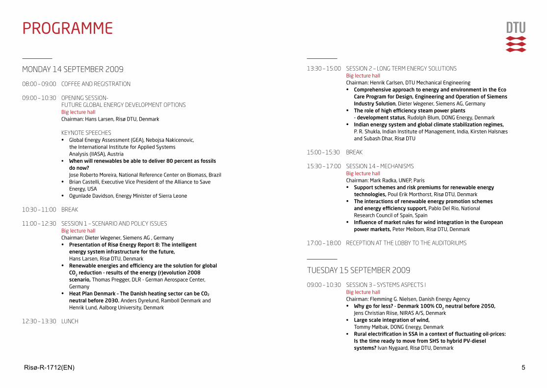
programmE

13:30 – 15:00 sessioN 2 – loNg teRM eNeRgy solutioNs big lecture hall

Chairman: Henrik Carlsen, dtu mechanical Engineering • Comprehensive approach to energy and environment in the Eco

Care Program for Design, Engineering and Operation of Siemens Industry Solution, dieter Wegener, siemens ag, germany

• The role of high efficiency steam power plants - development status, rudolph blum, dong Energy, denmark

• Indian energy system and global climate stabilization regimes, p. r. shukla, indian institute of management, india, kirsten Halsnæs

and subash dhar, risø dtu

15:00 – 15:30 bReaK 15:30 – 17:00 sessioN 14 – MeChaNisMs big lecture hall

Chairman: mark radka, unEp, paris • Support schemes and risk premiums for renewable energy

technologies, poul Erik morthorst, risø dtu, denmark • The interactions of renewable energy promotion schemes and energy efficiency support, pablo del rio, national research Council of spain, spain

• Influence of market rules for wind integration in the European power markets, peter meibom, risø dtu, denmark

17:00 – 18:00 ReCePtioN at the lobby to the auDitoRiuMs

tuesDay 15 sePteMbeR 2009

09:00 – 10:30 sessioN 3 – systeMs asPeCts i big lecture hall Chairman: flemming g. nielsen, danish Energy agency

• Why go for less? - Denmark 100% CO2 neutral before 2050, Jens Christian riise, niras a/s, denmark • Largescaleintegrationofwind,

tommy mølbak, dong Energy, denmark • RuralelectrificationinSSAinacontextoffluctuatingoil-prices:

Is the time ready to move from SHS to hybrid PV-diesel systems? ivan nygaard, risø dtu, denmark

MoNDay 14 sePteMbeR 2009

08:00 – 09:00 Coffee aND RegistRatioN

09:00 – 10:30 oPeNiNg sessioN- futuRe global eNeRgy DeveloPMeNt oPtioNs big lecture hall Chairman: Hans larsen, risø dtu, denmark

KeyNote sPeeChes • global Energy assessment (gEa), nebojsa nakicenovic,

the international institute for applied systems analysis (iiasa), austria

• When will renewables be able to deliver 80 percent as fossils do now? Jose roberto moreira, national reference Center on biomass, brazil

• brian Castelli, Executive vice president of the alliance to save Energy, usa

• ogunlade davidson, Energy minister of sierra leone 10:30 – 11:00 bReaK

11:00 – 12:30 sessioN 1 – sCeNaRio aND PoliCy issues big lecture hall

Chairman: dieter Wegener, siemens ag , germany • PresentationofRisøEnergyReport8:Theintelligent

energy system infrastructure for the future, Hans larsen, risø dtu, denmark • Renewableenergiesandefficiencyarethesolutionforglobal CO2 reduction - results of the energy (r)evolution 2008 scenario, thomas pregger, dlr - german aerospace Center, germany

• Heat Plan Denmark – The Danish heating sector can be CO2 neutral before 2030. anders dyrelund, ramboll denmark and Henrik lund, aalborg university, denmark

12:30 – 13:30 luNCh

Risø-R-1712(EN) 5

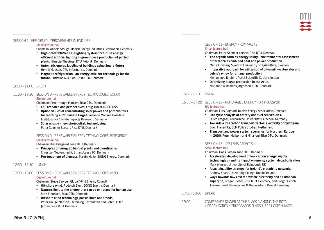
sessioN 11 – eNeRgy fRoM Waste

small lecture hall Chairman: peter sommer larsen, risø dtu, denmark

• The organic farm as energy utility - environmental assessment of farm-scale combined heat and power production,

marie kimming, swedish university of agriculture, sweden • Integrativeapproachforutilizationofolivemillwastewaterand

Lebna’swheyforethanolproduction, mohammed ibrahim, royal scientific society, Jordan

• OptimizingbiogasproductionintheArtic, marianne Willemoes Jørgensen, dtu, denmark

15:00 – 15:30 bReaK 15:30 – 17:00 sessioN 12 – ReNeWable eNeRgy foR tRaNsPoRt big lecture hall

Chairman: lars aagaard, danish Energy association, denmark • Lifecycleanalysisofbatteryandfuelcellvehicles, ulrich Wagner, technische universität münchen, germany • Towardsalowcarbontransportsector:electricityorhydrogen? Coen Hanschke, ECn policy studies, netherland • TransportandpowersystemscenariosforNorthernEurope

in 2030, peter meibom and nina Juul, risø dtu, denmark

sessioN 15 – systeMs asPeCts ii small lecture hall

Chairman: Hans larsen, risø dtu, denmark • Accelerateddevelopmentoflowcarbonenergysupply

technologies - and its impact on energy system decarbonisation, mark Winskel, university of Edinburgh, uk • AsustainabilitystrategyforIreland’selectricitynetwork, andrew keane, university College dublin, ireland • WaystowardslowcostrenewableelectricityandaEuropean

supergrid, gregor giebel, risø dtu, denmark, and gregor Czisch, transnational renewables & university of kassel, germany

17:00 – 18:00 bReaK

19:00 CoNfeReNCe DiNNeR at the blaCK DiaMoND, the Royal libRaRy, søReN KieRKegaaRDs PlaDs 1, 1221 CoPeNhageN

sessioN 6 – effiCieNCy iMPRoveMeNts iN eND-use small lecture hall Chairman: anders stouge, danish Energy industries federation, denmark

• High-powerblu/redLEDlightingsystemforfutureenergy efficientartificiallightingingreenhouseproductionofpotted plants, birgitte thestrup, dtu fotonik, denmark

• AutomaticenergylabelingofbuildingsusingSmartMeters, Henrik madsen, dtu informatics, denmark • Magneticrefrigeration-anenergyefficienttechnologyforthe

future, Christian r.H. bahl, risø dtu, denmark 10:30 – 11:00 bReaK

11:00 – 12:30 sessioN 8 – ReNeWable eNeRgy teChNologies: solaR big lecture hall Chairman: peter Hauge madsen, risø dtu, denmark

• CSPresearchandperspectives, Craig turchi, nrEl, usa • Option values of concentrating solar power and photovoltaics

for reaching a 2°C climate target, susanne manger, potsdam insititute for Climate impacts research, germany

• Solarenergy-newphotovoltaictechnologies, peter sommer-larsen, risø dtu, denmark sessioN 9 – ReNeWable eNeRgy teChNologies: bioeNeRgy i small lecture hall

Chairman: kim pilegaard, risø dtu, denmark • Principlesofsizing2Gbiofuelplantsandbiorefineries, Chresten meulengracht, Ethanolease i/s, denmark • Pre-treatmentofbiomass,martin møller, dong Energy, denmark

12:30 – 13:30 luNCh 13:30 – 15:00 sessioN 7 – ReNeWable eNeRgy teChNologies: WiND big lecture hall

Chairman: steve sawyer, global Wind Energy Council • Off-shore wind, rudolph blum, dong Energy, denmark • Nature’slimittotheenergythatcanbeextractedforhumanuse, sten frandsen, risø dtu, denmark • Offshorewindtechnology,possibilitiesandtrends,

peter Hauge madsen, flemming rasmussen and peter Hjuler Jensen, risø dtu, denmark

Risø-R-1712(EN) 6

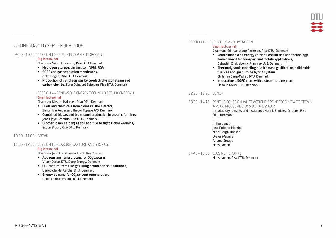
WeDNesDay 16 sePteMbeR 2009

09:00 – 10:30 sessioN 10 – fuel Cells aND hyDRogeN i big lecture hall Chairman: søren linderoth, risø dtu, denmark

• Hydrogen storage, lin simpson, nrEl, usa • SOFCandgasseparationmembranes,

anke Hagen, risø dtu, denmark • Productionofsynthesisgasbyco-electrolysisofsteamand

carbondioxide,sune dalgaard Ebbesen, risø dtu, denmark

sessioN 4 – ReNeWable eNeRgy teChNologies: bioeNeRgy ii small lecture hall Chairman: kirsten Halsnæs, risø dtu, denmark

• Fuelsandchemicalsfrombiomass:TheC-factor, simon ivar andersen, Haldor topsøe a/s, denmark • Combinedbiogasandbioethanolproductioninorganicfarming, Jens Ejbye schmidt, risø dtu, denmark • Biochar(blackcarbon)assoiladditivetofightglobalwarming, Esben bruun, risø dtu, denmark 10:30 – 11:00 bReaK

11:00 – 12:30 sessioN 13 – CaRboN CaPtuRe aND stoRage big lecture hall

Chairman: John Christensen, unEp risø Centre • AqueousammoniaprocessforCO2 capture,

victor darde, dtu/dong Energy, denmark • CO2 capture from flue gas using amino acid salt solutions, benedicte mai lerche, dtu, denmark • EnergydemandforCO2 solvent regeneration,

philip loldrup fosbøl, dtu, denmark

sessioN 16 – fuel Cells aND hyDRogeN ii small lecture hall Chairman: Erik lundtang petersen, risø dtu, denmark

• Solidammoniaasenergycarrier:Possibilitiesandtechnology development for transport and mobile applications,

debasish Chakraborty, amminex a/s, denmark • Thermodynamicmodelingofabiomassgasification,solidoxide

fuel cell and gas turbine hybrid system, Christian bang-møller, dtu, denmark

• IntegratingaSOFCplantwithasteamturbineplant, masoud rokni, dtu, denmark

12:30 – 13:30 luNCh

13:30 – 14:45 PaNel DisCussioN: What aCtioNs aRe NeeDeD NoW to obtaiN a PeaK iN Co2 eMissioNs befoRe 2020? introductory remarks and moderator: Henrik bindslev, director, risø dtu, denmark

in the panel: Jose roberto moreira niels bergh-Hansen dieter Wegener anders stouge Hans larsen

14:45 – 15:00 ClosiNg ReMaRKs Hans larsen, risø dtu, denmark

Risø-R-1712(EN) 7

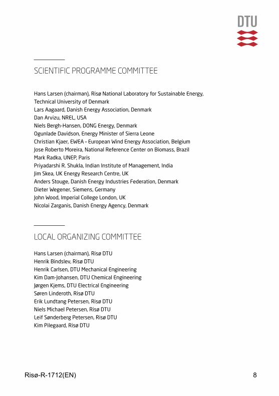
sCieNtifiC PRogRaMMe CoMMittee

Hans Larsen (chairman), Risø National Laboratory for Sustainable Energy,

Technical University of Denmark

Lars Aagaard, Danish Energy Association, Denmark

Dan Arvizu, NREL, USA

Niels Bergh-Hansen, DONg Energy, Denmark

Ogunlade Davidson, Energy Minister of Sierra Leone

Christian Kjaer, EWEA – European Wind Energy Association, Belgium

Jose Roberto Moreira, National Reference Center on Biomass, Brazil

Mark Radka, UNEP, Paris

Priyadarshi R. Shukla, indian institute of Management, india

Jim Skea, UK Energy Research Centre, UK

Anders Stouge, Danish Energy industries Federation, Denmark

Dieter Wegener, Siemens, germany

John Wood, imperial College London, UK

Nicolai Zarganis, Danish Energy Agency, Denmark

loCal oRgaNiziNg CoMMittee

Hans Larsen (chairman), Risø DTU

Henrik Bindslev, Risø DTU

Henrik Carlsen, DTU Mechanical Engineering

Kim Dam-Johansen, DTU Chemical Engineering

Jørgen Kjems, DTU Electrical Engineering

Søren Linderoth, Risø DTU

Erik Lundtang Petersen, Risø DTU

Niels Michael Petersen, Risø DTU

Leif Sønderberg Petersen, Risø DTU

Kim Pilegaard, Risø DTU

Risø-R-1712(EN) 8

Opening session

Risø-R-1712(EN) 9

9/7/2009

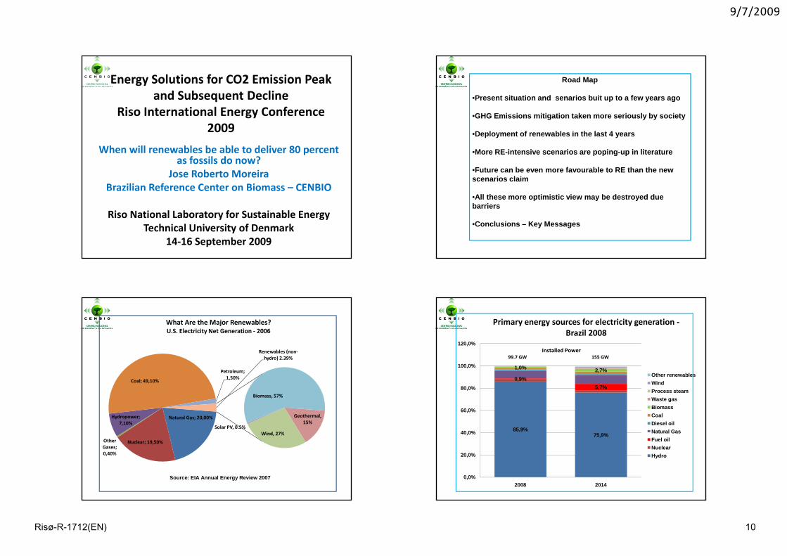
Energy Solutions for CO2 Emission Peak and Subsequent Decline

Riso International Energy Conference 2009

When will renewables be able to deliver 80 percent as fossils do now?

Jose Roberto MoreiraBrazilian Reference Center on Biomass – CENBIOa a e e e ce Ce te o o ass C O

Riso National Laboratory for Sustainable EnergyTechnical University of Denmark

14‐16 September 2009

Road Map

•Present situation and senarios buit up to a few years ago

•GHG Emissions mitigation taken more seriously by society

•Deployment of renewables in the last 4 years

•More RE-intensive scenarios are poping-up in literature

•Future can be even more favourable to RE than the new scenarios claim

•All these more optimistic view may be destroyed due barriers

•Conclusions – Key Messages

Renewables (non‐hydro) 2.39%

What Are the Major Renewables?U.S. Electricity Net Generation ‐ 2006

Natural Gas; 20,00%Hydropower; 7,10%

Coal; 49,10%

Petroleum; 1,50%

Geothermal, 15%

Wind 27%Solar PV, 0.5%

Biomass, 57%

Nuclear; 19,50%Other Gases; 0,40%

Wind, 27%

Source: EIA Annual Energy Review 2007

100 0%

120,0%

Primary energy sources for electricity generation ‐Brazil 2008

Installed Power99.7 GW 155 GW

85,9%

0,9%5,7%

1,0% 2,7%

40 0%

60,0%

80,0%

100,0%

Other renewablesWindProcess steamWaste gasBiomassCoalDiesel oilNatural Gas75,9%

0,0%

20,0%

40,0%

2008 2014

Natural GasFuel oilNuclearHydro

Risø-R-1712(EN) 10

9/7/2009

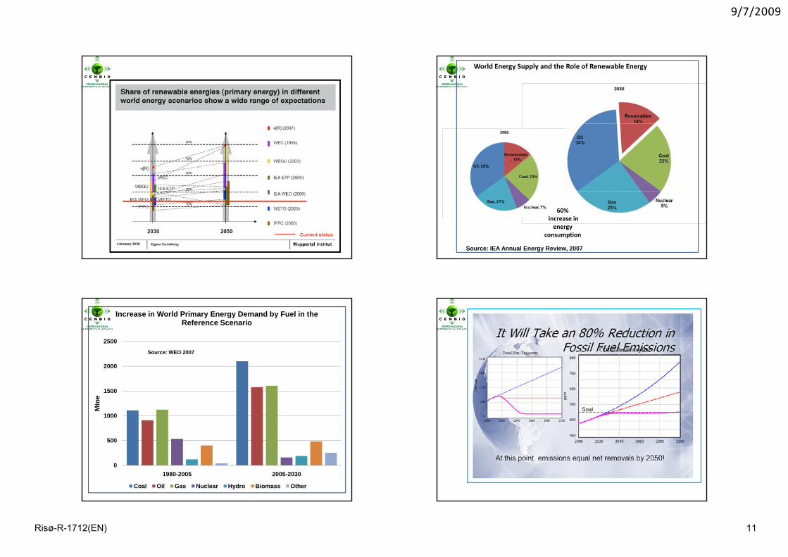
World Energy Supply and the Role of Renewable Energy

60%increase in energy

consumption

Source: IEA Annual Energy Review, 2007

2000

2500

Increase in World Primary Energy Demand by Fuel in the Reference Scenario

Source: WEO 2007

1000

1500

2000

Mto

e

0

500

1980-2005 2005-2030

Coal Oil Gas Nuclear Hydro Biomass Other

Risø-R-1712(EN) 11

9/7/2009

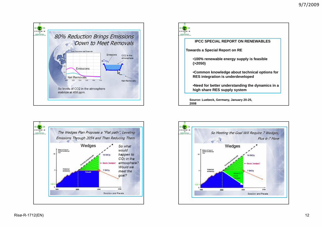
IPCC SPECIAL REPORT ON RENEWABLES

Towards a Special Report on RETowards a Special Report on RE

•100% renewable energy supply is feasible (>2050)

•Common knowledge about technical options for RES integration is underdevelopedg p

•Need for better understanding the dynamics in a high share RES supply system

Source: Luebeck, Germany, January 20-25, 2008

Risø-R-1712(EN) 12

9/7/2009

100

120

140

ars

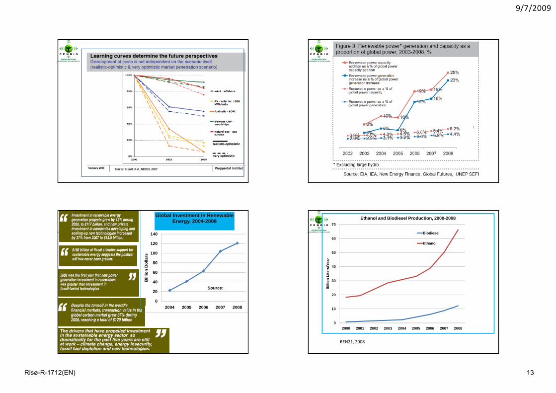
Global Investment in Renewable Energy, 2004-2008

0

20

40

60

80

2004 2005 2006 2007 2008

Bill

ion

Dol

la

Source:

2004 2005 2006 2007 2008

50

60

70

r

Ethanol and Biodiesel Production, 2000-2008

Biodiesel

Ethanol

20

30

40

Bill

ion

Lite

rs/Y

ear

0

10

2000 2001 2002 2003 2004 2005 2006 2007 2008

REN21, 2008

Risø-R-1712(EN) 13

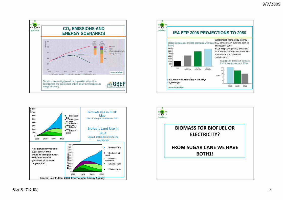
9/7/2009

Accelerated Technology ‐Energy CO2 emissions in 2050 are back to the level of 2005.BLUE Map‐ Energy CO2 emissions in 2050 are half those of 2005. This is similar to the “450 PPM Stabilization

3400 Mtoe = 62 Mboe/day = 148 EJ/yr = 3,600 Bl/yr

200

300

400

500

600

700

800

Mto

e

Biodiesel -BtL

Biodiesel -oil seed

Ethanol -cellulosic

Ethanol -cane

Ethanol -

Biofuels Use in BLUE Map

26% of Transport Fuel Use in 2050

Biofuels Land Use in

0

100

2005 2020 2035 2050

Ethanol grain

120140160180200

res

Biodiesel: BtL

Biodiesel: oil seed

BlueAbout 150 million hectares

worldwide

If all biofuel derived from sugar cane 74 Mha would be used plus 1,580

020406080

100120

2005 2020 2035 2050

Mill

ion

hect

a seedEthanol:

cellulosicEthanol: cane

Ethanol: grain

p ,TWh/yr or 5% of all global electricity could be generated

Source: Lew Fulton, 2008, International Energy Agency

BIOMASS FOR BIOFUEL OR ELECTRICITY?

FROM SUGAR CANE WE HAVE BOTH1!

Risø-R-1712(EN) 14

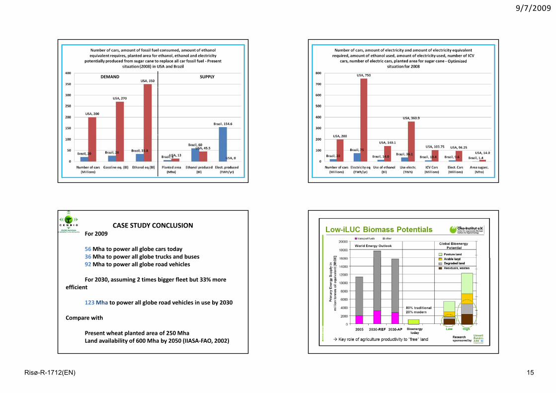
9/7/2009

DEMAND SUPPLY

CASE STUDY CONCLUSIONFor 2009

56 Mha to power all globe cars today36 Mha to power all globe trucks and buses36 Mha to power all globe trucks and buses92 Mha to power all globe road vehicles

For 2030, assuming 2 times bigger fleet but 33% more efficient

123Mha to power all globe road vehicles in use by 2030

Compare with

Present wheat planted area of 250 MhaLand availability of 600 Mha by 2050 (IIASA‐FAO, 2002)

Risø-R-1712(EN) 15

9/7/2009

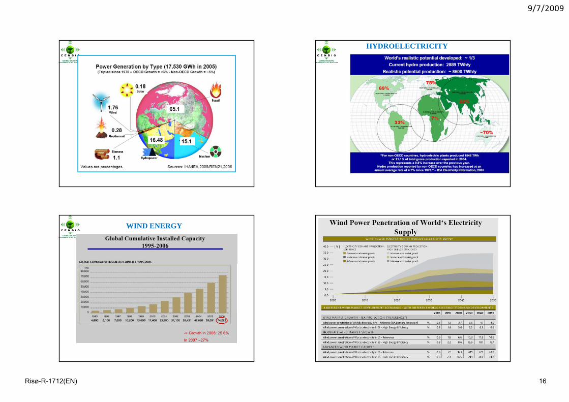
HYDROELECTRICITY

WIND ENERGY

Risø-R-1712(EN) 16

9/7/2009

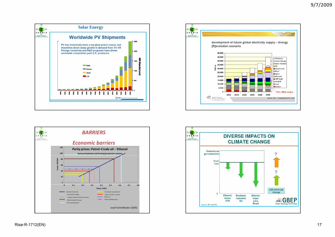
Solar Energy

Parity prices: Petrol–Crude oil – EthanolVarious feedstocks and farming/production systems100

120

BARRIERS

Economic barriers

0

20

40

60

80

Crud

e, US$/bbl

0 0.1 0.2 0.3 0.4 0.5 0.6 0.7 0.8

Petrol, US$/l

Gasoline‐Crude US$ Cane Brazil, top producers

Cane, Brazil, average Cassava, Thaioil, 2 mio l/d

Cassava, Thailand, OTC joint venture Maize, US

Mixed feedstock Europe Palmoil, MPOB project

Josef Schmidhuber (2005)

BTL: Synfuel/Synfuel

Risø-R-1712(EN) 17

9/7/2009

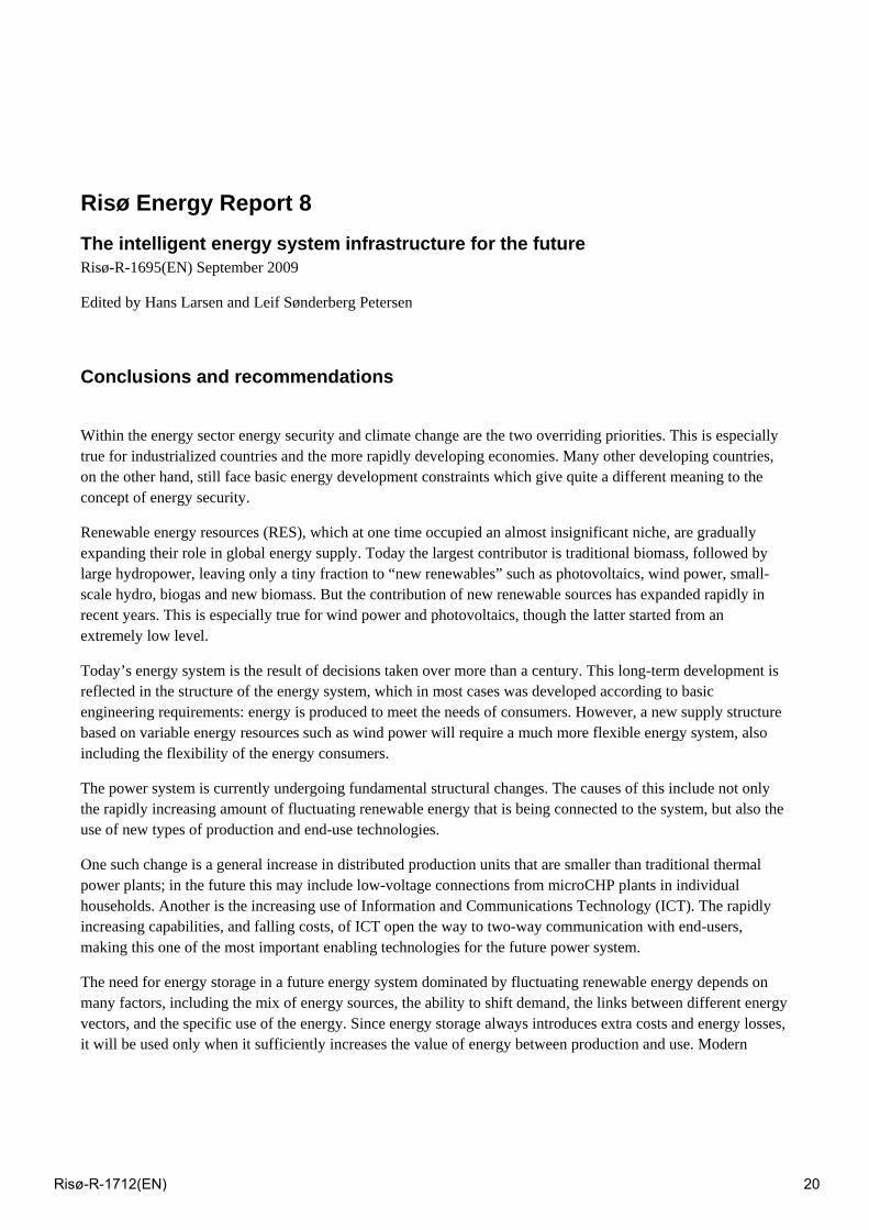
Palm oil0,60%

Sugar cane1,25%

Sugar beet0,33%

Corn8,83%

Soy

Land use in the world (%) in 2006

Soy5,69% Rape seed

1,70%

Wheat13,22%

Other64 98%

Barley3,40%

64,98%

Sources: http://faostat.fao.org and Product Board MVO.The total land area in use is 1,608 million hectares in 1999. For 2006 an estimate of 1,635 million hectares is made (Dornburg et al, 2006)

CONCLUSIONS ‐ KEY MESSAGES

1. Necessity of immediate actions to curb GHGs emissions in the next 20 years.

2. Short –term resource potential is significant but diti l i t li k d ith i lt l tconditional; interlinked with agricultural management

(bioenergy), investment, and governance (other RES)3. Significant GHG mitigation potential (most RES) and

under key conditions also for bioenergy.3. Rapidly changing policy context driving RES to more

sustainable options and approaches. 4 Barriers are significant either due incomplete4. Barriers are significant, either due incomplete

understanding of the physical and economic potential, as well as ways to avoid social and environmental conflicts, or due to economic interest related with the use of conventional energy sources.

Risø-R-1712(EN) 18

Session 1 – Scenario and policy issues

Risø-R-1712(EN) 19

Risø Energy Report 8 The intelligent energy system infrastructure for the future Risø-R-1695(EN) September 2009

Edited by Hans Larsen and Leif Sønderberg Petersen

Conclusions and recommendations

Within the energy sector energy security and climate change are the two overriding priorities. This is especially true for industrialized countries and the more rapidly developing economies. Many other developing countries, on the other hand, still face basic energy development constraints which give quite a different meaning to the concept of energy security.

Renewable energy resources (RES), which at one time occupied an almost insignificant niche, are gradually expanding their role in global energy supply. Today the largest contributor is traditional biomass, followed by large hydropower, leaving only a tiny fraction to “new renewables” such as photovoltaics, wind power, small-scale hydro, biogas and new biomass. But the contribution of new renewable sources has expanded rapidly in recent years. This is especially true for wind power and photovoltaics, though the latter started from an extremely low level.

Today’s energy system is the result of decisions taken over more than a century. This long-term development is reflected in the structure of the energy system, which in most cases was developed according to basic engineering requirements: energy is produced to meet the needs of consumers. However, a new supply structure based on variable energy resources such as wind power will require a much more flexible energy system, also including the flexibility of the energy consumers.

The power system is currently undergoing fundamental structural changes. The causes of this include not only the rapidly increasing amount of fluctuating renewable energy that is being connected to the system, but also the use of new types of production and end-use technologies.

One such change is a general increase in distributed production units that are smaller than traditional thermal power plants; in the future this may include low-voltage connections from microCHP plants in individual households. Another is the increasing use of Information and Communications Technology (ICT). The rapidly increasing capabilities, and falling costs, of ICT open the way to two-way communication with end-users, making this one of the most important enabling technologies for the future power system.

The need for energy storage in a future energy system dominated by fluctuating renewable energy depends on many factors, including the mix of energy sources, the ability to shift demand, the links between different energy vectors, and the specific use of the energy. Since energy storage always introduces extra costs and energy losses, it will be used only when it sufficiently increases the value of energy between production and use. Modern

Risø-R-1712(EN) 20

transport depends heavily on fossil fuels. Ways to reduce emissions from transport are to shift to renewable or at least CO2-neutral energy sources, and to link the transport sector to the power system. Achieving this will require new fuels and traction technologies, and new ways to store energy in vehicles.

A future electricity system with a considerable amount of fluctuating supply implies quite volatile hourly prices at the power exchange. Economists argue that exposing customers to these varying prices will create flexible demand that matches the fluctuations in supply. Persuading customers to react to hourly prices would improve market efficiency, reduce price volatility, and increase welfare.

Customers show some reluctance to react to hourly pricing, partly because their average gain is less than 0.5% of the electricity bill. Gains vary considerable between years, however, and depend crucially on the variation in prices, which in turn depends on the amount of fluctuating supply. Increasing the proportion of wind power in the system increases the benefits to consumers of acting flexible.

Recommendations

The global economy has in recent years faced a number of changes and challenges.

Globalization and free market economics have dominated the last decade, but the current financial crisis is rapidly changing the political landscape.

In the energy sector, energy security and climate change mitigation are the two overriding priorities. This is especially true for industrialized countries and the more rapidly developing economies; whereas many developing countries still face basic energy development constraints that give quite a different meaning to the concept of energy security.

We have several options in addressing climate change and energy security issues, but all of them will require strong global and national policy action focusing on low-carbon energy sources and gradual changes in the way the overall energy systems are designed:

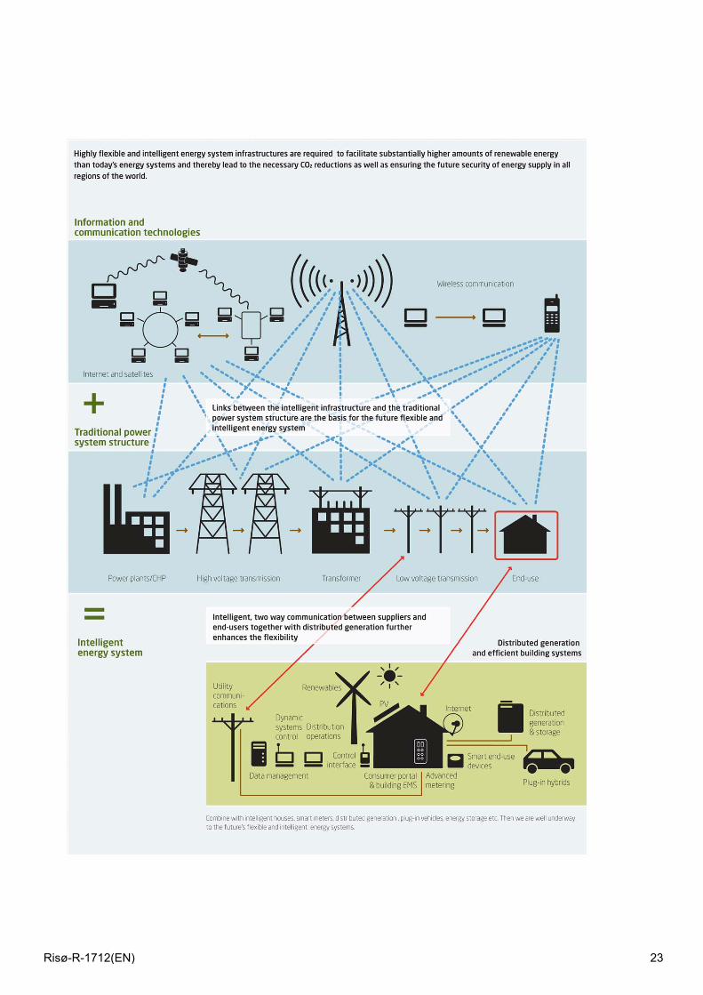
• More flexible and intelligent energy system infrastructures are required to facilitate substantially higher amounts of renewable energy compared to today’s energy systems. Flexible and intelligent infrastructures are a prerequisite to achieving the necessary CO2 reductions and secure energy supplies in every region of the world.

During the transition to the flexible and intelligent energy systems of the future, short-term policy actions need to be combined with longer-term research on new energy supply technologies, end-use technologies, and the broader system interaction aspects.

Prerequisites to the development of flexible and intelligent energy system infrastructures are the ability to:

• effectively accommodate large amounts of varying renewable energy; • integrate the transport sector through the use of plug-in hybrids and electric vehicles; • maximise the gains from a transition to intelligent, low-energy buildings; and • introduce advanced energy storage facilities in the system.

Risø-R-1712(EN) 21

It is important that flexible and intelligent energy systems are economically efficient and can be build up at affordable cost.

To allow high proportions of fluctuating renewable power production in the future energy system it is necessary to have:

• Long-term targets for renewable energy deployment and stable energy policies are needed in order to reduce uncertainty for investors. A mix of distributed energy resources is needed to allow system balancing and provide flexibility in the electricity system. Electric vehicles, electric heating, heat pumps and small-scale distributed generation, such as fuel-cell-based microCHP, are promising options.

For the electrical power system, the following issues should also be addressed in the planning of the intelligent power grid:

• energy shifting – the movement in time of bulk electricity through pumped hydro and compressed air storage;

• “smart” electricity meters in houses, businesses and factories, providing two-way communication between suppliers and users, and allowing power-using devices to be turned on and off automatically depending on the supply situation;

• communication standards to ensure that the devices connected to the intelligent power system are compatible, and the ability of the system to provide both scalability (large numbers of units) and flexibility (new types of units);

• optimal use of large cooling and heating systems, whose demand may be quite time-flexible; • large-scale use of electric vehicles is highly advantageous from the point of view of the power system as

well as the transport system.

The integration of a larger share of fluctuating wind power is expected to increase the volatility of power prices; demand response facilitates integration by counteracting fluctuations in supply.

Finally, there is a strong need to pursue long-term research and demonstration projects on new energy supply technologies, end-use technologies, and overall systems design. Existing research programmes in these areas should be redefined and coordinated so that they provide the best contribution to the g oal of a future intelligent energy system.

Risø-R-1712(EN) 22

Risø-R-1712(EN) 23

Renewable energies and efficiency are the solution for global CO2 reduction - results of the Energy [R]evolution 2008 scenario Thomas Pregger, Wolfram Krewitt, Sonja Simon

DLR - German Aerospace Center, Institute of Technical Thermodynamics, Department Systems Analysis & Technology Assessment, Pfaffenwaldring 38-40, D-70569 Stuttgart, Germany

Abstract The Energy [R]evolution 2008 scenario is a target oriented scenario of future energy demand and supply. It takes up recent trends in global socio-economic developments, and analyses how they affect chances for achieving climate protection targets. The main target is to reduce global CO2 emissions to around 10 Gt/a in 2050, which is seen as one of the prerequisites to reach a limitation of the global average temperature increase to about 2°C. A global energy system model was used at DLR for simulating energy supply strategies for the ten world regions. Long term energy demand projections are developed based on the assessment of energy efficiency measures in the key demand sectors of each region. Energy supply scenarios focus on the deployment of renewable energy resources, taking into account the regional availability of sustainable renewable energy resources. Scenario results show that achieving ambitious CO2 reduction targets is possible without relying on CCS or nuclear energy technologies. Renewable energy could provide more than half of the world’s energy needs by 2050. Developing countries can virtually stabilise their CO2 emissions, whilst at the same time increasing energy consumption through economic growth. OECD countries will be able to reduce their emissions by up to 80%. Compared to a business-as-usual development, increasing energy efficiency and shifting energy supply to renewable resources on the long term significantly reduces the costs for energy supply.

1 Objectives and approach The main objective of the Energy [R]evolution scenario (Greenpeace/EREC, 2008) is to show a possible and promising pathway to transform our unsustainable global energy supply system into a system which complies with climate protection targets. The scenario aims at demonstrating the feasibility of reducing global CO2 emissions to 10 Gt per year in 2050, which is seen as one important prerequisite to limit global average temperature increase to around 2°C (compared to pre-industrial level) and thus preventing severe effects on the climate system (see IPCC, 2007).

Compared to the new Wold Energy Outlook (WEO) 2008 of the International Energy Agency (IEA, 2008), the Energy [R]evolution scenario is much more optimistic regarding the role renewable energies could play in the energy systems of the world until 2050. Although the WEO 2008 points out that renewable energies will become soon a major source of electricity, it states that achieving the ambitious climate protection target is not possible without a massive expansion of nuclear and carbon capture and sequestration (CCS) power plants. In contrary, the aim of Energy [R]evolution is to show that without relying on nuclear and CCS there is no principal technical obstacle in curbing CO2 emissions at the pace required to achieve the 2° target. Its strategy is based on energy efficiency and high shares of renewable energies to supply power, heat, and transport demand. The pathways proposed also offer economic benefits and new options for economic development. Political will for change and appropriate policy measures are needed to overcome the inertia inherent in our current energy supply system.

Risø-R-1712(EN) 24

The Energy [R]evolution 2008 scenario is an update of the first Energy [R]evolution scenario published in 2007. It is a target oriented scenario developed in a back-casting process. The global energy supply strategies were simulated with a 10-region global energy system model implemented in the MESAP/PlaNet environment (MESAP, 2008). The ten regions correspond to the world regions as specified by the IEA’s WEO 2007 (Africa, China, India, Latin America, Middle East, OECD Europe, OECD North America, OECD Pacific, Other Developing Asia, Transition Economies) (IEA, 2007a). IEA energy statistics (IEA, 2007b, c) were used to calibrate the model for the base year 2005. Population development projections are taken from the United Nations’ World Population Prospects (UNDP, 2007). Projection of gross domestic product (GDP) was taken from WEO 2007 and the WEO 2007 Reference scenario was used as the business-as-usual projection. Both data sets were extrapolated to 2050 by own assumptions.

Scenario pathways were developed based on assessments of renewable energy resources for each world region and assumed technological and economical developments. The story lines were integrated into the model as exogenous model parameters and constraints. The demand scenarios are driven by the development of population and GDP as the key drivers and by assumptions regarding the potentials and exploitation of efficiency measures which were analysed in detail by (Graus and Blomen, 2008). A future without CCS technologies and new nuclear power plants but also the phasing out of existing nuclear power plants until 2050 are constraints of the Energy [R]evolution scenario. Worldwide renewable energy resources were assessed based on several studies above all on the global level from (REN21, 2008; Hoogwijk and Graus, 2008). As a response to the controversial discussion on the availability of biomass resources, a study on the global potential for sustainable biomass was commissioned as part of the Energy [R]evolution 2008 project (Seidenberger et al., 2008). Beside population development and economic growth, future energy price projections, CO2 emission costs and power plant investment costs were projected as other key system drivers which affect technology choices of the future but also total system costs and benefits due to investments and the substitution of fossil fuel consumption.

Demand and supply scenarios were developed in an iterative process. A close cooperation with regional counterparts, representing research organisations and NGOs from the respective world regions enabled an extensive review process. Also the renewable energy industry represented by the European Renewable Energy Council (EREC) was part of this process and contributed their views on production capacities and future potentials and constraints. The regional counterparts provided input on renewable energy potentials, and reviewed detailed scenario assumptions, taking into account the energy policy context in the respective world regions.

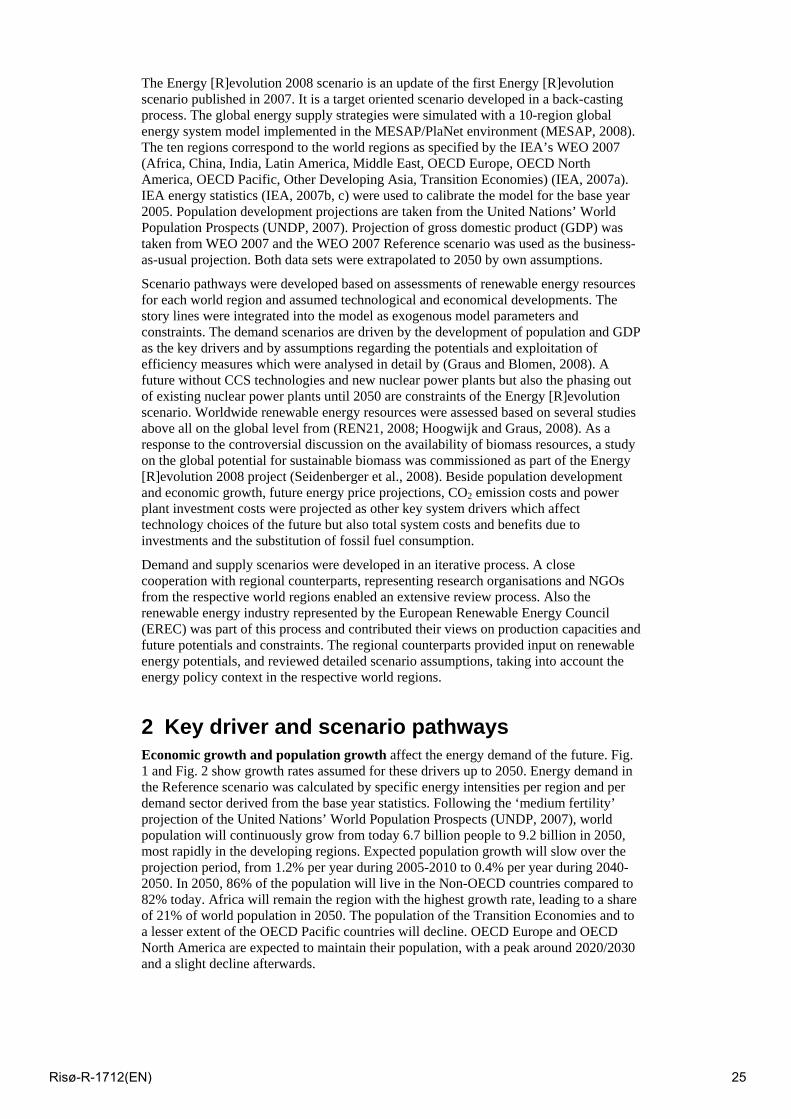
2 Key driver and scenario pathways Economic growth and population growth affect the energy demand of the future. Fig. 1 and Fig. 2 show growth rates assumed for these drivers up to 2050. Energy demand in the Reference scenario was calculated by specific energy intensities per region and per demand sector derived from the base year statistics. Following the ‘medium fertility’ projection of the United Nations’ World Population Prospects (UNDP, 2007), world population will continuously grow from today 6.7 billion people to 9.2 billion in 2050, most rapidly in the developing regions. Expected population growth will slow over the projection period, from 1.2% per year during 2005-2010 to 0.4% per year during 2040-2050. In 2050, 86% of the population will live in the Non-OECD countries compared to 82% today. Africa will remain the region with the highest growth rate, leading to a share of 21% of world population in 2050. The population of the Transition Economies and to a lesser extent of the OECD Pacific countries will decline. OECD Europe and OECD North America are expected to maintain their population, with a peak around 2020/2030 and a slight decline afterwards.

Risø-R-1712(EN) 25

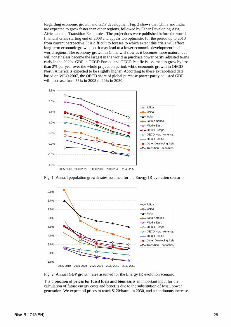
Regarding economic growth and GDP development Fig. 2 shows that China and India are expected to grow faster than other regions, followed by Other Developing Asia, Africa and the Transition Economies. The projections were published before the world financial crisis starting end of 2008 and appear too optimistic for the period up to 2010 from current perspective. It is difficult to foresee to which extent this crisis will affect long-term economic growth, but it may lead to a lower economic development in all world regions. The economy growth in China will slow as it becomes more mature, but will nonetheless become the largest in the world in purchase power parity adjusted terms early in the 2020s. GDP in OECD Europe and OECD Pacific is assumed to grow by less than 2% per year over the whole projection period, while economic growth in OECD North America is expected to be slightly higher. According to these extrapolated data based on WEO 2007, the OECD share of global purchase power parity adjusted GDP will decrease from 55% in 2005 to 29% in 2050.

-1.0%

-0.5%

0.0%

0.5%

1.0%

1.5%

2.0%

2.5%

2005-2010 2010-2020 2020-2030 2030-2040 2040-2050

AfricaChinaIndiaLatin AmericaMiddle EastOECD EuropeOECD North AmericaOECD PacificOther Developing AsiaTransition Economies

Fig. 1: Annual population growth rates assumed for the Energy [R]evolution scenario.

1.0%

2.0%

3.0%

4.0%

5.0%

6.0%

7.0%

8.0%

9.0%

2005-2010 2010-2020 2020-2030 2030-2040 2040-2050

AfricaChinaIndiaLatin AmericaMiddle EastOECD EuropeOECD North AmericaOECD PacificOther Developing AsiaTransition Economies

Fig. 2: Annual GDP growth rates assumed for the Energy [R]evolution scenario.

The projection of prices for fossil fuels and biomass is an important input for the calculation of future energy costs and benefits due to the substitution of fossil power generation. We expect oil prices to reach $120/barrel in 2030, and a continuous increase

Risø-R-1712(EN) 26

up to $140/barrel in 2050. In the WEO 2008 reference scenario IEA expects the oil price to reach $110 per barrel in 2030 ($2007 122/barrel). In contrast to IEA, we assume that coal prices continue to rise in the long term, reaching $250/t in 2030 and $360/t in 2050. Natural gas prices are assumed to rise by a factor of four compared to 2005 and to reach between 23 and 25 $/GJ until 2050. Biomass prices are expected to rise up to 5 $/GJ until 2050 outside of Europe and up to 11 $/GJ in Europe.

Estimations of future CO2 emission costs are subject to large uncertainty. It was assumed that in each world region a market for CO2 allowances will exist, in Non-Annex B countries only after 2020. We assume that average CO2 costs rise linearly from $10/tCO2 in 2010 to $50/tCO2 in 2050. Compared to WEO 2008 scenario, we expect much lower CO2 reduction costs due to the more comprehensive exploitation of cost-effective renewable energy potentials. In the 450 ppm scenario of WEO 2008 CO2 costs were assumed to reach up to $160/tCO2 ($2007 180/tCO2) in 2030.

Table 1 shows power plant investment costs assumed for the future. For fossil fuel based energy technologies we assume an advanced phase of market development, thus we expect only little potentials for further cost reduction. CCS technology was not considered as this still unproven concept cannot guarantee safe and permanent underground storage of CO2, has significant energy consumption and costs and is expected not to be available before 2030. The renewable energy technologies considered in the Energy [R]evolution scenario have different technical maturity, costs, and development potentials but are all already in commercial operation or expected to reach commercial operation soon. Large potential for cost reductions were assumed for most of these technologies because of the still relatively early technology development phase. The capacity factors of these technologies might differ significantly, also depending on the world regions and their resources. Investment costs for concentrating solar thermal power plants include thermal storage systems which facilitate high capacity factors.

Table 1: Assumptions on specific investment cost development (in $/kW) for selected power plant technologies

2010 2030 2050 Coal condensing power plant 1230 1160 1100 Natural gas combined cycle 690 610 550 Wind onshore 1370 1110 1090 Wind offshore 3480 2200 1890 Photovoltaic 3760 1280 1080 Biomass CHP 4970 3380 2950 Geothermal CHP 13050 7950 6310 Concentrating solar power plant 6340 4430 4320 Ocean energy 5170 2240 1670

The Energy [R]evolution scenario is a low energy demand scenario which takes into account an ambitious deployment of energy saving measures in all demand sectors. Efficiency improvements already occur in the Reference scenario based on IEA WEO 2007. Additional individual efficiency measures were quantified compared to the Reference energy demand projection. It is assumed that equipment is replaced only at the end of its economic lifetime. Details of the methodology applied can be found in (Greenpeace/EREC, 2008) and in (Graus and Blomen, 2008). Final energy demand in the Reference projection (excluding non-energy use) will nearly double until 2050, from 299 EJ in 2005 to 570 EJ in 2050, driven by the population and GDP increases.

In the transport sector we analysed three options for reducing energy demand, namely the reduction of transport demand, modal shift from high energy intensive to low energy intensive transport modes, and energy efficiency improvements. Per capita transport demand in OECD countries and in Transition Economies was expected to be reduced by 5% in 2050 compared to the Reference scenario, whereas in non-OECD countries no reduction in transport demand was assumed. Regarding modal shifts we assume that 2.5% of passenger transport shifts from air (short distance) to rail, 2.5% from car to rail, and 2.5% from car to bus compared to the Reference scenario. For freight transport we

Risø-R-1712(EN) 27

assume that 5% of the transport volume shifts from medium trucks to rail, and 2.5% from heavy trucks to rail. Light duty vehicles with lower fuel consumption were assumed for all world regions. Detailed technology analyses result in energy intensities of around 1.6 litre gasoline-equivalents (lge) per 100 km in 2050 (for new European drive cycle – NEDC) for small cars, 2.5 lge/100 km for medium size cars and 3.5 lge/100 km for large-size cars compared to current intensities of e.g. 11.5 lge/100 km in North America and 8 lge/100 km in OECD Europe. High shares of plug-in electric and hybrid cars have been assumed to occur between 2030 and 2050 especially in the OECD regions with even lower energy consumption due to the high efficiency of the electric drive train. Test cycle values are adjusted to real-world driving by applying a factor of 1.2 for fossil fuel and 1.7 for battery electric driven vehicles. Due to these changes, the world average fuel consumption of vehicles in the Energy [R]evolution scenario will drop from 10 lge/100 km today to 4 lge/100 km in 2050. Energy intensity of air and rail transport was also expected to be reduced by around 50% until 2050.

Long-term energy efficiency potentials in energy intensive industries such as chemical and petrochemical industry, the iron and steel industry, and the processing of non-metallic minerals were quantified by analysing individual measures. Average worldwide energy efficiency improvements are between 0.4% and 1.4% per year depending on industry with an average of 1.2% per year for the total industry sector. The energy efficiency potential of the remaining industry was considered as decrease of average energy intensity per world region. More sector and region specific details are available in (Greenpeace/EREC, 2008) and (Graus and Blomen, 2008).

Energy consumption in the ‘other’ sectors (residential, commercial and public services, agriculture) represents nowadays about 40% of global final energy consumption, in most world regions dominated by the residential sector. The reduction of heating and cooling demand due to improved insulation and building design, and the use of efficient electric appliances, lighting and air conditioning are the main measures analysed and applied in the Energy [R]evolution scenario. Table 2 summarises saving potentials in the ‘other’ sectors resulting from the detailed analysis of measures and their potential.

Table 2: Saving potentials by type of energy use in the buildings sector (Graus and Blomen, 2008). Percentages related to heat/electricity demand in ‘Other’ sectors.

Heating -new

Heating -retrofit

Standby Lighting Appli-ances

Cold ap-pliances

Air con-ditioning

Computer/ server

Other

OECD Europe 58% 40% 72% 60% 50% 64% 55% 55% 57% OECD North-America

38% 26% 72% 42% 50% 64% 55% 55% 53%

OECD Pacific 8% 5% 72% 49% 50% 64% 55% 55% 55% Transition Economies

35% 24% 72% 67% 50% 64% 55% 55% 58%

China 38% 72% 18% 50% 64% 55% 55% 48% Other regions 72% 67% 50% 64% 55% 55% 58%

The main objective of the project was to develop a renewable energy oriented supply scenario. Availability of renewable energy sources differs considerably between world regions. Renewable potentials were analysed based on three global studies and several information for individual world regions and countries and reviewed by the regional counterparts. Investments in new highly efficient fossil power plants, together with an increasing capacity of wind turbines, biomass, concentrating solar power plants and photovoltaics lead to electricity generation dominated by renewable energy technologies. Fossil electricity generation will peak around 2020, followed by a continuous decline, with a shift from coal to gas fired power plants which helps to compensate for power fluctuations of renewable energy sources. 24% of the global heat demand today is covered by renewable energies, mainly by the traditional use of biomass. In the Energy [R]evolution scenario solar collectors, modern biomass and geothermal energy are increasingly substituting fossil fuel-fired systems. In the transport sector a growing but

Risø-R-1712(EN) 28

limited share of biofuels is expected and a massive market introduction of electric vehicles (both battery vehicles and electric hybrid vehicles) after 2020 was assumed.

3 Results In the following some main results of the Energy [R]evolution scenario are shown. Table 3 shows the resulting final energy demand by world region and demand sector. Additional efficiency measures considered in the Energy [R]evolution scenario lead to an only moderate growth of energy demand compared to the Reference scenario. Global final energy demand grows up to 350 EJ in 2050, 40% lower than in the Ref. scenario. Transport energy demand in 2050 is even lower than today although worldwide transport volume increases. In the “Other sectors” demand grows by 26% compared to 2005.

Table 3: Development of final energy demand in PJ/a under the Energy [R]evolution scenario by region (excluding non-energy use).

2005 2010 2020 2030 2040 2050 World 299,300 327,393 347,127 354,335 353,803 349,845 Transport 83,936 92,889 92,233 89,980 85,796 83,306 Industry 91,759 102,321 112,295 114,021 113,583 110,787 Other 123,665 132,183 142,598 150,334 154,423 155,752 Africa 18,073 20,003 22,174 24,412 26,409 28,286 Transport 2,812 3,254 3,759 4,265 4,770 5,276 Industry 3,345 3,720 3,933 4,016 4,111 4,071 Other 11,916 13,029 14,482 16,132 17,527 18,939 China 43,677 55,359 67,869 71,370 72,412 73,120 Transport 5,062 7,557 9,992 12,054 13,970 17,296 Industry 20,405 27,453 34,646 35,245 34,024 31,365 Other 18,210 20,349 23,231 24,071 24,419 24,458 India 13,569 16,009 21,188 26,174 31,247 36,263 Transport 1,549 2,156 3,786 5,417 7,047 8,677 Industry 4,145 5,431 7,582 9,531 11,525 13,421 Other 7,875 8,422 9,819 11,227 12,676 14,165 Latin America 15,484 17,288 18,894 20,242 21,637 23,229 Transport 5,131 5,595 5,718 5,842 5,965 6,089 Industry 5,683 6,547 7,288 7,722 7,978 8,136 Other 4,670 5,146 5,888 6,679 7,694 9,005 Middle East 12,011 14,266 16,437 17,575 18,648 19,564 Transport 4,460 5,226 5,004 4,686 4,332 3,990 Industry 3,324 4,266 5,604 6,198 6,637 6,751 Other 4,226 4,774 5,829 6,690 7,680 8,823 OECD Europe 53,833 54,781 48,833 43,902 40,751 39,231 Transport 16,080 16,860 14,377 11,770 9,779 8,693 Industry 15,380 15,374 13,636 12,430 12,038 11,908 Other 22,374 22,547 20,821 19,702 18,934 18,630 OECD North America 72,218 74,483 74,003 72,152 65,727 55,459 Transport 31,310 32,466 30,419 27,520 22,297 16,721 Industry 16,067 15,337 14,332 13,719 13,106 12,356 Other 24,840 26,680 29,252 30,913 30,324 26,383 OECD Pacific 21,322 22,243 21,678 20,397 18,513 16,669 Transport 6,716 7,256 6,515 5,774 5,033 4,035 Industry 6,847 7,159 7,251 6,913 6,284 5,723 Other 7,760 7,828 7,912 7,710 7,196 6,911 Other Developing Asia 20,553 23,448 26,357 28,651 30,330 31,625 Transport 4,964 5,988 6,637 7,189 7,740 8,292 Industry 6,285 7,334 8,292 8,898 9,203 9,300 Other 9,305 10,126 11,428 12,565 13,387 14,033 Transition Economies 28,620 29,511 29,693 29,460 28,128 26,399 Transport 5,853 6,531 6,025 5,464 4,863 4,237 Industry 10,277 9,700 9,732 9,350 8,678 7,756 Other 12,491 13,280 13,936 14,645 14,587 14,405

Risø-R-1712(EN) 29

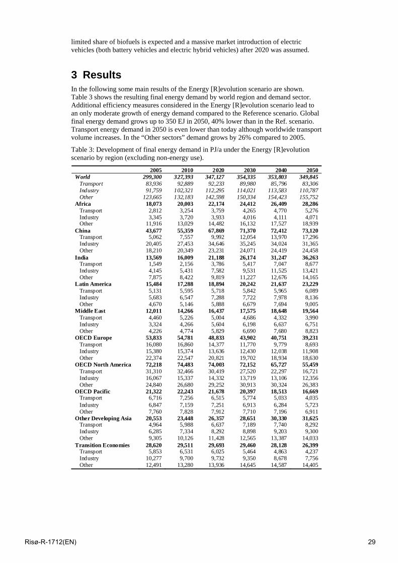
Electricity generation from renewable energies reaches 28,600 TWh/a in 2050 in the Energy [R]evolution scenario, which is 77% of the electricity produced worldwide. Solar energy will be the main source of electricity generation in the long-term, both from PV cells and from concentrating solar thermal power plants. The installed capacity of renewable energy technologies will grow from the current 1,000 GW to 9,100 GW in 2050. Growing electricity generation in combined heat and power (CHP) applications (2005: 1915 TWh; 2050: 6400 TWh) improves the overall efficiency of the energy supply system, with biomass being the main fuel for CHP applications in 2050. After 2030 there is a rapidly growing additional electricity demand induced by the market introduction of electric vehicles which can largely be covered by renewable energy sources. Fig. 3 and 4 show the shares of electricity consumption by energy sources and by world region for the base year 2005 and the year 2050.

Fig. 3: Electricity supply by technologies and world regions in 2005 (IEA, 2007b, c).

Fig. 4: Electricity supply by technologies and world regions in 2050 in the Energy [R]evolution scenario.

0%

10%

20%

30%

40%

50%

60%

70%

80%

90%

100%

Africa

China India

Latin A

merica

Middle

East

OECD Europe

OECD N. A

merica

OECD Pacific

Other Dev

elop. A

sia

Transit

ion Eco

nomies

shar

e of

ele

ctri

city

pro

duct

ion Ocean Energy

Solar ThermalGeothermalBiomassPVWindHydroOilGasCoal

2076 9261 4435 2615 2171 3252 6756 2111 2356 2083 TWh/a

0%

10%

20%

30%

40%

50%

60%

70%

80%

90%

100%

Africa

China

India

Latin A

merica

Middle

East

OECD Europe

OECD N. A

merica

OECD Pacif

ic

Other D

evelop

. Asia

Transit

ion Econ

omies

shar

e of

ele

ctri

city

pro

duct

ion Ocean Energy

Solar ThermalGeothermalBiomassPVWindHydroNuclearOilGasCoal

564 2539 699 906 640 3481 5118 1780 901 1598 TWh/a

Risø-R-1712(EN) 30

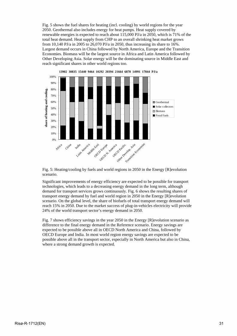
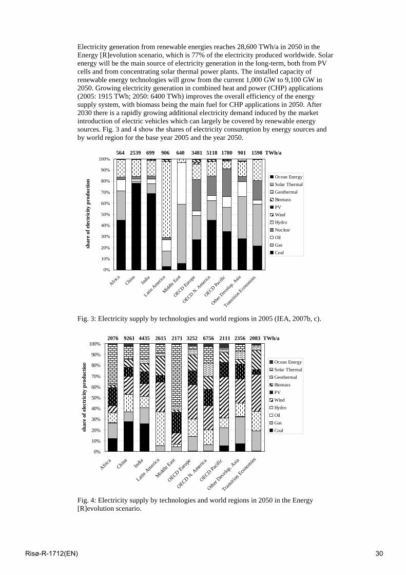
Fig. 5 shows the fuel shares for heating (incl. cooling) by world regions for the year 2050. Geothermal also includes energy for heat pumps. Heat supply covered by renewable energies is expected to reach about 115,000 PJ/a in 2050, which is 71% of the total heat demand. Heat supply from CHP to an overall shrinking heat market grows from 10,140 PJ/a in 2005 to 26,070 PJ/a in 2050, thus increasing its share to 16%. Largest demand occurs in China followed by North America, Europe and the Transition Economies. Biomass will be the largest source in Africa and Latin America followed by Other Developing Asia. Solar energy will be the dominating source in Middle East and reach significant shares in other world regions too.

Fig. 5: Heating/cooling by fuels and world regions in 2050 in the Energy [R]evolution scenario.

Significant improvements of energy efficiency are expected to be possible for transport technologies, which leads to a decreasing energy demand in the long term, although demand for transport services grows continuously. Fig. 6 shows the resulting shares of transport energy demand by fuel and world region in 2050 in the Energy [R]evolution scenario. On the global level, the share of biofuels of total transport energy demand will reach 15% in 2050. Due to the market success of plug-in-vehicles electricity will provide 24% of the world transport sector’s energy demand in 2050.

Fig. 7 shows efficiency savings in the year 2050 in the Energy [R]evolution scenario as difference to the final energy demand in the Reference scenario. Energy savings are expected to be possible above all in OECD North America and China, followed by OECD Europe and India. In most world region energy savings are expected to be possible above all in the transport sector, especially in North America but also in China, where a strong demand growth is expected.

0%

10%

20%

30%

40%

50%

60%

70%

80%

90%

100%

Africa

China

India

Latin A

merica

Middle

East

OECD Europe

OECD N. A

merica

OECD Pacific

Other D

evelo

p. Asia

Transit

ion Eco

nomies

shar

e of

hea

ting

and

cool

ing.

GeothermalSolar collectorsBiomass Fossil fuels

13902 30835 15440 9464 10292 20394 21664 6878 14991 17844 PJ/a

Risø-R-1712(EN) 31

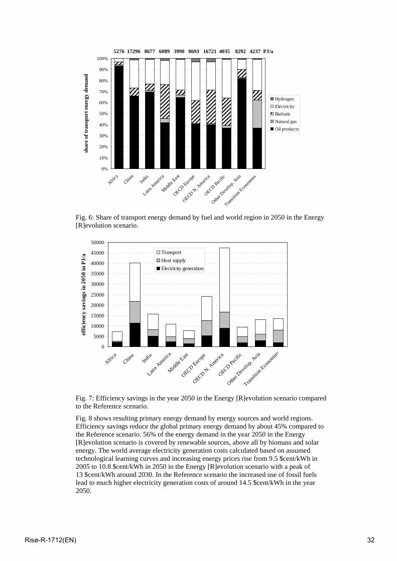
Fig. 6: Share of transport energy demand by fuel and world region in 2050 in the Energy [R]evolution scenario.

0

5000

10000

15000

20000

25000

30000

35000

40000

45000

50000

Africa

China

India

Latin A

merica

Middle

East

OECD Europe

OECD N. A

merica

OECD Pacif

ic

Other D

evelo

p. Asia

Transit

ion Econ

omies

effic

ienc

y sa

ving

s in

2050

in P

J/a Transport

Heat supplyElectricity generation

Fig. 7: Efficiency savings in the year 2050 in the Energy [R]evolution scenario compared to the Reference scenario.

Fig. 8 shows resulting primary energy demand by energy sources and world regions. Efficiency savings reduce the global primary energy demand by about 45% compared to the Reference scenario. 56% of the energy demand in the year 2050 in the Energy [R]evolution scenario is covered by renewable sources, above all by biomass and solar energy. The world average electricity generation costs calculated based on assumed technological learning curves and increasing energy prices rise from 9.5 $cent/kWh in 2005 to 10.8 $cent/kWh in 2050 in the Energy [R]evolution scenario with a peak of 13 $cent/kWh around 2030. In the Reference scenario the increased use of fossil fuels lead to much higher electricity generation costs of around 14.5 $cent/kWh in the year 2050.

0%

10%

20%

30%

40%

50%

60%

70%

80%

90%

100%

Africa

China

India

Latin A

merica

Middle

East

OECD Europe

OECD N. A

merica

OECD Pacif

ic

Other D

evelop

. Asia

Transit

ion Econ

omies

shar

e of

tran

spor

t ene

rgy

dem

and

HydrogenElectricityBiofuelsNatural gasOil products

5276 17296 8677 6089 3990 8693 16721 4035 8292 4237 PJ/a

Risø-R-1712(EN) 32

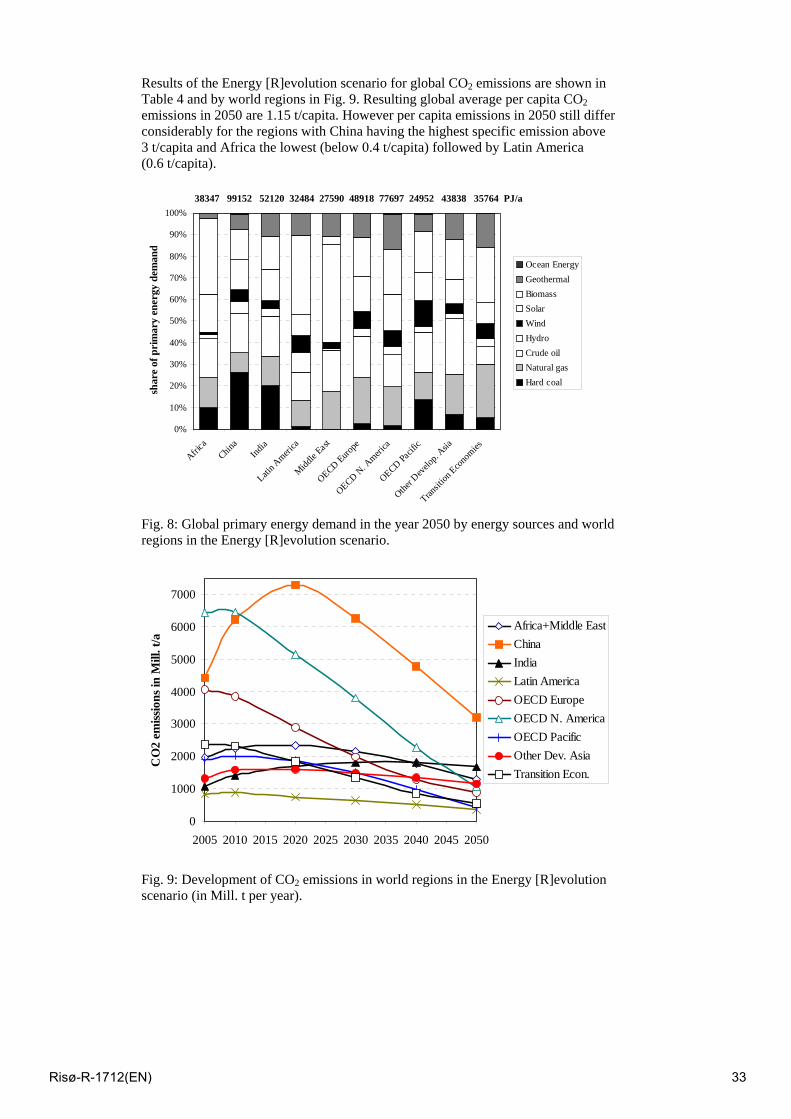
Results of the Energy [R]evolution scenario for global CO2 emissions are shown in Table 4 and by world regions in Fig. 9. Resulting global average per capita CO2 emissions in 2050 are 1.15 t/capita. However per capita emissions in 2050 still differ considerably for the regions with China having the highest specific emission above 3 t/capita and Africa the lowest (below 0.4 t/capita) followed by Latin America (0.6 t/capita).

0%

10%

20%

30%

40%

50%

60%

70%

80%

90%

100%

Africa

China

India

Latin A

merica

Middle

East

OECD Europe

OECD N. A

merica

OECD Pacif

ic

Other D

evelo

p. Asia

Transit

ion Eco

nomies

shar

e of

pri

mar

y en

ergy

dem

and

Ocean EnergyGeothermalBiomass SolarWindHydroCrude oilNatural gasHard coal

Fig. 8: Global primary energy demand in the year 2050 by energy sources and world regions in the Energy [R]evolution scenario.

0

1000

2000

3000

4000

5000

6000

7000

2005 2010 2015 2020 2025 2030 2035 2040 2045 2050

CO

2 em

issio

ns in

Mill

. t/a

Africa+Middle EastChinaIndiaLatin AmericaOECD EuropeOECD N. AmericaOECD PacificOther Dev. AsiaTransition Econ.

Fig. 9: Development of CO2 emissions in world regions in the Energy [R]evolution scenario (in Mill. t per year).

38347 99152 52120 32484 27590 48918 77697 24952 43838 35764 PJ/a

Risø-R-1712(EN) 33

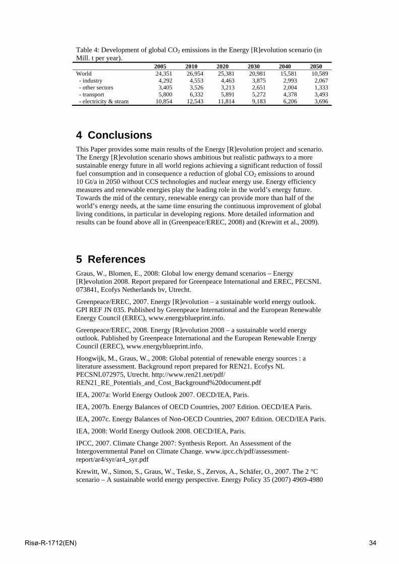
Table 4: Development of global CO2 emissions in the Energy [R]evolution scenario (in Mill. t per year). 2005 2010 2020 2030 2040 2050 World 24,351 26,954 25,381 20,981 15,581 10,589 - industry 4,292 4,553 4,463 3,875 2,993 2,067 - other sectors 3,405 3,526 3,213 2,651 2,004 1,333 - transport 5,800 6,332 5,891 5,272 4,378 3,493 - electricity & steam 10,854 12,543 11,814 9,183 6,206 3,696

4 Conclusions This Paper provides some main results of the Energy [R]evolution project and scenario. The Energy [R]evolution scenario shows ambitious but realistic pathways to a more sustainable energy future in all world regions achieving a significant reduction of fossil fuel consumption and in consequence a reduction of global CO2 emissions to around 10 Gt/a in 2050 without CCS technologies and nuclear energy use. Energy efficiency measures and renewable energies play the leading role in the world’s energy future. Towards the mid of the century, renewable energy can provide more than half of the world’s energy needs, at the same time ensuring the continuous improvement of global living conditions, in particular in developing regions. More detailed information and results can be found above all in (Greenpeace/EREC, 2008) and (Krewitt et al., 2009).

5 References Graus, W., Blomen, E., 2008: Global low energy demand scenarios – Energy [R]evolution 2008. Report prepared for Greenpeace International and EREC, PECSNL 073841, Ecofys Netherlands bv, Utrecht.

Greenpeace/EREC, 2007. Energy [R]evolution – a sustainable world energy outlook. GPI REF JN 035. Published by Greenpeace International and the European Renewable Energy Council (EREC), www.energyblueprint.info.

Greenpeace/EREC, 2008. Energy [R]evolution 2008 – a sustainable world energy outlook. Published by Greenpeace International and the European Renewable Energy Council (EREC), www.energyblueprint.info.

Hoogwijk, M., Graus, W., 2008: Global potential of renewable energy sources : a literature assessment. Background report prepared for REN21. Ecofys NL PECSNL072975, Utrecht. http://www.ren21.net/pdf/ REN21_RE_Potentials_and_Cost_Background%20document.pdf

IEA, 2007a: World Energy Outlook 2007. OECD/IEA, Paris.

IEA, 2007b. Energy Balances of OECD Countries, 2007 Edition. OECD/IEA Paris.

IEA, 2007c. Energy Balances of Non-OECD Countries, 2007 Edition. OECD/IEA Paris.

IEA, 2008: World Energy Outlook 2008. OECD/IEA, Paris.

IPCC, 2007. Climate Change 2007: Synthesis Report. An Assessment of the Intergovernmental Panel on Climate Change. www.ipcc.ch/pdf/assessment-report/ar4/syr/ar4_syr.pdf

Krewitt, W., Simon, S., Graus, W., Teske, S., Zervos, A., Schäfer, O., 2007. The 2 °C scenario – A sustainable world energy perspective. Energy Policy 35 (2007) 4969-4980

Risø-R-1712(EN) 34

Krewitt, W., Teske, S., Simon, S., Pregger, T., Graus, W., Blomen, E., Schmid, S., Schäfer, O., 2009: Energy [R]evolution 2008 - a sustainable world energy perspective. (submitted to Journal of Energy Policy).

MESAP 2008. http://www.seven2one.de/mesap.php

REN21, 2008: Renewable Energy Potentials - Summary Report. REN21 Secretariat, Paris. http://www.ren21.net/pdf/REN21_Potentials_Report.pdf

Seidenberger, T., Thrän, D., Offermann, R., Seyfert, U., Buchhorn, M., Zeddies, J., 2008: Global Biomass Potentials. Report prepared for Greenpeace International, German Biomass Research Center, Leipzig.

UNPD, 2007. World Population Prospects: The 2006 Revision, United Nations, Department of Economic and Social Affairs, Population Division. http://esa.un.org/unpp/ (1.2.2008)

Acknowledgment The authors would like to thank the many partners who provided helpful input during the scenario development: S. Teske, W. Graus, E. Blomen, S. Schmid, O. Schäfer, R. Banerjee, T. Buakamsri, J. Coeguyt, K. Davies, M. Ellis, J. Fujii, M. Furtado, V. Gopal, N. Grossmann, T. Iida, J. Inventor, S. Kumar, H. Matsubara, C. Miller, M. Ohbayashi, S. Rahut, J. Sawin, F. Sverrisson, V. Tchouprov, L. Vargas, J. Vincent, A. Yang, X.L. Zhang. The sole responsibility for the content of the paper remains with the authors.

Risø-R-1712(EN) 35

Heat Plan Denmark – The Danish heating sector can be CO2 neutral before 2030 by Anders Dyrelund, Ramboll Denmark Henrik Lund, Aalborg University Abstract Heat Plan Denmark is an R&D study financed by the Danish District Heating Association (DDHA). It demonstrates that District heating is the key technology for implementing a CO2 neutral Danish heating sector in a cost effective way. Since 1980 annual CO2 emissions have been reduced from approximately 25 kg/m2 to 10 kg/m2 floor area. This is due to two efforts: firstly, consumers have saved 25% on heat; secondly, the heat market share of district heating has increased from 30% to 46% and the district heating has utilized combined heat and power (CHP) and renewable energy. Heat Plan Denmark shows that it is possible to continue this progressive development, so that CO2 emissions from the heating sector can be reduced by another 50% by 2020 and that an almost CO2 neutral heating sector is achievable by 2030. The plan shows that this is possible with to-days technology by combining:

• additional 25% reduction of the heat demand • a further reduction of the return temperature to 35 dgr. C. • more district heating up to a market share of 70% • more integration of renewable energy in the district heating systems,

such as large scale solar heating, geothermal energy, waste to energy, biomass CHP and heat pumps in combination with large thermal storages and CHP plants to utilize the fluctuating wind energy

• heat pumps, wood pellet boilers and solar heating for the remaining individual heat market.

Paper Heat Plan Denmark is an R&D study financed by the Danish District Heating Association (DDHA). It demonstrates that District heating is the key technology for implementing a CO2 neutral Danish heating sector in a cost effective way. Since the first oil crisis in 1973, improvements in the heating sector have played a crucial role in the Danish energy supply mix. The heat supply act and the gas supply act in 1979 started a target oriented, least-cost planning process and widespread implementation of natural gas and district heating networks.

Risø-R-1712(EN) 36

Since 1980 annual CO2 emissions have been reduced from approximately 25 kg/m2 to 10 kg/m2 floor area. This is due to two efforts: firstly, consumers have saved 25% on heat; secondly, the heat market share of district heating has increased from 30% to 46% (corresponding to 60% of the dwellings in Denmark). The district heating expansion has made it possible to utilize combined heat and power (CHP) and renewable energy. Natural gas has also had an important role. The current awareness of climate change and the decision of the Danish Government to base future energy supply in Denmark on renewable sources has once again brought the heating sector and the possibilities of district heating into focus. Heat Plan Denmark shows that it is possible to continue this progressive development, so that CO2 emissions from the heating sector can be reduced by another 50% by 2020 and that an almost CO2 neutral heating sector is achievable by 2030. Heat Plan Denmark shows how these benefits can be achieved by 2020 in a cost effective way through a combination of the following initiatives: • Consumers save another 25% on heating and reduce their return

temperature to the district heating network to around 35 dgr.C, e.g. in connection with renovation of the building envelope.

• District heating is expanded from 46% to around 63% of the market share,

starting with the very profitable conversion of large gas fuelled boiler plants to district heating based on CHP and renewables.

• The majority (approximately 70%) of new buildings, for which intelligent

urban planning is possible and cost effective, are connected to district heating or block heating, whereas the remaining will be individually supplied low energy houses.

• District heating systems are further interconnected so that utilisation of

excess heat in the summer, mainly from waste to energy plants, is improved, and competition between the heat sources is intensified

• District heating production is expanded with more heat storage tanks, more

renewable energy, in particular more efficient waste to energy CHP plants with fluegas condensation, large scale solar heating, biomass boilers and CHP, biogas CHP, geothermal energy and excess wind energy.

• The remaining heat market will be covered by heat pumps and wood pellet

boilers in combination with individual solar heating.

Risø-R-1712(EN) 37

The study compares 3 cases for the development after 2020. Case A: a 70% district heating market share and constant heat demand from 2020, taking into account the effects of electricity savings and increasing comfort, which could be a realistic alternative in case of increasing fuel prices, cost based price signals to the consumers and a strong heat planning. Case B: a 70% district heating market share and additional 25% heat savings after 2020, corresponding to a total 50% heat savings compared to the 2008 level. This could be an alternative to case A in case of strong enforcement of investments in the building sector. Case C: a constant 63% district heating market share and a constant heat demand from 2020, which could be an alternative in case of modest fuel prices and a modest energy policy after 2020. Comparisons show that the additional heat savings of 25% to 50% in case B do not contribute to any additional CO2 reduction – only less consumption of biomass. Moreover, a detailed analysis of numerous heat saving options shows that the cost per saved MWh increase dramatically in case the saving exceeds 25%. However, further savings may be needed in a long-term perspective in which Denmark is heading for an energy system based 100% on renewable energy. Detailed analysis of the heat market, which could shift to district heating (from 46% up to 70% market share), shows that district heating and heat pumps are the best solutions combining CO2 emission reductions and costs in a future CO2 neutral society around 2060. This will be the case even if consumers in these districts reduce the space heating demand by up to 75%, provided the district heating adjust the networks to lower demand and lower return temperature. Moreover, compared to individual heat pumps, district heating will further strengthen the reliability and flexibility of the energy system for integrating large amounts of wind energy, (e.g. up to a market share of 70 % wind energy in the electricity market), by combining CHP, large thermal storages, heat pumps and electric boilers, which can absorb excess wind energy and balance the fluctuating wind energy. With regard to new buildings and new city districts, our analysis shows that district heating combined with CHP and renewable energy is more cost effective than individual solutions based on more investments in the building envelope and/or investments in individual renewable energy solutions. Thus our analysis confirms that it is a very good idea that the EU directives on renewable energy and on energy performance of buildings require that the CO2

Risø-R-1712(EN) 38

emission shall be reduced in a cost effective way, taking into account local conditions and options for utilizing district heating, block heating and CHP. Therefore the study presents case A as the preferred option. The figures below show the heat market development from 1980 to 2050: heated floor area, heat demand, share of the heat market, district heating demand, district heating production and CO2 emissions. We note that the CO2 emission from waste to energy is assumed to be zero, as waste to energy is more environmentally sustainable than landfilling waste and that utilization of the excess heat does not contribute to CO2 emissions. We consider that the fossil fuel components in the waste are used by industries which produce plastic or utilize plastic in their products, not by those who utilize waste heat from the most environmentally friendly treatment of the waste. We note that the very dramatic increase in the heat utilization from waste to energy is mainly due to more efficient CHP plants with fluegas condensation and maximal utilization of the summer load. The heat plan for Denmark has been prepared by experts from Ramboll’s district heating services department and Aalborg University, Department of Development and Planning. The work was commissioned by the Danish District Heating Association (DDHA) and can be downloaded from www.danskfjernvarme.dk Further information: ad@ramboll.dk lund@plan.aau.dk

Risø-R-1712(EN) 39

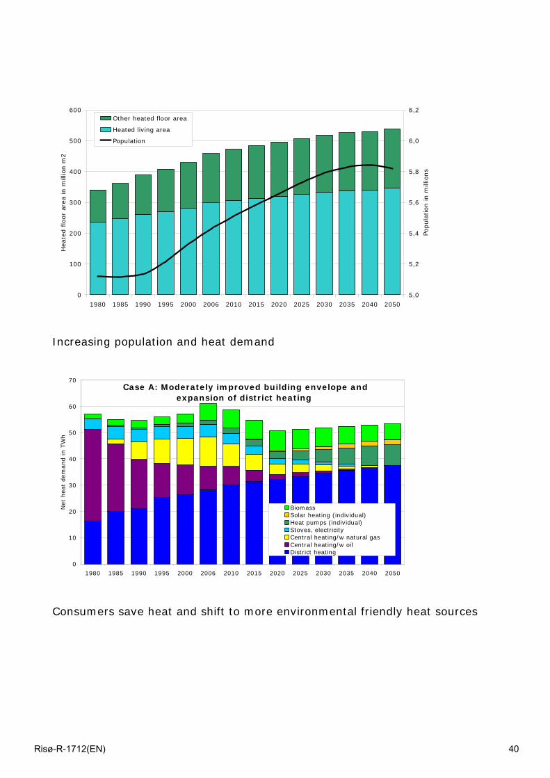
Increasing population and heat demand Consumers save heat and shift to more environmental friendly heat sources

0

100

200

300

400

500

600

1980 1985 1990 1995 2000 2006 2010 2015 2020 2025 2030 2035 2040 2050

Hea

ted f

loor

area

in m

illio

n m

2

5,0

5,2

5,4

5,6

5,8

6,0

6,2

Popula

tion in m

illio

ns

Other heated floor area

Heated living area

Population

0

10

20

30

40

50

60

70

1980 1985 1990 1995 2000 2006 2010 2015 2020 2025 2030 2035 2040 2050

Net

hea

t dem

and in T

Wh

BiomassSolar heating (individual)Heat pumps (individual)Stoves, electricityCentral heating/w natural gasCentral heating/w oilDistrict heating

Case A: Moderately improved building envelope and expansion of district heating

Risø-R-1712(EN) 40

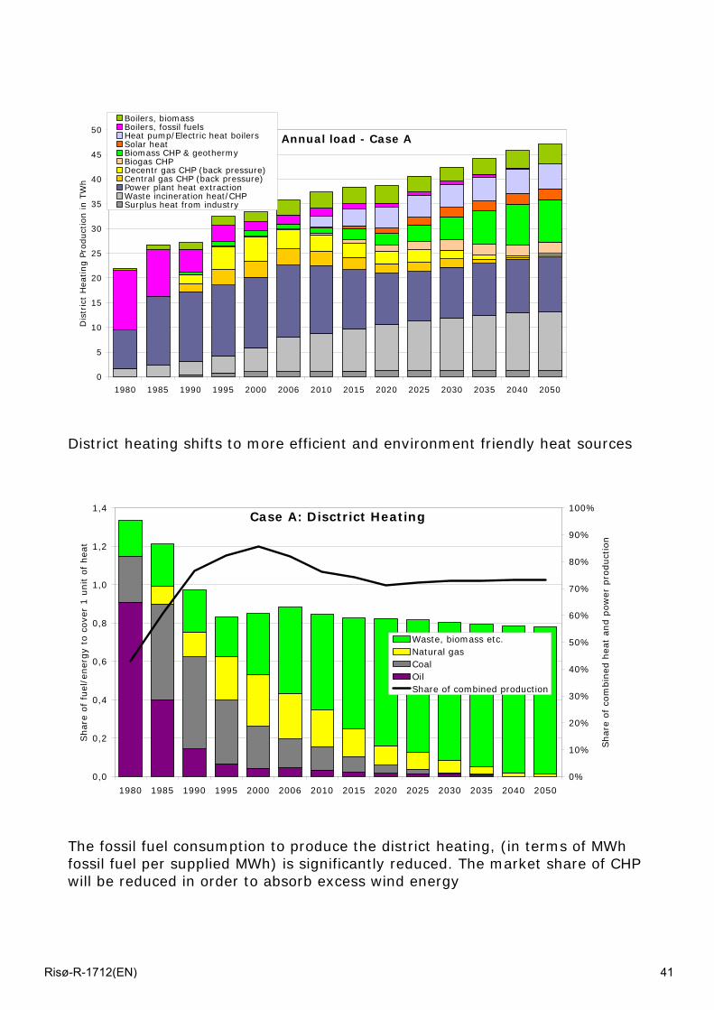
District heating shifts to more efficient and environment friendly heat sources The fossil fuel consumption to produce the district heating, (in terms of MWh fossil fuel per supplied MWh) is significantly reduced. The market share of CHP will be reduced in order to absorb excess wind energy

0

5

10

15

20

25

30

35

40

45

50

1980 1985 1990 1995 2000 2006 2010 2015 2020 2025 2030 2035 2040 2050

Dis

tric

t H

eating P

roduct

ion in T

Wh

Boilers, biomassBoilers, fossil fuelsHeat pump/Electric heat boilersSolar heatBiomass CHP & geothermyBiogas CHPDecentr gas CHP (back pressure) Central gas CHP (back pressure) Power plant heat extractionWaste incineration heat/CHPSurplus heat from industry

Annual load - Case A

0,0

0,2

0,4

0,6

0,8

1,0

1,2

1,4

1980 1985 1990 1995 2000 2006 2010 2015 2020 2025 2030 2035 2040 2050

Shar

e of

fuel

/ener

gy

to c

ove

r 1 u

nit o

f hea

t

0%

10%

20%

30%

40%

50%

60%

70%

80%

90%

100%

Shar

e of

com

bin

ed h

eat

and p

ow

er p

roduct

ion

Waste, biomass etc.Natural gasCoalOilShare of combined production

Case A: Disctrict Heating

Risø-R-1712(EN) 41

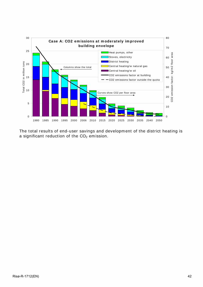
The total results of end-user savings and development of the district heating is a significant reduction of the CO2 emission.

0

5

10

15

20

25

30

1980 1985 1990 1995 2000 2006 2010 2015 2020 2025 2030 2035 2040 2050

Tota

l CO

2 in m

illio

n t

ons

0

10

20

30

40

50

60

70

80

CO

2 e

mis

sion fact

or:

kg/m

2 f

loor

area

Heat pumps, other

Stoves, electricity

District heating

Central heating/w natural gas

Central heating/w oil

CO2 emissions factor at building

CO2 emissions factor outside the quota

Case A: CO2 emissions at moderately improved building envelope

Curves show CO2 per floor area

Columns show the total

Risø-R-1712(EN) 42

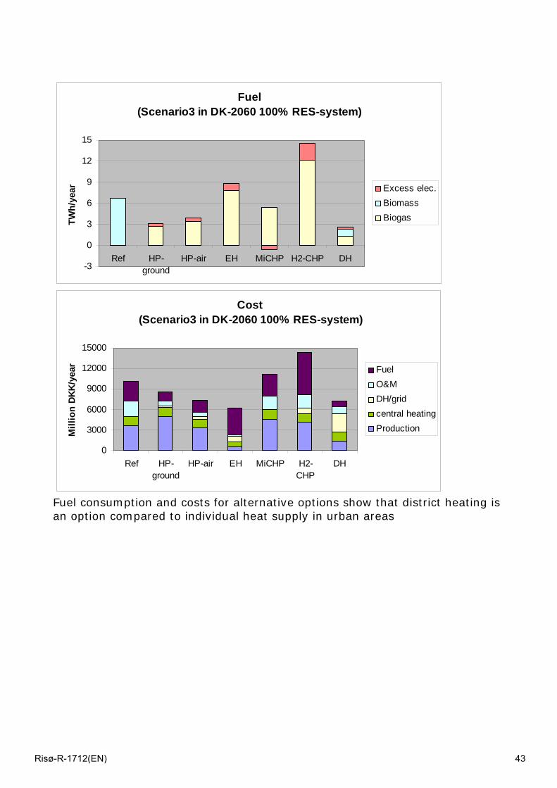
Fuel (Scenario3 in DK-2060 100% RES-system)

-3

0

3

6

9

12

15

Ref HP-ground

HP-air EH MiCHP H2-CHP DH

TWh/

year Excess elec.

BiomassBiogas

Cost (Scenario3 in DK-2060 100% RES-system)

0

3000

6000

9000

12000

15000

Ref HP-ground

HP-air EH MiCHP H2-CHP

DH

Mill

ion

DKK

/yea

r FuelO&MDH/gridcentral heatingProduction

Fuel consumption and costs for alternative options show that district heating is an option compared to individual heat supply in urban areas

Risø-R-1712(EN) 43

Session 2 – Long term energy solutions

Risø-R-1712(EN) 44

Paper at: RISO International Energy Conference, 14 – 16 September 2009, Copenhagen

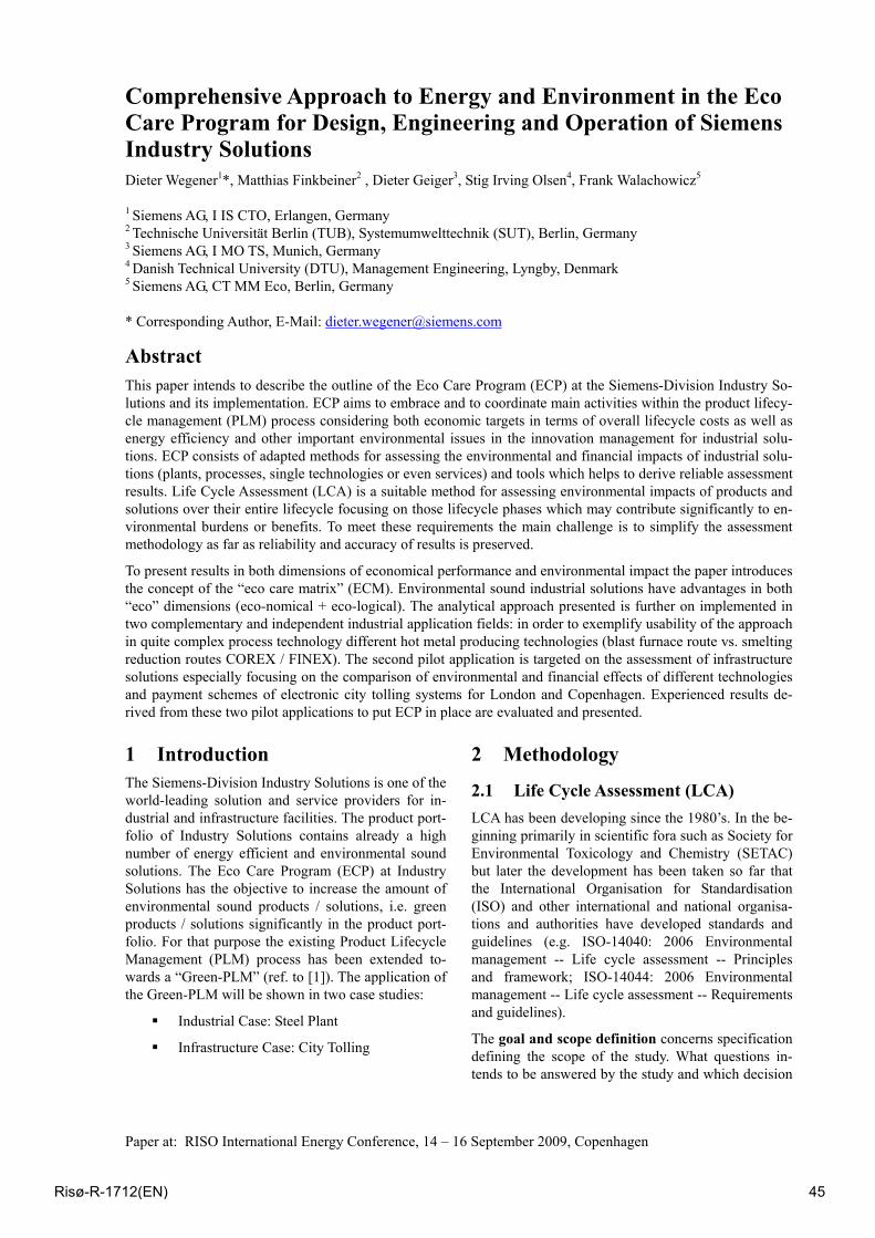
Comprehensive Approach to Energy and Environment in the Eco Care Program for Design, Engineering and Operation of Siemens Industry Solutions Dieter Wegener1*, Matthias Finkbeiner2 , Dieter Geiger3, Stig Irving Olsen4, Frank Walachowicz5 1 Siemens AG, I IS CTO, Erlangen, Germany 2 Technische Universität Berlin (TUB), Systemumwelttechnik (SUT), Berlin, Germany 3 Siemens AG, I MO TS, Munich, Germany 4 Danish Technical University (DTU), Management Engineering, Lyngby, Denmark 5 Siemens AG, CT MM Eco, Berlin, Germany * Corresponding Author, E-Mail: dieter.wegener@siemens.com

Abstract This paper intends to describe the outline of the Eco Care Program (ECP) at the Siemens-Division Industry So-lutions and its implementation. ECP aims to embrace and to coordinate main activities within the product lifecy-cle management (PLM) process considering both economic targets in terms of overall lifecycle costs as well as energy efficiency and other important environmental issues in the innovation management for industrial solu-tions. ECP consists of adapted methods for assessing the environmental and financial impacts of industrial solu-tions (plants, processes, single technologies or even services) and tools which helps to derive reliable assessment results. Life Cycle Assessment (LCA) is a suitable method for assessing environmental impacts of products and solutions over their entire lifecycle focusing on those lifecycle phases which may contribute significantly to en-vironmental burdens or benefits. To meet these requirements the main challenge is to simplify the assessment methodology as far as reliability and accuracy of results is preserved.

To present results in both dimensions of economical performance and environmental impact the paper introduces the concept of the “eco care matrix” (ECM). Environmental sound industrial solutions have advantages in both “eco” dimensions (eco-nomical + eco-logical). The analytical approach presented is further on implemented in two complementary and independent industrial application fields: in order to exemplify usability of the approach in quite complex process technology different hot metal producing technologies (blast furnace route vs. smelting reduction routes COREX / FINEX). The second pilot application is targeted on the assessment of infrastructure solutions especially focusing on the comparison of environmental and financial effects of different technologies and payment schemes of electronic city tolling systems for London and Copenhagen. Experienced results de-rived from these two pilot applications to put ECP in place are evaluated and presented.

1 Introduction The Siemens-Division Industry Solutions is one of the world-leading solution and service providers for in-dustrial and infrastructure facilities. The product port-folio of Industry Solutions contains already a high number of energy efficient and environmental sound solutions. The Eco Care Program (ECP) at Industry Solutions has the objective to increase the amount of environmental sound products / solutions, i.e. green products / solutions significantly in the product port-folio. For that purpose the existing Product Lifecycle Management (PLM) process has been extended to-wards a “Green-PLM” (ref. to [1]). The application of the Green-PLM will be shown in two case studies:

Industrial Case: Steel Plant

Infrastructure Case: City Tolling

2 Methodology

2.1 Life Cycle Assessment (LCA) LCA has been developing since the 1980’s. In the be-ginning primarily in scientific fora such as Society for Environmental Toxicology and Chemistry (SETAC) but later the development has been taken so far that the International Organisation for Standardisation (ISO) and other international and national organisa-tions and authorities have developed standards and guidelines (e.g. ISO-14040: 2006 Environmental management -- Life cycle assessment -- Principles and framework; ISO-14044: 2006 Environmental management -- Life cycle assessment -- Requirements and guidelines).

The goal and scope definition concerns specification defining the scope of the study. What questions in-tends to be answered by the study and which decision

Risø-R-1712(EN) 45

Paper at: RISO International Energy Conference, 14 – 16 September 2009, Copenhagen

should it support. A crucial point in LCA is the use of a functional unit which serves as the reference for the assessment, e.g. 1 ton of hot metal - or for a paint; e.g. the protection of a 10m2 surface for 10 year. The system boundary determines which unit processes are included in the LCA and must reflect the goal of the study. The intended data requirements are also de-scribed. Finally the goal and scope phase includes a description of the method applied for assessing poten-tial environmental impacts.

The life cycle inventory concerns the collection of data for inputs (energy, materials etc.) and outputs (products, waste, emissions) for each of the processes that are included in the study. All data are aggregated into one number for each input/output, e.g. the amount of CO2 emitted in each process is summed into one figure in the inventory.

The third phase 'Life Cycle Impact Assessment' is aimed at evaluating the contribution of each of the inventory items to impact categories such as global warming, acidification etc. Normally around 10 cate-gories are assessed: Global warming, ozone depletion, acidification, photochemical ozone formation, eutro-phication, toxicity to humans, ecotoxicity, land use, some solid waste, and resource use. Characterisation is the first step, in which the contribution of each in-ventory item to each impact category is calculated us-ing the characterisation factors of an impact assess-ment methodology. Characterisation factors are often expressed as an equivalent of a substance, e.g. for global warming CO2-equivalents are used. Different substances contribute to different extent to the impact, for example methane (CH4) has a global warming po-tential that is 25 times larger than CO2, i.e. 25 CO2-equivalents and nitrous oxide (laughing gas) has a po-tential of 250 CO2-equivalents. In this way 1 kg of methane and 1 kg of nitrous oxide can be summed to 275 kg CO2-equivalents. The next steps are normali-zation and weighting, but these are both voluntary according the ISO standard. Normalization is often expressed in person-equivalents i.e. what is the con-tribution of the assessed system compared to the total contribution of one person per year to that impact category. The normalisation provides a basis for com-paring different types of environmental impact cate-gories (all impacts get the same unit, person equiva-lents). The seriousness of the impacts can be taken into account through weighting. Weighting of the re-sults can be done in different ways e.g. expert panels, questionnaires or as distance to politically set reduc-tion targets. With the current global concern for cli-mate change it is plausible that global warming would receive a higher weighting than for instance photo-chemical ozone formation, which is a local/regional impact. Weighting of the results would change the

environmental profiles of the different systems ana-lysed and probably also the difference between them.

The 'interpretation' phase relates the results to the goal and scope. An analysis of major contributions, sensitivity analysis and uncertainty analysis leads to the conclusion whether the ambitions from the goal and scope can be met. More important; what can be learned form the LCA? All conclusions are drafted during this phase. Sometimes an independent critical review is necessary, especially when comparisons are made that are used in the public domain (ref. to [2]).

The European Union is in the process of developing The “International Reference Life Cycle Data Sys-tem” (ILCD) for good practice in LCA with aim of ensuring comparable and quality-assured LCA studies and applications in business and the public sector. The ILCD includes handbooks with requirements on method, quality, nomenclature, documentation, and review. Plus supporting documents and tools. And it goes a little further in the specifications than the ISO standards (refer to the European Commission home-page for Life Cycle Thinking in reference [3]).

Also the United States have developed a reference document for LCA. The LCA101 document from 2006, entitled "Life Cycle Assessment: Principles and Practice," provides an introductory overview of LCA and describes the general uses and major components of LCA. They also developed a Life Cycle Impact As-sessment methodology (TRACI) that is widely used in the US. All US EPA documents on LCA can be as-sessed (ref. to [4]).

The United Nations Environment Program, UNEP and the Society for Environmental Toxicology and Chemistry, SETAC launched an International Life Cycle Partnership, known as the Life Cycle Initiative, to enable users around the world to put life cycle thinking into effective practice. The mission of the Life Cycle Initiative is: “To develop and disseminate practical tools for evaluating the opportunities, risks, and trade-offs, associated with products and services over their whole life cycle.” The Life Cycle Initiative does not as such produce guidance documents but merely aims to further the use of life cycle thinking. At their website a range of documents related to LCA can be found (ref. to [5]).

In many other places around the world national initia-tives for building up LCA competences has been ini-tiated. At the Life cycle initiative website a good overview can be found, but one of the most notewor-thy is the LCA project in Japan, which is as far or even further than the European and US initiatives. More information about this can be found the home-page of the Japanese Environmental Management As-sociation for Industry (JEMAI, ref. to [6]).

Risø-R-1712(EN) 46

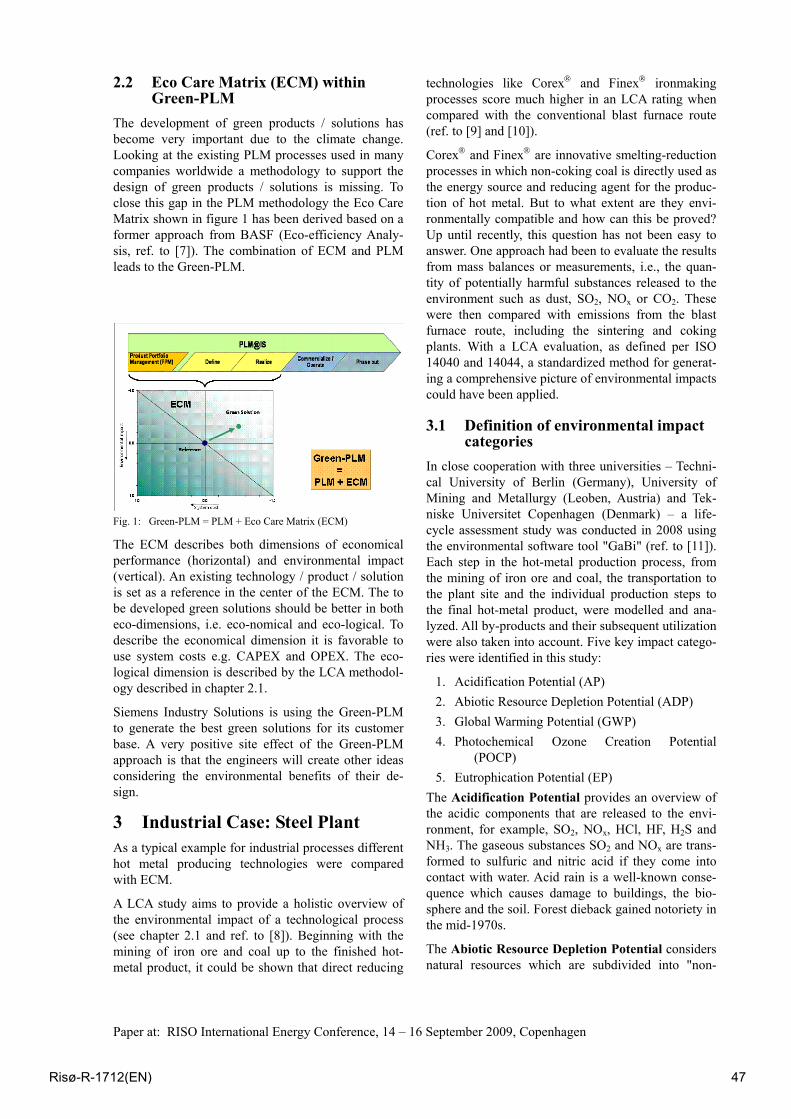
Paper at: RISO International Energy Conference, 14 – 16 September 2009, Copenhagen

2.2 Eco Care Matrix (ECM) within Green-PLM

The development of green products / solutions has become very important due to the climate change. Looking at the existing PLM processes used in many companies worldwide a methodology to support the design of green products / solutions is missing. To close this gap in the PLM methodology the Eco Care Matrix shown in figure 1 has been derived based on a former approach from BASF (Eco-efficiency Analy-sis, ref. to [7]). The combination of ECM and PLM leads to the Green-PLM.

Fig. 1: Green-PLM = PLM + Eco Care Matrix (ECM)

The ECM describes both dimensions of economical performance (horizontal) and environmental impact (vertical). An existing technology / product / solution is set as a reference in the center of the ECM. The to be developed green solutions should be better in both eco-dimensions, i.e. eco-nomical and eco-logical. To describe the economical dimension it is favorable to use system costs e.g. CAPEX and OPEX. The eco-logical dimension is described by the LCA methodol-ogy described in chapter 2.1.

Siemens Industry Solutions is using the Green-PLM to generate the best green solutions for its customer base. A very positive site effect of the Green-PLM approach is that the engineers will create other ideas considering the environmental benefits of their de-sign.

3 Industrial Case: Steel Plant As a typical example for industrial processes different hot metal producing technologies were compared with ECM.

A LCA study aims to provide a holistic overview of the environmental impact of a technological process (see chapter 2.1 and ref. to [8]). Beginning with the mining of iron ore and coal up to the finished hot-metal product, it could be shown that direct reducing

technologies like Corex® and Finex® ironmaking processes score much higher in an LCA rating when compared with the conventional blast furnace route (ref. to [9] and [10]).

Corex® and Finex® are innovative smelting-reduction processes in which non-coking coal is directly used as the energy source and reducing agent for the produc-tion of hot metal. But to what extent are they envi-ronmentally compatible and how can this be proved? Up until recently, this question has not been easy to answer. One approach had been to evaluate the results from mass balances or measurements, i.e., the quan-tity of potentially harmful substances released to the environment such as dust, SO2, NOx or CO2. These were then compared with emissions from the blast furnace route, including the sintering and coking plants. With a LCA evaluation, as defined per ISO 14040 and 14044, a standardized method for generat-ing a comprehensive picture of environmental impacts could have been applied.

3.1 Definition of environmental impact categories

In close cooperation with three universities – Techni-cal University of Berlin (Germany), University of Mining and Metallurgy (Leoben, Austria) and Tek-niske Universitet Copenhagen (Denmark) – a life-cycle assessment study was conducted in 2008 using the environmental software tool "GaBi" (ref. to [11]). Each step in the hot-metal production process, from the mining of iron ore and coal, the transportation to the plant site and the individual production steps to the final hot-metal product, were modelled and ana-lyzed. All by-products and their subsequent utilization were also taken into account. Five key impact catego-ries were identified in this study:

1. Acidification Potential (AP) 2. Abiotic Resource Depletion Potential (ADP) 3. Global Warming Potential (GWP) 4. Photochemical Ozone Creation Potential

(POCP) 5. Eutrophication Potential (EP)

The Acidification Potential provides an overview of the acidic components that are released to the envi-ronment, for example, SO2, NOx, HCl, HF, H2S and NH3. The gaseous substances SO2 and NOx are trans-formed to sulfuric and nitric acid if they come into contact with water. Acid rain is a well-known conse-quence which causes damage to buildings, the bio-sphere and the soil. Forest dieback gained notoriety in the mid-1970s.

The Abiotic Resource Depletion Potential considers natural resources which are subdivided into "non-

Risø-R-1712(EN) 47

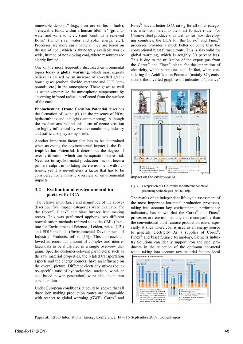
Paper at: RISO International Energy Conference, 14 – 16 September 2009, Copenhagen

renewable deposits" (e.g., iron ore or fossil fuels), "renewable funds within a human lifetime" (ground-water and some soils, etc.) and "continually renewed flows" (wind, river water and solar energy, etc.). Processes are more sustainable if they are based on the use of coal, which is abundantly available world-wide, instead of non-coking coal, where resources are clearly limited.

One of the most frequently discussed environmental topics today is global warming, which most experts believe is caused by an increase of so-called green-house gases (carbon dioxide, methane and CFC com-pounds, etc.) in the atmosphere. These gases as well as water vapor raise the atmospheric temperature by absorbing infrared radiation reflected from the surface of the earth.

Photochemical Ozone Creation Potential describes the formation of ozone (O3) in the presence of NOx, hydrocarbons and sunlight (summer smog). Although the mechanisms behind this form of ozone creation are highly influenced by weather conditions, industry and traffic also play a major role.

Another important factor that has to be determined when assessing the environmental impact is the Eu-trophication Potential. It determines the degree of over-fertilization, which can be aquatic or terrestrial. Needless to say, hot-metal production has not been a primary culprit in polluting the environment with nu-trients, yet it is nevertheless a factor that has to be considered for a holistic overview of environmental impacts.

3.2 Evaluation of environmental im-pacts with LCA

The relative importance and magnitude of the above-described five impact categories were evaluated for the Corex®, Finex® and blast furnace iron making routes. This was performed applying two different normalization methods referred to as the CML (Insti-tute for Environmental Sciences, Leiden, ref. to [12]) and EDIP methods (Environmental Development of Industrial Products, ref. to [13]). This approach al-lowed an enormous amount of complex and interre-lated data to be illustrated in a single overview dia-gram. Specific customer-relevant parameters, such as the raw material properties, the related transportation aspects and the energy sources, have an influence on the overall picture. Different electricity mixes (coun-try-specific ratio of hydroelectric-, nuclear-, wind- or coal-based power generation) were also taken into consideration.

Under European conditions, it could be shown that all three iron making production routes are comparable with respect to global warming (GWP). Corex® and

Finex® have a better LCA rating for all other catego-ries when compared to the blast furnace route. For Chinese steel producers, as well as for most develop-ing countries, the LCA for the Corex® and Finex® processes provides a much better outcome than the conventional blast furnace route. This is also valid for global warming, which is roughly 30 percent less. This is due to the utilization of the export gas from the Corex® and Finex® plants for the generation of electricity, which substitutes coal. In fact, when con-sidering the Acidification Potential (mainly SO2 emis-sions), the inverted graph result indicates a "positive"

impact on the environment.

Fig. 2: Comparison of LCA results for different hot metal producing technologies (ref. to [10]).

The results of an independent life-cycle assessment of the most important hot-metal production processes, taking into account key environmental performance indicators, has shown that the Corex® and Finex® processes are environmentally more compatible than the conventional blast furnace production route, espe-cially at sites where coal is used as an energy source to generate electricity. As a supplier of Corex®, Finex® and blast furnace technology, Siemens Indus-try Solutions can ideally support iron and steel pro-ducers in the selection of the optimum hot-metal route, taking into account raw material factors, local

Risø-R-1712(EN) 48

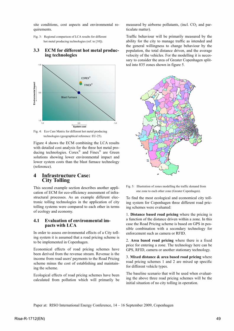
Paper at: RISO International Energy Conference, 14 – 16 September 2009, Copenhagen

site conditions, cost aspects and environmental re-quirements.

Fig. 3: Regional comparison of LCA results for different hot metal producing technologies (ref. to [10]).

3.3 ECM for different hot metal produc-ing technologies

Fig. 4: Eco Care Matrix for different hot metal producing technologies (geographical reference: EU-25).

Figure 4 shows the ECM combining the LCA results with detailed cost analysis for the three hot metal pro-ducing technologies. Corex® and Finex® are Green solutions showing lower environmental impact and lower system costs than the blast furnace technology (reference).

4 Infrastructure Case: City Tolling

This second example section describes another appli-cation of ECM for eco-efficiency assessment of infra-structural processes. As an example different elec-tronic tolling technologies in the application of city tolling systems were compared to each other in terms of ecology and economy.

4.1 Evaluation of environmental im-pacts with LCA

In order to assess environmental effects of a City toll-ing system it is assumed that a road pricing scheme is to be implemented in Copenhagen.

Economical effects of road pricing schemes have been derived from the revenue stream. Revenue is the income from road users' payments to the Road Pricing scheme minus the cost of establishing and maintain-ing the scheme.

Ecological effects of road pricing schemes have been calculated from pollution which will primarily be

measured by airborne pollutants, (incl. CO2 and par-ticulate matter).

Traffic behaviour will be primarily measured by the ability for the city to manage traffic as intended and the general willingness to change behaviour by the population, the total distance driven, and the average velocity of the vehicles. For the modelling it is neces-sary to consider the area of Greater Copenhagen split-ted into 835 zones shown in figure 5.

Fig. 5: Illustration of zones modelling the traffic demand from one zone to each other zone (Greater Copenhagen).

To find the most ecological and economical city toll-ing system for Copenhagen three different road pric-ing schemes were evaluated:

1. Distance based road pricing where the pricing is a function of the distance driven within a zone. In this case the Road Pricing scheme is based on GPS in pos-sible combination with a secondary technology for enforcement such as camera or RFID.

2. Area based road pricing where there is a fixed price for entering a zone. The technology here can be GPS, RFID, camera or another stationary technology.

3. Mixed distance & area based road pricing where road pricing schemes 1 and 2 are mixed up specific for different vehicle types.

The baseline scenario that will be used when evaluat-ing the above three road pricing schemes will be the initial situation of no city tolling in operation.

-1,0

0,0

1,0-1,00,01,0

Env

ironm

enta

l Im

pact

System cost

Blast Furnace

COREX®

FINEX®

Risø-R-1712(EN) 49

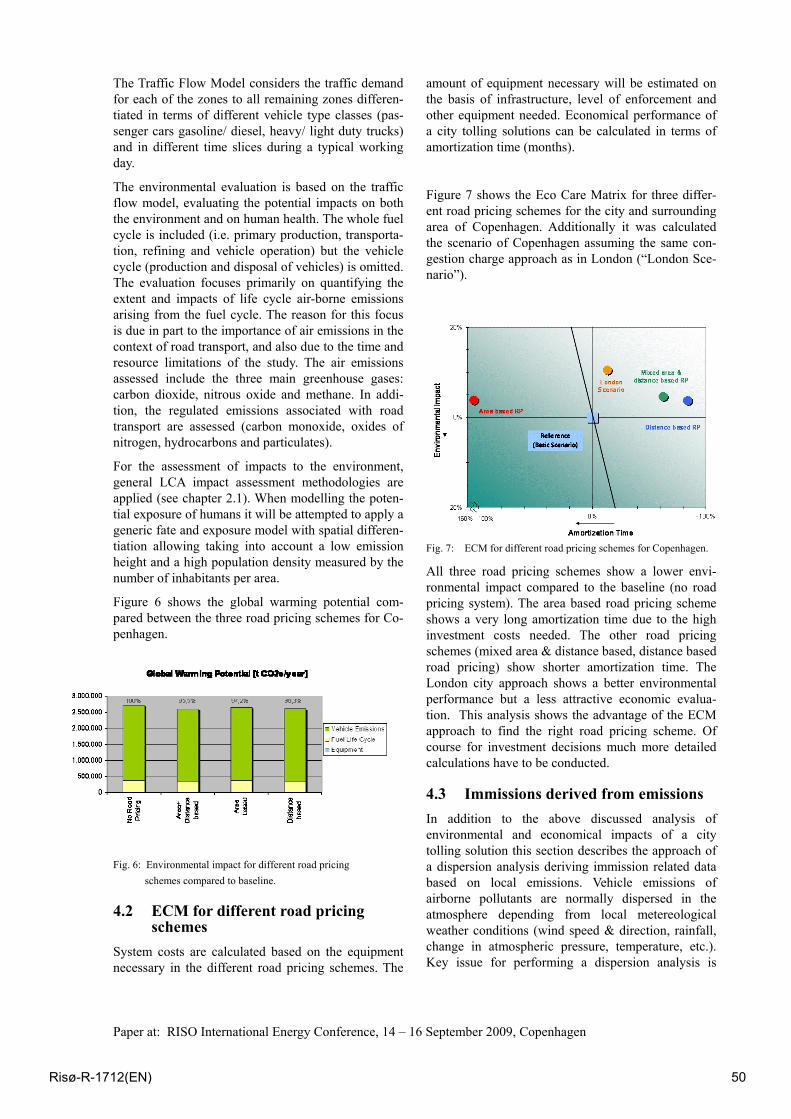
Paper at: RISO International Energy Conference, 14 – 16 September 2009, Copenhagen

The Traffic Flow Model considers the traffic demand for each of the zones to all remaining zones differen-tiated in terms of different vehicle type classes (pas-senger cars gasoline/ diesel, heavy/ light duty trucks) and in different time slices during a typical working day.

The environmental evaluation is based on the traffic flow model, evaluating the potential impacts on both the environment and on human health. The whole fuel cycle is included (i.e. primary production, transporta-tion, refining and vehicle operation) but the vehicle cycle (production and disposal of vehicles) is omitted. The evaluation focuses primarily on quantifying the extent and impacts of life cycle air-borne emissions arising from the fuel cycle. The reason for this focus is due in part to the importance of air emissions in the context of road transport, and also due to the time and resource limitations of the study. The air emissions assessed include the three main greenhouse gases: carbon dioxide, nitrous oxide and methane. In addi-tion, the regulated emissions associated with road transport are assessed (carbon monoxide, oxides of nitrogen, hydrocarbons and particulates).

For the assessment of impacts to the environment, general LCA impact assessment methodologies are applied (see chapter 2.1). When modelling the poten-tial exposure of humans it will be attempted to apply a generic fate and exposure model with spatial differen-tiation allowing taking into account a low emission height and a high population density measured by the number of inhabitants per area.

Figure 6 shows the global warming potential com-pared between the three road pricing schemes for Co-penhagen.

Fig. 6: Environmental impact for different road pricing schemes compared to baseline.

4.2 ECM for different road pricing schemes

System costs are calculated based on the equipment necessary in the different road pricing schemes. The

amount of equipment necessary will be estimated on the basis of infrastructure, level of enforcement and other equipment needed. Economical performance of a city tolling solutions can be calculated in terms of amortization time (months).

Figure 7 shows the Eco Care Matrix for three differ-ent road pricing schemes for the city and surrounding area of Copenhagen. Additionally it was calculated the scenario of Copenhagen assuming the same con-gestion charge approach as in London (“London Sce-nario”).

Fig. 7: ECM for different road pricing schemes for Copenhagen.

All three road pricing schemes show a lower envi-ronmental impact compared to the baseline (no road pricing system). The area based road pricing scheme shows a very long amortization time due to the high investment costs needed. The other road pricing schemes (mixed area & distance based, distance based road pricing) show shorter amortization time. The London city approach shows a better environmental performance but a less attractive economic evalua-tion. This analysis shows the advantage of the ECM approach to find the right road pricing scheme. Of course for investment decisions much more detailed calculations have to be conducted.

4.3 Immissions derived from emissions In addition to the above discussed analysis of environmental and economical impacts of a city tolling solution this section describes the approach of a dispersion analysis deriving immission related data based on local emissions. Vehicle emissions of airborne pollutants are normally dispersed in the atmosphere depending from local metereological weather conditions (wind speed & direction, rainfall, change in atmospheric pressure, temperature, etc.). Key issue for performing a dispersion analysis is

Risø-R-1712(EN) 50

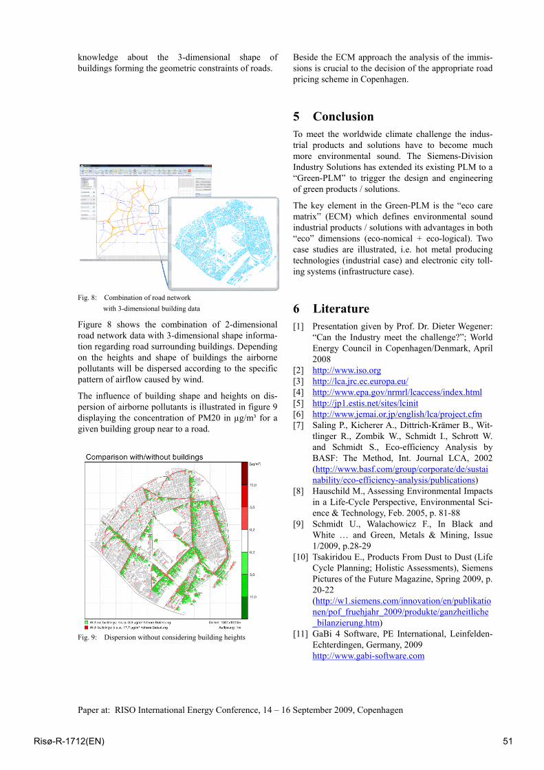
Paper at: RISO International Energy Conference, 14 – 16 September 2009, Copenhagen

knowledge about the 3-dimensional shape of buildings forming the geometric constraints of roads.

Fig. 8: Combination of road network with 3-dimensional building data

Figure 8 shows the combination of 2-dimensional road network data with 3-dimensional shape informa-tion regarding road surrounding buildings. Depending on the heights and shape of buildings the airborne pollutants will be dispersed according to the specific pattern of airflow caused by wind.

The influence of building shape and heights on dis-persion of airborne pollutants is illustrated in figure 9 displaying the concentration of PM20 in µg/m³ for a given building group near to a road.

Fig. 9: Dispersion without considering building heights

Beside the ECM approach the analysis of the immis-sions is crucial to the decision of the appropriate road pricing scheme in Copenhagen.

5 Conclusion To meet the worldwide climate challenge the indus-trial products and solutions have to become much more environmental sound. The Siemens-Division Industry Solutions has extended its existing PLM to a “Green-PLM” to trigger the design and engineering of green products / solutions.

The key element in the Green-PLM is the “eco care matrix” (ECM) which defines environmental sound industrial products / solutions with advantages in both “eco” dimensions (eco-nomical + eco-logical). Two case studies are illustrated, i.e. hot metal producing technologies (industrial case) and electronic city toll-ing systems (infrastructure case).

6 Literature [1] Presentation given by Prof. Dr. Dieter Wegener:

“Can the Industry meet the challenge?”; World Energy Council in Copenhagen/Denmark, April 2008

[2] http://www.iso.org [3] http://lca.jrc.ec.europa.eu/ [4] http://www.epa.gov/nrmrl/lcaccess/index.html [5] http://jp1.estis.net/sites/lcinit [6] http://www.jemai.or.jp/english/lca/project.cfm [7] Saling P., Kicherer A., Dittrich-Krämer B., Wit-

tlinger R., Zombik W., Schmidt I., Schrott W. and Schmidt S., Eco-efficiency Analysis by BASF: The Method, Int. Journal LCA, 2002 (http://www.basf.com/group/corporate/de/sustainability/eco-efficiency-analysis/publications)

[8] Hauschild M., Assessing Environmental Impacts in a Life-Cycle Perspective, Environmental Sci-ence & Technology, Feb. 2005, p. 81-88

[9] Schmidt U., Walachowicz F., In Black and White … and Green, Metals & Mining, Issue 1/2009, p.28-29

[10] Tsakiridou E., Products From Dust to Dust (Life Cycle Planning; Holistic Assessments), Siemens Pictures of the Future Magazine, Spring 2009, p. 20-22 (http://w1.siemens.com/innovation/en/publikationen/pof_fruehjahr_2009/produkte/ganzheitliche_bilanzierung.htm)

[11] GaBi 4 Software, PE International, Leinfelden-Echterdingen, Germany, 2009

http://www.gabi-software.com

Risø-R-1712(EN) 51

Paper at: RISO International Energy Conference, 14 – 16 September 2009, Copenhagen

[12] Heijungs, R.; et al. Environmental Life Cycle Assessment of Products; Guide Report No. 9266, Institute of Environmental Sciences, Lei-den University, The Netherlands, 1992.

[13] Wenzel, H.; Hauschild, M. Z.; Alting, L. Envi-ronmental Assessment of Products: Methodol-ogy, Tools, Techniques and Case Studies in Product Development; Kluwer Academic Pub-lishers: Hingham, MA, 1997; Vol. 1.

Risø-R-1712(EN) 52

Report

DONG Energy Power A/S Kraftværksvej 53 7000 Fredericia Denmark Tel +45 99 55 11 11 Fax +45 76 22 19 62 www.dongenergy.com Company No. 18 93 66 74

15 July 2009

Our ref. JORBU/LIBPE Doc. No. 570825 Project No. 141154-02 Responsible: QA: jorbu@dongenergy.dk Tel +45 99 55 75 58

Report title The role of high efficiency steam power plants - development status Authors Rudolph Blum, Director,

Head Technology Development, DONG Energy Power, Engi-

neering and Technology, Kraftværksvej 53,

DK-7000 Fredericia, Denmark.

E-mail: rblum@dongenergy.dk. Telephone: +45 99 55 12 46.

Jørgen Bugge, Senior Manager,

DONG Energy Power, Engineering and Technology,

Kraftværksvej 53, DK-7000 Fredericia, Denmark.

E-mail: jorbu@dongenergy.dk. Telephone: +45 99 55 75 58.

Risø-R-1712(EN) 53

Doc. No. 570825

Abstract The political ambition of replacing fossil energy with renewable energy will be a huge task, and contrary to the first thought, the development of high efficiency steam plants will still play an important role in future as renewable energy is characterised by its fluctuating nature – wind and solar energy over days and weeks, and biomass over years. Coal based and/or nuclear power will still be necessary for a long time to come in order to guarantee the stability and security of supply. The coal-based steam plant also offers the most efficient utilisation of biomass and it can be equipped with carbon capture. This paper will describe the current status - which involves steam temperatures around 600 oC and steam pressure close to 300 bar – and the possible lines of development. The thermodynamic process can be optimised with features such as double reheat and more sophisticated cycles such as the Master Cycle. In order to compensate for the fluctuating nature of mainly wind energy, it will be important to maximise ‘load following’ capability and to be able to operate at low minimum loads. The work on the 700 oC steam temperature plant (AD 700) is now so advanced that E.ON has declared its readiness to build such a plant. As a new development the possibility of getting steel which would allow steam temperatures up to 650 oC has now become much more realistic as the Z-phase steel is now in the process of qualification, and if it is qualified it will offer a more economic solution than AD 700. Regarding Carbon Capture, the MEA-based absorption plant is the only avail-able commercially mature solution today, but other absorption technologies are under development. Another post combustion technology is oxyfuel involving combustion in an at-mosphere of oxygen and re-circulated CO2. This simplifies the carbon capture process as there is no need for handling large amounts of Nitrogen. The IGCC plant has not yet had success in electricity production, but might have advantages in the future in relation to carbon capture. 1. The importance of coal

Although the amount of power production based on renewable energy is ex-pected to more than double from 2005 to 2030 on a global basis, the amount of power production based on coal in the same period is also expected to be dou-bled. These assumptions are based on a doubling of the total power production. In Europe, power based on renewable energy is foreseen to be tripled and power based on coal is expected to remain at nearly the same level in the same period.

Risø-R-1712(EN) 54

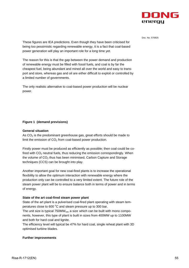
Doc. No. 570825

These figures are IEA predictions. Even though they have been criticised for being too pessimistic regarding renewable energy, it is a fact that coal-based power generation will play an important role for a long time yet. The reason for this is that the gap between the power demand and production of renewable energy must be filled with fossil fuels, and coal is by far the cheapest fuel, being abundant and mined all over the world and easy to trans-port and store, whereas gas and oil are either difficult to exploit or controlled by a limited number of governments. The only realistic alternative to coal-based power production will be nuclear power. Figure 1 (demand previsions) General situation As CO2 is the predominant greenhouse gas, great efforts should be made to limit the emission of CO2 from coal-based power production. Firstly power must be produced as efficiently as possible; then coal could be co-fired with CO2 neutral fuels, thus reducing the emission correspondingly. When the volume of CO2 thus has been minimised, Carbon Capture and Storage techniques (CCS) can be brought into play. Another important goal for new coal-fired plants is to increase the operational flexibility to allow the optimum interaction with renewable energy where the production only can be controlled to a very limited extent. The future role of the steam power plant will be to ensure balance both in terms of power and in terms of energy. State of the art coal-fired steam power plant State of the art plant is a pulverised coal-fired plant operating with steam tem-peratures close to 600 oC and steam pressure up to 300 bar. The unit size is typical 750MWnet, a size which can be built with mono compo-nents, however, this type of plant is built in sizes from 400MW up to 1100MW and both for hard coal and lignite. The efficiency level will typical be 47% for hard coal, single reheat plant with 3D optimised turbine blades. Further improvements

Risø-R-1712(EN) 55

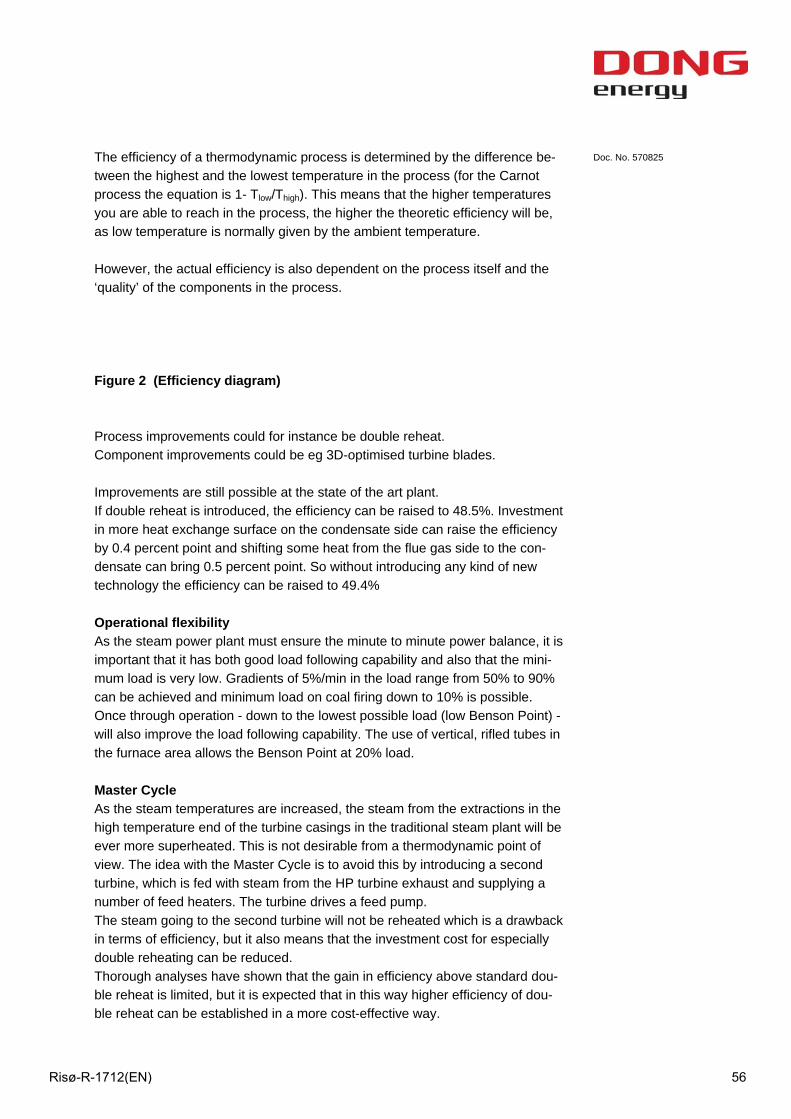
Doc. No. 570825

The efficiency of a thermodynamic process is determined by the difference be-tween the highest and the lowest temperature in the process (for the Carnot process the equation is 1- Tlow/Thigh). This means that the higher temperatures you are able to reach in the process, the higher the theoretic efficiency will be, as low temperature is normally given by the ambient temperature. However, the actual efficiency is also dependent on the process itself and the ‘quality’ of the components in the process. Figure 2 (Efficiency diagram) Process improvements could for instance be double reheat. Component improvements could be eg 3D-optimised turbine blades. Improvements are still possible at the state of the art plant. If double reheat is introduced, the efficiency can be raised to 48.5%. Investment in more heat exchange surface on the condensate side can raise the efficiency by 0.4 percent point and shifting some heat from the flue gas side to the con-densate can bring 0.5 percent point. So without introducing any kind of new technology the efficiency can be raised to 49.4% Operational flexibility As the steam power plant must ensure the minute to minute power balance, it is important that it has both good load following capability and also that the mini-mum load is very low. Gradients of 5%/min in the load range from 50% to 90% can be achieved and minimum load on coal firing down to 10% is possible. Once through operation - down to the lowest possible load (low Benson Point) -will also improve the load following capability. The use of vertical, rifled tubes in the furnace area allows the Benson Point at 20% load. Master Cycle As the steam temperatures are increased, the steam from the extractions in the high temperature end of the turbine casings in the traditional steam plant will be ever more superheated. This is not desirable from a thermodynamic point of view. The idea with the Master Cycle is to avoid this by introducing a second turbine, which is fed with steam from the HP turbine exhaust and supplying a number of feed heaters. The turbine drives a feed pump. The steam going to the second turbine will not be reheated which is a drawback in terms of efficiency, but it also means that the investment cost for especially double reheating can be reduced. Thorough analyses have shown that the gain in efficiency above standard dou-ble reheat is limited, but it is expected that in this way higher efficiency of dou-ble reheat can be established in a more cost-effective way.

Risø-R-1712(EN) 56

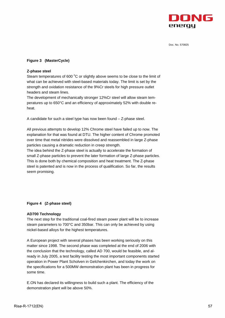
Doc. No. 570825

Figure 3 (MasterCycle) Z-phase steel Steam temperatures of 600 oC or slightly above seems to be close to the limit of what can be achieved with steel-based materials today. The limit is set by the strength and oxidation resistance of the 9%Cr steels for high pressure outlet headers and steam lines. The development of mechanically stronger 12%Cr steel will allow steam tem-peratures up to 650°C and an efficiency of approximately 52% with double re-heat. A candidate for such a steel type has now been found – Z-phase steel. All previous attempts to develop 12% Chrome steel have failed up to now. The explanation for that was found at DTU. The higher content of Chrome promoted over time that metal nitrides were dissolved and reassembled in large Z-phase particles causing a dramatic reduction in creep strength. The idea behind the Z-phase steel is actually to accelerate the formation of small Z-phase particles to prevent the later formation of large Z-phase particles. This is done both by chemical composition and heat treatment. The Z-phase steel is patented and is now in the process of qualification. So far, the results seem promising. Figure 4 (Z-phase steel) AD700 Technology The next step for the traditional coal-fired steam power plant will be to increase steam parameters to 700°C and 350bar. This can only be achieved by using nickel-based alloys for the highest temperatures. A European project with several phases has been working seriously on this matter since 1998. The second phase was completed at the end of 2006 with the conclusion that the technology, called AD 700, would be feasible, and al-ready in July 2005, a test facility testing the most important components started operation in Power Plant Scholven in Gelchenkirchen, and today the work on the specifications for a 500MW demonstration plant has been in progress for some time. E.ON has declared its willingness to build such a plant. The efficiency of the demonstration plant will be above 50%.

Risø-R-1712(EN) 57

Doc. No. 570825

Efficiency can be increased to 53% by using double reheat and introducing the Master Cycle. Co-firing of biomass Biomass is considered to be CO2 neutral and can be co-fired with coal. Up to 10% biomass on energy basis can be co-fired without this causing any prob-lems, as the corrosive elements in the biomass (especially in straw) are neutral-ised by the coal ash. Co-firing of biomass in a high efficiency coal-fired plant demonstrates by far the most CO2-reducing effect. Combusting biomass in a stand-alone biomass-fired boiler gives a lower potential for CO2-reduction due to the lower steam parameters caused by the fireside corrosion beginning at a steam temperature of 540°C. The biomass will normally be residual products from farming and the wood in-dustry, but it can also come from household waste. The 10% limit is set by the standards for utilisation of the fly ash in the produc-tion of cement and concrete. Up to 20% straw has been co-fired without corro-sion problems and deterioration of the catalyst in the DeNOx plant. In fact, the boiler can be fired entirely with wood pellets, if that is considered an option. In future, the general trend will be to design the modern steam plant for a very high degree of fuel flexibility, because it will be up to the plant to ensure the energy balance in the electrical system. Another trend might lead towards smaller plants due to the problem of trans-porting and handling of the greater volumes of biomass (as long as the effi-ciency is not significantly reduced). The investment cost of the mentioned co-firing possibilities is relatively small. For the most difficult types of biomass there is the possibility of gasifying it in a separate gasifier and burn the gas in the normal boiler. In this way, corrosion problems and contamination of the useful fly ash can be avoided. Post combustion Carbon Capture Carbon Capture has very high priority, but at the moment, it is not clear what the best technology will be and there might actually be a number of technolo-gies which will be relevant in the same way as a number of technologies will be relevant to power production. At the moment, there is only one commercial technology available and it is based on absorption by amines of which mono-ethanol-amine (MEA) is the standard absorbent. It has been commercially available for many years for the

Risø-R-1712(EN) 58

Doc. No. 570825

production of CO2 for industrial applications, and the EU-funded CASTOR pro-ject has shown that it can also be used for flue gasses from coal-fired power plants. Unfortunately, the energy consumption for the process is very high and implies a reduction in efficiency of about 10 percentage points. MEA is relatively corrosive and the consumption of MEA in the process is also relatively high. Great efforts are made to find absorbents with lower energy consumption and better chemical properties. Several vendors have announced processes with significant lower energy consumption; however, these processes have not yet been proven in large scale on flue gasses from coal-fired power plants. A new and very interesting process is called chilled ammonia. This process has much lower energy consumption, but the process is in a very early stage of development. The absorption takes place at temperatures between 2 and 10oC. The low temperature has several advantages, but the important question is whether the low temperature will bring sufficient absorption kinetics to obtain an acceptable plant. In any case the process is interesting. In 2006, the process was patented by Alstom and the first pilot plant is now in operation. The first test results are expected to be available by the end of 2009. The amine processes and the chilled ammonia process are called post-combustion technologies, as the CO2 is removed after the combustion process. They are suitable both for new plants and for retrofit of existing plants. Oxyfuel combustion Another version of the coal-fired steam power plant is the oxyfuel combustion plant. In this process the combustion takes place in an atmosphere of oxygen and re-circulated CO2. The combustion ‘air’ is pure oxygen from an air separa-tion plant and CO2 is re-circulated to ‘ease’ the combustion conditions in the boiler. The flue gas will consist of water vapour and CO2 and smaller amounts of other gases, among which SOx and NOx will be the most important. Water can be separated from CO2 by simple cooling, and by subsequent compression the largest part of the impurities will follow the water. However, it is unclear if addi-tional purification of the CO2 is required. Oxyfuel Combustion can have advantages in relation to Carbon Capture be-cause smaller volumes are to be handled in the capture plant as Nitrogen is excluded from the process. Oxyfuel is also a post-combustion capture technology Oxyfuel pilot plants are now in operation and many consider the technology to be very promising, although it is generally assumed that it will take longer time for this technology to mature than the post-combustion processes described above. Figure 5 (CCS technologies)

Risø-R-1712(EN) 59

Doc. No. 570825

Integrated Gasification Combined Cycle (IGCC) An alternative to the traditional steam power plant is the IGCC plant where coal is gasified (normally in pure oxygen) in a gasifier and steam is added to the CO rich gas and a shift reaction takes place, where the CO takes the Oxygen atom from the water molecule. The resulting gas will get a high content of hydrogen (and CO2). The hydrogen is subsequently burned in a gas turbine followed by a traditional combined cycle. The IGCC plant has the potential for high efficiency, but the technology is much more complex than the traditional steam cycle, and consequently the availability has been limited up until now. The plants which are in commercial operation are all run in connection with refineries where petro-coke or other oil residues can be used as fuel and the hydrogen, alternatively, can be used in chemical proc-esses. In terms of CO2 capture, IGCC might have an advantage compared to the tradi-tional steam plant as the concentration of CO2 in the gas is high and the gas is under pressure, so the CO2 separation plant can be much smaller. As the CO2 is removed before the final combustion in the gas turbine the process is called pre-combustion capture.

Risø-R-1712(EN) 60

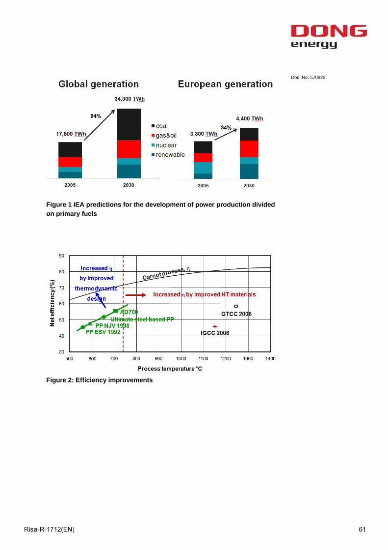
Doc. No. 570825

Figure 1 IEA predictions for the development of power production divided on primary fuels

Figure 2: Efficiency improvements

Risø-R-1712(EN) 61

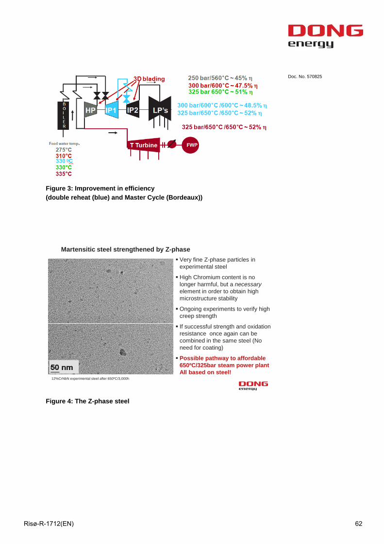
Doc. No. 570825

Figure 3: Improvement in efficiency (double reheat (blue) and Master Cycle (Bordeaux))

Martensitic steel strengthened by Z-phaseVery fine Z-phase particles in experimental steel

High Chromium content is no longer harmful, but a necessaryelement in order to obtain high microstructure stability

Ongoing experiments to verify high creep strength

If successful strength and oxidation resistance once again can be combined in the same steel (No need for coating)

Possible pathway to affordable 650ºC/325bar steam power plant All based on steel!

12%CrNbN experimental steel after 650ºC/3,000h

Figure 4: The Z-phase steel

Risø-R-1712(EN) 62

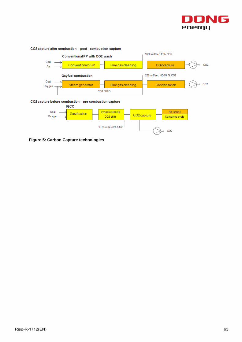
Doc. No. 570825

Figure 5: Carbon Capture technologies

Risø-R-1712(EN) 63

Session 3 – Systems aspects 1

Risø-R-1712(EN) 64

Why go for less? – Denmark 100% C02-neutral on energy production before 2050 Jens Christian Riise, Torben Chrintz, Niels Bahnsen and Erik C. Wormslev

NIRAS A/S, Climate Change and Energy

Sortemosevej 2

DK-3450 Allerød, Denmark

Telephone: + 45 48 10 46 97

Fax: +45 48 10 00 00

E-mail: jcr@niras.dk Website: www.niras.com

Abstract It has been argued, that the necessary technologies will be at hand to make total switch from the present reliance on fossil energy to a 100% non-fossil energy supply in Denmark already by 2050. Apart from efficient storage and transformation of energy, three areas will become the back-bone of the future energy system:

a. Intelligent energy use and consumption-reduction in households, industry and transportation;

b. Electric energy transformation from the sun via photovoltaics, wind and wave energy, and

c. Biomass conversion to electricity, heat, feeds and biofuels.

Based on a recent study in Region Nordjylland, the northern-most part of Denmark, the paper will present how energy production and consumption may be balanced in 2050, with particular focus on biomass production and its use. It is important to acknowledge that land-use and land-use change and forestry (LULUCF) will play a pivotal role in reaching the goal of 80-90% reduction of green-house-gas emissions before 2050. Even if energy supply and consumption have become 100% renewable, agriculture and industry, and in particular animal husbandry will continue to emit large quantities of green-house-gasses, and Danish consumption of imported goods will continue to emit large amounts in other countries.

The authors argue that it is possible for the Danish energy sector to become 100% fossil free by 2050, and the biggest challenge is not in the energy sector. The biggest challenges will be reducing green-house-gas emissions from food production and consumption, how to produce enough biomass and how to convert the biomass into energy, without degrading its value.

1.1 Introduction There is a growing consensus that we need to move as fast as possible from a dependency on coal, oil and natural gas to a fossil-free future. At the DTU-Risø conference in January 2009, the Director of the Swedish Energy Agency Thomas Kåberger argued that in many countries this may not even be futuristic idea, as biomass conversion to heat and power, hydropower and geothermal heat and are well-developed techniques. The underlying rationale behind moving from fossil fuels to renewables may differ, depending on the focus being energy efficiency, energy supply security or reductions in green-house-gas emissions to reduce the risk of the global average temperature rising to more than 2 degrees centigrade. One overriding argument for all

Risø-R-1712(EN) 65

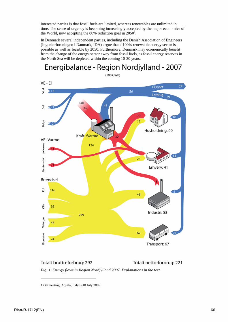
interested parties is that fossil fuels are limited, whereas renewables are unlimited in time. The sense of urgency is becoming increasingly accepted by the major economies of the World, now accepting the 80% reduction goal in 20501.

In Denmark several independent parties, including the Danish Association of Engineers (Ingeniørforeningen i Danmark, IDA) argue that a 100% renewable energy sector is possible as well as feasible by 2050. Furthermore, Denmark may economically benefit from the change of the energy sector away from fossil fuels, as fossil energy reserves in the North Sea will be depleted within the coming 10-20 years.

Fig. 1. Energy flows in Region Nordjylland 2007. Explanations in the text.

1 G8 meeting, Aquila, Italy 8-10 July 2009.

Risø-R-1712(EN) 66

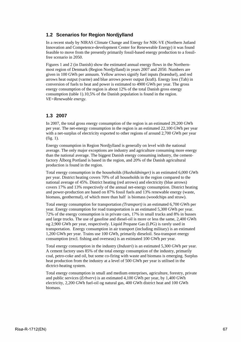
1.2 Scenarios for Region Nordjylland In a recent study by NIRAS Climate Change and Energy for NIK-VE (Northern Jutland Innovation and Competence-development Center for Reneweable Energy) it was found feasible to move from the presently primarily fossil-based energy production to a fossil-free scenario in 2050.

Figures 1 and 2 (in Danish) show the estimated annual energy flows in the Northern-most region of Denmark (Region Nordjylland) in years 2007 and 2050. Numbers are given in 100 GWh per annuum. Yellow arrows signify fuel inputs (brændsel), and red arrows heat output (varme) and blue arrows power output (kraft). Energy loss (Tab) in conversion of fuels to heat and power is estimated to 4900 GWh per year. The gross energy consumption of the region is about 12% of the total Danish gross energy consumption (table 1).10,5% of the Danish population is found in the region. VE=Renewable energy.

1.3 2007 In 2007, the total gross energy consumption of the region is an estimated 29,200 GWh per year. The net-energy consumption in the region is an estimated 22,100 GWh per year with a net-surplus of electricity exported to other regions of around 2,700 GWh per year (fig. 1).

Energy consumption in Region Nordjylland is generally on level with the national average. The only major exceptions are industry and agriculture consuming more energy than the national average. The biggest Danish energy consuming industry, the cement-factory Ålborg Portland is based in the region, and 20% of the Danish agricultural production is found in the region.

Total energy consumption in the households (Husholdninger) is an estimated 6,000 GWh per year. District heating covers 70% of all households in the region compared to the national average of 45%. District heating (red arrows) and electricity (blue arrows) covers 17% and 13% respectively of the annual net-energy consumption. District heating and power-production are based on 87% fossil fuels and 13% renewable energy (waste, biomass, geothermal), of which more than half is biomass (woodchips and straw).

Total energy consumption for transportation (Transport) is an estimated 6,700 GWh per year. Energy consumption for road transportation is an estimated 5,300 GWh per year. 72% of the energy consumption is in private cars, 17% in small trucks and 8% in busses and large trucks. The use of gasoline and diesel-oil is more or less the same, 2,400 GWh og 2,900 GWh per year, respectively. Liquid Propane Gas (LPG) is rarely used in transportation. Energy consumption in air transport (including military) is an estimated 1,200 GWh per year. Trains use 100 GWh, primarily dieseloil. Sea-transport energy consumption (excl. fishing and overseas) is an estimated 100 GWh per year.

Total energy consumption in the industry (Industri) is an estimated 5,300 GWh per year. A cement factory uses 85% of the total energy consumption of the industry, primarily coal, petro-coke and oil, but some co-firing with waste and biomass is emerging. Surplus heat production from the industry at a level of 500 GWh per year is utilised in the dictrict-heating system.

Total energy consumption in small and medium enterprises, agriculture, forestry, private and public services (Erhverv) is an estimated 4,100 GWh per year, by 1,400 GWh electricity, 2,200 GWh fuel-oil og natural gas, 400 GWh district heat and 100 GWh biomass.

Risø-R-1712(EN) 67

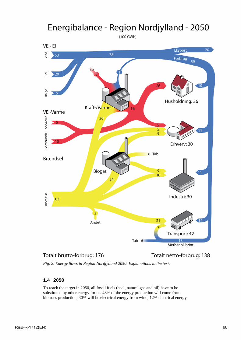
Fig. 2. Energy flows in Region Nordjylland 2050. Explanations in the text.

1.4 2050 To reach the target in 2050, all fossil fuels (coal, natural gas and oil) have to be substituted by other energy forms. 48% of the energy production will come from biomass production, 30% will be electrical energy from wind, 12% electrical energy

Risø-R-1712(EN) 68

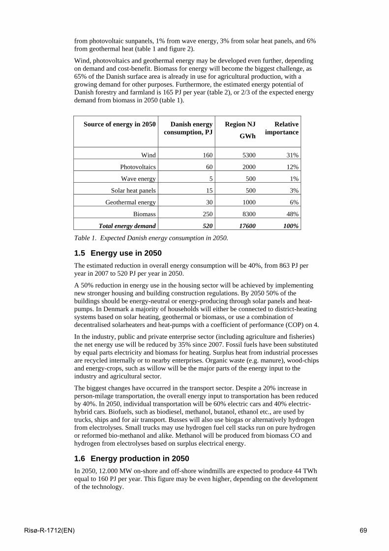
from photovoltaic sunpanels, 1% from wave energy, 3% from solar heat panels, and 6% from geothermal heat (table 1 and figure 2).

Wind, photovoltaics and geothermal energy may be developed even further, depending on demand and cost-benefit. Biomass for energy will become the biggest challenge, as 65% of the Danish surface area is already in use for agricultural production, with a growing demand for other purposes. Furthermore, the estimated energy potential of Danish forestry and farmland is 165 PJ per year (table 2), or 2/3 of the expected energy demand from biomass in 2050 (table 1).

Source of energy in 2050 Danish energy consumption, PJ

Region NJ

GWh

Relative importance

Wind 160 5300 31%

Photovoltaics 60 2000 12%

Wave energy 5 500 1%

Solar heat panels 15 500 3%

Geothermal energy 30 1000 6%

Biomass 250 8300 48%

Total energy demand 520 17600 100%

Table 1. Expected Danish energy consumption in 2050.

1.5 Energy use in 2050 The estimated reduction in overall energy consumption will be 40%, from 863 PJ per year in 2007 to 520 PJ per year in 2050.

A 50% reduction in energy use in the housing sector will be achieved by implementing new stronger housing and building construction regulations. By 2050 50% of the buildings should be energy-neutral or energy-producing through solar panels and heat-pumps. In Denmark a majority of households will either be connected to district-heating systems based on solar heating, geothermal or biomass, or use a combination of decentralised solarheaters and heat-pumps with a coefficient of performance (COP) on 4.

In the industry, public and private enterprise sector (including agriculture and fisheries) the net energy use will be reduced by 35% since 2007. Fossil fuels have been substituted by equal parts electricity and biomass for heating. Surplus heat from industrial processes are recycled internally or to nearby enterprises. Organic waste (e.g. manure), wood-chips and energy-crops, such as willow will be the major parts of the energy input to the industry and agricultural sector.

The biggest changes have occurred in the transport sector. Despite a 20% increase in person-milage transportation, the overall energy input to transportation has been reduced by 40%. In 2050, individual transportation will be 60% electric cars and 40% electric-hybrid cars. Biofuels, such as biodiesel, methanol, butanol, ethanol etc., are used by trucks, ships and for air transport. Busses will also use biogas or alternatively hydrogen from electrolyses. Small trucks may use hydrogen fuel cell stacks run on pure hydrogen or reformed bio-methanol and alike. Methanol will be produced from biomass CO and hydrogen from electrolyses based on surplus electrical energy.

1.6 Energy production in 2050 In 2050, 12.000 MW on-shore and off-shore windmills are expected to produce 44 TWh equal to 160 PJ per year. This figure may be even higher, depending on the development of the technology.

Risø-R-1712(EN) 69

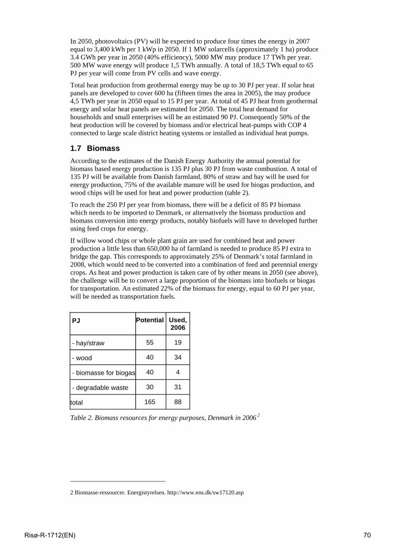
In 2050, photovoltaics (PV) will be expected to produce four times the energy in 2007 equal to 3,400 kWh per 1 kWp in 2050. If 1 MW solarcells (approximately 1 ha) produce 3.4 GWh per year in 2050 (40% efficiency), 5000 MW may produce 17 TWh per year. 500 MW wave energy will produce 1,5 TWh annually. A total of 18,5 TWh equal to 65 PJ per year will come from PV cells and wave energy.

Total heat production from geothermal energy may be up to 30 PJ per year. If solar heat panels are developed to cover 600 ha (fifteen times the area in 2005), the may produce 4,5 TWh per year in 2050 equal to 15 PJ per year. At total of 45 PJ heat from geothermal energy and solar heat panels are estimated for 2050. The total heat demand for households and small enterprises will be an estimated 90 PJ. Consequently 50% of the heat production will be covered by biomass and/or electrical heat-pumps with COP 4 connected to large scale district heating systems or installed as individual heat pumps.

1.7 Biomass According to the estimates of the Danish Energy Authority the annual potential for biomass based energy production is 135 PJ plus 30 PJ from waste combustion. A total of 135 PJ will be available from Danish farmland. 80% of straw and hay will be used for energy production, 75% of the available manure will be used for biogas production, and wood chips will be used for heat and power production (table 2).

To reach the 250 PJ per year from biomass, there will be a deficit of 85 PJ biomass which needs to be imported to Denmark, or alternatively the biomass production and biomass conversion into energy products, notably biofuels will have to developed further using feed crops for energy.

If willow wood chips or whole plant grain are used for combined heat and power production a little less than 650,000 ha of farmland is needed to produce 85 PJ extra to bridge the gap. This corresponds to approximately 25% of Denmark’s total farmland in 2008, which would need to be converted into a combination of feed and perennial energy crops. As heat and power production is taken care of by other means in 2050 (see above), the challenge will be to convert a large proportion of the biomass into biofuels or biogas for transportation. An estimated 22% of the biomass for energy, equal to 60 PJ per year, will be needed as transportation fuels.

PJ Potential Used, 2006

- hay/straw 55 19

- wood 40 34

- biomasse for biogas 40 4

- degradable waste 30 31

total 165 88

Table 2. Biomass resources for energy purposes, Denmark in 2006 2

2 Biomasse-ressourcer. Energistyrelsen. http://www.ens.dk/sw17120.asp

Risø-R-1712(EN) 70

1.8 Discussion Many reports focus on the challenges relating to an increased input of electrical energy into the energy systems. Most of these studies show that conversion from primarily coal-fired power-plants to renewable power production by wind, solar and wave energy is possible and even an economic benefit for the society as a whole. The reduction of overall energy consumption by 40% by 2050 is also feasible, even by the technical standards available today. In particular if we take into consideration, that 60% or more of the energy use for transportation will be based on renewable energy in 2050 with an energy conversion efficiency of factor 4-5.

The biggest challenge will be to include biomass in the energy sector to a level where up to 50% of the society’s energy demand will be based on biomass. Agricultural land is already under pressure, and as the need for more CO2-binding areas is growing, more and more land will be converted into grasslands and woods.

Another big challenge is to move not just to a fossil-free society but to an ash-free society, where combustion for energy purposes is reduced. The ultimate goal is as far as possible to avoid combustion of biomass, as valuable nutrients such as phosphorus will become non-accessible for plants. By reducing the combustion and recycling nutrients, the need for importing expensive and increasingly scarce inorganic fertilizers is also reduced. We will need to look at not only carbon balance, but maybe more importantly phosphorus as a limited resource in the near future.

The available biomass will thus have to be used intelligently according to the value in the food-chain of each type of biomass. One solution may be, that easily digestible biomass-components as corn, grain, beans and micro- and macroalgae may be used foremost for human consumption and feedstuffs, whereas grass, wood and other lignocellulotic biomass in need of enzymatic and bacteriological digestion may be used for biofuels and for construction materials, that may ultimatively be converted into bio-digestible waste.

Another important pathway is to develop biological refineries making it possible to process bio-products for food, feed, fertilizers, chemicals and fuels, according to needs.

But maybe most importantly, crop production and animal production will have to developed intelligently to reduce the vast outputs of green-house –gasses from industrial land-use and land-use-change and forestry, not directly related to energy production. Reducing outputs of greenhouse-gasses (GHG) by 80-90% by 2050 not only encompasses a fossil-free energy production, but also relies on a total reconstruction of how we live, eat and transport ourselves.

In Denmark the average domestic per capita outlet of green-house gasses in 2008 is roughly 12 -16 tonnes per year, depending on calculation method. This amount will have to be reduced to 2,5-3 tonnes per person per year by 2050, to reach the global targets for GHG reductions.

Food consumption will have to be changed to less meat and more vegetables, and in particular less beef and other ruminants. On average the consumption of one kg beef, pork and poultry in EU produces 28, 10 and 4 kg CO2-equivalents, respectively (excl. land-use effects (LULUCF)). As the meat consumption from each Danish citizen on average is at least 100 kg meat and dairy products per year, more than 2 tonnes of C02-equiv. per person may stem from meat consumption alone.

As a consequence, to make room for consumption of food and industrial products, the energy sector will have to be not only CO2-neutral, but CO2 negative by 2050. The energy sector will have to have negative emission of CO2, by intelligent use of biomass and using tools such as CCS and CDM.

Risø-R-1712(EN) 71

Conclusion

In conclusion, we argue that it is possible for the Danish energy sector to become 100% fossil free by 2050. However, the biggest challenge is not the energy sector, although electrification demands an intelligent grid, an open market and multiple usage and storage facilities, and not least major parts of the transport sector electrified.

The biggest challenges will be reducing green-house-gas emissions from food production and consumption, and how to produce enough biomass and how to convert the biomass into energy, without degrading its nutrient value. Keeping nutrients, nut just carbon, but foremost phosphorus in the organic recycling system will be major task.

References

1. IDA 2009. Klimaplan 2050. 2. NIK-VE (2009) Fremtidens Energi I Region Nordjylland. Fremtidsscenarier.

Energiforbrug og –produktion i 2025, 2050 og 2100. Nordjysk Innovations- og Kompetencecenter for Vedvarende Energi. DRAFT report. June 2009

3. Energinet.dk (2009). Effektiv anvendelse af vindkraftbaseret el i Danmark. Samspil mellem vindkraft, varmepumper og elbiler. Energinet.dk, March 2009

Risø-R-1712(EN) 72

Rural electrification in Sub Saharan Africa in a context of fluctuating oil-prices

Is the time ready to move from solar home systems

to hybrid PV-diesel systems?

Ivan Nygaard, UNEP Risø Centre, Risø DTU, Denmark

Henrik Bindner, Wind Energy Division, Risø DTU, Denmark

Ivan Katic, Energy & Climate Division, Danish Technological Institute, Denmark

Abstract Solar PV is one among other low carbon technologies for rural electrification in Sub Saharan Africa (SSA). Solar PV systems have for almost 30 years been disseminated in SSA, resulting in more than half a million installations concentrated in a few countries. While PV systems have technically matured and markets have gradually developed, PV for rural electrification has often been perceived with scepticism from potential users, donors, government officials and researchers, and solar PV has in many camps been labelled as donor driven, expensive and fragile technology mainly serving the richest parts of the populations and with little or no value for productive uses.

However, feasibility for solar PV has improved in the last few years. Retail prices for solar photovoltaic modules are reduced by 20-30% since 2001, and although far from the peak in 2008, oil prices in the next two years to come are expected to settle at a level, which is about three times the world market average in the years from 1985-2003. Therefore, rather than being limited to a niche for populations living in dispersed settlements outside the reach of grid electrification, solar PV is expected to play an important role in mini grid rural electrification schemes based on hybrid solar PV- diesel generators. This may bring PV systems in line with fossil fuel based systems in terms of consumer cost and options for productive use and it changes the market for PV from mainly donor supported schemes into mainstream rural electrification schemes governed and financed by electric utilities and rural electrification agencies.

Based on a literature review and the experience with a full scale hybrid wind/PV diesel system at RISØ DTU, this paper provides cost estimates for hybrid PV-diesel systems and policy recommendations to change the application of PV technologies for development in SSA.

Risø-R-1712(EN) 73

1 Introduction Energy services are generally acknowledged to play a significant role in facilitating both social and economic development, and rural people desire electricity for light, telecommunication and for income generating activities (GNESD, 2007). It is therefore considered to be a serious social and economic problem that access to electricity is extremely low in most developing countries and that more than 0.5 billion people, or more than 70 % of the population in SSA, have no access to electricity (IEA, 2006).

Environmental concerns, which have increasingly been translated into concerns for climate change, is an important element influencing the debate on access to electricity. Binding targets for CO2 emissions in the North, emission trading and Clean Development Mechanism (CDM) have entered the development agenda, but while there is growing concern of the need for mitigation in the fast developing countries, such as India and China, it is increasingly acknowledged that climate change mitigation is not the first priority in SSA. Per capita emissions and poverty in SSA are today at a level that focus should be on economic and social development. This means that there is an emerging consensus among policy makers and in the donor community that least-cost options should be pursued, although still with due diligence to benefit from options for cleaner development (WB, 2007).

Electricity options for rural dwellers in SSA highly depend on whether they live in nucleated villages, outskirts of nucleated villages or in dispersed settlements. Solar Home Systems (SHS) are an interesting option for dispersed settlements, because grid electricity is not likely to be available for the next decades in most SSA countries. In this context SHS competes with charging of batteries in a nearby town, with a small gen-set or with a PV charging station. Mini-grids, in turn, are generally the most favourable option for nucleated villages, which are out of reach of the national grid. Most often, mini-grids will be established in the most densely populated part of the village, where electricity may be used for income generating purposes in shops, restaurants, workshops and in public service institutions for water, health, education and administration. Outskirts of nucleated villages may in some cases be serviced by the mini-grid, but in most cases mini-grids will for the first many years only serve the a smaller part of the population. SHS may therefore also be an interesting option in the outskirts of nucleated villages (Banks, 2007: 123)

The advantages of mini-grids compared to low voltage SHS are many. First of all, the mini-grid provides the consumer with high voltage electricity, which has advantages for productive use of electricity, whether it is for lighting, cooling or motive power, and which allows consumers to use cheaper standard AC power appliances. Secondly, investment in a mini-grid can be seen as a transitional investment for a long term strategy of being connected to the national grid, with the benefits that may give in terms of cheaper electricity from large scale hydro, natural gas or coal. Small diesel engines in the range from 10 kW up to several MW are the baseline production units for these mini-grids, and although production costs from these units are relatively high because of low efficiency and high maintenance costs, mini-grids may be a least cost option the first 5 to 10 years after establishment, when demand gradually builds up.1

Third, the mini-grid it-self, may be supplied by electricity produced from mini and micro-hydropower schemes and from co-generation from biomass waste, where such resources are available in non-grid connected areas (EUEI, 2007). Hybrid wind-diesel systems are economically feasible options in specific areas with good and medium wind potential (Lundsager et al., 2001). The recent dramatic increase in oil prices from a level

1 The max distance for grid extension depends on a number of factors, such as the price of grid

electricity, expected load in the village, prices of diesel fuel, options for clustering villages, and the price of transmission line. SWER technology has been introduced in a number of countries, among those SA, in order to reduce the investment costs in transmission lines (Banks, 2007)

Risø-R-1712(EN) 74

of 20-30 US$ for the last two decades to the present level of above 70 US$/barrel has changed the market conditions significantly, and recent research indicates that there is also economic feasible hybrid options for inland localities with low wind potential, in terms of PV-diesel hybrids may be economically competitive compared to pure diesel solutions (Nfah et al., 2008; Mahmoud and Ibrik, 2006; Shaahid and Elhadidy, 2008; Indradip, 2005; Givler and Lilienthal, 2005; Banks and Aitken, 2004).

On this background the present article explores to which extent increasing oil prices and declining costs of solar PV will allow hybrid PV systems to be competitive to dedicated diesel systems and hereby contributing to a cleaner energy production.

2 Solar PV in a context of development aid So far solar PV has almost entirely been used for individual applications in terms of SHS in non-electrified areas. The current status of implementation of SHS points at more than 500,000 systems in Africa, concentrated in a few countries which have engaged in specific SHS programmes. Kenya has about 200,000 units, South Africa about 150,000, Zimbabwe 85,000, Morocco 37,000 and Uganda about 20,000 (REN21, 2008; Moner-Girona et al., 2006). Solar PV battery charging stations have been promoted as an option for a cheaper alternative to SHS, but has only had a limited market penetration (REN21, 2008).

Besides individual use, PV systems have been used for electricity supply to radio and telecommunication amplifiers in remote areas in most of SSA. PV has been used for pumping of drinking water in West Africa, Niger, Namibia and Zimbabwe (REN21, 2008), but compared to the SHS the numbers are limited, and a high share of installations is no longer in use due to theft of modules and lack of maintenance. 2 PV is also used in stand-alone systems providing lighting of village infrastructure such as schools, health centres, police stations, street lighting etc. and for refrigeration at health centres and maternities (FEM, 1999), but although this use is widespread in all SSA countries, estimations of total numbers have not been available. PV has only in some rare cases been used as input to production, such as irrigation, mainly because of high initial costs compared to alternatives such as small diesel and petrol engines (Erickson and Chapman, 1995; Karekezi and Kithyoma, 2002: 1079).

The market for PV installations in developing countries has until today mainly been driven by direct and indirect donor funding. PV installations have been applied in a number of cases although far from being a least-cost solution, when compared to small diesel grids and not grid-extension (Drennen et al., 1996). 3 A number of observers have asked the moral question, why the poorest should pay for the most expensive technology (Drennen et al., 1996: 15; Villavicencio, 2004: 63), 4 and researchers have increasingly challenged the arguments in favour of PV compared to traditional sources (Wamukonya, 2007, Karekezi and Kithyoma, 2002, Jacobson, 2007). In a well researched study from Kenya, Jacobson (2007) shows: i) that the benefits of solar electrification is mainly captured by the rural middle class, ii) that solar PV plays a modest role in supporting economically productive and education –related activities, and iii) that solar PV is more closely tied to increased use of TV, and other ‘connective’ applications such as radio and cellular phones, than to income generation, poverty

2 According to Togola (2001) only 40 % of installed PV pumps for water were functioning in 2000.

Newer estimates propose that more than 1000 PV pumps were in use in West Africa in 2007.

3 The price for SHS are often compared to grid extension although the least-cost option would be small-scale diesel grids, or even battery charging by means of small gasoline gen-sets, as shown by Erickson and Clapman (1995).

4 This has moral implications as long as it is a non efficient use of donor financing from the North, and severe economic consequences for the SSA governments, when the financing of large projects has been based on loans.

Risø-R-1712(EN) 75

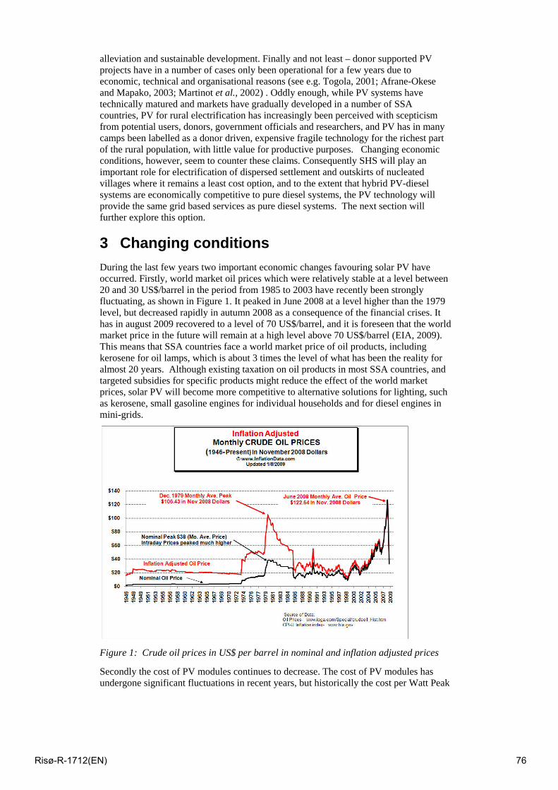
alleviation and sustainable development. Finally and not least – donor supported PV projects have in a number of cases only been operational for a few years due to economic, technical and organisational reasons (see e.g. Togola, 2001; Afrane-Okese and Mapako, 2003; Martinot et al., 2002) . Oddly enough, while PV systems have technically matured and markets have gradually developed in a number of SSA countries, PV for rural electrification has increasingly been perceived with scepticism from potential users, donors, government officials and researchers, and PV has in many camps been labelled as a donor driven, expensive fragile technology for the richest part of the rural population, with little value for productive purposes. Changing economic conditions, however, seem to counter these claims. Consequently SHS will play an important role for electrification of dispersed settlement and outskirts of nucleated villages where it remains a least cost option, and to the extent that hybrid PV-diesel systems are economically competitive to pure diesel systems, the PV technology will provide the same grid based services as pure diesel systems. The next section will further explore this option.

3 Changing conditions During the last few years two important economic changes favouring solar PV have occurred. Firstly, world market oil prices which were relatively stable at a level between 20 and 30 US$/barrel in the period from 1985 to 2003 have recently been strongly fluctuating, as shown in Figure 1. It peaked in June 2008 at a level higher than the 1979 level, but decreased rapidly in autumn 2008 as a consequence of the financial crises. It has in august 2009 recovered to a level of 70 US$/barrel, and it is foreseen that the world market price in the future will remain at a high level above 70 US$/barrel (EIA, 2009). This means that SSA countries face a world market price of oil products, including kerosene for oil lamps, which is about 3 times the level of what has been the reality for almost 20 years. Although existing taxation on oil products in most SSA countries, and targeted subsidies for specific products might reduce the effect of the world market prices, solar PV will become more competitive to alternative solutions for lighting, such as kerosene, small gasoline engines for individual households and for diesel engines in mini-grids.

Figure 1: Crude oil prices in US$ per barrel in nominal and inflation adjusted prices

Secondly the cost of PV modules continues to decrease. The cost of PV modules has undergone significant fluctuations in recent years, but historically the cost per Watt Peak

Risø-R-1712(EN) 76

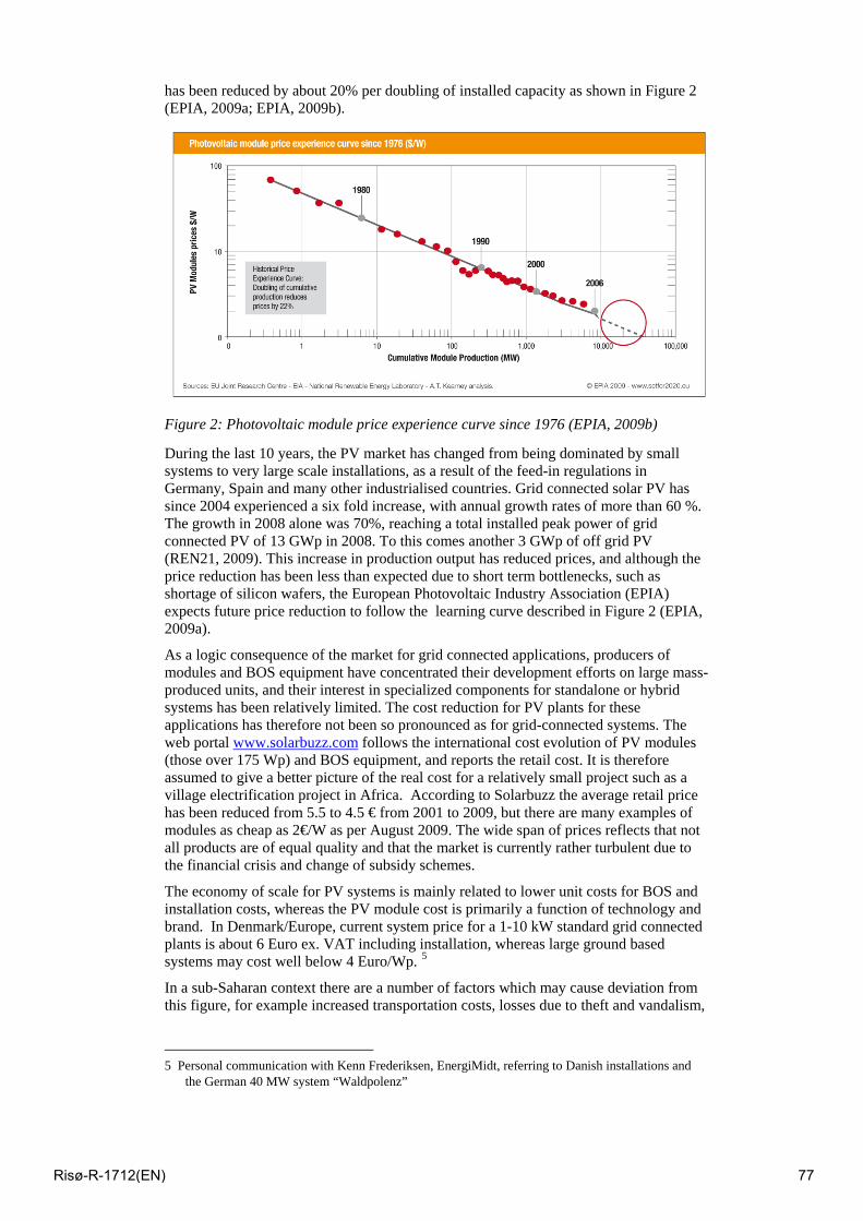
has been reduced by about 20% per doubling of installed capacity as shown in Figure 2 (EPIA, 2009a; EPIA, 2009b).

Figure 2: Photovoltaic module price experience curve since 1976 (EPIA, 2009b)

During the last 10 years, the PV market has changed from being dominated by small systems to very large scale installations, as a result of the feed-in regulations in Germany, Spain and many other industrialised countries. Grid connected solar PV has since 2004 experienced a six fold increase, with annual growth rates of more than 60 %. The growth in 2008 alone was 70%, reaching a total installed peak power of grid connected PV of 13 GWp in 2008. To this comes another 3 GWp of off grid PV (REN21, 2009). This increase in production output has reduced prices, and although the price reduction has been less than expected due to short term bottlenecks, such as shortage of silicon wafers, the European Photovoltaic Industry Association (EPIA) expects future price reduction to follow the learning curve described in Figure 2 (EPIA, 2009a).

As a logic consequence of the market for grid connected applications, producers of modules and BOS equipment have concentrated their development efforts on large mass-produced units, and their interest in specialized components for standalone or hybrid systems has been relatively limited. The cost reduction for PV plants for these applications has therefore not been so pronounced as for grid-connected systems. The web portal www.solarbuzz.com follows the international cost evolution of PV modules (those over 175 Wp) and BOS equipment, and reports the retail cost. It is therefore assumed to give a better picture of the real cost for a relatively small project such as a village electrification project in Africa. According to Solarbuzz the average retail price has been reduced from 5.5 to 4.5 € from 2001 to 2009, but there are many examples of modules as cheap as 2€/W as per August 2009. The wide span of prices reflects that not all products are of equal quality and that the market is currently rather turbulent due to the financial crisis and change of subsidy schemes.

The economy of scale for PV systems is mainly related to lower unit costs for BOS and installation costs, whereas the PV module cost is primarily a function of technology and brand. In Denmark/Europe, current system price for a 1-10 kW standard grid connected plants is about 6 Euro ex. VAT including installation, whereas large ground based systems may cost well below 4 Euro/Wp. 5

In a sub-Saharan context there are a number of factors which may cause deviation from this figure, for example increased transportation costs, losses due to theft and vandalism,

5 Personal communication with Kenn Frederiksen, EnergiMidt, referring to Danish installations and

the German 40 MW system “Waldpolenz”

Risø-R-1712(EN) 77

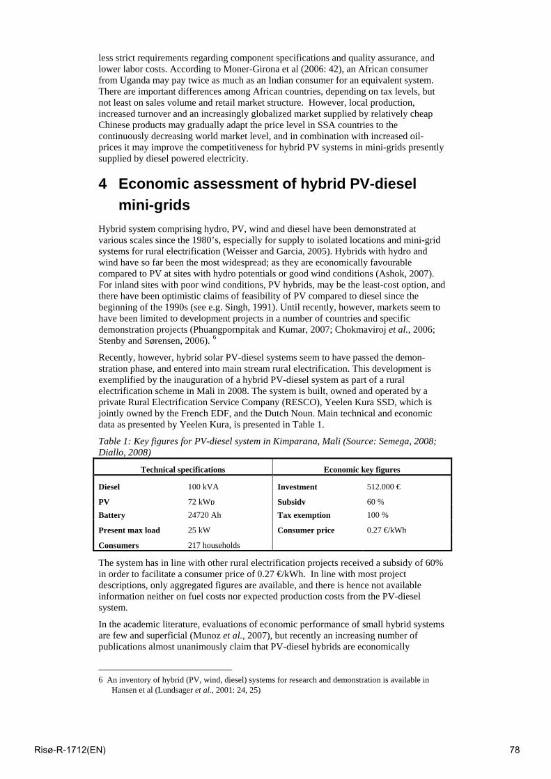
less strict requirements regarding component specifications and quality assurance, and lower labor costs. According to Moner-Girona et al (2006: 42), an African consumer from Uganda may pay twice as much as an Indian consumer for an equivalent system. There are important differences among African countries, depending on tax levels, but not least on sales volume and retail market structure. However, local production, increased turnover and an increasingly globalized market supplied by relatively cheap Chinese products may gradually adapt the price level in SSA countries to the continuously decreasing world market level, and in combination with increased oil-prices it may improve the competitiveness for hybrid PV systems in mini-grids presently supplied by diesel powered electricity.

4 Economic assessment of hybrid PV-diesel mini-grids

Hybrid system comprising hydro, PV, wind and diesel have been demonstrated at various scales since the 1980’s, especially for supply to isolated locations and mini-grid systems for rural electrification (Weisser and Garcia, 2005). Hybrids with hydro and wind have so far been the most widespread; as they are economically favourable compared to PV at sites with hydro potentials or good wind conditions (Ashok, 2007). For inland sites with poor wind conditions, PV hybrids, may be the least-cost option, and there have been optimistic claims of feasibility of PV compared to diesel since the beginning of the 1990s (see e.g. Singh, 1991). Until recently, however, markets seem to have been limited to development projects in a number of countries and specific demonstration projects (Phuangpornpitak and Kumar, 2007; Chokmaviroj et al., 2006; Stenby and Sørensen, 2006). 6

Recently, however, hybrid solar PV-diesel systems seem to have passed the demon-stration phase, and entered into main stream rural electrification. This development is exemplified by the inauguration of a hybrid PV-diesel system as part of a rural electrification scheme in Mali in 2008. The system is built, owned and operated by a private Rural Electrification Service Company (RESCO), Yeelen Kura SSD, which is jointly owned by the French EDF, and the Dutch Noun. Main technical and economic data as presented by Yeelen Kura, is presented in Table 1.

Table 1: Key figures for PV-diesel system in Kimparana, Mali (Source: Semega, 2008; Diallo, 2008)

Technical specifications Economic key figures

Diesel 100 kVA Investment 512.000 €

PV 72 kWp Subsidy 60 %Battery 24720 Ah Tax exemption 100 %

Present max load 25 kW Consumer price 0.27 €/kWh

Consumers 217 households

The system has in line with other rural electrification projects received a subsidy of 60% in order to facilitate a consumer price of 0.27 €/kWh. In line with most project descriptions, only aggregated figures are available, and there is hence not available information neither on fuel costs nor expected production costs from the PV-diesel system.

In the academic literature, evaluations of economic performance of small hybrid systems are few and superficial (Munoz et al., 2007), but recently an increasing number of publications almost unanimously claim that PV-diesel hybrids are economically

6 An inventory of hybrid (PV, wind, diesel) systems for research and demonstration is available in

Hansen et al (Lundsager et al., 2001: 24, 25)

Risø-R-1712(EN) 78

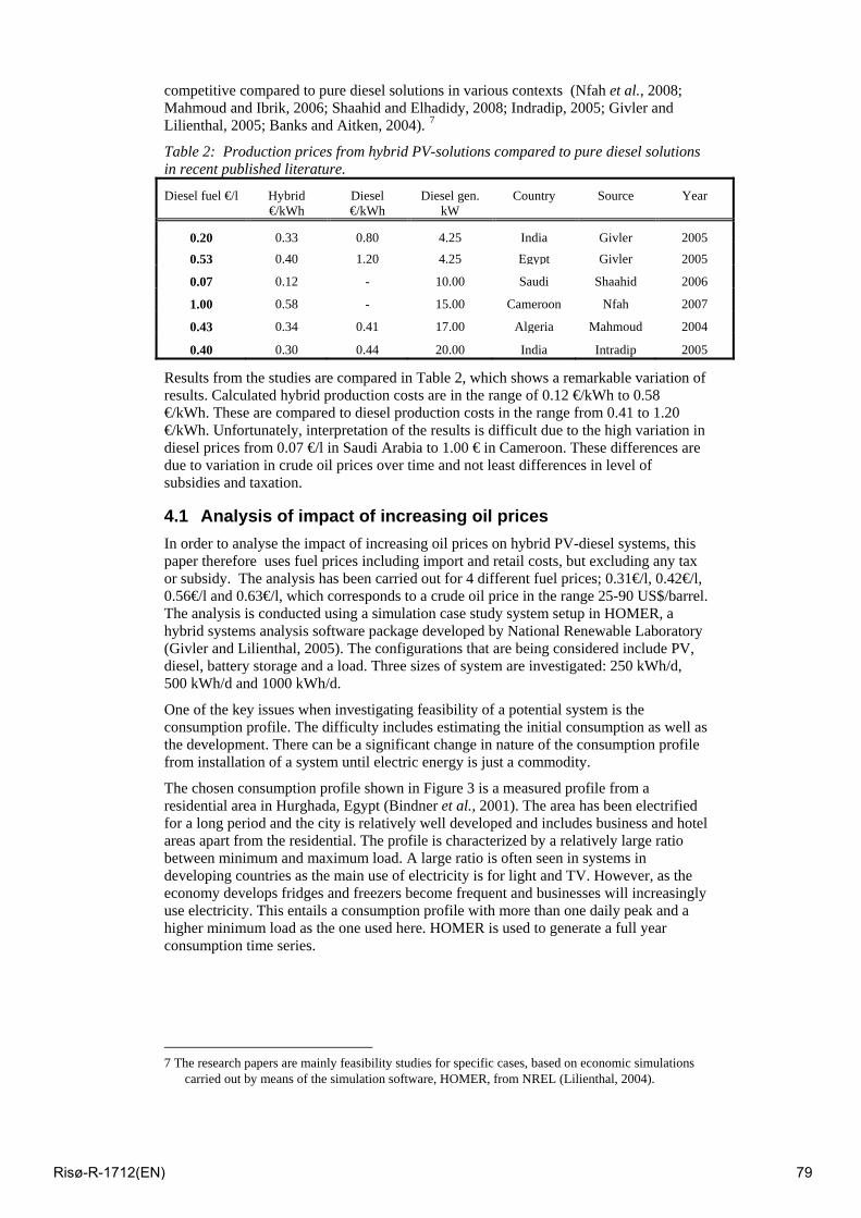
competitive compared to pure diesel solutions in various contexts (Nfah et al., 2008; Mahmoud and Ibrik, 2006; Shaahid and Elhadidy, 2008; Indradip, 2005; Givler and Lilienthal, 2005; Banks and Aitken, 2004). 7

Table 2: Production prices from hybrid PV-solutions compared to pure diesel solutions in recent published literature.

Diesel fuel €/l Hybrid €/kWh

Diesel €/kWh

Diesel gen. kW

Country Source Year

0.20 0.33 0.80 4.25 India Givler 2005

0.53 0.40 1.20 4.25 Egypt Givler 2005

0.07 0.12 - 10.00 Saudi Shaahid 2006

1.00 0.58 - 15.00 Cameroon Nfah 2007

0.43 0.34 0.41 17.00 Algeria Mahmoud 2004

0.40 0.30 0.44 20.00 India Intradip 2005

Results from the studies are compared in Table 2, which shows a remarkable variation of results. Calculated hybrid production costs are in the range of 0.12 €/kWh to 0.58 €/kWh. These are compared to diesel production costs in the range from 0.41 to 1.20 €/kWh. Unfortunately, interpretation of the results is difficult due to the high variation in diesel prices from 0.07 €/l in Saudi Arabia to 1.00 € in Cameroon. These differences are due to variation in crude oil prices over time and not least differences in level of subsidies and taxation.

4.1 Analysis of impact of increasing oil prices In order to analyse the impact of increasing oil prices on hybrid PV-diesel systems, this paper therefore uses fuel prices including import and retail costs, but excluding any tax or subsidy. The analysis has been carried out for 4 different fuel prices; 0.31€/l, 0.42€/l, 0.56€/l and 0.63€/l, which corresponds to a crude oil price in the range 25-90 US$/barrel. The analysis is conducted using a simulation case study system setup in HOMER, a hybrid systems analysis software package developed by National Renewable Laboratory (Givler and Lilienthal, 2005). The configurations that are being considered include PV, diesel, battery storage and a load. Three sizes of system are investigated: 250 kWh/d, 500 kWh/d and 1000 kWh/d.

One of the key issues when investigating feasibility of a potential system is the consumption profile. The difficulty includes estimating the initial consumption as well as the development. There can be a significant change in nature of the consumption profile from installation of a system until electric energy is just a commodity.

The chosen consumption profile shown in Figure 3 is a measured profile from a residential area in Hurghada, Egypt (Bindner et al., 2001). The area has been electrified for a long period and the city is relatively well developed and includes business and hotel areas apart from the residential. The profile is characterized by a relatively large ratio between minimum and maximum load. A large ratio is often seen in systems in developing countries as the main use of electricity is for light and TV. However, as the economy develops fridges and freezers become frequent and businesses will increasingly use electricity. This entails a consumption profile with more than one daily peak and a higher minimum load as the one used here. HOMER is used to generate a full year consumption time series.

7 The research papers are mainly feasibility studies for specific cases, based on economic simulations

carried out by means of the simulation software, HOMER, from NREL (Lilienthal, 2004).

Risø-R-1712(EN) 79

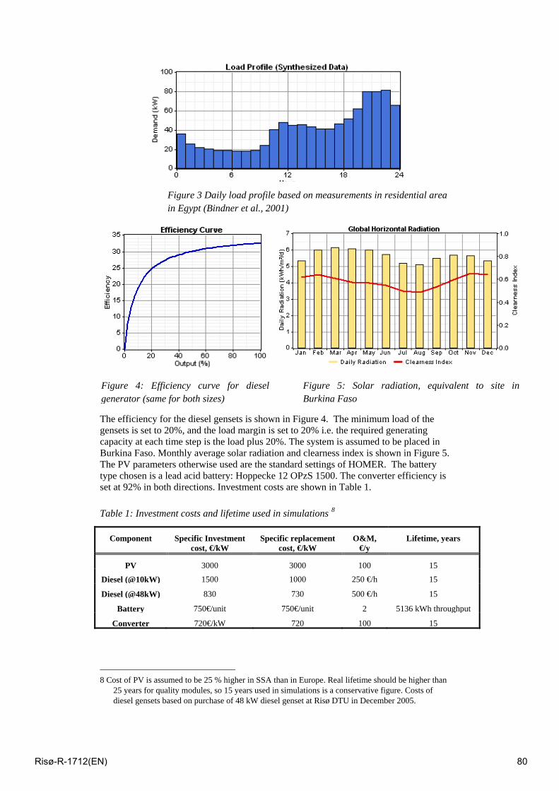
Figure 3 Daily load profile based on measurements in residential area

r the diesel gensets is shown in

in Egypt (Bindner et al., 2001)

The efficiency fo Figure 4. The minimum load of the gensets is set to 20%, and the load margin is set to 20% i.e. the required generating

re 5.

cost, €/kW cost, €/kW O&M,

€/y Lifetime, years

Figure 5: Solar radiation, equivalent to site inBurkina Faso

Figure 4: Efficiency curve for dieselgenerator (same for both sizes)

capacity at each time step is the load plus 20%. The system is assumed to be placed inBurkina Faso. Monthly average solar radiation and clearness index is shown in FiguThe PV parameters otherwise used are the standard settings of HOMER. The battery type chosen is a lead acid battery: Hoppecke 12 OPzS 1500. The converter efficiency is set at 92% in both directions. Investment costs are shown in Table 1.

Table 1: Investment costs and lifetime used in simulations 8

Component Specific Investment Specific replacement

PV 3000 3000 100 15

Diesel (@10kW) 250 1500 1000 €/h 15

Diesel (@48kW) 830 730 500 €/h 15

Battery 750€/unit 750€/unit 5136 kWh throu2 ghput

C 100onverter 720€/kW 720 15

8 Cost of PV is assumed to be 25 % higher in SSA than in Europe. Real lifetime should be higher than

25 years for quality modules, so 15 years used in simulations is a conservative figure. Costs of diesel gensets based on purchase of 48 kW diesel genset at Risø DTU in December 2005.

Risø-R-1712(EN) 80

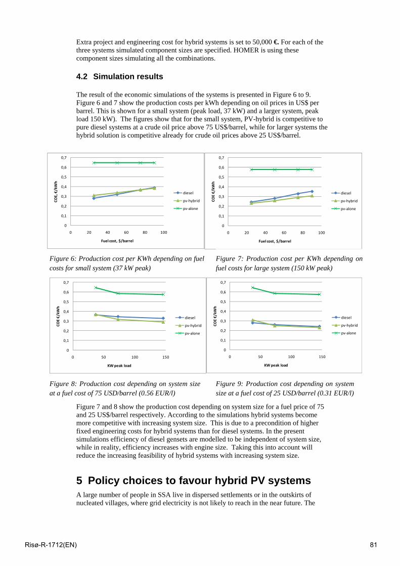
Extra project and engineering cost for hybrid systems is set to 50,000 €. For each of the three systems simulated component sizes are specified. HOMER is using these component sizes simulating all the combinations.

4.2 Simulation results

The result of the economic simulations of the systems is presented in Figure 6 to 9. Figure 6 and 7 show the production costs per kWh depending on oil prices in US$ per barrel. This is shown for a small system (peak load, 37 kW) and a larger system, peak load 150 kW). The figures show that for the small system, PV-hybrid is competitive to pure diesel systems at a crude oil price above 75 US$/barrel, while for larger systems the hybrid solution is competitive already for crude oil prices above 25 US$/barrel.

Figure 7 and 8 show the production cost depending on system size for a fuel price of 75 and 25 US$/barrel respectively. According to the simulations hybrid systems become more competitive with increasing system size. This is due to a precondition of higher fixed engineering costs for hybrid systems than for diesel systems. In the present simulations efficiency of diesel gensets are modelled to be independent of system size, while in reality, efficiency increases with engine size. Taking this into account will reduce the increasing feasibility of hybrid systems with increasing system size.

5 Policy choices to favour hybrid PV systems A large number of people in SSA live in dispersed settlements or in the outskirts of nucleated villages, where grid electricity is not likely to reach in the near future. The

Figure 7: Production cost per KWh depending eon fu lcosts for small system (150 kW peak)

0

0,1

0,2

0,3

0,4

0,5

0,6

0,7

0 50 100 150

COE €/kW

h

KW peak load

diesel

pv‐hybrid

pv‐alone

0

0,1

2

3

0,4

0,5

0,6

0,7

0 20 40 60 80 100

E €/kW

h

Fuel cost, $/barrel

0,

0,

CO

diesel

pv‐hybrid

pv‐alone

0

0,1

0,2

0,3

0,4

0,5

0,6

0,7

0 20 40 60 80 100

COE, €/kWh

Fuel cost, $/barrel

diesel

pv‐hybrid

pv‐alone

0

0,1

0,2

0,3

0,4

0,5

0,6

0,7

0 50 100 150

COE €/kW

h

KW peak load

diesel

pv‐hybrid

pv‐alone

Figure 6: Production cost per KWh depending on fuelcosts for small system (37 kW peak)

Figure 7: Production cost per KWh depending onfuel costs for large system (150 kW peak)

Figure 8: Production cost depending on system sizeat a fuel cost of 75 USD/barrel (0.56 EUR/l)

Figure 9: Production cost depending on systemsize at a fuel cost of 25 USD/barrel (0.31 EUR/l)

Risø-R-1712(EN) 81

increased oil prices will leave this important market to individual solutions in terms of SHSs. For these areas stand alone systems using PV have been promoted through various types of delivery models (see e.g. Nygaard, 2009). Due to different market structures for individual and collective energy solutions as outlined above, these models need be revisited for the purpose of hybrid systems.

The first step in promoting hybrid PV is to create a level playing field for PV and fossil fuels solutions, either by removing fuel subsidies or by subsidizing PV. Fuel for electricity production is often subsidized in SSA. In some cases, it is a legacy from the pre-liberalization regime, while in others; it is a reaction against increasing oil prices. Price signals at the country levels are thus not reflecting world market prices. The first condition for enhanced use of hybrid systems is therefore to levelling the playing field by harmonising import tax levels and subsidy levels for solar PV and for fossil fuel based solutions. In most cases, this will be to the benefit of solar PV.

Secondly, although economically feasible under the condition of a level playing field, it is important to create a project volume that will reduce project risk as well as planning, engineering and other overhead costs of hybrid systems to a minimum. Increasing project volume might be facilitated by state owned utilities or through concession agreements, where rural electrification in whole regions is attributed to external investors through an international tendering process. As well the state owned utilities (e.g. in Morocco) and the concessionaires (e.g. in SA, Mali and Senegal) have the advantage compared to smaller actors that they can benefit from applying solutions such as hybrid systems, which may only be least cost options if applied in packages of 10 to 100 installations. The concession model based on large external operators may further have the advantage compared to utilities that they have access to capital necessary for the extra initial investment compared to diesel solutions.

Where such measures are in place the calculations show that hybrid PV-diesel systems are economic feasible already today. If, as expected, oil prices remain above 70 UDS/barrel in the future, PV-diesel hybrid will most likely prevail in rural electrification in SSA within the next decade. This ensures that PV systems are comparable to fossil fuel based systems in terms of consumer cost and options for productive use, while at the same time contributing to cleaner energy production.

References Afrane-Okese and M. Mapako, 2003, 'Solar PV Rural Electrification Lessons from South Africa and Zimbabwe' in L. S. Petersen and H. Larsen (eds.), Energy Technologies for Post Kyoto Targets in the Medium Term. Proceedings Risø International Energy Conference, Roskilde, Denmark: Risø National Laboratory, pp. 337-354

Ashok, S., 2007, 'Optimised Model for Community-Based Hybrid Energy System', Renewable Energy, Vol. 32, No. 7, pp. 1155-1164

Banks, Douglas, 2007, 'Perspectives on Providing Energy Services in Rural Areas' Proceedings: Hybrid Electricity Systems Powering Mini-Grids: A Southern African Perspective, Desert Research Foundation of Namibia, Restio Energy, pp. 111-127

Banks, Douglas and Robert Aitken, 2004, KwaZulu-Natal Mini-grid Feasibility Study, South Africa: National Electricity Regulator.

Bindner, Henrik, P. Lundsager, L. Saleh et al. 2001, 'Load patterns for performance assessment of autonomous wind diesel systems.' in P. Helm and A. Zervos (eds.), Wind energy for the new millennium. Proceedings. 2001 European wind energy conference and exhibition (EWEC '01), Copenhagen (DK), 2-6 Jul 2001, pp. 923-927

Chokmaviroj, Somchai, Rakwichian Wattanapong and Yammen Suchart, 2006, 'Performance of a 500 KWP Grid Connected Photovoltaic System at Mae Hong Son Province, Thailand', Renewable Energy, Vol. 31, No. 1, pp. 19-28

Risø-R-1712(EN) 82

Diallo, Amadou I., 2008, Société de services décentralises: SSD EN SA Yéelen Kura, Presentation par Diallo Amadou Isaac, Directeur Général SSD Yéelen Kura:

Drennen, Thomas E., Jon D. Erickson and Duane Chapman, 1996, 'Solar Power and Climate Change Policy in Developing Countries', Energy Policy, Vol. 24, No. 1, pp. 9-16

EIA, 2009, Energy Information Administration. Official Energy statistics from the American Government, www.eia.doe.gov.

EPIA, 2009a, Global Market Outlook for Photovoltaics until 2013, http://www.epia.org/: The European Photovoltaic Industry Association (EPIA).

EPIA, 2009b, Set for 2020. Solar Photovoltaic Electricity: A mainstream solar power source in Europe by 2020, http://www.setfor2020.eu: European Photovoltaic Industry Association (EPIA).

Erickson, Jon D. and Duane Chapman, 1995, 'Photovoltaic Technology: Markets, Economics, and Rural Development', World Development, Vol. 23, No. 7, pp. 1129-1141

EUEI, 2007, Poverty Alleviation through Cleaner Energy from Agro-industries in Africa (PACEAA): Fact sheet, http://ec.europa.eu/energy/intelligent/projects/africa_en.htm.

FEM, 1999, Programme Régional Solaire: Enseignements et perspectives, Bruxelles: CILLS, Commission Européenne, Fondation Enerties pour le Monde.

Givler, T. and P. Lilienthal, 2005, Using HOMER® Software, NREL's Micropower Optimization Model to Explore the Role of Gen-sets in Small Solar Power Systems. Case Study: Sri Lanka, Golden, Colorado: National Renewable Energy Laboratory.

GNESD, 2007, Reaching the Millennium Development Goals and beyond: access to moder forms of energy as a prereguisite, Roskilde, Denmark: Global Network on Energy for Sustainable Development.

IEA, 2006, World Energy Outlook 2006, Paris: OECD/IEA.

Indradip, Mitra, 2005, 'A Study on Solar Photovoltaic Based Mini-Grid Systems for Rural Electrification', SESI Journal : Journal of the Solar Energy Society of India, Vol. 15, No. 1, pp. 25-35

Jacobson, Arne, 2007, 'Connective Power: Solar Electrification and Social Change in Kenya', World Development, Vol. 35, No. 1, pp. 144-162

Karekezi, Stephen and Waeni Kithyoma, 2002, 'Renewable Energy Strategies for Rural Africa: Is a PV-Led Renewable Energy Strategy the Right Approach for Providing Modern Energy to the Rural Poor of Sub-Saharan Africa?', Energy Policy, Vol. 30, No. 11-12, pp. 1071-1086

Lilienthal, P., 2004, The HOMER® Micropower Optimization Model, http://www.nrel.gov/docs/fy05osti/37606.pdf: Conference paper presented at the 2004 DOE Solar Energy Technologies Programme Review Meeting, October 25-28, Denver Colorado.

Lundsager, Per, Henrik Bindner, Niels-Erik Clausen et al. 2001, Isolated Systems with Wind Power. Main Report, Risø-R-1256, Roskilde, Denmark: Risø National Laboratory.

Mahmoud, Marwan M. and Imad H. Ibrik, 2006, 'Techno-Economic Feasibility of Energy Supply of Remote Villages in Palestine by PV-Systems, Diesel Generators and Electric Grid', Renewable and sustainable energy reviews, Vol. 10, No. 2, pp. 128-138

Risø-R-1712(EN) 83

Martinot, Eric, Akanksha Chaurey, Debra Lew et al. 2002, 'Renewable Energy Markets in Developing Countries', Annual Review of Energy and the Environment, Vol. 27, No. 1, pp. 309-348

Moner-Girona, Magda, Rebecca Ghanadan, Arne Jacobson et al. 2006, 'Decreasing PV Costs in Africa: Opportunities for Rural Electrification Using Solar PV in Sub-Saharan Africa', Refocus, Vol. 7, No. 1, pp. 40-45

Munoz, J., L Navarte and E. Lorenzo, 2007, 'Experience With PV-Diesel Hybrid Village Power Systems in Southern Morocco', Progress in Photovoltaics: Research and Applications, Vol. 15, pp. 529-539

Nfah, E. M., J. M. Ngundam, M. Vandenbergh et al. 2008, 'Simulation of Off-Grid Generation Options for Remote Villages in Cameroon', Renewable Energy, Vol. 33, No. 5, pp. 1064-1072

Nygaard, Ivan, 2009, 'Compatibility of Rural Electrification and Promotion of Low-Carbon Technologies in Development Countries: The Case of Solar PV for Sub-Saharan Africa', European Review of Energy Markets, Vol. 3, No. 2

Phuangpornpitak, N. and S. Kumar, 2007, 'PV Hybrid Systems for Rural Electrification in Thailand', Renewable and sustainable energy reviews, Vol. 11, No. 7, pp. 1530-1543

REN21, 2008, Renewables 2007 Global status report, www.ren21.net: REN21 Secretariat and Worldwatch Institute.

REN21, 2009, Renewables global status report - 2009 update, http://www.ren21.net/: Renewable Energy Policy Network for the 21st Century.

Semega, Dibril, 2008, Centrale hybride solaire PV-diesel: Electrification de la localité de Kimparana, Mali, Presentationa à la reunion du club Agences en charge d'Electrification Rurale, Bamako 2008.

Shaahid, S. M. and M. A. Elhadidy, 2008, 'Economic Analysis of Hybrid Photovoltaic-Diesel-Battery Power Systems for Residential Loads in Hot Regions--A Step to Clean Future', Renewable and sustainable energy reviews, Vol. 12, No. 2, pp. 488-503

Singh, P., 1991, 'Incorporating Solar Electric-Power Into Rural Electrification Programs - A Case-Study of Kenya', Energy Sources, Vol. 13, No. 1, pp. 67-75

Stenby, Jacob and Martha K. Sørensen, 2006, Implementation and design of hybrid energy systems in remote areas, Master thesis, Department of Mechanical Engineering, Technical University of Denmark.

Togola, Ibrahim, 2001, 'PV experiences in southern Mali' in N. Wamukonya (ed.), Experience with PV systems in Africa: Summary of selected cases, Roskilde: UNEP Collaborating Centre on Energy and Environment, pp. 49-51

Villavicencio, Arthuro, 2004, A systems view of sustainable energy development, Roskilde, Denmark: Unep Risoe Centre.

Wamukonya, Njeri, 2007, 'Solar Home System Electrification As a Viable Technology Option for Africa's Development', Energy Policy, Vol. 35, pp. 6-14

WB, 2007, Clean Energy for Development Investment Framework: The World Bank Group Action Plan, Washington DC: World Bank.

Weisser, Daniel and Raquel S. Garcia, 2005, 'Instantaneous Wind Energy Penetration in Isolated Electricity Grids: Concepts and Review', Renewable Energy, Vol. 30, No. 8, pp. 1299-1308

Risø-R-1712(EN) 84

Session 4 – Renewable energy technologies: Bioenergy II

Risø-R-1712(EN) 85

Biochar soil application to mitigate climate change 1Bruun, E.W. (esbr@risoe.dtu.dk); 1Hauggaard-Nielsen, H.; 1Ambus P.; 1Egsgaard, H.; 2Jensen P. A. 1Biosystems Division, Risø National Laboratory for Sustainable Energy, Technical University of Denmark, DK-4000 Roskilde, Denmark; 2Division of Chemical Engineering Competences. Technical University of Denmark, DK-2800 Lyngby, Denmark

Abstract Production of energy carriers (oil, gas) and biochar from pyrolysis of biomass is by many considered a promising technology for combined production of bioenergy and recalcitrant C suitable for sequestration in soil. The mechanism behind biochar-C sequestration is straightforward: Due to its recalcitrant characteristics the microbial decomposition of biochar is much slower in comparison to the mineralization of the original feedstock. Conversion of organic residues like household waste or cereal straw to biochar is hence proposed a way to withdraw CO2 from the atmosphere and sequester it on a long term basis in the soil. The experiments presented here illustrate the C sequestration potentials of biochar originating from fast pyrolysis of wheat straw. It is documented that after 47 days in soil 95 % of the added biochar-C is still present in the soil as compared to only 56 % if straw is applied untreated to the soil.

The type and settings of pyrolysis influence the chemical quality of the biochar produced significantly. Biochar chemical analysis revealed that the degradation of biochar in soil appears to be proportional with the biochar cellulosic and hemicellulosic fraction. Furthermore, the pyrolyzer temperature settings strongly influence the proportion of cellulose and hemicellulose remaining in the biochar. As these biochar fractions relatively rapidly are mineralized to CO2 by microbial respiration they are – in climate mitigation perspective - unwanted.

At the upcoming Climate Conference in Copenhagen (COP15) December 2009, the use of biochar as a mitigation tool will be on the agenda and for the time being (July 2009) 20 countries and Parties to the United Nations Framework Convention on Climate Change (UNFCCC) have made submissions to the UNFCCC seeking the inclusion of biochar as a climate mitigation and adaptation tool.

1 Introduction One of several strategies to mitigate the impact of climate change is to sequester carbon in the soil. In a press release (5th of March 2009) the European Commission underline the crucial role soils play in mitigating climate change referring to CLIMSOIL report (Schils et al., 2008) that provides a comprehensive review on the interrelations between soil and climate change. Soils contain around twice as much C as the atmosphere, and five times the amount to be found in vegetation and hence constitute an enormous C reservoir. While poor agricultural management can have serious consequences dramatically speeding up the release of C emissions from soil, other practices can increase the soil C stock significantly and thereby mitigate climate change (Schils et al. 2008).

Pyrolysis of biomass followed by the application of the biochar residue to soils is a way to increase the soil C stock. In the pyrolysis process a biomass feedstock is heated up to 300-600°C in an oxygen-free environment and transformed into bio-oil, pyrolysis

Risø-R-1712(EN) 86

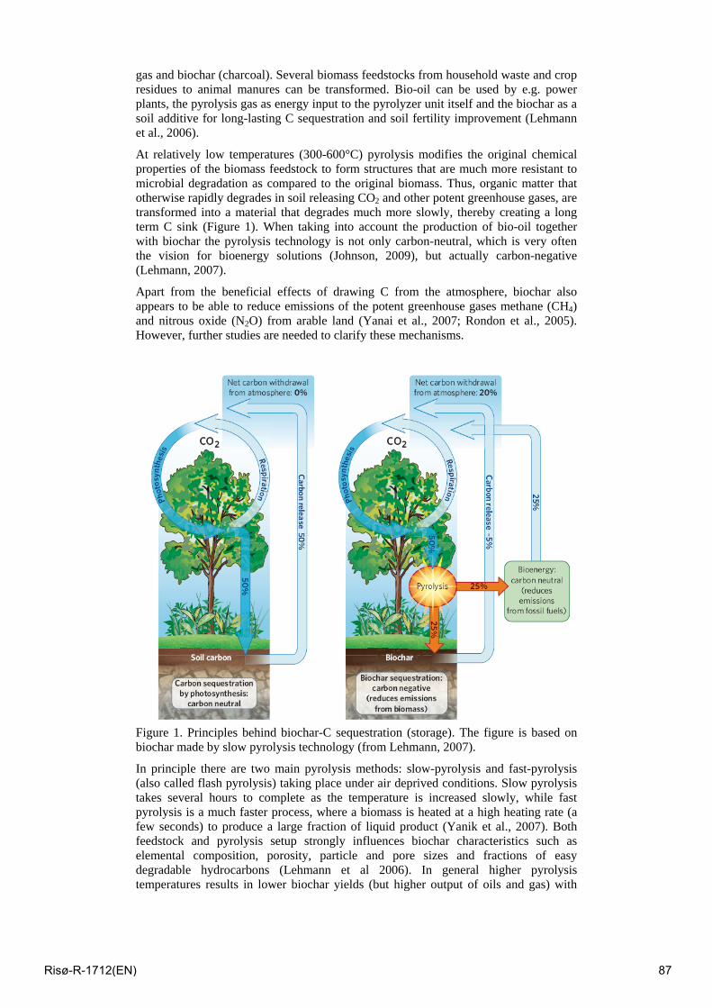
gas and biochar (charcoal). Several biomass feedstocks from household waste and crop residues to animal manures can be transformed. Bio-oil can be used by e.g. power plants, the pyrolysis gas as energy input to the pyrolyzer unit itself and the biochar as a soil additive for long-lasting C sequestration and soil fertility improvement (Lehmann et al., 2006).

At relatively low temperatures (300-600°C) pyrolysis modifies the original chemical properties of the biomass feedstock to form structures that are much more resistant to microbial degradation as compared to the original biomass. Thus, organic matter that otherwise rapidly degrades in soil releasing CO2 and other potent greenhouse gases, are transformed into a material that degrades much more slowly, thereby creating a long term C sink (Figure 1). When taking into account the production of bio-oil together with biochar the pyrolysis technology is not only carbon-neutral, which is very often the vision for bioenergy solutions (Johnson, 2009), but actually carbon-negative (Lehmann, 2007).

Apart from the beneficial effects of drawing C from the atmosphere, biochar also appears to be able to reduce emissions of the potent greenhouse gases methane (CH4) and nitrous oxide (N2O) from arable land (Yanai et al., 2007; Rondon et al., 2005). However, further studies are needed to clarify these mechanisms.

Figure 1. Principles behind biochar-C sequestration (storage). The figure is based on biochar made by slow pyrolysis technology (from Lehmann, 2007).

In principle there are two main pyrolysis methods: slow-pyrolysis and fast-pyrolysis (also called flash pyrolysis) taking place under air deprived conditions. Slow pyrolysis takes several hours to complete as the temperature is increased slowly, while fast pyrolysis is a much faster process, where a biomass is heated at a high heating rate (a few seconds) to produce a large fraction of liquid product (Yanik et al., 2007). Both feedstock and pyrolysis setup strongly influences biochar characteristics such as elemental composition, porosity, particle and pore sizes and fractions of easy degradable hydrocarbons (Lehmann et al 2006). In general higher pyrolysis temperatures results in lower biochar yields (but higher output of oils and gas) with

Risø-R-1712(EN) 87

less original structures and chemical components remaining. In the present study we focus on fast-pyrolysis.

Besides soil C sequestration, biochar seems to have beneficial effects on soil quality and fertility. A number studies have examined biochars effect on soil fertility and the majority of these have documented beneficial effects on crop yields (Lehmann et al., 2006; Oguntunde et al., 2004; Glaser et al., 2002). Amazon Basin dark-coloured soils (Terra Pretta), that in ancient time has been amended with large amounts of biochar by the native population, are supporting these findings, as these soils currently possess high levels of nutrients and support great crop yields (Steiner et al., 2008a). In addition, studies have shown that application of biochar together with fertilizer (NH4

+) increases crop yields as compared to pure fertilizer application (Chan et al., 2007; Steiner et al., 2007). However, it is important to note, that the majority of biochar-studies so far have been done on highly weathered tropical soils or northern boreal forest soils with low natural soil organic C levels (Kolb et al., 2009). Hence studies with are needed in e.g. temperate regions like in Denmark with rather fertile soils to validate possible different plant and microbial responses to biochar soil application.

The main objective of the present study is to improve the understanding of short-term microbial degradation of fast pyrolysis biochar in relation to different pyrolysis temperatures.

2 Materials and methods 2.1 Experimental design The soil used was collected (0-25 cm) in an agricultural field characterized as a sandy loam (Typic Hapludalf) with 11% clay, 14% silt, 49% fine sand and 25% coarse sand (Hauggaard-Nielsen et al., 2001). The soil was sieved (2 mm) and mixed thoroughly with biochar in 100ml containers (ID=48mm) containing 40g soil (38g dry weight) and 2g of biochar produced at different temperatures, i.e.475°C, 500°C, 525°C, 550°C and 575°C on a pilot scale pyrolyzer (Bech et al., 2009). The biochar was derived from conventional wheat straw (Triticum sp.) having a moisture content of 6.20 wt% and an ash content of 6.02 wt%. The straw was dried to constant weight and grinded (2 mm) before pyrolysis. The particle sizes of the added biochar decreased with increasing pyrolysis temperature (Table 1).

It is an ongoing experiment (72 days so far) where the soil is kept at constant water content (30% WHC) by regularly weighing of the containers and replacing lost water. The incubation is conducted at room temperature (monitored to range between 20-24°C).

Using a similar incubation setup, a parallel study was performed comparing the decomposition of biochar made at 525°C with that of untreated wheat straw to document the effect of pyrolysis on soil C sequestration.

Table 1. Average particle sizes of the added biochars.

Biochar 475°C

Biochar 500°C

Biochar 525°C

Biochar 550°C

Biochar 575°C

Average size (µm ±SE) 70.9±6 49.7±4.5 17.1±1.4 12±0.9 11.5±0.8

Min-max size 18.8-489.7 10.7-223.3 2.9-100.5 2.2-55.8 2.1-59.7

Risø-R-1712(EN) 88

2.2 Analysis The microbial carbon dioxide (CO2) respiration from each container was measured using infra-red gas analysis (LICOR 8100). Total C and N was measured in air dried and finely ground soil samples by Dumas combustion on an elemental analyzer (EA 1110 CHN CE instruments) using 30mg subsamples.

The bulk composition of the biochar was determined by classical wet chemical methods. This implies that the biochar is subjected to a strong acid hydrolysis, where a sample is treated with 72 w/w% H2SO4 at 30°C for one hour, then diluted to 4 w/w-% H2SO4 and eventually autoclaved at 121°C for one hour. The hydrolysates are filtrated, and the lignin plus char content is determined as the weight of the filter cake subtracted its ash content. The composition of the released carbohydrates found in the filtrate is determined by HPLC-analysis. In addition the carbohydrates are converted into acetates and analyzed by GCMS in order to further support the identity of the carbohydrates.

3 Results and discussion The stability of biochar is of fundamental importance as it determines how long C applied to soil as biochar will remain sequestered in soil (residence time). Biochar residence time estimations are currently under debate, with opinions ranging from millennial (as some dating of naturally occurring biochar suggests) to centennial timescales (Preston and Schmidt, 2006; Lehmann et al., 2006). According to Lehmann et al. (2006) as much as 90% of the biochar-C remains in the soil after hundred years. However, the feedstock origin, pyrolysis settings, labile fraction and environmental factors such as soil type, soil water content and climate all have more or less profound influence on biochar degradation. In principle, long term studies of several years are required to fully address biochar potentials and limitation. But long term studies are rare and therefore residence time estimates are typically based on shorter term studies (months to a few years) and the use of dynamic models (Lehmann et al., 2009). Although the shorter-term studies do not give direct information about the longer term stability of biochar, increased knowledge about short-term dynamics can improve the model interpretations of longer term stability. For instance, newly produced and applied biochar usually contains a fraction of easy decomposable hydrocarbons (Lehmann et al., 2009), which through short-term studies like the present can be quantified. Such quantification determines how much recalcitrant biochar that remains in the soil after the first initial period of decomposition.

3.1 Biochar carbon sequestration potential A substantial greater CO2 emission was emitted from conventional straw in the principal soil incubation study compared to biochar made at 525°C (Figure 2). Approximately 44% of the added straw was lost as CO2 after 47 days as compared to 5.2% of the added biochar C, despite a similar carbon-to-nitrogen ratio (Table 2). The curve pattern after 40 days indicates a stabile plateau suggesting that biochar-C remains to a great extent in the soil emphasizing a comprehensive C sequestration potential.

However, in general biochar-C short-term degradations above a few percent are rather high compared to other studies with short-term degradations (e.g. Baldock and Smernik 2002; Hamer et al., 2008). This might be explained by the fact that most other studies so far have been done on slow pyrolysis biochar, which contains less cellulose, oils and tars than fast pyrolysis biochar (Lehmann, 2007).

Risø-R-1712(EN) 89

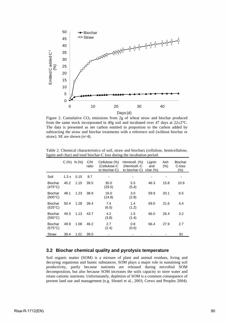
0

5

10

15

20

25

30

35

40

45

50

0 10 20 30 40

Em

itted

C a

dded

C-1

(%)

Days (d)

BiocharStraw

Figure 2. Cumulative CO2 emissions from 2g of wheat straw and biochar produced from the same stock incorporated in 40g soil and incubated over 47 days at 22±2°C. The data is presented as net carbon emitted in proportion to the carbon added by subtracting the straw and biochar treatments with a reference soil (without biochar or straw). SE are shown (n=4).

Table 2. Chemical characteristics of soil, straw and biochars (cellulose, hemicellulose, lignin and char) and total biochar-C loss during the incubation period.

C (%) N (%) C/N ratio

Cellulose (%) (Cellulose-Cto biochar-C)

Hemicell. (%)(Hemicell.-Cto biochar-C)

Lignin and

char (%)

Ash (%)

Biochar C-loss

(%)

Soil 1.3 ± 0.15 8.7 - - - - -

Biochar (475°C)

45.2 1.15 39.5 30.0 (29.5)

5.5 (5.4)

46.3 15.8 10.9

Biochar (500°C)

48.1 1.23 38.9 16.0 (14.8)

3.0 (2.8)

59.9 20.1 6.5

Biochar (525°C)

50.4 1.28 39.4 7.4 (6.5)

1.4 (1.2)

69.0 21.6 4,4

Biochar (550°C)

49.3 1.13 43.7 4.2 (3.8)

1.5 (1.4)

66.0 26.4 3.2

Biochar (575°C)

49.9 1.08 46.2 2.7 (2.4)

0.8 (0.6)

66.4 27.9 2.7

Straw 39.4 1.01 39.0 - - - - 81

3.2 Biochar chemical quality and pyrolysis temperature Soil organic matter (SOM) is a mixture of plant and animal residues, living and decaying organisms and humic substances. SOM plays a major role in sustaining soil productivity, partly because nutrients are released during microbial SOM decomposition, but also because SOM increases the soils capacity to store water and retain cationic nutrients. Unfortunately, depletion of SOM is a common consequence of present land use and management (e.g. Sleutel et al., 2003; Crews and Peoples 2004).

Risø-R-1712(EN) 90

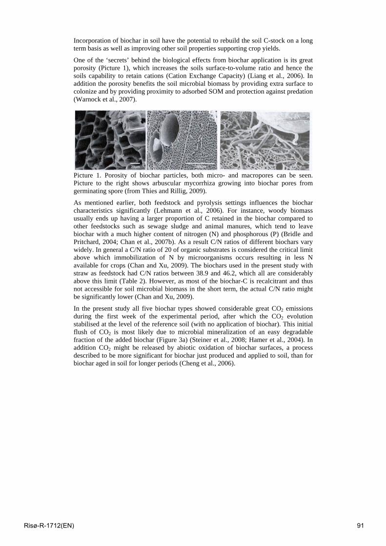
Incorporation of biochar in soil have the potential to rebuild the soil C-stock on a long term basis as well as improving other soil properties supporting crop yields.

One of the ‘secrets’ behind the biological effects from biochar application is its great porosity (Picture 1), which increases the soils surface-to-volume ratio and hence the soils capability to retain cations (Cation Exchange Capacity) (Liang et al., 2006). In addition the porosity benefits the soil microbial biomass by providing extra surface to colonize and by providing proximity to adsorbed SOM and protection against predation (Warnock et al., 2007).

Picture 1. Porosity of biochar particles, both micro- and macropores can be seen. Picture to the right shows arbuscular mycorrhiza growing into biochar pores from germinating spore (from Thies and Rillig, 2009).

As mentioned earlier, both feedstock and pyrolysis settings influences the biochar characteristics significantly (Lehmann et al., 2006). For instance, woody biomass usually ends up having a larger proportion of C retained in the biochar compared to other feedstocks such as sewage sludge and animal manures, which tend to leave biochar with a much higher content of nitrogen (N) and phosphorous (P) (Bridle and Pritchard, 2004; Chan et al., 2007b). As a result C/N ratios of different biochars vary widely. In general a C/N ratio of 20 of organic substrates is considered the critical limit above which immobilization of N by microorganisms occurs resulting in less N available for crops (Chan and Xu, 2009). The biochars used in the present study with straw as feedstock had C/N ratios between 38.9 and 46.2, which all are considerably above this limit (Table 2). However, as most of the biochar-C is recalcitrant and thus not accessible for soil microbial biomass in the short term, the actual C/N ratio might be significantly lower (Chan and Xu, 2009).

In the present study all five biochar types showed considerable great CO2 emissions during the first week of the experimental period, after which the CO2 evolution stabilised at the level of the reference soil (with no application of biochar). This initial flush of CO2 is most likely due to microbial mineralization of an easy degradable fraction of the added biochar (Figure 3a) (Steiner et al., 2008; Hamer et al., 2004). In addition CO2 might be released by abiotic oxidation of biochar surfaces, a process described to be more significant for biochar just produced and applied to soil, than for biochar aged in soil for longer periods (Cheng et al., 2006).

Risø-R-1712(EN) 91

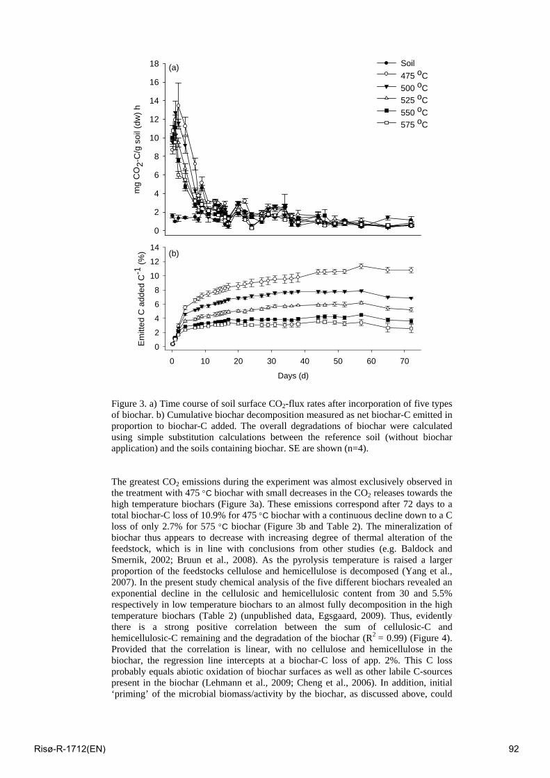
Days (d)

0 10 20 30 40 50 60 70

Emitt

ed C

add

ed C

-1 (%

)

0

2

4

6

8

10

12

14

(a)

mg

CO

2-C

/g s

oil (

dw) h

0

2

4

6

8

10

12

14

16

18

(b)

Soil475 oC500 oC525 oC550 oC575 oC

Figure 3. a) Time course of soil surface CO2-flux rates after incorporation of five types of biochar. b) Cumulative biochar decomposition measured as net biochar-C emitted in proportion to biochar-C added. The overall degradations of biochar were calculated using simple substitution calculations between the reference soil (without biochar application) and the soils containing biochar. SE are shown (n=4).

The greatest CO2 emissions during the experiment was almost exclusively observed in the treatment with 475 °C biochar with small decreases in the CO2 releases towards the high temperature biochars (Figure 3a). These emissions correspond after 72 days to a total biochar-C loss of 10.9% for 475 °C biochar with a continuous decline down to a C loss of only 2.7% for 575 °C biochar (Figure 3b and Table 2). The mineralization of biochar thus appears to decrease with increasing degree of thermal alteration of the feedstock, which is in line with conclusions from other studies (e.g. Baldock and Smernik, 2002; Bruun et al., 2008). As the pyrolysis temperature is raised a larger proportion of the feedstocks cellulose and hemicellulose is decomposed (Yang et al., 2007). In the present study chemical analysis of the five different biochars revealed an exponential decline in the cellulosic and hemicellulosic content from 30 and 5.5% respectively in low temperature biochars to an almost fully decomposition in the high temperature biochars (Table 2) (unpublished data, Egsgaard, 2009). Thus, evidently there is a strong positive correlation between the sum of cellulosic-C and hemicellulosic-C remaining and the degradation of the biochar (R2 = 0.99) (Figure 4). Provided that the correlation is linear, with no cellulose and hemicellulose in the biochar, the regression line intercepts at a biochar-C loss of app. 2%. This C loss probably equals abiotic oxidation of biochar surfaces as well as other labile C-sources present in the biochar (Lehmann et al., 2009; Cheng et al., 2006). In addition, initial ‘priming’ of the microbial biomass/activity by the biochar, as discussed above, could

Risø-R-1712(EN) 92

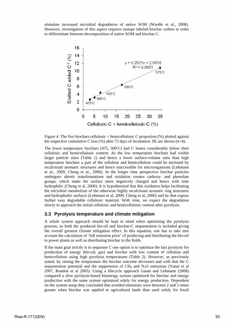
stimulate increased microbial degradation of native SOM (Wardle et al., 2008). However, investigation of this aspect requires isotope labeled biochar carbon in order to differentiate between decomposition of native SOM and biochar C.

Figure 4. The five biochars cellulosic + hemicellulosic C proportion (%) plotted against the respective cumulative C loss (%) after 72 days of incubation. SE are shown (n=4).

The lower temperature biochars (475, 500°C) had C losses considerably below their cellulosic and hemicellulosic content. As the low temperature biochars had visible larger particle sizes (Table 1) and hence a lower surface-volume ratio than high temperature biochars a part of the cellulose and hemicellulose could be enclosed by recalcitrant aromatic structures and hence inaccessible for microorganisms (Lehmann et al., 2009; Cheng et al., 2006). In the longer time perspective biochar particles undergoes abiotic transformations and oxidation creates carboxy- and phenolate groups, which make the surface more negatively charged and hence with time hydrophilic (Cheng et al, 2006). It is hypothesized that this oxidation helps facilitating the microbial metabolism of the otherwise highly recalcitrant aromatic ring structures and hydrophobic surfaces (Lehmann et al, 2009; Cheng et al, 2006) and by that expose further easy degradable cellulosic material. With time, we expect the degradation slowly to approach the initial cellulosic and hemicellulosic content after pyrolysis.

3.3 Pyrolysis temperature and climate mitigation A whole system approach should be kept in mind when optimising the pyrolysis process, so both the produced bio-oil and biochar-C sequestration is included giving the overall greatest climate mitigation effect. In this equation, one has to take into account the calculation of ‘full emission price’ of producing and distributing the bio-oil to power plants as well as distributing biochar to the fields.

If the main goal strictly is to sequester C one option is to optimize the fast pyrolysis for production of energy (bio-oil, gas) and biochar with low content of cellulose and hemicellulose using high pyrolysis temperatures (Table 2). However, as previously stated, by raising the temperature the biochar outcome decreases and with that the C sequestration potential and the suppression of CH4 and N2O emissions (Yanai et al 2007, Rondon et al 2005). Using a lifecycle approach Gaunt and Lehmann (2008) compared a slow pyrolysis-based bioenergy system optimized for biochar and energy production with the same system optimized solely for energy production. Dependent on the system setup they concluded that avoided emissions were between 2 and 5 times greater when biochar was applied to agricultural lands than used solely for fossil

Risø-R-1712(EN) 93

energy offsets (Gaunt and Lehmann 2008). It still needs though, to be assessed on a real agricultural system and if the same is true for a fast pyrolysis-based bioenergy system.

The Amazonian Indians used biochar to enhance their fragile, nutrient-poor tropical soils increasing food productivity. If the main goal is enhancement of soil fertility, crop yields and sustainability, it might make more sense to add a low-temperature biochar with more of the original feedstock structures to provide the soil with easy degradable organic matter and by returning a larger proportion of the original feedstock back to the field. In order to mitigate climate change it seems sound addressing this in the light of food and energy security and thus the optimum might be a compromise of the two goals.

4 Conclusion Fast pyrolysis of straw to biochar with following soil amendment provides C sequestration, but the degradability of biochar is correlated with the degree of thermal alteration of the feedstock. It appears that the short-term degradation of biochar is proportional to the cellulosic and hemicellulosic proportion left in the biochar. Furthermore the temperature settings of fast pyrolysis are important to consider, as this strongly influences the amount of cellulose and hemicellulose remaining in the biochar.

5 Acknowledgement We acknowledge the funding from the Technical University of Denmark (National Globalization Funding) enabling collaboration between Biosystems Division, Risø-DTU and Division of Chemical Engineering Competences, DTU. The project cover the development of a flash pylolysis unit for production of biooil/biochar (WP1), evaluation of environmental effects of applying biochar to soil (WP2) and physical/chemical characteristics of produced oil and biochar (WP3).

Risø-R-1712(EN) 94

6 References Baldock J. A. and Smernik R. J. (2002). Chemical composition and bioavailability of

thermally altered Pinus resinosa (Red pine) wood. Organic Geochemistry 33:1093-1109

Bech N., Larsen M.B., Jensen P.A., Dam-Johansen K. (2009). Modelling solid-convective flash pyrolysis of straw and wood in the Pyrolysis Centrifuge Reactor. Biomass and Bioenergy 33:999 – 1011

Bridle T. R. and Pritchard D. (2004) ‘Energy and nutrient recovery from sewage sludge via pyrolysis’. Water Science and Technology 50:169-175

Bruun S., Jensen E. J., Jensen L. (2008). Microbial mineralization and assimilation of black carbon:Dependency on degree of thermal alteration. Organic Geochemistry 39:839–845

Chan K. Y. and Z. Xu (2009). Biochar: Nutrient Properties and Their Enhancement. In Lehmann J. and Joseph S. (eds). Biochar for environmental management – Science and technology. Earthscan :183-205

Chan K. Y.,Van Zwieten L., Meszaros I., Downie A. and Joseph S. (2007). Agronomic values of green waste biochar as a soil amendment. Australian Journal of Soil Research 45:629-634

Chan K. Y., Van Zwieten L., Meszaros I., Downie A. and Joseph S. (2007b). Assessing the agronomic values of contrasting char materials on Australian hardsetting soil. In Conference of the International Agrichar Initiative, 30 April- 2 May 2007, Terrigal, NSW, Australia

Cheng C.H., Lehmann J., Thies J.E., Burton S.D. and Engelhard M.H. (2006). Oxidation of black C by biotic and abiotic processes. Organic Geochemistry 37 (11):1477-1488

Crews T.E. and Peoples M.B. (2004). Legume versus fertilizer sources of nitrogen:ecological tradeoffs and human needs. Agr. Ecosyst. Environ. 102:279-297

Gaunt J. L. and Lehmann J. (2008). Energy Balance and Emissions Associated with Biochar Sequestration and Pyrolysis Bioenergy Production. Environmental Science and Technology 42:4152-4158

Glaser B., Lehmann J. and Zech W. (2002). Ameliorating physical and chemical properties of highly weathered soils in the tropics with charcoal – a review. Biol. Fertile Soils 35:219-230

Gupta A. K. and Lilley D.G. (2003). Thermal destruction of wastes and plastics. In A. L. Andrady (ed) Plastics and the Environment. Wiley-Interscience:384-410

Lehmann J. (2007). A handful of carbon. Nature 447:143–144

Lehmann J., Czimczik C., Laird D., Sohi S. (2009). Stability of biochar in the soil. In Lehmann J. and Joseph S. (eds). Biochar for environmental management – Science and technology. Earthscan :183-205

Lehmann J., Gaunt J. and Rondon M. (2006). Bio-char sequestration in terrestrial ecosystems – a review. Mitigation and Adaptation Strategies for Global Change 11:403–427

Liang B., Lehmann J., Solomon D., Kinyangi J., Grossman J., O’Neill B., Skjemstad J. O., Thies J., Luizão F. J., Petersen J. and Neves E. G. (2006). Black carbon increases cation exchange capacity in soils. Soil Science Society of America Journal 72:1719-1730

Hamer U., Marschner B., Brodowski S. and Amelung W. (2004). Interactive Priming of black carbon and glucose mineralization. Organic Geochemistry 35:823-830

Risø-R-1712(EN) 95

Oguntunde P. G., Fosu M., Ajayi A. E., and Giesen N. (2004). Effects of charcoal production on maize yield, chemical properties and texture of soil. Biology and Fertility of Soils 39(4):295-299

Preston C. M. and Schmidt M. W. I. (2006). Black (pyrogenic) carbon:a synthesis of current knowledge and uncertainties with special consideration of boreal regions. Biogeosciences 3:397-420

Rondon, M. A., Lehmann J., Ramirez J. and Hurtado M. (2007). Biological nitrogen fixation by common beans (Phaseolus vulgaris L.) increases with bio-char additions. Biology and Fertility of Soils 43:699-728

Schils et al. (2008). Review of existing information on the interrelationships between soil and climate change. The CLIMSOIL report:http://ec.europa.eu/environment/soil/review_en.htm

Sleutel S., De Neve, S., Hofman, G. (2003). Estimates of carbon stock changes in Belgian cropland. Soil use & management 19:166-171

Smith P., Andrén O., Karlsson T., Perälä P., Regina K., Rounsevell M. and Van Wesemael B. (2005). Carbon sequestration potential in European croplands has been overestimated. Global Change Biology 11:2153-2163

Steiner C., Das K. C., Garcia M., Forster B. and Zech W. (2008b). Charcoal and smoke extract stimulate the soil microbial community in a highly weathered xanthic Ferralsol. Pedobiologia 51:359-366

Steiner C., Glaser B., Teixeira W. G, Lehmann. J., Blum W.E.H., and Zech W. (2008a). Nitrogen retention and plant uptake on a highly weathered central Amazonian Ferralsol amended with compost and charcoal. Plant Nutr. Soil Science 171:893–899

Steiner C., Teixeira W.G., Lehmann J., Nehls T., de Macedo J., Blum W.E.H., and Zech W. (2007). Long term effect of manure, charcoal and mineral fertilisation on crop production and fertility on a highly wetheared Central Amazonian upland soil. Plant and Soil 291:275-290

Thies E. J and Rillig M. C. (2009). Charecteristics of Biochar:Biological Properties. In Lehmann J. and Joseph S. (eds). Biochar for environmental management – Science and technology. Earthscan:85-105

Yanai Y., Toyota K. and Okazaki M. (2007). Effects of charcoal addition on N2O emissions from soil resulting from rewetting air-dried soil in short-term laboratory experiments. Soil Science and Plant Nutrition 53:181-188

Yang H., Yan R., Chen H., Lee D. H. and Zheng C. (2007). Characteristics of hemicellulose, cellulose and lignin pyrolysis. Fuel 86:1781-1788

Yanik J., Kornmayer C., Saglam M. and Yüksel M. (2007). Fast pyrolysis of aggriculteral wastes:Characterization of pyrolysis products. Fuel Processing Technology 88:942-947

Wardle D. A., Nilson M. C. and Zackrisson O. (2008). Fire-derived charcoal causes loss of forest humus. Science 320:629-629

Warnock D. D., Lehmann J., Kuyper T. W. and Rillig M. C. (2007). Mycorrhizal responses to biochar in soil - concepts and mechanisms. Plant and Soil 300:9-20

Risø-R-1712(EN) 96

Session 6 – Efficiency improvements in end-use

Risø-R-1712(EN) 97

High-power blue/red LED lighting system for future energy efficient artificial lighting in greenhouse production of potted plants Birgitte Thestrupa, Carsten Dam-Hansena, Henning Engelbrecht Larsena, Janni

Bjerregaard Lundb, Eva Rosenqvistc, and Claus Kjærgaardd

aDepartment of Photonics Engineering, Technical University of Denmark, 4000

Roskilde, Denmark

bAgroTech A/S, Institute for Agro Technology and Food Innovation, 2630 Taastrup,

Denmark

cDepartment of Agricultural Science, University of Copenhagen, 2630 Taastrup,

Denmark

dØrsted DTU, Technical University of Denmark, 2800 Kgs. Lyngby, Denmark

Abstract Supplementary lighting in greenhouses is an essential factor in optimization of production of e.g. potted plants and has resulted in increasing energy consumption for artificial lighting over the past years. Here, we present a newly developed blue/red LED lighting system for photosynthetic research on potted plants. The LED system performance, regarding spectral composition and irradiance level, is examined and compared with standard high power sodium (HPS) illumination over a 60 cm x 60 cm growth area in a typical greenhouse. Furthermore, the energy efficiency of the two different light sources, in the photosynthetic active radiation (PAR) wavelength region, is calculated and compared. The perspectives for LED lighting systems as future energy efficient artificial lighting in greenhouse production of potted plants are discussed.

1 Introduction In Denmark, we have a relatively large greenhouse production of potted plants used mainly for export. In 2003 the value of this production was close to 400 million € (3 billion Danish crowns). Due to the dark winter period in Denmark and in order to produce homogeneous plants of high quality all around the year, the nurseries have corresponding high energy consumption for artificial lighting. From year 2000 to 2006 the energy consumption for artificial lighting has increased by 10% from 90 kWh/m2 greenhouse area to 101 kWh/m2 greenhouse area. This increase is unfortunate since the nurseries in the past years have been subject for massive influence by the Danish Energy Agency for reducing their energy consumption.

HPS lamps are the preferred artificial light sources used in greenhouses today due to their high external energy efficiency up to 35%. However, only part of the light from these lamps can be used for photosynthesis, i.e. plant growth. During photosynthesis

Risø-R-1712(EN) 98

plants use energy from photons in the visible part of the light spectrum from 400 nm to 700 nm, called the PAR wavelength region. Energy is primarily harvested from the blue and the red part of the spectrum by the two green pigments Chlorophyll a and b. Chlorophyll a has absorption peaks at 435 nm and 665 nm while Chlorophyll b has absorption peaks at 465 nm and 640 nm [1]. HPS lamps are most efficient in the yellow-orange part of the spectrum outside these absorption peaks. In addition, HPS lamps have a relatively high heat radiation. As a result only part of the energy consumed by the HPS lamps is converted to energy that can be used directly by the potted plants. Furthermore HPS lamps have poor flexibility regarding spectral control and dimming possibilities.

In contrast to HPS lamps, light emitting diodes (LEDs) have a relative narrow spectrum and come in many different colours which give the possibility of designing an optimal light spectrum for the given application by combining LEDs of suitable colours. LEDs have the advantage of long lifetimes up to 50.000 hours and they can easily be dimmed. Furthermore, the energy efficiency of high-power LEDs is expected to reach 50% within the near future which makes LEDs an attractive candidate and alternative to HPS lamps for supplementary lighting in greenhouse production.

In the present paper, we compare the performance of a standard HPS lamp used in greenhouse production and one of our LED lamps developed for photosynthetic research, with respect to spectral composition and irradiance level over a 60 cm x 60 cm plant area. Furthermore, we calculate and compare the efficiency of the two different lamp types and discuss the perspectives for LED lighting systems as future energy efficient artificial lighting in greenhouse production of potted plants.

2 LED lighting system The LED lighting system consists of four similar LED lamps, with red and blue LEDs, developed for photosynthesis research experiments. A detailed description of the lighting system can be found in reference [2]. The LEDs used in the lamps are chosen in such a way that their peaks wavelengths are close to the absorption peaks of Chlorophyll in order to optimize photosynthesis. The high-power LEDs used in the lamps belong to the most energy-efficient LEDs at these wavelength that were commercial available at the time of the system development1.

A photo of a single LED lamp as seen from the side is shown in Figure 1. It consists of 72 closely packed red and royal blue Luxeon K2 LEDs that are reflow soldered on an Ø110 mm circular alumina print for optimum heat transfer. The print is mounted on a polished copper block with water flow channels and the LED device is actively cooled through a water cooling system that keeps the water at a temperature of 21° C during experiments. A temperature sensor placed on the alumina print prevents overheating of the LED lamp by turning the lamp off in case of overheating.

The LED lighting system is designed for experiments in which the light level and the spectral composition can be controlled. The LEDs are driven at a constant operation current of 700 mA using 12 individual constant current drivers per lamp (6 LEDs per driver) with pulse width modulation for dimming. A graphical user interface developed in LabView allows the user to control the dimming of the LEDs in groups of 6 LEDs in order to be able to change the overall light level and spectral composition (blue/red light ratio) of the emitted light.

The power consumption at 700 mA is approximately 2.5 W per LED according to the data sheet giving a maximum total power consumption of approximately180 W per LED lamp. In the present experiment, the lamps are running at 60 % of the maximum power. The LEDs have a viewing angle 2θ½ of approximately 140° and a slightly flat topped

1 Since development of the lamps described here, more power full and energy efficient LEDs have

become commercial available.

Risø-R-1712(EN) 99

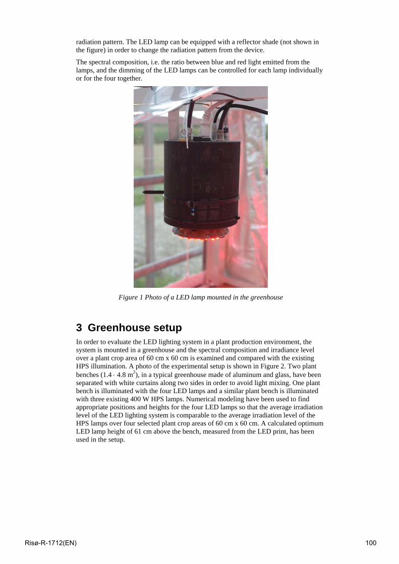
radiation pattern. The LED lamp can be equipped with a reflector shade (not shown in the figure) in order to change the radiation pattern from the device.

The spectral composition, i.e. the ratio between blue and red light emitted from the lamps, and the dimming of the LED lamps can be controlled for each lamp individually or for the four together.

Figure 1 Photo of a LED lamp mounted in the greenhouse

3 Greenhouse setup In order to evaluate the LED lighting system in a plant production environment, the system is mounted in a greenhouse and the spectral composition and irradiance level over a plant crop area of 60 cm x 60 cm is examined and compared with the existing HPS illumination. A photo of the experimental setup is shown in Figure 2. Two plant benches (1.4 ⋅ 4.8 m2), in a typical greenhouse made of aluminum and glass, have been separated with white curtains along two sides in order to avoid light mixing. One plant bench is illuminated with the four LED lamps and a similar plant bench is illuminated with three existing 400 W HPS lamps. Numerical modeling have been used to find appropriate positions and heights for the four LED lamps so that the average irradiation level of the LED lighting system is comparable to the average irradiation level of the HPS lamps over four selected plant crop areas of 60 cm x 60 cm. A calculated optimum LED lamp height of 61 cm above the bench, measured from the LED print, has been used in the setup.

Risø-R-1712(EN) 100

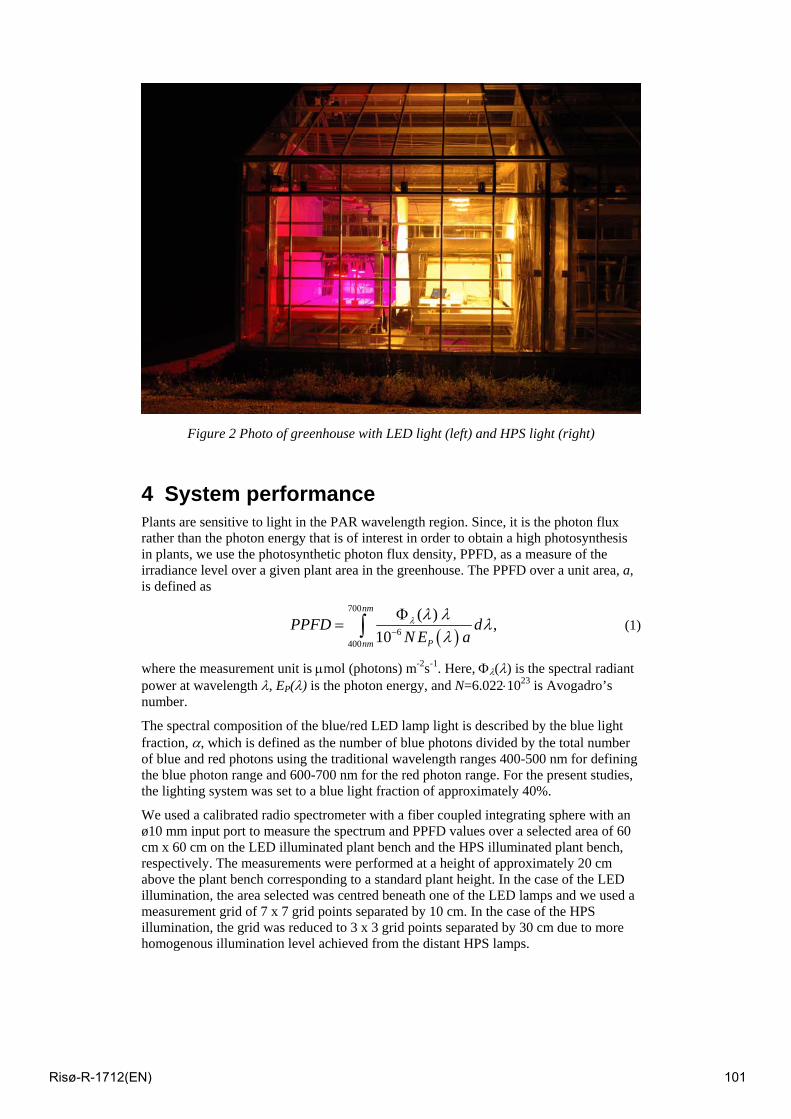
Figure 2 Photo of greenhouse with LED light (left) and HPS light (right)

4 System performance Plants are sensitive to light in the PAR wavelength region. Since, it is the photon flux rather than the photon energy that is of interest in order to obtain a high photosynthesis in plants, we use the photosynthetic photon flux density, PPFD, as a measure of the irradiance level over a given plant area in the greenhouse. The PPFD over a unit area, a, is defined as

( )700

6400

( ) ,10

nm

Pnm

PPFD dN E aλ λ λ λ

λ−

Φ= ∫ (1)

where the measurement unit is μmol (photons) m-2s-1. Here, Φλ(λ) is the spectral radiant power at wavelength λ, EP(λ) is the photon energy, and N=6.022⋅1023 is Avogadro’s number.

The spectral composition of the blue/red LED lamp light is described by the blue light fraction, α, which is defined as the number of blue photons divided by the total number of blue and red photons using the traditional wavelength ranges 400-500 nm for defining the blue photon range and 600-700 nm for the red photon range. For the present studies, the lighting system was set to a blue light fraction of approximately 40%.

We used a calibrated radio spectrometer with a fiber coupled integrating sphere with an ø10 mm input port to measure the spectrum and PPFD values over a selected area of 60 cm x 60 cm on the LED illuminated plant bench and the HPS illuminated plant bench, respectively. The measurements were performed at a height of approximately 20 cm above the plant bench corresponding to a standard plant height. In the case of the LED illumination, the area selected was centred beneath one of the LED lamps and we used a measurement grid of 7 x 7 grid points separated by 10 cm. In the case of the HPS illumination, the grid was reduced to 3 x 3 grid points separated by 30 cm due to more homogenous illumination level achieved from the distant HPS lamps.

Risø-R-1712(EN) 101

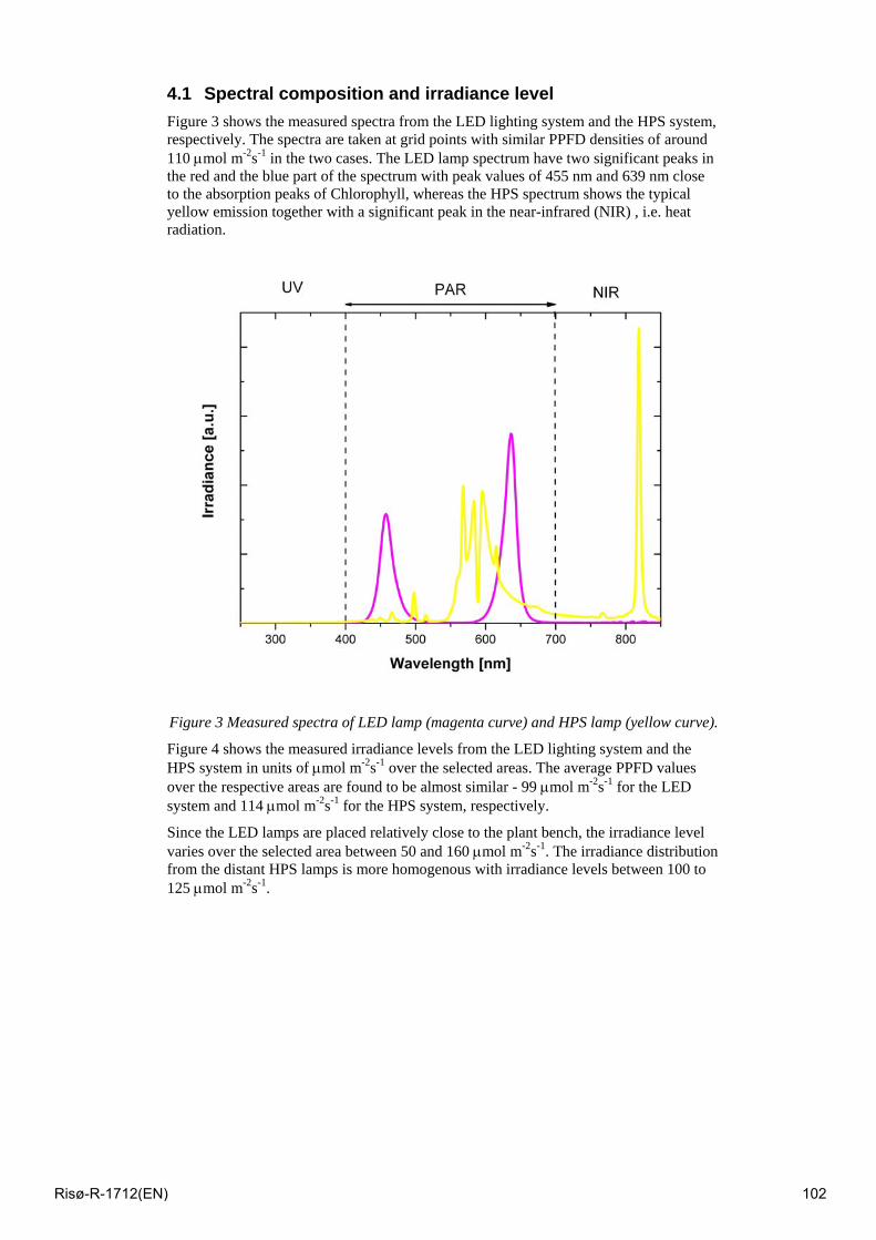
4.1 Spectral composition and irradiance level Figure 3 shows the measured spectra from the LED lighting system and the HPS system, respectively. The spectra are taken at grid points with similar PPFD densities of around 110 μmol m-2s-1 in the two cases. The LED lamp spectrum have two significant peaks in the red and the blue part of the spectrum with peak values of 455 nm and 639 nm close to the absorption peaks of Chlorophyll, whereas the HPS spectrum shows the typical yellow emission together with a significant peak in the near-infrared (NIR) , i.e. heat radiation.

Figure 3 Measured spectra of LED lamp (magenta curve) and HPS lamp (yellow curve).

Figure 4 shows the measured irradiance levels from the LED lighting system and the HPS system in units of μmol m-2s-1 over the selected areas. The average PPFD values over the respective areas are found to be almost similar - 99 μmol m-2s-1 for the LED system and 114 μmol m-2s-1 for the HPS system, respectively.

Since the LED lamps are placed relatively close to the plant bench, the irradiance level varies over the selected area between 50 and 160 μmol m-2s-1. The irradiance distribution from the distant HPS lamps is more homogenous with irradiance levels between 100 to 125 μmol m-2s-1.

Risø-R-1712(EN) 102

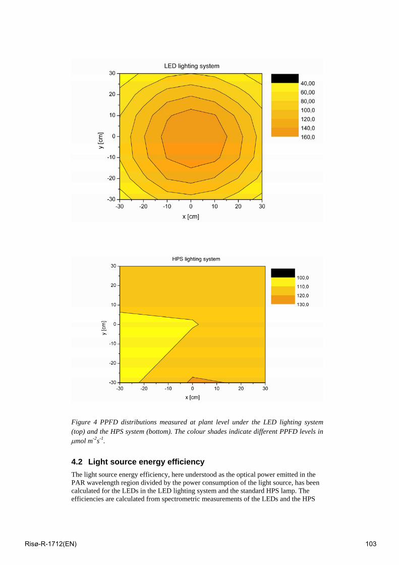
Figure 4 PPFD distributions measured at plant level under the LED lighting system (top) and the HPS system (bottom). The colour shades indicate different PPFD levels in μmol m-2s-1.

4.2 Light source energy efficiency The light source energy efficiency, here understood as the optical power emitted in the PAR wavelength region divided by the power consumption of the light source, has been calculated for the LEDs in the LED lighting system and the standard HPS lamp. The efficiencies are calculated from spectrometric measurements of the LEDs and the HPS

Risø-R-1712(EN) 103

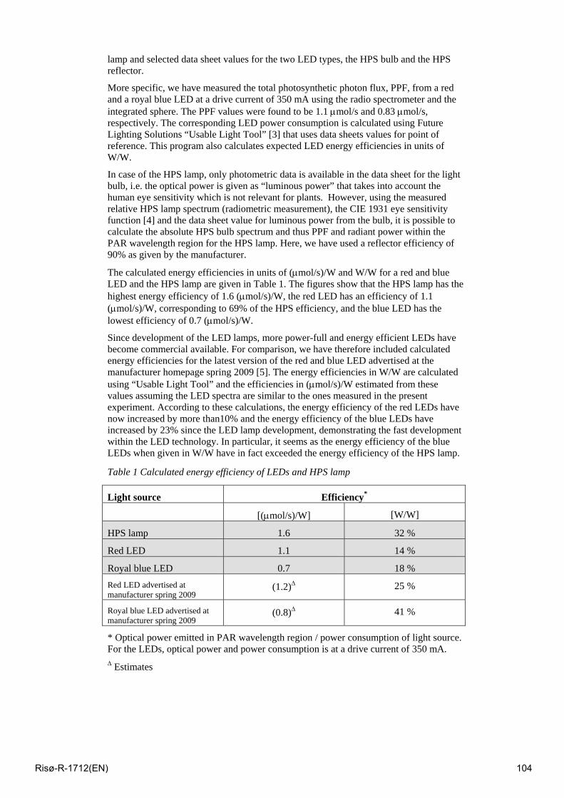
lamp and selected data sheet values for the two LED types, the HPS bulb and the HPS reflector.

More specific, we have measured the total photosynthetic photon flux, PPF, from a red and a royal blue LED at a drive current of 350 mA using the radio spectrometer and the integrated sphere. The PPF values were found to be 1.1 μmol/s and 0.83 μmol/s, respectively. The corresponding LED power consumption is calculated using Future Lighting Solutions “Usable Light Tool” [3] that uses data sheets values for point of reference. This program also calculates expected LED energy efficiencies in units of W/W.

In case of the HPS lamp, only photometric data is available in the data sheet for the light bulb, i.e. the optical power is given as “luminous power” that takes into account the human eye sensitivity which is not relevant for plants. However, using the measured relative HPS lamp spectrum (radiometric measurement), the CIE 1931 eye sensitivity function [4] and the data sheet value for luminous power from the bulb, it is possible to calculate the absolute HPS bulb spectrum and thus PPF and radiant power within the PAR wavelength region for the HPS lamp. Here, we have used a reflector efficiency of 90% as given by the manufacturer.

The calculated energy efficiencies in units of (μmol/s)/W and W/W for a red and blue LED and the HPS lamp are given in Table 1. The figures show that the HPS lamp has the highest energy efficiency of 1.6 (μmol/s)/W, the red LED has an efficiency of 1.1 (μmol/s)/W, corresponding to 69% of the HPS efficiency, and the blue LED has the lowest efficiency of 0.7 (μmol/s)/W.

Since development of the LED lamps, more power-full and energy efficient LEDs have become commercial available. For comparison, we have therefore included calculated energy efficiencies for the latest version of the red and blue LED advertised at the manufacturer homepage spring 2009 [5]. The energy efficiencies in W/W are calculated using “Usable Light Tool” and the efficiencies in (μmol/s)/W estimated from these values assuming the LED spectra are similar to the ones measured in the present experiment. According to these calculations, the energy efficiency of the red LEDs have now increased by more than10% and the energy efficiency of the blue LEDs have increased by 23% since the LED lamp development, demonstrating the fast development within the LED technology. In particular, it seems as the energy efficiency of the blue LEDs when given in W/W have in fact exceeded the energy efficiency of the HPS lamp.

Table 1 Calculated energy efficiency of LEDs and HPS lamp

Light source Efficiency*

[(μmol/s)/W] [W/W]

HPS lamp 1.6 32 %

Red LED 1.1 14 %

Royal blue LED 0.7 18 % Red LED advertised at manufacturer spring 2009

(1.2)Δ 25 %

Royal blue LED advertised at manufacturer spring 2009

(0.8)Δ 41 %

* Optical power emitted in PAR wavelength region / power consumption of light source. For the LEDs, optical power and power consumption is at a drive current of 350 mA. Δ Estimates

Risø-R-1712(EN) 104

5 Discussion Even though the energy efficiency in (μmol/s)/W of the HPS lamp exceeds the efficiency of the blue and red LEDs available today, LED lighting systems are still an attractive candidate as energy efficient supplementary lighting in greenhouse production of potted plants.

First of all, the relative rate of photosynthesis for crop plants is known to be significantly lower (at least 5-15%) in the yellow-orange part of the light spectrum, where the HPS lamp is most efficient, than in the red part of the light spectrum [1], i.e., around the absorption peaks of Chlorophyll, where the red LEDs are efficient.

Secondly, HPS lamps do not “like” to be turned on and off during the day, why nurseries today turns on the HPS light in many hours during a day. In contrast, the LED light have the possibility to be controlled in such a way that light is turned on only when necessary and with a light level adjusted for optimized growth. Furthermore, the LED light offers a possibility for spectral control, i.e. the spectrum can be dynamically controlled during the day and/or during a growth period in order to optimize growth and flowering.

With the present blue/red LED lighting system, we have developed a useful research tool that can aid in determining some of these optimization parameters, since the LED lighting system can be used for real greenhouse experiments in which results on potted plant crops with LED illumination and HPS illumination can be directly compared.

Given the rapid increase in energy efficiency of LEDs, that is expected to reach 50% within the near future, combined with further horticulture research on potted plant cultures illuminated with LED lighting systems, LED light will play an increasing role in the nurseries efforts to reduce their energy consumption for artificial lighting in the years to come.

6 Summary In summary, we have presented a blue/red LED lighting system, consisting of four identical LED lamps with high-power LEDs, developed for photosynthetic research on potted plants. The LED lamps can be controlled regarding blue/red spectral composition and dimming.

The spectrum and irradiance level of the LED lighting system and a standard HPS lighting system is measured over a 60 cm x 60 cm growth area in a typical greenhouse. The LED lamp spectrum has two significant peaks in the red and blue part of the visible spectrum at 455 nm and 639 nm close to the absorption peaks of Chlorophyll, whereas the HPS spectrum shows the typical yellow emission together with a heat radiation peak outside the PAR wavelength region. The average irradiation levels (PPFD values) over the respective growth areas are found to be almost similar for the LED system and the HPS system, around 99 μmol m-2s-1 and 114 μmol m-2s-1, respectively.

The HPS lamp has the highest energy efficiency in the PAR wavelength region of 1.6 (μmol/s)/W when comparing with the red and blue LED used in the LED system. The red LED has an efficiency of 1.1 (μmol/s)/W, corresponding to 69% of the HPS efficiency, and the blue LED has an efficiency of 0.7 (μmol/s)/W. The increase in energy efficiency of the red and the blue LED since the development of the LED lighting system is calculated to be more than 10% (red LED) and 23% (blue LED) indicating that LED lighting systems are attractive as energy efficient supplementary lighting in greenhouse production of potted plants.

The authors want to acknowledge ELFORSK grant no 338-022 and 340-040 for financial support.

Risø-R-1712(EN) 105

7 References [1] K. J. McCree (1972), The action spectrum, absorptance and quantum yield of photosynthesis in crop plants, Agric. Meteorol. 9, 191-216

[2] C. Dam-Hansen, B. Thestrup, E. Rosenqvist, J. Bjerregaard Lund, and C. Kjærgaard, Irradiance and spectral characteristics of a blue/red high-power LED lighting system: Influence on photosynthetic response of a plant canopy, to be published

[3] www.futurelightingsolutions.com

[4] Color Science: Concepts and Methods, Quantitative data and Formulae, 2nd ed., G. Wyszecki and W.S. Stiles (Wiley, New York, 2000)

[5] www.philipslumileds.com

Risø-R-1712(EN) 106

Magnetic Refrigeration – an Energy Efficient Technology for the Future C.R.H. Bahl, A. Smith, N. Pryds and S. Linderoth

Fuel Cells and Solid State Chemistry Division Risø National Laboratory for Sustainable Energy Technical University of Denmark - DTU

Abstract Magnetic refrigeration is an emerging technology that has the potential to significantly reduce the energy consumption in the refrigeration sector. The technology relies on the heating and cooling of magnetic materials upon the application and removal of a magnetic field, respectively. This magnetocaloric effect is inherent to all magnetic materials, but manifests itself stronger in some materials. The thermodynamically reversible nature of the magnetocaloric effect holds out the promise of a more energy efficient method of refrigeration compared to conventional compressor technology. Coupling this with an absence of ozone depleting and greenhouse contributing gasses gives magnetic refrigeration the potential to become an environmentally sustainable technology.

The magnetic refrigeration group at Risø DTU aims to demonstrate the technology in a prototype magnetic refrigeration device. Our work spans a wide range of scientific and technological areas. At the pure science end there is the development and understanding of new magnetocaloric materials, while the design and implementation of a prototype device along with the processing of materials is at the technological engineering end. Tying the work together are advanced numerical computer models of the individual parts of the prototype. A simple yet versatile test machine located at Risø DTU is used to test and characterise new materials and to test the design, configuration and operating conditions relevant for a prototype device, while ensuring understanding through consistency with the numerical models.

1 Introduction As is well known the global energy consumption is increasing at an unprecedented rate. The growing affluence of the third world brings with it the desire for commodities such as lighting, heating/cooling and consumer electronics. Of these, refrigeration accounts for a substantial fraction of the energy consumption. Refrigeration is used for space cooling in air conditioning equipment and for storage and transportation of food products both domestically and commercially.

Depending on the exact definition of the different sectors, the fraction of reported electricity consumption for refrigeration is around 15% - 20% in the western world [1]. Obviously the fraction would be higher for countries in hotter climates, to the extent that cooling is affordable.

An increase in the energy efficiency of refrigeration would be able to significantly reduce the world energy consumption, and thus the emission of CO2 into the atmosphere. Although the efficiency of, e.g., domestic refrigerators is continuously improved, there are still some inherent losses that increase energy consumption.

Conventional compressor refrigeration is based on the compression and expansion of volatile, often harmful gasses. Although the infamous ozone layer depleting CFC gasses have been almost phased out, the HCFC and HFC gasses that substituted these still have a small ozone layer depletion potential and a significant greenhouse effect contribution

Risø-R-1712(EN) 107

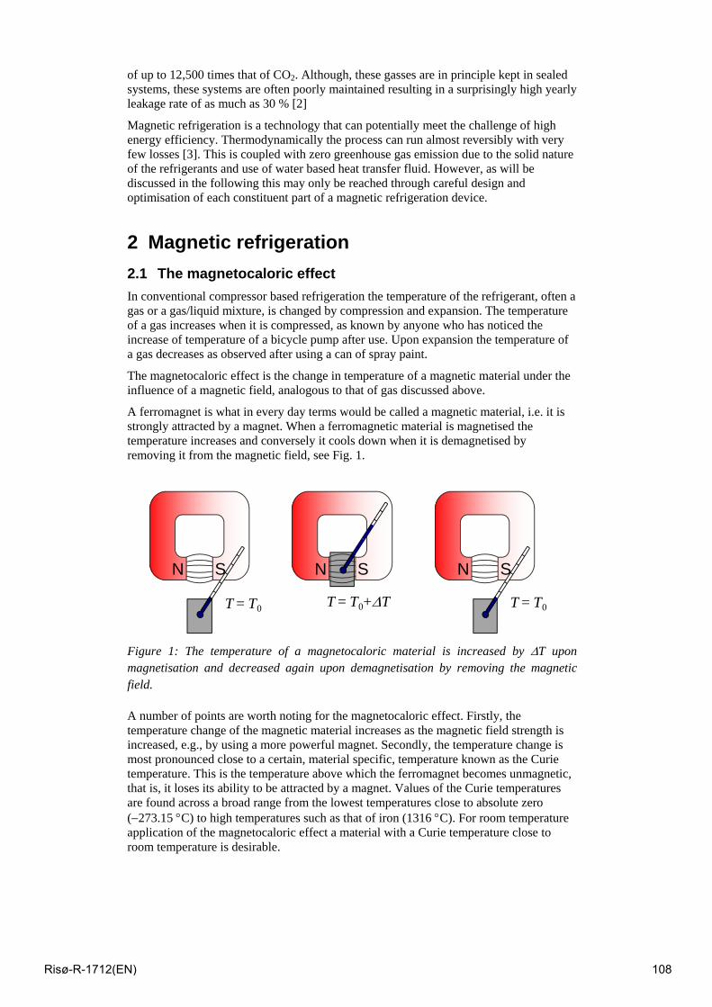
of up to 12,500 times that of CO2. Although, these gasses are in principle kept in sealed systems, these systems are often poorly maintained resulting in a surprisingly high yearly leakage rate of as much as 30 % [2]

Magnetic refrigeration is a technology that can potentially meet the challenge of high energy efficiency. Thermodynamically the process can run almost reversibly with very few losses [3]. This is coupled with zero greenhouse gas emission due to the solid nature of the refrigerants and use of water based heat transfer fluid. However, as will be discussed in the following this may only be reached through careful design and optimisation of each constituent part of a magnetic refrigeration device.

2 Magnetic refrigeration 2.1 The magnetocaloric effect In conventional compressor based refrigeration the temperature of the refrigerant, often a gas or a gas/liquid mixture, is changed by compression and expansion. The temperature of a gas increases when it is compressed, as known by anyone who has noticed the increase of temperature of a bicycle pump after use. Upon expansion the temperature of a gas decreases as observed after using a can of spray paint.

The magnetocaloric effect is the change in temperature of a magnetic material under the influence of a magnetic field, analogous to that of gas discussed above.

A ferromagnet is what in every day terms would be called a magnetic material, i.e. it is strongly attracted by a magnet. When a ferromagnetic material is magnetised the temperature increases and conversely it cools down when it is demagnetised by removing it from the magnetic field, see Fig. 1.

N S

T = T0

N S

T = T0

N S

T = T0+ΔT

Figure 1: The temperature of a magnetocaloric material is increased by ΔT upon magnetisation and decreased again upon demagnetisation by removing the magnetic field.

A number of points are worth noting for the magnetocaloric effect. Firstly, the temperature change of the magnetic material increases as the magnetic field strength is increased, e.g., by using a more powerful magnet. Secondly, the temperature change is most pronounced close to a certain, material specific, temperature known as the Curie temperature. This is the temperature above which the ferromagnet becomes unmagnetic, that is, it loses its ability to be attracted by a magnet. Values of the Curie temperatures are found across a broad range from the lowest temperatures close to absolute zero (−273.15 °C) to high temperatures such as that of iron (1316 °C). For room temperature application of the magnetocaloric effect a material with a Curie temperature close to room temperature is desirable.

Risø-R-1712(EN) 108

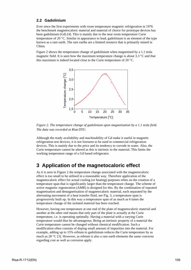
2.2 Gadolinium Ever since the first experiments with room temperature magnetic refrigeration in 1976 the benchmark magnetocaloric material and material of choice for prototype devices has been gadolinium (Gd) [4]. This is mainly due to the near room temperature Curie temperature of 20 °C. Similar in appearance to lead; gadolinium is an element of the type known as a rare earth. The rare earths are a limited resource that is primarily mined in China.

Figure 2 shows the temperature change of gadolinium when magnetised by a 1.1 tesla magnetic field. It is seen how the maximum temperature change is about 3.3 °C and that this maximum is indeed located close to the Curie temperature of 20 °C.

0 5 10 15 20 25 30 351,5

2,0

2,5

3,0

3,5

Te

mpe

ratu

re c

hang

e [o C

]

Temperature [oC]

Figure 2. The temperature change of gadolinium upon magnetisation by a 1.1 tesla field. The data was recorded at Risø DTU.

Although the ready availability and machinability of Gd make it useful in magnetic refrigeration test devices, it is not foreseen to be used in commercial refrigeration devices. This is mainly due to the price and its tendency to corrode in water. Also, the Curie temperature cannot be altered as this is intrinsic to the material. This limits the working temperature range of a Gd based refrigerator.

3 Application of the magnetocaloric effect As it is seen in Figure 2 the temperature change associated with the magnetocaloric effect is too small to be utilised in a reasonable way. Therefore application of the magnetocaloric effect for actual cooling (or heating) purposes relies on the creation of a temperature span that is significantly larger than the temperature change. The scheme of active magnetic regeneration (AMR) is designed for this. By the combination of repeated magnetisation and demagnetisation of magnetocaloric material, each separated by the alternating movement of a heat transfer fluid, see Fig. 3, a temperature span is progressively built up. In this way a temperature span of as much as 6 times the temperature change of the isolated material has been reached.

However, having one temperature at one end of the plate of magnetocaloric material and another at the other end means that only part of the plate is actually at the Curie temperature, i.e. is operating optimally. Having a material with a varying Curie temperature would thus be advantageous. Being an intrinsic property of a material the Curie temperature cannot be changed without chemical modification. Such a modification often consists of doping small amount of impurities into the material. For example, adding up to 15% erbium to gadolinium reduces the Curie temperature by as much as 28 °C [3]. However, as erbium is also a rare earth elements the same concerns regarding cost as well as corrosion apply.

Risø-R-1712(EN) 109

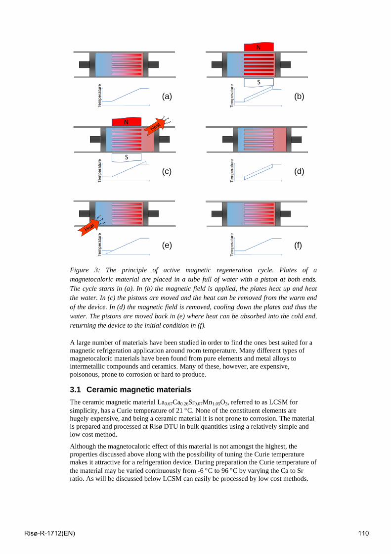
Tem

pera

ture

(a)

S

N

(b)

Tem

pera

ture

S

N

(c)

Tem

pera

ture

(d)

Tem

pera

ture

(e)

Tem

pera

ture

(f)

Tem

pera

ture

Figure 3: The principle of active magnetic regeneration cycle. Plates of a magnetocaloric material are placed in a tube full of water with a piston at both ends. The cycle starts in (a). In (b) the magnetic field is applied, the plates heat up and heat the water. In (c) the pistons are moved and the heat can be removed from the warm end of the device. In (d) the magnetic field is removed, cooling down the plates and thus the water. The pistons are moved back in (e) where heat can be absorbed into the cold end, returning the device to the initial condition in (f).

A large number of materials have been studied in order to find the ones best suited for a magnetic refrigeration application around room temperature. Many different types of magnetocaloric materials have been found from pure elements and metal alloys to intermetallic compounds and ceramics. Many of these, however, are expensive, poisonous, prone to corrosion or hard to produce.

3.1 Ceramic magnetic materials The ceramic magnetic material La0.67Ca0.26Sr0.07Mn1.05O3, referred to as LCSM for simplicity, has a Curie temperature of 21 °C. None of the constituent elements are hugely expensive, and being a ceramic material it is not prone to corrosion. The material is prepared and processed at Risø DTU in bulk quantities using a relatively simple and low cost method.

Although the magnetocaloric effect of this material is not amongst the highest, the properties discussed above along with the possibility of tuning the Curie temperature makes it attractive for a refrigeration device. During preparation the Curie temperature of the material may be varied continuously from -6 °C to 96 °C by varying the Ca to Sr ratio. As will be discussed below LCSM can easily be processed by low cost methods.

Risø-R-1712(EN) 110

3.2 Magnets An important part of any device that utilises the magnetocaloric effect is the magnetic field source. Magnetic fields may be created using electromagnets. The power consumption of these is, however, very high in order to create even a modest magnetic field. An alternative is to utilise superconducting magnets. While these provide a very high magnetic field, they are often large and complex and require cooling by, e.g., liquid helium, which is expensive.

At present, permanent magnets present the only viable option, certainly for small scale applications. The magnet material of choice is NdFeB. Discovered in 1982, with only minor improvements since then, it remains today the most powerful magnet material available. NdFeB magnets are found in a very wide range of applications from electro-motors and magnetically levitated trains to paper clip holders and children’s toys.

3.3 World status on devices A biannual conference series on magnetic refrigeration at room temperature is held under the auspice of the International Institute of Refrigeration with the attendance of about 100 people from around the world.

Around the world a number of research teams are working on different aspects of the implementation of the magnetocaloric effect. This has resulted in the construction of more than 29 magnetic refrigeration test devices [4].

A noteworthy machine is the one built by a Japanese group led by Professor Okamura. This gives a cooling capacity of up to 550 W, significantly higher than even a large domestic refrigerator. However, the machine is very large and heavy and the maximum temperature span is only 7.5 °C. Another important machine is the one built by a Canadian group led by Dr. Rowe. This is very small and compact, yielding up to 50 W of cooling and a maximum temperature span of 29 °C. Inherent to all machines is that when yielding the maximum cooling power the temperature span is zero, conversely when achieving the maximum temperature span the cooling power is zero. Therefore, operating a machine in some intermediate way, that gives a reasonable cooling power, whilst still maintaining a useful temperature span is desired.

4 Magnetic refrigeration at Risø DTU At Risø DTU there is a group of about 15 people working on different aspects of magnetic refrigeration. The various challenges related to the application are addressed.

The aim is to design and construct a prototype magnetic refrigeration machine with commercially relevant cooling power and temperature span. As the success of such a machine is very dependent on the optimised design, a simple test device has been constructed. The idea is that as many lessons as possible will be learnt from the test device in order to implement a more complex prototype machine with fixed design elements.

4.1 Simple test device The simple test device constructed at Risø DTU has been designed to be modular, versatile and easy to use [5]. Plates of a magnetocaloric material are held in place with a certain spacing in a plastic block with Perspex tubes fixed at eachend. Water (or any other heat transfer fluid) is moved in between the plates by pistons in the tubes, see Fig. 4. The whole system can be moved in and out of a permanent magnet assembly yielding a 1.1 tesla magnetic field.

All movements and timings can be controlled accurately and the temperature span and cooling load can be measured. Indeed, such control of the process is very important as the output of the device has been found to be very sensitive to even minor changes.

Risø-R-1712(EN) 111

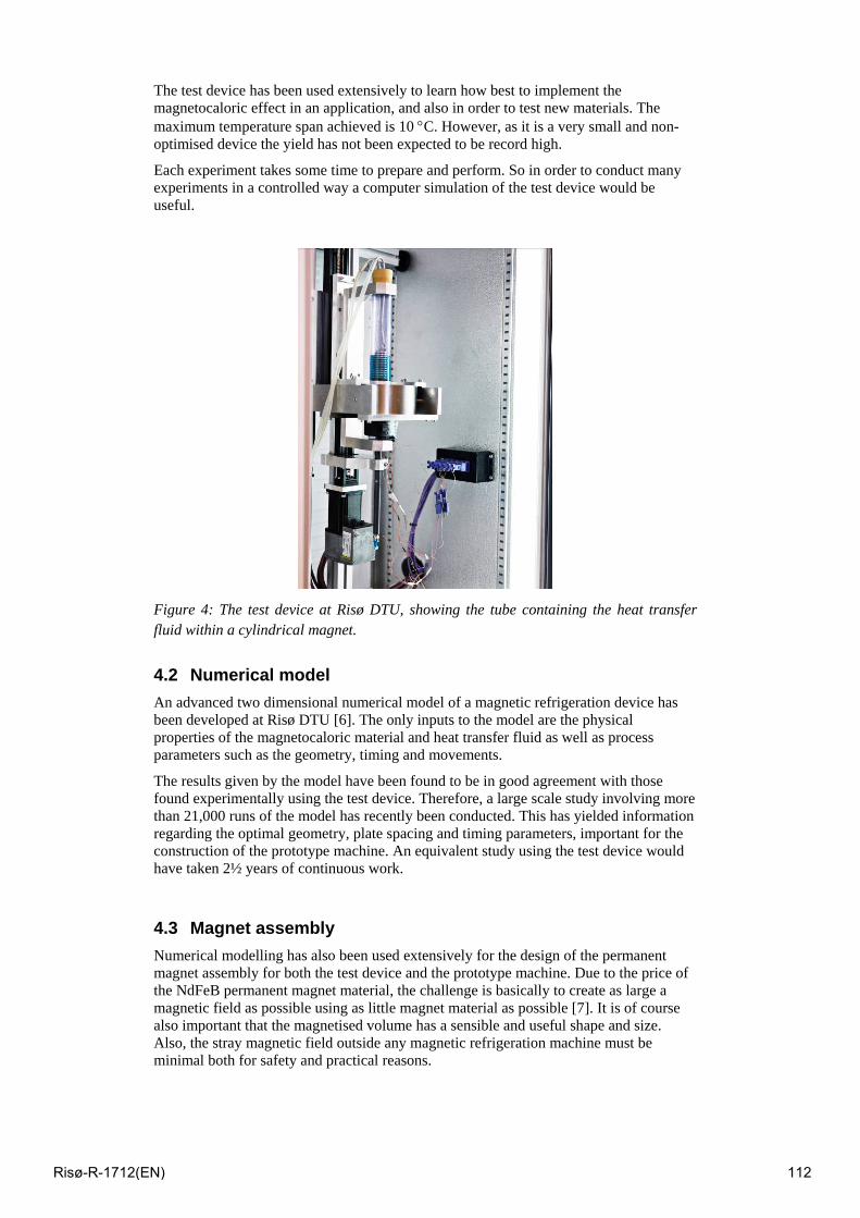
The test device has been used extensively to learn how best to implement the magnetocaloric effect in an application, and also in order to test new materials. The maximum temperature span achieved is 10 °C. However, as it is a very small and non-optimised device the yield has not been expected to be record high.

Each experiment takes some time to prepare and perform. So in order to conduct many experiments in a controlled way a computer simulation of the test device would be useful.

Figure 4: The test device at Risø DTU, showing the tube containing the heat transfer fluid within a cylindrical magnet.

4.2 Numerical model An advanced two dimensional numerical model of a magnetic refrigeration device has been developed at Risø DTU [6]. The only inputs to the model are the physical properties of the magnetocaloric material and heat transfer fluid as well as process parameters such as the geometry, timing and movements.

The results given by the model have been found to be in good agreement with those found experimentally using the test device. Therefore, a large scale study involving more than 21,000 runs of the model has recently been conducted. This has yielded information regarding the optimal geometry, plate spacing and timing parameters, important for the construction of the prototype machine. An equivalent study using the test device would have taken 2½ years of continuous work.

4.3 Magnet assembly Numerical modelling has also been used extensively for the design of the permanent magnet assembly for both the test device and the prototype machine. Due to the price of the NdFeB permanent magnet material, the challenge is basically to create as large a magnetic field as possible using as little magnet material as possible [7]. It is of course also important that the magnetised volume has a sensible and useful shape and size. Also, the stray magnetic field outside any magnetic refrigeration machine must be minimal both for safety and practical reasons.

Risø-R-1712(EN) 112

The design chosen for the test device is the so-called Halbach cylinder, named after Klaus Halbach who invented it in 1981, see, e.g. [7]. This is basically a hollow cylinder that is divided into segments, each magnetised in a certain direction, see Fig 5. The bore within the cylinder has a high and homogeneous magnetic field and the field outside the cylinder is essentially negligible.

Figure 5: The Halbach magnet for the test device. Left: Picture of the actual magnet at Risø DTU. Right: Result of a computer simulation of the magnet. Red indicates a high magnetic field, blue a low magnetic field. The arrows indicate the direction of magnetisation for the individual blocks.

4.4 Designing the prototype Although the Halbach cylinder is useful for the test device due to its simple design and relative ease of assembly it is not considered to be applicable for the final prototype design.

Instead of moving the magnetocaloric material linearly in and out of the bore in a cylinder it seems more practical to design a magnet with high and low field regions within it. Such a magnet assembly has been designed at Risø DTU and is presently being constructed. The magnetocaloric material will be rotated around from region to region, allowing a more smooth and continuous movement. Also, the magnet is continuously utilised in contrast to the Halbach situation where the high field region is left empty half of the time.

Processing the magnetocaloric materials into the right shape and size is of the utmost importance for the success of a refrigeration device. Easy passage of the fluid through the machine is important to keep the energy consumption low. Conventionally the magnetocaloric material is in the form of packed powder through which fluid is forced. To minimise pressure losses the prototype machine at Risø DTU will have regular channels for the fluid. A way of achieving this is by using regularly spaced flat plates of magnetocaloric material.

4.5 Materials processing Results from the numerical model and the test device indicate that the magnetocaloric plates should be as thin as possible with the minimum possible spacing. The ceramic materials discussed above are well suited for this as they may fairly easily be processed.

One of the methods for processing the ceramics is tape casting. Here, powder of the ceramic material is suspended in a paste. This is poured onto a moving tape the thickness being adjusted by a so-called doctor blade, see Fig 6. After drying and sintering the result is thin plates of the ceramic material. The advantage of this approach is that large amounts of the plates can be made fairly easily and cheaply. Also, by modifying the paste dispenser for the tape caster, tapes of several different materials may be

Risø-R-1712(EN) 113

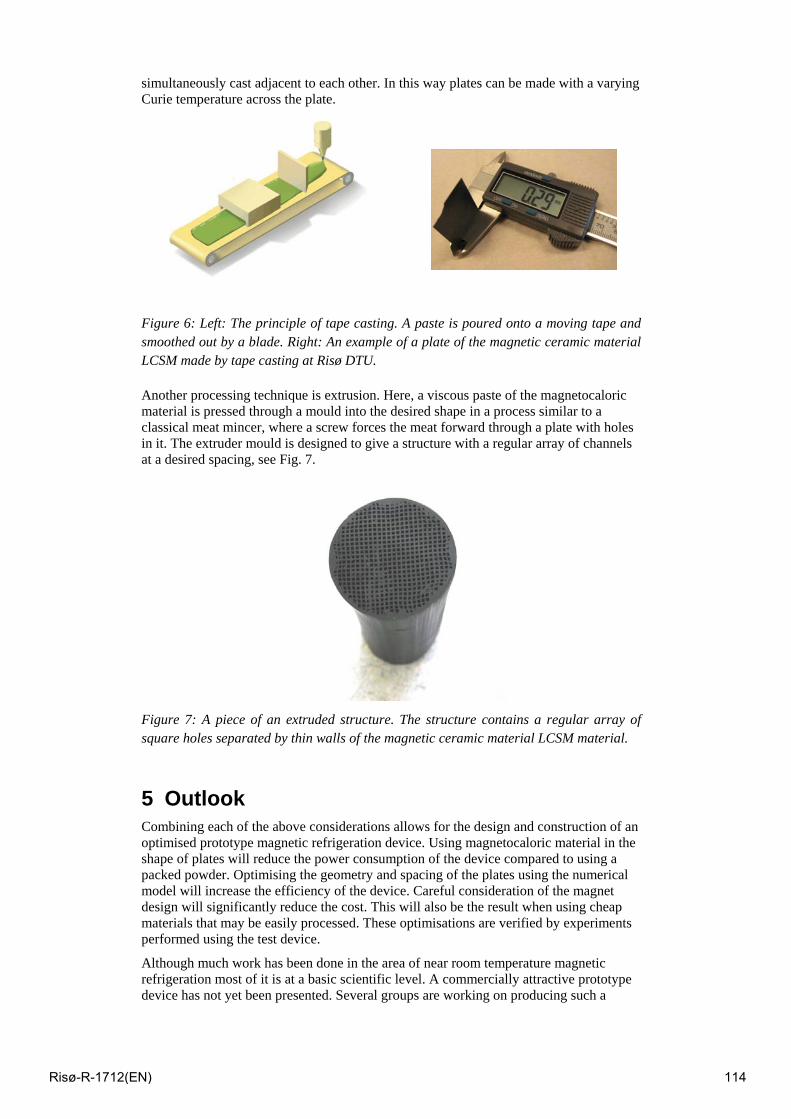
simultaneously cast adjacent to each other. In this way plates can be made with a varying Curie temperature across the plate.

Figure 6: Left: The principle of tape casting. A paste is poured onto a moving tape and smoothed out by a blade. Right: An example of a plate of the magnetic ceramic material LCSM made by tape casting at Risø DTU.

Another processing technique is extrusion. Here, a viscous paste of the magnetocaloric material is pressed through a mould into the desired shape in a process similar to a classical meat mincer, where a screw forces the meat forward through a plate with holes in it. The extruder mould is designed to give a structure with a regular array of channels at a desired spacing, see Fig. 7.

Figure 7: A piece of an extruded structure. The structure contains a regular array of square holes separated by thin walls of the magnetic ceramic material LCSM material.

5 Outlook Combining each of the above considerations allows for the design and construction of an optimised prototype magnetic refrigeration device. Using magnetocaloric material in the shape of plates will reduce the power consumption of the device compared to using a packed powder. Optimising the geometry and spacing of the plates using the numerical model will increase the efficiency of the device. Careful consideration of the magnet design will significantly reduce the cost. This will also be the result when using cheap materials that may be easily processed. These optimisations are verified by experiments performed using the test device.

Although much work has been done in the area of near room temperature magnetic refrigeration most of it is at a basic scientific level. A commercially attractive prototype device has not yet been presented. Several groups are working on producing such a

Risø-R-1712(EN) 114

prototype, amongst these the group at Risø DTU where the prototype is planned to be ready at the end of 2010.

As only laboratory scale devices exist it is difficult to assess performance of such a full size device. However, the results from these experimental devices indicate the possibility of a high efficiency if the device is constructed in an optimised manner.

Another area where the magnetocaloric effect may be applied is heat pumps. Heat pumps are becoming increasingly popular for domestic heating purposes. Although this has not been the focus of studies into magnetic refrigeration the technology may just as well be applied in reverse to create a heat pump. Utilising the high energy efficiency expected from magnetic refrigeration for heating purposes would be able to further reduce CO2 emissions.

Acknowledgements The authors would like to acknowledge the contributions from all of our colleagues in the magnetic refrigeration group. Also, the authors would like to acknowledge the support of the Programme Commission on Energy and Environment (EnMi) (Contract No. 2104-06-0032) which is part of the Danish Council for Strategic Research.

References [1] Energy Information Administration, U.S. Department of Energy, Annual Energy Outlook 2009, www.eia.doe.gov/oiaf/aeo

[2] Intergovernmental Panel on Climate Change (IPCC), Special Report on Safeguarding the Ozone Layer and the Global Climate System: Issues Related to Hydrofluorocarbons and Perfluorocarbons, Cambridge University Press, 2005.

[3] A.M. Tishin and Y.I. Spichkin, The Magnetocaloric Effect and its Applications, Institute of Physics, 2003.

[4] K.A. Gschneidner Jr. and V.K. Pecharsky, Thirty years of near room temperature magnetic cooling: Where we are today and future prospects, Int. J. Refrig. 31, 945, (2009).

[5] C.R.H. Bahl, T.F. Petersen, N. Pryds and A. Smith, A versatile Magnetic Refrigeration test device, Rev. Sci. Instrum. 79, 093906 (2008).

[6] K.K. Nielsen, C.R.H. Bahl, A. Smith, R. Bjørk, N. Pryds and J. Hattel, Detailed numerical modeling of a linear parallel-plate Active Magnetic Regenerator, Int. J. Refrig. (in press) (2009).

[7] R. Bjørk, C.R.H. Bahl, A. Smith and N. Pryds, Optimization and improvement of Halbach cylinder design, J. Appl. Phys. 104, 013910 (2008).

Further reading www.magneticrefrigeration.dk

S.L. Russek and C.B. Zimm, Potential for Cost-effective Magnetocaloric Air-conditioning Systems, Bulletin of the IIR 2006-2

P.W. Egolf and R.E. Rosensweig, Magnetic Refrigeration at Room Temperature, Bulletin of the IIR 2007-5

Proceedings of the 3rd IIF-IIR International Conference on Magnetic Refrigeration at Room Temperature, Des Moines, USA, May 11-15, 2009.

Risø-R-1712(EN) 115

Session 7 – Renewable energy technologies: Wind

Risø-R-1712(EN) 116

Risø-R-1712(EN) 117

Risø-R-1712(EN) 118

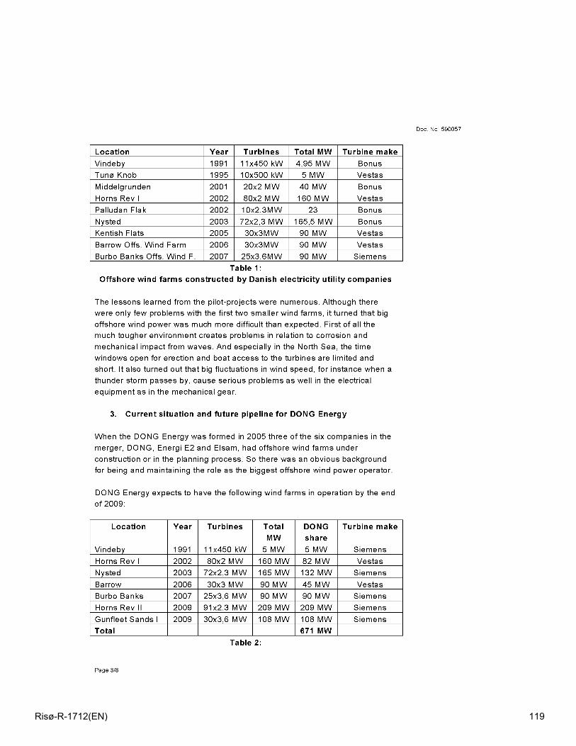
Risø-R-1712(EN) 119

Risø-R-1712(EN) 120

Risø-R-1712(EN) 121

Risø-R-1712(EN) 122

Session 8 – Renewable energy technologies: Solar

Risø-R-1712(EN) 123

Option values of concentrating solar power and photovoltaic for reaching a 2°C climate target S. Manger, R. Pietzcker, N. Bauer, T. Bruckner, G. Luderer

Abstract In this paper we discuss the role of solar electricity as well as the relative importance of concentrating solar power (CSP) and photovoltaics (PV) for reaching cost-optimal energy related greenhouse gas abatement under the constraint of a 2°C climate protection target.

We use the hybrid energy-economy-climate model ReMIND to analyze the use of solar electricity to understand which parameters determine the deployment of one or both solar technologies. We first carry out a literature review of recent studies on costs and potentials of CSP and PV. After consolidating the data into one set of parameters, we implement the two technologies in ReMIND. The results show that solar power technologies supply a significant share of electricity in the optimal abatement scenario. A sensitivity analysis of the investment costs of CSP demonstrates that while investment costs have a major influence on technology deployment, CSP is used over a wide range of values. Furthermore we calculate option values for the solar technologies by running different climate stabilization scenarios in which either PV, CSP, or both, are excluded. These option values serve as an indicator for the strategic relevance of individual technologies to achieve the climate protection target. Our results suggest that excluding solar electricity from the generation mix increases the total mitigation costs as measured by GDP differences by about 80%.

Keywords: Photovolatic, Concentrating solar power, Learning rates, Modelling

1 Motivation After the rapid installation of wind power capacity since the mid 1990s, power generation directly from the sun using PV or CSP is increasingly being recognized as a major contributor in the future energy mix. A recent example of this increased interest is the German “Desertec” project which brings together leading companies and utilities in order to develop CSP systems as part of an African-European partnership. The decreased availability of fossil fuels and the aspired realization of the 2 degree climate protection target requiring substantial CO2 abatement are leading the R&D to environmentally sound technologies (like PV or CSP). Solar energy has a huge potential – approximately 3 900 000 EJ reach the earth surface every year, which is one order of magnitude larger than the assessed potential of non-renewable energy sources [9]. However, as both PV and CSP were only recently developed and have high initial costs, only minor deployment has taken place: in 2007, solar energy contributed less than 0.2% to the global primary energy consumption. Nevertheless, both technologies have experienced and will continue to see major cost decreases due to technological learning as cumulated capacity increases. This expectation has lead to an impressive market growth for PV in the last ten years, and renewed interest in CSP projects in Spain, California and North Africa over the last five years. In the future, both technologies will compete with each other in two different ways:

1. Due to their dependency on solar radiation, both technologies require similar site conditions. However this rivalry is partly reduced as (a) the overall solar potential is very large, (b) PV – contrary to CSP – only requires diffuse sunlight and can be used at low irradiances and (c) PV is well-suited to distributed applications.

Risø-R-1712(EN) 124

2. Both technologies are deemed “learning technologies”. The concept of technological learning describes cost reductions due to capacity development, design improvements or cost reductions associated with economies of scale. Thus, the two technologies compete for private investments and governmental support during the learning phase until they break even with incumbent technologies in terms of electricity production costs.

2 Technology Background Solar energy can be converted directly into electricity using photovoltaics, or indirectly with thermal CSP plants. PV cells generally exploit semiconductor materials to use the photoelectric effect. The production of PV is currently dominated by poly and mono-crystalline silicon modules, which present 94% of the market. Better understanding of materials and device properties has resulted in continually increasing cell efficiencies, but single-junction cells are thermodynamically limited to a maximum theoretical power conversion efficiency of about 31%. The other 6% include new technologies like thin films made of amorphous silicon or cadmium telluride and organic photovoltaics. [7]

PV power generation is easily scalable to adapt to local requirements: for the decentral powering of a water pump it is possible to use single modules with 200W capacity, for grid-connected power supply they can be combined into arrays of up to 60MW capacity.

CSP technologies use focusing optics like mirrors for concentrating sunlight on an absorber. The absorber contains a heat transfer medium like water or oil which is heated to high temperatures of 400 or 1000°C, depending on the technology. The thermal energy can either be directly used in a secondary circuit to generate electricity via steam turbines or be stored for a transformation into electricity at a later time. The two main viable types of CSP systems are linear trough systems and power tower systems. A trough system uses either long, parabolic mirrors or Fresnel mirrors constructed from many flat mirrors positioned at different angles to focus solar radiation to a line absorber. A power tower system consists of a large field of mirrors (heliostats), concentrating sunlight onto a point-like receiver at the top of a tower, thus producing higher radiation densities and heating the working fluid to about 1000°C.

The present paper focuses on PV and a generalized CSP technology. The issue of differentiation between the main types of CSP systems is not elaborated here.

3 The ReMIND-G Model We use the hybrid model ReMIND – G that couples a macroeconomic growth model with a highly disaggregated energy system model [1] and the climate model ACC2 [21] to determine the role of solar electricity under the constraint of an upper limit on global mean temperature change (cf. Figure 1). [2],[12]

The macroeconomic growth model belongs to the class of Ramsey-type growth models and is formulated as a centralized maximization problem of an intertemporal welfare function. The Ramsey model is generally used for the analysis of intertemporal consumption, saving, and investment decisions. But it is also used within the context of energy, climate change and technological learning due to improved technologies and future scarcities, increased resource costs and emissions restrictions. Subject to a number of constraints ReMIND calculates a general equilibrium solution over the time horizon 2005 to 2100 in time steps of five years. For all experiments, a pure rate of time preference of 1% was used.

The energy system model represents the economic sector of ReMIND at a high level of techno-economic disaggregation of the energy system. Each technology is an energy conversion process that requires capital and fuels. The model distinguishes between exhaustible and renewable primary energy carriers. The extraction costs of the

Risø-R-1712(EN) 125

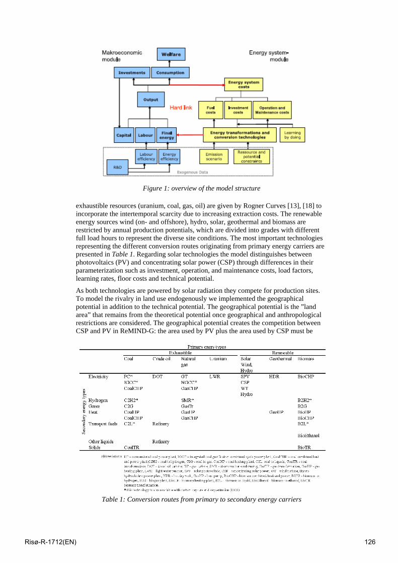
Figure 1: overview of the model structure

exhaustible resources (uranium, coal, gas, oil) are given by Rogner Curves [13], [18] to incorporate the intertemporal scarcity due to increasing extraction costs. The renewable energy sources wind (on- and offshore), hydro, solar, geothermal and biomass are restricted by annual production potentials, which are divided into grades with different full load hours to represent the diverse site conditions. The most important technologies representing the different conversion routes originating from primary energy carriers are presented in Table 1. Regarding solar technologies the model distinguishes between photovoltaics (PV) and concentrating solar power (CSP) through differences in their parameterization such as investment, operation, and maintenance costs, load factors, learning rates, floor costs and technical potential.

As both technologies are powered by solar radiation they compete for production sites. To model the rivalry in land use endogenously we implemented the geographical potential in addition to the technical potential. The geographical potential is the ”land area” that remains from the theoretical potential once geographical and anthropological restrictions are considered. The geographical potential creates the competition between CSP and PV in ReMIND-G: the area used by PV plus the area used by CSP must be

Table 1: Conversion routes from primary to secondary energy carriers

Risø-R-1712(EN) 126

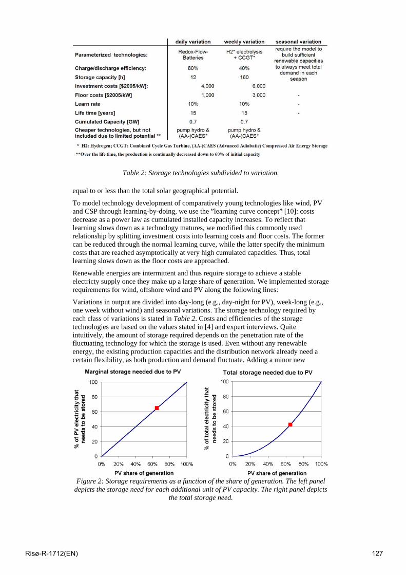
Table 2: Storage technologies subdivided to variation.

equal to or less than the total solar geographical potential.

To model technology development of comparatively young technologies like wind, PV and CSP through learning-by-doing, we use the ”learning curve concept” [10]: costs decrease as a power law as cumulated installed capacity increases. To reflect that learning slows down as a technology matures, we modified this commonly used relationship by splitting investment costs into learning costs and floor costs. The former can be reduced through the normal learning curve, while the latter specify the minimum costs that are reached asymptotically at very high cumulated capacities. Thus, total learning slows down as the floor costs are approached.

Renewable energies are intermittent and thus require storage to achieve a stable electricty supply once they make up a large share of generation. We implemented storage requirements for wind, offshore wind and PV along the following lines:

Variations in output are divided into day-long (e.g., day-night for PV), week-long (e.g., one week without wind) and seasonal variations. The storage technology required by each class of variations is stated in Table 2. Costs and efficiencies of the storage technologies are based on the values stated in [4] and expert interviews. Quite intuitively, the amount of storage required depends on the penetration rate of the fluctuating technology for which the storage is used. Even without any renewable energy, the existing production capacities and the distribution network already need a certain flexibility, as both production and demand fluctuate. Adding a minor new

Figure 2: Storage requirements as a function of the share of generation. The left panel depicts the storage need for each additional unit of PV capacity. The right panel depicts

the total storage need.

Risø-R-1712(EN) 127

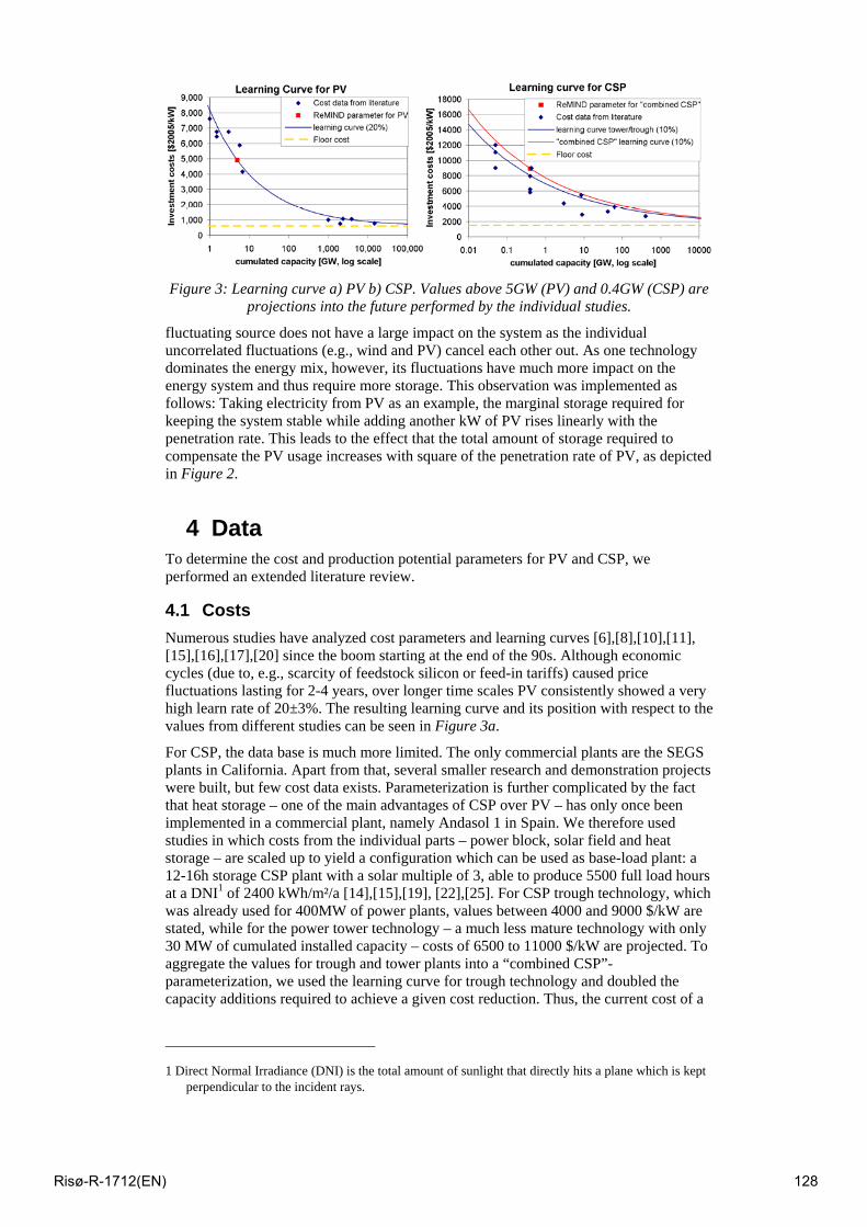
Figure 3: Learning curve a) PV b) CSP. Values above 5GW (PV) and 0.4GW (CSP) are

projections into the future performed by the individual studies.

fluctuating source does not have a large impact on the system as the individual uncorrelated fluctuations (e.g., wind and PV) cancel each other out. As one technology dominates the energy mix, however, its fluctuations have much more impact on the energy system and thus require more storage. This observation was implemented as follows: Taking electricity from PV as an example, the marginal storage required for keeping the system stable while adding another kW of PV rises linearly with the penetration rate. This leads to the effect that the total amount of storage required to compensate the PV usage increases with square of the penetration rate of PV, as depicted in Figure 2.

4 Data To determine the cost and production potential parameters for PV and CSP, we performed an extended literature review.

4.1 Costs Numerous studies have analyzed cost parameters and learning curves [6],[8],[10],[11], [15],[16],[17],[20] since the boom starting at the end of the 90s. Although economic cycles (due to, e.g., scarcity of feedstock silicon or feed-in tariffs) caused price fluctuations lasting for 2-4 years, over longer time scales PV consistently showed a very high learn rate of 20±3%. The resulting learning curve and its position with respect to the values from different studies can be seen in Figure 3a.

For CSP, the data base is much more limited. The only commercial plants are the SEGS plants in California. Apart from that, several smaller research and demonstration projects were built, but few cost data exists. Parameterization is further complicated by the fact that heat storage – one of the main advantages of CSP over PV – has only once been implemented in a commercial plant, namely Andasol 1 in Spain. We therefore used studies in which costs from the individual parts – power block, solar field and heat storage – are scaled up to yield a configuration which can be used as base-load plant: a 12-16h storage CSP plant with a solar multiple of 3, able to produce 5500 full load hours at a DNI1 of 2400 kWh/m²/a [14],[15],[19], [22],[25]. For CSP trough technology, which was already used for 400MW of power plants, values between 4000 and 9000 $/kW are stated, while for the power tower technology – a much less mature technology with only 30 MW of cumulated installed capacity – costs of 6500 to 11000 $/kW are projected. To aggregate the values for trough and tower plants into a “combined CSP”- parameterization, we used the learning curve for trough technology and doubled the capacity additions required to achieve a given cost reduction. Thus, the current cost of a

1 Direct Normal Irradiance (DNI) is the total amount of sunlight that directly hits a plane which is kept

perpendicular to the incident rays.

Risø-R-1712(EN) 128

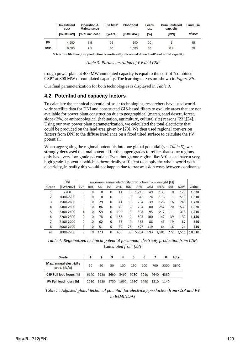
Table 3: Parameterization of PV and CSP

trough power plant at 400 MW cumulated capacity is equal to the cost of “combined CSP” at 800 MW of cumulated capacity. The learning curves are shown in Figure 3b.

Our final parameterization for both technologies is displayed in Table 3.

4.2 Potential and capacity factors To calculate the technical potential of solar technologies, researchers have used world-wide satellite data for DNI and constructed GIS-based filters to exclude areas that are not available for power plant construction due to geographical (marsh, sand desert, forest, slope>2%) or anthropological (habitation, agriculture, cultural site) reasons [23],[24]. Using our own power plant parameterization, we calculated the total electricity that could be produced on the land area given by [23]. We then used regional conversion factors from DNI to the diffuse irradiance on a fixed tilted surface to calculate the PV potential.

When aggregating the regional potentials into one global potential (see Table 5), we strongly decreased the total potential for the upper grades to reflect that some regions only have very low-grade potentials. Even though one region like Africa can have a very high grade 1 potential which is theoretically sufficient to supply the whole world with electricity, in reality this would not happen due to transmission costs between continents.

Table 4: Regionalized technical potential for annual electricity production from CSP. Calculated from [23]

Table 5: Adjusted global technical potential for electricity production from CSP and PV in ReMIND-G

Risø-R-1712(EN) 129

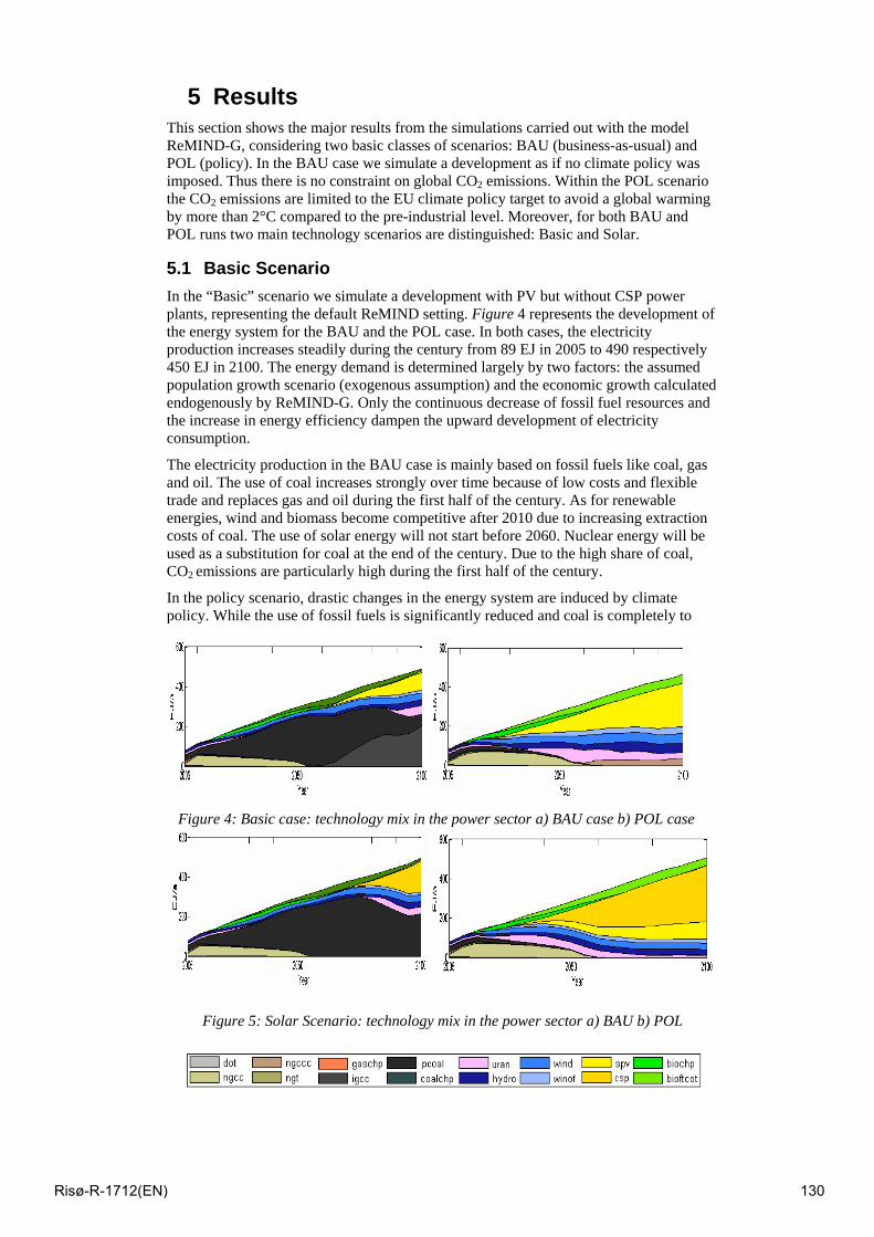
5 Results This section shows the major results from the simulations carried out with the model ReMIND-G, considering two basic classes of scenarios: BAU (business-as-usual) and POL (policy). In the BAU case we simulate a development as if no climate policy was imposed. Thus there is no constraint on global CO2 emissions. Within the POL scenario the CO2 emissions are limited to the EU climate policy target to avoid a global warming by more than 2°C compared to the pre-industrial level. Moreover, for both BAU and POL runs two main technology scenarios are distinguished: Basic and Solar.

5.1 Basic Scenario In the “Basic” scenario we simulate a development with PV but without CSP power plants, representing the default ReMIND setting. Figure 4 represents the development of the energy system for the BAU and the POL case. In both cases, the electricity production increases steadily during the century from 89 EJ in 2005 to 490 respectively 450 EJ in 2100. The energy demand is determined largely by two factors: the assumed population growth scenario (exogenous assumption) and the economic growth calculated endogenously by ReMIND-G. Only the continuous decrease of fossil fuel resources and the increase in energy efficiency dampen the upward development of electricity consumption.

The electricity production in the BAU case is mainly based on fossil fuels like coal, gas and oil. The use of coal increases strongly over time because of low costs and flexible trade and replaces gas and oil during the first half of the century. As for renewable energies, wind and biomass become competitive after 2010 due to increasing extraction costs of coal. The use of solar energy will not start before 2060. Nuclear energy will be used as a substitution for coal at the end of the century. Due to the high share of coal, CO2 emissions are particularly high during the first half of the century.

In the policy scenario, drastic changes in the energy system are induced by climate policy. While the use of fossil fuels is significantly reduced and coal is completely to

Figure 4: Basic case: technology mix in the power sector a) BAU case b) POL case

Figure 5: Solar Scenario: technology mix in the power sector a) BAU b) POL

Risø-R-1712(EN) 130

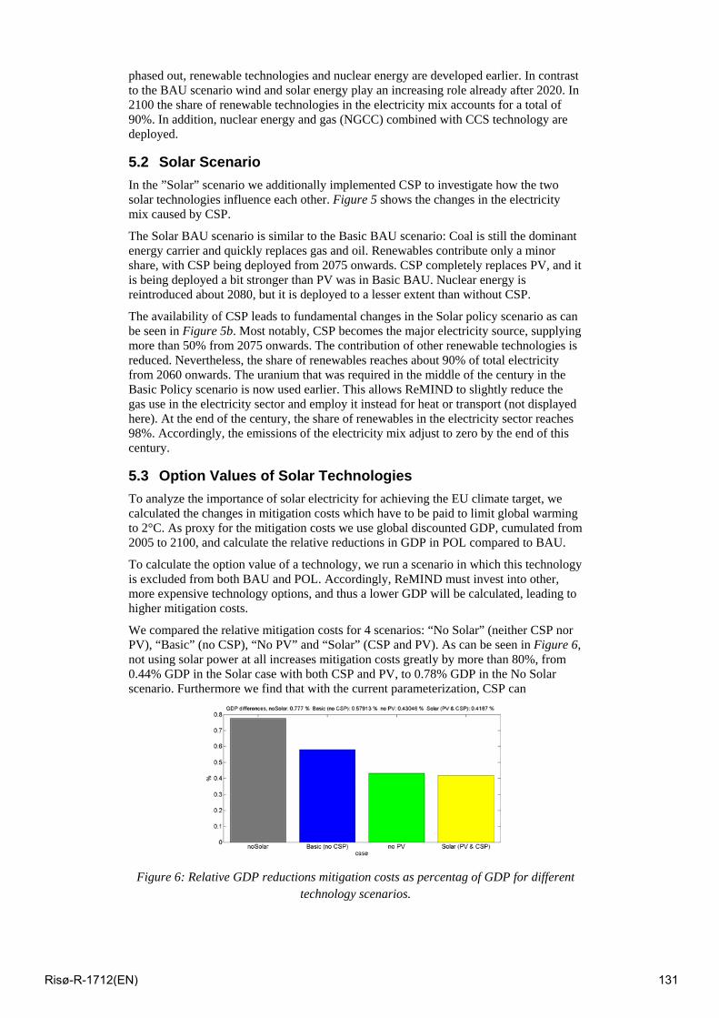
phased out, renewable technologies and nuclear energy are developed earlier. In contrast to the BAU scenario wind and solar energy play an increasing role already after 2020. In 2100 the share of renewable technologies in the electricity mix accounts for a total of 90%. In addition, nuclear energy and gas (NGCC) combined with CCS technology are deployed.

5.2 Solar Scenario In the ”Solar” scenario we additionally implemented CSP to investigate how the two solar technologies influence each other. Figure 5 shows the changes in the electricity mix caused by CSP.

The Solar BAU scenario is similar to the Basic BAU scenario: Coal is still the dominant energy carrier and quickly replaces gas and oil. Renewables contribute only a minor share, with CSP being deployed from 2075 onwards. CSP completely replaces PV, and it is being deployed a bit stronger than PV was in Basic BAU. Nuclear energy is reintroduced about 2080, but it is deployed to a lesser extent than without CSP.

The availability of CSP leads to fundamental changes in the Solar policy scenario as can be seen in Figure 5b. Most notably, CSP becomes the major electricity source, supplying more than 50% from 2075 onwards. The contribution of other renewable technologies is reduced. Nevertheless, the share of renewables reaches about 90% of total electricity from 2060 onwards. The uranium that was required in the middle of the century in the Basic Policy scenario is now used earlier. This allows ReMIND to slightly reduce the gas use in the electricity sector and employ it instead for heat or transport (not displayed here). At the end of the century, the share of renewables in the electricity sector reaches 98%. Accordingly, the emissions of the electricity mix adjust to zero by the end of this century.

5.3 Option Values of Solar Technologies To analyze the importance of solar electricity for achieving the EU climate target, we calculated the changes in mitigation costs which have to be paid to limit global warming to 2°C. As proxy for the mitigation costs we use global discounted GDP, cumulated from 2005 to 2100, and calculate the relative reductions in GDP in POL compared to BAU.

To calculate the option value of a technology, we run a scenario in which this technology is excluded from both BAU and POL. Accordingly, ReMIND must invest into other, more expensive technology options, and thus a lower GDP will be calculated, leading to higher mitigation costs.

We compared the relative mitigation costs for 4 scenarios: “No Solar” (neither CSP nor PV), “Basic” (no CSP), “No PV” and “Solar” (CSP and PV). As can be seen in Figure 6, not using solar power at all increases mitigation costs greatly by more than 80%, from 0.44% GDP in the Solar case with both CSP and PV, to 0.78% GDP in the No Solar scenario. Furthermore we find that with the current parameterization, CSP can

Figure 6: Relative GDP reductions mitigation costs as percentag of GDP for different technology scenarios.

Risø-R-1712(EN) 131

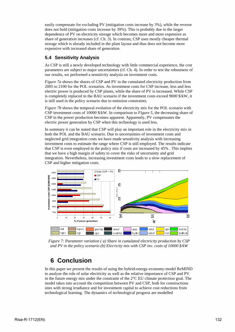
easily compensate for excluding PV (mitigation costs increase by 3%), while the reverse does not hold (mitigation costs increase by 39%). This is probably due to the larger dependence of PV on electricity storage which becomes more and more expensive as share of generation increases (cf. Ch. 3). In contrast, CSP uses mostly cheaper thermal storage which is already included in the plant layout and thus does not become more expensive with increased share of generation.

5.4 Sensitivity Analysis As CSP is still a newly developed technology with little commercial experience, the cost parameters are subject to major uncertainties (cf. Ch. 4). In order to test the robustness of our results, we performed a sensitivity analysis on investment costs.

Figure 7a shows the shares of CSP and PV in the cumulated electricity production from 2005 to 2100 for the POL scenarios. As investment costs for CSP increase, less and less electric power is produced by CSP plants, while the share of PV is increased. While CSP is completely replaced in the BAU scenario if the investment costs exceed 9000 $/kW, it is still used in the policy scenario due to emission constraints.

Figure 7b shows the temporal evolution of the electricity mix for the POL scenario with CSP investment costs of 10000 $/kW. In comparison to Figure 5, the decreasing share of CSP in the power production becomes apparent. Apparently, PV compensates the electric power generation by CSP when this technology is used less.

In summary it can be stated that CSP will play an important role in the electricity mix in both the POL and the BAU scenario. Due to uncertainties of investment costs and neglected grid integration costs we have made sensitivity analysis with increasing investment costs to estimate the range where CSP is still employed. The results indicate that CSP is even employed in the policy mix if costs are increased by 45% . This implies that we have a high margin of safety to cover the risks of uncertainty and grid integration. Nevertheless, increasing investment costs leads to a slow replacement of CSP and higher mitigation costs.

Figure 7: Parameter variation ( a) Share in cumulated electricity production by CSP and PV in the policy scenario (b) Elecricity mix with CSP inv. costs of 10000 $/kW

6 Conclusion In this paper we present the results of using the hybrid-energy-economy-model ReMIND to analyze the role of solar electricity as well as the relative importance of CSP and PV in the future energy mix under the constraint of the 2°C EU climate protection goal. The model takes into account the competition between PV and CSP, both for constructions sites with strong irradiance and for investment capital to achieve cost reductions from technological learning. The dynamics of technological progress are modelled

Risø-R-1712(EN) 132

endogenously through a learning curve approach. To determine the robustness of the model results, we varied the investment costs of CSP.

The results show that solar power technologies will supply a significant share of electricty in the optimal abatement scenario if a stringent climate target of 2°C is to be met. In the BAU scenario coal dominates the electricty mix due to low costs. Either PV or CSP are deployed from 2070 onwards, with both cases resulting in the same GDP values.

In the Policy scenario the energy system is radically restructured due to the required CO2 abatement, leading to an electricity mix that is dominated by renewable energies, especially CSP and PV. Without CSP implemented, PV plays the major role in the energy mix, supplying about 50% in 2100. When CSP is introduced, it becomes the major electricity source, supplying more than 50% from 2075 onwards. It replaces most of PV, the other renewables are reduced, nuclear energy is used earlier and CCS is not used anymore in the electricity sector.

To analyze the importance of the two solar technogies, we calculated how the GDP difference between BAU and POL cases, which acts as proxy for mitigation costs, changes when an individual technology is removed from the model. We find that exluding solar electricity increases GDP losses by more than 80%. Furthermore, if only one solar technology is used, PV is readily replaced by CSP with only minor GDP losses, while the inverse is not true.

We can conclude that if policy makers decide to enforce climate protection, CSP will play an important role in the power mix due to its base load capability and the resulting low electricity production costs. This result is emphazised by our sensitivity analysis: Up to a cost increase of 45%, CSP remains part of the generation mix in the Policy scenario. This leaves a wide safety margin for possibly underestimated investment costs or grid integration costs, which are neglected in ReMIND. Therefore it seems important to implement CSP in other models to test and consolidate the herein discussed results.

In ReMIND, the PV share of electricity generation is greatly reduced as CSP is introduced into the model. In reality, the rivalry and the resulting crowding-out will probably not be as severe due to several reasons:

1. while CSP plants will only be built by major energy suppliers, PV was in the past mainly financed decentrally by private capital. As increased private capital flowing into PV is expected once grid parity is achieved, small-scale PV growth may even accelerate much faster in the future.

2. It is impossible to know if all expectations about technological learning will come true. Thus, a prudent policymaker will not solely rely on one learning technology but rather try to promote both.

3. Due to its scalability, PV can be used in many less-developped regions to power villages not connected to a central electricity grid. This is not possible with CSP plants which require the economies of scale of 50-400MW-plants to be economically feasible.

4. In certain regions, CSP cannot be used due to low direct sunlight. PV only requires diffuse light, so its geographic deployment zone is larger than that of CSP.

To better analyze the influence of regionally limited potentials and to avoid overestimating CSP deployment, it is necessary to implement CSP systems in a model with a higher regional resolution. This might also allow the estimation of grid integration costs via the proxy of interregional electricty imports and exports and would probably lead to a partial replacement of CSP by PV due to its decentralized utilization.

Furthermore, it needs to be stressed that there is little commercial experience with both tower CSP and thermal storage. Thus, the results of our analysis might change in the near future when cost data from several projects being realized in 2009 or 2010 (more

Risø-R-1712(EN) 133

than 5GW of new constructions are projected until 2012) is included in our parameterization.

Owing to these caveats, the presented results should only be seen as a first sketch of the possible importance and deployment of solar technologies as we could not give adequate credit to all possible barriers and constraints.

7 References [1] Bauer, N., Edenhofer, O. and Kypreos, S.: “Linking Energy Systems and Macro-

Economic Growth Models”. Journal of Computational Management Science (Special Issues on Managing Energy and the Environment), 2006, 5, 95-117.

[2] Bauer, N. et. al: “Impact of technology and emission oriented policies on the system, welfare and the climate system”. In Preparation

[3] BMU: „Erneuerbare Energien in Zahlen – Nationale und International Entwicklung“. Internet Update. 2008

[4] Chen, H., Cong, T.N., Yang, W., Tan, C, Li, Y. and Ding, Y.: “Progress in Electrical Energy Storage Systems: A Critical Review”. Progress in Natural Science, 2009, 19, 291-312

[5] EU PV Technology Platform: “A Strategic Research Agenda for Photovoltaic Solar Energy Technology”. European Communities, 2007

[6] Frankl, P., Menichetti, E. and Raugei, M.: “Final report on technical data, costs and life cycle inventories of PV applications”. Deliverable n° 11.2 - RS 1a of the NEEDS (New Energy Externalities Developments for Sustainability) project. 2005

[7] Ginley, D., Green, M. A. and Collins, R: ”Solar Energy Conversion Towards 1 Terawatt”. MRS Bulletin. 2008, 33, 355-372

[8] International Energy Agency: ”Energy Technology Perspectives 2008 –Scenarios & Strategies to 2050”. 2008

[9] Johansson, T. B., McCormick, K., Neij, L. and Turkenburg, W.: “The Potential of Renewable Energy”. International Conference for Renewable Energies, Bonn, 2004

[10] Junginger, M., Lako, P. Lensink, S., van Sark, W. and Weiss, M.: ”Technological Learning in The Energy Sector”. ECN, University Utrecht, 2008

[11] Keshner, M. and Arya, R.: ”Study of Potential Cost Reductions Resulting from Super-Large-Scale Manufacturing of PV Modules”. National Renewable Energy Laboratory, 2004,

[12] Leimbach, M., Bauer, N., Baumstark L. and Edenhofer, O.: ”Mitigation Costs in a Globalized World: Climate Policy Analysis with ReMIND-R”. Accepted for Publication in Environmental Modeling and Assessment, 2009

[13] Nuclear Energy Agency: “Uranium 2003 - Resources, Production and Demand”. 2003

[14] Neij, L., Borup, M., Blesl, M. and Mayer-Spohn, O: ”Cost Development—an Analysis Based on Experience Curves”. Deliverable 3.3—RS1A of the NEEDS (New Energy Externalities Development for Sustainability) project. 2006

[15] Neji, L.: ”Cost Development of Future Technologies for Power Generation – A Study Based on Experience Curves and Complementary Bottom-Up Assessments”. Energy Policy, 2008, 36(6), 2200-2211

[16] Nemet, G.F.: ”Interim Monitoring of Cost Dynamics for Publicy Supported Energy Technologies”. Energy Policy, 2009, 37, 825-835

[17] PV-Track: ”A Vision for Photovoltaic Technology”. European comission, 2005

Risø-R-1712(EN) 134

[18] Rogner, H.: “An Assessment of World Hydrocarbon Resources”. Annual Review of Energy and the Environment, 1997, 22, 217-262

[19] Sargent&Lundy LLC Consulting Group Chicago: ”1. Assessment of Parabolic Trough and Power Tower Solar Technology Cost and Performance Forecasts”. National Renewable Energy Laboratory, 2003

[20] Schaeffer, G.J., Seebregts, A.J., Beurskens, L.W.M., de Moor, H.H.C., Alsema, E.A., Sark, W., Durstewicz, M., Perrin, M., Boulanger, P., Laukamp, H. and Zuccaro, C.: “Learning from the Sun”. Final Report of the PHOTEX Project. Report ECN DEGO: ECN-C–04-035, ECN Renewable Energy in the Built Environment. 2004,

[21] Tanaka, K. and Kriegler, E.: “Aggregated Carbon Cycle, Atmospheric Chemistry and Climate Model (ACC2)”. Reports on Earth Systems Science 40, Max-Planck-Institute of Meteorology, Hamburg, 2007

[22] Trieb, F.: ”ATHENE - Ausbau thermischer Solarkraftwerke für eine nachhaltige Energieversorgung“. Working Package 1.3 of the DLR Project „SOKRATES (Solarthermische Kraftwerkstechnologie für den Schutz des Erdklimas)“. 2004

[23] Trieb, F., Schillings, C., O’Sullivan, M., Pregger, T. and Hoyer-Klick, C.: “Global Potential of Concentrating Solar Power”. SolarPaces Conference Berlin, September 2009.

[24] Tzscheutschler, P.:”Globales technisches Potenzial solarthermischer Stromerzeugung”. Energie Management Verlagsgesellschaft mbH, IFE, 48 , 2005

[25] Viebahn, P., Kronshage, S., Trieb, F. and Lechon, Y.: ”Final Report on Technical Data, Costs, and Life Cycle Inventories of Solar Thermal Power Plants”. Deliverable 12.2-RS Ia of the NEEDS Project. 2008,

Risø-R-1712(EN) 135

Solar energy – new photovoltaic technologies Peter Sommer-Larsen Risø National Laboratory for Sustainable Energy, Technical University of Denmark

Abstract Solar energy technologies directly convert sunlight into electricity and heat, or power chemical reactions that convert simple molecules into synthetic chemicals and fuels. The sun is by far the most abundant source of energy, and a sustainable society will need to rely on solar energy as one of its major energy sources.

Solar energy is a focus point in many strategies for a sustainable energy supply. The European Commission’s Strategic Energy Plan (SET-plan) envisages a Solar Europe Initiative, where photovoltaics and concentrated solar power (CSP) supply as much power as wind mills in the future.

Much focus is directed towards photovoltaics presently. Installation of solar cell occurs at an unprecedented pace and the expectations of the photovoltaics industry are high: a total PV capacity of 40 GW by 2012 as reported by a recent study.

The talk progresses from general solar energy topics to photovoltaics with a special focus on the new photovoltaic technologies that promises ultra low cost solar cells. Unlike many other renewable energy technologies, a pipeline of new technologies is established and forms a road towards low cost energy production directly from the sun.

1 Solar energy technologies Solar energy may become a major component of future sustainable energy supply in the form of solar thermal heating, photovoltaics and concentrating solar power. Targets for deploying solar energy are continually increasing, and it is too early to definitively state how much energy solar systems will supply globally.

Theoretically, solar energy is the largest renewable energy source. The Earth receives more energy from the sun in just 1 hour than humanity uses in a whole year. Solar cells, solar thermal heating systems and concentrating solar power plants are well-proven and mature technologies that have been installed at an unprecedented pace in the past few years.

A continuing increase in the installation rate is strongly correlated with declining production costs. This reduction is still needed to make photovoltaics in particular and, to a lesser degree, solar thermal heating and concentrating solar power cost efficient and to make the price of energy produced by these technologies similar to other sources of electrical power, heating and cooling.

Various industry segments, research institutions and public bodies such as the European Technology Platforms have laid roadmaps for incrementally improving the technology, scaling up capacity and deployment scenarios. These plans target the need to reduce production costs and are the background for the ambitious targets described below.

Solar thermal heating and photovoltaic technologies include both centralized and distributed generation of energy and offer a geographical spread of generation over most of the industrialized world. Concentrating solar power targets power plants located in the sunniest regions of the world. The visions of the solar energy sector call for massive deployment of both centralized power plants and distributed power generation: building integrated heating and photovoltaic panels.

This vision constitutes a paradigm shift in energy supply. It requires adopting control and storage technologies that allow the harvested energy to be utilized. Fulfilling the vision

Risø-R-1712(EN) 136

requires planning, and starting now, deployment on a large scale, and the industry must strive to reduce production costs while building up production capacity.

Globally, a capacity of 145 GW of thermal equivalent (GWth) of solar thermal heating was installed by 2008; 13 GW grid-connected and approximately 14 GW total photovoltaic electric capacity (GWel) was installed by 2008; and about 1 GWel of concentrating solar power by 2008. The solar thermal heating market has grown by at least 30% annually in recent years. The photovoltaics market increased by 110% from 2007 to 2008, and several new concentrating solar power plants are under construction.

2 The promises of current photovoltaic technologies The European Commission’s Strategic Energy Plan (SET-plan) envisages a Solar Europe Initiative, where photovoltaics and concentrated solar power (CSP) supply as much power as wind mills in the future. The European Photovoltaic Industry Association (EPIA) in their proposal for a Solar Europe Industry Initiative establish a roadmap for research, development, and deployment resulting in much reduced production costs for photovoltaics – reductions that form the basis for establishing PV as a mainstream clean and sustainable energy technology providing up to 12% of the European electricity demand by 2020, and 20% by 2030, and even 50% by 2050.

This roadmap deals with current Silicon and thin film solar cells and it relies on a careful analysis of the incremental progress in technology and production methods. It is strongly related to the historic and anticipated relation between production costs and production volume – exemplified in a very high learning rate of 22% until 2006 and an anticipated future learning rate of 20%, which slowly decrease to 15% over the next decade.

The milestones for cost reduction and technological progress in the SEII are: typical turn-key large system price of 2 €/Wp by 2015 and <1.5 €/Wp by 2020; PV electricity generation cost in Southern EU of 0.13 €/kWh in 2015 (below retail electricity prices = grid parity) and below 0.06 €/kWh by 2030 (below wholesale electricity prices); grid parity in most of EU by 2020; Typical commercial flat-plate module efficiency up to 20% by 2015 and up to 25% by 2030; Lifetime of PV modules of up to 40 years for c-Si and thin film technologies by 2020.

3 New photovoltaic technologies A host of new solar cell technologies are currently being investigated and developed. Approaches based on classical semi-conductors like quantum well solar cells and perfect crystalline nano-structures are well described in [1] as is also the dye sensitized solar cells and organic photovoltaics.

From the group of organic photovoltaics the present presentation deals with polymer solar cells [2-5] as perhaps the most promising technologies for future ultra-low cost solar cells. These organic conjugated polymer based solar cells take advantage of low-cost, large area, solution-based manufacturing via spin coating, ink-jet printing and screen printing, and allowing the development of applications on flexible substrates. A recent series of papers details printing and processing methods of polymer solar cells and demonstrate the feasibility of these production methods [6-10]. The US based Konarka Technologies Inc is now marketing polymer solar cells. During the last decades, polymer solar cells have been widely investigated, and power conversion efficiency (PCE) up to 5% has been obtained. But still, the criteria of PCE and large area processing presently limit the commercialization of the polymer solar cells. It is conceivable those polymer PV systems become economically competitive in the future and that they may be more environmentally friendly to produce.

Risø-R-1712(EN) 137

A very recent paper [11] evaluates the environmental and economical potential of polymer solar cells. In particular the environmental impact – take an example expressed as energy payback time – of polymer solar cells is evaluated to potentially become much lower than for traditional multicrystalline Silicon (mc-Si) solar cells: the paper estimates an energy payback time as low as 2½ months for a flexible solar cell in contrast to 2 years for mc-Si cells.

The energy payback time is in fact a key figure in evaluating the net energy generation of a solar cell technology in a deployment phase. As all roadmaps are based on a relative fast deployment, it appears that the net-generation within the deployment period may become substantially higher for polymer solar cells than for Silicon solar cells despite their lower efficiency and lifetime. Due to the reduced lifetime, it takes a larger installed capacity of polymer solar cell than mc-Si cells to generate the same amount of energy after the deployment period has ended.

4 References 1. Pagliaro M, Palmisano G, Ciriminna R, Flexible Solar Cells, Wiley-VCH, 2008

2 Yu G, Gao J, Hummelen JC, Wudl F, Heeger AJ , SCIENCE 270 (5243), 1789-1791, 1995

3. Brabec CJ, Sariciftci NS, Hummelen JC. Plastic solar cells. Advanced Functional Materials 11(1): 15–26, 2001

4. Spanggaard H, Krebs FC. A brief history of the development of organic and polymeric photovoltaics. Solar Energy Materials & Solar Cells 2004; 83(2–3): 125–146

5. Hoppe H, Sariciftci NS. Organic solar cells: an overview. Journal of Materials Research 19(7), 1924–1945, 2004

6. Krebs FC, Fabrication and processing of polymer solar cells: A review of printing and coating techniques, SOLAR ENERGY MATERIALS AND SOLAR CELLS 93 (4), 394-412, 2009

7. Krebs FC, Polymer solar cell modules prepared using roll-to-roll methods: Knife-over-edge coating, slot-die coating and screen printing, SOLAR ENERGY MATERIALS AND SOLAR CELLS 93 (4), 465-475, 2009

8. Krebs FC, Gevorgyan SA, Alstrup, J, A roll-to-roll process to flexible polymer solar cells: model studies, manufacture and operational stability studies, JOURNAL OF MATERIALS CHEMISTRY 19 (30), 5442-5451, 2009

9. Krebs FC, All solution roll-to-roll processed polymer solar cells free from indium-tin-oxide and vacuum coating steps, ORGANIC ELECTRONICS 10 (5), 761-768, 2009

10. Krebs FC, Roll-to-roll fabrication of monolithic large-area polymer solar cells free from indium-tin-oxide , SOLAR ENERGY MATERIALS AND SOLAR CELLS 93 (9), 1636-1641, 2009

11. Roes AL, Alsema EA, Blok K, Patel MK, Ex-ante Environmental and Economic Evaluation of Polymer Photovoltaics, Prog. Photovolt: Res. Appl. 17, 372–393, 2009

Risø-R-1712(EN) 138

Session 9 – Renewable energy technologies: Bioenergy I

Risø-R-1712(EN) 139

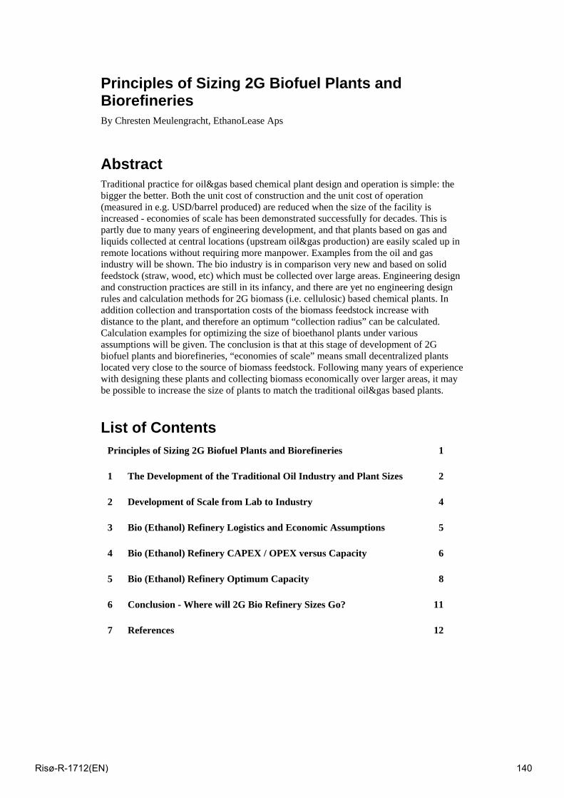
Principles of Sizing 2G Biofuel Plants and Biorefineries By Chresten Meulengracht, EthanoLease Aps Abstract Traditional practice for oil&gas based chemical plant design and operation is simple: the bigger the better. Both the unit cost of construction and the unit cost of operation (measured in e.g. USD/barrel produced) are reduced when the size of the facility is increased - economies of scale has been demonstrated successfully for decades. This is partly due to many years of engineering development, and that plants based on gas and liquids collected at central locations (upstream oil&gas production) are easily scaled up in remote locations without requiring more manpower. Examples from the oil and gas industry will be shown. The bio industry is in comparison very new and based on solid feedstock (straw, wood, etc) which must be collected over large areas. Engineering design and construction practices are still in its infancy, and there are yet no engineering design rules and calculation methods for 2G biomass (i.e. cellulosic) based chemical plants. In addition collection and transportation costs of the biomass feedstock increase with distance to the plant, and therefore an optimum “collection radius” can be calculated. Calculation examples for optimizing the size of bioethanol plants under various assumptions will be given. The conclusion is that at this stage of development of 2G biofuel plants and biorefineries, “economies of scale” means small decentralized plants located very close to the source of biomass feedstock. Following many years of experience with designing these plants and collecting biomass economically over larger areas, it may be possible to increase the size of plants to match the traditional oil&gas based plants.

List of Contents Principles of Sizing 2G Biofuel Plants and Biorefineries 1

1 The Development of the Traditional Oil Industry and Plant Sizes 2

2 Development of Scale from Lab to Industry 4

3 Bio (Ethanol) Refinery Logistics and Economic Assumptions 5

4 Bio (Ethanol) Refinery CAPEX / OPEX versus Capacity 6

5 Bio (Ethanol) Refinery Optimum Capacity 8

6 Conclusion - Where will 2G Bio Refinery Sizes Go? 11

7 References 12

Risø-R-1712(EN) 140

1 The Development of the Traditional Oil Industry and Plant Sizes (Ref [1] – [7])

The oil industry started similar to other industries with small (and risky) production plants. The early beginning took place in the US where Colonel Drake pioneered the modern methods for drilling for oil in Pennsylvania in the 1850’ies.

By 1860 there were 15 refineries in operation in the US. Known as "tea kettle" stills, they consisted of a large iron drum and a long tube which acted as a condenser. The capacity of these stills ranged from 1 to 100 barrels a day.

In the early 1900's, the introduction of the internal combustion engine and its use in automobiles created a market for gasoline that laid the foundation for rapid growth of the petroleum industry.

Prior to World War II in the early 1940s, most petroleum refineries in the United States consisted simply of crude oil distillation units. Most modern refining processes became commercially available within 5 to 10 years after the war ended and the worldwide petroleum industry experienced very rapid growth.

In the United States the construction of new refineries came to a virtual stop in about the 1980's. However, many of the existing refineries have revamped many of their units and/or constructed add-on units in order to increase their crude oil processing capacity. Figure 1 shows that the number of refineries decreased since 1980 in the United States, as capacity increased – slowly.

Figure 1 – Number of US Refineries pr. 1.January 2009 (Ref. [6])

The 1980s saw the development of offshore exploration projects, which were in much more challenging conditions than had previously been attempted. The Troll field in Norway was one example; another was in the Gulf of Mexico where a new well was drilled at a depth of 2.3 km, a new record.

The size of upstream drilling and production facilities has been increasing steadily over the decades, to reach greater drilling depths, water depths and production capacities. This has happened both to keep feeding the ever increasing market demand for oil and gas and to drive down costs per barrel of oil (or gas equivalent) produced.

This is clearly demonstrated by the below Figure 2 which shows incremental increases in water depth with time.

Risø-R-1712(EN) 141

Figure 2 – Subsea completion records by PetroBras offshore Brazil (Ref. [7])

The above are just a few clear indications that progress takes place to i) increase capacity per plant to reduce costs per barrel and ii) the changes takes place incrementally building on prior experience and not in great risky quantum leaps.

There are a number of reasons for this (intuitively logical) development:

1. The costs of oil and gas plants are great, sometimes exceeding a billion USD per field or per refinery

2. You can implement a certain limited number of improvements compared to previous plants since R&D activities take time to develop new technology

3. Most large scale industries are very risk averse since failure will be remembered for many years

Risø-R-1712(EN) 142

2 Development of Scale from Lab to Industry (Ref [8] – [9])

A number of stages should be used when conducting development from idea to industrial production of any chemical process, as a minimum :

1. Laboratory Experiments: Certain aspects of the process are investigated by handling small amounts of raw materials, in order to characterize the chemical reactions in mathematical terms.

2. Pilot plant experiments: During this phase the first scale-up problems are identified and dealt with, such as impurities in the raw materials, operation over long periods, equipment reliability and heat losses.

3. Demonstration unit: This is the first industrial unit on a modest scale, e.g. 1/10 of the expected industrial production level. This is however an expensive and time-consuming step which often is attempted to dispense with.

4. Full scale (proto-type) production unit: This is a full scale plant, and since it is the first of its kind, it will require longer than normal to commission, and design and equipment may have to further optimized.

The key issues making it necessary to scale up in steps rather than going directly from laboratory scale to industrial scale are heat and mass transfer issues, especially those due to convection. Temperature has a major impact on the speed of reactions, and conversion rates are therefore highly influenced by e.g. equipment geometry which impacts flow patterns and thereby temperature profiles. The presence of turbulence measured by the Reynolds number is important for e.g. CSTRs – continuously stirred tank reactors, to achieve proper blending and uniform reaction conditions.

As part of the scale-up efforts is necessary to develop mathematical process simulation models to be able to predict the process under varying process conditions, and design equipment. This model will typically be able to calculate reaction rates and heats, heat losses and mechanical losses such as friction losses and losses in pumps and compressors.

By a 2G bio refinery is meant a chemical process plant based on solid non-food biomass such as straw, corn stover or wood as raw material. In theory almost all chemical compounds can be produced on the basis of biomass, but in the following only bioethanol production plants based on fermentation of cellulose and hemicellulose will be considered.

The 2G bioethanol industry is still in its infancy and just at the brink of embarking on demonstration and prototype plants. This again means that engineering knowledge and experience is also at its infancy and there is only little operational experience available for developing engineering rules. This also means that it is not currently possible to construct successful large scale plants from a pure engineering point of view.

Verenium in Louisiana is a case that demonstrates these principles. Firstly, a pilot plant was opened in 1999, and during 2006 the company completed upgrades on the pilot facility, enabling it to conduct combined C5 and C6 fermentations. This pilot plant can process approximately two tons of biomass per day into ethanol. It is operated as an R&D facility to improve the company’s process technology and to validate the company’s process on a wide variety of biomass feedstocks.

Next door to the pilot facility, Verenium has recently constructed a 1.4 million gallon per year demonstration plant and plan to have it in operation by year end.. Preparations are also being made for Verenium’s first commercial-scale facilities, which are expected to produce 30 million gallons of ethanol per year.

Risø-R-1712(EN) 143

3 Bio (Ethanol) Refinery Logistics and Economic Assumptions In order to carry out economic evaluation of the optimum bio refinery size, the key technical and economic assumptions need to be defined.

The key differences between oil and gas based production facilities and 2G biomass based production facilities are:

1. Collection and transportation costs per energy unit are much higher for 2G biomass based production plants than for oil and gas. Oil and gas can be transported in pipelines with pumps and compressors. This technology has been developed over decades and is highly efficient. The bigger the transportation capacity, the lower the costs per unit volume. Solid biomass in the form of straw, corn stover and wood is on the contrary much more energy and time consuming to collect and transport.

2. Current technology is adapted to direct use of oil and gas is both refineries and chemical factories. Biomass, on the other hand has to be pretreated in order to release the valuable chemical components, C5 and C6 sugars, for further processing to useful chemical compounds such as ethanol.

The above two factors are challenge both technologically and economically. The technology is under development but it is currently not known what the optimum plant sizes are.

The previous sections have been concerned with showing that from an engineering point of view, the 2G Bio Refinery industry must go through further engineering development before large capacity plants can be constructed. This is similar to the oil and gas industry which has undergone continuous development for more than a century, both from a technology and a production capacity point of view.

The following sections will be concerned with showing that with current technology, 2G bio refineries have an optimum size under a given set of assumptions, and this size should obviously be sought to make them as economic as possible.

For simplification we will only look at production of 2G bioethanol (also written as EtOH in the following). This type of facility has all the challenges, including collection and transport of 2G biomass and conversion of all types of sugars.

The economic competitiveness of 2G bioethanol production is highly dependent on feedstock cost, which constitutes 35-50% of the total ethanol production cost, depending on various geographical factors and the types of systems used for harvesting, collecting, preprocessing, transporting, and handling the material.

In the following sections 5 and 6, the following key reference plant data will be used:

Production capacity = 12 M3 / day

Plant CAPEX = 3.1 MM EUR

Plant OPEX = 2 MM EUR

Straw cost = 87 EUR / MT

Average supply of straw = 2 MT per hectare (assumed to be 50% of the capacity if land is only used for straw based crop production)

Plant CAPEX and OPEX have been based on general industry norms and experience at current price levels.

Risø-R-1712(EN) 144

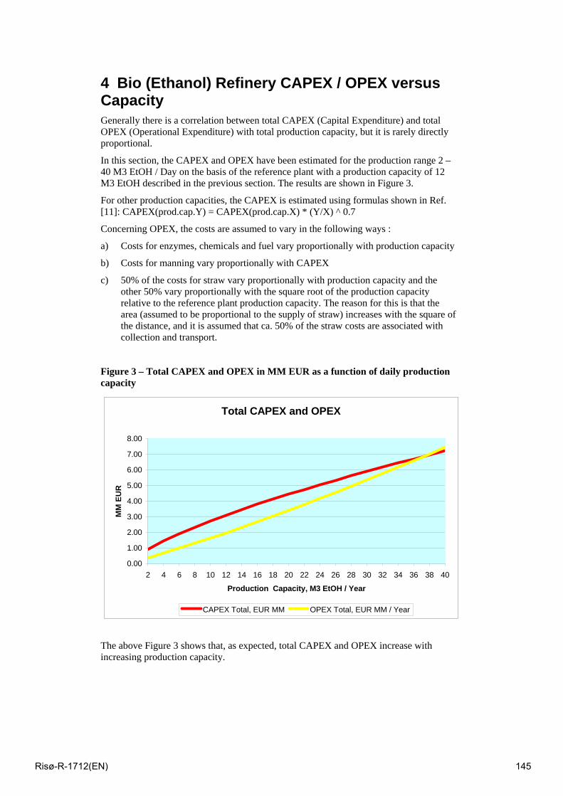
4 Bio (Ethanol) Refinery CAPEX / OPEX versus Capacity Generally there is a correlation between total CAPEX (Capital Expenditure) and total OPEX (Operational Expenditure) with total production capacity, but it is rarely directly proportional.

In this section, the CAPEX and OPEX have been estimated for the production range 2 – 40 M3 EtOH / Day on the basis of the reference plant with a production capacity of 12 M3 EtOH described in the previous section. The results are shown in Figure 3.

For other production capacities, the CAPEX is estimated using formulas shown in Ref. [11]: CAPEX(prod.cap.Y) = CAPEX(prod.cap.X) * (Y/X) ^ 0.7

Concerning OPEX, the costs are assumed to vary in the following ways :

a) Costs for enzymes, chemicals and fuel vary proportionally with production capacity

b) Costs for manning vary proportionally with CAPEX

c) 50% of the costs for straw vary proportionally with production capacity and the other 50% vary proportionally with the square root of the production capacity relative to the reference plant production capacity. The reason for this is that the area (assumed to be proportional to the supply of straw) increases with the square of the distance, and it is assumed that ca. 50% of the straw costs are associated with collection and transport.

Figure 3 – Total CAPEX and OPEX in MM EUR as a function of daily production capacity

Total CAPEX and OPEX

0.00

1.00

2.00

3.00

4.00

5.00

6.00

7.00

8.00

2 4 6 8 10 12 14 16 18 20 22 24 26 28 30 32 34 36 38 40

Production Capacity, M3 EtOH / Year

MM

EU

R

CAPEX Total, EUR MM OPEX Total, EUR MM / Year

The above Figure 3 shows that, as expected, total CAPEX and OPEX increase with increasing production capacity.

Risø-R-1712(EN) 145

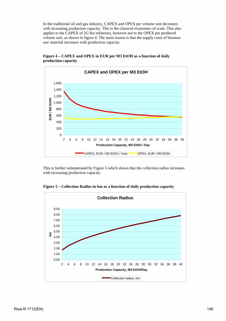
In the traditional oil and gas industry, CAPEX and OPEX per volume unit decreases with increasing production capacity. This is the classical economies of scale. This also applies to the CAPEX of 2G bio refineries, however not to the OPEX per produced volume unit, as shown in figure 4. The main reason is that the supply costs of biomass raw material increases with production capacity.

Figure 4 – CAPEX and OPEX in EUR per M3 EtOH as a function of daily production capacity

CAPEX and OPEX per M3 EtOH

0

200

400

600

800

1,000

1,200

1,400

1,600

2 4 6 8 10 12 14 16 18 20 22 24 26 28 30 32 34 36 38 40

Production Capacity, M3 EtOH / Day

EUR

/ M

3 Et

OH

CAPEX, EUR / M3 EtOH / Year OPEX, EUR / M3 EtOH

This is further substantiated by Figure 5 which shows that the collection radius increases with increasing production capacity.

Figure 5 – Collection Radius in km as a function of daily production capacity

Collection Radius

0.00

1.00

2.00

3.00

4.00

5.00

6.00

7.00

8.00

9.00

2 4 6 8 10 12 14 16 18 20 22 24 26 28 30 32 34 36 38 40

Production Capacity, M3 EtOH/Day

km

Collection radius, km

Risø-R-1712(EN) 146

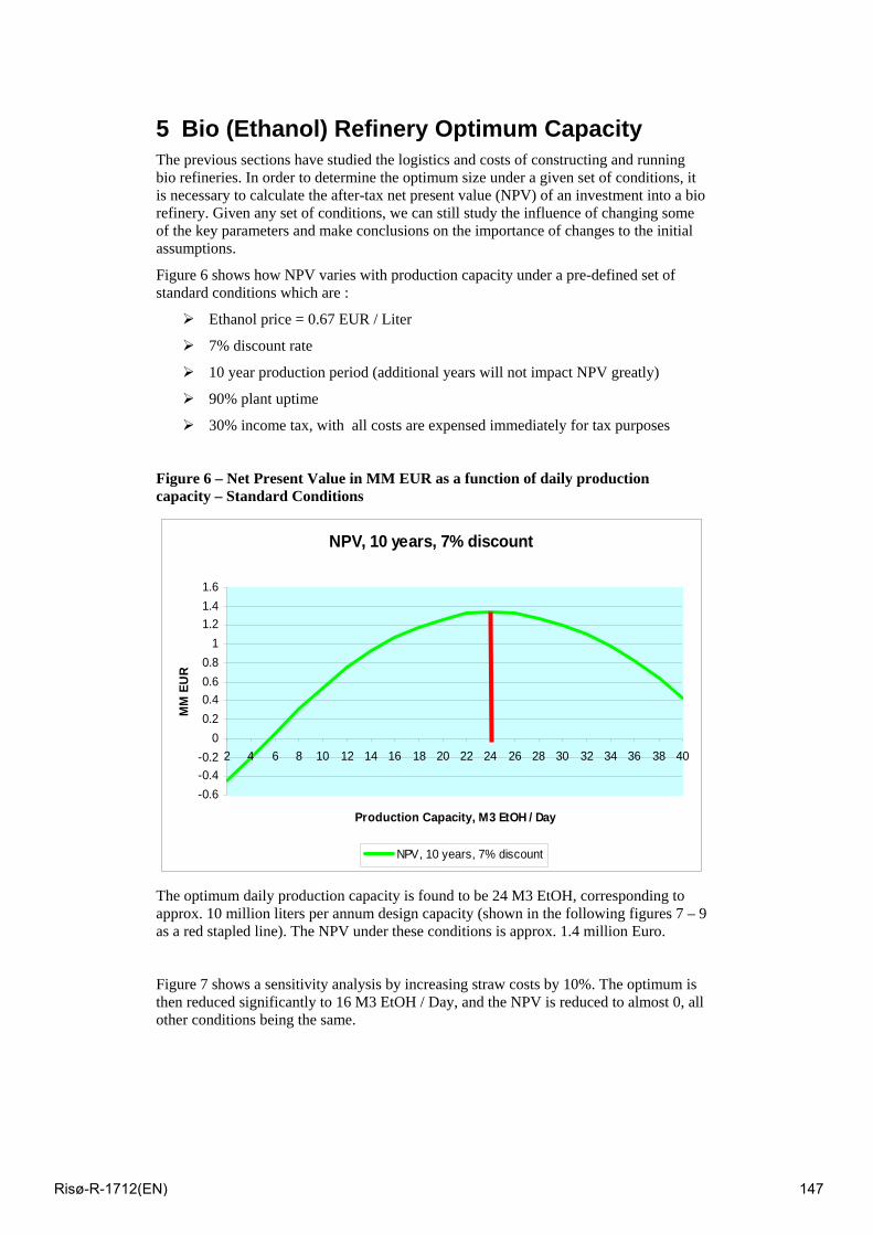
5 Bio (Ethanol) Refinery Optimum Capacity The previous sections have studied the logistics and costs of constructing and running bio refineries. In order to determine the optimum size under a given set of conditions, it is necessary to calculate the after-tax net present value (NPV) of an investment into a bio refinery. Given any set of conditions, we can still study the influence of changing some of the key parameters and make conclusions on the importance of changes to the initial assumptions.

Figure 6 shows how NPV varies with production capacity under a pre-defined set of standard conditions which are :

Ethanol price = 0.67 EUR / Liter

7% discount rate

10 year production period (additional years will not impact NPV greatly)

90% plant uptime

30% income tax, with all costs are expensed immediately for tax purposes

Figure 6 – Net Present Value in MM EUR as a function of daily production capacity – Standard Conditions

The optimum daily production capacity is found to be 24 M3 EtOH, corresponding to approx. 10 million liters per annum design capacity (shown in the following figures 7 – 9 as a red stapled line). The NPV under these conditions is approx. 1.4 million Euro.

Figure 7 shows a sensitivity analysis by increasing straw costs by 10%. The optimum is then reduced significantly to 16 M3 EtOH / Day, and the NPV is reduced to almost 0, all other conditions being the same.

NPV, 10 years, 7% discount

-0.6-0.4-0.2

00.20.40.60.8

11.21.41.6

2 4 6 8 10 12 14 16 18 20 22 24 26 28 30 32 34 36 38 40

Production Capacity, M3 EtOH / Day

MM

EU

R

NPV, 10 years, 7% discount

Risø-R-1712(EN) 147

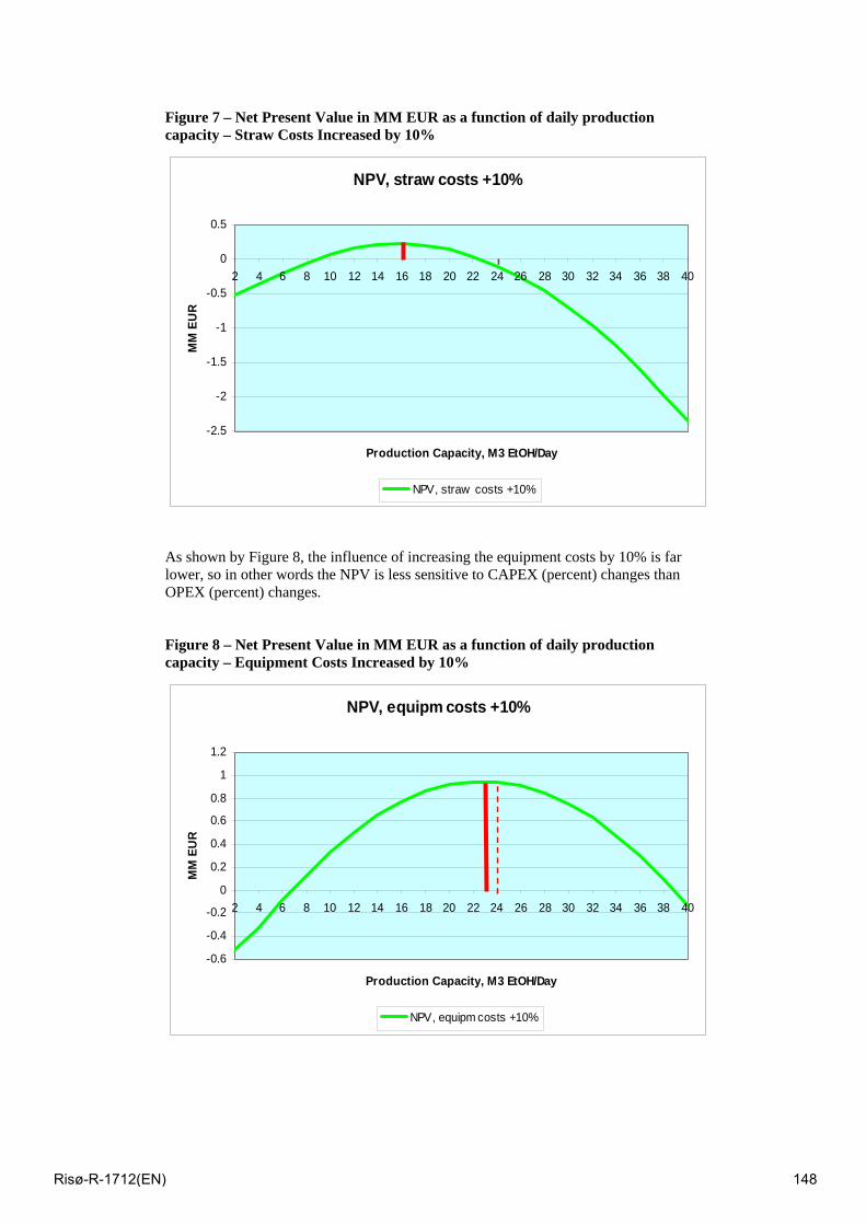
Figure 7 – Net Present Value in MM EUR as a function of daily production capacity – Straw Costs Increased by 10%

As shown by Figure 8, the influence of increasing the equipment costs by 10% is far lower, so in other words the NPV is less sensitive to CAPEX (percent) changes than OPEX (percent) changes.

Figure 8 – Net Present Value in MM EUR as a function of daily production capacity – Equipment Costs Increased by 10%

NPV, straw costs +10%

-2.5

-2

-1.5

-1

-0.5

0

0.5

2 4 6 8 10 12 14 16 18 20 22 24 26 28 30 32 34 36 38 40

Production Capacity, M3 EtOH/Day

MM

EU

R

NPV, straw costs +10%

NPV, equipm costs +10%

-0.6

-0.4

-0.2

0

0.2

0.4

0.6

0.8

1

1.2

2 4 6 8 10 12 14 16 18 20 22 24 26 28 30 32 34 36 38 40

Production Capacity, M3 EtOH/Day

MM

EU

R

NPV, equipm costs +10%

Risø-R-1712(EN) 148

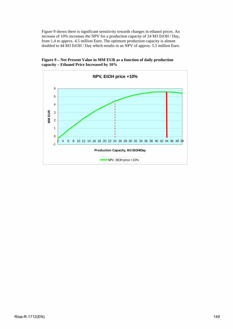
Figure 9 shows there is significant sensitivity towards changes in ethanol prices. An increase of 10% increases the NPV for a production capacity of 24 M3 EtOH / Day, from 1.4 to approx. 4.5 million Euro. The optimum production capacity is almost doubled to 44 M3 EtOH / Day which results in an NPV of approx. 5.5 million Euro.

Figure 9 – Net Present Value in MM EUR as a function of daily production capacity – Ethanol Price Increased by 10%

NPV, EtOH price +10%

-1

0

1

2

3

4

5

6

2 4 6 8 10 12 14 16 18 20 22 24 26 28 30 32 34 36 38 40 42 44 46 48 50

Production Capacity, M3 EtOH/Day

MM

EU

R

NPV, EtOH price +10%

Risø-R-1712(EN) 149

6 Conclusion - Where will 2G Bio Refinery Sizes Go?

Traditional economies of scale apply to upstream and downstream oil and gas plants, where the unit cost of production decreases with increasing production capacity. This has resulted in increasing plant sizes since the beginning of the oil and gas industry 150 years ago.

On the other hand, 2G bio refineries have an optimum size which depends on a range of factors. In this paper 2G bioethanol plant economics was studied under a realistic set of assumptions.

Under these assumptions it was found that the optimum size is a design capacity of 10 million liters per annum of bioethanol. This corresponds to a collection radius of approx. 6 km, given that 50% of the surrounding land is used for straw based crop production.

It seems that the optimum plant size is most sensitive to straw costs (and thereby collection radius) and (fuel) ethanol prices. These are obviously very hard parameters to control, so it seems advisable to enter into long term contracts for both purchasing straw and selling bioethanol to ensure that the economics is well managed.

There is currently a lack of engineering knowledge and experience for designing and operating 2G bio refineries. As the experience base grows over the years the basis for reducing the unit cost of production will also grow. As technology develops both for collection and transport of biomass, and processing equipment, a shift of the optimum production capacity will probably take place.

The optimum production capacity may shift will be towards smaller and more local plants, if the main improvement is in CAPEX. However if the main improvement is in collection and transport costs, the shift may be towards larger and more central plants.

Risø-R-1712(EN) 150

7 References

1. www.petroleumhistory.org

2. www.shell.com

3. www.exxonmobil.com

4. www.wikipedia.com

5. en.citizendium.org

6. Energy Information Administration

7. PetroBras Cap 3000 presentation, 2006

8. Scale-up Methodology for Chemical Processes, J.P.Euzen/T.Trambouze/J.P.Wauquier, Editions Technip, 1993

9. www.verenium.com

10. www.biofpr.com

11. Plant Design and Economics for Chemical Engineers, Max. S.Peters & Klaus D.Timmerhaus, McGraw- Hill, 1981

12. Biorefineries – Industrial Processes and Products, B.Kamm, P.R.Gruber, M.Kamm, Wiley-VCH, 2006

Risø-R-1712(EN) 151

Session 10 – Fuel cells and hydrogen I

Risø-R-1712(EN) 152

SOFC and Gas Separation Membranes A. Hagen, P.V. Hendriksen, M. Søgaard

Risoe National Laboratory for Sustainable Energy

Risoe DTU, Frederiksborgvej 399, DK-4000 Roskilde

Abstract How will the future, sustainable energy system look like? The answer to this difficult question depends on a number of technical but also political and socio-economic issues. Besides a massive demand to build up of power supply systems based on renewables, there is a strong need to reduce losses, increase the efficiency of power production processes from fossil fuels and also to consider carbon capture and sequestration (CCS).

Solid oxide fuel cells (SOFCs) convert the chemical energy bound in a fuel directly into electrical energy at temperatures ranging from 600 to 1000 oC, depending on the materials used in the SOFCs. Due to the high efficiencies, the amount of CO2 emitted from carbon containing fuels is smaller compared to conventional energy production technologies based on fuel combustion. Furthermore, CO2 is formed at the anode side of the fuel cell together with steam, and thus separated from air. Subsequent separation and sequestration of CO2 is therefore easier on a SOFC plant than on conventional power plants based on combustion.

Oxide ion conducting materials may be used for gas separation purposes with close to 100 % selectivity. They typically work in the same temperature range as SOFCs. Such membranes can potentially be used in Oxyfuel processes as well as in IGCC (Integrated Gasification Combined Cycle) power plants for supply of process oxygen, which may reduce cost of carbon capture and storage as dilution of the flue gas with nitrogen is avoided.

Both technologies are very attractive for combination with biomass conversion. A brief status of the Risø DTU activities in the SOFC and membrane areas is presented. Ideas for the use of these technologies in a future more sustainable energy system will be discussed with special emphasis on their combination with biomass conversion and CCS-schemes.

1 Introduction The Fuel Cells and Solid State Chemistry Division at Risoe DTU carries out research and development on advanced functional ceramics for energy efficient technologies. Solid Oxide Fuel Cells and oxide ion conducting membranes are among the most promising and attractive technologies.

In a SOFC, the chemical energy of a fuel such as hydrogen or methane is directly converted to electricity and heat; thereby the detour via thermal energy as in conventional power production is avoided and high efficiencies can be achieved.

Research on fuel cells has been carried out at Risø since the 1980s. For the effective development and commercialization of Danish SOFC technology a close collaboration with the Danish company Haldor Topsøe A/S (today Topsoe Fuel Cell A/S – TOFC, fully owned by Haldor Topsøe A/S) has been realized and formalized in a consortium agreement in 2001. The company is dedicated to development, manufacturing and marketing of SOFC technology. Our strategy is based on accomplishing technological development based on and in parallel with fundamental research.

Risø-R-1712(EN) 153

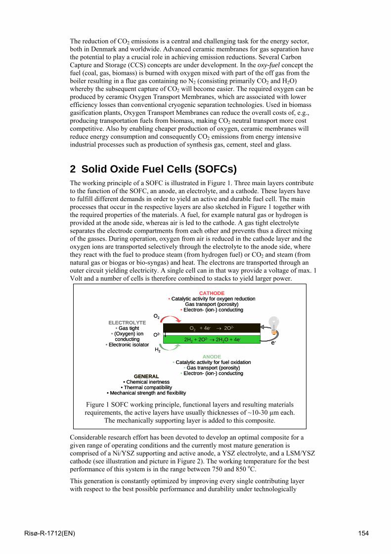
The reduction of CO2 emissions is a central and challenging task for the energy sector, both in Denmark and worldwide. Advanced ceramic membranes for gas separation have the potential to play a crucial role in achieving emission reductions. Several Carbon Capture and Storage (CCS) concepts are under development. In the oxy-fuel concept the fuel (coal, gas, biomass) is burned with oxygen mixed with part of the off gas from the boiler resulting in a flue gas containing no N2 (consisting primarily CO2 and H2O) whereby the subsequent capture of CO2 will become easier. The required oxygen can be produced by ceramic Oxygen Transport Membranes, which are associated with lower efficiency losses than conventional cryogenic separation technologies. Used in biomass gasification plants, Oxygen Transport Membranes can reduce the overall costs of, e.g., producing transportation fuels from biomass, making CO2 neutral transport more cost competitive. Also by enabling cheaper production of oxygen, ceramic membranes will reduce energy consumption and consequently CO2 emissions from energy intensive industrial processes such as production of synthesis gas, cement, steel and glass.

2 Solid Oxide Fuel Cells (SOFCs) The working principle of a SOFC is illustrated in Figure 1. Three main layers contribute to the function of the SOFC, an anode, an electrolyte, and a cathode. These layers have to fulfill different demands in order to yield an active and durable fuel cell. The main processes that occur in the respective layers are also sketched in Figure 1 together with the required properties of the materials. A fuel, for example natural gas or hydrogen is provided at the anode side, whereas air is led to the cathode. A gas tight electrolyte separates the electrode compartments from each other and prevents thus a direct mixing of the gasses. During operation, oxygen from air is reduced in the cathode layer and the oxygen ions are transported selectively through the electrolyte to the anode side, where they react with the fuel to produce steam (from hydrogen fuel) or CO2 and steam (from natural gas or biogas or bio-syngas) and heat. The electrons are transported through an outer circuit yielding electricity. A single cell can in that way provide a voltage of max. 1 Volt and a number of cells is therefore combined to stacks to yield larger power.

Considerable research effort has been devoted to develop an optimal composite for a given range of operating conditions and the currently most mature generation is comprised of a Ni/YSZ supporting and active anode, a YSZ electrolyte, and a LSM/YSZ cathode (see illustration and picture in Figure 2). The working temperature for the best performance of this system is in the range between 750 and 850 oC.

This generation is constantly optimized by improving every single contributing layer with respect to the best possible performance and durability under technologically

O2

O2 + 4e- → 2O2-

ANODE• Catalytic activity for fuel oxidation

• Gas transport (porosity)• Electron- (ion-) conducting

2H2 + 2O2- → 2H2O + 4e-

CATHODE• Catalytic activity for oxygen reduction

Gas transport (porosity)• Electron- (ion-) conducting

H2

O2-

ELECTROLYTE• Gas tight

• (Oxygen) ion conducting

• Electronic isolator e-

GENERAL• Chemical inertness

• Thermal compatibility• Mechanical strength and flexibility

O2

O2 + 4e- → 2O2-

ANODE• Catalytic activity for fuel oxidation

• Gas transport (porosity)• Electron- (ion-) conducting

2H2 + 2O2- → 2H2O + 4e-

CATHODE• Catalytic activity for oxygen reduction

Gas transport (porosity)• Electron- (ion-) conducting

H2

O2-

ELECTROLYTE• Gas tight

• (Oxygen) ion conducting

• Electronic isolator e-

GENERAL• Chemical inertness

• Thermal compatibility• Mechanical strength and flexibility

Figure 1 SOFC working principle, functional layers and resulting materials requirements, the active layers have usually thicknesses of ~10-30 µm each.

The mechanically supporting layer is added to this composite.

Risø-R-1712(EN) 154

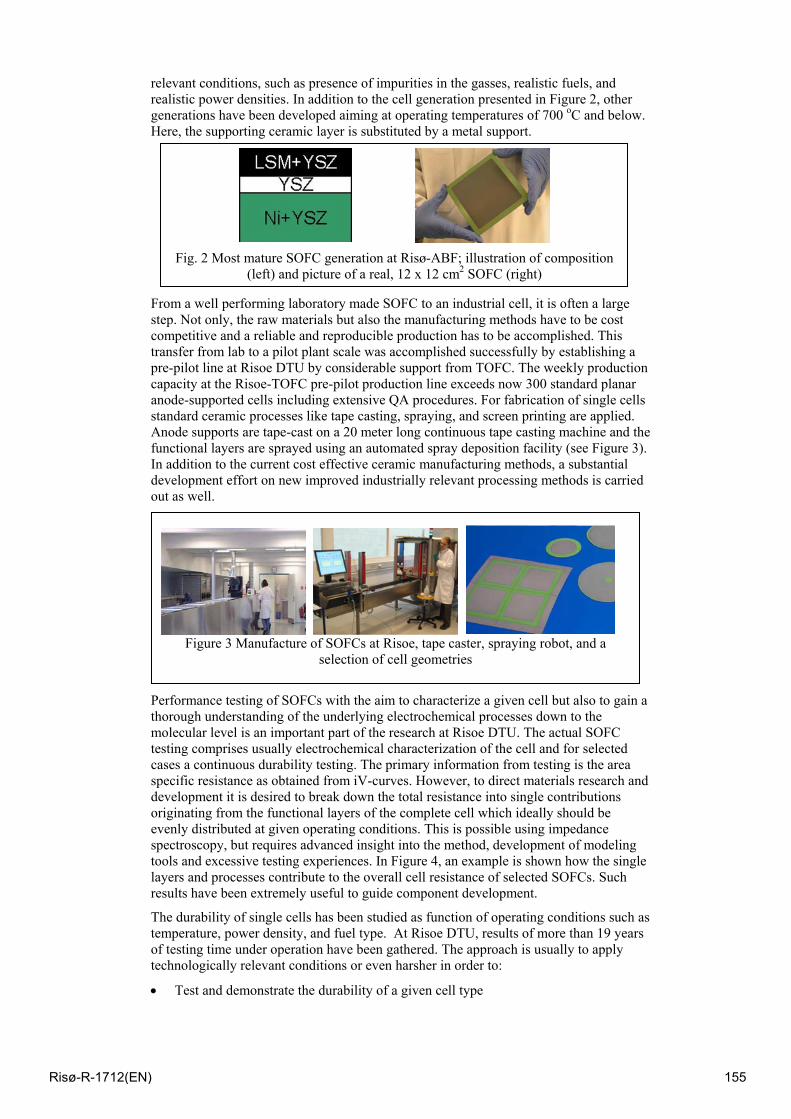
relevant conditions, such as presence of impurities in the gasses, realistic fuels, and realistic power densities. In addition to the cell generation presented in Figure 2, other generations have been developed aiming at operating temperatures of 700 oC and below. Here, the supporting ceramic layer is substituted by a metal support.

From a well performing laboratory made SOFC to an industrial cell, it is often a large step. Not only, the raw materials but also the manufacturing methods have to be cost competitive and a reliable and reproducible production has to be accomplished. This transfer from lab to a pilot plant scale was accomplished successfully by establishing a pre-pilot line at Risoe DTU by considerable support from TOFC. The weekly production capacity at the Risoe-TOFC pre-pilot production line exceeds now 300 standard planar anode-supported cells including extensive QA procedures. For fabrication of single cells standard ceramic processes like tape casting, spraying, and screen printing are applied. Anode supports are tape-cast on a 20 meter long continuous tape casting machine and the functional layers are sprayed using an automated spray deposition facility (see Figure 3). In addition to the current cost effective ceramic manufacturing methods, a substantial development effort on new improved industrially relevant processing methods is carried out as well.

Performance testing of SOFCs with the aim to characterize a given cell but also to gain a thorough understanding of the underlying electrochemical processes down to the molecular level is an important part of the research at Risoe DTU. The actual SOFC testing comprises usually electrochemical characterization of the cell and for selected cases a continuous durability testing. The primary information from testing is the area specific resistance as obtained from iV-curves. However, to direct materials research and development it is desired to break down the total resistance into single contributions originating from the functional layers of the complete cell which ideally should be evenly distributed at given operating conditions. This is possible using impedance spectroscopy, but requires advanced insight into the method, development of modeling tools and excessive testing experiences. In Figure 4, an example is shown how the single layers and processes contribute to the overall cell resistance of selected SOFCs. Such results have been extremely useful to guide component development.

The durability of single cells has been studied as function of operating conditions such as temperature, power density, and fuel type. At Risoe DTU, results of more than 19 years of testing time under operation have been gathered. The approach is usually to apply technologically relevant conditions or even harsher in order to:

• Test and demonstrate the durability of a given cell type

Figure 3 Manufacture of SOFCs at Risoe, tape caster, spraying robot, and a

selection of cell geometries

Fig. 2 Most mature SOFC generation at Risø-ABF; illustration of composition (left) and picture of a real, 12 x 12 cm2 SOFC (right)

Risø-R-1712(EN) 155

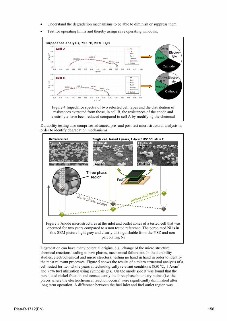
• Understand the degradation mechanisms to be able to diminish or suppress them

• Test for operating limits and thereby assign save operating windows.

Durability testing also comprises advanced pre- and post test microstructural analysis in order to identify degradation mechanisms.

Degradation can have many potential origins, e.g., change of the micro structure, chemical reactions leading to new phases, mechanical failure etc. In the durability studies, electrochemical and micro structural testing go hand in hand in order to identify the most relevant processes. Figure 5 shows the results of a micro structural analysis of a cell tested for two whole years at technologically relevant conditions (850 oC, 1 A/cm2 and 75% fuel utilization using synthesis gas). On the anode side it was found that the percolated nickel fraction and consequently the three phase boundary points (i.e. the places where the electrochemical reaction occurs) were significantly diminished after long term operation. A difference between the fuel inlet and fuel outlet region was

Impedance analysis, 750 oC, 20% H2O

56,000 Hz10,000 Hz

790 Hz

110 Hz19 Hz

0.00

0.05

0.10

0.15

0.20

0.10 0.15 0.20 0.25 0.30 0.35 0.40 0.45 0.50 0.55 0.60 0.65 0.70 0.75 0.80Z' [Ω cm2]

-Z'' [

Ω c

m2 ]

FitCat IAno ICat IIDiffusionConversionCell #A

Cell A

43,000 Hz 5,500 Hz 680 Hz56 Hz 18 Hz

0.00

0.05

0.10

0.15

0.20

0.10 0.15 0.20 0.25 0.30 0.35 0.40 0.45 0.50 0.55 0.60 0.65 0.70 0.75 0.80

Z' [Ω cm2]

-Z'' [

Ω c

m2 ]

FitCat IAno ICat IIDiffusionConversionCell #B

Cell B

Cathode

AnodeElectro-

lyte

Convs.Diff.

CathodeAnode

Electro-lyte

Convs.Diff.

Impedance analysis, 750 oC, 20% H2O

56,000 Hz10,000 Hz

790 Hz

110 Hz19 Hz

0.00

0.05

0.10

0.15

0.20

0.10 0.15 0.20 0.25 0.30 0.35 0.40 0.45 0.50 0.55 0.60 0.65 0.70 0.75 0.80Z' [Ω cm2]

-Z'' [

Ω c

m2 ]

FitCat IAno ICat IIDiffusionConversionCell #A

Cell A

43,000 Hz 5,500 Hz 680 Hz56 Hz 18 Hz

0.00

0.05

0.10

0.15

0.20

0.10 0.15 0.20 0.25 0.30 0.35 0.40 0.45 0.50 0.55 0.60 0.65 0.70 0.75 0.80

Z' [Ω cm2]

-Z'' [

Ω c

m2 ]

FitCat IAno ICat IIDiffusionConversionCell #B

Cell B

Cathode

AnodeElectro-

lyte

Convs.Diff.

Cathode

AnodeElectro-

lyte

Convs.Diff.

Cathode

AnodeElectro-

lyte

Convs.Diff.

CathodeAnode

Electro-lyte

Convs.Diff.

CathodeAnode

Electro-lyte

Convs.Diff.

CathodeAnode

Electro-lyte

Convs.Diff.

Figure 4 Impedance spectra of two selected cell types and the distribution of resistances extracted from those, in cell B, the resistances of the anode and

electrolyte have been reduced compared to cell A by modifying the chemical

FuelFuel

Three phaseregion

Three phaseregion

anode resistancethree phase points

Single cell, tested 2 years, 1 A/cm2, 850 oC, s/c = 2

Fuel in

ElectrolyteAnode

Fuel out

ElectrolyteAnode

Single cell, tested 2 years, 1 A/cm2, 850 oC, s/c = 2

Fuel in

ElectrolyteAnode

Fuel out

ElectrolyteAnode

ElectrolyteAnode

Reference cellElectrolyteAnode

Reference cell

Figure 5 Anode microstructures at the inlet and outlet zones of a tested cell that was operated for two years compared to a non tested reference. The percolated Ni is in

this SEM picture light grey and clearly distinguishable from the YSZ and non-percolating Ni

Risø-R-1712(EN) 156

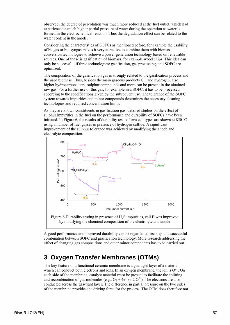
observed; the degree of percolation was much more reduced at the fuel outlet, which had experienced a much higher partial pressure of water during the operation as water is formed in the electrochemical reaction. Thus the degradation effect can be related to the water content in the anode.

Considering the characteristics of SOFCs as mentioned before, for example the usability of biogas or bio syngas makes it very attractive to combine them with biomass conversion technologies to achieve a power generation technology based on renewable sources. One of those is gasification of biomass, for example wood chips. This idea can only be successful, if three technologies: gasification, gas processing, and SOFC are optimized.

The composition of the gasification gas is strongly related to the gasification process and the used biomass. Thus, besides the main gaseous products CO and hydrogen, also higher hydrocarbons, tars, sulphur compounds and more can be present in the obtained raw gas. For a further use of this gas, for example in a SOFC, it has to be processed according to the specifications given by the subsequent use. The tolerance of the SOFC system towards impurities and minor compounds determines the necessary cleaning technologies and required concentration limits.

As they are known constituents in gasification gas, detailed studies on the effect of sulphur impurities in the fuel on the performance and durability of SOFCs have been initiated. In Figure 6, the results of durability tests of two cell types are shown at 850 oC using a number of fuel gasses in presence of hydrogen sulfide. A significant improvement of the sulphur tolerance was achieved by modifying the anode and electrolyte composition.

A good performance and improved durability can be regarded a first step to a successful combination between SOFC and gasification technology. More research addressing the effect of changing gas compositions and other minor components has to be carried out.

3 Oxygen Transfer Membranes (OTMs) The key feature of a functional ceramic membrane is a gas-tight layer of a material which can conduct both electrons and ions. In an oxygen membrane, the ion is O2–. On each side of the membrane, catalyst material must be present to facilitate the splitting and recombination of gas molecules (e.g., O2 + 4e– ↔ 2 O2–). The electrons are also conducted across the gas-tight layer. The difference in partial pressure on the two sides of the membrane provides the driving force for the process. The OTM does therefore not

400

500

600

700

800

0 500 1000 1500 2000Time under current in h

Cel

l vol

tage

in m

V

1 A/cm2H2SH2S

H2S

cell A

cell B

CH4/H2O/H2O

CH4/H2O/H2O

H2/H2O

Figure 6 Durability testing in presence of H2S impurities, cell B was improved

by modifying the chemical composition of the electrolyte and anode

Risø-R-1712(EN) 157

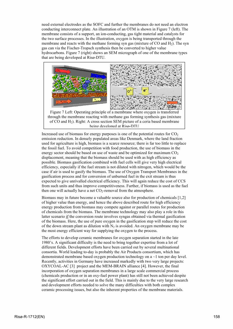
need external electrodes as the SOFC and further the membranes do not need an electron conducting interconnect plate. An illustration of an OTM is shown in Figure 7 (left). The membrane consists of a support, an ion-conducting, gas tight material and catalysts for the two surface processes. In the illustration, oxygen is being transported through the membrane and reacts with the methane forming syn gas (mixture of CO and H2). The syn gas can via the Fischer-Tropsch synthesis then be converted to higher value hydrocarbons. Figure 7 (right) shows an SEM micrograph of one of the membrane types that are being developed at Risø-DTU.

Increased use of biomass for energy purposes is one of the potential routes for CO2 emission reduction. In densely populated areas like Denmark, where the land fraction used for agriculture is high, biomass is a scarce resource; there is far too little to replace the fossil fuel. To avoid competition with food production, the use of biomass in the energy sector should be based on use of waste and be optimized for maximum CO2 displacement, meaning that the biomass should be used with as high efficiency as possible. Biomass gasification combined with fuel cells will give very high electrical efficiency, especially if the fuel stream is not diluted with nitrogen, which would be the case if air is used to gasify the biomass. The use of Oxygen Transport Membranes in the gasification process and for conversion of unburned fuel in the exit stream is thus expected to give unrivalled electrical efficiency. This will again reduce the cost of CCS from such units and thus improve competitiveness. Further, if biomass is used as the fuel then one will actually have a net CO2-removal from the atmosphere.

Biomass may in future become a valuable source also for production of chemicals [1,2] of higher value than energy, and hence the above described route for high efficiency energy production from biomass may compete against or parallel routes for production of chemicals from the biomass. The membrane technology may also play a role in this latter scenario if the conversion route involves syngas obtained via thermal gasification of the biomass. Here, the use of pure oxygen in the gasification step will reduce the cost of the down stream plant as dilution with N2 is avoided. An oxygen membrane may be the most energy efficient way for supplying the oxygen to the process.

The efforts to develop ceramic membranes for oxygen separation started in the late 1980’s. A significant difficulty is the need to bring together expertise from a lot of different fields. Development efforts have been carried out by several multinational consortia. World leading to-day is probably the Air Products consortium, which has demonstrated membrane based oxygen production technology on a ~1 ton per day level. Recently, activities in Germany have increased markedly with two very large projects: OXYCOAL-AC [3] project and the MEM-BRAIN alliance [4]. However, the final incorporation of oxygen separation membranes in a large scale commercial process (chemicals production or in an oxy-fuel power plant) has still not been achieved despite the significant effort carried out in the field. This is mainly due to the very large research and development efforts needed to solve the many difficulties with both complex ceramic processing issues, but also the inherent properties of the membrane materials.

Figure 7 Left: Operating principle of a membrane where oxygen is transferred through the membrane reacting with methane gas forming synthesis gas (mixture of CO and H2). Right: A cross section SEM picture of a ceria based membrane

being developed at Risø-DTU

Risø-R-1712(EN) 158

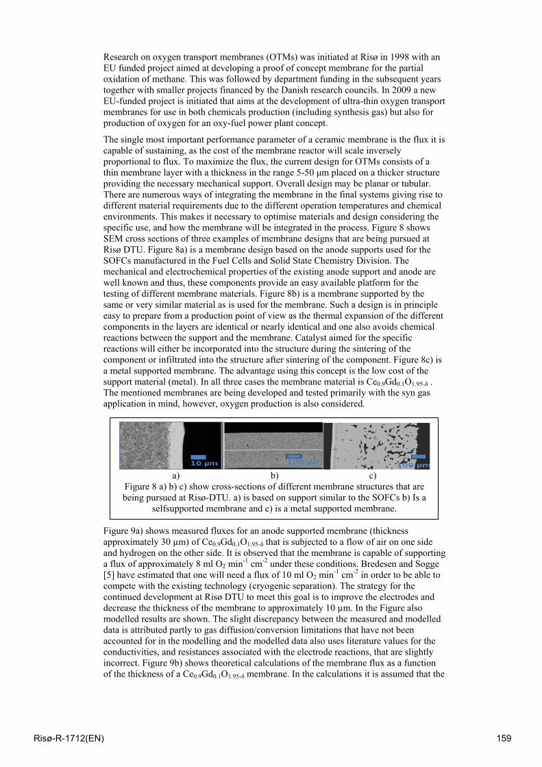
Research on oxygen transport membranes (OTMs) was initiated at Risø in 1998 with an EU funded project aimed at developing a proof of concept membrane for the partial oxidation of methane. This was followed by department funding in the subsequent years together with smaller projects financed by the Danish research councils. In 2009 a new EU-funded project is initiated that aims at the development of ultra-thin oxygen transport membranes for use in both chemicals production (including synthesis gas) but also for production of oxygen for an oxy-fuel power plant concept.

The single most important performance parameter of a ceramic membrane is the flux it is capable of sustaining, as the cost of the membrane reactor will scale inversely proportional to flux. To maximize the flux, the current design for OTMs consists of a thin membrane layer with a thickness in the range 5-50 μm placed on a thicker structure providing the necessary mechanical support. Overall design may be planar or tubular. There are numerous ways of integrating the membrane in the final systems giving rise to different material requirements due to the different operation temperatures and chemical environments. This makes it necessary to optimise materials and design considering the specific use, and how the membrane will be integrated in the process. Figure 8 shows SEM cross sections of three examples of membrane designs that are being pursued at Risø DTU. Figure 8a) is a membrane design based on the anode supports used for the SOFCs manufactured in the Fuel Cells and Solid State Chemistry Division. The mechanical and electrochemical properties of the existing anode support and anode are well known and thus, these components provide an easy available platform for the testing of different membrane materials. Figure 8b) is a membrane supported by the same or very similar material as is used for the membrane. Such a design is in principle easy to prepare from a production point of view as the thermal expansion of the different components in the layers are identical or nearly identical and one also avoids chemical reactions between the support and the membrane. Catalyst aimed for the specific reactions will either be incorporated into the structure during the sintering of the component or infiltrated into the structure after sintering of the component. Figure 8c) is a metal supported membrane. The advantage using this concept is the low cost of the support material (metal). In all three cases the membrane material is Ce0.9Gd0.1O1.95-δ . The mentioned membranes are being developed and tested primarily with the syn gas application in mind, however, oxygen production is also considered.

Figure 9a) shows measured fluxes for an anode supported membrane (thickness approximately 30 µm) of Ce0.9Gd0.1O1.95-δ that is subjected to a flow of air on one side and hydrogen on the other side. It is observed that the membrane is capable of supporting a flux of approximately 8 ml O2 min-1 cm-2 under these conditions. Bredesen and Sogge [5] have estimated that one will need a flux of 10 ml O2 min-1 cm-2 in order to be able to compete with the existing technology (cryogenic separation). The strategy for the continued development at Risø DTU to meet this goal is to improve the electrodes and decrease the thickness of the membrane to approximately 10 µm. In the Figure also modelled results are shown. The slight discrepancy between the measured and modelled data is attributed partly to gas diffusion/conversion limitations that have not been accounted for in the modelling and the modelled data also uses literature values for the conductivities, and resistances associated with the electrode reactions, that are slightly incorrect. Figure 9b) shows theoretical calculations of the membrane flux as a function of the thickness of a Ce0.9Gd0.1O1.95-δ membrane. In the calculations it is assumed that the

a) b) c)

Figure 8 a) b) c) show cross-sections of different membrane structures that are being pursued at Risø-DTU. a) is based on support similar to the SOFCs b) Is a

selfsupported membrane and c) is a metal supported membrane.

Risø-R-1712(EN) 159

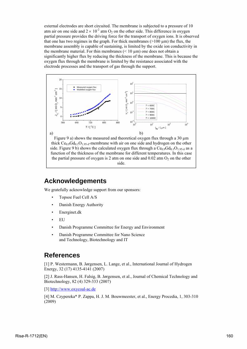
external electrodes are short circuited. The membrane is subjected to a pressure of 10 atm air on one side and 2 × 10-2 atm O2 on the other side. This difference in oxygen partial pressure provides the driving force for the transport of oxygen ions. It is observed that one has two regimes in the graph. For thick membranes (>100 µm) the flux, the membrane assembly is capable of sustaining, is limited by the oxide ion conductivity in the membrane material. For thin membranes (< 10 µm) one does not obtain a significantly higher flux by reducing the thickness of the membrane. This is because the oxygen flux through the membrane is limited by the resistance associated with the electrode processes and the transport of gas through the support.

Acknowledgements We gratefully acknowledge support from our sponsors:

• Topsoe Fuel Cell A/S

• Danish Energy Authority

• Energinet.dk

• EU

• Danish Programme Committee for Energy and Environment

• Danish Programme Committee for Nano Science and Technology, Biotechnology and IT

References [1] P. Westermann, B. Jørgensen, L. Lange, et al., International Journal of Hydrogen Energy, 32 (17) 4135-4141 (2007)

[2] J. Rass-Hansen, H. Falsig, B. Jørgensen, et al., Journal of Chemical Technology and Biotechnology, 82 (4) 329-333 (2007)

[3] http://www.oxycoal-ac.de

[4] M. Czypereka* P. Zappa, H. J. M. Bouwmeester, et al., Energy Procedia, 1, 303-310 (2009)

560 640 720 800 880

0

5

10

15

20

Measured oxygen flux Modelled oxygen flux

J O2 /

[ ml O

2 min

-1 c

m-2 ]

T / [ oC ]100 101 102 103

10-2

10-1

100

101

102

lEly / [ μm ] V

f / [ m

l O2 m

in-1

cm

-2]

T = 600C T = 700C T = 800C T = 900C T = 1000C

a) b)

Figure 9 a) shows the measured and theoretical oxygen flux through a 30 µm thick Ce0.9Gd0.1O1.95-δ-membrane with air on one side and hydrogen on the other

side. Figure 9 b) shows the calculated oxygen flux through a Ce0.9Gd0.1O1.95-δ as a function of the thickness of the membrane for different temperatures. In this case the partial pressure of oxygen is 2 atm on one side and 0.02 atm O2 on the other

side.

Risø-R-1712(EN) 160

[5] R. Bredesen, J. Sogge, in: Paper presented at: The United Nations Economic Commission for Europe Seminar on Ecological Applications of Innovative Membrane Technology in Chemical Industry; Chem/Sem. 21/R.12, Cetraro, Calabria,Italy, 1–4 May 1996.

Risø-R-1712(EN) 161

Production of Hydrogen and Synthesis Gas by High Temperature Electrolysis

Sune D. Ebbesen*, Jens Høgh, and Mogens Mogensen

Fuel Cells and Solid State Chemistry Division, Risø National Laboratory for Sustainable Energy, The Technical University of Denmark, Frederiksborgvej 399, 4000 Roskilde, Denmark.

Abstract Electrolysis of steam and co-electrolysis of steam and carbon dioxide was studied in stacks composed of Ni/YSZ electrode supported Solid Oxide Electrolysis Cells. The results of this study show that long term electrolysis is feasible in these solid oxide electrolysis stacks. The degradation of the electrolysis cells was found to be influenced by the adsorption of impurities from the gasses, whereas the application of chromium containing interconnect plates and glass sealings do not seem to influence the durability. Cleaning the inlet gasses to the Ni/YSZ electrode resulted in operation without any long term degradation, and may therefore be a solution for operating these Ni/YSZ based solid oxide electrolysis stacks without any long term cell stack degradation.

1 Introduction The widespread use of fossil fuels within the current energy infrastructure is considered as one of the largest sources of CO2 emissions, which is argued to cause global warming and climate changes. One of the top energy priorities is therefore exploring environmentally friendly alternatives to fossil fuels and thereby reducing and eventually eliminating CO2 emissions. The raw material for synthetic hydrocarbon fuels is synthesis gas, H2 + CO. This can be produced from renewable energy sources and may be a solution to reduce consumption of fossil fuels and carbon dioxide emissions. Hydrogen offers significant promise as a basis for a future energy technology, and is argued to be the most versatile, efficient and environmentally friendly fuel, although handling of hydrogen may be problematic. On the other hand, the production of synthetic hydrocarbon fuels can be applied without the need for modifications of existing infrastructure. Hydrogen production via electrolysis of steam (H2O → H2 + ½O2) and production of synthesis gas via co-electrolysis of steam and carbon dioxide (H2O + CO2 → H2 + CO + O2) using renewable energy sources may be an alternative route for producing hydrogen and synthesis gas without consuming fossil fuels or emitting green-house gases. Steam electrolysis in Solid Oxide Cells (SOC) for hydrogen production was under development during the early 1980s [1-3] and has again become increasingly investigated during recent years as a green energy technology. On the other hand, the feasibility of co-electrolysis has only been shown in a few studies [4-6]. Mainly single cells have been tested for electrolysis performance and durability, and only a relatively limited number of studies focusing on the performance and durability of high temperature electrolysis stacks have been conducted [5, 7-11]. When operating stacks, factors such as gas flow and thermal management, and chemical compatibility of cell components with interconnect materials become important. For example, it is well established that current state-of-the-art interconnect materials are significant sources of chromium vapour which has been shown to have a significant negative impact on cell performance when operated in fuel cell mode [12-15]. This process, known as chromium poisoning, may also play an important role for the durability of electrolysis stacks [9]. Electrolysis cells were found to degrade significantly when applying glass sealing [16-19]. For single cell tests, this glass sealing may be avoided [4], whereas for stack assembly, glass is the preferred sealing material because it

Risø-R-1712(EN) 162

can be modified to match the thermal expansion of other cell components, and show good hermeticity along with good thermal and chemical stability. It is the aim of the present study to examine the degradation of Ni/YSZ based Solid Oxide Electrolysis Cell Stacks (applying glass seals and chromium containing interconnects) during steam electrolysis and co-electrolysis of steam and carbon dioxide.

2 Experimental Three stacks were tested for electrolysis performance/durability. One Single Repeating Stack Unit (SRU) was tested for steam electrolysis performance/durability. The scope of the SRU is intermediary between that of a single cell testing, in which the performance characteristics of the individual cells is the main interest, and that of the multi-cell stack where additional factors such as gas flow and thermal management become significantly relevant. Two multi-cell stacks were tested, one for steam electrolysis and one for co-electrolysis performance/durability.

2.1 5×5 Single repeating stack unit (SRU) The electrolysis cell used for the single repeating stack unit (SRU) was a standard planar Ni/YSZ-supported SOC of 5×5 cm2 (with an active electrode area of 4×4 cm2). The cell details can be found elsewhere [20, 21]. At start-up, the nickel oxide in the Ni/YSZ electrode is reduced to nickel in hydrogen at 950°C. Interconnect plates were fabricated from Crofer 22 APU steel. The SRU was sealed at its edges between the two interconnect plates using a glass-ceramic seal as shown in Figure 1A. The voltage probes were placed on the tap of the interconnect plates while the current was supplied and withdrawn via the thick current collector plates.

2.2 12×12 cm2 Multi-cell stacks The electrolysis cells used for the multi cells stacks were also standard planar Ni/YSZ-supported SOCs of 12×12 cm2 (with an active electrode area of 9.6 × 9.6 cm2). At start-up, the nickel oxide in the Ni/YSZ electrode is reduced to nickel in hydrogen at 950°C. Two multi-cell stacks were tested, one for steam electrolysis and one for co-electrolysis performance/durability. The stacks were composed of either six (in the case of steam electrolysis) or ten (in the case of co-electrolysis) single repeating units, similar to the SRU, although the gas-channels were made directly in the interconnect plate as sketched in Figure 1B. The stack testing was performed at Risø National Laboratory with a proprietary stack design by Topsøe Fuel Cells A/S (TOFC). For the 6-cell stack, the gasses were applied as received, whereas the gasses applied for the 10-cell stack were cleaned before entering the stack. The 10-cell stack is still in operation and only initial performance and 500 hours of durability is therefore reported in this paper.

Figure 1.A: Schematic presentation of the single repeating stack unit (SRU) assembly in a cross-flow pattern, and schematic presentation of the assembly of two repeating units in a counter-flow pattern in the multi-cell stacks.

Risø-R-1712(EN) 163

2.3 Initial characterisation After reduction, the performance of the cells were examined by performing DC and AC characterisation at varying atmosphere at both the Ni/YSZ electrode (20% H2O – 80% H2, 50% H2O – 50% H2), and the LSM/YSZ electrode (pure oxygen or air, Technical air, Air Liquide). Steam was produced by reacting oxygen (industrial grade, O2 ≥ 99.5%), Air Liquide) with hydrogen (N30, H2 ≥ 99.9%, Air Liquide). When examining co-electrolysis in the 10-cell stack, additional DC and AC characterisation was performed in 45% H2O – 45% CO2 – 10% H2 at the Ni/YSZ electrode (CO2 ≥ 99.7%, Air Liquide). DC characterisation of the cell was performed by recording polarization curves (i-V curves) in both electrolysis and fuel cell mode by varying the current. The DC Area-Specific Resistance (ASRDC) was calculated from the i-V curves as the chord from OCV to the cell voltage measured at a current density of -0.15 A/cm2 (electrolysis mode) or 0.15 A/cm2 (fuel cell mode). AC characterisation at OCV was performed by Electrochemical Impedance Spectroscopy (EIS) using an external shunt and a Solartron 1260 frequency analyzer for the SRU, at frequencies from 82 kHz to 0.08 Hz at. From the impedance spectra, the ohmic resistance (RS) is calculated as the value of the real part of the impedance measured at 82 kHz. The polarization resistance (RP) is calculated as the difference in real part of the impedance at 82 kHz and 0.08 Hz. The total AC ASR (ASRAC) is calculated as the total resistance of the real part (RS + RP, to 0.08 Hz) of the impedance measured at OCV. AC characterisation at OCV for the multi-cell stacks was performed with an Yokogawa WT1600FC frequency analyzer, at frequencies from 50 kHz to 0.2 Hz. From the impedance spectra, RS is calculated as the value of the real part of the impedance measured at 50 kHz. RP is calculated as the difference in real part of the impedance at 50 kHz and 0.2 Hz. The total AC ASR (ASRAC) is calculated as the total resistance of the real part (RS + RP, to 0.2 Hz).

2.4 Durability of the solid oxide electrolysis stacks The durability of the Solid Oxide Cells during electrolysis of H2O and co-electrolysis of H2O and CO2 was examined for one SRU and two multi-cell stacks (one with six cells and another with ten cells), all operated at 850ºC. The durability for steam electrolysis was tested in the SRU and the six-stack, whereas co-electrolysis durability was tested in the 10-cell stack.

H2O Electrolysis in 5×5 cm2 single repeating stack unit (SRU) The durability during electrolysis of H2O was examined in 50% H2O – 50% H2 flown to the Ni/YSZ electrode, and a current density of -0.50 A/cm2. Oxygen was flown to the LSM/YSZ electrode (20 L/h) in order to avoid any transients in the polarisation resistance. The total flow rate to the Ni/YSZ electrode was 25 L/hour. At a current density of -0.50 A/cm2 and an active cell area of 16 cm2, the steam conversion was 28%. AC resistance was measured during electrolysis by EIS using an external shunt and a Solartron 1260 frequency response analyzer.

H2O Electrolysis in 12×12 cm2 6-cell stack The durability during electrolysis of H2O in the 6-cell stack was examined in 50% H2O – 50% H2 flowed to the Ni/YSZ electrode, and a current density of -0.25 A/cm2 (operated initially (20 hours) at -0.20 A/cm2). Oxygen was flown to the LSM/YSZ electrode (270 L/h). The total flow rate to the Ni/YSZ electrode was 666 L/h. At a current density of -0.25 A/cm2 and an active cell area of 6 × 92.2 cm2, the conversion was 10%.

Co-Electrolysis of H2O and CO2 in 12×12 cm2 10-cell stack Co-electrolysis examined in the 10-cell stack was performed with 45% H2O – 45% CO2 – 10% H2 flowed to the Ni/YSZ electrode, and a current density of -0.50 A/cm2. Again, oxygen was flown to the LSM/YSZ electrode (60 L/h). The total flow rate to the Ni/YSZ electrode was 360 L/hour. At a current density of -0.50 A/cm2 and an active cell area of 10 × 92.2 cm2, the conversion was 60%.

Risø-R-1712(EN) 164

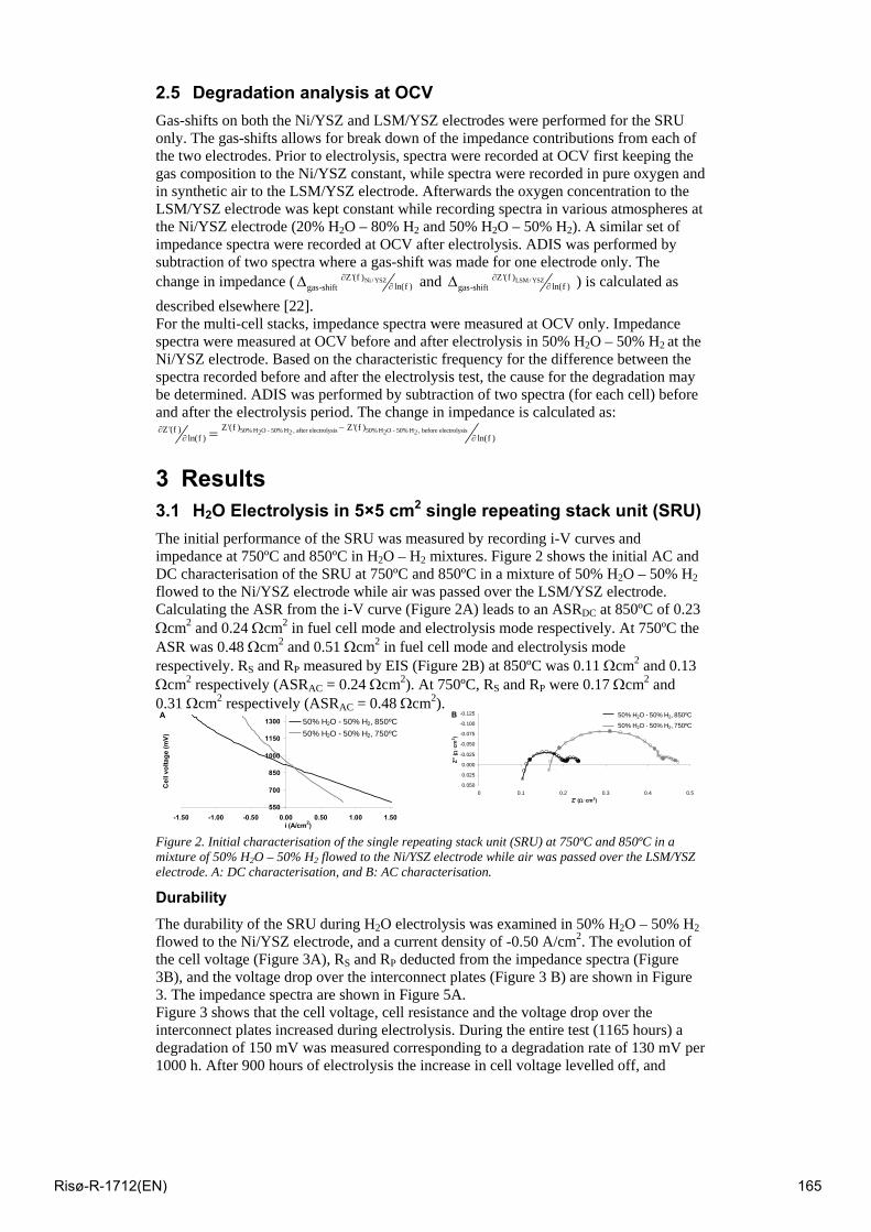
2.5 Degradation analysis at OCV Gas-shifts on both the Ni/YSZ and LSM/YSZ electrodes were performed for the SRU only. The gas-shifts allows for break down of the impedance contributions from each of the two electrodes. Prior to electrolysis, spectra were recorded at OCV first keeping the gas composition to the Ni/YSZ constant, while spectra were recorded in pure oxygen and in synthetic air to the LSM/YSZ electrode. Afterwards the oxygen concentration to the LSM/YSZ electrode was kept constant while recording spectra in various atmospheres at the Ni/YSZ electrode (20% H2O – 80% H2 and 50% H2O – 50% H2). A similar set of impedance spectra were recorded at OCV after electrolysis. ADIS was performed by subtraction of two spectra where a gas-shift was made for one electrode only. The change in impedance ( Ni / YSZZ'(f )

ln(f )gas-shift∂

∂Δ and LSM / YSZZ'(f )ln(f )gas-shift

∂∂Δ ) is calculated as

described elsewhere [22]. For the multi-cell stacks, impedance spectra were measured at OCV only. Impedance spectra were measured at OCV before and after electrolysis in 50% H2O – 50% H2 at the Ni/YSZ electrode. Based on the characteristic frequency for the difference between the spectra recorded before and after the electrolysis test, the cause for the degradation may be determined. ADIS was performed by subtraction of two spectra (for each cell) before and after the electrolysis period. The change in impedance is calculated as:

50% H O - 50% H , after electrolysis 50% H O - 50% H , before electrolysis 2 2 2 2Z'(f ) Z '(f )Z'(f )ln(f ) ln(f )

−∂∂ ∂=

3 Results 3.1 H2O Electrolysis in 5×5 cm2 single repeating stack unit (SRU) The initial performance of the SRU was measured by recording i-V curves and impedance at 750ºC and 850ºC in H2O – H2 mixtures. Figure 2 shows the initial AC and DC characterisation of the SRU at 750ºC and 850ºC in a mixture of 50% H2O – 50% H2 flowed to the Ni/YSZ electrode while air was passed over the LSM/YSZ electrode. Calculating the ASR from the i-V curve (Figure 2A) leads to an ASRDC at 850ºC of 0.23 Ωcm2 and 0.24 Ωcm2 in fuel cell mode and electrolysis mode respectively. At 750ºC the ASR was 0.48 Ωcm2 and 0.51 Ωcm2 in fuel cell mode and electrolysis mode respectively. RS and RP measured by EIS (Figure 2B) at 850ºC was 0.11 Ωcm2 and 0.13 Ωcm2 respectively (ASRAC = 0.24 Ωcm2). At 750ºC, RS and RP were 0.17 Ωcm2 and 0.31 Ωcm2 respectively (ASRAC = 0.48 Ωcm2).

550

700

850

1000

1150

1300

-1.50 -1.00 -0.50 0.00 0.50 1.00 1.50i (A/cm2)

Cel

l vol

tage

(mV)

50% H2O - 50% H2, 850ºC50% H2O - 50% H2, 750ºC

A -0.125

-0.100

-0.075

-0.050

-0.025

0.000

0.025

0.0500 0.1 0.2 0.3 0.4 0.5

Z' (Ω ·cm2)

Z'' (

Ω·c

m2 )

50% H2O - 50% H2, 850ºC50% H2O - 50% H2, 750ºC

B

Figure 2. Initial characterisation of the single repeating stack unit (SRU) at 750ºC and 850ºC in a mixture of 50% H2O – 50% H2 flowed to the Ni/YSZ electrode while air was passed over the LSM/YSZ electrode. A: DC characterisation, and B: AC characterisation.

Durability The durability of the SRU during H2O electrolysis was examined in 50% H2O – 50% H2 flowed to the Ni/YSZ electrode, and a current density of -0.50 A/cm2. The evolution of the cell voltage (Figure 3A), RS and RP deducted from the impedance spectra (Figure 3B), and the voltage drop over the interconnect plates (Figure 3 B) are shown in Figure 3. The impedance spectra are shown in Figure 5A. Figure 3 shows that the cell voltage, cell resistance and the voltage drop over the interconnect plates increased during electrolysis. During the entire test (1165 hours) a degradation of 150 mV was measured corresponding to a degradation rate of 130 mV per 1000 h. After 900 hours of electrolysis the increase in cell voltage levelled off, and

Risø-R-1712(EN) 165

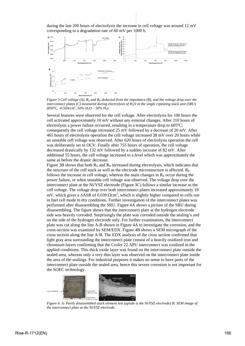
during the last 200 hours of electrolysis the increase in cell voltage was around 12 mV corresponding to a degradation rate of 60 mV per 1000 h.

1000

1050

1100

1150

1200

1250

0 200 400 600 800 1000 1200

Electrolysis time (h)

Cell

volta

ge (m

V)

Cell voltage A

0

5

10

15

20

25

30

35

40

45

0 200 400 600 800 1000 1200

Electrolysis time (h)

Vol

tage

dro

p ov

er

inte

rcon

nect

pla

te (m

V)

Voltage drop over interconnect plate at the Ni/YSZ electrode

Voltage drop over interconnect plate at the LSM/YSZ electrode

C

0.0

0.1

0.2

0.3

0.4

0 200 400 600 800 1000 1200

Electrolysis time (h)

Resi

stan

ce ( Ω

.cm

2 )

Polarisation resistance

Serial resistance

B

Figure 3 Cell voltage (A), RS and RP deducted from the impedance (B), and the voltage drop over the interconnect plates (C) measured during electrolysis of H2O in the single repeating stack unit (SRU) (850ºC, -0.50A/cm2, 50% H2O – 50% H2).

Several features were observed for the cell voltage. After electrolysis for 100 hours the cell activated approximately 10 mV without any external changes. After 210 hours of electrolysis a power failure occurred, resulting in a temperature drop to 605ºC; consequently the cell voltage increased 25 mV followed by a decrease of 20 mV. After 465 hours of electrolysis operation the cell voltage increased 38 mV over 20 hours while an unstable cell voltage was observed. After 620 hours of electrolysis operation the cell was deliberately set to OCV. Finally after 755 hours of operation, the cell voltage decreased drastically by 132 mV followed by a sudden increase of 82 mV. After additional 55 hours, the cell voltage increased to a level which was approximately the same as before the drastic decrease. Figure 3B shows that both RS and RP increased during electrolysis, which indicates that the structure of the cell stack as well as the electrode microstructure is affected. RP follows the increase in cell voltage, whereas the main changes in RS occur during the power failure, or when unstable cell voltage was observed. The voltage drop over the interconnect plate at the Ni/YSZ electrode (Figure 3C) follows a similar increase as the cell voltage. The voltage drop over both interconnect plates increased approximately 19 mV, which gives a ΔASR of 0.039 Ωcm2, which is slightly higher compared to cells run in fuel cell mode in dry conditions. Further investigation of the interconnect plates was performed after disassembling the SRU. Figure 4A shows a picture of the SRU during disassembling. The figure shows that the interconnect plate at the hydrogen electrode side was heavily corroded. Surprisingly the plate was corroded outside the sealing’s and on the side of the hydrogen electrode only. For further examination, the interconnect plate was cut along the line A-B shown in Figure 4A to investigate the corrosion, and the cross-section was examined by SEM/EDX. Figure 4B shows a SEM micrograph of the cross section along the line A-B. The EDX analysis of the cross section confirmed that light gray area surrounding the interconnect plate consist of a heavily oxidized iron and chromium layers confirming that the Crofer 22 APU interconnect was oxidized in the applied conditions. This thick oxide layer was found on the interconnect plate outside the sealed area, whereas only a very thin layer was observed on the interconnect plate inside the area of the sealings. For industrial purposes it makes no sense to have parts of the interconnect plate outside the sealed area, hence this severe corrosion is not important for the SOEC technology.

Cut for SEM/EDX A B

Interconnectplate at H2 side

Interconnectplate at O2 side

A B

100 μm

Crofer 22 APU

Fe/Cr oxide

Figure 4. A: Partly disassembled stack element test (upside is the Ni/YSZ electrode) B: SEM image of the interconnect plate at the Ni/YSZ electrode.

Risø-R-1712(EN) 166

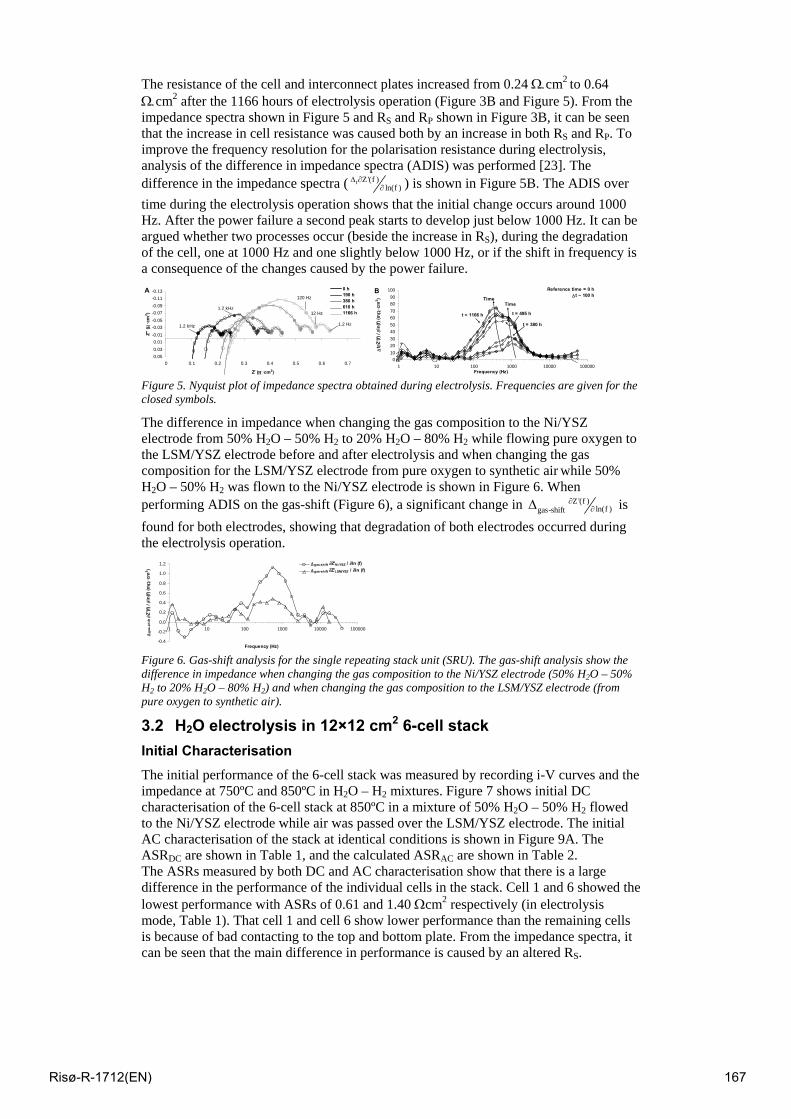
The resistance of the cell and interconnect plates increased from 0.24 Ω.cm2 to 0.64 Ω.cm2 after the 1166 hours of electrolysis operation (Figure 3B and Figure 5). From the impedance spectra shown in Figure 5 and RS and RP shown in Figure 3B, it can be seen that the increase in cell resistance was caused both by an increase in both RS and RP. To improve the frequency resolution for the polarisation resistance during electrolysis, analysis of the difference in impedance spectra (ADIS) was performed [23]. The difference in the impedance spectra ( t Z'(f )

ln(f )Δ ∂

∂ ) is shown in Figure 5B. The ADIS over time during the electrolysis operation shows that the initial change occurs around 1000 Hz. After the power failure a second peak starts to develop just below 1000 Hz. It can be argued whether two processes occur (beside the increase in RS), during the degradation of the cell, one at 1000 Hz and one slightly below 1000 Hz, or if the shift in frequency is a consequence of the changes caused by the power failure.

-0.13-0.11-0.09-0.07-0.05-0.03-0.010.010.030.05

0 0.1 0.2 0.3 0.4 0.5 0.6 0.7

Z' (Η ·cm2)

Z'' (

Η·c

m2 )

A 0 h190 h380 h610 h1166 h

1.2 kHz

1.2 kHz

120 Hz

12 Hz

v

1.2 Hz

0

102030405060708090

100

1 10 100 1000 10000 100000Frequency (Hz)

Δt ∂

Z'(f)

/ ∂l

n(f)

(mΩ

·cm

2 )

Reference time = 0 hΔt ~ 100 h

B

t = 1166 h

TimeTime

t = 380 h

t = 495 h

Figure 5. Nyquist plot of impedance spectra obtained during electrolysis. Frequencies are given for the closed symbols.

The difference in impedance when changing the gas composition to the Ni/YSZ electrode from 50% H2O – 50% H2 to 20% H2O – 80% H2 while flowing pure oxygen to the LSM/YSZ electrode before and after electrolysis and when changing the gas composition for the LSM/YSZ electrode from pure oxygen to synthetic air while 50% H2O – 50% H2 was flown to the Ni/YSZ electrode is shown in Figure 6. When performing ADIS on the gas-shift (Figure 6), a significant change in Z'(f )

ln(f )gas-shift∂

∂Δ is found for both electrodes, showing that degradation of both electrodes occurred during the electrolysis operation.

-0.4

-0.2

0.0

0.2

0.4

0.6

0.8

1.0

1.2

1 10 100 1000 10000 100000

Frequency (Hz)

Δga

s-sh

ift ∂

Z'(f)

/ ∂l

n(f)

(mΩ

·cm

2 )

Δgas-shift ∂Z'Ni/YSZ / ∂ln (f)Δgas-shift ∂Z'LSM/YSZ / ∂ln (f)

Figure 6. Gas-shift analysis for the single repeating stack unit (SRU). The gas-shift analysis show the difference in impedance when changing the gas composition to the Ni/YSZ electrode (50% H2O – 50% H2 to 20% H2O – 80% H2) and when changing the gas composition to the LSM/YSZ electrode (from pure oxygen to synthetic air).

3.2 H2O electrolysis in 12×12 cm2 6-cell stack Initial Characterisation The initial performance of the 6-cell stack was measured by recording i-V curves and the impedance at 750ºC and 850ºC in H2O – H2 mixtures. Figure 7 shows initial DC characterisation of the 6-cell stack at 850ºC in a mixture of 50% H2O – 50% H2 flowed to the Ni/YSZ electrode while air was passed over the LSM/YSZ electrode. The initial AC characterisation of the stack at identical conditions is shown in Figure 9A. The ASRDC are shown in Table 1, and the calculated ASRAC are shown in Table 2. The ASRs measured by both DC and AC characterisation show that there is a large difference in the performance of the individual cells in the stack. Cell 1 and 6 showed the lowest performance with ASRs of 0.61 and 1.40 Ωcm2 respectively (in electrolysis mode, Table 1). That cell 1 and cell 6 show lower performance than the remaining cells is because of bad contacting to the top and bottom plate. From the impedance spectra, it can be seen that the main difference in performance is caused by an altered RS.

Risø-R-1712(EN) 167

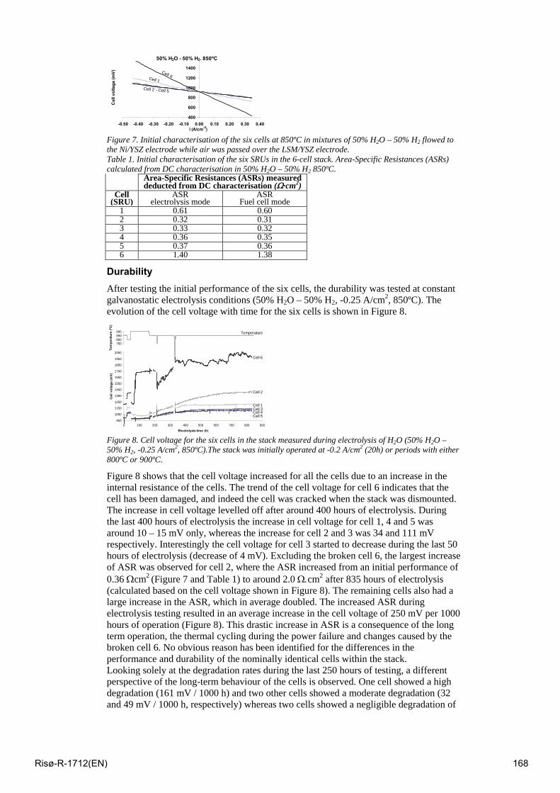
400

600

800

1000

1200

1400

1600

-0.50 -0.40 -0.30 -0.20 -0.10 0.00 0.10 0.20 0.30 0.40i (A/cm-2)

Cel

l vol

tage

(mV)

45% H2O - 45% CO2 - 10% H2, 850ºCB 50% H2O - 50% H2, 850ºC50% H2O - 50% H2, 850ºC

Cell 1

Cell 2 - Cell 5

Cell 6

Figure 7. Initial characterisation of the six cells at 850ºC in mixtures of 50% H2O – 50% H2 flowed to the Ni/YSZ electrode while air was passed over the LSM/YSZ electrode. Table 1. Initial characterisation of the six SRUs in the 6-cell stack. Area-Specific Resistances (ASRs) calculated from DC characterisation in 50% H2O – 50% H2 850ºC.

Area-Specific Resistances (ASRs) measured deducted from DC characterisation (Ω·cm2)

Cell (SRU)

ASR electrolysis mode

ASRFuel cell mode

1 0.61 0.602 0.32 0.313 0.33 0.324 0.36 0.355 0.37 0.366 1.40 1.38

Durability After testing the initial performance of the six cells, the durability was tested at constant galvanostatic electrolysis conditions (50% H2O – 50% H2, -0.25 A/cm2, 850ºC). The evolution of the cell voltage with time for the six cells is shown in Figure 8.

500550600650700750800850900

Tem

pera

ture

(ºC

)

Temperature

950

1050

1150

1250

1350

1450

1550

1650

1750

1850

1950

2050

0 100 200 300 400 500 600 700 800 900

Electrolysis time (h)

Cell

volta

ge (m

V)

Cell 4Cell 5

Cell 3Cell 1

Cell 2

Cell 6

Figure 8. Cell voltage for the six cells in the stack measured during electrolysis of H2O (50% H2O – 50% H2, -0.25 A/cm2, 850ºC).The stack was initially operated at -0.2 A/cm2 (20h) or periods with either 800ºC or 900ºC.

Figure 8 shows that the cell voltage increased for all the cells due to an increase in the internal resistance of the cells. The trend of the cell voltage for cell 6 indicates that the cell has been damaged, and indeed the cell was cracked when the stack was dismounted. The increase in cell voltage levelled off after around 400 hours of electrolysis. During the last 400 hours of electrolysis the increase in cell voltage for cell 1, 4 and 5 was around 10 – 15 mV only, whereas the increase for cell 2 and 3 was 34 and 111 mV respectively. Interestingly the cell voltage for cell 3 started to decrease during the last 50 hours of electrolysis (decrease of 4 mV). Excluding the broken cell 6, the largest increase of ASR was observed for cell 2, where the ASR increased from an initial performance of 0.36 Ωcm2 (Figure 7 and Table 1) to around 2.0 Ω.cm2 after 835 hours of electrolysis (calculated based on the cell voltage shown in Figure 8). The remaining cells also had a large increase in the ASR, which in average doubled. The increased ASR during electrolysis testing resulted in an average increase in the cell voltage of 250 mV per 1000 hours of operation (Figure 8). This drastic increase in ASR is a consequence of the long term operation, the thermal cycling during the power failure and changes caused by the broken cell 6. No obvious reason has been identified for the differences in the performance and durability of the nominally identical cells within the stack. Looking solely at the degradation rates during the last 250 hours of testing, a different perspective of the long-term behaviour of the cells is observed. One cell showed a high degradation (161 mV / 1000 h) and two other cells showed a moderate degradation (32 and 49 mV / 1000 h, respectively) whereas two cells showed a negligible degradation of

Risø-R-1712(EN) 168

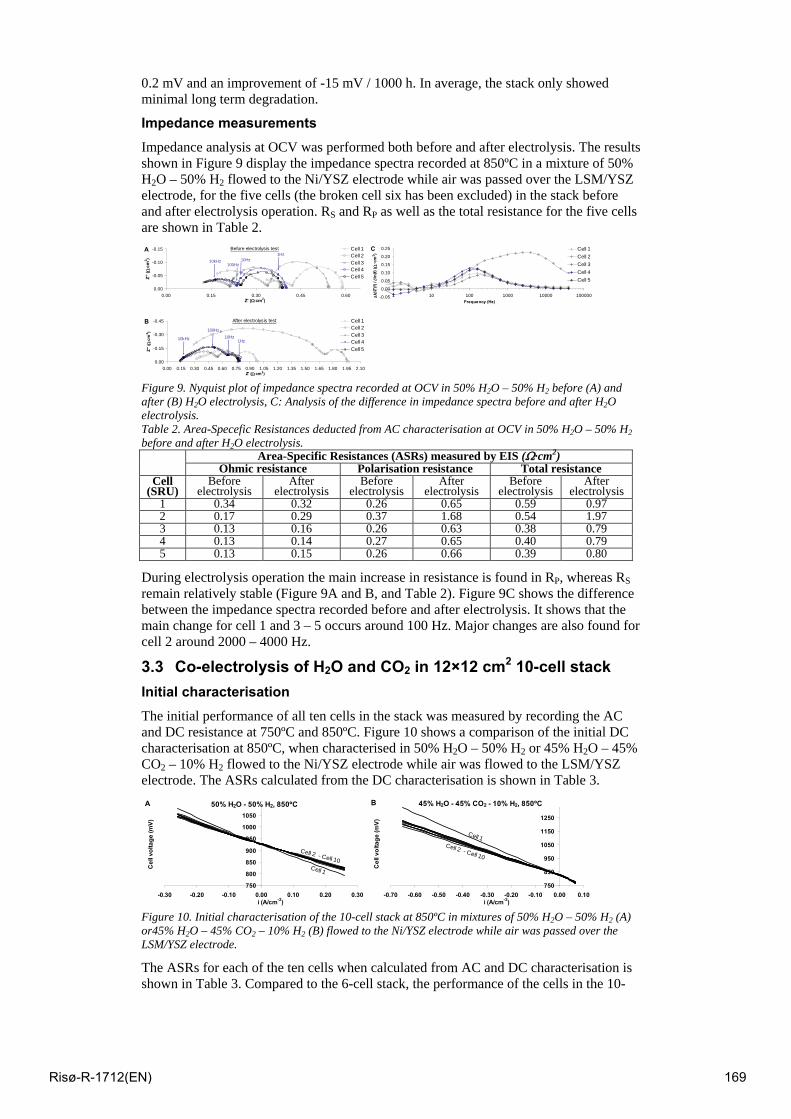
0.2 mV and an improvement of -15 mV / 1000 h. In average, the stack only showed minimal long term degradation.

Impedance measurements Impedance analysis at OCV was performed both before and after electrolysis. The results shown in Figure 9 display the impedance spectra recorded at 850ºC in a mixture of 50% H2O – 50% H2 flowed to the Ni/YSZ electrode while air was passed over the LSM/YSZ electrode, for the five cells (the broken cell six has been excluded) in the stack before and after electrolysis operation. RS and RP as well as the total resistance for the five cells are shown in Table 2.

-0.15

-0.10

-0.05

0.000.00 0.15 0.30 0.45 0.60

Z' (Ω cm2)

Z'' (

Ωcm

2 )

Cell 1Cell 2Cell 3Cell 4Cell 5

Before electrolysis test1Hz

10Hz100Hz

10kHz

A

-0.05

0.00

0.05

0.10

0.15

0.20

0.25

1 10 100 1000 10000 100000Frequency (Hz)

Δt ∂

Z'(f)

/ ∂l

n(f)

( Ω·c

m2 )

Cell 1Cell 2Cell 3Cell 4Cell 5

C

-0.45

-0.30

-0.15

0.000.00 0.15 0.30 0.45 0.60 0.75 0.90 1.05 1.20 1.35 1.50 1.65 1.80 1.95 2.10

Z' (Ω cm2)

Z'' (

Ωcm

2 )

Cell 1Cell 2Cell 3Cell 4Cell 5

1Hz10Hz

100Hz

10kHz

After electrolysis testB

Figure 9. Nyquist plot of impedance spectra recorded at OCV in 50% H2O – 50% H2 before (A) and after (B) H2O electrolysis, C: Analysis of the difference in impedance spectra before and after H2O electrolysis. Table 2. Area-Specefic Resistances deducted from AC characterisation at OCV in 50% H2O – 50% H2 before and after H2O electrolysis.

Area-Specific Resistances (ASRs) measured by EIS (Ω·cm2) Ohmic resistance Polarisation resistance Total resistance

Cell (SRU)

Before electrolysis

After electrolysis

Before electrolysis

After electrolysis

Before electrolysis

After electrolysis

1 0.34 0.32 0.26 0.65 0.59 0.97 2 0.17 0.29 0.37 1.68 0.54 1.97 3 0.13 0.16 0.26 0.63 0.38 0.79 4 0.13 0.14 0.27 0.65 0.40 0.79 5 0.13 0.15 0.26 0.66 0.39 0.80

During electrolysis operation the main increase in resistance is found in RP, whereas RS remain relatively stable (Figure 9A and B, and Table 2). Figure 9C shows the difference between the impedance spectra recorded before and after electrolysis. It shows that the main change for cell 1 and 3 – 5 occurs around 100 Hz. Major changes are also found for cell 2 around 2000 – 4000 Hz.

3.3 Co-electrolysis of H2O and CO2 in 12×12 cm2 10-cell stack Initial characterisation The initial performance of all ten cells in the stack was measured by recording the AC and DC resistance at 750ºC and 850ºC. Figure 10 shows a comparison of the initial DC characterisation at 850ºC, when characterised in 50% H2O – 50% H2 or 45% H2O – 45% CO2 – 10% H2 flowed to the Ni/YSZ electrode while air was flowed to the LSM/YSZ electrode. The ASRs calculated from the DC characterisation is shown in Table 3.

750

800

850

900

950

1000

1050

1100

-0.30 -0.20 -0.10 0.00 0.10 0.20 0.30i (A/cm-2)

Cel

l vol

tage

(mV)

A

Cell 1

Cell 2 - Cell 10

50% H2O - 50% H2, 850ºC

750

850

950

1050

1150

1250

1350

-0.70 -0.60 -0.50 -0.40 -0.30 -0.20 -0.10 0.00 0.10i (A/cm-2)

Cel

l vol

tage

(mV)

Cell 1Cell 2 - Cell 10

45% H2O - 45% CO2 - 10% H2, 850ºCB

Figure 10. Initial characterisation of the 10-cell stack at 850ºC in mixtures of 50% H2O – 50% H2 (A) or45% H2O – 45% CO2 – 10% H2 (B) flowed to the Ni/YSZ electrode while air was passed over the LSM/YSZ electrode.

The ASRs for each of the ten cells when calculated from AC and DC characterisation is shown in Table 3. Compared to the 6-cell stack, the performance of the cells in the 10-

Risø-R-1712(EN) 169

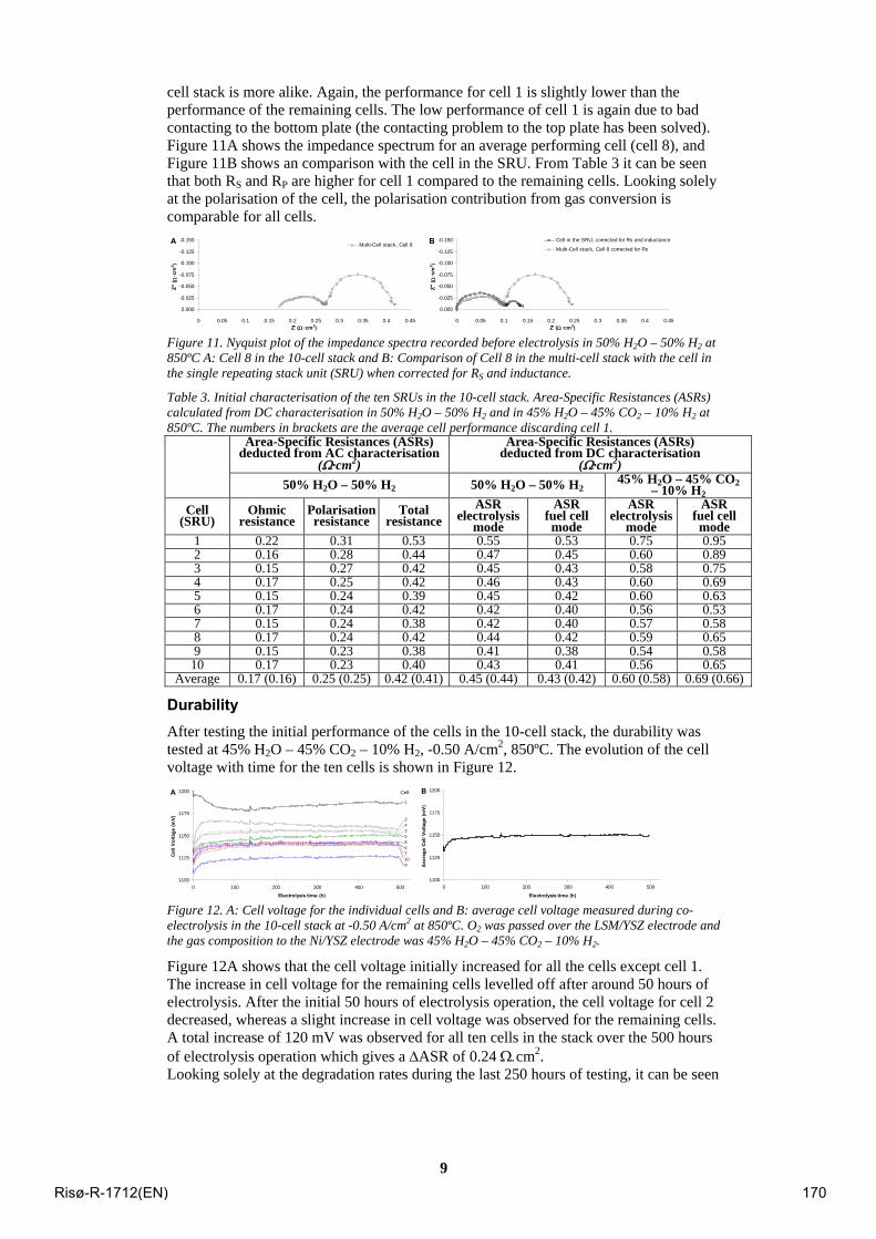
9

cell stack is more alike. Again, the performance for cell 1 is slightly lower than the performance of the remaining cells. The low performance of cell 1 is again due to bad contacting to the bottom plate (the contacting problem to the top plate has been solved). Figure 11A shows the impedance spectrum for an average performing cell (cell 8), and Figure 11B shows an comparison with the cell in the SRU. From Table 3 it can be seen that both RS and RP are higher for cell 1 compared to the remaining cells. Looking solely at the polarisation of the cell, the polarisation contribution from gas conversion is comparable for all cells.

-0.150

-0.125

-0.100

-0.075

-0.050

-0.025

0.000

0 0.05 0.1 0.15 0.2 0.25 0.3 0.35 0.4 0.45Z' (Ω ·cm2)

Z'' (

Ω·c

m2 )

Multi-Cell stack, Cell 8A

-0.150

-0.125

-0.100

-0.075

-0.050

-0.025

0.000

0 0.05 0.1 0.15 0.2 0.25 0.3 0.35 0.4 0.45Z' (Ω ·cm2)

Z'' (

Ω·c

m2 )

Cell in the SRU, corrected for Rs and inductance

Multi-Cell stack, Cell 8 corrected for RsB

Figure 11. Nyquist plot of the impedance spectra recorded before electrolysis in 50% H2O – 50% H2 at 850ºC A: Cell 8 in the 10-cell stack and B: Comparison of Cell 8 in the multi-cell stack with the cell in the single repeating stack unit (SRU) when corrected for RS and inductance.

Table 3. Initial characterisation of the ten SRUs in the 10-cell stack. Area-Specific Resistances (ASRs) calculated from DC characterisation in 50% H2O – 50% H2 and in 45% H2O – 45% CO2 – 10% H2 at 850ºC. The numbers in brackets are the average cell performance discarding cell 1.

Area-Specific Resistances (ASRs)

deducted from AC characterisation (Ω·cm2)

Area-Specific Resistances (ASRs) deducted from DC characterisation

(Ω·cm2) 50% H2O – 50% H2 50% H2O – 50% H2 45% H2O – 45% CO2

– 10% H2 Cell

(SRU) Ohmic

resistance Polarisation resistance

Total resistance

ASRelectrolysis

mode

ASR fuel cell mode

ASR electrolysis

mode

ASRfuel cell mode

1 0.22 0.31 0.53 0.55 0.53 0.75 0.952 0.16 0.28 0.44 0.47 0.45 0.60 0.893 0.15 0.27 0.42 0.45 0.43 0.58 0.754 0.17 0.25 0.42 0.46 0.43 0.60 0.695 0.15 0.24 0.39 0.45 0.42 0.60 0.636 0.17 0.24 0.42 0.42 0.40 0.56 0.537 0.15 0.24 0.38 0.42 0.40 0.57 0.588 0.17 0.24 0.42 0.44 0.42 0.59 0.659 0.15 0.23 0.38 0.41 0.38 0.54 0.58

10 0.17 0.23 0.40 0.43 0.41 0.56 0.65Average 0.17 (0.16) 0.25 (0.25) 0.42 (0.41) 0.45 (0.44) 0.43 (0.42) 0.60 (0.58) 0.69 (0.66)

Durability After testing the initial performance of the cells in the 10-cell stack, the durability was tested at 45% H2O – 45% CO2 – 10% H2, -0.50 A/cm2, 850ºC. The evolution of the cell voltage with time for the ten cells is shown in Figure 12.

1100

1125

1150

1175

1200

0 100 200 300 400 500

Electrolysis time (h)

Cel

l Vol

tage

(mV)

1

2435867109

Cell:A

1100

1125

1150

1175

1200

0 100 200 300 400 500

Electrolysis time (h)

Aver

age

Cell

Volta

ge (m

V)

B

Figure 12. A: Cell voltage for the individual cells and B: average cell voltage measured during co-electrolysis in the 10-cell stack at -0.50 A/cm2 at 850ºC. O2 was passed over the LSM/YSZ electrode and the gas composition to the Ni/YSZ electrode was 45% H2O – 45% CO2 – 10% H2.

Figure 12A shows that the cell voltage initially increased for all the cells except cell 1. The increase in cell voltage for the remaining cells levelled off after around 50 hours of electrolysis. After the initial 50 hours of electrolysis operation, the cell voltage for cell 2 decreased, whereas a slight increase in cell voltage was observed for the remaining cells. A total increase of 120 mV was observed for all ten cells in the stack over the 500 hours of electrolysis operation which gives a ΔASR of 0.24 Ω.cm2. Looking solely at the degradation rates during the last 250 hours of testing, it can be seen

Risø-R-1712(EN) 170

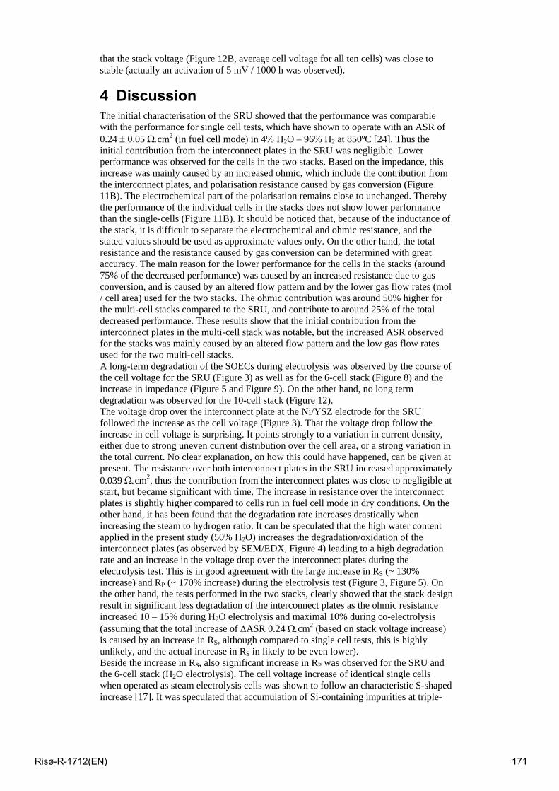
that the stack voltage (Figure 12B, average cell voltage for all ten cells) was close to stable (actually an activation of 5 mV / 1000 h was observed).

4 Discussion The initial characterisation of the SRU showed that the performance was comparable with the performance for single cell tests, which have shown to operate with an ASR of 0.24 ± 0.05 Ω.cm2 (in fuel cell mode) in 4% H2O – 96% H2 at 850ºC [24]. Thus the initial contribution from the interconnect plates in the SRU was negligible. Lower performance was observed for the cells in the two stacks. Based on the impedance, this increase was mainly caused by an increased ohmic, which include the contribution from the interconnect plates, and polarisation resistance caused by gas conversion (Figure 11B). The electrochemical part of the polarisation remains close to unchanged. Thereby the performance of the individual cells in the stacks does not show lower performance than the single-cells (Figure 11B). It should be noticed that, because of the inductance of the stack, it is difficult to separate the electrochemical and ohmic resistance, and the stated values should be used as approximate values only. On the other hand, the total resistance and the resistance caused by gas conversion can be determined with great accuracy. The main reason for the lower performance for the cells in the stacks (around 75% of the decreased performance) was caused by an increased resistance due to gas conversion, and is caused by an altered flow pattern and by the lower gas flow rates (mol / cell area) used for the two stacks. The ohmic contribution was around 50% higher for the multi-cell stacks compared to the SRU, and contribute to around 25% of the total decreased performance. These results show that the initial contribution from the interconnect plates in the multi-cell stack was notable, but the increased ASR observed for the stacks was mainly caused by an altered flow pattern and the low gas flow rates used for the two multi-cell stacks. A long-term degradation of the SOECs during electrolysis was observed by the course of the cell voltage for the SRU (Figure 3) as well as for the 6-cell stack (Figure 8) and the increase in impedance (Figure 5 and Figure 9). On the other hand, no long term degradation was observed for the 10-cell stack (Figure 12). The voltage drop over the interconnect plate at the Ni/YSZ electrode for the SRU followed the increase as the cell voltage (Figure 3). That the voltage drop follow the increase in cell voltage is surprising. It points strongly to a variation in current density, either due to strong uneven current distribution over the cell area, or a strong variation in the total current. No clear explanation, on how this could have happened, can be given at present. The resistance over both interconnect plates in the SRU increased approximately 0.039 Ω.cm2, thus the contribution from the interconnect plates was close to negligible at start, but became significant with time. The increase in resistance over the interconnect plates is slightly higher compared to cells run in fuel cell mode in dry conditions. On the other hand, it has been found that the degradation rate increases drastically when increasing the steam to hydrogen ratio. It can be speculated that the high water content applied in the present study (50% H2O) increases the degradation/oxidation of the interconnect plates (as observed by SEM/EDX, Figure 4) leading to a high degradation rate and an increase in the voltage drop over the interconnect plates during the electrolysis test. This is in good agreement with the large increase in RS (~ 130% increase) and RP (~ 170% increase) during the electrolysis test (Figure 3, Figure 5). On the other hand, the tests performed in the two stacks, clearly showed that the stack design result in significant less degradation of the interconnect plates as the ohmic resistance increased 10 – 15% during H2O electrolysis and maximal 10% during co-electrolysis (assuming that the total increase of ΔASR 0.24 Ω.cm2 (based on stack voltage increase) is caused by an increase in RS, although compared to single cell tests, this is highly unlikely, and the actual increase in RS in likely to be even lower). Beside the increase in RS, also significant increase in RP was observed for the SRU and the 6-cell stack (H2O electrolysis). The cell voltage increase of identical single cells when operated as steam electrolysis cells was shown to follow an characteristic S-shaped increase [17]. It was speculated that accumulation of Si-containing impurities at triple-

Risø-R-1712(EN) 171

phase boundaries in the Ni/YSZ electrode (determined post mortem by SEM) coursed the degradation of the SOECs [16-18]. When testing the SOC at identical conditions, but applying an gold seal instead of a glass seal [17], the cell voltage was shown to increase almost linear. The degradation phenomenon was therefore suggested to be a consequence of silica impurities originating from the glass seal. Because this degradation is caused by blockage of the active triple-phase boundaries, the increase in ASR shows as an increased RP only. Similar degradation behaviour was found to occur when operating SOCs as CO2 or co-electrolysis cells [4, 22], although in these cases, the impurities was speculated to originate from the applied gasses [4, 22]. Analysing this degradation by EIS, the degradation caused by blockage of the triple-phase boundaries (adsorption of impurities) was characterised by an increased resistance at 100 – 300 Hz [4, 19, 22]. It seems unlikely that the cell voltage shown in Figure 3 (SRU) follows this characteristic S-shaped curve. Further, the degradation caused an increase in both RS and RP, and the increase in RP was observed, not only for the Ni/YSZ electrode, but also for the LSM/YSZ electrode and was characterised by a frequency of around 1000 Hz (Figure 5 and Figure 6). It therefore seems likely that the exposed glass area and/or the composition of the glass-ceramic used in the single-cell electrolysis stack minimise this silica evaporation from the sealing. Further more, no silica could be found by post mortem SEM analysis. It can be argued whether the cell voltage observed for the 6-cell stack showed the characteristic S-curve (Figure 8). The degradation was characterised by a frequency around 100 – 300 Hz, which may indicate blockage of the active triple-phase boundaries. Post mortem analysis by SEM did not reveal any silica depositions close to the triple-phase boundaries. It should be noticed that no silica was found do not exclude the presence of small amounts of silica close to the triple-phase boundaries. No long term degradation was observed for the 10-cell stack (Figure 12), which was operated with identical glass sealing’s as the 6-cell stack. The main difference in operating conditions for the six and 10-cell stack, is, beside the added CO2, the application of clean gasses in the 10-cell stack (the steam concentration was similar for the two stacks, 50% for the 6-cell stack and 45% for the 10-cell stack). That degradation (by adsorption of impurities) was observed for the 6-cell stack and not for the 10-cell stack indicates that impurities in the inlet gasses may play an important role for the durability of these electrolysis stacks as have previously been speculated for single cells [4, 22]. On the other hand, the application of chromium containing interconnect plates and glass sealing’s do not seem to negatively influence the durability. Cleaning the inlet gasses to the Ni/YSZ electrode resulted in operation without any long term degradation, and may therefore be a solution for operating these Ni/YSZ based solid oxide electrolysis stacks without any degradation.

5 Conclusion The initial performance of the SRU was comparable with the performance for single cell tests, whereas the performance for the multi-cell stacks was slightly lower than for the single cells. The ohmic resistance seems to be slightly higher, showing a slightly higher contribution from the interconnect plates in the multi-cell stacks. The contribution from the interconnect plates in the SRU , which was close to negligible at start, became significant with time, whereas for the multi-cell stack, an initial increase of only maximal 10% was observed. For all tests, the cell voltage (and stack voltage) reached a stable level during the last part of the tests, which may point towards a reasonable stable long-term performance. The degradation of the electrolysis cells is influenced by the adsorption of impurities from the gasses, whereas the application of chromium containing interconnect plates and glass sealing’s do not seem to influence the durability. Cleaning the inlet gasses to the Ni/YSZ electrode resulted in operation without any long term degradation, and may be a solution for operating these Ni/YSZ based solid oxide electrolysis stacks without any degradation.

Risø-R-1712(EN) 172

6 Acknowledgements This work was financially supported by The Danish National Advanced Technology Foundations advanced technology platform "Development of 2nd generation bioethanol process and technology", the Danish Council for Strategic Research, via the Strategic Electrochemistry Research Center (SERC, www.serc.dk), and the European Commission via the project “Hi2H2,” contract no. FP6-503765.

7 References [1] W. Doenitz, R. Schmidberger, E. Steinheil, R. Streicher, Int. J. Hydrogen Energy,

5 (1980) 55-63. [2] A.O. Isenberg, Solid State Ionics, 3-4 (1981) 431-437. [3] Electrochemical hydrogen technologies: Electrochemical production and

combustion of hydrogen, H. Wendt(eds.), Elsevier, Amsterdam, The Netherlands (1990).

[4] S.D. Ebbesen, C. Graves, M. Mogensen, Submitted to Int. J. Green Energy (2009) [5] C.M. Stoots, J.E. O'Brien, J.S. Herring, J.J. Hartvigsen, J. Fuelcell. Sci. Tech., 6

(2009) 011014- [6] Z. Zhan, W. Kobsiriphat, J.R. Wilson, M. Pillai, I. Kim, S.A. Barnett, Energy &

Fuels, 23 (2009) 3089-3096. [7] Electrochemical hydrogen technologies: Electrochemical production and

combustion of hydrogen, H. Wendt(eds.), Elsevier, Amsterdam, The Netherlands (1990).

[8] J.S. Herring, J.E. O'Brien, C.M. Stoots, G.L. Hawkes, J.J. Hartvigsen, M. Shahnam, Int. J. Hydrogen Energy, 32 (2007) 440-450.

[9] J.R. Mawdsley, J.D. Carter, A.J. Kropf, B. Yildiz, V.A. Maroni, Int. J. Hydrogen Energy, 34 (2009) 4198-4207.

[10] J.E. O'Brien, C.M. Stoots, J.S. Herring, J. Hartvigsen, J. Fuelcell. Sci. Tech., 3 (2006) 213-219.

[11] J.E. O'Brien, C.M. Stoots, J.S. Herring, J.J. Hartvigsen, Nuclear Technology, 158 (2007) 118-131.

[12] C. Gindorf, L. Singheiser, K. Hilpert, Steel Res., 72 (2001) 528-533. [13] K. Hilpert, D. Das, M. Miller, D.H. Peck, R. Weiss, J. Electrochem. Soc., 143

(1996) 3642-3647. [14] S.C. Paulson , V.I. Birss, J. Electrochem. Soc., 151 (2004) A1961-A1968. [15] Y. Matsuzaki , I. Yasuda, J. Electrochem. Soc., 148 (2001) A126-A131. [16] A. Hauch, J.R. Bowen, L.T. Kuhn, M. Mogensen, Electrochem. Solid State Lett.,

11 (2008) B38-B41. [17] A. Hauch, S.D. Ebbesen, S.H. Jensen, M. Mogensen, J. Electrochem. Soc., 155

(2008) B1184-B1193. [18] A. Hauch, S.H. Jensen, J.B. Bilde-Sørensen, M. Mogensen, J. Electrochem. Soc.,

154 (2007) A619-A626. [19] A. Hauch, S.H. Jensen, S. Ramousse, M. Mogensen, J. Electrochem. Soc., 153

(2006) A1741-A1747. [20] A. Hagen, R. Barfod, P.V. Hendriksen, Y.L. Liu, S. Ramousse, J. Electrochem.

Soc., 153 (2006) A1165-A1171. [21] P. H. Larsen, C. Bagger, S. Linderoth, M. Mogensen, S. Primdahl, M. J.

Jørgensen, P. V. Hendriksen, B. Kindl, N. Bonanos, F. W. Poulsen, and K. A. Maegaard, in: Proceedings of Solid Oxide Fuel Cell VII (SOFC VII), Electrochem.Soc. (2001) 28-37.

[22] S.D. Ebbesen , M. Mogensen, J. Power Sources, 193 (2009) 349-358. [23] S.H. Jensen, A. Hauch, P.V. Hendriksen, M. Mogensen, N. Bonanos, T. Jacobsen,

J. Electrochem. Soc., 154 (2007) B1325-B1330. [24] A. Hagen, M. Menon, R. Barfod, P.V. Hendriksen, S. Ramousse, P.H. Larsen,

Fuel Cells, 6 (2006) 146-150.

Risø-R-1712(EN) 173

Session 11 – Energy from waste

Risø-R-1712(EN) 174

The organic farm as energy utility – environmental and economic assessment of small-scale CHP production from agricultural residues

M. Kimming a * , C. Sundberg a , Å. Nordberg b , P.-A. Hansson a

a Swedish University of Agricultural Sciences, Department of Energy and Technology, P.O. Box 7032, SE 750 07 Uppsala, Sweden b Swedish Institute of Agricultural and Environmental Engineering, P.O. Box 7033, SE 750 07 Uppsala, Sweden

Abstract The impact on greenhouse gas emissions from using a ley crop from an organic crop rotation as substrate for biogas production instead of ploughing it down as fertilizer (green manure) was analysed using lifecycle assessment methodology. The biogas was combusted in a microturbine (100 kW(e)) for production of heat and electricity. The economic viability for a farm investing in the technical system for commercial production was also estimated.

Greenhouse gas emissions were significantly lowered compared to the reference scenario, in which the village is supplied with energy produced with natural gas as fuel in a large-scale plant. The carbon content of the soil increases and the nitrous oxide emissions are lowered due to the application of digestion residues instead of undigested ley as fertilizer (also a result of the more timely application). The economic return on the investment in the energy plant for the farm is however heavily burdened with the investment cost for the culverts in the heating system, and highly sensitive to the energy prices, in particular the price of heat. Given Swedish market conditions in 2009, the energy production would not even be at breakeven without the Swedish quota system for renewable energy production. This makes it an uncertain investment unless financial policy instruments such as investment subsidies, feed-in tariffs or quota systems are available.

Risø-R-1712(EN) 175

1 Introduction The need for new sources of renewable energy is increasing, as ambitious policies aiming at reducing greenhouse gases and dependency on fossil fuels for energy supply are taken into effect. Biomass for energy is one such source, with in particular biomass of agricultural origin being a massive but largely unutilized resource (EEA 2006).

One problem with the use of biomass from agriculture in central energy plants is the low energy and cost efficiency associated with the transport. An alternative to the central plants would be a decentralized system of small-scale plants, perhaps even located at the farm producing the biomass. The development of new technologies for the utilization of biomass in small-scale (<100 kWe) combined heat and power (CHP) systems has progressed fast over the last few years, and there are now several technical systems available – some in commercial production, like biogas production systems, some on the verge of being commercialized, as for example the fuel-flexible small-scale Stirling engine, and some still only available in demonstration plants, like small-scale biomass gasifiers (Kjellström 2007).

Production of biomass for energy on agricultural land is however in conflict with food production over available agricultural land (Klöverpris 2008), and there are adverse environmental impacts of transformation of natural or semi-natural land to plantations for biomass or bioliquids (Börjesson 2009). A way of going around this problem is to focus on the use of agricultural byproducts for energy production, or production of biomass on set-aside or marginal land not in use for food production. Moreover, reliable methods for measuring the environmental impact of the use of the biomass as primary energy source are crucial in order for policymakers and decisionmakers to make informed choices on energy supply system. One such method that is gaining attention and fields of application is the lifecycle assessment (LCA) methodology, in which the entire production chain is analysed and emissions quantified and summarized as different impact categories, as for example Global Warming Potential (GWP) (Baumann and Tillman 2004).

In this study, a CHP production system placed and operated on an organic farm was analyzed with LCA methodology, with focus on global warming. A ley crop used as green manure is harvested instead of ploughed down and used as substrate for biogas production, the raw material production thereby not being in conflict with food production. Straw is used to meet extra heating demand in the winter. The system was compared to a reference system based on fossil fuel use and dimensioned to supply a nearby village with its entire heat and electricity demand. The environmental analysis is supplemented with an economic analysis in order to give an idea of the potential profitability of the plant.

2 Methodology

2.1 Environmental assessment approach The environmental assessment of the on-farm CHP production system is focused on emissions with global warming potential (GWP) and is performed with a simplified lifecycle assessment (LCA) approach. The functional unit is the supply of heat and electricity to a village of 150 households for one year.

Risø-R-1712(EN) 176

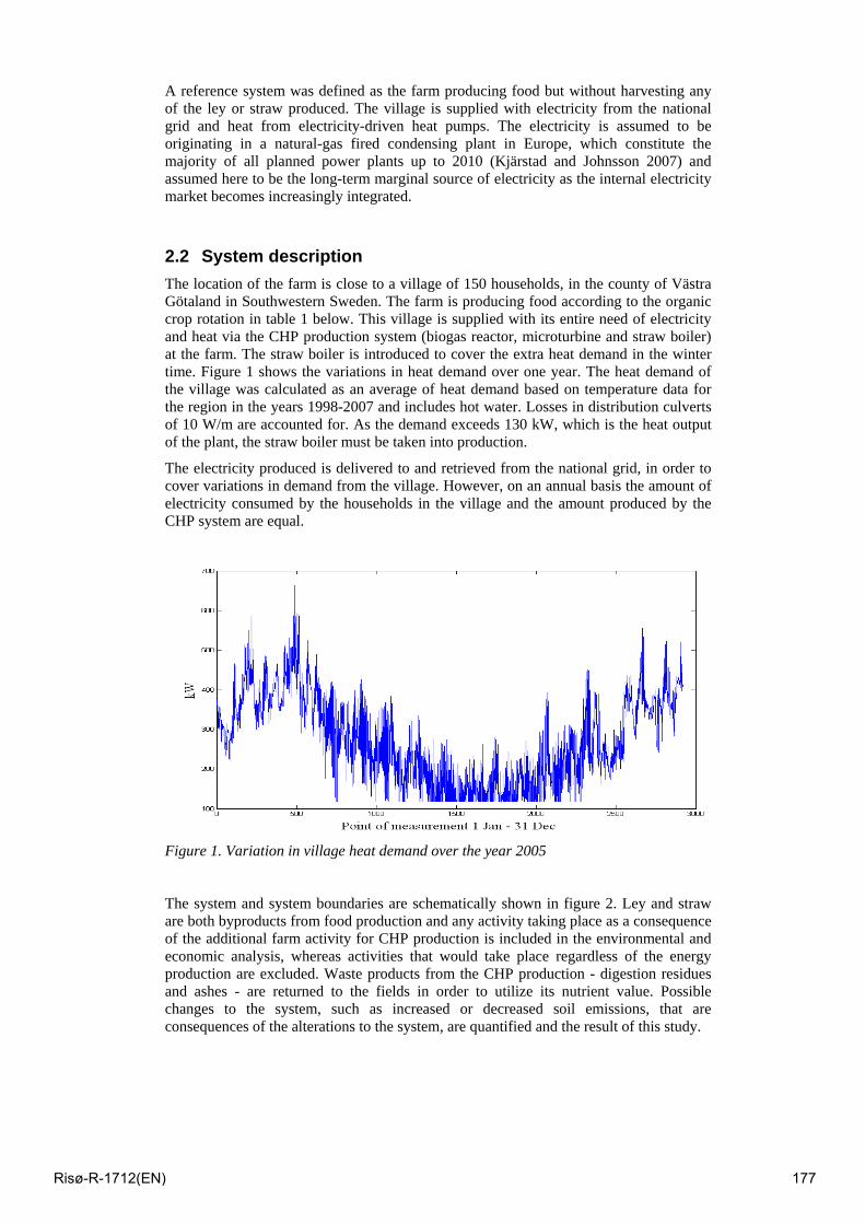
A reference system was defined as the farm producing food but without harvesting any of the ley or straw produced. The village is supplied with electricity from the national grid and heat from electricity-driven heat pumps. The electricity is assumed to be originating in a natural-gas fired condensing plant in Europe, which constitute the majority of all planned power plants up to 2010 (Kjärstad and Johnsson 2007) and assumed here to be the long-term marginal source of electricity as the internal electricity market becomes increasingly integrated.

2.2 System description The location of the farm is close to a village of 150 households, in the county of Västra Götaland in Southwestern Sweden. The farm is producing food according to the organic crop rotation in table 1 below. This village is supplied with its entire need of electricity and heat via the CHP production system (biogas reactor, microturbine and straw boiler) at the farm. The straw boiler is introduced to cover the extra heat demand in the winter time. Figure 1 shows the variations in heat demand over one year. The heat demand of the village was calculated as an average of heat demand based on temperature data for the region in the years 1998-2007 and includes hot water. Losses in distribution culverts of 10 W/m are accounted for. As the demand exceeds 130 kW, which is the heat output of the plant, the straw boiler must be taken into production.

The electricity produced is delivered to and retrieved from the national grid, in order to cover variations in demand from the village. However, on an annual basis the amount of electricity consumed by the households in the village and the amount produced by the CHP system are equal.

Figure 1. Variation in village heat demand over the year 2005

The system and system boundaries are schematically shown in figure 2. Ley and straw are both byproducts from food production and any activity taking place as a consequence of the additional farm activity for CHP production is included in the environmental and economic analysis, whereas activities that would take place regardless of the energy production are excluded. Waste products from the CHP production - digestion residues and ashes - are returned to the fields in order to utilize its nutrient value. Possible changes to the system, such as increased or decreased soil emissions, that are consequences of the alterations to the system, are quantified and the result of this study.

Risø-R-1712(EN) 177

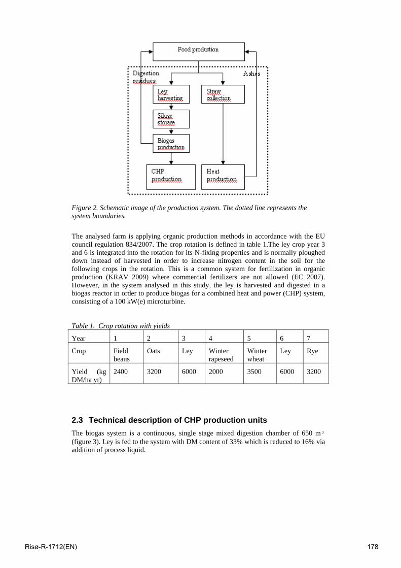
Figure 2. Schematic image of the production system. The dotted line represents the system boundaries.

The analysed farm is applying organic production methods in accordance with the EU council regulation 834/2007. The crop rotation is defined in table 1.The ley crop year 3 and 6 is integrated into the rotation for its N-fixing properties and is normally ploughed down instead of harvested in order to increase nitrogen content in the soil for the following crops in the rotation. This is a common system for fertilization in organic production (KRAV 2009) where commercial fertilizers are not allowed (EC 2007). However, in the system analysed in this study, the ley is harvested and digested in a biogas reactor in order to produce biogas for a combined heat and power (CHP) system, consisting of a 100 kW(e) microturbine.

Table 1. Crop rotation with yields

Year 1 2 3 4 5 6 7

Crop Field beans

Oats Ley Winter rapeseed

Winter wheat

Ley Rye

Yield (kg DM/ha yr)

2400 3200 6000 2000 3500 6000 3200

2.3 Technical description of CHP production units The biogas system is a continuous, single stage mixed digestion chamber of 650 m³ (figure 3). Ley is fed to the system with DM content of 33% which is reduced to 16% via addition of process liquid.

Risø-R-1712(EN) 178

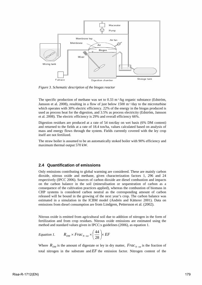
Figure 3. Schematic description of the biogas reactor

The specific production of methane was set to 0.33 m³/kg organic substance (Edström, Jansson et al. 2008), resulting in a flow of just below 1500 m³/day to the microturbine which operates with 30% electric efficiency. 22% of the energy in the biogas produced is used as process heat for the digestion, and 3.5% as process electricity (Edström, Jansson et al. 2008). The electric efficiency is 29% and overall efficiency 66%.

Digestion residues are produced at a rate of 54 ton/day on wet basis (6% DM content) and returned to the fields at a rate of 18.4 ton/ha, values calculated based on analysis of mass and energy flows through the system. Fields currently covered with the ley crop itself are not fertilized.

The straw boiler is assumed to be an automatically stoked boiler with 90% efficiency and maximum thermal output 570 kW.

2.4 Quantification of emissions Only emissions contributing to global warming are considered. These are mainly carbon dioxide, nitrous oxide and methane, given characterization factors 1, 296 and 24 respectively (IPCC 2006). Sources of carbon dioxide are diesel combustion and impacts on the carbon balance in the soil (mineralisation or sequestration of carbon as a consequence of the cultivation practices applied), whereas the combustion of biomass in CHP systems is considered carbon neutral as the corresponding amount of carbon released will be bound in the growing of the next year’s crop. The carbon balance was estimated in a simulation in the ICBM model (Andrén and Kätterer 2001). Data on emissions from diesel consumption are from Lindgren, Pettersson et al. (2002).

Nitrous oxide is emitted from agricultural soil due to addition of nitrogen in the form of fertilization and from crop residues. Nitrous oxide emissions are estimated using the method and standard values given in IPCC:s guidelines (2006), as equation 1.

Equation 1. EFFracR totNDM ×⎟⎠⎞

⎜⎝⎛×× − 28

44

Where DMR is the amount of digestate or ley in dry matter, totNFrac − is the fraction of total nitrogen in the substrate and EF the emission factor. Nitrogen content of the

Risø-R-1712(EN) 179

substrate is taken from (Edström, Jansson et al. 2008) and the emission factor from IPCC (2006).

Methane is emitted from digestion residues spread on the fields after digestion and calculated using the IPCC method, as in equation 2 (IPCC 2006).

Equation 2. MCFBDGOM ××× 71.00

Where OMDG is the amount of digestion residues spread on the fields, 0B the maximum methane production capacity, 0.71 the density of the gas in kg/m³ and MCF the methane conversion factor, i.e. amount of potentially produced methane that is produced and emitted. Maximum methane production capacity, 0B , of the substrate after digestion are taken from (Edström, Jansson et al. 2008) and the methane emission factors were assumed to be equal to emission factors for manure, taken from Dustan (2002) for liquid manure. Potential leakage from the technical components of the biogas production system was assumed to be negligible.

2.5 Costs and revenues Potential profitability of production of heat and electricity from biogas production was calculated for the system described. Total costs and revenues on a yearly basis are described below.

The cost of the ley substrate was set to 0.31 SEK/kg DM (Gunnarsson, Spörndly et al. 2007), which includes the cost of harvesting using a machine system comprising a chopper followed by ensiling. For straw, the collection of the straw from the fields was set to 0.245 SEK/kg DM, reworked data from Bernesson and Nilsson (2005), including collection, baling, transport and outdoor storage. The cost of spreading digestion residues on the fields was set to 0.03 SEK/kg DM, including loading and transport (Rodhe, Salomon et al. 2006) and the cost for spreading straw ashes was assumed to be the same.

The investment cost for the CHP system was assumed to be 4 million for the biogas reactor, microturbine and straw boiler with a write-off time of 10 years. The interest rate was assumed to be 6%, which means 3% average interest rate over the write-off period. Costs for maintenance of biogas systems was set to 2.5% of the investment cost (Edström, Jansson et al. 2008). The cost of the biogas production itself was set equal to the process electricity required and 2 manhours per week á 140 SEK/h. The culvert system was assumed to cost 10 million SEK for the investment and installation for 150 villas (Schneider 2009) with a write-off time of 30 years and average interest rate 3%. Maintenance cost was set to 1.5% of the investment cost on an annual basis.

Revenues from sales of electricity are based on the average price of electricity on the Nordpool market in 2008, 0.49 SEK/kWh (Nordpool 2009), and the average price of a Swedish green certificate between May 19 2008 and May 19 2009, 0.29 SEK/kWh (SvenskaKraftnät 2009). The system of green certificates was introduced by the Swedish government in 2003 and aims at supporting investment in renewable electricity production by stipulating a quota of renewable electricity that each energy utility is obliged to purchase, and the price is determined by market forces. The revenues from heat production are based on the average price of heat in the county of Västra Götaland in 2008, 0.62 SEK/kWh (SvenskFjärrvärme 2009).

Risø-R-1712(EN) 180

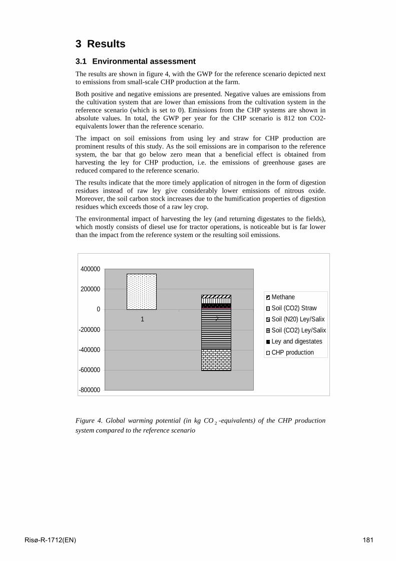
3 Results 3.1 Environmental assessment The results are shown in figure 4, with the GWP for the reference scenario depicted next to emissions from small-scale CHP production at the farm.

Both positive and negative emissions are presented. Negative values are emissions from the cultivation system that are lower than emissions from the cultivation system in the reference scenario (which is set to 0). Emissions from the CHP systems are shown in absolute values. In total, the GWP per year for the CHP scenario is 812 ton CO2-equivalents lower than the reference scenario.

The impact on soil emissions from using ley and straw for CHP production are prominent results of this study. As the soil emissions are in comparison to the reference system, the bar that go below zero mean that a beneficial effect is obtained from harvesting the ley for CHP production, i.e. the emissions of greenhouse gases are reduced compared to the reference scenario.

The results indicate that the more timely application of nitrogen in the form of digestion residues instead of raw ley give considerably lower emissions of nitrous oxide. Moreover, the soil carbon stock increases due to the humification properties of digestion residues which exceeds those of a raw ley crop.

The environmental impact of harvesting the ley (and returning digestates to the fields), which mostly consists of diesel use for tractor operations, is noticeable but is far lower than the impact from the reference system or the resulting soil emissions.

Figure 4. Global warming potential (in kg CO 2 -equivalents) of the CHP production system compared to the reference scenario

-800000

-600000

-400000

-200000

0

200000

400000

1 2

MethaneSoil (CO2) StrawSoil (N20) Ley/SalixSoil (CO2) Ley/SalixLey and digestatesCHP production

Risø-R-1712(EN) 181

3.2 Economic assessment

The result of the economic assessment shows that given the assumptions made, the economic result is 0 SEK/yr - point of break-even is reached but no profit made. However, if the culvert cost can be covered by for example customer connection fees, the situation would be radically different with an annual profit of almost 800 000 SEK (see table 2) or 0.87 SEK/MWh primary energy.

4 Sensitivity analysis

In order to determine how sensitive the result is to variations in key parameters, a sensitivity analysis was conducted where parameters were altered. The results show that with a 20% increase in ley yield the GWP compared to the reference scenario decreases 3%, and with a 20% decrease in ley yield the GWP means an increase of 2%. Increasing the emission factor for nitrous oxide +50% results in the difference to the reference scenario becoming 23% higher (i.e., better comparative result), and vice versa for a 50% lower emission factor for nitrous oxide.

The economic result is highly affected by the energy prices, in particular the price for heat, which also implies that the economic viability of the system is dependent on a reliable market for the heat produced (table 3). The profit is also quite sensitive to a change in electricity price. Yields per hectare are irrelevant in this case as only a set amount of substrate is requested, which is assumed to be available without any opportunity cost of land. The cost of harvest is assumed to only be dependent on the amount of raw material and not the area over which the material is spread.

Table 2. Potential profit from the system when altering key parameters (SEK/yr). In the basic scenario, the profit is 0 SEK/yr

Alternative scenario

Excluding investment costs for culverts 771727

Altered parameter (+20%/-20%)

Electricity price 70689/-73901

Heat price 292698/-295910

Electricity certificates 46244/-49456

5 Discussion and conclusions The result of the environmental assessment points clearly in favor of including biogas production from ley in the farm cultivation system and replacing natural gas as energy source for heat and electricity to the village. In fact, the carbon sequestration effect after processing the ley in the biogas reactor rather than ploughing it down raw is the most important parameter for reduction of greenhouse gas emissions, followed by the reduction of emissions from the CHP production itself, which in the biogas scenario is

Risø-R-1712(EN) 182

carbon neutral. The third largest post is the reduction in nitrous oxide emissions after a more controlled application of N-fertilizer. Removing straw for the straw boiler means removal of carbon from the fields, which has an adverse affect on the greenhouse gas balance. This however has a small impact in this case (figure 4).

In economic terms, the system can be a viable business option but is heavily weighed down by the high cost of culvert systems – which for example can be reduced or eliminated by for example connection fees charged to the end-users. Selling sufficient amounts of heat is however crucial for economic survival of the system, as it will not survive on only electricity sales alone. Moreover, a drop in heat price, electricity price or price of renewable electricity quotas – however in particular the heat price - would jeopardize the total profitability of the system, which is a clear weakness of the system. As prices are market-based, this would only be stabilized with some type of price guarantee for the producer.

Risø-R-1712(EN) 183

REFERENCES Andrén, O. and T. Kätterer (2001). "Basic Principles for Soil Carbon Sequestration and

Calculating Dynamic Country-level Balances Including Future Scenarios." Assessment Methods for Soil Carbon: 495-511.

Baumann, H. and A.-M. Tillman (2004). The Hitch Hiker's Guide to LCA. Lund, Studentlitteratur AB.

Bernesson, S. and D. Nilsson (2005). Straw as an energy source. Uppsala, SLU - Department of Biometry and Engineering.

Börjesson, P. (2009). "Good or bad bioethanol from a greenhouse gas perspective - What determines this?" Applied Energy 86(5): 589-594.

Dustan, A. (2002). Review of methane and nitrous oxide emission factors for manure management in cold climates. Uppsala, Swedish Institute of Agricultural and Environmental Engineering.

EC (2007). Council Regulation (EC) No 834/2007 on organic production and labelling of organic products, Official Journal of the European Union. 189:1.

Edström, M., L.-E. Jansson, et al. (2008). Farm-scale biogas production. Report 42. Uppsala, Swedish Institute for Agricultural and Environmental Engineering.

EEA (2006). How much bioenergy can Europe produce without harming the environment? Copenhagen, European Environment Agency.

Gunnarsson, C., R. Spörndly, et al. (2007). Optimisation of machinery systems for high quality forage harvest. Uppsala, SLU - Department of Biometry and Engineering.

IPCC (2006). IPCC Guidelines for National Greenhouse Gas Inventory.

Kjellström, B. (2007). Forskning och utveckling med tillämpning för småskalig kraftvärmeproduktion ur biobränslen. Eskilstuna, Swedish Energy Agency.

Kjärstad, J. and F. Johnsson (2007). "The European power plant infrastructure--Presentation of the Chalmers energy infrastructure database with applications." Energy Policy 35(7): 3643-3664.

Klöverpris, J. (2008). Consequential life cycle inventory modelling of land use induced by crop consumption. Department of Management Engineering. Copenhagen, Danish Technical University. Industrial Ph.D. Thesis.

KRAV (2009). Ekologisk odling - En broschyr om ekologisk växtodling enligt KRAVs regler, med information om EUs regler, KRAV.

Lindgren, M., O. Pettersson, et al. (2002). Engine load pattern and engine exhaust gas emissions from off-road vehicles and methods to reduce fuel-consumption and engine exhaust gas emissions. Uppsala, Swedish Institute of Agricultural and Environmental Engineering.

Nordpool. (2009).

Rodhe, L., E. Salomon, et al. (2006). Handling of digestate on farm level. Uppsala, Swedish Institute of Agricultural and Environmental Engineering.

Schneider, C. (2009). Cost of culverts in district heating grids. Uppsala.

SvenskaKraftnät (2009).

SvenskFjärrvärme (2009).

Risø-R-1712(EN) 184

Integrative approach for utilization of olive mill

wastewater and lebna’s whey for ethanol production

Mohammed A. Ibrahim*, Bassam O. Hayek, Nisreen Al-Hmoud, Laila

Al-Gogazeh

Royal Scientific Society, Environmental Research Centre, Amman,

Jordan

P.O. Box 1438 Al-Jubeiha 11941 Jordan

Abstract

The industry of olive oil extraction in Jordan involves an intensive consumption of water and

generates large quantities of olive mill wastewater (OMW). This wastewater has a high

pollution risk with biological oxygen demand (BOD). The organic fraction of OMW includes

sugars, tannins, polyphenols, polyalcohols, pectins and lipids. The presence of remarkable

amounts of aromatic compounds in OMW is responsible for its phytotoxic and antimicrobial

effects. The environmental problems and potential hazards caused by OMW had led olive oil

producing countries to limit their discharge and to propose and develop new technologies for

OMW treatments, such as physicochemical and biological treatments. In the present

investigation lebna’s whey a local byproduct of widely consumed local yogurt was used with

OMW for ethanol production. The obtained results showed that the proteins of lebna’s whey

can remove substantial amounts of aromatic compounds present in OMW. This was

reflected on the reduction of the intensity of black color of OMW and removal of 37%

polyphenols. Moreover, the production of ethanol was ascertained in fermentation media

composed of whey and in presence of various concentrations of OMW up to 20% OMW. The

obtained results showed the possibility to develop a process for improvement and

enhancement of ethanol production from whey and olive oil waste in mixed yeast cultures.

Key words: biofuels, ethanol, olive mill wastewater, whey

rof_mibrahim@yahoo.compmail: -*Corresponding author. E

Risø-R-1712(EN) 185

Introduction

Sustainable waste management is an important issue considering the challenges facing

disposal of organic wastes (biowaste) generated from food industries. Food industries

wastes are organic residues from processing of agricultural raw materials to food products,

which arise as liquid (wastewater) and solid waste (Oreopoulou and Russ, 2007). Efforts are

made to optimize food processing technologies to minimize the amount of biowastes,

however, the remaining wastes will continue being one of main problems which confronts

food industries.

Olive mill wastewater (OMW), is one of important wastes of food industries in Jordan; the

industry of olive oil in Jordan consumes large amount of water for oil extraction,

approximately one ton water is used per ton olive fruits, and as a result large amounts of

black colored olive mill wastewaters (OMW) are produced and present a major

environmental problem, if not treated before dissipation. The large amounts of OMW

generated, combined with its high polluting power as well as its high biological oxygen

demand (BOD), represent the main difficulties in finding a solution for the management of

this kind of wastewater. However, it could be upgraded by removing or reducing its phenolic

compounds and using its carbohydrate fraction to produce useful products (Massadeh and

Modallaln, 2008). Other type of waste of food industries is whey which is produced from

processing of milk in dairy industries. Whey is mainly the by-product of cheese production in

the global market; it is the serum component which separates from milk after addition of

rennet or an edible acidic substance. Cheese whey contains lactose, vitamins and minerals

along with traces of fat. Another type of whey is produced in the Middle East countries and is

known as Lebna whey, which is made from yogurt after removal of serum. Lebna whey is

also rich in lactose, vitamins and minerals. Both types of whey represent an important

source of environmental pollution due to their enormous production and high organic matter

content (Ferrari et al., 1994. , Bonnet et al., 1999).

Production of ethanol from wastes of food industries represents an opportunity for

minimizing waste and producing useful product. In this respect ethanol is utilized in products

as diverse as solvent, antifreeze, perfumes, printing ink, white vinegar, beverage,

pharmaceutical, and used as intermediate raw material in the chemical synthesis of

innumerable organic compounds (Roehr, 2001). Other important application of ethanol is in

the fuel sector; in this respect, it is considered as one of the important renewable energy

Risø-R-1712(EN) 186

sources (Sagar and Kartha, 2007; Goldemberg 2007). Nowadays, economic and

environmental concerns added emphasis on ethanol as a source of renewable fuel. Thus,

economy of ethanol productivity by microbial cells in fermentation medium is the final goal of

experts in this field. Several approaches have been investigated to reduce the cost of

ethanol which is currently could be produced either by batch or continuous immobilized

cultures using certain types of bacteria and yeast (Bai et al. 2008). Recent economic insights

into ethanol fermentation technology pointed to possible utilization of food industries wastes

for ethanol production.

In the present work an investigation was carried out to ascertain the possibility of utilization

of above mentioned food industries wastes (OMW and lebna whey) for ethanol production.

Materials and methods

Sources of wastes

Olive mill waste water was obtained from Jazaiza olive oil factory/Al-Salt-Jordan , whereas

lebna whey was obtained from Al-Maha Dairy factory/ Rusaifa-Jordan .

Chemical analysis

Total nitrogen(TKN), total phosphate(TP), total soluble solids (TSS), biological oxygen

demand (BOD), chemical oxygen demand (COD) and polyphenols were determined

following American Standard Methods (ASM) for the examination of water and wastewater:

4500 ( Norg-B ), 4500 ( PO4-C ) , 2540-D 5210,13, 5220,B and 5550 respectively. Ethanol

concentrations were analyzed by Gas Chromatography (Hewlett Packard HP 6890 series)

according to AOAC, 2005.

Yeast strain

Lactose fermenting yeast was isolated from local habitat and preserved on whey agar slants

at 4°C. Suitable selected yeast isolates were used for ethanol production in whey-OMW

based media. Baker’s yeast was used in mixed fermentation with lactose fermenting yeast.

Fermentation media and cultural conditions

Liquid fermentation media were prepared from wastes of lebna whey and various

concentrations of OMW. The pH value of fermentation media was adjusted to 4.4 before

sterilization. The fermentation medium was inoculated with 3% freshly prepared yeast

culture and incubated for 48 hours at 32° C.

Removal of polyphenols from OMW

Risø-R-1712(EN) 187

Proteins of Lebna whey were precipitated by adjustment of pH value followed by heating.

The precipitated proteins were collected by centrifugation for 15 minutes at 4500 rpm.

Reaction mixture (RM) was prepared from non diluted OMW containing 18% w/v of whey

proteins, RM was incubated at various time intervals ( 1, 2, 3 and 4 hours) with shaking at

25°C. At end of each incubation interval the RM was centrifuged and the polyphenols were

measured in the supernatant.

Results and discussion

Chemical analysis of wastes

It had been reported that the organic fraction of olive mill waste includes sugars, tannins,

polyphenols, polyalcohols, pectins and lipids (Hamdi, 1996). In addition, it had been reported

that OMW contains remarkable amounts of aromatic compounds which are also responsible for

its phytotoxic and antimicrobial effects (Fluori et al., 1996); whereas cheese whey contains

lactose, vitamins and minerals along with traces of fat (Zafar and Owais, 2006). The chemical

analysis of two types of wastes (Lebna whey and OMW) obtained from local food industries

had shown variation in their chemical compositions (Table 1). OMW was found rich in TSS

(16.545 g/l), organic nitrogen (0.083 g/l), and minerals; on the other hand lebna whey

composed of 57.797 g/l TSS which is mainly lactose sugar and 6.04 g/l organic nitrogen (Table

1). Same table showed the BOD and COD of OMW and whey which were 26.805, 12.456,

41.076 and 104.540 g/l respectively. In this respect it was reported that the BOD values of

OMW were in the range of 89–100 g/l, and chemical oxygen demand (COD) values in the

range of 80–200 g/l (Hamdi, 1996). The obtained results in this work showed that lebna whey

had higher BOD and COD values as compared with OMW.

Ethanol production in Whey-OMW media

It is possible to produce ethanol from various sources of sugars providing using suitable yeast

strains. Lactose fermenting yeast is used for production of ethanol from whey, whereas

baker's yeast is used for production of ethanol from sucrose (Zafar and Owais 2006; Reddy

and Reddy 2006). In the present investigation it was possible to isolate lactose fermenting

yeast from contaminated yogurt samples and most efficient yeast isolate was used for

ethanol production from whey. Table (2) showed various compositions of fermentation media,

based on OMW and whey, which were used in production of ethanol. Three concentrations

(5%, 10% and 20%) of OMW were used with whole whey (WW) or deproteinized whey (DW)

to prepare various types of fermentation media. The results which were shown in figure (1)

Risø-R-1712(EN) 188

revealed that the values of ethanol production in WW fermentation media was almost similar

to theoretical ethanol yield, while presence of 5 and 10% of OMW in fermentation media

caused 4 and 7 % reduction in ethanol production respectively as compared with fermentation

media composed of WW only. On the other hand presence of 20% of OMW in OMW-WW

fermentation media resulted in 52% reduction of ethanol production in comparision with

ethanol production in WW fermentation media; this might be due to toxic effects of

polyphenolic compounds present in OMW. The results presented in figure (2) showed that

the values of ethanol production in OMW-DW fermentation media in presence of 5, 10% and

20% of OMW were reduced by 12, 34 and 69% respectively in comparison with fermentation

media composed of DW. These results suggested that presence of Lebna whey proteins in

fermentation have positive effect on removal or neutralization of possible toxic effects of

polyphenols present in OMW on yeast cells or on ethanol production.

Removal of polyphenols from OMW

The above mentioned observation on possible detoxification or neutralization of polyphenols

by lebna whey proteins, suggested the possibility of using the separated lebna whey proteins

for removal of polyphenols from OMW. In this study, the obtained results of mixing lebna

protein with OMW resulted in significant reduction of polyphenolic compounds in OMW. The

study showed that the original amount of polyphenols present in OMW was 591±51 mg/l,

after treatment of OMW for four hours with lebna proteins it was possible to measure 37%

reduction in the amount of polyphenols.

Further work

An investigation was carried out to ascertain the possibility of alcoholic fermentation under

higher sugar concentration by using mixed fermentation. Sucrose was added to give final

concentration of 10% w/v in OMW-WW fermentation media and baker's yeast was used to

ferment sucrose after completion of lactose fermentation by lactose fermenting yeast. The

obtained results showed the importance of this approach in regard of utilization of sucrose

waste from other food industries as carbon source. Moreover, it was possible to enhance

ethanol production by using certain products of olive mill wastes under high gravity

fermentation.

Conclusions

Whey and olive mill wastewater (OMW) are major wastes of food industries in Jordan. OMW

is considered source of water and minerals, whereas whey is source of sugar and nitrogen.

Risø-R-1712(EN) 189

The preliminary results reported in this study suggested the possibility of production of

ethanol by utilizing both wastes in an integrative way. Moreover the obtained results showed

that lebna whey proteins could reduce inhibitory effects of polyphenols present in OMW on

ethanol production.

Acknowledgements

The research work is supported by The Higher Council for Science and Technology, Amman,

Jordan. M. Ibrahim is grateful to International Institute of Education for the fellowship.

References

Bai FW, Anderson WA, Moo-Young M (2008) Ethanol fermentation technologies from sugar

and starch feed stocks. Biotechnology Advances, 26: 89 –105

Bonnet J, Bogaerts P , Bohatier J (1999) Biological treatment of whey by

Tetrahymena pyriformis and impact study on laboratory scale wastewater lagoon

process. Chemosphere, 38(13): 2979-2993

Ferrari M D, Loperena L, Varela H. (1994) Ethanol production from concentrated whey

permeates using a fed-batch culture of Kluyveromyces fragilis. Biotechnology letters,

16(2):205-210

Fluori F, Sotirchos D, Ioannidou S, Balis C (1996) Decolorization of olive oil Mill liquid

wastes by chemical and biological means. International Biodetcrioration & Biodegradation,

189-192

Goldemberg J (2007) Ethanol for a sustainable energy future. Science, 315: 808-810

Hamdi M (1996) Aaerobic digestion of olive mill wastewaters.ProcessBiochemistry, 31(2):

105-110Anaerobic Digestion of Olive

Massadeh M I.; Modallaln N. ( 2008 ) Ethanol Production from Olive Mill Wastewater (OMW)

Pretreated with Pleurotus sajor-caju International Conference on Bioenergy Outlook 2007 ,

SINGAPOUR (26/04/2007) vol. 22(1): 150-154

Oreopoulou V, Russ W (2007) Utilization of by-products and treatment of waste

in the food industry. Springer, New York

Reddy LVA, Reddy OVS ( 2006 ) Rapid and enhanced production of ethanol in

very high gravity (VHG) sugar fermentation by Saccharomyces cerevisiae: Role of

Risø-R-1712(EN) 190

finger millet (Eleusine coracana L.) flour. Process Biochemistry, 41: 726 –729

Roehr M ( 2001 ) The biotechnology of ethanol. Publisher: WILEY-VCH Verlag

GmbH, D-69469 Weinheim ,Federal Republic of Germany.

Sagar AD, Kartha S ( 2007 ) Bioenergy and sustainable development. Annu. Rev.

Environm.Resourc., 32:131-167

Zafar S, Owais M ( 2006 ) Ethanol production from crude whey by

Kluyveromyces marxianus . Biochemical Engineering Journal 27: 295–298

.

Risø-R-1712(EN) 191

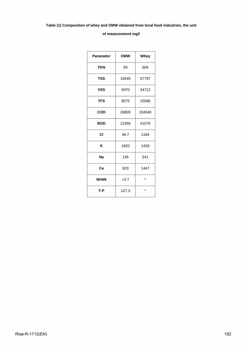
Table (1) Composition of whey and OMW obtained from local food industries, the unit

of measurement mg/l

Parameter OMW Whey

TKN 83 604

TSS 16545 57797

VSS 5970 34712

TFS 9575 15085

COD 26805 104540

BOD 12456 41076

Cl 46.7 1184

K 1820 1426

Na 145 541

Ca 823 1447

NH4N <3.7 *

T-P 127.3 *

Risø-R-1712(EN) 192

Table (2) Composition of whey-OMW (%v/v) fermentation media, WW and DW indicate

whole and deproteinized whey respectively.

Media Composition

OMW-WW

0% OMW

5% OMW, 95% WW

10% OMW, 90% WW

20% OMW, 80% WW

OMW-DW

0% OMW

5% OMW, 95% DW

10% OMW, 90% DW

20% OMW, 80% DW

Risø-R-1712(EN) 193

Figure 1 Ethanol production by lactose fermenting yeast in fermentation media OMW-WW,

composed of whole whey and various concentrations of OMW.

Key : OL, FL, CL, TE, AE1, AE2 indicate original lactose (% w/w), final lactose(% w/w),

consumed lactose(% w/w), theoretical ethanol yield (% w/w), actual ethanol yield (% w/w)and

actual ethanol yield (% v/v).

OMW-Whole whey

0

1

2

3

4

5

6

7

OL FL CL TE AE1 AE2

0%5%10%20%

Risø-R-1712(EN) 194

Figure 2 Ethanol productions by lactose fermenting yeast in fermentation media OMW-DW,

composed of deproteinized whey and various concentrations of OMW.

Key: OL, FL, CL, TE, AE1, AE2 indicate original lactose (% w/w), final lactose, consumed

lactose (%w/w), theoretical ethanol yield (% w/w), actual ethanol yield (% w/w) and actual

ethanol yield (% v/v).

OMW-Deproteinized Whey

0

1

2

3

4

5

6

7

OL FL CL TE AE1 AE2

0%

5%

10%

20%

Risø-R-1712(EN) 195

Session 12 – Renewable energy for transport

Risø-R-1712(EN) 196

Life Cycle Analysis of Battery and Fuel Cell Vehicles Ulrich Wagner, Lehrstuhl für Energiewirtschaft und Anwendungstechnik at TU München, Forschungsstelle für Energiewirtschaft e.V., München

Michael Beer, Jochen Habermann, Forschungsstelle für Energiewirtschaft e.V., München

Abstract This paper shows a life cycle analysis of different potential fuels and powertrains for passenger cars. The focus of the study lies on electric vehicles powered by batteries and fuel cells. At first the cumulative energy demand (CED) is introduced as an instrument to compare the different technologies. Subsequently several process chains for transportation are shown in a holistic approach. Finally a sensitivity analysis is used to determine the energetic break-even points for hydrogen and electric powertrains. The results are taken from several reports for the Bavarian Hydrogen Initiative (wiba), which is coordinated by the authors.

1 Introduction In all industrialized and developing countries, a steady increase of motor-driven traffic is taking place. Between 1965 and today, traffic has almost tripled. During the same time, significant progress in automotive engineering has been achieved, especially in terms of fuel consumption. However, these advancements were compensated by higher motor power, a multitude of supplementary equipment and higher vehicle weight. Consequently, only a slight decrease in average fuel consumption has taken place.

At present, the biggest part of the energy demand for transportation applications is covered by petroleum products. Considered the limitation of limited fossil energy sources and an estimated significant increase in global energy demand, the search for alternative energy carriers and powertrain concepts is increasing. Discussions about greenhouse gas emissions and global warming are further forcing the need for innovative and sustainable energy systems.

Previous to a full-scale introduction of alternative energy carriers and powertrains, the ecological advantages and disadvantages in comparison to established, conventional process chains must be evaluated and weighed up. In terms of a full life cycle assessment, environmental impacts such as primary energy (PE) demand, space requirements, greenhouse gas emissions, appearance of ecotoxic and human-toxicological substances are of special interest. Furthermore, economic and social facets as well as availability of resources have to be considered [1].

2 Definitions and methodology For the production and use of a certain fuel, a multitude of different processes must be analysed. These are interlinked with each other in so-called process chains, sometimes in a complex manner. For each process, an energetic input-output-analysis based on lower heating value (LHV) was performed and for each process chain an individual analysis was carried out, yielding cumulative energy demand (CED) and cumulative emissions for a specific product or provision of services.

In general, the CED is defined as the sum of the PE demand evolving from production, use and disposal of an economic good or object, respectively, the PE demand which can

Risø-R-1712(EN) 197

be causally assigned to this economic good or object (both, products and services). Thus, the CED represents the sum of the CEDs for the production (CEDP), use (CEDU) and disposal (CEDD) of an object [2],[3].

In [4], characteristic parameters are defined and a methodology is introduced which allows for a sophisticated analysis of different energy systems and a well-balanced assessment of the individual technologies. According to this methodological approach, regenerative and non-regenerative energy demands are investigated separately by using the following definitions:

(i) Cumulative regenerative energy demand (CRED): The sum of the regenerative energy demands for a product or provision of services is defined as CRED. All of the further considerations in this study assume that regenerative energies are inexhaustibly available.

(ii) Cumulative non-regenerative energy demand (CNRED): The sum of non-regenerative energy demands for a product or provision of services is defined as CNRED.

Thus, the CED can be split into the two subcomponents CRED and CNRED:

CED = CEDP + CEDU + CEDD = CRED + CNRED (1)

To assess the input of regenerative energies in process chain analyses, the regenerative PE input was set equal to the amount of useful energy produced according to the practice of the United Nations Department of Economic and Social Affairs Statistics Division [5] and the Statistical Office of European Communities (SOEC) [6]. In doing so, energy converters using regenerative energy sources are in fact evaluated in terms of their energetic benefit rather than in terms of their technical capacities, respectively efficiencies. This procedure offers the possibility to set up and quantify the energy flows and energy balance within the individual system boundaries without overweighing the regenerative energy inputs.

For the assessment of non-regenerative energy inputs (fossil and nuclear) on a PE basis, the overall efficiency of supply (OES) was used. In the case of fuels and other materials with an LHV, OESf is defined as the ratio of the LHV and the cumulative energy demand for the supply of the fuel (CEDs) [2]:

s

f CEDLHVOES = (2)

Thus, the energetic efforts for the supply as well as for the production and the disposal of the plants, all valued as primary energy, must be considered for the calculation of CEDs.

Accordingly, the overall efficiency of electricity supply (OESel) includes the overall efficiencies of generation and distribution to the end-user and is defined as the ratio of electrical energy Wel and CEDs [2]:

s

elel CED

WOES = (3)

3 Extraction, conversion and distribution of fuels Within the scope of this study, state of the art and future ways of fuel supply as depicted in Figure 1 are considered. A PE carrier has to be supplied and converted into a fuel, which is transported and distributed to the final consumer. Utilization of different fuels can take place either in a vehicle powered by an internal combustion engine (ICE), in a battery electric car or in a fuel cell (FC) vehicle.

Risø-R-1712(EN) 198

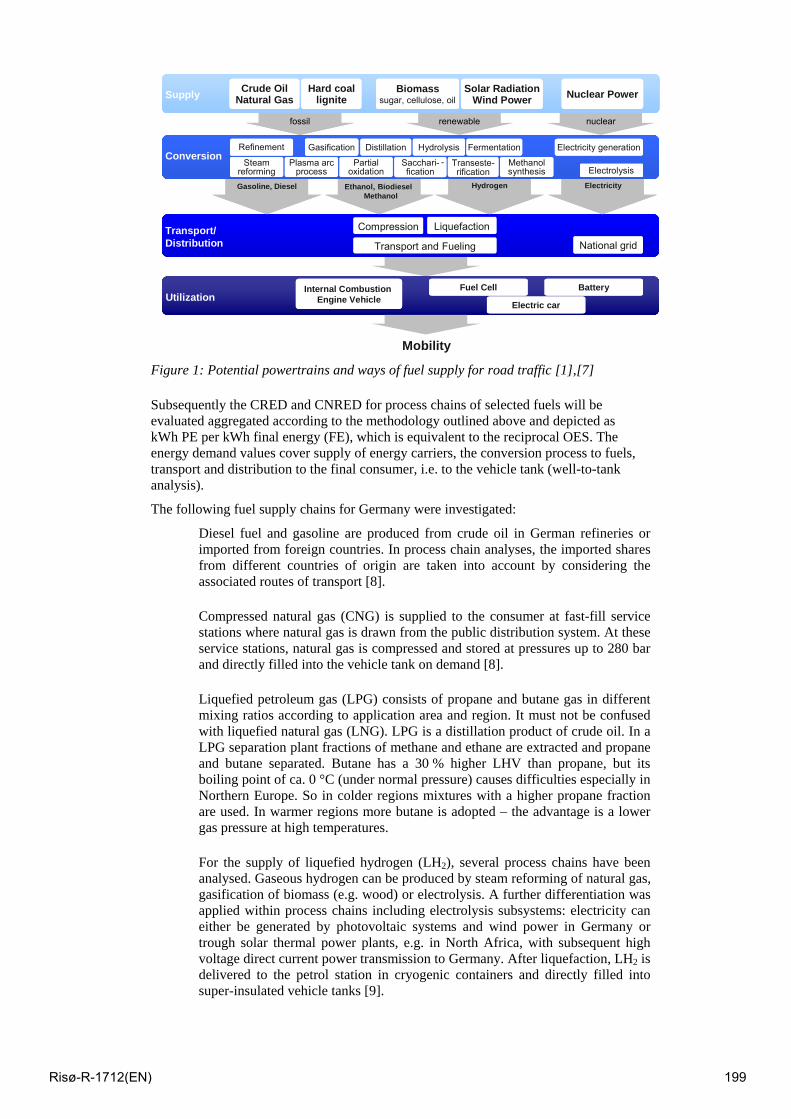
Conversion

Transport/Distribution

Utilization

Supply

Fuel CellFuel CellInternal CombustionEngine Vehicle

Internal CombustionEngine Vehicle

Mobility

Crude OilNatural GasCrude Oil

Natural Gas

Gasoline, DieselGasoline, Diesel

Solar RadiationWind Power

Solar RadiationWind Power

ElectrolysisElectrolysis

Electricity generationElectricity generation

HydrogenHydrogen

Biomasssugar, cellulose, oil

Biomasssugar, cellulose, oil

Ethanol, BiodieselMethanol

Ethanol, BiodieselMethanol

MethanolsynthesisMethanolsynthesis

-GasificationGasificationGasificationGasification

Sacchari-fication

Sacchari-fication

HydrolysisHydrolysis- Transeste-

rificationTranseste-rification

FermentationFermentationDistillationDistillation

LiquefactionCompression

Transport and Fueling

RefinementRefinement

Nuclear PowerNuclear PowerHard coallignite

Hard coallignite

Steamreforming

Steamreforming

Plasma arcprocess

Plasma arcprocess

Partialoxidation

Partialoxidation

ElectricityElectricity

fossilfossil renewable nuclear

National gridNational grid

BatteryBattery

Electric carElectric car

Figure 1: Potential powertrains and ways of fuel supply for road traffic [1],[7]

Subsequently the CRED and CNRED for process chains of selected fuels will be evaluated aggregated according to the methodology outlined above and depicted as kWh PE per kWh final energy (FE), which is equivalent to the reciprocal OES. The energy demand values cover supply of energy carriers, the conversion process to fuels, transport and distribution to the final consumer, i.e. to the vehicle tank (well-to-tank analysis).

The following fuel supply chains for Germany were investigated:

Diesel fuel and gasoline are produced from crude oil in German refineries or imported from foreign countries. In process chain analyses, the imported shares from different countries of origin are taken into account by considering the associated routes of transport [8].

Compressed natural gas (CNG) is supplied to the consumer at fast-fill service stations where natural gas is drawn from the public distribution system. At these service stations, natural gas is compressed and stored at pressures up to 280 bar and directly filled into the vehicle tank on demand [8].

Liquefied petroleum gas (LPG) consists of propane and butane gas in different mixing ratios according to application area and region. It must not be confused with liquefied natural gas (LNG). LPG is a distillation product of crude oil. In a LPG separation plant fractions of methane and ethane are extracted and propane and butane separated. Butane has a 30 % higher LHV than propane, but its boiling point of ca. 0 °C (under normal pressure) causes difficulties especially in Northern Europe. So in colder regions mixtures with a higher propane fraction are used. In warmer regions more butane is adopted – the advantage is a lower gas pressure at high temperatures.

For the supply of liquefied hydrogen (LH2), several process chains have been analysed. Gaseous hydrogen can be produced by steam reforming of natural gas, gasification of biomass (e.g. wood) or electrolysis. A further differentiation was applied within process chains including electrolysis subsystems: electricity can either be generated by photovoltaic systems and wind power in Germany or trough solar thermal power plants, e.g. in North Africa, with subsequent high voltage direct current power transmission to Germany. After liquefaction, LH2 is delivered to the petrol station in cryogenic containers and directly filled into super-insulated vehicle tanks [9].

Risø-R-1712(EN) 199

Methanol (MeOH) is produced from a CO-, CO2- and H2-containing synthesis gas. Two techniques were chosen for the production of the synthesis gas: combined steam reforming of natural gas [8] and gasification of biomass (residual forest wood in particular) [10]. Distribution of methanol to filling stations and vehicle fueling takes place in the same way as with conventional liquid fuels.

Rape methyl ester (RME, biodiesel) is produced from raw rape oil by refining or transesterification and supplied at petrol stations like diesel fuel. All of the co-products (rape straw, shred, glycerine) along the process chain are used [4].

Electric Vehicles (EV) are passenger cars powered by an electric motor in connection with an accumulator. The calculation is based on the electricity supply by the German electricity mix, i.e. a primary energy adoption of ca. 50 % coal, 32 % nuclear power, 11 % natural gas and 7 % others (incl. renewable energy carriers) for the year 2005. The accumulator’s efficiency is assumed to be 80 %.

4 Results of process chain analyses 4.1 Provision of Hydrogen Aquatic electrolysis For the aquatic electrolysis water is fractionised in its components hydrogen (H2) and oxygen (O2) using DC-voltage. H2 is collected at the cathode, O2 at the anode. A semi-permeable membrane separates the emerging gases and enables charge equalisation.

For lower capacity up to 20 m³/h PEM-electrolysers (PEM: proton exchange membrane, also: polymer electrolyte membrane) are adopted [11]. Alongside the alkaline aquatic electrolysis is one of the most usual processes. In this kind of electrolysis the ions needed for the ion exchange are typically provided by a caustic potash solution, but the underlying type of process is the same [12].

Figure 2 shows a flow diagram for the electrolytic provision of hydrogen using electricity from the German electricity mix in 2005. According to that for provision of hydrogen a 4-times higher PE-adoption is needed compared to its energy content. The major losses are caused by the supply of electricity, but the electrolysis itself and the compression of the hydrogen to 300 up to 700 bar pressure are lossy as well.

Risø-R-1712(EN) 200

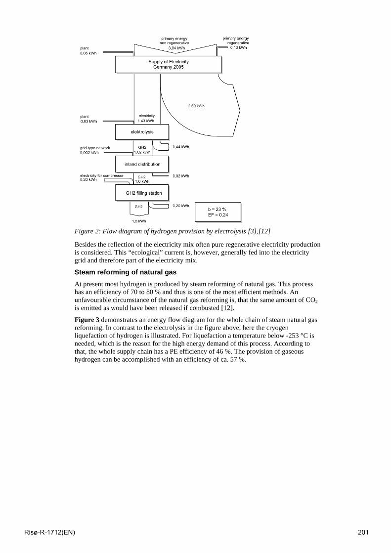
Figure 2: Flow diagram of hydrogen provision by electrolysis [3],[12]

Besides the reflection of the electricity mix often pure regenerative electricity production is considered. This “ecological” current is, however, generally fed into the electricity grid and therefore part of the electricity mix.

Steam reforming of natural gas At present most hydrogen is produced by steam reforming of natural gas. This process has an efficiency of 70 to 80 % and thus is one of the most efficient methods. An unfavourable circumstance of the natural gas reforming is, that the same amount of CO2 is emitted as would have been released if combusted [12].

Figure 3 demonstrates an energy flow diagram for the whole chain of steam natural gas reforming. In contrast to the electrolysis in the figure above, here the cryogen liquefaction of hydrogen is illustrated. For liquefaction a temperature below -253 °C is needed, which is the reason for the high energy demand of this process. According to that, the whole supply chain has a PE efficiency of 46 %. The provision of gaseous hydrogen can be accomplished with an efficiency of ca. 57 %.

Risø-R-1712(EN) 201

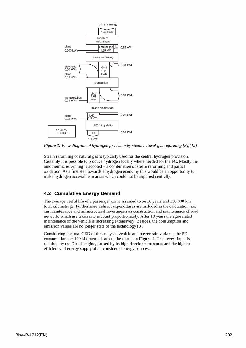
Figure 3: Flow diagram of hydrogen provision by steam natural gas reforming [3],[12]

Steam reforming of natural gas is typically used for the central hydrogen provision. Certainly it is possible to produce hydrogen locally where needed for the FC. Mostly the autothermic reforming is adopted – a combination of steam reforming and partial oxidation. As a first step towards a hydrogen economy this would be an opportunity to make hydrogen accessible in areas which could not be supplied centrally.

4.2 Cumulative Energy Demand The average useful life of a passenger car is assumed to be 10 years and 150.000 km total kilometrage. Furthermore indirect expenditures are included in the calculation, i.e. car maintenance and infrastructural investments as construction and maintenance of road network, which are taken into account proportionately. After 10 years the age-related maintenance of the vehicle is increasing extensively. Besides, the consumption and emission values are no longer state of the technology [3].

Considering the total CED of the analysed vehicle and powertrain variants, the PE consumption per 100 kilometres leads to the results in Figure 4. The lowest input is required by the Diesel engine, caused by its high development status and the highest efficiency of energy supply of all considered energy sources.

Risø-R-1712(EN) 202

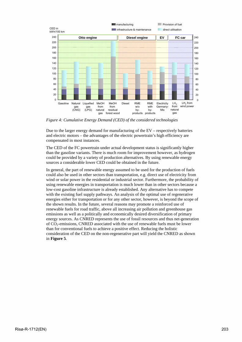
0

20

40

60

80

100

120

140

160

180

200

220

240

Gasoline Natural gas

(CNG)

Liquefiedgas

(LPG)

MeOHfrom

natural gas

MeOHfrom

residualforest wood

Diesel RMEw/oby-

products

RMEwithby-

products

ElectricityGermany-

Mix

LH2from

naturalgas

LH2 fromwind power

CED in kWh/100 km

manufacturing

infrastructure & maintenance

Provision of fuel

direct utilisation

Otto engine EVDiesel engine FC car

0

20

40

60

80

100

120

140

160

180

200

220

240

Figure 4: Cumulative Energy Demand (CED) of the considered technologies

Due to the larger energy demand for manufacturing of the EV – respectively batteries and electric motors – the advantages of the electric powertrain’s high efficiency are compensated in most instances.

The CED of the FC powertrain under actual development status is significantly higher than the gasoline variants. There is much room for improvement however, as hydrogen could be provided by a variety of production alternatives. By using renewable energy sources a considerable lower CED could be obtained in the future.

In general, the part of renewable energy assumed to be used for the production of fuels could also be used in other sectors than transportation, e.g. direct use of electricity from wind or solar power in the residential or industrial sector. Furthermore, the probability of using renewable energies in transportation is much lower than in other sectors because a low-cost gasoline infrastructure is already established. Any alternative has to compete with the existing fuel supply pathways. An analysis of the optimal use of regenerative energies either for transportation or for any other sector, however, is beyond the scope of the shown results. In the future, several reasons may promote a reinforced use of renewable fuels for road traffic, above all increasing air pollution and greenhouse gas emissions as well as a politically and economically desired diversification of primary energy sources. As CNRED represents the use of fossil resources and thus net-generation of CO2-emissions, CNRED associated with the use of renewable fuels must be lower than for conventional fuels to achieve a positive effect. Reducing the holistic consideration of the CED on the non-regenerative part will yield the CNRED as shown in Figure 5.

Risø-R-1712(EN) 203

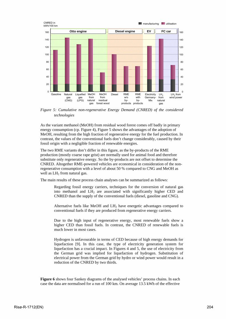
0

20

40

60

80

100

120

140

160

CNRED inkWh/100 km

manufacturing utilisation

Otto engine EVDiesel engine FC car

Gasoline Natural gas

(CNG)

Liquefiedgas

(LPG)

MeOHfrom

natural gas

MeOHfrom

residualforest wood

Diesel RMEw/oby-

products

RMEwithby-

products

ElectricityGermany-

Mix

LH2from

naturalgas

LH2 fromwind power

0

20

40

60

80

100

120

140

160

Figure 5: Cumulative non-regenerative Energy Demand (CNRED) of the considered technologies

As the variant methanol (MeOH) from residual wood forest comes off badly in primary energy consumption (cp. Figure 4), Figure 5 shows the advantages of the adoption of MeOH, resulting from the high fraction of regenerative energy for the fuel production. In contrast, the values of the conventional fuels don’t change considerably, caused by their fossil origin with a negligible fraction of renewable energies.

The two RME variants don’t differ in this figure, as the by-products of the RME production (mostly coarse rape grist) are normally used for animal food and therefore substitute only regenerative energy. So the by-products are not offset to determine the CNRED. Altogether RME-powered vehicles are economical in consideration of the non-regenerative consumption with a level of about 50 % compared to CNG and MeOH as well as LH2 from natural gas.

The main results of these process chain analyses can be summarized as follows:

Regarding fossil energy carriers, techniques for the conversion of natural gas into methanol and LH2 are associated with significantly higher CED and CNRED than the supply of the conventional fuels (diesel, gasoline and CNG).

Alternative fuels like MeOH and LH2 have energetic advantages compared to conventional fuels if they are produced from regenerative energy carriers.

Due to the high input of regenerative energy, most renewable fuels show a higher CED than fossil fuels. In contrast, the CNRED of renewable fuels is much lower in most cases.

Hydrogen is unfavourable in terms of CED because of high energy demands for liquefaction [9]. In this case, the type of electricity generation system for liquefaction has a crucial impact. In Figures 4 and 5, the use of electricity from the German grid was implied for liquefaction of hydrogen. Substitution of electrical power from the German grid by hydro or wind power would result in a reduction of the CNRED by two thirds.

Figure 6 shows four Sankey diagrams of the analysed vehicles’ process chains. In each case the data are normalised for a run of 100 km. On average 13.5 kWh of the effective

Risø-R-1712(EN) 204

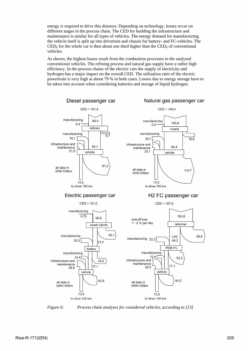
energy is required to drive this distance. Depending on technology, losses occur on different stages in the process chain. The CED for building the infrastructure and maintenance is similar for all types of vehicles. The energy demand for manufacturing the vehicle itself is split up into drivetrain and chassis for battery- and FC-vehicles. The CEDP for the whole car is then about one third higher than the CEDP of conventional vehicles.

As shown, the highest losses result from the combustion processes in the analysed conventional vehicles. The refining process and natural gas supply have a rather high efficiency. In the process chains of the electric cars the supply of electricity and hydrogen has a major impact on the overall CED. The utilisation ratio of the electric powertrain is very high at about 79 % in both cases. Losses due to energy storage have to be taken into account when considering batteries and storage of liquid hydrogen.

Figure 6: Process chain analyses for considered vehicles, according to [13]

Risø-R-1712(EN) 205

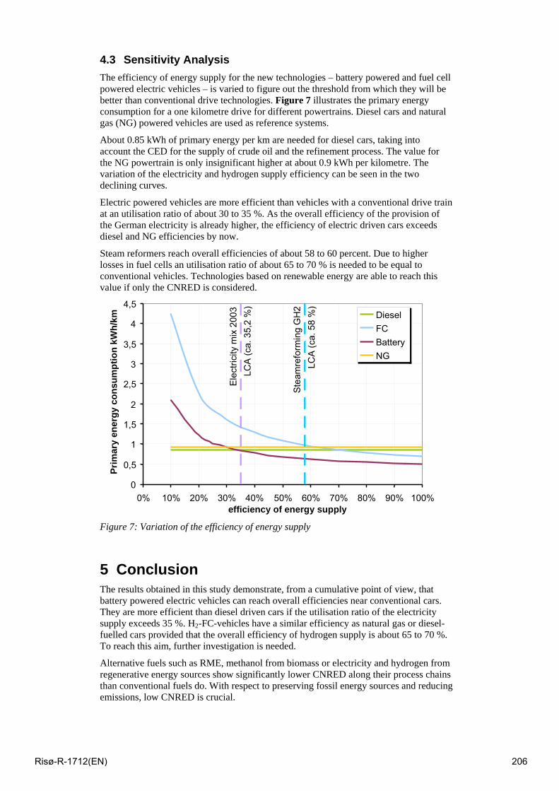
4.3 Sensitivity Analysis The efficiency of energy supply for the new technologies – battery powered and fuel cell powered electric vehicles – is varied to figure out the threshold from which they will be better than conventional drive technologies. Figure 7 illustrates the primary energy consumption for a one kilometre drive for different powertrains. Diesel cars and natural gas (NG) powered vehicles are used as reference systems.

About 0.85 kWh of primary energy per km are needed for diesel cars, taking into account the CED for the supply of crude oil and the refinement process. The value for the NG powertrain is only insignificant higher at about 0.9 kWh per kilometre. The variation of the electricity and hydrogen supply efficiency can be seen in the two declining curves.

Electric powered vehicles are more efficient than vehicles with a conventional drive train at an utilisation ratio of about 30 to 35 %. As the overall efficiency of the provision of the German electricity is already higher, the efficiency of electric driven cars exceeds diesel and NG efficiencies by now.

Steam reformers reach overall efficiencies of about 58 to 60 percent. Due to higher losses in fuel cells an utilisation ratio of about 65 to 70 % is needed to be equal to conventional vehicles. Technologies based on renewable energy are able to reach this value if only the CNRED is considered.

0

0,5

1

1,5

2

2,5

3

3,5

4

4,5

0% 10% 20% 30% 40% 50% 60% 70% 80% 90% 100%efficiency of energy supply

Prim

ary

ener

gy c

onsu

mpt

ion

kWh/

km DieselFCBatteryNG

Elec

trici

ty m

ix 2

003

LCA

(ca.

35,

2 %

)

Stea

mre

form

ing

GH

2LC

A (c

a. 5

8 %

)

Figure 7: Variation of the efficiency of energy supply

5 Conclusion The results obtained in this study demonstrate, from a cumulative point of view, that battery powered electric vehicles can reach overall efficiencies near conventional cars. They are more efficient than diesel driven cars if the utilisation ratio of the electricity supply exceeds 35 %. H2-FC-vehicles have a similar efficiency as natural gas or diesel-fuelled cars provided that the overall efficiency of hydrogen supply is about 65 to 70 %. To reach this aim, further investigation is needed.

Alternative fuels such as RME, methanol from biomass or electricity and hydrogen from regenerative energy sources show significantly lower CNRED along their process chains than conventional fuels do. With respect to preserving fossil energy sources and reducing emissions, low CNRED is crucial.

Risø-R-1712(EN) 206

Both technologies – H2 powered FC and electric vehicles – have their advantages as they are emission free at the site of use. This includes the possibility of CO2 sequestration in more efficient central facilities. Therefore fossil fuels could be used with reduced impact on climate change. This leads to a huge variety of primary energy carriers that can be utilised for transportation.

Even though electric vehicles – battery and fuel cell powered – show a significantly higher CEDP than gasoline and diesel ICE vehicles, the chance to use renewable energy carriers is yielding the lowest specific CNRED and CO2-emissions over the lifetime. In the case of fossil fuels, CNRED and CO2-emissions are dominated by the individual fuel supply chains and direct consumption, not by vehicle production, maintenance and disposal. Due to the inherent CNRED- and CO2-neutrality of regenerative fuels, CNRED and CO2-emissions during utilization are virtually zero. As long as no hydrogen infrastructure is provided, on-board storage of hydrogen and also electricity remains a crucial problem, use of RME in an ICE vehicle or methanol from biomass in a PEFC vehicle represent reasonable transitional solutions.

By comparing different powertrain concepts, respectively ICE and electric systems, one has to bear in mind that these represent strongly unequal evolutionary states. Whilst ICE vehicles are being mass-produced, FC and electric vehicles are still in a research and development status. Consequently, the database for the propulsion concepts under consideration also strongly varies in quality and quantity. In the future, both technologies will undergo significant improvements and other technologies will also have to be taken into account, e.g. most notably hybrid systems. Thus, a continuous assessment of different powertrain systems with the associated fuel supply chains is compulsory in order to fill data gaps and evaluate the environmental impacts of each technology. In addition to technological issues, social and economic factors such as consumer acceptance and availability of fuels are of equal importance.

The most important criterion for decision-making in the cases considered in this paper are the costs, both for the propulsion system as well as for the supply and distribution of fuels. Even though fuel cells and electric vehicles can be regarded as cleaner and more efficient automotive engines, many challenges still have to be met before a successful commercialisation of fuel cell vehicles can be achieved [14],[15]. Consequently, the design of the automotive industry in the future will inevitably be connected with the design and configuration of a low-cost fuel infrastructure. Given the considerable business risk involved in creating an automotive fuel infrastructure based on regenerative fuels, a supportive political framework and diversification of the risk with individual corporate strategies will be essential.

In the near future storage of electricity, produced by fluctuating renewable energy sources, could be a new field of business for energy suppliers. Electric vehicles, powered by batteries as well as by electrolytic hydrogen, may contribute as additional electricity consumers. An intelligent control of timed electricity supply and demand provides the ability to meet future challenges for the energy economy.

6 References [1] Wagner, U.; Eckl, R.; Tzscheutschler, P.: Energetic life cycle assessment of fuel

cell powertrain systems and alternative fuels in Germany, in: science direct energy, Amsterdam: Elsevier B.V., 2005

[2] German Association of Engineers – Society for Energy Technology (VDI-GET): Cumulative energy demand – terms, definitions, methods of calculation, VDI guideline no. 4600:1997. Berlin, Germany: Beuth Verlag GmbH, 1997.

[3] Wagner, U.; Geiger, B.; Schäfer, H.: Energy life cycle analysis of hydrogen systems, International Journal of Hydrogen Energy 1998; 23(1):1-6.

Risø-R-1712(EN) 207

[4] Dreier, T.: Cumulative system analysis and potentials of biofuels, Herrsching, Germany: E&M Energie und Management Verlagsgesellschaft mbH, 2000

[5] United Nations Department of Economic and Social Affairs Statistics Division: 2000 Energy Statistics Yearbook, New York: United Nations Publication, 2002.

[6] Carvalho Neto, J.; Deimezis, N.; Lecloux, M.; Karadelogou, P.; Bailey, RA.: Energy in Europe - Annual Energy Review, Brussels, Belgium: Commission of the European Communities, 1991.

[7] Richter, S., Wagner, U.: Hydrogen Production, München: Forschungsstelle für Energiewirtschaft e.V., in: Landolt-Börnstein Numerical Data and Functional Relationships Volume VIII/3, Springer-Verlag, Berlin, 2006

[8] Forschungsvereinigung Verbrennungskraftmaschine e.V. (FVV): Fuel cell study final report, project no. 686:1998. Frankfurt, Germany: FVV e.V., 1998

[9] Angerloher, J.; Dreier, Th.: Techniken und Systeme zur Wasserstoff-bereitstellung – Perspektiven einer Wasserstoff-Energiewirtschaft (Teil 1), Bavarian Hydrogen Initiative, Forschungsstelle für Energiewirtschaft, München, 2000

[10] Dreier T.: Biofuels – energetic, environmental and economic analysis, Herrsching, Germany: E&M Energie und Management Verlagsgesellschaft mbH, 1999

[11] Energiewelt Wasserstoff – Wissen, Technologie, Perspektive, TÜV Süddeutschland, München, 2002

[12] Beer, M.; Fieger, C.: Perspektiven der Brennstoffzellen- und Wasserstoff-technologie - Einsatz innovativer KWK-Technologien in der Hausenergieversorgung, Forschungsstelle für Energiewirtschaft e.V., München, 2008

[13] Corradini, R.; Krimmer, A.: Perspektivenstudie 4 - Systemvergleich alternativer Antriebstechnologien, München: Forschungsstelle für Energiewirtschaft e.V. (FfE), 2003

[14] Beer, M.; Gobmaier, T.; Hauptmann, F.; Mauch, W.; Podhajsky, R.; Steck, M.; von Roon, S.: Ganzheitliche dynamische Bewertung der KWK mit Brennstoffzellentechnologie - Forschungsvorhaben im Forschungsverbund EduaR&D, München: Forschungsstelle für Energiewirtschaft e.V. (FfE), 2007

[15] Wagner, U.; Richter, S.; von Roon, S.: Strategiepapier zum Forschungsbedarf in der Wasserstoff-Energietechnologie, München: Forschungsstelle für Energiewirtschaft e.V. (FfE), 2005

[16] Blank, T.: Elektrostraßenfahrzeuge - Elektrizitätswirtschaftliche Einbindung von Elektrostraßenfahrzeugen, München: Forschungsstelle für Energiewirtschaft e.V. (FfE), 2007

[17] Roth, H.; Kuhn, P.; Gohla-Neudecker, B.: Sustainable Mobility – Cost-Effective and Zero Emission Integration of Germany‘s EV Fleet, Proceedings „2nd International Conference on Clean Electrical Power – Renewable Energy Resources Impact” IEEE, Capri, June 2009

[18] Roth, H.; Gohla-Neudecker, B.: Netzintegration von ESF – Ausblick auf mögliche Entwicklungen in der Stromerzeugung. VDI-Berichte 2058, VDI-Verlag, Düsseldorf, 2009

Risø-R-1712(EN) 208

Transport and Power System Scenarios for Northern Europe in 2030

PhD candidate Nina Juul*, Risø National Laboratory for Sustainable Energy, Technical University of Denmark Senior Scientist Peter Meibom, Risø National Laboratory for Sustainable Energy, Technical University of Denmark

Abstract Increasing focus on sustainability affects all parts of the energy system. Integrating the power and transport system in future energy system planning, influences the economically optimal investments and optimal operation of the power system as well as the transport system. This work presents analysis of the optimal configuration and operation of the integrated power and transport system in Northern Europe. Optimal configuration and operation is obtained using the optimisation model, Balmorel [1], with a transport model extension. For electric drive vehicles with plug-in capabilities it is assumed that power can go both from grid-to-vehicle and vehicle-to-grid. Oil prices are assumed to be $120/barrel, and CO2 price 40 €/ton. This results in an optimal investment path with a large increase in sustainable energy; primarily wind energy, as well as an increase in the electric drive vehicles fleet. Furthermore, the increase in wind power production exceeds the required increase in power production.

1 Introduction Moving towards 100% renewables in the energy system is a challenge for both the power and transport system. Sustainable energy sources like solar and wind are stochastic by nature and call for a larger flexibility in the remainder of the energy system. Moving the means of transportation towards electric drive vehicles (EDVs) with plug-in facility leads to cleaner transportation provided the power used is produced on renewables. Furthermore, the charging of EDVs from the grid (G2V) and even loading of power back to the grid (V2G), can deliver some of the desired flexibility. Based on the model of the integrated power and transport system described in [2], scenarios are analysed for the northern European power system. The contribution of this article is a study of means for providing an energy system with a large share of renewables that is economically optimal, and whether the economically optimal investments support a move towards 100% renewables in the energy system. Also, competition between the different vehicle types is studied as well as competition between sources of flexibility, e.g., EDVs versus heat storage in combination with electric heat boilers. Research has been done within various fields related to the integrated power and transport system, i.e., infrastructure, transition paths, potential benefits for both the power system and the customer, and quantifying the impact and benefits. The contribution of this work is analyses of differences in optimal investment paths and configuration of the power and transport system for various scenarios for northern Europe in 2030, and, thereby, finding key drivers contributing to the path towards a 100% renewable energy system. Using electrical power in the transport system has

* Corresponding author

Risø-R-1712(EN) 209

consequences for the entire energy system as does the introduction of, e.g., V2G and control of the loading and unloading of the batteries. Kempton and Tomic [3] explain the concept of V2G and touch on the potential benefits of V2G. Details on the economics of services provided to the power system by the EDVs have been analysed by Kempton et al. [4]. Potential benefits of providing particular services have been studied in terms of peak load shaving [5], and regulation and ancillary services [6]. Integration of battery electric vehicles (BEVs) with particular focus on benefits of vehicles providing ancillary services has been looked into by Brooks [7]. Moura [8] has made cost comparisons of providing the different services, comparing the EDVs with the different technologies providing the same services today. A brief overview of potentials of the G2V and V2G capabilities is given in [9]. Integration of the power and transport systems requires a number of changes and additions, e.g., monitoring and metering of the vehicles, aggregators dealing with the system operator, connection standards, communication with the vehicles etc. In order to control the use of the EDVs in the model, all these changes and additions are assumed to have taken place. Possible infrastructure solutions and system needs have been the focus of several articles. Kempton et al. [4] have suggested an infrastructure in terms of, e.g., business models and connection standards. Business models are also a subject of [10] as are thoughts on dispatch of vehicles. Brooks and Gage [11] have given an introduction to relevant factors in the system setup, and Kempton and Letendre [12] include suggestions on computer functionalities. Regarding the transition path, studies have focused on how to ensure a smooth transition path from today’s vehicle fleet to a fleet of plug-in hybrid electric vehicles (PHEVs) and BEVs [10] and further on to fuel cell electric vehicles (FCEVs) [13], [14], [15]. The impacts of availability of V2G in terms of benefits and changes in the vehicles technology market shares, has been looked into by Turton and Moura [16], focusing on scenarios including climate policy scenarios. Retail and lifecycle cost analyses have been made for BEVs [17] and PHEVs [18]. Furthermore, an advanced model returning, e.g., energy usage for different vehicles types, divided on different parts of the vehicles has been developed (ADVISOR) [19]. For optimising future configuration and operation of the integrated power and transport system, assumptions and calculations are made in terms of, e.g., costs of vehicles, availability, and energy usage as studied above. Integration of the power and transport systems influences the power production. This impact has been quantified by few so far. McCarthy, Yang and Ogden [20] have for California’s energy market developed a simplified dispatch model to investigate the impacts of EDVs being part of the energy system. Short & Denholm [21] have studied the impact on wind installations with the introduction of EDVs with G2V and V2G capabilities, and Denholm and Short [22] have studied the power system impacts with optimal dispatch of EDV charging. However, investment analysis has not been included in any of these studies, i.e. configuration of both the power system and the vehicle fleet was inputs in the analyses. In this article the power and transport systems are integrated in a way that allows us to analyse the effects the changes in one system has on both the power and transport system. In section 2 we give a presentation of the model used for the analyses, followed by a touch on some of the assumptions in section 3. The model is applied to a number of cases presented in section 4 and results from running the model are presented in section 5. Finally, discussions about the model, results, and the assumptions are given in section 6. Section 7 concludes.

Risø-R-1712(EN) 210

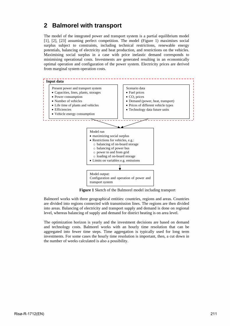
2 Balmorel with transport The model of the integrated power and transport system is a partial equilibrium model [1], [2], [23] assuming perfect competition. The model (Figure 1) maximises social surplus subject to constraints, including technical restrictions, renewable energy potentials, balancing of electricity and heat production, and restrictions on the vehicles. Maximising social surplus in a case with price inelastic demand corresponds to minimising operational costs. Investments are generated resulting in an economically optimal operation and configuration of the power system. Electricity prices are derived from marginal system operation costs.

Balmorel works with three geographical entities: countries, regions and areas. Countries are divided into regions connected with transmission lines. The regions are then divided into areas. Balancing of electricity and transport supply and demand is done on regional level, whereas balancing of supply and demand for district heating is on area level. The optimization horizon is yearly and the investment decisions are based on demand and technology costs. Balmorel works with an hourly time resolution that can be aggregated into fewer time steps. Time aggregation is typically used for long term investments. For some cases the hourly time resolution is important, then, a cut down in the number of weeks calculated is also a possibility.

Present power and transport system • Capacities, lines, plants, storages • Power consumption • Number of vehicles • Life time of plants and vehicles • Efficiencies • Vehicle energy consumption

Scenario data • Fuel prices • CO2 prices • Demand (power, heat, transport) • Prices of different vehicle types • Technology data future units

Model run • maximizing social surplus • Restrictions for vehicles, e.g.:

o balancing of on-board storage o balancing of power bus o power to and from grid o loading of on-board storage

• Limits on variables e.g. emissions

Model output: Configuration and operation of power and transport system

Input data

Figure 1 Sketch of the Balmorel model including transport

Risø-R-1712(EN) 211

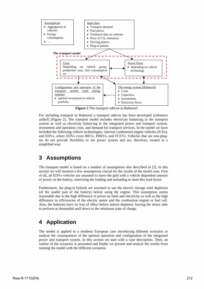
For including transport in Balmorel a transport add-on has been developed [reference artikel] (Figure 2). The transport model includes electricity balancing in the transport system as well as electricity balancing in the integrated power and transport system, investment and operation costs, and demand for transport services. In the model we have included the following vehicle technologies; internal combustion engine vehicles (ICEs), and EDVs, where EDVs cover BEVs, PHEVs, and FCEVs. Vehicles that are non-plug-ins do not provide flexibility to the power system and are, therefore, treated in a simplified way.

3 Assumptions The transport model is based on a number of assumptions also described in [2]. In this section we will mention a few assumptions crucial for the results of the model runs. First of all, all EDVs vehicles are assumed to leave the grid with a vehicle dependent amount of power on the battery, restricting the loading and unloading to meet this load factor. Furthermore, the plug-in hybrids are assumed to use the electric storage until depletion (of the usable part of the battery) before using the engine. This assumption seems reasonable due to the high difference in prices on fuels and electricity as well as the high difference in efficiencies of the electric motor and the combustion engine or fuel cell. Also, the batteries have no loss of effect before almost depleted, leaving the motor able to perform as demanded until down to the minimum state of charge.

4 Application The model is applied to a northern European case introducing different scenarios to analyse the consequences of the optimal operation and configuration of the integrated power and transport system. In this section we start with a case description. Then, an outline of the scenarios is presented and finally we present and analyse the results from running the model with the different scenarios.

Power flows • depending on vehicle

technology

Costs Depending on vehicle group, production year, fuel consumption etc.

Configuration and operation of the transport system (and energy system) • optimal investment in vehicle

portfolio

The energy system (Balmorel) • Costs • Capacities • Investments • Electricity flows

Input data • Transport demand • Fuel prices • Technical data on vehicles • Price of CO2 emissions • Driving pattern • Plug-in pattern

The transport model

Figure 3 The transport add-on in Balmorel

Assumptions • Aggregation of

vehicles • Energy

consumption • …

Figure 2 The transport add-on in Balmorel

Risø-R-1712(EN) 212

4.1 Base case Balmorel is run for the year 2030 for the Northern European countries including the Scandinavian countries and Germany. In order to be able to run the model within reasonable computation time for Norway, Sweden and Finland each country is aggregated into one region. For Germany we have aggregated the regions into two in order to represent the transmission bottlenecks between Northern Germany with a large share of wind power and the consumption centres in Central Germany. Denmark is split into two regions representing Western Denmark being synchronous with the UCTE power system and Eastern Denmark being synchronous with the Nordel power system. A number of inputs are required for running the model, e.g., fuel prices, CO2 prices, demand data, and vehicle and power system technology data, which are all given exogenously. In the base case, oil-prices are assumed to be $120/barrel, assuming constant price elasticities as in [23]. CO2-prices are assumed to be €40/ton. Data, such as the demand data, is to be given on a regional level (Table 1). Currently, there is no transmission between the two regions in Denmark, but for the year 2030 we have assumed a transmission capacity of 1.2 GW and a transmission loss of 1%.

Table 1 Demand input data year 2030 (source for all but Norway [25])

Denmark East

Denmark West Sweden Norway Finland Germany

Electricity demand (TWh/yr) 16 24 153 145 104 620

District heat demand (TWh/yr) 12 15 46 9 56 102

Transport demand (b. persons km/yr) 31 41 148 69 86 1262

In order for Balmorel to balance power demand and power supply, new technologies must be available for investment. Table 2 shows the technologies we have made available for investment in 2030 for the base case. With the analysis focusing on competition between technologies and incorporating more renewables, we find this list of technologies to be a good basis.

Table 2 Technology investment options in the simulation (all data except data on Electric boiler are from the Danish Energy Authority [26]). Investment costs for heat

storage and hydrogen storage are given as M€/MWh storage capacity.

Investment costs (M€/MW)

Variable costs (€/MW)

Annual costs (k€/MW)

Efficiency

Onshore wind 0.5 7 0 1 Offshore wind 1 4 4 1 CHP plant, biomass 1.3 2.7 25 0.45 Open cycle gas turbine 0.5 2 72 0.4 Combined cycle gas turbine, condensing 0.54 0.67 13.39 0.55

Combined cycle gas turbine, extraction 0.55 1.5 12.5 0.56

Heat storage 0.6 0 1 1 Heat pump 0.6 0 3 3.9 Electric boiler 0.04 0 1.2 0.98 Coal extraction 1.2 1.8 16 0.5 Heat boiler, biomass 0.32 4.02 19.28 0.85 Heat boiler, natural gas 0.05 0.67 0.54 0.95 Nuclear 1.89 1.37 37.75 0.35 Solid oxide electrolysis 0.18 0 5.4 0.93 Hydrogen storage, cavern 0.00058 0 0 0.83

Risø-R-1712(EN) 213

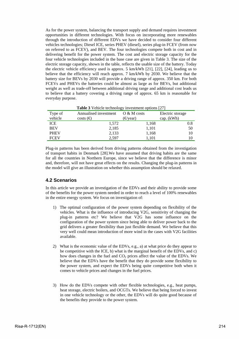
As for the power system, balancing the transport supply and demand requires investment opportunities in different technologies. With focus on incorporating more renewables through the introduction of different EDVs we have decided to consider four different vehicles technologies; Diesel ICE, series PHEV (diesel), series plug-in FCEV (from now on referred to as FCEV), and BEV. The four technologies compete both in cost and in delivering benefit for the power system. The cost and electric storage capacity for the four vehicle technologies included in the base case are given in Table 3. The size of the electric storage capacity, shown in the table, reflects the usable size of the battery. Today the electric vehicle efficiency used is approx. 5 km/kWh [21], [22], [24], leading us to believe that the efficiency will reach approx. 7 km/kWh by 2030. We believe that the battery size for BEVs by 2030 will provide a driving range of approx. 350 km. For both FCEVs and PHEVs the batteries could be almost as large as for BEVs, but additional weight as well as trade-off between additional driving range and additional cost leads us to believe that a battery covering a driving range of approx. 65 km is reasonable for everyday purpose.

Table 3 Vehicle technology investment options [27] Type of vehicle

Annualised investment costs (€)

O & M costs (€/year)

Electric storage cap. (kWh)

ICE 1,572 1,168 0.8 BEV 2,185 1,101 50 PHEV 2,133 1,168 10 FCEV 2,597 1,101 10

Plug-in patterns has been derived from driving patterns obtained from the investigation of transport habits in Denmark [28].We have assumed that driving habits are the same for all the countries in Northern Europe, since we believe that the difference is minor and, therefore, will not have great effects on the results. Changing the plug-in patterns in the model will give an illustration on whether this assumption should be relaxed.

4.2 Scenarios In this article we provide an investigation of the EDVs and their ability to provide some of the benefits for the power system needed in order to reach a level of 100% renewables in the entire energy system. We focus on investigation of:

1) The optimal configuration of the power system depending on flexibility of the vehicles. What is the influence of introducing V2G, sensitivity of changing the plug-in patterns etc? We believe that V2G has some influence on the configuration of the power system since being able to deliver power back to the grid delivers a greater flexibility than just flexible demand. We believe that this very well could mean introduction of more wind in the cases with V2G facilities available.

2) What is the economic value of the EDVs, e.g., a) at what price do they appear to

be competitive with the ICE, b) what is the marginal benefit of the EDVs, and c) how does changes in the fuel and CO2 prices affect the value of the EDVs. We believe that the EDVs have the benefit that they do provide some flexibility to the power system, and expect the EDVs being quite competitive both when it comes to vehicle prices and changes in the fuel prices.

3) How do the EDVs compete with other flexible technologies, e.g., heat pumps, heat storage, electric boilers, and OCGTs. We believe that being forced to invest in one vehicle technology or the other, the EDVs will do quite good because of the benefits they provide to the power system.

Risø-R-1712(EN) 214

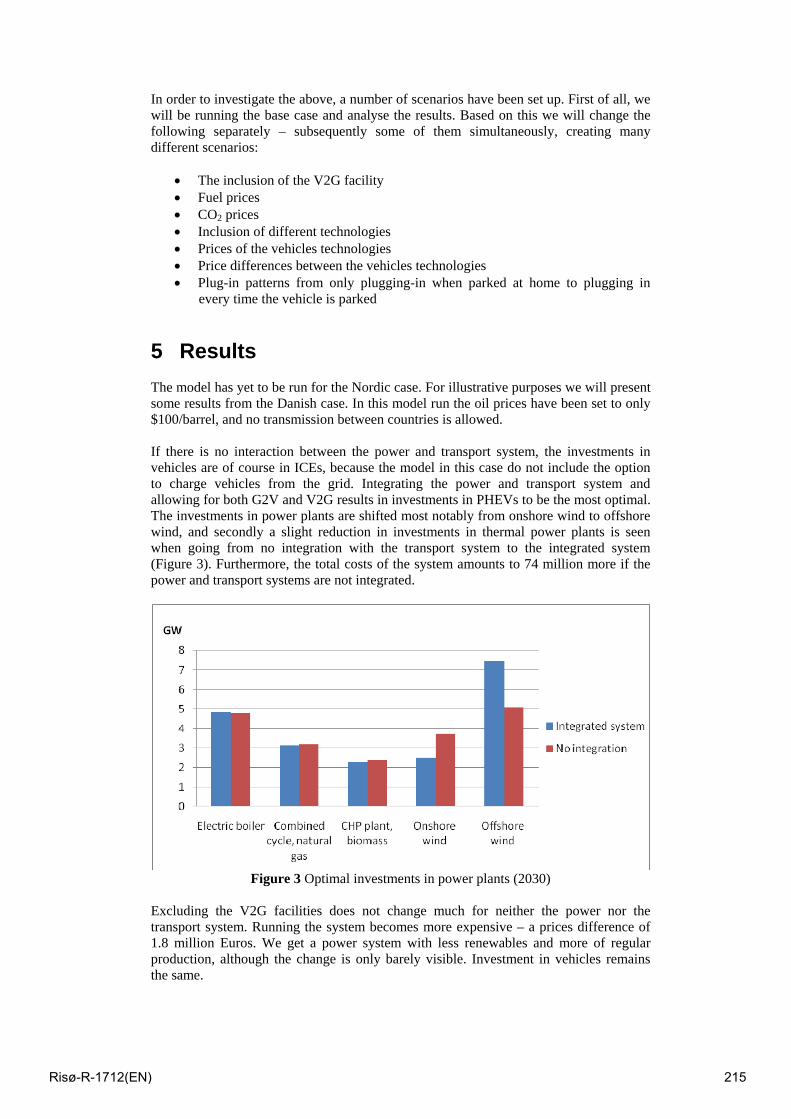
In order to investigate the above, a number of scenarios have been set up. First of all, we will be running the base case and analyse the results. Based on this we will change the following separately – subsequently some of them simultaneously, creating many different scenarios:

• The inclusion of the V2G facility • Fuel prices • CO2 prices • Inclusion of different technologies • Prices of the vehicles technologies • Price differences between the vehicles technologies • Plug-in patterns from only plugging-in when parked at home to plugging in

every time the vehicle is parked

5 Results The model has yet to be run for the Nordic case. For illustrative purposes we will present some results from the Danish case. In this model run the oil prices have been set to only $100/barrel, and no transmission between countries is allowed. If there is no interaction between the power and transport system, the investments in vehicles are of course in ICEs, because the model in this case do not include the option to charge vehicles from the grid. Integrating the power and transport system and allowing for both G2V and V2G results in investments in PHEVs to be the most optimal. The investments in power plants are shifted most notably from onshore wind to offshore wind, and secondly a slight reduction in investments in thermal power plants is seen when going from no integration with the transport system to the integrated system (Figure 3). Furthermore, the total costs of the system amounts to 74 million more if the power and transport systems are not integrated.

Figure 3 Optimal investments in power plants (2030) Excluding the V2G facilities does not change much for neither the power nor the transport system. Running the system becomes more expensive – a prices difference of 1.8 million Euros. We get a power system with less renewables and more of regular production, although the change is only barely visible. Investment in vehicles remains the same.

Risø-R-1712(EN) 215

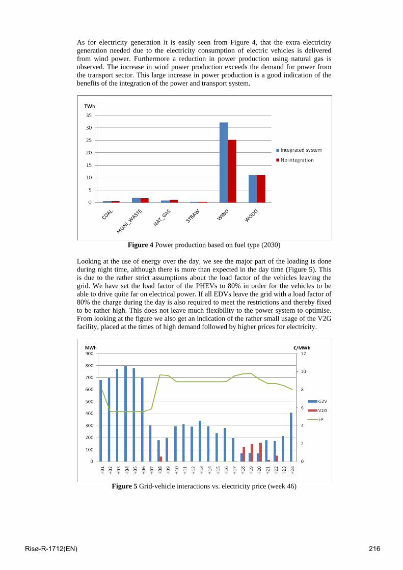
As for electricity generation it is easily seen from Figure 4, that the extra electricity generation needed due to the electricity consumption of electric vehicles is delivered from wind power. Furthermore a reduction in power production using natural gas is observed. The increase in wind power production exceeds the demand for power from the transport sector. This large increase in power production is a good indication of the benefits of the integration of the power and transport system.

Figure 4 Power production based on fuel type (2030)

Looking at the use of energy over the day, we see the major part of the loading is done during night time, although there is more than expected in the day time (Figure 5). This is due to the rather strict assumptions about the load factor of the vehicles leaving the grid. We have set the load factor of the PHEVs to 80% in order for the vehicles to be able to drive quite far on electrical power. If all EDVs leave the grid with a load factor of 80% the charge during the day is also required to meet the restrictions and thereby fixed to be rather high. This does not leave much flexibility to the power system to optimise. From looking at the figure we also get an indication of the rather small usage of the V2G facility, placed at the times of high demand followed by higher prices for electricity.

Figure 5 Grid-vehicle interactions vs. electricity price (week 46)

Risø-R-1712(EN) 216

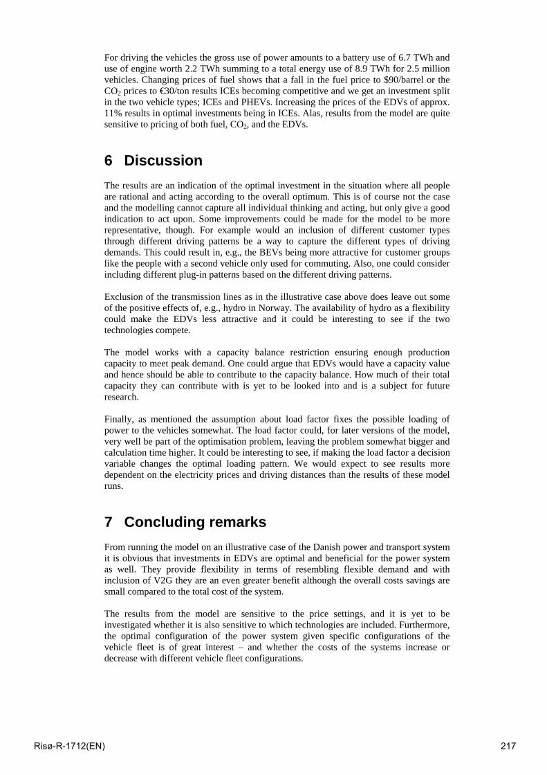
For driving the vehicles the gross use of power amounts to a battery use of 6.7 TWh and use of engine worth 2.2 TWh summing to a total energy use of 8.9 TWh for 2.5 million vehicles. Changing prices of fuel shows that a fall in the fuel price to $90/barrel or the CO2 prices to €30/ton results ICEs becoming competitive and we get an investment split in the two vehicle types; ICEs and PHEVs. Increasing the prices of the EDVs of approx. 11% results in optimal investments being in ICEs. Alas, results from the model are quite sensitive to pricing of both fuel, CO2, and the EDVs.

6 Discussion The results are an indication of the optimal investment in the situation where all people are rational and acting according to the overall optimum. This is of course not the case and the modelling cannot capture all individual thinking and acting, but only give a good indication to act upon. Some improvements could be made for the model to be more representative, though. For example would an inclusion of different customer types through different driving patterns be a way to capture the different types of driving demands. This could result in, e.g., the BEVs being more attractive for customer groups like the people with a second vehicle only used for commuting. Also, one could consider including different plug-in patterns based on the different driving patterns. Exclusion of the transmission lines as in the illustrative case above does leave out some of the positive effects of, e.g., hydro in Norway. The availability of hydro as a flexibility could make the EDVs less attractive and it could be interesting to see if the two technologies compete. The model works with a capacity balance restriction ensuring enough production capacity to meet peak demand. One could argue that EDVs would have a capacity value and hence should be able to contribute to the capacity balance. How much of their total capacity they can contribute with is yet to be looked into and is a subject for future research. Finally, as mentioned the assumption about load factor fixes the possible loading of power to the vehicles somewhat. The load factor could, for later versions of the model, very well be part of the optimisation problem, leaving the problem somewhat bigger and calculation time higher. It could be interesting to see, if making the load factor a decision variable changes the optimal loading pattern. We would expect to see results more dependent on the electricity prices and driving distances than the results of these model runs.

7 Concluding remarks From running the model on an illustrative case of the Danish power and transport system it is obvious that investments in EDVs are optimal and beneficial for the power system as well. They provide flexibility in terms of resembling flexible demand and with inclusion of V2G they are an even greater benefit although the overall costs savings are small compared to the total cost of the system. The results from the model are sensitive to the price settings, and it is yet to be investigated whether it is also sensitive to which technologies are included. Furthermore, the optimal configuration of the power system given specific configurations of the vehicle fleet is of great interest – and whether the costs of the systems increase or decrease with different vehicle fleet configurations.

Risø-R-1712(EN) 217

In this model the wind power production is predictive and not stochastic. Making the wind power stochastic would probably change the results quite a lot and is a subject for future research. With unknown actual production the need for reserves will be different and we would expect the value of the EDVs to rise. Future research also includes transforming the load factor into a decision variable, creating different customer profiles, having EDVs provide capacity credit, as well as vehicles with different features for each vehicle technology.

References [1]. Ravn H, et al., Balmorel: A Model for Analyses of the Electricity and CHP

Markets in the Baltic Sea Region., http://balmorel.com/Doc/B-MainReport03.pdf, 2001)

[2]. Juul, N. and Meibom, P., Optimal configuration of future energy systems including road transport and vehicle-to-grid capabilities, to be submitted to Journal of Power Sources, 2009.

[3]. Kempton, W. and Tomic, J., Vehicle-to-grid power fundamentals: Calculating capacity and net revenue, Journal of Power Sources, Vol. 144, pp 268-279, 2005

[4]. Kempton, W., Tomic, J., Letendre, S., Brooks, A., and Lipman, T., Vehicle-to-Grid Power: Battery, Hybrid, and Fuel Cell Vehicles as Resources for Distributed Electric Power in California, UCD-ITS-RR-01-03, 2001

[5]. Kempton W and T. Kubo, Electric-drive vehicles for peak power in Japan, Energy Policy 28, pp 9-18, 2000

[6]. Tomic, J. and Kempton, W., Using fleets of electric-drive vehicles for grid support, Journal of Power Sources, Vol. 168, No. 2, pp 459-468, 2007

[7]. Brooks, A., Vehicle-to-grid Demonstration Project: Grid Regulation Ancillary Service with a Battery Electric Vehicle, Report, AC Propulsion Inc., 2002

[8]. Moura, F., Driving energy system transformation with “vehicle-to-grid” power, Interim Report IR-06-025, 2006

[9]. Lipman, T., Integration of Motor Vehicle and Distributed Energy Systems, Encyclopedia of Energy, Vol. 3, pp 475-486, 2004

[10]. Kempton, W. and Tomic, J., Vehicle-to-grid power implementation: From stabilizing the grid to supporting large scale renewable energy, Journal of Power Sources, Vol. 144, pp 280-294, 2005

[11]. Brooks, A. and Gage, T., Integration of Electric Drive Vehicles with the Electric Power Grid -- a New Value Stream, Conference Proceeding, 18th International Electric Vehicle Symposium (EVS-18), 2001

[12]. Kempton, W. and Letendre, S., Electric vehicles as a new power source for electric utilities, Transportation Research, Vol. 2, No. 3, pp 157-175, 1997

[13]. Greene, D. L., Leiby, P. N., James, B., Perez, J., Melendez, M., Milbrandt, A., Unnasch, S., Rutherford, D., and Hooks, M., Hydrogen Scenario Analysis Summary Report: Analysis of the Transition to Hydrogen Fuel Cell Vehicles and the Potential Hydrogen Energy Infrastructure Requirements, Technical report, ORNL/TM-2008/030, 2008

[14]. Lipman, T. and Hwang, R., Hybrid Electric And Fuel Cell Vehicle Technological Innovation: Hybrid and Zero-Emission Vehicle Technology Links, 20th International Electric Vehicle Symposium and Exposition, 2003

[15]. Williams, B. D. and Kurani, K. S., Commercializing light-duty plug-in/plug-out hydrogen-fuel-cell vehicles: “Mobile Electricity” technologies and opportunities, Journal of Power Sources, Vol. 166, No. 2, pp 549-566, 2007

[16]. Turton, H. and Moura, F., Vehicle-to-grid systems for sustainable development: An integrated energy analysis, Technological Forecasting and Social Change, 2008, doi:10.1016/j.techfore.2007.11.013

[17]. Delucchi, M. A. and Lipman, T., An analysis of the retail and lifecycle cost of battery-powered electric vehicles, Transportation Research Part D: Transport and Environment, Vol. 6, No. 6, pp 371-404, 2001

Risø-R-1712(EN) 218

[18]. Lipman, T. and Delucchi, M. A., Hybrid-Electric Vehicle Design Retail and Lifecycle Cost Analysis, report, UCD-ITS-RR-03-01, 2003

[19]. Markel, T., Brooker, A., Hendricks, T., Johnson, V., Kelly, K., Kramer, B., O'Keefe, M., Sprik, S., and Wipke, K., ADVISOR: a systems analysis tool for advanced vehicle modelling, Journal of Power Sources, Vol. 110, No. 2, pp 255-266, 2002

[20]. McCarthy, R. W., Yang, C., and Ogden, J. M., Impacts of electric-drive vehicles on California's energy system, report, UCD-ITS-RP-08-24, 2008

[21]. Short, W. and Denholm, P., A Preliminary Assessment of Plug-In Hybrid Electric Vehicles on Wind Energy Markets, Technical Report, NREL/TP-620-39729, 2006

[22]. Denholm, P. and Short, W., Evaluation of Utility System Impacts and Benefits of Optimally Dispatched Plug-In Hybrid Electric Vehicles, technical report, NREL/TP-620-40293, 2006

[23]. Karlsson, K. and Meibom, P., Optimal investment paths for future renewable based energy systems—Using the optimisation model Balmorel, Int J Hydrogen Energy, doi:10.1016/j.ijhydene.2008.01.031, 2008

[24]. Delucchi, M. A., Burke, A., Lipman, T., Miller, M., Electric and Gasoline Vehicle Lifecycle Cost and Energy-Use Model, report, UCD-ITS-RR-99-04, 2000

[25]. European Commission, Directorate of Energy and Transport, European energy and Transport Trends to 2030 – Update 2007, ISBN 978-92-79-07620-6, 2007

[26]. Danish Energy Authority, Technology Data for Electricity and Heat Generating Plants, ISBN: 87-7844-502-7, 2005

[27]. Energistyrelsen (Danish Energy Authority), Teknologivurdering af alternative drivmidler til transportsektoren, Report, http://193.88.185.141/Graphics/Lovstof/hoeringer/COWIrapport%20Alt%20drivmidler.pdf , may, 2007

[28]. Transport, DTU, ”Transportvaneundersøgelsen“, http://www.dtu.dk/centre/modelcenter/TU.aspx, 2006

Risø-R-1712(EN) 219

Session 13 – Carbon capture and storage

Risø-R-1712(EN) 220

Aqueous ammonia process for CO2 capture Victor Darde1, 2, Kaj Thomsen1, Willy J.M. van Well2 and Erling H. Stenby1

1Department of Chemical and Biochemical Engineering, Technical University of Denmark 2Chemical & Materials Department, DONG Energy Power, Denmark

Abstract This work deals with the study of a post combustion carbon dioxide capture process using aqueous solutions of ammonia as solvent. Amine solutions have been commonly used for the commercial production of CO2. The main disadvantage related to the use of amine solutions is the high energy consumption (3.5 - 4 GJ/ton CO2) and the high degradation rate of the amines. The heat of absorption of carbon dioxide by ammonia is significantly lower than for alkanolamines. Hence, this process shows good perspectives. However, a scientific understanding of the processes is required. In order to simulate and optimize the process, a thermodynamic model for the system is required. The properties of the NH3-CO2-H2O system were previously modeled using the Extended UNIQUAC electrolyte model in the temperature range from 0 to 110°C, the pressure range from 0 to 100 bars and for a molality of ammonia up to approximately 80 [1]. In this work, the validity of this model was extended up to 150°C. Also additional data for the enthalpy of partial evaporation and speciation data were used. The equilibrium composition and enthalpy of the different streams of the process have been studied, based on the information from the patent [2]. The results show that solid phases consisting of ammonium carbonate compounds are formed in the absorber. It also shows that the pure CO2 stream that leaves the stripper is pressurized. The energy requirements in the absorber and in the desorber have been studied. An energy consumption in the desorber lower than 2 GJ/ton CO2 can be reached.

1 Introduction The proportion of carbon dioxide emissions from power production is very significant in industrialized countries. In Denmark, in 2004, they represented 61% of the total CO2 emissions [3]. Therefore, regarding the reduction objectives endorsed by many governments, efforts are being made to develop technologies allowing the decrease of the emissions from the power plants. Carbon dioxide capture implies separating the CO2 from the flue gases from a power plant or other industry instead of releasing the CO2 in the atmosphere. Different methods are under development to capture CO2 from coal-fired power plants. Post-combustion techniques separate the carbon dioxide from the flue gas after a traditional combustion process. The main advantage of such technique is that the combustion at the power plant is unaltered, so the process can be implemented on existing power plants. Amine solutions have been commonly used for the commercial production of CO2 and have been tested for CO2 capture on pilot scale. However such technologies require a large amount of energy, especially in the desorption part of the process [4]. In addition, the use of amines entails some problems related to solvent degradation and corrosion [5, 6]. Therefore, new alternatives for post-combustion capture are searched for. Processes using aqueous ammonia as solvent are some of the promising alternatives. The ammonia process is found in two variants, depending on the temperature of absorption. The first variant absorbs the CO2 at low temperature (2-10°C)

Risø-R-1712(EN) 221

and is therefore called chilled ammonia process. The low temperature process has the advantage of decreasing the ammonia slip in the absorber and decreasing the flue gas volume. This process allows precipitation of several ammonium carbonate compounds in the absorber. The second process absorbs CO2 at ambient temperature (25-40°C) and does not allow precipitation. This study focuses on the chilled ammonia process.

2 Description of the patented process The use of chilled ammonia to capture carbon dioxide was patented in 2006 by Eli Gal [2]. The process described in the patent requires several steps. First, the purpose of the process is to absorb the carbon dioxide at a low temperature. The patent indicates a temperature range from 0 to 20°C, and preferably from 0 to 10°C. Hence, it is first necessary to cool down the flue gas that contains the CO2. This is done by using Direct Contact Coolers at the entrance of the process. The temperature of the gas that leaves the cooling subsystem is between 0 and 10°C. This stream contains low moisture and almost no particulate matter, acidic or volatile species. Indeed, the low temperature decreases the vapor pressure of these compounds as it promotes their condensation into the water. Then, the flue gas enters the CO2 capture and regeneration subsystem. This subsystem consists, like the capture processes using amines, of absorption and desorption columns. The cold flue gas enters the bottom of the absorber while the CO2-lean stream enters the top of it. The CO2-lean stream is mainly composed of water, ammonia and carbon dioxide. The mass fraction of ammonia in the solvent is typically to 10wt%. The pressure in the absorber should be close to atmospheric pressure, while the temperature should be in the range 0-20°C, and preferably 0-10°C. This low temperature prevents the ammonia from evaporating. According to the patent, the CO2-lean stream should have a CO2 loading (the ratio of the number of mole of carbon dioxide and ammonia in their various aqueous forms) between 0.25 and 0.67, and preferably between 0.33 and 0.67. A low CO2 loading in the top of the absorber where the CO2-lean stream is fed in increases the vapor pressure of ammonia which implies its evaporation. On the other hand, a high CO2 loading for the CO2-lean stream decreases the efficiency of the absorption. Under the conditions described above and according to the patent, more than 90% of the CO2 from the flue gas can be captured. The cleaned gas stream can leave the absorber by its top. This stream contains residual ammonia, which is washed out by using cold water and an acidic solution. The treated stream is reintroduced into the system. The cleaned gas mainly contains nitrogen, oxygen and a low concentration of carbon dioxide. The CO2-rich stream leaves the bottom of the absorber. It might be composed of a solid and a liquid phase. Indeed, at this temperature and under those conditions, the solubility limits may be reached. Hence, the CO2-rich stream is a slurry. Its CO2 loading is between 0.5 and 1, and preferably between 0.67 and 1. The patent mentions that a part of the CO2-rich stream could be recycled to the absorber in order to increase the CO2 loading of the CO2-rich stream by producing more solids.

The CO2-rich stream is pressurized and pumped to a heat exchanger where its temperature increases, and then sent to the desorber using a high pressure pump. The desorber temperature is in the range of 50-200°C, and preferably 100-150°C while the pressure is in the range of 2-136 atmospheres. Under those conditions, the vaporization of ammonia and water implied by the high temperature is reduced. The conditions cause CO2 to evaporate from the solution. It leaves the top of the desorber as a relatively clean and high pressure stream. The water vapor and the ammonia that are contained in this stream can be recovered by cold washing, possibly using weak acid to increase the efficiency.

The desorption reaction is endothermic, but the energy that has to be supplied is much lower than for MEA or other amines according to the patent. This energy highly depends

Risø-R-1712(EN) 222

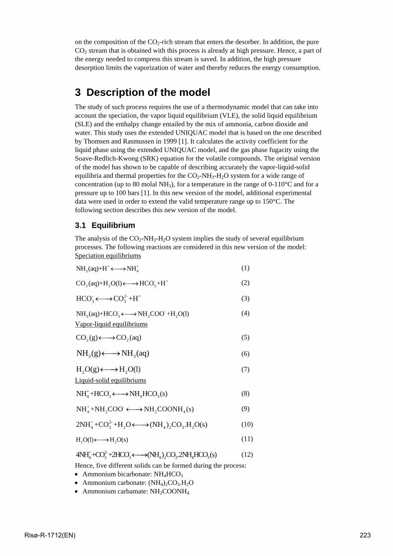
on the composition of the CO2-rich stream that enters the desorber. In addition, the pure CO2 stream that is obtained with this process is already at high pressure. Hence, a part of the energy needed to compress this stream is saved. In addition, the high pressure desorption limits the vaporization of water and thereby reduces the energy consumption.

3 Description of the model The study of such process requires the use of a thermodynamic model that can take into account the speciation, the vapor liquid equilibrium (VLE), the solid liquid equilibrium (SLE) and the enthalpy change entailed by the mix of ammonia, carbon dioxide and water. This study uses the extended UNIQUAC model that is based on the one described by Thomsen and Rasmussen in 1999 [1]. It calculates the activity coefficient for the liquid phase using the extended UNIQUAC model, and the gas phase fugacity using the Soave-Redlich-Kwong (SRK) equation for the volatile compounds. The original version of the model has shown to be capable of describing accurately the vapor-liquid-solid equilibria and thermal properties for the CO2-NH3-H2O system for a wide range of concentration (up to 80 molal NH3), for a temperature in the range of 0-110°C and for a pressure up to 100 bars [1]. In this new version of the model, additional experimental data were used in order to extend the valid temperature range up to 150°C. The following section describes this new version of the model.

3.1 Equilibrium The analysis of the CO2-NH3-H2O system implies the study of several equilibrium processes. The following reactions are considered in this new version of the model: Speciation equilibriums

+ +3 4NH (aq)+H NH←⎯→ (1)

- +2 2 3CO (aq)+H O(l) HCO +H←⎯→ (2)

- 2- +3 3HCO CO +H←⎯→ (3)

- -3 3 2 2NH (aq)+HCO NH COO +H O(l)←⎯→ (4)

Vapor-liquid equilibriums

2 2CO (g) CO (aq)←⎯→ (5)

3 3NH (g) NH (aq)←⎯→ (6)

2 2H O(g) H O(l)←⎯→ (7) Liquid-solid equilibriums

+ -4 3 4 3NH +HCO NH HCO (s)←⎯→ (8)

+ -4 2 2 4NH +NH COO NH COONH (s)←⎯→ (9)

+ 2-4 3 2 4 2 3 22NH +CO +H O (NH ) CO .H O(s)←⎯→ (10)

2 2H O(l) H O(s)←⎯→ (11)

+ 2- -4 3 3 4 2 3 4 34NH +CO +2HCO (NH ) CO .2NH HCO (s)←⎯→ (12)

Hence, five different solids can be formed during the process: • Ammonium bicarbonate: NH4HCO3 • Ammonium carbonate: (NH4)2CO3.H2O • Ammonium carbamate: NH2COONH4

Risø-R-1712(EN) 223

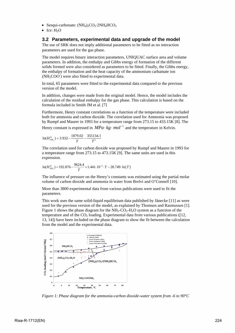
• Sesqui-carbonate: (NH4)2CO3·2NH4HCO3 • Ice: H2O

3.2 Parameters, experimental data and upgrade of the model The use of SRK does not imply additional parameters to be fitted as no interaction parameters are used for the gas phase.

The model requires binary interaction parameters, UNIQUAC surface area and volume parameters. In addition, the enthalpy and Gibbs energy of formation of the different solids formed were also considered as parameters to be fitted. Finally, the Gibbs energy, the enthalpy of formation and the heat capacity of the ammonium carbamate ion (NH2COO-) were also fitted to experimental data.

In total, 65 parameters were fitted to the experimental data compared to the previous version of the model.

In addition, changes were made from the original model. Hence, the model includes the calculation of the residual enthalpy for the gas phase. This calculation is based on the formula included in Smith JM et al. [7]

Furthermore, Henry constant correlations as a function of the temperature were included both for ammonia and carbon dioxide. The correlation used for Ammonia was proposed by Rumpf and Maurer in 1993 for a temperature range from 273.15 to 433.15K [8]. The Henry constant is expressed in 1MPa kg mol−⋅ ⋅ and the temperature in Kelvin.

3 2

1879.02 355134.1ln( ) 3.932mNHH

T T= − −

The correlation used for carbon dioxide was proposed by Rumpf and Maurer in 1993 for a temperature range from 273.15 to 473.15K [9]. The same units are used in this expression.

( )3

29624.4ln( ) 192.876 1.441 10 28.749 lnmNHH T T

T−= − + ⋅ ⋅ − ⋅

The influence of pressure on the Henry’s constants was estimated using the partial molar volume of carbon dioxide and ammonia in water from Brelvi and O’Connell [10].

More than 3800 experimental data from various publications were used to fit the parameters.

This work uses the same solid-liquid equilibrium data published by Jänecke [11] as were used for the previous version of the model, as explained by Thomsen and Rasmussen [1]. Figure 1 shows the phase diagram for the NH3-CO2-H2O system as a function of the temperature and of the CO2 loading. Experimental data from various publications ([12, 13, 14]) have been included on the phase diagram to show the fit between the calculation from the model and the experimental data.

0

0,1

0,2

0,3

0,4

0,5

0,6

0,7

0,8

-6 4 14 24 34 44 54 64 74 84Temperature, °C

CO

2 loa

ding

(mol

CO 2

/mol

NH 3

)

Extended UNIQUACJänecke (1929)Terres & Weiser (1921)Terres & Behrens (1928)Guyer & Piechowicz (1944)

(NH4)2CO3•H2O

NH2COONH4

NH4HCO3

(NH4)2CO3•2NH4HCO3

Figure 1: Phase diagram for the ammonia-carbon dioxide-water system from -6 to 90°C

Risø-R-1712(EN) 224

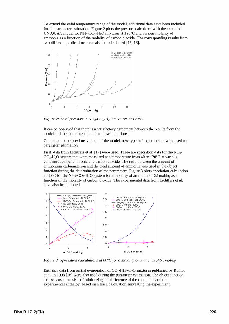
To extend the valid temperature range of the model, additional data have been included for the parameter estimation. Figure 2 plots the pressure calculated with the extended UNIQUAC model for NH3-CO2-H2O mixtures at 120°C and various molality of ammonia as a function of the molality of carbon dioxide. The corresponding results from two different publications have also been included [15, 16].

0

10

20

30

40

50

0 2 4 6 8 10 12

CO2 mol kg-1

Pres

sure

(Bar

)

Göppert et al. (1988)Müller et al. (1988)Extended UNIQUAC

Figure 2: Total pressure in NH3-CO2-H2O mixtures at 120°C

It can be observed that there is a satisfactory agreement between the results from the model and the experimental data at these conditions.

Compared to the previous version of the model, new types of experimental were used for parameter estimation.

First, data from Lichtfers et al. [17] were used. These are speciation data for the NH3-CO2-H2O system that were measured at a temperature from 40 to 120°C at various concentrations of ammonia and carbon dioxide. The ratio between the amount of ammonium carbamate ion and the total amount of ammonia was used in the object function during the determination of the parameters. Figure 3 plots speciation calculation at 80°C for the NH3-CO2-H2O system for a molality of ammonia of 6.1mol/kg as a function of the molality of carbon dioxide. The experimental data from Lichtfers et al. have also been plotted.

0

1

2

3

4

5

6

7

0 2 4

m CO2 mol/kg

NH3(aq), Extended UNIQUACNH4+, Extended UNIQUACNH2COO-, Extended UNIQUACNH3, Lichtfers, 2000NH4+, Lichtfers, 2000NH2COO-, Lichtfers, 2000

0

0,5

1

1,5

2

2,5

3

3,5

4

0 2 4

m CO2 mol/kg

HCO3-, Extended UNIQUACCO3--, Extended UNIQUACCO2(aq), Extended UNIQUACCO2, Lichtfers, 2000CO3--, Lichtfers, 2000HCO3-, Lichtfers, 2000

Figure 3: Speciation calculations at 80°C for a molality of ammonia of 6.1mol/kg

Enthalpy data from partial evaporation of CO2-NH3-H2O mixtures published by Rumpf et al. in 1998 [18] were also used during the parameter estimation. The object function that was used consists of minimizing the difference of the calculated and the experimental enthalpy, based on a flash calculation simulating the experiment.

Risø-R-1712(EN) 225

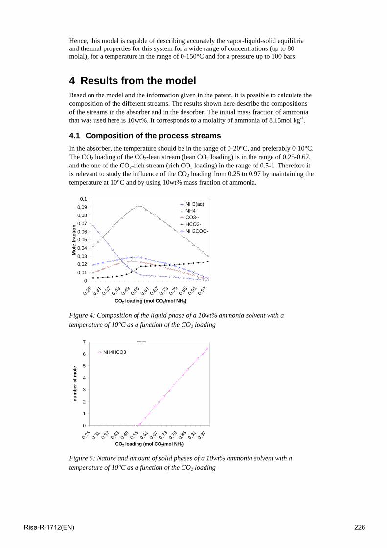
Hence, this model is capable of describing accurately the vapor-liquid-solid equilibria and thermal properties for this system for a wide range of concentrations (up to 80 molal), for a temperature in the range of 0-150°C and for a pressure up to 100 bars.

4 Results from the model Based on the model and the information given in the patent, it is possible to calculate the composition of the different streams. The results shown here describe the compositions of the streams in the absorber and in the desorber. The initial mass fraction of ammonia that was used here is 10wt%. It corresponds to a molality of ammonia of 8.15mol kg-1.

4.1 Composition of the process streams In the absorber, the temperature should be in the range of 0-20°C, and preferably 0-10°C. The CO2 loading of the CO2-lean stream (lean CO2 loading) is in the range of 0.25-0.67, and the one of the CO2-rich stream (rich CO2 loading) in the range of 0.5-1. Therefore it is relevant to study the influence of the CO2 loading from 0.25 to 0.97 by maintaining the temperature at 10°C and by using 10wt% mass fraction of ammonia.

00,01

0,020,030,040,050,060,070,08

0,090,1

0,25

0,

31 0,

37 0,

43 0,

49 0,

55 0,

61 0,

67 0,

73 0,

79 0,

85 0,

91 0,

97

CO2 loading (mol CO2/mol NH3)

Mol

e fr

actio

n

NH3(aq)NH4+CO3--HCO3-NH2COO-

Figure 4: Composition of the liquid phase of a 10wt% ammonia solvent with a temperature of 10°C as a function of the CO2 loading

NH4HCO3

0

1

2

3

4

5

6

7

0,25

0,

31 0,

37 0,

43 0,

49 0,

55 0,

61 0,

67 0,

73 0,

79 0,

85 0,

91 0,

97

CO2 loading (mol CO2/mol NH3)

num

ber o

f mol

e

NH4HCO3

Figure 5: Nature and amount of solid phases of a 10wt% ammonia solvent with a temperature of 10°C as a function of the CO2 loading

Risø-R-1712(EN) 226

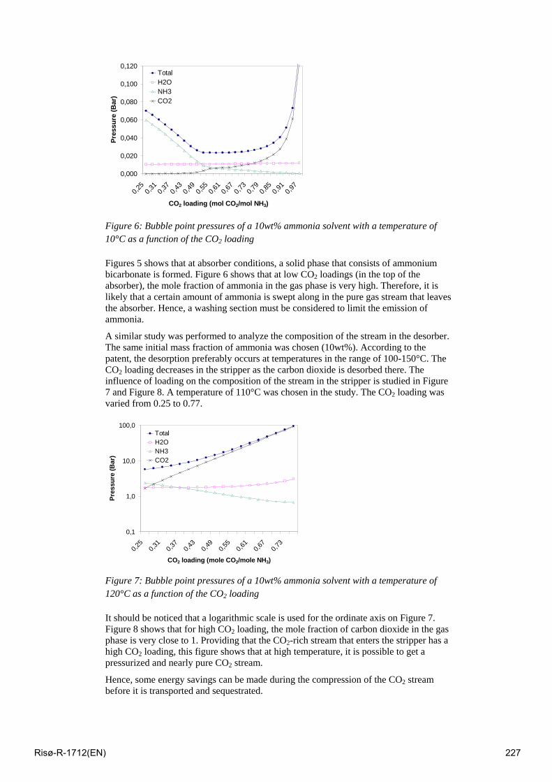
0,000

0,020

0,040

0,060

0,080

0,100

0,120

0,25

0,

31 0,

37 0,

43 0,

49 0,

55 0,

61 0,

67 0,

73 0,

79 0,

85 0,

91 0,

97

CO2 loading (mol CO2/mol NH3)

Pres

sure

(Bar

)

TotalH2ONH3CO2

Figure 6: Bubble point pressures of a 10wt% ammonia solvent with a temperature of 10°C as a function of the CO2 loading

Figures 5 shows that at absorber conditions, a solid phase that consists of ammonium bicarbonate is formed. Figure 6 shows that at low CO2 loadings (in the top of the absorber), the mole fraction of ammonia in the gas phase is very high. Therefore, it is likely that a certain amount of ammonia is swept along in the pure gas stream that leaves the absorber. Hence, a washing section must be considered to limit the emission of ammonia.

A similar study was performed to analyze the composition of the stream in the desorber. The same initial mass fraction of ammonia was chosen (10wt%). According to the patent, the desorption preferably occurs at temperatures in the range of 100-150°C. The CO2 loading decreases in the stripper as the carbon dioxide is desorbed there. The influence of loading on the composition of the stream in the stripper is studied in Figure 7 and Figure 8. A temperature of 110°C was chosen in the study. The CO2 loading was varied from 0.25 to 0.77.

0,1

1,0

10,0

100,0

0,25

0,

31

0,37

0,

43

0,49

0,

55

0,61

0,

67

0,73

CO2 loading (mole CO2/mole NH3)

Pres

sure

(Bar

)

TotalH2ONH3CO2

Figure 7: Bubble point pressures of a 10wt% ammonia solvent with a temperature of 120°C as a function of the CO2 loading

It should be noticed that a logarithmic scale is used for the ordinate axis on Figure 7. Figure 8 shows that for high CO2 loading, the mole fraction of carbon dioxide in the gas phase is very close to 1. Providing that the CO2-rich stream that enters the stripper has a high CO2 loading, this figure shows that at high temperature, it is possible to get a pressurized and nearly pure CO2 stream.

Hence, some energy savings can be made during the compression of the CO2 stream before it is transported and sequestrated.

Risø-R-1712(EN) 227

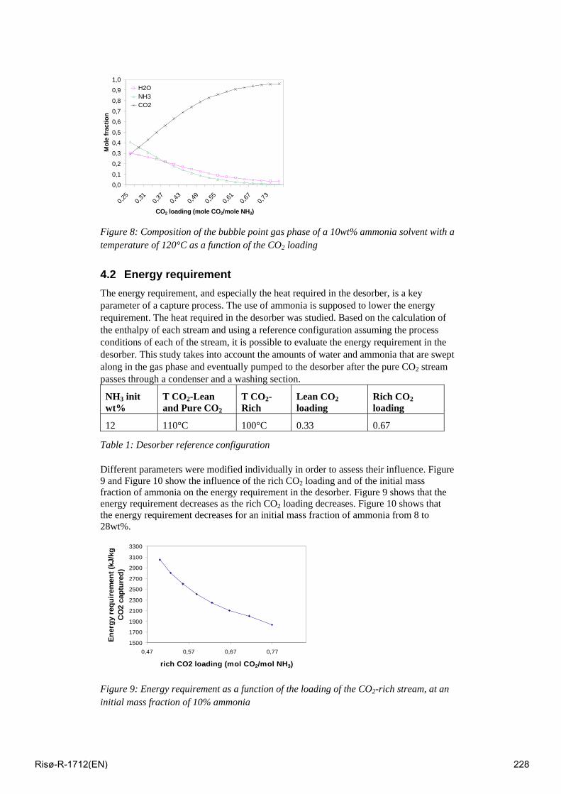
0,00,1

0,20,3

0,4

0,5

0,6

0,7

0,8

0,9

1,0

0,25

0,

31

0,37

0,

43

0,49

0,

55

0,61

0,

67

0,73

CO2 loading (mole CO2/mole NH3)

Mol

e fr

actio

n

H2ONH3CO2

Figure 8: Composition of the bubble point gas phase of a 10wt% ammonia solvent with a temperature of 120°C as a function of the CO2 loading

4.2 Energy requirement The energy requirement, and especially the heat required in the desorber, is a key parameter of a capture process. The use of ammonia is supposed to lower the energy requirement. The heat required in the desorber was studied. Based on the calculation of the enthalpy of each stream and using a reference configuration assuming the process conditions of each of the stream, it is possible to evaluate the energy requirement in the desorber. This study takes into account the amounts of water and ammonia that are swept along in the gas phase and eventually pumped to the desorber after the pure CO2 stream passes through a condenser and a washing section.

NH3 init wt%

T CO2-Lean and Pure CO2

T CO2-Rich

Lean CO2 loading

Rich CO2 loading

12 110°C 100°C 0.33 0.67

Table 1: Desorber reference configuration

Different parameters were modified individually in order to assess their influence. Figure 9 and Figure 10 show the influence of the rich CO2 loading and of the initial mass fraction of ammonia on the energy requirement in the desorber. Figure 9 shows that the energy requirement decreases as the rich CO2 loading decreases. Figure 10 shows that the energy requirement decreases for an initial mass fraction of ammonia from 8 to 28wt%.

1500

1700

1900

2100

2300

2500

2700

2900

3100

3300

0,47 0,57 0,67 0,77

rich CO2 loading (mol CO2/mol NH3)

Ener

gy r

equi

rem

ent (

kJ/k

g C

O2

capt

ured

)

Figure 9: Energy requirement as a function of the loading of the CO2-rich stream, at an initial mass fraction of 10% ammonia

Risø-R-1712(EN) 228

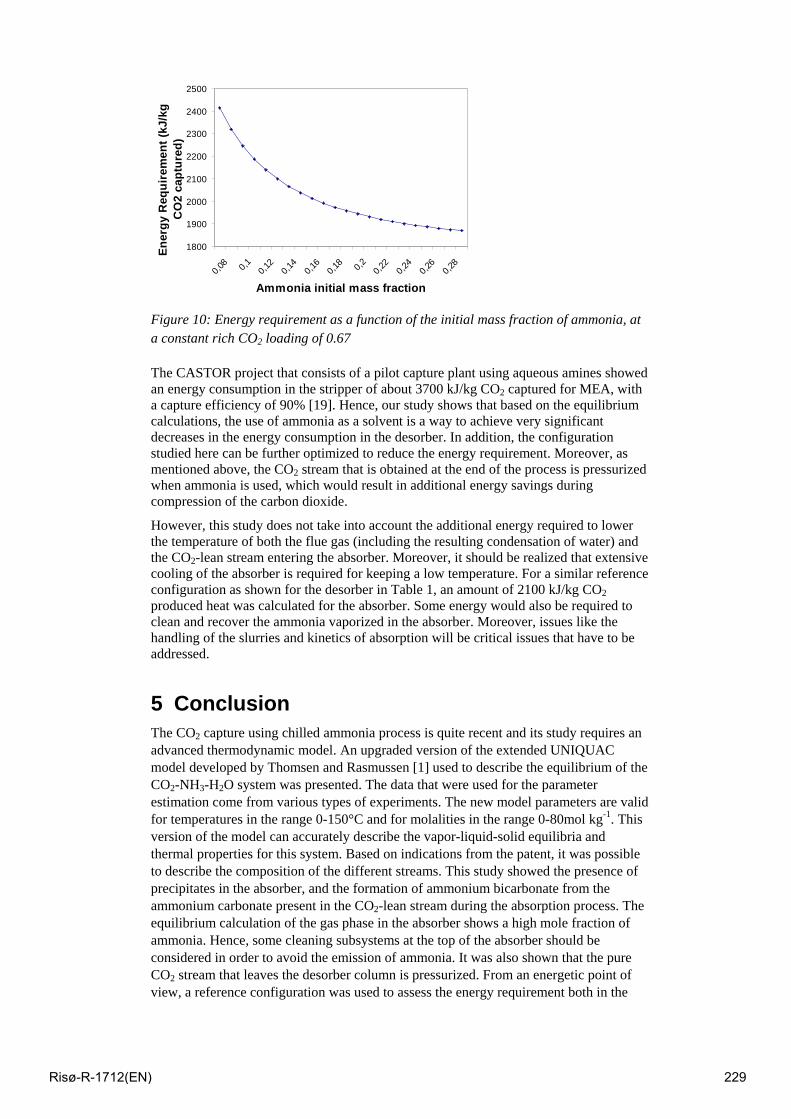
1800

1900

2000

2100

2200

2300

2400

2500

0,28

0,26

0,24

0,220,20,1

80,1

60,1

40,1

20,10,08

Ammonia initial mass fraction

Ener

gy R

equi

rem

ent (

kJ/k

g C

O2

capt

ured

)

Figure 10: Energy requirement as a function of the initial mass fraction of ammonia, at a constant rich CO2 loading of 0.67

The CASTOR project that consists of a pilot capture plant using aqueous amines showed an energy consumption in the stripper of about 3700 kJ/kg CO2 captured for MEA, with a capture efficiency of 90% [19]. Hence, our study shows that based on the equilibrium calculations, the use of ammonia as a solvent is a way to achieve very significant decreases in the energy consumption in the desorber. In addition, the configuration studied here can be further optimized to reduce the energy requirement. Moreover, as mentioned above, the CO2 stream that is obtained at the end of the process is pressurized when ammonia is used, which would result in additional energy savings during compression of the carbon dioxide.

However, this study does not take into account the additional energy required to lower the temperature of both the flue gas (including the resulting condensation of water) and the CO2-lean stream entering the absorber. Moreover, it should be realized that extensive cooling of the absorber is required for keeping a low temperature. For a similar reference configuration as shown for the desorber in Table 1, an amount of 2100 kJ/kg CO2 produced heat was calculated for the absorber. Some energy would also be required to clean and recover the ammonia vaporized in the absorber. Moreover, issues like the handling of the slurries and kinetics of absorption will be critical issues that have to be addressed.

5 Conclusion The CO2 capture using chilled ammonia process is quite recent and its study requires an advanced thermodynamic model. An upgraded version of the extended UNIQUAC model developed by Thomsen and Rasmussen [1] used to describe the equilibrium of the CO2-NH3-H2O system was presented. The data that were used for the parameter estimation come from various types of experiments. The new model parameters are valid for temperatures in the range 0-150°C and for molalities in the range 0-80mol kg-1. This version of the model can accurately describe the vapor-liquid-solid equilibria and thermal properties for this system. Based on indications from the patent, it was possible to describe the composition of the different streams. This study showed the presence of precipitates in the absorber, and the formation of ammonium bicarbonate from the ammonium carbonate present in the CO2-lean stream during the absorption process. The equilibrium calculation of the gas phase in the absorber shows a high mole fraction of ammonia. Hence, some cleaning subsystems at the top of the absorber should be considered in order to avoid the emission of ammonia. It was also shown that the pure CO2 stream that leaves the desorber column is pressurized. From an energetic point of view, a reference configuration was used to assess the energy requirement both in the

Risø-R-1712(EN) 229

absorber and in the desorber. Based on equilibrium calculations, this study showed that the chilled ammonia process allows for a significant reduction of the energy consumption in the desorber compared to the energy consumption of the process using amines.

6 Acknowledgement The author would like to thank the Danish ministry of science technology and innovation for financial support.

7 References [1] K. Thomsen, P. Rasmussen, Modeling of Vapor-liquid-solid equilibrium in gas-aqueous electrolyte system, Chem. Eng. Sc. 54 (1999)1787-1802

[2] E. Gal, Ultra cleaning combustion gas including the removal of CO2, World Intellectual Property, Patent WO 2006022885 (2006)

[3] Denmark’s 4th National Communication to the United Nations Framework Convention on Climate Change and Report on Demonstrable Progress under the Kyoto Protocol (2005)

[4] S. Freguia and GT. Rochelle, Modeling of CO2 capture by aqueous Monoethanolamine. AIChE Journal 49 (2003) 1676-1686.

[5] J. Reza and A. Trejo, Degradation of Aqueous Solutions of Alkanolamine Blends at High Temperature, under the Presence of CO2 and H2S. Chem. eng. Com 193 (2006) 129-138

[6] O. Lawal, A .Bello, R. Idem, The role of methyl diethanolamine (MDEA) in preventing the oxidative degradation of CO2 loaded and concentrated aqueous monoethanolamine (MEA)-MDEA blends during CO2 absorption from flue gases. Ind. & Eng. chem res 44 (2005) 1874-1896

[7] JM. Smith, HC. Van Ness, MM. Abbott, Introduction to Chemical Engineering Thermodynamics 6th edition, 2001

[8] B. Rumpf, G. Maurer, Solubility of Ammonia Solutions of Sodium Sulfate and Ammonium Sulfate at temperatures from 333.15K to 433.15K and pressure up to 3MPa, ind. Eng. Chem. Res. 32(1993), 1780-1789

[9] B. Rumpf, G. Maurer, An experimental and theoratical Investigation on the Solubility of Carbon Dioxide in Aqueous Solutions of Strong Electrolytes, Ber. Bunsenges. Phys. Chem. 97 (1993), 85-98

[10] SW. Brelvi, JP. OConnell, Corresponding states correlations for liquid compressubility and partial molal volumes of gases at infinite dilution in liquids, AICHE 18 (1972) 1239

[11] E. Jänecke, Über das System H2O, CO2 und NH3. Zeitschrift fuer Elektrochemie, 39 (1929) 332-334+716-728

[12] E. Terres and H. Weiser, Beitrag zur Kenntnis der Ammoniak-Kohlensäureverbindungen im Gleigewicht mit ihren wässerigen Lösungen. Zeitschrift fuer Elektrochemie 27 (1921) 177-193

[13] E. Terres and H. Behrens, Zur Kenntnis des physikalisch-chemischen Grundlagen der Harnstoffsynthese aus Ammoniak, Kohlensäure und Wasser. Zeitschrift fuer Physikalische Chemie 139 (1928) 693-716

[14] A. Guyer and T. Piechowicz T, Lösungsgleichgewichte in wässringen Systemen. Das System CO2-NH3-H2O bei 20-50°. Helvitica Chimica Acta 27 (1944) 858-867

Risø-R-1712(EN) 230

[15] U. Göppert, G. Maurer, Vapor-liquid equilibria in aqueous solutions of Ammonia and Carbon Dioxide at Temperatures Between 333 and 393K, Fluid Phase Equilibria 41(1988)153-185

[16] G. Müller, E. Bender, G. Maurer, Das Dampf-Flüssigkeitsgleichgewicht des ternären Systems NH3-CO2-H2O, Ber. Bunsenges. Phys. Chem. 92(1988)148-160

[17] Lichtfers U, Spektroskopische Untersuchungen zur ermittlung von Speziesverteilungen im System Ammoniak-Kohlendioxid-Wasser, (2001) Aachen, Shaker Verlag

[18] B. Rumpf, F. Weyrich, G. Maurer, Enthalpy changes upon Partial Evaporation of Aqueous Solutions containing Ammonia and Carbon Dioxide, Ind. Eng. Chem. Res 37 (1998) 2983-2995

[19] JN. Knudsen, JN. Jensen, O. Biede, Castor SP2: Experiments on Pilot Plant, CASTOR-ENCAP-CACHET-DYNAMIS common Technical Training Workshop (2008)

Risø-R-1712(EN) 231

CO2 Capture From Flue Gas Using Amino Acid Salt Solutions Benedicte Mai Lerche, Erling H. Stenby and Kaj Thomsen

Technical University of Denmark

The reversible absorption of CO2 into a chemical solvent is currently the leading CO2 capture technology. Available solvents are almost exclusively based on aqueous alkanolamine solutions, which entail both economic and environmental complications, making the commercialization of the technology difficult. Amino acid salt solutions have emerged as an alternative to the alkanolamine solutions. A number of advantages make amino acid salt solutions attractive solvents for CO2 capture from flue gas. In the present study CO2 absorption in aqueous solutions of 0.5 M potassium glycinate and 0.5 M monoethanolamine (MEA) were performed, using a stirred cell reactor experimental set-up. The absorption of gas containing 10 mol % CO2 and 90 mol % N2 was followed by measuring the percentage of CO2 in the outlet gas. Also the temperature and pH in the solutions were measured during the absorption. The results showed that the CO2 absorption curves of potassium glycinate and MEA are very similar indicating a potential for potassium glycinate as replacement for MEA in chemical absorption of CO2 from flue gas. For both the potassium glycinate and the MEA solutions the CO2 loading capacity was 0.8 mol CO2/mol amine and the pH dropped between 2 and 3 units during the absorption process. In both types of solutions the temperature increased as a result of the CO2 absorption, which is expected due to the exothermic nature of the absorption reaction. The increase in temperature for the potassium glycinate was lower than for MEA indicating a lower heat of absorption/desorption.

Risø-R-1712(EN) 232

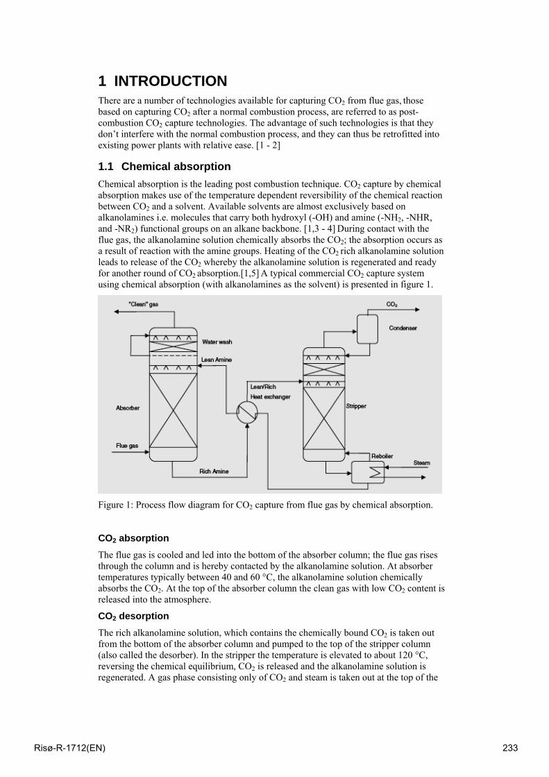
1 INTRODUCTION There are a number of technologies available for capturing CO2 from flue gas, those based on capturing CO2 after a normal combustion process, are referred to as post-combustion CO2 capture technologies. The advantage of such technologies is that they don’t interfere with the normal combustion process, and they can thus be retrofitted into existing power plants with relative ease. [1 - 2]

1.1 Chemical absorption Chemical absorption is the leading post combustion technique. CO2 capture by chemical absorption makes use of the temperature dependent reversibility of the chemical reaction between CO2 and a solvent. Available solvents are almost exclusively based on alkanolamines i.e. molecules that carry both hydroxyl (-OH) and amine (-NH2, -NHR, and -NR2) functional groups on an alkane backbone. [1,3 - 4] During contact with the flue gas, the alkanolamine solution chemically absorbs the CO2; the absorption occurs as a result of reaction with the amine groups. Heating of the CO2 rich alkanolamine solution leads to release of the CO2 whereby the alkanolamine solution is regenerated and ready for another round of CO2 absorption.[1,5] A typical commercial CO2 capture system using chemical absorption (with alkanolamines as the solvent) is presented in figure 1.

Figure 1: Process flow diagram for CO2 capture from flue gas by chemical absorption.

CO2 absorption The flue gas is cooled and led into the bottom of the absorber column; the flue gas rises through the column and is hereby contacted by the alkanolamine solution. At absorber temperatures typically between 40 and 60 °C, the alkanolamine solution chemically absorbs the CO2. At the top of the absorber column the clean gas with low CO2 content is released into the atmosphere.

CO2 desorption The rich alkanolamine solution, which contains the chemically bound CO2 is taken out from the bottom of the absorber column and pumped to the top of the stripper column (also called the desorber). In the stripper the temperature is elevated to about 120 °C, reversing the chemical equilibrium, CO2 is released and the alkanolamine solution is regenerated. A gas phase consisting only of CO2 and steam is taken out at the top of the

Risø-R-1712(EN) 233

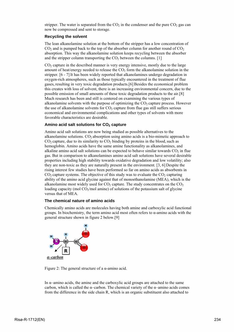
stripper. The water is separated from the CO2 in the condenser and the pure CO2 gas can now be compressed and sent to storage.

Recycling the solvent The lean alkanolamine solution at the bottom of the stripper has a low concentration of CO2 and is pumped back to the top of the absorber column for another round of CO2 absorption. This way the alkanolamine solution keeps recycling between the absorber and the stripper column transporting the CO2 between the columns. [1]

CO2 capture in the described manner is very energy intensive, mostly due to the large amount of heat/energy needed to release the CO2 form the alkanolamine solution in the stripper. [6 - 7] It has been widely reported that alkanolamines undergo degradation in oxygen-rich atmospheres, such as those typically encountered in the treatment of flue gases, resulting in very toxic degradation products.[6] Besides the economical problem this creates with loss of solvent, there is an increasing environmental concern, due to the possible emission of small amounts of these toxic degradation products to the air.[8]

Much research has been and still is centered on examining the various types of alkanolamine solvents with the purpose of optimizing the CO2 capture process. However the use of alkanolamine solvents for CO2 capture from flue gas still suffers serious economical and environmental complications and other types of solvents with more favorable characteristics are desirable.

Amino acid salt solutions for CO2 capture Amino acid salt solutions are now being studied as possible alternatives to the alkanolamine solutions. CO2 absorption using amino acids is a bio-mimetic approach to CO2 capture, due to its similarity to CO2 binding by proteins in the blood, such as hemoglobin. Amino acids have the same amine functionality as alkanolamines, and alkaline amino acid salt solutions can be expected to behave similar towards CO2 in flue gas. But in comparison to alkanolamines amino acid salt solutions have several desirable properties including high stability towards oxidative degradation and low volatility; also they are non-toxic as they are naturally present in the environment. [3, 6] Despite the rising interest few studies have been performed so far on amino acids as absorbents in CO2 capture systems. The objective of this study was to evaluate the CO2 capturing ability of the amino acid glycine against that of monoethanolamine (MEA), which is the alkanolamine most widely used for CO2 capture. The study concentrates on the CO2 loading capacity (mol CO2/mol amine) of solutions of the potassium salt of glycine versus that of MEA.

The chemical nature of amino acids Chemically amino acids are molecules having both amine and carboxylic acid functional groups. In biochemistry, the term amino acid most often refers to α-amino acids with the general structure shown in figure 2 below.[9]

Figure 2: The general structure of a α-amino acid.

In α–amino acids, the amine and the carboxylic acid groups are attached to the same carbon, which is called the α–carbon. The chemical variety of the α–amino acids comes from the difference in the side chain R, which is an organic substituent also attached to

α–carbon

Risø-R-1712(EN) 234

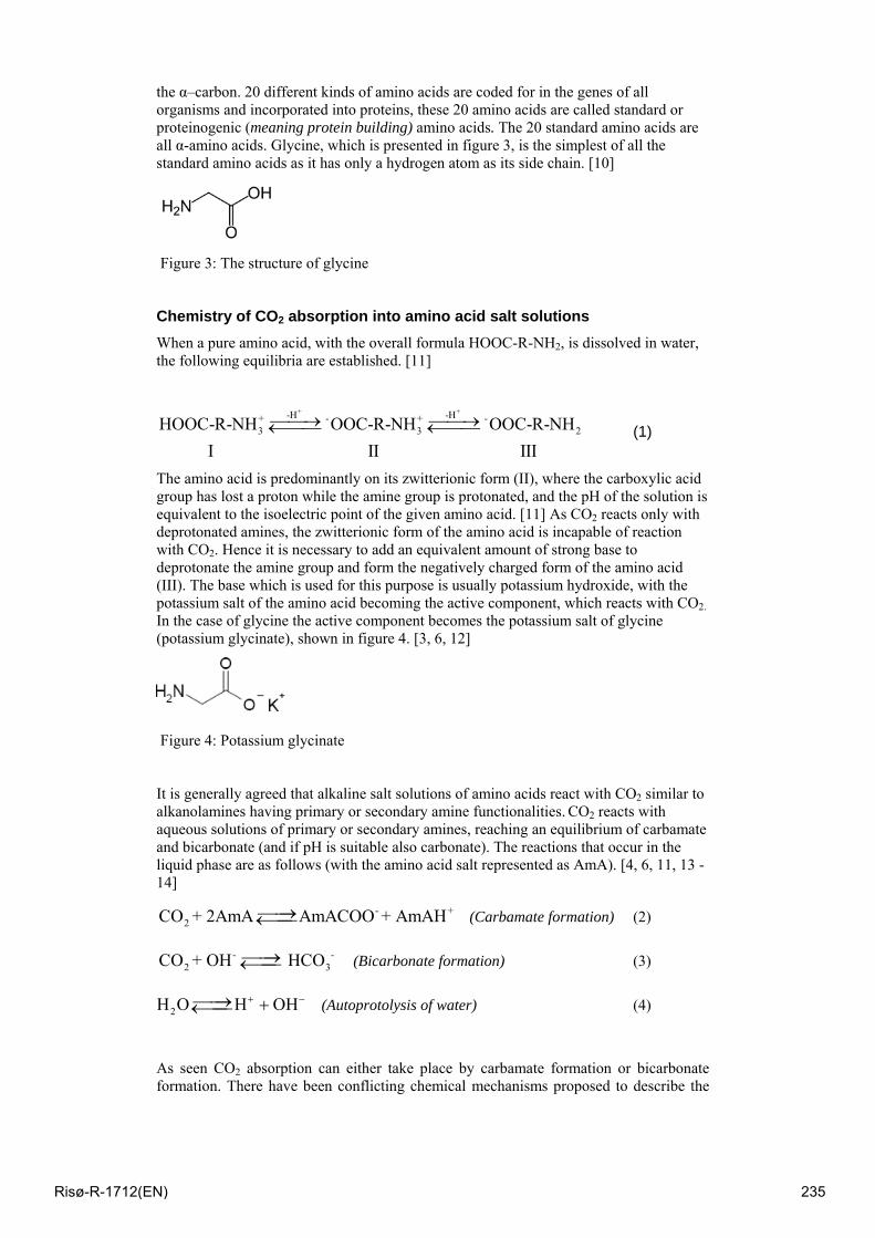
the α–carbon. 20 different kinds of amino acids are coded for in the genes of all organisms and incorporated into proteins, these 20 amino acids are called standard or proteinogenic (meaning protein building) amino acids. The 20 standard amino acids are all α-amino acids. Glycine, which is presented in figure 3, is the simplest of all the standard amino acids as it has only a hydrogen atom as its side chain. [10]

Figure 3: The structure of glycine

Chemistry of CO2 absorption into amino acid salt solutions When a pure amino acid, with the overall formula HOOC-R-NH2, is dissolved in water, the following equilibria are established. [11]

+ +-H -H+ - + -

3 3 2HOOC-R-NH OOC-R-NH OOC-R-NH I II III

⎯⎯→ ⎯⎯→←⎯⎯ ←⎯⎯ (1)

The amino acid is predominantly on its zwitterionic form (II), where the carboxylic acid group has lost a proton while the amine group is protonated, and the pH of the solution is equivalent to the isoelectric point of the given amino acid. [11] As CO2 reacts only with deprotonated amines, the zwitterionic form of the amino acid is incapable of reaction with CO2. Hence it is necessary to add an equivalent amount of strong base to deprotonate the amine group and form the negatively charged form of the amino acid (III). The base which is used for this purpose is usually potassium hydroxide, with the potassium salt of the amino acid becoming the active component, which reacts with CO2.

In the case of glycine the active component becomes the potassium salt of glycine (potassium glycinate), shown in figure 4. [3, 6, 12]

Figure 4: Potassium glycinate

It is generally agreed that alkaline salt solutions of amino acids react with CO2 similar to alkanolamines having primary or secondary amine functionalities. CO2 reacts with aqueous solutions of primary or secondary amines, reaching an equilibrium of carbamate and bicarbonate (and if pH is suitable also carbonate). The reactions that occur in the liquid phase are as follows (with the amino acid salt represented as AmA). [4, 6, 11, 13 - 14]

- +2CO + 2AmA AmACOO + AmAH⎯⎯→←⎯⎯ (Carbamate formation) (2)

- - 2 3CO + OH HCO⎯⎯→←⎯⎯ (Bicarbonate formation) (3)

2H O H OH+ −⎯⎯→ +←⎯⎯ (Autoprotolysis of water) (4)

As seen CO2 absorption can either take place by carbamate formation or bicarbonate formation. There have been conflicting chemical mechanisms proposed to describe the

Risø-R-1712(EN) 235

absorption process. However, it is clear from the reaction rates that the initial absorption reaction is the formation of the carbamate. [3, 5, 11, 13, 14, 15]

2 MATERIALS AND METHODS

2.1 Chemicals The 0,5M potassium glycinate solutions were prepared by adding to glycine (>99.9% pure) an equimolar quantity of potassium hydroxide (>85% pure) in a volumetric flask and filling it to the mark with deionized water. The MEA solutions were prepared by adding MEA (>99.5% pure) to a volumetric flask and filling it to the mark with deionized water. All chemicals were purchased from Sigma Aldrich.

2.2 Experimental Set-up The experimental setup used in this study is shown in figure 5a and 5b. It is a stirred cell experimental set-up with a magnetic stirrer (MS). The Analytic cell (AC) is a 1 litter six-necked round-bottom flask. In each CO2 absorption experiment 0.5L of the prepared 0.5M amine solution (potassium glycinate or MEA) was transferred to the cell. Trough one of the inlets a tube connected to a gas cylinder containing synthetic flue gas (SFG) (10 mol% CO2 and 90 mol% N2) was brought into contact with the amine solution. A gas distributor (GD) at the end of the tube insured a high mass transfer area between gas and solution. A flow controller (FC) (Bronkhorst High-Tech) controlled the flow rate of the gas from the gas cylinder to the solution. The gas flow rate in the experiments was 1L gas/min which equals 0.0041mol CO2/min or 6.83·10-5 mol CO2/sec.

During the experiment the pH and the temperature of the solution was measured using a pH meter (phM) (Metrohn 691 pH Meter) and a Pt100 placed in contact with the solution through 2 separate inlets. A CO2 analyzer (CA) (Vaisala CARBOCAP, Carbon dioxide Transmitter series GMT220) placed in another inlet measured the percentage of CO2 in the outlet gas throughout the experiment. One inlet was used as a vent, and the last inlet to the cell was closed off. The pH meter, the Pt100, and the CO2 analyzer were connected to a computer and data from the 3 instruments were collected during the experiment. Each absorption experiment was started by turning on the gas flow and at the same time starting the data collection (DC) program. Data were collected every fifth second resulting in data points of pH, temperature, and percentage CO2 (in the outlet gas) as a function of time. When the percentage of CO2 and the pH had been constant (and temperature had been almost constant) for 15 minutes, the system was assumed to be very near equilibrium, and the experiment was terminated.

Risø-R-1712(EN) 236

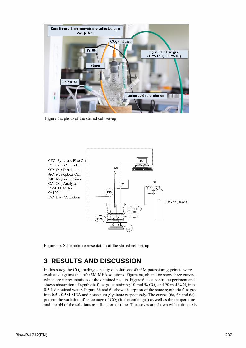
Figure 5a: photo of the stirred cell set-up

Figure 5b: Schematic representation of the stirred cell set-up

3 RESULTS AND DISCUSSION In this study the CO2 loading capacity of solutions of 0.5M potassium glycinate were evaluated against that of 0.5M MEA solutions. Figure 6a, 6b and 6c show three curves which are representatives of the obtained results. Figure 6a is a control experiment and shows absorption of synthetic flue gas containing 10 mol % CO2 and 90 mol % N2 into 0.5 L deionized water. Figure 6b and 6c show absorption of the same synthetic flue gas into 0.5L 0.5M MEA and potassium glycinate respectively. The curves (6a, 6b and 6c) present the variation of percentage of CO2 (in the outlet gas) as well as the temperature and the pH of the solutions as a function of time. The curves are shown with a time axis

Risø-R-1712(EN) 237

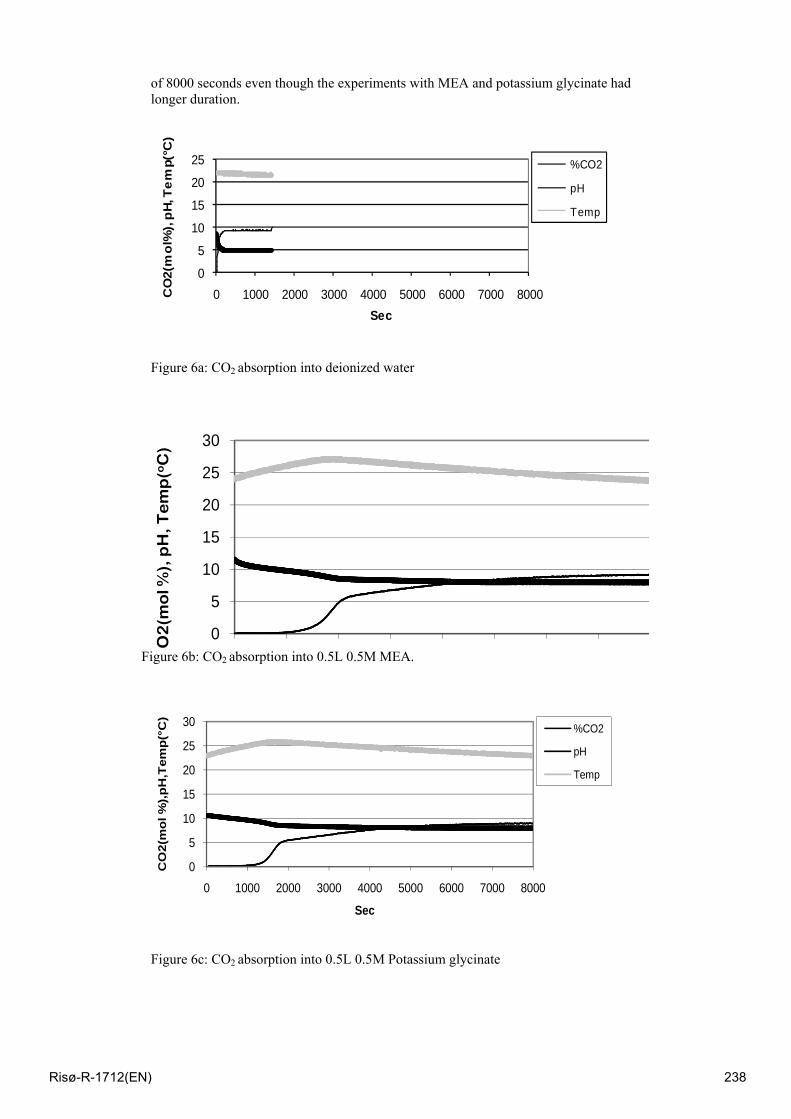
of 8000 seconds even though the experiments with MEA and potassium glycinate had longer duration.

0

5

10

15

20

25

0 1000 2000 3000 4000 5000 6000 7000 8000CO

2(m

ol%

), p

H, T

em

p(°C

)

Sec

%CO2

pH

Temp

Figure 6a: CO2 absorption into deionized water

0

5

10

15

20

25

30

O2

(mo

l %),

pH

, T

em

p(o

C)

Figure 6b: CO2 absorption into 0.5L 0.5M MEA.

0

5

10

15

20

25

30

0 1000 2000 3000 4000 5000 6000 7000 8000

CO

2(m

ol %

),p

H,T

emp

(°C

)

Sec

%CO2

pH

Temp

Figure 6c: CO2 absorption into 0.5L 0.5M Potassium glycinate

Risø-R-1712(EN) 238

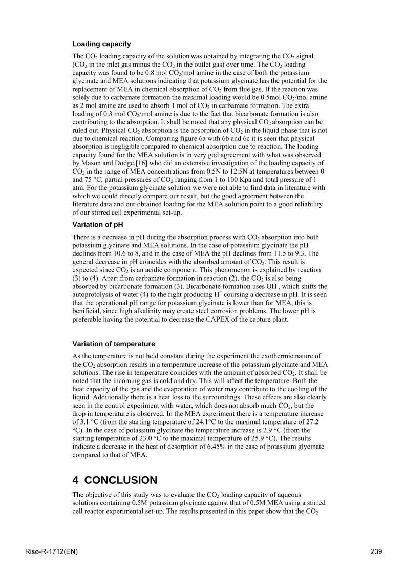
Loading capacity The CO2 loading capacity of the solution was obtained by integrating the CO2 signal (CO2 in the inlet gas minus the CO2 in the outlet gas) over time. The CO2 loading capacity was found to be 0.8 mol CO2/mol amine in the case of both the potassium glycinate and MEA solutions indicating that potassium glycinate has the potential for the replacement of MEA in chemical absorption of CO2 from flue gas. If the reaction was solely due to carbamate formation the maximal loading would be 0.5mol CO2/mol amine as 2 mol amine are used to absorb 1 mol of CO2 in carbamate formation. The extra loading of 0.3 mol CO2/mol amine is due to the fact that bicarbonate formation is also contributing to the absorption. It shall be noted that any physical CO2 absorption can be ruled out. Physical CO2 absorption is the absorption of CO2 in the liquid phase that is not due to chemical reaction. Comparing figure 6a with 6b and 6c it is seen that physical absorption is negligible compared to chemical absorption due to reaction. The loading capacity found for the MEA solution is in very god agreement with what was observed by Mason and Dodge,[16] who did an extensive investigation of the loading capacity of CO2 in the range of MEA concentrations from 0.5N to 12.5N at temperatures between 0 and 75 °C, partial pressures of CO2 ranging from 1 to 100 Kpa and total pressure of 1 atm. For the potassium glycinate solution we were not able to find data in literature with which we could directly compare our result, but the good agreement between the literature data and our obtained loading for the MEA solution point to a good reliability of our stirred cell experimental set-up.

Variation of pH There is a decrease in pH during the absorption process with CO2 absorption into both potassium glycinate and MEA solutions. In the case of potassium glycinate the pH declines from 10.6 to 8, and in the case of MEA the pH declines from 11.5 to 9.3. The general decrease in pH coincides with the absorbed amount of CO2. This result is expected since CO2 is an acidic component. This phenomenon is explained by reaction (3) to (4). Apart from carbamate formation in reaction (2), the CO2 is also being absorbed by bicarbonate formation (3). Bicarbonate formation uses OH-, which shifts the autoprotolysis of water (4) to the right producing H+ coursing a decrease in pH. It is seen that the operational pH range for potassium glycinate is lower than for MEA, this is benificial, since high alkalinity may create steel corrosion problems. The lower pH is preferable having the potential to decrease the CAPEX of the capture plant.

Variation of temperature As the temperature is not held constant during the experiment the exothermic nature of the CO2 absorption results in a temperature increase of the potassium glycinate and MEA solutions. The rise in temperature coincides with the amount of absorbed CO2. It shall be noted that the incoming gas is cold and dry. This will affect the temperature. Both the heat capacity of the gas and the evaporation of water may contribute to the cooling of the liquid. Additionally there is a heat loss to the surroundings. These effects are also clearly seen in the control experiment with water, which does not absorb much CO2, but the drop in temperature is observed. In the MEA experiment there is a temperature increase of 3.1 °C (from the starting temperature of 24.1°C to the maximal temperature of 27.2 °C). In the case of potassium glycinate the temperature increase is 2.9 °C (from the starting temperature of 23.0 °C to the maximal temperature of 25.9 °C). The results indicate a decrease in the heat of desorption of 6.45% in the case of potassium glycinate compared to that of MEA.

4 CONCLUSION The objective of this study was to evaluate the CO2 loading capacity of aqueous solutions containing 0.5M potassium glycinate against that of 0.5M MEA using a stirred cell reactor experimental set-up. The results presented in this paper show that the CO2

Risø-R-1712(EN) 239

absorption curves of potassium glycinate and MEA are very similar indicating a potential for potassium glycinate as replacement for MEA in chemical absorption of CO2 from flue gas. Solutions of 0.5M potassium glycinate and 0.5M MEA both have a CO2 loading capacity of 0.8 mol CO2/mol amine for the given synthetic gas of 10 mol% CO2. In addition the results show a lower operational pH area as well as a lower heat of desorption for potassium glycinate compared with MEA, both of which have the potential for a cost reduction of the capture process.

Acknowledgments This research is part of a project which is sponsored by DONG Energy and Vattenfall A/S Heat Nordic. The authors would like to thank these companies for their economical support as well as helpful discussions on power plant technology and post combustion CO2 capture.

References 1. IPCC: Intergovernmental Panel on Climate Change, “IPCC Special Report on Carbon Dioxide Capture and Storage”, America by Cambridge University Press, New York, 2005.

2. A. Garg , L. R. Appelquist, E. H. Stenby, “CO2 capture and storage”, Risø Energy Report 6.

3. J. van Holst, P.P. Politiek, J.P.M. Niederer, G.F. Versteeg, “CO2 capture from flue gas using amino acid salt solutions”,.GHGT8 Trondheim.

4. P.S. Kumar, J.A. Hogendoorn, G.F. Versteeg, “Kinetics of the Reaction of CO2 with Aqueous Potassium Salt of Taurine and Glycine”, AIChE Journal, 2003, vol. 49, no. 1, pp. 203-213.

5. R.J. Hook, “An Investigation of Some Sterically Hindered Amines as Potential Carbon Dioxide Scrubbing Compounds”, Ind. Eng. Chem. Res., 1997, vol. 36, pp.1779-1790. 6. P.S. Kumar, J.A. Hogendoorn, P.H.M. Feron, G.F. Versteeg, “Equilibrium Solubility of CO2 in Aqueous Potassium Taurate Solutions: Part 1. Crystallization in Carbon Dioxide Loaded Aqueous Salt Solution of Amino Acids”, Ind. Eng. Chem. Res., 2003, vol. 42, pp. 2832-2840.

7. J. Gabrielsen, H. F. Svendsen, M. L. Michelsen, E. H. Stenby,G. M. Kontogeorgis, “Experimental validation of a rate-based model for CO2 capture using an AMP solution”, Chemical Engineering Science, 2007, vol. 62, pp. 2397 – 2413.

8. J. Gabrielsen, “CO2 Capture from Coal Fired Power Plants”, Ph.D. Thesis, IVC-SEP Department of Chemical and Biochemical Engineering ,Technical University of Denmark, 2007.

9. C.K. Mathews, K.E. van Holde, K.G. Ahern, “Biochemistry”, Third edition, Addison

Wesley Longman, Inc., 2000, Ch.5.

10. B. Alberts, A. Johnsen, J. Lewis, M. Raff, K. Roberts, P. Walter, “Molecular Biology THE CELL”, Fourth edition, Garland Science Taylor & Francis Group, 2002, Chap. 2.

11. P.S. Kumar, J.A Hogendoorn, P.H.M. Feron, G.F Versteeg, “New absorption liquids for the removal of CO2 from dilute gas streams using membrane contactors”, Chemical Engineering Science, 2002, vol. 57, pp. 1639-1651.

12. A.F. Portugal, F.D. Magalhães, A. Mendes, ”Carbon dioxide absorption kinetics in potassium threonate”, Chemical Engineering Science, 2008, vol. 63 pp. 3493–3503.

Risø-R-1712(EN) 240

13. A.F. Portugal, P.W.J. Derks, G.F. Versteeg, F.D. Magalhães, A. Mendes, “Characterization of potassium glycinate for carbon dioxide absorption purposes”, Chemical Engineering Science, 2007, vol. 62, pp. 6534–6547.

14. J.P. Brouwer, P.H.M. Feron, N.A.M. ten Asbroek, “Amino-acid salts for CO2 capture from flue gases” TNO Science & Industry Department of Separation Technology. The Netherlands. http://www.netl.doe.gov/publications/proceedings/05/carbon-seq/Poster%20147.pdf, (19/11/2008).

15. E.F. da Silva, H. F. Svendsen, “Computational chemistry study of reactions, equilibrium and kinetics of chemical CO2 absorption”, International Journal of Greenhouse Gas Control, 2007, vol.1, no.2, pp. 151–157.

16. Jesse W. Mason, Barnett F. Dodge, ”Equilibrium absorption of carbon dioxide by solutions of the ethanolamines”, American institute of Chemical Engineers, 1936, vol. 32, no. 27, pp. 27-47.

Risø-R-1712(EN) 241

Energy demand for CO2 solvent regeneration Philip L. Fosbøl, Kaj Thomsen, Erling H. Stenby

Technical University of Denmark, DTU

Building 229

DK-2800 Kongens Lyngby

Denmark

Abstract CO2 capture by amine scrubbing is the state of the art technology for CO2 capture. Large bench scale tests have proven that the system is successful in capturing CO2 from coal fires power plants. On a long term basis new processes may substitute this equipment. In the mean time the amine units will be successful in reducing the emission of CO2, especially from coal fired power plants. There is a huge potential to reduce the energy demand with the existing technology. In this work the energy intensive part of the conventional capture plant is being studied. A detailed modelling of the desorption process has been carried out. This involves a complete rate based equation scheme for the column, linked to models of the reboiler and condenser. The calculations show the properties inside the column as function of column height, compared to experimental measurements. The energy consumption for reboiler and condenser are calculated and evaluated. The results show the energy consumption as function of percent CO2 recovery. Optimal design specifications are discussed in order to achieve a high CO2 stripping from the CO2 rich amine solutions, using less energy.

1 Introduction Electricity production is by most end users thought of as an unlimited resource of energy, especially in the developed countries. The production often drives the economies and consequently a great political drive is observed in order to maintain this status. Unfortunately most used power technologies emit an unreasonable high amount of green house gases. Recently the public opinion has shifted drastically and it has become a great political issue to limit the impact of green house gas emission. A number of informative reports were published recently, one is the IPCC (Intergovernmental Panel on Climate Change) report of 20051, which focuses on green house gasses. It is concluded that the cause of most natural catastrophes are the consequence of pollution from human energy production.

To maintain the current state of welfare and simultaneously reducing e.g. carbon dioxide emissions, requires the industry to be prepared to either retrofit their existing energy production or change to another technology. Both scenarios are costly. One is the short term solution whereas the other is the long term. The second can not be used on a short term basis, since a large amount of power is needed which currently and unfortunately can not be produced by means of renewable energy. It takes decades to revamp the power industry and shift to wind, solar, or wave energy production.

The situation is that we can lean back and let the industry change to renewable energy or we can spend resources and capture CO2 while the industry in addition invests in renewable energy.

It has been argued by some organizations that the attention is better spent on not capturing CO2 and focusing only on renewable energy. This is to some extent a rather idealistic and gullible opinion since fossil fuels will be used by underdeveloped countries

Risø-R-1712(EN) 242

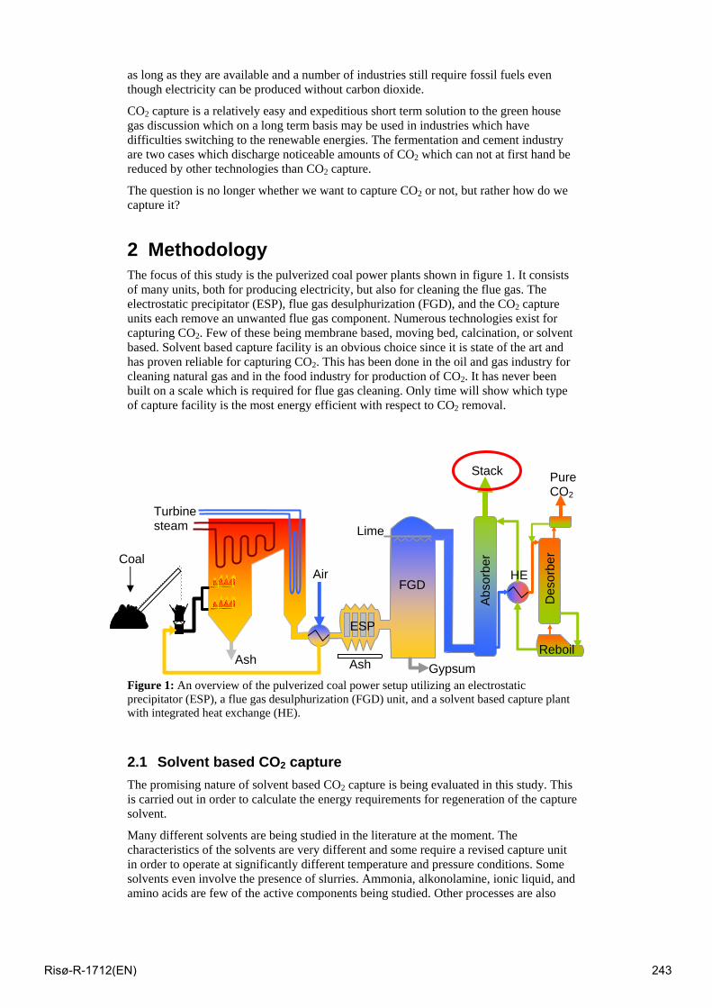
as long as they are available and a number of industries still require fossil fuels even though electricity can be produced without carbon dioxide.

CO2 capture is a relatively easy and expeditious short term solution to the green house gas discussion which on a long term basis may be used in industries which have difficulties switching to the renewable energies. The fermentation and cement industry are two cases which discharge noticeable amounts of CO2 which can not at first hand be reduced by other technologies than CO2 capture.

The question is no longer whether we want to capture CO2 or not, but rather how do we capture it?

2 Methodology The focus of this study is the pulverized coal power plants shown in figure 1. It consists of many units, both for producing electricity, but also for cleaning the flue gas. The electrostatic precipitator (ESP), flue gas desulphurization (FGD), and the CO2 capture units each remove an unwanted flue gas component. Numerous technologies exist for capturing CO2. Few of these being membrane based, moving bed, calcination, or solvent based. Solvent based capture facility is an obvious choice since it is state of the art and has proven reliable for capturing CO2. This has been done in the oil and gas industry for cleaning natural gas and in the food industry for production of CO2. It has never been built on a scale which is required for flue gas cleaning. Only time will show which type of capture facility is the most energy efficient with respect to CO2 removal.

Figure 1: An overview of the pulverized coal power setup utilizing an electrostatic precipitator (ESP), a flue gas desulphurization (FGD) unit, and a solvent based capture plant with integrated heat exchange (HE).

2.1 Solvent based CO2 capture The promising nature of solvent based CO2 capture is being evaluated in this study. This is carried out in order to calculate the energy requirements for regeneration of the capture solvent.

Many different solvents are being studied in the literature at the moment. The characteristics of the solvents are very different and some require a revised capture unit in order to operate at significantly different temperature and pressure conditions. Some solvents even involve the presence of slurries. Ammonia, alkonolamine, ionic liquid, and amino acids are few of the active components being studied. Other processes are also

Coal

Turbine steam

Air

ESP

FGD

Stack PureCO2

Abs

orbe

r

Des

orbe

r

Reboil Ash

HE

Gypsum

Lime

Ash

Risø-R-1712(EN) 243

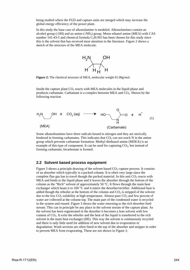
being studied where the FGD and capture units are merged which may increase the global energy efficiency of the power plant.

In this study the base case of alkonolamine is modeled. Alkonolamines contain an alcohol group (-OH) and an amine (-NH2) group. Mono ethanol amine (MEA) with CAS number 141-43-5 and chemical formula C2H7NO has been chosen for this study since this is the solvent that has received most attention in the literature. Figure 2 shows a sketch of the structure of the MEA molecule.

NH2 OH

H H HH Figure 2: The chemical structure of MEA, molecular weight 61.08g/mol.

Inside the capture plant CO2 reacts with MEA molecules in the liquid phase and produces carbamate. Carbamate is a complex between MEA and CO2. Shown by the following reaction

NH2 OH CO2

NH

OHO

O H++

(MEA)

+

(Carbamate)

(aq)

(1)

Some alkanoleamines have three radicals bound to nitrogen and they are sterically hindered in forming carbamates. This indicates that CO2 can not reach N in the amine group which prevents carbamate formation. Methyl diethanol amine (MDEA) is an example of this type of component. It can be used for capturing CO2, but instead of forming carbamate, bicarbonate is formed.

2.2 Solvent based process equipment Figure 3 shows a principle drawing of the solvent based CO2 capture process. It consists of an absorber which typically is a packed column. It is often very large since the complete flue gas has to travel though the packed material. In this unit CO2 reacts with MEA and binds to the liquid phase and it leaves the absorber through the bottom of the column as the “Rich” solvent of approximately 50 °C. It flows through the main heat exchanger which heats it to 100 °C and it enters the desorber/rectifier. Additional heat is added though the reboiler at the bottom of the column and CO2 is stripped of the solvent due to the low CO2 solubility at high temperature. Almost pure CO2 and few percent of water are collected at the column top. The main part of the condensed water is recycled in the system and reused. Figure 3 shows the water returning to the rich desorber feed stream. This can in principle be any place in the solvent stream of the capture plant. As the solvent has been regenerated in the desorber it becomes a lean solvent with low content of CO2. It exits the reboiler and the heat of the liquid is transferred to the rich solvent in the main heat exchanger (HE). This way the solvent is continuously recycled and there is only little need for addition of new solvent due to evaporation or degradation. Wash sections are often fitted to the top of the absorber and stripper in order to prevent MEA from evaporating. These are not shown in Figure 3.

Risø-R-1712(EN) 244

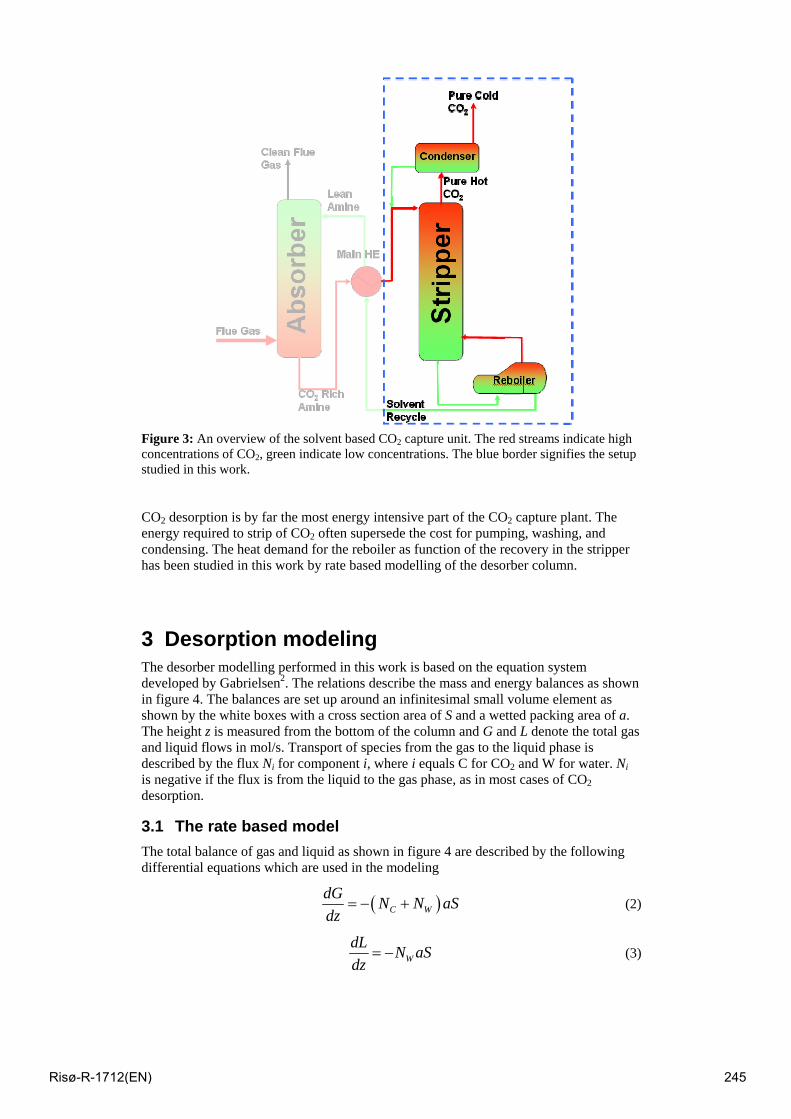
Figure 3: An overview of the solvent based CO2 capture unit. The red streams indicate high concentrations of CO2, green indicate low concentrations. The blue border signifies the setup studied in this work.

CO2 desorption is by far the most energy intensive part of the CO2 capture plant. The energy required to strip of CO2 often supersede the cost for pumping, washing, and condensing. The heat demand for the reboiler as function of the recovery in the stripper has been studied in this work by rate based modelling of the desorber column.

3 Desorption modeling The desorber modelling performed in this work is based on the equation system developed by Gabrielsen2. The relations describe the mass and energy balances as shown in figure 4. The balances are set up around an infinitesimal small volume element as shown by the white boxes with a cross section area of S and a wetted packing area of a. The height z is measured from the bottom of the column and G and L denote the total gas and liquid flows in mol/s. Transport of species from the gas to the liquid phase is described by the flux Ni for component i, where i equals C for CO2 and W for water. Ni is negative if the flux is from the liquid to the gas phase, as in most cases of CO2 desorption.

3.1 The rate based model The total balance of gas and liquid as shown in figure 4 are described by the following differential equations which are used in the modeling

( )C WdG N N aSdz

= − + (2)

WdL N aSdz

= − (3)

Risø-R-1712(EN) 245

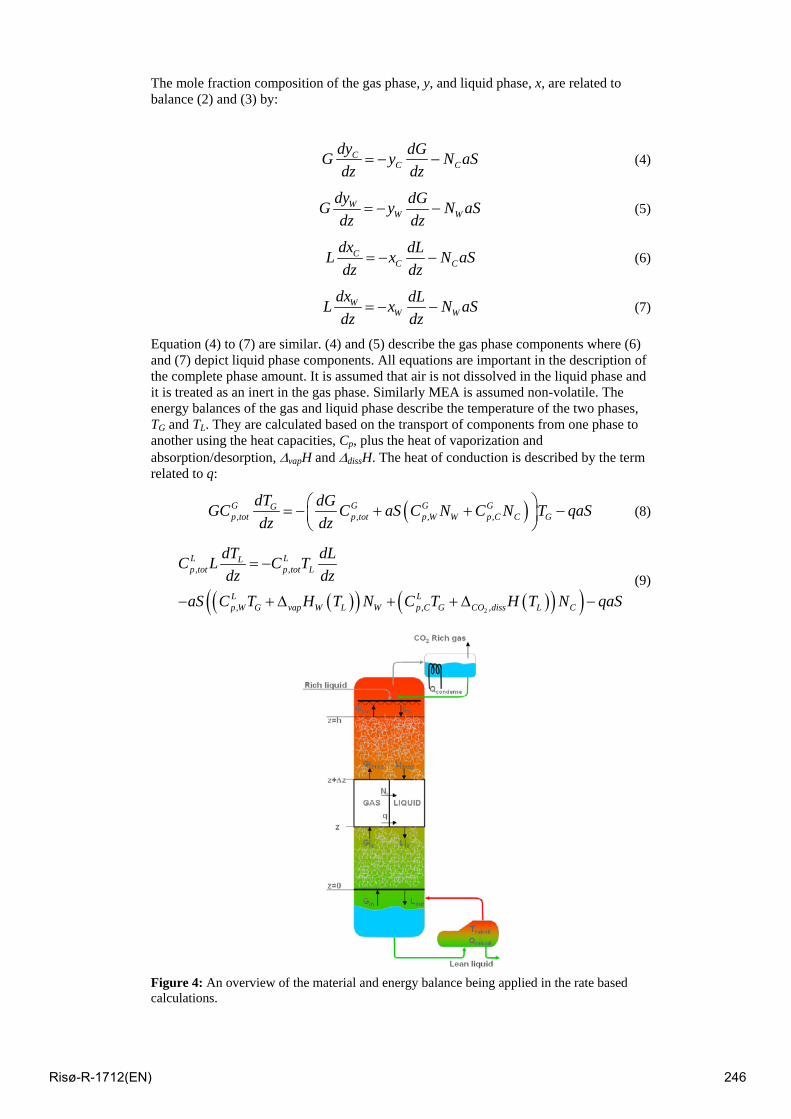
The mole fraction composition of the gas phase, y, and liquid phase, x, are related to balance (2) and (3) by:

CC C

dy dGG y N aSdz dz

= − − (4)

WW W

dy dGG y N aSdz dz

= − − (5)

CC C

dx dLL x N aSdz dz

= − − (6)

WW W

dx dLL x N aSdz dz

= − − (7)

Equation (4) to (7) are similar. (4) and (5) describe the gas phase components where (6) and (7) depict liquid phase components. All equations are important in the description of the complete phase amount. It is assumed that air is not dissolved in the liquid phase and it is treated as an inert in the gas phase. Similarly MEA is assumed non-volatile. The energy balances of the gas and liquid phase describe the temperature of the two phases, TG and TL. They are calculated based on the transport of components from one phase to another using the heat capacities, Cp, plus the heat of vaporization and absorption/desorption, ΔvapH and ΔdissH. The heat of conduction is described by the term related to q:

( ), , , ,G G G GGp tot p tot p W W p C C G

dT dGGC C aS C N C N T qaSdz dz

⎛ ⎞= − + + −⎜ ⎟⎝ ⎠

(8)

( )( ) ( )( )( )2

, ,

, , ,

L LLp tot p tot L

L Lp W G vap W L W p C G CO diss L C

dT dLC L C Tdz dz

aS C T H T N C T H T N qaS

= −

− + Δ + + Δ − (9)

Figure 4: An overview of the material and energy balance being applied in the rate based calculations.

Risø-R-1712(EN) 246

3.2 Calculation of dependent variables The eight independent variables, L, G, yC, yW, xC, xW, TG, and TL are solved as function of the column height, z. This is only possible since the fluxes, Ni, are calculated using the independent variables from the following mass transport correlation

( )( )*, ,C G C tot C C L iN K a P y p T x= − (10)

( )( )*, ,W G W tot W sat W L wN K a P y p T x= − (11)

Where KG,i are the overall mass transport coefficients and Ptot is the known total pressure in the system. *

Cp and *Wp are the equilibrium partial pressures of CO2 and water

respectively calculated using the equilibrium model of Gabrielsen2 and a simple Antoine equation for water. The overall mass transfer coefficient of CO2 is calculated from the following combined relation of liquid and gas side mass transfer coefficients, applying a Henry’s law, HC, and the enhancement factor, E:

,

, ,

11

·

G CC

G C L C

K a Hk a E k a

=+

(12)

The mass transfer coefficients are obtained from the theory of either Rocha et al.3,4 or Billet and Schultes5. The Henry’s law constant is calculated from the work of Wang et al.6 and the N2O analogy parameters of Browning and Weiland7. The enhancement factor is calculated slightly differently compared to the work of Gabrielsen2, since the absorption phenomenon is not directly transferable to desorption theory and the implicit instantaneous enhancement factor of Astarita8 was used in the implicit calculation of the enhancement factor. The heat transferred by conduction, q, is calculated using the heat transfer coefficient hG and the Colburn analogy to mass transfer by

( )G G Lq h T T= − (13)

A number of physical properties are needed in the calculation of the transfer coefficients, like the liquid diffusivities of CO2 and MEA, density, surface tension, viscosity, rate constant of CO2 reaction with MEA, gas viscosity, and gas diffusivity of CO2 and water, all which have been calculated by the same principles as used by Gabrielsen2. Except a number of the correlations were updated in order to be more accurate at the high temperatures observed in the desorber and more robust at low the temperatures.

3.3 Numerical solution and boundary conditions The equation scheme formulated by (2) to (9) is an ordinary differential equation system, which can be solved numerically as a boundary value problem (BVP). In order to obtain a solution the equations are discretized in the interval from z=0 to z=h. 30 steps are used as an initial discretization. A routine which automatically revises the section lengths is used. This is done in order to acquire a more accurate solution and the final number of discretizations is typically 30 to 200. The high number of steps is used due to the steep gradients of temperature profiles seen in the column in- and outlets. The solution of this type of high gradient BVP’s always requires a fine mesh. The known boundary conditions which are used in order to solve the equations are the four gas phase properties, G, yC, yW, and TG in the bottom of the column a z=0 and the liquid phase properties, L, xC, xW, TL in the top of the column at z=h. The equivalent four variables for top gas outlet and bottom liquid outlet are calculated by the BVP solver.

Risø-R-1712(EN) 247

The BVP solver needs an initial guess of all the independent variables to achieve a solution, these are basically not known. Flat profiles of the above eight known inlet variables are used for the whole column. In most cases this will not result in a solution of the BVP problem, but using a special kind of mass transfer damping with an initial value of 0.01 guarantees a solution to the problem. This is the case since very low mass-transfer coefficients results in the flat profiles just described. The first solution is obtained at values of 0.01 of the “real” mass transfer coefficient. This solution is then reused in a new iterative step while the special damping factor is slowly turned up. If the step in the damping factor is too high and the solution fails, then the failed solution is discarded and the previous “good” solution is used again as an initial guess but with a lower turn up of the damping. This way a solution can always be guaranteed while for turn up values going towards zero it will by definition result in a solution very close to the last known “good” solution. It may of course require many iterations if the turn up value is very low.

The reboiler and condenser are solved as PT-flashes. A condition which must be obeyed is that the temperature needs to be above the boiling point or else no vapor phase is created. A solution can simply not be obtained if the vapor inlet stream to the column is non existent. The initial guess of the gas stream into column is obtained by taking the feed directly to the reboiler as if nothing happened in the column, consistent with the damping scheme mentioned above.

An outer loop is used in order to converge for the reboiler top gas stream around the column and a second outer loop is employed in order to converge the condensate flow. The condensate flow typically converges in 3 to 5 iterations and the reboiler top stream converges in 5 to 20 iterations. An initial guess of zero condensate flow is a very good starting guess which seems to give a solution at almost any conditions. Other types of initial guesses have been tested e.g. where the condensate flow is obtained by assuming reboiler gas flow going directly to the condenser and converging that while assuming no CO2 transfer in the column. This will result in highly unrealistic condensate flows close to normal operating conditions. It must also be said that the reboiler top stream needs damping or else it may be very difficult to obtain a solution in certain industrial relevant temperature intervals.

4 Energy consumptions The energy consumption for a CO2 capture plant, as shown in figure 3, is calculated entirely from the heat input to the reboiler. Heat is typically removed in the condenser by seawater, but it does not contribute to the overall energy requirements for steam availability. No other heat sources are involved in the calculation and heat losses to the surroundings are assumed low.

The calculations were performed using the model described above. A simple non-industrial pilot case of a 4.5 m structured packing column with 15cm in diameter is modeled. The inlet rich liquid temperature is assumed to be 100 °C with a loading of approx. 0.45 mol CO2/mol MEA and a 30wt% aqueous MEA solvent.

The following results show the principle and trends of a CO2 capture facility. Due to the relatively small size of the column the calculations may not be directly transferable to industrially situations. A bigger column may show the same trends even though the absolute values may be different.

Figure 5 demonstrates the energy consumption as function of reboiler temperature at two different operating pressures. As the temperature increases, the energy requirements increase. The figure show the consumption calculated relative to the amount of recovered CO2 in the top of the stripper. A low reboiler temperature leads to almost no CO2 being desorbed and the majority of the CO2 is recycle to the absorber. At these

Risø-R-1712(EN) 248

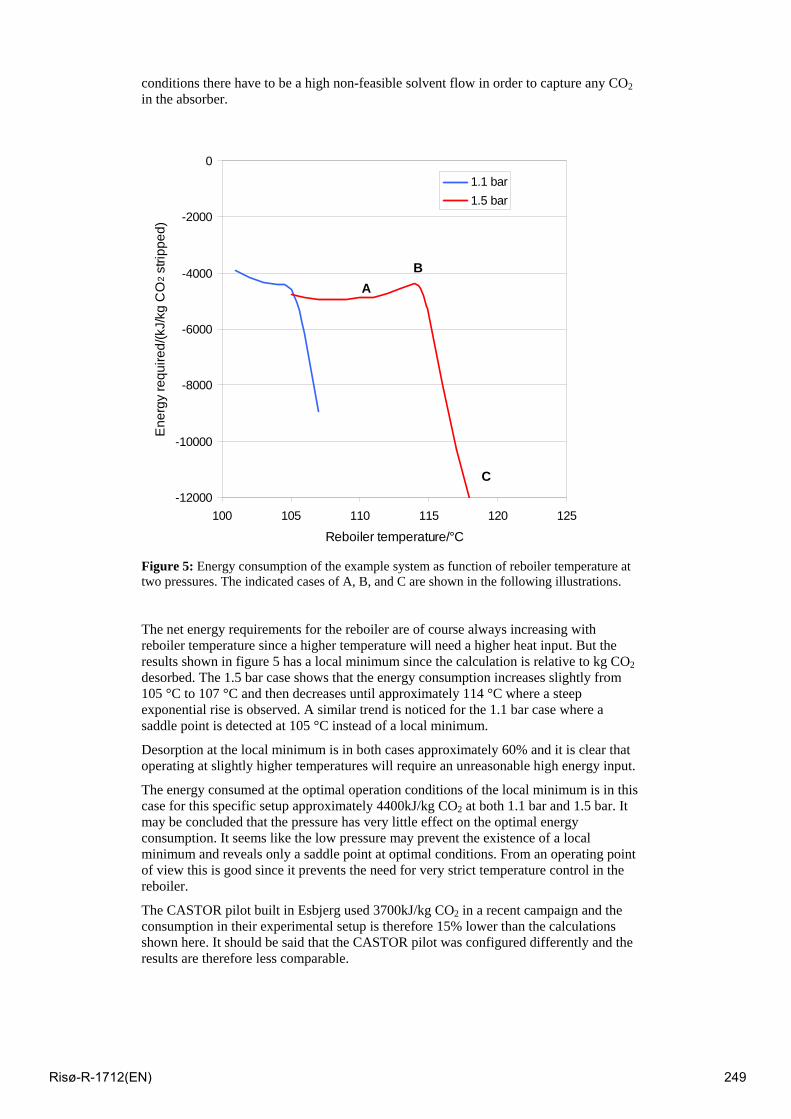
conditions there have to be a high non-feasible solvent flow in order to capture any CO2 in the absorber.

-12000

-10000

-8000

-6000

-4000

-2000

0

100 105 110 115 120 125

Reboiler temperature/°C

Ene

rgy

requ

ired/

(kJ/

kg C

O 2

strip

ped)

1.1 bar1.5 bar

AB

C

Figure 5: Energy consumption of the example system as function of reboiler temperature at two pressures. The indicated cases of A, B, and C are shown in the following illustrations.

The net energy requirements for the reboiler are of course always increasing with reboiler temperature since a higher temperature will need a higher heat input. But the results shown in figure 5 has a local minimum since the calculation is relative to kg CO2 desorbed. The 1.5 bar case shows that the energy consumption increases slightly from 105 °C to 107 °C and then decreases until approximately 114 °C where a steep exponential rise is observed. A similar trend is noticed for the 1.1 bar case where a saddle point is detected at 105 °C instead of a local minimum.

Desorption at the local minimum is in both cases approximately 60% and it is clear that operating at slightly higher temperatures will require an unreasonable high energy input.

The energy consumed at the optimal operation conditions of the local minimum is in this case for this specific setup approximately 4400kJ/kg CO2 at both 1.1 bar and 1.5 bar. It may be concluded that the pressure has very little effect on the optimal energy consumption. It seems like the low pressure may prevent the existence of a local minimum and reveals only a saddle point at optimal conditions. From an operating point of view this is good since it prevents the need for very strict temperature control in the reboiler.

The CASTOR pilot built in Esbjerg used 3700kJ/kg CO2 in a recent campaign and the consumption in their experimental setup is therefore 15% lower than the calculations shown here. It should be said that the CASTOR pilot was configured differently and the results are therefore less comparable.

Risø-R-1712(EN) 249

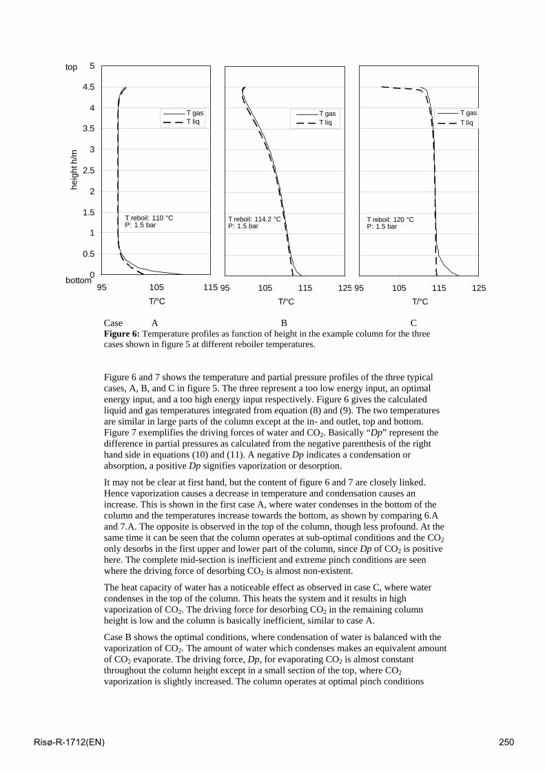
0

0.5

1

1.5

2

2.5

3

3.5

4

4.5

5

95 105 115 T/°C

heig

ht h

/m

T gasT liq

top

bottom

T reboil: 110 °CP: 1.5 bar

95 105 115 125 T/°C

T gasT liq

T reboil: 114.2 °CP: 1.5 bar

95 105 115 125 T/°C

T gasT liq

T reboil: 120 °CP: 1.5 bar

Case A B C Figure 6: Temperature profiles as function of height in the example column for the three cases shown in figure 5 at different reboiler temperatures.

Figure 6 and 7 shows the temperature and partial pressure profiles of the three typical cases, A, B, and C in figure 5. The three represent a too low energy input, an optimal energy input, and a too high energy input respectively. Figure 6 gives the calculated liquid and gas temperatures integrated from equation (8) and (9). The two temperatures are similar in large parts of the column except at the in- and outlet, top and bottom. Figure 7 exemplifies the driving forces of water and CO2. Basically “Dp” represent the difference in partial pressures as calculated from the negative parenthesis of the right hand side in equations (10) and (11). A negative Dp indicates a condensation or absorption, a positive Dp signifies vaporization or desorption.

It may not be clear at first hand, but the content of figure 6 and 7 are closely linked. Hence vaporization causes a decrease in temperature and condensation causes an increase. This is shown in the first case A, where water condenses in the bottom of the column and the temperatures increase towards the bottom, as shown by comparing 6.A and 7.A. The opposite is observed in the top of the column, though less profound. At the same time it can be seen that the column operates at sub-optimal conditions and the CO2 only desorbs in the first upper and lower part of the column, since Dp of CO2 is positive here. The complete mid-section is inefficient and extreme pinch conditions are seen where the driving force of desorbing CO2 is almost non-existent.

The heat capacity of water has a noticeable effect as observed in case C, where water condenses in the top of the column. This heats the system and it results in high vaporization of CO2. The driving force for desorbing CO2 in the remaining column height is low and the column is basically inefficient, similar to case A.

Case B shows the optimal conditions, where condensation of water is balanced with the vaporization of CO2. The amount of water which condenses makes an equivalent amount of CO2 evaporate. The driving force, Dp, for evaporating CO2 is almost constant throughout the column height except in a small section of the top, where CO2 vaporization is slightly increased. The column operates at optimal pinch conditions

Risø-R-1712(EN) 250

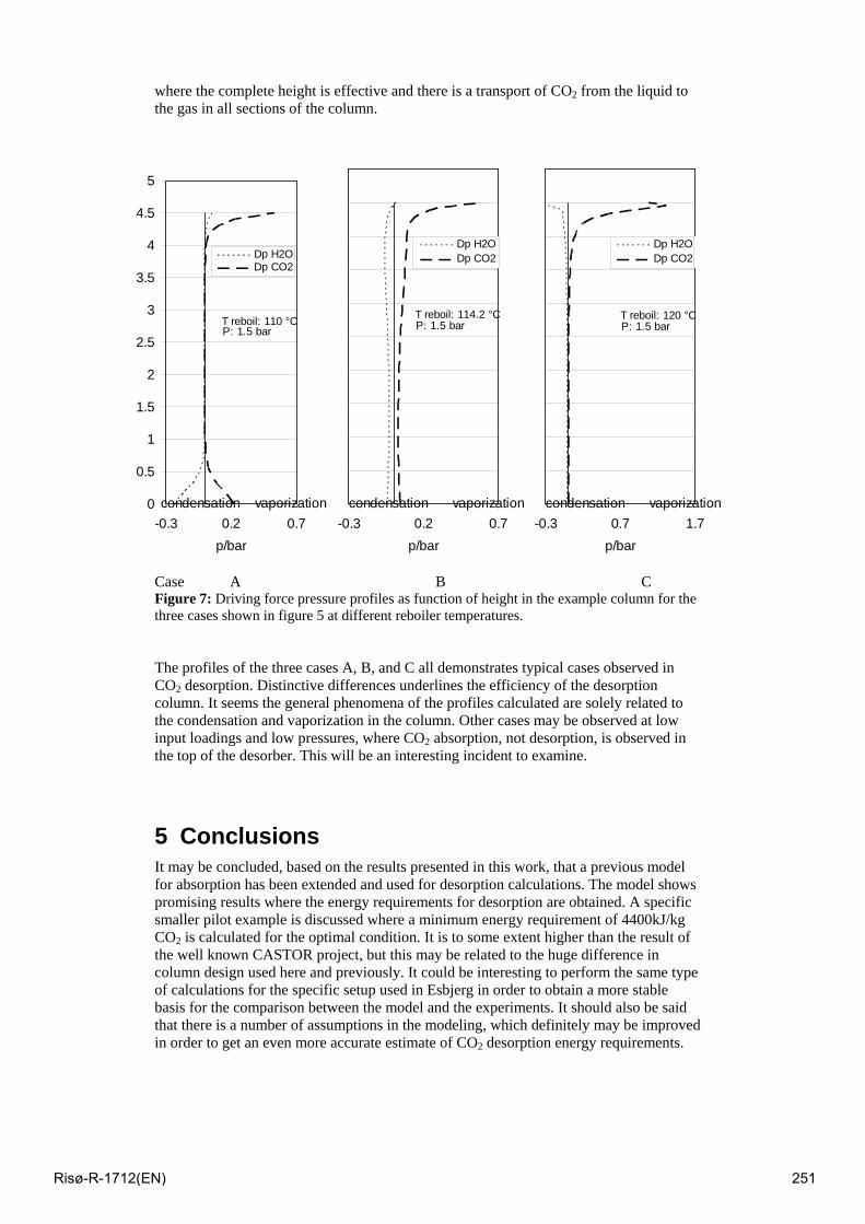
where the complete height is effective and there is a transport of CO2 from the liquid to the gas in all sections of the column.

0

0.5

1

1.5

2

2.5

3

3.5

4

4.5

5

-0.3 0.2 0.7p/bar

Dp H2ODp CO2

condensation vaporization

T reboil: 110 °CP: 1.5 bar

-0.3 0.2 0.7p/bar

Dp H2ODp CO2

condensation vaporization

T reboil: 114.2 °CP: 1.5 bar

-0.3 0.7 1.7p/bar

Dp H2ODp CO2

condensation vaporization

T reboil: 120 °CP: 1.5 bar

Case A B C Figure 7: Driving force pressure profiles as function of height in the example column for the three cases shown in figure 5 at different reboiler temperatures.

The profiles of the three cases A, B, and C all demonstrates typical cases observed in CO2 desorption. Distinctive differences underlines the efficiency of the desorption column. It seems the general phenomena of the profiles calculated are solely related to the condensation and vaporization in the column. Other cases may be observed at low input loadings and low pressures, where CO2 absorption, not desorption, is observed in the top of the desorber. This will be an interesting incident to examine.

5 Conclusions It may be concluded, based on the results presented in this work, that a previous model for absorption has been extended and used for desorption calculations. The model shows promising results where the energy requirements for desorption are obtained. A specific smaller pilot example is discussed where a minimum energy requirement of 4400kJ/kg CO2 is calculated for the optimal condition. It is to some extent higher than the result of the well known CASTOR project, but this may be related to the huge difference in column design used here and previously. It could be interesting to perform the same type of calculations for the specific setup used in Esbjerg in order to obtain a more stable basis for the comparison between the model and the experiments. It should also be said that there is a number of assumptions in the modeling, which definitely may be improved in order to get an even more accurate estimate of CO2 desorption energy requirements.

Risø-R-1712(EN) 251

6 Acknowledgement The sponsoring of the work performed in this study was partly funded by DONG Energy, Vattenfall A/S Heat Nordic, and the Danish Council for Strategic Research. The valuable support is gratefully acknowledged.

7 Literature Cited [1] Metz, B.; O. Davidson; de Coninck, H. C.; Loos,. M.; Meyer, L. A. (eds.). IPCC

special report on Carbon Dioxide Capture and Storage. Cambridge University Press, Cambridge, United Kingdom and New York, NY, USA, 2005.

[2] Gabrielsen, J. CO2 Capture From Coal Fires Power Plants. PhD. Thesis, IVC-SEP, department of chemical engineering, Technical University of Denmark, Kongens Lyngby, Denmark, 2007.

[3] Rocha J.A.; Bravo, J.L.; Fair J. R. Distillation columns containing structured packings: A comprehensive model for their performance. 1. Hydraulic models. Ind. Eng. Chem. Res. 32, 641-651, 1993.

[4] Rocha J.A.; Bravo, J.L.; Fair J. R. Distillation columns containing structured packings: A comprehensive model for their performance. 2. Mass-transfer model. Ind. Eng. Chem. Res. 35, 1660-1667, 1996.

[5] Billet, R; Schultes, M. Prediction of mass transfer columns with dumped and arranged packings updated summary of the calculation method of Billet and Schultes. Trans IChemE 77, 498-504, 1999.

[6] Wang, Y. W.; Xu, S.; Otto, F.D.; Mather, A. E. Solubility of N2O in alkonolamines and in mixed solvents,. Chem. Eng. J. and Bio. Eng. J. 48, 31-40, 1992.

[7] Browning, G. J.; Weiland, R. H. Physical solubility of carbon dioxide in aqueous alkonolamines via nitrous oxide analogy. J. Chem. Eng. Data 39, 817-822, 1994.

[8] Astarita, G; Savage, D. W. Gas absorption and desorption with reversible instantaneous chemical reaction. Chemical Engineering Science 35(8), 1755-1764, 1980.

Risø-R-1712(EN) 252

Session 14 – Mechanisms

Risø-R-1712(EN) 253

The interactions of renewable energy promotion and energy efficiency support schemes. An scenario comparison. Pablo del Río. Institute for Public Policies and Goods (IPP) Centro de Ciencias Humanas y Sociales Consejo Superior de Investigaciones Científicas (CSIC) C/Albasanz 26-28 28037 Madrid Spain Tel: +34 91 6022560 E-mail: pablo.delrio@cchs.csic.es Abstract CO2 emissions reduction, renewable energy deployment and energy efficiency are three main energy/environmental goals, particularly in Europe. Their relevance has led to the implementation of support schemes in these realms. The coexistence of these mechanisms may lead to overlaps, synergies and conflicts between them. The aim of this paper is to analyse those interactions. Previous analyses have only focused on the interactions between two instruments (emissions trading schemes and energy efficiency measures and emissions trading and renewable energy promotion schemes) whereas the mutual impacts between energy efficiency measures and renewable energy promotion have been much less studied. 1.- Introduction. Climate change mitigation and security of energy supply have allegedly triggered the implementation of a wide array of policies in Europe and, likely soon, in the U.S. This paper focuses on three of these policies: emissions trading schemes (ETS), support schemes for electricity produced with renewable energy sources (RES-E) and measures to encourage energy efficiency (EE)1. The discussion in this paper concentrates on the EU case. Both EE and RES-E support schemes are relatively common in the Member States and some of these instruments have been implemented for quite a long time, whereas the EU ETS is in its fifth year of operation. However, this analysis can be extrapolated to other territories where a combination of the three instruments already exist or will be implemented in the future. The combination of these instruments raises concerns about overlaps, conflicts and synergies in their interaction. Previous analyses have focused on the interactions between the EU ETS and RES-E promotion and between the EU ETS and EE policies. However, the analysis of the interaction between the three instruments (ETS, EE and RES-E promotion) and, especially, between the last two has been very scarce2 and limited to two specific RES-E and EE instruments based on “certificates”: tradable green and white certificates (TGCs and TWCs, respectively)3.

1 For illustrative purposes, i.e., to highlight the possible interactions between instruments, this paper focuses on electricity. 2 NERA (2005) focuses on the interaction between those instruments, but in a separate manner (i.e., for ETS and TWC and ETS and TGC) but the simultaneous interaction between TWC, ETS and TGC and even between TGCs and TWCs is disregarded. 3 See, among others, Bertoldi and Huld (2006), Oikonomou and Patel (2004), Farinelli et al (2005) and Klink and Langniss (2006). For example, Oikonomou and Patel (2004) observe that an integrated scheme

Risø-R-1712(EN) 254

Thus, this paper tries to cover two gaps in the literature. First, it analyses the impact of the interactions between the three instruments on several key variables in the electricity sector. Special attention is paid to the interactions between EE and RES-E support schemes4. Second, the analysis transcends the “certificate” debate (i.e., TGCs and TWCs) and considers other instruments, particularly feed-in tariffs for RES-E, in order to identify whether the choice of specific instruments affects the results of those interactions5. Accordingly, this paper is structured as follows. The following section discusses the methodology and the main assumptions. The main scenarios for linking ETS, RES-E and EE support schemes are briefly described in section 3 and section 4 compares the results of those scenarios. Section 5 identifies whether different support schemes lead to different interaction results. The paper closes with some concluding remarks. 2.- Methodology and main assumptions. 2.1. Methodology. The analysis of interactions performed in this paper uses a qualitative and graphical method in a partial equilibrium framework, where the electricity sector is represented. The impacts of the interaction between those instruments can be assessed by investigating how they affect a number of criteria (effectiveness and cost-effectiveness in CO2 emissions reductions and dynamic efficiency) and variables (electricity demand, wholesale and retail electricity prices, RES-E generation and investments, investments in EE measures and abatement costs). In general, the objectives of these instruments are depicted in specific energy, emissions, or other environmental targets and can conflict, overlap, complement or be neutral towards each other (Oikonomou and Jepma (2008). This theoretical/methodological framework based on a graphical analysis has been used in the past by, among others, del Río et al (2005), del Río (2006), Jensen and Skytte (2003) and Sorrell et al (2009). This paper complements other studies, which either analyse the interactions between TGC and ETS (NERA 2005, Jensen and Skytte 2002, 2003; Morthorst 2003), between TWC and ETS (Sorrell et al 2009, NERA 2005) or between different EE policies (Boonekamp 2006)6. 2.2. Main assumptions. -We assume separation between the three instruments, i.e., the commodities (certificates) from EE measures and RES-E promotion schemes are not translated into a CO2 emissions reduction value. Non-integration has taken place in countries with both a TWC and a TGC

of TWCs and TGCs could be feasible in terms of institutional setup. Bertoldi and Huld (2006) propose a combined tradable certificate scheme in which both RES and demand-side EE measures could bid in real time through the Internet to meet a specific obligation. Furthermore, they deal with the integration of both instruments and not on their mutual interactions. Our focus is not on the integration of schemes, which has proved a difficult issue anyway (see NERA 2005 and Oikonomou and Patel 2004), but on their interactions. 4 It has focused only on the issue of “integration” of instruments, whereas the real situation in the European countries is one of intended separation between both instruments 5 This analysis is deemed highly necessary because only six EU-27 countries have adopted “certificates” to promote RES-E and EE, whereas the majority use feed-in tariffs for RES-E promotion and non-certificate instruments to encourage EE (see European Commission 2008). 6 The graphical method strongly draws on NERA (2005) and Sorrell et al (2009). See del Río (2007) for an overview of the interaction literature, mostly focused on the interaction between ETS and RES-E support schemes.

Risø-R-1712(EN) 255

scheme in place (UK and Italy).7 This choice has lower transaction costs8 and mitigates the risk of double counting, which would undermine the ETS CO2 cap. Finally, integration would discourage RES promotion because EE measures are cheaper than most RES alternatives (Oikonomou 2004). -A competitive electricity market is assumed, i.e., the costs of EE and RES-E support measures are fully passed to electricity consumers. RES-E and EE support schemes entail a cost (the so-called “add-on”), which is fully paid by electricity consumers in their bills9. -EE measures only apply to the electricity sector, i.e., to increase the efficiency of energy conversion in the generation of electricity (i.e., not increase end-use efficiency). This assumption has also been used in other studies (i.e., Sorrel et al 2009; NERA 2005) and allows us to isolate the most relevant effects regarding the interactions of an ETS, EE and RES promotion within the boundaries of the electricity sector. -No EE measures and RES-E technologies simultaneously fall under EE and RES-E support schemes10. -In general secondary effects are disregarded, except for the increase in retail electricity prices due to the implementation of EE and RES-E support instruments, which triggers some relevant effects that ought to be considered. 3. Linking ETS, RES-E and EE support schemes: instruments, assessment criteria and scenarios. 3.1. Instruments for the promotion of RES-E and EE. Several instruments are available to improve EE in different sectors (industry, services, buildings, households and transport). Some of them are currently applied in EU countries, such as taxes, voluntary agreements, subsidies, tax deductions, standards, information campaigns and soft loans. Regarding instruments to improve electricity efficiency11 and reduce electricity consumption more specifically, mandatory saving targets (with or without TWCs) and taxes have received most of the attention. Other instruments include best available technologies (BAT) prescriptions, subsidies, procurement, demand-side management and information campaigns to electricity consumers. On the other hand, RES-E promotion in Europe has traditionally been based on two main (primary) mechanisms12: feed-in tariffs (FITs) and TGCs, whereas the implementation of a third instrument (bidding/tendering) has been less widespread13:

7 This is also the choice of the proposed RES Directive: Transferable GOs do not include a CO2 value. ETS remains the only way to trade CO2. 8 Linking requires robust tracking and data management across markets and will increase the administrative complexity (Bertoldi et al 2005). 9 Farinelli et al (2005) assume that the policy for EE (TWC) does not have a cost, i.e., that the increase in EE is free of costs to society. However, assuming no-cost of EE measures is a highly unrealistic situation, although it is possible that the add-on for EE support is lower than for RES-E support given that many EE options are considered to be low-cost (European Commission 2005). 10 This is the case in those countries where TGCs and TWCs have been applied (Italy and U.K.). 11 In the context of this paper, the term “electricity efficiency” refers to a reduction in electricity demand, improvement in conversion efficiencies and reduction in transmission and distribution losses. 12 Since this paper focuses on the analysis of the impact of different RES-E support schemes on the interactions, we provide a more detailed albeit still short description of these instruments. 13 These instruments have been supplemented by other complementary instruments (investment subsidies, fiscal and financial incentives and green pricing). See del Río and Gual (2004) for a more detailed explanation of the functioning of all these systems.

Risø-R-1712(EN) 256

FITs are subsidies per kWh generated paid in the form of a total quantity (regulated tariff) or as an amount on top of the wholesale price of electricity (premium) fed into the grid. Both FIT design options are combined with a purchase obligation by the utilities. TGCs are certificates issued for every MWh of RES-E, allowing RES-E generators to obtain additional revenue to the sale of electricity (i.e., two streams of revenue). Demand for TGCs generally originates from an obligation on electricity distribution companies to surrender a number of TGCs as a share of their annual consumption. Otherwise, they would have to pay a penalty. In both cases (TGCs and FITs), the costs are borne by consumers. 3.2. Assessment criteria and variables The coexistence and interactions between instruments can be assessed according to several criteria (see, among others, Oikonomu and Jepma 2008, Konidari and Mavrakis 2007 and del Río and Gual 2004). However, the focus in this paper is on the effectiveness and economic efficiency (static and dynamic)14. * Effectiveness. An instrument is effective if it is able to achieve a certain target (i.e., emissions reductions, RES-E and EE investments). * Cost-effectiveness refers to the achievement of a given emissions reduction, RES-E or EE target at the lowest possible cost. Cost-effectiveness is attained when an instrument encourages proportionally greater emissions reductions, RES-E or EE investments by firms with lower costs and lower emissions reductions RES-E or EE investments by companies with higher costs, leading to an equalisation of marginal costs across firms/plants (equimarginality). The administrative/transaction costs of the instruments are also part of the cost-effectiveness criteria. * Dynamic efficiency refers to the ability of an instrument to generate a continuous incentive for technical improvements and costs reductions in renewable energy technologies in the medium and long term. Currently expensive technologies with significant quality improvement and costs reduction potentials need to be supported today in order to have them available in the future to reach new targets at moderate costs15. We thus analyse the impact of the interactions on several key variables pertaining to the aforementioned three criteria. -Regarding the effectiveness criteria, CO2 emissions, electricity demand and RES-E generation and investments are the main variables. -Regarding static efficiency, the focus is on consumer costs (as shown by variations in the retail price of electricity, Pr). Pr is the result of adding the wholesale price of electricity (Pw) to the add-on for RES-E and EE support, whereas RES-E depends on Pw and the add-on for RES, EE investments mostly depends on the Pr. -Regarding dynamic efficiency, we analyse the impact on RES-E and EE investments and particularly on the least mature technologies. 3.3. The scenarios. Several scenarios are considered. Instruments are sequentially added to a baseline or reference scenario and their impact on the aforementioned variables is identified. 14 Efficiency and effectiveness are always present in any evaluation of instruments. While important, other criteria (such as equity and political acceptability/feasibility) are not considered here. 15 The importance of these dynamic efficiency effects are shown by, both, renewable energy models (see Huber et al 2004) and climate change models (see Stern 2006).

Risø-R-1712(EN) 257

(i) Reference scenario. No ETS, RES-E and EE support schemes are implemented. This scenario is quite unrealistic, though, given the policy instruments currently implemented or being proposed in most OECD countries. (ii) ETS. In this case, an ETS is introduced but no EE or RES-E support schemes are in place. (iii) ETS + RES-E. A RES-E support scheme is introduced in a situation with a pre-existing ETS, but no EE support policy. (iv) ETS + EE. In this case, a support scheme for EE is added to an ETS but without a RES-E support scheme. (v) ETS + RES-E + EE. Instruments are sequentially introduced in this order: First an ETS, then RES-E support schemes and finally EE support. (vi) ETS + EE + RES-E. In this case, EE support is introduced before RES-E support. 4.- Analysing the interactions: results of the scenario comparison. In this section we identify and compare the impact of the different scenarios on the key variables and criteria. The results of the comparison between scenarios are shown in table 1 for different variables/criteria16. 4.1. Case 1: Comparing scenario ii to i (lack of regulation → ETS). The introduction of an ETS results in higher electricity generation costs (an upward shift of the electricity supply curve), an increase in wholesale (Pw) and retail (Pr) electricity prices (assuming cost pass through into prices) and, thus, a lower electricity demand. CO2 emissions are obviously reduced. The higher Pr encourages the adoption of EE measures17. In turn, the higher costs for conventional, carbon-intensive electricity makes RES-E more competitive and, thus, increases its penetration. However, this increase in EE and RES-E may not be enough to achieve EE and RES-E goals and, thus, specific support instruments may be needed. 4.2. Case 2. Comparing iii to ii (ETS → ETS+RES-E) The introduction of RES-E support increases RES-E deployment, reduces conventional electricity generation and Pw. However, this policy is paid for by consumers in their electricity bills, leading to an increase in Pr (addition of RES-E support to Pw) and reducing electricity demand as a secondary effect, given the slight increase in Pr, triggering a modest impact on the adoption of EE measures. CO2 emissions are unaffected. The RES-E support scheme would not lead to additional reductions to those achieved by an ETS since the emissions reduced by RES-E are already covered by the ETS. One way to make RES-E deployment effectively contribute to CO2 emissions reductions in an ETS is by considering the emissions reductions to be achieved by the expected RES-E deployment when setting the CO2 emissions target.

16 However, for reasons of space, the figures are not reported here but only the main results of the analysis. They are available by the author upon request. 17 The term “measures” in this context refers to EE technologies and practices.

Risø-R-1712(EN) 258

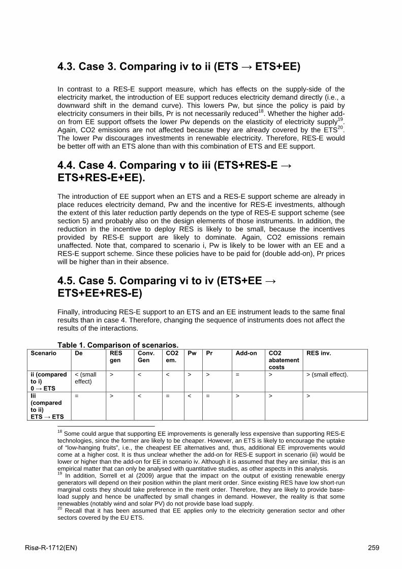
4.3. Case 3. Comparing iv to ii (ETS → ETS+EE) In contrast to a RES-E support measure, which has effects on the supply-side of the electricity market, the introduction of EE support reduces electricity demand directly (i.e., a downward shift in the demand curve). This lowers Pw, but since the policy is paid by electricity consumers in their bills, Pr is not necessarily reduced18. Whether the higher add-on from EE support offsets the lower Pw depends on the elasticity of electricity supply19. Again, CO2 emissions are not affected because they are already covered by the ETS20. The lower Pw discourages investments in renewable electricity. Therefore, RES-E would be better off with an ETS alone than with this combination of ETS and EE support. 4.4. Case 4. Comparing v to iii (ETS+RES-E → ETS+RES-E+EE). The introduction of EE support when an ETS and a RES-E support scheme are already in place reduces electricity demand, Pw and the incentive for RES-E investments, although the extent of this later reduction partly depends on the type of RES-E support scheme (see section 5) and probably also on the design elements of those instruments. In addition, the reduction in the incentive to deploy RES is likely to be small, because the incentives provided by RES-E support are likely to dominate. Again, CO2 emissions remain unaffected. Note that, compared to scenario i, Pw is likely to be lower with an EE and a RES-E support scheme. Since these policies have to be paid for (double add-on), Pr prices will be higher than in their absence. 4.5. Case 5. Comparing vi to iv (ETS+EE → ETS+EE+RES-E) Finally, introducing RES-E support to an ETS and an EE instrument leads to the same final results than in case 4. Therefore, changing the sequence of instruments does not affect the results of the interactions. Table 1. Comparison of scenarios.

Scenario De RES gen

Conv. Gen

CO2 em.

Pw Pr Add-on CO2 abatement costs

RES inv.

ii (compared to i) 0 → ETS

< (small effect)

> < < > > = > > (small effect).

Iii (compared to ii) ETS → ETS

= > < = < = > > >

18 Some could argue that supporting EE improvements is generally less expensive than supporting RES-E technologies, since the former are likely to be cheaper. However, an ETS is likely to encourage the uptake of “low-hanging fruits”, i.e., the cheapest EE alternatives and, thus, additional EE improvements would come at a higher cost. It is thus unclear whether the add-on for RES-E support in scenario (iii) would be lower or higher than the add-on for EE in scenario iv. Although it is assumed that they are similar, this is an empirical matter that can only be analysed with quantitative studies, as other aspects in this analysis. 19 In addition, Sorrell et al (2009) argue that the impact on the output of existing renewable energy generators will depend on their position within the plant merit order. Since existing RES have low short-run marginal costs they should take preference in the merit order. Therefore, they are likely to provide base-load supply and hence be unaffected by small changes in demand. However, the reality is that some renewables (notably wind and solar PV) do not provide base load supply. 20 Recall that it has been assumed that EE applies only to the electricity generation sector and other sectors covered by the EU ETS.

Risø-R-1712(EN) 259

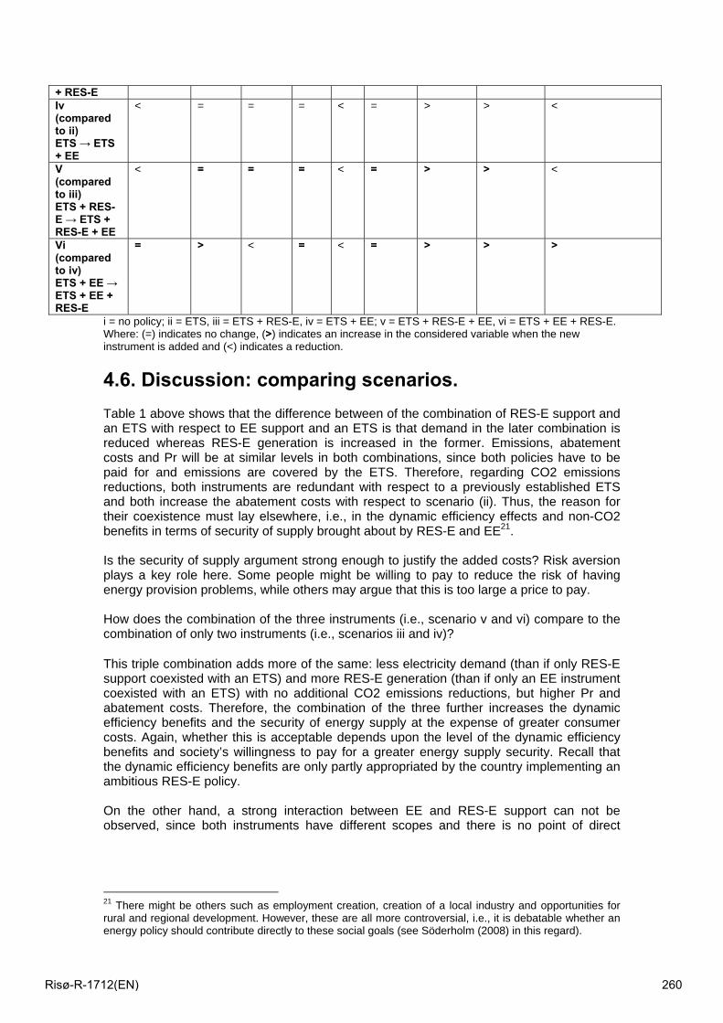
+ RES-E Iv (compared to ii) ETS → ETS + EE

< = = = < = > > <

V (compared to iii) ETS + RES-E → ETS + RES-E + EE

< = = = < = > > <

Vi (compared to iv) ETS + EE → ETS + EE + RES-E

= > < = < = > > >

i = no policy; ii = ETS, iii = ETS + RES-E, iv = ETS + EE; v = ETS + RES-E + EE, vi = ETS + EE + RES-E. Where: (=) indicates no change, (>) indicates an increase in the considered variable when the new instrument is added and (<) indicates a reduction. 4.6. Discussion: comparing scenarios. Table 1 above shows that the difference between of the combination of RES-E support and an ETS with respect to EE support and an ETS is that demand in the later combination is reduced whereas RES-E generation is increased in the former. Emissions, abatement costs and Pr will be at similar levels in both combinations, since both policies have to be paid for and emissions are covered by the ETS. Therefore, regarding CO2 emissions reductions, both instruments are redundant with respect to a previously established ETS and both increase the abatement costs with respect to scenario (ii). Thus, the reason for their coexistence must lay elsewhere, i.e., in the dynamic efficiency effects and non-CO2 benefits in terms of security of supply brought about by RES-E and EE21. Is the security of supply argument strong enough to justify the added costs? Risk aversion plays a key role here. Some people might be willing to pay to reduce the risk of having energy provision problems, while others may argue that this is too large a price to pay. How does the combination of the three instruments (i.e., scenario v and vi) compare to the combination of only two instruments (i.e., scenarios iii and iv)? This triple combination adds more of the same: less electricity demand (than if only RES-E support coexisted with an ETS) and more RES-E generation (than if only an EE instrument coexisted with an ETS) with no additional CO2 emissions reductions, but higher Pr and abatement costs. Therefore, the combination of the three further increases the dynamic efficiency benefits and the security of energy supply at the expense of greater consumer costs. Again, whether this is acceptable depends upon the level of the dynamic efficiency benefits and society’s willingness to pay for a greater energy supply security. Recall that the dynamic efficiency benefits are only partly appropriated by the country implementing an ambitious RES-E policy. On the other hand, a strong interaction between EE and RES-E support can not be observed, since both instruments have different scopes and there is no point of direct

21 There might be others such as employment creation, creation of a local industry and opportunities for rural and regional development. However, these are all more controversial, i.e., it is debatable whether an energy policy should contribute directly to these social goals (see Söderholm (2008) in this regard).

Risø-R-1712(EN) 260

interaction between them. Their mutual impacts are mediated through the electricity market, with one instrument acting on the supply side and the other on the demand side22. 5. Are different RES-E instruments likely to affect the results of the interactions? We start by analysing the interactions when the RES-E support instrument is a TGC scheme and the EE instrument is a TWC scheme. We then analyse whether the results of the interactions change when a different RES-E support scheme is introduced. In principle, the addition of a TGC scheme to a TWC scheme does not affect the functioning of the later and indirectly influences the uptake of EE measures, due to an increase in Pr stemming from the application of the RES-E promotion scheme. On the other hand, adding a TWC scheme (or any other EE support scheme) to a TGC scheme can affect the TGC market, but only if the RES-E quota is set in percentage terms (i.e., with respect to electricity sales). In this case, a TWC would reduce electricity demand/production and the absolute requirement for RES-E23. Jensen and Skytte (2002) observe that Pw and the TGC price (Ptgc) move in opposite directions24, i.e., a reduction in Pw triggers an increase in Ptgc. This could lead to an erroneous interpretation of the impact of EE measures on TGCs if it is argued that the subsequent reduction in Pw would increase Ptgc, leaving total support constant. However, support does not remain constant when electricity demand is reduced. Indeed, with a large demand reduction and a highly inelastic RES-E supply curve (MCres-e), there could be both a reduction in Pw and Ptgc (figure 2). In this case, there would be a double disincentive for RES-E investments if an EE measure is added to a TGC scheme.

22 In spite of being limited, the addition of an EE instrument to a RES-E support measure has a slightly greater effect on RES-E support than the addition of RES-E support to an EE scheme has on the later. 23 A lower TGC price would result and, thus, the highest cost renewable energy technologies which were previously needed to fulfil the quota would no longer be needed. 24 The Ptgc is the difference between the marginal costs of the marginal technology to meet the quota and Pw.

Risø-R-1712(EN) 261

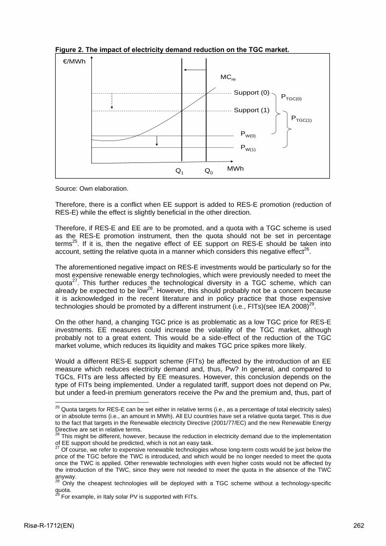
Figure 2. The impact of electricity demand reduction on the TGC market. Source: Own elaboration. Therefore, there is a conflict when EE support is added to RES-E promotion (reduction of RES-E) while the effect is slightly beneficial in the other direction. Therefore, if RES-E and EE are to be promoted, and a quota with a TGC scheme is used as the RES-E promotion instrument, then the quota should not be set in percentage terms25. If it is, then the negative effect of EE support on RES-E should be taken into account, setting the relative quota in a manner which considers this negative effect26. The aforementioned negative impact on RES-E investments would be particularly so for the most expensive renewable energy technologies, which were previously needed to meet the quota27. This further reduces the technological diversity in a TGC scheme, which can already be expected to be low28. However, this should probably not be a concern because it is acknowledged in the recent literature and in policy practice that those expensive technologies should be promoted by a different instrument (i.e., FITs)(see IEA 2008)29. On the other hand, a changing TGC price is as problematic as a low TGC price for RES-E investments. EE measures could increase the volatility of the TGC market, although probably not to a great extent. This would be a side-effect of the reduction of the TGC market volume, which reduces its liquidity and makes TGC price spikes more likely. Would a different RES-E support scheme (FITs) be affected by the introduction of an EE measure which reduces electricity demand and, thus, Pw? In general, and compared to TGCs, FITs are less affected by EE measures. However, this conclusion depends on the type of FITs being implemented. Under a regulated tariff, support does not depend on Pw, but under a feed-in premium generators receive the Pw and the premium and, thus, part of 25 Quota targets for RES-E can be set either in relative terms (i.e., as a percentage of total electricity sales) or in absolute terms (i.e., an amount in MWh). All EU countries have set a relative quota target. This is due to the fact that targets in the Renewable electricity Directive (2001/77/EC) and the new Renewable Energy Directive are set in relative terms. 26 This might be different, however, because the reduction in electricity demand due to the implementation of EE support should be predicted, which is not an easy task. 27 Of course, we refer to expensive renewable technologies whose long-term costs would be just below the price of the TGC before the TWC is introduced, and which would be no longer needed to meet the quota once the TWC is applied. Other renewable technologies with even higher costs would not be affected by the introduction of the TWC, since they were not needed to meet the quota in the absence of the TWC anyway. 28 Only the cheapest technologies will be deployed with a TGC scheme without a technology-specific quota. 29 For example, in Italy solar PV is supported with FITs.

PW(0)

Support (0)

PW(1)

Support (1)

PTGC(0)

PTGC(1)

Q1

€/MWh

MWh

MCre

Q0

Risø-R-1712(EN) 262

the total support is affected. The reduction in Pw triggered by EE support reduces the overall incentive to invest in RES-E. To sum up, the type of support scheme does have an impact on the results of the interactions, but this effect is mostly mediated by the design elements of those instruments, an issue left for future research. 6. Conclusions. Traditionally, policy analysis of climate policy instruments has been based on an individual approach, i.e., separated from other measures with which they are likely to interact. However, the functioning of these instruments depends on these interactions. Indeed, policy setting in the presence of multiple objectives has been identified as one of the important problem areas for the future (Farinelli et al 2005). At least in the EU, this debate transcends the boundaries of academic discussions, however, because it has real policy implications, given the coexistence of the EU ETS with RES-E support schemes and EE instruments. This coexistence may lead to overlapping effects, synergies and conflicts. This paper has focused on the interactions between RES-E and EE support schemes, which have received less attention in the literature. The following are the main conclusions of this paper. In general, the interactions between RES-E support and EE measures are modest. The reason for this limited interaction is that these later two instruments have different scopes, with no point of direct interaction. Their mutual impacts are mediated through electricity markets, with one instrument acting on the supply side and the other on the demand side. The most relevant interactions between those two instruments occur when EE support is added to RES-E promotion, especially when TGCs with a relative quota have been implemented. EE measures would put a downward pressure on electricity demand reducing the absolute requirement for RES-E. The highest cost renewable energy technologies which were previously needed to set the quota would no longer be needed. In contrast, the direct interactions on the opposite direction (i.e., from RES support to EE support) are more limited because there is basically an addition of effects (complementarity), although indirect interactions take place through the impact of both measures on the retail price. In order for an instrument to be part of an optimal set of policy measures, it should complement already existing measures, not overlap or lead to conflicts. In principle, adding EE and RES-E promotion measures to an ETS does not lead to additional CO2 emissions reductions. Therefore, those instruments could be deemed redundant and their combination is more costly with respect to CO2 emissions reductions. However, when a dynamic efficiency perspective (which is crucial in the climate policy debate) is adopted, then such combination may not be so redundant. Both renewable energy and energy efficiency technologies will be needed in the future at moderate costs. They do not contribute cost-effectively to emissions reductions in the short term when there is a pre-existing ETS covering the same emissions. However, encouraging their development/deployment and cost reductions will allow reaching more ambitious emissions targets at lower costs in the future and/or to set more ambitious emissions targets30. The more stringent the targets, the greater the emissions reductions and the need to invest earlier in technologies to have them at reasonable costs in the future.

30 Other arguments which justify the coexistence of instruments include security of supply and other national and local benefits.

Risø-R-1712(EN) 263

Notwithstanding, the effects of the interactions on dynamic efficiency are ambiguous as suggested above: adding an EE instrument to a TGC scheme reduces the incentive to invest in RES-E technologies, but the increase in retail prices as a result of such combination increases the incentive to implement EE practices and technologies.

Different instruments for RES-E and EE support may affect the results of the interactions differently. Particularly, the case of RES-E support schemes (FITs and TGCs) has been discussed. It has been shown that such interaction is likely to be more conflictive when a TGC scheme is adopted (rather than a FIT). This paper has illustrated the mechanisms at work. It should be followed by quantitative analysis, preferably with general equilibrium models. The approach followed in this paper is no substitute for such an analysis. Acknowledgements Financial support from the Spanish National Council for Scientific Research is gratefully acknowledged. References Bertoldi, P. and Huld , T. (2006). “Tradable certificate for renewable electricity and energy saving”, Energy Policy, 34(2), 212-222 Bertoldi, P., Rezessy, S., Langniss, O., Voogt, M. (2005). White, Green and Brown certificates: how to make the most of them?. European Commission, Joint Research Centre. Boonekamp, P. (2006). “Actual interaction effects between policy measures for energy efficiency—A qualitative matrix method and quantitative simulation results for households”. Energy, 31(14), 2848-2873 European Commission (2005). Green Paper on Energy Efficiency, or Doing More With Less. Brussels. European Commission (2008). The support of electricity from renewable energy sources Commission staff working document. Accompanying document to the Proposal for a Directive of the European Parliament and of the Council on the promotion of the use of energy from renewable sources COM(2008) 19. SEC(2008) 57. Brussels. Farinelli, U., Johansson, T., McCormick, K., Mundaca, L., Oikonomou, V., Ortenvik, M., Patel, M., Santi, F. (2005). ‘‘White and Green: comparison of market-based instruments to promote energy efficiency”. Journal of Cleaner Production 13 (10–11), 1015–1026. Huber, C., Faber, T., Haas, R., Resch, G., Green, J., Olz, S., White, S., Cleijine, H., Ruijgrok, W., Morthorst, P.E., Skytte, K., Gual, M., del Rio, P., Hernandez, F., Tacsir, A., Ragwitz, M., Schleich, J., Orasch, W., Bokemann, M., Lins, C., 2005. Green X Total Deriving Optimal Promotion Strategies for Increasing the Share of RES-E in a Dynamic European Electricity Market. Energy Economics Group, Institute of Power Systems and Energy Economics, Vienna University of Technology, Vienna. International Energy Agency (IEA)(2008). Deploying Renewables. Principles for Effective Policies. Paris. Jensen, S.G., Skytte, K. (2002). ”Interactions between the power and green certificate markets”. Energy Policy 30 (5), 425–435.

Risø-R-1712(EN) 264

Jensen, S.G., Skytte, K. (2003). ”Simultaneous attainment of energy goals by means of green certificates and emission permits”. Energy Policy 31 (1), 63–71. Konidari, P. Mavrakis, D. (2007). “A multi-criteria evaluation method for climate change mitigation policy instruments”. Energy Policy, 35(12), 6235-6257. Langniss, O., Klink, J. (2006). White certificate schemes and (national) green certificate schemes. EuroWhiteCert Project, Work Package 3.2 Task Report. Morthorst, P.E. (2003). “A green certificate market combined with a liberalised electricity market”. Energy Policy 31, 1393–1402. NERA (2005). Interactions of the EU ETS with Green and White Certificate Schemes. NERA Economic consulting. London. Oikonomou, V. and Jepma, C.J. (2008). “A framework on interactions of climate and energy policy instruments”. Mitigation and Adaptation Strategy for Global Change 13, 131-156 Oikonomou V., Patel M. (2004). An inventory of innovative policies and measures for energy efficiency, Phase I of the EU SAVE “White and Green” project, Copernicus Institute, NWS-E-2004-113, Utrecht University.

Del Río, P. (2006). “Linking renewable energy CDM projects and TGC schemes. An analysis of different options”. Energy Policy, 34, 3173-3183. Del Río, P. (2007). “The interaction between emissions trading and renewable electricity support schemes. an overview of the literature”. Mitigation and Adaptation Strategies for Global Change (2007), 12(8), 1363-1390. Del Río, P. and Gual, M.A. (2004). “The promotion of green electricity in Europe: Present and future”. European Environment Journal, 14, 219-234. Del Río, P. Hernández, F. and Gual, M.A. (2005). “The Implications of the Kyoto project mechanisms for the deployment of renewable electricity in Europe”. Energy Policy, 33(5), 2010-2022. Söderholm, P. (2008). “The political economy of international green certificate markets”. Energy Policy, 36(6), 2051-2062 Sorrell, S., (2003). “Who owns the carbon? Interactions between the EU emissions trading scheme and the UK renewables obligation and energy efficiency commitment”. Energy and Environment 14 (5), 677–703. Sorrell, S., Harrison, D., Radov, D., Klevnas, P., Foss, A. (2009). “White certificate schemes: Economic analysis and interactions with the EU ETS”. Energy Policy, 37, 29–42 Stern, N. (2006). The Economics of Climate Change. The Stern Review. Cambridge University Press. Cambridge.

Risø-R-1712(EN) 265

Session 15 – Systems aspects II

Risø-R-1712(EN) 266

Accelerated Development of Low Carbon Energy Supply Technologies – and its impact on Energy System Decarbonisation

Dr Mark Winskel, UK Energy Research Centre and University of Edinburgh

Nils Markusson, Brighid Moran and Henry Jeffrey (Edinburgh University); Chiara Candelise, Sophie Jablonski, Christos Kalyvas and Nick Hughes (Imperial College, London); Donna Clarke and Gail Taylor (Southampton University), Hannah Chalmers (Surrey University); Geoff Dutton (Rutherford Appleton Laboratories); Paul Howarth (Manchester University); and David Ward (UKAEA Culham)

Abstract The UK Energy Research Centre (UKERC) recently undertook a major cross-disciplinary research project, Energy 2050, to examine the means by which the UK can move towards a low-carbon energy system over the next forty years. As part of this, UKERC’s Energy Supply Working Group examined the prospects for accelerated technological development of a range of low carbon energy supply technologies, and the potential impact of this on UK energy system decarbonisation pathways. A series of scenarios were developed to represent the prospects for accelerated technological development. Then, using the Markal energy systems model, the impact of this acceleration on the decarbonisation of UK energy system was examined.

The results indicate that there are significant prospects for accelerated development for a range of renewable and other low carbon energy supply technologies, and that this acceleration could make a substantial impact on decarbonisation of the UK energy system from now to 2050. Accelerated technological development offers substantial benefit, in reducing the overall costs of decarbonisation over the longer term. However, because most of this impact is manifested after 2030, rather than over the next decade, the results suggest a disparity between technology performance and cost, and political aspirations for low carbon technology deployment from now to 2020.

1 Introduction: the UKERC Accelerated Technology Development Scenarios This paper focuses on the prospects for accelerated development of a range of emerging low-carbon energy supply technologies – and the possible impact of this on decarbonising the UK energy system. The technologies analysed here include a number of renewables (wind power, marine energy, solar PV and bioenergy) and other emerging low carbon technologies (advanced designs of nuclear power, carbon capture and storage (CCS) and hydrogen / fuel cells).

The research involved devising accelerated technology development (ATD) scenarios of UK energy system decarbonisation (which assume high levels of technological progress over time), and comparing these with non-accelerated decarbonisation scenarios (see Table 1). Given the large uncertainties involved, the results should be seen as illustrating the possible impact of supply side technology progress, rather than a detailed mapping out of system change over the next decade or beyond.

For each supply technology, the prospects for accelerated development were considered by short statements, or narratives, which highlighted potential trends and breakthroughs in availability, performance and cost from now to 2050. These narratives were developed by technology specialists using research landscape and roadmap reports produced for the

Risø-R-1712(EN) 267

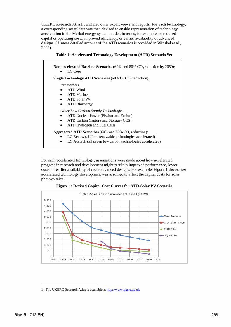
UKERC Research Atlas1 , and also other expert views and reports. For each technology, a corresponding set of data was then devised to enable representation of technology acceleration in the Markal energy system model, in terms, for example, of reduced capital or operating costs, improved efficiency, or earlier availability of advanced designs. (A more detailed account of the ATD scenarios is provided in Winskel et al., 2009).

Table 1: Accelerated Technology Development (ATD) Scenario Set

For each accelerated technology, assumptions were made about how accelerated progress in research and development might result in improved performance, lower costs, or earlier availability of more advanced designs. For example, Figure 1 shows how accelerated technology development was assumed to affect the capital costs for solar photovoltaics.

Figure 1: Revised Capital Cost Curves for ATD-Solar PV Scenario

0

500

1,000

1,500

2,000

2,500

3,000

3,500

4,000

4,500

5,000

2000 2005 2010 2015 2020 2025 2030 2035 2040 2045 2050 2055

Solar PV-ATD cost curve-decentralised (£/kW)

Core Scenario

Crystalline silicon

THIN FILM

Organic PV

1 The UKERC Research Atlas is available at http://www.ukerc.ac.uk

Non-accelerated Baseline Scenarios (60% and 80% CO2 reduction by 2050): • LC Core

Single Technology ATD Scenarios (all 60% CO2 reduction):

Renewables • ATD Wind • ATD Marine • ATD Solar PV • ATD Bioenergy

Other Low Carbon Supply Technologies • ATD Nuclear Power (Fission and Fusion) • ATD Carbon Capture and Storage (CCS) • ATD Hydrogen and Fuel Cells

Aggregated ATD Scenarios (60% and 80% CO2 reduction): • LC Renew (all four renewable technologies accelerated) • LC Acctech (all seven low carbon technologies accelerated)

Risø-R-1712(EN) 268

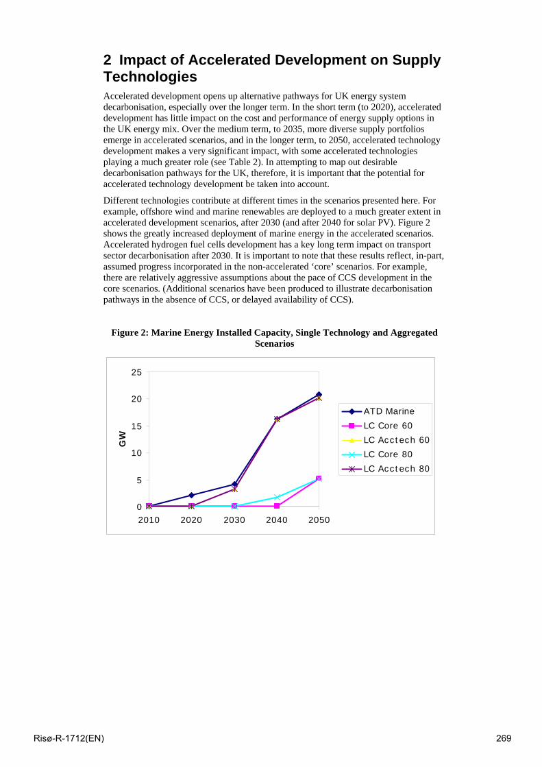
2 Impact of Accelerated Development on Supply Technologies Accelerated development opens up alternative pathways for UK energy system decarbonisation, especially over the longer term. In the short term (to 2020), accelerated development has little impact on the cost and performance of energy supply options in the UK energy mix. Over the medium term, to 2035, more diverse supply portfolios emerge in accelerated scenarios, and in the longer term, to 2050, accelerated technology development makes a very significant impact, with some accelerated technologies playing a much greater role (see Table 2). In attempting to map out desirable decarbonisation pathways for the UK, therefore, it is important that the potential for accelerated technology development be taken into account.

Different technologies contribute at different times in the scenarios presented here. For example, offshore wind and marine renewables are deployed to a much greater extent in accelerated development scenarios, after 2030 (and after 2040 for solar PV). Figure 2 shows the greatly increased deployment of marine energy in the accelerated scenarios. Accelerated hydrogen fuel cells development has a key long term impact on transport sector decarbonisation after 2030. It is important to note that these results reflect, in-part, assumed progress incorporated in the non-accelerated ‘core’ scenarios. For example, there are relatively aggressive assumptions about the pace of CCS development in the core scenarios. (Additional scenarios have been produced to illustrate decarbonisation pathways in the absence of CCS, or delayed availability of CCS).

Figure 2: Marine Energy Installed Capacity, Single Technology and Aggregated Scenarios

0

5

10

15

20

25

2010 2020 2030 2040 2050

GW

ATD Marine

LC Core 60

LC Acctech 60

LC Core 80

LC Acctech 80

Risø-R-1712(EN) 269

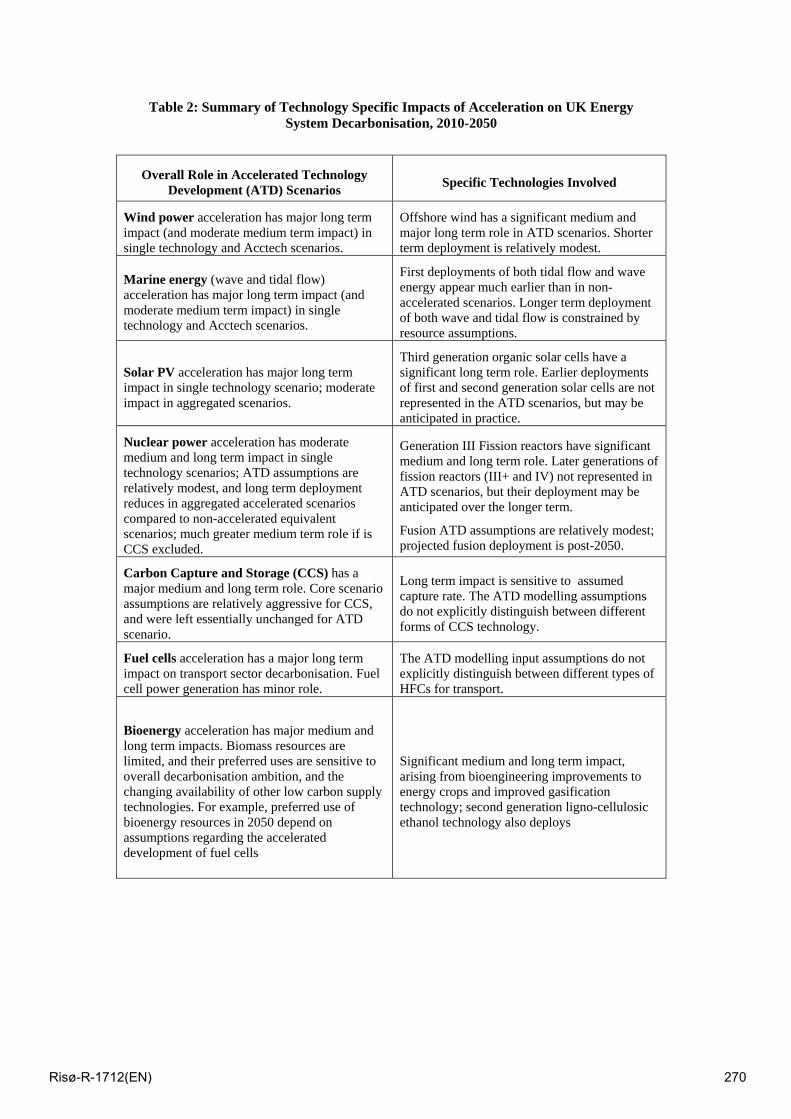
Table 2: Summary of Technology Specific Impacts of Acceleration on UK Energy System Decarbonisation, 2010-2050

Overall Role in Accelerated Technology Development (ATD) Scenarios Specific Technologies Involved

Wind power acceleration has major long term impact (and moderate medium term impact) in single technology and Acctech scenarios.

Offshore wind has a significant medium and major long term role in ATD scenarios. Shorter term deployment is relatively modest.

Marine energy (wave and tidal flow) acceleration has major long term impact (and moderate medium term impact) in single technology and Acctech scenarios.

First deployments of both tidal flow and wave energy appear much earlier than in non-accelerated scenarios. Longer term deployment of both wave and tidal flow is constrained by resource assumptions.

Solar PV acceleration has major long term impact in single technology scenario; moderate impact in aggregated scenarios.

Third generation organic solar cells have a significant long term role. Earlier deployments of first and second generation solar cells are not represented in the ATD scenarios, but may be anticipated in practice.

Nuclear power acceleration has moderate medium and long term impact in single technology scenarios; ATD assumptions are relatively modest, and long term deployment reduces in aggregated accelerated scenarios compared to non-accelerated equivalent scenarios; much greater medium term role if is CCS excluded.

Generation III Fission reactors have significant medium and long term role. Later generations of fission reactors (III+ and IV) not represented in ATD scenarios, but their deployment may be anticipated over the longer term.

Fusion ATD assumptions are relatively modest; projected fusion deployment is post-2050.

Carbon Capture and Storage (CCS) has a major medium and long term role. Core scenario assumptions are relatively aggressive for CCS, and were left essentially unchanged for ATD scenario.

Long term impact is sensitive to assumed capture rate. The ATD modelling assumptions do not explicitly distinguish between different forms of CCS technology.

Fuel cells acceleration has a major long term impact on transport sector decarbonisation. Fuel cell power generation has minor role.

The ATD modelling input assumptions do not explicitly distinguish between different types of HFCs for transport.

Bioenergy acceleration has major medium and long term impacts. Biomass resources are limited, and their preferred uses are sensitive to overall decarbonisation ambition, and the changing availability of other low carbon supply technologies. For example, preferred use of bioenergy resources in 2050 depend on assumptions regarding the accelerated development of fuel cells

Significant medium and long term impact, arising from bioengineering improvements to energy crops and improved gasification technology; second generation ligno-cellulosic ethanol technology also deploys

Risø-R-1712(EN) 270

3 Accelerated Development and UK Energy System Decarbonisation The overall impacts of accelerated technology development on UK energy system decarbonisation are complex, changing over time as different low carbon supply options are made available, and as overall decarbonisation ambitions increase. For example, accelerated fuel cells development changes the relative attractiveness of decarbonising different energy services, and the supply technologies involved. The most attractive supply technologies – and the research priorities associated with their commercialisation – are also sensitive to the overall level of decarbonisation ambition. Raising the decarbonisation ambition from 60% to 80% does not simply mean doing ‘more of the same’ – it introduces new technology preferences and research priorities. For example, the preferred use of bioenergy resources switches between electricity, heating and transport, according to the overall level of decarbonisation ambition and the availability of alternative ways of decarbonising particular energy services.

In terms of decarbonisation by sector, the electricity supply sector decarbonises first and most deeply, and is substantially decarbonised by 2030 in all 80% scenarios, with or without accelerated technology development. Other carbon intensive energy services (especially transport, but also residential demand) decarbonise in the medium and longer terms. Accelerated development makes some difference to this broad pattern. For example, the introduction of fuel cells acceleration is associated with greater decarbonisation of transport (and reduced decarbonisation of the residential sector) over the longer term.

The same broad pattern of declining overall energy demand, as the energy system decarbonises, is followed with or without accelerated technology development. Gas and coal remain important primary fuels in 2050, although gas has much reduced demand, and oil is almost absent from the energy mix by 2050. The introduction of accelerated fuels cells development means that hydrogen has become the dominant transport fuel in the accelerated scenario by 2050.In terms of final energy demand by sector, however, accelerated technology development makes a significant difference over the long term. In the non-accelerated scenario, residential energy demand almost halves between 2035 and 2050 – a key contributor to long term system decarbonisation. In Acctech, however, residential energy demand declines much less steeply – only by around 20% between 2035 and 2050.

4 Costs and Benefits of Acceleration The modelling results offer some indication of the overall advantages of supply side technology acceleration on energy system decarbonisation. These advantages accrue mostly in the long term, as accelerated development provides more affordable ways to achieve deeper decarbonisation. Two Markal modelling parameters – the marginal cost of CO2 abatement, and the overall ‘welfare cost’ of decarbonisation – provide some quantification of this benefit. Given the high levels of uncertainty embedded in the scenarios, especially over the longer term, these figures only offer an illustration of the possible benefits of accelerated development, under assumptions of high levels of progress.

The marginal cost of carbon abatement increases over the longer term as progressively more expensive carbon abatement options are deployed. In the accelerated development scenarios, however, this increase is considerably less than in non-accelerated equivalent scenarios – by 2050, the marginal cost of CO2 abatement is around £130/tonne in the Acctech accelerated development scenarios, compared to £170/tonne in the equivalent non-accelerated scenario.

Risø-R-1712(EN) 271

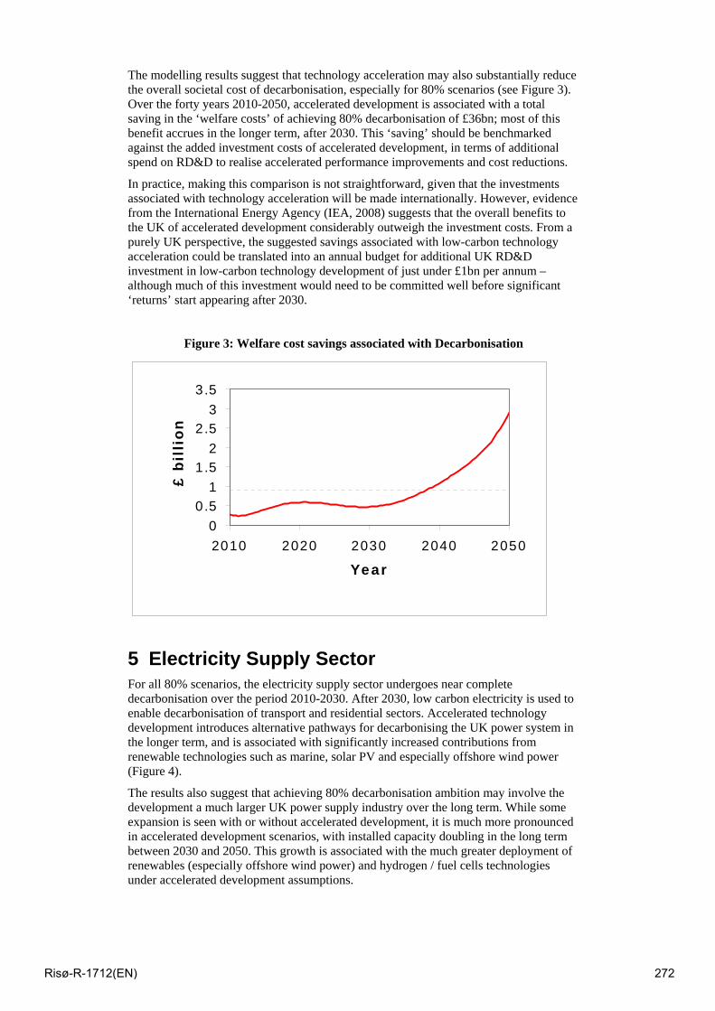
The modelling results suggest that technology acceleration may also substantially reduce the overall societal cost of decarbonisation, especially for 80% scenarios (see Figure 3). Over the forty years 2010-2050, accelerated development is associated with a total saving in the ‘welfare costs’ of achieving 80% decarbonisation of £36bn; most of this benefit accrues in the longer term, after 2030. This ‘saving’ should be benchmarked against the added investment costs of accelerated development, in terms of additional spend on RD&D to realise accelerated performance improvements and cost reductions.

In practice, making this comparison is not straightforward, given that the investments associated with technology acceleration will be made internationally. However, evidence from the International Energy Agency (IEA, 2008) suggests that the overall benefits to the UK of accelerated development considerably outweigh the investment costs. From a purely UK perspective, the suggested savings associated with low-carbon technology acceleration could be translated into an annual budget for additional UK RD&D investment in low-carbon technology development of just under £1bn per annum – although much of this investment would need to be committed well before significant ‘returns’ start appearing after 2030.

Figure 3: Welfare cost savings associated with Decarbonisation

00.5

11.5

22.5

33.5

2010 2020 2030 2040 2050

Year

£ b

illi

on

5 Electricity Supply Sector For all 80% scenarios, the electricity supply sector undergoes near complete decarbonisation over the period 2010-2030. After 2030, low carbon electricity is used to enable decarbonisation of transport and residential sectors. Accelerated technology development introduces alternative pathways for decarbonising the UK power system in the longer term, and is associated with significantly increased contributions from renewable technologies such as marine, solar PV and especially offshore wind power (Figure 4).

The results also suggest that achieving 80% decarbonisation ambition may involve the development a much larger UK power supply industry over the long term. While some expansion is seen with or without accelerated development, it is much more pronounced in accelerated development scenarios, with installed capacity doubling in the long term between 2030 and 2050. This growth is associated with the much greater deployment of renewables (especially offshore wind power) and hydrogen / fuel cells technologies under accelerated development assumptions.

Risø-R-1712(EN) 272

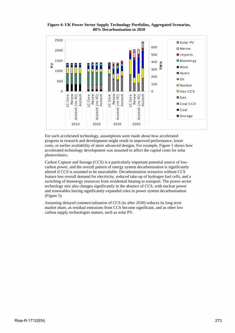
Figure 4: UK Power Sector Supply Technology Portfolios, Aggregated Scenarios, 80% Decarbonisation to 2050

0

500

1000

1500

2000

2500

LC C

ore

Renew

Acc

tech

(no F

C)

Acc

tech

LC C

ore

Renew

Acc

tech

(no F

C)

Acc

tech

LC C

ore

Renew

Acc

tech

(no F

C)

Acc

tech

LC C

ore

Renew

Acc

tech

(no F

C)

Acc

tech

2010 2020 2035 2050

PJ

0

100

200

300

400

500

600

TW

h

Solar PV

Marine

Imports

Bioenergy

Wind

Hydro

Oil

Nuclear

Gas CCS

Gas

Coal CCS

Coal

Storage

For each accelerated technology, assumptions were made about how accelerated progress in research and development might result in improved performance, lower costs, or earlier availability of more advanced designs. For example, Figure 1 shows how accelerated technology development was assumed to affect the capital costs for solar photovoltaics.

Carbon Capture and Storage (CCS) is a particularly important potential source of low-carbon power, and the overall pattern of energy system decarbonisation is significantly altered if CCS is assumed to be unavailable. Decarbonisation scenarios without CCS feature less overall demand for electricity, reduced take-up of hydrogen fuel cells, and a switching of bioenergy resources from residential heating to transport. The power sector technology mix also changes significantly in the absence of CCS, with nuclear power and renewables having significantly expanded roles in power system decarbonisation (Figure 5).

Assuming delayed commercialisation of CCS (to after 2030) reduces its long term market share, as residual emissions from CCS become significant, and as other low carbon supply technologies mature, such as solar PV.

Risø-R-1712(EN) 273

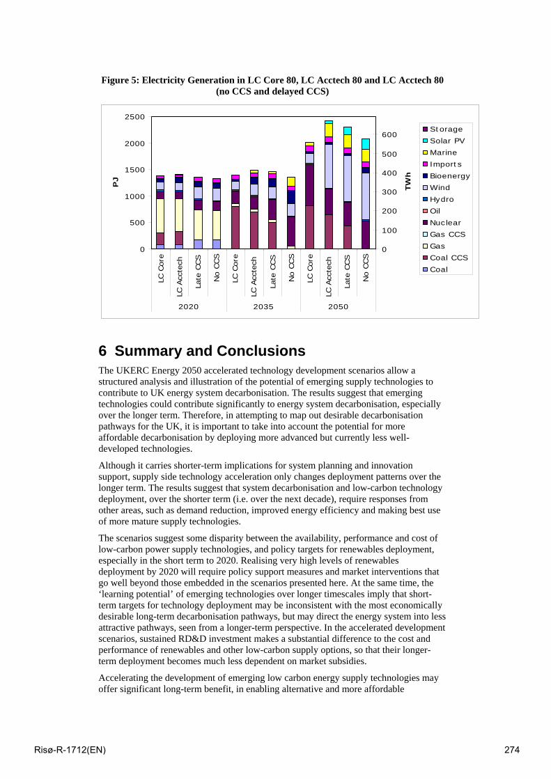
Figure 5: Electricity Generation in LC Core 80, LC Acctech 80 and LC Acctech 80 (no CCS and delayed CCS)

0

500

1000

1500

2000

2500

LC C

ore

LC A

ccte

ch

Late

CCS

No C

CS

LC C

ore

LC A

ccte

ch

Late

CCS

No C

CS

LC C

ore

LC A

ccte

ch

Late

CCS

No C

CS

2020 2035 2050

PJ

0

100

200

300

400

500

600

TW

h

Storage

Solar PV

Marine

Imports

Bioenergy

Wind

Hydro

Oil

Nuclear

Gas CCS

Gas

Coal CCS

Coal

6 Summary and Conclusions The UKERC Energy 2050 accelerated technology development scenarios allow a structured analysis and illustration of the potential of emerging supply technologies to contribute to UK energy system decarbonisation. The results suggest that emerging technologies could contribute significantly to energy system decarbonisation, especially over the longer term. Therefore, in attempting to map out desirable decarbonisation pathways for the UK, it is important to take into account the potential for more affordable decarbonisation by deploying more advanced but currently less well-developed technologies.

Although it carries shorter-term implications for system planning and innovation support, supply side technology acceleration only changes deployment patterns over the longer term. The results suggest that system decarbonisation and low-carbon technology deployment, over the shorter term (i.e. over the next decade), require responses from other areas, such as demand reduction, improved energy efficiency and making best use of more mature supply technologies.

The scenarios suggest some disparity between the availability, performance and cost of low-carbon power supply technologies, and policy targets for renewables deployment, especially in the short term to 2020. Realising very high levels of renewables deployment by 2020 will require policy support measures and market interventions that go well beyond those embedded in the scenarios presented here. At the same time, the ‘learning potential’ of emerging technologies over longer timescales imply that short-term targets for technology deployment may be inconsistent with the most economically desirable long-term decarbonisation pathways, but may direct the energy system into less attractive pathways, seen from a longer-term perspective. In the accelerated development scenarios, sustained RD&D investment makes a substantial difference to the cost and performance of renewables and other low-carbon supply options, so that their longer-term deployment becomes much less dependent on market subsidies.

Accelerating the development of emerging low carbon energy supply technologies may offer significant long-term benefit, in enabling alternative and more affordable

Risø-R-1712(EN) 274

decarbonisation. It may well also offer wider benefits in terms of system diversity and security. Realising this potential will require the UK to participate fully in global efforts at low-carbon technology innovation. A step-change increase in RD&D investment is economically justified, and promises significant reward in the longer term.

There are many uncertainties involved here, and no simple messages in terms of ‘picking winners’ – many of the technologies analysed here, and many others not included – have a significant potential role in UK energy system decarbonisation. Rather than a premature selection of ‘silver bullets’, the need is for sustained international support of a broad range of emerging low-carbon technologies, with the UK playing a committed role as a developer and deployer in the wider international context.

7 References UK Department for Business, Enterprise & Regulatory Reform (BERR) (2008) Digest of UK Energy Statistics: Long Term Trends. UK Department for Business, Enterprise & Regulatory Reform. London

International Energy Agency (IEA) (2008) Energy Technology Perspectives: Scenarios and Strategies to 2050. Paris, IEA.

United Nations Environment Programme (UNEP) (2008) Global Trends in Sustainable Energy Investment 2008. Available from: http://sefi.unep.org/english/globaltrends.html

Winskel, M. et al. (2009) Decarbonising the UK Energy System: Accelerated Development of Low Carbon Energy Supply Technologies, UKERC Energy 2050 Research Report No. 2, March 2009. UK Energy Research Centre, London.

Risø-R-1712(EN) 275

A Sustainability Strategy for Ireland’s Electricity Network

J. O’Sullivan, J. Shine, A. Walsh: ESB Networks

A. Keane, D. Flynn, M. O’Malley: Electricity Research Centre, University College Dublin

Abstract

The electricity system of Ireland is unique as it has no synchronous connections to other systems, while the existing non-synchronous connection provides limited flexibility. When coupled with a target of 40% electricity from renewables by 2020, exceeding any other country, the challenge is truly striking. However, this challenge also gives Ireland the opportunity to be the world leader in this area. The unique experience in solving this problem will provide the technology and knowledge to harness renewable energy sources globally and limit the dependency on petrochemicals. The continued development of the electricity distribution network as a smart network is a critical element of this process which spans electricity generation, transportation and energy end use. This paper described the various elements of ESB Networks’ sustainability strategy and the associated research themes being jointly pursued by ESB Networks, the Electric Power Research Institute (EPRI) and the Electricity Research Centre, University College Dublin.

1 Introduction Electricity networks are complex and expensive to build. It is estimated that the European transmission and distribution (T & D) system has over 230,000 km of transmission lines (220 kV or above) and five million kilometres of distribution lines. The investment value in these networks exceeds €600 bn with another €500 bn of investment required over the next 20 years. Very similar figures apply to the US. In Ireland, there is close on 200,000 km of T & D networks, almost four times per capita the European average because of Ireland’s dispersed population, and investment in the period 2001-2010 will exceed €6 bn. Electricity networks are a vital national infrastructure in terms of supporting economic development. However, electricity networks are also fundamental to the delivery of EU and national sustainability targets. For success in this role radical change is needed in the design, operation and embedded intelligence of electricity networks – a development sometimes described as smart networks or smart grid. Networks of the future will need to be smarter, more accessible and more efficient. In the US, the new administration has included almost $5bn to promote smart grid. In Europe the SmartGrids Technology Platform has set out deployment priorities for smart networks [1]. In Ireland many of the building blocks for smart networks are already in place or are being developed. Three areas of particular focus are electricity generation, transportation and energy end use.

2 Smart Network Elements

2.1 Electricity generation

Electricity generation in Europe accounts for 33% of CO2 production [2]. Governments and utilities everywhere recognise that addressing this issue means a major change in generation technology. The vast resources of coal on the planet, particularly in the US and China, have created an imperative to solve the technology challenge of removing CO2 emissions from

Risø-R-1712(EN) 276

coal-fired generation. For some countries nuclear generation is back on the agenda. In the last decade the development and deployment of wind generation has exceeded all expectations: Europe had 65,000 MW of wind installed by the end of 2008. Ocean and tidal energy are finally getting serious attention. Ireland has set a target of 40% of electricity from renewable sources by 2020 [3], a challenge that all the players in Ireland’s electricity sector are focused on making happen. The Electricity Supply Board (ESB) has set out a timeline and targets to reach a position of net carbon neutral by 2035, one of the first utilities in Europe to do so.

2.2 Cleaning up transport

Road transport in Europe accounts for 23% of CO2 emissions with an even higher figure for Ireland (29%) [4]. Governments and the major car manufacturers recognise that the current energy model for transport is no longer tenable and all are seriously looking at the electric vehicle (EV) in some shape or form. The EV has the advantage that the energy supply infrastructure it requires is largely there – it’s called the electricity network! Undoubtedly, there are significant challenges and the networks of the future must adapt to address these.

2.3 Energy in buildings

Energy use in residential and commercial buildings accounts for c. 30% of CO2 emissions in Europe. Building design, new materials, new standards and major investment in the upgrade of buildings will transform the energy performance of this sector over the next few decades. The installation of local generation, buildings/home area networks (HAN) and smart appliances are all part of this transformation. Eventually, the net energy requirements of the sector suggest that ‘carbon free’ electricity will be the only external energy source needed.

3 Smart networks – an enabler Ensuring society can leverage from the increasing advantage electricity will bring as a decarbonised energy source presents a major challenge to Electricity Network Operators. ESB Networks’ vision of how all these developments come together is best captured by the model in Fig. 1 [5]. Smart networks are simply a key link in the integration of clean and renewable generation all along the electricity value chain to customers and their energy devices. It is critical that developments in each area are advanced in an integrated way.

Figure 1: Smart network model evolution

Risø-R-1712(EN) 277

3.1 Renewables and distributed generation

Delivering on Ireland’s target of over 40% of electricity from renewable sources requires over 6,000 MW of renewable generation to be connected to the electricity network. The nature and scale of Ireland’s system means large numbers of relatively small wind farms. Approximately half of the total capacity will be connected to the distribution system, a unique development compared to most other countries. 1,100 MW of wind plant is already connected, 1,400 MW of projects are at contract approved stage and a further 3,900 MW have recently been approved by the Commission for Energy Regulation (CER) [6]. The national target for increased penetration of microgeneration with export facility could result in many small generators being connected at low voltage levels. ESB has announced support for the first 4,000 installations by way of a top up of 10 c per kWh on the ESB Customer Supply export tariff of 9 c and free installation of smart metering. These measures, as well as strong support and promotion by Sustainable Energy Ireland (SEI), are driving interest and applications. However, a conflict exists between support for microgeneration and large-scale wind generation. Fuel cells to enhance efficiency in replacement / new domestic gas boilers would appear to be the most viable microgeneration option. Networks of the future could have bidirectional power flows at different voltage levels, with generators at customer sites exporting energy on to the system. Resolving these challenges in ways that are economically viable and enhance security of supply are critical elements of the smart networks journey.

3.2 Electric vehicles

Governments in Europe and the US have signalled a major commitment to developing the electrification of transport. In Ireland, a target of 10% penetration of passenger electric vehicles by 2020 has been set. Ireland should be particularly suited for electric vehicles since the average travelling distance for private cars of 47 km/day is less than the EU average of 60 km/day [4]. However, turning this target into reality is not going to happen without major national commitment and industry leadership. Many challenges lie ahead including:

• Roll out of national public charging infrastructure • Standardisation of charging connections and interoperability between cars

changing infrastructure and electricity networks • Smart charging to minimise system peak implications of high penetration of

EVs • Open and flexible IT and data management systems to enable all electricity

suppliers to compete for EV charging.

3.3 Smart metering

Developments in the areas of smart metering and utility advanced metering infrastructure (AMI) are seen as a gateway between electricity networks and customers. Smart meters are simply intelligent two-way communications devices with digital real-time power measurement. Apart from the obvious advantages of remote operation and remote meter reading they also offer the potential for real-time pricing, new tariff options and demand side management (DSM) and an interface with home area networks (HAN). They also have the potential to act as intelligent nodes on the electricity system. Their deployment offers uniquely valuable information for improved management of voltage, supply quality, outages and networks assets. Roll-out is expensive and complex, and decisions on functionality are critical. For example, including water and gas in the AMI is technically feasible but would add significantly to project and IT risks. ESB Networks is currently operating two evaluation trials for smart meters in conjunction with the Commission for Energy Regulation (CER) and the industry here in Ireland. One trial involving 6,000 customers is well advanced and will look at the potential to influence customers’ behaviour in terms of demand/energy levels when offered different price/tariff incentives. A second trial will look at various smart metering systems including different meters, communications technologies like power line carrier (PLC) technology, radio technologies and IT interfaces. The trials will inform a full business case analysis for a final decision on national roll-out. The challenges are complex – the final system should ideally:

Risø-R-1712(EN) 278

• be able to integrate with existing enterprise systems and emerging smart network systems and have a lifespan of 15-20 years;

• incorporate open standards and interoperability between meter and system vendors; and

• be capable of handling the massive date flows and high levels of cyber security. Smart metering and/or future energy home area networks will facilitate interaction between the networks/grid demand requirements, appliances and demand levels within the home. The objectives of improved energy efficiency, improved performance and lower costs are all driving developments in this area. This is an area open to new developments and there are clear business opportunities emerging for the creation of exciting new products and services. Smart networks are not simply about enabling renewables and customer response. Intelligent systems like ESB Networks’ SCADA and Operations Management System (OMS) are recognised as being at the leading edge of utility best practice in terms of remote control and system management. Over 1,000 intelligent switches have been installed on medium voltage overhead networks and fully integrated into SCADA over the last three years and further roll-out is planned. These systems along with AMI represent some of the building blocks for smart networks. It is important, however, to keep a perspective on the SmartGrid concept – the only reason to support a smart grid is to provide worthwhile benefits to customers, i.e. cheap and reliable electricity with lower carbon emissions. Smart grids and distributed generation should not be considered as an end objective in themselves. Accordingly, the term SmartGrid, as used by ESB Networks, not only encompasses ICT technology, but any other development in materials or design (e.g. high temperature conductors) which can deliver customer benefits economically. It is also becoming clear that there are major synergies from the use of different technologies e.g. when a network is sectionalised and automated to improve continuity a by-product is that losses are substantially reduced, thus subsidising the costs of automation. There are also new opportunities:

• active networks management, for example, enable voltage and reactive power control to support increased wind penetration on distribution networks;

• additional distributed intelligence and sensors to help improve load factor, system losses, outage performance and ‘self healing’ in the event of faults; and,

• leveraging from the latest developments in materials, superconductivity, energy storage and power electronics.

ESB Networks has commenced work on many of these areas already and is linked with the Electric Power Research Institute (EPRI) in the US, the Electricity Research Centre (ERC) in University College Dublin (UCD) and Sustainable Energy Ireland (SEI), along with ESB International, to investigate and research the complex solutions required to bring the many components of smart networks to a successful implementation stage. Smart networks will bring enormous changes in terms of enabling the generation, transportation and utilisation of cleaner electricity – some would suggest not unlike the impact of the internet on telecommunications. However, the real issue is the extent to which they can create value along the entire industry value chain. The bottom line is, of course, the value they create for customers and the economy. Crucially, the roadmap and implementation path for smart networks must be focused on delivering:

• lower electricity prices; • less carbon emissions; • increased quality and security of supply.

Smart networks, as part of a co-ordinated strategy across the energy industry to address national energy efficiency and CO2 challenges, has the potential to achieve even more in terms of opportunities for the research, development and commercialisation of new systems and products that will be needed to support a more sustainable future.

Risø-R-1712(EN) 279

4 Research Strategy The ERC together with ESB Networks has developed a number of key research streams which are aligned to ESB Networks’ own smart network roadmap. In conjunction with EirGrid (the transmission system operator for Ireland) and the remaining industrial members of the ERC, key research questions to be addressed are the reactive power control of distributed generation at the DSO / TSO interface, dedicated renewable energy networks and the integration of electric vehicles and demand side management to assist EirGrid in matching load to wind variations, and suppliers to hedge demand. Different aspects of these challenges are outlined below. The ability to control reactive power requirements at large DSO / TSO stations (typically 110 kV/MV or 110/38 kV) requires control over both wind generator power factor and busbar voltage. A range of novel solutions to relieve voltage constraints, incorporating autotransformers, generator reactive power controls, on-load tap changer controls, FACTS devices and other power electronic converters will be investigated. While each option can ease voltage rise constraints, none is sufficient to completely overcome the problem. As a result, co-ordinated control and operation of these resources is required. Active co-ordinated control of these various resources will be assessed, network control options investigated which can accommodate increased wind generation capacity, while also proposing novel wind farm control strategies. The exploitation of offshore renewable resources will require the development of offshore networks to collect power from the various devices and deliver it to appropriate onshore delivery points (not necessarily at the closest point onshore). Offshore networks are not constrained by legacy developments so a wide range of novel architectures and controls can be considered. The research will investigate alternative topologies and technical characteristics for offshore networks, considering their feasibility, reliability and economy, and will assess the interaction of network characteristics and the performance of the offshore energy conversion devices. Demand side management can be seen as a potential mechanism to aid in the management of wind variability, particularly as conventional generation is displaced from the system. Implemented strategies have focussed on peak saving (peak reduction due to efficiency measures), peak shifting (deferring peak until a later time) and peak shaving (deferring peak load permanently). These schemes are typically planned in advance and give little opportunity for shorter-term dynamic operational issues. However, the advent of smart metering and its potential for real-time pricing could encourage greater load flexibility. The flexible load resource for Ireland is being investigated, along with its availability to provide system services in a reliable and economic manner. The implications of wide-scale deployment of electric vehicles on system operation and distribution network development must also be understood. The capability of the existing network to facilitate vehicle charging will need to be assessed and if constraints present themselves methods for optimal use of the existing assets and network investment strategies will need to be devised. From a system operation perspective, it is likely that night-time charging of vehicle batteries will be encouraged, such that system balancing opportunities could exist from the storage capability provided. Since vehicle charging is discretionary rather than essential load, system support services could be provided. In addition, ramp rate limits, e.g. during morning rise, regional load control, e.g. voltage considerations, could all be beneficial. Switching of charging loads could be initiated by smart metering and / or home area networks, by sending controls to on-street chargers or even by in-built car intelligence. Vehicle to home (V2H) or vehicle to grid (V2G) roles could also be feasible, but will require consideration of the domestic supply, local network and vehicle electronics.

5 Conclusion It is evident that the term smart networks spans a range of developing areas within the electricity industry. This paper has set out Ireland’s vision of how the proposed benefits of a

Risø-R-1712(EN) 280

smarter network can be attained. It will require co-operation and collaboration of industry stakeholders and research institutes but is realistically achievable over the next ten years. A key issue to be remembered is the primary function of the electricity network, that being to deliver a secure and reliable supply of electricity to every customer. The current high standards of supply must be maintained if the development of smarter networks can claim to achieve its stated goals.

6 References [1] European Commission SmartGrids Advisory Council, “SmartGrids: strategic

deployment document for Europe’s electricity network of the future”, September 2008

[2] European Enivronment Agency, “National emissions reported to the UNFCCC and to the EU greenhouse gas monitoring mechanism”, 2009

[3] Parliamentary Debates Dáil Éireann, Vol. 663, No. 4, P792

[4] Central Statistics Office, “Transport 2007”, http://www.cso.ie/

[5] J. Shine, “A Roadmap for Smart networks”, Engineers Journal, Volume 63: Issue 5, June 2009, http://engineersireland.ie/

[6] Commission for Energy Regulation, “Criteria for gate 3 renewable generator connection offers and related matters”, December 2008, http://www.cer.ie/

Risø-R-1712(EN) 281

Session 16 – Fuel cells and hydrogen II

Risø-R-1712(EN) 282

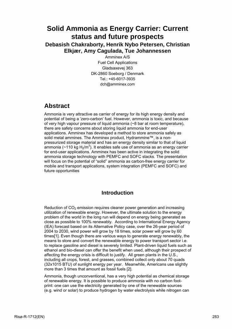
Solid Ammonia as Energy Carrier: Current status and future prospects

Debasish Chakraborty, Henrik Nybo Petersen, Christian Elkjær, Amy Cagulada, Tue Johannessen

Amminex A/S Fuel Cell Applications

Gladsaxevej 363 DK-2860 Soeborg / Denmark

Tel.: +45-6017-3935 dch@amminex.com

Abstract Ammonia is very attractive as carrier of energy for its high energy density and potential of being a ‘zero-carbon’ fuel. However, ammonia is toxic, and because of very high vapour pressure of liquid ammonia (~8 bar at room temperature), there are safety concerns about storing liquid ammonia for end-user applications. Amminex has developed a method to store ammonia safely as solid metal ammines. The Amminex product, Hydrammine™, is a non-pressurized storage material and has an energy density similar to that of liquid ammonia (~110 kg H2/m3). It enables safe use of ammonia as an energy carrier for end-user applications. Amminex has been active in integrating the solid ammonia storage technology with PEMFC and SOFC stacks. The presentation will focus on the potential of “solid” ammonia as carbon-free energy carrier for mobile and transport applications, system integration (PEMFC and SOFC) and future opportunities

Introduction

Reduction of CO2 emission requires cleaner power generation and increasing utilization of renewable energy. However, the ultimate solution to the energy problem of the world in the long run will depend on energy being generated as close as possible to 100% renewably. According to International Energy Agency (IEA) forecast based on its Alternative Policy case, over the 26-year period of 2004 to 2030, wind power will grow by 18 times, solar power will grow by 60 times[1]. Even though there are various ways to generate energy renewably, the means to store and convert the renewable energy to power transport sector i.e. to replace gasoline and diesel is severely limited. Plant-driven liquid fuels such as ethanol and bio-diesel can offer the benefit when used, although their prospect of affecting the energy crisis is difficult to justify. All green plants in the U.S., including all crops, forest, and grasses, combined collect only about 70 quads (32x1015 BTU) of sunlight energy per year. Meanwhile, Americans use slightly more than 3 times that amount as fossil fuels [2].

Ammonia, though unconventional, has a very high potential as chemical storage of renewable energy. It is possible to produce ammonia with no carbon foot-print: one can use the electricity generated by one of the renewable sources (e.g. wind or solar) to produce hydrogen by water electrolysis while nitrogen can

Risø-R-1712(EN) 283

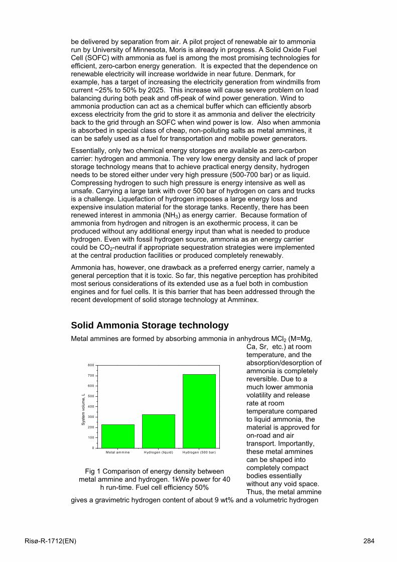
be delivered by separation from air. A pilot project of renewable air to ammonia run by University of Minnesota, Moris is already in progress. A Solid Oxide Fuel Cell (SOFC) with ammonia as fuel is among the most promising technologies for efficient, zero-carbon energy generation. It is expected that the dependence on renewable electricity will increase worldwide in near future. Denmark, for example, has a target of increasing the electricity generation from windmills from current ~25% to 50% by 2025. This increase will cause severe problem on load balancing during both peak and off-peak of wind power generation. Wind to ammonia production can act as a chemical buffer which can efficiently absorb excess electricity from the grid to store it as ammonia and deliver the electricity back to the grid through an SOFC when wind power is low. Also when ammonia is absorbed in special class of cheap, non-polluting salts as metal ammines, it can be safely used as a fuel for transportation and mobile power generators.

Essentially, only two chemical energy storages are available as zero-carbon carrier: hydrogen and ammonia. The very low energy density and lack of proper storage technology means that to achieve practical energy density, hydrogen needs to be stored either under very high pressure (500-700 bar) or as liquid. Compressing hydrogen to such high pressure is energy intensive as well as unsafe. Carrying a large tank with over 500 bar of hydrogen on cars and trucks is a challenge. Liquefaction of hydrogen imposes a large energy loss and expensive insulation material for the storage tanks. Recently, there has been renewed interest in ammonia (NH3) as energy carrier. Because formation of ammonia from hydrogen and nitrogen is an exothermic process, it can be produced without any additional energy input than what is needed to produce hydrogen. Even with fossil hydrogen source, ammonia as an energy carrier could be CO2-neutral if appropriate sequestration strategies were implemented at the central production facilities or produced completely renewably.

Ammonia has, however, one drawback as a preferred energy carrier, namely a general perception that it is toxic. So far, this negative perception has prohibited most serious considerations of its extended use as a fuel both in combustion engines and for fuel cells. It is this barrier that has been addressed through the recent development of solid storage technology at Amminex.

Solid Ammonia Storage technology Metal ammines are formed by absorbing ammonia in anhydrous MCl2 (M=Mg,

Ca, Sr, etc.) at room temperature, and the absorption/desorption of ammonia is completely reversible. Due to a much lower ammonia volatility and release rate at room temperature compared to liquid ammonia, the material is approved for on-road and air transport. Importantly, these metal ammines can be shaped into completely compact bodies essentially without any void space. Thus, the metal ammine

gives a gravimetric hydrogen content of about 9 wt% and a volumetric hydrogen

Fig 1 Comparison of energy density between metal ammine and hydrogen. 1kWe power for 40

h run-time. Fuel cell efficiency 50%

M etal am m ine H ydrogen (liquid) H ydrogen (500 bar)0

100

200

300

400

500

600

700

800

Sys

tem

vol

ume,

L

Risø-R-1712(EN) 284

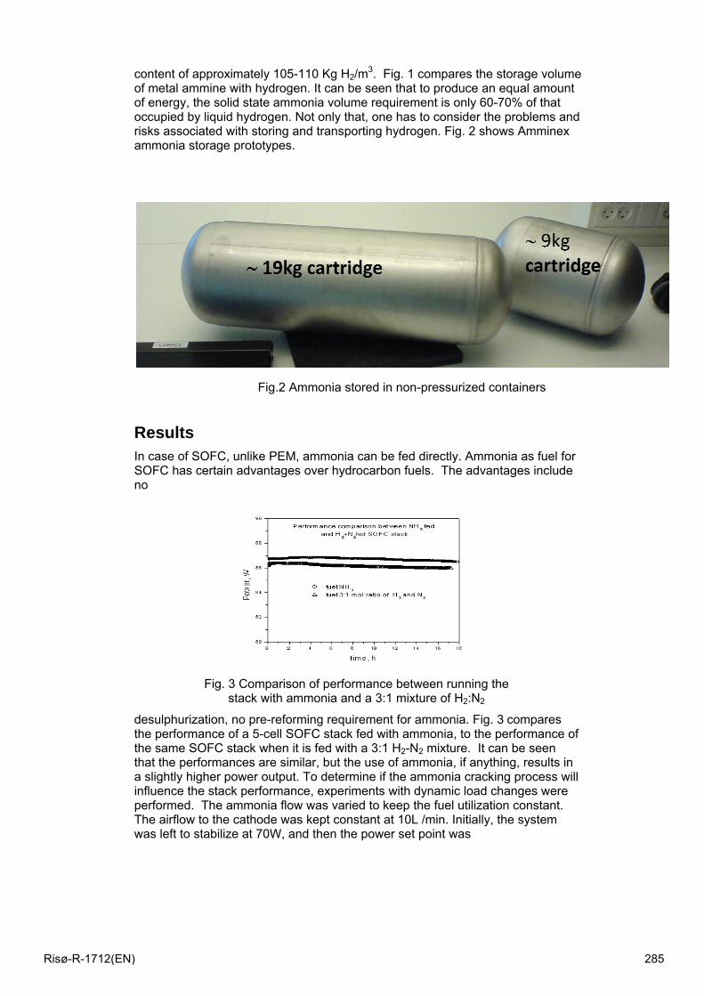
content of approximately 105-110 Kg H2/m3. Fig. 1 compares the storage volume of metal ammine with hydrogen. It can be seen that to produce an equal amount of energy, the solid state ammonia volume requirement is only 60-70% of that occupied by liquid hydrogen. Not only that, one has to consider the problems and risks associated with storing and transporting hydrogen. Fig. 2 shows Amminex ammonia storage prototypes.

Fig.2 Ammonia stored in non-pressurized containers

Results In case of SOFC, unlike PEM, ammonia can be fed directly. Ammonia as fuel for SOFC has certain advantages over hydrocarbon fuels. The advantages include no

Fig. 3 Comparison of performance between running the stack with ammonia and a 3:1 mixture of H2:N2

desulphurization, no pre-reforming requirement for ammonia. Fig. 3 compares the performance of a 5-cell SOFC stack fed with ammonia, to the performance of the same SOFC stack when it is fed with a 3:1 H2-N2 mixture. It can be seen that the performances are similar, but the use of ammonia, if anything, results in a slightly higher power output. To determine if the ammonia cracking process will influence the stack performance, experiments with dynamic load changes were performed. The ammonia flow was varied to keep the fuel utilization constant. The airflow to the cathode was kept constant at 10L /min. Initially, the system was left to stabilize at 70W, and then the power set point was

Risø-R-1712(EN) 285

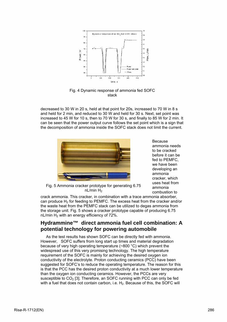
Fig. 4 Dynamic response of ammonia fed SOFC stack

decreased to 30 W in 20 s, held at that point for 20s, increased to 70 W in 8 s and held for 2 min, and reduced to 30 W and held for 30 s. Next, set point was increased to 45 W for 10 s, then to 70 W for 30 s, and finally to 85 W for 2 min. It can be seen that the power output curve follows the set point which is a sign that the decomposition of ammonia inside the SOFC stack does not limit the current.

Because ammonia needs to be cracked before it can be fed to PEMFC, we have been developing an ammonia cracker, which uses heat from ammonia combustion to

crack ammonia. This cracker, in combination with a trace ammonia absorber, can produce H2 for feeding to PEMFC. The excess heat from the cracker and/or the waste heat from the PEMFC stack can be utilized to degas ammonia from the storage unit. Fig. 5 shows a cracker prototype capable of producing 6.75 nL/min H2 with an energy efficiency of 72%.

Hydrammine™ direct ammonia fuel cell combination: A potential technology for powering automobile

As the test results has shown SOFC can be directly fed with ammonia. However, SOFC suffers from long start up times and material degradation because of very high operating temperature (~800 °C) which prevent the widespread use of this very promising technology. The high temperature requirement of the SOFC is mainly for achieving the desired oxygen ion conductivity of the electrolyte. Proton conducting ceramics (PCC) have been suggested for SOFC’s to reduce the operating temperature. The reason for this is that the PCC has the desired proton conductivity at a much lower temperature than the oxygen ion conducting ceramics. However, the PCCs are very susceptible to CO2 [3]. Therefore, an SOFC running with PCC can only be fed with a fuel that does not contain carbon, i.e. H2. Because of this, the SOFC will

Fig. 5 Ammonia cracker prototype for generating 6.75 nL/min H2

Risø-R-1712(EN) 286

largely lose its competitive edge over the PEMFC if PCC is used as the electrolyte. However, if ammonia is used as fuel combined with PCC electrolytes fuel cells can be developed that can harness all the advantages of SOFCs even though the operating temperature remains much lower (400-500 °C).

The intermediate temperature direct ammonia fuel cell (DAFC), if implemented, has the potential to power an automobile. Two characteristics are desirable for fuel cells in vehicular applications: a high power density and an intermediate operating temperature. The PEMFC is an excellent fuel cell when fed with pure hydrogen, but is not ideal for using with a reformer because the PEMFC and reformer have different operating temperatures. The SOFC is also not suitable because its operating temperature is too high. Limited by reformer compatibility, the target operating temperature of a fuel cell around 400-500 °C. In this range, the design criteria are manageable and the temperature is high enough for cracking/reforming of the fuel [4]. From this perspective, direct ammonia fuel cells exhibit great potential as a locally or overall carbon free (depending on the production method) energy conversion device. The heart of the fuel cell is the proton conducting ceramic (PCC) electrolyte. This kind of electrolyte has been already used in solid electrolyte cells for ammonia synthesis [5,6] . Ammonia is fed at the anode chamber which contains a suitable catalyst that can both decompose NH3 to H2/N2 and ionize H2 to H+ and an electron. The proton travels through the membrane to the cathode where it reduces oxygen from air to form water. Therefore, the byproducts of a DAFC fuelled with NH3 are N2 are unconverted H2 and NH3 (ppm level) from the anode, and water from the cathode. Because water is formed at the cathode side, the fuel will not be diluted at the anode side: hence higher fuel utilization can be expected with this kind of fuel cell. Because hydrogen is consumed by the fuel cell in generating electricity, the equilibrium of the reaction NH3 ↔ N2 + H2 shifts to the right and almost complete conversion of ammonia can be expected even at 400ºC. It is worthwhile to mention that because of water production at the cathode side any gas phase mass transfer limitation of oxygen in air should expected to be worsened in the PCC –intermediate temperature fuel cell compared to SOFC. Because of much higher temperature of operation compared to PEMFC, it will not be necessary to use noble metal Pt as electrode catalyst. This has the potential to make DAFCs much affordable compared to PEMFC.

Scientists at Toyota Motor Corp. tested intermediate temperature fuel cell with ultra thin proton conductor electrolyte [4]. The test cells were operated at 400-600 °C. The cell had a thin ( ~2μm) PCC electrolyte on top of a 100 μm Pd layer which was termed as hydrogen membrane. The obvious purpose of the membrane is to separate the CO2 from the reformate stream to prevent any contamination of the PCC electrolyte by CO2. If ammonia is used as fuel instead, one could easily avoid the use of thick Pd layer and consequently reduce IR drop. Because Pd is a noble metal, exclusion of it in cell fabrication is important from price perspective also.

The combination of DAFC and solid ammonia storage is very attractive for automotive applications for several reasons. First of all, the operating temperature (400-600 °C) of this type of fuel cell is ideal for ammonia decomposition. So, there is a very nice synergy between the reforming and fuel cell operation. The thermal desorption of ammonia from the solid storage materials can be done by the waste heat from the stack because the waste heat from a DAFC stack operating at ~500 °C will be of very good ‘quality’ to utilize to degas ammonia. This will improve the overall system efficiency. Finally, the startup time, which is one of the most important factors for fuel cells to be considered for automobile applications, should be much lower compared to SOFC. The relatively lower operating temperature compared to SOFC will also offer more options for selection of materials.

Risø-R-1712(EN) 287

References [1]R. Asplund, Profiting from Clean Energy, 70-72, 2008, Wiley Trading, New Jersey.

[2]D. Pimentel and M. Pimentel, Energies, 35-36, 1(2008)

[3] K.D. Kreuer, Annu. Rev. Mater. Res. 33 (2003) 333

[4] N. Ito, M. Iijima, K.Kimura, S. Iguchi, J. Power Sources, 152 (2005) 200

[5] G. Marnellos and M. Stoukides, Science 282 (1998) 98

[6] A. McFarlan, L.Pelletier, N. Maffei, J. Electrochem. Soc. 151(2004) A930.

Risø-R-1712(EN) 288

Modelling of a Biomass Gasification Plant Feeding a Hybrid Solid Oxide Fuel Cell and Micro Gas Turbine System

Christian Bang-Møller* and Masoud Rokni

Technical University of Denmark

Department of Mechanical Engineering

2800 Kgs. Lyngby, Denmark

Abstract

A system level modelling study on two combined heat and power (CHP) systems both

based on biomass gasification. One system converts the product gas in a solid oxide fuel

cell (SOFC) and the other in a combined SOFC and micro gas turbine (MGT)

arrangement. An electrochemical model of the SOFC has been developed and calibrated

against published data from Topsoe Fuel Cells A/S (TOFC) and Risø National

Laboratory. The modelled gasifier is based on an up scaled version of the demonstrated

low tar gasifier, Viking, situated at the Technical University of Denmark. The MGT

utilizes the unconverted syngas from the SOFC to produce more power as well as

pressurizing the SOFC bettering the electrical efficiency compared to operation with the

SOFC alone - from ηel=36.4% to ηel=50.3%.

Keywords: System modelling, biomass gasification, micro gas turbine, SOFC

Nomenclature aohm, bohm coefficients for Eq. (24) ASR area specific resistance E reversible open circuit voltage F Faradays constant gf Gibbs free energy of formation i current density LHV lower heating value n& molar flow ne transferred electrons per molecule of fuel p pressure/partial pressure P power production R universal gas constant T temperature UF fuel utilization factor for SOFC V potential/overpotential y molar fraction δ SOFC layer thickness η efficiency Subscripts: a anode c cathode con consumption e electrolyte i interconnect

* Corresponding author: Email: chrbm@win.dtu.dk Phone: +45 45254123

Risø-R-1712(EN) 289

1 Introduction

Development of sustainable and efficient production plants of combined heat and power

(CHP) tends to gain more attention as climate changes, security of supply and depletion

of fossil fuels have become well known issues. The share of biomass in CHP production

are expected to increase in the future and decentralized CHP plants are also of interest to

avoid costs of biomass transportation. Efficient power producing technologies for small

scale productions are typically gas engines, micro gas turbines (MGT) and fuel cells – all

requiring gaseous fuel. Gasification can deliver biomass based gaseous fuel so the

combination of biomass gasification and efficient syngas conversion are potentially a

sustainable and efficient CHP plant.

Solid oxide fuel cells (SOFCs) can electrochemically convert H2 and CO as well as

internally reform CH4 into more H2 and CO due to their high operating temperature. This

makes SOFCs very fuel flexible and ideal for converting syngas compared to other fuel

cell types.

The performance and system design of integrated biomass gasifier and SOFC systems in

the 100-1000kWe class have been investigated by several. An innovative design

including heat pipes between a SOFC stack and an allothermal gasifier is described in

[1]. Fryda et al. [2] studies the performance of a CHP system of less than 1MWe and

consisting of an autothermal gasifier combined with a MGT and/or SOFC.

This study focus on the performance of a system combining an up scaled version

(~500kWth) of the two-stage gasifier named Viking and a SOFC or a SOFC-MGT

system. Viking is a 75kWth autothermal (air blown) fixed bed biomass gasifier

demonstrated at the Technical University of Denmark and it is described in detail in [3]. The Viking gasifier produces almost no tars, which is favourable for downstream SOFC

operation. Hofmann et al. [4] has operated a SOFC on cleaned syngas from the Viking gasifier for 150 hours without degradation.

The present study is based on zero dimensional and steady-state modelling in the

simulation tool DNA [5]. DNA has incorporated thermodynamic property data, is component based and is developed at The Technical University of Denmark.

2 System description

Two different combined heat and power systems are investigated in this study, both

based on syngas production from an up scaled Viking gasifier. A flow sheet of the two

systems is depicted in Figure 1. The modelled gasifier system is slightly simplified, but

aims at the same resulting gas composition and cold gas efficiency as for the Viking

gasifier. In the gasifier model the dryer is heated by hot syngas. The steam production

from the dryer is added to the preheated air and dry wood together with mixed air and

steam are fed to the gasifier. The raw product gas is cooled to 90°C in three steps; air

preheating, wood drying and syngas cooling producing hot water for district heating. The

cooled syngas is then cleaned from impurities as particles and sulphur compounds before

some of the water in the gas is condensed through cooling to 50°C. The cleaned and

partly dried syngas is then converted into electricity and heat in a bottoming cycle

consisting of a SOFC or both a SOFC and a MGT. These two system configurations will

from now on be referred as the Gasifier-SOFC and the Gasifier-SOFC-MGT

configuration, respectively. In the Gasifier-SOFC-MGT configuration all the

components in the flow sheet are in use. With respect to Figure 1 the recuperator and gas

turbine are bypassed in the Gasifier-SOFC arrangement, thus the syngas and air

compressors work as blowers due to no pressurization. In addition the syngas

compressor works as a roots blower for the gasifier system and not illustrated is a

generator. In the Gasifier-SOFC configuration the syngas and air blowers are driven by

an electric motor.

Risø-R-1712(EN) 290

Gasifier

Dry woodWet wood Dryer

Steam

Raw

syngas

Air

Air+steam

Ash

Syngas

coolerCondenser

Gas

cleaner

Condensate

Water

Water

Air

Anode

Cathode

Syngas

compressor

Cleaned and

partly dried syngas

Air

compressor

Air

Gas turbine

Gasifier and SOFC/MGT system interface

Burner

Exhaust cooler

Water

Exhaust

Recuperator

SOFCSyngas

preheater

Air

preheater

Flow direction in Gasifier-SOFC configuration

Impurities

15°C

15°C

30°C

30°C 80°C

80°C

30°C80°C

120°C

Max

900°C

800°C

800°C

50°C

90°C

600°C

650°C

15°C

800°C

Figure 1: Flow sheet of the hybrid systems

3 Gasifier model

The gasifier component calculates the produced syngas composition as well as the

produced ashes based on the inlet media composition and the operating conditions. The

input parameters defining the operating conditions for the gasifier submodel are given in

Table 1. The gasifier pressure loss is defined as the difference between the inlet air and

steam mixture and the outlet syngas.

Operating pressure pgasifier 0.998 bar Operating temperature Tgasifier 800°C Pressure loss ∆pgasifier 5 mbar Non-equilibrium methane METH 0.01

Table 1: Inputs to the gasifier submodel

In the gasifier the incoming flows are converted into a syngas and ashes. The ashes come

from a defined ash content in the biomass. The syngas can consist of the following

species: H2, O2, N2, CO, NO, CO2, H2O, NH3, H2S, SO2, CH4, NO2, HCN, COS and Ar.

It is assumed that equilibrium is reached at the operating temperature and pressure,

where the total Gibbs energy has its minimum value. With this assumption the syngas

outlet composition can be found by the Gibbs minimization method [6]. A possibility for bypassing an amount of methane from the equilibrium calculations is added in order to

reach syngas compositions, which contain more methane than the corresponding one at

equilibrium. Thus the syngas composition can be adjusted to match real syngas

compositions, e.g. from the Viking gasifier. The input parameter METH is used for this

bypassing and is defined as the fraction of methane that is not included in the

equilibrium calculations and instead flows through the gasifier and appears in the outlet

syngas.

3.1 Gasifier model validation

The model validation for the gasifier is done for all of the gasification plant from the

biomass input to the cleaned and dried syngas. Thus data from the Viking gasifier plant

can be used for validation.

Risø-R-1712(EN) 291

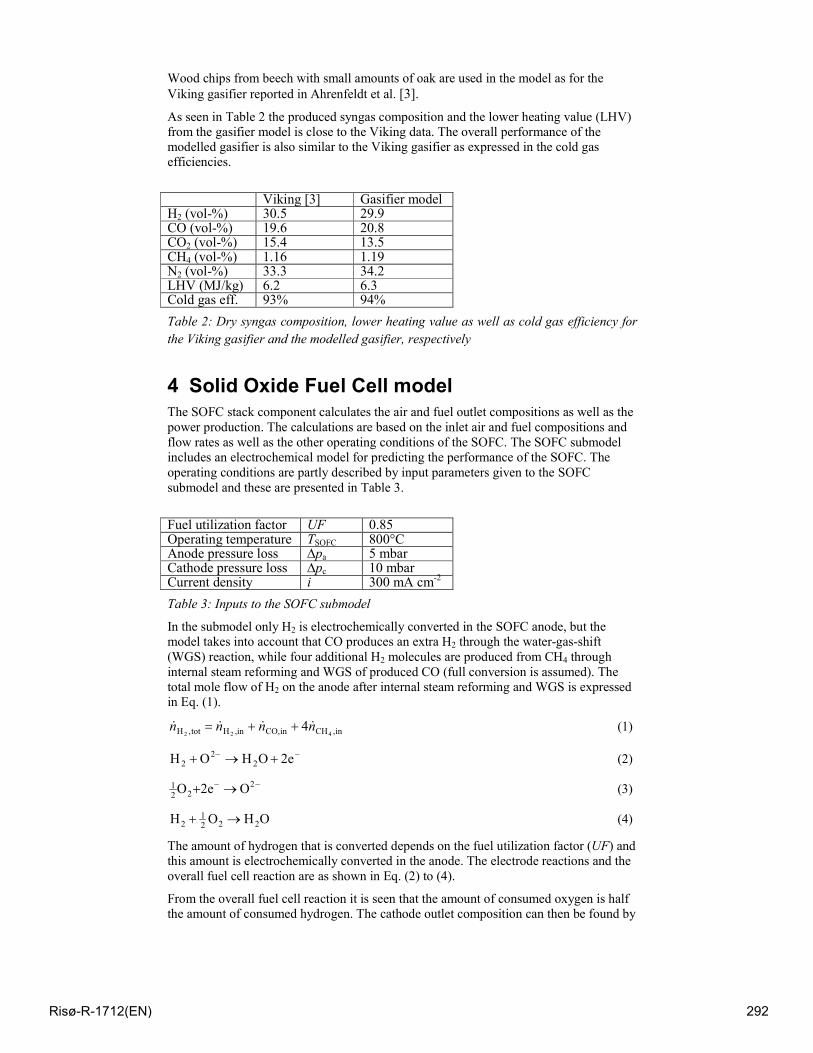
Wood chips from beech with small amounts of oak are used in the model as for the

Viking gasifier reported in Ahrenfeldt et al. [3].

As seen in Table 2 the produced syngas composition and the lower heating value (LHV)

from the gasifier model is close to the Viking data. The overall performance of the

modelled gasifier is also similar to the Viking gasifier as expressed in the cold gas

efficiencies.

Viking [3] Gasifier model H2 (vol-%) 30.5 29.9 CO (vol-%) 19.6 20.8 CO2 (vol-%) 15.4 13.5 CH4 (vol-%) 1.16 1.19 N2 (vol-%) 33.3 34.2 LHV (MJ/kg) 6.2 6.3 Cold gas eff. 93% 94%

Table 2: Dry syngas composition, lower heating value as well as cold gas efficiency for

the Viking gasifier and the modelled gasifier, respectively

4 Solid Oxide Fuel Cell model

The SOFC stack component calculates the air and fuel outlet compositions as well as the

power production. The calculations are based on the inlet air and fuel compositions and

flow rates as well as the other operating conditions of the SOFC. The SOFC submodel

includes an electrochemical model for predicting the performance of the SOFC. The

operating conditions are partly described by input parameters given to the SOFC

submodel and these are presented in Table 3.

Fuel utilization factor UF 0.85 Operating temperature TSOFC

800°C

Anode pressure loss ∆pa 5 mbar Cathode pressure loss ∆pc 10 mbar Current density i 300 mA cm-2

Table 3: Inputs to the SOFC submodel

In the submodel only H2 is electrochemically converted in the SOFC anode, but the

model takes into account that CO produces an extra H2 through the water-gas-shift

(WGS) reaction, while four additional H2 molecules are produced from CH4 through

internal steam reforming and WGS of produced CO (full conversion is assumed). The

total mole flow of H2 on the anode after internal steam reforming and WGS is expressed

in Eq. (1).

in,CHinCO,in,Htot,H 4224nnnn &&&& ++= (1)

−− +→+ 2eOHOH 22

2 (2)

−− →+ 222

1 O2eO (3)

OHOH 2221

2 →+ (4)

The amount of hydrogen that is converted depends on the fuel utilization factor (UF) and

this amount is electrochemically converted in the anode. The electrode reactions and the

overall fuel cell reaction are as shown in Eq. (2) to (4).

From the overall fuel cell reaction it is seen that the amount of consumed oxygen is half

the amount of consumed hydrogen. The cathode outlet composition can then be found by

Risø-R-1712(EN) 292

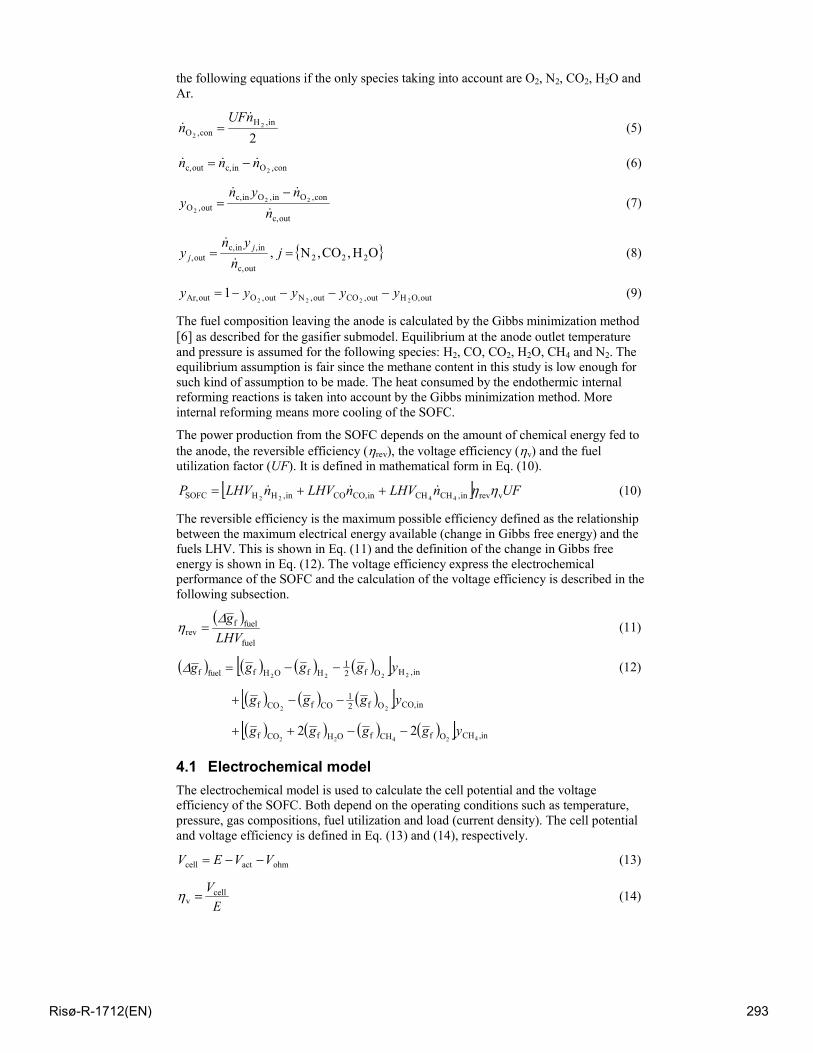
the following equations if the only species taking into account are O2, N2, CO2, H2O and

Ar.

2

in,H

con,O2

2

nUFn

&& = (5)

con,Oinc,outc, 2nnn &&& −= (6)

outc,

con,Oin,Oinc,

out,O22

2 n

nyny

&

&& −= (7)

outc,

in,inc,

out,n

yny

j

j&

&= , OH,CO,N 222=j (8)

outO,Hout,COout,Nout,OoutAr, 22221 yyyyy −−−−= (9)

The fuel composition leaving the anode is calculated by the Gibbs minimization method

[6] as described for the gasifier submodel. Equilibrium at the anode outlet temperature and pressure is assumed for the following species: H2, CO, CO2, H2O, CH4 and N2. The

equilibrium assumption is fair since the methane content in this study is low enough for

such kind of assumption to be made. The heat consumed by the endothermic internal

reforming reactions is taken into account by the Gibbs minimization method. More

internal reforming means more cooling of the SOFC.

The power production from the SOFC depends on the amount of chemical energy fed to

the anode, the reversible efficiency (ηrev), the voltage efficiency (ηv) and the fuel

utilization factor (UF). It is defined in mathematical form in Eq. (10).

[ ] UFnLHVnLHVnLHVP vrevin,CHCHinCO,COin,HHSOFC 4422ηη&&& ++= (10)

The reversible efficiency is the maximum possible efficiency defined as the relationship

between the maximum electrical energy available (change in Gibbs free energy) and the

fuels LHV. This is shown in Eq. (11) and the definition of the change in Gibbs free

energy is shown in Eq. (12). The voltage efficiency express the electrochemical

performance of the SOFC and the calculation of the voltage efficiency is described in the

following subsection.

( )fuel

fuelfrev

LHV

g∆η = (11)

( ) =fuelfg∆ ( ) ( ) ( )[ ] in,HOf2

1HfOHf 2222

yggg −− (12)

( ) ( ) ( )[ ] inCO,Of21

COfCOf22

yggg −−+

( ) ( ) ( ) ( )[ ] in,CHOfCHfOHfCOf 4242222 ygggg −−++

4.1 Electrochemical model

The electrochemical model is used to calculate the cell potential and the voltage

efficiency of the SOFC. Both depend on the operating conditions such as temperature,

pressure, gas compositions, fuel utilization and load (current density). The cell potential

and voltage efficiency is defined in Eq. (13) and (14), respectively.

ohmactcell VVEV −−= (13)

E

Vcellv =η (14)

Risø-R-1712(EN) 293

In the following the reversible open circuit voltage (E), the activation overpotential (Vact)

and the ohmic overpotential (Vohm) are calculated. Traditionally a concentration

overpotential term is included in Eq. (13). The concentration overpotential is a result of

the limitations of transporting the reactants to the active cell area. In Larminie et al. [7] it

is described as a voltage drop caused by the pressure change associated with the

consumption of reactants. As a result of the current being drawn from the cell, the

average partial pressure of reactants is lower than at the inlet. Thus, in this study the

concentration overvoltage is taken into account by using average partial pressures when

calculating E and Vact.

E can be calculated from the Nernst equation:

+

−=

OH

Otot,H

ee

0

f

2

22ln∆

p

pp

Fn

RT

Fn

gE (15)

Since it is assumed that all CO and CH4 are converted to H2 before the electrochemical

reactions take place, the change in standard Gibbs free energy (0

f∆g ) is and the number

of electrons transferred for each molecule of fuel (ne) are determined for the reaction of

H2 only. Thus, ne = 2 and ( ) ( ) ( )222 O

0

f21

H

0

fOH

0

f

0

f∆ gggg −−= . The partial pressure of

species j is an average across the respective electrode and is here defined as an arithmetic

mean between inlet and outlet as shown in Eq. (16) and (17). The average partial

pressure of available hydrogen after internal steam reforming and WGS of CH4 and CO

can be determined from the overall steam reforming and WGS reaction including all

species. It is defined in Eq. (18).

a

in,out,

2p

yyp

jj

j

−= , 22242 NO,H,CO,CHCO,,H=j (16)

c

in,Oout,O

O2

22

2p

yyp

−= (17)

a

NOHCOCHCOH

CHCOH

tot,H

22242

42

2 3

4p

pppppp

pppp

+++++

++= (18)

The activation overpotential is due to an energy barrier (activation energy) that the

reactants must overcome in order to drive the electrochemical reactions. The activation

overpotential is non-linear and is dominant at low current densities (i). The activation

overpotential is defined as (cf. [8]):

actV cact,aact, VV +=

++

+= −−

c0,

n1

a0,

n1

e 2sinh

2sinh

2

i

ii

i

ii

Fn

RT (19)

The internal current density (in) is added to the actual fuel cell current density in order to

account for the mixed potential caused by fuel crossover. The importance of the internal

current density in the case of SOFCs is much less than for low temperature fuel cells and

the value of in is usually very small [7]. The exchange current density (i0) is a measure of

the level of activity on the electrode at i=0 mA cm-2 and is defined as (cf. [9]):

−

×=

RTp

ppi

110000exp102.13

2

a

OHtot,H7a0,

22 (20)

−

×=

RTp

pi

110000exp1049.1

25.0

c

O7c0,

2 (21)

Risø-R-1712(EN) 294

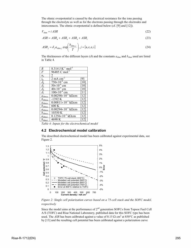
The ohmic overpotential is caused by the electrical resistance for the ions passing

through the electrolyte as well as for the electrons passing through the electrodes and

interconnects. The ohmic overpotential is defined below (cf. [9] and [12]).

ASRiV =ohm (22)

ieca ASRASRASRASRASR +++= (23)

=

T

baASR

j

jjj

ohm,

ohm, expδ , ie,c,a,=j (24)

The thicknesses of the different layers (δ) and the constants aohm and bohm used are listed in Table 4.

R 8.314 J K

-1 mol

-1

F 96485 C mol-1

ne 2 in 2 mA cm-2 [9] δa 750×10-4 cm [10] δc 50×10-4 cm [10] δe 40×10-4 cm [10] δi 100×10-4 cm [11] aohm,a 0.00298×10

-3 kΩcm [12]

bohm,a -1392 K [12] aohm,c 0.00811×10-3 kΩcm [12] bohm,c 600 K [12] aohm,e 0.00294×10-3 kΩcm [12] bohm,e 10350 K [12] aohm,i 0.1256×10-3 kΩcm [12] bohm,i 4690 K [12]

Table 4: Inputs for the electrochemical model

4.2 Electrochemical model calibration

The described electrochemical model has been calibrated against experimental data, see

Figure 2.

0

0.1

0.2

0.3

0.4

0.5

0.6

0.7

0.8

0.9

1

1.1

1.2

1.3

0 100 200 300 400 500 600 700Current density / mA cm

-2

Cell potential / V

-5%

-4%

-3%

-2%

-1%

0%

1%

2%

3%

4%

5%

Error

TOFC 75-cell stack (800°C)Modelled cell potential (900°C)Modelled cell potential (800°C)Modelled cell potential (700°C)Error at 800°C relative to TOFC

Figure 2: Single cell polarization curves based on a 75-cell stack and the SOFC model,

respectively

Since the model aims at the performance of 2nd generation SOFCs from Topsoe Fuel Cell

A/S (TOFC) and Risø National Laboratory, published data for this SOFC type has been

used. The ASR has been calibrated against a value of 0.15 Ω cm2 at 850°C as published

by [13] and the resulting cell potential has been calibrated against a polarization curve

Risø-R-1712(EN) 295

(75-cell stack, 12 x 12 cm2, 800°C and fuelled with H2 and N2) published by [14]. An

active cell area of 81 cm2 has been assumed. Both modelled and experimental data as

well as the error relative to the experimental data are presented in Figure 2.

The model shows excellent agreement with the experimental data above a current density

of 100 mA cm-2. The current density of 300 mA cm

-2 is chosen to represent the SOFC

load in the following results.

5 Peripheral equipment

Modelling of peripheral components like compressors, turbines and heat exchangers are

standard and therefore not described in detail.

The throughput of wet biomass is 154.8 kg h-1 (corresponds to 499.2 kWth (LHV)). Thus

it is assumed that the Viking gasifier can be scaled up from a nominal ~75 kWth [3]. The biomass dryer reduces the water content in the biomass from 32.2 wt-% to 5 wt-% by

heating it to 150°C and the air for the gasifier is preheated to 780°C by the hot product

gas.

The inlet temperature to the SOFC anode and cathode are maintained at 150°C and

200°C below the outlet temperature, respectively.

The pressure loss in every component in the SOFC air supply stream and burner exhaust

stream is assumed to be 10 mbar, while the pressure loss in each of the rest of the

components is assumed to be 5 mbar, except the burner that has a pressure loss of 0.6‰

(equals 1.5 mbar when 2.5 bar at inlet).

The gas cleaner is a baghouse filter removing particulates and it is assumed that the

cleaned syngas can be used directly in a SOFC. The condenser removes some of the

water content in the syngas resulting in a content of water in the cleaned and dried

syngas of 12.7 vol-%. The resulting steam to carbon ratio (S/C) is 0.41, which is

somewhat low, but is justified by the very low tar content in the Viking syngas.

The isentropic and mechanical efficiency of the compressors are 75% and 98%,

respectively, and the isentropic efficiency of the MGT expander is 84%. The

performance of the compressors and the MGT expander are taken from Fryda et al. [2] and corresponds to common performance data for a MGT of this scale. The recuperator

effectiveness is assumed to be 85% and the generator efficiency is assumed to be 99%.

In the Gasifier-SOFC configuration the SOFC operating pressure is ~1 bar and in the

Gasifier-SOFC-MGT case the SOFC operating pressure is 2.5 bar (this pressure is varied

in the results section).

No heat losses are taken into account. Introducing heat losses from the gas cleaner will

only affect the heat production from the condenser since the temperature after the

condenser is fixed to 50°C.

The outlet pressure from the MGT depends on the total pressure loss downstream the

MGT, since it is the exhaust pressure which is fixed to 1.013 bar. Because of the

recuperator and exhaust cooler the outlet pressure from the MGT is 1.033 bar. The

district heating (DH) water is assumed to be 30°C at inlet and 80°C at outlet.

6 Results and discussion

In the following results the inputs presented in the previous sections are used unless

something else is stated. The system configurations are previously described in detail.

The performance of the different system configurations vary greatly with the operating

conditions and namely the operating pressure of the SOFC (in the Gasifier-SOFC-MGT

case) are of great importance to the resulting system performance. The Gasifier-SOFC-

MGT configuration has an optimum with regard to its operating pressure, while the

Risø-R-1712(EN) 296

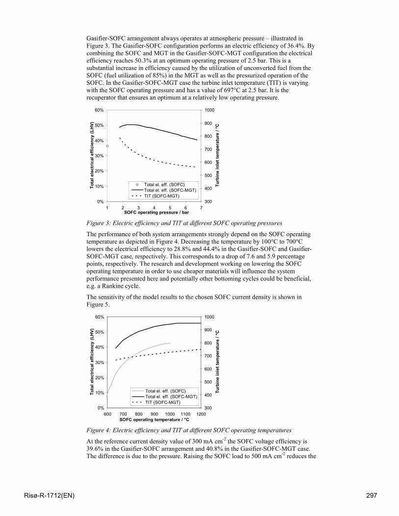
Gasifier-SOFC arrangement always operates at atmospheric pressure – illustrated in

Figure 3. The Gasifier-SOFC configuration performs an electric efficiency of 36.4%. By

combining the SOFC and MGT in the Gasifier-SOFC-MGT configuration the electrical

efficiency reaches 50.3% at an optimum operating pressure of 2.5 bar. This is a

substantial increase in efficiency caused by the utilization of unconverted fuel from the

SOFC (fuel utilization of 85%) in the MGT as well as the pressurized operation of the

SOFC. In the Gasifier-SOFC-MGT case the turbine inlet temperature (TIT) is varying

with the SOFC operating pressure and has a value of 697°C at 2.5 bar. It is the

recuperator that ensures an optimum at a relatively low operating pressure.

0%

10%

20%

30%

40%

50%

60%

1 2 3 4 5 6 7SOFC operating pressure / bar

Total electrical efficiency (LHV)

300

400

500

600

700

800

900

1000

Turbine inlet temperature / °C

Total el. eff. (SOFC)

Total el. eff. (SOFC-MGT)

TIT (SOFC-MGT)

Figure 3: Electric efficiency and TIT at different SOFC operating pressures

The performance of both system arrangements strongly depend on the SOFC operating

temperature as depicted in Figure 4. Decreasing the temperature by 100°C to 700°C

lowers the electrical efficiency to 28.8% and 44.4% in the Gasifier-SOFC and Gasifier-

SOFC-MGT case, respectively. This corresponds to a drop of 7.6 and 5.9 percentage

points, respectively. The research and development working on lowering the SOFC

operating temperature in order to use cheaper materials will influence the system

performance presented here and potentially other bottoming cycles could be beneficial,

e.g. a Rankine cycle.

The sensitivity of the model results to the chosen SOFC current density is shown in

Figure 5.

0%

10%

20%

30%

40%

50%

60%

600 700 800 900 1000 1100 1200

SOFC operating temperature / °C

Total electrical efficiency (LHV)

300

400

500

600

700

800

900

1000

Turbine inlet temperature / °C

Total el. eff. (SOFC)

Total el. eff. (SOFC-MGT)

TIT (SOFC-MGT)

Figure 4: Electric efficiency and TIT at different SOFC operating temperatures

At the reference current density value of 300 mA cm-2 the SOFC voltage efficiency is

39.6% in the Gasifier-SOFC arrangement and 40.8% in the Gasifier-SOFC-MGT case.

The difference is due to the pressure. Raising the SOFC load to 500 mA cm-2 reduces the

Risø-R-1712(EN) 297

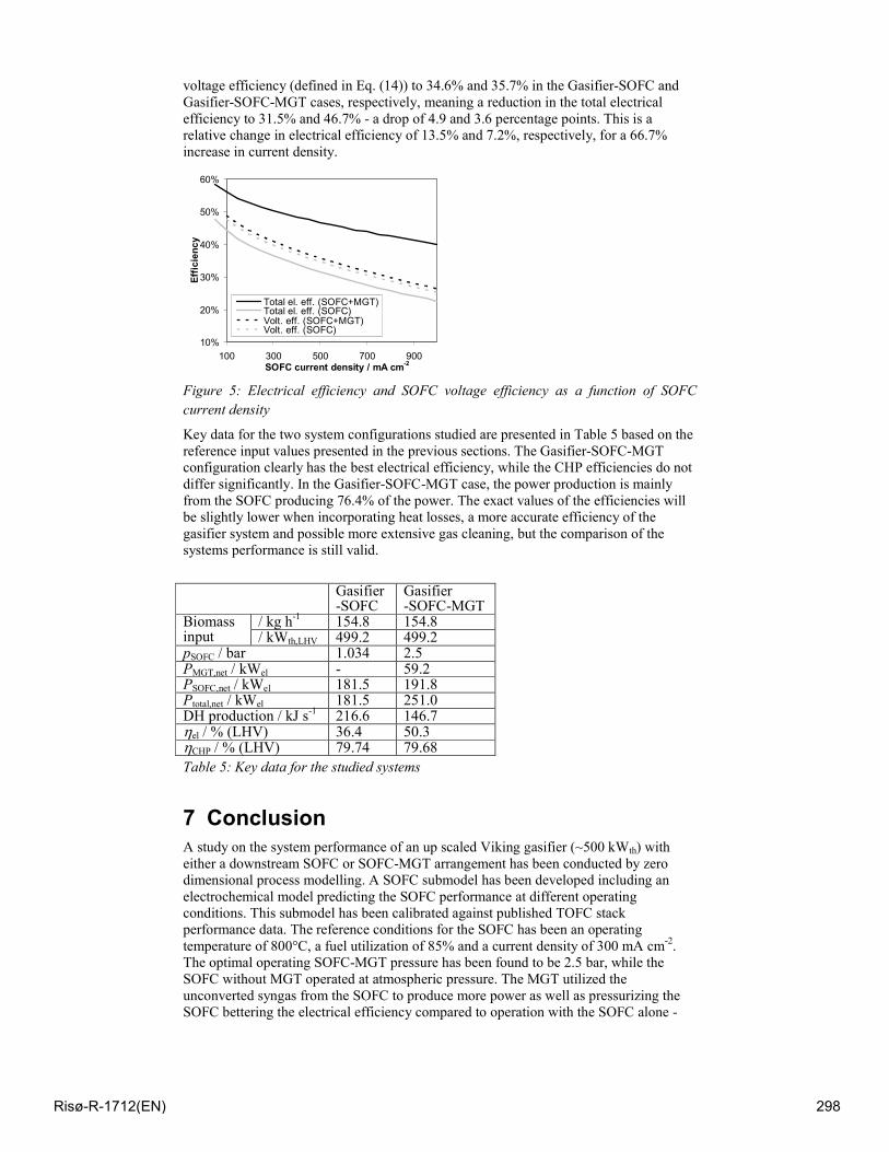
voltage efficiency (defined in Eq. (14)) to 34.6% and 35.7% in the Gasifier-SOFC and

Gasifier-SOFC-MGT cases, respectively, meaning a reduction in the total electrical

efficiency to 31.5% and 46.7% - a drop of 4.9 and 3.6 percentage points. This is a

relative change in electrical efficiency of 13.5% and 7.2%, respectively, for a 66.7%

increase in current density.

10%

20%

30%

40%

50%

60%

100 300 500 700 900SOFC current density / mA cm

-2

Efficiency

Total el. eff. (SOFC+MGT)Total el. eff. (SOFC)Volt. eff. (SOFC+MGT)Volt. eff. (SOFC)

Figure 5: Electrical efficiency and SOFC voltage efficiency as a function of SOFC

current density

Key data for the two system configurations studied are presented in Table 5 based on the

reference input values presented in the previous sections. The Gasifier-SOFC-MGT

configuration clearly has the best electrical efficiency, while the CHP efficiencies do not

differ significantly. In the Gasifier-SOFC-MGT case, the power production is mainly

from the SOFC producing 76.4% of the power. The exact values of the efficiencies will

be slightly lower when incorporating heat losses, a more accurate efficiency of the

gasifier system and possible more extensive gas cleaning, but the comparison of the

systems performance is still valid.

Gasifier

-SOFC Gasifier -SOFC-MGT

/ kg h-1 154.8 154.8 Biomass

input / kWth,LHV 499.2 499.2 pSOFC / bar 1.034 2.5 PMGT,net / kWel - 59.2 PSOFC,net / kWel 181.5 191.8 Ptotal,net / kWel 181.5 251.0 DH production / kJ s-1 216.6 146.7 ηel / % (LHV) 36.4 50.3 ηCHP / % (LHV) 79.74 79.68

Table 5: Key data for the studied systems

7 Conclusion

A study on the system performance of an up scaled Viking gasifier (~500 kWth) with

either a downstream SOFC or SOFC-MGT arrangement has been conducted by zero

dimensional process modelling. A SOFC submodel has been developed including an

electrochemical model predicting the SOFC performance at different operating

conditions. This submodel has been calibrated against published TOFC stack

performance data. The reference conditions for the SOFC has been an operating

temperature of 800°C, a fuel utilization of 85% and a current density of 300 mA cm-2.

The optimal operating SOFC-MGT pressure has been found to be 2.5 bar, while the

SOFC without MGT operated at atmospheric pressure. The MGT utilized the

unconverted syngas from the SOFC to produce more power as well as pressurizing the

SOFC bettering the electrical efficiency compared to operation with the SOFC alone -

Risø-R-1712(EN) 298

from ηel=36.4% to ηel=50.3%. These efficiencies were very sensitive to the SOFC

operating temperature, while only a moderate sensitivity to the SOFC current density

was observed.

8 References [1] Karellas S, Karl J, Kakaras E. An innovative biomass gasification process and

its coupling with microturbine and fuel cell systems. Energy 2008;33:284–291. [2] Fryda L, Panopoulos KD, Kakaras E. Integrated CHP with autothermal

biomass gasification and SOFC–MGT. Energy Conversion and Management 2008;49:281–290.

[3] Ahrenfeldt J, Henriksen U, Jensen TK, Gøbel B, Wiese L, Kather L, Egsgaard H. Validation of a Continuous Combined Heat and Power (CHP) Operation of a Two-Stage Biomass Gasifier. Energy & Fuels 2006;20:2672-2680.

[4] Hofmann Ph, Schweiger A, Fryda L, Panopoulos KD, Hohenwarter U, Bentzen JD, Ouweltjes JP, Ahrenfeldt J, Henriksen U, Kakaras E. High temperature electrolyte supported Ni-GDC/YSZ/LSM SOFC operation on two-stage Viking gasifier product gas. J. Power Sources 2007;173:357–366.

[5] Elmegaard B, Houbak N. DNA – A General Energy System Simulation Tool, In: Proceedings of the 46th Conf. on Simulation and Modeling, Trondheim, 2005.

[6] Smith JM, Van Ness HC, Abbott MM. Introduction to Chemical Engineering Thermodynamics. 7

th ed. Boston: McGraw-Hill, 2005.

[7] Larminie J, Dicks A. Fuel Cell Systems Explained. 2nd ed. West Sussex: John Wiley & Sons Ltd., 2003.

[8] Aloui T, Halouani K. Analytical modeling of polarizations in a solid oxide fuel cell using biomass syngas product as fuel. Appl. Therm. Eng. 2007;27:731-737.

[9] Calise F, Dentice d’Accadia M, Palombo A, Vanoli L. Simulation and exergy analysis of a hybrid Solid Oxide Fuel Cell (SOFC)–Gas Turbine System. Energy 2006;31:3278-3299.

[10] Chan SH, Khor KA, Xia ZT. A complete polarization model of a solid oxide fuel cell and its sensitivity to the change of cell component thickness. J. Power Sources 2001;93:130-140.

[11] Chan SH, Low CF, Ding OL. Energy and exergy analysis of simple solid-oxide fuel-cell power systems. J. Power Sources 2002;103:188-200.

[12] Bessette NF II, Wepfer WJ, Winnick J. A Mathematical Model of a Solid Oxide Fuel Cell. J. Electrochem. Soc. 1995;142:3792-3800.

[13] Christiansen N, Hansen JB, Holm-Larsen H, Linderoth S, Larsen PH, Hendriksen PV, Mogensen M. Solid oxide fuel cell development at Topsoe Fuel Cell and Risø. Fuel Cells Bulletin 2006;2006(8):12-15.

[14] Linderoth S, Larsen PH, Mogensen M, Hendriksen PV, Christiansen N, Holm-Larsen H. Solid Oxide Fuel Cell (SOFC) Development in Denmark. Materials Science Forum 2007;539-543:1309-1314.

Risø-R-1712(EN) 299

Integrating a SOFC Plant with a Steam Turbine Plant Masoud Rokni and Fabio Scappin

Technical University of Denmark, Dept. Mechanical Engineering,

Thermal Energy System, Building 402, 2800 Kgs, Lyngby, Denmark

E-mail: MR@mek.dtu.dk

Abstract A Solid Oxide Fuel Cell (SOFC) is integrated with a Steam Turbine (ST) cycle. Different hybrid configurations are studied. The fuel for the plants is assumed to be natural gas (NG). Since the NG cannot be sent to the anode side of the SOFC directly, a desulfurization reactor is used to remove the sulfur content in the NG and afterwards a pre-reformer break down the heavier hydrocarbons. Both ASR (Adiabatic Steam Reformer) and CPO (Catalytic Partial Oxidation) fuel reformer reactors are considered in this study. The gases from the SOFC stacks enter into a burner to burn the rest of the fuel. The off-gases after the burner are now used to generate steam in a Heat Recovery Steam Generator (HRSG). The generated steam is expanded in a ST to produce additional power. Different systems layouts are considered. Cyclic efficiencies up to 67% are achieved which is considerably higher than the conventional combined cycles (CC).

1 Introduction The Solid Oxide Fuel Cell (SOFC) is an electrochemical reactor currently under development by several companies for power-heat generation application. Depending on the type of the electrolyte they are operating at temperature levels of more than about 750°C up to 1000°C. The lower temperature alternative is now being developed for market entry during the next decade. Due to material complication on the BoP (Balance of Plant) components many companies are trying to find new materials for the SOFC cells to decrease the operating temperature. Temperatures of about 650°C are also mentioned.

The biggest advantage of the SOFC in comparison with other types of fuel cells may be in its flexibility in using different types of fuel. However, in planar SOFCs one needs to pre-process most kind of fuels in order to remove the sulphur content and break down the heavier hydro-carbons which may otherwise damage the fuel pre-heater and the stacks. Such pre-processing can be done in two different catalytic reactors operating at different temperature levels indicated by reactor manufacturers.

SOFC – based power plants have been studied for a while and some companies, such as Wärtsilä, are trying to realize such a system for CHP (Combined Heat and Power) applications; see e.g. Fontell et al (2004). The SOFC is also combined with CC (Combined Cycles) in the literature to achieve ultra high electrical efficiencies, see e.g. Rokni (1993) and Riensche etal. (2000). Due to current operating temperature of the SOFC stacks (more than about 750°C), hybrid SOFC and GT (Gas Turbine) systems has also been studied extensively in the literature, e.g. in Pålson et al (2000) for CHP applications. Characterization, quantification and optimization of hybrid SOFC – GT systems have also been studied by e.g. Subramanyan et al. (2005). In Roberts and Brouwer (2006) modeling results are compared with measured data for a 220 kW hybrid planar SOFC – GT power plant. Details on design, dynamics, control and startup of such hybrid power plants are studied in Rokni et al. (2005).

Risø-R-1712(EN) 300

While hybrid SOFC–GT plants have been extensively studied by many researchers, the investigations on combined SOFC and ST (Steam Turbine) are limited see Dunbar et al. (1991). In addition the SOFC manufactures are trying to decrease the operating temperature of the SOFC stacks, which makes the combination of SOFC–ST hybrid system would be more attractive than the SOFC–GT systems. By decreasing the operating temperature, the material cost for the SOFC stacks will be decreased as well as many problems associating with the BoP components will be diminished.

Fuel pre-reforming can be done in different reactors such as ASR (Adiabatic Steam Reformer) and CPO (Catalytic Partial Oxidation). The disadvantages of an ASR reactor is that it needs superheated steam during start–up (depending on the operating temperature of the reactor, i.e. 400°C) which is an extremely power consuming process. During normal operation steam is available after the anode side of the SOFC stacks, which can be recycled into the system. However, in a CPO reactor additional air is needed for the fuel pre-reforming process, which in turn increases the plant power consumption (compressor effect) and thereby the plant efficiency will be decreased. In this study, ASR reforming process versus CPO reforming process is studied in terms of plant design, plant efficiency and plant output power.

In the Rankine cycle a dual pressure levels with reheat between the turbines is applied to study plants design, plants efficiency and plants output power. In addition, the off–gases from the Heat Recovery Steam Generator (HRSG) are used to preheat the incoming air into the SOFC stacks (called as recuperation). The effect of such suggested air preheating on plant efficiency and output power is also studied. All the configurations studied here are novels in terms of designing new plants with very high efficiencies.

2 Methodology The results of this paper are obtained using the simulation tool DNA (Dynamic Network Analysis), see Elmegaard and Houbak (2005), which is a simulation tool for energy system analysis. It is the present result of an ongoing development at the Department of Mechanical Engineering, Technical University of Denmark, which began with a Master’s Thesis work in Perstrup, 1989. Since then the program has been developed to be generally applicable covering many features of networks simulations. Some of the important features are:

• Simulation of both steady state (algebraic equations) and dynamic models (differential equations)

• Handling of discontinuities in dynamic equations • Use of a sparse-matrix-based simultaneous solver for algebraic equations • No causality implied on the model input, i.e. no restriction of the choice of

inputs and outputs • Medium compositions can be variables • Models of thermodynamic states, transport variables and radiative properties for

relevant fluids, e.g. steam, ideal gases and refrigerants • Features for modeling solid fuels of arbitrary components

The program library includes various components models such as; of heat exchangers, burners, turbo machinery, gasifiers, dryers, energy storages, engines, valves, controllers as well as more specialized components and utility components.

The mathematical equations include mass and energy conservation for all components, as well as relations for thermodynamic properties of the fluids involved. In addition, the components include a number of constitutive equations representing their physical properties, e.g. heat transfer coefficients for heat exchangers and isentropic efficiencies for compressors and turbines. During the development of DNA the four key terms, portability, robustness, efficiency, and flexibility have been kept in mind as the important features for making a generally applicable tool for energy system studies. The program is written in FORTRAN.

Risø-R-1712(EN) 301

2.1 Modelling of SOFC

The SOFC model used in this investigation is based on the planar type developed by DTU-Risø and TOPSØE Fuel Cell. The model is calibrated against experimental data in the range of 650°C to 800°C (SOFC operational temperature) as described in Petersen et al. (2005). The operational voltage (EFC) is found to be

offsetconcohmactNernstFC EEEEEE Δ−Δ−Δ−Δ−= (1)

where ENernst , ΔEact , ΔEohm , ΔEconc , ΔEoffset are the Nernst ideal reversible voltage, activation polarization, ohmic polarization, concentration polarization and the offset polarization respectively. The activation polarization can be evaluated from Butler – Volmer equation (see Keegan et al. 2002). The activation polarization is isolated from other polarization to determine the charge transfer coefficients as well as exchange current density from the experiment by curve fitting technique. It follows,

( ) ( )⎥⎦⎤

⎢⎣

⎡−−

=Δ −4

1

x10096.1087.132sinh

254.1001698.0 Ti

FTRTE d

act (2)

where R, T, F and id are the universal gas constant, operating temperature, Faradays constant and current density respectively. Ohmic polarization depends on the electrical conductivity of the electrodes as well as the ionic conductivity of the electrolyte and can be described as

dca

ca

el

el

an

anohm i

tttE ⎟⎟

⎠

⎞⎜⎜⎝

⎛++=Δσσσ

(3)

where tan = 600 μm, tel = 50 μm and tca =10 μm are the anode thickness, electrolyte thickness and cathode thickness respectively. σan, σel and σca are the conductivity of anode, electrolyte and cathode respectively.

510=anσ , ⎟⎠⎞

⎜⎝⎛−= − TTca 5

7

10x617.8117.0expx10760.5σ (4)

54.604679.010x101.110x588.8 2438 −+−= −− TTTelσ (5)

Concentration polarization is dominant at high current densities for anode – supported SOFC, wherein insufficient amounts of reactants will be transported to the electrodes and the voltage will then reduce significantly. Neglecting the cathode contribution (see e.g. Kim and Virkar 2002), it can be modeled as

⎟⎟⎠

⎞⎜⎜⎝

⎛⎟⎟⎠

⎞⎜⎜⎝

⎛−−⎟⎟

⎠

⎞⎜⎜⎝

⎛++=Δ

as

d

asOH

dHconc i

iipip

BE 1ln1ln 2

2 (6)

where B is the diffusion coefficient and is calibrated against experimental data which found to be,

( )refTT007272.00.008039XB 1-

H2 −= (7)

In the above equations pH2 and pH2O are the partial pressures for the H2 and H2O respectively, while Tref is the reference temperature (1023 K). The anode limiting current is defined as

anan

anbinHas tTR

VDpFi

τ 2 2= (8)

Risø-R-1712(EN) 302

where Van andτan are the porosity and tortuosity of the anode and are the physical characteristics as 30% and 2.5 μm in the experimental setup. The binary diffusion coefficient is given by

( )P

PTTXD ref

refHbin

75.1

52

5 10x704.810x107.4 ⎟⎟⎠

⎞⎜⎜⎝

⎛+−= −− (9)

which is also calibrated against the experimental data. Pref is the reference pressure as 1.013 bar and XH2 is the mass reaction rate of H2. Finally the current density id is directly proportional to the amount of reacting hydrogen according to the Faraday’s law;

A

Fni Hd

22

•

= (10)

where 2Hn•

is molar reaction rate of H2. The area A is the physical property of the cell and is 144 cm2.

2.2 Modelling of Fuel Pre – Reforming

The reforming process is assumed to be equilibrium by minimizing the Gibbs free energy as described in Elmegaard and Houbak (1999). The Gibbs free energy of a gas (assumed to be a mixture of k perfect gases) is given by

( )[ ]∑=

••

+=k

iiii pnRTgnG

1

0 ln (11)

where g0 , R an T are the specific Gibbs free energy, universal gas constant and gas temperature respectively. Each atomic element in the inlet gas is balance with the outlet gas composition, which yields the flow of each atom has to be conserved. For N elements this is expressed as

,Njnnk

iijouti

k

iijini 1for

1,

1, == ∑∑

=

•

=

•

AA (12)

The N elements corresponds to H2, CO2 , H2O and CH4 in such pre – reforming process. Ai,j is a matrix with information of the mole j in each mole of i (H2, CO2 , H2O and CH4). The minimization of Gibbs free energy can be formulated by introducing a Lagrange multiplier, μ, for each of the N constrains obtained in Eq. (12). After adding the constrains, the expression to be minimized is then

∑ ∑= =

•••

⎥⎦

⎤⎢⎣

⎡⎟⎠

⎞⎜⎝

⎛⎟⎠⎞

⎜⎝⎛ −+=

N

j

k

iijoutioutijout AnnG

1 1,,μφ (13)

The partial derivation of this equation with respect to outin ,

•

can be writes as

( ) kipnTR

g

n

k

jijjoutouti

outi

outi

,1for ln 1

,

0,

,

=++=∂

∂ ∑=

• Aμφ (14)

At the minimum each of these is then zero. The additional equation to make the system consistent is the summation of molar fractions of the outlet gas to be

11

, =∑=

k

ioutin (15)

Risø-R-1712(EN) 303

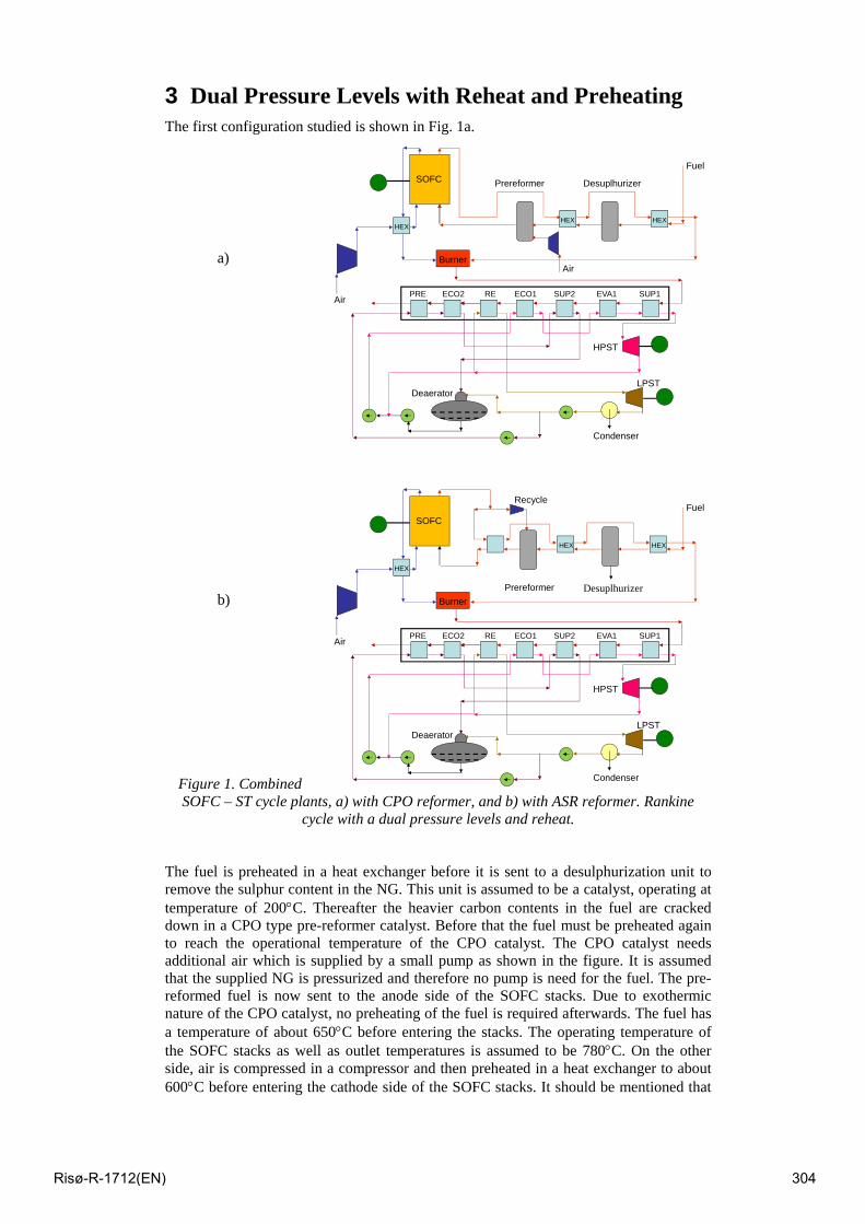
3 Dual Pressure Levels with Reheat and Preheating The first configuration studied is shown in Fig. 1a.

a)

b)

Figure 1. Combined SOFC – ST cycle plants, a) with CPO reformer, and b) with ASR reformer. Rankine

cycle with a dual pressure levels and reheat.

The fuel is preheated in a heat exchanger before it is sent to a desulphurization unit to remove the sulphur content in the NG. This unit is assumed to be a catalyst, operating at temperature of 200°C. Thereafter the heavier carbon contents in the fuel are cracked down in a CPO type pre-reformer catalyst. Before that the fuel must be preheated again to reach the operational temperature of the CPO catalyst. The CPO catalyst needs additional air which is supplied by a small pump as shown in the figure. It is assumed that the supplied NG is pressurized and therefore no pump is need for the fuel. The pre-reformed fuel is now sent to the anode side of the SOFC stacks. Due to exothermic nature of the CPO catalyst, no preheating of the fuel is required afterwards. The fuel has a temperature of about 650°C before entering the stacks. The operating temperature of the SOFC stacks as well as outlet temperatures is assumed to be 780°C. On the other side, air is compressed in a compressor and then preheated in a heat exchanger to about 600°C before entering the cathode side of the SOFC stacks. It should be mentioned that

AirECO2 RE SUP1EVA1SUP2ECO1PRE

HPST

LPST

Condenser

Deaerator

SOFCFuel

HEX

Burner

Recycle

HEX

DesuplhurizerPrereformer

HEXHEX

AirECO2 RE SUP1EVA1SUP2ECO1PRE

HPST

LPST

Condenser

Deaerator

SOFCFuel

DesuplhurizerPrereformer

Air

HEXHEXHEX

Burner

Risø-R-1712(EN) 304

these entering temperatures are essential requirements for proper functioning of SOFC stacks. Otherwise, the stacks will shut down automatically. Since the fuel in the SOFC stacks will not burn completely, the rest of the fuel together with the air coming out of the cathode side of the stacks are burned in a catalytic burner. The off-gases from the burner have a high heat quality which can be used to generate steam in a Heat Recovery Steam Generator (HRSG).

In the Rankine cycle, two pressure levels are considered in this study. The higher pressure steam is generated in the high-pressure-economizer (ECO1), high-pressure-evaporator (EVA1) and the high-pressure-super-heater (SUP1), while the low pressure steam is generated in the corresponding super-heater (SUP2) and economizer (ECO2). The generated steam is then expanded firstly in a High Pressure Steam Turbine (HPST) and then in a Low Pressure Steam Turbine (LPST). The steam between these turbines is reheated (in REH). Part of the steam after the HPST is sent to a deaerator. The expanded steam after the LPST is then cooled down in a condenser before pumping to the deaerator. The low pressure water before deaerator is preheated (in PRE). For the sake of clarity the drums are not shown in the figures.

As mentioned earlier, superheated steam is needed in a ASR reformer. During start–up steam must be supplied to the reformer externally, while during normal operation steam is available after SOFC stacks due to internal reactions of hydrogen and oxygen. Therefore, the stream after the anode side of SOFC is recycled as shown in Fig. 1b. There exist three alternatives for such a recirculation unit, a pump, a turbocharger and an ejector. In a real plant, due to high temperature of this stream (more than 700°C) the cost of a pump will be rather expensive. This is also true for a turbocharger which is working at such mass flows and pressures. Moreover, using an ejector brings up problems associated with the size and dimensioning of the ejector (due to combination of pressure drop and mass flows), which is out of the scope of this investigation. Based on these facts and for the sake of simplicity a pump is used in the calculations. Besides the recycle part, the plant configuration is the same as in the CPO reformer case, see Fig. 1b.

The main parameters for the plant are set in table 1. The pressure drops are the setting values for the program, however, pressure drops are a function of channel sizes and mass flows and the channel geometry is not kwon. Therefore, these values are calculated based on the available data for each channel mass flow and dimensions. In addition, the calculations show that the final values in terms of plant power and efficiency do not change significantly if these values are changed slightly. The SOFC plant provides direct current and must be converted to AC through a convertor. Further, the efficiency of the DC/AC convertor is neglected. Several calculations have been carried out to find the optimal extraction pressure as well as the optimum live steam pressure which are not included in this study.

Table 1. Main parameters for design point calculations of Fig. 1.

Parameter CPO ASR

Compressor intake temperature 25°C 25°C

Compressor isentropic efficiency 0.85 0.85

Compressor mechanical efficiency 0.95 0.95

SOFC cathode inlet temperature 600°C 600°C

SOFC cathode outlet temperature 780°C 780°C

SOFC utilization factor 0.80 0.80

SOFC number of cells 74 74

SOFC number of stacks 10000 10000

SOFC cathode side pressure drop ratio 0.05 bar 0.05 bar

Risø-R-1712(EN) 305

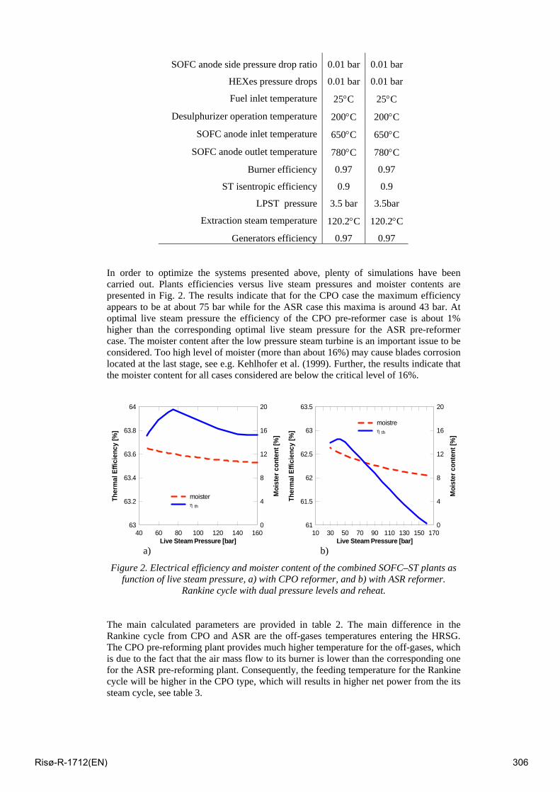
SOFC anode side pressure drop ratio 0.01 bar 0.01 bar

HEXes pressure drops 0.01 bar 0.01 bar

Fuel inlet temperature 25°C 25°C

Desulphurizer operation temperature 200°C 200°C

SOFC anode inlet temperature 650°C 650°C

SOFC anode outlet temperature 780°C 780°C

Burner efficiency 0.97 0.97

ST isentropic efficiency 0.9 0.9

LPST pressure 3.5 bar 3.5bar

Extraction steam temperature 120.2°C 120.2°C

Generators efficiency 0.97 0.97

In order to optimize the systems presented above, plenty of simulations have been carried out. Plants efficiencies versus live steam pressures and moister contents are presented in Fig. 2. The results indicate that for the CPO case the maximum efficiency appears to be at about 75 bar while for the ASR case this maxima is around 43 bar. At optimal live steam pressure the efficiency of the CPO pre-reformer case is about 1% higher than the corresponding optimal live steam pressure for the ASR pre-reformer case. The moister content after the low pressure steam turbine is an important issue to be considered. Too high level of moister (more than about 16%) may cause blades corrosion located at the last stage, see e.g. Kehlhofer et al. (1999). Further, the results indicate that the moister content for all cases considered are below the critical level of 16%.

Live Steam Pressure [bar]

Ther

mal

Effi

cien

cy [%

]

Moi

ster

con

tent

[%]

40 60 80 100 120 140 16063 0

63.2 4

63.4 8

63.6 12

63.8 16

64 20

moisterη th

Live Steam Pressure [bar]

Ther

mal

Effi

cien

cy [%

]

Moi

ster

con

tent

[%]

10 30 50 70 90 110 130 150 17061 0

61.5 4

62 8

62.5 12

63 16

63.5 20

moistreη th

a) b)

Figure 2. Electrical efficiency and moister content of the combined SOFC–ST plants as function of live steam pressure, a) with CPO reformer, and b) with ASR reformer.

Rankine cycle with dual pressure levels and reheat.

The main calculated parameters are provided in table 2. The main difference in the Rankine cycle from CPO and ASR are the off-gases temperatures entering the HRSG. The CPO pre-reforming plant provides much higher temperature for the off-gases, which is due to the fact that the air mass flow to its burner is lower than the corresponding one for the ASR pre-reforming plant. Consequently, the feeding temperature for the Rankine cycle will be higher in the CPO type, which will results in higher net power from the its steam cycle, see table 3.

Risø-R-1712(EN) 306

Table 2. Main calculated parameters for design point calculations of Fig. 1.

Parameter CPO ASR

Compressor mass flow 51.3 kg/s 58.7 kg/s

Fuel mass flow 1.32 kg/s 1.30 kg/s

SOFC anode mass flow 1.45 kg/s 1.72 kg/s

Burner inlet fuel mass flow 5.17 kg/s 5.13 kg/s

Burner inlet air mass flow 47.6 kg/s 54.9 kg/s

HRSG gas side inlet temperature 528.0°C 458.1°C

HRSG gas side outlet temperature = Stack temperature 165.3°C 173.1°C

HPST inlet steam temperature 498.0°C 428.1°C

LPST inlet steam temperature 196.8°C 194.2°C

HPST inlet mass flow 6.32 kg/s 5.81 kg/s

LPST mass flow 6.32 kg/s 5.81 kg/s

Live steam pressure 75 bar 43 bar

The plants net powers and thermal efficiencies (based on LHV, Lower Heating Value) are shown in table 3. The net power output of the hybrid plant with CPO pre-reforming is calculated to be about 1 MW higher than the corresponding plant with the ARS pre-reforming.

Table 3. Net powers and efficiencies of the plants for Fig. 1.

Parameter CPO ASR

Net power output 38.62 MW 37.41 MW

Net power from SOFC cycle 30.96 MW 31.14 MW

Net power from ST cycle 7.65 MW 6.27 MW

Electrical efficiency of steam cycle (LHV) 0.358 0.331

Electrical efficiency of SOFC cycle 0.513 0.523

Plant Electrical efficiency (LHV) 0.640 0.628

The main reason is that the steam cycle in the CPO type plant produces somewhat higher power than the corresponding ASR type plant (higher off–gases temperature for the CPO pre-reforming). As a result the electrical efficiency of the plant with CPO pre-reforming will be higher than the corresponding plant with ASR pre-reforming. However, the electrical efficiency of the SOFC plant (not the hybrid one) with ASR pre-reforming is calculated to be about 1% higher than the SOFC plant with CPO pre-reforming. This is due to the fact that CPO pre-reforming needs additional air mass flow which must be provided by additional compressor flow (or additional compressor) which in turn needs additional electrical power.

It can be shown that the electrical efficiency of the integrated systems can be calculated by

( ) HRSGSOFCSTSOFCth εηηηη −+= 1 (16)

airinHRSG

outHRSGinHRSGHRSG TT

TT−

−=

,

,,ε (17)

Risø-R-1712(EN) 307

where ηSOFC and ηST are the SOFC cycle efficiency and steam cycle efficiency respectively. εHRSG is the efficiency of the heat recovery steam generator, which describes the amount of heat that has been transferred from the SOFC cycle to the steam cycle. These equations provide HRSG efficiencies 0.721 and 0.658 for CPO respective ARS. Electrical efficiencies can then be calculated as 0.639 and 0.627 for CPO respective ASR. These values are in agreement with the numerical results given in table 3.

3.1 Effects of Cathode Air Preheating (Hybrid Recuperating)

The energy left after the HRSG in the previous designs are rather high; see the outlet temperatures of HRSG in both cases. The reason is that decreasing the live steam pressure decreases the dissipated gas temperature form the HRSG, but also the steam cycle electrical efficiency and thereby the combined plant efficiency.

a)

b)

Figure 3. Combined SOFC – ST cycle plants, a) with CPO reformer, and b) with ASR reformer. Rankine

cycle with a single pressure level and cathode preheating in the SOFC cycle.

Therefore, this energy can be used to preheat the cathode air flow and thereby decrease the energy from the SOFC cycle which is used for air preheating. This will in turn increase the energy of the off–gases through the HRSG and thereby increase the

AirECO2 RE SUP1EVA1SUP2ECO1PRE

HPST

LPST

Condenser

Deaerator

SOFCFuel

DesuplhurizerPrereformer

Air

HEXHEXHEX

Burner

HEX

AirECO2 RE SUP1EVA1SUP2ECO1PRE

HPST

LPST

Condenser

Deaerator

SOFCFuel

HEX

Burner

Recycle

HEX

DesuplhurizerPrereformer

HEXHEX

HEX

Risø-R-1712(EN) 308

efficiency of the steam cycle. Figure 3 shows the suggested plants with cathode air preheating. It will be shown that the SOFC cycle efficiency will not decrease significantly by such preheating. In addition, the stack temperature (dissipated gas temperature) is set to 90°C which is an acceptable value with respect to the purity of the off–gases after the pre–reforming reactor and the internal reforming of the SOFC cells. Several calculations for each pre-reformer type are carried out to find the optimal electrical efficiency of the systems. The calculation shows that the plants electrical efficiencies increase when the live steam pressure (in this case high pressure level) is increased. Such an increase is more sever in the ASR case than in the CPO case. In addition, increasing the live steam pressure limits the availability of the steam turbine with respect to the mass flow and blade size. The results presented below are for live steam pressure to be 80 bar in both pre–reforming types. Table 4 shows the main plant parameters for plants presented in Fig. 3. The electrical efficiency of the SOFC is defined as ( )drecuperateinSOFCSOFC QQE +=η .

Table 4. Net powers and efficiencies of the plants for Fig. 1.

Parameter CPO ASR

Net power output 40.42 MW 39.80 MW

Output power from SOFC cycle 31.29 MW 31.74 MW

Output power from ST cycle 9.13 MW 8.06 MW

Stack temperature 90°C 90°C

Pre– heater temperature 152.8°C 167. 0°C

Steam Temperature 556.9°C 499.9°C

Electrical efficiency of steam cycle (LHV) 0.355 0.333

Moister content after ST 13.0% 12.1%

Electrical efficiency of SOFC cycle 0.512 0.493

Plant electrical efficiency (LHV) 0.670 0.668

As mentioned above the stack temperature is set to 90°C due to the purity of the off- gases after several stages of fuel pre–treatment catalysts such as desulfurization unit, pre–reformer reactor and SOFC stacks. However, increasing the stack temperature decreases the plant efficiency as shown in Fig. 4.

Figure 4. Electrical efficiencies as function of HRSG outlet gas

temperature.

Stack Temperature [°C]

Effic

ienc

y [%

]

90 95 100 105 110 115 12065

65.5

66

66.5

67

67.5

ASRCPO

Risø-R-1712(EN) 309

The results indicate that increasing the stack temperature from 90°C to 120°C will cause a drop on electrical efficiency of the CPO type from 67.0% to 65.7%. Similar tendency is also valid for the ARS type that the electrical efficiency will be decreased from 66.8% to 65.6%. However, these efficiencies are still much higher compared to the traditional plants for such sizes. It can mathematically be shown by that the efficiency of the air preheated (recuperating) plants can be from

( )[ ]HRSGSOFCSTSOFCin

drecuperateth Q

Qεηηηη −+⎟⎟

⎠

⎞⎜⎜⎝

⎛+= 11 (18)

where Qrecuperated is the heat recuperated to the SOFC cycle and Qin is the heat supplied to the plant through fuel. For the CPO pre-reforming case Qrecuperated / Qin and εHRSG are calculated as 0.0835 and 0.7828 respectively. Inserting these values into the Eq. (18) together with the cycle efficiencies gives the plant electrical efficiency as 0.669 which is in agreement with the corresponding value shown in Table 4. For the ASR pre-reforming case Qrecuperated / Qin and εHRSG are calculated as 0.0821 and 0.7293 respectively. Inserting these values into Eq. (18) gives plant electrical efficiency as 0.666 which is also in agreement with the corresponding calculated value shown in Table 4.

4 Conclusions Hybrid combined SOFC–ST plants are presented and analyzed. The plants are fired with natural gas and therefore the fuel is desuphurized and pre-reformed before entering the anode side of the fuel cells. Both CPO and ARS pre-reforming processed are used and compared. The results indicate that for simple combinations the electrical efficiencies of the system can reach to about 63% – 64% depending on the pre-reforming process. The SOFC cycle efficiency in the ASR performing type is higher than the corresponding SOFC cycle with CPO pre-reforming type. However, the efficiency of the hybrid plant with CPO case is larger than the corresponding hybrid plant with ARS case. This is due to the fact that in the CPO pre–reforming type the temperature of the off–gases entering the HRSG is larger than the corresponding temperature in the ARS pre–reforming type. This results in higher efficiency in the bottoming cycle (steam cycle) and thereby better efficiency for the hybrid plant.

In another system configuration it is proposed to recycle back the off–gases from the HRSG into the toping SOFC cycle and preheat the cathode air flow of the fuel cells. Using such strategy the energy of the off–gases in the HRSG can be further used and thereby the electrical efficiencies of the hybrid plants are increased to about 67% for both CPO and ASR pre-reforming types. Such cathode air preheating does not change the SOFC plant efficiency significantly with CPO pre-reformer, while it decreases somewhat the SOFC cycle with ASR pre-reformer. However, the gain on the steam cycle efficiency is significant and therefore the hybrid plant efficiency increases as well.

5 References [1] Fontell, E., Kivisaari, T., Christiansen, N., Hansen, J.-B. and Pålsson, J. 2004,

”Conceptional study of a 250 kW planar SOFC System for CHP Application”, J. Power Sources, Vol. 131, pp. 49 – 56.

[2] Rokni, M., 2003, “Introduction of a Fuel Cell into Combined Cycle: A Competitive Choice for Future Cogeneration”, ASME Cogen – Turbo, IGTI vol. 8, pp. 255 – 261.

[3] Riensche, E., Achenbach, E., Froning, D., Haines, M. R., Heidug, W. K., Lokurlu, A., and von Andrian, S., 2000, “Clean Combined-cycle SOFC Power Plant – Cell Modeling and Process Analysis”, J. Power Sources, Vol. 86, pp. 404 – 410.

Risø-R-1712(EN) 310

[4] Pålsson, J., Selimovic, A. and Sjunnesson, L., 2000 “Combined Solid Oxide Fuel Cell and Gas Turbine System for Efficient Power and Heat Generation”, J. Power Sources, Vol. 86, pp. 442 – 448.

[5] Subramanyan, K. and Diwekar, U. M., 2005 “Characterization and Quantification of Uncertainty in Solid Oxide Fuel Cell Hybrid Power Plants”, J. Power Sources, Vol. 142, pp. 103 – 116.

[6] Roberts. R. A. and Brouwer, J. 2006, “Dynamic Simulation of a Pressurized 220 kW Solid Oxide Fuel-Cell – Gas-Turbine Hybrid System: Modeled Performance Compared to measured Results”, J. Fuel Cell Science and Technology, Vol. 3, No. 1, pp. 18 – 25.

[7] Rokni, M., Fontell, E., Ylijoki, Y., Tiihonen, O., Hänninen, M., 2005, ”Dynamic Modeling of Wärtsilä 5kW SOFC System”, Ninth International Symposium on Solid Oxide Fuel cell (SOFC IX), Quebec, Eds. S.C. Singhal and J. Mizusaki, pp. 865 – 875.

[8] Dunbar, W.R., Lior, N., Gaggioli, R.A., 1991, “Combining Fuel Cells with Fuel – Fired Power Plants for Improved Exergy Efficiency”. J. of Energy, Vol. 16, No. 10, pp. 1259 – 1274.

[9] Elmegaard, B, Houbak, N, 2005, “DNA – A General Energy System Simulation Tool,” Proceeding of SIMS 2005, Trondheim, Norway.

[10] Perstrup C. Analysis of power plant installation based on network theory (in Danish). M.Sc. thesis, Technical University of Denmark, Laboratory of Energetics, Denmark, 1991.

[11] Petersen, T.F., Houbak, N. and Elmegaard, B., 2005, “Development of a Zero-Dimensional Model of a 2ND Generation Planar SOFC with Empirical Calibration of Electrochemical Parameters”,

[12] Keegan, K. M., Khaleel M., Chick L. A., Recknagle K., Simner S.P. and Diebler J., 2002, “Analysis of a Planar Solid Oxide Fuel Cell Based Automotive Auxiliary Power Unit”, SAE Technical Paper Series No. 2002-01-0413.

[13] Kim, J.W. and Virkar, A.V., 1999, “The Effect of Anode Thickness on the Performance of Anode – Supported Solid Oxide Fuel Cell”, Proc. of the Sixth Int. Symp. On SOFCs, (SOFC – VI), PV99 – 19, The Electrochemical Society, pp. 830 – 839.

[14] Elmegaard, B, Houbak, N, 1999, “On the implementation of energy simulators with emphasis on chemical equilibrium gasifier models”, Proceedings of ECOS'99 (ISBN: 4-9980762-0-5) , pages: 258-263, 1999, ECOS'99, Tokyo.

[15] Kehlhofer, R.H., Warner, J., Nielsen, H. and Bachmann, R., 1999, “Combined – Cycle Gas Steam Turbine Power Plants”, PennWell, ISBN: 0-87814-736-5.

Risø-R-1712(EN) 311

Risø International Energy Conference 2009 Energy Solutions for CO2 Emission Peak and Subsequent Decline

At Risø National Laboratory for Sustainable Energy, Technical University of Denmark

List of participants Norma Acosta Romero Embassy of Mexico Denmark Ovais Ahmed DAWN NEWS TV Pakistan Per Ambus Risø DTU Denmark Frits Møller Andersen Risø DTU Denmark Christian Bahl Risø DTU Denmark Christian Bang-Møller DTU/Mechanical Engineering Denmark Anca-Diana Barbu European Environment Agency Denmark Janet Jonna Bentzen Risø DTU Denmark Niels Bergh-Hansen DONG Energy Power Denmark Henrik Bindslev Risø DTU Denmark Jens Bjørnmose COWI, Olie og Gas Denmark Rudolph Blum Dong Energy Denmark Simon Bolwig Risø DTU, DTU Climate Centre Denmark Esben Bruun RISØ-DTU Denmark Inger Byriel Energinet.dk Denmark Henrik Carlsen DTU Mekanik Denmark Brian Castelli Alliance to Save Energy United States Debasish Chakraborty Amminex A/S Denmark Børge Holm Christensen Biosystemer ApS Denmark John Christensen UNEP Risø Center Denmark Subash Dahr UNEP Risø Center Denmark John P. Danielsen Elselskabet SEV the Faroe Islands Victor Darde DTU Denmark Ogunlade Davidson Energy Minister of Sierra Leone Sierra Leone Moreno de Respinis DTU Denmark Pablo Del Rio CSIC Spain Hákun Djurhuus Elselskabet SEV the Faroe Islands Ndumiso Dlamini Kyoto University Japan Anders Dyrelund Rambøll Denmark Denmark Sune Ebbesen Risø DTU Denmark Claus Fertin DONG Energy Power A/S Denmark Philip Loldrup Fosbøl DTU Denmark Sten Frandsen Risø DTU Denmark Leif Getreuer Siemens A/S Denmark Christopher Graves Risø DTU / Columbia University Denmark Giebel Gregor Risø DTU, Wind Energy Division Denmark Anke Hagen Risoe DTU Denmark Andrea Hahmann Risoe-DTU Denmark Kirsten Halsnæs Risø DTU, DTU Climate Centre Denmark Coen Hanschke ECN The Netherlands Henrik Hauggaard-Nielsen Risø DTU Denmark Karsten Hedegaard Risø DTU Denmark

Risø-R-1712(EN) 312

2

Alfred Heller DTU Denmark Charlotte Eidsdal Henriksen Danish Energy Industries Federation Denmark Jeffrey Huntington European Environment Agency Denmark Mohammed Awal Ibrahim Royal Scientific Society Jordan Finn Jakobsen Elselskabet SEV the Faroe Islands Klaus Rosenfeldt Jakobsen Danish Agency for Science Technology and Innovation Denmark John Jensen Danisco Sugar A/S Denmark Dorte Juul Jensen Risø DTU Denmark Malene Kauffmann Risø DTU, DTU Climate Centre Denmark Andrew Keane University College Dublin Ireland John Kennedy JK Environmental & Energy Services Northern Ireland Marie Kimming SLU Sweden Søren Knudsen Risø DTU Denmark Emmanuel Koukios NTUA Greece Hans Larsen Risø DTU Denmark Søren Larsen Risø DTU Denmark Benedicte Mai Lerche DTU Denmark Jun Li IDDRI France Søren Linderoth Risø DTU Denmark Peter Hauge Madsen Risø DTU, Wind Energy Dept Denmark Henrik Madsen DTU Informatics Denmark Susanne Manger Leipzig University Germany Peter Meibom Risø DTU Denmark Chresten Meulengracht Ethanolease ApS Denmark Jose Roberto Moreira University of Sao Paulo Brazil Vivi Nymark Morsing Risø DTU Denmark Poul Erik Morthorst Risø DTU Denmark Tommy Møbak Dong Energy Denmark Martin Møller Dong Energy Denmark Nebojsa Nakicenovic IIASA and TU Wien Austria Peter Newton Swinburne University of Technology Australia Jørgen Steen Nielsen Dagbladet Information Denmark Charles Nielsen DONG Energy Power A/S Denmark Niels Axel Nielsen DTU - Public Sector Consultancy Denmark Flemming G. Nielsen Danish Energy Agency Denmark Ivan Nygaard UNEP Risø Centre, Risø DTU Denmark Shyam Pariyar University of Bonn Germany Leif Sønderberg Petersen Risø DTU Denmark Erik Lundtang Petersen Risø DTU Denmark Kim Pilegaard Risø DTU Denmark Thomas Pregger German Aerospace Center (DLR) -ITT Germany Holger Pries RETC GmbH Germany Mark Radka UN Environment Programme France Iben Moll Rasmussen Energistyrelsen Denmark Lykke Margot Ricard DTU Management Denmark Jens Christian Riise NIRAS A/S Climate and Energy Denmark Masoud Rokni DTU - MEK Denmark Hanne Roulund Danish Energy Industries Federation Denmark Steve Sawyer Global Wind Energy Council Belgium Jens Ejbye Schmidt Risø DTU Denmark Ralph-Matthias Schoth Danisco Sugar A/S Denmark Lin Simpson National Renewable Energy Laboratory United States

Risø-R-1712(EN) 313

3

Jim Skea UK Energy Research Centre UK Peter Sommer-Larsen Risø DTU Denmark Anders Stouge Danish Energy Industries Federation Denmark Bent Sundby Olsen Siemens A/S Denmark Henrik Søndergaard DTU Denmark Birgitte Thestrup DTU Fotonik Denmark Craig Turchi National Renewable Energy Lab United States Ulrich Wagner Technische Universität München Germany Frank Walachowicz Siemens AG Germany Aksel Walløe Hansen Niels Bohr Instituttet

Københavns Universitet Denmark Dieter Wegener Siemens AG, I IS CTO Germany Marianne Willemoes Jørgensen DTU Environment Denmark Mark Winskel UK Energy Research Centre, Institute for Energy Systems UK T. Helene Ystanes Føyn DTU Climate Centre, Risø Denmark Lars Aagaard Dansk Energy Denmark

Risø-R-1712(EN) 314

Risø DTU is the National Laboratory for Sustainable Energy. Our research focuses on development of energy technologies and systems with minimal effect on climate, and contributes to innovation, education and policy. Risø has large experimental facilities and interdisciplinary research environments, and includes the national centre for nuclear technologies.

Risø DTU National Laboratory for Sustainable Energy Technical University of Denmark Frederiksborgvej 399 PO Box 49 DK-4000 Roskilde Denmark Phone +45 4677 4677 Fax +45 4677 5688 www.risoe.dtu.dk

Risø-R-1712(EN)