Engineering Critical Assessments of Subsea Pipelines under

Engineering Critical Assessments of Subsea Pipelines under High-

pressure/High-temperature Service Conditions

Ankang Cheng

Submitted for the degree of Doctor of Philosophy (PhD)

June 2019

School of Engineering

Newcastle University

i

Abstract

Due to the world’s continuously increasing energy demand and currently limited alternatives,

the exploration and exploitation activities of offshore oil and gas are heading into deep waters.

In this process, subsea production systems are faced with severe challenges from development

environments such as high-pressure/high-temperature reservoirs. As the part of a subsea

production system that occupies most extension in space, failures of subsea pipelines may

result in enormous economic loss as well as catastrophic environmental disasters. Therefore,

it is of significant importance to reasonably assess the structural integrity of subsea pipelines

under high-pressure/high-temperature service conditions, especially for critical issues such as

corrosion fatigue and low-cycle fatigue that are highly likely to occur.

Engineering critical assessment has been widely adopted in industries for structural integrity

assessment. However, the cracking and fatigue processes in the cases of corrosion fatigue and

low-cycle fatigue are complicated, involving both mechanical and environmental factors.

Current industrial standards for engineering critical assessment only provide limited guidance

in particular for corrosion fatigue. Low-cycle fatigue is even out of their scopes. So there

exists controversy about the applicability and hence the results of the current industrial

standards when conducting engineering critical assessments for subsea pipelines serving high-

pressure/high-temperature reservoirs.

Based on these facts, the author in this research developed an engineering critical assessment

approach in particular for corrosion fatigue and established a model for predicting the crack

growth under low-cycle fatigue loads. Applications have been made. Comparisons with the

experimental data showed that the proposed engineering critical assessment approach and

fatigue crack growth model can reasonably assess the structural integrity of subsea pipelines

under high-pressure/high-temperature service conditions.

ii

iii

Acknowledgement

The author would like first to give his sincere gratitude and appreciation to his supervisor,

Prof. Nianzhong Chen. Prof. Chen’s substantial industrial experience and exceptional

academic background have benefited the author a lot. Without his continuous solid support

and enlightening guidance, the author would not have achieved so much.

The author would also like to show his deep thanks to Dr. Yongchang Pu, for the good

support and encouragement he received to accomplish this journey.

Many thanks to Dr. Ilinca Stanciulescu and Prof. Pol D. Spanos at Rice University as well as

Dr. Wanhai Xu at Tianjin University in particular for the inspiration and help the author

received from them in his master and bachelor programs.

The support from all the friends and colleagues that the author has met along the years he

spent as a student across countries must also be appreciated. Special appreciation goes to

Lourdes Lilley and Keith Lilley. The couple made the days when the author served as the

student chair of the Society of Naval Architects and Marine Engineers at Newcastle

University so memorable.

Further acknowledgement must be expressed to the faculty and staff in the School of Marine

Science and Technology, which is now the part of the School of Engineering, at Newcastle

University, for the kind financial support the author received for his PhD research.

Last but not least, the author dedicates this research in token of affection and gratitude to his

parents, his sister, and his beloved lady, Ms. Lang. They have inspired and supported him so

much all the time. They are the source of his courage to go through so many difficulties.

iii

Abstract ...................................................................................................................................... i

Acknowledgement ..................................................................................................................... ii

Table of Contents ..................................................................................................................... iii

List of Figures ........................................................................................................................... v

List of Tables ............................................................................................................................ ix

List of Publications ................................................................................................................... x

Chapter 1. Introduction ........................................................................................................... 1

1.1 Research Background ....................................................................................................... 1

1.2 Research Objectives .......................................................................................................... 3

1.3 Thesis Structure ................................................................................................................ 4

Chapter 2. Literature Review .................................................................................................. 6

2.1 Subsea Pipelines Serving High-pressure/High-temperature Wells ................................... 6

2.1.1 Environmental Loads ................................................................................................. 8

2.1.2 Corrosion Mechanisms ............................................................................................ 11

2.2 Fatigue Analysis .............................................................................................................. 15

2.2.1 Linear Elastic Fracture Mechanics ........................................................................... 16

2.2.2 Elastoplastic Fracture Mechanics ............................................................................. 19

2.3 Environmental-assisted Cracking ................................................................................... 22

2.3.1 Stress Corrosion Cracking ....................................................................................... 23

2.3.2 Corrosion Fatigue ..................................................................................................... 24

2.4 Engineering Critical Assessment .................................................................................... 26

2.4.1 Failure Modes .......................................................................................................... 27

2.4.2 Assessing Procedures ............................................................................................... 31

2.5 Summary ......................................................................................................................... 33

Chapter 3. Corrosion Fatigue Assessment ........................................................................... 35

3.1 Hydrogen-enhanced Fatigue Crack Growth ................................................................... 35

3.1.1 Hydrogen Embrittlement Effect ............................................................................... 36

3.1.2 Fatigue Crack Growth Modelling ............................................................................ 37

3.1.3 Discussion ................................................................................................................ 48

3.1.4 Model Applications .................................................................................................. 50

3.1.5 Summary .................................................................................................................. 54

3.2 Corrosion Fatigue Crack Growth in Seawater ................................................................ 54

3.2.1 Corrosion Fatigue Mechanisms ............................................................................... 55

3.2.2 Model Development ................................................................................................. 56

3.2.3 Model Applications .................................................................................................. 65

3.2.4 Summary .................................................................................................................. 72

iv

3.3 Extended Engineering Critical Assessment Approach .................................................... 73

3.3.1 Traditional Approach ................................................................................................ 74

3.3.2 Extended Approach .................................................................................................. 76

3.3.3 Applications .............................................................................................................. 81

3.3.4 Summary ................................................................................................................... 92

Chapter 4. Fatigue Assessment .............................................................................................. 95

4.1 Crack Growth under High-cycle Fatigue Loads .............................................................. 95

4.1.1 Fracture Mechanics Based Model Development ...................................................... 97

4.1.2 Energy Principles Based Model Development ....................................................... 101

4.1.3 Model Application and Discussion ......................................................................... 108

4.1.4 Summary ................................................................................................................. 117

4.2 Crack Growth under Low-cycle Fatigue Loads ............................................................ 118

4.2.1 Model Development ............................................................................................... 119

4.2.2 Model Application and Discussion ......................................................................... 132

4.2.3 Summary ................................................................................................................. 139

Chapter 5. Conclusions ......................................................................................................... 141

5.1 Contributions ................................................................................................................. 142

5.2 Future Research ............................................................................................................. 143

References .............................................................................................................................. 145

v

Lists of Figures

Figure 1.1 Research objectives of the PhD thesis ............................................................................. 4

Figure 2.1 World’s primary energy consumption by fuel ................................................................ 6

Figure 2.2 A typical subsea production system ................................................................................. 8

Figure 2.3 Lateral buckling of subsea pipeline under high-pressure/high-temperature service

conditions ................................................................................................................................................ 9

Figure 2.4 Vortex-induced vibrations of free spanned subsea pipeline ....................................... 10

Figure 2.5 An S-N plot showing low-cycle fatigue and high-cycle fatigue regions .................. 15

Figure 2.6 Stress state in the polar coordinate system .................................................................... 17

Figure 2.7 𝐽-integral path around a crack tip ................................................................................... 20

Figure 2.8 Mechanisms of corrosion fatigue crack growth ........................................................... 25

Figure 2.9 The typical structure of engineering critical assessment ............................................. 27

Figure 2.10 Schematic diagram of a normal fatigue cracking process ......................................... 29

Figure 2.11 Existing standard approach of engineering critical assessment for corrosion

fatigue .................................................................................................................................................... 32

Figure 3.1 Schematic diagram of a typical hydrogen-enhanced fatigue cracking ...................... 38

Figure 3.2 Schematic diagram of the corrosion-crack correlation model .................................... 39

Figure 3.3 (a) ∆𝐾th-𝑅 relationship; (b) Influence of 𝐾ICon ∆𝐾th (given that ∆𝐾0 keeps

constant) ................................................................................................................................................ 40

Figure 3.4 Schematic diagram of stress distribution in front of crack tip .................................... 42

Figure 3.5 (a) 𝑓C definition; (b) 𝑟EAZ-𝑟p relationship ...................................................................... 44

Figure 3.6 Relationship between 𝐾tran and 𝑓 .................................................................................. 46

Figure 3.7 Comparison between predicted 𝐾tran and experimental data of X65 steel ............... 49

Figure 3.8 Comparison between model prediction and experimental data of X42 (a) 𝑅 = 0.1;

(b) 𝑅 = 0.8 ........................................................................................................................................... 51

Figure 3.9 Comparison between model prediction and experimental data of X65 .................... 52

Figure 3.10 Comparison between model prediction and experimental data of X70 .................. 53

vi

Figure 3.11 Comparison between model prediction and experimental data of X80 .................. 53

Figure 3.12 Corrosion fatigue behaviour patterns: (a) Type A; (b) Type B; (c) Mixed type ... 55

Figure 3.13 Experimental corrosion fatigue data in comparison with model predictions of API

579-1/ASME FFS-1 and BS 7910: (a) Simple linear model; (b) Bilinear model ...................... 56

Figure 3.14 Anodic dissolution influence on the shape of crack growth curve: (a) X65; (b)

X70........................................................................................................................................................ 60

Figure 3.15 Pipeline steel specimens in seawater with and without cathodic protection: (a)

X65; (b) X70 ........................................................................................................................................ 60

Figure 3.16 Model of crack growth for the hydrogen embrittlement part of corrosion fatigue:

(a) Corrosion-crack correlation; (b) Two-stage Forman equation model ................................... 63

Figure 3.17 Model application to X65 pipeline steels with R=0.5: (a) crack growth; (b) crack

evolution ............................................................................................................................................... 66

Figure 3.18. Loading frequency effect on 𝐾t .................................................................................. 68

Figure 3.19 Stress ratio effect on model performance: (a) crack growth with 𝑅 = 0.1; (b)

crack growth with 𝑅 = 0.8; (c) crack evolution with 𝑅 = 0.1; (d) crack evolution with 𝑅 =

0.8; (e) remaining fatigue life with 𝑅 = 0.1; (f) remaining fatigue life with 𝑅 = 0.8 .............. 70

Figure 3.20 Environmental temperature effect on 𝐾t ..................................................................... 72

Figure 3.21 Comparison between model prediction and experimental data ............................... 76

Figure 3.22 Corrosion fatigue crack evolution ............................................................................... 78

Figure 3.23 Prediction of transition stress intensity factors for X65 under corrosion fatigue

with various load frequencies ............................................................................................................ 83

Figure 3.25 Crack growth curves of X65 under corrosion fatigue with various load

frequencies ........................................................................................................................................... 84

Figure 3.25. Geometry and the geometry function of the single-edge notched specimen ........ 85

Figure 3.26 Corrosion fatigue crack curves for X65 steels with initial crack size ai = 1 mm:

(a) Crack growth; (b) Crack evolution ............................................................................................. 87


(a) Crack growth; (b) Crack evolution ............................................................................................. 87

vii


(a) Crack growth; (b) Crack evolution .............................................................................................. 87

Figure 3.29 Load frequency effect on corrosion fatigue life prediction for X65 steels under

various initial crack sizes .................................................................................................................... 88

Figure 3.30 Prediction by standard models for corrosion fatigue life of X65 steels with

various initial crack sizes .................................................................................................................... 89

Figure 3.31 Comparison of life prediction for X65 under various load frequencies .................. 91

Figure 3.32 Proposed approach of engineering critical assessment for corrosion fatigue ......... 94

Figure 4.1 Fatigue crack growth with 𝑅 = −1 ................................................................................ 96

Figure 4.2 (a) Mechanism of crack growth under constant amplitude cyclic load; (b) Stress-

strain relationship under constant amplitude cyclic load ............................................................... 97

Figure 4.3 Crack-tip stress distribution at the peak stress of a load cycle ................................. 100

Figure 4.4 The strain energy density required for material elements to fracture ...................... 104

Figure 4.5 Main routine implementing the proposed model for predicting fatigue crack growth

.............................................................................................................................................................. 109

Figure 4.6 Subroutine for calculating the initiation crack size of fatigue crack growth .......... 109

Figure 4.7 Comparison between model prediction and test data for A533-B1 Steel ............... 111

Figure 4.8 Comparison between model prediction and test data for AISI 4340 Steel ............. 112

Figure 4.9 Comparison between model prediction and test data for AISI 4140 Steel ............. 112

Figure 4.10 Comparison between model prediction and test data for 25CrMo4 Steel ............ 113

Figure 4.11 Comparison between model prediction and test data for 2024-T351 Al .............. 113

Figure 4.12 Comparison between model prediction and test data for 7075-T6 Al ................... 114

Figure 4.13 Comparison between model prediction and test data for 7175 Al ......................... 114

Figure 4.14 Comparison between model prediction and test data for Ti6Al4V Alloy ............ 115

Figure 4.15 Model application to consider the 𝑅 effect for AISI 4340 Steel: (a) 𝑅 effect on

fatigue crack growth rates; (b) model application ......................................................................... 116

viii

Figure 4.16 Model application to consider the 𝑅 effect for 7075-T6 Al: (a) 𝑅 effect on fatigue

crack growth rates; (b) model application. .................................................................................... 117

Figure 4.17 (a) Stress-strain curves under monotonic and cyclic loads; (b) stress-strain

response under a specified cyclic strain load ................................................................................ 120

Figure 4.18 Mechanism of crack growth under low-cycle fatigue conditions ......................... 123

Figure 4.19 Graphical interpretation of Neuber’s rule, equivalent strain energy density

(ESED) rule, and modified ESED rule .......................................................................................... 125

Figure 4.20 Strain energy density required for material elements to fracture .......................... 128

Figure 4.21 Variation of energy ratios with stress amplitude ratio ............................................ 130

Figure 4.22 Flow diagram of the proposed model ....................................................................... 131

Figure 4.23 Comparison between the test data and the model prediction for A533-B1 Steel

without modification ........................................................................................................................ 133

Figure 4.24 Comparison between the test data and the model prediction for A533-B1 Steel

with modification .............................................................................................................................. 134

Figure 4.25 Comparison of crack evolution data generated by tests and model for A533-B1

Steel .................................................................................................................................................... 135

Figure 4.26 Comparison between the test data and the model prediction for AISI 4340 Steel

(a) without modification; (b) with modification ........................................................................... 137

Figure 4.27 Comparison between the test data and the model prediction for 2024-T3 Al (a)

without modification; (b) with modification ................................................................................. 137

Figure 4.28 Comparison between the test data and the model prediction for 7075-T6 (a)


Figure 4.29 Comparison between the test data and the model prediction for Ti6Al4V Alloy (a)


Figure 5.1 Whole structure of the PhD research ........................................................................... 141

ix

x

Lists of Tables

Table 3.1 Experimental data for API grade pipeline carbon steels .............................................. 45

Table 3.2 Model predictions for API grade pipeline carbon steels .............................................. 45

Table 3.3 Model parameters from experimental data .................................................................... 45

Table 3.4 Model calculation results for X65 pipeline steel ........................................................... 60

Table 3.5 Model calculation results for X42 pipeline steels at different stress ratios ............... 64

Table 3.6 Material properties of API X65 steel .............................................................................. 74

Table 3.7 Predicted transition stress intensity factors for X65 pipeline carbon steels under

corrosion fatigue ................................................................................................................................. 74

Table 3.8 Parameters of corrosion fatigue crack growth curves regressed from test data ........ 76

Table 3.9 Parameters of crack growth curves with 𝑅 < 0.5 from BS 7910 ............................... 77

Table 3.10 Prediction of BS 7910 simplified and bilinear models and experimental results ... 78

Table 4.1 Material input parameters for model application ........................................................ 100

Table 4.2 Fatigue crack growth test information .......................................................................... 100

Table 4.3 Input parameters of some materials for model application ........................................ 122

Table 4.4 Test information of fatigue crack growth rate for applied materials ........................ 122

xi

List of Publications

Journal Papers

Cheng, A., Chen, N.Z. and Pu, Y., 2019. An energy principles based model for fatigue crack

growth prediction. International Journal of Fatigue, 128, p.105198.

Cheng, A. and Chen, N.Z., 2018. An extended engineering critical assessment for corrosion

fatigue of subsea pipeline steels. Engineering Failure Analysis, 84, pp.262-275.

Cheng, A. and Chen, N.Z., 2017. Corrosion fatigue crack growth modelling for subsea

pipeline steels. Ocean Engineering, 142, pp.10-19.

Cheng, A. and Chen, N.Z., 2017. Fatigue crack growth modelling for pipeline carbon steels

under gaseous hydrogen conditions. International Journal of Fatigue, 96, pp.152-161.

Under review

Cheng, A., Chen, N.Z., Pu, Y., and Yu, J.. Fatigue crack growth prediction for small-scale

yielding (SSY) and non-SSY conditions.

Cheng, A., Chen, N.Z., and Pu, Y.. Engineering critical assessment for subsea pipelines under

high-pressure/high-temperature (HP/HT) service conditions.

Conference Papers

Cheng, A. and Chen, N.Z., 2018, June. A benchmark study on applying extended finite

element method to the structural integrity assessment of subsea pipelines at HPHT service

conditions. In ASME 2018 37th International Conference on Ocean, Offshore and Arctic

Engineering (pp. V11BT12A037). American Society of Mechanical Engineers.

Cheng, A. and Chen, N.Z., 2017, June. Corrosion fatigue mechanisms and fracture mechanics

based modelling for subsea pipeline steels. In ASME 2017 36th International Conference on

Ocean, Offshore and Arctic Engineering (pp. V004T03A002). American Society of

Mechanical Engineers.

Cheng, A. and Chen, N.Z., 2017. A modified method assessing the integrity of carbon steel

structures subjected to corrosion fatigue. In Soares, C.G. (Ed.), Progress in the Analysis and

Design of Marine Structures: Proceedings of the 6th International Conference on Marine

Structures (MARSTRUCT 2017), pp. 659-666. CRC Press.

xii

Note

Some of the chapters (i.e. Chapter 3 and Chapter 4) in this thesis actually consist of the

research works either published or under review where the author’s name appears as the first

author, meaning that the author has contributed the main idea and taken the most research and

text work. The author has received the permission from other authors to use them in this

thesis and would like to acknowledge the courtesy of the publishers. Those works have been

well listed with their details in the List of Publications as well as in the Reference.

1

Chapter 1. INTRODUCTION

Since renewable energy is blooming worldwide and the oil price is still under some pressure,

some people may question the necessity of continuous research focusing on offshore oil and

gas. However, the current consensus of energy industry is that the world’s main energy source

is and will continue to be oil and gas in the near future, at least in the several decades to come

(BP, 2019). Compared with other sources such as shale oil and gas, offshore oil and gas have

their advantages and therefore are expected to continue to play important roles in the global

energy supply.

1.1 Research Background

Pipelines have been employed as one of the most practical and low-price methods for large

offshore oil and gas transport since 1950s. The installations of subsea pipelines have

witnessed drastic increase in the past several decades. The accompanying structural failures

and the associated potentially tremendous economic loss as well as disastrous effect on ocean

environment are drawing more and more public attention. Many investigations have pointed

to initially small flaws on the structures for initiating structural failures. But as metallic

welded structures, subsea pipelines cannot avoid flaws either as a consequence of

manufacturing process (i.e. deep machining marks or voids in welds) and metallurgical

discontinuities (i.e. inclusions), or simply due to service loads and environments. Structural

integrity is often used to describe the quality of a component/structure being whole and

complete or the state of being unimpaired from undertaking its designed function. The

presence of flaws can severely damage the structural integrity of a component/structure and

further impose a huge risk of structural failure. Therefore, assessing the structural integrity in

presence of flaws is very important from the perspective of ensuring the safety of engineering

structures during operation.

Pioneer researchers proposed the concept of engineering critical assessment for evaluating the

structural integrity of safety-critical structures (Kumar et al., 1981). Engineering critical

assessment is a fit-for-service procedure that uses fracture mechanics principles to determine

the defect tolerance of safety critical items. It enables engineers to make informed and

confident decisions on the most appropriate remedial measures to take. There has been an

increasing popularity of engineering critical assessment since it was proposed in the late

1970s to early 1980s. Nowadays engineering critical assessments are routinely performed in

evaluating the integrity of structures such as pipelines and pressure vessels, platforms, rigs

2

and wind turbines. Several standards specific to engineering critical assessments for oil and

gas pipelines have been developed so far. The most commonly used of these are API 1104

Appendix A (2013), BS 7910 (2015), CSA Z662 Annex K (2015) and API 579-1/ASME FFS-

1 (2016). In supplement, ABS and DNVGL provide their own guidance specifically for

subsea pipelines, e.g. ABS’s Guide for Building and Classing Subsea Pipeline Systems (2018)

and DNVGL-RP-F108 (2017). By integrating engineering critical assessment with other

techniques such as non-destructive test, structured programs can be established for structural

integrity management of subsea pipelines (DNVGL-ST-F101, 2017). Satisfactory results are

often obtained. However, as the continuously increasing global energy demand drives the

exploration and exploitation activities of offshore oil and gas into ever deeper waters, more

and more high-pressure/high-temperature reservoirs are being encountered by the industry. A

variety of new challenges to subsea pipelines due to the harsh environments, both internally

and externally, have been introduced by the high-pressure/high-temperature service

conditions. Foremost among them are corrosion fatigue and low-cycle fatigue (Pargeter and

Baxter, 2009; Bai and Bai, 2014). Both corrosion fatigue and low-cycle fatigue may result in

fast fracture or premature failure of the structures. However, current industrial standards

provide only limited guidance on engineering critical assessments for corrosion fatigue.

Specifically, unified behaviour model for subcritical fatigue crack growth is suggested

although the corrosion fatigue crack growth behaviour may differ as the combination of

environmental and mechanical factors changes, which often leads to either over conservatism

or under estimation in assessment results (Cheng and Chen, 2018a). Subcritical crack growth

of low-cycle fatigue is even out of the scope of the current industrial standards (BS 7910,

2015; API 579-1, 2016). So there exists controversy surrounding the applicability and hence

the results of the current industrial standards when conducting engineering critical assessment

for subsea pipelines serving high-pressure/high-temperature wells.

Individually, corrosion fatigue and low-cycle fatigue have been long researched by many

researchers. But there is a lack of research performed in particular for subsea pipelines under

high-pressure/high-temperature service conditions and in the aspect of engineering critical

assessment. While the industry has noticed for some time that the high-pressure/high-

temperature service conditions are highly likely to cause corrosion fatigue and low-cycle

fatigue issues for subsea pipelines and therefore improvement of current industrial standards

is necessary (Buitrago et al., 2008; Holtam, 2010; Kumar et al., 2014). Through the years

limited progress has been achieved by the research carried out (Chong et al., 2016; Holtam et

al., 2018). In other words, standardized guidance to conducting engineering critical

3

assessments with specific consideration of corrosion fatigue and low-cycle fatigue for subsea

pipelines that operate under high-pressure/high-temperature conditions is currently not readily

available. Related research is still in necessity.

1.2 Research Objectives

Rooted in the real industry needs mentioned above, the research focus of this PhD thesis will

be engineering critical assessments of subsea pipelines under high-pressure/high-temperature

service conditions accounting for corrosion fatigue and low-cycle fatigue. The main research

objectives are briefly outlined as follows:

1) Specifying the critical issues faced by subsea pipelines under high-pressure/high-

temperature service conditions and the associated mechanisms,

2) Developing a reasonable approach of engineering critical assessment in particular for

corrosion fatigue,

3) Establishing a prediction model of fatigue crack growth applicable for low-cycle

fatigue.

The author’s most research effort will be put on the last two main objectives. Each of them

can be divided into several sub-objectives and research concentrating on each sub-objective

will be carried out in a sequence as the following:

In developing a reasonable approach of engineering critical assessment in particular for

corrosion fatigue, consistent research work will be performed in 3 levels,

1) in level 1, the research work will focus on modelling the fatigue crack growth

behaviour under the impact of hydrogen embrittlement only,

2) then a corrosion fatigue crack growth model based on the damage mechanisms will be

constructed in level 2,

3) based on those foundations, the approach existing in current industrial standards for

engineering critical assessment will be extended with particular consideration on

corrosion fatigue;

In establishing a prediction model of fatigue crack growth applicable for low-cycle fatigue,

1) the author will start from building up an energy principles based model using the

stress intensity factor range, ∆𝐾 to predict the fatigue crack growth of metallic

materials subjected to high-cycle fatigue,

4

2) afterwards, the model for predicting fatigue crack growth in low-cycle fatigue will be

established following a similar idea but using the cyclic 𝐽-integral, ∆𝐽 to ensure the

model’s applicability to fatigue crack growth under both small-scale yielding and non-

small-scale yielding conditions.

Figure 1.1 shows an overview of all the research objectives of this PhD thesis. Note that the

purpose of this research is not to demonstrate the detailed process of performing engineering

critical assessment for subsea pipelines under high-pressure/high-temperature service

conditions, but rather to spotlight on some critical issues faced by the industry and to bridge

the gaps between the current industrial standards and the engineering reality, which may also

provide useful reference for engineering critical assessments or fatigue analysis of welded

metallic structures in a broader sense.

Figure 1.1 Research objectives of the PhD thesis

1.3 Thesis Structure

In accordance to the research objectives mentioned in Section 1.2, the thesis is organized into

5 chapters. Chapter 1 briefly introduces the background, objectives and the structure of the

research. Chapter 2 is the literature review, where the detailed challenges faced by subsea

pipelines under high-pressure/high-temperature service conditions are investigated and

analysed, the current research status of associated issues such as corrosion fatigue and low-

cycle fatigue are reviewed, and the state-of-the-art technologies for engineering critical

assessment is introduced. In Chapter 3, an approach of engineering critical assessment in

Engineering Critical Assessments of Subsea Pipelines under

High-pressure/High-temperature Service Conditions

Critical issues and the

associated mechanisms

Corrosion Fatigue

Assessment Fatigue Assessment

Hydrogen-

enhanced

fatigue

crack

growth

Corrosion

fatigue

crack

growth in

seawater

Extended

engineering

critical

assessment

approach

Crack

growth

under high-

cycle

fatigue

loads

Crack

growth

under low-

cycle

fatigue

loads

5

particular for corrosion fatigue is developed consistently in 3 different levels, centring on

hydrogen embrittlement, corrosion fatigue and assessment approach, respectively. While in

Chapter 4, issues of fatigue crack growth under both small-scale yielding and non-small-scale

yielding conditions are focused and prediction models are proposed for both high-cycle

fatigue and low-cycle fatigue. Finally, Chapter 5 draws conclusions from the research work in

previous chapters and points out potential future research directions under the topic of

engineering critical assessments for subsea pipelines under high-pressure/high-temperature

service conditions.

It should be noted that Chapter 3 and Chapter 4 are actually consisting of the research works

either published or under review by the author as first author (Cheng and Chen, 2017a; Cheng

and Chen, 2017b; Cheng and Chen, 2018a; Cheng et al., 2019). Hence each subchapter is

fully structured and may be viewed as an individual research task, but meanwhile is well

related to others and consistent in the view of this PhD thesis as whole.

6

Chapter 2. LITERATURE REVIEW

According to BP’s 2019 Energy Outlook (2019), in the future several decades, the transition

of current energy system to a lower-carbon one will be apparent. But oil and gas will keep

being the world’s main energy source, still totally accounting for over half of the world’s

primary energy consumption in the year 2040 as seen in figure 2.1. Since the world’s total

energy demand is expected to increase continuously, the absolute amount of energy

consumption covered by oil and gas will increase remarkably as well. However, the

conventional oil and gas reservoirs are dwindling. While shale oil and gas are booming for

their low cost in recent years, offshore oil and gas still play important roles in the today’s

global energy supply and have tremendous potential of growth. This may be attributed to two

basic facts. One is that the cost of offshore oil and gas production is being significantly

reduced through integrating new technologies and management strategies since the steep drop

of oil price in 2014. The other is that although offshore oil and gas production requires a lot of

upfront investment, once operational it can keep a steady production stream for years and

decades to come, overwhelming shale production in the view of business.

Figure 2.1 World’s primary energy consumption by fuel (BP, 2019)

2.1 Subsea Pipelines Serving High-pressure/High-temperature Wells

Offshore developments of oil and gas reservoirs are one of the most challenging engineering

tasks in the world. The Deepwater Horizon incident in 20 April 2010 is a prudent evidence as

well as a reminder to the whole world about the safety aspect and moreover the consequences

of structural failures in exploring and exploiting offshore oil and gas sources. Unfortunately,

as the world’s continuously increasing energy demand drives those activities to move into

7

deeper waters, the industry is being encountered with more and more high-pressure/high-

temperature offshore oil and gas reservoirs, which brings about even more serious challenges

to the structural safety.

According to API 17TR8 (2015), high-pressure/high-temperature environments are intended

to be one or a combination of the following well conditions:

1) The completion of the well requires completion equipment or well control equipment

assigned a pressure rating greater than 103 MPa or a temperature rating greater than

177°C;

2) The maximum anticipated surface pressure or shut-in tubing pressure is greater than

103 MPa on the seafloor for a well with a subsea wellhead or tied back to the surface

and terminated with surface operated equipment; or

3) The flowing temperature is greater than 177°C on the seafloor for a well with a subsea

wellhead or tied back to the surface and terminated with surface operated equipment.

In the later 1970s to early 1980s the Mongure Prospect and Mobile Bay projects pioneered

initially dealt with 158.6 MPa and 232°C high sour gas conditions (Skeels, 2014). These

projects pushed way beyond the known boundaries of conventional offshore oil and gas

reservoirs. Stringently controlled high-strength alloy steels were used for casing and liner

pipes to withstand the excessive mechanical loads and well pressures while being de-rated for

extreme wellbore temperatures. What’s worse, high H2S and/or CO2 concentration were found

to be accompanied with production fluid of the wells, which was later proven to be mostly

true for worldwide offshore high-pressure/high-temperature reservoirs. New corrosion

resistant alloys such as Hastelloy C were then employed to withstand the excessive H2S

conditions associated with flow testing and producing of these wells. Since these projects, the

technical interest on high-pressure/high-temperature decayed as such wells quickly became

uneconomic during the economic bust of 1980s and 90s. Most of the industry’s interest went

back out the high-pressure/high-temperature range until the late 1990s when economic and

geological conditions renewed the prospects of high-pressure/high-temperature reservoirs.

In the last decades, the oil and gas industry has come to accept the subsea production system

as the technology of choice for developing deep and ultra-deep water findings. A subsea

production system is comprised of a wellhead and valve tree (‘x-max tree’) equipment,

pipelines, and structures and a piping system, and in many instances, a number of wellheads

have to be controlled from a single location (Wang et al., 2012). As safety critical structures

primarily used to transport oil and gas, subsea pipelines occupy the most extension through

8

space in a subsea production system, and are most probably trapped in harsh environmental or

geological conditions. Their construction often needs giant investment and hence are often

required to have a long designed service life, e.g. 20 years, for the economic reason. But

subsea pipelines serving high-pressure/high-temperature oil and gas reservoirs have to face

serious challenges from both the internal and external environments since the date of their

commissioning, which may greatly affect the real service life. Therefore, it is of significant

importance to assess the structural integrity with the challenges from high-pressure/high-

temperature service conditions reasonably considered. To achieve this goal, first it is

necessary to understand the impact from high-pressure/high-temperature service conditions on

the structural integrity of subsea pipelines. The impact is complicated and multi-aspect.

Detailed analyses will be conducted in this section.

Figure 2.2 A typical subsea production system (Gavem et al., 2015, modified)

2.1.1 Environmental Loads

In the aspect of mechanics, the loads resulting from both the internal and external

environments of subsea pipelines serving high-pressure/high-temperature reservoirs can be

classified into the following (ABS, 2014):

1) Internal and external pressure

2) Ambient and elevated operating temperatures

3) Static and dynamic mechanical loads

4) Pressure/temperature induced loadings

More specifically, huge external hydrostatic pressure will be imposed on the pipe structure in

the deep-water environment, additional static loads by thermal and pressure expansion and

9

contraction should also be noticed. What’s more, the operations such as shut-down and start-

up of subsea pipelines can induce longitudinal thermal and pressure expansions and

contractions under high-pressure/high-temperature service conditions, and further cause

resistance force of friction between pipelines and the seabed soil. Therefore some pipeline

sections may experience large tensile and compressive loads at certain locations periodically

during the service life. When the compressive load is sufficiently high, i.e. exceeding the

critical buckling capacity, the pipeline section will go through global buckling. Depending on

the load and constraint conditions, either upheaval or lateral buckling may happen. For subsea

pipelines buried or rock dumped in trench, while lateral buckling is not likely to happen,

upheaval buckling with even higher loads can occur (Carr et al., 2003). For those exposed on

the seabed, the global buckling is generally in lateral direction. If the sectional pipeline is free

spanned, downward buckling is also possible. In this study, the lateral buckling of subsea

pipelines is focused since it’s the main buckling type that may cause low-cycle fatigue, as

shown in figure 2.3.

Figure 2.3 Lateral buckling of subsea pipeline under high-pressure/high-temperature service

conditions

While as a load response, global buckling may impose some impact on the flow assurance of

subsea pipelines, it is not a failure mode in itself. In fact global buckling can effectively relive

the compressive loads locally, but the accompanying excessive plastic strain due to the

bending moment in the area around the buckle apex may exceed the yield limit, inducing

serious plastic deformation, i.e. local buckling or plastic collapse, or fracture and hence

pipeline failure. Records of subsea pipeline failures induced by buckling are many. For

example, in January 2000, a 17km 16-Inch pipeline in Guanabara Bay, Brazil, suddenly

buckled 4m laterally and ruptured, leading to a damaging release of about 10,000 barrels of

10

oil and a great loss to the operator (Bai and Bai, 2014). To avoid such failures, the design

concept called planned buckle is introduced by the industry. In such a design, buckles in some

sections of the pipeline are allowed to eliminate the possibility of rogue buckles where the

bending moment and strains could exceed the allowable limits. Planned buckle is realized by

setting buckle initiators, such as sleepers and buoyancy sections at a planned interval where

the maximum strain in the possible buckle should be within the limit. Through proper design,

potential strength problems of pipe structures could be effectively controlled (Sun et al.,

2012). However, cyclic buckling/bending may still induce strains that are large even close to

the material’s yield strength, especially when in areas where stress concentrations exist. High-

strain cycles can bring about low-cycle fatigue, severely threatening the structural integrity of

subsea pipelines (Bai and Bai, 2005). In this regard, the fatigue resistance of subsea pipelines

should be seriously considered.

Figure 2.4 Vortex-induced vibrations of free spanned subsea pipeline

On the other hand, wave, current and other met-ocean events may also be the sources of

fatigue loads for pipeline sections under the circumstances of free spanning. When flows

cross the free spans, potential formation and shedding of vertices can induce changes of flow

pressures on different sides of the pipe structure. In response, the free spanned pipeline

section may vibrate in changing directions, called vortex-induced vibration, generating in

cyclic strain/stress loads, as shown in figure 2.4. Resultantly, fatigue damage will be

accumulated in the pipe structure or the girth welds depending on the situations. There have

been some cases of pipeline failures due to vortex-induced vibrations of free spans. For

example, 14 failures of subsea pipelines in the Cook inlet in South Alaska were reported to be

caused by vortex-induced vibration between 1965 and 1976, and two local failures of Ping Hu

pipeline in the East China sea during the autumn of 2000 were found to be associated with

11

vortex-induced vibrations of free spanned pipeline sections (Knut et al., 2013). Note that free

spans may be more prone to appear for subsea pipelines under high-pressure/high-temperature

service conditions (Drago et al., 2015).

Additional fatigue loads on subsea pipelines may be induced by intervention vessels as well

as flow assurance problems (API 17TR8, 2015). Particularly, subsea pipelines serving high-

pressure/high-temperature oil and gas wells tend to have problems such as wax, hydrate and

asphalt etc.. These problems not only severely undermine the pipelines’ ability of producing

hydrocarbons efficiently (flow assurance), but also induce considerable internal pressure

fluctuations that may affect their service lives. Therefore in recent years, flow assurance

problems are receiving remarkable attention from both engineers and researchers (Mokhatab

et al., 2007; Kang et al., 2014; Bomba et al., 2018). Flow assurance is a newly emerged

research area that involves multiple disciplines. Substantial research work in the area is

undergoing worldwide and many questions remain to be answered. Technical difficulty still

exists in modelling and controlling of pipelines’ internal multi-phase flow. For this reason, no

detailed discussion about flow assurance and the associated internal fluctuations is carried out

here. For any further interests, please refer to the work by Reda et al. (2011) and Makogon

(2019).

It can be concluded from the above discussion that fatigue loads are inevitable during the

service lives of subsea pipelines. For subsea pipelines serving high-pressure/high-temperature

oil and gas wells, fatigue is an issue that must be carefully considered.

2.1.2 Corrosion Mechanisms

In the aspect of corrosion, subsea pipelines under high-pressure/high-temperature service

conditions are highly likely to be exposed to aggressive environments both internally and

externally. Subsea pipelines are usually constructed by API grade carbon steels and steel

alloys for base and weld materials respectively, while the production fluid of high-

pressure/high-temperature reservoirs is often found to contain chemicals such as CO2 and/or

H2S that are highly corrosive to those materials. To protect the metal structure from corrosion,

tape or coating are essential for subsea pipelines. However, either the tenting of tape or

coating at the long-seam welds or under tape wrinkles on the pipeline outside may still create

space for seawater contacting the bare metal. The potential contact of bare metal or girth

welds with CO2 and/or H2S from the production fluid as well as with water/seawater will not

only cause corrosion. The corrosive chemicals in the cavities of pre-existing flaws such as as-

built pipeline defects including grooves and weld defects, dents caused by third-party

12

interference, and corrosion pits may also severely degrade the local material’s mechanical

properties, such as fracture resistance, and further initiating the environment-assisted cracking

under previously mentioned complicated environmental loads.

2.1.2.1 Sweet Corrosion – CO2

CO2 in the presence of water forms the corrosive carbonic acid, causing the most common

form of sweet corrosion, i.e. uniform weight loss in carbon pipeline steels. A variety of

models can be used to predict such corrosion. Factors including partial pressure of CO2,

temperature, water content, flow rate, and pH of water phase can significantly affect the

corrosion rate. On the other hand, a protective scale layer may form on the metal surface

depending on the temperature and pH, reducing the corrosion rate. However, if turbulent flow

presents and breaks down locally the protective scale, localized corrosion may occur. The

presence of oxygen or organic acids may also reduce the protectiveness of the scale.

Localized corrosion may also occur in gas fields where the temperature along the pipeline

falls below the dew point and gas condensate containing CO2 begins to form along the pipe

internal walls. “Top of the line” corrosion in gas field pipelines is an example of this

corrosion mechanism. Sweet corrosion can be mitigated by the use of a qualified corrosion

inhibitor for carbon pipeline steel (Iannuzzi, 2011).

The electrochemical reaction for CO2 corrosion is shown below (Ossai, 2015):

- Absorption:

CO2(g) + H2O(l) ↔ H2CO3(aq) (2 − 1)

H2CO3 ↔ H+ + HCO3− (2 − 2)

HCO3− ↔ H+ + CO3

2− (2 − 3)

- Cathodic reaction:

2H+ + 2e− → H2 (2 − 4)

H2CO3 + e− → HCO3− +

1

2H2 (2 − 5)

HCO3− → CO3

2− +1

2H2 (2 − 6)

- Anodic reaction:

Fe → Fe2+ + 2e− (2 − 7)

- Oxide film formation:

Fe2+ + CO32− → FeCO3 (2 − 8)

Fe2+ + 2HCO3− → Fe(HCO3)2 (2 − 9)

Fe(HCO3)2 → FeCO3 + CO2 + H2O (2 − 10)

13

2.1.2.2 Sour Corrosion – H2S

While there is a standardized definition of sour service based on the partial pressure of H2S in

production flow, it is suggested that all high-pressure/high-temperature wells should be

treated as sour service and given consideration of possibly increasing H2S content over the

life of the well (Kumar et al., 2014). H2S corrosion is highly likely to be in the form of pitting

corrosion. Elemental sulphur have been reported by some researchers as being responsible for

the localized corrosion appearance, however, Song et al. (2012) suggested that other

substances such as SO42−, SO3

2−, S2O32− and H+ may also have non-negligible contribution.

The general equation of H2S corrosion is shown below:

H2S + Fe + H2O → FeSx + 2H+ + H2O (2 − 11)

Note that the iron sulphide (FeSx) generated may act as a protective scale preventing the

chemicals (H2S) from contacting the bare metal for further corrosion. However, just as in the

case of CO2 corrosion, erosion and turbulence in pipelines may mechanically remove it, or

chemical reactions necessitated by microorganisms or operating condition of the flowing oil

and/or gas may dissolve it, giving room for more corrosion (API 17TR8, 2015).

2.1.2.3 Chloride Corrosion

Chlorides can induce both general and localized corrosion in carbon pipeline steels by

lowering the environmental pH. This may be addressed with coatings or the use of CRAs.

However, some CRAs are prone to localized corrosion in the form of pitting or crevice in

chloride containing environments. Temperature is also an important factor that may affect

corrosion in chloride containing environments. Hence CRAs are selected based upon their

critical pitting temperature and critical crevice temperature below which pitting and crevice

corrosion does not occur. For chloride corrosion, the equations representing the general

electrochemical reaction are shown below:

- Cathodic reaction

1

2O2 + H2O + 2e− → 2(OH−) (2 − 12)

- Anodic reaction

Fe → Fe2+ + 2e− (2 − 13)

- Local acidity increased

FeCl2 + 2H2O → Fe(OH)2 + 2HCl (2 − 14)

14

According to Ma (2012), pH of the electrolyte inside a pit by chloride corrosion can decrease

from 6 to as low as 2~3, accelerating the local corrosion. Large ratio between the anode and

cathode areas may accelerate the corrosion as well. Corrosion product such as Fe(OH)3 may

protect the metal from further corrosion for some time, but finally be damaged following

similar mechanisms in the cases of CO2 corrosion and H2S corrosion. It is worth noting that

chloride corrosion consumes oxygen, as indicated by (2-12). However, there is a lack of

oxygen in deep-water environment. While oxygen can be introduced inside the pipeline by

injection of surficial seawater for secondary recovery, a continuous supply of oxygen is not

practical. Thus for subsea pipelines, the chloride corrosion, even if occurred, can be limited

and self-confined, regardless of position (i.e. inside or outside the pipeline) (Iannuzzi, 2011).

2.1.2.4 Hydrogen Embrittlement in Seawater with Cathodic Protection

Cathodic protection of metallic materials submerged in seawater may result in formation of

hydrogen protons through direct seawater dissociation. The generated hydrogen protons may

then diffuse into the metal and cause hydrogen embrittlement. Depending upon the specific

conditions (i.e. extent of the cracking, toughness of the material, etc.), hydrogen

embrittlement can lead to rapid fracture at stresses well below the yield strength. Strictly

speaking, cathodic protection induced hydrogen embrittlement doesn’t involve the process of

“corrosion” (if it means some metal dissolution exists at least). Some researchers tend to

classify it into environment-assisted cracking (Gangloff, 1990). However, it is introduced here

following the ideology of API 17TR8 (2015) and will not be re-introduced when discussing

environment-assisted cracking.

Methods to prevent hydrogen embrittlement include barrier coatings and material selection

with hardness below a threshold value. No industry standard currently exists for more detailed

ranking of alloy susceptibility to hydrogen embrittlement. But usually it is thought lower

strength alloys and those containing low inclusion and precipitate are less prone to hydrogen

embrittlement. Nickel-based alloys are generally superior to steels in resistance to hydrogen

embrittlement.

Sometimes microbiological-induced corrosion is also mentioned for oil and gas pipelines.

However, it may not be a likely source of corrosion damage for subsea pipelines under high-

pressure/high-temperature service conditions since its required temperature is relatively mild

in a range of 10~50°C (Chandrasatheesh et al., 2014).

Based on extensive corrosion data obtained from experiments conducted in laboratories and

from field monitoring, a number of models predicting different types of corrosion have been

15

proposed by researchers. But since pure corrosion is not the focus of this thesis, no further

discussion will be performed on in this regard. In case of any special interest from readers, the

works by Fontana (2005), Palmer and King (2004), and Perez (2013) are recommended.

The widespread anti-corrosion design of oil and gas pipeline is to add a corrosion allowance

in the range of 0-6 mm in the wall thickness (Masson et al., 2015). Using a uniform

estimation of cumulative corrosion over the service life actually deviates from the corrosion

nature, i.e. corrosion can be different from location to location along pipelines. For example,

in low spots where produced water might settle out of the production, the corrosion may be

more significant than other regions. Missing the due diligence to the localized effect of

corrosion defects may lead to neglecting the potential initiation of environment-assisted

cracking from those sites.

2.2 Fatigue Analysis

Traditional fatigue design approach often adopts S-N curves, as shown in figure 2.5. S is the

applied stress range and N stands for the number of stress cycles to failure. A series of fatigue

tests are required to obtain the material’s S-N curve.

Figure 2.5 A typical S-N plot showing low-cycle fatigue (LCF) and high-cycle fatigue (HCF)

regions

In the cases where the specimen is loaded with a significant stress range, it is often found to

survive only a few load cycles. This is believed to be caused by the resultant large strain range

exceeding the material’s yield strain, both in tension and compression. Researchers divide the

total strain into elastic and plastic strain. Experimental observation has proven that as the

plastic strain amplitude is reduced, the specimens can bear a larger number of load cycles

16

before failure occurs. Thus, a gradual transition exists from fatigue under significant plastic

strain to that of elastic behaviour. The former is often referred to as low-cycle fatigue and the

latter is commonly called high-cycle fatigue. A more straightforward distinction between low-

cycle fatigue and high-cycle fatigue can be seen in the S-N plot shown in figure 2.5.

The transition between low-cycle fatigue and high-cycle fatigue can be considered to be

located in the region of 104 to 105 load cycles. However, note that in the S-N plot, the number

of load cycles 𝑁 includes both crack initiation and crack growth, thus it should be called as

the total fatigue life. To the author’s best knowledge, traditional research on fatigue has

focused on the total fatigue life, either low-cycle fatigue or high-cycle fatigue, for the benefit

of design (Fatemi and Yang, 1998). It is only after 1950s when linear elastic fracture

mechanics was established and later 1970s-1980s when the concept of engineering critical

assessment was proposed that the process of fatigue crack growth started to receive increasing

research attention (Cui, 2002). The presence of a crack can significantly reduce the strength of

an engineering structure/component due to brittle fracture. However, it is unusual for a crack

of dangerous size to exist initially, although this can occur, as when large defects exist in the

material used to make a component. In a more common situation, a small flaw that was

initially present develops into a crack and then grows until it reaches the critical size for

brittle fracture. Therefore the fatigue crack growth of a crack is of significant importance.

Engineering analysis of fatigue crack growth is often required and can be done with the

fracture mechanics. The fatigue crack growth of high-cycle fatigue is often depicted by the

theory of linear elastic fracture mechanics, while the research on the fatigue crack growth of

low-cycle fatigue is relatively rare (Ljustell, 2007). In the following subsections, a brief

introduction to linear elastic fracture mechanics and elastoplastic fracture mechanics is made.

2.2.1 Linear Elastic Fracture Mechanics

Fracture mechanics is derived from crack-tip stress analysis. There are two early approaches

to analysing stresses in cracked bodies developed by Westergaard (1939) and Williams (1952;

1957), respectively. The former approach connects the local fields to global boundary

conditions providing certain configurations, while the latter considers the local crack-tip fields

under generalized in-plane loading. Herein the latter approach is simply illustrated. Consider a

crack tip in an infinite plane body in a polar coordinate system defined at the crack tip as

shown in figure 2.6.

17

Figure 2.6 Stress state in the polar coordinate system

The different stress components can be expressed as

𝜎θθ =𝜕2𝜙

𝜕𝑟2 (2 − 15𝑎)

𝜎rr =1

𝑟

𝜕𝜙

𝜕𝑟+

1

𝑟2

𝜕2𝜙

𝜕𝜃2 (2 − 15𝑏)

𝜎rθ =1

𝑟2

𝜕𝜙

𝜕𝜃−

1

𝑟

𝜕2𝜙

𝜕𝑟𝜕𝜃 (2 − 15𝑐)

where 𝜙 is the Airy stress function. Equilibrium is automatically satisfied since the stresses

are expressed through the Airy function. To ensure compatibility, when expressed in terms of

the Airy function, the biharmonic equation is required to be satisfied

∇2(∇2𝜙) = 0 (2 − 16)

where

∇2=𝜕2

𝜕𝑟2+

1

𝑟

𝜕

𝜕𝑟+

1

𝑟2

𝜕

𝜕𝜃2 (2 − 17)

In order to solve equation (2-16), boundary conditions are needed. Since the crack is assumed

to be traction-free, the boundary conditions become

𝜎θθ = 𝜎rθ = 0 with 𝜃 = ±𝜋 (2 − 18)

While a solution of separate type is assumed

𝜙 = 𝑟𝜆+1𝑓(𝜃) (2 − 19)

18

where 𝑓(𝜃) is the angular function that describes the variation in the 𝜃-direction. Inserting

equation (2-19) into the equation (2-16) leads to an eigen value problem with the solution

𝜙 = ∑ 𝑟1+𝜆 [𝐶n (𝑐𝑜𝑠(𝜆 − 1)𝜃 −𝜆 − 1

𝜆 + 1𝑐𝑜𝑠(𝜆 + 1)𝜃)

𝑛=1,3,…

+ 𝐷n(𝑠𝑖𝑛(𝜆 − 1)𝜃 − 𝑠𝑖𝑛(𝜆 + 1)𝜃)]

+ ∑ 𝑟1+𝜆 [𝐶n(𝑐𝑜𝑠(𝜆 − 1)𝜃 − 𝑐𝑜𝑠(𝜆 + 1)𝜃)

𝑛=2,4,…

+ 𝐷n (𝑠𝑖𝑛(𝜆 − 1)𝜃 −𝜆 − 1

𝜆 + 1𝑠𝑖𝑛(𝜆 + 1)𝜃)] (2 − 20)

where 𝜆 = 𝑛 2⁄ . Physically admissible values for 𝜆 in order to satisfy the criterion of finite

displacements and bounded strain energy at the crack tip (𝜙 < ∞ when 𝑟 → 0) give

𝜆 =1

2, 1,

2

3,… (2 − 21)

Substitution of the expression of 𝜙 into equation (2 − 15) and differentiation give the stress

distribution around the crack. Assuming that the singular term will dominate the stress field in

the vicinity of the crack tip, all but the first term will be truncated. Further rewriting the

constants 𝐶1 and 𝐷1 into 𝐾I √2𝜋⁄ and 𝐾II √2𝜋⁄ , respectively, gives

𝜎rr =𝐾I

√2𝜋𝑟[5

4𝑐𝑜𝑠

𝜃

2−

1

4𝑐𝑜𝑠

3𝜃

2] (2 − 22𝑎)

𝜎θθ =𝐾I

√2𝜋𝑟[3

4𝑐𝑜𝑠

𝜃

2+

1

4𝑐𝑜𝑠

3𝜃

2] (2 − 22𝑏)

𝜏rθ =𝐾I

√2𝜋𝑟[1

4𝑠𝑖𝑛

𝜃

2+

1

4𝑠𝑖𝑛

3𝜃

2] (2 − 22𝑐)

for the Mode-I case. And

𝜎rr =𝐾II

√2𝜋𝑟[−

5

4𝑠𝑖𝑛

𝜃

2+

3

4𝑠𝑖𝑛

3𝜃

2] (2 − 23𝑎)

𝜎θθ =𝐾II

√2𝜋𝑟[−

3

4𝑠𝑖𝑛

𝜃

2−

3

4𝑠𝑖𝑛

3𝜃

2] (2 − 23𝑏)

𝜏rθ =𝐾II

√2𝜋𝑟[1

4𝑐𝑜𝑠

𝜃

2+

3

4𝑐𝑜𝑠

3𝜃

2] (2 − 23𝑐)

19

for the Mode-II case. The anti-plane shearing Mode III is more straightforward to derive. 𝐾I,

𝐾II and 𝐾III are the so-called stress intensity factors by Irwin (1957) corresponding to different

cracking modes and defined generally as

𝐾 = 𝜎√𝜋𝑎 (2 − 24)

where 𝜎 is the applied stress and 𝑎 is the size of the crack in its characteristic dimension. For

through-thickness cracks, 𝑎 represents the half crack length, for surface cracks, 𝑎 is the flaw

height, and for embedded cracks, 𝑎 is the half height. Since the strains and stresses in the

elastic range increase in proportion to stress intensity factors and the above equations describe

a first order approximation of the field quantities near the crack tip. The validity of such an

approximation requires the condition that the size of the plastic zone is small compared to the

crack length. In other words, the basic assumption of linear elastic fracture mechanics is

small-scale yielding.

Stress intensity factor can not only be used as a parameter describing the strength of the

singularity at the crack tip, but also used as a parameter describing the onset of rapid crack

growth or fracture. It should be stated that for simplicity only Mode-I cracking is considered

in this research. The critical value of stress intensity factor, termed “fracture toughness”, in

Mode I is then labelled 𝐾IC. Note that 𝐾 depends on the loading and the crack size and might

vary with position around a crack front.

Considering a growing crack that increases its length by an amount of ∆𝑎 due to the

application of a number of cycles ∆𝑁, then the fatigue crack growth rate can be defined by the

ratio ∆𝑎 ∆𝑁⁄ or, for small intervals, by the derivative 𝑑𝑎 𝑑𝑁⁄ . Paris and Erdogan (1963) in the

early 1960s proposed the famous equation as follows to describe the fatigue crack growth

𝑑𝑎

𝑑𝑁= 𝐶(∆𝐾)𝑚 (2 − 25)

where 𝐶 is a constant and 𝑚 is the slope on the log-log plot of 𝑑𝑎 𝑑𝑁⁄ vs ∆𝐾. Note that in a

load cycle, ∆𝐾 = 𝐾max − 𝐾min. Named as Paris’ law, this equation actually started the

application of fracture mechanics to fatigue.

2.2.2 Elastoplastic Fracture Mechanics

Stress intensity factor has been widely used to describe fatigue crack growth. However,

researchers found that being based on linear elastic fracture mechanics, 𝐾 doesn’t work well

for situations where crack tips undergo significant plastic deformation. Even its physical

meaning was questioned when large plasticity is involved. Thus, a more general parameter

20

capable of accounting for plasticity effects is needed for non-small-scale yielding conditions.

The most likely candidate is the 𝐽-integral, which has the expression below

𝐽 = ∫ (𝑊𝑑𝑦 − �� 𝜕��

𝜕𝑥𝑑𝑠)

Γ

(2 − 26)

As originated by Rice (1968), 𝐽 is the two-dimensional path-independent line integral

illustrated as figure 2.7.

Figure 2.7 𝐽-integral path around a crack tip

Counter-clockwise integration is performed around a path Γ connecting the crack faces, with

𝑥 and 𝑦 being the coordinates indicated, �� the displacement, and 𝑠 the arc length along Γ. 𝑊

is the strain energy density,

𝑊 = ∫ 𝜎ij𝑑휀ij

ij

0

(2 − 27)

where 𝜎ij and 휀ij are the stress and strain tensors, respectively. The traction �� is a stress vector

at a given point on the contour Γ. The components of �� is,

𝑇i = 𝜎ij𝑛j (2 − 28)

where 𝜎ij is the stress component, 𝑛j is the component of the unit vector normal to Γ.

Hutchinson (1968) and Rice and Rosengren (1968) independently showed that the 𝐽-integral

characterizes crack-tip conditions in a nonlinear elastic material. They each assumed a power-

law relationship between plastic strain and stress. If elastic strains are included, this

relationship for uniaxial deformation becomes

휀

휀0=

𝜎

𝜎0+ 𝛼 (

𝜎

𝜎0)𝑛

(2 − 29)

21

where 𝜎0 is the yield strength, 휀0 = 𝜎0 𝐸⁄ , 𝛼 is dimensionless constant, and 𝑛 = strain-

hardening exponent.

The above equation is known as the Ramberg-Osgood equation, and is widely used for curve-

fitting stress-strain data. Hutchinson (1968) and Rice and Rosengren (1968) showed that in

order to remain path independent, stress-strain must vary as 1 𝑟⁄ near the crack tip. At

distances very close to the crack tip, well within the plastic zone, elastic strains are small in

comparison to the total strain, and the stress-strain behaviour reduces to a simple power law.

These two conditions imply the following variation of stress and strain ahead of the crack tip:

𝜎ij = 𝑘1 (𝐽

𝑟)1 (𝑛+1)⁄

(2 − 30𝑎)

휀ij = 𝑘2 (𝐽

𝑟)𝑛 (𝑛+1)⁄

(2 − 30𝑏)

where 𝑘1 and 𝑘2 are proportionality constants, which are defined more precisely below. For a

linear elastic material, 𝑛 = 1, then the above equation predicts a 1 √𝑟⁄ singularity, which is

consistent with linear elastic fracture mechanics. The actual stress and strain distributions are

obtained by applying appropriate boundary conditions (Anderson, 2005):

𝜎ij = 𝜎0 (𝐸𝐽

𝛼𝜎02𝐼n𝑟

)

1 (𝑛+1)⁄

��ij(𝑛, 𝜃) (2 − 31𝑎)

휀ij =𝛼𝜎0

𝐸(

𝐸𝐽

𝛼𝜎02𝐼n𝑟

)

𝑛 (𝑛+1)⁄

휀ij(𝑛, 𝜃) (2 − 31𝑏)

where 𝐼n is an integration constant that depends on 𝑛, and ��ij and 휀ij are the dimensionless

functions of 𝑛 and 𝜃. These parameters also depends on the assumed stress state (i.e., plane

stress or plane strain). The above equation is commonly called the HRR solution of crack-tip

stress/strain field, named after Hutchinson, Rice, and Rosengren. For details of calculating 𝐼n

and ��ij(𝑛, 𝜃), the works by Guo (1993a; 1993b; 1995) and Galkiewicz and Graba (2006) are

recommended.

Dowling (1976) applied ∆𝐽 to describe the fatigue crack growth of low-cycle fatigue, and

suggested that the 𝐽-integral form of Paris’ law can describe the fatigue crack growth with

gross plasticity.

𝑑𝑎

𝑑𝑁= 𝐶j(∆𝐽)𝑚j (2 − 32)

22

where 𝐶j is a constant and 𝑚j is the slope on the log-log plot of 𝑑𝑎 𝑑𝑁⁄ vs ∆𝐽. Lamba (1975)

proposed that the cyclic form of 𝐽-integral may be calculated following that of the monotonic

𝐽-integral as

∆𝐽 = ∫ (∆𝑊𝑑𝑦 − ∆𝑇i

𝜕∆𝑢i

𝜕𝑥)

Γ

𝑑𝑠 (2 − 33)

with

∆𝑊 = ∫ ∆𝜎ij𝑑∆휀ij

∆ ij

0

(2 − 34)

The symbol ∆ preceding the component stress, strain, traction and displacement designates

the changes of these quantities. Note that ∆𝐽 ≠ 𝐽max − 𝐽min.

It is worth noting there are conditions called very large-scale yielding where 𝐽-integral loses it

capability of characterizing the crack-tip stress/strain field. In component/structural level, they

are manifested as failures after an extreme low number of load cycles. With very large-scale

yielding, single-parameter fracture mechanics can no longer be applied. Actually, ultra-low

cycle fatigue is rare in engineering practice. Even in the limited cases, general fatigue life

(including initiation and a small part of propagation) instead of fatigue crack growth is what

the engineers/researchers care. Relevant research is beyond the scope of this thesis. Therefore

no further discussion is performed in this regard. However, if it is in the reader’s interest, the

works by Nip et al. (2010), Martinez et al. (2015), and Jia and Ge (2018) may serve as

references.

2.3 Environment-assisted Cracking

It is well known that the cracking process of metals such as carbon steels can be severely

aggravated by the aggressive environment. This phenomenon is usually called environment-

assisted cracking. Unfortunately, subsea pipelines are exposed to aggressive service

environments both internally and externally, and often contain stress concentrations such as

as-built pipeline defects or dents caused by interference as well as corrosion pits. The contact

of salts and water with the metal, either on the inside or outside pipeline surfaces, gives

environment-assisted cracking a chance to happen and the stress concentrations may act as

initiating sites. Potential CO2 and H2S in the production fluid make the situation even worse.

Therefore, environment-assisted cracking has become one of the main challenges to the

structural integrity of subsea pipelines under high-pressure/high-temperature service

23

conditions. To eliminate the failure risk during the pipeline service life, it is crucial to

understand the mechanisms and kinetics of environment-assisted cracking, which is to be

introduced in this section.

2.3.1 Stress Corrosion Cracking

Depending on the loading profile, there are two major categories of environment-assisted

cracking: stress corrosion cracking and corrosion fatigue. As indicated by the names, stress

corrosion cracking is the environment-assisted cracking under static loads, while corrosion

fatigue is the environment-assisted cracking under cyclic loads. In contrast to corrosion

fatigue, researches on stress corrosion cracking are relatively extensive and fruitful (Parkins,

2000; Woodtli and Kieselbach, 2000; Beavers and Harle, 2001; Fang et al., 2003).

Cracks in stress corrosion cracking are found to initiate from the bottoms of surface

blemishes, and then propagate into the material either transgranularly, intergranularly or

sometimes in a mixed way, affected by on the interaction of corrosion reaction and

mechanical stress. For high-pH (9-13) stress corrosion cracking, cracks often grow along

intergranular paths. This is thought to be associated with the strong environmental influence it

receives. In reality, high-pH stress corrosion cracking is unlikely to happen to subsea

pipelines. Thus, the near-neutral pH (5-7) stress corrosion cracking, which generates

transgranular crack path will be discussed in detail. The transgranular crack path has been

suggested to be associated with local corrosion and ingress of hydrogen, a by-product of

corrosion reactions, at the crack tip. That is to say that near-neutral pH stress corrosion

cracking is mixture of two damage modes, namely stress-assisted corrosion or briefly stress

corrosion and hydrogen-assisted cracking.

In the case of stress corrosion, the primary driving force for crack growth comes from the

localized chemical corrosion processes occurring at the crack tip, which is usually explained

by the theory of anodic dissolution (Logan, 1952; Parkins, 1979). Various models for

estimating the crack growth rate were proposed based on either theoretical formulae such as

Faraday’s law or experimental tests or both (Endo, et al., 1981).

As for hydrogen-assisted cracking, crack growth is associated with absorbed hydrogen in the

material. Hydrogen may come from corrosion reactions in aqueous solutions, cathodic

protection, or high-pressure hydrogen gas, and then diffuse into the material in its atomic state

through a pre-existing flaw with stresses applied. Consequently, enhanced crack growth

occurs and fracture happens at a lower stress level compared to that of the same material

loaded in air or inert gas. This phenomenon is hydrogen embrittlement. There is still

24

controversy centred on the extent to which hydrogen-assisted cracking explains subcritical

crack growth in metals stressed in environments that support concurrent crack tip dissolution,

passive film formation, and atomic hydrogen production. Nevertheless, an agreement has

been reached that hydrogen embrittlement normally prevails for subsea metal structures with

cathodic protection as well as those exposed to gaseous hydrogen (Barnoush, 2011).

Numerous theories have been raised to explain the degradation of mechanical properties

observed in hydrogen embrittlement. To date three of them have been widely accepted:

hydrogen-enhanced de-cohesion, hydrogen-enhanced localized plasticity, and adsorption-

induced dislocation emission. Arguments supporting each are not definitive, even not

exclusive. A critical review was provided by Lynch in 2011. A consensus is emerging that

hydrogen-enhanced de-cohesion is likely to be the dominant (Gangloff, 2008).

Conclusively, anodic dissolution and hydrogen embrittlement should be mainly responsible

for the crack-tip material damage in near-neutral pH stress corrosion cracking.

2.3.2 Corrosion Fatigue

BS 7910 (2015) defines corrosion fatigue as a type of damage similar to fatigue, except that

the environment is corrosive. The fatigue failure process of a component or specimen usually

begins with crack initiation (stage I), and the cracks grow under continued cyclic loads (stage

II), sequentially comes the rapid crack growth that finally leads to rupture (stage III). In

contrast, the corrosive environment causes degradation of the material first, with the most

common visible effect being pitting or etching. These notch-like flaws may act as stress

raisers and become the initiating sites of nucleation, which significantly shortens the time of

crack initiation (Ellyin, 2012). Once cracks are initiated, subsequent crack growth rate will be

further enhanced by the environmental corrosiveness.

Given the fact that practical operations commonly generate varying working stresses in

engineering structures, some researchers even consider stress corrosion cracking as a special

case of corrosion fatigue where the stress ratio reaches unity (Shipilov, 2002). BS 7910

(2015) has recognized the fact that engineering structures are seldom subjected to pure static

loads and the threshold of stress corrosion cracking can be considerably reduced if a cyclic

component, even of very small magnitude, is superimposed on the static loading, therefore

suggests assessing corrosion fatigue threshold instead of stress corrosion cracking threshold is

more appropriate. Hence, it is of significant necessity to fully understand and reasonably

assess the damage on structural integrity due to corrosion fatigue.

25

Interestingly, corrosion fatigue cracks usually follow a transgranular path. Based on the

difference in crack morphology and environmental conditions, it has been pointed out that

among the two basic modes of stress corrosion cracking, i.e. high-pH and near-neutral pH, the

latter shares a similar morphology sometimes as well as the environmental conditions with

those of corrosion fatigue. The similarity in crack morphologies and environment conditions

may imply a similarity in cracking mechanisms. Further studies confirm that the mechanisms,

which have generally been proposed to explain near-neutral pH stress corrosion cracking, are

also applicable for corrosion fatigue (Shipilov, 2002). That is to say corrosion fatigue is also a

mixture of two crack-tip damage modes, namely stress corrosion and hydrogen-assisted

cracking, as illustrated in figure 2.8.

Figure 2.8 Mechanisms of corrosion fatigue crack growth (Yuyama et al., 1983)

Experimental observations (Vosikovsky, 1975; Stephens et al., 2000; Holtam, 2010; Weng et

al., 2013) have confirmed that corrosion fatigue can change the crack growth behaviour and

lead to remarkably higher crack growth rate than that of fatigue in air for pipeline carbon

steels such as X65. Some researchers have examined the corrosion fatigue damage in the view

of the consequently lower overall fatigue life. For example, Baxter et al. (2007), based on

their experimental results, found fatigue lives of steels in seawater, with or without cathodic

protection, at high stress range can be a factor of three lower than those in air. Most relevant

researchers have been aware that load frequency has an important influence on the crack

growth in the case of corrosion fatigue, which is quite different from fatigue crack growth in

dry-air environments (Yu et al., 2015). Other researchers such as Holtam (2010), has

investigated the effect of crack size on corrosion fatigue crack growth.

26

However, current industrial standards for engineering critical assessment only provide limited

guidance for corrosion fatigue, without sufficient consideration of its damage mechanisms

and the resultant unique behaviour.

2.4 Engineering Critical Assessment

The structural integrity of pipelines, plant, equipment and structures is vital to ensure a

continued, safe and economic operation. While the presence of flaws may severely damage

the structural integrity, imposing a risk of failure during operation, flaws such as cracks,

welding defects and corrosion damage may be inevitable during stages of manufacture and

commissioning. But not all flaws are harmful, as some of them will not cause failure during

the designed life, thus the replacement or repair of such ‘insignificant’ flaws is unnecessary

and economically wasteful. Engineering critical assessment enables engineers to make the

assessment that whether a detected flaw is ‘critical’ or in other words, whether the

structure/component is still fit-for-service.

Beginning in the late 1970s to early 1980s, engineering critical assessment originally emerged

as an alternative to traditional workmanship criteria. Previously most welding fabrication

codes specify maximum tolerable flaw sizes and minimum tolerable Charpy energy, based on

good workmanship, i.e. what can reasonably be expected following normal working practices.

Since the workmanship criteria were developed with a limited understanding of material

characteristics, their requirements tend to be somewhat arbitrary, and consequently failure to

achieve them does not necessarily mean that the structure/component is at risk of failure.

While engineering critical assessment relies heavily on fracture mechanics. Its flaw

acceptance criteria considered additional factors such as stress history, yield strength, fracture

toughness, flaw orientation et al. (BS 7910, 2015). Together, these additional factors allow for

more scientific flaw acceptance criteria, resulting in fewer unnecessarily repaired welds.

Nowadays methods for engineering critical assessment have been standardized in standards

like the UK nuclear industry’s fracture assessment code R6 (2001), ISO 19902 (ISO, 2014),

BS 7910 (2015) and API 579-1/ASME FFS-1 (2016) etc. are routinely used by the nuclear,

oil and gas, aerospace, petrochemical and power industries to ensure the structural integrity of

their safety critical components/structures. Figure 2.9 shows a typical structured program of

engineering critical assessment. In this thesis, research focus is put on the engineering critical

assessments in the commissioning stage of the component/structure.

27

Figure 2.9 The typical structure of engineering critical assessment

2.4.1 Failure Modes

In engineering critical assessment, the following points should be assessed for each flaw:

1) The potential modes of final failure; and

2) Any possible material damage mechanisms leading to property degradation or sub-

critical flaw growth.

BS 7910 (2015) suggests potential failure modes for a component/structure as follows:

1) failure by fracture and plastic collapse

2) damage by fatigue

3) damage by creep and creep fatigue

4) failure by leakage of containment vessels

5) damage by corrosion and/or erosion

6) damage by environmentally assisted cracking

7) failure by instability (buckling)

Some damage mechanisms associated with the aforementioned failure modes includes

embrittlement, fatigue, corrosion fatigue, creep cracking, internal corrosion, external

corrosion and under lagging corrosion, stress corrosion cracking, hydrogen and hydrogen

sulphide related cracking, erosion and cavitation et al.. Note that material damage and sub-

critical flaw growth can be affected by the material itself, design features, stress levels, time,

cyclic loading, composition and concentration of process fluids and additive, flow rates,

operating temperatures, external environment and so on, though not all these considerations

28

apply to any given material damage mechanism (BS 7910, 2015). Similarly, not all the

aforementioned failure mode are relevant in all applications. In the preliminary analysis of an

engineering critical assessment, all operating conditions should be screened, including start-

up, shut-down, process upset and external environment, to find which failure mode is relevant

to the component/structure under consideration. Then possible interaction between various

damage mechanisms should be taken into account.

Among those failure modes and damage mechanisms, fracture and fatigue are the most well

understood ones so far. The treatment provided for the two failure modes by industrial

standards with respect to the depth and generality is inapproachable for other failure modes.

2.4.1.1 Fracture Mode

Fracture in components/structures due to tensile stress (Mode I) is normally evaluated

invoking the failure assessment diagram, which combines two potential failure modes, i.e.

brittle fracture and plastic collapse (ABS, 2018). Various types of imperfections are possible

in girth welds. When evaluating the risk of fracture failure for girth welds, assumptions are to

be made regarding types, dimensions and locations of weld defects. The most frequently seen

type of planar/crack-like defect in one-sided shielded metal arc welding is lack-of-fusion

defects. Such defects can be located near the surface, at the root of the weld toe or they can be

surface-breaking and may have gone undetected when following the procedures of non-

destructive test according to API 1104 (2013).

Despite ABS recommends three levels for assessing defects in girth welds, only the

assessment using failure assessment diagram and tearing stability analysis from API 579-

1/ASME FFS-1 (2016), BS 7910 (2015) or equivalent to obtain the critical stress levels with

respect to failure (e.g., fracture, plastic collapse of remaining ligament) as a function of the

flaw’s characteristic dimension based on fracture mechanics will be briefly introduced here.

The maximum weld flaws are to be used as the basic input for the assessment. Surface flaw is

chosen as the worst scenario from acceptable flaws specified in the welding procedure

specifications. The defect sizes to be used in the fracture assessment are to be based on the

welding methods used and the accuracy of the non-destructive test during construction. If no

detailed information is available, the defects and material may be taken as provided by ABS

(2018). The corresponding critical strain level is estimated assuming the material’s stress-

strain relationship can be depicted by Ramberg-Osgood equation. BS 7910 (2015) level 2

provides three failure assessment diagrams as options and its level 3 covers tearing instability

analysis. In assessing the fracture failure capacity of the pipe or its weld due to longitudinal

29

strain, surface breaking flaws may be idealized as semi-elliptical surface defects of depth, 𝑎,

and total length, 2𝑐. 𝑎 and 𝑐 are to be based on measurements by non-destructive test with a

minimum of no less than the minimum detectable crack size of the applied non-destructive

test technology. Parametric solutions for 𝐾 are available in codes such as BS 7910 (2015) and

API 579-1/ASME FFS-1 (2016).

2.4.1.2 Fatigue Mode

While the presence of defects such as cracks and crack-like anomalies may severely damage

the integrity of structures, imposing risks of failure during operation, not all of them are

immediately harmful (BS 7910, 2015). Fatigue is a time-dependent damage mechanism.

Components/structures subjected to fatigue experience sever subcritical growth of defects

before their final failures. Fatigue life is defined as the time it takes to develop a through-wall-

thickness crack under cyclic loads. For convenience, the number of load cycles 𝑁 is often

used in fracture mechanics based calculation. In an inert environment, the surface of fatigue

crack tends to be transgranular and follows a path normal to the maximum principal tensile

stress; the crack growth in principle starts from the “stage I”, mainly being “short crack” with

characteristic length < 1 mm, and grows with being “long crack” in stage II and finally enters

the stage III with “rapid growth” towards fracture (Suresh and Ritchie, 1984; Pugno, 2006).

Figure 2.10 Schematic diagram of a fatigue cracking process

In engineering critical assessments, the fatigue crack growth rate of stage II is the primary

concern. The reasons are as follows:

1) fatigue crack growth curves used by current industrial standards of engineering critical

assessment for life prediction and maintenance scheduling are usually generated using

30

fracture mechanics specimens with crack lengths typically greater than 1mm (Suresh

and Ritchie, 1984; Turnbull, 2014)

2) short cracks can be strongly influenced by local microstructures, implying LEFM

becomes invalid for stage I crack growth (BS 7910, 2015; API 579-1, 2016)

3) while short crack growth may play an important role given its share of total fatigue

life, in practical engineering the minimum reliably detectable flaw size of non-

destructive testing (NDT) techniques is in the order of 1 mm (Tavares and De Castro,

2017; Smith et al., 2018).

Therefore, in this thesis, wherever “fatigue crack growth” is mentioned, it is referred to the

stable fatigue crack growth of stage II except as otherwise specified. The fatigue crack growth

rate is to be calculated using Paris’ law and the final fracture found in accordance with

recognized failure assessment diagrams.

Subsea pipelines may be subjected to fatigue damage since its commissioning. Potential

cyclic loads that can cause fatigue damage includes vortex-induced vibrations, wave-induced

hydrodynamic loads (not applicable in the deep-water situation), floating installation

movements and cyclic operation such as start-up and shut-down. Free spanned pipeline

sections, welds, and cyclic buckle apex area should be considered for fatigue. The fatigue

crack growth rate may be obtained following the procedure described in ABS (2018) or

referring to the well-accepted industrial standards such as BS 7910 (2015), API 579-1/ASME

FFS-1 (2016) or equivalent. In the assessment, the actual 𝑑𝑎 𝑑𝑁⁄ versus ∆𝐾 and ∆𝐾 data

should be used wherever possible to fit Paris’ equation over the entire range of data or fit

alternative crack growth law (e.g., Forman equation, see API 579-1/ASME FFS-1 for others).

Alternatively, fitting Paris’ equation in a piecewise linear manner. The latter is preferred for

fatigue crack growth in seawater with and without cathodic protection. In the absence of

specific 𝑑𝑎 𝑑𝑁⁄ data, the upper bound relationships in BS 7910, API 579-1/ASME FFS-1 or

equivalent may be used. Fatigue crack growth life versus crack size 𝑎 may be predicted by

transferring the ∆𝑎 ∆𝑁⁄ versus ∆𝐾 relationship in the domain of 𝑎 then integrating using a

cycle-by-cycle approach provided a constant amplitude cyclic load.

However, it must be noted that the success of Paris’ equation describing fatigue crack growth

is mainly attributed to the fact that engineering structures are usually designed to withstand

loads well below the material’s yield strength, justifying the small-scale yielding assumption

of linear elastic fracture mechanics and hence qualifying its application. in engineering

practice fatigue with non-small-scale yielding crack-tip conditions is still possible to happen.

The plasticity introduced will significantly reduce the number of load cycles to be

31

experienced by the structure, thus causing the so-called low-cycle fatigue. Low-cycle fatigue

in marine structures have long been recognized and studied by various researchers (Garbatov

et al., 2018). For instance, under rough weather conditions, the amplitudes of wave-induced

cyclic stresses at locations such as welding toes in ships may be comparable to or even larger

than the material’s yield strength (Chen, 2016). For floating production storage and offloading

(FPSO) vessels, the loading and offloading operations can introduce high-amplitude stresses

(Kaminski, 2007; ABS, 2018). Similarly, subsea pipelines serving high-pressure/high-

temperature reservoirs may also suffer cyclic operational stresses above the small-scale

yielding limit (Bai and Bai, 2014; Cheng and Chen, 2018b). Non-small-scale yielding

conditions violates the assumption of linear elastic fracture mechanics. Therefore, linear

elastic fracture mechanics and models based on it can no longer be applied to predicting the

crack growth under low-cycle fatigue loads. In conclusion, no current industrial standards are

capable of providing guidance on conducting engineering critical assessments for structures

subjected to low-cycle fatigue.

2.4.2 Assessing Procedures

Engineering critical assessment requires thorough examination by non-destructive test using

techniques capable of locating and sizing flaws in critical areas. The non-destructive tests are

normally carried out after any post weld heat treatment and/or proof test. A major objective of

engineering critical assessment is to reduce costs by eliminating unnecessary repairs. The

derivation of acceptance levels for flaws in assessments is based upon the fit-for-service

principle. By this principle a component/structure is considered adequate for its purpose, as

long as the conditions to cause failures are not reached. But it should be noted that

engineering critical assessment is not an alternative to good workmanship for quality control.

Quality control levels are usually conservative. Hence flaws that are less severe than such

quality control levels as given are acceptable without further consideration. If flaws are more

severe than the quality control levels, decisions on whether rejecting, down rating and/or

repairing should then be based on engineering critical assessments. It is emphasized, however,

that a proliferation of flaws, even if shown to be acceptable by an engineering critical

assessment, is regarded as indicating that quality is in need of improvement (BS 7910, 2015).

The following general procedures are recommended for carrying out an engineering critical

assessment for a known flaw (BS 7910, 2015):

1) Identify the flaw type, i.e. planar, non-planar or shape

2) Establish the cause of the flaw

32

3) Establish the essential data, relevant to the particular structure

4) Determine the size of the flaw

5) Assess possible material damage mechanism and damage rates

6) Determine the limiting size for the final modes of failure

7) Based on the damage rate, assess whether the flaw would grow to this final size within

the remaining life of the structure or the in-service inspection interval, by sub-critical

crack growth

8) Assess the consequences of failure

9) Carry out sensitivity analysis

10) If the flaw would not grow to the limiting size, including appropriate factors of safety,

it is acceptable. The safety factors should take account both of the confidence in the

assessment and of the consequences of failure.

Note that if engineering critical assessment is used for the purpose of design, according to

ABS (2018), the design criteria for fatigue life should be at least 10 times the service life for

all components. The initial flaw size should be the maximum acceptable flaw specified for the

non-destructive test during manufacturing the component in question. Modelling techniques

such as finite element analysis are sometimes asked to augment these standardized approaches

of engineering critical assessment to determine the crack loading and collapse loads of

cracked structures undergoing complex modes of loading.

Figure 2.11 Existing standard approach of engineering critical assessment for corrosion

fatigue (BS 7910, 2015; API 579-1, 2016)

The approach of engineering critical assessment for corrosion fatigue existing in current

industrial standards, e.g. BS 7910 (2015) and API 579-1 (2016), is illustrated in figure 2.11

33

(in red). It includes two parts: for the case of corrosion fatigue in seawater, the two types of

models, i.e. the simplified linear and the bilinear, can be used to describe the corrosion fatigue

crack growth with provided parameters. But for other cases of corrosion fatigue, fatigue crack

growth tests employing environmental and loading conditions that are representative of those

encountered in service are needed.

2.5 Summary

For a component/structure subjected to fatigue loading, creep, brittle fracture and general

volumetric corrosion, procedures are given in industry standards for assessing the

acceptability of flaws found in service in relation to their effects on fatigue strength, both in

welded and unwelded parts, or for estimating the tolerable crack sizes based on fit-for-service

principles. The likelihood of failure from the operation of these failure modes and the

associated damage mechanisms can be predicted with varying degrees of confidence and

accuracy using current industrial standards for engineering critical assessment, such as BS

7910 (2015), API 579-1/ASME FFS-1 (2016) etc. This is because the behaviour of a

component/structure subjected to these failure modes and damage mechanisms is relatively

well understood.

However, the engineering critical assessment of subsea pipelines under high-pressure/high-

temperature service conditions is more complicated and challenging for the lack of

understanding on the material behaviour in such combined aggressive environment. While the

industry has noticed for some time that the high-pressure/high-temperature service conditions

are highly likely to cause corrosion fatigue and low-cycle fatigue issues for subsea pipelines,

current standards (BS 7910, 2015; API 579-1/ASME FFS-1, 2016) are not able to provide as

detailed, in depth and generality, and accurate treatments to corrosion fatigue as to the

aforementioned failure mode and low-cycle fatigue is even left out of their scopes. Therefore,

improvement of current industrial standards is necessary (Buitrago et al., 2008; Holtam, 2010;

Kumar et al., 2014). This is the most critical challenge faced by engineers when reasonable

engineering critical assessments for subsea pipelines under high-pressure/high-temperature

service conditions are required. DNV has started systematic research on related topics since

around 2014 (Kumar et al., 2014; Chong et al., 2016), however, the progress so far has been

limited (Holtam et al., 2018). Standardized guidance to performing engineering critical

assessments with particular consideration of corrosion fatigue and low-cycle fatigue for

subsea pipelines that operate under high-pressure/high-temperature conditions is still not

34

readily available. Thus, the need is practical and pressing to develop a reasonable approach of

engineering critical assessment in particular for corrosion fatigue and establish a prediction

model of fatigue crack growth applicable for low-cycle fatigue.

Basically, the following two chapters will present the research work done in this PhD thesis to

fulfil the objectives mentioned in Section 1.2 in detail.

35

Chapter 3. CORROSION FATIGUE ASSESSMENT

Engineering critical assessment concerns potential subcritical growth of detected flaws and

utilizes fracture mechanics to determine the defect tolerance of structures. These flaws can be

either original welding flaws (which are idealized as sharp cracks) or cracks formed in service

by other mechanisms such as corrosion, fatigue and external interference. In the case of

subsea pipelines under high-pressure/high-temperature service conditions, the structures are

more prone to have free spans and cyclic buckling due to cyclic thermal and pressure

expansion and contraction along periodic operations. The dynamic responses in both cases

tend to cause tenting of tape or coating at long seam welds and tape wrinkles on the outside

surface. The contact of corrosive medium (e.g. seawater) with metal gives corrosion fatigue,

where the environmental corrosiveness accelerates the fatigue crack growth process, a chance

to occur.

The research work to be presented in this Chapter is centred on developing a reasonable

approach of engineering critical assessment in particular for corrosion fatigue. It consists of 3

sections. Section 3.1 deals with modelling the fatigue crack growth behaviour under the

impact of hydrogen embrittlement only. Section 3.2 demonstrates the procedure of

establishing a corrosion fatigue crack growth model based on damage mechanisms. Section

3.3 extends the approach of corrosion fatigue in current industrial standards to account for

effects of initial size and loading frequency.

3.1 Hydrogen-enhanced Fatigue Crack Growth

As nowadays the renewable energy such as wind and solar is booming in its development, the

corresponding energy storage technology is attracting more and more attention. In a possible

scheme proposed, the fresh energy is converted into gaseous hydrogen by separating water,

and then stored and transmitted by pipelines (Leighty et al., 2006). This idea is especially

practical for offshore wind and solar farms where water supply is not a problem. Modern

pipelines are usually made of medium or low strength steels and often designed by use of

defect-tolerant principles, where knowledge of defect size and fatigue crack growth rate can

be used to determine the remaining service life of a component. Several comprehensive

reviews on the fatigue crack growth behaviour of pipeline carbon steels exposed to gaseous

hydrogen were performed by Lam (2006), Nanninga (2010), and Liu (2013).

36

As seen from the above brief review of literature, it is clear that hydrogen embrittlement has a

significant impact on fatigue crack growth behaviour of carbon pipeline steels, especially

under high hydrogen pressures and varying loading frequencies. Although both corrosion

fatigue and hydrogen-enhanced fatigue cracking show some frequency dependence, Nanninga

(2010) pointed out that the mechanisms and models used to predict hydrogen-enhanced

fatigue cracking in hydrogen may still differ significantly from those used for statically loaded

applications or in fatigue situations where the hydrogen derives from aqueous liquids, which

usually accompanies corrosion or/and negative potential. Moreover, unlike the situation for

sustained load cracking in hydrogen environments, it was found that medium- even low-

strength pipeline steels are highly susceptible to hydrogen-enhanced fatigue cracking (Liu,

2013). However, there is still a lack of such models that can rationally account for the

mechanisms of hydrogen-enhanced fatigue cracking, just as what is mentioned in API 579-

1/ASME FFS-1 (2016), equations/models that describe fatigue crack growth behaviour in

aggressive environments are only available for limited stress intensity ranges and most often

intended for aqueous liquids.

In order to solve this problem, a corrosion-crack correlation model is developed in this section

based on the concepts of environment-affected zone and plastic zone. In the model, fatigue

crack growth rate is predicted by Forman equation to take into account the influence from

fracture toughness. The critical frequency and the “transition” stress intensity factor are

derived from theoretical basis of stress-driven hydrogen diffusion and hydrogen-enhanced de-

cohesion. Furthermore, an approximation formula involving the threshold stress intensity

factor range and stress ratio is established to describe the phenomenon of crack growth rate

plateau. In addition, a formula is proposed to estimate the final fracture toughness determined

by the equilibrium between crack growth and hydrogen delivery rates.

3.1.1 Hydrogen Embrittlement Effect

A brief description for the hydrogen-enhanced fatigue cracking process of pipeline carbon

steels will be presented here, with the purpose of providing a theoretical basis and clarifying

physical meaning to the mathematical equations given in the next part.

As Oriani claimed in 1972, the basic notion of hydrogen-enhanced de-cohesion is that

hydrogen embrittlement cracking occurs when the local opening tensile stress in front of crack

tip exceeds the maximum-local atomic cohesion strength, which has been lowered by the

presence of hydrogen. Based on this notion, Wang et al. (2013) established a model that can

predict the degradation of fracture toughness for alloy steels exposed to gaseous hydrogen.

37

Good agreement was observed between the prediction and experimental data. The success of

this model indicates that the theory of hydrogen-enhanced de-cohesion works well on

explaining the hydrogen embrittlement of pipeline carbon steels. However, it should be noted

that the degraded fracture toughness was measured by testing pre-cracked specimens under

sustained loading condition (Gutierrez-Solana, 1982), where there is sufficient time for

hydrogen atoms to diffuse to the maximum tensile stress location. Thus fracture resistance is

degraded and cracking is enhanced to the same extent corresponding to the hydrogen pressure

along the whole test. The fracture toughness measured in such a way is called the saturated

fracture toughness for the ambient hydrogen pressure.

However, if crack growth goes beyond a specific speed (usually around the point when rapid

unstable crack growth begins), diffusing hydrogen cannot keep pace with the growing crack,

resulting in an increased resistance against the rapid crack growth and in turn the rate itself

slows its acceleration to establish an equilibrium with the hydrogen delivery rate. Subcritical

crack growth may then continue along the equilibrium rate toward an “equilibrium fracture

toughness” (API 579-1/ASME FFS-1, 2016). Such a hydrogen-enhanced fatigue crack

process can be observed in fatigue tests performed in hydrogen gas for pipeline steels

spanning from low grades such as X42 (Cialone and Holbrook, 1985) to grades as high as

X100 (Amaro et al., 2014).

If viewing hydrogen damage as a special case of corrosion, the foresaid process then describes

the corrosion-crack correlation mechanism existing in hydrogen-enhanced fatigue cracking.

Based on the typical process description, for a specimen tested in high-pressure hydrogen gas

with fatigue loading, three specified types of fracture toughness are defined, namely the

inherent fracture toughness, 𝐾IN, which is measured in a non-aggressive environment with the

same loading conditions; the saturated fracture toughness, 𝐾IH, which is obtained under high

hydrogen pressure using procedures defined in ASTM E1820-17 (2017); the equilibrium

fracture toughness, 𝐾IE, namely the final fracture toughness displayed in the fatigue test.

3.1.2 Fatigue Crack Growth Modelling

As mentioned in 2.4.1.2, for normal fatigue cracking (where aggressive environment is not

applicable), in principle, crack growth starts from the “stage I” (the “initiation” phase), mainly

being “short crack”, and continues with the “propagation” phase of stage II and stage III (fast

crack growth), being “long crack” toward final failure (Pugno, 2006), as shown in figure 2.10.

However, the process will be changed when hydrogen embrittlement is introduced. A typical

hydrogen-enhanced fatigue cracking process of pipeline carbon steels in hydrogen gas with

38

constant amplitude loading is shown in figure 3.1 by the solid curve. The process is consisted

of three stages. In the beginning, the crack rate grows along the sigmoidal curve dictated by

𝐾IH, which is recognized as stage 1. The enhanced fatigue crack growth results from the

hydrogen delivered at the crack tip through diffusion. When the crack growth rate goes

beyond the hydrogen delivery rate, the crack propagates into the bulk material with little

hydrogen, and as a consequence encounters larger resistance. So the growth acceleration

decreases, and transition happens, indicating the commencement of stage 2. An equilibrium

between the crack growth rate and hydrogen delivery rate is achieved later. Due to the

continuity of hydrogen charging and crack growth, the cracking rate will not drop. Instead a

plateau, where the crack growth rate keeps constant at the equilibrium rate, appears in the

crack growth curve and lasts over some range along the abscissa of 𝐾max. Stage 3 starts when

the curve merges into the sigmoid oriented by the equilibrium fracture toughness 𝐾IE, which

is closer to the inherent fracture toughness 𝐾IN. The sigmoidal fatigue crack growth curves

oriented by 𝐾IH and 𝐾IN are both plotted using dash lines in the same figure.

Figure 3.1 Schematic diagram of a typical hydrogen-enhanced fatigue cracking

At present, linear elastic fracture mechanics based analysis has been widely applied to

engineering critical assessment for steel structures. The main purpose of the assessment is to

predict the remaining service life of a component with use of Paris’ law (Paris and Erdogan,

1963), which is defined as:

𝑑𝑎

𝑑𝑁= 𝐴(∆𝐾)𝑛 (3 − 1)

where 𝐴 and 𝑛 are the Paris coefficients, and ∆𝐾 is the stress intensity factor range, which can

be calculated as

39

∆𝐾 = 𝐹∆𝑆√𝜋𝑎 (3 − 2)

where 𝐹 is the geometry function, and ∆𝑆 is the stress range (𝑆max − 𝑆min). 𝑎 is the

characteristic dimension of the crack. For through-thickness cracks, 𝑎 represents the half

crack length, for surface cracks, 𝑎 is the flaw height, and for embedded cracks, 𝑎 is the half

height.

It is generally agreed that linear elastic fracture mechanics can provide reasonable fatigue life

estimates for long cracks (Stephens, 2000) and Paris’ Law works well for predicting the

fatigue crack growth rate in stage II. For more complicated fatigue crack growth curves that

are not straight lines in log-log plots, multi-segment lines are usually constructed in order to

model the real curve.

Figure 3.2 Schematic diagram of the corrosion-crack correlation model

As discussed in 3.1.1, degradation of fracture toughness of pipeline carbon steels will

normally happen in high-pressure hydrogen gas. However, there is no link between crack

growth rate and fracture toughness variation in Paris’ Law, which is the main manifestation of

material degradation in hydrogen gas. In 1967, Foreman at al. proposed an equation as:

𝑑𝑎

𝑑𝑁=

𝐵∆𝐾𝑚

[(1 − 𝑅)𝐾IC − ∆𝐾] (3 − 3)

where 𝐾IC stands for the fracture toughness in a general sense. The equation covers both stage

II and III considering the fracture toughness variation. Therefore, Forman equation is adopted

herein as the basic formulation for establishing the fatigue crack growth model of pipeline

steels tested in high-pressure hydrogen gas. The model to be constructed is basically a two-

stage Foreman equation model, as shown in figure 3.2 in comparison with the hydrogen-

40

enhanced fatigue crack growth curve and the fatigue crack growth curve in a non-aggressive

environment. As seen from figure 3.2, to schematically describe the hydrogen-enhanced

fatigue crack growth process, four key points should be seized, i.e. the threshold stress

intensity factor range ∆𝐾th, the Transition stress intensity factor 𝐾tran , plateau stress intensity

range 𝐾p, and the equilibrium fracture toughness 𝐾IE.

3.1.2.1 Threshold Stress Intensity Factor Range

∆𝐾th determines when crack starts advancement. Three varying parameters may affect the

∆𝐾th of pipeline carbon steels in high-pressure hydrogen gas, namely the stress ratio 𝑅,

fracture toughness, 𝐾IC, and hydrogen pressure.

(a) (b)

Figure 3.3 (a) ∆𝐾th-𝑅 relationship, with experimental data by Davenport and Brook (1979);

(b) Influence of 𝐾ICon ∆𝐾th (given that ∆𝐾0 keeps constant)

Based on the relation proposed by Davenport and Brook (1979), for fatigue crack cracking

under non-aggressive conditions, its threshold stress intensity factor range ∆𝐾th is given by:

∆𝐾th = ∆𝐾0 ((𝐾IC − 𝐾max)(1 − 𝑅)

(𝐾IC − ∆𝐾0))

13

(3 − 4)

where ∆𝐾0 represents the threshold stress intensity factor range at 𝑅 = 0, and 𝐾max is the

maximum stress intensity factor. Meanwhile, it should be noted that

∆𝐾th = 𝐾maxth(1 − 𝑅) (3 − 5)

and that

∆𝐾0 = 𝐾max0 (3 − 6)

41

where 𝐾maxth and 𝐾max0 correspond to the maximum stress intensity factors at ∆𝐾th and at

𝑅 = 0, respectively. ∆𝐾0 is usually obtained from experiments. Based on equations (3 − 4) to

(3 − 6), it follows that,

𝐾maxth

𝐾max0= (1 − 𝑅)−

23 (

𝐾IC − 𝐾maxth

𝐾IC − 𝐾max0)

13 (3 − 7)

As an example, the relation between 𝑅 and ∆𝐾th of a 0.15%C-1.5%Mn steel is drawn in

figure 3.3(a). The experimental data were collected from the work by Davenport and Brook

(1979). On the other hand, figure 3.3(b) shows that the variation in 𝐾IC gives little impact (up

to 4%) on the threshold stress intensity factor range. This may be because the variation of

threshold stress intensity factor range of metals exposed to hydrogen mainly comes from the

change of threshold stress intensity factor range at R = 0 under different hydrogen pressures.

Somerday et al. (2007) gave a critical review on hydrogen influence on fatigue crack growth

and concluded that at ∆𝐾 values near ∆𝐾th, the effect of hydrogen environment on both the

crack growth or on the value of ∆𝐾th was not evident. This conclusion was supported by

previous experiments conducted by Pendse and Ritchie (1985), and Dauskardt and Ritchie

(1986). Therefore, in this research, the degradation of ∆𝐾th due to hydrogen influence is

assumed to be 1 𝑀𝑃𝑎√𝑚 for all hydrogen pressures. The threshold stress intensity factor

range for pipeline carbon steels tested in high-pressure hydrogen gas is assumed to be:

∆𝐾tH = ∆𝐾th − 1 (3 − 8)

3.1.2.2 Transition Stress Intensity Factor

Transition stress intensity factor, 𝐾tran, is determined by establishing the corrosion-crack

correlation model, which interprets the fatigue crack growth behaviour of pipeline carbon

steel under hydrogen embrittlement influence as the manifestation of the correlation between

the sizes of the environment-affected zone, rEAZ, and plastic zone rp. Penetration of chemical

agents into a localized crack-tip region would severely damage the bulk of material near the

crack tip. The damaged material no longer represents the original bulk material and exhibits

accelerated crack growth rates as compared to its baseline behaviour. This damaged zone is

called the environment-affected zone. In the case of hydrogen-enhanced fatigue crack growth

testing, hydrogen is considered the primary source for creating the damaged zone. According

to the theory of hydrogen-enhanced de-cohesion, hydrogen damage sites are located at a

distance ahead of the crack tip surface where tensile stresses are maximized, namely the

42

plastic-elastic boundary. The elastic-plastic stress field near the crack tip was schematically

plotted in figure 3.4.

Figure 3.4 Schematic diagram of stress distribution in front of crack tip

Hill (1998) performed a detailed analysis on the stress field in front of a crack tip with crack

tip radius 𝜌. It was found that the hydrostatic stress within plastic zone 𝜎h, can be expressed

as

𝜎h = 𝜎ys [1

2+ ln (1 +

𝑟

𝜌)] (3 − 9)

where 𝑟 is the distance in front of the crack tip, and 𝜎ys corresponds to the yield strength.

For hydrogen atoms diffusing into the crack-tip region, their energetic driving force 𝜇, which

is created by the chemical potential can be written as

𝜇 = 𝜇0 + 𝑘B𝑇 ln𝑐

1 + 𝑐+ 𝜎h𝑉H (3 − 10)

where 𝑐 is the hydrogen concentration at 𝑟, 𝑉H is the partial volume of hydrogen, 𝑘B is the

Boltzmann constant, 𝑇 is the temperature and 𝜇0 is a constant.

Thus the velocity of hydrogen atoms from the crack tip Vr has the expression

𝑉r = −𝐷

𝑘B𝑇(∇𝜇)r (3 − 11)

where 𝐷 is the diffusion coefficient, and is calculated from the ratio of hydrogen permeability

and solubility for carbon steel (Gadgeel and Johnson, 1979).

Note that the H concentration 𝑐 ≪ 1 when the location is away from the immediate crack tip,

so the concentration driven part is so small that any explicit concentration dependence of

43

diffusion can be neglected. Also, the aggregation and redistribution process of local hydrogen

around the crack tip is quite short and it has no significant influence on the time required for

hydrogen atoms to reach the near-crack-tip region (Song and Curtin, 2011). Therefore the

dominant force driving hydrogen to diffuse is the hydrostatic pressure in front of the crack tip

and the hydrogen concentration at diffusion font line can be viewed as being constant. This

analysis yields the following expression for hydrogen diffusion velocity 𝑉r,

𝑉r = −𝐷𝑉H

𝑘B𝑇(𝜎ys

1𝜌

1 +𝑟𝜌

) (3 − 12)

On the other hand, 𝑉r = −𝑑𝑟 𝑑𝑡⁄ . So, after time 𝑡, hydrogen atoms can be spread within a

distance of 𝑟 = 𝑅 in front of the crack tip, where

𝑅 = √2𝐷𝑉H𝜎ys

𝑘B𝑇𝑡 (3 − 13)

In a stress cycle, when unloading starts, the residual stress can cause compression in front of

the crack tip, since hydrogen embrittlement effect is limited to tensile stress state, only half

time of a cycle contributes to the H accumulation at the near crack-tip region. This limited

distance is defined as 𝑟EAZ. If this distance in front of the crack tip is no larger than the plastic

zone size, it can be calculated by

𝑟EAZ = √𝐷𝑉H𝜎ys

𝑘B𝑇∙1

𝑓 (3 − 14)

where 𝑓 is the loading frequency.

For Mode I loading under the elastic condition, the stress 𝜎yy perpendicular to the crack plane

at a distance of 𝑟 off the crack tip can be expressed in a function of 𝐾I, as

𝜎yy =𝐾I

√2𝜋𝑟 (3 − 15)

The maximum principal stress happens at the elastic-plastic boundary 𝑟c, where,

𝜎max = 𝜎yy = 𝜔𝜎ys (3 − 16)

𝜔 is a magnification factor of value 3 ~ 5 accounting for the material’s working hardening

effect.

44

Accordingly, at fracture initiation point, where 𝐾I = 𝐾IN, equation (3 − 15) can be rewritten

as

𝑟c =1

2𝜋

𝐾IN2

(𝜔𝜎ys )2 (3 − 17)

Since the loading frequency may vary when comparing different loading cases, a critical

frequency, 𝑓c, is determined as where the environment-affected zone reaches the elastic-

plastic boundary, i.e. 𝑟EAZ = 𝑟c. Accordingly,

𝑓C =4𝜋2𝐷𝑉H(𝜔𝜎ys)

4𝜎ys

𝑘B𝑇𝐾IN4 (3 − 18)

To give a clear picture of the process described by equations (3 − 9) ~ (3 − 18), X60 steel

was used as an example. Calculation was performed with the experiment data obtained by Yu

et al. (2015). The definition of 𝑓C and the 𝑟EAZ-𝑟p relationship were both plotted in figure 3.5.

(a) (b)

Figure 3.5 (a) 𝑓C definition; (b) 𝑟EAZ-𝑟p relationship

In figure 3.5(a), it can be seen that 𝑟EAZ varies as the loading frequency changes. A higher

loading frequency corresponds to a smaller size of environment-affected zone, and thus a

weaker corrosion effect, which is in agreement with experimental observations. At the critical

frequency 𝑓C, the frontline of environment-affected zone draws back to the elastic-plastic

boundary, i.e. 𝑟EAZ = 𝑟c. The plastic zone size 𝑟p varies differently under different loading

frequencies. If the loading frequency 𝑓 < 𝑓C, 𝑟EAZ will be larger than 𝑟p and the relation

𝑟EAZ > 𝑟c ≥ 𝑟p holds over the whole fatigue crack growth process as shown in figure 3.5(b). If

𝑓 > 𝑓C, which represents a typical hydrogen-enhanced fatigue cracking process of pipeline

carbon steels in hydrogen gas shown in figure 3.1, 𝑟p maybe smaller than 𝑟EAZ at first,

corresponding to the stage 1 crack growth. However, as 𝐾max increases, the growing 𝑟p comes

𝑟EAZ > 𝑟c ≥ 𝑟p

𝑟EAZ = 𝑟p

𝐾IC

𝑟EAZ > 𝑟p

𝑟EAZ = 𝑟p = 𝑟c

𝑟EAZ < 𝑟p ≤ 𝑟c

𝑟EAZ = 𝑟c

𝑓C

45

equal to and then goes beyond 𝑟EAZ at some point before 𝐾max reaches 𝐾IC, corresponding to

the stage 1 and 3 crack growth respectively. For the whole fatigue crack growth process,

𝑟EAZ < 𝑟p ≤ 𝑟c stays valid. If 𝑓 = 𝑓C, 𝑟p grows and achieves the equilibrium 𝑟EAZ = 𝑟p = 𝑟c at

the point where 𝐾max = 𝐾IC.

Before having an insight into the transition stress intensity factor, the assumption that 𝑟c is

independent of hydrogen (Wang et al., 2013) is introduced, thus the mechanism of hydrogen-

enhanced de-cohesion can be mathematically expressed as (Oriani, 1977)

𝜎maxH = 𝜎max0 − 𝛽𝐶 (3 − 19)

where 𝜎maxH and 𝜎max0 are the maximum principal stress at 𝑟c with and without hydrogen

when cracking initiates, respectively. 𝛽 is a parameter related to loss of critical cohesive stress

by hydrogen impurity, and 𝐶 is the local hydrogen concentration.

Insert equation (3 − 16) into equation (3 − 19), it follows that

𝜔H = 𝜔 −𝛽𝐶

𝜎ys (3 − 20)

𝜔H accounts for the material’s work hardening effect with hydrogen introduced. Provided that

𝐾IH and 𝐾IN have been determined, then equation (3 − 20) can be written as

𝜔H = 𝜔𝐾IH

𝐾IN (3 − 21)

Based on this model, the point where the crack growth curve starts transition is the very point

where 𝑟p grows to an equilibrium with 𝑟EAZ, i.e.

𝑟p = 𝑟EAZ (3 − 22)

Inserting equation (3 − 14), equation(3 − 15), and equation (3 − 17) into equation

(3 − 22), the transition stress intensity factor can be obtained as

𝐾tran = 𝜔𝜎ys

𝐾IH

𝐾IN(4𝜋2𝐷𝑉H𝜎ys

𝑘B𝑇𝑓)

14

(3 − 23)

If the time interval lasts so long that the hydrogen passes the elastic-plastic boundary,

diffusing into the elastic stress field, then the hydrostatic stress afterward holds the following

expression (Liu, 2005)

𝜎h =2(1 + 𝑣)

3

𝐾I

√2𝜋𝑟 (3 − 24)

46

The size of environment-affected zone then should be a sum of hydrostatic stress contribution

from both the plastic and elastic zones. But since the summated size is definitely larger than

that of the critical plastic zone and maximum stress still occurs at the elastic-plastic boundary,

the cracking happens in the same way with that of the situation where 𝑟EAZ = 𝑟p.

Note that it was observed by experiments, as mentioned in 3.1, that hydrogen influence on

crack growth rate is not evident at ∆𝐾 values near threshold stress intensity factor range. This

results in the lower boundary condition for 𝐾tran. While the upper boundary of 𝐾tran is 𝐾IH.

Thus, the controlling function for 𝐾tran can be established as

𝐾tran = 𝑚𝑖𝑛 {𝑚𝑎𝑥 {𝐾tran,∆𝐾0

(1 − 𝑅)} , 𝐾IH} (3 − 25)

Equation (3 − 25) is plotted in figure 3.6 in the domain of 𝑓, using X60 steel as an example.

The calculation is performed based on the experimental data provided by Yu et al. (2015).

Figure 3.6 Relationship between 𝐾tran and 𝑓

It can be seen that though the loading frequency 𝑓 can vary in a large range (10-5 – 10-6 Hz in

the plotting), 𝐾tran is restricted to a bounded range by the threshold stress intensity factor

range and the saturated fracture toughness, as the lower and upper boundaries respectively.

The value of 𝑓 determines the value of 𝐾tran. If 𝐾tran is located at the boundary 𝐾IH, it means

the crack will grow with saturated hydrogen diffusion along the fatigue crack growth curve

dictated by the fully degraded fracture toughness 𝐾IH until final fracture happens. In other

words, if the 𝐾tran value calculated via equation (3 − 23) is no smaller than 𝐾IH, transition

behaviours may not be expected, and fractures may happen as 𝐾max approaches 𝐾IH. This is in

𝐾tran = 𝜔0

𝐾IH

𝐾IN𝜎ys (

4𝜋2𝐷𝑉H𝜎ys

𝑘B𝑇𝑓)

14

𝐾tran =∆𝐾0

(1 − 𝑅)

𝐾tran = 𝐾IH

47

accordance with the fact that the lower the loading frequency, the stronger the corrosion

effect.

3.1.2.3 Plateau Stress Intensity Range

In this research, 𝐾pis defined as

𝐾p =∆𝐾tH

(1 − 𝑅) (3 − 26)

𝐾pcan be found in figure 3.2 where a nearly constant crack growth rate will be kept before the

crack growth curve catches up and evolve along the new curve that has a fracture toughness

locating between the 𝐾IN and 𝐾IH.

3.1.2.4 Fracture Toughness

As mentioned in 3.1.1, three types of fracture toughness should be determined, i.e. the

inherent fracture toughness 𝐾IN, the saturated fracture toughness 𝐾IH, and the equilibrium

fracture toughness 𝐾IE.

𝐾IN is normally obtained from experiments (Gutierrez-Solana, 1982; Oh et al. 2007;

Godefroid et al., 2014; Santos et al., 2010). For most of materials, the inherent fracture

toughness 𝐾IN can be expressed in terms of any one of the three parameters 𝐽IN, CTOD and

𝐾IN. If the valid data of 𝐾IN are not available, 𝐾IN may be approximately estimated by one of

the following equations (Broek, 1974):

𝐾IN2 =

𝐽IN ∙ 𝐸

(1 − 𝑣2) (3 − 27)

𝐶𝑇𝑂𝐷 =4

𝜋

𝐾IN2

𝐸𝜎ys (3 − 28)

where 𝐸 and 𝑣 are the Young’s Modulus and Poisson’s ratio of material, respectively.

𝐾IH is calculated herein using Wang’s model (Wang et al., 2013):

𝐾IH

𝐾IN= 1 − 𝛽𝑠

√𝑃

𝜔𝜎ysexp [

2(1 + 𝑣)

3

𝑉H

𝑘B𝑇

𝐾IH

𝐾IN𝜔𝜎ys] (3 − 29)

where 𝑃 is the hydrogen pressure, and 𝑠 is the solubility. Once all the parameters besides 𝐾IH

are provided, 𝐾IH is then predictable.

Based on equations (3 − 14), (3 − 17), and (3 − 18), a formula is proposed for the

equilibrium fracture toughness 𝐾IE as:

48

𝐾IE = {[1 − (

𝑟EAZ

𝑟c)𝜆

] 𝐾IN, 𝑓 > 𝑓C

𝐾IH, 𝑓 ≤ 𝑓C

(3 − 30)

In general, 𝐾IE is achieved by applying the corrosion-crack correlation theory and equation

(3 − 30) is the correlation function of equations (3 − 14), (3 − 17), and (3 − 18). 𝑓C is

calculated from equation (3 − 18), 𝑟EAZ is decided by equation (3 − 14), and 𝑟c is obtained

from equation (3 − 17). When 𝑟EAZ 𝑟c⁄ ≥ 1 ⇒ 𝑓 ≤ 𝑓C, 𝐾IE = 𝐾IH; when 0 < 𝑟EAZ 𝑟p⁄ < 1 ⇒

0 < 𝑟EAZ 𝑟c⁄ < 1 ⇒ 𝑓 > 𝑓C, 𝐾IE = [1 − (𝑟EAZ

𝑟c)𝜆

] 𝐾IN; when 𝑟EAZ 𝑟c⁄ ⟶ 0 ⇒ 𝑓 ≫ 𝑓C,

𝐾IE ⟶ 𝐾IN. A non-negative parameter 𝜆 is used to adjust the rate with which the equilibrium

fracture toughness tends toward the inherent fracture toughness. The larger the value of 𝜆, the

smaller the difference between 𝐾IE and 𝐾IN. Material properties and environment conditions

can have an impact on the value of 𝜆. Further investigation on this parameter may be

conducted in the future. In this research, 𝜆 = 1 is adopted for demonstration purpose.

3.1.3 Discussion

The range of loading frequency in practice for pipelines transporting oil and gas is typically

between 10−1 to 10−6 Hz (Yu et al., 2015). For most of the commonly used alloys, the

frequency effect of constant-amplitude load on crack growth rate is negligible in dry-air

environments. However, because of the presence of hydrogen, the frequency effect on fatigue

crack growth behaviour appears for materials under constant-amplitude load. It is generally

believed that the fatigue crack growth rate increases with lowering frequency, because lower

cyclic loading frequency extends the exposure time of the material to the aggressive

environment, which allows more hydrogen atoms to diffuse to a longer distance in front of the

crack tip within each loading cycle. Thus the material properties near crack-tip is furtherly

degraded. But observations from fatigue tests in aggressive environments have shown that

there exists a critical frequency 𝑓C, under which the material properties always show the same

extent of degradation. The critical frequency changes as testing material varies (Zhao et al.,

2014). The proposed equation (3 − 18) for 𝑓C only depends on material properties and it is

thus unique to the material, which agrees with the observations.

To demonstrate the validity of equation (3 − 18) for predicting the𝑓C, an experiment

conducted by Yu et al.(2015) is utilized for a comparison between model prediction and

experimental results. The experiment was performed on X60 pipeline steel and the measured

critical frequency was 1.04 × 10−3 𝐻𝑧. According to the experimental conditions, 𝜎ys of X60

pipeline steel = 414 𝑀𝑃𝑎, 𝑇 = 303 𝐾, 𝑣 = 0.31, 𝑉H = 2 × 10−6 𝑚3/𝑚𝑜𝑙. Inherent fracture

49

toughness 𝐾IN, is assumed as 142 𝑀𝑃𝑎 as reported by Guedri et al. (2004). Since the

material’s working hardening effect 𝜔 usually ranges from 3 to 5, 𝑓C is calculated to be in the

range of 4.4 × 10−4 and 3.4 × 10−3 𝐻𝑧. While the measured critical frequency is

1.04 × 10−3 𝐻𝑧 that exactly falls in the predicted range of 4.4 × 10−4 and 3.4 ×

10−3 𝐻𝑧, which shows the critical frequency of the experiment is captured by equation

(3 − 18). It is thus indicated that equation (3 − 18) may provide reasonable prediction for

the critical frequency of a specific material under a given loading frequency if the 𝜔 is

known.

So far only a few of investigations have been done on environment-affect zone. Kim and

Manning (1983) hypothesized that, the size of environment-affected zone, 𝑟EAZ is in

proportion to the crack-tip plastic zone size (which is a function of 𝐾I), hydrogen diffusion

coefficient for the material, and hold time in the loading profile. However, based on a vast

number of experimental data obtained from fatigue tests for Inco 718 alloy under high

temperature, Chang (1988) found that 𝑟EAZ was a function of hold time and temperature,

independent of 𝐾I. As seen from the proposed equation (3 − 14), the estimate of 𝑟EAZ is also

only related to the loading frequency and it is independent of 𝐾I, which is well supported by

Chang’s observation.

Figure 3.7 Comparison between predicted 𝐾tran and experimental data of X65 steel

(Vosikovsky, 1975)

Furthermore, the experimental data from tests conducted by Vosikovsky (1975) for API X65

pipeline steels under free corrosion in seawater with a series of loading frequencies can be

used to confirm the validity of equation(3 − 23), since the hydrogen diffusion of a corrosion

fatigue process without cathodic protection is also mainly stress-driven. As the saturated

𝐾tran

50

fracture toughness is hard to be decided for a component in the free corrosion seawater

environment, a degradation factor 𝛿, with a value of 0 ~ 1, was multiplied by the inherent

fracture toughness to approximate the remaining fracture toughness, namely

𝐾IH = 𝛿𝐾IN (3 − 31)

Assume 𝛿 = 0.8, i.e. 80 percent of the inherent fracture toughness is left providing a saturated

diffusion condition, then the predicted transitional fracture toughness was calculated and

plotted together with the test data in figure 3.7. Good agreement between model prediction

(equation (3 − 23)) and experimental data is observed.

3.1.4 Model Applications

The effectiveness of the proposed corrosion-crack correlation model is demonstrated by

applying it to four types of API pipeline carbon steels and comparing with experimental data,

i.e., X42 (Cialone and Holbrook, 1985), X65 (Ronevich et al., 2016), X70 (Drexler et al.,

2014) and X80 (Stalheim et al., 2010). X42 were tested in 6.9 𝑀𝑃𝑎 hydrogen gas at 𝑓 = 1 𝐻𝑧

and 𝑅 = 0.1 and 𝑅 = 0.8. X65 were tested in 21 𝑀𝑃𝑎 hydrogen gas at 𝑅 = 0.5 and 𝑓 =

1 𝐻𝑧. X70 were tested in 5.5 𝑀𝑃𝑎 hydrogen gas at 𝑅 = 0.5 and 𝑓 = 1 𝐻𝑧. X80 were tested in

21 𝑀𝑃𝑎 hydrogen gas at 𝑅 = 0.5 and 𝑓 = 1 𝐻𝑧. The aforementioned information are

summarized in table 3.1.

API grade 𝑅 𝑃 𝑓 Inherent fracture toughness

fatigue test data 𝑑𝑎 𝑑𝑁⁄ -∆𝐾

X42 0.1 6.9 1 Gutierrez-Solana

(1982) Cialone and Holbrook

(1985)

X42 0.8 6.9 1 Gutierrez-Solana

(1982) Cialone and Holbrook

(1985)

X65 0.5 21 1 Oh et al. (2007) Ronevich et al. (2016)

X70 0.5 5.5 1 Godefroid et al.

(2014) Drexler et al. (2014)

X80 0.5 21 1 Santos et al. (2010) Stalheim et al. (2010)

Unit - MPa Hz MPa√m mm/cycle − MPa√m

Table 3.1 Experimental data for pipeline carbon steels of different API grades

The model application can be divided into two main steps. The first step is to calculate the

parameters 𝑓C and 𝐾tranbased on the actual experimental conditions. The second step is to

achieve the Foreman coefficients using the test measured data of fatigue crack growth. The

predicted model parameters are listed in table 3.2. The Foreman coefficients obtained by

model calibration with experimental data are given in table 3.3. The comparison results

between model prediction and experimental data are plotted in figures 3.8 ~ 3.11.

51

API grade

𝑅 𝑃 ∆𝐾𝑡ℎ 𝐾𝑡𝑟𝑎𝑛 𝐾𝑝 𝑓𝐶 𝐾𝐼𝐸 𝜔 𝜆

X42 0.1 6.9 5.7 8.5 6.4 1.6 x 10-4 145.4 4.2 1

X42 0.8 6.9 2.8 35 14.1 1.6 x 10-4 145.4 4.2 1

X65 0.5 21 6.8 21.2 13.5 0.0013 158.4 4.8 1

X70 0.5 5.5 6.8 21.4 13.5 0.0020 188.2 4.0 1

X80 0.5 21 6.8 20 13.6 0.0014 188.7 3.2 1

Unit - MPa MPa√m MPa√m MPa√m Hz MPa√m - -

Table 3.2 Model predictions for pipeline carbon steels of different API grades

API grade

𝑅 𝑃 𝐵1 𝐵2 𝑚1 𝑚2

X42 0.1 6.9 6.7 x 10-10 1.6 x 10-6 7.0 4.4

X42 0.8 6.9 1.0x10-7 5.2 x 10-6 4.2 4.5

X65 0.5 21 8.2 x 10-9 1.2 x 10-5 4.4 2.7

X70 0.5 5.5 1.7 x 10-10 1.0 x 10-5 6.4 3.1

X80 0.5 21 1.0 x 10-7 2.3 x 10-6 3.9 3.4

Unit - MPa - - - -

Table 3.3 Model parameters calculated from the experimental data

(a) (b)

Figure 3.8 Comparison between model prediction and experimental data of X42 (Cialone and

Holbrook, 1985) (a) 𝑅 = 0.1; (b) 𝑅 = 0.8

Figure 3.8 shows that there is significant difference in crack growth behaviour observed from

the comparison between experimental data obtained under hydrogen gas and non-aggressive

conditions at 𝑅 = 0.1 and 𝑅 = 0.8. As shown in table 3.2, the critical frequency 𝑓C for the

X42 specimen under experimental conditions calculated by equation (3 − 18) is smaller than

the specific loading frequency 𝑓. Figure 3.8 also shows that the transitions in the hydrogen-

52

enhanced fatigue crack growth curves exactly happen at the 𝐾tran predicted by

equation (3 − 23), which is listed in table 3.2. As shown in figure 3.8, 𝐾p determined by

equation (3 − 26) yields a good approximation to the stress intensity range of the crack

growth rate plateau and good agreements can be observed in each stage of the hydrogen-

enhanced fatigue crack growth. This indicates that the model provides good prediction and

also successfully captures the essence of the hydrogen-enhanced fatigue crack growth

behaviour of X42 specimens tested in 6.9 𝑀𝑃𝑎 hydrogen gas at 𝑓 = 1 𝐻𝑧 and 𝑅 = 0.1 and

𝑅 = 0.8. The results show that the proposed model works well to predict the hydrogen-

enhanced fatigue crack growth behaviour of X42 pipeline carbon steels under both low and

high stress ratios. This illustrates that the proposed corrosion-crack correlation model can be

applied to predict the hydrogen-enhanced fatigue crack growth behaviour of low-strength

pipeline carbon steels under different stress ratios.

Figure 3.9 Comparison between model prediction and experimental data of X65 (Ronevich et

al., 2016)

Figure 3.9 shows that the model curve agrees well with the experimental data of medium-

strength carbon steel X65 tested in 21 𝑀𝑃𝑎 hydrogen gas at 𝑅 = 0.5 and 𝑓 = 1 𝐻𝑧. The

critical frequency 𝑓C calculated from equation (3 − 18) for the tested X65 specimens, as

listed in table 3.2, is smaller than the specific loading frequency 𝑓. As shown in figure 3.9,

transition of the fatigue crack growth curve occurred at the point on the abscissa as predicted

by equation (3 − 23) and then a plateau of crack growth rate appeared and lasted over a range

of 𝐾p(1 − 𝑅). As 𝐾max is increased continually, the crack propagates with a rapid crack

growth rate approaching the critical size determined by 𝐾IE. It is found that in each stage of

the hydrogen-enhanced fatigue crack growth, the model curve agrees well with the

53

experimental data. Again, the results shown in figure 3.9 indicate that the proposed corrosion-

crack correlation model provides good prediction for the fatigue crack growth behaviour of

medium-strength pipeline carbon steels.

Figure 3.10 Comparison between model prediction and experimental data of X70 (Drexler et

al., 2014)

Figure 3.11 Comparison between model prediction and experimental data of X80 (Stalheim et

al., 2010)

Figures 3.10 and 3.11 shows that the proposed model also works well for prediction of the

hydrogen-enhanced fatigue crack growth behaviour of high-strength pipeline carbon steels

X70 and X80. As predicted, table 3.2 also shows that the critical frequencies 𝑓C estimated by

equation (3 − 18) under their experimental conditions are smaller than the specific loading

frequency 𝑓. It can be seen in figures 3.10 and 3.11 that both transitions of the hydrogen-

enhanced fatigue crack growth curves happen at predicted 𝐾tran listed in table 3.2. Both

54

figures also show that 𝐾p calculated from equation (3 − 26) provides a good approximation

to the stress intensity range over which the crack growth rate plateau phenomenon occurs.

Good agreements are observed between the predicted hydrogen-enhanced fatigue crack

growth curve and the actual experimental data of high-strength pipeline carbon steels.

3.1.5 Summary

In this 3.1 section, a corrosion-crack correlation model accounting for the influence from

fracture toughness was developed based on the correlation model of environment-affected

zone and plastic zone. The model is capable of modelling fatigue crack growth of pipeline

carbon steels under gaseous hydrogen conditions. Experiments performed on X60 pipeline

steel and corrosion fatigue tests on X65 pipelines steels were ussed to demonstrate the validity

of the proposed formulae for predicting the critical frequency 𝑓𝐶 and the transition stress

intensity factor 𝐾tran. A series of experiments for pipeline carbon steels of four API grades,

X42 (low-strength), X65 (medium-strength), X70 (high-strength) and X80 (high-strength),

were utilized for demonstrating the model effectiveness. The results show that

1) For the hydrogen-enhanced fatigue crack growth, the derived equations (3 − 18) and

(3 − 23) provides good estimation for the critical frequency and the transition stress

intensity factor.

2) The proposed corrosion-crack correlation model provides good prediction for the

fatigue crack growth behaviour of low-strength, medium-strength, and also high-

strength pipeline carbon steels.

3) Plateau stress intensity range 𝐾p calculated from the proposed equation (3 − 26)

provides a good approximation to the stress intensity range over which the crack

growth rate plateau phenomenon occurs.

The research work in this section has been summarized and published by Cheng and Chen

(2017a).

3.2 Corrosion Fatigue Crack Growth in Seawater

Corrosion fatigue is receiving more and more attention in recent years. A number of models

have been developed for corrosion fatigue of metals in aqueous environments (Kim et al.,

1998). However, most of them are just phenomenological because the material’s corrosion

fatigue cracking behavior is quite complicated and considerable variables can impose their

impacts, while the involved mechanisms are not very clear. Based on the recent research on

55

the mechanisms and modelling of environment-assisted cracking (Rhodin, 1959; McEvily and

Wei, 1972; Gerberich et al., 1988; Parkins, 1992; Rhodes, 2001; Gangloff, 2008; Wang et al.,

2013), a two-component corrosion fatigue crack growth model for subsea pipeline steels is

proposed in this section, in which the hydrogen embrittlement model established in the last

section is integrated with an anodic dissolution model in the frame of fracture mechanics. The

model is then applied to modelling the corrosion fatigue crack growth of X65 pipeline steel

and the impact of loading frequency, stress ratio, temperature, and hydrogen concentration on

the model performance is discussed.

3.2.1 Corrosion Fatigue Mechanisms

No metal is immune from some reduction of its resistance to cyclic loading if the metal is put

in a corrosive environment. But different environment-material systems may exhibit distinct

corrosion fatigue cracking behaviours. According to McEvily and Wei (1972), those

behaviours belong to three types, type A, type B, and the mixed type. Each type is

schematically plotted in figure 3.12.

Figure 3.12 Corrosion fatigue behaviour: (a) Type A; (b) Type B; (c) Mixed type. (McEvily

and Wei 1972, log-log plot).

Type A describes the behavior where the threshold 𝐾th is reduced and crack growth rate is

enhanced by the presence of the corrosive environment at all levels of 𝐾. Type B represents

the behavior typified by the enhanced crack growth beyond the 𝐾t and is characterized with a

plateau in crack growth rate. The mixed type, where type B behavior happens above 𝐾t with

type C behavior superimposed on at all 𝐾 levels below, is exhibited by a broad range of

material-environment systems, and is typical of pipeline steels in seawater.

Due to the complicated nature of corrosion fatigue, current simplified corrosion fatigue crack

growth models often provides predictions that are either over-conservative or under-

estimated. For example, as shown in figure 3.13(a), the over conservatism in predictions by

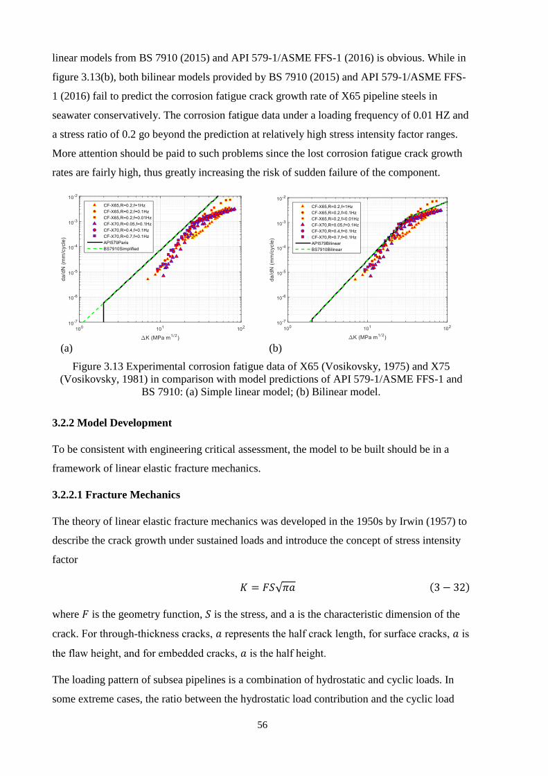
56

linear models from BS 7910 (2015) and API 579-1/ASME FFS-1 (2016) is obvious. While in

figure 3.13(b), both bilinear models provided by BS 7910 (2015) and API 579-1/ASME FFS-

1 (2016) fail to predict the corrosion fatigue crack growth rate of X65 pipeline steels in

seawater conservatively. The corrosion fatigue data under a loading frequency of 0.01 HZ and

a stress ratio of 0.2 go beyond the prediction at relatively high stress intensity factor ranges.

More attention should be paid to such problems since the lost corrosion fatigue crack growth

rates are fairly high, thus greatly increasing the risk of sudden failure of the component.

(a) (b)

Figure 3.13 Experimental corrosion fatigue data of X65 (Vosikovsky, 1975) and X75

(Vosikovsky, 1981) in comparison with model predictions of API 579-1/ASME FFS-1 and

BS 7910: (a) Simple linear model; (b) Bilinear model.

3.2.2 Model Development

To be consistent with engineering critical assessment, the model to be built should be in a

framework of linear elastic fracture mechanics.

3.2.2.1 Fracture Mechanics

The theory of linear elastic fracture mechanics was developed in the 1950s by Irwin (1957) to

describe the crack growth under sustained loads and introduce the concept of stress intensity

factor

𝐾 = 𝐹𝑆√𝜋𝑎 (3 − 32)

where 𝐹 is the geometry function, 𝑆 is the stress, and a is the characteristic dimension of the

crack. For through-thickness cracks, 𝑎 represents the half crack length, for surface cracks, 𝑎 is

the flaw height, and for embedded cracks, 𝑎 is the half height.

The loading pattern of subsea pipelines is a combination of hydrostatic and cyclic loads. In

some extreme cases, the ratio between the hydrostatic load contribution and the cyclic load

57

contribution in subsea pipelines may be greater than unity. This can be accounted for by the

mean stress effects in fracture mechanics analysis (Bannantine et al., 1990).

The assumed fatigue crack growth rate at Stage II usually follows of Paris’ law (Paris and

Erdogan, 1963)

𝑑𝑎

𝑑𝑁= 𝐶(∆𝐾)𝑚 (3 − 33)

where 𝑚 and 𝐶 are constants for a specific material; ∆𝐾 is the so-called stress intensity factor

range and is calculated by

∆𝐾 = (1 − 𝑅)𝐾max (3 − 34)

with 𝑅 and 𝐾max being the stress ratio (i.e. 𝑆min 𝑆max⁄ ) and maximum stress intensity factor

encountered in a stress cycle, respectively.

In a log-log plot of 𝑑𝑎 𝑑𝑁⁄ vs ∆𝐾, Paris law represents a straight line of a slope 𝑚. Behavior

of short cracks, i.e. cracks in stage I, departs from a simple Paris’ law representation. Below a

certain value of ∆𝐾 (known as the threshold value, ∆𝐾th) no macrocrack growth is expected.

Whereas when 𝐾max approaches 𝐾IC the crack growth rate increases rapidly. The fatigue life

of a component in an inert environment can be roughly divided into two parts: crack initiation

and crack growth. Fracture mechanics being applied to corrosion fatigue enables the

corrosion fatigue life fractions to be defined within the criteria of crack initiation and

propagation. For the engineering critical assessment applied at design stage, prediction of life

before crack initiation is decisive, since the initiation process can cost much longer time.

However, for the assessment applied in-service for to determine inspection intervals, since

cracks already exist, prediction of life after crack initiation becomes decisive. In a typical

corrosion fatigue situation, cracks initiate from corrosion sites and grows under the influence

from environment, thus the initiation stage is often bypassed. Moreover, in practice, cracks

detected on subsea pipelines are mostly at the propagation stage. Therefore, the research work

of this section focuses on the crack growth in the stage of crack growth and linear elastic

fracture mechanics is applied to establish a typical corrosion fatigue model for subsea

pipelines at service.

3.2.2.2 General Model

Several attempts have been made to model environmentally-assisted crack growth under

cyclic loading by superposing different processes. The classic model proposed by Landes and

Wei (1969), as shown in equation (3 − 35), simply treats the rate of corrosion fatigue crack

58

growth (𝑑𝑎 𝑑𝑁⁄ )CF, as the algebraic sum of the rate of crack growth in an inert

environment (𝑑𝑎 𝑑𝑁⁄ )F, and that of stress corrosion cracking (𝑑𝑎 𝑑𝑁⁄ )SCC in the identical

aggressive environment.

(𝑑𝑎

𝑑𝑁)CF

= (𝑑𝑎

𝑑𝑁)F+ (

𝑑𝑎

𝑑𝑁)SCC

(3 − 35)

The process competition model of Austen and Walker (1977) is based on the assumptions that

fatigue and stress corrosion cracking are two mutually competitive processes and that the

crack will propagate at a faster rate pertinent to the prevailing stress intensity factor.

However, to ensure compatibility in terms of crack growth rate per cycle rather than per

second, the plateau crack growth rate must be adjusted to the appropriate frequency or to the

frequency, stress intensity and stress ratio. The influences of high frequencies on the crack

growth rate plateau are predicted better than those of low frequencies. Other models (Hagn,

1988; Kim et al., 1998) modified these assumptions mostly by adding parameters.

3.2.2.3 Component Model

Based on the previous investigation on mechanisms of stress corrosion cracking and corrosion

fatigue, the latter can be viewed as a joint action of stress corrosion and hydrogen

embrittlement. A two-component physical model is proposed herein as

(𝑑𝑎

𝑑𝑁)CF

= (𝑑𝑎

𝑑𝑁)SC

+ (𝑑𝑎

𝑑𝑁)HAC

(3 − 36)

where (𝑑𝑎 𝑑𝑁⁄ )HAC is the crack growth rate by hydrogen-assisted cracking. The proposed

model basically means that (𝑑𝑎 𝑑𝑁⁄ )CF is an aggregate of the rates of stress corrosion,

(𝑑𝑎 𝑑𝑁⁄ )SC and hydrogen-assisted cracking, (𝑑𝑎 𝑑𝑁⁄ )HAC. The two-component description

holds as long as corrosion fatigue is composed of stress corrosion and hydrogen-assisted

cracking, in spite of possible interaction between the two processes. Anderson (2005)

mentioned a similar superposition model, however, it superposed cycle-dependent corrosion

fatigue with time-dependent corrosion fatigue, both of which are defined in a

phenomenological way, leading to difficulty in implementing the model. In contrast, this

proposed two-component model proposed is based upon physics while still being compatible

with fracture mechanics.

Anodic Dissolution

Several models have been developed for explaining the crack growth in stress corrosion

cracking due to anodic dissolution. A well-accepted one (Parkins, 1979) is the film rupture

59

model, which states while the metal surface is covered by a passive or protective layer, the

crack tip is kept free from protective layers continuously or discontinuously by local chemical

and mechanical effects, and this allows the accelerated anodic dissolution of local material.

To a large extent, anodic dissolution models for corrosion fatigue are extension of those

proposed for stress corrosion cracking. In such a view, the anodic dissolution process of

corrosion fatigue is described as cyclic plastic strain ruptures a protective film at the crack tip,

resulting in transient anodic dissolution, followed by possible re-passivation. The amount of

environmental crack growth per fatigue cycle depends on the kinetics of the reaction on the

clean metal surface as well as the time between film ruptures. All factors imposing influence

on corrosion fatigue process seem to work through the film rupture mechanism. Based on the

physical facts, a formula is proposed for the crack growth by stress corrosion over the whole

regime of 𝐾max

(𝑑𝑎

𝑑𝑁)SC

= (𝑑𝑎

𝑑𝑁)AD

= ℎ(∆𝐾, 𝑅, 𝑓) = {ℎ1(∆𝐾, 𝑅, 𝑓), 𝐾max < 𝐾t

ℎ2(∆𝐾, 𝑅, 𝑓), 𝐾max ≥ 𝐾t (3 − 37)

where (𝑑𝑎 𝑑𝑁⁄ )AD is the crack growth rate due to anodic dissolution, 𝑓 is the stress cycle

frequency, and 𝐾t is the transition stress intensity factor, i.e. where the crack growth rate

plateau starts in a abscissa of 𝐾max. Endo et al. (1981) conducted a series of experiments on

carbon steels in NaCl solution to investigate the stress corrosion crack growth rate of steels

due to anodic dissolution under fatigue loading conditions. They claimed that the observed

corrosion fatigue crack growth followed the sequential model,

(𝑑𝑎

𝑑𝑁)CF

= (𝑑𝑎

𝑑𝑁)F+ (

𝑑𝑎

𝑑𝑁)AD

(3 − 38)

where

(𝑑𝑎

𝑑𝑁)AD

= 𝐴𝑓𝑏(1 − 𝑅)c∆𝐾𝑚 (3 − 39)

𝐴, 𝑏 and 𝑐 are the material-environment system coefficients. According to the experimental

data, 𝐴 = 4.93 × 10−12, 𝑏 = −0.36, 𝑐 = 2 and 𝑚 is the same as that in the expression of

crack growth in air, i.e. equation (3 − 33). The negative value of 𝑏 is consistent with the

experimental observation by Bartlett and Hudak (1990) that the higher the frequency, the

lower the anodic dissolution rate, which means 𝑏 is usually negative. It is suspected that the

frequency and stress ratio dependence is determined by the solution conditions. Thus for a

medium such as seawater, 𝑏 may considered the same as that of the NaCl solution. So

ℎ1(∆𝐾, 𝑅, 𝑓) = 𝐴𝑓−0.36(1 − 𝑅)2∆𝐾𝑚 (3 − 40)

60

Effects of coefficient A on the shape of the crack growth curve are shown in figure 3.14.

(a) (b)

Figure 3.14 Anodic dissolution influence on the shape of crack growth curve: (a) X65

(Ronevich et al., 2016); (b) X70 (Drexler et al., 2014)

(a) (b)

Figure 3.15 Pipeline steel specimens in seawater with and without cathodic protection (CP):

(a) X65 (Vosikovsky, 1975); (b) X70 (Vosikovsky, 1981)

Aware that cathodic protection works through inhibiting the corrosion process. More

specifically, cathodic protection prevents the occurrence of anodic dissolution at the crack tip.

The corrosion fatigue crack growth data of X65 pipeline steel specimen in NaCl water with

and without cathodic protection are plotted in figure 3.15, as well as those of X70

(Vosikovsky, 1975; Vosikovsky, 1981). As can be seen, the change of crack growth rates

after imposing a cathodic protection is very small when ∆𝐾 goes beyond the plateau, thus

roughly

ℎ2(∆𝐾, 𝑅, 𝑓) ≈ 𝐴𝑓−0.36(1 − 𝑅)2𝐾t𝑚 (3 − 41)

This is consistent with the aforementioned anodic dissolution mechanism. According to the

anodic dissolution mechanism, as ∆𝐾 is growing, there is a critical value of ∆𝐾 where

61

repassiviation disappears. Below this value, anodic dissolution occurs discontinuously; above

this value, anodic dissolution effect will be constant. Compared with the increasing hydrogen-

assisted cracking rate, this constant rate is very small and its ratio to the hydrogen-assisted

cracking rate is still decreasing, evidenced as the pair of crack growth curves with and without

cathodic protection approaching each other after the transition point, as shown in figure 3.15.

Hydrogen Embrittlement

As for hydrogen-assisted cracking, crack growth is associated with hydrogen impurity in the

material. The hydrogen may be a by-product of corrosion reactions in aqueous solutions or

cathodic protection. The absorbed hydrogen atoms diffuse to the region near the crack tip with

stresses applied. The presence of hydrogen in metal is known to have an adverse effect on the

material’s properties, more specifically the concentration of hydrogen ahead of a crack tip can

cause a significant reduction in the material’s resistance to fracture (Humphries et al., 1989).

In such a situation, cracking happens at a lower stress level compared to that of the same

material without hydrogen absorption and crack propagates in an enhanced rate. This

phenomenon is called hydrogen embrittlement. Although there is still controversy as to the

extent to which hydrogen-assisted cracking explains subcritical crack growth in metals

stressed in environments that support concurrent crack tip dissolution, passive film formation,

and atomic hydrogen production. An agreement has been reached that hydrogen

embrittlement normally prevail for subsea metal structures with cathodic protection as well as

those exposed to gaseous hydrogen (Barnoush, 2011). Studies on the mechanism of hydrogen

embrittlement started several decades ago and are still ongoing. Among the numerous

mechanisms that have been raised so far, three have stood critical examinations and been

widely accepted, i.e. hydrogen-enhanced de-cohesion, hydrogen-enhanced localized

plasticity, and adsorption-induced dislocation emission. Arguments supporting each are not

definitive, even not exclusive. For those who are interested, ample information can be found

in a recent critical review by Lynch (2012). Not surprisingly, hydrogen-enhanced de-cohesion

has been frequently used as the theoretical basis for modelling hydrogen embrittlement

because of its explicit compatibility with fracture mechanics.

Hydrogen-enhanced de-cohesion provides the basic notion that hydrogen damage occurs in

the crack-tip plastic zone when the local crack tip opening tensile stress exceeds the

maximum-local atomic cohesion strength, which has been lowered by the presence of

hydrogen (Oriani, 1972). Hence locations of hydrogen damage initial sites are at a distance

ahead of the crack tip, i.e. the locations where tensile stresses are maximized. Thus

mechanical characteristics of the region near the crack tip should be analyzed, since it can

62

control the precise damage location. A model based on the theory of hydrogen-enhanced de-

cohesion should involve factors such as the tensile stress distribution in front of a crack tip,

the plastic strain and the associated dislocation density profile about the crack tip, the

distribution of hydrogen trap sites, and the concentration of environmentally produced

hydrogen in the crack-tip area. To establish such a model, the mathematically formulated

mechanism of hydrogen-enhanced de-cohesion by Lee and Unger (1988) was adopted, i.e.

𝜎maxH = 𝜎max0 − 𝛽𝐶H (3 − 42)

where 𝜎maxH and 𝜎max0 are the maximum principal stress at elastic-plastic boundary with and

without hydrogen when cracking initiates, respectively. 𝛽 is a parameter related to loss of

critical cohesive stress by hydrogen impurity, and 𝐶H is the local hydrogen concentration. It

represents the assumption that fracture occurs when the maximum crack-tip-opening stress

exceeds the hydrogen-reduced cohesive strength within an area in front of the crack tip.

𝐶H can be calculated by Fick’s law with respect to the hydrostatic stress (Van Leeuwen, 1974)

𝐶H = 𝐶H0exp (𝜎h𝑉H

𝑘B𝑇) (3 − 43)

where 𝐶H0 is the local hydrogen concentration in unstressed state, 𝜎h is the hydrostatic stress

within plastic zone, 𝑉H is the partial volume of hydrogen, 𝑘B is the Boltzmann constant, and 𝑇

is the temperature.

With the help of linear elastic fracture mechanics, expressions of the hydrostatic stress 𝜎h and

the maximum crack-tip-opening stress in front of crack tip 𝜎max under mode I with plane

strain condition are (Broek, 1974),

𝜎h =2

3(1 + 𝑣)

𝐾

√2𝜋𝑟 (3 − 44)

𝜎max = 𝜎yy =𝐾

√2𝜋𝑟 (3 − 45)

where 𝑟 is the radial distance from crack tip, 𝑣 is the Poisson’s ratio, and σyy is the stress

along the Y direction. Combining equations (3 − 41) ~ (3 − 44), with the assumption that

the location of the crack initiation does not change with hydrogen concentration, Wang et al.

(2013) obtained the following formula for predicting the hydrogen-degraded fracture

toughness,

63

𝐾IH = 𝐾IC {1 − (𝛽𝐶H0

𝜔𝜎ys) exp [

𝑉H𝜎ys

𝑘B𝑇∙2(1 + 𝑣)

3∙𝐾IH

𝐾IC]} (3 − 46)

where 𝜔 is a magnification factor of value 3 5 accounting for the material’s working

hardening effect, and 𝐾IH is the saturated fracture toughness, i.e. the fracture toughness fully

degraded in the environment with a specific hydrogen concentration. This model has been

applied to a series of steels to describe the dependence of fracture toughness on hydrogen

concentration, and the predicted results match well with the experimental data.

(a) (b)

Figure 3.16 Model of crack growth for the hydrogen embrittlement part of corrosion fatigue:

(a) Corrosion-crack correlation; (b) Two-stage Forman equation model.

Instead of Paris’ law, Forman equation is adopted for its integration of mean stress influence

via the stress ratio 𝑅 and the static failure via 𝐾IC in region II and region III,

𝑑𝑎

𝑑𝑁=

𝐵(∆𝐾)𝑚

[(1 − 𝑅)𝐾IC − ∆𝐾] (3 − 47)

In Section 3.1, a two-stage Forman equation model was proposed for the hydrogen-enhanced

fatigue crack growth in hydrogen gas. It is based on the corrosion-crack correlation and the

theory of hydrogen-enhanced de-cohesion, which is consistent with equation (3 − 45). The

key assumption in this model is the stress-driven hydrogen diffusion, namely the absorption

of the hydrogen ions into the crack tip is through transporting up the hydrostatic stress

gradients. This process is schematically plotted in figure 3.16.

Such an assumption enables the model to calculate several crucial points to capture features of

the hydrogen-enhanced fatigue crack growth. Note that this assumption is not applicable to

the fatigue cracking of subsea pipeline steels under cathodic protection. Cathodic protection

provides a potential intensifying the hydrogen absorption, which is mainly manifested as the

decrease or left shift of 𝐾t in the crack growth curve, as seen in figure 3.16.

64

The transition stress intensity factor 𝐾t, i.e. the point where the environment affected zone is

passed by the plastic zone in front of crack tip and the plateau section of the crack growth

curve starts, can be calculated as

𝐾t = 𝑚𝑖𝑛 {𝑚𝑎𝑥 {𝐾tran,∆𝐾0

(1 − 𝑅)} , 𝐾IH} (3 − 48)

where ∆𝐾0 represents the threshold stress intensity factor range at 𝑅 = 0 (usually obtained

from experiments), and


𝐾IH

𝐾IC(4𝜋2𝐷𝑉H𝜎ys

𝑘B𝑇𝑓)

14

(3 − 49)

The range length of stress intensity factor over which the crack growth rate plateau lasts is

approximated by

𝐾p =∆𝐾tH

(1 − 𝑅) (3 − 50)

where ∆𝐾tH is obtained by following equation

∆𝐾tH = ∆𝐾th − 1 (3 − 51)

The final fracture toughness displayed under a fatigue load, or alternatively the equilibrium

fracture toughness 𝐾IE, is proposed to be

𝐾IE =

{

[1 − (

2𝜋(𝜔𝜎ys)2

𝐾IC2

√𝐷𝑉H𝜎ys

𝑘BT𝑓)

𝜆

] 𝐾IN, 𝑓 > 𝑓C

𝐾IH, 𝑓 ≤ 𝑓C

(3 − 52)

where 𝜆 is a non-negative parameter used to adjust the rate with which 𝐾IE approaches 𝐾IC,

i.e. the inherent fracture toughness. In consistence with last section, 𝜆 is considered to be 1.0.

Then 𝐾IC in equation (3 − 47)is substituted by 𝐾IH and 𝐾IE respectively for the first and

second stage Forman equations. Good agreement can be seen from the application of the two-

stage Forman equation model to a wide range of carbon pipeline steels in Section 3.1. Thus,

the hydrogen-assisted cracking rate of the two-component corrosion fatigue model, is

established as

65

(𝑑𝑎

𝑑𝑁)HAC

= (𝑑𝑎

𝑑𝑁)HE

= 𝑔(∆𝐾, 𝑅, 𝑓, 𝐾IC, 𝐶H0)

= {𝑔1(∆𝐾, 𝑅, 𝑓, 𝐾IH, 𝐶H0), 𝐾max < 𝐾t

𝑔2(∆𝐾, 𝑅, 𝑓, 𝐾IE, 𝐶H0), 𝐾max ≥ 𝐾t (3 − 53)

where

𝑔1(∆𝐾, 𝑅, 𝑓, 𝐾IH, 𝐶H0) =𝐵1(∆𝐾)𝑚1

[(1 − 𝑅)𝐾IH − ∆𝐾] (3 − 54)

𝑔2(∆𝐾, 𝑅, 𝑓, 𝐾IE, 𝐶H0) =𝐵2(∆𝐾)𝑚2

[(1 − 𝑅)𝐾IE − ∆𝐾] (3 − 55)

(𝑑𝑎 𝑑𝑁⁄ )HE is the crack growth rate due to hydrogen embrittlement. Note that 𝐵1 and 𝑚1 are

acquired from the crack growth data measured before ∆𝐾 reaches (1 − 𝑅)𝐾t, while 𝐵2 and

𝑚2 are acquired from the crack growth data measured after the point (1 − 𝑅)(𝐾t + 𝐾p).

3.2.3 Model Applications

In terms of equations (3 − 36), (3 − 37), and (3 − 53), the two-component model can be

reformulated as

(𝑑𝑎

𝑑𝑁)CF

= (𝑑𝑎

𝑑𝑁)AD

+ (𝑑𝑎

𝑑𝑁)HE

= {ℎ1(∆𝐾, 𝑅, 𝑓) + 𝑔1(∆𝐾, 𝑅, 𝑓, 𝐾IH, 𝐶H0), 𝐾max < 𝐾t

ℎ2(∆𝐾, 𝑅, 𝑓) + 𝑔2(∆𝐾, 𝑅, 𝑓, 𝐾IE, 𝐶H0), 𝐾max ≥ 𝐾t (3 − 56)

In this part, the proposed model will be applied to X65 pipeline steels to display its general

performance. X65, the medium strength pipeline steel, is commonly adopted in offshore oil

and gas production systems and is currently one of the highest API grade C-Mn steels for

offshore service for its good ductility and toughness. In this application, the influence of

wedge effect caused by the accumulation of corrosion product within the crack tip cavity is

ruled out by using ∆𝐾eff as the default ∆𝐾.

The two-component model allows the superposition of anodic dissolution and hydrogen

embrittlement cracking rates. Due to a lack of exact experimental data for determining the

anodic dissolution rate of corrosion fatigue in pipeline steels, the related coefficients will be

given approximated values for the demonstrative purpose. On the other hand, corrosion

fatigue in seawater shares the same hydrogen embrittlement nature with the hydrogen-assisted

cracking of pipeline steels in hydrogen gas, while the experimental data of hydrogen-

enhanced fatigue cracking in hydrogen gas are plentiful. Ronevich et al. (2016) performed a

66

series of tests on X65 pipeline steels and obtained the hydrogen-enhanced fatigue crack

growth data. Experimental data of mechanical properties for X65 pipeline steels both in dry

air and hydrogen gas were collected by Somerday and Marchi (2007). For the gaseous

hydrogen environment, 𝐶H0 is calculated as the product of solubility and the square root of

pressure. The values of coefficients for determining the hydrogen embrittlement rate in the

proposed model for X65 pipeline steel are adopted in accordance with the research work in

the previous Section 3.1.

As for 𝛽, as stated in the notion of hydrogen-enhanced de-cohesion, 𝛽 is a parameter related

to the loss of critical cohesive stress by hydrogen impurity, which is a material property.

Gutierrez-Solana and Elices (1982), and Cialone and Holbrrok (1985), conducted a series of

tests on the fracture toughness degradation of X42 and X70 pipeline steels in hydrogen gas of

different pressures, respectively. Based on the fact that pipeline carbon steels usually share

similar chemical composition and exhibit a common ferritic-pearlitic microstructure (Holtam,

2010). It is expected that the sensitivities of C-Mn steels of different strengths to hydrogen

embrittlement should follow some relationship. In this research, linear interpolation between

the 𝛽 values of X42 and X70 is used with respect to the yield strength, and the 𝛽 value of X65

pipeline steels is thus determined as 1.56 × 104 MPa m3(mol H2)−1.

(a) (b)

Figure 3.17 Model application to X65 pipeline steels with R=0.5 (Ronevich et al., 2016): (a)

crack growth; (b) crack evolution.

The model implemented for X65 pipeline steel is shown in figure 3.17 and the related

calculation results are listed in table 3.4 (𝐴 = 3.93 × 10−11 is adopted in the model

calculation for demonstration). In the diagram of remaining fatigue life the effect of hydrogen

embrittlement and corrosion fatigue on remaining fatigue life can be seen straightforward.

The two-component model, by imposing the anodic dissolution rate to the hydrogen

embrittlement rate, reasonably simulates the shape of the total crack growth curve. Obviously,

67

the anodic dissolution process gives a rise of the crack growth curve before (1 − 𝑅)𝐾t. This

effect is quite significant at low ∆𝐾 regime. An analysis on the influence of the many factors

involved in the proposed model is displayed below.

X65 𝑹 𝑲𝐭 Crack evolution time

Life reduction

Fatigue 0.5 - 1.7110×106 -

Hydrogen embrittlement

0.5 24 6.5756×105 61.568%

Corrosion fatigue

0.5 24 3.3674×105 80.318%

Unit - MPa√m Cycle -

Table 3.4 Model calculation results for X65 pipeline steel

3.2.3.1 Loading Frequency

For most of commonly used alloys, the effect of frequency on crack growth under constant-

amplitude fatigue loads in inert environments is negligible. However in the presence of a

corrosive environment, the effect of frequency is magnified since it is directly related to

hydrogen diffusion and thus hydrogen embrittlement. The time dependent characteristic of

hydrogen diffusion indicates that the loading frequency 𝑓 may have an impact to the corrosion

fatigue crack growth. More specifically, lowering the loading frequency increases the

exposure time of the metal to the corrosive environment, thus within each load cycle more

atomic hydrogen may enter the material via the crack tip and diffuse a longer distance.

Observations from fatigue tests in corrosive environments have proven the existence of

critical frequency 𝑓C, below which the material always shows no frequency dependence. For

a corrosion fatigue process at 𝑓C, its propagation curve should be in a shape like that plotted

in figure 3.13(a), which is not the typical type of corrosion fatigue behavior for pipeline steels

in seawater. Hence this research puts its focus on the case where 𝑓 > 𝑓C, which is typical for

corrosion fatigue of subsea pipeline steels in seawater.

In a typical situation, the influence of loading frequency can be divided into two parts, one is

on the anodic dissolution process before ∆𝐾 reaches 𝐾t(1 − 𝑅). The decrease of 𝑓 will cause

the increase of anodic dissolution rates at each level of ∆𝐾, as predicted by equation

(3 − 39). This is because anodic dissolution rate is affected by the time available for

chemisorption at the crack tip during each cycle. The higher growth rate result at lower

frequencies occurs because the corrosive environment has more contact time with the crack

surfaces, while at higher frequencies, the corrosive environment cannot fully penetrate the

crack tip before the crack begins to close again. The experimental observation by Bartlett and

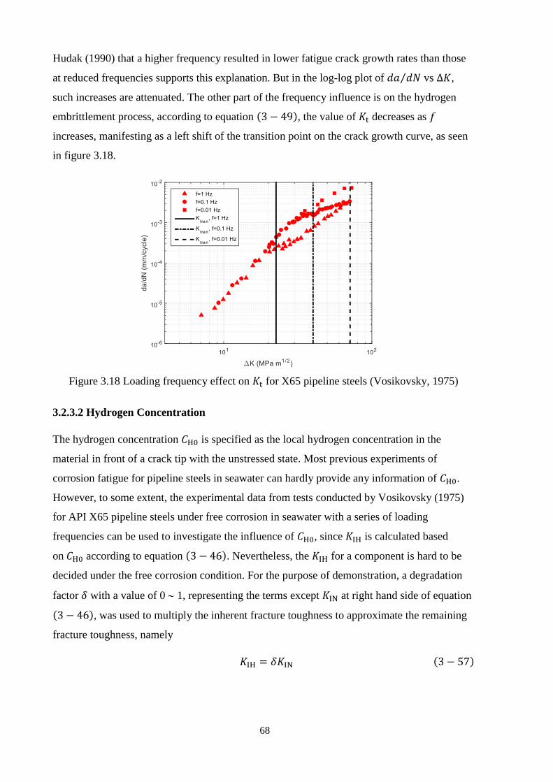
68

Hudak (1990) that a higher frequency resulted in lower fatigue crack growth rates than those

at reduced frequencies supports this explanation. But in the log-log plot of 𝑑𝑎 𝑑𝑁⁄ vs ∆𝐾,

such increases are attenuated. The other part of the frequency influence is on the hydrogen

embrittlement process, according to equation (3 − 49), the value of 𝐾t decreases as 𝑓

increases, manifesting as a left shift of the transition point on the crack growth curve, as seen

in figure 3.18.

Figure 3.18 Loading frequency effect on 𝐾t for X65 pipeline steels (Vosikovsky, 1975)

3.2.3.2 Hydrogen Concentration

The hydrogen concentration 𝐶H0 is specified as the local hydrogen concentration in the

material in front of a crack tip with the unstressed state. Most previous experiments of

corrosion fatigue for pipeline steels in seawater can hardly provide any information of 𝐶H0.

However, to some extent, the experimental data from tests conducted by Vosikovsky (1975)

for API X65 pipeline steels under free corrosion in seawater with a series of loading

frequencies can be used to investigate the influence of 𝐶H0, since 𝐾IH is calculated based

on 𝐶H0 according to equation (3 − 46). Nevertheless, the 𝐾IH for a component is hard to be

decided under the free corrosion condition. For the purpose of demonstration, a degradation

factor 𝛿 with a value of 0 1, representing the terms except 𝐾IN at right hand side of equation

(3 − 46), was used to multiply the inherent fracture toughness to approximate the remaining

fracture toughness, namely

𝐾IH = 𝛿𝐾IN (3 − 57)

69

Assume 𝛿 = 0.8, i.e., 80 percent of the inherent fracture toughness is left providing a

saturated hydrogen diffusion condition, then the predicted transitional points 𝐾t on crack

growth curves were calculated and plotted together with the test data in figure 3.18.

Good agreement between model prediction and experimental data is observed in figure3.19.

This means that if 𝐶H0 can be appropriately measured or determined, the corrosion fatigue

behaviour of pipeline steels in seawater can be predicted pretty well. Also, if 𝐾t is known or

can be measured for a specific material-environment system, it may in turn help investigate

the relationship of crack-cavity environment and the 𝐶H0.

3.2.3.3 Stress Ratio

The experimental data of X42 pipeline steels in hydrogen gas provided by Gutierrez-Solana

and Elices (1982) are used to investigate the influence of 𝑅 on the model performance. The

modelled crack growth processes and their evolution curves with different stress ratios in the

situation of corrosion fatigue, hydrogen embrittlement, and fatigue, are plotted in figure 3.19.

Figure 3.19(a) and (b) show that the hydrogen embrittlement model can well capture the

features of hydrogen-assisted cracking behavior of X42 pipeline steels under different stress

ratios and the influence of anodic dissolution on cracking process is larger at lower stress

ratios (e.g. 𝑅 = 0.1) than that at higher ones (e.g. 𝑅 = 0.8). Figure 3.19(c) ~ (f) show that

both hydrogen embrittlement and anodic dissolution’s influence on the crack evolution time

(cycles) or the remaining fatigue life is closely related to the change of stress ratio 𝑅. More

specifically, as shown in figure 3.19(c) and (d), at the low stress ratio 𝑅 = 0.1, hydrogen

embrittlement can cause a much larger reduction of crack evolution time or fatigue life than it

at the high stress ratio 𝑅 = 0.8, and thus anodic dissolution occupies a bigger portion of the

life reduction in the latter case. Within each case, hydrogen embrittlement is more significant

than anodic dissolution in reducing the fatigue life, while the critical crack size doesn’t

change much for fatigue, hydrogen-enhanced fatigue and corrosion fatigue. The little

variation of critical crack size is attributed to the fact that when crack growth rate is high,

hydrogen supply to the crack-tip region will be insufficient, leading to the recovery of

material’s fracture resistance, which is consistent with equation (3 − 52) for 𝑓 > 𝑓C. On the

other hand, figure 3.19(e) and (f) indicate that the high stress ratio 𝑅 = 0.8 provides a higher

crack size where crack growth starts for either fatigue, hydrogen-enhanced fatigue or

corrosion fatigue. Meanwhile the remaining life of either hydrogen-enhanced fatigue or

corrosion fatigue decreases more heavily at the low stress ratio 𝑅 = 0.1 than it at the high

stress ratio 𝑅 = 0.8 as the crack size extends. The model incorporates the effects of stress

70

ratio by equations (3 − 40) and (3 − 47). Equation (3 − 47), i.e. the Forman equation,

includes the 𝑅 effect in its denominator.

(a) (b)

(c) (d)

(e) (f)

Figure 3.19 Stress ratio effect on model performance with experimental data collected from

the work by Cialone and Holbrook (1985): (a) crack growth with 𝑅 = 0.1; (b) crack growth

with 𝑅 = 0.8; (c) crack evolution with 𝑅 = 0.1; (d) crack evolution with 𝑅 = 0.8; (e)

remaining fatigue life with 𝑅 = 0.1; (f) remaining fatigue life with 𝑅 = 0.8.

71

While equation (3 − 40) states that for corrosion fatigue, a high stress ratio can lead to a low

anodic dissolution rate at crack tip. It seems that the hydrogen embrittlement process

dominates the influence of 𝑅 on corrosion fatigue, represented as the shifts of transition points

as shown by Vosikovsky (1981). The accompanying changes in crack growth rates can be

seen as well in the experimental data by Vosikovsky (1981) for X70 pipeline steel specimens

tested in seawater. In conclusion, the increase of stress ratio can cause a left shift of the

transition point in the crack growth curve and a decrease of fatigue life reduction due to

corrosion fatigue. Detailed calculation results for X42 pipeline steel are listed in table 3.5.

X42 𝑹 𝑲𝐭 Crack evolution

time

Life reduction

Fatigue 0.1 - 2.0684×106 -


0.1 9.7424 2.2721×105 89.016%

Corrosion fatigue

0.1 9.7424 7.8647×104 96.198%

Fatigue 0.8 - 1.0645×107 -


0.8 35 9.1655×106 13.902%

Corrosion fatigue

0.8 35 8.4309×106 20.803%

Unit - MPa√m Cycle -

Table 3.5 Model calculation results for X42 pipeline steels at different stress ratios

3.2.3.4 Temperature

Temperature has impacts on the structural integrity in a few aspects. On the one hand, as

indicated by equations (3 − 46) and (3 − 49), temperature may affect the hydrogen diffusion

process and furtherly impose an influence on 𝐾t. On the other hand, the temperature variation

may induce a stress/strain variation in the components (i.e. the so-called thermal load).

Moreover, the temperature variation in the environment may even change the material’s

properties. For instance, at low temperatures steels could exhibit severe mechanical property

degradation which is well known as ductile-brittle transition. The change of mechanical

properties is usually obtained by tests and is out of this research’s scope. To study the impact

that temperature may have on 𝐾t, a temperature range of 20 °C ~ 300 °C is selected. Within

this temperature range, both ductile-brittle transition and creep are unlikely to happen to

carbon steels (Moura et al., 2009).

72

The variation trend of 𝐾t of X65 pipeline steels in such a temperature range is plotted in

figure 3.20. Figure 3.20 shows that 𝐾t increases as the environmental temperature increases,

however, the increment is not very significant. When the temperature increases from 20 °C to

300 °C, 𝐾t only increases from 19 MPa√m to a value less than 28 MPa√m. However, the

increase of 𝐾t doesn’t necessarily mean the effects of environment-assisted cracking on the

material under low temperature is less severe than that under high temperature. First, the

environment temperature in this analysis only varies in a limited range where ductile-brittle

transition and creep are unlikely to occur. Second, 𝐾t is only used to assess the immediate

structural integrity state and therefore can hardly give any information on the whole process

of corrosion fatigue, especially if higher cracking rate appears. Lasebikan et al. (2013)

concluded from a series of experiments conducted over a range of temperatures that the strain

hardening index of steels can be reduced at elevated temperatures. Note that the strain

hardening index has a negative correlation with the crack growth rate in an elastic-plastic way

(𝐽-integral). It is very likely that higher crack growth rate occurs at elevated environmental

temperatures.

Figure 3.20 Environmental temperature effect on 𝐾t

3.2.4 Summary

Subsea pipelines are vulnerable to corrosion fatigue which is a severe type of environment-

assisted cracking. There is a practical need to develop constitutive models for describing the

corrosion fatigue process of pipeline steels in seawater. In this 3.2 section, the mechanisms of

corrosion fatigue for subsea pipeline steels were investigated and it was found that corrosion

fatigue is driven by stress corrosion and hydrogen-assisted cracking. A two-component model

was then proposed for subsea pipeline steels where both the anodic dissolution and hydrogen

73

embrittlement models are integrated based on fracture mechanics. The proposed model was

applied to simulate the corrosion fatigue crack growth of X65 pipeline steels and the

influences of factors of 𝑓, 𝐶H0, R and T on the model performance were analyzed and

discussed. The results show that

1) The proposed two-component model can reasonably simulate the total crack growth

curve. Both the exacerbated cracking rate and behavior features can be well captured

with appropriate consideration of the effects of mechanical and environmental

parameters.

2) The increase of frequency will induce the decrease of anodic dissolution rates and a

left shift of the transition point on the corrosion fatigue crack growth curve.

3) If 𝐶H0 can be properly measured, the transition behavior of the corrosion fatigue crack

growth curves of pipeline steels in seawater can be well predicted.

4) The increase of stress ratio can cause a left shift of the transition point for the crack

growth curve and a decrease in fatigue life reduction due to corrosion fatigue.

5) In a limited temperature range where ductile-brittle transition and creep are unlikely to

occur, 𝐾t increases with the increase of the environmental temperature.


(2017b).

3.3 Extended Engineering Critical Assessment for Corrosion Fatigue

Engineering critical assessment has been regularly performed in today’s offshore oil and gas

industry to ensure the safe operation of critical structures as well as to maximize their earning

capabilities (Holtam, 2010). There are several industry standards that can provide guidance on

conducting engineering critical assessments, such as SINTAP (2000), FITNET (2008), ISO

19902 (2014), BS 7910 (2015), API 579-1/ASME FFS-1 (2016) etc. Although these standards

have specified corrosion fatigue as an important damage mechanism, they are not able to

provide as detailed, in depth and generality, and accurate assessments to corrosion fatigue as

to failure modes such as fracture/collapse, fatigue, creep fatigue, etc. (BS 7910, 2015). Such

insufficiency often leads to overestimation or underestimation of the damage by corrosion

fatigue to structural integrity. Offshore structures, for instance subsea pipelines, are

vulnerable to corrosion fatigue. The excessive conservatism can ensure safe operation, but

74

also leads to unnecessary and costly underwater inspections; while the lack of conservatism

will put the structure at a high risk of failure, which may result in enormous economic loss as

well as catastrophic environmental disasters. There is thus a practical and pressing need to

improve the traditional engineering critical assessment for the marine structures suffering

corrosion fatigue.

Based upon previous research work in sections 3.1 and 3.2, a critical stress intensity factor is

proposed in this section. It accounts for the influence of load frequency and initial crack size

on the model selection in engineering critical assessments of marine structures subjected to

corrosion fatigue. The critical stress intensity factor is calculated invoking the corrosion-crack

correlation model established in Section 3.1 for different patterns of corrosion fatigue crack

growth behaviour. While the subcritical crack growth is estimated using a three-stage model

for corrosion fatigue crack growth based on the research work done in Section 3.2. Each stage

of the model involves both the cracking processes assisted by anodic dissolution and by

hydrogen embrittlement. Finally, X65 grade pipeline carbon steels subjected to corrosion

fatigue in seawater is used to demonstrate the capability of the extended engineering critical

assessment.

3.3.1 Traditional Approach

Since it was developed in the 1950s by Irwin (1957), linear elastic fracture mechanics has

been widely applied to engineering critical assessments for steel structures. It introduces the

concept of stress intensity factor 𝐾 to describe the crack growth under sustained loads, where

𝐾 = 𝑌𝑆√𝜋𝑎 (3 − 58)

with 𝑌 being the geometry function, 𝑆 the applied stress perpendicular to the crack plane, and

𝑎 the characteristic dimension of the crack. For through-thickness cracks, 𝑎 represents the half

crack length, for surface cracks, 𝑎 is the flaw height, and for embedded cracks, 𝑎 is the half

height.

For the case of fatigue crack growth, the applied loading is characterized by an applied stress

range (∆𝑆 = 𝑆max − 𝑆min) rather than a single value of stress, and in fracture mechanics

terms, a given crack can then be considered to experience a stress intensity factor range (∆𝐾),

which is calculated as

∆𝐾 = 𝑌∆𝑆√𝜋𝑎 (3 − 59)

75

where 𝑌 is the geometry function. ∆𝐾 also has a relationship with the maximum stress

intensity factor 𝐾max in each load cycle as shown below,

𝐾max =∆𝐾

(1 − 𝑅) (3 − 60)

For normal fatigue cracking (i.e. fatigue cracking in an inert environment), in principle, crack

growth starts from the “stage I” (the “initiation” phase), mainly being “short crack”, and

continues with the “propagation” phase of stage II and stage III (fast crack growth), being

“long crack” towards final failure with 𝐾max in each load cycle approaching the fracture

toughness 𝐾IC (Pugno, 2006). Cracks detected at service are usually in the stage II. And it is

generally agreed that linear elastic fracture mechanics can provide reasonable fatigue life

prediction for long cracks (Stephens, 2000). Paris Law (Paris and Erdogan, 1963), which

describes the relationship between cyclic crack growth rate 𝑑𝑎 𝑑𝑁⁄ and stress intensity factor

range ∆𝐾 in stage II is the tool used in linear elastic fracture mechanics to predict the fatigue

life, and has the expression as below,

𝑑𝑎

𝑑𝑁= 𝐶(∆𝐾)𝑚 (3 − 61)

where 𝐶 and 𝑚 are material constants.

Traditional guidelines for engineering critical assessment have noticed that fatigue crack

growth in the presence of corrosion is different from that in an inert environment. However,

they are still unable to provide treatments for corrosion fatigue in the same depth and

generality as is provided for the aforementioned failure modes. For example, BS 7910 (2015)

only offers a brief guideline in its Clause 10 for the assessment of corrosion fatigue as a part

of environment-assisted cracking, which has a procedure as shown in figure 2.11. As in most

other industry standards, the defects undergoing environment-assisted cracking are evaluated

based on avoiding the phenomena by limiting 𝐾. More specifically, BS 7910 (2015) describes

a crack acceptance criterion for mode I cracking as follows

𝐾I <𝐾ISCC

𝐹 (3 − 62)

where 𝐾I is the applied stress intensity factor, F is a factor of safety to be agreed between the

parties involved in the structural integrity assessment and 𝐾ISCC indicates the point when

stress corrosion cracking happens. Following such an idea, the corresponding characterizing

parameter for corrosion fatigue should be ∆𝐾 where corrosion fatigue starts. BS 7910 (2015)

advises that the threshold stress intensity factor range at 𝑅 = 0, ∆𝐾0, for the growth of fatigue

76

cracks under the environmental and loading conditions of interest be chosen to assess the

significance of cracks. To assessment the subcritical crack growth before the crack size

(length or depth) reaches the failure criterion, the simplified model, which is actually a plot of

Paris law in a log-log scale, and the bilinear model, which is a plot of a two-stage Paris

equation, are recommended. However, it is often challenging to use ∆𝐾0 for assessment,

because the fatigue crack growth rate is very small and hard to measure in the very low ∆𝐾

regime, and such an assessment approach is actually in a preliminary level. While the

simplified model and bilinear model are not always good descriptions of the specified

corrosion fatigue crack growth. Thus, it is often seen that traditional engineering critical

assessment for corrosion fatigue may result in unnecessary cost as well as high risk of failure

arising through the structure’s service life.

3.3.2 Extended Approach

The fatigue crack growth process will be different in the presence of corrosion. According to

McEvily and Wei (1972), corrosion fatigue crack growths of metals may be broadly

categorized in three behaviour patterns as illustrated schematically in figure 3.13.

Figure 3.21 Comparison between BS 7910 model prediction and experimental data

(Vosikovsky, 1975)

Type A pattern is typical as that of the aluminium-water system and is characterized by a

reduction in the apparent threshold for crack growth and increases in the rate of crack growth

at given 𝐾max levels. As 𝐾max approaches 𝐾IC, the environmental influence diminishes. Type

B pattern is typical for the steel-hydrogen systems. An abrupt increase of crack growth rate

occurs somewhere along the abscissa, indicating quite strong environmental effects above

some critical 𝐾max but negligible effects below this level. A broad range of material-

77

environment systems such as seawater-steel systems exhibit behaviours that fall in Type C

pattern, with Type A behaviour at 𝐾max levels below the apparent threshold and Type B

behaviour above.

For steels freely corroding in a marine environment, current industry standards suggest the

simplified or bilinear models to be used in the engineering critical assessment of corrosion

fatigue. Take BS 7910 for instance, it provides the simplified model, the mean bilinear model

and the mean plus two standard deviations (mean+2SD) bilinear model for assessments of

different accuracies. Two sets of parameters are available for the cases R < 0.5 and R ≥ 0.5

respectively in the mean bilinear model as well as the mean+2SD bilinear model. However, as

seen in figure 3.21, with the experimental data from Vosikovsky (1975) for fatigue crack

growth of X65 pipeline carbon steels tested in seawater as the reference, the models are often

not good descriptions of the whole corrosion fatigue crack growth. On the other hand, the

experimental observation of fatigue crack growth curves of steels tested in seawater with and

without CP clearly show that the hydrogen embrittlement induced degradation of fracture

toughness is the reason causing crack behaviour features such as transition and plateau

(Shipilov, 2002). But Paris law in itself doesn’t link the crack growth behaviour with the

fracture toughness degradation. In order to reasonably describe the hydrogen-enhanced

fatigue crack growth of pipeline steels, a two-stage Forman equation model was developed in

Section 3.1 as

𝑑𝑎

𝑑𝑁=

{

𝐵1(∆𝐾)𝑛1

[(1 − 𝑅)𝐾IH − ∆𝐾], 𝐾max < 𝐾t

𝐵2(∆𝐾)𝑛2

[(1 − 𝑅)𝐾IE − ∆𝐾] , 𝐾max ≥ 𝐾t

(3 − 63)

where 𝐵1, 𝐵2, 𝑛1, and 𝑛2 are material constants, f is the load frequency, 𝐾IH is the saturated

fracture toughness which is obtained with sufficient hydrogen supplement using procedures

defined in ASTM E1820-17 (2017), 𝐾IE is the equilibrium fracture toughness, namely the

final fracture toughness displayed in the fatigue test conducted in hydrogen gas, and 𝐾t is the

transition stress intensity factor connecting the two stages, corresponding to the transition

point in the corrosion fatigue crack growth curve.

This model is based on the fatigue cracking of steels in high-pressure hydrogen gas depicted

by API 579-1/ASME FFS-1 (2016). Accordingly, the typical hydrogen-enhanced fatigue

cracking process of steels with constant amplitude loading is divided into three stages,

denoted as stage 1, 2 and 3 as shown in figure 3.22. In stage 1, the hydrogen delivered at the

crack tip leads to an enhanced fatigue crack growth compared with the normal fatigue

78

cracking, causing the crack grows along the sigmoidal curve dedicated by 𝐾IH. However,

when the crack growth rate goes beyond the hydrogen delivery rate, the crack propagates into

the bulk material with less hydrogen delivered at the crack tip. As a consequence, larger

cracking resistance is encountered, inducing a decrease in the growth acceleration which

manifests as a transition in the crack growth curve and indicates the commencement of stage

2. Due to the continuity of hydrogen charging and crack growth, the cracking rate will not

drop. But later as the equilibrium between the crack growth rate and hydrogen delivery rate is

achieved, a plateau of crack growth rate appears in the crack growth curve and lasts over a

range of 𝐾max, denoted as 𝐾pl. In stage 3, as 𝐾max approaching the equilibrium fracture

toughness 𝐾IE, the crack growth curve merges into the sigmoid oriented by 𝐾IE. The two-stage

Forman model consists of two segments of sigmoidal fatigue crack growth curves oriented by

𝐾IH and 𝐾IN connected by 𝐾t both plotted using dash lines in the same figure.

Figure 3.22 Crack-corrosion correlation model based corrosion fatigue crack growth

As previously stated, corrosion fatigue involves two damage mechanisms, i.e. anodic

dissolution and hydrogen embrittlement. Thus, based on the two-stage Forman model, a two-

stage corrosion fatigue crack growth model was further established in Section 3.2 as shown

below,

𝑑𝑎

𝑑𝑁=

{

𝐴𝑓−0.36(1 − 𝑅)2(∆𝐾)3 +

𝐵1(∆𝐾)𝑛1

[(1 − 𝑅)𝐾IH − ∆𝐾], 𝐾max < 𝐾t

𝐴𝑓−0.36(1 − 𝑅)3(𝐾t)3 +

𝐵2(∆𝐾)𝑛2

[(1 − 𝑅)𝐾IE − ∆𝐾] , 𝐾max ≥ 𝐾t

(3 − 64)

where the anodic dissolution effect is considered by the former part while the hydrogen

embrittlement assisted cracking process is represented by the latter part in each stage, and 𝐴 =

79

4.93 × 10−12 was obtained by Endo et al. (1981) from their experiments. The other

parameters have the same definition as in equation (3 − 63) but for corrosion fatigue in the

seawater-steel system. As seen in equation (3 − 64), each stage involves both the cracking

processes assisted by anodic dissolution and hydrogen embrittlement.

However, as seen in figure 3.21, the plateau in the crack growth curves of carbon pipeline

steels such as X65 in seawater is not evident, and most importantly, the stress intensity factors

of cracks detected at service usually locate within the range defined as long crack growth.

Thus it may be reasonable and convenient to use Paris law for the specified range of ∆𝐾,

instead of Forman equation, from a view of practical engineering. Furthermore, a three-stage

corrosion fatigue crack growth model, which has the expression shown below was built for

corrosion fatigue of pipeline carbon steels in seawater,

𝑑𝑎

𝑑𝑁= {

𝐴𝑓−0.36(1 − 𝑅)2(∆𝐾)3 + 𝐶1(∆𝐾)𝑚1 , 𝐾max < 𝐾t

𝐴𝑓−0.36(1 − 𝑅)5(𝐾t)3 + 𝐶1[(1 − 𝑅)𝐾t]

𝑚1 , 𝐾t ≤ 𝐾max < 𝐾t + 𝐾pl

𝐴𝑓−0.36(1 − 𝑅)5(𝐾t)3 + 𝐶2(∆𝐾)𝑚2 , 𝐾max ≥ 𝐾t + 𝐾pl

(3 − 65)

where 𝐴 is set the same as in equation (3 − 64), 𝐶1, 𝐶2, 𝑚1, and 𝑚2 are material constants,

and the 𝐾max range 𝐾pl = ∆𝐾tH (1 − 𝑅)⁄ according to Section 3.1, with the threshold stress

intensity factor range for corrosion fatigue ∆𝐾tH = 2 MPa ∙ m1/2 from API 579-1/ASME

FFS-1 (2016).

Experimental observation shows that as 𝐾max increases, before each 𝐾t is achieved, the crack

with load frequencies of 1 Hz, 0.1 Hz, and 0.01 Hz, grows almost along the same curve,

however, their growth curves deviate after 𝐾t, which has an obvious dependence on the load

frequency. Such a deviation has a direct influence on the crack growth rate and therefore the

fatigue life. For the reasons stated above, 𝐾t is proposed to be the critical value for stress

intensity factor and particular check may be necessary on this value before conducting

engineering critical assessments for critical structures under corrosion fatigue. The expression

of 𝐾t is derived from the corrosion-crack correlation model which is used to explain the

process of hydrogen-enhanced fatigue cracking as shown in Section 3.1 and schematically

plotted in figure 3.22.

In linear elastic fracture mechanics, the stress perpendicular to the crack plane in Mode I

loading, 𝜎yy, is expressed by

𝜎yy =𝐾I

√2𝜋𝑟 (3 − 66)

80

where 𝑟 is the distance in front of the crack tip, and 𝐾I is the stress intensity factor in Mode I.

And the maximum principal stress happens at the elastic-plastic boundary as,

𝜎max = 𝜎yy = 𝜔𝜎ys (3 − 67)

where 𝜔 is a magnification factor accounting for the material’s working hardening effect and

it is usually considered to be in a range of value 3 ~ 5 (Wang et al., 2013).

Thus the plastic zone size 𝑟p has the expression

𝑟p =1

2𝜋

𝐾I2

(𝜔𝜎ys)2 (3 − 68)

The concept of environment-affected zone is introduced to define the damaged zone where

the material exhibits a property different from that of the bulk material due to the penetration

of chemical agents into a localized crack-tip region (Liu, 2005). Assuming that the hydrogen

diffusion in the material of crack-tip region is primarily stress-driven, then based on the work

done in Section 3.1, 𝑟EAZ has an expression as:

𝑟EAZ = √𝐷𝑉H𝜎ys

𝑘B𝑇∙1

𝑓 (3 − 69)

where 𝐷 corresponds to the diffusion coefficient and is calculated from the ratio of hydrogen

permeability and solubility for carbon steel (Gadgeel and Johnson, 1979), 𝑓 is the load

frequency, 𝑉H is the partial volume of hydrogen, 𝑘B is the Boltzmann constant, 𝑇 is the

temperature in Kelvins and 𝜎ys is the material’s yield strength.

As can be seen from equation (3 − 68), 𝑟p grows as 𝐾I increases. In accordance with the

corrosion-crack correlation model, the point where the crack growth curve starts transition is

the very point where 𝑟p grows to an equilibrium with the environment-affected zone size 𝑟EAZ,

i.e.

𝑟p = 𝑟EAZ (3 − 70)

Combining equations (3 − 66) ~ (3 − 70), it follows that

𝐾tran = 𝜔H𝜎ys (4𝜋2𝐷𝑉H𝜎ys

𝑘B𝑇𝑓)

1/4

(3 − 71)

where 𝜔H accounts for the material’s working hardening effect in the presence of hydrogen.

81

Note that fracture happens when 𝐾I reaches the fracture toughness of the material, and the

corresponding critical plastic zone size 𝑟c keeps the same regardless of hydrogen ingress

(Wang, et al., 2013), the following equation can be achieved

𝜔

𝜔H=

𝐾IN

𝐾IH (3 − 72)

where 𝐾IN is the inherent fracture toughness. Wang et al. (2013) gives an equation for

calculating 𝐾IH based on the theory of hydrogen-enhanced de-cohesion,

𝐾IH

𝐾IN= 1 −

𝛽𝑐

𝜔𝜎ysexp [

2(1 + 𝑣)

3

𝑉H

𝑘B𝑇

𝐾IH

𝐾IN𝜔𝜎ys] (3 − 73)

where 𝛽 is a parameter related to the loss of critical cohesive stress by hydrogen impurity, 𝑐

refers to the hydrogen concentration in the material under a unstressed state, and 𝑣 is the

Poisson ratio.

Inserting equation (3 − 72) into equation (3 − 71), a preliminary calculation of the transition

stress intensity factor is performed, yielding


𝐾IH

𝐾IN(4𝜋2𝐷𝑉H𝜎ys

𝑘B𝑇𝑓)

14

(3 − 74)

To obtain the valid transition stress intensity factor 𝐾t, the following formula is used

𝐾t = min {max {𝐾tran,∆𝐾0

(1 − 𝑅)} , 𝐾IH} (3 − 75)

3.3.3 Applications

For pipeline carbon steels, the frequency effect on the crack growth rate is normally negligible

in dry-air environments. However, under corrosion fatigue, the frequency effect appears to be

obvious for materials under constant-amplitude load. It is generally believed that in an

environment with stable corrosiveness, the fatigue crack growth rate increases with the

decrease of the frequency. But as mentioned in Yu et al. (2015), observations from fatigue

tests in corrosive environments showed that there exists a critical frequency 𝑓c, under which

the material properties show the same level of degradation. According to the corrosion-crack

correlation model, the lower cyclic load frequency extends the exposure time of the material

to the corrosive environment, and this allows more hydrogen atoms to diffuse to a longer

distance in front of the crack tip within each loading cycle and thus a higher 𝐾t. When 𝑓 < 𝑓c,

82

the whole corrosion fatigue crack growth maintains high crack growth rate, namely no

transition appears in the growth curve. Thus, 𝑓c is decided by the relationship below:

𝐾tran = 𝐾IH (3 − 76)

Combining equations (3 − 74) and (3 − 76), it follows that

𝑓c =4𝜋2𝐷𝑉H𝜎ys

𝑘B𝑇(𝜔𝜎ys

𝐾IN)4

(3 − 77)

To validate the corrosion-crack correlation model, the results of an experiment conducted by

Yu et al. (2015) are compared with the prediction by equation (3 − 77) for 𝑓c. The

experiment was performed on X60 pipeline steel and the measured critical frequency was

1.04×10-3 Hz. According to the experimental conditions and material properties provided, the

𝑓c of X60 pipeline carbon steels is calculated to be in the range of 4.4×10-4 to 3.4×10-3 Hz,

with a consideration of ω ranging from 3 to 5. While the measured 𝑓c is 1.04×10-3 Hz that

exactly falls in the predicted range of 4.4×10-4 and 3.4×10-3 Hz, which shows the critical

frequency of the experiment is captured by equation (3 − 77).

Material Yield strength

(𝝈𝒚𝒔)

Poisson ratio (𝒗)

Diffusion coefficient

(𝑫)

Threshold stress

intensity factor range

(∆𝑲𝟎)

Inherent fracture

toughness (𝑲𝑰𝑵)

Partial volume of hydrogen

(𝑽𝑯)

X65 458.5 0.3 5.3 × 10−9 2.0 197.9 2.0 × 106

Unit MPa -

(mol H2)/m3

∙ MPa1/2 MPa ∙ m1/2 MPa ∙ m1/2 m3mol−1

Table 3.6 Material properties of API X65 steel (Guedri et al., 2004; Yu et al., 2015)

Similarly, using the material in table 3.6, the 𝑓c of X65 pipeline carbon steels falls in a range

of 1.8×10-4 to 1.4×10-3 Hz, which is reasonable since it is well below the sample frequency

0.01 Hz. Furthermore, the validity of equation (3 − 74) can be confirmed by the experimental

data from tests conducted by Vosikovsky (1975) for API X65 pipeline steels freely corroding

in seawater with a series of load frequencies. As the saturated fracture toughness is hard to be

decided for a component with free corrosion in seawater, a degradation factor 𝛿, with a value

of 0 ~ 1.0, is multiplied by the inherent fracture toughness to approximate the remaining

fracture toughness, namely

𝐾IH = 𝛿𝐾IN (3 − 78)

83

Assuming 𝛿 = 0.8, i.e. 80 percent of the inherent fracture toughness is left providing a

saturated diffusion condition, which corresponds to the worst corrosion fatigue case where

pH=5, 𝐾t are calculated using the material property data provided in table 3.6 and then plotted

together with the experimental data in figure 3.23. Good agreement between the model

prediction and experimental data is observed as shown in figure 3.23, which indicates that

equation (3 − 74) is an effective formula to predict the 𝐾t for corrosion fatigue crack growth

curves above 𝑓c. The results of the model prediction are summarized in table 3.7.

Figure 3.23 Prediction of transition stress intensity factors for X65 under corrosion fatigue

with various load frequencies (Vosikovsky, 1975)

Material Stress Ratio (𝑹)

Load frequency (𝒇)

Transition SIF (𝑲𝒕)

Transition SIF range (∆𝑲𝒕)

X65 0.2 1 28.8 23.0

X65 0.2 0.1 40.3 32.3

X65 0.2 0.01 62.0 49.6

Unit - Hz MPa ∙ m1/2 MPa ∙ m1/2 Table 3.7 Predicted transition stress intensity factors for X65 pipeline carbon steels under

corrosion fatigue

Crack growth curve 𝑲𝒎𝒂𝒙 < 𝑲𝒕 𝑲𝒎𝒂𝒙 ≥ 𝑲𝒕 𝑲𝒕 𝐶1 𝑚1 𝐶2 𝑚2

X65, 𝒇 = 𝟏 𝑯𝒛 2.30×10-9 3.69 2.67×10-8 2.76 28.8

X65, 𝒇 = 𝟎. 𝟏 𝑯𝒛 4.01×10-10 4.34 9.72×10-6 1.36 40.3

X65, 𝒇 = 𝟎. 𝟎𝟏 𝑯𝒛 8.79×10-11 4.58 4.15×10-7 2.17 62.0

Unit - - - - MPa ∙ m1/2 Table 3.8 Parameters of corrosion fatigue crack growth curves regressed from test data

The initial crack size ai in this research is defined as the size when the crack is detected using

a reliable non-destructive technique. It characterizes the initial state of the crack in the

84

engineering critical assessment to be conducted. The initial crack size in pressure vessels may

range from several millimetres to some centimetres (Visser, 2002). Three cases where the

initial crack size 𝑎i = 1 mm, 4 mm, 12 mm are investigated based on experimental data

(Vosikovsky, 1975). Since 𝐾t of corrosion fatigue crack growth curves of X65 pipeline

carbon steels under various load frequencies have been acquired, the experimental data are

regressed to follow the three-stage corrosion fatigue model. The parameter values from

regression are summarized in table 3.8. Crack growth curves generated by each model are

plotted in figure 3.24, with the experimental data plotted as reference.

Figure 3.24 Crack growth curves of X65 under corrosion fatigue with various load

frequencies (Vosikovsky, 1975)

The fatigue life in cycles over the range of crack sizes 𝑎i to 𝑎f is calculated as:

𝑁if = ∫1

𝐶(𝑌∆𝑆√𝜋𝑎)𝑚

𝑎f

𝑎i

𝑑𝑎

𝑎𝑚/2 (3 − 79)

Vosikovsky (1975) used single-edge notched specimens, with a width 𝑏 of 76.2 mm and a

half length ℎ of 580 mm, in his tests. The specimen is plotted in figure 3.25. Accordingly, the

following function for calculating the geometry factor 𝑌 is used (Dowling, 2012):

𝑌 = (1 + 0.122cos4𝜋𝛼

2)√

2

𝜋𝛼tan

𝜋𝛼

2 (3 − 80)

where 𝛼 is the ratio of crack length a to the width of specimen. Equation (3 − 80) is also

plotted in figure 3.25. It is obvious that the geometry effect is relatively stable before α

reaches 0.6, i.e. before the length of crack grows to a length of 0.6 times the width. So the

failure criteria in this case is set as the crack grows to a length of 45.7 mm, i.e. 𝑎f =

85

45.7 mm. The ratio of applied stress to the material’s yield strength is adjusted to 0.4 so that

the range of ∆𝐾I for evaluation approximately equals that where experimental data are

available and the small yielding assumption of linear elastic fracture mechanics is met.

Figure 3.25. Geometry and the geometry function of the single-edge notched specimen

To evaluate the influence from the load frequency as well as the initial crack size on the

performance of standard models in predicting corrosion fatigue life, a comparison is made

among each group in terms of load frequency and initial crack size. Conservatism is used as

the evaluation parameter, which is defined as:

Conservatism =Experimental prediction − Model prediction

Experimental prediction× 100% (3 − 81)

Negative conservatism means the model predicts a larger life than that of the experiment, i.e.

the prediction by standard model is unconservative, which is usually not allowed in

engineering practices. In other words, a negative conservatism indicates that the model should

be rejected for the engineering critical assessment. Conversely, positive conservatism stands

for a redundancy in life prediction of the model, and the smaller the conservatism the better

the performance of the model in the engineering critical assessment. Only the simplified

model and the bilinear model of mean plus two standard deviations (mean+2SD) are used for

fatigue life prediction and comparison with experimental data, since the mean bilinear model

is obviously short of conservatism for engineering critical assessments of corrosion fatigue, as

indicated in figure3.21. The values of parameters of the simplified and bilinear models

suggested in BS 7910 (2015) are summarized in table 3.9 for the experimental case where

𝑅 = 0.2. The calculation results for each case are summarized in table 3.10.

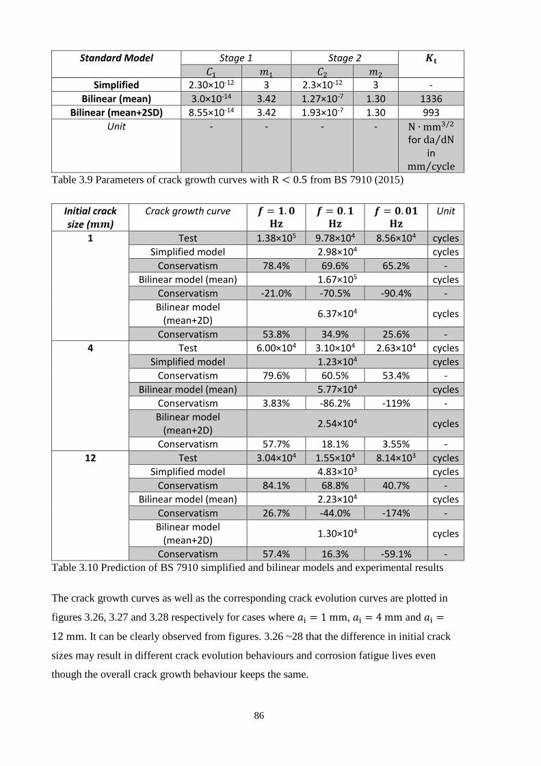
86

Standard Model Stage 1 Stage 2 𝑲𝐭

𝐶1 𝑚1 𝐶2 𝑚2 Simplified 2.30×10-12 3 2.3×10-12 3 -

Bilinear (mean) 3.0×10-14 3.42 1.27×10-7 1.30 1336

Bilinear (mean+2SD) 8.55×10-14 3.42 1.93×10-7 1.30 993

Unit - - - - N ∙ mm3/2 for da dN⁄

in mm cycle⁄

Table 3.9 Parameters of crack growth curves with R < 0.5 from BS 7910 (2015)

Initial crack size (𝒎𝒎)

Crack growth curve 𝒇 = 𝟏. 𝟎 𝐇𝐳

𝒇 = 𝟎. 𝟏 𝐇𝐳

𝒇 = 𝟎. 𝟎𝟏 𝐇𝐳

Unit

1 Test 1.38×105 9.78×104 8.56×104 cycles

Simplified model 2.98×104 cycles

Conservatism 78.4% 69.6% 65.2% -

Bilinear model (mean) 1.67×105 cycles

Conservatism -21.0% -70.5% -90.4% -

Bilinear model (mean+2D)

6.37×104 cycles

Conservatism 53.8% 34.9% 25.6% -

4 Test 6.00×104 3.10×104 2.63×104 cycles


Conservatism 79.6% 60.5% 53.4% -


Conservatism 3.83% -86.2% -119% -


2.54×104 cycles

Conservatism 57.7% 18.1% 3.55% -

12 Test 3.04×104 1.55×104 8.14×103 cycles


Conservatism 84.1% 68.8% 40.7% -


Conservatism 26.7% -44.0% -174% -


1.30×104 cycles

Conservatism 57.4% 16.3% -59.1% - Table 3.10 Prediction of BS 7910 simplified and bilinear models and experimental results

The crack growth curves as well as the corresponding crack evolution curves are plotted in

figures 3.26, 3.27 and 3.28 respectively for cases where 𝑎i = 1 mm, 𝑎i = 4 mm and 𝑎i =

12 mm. It can be clearly observed from figures. 3.26 ~28 that the difference in initial crack

sizes may result in different crack evolution behaviours and corrosion fatigue lives even

though the overall crack growth behaviour keeps the same.

87

(a) (b)


(a) Crack growth; (b) Crack evolution.

(a) (b)



(a) (b)



88

Corrosion fatigue lives calculated based on the experiment data are plotted in figure 3.29 and

those predicted using standard models from BS 7910 are plotted in figure 3.30. Conservatisms

calculated from equation (3 − 81) for each model are plotted in figure 3.31 as histograms.

The histograms are clustered in terms of load frequencies, and within each cluster the

histograms are lined in a sequence of initial crack size 1 mm, 4 mm, and 12 mm from left to

right.

As shown in figure 3.29, the fatigue life of structures subjected to corrosion fatigue is tightly

related with the load frequency 𝑓. The lower the frequency, the higher the crack growth rate

and thus the lower the fatigue life, represented by the experiment based prediction. This is

believed to be caused by the increase in the value of ∆𝐾t resulting from the decrease of load

frequency. However, the standard models from industrial standards such as BS 7910 (2015),

ignore the load frequency effect in corrosion fatigue, causing either overestimation or

underestimation of the structure’s fatigue life. Figure 3.29 also implies that the corrosion

fatigue life in low regime of ∆𝐾 occupies a much bigger fraction in overall fatigue life than

that in high ∆𝐾 regime, which means more cycles are spent to drive the crack growth when

the crack size is small. Combining the aforementioned two findings with the observation, it is

found that the increase of fatigue life accelerates as 𝑓 increases.

Figure 3.29 Load frequency effect on corrosion fatigue life prediction for X65 steels under

various initial crack sizes

Figure 3.30 shows that among the corrosion fatigue lives predicted by the standard models

using the parameter values provided by BS 7910, the corrosion fatigue life predicted by the

bilinear model (mean) is always the highest, and then comes that by the bilinear model

(mean+2SD), and the corrosion fatigue life predicted by the simplified model is the lowest.

ai=1mm

ai=4mm

ai=12mm0.00E+00

2.00E+04

4.00E+04

6.00E+04

8.00E+04

1.00E+05

1.20E+05

1.40E+05

1.60E+05

0.01Hz 0.1Hz 1Hz

Fati

gue

life

Test results

89

All the three predicted values decrease as the initial crack size increases. And quite obviously,

the difference among them decreases as well.

Figure 3.30 Prediction by standard models for corrosion fatigue life of X65 steels with

various initial crack sizes

As seen in figure 3.21 that there is some underestimation of the corrosion fatigue crack

growth rate from the bilinear model in the high ∆𝐾 regime for low load frequencies, while the

simplified model always overestimates the crack growth rate. But this doesn’t mean the

simplified model is better than the bilinear model, because the underestimation of the

corrosion fatigue crack growth rate for low frequencies such as 0.01Hz from the bilinear

model in high ∆𝐾 regime can be balanced by the overestimation from the bilinear model in

low ∆𝐾 regime. Keeping in mind that the crack growth in low ∆𝐾 regime contributes much

more than that in high ∆𝐾 regime, the bilinear model may give a prediction that is overall

conservative, but with a much better performance in the view of conservatism. For example,

the conservatism of the prediction by bilinear model (mean+2SD) for a crack of the initial

size 4 mm with a load frequency of 0.01 Hz is as low as 3.55%, as indicated in table 3.10.

Figure 3.31(a) shows that the simplified model always give a conservative life prediction for

corrosion fatigue cracks with various initial crack sizes. While the conservatisms in the life

prediction by the simplified model remain relatively large, they decrease as the load

frequency decreases. Additionally, the sensitivity of the conservatism to load frequency is

higher for a larger initial crack size, and this is also true for figures 3.31(b) and (c). Figure

3.31(b) implies that among all the possible 9 combinations of load frequencies and initial

crack sizes, the bilinear model (mean) can only be used for engineering critical assessments of

two cases, i.e. 𝑓 = 1 Hz with 𝑎i = 4 mm, and 𝑓 = 1 Hz with 𝑎i = 12 mm. In figure 3.31(c),

Simplified model

Bilinear model (mean)

Bilinear model

(mean+2SD)

0.00E+00

2.00E+04

4.00E+04

6.00E+04

8.00E+04

1.00E+05

1.20E+05

1.40E+05

1.60E+05

1.80E+05

1mm 4mm 12mm

Fati

gue

life

Model prediction

90

only the case where 𝑓 = 0.01 Hz with 𝑎i = 12 mm is not fit for engineering critical

assessment conducted using the bilinear model (mean+2SD). In a general view, with the load

frequency decreasing, the conservatisms of the simplified, bilinear (mean) as well as bilinear

(mean+2SD) models decrease, and the bilinear model (mean+2SD) performs best. The

conservatism generated by the standard models in life prediction accumulates with the crack

growth. The inefficient performance of the simplified model, indicated by its large

conservatisms on average, is due to the ignorance of the transition in the corrosion fatigue

crack growth curve. As revealed by equation (3 − 74), the transition stress intensity factor is

determined by the load frequency. Depending on both the load frequency and the initial crack

size/stress intensity factor range, the corrosion fatigue life, as seen in figure 3.29, may be

heavily influenced, and so is the conservatism. The transition stress intensity factor specified

in the bilinear model (mean+2SD) happens to be close to that of the crack growth curve with

a load frequency of 0.1 Hz, as seen in figure 3.21, which makes the conservatism in life

prediction by the bilinear model (mean+2SD) small overall. But for cases where the load

frequencies are lower than 0.1 Hz, the bilinear model (mean+2SD) tends to underestimate the

crack growth rate after ∆𝐾t, contributing a negative value to the overall conservatism

afterward; while for the cases where load frequencies are higher than 0.1 Hz, the bilinear

model tends to overestimate the crack growth rate after ∆𝐾t, contributing a positive value to

the overall conservatism afterward. Based on the conclusion drawn for figure 3.29, the

increase of the sensitivity of conservatism to load frequency with the increasing initial crack

size, which has been shown in figure 3.31, is explained to be due to the increase in initial

crack size reducing the portion of the low-∆𝐾 crack growth in the predicted life.

Figure 3.31 also shows that a large initial crack size combined with a low load frequency tend

to provide small even negative conservatism. Caution is needed when the case to be assessed

involves either low frequency or large initial crack size or both. When assessing cases where

𝑓 ≤ 0.01 Hz, the simplified model is suggested to be used. If more accuracy is required, it

may work to use the bilinear model (mean+2SD) before ∆𝐾 reaches ∆𝐾t specified by BS

7910 (2015) and then use the simplified model. Large initial crack size implies a high ∆𝐾.

Even though most cracks found at service are in a scale of several millimetres, this doesn’t

equivalently mean that their ∆𝐾 usually falls in the regime of low ∆𝐾 range. It is also

necessary to consider the stress history and future working load conditions. For cracks

detected with high ∆𝐾, the simplified model is suggested to be used for engineering critical

assessment since it can always provide positive conservatism. As shown in table 3.10, in the

case where the crack has an initial size of 12 mm under a load frequency of 0.01 Hz, the use

91

of the bilinear model provides unconservative life prediction (conservatism = -59.1%),

however, the use of the simplified model still provides conservative life prediction

(conservatism = 40.7%).

(a)

(b)

(c)

Figure 3.31 Comparison of corrosion fatigue life prediction for X65 under various load

frequencies

0.00%

10.00%

20.00%

30.00%

40.00%

50.00%

60.00%

70.00%

80.00%

90.00%

f=0.01Hz f=0.1Hz f=1Hz

Co

nse

rvat

ism

Simplified model

ai=1mm

ai=4mm

ai=12mm

-200.00%

-150.00%

-100.00%

-50.00%

0.00%

50.00%

Co

nse

rvat

ism

Bilinear model (mean)

ai=1mm

ai=4mm

ai=12mm

-60.00%

-40.00%

-20.00%

0.00%

20.00%

40.00%

60.00%

Co

nse

rvat

ism

Bilinear model (mean+2SD)

ai=1mm

ai=4mm

ai=12mm

92

In traditional engineering critical assessments, the effect of the load frequency and initial

crack size (in long-crack domain) is ignored due to their little influence on fatigue crack

growth in an inert environment. However, for a structure subjected to corrosion fatigue, the

effect of the load frequency and initial crack size on the corrosion fatigue crack growth is

important. Such an effect can be taken into account through the parameter 𝐾t or ∆𝐾t.

According to equation (3 − 74), 𝐾t or ∆𝐾t is directly related to the load frequency. The

higher the load frequency, the smaller the value of 𝐾t or ∆𝐾t. Meanwhile, the initial crack size

may be well above the crack size corresponding to Kt or ∆𝐾t. As analysed before,

conservatism accumulates as the crack grows, thus the crack growth curve after 𝐾t or ∆𝐾t

may impose a significant influence on the performance of the model. Equation (3 − 74),

which is derived from the corrosion-crack correlation model, provides an effective way of

calculating 𝐾t or ∆𝐾t. It is thus believed that the calculation of 𝐾t or ∆𝐾t and an analysis on

the fatigue crack growth behaviour for the structures under corrosion fatigue would benefit

the subsequent engineering critical assessment.

3.3.4 Summary

An extended engineering critical assessment was developed in this 3.3 section, in which a

critical stress intensity factor was proposed, accounting for the influence of load frequency

and initial crack size, to direct the model selection within current industrial standards for

assessing the integrity of structures subjected to corrosion fatigue. For the specific corrosion

fatigue cracking behavior pattern, a three-stage fracture mechanics based corrosion fatigue

crack growth model is used to predict the subcritical crack growth. This extended engineering

critical assessment was applied to X65 grade pipeline carbon steels and the results indicate

that

1) The load frequency and initial crack size impose significant impact on the corrosion

fatigue crack growth.

2) The proposed critical stress intensity factor 𝐾t extends the traditional engineering

critical assessment for corrosion fatigue in that it accounts for the influence of load

frequency and initial crack size on the model selection for the engineering critical

assessments of marine structures under corrosion fatigue.

3) For X65 pipeline steels, the simplified model always gives a conservative life

prediction for corrosion fatigue cracks with various initial crack sizes

4) When assessing corrosion fatigue cases of X65 pipeline steels where 𝑓 ≥ 1 Hz, the

life prediction by the bilinear model (mean) from BS 7910 (2015) is conservative only

93

if the initial crack size is larger than the crack size corresponding to 𝐾t or ∆𝐾t under

the specified load history.

5) When assessing cases of X65 pipeline steels where 𝑓 ≤ 0.01 Hz, the simplified model

is suggested to be used. If more accuracy is required, it may work to use the bilinear

model (mean+2SD) before ∆𝐾 reaches ∆𝐾t values specified by BS 7910 (2015) and

the simplified model afterward.

In summary, the proposed approach of engineering critical assessments in particular for

subsea pipelines suffering corrosion fatigue has procedures as shown in figure 3.32. It

includes two parts: a strategy of selecting crack growth models and their parameters from

current industrial standards for corrosion fatigue in seawater; and a three-stage corrosion

fatigue crack growth model, which is used in this Section 3.3 to provide basis for comparisons

among various models, for corrosion fatigue of other cases.

The detailed procedure of proposed engineering critical assessment for corrosion fatigue in

seawater are furtherly demonstrated in figure 3.32. In words it would be as follows: in the

beginning of assessment, the ∆𝐾t of the component’s material should be calculated and then

be compared with the values for the bilinear (mean+2D) model from industrial standards such

as BS 7910 (2015). If the calculated value of ∆𝐾t is smaller than the provided value, then the

bilinear model (mean+2D) is proper to be used. But if the calculated value is larger than the

provided value, then the bilinear model (mean+2D) should not be simply applied. It is

suggested that the initial ∆𝐾 of the aimed inspection interval should then be determined using

the detected characteristic dimension of the crack together with the component’s load

information. If the initial ∆𝐾 is larger than the provided ∆𝐾t, the simplified linear model is

recommended for use, otherwise, the bilinear model (mean+2D) may be used before ∆𝐾

reaches the provided ∆𝐾t, but afterward the simplified linear model is again recommended for

use.

Note that the material ∆𝐾t is related to the loading frequency and the initial ∆𝐾 is actually

related the initial crack size. Hence the proposed approach actually extends the traditional

ECA approach to account for the influence from both loading frequency and initial crack size.


(2018a).

94

Figure 3.32 Proposed approach of engineering critical assessment for corrosion fatigue

Detailed procedures of proposed engineering critical

assessment for corrosion fatigue in seawater

95

Chapter 4. FATIGUE ASSESSMENT

While most engineering structures are designed to withstand loads well below the material’s

yield strength, low-cycle fatigue in practice is still possible to happen. For subsea pipelines

under high-pressure/high-temperature service conditions, cyclic buckling may happen either

as planned or unexpectedly. In each way, the structures can suffer cyclic operational stresses

close to or larger than the material’s yield strength, which in this thesis is called low-cycle

fatigue loads. In such cases, the small-scale yielding assumption of linear elastic fracture

mechanics is violated. Therefore, linear elastic fracture mechanics and models based on it can

no longer be applied. Unfortunately, most current industrial standards adopt fatigue crack

growth models based on linear elastic fracture mechanics to predict the subcritical growth of

detected flaws.

The research work to be presented in this Chapter is centred on establishing a prediction

model of fatigue crack growth applicable for low-cycle fatigue. It consists of 2 sections. In

Section 4.1, an energy principles based model is built up using the characteristic parameter of

linear elastic fracture mechanics, ∆𝐾 to predict the crack growth of metallic materials under

high-cycle fatigue loads. In Section 4.2, crack growth under low-cycle fatigue loads is

predicted through establishing a model following a similar idea of last section, but using the

characteristic parameter of elastoplastic fracture mechanics, ∆𝐽 to ensure the model’s

applicability to crack growth under both high-cycle and low-cycle fatigue loads.

4.1 Crack Growth under High-cycle Fatigue Loads

Following the pioneering work of Paris and Erdogan (1963), a number of models relating the

range of stress intensity factor, ∆𝐾 and the crack growth rate, 𝑑𝑎/𝑑𝑁, have been developed to

describe the fatigue crack growth under small-scale yielding conditions (Nguyen et al., 2001;

Pugno et al., 2006; Beden et al., 2009; Santecchia et al., 2016). For most of these models,

fatigue crack growth data from tests are required to determine the empirical curve-fitting

parameters within the models.

Many researchers have recognized that it is possible to build models capable of predicting

fatigue crack growth primarily from the fundamental deformation properties including low-

cycle fatigue properties and monotonic and cyclic tensile properties, which are easier to be

obtained experimentally and are often required for the purpose of design (Kaisand and

Mowbray, 1984; Li et al., 1998; Pandey and Chand, 2003; Hurley and Evans, 2007; Ellyin,

96

2012; Shi et al., 2016; Huffman, 2016; Wu et al., 2017). Some of them also tapped energy

principles in their model development (Pandey and Chand, 2003; Shi et al., 2016; Huffman,

2016). However, in addition to the aforesaid fundamental deformation properties, the

threshold range, ∆𝐾th of the material is often required by these models as an input parameter,

for calculating either the length of the fracture process zone ahead of crack tip (Li et al., 1998;

Pandey and Chand, 2003; Ellyin, 2012) or the critical crack blunting radius (Shi et al., 2016;

Wu et al., 2017). Notably, ∆𝐾th is obtained by fatigue crack growth tests and it is thus not

widely available due to the high complexity and cost of the tests. Moreover, fatigue crack

growth rates will be generated along the tests, undermining the necessity of model prediction.

Figure 4.1 Fatigue crack growth with 𝑅 = −1

In this section, a model based on energy principles for fatigue crack growth prediction is

developed. As schematically illustrated in figure 4.1, the model is developed for Mode-I

cracking under constant-amplitude cyclic loading. Fracture process zone is defined as the

region where microscopic events that lead to fracture processing occur. In light of the law of

energy conservation, for each load cycle the strain energy released accompanying fatigue

crack growth may be attributed to the stored energy accumulated along the length of fracture

process zone. By the definition, fatigue crack growth rate 𝑑𝑎 𝑑𝑁⁄ is the crack growth per load

cycle, and thus it can be calculated through dividing the accumulated stored energy by the

elementary fracture released energy. The length of fracture process zone is determined from

the critical stored energy that is obtained by integrating the stresses normal to crack plane

over the length of fracture process zone. The stress distribution of stresses normal to crack

plane is constructed on the ground of blunting and re-sharpening fatigue crack growth

97

mechanism and fracture mechanics within the length of fracture process zone. Only

fundamental deformation properties are required for the model prediction.

The description of the proposed model is divided into two parts in the present section: the part

based on fracture mechanics (4.1.1) and the part based on energy principles (4.1.2); 4.1.3

shows comparison between the model prediction and the test data of metallic materials;

Conclusions are drawn in 4.1.4.

4.1.1 Fracture Mechanics Based Model Development

The model development work based on fracture mechanics roots in the widely accepted

blunting and re-sharpening theory explaining the fatigue crack growth. The theory states that

during loading, the crack tip is blunted by slips along two slip planes with approximately 45°

to the crack plane respectively at the same time; upon unloading, the crack tip is re-sharpened

by reversed slips; thus the fatigue crack growth is controlled through the repeating process of

blunting and re-sharpening under cyclic loads.

(a) (b)

Figure 4.2 (a) Mechanism of fatigue crack growth under constant amplitude cyclic load; (b)

Stress-strain relationship under constant-amplitude cyclic load

The process described by the theory may be reasonably restructured, as briefly depicted in

figure 4.2(a):

1) in each load cycle, upon the start of loading (point A), crack is blunted to some radius;

2) as the load keeps increasing (point B), the blunted crack keeps static and crack-tip

radius stays constant;

3) right at the end of loading (point C), crack growth occurs along the crack plane with a

sharp crack tip;

4) as the load decreases (point D), the re-sharpened crack keeps static;

5) Another load cycle starts and the newly formed crack repeats the process.

98

To give a clearer illustration, the crack status at point D’ in the previous load cycle and at the

point A’ in the next load cycle are also plotted.

In this section, the restructuring of the fatigue crack growth process based on the blunting and

re-sharpening mechanism is important for establishing the prediction model. It defines a

fatigue crack growth in a step-wise way, which allows to link the change of strain energy

release rate with the fatigue crack growth rate. Also, the notch-like blunted crack before crack

growth enables the distribution of stresses normal to the crack plane to be constructed

utilizing the methods used for notch analysis. This is based on the fact that there is no

fundamental difference in the cracking behaviours of notch and crack, indicating that the

methods for notch analysis may also be applicable for cracks, as supported by the theory of

critical distance proposed by David Taylor (1999) and its applications in fatigue (Taylor,

2008; Susmel, 2008; Araújo et al., 2017; Benedetti and Santus, 2019).

4.1.1.1 Strain-life and Stress-strain Relationships

The strain-life relationship is often expressed in the form of Basquin-Coffin-Manson equation

∆휀

2=

𝜎f′

𝐸(2𝑁f)

𝑏 + 휀f′(2𝑁f)

𝑐 (4 − 1)

where ∆휀 is the strain range, 𝐸 the Young’s modulus, 2𝑁f the reversals to failure, 𝜎f′, 휀f

′, 𝑏

and 𝑐 refer to the cyclic fatigue strength coefficient, the fatigue ductility coefficient, the

fatigue strength exponent and the fatigue ductility exponent. The strain-life relationship is

normally curve fitted from low-cycle fatigue test data and thus 𝜎f′, 휀f

′, 𝑏 and 𝑐 are also called

as the low-cycle fatigue properties of the material.

The stress-strain relationship of metallic materials is often described using a power law

model. In the context of cyclic loading, the cyclic stress-strain curve is drawn by joining the

tip locus of the stabilized hysteresis loops obtained via fatigue tests, and its mathematical

expression is

휀a =𝜎a

𝐸+ (

𝜎a

𝐻′)

1𝑛′

(4 − 2)

where 휀a is the strain amplitude, 𝜎a the stress amplitude, 𝐻′ the cyclic strength coefficient,

and 𝑛′ the cyclic strain hardening exponent. Figure 4.2(b) is a nominal stress-nominal strain

plot. With reference to equation (4 − 2), it is not unexpected to see the stabilized hysteresis

loop. The cyclic stress-strain curve is also plotted in the figure. Assuming the material

exhibits a Masing behaviour, equation (4 − 2) can be rewritten into

99

∆휀

2=

∆𝜎

2𝐸+ (

∆𝜎

2𝐻′)1/𝑛′

(4 − 3)

where the strain range ∆휀 = 2휀a and the stress range ∆𝜎 = 2𝜎a.

4.1.1.2 Crack-tip Stress Distribution

Under monotonical loading conditions, the crack-tip stress field of a material described by

Hutchinson-Rice-Rosengren or briefly HRR solution (Hutchinson, 1968; Rice and Rosengren,

1968) may be written as

𝜎ij = 𝜎0 (𝐾2

𝛼𝜎02𝐼n𝑟

)

𝑛 (𝑛+1)⁄

��ij (4 − 4)

with

𝛼 =𝐸

𝜎0(𝜎0

𝐻)1 𝑛⁄

(4 − 5)

where 𝜎0 is the yield strength, 𝐾 the stress intensity factor, 𝑟 the distance off the crack tip

along the crack plane, 𝑛 the strain-hardening exponent, 𝐼n an integration constant depending

on 𝑛, and ��ij the non-dimensional angular distribution function. For details of calculating ��ij

and 𝐼n, please refer to the works by Guo (1993a; 1993b) and Galkiewicz and Graba (2006).

Note that the implicit assumption of the HRR solution is that the material behaviours

following the monotonic stress-strain curve, which is mathematically expressed as

휀 =𝜎

𝐸+ (

𝜎

𝐻)1/𝑛

(4 − 6)

where 𝜎 and 휀 are the stress and strain respectively, and 𝐻 is the strength coefficient.

HRR solution is valid to describe the stress distribution from some small distance off the

crack tip through the fracture process zone but not appropriate for the region very close to the

crack tip (Anderson, 2017) since it predicts singularity at the crack tip. In reality an infinite

stress is impossible due to the crack-tip blunting and the strain hardening effect. Hill solution

(Hill, 1998) has been widely adopted to describe the stress distribution very close to the root

of notch with a radius 𝑟0. For the stress normal to the crack plane, 𝜎yy, it follows that

𝜎yy = 𝜎0 [1 + ln (1 +𝑟

𝑟0)] (4 − 7)

Tetelman and McEvilly (1967) modified equation (4 − 7) with 2/√3𝜎c replacing 𝜎0, where

𝜎c represents the flow stress. Considering the crack blunting, 𝑟0 may be replaced by 𝜌. It is

100

easy to tell that at the blunted crack tip, 𝜎yy = 2/√3𝜎c, i.e. the crack-tip local stress equals

2/√3𝜎c. Hence if the crack-tip local stress is known, 𝜎c can be obtained.

4.1.1.3 Crack-tip Radius

As sketched in figure 4.1, the crack-tip radius 𝜌 caused by blunting has an approximate

relationship with the crack tip opening displacement (CTOD) as below

𝜌 = 𝐶𝑇𝑂𝐷/2 (4 − 8)

While 𝐽-integral, which is the two-dimensional path-independent line integral around the

crack tip, is widely used to correlate with 𝐶𝑇𝑂𝐷, Well’s (1961) original estimate of CTOD

under small-scale yielding conditions is in the form as

𝐶𝑇𝑂𝐷 =𝐺

𝑚𝜎0 (4 − 9)

where 𝑚 is a dimensionless constant that depends on the stress state and material properties,

and 𝐺 is the crack extension force or strain energy release rate (in SI units J m2⁄ or

equivalently Pa ∙ m). The experimental observation by Dawes (1979) and the finite element

analysis results by Shih and German (1981) clearly show that the linear relationship between

𝐺 and 𝐶𝑇𝑂𝐷 indicated by equation (4 − 9) is extended to elastoplastic conditions. Different

expressions of 𝑚 have been formulated as functions of crack aspect ratios from extensive

experiments and elastic-plastic finite element analyses (Zhu and Joyce, 2012; ASTM E1820-

17, 2017). To consider the strain hardening effect, the yield strength 𝜎0 in equation (4 − 9) is

commonly replaced by the effective yield strength 𝜎Y that is the average of 𝜎0 and the

ultimate tensile strength 𝜎u.

Figure 4.3 Crack-tip stress distribution at the peak stress of a load cycle

101

Combining equations (4 − 1) ~ (4 − 9), the distribution of 𝜎yy in front of crack tip can thus

be constructed, as sketched in figure 4.3. The abscissa coordinate of the intersection point P,

𝑟int can be obtained and the corresponding peak stress 𝜎int can be also calculated by either

equation (4 − 4) or equation (4 − 7). Note that in reality the peak stress along the crack

plane, 𝜎yymax may occur at the point with the abscissa coordinate 𝑟max, different from the point

P predicted by equation (4 − 4) and (4 − 7), but the shaded areas under the predicted stress

distribution curve and the real may be viewed as approximately equal. This is supported by

the work of De Jesus and Correia (2013). They compared the stress distribution ahead of the

crack tip along the crack plane obtained analytically using a similar local-strain method and

that obtained numerically using the finite element analysis. It was found that for the case of

small-scale yielding conditions, the portions before 𝜎yymax of both stress distribution curves are

very small and agree well with each other in general.

Assuming the linear relationship represented by equation (4 − 9) applies in the case of cyclic

loading, the cyclic strain energy release rate, ∆𝐺 should be used in place of 𝐺 in equation

(4 − 9). The model development work based on fracture mechanics now has been fulfilled.

4.1.2 Energy Principles Based Model Development

In this section, details of the model development work based on energy principles are

presented, including the calculation of crack-tip local stress, determination of the length of

fracture process zone, and the prediction of fatigue crack growth rate. In addition, it should be

pointed out herein that in this research the term “energy” is commonly used in analysis based

on energy principles particularly for material elements. But strictly speaking, when the bulk

material is considered, either “energy per unit area” (J m2⁄ or equivalently Pa ∙ m) or “energy

per unit volume” (J m3⁄ or equivalently Pa) may be more appropriate depending on the

situation.

4.1.2.1 Crack-tip Local Stress

It is possible to obtain the local stresses at blunted crack tip invoking energy principles.

Molski and Glinka (1981) proposed the equivalent strain energy density rule, which assumes

that the strain energy density at the notch root is nearly the same for linear elastic notch

behaviour (𝑊n) and elastic-plastic notch behaviour (𝑊t) and it has achieved good results in

calculating the local stresses at notch roots (Stephens et al., 2000). In the case of monotonic

loading, the equivalent strain energy density rule can be expressed in the form as

102

(𝐾t)2𝑊n = 𝑊t (4 − 10)

where 𝐾t is the stress concentration factor at the crack tip, and

{𝑊n =

𝑆𝑒

2 (4 − 11𝑎)

𝑊t =𝜎2

2𝐸+

𝜎

𝑛 + 1(𝜎

𝐻)1/𝑛

(4 − 11𝑏)

where 𝑆 and 𝑒 is the nominal elastic stress and strain respectively, and 𝜎 is the local stress.

In the case of cyclic loading condition, 𝑊n and 𝑊t in equations (4 − 10) and (4 − 11) are

replaced by ∆𝑊n and ∆𝑊t, where

{

∆𝑊n =∆𝑆∆𝑒

2 (4 − 12𝑎)

∆𝑊t =∆𝜎2

2𝐸+

2∆𝜎

𝑛′ + 1(∆𝜎

2𝐻′)1/𝑛′

(4 − 12𝑏)

with ∆𝑆 and ∆𝑒 being the nominal elastic stress and strain ranges respectively, and ∆𝜎 the

local stress range. This enables the equivalent strain energy density rule, i.e. equation (4 −

10) to be re-written as

(𝐾t)2∆𝑆∆𝑒 = ∆𝜎∆휀 + ∆𝑊h (4 − 13)

where ∆휀 has the expression indicated by equation (4 − 3) and ∆𝑊h actually corresponds to

the hysteresis energy calculated by

∆𝑊h =(1 − 𝑛′)2∆𝜎

𝑛′ + 1(∆𝜎

2𝐻′)1/𝑛′

(4 − 14)

From the perspective of thermodynamics, equation (4 − 13) states that the theoretical work

∆𝑆∆𝑒 applied to the material element at the notch root due to the nominal stress range is

transformed into the real total strain energy ∆𝜎∆휀 absorbed by the notch-root material

element and the dissipated hysteresis energy ∆𝑊h. However, it has been pointed out that

actually a part of ∆𝑊h will also contribute to the local stress and strain ranges at the notch

root, and therefore only the remaining part of ∆𝑊h will be dissipated into heat at the notch

root due to plasticity (Ye et al., 2004). Accordingly, the modified rule of equivalent strain

energy density for cyclic loading conditions was proposed, i.e.

(𝐾t)2∆𝑆∆𝑒 = ∆𝜎∆휀 + ∆𝑊q (4 − 15)

103

where the part of hysteresis energy dissipated into heat is denoted as ∆𝑊q, and has an

expression as the following

∆𝑊q =2(1 − 2𝑛′)∆𝜎

1 + 𝑛′(∆𝜎

2𝐻′)1/𝑛′

(4 − 16)

Combining equations (4 − 10) ~ (4 − 16), the modified rule of equivalent strain energy

density, i.e. equation (4 − 15) can be rewritten into

(𝐾f)2∆𝑆2

𝐸=

∆𝜎2

𝐸+

2(2 − 𝑛′)∆𝜎

1 + 𝑛′(∆𝜎

2𝐻′)1/𝑛′

(4 − 17)

The modified rule of equivalent strain energy density, represented by equation (4 − 15), is

adopted in this research to calculate the local stress range at “notch” root under small-scale

yielding conditions. But instead of 𝐾t, 𝐾f, which is called the fatigue stress concentration

factor (Arola and Williams, 2002; Chen, 2016), is used in equation (4 − 15) to account for

the “notch” size effect (Topper et al., 1967) since the crack-tip radius due to blunting is very

small. According to Neuber (1958), 𝐾f can be calculated by

𝐾f = 1 +𝐾t − 1

1 + √𝜌0/𝜌 (4 − 18)

where 𝜌 represents the crack-tip radius instead of the notch root radius. 𝜌0 is the so-called

Neuber’s material characteristic length. As indicated by equation (4 − 18), the larger 𝜌 is, the

smaller difference between 𝐾f and 𝐾t is. Approximating the blunted crack tip by an elliptical

notch, 𝐾t can be calculated as (Pilkey and Pilkey, 2008)

𝐾t = 0.855 + 2.21√𝑎/𝜌 (4 − 19)

with 𝑎 being the crack’s characteristic dimension. For through-thickness cracks, 𝑎 represents

the half crack length, for surface cracks, 𝑎 is the flaw height, and for embedded cracks, 𝑎 is

the half height.

The crack-tip local stresses and thus 𝜎c can be found following the steps mentioned above.

Obviously 𝜎c is not a constant like 𝜎0, which is also supported by the study of Ganesh et al.

(2019). With 𝜎c is known, the construction of 𝜎yy distribution along the length of fracture

process zone ahead of a crack tip is accomplished.

4.1.2.2 Length of Fracture Process Zone

104

It has been experimentally been proven that when a notched metallic specimen is

monotonically loaded to be plastically deformed, the bulk of the supplied plastic strain energy

is dissipated in the form of heat and vibration, and perhaps slip along the crystallographic

planes and dislocation movements in front of the notch, while the remaining part is stored in

the material along the loading path (Ellyin, 2012). With the introduction of unloading, the

elastic part of the stored energy is recovered, and the remaining part of the stored energy may

be associated with residual stresses generated in the metal after unloading (Kim, 1990; Klesnil

and Lukac, 1992; Ye et al., 2004). Therefore, the supplied strain energy can be viewed as the

sum of two types of energy: the recoverable type and the irrecoverable type. The recoverable

energy is the elastic part of the energy stored along loading. The irrecoverable energy includes

the remainder part of the stored energy and the dissipated energy. For a cracked specimen, as

the crack grows under cyclic loads, the irrecoverable stored energy of the fractured material

could be released (Benaarbia et al., 2014). Under cyclic loads, the hysteresis energy,

represented by the area enclosed by ABCD in figure 4.2(b) or figure 4.4, is often taken to

represent the total irrecoverable energy (Ellyin, 2012).

Figure 4.4 Strain energy density required for material elements to fracture

According to Skelton (1987), for a material element, the irrecoverable stored energy, denoted

as ∆𝑊s corresponds only to its tension half cycle of the hysteresis loop as illustrated in figure

4.4 by the area shaded in dark grey. Thus ∆𝑊s is expressed by

∆𝑊s = Area ABC = ∫ 휀′∆𝜎

0

𝑑𝜎′ −∆𝜎2

2𝐸 (4 − 20)

Combined with equation (4 − 3), ∆𝑊s can be rewritten into

105

∆𝑊s =2𝑛′∆𝜎

𝑛′ + 1(∆𝜎

2𝐻′)1 𝑛′⁄

(4 − 21)

In front of a crack tip, the accumulation of irrecoverable stored energy starts from the point

where it must be released or can no more be stored, and ends at the point where it must be

released or can no more be stored. The limit of irrecoverable stored energy for the material in

a load cycle is the ∆𝑊s of the special case where 𝑁f = 1 2⁄ . Denoted as ∆𝑊s, this limit is

called the critical stored energy and it is adopted to define the range of fracture process zone

along the crack plane. The boundary conditions are therefore given by

{

∆𝑊s|𝑟prz1

= ∆𝑊s with ∆𝜎 =2

√3𝜎c [1 + 𝑙𝑛 (1 +

𝑟

𝜌)] (4 − 22)

∆𝑊s|𝑟prz2= ∆𝑊s with ∆𝜎 = ∆𝜎0 (

∆𝐾2

𝛼′∆𝜎02𝐼n′𝑟

)

𝑛′ (𝑛′+1)⁄

��ij (4 − 23)

where 𝑟prz1 and 𝑟prz2 are the abscissa coordinates of the left and right boundary points,

respectively, and 𝛼′ corresponds to 𝛼 in equation (4 − 5) but it is derived based on equation

(4 − 3) as

𝛼′ =2𝐸

(2𝐻′)1 𝑛′⁄ ∆𝜎0(𝑛′−1) 𝑛′⁄

(4 − 24)

where ∆𝜎0~2𝜎0′ , 𝜎0

′ is the cyclic yield strength calculated as the 0.2% offset value if not

specified. Equations (4 − 22) and (4 − 23) indicate that length of fracture process zone or

[𝑟pz1, 𝑟pz2] may vary with the level of applied stresses, which is supported by the observations

of Li et al. (1998) and Ellyin (2012) et al.

4.1.2.3 Fatigue Crack Growth Rate

Called the cyclic strain energy release rate, ∆𝐺 could be physically interpreted as the energy

released per unit of newly created crack surface area under cyclic loads. It should be noted

that ∆𝐺 ≠ 𝐺max − 𝐺min. ∆𝐺 is more like an “equivalent” strain energy release rate which is

calculated based on the “equivalent” stress ∆𝜎 and the “equivalent” strain ∆휀. As per the

analysis in 4.1.2.2, for a load cycle ABCD in figure 4.2(b), the cyclic strain energy released

accompanying the crack growth at B could be attributed to the irrecoverable strain energy

stored along the loading branch. Then for each load cycle, the energy conservation law yields

∆𝑎∆𝑊f = ∆ΠFPZ (4 − 25)

106

where ∆𝑎 is the increment of 𝑎 at the end of load cycle, ∆𝑊f is the elementary fracture

released energy or more specifically the unit of energy per unit volume, which will be

explained and calculated later in this part, and ∆ΠFPZ is the total irrecoverable stored strain

energy accumulated along the length of fracture process zone, or briefly the accumulated

stored energy, in the load cycle before ∆𝑎 occurs. Therefore ∆𝑎 equals the fatigue crack

growth rate by its definition. Correspondingly equation (4 − 25) is rewritten as

𝑑𝑎

𝑑𝑁=

∆ΠFPZ

∆𝑊f

(4 − 26)

Elementary fracture released energy (∆𝑾𝐟)

To find ∆𝑊f, recall that for linear elastic materials under plane stress condition,

∆𝐺 =∆𝐾2

𝐸 (4 − 27)

where the stress intensity factor range ∆𝐾 is calculated through

∆𝐾 = 𝐹∆𝑆√𝜋𝑎 (4 − 28)

with 𝐹 accounting for stress amplification by net-section (Chandran, 2017). However, when

fracturing the material element within one load cycle, significant plasticity will be introduced

and the material will behave in an elastoplastic manner, invalidating the equilibrium indicated

by equation (4 − 27). The approach proposed by Dowling (1977) is adopted herein to

estimate ∆𝐺 under elastoplastic conditions. ∆𝐺 is first split into two components,

∆𝐺 = ∆𝐺e + ∆𝐺p (4 − 29)

∆𝐺e and ∆𝐺p represents the contributions of the elastic and plastic terms in equation (4 − 3),

respectively. ∆𝐺e can be approximated using equation (4 − 27). Note that the elastic strain

energy of a material element is

∆𝑊e =∆𝑆2

2𝐸 (4 − 30)

Upon substituting equations (4 − 29) and (4 − 30) into equation (4 − 27), it follows that

∆𝐺e = 2𝜋𝑎𝐹2∆𝑊e (4 − 31)

Assuming the energy correction factor 𝐹2 is also applied to ∆𝐺p, then referring to equation

(4 − 31), ∆𝐺p may be approximated by

107

∆𝐺p = 2𝜋𝑎𝐹2𝑓(𝑛′)∆𝑊p (4 − 32)

where 𝑓(𝑛′) is introduced to consider the influence of plasticity, and ∆𝑊p is the plastic strain

energy. Various formulae have been derived for estimating 𝑓(𝑛′) (Shih and Hutchinson,

1976; Ngoula et al., 2018). Considering the stress-strain relationship represented by equation

(4 − 3), ∆𝑊p has the expression as below

∆𝑊p =2∆𝑆

𝑛′ + 1(∆𝑆

2𝐻′)

1𝑛′

(4 − 33)

Then equation (4 − 29) is rewritten into

∆𝐺 = 2𝜋𝑎𝐹2[∆𝑊e + 𝑓n′∆𝑊p] (4 − 34)

As indicated by the above equation, ∆𝐺 is a function of 𝑎 when the nominal stress ∆𝑆 is

constant. In fact ∆𝐺, similar to 𝐺, is uniquely defined for a specimen cyclic loaded under the

nominal stress range ∆𝑆 with a crack of characteristic dimension 𝑎. In this sense, ∆𝐺 is a

global concept. Assuming there is a small increment of 𝑎, denoted as 𝛿𝑎, occurs at the end of

some load cycle, ∆𝐺 will be increased by 𝛿∆𝐺 accordingly, which is calculated as

𝛿∆𝐺 = 2𝜋 [∆𝑆2

2𝐸 + 2𝑓n′∆𝑆 (

∆𝑆

2𝐻′)

1𝑛′

] [𝐹|𝑎+𝛿𝑎2(𝑎 + 𝛿𝑎) − 𝐹|𝑎

2𝑎] (4 − 35)

Note that before the crack shows unstable growth, 𝐹 usually has a flat slope. Hence when 𝛿𝑎

is small, 𝐹|𝑎+𝛿𝑎 ≅ 𝐹|𝑎. Thus equation (4 − 35) becomes

∆𝑊f =𝛿∆𝐺

𝛿𝑎= 2𝜋(𝐹|𝑎

2) [∆𝑆2

2𝐸 + 2𝑓n′∆𝑆 (

∆𝑆

2𝐻′)

1𝑛′

] (4 − 36)

The above equation can be explained as that an increase ∆𝑊f of the energy released per unit

volume is required globally to grow the crack by 𝛿𝑎 in its characteristic dimension. Note that

while the crack grows by 𝛿𝑎 globally, locally the crack-tip material element is fractured.

Therefore, particular analysis on the crack-tip material element is needed.

Different from the global specimen, for the material element to be fractured in one load cycle

ahead of the crack tip, there is no crack in the element at the beginning of the load cycle. Thus

𝐹|𝑎2 = 1. With reference to the reconstructed process of fatigue crack growth, the strain

range that can fracture the material element by a loading half cycle is found through equation

(4 − 1) by setting 𝑁f = 1 2⁄ . Combined with equation (4 − 3), the specific stress range can

108

be found. Substituting this specific stress range into equation (4 − 36), the energy released by

fracturing the material element of unit volume, i.e. the elementary fracture released energy,

∆𝑊f is obtained.

Accumulated stored energy (∆𝚷𝐅𝐏𝐙)

Based on the previous work, ∆ΠFPZ can be calculated by integrating ∆𝑊s over the domain of

[𝑟pz1, 𝑟pz2], i.e.

∆ΠFPZ = ∫ 𝐹2∆𝑊s

𝑟pz2

𝑟pz1

𝑑𝑟 (4 − 37)

Combining equations (4 − 3) and (4 − 21), the equation (4 − 37) can be rewritten into

∆ΠFPZ =2𝑛′

1 + 𝑛′(

1

2𝐻′)1/𝑛′

𝐹2 ∫ ∆𝜎1+1/𝑛′𝑟pz2

𝑟pz1

𝑑𝑟 (4 − 38)

The distribution of ∆𝜎 within [𝑟pz1, 𝑟pz2] under a constant-amplitude cyclic load is estimated

based on the model development work in fracture mechanics,

∆𝜎 =

{

2

√3𝜎c [1 + 𝑙𝑛 (1 +

𝑟

𝜌)] 𝑟 ∈ [𝑟pz1, 𝑟int) (4 − 39𝑎)

∆𝜎0 (∆𝐾2


)

𝑛′ (𝑛′+1)⁄

��ij 𝑟 ∈ [𝑟int, 𝑟pz2] (4 − 39𝑏)

In the context of cyclic loading, the effective yield strength 𝜎Y in equation (4 − 9) should be

calculated as the average of 𝜎0′ and 𝜎𝑓

′. The later applications of the proposed model in

different metals find the peak stresses normal to the crack plane 𝜎𝑦𝑦max agrees with the

expectation that 𝜎𝑦𝑦max = 3~5𝜎0 (Ritchie and Thompson, 1985).

4.1.3 Model Application and Discussion

Figure 4.5 is the flow diagram of main routine implementing the proposed model. In the

manner of cycle-by-cycle calculation, ∆𝑁 equals 1 and ∆𝑎 is then the value of the fatigue

crack growth rate. The fatigue crack growth begins as the calculated ∆ΠFPZ > 0. The

subroutine used to find the corresponding ∆𝐾 threshold is given in figure 4.6, where a self-

adaptive iterative algorithm in response to the applied stress is illustrated. It requires the same

input material properties and loading conditions as provided for the main procedure. Both the

main routine and subroutine are coded using MATLAB. As long as the subroutine finishes,

the main routine begins.

109

Figure 4.5 Main routine implementing the proposed model for predicting fatigue crack growth

(FCG) rate

Figure 4.6 Subroutine for calculating the initiation crack size of fatigue crack growth

While the test data of materials’ fundamental deformation properties for different materials

generated are plentiful in literature, and the fatigue crack growth rate data generated by tests

for some materials under fully reversed constant-amplitude cyclic loads are available, there is

a lack of research where both types of data are provided for the same material. Hence, only

following metals are used for model validation, i.e. A533-B1 steel, AISI 4340 steel, AISI

110

4140 steel, 25CrMo4 steel, 2024-T351 aluminium, 7075-T6 aluminium, 7175-T6 aluminium

and Ti6Al4V alloy. Their fundamental deformation properties, i.e. monotonic and cyclic

tensile material properties and low-cycle fatigue material properties, and the test data of

fatigue crack growth rates are collected from literature, with the data compatibility confirmed

by either previous researchers (Li et al., 1998; Silva, 2005; Wu et al., 2017) or the author.

After model validation, AISI 4340 steel and 7075-T6 aluminium are utilized to investigate the

potential model application under different stress ratios (𝑅 = −1, 0, 0.5). The input

parameters of the model for each material is tabulated in table 4.1 together with the data

sources. The information of the fatigue crack growth tests for each material is listed in table

4.2. For more testing details, please refer to the references given in table 4.2.

Parameters Monotonic and cyclic tensile properties

Low-cycle fatigue properties Data source

Material 𝝈𝟎 𝑬 𝝈𝐮 𝑲′ 𝒏′ 𝝈𝒇′ 𝒃 𝜺𝒇

′ 𝒄

A533-B1 Steel

482 200 627 1047 0.165 869 -

0.085 0.32

-0.52

Li et al., 1998

AISI 4340 Steel

634 192 826 1384 0.17 1232 -0.10 0.53 -

0.56 Noroozi et al.,

2005

SAE 4140 Steel

1341 201 1474 1110 0.036 1424 -

0.053 2.65

-0.84

Rteil and Topper, 2005

25CrMo4 Steel

512 206 674 892 0.11 900 -

0.072 0.90

-0.69

Wu et al., 2017

2024-T351 Al

379 73 469 662 0.07 927 -

0.113 0.41

-0.71

Noroozi et al., 2005

7075-T6 Al 520 71 578 977 0.106 1466 -

0.143 0.26

-0.62

Dowling, 2012

7175 Al 611 72 656 779 0.038 814 -

0.059 0.67

-1.18

Salerno, 2007

Ti6Al4V Alloy

805 122 845 1288 0.095 1293 -

0.088 0.26

-0.72

ASM, 1996

Unit MPa GPa MPa MPa - MPa - - -

Table 4.1 Material input parameters for model application

Material Stress ratio Test data(∆) Data source

A533-B1 Steel -1 Yes Dowling, 1977

AISI 4340 Steel

-1 Yes

Newman, 2007 0 Yes

0.5 Yes

SAE 4140 Steel -1 Yes Stephens et al., 1979

25CrMo4 Steel -1 Yes Luke, 2010

2024-T351 Al -1 Yes Forman et al., 2005

7075-T6 Al

-1 Yes

Newman et al., 1994 0 Yes

0.5 Yes

7175 Al -1 Yes Silva, 2005

Ti6Al4V Alloy -1 Yes Silva, 2005

Table 4.2 Fatigue crack growth test information

111

4.1.3.1 General Application

The fatigue crack growth curves of materials of A533-B1 steel, AISI 4340 steel, AISI 4140

steel, 25CrMo4 steel, 2024-T351 aluminium, 7075-T6 aluminium, 7175-T6 aluminium and

Ti6Al4V alloy under constant-amplitude cyclic loads with 𝑅 = −1 were predicted by the

proposed model and plotted in figures 4.7 ~ 4.14 against the corresponding test data.

As can be seen in those figures, the model predictions for all those metallic materials are

pretty good in spite of some local deviations. The predicted fatigue crack growth curves agree

well with the test data in both the near-threshold regime and the stable-growth regime of ∆𝐾.

More specifically, for those materials of which the start of fatigue crack growth may not be

well defined by their test data, such as AISI 4340 steel, 25CrMo4 steel, 7075-T6 aluminium,

and Ti6Al4V alloy, the predicted curve by the proposed model provides good prediction. For

those materials of which the start of fatigue crack growth may be clearly observed in the test

data provided, such as A533-B1 steel, AISI 4140 steel, 2024-T351 aluminium, and 7175

aluminium, the proposed model not only works well to predict the fatigue crack growth but

also captures the start of real fatigue crack growth with good accuracy. In general, figures 4.7

~ 4.14 show that the proposed model can provide good prediction for the fatigue crack growth

and its start for metallic materials under constant-amplitude cyclic loads with 𝑅 = −1.

Figure 4.7 Comparison between model prediction and test data (Dowling, 1977) for A533-B1

112

Figure 4.8 Comparison between model prediction and test data (Newman, 2007) for AISI

4340 Steel

Figure 4.9 Comparison between model prediction and test data (Stephens et al., 1979) for

AISI 4140 Steel

113

Figure 4.10 Comparison between model prediction and test data (Luke et al., 2010) for

25CrMo4 Steel

Figure 4.11 Comparison between model prediction and test data (Forman et al., 2005) for

2024-T351 Al

114

Figure 4.12 Comparison between model prediction and test data (Newman et al., 1994) for

7075-T6 Al

Figure 4.13 Comparison between model prediction and test data (Silva, 2005) for 7175 Al

115

Figure 4.14 Comparison between model prediction and test data (Silva, 2005) for Ti6Al4V

Alloy

4.1.3.2 Stress Ratio Effect

In the case of constant-amplitude fatigue loading, the stress ratio 𝑅 can have a significant

effect on the fatigue crack growth. An increase in 𝑅 usually causes growth rates for a given

∆𝐾 to be larger, as illustrated by figure 4.15(a) and figure 4.16(a) for AISI 4340 steel and

7075-T6 aluminium respectively. While the proposed model is developed for the case of fully

reversed constant-amplitude cyclic loading, i.e. 𝑅 = −1, it is possible to be used for

predicting the fatigue crack growth rates for metallic materials loaded at different 𝑅 levels.

Various relationships have been proposed to characterize the effect of 𝑅 on fatigue crack

growth rates. Walker equation is one of the most widely accepted. Based on Paris’ law, the

fatigue crack growth data at each 𝑅 level can be described using a straight line in the log-log

plot. Basically, the Walker equation consolidates all the fatigue crack growth data at different

𝑅 levels along one single straight line, i.e. the one plotted when 𝑅 = 0. Walker equation may

be written as below,

𝑑𝑎

𝑑𝑁= 𝐶(∆𝐾 )𝑚 (4 − 40)

116

where 𝐶 and 𝑚 are material constants. ∆𝐾 is called the equivalent zero-to-constant stress

intensity factor and is calculated by

∆𝐾 =∆𝐾

(1 − 𝑅)1−𝛾 (4 − 41)

with 𝛾 being a material constant.

Since the proposed model is developed for the case of fatigue crack growth under fully

reversed constant-amplitude cyclic loads, i.e. 𝑅 = −1. To match with the proposed model,

Walker equation should be modified by reformulating equation (4 − 41) into

∆𝐾 = (2

1 − 𝑅)1−𝛾

∆𝐾 (4 − 42)

The above equation consolidates the fatigue crack growth data at different 𝑅 levels along the

straight line of which 𝑅 = −1. Thus, the proposed model can be applied in combination with

the modified Walker equation when accounting for the 𝑅 effect is required as follows: the

fatigue crack growth curve for 𝑅 = −1 is first obtained using the proposed model; based on

the fatigue crack growth curve and equation (4 − 42), the fatigue crack growth rates at

different 𝑅 levels can then be calculated. To illustrate the effectiveness of the method, AISI

4340 steel and 7075-T6 aluminium are used.

(a) (b)

Figure 4.15 Model application to consider the 𝑅 effect for AISI 4340 Steel: (a) 𝑅 effect on

fatigue crack growth rates (Newman, 2007); (b) model application.

117

(a) (b)

Figure 4.16 Model application to consider the 𝑅 effect for 7075-T6 Al: (a) 𝑅 effect on fatigue

crack growth rates (Newman et al., 1994); (b) model application.

Figures 4.15 and 4.16 show the model applications to AISI 4340 steel and 7075-T6

aluminium respectively. For each material, three sets of fatigue crack growth data at different

𝑅 levels (𝑅 = −1,0,0.5) are provided. As shown in figure 4.15(a) and figure 4.16(a), the 𝑅

effect on the fatigue crack growth is significant. The increase of 𝑅 causes the increase of

fatigue crack growth rates for a given ∆𝐾. The data of fatigue crack growth rates at different

𝑅 levels can be regressed into parallel straight lines using the Paris’ law. By introducing

equation (4 − 42), those parallel straight lines can be consolidated into a single straight line.

Instead of the Pars’ law, the proposed model predicts the material’s fatigue crack growth

curve from the its fundamental deformation properties for 𝑅 = −1 with higher accuracy, as

illustrated in figure 4.15(b) and figure 4.16(b). The fatigue crack growth rates at different 𝑅

levels can thus be found using ∆𝐾 calculated by equation (4 − 42). While for AISI 4340 steel

and 7075-T6 aluminium, the starts of fatigue crack growth at different 𝑅 levels seem to be

consolidated well following the equation (4 − 42), it should be noted that they may vary in a

slightly different extent for other materials. In conclusion, the proposed model has a good

potentiality of considering the 𝑅 effect.

4.1.4 Summary

In this 4.1 section, a model based on elastoplastic fracture mechanics and energy principles

was proposed for predicting fatigue crack growth of metallic materials under small-scale

yielding conditions. Only monotonic and cyclic tensile material properties and low-cycle

118

fatigue properties are required for the model prediction. The test data of A533-B1 steel, AISI

4340 steel, AISI 4140 steel, 25CrMo4 steel, 2024-T351 aluminium, 7075-T6 aluminium,

7175-T6 aluminium and Ti6Al4V alloy were chosen for the comparison with model

prediction. The results show that

1) The proposed model works well to predict the fatigue crack growth under fully

reversed constant-amplitude cyclic loads where 𝑅 = −1.

2) In combination with Walker equation, the proposed model can provide good

prediction for fatigue crack growth accounting for the 𝑅 effect.

3) The proposed model only needs fundamental deformation properties of the material,

i.e. monotonic and cyclic tensile material properties and low-cycle fatigue material

properties, to predict the fatigue crack growth.

The research work in this section has been summarized and published by Cheng et al. (2019).

4.2 Crack Growth under Low-cycle Fatigue Loads

Engineering critical assessment is gaining popularity in industries nowadays (BS 7910, 2015).

As a fitness-for-service procedure, it invokes fracture mechanics to determine the defect

tolerance of safety critical items. Among the many models developed in particular for

assessing fatigue, those based on linear elastic fracture mechanics are the most welcomed for

their capability of predicting fatigue crack growth (Santecchia et al., 2016). They are often

expressed in some formats of Paris’ law and give good performance as evidenced by both lab

experiments and engineering practices (Dowling, 2012; BS 7910, 2015). Such a success is

mainly attributed to the fact that engineering structures are usually designed to withstand

loads well below the material’s yield strength, justifying the small-scale yielding assumption

of linear elastic fracture mechanics and hence qualifying its application.

However, in engineering practice fatigue with non-small-scale yielding crack-tip conditions is

still possible to happen. Subsea pipelines serving high-pressure/high-temperature reservoirs

are highly possible to suffer cyclic operational stresses comparable to or even larger than the

material’s yield strength, which means the non-small-scale yielding conditions may occur

(Bai and Bai, 2014; Cheng and Chen, 2018b). On the one hand, the plasticity introduced will

significantly reduce the number of load cycles to be experienced by the structure, thus causing

the so-called low-cycle fatigue. On the other hand, non-small-scale yielding conditions

violates the assumption of linear elastic fracture mechanics. Therefore, linear elastic fracture

119

mechanics and models based on it can no longer be applied. Elastoplastic fracture mechanics

and its characteristic parameter 𝐽-integral, for being capable of describing the crack-tip

plasticity under both small-scale yielding and non-small-scale yielding conditions, has

received much attention over the past several decades. (Dowling, 1977; Tanka, 1983; Ljustell,

2007; Ngoula et al., 2018).

Meanwhile, various models have been established to use fundamental deformation properties,

i.e. a material’s monotonic and cyclic tensile properties and the low-cycle fatigue properties,

to predict fatigue crack growth (Kujawski and Ellyin, 1984; Li et al., 1998; Pandey and

Chand, 2003; Shi et al., 2016; Wu et al., 2017). This is because compared with the parameters

in Paris’ law, fundamental deformation properties are easy to be obtained by test. Also, they

are routinely asked in engineering practice for the purpose of structure design and hence are

widely available in literature (ASM, 1996). But this type of fatigue crack growth models

mostly adopts ∆𝐾 as the characteristic parameter, limiting their applicability to small-scale

yielding conditions only. Besides, the threshold stress intensity factor range, ∆𝐾th often has to

be introduced in addition to fundamental deformation properties, requiring fatigue crack

growth tests to be carried out and thus contradicting the original intention.

With these facts being recognized, a prediction model for fatigue crack growth of metals

using the cyclic 𝐽-integral, ∆𝐽 is developed in this section in the frame of elastoplastic fracture

mechanics. The model is inspired by the blunting and re-sharpening mechanism of fatigue

crack growth and only needs fundamental deformation properties as material inputs. For each

load cycle, ∆𝐽 is first estimated to obtain the crack-tip radius. Invoking the modified rule of

equivalent strain energy density, the crack-tip normal stress distribution along the crack plane

is constructed. Then the fatigue crack growth process is re-arranged. Based on the energy

balance and the re-arranged fatigue crack growth process, a governing equation for fatigue

crack growth is proposed. The elementary fracture released energy and the critical stored

energy required for calculating the fatigue crack growth rate are derived from fundamental

deformation properties.

4.2.1 Model Development

Before introducing the detailed work of model development, it should be pointed out that the

term “energy” in this thesis is commonly used in energy-based analysis particularly for

material elements. But in a strict sense, when the bulk material is considered, either “energy

per unit area” or “energy per unit volume” may be more appropriate depending on the

situation. Dimensional consistency of equations has been thoroughly checked and assured.

120

Fracture mechanics predicts singularity at crack tip where 𝑟 and 𝜃 both equal to 0. However,

in reality an infinite stress is impossible due to the crack-tip blunting and the strain hardening

effect. Since there is no fundamental difference between in the cracking behaviours of notch

and crack (Taylor, 1999), the methods for notch analysis may also be applicable for cracks, or

more specifically the notch-like blunted cracks, and vice versa (Shin et al., 1994). This

enables the construction of a close-to-reality stress distribution in front of the crack tip.

4.2.1.1 Cyclic Material Behaviour

Material behaviour often can be described in some format of Ramberg-Osgood equation. For

the case of monotonic loading, the material behaviour is described by the monotonic stress-

strain curve, as shown in figure 4.17(a), which is mathematically expressed as follows

휀a =𝜎a

𝐸+ (

𝜎a

𝐻)1/𝑛

(4 − 43)

where 𝜎a is the stress amplitude, 휀a the strain amplitude, 𝐸 the Young’s modulus, 𝐻 the

strength coefficient, and 𝑛 the strain-hardening exponent.

(a) (b)

Figure 4.17 (a) Stress-strain curves under monotonic and cyclic loads; (b) stress-strain

response under a specified cyclic strain load

For the case of cyclic loading, the cyclic stress-strain curve, also shown in figure 4.17(a), is

obtained by joining the tip locus of a series of stabilized hysteresis loops (ASTM E606M-12,

2012). The cyclic stress-strain curve can be described by

휀a =𝜎a

𝐸+ (

𝜎a

𝐻′)1/𝑛′

(4 − 44)

where 𝐻′ is the cyclic strength coefficient, and 𝑛′ is the cyclic strain hardening exponent.

Assuming the material exhibits a Masing behaviour, equation (4 − 44) can be rewritten into

121

∆휀

2=

∆𝜎

2𝐸+ (

∆𝜎

2𝐻′)1/𝑛′

(4 − 45)

since the strain range ∆휀 = 2휀a and the stress ∆𝜎 = 2𝜎a. Note that the stress-strain curve is

not closed in the beginning. As the number of load cycles increases, the material response

finally achieves a stabilized state and generates a hysteresis loop, as illustrated in figure

4.17(b). Hence, strictly speaking equations (4 − 44) and (4 − 45) describes the material’s

stabilized stress-strain behaviour.

4.2.1.2 Strain-life Correlation

For the case of low-cycle fatigue, the Basquin-Coffin-Manson (BCM) equation, which

correlates the load strain range ∆휀 and fatigue life 𝑁f, is often used in practice when

estimating fatigue life is required. The BCM equation is written as

∆휀

2=

𝜎f′

𝐸(2𝑁f)

𝑏 + 휀f′(2𝑁f)

𝑐 (4 − 46)

where 𝜎f′, 휀f

′, 𝑏 and 𝑐 refer to the cyclic fatigue strength coefficient, the fatigue ductility

coefficient, the fatigue strength exponent and the fatigue ductility exponent, respectively. The

four parameters are also called low-cycle fatigue properties as a whole since they are curve

fitted from the data obtained by low-cycle fatigue tests where the loads are constant-amplitude

strain with fully reversed cycles (Stephens, 2000).

4.2.1.3 Crack-tip stress field

According to Hutchinson (1968), and Rice and Rosengren (1968) the crack-tip stress field of

nonlinear elastic solids obeying the power-law stress-strain relationship (equation (4 − 48)),

is represented by

𝜎ij = 𝜎0 (𝐸𝐽

𝛼𝜎02𝐼n𝑟

)

𝑛 (𝑛+1)⁄

��ij (4 − 47)

where 𝑟 is the radial distance off the crack tip in the direction of crack plane, 𝜎0 is the yield

strength, ��ij is the non-dimensional angular distribution function, 𝐼n is the non-dimensional

parameter of exponent 𝑛, 𝐽 is the two-dimensional path-independent line integral around the

crack tip and 𝛼 is an equation derived based on equation (4 − 43) and has an expression as

𝛼 =𝐸

𝜎0(𝜎0

𝐻)1 𝑛⁄

(4 − 48)

122

For details of calculating ��ij and 𝐼n, please refer to the work by Guo (1993a; 1993b) and

Galkiewicz and Graba (2006). Hill (1998) proposed a formula for the stress normal to the

crack plane, 𝜎yy based on the slip line theory to describe the distribution of 𝜎yy off the notch

root but before it reaches its peak value. Tetelman and McEvilly (1967) modified Hill’s

solution with 2/√3𝜎c replacing 𝜎0 to account for strain hardening and reached

𝜎yy =2

√3𝜎c [1 + ln (1 +

𝑟

𝑟0)] (4 − 49)

where 𝜎c represents the flow stress and 𝑟0 represents the notch radius. Considering the crack

blunting effect, 𝑟0 may be replaced by the crack-tip radius due to blunting 𝜌. Then combining

equations (4 − 47) ~ (4 − 49), the abscissa coordinate of the intersection point P shown in

figure 4.3, 𝑟int can be obtained and the corresponding peak stress 𝜎int can be also calculated

by either equation (4 − 47) or equation (4 − 49). Note that in reality, the peak stress along

the crack plane, 𝜎yymax may occur at the point with a distance, 𝑟max, different from the location

of P predicted by equations (4 − 47) and (4 − 49), but the shaded areas under the artificial

stress distribution curve and the real may be viewed as approximately equal. 𝜎c can be

obtained following equation (4 − 49) if the local stress at the blunted crack-tip root is known.

The finite displacement at the crack tip generated from blunting is commonly referred as the

crack tip opening displacement (CTOD). As depicted in figure 4.18, 𝜌 can then be

approximated by a half of CTOD, i.e.

𝜌 = 𝐶𝑇𝑂𝐷/2 (4 − 50)

It has been experimentally proven that CTOD is uniquely related to 𝐽-integral via the

following equation (Rice and Rosengren, 1968)

𝐽 = 𝑚𝜎0𝐶𝑇𝑂𝐷 (4 − 51)

where 𝑚 is a dimensionless constant that depends on the stress state and material properties.

To consider the strain hardening effect, 𝜎0 in the equation upon is commonly replaced by the

effective yield strength 𝜎Y that is the average of 𝜎0 and the ultimate tensile strength 𝜎u. Dawes

(1979) observed that the linear relationship between 𝐽 and CTOD indicated by equation (4 −

51) keeps well even under elastoplastic conditions where mild plasticity exists. Different

expressions of 𝑚 have been formulated as functions of crack aspect ratios from extensive

elastoplastic finite element analyses (Zhu and Joyce, 2012; ASTM E1820-17, 2017). In the

case of cyclic loading, ∆𝐽 should replace 𝐽 in constructing the crack-tip stress distribution

123

normal to the crack plane, and the associated 𝜎Y is calculated as the average of 𝜎f′ and the

cyclic yield strength 𝜎0′ .

Figure 4.18 Mechanism of crack growth under low-cycle fatigue conditions

Different from the case of static loading, crack blunting is alternated with re-sharpening and

thus controls the process of fatigue crack growth under cyclic loads. During loading, slip

takes place along the two slip planes approximately 45° to the crack plane at the same time,

blunting the crack tip; Upon unloading, reversed slip occurs, re-sharpening the crack tip. To

allow for a clear definition of ∆𝐽 and the application of notch based methods, the fatigue crack

growth process in each load cycle is simply rearranged as schematically depicted in figure

4.19:

1) in each load cycle, upon the start of unloading (point A), crack growth occurs along

the crack plane with a sharp crack tip;

2) as the load decreases (point B and point C−), the sharp crack keeps static;

3) right at the start of loading (point C), crack is blunted to some radius;

4) as the load keeps increasing (point D), the blunted crack keeps static and crack-tip

radius stays constant.

5) As the load finishes increasing (point A’), another load cycle starts and the crack

grows with re-sharpened tip, repeating the above process.

In essence, 𝐽-integral is a way of calculating the energy release rate 𝐺 (in SI units J m2⁄ or

equivalently Pa ∙ m). Based on the rearranged fatigue crack growth process, ∆𝐽 may also be

interpreted as ∆𝐺 or physically the rate at which energy is released as crack growth occurs per

load cycle (following the path illustrated above), which is consistent with that of 𝐺. Dowling

(1977) proposed an approach to estimate ∆𝐽 invoking the concept of strain energy. It actually

corresponds to ∆𝐽’s aforesaid physical meaning, as supported by the work of Yao et al. (2007)

124

where ∆𝐺 is decomposed into strain energy items. In Dowling’s approach, ∆𝐽 is split into an

elastic component ∆𝐽e and a fully-plastic component ∆𝐽p, i.e.

∆𝐽 = ∆𝐽e + ∆𝐽p (4 − 52)

Assuming plane stress, ∆𝐽e is related to ∆𝐾 as follows

∆𝐽e =∆𝐾2

𝐸 (4 − 53)

where ∆𝐾 is given by

∆𝐾 = 𝐹∆𝑆√𝜋𝑎 (4 − 54)

where 𝐹 is the geometric function, ∆𝑆 is the range of nominal stress normal to the crack plane,

and 𝑎 is the characteristic dimension of the crack. For through-thickness cracks, 𝑎 represents

the half crack length, for surface cracks, 𝑎 is the flaw height, and for embedded cracks, 𝑎 is

the half height. Note that the elastic strain energy of a material element can be calculated as

∆𝑊e =∆𝑆2

2𝐸 (4 − 55)

Substituting equations (4 − 54) and (4 − 55) into equation (4 − 53), it follows that

∆𝐽e = 2𝜋𝑎𝐹2∆𝑊e (4 − 56)

Assuming the geometric correction factor 𝐹 also applies to ∆𝐽p. Referring to equation (4 −

56), it yields that

∆𝐽p = 2𝜋𝑎𝐹2𝑓n′∆𝑊p (4 − 57)

where 𝑓n′ is a function of the cyclic strain hardening exponent 𝑛′ considering the influence of

plasticity, and ∆𝑊p is the plastic strain energy. Considering the stress-strain relationship

indicated by equations (4 − 44) and (4 − 45), ∆𝑊p is calculated by

∆𝑊p =2∆𝑆

𝑛′ + 1(∆𝑆

2𝐻′)

1𝑛′

(4 − 58)

Then equation (4 − 52) is rewritten as

∆𝐽 = 2𝜋𝑎𝐹2[∆𝑊e + 𝑓n′∆𝑊p] (4 − 59)

For different geometries of specimens, 𝐹 and 𝑓n′ can be found in the works by Shih and

Hutchinson (1976), Kumar et al. (1981), Dowling (2012) et al..

125

4.2.1.3 Crack-tip radius

Neuber’s rule (Neuber, 1961) has been frequently used to obtain local stresses at notch roots

since its proposal. From the perspective of strain energy (Stephens et al., 2000), Neuber’s rule

states that for the material element at notch root,

(𝐾t)2𝑊n = 𝑊t (4 − 60)

where

{𝑊n =

𝑆𝑒

2 (4 − 61)

𝑊t =𝜎2

2𝐸+

𝜎

𝑛 + 1(𝜎

𝐻)1/𝑛

(4 − 62)

with 𝐾t being the elastic stress concentration factor at the crack tip and the nominal stress in

the linear elastic range.

Figure 4.19 Graphical interpretation of Neuber’s rule, equivalent strain energy density

(ESED) rule, and modified ESED rule

More straightforward, in figure 4.19, the grey shadowed area is the nominal applied strain

energy 𝑊n and the black hatched area the secant strain energy 𝑊t. Later, Molski and Glinka

(1981) proposed the equivalent strain energy density rule, which suggests the use of the

elastoplastic strain energy 𝑊σ on the right hand side of equation (4 − 60). 𝑊σ is calculated as

𝑊σ =𝜎2

2𝐸+

𝜎

𝑛 + 1(𝜎

𝐻)1/𝑛

(4 − 63)

126

In figure 4.19, the area hatched in blue represents the strain energy 𝑊σ calculated based on the

equivalent strain energy density rule. In the case of cyclic loading, 𝑊n and 𝑊σ in the

equivalent strain energy density rule are changed into their cyclic counterparts, ∆𝑊n and ∆𝑊σ,

where

∆𝑊σ =∆𝜎2

2𝐸+

2∆𝜎

𝑛′ + 1(∆𝜎

2𝐻′)1/𝑛′

(4 − 64)

while ∆𝑊n is calculated by replacing 𝑆 and 𝑒 with their cyclic counterparts, ∆𝑆 and ∆𝑒. Ye et

al. (2004) proposed that the equivalent strain energy density rule should be modified with

consideration of thermodynamics. In the case of cyclic loading, the theoretical work ∆𝑊n

applied to the material element at the notch root due to the nominal stress range is

transformed into the real total strain energy ∆𝜎∆휀 absorbed by the element and the portion of

hysteresis energy dissipated by the element during cyclic plastic deformation, ∆𝑊q, which can

be calculated by

∆𝑊q =2(1 − 2𝑛′)∆𝜎

1 + 𝑛′(∆𝜎

2𝐻′)1/𝑛′

(4 − 64)

Therefore, the mathematical expression of modified rule of equivalent strain energy density

for cyclic loading is

(𝐾t)2∆𝑆2

𝐸=

∆𝜎2

𝐸+

2(2 − 𝑛′)∆𝜎

1 + 𝑛′(∆𝜎

2𝐻′)1/𝑛′

(4 − 65)

The strain energy on the right hand side of equation (4 − 65) is the red hatched area

subtracting the red dashed area in figure 4.19. The graphical interpretations of Neuber’s rule,

equivalent strain energy density rule, and Modified rule of equivalent strain energy density

are plotted together in figure 4.19. In this research, the modified rule of equivalent strain

energy density is adopted. But given the potential non-small-scale yielding conditions,

equation (4 − 64) is further written into

(𝐾t)2 [

∆𝑆2

𝐸+

4(1 − 𝑛′)∆𝑆

1 + 𝑛′(∆𝑆

2𝐻′)1/𝑛′

] =∆𝜎2

𝐸+

2(2 − 𝑛′)∆𝜎

1 + 𝑛′(∆𝜎

2𝐻′)1/𝑛′

(4 − 66)

To account for the notch size effect, Topper et al. (1969) suggested the use of the fatigue

stress concentration factor 𝐾f, in place of 𝐾t when evaluating the notch-root stress. The

replacement was supported by the better agreement with experimental fatigue life data as they

observed. Therefore, 𝐾f is used in this research when applying equation (4 − 66). 𝐾f is

calculated according to Neuber (1958),

127

𝐾f = 1 +𝐾t − 1

1 + √𝜌0/𝜌 (4 − 67)

where 𝜌0 is the so-called Neuber’s material characteristic length. 𝐾t is obtained based on

fracture mechanics (Shin et al., 1994)

𝐾t = 1 + 2𝐹√𝑎/𝜌 (4 − 68)

Note that 𝐾t in the above equation is derived from the gross section, while 𝐾t in equation

(4 − 67) is defined using the net section. Hence conversion may be necessary. The crack-tip

distribution of 𝜎yy along the length of fracture process zone is thus be constructed.

4.2.1.4 Fatigue crack growth

Ellyin (2012) pointed out that for a notched metallic specimen undergoes plastic deformation,

the bulk of the supplied strain energy is dissipated into heat, while the remaining part is stored

in the material. If unloading comes subsequently, the elastic part of the stored energy will be

recovered, but the plastic part of stored energy is irrecoverable and most possibly associated

with the residual stresses after unloading (Chrysochoos et al., 1989; Kim, 1990; Klesnil and

Lukac, 1992). Similarly in the case of a cracked specimen under cyclic loads, following the

path ABCDA’ as shown in figure 4.20, the only energy retained by the material element

before crack growing through is the irrecoverable stored energy (Oilferuk et al., 2001; Ye et

al., 2004). Therefore the energy to be released as the crack grows may be attributed to the

irrecoverable stored energy, which goes back to the definition of ∆𝐽 being the change in the

stored energy per unit change in crack surface area (Bever et al., 1973; Mars and Fatemi,

2002; Benaarbia et al., 2014). Assuming that for a material element of unit volume, the

irrecoverable stored energy along the loading path is ∆𝑊s, and the energy released by

fracturing it is ∆𝑊f. Obviously, there exists a relationship between ∆𝑊s and ∆𝑊f (Morrow,

1965). The following equation is hence proposed for a crack to grow at arbitrary load cycle,

∆𝑊f∆𝑎 = ∆ΠFPZ (4 − 69)

where ∆𝑎 is the extension of crack characteristic dimension 𝑎 in the load cycle, ∆𝑊f is the

elementary fracture released energy, i.e. the energy released by fracturing the material

element of unit volume, and ∆ΠFPZ is the total irrecoverable stored strain energy accumulated

along the length of fracture process zone before ∆𝑎 occurs, or briefly the accumulated stored

energy. The above equation is thought as the governing equation of fatigue crack growth.

Physically it states that the accumulated irrecoverable energy stored before crack grows

provides the energy to be released during the crack growth.

128

Figure 4.20 Strain energy density required for material elements to fracture

According to Skelton (1987), the stored energy ∆𝑊s of a material element can be represented

by area ADE, which is shaded in heavy grey in figure 4.20. Therefore

∆𝑊s = Area ABC = ∫ 휀′∆𝜎

0

𝑑𝜎′ −∆𝜎2

2𝐸 (4 − 70)

Combined with equation (4 − 45), it follows that

∆𝑊s =2𝑛′∆𝜎

𝑛′ + 1(∆𝜎

2𝐻′)1 𝑛′⁄

(4 − 71)

Fracture process zone is where the microscopic events that lead to fracture processing occur.

Its length is the dimension in the direction of crack plane. In this thesis the length of fracture

process zone is defined to start from the material point of which ∆𝑊s must be released or ∆𝑊s

can no more be stored, and end at the material point of which ∆𝑊s must be released or ∆𝑊s

can no more be stored. Obviously the limit of storing energy for a material point in one cycle

is the is the ∆𝑊s of the special case where the reversal number 2𝑁f = 1. Denoting this critical

energy as ∆𝑊s, the boundary conditions of fracture process zone are thus given by

{

∆𝑊s|𝑟prz1

= ∆𝑊s with ∆𝜎 =2

√3𝜎c [1 + 𝑙𝑛 (1 +

𝑟

𝜌)] (4 − 72)

∆𝑊s|𝑟prz2= ∆𝑊s with ∆𝜎 = ∆𝜎0 (

𝐸∆𝐽


)

𝑛′ (𝑛′+1)⁄

��ij (4 − 73)

where 𝑟prz1 and 𝑟prz2 are the abscissa coordinates of the left and right boundary points,

respectively, and 𝛼′ corresponds to 𝛼 in equation (4 − 47) but is derived based on equation

(4 − 45) and thus has the following expression

129

𝛼′ =2𝐸

(2𝐻′)1 𝑛′⁄ ∆𝜎0(𝑛′−1) 𝑛′⁄

(4 − 74)

where ∆𝜎0 = 2𝜎0′ . Equations (4 − 72) and (4 − 73) indicate that length of fracture process

zone or [𝑟pz1, 𝑟pz2] may vary depends on the level of applied stress, which is supported by the

observations of Li et al. (1998) and Ellyin (2012) et al. With the boundaries known, ∆ΠFPZ

can be calculated mathematically as an integral in the domain [𝑟pz1, 𝑟pz2],

∆ΠFPZ = 𝐹2 ∫ ∆𝑊s

𝑟pz2

𝑟pz1

𝑑𝑟 (4 − 75)

where 𝐹2 is introduced following equation (4 − 59). Combining equations (4 − 45) and

(4 − 72), the equation (4 − 75) is rewritten into

∆ΠFPZ =2𝑛′

1 + 𝑛′(

1

2𝐻′)1/𝑛′

𝐹2 ∫ ∆𝜎1+1/𝑛′𝑟pz2

𝑟pz1

𝑑𝑟 (4 − 76)

The stress distribution along the length of fracture process zone in the direction of crack path

under constant-amplitude cyclic loads is estimated from equations (4 − 47) ~ (4 − 49) as

∆𝜎 =

{

2

√3𝜎c [1 + 𝑙𝑛 (1 +

𝑟

𝜌)] 𝑟 ∈ [𝑟pz1, 𝑟int) (4 − 77𝑎)

∆𝜎0 (𝐸∆𝐽


)

𝑛′ (𝑛′+1)⁄

��ij 𝑟 ∈ [𝑟int, 𝑟pz2] (4 − 77𝑏)

The later application finds that for different types of metals, the amplitude of the peak stress

normal to the crack plane 𝜎𝑦𝑦max usually falls into the expected range of 3~5𝜎0 (Ritchie and

Thompson, 1985).

As indicated by equation (4 − 59), ∆𝐽 is a function of 𝑎 when the amplitude of the load stress

is constant. If a small increment of 𝑎, denoted as 𝛿𝑎 occurs, ∆𝐽 will increase accordingly by

𝛿∆𝐽, which has the expression as

𝛿∆𝐽 = 2𝜋 [∆𝑆2

2𝐸 + 2𝑓n′∆𝑆 (

∆𝑆

2𝐻′)

1𝑛′

] [𝐹|𝑎+𝛿𝑎2(𝑎 + 𝛿𝑎) − 𝐹|𝑎

2𝑎] (4 − 78)

Before the crack shows unstable growth, 𝐹 usually stays stable providing 𝛿𝑎 is small,

therefore 𝐹|𝑎+𝛿𝑎 ≅ 𝐹|𝑎. Then equation (4 − 78) becomes

130

𝛿∆𝐽 = 2𝜋 [∆𝑆2

2𝐸 + 2𝑓n′∆𝑆 (

∆𝑆

2𝐻′)

1𝑛′

] (𝐹|𝑎2𝛿𝑎) (4 − 79)

As explained in 4.2.1.3, ∆𝐽 accounts for the cyclic energy release rate, hence the physical

interpretation of 𝛿∆𝐽 may be the change of cyclic energy release rate due to 𝛿𝑎 in some load

cycle. In other words, the change of energy release rate comes from fracturing the material of

unit area in a length 𝛿𝑎 ahead of the crack tip. Based on the physical meaning of 𝛿∆𝐽, 𝛿∆𝐽 𝛿𝑎⁄

should be seen as the change of released energy per fracturing a unit volume of the crack-tip

material. Denote this averaged energy change as ∆𝑊f, then

∆𝑊f = 2𝜋(𝐹|𝑎)2 [

∆𝑆2

2𝐸 + 2𝑓n′∆𝑆 (

∆𝑆

2𝐻′)

1𝑛′

] (4 − 80)

For the use of ∆𝑆 in the above equation, ∆𝑊f is still a global concept as ∆𝐽. While the whole

specimen may experience many cycles before the failure criteria is reached, the crack tip

advances and hence crack grows under each load cycle, which means locally the crack-tip

material elements are fractured by only one cycle. By setting 2𝑁f = 1, the elementary fracture

released energy ∆𝑊f, i.e. the energy to be released by fracturing the material element with

one load cycle, can be found using equation (4 − 80) in combination with equations

(4 − 45) and (4 − 46). It should be noted that since no cracks are assumed to exist in the

crack-tip material elements at the beginning of arbitrary load cycle, 𝐹|𝑎2 = 1.

Figure 4.21 Variation of energy ratios with stress amplitude ratio

Equation (4 − 80) indicates that ∆𝑊f is composed of two parts, i.e. the part associated with

elastic strain energy ∆𝑊fe and the part associated with plastic strain energy ∆𝑊fp. If the ratios

of both parts to ∆𝑊f are the plotted as functions of 𝑆a 𝜎0⁄ in the same figure, as shown in

131

figure 4.21 using A533-B1 steel for instance, it can be found that at 2𝑁f = 1 ∆𝑊fp contributes

most, if not all, to ∆𝑊f. This actually suggests that the elementary fracture released energy

∆𝑊f is provided by the plastic strain energy, or equivalently the energy to be released by

fracturing the material element with one load cycle is provided by the plastic strain energy.

This is consistent with the governing equation, i.e. equation (4 − 68), in that both energies on

the two sides of the equation are from plastic strain energy. Such a consistency agrees with

Morrow’s suggestion that plastic strain energy is closely related to the fatigue process

(Morrow, 1965) and the models developed based on it (Ellyin and Kujawski, 1984; Dasgupta

et al., 1992; Ellyin, 2012). Thus to some extent it supports the governing equation.

Figure 4.22 Flow diagram of the proposed model for predicting fatigue crack growth (FCG)

rate

Note that for a specific load cycle, ∆𝑎 by definition is the fatigue crack growth rate, thus with

∆ΠFPZ and ∆𝑊f determined, the law of energy conservation, i.e. equation (4 − 68) yields

𝑑𝑎

𝑑𝑁=

∆ΠFPZ

∆𝑊f

(4 − 81)

Clearly, by using ∆𝐽 and energy principles the above steps bypass the discussion on the crack-

tip yielding conditions during fatigue crack growth. Figure 4.22 is the flow diagram of how to

132

implement the model. In the cycle-by-cycle calculation, ∆𝑁 equals 1 and ∆𝑎 has the value of

the fatigue crack growth rate. ∆ΠFPZ > 0 is set as the criterion when fatigue crack growth

starts. The corresponding crack size is taken as the threshold crack size.

4.2.2 Model Application and Discussion

Given the availability of fatigue crack growth test data at 𝑅 = −1 in the published literature,

the proposed model is first applied to A533-B1 steel and then modified based on the

application result. General application of the modified model is carried out afterward on

several other metallic materials such as AISI 4340 steel, 2024-T3 aluminium, 2024-T351

aluminium, 7075-T6 aluminium, and Ti6Al4V alloy. The predicted curves are always plotted

against the applied material’s test data for the purpose of validation.

4.2.2.1 Model Correction

The proposed model was first applied to A533-B1 steel. The monotonic and cyclic tensile

properties and the low-cycle fatigue properties of A533-B1 steel to be input into the model are

tabulated in table 4.3. The fatigue crack growth test data of A533-B1 steel were collected

from the work by Dowling (1977), as indicated in table 4.4, and plotted against the predicted

curves by the proposed model. Since 𝑆max is critical to determining the yielding scale, three

load cases where 𝑆max = 0.2𝜎0, 0.7𝜎0 and 1.2𝜎0 respectively were chosen to apply the

proposed model. 𝑆max = 0.7𝜎0 can be roughly regarded as the small-scale yielding load limit.

Below this limit, for instance 𝑆max = 0.2𝜎0, the fatigue crack growth is considered under

small-scale yielding conditions; above this limit, for instance 𝑆max = 1.2𝜎0, the fatigue crack

growth is considered under non-small-scale yielding conditions. Thus the validity of the

model is checked for both small-scale and non-small-scale yielding conditions.

As can be seen in figure 4.23, the predicted curves agree pretty well with the test data at

𝑆max = 0.2𝜎0. However, it was found that as 𝑆max changes, some deviation occurs between

the predicted curve and the test data. As observed in area A that is boxed by green dot lines in

figure 4.23, the predicted curve rises above the test data as 𝑆max increases. While obviously in

area B boxed by blue dot lines, the predicted curve falls below the test data as 𝑆max increases.

In both regimes, the higher value of 𝑆max, the larger deviation of the predicted fatigue crack

growth rate from the test data. Such discrepancies among different load cases are not

unexpected. According to the review by Cui (2002), 1 mm could be treated as the consent

boundary between short and long cracks. In the case of A533-B1 steel, it corresponds to a ∆𝐽

of 24.3 MPa ∙ mm for 𝑆max = 0.7𝜎0 and 708 MPa ∙ mm for 𝑆max = 1.2𝜎0.

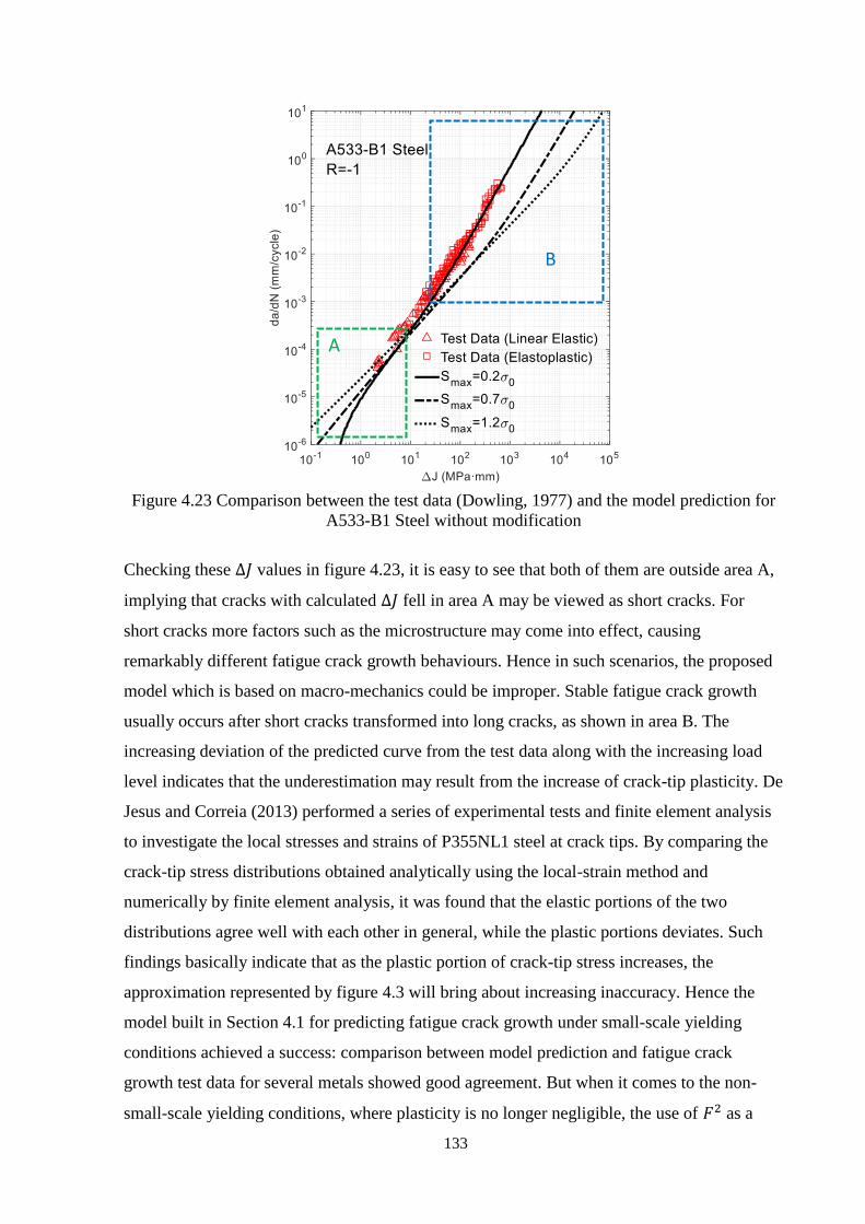
133

Figure 4.23 Comparison between the test data (Dowling, 1977) and the model prediction for

A533-B1 Steel without modification

Checking these ∆𝐽 values in figure 4.23, it is easy to see that both of them are outside area A,

implying that cracks with calculated ∆𝐽 fell in area A may be viewed as short cracks. For

short cracks more factors such as the microstructure may come into effect, causing

remarkably different fatigue crack growth behaviours. Hence in such scenarios, the proposed

model which is based on macro-mechanics could be improper. Stable fatigue crack growth

usually occurs after short cracks transformed into long cracks, as shown in area B. The

increasing deviation of the predicted curve from the test data along with the increasing load

level indicates that the underestimation may result from the increase of crack-tip plasticity. De

Jesus and Correia (2013) performed a series of experimental tests and finite element analysis

to investigate the local stresses and strains of P355NL1 steel at crack tips. By comparing the

crack-tip stress distributions obtained analytically using the local-strain method and

numerically by finite element analysis, it was found that the elastic portions of the two

distributions agree well with each other in general, while the plastic portions deviates. Such

findings basically indicate that as the plastic portion of crack-tip stress increases, the

approximation represented by figure 4.3 will bring about increasing inaccuracy. Hence the

model built in Section 4.1 for predicting fatigue crack growth under small-scale yielding

conditions achieved a success: comparison between model prediction and fatigue crack

growth test data for several metals showed good agreement. But when it comes to the non-

small-scale yielding conditions, where plasticity is no longer negligible, the use of 𝐹2 as a

B

A

134

correction factor for ∆ΠFPZ may be insufficient. Since 𝐹 only considers the geometric

amplification of stress (Chandran, 2017). In order to diminish such deviation and hence

provide better prediction, a more proper correction factor should be considered. Instead of 𝐹2,

a new correction factor, 𝐶p is proposed as

𝐶p = [1 + √𝜌

𝜌0]

1 𝑛′⁄

(4 − 82)

Since 𝜌 is linearly related to ∆𝐽 which incorporates 𝐹 for calculation, the above equation in

fact takes account of both the geometric effect and strain hardening effect (𝑛′).

Applying the proposed model with 𝐶p in place of 𝐹2 in equation (4 − 74) to A533-B1 steel,

another set of predicted curves for three load levels, i.e. 𝑆max = 0.2𝜎0, 0.7𝜎0 and 1.2𝜎0 were

obtained respectively using the same input parameters by Li et al. (1998). The newly obtained

fatigue crack growth curves were plotted with the test data by Dowling (1977) in figure 4.24.

Figure 4.24 Comparison between the test data (Dowling, 1977) and the model prediction for

A533-B1 Steel with modification

Observation shows that while the modified proposed model gives good prediction of fatigue

crack growth for the load case where 𝑆max = 0.2𝜎0, no obvious change presents in area A for

load cases where 𝑆max = 0.7𝜎0 and 1.2𝜎0. This is believed due to the fact that the proposed

model is not designed for short cracks. Checking the ∆𝐽 values corresponding to the boundary

crack size 𝑎 = 1 mm for load levels of 𝑆max = 0.7𝜎0 and 1.2𝜎0 respectively in figure 4.24, it

B

A

135

is easy to see that both of them are outside the regime of low ∆𝐽 where the modified proposed

model generates discrepancies for different load levels. In contrast to figure. 4.23, the

improvement in area B is quite impressive. The deviations among the predicted curves under

different load levels have been significantly diminished by introducing the modification.

While in Dowling’s elastoplastic tests, the smallest crack size recorded is about 0.05 mm, in

practical engineering the detectable flaw size using the technique of non-destructive test with

satisfactory confidence level is usually larger than 1 mm. Therefore, the part of fatigue crack

growth curve in the regime of low ∆𝐽 for load cases where 𝑆max = 0.7𝜎0 and 1.2𝜎0 may not

important or even not meaningful from the point of view of engineering practice.

For further validating the modified proposed model, a plot of crack characteristic length

(depth in Dowling’s work) versus fraction of fatigue life, i.e. 𝑁 𝑁f⁄ is produced, as shown

figure 4.25. 𝑁 is the number of load cycles experienced when the crack characteristic length 𝑎

is reached. 𝑁 is found by integrating the inverse of 𝑑𝑎 𝑑𝑁⁄ over a finite growth of 𝑎. 𝑁f is

calculated by equation (4 − 46). Generally good agreement can be observed between

predicted crack evolution curve by the modified proposed model and Dowling’s experimental

measurements.

Figure 4.25 Comparison of crack evolution data generated by tests (Dowling, 1977) and

model for A533-B1 Steel

4.2.2.2 General Application

General model applications are performed to AISI 4340 steel, 2024-T3 aluminium, 7075-T6

aluminium, and Ti6Al4V alloy. These metals are selected for their availability of test data of

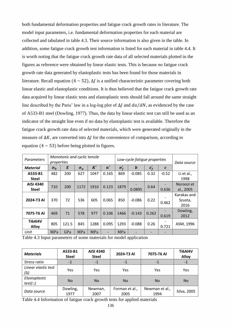
136

both fundamental deformation properties and fatigue crack growth rates in literature. The

model input parameters, i.e. fundamental deformation properties for each material are

collected and tabulated in table 4.3. Their source information is also given in the table. In

addition, some fatigue crack growth test information is listed for each material in table 4.4. It

is worth noting that the fatigue crack growth rate data of all selected materials plotted in the

figures as reference were obtained by linear elastic tests. This is because no fatigue crack

growth rate data generated by elastoplastic tests has been found for those materials in

literature. Recall equation (4 − 52), ∆𝐽 is a unified characteristic parameter covering both

linear elastic and elastoplastic conditions. It is thus believed that the fatigue crack growth rate

data acquired by linear elastic tests and elastoplastic tests should fall around the same straight

line described by the Paris’ law in a log-log plot of ∆𝐽 and 𝑑𝑎 𝑑𝑁⁄ , as evidenced by the case

of A533-B1 steel (Dowling, 1977). Thus, the data by linear elastic test can still be used as an

indicator of the straight line even if no data by elastoplastic test is available. Therefore the

fatigue crack growth rate data of selected materials, which were generated originally in the

measure of ∆𝐾, are converted into ∆𝐽 for the convenience of comparison, according to

equation (4 − 53) before being plotted in figures.

Parameters Monotonic and cyclic tensile properties

Low-cycle fatigue properties Data source

Material 𝝈𝟎 𝑬 𝝈𝐮 𝑲′ 𝒏′ 𝝈𝒇′ 𝒃 𝜺𝒇

′ 𝒄

A533-B1 Steel

482 200 627 1047 0.165 869 -0.085 0.32 -0.52 Li et al., 1998

AISI 4340 Steel

710 200 1172 1910 0.123 1879 -

0.0895 0.64

-0.636

Noroozi et al., 2005

2024-T3 Al 370 72 536 605 0.065 850 -0.086 0.22 -

0.462

Karakas and Szusta, 2016

7075-T6 Al 469 71 578 977 0.106 1466 -0.143 0.262 -

0.619 Dowling,

2012

Ti6Al4V Alloy

805 121.5 845 1288 0.095 1293 -0.088 0.26 -

0.721 ASM, 1996

Unit MPa GPa MPa MPa - MPa - - -

Table 4.3 Input parameters of some materials for model application

Materials A533-B1

Steel AISI 4340

Steel 2024-T3 Al 7075-T6 Al

Ti6Al4V Alloy

Stress ratio -1 -1 -1 -1 -1

Linear elastic test (∆)

Yes Yes Yes Yes Yes

Elastoplastic test(□)

No No No No No

Data source Dowling,

1977 Newman,

2007 Forman et al.,

2005 Newman et al.,

1994 Silva, 2005

Table 4.4 Information of fatigue crack growth tests for applied materials

137

(a) (b)

Figure 4.26 Comparison between the test data (Newman, 2007) and the model prediction for

AISI 4340 Steel (a) without modification; (b) with modification

(a) (b)

Figure 4.27 Comparison between the test data (Forman et al., 2005) and the model prediction

for 2024-T3 Al (a) without modification; (b) with modification

For each material, both models without and with modification were used to predict the fatigue

crack growth curves for three load levels, i.e. 𝑆max = 0.2𝜎0, 0.7𝜎0 and 1.2𝜎0. The predicted

curves have been plotted against the test data of the applied material in figures 4.26 ~ 4.29. It

can be observed that compared with the other two load levels, when 𝑆max = 0.2𝜎0 the

138

proposed model without modification can give pretty good prediction for fatigue crack growth

in both low and high ∆𝐽 regimes, or alternatively, the proposed model without modification

works well for predicting the fatigue crack growth under small-scale yielding conditions. As

𝑆max increases across the small-scale yielding load limit, trends similar to that in the case of

A533-B1 steel are demonstrated: the predicted curve goes above the test data in the regime of

high ∆𝐽; the predicted curve falls below the test data in the regime of high ∆𝐽; in both regimes,

a higher 𝑆max usually causes larger deviation between the predicted curve and the test data. It

is also illustrated in figures 4.26 ~ 4.29 that the deviation of the model prediction from the test

data in the regime of high ∆𝐽 can be eliminated by replacing 𝐹2 with the newly proposed

correction factor 𝐶p expressed by equation (4 − 81) in the proposed model. The predicted

curves by the proposed model with modification generally have good agreements with the test

data of the applied material despite the change of 𝑆max in the regime of high ∆𝐽. The modified

proposed model works well for predicting fatigue crack growth in both high and low ∆𝐽

regimes for the case of 𝑆max = 0.2𝜎0. While the deviation among the predicted curves exist in

the regime of low ∆𝐽, it is suggested that they may not have of significant engineering

importance and hence could be neglected. Based on those facts, it is achieved that the

modified proposed model works well for predicting the stable fatigue crack growth of metals

with 𝑅 = −1 under both small-scale yielding and non-small-scale yielding conditions.

(a) (b)

Figure 4.28 Comparison between the test data (Newman et al., 1994) and the model prediction

for 7075-T6 (a) without modification; (b) with modification

139

(a) (b)

Figure 4.29 Comparison between the test data (Silva, 2005) and the model prediction for

Ti6Al4V Alloy (a) without modification; (b) with modification

Figures 4.26 ~ 4.29 also illustrate that the aforementioned trends have been significantly

moderated by replacing 𝐹2 with newly proposed correction factor 𝐶p into calculation as

implied in equation (4 − 84). The fatigue crack growth curves predicted by the proposed

model with modification generally have good agreements with the test data of the applied

material despite the change of 𝑆max in the regime of high ∆𝐽. While the deviation among the

predicted curves exist in the regime of low ∆𝐽, it is suggested that they may not have of

significant engineering importance and hence could be neglected. Based on those facts, it is

achieved that the proposed model with modification works well for predicting fatigue crack

growth rates of metallic materials under both small-scale yielding and non-small-scale

yielding conditions with 𝑅 = −1.

4.2.3 Summary

In this 4.2 section, a prediction model was established based on energy principles and

elastoplastic fracture mechanics for fatigue crack growth in metallic materials with 𝑅 = −1.

Several types of metals such as A533-B1 steel, AISI 4130 steel, 2024-T3 aluminium, 7075-T6

aluminium, and Ti6Al4V alloy were chosen to apply the model given the availability of their

fatigue crack growth test data as well as fundamental deformation properties. For each

material, both predicted fatigue crack growth curves from the models without and with

correction were plotted against its fatigue crack growth test data for comparison. The results

show that

140

1) The proposed model based on energy principles represented by equation (4 − 68) can

predict the fatigue crack growth of metals with 𝑅 = −1 using ∆𝐽 and only needs the

fundamental deformation properties as the material inputs.

2) The proposed model without modification works well to predict the fatigue crack

growth of metals under small-scale yielding conditions, but under non-small-scale

yielding conditions, discrepancies occur in both the low and high ∆𝐽 regimes, and the

higher the load level, i.e. 𝑆max, the larger the deviation of the predicted fatigue crack

growth curve from the test data.

3) By introducing the new correction factor 𝐶p expressed by equation (4 − 81), the

modified proposed model is enabled to give generally good predictions for stable

fatigue crack growth in metals under both small-scale yielding and non-small-scale

yielding conditions.

The research work in this section has been summarized by Cheng et al. and is under review

for publication in journal.

141

Chapter 5. Conclusions

Subsea pipelines serving high-pressure/high-temperature oil and gas reservoirs often have to

face serious challenges from both the internal and external environments since the date of

their commissioning, which may seriously endanger the structural integrity and finally lead to

premature failures. Foremost among those challenges are corrosion fatigue and low-cycle

fatigue. Therefore, corrosion fatigue and low-cycle fatigue are two crucial issues that must be

carefully dealt with when assessing the structural integrity of subsea pipelines under high-

pressure/high-temperature service conditions using engineering critical assessments.

However, current industrial standards for conducting engineering critical assessments provide

only limited guidance in particular for corrosion fatigue. Low-cycle fatigue is even out of

their scope.

This PhD thesis is an attempt to bridge such gaps between current industrial standards and

engineering practices. In the thesis, the environmental loads and corrosion mechanisms of

subsea pipelines serving high-pressure/high-temperature reservoirs are analysed first. Further

research work has been carried out in two stages centring on the engineering critical

assessments of subsea pipelines under high-pressure/high-temperature service conditions, as

illustrated by figure 5.1.

Figure 5.1 Whole structure of the PhD research

In the first stage, an extended approach of engineering critical assessment for corrosion

fatigue is developed consistently in 3 levels. In level 1, a model describing the fatigue crack

142

growth under the impact of hydrogen embrittlement is built with the corrosion-crack

correlation mathematically constructed. Then a two-component corrosion fatigue crack

growth model considering both the contribution from anodic dissolution and hydrogen

embrittlement is established in level 2. On those foundations, the approach of engineering

critical assessment in particular for corrosion fatigue is finally proposed, with effects of both

initial crack size and loading frequency accounted for.

In the second stage, a fatigue crack growth model for low-cycle fatigue based on low-cycle

fatigue properties, energy principles and elastoplastic fracture mechanics is developed. It’s

applicability to fatigue crack growth under small-scale yielding conditions, i.e. high-cycle

fatigue is first checked and then is modified and applied to predicting the fatigue crack growth

under non-small-scale yielding conditions, i.e. low-cycle fatigue.

5.1 Contributions

The contributions of each section of the research work are briefly summarised here,

1) In developing the approach of engineering critical assessment in particular for corrosion

fatigue, the author first studied the fatigue crack growth of pipeline carbon steels under

gaseous hydrogen conditions, where a new corrosion-crack correlation model for

fatigue behaviour is established based on the concept of environment-affected zone and

the theory of linear elastic fracture mechanics. The model is applied to different API

grade pipeline steels and it is found that the fatigue crack growth behaviour of those

pipeline carbon steels in hydrogen gas can be well captured.

2) Then a two-component model is proposed for the corrosion fatigue crack growth of

subsea pipeline steels considering both the stress corrosion and hydrogen-assisted

cracking. The model is constructed within the frame of linear elastic fracture mechanics,

characterizes both environmental and mechanical conditions and bridges the physics of

corrosion fatigue and the corrosion fatigue crack growth behaviour. Based on the

application of the model to X65 pipeline carbon steel, the influence of factors such as

load frequency 𝑓 , hydrogen concentration 𝐶H0 , stress ratio 𝑅 and temperature 𝑇 is

analysed.

3) On the foundation of previous research, an extended approach of engineering critical

assessment in particular for corrosion fatigue is developed, in which a critical stress

intensity factor was suggested to account for the influence of load frequency and initial

143

crack size, thus directing the model selection within current industrial standards (e.g.

BS 7910) for assessing the integrity of structures suffering corrosion fatigue. The

extended approach is applied to X65 grade pipeline carbon steels and the results indicate

that it can provide reasonable results with significantly reduced conservatism.

4) In establishing the prediction model of fatigue crack growth applicable for low-cycle

fatigue, the author started his research from building up an energy principles based

model for predicting the fatigue crack growth of metallic materials subjected to high-

cycle fatigue. The model built only requires the material’s fundamental deformation

properties, such as monotonic and cyclic tensile material properties and low-cycle

fatigue material properties as input parameters. Application of the model to different

types of materials shows that the model can predict the high-cycle fatigue crack

growth under fully reversed constant amplitude cyclic loads. In combination with the

Manson-Halford equation, the model can provide good prediction for high-cycle

fatigue crack growth in cases of negative stress ratios (i.e. 𝑅 ≤ 0), which is typical for

offshore structures.

5) Following a similar idea in building up the prediction model of fatigue crack growth in

high-cycle fatigue, the author established a model using the cyclic 𝐽-integral ∆𝐽 to

predict fatigue crack growth in low-cycle fatigue. The model is applicable for both

small-scale yielding and non-small-scale yielding fatigue crack growth as long as 𝐽-

integral is applicable. Application of the model to different types of metallic materials

shows that the model works well for predicting fatigue crack growth under small-scale

yielding conditions from the materials’ fundamental deformation properties. By

introducing a correction factor 𝐶p, the model works roughly well for predicting the

fatigue crack growth under non-small-scale yielding conditions, i.e. low-cycle fatigue

crack growth as well.

5.2 Future Research

Future research may be conducted in:

1) verifying the effectiveness of the proposed approach of engineering critical assessment

in the presence of different chemicals and their combination experimentally,

2) extending the applicability of the proposed fatigue crack growth model to wider range

of stress ratios,

144

3) modifying the proposed fatigue crack growth model to take the load sequence effect

into consideration,

4) correlating the cracking process with corrosion under the circumstances of low-cycle

fatigue, and so on.

As discussed in the literature review, high-pressure/high-temperature reservoirs are

increasingly encountered in recent years as the exploration and exploitation activities of

offshore oil and gas heading into deep waters, while there is no well accepted industrial

standards for engineering critical assessments that can give reasonably consideration of the

critical issues faced by subsea pipelines under high-pressure/high-temperature service

conditions. This research is an attempt to tackle some of the most critical issues faced by

current industrial standards.

Environment-assisted cracking and low-cycle fatigue are complex issues that involves

multidisciplinary knowledge, and widely exist in various industries. For safety critical

structures of which the failures could result tremendous economic loss and catastrophic

environmental disasters, the possibility of suffering environment-assisted cracking and low-

cycle fatigue should be seriously taken into account. Good understandings on the mechanisms

and behaviours of environment-assisted cracking and low-cycle fatigue are crucial to

achieving high-quality engineering critical assessments. Therefore environment-assisted

cracking and low-cycle fatigue deserve researchers’ continuous research effort. The outcomes

of this research may, at least to some extent, bridge the gaps between the current industrial

standards and the engineering practice in developing high-pressure/high-temperature offshore

oil and gas sources, meanwhile providing useful reference for engineering critical assessment

of metallic welded structures in a broader sense.

145

References

ABS, 2014. ABS Rules for building and classing: Floating production installations. American

Bureau of Shipping, Houston, US.

ABS, 2018. ABS Guide for building and classing subsea pipeline systems. American Bureau

of Shipping, Houston, US.

Amaro, R.L., Rustagi, N., Findley, K.O., Drexler, E.S. and Slifka, A.J., 2014. Modeling the

fatigue crack growth of X100 pipeline steel in gaseous hydrogen. International Journal of

Fatigue, 59, pp.262-271.

Anderson, T.L., 2017, Fracture mechanics: fundamentals and applications. CRC press.

API, 2009. API Recommended Practice 17N: Subsea production system reliability and

technical risk management. American Petroleum Institute, Houston, US.

API, 2013. API Standard 1104: Welding of pipelines and related facilities. American

Petroleum Institute, Houston, US.

API, 2015. API Technical Report 17TR8: High-pressure high-temperature design guidelines.

American Petroleum Institute, Houston, US.

API, 2016. API Standard 579-1/ASME FFS-1: Fitness-for-service. American Petroleum

Institute, Houston, US.

Araújo, J.A., Susmel, L., Pires, M.S.T. and Castro, F.C., 2017. A multiaxial stress-based

critical distance methodology to estimate fretting fatigue life. Tribology International, 108,

pp.2-6.

Arola, D. and Williams, C.L., 2002. Estimating the fatigue stress concentration factor of

machined surfaces. International Journal of fatigue, 24(9), pp.923-930.

ASM, 1996. Handbook, vol. 19, Fatigue and fracture. American Society for Metals (ASM)

International, Cleveland, US.

ASTM International, 2012. E606M-12 Standard test method for strain-controlled fatigue

testing. West Conshohocken, US.

ASTM International, 2017. E1820-17 Standard test method for measurement of fracture

toughness. West Conshohocken, US.

146

Austen, I.M. and Walker, E.F., 1977, Quantitative understanding of the effects of mechanical

and environmental variables on corrosion fatigue crack growth behaviour. In The Influence of

Environment on Fatigue. I Mech E Conference Publications, London, pp.1-10.

Bai, Y. and Bai, Q. eds., 2005. Subsea pipelines and risers. Elsevier.

Bai, Q. and Bai, Y., 2014. Subsea pipeline design, analysis, and installation. Gulf Professional

Publishing.

Bannantine, J.A., Comer, J.J., and Handrock, J.L., 1990. Fundamentals of metal fatigue

analysis. Prentice Hall.

Barnoush, A., 2011. Hydrogen embrittlement. Saarland University.

Bartlett, M.L. and Hudak, Jr S.J., 1990. The Influence of Frequency-Dependent Crack

Closure on Corrosion Fatigue Crack Growth (Retroactive Coverage). Fatigue 90, pp.1783-

1788.

Baxter, D.P., Maddox, S.J. and Pargeter, R.J., Corrosion fatigue behaviour of welded risers

and pipelines. Stress, 2007, 10(100), p.1000.

Beavers, J.A. and Harle, B.A., 2001. Mechanisms of high-pH and near-neutral-pH SCC of

underground pipelines. Journal of Offshore Mechanics and Arctic Engineering, 123(3),

pp.147-151.

Beden, S.M., Abdullah, S. and Ariffin, A.K., 2009. Review of fatigue crack propagation

models for metallic components. European Journal of Scientific Research, 28(3), pp.364-397.

Benaarbia, A., Chrysochoos, A. and Robert, G., 2014. Kinetics of stored and dissipated

energies associated with cyclic loadings of dry polyamide 6.6 specimens. Polymer Testing,

34, pp.155-167.

Benedetti, M. and Santus, C., 2019. Notch fatigue and crack growth resistance of Ti-6Al-4V

ELI additively manufactured via selective laser melting: A critical distance approach to defect

sensitivity. International Journal of Fatigue, 121, pp.281-292.

Bever, M.B., Holt, D.L. and Titchener, A.L., 1973. The stored energy of cold work. Progress

in Materials Science, 17, pp.5-177.

Bomba, J., Chin, D., Kak, A. and Meng, W., 2018, April. Flow Assurance Engineering in

Deepwater Offshore-Past, Present, and Future. In Offshore Technology Conference. Offshore

Technology Conference.

147

British Energy, 2001. R6: Assessment of the integrity of structures containing defects.

Broek, D., 2012. Elementary engineering fracture mechanics. Springer Science & Business

Media.

BSI, 2015. BS 7910: Guidance on methods for assessing the acceptability of flaws in fusion

welded structures. British Standards Institution, London, UK.

Buitrago, J., Hudak, S. and Baxter, D., 2008. High-cycle and low-cycle fatigue resistance of

girth welds in sour service. In ASME 2008 27th International Conference on Offshore

Mechanics and Arctic Engineering (pp. 365-372). American Society of Mechanical

Engineers.

Cabrini, M. and Pastore, T., 2006. Hydrogen diffusion and EAC of pipeline steels under

cathodic protection. Fracture of Nano and Engineering Materials and Structures, pp. 1005-

1006. Springer, Netherlands.

CSA, 2015. CSA Z662: Oil & gas pipeline systems. Canadian Standards Association,

Mississauga, Canada.

Carr, M., Bruton, D. and Leslie, D., 2003, February. Lateral buckling and pipeline walking, a

challenge for hot pipelines. In Offshore Pipeline Technology Conference (pp. 1-36),

Amsterdam.

Chandran, K.R., 2017. Insight on physical meaning of finite-width-correction factors in stress

intensity factor (K) solutions of fracture mechanics. Engineering Fracture Mechanics, 186,

pp.399-409.

Chandrasatheesh, C., Jayapriya, J., George, R.P. and Mudali, U.K., 2014. Detection and

analysis of microbiologically influenced corrosion of 316 L stainless steel with

electrochemical noise technique. Engineering Failure Analysis, 42, pp.133-142.

Chang, K.M., 1988. An empirical model for environmental damage at the crack tip. In MRS

Proceedings (Vol. 125, p. 243). Cambridge University Press.

Chen, N.Z., Wang, G., Guedes Soares, C., 2011. Palmgren-Miner’s rule and fracture

mechanics based inspection planning. Engineering Fracture Mechanics, 78, pp.3166-3182.

Chen, N.Z., 2016. A stop-hole method for marine and offshore structures. International

Journal of Fatigue, 88, pp.49-57.

148

Cheng, A. and Chen, N.Z., 2017a. Fatigue crack growth modelling for pipeline carbon steels

under gaseous hydrogen conditions. International Journal of Fatigue, 96, pp.152-161.

Cheng, A. and Chen, N.Z., 2017b. Corrosion fatigue crack growth modelling for subsea

pipeline steels. Ocean Engineering, 142, pp.10-19.

Cheng, A. and Chen, N.Z., 2018a. An extended engineering critical assessment for corrosion

fatigue of subsea pipeline steels. Engineering Failure Analysis, 84, pp.262-275.

Cheng, A. and Chen, N.Z., 2018b, June. A benchmark study on applying extended finite

element method to the structural integrity assessment of subsea pipelines at HPHT service

conditions. In ASME 2018 37th International Conference on Ocean, Offshore and Arctic

Engineering. Paper NO. V11BT12A037. American Society of Mechanical Engineers.

Cheng, A., Chen, N.Z. and Pu, Y., 2019. An energy principles based model for fatigue crack

growth prediction. International Journal of Fatigue, 128, p.105198.

Chong, T.V.S., Kumar, S.B., Tronskar, J.P., Lai, M.O. and Loh, W.L., 2016. Engineering

critical assessment of nickel-based clad pipeline girth welds in a wet H2S-containing

environment. Engineering Fracture Mechanics, 160, pp.42-51.

Chrysochoos, A., Maisonneuve, O., Martin, G., Caumon, H. and Chezeaux, J.C., 1989. Plastic

and dissipated work and stored energy. Nuclear Engineering and Design, 114(3), pp.323-333.

Cialone, H.J. and Holbrook, J.H., 1985. Effects of gaseous hydrogen on fatigue crack growth

in pipeline steel. Metallurgical Transactions A, 16(1), pp.115-122.

Cui, W., 2002. A state-of-the-art review on fatigue life prediction methods for metal

structures. Journal of marine science and technology, 7(1), pp.43-56.

Dasgupta, A., Oyan, C., Barker, D. and Pecht, M., 1992. Solder creep-fatigue analysis by an

energy-partitioning approach. Journal of Electronic Packaging, 114(2), pp.152-160.

Dauskardt, R.H. and Ritchie, R.O., 1986. Fatigue crack propagation behavior in pressure-

vessel steels for high-pressure hydrogen service. Properties of High-Strength Steels for High-

Pressure Containments, American Society of Mechanical Engineers, pp.17-28.

Davenport, R.T. and Brook, R., 1979. The threshold stress intensity range in fatigue. Fatigue

& Fracture of Engineering Materials & Structures, 1(2), pp.151-158.

Dawes, M.G., 1979. Elastic-plastic fracture toughness based on the COD and J-contour

integral concepts. In Elastic-plastic fracture. ASTM International.

149

De Jesus, A.M. and Correia, J.A., 2013. Critical assessment of a local strain-based fatigue

crack growth model using experimental data available for the P355NL1 steel. Journal of

Pressure Vessel Technology, 135(1), p.011404.

DNVGL, 2017. DNVGL-RP-F108: Assessment of flaws in pipeline and riser girth welds. Det

Norske Veritas, Oslo, Norway.

DNVGL, 2017. DNVGL-ST-F101: Submarine pipeline systems. Det Norske Veritas, Oslo,

Norway.

Dowling, N.E. and Begley, J.A., 1976. Fatigue crack growth during gross plasticity and the J-

integral. In Mechanics of crack growth. ASTM International.

Dowling, N.E., 1977. Crack growth during low-cycle fatigue of smooth axial specimens. In

Cyclic stress-strain and plastic deformation aspects of fatigue crack growth. ASTM

International.

Dowling, N.E., 2012. Mechanical behavior of materials: engineering methods for

deformation, fracture, and fatigue. Pearson.

Drexler, E.S., Slifka, A.J., Amaro, R.L., Barbosa, N., Lauria, D.S., Hayden, L.E. and

Stalheim, D.G., 2014. Fatigue crack growth rates of API X70 pipeline steel in a pressurized

hydrogen gas environment. Fatigue & Fracture of Engineering Materials & Structures, 37(5),

pp.517-525.

Ellyin, F. and Kujawski, D., 1984. Plastic strain energy in fatigue failure. Journal of Pressure

Vessel Technology, 106(4), pp.342-347.

Ellyin, F., 2012. Fatigue damage, crack growth and life prediction. Springer Science &

Business Media.

Endo, K., Komai, K. and Matsuda, Y., 1981. Mechanical effects of corrosion products in

corrosion fatigue crack growth of a steel. Bulletin of Japanese Society of Mechanical

Engineers, 24(194), pp.1319-1325.

Fahr, A., 2013. Aeronautical applications of non-destructive testing. DEStech Publications,

Inc.

Fang, B.Y., Atrens, A., Wang, J.Q., Han, E.H., Zhu, Z.Y. and Ke, W., 2003. Review of stress

corrosion cracking of pipeline steels in “low” and “high” pH solutions. Journal of Materials

Science, 38(1), pp. 127-132.

150

Fatemi, A. and Yang, L., 1998. Cumulative fatigue damage and life prediction theories: a

survey of the state of the art for homogeneous materials. International journal of fatigue,

20(1), pp.9-34.

Fontana, M.G., 2005. Corrosion engineering. Tata McGraw-Hill Education.

Forman, R.G., Shivakumar, V., Cardinal, J.W., Williams, L.C. and McKeighan, P.C., 2005.

Fatigue crack growth database for damage tolerance analysis (Final Report No.

DOT/FAA/AR-05/15). US Department of Transportation Federal Aviation Administration

(FAA), Office of Aviation Research Washington, US.

Gadgeel, V.L. and Johnson, D.L., 1979. Gas-phase hydrogen permeation and diffusion in

carbon steels as a function of carbon content from 500 to 900 K. Journal of Materials for

Energy Systems, 1(2), pp.32-40.

Gałkiewicz, J. and Graba, M., 2006. Algorithm for determination of ��𝑖𝑗(𝑛, 𝜃), 휀��𝑗(𝑛, 𝜃),

��𝑖(𝑛, 𝜃), 𝑑𝑛(𝑛, 𝜃) and 𝐼𝑛(𝑛) functions in Hutchinson Rice Rosengren solution and its 3D

generalization. Journal of Theoretical and Applied Mechanics, 44, pp.19-30.

Ganesh Kumar, J., Ganesan, V. and Laha, K., 2019. High temperature tensile properties of

316LN stainless steel investigated using automated ball indentation technique. Materials at

High Temperatures, 36(1), pp.48-57.

Gangloff, R.P., 1990. Corrosion fatigue crack propagation in metals (No. NASA-CR-4301).

National Aeronautics and Space Administration (NASA), Langley Research Center,

Hampton, US.

Gangloff, R.P., 2008. Critical issues in hydrogen assisted cracking of structural alloys. In

Environment-induced cracking of materials, pp. 141-165. Elsevier.

Garbatov, Y., As, S. K., Branner, K., Choi, B. K., den Besten, J. H., Dong, P., ... Yuan, Y.,

2018. Committee III.2: Fatigue and fracture. In M. L. Kaminski, & P. Rigo (Eds.),

Proceedings of the 20th International Ship and Offshore Structures Congress (ISSC 2018)

(Vol. 1, pp. 441-547). CRC Press.

Gavem, T., Kumar, A., Panga, V., Stratton, M. and Harry, J.J., 2015, May. Critical HP/HT

flowline design challenges associated with deepwater miocene GoM fields. In Offshore

Technology Conference. Offshore Technology Conference.

151

Gerberich, W. W., Livne, T., Chen, X. F. and Kaczorowski, M., 1988. Crack growth from

internal hydrogen-temperature and microstructure effects in 4340 steel. Metallurgical and

Materials Transactions A, 19(5), pp.1319-1344.

Godefroid, L.B., Cândido, L.C., Toffolo, R.V.B. and Barbosa, L.H.S., 2014. Microstructure

and mechanical properties of two API steels for iron ore pipelines. Materials Research, 17,

pp.114-120.

Guedri, A., Merzoug, B. and Zeghloul, A., 2004. Improving mechanical properties of API

X60/X70 welded pipeline steel. Sciences & Technologie B, (29), pp.51-58.

Guo, W., 1993a. Elastoplastic three dimensional crack border field—I. Singular structure of

the field. Engineering Fracture Mechanics, 46(1), pp.93-104.

Guo, W., 1993b. Elastoplastic three dimensional crack border field—II. Asymptotic solution

for the field. Engineering Fracture Mechanics, 46(1), pp.105-113.

Gutierrez-Solana, F. and Elices M., 1982, High-pressure hydrogen behavior of a pipeline

steel. In Current solutions to hydrogen problems in steels, pp.181-185.

Haritos, G.K., Nicholas, T. and Lanning, D.B., 1999. Notch size effects in HCF behavior of

Ti–6Al–4V. International Journal of Fatigue, 21(7), pp.643-652.

Hill, R., 1998. The mathematical theory of plasticity (Vol. 11). Oxford university press.

Holtam, C., 2010. Structural integrity assessment of C-Mn pipeline steels exposed to sour

environments. PhD thesis, Loughborough University, UK.

Holtam, C., Saraswat, R., Thodla, R. and Gui, F., 2018. A modified engineering critical

assessment approach for offshore pipelines. In ASME 2018 37th International Conference on

Ocean, Offshore and Arctic Engineering (pp. V004T03A011-V004T03A011). American

Society of Mechanical Engineers.

Huffman, P.J., 2016. A strain energy based damage model for fatigue crack initiation and

growth. International Journal of Fatigue, 88, pp.197-204.

Humphries, M.J., McLaughlin, J.E. and Pargeter, R., 1989. Toughness characteristics of

hydrogen charged pressure vessel steels. In International Conference on Interaction of Steels

with Hydrogen in Petroleum Industry Pressure Vessel Service, Paper No. 243.

Hurley, P.J. and Evans, W.J., 2007. A new method for predicting fatigue crack propagation

rates. Materials Science and Engineering: A, 466(1-2), pp.265-273.

152

Hutchinson, J.W., 1968. Singular behaviour at the end of a tensile crack in a hardening

material. Journal of the Mechanics and Physics of Solids, 16(1), pp.13-31.

Iannuzzi, M., 2011. Environmentally assisted cracking (EAC) in oil and gas production. In

Stress Corrosion Cracking (pp. 570-607). Woodhead Publishing.

Irwin, G. R., 1957. Analysis of stresses and strains near the end of a crack traversing a plate.

Journal of Applied Mechanics 24, pp.361-364.

ISO, 2014. ISO 19902 (2014): Petroleum and natural gas industries-fixed steel offshore

structures. International Organization for Standardization, Geneva, Switzerland.

Jia, L.J. and Ge, H., 2018. Ultra-Low Cycle Fatigue Failure of Metal Structures Under Strong

Earthquakes. Springer.

Kaisand, L.R. and Mowbray, D.F., 1979. Relationships between low-cycle fatigue and fatigue

crack growth rate properties. Journal of Testing and Evaluation, 7(5), pp.270-280.

Kaminski, M.L., 2007, January. Sensing and understanding fatigue lifetime of new and

converted FPSOs. In Offshore Technology Conference. Offshore Technology Conference.

Kang, P.S., Lee, D.G. and Lim, J.S., 2014, August. Status of wax mitigation technologies in

offshore oil production. In The Twenty-fourth International Ocean and Polar Engineering

Conference. International Society of Offshore and Polar Engineers.

Karakaş, Ö. and Szusta, J., 2016. Monotonic and low cycle fatigue behaviour of 2024-T3

aluminium alloy between room temperature and 300°C for designing VAWT components.

Fatigue & Fracture of Engineering Materials & Structures, 39(1), pp.95-109.

Kim, Y.H. and Manning, S.D., 1983, January. A superposition model for corrosion-fatigue

crack propagation in aluminum alloys. In Fracture Mechanics: Fourteenth Symposium—

Volume I: Theory and Analysis. ASTM International.

Kim, K.S. and Leckie, F.A., 1990. On the calculations of the stored energy of cold work.

Journal of Engineering Materials and Technology, 112, p.465.

Kim S.S., Choe S.J., Shin K.S., 1998. Quantitative models on corrosion fatigue crack growth

rates in metals: Part I. Overview of quantitative crack growth models. Metals and Materials

International, 4(1), pp.1-13.

Klesnil, M. and Lukac, P., 1992. Fatigue of metallic materials (Vol. 71). Elsevier.

153

Kuhn, P. and Hardrath, H.F., 1952. An engineering method for estimating notch-size effect in

fatigue tests on steel (Technical Note 2805). National Advisory Committee for Aeronautics

(NACA), Langley Aeronautical Laboratory, Langely Field, US.

Koçak, M., Webster, S., Janosch, J.J., Ainsworth, R.A., and Koers, R., 2008. FITNET fitness-

for-service (FFS) – procedure. GKSS Research Center, Germany.

Kuhn, P. and Figge, I.E., 1962. Unified notch-strength analysis for wrought aluminum alloys

(No. NASA-TN-D-1259). National Aeronautics and Space Administration (NASA), Langley

Research Center, Hampton, US.

Kumar, S.B., Chong, S., Tornqvist, R., Tronskar, J.P., Lai, M.O. and Loh, W.L., 2014. ECA

of high pressure and high temperature (HP/HT) CRA pipelines. In Offshore Technology

Conference-Asia. Offshore Technology Conference.

Kumar, V.G.M.D., German, M.D. and Shih, C.F., 1981. Engineering approach for elastic-

plastic fracture analysis. No. EPRI-NP—1931, General Electric Co..

Kujawski, D. and Ellyin, F., 1984. A fatigue crack propagation model. Engineering Fracture

Mechanics, 20(5-6), pp.695-704.

Lam, P., 2006. Gaseous hydrogen effects on the mechanical properties of carbon and low

alloy steels (U) (No. WSRC-TR-2006-00119). SRS.

Lamba, H.S., 1975. The J-integral applied to cyclic loading. Engineering Fracture Mechanics,

7(4), pp.693-703.

Landes, J.D. and Wei, R.P., 1969. Correlation between sustained-load and fatigue crack

growth in high-strength steels. National Aeronautics and Space Administration (NASA),

Langley Research Center, Hampton, US.

Lasebikan, B.A., Akisanya, A.R. and Deans, W.F., 2013. The mechanical behavior of a 25Cr

super duplex stainless steel at elevated temperature. Journal of Materials Engineering and

Performance, 22(2), pp.598-606.

Lee, S.L. and Unger, D.J., 1988. A decohesion model of hydrogen assisted cracking.

Engineering Fracture Mechanics, 31, pp.647-660.

Leighty, W., Holloway, J., Merer, R., Somerday, B., San Marchi, C., Keith, G., White, D. and

Economics, S.E., 2006, April. Compressorless hydrogen transmission pipelines deliver large-

scale stranded renewable energy at competitive cost. In Proceedings of the 16th World

Hydrogen Energy Conference, Lyon, FR, June (Vol. 6).

154

Li, D.M., Nam, W.J. and Lee, C.S., 1998. An improvement on prediction of fatigue crack

growth from low cycle fatigue properties. Engineering Fracture Mechanics, 60(4), pp.397-

406.

Liu, A.F., Mechanics and mechanisms of fracture: an introduction. ASM International, 2005.

Liu, Q. and Atrens, A., 2013. A critical review of the influence of hydrogen on the

mechanical properties of medium-strength steels. Corrosion Reviews, 31(3-6), pp.85-103.

Ljustell, P., 2007. Large scale yielding fatigue crack growth: A literature survey.

Logan, H.L., 1952. Film-rupture mechanism of stress corrosion. Journal of Research of the

National Bureau of Standards, 48(2), pp.99-105.

Loginow, A.W. and Phelps, E.H., 1975. Steels for seamless hydrogen pressure vessels.

Journal of Engineering for Industry, 97(1), pp.274-282.

Luke, M., Varfolomeev, I., Lütkepohl, K. and Esderts, A., 2010. Fracture mechanics

assessment of railway axles: experimental characterization and computation. Engineering

Failure Analysis, 17(3), pp.617-623.

Lynch, S.P., 2011. Hydrogen embrittlement (HE) phenomena and mechanisms. In Stress

Corrosion Cracking, pp. 90-130. Woodhead Publishing.

Ma, F.Y., 2012. Corrosive effects of chlorides on metals. In Pitting corrosion. IntechOpen.

Makogon, T.Y., 2019. Handbook of Multiphase Flow Assurance. Gulf Professional

Publishing.

Manson, S.S. and Halford, G.R., 1981. Practical implementation of the double linear damage

rule and damage curve approach for treating cumulative fatigue damage. International Journal

of Fracture, 17(2), pp.169-192.

Martinez, X., Oller, S., Barbu, L.G., Barbat, A.H. and De Jesus, A.M.P., 2015. Analysis of

Ultra Low Cycle Fatigue problems with the Barcelona plastic damage model and a new

isotropic hardening law. International Journal of Fatigue, 73, pp.132-142.

Masson, C., Lou, J., Saranyasoontorn, K., Jesudasen, A.S., Zeng, W., Wang, L. and Hahn,

G.D., 2015, October. A review of fitness-for-service and life extension assessment

methodologies relating to corrosion features in fatigue sensitive risers and pipelines. In OTC

Brasil. Offshore Technology Conference.

155

Mars, W.V. and Fatemi, A., 2002. A literature survey on fatigue analysis approaches for

rubber. International Journal of fatigue, 24(9), pp.949-961.

McEvily, A. J. and Wei, R.P., 1972. Fracture mechanics and corrosion fatigue. Connecticut

University Storrs Department of Metallurgy.

Mokhatab, S., Wilkens, R.J. and Leontaritis, K.J., 2007. A review of strategies for solving

gas-hydrate problems in subsea pipelines. Energy Sources, Part A, 29(1), pp.39-45.

Molski, K. and Glinka, G., 1981. A method of elastic-plastic stress and strain calculation at a

notch root. Materials Science and Engineering, 50(1), pp.93-100.

Morrow, J., 1965. Cyclic plastic strain energy and fatigue of metals. In Internal friction,

damping, and cyclic plasticity. ASTM International.

Moura, C.M., Vilela, J.J., Rabello, E.G., Martins, D.G.P. and Carneiro, J.R.G., 2009.

Evaluation of the ductile-to-brittle transition temperature in steel low carbon. International

Nuclear Atlantic Conference (INAC), 2009.

Nanninga, N., Slifka, A., Levy, Y. and White, C., 2010. A review of fatigue crack growth for

pipeline steels exposed to hydrogen. Journal of research of the National Institute of Standards

and Technology, 115(6), p.437.

Neuber, H., Kerbspannungstehre, Springer, Berlin, 1958. Translation theory of notch stresses.

U.S. Office of Technical Services, Washington, US.

Neuber, H., 1961. Theory of stress concentration for shear-strained prismatical bodies with

arbitrary nonlinear stress-strain law. Journal of Applied Mechanics, 28(4), pp.544-550.

Newman, J.C., Wu, X.R., Venneri, S.L. and Li, C.G., 1994. Small-crack effects in high-

strength aluminum alloys (NASA-RP-1309). National Aeronautics and Space Administration

(NASA), Langley Research Center, Hampton, VA.

Newman, J.C., 2007. Analyses of fatigue crack growth databases for use in a damage

tolerance approach for aircraft propellers and rotorcraft. US Department of Transportation,

Federal Aviation Administration.

Ngoula, D.T., Madia, M., Beier, H.T., Vormwald, M. and Zerbst, U., 2018. Cyclic J-integral:

Numerical and analytical investigations for surface cracks in weldments. Engineering Fracture

Mechanics, 198, pp.24-44.

156

Nguyen, O., Repetto, E.A., Ortiz, M. and Radovitzky, R.A., 2001. A cohesive model of

fatigue crack growth. International Journal of Fracture, 110(4), pp.351-369.

Nip, K.H., Gardner, L., Davies, C.M. and Elghazouli, A.Y., 2010. Extremely low cycle

fatigue tests on structural carbon steel and stainless steel. Journal of constructional steel

research, 66(1), pp.96-110.

Noroozi, A.H., Glinka, G. and Lambert, S., 2005. A two parameter driving force for fatigue

crack growth analysis. International Journal of Fatigue, 27(10-12), pp.1277-1296.

Oh, C.K., Kim, Y.J., Baek, J.H., Kim, Y.P. and Kim, W., 2007. A phenomenological model

of ductile fracture for API X65 steel. International Journal of Mechanical Sciences, 49(12),

pp.1399-1412.

Oliferuk, W., Korbel, A. and Bochniak, W., 2001. Energy balance and macroscopic strain

localization during plastic deformation of polycrystalline metals. Materials Science and

Engineering: A, 319, pp.250-253.

Oriani, R.A., 1972. A mechanistic theory of hydrogen embrittlement of steels. Berichte der

Bunsengesellschaft für physikalische Chemie, 76(8), pp.848-857.

Oriani, R.A. and Josephic, P.H., 1977. Equilibrium and kinetic studies of the hydrogen-

assisted cracking of steel. Acta Metallurgica, 25(9), pp.979-988.

Ossai, C.I., Boswell, B. and Davies, I.J., 2015. Pipeline failures in corrosive environments–A

conceptual analysis of trends and effects. Engineering Failure Analysis, 53, pp.36-58.

Palmer, A.C. and King, R.A., 2004. Subsea pipeline engineering. Penn Well Books.

Pandey, K.N. and Chand, S., 2003. An energy based fatigue crack growth model.

International Journal of Fatigue, 25(8), pp.771-778.

Pargeter, R.J. and Baxter, D.P., 2009, January. Design of pipelines dubject to lateral buckling

to resist corrosion fatigue. In Corrosion 2009. NACE International.

Paris, P.C. and Erdogan, F., 1963. A critical analysis of crack propagation laws. Journal of

Basic Engineering, 85(4), pp.528-533.

Parkins, R.N., 1979. Environment sensitive fracture and its prevention. British Corrosion

Journal, 14(1), pp.5-14.

Parkins, R.N., 1992. Current understanding of stress-corrosion cracking. Journal of the

Mineral, Metals and Materials Society, 44(12), pp.12-19.

157

Parkins, R.N., 2000, January. A review of stress corrosion cracking of high pressure gas

pipelines. In Corrosion 2000. NACE International.

Pendse, R.D. and Ritchie, R.O., 1985. A study of fatigue crack propagation in prior hydrogen

attacked pressure vessel steels. Metallurgical Transactions A, 16(8), pp.1491-1501.

Pilkey, W.D. and Pilkey, D.F., 2008. Peterson's stress concentration factors. John Wiley &

Sons.

Pugno, N., Ciavarella, M., Cornetti, P. and Carpinteri, A., 2006. A generalized Paris’ law for

fatigue crack growth. Journal of the Mechanics and Physics of Solids, 54(7), pp.1333-1349.

Reda, A.M., Forbes, G.L. and Sultan, I.A., 2011. Characterisation of slug flow conditions in

pipelines for fatigue analysis. In ASME 2011 30th International Conference on Ocean,

Offshore and Arctic Engineering (pp. 535-547). American Society of Mechanical Engineers.

Rhodes, P.R., 2001. Environment-assisted cracking of corrosion-resistant alloys in oil and gas

production environments: a review. Corrosion, 57(11), pp.923-966.

Rhodin, T. N. (ed.), 1959. Physical metallurgy of stress corrosion fracture. Interscience, New

York, US.

Rice, J.R., 1968. A path independent integral and the approximate analysis of strain

concentration by notches and cracks. Journal of applied mechanics, 35(2), pp.379-386.

Rice, J. and Rosengren, G.F., 1968. Plane strain deformation near a crack tip in a power-law

hardening material. Journal of the Mechanics and Physics of Solids, 16(1), pp.1-12.

Ritchie, R.O. and Thompson, A.W., 1985. On macroscopic and microscopic analyses for

crack initiation and crack growth toughness in ductile alloys. Metallurgical Transactions A,

16(1), pp.233-248.

Robinson, S.L. and Stoltz, R.E., 1980. Toughness losses and fracture behavior of low-strength

carbon-manganese steels in hydrogen. Hydrogen Effects in Metals, pp.987-995.

Ronevich, J.A., Somerday, B.P. and San Marchi, C.W., 2016. Effects of microstructure

banding on hydrogen assisted fatigue crack growth in X65 pipeline steels. International

Journal of Fatigue, 82, pp.497-504.

Rteil, A.A. and Topper, T.H., 2005. Fatigue behavior, monotonic properties and

microstructure data for SAE 4140, quenched and Tempered Steel (Iteration No. 69).

American Iron and Steel Institute (AISI), Washington, US.

158

Salerno, G., Magnabosco, R. and de Moura Neto, C., 2007. Mean strain influence in low

cycle fatigue behavior of AA7175-T1 aluminum alloy. International Journal of Fatigue, 29(5),

pp.829-835.

San Marchi, C. and Somerday, B.P., 2008. Technical reference on hydrogen compatibility of

materials. SAND2008-1163, Sandia National Laboratories, Livermore, US.

Santecchia, E., Hamouda, A.M.S., Musharavati, F., Zalnezhad, E., Cabibbo, M., El Mehtedi,

M. and Spigarelli, S., 2016. A review on fatigue life prediction methods for metals. Advances

in Materials Science and Engineering, 2016.

Santos, T.F.A., Hermenegildo, T.F.C., Afonso, C.R.M., Marinho, R.R., Paes, M.T.P. and

Ramirez, A.J., 2010. Fracture toughness of ISO 3183 X80M (API 5L X80) steel friction stir

welds. Engineering Fracture Mechanics, 77(15), pp.2937-2945.

Schütz, W., 1993. Fatigue life prediction—a review of the state of the art. Structural Failure,

Product Liability and Technical Insurance, 4.

Shi, K.K., Cai, L.X., Qi, S. and Bao, C., 2016. A prediction model for fatigue crack growth

using effective cyclic plastic zone and low cycle fatigue properties. Engineering Fracture

Mechanics, 158, pp.209-219.

Shih, C.F. and Hutchinson, J.W., 1976. Fully plastic solutions and large scale yielding

estimates for plane stress crack problems. Journal of Engineering Materials and Technology,

98(4), pp.289-295.

Shih, C.F. and German, M.D., 1981. Requirements for a one parameter characterization of

crack tip fields by the HRR singularity. International Journal of Fracture, 17(1), pp.27-43.

Shin, C.S., Man, K.C. and Wang, C.M., 1994. A practical method to estimate the stress

concentration of notches. International Journal of Fatigue, 16(4), pp.242-256.

Silva, F.S., 2005. The importance of compressive stresses on fatigue crack propagation rate.

International journal of fatigue, 27(10-12), pp.1441-1452.

SINTAP, November 1999. Structural integrity assessment procedures for European industry,

final procedure. European Union Brite-Euram Programme (Project No. BE95-1426), British

Steel, Rotherham, UK.

Shipilov, S.A., 2002. Mechanisms for corrosion fatigue crack propagation. Fatigue & Fracture

of Engineering Materials & Structures, 25(3), pp.243-259.

159

Skeels, H.B., 2014. API 17TR8-HPHT design guideline for subsea equipment. In Offshore

Technology Conference. Offshore Technology Conference.

Skelton, R.P., 1987. Cyclic stress-strain properties during high strain fatigue. In High

Temperature Fatigue (pp. 27-112). Springer, Dordrecht.

Smith, A.T., Schneider, C.R.A., Bird, C.R., Wall, M., 2019. Use of non-destructive testing for

engineering critical assessment: Background to the advice given in BS 7910:2013,

International Journal of Pressure Vessels and Piping, 169, pp. 153-159.

Somerday, B.P., 2008. Technical reference on hydrogen compatibility of materials-Plain

Carbon Ferritic Steels: C-Mn Alloys (Code 1100) (Report No. SAND2008-1163). Sandia

National Laboratories, Livermore, CA.

Song, J. and Curtin, W.A., 2011. A nanoscale mechanism of hydrogen embrittlement in

metals. Acta Materialia, 59(4), pp.1557-1569.

Song, Y., Palencsár, A., Svenningsen, G., Kvarekvål, J. and Hemmingsen, T., 2012. Effect of

O2 and temperature on sour corrosion. Corrosion, 68(7), pp.662-671.

Stalheim, D., Boggess, T., San Marchi, C., Jansto, S., Somerday, B., Muralidharan, G. and

Sofronis, P., 2010, January. Microstructure and mechanical property performance of

commercial grade API pipeline steels in high pressure gaseous hydrogen. In 2010 8th

International Pipeline Conference (pp. 529-537). American Society of Mechanical Engineers.

Stephens, R.I., Benner, P.H., Mauritzson, G. and Tindall, G.W., 1979. Constant and variable

amplitude fatigue behavior of eight steels. Journal of Testing and Evaluation, 7(2), pp.68-81.

Stephens, R.I., Fatemi, A., Stephens, R.R. and Fuchs, H.O., 2000. Metal fatigue in

engineering. John Wiley & Sons.

Sun, J., Jukes, P. and Shi, H., 2012, January. Thermal expansion/global buckling mitigation of

HPHT deepwater pipelines, sleeper or buoyancy? In The Twenty-second International

Offshore and Polar Engineering Conference. International Society of Offshore and Polar

Engineers.

Suresh, S. and Ritchie, R.O., 1984. Propagation of short fatigue cracks. International Metals

Reviews, 29(1), pp.445-475.

Susmel, L., 2008. The theory of critical distances: a review of its applications in fatigue.

Engineering Fracture Mechanics, 75(7), pp.1706-1724.

160

Tanaka, K., 1983. The cyclic J-integral as a criterion for fatigue crack growth. International

Journal of Fracture, 22(2), pp.91-104.

Tavares, S.M.O. and De Castro, P.M.S.T., 2017. An overview of fatigue in aircraft structures.

Fatigue & Fracture of Engineering Materials & Structures, 40(10), pp.1510-1529.

Taylor, D., 1999. Geometrical effects in fatigue: a unifying theoretical model. International

Journal of Fatigue, 21(5), pp.413-420.

Taylor, D., 2008. The theory of critical distances. Engineering Fracture Mechanics, 75(7),

pp.1696-1705.

Tetelman, A.S. and McEvily, A.J., 1967. Fracture of structural materials. Science &

Technology of Materials.

Topper, T., Wetzel, R.M. and Morrow, J., 1967. Neuber's rule applied to fatigue of notched

specimens. Illinois University at Urbana Department of Theoretical and Applied Mechanics.

Turnbull, A., 2014. Corrosion pitting and environmentally assisted small crack growth.

Proceedings of the Royal Society A: Mathematical, Physical and Engineering Sciences,

470(2169), p.20140254.

Van Leeuwen, H.P., 1974. The kinetics of hydrogen embrittlement: a quantitative diffusion

model. Engineering Fracture Mechanics, 6, pp.141 - 161.

Visser, W., 2002. POD/POS curves for non-destructive examination. HSE Books.

Vosikovsky, O., 1975. Fatigue-crack growth in an X-65 line-pipe steel at low cyclic

frequencies in aqueous environments. Journal of Engineering Materials and Technology,

97(4), pp.298-304.

Vosikovsky, O., 1981. Fatigue crack closure in an X70 steel. International Journal of

Fracture, 17(3), pp.301-309.

Wang, Y., Gong, J. and Jiang, W., 2013. A quantitative description on fracture toughness of

steels in hydrogen gas. International Journal of Hydrogen Energy, 38(28), pp.12503-12508.

Wang, Y., Duan, M., Xu, M., Wang, D. and Feng, W., 2012. A mathematical model for

subsea wells partition in the layout of cluster manifolds. Applied Ocean Research, 36, pp.26-

35.

Wells, A., 1961, September. Unstable crack propagation in metals: cleavage and fast fracture.

In Proceedings of the crack propagation symposium (Vol. 1, No. 84).

161

Weng, L., Zhang, J., Kalnaus, S., Feng, M. and Jiang, Y., 2013. Corrosion fatigue crack

growth of AISI 4340 steel. International Journal of Fatigue, 48, pp.156-164.

Westergaard, H.M., 1939. Bearing pressures and cracks. Journal of Applied Mechanics, Vol.

6, pp. 49–53.

Williams, M.L., 1952. Stress singularities resulting from various boundary conditions in

angular corners of plates in extension. Journal of Applied Mechanics, Vol. 19, pp. 526–528.

Williams, M.L., 1957. On the stress distribution at the base of a stationary crack. Journal of

Applied Mechanics, Vol. 24, pp. 109–114.

Woodtli, J. and Kieselbach, R., 2000. Damage due to hydrogen embrittlement and stress

corrosion cracking. Engineering Failure Analysis, 7(6), pp.427-450.

Woollin, P. and Murphy, W., 2001. Hydrogen embrittlement stress corrosion cracking of

superduplex stainless steel. Stainless Steel World, 13(JUN), pp.48-58.

Wu, S.C., Xu, Z.W., Yu, C., Kafka, O.L. and Liu, W.K., 2017. A physically short fatigue

crack growth approach based on low cycle fatigue properties. International Journal of Fatigue,

103, pp.185-195.

Yao, Y., Fine, M.E. and Keer, L.M., 2007. An energy approach to predict fatigue crack

propagation in metals and alloys. International Journal of Fracture, 146(3), pp.149-158.

Ye, D., Matsuoka, S., Suzuki, N. and Maeda, Y., 2004. Further investigation of Neuber’s rule

and the equivalent strain energy density (ESED) method. International Journal of Fatigue,

26(5), pp.447-455.

Yu, M., Xing, X., Zhang, H., Zhao, J., Eadie, R., Chen, W., Been, J., Van Boven, G. and

Kania, R., 2015. Corrosion fatigue crack growth behavior of pipeline steel under underload-

type variable amplitude loading schemes. Acta Materialia, 96, pp.159-169.

Zhao, J., Chen, W., Keane, S., Been, J. and Van Boven, G., 2014, December. Development

and validation of load-interaction based models for crack growth prediction. In 2014 10th

International Pipeline Conference. American Society of Mechanical Engineers Digital

Collection.

Zhu, X.K. and Joyce, J.A., 2012. Review of fracture toughness (G, K, J, CTOD, CTOA)

testing and standardization. Engineering Fracture Mechanics, 85, pp.1-46.

162

Yuyama, S. and Kishi, T., 1983. AE analysis during corrosion, stress corrosion cracking and

corrosion fatigue processes. Journal of Acoustic Emission 2, 71.

Documents

Engineering Critical Assessments of Subsea Pipelines under