UNIVERSIT�A DEGLI STUDI DI PISADIPARTIMENTO DI INFORMATICADOTTORATO DI RICERCA IN INFORMATICAUniversit�a di Pisa-Genova-UdinePh.D. Thesis: TD-08/96Enhanced Operational Semanticsfor ConcurrencyCorrado PriamiAbstract. In this study we extend the classical structural operational semantics toimplement the possibility of having di�erent views of the same system that are allconsistent to one another and that can be recovered mechanically from a single, con-crete representation. We apply this idea to concurrent and distributed systems, andespecially to mobile agents.Our concrete representation is a transition system (called proved and de�ned in SOSstyle), whose transitionsare labelledby encodingsof their deduction trees. The labels oftransitions allow us to retrieve all the main semantic models presented in the literatureand also to de�ne new semantics (e.g. a new causality). These semantics are retrievedfrom the proved transition system through relabelling functions that only maintain therelevant information in the labels of transitions. We show that our approach is robust:it scales up smoothly to higher-order process calculi and even to real programminglanguages like Facile. Its applicability is made evident through an example of debuggingof Facile \real code" for an application on mobile agents.To automate the above approach for veri�cation of distributed systems, we study thestate explosion problem. We overcome it for languages that do not contain scopeoperators like CCS restriction. Under this assumption we obtain a compact provedtransition system that is linear (in average) with the occurrences of actions in a processand that preserves non interleaving bisimulation-based equivalences (thus checked inpolynomial time instead of exponential one). We describe two prototypes that allowtheir user to change easily from a semantic model to another.We also study the re�nement of speci�cations towards real code. Since implementationsmust meet performance constraints, we �rst enhance our proved semantics to derivefrom it stochastic models on which performance can be evaluated. We also show how itis possible to merge semantic descriptions with information on architecture topologiesin order to get evaluations that are more accurate as machine sensible. Along thisline, we describe how to re�ne proved semantics in order to avoid global manager ofnames in distributed systems. The resulting description is actually a speci�cation fordistributed name managers that could help improving distributed implementations.March 1996C.so Italia 40, 56125 Pisa, Italy - (39)50 887111 - priami@di.unipi.it

To my wife Silvia

O, that a man might knowthe end of this day's business ere it come!But it su�ceth, that the day will end.And then the end is known.(W. Shakespeare, Julius Caesar)

AcknowledgementsFirst of all, I thank Pierpaolo Degano for his useful suggestions duringthese years and for his patience in introducing me to the academic jungle.He was also incomparable in helping me to debug this work.I thank Paola Inverardi and Daniel Yankelevich for the numerous jointworks we have done, always in a joyful environment.I thank Alessandro Bianchi, Chiara Bodei, Roberta Borgia, Stefano Coluc-cini and Alan Mycroft that were nice co-workers as well.I thank Lone Leth and Bent Thomsen for their suggestions, especially onthe Facile chapter.I thank also Luca Aceto, Marco Bernardo, Michele Boreale, Nadia Busi,Rocco De Nicola, Gianluigi Ferrari, Roberto Gorrieri, Ugo Montanari,Marco Pistore, Laura Semini and Marco Vanneschi for their comments onparts of this work.I thank my external referees Davide Sangiorgi and Bent Thomsen for theircareful reading of a preliminary draft of this thesis and for their commentsand suggestions.This work has been partially supported by ESPRIT Basic Research Action8130 - LOMAPS.

Contents1 Introduction 131.1 Formal methods : : : : : : : : : : : : : : : : : : : : : : : : 141.2 Operational semantics : : : : : : : : : : : : : : : : : : : : : 161.2.1 Structural approach : : : : : : : : : : : : : : : : : : 191.3 Abstraction levels : : : : : : : : : : : : : : : : : : : : : : : : 221.3.1 Interleaving theory for concurrency : : : : : : : : : : 231.3.2 Mobile agents : : : : : : : : : : : : : : : : : : : : : : 231.3.3 Non interleaving semantics : : : : : : : : : : : : : : 251.3.4 Parametricity : : : : : : : : : : : : : : : : : : : : : : 281.4 Computer aided veri�cation : : : : : : : : : : : : : : : : : : 301.4.1 State explosion : : : : : : : : : : : : : : : : : : : : : 311.4.2 Equivalences : : : : : : : : : : : : : : : : : : : : : : 331.4.3 User-friendliness : : : : : : : : : : : : : : : : : : : : 341.5 Towards implementations : : : : : : : : : : : : : : : : : : : 351.5.1 Quantitative analysis : : : : : : : : : : : : : : : : : : 361.5.2 Implementation-dependent information : : : : : : : 391.6 Suitability of SOS as formal method : : : : : : : : : : : : : 411.7 Outline of the work : : : : : : : : : : : : : : : : : : : : : : : 421.8 The origins of the chapters : : : : : : : : : : : : : : : : : : 45I Preliminaries 472 Mathematical Background 491

CONTENTS 22.1 Mathematical Logic : : : : : : : : : : : : : : : : : : : : : : 492.2 Sets : : : : : : : : : : : : : : : : : : : : : : : : : : : : : : : 542.3 Relations and Functions : : : : : : : : : : : : : : : : : : : : 572.4 Frequently used structures : : : : : : : : : : : : : : : : : : : 592.5 Algebra : : : : : : : : : : : : : : : : : : : : : : : : : : : : : 602.6 Complete partial orders : : : : : : : : : : : : : : : : : : : : 642.7 Formal Languages : : : : : : : : : : : : : : : : : : : : : : : 662.8 Continuous time Markov chains : : : : : : : : : : : : : : : : 703 Structural Operational Semantics 733.1 Transition systems : : : : : : : : : : : : : : : : : : : : : : : 733.2 SOS de�nitions : : : : : : : : : : : : : : : : : : : : : : : : : 784 Semantics for Concurrency 814.1 �-calculus : : : : : : : : : : : : : : : : : : : : : : : : : : : : 814.1.1 Early semantics : : : : : : : : : : : : : : : : : : : : : 824.1.2 Late semantics : : : : : : : : : : : : : : : : : : : : : 854.1.3 Equivalences : : : : : : : : : : : : : : : : : : : : : : 864.1.4 Late vs. early semantics : : : : : : : : : : : : : : : : 874.1.5 Calculus of communicating systems : : : : : : : : : : 884.1.6 Operators from other calculi : : : : : : : : : : : : : 894.2 Higher order �-calculus : : : : : : : : : : : : : : : : : : : : 894.2.1 Syntax : : : : : : : : : : : : : : : : : : : : : : : : : : 894.2.2 Operational semantics : : : : : : : : : : : : : : : : : 904.3 Facile : : : : : : : : : : : : : : : : : : : : : : : : : : : : : : 904.3.1 Syntax : : : : : : : : : : : : : : : : : : : : : : : : : : 924.3.2 Operational semantics : : : : : : : : : : : : : : : : : 944.4 Other models : : : : : : : : : : : : : : : : : : : : : : : : : : 964.4.1 Petri nets : : : : : : : : : : : : : : : : : : : : : : : : 964.4.2 Event structures : : : : : : : : : : : : : : : : : : : : 97II Semantic Descriptions 1035 Proved Transition System 105

3 CONTENTS5.1 Proved operational semantics : : : : : : : : : : : : : : : : : 1055.2 Properties : : : : : : : : : : : : : : : : : : : : : : : : : : : : 1105.3 Finite branching early semantics : : : : : : : : : : : : : : : 1125.4 An Algebra of Proved Trees : : : : : : : : : : : : : : : : : : 1176 Non Interleaving Semantics 1216.1 Non interleaving relations : : : : : : : : : : : : : : : : : : : 1226.2 Causality : : : : : : : : : : : : : : : : : : : : : : : : : : : : 1276.2.1 Causal relation : : : : : : : : : : : : : : : : : : : : : 1286.2.2 An Example : : : : : : : : : : : : : : : : : : : : : : 1326.3 Locality, Precedence and Enabling : : : : : : : : : : : : : : 1356.3.1 Locality : : : : : : : : : : : : : : : : : : : : : : : : : 1366.3.2 Precedence : : : : : : : : : : : : : : : : : : : : : : : 1376.3.3 Enabling : : : : : : : : : : : : : : : : : : : : : : : : 1396.4 Independence : : : : : : : : : : : : : : : : : : : : : : : : : : 1426.5 Concurrency : : : : : : : : : : : : : : : : : : : : : : : : : : 1436.5.1 Concurrency relation : : : : : : : : : : : : : : : : : : 1446.5.2 Time-independence : : : : : : : : : : : : : : : : : : : 1486.5.3 Comparisons : : : : : : : : : : : : : : : : : : : : : : 1506.5.4 Higher-dimension transitions : : : : : : : : : : : : : 1516.6 Equivalences : : : : : : : : : : : : : : : : : : : : : : : : : : 1546.7 Higher-Order Mobile Processes : : : : : : : : : : : : : : : : 1616.8 Related Works : : : : : : : : : : : : : : : : : : : : : : : : : 1636.8.1 Boreale and Sangiorgi's causal transition system : : 1646.8.2 Other causal models: graph rewriting, data- ow andPetri nets : : : : : : : : : : : : : : : : : : : : : : : : 1686.9 The causal transition system : : : : : : : : : : : : : : : : : 1697 Partial Ordering Semantics 1757.1 Partial and mixed orderings : : : : : : : : : : : : : : : : : : 1767.2 po relabelling : : : : : : : : : : : : : : : : : : : : : : : : : : 1787.3 mo vs. po semantics : : : : : : : : : : : : : : : : : : : : : : 1817.4 SOS po semantics : : : : : : : : : : : : : : : : : : : : : : : : 1837.5 Proof of Theorem 7.3.1 : : : : : : : : : : : : : : : : : : : : : 184

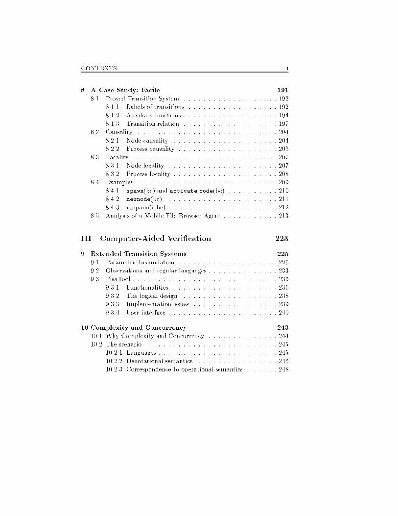
CONTENTS 48 A Case Study: Facile 1918.1 Proved Transition System : : : : : : : : : : : : : : : : : : : 1928.1.1 Labels of transitions : : : : : : : : : : : : : : : : : : 1928.1.2 Auxiliary functions : : : : : : : : : : : : : : : : : : : 1948.1.3 Transition relation : : : : : : : : : : : : : : : : : : : 1978.2 Causality : : : : : : : : : : : : : : : : : : : : : : : : : : : : 2048.2.1 Node causality : : : : : : : : : : : : : : : : : : : : : 2048.2.2 Process causality : : : : : : : : : : : : : : : : : : : : 2068.3 Locality : : : : : : : : : : : : : : : : : : : : : : : : : : : : : 2078.3.1 Node locality : : : : : : : : : : : : : : : : : : : : : : 2078.3.2 Process locality : : : : : : : : : : : : : : : : : : : : : 2088.4 Examples : : : : : : : : : : : : : : : : : : : : : : : : : : : : 2098.4.1 spawn(be) and activate code(be) : : : : : : : : : : 2108.4.2 newnode(be) : : : : : : : : : : : : : : : : : : : : : : 2118.4.3 r spawn(e,be) : : : : : : : : : : : : : : : : : : : : : : 2128.5 Analysis of a Mobile File Browser Agent : : : : : : : : : : : 213III Computer-Aided Veri�cation 2239 Extended Transition Systems 2259.1 Parametric bisimulation : : : : : : : : : : : : : : : : : : : : 2269.2 Observations and regular languages : : : : : : : : : : : : : : 2339.3 PisaTool : : : : : : : : : : : : : : : : : : : : : : : : : : : : : 2369.3.1 Functionalities : : : : : : : : : : : : : : : : : : : : : 2369.3.2 The logical design : : : : : : : : : : : : : : : : : : : 2389.3.3 Implementation issues : : : : : : : : : : : : : : : : : 2399.3.4 User interface : : : : : : : : : : : : : : : : : : : : : : 24010 Complexity and Concurrency 24310.1 Why Complexity and Concurrency : : : : : : : : : : : : : : 24410.2 The scenario : : : : : : : : : : : : : : : : : : : : : : : : : : 24510.2.1 Languages : : : : : : : : : : : : : : : : : : : : : : : : 24510.2.2 Denotational semantics : : : : : : : : : : : : : : : : 24610.2.3 Correspondence to operational semantics : : : : : : 248

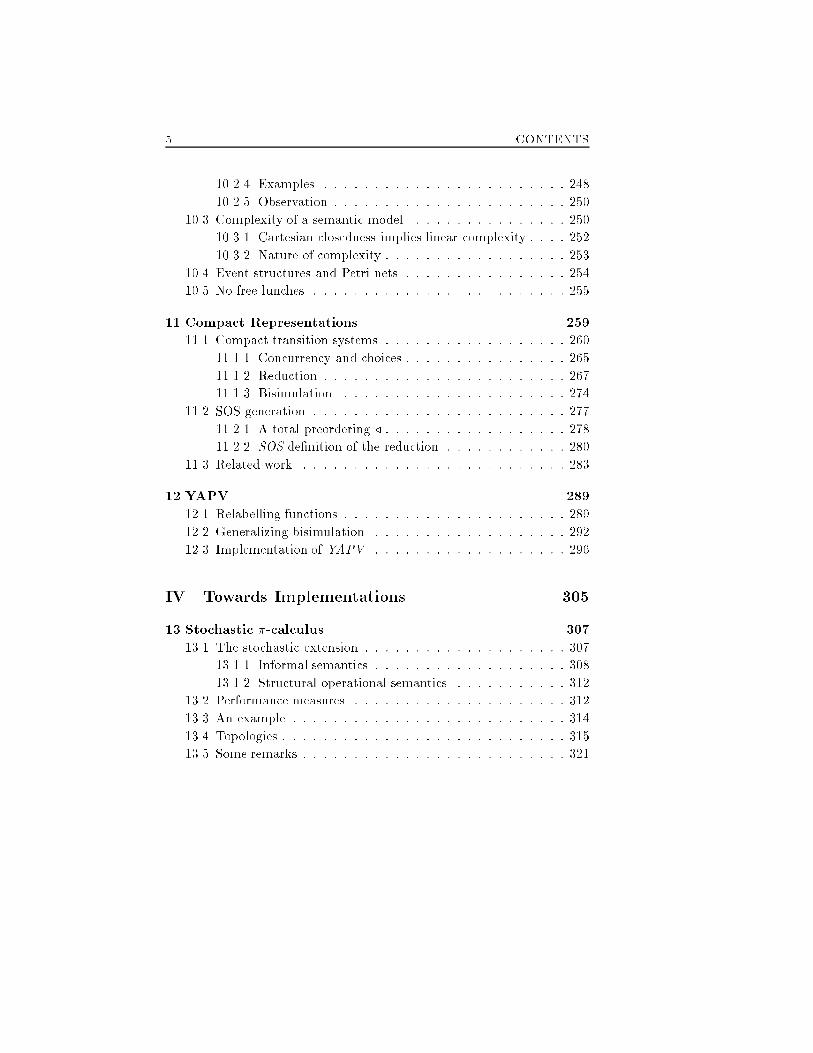
5 CONTENTS10.2.4 Examples : : : : : : : : : : : : : : : : : : : : : : : : 24810.2.5 Observation : : : : : : : : : : : : : : : : : : : : : : : 25010.3 Complexity of a semantic model : : : : : : : : : : : : : : : 25010.3.1 Cartesian closedness implies linear complexity : : : : 25210.3.2 Nature of complexity : : : : : : : : : : : : : : : : : : 25310.4 Event structures and Petri nets : : : : : : : : : : : : : : : : 25410.5 No free lunches : : : : : : : : : : : : : : : : : : : : : : : : : 25511 Compact Representations 25911.1 Compact transition systems : : : : : : : : : : : : : : : : : : 26011.1.1 Concurrency and choices : : : : : : : : : : : : : : : : 26511.1.2 Reduction : : : : : : : : : : : : : : : : : : : : : : : : 26711.1.3 Bisimulation : : : : : : : : : : : : : : : : : : : : : : 27411.2 SOS generation : : : : : : : : : : : : : : : : : : : : : : : : : 27711.2.1 A total preordering / : : : : : : : : : : : : : : : : : : 27811.2.2 SOS de�nition of the reduction : : : : : : : : : : : : 28011.3 Related work : : : : : : : : : : : : : : : : : : : : : : : : : : 28312 YAPV 28912.1 Relabelling functions : : : : : : : : : : : : : : : : : : : : : : 28912.2 Generalizing bisimulation : : : : : : : : : : : : : : : : : : : 29212.3 Implementation of YAPV : : : : : : : : : : : : : : : : : : : 296IV Towards Implementations 30513 Stochastic �-calculus 30713.1 The stochastic extension : : : : : : : : : : : : : : : : : : : : 30713.1.1 Informal semantics : : : : : : : : : : : : : : : : : : : 30813.1.2 Structural operational semantics : : : : : : : : : : : 31213.2 Performance measures : : : : : : : : : : : : : : : : : : : : : 31213.3 An example : : : : : : : : : : : : : : : : : : : : : : : : : : : 31413.4 Topologies : : : : : : : : : : : : : : : : : : : : : : : : : : : : 31513.5 Some remarks : : : : : : : : : : : : : : : : : : : : : : : : : : 321

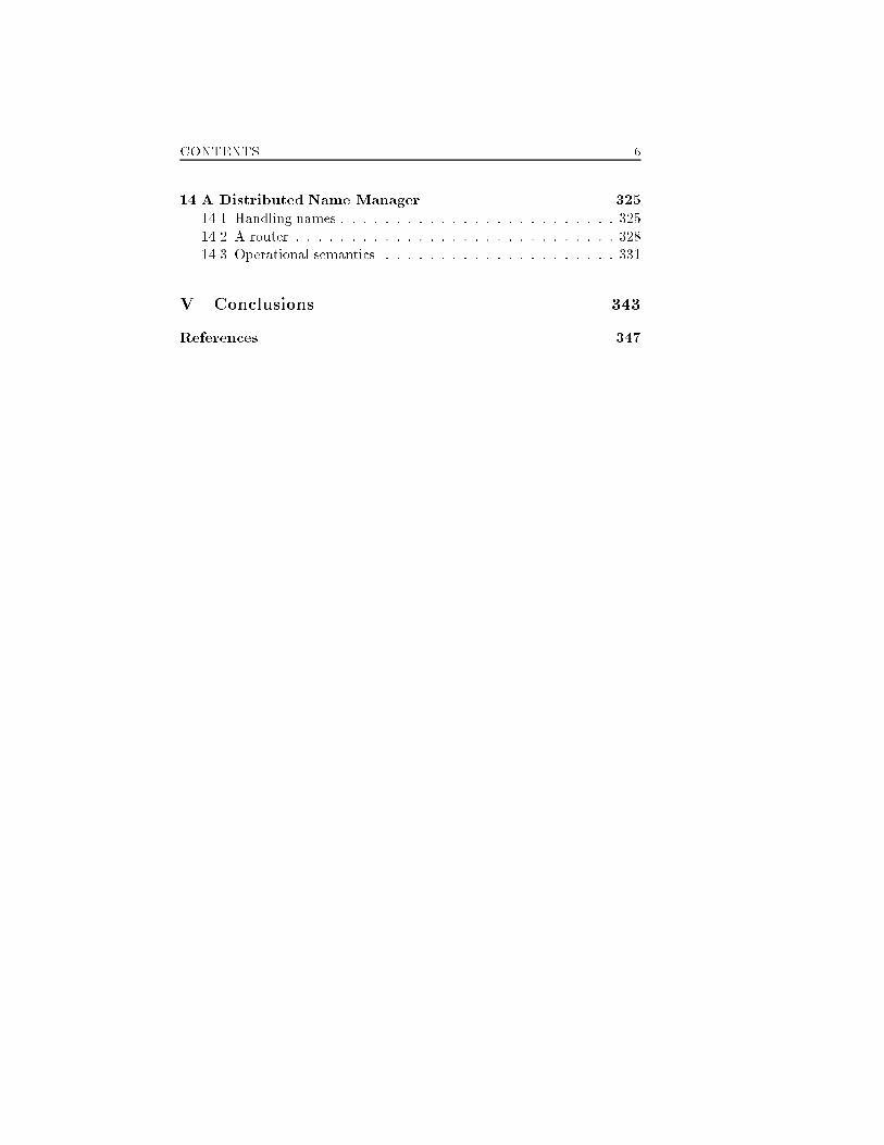
CONTENTS 614 A Distributed Name Manager 32514.1 Handling names : : : : : : : : : : : : : : : : : : : : : : : : : 32514.2 A router : : : : : : : : : : : : : : : : : : : : : : : : : : : : : 32814.3 Operational semantics : : : : : : : : : : : : : : : : : : : : : 331V Conclusions 343References 347

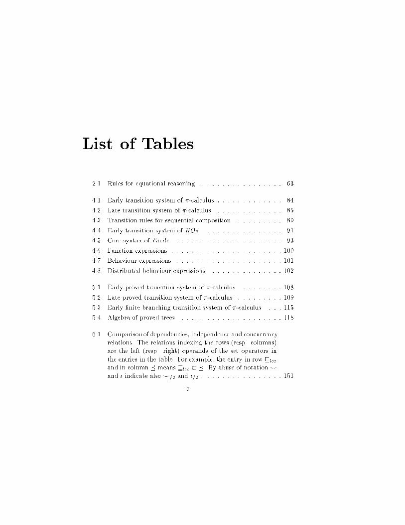
List of Tables2.1 Rules for equational reasoning. : : : : : : : : : : : : : : : : 634.1 Early transition system of �-calculus. : : : : : : : : : : : : : 844.2 Late transition system of �-calculus. : : : : : : : : : : : : : 854.3 Transition rules for sequential composition. : : : : : : : : : 894.4 Early transition system of HO�. : : : : : : : : : : : : : : : 914.5 Core syntax of Facile. : : : : : : : : : : : : : : : : : : : : : 934.6 Function expressions. : : : : : : : : : : : : : : : : : : : : : : 1004.7 Behaviour expressions. : : : : : : : : : : : : : : : : : : : : : 1014.8 Distributed behaviour expressions. : : : : : : : : : : : : : : 1025.1 Early proved transition system of �-calculus. : : : : : : : : 1085.2 Late proved transition system of �-calculus. : : : : : : : : : 1095.3 Early �nite branching transition system of �-calculus. : : : 1155.4 Algebra of proved trees. : : : : : : : : : : : : : : : : : : : : 1186.1 Comparison of dependencies, independence and concurrencyrelations. The relations indexing the rows (resp. columns)are the left (resp. right) operands of the set operators inthe entries in the table. For example, the entry in row vlocand in column � means vloc � �. By abuse of notation^and � indicate also ^=2 and �=2. : : : : : : : : : : : : : : : : 1517

LIST OF TABLES 86.2 Some relationships between equivalences. The processesindexing the rows (resp. columns) are the left (resp. right)operands of the equivalences in the entries in the table.For example, the entry in row P4 and in column P6 meansP4 6�v P6, P4 �� P6, P4 6�� P6 and P4 6�^ P6. : : : : : : : 1616.3 Early proved transition system of HO�. : : : : : : : : : : : 1636.4 Some relationships between equivalences. : : : : : : : : : : 1676.5 Early causal transition system for visible actions : : : : : : 1726.6 Early causal transition system for invisible actions. Thede�nition of A00 and B00 in the conclusion of rule Close isin the text. : : : : : : : : : : : : : : : : : : : : : : : : : : : 1737.1 Early po causal transition system for visible actions : : : : : 1897.2 Early po causal transition system for invisible actions. Thede�nition of A00 and B00 in the conclusion of rule Close isin the text. : : : : : : : : : : : : : : : : : : : : : : : : : : : 1908.1 Proved function expressions of Facile. : : : : : : : : : : : : 1988.2 Proved behaviour expressions of Facile. : : : : : : : : : : : 2008.3 Proved distributed behaviour expressions of Facile. : : : : : 2018.4 Proved distributed behaviour expressions of Facile (contd). 2188.5 Proved distributed behaviour expressions of Facile (contd). 2198.6 Proved programs of Facile. : : : : : : : : : : : : : : : : : : 21910.1 Comparison of concurrency models. : : : : : : : : : : : : : : 25713.1 Early proved transition system of S�. : : : : : : : : : : : : 32313.2 Stochastic �-calculus with topologies : : : : : : : : : : : : : 32414.1 Late proved transition system of �-calculus. : : : : : : : : : 341

List of Figures6.1 Behaviour of S. : : : : : : : : : : : : : : : : : : : : : : : : : 1346.2 A fragment of a higher-dimensional transition systems. : : : 1536.3 Partial ordering of transitions. : : : : : : : : : : : : : : : : 1536.4 Proved trees of processes P1; : : : ; P6. : : : : : : : : : : : : : 1556.5 Precedence trees of processes P1; : : : ; P6. : : : : : : : : : : : 1566.6 Enabling trees of processes P1; : : : ; P6. : : : : : : : : : : : : 1576.7 Causal trees of processes P1; : : : ; P6. : : : : : : : : : : : : : 1586.8 Locational trees of processes P1; : : : ; P6. : : : : : : : : : : : 1596.9 Independence trees of processes P1; : : : ; P6. : : : : : : : : : 1606.10 Concurrency trees of processes P1; : : : ; P6. : : : : : : : : : : 1627.1 Two event structures po, but no mo, equivalent : : : : : : : 1778.1 A computation of a Facile program. : : : : : : : : : : : : : 1948.2 A computation involving a spawn operation. : : : : : : : : : 2108.3 A computation involving an activate code operation. : : : 2118.4 A computation involving a newnode operation. : : : : : : : 2128.5 A computation involving an r spawn operation. : : : : : : : 2208.6 A computation of the client-server system for mobile agents. 2219.1 ETS's with acyclic initial con�gurations of P = a:P (1) andof P 0 = a:a:P 0 (2). : : : : : : : : : : : : : : : : : : : : : : : 2309.2 ETS's with acyclic initial con�gurations of P = P1 + P2where P1 = a:c:P1 and P2 = a:b:P2 (1) and ofP 0 = a:(b:P 0+c:P 0) (2). : : : : : : : : : : : : : : : : : : : : : : : : : : : : 2319

LIST OF FIGURES 109.3 Concrete architecture of PisaTool. : : : : : : : : : : : : : : 23910.1 Comparing trees and DAG's. : : : : : : : : : : : : : : : : : 25411.1 Consecutive concurrent transitions occur in any order. : : : 26111.2 Transitivity of <. : : : : : : : : : : : : : : : : : : : : : : : : 26211.3 Forward stability. : : : : : : : : : : : : : : : : : : : : : : : : 26311.4 Concurrency does not operate choices. : : : : : : : : : : : : 26711.5 Reconstruction of the full transition system of process a j b:a+c. : : : : : : : : : : : : : : : : : : : : : : : : : : : : : : : : : 27411.6 Compact transition systems of (a) a j b and of (b) a:b+ b:a. 27711.7 Compact and whole PTS of ((a:e j (a+ b)) j � ) + (d j c). Forreadability we do not report proof terms in the �gure. : : : 28611.8 PTS (a) and cPTS (b) of a:bk:c j d. : : : : : : : : : : : : : : 28712.1 Proved (a) and enabling (b) transition system of P = a:b:P . 29012.2 Proved (a) and enabling (b) transition system of a:b+ a:c:b. 29112.3 Enabling relabelled PTS of P = a:P (a) and of P 0 = a:Pafter their Unf1 (b). A and B denotes the two transition ofthe part (a), while P , Q and R are the transitions of part(b). : : : : : : : : : : : : : : : : : : : : : : : : : : : : : : : : 29312.4 PTS of a:niljb:niljc:niljd:nilje:nil : : : : : : : : : : : : : : : 29512.5 Compact PTS of a:niljb:niljc:niljd:nilje:nil : : : : : : : : : 29712.6 Textual representation of PTS's. : : : : : : : : : : : : : : : 29812.7 Maximal computations. : : : : : : : : : : : : : : : : : : : : 29912.8 Reachability of states. : : : : : : : : : : : : : : : : : : : : : 30012.9 Detection of deadlocks. : : : : : : : : : : : : : : : : : : : : : 30112.10Interleaving bisimulation. : : : : : : : : : : : : : : : : : : : 30212.11Causal bisimulation. : : : : : : : : : : : : : : : : : : : : : : 30313.1 Transition system (a) and CTMC (b) of Sys. : : : : : : : : 31613.2 A network architecture : : : : : : : : : : : : : : : : : : : : : 31914.1 The tree of (sequential) processes of (P0jP1)j(P2j(P3jP4)) : 32714.2 The three possible placements of the generator (G), thesender (S) and the receiver (R) of a name. : : : : : : : : : : 330

11 LIST OF FIGURES14.3 A computation of 1) a(x):(xy jx(z):(� x)xv:(x(y) jxz)). : : 338

LIST OF FIGURES 12

Chapter 1IntroductionThe design of complex systems requires a huge amount of human resources.Many people interact and cooperate during this phase. Therefore, humancommunications must be organized in such a way that misunderstandingsare not possible. Formal methods to specify the system under planningmay help. These methods also improve the intellectual control over therunning activities. The need of formal methods in developing complexsystems is becoming mandatory.Formal speci�cations of systems can also be used as documentationprovided to implementors. Their work will be the production of a softwaremodule whose behaviour coincides exactly with its speci�cation, againstwhich it has to be tested. In the area of safety-critical control systems andsecurity (nuclear generating stations, tra�c alert and collision avoidancesystems, railway signalling systems, medical instruments, etc.), where sys-tem failures may cause loss of human life, �nancial loss or environmentaldamage, the veri�cation must be certi�ed. Here, formal techniques areincreasingly urgent. In fact, mathematical techniques are often supportedby reasoning and veri�cation tools. However, note that formal methodsonly ensure that starting from a given speci�cation its subsequent re�ne-ments are correct, but not that the produced system is correct at all!There is a gap between research on the theoretical aspects of formal13

Chapter 1. Introduction 14methods and their industrial applications. A crucial point concerns show-ing these methods scalable from theoretical examples up to real applica-tions.Another important aspect is the availability of automatic tools to assistthe stakeholders of the project. In most cases, tools are only available fortoy examples. They must be re-engineered to deal with large applicationsand to be included in programming environment.Programming languages should have adequate semantic bases to sup-port the full application of formalmethods. This should allow the stepwisere�nement of speci�cations making them closer and closer to implementa-tions. This calls for more attention on implementation issues like real-timeand performance evaluation within formal methods.A dissemination of formal methods requires notations and underlyingsemantic theories comprehensible and usable by non experts in mathemat-ics or logics.In this study we propose a general, structural operational approach tosemantics called enhanced because it expresses (almost) all the informationneeded during software production. Indeed, it can be easily specialised tocover both the various di�erent aspects relevant to the project phases, andto re�ne more and more in detail speci�cations towards implementations.1.1 Formal methodsHistorically, there has been a tendency to de�ne formalmethods as logically-based sets of axioms and proof techniques. More generally, these methodsshould be mathematical frameworks in which their users model unambigu-ously a system and its behaviour. Also, a formal way to test speci�cationagainst their implementations and to possibly prove properties of systemsmust be available. This last aspects are usually referred to as programveri�cation.The �rst attempts to describe formally the behaviours of computerbased systems date back to Turing and Church. Together with McCarthy,Landin, Strachey, Floyd and many others, they aimed at describing thefeatures of programming languages showing deep theoretical issues in the

15 1.1. Formal methodsmathematics of programs. Their work made also evident the possibilityof mechanical proof of programs or even their mechanical derivation.In the last decades the research in this area produced formal de�nitionsof many di�erent programming paradigms and their complex features. Anincomplete list includes abstract machines, compilers, hierarchical struc-tures of systems, speci�cation languages for concurrent and distributedprocesses, object-oriented and logically-based languages. The theory de-veloped was applied to practical applications of medium size. The realindustrialization of this features began when certi�cation of properties ofsystems was mandatory (Bowen & Hinchey, 1994a).A systematic generation of test examples has been the �rst step to-wards the practical application of program veri�cation. Then, a lot ofacademic attention has been devoted to the so-called automatic veri�ca-tion of program correctness, stimulating the study and the construction of(semi-)automatic theorem provers (Boyer & Moore, 1979). Only recently,model checking and veri�cation of equivalences can be carried out throughautomatic tools (Cleaveland et al., 1993).Formal methods are beginning to be used in practice for industrialscale production (see the survey of industrial application of formal meth-ods in (Craigen et al., 1993)). The success of huge and safety-criticalprojects, like INMOS T800 oating-point chip, Darlinghton nuclear facil-ity, Tektronix oscilloscopes, Hewelett-Packard medical instruments, IBMcustomer information control system, Airbus A330/340 cabin communica-tion system, witnesses the applicability of formal methods in an industrialsetting. The survey mentioned above reports that the application of for-mal methods requires neither mathematicians nor extensive mathematicaltraining of programmers and designers, decreases production costs andspeeds up the release of products. For the applications of formal methodssee also (Hinchey & Bowen, 1995) and for an attempt to dispel popularmisconceptions on them see (Hall, 1990; Bowen & Hinchey, 1994b).According to (Craigen et al., 1993), the use of formalmethods on indus-trial scale mainly consists in describing the behaviour of systems throughabstract state machines and modularization techniques. Tool support isalmost always reduced to text processors. There is a general agreement

Chapter 1. Introduction 16that simple mathematical structures like sets, sequences, graphs, func-tions, grammars, together with abstract state machines, su�ce for de-scribing real systems. Indeed, (Craigen et al., 1993) claim that \the math-ematics is so basic, something that could be understood by a talent highschool student and certainly by undergraduates." Sometimes hierarchicalspeci�cations connected by mappings are used to yield descriptions closerand closer to machine code. These simple techniques are quite often suf-�cient to obtain good quality standards. For instance, projects like theIBM CICS transaction system (Houston & King, 1991) and the INMOST800 oating point unit for the Transputer (May et al., 1992) have beenhonoured by the UK Queen's Award for Technological Achievement in1990 and 1992As emerged from the analysis of industrial projects, the use of formalmethods in the design and realization of real-time and distributed systemsis still premature because there is not yet a widely accepted and well-established theory to model these systems. Presently, simulation replacesformal techniques in this area. In fact, the INMOS used the Calculus ofCommunicating Systems (Milner, 1989) and Communicating SequentialProcesses (Hoare, 1985) to handle the concurrency issues of the Transputerchip, while used simulators to analyse the real-time features.In the next section we introduce structural operational semantics andwe show how it can be used as a formal method to cover the life-cycle ofcomplex systems. This technique is a �rst step towards the applicationof formal methods also in a di�cult �eld like the one of real-time anddistributed systems.1.2 Operational semanticsSince the very beginning of computer science, the behaviour of machineshas been given through an operational approach that describes the transi-tions between states that a machine performs while computing. A graph-ical representation of behaviours as oriented graphs usually called tran-sition systems is quite easy: nodes represents the set of states that themachine can pass through, and the arcs denote the transitions between

17 1.2. Operational semanticsstates. Transitions can be labelled with a description of the correspondingactivity.We enumerate below some peculiarities of the operational semantics.Compare these peculiarities with the guidelines for the use of formalmeth-ods reported in (Bowen & Hinchey, 1995).� Close to intuition. Operational semantics describes the essentialfeatures that any computing device has. In fact, the de�nition shoulddescribe an abstract machine for the execution of the system underspeci�cation. Thus, also customers may grasp the meaning of ade�nition driven by their experience on their own machine.� Guidelines to implementors. Since operational de�nitions provideabstract machines, they also highlight implementation issues likedistribution of resources or allocation of data structures. However,the solution adopted at semantic level still leave implementors freeto choose their own solution. The advantage is that semantic de-scriptions alert implementors of potential troubles.� Mathematically simple. Operational description needs only very sim-ple mathematical structures like graphs, sets, sequences, functionsand operations on data. These concepts are so basic that it is veryeasy to get con�dence over them. This makes operational semanticsapplicable by a wider class of people than other descriptions likethe denotational or the categorical ones. Furthermore, the repre-sentation of abstract machines like transition systems is reminiscentof ow diagrams that have been extensively used also in industrialprojects.� No training. Due to the simplicity of the mathematics that supportsoperational semantics, there is no need of extensive training for pro-grammers and designers. This makes economic the application offormal techniques since the �rst projects based on them.� Easy and early prototyping. Since operational descriptions consistin the de�nition of the behaviour of an abstract machines, once asimulator for the machine is available, we have an interpreter for the

Chapter 1. Introduction 18speci�cation under investigation. Since the structure of the machineis usually simple, it should be easy to build an interpreter. An-other important aspect of having executable speci�cations concernstheir debugging. Indeed, formal methods are applied by humans,and hence their use alone does not ensure the correctness of theresulting system. We can only state that it is correct with respectto its speci�cation. This stresses the need of debugging of formalspeci�cation through interaction with customers. The interactionis possible due to the simplicity of operational semantics. Indeed,system development is an iterative and non-linear process that im-poses reworking of produced material. If the speci�cation can besimulated by tools, the interaction with customers may be easierand errors may be discovered as early as possible.� Easy integration. The simple mathematics and the easy presentationin graphical form of operational semantics, allows the designers tointegrate classical structured techniques for software developmentwith this formal descriptions. The resulting documentation can beused both to interact with customers and as a precise speci�cationfor implementors.The term operational semantics appeared in the literature around thesixties due to the work of (McCarthy, 1963). Other references to opera-tional semantics are in (Scott, 1970; Lucas, 1973). In this framework aprogram is seen as a sequence of atomic instructions that operate on thestates of the machine. States consists of the program itself and some auxil-iary data which can represents the store or the data structure on which theprogram works. Then, a function from states to states says which are themoves from a given con�guration to another, with additional informationon the activity performed. Finally, a run of a program (or computation)is represented through a sequence of states where each state is connectedto the next one through the transition function. The last state of the se-quence, if any, is the �nal con�guration of the machine after the executionof the program. PL/I and Algol 60 are the �rst programming languagesequipped with this kind of semantics.

19 1.2. Operational semanticsThe main criticism moved to operational semantics is that it providesthe meaning of programs only indirectly. In fact, the execution sequenceof a program is needed to give the semantics of the program. Examples ofsemantics may be a mapping from the initial con�guration to the last one,or a mapping from the initial con�guration to the execution sequence. Asa consequence, the semantic de�nition may become unstructured as soonas large languages are taken into into account. In this way we loose anessential property of semantic de�nitions: compositionality.The property of compositionality states that the meaning of a programmust be a function of the meanings of its components. This feature isessential to give a semantics to programming languages in a �nite way.In fact, any non-trivial language allows one to write an in�nite number ofprograms. If the meaning of any program needs an ad hoc de�nition, thesemantics of the language cannot be �nitely expressed. On the contrary,if the semantics is compositional, it is enough to provide the meaning ofthe basic constructs of the language. Then, the meaning of any programis obtained by composing the meaning of its component.The idea of compositionality appeared in the framework of operationalsemantics in the early seventies when the steps of a component was de�nedin terms of the steps of its subcomponents (de Bakker & de Roever, 1972;Hoare & Lauer, 1974). These early ideas inspired Plotkin for the de�nitionof a structural operational semantics that we discuss more in detail in thenext subsection.1.2.1 Structural approachA renewed interest in operational semantics is due to Plotkin, and tohis approach called structural operational semantics (Plotkin, 1981). Thenovelty of the approach is the logically-based way in which transitions arededuced, by inducing on the syntactic structure of the machine itself. Inthis way, one exploits the duality between languages and abstract ma-chines. In fact states are eventually programs expressed according to theabstract syntax of the considered language de�ned through a BNF-likegrammar.

Chapter 1. Introduction 20Inductive de�nitions are given through sets of rules of the formPremisesConclusionwhose meaning is that whenever the premises are satis�ed, the conclusionis satis�ed as well. In an operational framework, we can further specifythe above rule saying that whenever the premises occurred (interpretingthem as possible computational steps), then the conclusion will occur aswell. Since our inductive de�nitions deal with purely syntactic objectswith a �xed structure, the resulting induction is called structural induc-tion. Note that the rules we use are very close to a natural language whereonly sentences of the form if premises than conclusion are allowed. If morethan one premise is present, connectives like not, or and and are also al-lowed. Therefore, it is easy to merge formal de�nition with a quite preciserephrasing in natural language that helps in presenting speci�cations tocustomers. In fact, the style of structural induction de�nitions is easy andquick to become familiar with.The structural operational semantics still has the characteristics ofoperational semantics discussed above, but it has even more beautifulproperties that support its candidature as a formal method. Also for theitems below see (Bowen & Hinchey, 1995).� Notation. There is a myriad of speci�cation languages and eachone has its own advantages. Important aspects to be considered arethe expressiveness of the language. The choice of the adequate no-tation has a great in uence on whether or not a project succeeds.Structural operational semantics is a method to de�ne the meaningof constructs and to compose them in order to have more complexprograms with a de�ned behaviour. The focus of SOS de�nitionis therefore not on a speci�c language but on the way in which ismeaning is provided. Therefore, the speci�cation language can beexpanded during the project or tuned to the problems under inves-tigation without a�ecting the work already done. In fact, if thede�nitional style is �xed, new constructs can be easily integrated at

21 1.2. Operational semanticsany stage in the projects. As a consequence we have a neat sepa-ration between concept de�nition and concept use (see also (Bloom,1995)). This separation increases modularity of speci�cations andhelps readers understand them.� Generality. The other important aspects of speci�cations is theirlevel of abstraction. If they are too abstract, it is di�cult to de-termine omissions and the real behaviour of the system. Instead, ifdescriptions are too concrete, implementation details are �xed tooearly in the development process. Since it is possible to de�ne themore adequate constructs in the SOS framework, the abstractionlevel can be tuned times to times. Hence, in di�erent projects it ispossible di�erent speci�cation languages, without additional train-ing for the stakeholders: the formal method is unchanged. This ideais strictly connected to the one of Protean languages introduced in(Bloom, 1995).� Library population and reuse. It is di�cult to extract module of soft-ware and to make them as a stand alone ones. Furthermore, oncea library has been created is di�cult to identify the modules whichare suitable for the problem at hand. The separation of conceptde�nition and use makes easier the de�nition of packages that canthen be used in larger speci�cations in a sound way. The simplicityof the de�nition of components permits one to easily check the be-haviour of the component and to determine whether it is adequatefor the problem under investigation. The abstract machine level ofspeci�cation permits reuse because implementors (even if obtainsguidelines from speci�cations) have the freedom of doing their ownchoices.� Proof methods. Since the relation de�ning the transitions of the sys-tem under speci�cation is inductively given through inference rules,we immediately have a logically-based proof system, i.e. a methodfor generating proofs. In fact, the derivation of a transition is theproof of its deduction in the proof system originated by the inferencerules. This property of structural operational semantics is heavily

Chapter 1. Introduction 22used in the generation of theorem provers and automatic proofs as-sistant. Therefore, the structural approach is very suitable to de�neautomatic support tools. Furthermore, the deduction of a transi-tion encodes all the information needed to study the properties ofthe deduced transitions. This information is also crucial to establishwhether or not two transitions are related in some way.We have examined only the �rst level of application of formal methodsin software production. It concerns the formal speci�cation of the systemto be realized in order to avoid ambiguities. Before starting the re�ne-ment of a speci�cation towards the actual code, designers must validatethe speci�cation, i.e. they must convince themselves (and possibly cus-tomers) that their model is an acceptable description of the reality. Inthis phase it is crucial the possibility of having abstraction mechanismsthat provides designers with di�erent views of the same system that areall consistent to one another. Each view correspond to a di�erent descrip-tion of the same system that highlights di�erent aspects. This permitsthe people involved in a project to choose their own abstraction levelwithout changing formalism. We devote all next section to discuss howoperational semantics can be enhanced to provide its users with the abovefeature without loosing the simplicity requirement (see also (Degano &Priami, 1996). Actually, this topic is also a major aspect of the workpresented in Part II.Hereafter, we refer to concurrent and distributed systems because it isharder to de�ne formal methods for them.1.3 Abstraction levelsIn this section we discuss how structural operational semantics can be usedto obtain easily many di�erent views (descriptions) of the same systemthat are all consistent to one another. We �rst recall the main notionsof the interleaving semantics. We then discuss mobile agents, that aremore and more widespread, because they are our main �eld of study. Wealso introduce a description of non-interleaving semantics. Then, we say

23 1.3. Abstraction levelshow it is possible to derive all the main semantic models presented in theliterature from a single representation yielding what we call parametricity.1.3.1 Interleaving theory for concurrencyWe brie y recall the basic concepts of the interleaving theory for concur-rency (Hoare, 1985; Milner, 1989). A distributed concurrent system ismade up of several parts with their own identity that persists throughtime. These parts are called agents to highlight their active role in theevolution of the system. The actions that the agents perform are local totheir environment or they are interactions with other agents. Finally, theoverall behaviour of a complex system is what an external observer maysee from the execution of the system.The interleaving semantics is appealing because of its simplicity andelegance. It abstracts from a lot of details and thus it is trivially imple-mentation independent. Furthermore, interleaving theories have a cleanalgebraic style so that mathematical reasoning on programs and systemsis easy.The basic assumption of interleaving is that every system has a globalstate and a global clock. Thus, an operation on a node of a distributed sys-tem in uences all operations of any other node. Under these assumptions,when one sends an e-mail, the local clocks of all internet sites would beincreased and their states would change. As a consequence of the globalassumptions, two concurrent actions are represented in a transition systemthrough all their interleavings.This point of view is very suitable for the �nal user of a system thatwants to study the observable behaviour of a computation. For instance,an user that queries a distributed database wants to observe the answerand wants to abstract from the physical distribution of resources and �les.1.3.2 Mobile agentsWith the emergence of mobile agent based systems a new class of appli-cations has started to roam the information highway. Mobile agent basedsystems bring the promise of new, more advanced and more exible ser-

Chapter 1. Introduction 24vices and systems. Mobile agents are self-contained pieces of softwarethat can move between computers on a network. Agents can serve as lo-cal representatives for remote services, provide interactive access to datathey accompany, and carry out tasks for a mobile user temporarily dis-connected from the network. Agents also provide a means for the set ofsoftware available to a user to change dynamically according to the user'sneeds and interests (Thomsen et al., 1995b).Mobile agents bring with them the fear of viruses, Troyan horses andother nastities. To avoid viruses, Troyan horses and the like the main ap-proach to agent based systems is based on development of safe languages,i.e. languages that do not allow peek and poke, unsafe pointer manipu-lations and unrestricted access to �le operations. This is often achievedthrough interpreted languages. Java(Gosling & McGilton, 1995), Safe-TCL(Gallo, 1994), Telescript(White, 1994) are examples of this approach.Even when the fear of viruses has been eliminated, mobile agent sys-tems may be a magnitude more complex to develop than traditionalclient/server applications since it is very easy to create agents that willcounter act each other or inadvertently \steal" resources fromother agents.Since an agent can move from place to place, it can be very hard to tracethe execution of such systems and special care must be taken when con-structing them.However, apart from being safe languages in the above sense, thementioned languages are rather traditional, based on the object orientedparadigm and/or traditional imperative scripting language techniques.Thus these languages o�er very little support for the analysis of systems.Facile (Giacalone et al., 1989; Giacalone et al., 1990; Thomsen et al.,1992; Thomsen et al., 1993) is a viable alternative to the above mentionedlanguages. Facile is a multi-paradigm programming language combiningfunctional and concurrent programming. Facile has a formal de�nitiongiven through a structural operational descriptions, and thus it is suitablefor our framework. The language is conceived for programming of reactivesystems and distributed systems, in particular the construction of systemsbased on the emerging mobile agent principle since processes and channelsnaturally are treated as �rst class objects. Facile provides safe executionof mobile agents because they only have access to resources they have

25 1.3. Abstraction levelsbeen given explicitly. Facile o�ers integration of di�erent computationalparadigms in a clean and well understood programming model that allowsformal reasoning about program behaviour and properties.Although Facile is still in an experimental phase, it is mature enoughthat it has been used successfully to implement some large distributed ap-plications. One example is the Calumet teleconferencing system (Talpin,1994; Talpin et al., 1994), which supports cooperative work through real-time presentations of visual and audio information across wide area net-works, and Einrichten (Ahlers et al., 1994), an application that meldsdistribution, sophisticated graphics, and live video to permit collabora-tive interior design work for widely-separated participants. The latterapplication was demonstrated at the 1995 G7 technology summit in Brus-sels. Another example, the Mobile Service Agent (MSA) demonstration(Thomsen et al., 1995a), given at the EITC'95 Exhibition in Brussels, isused as a case study to apply our approach in Chapt. 8.The semantics of Facile has been studied quite extensively (Giacaloneet al., 1989; Giacalone et al., 1990; Thomsen et al., 1992; Leth & Thomsen,1995; Amadio et al., 1995), focusing on de�ning the (abstract) executionof programs in terms of transition systems, reduction systems or abstractmachines or are concerned with the development of program equivalences.So far the approach to semantics for Facile has been based on the inter-leaving approach to modeling concurrency.In the next subsection we introduce non interleaving semantics thatare then applied both to theoretical languages such as �-calculus and toreal programming languages like Facile introduced so far.1.3.3 Non interleaving semanticsLower level information than the one expressed by the interleaving seman-tics could help when the semantics is used to reason on speci�cations ofsystems, especially if mobile agents based. For example, the designer ofa distributed system is interested in the frequency of interaction of twoconcurrent processes to better allocate them. Another important issueis the minimization of communication costs. Two processes that interactfrequently will be placed on the same physical node or at least on nodes

Chapter 1. Introduction 26connected directly by a physical link. Implementors need low level infor-mation as well. For instance, when debugging a system, it might be veryexpensive to examine all transitions which precede a detected bug. It ismuch simpler only to look at the transitions which have in uenced thebug. These are identi�ed by a causality relation which traces the e�ectsthat an action has on those it causes. Also data-base theory get somebene�t from the causality relation between transitions. In fact, the con-currency control module which serializes transactions in order to ensurethe consistency of the data base builds a partial order of actions based oncausality (Badrinath & Ramamritham, 1992). As far as architectures areconcerned, e�cient memories can be implemented if their consistency istested against causal relations between accesses rather than against tem-poral ordering (Ahamad et al., 1995). Algorithms can be improved aswell by a notion of causality. For instance, this is the case of genetic al-gorithms (Rosca, 1995; Rosca & Ballard, 1995). Also spatial informationon the system under investigation can help. For instance, the locationof actions when dealing with failures of nodes in distributed systems isessential to choose the sub-system which must be investigated (Amadio &Prasad, 1994).To include the above information in a de�nition of the semantics of alanguage we need to release the interleaving assumptions and to considerdistributed states and local clocks. Examples of models that satisfy theseassumptions are Petri nets, event structures, asynchronous transition sys-tems. In the literature these approaches are called truly concurrent or noninterleaving. Unfortunately, the models above do not have a simple andappealing theory as for the interleaving case.The concept of action is essential in the interleaving theory. An ac-tion is what is observed out of the execution of a pre�x of the language(or equivalently out of a transition). The set of actions coincides withthe labelling alphabet of transitions. Behavioural equivalences as wellas their logical characterizations are de�ned starting from this set of ac-tions (Hennessy & Milner, 1985). From an algebraic point of view themain di�erence between truly concurrent and interleaving semantics con-cerns the constructors which model the parallel composition of processes.

27 1.3. Abstraction levelsWithin interleaving theories these constructors can be always expressedas a combination of other operators of the language not modelling parallelcomposition. The combination yields the well known expansion law. Inother word, parallel composition is a derived operator. On the other hand,non interleaving theories assume parallel composition as a primitive oper-ator, i.e. they cannot be expressed as combinations of other constructorsof the language. The classical example is given by the CCS-like paralleloperator. In the interleaving case we havea j b = a:b+ b:a;that does not hold for non interleaving semantics. The importance ofthe expansion law is evident in developing normal forms of agents andequational theories of bisimulation based equivalences.Another di�erence between interleaving and non-interleaving seman-tics is that the latter did not have a good operational theory in termsof processes and transitions. A �rst step to �ll this gap is presented in(Meseguer & Montanari, 1990; Degano et al., 1992), even if a too much dif-�cult mathematics is used for large scale application of the method. Otherapproaches to non interleaving operational semantics usually enrich statesof transition systems to keep track of the history of computations (Deganoet al., 1985; Darondeau & Degano, 1989; Ferrari, 1990; Ferrari et al., 1991;Kiehn, 1991; Thomsen et al., 1992; Boudol et al., 1993; Sangiorgi, 1994;Boreale & Sangiorgi, 1995; Ferrari et al., 1996). This choice makes rep-resentations dramatically larger than the classical interleaving ones, andthis limits their applicability. For instance, if we record the transition �redin the states, any recursive process originates an in�nite representation.In fact, whenever a transition is deduced, its target state is enriched withsomething representing the transition itself. The state reached is new andmust be added to the ones reached beforehand. Thus, these transition sys-tems are DAG's and not general graphs. As a consequence, representationof processes are always in�nite in presence of recursion. Note that it is notso in the classical interleaving theory where states are simply processes.Summing up, non interleaving semantics allows us to� split global information into smaller local pieces,

Chapter 1. Introduction 28� de�ne descriptions of systems closer to implementations,� derive more accurate performance measures from speci�cations.Therefore, non interleaving semantics are essential when descriptions arere�ned towards implementations. On the other hand, interleaving modelsare well-suited to describe the overall behaviour of complex system in away that is presentable to end-users.1.3.4 ParametricityFrom the above discussion it issues that interleaving and non interleavingsemantics do not compete each other, but rather, they are both essentialfor a better understanding of the system at hand. In fact, interleavingtheory are easier from a mathematical point of view, while the others pro-vide some insights on the real nature of distributed systems. Our idea isto have a low level model that contains all information needed to retrieveas many semantic models as possible. This concept we call parametric-ity. Also, this very concrete model must be interleaving in style in orderto retain all advantages and to re-use almost without modi�cations theinterleaving theory.Parametric theories go towards the de�nition of integrated environ-ment for the development of distributed systems. Any user of the en-vironment can select the abstraction level that prefers, while the otherdetails are hidden in the (automatic) transformation of one model intoanother. For instance, this facility is particularly useful in the design ofergonomic user interfaces. In fact, the applications that output a largeamount of data need an accurate design of screen windows. If we asso-ciate any window with a particular semantic model, we can output onlythe data corresponding to the abstraction level selected. As an example,consider the debugging of a distributed system. When a node fails, it isuseful to look at the computations of the failed node alone. If we use arelation that describes the distribution of processes, we can visualize theinteresting data only (see (Priami & Yankelevich, 1993)).Before introducing a technique to implement parametricity in a SOSsetting still relaying on an interleaving theory, we discuss a relation be-

29 1.3. Abstraction levelstween dependencies of transitions and their deduction trees in the proofsystem originated by the SOS rules. We consider here causality as anexample of dependency (many other relations are discussed in Chapt. 6).A transition �1 is caused by a transition �0 if �0 occurs before �1 and theexecution of �0 a�ects the one of �1. We have essentially two cases. Inthe �rst one, the actions corresponding to �0 and �1 are both originatedby a sequential component of the system. In the second case, they aresequentialized by a communication in which the component of �0 sendssome data to the one of �1. (For simplicity we do not consider chains ofcommunications that can be handled through the transitive closure of therelation obtained.) In the �rst case, the sequence of inductive rules appliedto derive the transitions are the same (or the sequence for �0 is a pre�xof the one for �1 if some context may be discarded). In the other case, wehave a rule whose premises are deduced through sequences of rules thatare pre�xes of those used in the deduction of �0 and �1. In fact, the twocomponents must derive some transition in order to synchronize (actually,a component performs a send operation and the other a receive).The above rough intuition on how deriving causality from proof of tran-sitions can be easily generalized to any non interleaving relation. There-fore, we only need to enrich the labels of transitions with encodings oftheir deduction trees. This can be done without modifying the structureof the SOS rules used in the interleaving case, but only by adding to thelabel in the conclusion of each rule a tag that records the application ofthe rule itself. Note that even if labels may become long-wired, they haveno structure being simply strings. Therefore, these labels can be easilydealt with mechanically.An implementation of the motto TRANSITIONS AS PROOFS as describedabove yields the proved transition systems (Degano et al., 1985; Boudol& Castellani, 1988) whose transitions are labelled by encodings of theirproofs. We then instantiate it to speci�c models through relabelling func-tions, which maintain only the relevant information in the labels. Therelabelling yields an action, as usual, and a combination of dependencies.Dependencies are usually represented through a set of references to previ-ous transitions. References may be either unique names of transitions inthe style of (Kiehn, 1991) or backward pointers in the style of (Darondeau

Chapter 1. Introduction 30& Degano, 1989). This approach permits us to use the standard de�ni-tions of bisimulation and to inherit their axiomatizations almost withoutmodi�cations, as well as the modal characterizations of processes. Moregenerally, the theory and the tools developed in the interleaving approachcan be re-used in a truly concurrent setting.Finally recall that other parametric theories for concurrent distributedsystems have been presented in the literature (Ferrari, 1990; Degano et al.,1985; Degano et al., 1993; Yankelevich, 1993; Ferrari et al., 1996), butall of them su�er from the limitations already discussed in the previoussubsection.The concept illustrated in this section can help stakeholders of projects,but they must be assisted by computer-based tools to be e�ective. In thenext section we discuss the main topics related to automatic programveri�cation within an operational framework. These aspects will be dealtwith in Part III, where two examples of automatic support to parametrictheories are reported.1.4 Computer aided veri�cationAt some point in the development of a system, designers must be surethat the speci�cation is correct. They must then check whether the im-plementation of the system behaves equivalently to its speci�cation withrespect to a certain notion of equivalence. We consider here that part ofprogram veri�cation which does not consider quantitative parameters ofthe system at hand, and we refer to it as behavioural analysis.Behavioural analysis consists of many repetitive, error-prone steps withonly a few conceptual activities which need human interaction. This isoften tedious and delicate even for moderate size systems, because a largestate space may be generated. Computer assistance is therefore essential tomake this analysis feasible and to ensure the correctness of the veri�cationalgorithm.Veri�cation tools should (semi-)automatically check whether a speci�-cation is equivalent to its implementation with respect to a (behavioural)

31 1.4. Computer aided verificationequivalence or preorder selected. Behavioural equivalences allow one toprove that two di�erent processes can simulate to one another when un-interesting details are ignored. Preorders are suitable for proving that alow level speci�cation is a satisfactory implementation of a more abstractone, i.e. the implementation has at least the properties of its implemen-tation. Tools also allow users to investigate liveness and safety propertieslike reachability and deadlock-freedom.In the past few years, there has been a growing interest in the �eld ofbehavioural analysis. A number of tools have been developed: ACP-tool(Zuidweg, 1989), Aldebaran (Fernandez & Mounier, 1991), Auto (Boudolet al., 1990), CIRCAL (Milne, 1991), CRLAB (De Nicola et al., 1991),CWB (Cleaveland et al., 1993), Ecrins (Madeleine & Vergamini, 1992),JACK (Bouali et al., 1994), MEC (Bates, 1990), MWB (Victor & Moller,1994), PAM (Lin, 1991), PisaTool (Inverardi et al., 1994), PSF (Mauw &Veltink, 1991), PVE (Estenfeld et al., 1991), Squiggles (Bolognesi & Can-eve, 1989), TAV (Godskesen et al., 1989), VTSIM (Cleveland et al., 1993),Winston (Malhotra et al., 1988), YAPV (Bianchi et al., 1995). Most ofthem support the simulation of execution and/or the veri�cation of se-mantics properties of processes represented as transition systems. Bothfacilities, execution and veri�cation, are provided according to the seman-tics of the formalism considered. For a detailed comparison of the toolssee (Inverardi & Priami, 1996).The features above can be integrated with (modal) logic-based tools,thanks to the de�nition of logics for calculi speci�ed in SOS style (Hen-nessy & Milner, 1985). It is then possible to design more exible andpowerful environments. The tools which have logical languages (usuallymodal logic) as input are classi�ed as model checkers, while the others arecalled veri�cation tools. Hereafter, we only consider veri�cation tools, andwe discuss their main characteristics.1.4.1 State explosionVeri�cation tools usually adopt labelled transition systems as representa-tions of processes. We can distinguish between tools which actually con-struct the global automaton and the ones which simulate the �nite state

Chapter 1. Introduction 32machine construction while proving properties or equivalences. One of themajor drawbacks of the former tools is the limited size of representablesystems. In fact, the state space of a system may increase exponentiallyin the size of its description because of parallel composition and scopeoperators like CCS restriction. This is usually known as state explosionproblem.Interleaving de�nitions introduce many permutations of the same com-putation in the transition system, but the di�erent order of the individualconcurrent transitions make the system go through di�erent states. Toovercome the problem, minimization algorithms must be applied at gen-eration time. The idea of local minimization before parallel compositiondoes not take into account context constraints such as restriction and hid-ing of actions. This may cause the construction of sub-systems which areeven larger than the global system. To cope with this problem variousapproaches can be adopted. In (Graf & Ste�en, 1990), interface processeswhich provide context information are supplied by the user to guide thereduction of the transition systems. Complex processes can be manipu-lated by means of axioms to obtain a con�guration which is optimal forsuccessive reduction. Such a con�guration could be one where restrictionand hiding operators are driven as deep as possible into the process. Theminimizations carried out by the existing tools are usually performed ac-cording to the behavioural equivalence selected. In recent years attemptsat using a di�erent representation, the binary decision diagrams (BDD)(Bryant, 1986), for state based structures have been proposed in order toobtain more compact representations. The use of BDD's has been testedwith encouraging results in (Enders et al., 1992) and (Bouali & de Simone,1992).More general approaches to the state explosion problem are presentedin (Godefroid & Wolper, 1991; Janicki & Koutny, 1990; McMillan, 1992)when dealing with non interleaving semantics, where each agent of thesystem has its own state and its own clock. Under these assumptions, asingle computation among the ones di�ering in the order of concurrenttransition su�ces. However, all these techniques only preserve safety andliveness properties, but not equivalences. Two approaches that preserveequivalences are in (Clegg & Valmari, 1991) and in Chapters 11 and 12.

33 1.4. Computer aided verificationIn (Clegg & Valmari, 1991) a reduction function is reported based on theconcurrency and mutual exclusion relations between transitions that pre-serves the failure semantics of CSP. Our proposal in Chapt. 11 is basedon the idea of keeping just one computation, when possible. It yields arepresentation of (possibly recursive, �nite state) processes as transitionsystems that we call compact. They have a number of transitions andnodes linear (in average) with the number of occurrences of actions inthe processes. Many properties can be e�ciently checked on these com-pact representations like non interleaving equivalences. We also de�ne anSOS semantics that directly generates compact transition systems. Thisallows us to have a linguistic level to make the speci�cation of systemseasier. Since we need a concurrency and con ict (mutual exclusion) rela-tion between transitions to de�ne compact representations, we start withproved transition systems. Then, relabelling functions allow us to choosethe semantic model suitable for the problem at hand. Compact transi-tion systems are the internal representation of processes in the tool YAPV(Chapt. 12).1.4.2 EquivalencesAs far as veri�cation of equivalences is concerned, many tools use thenotion of bisimulation (Park, 1981). Intuitively, two systems are bisimilarif, whenever the �rst may perform a (possibly complex) activity, the otherone may as well reaching states that are still bisimilar, and vice versa.Bisimulation algorithms should be taken into account, as well. Wedistinguish the minimal and the maximal approach to decide whether twotransition systems are bisimilar.The minimal approach identi�es the two transition systems with theirtwo initial states, and the algorithm tries to construct a bisimulationwhichcontains them (Larsen, 1986). If such a bisimulation exists, then the twotransition systems are bisimilar, otherwise the algorithm terminates andfails. The complexity of this algorithm is exponential. The maximal ap-proach is based on partition-re�nement algorithms that are applied to theunion of two transition systems. If the two initial states appear in thesame equivalence class of the �nal partition, then the two transition sys-

Chapter 1. Introduction 34tems are bisimilar. Two well-known algorithms are the one by (Kanellakis& Smolka, 1983) and the more advanced one by (Paige & Tarjan, 1987),which have complexity O(number of transition � number of states) andO(number of transition � log(number of states)), respectively. Note thatthese algorithms are designed for graphs, and their complexity is given interms of the dimension of a graph. When they are used to check bisimilar-ity, they become exponential because of the exponential size of transitionsystems generated by processes. These methods initially build a partitioncontaining all states of the two transition systems, and then iterativelyre�ne the partition until the associated equivalence relation becomes abisimulation. The two algorithms above di�er for the splitting functionsin the re�nement phase. An e�cient algorithm is also given in (Groote &Vaandrager, 1990) for branching bisimulation.These algorithms can also be used to minimize transition systems.After a bisimulation equivalence is computed on a transition system T ,we collapse each block of the �nal partition of T into a single state of theminimal transition system T 0, and for each transition from a state of ablock B to a state of a block B0, we introduce a transition from the statewhich represents B in T 0 to the state which represents B0 in T 0.In order to make veri�cation tools of help, the algorithms for equiva-lence checking should be integrated with a diagnostic manager. In fact,if two systems are not behaviorally equivalent, it is useful to know whythey are not, and which is the part of each one that gives raise to theinequivalence.1.4.3 User-friendlinessThe experimental nature of veri�cation tools and the lack of stable supportfor them has not favoured their introduction in industrial contexts. At-tention should thus be focused on the user-friendliness parameters whichrange from the end-user interaction facilities to the designer needs (e.g.integrability, adaptability, modi�ability, etc.).A graphical representation of processes and a graphical simulation oftheir temporal evolution is a fundamental property. Graphical interfaceand simulation call for the construction of a complex environment, espe-

35 1.5. Towards implementationscially if coupled with error reporting modules and performance constraints.Therefore, the e�ort needed to implement such a system are repaid if theveri�cation tool has general applicability. Examples are the PisaTool andYAPV that are the unique parametric prototypes. By parametric (seealso next section) we mean that the user of the tool can select the seman-tic model and the equivalence of interest without changing the internalrepresentation of the system or its speci�cation. Therefore, these toolscan assist designers also in the re�nement process of speci�cations be-cause they support interleaving as well as non interleaving (and thus moreconcrete) semantics.A further remark should be made on the integrability of veri�ca-tion tools that is a very desirable property. In this respect, JACK is agood experiment of integration between the AUTO system (de Simone& Vergamini, 1989), the EMC model checker (Clarke et al., 1986) andother tools like PisaTool and a veri�cation environment for the �-calculus(Ferrari et al., 1995). If integrability is achieved, attention can be focusedon single and well-delimited problems during the realization of such tools.Unfortunately, not all existing tools permit the exportation their repre-sentations in a standard format. Therefore, translators from one internalstructure to the others have to be implemented in order to make the in-tegrability e�ective. Moreover, standard internal representations wouldneed to be de�ned for processes to which one refers when constructingnew tools. This would avoid the proliferation of structure translators. Atpresent, a common format has been proposed for tools based on �nite rep-resentations such as transition systems: it is the Format Commun (FC)(Roy & de Simone, 1989). However, such a representation may be ex-tremely large when dealing with processes containing parallel components(state explosion).1.5 Towards implementationsThe implementation of distributed systems requires to take a huge amountof information into account. This makes also the re�nement of speci�-cations towards implementations an error-prone activity. Hence, formal

Chapter 1. Introduction 36methods (possibly automated) are badly needed also in this phase.Implementation of systems deals with information on the external envi-ronment such as characteristic of architectures or performance constraints.Thus, the semantic descriptions suitable for this task must be more con-crete (encode more information) than the ones discussed so far.However, formal methods for the design phase and the ones for im-plementation should not be in con ict. The idea is to have a hierarchyof de�nitions which are closer and closer to implementations, but thatare related one to another. The re�nement of semantic models proceedscoupled with the progress of a speci�c implementation.A long term goal would be the de�nition of functions that maps se-mantic descriptions into more concrete ones. These should preserve theproperties of interest both qualitative (like absence of deadlocks, distribu-tion of resources) and quantitative (like performance measures). Provedtransition system is again a means for this achievement.We describe how to integrate behavioural analysis with quantitativeparameters for performance evaluation within the structural operationalsemantics. Then, we also suggest how to include architecture constraintsinto semantic descriptions in order to make performance evaluation moreprecise. This allows to re�ne speci�cations towards implementations bothfrom a behavioural and a quantitative point of view. As a consequence, be-havioural inconsistencies or unacceptable performances are detected ear-lier in the project development making easier their correction.In the next subsection we discuss how to merge behavioural descrip-tions with quantitative parameters to allow quantitative analysis. Then,we brie y discuss how to handle implementation-dependent informationwithin our formal framework.1.5.1 Quantitative analysisQuantitative information is relevant to develop concurrent distributed sys-tems. Assume that we are implementing a distributed system for air-seatsreservation. If the implementation meets all behavioural requirements(i.e., it is equivalent to its speci�cation), but a reservation takes hours,the system must be rejected. Performance analysis is often delayed until

37 1.5. Towards implementationsthe system is completely implemented. This delay may cause high extra-costs. In order to avoid waste of time and resources, performance analysisshould be closely integrated in a design methodology with behaviouralanalysis (Harvey, 1986).The literature presents some attempts to include quantitative infor-mation for performance evaluation into process algebras, whose semanticsis given in SOS style. There are two approaches: the probabilistic andthe temporal one. Probabilistic process algebras rule out nondetermin-ism by attaching probabilities to branching points, see for instance (vanGlabbeek et al., 1990; Larsen & Skou, 1992), but almost all proposals dealwith synchronous calculi, thus limiting expressiveness. Temporal processalgebras (for a survey see (Nicollin & Sifakis, 1991)) use time informationto evaluate the duration of a speci�c execution either by associating �xeddurations to all actions with the same name or interleaving explicit timedsteps with action steps. Absolute duration of actions is sometimes unrealbecause the time spent by an action heavily depends on the state of re-sources, on the con icts for accessing them and so on. In any case, theduration of a speci�c execution does not provide the means for perfor-mance evaluation of the whole system.Stochastic process algebras (G�otz et al., 1992; Hillston, 1994a; Bernardoet al., 1994; Buchholz, 1994) integrate performance and behavioural as-pects of distributed systems by enriching pre�xes of classical process al-gebras (usually atoms denoting inputs, outputs or invisible actions) withprobabilistic distributions. The actual �ring of a pre�x enabled occursafter a delay �t drawn from the distribution associated to that pre�x. Inother words, �t may be the duration of the action described by the pre�x.For instance, the intuitive stochastic semantics of a process that performsan a followed by b and then stops says that it executes a after a delay �t,then waits �t0 and subsequently �res b. Rules of synchronizations onlyneed some bookkeeping for probabilistic distributions. The speed of syn-chronizations must re ect the one of their slower components. Note thatalmost all probabilistic, temporal and stochastic process algebras have aninterleaving in style operational semantics.The stochastic process algebras presented in the literature use exponen-

Chapter 1. Introduction 38tial distributions (apart from an early version of TIPP (G�otz et al., 1992)that deals with general distributions). These distributions are uniquelycharacterized by a single parameter. Thus pre�xes are pairs (a; r): Their�rst component is the action name and the second one is the parameterof an exponential distribution.Exponential distributions enjoy the memoryless property. Roughlyspeaking, the time at which a transition occurs is independent of the timeat which the last transition occurred. Therefore, there is no need to recordthe time elapsed to reach the current state.A race condition drives the dynamic behaviour of processes. This con-dition rules out nondeterminism from stochastic process algebras. Allactivities enabled attempt to proceed, but only the fastest (the �rst whichends its delay) succeeds.Exponential distributions allow us to recover from the transition sys-tem of a process a continuous time Markov chain that is used to obtainperformance measures with standard numerical techniques. This showsthe practical relevance of these calculi. In fact, an automatic tool forperformance evaluation based on the stochastic process algebra PEPA(Hillston, 1994a) has been implemented (Gilmore & Hillston, 1994).Recently, classical process algebras have been extended to cope withdynamically recon�gurable networks and with the possibility of exchang-ing processes in communications. These features are present in calculi like�-calculus (Milner et al., 1992a), HO-� (Sangiorgi, 1992), CHOCS andPlain CHOCS (Thomsen, 1990; Thomsen, 1993), LCCS (Leth, 1991).The possibility of expressing mobility, i.e., of dynamically changingthe control structure of processes, makes the new calculus more expres-sive than classical process algebras, where mobility can be described, atthe best, indirectly. The expressive power of �-calculus is also shown byencoding with it data types (Milner, 1991), �-calculus (Milner, 1992b),object-oriented programming languages (Walker, 1994) and higher-orderprocesses (Sangiorgi, 1992). Application studies on mobile telecommu-nication networks and on high speed networks (Orava & Parrow, 1992;Orava, 1994) prove its practical relevance. These studies specify real dis-tributed systems that could be annotated with probabilistic distributions

39 1.5. Towards implementationsto obtain performance measures. These might show critical points andmight help improve the implementation. The de�nition of a stochasticversion of �-calculus allows the study of performance also within thesemore expressive calculi. The de�nition is based on the proved semanticsof the calculus and it is reported in Chapt. 13.In order to re�ne performance evaluation together with behaviouralspeci�cations during the project development, we need to include moreinformation on the real architecture in the semantic models. We can useagain the proved transition system. Recall that the labels of transitionsencodes (among the others) the parallel structure of processes throughstring over the tags representing the application of the rule for parallelcomposition. We can associate through a function (mapping) sequentialprocesses and physical nodes of the network for instance in the case of adistributed application in a setting like Web and Internet. Then, we canuse probabilistic distribution to take into account routing information andcon icts in accessing distributed resources. It is also possible to extend theproved transition system in order to keep track of the above informationonce the interconnection topology is de�ned through inference rules thatoriginates a transition system labelled with the same tags of the semanticsof the language selected.1.5.2 Implementation-dependent informationWe consider here the problem of handling names in distributed settings.The aim of this subsection is to show how structural operational semantics(and in particular its proved version) is versatile in handling problems atdi�erent levels of abstractions.E�ciency considerations suggest implementations that provide eachmobile process composing the system with its own local environment. Inthe �-calculus (Milner et al., 1992a) view, this amounts to saying thateach process has its own space of private names. Possibly, some of thesenames are communicated to another process and so they become sharedby di�erent local environments.A structural operational semantics of �-calculus that considers nameslocalized to their owners is presented in Chapt. 14. In other words, each

Chapter 1. Introduction 40sequential mobile process has its local space of names and a local namemanager that generates a fresh name, whenever necessary. When a nameis exported, it is equipped with the information needed to point back tothe local environment where it has been installed as fresh. More precisely,while deducing a communication (or an extrusion), the name exportedrecords the path from the receiving process to the one that generated thename (not to the sender). We call this path relative address. Note thatpaths between processes are simply strings of tags recording the applica-tion of rules for parallel composition. In this way, names generated bydi�erent environments will be certainly kept distinct. There is no needof a global, thus ine�cient, check that a name involved in a transitioncaptures names already in use. Also, �-conversions on the theoretical sideand centralized conversion tables on the implementation side are no morenecessary to enforce disjointness of local environments (cfr. the semanticde�nitions of the calculi for mobile processes). The resulting transitionsystem is necessarily more concrete and detailed than the original one,because it is closer to an implementation. However, the two are stronglyrelated. A transition is present in the concrete transition system if andonly if a variant of its is present in the original one.The above de�nition of a distributed name manager is still based onthe proved transition systems, thus making evident that our approach canbe applied at di�erent level of abstractions without changing formalism.Needless to say, the results above can be easily transferred to realprogramming languages that already have an SOS semantics (see nextsection). The work is particularly easy for the language Facile (Giacaloneet al., 1990; Thomsen et al., 1993) that already has a proved operationalsemantics (Borgia, 1995). We admit that the extended names are quite un-readable. However, they are to be used as internal names for speci�cationscloser to e�cient implementations, rather than in high-level speci�cations,where a global space of names and global checks are acceptable.

41 1.6. Suitability of SOS as formal method1.6 Suitability of SOS as formal methodSince the characteristic that a formal method should have are enjoyed bystructural operational semantics, it is a good candidate to be used on largescale projects. We outline here other motivation for choosing SOS.If one is interested in a formal method that can assist stakeholdersuntil a real implementation of a system, real programming languages mustbe tractable within the method. An essential pre-condition is that theprogramming language selected must have a formal semantics compatiblewith the technique used. The main reason that we advocate in selectingstructural operational semantics is the existence of the real programminglanguage with such a semantics like PICT (Pierce & Turner, 1995), Facile(Giacalone et al., 1990; Thomsen et al., 1992; Thomsen et al., 1993), CML(Milner et al., 1992b; Reppy, 1992; Nielson & Nielson, 1993).In (Bowen & Hinchey, 1995) it is stated that the success of a projectbased on formal methods highly depends on the availability of expertsin the method selected. Structural operational techniques are describedin many introductory books (Plotkin, 1981; Hoare, 1985; Milner, 1989;Hennessy, 1990; Nielson & Nielson, 1992). Therefore, after a short trainingof the stakeholders, the books may substitute experts and guarantee thecomprehension and the assistance during the project development.Finally, we brie y consider heterogeneous systems. The explosionof Web and the Internet navigators calls for an integration of di�erentapplications from di�erent sites. Each application is potentially writ-ten with languages based on di�erent programming paradigms (imper-ative, functional, logic, object-oriented, etc.). Therefore, the speci�ca-tion/veri�cation techniques must be modular and language independent.This is the case of structural operational semantics which is a method tospecify behaviours, rather than a method to specify the semantics of a�xed language. As a consequence, any aspect of a system can be dealtwith the more appropriate language and then the uniqueness of the systemis obtained again at the level of the semantic description on which proofsand veri�cation is carried out.

Chapter 1. Introduction 421.7 Outline of the workThe thesis is divided into four parts. The �rst one, Preliminaries, surveysthe notions and notations used in this thesis. In particular:Chapter 2 reports the mathematical background needed in the mainbody of this work: logical notation, set theory, relations and func-tions, graphs, algebras, complete partial orders, formal language the-ory and continuous time Markov chains.Chapter 3 recall the theory of transition systems because our studyrelies on structural operational de�nition of languages or systems.Chapter 4 introduces the main notions and notations of the se-mantics of distributed concurrent systems. We report the descrip-tions of speci�cation formalisms like the Calculus of Communicat-ing Systems, the �-calculus, the Higher Order �-calculus and Facile,together with their standard operational semantics. Bisimulationbased equivalences are introduced as well. We also report in thischapter other models for concurrency that do not directly rely ontransition systems. They are used to compare concurrency modelswith respect to their structural complexity in Chapter 10.In the second part, Semantic Descriptions, we de�ne a general pare-metric theory that allows one to recover all the main semantic modelspresented in the literature from a single representation. In particular,Chapter 5 introduces a very concrete transition system whose tran-sitions are labelled by encodings of their proof (proved transitionsystem). We then show some properties of proved transition sys-tem. Finally, we de�ne a denotational semantics of CCS inducedby an algebra of proved trees (i.e. unfoldings of the proved transi-tion system) that is fully abstract with respect to the operationalsemantics.Chapter 6 show how to extract non interleaving relations like causal-ity, locality, concurrency etc. from the proved transition system. We

43 1.7. Outline of the workthen propose a relabelling function parameterised with these rela-tions that yields the main semantic models presented in the literaturesimply discarding unwanted details from labels of transitions. Thechapter exemplify the approach both on the �-calculus and on theHigher Order �-calculus.Chapter 7 extends the result of the previous chapter for a furtherabstraction with respect to time. Actually, we show how to derivepartial ordering semantics from the proved transition system withoutusing auxiliary data structure or non standard con�gurations. Therelabelling function allows us to de�ne directly a transition systemwhich yield a partial ordering semantics.Chapter 8 presents a proved semantics of the real programming lan-guage Facile. It reports also the de�nition of causal and locationalrelations in the same style of the ones de�ned for the �-calculus andits higher order version. The chapter ends with an application ofthe approach to debug the \real code" written for the Mobile Ser-vice Agent (MSA) demonstration (Thomsen et al., 1995a), given atthe EITC'95 Exhibition in Brussels.The third part, Computer-Aided Veri�cation, deals with the implemen-tation of automatic tools to assist the stakeholders of projects during allphases of development. We deal with issues related to state explosion ofrepresentations and with parametricity of these veri�cators. In particular,Chapter 9 de�nes the extended transition system, a new kind ofproved transition system with nodes labelled by regular expressionsdenoting all the proved computations from the initial state to thecurrent one. They have been introduced to cope automatically with�nite state systems in a non interleaving setting. In fact, they arethe internal representation of processes in the parametric veri�catorPisaTool that is described at the end of the chapter.Chapter 10 compares semantic models for concurrent systems withrespect to the structural complexity of their representations. This

Chapter 1. Introduction 44study highlights which are the models more suitable to be auto-mated.Chapter 11 proposes a solution to the state explosion problem bypresenting a compact representation that is linear (in average) withrespect to the number of the pre�xes in a program and that is gener-ated directly. The representation preserves non interleaving bisim-ulation when no scope operator is used. The bisimulation is thuschecked in polynomial time (in average) instead of exponential time.Chapter 12 describes another parametric prototype for the veri�ca-tion of non interleaving properties of concurrent systems. It relieson the compact representations introduced in the previous chapter.Furthermore, it is based on the proved transition system insteadof on the extended transition system. This further improves thee�ciency of the tool because there is no need to handle regular ex-pressions, but only labels of transitions.The last part, Towards Implementations, describes how to re�ne spec-i�cations of systems to obtain descriptions that are closer and closer toimplementations. We report here two examples, both based on the provedtransition system. The former is the integration of behavioural and quan-titative analysis of systems, while the latter concerns the speci�cation ofmobile processes with local environments. In particular,Chapter 13 de�nes a stochastic extension of the �-calculus to copewith performance modelling. The resulting transition system isturned into a continuous time Markov chain on which performanceis evaluated. An SOS semantics that yields directly the continuoustime Markov chain associated to a process is given as well. A fur-ther re�nement is obtained by including in the semantic descriptionof systems information on the physical network topology.Chapter 14 describes how to release the assumption of global envi-ronments of names for mobile processes. The de�nition of local en-vironments permits to avoid bottleneck in distributed systems when

45 1.8. The origins of the chaptersexporting or importing names. The new semantics turns out to bea speci�cation for a distributed name manager.1.8 The origins of the chaptersSince many chapters of this thesis are based on already published papers,we report below their bibliographic sources. In particular,Chapter 5 is based on the ideas developed in (Degano & Priami,1992; Degano & Priami, 1995a; Degano & Priami, 1995d; Priami,1995b).Chapter 6 is based on the ideas developed in (Degano & Priami,1992; Priami & Yankelevich, 1994; Degano & Priami, 1995a; Degano& Priami, 1995b).Chapter 7 is based on the ideas developed in (Priami, 1995a; Degano& Priami, 1995c).Chapter 9 is based on the ideas developed in (Inverardi & Priami,1991; Inverardi et al., 1992b; Inverardi et al., 1992a; Inverardi et al.,1993; Inverardi et al., 1994; Inverardi & Priami, 1996).Chapter 10 is based on the ideas developed in (Mycroft et al., 1995).Chapter 11 is based on the ideas developed in (Degano & Priami,1994).Chapter 12 is based on the ideas developed in (Bianchi et al., 1995).Chapter 13 is based on the ideas developed in (Priami, 1995b; Pri-ami, 1996).Chapter 14 is based on the ideas developed in (Bodei et al., 1996).

Chapter 1. Introduction 46

Part IPreliminaries47

Chapter 2MathematicalBackgroundWe recall the mathematic notions, notations and conventions that areused throughout this work. We start with the basic de�nitions of sets,relations and functions. Structures that are used frequently such as graphsor monoids are de�ned as well. Since the main body of our work is basedon the algebraic de�nition of languages and their semantics, we brie ydiscuss the main notions of �-algebras. There is also a section introducingcomplete partial orders, the basis for the de�nition of semantic domains.We also recall the basic notions of formal languages and abstract syntax.Finally, we brie y introduce stochastic processes and Markov chains.The reader familiar with the notions listed above can safely skip this chap-ter.2.1 Mathematical LogicHere, we recall some logical notions from (Bell & Machover, 1977). Westart with the de�nition of an arbitrary �rst order language L. The sym-bols of L are 49

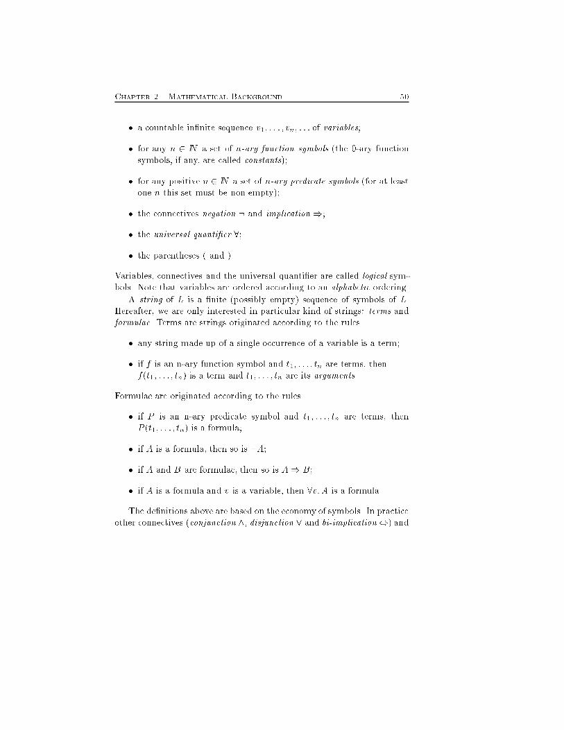
Chapter 2. Mathematical Background 50� a countable in�nite sequence v1; : : : ; vn; : : : of variables;� for any n 2 IN a set of n-ary function symbols (the 0-ary functionsymbols, if any, are called constants);� for any positive n 2 IN a set of n-ary predicate symbols (for at leastone n this set must be non empty);� the connectives negation : and implication );� the universal quanti�er 8;� the parentheses ( and ).Variables, connectives and the universal quanti�er are called logical sym-bols. Note that variables are ordered according to an alphabetic ordering.A string of L is a �nite (possibly empty) sequence of symbols of L.Hereafter, we are only interested in particular kind of strings: terms andformulae. Terms are strings originated according to the rules� any string made up of a single occurrence of a variable is a term;� if f is an n-ary function symbol and t1; : : : ; tn are terms, thenf(t1; : : : ; tn) is a term and t1; : : : ; tn are its arguments.Formulae are originated according to the rules� if P is an n-ary predicate symbol and t1; : : : ; tn are terms, thenP (t1; : : : ; tn) is a formula;� if A is a formula, then so is :A;� if A and B are formulae, then so is A) B;� if A is a formula and v is a variable, then 8v:A is a formula.The de�nitions above are based on the economy of symbols. In practiceother connectives (conjunction ^, disjunction _ and bi-implication,) and

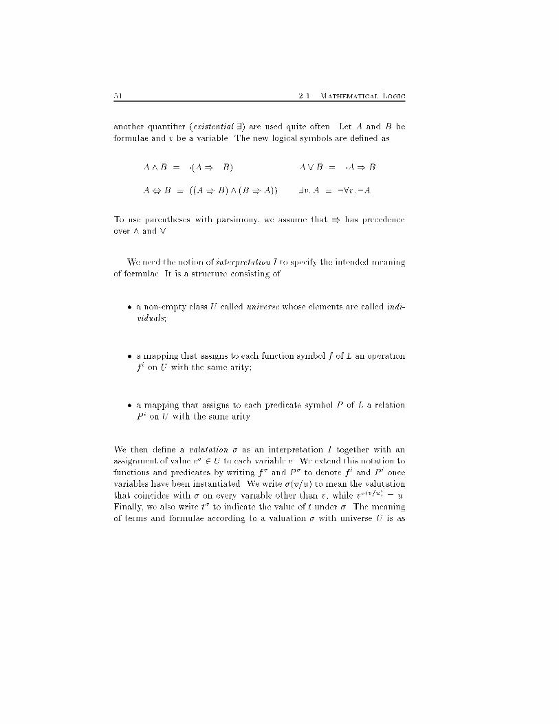
51 2.1. Mathematical Logicanother quanti�er (existential 9) are used quite often. Let A and B beformulae and v be a variable. The new logical symbols are de�ned asA ^B = :(A) :B) A _B = :A) BA, B = ((A) B) ^ (B ) A)) 9v:A = :8v::ATo use parentheses with parsimony, we assume that ) has precedenceover ^ and _.We need the notion of interpretation I to specify the intended meaningof formulae. It is a structure consisting of� a non-empty class U called universe whose elements are called indi-viduals;� a mapping that assigns to each function symbol f of L an operationf i on U with the same arity;� a mapping that assigns to each predicate symbol P of L a relationP i on U with the same arity.We then de�ne a valutation � as an interpretation I together with anassignment of value v� 2 U to each variable v. We extend this notation tofunctions and predicates by writing f� and P � to denote f i and P i oncevariables have been instantiated. We write �(v=u) to mean the valutationthat coincides with � on every variable other than v, while v�(v=u) = u.Finally, we also write t� to indicate the value of t under �. The meaningof terms and formulae according to a valuation � with universe U is as

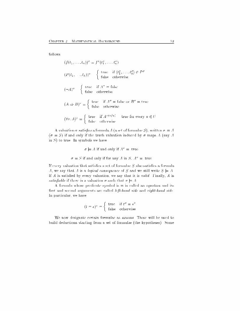
Chapter 2. Mathematical Background 52follows. (f(t1; : : : ; tn))� = f�(t�1 ; : : : ; t�n)(P (t1; : : : ; tn))� = � true if ht�1 ; : : : ; t�ni 2 P �false otherwise(:A)� = � true if A� = falsefalse otherwise(A) B)� = � true if A� = false or B� = truefalse otherwise(8v:A)� = � true if A�(v=u) = true for every u 2 Ufalse otherwiseA valuation � satis�es a formulaA (a set of formulae S), written � j= A(� j= S) if and only if the truth valuation induced by � maps A (any Ain S) to true. In symbols we have� j= A if and only if A� = true� j= S if and only if for any A in S, A� = trueIf every valuation that satis�es a set of formulae S also satis�es a formulaA, we say that A is a logical consequence of S and we still write S j= A.If A is satis�ed by every valuation, we say that it is valid. Finally, A issatis�able if there is a valuation � such that � j= A.A formula whose predicate symbol is = is called an equation and its�rst and second arguments are called left-hand side and right-hand side.In particular, we have(t = s)� = � true if t� = s�false otherwiseWe now designate certain formulae as axioms. These will be used tobuild deductions starting from a set of formulae (the hypotheses). Some

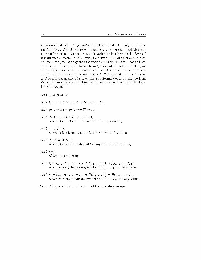
53 2.1. Mathematical Logicnotation could help. A generalisation of a formula A is any formula ofthe form 8v1 : : :8vk A, where k � 1 and v1; : : : ; vk are any variables, notnecessarily distinct. An occurrence of a variable v in a formulaA is bound ifit is within a subformula of A having the form 8v:B. All other occurrencesof v in A are free. We say that the variable v is free in A it v has at leastone free occurrence in A. Given a term t, a formulaA and a variable v, wede�ne Aft=vg as the formula obtained from A when all free occurrencesof v in A are replaced by occurrences of t. We say that t is free for v inA if no free occurrence of v is within a subformula of A having the form8v0: B, where v0 occurs in t. Finally, the axiom scheme of �rst-order logicis the following.Ax.1 A) B ) A;Ax.2 (A) B ) C)) (A) B)) A) C;Ax.3 (:A) B)) (:A) :B)) A;Ax.4 8v: (A) B)) 8v:A) 8v:B,where A and B are formulae and v is any variable;Ax.5 A) 8v:A,where A is a formula and v is a variable not free in A;Ax.6 8v:A) Aft=vg,where A is any formula and t is any term free for v in A;Ax.7 t = t,where t is any term;Ax.8 t1 = tn+1 ) : : : tn = t2n ) f(t1; : : : ; tn)) f(tn+1; : : : ; t2n),where f is any function symbol and t1; : : : ; t2n are any terms;Ax.9 t1 = tn+1 ) : : : tn = t2n ) P (t1; : : : ; tn)) P (tn+1; : : : ; t2n),where P is any predicate symbol and t1; : : : ; t2n are any terms;Ax.10 All generalizations of axioms of the preceding groups.

Chapter 2. Mathematical Background 54Let S be a set of formulae. A deduction from S is a �nite, non-emptysequence of formulae A1; : : : ; An such that, for all k (1 � k � n), either� Ak is an axiom, or� Ak 2 S, or� 9i; j < k :Aj � Ai ) Ak.The set S is called a set of hypotheses. A proof is a deduction from theempty set of hypotheses. We use ` to denote deducibility. More precisely,we write S ` A to assert that A is deducible from S. If S is empty, wesay that A is provable (or it is a theorem) and we write ` A. Recall thatS ` A ) S j= A:In the above description, we have assumed as unique inference rulethe modus pones, i.e. the operation of passing from two formulas A andA) B to the formula B. In other words, we havefA;A) Bg j= B:An inference rule has a set of premises and a conclusion. Notation Pcmeans that from the premises P we can infer c. Note that axioms areinference rules with empty premises. This allows us to arrange proofs ina tree-structure called deduction tree. The root of the tree is the theoremand its leaves are the hypotheses. Any internal node is a premise of arule. If we view axioms as inference rule we can say that a proof is a�nite, non-empty sequence of formulae in which any formula is obtainedfrom the preceding ones by applying any inference rule. Sometimes, weneed a larger set E of inference rules. In these case, we annotate it in thededuction symbol, i.e. we write S `E A.2.2 SetsWe assume as primitive the concept of set. Intuitively, it is an unorderedcollection of objects called elements or members. Expression x 2 A means

55 2.2. Setsthat x is an element of set A. The negation of being member is writtenx 62 A. We equate two sets if they have the same elements(8x : (x 2 A , x 2 B)) , A = B:A set A is a subset of a set B, if any element of A is also element of B8x : x 2 A ) x 2 Band we write A � B. To express that A � B, but A 6= B, we write A � B.To de�ne a set we only need to enumerate all its elements, if possible.For instance, f2; 3g is the set made up of numbers 2 and 3. The special setwhich has no element is called empty set and is denoted by ;. The emptyset is unique because we distinguish sets according to their elements, andthe empty set has no element. Furthermore, for any set A we have ; � A.A singleton is a set with a single element. For the sake of notation weoften omit braces in the de�nition of singletons.The de�nition by enumeration is not applicable for sets such as IN orIR which have in�nite elements. In alternative, the elements of a set canbe identi�ed by giving a property which is satis�ed by all of them. Let Abe a set and P (x) be a property which make sense for the elements of A,then we write fx 2 A jP (x)gfor the subset of A whose elements satisfy P (x). Sometimes we writefx jP (x)g when the domain of P is clear from the context.Note that we can de�ne a set through a property P if we already havea set and we specify one of its subsets. Without this assumption, we havethe Russel's paradox. In fact, assume that the expressionfx jx 62 xgis a set s. It would be the set of all sets that do not contain themselvesas element. If s 2 s it must be s 62 s because this is the de�ning propertyof s and must be satis�ed by all its elements. On the other hand, if s 62 sit must be s 2 s by de�nition of s. Hence, we have the paradox. We canconclude that the set of all sets does not exist.

Chapter 2. Mathematical Background 56We now report some fundamental operations on sets. The union oftwo sets A [B is a set whose elements belong to A or BA [B = fx jx 2 A _ x 2 BgThe intersection of two sets A\B is a set whose elements belong to bothA and B A \B = fx jx 2 A ^ x 2 BgIf A and B have no element in common, then A \B = ;. In this case wesay that the two sets are disjoint. The di�erence of two sets A�B is theset of the elements of A which are not in BA�B = fx jx 2 A ^ x 62 BgThe powerset of a set A is the set 2A whose elements are all subsets of A2A = fX jX � AgWe write 2Af for the powerset of A consisting of the �nite subsets of Aonly.The product of two sets A � B is the set of the ordered pairs whose �rstcomponent is an element of A and whose second component is an elementof B A� B = f(x; y) jx 2 A ^ y 2 BgNote that we can similarly de�ne the product of n sets. The disjoint unionof two sets A1 ] A2 is the union of the two sets f1g � A1 and f2g � A2.Their elements are pairs whose �rst component is an index that uniquelyidenti�es one of the two setsA1 ]A2 = (f1g � A1) [ (f2g � A2)Unlike union, the operation above keeps distinct two equal elements com-ing from distinct sets by duplicating them.Union and intersection can be extended to cope with possibly in�nitefamilies of sets. Let F be a family of sets, then the big union of F is theset whose elements belong to some set of F[X2F X = fx j 9X :X 2 F ^ x 2 Xg

57 2.3. Relations and FunctionsThe big intersection of F is the set whose elements belong to all sets of F\X2F X = fx j 8X :X 2 F ) x 2 XgHereafter, we use the shorthand 8x 2 A (8x62A) for 8x: x 2 A (8x: x62A).A similar notation is adopted for the existential quanti�er, as well.A set A � B is closed for an operation ? : Bn ! B if wheneverb1; : : : ; bn 2 A we have ?(b1; : : : ; bn) 2 A.2.3 Relations and FunctionsA binary relation between two sets A and B is an element of 2A�B , orequivalently a subset of A�B. Given a relation R � A�B, we often writexRy for (x; y) 2 R. A well-founded relation is a binary relation � on a setA such that there is no in�nite descending chain : : : � xi � : : : � x1 � x0.If xi � xj we say that xi is a predecessor of xj .A relation f � A�B is called function ormapping (written f : A! B)if for any x 2 A there is at most a single y 2 B such that xfy. In this casewe write f(x) = y and we say that f(x) is de�ned. If there is no y 2 Bsuch that f(x) = y, f(x) is unde�ned. If for any x 2 A there exists y 2 Bsuch that f(x) = y, f is total, otherwise it is partial. If we want to stressthat function f is partial, we write f : A * B. Set A is the domain of thefunction, and set B is the codomain. Given X � A, we write f(X) for theset whose elements are related to some elements of X through ff(X) = fy j y 2 B ^ (9x 2 X : f(x) = y)gor simply f(X) = ff(x) jx 2 Xg. A function f : A ! B is surjective iff(A) = B. Function f is injective if8x1 2 A; 8x2 2 A : f(x1) = f(x2)) x1 = x2Function f is bijective if ti is both surjective and injective.

Chapter 2. Mathematical Background 58The basic operation between relations, and thus between functions, iscomposition. The composition of two relations R � A�B and S � B�Cis a relation between A and CS �R = f(x; z) 2 A� C j 9y 2 B : (x; y) 2 R ^ (y; z) 2 SgThe composition of two functions f : A ! B and g : B ! C is thenfunction g � f : A! C de�ned asg � f = f(x; g(f(x))) jx 2 AgAny set A is equipped with a special function IA called identity on Ade�ned as IA = f(x; x) jx 2 AgFunction f : A! B has an inverse g : B ! A i�8x 2 A : g(f(x)) = x ^ 8y 2 B : f(g(y)) = yIn this case sets A and B are in 1-1 correspondence. Sets which are in 1-1correspondence with IN are said countable.An equivalence relation on a set A is a re exive, symmetric and tran-sitive relation, i.e., 8x 2 A; 8y 2 A; 8z 2 AxRx ^ xRy ) yRx ^ (xRy ^ yRz)) xRzThe set of all elements equivalent to x is denoted [x] and is called theequivalence class of x. More formally,[x] = fy j y 2 A ^ xRygTwo equivalence classes are disjoint or coincide. Thus, the set F of allequivalence classes is a subset of 2A such that� 8S 2 F : S 6= ;� 8S 2 F; 8T 2 F : S 6= T ) S \ T = ;� SS2F S = A.

59 2.4. Frequently used structuresA family F of subsets of A with the properties above is said a partitionof A. A family with only the last property is said a covering of A. Anequivalence relation R on A singles out a partition of A that is calledquotient of A with respect to R and it is written A=R.A binary relation on a set A is an ordering if it is re exive, transitiveand antisymmetric relation. If the antisymmetric property does not hold,the relation is a preordering.We end this section by introducing multisets. A multiset over a set A isa total function f : A! IN , associating natural numbers, possibly 0, witheach element of A. We denote �nite multisets by listing their elementsbetween the symbols fj and jg. Note that we list an element a 2 A asmany times as f(a). The operations on multisets are the same of thoseon sets, except that replication is allowed.2.4 Frequently used structuresIn this section we recall the de�nition and some properties of some usefulmathematical structure in computer science. We start with graphs.A graph G is a pair hN;Ei where N is a set of nodes and E � 2Nwith jEj � 2 is the set of edges. A directed graph or digraph is a graphwith directions assigned to its edges. Edges of digraphs are called arcs.Formally, for digraphs we have E � N � N . If G = hN;Ei is a graphand e = hn1; n2i 2 E is an edge, we say that n1 and n2 are adjacent ande is incident upon the two nodes. The degree of a node is the number ofincident edges upon it. A walk in G is a sequence of edges [e1; e2; : : : ; ek]such that ei = hni; ni+1i for i = 1; : : : ; k. The walk is closed if n1 = nk+1.A walk without any repeated node is a path. A closed walk with nonodes repeated other than its �rst and last one is called a circuit or cycle.The length of a walk, a path or a cycle is the number of its edges. Thisterminology applies to directed graphs as well.A graph is connected if there is a path between any two nodes in it. Atree T = hN;Ei is a connected graph without cycles. A forest is a set of

Chapter 2. Mathematical Background 60node disjoint trees. Sometimes, directed and acyclic graphs are denotedas DAG's.A labelled graph is a triple G = hN;A;Ei where hN;Ei is a graph, butedges are labelled with elements of A. We can de�ne labelled digraph andlabelled trees as well.Let A be a set and ? be a binary operation on A. Then, hA; ?i is amonoid i�� 9e : 8a 2 A : e ? a = a ? e = e, and� 8a; a0; a00 2 A : (a ? a0) ? a00 = a ? (a0 ? a00).A commutative monoid is a monoid such that� 8a; a0 2 A : a ? a0 = a0 ? a.A group is a monoid such that� 8a 2 A : 9a�1 2 A : a ? a�1 = a�1 ? a = e.2.5 AlgebraAn algebra is a mathematical structure which is widely used in computerscience to model programming features. The basic theory is here recalledfrom (Hennessy, 1988).A signature � is a set of function symbols. In other words, � is the setof symbols of a �rst order language (see Section 2.1) made up of functionsymbols only. The arity of a signature is a mapping ar : � ! IN thatassociates with each symbol its arity. We write �n to denote the set offunction symbols in � with arity n.Given a signature �, a �-algebra is a pair hA;�Ai where A is a set calledcarrier and �A is a set of functions ffA : An ! A j f 2 � ^ ar(f) = ng.Essentially a �-algebra is an interpretation of a signature �. A signaturemay have many di�erent interpretation even over the same carrier.A special interpretation for a signature � is its term or free algebra.This algebra is a purely syntactic object: the carrier is the set of strings

61 2.5. Algebra(terms) built with the symbols in � and the functions only syntacticallymanipulate them. More formally, the set T� of terms over � is the leastset of strings that satisfy� f 2 � ^ ar(f) = 0 ) f 2 T�, and� f 2 � ^ ar(f) = k > 0 ^ t1; : : : ; tk 2 T� ) f(t1; : : : ; tk) 2 T�.Note that if no constant is in the signature, the set of terms is empty. Thefunctions of the term algebra construct new terms. For any f 2 � withar(f) = k, we let fT� : T k� ! T� be the function which maps tuples ofterms ht1; : : : ; tki into the term f(t1; : : : ; tk). By abuse of notation we willdenote the term algebra as T�.We now introduce the concept of structural induction which we fre-quently use throughout this work. The carrier of T� is de�ned inductively.It is the least set of strings that contains constants and is closed underthe operations f�. The method of structural induction says that to provea property P of all terms in T�, we only need to prove that P holds of� all constant symbols in �, and� the term f(t1; : : : ; tk) for every f 2 � with ar(f) = k > 0, assumingthat the property holds of the terms t1; : : : ; tk.Structural induction may be also used to de�ne a function g on T�.� De�ne g over constants, and� de�ne g over f(t1; : : : ; tk) in terms of g(t1); : : : ; g(tk), for every f 2 �with ar(f) = k > 0.In logical notation the principle of structural induction can be ex-pressed as8f 2 � : [ar(f) = 0) P (f) ^ ar(f) = k )(8t1; : : : ; tn 2 T� : P (t1) ^ : : :^ P (tn)) P (f(t1; : : : ; tn))]) 8t 2 T� : P (t)where P is the property investigated.

Chapter 2. Mathematical Background 62Some terminology: the �rst conjunct before the last implication isthe basis of the induction, the second conjunct is the induction step, andthe P -part of the left-hand side of the induction step is the inductionhypothesis.It is possible to de�ne functions (called �-homomorphisms) betweencarriers of �-algebras which preserve the structure of their domain. LethA;�Ai and hB;�Bi be two �-algebras, and h : A! B a function. Thenh is a �-homomorphism if8f 2 �; ar(f) = k; h(fA(a1; : : : ; ak)) = fB(h(a1); : : : ; h(ak)):The fundamental property of term algebras says that for every �-algebra hA;�Ai, there exists a unique �-homomorphism iA : T� ! A.Let C be a class of �-algebras. A �-algebra I is initial in C if for everyJ 2 C there is a unique �-homomorphism from I to J . Thus, we can saythat T� is initial in the class of all �-algebras.A �-congruence is an equivalence relation on �-algebras which pre-serves the structure induced by �. Given a �-algebra hA;�Ai, a relationC over A is a �-congruence if it is an equivalence relation and8f 2 �; ar(f) = k; 8i : 0 � i � k; hai; a0ii 2 C )hfA(a1; : : : ; ak); fA(a01; : : : ; a0k)i 2 C:Let [a]C = fa0 j ha; a0i 2 Cg be the equivalence class of a induced by C.Then, the set of equivalence classes is A=C = f[a]C j a 2 Ag.A �-algebra A satis�es a �-congruence C if iA(t) = iA(t0) wheneverht; t0i 2 C. We denote with C(C) the class of all �-algebras that sat-isfy C. The extension of the foundamental property of term algebras tocongruences says that the �-algebra T�=C is initial in the class C(C).Particular classes of �-algebras can be de�ned through equations. Anequation is determined by two terms possibly with variables. The valua-tion of these terms is modulo an assignment of values to variables.Let V be a set of variables ranged over by v; v1; vi; : : :. We extend asignature � to �(V ) to include variables. For any f 2 � we also havef 2 �(V ). Furthermore, any v 2 V is a function symbol of arity 0 in

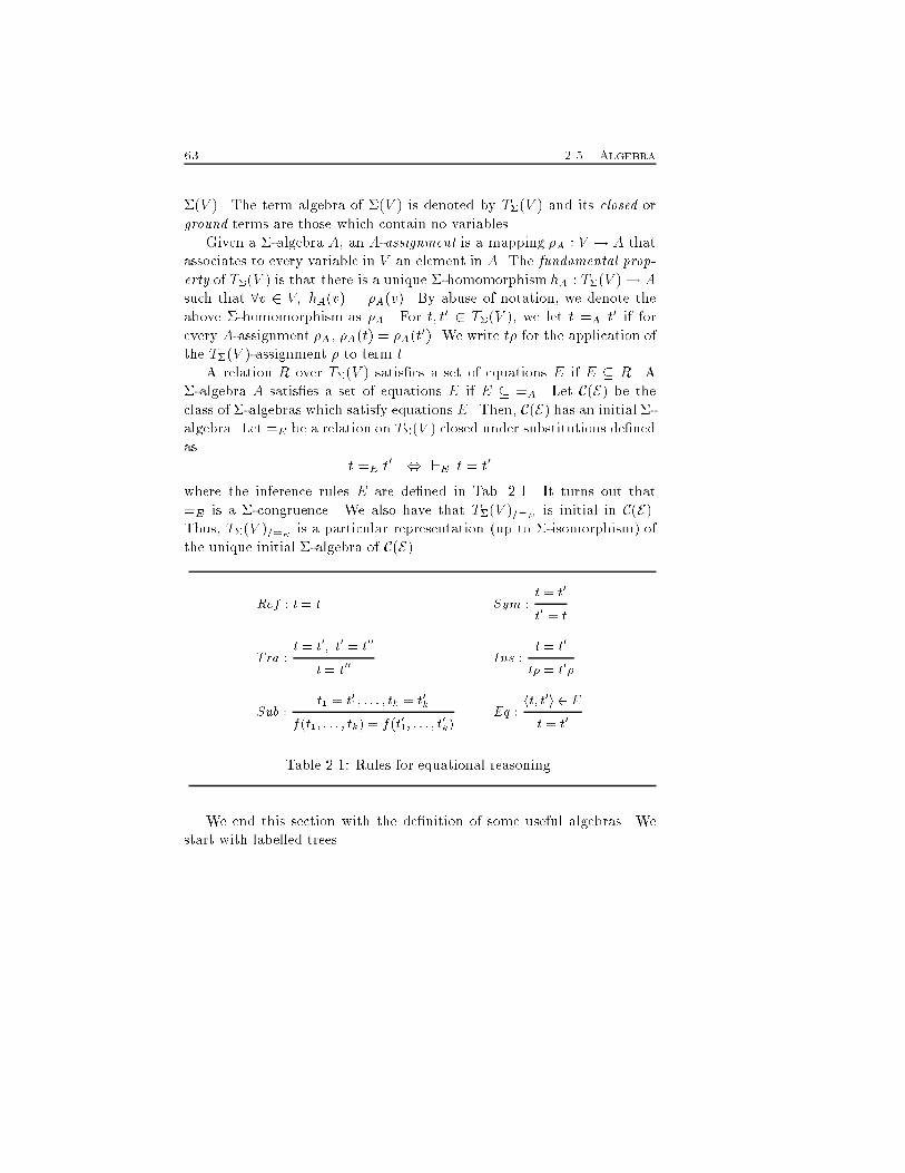
63 2.5. Algebra�(V ). The term algebra of �(V ) is denoted by T�(V ) and its closed orground terms are those which contain no variables.Given a �-algebra A, an A-assignment is a mapping �A : V ! A thatassociates to every variable in V an element in A. The fundamental prop-erty of T�(V ) is that there is a unique �-homomorphism hA : T�(V )! Asuch that 8v 2 V; hA(v) = �A(v). By abuse of notation, we denote theabove �-homomorphism as �A. For t; t0 2 T�(V ), we let t =A t0 if forevery A-assignment �A, �A(t) = �A(t0). We write t� for the application ofthe T�(V )-assignment � to term t.A relation R over T�(V ) satis�es a set of equations E if E � R. A�-algebra A satis�es a set of equations E if E � =A. Let C(E) be theclass of �-algebras which satisfy equations E. Then, C(E) has an initial �-algebra. Let =E be a relation on T�(V ) closed under substitutions de�nedas t =E t0 , `E t = t0where the inference rules E are de�ned in Tab. 2.1. It turns out that=E is a �-congruence. We also have that T�(V )==E is initial in C(E).Thus, T�(V )==E is a particular representation (up to �-isomorphism) ofthe unique initial �-algebra of C(E).Ref : t = t Sym : t = t0t0 = tTra : t = t0; t0 = t00t = t00 Ins : t = t0t� = t0�Sub : t1 = t01; : : : ; tk = t0kf(t1; : : : ; tk) = f(t01; : : : ; t0k) Eq : ht; t0i 2 Et = t0Table 2.1: Rules for equational reasoning.We end this section with the de�nition of some useful algebras. Westart with labelled trees.

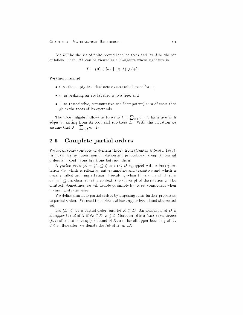
Chapter 2. Mathematical Background 64Let RT be the set of �nite rooted labelled trees and let A be the setof labels. Then, RT can be viewed as a �-algebra whose signature is� = f0g [ fa � j a 2 Ag [ f+g:We then interpret� 0 as the empty tree that acts as neutral element for +,� a� as pre�xing an arc labelled a to a tree, and� + as (associative, commutative and idempotent) sum of trees thatglues the roots of its operands.The above algebra allows us to write T = Pi2I ai � Ti for a tree withedges ai exiting from its root and sub-trees Ti. With this notation weassume that 0 =Pi2; ai � Ti.2.6 Complete partial ordersWe recall some concepts of domain theory from (Gunter & Scott, 1990).In particular, we report some notation and properties of complete partialorders and continuous functions between them.A partial order po = hD;�Di is a set D equipped with a binary re-lation �D which is re exive, anti-symmetric and transitive and which isusually called ordering relation. Hereafter, when the set on which it isde�ned �D is clear from the context, the subscript of the relation will beomitted. Sometimes, we will denote po simply by its set component whenno ambiguity can arise.We de�ne complete partial orders by imposing some further propertiesto partial orders. We need the notions of least upper bound and of directedset.Let hD;�i be a partial order, and let X � D. An element d of D isan upper bound of X if 8x 2 X :x � d. Moreover, d is a least upper bound(lub) of X if d is an upper bound of X, and for all upper bounds q of X,d � q. Hereafter, we denote the lub of X as tX.

65 2.6. Complete partial ordersA directed set M is a subset of D such that all its �nite subsets havean upper bound in M , i.e. for any �nite X �M there is an upper boundm 2M for X.A complete partial order (cpo) is a partial order that has a least ele-ment denoted ? and all its directed subsets have a lub. An alternativecharacterization of complete partial orders relies on !-chains. An !-chainis an increasing chain d0 � d1 � : : : � dn � : : : of elements of the partialorder. A cpo is a partial order with ? and such that all its !-chains havea lub.Let D and E be cpos. A function f : D ! E is monotonic if8d; d0 2 D : d �D d0 ) f(d) �E f(d0):The set of monotonic functions between D and E is denoted by D mo�! E.Function f is continuous if it is monotonic and for all chainsd0 �D d1 �D : : : �D dn �D : : :in D it is tn2!f(dn) = f(tn2!dn)where tn2!f(dn) is a shorthand for tff(dn) jn 2 !g. The set of con-tinuous functions between D and E is denoted by D co�! E. Function fis strict if f(?) = ?. Note that continuous functions preserve limits ofincreasing sequences.The following notion of �xed point is useful in dealing with recursivede�nitions.Let D be a cpo, and let f : D ! D be a continuous function. A�xed point of f is a d 2 D such that f(d) = d. A pre�xed point off is a d 2 D such that f(d) � d. The set of pre�xed point of f ispre(f) = fd 2 D j d � f(d)g.If we require to each subset of a cpo D to have a least upper bound,we obtain a complete lattice (cl). Then, any subset X has a greatest lowerbound and it is denoted uX. We write ? for uD and > for tD.

Chapter 2. Mathematical Background 66We now report the �xed-point theorem that allows us to solve recursiveequations. Let f : D ! D be a continuous function on cpo D. Putf = tn2!fn(?):Then, f is the least �xed point of f .2.7 Formal LanguagesProgramming languages have foundations on formal language theory. Werecall in this section grammars, regular expressions and �nite state au-tomata.An alphabet is a �nite, non empty set of symbols used to build strings.The length of a string x is the number of its symbols (written jxj). Aspecial string is the empty string � that has length 0. The concatenationof two strings x and y is the string x �y, or simply xy obtained by followingthe symbols of x by the symbols y. Note that a set of strings with con-catenation and neutral element � is a monoid. Exponentiation of stringsrepresent iterated concatenation. For instance, x3 denotes xxx. By con-vention, we let x0 = �. A pre�x of x is a string obtained by discarding 0 ormore trailing symbols of x. A su�x of x is a string obtained by deleting0 or more leading symbols of x. A substring of x is a string obtained byerasing a pre�x and a su�x of x. A string y is a proper pre�x, su�x orsubstring of x if y 6= x.A language is a set of strings formed from a speci�c alphabet. Twoparticular languages are ; (the empty language) and f�g (the languagemade up of the empty string alone). Note that the de�nition of languagedoes not assign any meaning to its strings. Therefore, languages are purelysyntactic objects. We extend concatenation to languages as followsLM = fxy jx 2 L ^ y 2MgSimilarly to strings, we de�ne exponentiation of languages, assuming thatf�gL = Lf�g = L. A set of languages with concatenation and neutralelement f�g is a monoid. Since languages are sets, they are equipped with

67 2.7. Formal Languagesunion, as well. We write L� for the concatenation of L with itself anynumber of times. More formally,L� = 1Xi=0 LiHereafter, we use the shorthand L+ for L(L�). We call the post�x operator� closure and + positive closure.There are three ways to �nitely de�ne in�nite languages. A languageis the set of strings generated by a �nite structure called grammar. Inalternative, a language is the set of strings recognized or accepted by a�nite structure called automaton. Finally, a language is the solution of asystem of algebraic relations.A grammar is a quadrupleG = (N;�; P; S)where N is a �nite set of nonterminal symbols, � is an alphabet of terminalsymbols,P � (N[�)��(N[�)� is the �nite set of productions, and S 2 Nis the start symbol. We adopt the following conventions: A;B; : : : 2 N ,a; b; : : : 2 �, X;Y; : : : 2 (N [�), x; y; : : : 2 ��, and �; �; : : : 2 (N [ �)�.We often write � �! �, �; � 2 (N [�)�, for a production h�; �i 2 P .The language de�ned by G isL(G) = fw jw 2 ��; S �!� wgwhere �!� is the re exive and transitive closure of �!.A grammar is context free if all its productions have the form A �! �.A grammar is regular if all its productions have the form A �! aB orA �! a.We concentrate on context free grammars because they are used tospecify the peculiar features of programming languages. The structure ofthe derivation of a string is represented through a tree, called derivationtree. It is a �nite tree such that� its root is labelled S;

Chapter 2. Mathematical Background 68� any node which is not a leaf has a label from N ;� any leaf has a label from �;� if a node labelledX has sons labelled (from left to right) X1; : : : ; Xn,then X ! X1; : : : ; Xn 2 P:The string corresponding to a derivation tree is the concatenation of itsleaves from left to right. We have di�erent derivations corresponding tothe same derivation tree, according to the order in which productions areapplied. We introduce leftmost derivations (the ones which expands ateach step the leftmost nonterminal) to have a unique derivation associatedwith a tree.A context free grammar G is ambiguous if there is a string in L(G)which can be generated with two di�erent leftmost derivations. A languageL is ambiguous if all grammars that generate it are ambiguous.We consider regular languages as an example of de�nition of a languagethrough an acceptor of its strings. A �nite state automaton is a structureM = (Q;�; �; q0; F )where Q is a �nite set of states, � is the input alphabet, � : Q�� �! 2Qis the state transition relation, q0 2 Q is the initial state, and F � Q isthe set of �nal states.The behaviour of a �nite state automaton is determined by the set ofstrings that it acceptsL(M ) = fw 2 �� j ��(hq0; wi) 2 Fgwhere �� is the re exive and transitive closure of the transition relation.Languages originated by regular grammars can be also represented byregular expressions. A regular expression is a string generated by thefollowing context free grammarG = (fEg; T; E; P ) with T = f�; ;;+; �; �; ); (g[A

69 2.7. Formal Languageswhere A is an alphabet and the productions areE �! (E +E) j (E �E) j (E)� j � j ; j ai 2 AThe language L(G) is the set of regular expressions over the alphabet A.We associate a language (that turns out to be regular) to any regularexpressions as follows.L[;] = ; L[�] = f�gL[ai] = faig L[e1 + e2] = L[e1] [ L[e2]L[e1 � e2] = L[e1]L[e2] L[e�] = (L[e])�We recall the following property of regular expressions that will beuseful in Chapt. 9: (e1 + e2)� = (e�1e�2)�:A regular language denoted by a regular expression E can be obtainedas the solution of a system of linear equations of the form X = AX + B,where A and B are known languages. From formal language theory,the solution of the equation above is the least �x-point of the functionF (X) = AX + B and it has the form A�B. The linear system can besolved by substitution. We can generate L(E) as a chain of approxima-tions L1(E); : : : ; Ln(E); : : :, with Lj(E) = fw jw 2 L(E); jwj = jg. Thisderives from the structure of regular grammars which impose the deriva-tion of exactly one terminal symbol from each application of a production.Note that a signature can be expressed as a grammar. The symbols ofthe signature correspond to terminal symbols of the grammar, the domainand codomain of the functions associated to the symbols in the signatureare the nonterminals of the grammar. For instance, the operator + inter-preted as + : Exp�Exp! Exp in the �-algebra originates the productionExp ::= Exp+Exp in the grammar.We end this section by introducing the abstract syntax of a language.The concrete syntax of a language is a set of strings over an alphabet. Itis usually speci�ed through a context free grammar G. Sometimes con-text free grammars contains nonterminals and productions which are not

Chapter 2. Mathematical Background 70needed to derive the string of a language. They are introduced to rule outambiguities from grammars. This allows us to de�ne deterministic algo-rithms (parsers) to decide whether a string belong or not to a language.For instance, a non ambiguous grammar for arithmetic expressions hasthe following productions E ! E + T jTT ! T � F jFF ! (E) j ewhere e is a terminal symbol. The arithmetic expressions can also bederived with the productionsE ! E +E jE �E j (E) j ethat originate an ambiguous grammar.The abstract syntax constitutes an interface between concrete syntaxand semantic interpretations of languages. Abstract syntax is obtained byerasing from the concrete one irrelevant information such as precedenceamong operators, hierarchies of derivation and so on. When dealing withsemantic issues, we are not interested in the way in which strings arederived, but only in their meaning. Derivation trees can be thus simpli�edby collapsing sequences of nonterminals along a path. The set of treesobtained in this way constitute the abstract syntax trees and the grammar(possibly ambiguous) that originates them is the abstract syntax.Note that the structure of an abstract grammar originates a signature.Therefore, we can say that the abstract syntax of a language is a termalgebra. Since a term algebra is completely individuated by its signature,we can de�ne the semantics of the language by interpreting into a �-algebra the symbols of the signature.2.8 Continuous time Markov chainsWe brie y recall stochastic processes and continuous time Markov chains(Allen, 1978).

71 2.8. Continuous time Markov chainsA family of random variables fX(t); t 2 Tg is a stochastic process withindex set T . The set T is usually called time parameter and t time. Theprocess is discrete time or continuous time if T is a discrete or a continuousset, respectively. The state space of the process is the set of possible valuesthat X(t) can assume. Intuitively, X(t) is the state of the process at timet. Examples of stochastic processes are the waiting time of an arrivingrequest until processing is begun by a server, the average time to run aprogram on a computer, the occurrence probability of a hardware or asoftware failure.Many systems arising in practice have the property that, given thepresent state, the past states have no in uence on the future. This is thememoryless or Markov property and the stochastic processes satisfying itare called Markov chains or Markov processes depending whether theirstate space is discrete or continuous, respectively.The family of random variables fX(t); t � 0g is a continuous timeMarkov chain (CTMC) if for any set of n+1 values t1 < : : : < tn+1 in theindex set, and any set fx1; : : : ; xn+1g of n+ 1 states we havep(X(tn+1) = xn+1 jX(t1) = x1; : : : ; X(tn) = xn) =p(X(tn+1) = xn+1 jX(tn) = xn)with p(AjB) the conditional probability of A given B. Hereafter, we writeCTMC(X(t0)) for the CTMC with initial state X(t0).The one-step transition probabilityp(X(tn+1) = xn+1 jX(tn) = xn)is usually dependent on the index n. When it is independent of n, it iswritten pn(n+1), and the corresponding CTMC is said homogeneous in timeor to have stationary transition probabilities. We are mainly interested inthese CTMC as their transition probabilities can be arranged in a squarematrix (transition matrix) and performance analysis can be performed bystandard numerical techniques.Let �t(xi) = p(X(t) = xi) be the probability that CTMC(X(t0)) isin state xi at time t, and let �0 = (�0(x0); : : : ;�0(xn)) be the initial

Chapter 2. Mathematical Background 72distribution of states x0; x1; : : : ; xn. Then, CTMC(X(t0)) is said to have astationary probability distribution � = (�(x0); : : : ;�(xn)) if it is satis�edthe matrix equation �Pij = � with Xi �(xi) = 1where Pij is the transition matrix.We now characterize the Markov chains which always admit an equi-librium distribution. State xi is recurrent if a Markov chain starting atxi returns to xi with probability one. If the expected number of stepsuntil the chain returns to xi is less than in�nity, then the state is positiverecurrent. If xi is recurrent and the chain visits it at least once, thenit does so in�nitely often. A Markov chain is recurrent (positive recur-rent) if all its states are recurrent (positive recurrent); it is irreducible ifevery state leads back to itself and also to every other state. All statesof an irreducible Markov chain with �nite state space are positive recur-rent. Finally, positive recurrent Markov chains have a unique stationarydistribution �, given by �(xi) = 1=mxiwhere mxi is the mean return time to xi for a chain starting at xi.

Chapter 3Structural OperationalSemanticsIn this chapter we present transition systems and their intensional de�ni-tion through inference rules. We essentially follow (Plotkin, 1981) in thepresentation. As for the previous chapter, we introduce notations thatwill be used later.The reader familiar with the notions listed above can safely skip this chap-ter.3.1 Transition systemsA system is usually a collection of entities that cooperate to carry out anactivity. We assume that a system is a mathematical model of the phe-nomenon under investigation. It is characterized at time t by its internalstate (con�guration) that is made up of a control program and some data.This is a static description of a system. It changes its internal state ac-cording to stimuli from the environments or to particular values of data.The set of con�gurations that a system may pass through and their rela-73

Chapter 3. Structural Operational Semantics 74tions characterize the dynamic behaviour. Since we are interested in thedynamic behaviour of systems, we call our models transition systems.De�nition 3.1.1 (transition system) A transition system is a struc-ture (�;�!), where � is a set of elements called con�gurations and thebinary relation �! � �� � is called transition relation.Hereafter, we write �! 0 for h ; 0i 2 �!.Transition systems can specify many concepts from formal languagetheory. For instance, �nite state automata are obtained by imposing � tobe a �nite set and by picking out a set of terminal states. The resultingtransition system is a terminal transition system.De�nition 3.1.2 (terminal transition system) A terminal transitionsystem is a structure (�;�!; T ) where (�;�!) is a transition system, andT � � is the set of �nal con�gurations such that 8 2 T; 0 2 � : 6�! 0.We now formalize the representation of a �nite state automatonM = (Q;�; �; q0; F )as terminal transition system. We de�ne � = Q��� and hq; awi ` hq0; wiwhenever q0 2 �(q; a). The set of terminal con�gurations isT = fhq; �i j q 2 Fg;where � denotes the empty string.The behaviour of a �nite state automaton is determined by the set ofstrings that it accepts L(M ) = fw 2 �� j ��(hq0; wi) 2 Fg. The samebehaviour can be obtained by a terminal transition system with initialstate.De�nition 3.1.3 (initial terminal transition system) An initial ter-minal transition system is a structure (�;�!; T; I) where (�;�!; T ) is aterminal transition system, and I � � is the set of initial con�gurationssuch that whenever 0 �! 00 there exists 2 I and �!� 0.

75 3.1. Transition systemsFinally, automaton M is completely described by the initial terminaltransition system (Q� ��;`; F � f�g; fq0g)Similarly, we can express context free grammars through transitionsystems. The initial terminal transition system corresponding toG = (N;�; P; S)is ((N [�)�;�!; T; fSg)where wXv �! wxv if (X;x) 2 P and T is the set of con�gurations whichdo not contain symbols from N .Transition systems allows us to study properties which are indepen-dent of the kind of the individual transitions. For instance, if one isinterested in all con�gurations which are reachable from a given one, thekind of transitions is irrelevant. Other properties need more informationon transitions to be investigated. For example, to study the frequency ofoccurrence of a given action, we must associate to each transition a namethat identi�es the corresponding action. This leads to the de�nition oflabelled transition systems.De�nition 3.1.4 (labelled transition system)A labelled transition system is a structure (�; A;�!) where � is a set ofcon�gurations, A is a set of labels (sometimes called actions or operations)and �!� �� A� � is the transition relation.Hereafter, we write a�! 0 for h ; a; 0i 2 �!, 6 a�! 0 for h ; a; 0i62 �!, �! 0 for 9a 2 A : h ; a; 0i 2 �!, and 6�! for 8a 2 A; 8 0 2 � : 6 a�! 0.Labelled transition systems can be considered in their initial or termi-nal version, as well. We now generalize the re exive and transitive closureof the transition relation to labelled transition systems as w�!+ 0 , 9 1; : : : ; n : = 0 a1�! 1 : : : an�! n = 0; n > 0

Chapter 3. Structural Operational Semantics 76 w�!� 0 , 9 1; : : : ; n : = 0 a1�! 1 : : : an�! n = 0; n � 0where w = a1 : : :an.Labelled initial terminal transition systems may be used to simplifythe speci�cation of �nite state automata. In particular, they allow us todrop the component �� from con�gurations. The automaton M of theexample above can now be de�ned as(Q;�;�!; F; fq0g)with qi a�! qj whenever qj 2 �(qi; a).The general technique of simplifying the structure of con�gurations byadding information to the label of transitions will be frequently used inthis work. This allows us to gain compactness in the representation oftransition systems. In fact, the smaller is the set of con�gurations, thehigher is the probability of re-using con�gurations.Hereafter, we omit the adjective labelled, initial and terminal whenthe kind of transition system at hand is clear from the context.We now show that a transition system can be conveniently representedthrough a graph in which the con�gurations coincide with the nodes andthe arcs represent the possible transitions between them. The dynamicbehaviour of a system de�ne the form of this graph, that we call transitiongraph. Some auxiliary de�nitions are needed. Hereafter, we assume asgiven a labelled transition system (�; A;�!).De�nition 3.1.5 (derivative) Con�guration 0 is an immediate deriva-tive of , if a�! 0. It is simply a derivative, if w�!� 0.We de�ne con�gurations that do not occur within cycles.De�nition 3.1.6 (acyclic con�gurations) Con�guration is acyclicif there is no w such that w�!+ .Sometimes is useful to identify the set of derivatives of a given con�gura-tion.

77 3.1. Transition systemsDe�nition 3.1.7 (set of derivatives) The derivative set of a con�gu-ration is ds( ) = f 0 j w�!� 0g:Note that the union of the set of derivatives of the initial states of a systemde�ne all reachable con�gurations.We can now formalize the notion of derivation graph.De�nition 3.1.8 (derivation graph) Given a con�guration and itsset of derivatives ds( ), the derivation graph of isdg( ) = hds( ); A; f( i; a; j) j i 2 ds( ) ^ i a�! jgiwhere ds( ) is the set of nodes, A is the labelling alphabet, and the thirdset de�nes the arcs.The possible patterns of behaviour of a system are obtained by vis-iting its derivation graph. The sequences of consecutive transitions thatdescribes the behaviour are called computations.De�nition 3.1.9 (computation) Let i a�! j be a transition. Then, i is the source of the transition and j is its target. A computation of is a sequence of transitions = 0 a0�! 1 a1�! : : : starting from , andsuch that the target of any transition coincides with the source of the nextone. We let �; �0; �1; : : : range over computations, and we write � for theempty computation. The notions of source and target are extended in theobvious way to computations. We let C( ) be the set of computations withsource , and C( ; 0) be the set of computations with source and target 0.Note that whenever � is a �nite set, C( ; 0) is the language acceptedby the automaton (�; A;�!; f 0g; f g). If we call branching-free regularlanguages the ones that may be expressed through regular expressionsbuilt without the operator +, then C( ; 0) is a branching-free language.Sometimes is useful to have a linearization of all computations thata system may engage in. A possibility is to get the unfolding of thederivation graph, thus yielding a tree of computations.

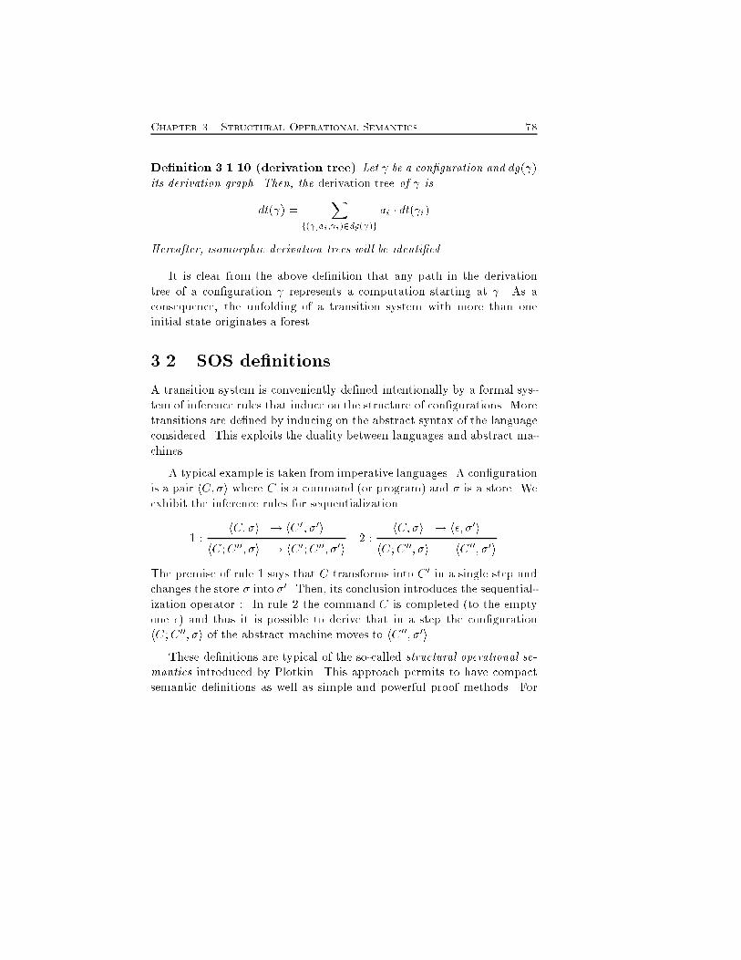
Chapter 3. Structural Operational Semantics 78De�nition 3.1.10 (derivation tree) Let be a con�guration and dg( )its derivation graph. Then, the derivation tree of isdt( ) = Xf( ;ai; i)2dg( )g ai � dt( i)Hereafter, isomorphic derivation trees will be identi�ed.It is clear from the above de�nition that any path in the derivationtree of a con�guration represents a computation starting at . As aconsequence, the unfolding of a transition system with more than oneinitial state originates a forest.3.2 SOS de�nitionsA transition system is conveniently de�ned intentionally by a formal sys-tem of inference rules that induce on the structure of con�gurations. Moretransitions are de�ned by inducing on the abstract syntax of the languageconsidered. This exploits the duality between languages and abstract ma-chines.A typical example is taken from imperative languages. A con�gurationis a pair hC; �i where C is a command (or program) and � is a store. Weexhibit the inference rules for sequentialization.1 : hC; �i �! hC 0; �0ihC;C 00; �i �! hC 0;C 00; �0i 2 : hC; �i �! h�; �0ihC;C 00; �i �! hC 00; �0iThe premise of rule 1 says that C transforms into C 0 in a single step andchanges the store � into �0. Then, its conclusion introduces the sequential-ization operator ;. In rule 2 the command C is completed (to the emptyone �) and thus it is possible to derive that in a step the con�gurationhC;C 00; �i of the abstract machine moves to hC 00; �0i.These de�nitions are typical of the so-called structural operational se-mantics introduced by Plotkin. This approach permits to have compactsemantic de�nitions as well as simple and powerful proof methods. For

79 3.2. SOS definitionsinstance, structural induction and induction on the depth of the proof oftransitions are among the widely used proof methods in this setting. Fur-thermore, the set of inference rules that originates the transition systemsconstitutes an abstract machine for the language that is under speci�ca-tion. These are the reasons which lead to a renewed interest in operationalsemantics especially in the �eld of concurrency.

Chapter 3. Structural Operational Semantics 80

Chapter 4Semantics forConcurrencyIn this chapter we present the basic notions of semantic models for concur-rent distributed systems that will be used later. We start with �-calculusin its early and late version. For presentation purposes, we then intro-duce the calculus of communicating systems (CCS) and the higher order�-calculus (HO-�) as a restriction and an extension of �-calculus, respec-tively. When dealing with CCS we also discuss how it is possible to derivethe operational semantics of operators primitive in other process alge-bras like ; of CSP. Then, we recall the syntax and operational semanticsof Facile, a real distributed programming language that integrates func-tional and concurrent programming paradigms. Finally, we brie y surveyPetri nets and event structures.4.1 �-calculusIn this section we recall the basic theory of �-calculus (Milner et al.,1992a), a model of concurrent communicating processes based on the no-tion of naming. The calculus allows one to easily express systems which81

Chapter 4. Semantics for Concurrency 82have a dynamically changing structure. The syntax of agents or processesis de�ned below.De�nition 4.1.1 Let N be a countable in�nite set of names ranged overby a; b; : : : ; x; y; : : : with � 62 N . We also assume a set of agent identi�ersranged over by A;A0; Ai; : : :. Processes (denoted by P;Q;R; : : : 2 P) arebuilt from names according to the syntaxP ::= 0 j �:P j (�x)P j [x = y]P j P jP j P + P j A(y1; : : : ; yn)where � may be either x(y) for input, or xy for output (where x is thesubject and y the object) or � for silent moves. The order of precedenceamong the operators is the order (from left to right) listed above. Hereafter,the trailing 0 will be omitted.The pre�x � denotes the �rst atomic action that the process �:P canperform. The input pre�x binds the name y in the pre�xed process. In-tuitively, some name y is received along the link named x. The outputpre�x does not bind the name y which is sent along x. The silent pre-�x � denotes an action which is invisible to an external observer of thesystem. The operator (�x) acts as a static binder for the name x in theprocess P that it pre�xes. In other words, x is a unique name in P whichis di�erent from all external names. Matching [x = y]P is an if-thenoperator: process P is activated if x = y. The operator j describes paral-lel composition of processes. Summation denotes nondeterministic choice.Finally, P (y1; : : : ; yn) is the de�nition of constants (hereafter ~y denotesthe sequence y1; : : : ; yn). Each agent identi�er A has a unique de�ningequation of the form A(y1; : : : ; yn) = P , where the yi are distinct andfn(P ) � fy1; : : : ; yng (see next subsection for the de�nition of free namesfn).4.1.1 Early semanticsThe early operational semantics for �-calculus is de�ned in the SOS styleand the labels of transitions are � for silent actions, xy for input, xy forfree output, and x(y) for bound output. We use � as a metavariable

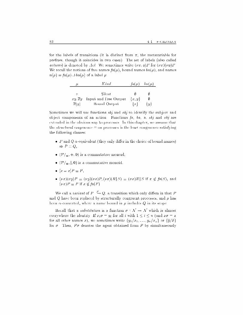
83 4.1. �-calculusfor the labels of transitions (it is distinct from �, the metavariable forpre�xes, though it coincides in two cases). The set of labels (also calledactions) is denoted by Act. We sometimes write (�x; y)P for (�x)(�y)P .We recall the notions of free names fn(�), bound names bn(�), and namesn(�) = fn(�) [ bn(�) of a label �.� Kind fn(�) bn(�)� Silent ; ;xy; xy Input and Free Output fx; yg ;x(y) Bound Output fxg fygSometimes we will use functions sbj and obj to identify the subject andobject components of an action. Functions fn, bn, n, sbj and obj areextended in the obvious way to processes. In this chapter, we assume thatthe structural congruence � on processes is the least congruence satisfyingthe following clauses:� P and Q �-equivalent (they only di�er in the choice of bound names)) P � Q,� (P=�;+;0) is a commutative monoid,� (P=�; j;0) is a commutative monoid,� [x = x]P � P ,� (�x)(�y)P � (�y)(�x)P; (�x)(R jS) � (�x)R jS if x 62 fn(S), and(�x)P � P if x 62 fn(P ).We call a variant of P ��! Q, a transition which only di�ers in that Pand Q have been replaced by structurally congruent processes, and � hasbeen �-converted, where a name bound in � includes Q in its scope.Recall that a substitution is a function � : N ! N which is almosteverywhere the identity. If xi� = yi for all i with 1 � i � n (and x� = xfor all other names x), we sometimes write fy1=x1; : : : ; yn=xng or f~y=~xgfor �. Then, P� denotes the agent obtained from P by simultaneously

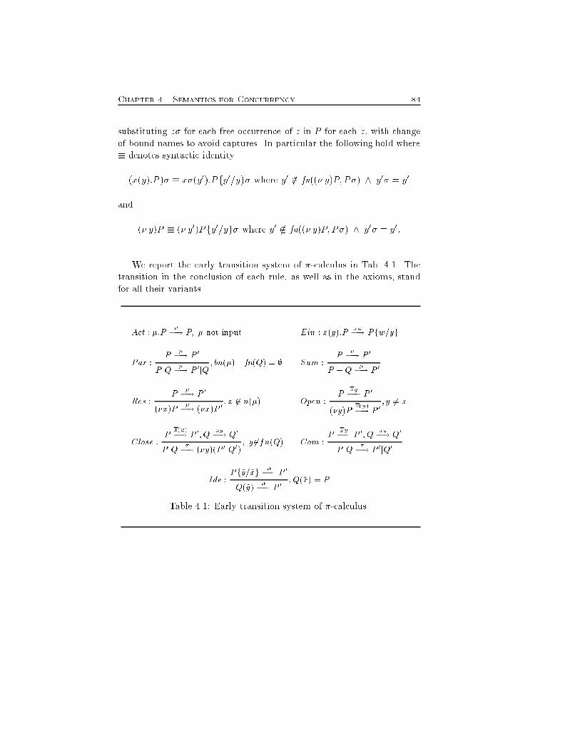
Chapter 4. Semantics for Concurrency 84substituting z� for each free occurrence of z in P for each z, with changeof bound names to avoid captures. In particular the following hold where� denotes syntactic identity(x(y):P )� � x�(y0):Pfy0=yg� where y0 62 fn((� y)P; P�) ^ y0� = y0and (� y)P � (� y0)Pfy0=yg� where y0 62 fn((� y)P; P�) ^ y0� = y0:We report the early transition system of �-calculus in Tab. 4.1. Thetransition in the conclusion of each rule, as well as in the axioms, standfor all their variants.Act : �:P ��! P; � not input Ein : x(y):P xw�! Pfw=ygPar : P ��! P 0P jQ ��! P 0jQ; bn(�) \ fn(Q) = ; Sum : P ��! P 0P +Q ��! P 0Res : P ��! P 0(�x)P ��! (�x)P 0 ; x 62 n(�) Open : P xy�! P 0(�y)P x(y)�! P 0 ; y 6= xClose : P x(y)�! P 0;Q xy�! Q0P jQ ��! (�y)(P 0jQ0) ; y 62fn(Q) Com : P xy�! P 0;Q xy�! Q0P jQ ��! P 0jQ0Ide : Pf~y=~xg ��! P 0Q(~y) ��! P 0 ;Q(~x) = PTable 4.1: Early transition system of �-calculus.

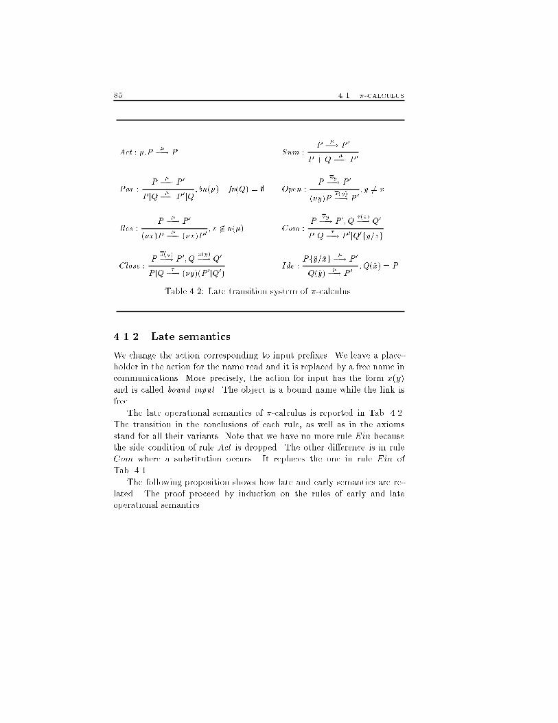
85 4.1. �-calculusAct : �:P ��! P Sum : P ��! P 0P +Q ��! P 0Par : P ��! P 0P jQ ��! P 0jQ; bn(�) \ fn(Q) = ; Open : P xy�! P 0(�y)P x(y)�! P 0 ; y 6= xRes : P ��! P 0(�x)P ��! (�x)P 0 ; x 62 n(�) Com : P xy�! P 0;Q x(z)�! Q0P jQ ��! P 0jQ0fy=zgClose : P x(y)�! P 0;Q x(y)�! Q0P jQ ��! (�y)(P 0jQ0) Ide : Pf~y=~xg ��! P 0Q(~y) ��! P 0 ;Q(~x) = PTable 4.2: Late transition system of �-calculus.4.1.2 Late semanticsWe change the action corresponding to input pre�xes. We leave a place-holder in the action for the name read and it is replaced by a free name incommunications. More precisely, the action for input has the form x(y)and is called bound input. The object is a bound name while the link isfree.The late operational semantics of �-calculus is reported in Tab. 4.2.The transition in the conclusions of each rule, as well as in the axiomsstand for all their variants. Note that we have no more rule Ein becausethe side condition of rule Act is dropped. The other di�erence is in ruleCom where a substitution occurs. It replaces the one in rule Ein ofTab. 4.1.The following proposition shows how late and early semantics are re-lated. The proof proceed by induction on the rules of early and lateoperational semantics.

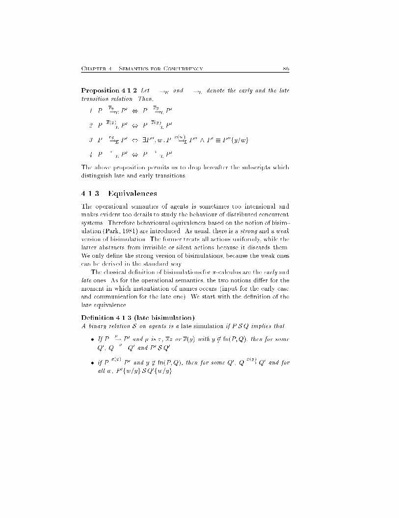
Chapter 4. Semantics for Concurrency 86Proposition 4.1.2 Let �!E and �!L denote the early and the latetransition relation. Then,1. P xy�!E P 0 , P xy�!L P 02. P x(y)�!E P 0 , P x(y)�!L P 03. P xy�!E P 0 , 9P 00; w : P x(w)�!L P 00 ^ P 0 � P 00fy=wg4. P ��!E P 0 , P ��!L P 0The above proposition permits us to drop hereafter the subscripts whichdistinguish late and early transitions.4.1.3 EquivalencesThe operational semantics of agents is sometimes too intensional andmakes evident too details to study the behaviour of distributed concurrentsystems. Therefore behavioural equivalences based on the notion of bisim-ulation (Park, 1981) are introduced. As usual, there is a strong and a weakversion of bisimulation. The former treats all actions uniformly, while thelatter abstracts from invisible or silent actions because it discards them.We only de�ne the strong version of bisimulations, because the weak onescan be derived in the standard way.The classical de�nition of bisimulations for �-calculus are the early andlate ones. As for the operational semantics, the two notions di�er for themoment in which instantiation of names occurs (input for the early caseand communication for the late one). We start with the de�nition of thelate equivalence.De�nition 4.1.3 (late bisimulation)A binary relation S on agents is a late simulation if P S Q implies that� If P ��! P 0 and � is � , xz or x(y) with y 62 fn(P;Q), then for someQ0, Q ��! Q0 and P 0 S Q0� if P x(y)�! P 0 and y 62 fn(P;Q), then for some Q0, Q x(y)�! Q0 and forall w, P 0fw=yg S Q0fw=yg

87 4.1. �-calculusThe relation S is a late bisimulation if both S and S�1 are late simulations.P is late bisimilar to Q (written P �L Q) if there exists a late bisimulationS such that P S Q.Note that late simulations have a strong requirement on bound inputactions. The early bisimulation release this requirement has early seman-tics has no bound input.De�nition 4.1.4 (early bisimulation) A binary relation S on agentsis an early simulation if P S Q implies that� If P ��! P 0 and � is any action with bn(�) \ fn(P;Q) = ;, then forsome Q0, Q ��! Q0 and P 0 S Q0The relation S is an early bisimulation if both S and S�1 are early simu-lations. P is early bisimilar to Q (written P � Q) if there exists an earlybisimulation S such that P S Q.To exploit the di�erence between the two equivalences, consider theprocesses P = a(y):R+ a(y):0 and Q = P + a(y):[y = b]Rwhere R 6= 0. It is P � Q, but P 6�LQ. The processes are early bisimilarbecause the instantiation of y is done by the input and the last summandof Q is equal to the �rst summand of P if y = b; otherwise it is equal tothe second summand of P . The late bisimulation instantiate y on demand.Therefore the last summand ofQ cannot be matched by P because distinctinstantiations of y distinguish [x = b]R from R and 0.4.1.4 Late vs. early semanticsA major drawback to the practical use of �-calculus is the in�nite branch-ing originated in the early semantics by inputs (rule Ein) and bound out-puts (rule Open). Rule Ein originates in�nite many transitions becauseany substitution of the placeholder y is allowed. In the other case the

Chapter 4. Semantics for Concurrency 88in�nite branching is a consequence of �-conversion. In fact, the restrictedname can be any of the ones not used yet.The late semantics of �-calculus, in which rule Ein is not present,avoids the in�nite many transitions originated by inputs. The instanti-ation of names only occurs in communications, when the actual value ise�ectively known. The late binding of names implies that the late transi-tion system of �-calculus does not contain all possible computations of aprocess. In fact, consider x(y):[y = z]awhich has a single transition derived through rule Act (it has no sidecondition) that leads to [y = z]a and is labelled x(y). However, theprocess can activate a when the name received is z. In �-calculus, thelack of computations is considered at bisimulation level. Essentially, it isrequired to build on demand all transitions of any process reached whennames are instantiated.Consider again the process above and early semantics. Although itoriginates in�nite many transitions, only two of them completely charac-terize its behaviour. In fact, if name z is received, the process will executethe a, otherwise it will not. Furthermore, since names are instantiatedby inputs (instead of communications), the early transition system has allcomputations. This partition of names leads to the de�nition of an early�nite branching semantics of �-calculus in SOS style (see Sect. 5.3).4.1.5 Calculus of communicating systemsAs far as the Calculus of Communicating Systems (CCS) and its relatedtheory is concerned, we refer to (Milner, 1989). Essentially, CCS is the�-calculus without objects and enriched with the relabelling operator �.Therefore, in the following chapters we will only consider CCS withoutrelabelling as the above mentioned portion of �-calculus.As for �-calculus, strong and weak bisimulation equivalences are in-troduced to abstract from too intensional de�nitions of behaviour. Thestrong bisimulation is the early one applied to processes without objects.Note that the condition bn(�)\fn(P;Q) = ; in Def. 4.1.4 is always satis�edbecause links are always free in the labels of transitions.

89 4.2. Higher order �-calculus4.1.6 Operators from other calculiOnly few basic operators constitute �-calculus. In practice could be usefulalso the sequential composition of agents P ;Q in the style of TCSP by(Hoare, 1985). The informal semantics of the operator says that Q beginswhen P ends. This implies that it is necessary to capture the event that Pends. To this purpose we introduce a special action tick (p) which an agentperforms to witness that it has �nished its execution. The operationalsemantics is de�ned by the rules in Tab. 4.3.Seq : P ��! P 0P ;Q ��! P 0;Q; � 6= p Seq0 : P p�! P 0P ;Q ��! QTable 4.3: Transition rules for sequential composition.4.2 Higher order �-calculusThe objects in �-calculus can be only �rst-order. By dropping this limita-tion we obtain the higher order �-calculus HO� (Sangiorgi, 1992). Namescan represent processes, and thus communications may cause processes tomigrate.4.2.1 SyntaxThe syntax of �-calculus is extended as follows. Let V be a set of processvariables ranged over by X;Y; : : :. Let K stand for a process or for a name,and let U stand for a variable or for a name. We substitute K and U forobjects in pre�x, and U for names in constant de�nition of �-calculus.Thus, we have the following syntaxP ::= 0 j X j �:P j P + P j P jP j (�x)P j [x = y]P j A(U1; : : : ; Un)where � may be either x(U ) for input, or xK for output, � for silent moves.

Chapter 4. Semantics for Concurrency 904.2.2 Operational semanticsThe early operational semantics of HO� is de�ned in SOS style and thelabel of the transitions are � for silent actions, xK for input, xK for freeoutput and x(K) for bound output. We will still use � as a metavariablefor the actions and we assume that the notions of free names, bound namesand names of a label � are tuned according to the new syntax. Similarly,we adapt the structural congruence on processes and the notion of variantof transitions.The transition relation of HO� is de�ned by the axioms and rulesin Tab. 4.4, where an auxiliary transition relation ��!I is used. Theset I contains names that can occur in a communicated process and areextruded. Rule Close uses I to include the receiving process as well intheir scope. Of course, rule Open updates the set of these names, thatClose empties (note that in rule Close it is I � fn(K)). The actualtransitions are generated by rule Ho� that discards index I.We end this section by noting that a late semantics can be de�ned forHO�, as well.4.3 FacileFacile (Giacalone et al., 1990; Giacalone et al., 1989) is an experimentallanguage that aims at integrating functional and concurrent programmingparadigms. Facile may be viewed as an extension of �-calculus with prim-itives for concurrency, communication and distribution. The language hasa binding operator (�-abstraction) to de�ne (possibly higher-order) func-tions. Functions, processes and channels may be either the result of theevaluation or the arguments of expressions.Facile handles concurrency through dynamic de�nition of processes,channels and virtual processing units (called nodes). Processes exchangemessages with send and receive primitives along channels that are explic-itly managed. Communication is synchronous.The functional and the concurrent parts of Facile are strongly inte-grated: processes evaluate expressions to values while expressions mayactivate processes or return channels and node identi�ers.

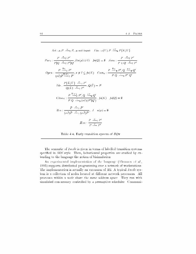
91 4.3. FacileAct : �:P ��!; P; � not input Ein : x(U):P xK�!; PfK=UgPar0 : P ��!I P 0P jQ ��!I P 0jQ; (bn(�) [ I) \ fn(Q) = ; Sum : P ��!I P 0P +Q ��!I P 0Open : P xK�!; P 0(�I)P x(K)�!I P 0 ; x 62 I � fn(K) Com0 : P xK�!; P 0;Q xK�!; Q0P jQ ��!; P 0jQ0Ide : Pf ~K= ~Ug ��!I P 0Q( ~K) ��!I P 0 ;Q( ~U ) = PClose0 : P x(K)�!I P 0;Q xK�!; Q0P jQ ��!; (�I)(P 0jQ0) ; fn(K) \ fn(Q) = ;Res : P ��!I P 0(�J)P ��!I (�J)P 0 ; J \ n(�) = ;Ho� : P ��!I P 0P ��! P 0Table 4.4: Early transition system of HO�.The semantic of Facile is given in terms of labelled transition systemsspeci�ed in SOS style. Then, behavioural properties are studied by ex-tending to the language the notion of bisimulation.An experimental implementation of the language (Thomsen et al.,1993) supports distributed programming over a network of workstations.The implementation is actually an extension of ML. A typical Facile sys-tem is a collection of nodes located at di�erent network processors. Allprocesses within a node share the same address space. They run withsimulated concurrency controlled by a preemptive scheduler. Communi-

Chapter 4. Semantics for Concurrency 92cations between nodes are implemented through inter-process mechanismsand network protocols. Any node can be viewed as a virtual processorwhich may or may not coincide with a physical one. Programmers canspecify on which node a process must be allocated. We refer to (Thomsenet al., 1992; Leth & Thomsen, 1995) for details on physical distributionin Facile.Since we are mainly interested in non interleaving semantics, we reporthere the distributed semantics of Facile introduced in (Thomsen et al.,1992).4.3.1 SyntaxWe only consider here the core syntax of Facile, i.e. the set of constructswhich is su�cient to de�ne any Facile program. A translation from thefull to the core syntax is in (Giacalone et al., 1990).The core syntax consists of three syntactic categories: expressions(functions) e, behaviour expressions (processes) be, and distributed be-haviour expressions (systems) dbe. The set of expressions, behaviour ex-pressions and distributed behaviour expressions are denoted by E, BE,and DBE, respectively. Expressions are statically typed and t ranges overtypes. The type system is reported in (Giacalone et al., 1990). Hereafter,we assume that all expressions are correctly typed. Note that processesand systems have no type. The core syntax is reported in Tab. 4.5.Hereafter we denote the set of syntactic values as Val, ranged over by v.Values are a subclass of expressions without free variables. Values can bepassed as parameters to functions or be communicated between processes,possibly residing on di�erent nodes in a system.We assume a countable set of variables denoted by x; xi; : : :. Constantsare ranged over by c, and these include integers, booleans, channel-valuedconstants, node identi�ers, and a distinguished, dummy value triv. Pre-de�ned operators such as if-then-else are denoted by c, as well. Weassume that all operations are in curried form to avoid the introductionof tuples and product types. Functions are de�ned and manipulated in�-calculus style with abstractions and applications. � is a variable binderwith the usual notion of free and bound variables. The set of free variables

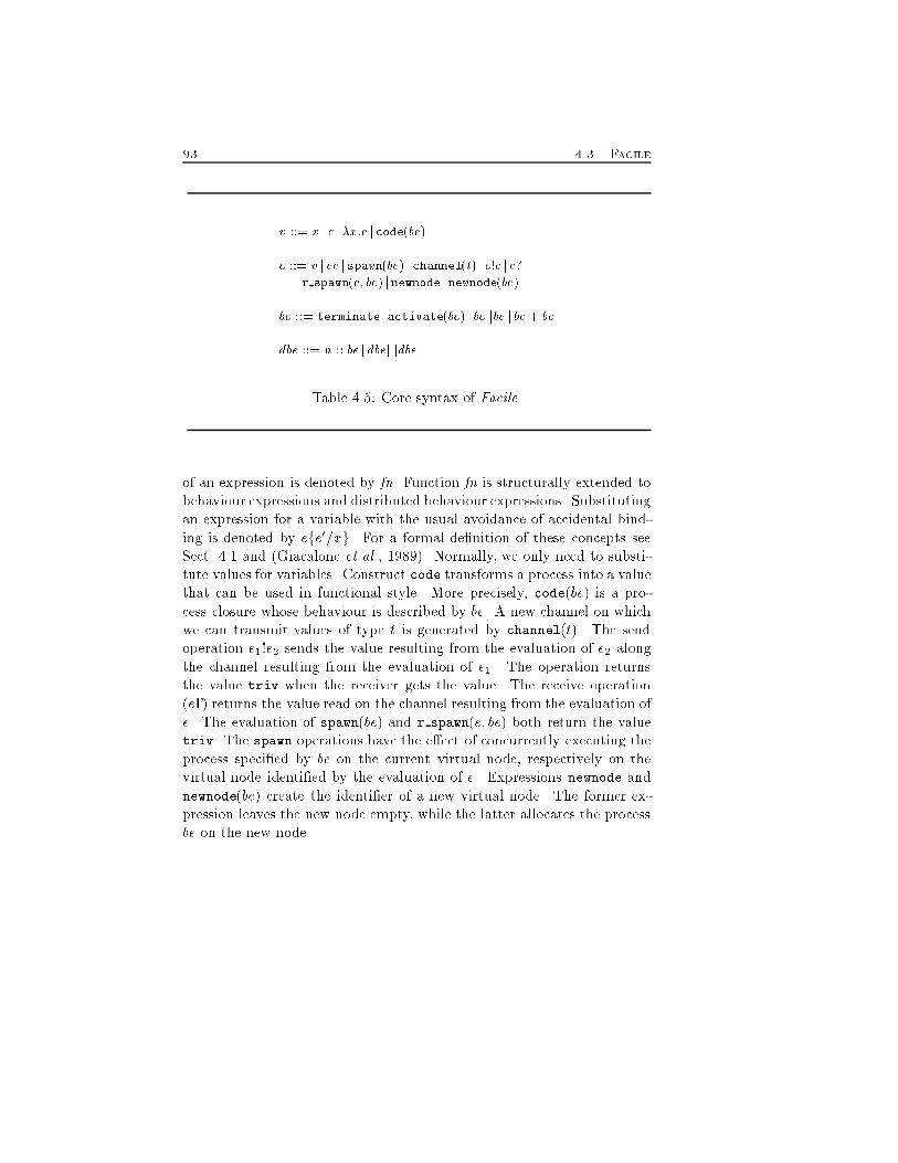
93 4.3. Facilev ::= x j c j�x:e jcode(be)e ::= v j ee jspawn(be) jchannel(t) j e!e j e?r spawn(e; be) jnewnode jnewnode(be)be ::= terminatejactivate(be) j bejjbe j be+ bedbe ::= n :: be jdbejjjdbeTable 4.5: Core syntax of Facile.of an expression is denoted by fn. Function fn is structurally extended tobehaviour expressions and distributed behaviour expressions. Substitutingan expression for a variable with the usual avoidance of accidental bind-ing is denoted by efe0=xg. For a formal de�nition of these concepts seeSect. 4.1 and (Giacalone et al., 1989). Normally, we only need to substi-tute values for variables. Construct code transforms a process into a valuethat can be used in functional style. More precisely, code(be) is a pro-cess closure whose behaviour is described by be. A new channel on whichwe can transmit values of type t is generated by channel(t). The sendoperation e1!e2 sends the value resulting from the evaluation of e2 alongthe channel resulting from the evaluation of e1. The operation returnsthe value triv when the receiver gets the value. The receive operation(e?) returns the value read on the channel resulting from the evaluation ofe. The evaluation of spawn(be) and r spawn(e; be) both return the valuetriv. The spawn operations have the e�ect of concurrently executing theprocess speci�ed by be on the current virtual node, respectively on thevirtual node identi�ed by the evaluation of e. Expressions newnode andnewnode(be) create the identi�er of a new virtual node. The former ex-pression leaves the new node empty, while the latter allocates the processbe on the new node.

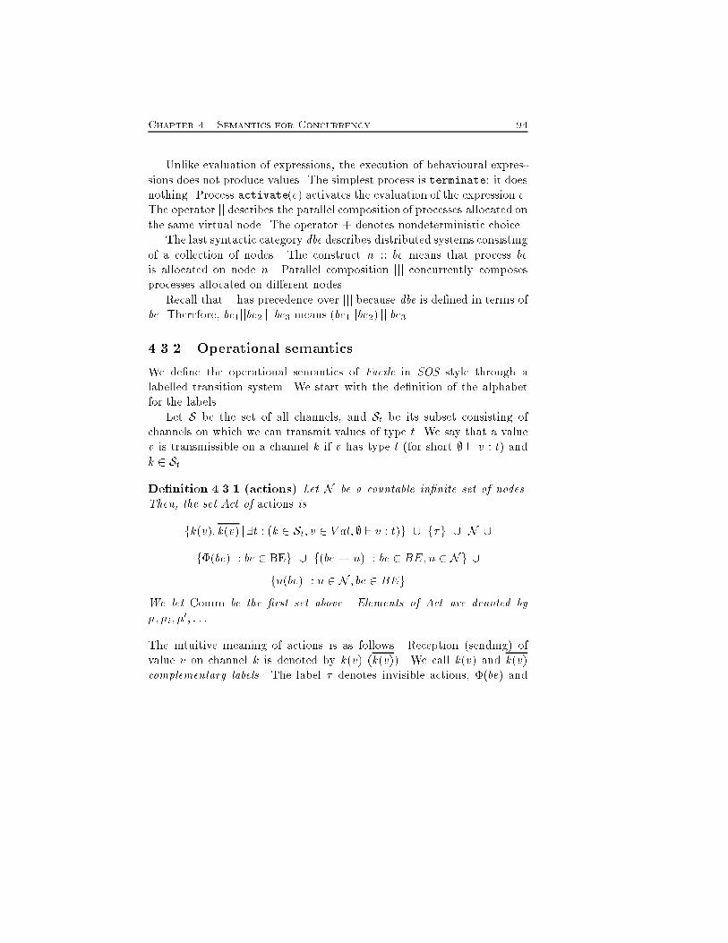
Chapter 4. Semantics for Concurrency 94Unlike evaluation of expressions, the execution of behavioural expres-sions does not produce values. The simplest process is terminate: it doesnothing. Process activate(e) activates the evaluation of the expression e.The operator jj describes the parallel composition of processes allocated onthe same virtual node. The operator + denotes nondeterministic choice.The last syntactic category dbe describes distributed systems consistingof a collection of nodes. The construct n :: be means that process beis allocated on node n. Parallel composition jjj concurrently composesprocesses allocated on di�erent nodes.Recall that jj has precedence over jjj because dbe is de�ned in terms ofbe. Therefore, be1jjbe2 jjjbe3 means (be1jjbe2) jjjbe3.4.3.2 Operational semanticsWe de�ne the operational semantics of Facile in SOS style through alabelled transition system. We start with the de�nition of the alphabetfor the labels.Let S be the set of all channels, and St be its subset consisting ofchannels on which we can transmit values of type t. We say that a valuev is transmissible on a channel k if v has type t (for short ; ` v : t) andk 2 St.De�nition 4.3.1 (actions) Let N be a countable in�nite set of nodes.Then, the set Act of actions isfk(v); k(v) j 9t : (k 2 St; v 2 V al; ; ` v : t)g [ f�g [ N [f�(be) : be 2 BEg [ f(be! n) : be 2 BE; n 2 Ng [fn(be) : n 2 N ; be 2 BEgWe let Comm be the �rst set above. Elements of Act are denoted by�; �i; �0; : : :.The intuitive meaning of actions is as follows. Reception (sending) ofvalue v on channel k is denoted by k(v) (k(v)). We call k(v) and k(v)complementary labels. The label � denotes invisible actions, �(be) and

95 4.3. Facile(be ! n) are introduced by spawn(be) and r spawn(n; be), respectively,and �nally, n and n(be) are introduced by newnode and newnode(be),respectively.We now de�ne con�gurations of the labelled transition system of Facile.Let 2Sf (ranged over by K) and 2Nf (ranged over by N ) be the set of �nitesubsets of S and N , respectively. These sets are used to ensure uniquenessof channels and nodes. Creation of channels and nodes inserts the newname into the corresponding set in con�gurations if it does not alreadyexist (see rules 4 and 8 in Tab. 4.6). The sets of con�gurations areEcon � 2Sf � 2Nf � E for expressionsBcon � 2Sf � 2Nf � BE for processesDBcon � 2Sf � 2Nf �DBE for systems.Transition relations between con�gurations are de�ned as follows. Therelation �!e � Econ �Act� Econevaluates expressions. The transition relation for processes is�!be � Bcon �Actn f�(be) : be 2 BEg �BconFinally, transitions for systems are expressed by�!dbe � DBcon� (Comm � N ) [ f�g �DBconWe can now de�ne the labelled transition system of Facile.De�nition 4.3.2 (labelled transition system) The labelled transitionsystem of Facile is LTS = hDBcon; Act; �!dbe i where DBcon is the setof con�gurations of systems, Act is the set of labels and �!dbe is thetransition relation de�ned by the axioms and rules in Tables 4.6, 4.7, 4.8.Detailed comments to the rules in Tables 4.6, 4.7, 4.8 are in (Thomsenet al., 1992). We introduce here some notations and shorthands that willbe used later on. The core of Facile has no operator for sequentialisation of

Chapter 4. Semantics for Concurrency 96expressions or processes. Term e1:e2 is implemented in the core languageas e1:e2 � (�x:e2)e1 if x 62 fn(e2):Instead, term e:be is translated ase:be � activate((�x:code(be))e) if x 62 fn(be)Hereafter, we will use sequentialisation to simplify the representation ofFacile systems. When the direction of communication is immaterial wemay simply write a:be and when an action is the last action of a processes,i.e. a:terminate we may drop the terminate behaviour expression andsimply write a.4.4 Other modelsIn this section we brie y survey other semantic models frequently used tostudy distributed systems. Besides transition systems the so-called alge-bras of transitions (Ferrari et al., 1991) yield transition graphs. A uniquename is associated to each transition (its proof) and composition oper-ators are de�ned on them according to the constructs of the languagewhich form the algebra of states. Since the synchronisation mechanism iscompletely free (because the treatment of restriction is) special transitionslabelled error must be introduced (e.g. for the (non-existent) synchroni-sation between a and b in a j b). This implies that more transitions thannecessary have to be generated and then, observing the labelling, have tobe erased. Moreover, since the name of the transitions is recorded in thestates, there is also an explosion in the number of nodes of the graph withrespect to classical approaches.4.4.1 Petri netsThe next model we consider is Petri nets (Reisig, 1985). A place-transitionnet is a quadruple N = hS; T; F;M0i consisting of two disjoint sets S and Tof places and transitions, of a ow multiset relation F � S�T [T �S andof the initial markingM0 : S ! IN (IN being the set of natural numbers).

97 4.4. Other modelsNote that the ow relation F can be interpreted also as a function weightW : S � T [ T � S ! IN .The dynamic behaviour of nets is de�ned by the token game. A tran-sition t 2 T is enabled under a marking M if 8s 2 S;M (s) � W (s; t).The occurrence of an enabled transition t produces a new marking M 0de�ned by 8s 2 S;M 0(s) = M (s) �W (s; t) + W (t; s). A marking M iscalled reachable if there exists a sequence of transitions that starts fromM0 and leads to M . Also, M is said to be safe if 8s 2 S;M (s) � 1. Aplace-transition net is said safe if all reachable markings are safe.In order to characterise runs of nets without abstracting from causalrelations between events, nonsequential processes were de�ned (Goltz &Reisig, 1983; Best & Devillers, 1987). We introduce the notion of pre- andpost-sets. Given an element x 2 S [ T , the pre-set of x is�x = fy 2 S [ T jW (y; x) 6= 0gand the post-set of x isx� = fy 2 S [ T jW (x; y) 6= 0g:Then, a process of a net N is a quadruple � = hB;E; F; pi such thathB;E; F i is a net with no initial marking, hB [E;F i is an acyclic graphand 8b 2 B; j�bj � 1 and jb�j � 1. Moreover, p : B [ E ! S [ T isa function that maps elements of B to elements of S, elements of E toelements of T and initial places of � (those with �b = ;) to places s suchthat M0(s) � 1. Also, 8e 2 E; 8s 2 S;W (s; p(e)) = jp�1(s) \� ej andW (p(e); s) = jp�1(s) \ e�j. Nielsen, Plotkin and Winskel (Nielsen et al.,1981) introduced occurrence nets which generalise processes by summaris-ing all the processes of a net as a single net. This is done in by removingthe restriction jb�j � 1 while preserving reachability by forbidding self-con ict.4.4.2 Event structuresWe now consider event structures (Nielsen et al., 1981; Winskel, 1982).Event structures consist of a set of labelled events together with relations

Chapter 4. Semantics for Concurrency 98of causality, independence and con ict between them. Indeed it is usefulto think of such event structures as having the occurrence net notion ofcondition, B above, replaced by its abstraction (these relations). Eventsmodel the occurrence of actions and are labelled with the action that theyrepresent. Note that an event is quite di�erent from a transition and froma state of the transition system. Indeed, many transitions may representthe same event (e.g. the two � transitions in the event structure originatedby the term a j b represent the same event). More formally, a (prime) eventstructure is a triple ES = hE;�;#i consisting of a set E of events thatare partially ordered by �, the causal dependency relation, and a binary,symmetric, irre exive relation # � E � E, the con ict relation whichsatis�es fe0je0 � eg is �nite and e#e0 � e00 ) e#e00 for all e; e0; e00 2 E.Two events, say e and e0, are concurrent or independent (written e ^ e0)i� they are neither in con ict nor in the causally related.A con�guration of an event structure is a subset x � E which iscon ict-free 8e; e0 2 x;:(e#e0)and downward-closed8e 2 x; e0 2 E; e0 � e) e0 2 x:The computations of a process are the paths in the partial ordered set ofthe con�gurations, ordered by inclusion.The inheritance property of con ict relation in prime event structuresimplies that if two events are in con ict, then all causal successors of oneevent are in con ict with all causal successors of the other event. As aconsequence, each event is enabled by a unique set of events and thisleads in general to duplication of events (and iteratively to asymptoticallygreater size) . Consider, e.g., the prime event structure associated to theterm (� + �); . The event is duplicated as it can be enabled by twodi�erent events.To avoid duplication of events, ow event structures have been intro-duced (Boudol, 1990). A ow event structure is a triple FES = hE;�;#iconsisting of a denumerable set E of events, a binary, irre exive ow re-lation �� E � E, and a binary, symmetric con ict relation # � E � E.

99 4.4. Other modelsCon�gurations are de�ned through proving sequences. A proving sequenceis a sequence of distinct events e1; : : : ; en such that fe1; : : : ; eng is con ict-free and 8ei; e; e � ei ) 9j < i : ej � ei and (e = ej or e#ej). Then,a subset of events x � E is a con�guration if there is a proving sequencee1; : : : ; en such that x = fe1; : : : ; eng. Note that ow event structures maygenerate self-con icting events that will never appear in any con�guration.An alternative to ow event structure for avoiding the unique enablingproperty of prime event structure are stable event structures (Winskel,1982). In these structures the causality or ow relation is substituted by anexplicit enabling relation. Thus, a stable event structure is a triple SES =hE;`;#i where E is a set of events, # � E�E is an irre exive, symmetricrelation, the con ict relation, and `� 2E � E is the enabling relationsatisfying consistency (F ` e) F[feg is con ict free) and stability (F ` eand G ` e) F [G is not con ict-free or F = G). Note that the stabilitycondition ensures that the causal relation between events is unambiguous.A proving sequence is a sequence of distinct events e1; : : : ; en such thatfe1; : : : ; eng is con ict-free and 8i; 9F � fe1; : : : ; ei�1g : F ` ei. Finally,a subset of the events x � E is a con�guration if there exists a provingsequence e1; : : : ; en such that x = fe1; : : : ; eng.The last class of event structures which we consider is that of bundleevent structures (Langerak, 1992). Here, the ow, causal or enabling re-lation is replaced by a bundle set X 7! e. It represents the set of causalcondition for an event e. In order to satisfy stability, all events in Xmust be pairwise in con ict. Formally, a bundle event structure is a tripleBES = hE; 7!;#i where E is a set of events, # � E �E is an irre exive,symmetric relation, the con ict relation, and 7!� 2E�E is the bundle setsatisfying X 7! e) 8e; e0 2 X : (e 6= e0 ) e#e0). A proving sequence is asequence of distinct events e1; : : : ; en such that fe1; : : : ; eng is con ict-freeand X 7! ei ) fe1; : : : ; ei�1g \X 6= ;. Finally, a subset of events x � Eis a con�guration if there exists a proving sequence e1; : : : ; en such thatx = fe1; : : : ; eng.As a last remark, note that all the above classes of event structure maybe equipped with a function which labels the events with the actions thatthey represent.

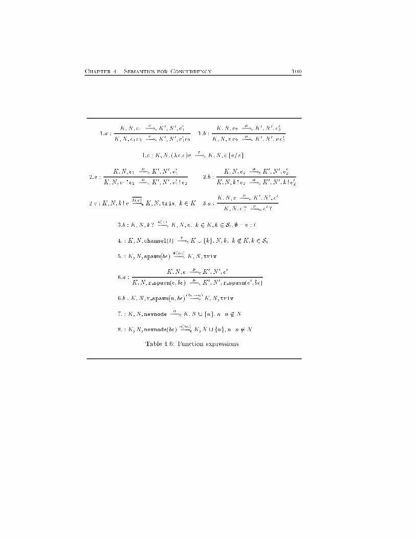
Chapter 4. Semantics for Concurrency 1001:a : K;N;e1 ��!eK 0;N 0; e01K;N; e1e2 ��!eK 0;N 0; e01e2 1:b : K;N; e2 ��!e K 0;N 0; e02K;N; v e2 ��!e K 0;N 0; v e021:c : K;N; (�x:e)v ��!e K;N; e fv=xg2:a : K;N; e1 ��!e K 0;N 0; e01K;N;e1 ! e2 ��!e K 0;N 0; e01 ! e2 2:b : K;N; e2 ��!e K 0;N 0; e02K;N; k ! e2 ��!e K 0;N 0; k ! e022:c : K;N; k ! v k(v)�!e K;N;triv; k 2 K 3:a : K;N; e ��!e K 0;N 0; e0K;N; e ? ��!e e0 ?3:b : K;N; k ? k(v)�!eK;N; v; k 2 K;k 2 St; ; ` v : t4: : K;N;channel(t) ��!e K [ fkg; N;k; k 62 K;k 2 St5: : K;N;spawn(be) �(be)�!eK;N;triv6:a : K;N; e ��!eK 0;N 0; e0K;N;r spawn(e; be) ��!eK 0;N 0;r spawn(e0; be)6:b : K;N;r spawn(n; be) (be!n)�!e K;N;triv7: : K;N;newnode n�!e K;N [ fng; n n 62 N8: : K;N;newnode(be) n(be)�!e K;N [ fng; n n 62 NTable 4.6: Function expressions.

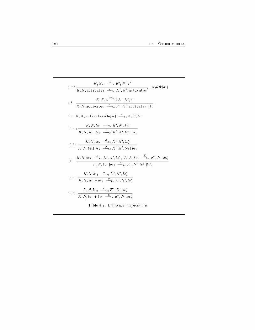
101 4.4. Other models9:a : K;N; e ��!e K 0;N 0; e0K;N;activatee ��!beK 0;N 0;activatee0 ; � 6= �(be)9:b : K;N; e �(be)�!e K 0;N 0; e0K;N;activatee ��!be K 0;N 0;activatee0jjbe9:c : K;N;activatecode(be) ��!beK;N;be10:a : K;N; be1 ��!beK 0;N 0; be01K;N; be1jjbe2 ��!beK 0;N 0; be01jjbe210:b : K;N; be2 ��!beK 0; N 0; be02K;N; be1jjbe2 ��!beK 0; N 0; be1jjbe0211: : K;N;be1 ��!be K 0;N 0; be01; K;N;be2 ��!be K 0;N 0; be02K;N; be1jjbe2 ��!beK 0;N 0; be01jjbe0212:a : K;N; be1 ��!beK 0;N 0; be01K;N; be1 + be2 ��!be K 0;N 0; be0112:b : K;N; be2 ��!beK 0;N 0; be02K;N; be1 + be2 ��!be K 0;N 0; be02Table 4.7: Behaviour expressions.

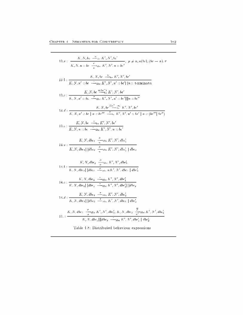
Chapter 4. Semantics for Concurrency 10213:a : K;N; be ��!beK 0;N 0; be0K;N;n :: be ��!dben K 0;N 0; n :: be0 ; � 6= n;n(be); (be! n); �13:b : K;N; be n�!be K 0;N 0; be0K;N;n0 :: be ��!dbe K 0;N 0; n0 :: be0jjjn :: terminate13:c : K;N; be n(be00)�!beK 0;N 0; be0K;N;n0 :: be ��!dbe K 0;N 0; n0 :: be0jjjn :: be0013:d : K;N; be (be00!n)�!be K 0;N 0; be0K;N;n0 :: bejjjn :: be000 ��!be K 0;N 0; n0 :: be0jjjn :: (be000jjbe00)13:e : K;N; be ��!be K 0;N 0; be0K;N;n :: be ��!dbe K 0;N 0; n :: be014:a : K;N; dbe1 ��!dben K 0; N 0; dbe01K;N;dbe1jjjdbe2 ��!dben K 0; N 0; dbe01jjjdbe214:b : K;N; dbe2 ��!dben K 0;N 0; dbe02K;N; dbe1jjjdbe2 ��!dbe nK 0;N 0; dbe1jjjdbe0214:c : K;N;dbe1 ��!dbeK 0;N 0; dbe01K;N; dbe1jjjdbe2 ��!dbeK 0;N 0; dbe01jjjdbe214:d : K;N; dbe2 ��!dbe K 0;N 0; dbe02K;N; dbe1jjjdbe2 ��!dbe K 0;N 0; dbe1jjjdbe0215: : K;N; dbe1 ��!dben K 0;N 0; dbe01;K;N; dbe2 ��!dben0 K 0;N 0; dbe02K;N; dbe1jjjdbe2 ��!dbeK 0;N 0; dbe01jjjdbe02Table 4.8: Distributed behaviour expressions.

Part IISemantic Descriptions103

Chapter 5Proved TransitionSystemWe present a very concrete transition system for �-calculus in which thelabels of transitions encode (a portion of) their deduction tree. We in-vestigate some structural properties of its states and transitions. Moreprecisely, we show that the proved transition system has the same statesof the standard transition system of �-calculus. Furthermore, its labelsuniquely identify the transitions exiting from an agent. Then, we de�nea �nite-branching early transition system of �-calculus. Finally, we intro-duce also an algebra of proved trees that induces a denotational semanticsfully abstract with the operational one for �-calculus without objects.5.1 Proved operational semanticsTo implement parametricity, we need a very detailed description of sys-tems. Following (Degano et al., 1985) and (Boudol & Castellani, 1988),we label transitions with encodings of their proofs. We start with thede�nition of the enriched labels (proof terms). In addition, we introduce afunction (`) that takes a proof term to the corresponding standard action105

Chapter 5. Proved Transition System 106label.De�nition 5.1.1 (proof terms) Let # 2 fjj0; jj1;+0;+1; (� x)g�. Thenthe set � of proof terms (with metavariable �) is de�ned by the followingsyntax � ::= #� j #hjj0#0�0; jj1#1�1iwith �0 = xz i� �1 is either xz or x(z), or vice versa.Function ` : �! Act is de�ned as`(��) = �; `(#hjj0#0�0; jj1#1�1i) = �:Note that in the above de�nition we have a tag (�x) for each name x.Symbol jj0 (jj1) means that the left (right) component of a parallel com-position is the active one in the �ring of a transition. Actually, tags jjirecords the applications of rules for parallel composition during a deriva-tion. Similarly, tag +0 (+1) records that the left (right) alternative of anondeterministic choice is chosen. Symbol (� x) says that there is a �lterover name x. For example, the proof termjj0(� b) +1 adescribes an action a that is the right alternative of a nondeterministicchoice (+1), passes successfully through the �lter (� b), and occurs in theleft location of a compound site (jj0).Since labels of transitions may be long wired, we write jjhi for a sequenceof h jji's. A similar convention holds for +i, as well.There is a proof term constructor for any operator of the languageapart from pre�x, matching and constant de�nitions.Functions fn, bn and n are extended to proof terms by letting themwork on the action part alone. Furthermore, we assume the structuralcongruence � on processes de�ned as the least congruence satisfying thefollowing clauses:� P and Q �-equivalent (they only di�er in the choice of bound names)) P � Q,� [x = x]P � P ,

107 5.1. Proved operational semantics� (�x)(�y)P � (�y)(�x)P; (�x)(R jS) � (�x)R jS if x 62 fn(S),(�x)(R jS) � R j (�x)S if x 62 fn(R), and (�x)P � P if x 62 fn(P ).Note that j and + are neither associative nor commutative. However,when studying behavioural properties of systems (after the relabelling oftransitions in the model selected) the commutativity and associativity ofthe two operators may be recovered if of importance. Our choice is onlyneeded to have a low level model that contains as much information asnecessary to recover many distinct semantic models. Another consequenceof j being not commutative is the additional clause with respect to thestandard de�nition for (�x)(RjS) in the third item of the de�nition of �.The early proved transition system of �-calculus is de�ned below.Again, the transitions in the conclusion of each rule stand for all theirvariants.De�nition 5.1.2 (early proved transition system) The early provedtransition system of �-calculus is the triple PTS = (P;�;�!). The tran-sition relation is de�ned by the axiom and rules in Tab. 5.1 (where thesymmetric rules for communications are omitted). Hereafter, we write[P ]pts for (P;�;�!; P ) (the portion of PTS with P as initial state).Our early proved transition system of �-calculus di�ers from the stan-dard one in the rules for parallel composition and communication. RulePar0 (Par1) adds to the label a tag jj0 (jj1) to record that the left (right)component is moving. The rules Com0 and Close0 have in their con-clusion a pair instead of a � to record the components which interacted.Their symmetric version Com1 and Close1 should be obvious. Also rulesfor summation and restriction are slightly modi�ed by adding in theirconclusions tags +i or (� x), respectively.As in Sect. 4.1, we can de�ne a late proved operational semantics.We only need to replace free input with bound input and to modify thede�nition of the transition relation. The late operational semantics isreported in Tab. 5.2.The following proposition shows how standard and proved operationalsemantics of �-calculus are related. Its proof is similar to the one of

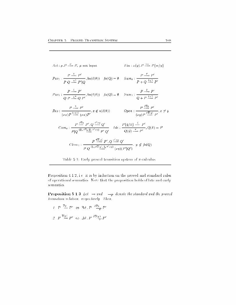
Chapter 5. Proved Transition System 108Act : �:P ��! P; � not input Ein : x(y):P xw�! Pfw=ygPar0 : P ��! P 0P jQ jj0��! P 0jQ; bn(`(�)) \ fn(Q) = ; Sum0 : P ��! P 0P +Q +0��! P 0Par1 : P ��! P 0QjP jj1��! QjP 0 ; bn(`(�)) \ fn(Q) = ; Sum1 : P ��! P 0Q+ P +1��! P 0Res : P ��! P 0(�x)P (�x)��! (�x)P 0 ; x 62 n(`(�)) Open : P #xy�! P 0(�y)P #x(y)�! P 0 ; x 6= yCom0 : P #xy�! P 0;Q #0xy�! Q0P jQ hjj0#xy;jj1#0xyi�! P 0jQ0 Ide : Pf~y=~xg ��! P 0Q(~y) ��! P 0 ;Q(~x) = PClose0 : P #x(y)�! P 0;Q #0xy�! Q0P jQ hjj0#x(y);jj1#0xyi�! (�y)(P 0jQ0) ; y 62 fn(Q)Table 5.1: Early proved transition system of �-calculus.Proposition 4.1.2, i.e. it is by induction on the proved and standard rulesof operational semantics. Note that the proposition holds of late and earlysemantics.Proposition 5.1.3 Let �! and �!P denote the standard and the provedtransition relation, respectively. Then,1. P xy�! P 0 , 9# : P #xy�!P P 02. P x(y)�! P 0 , 9# : P #x(y)�!P P 0

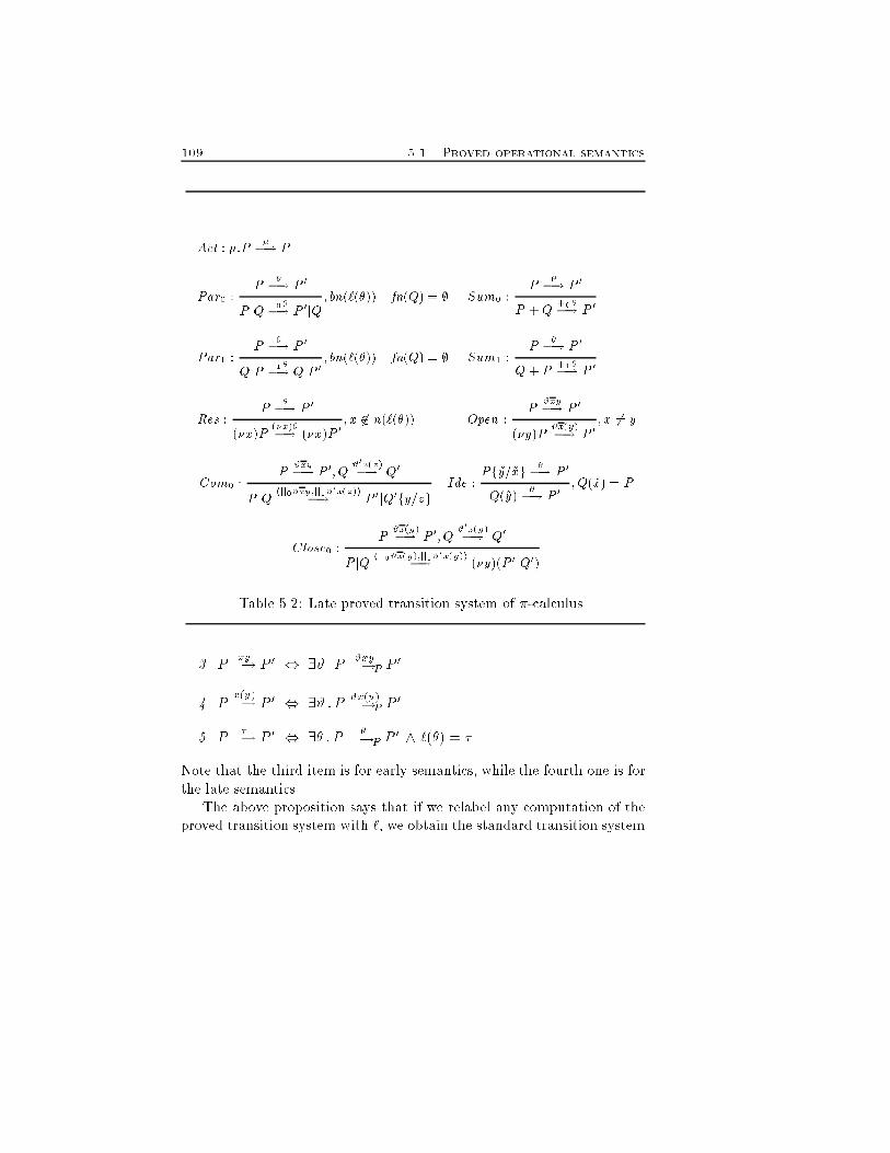
109 5.1. Proved operational semanticsAct : �:P ��! PPar0 : P ��! P 0P jQ jj0��! P 0jQ; bn(`(�)) \ fn(Q) = ; Sum0 : P ��! P 0P +Q +0��! P 0Par1 : P ��! P 0QjP jj1��! QjP 0 ; bn(`(�)) \ fn(Q) = ; Sum1 : P ��! P 0Q+ P +1��! P 0Res : P ��! P 0(�x)P (�x)��! (�x)P 0 ; x 62 n(`(�)) Open : P #xy�! P 0(�y)P #x(y)�! P 0 ; x 6= yCom0 : P #xy�! P 0;Q #0x(z)�! Q0P jQ hjj0#xy;jj1#0x(z)i�! P 0jQ0fy=zg Ide : Pf~y=~xg ��! P 0Q(~y) ��! P 0 ;Q(~x) = PClose0 : P #x(y)�! P 0;Q #0x(y)�! Q0P jQ hjj0#x(y);jj1#0x(y)i�! (�y)(P 0jQ0)Table 5.2: Late proved transition system of �-calculus.3. P xy�! P 0 , 9# : P #xy�!P P 04. P x(y)�! P 0 , 9# : P #x(y)�!P P 05. P ��! P 0 , 9� : P ��!P P 0 ^ `(�) = �Note that the third item is for early semantics, while the fourth one is forthe late semantics.The above proposition says that if we relabel any computation of theproved transition system with `, we obtain the standard transition system

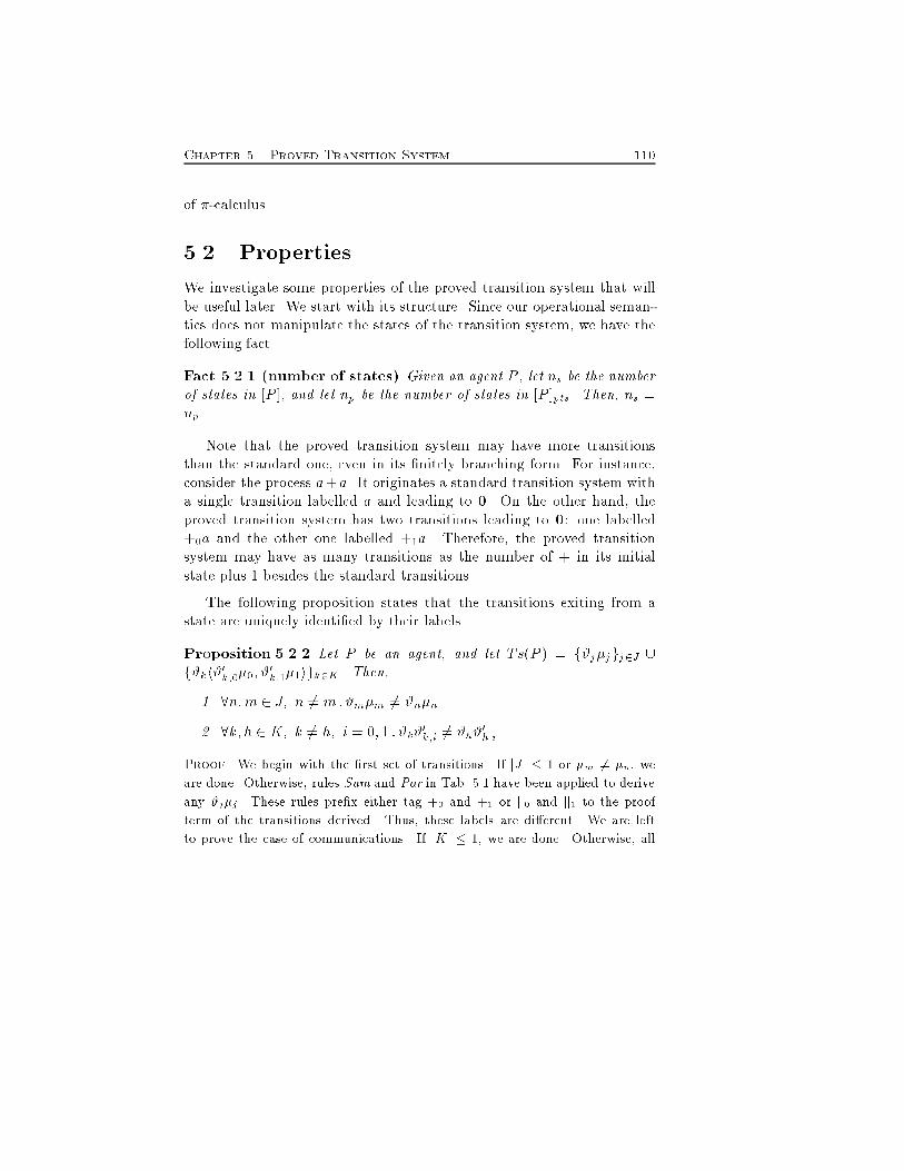
Chapter 5. Proved Transition System 110of �-calculus.5.2 PropertiesWe investigate some properties of the proved transition system that willbe useful later. We start with its structure. Since our operational seman-tics does not manipulate the states of the transition system, we have thefollowing fact.Fact 5.2.1 (number of states) Given an agent P , let ns be the numberof states in [P ], and let np be the number of states in [P ]pts. Then, ns =np.Note that the proved transition system may have more transitionsthan the standard one, even in its �nitely branching form. For instance,consider the process a+a. It originates a standard transition system witha single transition labelled a and leading to 0. On the other hand, theproved transition system has two transitions leading to 0: one labelled+0a and the other one labelled +1a. Therefore, the proved transitionsystem may have as many transitions as the number of + in its initialstate plus 1 besides the standard transitions.The following proposition states that the transitions exiting from astate are uniquely identi�ed by their labels.Proposition 5.2.2 Let P be an agent, and let Ts(P ) = f#j�jgj2J [f#kh#0k;0�0; #0k;1�1igk2K . Then,1. 8n;m 2 J; n 6= m:#m�m 6= #n�n2. 8k; h 2 K; k 6= h; i = 0; 1 : #k#0k;i 6= #h#0h;i.Proof. We begin with the �rst set of transitions. If jJ j � 1 or �m 6= �n, weare done. Otherwise, rules Sum and Par in Tab. 5.1 have been applied to deriveany #j�j. These rules pre�x either tag +0 and +1 or jj0 and jj1 to the proofterm of the transitions derived. Thus, these labels are di�erent. We are leftto prove the case of communications. If jKj � 1, we are done. Otherwise, all

111 5.2. Propertiescommunications are generated by the application of the rules Com or Close inTab. 5.1. Since jKj> 1, process P must contain at least a + or a j, besides theone which calls for the communication. Thus at least a Sum or a Par rule isapplied to �ll the premises of either Com or Close or to complete the derivationof the transition considered after the application of either Com or Close. Let#kh#0k;0�0; #0k;1�1i be the transition generated by the application of either Comor Close. Then, #0k;0, #0k;1 and #k are as the transitions of item 1 and the proofis concluded. 2Note that in communicationswe do not consider the actions of the partnersbecause the object of the input is �xed by the one of the output in theearly semantics and it is only a placeholder in the late semantics.The following corollary states that the transitions of an agent in whichno object appears are uniquely identi�ed by the proof part of their labels.The proof is immediate from Proposition 5.2.2 by noting that the sequen-tial components of an agent without objects can originate at most a singletransition within a �xed context with respect to +.Corollary 5.2.3 Let P be an agent without objects, and letTs(P ) = f#j�jgj2J [ f#kh#0k;0�0; #0k;1�1igk2K :Then,1. 8n;m 2 J; n 6= m:#m 6= #n2. 8k; h 2 K; k 6= h; i = 0; 1 : #k#0k;i 6= #h#0h;i.The corollary does not hold for �-calculus in general. In fact consider theprocess x(y):P jQthat can originate for instance the two transitionsjj0xz�! and jj0xy�! :Proposition 5.2.2 allows us to write � for a transition P ��! P 0 whenno ambiguity can arise. Similarly, we can write Ts(P ) = f�jP ��! P 0g forthe transitions that exit from P .

Chapter 5. Proved Transition System 112The behaviour of agents is determined by visiting the transition sys-tem. Indeed, any walk in the transition system is a possible computationof the agent. As usual, computations of agents can be conveniently orga-nized in trees, that we call proved trees. They are expressed in the usualalgebraic form.De�nition 5.2.4 (proved tree) The proved tree associated to an agentP is [P ]pt = Pi2I �i � [Pi]pt where 8i 2 I : �i 2 Ts(P ). The set of provedtrees originated by agents is denoted by PT .Actually, the proved tree [P ]pt is the unfolding of the proved transitionsystem [P ]pts.The structure of trees and Proposition 5.2.2 allows us to state thefollowing corollary.Corollary 5.2.5 Any transition of a proved tree [P ]pt is uniquely deter-mined by a pair (�; n), where n is its distance from the root.5.3 Finite branching early semanticsWe now de�ne an early proved transition system of �-calculus that is �nitebranching. We need to limit the transitions that are originated by rulesEin and Open in Tab. 5.1 (see Subsect. 4.1.4).Consider the process P = x(y):[y = z]P 0Although it originates in�nite many transitions by rule Ein, only two ofthem completely characterize its behaviour. In fact, if P reads name z,it will let its residual P 0 to proceed, otherwise it will not. This examplesuggests to partition the set of possible inputs into the names which mayhave e�ects on the future behaviour of the residual of the input and thosewhich may have not. According to (Montanari & Pistore, 1995a), the �rstset identi�es the active names of an agent, while the second set speci�esthe non active ones. Then, we only need to derive a transition for any

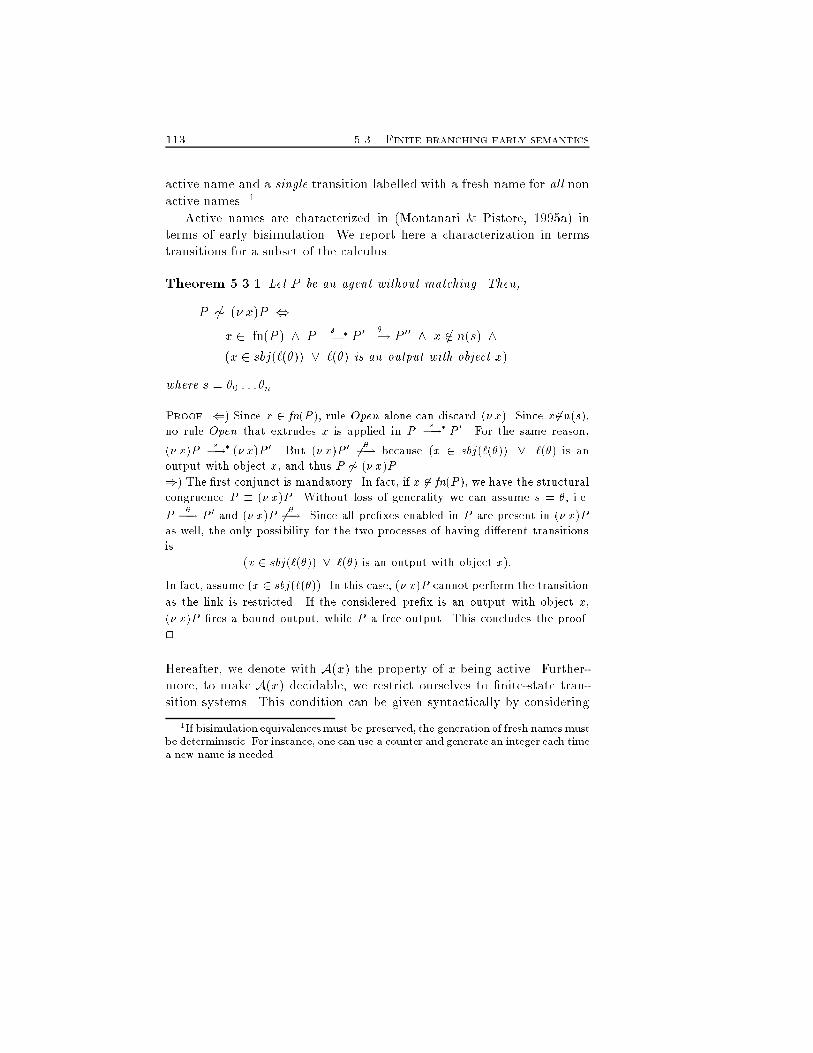
113 5.3. Finite branching early semanticsactive name and a single transition labelled with a fresh name for all nonactive names. 1Active names are characterized in (Montanari & Pistore, 1995a) interms of early bisimulation. We report here a characterization in termstransitions for a subset of the calculus.Theorem 5.3.1 Let P be an agent without matching. Then,P 6� (� x)P ,x 2 fn(P ) ^ P s�!� P 0 ��! P 00 ^ x 62 n(s) ^(x 2 sbj(`(�)) _ `(�) is an output with object x)where s = �0 : : : �n.Proof. () Since x 2 fn(P ), rule Open alone can discard (� x). Since x62n(s),no rule Open that extrudes x is applied in P s�!� P 0. For the same reason,(� x)P s�!� (� x)P 0. But (� x)P 0 6 ��! because (x 2 sbj(`(�)) _ `(�) is anoutput with object x, and thus P 6� (� x)P .)) The �rst conjunct is mandatory. In fact, if x 62 fn(P ), we have the structuralcongruence P � (� x)P . Without loss of generality we can assume s = �, i.e.P ��! P 0 and (� x)P 6 ��!. Since all pre�xes enabled in P are present in (� x)Pas well, the only possibility for the two processes of having di�erent transitionsis (x 2 sbj(`(�)) _ `(�) is an output with object x):In fact, assume (x 2 sbj(`(�)). In this case, (� x)P cannot perform the transitionas the link is restricted. If the considered pre�x is an output with object x,(� x)P �res a bound output, while P a free output. This concludes the proof.2Hereafter, we denote with A(x) the property of x being active. Further-more, to make A(x) decidable, we restrict ourselves to �nite-state tran-sition systems. This condition can be given syntactically by considering1If bisimulation equivalences must be preserved, the generation of fresh names mustbe deterministic. For instance, one can use a counter and generate an integer each timea new name is needed.

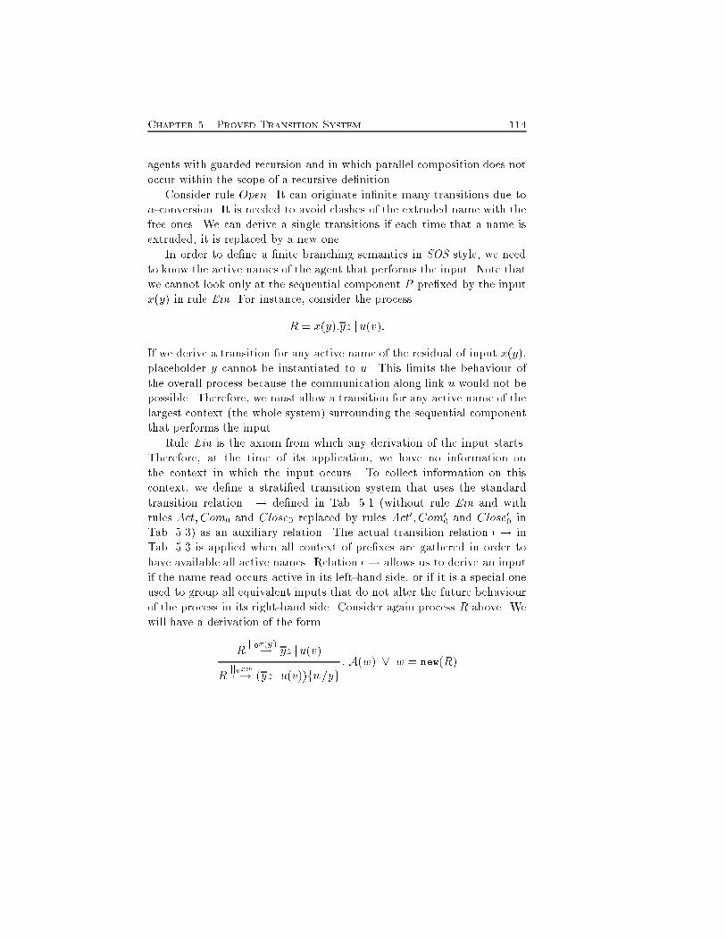
Chapter 5. Proved Transition System 114agents with guarded recursion and in which parallel composition does notoccur within the scope of a recursive de�nition.Consider rule Open. It can originate in�nite many transitions due to�-conversion. It is needed to avoid clashes of the extruded name with thefree ones. We can derive a single transitions if each time that a name isextruded, it is replaced by a new one.In order to de�ne a �nite branching semantics in SOS style, we needto know the active names of the agent that performs the input. Note thatwe cannot look only at the sequential component P pre�xed by the inputx(y) in rule Ein. For instance, consider the processR = x(y):yz ju(v):If we derive a transition for any active name of the residual of input x(y),placeholder y cannot be instantiated to u. This limits the behaviour ofthe overall process because the communication along link u would not bepossible. Therefore, we must allow a transition for any active name of thelargest context (the whole system) surrounding the sequential componentthat performs the input.Rule Ein is the axiom from which any derivation of the input starts.Therefore, at the time of its application, we have no information onthe context in which the input occurs. To collect information on thiscontext, we de�ne a strati�ed transition system that uses the standardtransition relation �! de�ned in Tab. 5.1 (without rule Ein and withrules Act; Com0 and Close0 replaced by rules Act0; Com00 and Close00 inTab. 5.3) as an auxiliary relation. The actual transition relation 7�! inTab. 5.3 is applied when all context of pre�xes are gathered in order tohave available all active names. Relation 7�! allows us to derive an inputif the name read occurs active in its left-hand side, or if it is a special oneused to group all equivalent inputs that do not alter the future behaviourof the process in its right-hand side. Consider again process R above. Wewill have a derivation of the formR jj0x(y)�! yz ju(v)R jj0xw7�! (yz ju(v))fw=yg ; A(w) _ w = new(R)

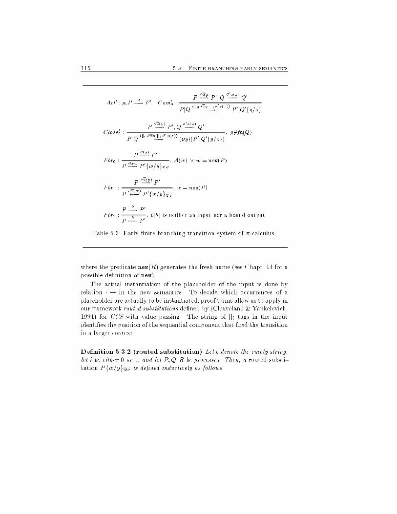
115 5.3. Finite branching early semanticsAct0 : �:P ��! P 0 Com00 : P #xy�! P 0;Q #0x(z)�! Q0P jQ hjj0#xy;jj1#0x(z)i�! P 0jQ0fy=zgClose00 : P #x(y)�! P 0;Q #0x(z)�! Q0P jQ hjj0#xy;jj1#0x(z)i�! (�y)(P 0jQ0fy=zg) ; y 62fn(Q)Fbr0 : P #(y)�! P 0P #xw7�! P 0fw=yg@# ; A(w) _ w = new(P )Fbr1 : P #x(y)�! P 0P #x(w)7�! P 0fw=yg@# ; w = new(P )Fbr2 : P ��! P 0P �7�! P 0 ; `(�) is neither an input nor a bound outputTable 5.3: Early �nite branching transition system of �-calculus.where the predicate new(R) generates the fresh name (see Chapt. 14 for apossible de�nition of new).The actual instantiation of the placeholder of the input is done byrelation 7�! in the new semantics. To decide which occurrences of aplaceholder are actually to be instantiated, proof terms allow us to apply inour framework routed substitutions de�ned by (Cleaveland & Yankelevich,1994) for CCS with value passing. The string of jji tags in the inputidenti�es the position of the sequential component that �red the transitionin a larger context.De�nition 5.3.2 (routed substitution) Let � denote the empty string,let i be either 0 or 1, and let P;Q;R be processes. Then, a routed substi-tution Pfw=yg@# is de�ned inductively as follows.

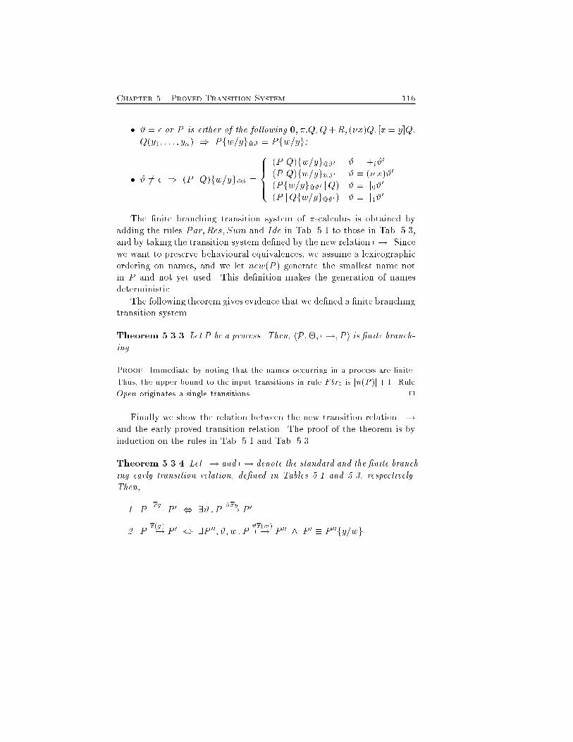
Chapter 5. Proved Transition System 116� # = � or P is either of the following 0; �:Q;Q+R; (�x)Q; [x= y]Q;Q(y1; : : : ; yn) ) Pfw=yg@# = Pfw=yg;� # 6= � ) (P jQ)fw=yg@# = 8>><>>: (P jQ)fw=yg@#0 # = +i#0(P jQ)fw=yg@#0 # = (� x)#0(Pfw=yg@#0 jQ) # = jj0#0(P jQfw=yg@#0) # = jj1#0The �nite branching transition system of �-calculus is obtained byadding the rules Par;Res; Sum and Ide in Tab. 5.1 to those in Tab. 5.3,and by taking the transition system de�ned by the new relation 7�!. Sincewe want to preserve behavioural equivalences, we assume a lexicographicordering on names, and we let new(P ) generate the smallest name notin P and not yet used. This de�nition makes the generation of namesdeterministic.The following theorem gives evidence that we de�ned a �nite branchingtransition system.Theorem 5.3.3 Let P be a process. Then, hP;�; 7�!; P i is �nite branch-ing.Proof. Immediate by noting that the names occurring in a process are �nite.Thus, the upper bound to the input transitions in rule Fbr0 is jn(P )j+1. RuleOpen originates a single transitions. 2Finally we show the relation between the new transition relation 7�!and the early proved transition relation. The proof of the theorem is byinduction on the rules in Tab. 5.1 and Tab. 5.3.Theorem 5.3.4 Let �! and 7�! denote the standard and the �nite branch-ing early transition relation, de�ned in Tables 5.1 and 5.3, respectively.Then,1. P xy�! P 0 , 9# : P #xy7�! P 02. P x(y)�! P 0 , 9P 00; #; w : P #x(w)7�! P 00 ^ P 0 � P 00fy=wg

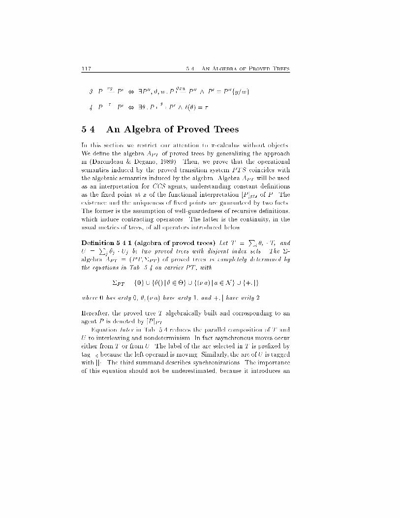
117 5.4. An Algebra of Proved Trees3. P xy�! P 0 , 9P 00; #; w : P #xw7�! P 00 ^ P 0 � P 00fy=wg4. P ��! P 0 , 9� : P �7�! P 0 ^ `(�) = �5.4 An Algebra of Proved TreesIn this section we restrict our attention to �-calculus without objects.We de�ne the algebra APT of proved trees by generalizing the approachin (Darondeau & Degano, 1989). Then, we prove that the operationalsemantics induced by the proved transition system PTS coincides withthe algebraic semantics induced by the algebra. Algebra APT will be usedas an interpretation for CCS agents, understanding constant de�nitionsas the �xed point at x of the functional interpretation [P ]pts of P . Theexistence and the uniqueness of �xed points are guaranteed by two facts.The former is the assumption of well-guardedness of recursive de�nitions,which induce contracting operators. The latter is the continuity, in theusual metrics of trees, of all operators introduced below.De�nition 5.4.1 (algebra of proved trees) Let T = Pi �i � Ti andU = Pj �j � Uj be two proved trees with disjoint index sets. The �-algebra APT = (PT;�PT ) of proved trees is completely determined bythe equations in Tab. 5.4 on carrier PT , with�PT = f0g [ f�() j � 2 �g [ f(� a) j a 2 Ng [ f+; jgwhere 0 has arity 0, �; (� a) have arity 1, and +; j have arity 2.Hereafter, the proved tree T algebraically built and corresponding to anagent P is denoted by [P ]PT .Equation Inter in Tab. 5.4 reduces the parallel composition of T andU to interleaving and nondeterminism. In fact asynchronous moves occureither from T or from U . The label of the arc selected in T is pre�xed bytag jj0 because the left operand is moving. Similarly, the arc of U is taggedwith jj1. The third summand describes synchronizations. The importanceof this equation should not be underestimated, because it introduces an

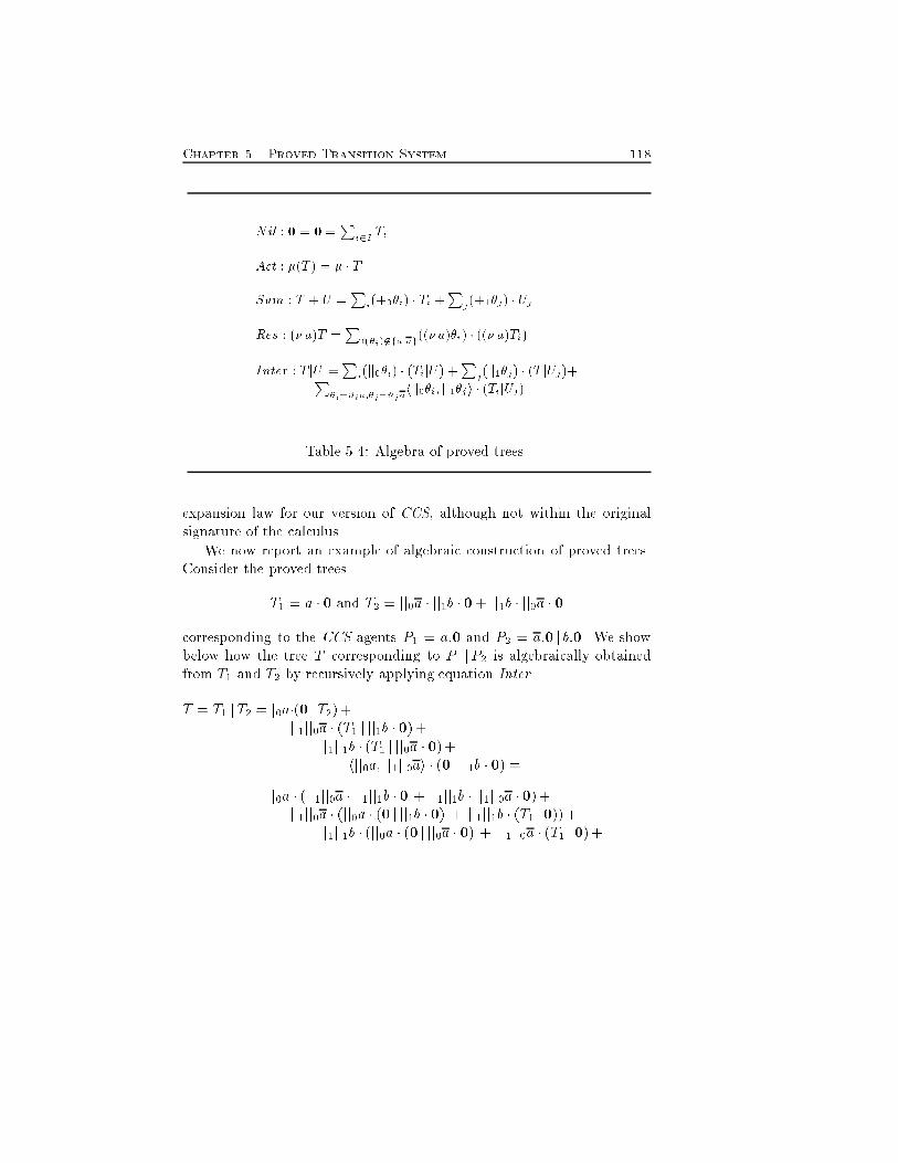
Chapter 5. Proved Transition System 118Nil : 0 = 0 =Pi2; TiAct : �(T ) = � � TSum : T + U =Pi(+0�i) � Ti +Pj(+1�j) � UjRes : (� a)T =P`(�i)62fa;ag((� a)�i) � ((� a)Ti)Inter : T jU =Pi(jj0�i) � (TijU) +Pj(jj1�j) � (T jUj)+P�i=#ia;�j=#jahjj0�i; jj1�ji � (TijUj)Table 5.4: Algebra of proved trees.expansion law for our version of CCS, although not within the originalsignature of the calculus.We now report an example of algebraic construction of proved trees.Consider the proved treesT1 = a � 0 and T2 = jj0a � jj1b � 0+ jj1b � jj0a � 0corresponding to the CCS agents P1 = a:0 and P2 = a:0 j b:0. We showbelow how the tree T corresponding to P1 jP2 is algebraically obtainedfrom T1 and T2 by recursively applying equation Inter.T = T1 jT2 =jj0a�(0 jT2)+jj1jj0a � (T1 j jj1b � 0)+jj1jj1b � (T1 j jj0a � 0)+hjj0a; jj1jj0ai � (0 j jj1b � 0) =jj0a � (jj1jj0a � jj1jj1b � 0 + jj1jj1b � jj1jj0a � 0)+jj1jj0a � (jj0a � (0 j jj1b � 0) + jj1jj1b � (T1 j0))+jj1jj1b � (jj0a � (0 j jj0a � 0) + jj1jj0a � (T1 j0)+

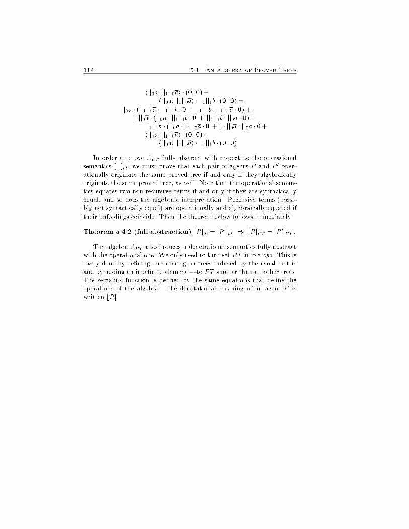
119 5.4. An Algebra of Proved Treeshjj0a; jj1jj0ai � (0 j0)+hjj0a; jj1jj0ai � jj1jj1b � (0 j0) =jj0a � (jj1jj0a � jj1jj1b � 0 + jj1jj1b � jj1jj0a � 0)+jj1jj0a � (jj0a � jj1jj1b � 0 + jj1jj1b � jj0a � 0)+jj1jj1b � (jj0a � jj1jj0a � 0 + jj1jj0a � jj0a � 0+hjj0a; jj1jj0ai � (0 j0)+hjj0a; jj1jj0ai � jj1jj1b � (0 j0)In order to prove APT fully abstract with respect to the operationalsemantics [�]pt, we must prove that each pair of agents P and P 0 oper-ationally originate the same proved tree if and only if they algebraicallyoriginate the same proved tree, as well. Note that the operational seman-tics equates two non recursive terms if and only if they are syntacticallyequal, and so does the algebraic interpretation. Recursive terms (possi-bly not syntactically equal) are operationally and algebraically equated iftheir unfoldings coincide. Then the theorem below follows immediately.Theorem 5.4.2 (full abstraction) [P ]pt = [P 0]pt , [P ]PT = [P 0]PT :The algebra APT also induces a denotational semantics fully abstractwith the operational one. We only need to turn set PT into a cpo. This iseasily done by de�ning an ordering on trees induced by the usual metricand by adding an inde�nite element ? to PT smaller than all other trees.The semantic function is de�ned by the same equations that de�ne theoperations of the algebra. The denotational meaning of an agent P iswritten [[P ]].

Chapter 5. Proved Transition System 120

Chapter 6Non InterleavingSemanticsWe introduce some non interleaving relations and we show how they caninduce non interleaving semantics through relabelling of the proved tran-sition system. We de�ne a new notion of causality di�erent from the clas-sical one. We point out a basic di�erence between temporal constraintsand causality. A temporal relation between two transitions does not im-ply that the �rst transition in uences the second one. The union of thetwo notions originates an enabling relation that was usually called causal-ity in the literature. We study concurrency and independence, as well.Concurrency is the complement of enabling, while independence is thecomplement of causality. We show that enabling is una�ected by shu�ingof concurrent transitions. The proved transition system permits us to de-�ne higher dimension transition systems whose transitions are labelled bysets of actions that represent concurrent activities. Our proposal appliesto higher-order calculi such as HO� or Plain CHOCS with little or nochanges. We compare the semantics induced by the above relations andtheir bisimulation based equivalences. We compare our semantics with theones presented in the literature for �-calculus and CCS, as well. Finally,we present the causal transition system which entails extending the syntax121

Chapter 6. Non Interleaving Semantics 122of processes to yield directly the causal relabelled proved computations.6.1 Non interleaving relationsIn the literature there are essentially two kinds of non-interleaving seman-tics, namely the causal (Pratt, 1986; Winskel, 1987; Boudol & Castellani,1988; Darondeau & Degano, 1989; Degano et al., 1990; Jategaonkar, 1993;Boreale & Sangiorgi, 1995; Montanari & Pistore, 1995b; Busi & Gorri-eri, 1995; Jategaonkar Jagadeesan & Jagadeesan, 1995) and the local one(Kiehn, 1991; Aceto, 1992; Montanari & Yankelevich, 1992; Boudol et al.,1993; Amadio & Prasad, 1994; Sangiorgi, 1994). Many subtle aspectsstill have to be clari�ed when considering �-calculus, especially relatedto the explicit distinction between input and output actions and to thedependencies induced by the usage of names.Causality is usually described in the literature regardless of the e�ectsthat the causing activity has on the caused one. In fact, it is su�cient fora to cause b that a occurs before b. This relation is an enabling relationrather than a causal one because amayhave no e�ect at all on b. Hereafter,we refer to this kind of relation as enabling. More precisely, we say thatan activity a enables an activity b i� a is a necessary conditionfor b.As links in �-calculus are directed, i.e. the sender and the receiver areidenti�ed in a communication, a better account can be given to causality.We instantiate the notion of e�ect by (Milner, 1992a), and the idea ofread-write causality introduced in (Priami & Yankelevich, 1994) for CCS.More precisely, we say thatan activity a causes an activity b i� a is a necessary conditionfor b and the execution of a in uences the execution of b.To show that enabling is quite di�erent from causality, consider theprocess(� x)(a:xy:bjc:x(z):dz) (6.1)

123 6.1. Non interleaving relationsand its computation(� x)(a:xy:bjc:x(z):dz) c�! (� x)(a:xy:bjx(z):dz) a�! (6.2)a�! (� x)(xy:bjx(z):dz) ��! (� x)(bjdy)According to (Milner, 1992a), the e�ect of the communication in uencesonly dy, the residual of the receiver of y. On the contrary, b is una�ectedbecause no ow of information is possible from c to b. Thus, we statethat there is no causal relation between c and b. Instead the two actionsare related by enabling because communication is hand-shaking and canoccur only when both partners are ready to proceed. Therefore, c mustalways occur before b. Asynchronous implementations of communications,typically through a bu�er, make even more evident the di�erence betweenenabling and causality. In this case, the sender writes a value in the bu�erand leaves its residual to proceed. The receiver reads the value from thebu�er and passes it to its own residual. In our example, the input of y onlink x can overlap with or even follow in time the execution of b, so thereis no e�ect of c over b.On the contrary, the communication induces a causal dependency be-tween a and dy. The e�ect of the communication on the residual of thereader is made evident by the instantiation of placeholder z to y. Weclaim that this notion of causality is suitable for mobile processes, be-cause it gives a more faithful account of the e�ects of a communication.Also, it can model both a synchronous, hand-shake implementation ofcommunications and an asynchronous one.From the above description of enabling and causality appears that theformer relation contains the latter one. We now investigate what is thedi�erence of the two relations. Consider the enabling relation between cand b in (6.2). The two actions are not related by causality. They areonly temporally dependent, i.e. c has implicitly got some precedence overb. Thus, we say thatan activity a has precedence over an activity b i� a is a nec-essary condition for b and the execution of a does not in uencethe execution of b.

Chapter 6. Non Interleaving Semantics 124In the example above, c does not in uence b because there is no ow ofvalues from the second component of the parallel composition to the �rstone. The characterization of precedence shows that enabling is the unionof causality and precedence.Another relation that we want to investigate is concurrency. This re-lation expresses which are the activities that can occur in parallel. There-fore, it must be time independent. Consider again the computation (6.2).Actions a and c are concurrent because there is neither a causal nor atemporal constraint between them. Actually, concurrency turns out to bethe complement of enabling. An independent description istwo activities a and b are concurrent i� they can be executedin any temporal ordering.The distinction between enabling and causality introduces another re-lation that is called independence. Two activities are independent whenneither of them has any e�ect on the calculation made by the other. How-ever, independent transitions may be forced to occur in a �xed temporalordering. An example of independent transitions in computation (6.2) arec and b. In this sense, independence is the complement of causality and isobtained by joining concurrency and precedence. Independence says thatan activity a and an activity b are independent i� the execu-tion of either of them does not in uence the execution of theother.Note that concurrency is contained in independence. In fact, if a and bcan occur in any order, they cannot in uence each other.We may de�ne a relation that is the complement of precedence, aswell. It says simply that an activity a and an activity b are related i� theexecution of a in uences the execution of b or if a and b are concurrent.This relation as well contains concurrency. We do not consider here thisrelation. The interested reader can de�ne it similarly to independence byreplacing causality with precedence.The last relation we consider is locality. Essentially, it describes thedistribution of resources. Two activities are related by locality if theyoccur at the same location. There are various approaches to describe

125 6.1. Non interleaving relationslocations. The assignment of locations can be either static or dynamic.In the former case, the parallel structure of processes is �xed at the toplevel of the description. In the dynamic case, new locations are generatedas soon as possible. For instance, the processa(x):(P jQ)originates a single location in the static approach, while the unique loca-tion is divided into two sub-locations after the input in the dynamic case.In general, we say thatan activity a and an activity b have a locality relation if bothoccurs at the same location.The relations above have been exempli�ed by showing structural de-pendencies, i.e. dependencies originated by the syntactic (actually theparallel) structure of processes. We now show examples of dependenciesoriginated by the usage of names. For example, inP = (� a)(xajay)the output on the link a in can occur only if a has been extruded by x(a).The in uence of the bound output on x(a) is evident because it operatesa scope extrusion on name a that is made visible. The causal dependencybetween the two actions is mandatory because the external behaviour ofP coincides with the one of (� a)xa:ay. Analogously, inQ = y(a):axthe output occurs on the channel read along link y, thus it depends on theinput. We will show later that a link dependency due to an input turnsout to be structural as well. Note that we establish a causal dependencyonly when an action uses as link a name bound by another. On the otherhand, if the extruded name (or the variable instantiated by an input) isthe value sent by an output no causality appears due to links. For examplein (� a)(xajya)

Chapter 6. Non Interleaving Semantics 126both components can extrude and thus they are causally independent, al-though not temporally independent. In fact, �rst a component extrudes,and then the other can only perform a free output. This shows a di�erentkind of precedence than the one established by a (synchronous) communi-cation. This kind of precedence as well can disappear if a higher-dimensiontransition models the simultaneous occurrence of two (or more) indepen-dent transitions (see Subsection 6.5.4, where a transition is labelled by aset of actions). In the above example, one can have the transition(� a)(xa j ya) (� a)fxa;yag�! 0 j0in which no precedence appears. However, this transition can be betterunderstood as an atomic sequence of two steps. The �rst is the invocationof a global manager of names that generates the fresh name a. The secondis the concurrent �ring of two free outputs.Throughout this chapter, we use a simpli�ed version of the proved transi-tion system. In fact, the only information that we need to recover the noninterleaving relations introduced above concerns the parallel structure ofprocesses. We consider proof terms with # 2 fjj0; jj1g�. This implies thatnondeterministic composition becomes commutative. Hence, we add tothe rules which de�ne the structural congruence on processes the follow-ing� (P=�;+;0) is a commutative monoid,and we replace the two rules Sum0 and Sum1 in Tab. 5.1 withSum : P ��! P 0P + Q ��! P 0Since we do not record anymore the information on restricted names inproof terms, also rule Res in Tab. 5.1 is replaced byRes : P ��! P 0(� x)P ��! (� x)P 0 ; x 62 n(`(�)):

127 6.2. CausalityFurthermore, we assume that any computation is fresh. Intuitively, ina fresh computation all names exported by an extrusion or imported byan input are never used in the preceding transitions (Boreale & Sangiorgi,1995). For a constructive operational de�nition of fresh computations seeChapter 14.De�nition 6.1.1 (fresh computation) A computation P0 �0�! P1 �1�!: : : is fresh when 8i � 0 if `(�i) = x(a) or `(�i) = xa, then a \ fn(Pi) = ;and 8j < i, a \ n(`(�j)) = ;; in this case we say that name a has beenintroduced in �i.Hereafter we consider only fresh computations, and we omit the adjectivefresh.In the next sections we de�ne the relations mentioned above and weshow how they can induce non interleaving semantics on �-calculus pro-cesses.6.2 CausalityThe notion of causality shows which transitions have an e�ect on theones that come later. We now de�ne the notion of dependency on thetransitions that occur in a computation. From this, it is straightforward torecover the more standard representation of causality as a partial orderingof events (a similar construction is in Subsect. 6.5.2).Following (Boreale & Sangiorgi, 1995), we consider two kinds of de-pendencies: those induced by the structure of processes (called structural),and those originated when names are bound (called link). Our transitionswill be labelled by an action, and by a combination of structural and linkdependencies. The two kinds of dependencies are kept distinct, since itcould be useful to examine the structure of control separately from theone induced by the ow of names. This separation allows us to reduce thenumber of events to be inspected, for instance when debugging a system,thus improving the e�ciency of the analysis. Furthermore, the distinctionbetween structural and link dependencies simpli�es the presentation.

Chapter 6. Non Interleaving Semantics 128Structural dependencies are similar to the read-write causality de�nedfor CCS in (Priami & Yankelevich, 1994): when a communication occurs,the sender transmits its causes to the residual of the receiver as well, butnot vice versa. Indeed, reading a name cannot causally a�ect the evolutionof the residual of the sender, while it may, and usually does, a�ect theevolution of the receiver. This re ects the e�ect of a communication asintroduced in (Milner, 1992a).Link dependencies are established when an action uses as its link aname bound by another through an input or an extrusion.The next sub-section de�nes the causal relation, while in Subsect. 6.2.2we justify the introduction of the new kind of causality.6.2.1 Causal relationThe de�nition of causality between the transitions of a computation isgiven in three steps. Roughly speaking, the �rst concerns structural de-pendencies. In the case of asynchronous transitions, it says that a tran-sition labelled #� depends on a previous transition labelled #0�0 if #0 is apre�x of # (the tuning needed to cover communications is made precisebelow). The underlying idea is that the two transitions have been derivedusing the same initial set of rules and are thus nested in a pre�x chain (orthey are connected by communications in a similar way).De�nition 6.2.1 (structural dependency)Let P0 �0�! P1 �1�! : : : �n�! Pn+1 be a proved computation, and hereafter leti; j 2 f0; 1g. Then, �n has a direct structural dependency on �h (written�h v1str �n) i� either� �n = #�, �h = #0�0 and #0 is a pre�x of #; or� �n = #�, �h = #0h#00�00; #01�01i and 9i : #0#0i is a pre�x of #; or� �n = #h#0�0; #1�1i, �h = #0�0, 9i : #0 is a pre�x of ##i and �i is anoutput; or� �n = #h#0�0; #1�1i, �h = #0h#00�00; #01�01i), 9i; j : #0#0j is a pre�x of##i and �i is an output.

129 6.2. CausalityThe structural dependencies of �n are obtained by the re exive and tran-sitive closure of v1str, i.e., vstr = (v1str)�. 1The last two items in Def. 6.2.1 say that a transition � causes a com-munication if it causes the output component of the communication. Thefollowing example shows the need to impose �i as an output in the abovede�nition. Consider the processP0 = (�b; c)((a:bxjb(y):c(z))jcw:d)and its computationP0 jj20a�! P1 jj0hjj0bx;jj1bxi�! P2 hjj0 jj1cw;jj1cwi�! P3 jj1d�! P4 = (�b; c)((0j0)j0):If we ignore the condition on �i as being an output, the following relationshold between these transitions:jj20a v1str jj0hjj0bx; jj1bxi v1str hjj0jj1cw; jj1cwi v1str jj1d:In particular, the second communication inherits the dependence on thetransition jj0jj0a through its input component. By transitive closurejj20a vstr jj1d;which erroneously makes the residual of the writer (d) inherit the causesof the reader.Note that in the second item of Def. 6.2.1 we do not distinguish be-tween output and input actions in the communication. We show that thedistinction is useless through an example. Consider the processP0 = (� b)(a:bx:c j d:b(y):e)and its computationP0 jj0a�! P1 jj1d�! P2 hjj0bx;jj1bxi�! P3 jj0c�! P4 jj1e�! (� b)(0 j0)1Afterwards, we will add a subscript � to the symbols denoting the relations betweenthe transitions of a computation �, when the latter is not clear from the context or whenit is important to identify a computation.

Chapter 6. Non Interleaving Semantics 130Assume that �n in Def. 6.2.1 is caused by the input. Then, �n inherits thecauses of the input because it occurs within the same sequential compo-nent. For instance, jj1d vstr jj1e in the computation above. Furthermore,�n inherits the causes of the output because a communication is caused bythe transitions which cause its output component (item 3 of Def. 6.2.1).An example is jj0a vstr jj1e in the computation above. On the other hand,let �n be caused by the output part of the communication. Then, it inher-its the causes of the output because they cause the communication (item3 of Def. 6.2.1) and also because it occurs within the same sequential com-ponent. For example, jj0a vstr jj0c. Finally, �n does not inherit the causesof the input component because they do not cause the communication. Infact, jj1d 6vstr jj0c.The second step de�nes link dependencies. It is simpli�ed by notingthat only extrusions do generate these dependencies. This is because alink dependency between an input which binds a name y and its followingusage always induces a structural dependency as well. Indeed, in theprocess P = x(y):Qthe scope of the binding occurrence of y is (at most) Q. 2 Since Q isguarded by x(y), the pre�xes of Q in which y occurs (free) are structurallydependent upon the input. The binding rules show that the input x(y) inP jR has no in uence upon R. Later, we will combine structural and linkdependencies, thus we may safely ignore input bindings in the de�nitionof the latter.De�nition 6.2.2 (link dependency) Let P0 �0�! P1 �1�! : : : �n�! Pn+1be a proved computation. Then, the link dependency of �n, if any, is theunique �h (�h <lnk �n) such that `(�h) = x(a), and `(�n) 2 faz; a(z); azg.Note that there is at most one such �h, because computations are fresh.Also, there is no need to implement the cross inheritance of link dependen-cies after a communication. Indeed, if one component of a communication2Actually, only the part of Q that is not guarded by a further binding of y must beconsidered. For instance, if Q = a:b:z(y):Q0, a and b alone are in the scope of x(y).

131 6.2. Causalityhas the form #x(a), the link is localised to the residual of the communi-cating processes via (�a), since a Close rule is used.As an example of how link dependencies are derived, consider the com-putation (�a)(xajb(y):a) jj0x(a)�! (0jb(y):a) jj1bc�! (0ja) jj1a�! (0j0):Since the name a has been extruded by the �rst transition, we establish alink dependency of jj1a on jj0x(a).It is now easy to relabel a computation in the proved transition system,in order to make causality explicit. This is our third step. All causesof a transition are the union of its structural dependencies, of its linkdependency �, and of the set containing the link and structural causesof �. The presence of the last set is justi�ed by the following example.Consider the process (�b; c)((a:bxjb(y):yc)jc):If link and structural causes are kept distinct, the only action on whichc depends is x(c). However, the extrusion depends on a (via bx) and soshould c. Thus, the transitive closure of the union of structural and linkdependencies is mandatory. All dependencies of a transition are capturedby the causal relation v = (vstr [ <lnk)�:We relabel each visible proved transition with a pairct = h�;Kiwhere the �rst component is the standard action label, and the secondcomponent is the set of its causes. Here, we adopt the reference mechanismof unique names for transitions introduced in (Kiehn, 1991). Only someauxiliary de�nitions are needed to encode causes as backward pointers, asin the original models of causal trees (Darondeau & Degano, 1989) (see(Degano & Priami, 1992)). As usual, we omit the self-reference from theset of causes (condition h 6= k in Def. 6.2.3) and we skip � -transitions(condition `(�h) 6= � in Def. 6.2.3).

Chapter 6. Non Interleaving Semantics 132De�nition 6.2.3 (causal relabelling)Let � = P0 �0�! P1 �1�! : : : �n�! Pn+1 be a proved computation. Its associ-ated causal computation Ct(�) is derived by relabelling any transition �kas ctk, wherectk = � � if `(�k) = �h`(�k); fh 6= kj�h v �k; `(�h) 6= �gi otherwiseWe now report an example of an application of the causal relabelling.Consider the processP0 = (�b)(a:b:c jd: b:(�z)(xzjzz))and its computationP0 jj0a�! P1 jj1d�! P2 hjj0b;jj1bi�! P3 jj1jj0x(z)�! P4 jj1jj1zz�! P5 jj0c�! P6 (6.3)Its associated causal computation isP0 ha;;i�! P1 hd;;i�! P2 ��! P3 hx(z);f0;1gi�! P4 hzz;f0;1;3gi�! P5 hc;f0gi�! P6;(integer i in a set of causes refers to the transition Pi �i�! Pi+1). Sincejj1, the proof part of b, is a pre�x of the proof part jj1jj0 of the boundoutput, x(z) depends upon the communication (Def. 6.2.1), and it thusinherits the causes of the sender (the reference 0 to the �rst transition).The bound output x(z) also depends on the second transition whose proofpart is a pre�x of its own. The output on link z depends upon the boundoutput, as z has been extruded by x(z) (Def. 6.2.2). By de�nition ofv, zz inherits all the causes of x(z), even if they are already present viavstr. The last transition depends upon the �rst one as they share thesame proof part. Note that the c-transition does not depend on the onelabelled jj1d, although the proof part of b is jj0, since the sender does notinherit the causes of the reader.6.2.2 An ExampleWe give an example which shows how the new notion of causality canimprove the debugging of formal speci�cations.

133 6.2. CausalityLet S be a system made up of a user U , a dispatcher D, a resourcemanager RM , and two resources R1 and R2. User U performs an actionb and then accesses resources for services. Two services s1 and s2 canbe requested by U , but it does not know which resource is demanded toabsolve them. Therefore, the user asks dispatcher D for the address ofthe right resource along channel ad and receives the address on link a.After receiving the service on link ans, U performs an action u and thenrestarts. Thus, U can be speci�ed by the processU = b:(ads1:a(r):r s1:ans(v):u:U + ad s2:a(r):r s2:ans(v):u:U )The dispatcher performs an action c and then waits either for a requestfrom the user (on link ad) or for an update of the addresses of resourcesfrom the resource manager on links na1 or na2. (For the sake of simplicity,we assume that the update of resource addresses has priority over userrequests, even if this is not speci�ed.) If the request is from the user,D sends to U the address and restarts. If the communication is fromRM , it simply updates the address (through the instantiation of the inputplaceholder) and then re-activates itself. The speci�cation of D can beD = c:(ad(s):([s = s1]ar1:D + [s = s2]ar2:D) + na1(r1):D + na2(r2):D)Resource manager RM recursively performs an action d and then com-municates to D the addresses of the available resources. Thus,RM = (� r1; r2)(d:(na1 r1:RM + na2 r2:RM ))Finally, resources wait for a request from the user on their links ri andthen answer on channel ans. Hence,Ri = ri(x):ans v:Ri; i = 1; 2The global system is given by the processS = (� a; ad; na1; na2; ans)(U jD jRM jR1 jR2)where the parallel composition associates to the left. A possible compu-tation of S isS jj20jj1d�! S1 jj30jj1c�! S2 jj40b�! S3 jj30hjj0ad s1;jj1ad s1i�! S4 jj30hjj0a r1 ;jj1a r1i�! S5

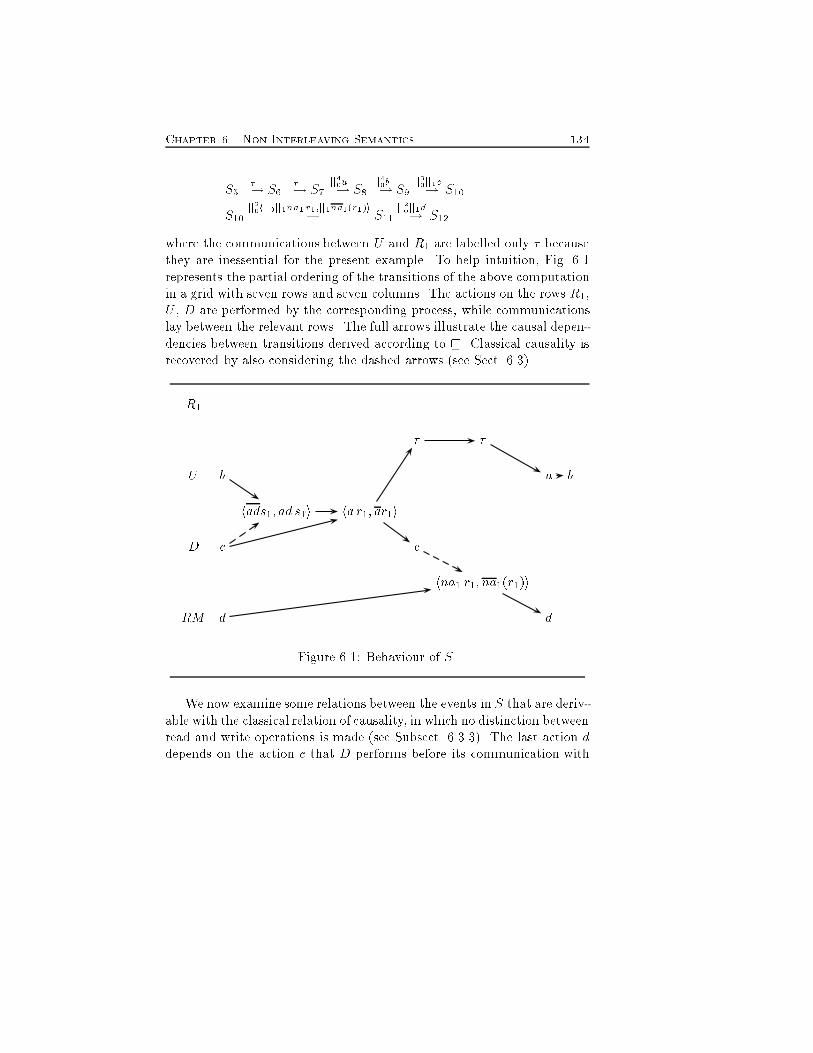
Chapter 6. Non Interleaving Semantics 134S5 ��! S6 ��! S7 jj40u�! S8 jj40b�! S9 jj30jj1c�! S10S10 jj20hjj0jj1na1 r1;jj1na1(r1)i�! S11 jj20jj1d�! S12where the communications between U and R1 are labelled only � becausethey are inessential for the present example. To help intuition, Fig. 6.1represents the partial ordering of the transitions of the above computationin a grid with seven rows and seven columns. The actions on the rows R1,U , D are performed by the corresponding process, while communicationslay between the relevant rows. The full arrows illustrate the causal depen-dencies between transitions derived according to v. Classical causality isrecovered by also considering the dashed arrows (see Sect. 6.3).R1 � �U b u bhads1; ad s1i ha r1; ar1iD c c hna1 r1; na1(r1)iRM d dFigure 6.1: Behaviour of S.We now examine some relations between the events in S that are deriv-able with the classical relation of causality, in which no distinction betweenread and write operations is made (see Subsect. 6.3.3). The last action ddepends on the action c that D performs before its communication with

135 6.3. Locality, Precedence and EnablingRM . This interpretation establishes too much causality, because D doesnot a�ect RM at all. More generally, receivers do not in uence sendersat all. This is re ected in our de�nitions.Note also that the �rst c does not cause the �rst communication be-tween D and U , as it would be with the classical notion of causality.Instead, the second communication between D and U depends on the �rstc also according to v. Finally, the second c causes the communicationbetween D and RM only with classical causality.We claim that our notion of causality is better suited than classicalcausality in the design of environments for debugging formal speci�cations.In particular, the new model allows us to decrease the number of eventsin the system history to be examined when an error is detected. Besidesthe example at hand, Proposition 6.3.12 also supports our claim.Assume that an error is found in the last d. If only the temporalbehaviour of S is available (interleaving semantics), we should analyze allthe eleven previous transitions looking for possible causes of the error.Causality o�ers a better approach to trace the possible sources of the bug.There are seven transitions that cause d according to classical causality,but only two transitions with our notion: hjj0jj0jj0jj1na1 r1; jj1na1(r1)i andjj0jj0jj1d.6.3 Locality, Precedence and EnablingThere are other non interleaving relations such as locality and enabling. Inaddition to those notions, we also study the relation of precedence whichspeci�es temporal constraints between transitions. All these truly con-current semantics can be de�ned easily, by slightly changing Def. 6.2.1.Also, we will use the proved computation (6.3) after Def. 6.2.3 to illustratethem. Finally, we will compare these new notions to each other, assumingthat they are de�ned on the same computation.The next subsection introduces the locality semantics. Subsect. 6.3.2 de-�nes the precedence relation. Precedence is what we need to add to causal-ity in order to retrieve enabling, which is dealt with in Subsect. 6.3.3.

Chapter 6. Non Interleaving Semantics 1366.3.1 LocalityLocality models distributed systems according to their geographical dis-tribution. In fact, the system is a collection of computational activitiesthat occur in di�erent sites called localities. The semantics provide anytransition with an indication of the site in which it is �red.Communications are completely ignored in a locality model, makinglink dependencies immaterial. Indeed, a link dependency between twotransitions is also structural when they occur at the same location (or oneat a sub-location of the other). We only need to keep the �rst item inDef. 6.2.1 of the causal relation v in order to ignore silent transitions.The local relation is then de�ned as�h vloc �n i� �n = #�, �h = #0�0 and #0 is a pre�x of #.With the relation above, we obtain the same semantics as (Sangiorgi,1994) (for the common fragment of the language), as shown by Proposi-tion 6.8.2.The relation vloc yield the classical notion of locality as de�ned forcalculi without value or name passing such as CCS (Kiehn, 1991; Boudolet al., 1993). The following is a corollary of Proposition 6.8.2.Corollary 6.3.1 Let P be an agent in which no object appears, then vloccoincides with the locality relation in (Boudol et al., 1993).By adopting the conventions used in Def. 6.2.3, we introduce a loca-tional relabelling.De�nition 6.3.2 (locational relabelling) Given a proved computation�, its associated locational computation Lt(�) is derived by relabelling anytransition �k by ltk, according to Def. 6.2.3 in which vloc replaces v.Consider computation (6.3). Its associated locational computation isP0 ha;;i�! P1 hd;;i�! P2 ��! P3 hx(z);f1gi�! P4 hzz;f1gi�! P5 hc;f0gi�! P6:The following proposition compares the local and causal relations.

137 6.3. Locality, Precedence and EnablingProposition 6.3.3 vloc � v.Proof. The inclusion is obvious because to de�ne vloc we delete some con-ditions from the de�nition of v. Furthermore, as is well known for CCS, theinclusion is strict because there are transitions that are causally, but not locallydependent such as jj0a and jj1jj0x(z) in computation (6.3). 26.3.2 PrecedencePrecedence expresses a temporal constraint between transitions, even ifthe former has no e�ect on the latter. In �-calculus precedences betweenactions can be de�ned implicitly, i.e., it is possible to sequentialize ina �xed ordering in all computations some transitions which neverthelessare causally independent. An example of precedence deriving from thedistinction between input and output actions is shown by process (6.1)in Sect. 6.1 where c always occurs before b, i.e., has precedence over b,although the two are causally independent. A second kind of implicitprecedence arises from the usage of names. See the process(�a)(xajya)also discussed in Sect. 6.1, where the restriction (�a) acts as a sequential-izer of the bound and free outputs. The �rst output is bound and let thesecond one to be free.Here, we de�ne precedence in two steps, according to its di�erent kindsexempli�ed above. Since the precedence due to communications is inducedby the structure of processes, we call it structural.De�nition 6.3.4 (structural precedence)Let P0 �0�! P1 �1�! : : : �n�! Pn+1 be a proved computation, and hereafterlet i; j 2 f0; 1g. Then, �h has a direct structural precedence over �n(�h �1str �n) i� either� �n = #h#0�0; #1�1i, �h = #0�0, 9i : #0 is a pre�x of ##i and �i is aninput; or

Chapter 6. Non Interleaving Semantics 138� �n = #h#0�0; #1�1i, �h = #0h#00�00; #01�01i, 9i; j : #0#0j is a pre�x of##i and �i is an input.The structural precedence relation�str is obtained by re exively and tran-sitively closing �1str and making it hereditary with respect to v, i.e., re-quiring(�k v �h �str �n)) �k �str �n and (�k �str �h v �n)) �k �str �n.Note that making�str hereditary means that precedence is preserved bycausality.We now examine precedence imposed by the usage of names. We callit object precedence, to recall that the name which gives precedence is anobject and not a link.De�nition 6.3.5 (object precedence) Let P0 �0�! P1 �1�! : : : �n�! Pn+1be a proved computation. Then, �h has an object precedence over �n(�h �obj �n) i� `(�h) = x(a) and `(�n) = ya, and the relation is heredi-tary with respect to v, i.e.,(�k v �h �obj �n)) �k �obj �n and (�k �obj �h v �n)) �k �obj �n.Finally, the precedence relation is de�ned as� = (�str [ �obj)�:The precedence relabelling is standard; we apply it to our runningexample.De�nition 6.3.6 (precedence relabelling) Given a proved computa-tion �, its associated precedence computation Pt(�) is derived by relabellingany transition �k by ptk, according to Def. 6.2.3 in which � replaces v.Consider computation (6.3). Its associated precedence computation isP0 ha;;i�! P1 hd;;i�! P2 ��! P3 hx(z);f1gi�! P4 hzz;f1;3gi�! P5 hc;f1gi�! P6:Reference 3 associated with the output of name z is an object precedence,while reference 1 in the last transition is structural.The following proposition compares precedence with causality.

139 6.3. Locality, Precedence and EnablingProposition 6.3.7 �str 6=vstr, �obj 6=<lnk and �6=v.Proof. We show a double non inclusion of the corresponding relations.6�) Consider the processes (�a)xa:az where x(a) vstr az, x(a) <lnk az, andx(a)6�az.6�) Consider the process (�a; b)(xa:bjb:ya) where jj0x(a)�str jj1ya, jj0x(a)�objjj1ya, and jj0x(a)6vjj1ya. 26.3.3 EnablingThe enabling relation describes, besides the causality between transitions,their temporal constraints as well. The enabling relation is, in fact, theunion of causality and precedence (see Proposition 6.3.12).By deleting the condition that �i is an output action from the de�nitionofvstr, we get the subject dependency of (Boreale & Sangiorgi, 1995) whichdoes not distinguish between senders and receivers. It is de�ned below.De�nition 6.3.8 (subject dependency)Let P0 �0�! P1 �1�! : : : �n�! Pn+1 be a proved computation, and hereafter leti; j 2 f0; 1g. Then, the direct subject dependency of �n on �h (�h �1str �n)is de�ned by the four items of Def. 6.2.1 where the condition on �i as beingan output is dropped.The subject dependencies of �n are obtained by the re exive and transitiveclosure of �1str, i.e., �str = (�1str)�.Subject dependencies yield the classical notion of causality as de�nedfor calculi without value or name passing such as in CCS (Degano et al.,1990; Darondeau & Degano, 1989; Kiehn, 1991). The following is a corol-lary of Proposition 6.8.1.Corollary 6.3.9 Let P be an agent in which no object appears, then �strcoincides with the causal relation in (Darondeau & Degano, 1989).In order to get the enabling relation, in the de�nition of <lnk we allowthe extruded name to be used as an object in a free input/output.

Chapter 6. Non Interleaving Semantics 140De�nition 6.3.10 (name enabling) Let P0 �0�! P1 �1�! : : : �n�! Pn+1be a proved computation. Then, the name enabler of �n, if any, is theunique �h (�h �nam �n) such that `(�h) = x(a), and `(�n) 2 faz; a(z); az; yag.Finally, we call enabling the relation de�ned as� = (�str [ �nam)�:Enabling turns out to coincide with the causality relation in (Boreale &Sangiorgi, 1995), as we will prove in Sect. 6.8.The next de�nition introduces enabling relabelling.De�nition 6.3.11 (enabling relabelling) Given a proved computation�, its associated enabling computation Et(�) is derived by relabelling anytransition �k by etk, according to Def. 6.2.3 in which � replaces v.Consider computation (6.3). Its associated enabling computation isP0 ha;;i�! P1 hd;;i�! P2 ��! P3 hx(z);f0;1gi�! P4 hzz;f0;1;3gi�! P5 hc;f0;1gi�! P6:The enabling computation is the same as the causal one, except for ref-erence 1 in the last transition. The new pointer is inserted since, in theenabling relation, the communication fully cross-updates causes.The following proposition relates enabling to the other relations.Proposition 6.3.12 v � �, � � �, and (� [ v) = �.Proof. Again, the inclusion v �� is obvious because we relax a condition fromthe de�nitions of vstr and of <lnk to obtain �. The inclusion is strict as thereare transitions which are dependent in the enabling relation, but independentin the causal one. For example, jj1c and jj0a in computation (6.3).Similarly, we can prove the strict inclusion of � into �.To prove (� [ v) = �, we show that � � (� [ v), as (� [ v) � � derivesfrom the two strict inclusions above.If �h � �n, assume that 8j : h < j < n (�h 6� �j ^ �j 6� �n). Thus �n directlydepends on �h. The general case (with no condition on �j) can easily be provedfrom this one by transitivity of the dependency relations.

141 6.3. Locality, Precedence and EnablingUnder the above assumption, by de�nition of � we have�h � �n ) �h �1str �n _ �h �nam �n:Assume �h �1str �n.If neither �h nor �n is a communication, then �h v1str �n, since in these casesno condition on the kind of actions is given in Def. 6.2.1.Consider the case in which both �h and �n are communications. Recall that�1str is obtained by erasing the conditions of Def. 6.2.1 on �i as being an output.This means that �i can either be an output or an input. If �i is an output then�h v1str �n. If �i is an input then �h �1str �n. A similar argument appliesalso when there is a single communication.Assume �h �nam �n.From Def. 6.3.10, we have `(�h) = x(a), and `(�n) 2 faz; a(z); azg [ fyag. The�rst (second) set of actions yields the de�nition of <lnk, see Def. 6.2.2 (of�obj ,see Def. 6.3.5). 2Note that vloc� � follows from Proposition 6.3.3 and from the �rst con-dition of Proposition 6.3.12. Also, (� [ vloc) � � follows from Proposi-tion 6.3.3 and from the last condition in Proposition 6.3.12.From the enabling and the local relations, we can easily de�ne for �-calculus global-local causes (Kiehn, 1991). We only need to relabel thevisible proved transitions with triplesgltk = h`(�k);K1;K2iwhere K1 is the set of enabling dependencies, and K2 is the set of localdependencies. More formally, we have the following de�nition.De�nition 6.3.13 (global-local relabelling)Let � = P0 �0�! P1 �1�! : : : �n�! Pn+1 be a proved computation. Its associ-ated global-local computation Glt(�) is derived by relabelling any transition�k as gltk, wheregltk = 8<: � if `(�k) = �h`(�k); fh 6= kj�h � �k; `(�h) 6= �g;fh 6= kj�h vloc �k; `(�h) 6= �gi otherwise.

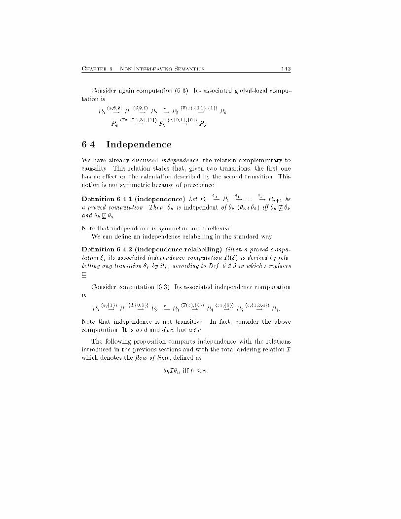
Chapter 6. Non Interleaving Semantics 142Consider again computation (6.3). Its associated global-local compu-tation isP0 ha;;;;i�! P1 hd;;;;i�! P2 ��! P3 hx(z);f0;1g;f1gi�! P4P4 hzz;f0;1;3g;f1gi�! P5 hc;f0;1g;f0gi�! P66.4 IndependenceWe have already discussed independence, the relation complementary tocausality. This relation states that, given two transitions, the �rst onehas no e�ect on the calculation described by the second transition. Thisnotion is not symmetric because of precedence.De�nition 6.4.1 (independence) Let P0 �0�! P1 �1�! : : : �n�! Pn+1 bea proved computation. Then, �h is independent of �k (�h � �k) i� �h 6v �kand �k 6v �h.Note that independence is symmetric and irre exive.We can de�ne an independence relabelling in the standard way.De�nition 6.4.2 (independence relabelling) Given a proved compu-tation �, its associated independence computation It(�) is derived by rela-belling any transition �k by itk, according to Def. 6.2.3 in which � replacesv. Consider computation (6.3). Its associated independence computationis P0 ha;f1gi�! P1 hd;f0;5gi�! P2 ��! P3 hx(z);f5gi�! P4 hzz;f5gi�! P5 hc;f1;3;4gi�! P6:Note that independence is not transitive. In fact, consider the abovecomputation. It is a � d and d � c, but a �= cThe following proposition compares independence with the relationsintroduced in the previous sections and with the total ordering relation Iwhich denotes the ow of time, de�ned as�hI�n i� h � n:

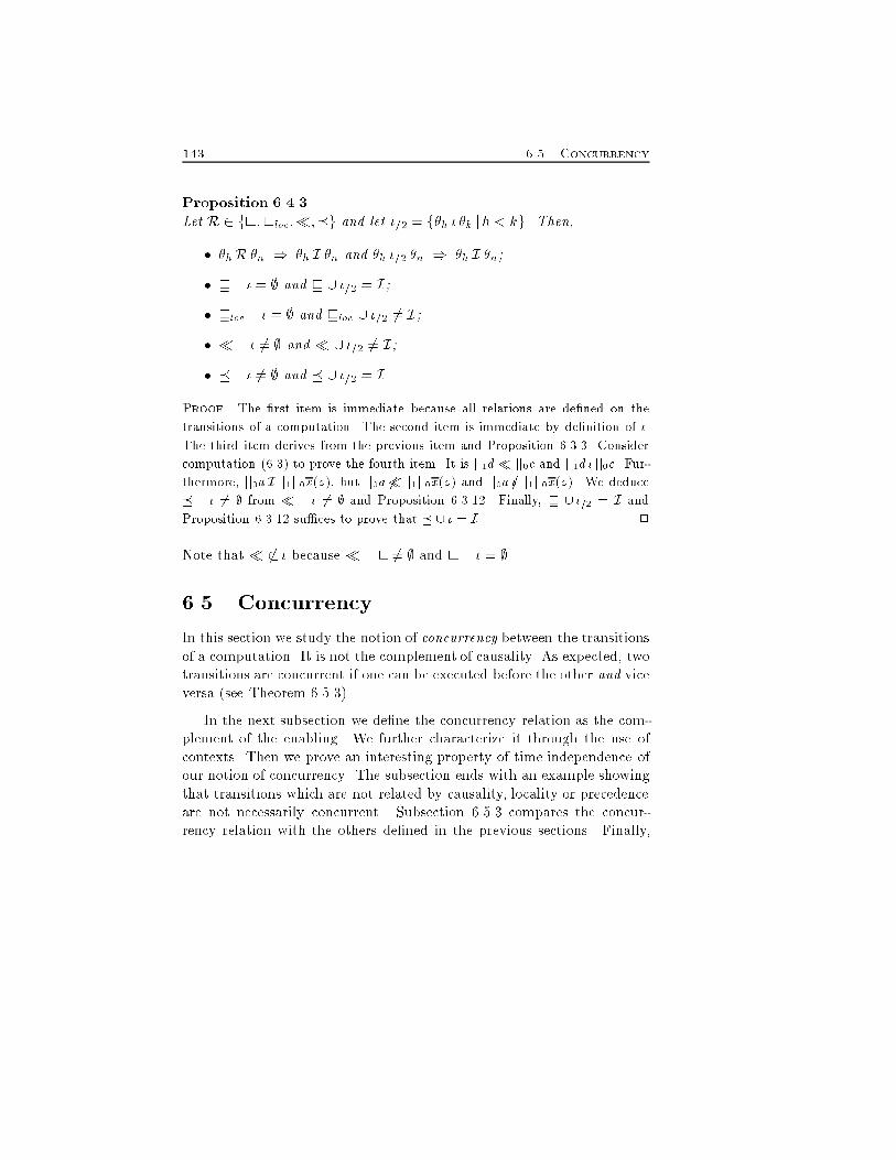
143 6.5. ConcurrencyProposition 6.4.3Let R 2 fv;vloc;�;�g and let �=2 = f�h � �k jh < kg. Then,� �hR �n ) �h I �n and �h �=2 �n ) �h I �n;� v \ � = ; and v [ �=2 = I;� vloc \ � = ; and vloc [ �=2 6= I;� � \ � 6= ; and � [ �=2 6= I;� � \ � 6= ; and � [ �=2 = I.Proof. The �rst item is immediate because all relations are de�ned on thetransitions of a computation. The second item is immediate by de�nition of �.The third item derives from the previous item and Proposition 6.3.3. Considercomputation (6.3) to prove the fourth item. It is jj1d� jj0c and jj1d � jj0c. Fur-thermore, jj0a I jj1jj0x(z), but jj0a 6� jj1jj0x(z) and jj0a �= jj1jj0x(z). We deduce� \ � 6= ; from � \ � 6= ; and Proposition 6.3.12. Finally, v [ �=2 = I andProposition 6.3.12 su�ces to prove that � [ � = I. 2Note that � 6� � because � \ v 6= ; and v \ � = ;.6.5 ConcurrencyIn this section we study the notion of concurrency between the transitionsof a computation. It is not the complement of causality. As expected, twotransitions are concurrent if one can be executed before the other and viceversa (see Theorem 6.5.3).In the next subsection we de�ne the concurrency relation as the com-plement of the enabling. We further characterize it through the use ofcontexts. Then we prove an interesting property of time independence ofour notion of concurrency. The subsection ends with an example showingthat transitions which are not related by causality, locality or precedenceare not necessarily concurrent. Subsection 6.5.3 compares the concur-rency relation with the others de�ned in the previous sections. Finally,

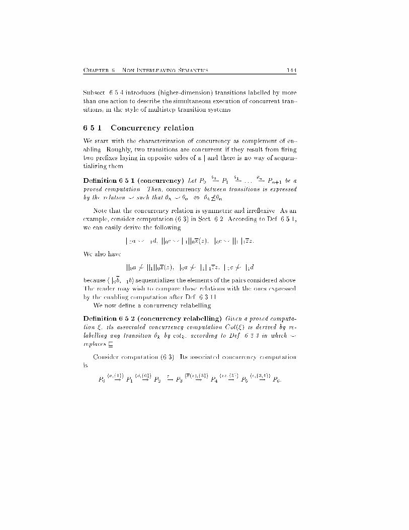
Chapter 6. Non Interleaving Semantics 144Subsect. 6.5.4 introduces (higher-dimension) transitions labelled by morethan one action to describe the simultaneous execution of concurrent tran-sitions, in the style of multistep transition systems.6.5.1 Concurrency relationWe start with the characterization of concurrency as complement of en-abling. Roughly, two transitions are concurrent if they result from �ringtwo pre�xes laying in opposite sides of a j and there is no way of sequen-tializing them.De�nition 6.5.1 (concurrency) Let P0 �0�! P1 �1�! : : : �n�! Pn+1 be aproved computation. Then, concurrency between transitions is expressedby the relation ^ such that �h ^ �n , �h 6��n.Note that the concurrency relation is symmetric and irre exive. As anexample, consider computation (6.3) in Sect. 6.2. According to Def. 6.5.1,we can easily derive the followingjj0a ^ jj1d; jj0c ^ jj1jj0x(z); jj0c ^ jj1jj1zz:We also have jj0a 6^ jj1jj0x(z); jj0a 6^ jj1jj1zz; jj0c 6^ jj1dbecause hjj0b; jj1bi sequentializes the elements of the pairs considered above.The reader may wish to compare these relations with the ones expressedby the enabling computation after Def. 6.3.11.We now de�ne a concurrency relabelling.De�nition 6.5.2 (concurrency relabelling) Given a proved computa-tion �, its associated concurrency computation Cot(�) is derived by re-labelling any transition �k by cotk, according to Def. 6.2.3 in which ^replaces v.Consider computation (6.3). Its associated concurrency computationis P0 ha;f1gi�! P1 hd;f0gi�! P2 ��! P3 hx(z);f5gi�! P4 hzz;f5gi�! P5 hc;f3;4gi�! P6:

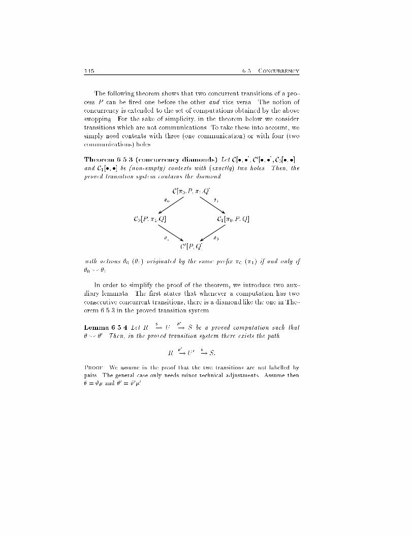
145 6.5. ConcurrencyThe following theorem shows that two concurrent transitions of a pro-cess P can be �red one before the other and vice versa. The notion ofconcurrency is extended to the set of computations obtained by the aboveswopping. For the sake of simplicity, in the theorem below we considertransitions which are not communications. To take these into account, wesimply need contexts with three (one communication) or with four (twocommunications) holes.Theorem 6.5.3 (concurrency diamonds) Let C[�; �]; C0[�; �]; C0[�; �]and C1[�; �] be (non-empty) contexts with (exactly) two holes. Then, theproved transition system contains the diamondC[�0:P; �1:Q]C0[P; �1:Q] C1[�0:P;Q]C0[P;Q]�0 �1�1 �0with actions �0 (�1) originated by the same pre�x �0 (�1) if and only if�0 ^ �1.In order to simplify the proof of the theorem, we introduce two aux-iliary lemmata. The �rst states that whenever a computation has twoconsecutive concurrent transitions, there is a diamond like the one in The-orem 6.5.3 in the proved transition system.Lemma 6.5.4 Let R ��! U �0�! S be a proved computation such that� ^ �0. Then, in the proved transition system there exists the pathR �0�! U 0 ��! S:Proof. We assume in the proof that the two transitions are not labelled bypairs. The general case only needs minor technical adjustments. Assume then� = #� and �0 = #0�0.

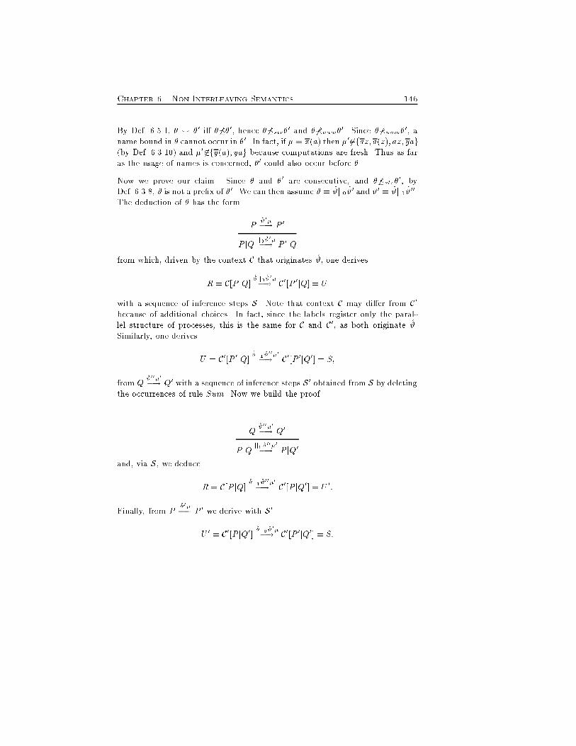
Chapter 6. Non Interleaving Semantics 146By Def. 6.5.1, � ^ �0 i� � 6��0, hence � 6�str�0 and � 6�nam�0. Since � 6�nam�0, aname bound in � cannot occur in �0. In fact, if � = x(a) then �0 62faz; a(z); az; yag(by Def. 6.3.10) and �0 62fy(a); yag because computations are fresh. Thus as faras the usage of names is concerned, �0 could also occur before �.Now we prove our claim. Since � and �0 are consecutive, and � 6�str�0, byDef. 6.3.8, # is not a pre�x of #0. We can then assume # = #jj0#0 and #0 = #jj1#00.The deduction of � has the form ...P #0��! P 0P jQ jj0 #0��! P 0jQfrom which, driven by the context C that originates #, one derivesR = C[P jQ] #jj0 #0��! C0[P 0jQ] = Uwith a sequence of inference steps S. Note that context C may di�er from C0because of additional choices. In fact, since the labels register only the paral-lel structure of processes, this is the same for C and C0, as both originate #.Similarly, one derives U = C0[P 0jQ] #jj1 #00�0�! C0[P 0jQ0] = S;from Q #00�0�! Q0 with a sequence of inference steps S 0 obtained from S by deletingthe occurrences of rule Sum. Now we build the proof...Q #00�0�! Q0P jQ jj1 #00�0�! P jQ0and, via S, we deduceR = C[P jQ] #jj1 #00�0�! C0[P jQ0] = U 0:Finally, from P #0��! P 0 we derive with S 0U 0 = C0[P jQ0] #jj0 #0��! C0[P 0jQ0] = S:

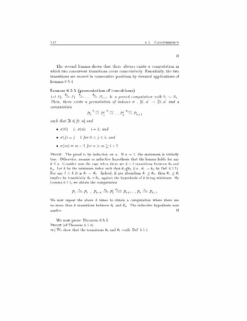
147 6.5. Concurrency2The second lemma shows that there always exists a computation inwhich two concurrent transitions occur consecutively. Essentially, the twotransitions are moved in consecutive positions by iterated applications ofLemma 6.5.4.Lemma 6.5.5 (permutation of transitions)Let P0 �0�! P1 �1�! : : : �n�! Pn+1 be a proved computation with �0 ^ �n.Then, there exists a permutation of indexes � : [0::n] ! [0::n] and acomputation P0 ��(h)�! P 01 ��(k)�! : : :P 0n ��(l)�! Pn+1such that 9i 2 [0::n] and� �(0) = i; �(n) = i + 1; and� �(j) = j � 1 for 0 < j � i; and� �(m) = m + 1 for n > m � i + 1Proof. The proof is by induction on n. If n = 1, the statement is triviallytrue. Otherwise, assume as inductive hypothesis that the lemma holds for anyk � n. Consider now the case when there are k + 1 transitions between �0 and�n. Let h be the minimum index such that �0 6��h (i.e., �0 ^ �h by Def. 6.5.1).For any l < h it is �l ^ �h. Indeed, if per absurdum �l � �h, then �0 � �limplies by transitivity �0 � �h, against the hypothesis of h being minimum. ByLemma 6.5.4, we obtain the computationP0 �0�! P1 : : : Ph�1 �h�! P 1h �h�1�! Ph+1 : : : Pn �n�! Pn+1We now repeat the above h times to obtain a computation where there areno more than k transitions between �0 and �n. The inductive hypothesis nowapplies. 2We now prove Theorem 6.5.3.Proof.(of Theorem 6.5.3))) We show that the transitions �0 and �1 verify Def. 6.5.1

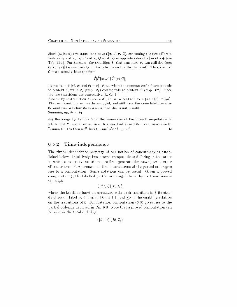
Chapter 6. Non Interleaving Semantics 148Since (at least) two transitions leave C[�0:P;�1:Q], consuming the two di�erentpre�xes �0 and �1, �0:P and �1:Q must lay in opposite sides of a j or of a + (seeTab. 13.1). Furthermore, the transition �1 that consumes �1 can still �re fromC0[P;�1:Q] (symmetrically for the other branch of the diamond). Thus, contextC must actually have the formC[C0[�0:P ] j C00[�1:Q]]Hence, �0 = #jj0#0�0 and �1 = #jj1#1�1, where the common pre�x # correspondsto context C, while #0 (resp. #1) corresponds to context C0 (resp. C00). Sincethe two transitions are consecutive, �0 6�str�1.Assume by contradiction #0 �nam #1, i.e. �0 = x(a) and �1 2 faz;a(z); az; yag.The two transitions cannot be swopped, and still have the same label, because�1 would use a before its extrusion, and this is not possible.Summing up, �0 ^ �1.() Rearrange by Lemma 6.5.5 the transitions of the proved computation inwhich both �0 and �1 occur, in such a way that �0 and �1 occur consecutively.Lemma 6.5.4 is then su�cient to conclude the proof. 26.5.2 Time-independenceThe time-independence property of our notion of concurrency is estab-lished below. Intuitively, two proved computations di�ering in the orderin which concurrent transitions are �red generate the same partial orderof transitions. Furthermore, all the linearizations of the partial order giverise to a computation. Some notations can be useful. Given a provedcomputation �, the labelled partial ordering induced by its transitions isthe triple hf� 2 �g; `;��iwhere the labelling function associates with each transition in � its stan-dard action label �, ` is as in Def. 5.1.1, and �� is the enabling relationon the transitions of �. For instance, computation (6.3) gives rise to thepartial ordering depicted in Fig. 6.3. Note that a proved computation canbe seen as the total ordering hf� 2 �g; id; I�i

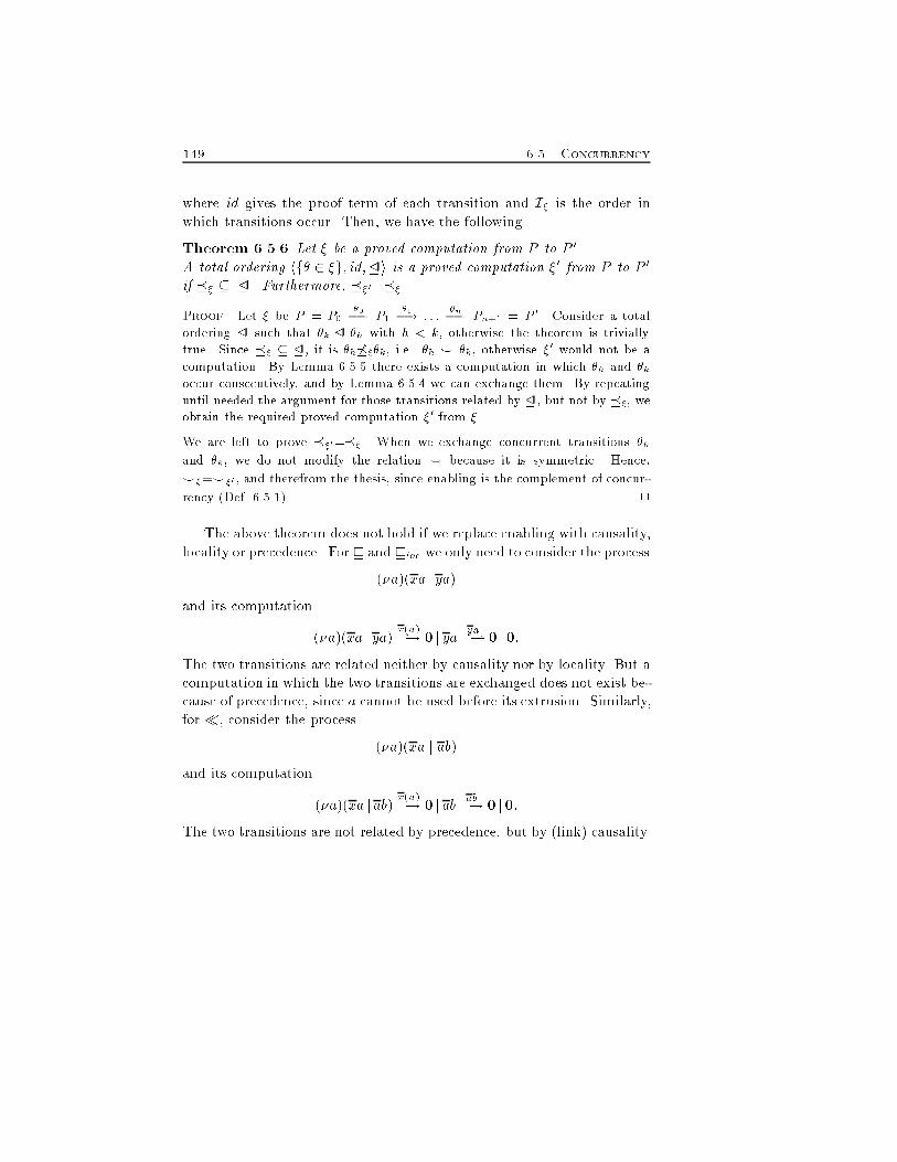
149 6.5. Concurrencywhere id gives the proof term of each transition and I� is the order inwhich transitions occur. Then, we have the following.Theorem 6.5.6 Let � be a proved computation from P to P 0.A total ordering hf� 2 �g; id;�i is a proved computation �0 from P to P 0if �� � � . Furthermore, ��0=�� .Proof. Let � be P = P0 �0�! P1 �1�! : : : �n�! Pn+1 = P 0. Consider a totalordering � such that �k � �h with h < k, otherwise the theorem is triviallytrue. Since �� � � , it is �h 6���k, i.e. �h ^ �k, otherwise �0 would not be acomputation. By Lemma 6.5.5 there exists a computation in which �h and �koccur consecutively, and by Lemma 6.5.4 we can exchange them. By repeatinguntil needed the argument for those transitions related by � , but not by ��, weobtain the required proved computation �0 from �.We are left to prove ��0=��. When we exchange concurrent transitions �hand �k, we do not modify the relation ^ because it is symmetric. Hence,^�=^�0 , and therefrom the thesis, since enabling is the complement of concur-rency (Def. 6.5.1). 2The above theorem does not hold if we replace enabling with causality,locality or precedence. Forv and vloc we only need to consider the process(�a)(xa j ya)and its computation(�a)(xa j ya) x(a)�! 0 j ya ya�! 0 j0:The two transitions are related neither by causality nor by locality. But acomputation in which the two transitions are exchanged does not exist be-cause of precedence, since a cannot be used before its extrusion. Similarly,for �, consider the process (�a)(xa j ab)and its computation (�a)(xa j ab) x(a)�! 0 j ab ab�! 0 j0:The two transitions are not related by precedence, but by (link) causality.

Chapter 6. Non Interleaving Semantics 1506.5.3 ComparisonsWe now compare concurrency with the relations introduced previously.The �rst item says that all the studied relations respect the ow of time.The second condition of the third item says that two transitions notcausally related can be non concurrent just because one has precedenceover the other.Proposition 6.5.7Let R 2 fv;vloc;�g and let ^=2= f�h ^ �k jh < kg. Then,� �hR �n )6( �h I �n, and �h � �n )6( �h I �n;� (^=2 [ �) = I;� (^ \ R) = ; and (^=2 [ R) 6= I;� ^� � and ^=2 [ �=2 6= I.Proof. The implications in the �rst item are proved by noticing that in thede�nition of any R and of �, if �n depends on �h it is h � n. The negatedimplications are obvious. The second item immediately follows from Def. 6.5.1.The third item derives from the second and from Proposition 6.3.12.We now prove the �rst equation of the last item. Let �h ^=2 �n. Thus �h I �nand this implies that either �h v �n or �h � �n. Since v \^=2= ; by second item,we have ^=2� �. The inclusion is strict because ^=2 \ �= ;, while �\ �6= ;.The second equation of the last item is immediate from Proposition 6.4.3. 2The second item above and the equality in Proposition 6.3.12 allow us tostate the equation in the following corollary, that in turn, with Proposi-tion 6.3.3, implies the inclusion below.Corollary 6.5.8(� [ v [ ^=2) = I and (� [ vloc [ ^=2) � I:The relations between causality, locality, enabling, concurrency, prece-dence and independence are collected in Tab. 6.1. By abuse of notation^

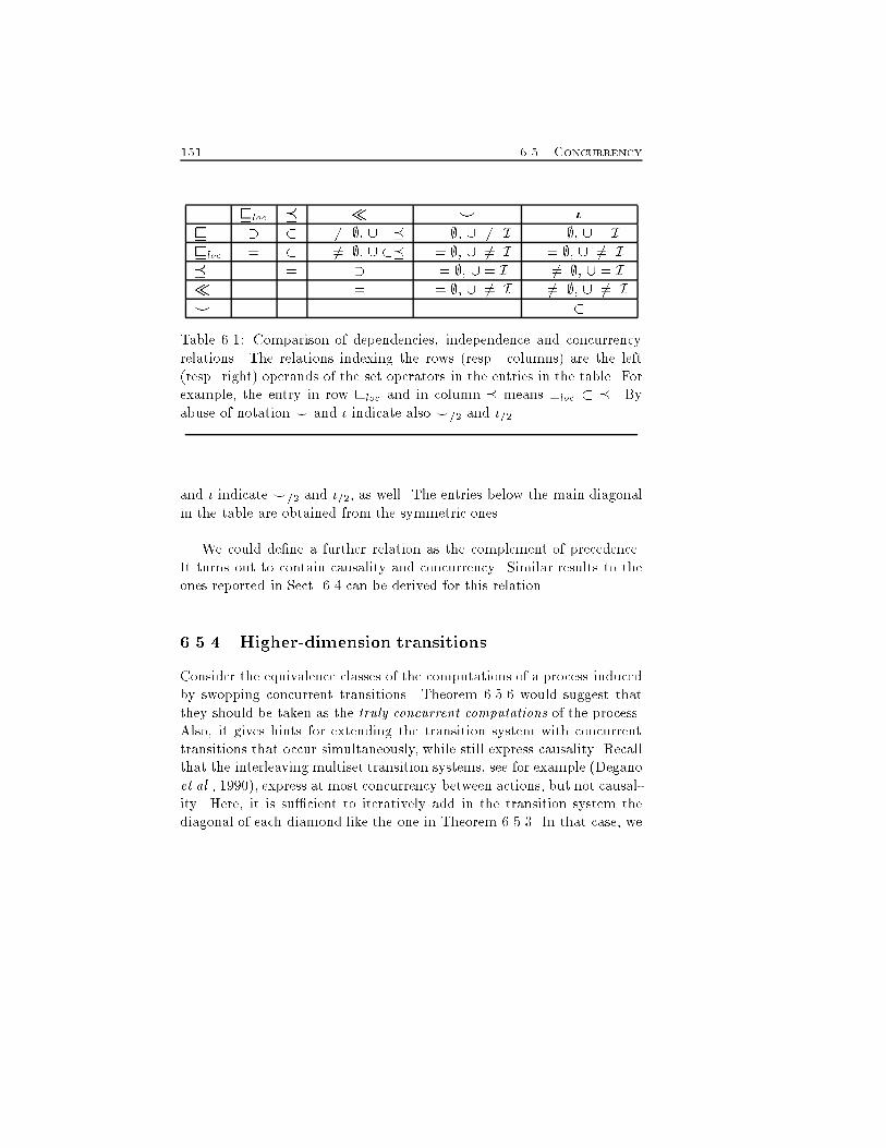
151 6.5. Concurrencyvloc � � ^ �v � � \ 6= ;, [ =� \ = ;, [ 6= I \ = ;, [ = Ivloc = � \ 6= ;, [ �� \ = ;, [ 6= I \ = ;, [ 6= I� = � \ = ;, [ = I \ 6= ;, [ = I� = \ = ;, [ 6= I \ 6= ;, [ 6= I^ = �Table 6.1: Comparison of dependencies, independence and concurrencyrelations. The relations indexing the rows (resp. columns) are the left(resp. right) operands of the set operators in the entries in the table. Forexample, the entry in row vloc and in column � means vloc � �. Byabuse of notation ^ and � indicate also ^=2 and �=2.and � indicate ^=2 and �=2, as well. The entries below the main diagonalin the table are obtained from the symmetric ones.We could de�ne a further relation as the complement of precedence.It turns out to contain causality and concurrency. Similar results to theones reported in Sect. 6.4 can be derived for this relation.6.5.4 Higher-dimension transitionsConsider the equivalence classes of the computations of a process inducedby swopping concurrent transitions. Theorem 6.5.6 would suggest thatthey should be taken as the truly concurrent computations of the process.Also, it gives hints for extending the transition system with concurrenttransitions that occur simultaneously, while still express causality. Recallthat the interleaving multiset transition systems, see for example (Deganoet al., 1990), express at most concurrency between actions, but not causal-ity. Here, it is su�cient to iteratively add in the transition system thediagonal of each diamond like the one in Theorem 6.5.3. In that case, we

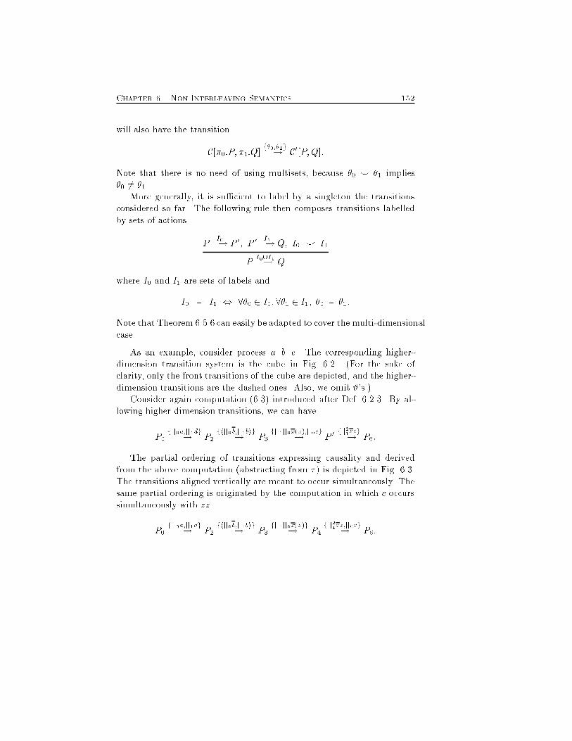
Chapter 6. Non Interleaving Semantics 152will also have the transitionC[�0:P; �1:Q] f�0;�1g�! C0[P;Q]:Note that there is no need of using multisets, because �0 ^ �1 implies�0 6= �1.More generally, it is su�cient to label by a singleton the transitionsconsidered so far. The following rule then composes transitions labelledby sets of actions P I0�! P 0; P 0 I1�! Q; I0 ^ I1P I0[I1�! Qwhere I0 and I1 are sets of labels andI0 ^ I1 , 8�0 2 I0; 8�1 2 I1; �0 ^ �1:Note that Theorem 6.5.6 can easily be adapted to cover the multi-dimensionalcase.As an example, consider process a j b j c. The corresponding higher-dimension transition system is the cube in Fig. 6.2. (For the sake ofclarity, only the front transitions of the cube are depicted, and the higher-dimension transitions are the dashed ones. Also, we omit #'s.)Consider again computation (6.3) introduced after Def. 6.2.3. By al-lowing higher dimension transitions, we can haveP0 fjj0a;jj1dg�! P2 fhjj0b;jj1big�! P3 fjj1jj0x(z);jj0cg�! P 0 fjj21zzg�! P6:The partial ordering of transitions expressing causality and derivedfrom the above computation (abstracting from � ) is depicted in Fig. 6.3.The transitions aligned vertically are meant to occur simultaneously. Thesame partial ordering is originated by the computation in which c occurssimultaneously with zz.P0 fjj0a;jj1dg�! P2 fhjj0b;jj1big�! P3 fjj1jj0x(z)g�! P4 fjj21zz;jj0cg�! P6:

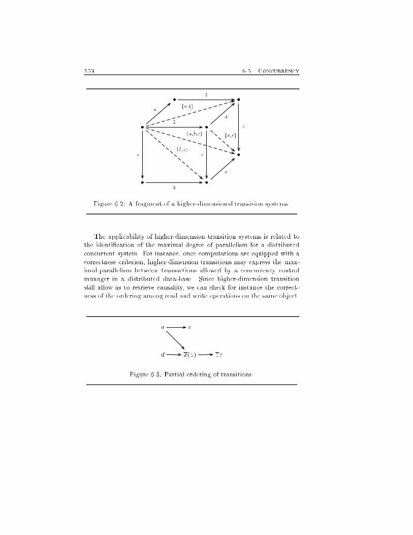
153 6.5. Concurrency� �� � �� �a bb a cfa;bgfa;b;cgbc c afb;cg fa;cgFigure 6.2: A fragment of a higher-dimensional transition systems.The applicability of higher-dimension transition systems is related tothe identi�cation of the maximal degree of parallelism for a distributedconcurrent system. For instance, once computations are equipped with acorrectness criterion, higher-dimension transitions may express the max-imal parallelism between transactions allowed by a concurrency controlmanager in a distributed data-base. Since higher-dimension transitionstill allow us to retrieve causality, we can check for instance the correct-ness of the ordering among read and write operations on the same object.a cd x(z) zzFigure 6.3: Partial ordering of transitions.

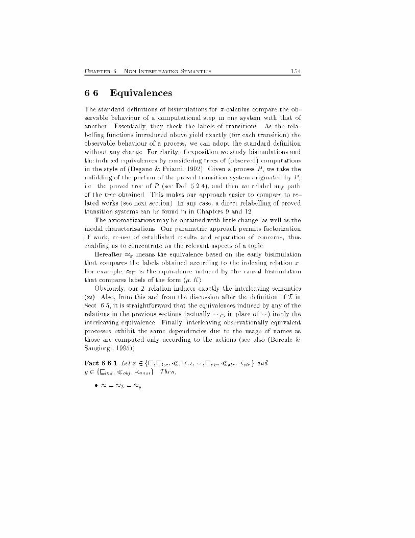
Chapter 6. Non Interleaving Semantics 1546.6 EquivalencesThe standard de�nitions of bisimulations for �-calculus compare the ob-servable behaviour of a computational step in one system with that ofanother. Essentially, they check the labels of transitions. As the rela-belling functions introduced above yield exactly (for each transition) theobservable behaviour of a process, we can adopt the standard de�nitionwithout any change. For clarity of exposition we study bisimulations andthe induced equivalences by considering trees of (observed) computationsin the style of (Degano & Priami, 1992). Given a process P , we take theunfolding of the portion of the proved transition system originated by P ,i.e. the proved tree of P (see Def. 5.2.4), and then we relabel any pathof the tree obtained. This makes our approach easier to compare to re-lated works (see next section). In any case, a direct relabelling of provedtransition systems can be found in in Chapters 9 and 12.The axiomatizations may be obtained with little change, as well as themodal characterizations. Our parametric approach permits factorizationof work, re-use of established results and separation of concerns, thusenabling us to concentrate on the relevant aspects of a topic.Hereafter �x means the equivalence based on the early bisimulationthat compares the labels obtained according to the indexing relation x.For example, �v is the equivalence induced by the causal bisimulationthat compares labels of the form h�;Ki.Obviously, our I relation induces exactly the interleaving semantics(�). Also, from this and from the discussion after the de�nition of I inSect. 6.5, it is straightforward that the equivalences induced by any of therelations in the previous sections (actually ^=2 in place of ^) imply theinterleaving equivalence. Finally, interleaving observationally equivalentprocesses exhibit the same dependencies due to the usage of names asthose are computed only according to the actions (see also (Boreale &Sangiorgi, 1995)).Fact 6.6.1 Let x 2 fv;vloc;�;�; �;^;vstr;�str;�strg andy 2 fvlnk;�obj;�namg. Then,� � = �I = �y

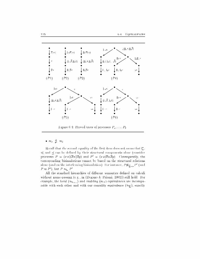
155 6.6. Equivalences� � � �� � � � �� � � � � �� � � � � �(P1) (P2) (P3) (P4)� �� � � �� � � � � �� � � � � �(P5) (P6)x(a)�ya jj0x(a)hjj0b;jj1bijj1ya jj0x(a)hjj0b;jj1bijj1ya jj0a jj1hjj0b;jj1bijj1hjj0b;jj1bi jj0a jj1jj1cjj1jj1c jj1jj1c jj0ajj0a �hjj0b;jj1bi jj0a jj1cjj1c jj1c jj0a jj0a �hjj0b;jj1bi jj0a jj1cjj1c jj1c jj0aFigure 6.4: Proved trees of processes P1; : : : ; P6.� �x )6( �IRecall that the second equality of the �rst item does not mean that v,� and � can be de�ned by their structural components alone (considerprocesses P = (� a)(xa j ay) and P 0 = (� a)xa:ay). Consequently, thecorresponding bisimulations cannot be based on the structural relationsalone (and on the interleaving bisimulation). For instance, P 6�vstrP 0 (andP � P 0), but P �v P 0.All the standard hierarchies of di�erent semantics de�ned on calculiwithout name-passing (e.g., in (Degano & Priami, 1992)) still hold. Forexample, the local (�vloc) and enabling (��) equivalences are incompa-rable with each other and with our causality equivalence (�v), exactly

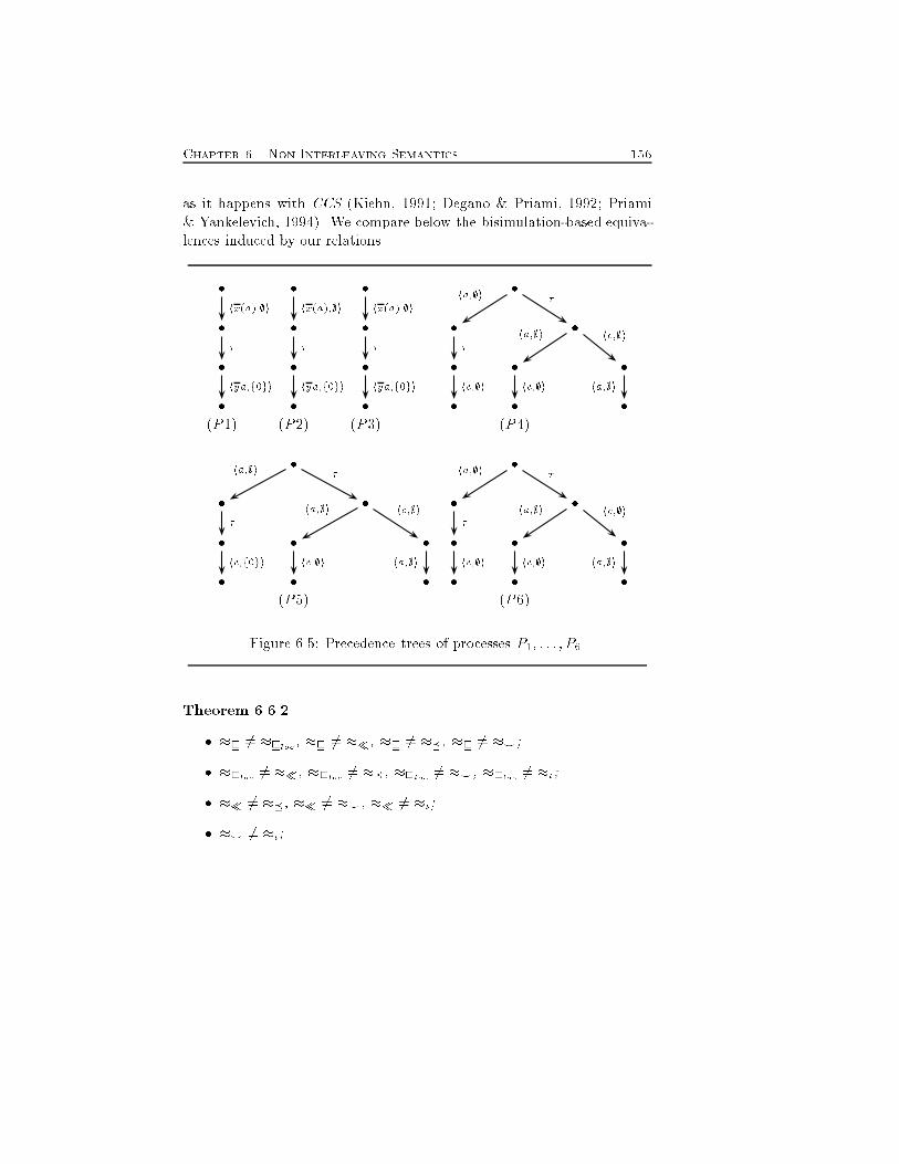
Chapter 6. Non Interleaving Semantics 156as it happens with CCS (Kiehn, 1991; Degano & Priami, 1992; Priami& Yankelevich, 1994). We compare below the bisimulation-based equiva-lences induced by our relations.� � � �� � � � �� � � � � �� � � � � �(P1) (P2) (P3) (P4)� �� � � �� � � � � �� � � � � �(P5) (P6)hx(a);;i�hya;f0gi hx(a);;i�hya;f0gi hx(a);;i�hya;f0gi ha;;i �� ha;;i hc;;ihc;;i hc;;i ha;;iha;;i �� ha;;i hc;;ihc;f0gi hc;;i ha;;i ha;;i �� ha;;i hc;;ihc;;i hc;;i ha;;iFigure 6.5: Precedence trees of processes P1; : : : ; P6.Theorem 6.6.2� �v 6= �vloc , �v 6= ��, �v 6= ��, �v 6= �^;� �vloc 6= ��, �vloc 6= ��, �vloc 6= �^, �vloc 6= ��;� �� 6= ��, �� 6= �^, �� 6= ��;� �^ 6= ��;

157 6.6. Equivalences� � � �� � � � �� � � � � �� � � � � �(P1) (P2) (P3) (P4)� �� � � �� � � � � �� � � � � �(P5) (P6)hx(a);;i�hya;f0gi hx(a);;i�hya;f0gi hx(a);;i�hya;f0gi ha;;i �� ha;;i hc;;ihc;;i hc;;i ha;;iha;;i �� ha;;i hc;;ihc;f0gi hc;;i ha;;i ha;;i �� ha;;i hc;;ihc;f0gi hc;;i ha;;iFigure 6.6: Enabling trees of processes P1; : : : ; P6.� �� = �^, �v = ��.Proof. The last item in the above theorem is proved by noting that enablingand concurrency, as well as causality and independence, encode the same infor-mation, because they are complementary (Def. 6.5.1 and Def. 6.4.1). For theother items, we report below the processes that allow us to compare all equiv-alences. (They are depicted in Fig. 6.4 in their proved version, while Figs. 6.5,6.6, 6.7, 6.8, 6.9 and 6.10 report the same trees relabelled according to eachrelation introduced previously). The relevant relations between these processesare in Tab. 6.2.

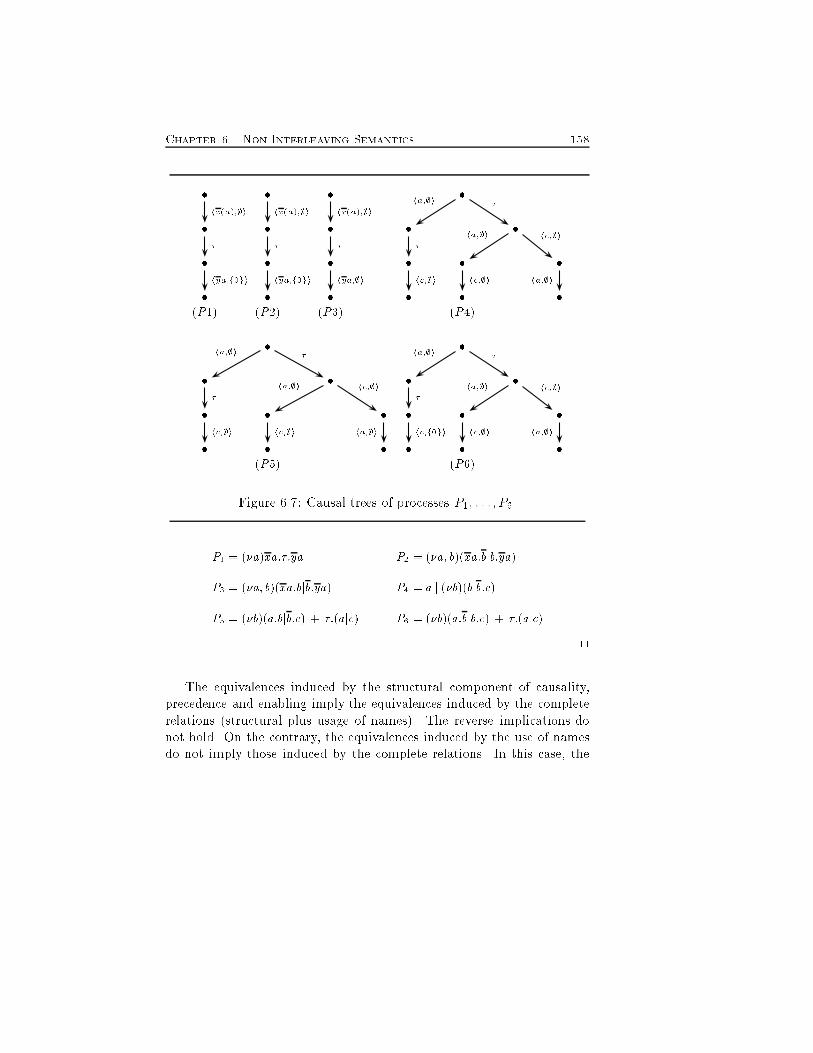
Chapter 6. Non Interleaving Semantics 158� � � �� � � � �� � � � � �� � � � � �(P1) (P2) (P3) (P4)� �� � � �� � � � � �� � � � � �(P5) (P6)hx(a);;i�hya;f0gi hx(a);;i�hya;f0gi hx(a);;i�hya;;i ha;;i �� ha;;i hc;;ihc;;i hc;;i ha;;iha;;i �� ha;;i hc;;ihc;;i hc;;i ha;;i ha;;i �� ha;;i hc;;ihc;f0gi hc;;i ha;;iFigure 6.7: Causal trees of processes P1; : : : ; P6.P1 = (�a)xa:�:ya P2 = (�a; b)(xa:bjb:ya)P3 = (�a; b)(xa:bjb:ya) P4 = a j (�b)(bjb:c)P5 = (�b)(a:bjb:c) + �:(ajc) P6 = (�b)(a:bjb:c) + �:(ajc) 2The equivalences induced by the structural component of causality,precedence and enabling imply the equivalences induced by the completerelations (structural plus usage of names). The reverse implications donot hold. On the contrary, the equivalences induced by the use of namesdo not imply those induced by the complete relations. In this case, the

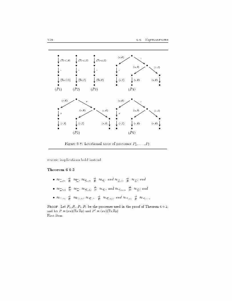
159 6.6. Equivalences� � � �� � � � �� � � � � �� � � � � �(P1) (P2) (P3) (P4)� �� � � �� � � � � �� � � � � �(P5) (P6)hx(a);;i�hya;f0gi hx(a);;i�hya;;i hx(a);;i�hya;;i ha;;i �� ha;;i hc;;ihc;;i hc;;i ha;;iha;;i �� ha;;i hc;;ihc;;i hc;;i ha;;i ha;;i �� ha;;i hc;;ihc;;i hc;;i ha;;iFigure 6.8: Locational trees of processes P1; : : : ; P6.reverse implications hold instead.Theorem 6.6.3� �vstr )6( �v, ��str )6( ��, and ��str )6( ��; and� �vlnk 6)( �v, ��obj 6)( ��, and ��nam 6)( ��; and� �vstr )6( �vlnk , ��str )6( ��obj , and ��str )6( ��nam .Proof. Let P2; P3; P4; P5 be the processes used in the proof of Theorem 6.6.2,and let P = (�a)(xajay) and P 0 = (�a)(xa:ay).First item.

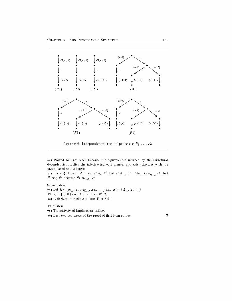
Chapter 6. Non Interleaving Semantics 160� � � �� � � � �� � � � � �� � � � � �(P1) (P2) (P3) (P4)� �� � � �� � � � � �� � � � � �(P5) (P6)hx(a);;i�hya;;i hx(a);;i�hya;;i hx(a);;i�hya;f0gi ha;;i �� ha;;i hc;;ihc;f0gi hc;f1gi ha;f1giha;;i �� ha;;i hc;;ihc;f0gi hc;f1gi ha;f1gi ha;;i �� ha;;i hc;;ihc;;i hc;f1gi ha;f1giFigure 6.9: Independence trees of processes P1; : : : ; P6.)) Proved by Fact 6.6.1 because the equivalences induced by the structuraldependencies implies the interleaving equivalence, and this coincides with thename-based equivalences.6() Let x 2 fv;�g. We have P �x P 0, but P 6�xstrP 0. Also, P2 6��strP3, butP2 �� P3 because P2 ��obj P3.Second item.6)) Let R 2 f6�v; 6��;�vlnk ;��namg and R0 2 f6��;��obj g.Then, (a j b) R (a:b+ b:a) and P4 R0 P5.() It derives immediately from Fact 6.6.1.Third item.)) Transitivity of implication su�ces.6() Last two sentences of the proof of �rst item su�ce. 2

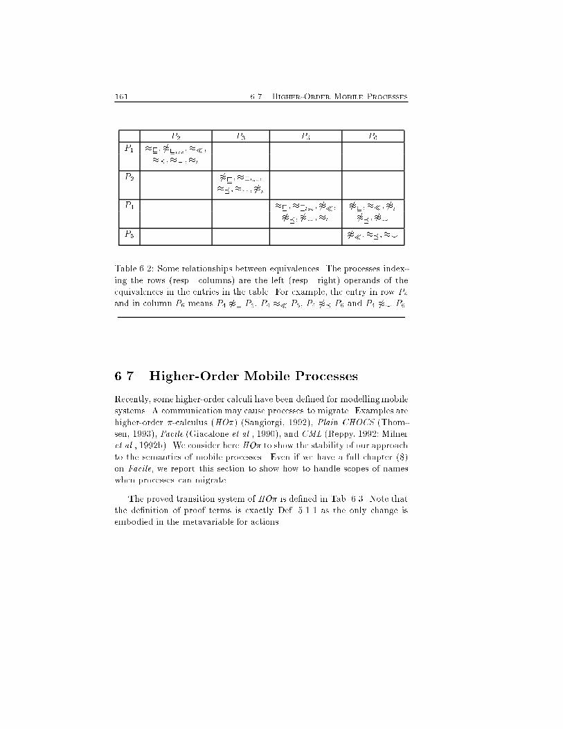
161 6.7. Higher-Order Mobile ProcessesP2 P3 P5 P6P1 �v; 6�vloc ;��;��;�^;��P2 6�v;�vloc ;��;�^; 6��P4 �v;�vloc ; 6��; 6�v;��; 6��6��; 6�^;�� 6��; 6�^P5 6��;��;�^Table 6.2: Some relationships between equivalences. The processes index-ing the rows (resp. columns) are the left (resp. right) operands of theequivalences in the entries in the table. For example, the entry in row P4and in column P6 means P4 6�v P6, P4 �� P6, P4 6�� P6 and P4 6�^ P6.6.7 Higher-Order Mobile ProcessesRecently, some higher-order calculi have been de�ned for modellingmobilesystems. A communicationmay cause processes to migrate. Examples arehigher-order �-calculus (HO�) (Sangiorgi, 1992), Plain CHOCS (Thom-sen, 1993), Facile (Giacalone et al., 1990), and CML (Reppy, 1992; Milneret al., 1992b). We consider here HO� to show the stability of our approachto the semantics of mobile processes. Even if we have a full chapter (8)on Facile, we report this section to show how to handle scopes of nameswhen processes can migrate.The proved transition system of HO� is de�ned in Tab. 6.3. Note thatthe de�nition of proof terms is exactly Def. 5.1.1 as the only change isembodied in the metavariable for actions.

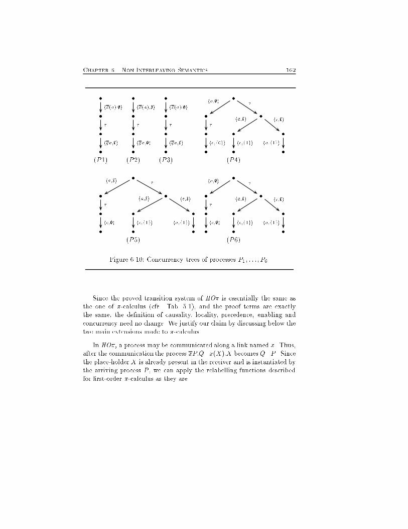
Chapter 6. Non Interleaving Semantics 162� � � �� � � � �� � � � � �� � � � � �(P1) (P2) (P3) (P4)� �� � � �� � � � � �� � � � � �(P5) (P6)hx(a);;i�hya;;i hx(a);;i�hya;;i hx(a);;i�hya;;i ha;;i �� ha;;i hc;;ihc;f0gi hc;f1gi ha;f1giha;;i �� ha;;i hc;;ihc;;i hc;f1gi ha;f1gi ha;;i �� ha;;i hc;;ihc;;i hc;f1gi ha;f1giFigure 6.10: Concurrency trees of processes P1; : : : ; P6.Since the proved transition system of HO� is essentially the same asthe one of �-calculus (cfr. Tab. 5.1), and the proof terms are exactlythe same, the de�nition of causality, locality, precedence, enabling andconcurrency need no change. We justify our claim by discussing below thetwo main extensions made to �-calculus.In HO�, a process may be communicated along a link named x. Thus,after the communication the process xP:Q j x(X):X becomes Q j P . Sincethe place-holder X is already present in the receiver and is instantiated bythe arriving process P , we can apply the relabelling functions describedfor �rst-order �-calculus as they are.

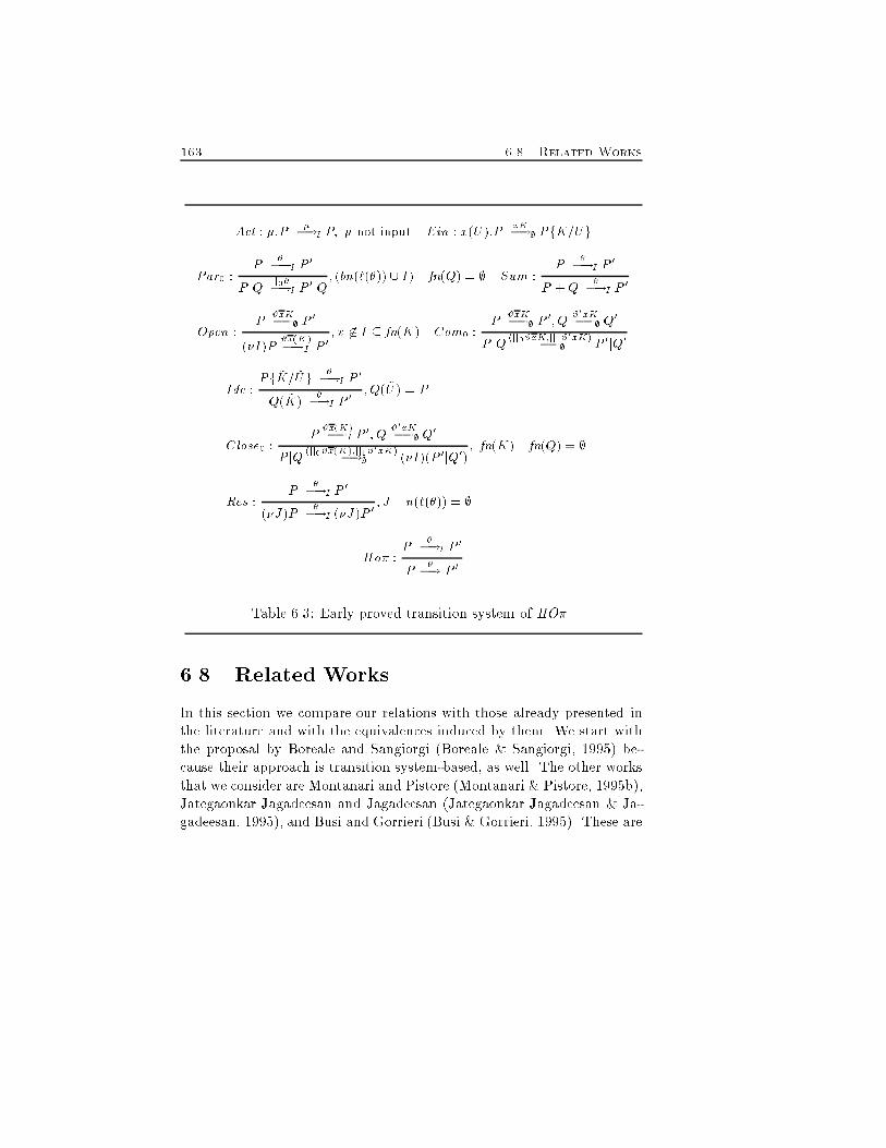
163 6.8. Related WorksAct : �:P ��!; P; � not input Ein : x(U):P xK�!; PfK=UgPar0 : P ��!I P 0P jQ jj0��!I P 0jQ; (bn(`(�)) [ I) \ fn(Q) = ; Sum : P ��!I P 0P +Q ��!I P 0Open : P #xK�!; P 0(�I)P #x(K)�!I P 0 ; x 62 I � fn(K) Com0 : P #xK�!; P 0;Q #0xK�!; Q0P jQ hjj0#xK;jj1#0xKi�!; P 0jQ0Ide : Pf ~K= ~Ug ��!I P 0Q( ~K) ��!I P 0 ;Q( ~U) = PClose0 : P #x(K)�!I P 0; Q #0xK�!; Q0P jQ hjj0#x(K);jj1#0xKi�!; (�I)(P 0jQ0) ; fn(K) \ fn(Q) = ;Res : P ��!I P 0(�J)P ��!I (�J)P 0 ; J \ n(`(�)) = ;Ho� : P ��!I P 0P ��! P 0Table 6.3: Early proved transition system of HO�.6.8 Related WorksIn this section we compare our relations with those already presented inthe literature and with the equivalences induced by them. We start withthe proposal by Boreale and Sangiorgi (Boreale & Sangiorgi, 1995) be-cause their approach is transition system-based, as well. The other worksthat we consider are Montanari and Pistore (Montanari & Pistore, 1995b),Jategaonkar Jagadeesan and Jagadeesan (Jategaonkar Jagadeesan & Ja-gadeesan, 1995), and Busi and Gorrieri (Busi & Gorrieri, 1995). These are

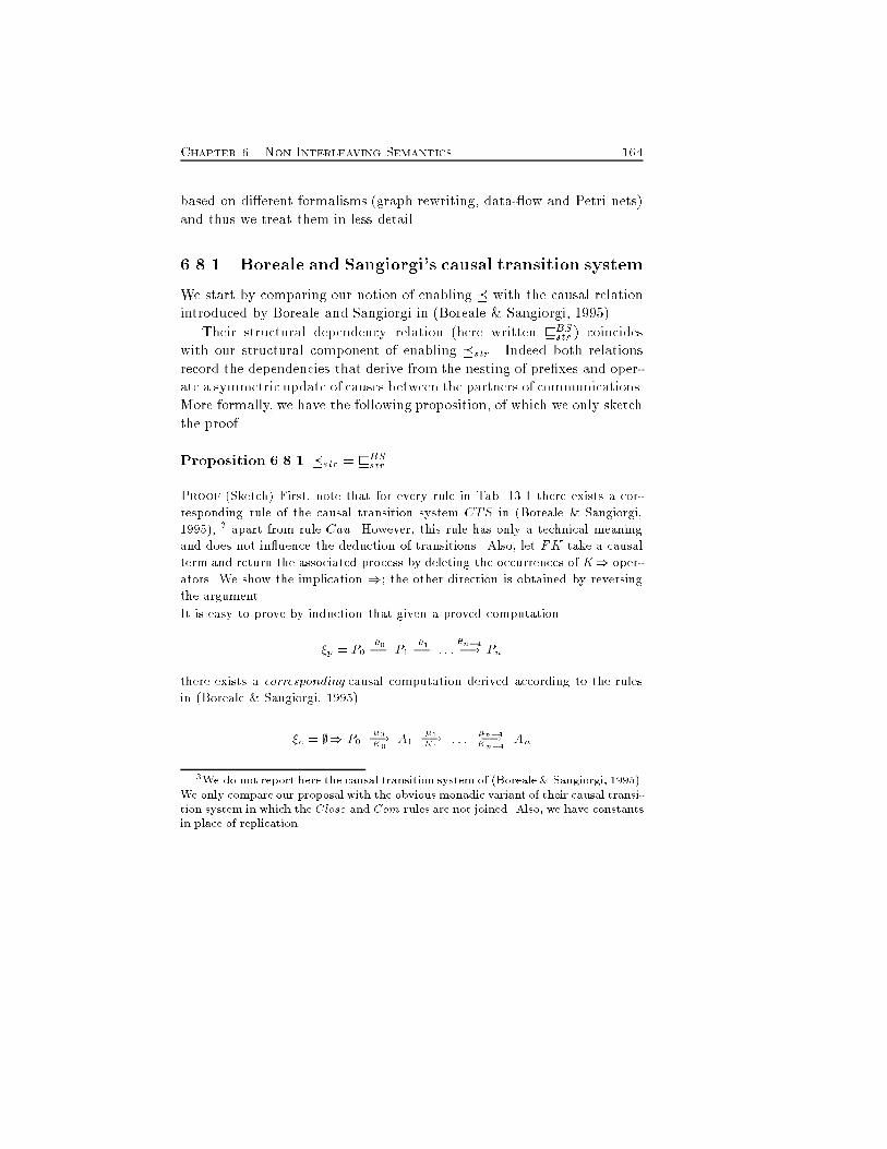
Chapter 6. Non Interleaving Semantics 164based on di�erent formalisms (graph rewriting, data- ow and Petri nets)and thus we treat them in less detail.6.8.1 Boreale and Sangiorgi's causal transition systemWe start by comparing our notion of enabling � with the causal relationintroduced by Boreale and Sangiorgi in (Boreale & Sangiorgi, 1995).Their structural dependency relation (here written vBSstr ) coincideswith our structural component of enabling �str. Indeed both relationsrecord the dependencies that derive from the nesting of pre�xes and oper-ate a symmetric update of causes between the partners of communications.More formally, we have the following proposition, of which we only sketchthe proof.Proposition 6.8.1 �str = vBSstrProof.(Sketch) First, note that for every rule in Tab. 13.1 there exists a cor-responding rule of the causal transition system CTS in (Boreale & Sangiorgi,1995), 3 apart from rule Cau. However, this rule has only a technical meaningand does not in uence the deduction of transitions. Also, let FK take a causalterm and return the associated process by deleting the occurrences of K) oper-ators. We show the implication ); the other direction is obtained by reversingthe argument.It is easy to prove by induction that given a proved computation�p = P0 �0�! P1 �1�! : : : �n�1�! Pnthere exists a corresponding causal computation derived according to the rulesin (Boreale & Sangiorgi, 1995)�c = ;) P0 �0�!K0 A1 �1�!K1 : : : �n�1�!Kn�1 An3We do not report here the causal transition system of (Boreale & Sangiorgi, 1995).We only compare our proposal with the obvious monadic variant of their causal transi-tion system in which the Close and Com rules are not joined. Also, we have constantsin place of replication.

165 6.8. Related Workssuch that the proof of Ai �i�!Ki Ai+1 corresponds rule by rule (except for appli-cations of Cau) to that of Pi �i�! Pi+1, and FK(Ai) = Pi. Indeed, the rulesto apply depend on the syntactical structure of Ai alone, i.e., on FK(Ai). Weare left to prove that the causes Ki are computed correctly. In other words, thedependencies on the transitions in �p originated by �str are all and only thoserecorded in �c.The proof is by induction on the length of the computation. The base case isgiven by a single transition, and it is trivial.Let �c be the causal computation corresponding to the proved one �p. By in-ductive hypothesis, �str�p � vBSstr�c . To prove the inductive step, let�0p = �p �n�! P 0 and �0c = �c �n�!Kn A0be the two corresponding computations. Two cases are possible: either the lasttransition is visible or it is not.1. `(�n) 6= �) We prove ctn = h�;Ki and K � Kn. Assume that j is themaximum index such that �j �str �n. Only two sub-cases are possible.(a) �j 6= #h�; �0i) Actions �j and �n are originated by two immediatelynested pre�xes �1 and �2 in some context C. This implies that instate C0[�2:Pi], reached after �ring �1, the causes pre�xed to �2according to CTS contain the reference to the transition originatedby �1 6= � (rule Out or Inp) as it happens in our case as well. If�1 = � no dependency is originated in both approaches. The causesinherited through �1, if any, are correct by inductive hypothesis,thus ctn = h�n;Ki.(b) �j = #h�; �0i) Action �n is originated by a pre�x following immedi-ately the one that originates either � or �0. Let �s (�r) be the directcause of � (�0). By inductive hypothesis, the reference to �s (�r)is recorded in the derivation of the premises of Com (or Close) in(Boreale & Sangiorgi, 1995) and these are correctly pre�xed to theirresiduals. Thus, the references to �s and �r are recorded in Kn.2. `(�n) = �) As silent transitions bear no causes, we only have to provethat communications transmit the correct causes to the residuals of thepartners. This derives from examining rule Com in (Boreale & Sangiorgi,

Chapter 6. Non Interleaving Semantics 1661995) which updates the references of each partner with the references tothe causes of the other one. This corresponds to the updating of causesperformed by our relation �str (see the last three items in Def. 6.3.8). 2In a similar way to the above proposition, we can prove the following,where vSloc is the locality relation de�ned by Sangiorgi in (Sangiorgi; 1994).Proposition 6.8.2 vloc = vSloc.We rephrase Boreale and Sangiorgi's object dependency relation.De�nition 6.8.3 (Boreale and Sangiorgi's object dependency)Let P0 �0�! P1 �1�! : : : �n�! Pn+1 be a computation. Then, the objectdependency of �n, if any, is the unique �h (�h <BSobj �n) such that`(�h) 2 fx(a); xag, and a 2 fn(`(�n)).We now compare our dependency relations with the causal relations in(Boreale & Sangiorgi, 1995).Proposition 6.8.4 �nam � <BSobj .Proof. The inclusion holds because �h can also be an input in Def. 6.8.3 of<BSobj , while it cannot in Def. 6.3.10 of �nam, and it is strict because in theproved computation x(y):y xb�! b b�! 0the second transition is object dependent on the �rst, but it is not name enabled.2Theorem 6.8.5 Let vBS= (vBSstr [ <BSobj )�. Then,1. � = vBS 2. v � vBS 3. �� vBS 4. vloc � vBS5. ^ \ vBS = ;

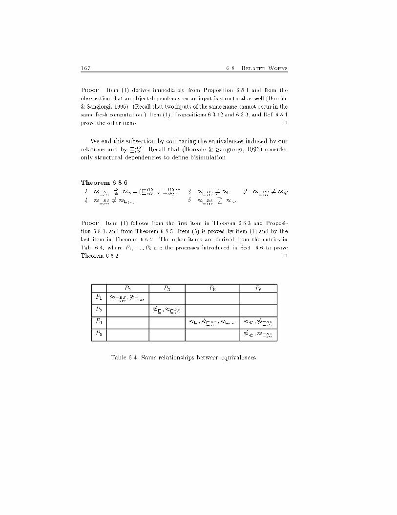
167 6.8. Related WorksProof. Item (1) derives immediately from Proposition 6.8.1 and from theobservation that an object dependency on an input is structural as well (Boreale& Sangiorgi, 1995). (Recall that two inputs of the same name cannot occur in thesame fresh computation.) Item (1), Propositions 6.3.12 and 6.3.3, and Def. 6.5.1prove the other items. 2We end this subsection by comparing the equivalences induced by ourrelations and by vBSstr . Recall that (Boreale & Sangiorgi, 1995) consideronly structural dependencies to de�ne bisimulation.Theorem 6.8.61. �vBSstr )6( ��= (vBSstr [ <BSobj )� 2. �vBSstr 6= �v 3. �vBSstr 6= ��4. �vBSstr 6= �vloc 5. �vBSstr )6( �^Proof. Item (1) follows from the �rst item in Theorem 6.6.3 and Proposi-tion 6.8.1, and from Theorem 6.8.5. Item (5) is proved by item (1) and by thelast item in Theorem 6.6.2. The other items are derived from the entries inTab. 6.4, where P1; : : : ; P6 are the processes introduced in Sect. 6.6 to proveTheorem 6.6.2. 2P2 P3 P5 P6P1 �vBSstr ; 6�vlocP2 6�v;�vBSstrP4 �v; 6�vBSstr ;�vloc ��; 6�vBSstrP5 6��;�vBSstrTable 6.4: Some relationships between equivalences.

Chapter 6. Non Interleaving Semantics 1686.8.2 Other causal models: graph rewriting, data- owand Petri netsA graph rewriting approach that induces a concurrent semantics for a sub-set of �-calculus (+ is omitted) is proposed by Montanari and Pistore in(Montanari & Pistore, 1995b). Processes are mapped into labelled hyper-graphs, whose arcs represent their sequential components and whose nodesrepresent names. A special kind of arc is used to single out unrestrictednames. To denote the graph corresponding to a whole process, some graphmanipulations are needed (graph composition, restriction and substitu-tion). Finally, a production schema is introduced to rewrite graphs, thusdescribing the dynamic behaviour of processes. Besides the rather di�er-ent technicalities, the crucial point that makes this proposal di�erent fromours is the possibility of parallel extrusion. More precisely, in (Montanari& Pistore, 1995b) the process (�a)(xa j ya)can perform concurrently the two actions x(a) and y(a), while in ourproposal, as in the standard interleaving semantics, only one of the two isactually a bound output.A data- ow analysis of �-calculus (and CCS) is described by Jate-gaonkar Jagadeesan and Jagadeesan in (Jategaonkar Jagadeesan & Ja-gadeesan, 1995). The key idea is to adapt Kahn's semantics of staticdeterminate data- ow to dynamic networks. This is done by allowingthe ow of structured tokens on a static network and by generalizing de-terminate networks to indeterminate ones. Indeterminacy is obtained bydescribing processes as sets of functions on suitable domains. These aredI-domains made up of sequences of the cartesian product of tree-likestructures.A distributed semantics for �-calculus based on P/T Petri nets withinhibitor arcs is presented by Busi and Gorrieri in (Busi & Gorrieri, 1995).The inhibitor arcs are introduced to solve con icts and to deal with re-stricted names. Each name a has a place (�a) which, when it contains atleast one token, inhibits any a- or a-transition. Choices are mapped into

169 6.9. The causal transition systemparallel compositions decorated by distinguished con ict names k and k.The net semantics is such that when the name k is enabled, k is inhib-ited, and vice versa. Their proposal requires only �ve rules to describethe dynamic behaviour of nets. The causality relation is made explicit bygenerating a causal tree (Darondeau & Degano, 1989) starting by a mark-ing of the network. The initial marking is given by decomposing processesinto their sequential components, in the style of (Degano et al., 1990).In the last two approaches, the resulting notion of causality is theclassical one which we believe coincides with our notion of enabling. Forexample, they identify the behaviour of processes such as (�a)(xa j ab)and (�a)(xa:ab). This claim is further supported as structural and namedependencies are not kept distinct.6.9 The causal transition systemWe show that the de�nitions of non interleaving relations and of the cor-responding relabelling functions drive us in directly de�ning a transitionsystem for the model selected. We de�ne here as a test bed the causaltransition system, simply by rephrasing the work done to de�ne the causalrelabelling function. Following (Kiehn, 1991), we identify transitions withunique names and we use these names to encode the causes in the labelsof transitions, i.e. we use explicit causes. The names denoting causes aretaken from an in�nite countable set K.We extend the language by pre�xing each process P with a pair of setsthat denote the structural (K) and the link (L) dependencies. The setL is made up of pairs whose �rst component is the name extruded by atransition � and the second component is the set of (link and structural)causes of �. The syntax of causal processes isA ::= (K;L)) A j AjA j (�x)A j Pwhere P is a standard process as in Def. 4.1.1. Some notation can help.We de�ne n(L) = fxjhx;Ki 2 Lg, (K;L)) (K 0; L0)) A = (K [K 0; L [L0) ) A and L � fyg = L � fhx;Ki jx = yg. We assume that (K;L) )distributes over all operators apart from pre�x. We write K(A) for the

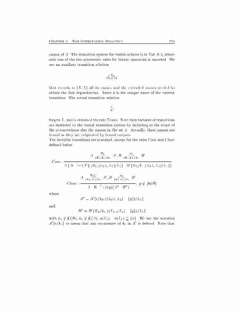
Chapter 6. Non Interleaving Semantics 170causes of A. The transition system for visible actions is in Tab. 6.5, whereonly one of the two symmetric rules for binary operators is reported. Weuse an auxiliary transition relation �7�!(K;L);kthat records in (K;L) all its causes and the extruded names needed toobtain the link dependencies. Name k is the unique name of the currenttransition. The actual transition relation��!Kforgets L, and is obtained via rule Trans. Note that variants of transitionsare extended to the causal transition system by including in the scope ofthe �-convertions also the names in the set L. Actually, these names arebound as they are originated by bound outputs.The invisible transitions are standard, except for the rules Com and Closede�ned belowCom : A xy7�!(K0;L0);k0 A0; B xy7�!(K1;L1);k1 B0A j B ��! (A0f�=k0; (L0 [ L1)=L0g j B0fK0=k1; (L0 [ L1)=L1g)Close : A x(y)7�!(K0;L0);k0 A0; B xy7�!(K1;L1);k1 B0A j B ��! (�y)(A00 j B00) ; y 62 fn(B)where A00 = A0f�=k0; ((L0 [ L1)� fyg)=L0gand B00 = B0fK0=k1; ((L0 [ L1)� fyg)=L1gwith k0 62 K(B), k1 62 K(A), n(L0) \ n(L1) � fxg. We use the notationA0f�=k0g to mean that any occurrence of k0 in A0 is deleted. Note that

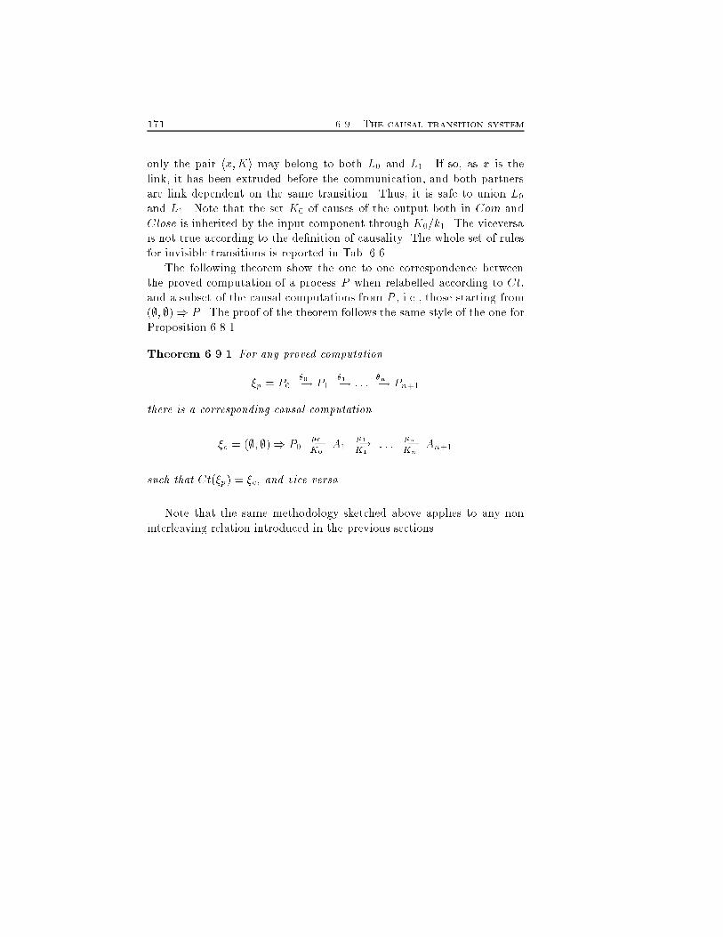
171 6.9. The causal transition systemonly the pair hx;Ki may belong to both L0 and L1. If so, as x is thelink, it has been extruded before the communication, and both partnersare link dependent on the same transition. Thus, it is safe to union L0and L1. Note that the set K0 of causes of the output both in Com andClose is inherited by the input component through K0=k1. The viceversais not true according to the de�nition of causality. The whole set of rulesfor invisible transitions is reported in Tab. 6.6.The following theorem show the one to one correspondence betweenthe proved computation of a process P when relabelled according to Ct,and a subset of the causal computations from P , i.e., those starting from(;; ;)) P . The proof of the theorem follows the same style of the one forProposition 6.8.1.Theorem 6.9.1 For any proved computation�p = P0 �0�! P1 �1�! : : : �n�! Pn+1there is a corresponding causal computation�c = (;; ;)) P0 �0�!K0 A1 �1�!K1 : : : �n�!Kn An+1such that Ct(�p) = �c, and vice versa.Note that the same methodology sketched above applies to any noninterleaving relation introduced in the previous sections.

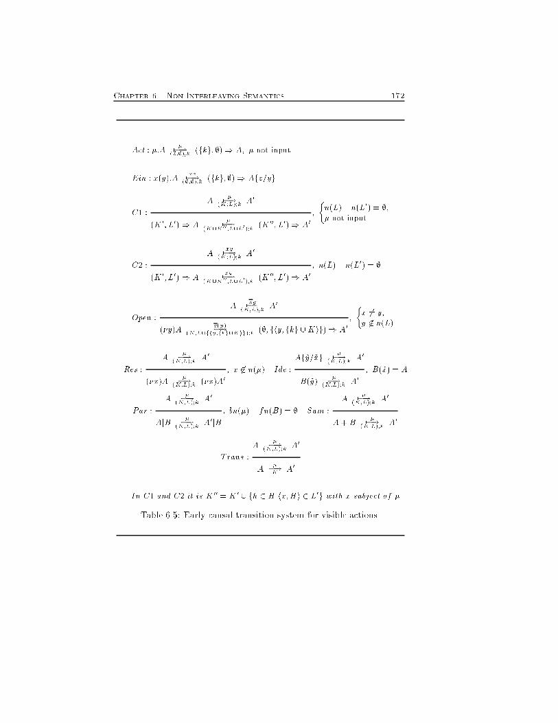
Chapter 6. Non Interleaving Semantics 172Act : �:A �7�!(;;;);k (fkg; ;)) A; � not inputEin : x(y):A xz7�!(;;;);k (fkg; ;)) Afz=ygC1 : A �7�!(K;L);k A0(K 0; L0)) A �7�!(K[K00;L[L0);k (K 00; L0)) A0 ; �n(L) \ n(L0) = ;;� not inputC2 : A xy7�!(K;L);k A0(K 0; L0)) A xy7�!(K[K00;L[L0);k (K 00; L0)) A0 ; n(L) \ n(L0) = ;Open : A xy7�!(K;L);k A0(�y)A x(y)7�!(K;L[fhy;fkg[Kig);k (;; fhy; fkg [Kig)) A0 ; �x 6= y;y 62 n(L)Res : A �7�!(K;L);k A0(�x)A �7�!(K;L);k (�x)A0 ; x 62 n(�) Ide : Af~y=~xg �7�!(K;L);k A0B(~y) �7�!(K;L);k A0 ; B(~x) = APar : A �7�!(K;L);k A0AjB �7�!(K;L);k A0jB ; bn(�) \ fn(B) = ; Sum : A �7�!(K;L);k A0A+B �7�!(K;L);k A0Trans : A �7�!(K;L);k A0A ��!K A0In C1 and C2 it is K 00 = K 0 [ fh 2 Hjhx;Hi 2 L0g with x subject of �Table 6.5: Early causal transition system for visible actions

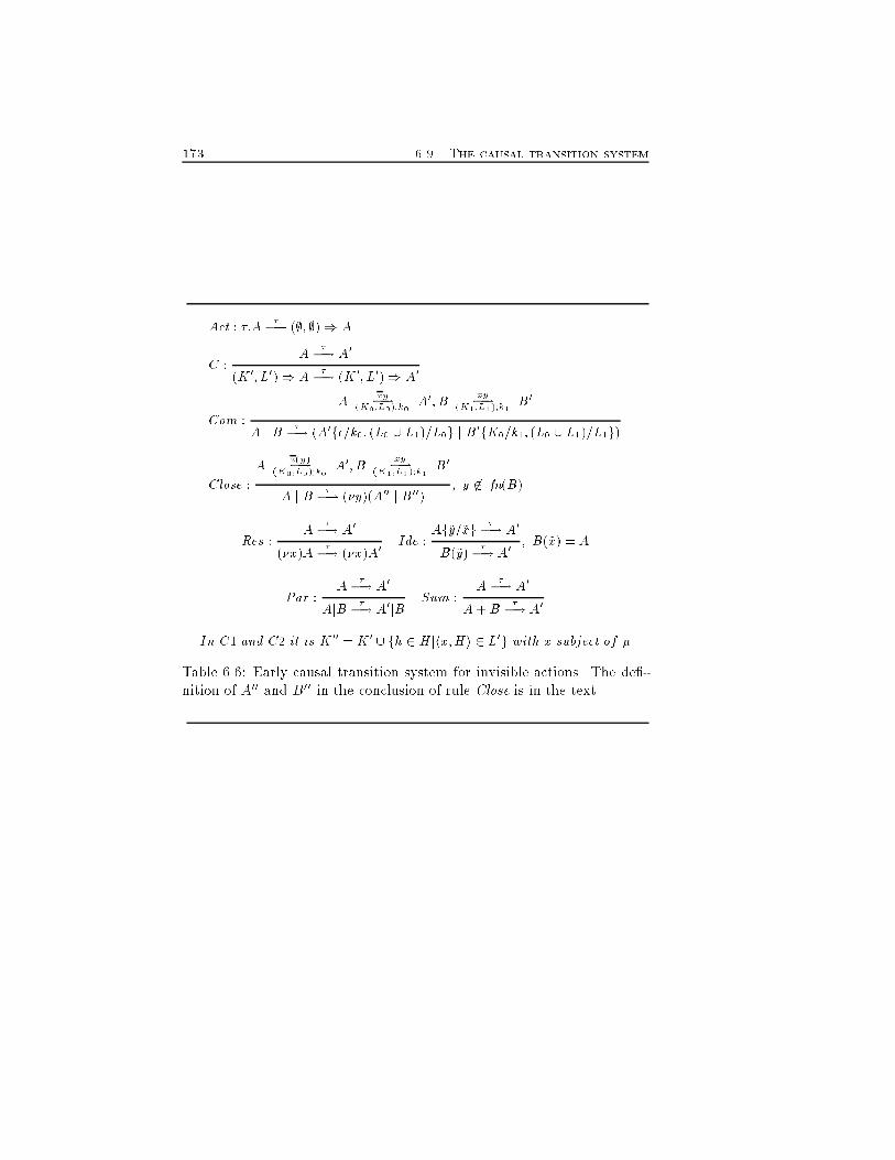
173 6.9. The causal transition systemAct : �:A ��! (;; ;)) AC : A ��! A0(K 0; L0)) A ��! (K 0; L0)) A0Com : A xy7�!(K0;L0);k0 A0;B xy7�!(K1;L1);k1 B0A j B ��! (A0f�=k0; (L0 [ L1)=L0g j B0fK0=k1; (L0 [ L1)=L1g)Close : A x(y)7�!(K0;L0);k0 A0;B xy7�!(K1;L1);k1 B0A j B ��! (�y)(A00 j B00) ; y 62 fn(B)Res : A ��! A0(�x)A ��! (�x)A0 Ide : Af~y=~xg ��! A0B(~y) ��! A0 ; B(~x) = APar : A ��! A0AjB ��! A0jB Sum : A ��! A0A+B ��! A0In C1 and C2 it is K 00 = K 0 [ fh 2 Hjhx;Hi 2 L0g with x subject of �Table 6.6: Early causal transition system for invisible actions. The de�-nition of A00 and B00 in the conclusion of rule Close is in the text.

Chapter 6. Non Interleaving Semantics 174

Chapter 7Partial OrderingSemanticsWe show here that partial ordering semantics can be de�ned in SOS style.We only need to change the referencing mechanism of unique names oftransition introduced in the previous chapter with action names, we obtaina more abstract class of semantics that we call partial ordering semantics.We also show that there is a hierarchy of models. The most concretemodel is the proved transition system. Then we abstract from the parallelstructure of processes and we obtain the semantics of the previous chap-ter, that we call mixed ordering semantics. When we abstract from thetemporal information through the new referencing mechanism we obtainthe partial ordering semantics. We de�ne a function that maps mixed intopartial ordering semantics. This de�nition drives us in de�ning directlypartial ordering transition systems. Finally, we restrict our attention toCCS, and we show that our partial ordering semantics is equivalent tothe one de�ned in (Degano et al., 1990) even if ours originates transitionsystems more compact because con�gurations are not modi�ed. In fact,we derive the causal relation between the labels of transitions withoutrecording nothing on the structure of processes in the con�gurations.175

Chapter 7. Partial Ordering Semantics 1767.1 Partial and mixed orderingsRecall from the Introduction that the intrinsic structure of transition sys-tems imposes an interleaving description of distributed systems. Essen-tially, two activities a and b that may evolve concurrently are representedby the two computations ab and ba. Due to their interleaving nature, tran-sition systems have not been considered suitable to study non-interleavingproperties, but only time-dependent ones.Since computations impose a total ordering on their transitions, noninterleaving semantics based on transition systems does not abstract fromthe ow of time. In fact, dependencies between transitions are encodedthrough unique names of transitions or pointers from the enabled to theenabling transitions in each computation. It is easy to see that also time isencoded in pointers. Therefore, the relations de�ned in this way originatea so-called mixed ordering (mo) of transitions (Degano et al., 1987), i.e.,a partial ordering enriched with a total ordering that is the generationordering of transitions imposed by computations.There are also semantics which abstract from the generation orderingwhen describing truly concurrent relations. The activities that a systemcan perform are collected in a set of events, partially ordered (po) by abinary, transitive relation. The events which are concurrent or mutualexclusive are not related by enabling. Examples of these models include(Pratt, 1986; Winskel, 1987; Degano et al., 1987; Montanari & Yankele-vich, 1992; Montanari & Pistore, 1995b). Note that it is important tode�ne partial ordering semantics in order to single out the set of trulyconcurrent computations, i.e. computations whose evolution steps aresets of transitions that can occur simultaneously. Partial ordering seman-tics are more abstract than the mixed ones. This further level abstractionmay help de�ning abstract concurrent machine. The set of concurrenttransitions may be used to specify for instance the concurrency managerin a distributed data-base. The manager schedule transactions so that themaximal degree of parallelism is ensured still preserving serializability ofoperations on the data-base. Actually, data-base theory relies on partialordering of events to establish correctness criteria for execution of transac-tions. Also object-oriented programming may bene�t from the de�nition

177 7.1. Partial and mixed orderingsof partial ordering semantics. Indeed, this semantics allows one to de�necorrectness criteria for the accesses to objects.Many non interleaving equivalences have been presented in the liter-ature to compare the behaviour of systems. Most of them are ad hocadaptations of the bisimulation equivalence (Park, 1981) to the po or morepresentations of systems discussed above. The po and mo equivalencesare di�erent as shown in (Rabinovich & Trakhtenbrot, 1988) by the ex-ample depicted in Fig. 7.1 (events are denoted by their labels, enabling byarrows and mutual exclusion by arcs labelled #). The two event structureare not mo bisimilar because the former selects the b to be �red whenchoosing the a, while the second does not. In fact, if the former eventstructure performs the second a, the only possible b is the one below it.Instead, the second event structure, after an a matching the one of theother still has two possible b. As far as po equivalence is concerned, theabove situation does not originate any problem because there is not areference to the particular a that causes the b.a a a a a ab b b b# ## #Figure 7.1: Two event structures po, but no mo, equivalentAs a matter of fact po and mo semantics are distinguished becauseof autoconcurrency. It occurs when two concurrent transitions share thesame label. For instance, the two a actions in the process a:bja are auto-concurrent. In these cases a confusion may arise between the occurrencesof the a's, for example in computation aab. It is possible to say explicitlywhich a enables the b, thus taking temporal ordering into account andyielding a mo, or simply say that b depends on (one of the) a, yielding apo. We show here that a po description of distributed systems is possiblealso by transition systems, in spite of their interleaving nature. Actually,

Chapter 7. Partial Ordering Semantics 178a transitional semantics that yields po descriptions is already presented in(Degano et al., 1990) for CCS. The authors modify the structure of thestates of the transition system to record which are the sequential com-ponents of a system. This is done after the derivation of any transitionthrough a function dec de�ned by structural induction on the syntax ofagents. Our semantics is simpler because we have no need of decomposingprocesses into their sequential components and we leave the structure ofstates unchanged. We simply modify the relabelling function in the pre-vious chapter to obtain a po semantics, leaving unchanged the de�nitionsof dependency.In the mo semantics the relabelling yields pairs whose �rst componentis an action and whose second component is a set of unique names oftransitions. The names act as pointers to the activating transitions of thecurrent one. In order to release the temporal information included in thislabelling, we substitute the set of unique names with a multiset of actions.Essentially, references are the actions labelling the activating transitions.It is clear from this description that if the system cannot produce multipleactions with the same name, the po andmo representations are isomorphic.The de�nition of the po relabelling function drive us in de�ning in SOSstyle a po semantics of �-calculus that directly originates a po transitionsystem. The semantics is shown equivalent to the ones obtained by rela-belling the proved transition system. As a consequence, the de�nition ofthe po semantics in SOS style allows us to use the classical de�nition ofbisimulation together with its axiomatizations with almost no change, aswell as the modal characterizations of systems.7.2 po relabellingIn this section we show how to relabel the proved transition system in or-der to obtain a po description of the enabling relation between transitions.This makes our representations more compact than other po representa-tions that modify the structure of con�gurations (e.g., (Degano et al.,1990)). We �rst report the de�nition of mixed ordering; the one of partialordering is in Sect. 2.6.

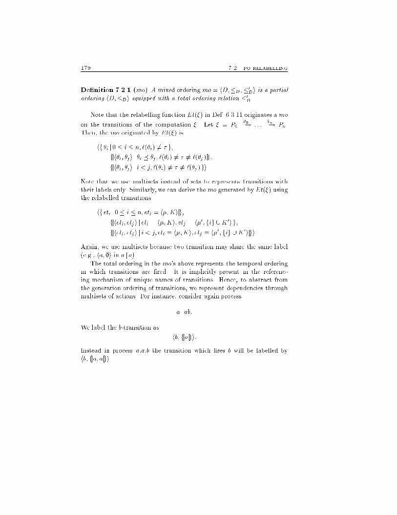
179 7.2. po relabellingDe�nition 7.2.1 (mo) A mixed ordering mo = hD;�D ;�0Di is a partialordering hD;�Di equipped with a total ordering relation �0D.Note that the relabelling function Et(�) in Def. 6.3.11 originates a moon the transitions of the computation �. Let � = P0 �0�! : : : �n�! Pn.Then, the mo originated by Et(�) ishfj�i j 0 � i � n; `(�i) 6= � jg;fjh�i; �ji j �i � �j ; `(�i) 6= � 6= `(�j)jg;fjh�i; �ji j i < j; `(�i) 6= � 6= `(�j )jgiNote that we use multisets instead of sets to represents transitions withtheir labels only. Similarly, we can derive the mo generated by Et(�) usingthe relabelled transitionshfjeti j 0 � i � n; eti = h�;Kijg;fjheti; etji j eti = h�;Ki; etj = h�0; fig [K 0ijg;fjheti; etji j i < j; eti = h�;Ki; etj = h�0; fig [K 0ijgiAgain, we use multisets because two transition may share the same label(e.g., ha; ;i in a j a).The total ordering in the mo's above represents the temporal orderingin which transitions are �red. It is implicitly present in the referenc-ing mechanism of unique names of transitions. Hence, to abstract fromthe generation ordering of transitions, we represent dependencies throughmultisets of actions. For instance, consider again processa j ab:We label the b-transition as hb; fjajgi:Instead in process a:a:b the transition which �res b will be labelled byhb; fja; ajgi.

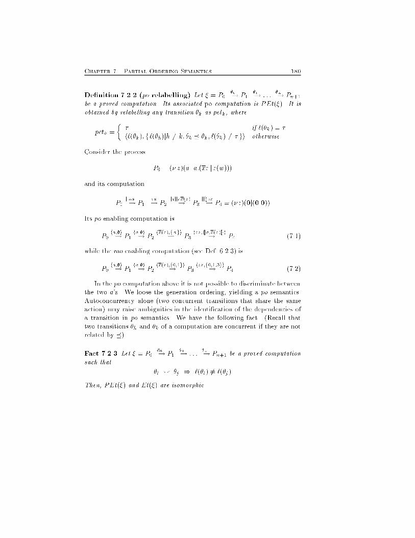
Chapter 7. Partial Ordering Semantics 180De�nition 7.2.2 (po relabelling) Let � = P0 �0�! P1 �1�! : : : �n�! Pn+1be a proved computation. Its associated po computation is PEt(�). It isobtained by relabelling any transition �k as petk, wherepetk = � � if `(�k) = �h`(�k); fj`(�h)jh 6= k; �h � �k; `(�h) 6= � jgi otherwiseConsider the process P0 = (� z)(a j a:(xz j z(w)))and its computationP0 jj0a�! P1 jj1a�! P2 jj1jj0x(z)�! P3 jj21zz�! P4 = (�z)(0j(0j0))Its po enabling computation isP0 ha;;i�! P1 ha;;i�! P2 hx(z);fjajgi�! P3 hzz;fja;x(z)jgi�! P4 (7.1)while the mo enabling computation (see Def. 6.2.3) isP0 ha;;i�! P1 ha;;i�! P2 hx(z);f0;1gi�! P3 hzz;f0;1;3gi�! P4 (7.2)In the po computation above it is not possible to discriminate betweenthe two a's. We loose the generation ordering, yielding a po semantics.Autoconcurrency alone (two concurrent transitions that share the sameaction) may raise ambiguities in the identi�cation of the dependencies ofa transition in po semantics. We have the following fact. (Recall thattwo transitions �h and �k of a computation are concurrent if they are notrelated by �).Fact 7.2.3 Let � = P0 �0�! P1 �1�! : : : �n�! Pn+1 be a proved computationsuch that �i ^ �j ) `(�i) 6= `(�j)Then, PEt(�) and Et(�) are isomorphic.

181 7.3. mo vs. po semanticsIn fact, whenever all concurrent transitions describe di�erent actions,their names act as unique pointers up to isomorphism. Note that twotransitions which are not concurrent may share the same label. In thiscase one transition enables the other, and the use of multisets rules outambiguities (see the example before Def. 7.2.2).Needless to say, besides po enabling, we can de�ne the po version ofall relations introduced in the previous chapter simply by replacing � inDef. 7.2.2 with the relation selected.7.3 mo vs. po semanticsThe relabelling functions of the proved transition system give an encodingof partial and mixed ordering of events without a precise identi�cation ofthe events. In this section we show how to extract these events and thestandard de�nition from computations that have been relabelled. Fur-thermore, we show that our po relabelling (Def. 7.2.2) actually yields thepo semantics in (Degano et al., 1990), when we restrict our attention toprocesses without objects (e.g., to CCS). The semantics obtained is alsocalled history preserving in (van Glabbeek & Goltz, 1989).Hereafter, we restrict ourselves to labelled orderings. More precisely weassume that any po and mo is equipped with a function f that associatesto each element a label. Furthermore, let [P ]mo and [P ]po be the transitionsystems obtained by relabelling any computation of P with the same moand po relations. The following theorem states that the ordering we extractfrom [P ]mo and [P ]po are actually an mo and a po. Furthermore, the po isisomorphic to the ordering obtained frommo by discarding the generationordering.Theorem 7.3.1 Let o = hE;�; f;�i and o0 = hE0;�po; f 0i be the order-ings of events extracted from [P ]mo and [P ]po, respectively. Then, o is amixed ordering, o0 is a partial ordering and hE;�; fi and o0 are isomor-phic.The proof of the theorem is quite long and technical, therefore we

Chapter 7. Partial Ordering Semantics 182report a detailed sketch in Sect. 7.5. We use Theorem 7.3.1 to prove thefollowing.Theorem 7.3.2 Let P be a process in which no object appears, and let[P ]po;� be the transition system obtained by the po enabling relabelling ofP . Then, the partial ordering extracted from [P ]po;� is isomorphic to theone obtained from P according to (Degano et al., 1990).Proof. Corollary 6.3.9 states that hE;�; f;�i originates the same relationbetween transitions de�ned in (Darondeau & Degano, 1989). Moreover, themixed ordering extracted from the causal trees of (Darondeau & Degano, 1989)is the same of the one de�ned in (Degano et al., 1990), as proved in (Conte,1991). Finally, the partial ordering relation introduced in (Degano et al., 1990)is isomorphic to the mixed ordering introduced in the same paper when thegeneration ordering is discarded from the latter. Now, Theorem 7.3.1 su�ces.2 The following theorem states the correspondence between our seman-tics and the one introduced in (Degano et al., 1990), when we restrict ourattention to �-calculus without objects.Theorem 7.3.3 Let P be a process in which no object appears, and let[P ]po;� be the transition system obtained by the po enabling relabellingof P . Then, the equivalence relation induced by bisimulation on [P ]po;�coincides with the one de�ned in (Degano et al., 1990).Proof. (Sketch) Recall that the transition system obtained by observing theproved one through PEt has the same nodes and transitions (up to x+x=x)of the standard interleaving one. The derivations that are allowed in (Deganoet al., 1990) are in one-to-one correspondence with those allowed by the stan-dard interleaving semantics. Hence, the structure and the actions compared inour approach and in (Degano et al., 1990) are the same. As the dependenciesassociated to a system in both approaches coincides, we are done. 2In addition, we can prove that the partial ordering extracted from thepo locality relabelling originates the semantics called abstract locality in(Montanari & Yankelevich, 1992).

183 7.4. SOS po semanticsTheorem 7.3.4 Let P be a process in which no object appears, and let[P ]po;vloc be the transition system obtained by the po locality relabelling ofP . Then, the partial ordering extracted from [P ]po;vloc is isomorphic tothe one obtained from P according to (Montanari & Yankelevich, 1992).Proof. Similar to the one of Theorem 7.3.2. 2We end this section by showing a hierarchy of models for distributedsystems. In fact, we de�ned relabelling functions from proved to mo andpo transition systems. We now discuss how to de�ne a relabelling functionthat maps mo transition systems to po ones.Recall that mo dependencies are expressed through set of pointers(unique names of transitions) to the activating transition of the currentone. Instead, po dependencies are expressed through multisets of actions.Therefore, we only need to replace unique names with their correspondingactions. More formally, we have the following de�nition.De�nition 7.3.5 (from mo to po) Let � = P0 ct0�! P1 ct1�! : : : ctn�! Pn+1be an mo computation. Its associated po computation is D(�) and is ob-tained by relabelling any transition ctk as pctk, wherepctk = � h�; fj`(�h) j �h 2 Sjg if ctk = h�; Si� otherwiseWe have established the following relation between proved, mixed andpartial ordering semanticsproved ! mixed ! partial:7.4 SOS po semanticsTransition systems that directly de�ne mo semantics have been presentedin the literature. The idea consists in enriching con�gurations with sets ofreferences to the activating transitions of the enabled ones. The de�nition

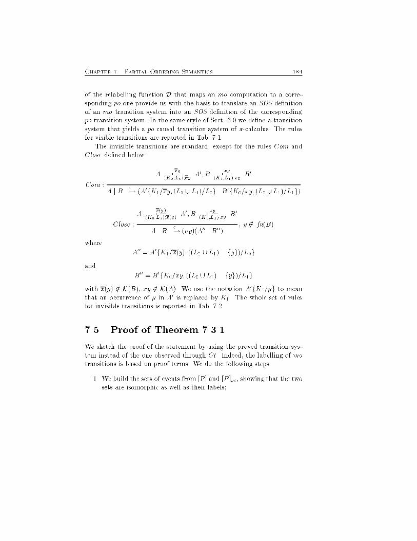
Chapter 7. Partial Ordering Semantics 184of the relabelling function D that maps an mo computation to a corre-sponding po one provide us with the basis to translate an SOS de�nitionof an mo transition system into an SOS de�nition of the correspondingpo transition system. In the same style of Sect. 6.9 we de�ne a transitionsystem that yields a po causal transition system of �-calculus. The rulesfor visible transitions are reported in Tab. 7.1.The invisible transitions are standard, except for the rules Com andClose de�ned belowCom : A xy7�!(K0;L0);xy A0; B xy7�!(K1;L1);xy B0A j B ��! (A0fK1=xy; (L0 [ L1)=L0g j B0fK0=xy; (L0 [L1)=L1g)Close : A x(y)7�!(K0;L0);x(y) A0; B xy7�!(K1;L1);xy B0A j B ��! (�y)(A00 j B00) ; y 62 fn(B)where A00 = A0fK1=x(y); ((L0 [ L1)� fyg)=L0gand B00 = B0fK0=xy; ((L0 [ L1) � fyg)=L1gwith x(y) 62 K(B), xy 62 K(A). We use the notation A0fK1=�g to meanthat an occurrence of � in A0 is replaced by K1. The whole set of rulesfor invisible transitions is reported in Tab. 7.2.7.5 Proof of Theorem 7.3.1We sketch the proof of the statement by using the proved transition sys-tem instead of the one observed through Ct. Indeed, the labelling of motransitions is based on proof terms. We do the following steps.1. We build the sets of events from [P ] and [P ]po, showing that the twosets are isomorphic as well as their labels;

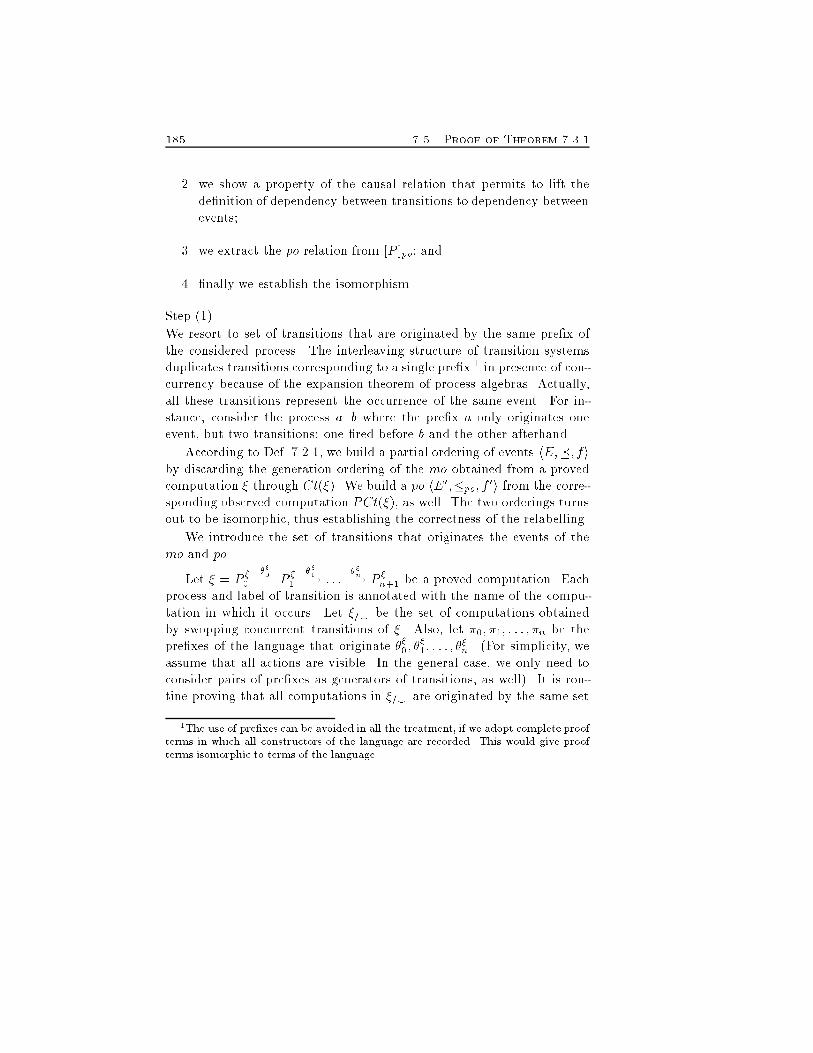
185 7.5. Proof of Theorem 7.3.12. we show a property of the causal relation that permits to lift thede�nition of dependency between transitions to dependency betweenevents;3. we extract the po relation from [P ]po; and4. �nally we establish the isomorphism.Step (1).We resort to set of transitions that are originated by the same pre�x ofthe considered process. The interleaving structure of transition systemsduplicates transitions corresponding to a single pre�x 1 in presence of con-currency because of the expansion theorem of process algebras. Actually,all these transitions represent the occurrence of the same event. For in-stance, consider the process a j b where the pre�x a only originates oneevent, but two transitions: one �red before b and the other afterhand.According to Def. 7.2.1, we build a partial ordering of events hE;�; fiby discarding the generation ordering of the mo obtained from a provedcomputation � through Ct(�). We build a po hE0;�po; f 0i from the corre-sponding observed computation PCt(�), as well. The two orderings turnsout to be isomorphic, thus establishing the correctness of the relabelling.We introduce the set of transitions that originates the events of themo and po.Let � = P �0 ��0�! P �1 ��1�! : : : ��n�! P �n+1 be a proved computation. Eachprocess and label of transition is annotated with the name of the compu-tation in which it occurs. Let �=^ be the set of computations obtainedby swopping concurrent transitions of �. Also, let �0; �1; : : : ; �n be thepre�xes of the language that originate ��0; ��1; : : : ; ��n. (For simplicity, weassume that all actions are visible. In the general case, we only need toconsider pairs of pre�xes as generators of transitions, as well). It is rou-tine proving that all computations in �=^ are originated by the same set1The use of pre�xes can be avoided in all the treatment, if we adopt complete proofterms in which all constructors of the language are recorded. This would give proofterms isomorphic to terms of the language.

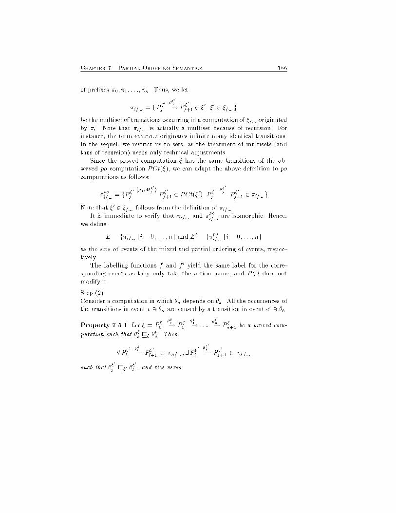
Chapter 7. Partial Ordering Semantics 186of pre�xes �0; �1; : : : ; �n. Thus, we let�i=^ = fjP �0j ��0j�! P �0j+1 2 �0 j �0 2 �=^ jgbe the multiset of transitions occurring in a computation of �=^ originatedby �i. Note that �i=^ is actually a multiset because of recursion. Forinstance, the term rec x a:x originates in�nite many identical transitions.In the sequel, we restrict us to sets, as the treatment of multisets (andthus of recursion) needs only technical adjustments.Since the proved computation � has the same transitions of the ob-served po computation PCt(�), we can adapt the above de�nition to pocomputations as follows:�poi=^ = fP �0j h�j ;M�0j i�! P �0j+1 2 PCt(�0) jP �0j ��0j�! P �0j+1 2 �i=^gNote that �0 2 �=^ follows from the de�nition of �i=^ .It is immediate to verify that �i=^ and �poi=^ are isomorphic. Hence,we de�neE = f�i=^ j i = 0; : : : ; ng and E0 = f�poi=^ j i = 0; : : : ; ngas the sets of events of the mixed and partial ordering of events, respec-tively.The labelling functions f and f 0 yield the same label for the corre-sponding events as they only take the action name, and PCt does notmodify it.Step (2).Consider a computation in which �n depends on �k. All the occurrences ofthe transitions in event e 3 �n are caused by a transition in event e0 3 �k.Property 7.5.1 Let � = P �0 ��0�! P �1 ��1�! : : : ��n�! P �n+1 be a proved com-putation such that ��k v� ��n. Then,8P �0l ��0l�! P �0l+1 2 �n=^ ; 9P �0j ��0j�! P �0j+1 2 �k=^such that ��0j v�0 ��0l , and vice versa.

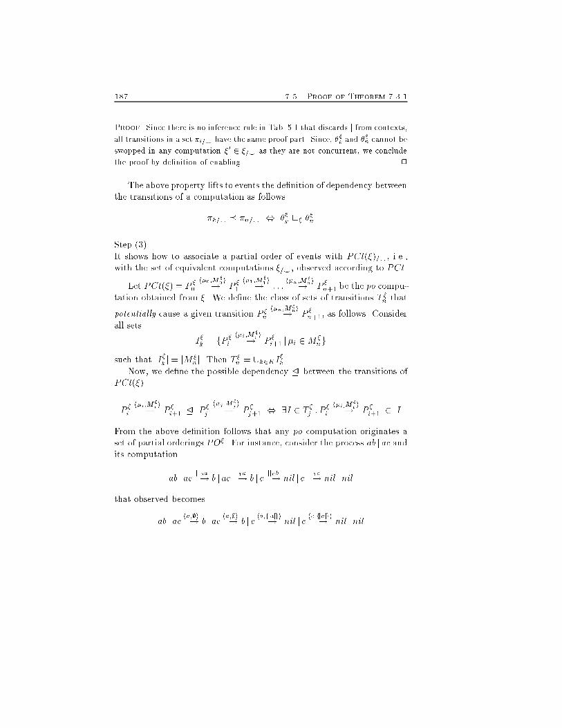
187 7.5. Proof of Theorem 7.3.1Proof. Since there is no inference rule in Tab. 5.1 that discards j from contexts,all transitions in a set �i=^ have the same proof part. Since, ��k and ��n cannot beswopped in any computation �0 2 �=^ as they are not concurrent, we concludethe proof by de�nition of enabling. 2The above property lifts to events the de�nition of dependency betweenthe transitions of a computation as follows�k=^ � �n=^ , ��k v� ��nStep (3).It shows how to associate a partial order of events with PCt(�)=^ , i.e.,with the set of equivalent computations �=^ , observed according to PCt.Let PCt(�) = P �0 h�0;M�0 i�! P �1 h�1 ;M�1 i�! : : : h�n;M�ni�! P �n+1 be the po compu-tation obtained from �. We de�ne the class of sets of transitions T �n thatpotentially cause a given transition P �n h�n;M�ni�! P �n+1, as follows. Considerall sets I�k = fP �i h�i ;M�i i�! P �i+1 j�i 2M �ngsuch that jI�kj = jM �nj. Then T �n = [k2KI�k .Now, we de�ne the possible dependency � between the transitions ofPCt(�).P �i h�i;M�i i�! P �i+1 � P �j h�j ;M�j i�! P �j+1 , 9I 2 T �j : P �i h�i;M�i i�! P �i+1 2 IFrom the above de�nition follows that any po computation originates aset of partial orderings PO�. For instance, consider the process ab j ac andits computationab j ac jj0a�! b j ac jj1a�! b j c jj0b�! nil j c jj1c�! nil jnilthat observed becomesab j ac ha;;i�! b j ac ha;;i�! b j c hb;fjajgi�! nil j c hc;fjajgi�! nil jnil

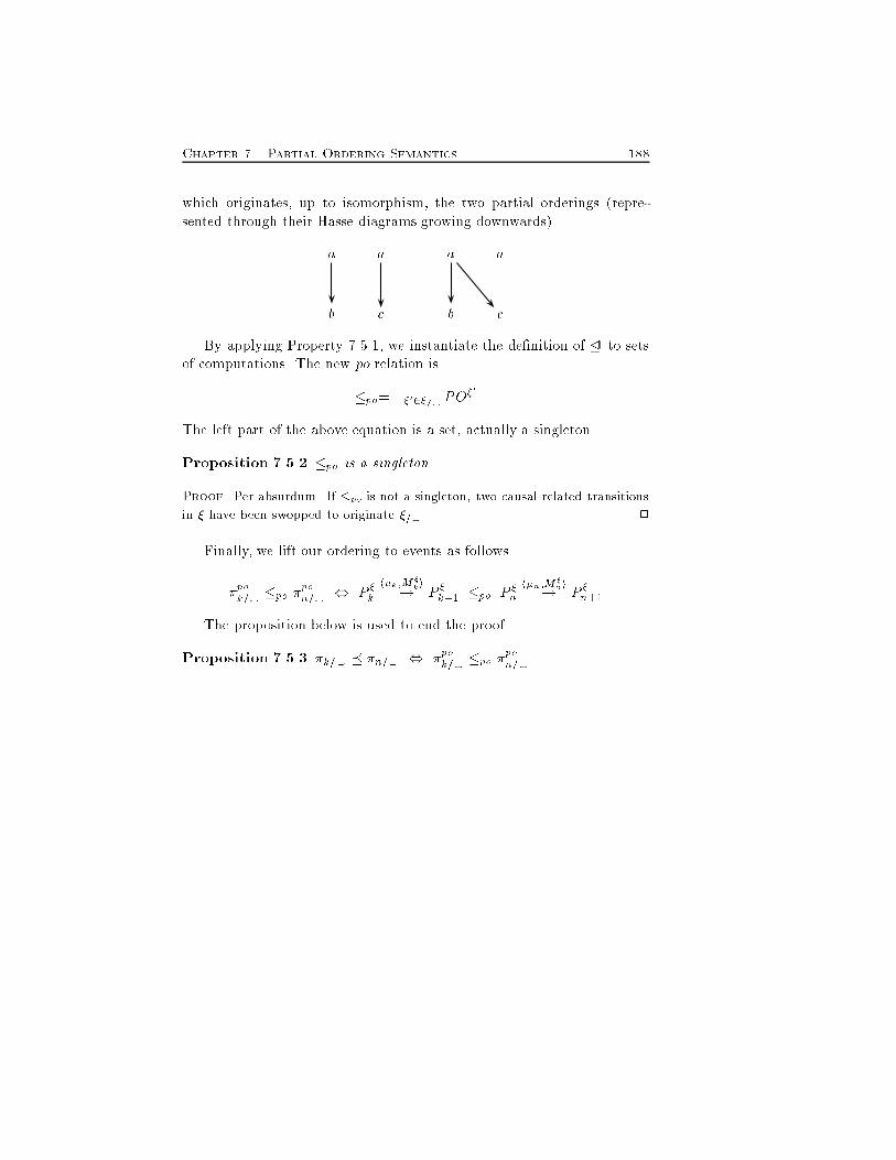
Chapter 7. Partial Ordering Semantics 188which originates, up to isomorphism, the two partial orderings (repre-sented through their Hasse diagrams growing downwards)a a a ab c b cBy applying Property 7.5.1, we instantiate the de�nition of � to setsof computations. The new po relation is�po= \�02�=^PO�0The left part of the above equation is a set, actually a singleton.Proposition 7.5.2 �po is a singleton.Proof. Per absurdum. If �po is not a singleton, two causal related transitionsin � have been swopped to originate �=^ . 2Finally, we lift our ordering to events as follows.�pok=^ �po �pon=^ , P �k h�k;M�ki�! P �k+1 �po P �n h�n;M�ni�! P �n+1The proposition below is used to end the proof.Proposition 7.5.3 �k=^ � �n=^ , �pok=^ �po �pon=^.

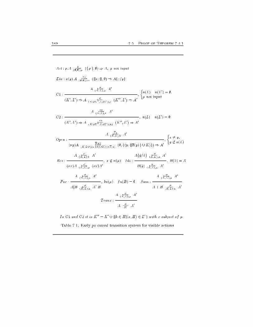
189 7.5. Proof of Theorem 7.3.1Act : �:A �7�!(;;;);� (fj�jg;;)) A; � not inputEin : x(y):A xz7�!(;;;);xz (fjxzjg;;)) Afz=ygC1 : A �7�!(K;L);� A0(K 0; L0)) A �7�!(K[K00;L[L0);� (K 00; L0)) A0 ; �n(L) \ n(L0) = ;;� not inputC2 : A xy7�!(K;L);k A0(K 0; L0)) A xy7�!(K[K00;L[L0);xy (K 00; L0)) A0 ; n(L) \ n(L0) = ;Open : A xy7�!(K;L);k A0(�y)A x(y)7�!(K;L[fhy;fkg[Kig);x(y) (;; fhy; fjx(y)jg [Kig)) A0 ; �x 6= y;y 62 n(L)Res : A �7�!(K;L);k A0(�x)A �7�!(K;L);� (�x)A0 ; x 62 n(�) Ide : Af~y=~xg �7�!(K;L);� A0B(~y) �7�!(K;L);� A0 ; B(~x) = APar : A �7�!(K;L);� A0AjB �7�!(K;L);� A0jB ; bn(�) \ fn(B) = ; Sum : A �7�!(K;L);� A0A+B �7�!(K;L);� A0Trans : A �7�!(K;L);� A0A ��!K A0In C1 and C2 it is K 00 = K 0 [ fjh 2 Hjhx;Hi 2 L0jg with x subject of �Table 7.1: Early po causal transition system for visible actions

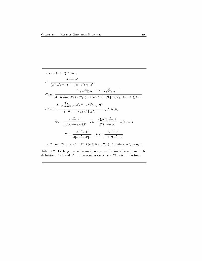
Chapter 7. Partial Ordering Semantics 190Act : �:A ��! (;; ;)) AC : A ��! A0(K 0; L0)) A ��! (K 0; L0)) A0 ;Com : A xy7�!(K0;L0);xy A0;B xy7�!(K1;L1);xy B0A j B ��! (A0fK1=xy; (L0 [ L1)=L0g j B0fK0=xy; (L0 [ L1)=L1g)Close : A x(y)7�!(K0;L0);x(y) A0;B xy7�!(K1;L1);xy B0A j B ��! (�y)(A00 j B00) ; y 62 fn(B)Res : A ��! A0(�x)A ��! (�x)A0 Ide : Af~y=~xg ��! A0B(~y) ��! A0 ; B(~x) = APar : A ��! A0AjB ��! A0jB Sum : A ��! A0A+B ��! A0In C1 and C2 it is K 00 = K 0 [ fh 2 Hjhx;Hi 2 L0g with x subject of �Table 7.2: Early po causal transition system for invisible actions. Thede�nition of A00 and B00 in the conclusion of rule Close is in the text.

Chapter 8A Case Study: FacileWe show how the approach presented in the previous chapters scales upto a real programming language like Facile. With respect to �-calculusand HO�, Facile distinguishes two di�erent levels of parallelism. Thereis a distribution of processes on nodes, and there is a certain degree ofparallelismwithin each node. As a consequence, there is an operator of thelanguage that allows the programmer to specify on which node a processmust be spawned. This operation need particular attention because maychange the parallel structure of processes and hence can make di�cultthe recovery of causal dependencies. Actually, we need to introduce someauxiliary transition rules to keep track of the evolution of the structure ofsystems. As usual, we start with the de�nition of the proved version ofthe operational semantics of the language. Then, we de�ne causality andlocality of transitions at two distinct levels. The former is the node level,while the latter study the relations between the transitions of processesallocated on the same node as well. Finally, we apply the proved semanticsto debug a real systems based on mobile agents and programmed in Facile.191

Chapter 8. A Case Study: Facile 1928.1 Proved Transition SystemWe de�ne the proved operational semantics of Facile by working on (Bor-gia, 1995). We �rst modify the core syntax of the language to drop theset N of nodes from con�gurations.Nodes are denoted by natural numbers that individuate positions ofnodes within Facile systems. We order nodes from left to right startingwith 1. We add a syntactic category program. A program is a distributedbehaviour expression with a begin and an end guard n, with n 2 INnf0g.The two guards denote the number of nodes in the system. To avoidconfusion between these guards and integers, we write them in boldface.The new syntax of Facile is obtained from the one in Tab. 4.5 by de�ningdistributed behaviour expressions asdbe ::= be jn j dbejjjdbeand programs as p ::= njjjdbejjjn:Hereafter, the set of programs will be denoted by P . Static checks ensurethat dbe in njjjdbejjjn does not contain any distributed behaviour expres-sion equal to n. To de�ne the semantics of r spawn(e; be) we add an endguard (x) to processes as well. Thus, we add to behavioural expressionsthe two following items be ::= : : : j bejjx j xAgain, static checks ensure that be in be jj x does not contain x. Finally, weassume that both jj and jjj are right associative to simplify the de�nitionof causal and local semantics of Facile.8.1.1 Labels of transitionsWe start with the de�nition of actions. In the following de�nition setComm is as in Def. 4.3.1.De�nition 8.1.1 (actions) The set Act of actions isComm [ f�g [ f(�; k) : k 2 Sg [ fnew(be) : be 2 BEg [

193 8.1. Proved Transition Systemf(be! n; i) : be 2 BE; n 2 IN; i 2 Zg:Elements of Act are denoted as �; �i; �0; : : :.Label (�; k) is originated by channel(t) and contains the name of the newchannel. Label new(be) denotes the creation of a new node on which be isactivated. Finally, (be! n; i) represents the creation of a new process tobe activated on node n. The value 0 is assigned to n for spawn(be) thatactivates be on the same node of the spawn operation. Integer i denotesthe number of jjj between node n and the one which performs the r spawn.Essentially, i is a relative address of the two nodes.According to the previous chapters, we extend action with the parallelstructure of the process which executes them.De�nition 8.1.2 (proof terms)Let � 2 Act, � 2 fjjj0; jjj1g�, and # 2 fjj0; jj1g�. The set � of proof termsis f�#�g [ f�#h�0#0�; �1#1��i : � 2 Commg [ f�0#0��1#1�gElements of � are denoted as �; �i; �0; : : :.Proof term �#� is the label of a generic action � executed by a processwhose position is encoded by �#. The synchronization of two processes islabelled �#h�0#0�; �1#1��i. Label �0#0��1#1� encodes either the creationof a new node or the allocation of a process through an r spawn; its usewill be clear afterwards.The following example shows the intuition behind proof terms. Con-sider the computation in Fig. 8.1.The label of the �rst transition jjj1jjj0jj0� says that the process atposition jjj1jjj0jj0 performs an internal action � . Since jjj and jj are right-associative, the transition is originated by pre�x spawn(be1).Unlike standard semantics of Facile (see Sect. 4.3), a new node is placedimmediately before the end guard (second transition). The proof partbefore � is the position of the process that performs the newnode withoutconsidering the node created. The proof part after � is the position of the

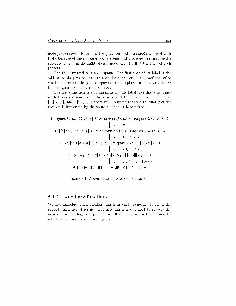
Chapter 8. A Case Study: Facile 194node just created. Note that the proof term of a newnode will end withjjj0jj0 because of the end guards of systems and processes that impose thepresence of a jjj at the right of each node and of a jj at the right of eachprocess.The third transition is an r spawn. The �rst part of its label is theaddress of the process that executes the operation. The proof part after� is the address of the process spawned that is placed immediately beforethe end guard of the destination node.The last transition is a communication. Its label says that v is trans-mitted along channel k. The sender and the receiver are located atjjj1jjj0jj1jj0 and jjj21jjj0jj0, respectively. Assume that the residual of thereceiver is in uenced by the value v. Then, it becomes 0.3 jjjspawn(be1):�jjk ! v:�jjxjjjk ?: jjnewnode(be4):�jjxjjjr spawn(2; be5):�jjxjjj33 jjj (�jjbe1)jjk ! v:�jjxjjjk ?: jjnewnode(be4):�jjxjjjr spawn(2; be5):�jjxjjj34 jjj (�jjbe1)jjk ! v:�jjxjjjk ?: jj�jjxjjjr spawn(2; be5):�jjxjjj be4jjxjjj44 jjj (�jjbe1)jjk ! v:�jjxjjjk ?: jj�jjbe5jjxjjj �jjxjjj be4jjxjjj44 jjj (�jjbe1)jj�jjxjjj 0jj�jjbe5jjxjjj �jjxjjj be4jjxjjj4jjj1 jjj0 jj0�jjj21 jjj0 jj1 jj0�jjj41 jjj0 jj0�jjj31 jjj0 jj0�jjj21 jjj0 jj21 jj0�jjj1 hjjj0 jj1 jj0k(v);jjj1 jjj0 jj0k(v)iFigure 8.1: A computation of a Facile program.8.1.2 Auxiliary functionsWe now introduce some auxiliary functions that are needed to de�ne theproved semantics of Facile. The �rst function ` is used to recover theaction corresponding to a proof term. It can be also used to obtain theinterleaving semantics of the language.

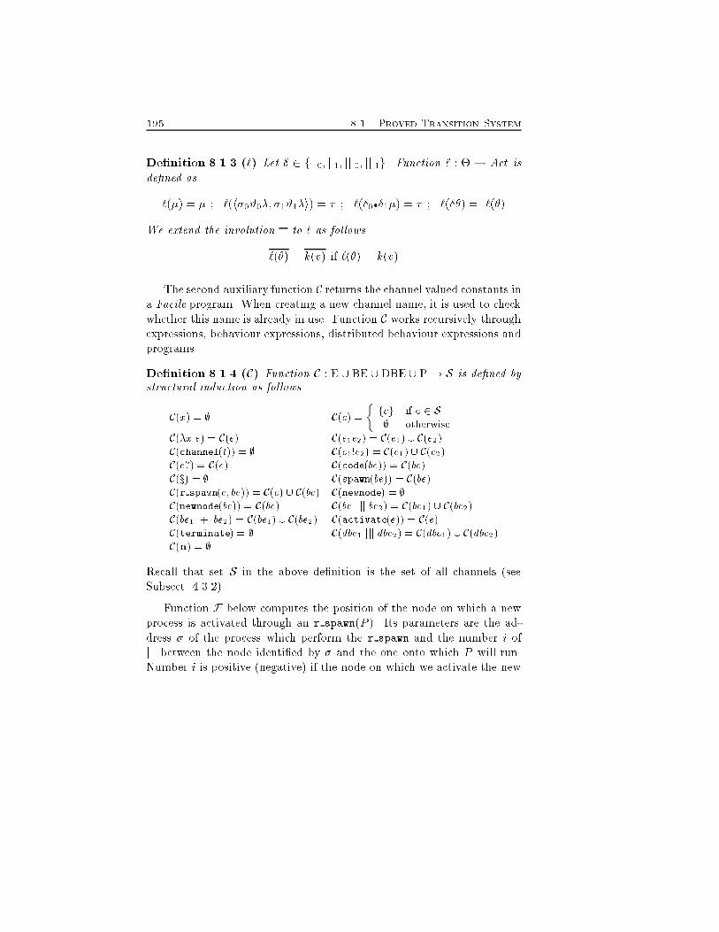
195 8.1. Proved Transition SystemDe�nition 8.1.3 (`) Let � 2 fjj0; jj1; jjj0; jjj1g. Function ` : � ! Act isde�ned as`(�) = � ; `(h�0#0�; �1#1��i) = � ; `(�0��1�) = � ; `(��) = `(�)We extend the involution to ` as follows.`(�) = k(v) if `(�) = k(v)The second auxiliary function C returns the channel valued constants ina Facile program. When creating a new channel name, it is used to checkwhether this name is already in use. Function C works recursively throughexpressions, behaviour expressions, distributed behaviour expressions andprograms.De�nition 8.1.4 (C) Function C : E [ BE [DBE [ P! S is de�ned bystructural induction as follows.C(x) = ; C(c) = � fcg if c 2 S; otherwiseC(�x:e) = C(e) C(e1e2) = C(e1) [ C(e2)C(channel(t)) = ; C(e1!e2) = C(e1) [ C(e2)C(e?) = C(e) C(code(be)) = C(be)C(x) = ; C(spawn(be)) = C(be)C(r spawn(e; be)) = C(e) [ C(be) C(newnode) = ;C(newnode(be)) = C(be) C(be1 jj be2) = C(be1) [ C(be2)C(be1 + be2) = C(be1) [ C(be2) C(activate(e)) = C(e)C(terminate) = ; C(dbe1 jjj dbe2) = C(dbe1) [ C(dbe2)C(n) = ;Recall that set S in the above de�nition is the set of all channels (seeSubsect. 4.3.2).Function F below computes the position of the node on which a newprocess is activated through an r spawn(P ). Its parameters are the ad-dress � of the process which perform the r spawn and the number i ofjjj between the node identi�ed by � and the one onto which P will run.Number i is positive (negative) if the node on which we activate the new

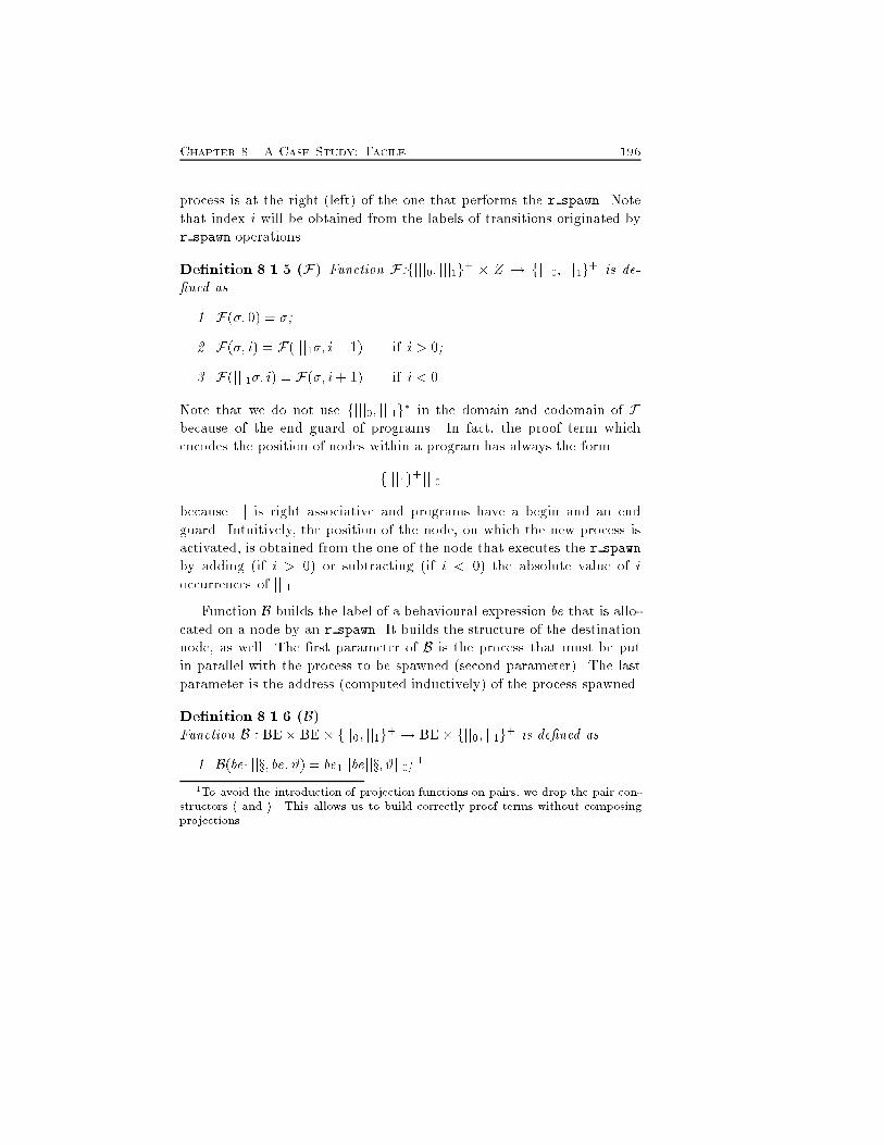
Chapter 8. A Case Study: Facile 196process is at the right (left) of the one that performs the r spawn. Notethat index i will be obtained from the labels of transitions originated byr spawn operations.De�nition 8.1.5 (F) Function F :fjjj0; jjj1g+ � Z ! fjjj0; jjj1g+ is de-�ned as1. F(�; 0) = �;2. F(�; i) = F(jjj1�; i� 1) if i > 0;3. F(jjj1�; i) = F(�; i+ 1) if i < 0Note that we do not use fjjj0; jjj1g� in the domain and codomain of Fbecause of the end guard of programs. In fact, the proof term whichencodes the position of nodes within a program has always the formfjjj1g+jjj0because jjj is right associative and programs have a begin and an endguard. Intuitively, the position of the node, on which the new process isactivated, is obtained from the one of the node that executes the r spawnby adding (if i > 0) or subtracting (if i < 0) the absolute value of ioccurrences of jjj1.Function B builds the label of a behavioural expression be that is allo-cated on a node by an r spawn. It builds the structure of the destinationnode, as well. The �rst parameter of B is the process that must be putin parallel with the process to be spawned (second parameter). The lastparameter is the address (computed inductively) of the process spawned.De�nition 8.1.6 (B)Function B : BE� BE � fjj0; jj1g+ ! BE � fjj0; jj1g+ is de�ned as1. B(be1jjx; be; #) = be1jjbejjx; #jj0; 11To avoid the introduction of projection functions on pairs, we drop the pair con-structors h and i. This allows us to build correctly proof terms without composingprojections.

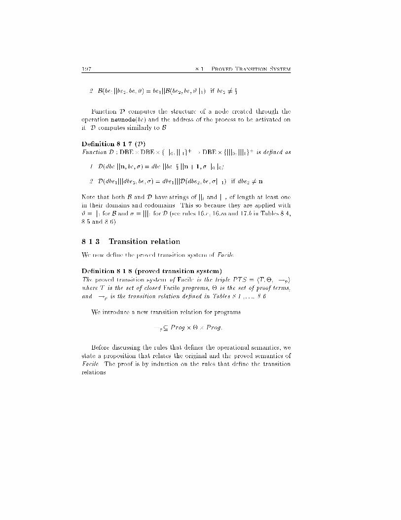
197 8.1. Proved Transition System2. B(be1jjbe2; be; #) = be1jjB(be2; be; #jj1) if be2 6= xFunction D computes the structure of a node created through theoperation newnode(be) and the address of the process to be activated onit. D computes similarly to B.De�nition 8.1.7 (D)Function D : DBE�DBE�fjjj0; jjj1g+ ! DBE�fjjj0; jjj1g+ is de�ned as1. D(dbejjjn; be; �) = dbejjjbejjxjjjn+ 1; �jjj0jj0;2. D(dbe1jjjdbe2; be; �) = dbe1jjjD(dbe2; be; �jjj1) if dbe2 6= nNote that both B and D have strings of jji and jjji of length at least onein their domains and codomains. This so because they are applied with# = jj1 for B and � = jjj1 for D (see rules 16:e, 16:m and 17:b in Tables 8.4,8.5 and 8.6).8.1.3 Transition relationWe now de�ne the proved transition system of Facile.De�nition 8.1.8 (proved transition system)The proved transition system of Facile is the triple PTS = hT;�;�!piwhere T is the set of closed Facile programs, � is the set of proof terms,and �!p is the transition relation de�ned in Tables 8.1 ,: : :, 8.6.We introduce a new transition relation for programs�!p� Prog �� � Prog:Before discussing the rules that de�nes the operational semantics, westate a proposition that relates the original and the proved semantics ofFacile. The proof is by induction on the rules that de�ne the transitionrelations.

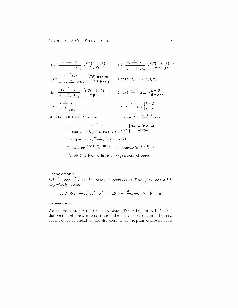
Chapter 8. A Case Study: Facile 1981:a : e1 ��!e e01e1e2 ��!e e01e2 ; � (�) = (�; k) )k 62 C(e2) 1:b : e2 ��!e e02ve2 ��!e ve02 ; � (�) = (�; k) )k 62 C(v)2:a : e1 ��!e e01e1 ! e2 ��!e e01!e2 ; � (�) = (�; k)) k 62 C(e2) 1:c : (�x:e)v ��!e efv=xg2:b : e2 ��!e e02k!e2 ��!e k!e02 ; � (�) = (�; h) )h 6= k 2:c : k!v k(v)�!e triv; �k 2 St; ` v : t3:a : e ��!e e0e? ��!e e0? 3:b : k? k(v)�!e v; �k 2 St; ` v : t4: : channel(t) (�;k)�!e k; k 2 St 5: : spawn(be) (be! 0;0)�!e triv6:a : e ��!e e0r spawn(e; be) ��!e r spawn(e0; be) ; � (�) = (�; k) )k 62 C(be)6:b : r spawn(n; be) (be! n;0)�!e triv; n > 07: : newnode new(terminate)�!e $ 8: : newnode(be) new(be)�!e $Table 8.1: Proved function expressions of Facile.Proposition 8.1.9Let ��! and ��!p be the transition relations in Defs. 4.3.2 and 8.1.8,respectively. Then,K;N; dbe ��! K 0; N 0; dbe0 , 9� : dbe ��!p dbe0 ^ `(�) = �ExpressionsWe comment on the rules of expressions (Tab. 8.1). As in Def. 4.3.2,the creation of a new channel returns the name of the channel. The newname cannot be already in use elsewhere in the program, otherwise name

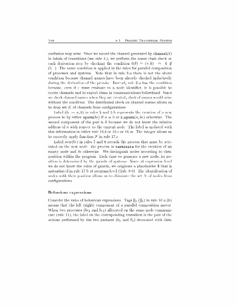
199 8.1. Proved Transition Systemconfusion may arise. Since we record the channel generated by channel(t)in labels of transitions (see rule 4:), we perform the name clash check ateach derivation step by checking the condition `(�) = (�; k) ) k 62C(�). The same condition is applied in the rules for parallel compositionof processes and systems. Note that in rule 3:a there is not the abovecondition because channel names have been already checked inductivelyduring the derivation of the premise. Instead, rule 6:a has the conditionbecause, even if e must evaluate to a node identi�er, it is possible tocreate channels and to export them in communications beforehand. Sincewe check channel names when they are created, clash of names would arisewithout the condition. The distributed check on channel names allows usto drop set K of channels from con�gurations.Label (be ! n; 0) in rules 5 and 6.b represents the creation of a newprocess be by either spawn(be) if n = 0 or r spawn(n; be) otherwise. Thesecond component of the pair is 0 because we do not know the relativeaddress of n with respect to the current node. The label is updated withthis information in either rule 16:b or 16:c or 16:m. The integer allows usto correctly apply function F in rule 17:c.Label new(be) in rules 7 and 8 records the process that must be acti-vated on the new node. the process is terminate for the creation of anempty node and be otherwise. We distinguish nodes according to theirposition within the program. Each time we generate a new node, its po-sition is determined by the guards of systems. Since at expression levelwe do not know the value of guards, we originate a placeholder $ that isinstantiated in rule 17.b at program level (Tab. 8.6). The identi�cation ofnodes with their position allows us to eliminate the set N of nodes fromcon�gurations.Behaviour expressionsConsider the rules of behaviour expressions. Tags jj0 (jj1) in rule 10.a (b)means that the left (right) component of a parallel composition moves.When two processes (be1 and be2) allocated on the same node communi-cate (rule 11), the label on the corresponding transition is the pair of theactions performed by the two partners (�1 and �2) decorated with their

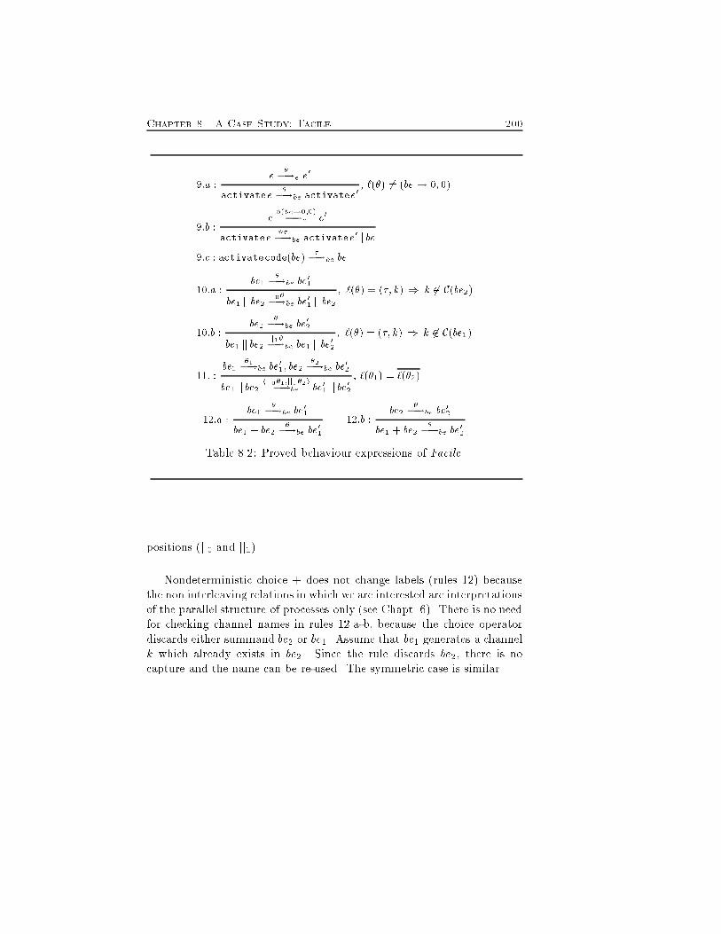
Chapter 8. A Case Study: Facile 2009:a : e ��!e e0activatee ��!be activatee0 ; `(�) 6= (be! 0; 0)9:b : e #(be!0;0)�!e e0activatee #��!be activatee0jj be9:c : activatecode(be) ��!be be10:a : be1 ��!be be01be1 jj be2 jj0��!be be01 jj be2 ; `(�) = (�; k) ) k 62 C(be2)10:b : be2 ��!be be02be1 jj be2 jj1��!be be1 jj be02 ; `(�) = (�; k) ) k 62 C(be1)11: : be1 �1�!be be01; be2 �2�!be be02be1 jj be2 hjj0�1;jj1�2i�!be be01 jj be02 ; `(�1) = `(�2)12:a : be1 ��!be be01be1 + be2 ��!be be01 12:b : be2 ��!be be02be1 + be2 ��!be be02Table 8.2: Proved behaviour expressions of Facile.positions (jj0 and jj1).Nondeterministic choice + does not change labels (rules 12) becausethe non interleaving relations in which we are interested are interpretationsof the parallel structure of processes only (see Chapt. 6). There is no needfor checking channel names in rules 12.a-b, because the choice operatordiscards either summand be2 or be1. Assume that be1 generates a channelk which already exists in be2. Since the rule discards be2, there is nocapture and the name can be re-used. The symmetric case is similar.

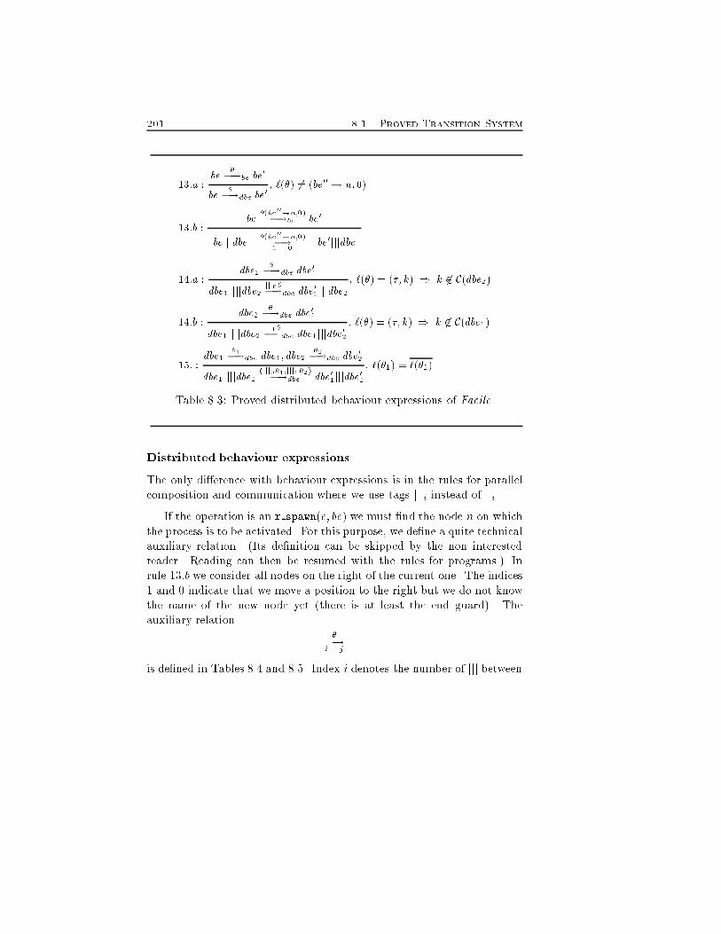
201 8.1. Proved Transition System13:a : be ��!be be0be ��!dbe be0 ; `(�) 6= (be00 ! n; 0)13:b : be #(be00!n;0)�!be be0#(be00!n;0)bejjjdbe �! be0jjjdbe1 014:a : dbe1 ��!dbe dbe01dbe1 jjjdbe2 jjj0��!dbe dbe01jjjdbe2 ; `(�) = (�; k) ) k 62 C(dbe2)14:b : dbe2 ��!dbe dbe02dbe1 jjjdbe2 jjj1��!dbe dbe1jjjdbe02 ; `(�) = (�; k) ) k 62 C(dbe1)15: : dbe1 �1�!dbe dbe1; dbe2 �2�!dbe dbe02dbe1 jjjdbe2 hjjj0�1;jjj1�2i�!dbe dbe01jjjdbe02 ; `(�1) = `(�2)Table 8.3: Proved distributed behaviour expressions of Facile.Distributed behaviour expressionsThe only di�erence with behaviour expressions is in the rules for parallelcomposition and communication where we use tags jjji instead of jji.If the operation is an r spawn(e; be) we must �nd the node n on whichthe process is to be activated. For this purpose, we de�ne a quite technicalauxiliary relation. (Its de�nition can be skipped by the non interestedreader. Reading can then be resumed with the rules for programs.) Inrule 13:b we consider all nodes on the right of the current one. The indices1 and 0 indicate that we move a position to the right but we do not knowthe name of the new node yet (there is at least the end guard). Theauxiliary relation ��!i jis de�ned in Tables 8.4 and 8.5. Index i denotes the number of jjj between

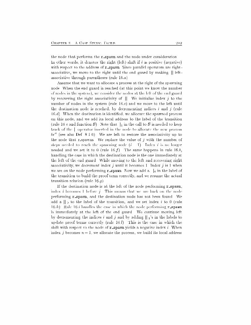
Chapter 8. A Case Study: Facile 202the node that performs the r spawn and the node under consideration.In other words, it denotes the right (left) shift if i is positive (negative)with respect to the address of r spawn. Since parallel operators are right-associative, we move to the right until the end guard by making jjj left-associative through parentheses (rule 16:a).Assume that we want to allocate a process at the right of the spawningnode. When the end guard is reached (at this point we know the numberof nodes in the system), we consider the nodes at the left of the end guardby recovering the right associativity of jjj. We initialise index j to thenumber of nodes in the system (rule 16:c) and we move to the left untilthe destination node is reached, by decrementing indices i and j (rule16:d). When the destination is identi�ed, we allocate the spawned processon this node, and we add its local address to the label of the transition(rule 16:e and function B). Note that jj1 in the call to B is needed to keeptrack of the jj operator inserted in the node to allocate the new processbe00 (see also Def. 8.1.6). We are left to restore the associativity up tothe node that r spawns. We replace the value of j with the number ofsteps needed to reach the spawning node (i � 1). Index i is no longerneeded and we set it to 0 (rule 16:f). The same happens in rule 16:b,handling the case in which the destination node is the one immediately atthe left of the end guard. While moving to the left and recovering rightassociativity, we decrement index j until it becomes 1. Index j is 1 whenwe are on the node performing r spawn. Now we add a jjj0 in the label ofthe transition to build the proof term correctly, and we resume the actualtransition relation (rule 16:g).If the destination node is at the left of the node performing r spawn,index i becomes 1 before j. This means that we are back on the nodeperforming r spawn, and the destination node has not been found. Weadd a jjj0 to the label of the transition, and we set index i to 0 (rule16:h). Rule 16:i handles the case in which the node performing r spawnis immediately at the left of the end guard. We continue moving leftby decrementing the indices i and j and by adding jjj1's in the labels toupdate proof terms correctly (rule 16:l). This is the case in which theshift with respect to the node of r spawn yields a negative index i. Whenindex j becomes n+ 1, we allocate the process, we build its local address

203 8.1. Proved Transition Systemand we resume the actual transition relation (rule 16m and function B).The last parameter of B is needed for the same reason as in rule 16:e (seeabove). Note that we store the index i � 1 in the label of the transition.This will be used by function F in rule 17:c.ProgramsWe now consider the rules of programs. Rule 17:b replaces the placeholder$ (generated by either rule 7 or 8) with the value of the guards plusone. Function D allocates the new node and recovers its address. Theparameter jjj1 keeps track of the jjj operator added to the program toallocate the new node. Note that the tag jj0 in the side condition ofrule 17:b keeps track of the end guard of nodes inserted by newnode. Atprogram level, if the operation is r spawn, we only need to complete thelabel with function F (rule 17:c). We internalise the creation of channelsby transforming its label into � (rule 17:d).Even if the labels of newnode and r spawn have the same structure atprogram level, we can always distinguish them. In fact, the r spawn labelhas at least one jj1 between the jjj0 that ends the sequence of jjji after �and the jj0 that ends the sequence of jji. The labels of newnode do nothave this as shown by the following proposition.Proposition 8.1.10 Let � and �0 be the labels of a newnode and anr spawn, respectively. Then,� = fjjj1g+jjj0fjj0; jj1g�jj0�fjjj1g+jjj0jj0�and �0 = fjjj1g+jjj0fjj0; jj1g�jj0�fjjj1g+jjj0fjj0; jj1g�jj1jj0�Proof. The proof part before � is the same for both � and �0 because this partencodes the position of the process which performs the operation. Tags jjj0 andjj0 are always present because of the end guards of programs and processes.Consider now the proof term which follows � in �. The tags jjj0 and jj0 arealways present for the same reasons as above. Since the nodes created areplaced immediately before the end guard of programs, their addresses end with

Chapter 8. A Case Study: Facile 204jjj0. The process allocated on the new node is at the left of the end guard x andthere is no other process on the node. Therefore, the process address is jj0.Finally, consider the proof part after � in �0. The same arguments as in the caseabove still hold for jjj0. Since r spawn places the process on an existing node,that therefore contains at least one process besides the end guard x, we havefjj0; jj1g�jj1 before the last jj0. 28.2 CausalityFacile can express the distribution of processors on nodes. As a conse-quence, several kinds of causality can be considered. We here explorenode and process causality. Node causality considers transitions at thenode level by assuming that the internal structure of each node is sequen-tial. This assumption correspond to have uniprocessor nodes. Processcausality is an extension of node causality introducing the parallel struc-ture of processes. This is the case of multiprocessor nodes. Hereafter, let 2 A [ f��#�g.8.2.1 Node causalityWe de�ne node causality by interpreting the parallel structure of systems.Therefore, we only consider the pre�x of proof terms made up of jjji. Forthe sake of readability, we distinguish between communications and otheroperations. Following this scheme we de�ne two dependency relations andthen we compose them to obtain node causality.De�nition 8.2.1 (v1) Let P0 �0�!p P1 �1�!p : : : �n�!p Pn+1 be a provedcomputation and let �n = �0#0 0. Then, �n has a direct dependency on�h (�h v11 �n) i� either �h = �0# or �h = �#��0#00� .The dependencies of �n are obtained by the re exive and transitive closureof v11, i.e., v1 = (v11)�.Note that we have reduced the pre�x relation between proof terms toequality because the language does not allow nodes to have sub-nodes.

205 8.2. CausalityDe�nition 8.2.2 (v2) Let P0 �0�!p P1 �1�!p : : : �n�!p Pn+1 be a provedcomputation, and hereafter let i; j 2 f0; 1g. Then, �n has a direct depen-dency on �h (�h v12 �n) i� either� �h = �#h�0#0�0; �1#1�1i; �n = �2#2 and 9i : �#�i#i�i v1 �n; or� �h = �2#2 ; �n = �#h�0#0�0; �1#1�1i; 9i : �h v1 �#�i#i�i and �iis a send; or� �h = �#h�0#0�0; �1#1�1i; �n = �0#0h�00#00�00; �01#01�01i;9i; j : �#�i#i�i v1 �0#0�0j#0j�0j , and �0j is a send.The dependencies of �n are obtained by the re exive and transitive closureof v12, i.e., v2 = (v12)�.Node causality is then de�ned asvn= (v1 [ v2)�:We now de�ne the relabelling function for node causality.De�nition 8.2.3 (node causality relabelling)Let � = P0 �0�! P1 �1�! : : : �n�! Pn+1 be a proved computation. Its as-sociated node causal computation NCt(�) is derived by relabelling anytransition �k as nctk, wherenctk = � � if `(�k) = �h`(�k); fh 6= kj�h vn �k; `(�h) 6= �gi otherwiseWe now report an example of application of node causality relabelling.Consider the programP0 = 2 jjj a:k ! v:bjjc:x ?:djjx jjj e:k?:f jjx !w:gjjxjjj2and its computationP0 jjj1jjj0jj0a�!p P1 jjj21jjj0jj0e�!p P2 jjj1hjjj0jj0k(v);jjj1jjj0jj0k(v)i�!p P3 (8.1)P3 jjj1jjj0jj1jj0c�!p P4 jjj21jjj0jj0f�!p P5 jjj1hjjj0jj1jj0x(w);jjj1jjj0jj1jj0x(w)i�!p P6P6 jjj1jjj0jj0b�!p P7 jjj1jjj0jj1jj0d�!p P8 jjj21jjj0jj1jj0g�!p P9

Chapter 8. A Case Study: Facile 206The corresponding node causality computation isP0 ha;;i�! P1 he;;i�! P2 ��! P3 hc;0i�! P4 hf;f0;1gi�! P5 ��! P6P6 hb;f0;1;3;4gi�! P7 hd;f0;1;3;4;6gi�! P8 hg;f0;1;4gi�! P9(as usual, integer i in a set of causes refers to the transition Pi �i�! Pi+1).8.2.2 Process causalityWe de�ne process causality by interpreting the parallel structure of sys-tems and processes. Therefore, we consider the pre�x of proof terms madeup of jjji and jji. For the sake of readability, we follow the same patternof de�nition of node causality. We de�ne two dependency relations andthen we compose them to obtain process causality.De�nition 8.2.4 (v3) Let P0 �0�!p P1 �1�!p : : : �n�!p Pn+1 be a provedcomputation and let �n = �0#0 0. Then, �n has a direct dependency on�h (�h v13 �n) i� either� �h = �# and �# is a pre�x of �0#0; or� �h = �#��00#00� and �00#00 is a pre�x of �0#0.The dependencies of �n are obtained by the re exive and transitive closureof v13, i.e., v3 = (v13)�.De�nition 8.2.5 (v4) The same of Def. 8.2.2 with v3 in place of v1.Process causality is obtained as re exive and transitive closure of thetwo relations above, i.e. vp= (v3 [ v4)�:The process causality is de�ned then below.De�nition 8.2.6 (process causality relabelling)The same as Def. 8.2.3 with vp in place of vn.

207 8.3. LocalityConsider again computation (8.1). Its associated process causal com-putation isP0 ha;;i�! P1 he;;i�! P2 ��! P3 hc;;i�! P4 hf;f0;1gi�! P5 ��! P6 hb;0i�! P7 hd;3i�! P8 hg;;i�! P9We end this section by comparing node and process causality.Proposition 8.2.7 vp�vn.Proof. As far as the inclusion is concerned, we only need to prove thatv13)v11.This follows by noting that if �i#i is a pre�x of �j#j then �i = �j.Consider now transition jjj1 jjj0 jj1 jj0c�! p of computation (8.1). It isjjj1jjj0jj0a vn jjj1jjj0jj1jj0c but jjj1jjj0jj0a 6vp jjj1jjj0jj1jj0c:Thus, the inclusion is strict. 28.3 LocalityWe have two locality semantics according to the granularity of localities.We consider the case in which localities coincide with nodes and the casein which processes within a node are allocated at di�erent locations.8.3.1 Node localityWe de�ne node locality by interpreting the parallel structure of systems.Therefore, we only consider the pre�x of proof terms made up of jjji.De�nition 8.3.1 (node locality) Let P0 �0�!p P1 �1�!p : : : �n�!p Pn+1be a proved computation and let �n = �0#0 0. Then, �n has a node localitydependency on �h (�h vnloc �n) i� �h = �0# .Note again that we have reduced the pre�x relation between proofterms to equality because the language does not allow nodes to have sub-nodes.We now de�ne the node locality relabelling.

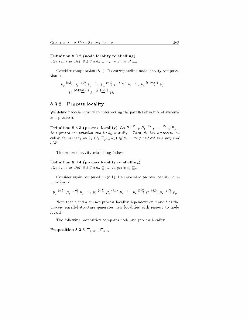
Chapter 8. A Case Study: Facile 208De�nition 8.3.2 (node locality relabelling)The same as Def. 8.2.3 with vnloc in place of vn.Consider computation (8.1). Its corresponding node locality computa-tion isP0 ha;;i�! P1 he;;i�! P2 ��! P3 hc;0i�! P4 hf;1i�! P5 ��! P6 hb;f0;3gi�! P7P7 hd;f0;3;6gi�! P8 hg;f1;4gi�! P98.3.2 Process localityWe de�ne process locality by interpreting the parallel structure of systemsand processes.De�nition 8.3.3 (process locality) Let P0 �0�!p P1 �1�!p : : : �n�!p Pn+1be a proved computation and let �n = �0#0 0. Then, �n has a process lo-cality dependency on �h (�h vploc �n) i� �h = �# and �# is a pre�x of�0#0.The process locality relabelling follows.De�nition 8.3.4 (process locality relabelling)The same as Def. 8.2.3 with vploc in place of vn.Consider again computation (8.1). Its associated process locality com-putation isP0 ha;;i�! P1 he;;i�! P2 ��! P3 hc;;i�! P4 hf;1i�! P5 ��! P6 hb;0i�! P7 hd;3i�! P8 hg;;i�! P9Note that c and d are not process locality dependent on a and b as theprocess parallel structure generates new localities with respect to nodelocality.The following proposition compares node and process locality.Proposition 8.3.5 vploc �vnloc.

209 8.4. ExamplesProof. Immediate by noting that v1ploc)v1nloc because if �i#i is a pre�xof �j#j then �i = �j. The strictness of the inclusion is proved by the sametransitions in the proof of Proposition 8.2.7. 2Finally, we compare causality and locality.Proposition 8.3.6 vnloc�vn, and vploc�vp.Proof. The inclusion in the �rst equation is immediate by noting that theconditions in Def. 8.3.1 are a subset of the ones in Def. 8.2.1. The inclusionis strict because there are transitions which are node causality, but not nodelocality dependent such as jjj1jjj0jj0a and jjj21jjj0jj0f in computation (8.1).For the inclusion in the second equation consider Def. 8.3.3 and Def. 8.2.4. Forthe strictness of the inclusion consider the same two transitions above. 2The following corollary follows from Propositions 8.3.5 and 8.3.6.Corollary 8.3.7 vploc�<n.8.4 ExamplesIn this section we report some examples of causal and locality semanticsthat deal with the main operators of Facile. Hereafter, we use the worddependency to mean both causal and local dependency. For instance, �ndepends on �h means that �n has a causal and a local dependency on �h.We will specify the kind of dependency when necessary.Some notation could help. We denote the operations executed by pro-cess bei as i; i0; : : : when their exact nature is irrelevant. Figures onlypresent the computations and the states of a Facile system that are inter-esting for the study at hand. Less signi�cant states are simply representedas �. To ease the understanding of labels (always listed on the right-handside of arcs), we write the operation corresponding to the actual transitionon the left-hand side of some arcs labelled � . The syntax is 0operation0 ;.For example newnode(be0);# jjj1jjj0jjj1�jjj21�

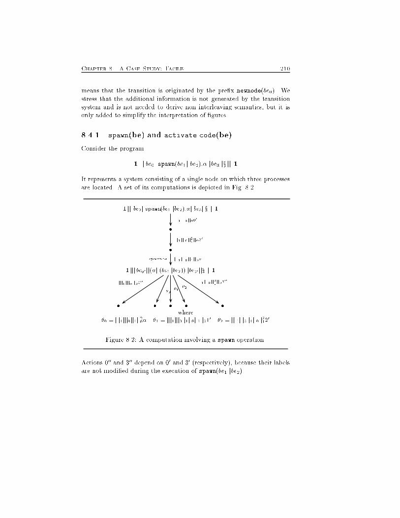
Chapter 8. A Case Study: Facile 210means that the transition is originated by the pre�x newnode(be0). Westress that the additional information is not generated by the transitionsystem and is not needed to derive non interleaving semantics, but it isonly added to simplify the interpretation of �gures.8.4.1 spawn(be) and activate code(be)Consider the program1 jjj be0jjspawn(be1jjbe2):�jjbe3jjx jjj1It represents a system consisting of a single node on which three processesare located. A set of its computations is depicted in Fig. 8.2.1 jjj be0jjspawn(be1jjbe2):�jjbe3jjx jjj1��1 jjj be00 jj(�jj(be1jjbe2))jjbe30 jjx jjj1� � � � �jjj1 jjj0 jj000jjj1 jjj0 jj21 jj030jjj1 jjj0 jj1 jj0�spawn;jjj1 jjj0 jj0000 �0 �1 �2 jjj1 jjj0 jj21 jj0300where�0 = jjj1jjj0jj1jj20� �1 = jjj1jjj0jj1jj0jj1jj010 �2 = jjj1jjj0jj1jj0jj2120Figure 8.2: A computation involving a spawn operation.Actions 000 and 300 depend on 00 and 30 (respectively), because their labelsare not modi�ed during the execution of spawn(be1jjbe2).

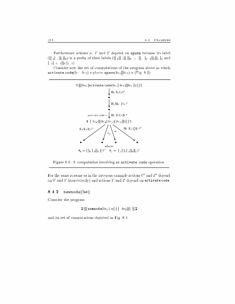
211 8.4. ExamplesFurthermore actions �, 10 and 20 depend on spawn because its label(jjj1jjj0jj1jj0) is a pre�x of their labels (jjj1jjj0jj1jj0jj0, jjj1jjj0jj1jj0jj1jj0 andjjj1jjj0jj1jj0jj1jj1).Consider now the set of computations of the program above in whichactivate code(be1jjbe2) replaces spawn(be1jjbe2):� (Fig. 8.3).1 jjj be0jjactivate code(be1jjbe2)jjbe3jjx jjj1��1 jjj be00 jj(be1jjbe2)jjbe30 jjx jjj1� � � �jjj1 jjj0 jj000jjj1 jjj0 jj21 jj030jjj1 jjj0 jj1 jj0�activate code;jjj1 jjj0 jj0000 �0 �1 jjj1 jjj0 jj21 jj0300where�0 = jjj1jjj0jj1jj2010 �1 = jjj1jjj0jj1jj0jj120Figure 8.3: A computation involving an activate code operation.For the same reasons as in the previous example actions 000 and 300 dependon 00 and 30 (respectively) and actions 10 and 20 depend on activatecode.8.4.2 newnode(be)Consider the program2 jjj newnode(be0):�jjx jjj be1jjx jjj2and its set of computations depicted in Fig. 8.4.

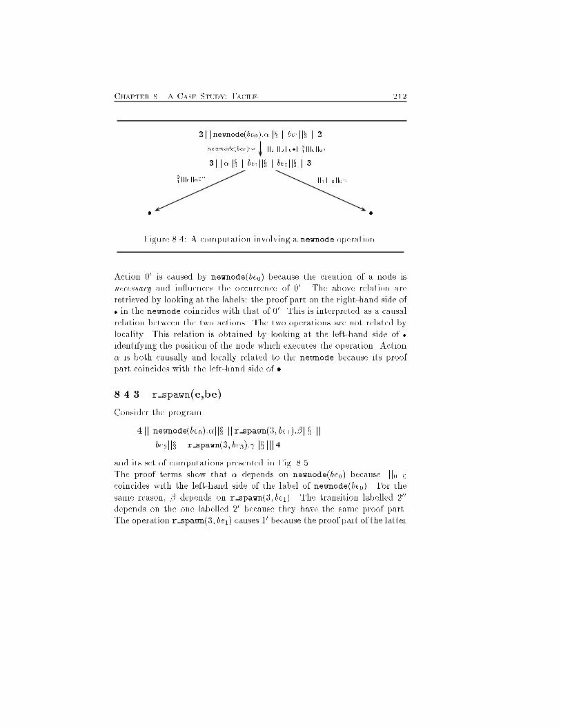
Chapter 8. A Case Study: Facile 2122 jjjnewnode(be0):�jjx jjj be1jjx jjj23 jjj�jjx jjj be1jjx jjj be0jjx jjj3� �jjj1 jjj0 jj0�jjj31 jjj0 jj0�newnode(be0);jjj31 jjj0 jj0000 jjj1 jjj0 jj0�Figure 8.4: A computation involving a newnode operation.Action 00 is caused by newnode(be0) because the creation of a node isnecessary and in uences the occurrence of 00. The above relation areretrieved by looking at the labels: the proof part on the right-hand side of� in the newnode coincides with that of 00. This is interpreted as a causalrelation between the two actions. The two operations are not related bylocality. This relation is obtained by looking at the left-hand side of �identifying the position of the node which executes the operation. Action� is both causally and locally related to the newnode because its proofpart coincides with the left-hand side of �.8.4.3 r spawn(e,be)Consider the program4 jjj newnode(be0):�jjx jjj r spawn(3; be1):�jjx jjjbe2jjx jjj r spawn(3; be3): jjx jjj4and its set of computations presented in Fig. 8.5.The proof terms show that � depends on newnode(be0) because jjj0jj0coincides with the left-hand side of the label of newnode(be0). For thesame reason, � depends on r spawn(3; be1). The transition labelled 200depends on the one labelled 20 because they have the same proof part.The operation r spawn(3; be1) causes 10 because the proof part of the latter

213 8.5. Analysis of a Mobile File Browser Agenttransition coincides with the right-hand side of the former. Similarly, 30is caused by r spawn(3; be3) and 00 is caused by newnode(be0). Finally, depends on r spawn(3; be3) because its proof part coincides with theleft-hand side of the label of the r spawn.8.5 Analysis of a Mobile File Browser AgentThe following is a scaled down version of a problem with causal dependen-cies of higher order processes and mobile channels. It originally arose inthe code for the Mobile Service Agent demonstration given at the EITC'95Exhibition (Thomsen et al., 1995a) (see also Subsect.1.3.2 for further dis-cussion). Using \traditional" debugging techniques it took two weeks totrack down the problem. We would like to point down that in this sectionwe will address the question of analysis of \real code".The problem is the following. We have an agent server that can becalled to deliver a client (FB) to the user and leave behind a server (FTP).There is a mistake in the FTP server in the sense that it should have beenrecursive to handle several calls from the FB client. However, there is alsoa mistake in the overall system, namely that all client/server pairs sharethe same channel. Thus even though there is a mistake in the FTP server,the system may continue to operate as long as we request more FB clients.Indeed each time we request an FB client we generate a new FTP serverwhich is waiting on the same channel, thus an old FB client may \steal"the new FTP server from a new FB client.Below we give the Facile code, both for running code (typewritten) inthe Facile Antigua Release (Thomsen et al., 1993), and a version writtenin core Facile (italic). We omit parts not relevant to our discussion. (Forinstance, we assume that all processes run on the same virtual node sothat we omit begin-end guards and jjj operators. The system activatesthe two processes FBS and AC. Process AC is busy waiting for an agentrequest. When the request arrives, AC creates a channel (reqch) andsends it to process FBS along their common channel getch. Now processAC is waiting for an agent from FBS. Once the process FBS has receivedthe channel name on which AC is waiting for the agent, FBS sends process

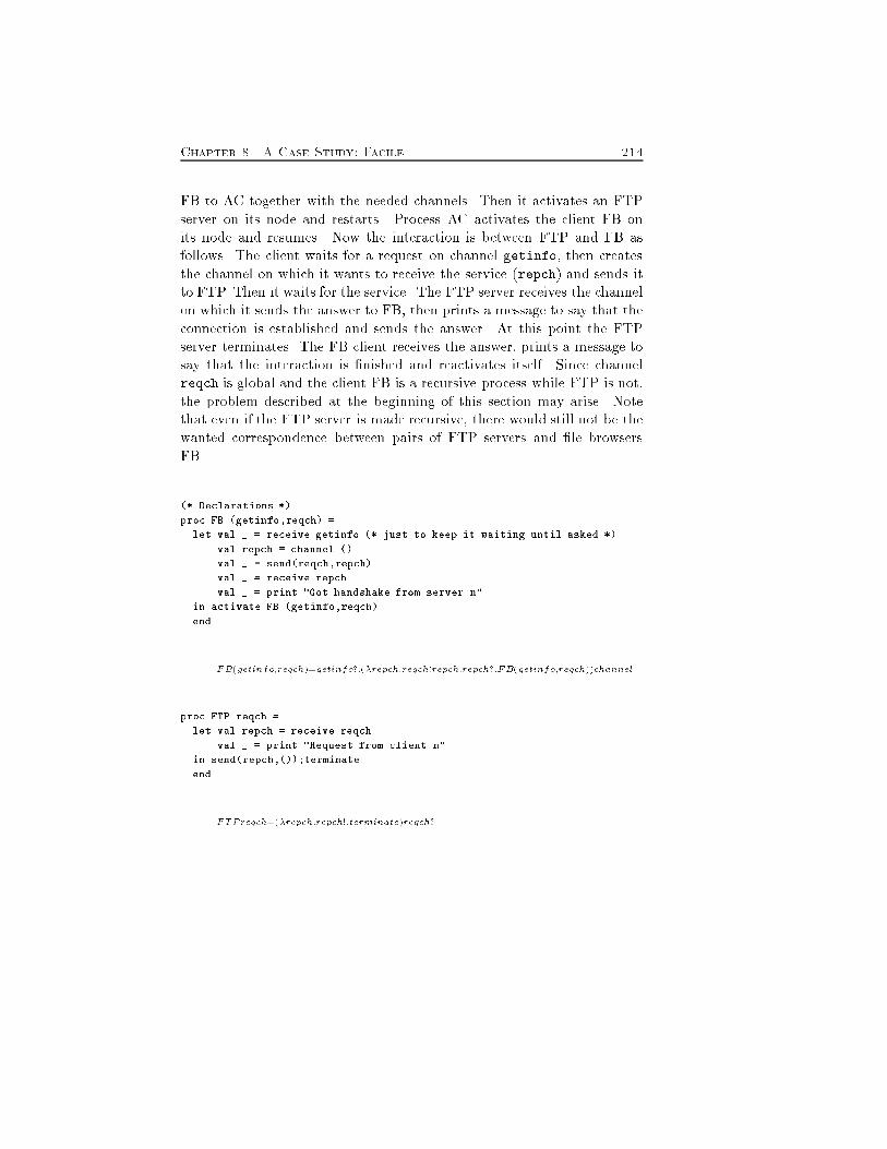
Chapter 8. A Case Study: Facile 214FB to AC together with the needed channels. Then it activates an FTPserver on its node and restarts. Process AC activates the client FB onits node and resumes. Now the interaction is between FTP and FB asfollows. The client waits for a request on channel getinfo, then createsthe channel on which it wants to receive the service (repch) and sends itto FTP. Then it waits for the service. The FTP server receives the channelon which it sends the answer to FB, then prints a message to say that theconnection is established and sends the answer. At this point the FTPserver terminates. The FB client receives the answer, prints a message tosay that the interaction is �nished and reactivates itself. Since channelreqch is global and the client FB is a recursive process while FTP is not,the problem described at the beginning of this section may arise. Notethat even if the FTP server is made recursive, there would still not be thewanted correspondence between pairs of FTP servers and �le browsersFB.(* Declarations *)proc FB (getinfo,reqch) =let val _ = receive getinfo (* just to keep it waiting until asked *)val repch = channel ()val _ = send(reqch,repch)val _ = receive repchval _ = print "Got handshake from server\n"in activate FB (getinfo,reqch)end FB(getinfo;reqch)=getinfo?:(�repch:reqch!repch:repch?:FB(getinfo;reqch))channelproc FTP reqch =let val repch = receive reqchval _ = print "Request from client\n"in send(repch,());terminateend FTPreqch=(�repch:repch!:terminate)reqch?

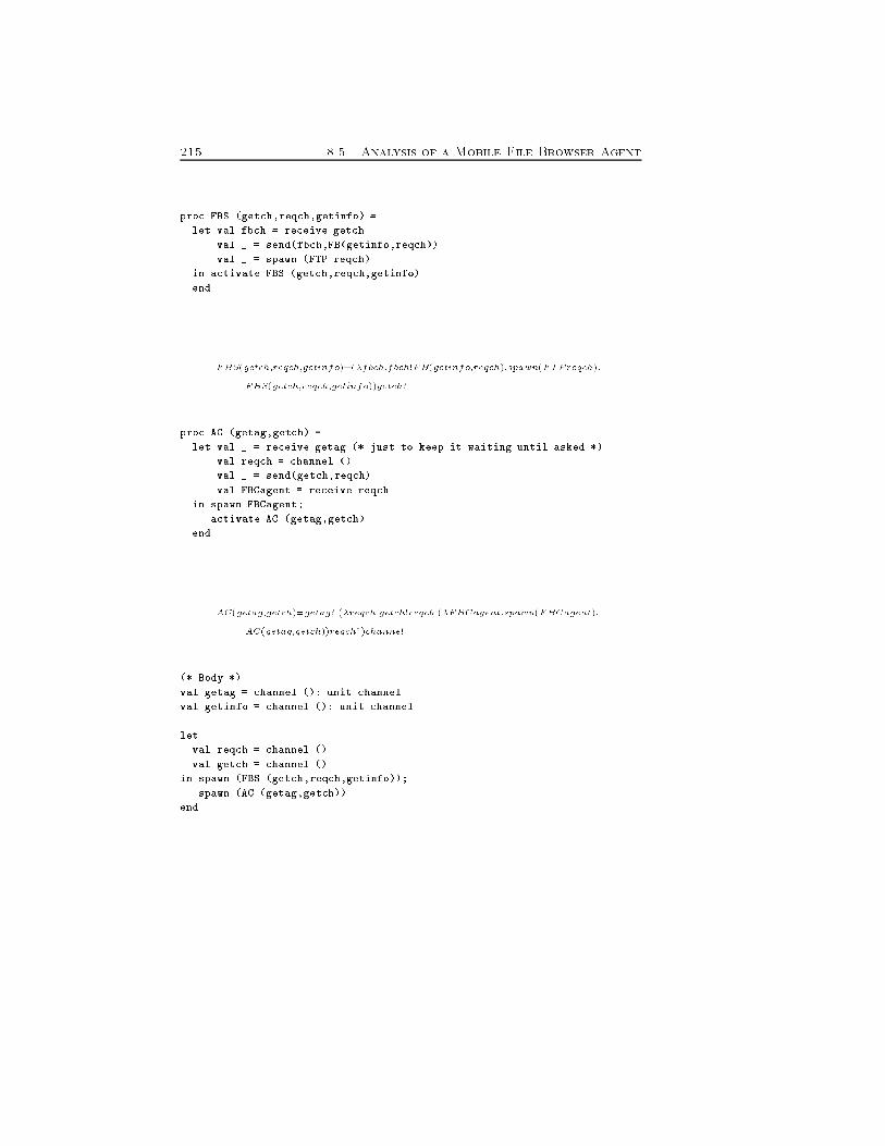
215 8.5. Analysis of a Mobile File Browser Agentproc FBS (getch,reqch,getinfo) =let val fbch = receive getchval _ = send(fbch,FB(getinfo,reqch))val _ = spawn (FTP reqch)in activate FBS (getch,reqch,getinfo)end FBS(getch;reqch;getinfo)=(�fbch:fbch!FB(getinfo;reqch):spawn(FTPreqch):FBS(getch;reqch;getinfo))getch?proc AC (getag,getch) =let val _ = receive getag (* just to keep it waiting until asked *)val reqch = channel ()val _ = send(getch,reqch)val FBCagent = receive reqchin spawn FBCagent;activate AC (getag,getch)end AC(getag;getch)=getag?:(�reqch:getch!reqch:(�FBCagent:spawn(FBCagent):AC(getag;getch))reqch?)channel(* Body *)val getag = channel (): unit channelval getinfo = channel (): unit channelletval reqch = channel ()val getch = channel ()in spawn (FBS (getch,reqch,getinfo));spawn (AC (getag,getch))end

Chapter 8. A Case Study: Facile 216(�reqch:�getch:spawn(FBC(getch;reqch;getinfo)):spawn(AC(getag;getch)))channel)channelWe now show how the error in the �rst version of the system can easily be singledout by using a causal relation between transitions. The idea is that the operations val= print "Request from client n" executed by any FTP server must be independentof one another. In fact, FTP serves and terminates. When the FB client interactswith two servers, thus leaving another client without its server, there is a chain of twoactions and the �rst causes the second.As an example consider the computation in Fig. 8.6 extracted from the transitionsystem of the incorrect code. Assume that two FTP servers and two FB clients havebeen activated, and that client FB1 steals the server of FB2.Process causality establishes that�1 = jj1jj1 request client 1 vp jj1jj0jj1 request client 2due to the inheritance of causal dependencies through communications.Indeed, �3 vp �4 because the reader of �3 has the same proof part of �4; inturn, the writer of �3 depends on (the reader of) �2, hence �2 vp �3. Since�1 causes (the writer of) �2, we have �1 vp �2. By transitivity, �1 vp �4.This causal dependency makes evident the misuse of channels.A �rst attempt to repair the error was to make FTP recursive throughthe codeproc FTP reqch =let val repch = receive reqchval _ = print "Request from client\n"in send(repch,());activate FTP reqchend FTPreqch=(�repch:repch!:activateFTPreqch)reqch?However, the same computation in Fig. 8.6 can still occur, apart fromstate s1 that now becomes equal to s0. This shows that FTP servers arenot private to FB clients. A way out is to make sure that each pair of FTPserver and FB shares a private channel. It is implemented by replacingFTP by the above recursive version, and replacing FBS and the body by

217 8.5. Analysis of a Mobile File Browser Agentproc FBS (getch,getinfo) =let val fbch = receive getchval reqch = channel ()val _ = send(fbch,FB(getinfo,reqch))val _ = spawn (FTP reqch)in activate FBS (getch,getinfo)end FBS(getch;getinfo)=(�fbch:(�reqch:fbch!FB(getinfo;reqch):spawn(FTPreqch):FBS(getch;reqch;getinfo))channel)getch?and by, respectivelyval getag = channel (): unit channelval getinfo = channel (): unit channelletval getch = channel ()in spawn (FBS (getch,getinfo));spawn (AC (getag,getch))end (�getch:spawn(FBC(getch;getinfo)):spawn(AC(getag;getch)))channelNow, it is straightforward to prove that a client FBi communicateswith a server FTPi along a private channel, generated by the same ithactivation of FBS that creates FBi and FTPi. As any FTP has only onechannel, it can serve only its client, and vice versa. Hence the problemhas been solved and the bug has been �xed.We end this section by remarking that nothing has to be changed ifthere are more nodes in the system because process causality considerboth process and system parallelism.

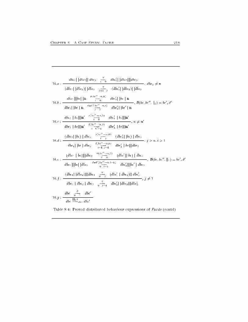
Chapter 8. A Case Study: Facile 21816:a : �dbe1jjjdbe2jjjdbe3 �! dbe01jjjdbe2jjjdbe3i 0�(dbe1jjjdbe2)jjjdbe3 �! (dbe01jjjdbe2)jjjdbe3i+1 0 ; dbe3 6= n16:b : #(be00!n;0)dbe1jjjbejjjn �! dbe01jjjbejjjni 0#�#0(be00!n;i)dbe1jjjbejjjn �! dbe01jjjbe0jjjn0 i ; B(be; be00; jj1) = be0; #016:c : #(be00!n;0)dbe1jjjbejjjn0 �! dbe01jjjbejjjn0i 0#(be00!n;0)dbe1jjjbejjjn0 �! dbe01jjjbejjjn0i n0�1 ; n 6= n016:d : #(be00!n;0)(dbe1jjjbe)jjjdbe3 �! (dbe01jjjbe)jjjdbe3i j#(be00!n;0)dbe1jjjbejjjdbe3 �! dbe01jjjbejjjdbe3i�1 j�1 ; j > n; i > 116:e : #(be00!n;0)(dbe1jjjbe)jjjdbe3 �! (dbe01jjjbe)jjjdbe3i n#�#0(be00!n;i�1)dbe1jjjbejjjdbe3 �! dbe01jjjbe0jjjdbe30 i�1 ; B(be; be00; jj1) = be0; #016:f : �(dbe1jjjdbe2)jjjdbe3 �! (dbe01jjjdbe2)jjjdbe030 j�dbe1jjjdbe2jjjdbe3 �! dbe01jjjdbe2jjjdbe030 j�1 ; j 6= 116:g : �dbe �! dbe00 1dbe jjj0��!dbe dbe0Table 8.4: Proved distributed behaviour expressions of Facile (contd).

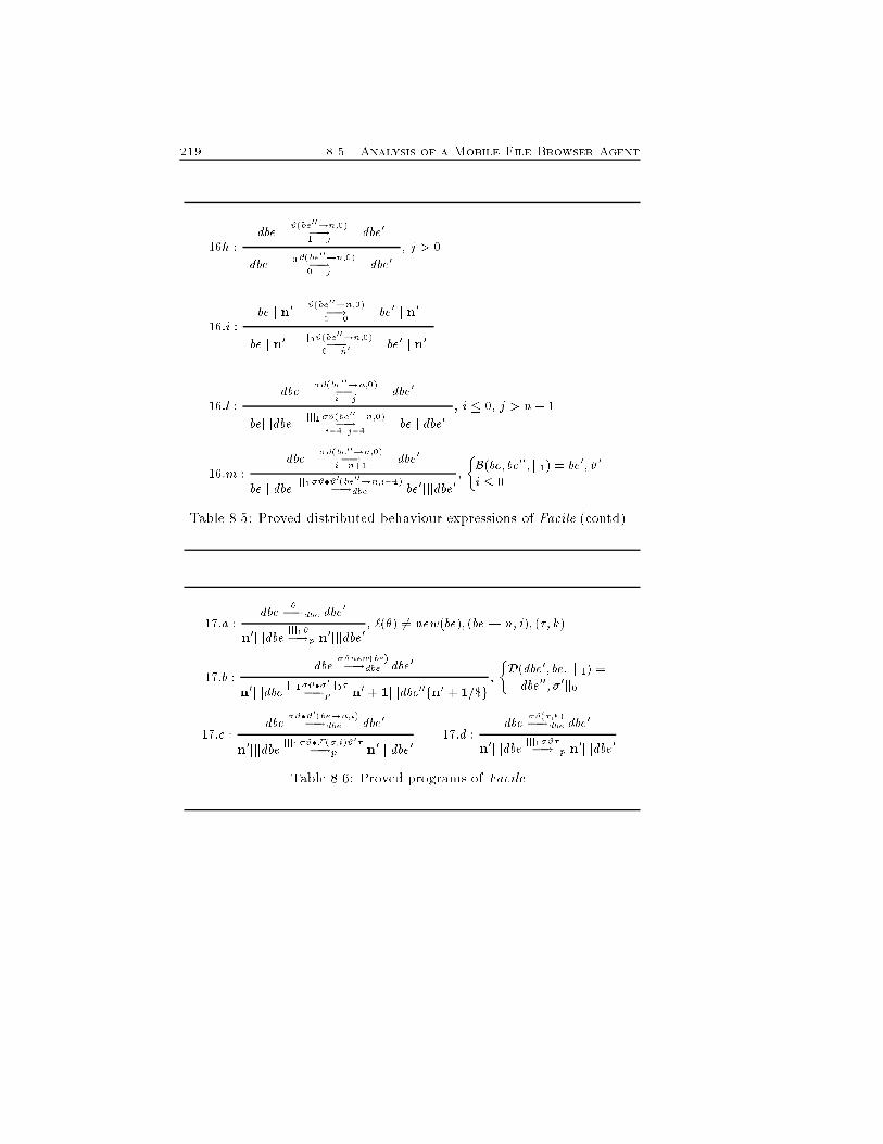
219 8.5. Analysis of a Mobile File Browser Agent16h : #(be00!n;0)dbe �! dbe01 jjjj0#(be00!n;0)dbe �! dbe00 j ; j > 016:i : #(be00!n;0)bejjjn0 �! be0jjjn01 0jjj0#(be00!n;0)bejjjn0 �! be0jjjn00 n016:l : �#(be00!n;0)dbe �! dbe0i jjjj1�#(be00!n;0)bejjjdbe �! bejjjdbe0i�1 j�1 ; i � 0; j > n+ 116:m : �#(be00!n;0)dbe �! dbe0i n+1bejjjdbe jjj1�#�#0(be00!n;i�1)�!dbe be0jjjdbe0 ; �B(be; be00; jj1) = be0; #0i � 0Table 8.5: Proved distributed behaviour expressions of Facile (contd).17:a : dbe ��!dbe dbe0n0jjjdbe jjj1��!p n0jjjdbe0 ; `(�) 6= new(be); (be! n; i); (�; k)17:b : dbe �#new(be)�!dbe dbe0n0jjjdbe jjj1�#��0jj0��!p n0 + 1jjjdbe00fn0 + 1=$g ; �D(dbe0; be; jjj1) =dbe00; �0jj017:c : dbe �#�#0(be!n;i)�!dbe dbe0n0jjjdbe jjj1�#�F(�;i)#0��!p n0jjjdbe0 17:d : dbe �#(�;k)�!dbe dbe0n0jjjdbe jjj1�#��! p n0jjjdbe0Table 8.6: Proved programs of Facile.

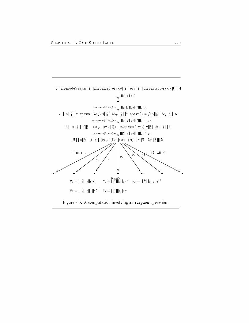
Chapter 8. A Case Study: Facile 2204 jjjnewnode(be0):�jjx jjjr spawn(3; be1):�jjx jjj be2jjx jjjr spawn(3; be3): jjx jjj4�5 jjj�jjx jjjr spawn(3; be1):�jjx jjj be20 jjx jjjr spawn(3; be3): jjx jjjbe0jjx jjj55 jjj�jjx jjj�jjx jjj (be20 jj(be1jjx)) jjjr spawn(3; be3): jjx jjjbe0jjx jjj55 jjj�jjx jjj�jjx jjj (be20 jj(be1jj(be3jjx))) jjj jjx jjjbe0jjx jjj5� � � � � � �jjj31 jjj0 jj020jjj1 jjj0 jj0�jjj51 jjj0 jj0�newnode(be0); jjj1 jjj0 jj0�jjj31 jjj0 jj1 jj0�r spawn(3;be1); jjj41 jjj0 jj0�jjj31 jjj0 jj21 jj0�r spawn(3;be3);jjj1 jjj0 jj0� �0 �1 �2 �3 �4 jjj51 jjj0 jj000where�0 = jjj21jjj0jj0� �1 = jjj31jjj0jj0200 �2 = jjj31jjj0jj1jj010�3 = jjj31jjj0jj21jj030 �4 = jjj41jjj0jj0 Figure 8.5: A computation involving an r spawn operation.

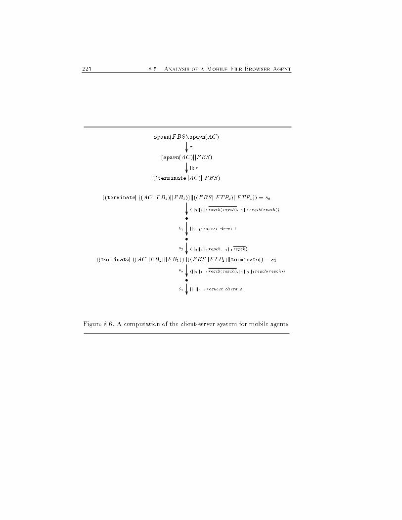
221 8.5. Analysis of a Mobile File Browser Agentspawn(FBS):spawn(AC)(spawn(AC)jjFBS)((terminatejjAC)jjFBS)...((terminatejj((ACjjFB2)jjFB1))jj((FBSjjFTP2)jjFTP1)) = s0��((terminatejj((ACjjFB2)jjFB1))jj((FBSjjFTP2)jjterminate)) = s1�...�jj0�hjj0jj1 jj1reqch(repch);jj1 jj1reqch(repch)ijj1 jj1request client 1�1 hjj0jj1 jj1repch;jj1 jj1repchi�2 hjj0 jj1 jj1reqch(repch);jj1 jj0 jj1reqch(repch)i�3 jj1 jj0 jj1request client 2�4Figure 8.6: A computation of the client-server system for mobile agents.

Chapter 8. A Case Study: Facile 222

Part IIIComputer-AidedVeri�cation223

Chapter 9Extended TransitionSystemsWe introduce a new kind of proved transition systems called extendedtransition systems. They extend the techniques of the previous part fromtree-structures to graphs. Any node n is labelled by a regular expres-sion that encodes all proved computations from the initial con�gurationto n. Since con�gurations of extended transition systems are expressionsof the language considered, these transition systems are �nite parametricrepresentations of �nite state systems. In fact, con�gurations do not dy-namically grow. Since parametricity is one of the basic properties that wewant to guarantee, we lift to regular expressions the relabelling functionsde�ned in the previous chapters on proved computations. Furthermore,extended transition systems are suitable for checking bisimulation equiva-lences between �nite-state systems (possibly relabelled). In fact, they arethe internal representation of processes of a parametric tool (PisaTool) forveri�cation of equivalences and study of properties of distributed systems.225

Chapter 9. Extended Transition Systems 2269.1 Parametric bisimulationWe extend to graphs the tree-based techniques introduced in the previouspart in order to cope with �nite state processes. We adopt node-labelledgraphs, called extended transition systems. Each node n is labelled by aregular expression which encodes all computations from the initial stateto n. Since any state is a process that does not grow dynamically as com-putation in (Montanari & Yankelevich, 1992; Yankelevich, 1993; Deganoet al., 1993), it is possible to have �nite parametric representations ofregular processes. For the sake of readability, we �rst introduce an inter-mediate step in which the de�nition of bisimulation on proved transitionsystems takes the history of computations into account. Then, we de�neextended transition systems and we equip them with a notion of bisimu-lation equivalent to the one of the intermediate step.Early parametric bisimulation on proved transition systems is de�nedby associating to each analysed node all possible computations leading toit. This de�nition is clearly not e�ective, even when dealing with �nite-state systems because in�nitely many computations can be associated toa node.De�nition 9.1.1 (early parametric bisimulation on PTS)Let O be any relabelling function of proved computations as de�ned in theprevious chapters. Then, a binary relation S on agents is an early para-metric simulation if hP; �i S hQ; �0i, with � and �0 proved computations,implies that� If P ��! P 0 and `(�) is any action with bn(`(�))\ fn(P;Q) = ;, thenfor some Q0, Q �0�! Q0, O(��) = O(�0�0), and hP 0; ��i S hQ0; �0�0iThe relation S is an early bisimulation if both S and S�1 are early sim-ulations. P is early bisimilar to Q (written P �pts Q) if there exists anearly bisimulation S such that P S Q.Note that the condition `(�) = `(�0) is implicitly ensured by imposingO(��) = O(�0�0).The soundness of the above de�nition is obtained by showing its equiv-alence with the bisimulations de�ned on proved trees.

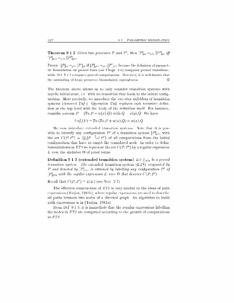
227 9.1. Parametric bisimulationTheorem 9.1.2 Given two processes P and P 0, then [P ]pt �pts [P 0]pt i�[P ]pts �pts [P 0]pts.Proof. [P ]pt �pts [P 0]pt i� [P ]pts �pts [P 0]pts because the de�nition of paramet-ric bisimulation on proved trees (see Chapt. 6.6) compares proved transitions,while Def. 9.1.1 compares proved computations. Moreover, it is well-known thatthe unwinding of loops preserves bisimulation equivalences. 2The theorem above allows us to only consider transition systems withacyclic initial state, i.e. with no transition that leads to the initial con�g-uration. More precisely, we introduce the one-step unfolding of transitionsystems (denoted Unf1). Operation Unf1 replaces each recursive de�ni-tion at the top level with the body of the de�nition itself. For instance,consider process P = (xa:P + w(x):Q) with Q = x(y):Q. We haveUnf1(P ) = xa:(xa:P +w(x):Q) +w(x):QWe now introduce extended transition systems. Note that it is pos-sible to identify any con�guration P 0 of a transition system [P ]pts withthe set C(P; P 0) = f�ijP ��!� P 0g of all computations from the initialcon�guration that have as target the considered node. In order to de�nebisimulations on ETS we represent the set C(P; P 0) by a regular expressionE over the alphabet � of proof terms.De�nition 9.1.3 (extended transition system) Let [t]pts be a provedtransition system. The extended transition system (ETS) originated byP and denoted by [P ]ets is obtained by labelling any con�guration P 0 of[P ]pts with the regular expression E over � that denotes C(P; P 0).Recall that C(P; P 0) = L(E) (see Sect. 2.7).The e�ective construction of ETS is very similar to the ideas of pathexpressions (Tarjan, 1981b), where regular expressions are used to describeall paths between two nodes of a directed graph. An algorithm to buildpath expressions is in (Tarjan, 1981a).From Def. 9.1.3, it is immediate that the regular expressions labellingthe nodes in ETS are computed according to the growth of computationsin PTS.

Chapter 9. Extended Transition Systems 228Proposition 9.1.4 (growth of computations) Let [P ]pts be a provedtransition system. Also, let P ��!� P 0 ��! P 00 be a computation, with E00the label of P 00 in [P ]ets. Then, �� 2 L(E00).The next step introduces the notion of bisimulation over ETS. Notethat, di�erently from Def. 9.1.1, the following de�nition provides an e�ec-tive checking algorithm on �nite state systems, due to the halting condi-tions expressed by the second group of items of Def. 9.1.6. Indeed, theyguarantee the existence of a �nite bisimulation to assert the equivalence(see Theorem 9.1.7). First, we introduce a notion of decomposition ofregular expressions.De�nition 9.1.5 (decomposition of regular expressions) Let E bea regular expression. Then, Ed is a regular expression called decomposi-tion of E i� Ed = �iei with ei regular expressions, and L(E) = L(Ed).Now, we de�ne parametric bisimulation on extended transition systemsassuming O lifted to sets in the usual way.De�nition 9.1.6 (early parametric bisimulation on ETS) Let O beany relabelling function of proved computations as de�ned in the previouschapters. Then, a binary relation Se on pairs hagent; regular expressioniis an early parametric simulation if hP;E1i Se hQ;E01i implies that� If P ��! P 0 with P 0 labelled by E2 and `(�) is any action withbn(`(�)) \ fn(P;Q) = ;, then for some Q0 labelled E02, Q �0�! Q0,O(e2) = O(e02) and hP 0; e2i Se hQ0; e02i, where e2 = E1�e3 with E2 =e2 + e, e02 = E01�0e03 with E02 = e02 + e0 for some decomposition of E2and E02, respectivelyThe relation Se is an early parametric bisimulation if both Se and S�1e areearly parametric simulations. P is early bisimilar to Q (written P �ets Q)if there exists an early bisimulation Se such that� hP; �iSehQ; �i

229 9.1. Parametric bisimulation� 8Pi 2 [P ]ets, let ei be the label of Pi, and let Ei = �jej such thathPi; eji Se hQh; ehi with L(ei) = L(Ei)� 8Qi 2 [Q]ets, let e0i be the label of Qi, and let E0i = �je0j such thathQi; e0ji Se hPh; ehi with L(E0i) = L(e0i)Some comments are in order. Early parametric bisimulation deals withthe relabelling of a regular expression. This topic is the argument of thenext section. The decompositions used in the de�nition are such thateach regular sub-expression extends the expression of the source node ofthe transition at least with its label (e.g., e2 = E1�e3). Su�x e3 takesthe possible extensions of the actual computation into account. In otherwords, we consider the maximal sub-expression of the label of the node athand which extends the actual computation and which can be simulatedby the other system. More generally, when hP1; E1i is inserted in Se,P �1�!� P1 is a pre�x of L(E1).We now show that early parametric bisimulation on ETS is actuallydecidable, provided that the equality of two regular expressions observedwith O is decidable and that the transition systems to be compared are�nite-state. Recall that the early transition system of �-calculus has a�nite-branching version (see Sect. 5.3).Theorem 9.1.7 (decidability) Let [P ]ets and [P 0]ets be two �nite-stateETS, and let O be an observation function. If O(E) = O(E0) is decidable,then [P ]ets �ets [P 0]ets is decidable.Proof. Assume [P ]ets �ets [P 0]ets. Then, at each step take as regular sub-expressions e1 and e01 the intersection of the languages accepted by P1 andP 01. This is always possible as regular languages are closed under intersection.Therefore, these decompositions are surely maximal. Also, the maximal decom-positions of a regular expression are �nite. So the expressions Ei and E0i in thesecond group of items in Def. 9.1.6 are always �nite summations (otherwise thelabels of Pi and P 0i would not be regular expressions). This implies that thenumber of pairs (hPi; eji; hPh; ehi) in the relation Se which contain process Piis �nite. Finally, since O(E) = O(E0) is decidable, we can build an early para-metric bisimulation, if any, in a �nite number of steps according to Def. 9.1.6.

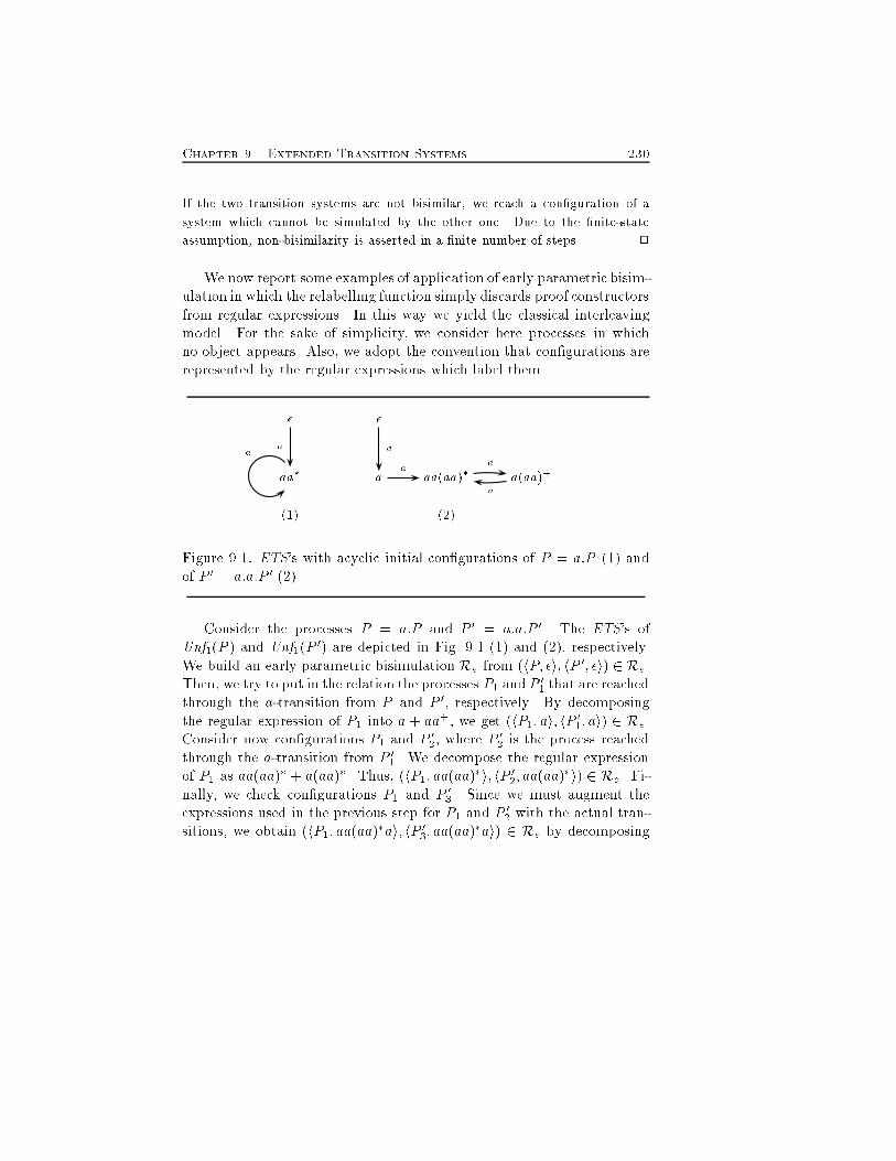
Chapter 9. Extended Transition Systems 230If the two transition systems are not bisimilar, we reach a con�guration of asystem which cannot be simulated by the other one. Due to the �nite-stateassumption, non-bisimilarity is asserted in a �nite number of steps. 2We now report some examples of application of early parametric bisim-ulation in which the relabelling function simply discards proof constructorsfrom regular expressions. In this way we yield the classical interleavingmodel. For the sake of simplicity, we consider here processes in whichno object appears. Also, we adopt the convention that con�gurations arerepresented by the regular expressions which label them.� �aa� a aa(aa)� a(aa)+(1) (2)aa a a aaFigure 9.1: ETS's with acyclic initial con�gurations of P = a:P (1) andof P 0 = a:a:P 0 (2).Consider the processes P = a:P and P 0 = a:a:P 0. The ETS's ofUnf1(P ) and Unf1(P 0) are depicted in Fig. 9.1 (1) and (2), respectively.We build an early parametric bisimulation Re from (hP; �i; hP 0; �i) 2 Re.Then, we try to put in the relation the processes P1 and P 01 that are reachedthrough the a-transition from P and P 0, respectively. By decomposingthe regular expression of P1 into a + aa+, we get (hP1; ai; hP 01; ai) 2 Re.Consider now con�gurations P1 and P 02, where P 02 is the process reachedthrough the a-transition from P 01. We decompose the regular expressionof P1 as aa(aa)� + a(aa)�. Thus, (hP1; aa(aa)�i; hP 02; aa(aa)�i) 2 Re. Fi-nally, we check con�gurations P1 and P 03. Since we must augment theexpressions used in the previous step for P1 and P 02 with the actual tran-sitions, we obtain (hP1; aa(aa)�ai; hP 03; aa(aa)�ai) 2 Re by decomposing

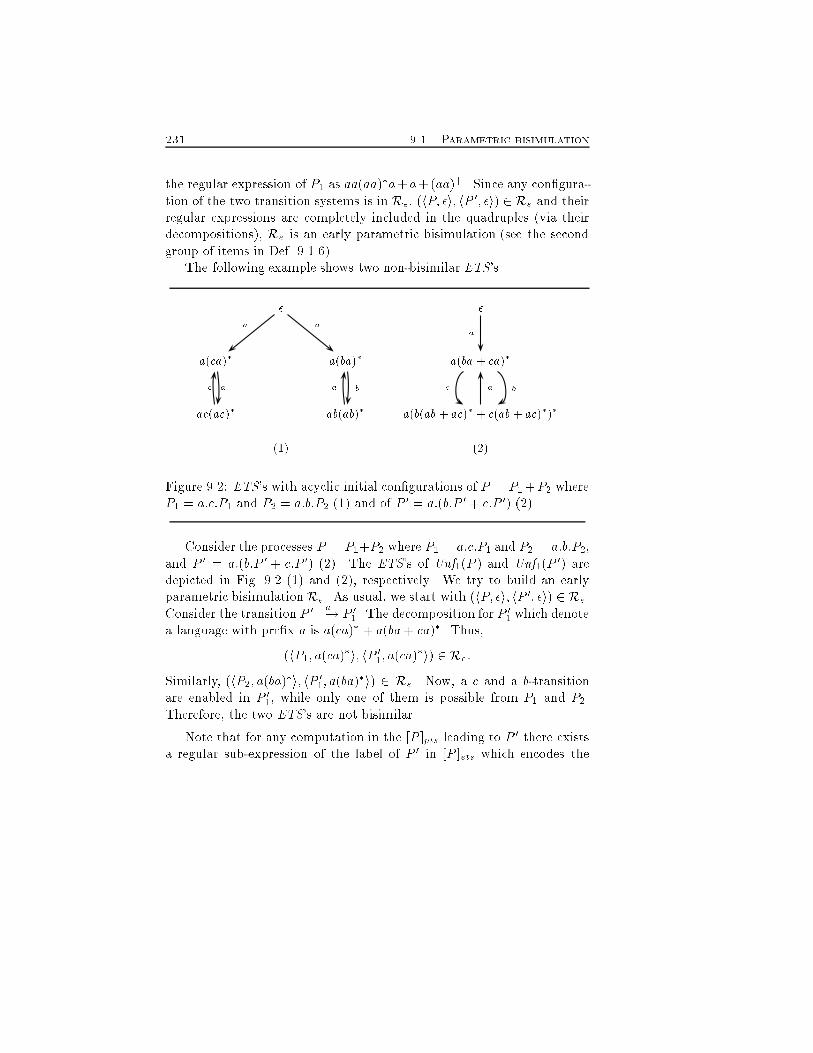
231 9.1. Parametric bisimulationthe regular expression of P1 as aa(aa)�a+a+(aa)+. Since any con�gura-tion of the two transition systems is in Re, (hP; �i; hP 0; �i) 2 Re and theirregular expressions are completely included in the quadruples (via theirdecompositions), Re is an early parametric bisimulation (see the secondgroup of items in Def. 9.1.6).The following example shows two non-bisimilar ETS's.� �a(ca)� a(ba)� a(ba + ca)�ac(ac)� ab(ab)� a(b(ab + ac)� + c(ab+ ac)�)�(1) (2)ac a a ba a a bcFigure 9.2: ETS's with acyclic initial con�gurations of P = P1+P2 whereP1 = a:c:P1 and P2 = a:b:P2 (1) and of P 0 = a:(b:P 0+ c:P 0) (2).Consider the processes P = P1+P2 where P1 = a:c:P1 and P2 = a:b:P2,and P 0 = a:(b:P 0 + c:P 0) (2). The ETS's of Unf1(P ) and Unf1(P 0) aredepicted in Fig. 9.2 (1) and (2), respectively. We try to build an earlyparametric bisimulationRe. As usual, we start with (hP; �i; hP 0; �i) 2 Re.Consider the transition P 0 a�! P 01. The decomposition for P 01 which denotea language with pre�x a is a(ca)� + a(ba+ ca)�. Thus,(hP1; a(ca)�i; hP 01; a(ca)�i) 2 Re:Similarly, (hP2; a(ba)�i; hP 01; a(ba)�i) 2 Re. Now, a c and a b-transitionare enabled in P 01, while only one of them is possible from P1 and P2.Therefore, the two ETS's are not bisimilar.Note that for any computation in the [P ]pts leading to P 0 there existsa regular sub-expression of the label of P 0 in [P ]ets which encodes the

Chapter 9. Extended Transition Systems 232considered computation. Thus, we can prove the equivalence of earlyparametric bisimulations on PTS and ETS.Theorem 9.1.8 (soundness) Let P and P 0 be processes. Then,[P ]ets �ets [P 0]ets , [P ]pts �pts [P 0]ptsProof. () Suppose that R is an early parametric bisimulation between [P ]ptsand [P 0]pts. De�ne a relation R0 as follows. For all �i; �j such that(hP1; �ii; hP2; �ji) 2 R;include the tuples (hP1; e1i; hP2; e2i) in R0 that verify1. e1 + E1 = E and e2 +E2 = E0 where E and E0 are the labels of P1 andP2 in [P ]ets and [P 0]ets, and2. L(e1) = f�ig and L(e2) = f�jg.By construction of ETS, there exist e1 and e2 that satisfy item 2 above.Moreover, since O(�i) = O(�j) we have that O(L(e1)) = O(L(e2)) by Def. 9.1.1.Since (hP;�i; hP 0; �i) 2 R, then (hP;�i; hP 0; �i) 2 R0 because we consider transi-tion systems after their Unf1.Assume that P1 �1�! P 01, P2 �2�! P 02, and (hP 01; �1�1i; hP 02; �2�2i) 2 R.If (hP1; e1i; hP2; e2i) 2 R0 and �1 2 L(e1) and �2 2 L(e2), then we prove that(hP 01; e01i; hP 02; e02i) 2 R0 with e01 = e1�1e3 and e02 = e2�2e03. From Proposi-tion 9.1.4, �1�1 2 L(E01) and �2�2 2 L(E02), where E01 and E02 are the labels ofP 01 and P 02, respectively. By construction of R0 (see items 1 and 2 above), weadd to R0 the pair (hP 01; e01i; hP 02; e02i) with L(e01) = f�0i j (hP1; �0ii; hP2; �0ji) 2 Rg(similarly for L(e02)). Since �1�1 2 L(e01) and �1 2 L(e1), e01 has the form e1�1e3(similarly for e02).)) Suppose that R is an early parametric bisimulation between [P ]ets and[P 0]ets. Construct a relation R0 as follows. For each (hP1; e1i; hP2; e2i) 2 R,include all tuples (ht1; �1i; ht2; �2i) in R0 such that �1 2 L(e1) and �2 2 L(e2)and O(�1) = O(�2). Since R contains all con�gurations of [P ]pts and [P 0]pts, andall its computations are represented through regular languages, R0 is a (possiblyin�nite) early parametric bisimulation on PTS. 2

233 9.2. Observations and regular languages9.2 Observations and regular languagesWe call here observation any function with the properties reported in thefollowing de�nition.De�nition 9.2.1 (observation) Let hD; �i be a monoid with neutral ele-ment �, where � is interpreted as concatenation of elements of D (hereafter,concatenation will be indicated by juxtaposition, omitting operator �).Let hD;�i be a partial ordering such that d0 � d00 i� d00 = d0d with dpossibly empty and d; d0; d00 2 D.Finally, let size : D ! IN be a total function such that if d1 � d2 thensize(d1) � size(d2).An observation is a total computable monotone functionO : hC(P );�prei ! hD;�i : � �pre �0 ) O(�) � O(�0)Note that the ordering � de�ned on the codomain of an observation O isa pre�x ordering on the structure of D. Intuitively, if d � d0 in D, then dis a sub-structure of d0.We now investigate some properties of observations. The extensionof observation functions to sets of computations (i.e., regular languagesbuilt upon labels) yields functions from the power set of computationsto the power set of their codomains. Powersets are partially ordered bysubset inclusion. Thus, they have a least element given by the empty setand each countable increasing chain of subsets has a limit given by theirunion. Hence, powersets are cpos (see Sect. 2.6). Therefore, observationslifted to sets are continuous as stated by the following proposition.Proposition 9.2.2 (observation are continuous) Let O : 2D1 ! 2D2be an observation. Then, O is continuous.Proof. Since 2D1 and 2D2 are cpos, each increasing chain has a limit. Letd1 v d2 v : : : v dn : : : be a chain in D1. Then, there exists a limit tndn = [ndnbecause each di is a regular language (a set of strings) and v coincides withsubset inclusion. Since O is an observation which is monotone (Def. 9.2.1) andwhich is lifted pointwise to 2D1 , O(tndn) = tnO(dn). 2

Chapter 9. Extended Transition Systems 234To apply the de�nition of early parametric bisimulation on ETS, weneed to check whether O(E) = O(E0), with E and E0 regular expressions.Recall that we use the obvious extension of O to sets and that by O(E)we mean O(L(E)). As a �rst result, we report the following fact.Fact 9.2.3 (languages and observations) Let E and E0 be two regu-lar expressions. Then,L(E) = L(E0) ) O(E) = O(E0)The one above is a su�cient condition to check equivalences by using well-known techniques from formal language theory. To further characteriseobservations for which equality is computable, we partition observationsinto incremental and non-incremental ones.De�nition 9.2.4 (incremental observations) Let �1; �01; �2; �02 be com-putations and let O be an observation. Then, O is incremental i�O(�1) = O(�01) ^ O(�2) = O(�02) ) O(�1�01) = O(�2�02)The incremental observation O(E) of a regular expression yields aregular language (and hence a regular expression).Proposition 9.2.5 Let E be a regular expression, and let O be an incre-mental observation. Then, there exists a regular expression E0 such thatO(E) = E0.Proof. Since O preserves the constructors of regular expressions � and con-catenation (see Def. 9.2.4), it is possible to concatenate observations and tocompute �nite iterations of them from a basic value. Thus, the observation of aregular expression is itself a regular expression on a di�erent alphabet. Recallthat + does not contribute to the structure of computations (see Sect. 3.1.1),but only re ects the branching structure of the transition system. 2Non-incremental observations may not preserve the structure of com-putations and therefore Proposition 9.2.5 does not apply. Clearly, if the

235 9.2. Observations and regular languagesregular expressions denote �nite languages, it is always possible to checkwhether O(E) = O(E0). In fact, O(E) and O(E0) are �nite sets as well,because O is a function (to each element of its domain is associated nomore than one element of its codomain). We now try to carry out a tech-nique to check for the equality of in�nite non-incremental observations.In order to check whether O(L(E)) = O(L(E0)), consider the increas-ing chains of sub-languages that generate L(E) and L(E0) by the �x-pointsolution of the linear systems derived from E and E0 (see Sect. 2.7). LetA1 � A2 � : : : � An : : : and B1 � B2 � : : : � Bm : : : be the two increas-ing chains. Then, if for each language Ai there exists a language Bj suchthat the observation of the former is contained in the one of the latterand viceversa, we can conclude that the observation of the two languagescoincides.Proposition 9.2.6 (observing approximations) Let E and E0 be tworegular expressions and let O be an observation. Let A1 � : : : � An : : :and B1 � : : : � Bm : : : be two increasing chains of regular languages thatapproximates L(E) and L(E0), respectively. Then,8i; 1 � i � n; 9j :O(Ai) � O(Bj ) ) O(L(E)) � O(L(E0))Proof. Since tnAn = [nAn, then 8i; 1 � i � n;Ai v tnAn. Similarly,8j; 1 � j �m;Bj v tmBm. Thus,8i; 1 � i � n;O(Ai) � O(tmBm) = O(L(E0))and O(tnAn) v O(L(E0)). Moreover, O is continuous by Proposition 9.2.2.Therefore, O(L(E)) = tnO(An) = O(tnAn) v O(L(E0)). 2The above proposition allows for inductive proofs of the check for theequality of observation of regular languages. More precisely, we proveequality by symmetric inclusionO(E) = O(E0) , O(E) � O(E0) ^ O(E0) � O(E)Even if the conditions reported above are enough to ensure the ver-i�cation of the common observation functions reported in the previous

Chapter 9. Extended Transition Systems 236chapters, they are not su�cient to ensure a general decidability theorem.The further conditions to be imposed on observation functions to yieldthe general results are under investigation.9.3 PisaToolWe describe here PisaTool, 1 the parametric veri�cation tools based onextended transition systems. The parametricity is obtained by relabellingthrough observations the extended transition systems. The observationsavailable as built-in functions permits the user to recover interleaving,multisets, partial ordering, locality, and ready-set semantics. Our toolhas been integrated in the veri�cation environment JACK (Bouali et al.,1994).This section is organized as follows. Next subsection deals with thefunctionalities of our tool. Subsection 9.3.2 describes the logical designof PisaTool. The implementation issues are reported in Subsect. 9.3.3.Finally, Subsect. 9.3.4 brie y describes the user interface.9.3.1 FunctionalitiesWe describe the operations that a user of PisaTool may perform. Pro-cesses are speci�ed in CCS. The tool deals with �nite state processes,i.e. CCS terms with guarded recursion and which no parallel operatorappears within the scope of a recursive de�nition. Note that it is easy toadapt our approach to support other languages. In this respect, an inter-face to a calculus compiler in the vein of (Cleaveland & Madelaine, 1992)would be an interesting extension. Some functionalities allow the user tocheck whether a process has deadlock states, to investigate reachabilityproperties or to perform the symbolic execution of a process. The editingof processes is possible, as well. The main feature is the veri�cation ofequivalences. The user can choose among strong, weak, and branching1The implementation of the prototype has been done by the author in collaborationwith Daniel Yanelevich, except for the bisimulation algorithm implemented by Gio-vanni Mandorino, and the window interface and the construction of regular expressionsimplemented by Maurizio Caneve.

237 9.3. PisaToolbisimulations and trace equivalence. Any of these equivalences is avail-able for any observation among the ones implemented and accessible in abuilt-in library: the choice of the equivalence is orthogonal to the choiceof the observation. The system also checks for the associated congruencesthat, in the weak cases, may be di�erent from the equivalence (once more,this depends on the observation chosen). The generality of PisaTool hassome costs in term of e�ciency in the veri�cation of equivalences with re-spect to specialised tools. In fact, we have to handle �nite state automataas labels instead of strings. This extra costs disappear in the parametricprototype YAPV described in Chapt. 12.PisaTool can be used as the basis for an abstract approach to debug-ging, in which users may de�ne what they want to see out of a computation(see (Priami & Yankelevich, 1993)). It is possible to consider causal depen-dencies or distribution in a computation, getting more information from asingle run than only the execution sequence. This can be done followingthe formal semantics of the language.Some comments are in order for the library of observations. Users canspecify which observation they want to use in three ways.� By choosing an observation from the library.� By de�ning a new observation algebra from scratch as a new modulein SML. This de�nition follows some standards: it has to ful�ll therequirements established in the signature (for example, the user isforced to de�ne an equality function over observations).� By applying an operator to the observation algebras that have al-ready been de�ned. At present, the operation we allow over obser-vation algebras is the product. This amounts to observe pairs ofobservations.There is a wide spectrum of observations to choose from. The de�ni-tion of new observations is also easy. In this way, if a new semantics isproposed in the context of observational theories of concurrency and it canbe modelled inside the methodology presented in this work, an automaticsupport for testing it can be obtained quite easily.

Chapter 9. Extended Transition Systems 238Many other operations can be de�ned over observation algebras, al-lowing the user to specify an observation domain as an expression in alanguage of observations. The point is how useful these operations are.For instance, the equivalence obtained by using weak bisimulation withthe product of the observations for locality and causality coincides withthe local/global cause equivalence by (Kiehn, 1991).9.3.2 The logical designWe describe the logical architecture of PisaTool and its interaction withthe external environment. The �rst step is the description of the system tobe manipulated in CCS. The tool then translates CCS speci�cations intothe corresponding proved transition system. This is the most concrete ob-servation we implement. Since we want provide users with the possibilityof de�ning their own observations, this is a module with a well-de�nedinterface. The interface speci�es what is exported outside the module,and therefore the functionalities o�ered.The second step concerns the selection of an observation from a library.Again, a signature speci�es the general characteristics of observations. Itde�nes the structure of processes, transitions and computations after thecorresponding structures of the proved transition system have been ob-served by means of relabelling functions. All modules which describe ob-servations must have this signature. Hence, their functionalities are para-metric with respect to a chosen algebra. This interface also contains allfunctions which manipulate processes and transitions. Moreover, it con-tains functions to perform the sequential composition and the equality oftwo computations. Note that the latter is not the syntactical equality: forinstance, if computations are partial orders, it implements an isomorphismchecking. In addition, a function to provide the string representation ofobserved transitions is given.Then, the description of the system at hand is translated into extendedtransition systems. The functionalities provided over extended transitionsystems are the equality up to associativity and commutativity, and re-duction up to strong bisimulation. Once the observation has been �xed,it is possible to check equivalences over the ETS's.

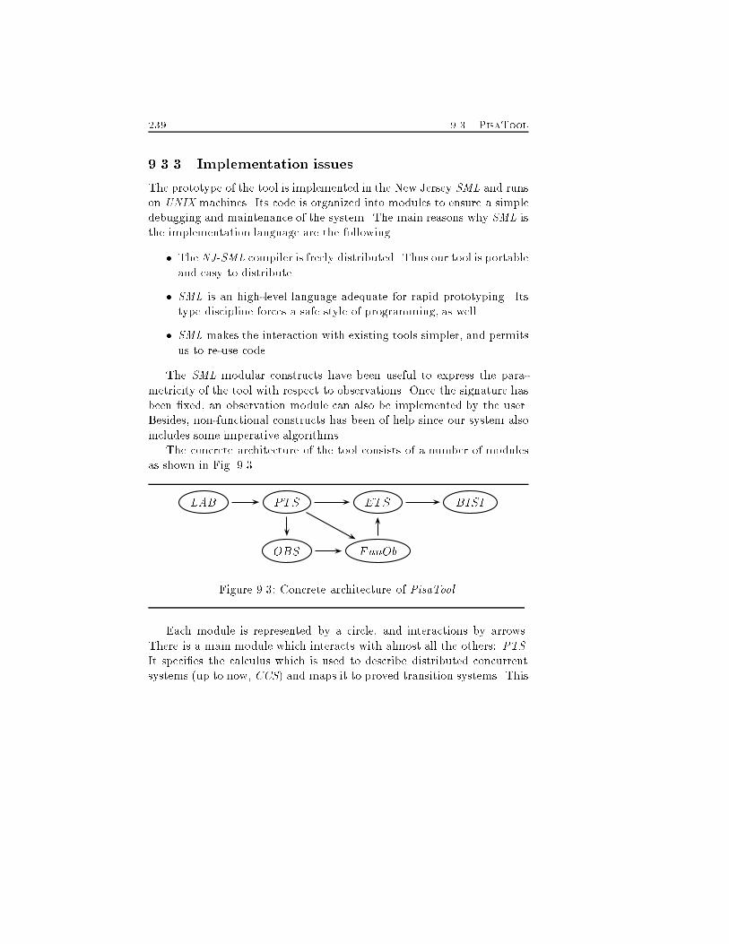
239 9.3. PisaTool9.3.3 Implementation issuesThe prototype of the tool is implemented in the New Jersey SML and runson UNIX machines. Its code is organized into modules to ensure a simpledebugging and maintenance of the system. The main reasons why SML isthe implementation language are the following.� The NJ-SML compiler is freely distributed. Thus our tool is portableand easy to distribute.� SML is an high-level language adequate for rapid prototyping. Itstype discipline forces a safe style of programming, as well.� SML makes the interaction with existing tools simpler, and permitsus to re-use code.The SML modular constructs have been useful to express the para-metricity of the tool with respect to observations. Once the signature hasbeen �xed, an observation module can also be implemented by the user.Besides, non-functional constructs has been of help since our system alsoincludes some imperative algorithms.The concrete architecture of the tool consists of a number of modulesas shown in Fig. 9.3.LAB PTS ETS BISIOBS FunObFigure 9.3: Concrete architecture of PisaTool.Each module is represented by a circle, and interactions by arrows.There is a main module which interacts with almost all the others: PTS.It speci�es the calculus which is used to describe distributed concurrentsystems (up to now, CCS) and maps it to proved transition systems. This

Chapter 9. Extended Transition Systems 240module deals with processes, transitions and computations. In order tosimplify the interaction between the user and the tool, all functions haveprocesses as parameters. The other objects (transitions and computations)are intermediate results, even if they can be manipulated, as well. ModuleLAB is used to denote the actions that a process may perform. ModuleOBS de�nes the observations. The signature of this module speci�es thestructure of processes, transitions and computations after the correspond-ing structures of PTS have been observed by means of observations. Foreach observed behaviour of processes, module FunOb provides the userwith the corresponding set of functionalities o�ered on PTS. Obviously,this functor needs the description of the current observation (OBS) andthe de�nition of the operations for PTS. Note that it is su�cient to knowthe signature of the current observation, not its complete implementation.This module implements the parametricity with respect to observations.Module ETS handles extended transition systems. Finally, module BISIsupports the veri�cation of behavioral equivalences of processes. Weak,strong and branching bisimulations are checked using a variant of the al-gorithm for partition re�nement presented in (Paige & Tarjan, 1987).The tool is still too ine�cient to be used with real systems. In general,we can say that there is a tradeo� between generality and usefulness.9.3.4 User interfaceThe user interacts with the system through an interface implemented in Cover X-Windows, using the Interviews package. Conceptually, the inter-face provides a main window which o�ers a help subwindow, a menu withthe available observations, a button to choose from two algebras, and anenvironment to edit, save and load CCS speci�cations.For either algebra chosen, a speci�c window is opened. Since changingfrom one algebra to another is time consuming, the actual load of theobservation is performed the �rst time it is used, and not when the windowis opened or chosen. Each window has a menu for the equivalences and amenu for the functions. A user can select the CCS process from the mainwindow and then apply a function from a speci�c window. The mainenvironment of the tool is made up of three windows: one for the input of

241 9.3. PisaToolprocesses to be veri�ed, another to choose the operations to be performed,and the last contains an on-line help for the available functionalities.

Chapter 9. Extended Transition Systems 242

Chapter 10Complexity andConcurrencyWe investigate some aspects of interexpressiveness of languages and their(denotational) semantic models by viewing semantic functions from theviewpoint of complexity theory. We classify semantic functions as polyno-mial or �nite if a language term of size n produces a meta-language objectrespectively polynomially bounded in n or �nite. Languages involving con-currency manifest most interest which we associate to the fact that theirsemantic models in general lack �-style abstraction, even if �-calculusovercomes this lack with the encoding of �-calculus (Milner, 1992b). Thischapter provides a quanti�able reason why labelled event structures forma more reasonable model for the choice and concurrency operators of CCSthan do synchronisation trees. Similarly we show the representation ofcon ict by places within (at least occurrence forms of) Petri nets is ex-ponentially larger than the relational representation within correspondingevent structures. An application is a criterion for selection of semanticmodels for real-world algorithmic purposes; for example, model checkingor veri�cation algorithms which use an exponentially larger semantic rep-resentation of programs are unlikely to be e�cient.243

Chapter 10. Complexity and Concurrency 24410.1 Why Complexity and ConcurrencyThe idea of a denotational semantics has several components. Firstly wehave an (object)-language whose (freely constructed) terms are to be givenmeaning. We also have a semantic function which homomorphically mapsobject terms into terms of a meta-language. Finally, and importantly,we have an equivalence relation on meta-language terms specifying whenthey are equal. For the typed �-calculus with constants as a meta-languagethis is typically ����-equality. Here we view object- and meta-languageterms as data-structures with a given representation|two di�erent repre-sentations for meta-language terms would count as two separate semanticmodels (see Subsect. 10.3.2 for more discussion). Also note our empha-sis on the separateness of translation into meta-language terms and theirequality|this is done in order to study the size of meta-language termswhich obviously, in general, is not preserved by replacing a term with anequal one.For classical programming languages (Pascal for example) the use oftyped �-calculus as a meta-language for their denotational semantics �ala Scott is widespread and undisputed. One debates the meaning of agiven programming language feature (e.g. parameter passing mechanism)within the meta-language. By contrast, there is a plethora of models forconcurrent systems and it seems at times that each feature requires a newmeta-language to describe it (witness inter alia the various forms of eventstructures).In spite of the huge amount of theoretical work on semantics for con-current systems, there is a lack of studies to show how practically usefulconcepts and theories are. Unfortunately, the choice among di�erent ap-proaches is quite often based on a matter of taste, rather than on compa-rable and measurable grounds. This is a major drawback because it allowsthe proliferation of proposals without a measure of their relative merits.This chapter amounts to one proposal for this measure.

245 10.2. The scenario10.2 The scenarioWe illustrate the basic concepts and notations that we adopt to evaluateconcurrency models with respect to their complexity.10.2.1 LanguagesFor the sake of simplicity, we consider a language with no name or valuepassing. Following the de�nition style of process algebras introduced inChapter 4, the processes of our general language L yields behaviours BE:be ::= 0 j a:be j a:be j �:be j be+ be0 j be j be0 j be; be0 jbe[�] j (� a)be j P j nonrec P:be j rec P:bewhere all operators have their standard meaning. The only new con-structor is nonrec that allows simple non-recursive de�nitions|see below.Hereafter, we assume processes guarded and closed. Sublanguages of L willbe denoted L[op1; : : : ; opn], and these always include process names P (ifrec or nonrec present) and 0. We also assume that whenever a language in-cludes a, a and j, it contains � as well. For example, L[a; a; �;+; j; �; �; rec]coincides with CCS (Milner, 1989), and L[a;+; rec] refers to the sublan-guage given by be ::= 0 j a:be j be+ be0 j P j rec P:bewhich is very close to the idea of classical regular expressions. The aboveprecision (for example separating rec and nonrec) is important becausewe argue about complexity results which alter greatly with changes tosemantic power. However, in examples, we will feel free to use Milner'soriginal notation of P1 ( be1� � �Pn ( benin be0instead of rec and nonrec.

Chapter 10. Complexity and Concurrency 246Languages (which are later de�ned to be free algebras introduced inSect. 2.5) have a simple notion of size, for example the number of con-structors.Note that all semantic models described in Sect. 4.4 may be viewed asalgebras (possibly containing in�nite terms). Thus, in order to generaliseour approach to the complexity of semantic models, we assume that themeta-language into which we map the object-language is an algebra.Although we rarely spell this out explicitly, it is necessary to regard ameta-language more intensionally than usual and to include its represen-tation as a data-structure. Thus we treat changing the representation ofa meta-language as changing the meta-language. Such �ne discriminationis necessary to avoid specious claims that all semantic functions are linearin size via the claim in that they all have a linear size representation of agiven object-language term, viz itself|see Subsect. 10.3.2.10.2.2 Denotational semanticsWe wish to cast our net wide in order to include many interpretationmechanisms (including simple translation) as semantic formalisms. Weaccordingly de�ne a denotational semantics to be a 4-tuple (S;M; Ei2I;�)where� S, the object-language, is a free algebra, possibly many-sorted. 1Sorts of S are referred to as syntactic categories. Identity, =, is theusual syntactic identity on free algebras.� M, themeta-language, is an algebra. Usually it is less well-structuredthan S, for example we might wish to consider S being Pascal andM being a set of owcharts. We allowM to contain in�nite termsin the style common in algebraic semantics (Guessarian, 1981). Var-ious CCS programs require in�nite event structures or Petri nets to1It is possible to extend this to allow it (as for the meta-language M) to be acontinuous free algebra. The complexity behaviour of limits is de�ned to be that oftheir approximants. This allows one to study the inate expressiveness of classes of eventstructures, Petri-nets and the like by giving mutual translations. This chapter does notstudy such issues.

247 10.2. The scenariorepresent them. It is convenient to require that the operators ofMpartition into free constructors which generate the algebra and un-free operators which are required to provide maps from free parts tofree parts (compare the idea of constructors and user-de�ned func-tions in languages like ML). We see examples of this below (inter-pretation of �x or par for synchronisation trees). Identity, =, is theusual algebraic equality of terms. This is syntactic identity for thecase of a free algebra but also takes into account equations de�ningany unfree constructors.� Ei2I : S ! M is an indexed family of semantic functions. Theseare required to be de�ned by (mutual) primitive recursion. Typicallythere is one (or more) semantic function for each syntactic category.2� � is an equivalence relation on M. It is commonly generated by areduction relation but here we are merely interested in equivalence.We require m = m0 ) m � m0Although the object- and meta-languages are seen as being (�rst-order) al-gebras we can choose to understand various terms as binding constructs|this is common for object languages, but the presence of the equivalencerelation, �, onM allows natural encoding of the binding rules (e.g. �- and�-equivalence) there too. Such a treatment would normally be considered2It is convenient to allow the notion of environment to be handled by this schemetoo. Often a semantic function (e.g. for a functional language) would be de�ned witha type such as E[[�]] : Expr ! (Var! Val )! Valwhere the various ! have di�ering meanings which require complicated explanationwhen our meta-language is �rst order and so lacks a full exponentiation type. Thiswould also make the primitive recursivity and complexity more clumsy to de�ne. How-ever, any possible environment is conveniently handled here by treating it as an indexto E. Hence we can write (continuing the functional programming example)E�[[�]] : Expr ! ValE�[[x]] = �(x)E�[[�x:e]] = lam(�v:E�[v=x][[e]])E�[[e e0]] = apphE�[[e]];E�[[e0]]iPrimitive recursivity bans the use of such an index as the main argument to E.

Chapter 10. Complexity and Concurrency 248lacking the necessary abstract elegance. However, we will justify it by ourinterest in implementation feasibility and complexity.To clarify the requirements onM above, suppose it is a meta-languagewith an operator �x x.e. It is possible to regard this operator eitheras a free constructor with equivalence caught by �, so that �x x:e �e[�x x:e=x] 6= �x x:e; or as a unfree operator so that e[�x x:e=x] = �x x:e.The former treatment is common in object languages and the �-calculusas a meta-language whilst the latter is common in event structure or Petri-nets as semantic meta-language for CCS. These treatments, of course, havevery di�erent complexity behaviour.10.2.3 Correspondence to operational semanticsOften an object language S comes complete with an operational semanticsand we wish to ensure that the denotational semantics is consistent. Forthe purposes here, we only require the equivalence relation � which holdswhen two programs s; s0 2 S are operationally indistinguishable (actuallyin all contexts C[�]). For concurrency purposes, � is typically one of theforms of bisimulation (strong, weak, interleaving, step, pomset, causality,history-preserving, locality etc.; see ()).Denotational semantics (S;M; Ei2I;�) is consistent with � (or it is�-respecting) if for all s; s0 2 S we haveE [[s]] � E [[s0]]) (8contexts C[�])(C[s] � C[s0]):It is computationally adequate ifE [[s]] � E [[s0]]( (8contexts C[�])(C[s]� C[s0])and fully abstract if both hold.10.2.4 Examples1. Take S to be that subset of Pascal generated by the syntactic cate-gories for command Cmd and expressions Exp with their usual BNFde�nition. M is the usual typed (with recursive types) �-calculus

249 10.2. The scenariowith ECmd[[�]] and EExp[[�]] de�ned in the usual manner. Equivalence is����-equivalence (we need �-rules for the �xpoint-taking constantsas an absolute minimum).2. Take S to be the language L[a;+; j ] with syntactic category BEgiven by be ::= 0 j a:be j be + be0 j be j be0with names a (we also use b in the example below) but no co-names.M can be synchronisation trees, ranged over by T; U . The semanticfunction is interesting|the pre�xing and + operators directly en-code as free tree-forming operators � and + (see Sect. 2.5) whereasthe j operator is represented by a non-free operator given by theexpansion theorem (this language does not require consideration ofname and co-name synchronisation):[[0]] =P; a � [[T]] = 0[[a:be]] = a � [[be]][[be+ be0]] =Pi2I ai � [[Ti]] +Pi2J ai � [[Ti]] =Pi2I[J ai � [[Ti]]where [[be]] =Pi2I ai � [[Ti]] and [[be0]] =Pi2J ai � [[Ti]][[be j be0]] = par([[be]]; [[be0]])where par (T; U ) =Pi2I ai � par(Ti; U ) +Pi2J bj � par(T; Uj)with Pi2I ai � Ti = T and Pi2J bj � Uj = UEquivalence � is induced by the strong bisimulation on synchro-nisation trees (i.e., tree isomorphism with additional axioms likeabsorption T + T � T and T + 0 � T ).3. Take S to be regular expressions. Two alternatives forM are sets ofstrings and �nite state automata. The corresponding semantic func-tions are given by the usual constructions in undergraduate texts.However, the focus we wish to make is that the mapping to �nitestate automata has �nitary images and is surjective but has a (rel-atively) complex equivalence which nevertheless is suitable for algo-rithms; whereas the mapping to sets of strings has in�nitary imagesbut with identity as equivalence between semantic images.

Chapter 10. Complexity and Concurrency 250To further bring out the discussion of interpreted versus free construc-tors consider the operator par above. As de�ned par is an unfree operatorwhich maps the program a1:nil j : : : j an:nil onto an exponentially biggersynchronisation tree. On the other hand, treating par as a free constructorgives a linear-sized semantic function, but with various identities like thatof par(a � 0; b � 0) and a � b � 0 + b � a � 0 left to be speci�ed in �.10.2.5 ObservationWhat we saw above is that there is a spectrum of semantic models andassociated semantic functions and equivalences for a given language S|even when its ostensible semantics is externally prescribed, for exampleby a relation � on object terms. Denotational semantics respecting � canrange from (essentially) S with identity as the semantic function and acomplicated equivalence � to (essentially) the term model given by S=�,the induced map to equivalence classes as semantic function and identityas the equivalence relation.Indeed, we can set up a partial order on semantics Ei : S ! Mi byordering (S;M1; E1;�1) v (S;M2; E2;�2) when(9f 2M1 !M2)(8m;m0 2M1)m �1 m0 ) f(m1) �2 f(m2):The term model is the minimal element of �-respecting semantics.Note that good (in the sense of being useful for proofs) semantic modelsare typically neither of the extremes discussed above|consider the �-calculus for imperative languages. When it comes to implementation,further considerations of representation e�ciency come to the fore and weconsider these in the next section.10.3 Complexity of a semantic modelGiven a language S and a semantics (S;M; E ;�) we say that the semanticsis �nite if every term of S has a �nite image in M. We say that thesemantics is polynomial (or indeed any other complexity class) if everyterm of size n in S has an image inM which is of at most polynomial size

251 10.3. Complexity of a semantic modelin n. We say it is in�nite if any (�nite) term has an image of in�nite size(e.g. due to expansion of recP:a:P as an in�nite Petri-net process). Notethat these de�nitions do not include the size of �. For example, takingS =M and the identity as a semantic function gives a linear semantics.Given an object language S, we say that a semantic modelM is poly-nomial (or again any other complexity class) if there exists a polynomialsemantic function. To avoid the trivialO(n) semantic function which mapsevery source term onto itself as meta-language term, this de�nition is onlyuseful when we have prescribed inequalities to preserve (from axioms orfrom an operational equivalence � as discussed above).When we restrict our attention to semantics which respect strong in-terleaving bisimulation we �nd that event structures (Nielsen et al., 1981)are quadratic for L[�;+; j ], but exponential for L[a; a;+; j ]. However, ow event structures (Boudol, 1990) are polynomial for L[a; a;+; j ] justas stable event structures (Winskel, 1982) and bundle event structures(Langerak, 1992) are, even if with a lower degree. Synchronisation treesalso with richer labelling (e.g., causal trees (Darondeau & Degano, 1989)and the like) are exponential for L[a; j] and in�nite for L[a; rec]. Transitionsystems (even if with independence relations like in (Winskel & Nielsen,1992; Bednarczyk, 1988; Stark, 1989)) are exponential for L[a; j ], but lin-ear for L[a; rec]. They become in�nite for L[a; j; rec]. Causal (Darondeau& Degano, 1989) and locational (Boudol et al., 1993) transitions systemsare in�nite also for L[a; rec]. This happens because the states are incresedat each unfolding with a reference to the activating transitions or to thoseoccurred in the same site, respectively.If one is interested in truly concurrent equivalences, the above modelshave the same complexity as for the interleaving semantics, while compacttransition systems (see Chapt. 11) are linear for L[a;+; j ] and polynomialfor L[a; a;+; j ] (without autoconcurrency).As a �nal remark, languages allowing value or name passing like �-calculus (Milner et al., 1992a) do not increase the complexity of theirrepresentations. In fact, the late semantics of �-calculus originates �nitebranching transition systems with the same size of CCS terms. Indeed,an input pre�x generates a single transition (see Tab. 4.2). The earlysemantics is a bit more expensive because an input pre�x needs as many

Chapter 10. Complexity and Concurrency 252transitions as the active names of the process (see Tab. 5.3). However, theresulting transition system is still �nite branching (see Sect. 5.3).These results are summarized in Tab. 10.1.10.3.1 Cartesian closedness implies linear complexityThe following result can justify why typed �-calculus su�ces for a greatmany applications, including classical programming languages. This tech-nique is used in (Christiansen & Jones, 1983) to simplify the semanticdescription language in the CERES compiler generator which uses a formof �-calculus.Suppose we have a semantic function E [[�]] for a syntactic categoryin a programming language. Suppose that the meta-language is (ratherabusing the term) cartesian-closed, i.e. there are notions of abstraction,application, pairing and projection. Its homomorphic (primitive recursive)nature means that we can write the semantics of an operator, binary +say, as E [[e1 + e2]] = : : :E [[e1]] : : :E [[e1]] : : :E [[e2]] : : :which can be transformed intoE [[e1 + e2]] = (�m1:�m2: : : :m1 : : :m1 : : :m2 : : :) (E [[e1]]) (E [[e2]]):Note that the former function produces an asymptotically exponentiallylarger meta-language meaning than the latter which is always linear.Similarly, suppose we have two or more mutually recursive semanticfunctions for a given syntactic category. This time pairing comes to ourrescue, and functions such asE [[e1 + e2]] = : : :E [[e1]] : : :F [[e1]] : : :E [[e2]] : : :F [[e1 + e2]] = : : :F [[e1]] : : :E [[e2]] : : :F [[e2]] : : :can be transformed intoG[[e1 + e2]] = � : : : �1G[[e1]] : : :�2G[[e1]] : : :�1G[[e2]] : : : ;: : : �2G[[e1]] : : :�1G[[e2]] : : :�2G[[e2]] : : : �

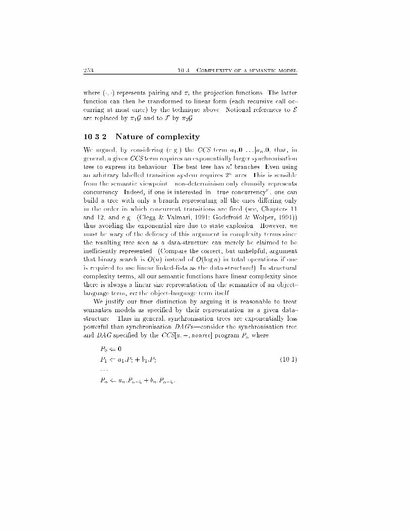
253 10.3. Complexity of a semantic modelwhere (�; �) represents pairing and �i the projection functions. The latterfunction can then be transformed to linear form (each recursive call oc-curring at most once) by the technique above. Notional references to Eare replaced by �1G and to F by �2G.10.3.2 Nature of complexityWe argued, by considering (e.g.) the CCS term a1:0j : : : jan:0, that, ingeneral, a given CCS term requires an exponentially larger synchronisationtree to express its behaviour. The best tree has n! branches. Even usingan arbitrary labelled transition system requires 2n arcs. This is sensiblefrom the semantic viewpoint|non-determinism only clumsily representsconcurrency. Indeed, if one is interested in \true concurrency", one canbuild a tree with only a branch representing all the ones di�ering onlyin the order in which concurrent transitions are �red (see, Chapters 11and 12, and e.g. (Clegg & Valmari, 1991; Godefroid & Wolper, 1991))thus avoiding the exponential size due to state explosion. However, wemust be wary of the delicacy of this argument in complexity terms sincethe resulting tree seen as a data-structure can merely be claimed to beine�ciently represented. (Compare the correct, but unhelpful, argumentthat binary search is O(n) instead of O(logn) in total operations if oneis required to use linear linked-lists as the data-structure!) In structuralcomplexity terms, all our semantic functions have linear complexity sincethere is always a linear size representation of the semantics of an object-language term, viz the object-language term itself.We justify our �ner distinction by arguing it is reasonable to treatsemantics models as speci�ed by their representation as a given data-structure. Thus in general, synchronisation trees are exponentially lesspowerful than synchronisation DAG's|consider the synchronisation treeand DAG speci�ed by the CCS[a;+; nonrec] program Pn whereP0 ( 0P1 ( a1:P0 + b1:P0 (10.1)� � �Pn ( an:Pn�1 + bn:Pn�1:

Chapter 10. Complexity and Concurrency 254From a structural complexity viewpoint these are trivially the same butthe tree has 2n arcs and the DAG 2n arcs (see Fig. 10.1).� �� � �� � � � �an bnan�1 bn�1 an�1 bn�1 anbn an�1bn�1Figure 10.1: Comparing trees and DAG's.Another important aspect we must take into account is the complex-ity of deducing a computation of a process (simulation) from its semanticrepresentation. Indeed, a transition system may have an exponential size(if interleaving properties are of interest and thus the compact form is notapplicable), but the simulation algorithm is linear. Therefore, if we wantan estimate of how good a model is for driving the choice of represen-tations for practical purposes, we cannot abstract from dynamic aspectslike simulation. A possibility is to associate with each semantic model thehigher complexity between the one of the representation and the one ofthe simulation.10.4 Event structures and Petri netsInterestingly, acyclic Petri-net models fail to be as expressive as eventstructures for some languages due to possible exponentially bigger repre-sentation of con ict (via places instead of a relation): consider the lan-guage L[a;+; j ], and terms of the form (a1:0 j b1:0) + � � �+ (an:0 j bn:0).

255 10.5. No free lunchesThis gives an event structure (E;�;#) with 2n events E, equality for thecausality relation � (i.e. size n) and con ict relation of size n(n�2) relat-ing each event ai (or bi) to every event in E�fai; big. This is of polynomialsize, and it turns out that every term in L[a;+; j ] can be so represented.The smallest bisimilar Petri net for the above term is exponential. It has2n places and 2n transitions (corresponding to the above events) and 2nplaces. Geometrically, visualise an n-dimensional hypercube with a tran-sition at the centre of every hyperface (dimension n� 1 hyperplane) andplace at every vertex (dimension 0-hyperplane) with an arc leading fromevery place (at vertex v) to every transition whose hyperface has v in itsboundary. Thus each transition has 2n�1 pre-places (i.e. half of all places).Of course, simple event structures are far from perfect in a complexitysense; for example the language L[a;+; nonrec] has linear complexity withacyclic Petri nets (or synchronisation DAG's) but exponential complexityfor event structures (or synchronisation trees). This time the programPn (10.1) provides a critique of event structures which was resolved byBoudol's ow event structures.Again, although the net and event structure constructions correspond-ing to CCS operators are well-known, looking at this issue from a com-plexity viewpoint forces one to contemplate the above consequences whichappear not to be well-known.These observations can be retrospectively seen as providing the moti-vation for the search for more implementation-apt models for CCS suchas extensions to elementary event structures.10.5 No free lunchesIt should be clear from the earlier discussions that low complexity andfull abstractness are mutually antagonistic. Indeed, if a language hasTuring power (for example full CCS) then its operational equivalence �is undecidable. Now, this means that any fully abstract semantics (withequality as meta-language equivalence) must be in�nite in the sense oftranslating some �nite term to an in�nite one.On the other hand, it is worth studying the complexity results for

Chapter 10. Complexity and Concurrency 256sub-languages because of the light such results cast on expressiveness ofobject- and meta-language constructs.The key to e�ective implementation of proof systems appears to beto choose a semantic model which answers quickly many of the questionswhich are likely to be posed, but is willing to admit defeat.

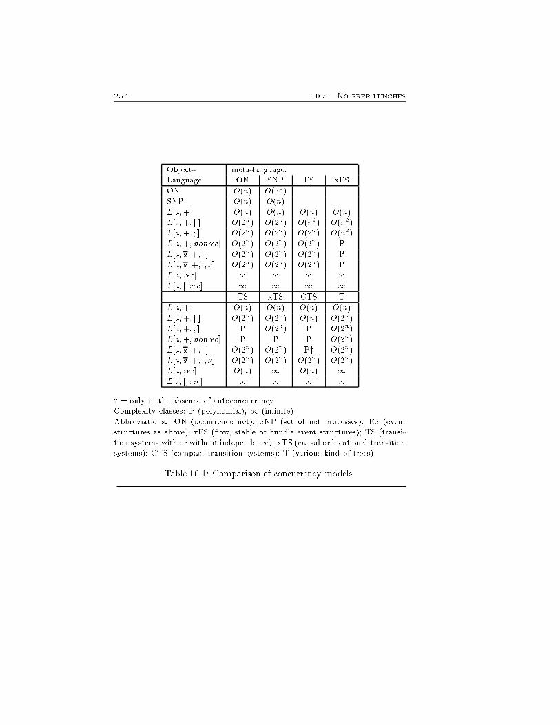
257 10.5. No free lunchesObject- meta-language:Language ON SNP ES xESON O(n) O(n2)SNP O(n) O(n)L[a;+] O(n) O(n) O(n) O(n)L[a;+; j ] O(2n) O(2n) O(n2) O(n2)L[a;+; ; ] O(2n) O(2n) O(2n) O(n2)L[a;+;nonrec] O(2n) O(2n) O(2n) PL[a; a;+; j ] O(2n) O(2n) O(2n) PL[a; a;+; j; �] O(2n) O(2n) O(2n) PL[a; rec] 1 1 1 1L[a; j; rec] 1 1 1 1TS xTS CTS TL[a;+] O(n) O(n) O(n) O(n)L[a;+; j ] O(2n) O(2n) O(n) O(2n)L[a;+; ; ] P O(2n) P O(2n)L[a;+;nonrec] P P P O(2n)L[a; a;+; j ] O(2n) O(2n) Py O(2n)L[a; a;+; j; �] O(2n) O(2n) O(2n) O(2n)L[a; rec] O(n) 1 O(n) 1L[a; j; rec] 1 1 1 1y = only in the absence of autoconcurrency.Complexity classes: P (polynomial), 1 (in�nite).Abbreviations: ON (occurrence net), SNP (set of net processes); ES (eventstructures as above), xES ( ow, stable or bundle event structures); TS (transi-tion systems with or without independence); xTS (causal or locational transitionsystems); CTS (compact transition systems); T (various kind of trees).Table 10.1: Comparison of concurrency models.

Chapter 10. Complexity and Concurrency 258

Chapter 11CompactRepresentationsWe characterise through axioms the transition systems which may be re-duced in size, still preserving strong bisimulation equivalences wheneverapplied to non interleaving models. This compact representation of pro-cesses permits to have a bisimulation algorithm for truly concurrent se-mantics with time complexity O(n3) in average, where n is the numberof occurrences of action in a (�nite state) possibly recursive process. Weexemplify our reduction technique on the subset of �-calculus withoutobjects and restriction. The limitation to object-free processes is a sim-pli�cation for presentation purposes. The absence of restriction is insteadneeded to make our approach work. We generate compact representa-tions of �nite state concurrent processes in SOS style. The representationrequires O(n) space in average. We de�ne a con ict relation betweentransitions that is used together with the concurrency relation to dropsome transitions from representations of processes. In compact transitionsystems, all computations which only di�er for the temporal ordering ofconcurrent transitions are represented by at least one computation, actu-ally a single one if all transitions involve visible actions and there is noautoconcurrency. The generation of compact transition systems is correct,259

Chapter 11. Compact Representations 260because we can retrieve from them the corresponding complete transitionsystems.11.1 Compact transition systemsThe main idea of our approach to limit state explosion is selecting a singlerepresentative in compact transition systems for all computations whichdi�er only in the temporal ordering in which their concurrent transitionsare �red. This allows us to e�ciently check truly concurrent bisimula-tion equivalences on compact transition systems. Before exploiting ourapproach, some notation could help. We �rst characterize through axiomsthe behaviour of concurrency by introducing the asynchronous transitionsystem. Then, we impose further restrictions on them so that concur-rency connot implicitly make choices (Subsect. 11.1.1). Subsection 11.1.2describes how to reduce the size of transition systems without loosingany information on their non-interleaving behaviour. Finally, we de�netruly concurrent bisimulation in Subsect. 11.1.3, and we prove that thereduction preserves these induced equivalences.If a transition system TS is equipped with a symmetric, irre exiveconcurrency relation between transitions (written ^ � a�! � a�!), weget an asynchronous transition system (also called transition system withindependence) aTS = h�; A;�!; P;^i:These transition systems have been introduced by (Winskel & Nielsen,1992), following the ideas of asynchronous transition systems by (Bednar-czyk, 1988), of concurrent transition systems by (Stark, 1989), of concur-rent machines by (Shields, 1985).The basic assumption under aTS is that concurrent transitions whichoccur consecutively are represented by all their interleavings. A formalcharacterization of these transition systems is given by the following ax-ioms (Joyal et al., 1994): 0 a�! 00 � 0 a�! 1 ) 00 = 1 (11.1)

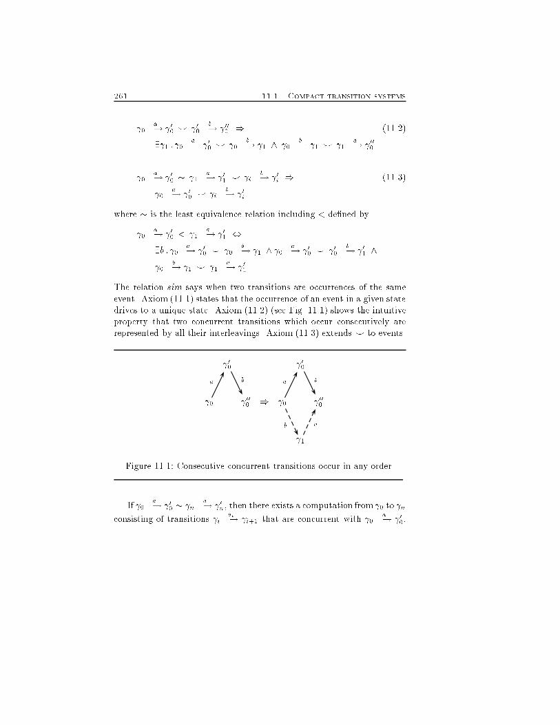
261 11.1. Compact transition systems 0 a�! 00 ^ 00 b�! 000 ) (11.2)9 1 : 0 a�! 00 ^ 0 b�! 1 ^ 0 b�! 1 ^ 1 a�! 000 0 a�! 00 � 1 a�! 01 ^ i b�! 0i ) (11.3) 0 a�! 00 ^ i b�! 0iwhere � is the least equivalence relation including < de�ned by 0 a�! 00 < 1 a�! 01 ,9b : 0 a�! 00 ^ 0 b�! 1 ^ 0 a�! 00 ^ 00 b�! 01 ^ 0 b�! 1 ^ 1 a�! 01The relation sim says when two transitions are occurrences of the sameevent. Axiom (11.1) states that the occurrence of an event in a given statedrives to a unique state. Axiom (11.2) (see Fig. 11.1) shows the intuitiveproperty that two concurrent transitions which occur consecutively arerepresented by all their interleavings. Axiom (11.3) extends ^ to events. 00 00 0 000 ) 0 000 1a b ab baFigure 11.1: Consecutive concurrent transitions occur in any order.If 0 a�! 00 � n a�! 0n, then there exists a computation from 0 to nconsisting of transitions i bi�! i+1 that are concurrent with 0 a�! 00,

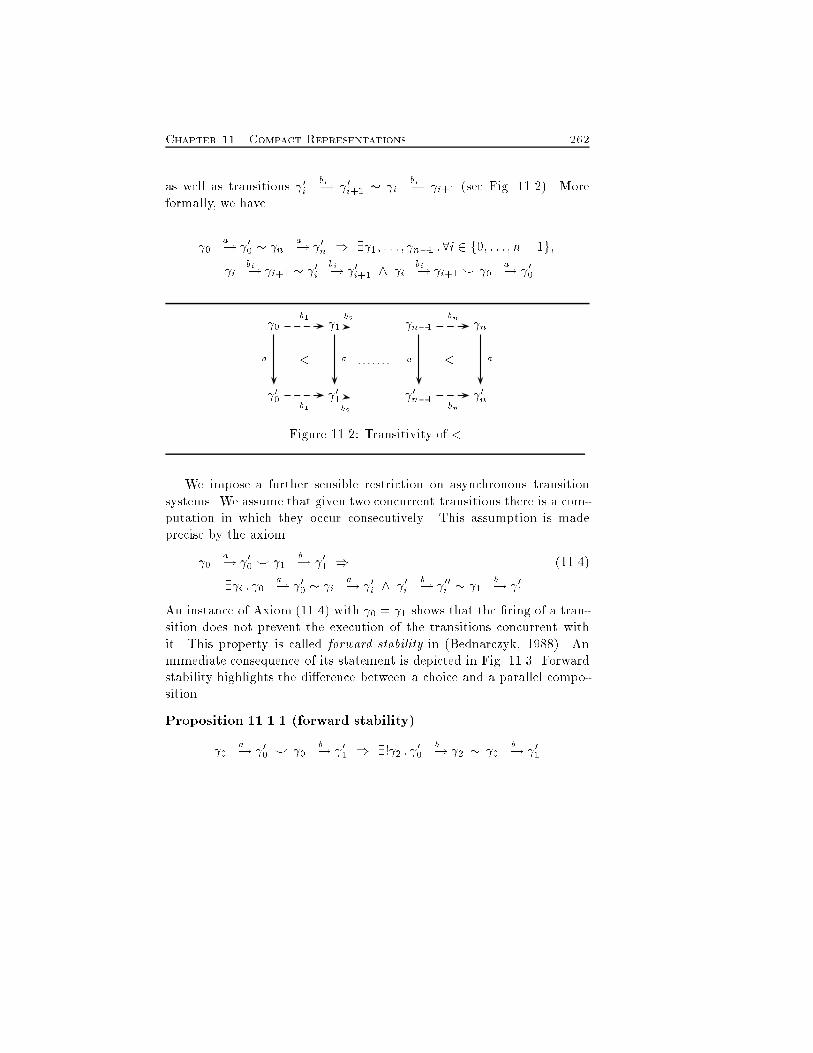
Chapter 11. Compact Representations 262as well as transitions 0i bi�! 0i+1 � i bi�! i+1 (see Fig. 11.2). Moreformally, we have 0 a�! 00 � n a�! 0n ) 9 1; : : : ; n�1 : 8i 2 f0; : : : ; n� 1g; i bi�! i+1 � 0i bi�! 0i+1 ^ i bi�! i+1 ^ 0 a�! 00 0 1 n�1 n< < 00 01 0n�1 0na b2b2a a ab1 bnb1 bnFigure 11.2: Transitivity of <.We impose a further sensible restriction on asynchronous transitionsystems. We assume that given two concurrent transitions there is a com-putation in which they occur consecutively. This assumption is madeprecise by the axiom 0 a�! 00 ^ 1 b�! 01 ) (11.4)9 i : 0 a�! 00 � i a�! 0i ^ 0i b�! 00i � 1 b�! 01An instance of Axiom (11.4) with 0 = 1 shows that the �ring of a tran-sition does not prevent the execution of the transitions concurrent withit. This property is called forward stability in (Bednarczyk, 1988). Animmediate consequence of its statement is depicted in Fig. 11.3. Forwardstability highlights the di�erence between a choice and a parallel compo-sition.Proposition 11.1.1 (forward stability) 0 a�! 00 ^ 0 b�! 01 ) 9! 2 : 00 b�! 2 � 0 b�! 01

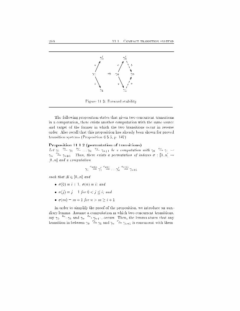
263 11.1. Compact transition systems 00 00 0 ) 0 2 1 1ab ab baFigure 11.3: Forward stability.The following proposition states that given two concurrent transitionsin a computation, there exists another computation with the same sourceand target of the former in which the two transitions occur in reverseorder. Also recall that this proposition has already been shown for provedtransition systems (Proposition 6.5.5, p. 147).Proposition 11.1.2 (permutation of transitions)Let 0 a0�! 1 a2�! : : : n an�! n+1 be a computation with 0 a0�! 1 ^ n an�! n+1. Then, there exists a permutation of indexes � : [0::n] ![0::n] and a computation 0 a�(h)�! 01 a�(l)�! : : : 0n a�(k)�! n+1such that 9i 2 [0::n] and� �(0) = i + 1; �(n) = i; and� �(j) = j � 1 for 0 < j � i; and� �(m) = m + 1 for n > m � i + 1In order to simplify the proof of the proposition, we introduce an aux-iliary lemma. Assume a computation in which two concurrent transitions,say 0 a0�! 1 and n an�! n+1, occurs. Then, the lemma states that anytransition in between 0 a0�! 1 and n an�! n+1 is concurrent with them.

Chapter 11. Compact Representations 264Lemma 11.1.3 Let 0 a0�! 1 a1�! : : : n an�! n+1 be a computation suchthat 0 a0�! 1 ^ n an�! n+1. Then,8j; 0 < j < n : ( i ai�! i+1 ^ 0 a0�! 1) _ ( i ai�! i+1 ^ n�1 an�! n):Proof. The proof is by contradiction. Assume that8j; 0 < j < n : ( i ai�! i+1 6^ 0 a0�! 1) ^ ( i ai�! i+1 6^ n�1 an�! n):The �rst conjunct implies that there is no computation 0 �!� i ai�! 0 a0�! 1with 0 a0�! 1 � 0 a0�! 1 and i ai�! 0 � i ai�! i+1. In fact, thecomputation above would imply i ai�! 0 ^ 0 a0�! 1 (by transitivity of <)and by Axiom (11.3) i ai�! i+1 ^ 0 a0�! 1 against the hypothesis.Similarly, by the second conjunct there is no computation i �!� n an�! n+1 ai�! i+1with n an�! n+1 � n an�! n+1 and n+1 ai�! i+1 � i ai�! i+1.The above implies that there is no computation 0 �!� n an�! 0 a0�! 1against Axiom (11.4). 2Proof. (of Proposition 11.1.2.) The proof is by induction on n. If n = 1, thestatement is trivially true by Axiom 11.2. Assume as inductive hypothesis thatthe proposition holds for any k � n. We prove it when there are k+1 transitionsbetween 0 a0�! 1 and n an�! n+1. Let h be the minimum index such that 0 a0�! 1 ^ h ah�! h+1. For any l < h it is l al�! l+1 ^ h ah�! h+1 byLemma 11.1.3. By Axiom (11.2) there exists the computation 0 a0�! 1 a1�! 2 : : : h�1 ah�! 1h ah�1�! h+1 ah+1�! h+2 : : : n�1 an�! nWe now repeat the above h times to obtain the computation 0 ah�! h1 a0�! h2 : : : n�1 an�! n:Since there are k transitions between h1 a0�! h2 and n�1 an�! n, the inductivehypothesis su�ces. 2

265 11.1. Compact transition systems11.1.1 Concurrency and choicesWe characterize transition systems that we can reduce, preserving bisimu-lation. The �rst point we make sure is that concurrency does not operatechoices. When some transitions may represent the interaction of moreelementary actions, say communications, their occurrence may made alsoa choice. Consider for example the CCS-like process(� c)((a + c)jb:c):The occurrence of a, concurrent with b and c, prevents the latter to syn-chronize because it is a private name. Keeping in mind that our inves-tigation has to do with cooperating processes, we we consider as giventhose transitions originated by cooperation of more than one process thatwe call compound and denote by g; gi; g0. Then, we will give a group ofaxioms ensuring that communication makes no hidden choice.Assume a family of (n+ 1)-ary (n � 2) relationsGn � (�!=� )n � (�!=� )over (equivalence classes of) transitions that identi�es the components ofa compound transition. The �rst n components of an element of Gn rep-resent the transitions of the partners originating the compound transition((n + 1)th component). We enrich asynchronous transition systems withthe family of relations above, thus yieldingaTS = h�; A;�!; P;^;Gni:With the following three axioms, the relations between concurrency andnondeterminism will be kept clear. Intuitively, we require that all compo-nents of a compound transition are enabled when the compound transitionis. Also, the occurrence of the latter prevents its components to occur,and vice versa.Assume in the following axioms that� = ([ i di�! 0i]1�i�n; [ 0 g�! 00]) 2 Gn:

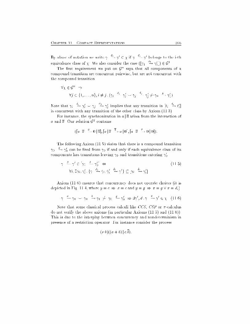
Chapter 11. Compact Representations 266By abuse of notation we write di�! 0 2 � if di�! 0 belongs to the i-thequivalence class of �. We also consider the case ([ 1 d1�! 01]) 2 G1.The �rst requirement we put on Gn says that all components of acompound transition are concurrent pairwise, but are not concurrent withthe compound transition.8� 2 Gn )8j 2 f1; : : : ; ng; i 6= j : ( i di�! 0i ^ j dj�! 0j 6^ 0 g�! 00)Note that i di�! 0i ^ j dj�! 0j implies that any transition in [ti di�! t0i]is concurrent with any transition of the other class by Axiom (11.3).For instance, the synchronization in a j a arises from the interaction ofa and a. Our relation G2 contains([a j a a�! 0 j a]; [a j a a�! a j0]; [a j a ��! 0 j0]):The following Axiom (11.5) states that there is a compound transition 0 g�! 00 can be �red from 0 if and only if each equivalence class of itscomponents has transitions leaving 0 and transitions entering 00. g�! 0 2 [ 0 g�! 00] , (11.5)8i; 9 i; 0i : f di�! i; 0i di�! 0g � [ i di�! 0i]Axiom (11.6) ensures that concurrency does not operate choices (it isdepicted in Fig. 11.4, where y = c ) x = c and y = g ) x = g _ x = di). a�! 0 ^ 0 b�! 1 6^ 0 g�! 00 ) 9 0; d : d�! 0 2 � (11.6)Note that some classical process calculi like CCS, CSP or �-calculusdo not verify the above axioms (in particular Axioms (11.5) and (11.6)).This is due to the interplay between concurrency and nondeterminism inpresence of a restriction operator. For instance consider the process(� b)((a+ b) j c:b):

267 11.1. Compact transition systems 0 00 0 00 1 ) 1 0a yb bax yFigure 11.4: Concurrency does not operate choices.It violates Axioms (11.5) and (11.6) because restriction prevents the com-ponents of the synchronization (b and b) to occur asynchronously. A simi-lar drawback arises in CSP, because the synchronization mechanism forcescommunications on a given set of labels. For example, the processa:b jjfbg c:bviolates Axiom (11.5) because the two b-transitions cannot be �red asyn-chronously. Finally, note instead that sequential composition of processes(usually written ;) rises no problem. Indeed, in P ;Q no action of Q canoccur concurrently with any action of P , nor they can be compound.As we will prove in the next sections, the subset of �-calculus withoutrestriction �ts the class of asynchronous transition system enriched withrelations Gn.11.1.2 ReductionWe show how to extract the canonical compact representative from a givenwhole transition systems. Since we are mainly interested in preservingbisimulation equivalences, we must choose deterministically the transitionto be kept (the leader) out of those concurrent outgoing from the samecon�guration . This will be done by ordering the transitions outgoingfrom according to a lexicographic ordering / on their labels.

Chapter 11. Compact Representations 268Some problems may be caused by autoconcurrency. Recall that twotransitions are autoconcurrent if they share the same action. In this case,we do not know which branch to discard. Thus, we choose to keep allautoconcurrent transitions. Technically, we use a total pre-ordering / onthe transitions exiting from a node which extends the ordering on theirlabels. Let R/ be the equivalence relation de�ned as 0 a�! 00 R/ 0 b�! 1 , 0 a�! 00 / 0 b�! 1 ^ 0 b�! 1 / 0 a�! 00Then, the pre-ordering / must be such that the equivalence classes origi-nated by R/ are made up of transitions with the same action.The following proposition states that / is actually an ordering if noautoconcurrency appears.The following proposition states that / is actually an ordering if noautoconcurrency appears.Proposition 11.1.4If a�! 0 ^ b�! 00 ) a 6= b, then / is an ordering.Proof. The proof is immediate by noting that / turns out to coincide with thelexigraphic ordering on labels. 2Now, we turn / into a total ordering on the transitions exiting froma node (still denoted as /) by using a well-known property of pre-orderedsets. We let[ 0 a�! 00] / [ 0 b�! 1] , 0 a�! 00 / 0 b�! 1where [ i a�! 0i] denotes the equivalence class of i a�! 0i with respectto R/.Let aTS = h�; A;�!; P;^;Gni be an asynchronous transition system.Then, cTS = h�0; A; ,!; P;^0;G0ni is the compact transition system ob-tained through iterated applications of Axiom (11.7) below, interpretedas a conditional rewriting rule. Note that �0 � �, ,!��!, ^0�^ and

269 11.1. Compact transition systemsG0n � Gn. Indeed, ^0 and G0n are the restriction of the relations ^ andGn to the transitions of cTS. 0 a�! 00 ^ 0 b�! 1; 0 a�! 00 / 0 b�! 1 ) 0 a,! 00 (11.7)Axiom (11.7) shows how to prune the set of transitions outgoing froma con�guration. Furthermore is immediate from the axiom that the equiv-alence classes with respect to � of the transitions verify[ 0 a,! 00] � [ 0 a�! 00]:We also have the following proposition.Proposition 11.1.5 If a�! 0 ^ b�! 00 ) a 6= b, then [ a,! 0] isa singleton.Proof. Since / is a total ordering (Proposition 11.1.4), there is only one tran-sition labelled a and exiting from . 2Note that the reduction is e�ective because it is applied to �nite stateand �nite branching transition systems.The basic idea under Axiom (11.7) is to �x an ordering in which con-current transitions are sequentially �red. Transition 0 b�! 1 is removedfrom the whole transition system, together with the subgraph G reachedonly through it. Indeed, a transition 0 b�! 1 � 0 b�! 1 will occurafter 0 a�! 00, due to (iterated applications of) forward stability. Then,the transitions of the process reached through 0 a,! 00 are pruned inthe same manner. Iterated applications of Axiom (11.7) may discard alsosome compound transition. For instance, consider process P = a j b:a.The reduction selects P a�! 0 j b:a as unique transition from P . Then,we have the transition 0 j b:a b,! 0 j a and �nally 0 j a a,! 0 j0. Since thereduction generates no state which enables both a transition with action aand one with action a, the corresponding synchronization does not occurin the compact transition system of P . However, this is by no means aloss of information, because we have([a j b:a a�! 0 j b:a]; [0j a a�! 0j0]; [aja ��! 0j0]) 2 G2:

Chapter 11. Compact Representations 270Note that the equivalence class of the synchronization is empty in G2 be-cause the corresponding transition is not generated. The class will be�lled during the reconstruction of the whole transition system (see Theo-rem 11.1.8).The following property states that compact transition systems arecanonical representatives of the corresponding whole transition systems.Proposition 11.1.6 Given a transition system TS, its compact transitionsystem cTS is uniquely and �nitely generated.Proof. The rewriting strategy is terminating as the size of the transition systemdecreases at each step, and i s�!� j is e�ective due to the �nite state and �nitebranching assumptions. Moreover, the compact transition system is uniqueas the generation is deterministic due to the total ordering / on the labels oftransitions. 2We claim that no information on the behaviour of a process is lostduring the generation of its compact representation. Indeed, it is possibleto rebuild the whole transition system TS of a process from the compactone cTS. We �rst introduce a property of ^ that permits us to simplifythe proof of Theorem 11.1.8 on the correctness of the reduction. Theproposition shows the relation between a transition concurrent with allthe components of a compound transition and the compound transitionitself.Proposition 11.1.7 Let([ i di�! 0i]1�i�n; [ 0 g�! 00]) 2 Gn ^8i : i di�! 0i ^ n a�! 00n ) 0 g�! 00 ^ n a�! 00nProof. By hp: ([ i di�! 0i]1�i�n; [ 0 g�! 00]) 2 Gn and Axiom (11.5) )9 1 : 1 d1�! 2 d2�! : : : dn�! n+1 with i di�! i+1 2 [ i di�! i+1]

271 11.1. Compact transition systems) (by hp:8i : i di�! 0i ^ n a�! 00n and iterated applications of Axiom (11.2))9~ 1; ~ n+1 : 1 a�! ~ 1 � n a�! 00n � n+1 a�! ~ n+1 ^~ 1 d1�! ~ 2 d2�! : : : dn�! ~ n+1 with ~ i di�! ~ i+1 2 [ i di�! i+1]) (by hp: ([ i di�! 0i]1�i�n; [ 0 g�! 00]) 2 Gn and Axiom (11.5)) 1 g�! n+1 � 0 g�! 00 � ~ 1 g�! ~ n+1) (by de�nition of �) 0 g�! 00 ^ n a�! 00n 2We now report the correctness result.Theorem 11.1.8 Let aTS = h�; A; a�!; P;^;Gni be an asynchronoustransition system, and let cTS = h�0; A; a,!; P;^0;G0ni be its compactform. Then,8 0 a�! 00 2 aTS; 9 ~ 0 a�! ~ 00 2 cTS : 0 a�! 00 � ~ 0 a�! ~ 00Moreover, let ([ i di�! 0i]1�i�n; [ 0 g�! 00]) 2 Gn. Then,8 0 g�! 00 2 aTS; 8 i ~ i di�! ~ 0i 2 cTS :~ i di�! ~ 0i � i di�! 0iProof. Consider a transition i a�! 0i of aTS not occurring in cTS. Wedistinguish two cases according to i. If i 2 �0, then 9 i b�! j 2 cTSwith i a�! 0i ^ i b�! j by de�nition of reduction. This implies that j s�!� ~ 0 a�! ~ 00 by Proposition 11.1.2.The other case is i 62 �0. Consider the minimal predecessor of i such thatthere is the computation in aTSP s�!� b�! 0 s0�!� iand 2 cTS. Since b�! 0 is not in cTS, there must exist c�! in cTSwith b�! 0 ^ c�! .If i a�! 0i ^ b�! 0, by Proposition 11.1.2 we have a�! j with a�! j � i a�! 0i and we proceed as in the previous case.

Chapter 11. Compact Representations 272If i a�! 0i 6^ b�! 0, we proceed by induction on the number oftransitions between and i.Base case. There is a single transition between and i ( 0 = i). Thetransition is b�! 0 which is concurrent with c�! . By forwardstability there exists 0 c�! 0 in aTS such that 0 c�! 0 � c�! 0. If 0 a�! 0i ^ 0 c�! 0, we are done. Otherwise by Axiom 11.6either 0 a�! 0i, or one of its components if it is a compound transition,exits from . By Axiom 11.5 all components of a compound transitionare concurrent and therefore they will appear in some computation from consecutively by permutation of transitions. Hence, we recover thecompound transition through relations Gn.Assume that the theorem holds when there are n transitions between and i. If one of these transitions is concurrent with i a�! 0i byProposition 11.1.2 we can decrease the distance of i from and applythe inductive hypothesis. Thus, assume that all n transitions are nonconcurrent with i a�! 0i. Since b�! 0 ^ c�! , we have also b�! 00 � b�! 0 by forward stability. Since an equivalent transitionto b�! 0 is in cTS there exists also a transition equivalent to i a�! 0i.2The above theorem allows us to retrieve a whole transition system fromits compact representation.Theorem 11.1.9 Let aTS = h�; A; a�!; P;^;Gni be an asynchronoustransition system, and let cTS = h�0; A; a,!; P;^0;G0ni be its compactform. Then, it is always possible to rebuild aTS from cTS.Proof. The transition system aTS is obtained by a �x-point construction thatcan be always applied to a compact transition system.Consider a sequence of transition systems aTSi = h�i;A; a�!i; P;^i;Gni i suchthat �i � �i+1, a�!i� a�!i+1, ^i�^i+1 and Gni � Gni+1. We abbreviate theabove conditions by saying aTSi � aTSi+1. Note that these conditions introducea family of equivalence relations �i de�ned according to ^i.We now de�ne a function : aTSi ! aTSi+1 such that 0 a�!i 1 b�!i 2; 0 a�!i 1 ^ 1 b�!i 2 )

273 11.1. Compact transition systems9 01 2 �i+1 : ( 0 b�!i+1 01 �i+1 1 b�!i 2) ^( 01 a�!i+1 2 �i+1 0 a�!i 1)The conditions on the equivalence relation �i+1 in the above axiom makes thecardinality of the equivalence classes in Gni+1 larger than the one of the corre-sponding classes in Gni . Instead, the number of classes is left unchanged.Let aTS0 = cTS and let n = (n�1), n � 1. Since an application of corresponds to a �nite (due to the �nite state and �nite branching assumptions)number of applications of Axiom (11.2), the added nodes and transitions wasalready present in aTS. Since is monotonic and 8n � 0; n(cTS) � aTS, has a unique �xed-point .Intuitively, the transformation applied to TSc rebuilds concurrency diamondsof aTS according to axiom 11.2. No compound transition is rebuilt. To thispurpose we de�ne another transition system transformation.Consider a sequence of transition systems aTS0i = h�;A; a�!i; P;^i;Gni i suchthat a�!i� a�!i+1, ^i�^i+1 and Gni � Gni+1. We abbreviate the above condi-tions by saying aTS0i � aTS0i+1.We now de�ne a function � : aTS0i ! aTS0i+1 such that8n � 1; 0 d1�!i 1 d2�!i : : : n�1 dn�! n;([ 0 d1�!i 1]; : : : ; [ n�1 dn�! n]; [ 0 g�!i 00]) 2 Gni ) 0 g�!i+1 n �i+1 0 g�!i 00The condition on �i+1 is such that the transition 0 g�!i+1 n is added to theequivalence class of the compound transition in Gni+1. If the class is empty, it is�lled with the new transition, otherwise the new transition is an occurrence ofthe elements in the class. The added compound transitions may originate newpairs for the relation ^i+1. These new elements are obtained starting from Gni+1according to Proposition 11.1.7.Let aTS00 = (cTS) and let �n = �(�n�1), n � 1. The added transitions wasalready present in TS due to Axioms (11.5) and (11.6). Therefore, since � ismonotonic and �n((TSc)) � TS, 8n � 0, � has a unique �xed-point �.The application of the transformation � to the result of the application of rebuilds the compound transitions of aTS starting from the relations Gn. Theadded transitions may generate new consecutive concurrent transitions enablingfurther application of . Therefore we must take the �xed-point of the com-position f = � � . Since aTS is still an upper bound for fn, we have that

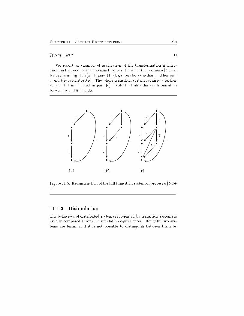
Chapter 11. Compact Representations 274f(cTS) = aTS. 2We report an example of application of the transformation intro-duced in the proof of the previous theorem. Consider the process a j b:a+c.Its cTS is in Fig. 11.5(a). Figure 11.5(b), shows how the diamond betweena and b is reconstructed. The whole transition system requires a furtherstep and it is depicted in part (c). Note that also the synchronizationbetween a and a is added.� � �� � � � �� � � �� � �(a) (b) (c)a a ab b ba a ac c cb ba a aa�Figure 11.5: Reconstruction of the full transition system of process a j b:a+c.11.1.3 BisimulationThe behaviour of distributed systems represented by transition systems isusually compared through bisimulation equivalences. Roughly, two sys-tems are bisimilar if it is not possible to distinguish between them by

275 11.1. Compact transition systemsobserving their behaviour. For simplifying the notation, in this subsectionwe omit from the de�nition of transition systems the relations ^ and Gnassuming implicitly their presence.Bisimulation equivalences (denoted here �) are preserved by our re-duction when the semantics considers the parallel composition non seman-tically reducible to any combination of sequential operators. We formalizethis intuition below. 0 a�! 00 ^ 0 b�! 000 ; 0 � 1 ) (11.8)9 01; 001 : 1 a�! 01 ^ 1 b�! 001 ; 00 � t01; 000 � 001We call the equivalences respecting Axiom 11.8 truly concurrent.We now prove that the reduction de�ned by rule 11.7 preserves trulyconcurrent bisimulation equivalences.Theorem 11.1.10 Let T = h�; A;�!; i and T 0 = h�0; A;�!; 0i be twotransition systems. Also, let cT = h�c; A; ,!; i and cT0 = h�0c; A; ,!; 0ibe the compact transition systems corresponding to T and T 0, respectively.If � is a truly concurrent bisimulation, thenT � T 0 , cT � cT0:Proof. Recall that we are considering truly concurrent bisimulation, thus thesame concurrency relation holds between the transitions that are related by abisimulation R.)) Let R be a truly concurrent bisimulation between T and T 0. De�neR0 = R� fh i; ji j i 62�c _ j 62�0cg:We prove that R0 is a bisimulation between cT and cT0.If h i; ji 2 R0, whenever i a,! i+1 there exists j+1 such that j a�! j+1and h i+1; j+1i 2 R. We are left to prove that j a,! j+1 so that j+1 2 �0c.Sh = fak j h ak�! kg and S0h = fak j h ak,! kg:Then, h i; ji 2 R0 � R ) Si = Sj ) min/Si = min/Sj ) S0i = S0j :

Chapter 11. Compact Representations 276Therefore, i a,! i+1; j a�! j+1 ^ h i+1; j+1i 2 R ) h i+1; j+1i 2 R0:Finally, since h ; 0i 2 R0, we conclude that R0 is a bisimulation between cTand cT0, i.e., cT � cT0. The same arguments hold if j moves �rst.() Let R be a truly concurrent bisimulation between cT and cT0 and assumethat h i; ji 2 R with i 2 �c and j 2 �0c. Then, there exist i�1 2 �c and j�1 2 �0c such thath i�1; j�1i 2 R ^ i�1 a�! i ^ j�1 a�! j :Also, h i; ji 2 R implies thatfak j i ak,! kg = fak j j ak,! 0kg:Therefore, if the two sets above are non empty, there are k 2 �c and 0k 2 �0csuch that h k; 0ki 2 R ^ i ak�! 0k ^ j ak�! 0k:Assume a ^ ak and apply to the nodes corresponding to these transition thetransformation of Theorem 11.1.9. The application of adds to cT the node i1 and the transitions i ak�! i1 a�! kwhich are in T due to Theorem 11.1.8. Similarly, cT0 is extended with the node j1 and the transitions j ak�! j1 a�! 0kwhich are in T 0.Consider now R0 = R[ fh i1 ; j1ig:The relation R0 is still a truly concurrent bisimulation between the transitionsystems resulting from one application of as the pair added to R relates twonodes by transitions with the same labels and that have the same concurrencyrelation with the preceding transitions in a computation from the starting states.Similarly for the transformation � of Theorem 11.1.9.Let R be the bisimulation obtained when both � � (cT) and � � (cT0) arereached. Since � �(cT) = T and � �(cT0) by Theorem 11.1.9, we are done.2

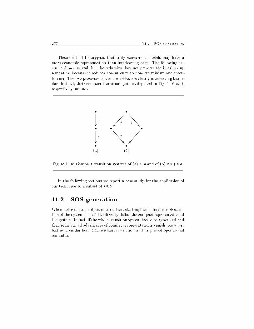
277 11.2. SOS generationTheorem 11.1.10 suggests that truly concurrent models may have amore economic representation than interleaving ones. The following ex-ample shows instead that the reduction does not preserve the interleavingsemantics, because it reduces concurrency to nondeterminism and inter-leaving. The two processes a j b and a:b+b:a are clearly interleaving bisim-ilar. Instead, their compact transition systems depicted in Fig. 11.6(a,b),respectively, are not. � �� � �� �(a) (b)ab a bb aFigure 11.6: Compact transition systems of (a) a j b and of (b) a:b+ b:a.In the following sections we report a case study for the application ofour technique to a subset of CCS.11.2 SOS generationWhen behavioural analysis is carried out starting from a linguistic descrip-tion of the system is useful to directly de�ne the compact representative ofthe system. In fact, if the whole transition system has to be generated andthen reduced, all advantages of compact representations vanish. As a testbed we consider here CCS without restriction and its proved operationalsemantics.

Chapter 11. Compact Representations 278The following theorem makes evident that this fragment of the calculuswith no autoconcurrency generates transition systems which satisfy theaxioms introduces in the previous section.Theorem 11.2.1 Let PTS = hP;�;�!i be the proved transition systemof CCS without restriction. Then, T satis�es the Axioms 11.1-11.6.Proof. PTS satis�es Axiom 11.1 as a consequence of Corollary 5.2.3. Propo-sition 6.5.5 makes evident that PTS satis�es Axioms 11.2, 11.3 and 11.4. Sincethe premise of the rules for communications in PTS are �lled through the rulesfor parallel composition, Axiom 11.5 holds as well. Finally, Axiom 11.6 is satis-�ed by PTS because the rules for parallel compositions (that are the ones whichgive raise to concurrent transitions) do not alter process contexts. 2We now de�ne a new SOS operational semantics that yields a compactproved transition system. Since we aim at maintaining all the informationrelevant to truly concurrent bisimulations, we will keep all autoconcurrenttransitions of a process. Thus, we de�ne a total preordering / on the tran-sitions outgoing from the same node, as illustrated in the next subsection.Then, Subsect. 11.2.2 reports SOS de�nitions.11.2.1 A total preordering /The de�nition of a total preordering / on the proved transitions of a pro-cess is de�ned on their labels, due to Corollary 5.2.3. Note that comparingtwo proof terms with / requires O(n) steps, where n is the number of oc-currences of actions in the given process. For technical reasons, hereafterwe distinguish the alphabet of recursive names by adding a subscript r toall �rst transitions of recursive de�nitions.De�nition 11.2.2 (preordering /) Let �1; �2 2 Ts(t). Let / the pre-ordering obtained by extending the lexicographic ordering on names, asfollows. 8a1; a2 2 Act, and 8ar ; a0r 2 Actr we de�ne� � / a1 / a2 / ar

279 11.2. SOS generation� a1 / a1 , a1 / a2� ar / a0r ^ a0r / ar.Then, by abuse of notation, �1 / �2 if and only if `(�1) / `(�2).Note that the third item of Def. 11.2.2 is not the only reason for � / �0 / �does not implies � = �0. Another reason is autocon ict: for instance theprocess a+ a.Theorem 11.2.3 (/ is total) The relation / is a total preordering overTs(t).Proof. The relation / on Act[Actr is total because all names are comparable,and it is trivially re exive. We are left to prove that it is transitive. Sincerecursive names are all equivalent, as well as the invisible actions (�), / enjoysthe transitive property over them. For names the transitivity holds because theyare ordered lexicographically. Finally, transitivity is extended to the whole setAct [Actr by the �rst item of Def. 11.2.2. 2For instance, consider process P = ((aja) j (b+ c)) + (d j d). Its transi-tions are�1 = +0jj0jj0a; �2 = +0jj0jj1a; �3 = +0jj0ha; ai; �4 = +0jj1 +0 b;�5 = +0jj1 +1 c; �6 = +1jj0d; �7 = +1jj1d:According to Def. 11.2.2, the complete preordering of Ts(P ) is�3 / �1 / �4 / �6 /. �7 / �5 / �2:Consider now process P 0 = ((a: j (a+ b)) j � ) + (d j c). Its transitions are�1 = +0jj0jj0a; �2 = +0jj0jj1 +0 a; �3 = +0jj0jj1 +1 b; �4 = +0jj1�;�5 = +1jj0d; �6 = +1jj1c:The complete preordering of Ts(P 0) is�4 / �1 /. �2 / �3 / �5 / �6:

Chapter 11. Compact Representations 280We de�ne the total ordering / in the standard way through the relationR/ as described in Subsect. 11.1.2.The following property characterises the transitions that belong to thesame equivalence class with respect to R/. In particular, these transitionsare autoconcurrent or autocon icting (�rst item) or they are recursivetransitions that initiate a loop (second item).Proposition 11.2.4 (equivalence classes of R/)Given a process P , let [�] 2 Ts(P )=R/ and let �0 2 [�]. Then, either� `(�) = `(�0) and (� ^ �0 or �#�0), or� � is recursive and �0 is recursive.Proof. If L(�) = L(�0), then �/�0 and �0/�. Thus, the two transitions belong tothe same equivalence class. Also, � ^ �0 or �#�0 because the transitions in Ts(t)are concurrent or con icting. The second item is an immediate consequence ofthe third item of Def. 11.2.2 and of the fact that recursive labels are larger thannon recursive ones (see �rst item of Def. 11.2.2). 211.2.2 SOS de�nition of the reductionWe now modify the SOS semantics of the calculus to generate the compactrepresentatives de�ned in the previous subsection. Since our reductionacts on asynchronous concurrent transitions in order to �x an orderingon their �ring, we add a rule �ltering only the wanted transitions. Inparticular, given a process P with leader transitions f�hg, we prevent thededuction of the transitions of P concurrent with �h. More precisely, wedelay their generation in the target states of �h. We use negative premisesin the Red rule in order to drive correctly the deduction of transitions.Note that this negative premise does not a�ect the e�ectiveness of thededuction because of the �nite branching property of our �nite state tran-sition systems.De�nition 11.2.5 (compact proved transition system)The compact proved transition system is cPTS = hP; �; �!c i, where

281 11.2. SOS generationP is the set of closed CCS processes without restriction and �!c is thetransition relation de�ned by the following rule which has �! (the stan-dard transition relation of CCS as auxiliary arrow.Red : P ��! P 0; P 6 �0�!; �0 ^ �; �0 / �P ��!c P 0For instance, consider the process((a:e j (a+ b)) j � ) + (d j c)Its cPTS is illustrated in Fig. 11.7 (full color). The compact representationsaves 7 states and 20 transitions (dotted in the �gure) with respect to thewhole PTS.Note that the 3 transitions of cPTS jj0jj1 +0 a and jj0jj1 +1 b followed byjj0jj0a together with the state between them are only taken because of theautoconcurrency between the a's in the left summand.As far as recursive processes are concerned, consider the processP = P 0 jP 00 with P 0 = a:b:P 0 and P 00 = c:P 00Since all initial transitions are labelled by actions with tag r (i.e., jj0arand jj1cr), we take them all. The c-transition leads to P again and thusno further transitions are to be investigated. The a-transition leads tothe process b:P 0 jP 00 that has two concurrent transitions (jj0b and jj1cr)leading to P again. The leader is jj0b because it has no tag r.We show that the premises of Red coincide with the conditions requiredfor applying the reduction R of Subsect. 11.1.2.Theorem 11.2.6 Let [P ]c be the portion of the compact proved transitionsystem with initial state P and let TS be the whole proved transition systemof P . Then, [P ]c = cTS.Proof. Immediate, by noticing that rule Red is only a di�erent way of writingrule R of Subsect. 11.1.2. 2

Chapter 11. Compact Representations 282We now estimate the space and time average complexity of our reduc-tion.Theorem 11.2.7 Given a process P with n occurrences of actions, let alllabels and all operators of the language have the same probability to occur,and let 1 be the generation cost of a transition. Then, the average spacecomplexity of the compact transition system of P is O(n) and its averagegeneration time is O(n3).Proof. First, note that autoconcurrency a�ects only the multiplicative constantof the average complexity because all labels and operators of the language havethe same probability to occur in a process. Indeed, if the alphabet of actionshas cardinality m, then two autoconcurrent transitions may occur in the (wholeor compact) transition system of a term with n actions with probability O(n)�1=(5m2). Thus, their occurrence probability decreases to 0 asm grows. Similarlyfor the recursive operator.Given a process P , the set of its transitions Ts(P ) is made up of O(n) transitionswhich are generated in O(n) time, because the deduction of a transition has unitcost. The transitions enabled by rule Red are computed according to / and to^. This requires O(n2) comparisons because proof terms have length at mostn. Summing up, the average complexity of generating the O(n) transitions ofthe compact transition system is O(n3). 2We do not give worst case complexity of the reduction because theautoconcurrent transitions are ignored only on probabilistic grounds. Thisleads to an average complexity. Consider the fragment of the language thatoriginates no autoconcurrency. In this case the above theorem providesan upper bound.Corollary 11.2.8 (complexity with no autoconcurrency) Let P bea process originating no autoconcurrency. Under the same hypotheses ofTheorem 11.2.7, the space complexity of the compact transition system ofP is O(n) and its generation time is O(n3).Finally, no claim can be made on the minimality of the compact tran-sition system. This is due to /, that preorders transitions arbitrarily.Forinstance, if a/b and d/c, the compact transition system of a j (b:c+d) has

283 11.3. Related work4 arcs, while the one for b j (a:c+ d) has 5 arcs for the duplication of anarc labelled b. This remark suggests that the same problem will show upwith any ordering, and that the best we can do is keeping the size of thecompact transition system linear with the actions occurring in a process.We report below an example which give an intuitive idea of the numberof transitions saved by the cPTS. Of course, the larger is the number ofparallel operators in the process considered, the larger is the space saved.Consider for instance the processP = a:bk:c j dwhere bk means a sequence of k b's. Its PTS is illustrated in Fig. 11.8(a)where the dotted lines represents k � 1 arcs labelled jj0b. The wholetransition system has n = 3(k + 2) arcs, the compact one, illustrated inFig. 11.8(b) has (k + 3) arcs.Note that there are cases where the number of arcs saved is much greater.For instance, consider the process P 0 = a:bk:c j (d1+ : : :+dm) with d1/dm.Its proved transition system is similar to the one in Fig. 11.8(a), exceptthat each arc d is replaced by the m arcs of the subprocess (d1+ : : :+dm).In this case the number of transitions of P 0 is (m+2)(k+2). The compacttransition system is obtained from the one in Fig. 11.8(b) by substitutingthe obvious branching with m arcs for the last arc. Thus, the number oftransitions is only k +m + 1.11.3 Related workSome related works similar to ours are sketched below. In (Godefroid,1990; Godefroid & Wolper, 1991) the problem is addressed of �nding com-pact representation of processes for studying safety properties like absenceof deadlock. No care is devoted to preserve bisimulation equivalences, andso the run to be kept among the mutually concurrent ones is chosen ran-domly. This leads to quite an e�cient solution. The solution by (Clegg &Valmari, 1991; Valmari, 1990) represents processes as compact transitionsystems obtained by exploiting the properties of concurrecy and mutualexclusion of events, as in our case. The compact representatives preserve

Chapter 11. Compact Representations 284the failure CSP semantics (Brookes et al., 1984); however, nothing is saidabout bisimulations. Also (Valmari & Tienari, 1991) discuss a reductiontechnique of labelled transition systems. The compact representatives pre-serve an equivalence based on the notions of stable failure and divergence.The used semantic model conforms with the semantics of CSP up to the�rst divergence of the system. A prede�ned relation of independence ofevents is used in (Peled, 1993) for constructing a transition system thatcontains at least one representative path among those obtained by shuf- ing its independent events. A tool is implemented, yielding a state graphon which model checking may be performed e�ciently. The method pre-sented by (Janicki & Koutny, 1990) is quite ad hoc: it has been developedin order to check deadlock and liveness properties for a particular class ofPetri nets. The simpli�cation relies on a kind of reachability relation oncomputations. The approach of (McMillan, 1992) is based on unfoldingsof Petri nets that make it easier to establish reachability, but it does notpreserve semantic equivalences. In the solution by (Probst & Li, 1990)the user must supply an ad hoc pomset grammar (constructed by hand)which describes the behaviour of the considered system. Thus, it is notautomatic as the other methods.

285 11.3. Related work

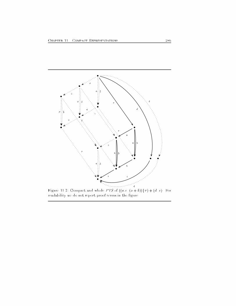
Chapter 11. Compact Representations 286��� ��� ��� � � ���� d cbaeb b ae c daaa ���� �aaa bbb ee aa

Figure 11.7: Compact and whole PTS of ((a:e j (a + b)) j � ) + (d j c). Forreadability we do not report proof terms in the �gure.

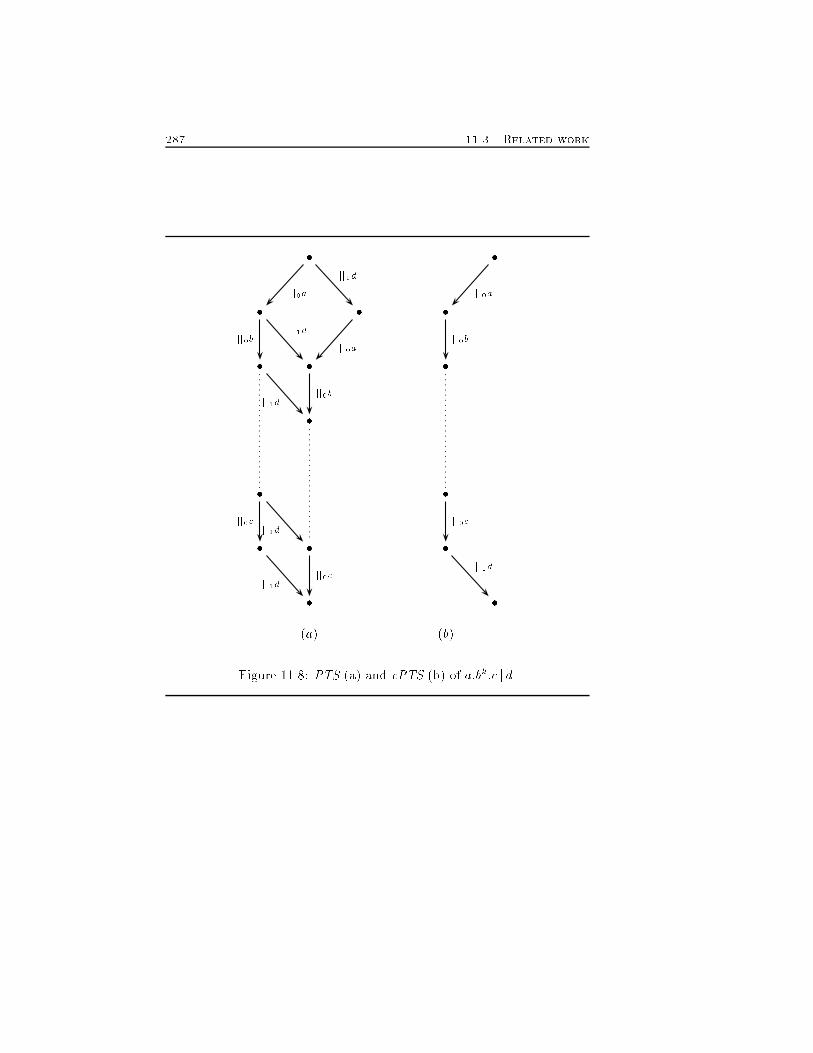
287 11.3. Related work� �� � �� � ��� �� � �� �(a) (b)jj0a jj1djj0b jj1d jj0ajj0bjj1djj1djj1djj0c jj0c

jj0ajj0bjj0c jj1dFigure 11.8: PTS (a) and cPTS (b) of a:bk:c j d.

Chapter 11. Compact Representations 288

Chapter 12YAPVWe present a parametric tool for the behavioural analysis of distributedconcurrent systems expressed in CCS. Processes are internally representedas compact proved transition systems. We work on extended transitionsystem to increase the e�ciency of the relabelling step. We replace regularexpressions on nodes with physical pointers on transitions. This allowsus to de�ne simpler (and thus more e�cient) relabelling functions. Theresulting tool called YAPV (Yet Another Property Veri�er) supports thedesigner of distributed and concurrent systems in various activities. Itprovides the standard editing facilities for the input of processes, speci�edup to now in restriction-free CCS. The graphical representation of thetransition system is also displayed and animated. The semantical featuresof YAPV concern the equivalence checking of two processes according toa selected semantic model and some simulation operations.12.1 Relabelling functionsWe de�ne the mechanism that allows us to discard unwanted details fromlabels of transitions according to the aspects under investigation. Thistask is accomplished by relabelling functions that extend the techniquepresented in Chapt. 6. The models that can be recovered in the present289

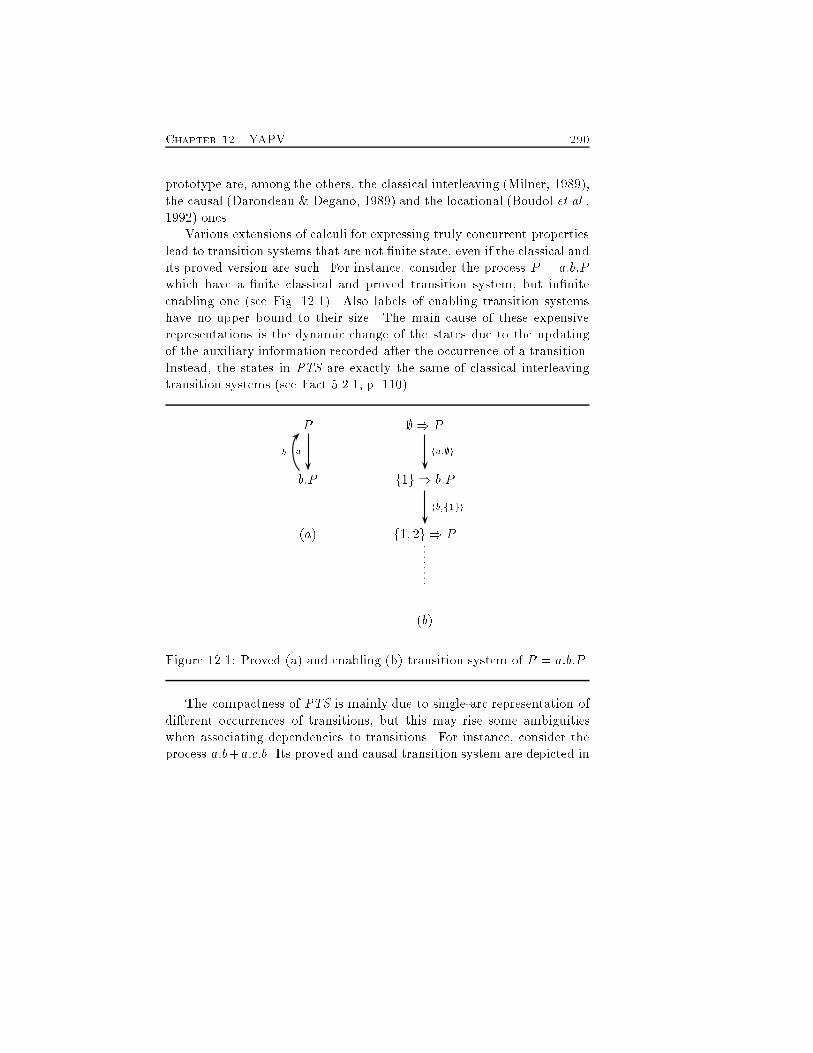
Chapter 12. YAPV 290prototype are, among the others, the classical interleaving (Milner, 1989),the causal (Darondeau & Degano, 1989) and the locational (Boudol et al.,1992) ones.Various extensions of calculi for expressing truly concurrent propertieslead to transition systems that are not �nite state, even if the classical andits proved version are such. For instance, consider the process P = a:b:Pwhich have a �nite classical and proved transition system, but in�niteenabling one (see Fig. 12.1). Also labels of enabling transition systemshave no upper bound to their size. The main cause of these expensiverepresentations is the dynamic change of the states due to the updatingof the auxiliary information recorded after the occurrence of a transition.Instead, the states in PTS are exactly the same of classical interleavingtransition systems (see Fact 5.2.1, p. 110).P ; ) Pb:P f1g ) b:P(a) f1; 2g ) P(b)ab ha;;ihb;f1giFigure 12.1: Proved (a) and enabling (b) transition system of P = a:b:P .The compactness of PTS is mainly due to single-arc representation ofdi�erent occurrences of transitions, but this may rise some ambiguitieswhen associating dependencies to transitions. For instance, consider theprocess a:b+a:c:b. Its proved and causal transition system are depicted in

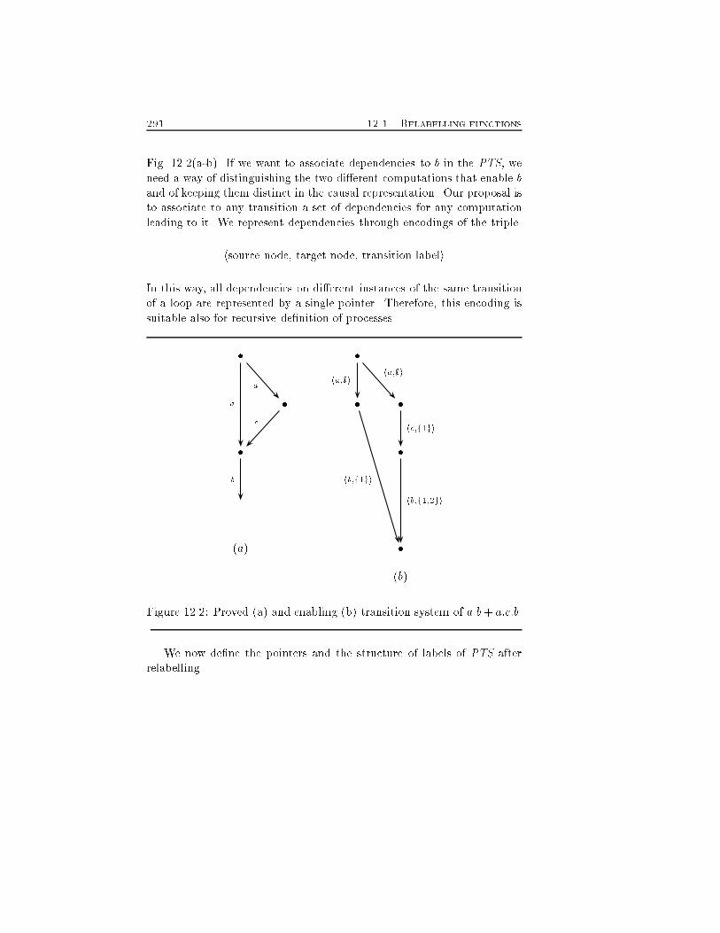
291 12.1. Relabelling functionsFig. 12.2(a-b). If we want to associate dependencies to b in the PTS, weneed a way of distinguishing the two di�erent computations that enable band of keeping them distinct in the causal representation. Our proposal isto associate to any transition a set of dependencies for any computationleading to it. We represent dependencies through encodings of the triplehsource node, target node, transition labeliIn this way, all dependencies on di�erent instances of the same transitionof a loop are represented by a single pointer. Therefore, this encoding issuitable also for recursive de�nition of processes.� �� � �� �(a) �(b)aa cb ha;;i ha;;ihb;f1gi hc;f1gihb;f1;2giFigure 12.2: Proved (a) and enabling (b) transition system of a:b+ a:c:b.We now de�ne the pointers and the structure of labels of PTS afterrelabelling.

Chapter 12. YAPV 292De�nition 12.1.1 (pointers and observed labels)A pointer is a triple hsource node, target node, proof termi.An observed label is an element of Act � 2Point, where Act is the set ofactions and Point is the set of pointersAn observed transition system is obtained from proved transition systemsby replacing proof terms with observed labels according to a relabellingfunction.In order to simplify the de�nition of bisimulation given in the nextsection, we unwind all loops in PTS exactly once through operation Unf1introduced in Sect. 9.1 before Def. 9.1.3.We adapt the relabelling functions presented in Part II to work onproved transition systems. As a test bed we examine the case of en-abling. The treatment applies to any other relation by replacing � withthe relation selected. Hereafter, we write C(P; Pi ��! Pj) for the set ofcomputations with source P and ending with the transition Pi ��! Pj.Then, the enabling relabelling function is the following.De�nition 12.1.2 (enabling relabelling) Consider the proved compu-tation � = Unf1(P0) �0�! P1 �1�! : : : �n�! Pn+1. Its associated enablingcomputation Et(�) is derived by relabelling any transition �k as etk, whereetk = � � if `(�k) = �h`(�k);Kei otherwisewith C(Unf1(P0); �k) = fc0; : : : ; cng, Ke = fk0; : : : ; kng andki = fPj �j�! pj+1 2 ci j �j � �kg. The last set contains the dependenciesof computation ci.Besides enabling, YAPV presently supports also locality and global-local cause semantics.12.2 Generalizing bisimulationWe need to extend the de�nition of bisimulation to take pointers intoaccount. This is done in several steps. First, we de�ne when two pointers

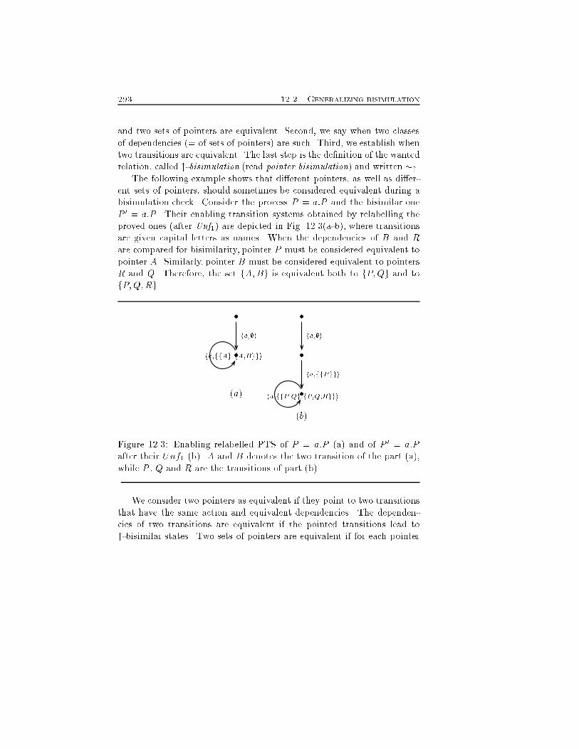
293 12.2. Generalizing bisimulationand two sets of pointers are equivalent. Second, we say when two classesof dependencies (= of sets of pointers) are such. Third, we establish whentwo transitions are equivalent. The last step is the de�nition of the wantedrelation, called "-bisimulation (read pointer bisimulation) and written �".The following example shows that di�erent pointers, as well as di�er-ent sets of pointers, should sometimes be considered equivalent during abisimulation check. Consider the process P = a:P and the bisimilar oneP 0 = a:P . Their enabling transition systems obtained by relabelling theproved ones (after Unf1) are depicted in Fig. 12.3(a-b), where transitionsare given capital letters as names. When the dependencies of B and Rare compared for bisimilarity, pointer P must be considered equivalent topointer A. Similarly, pointer B must be considered equivalent to pointersR and Q. Therefore, the set fA;Bg is equivalent both to fP;Qg and tofP;Q;Rg. � �� �(a) �(b)ha;;iha;ffAg;fA;Bggi ha;;iha;ffPggiha;ffP;Qg;fP;Q;RggiFigure 12.3: Enabling relabelled PTS of P = a:P (a) and of P 0 = a:Pafter their Unf1 (b). A and B denotes the two transition of the part (a),while P , Q and R are the transitions of part (b).We consider two pointers as equivalent if they point to two transitionsthat have the same action and equivalent dependencies. The dependen-cies of two transitions are equivalent if the pointed transitions lead to"-bisimilar states. Two sets of pointers are equivalent if for each pointer

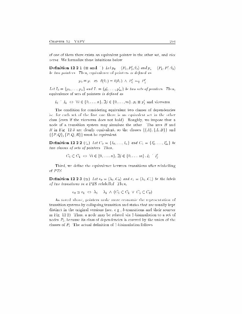
Chapter 12. YAPV 294of one of them there exists an equivalent pointer in the other set, and viceversa. We formalize these intuitions below.De�nition 12.2.1 (� and :=) Let p0 = hP0; P 00; �0i and p1 = hP1; P 01; �1ibe two pointers. Then, equivalence of pointers is de�ned asp0 � p1 , `(�0) = `(�1) ^ P 00 �" P 01Let I0 = fp0; : : : ; png and I1 = fp00; : : : ; p0mg be two sets of pointers. Then,equivalence of sets of pointers is de�ned asI0 := I1 , 8i 2 f0; : : : ; ng; 9j 2 f0; : : : ;mg : pi � p0j and viceversaThe condition for considering equivalent two classes of dependenciesis: for each set of the �rst one there is an equivalent set in the otherclass (even if the viceversa does not hold). Roughly, we impose that anode of a transition system may simulate the other. The arcs B andR in Fig. 12.3 are clearly equivalent, so the classes ffAg; fA;Bgg andffP;Qg; fP;Q;Rggmust be equivalent.De�nition 12.2.2 (�) Let C0 = fI0; : : : ; Ing and C1 = fI 00; : : : ; I 0mg betwo classes of sets of pointers. Then,C0 � C1 , 8i 2 f0; : : : ; ng; 9j 2 f0; : : : ;mg : Ii := I 0jThird, we de�ne the equivalence between transitions after relabellingof PTS.De�nition 12.2.3 (') Let e0 = h�0; C0i and e1 = h�1; C1i be the labelsof two transitions in a PTS relabelled. Then,e0 ' e1 , �0 = �1 ^ (C0 � C1 _ C1 � C0)As noted above, pointers make more economic the representation oftransition systems by collapsing transition and states that are usually keptdistinct in the original versions (see, e.g., b-transitions and their sourcesin Fig. 12.2). Thus, a node may be related via "-bisimulation to a set ofnodes Pi, because its class of dependencies is covered by the union of theclasses of Pi. The actual de�nition of "-bisimulation follows.

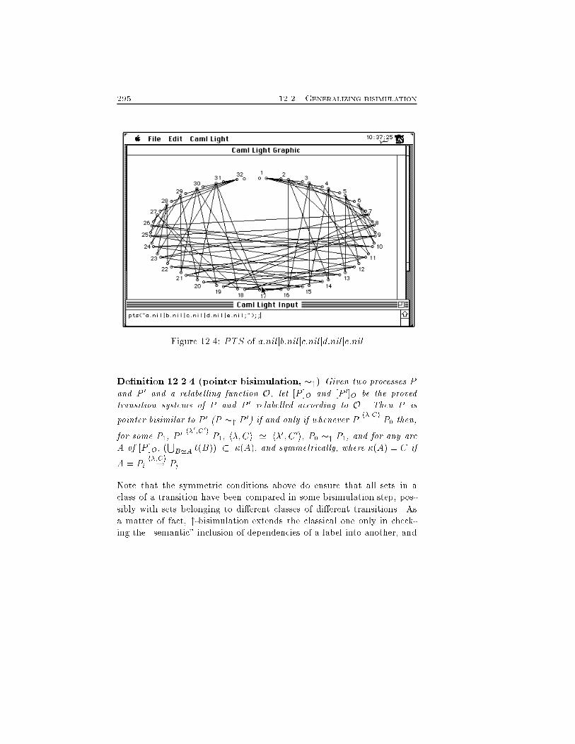
295 12.2. Generalizing bisimulationFigure 12.4: PTS of a:niljb:niljc:niljd:nilje:nilDe�nition 12.2.4 (pointer bisimulation, �") Given two processes Pand P 0 and a relabelling function O, let [P ]O and [P 0]O be the provedtransition systems of P and P 0 relabelled according to O. Then P ispointer bisimilar to P 0 (P �" P 0) if and only if whenever P h�;Ci�! P0 then,for some P1, P 0 h�0;C0i�! P1, h�;Ci ' h�0; C 0i, P0 �" P1, and for any arcA of [P ]O, (SB'A `(B)) � �(A), and symmetrically, where �(A) = C ifA = Pi h�;Ci�! Pj.Note that the symmetric conditions above do ensure that all sets in aclass of a transition have been compared in some bisimulation step, pos-sibly with sets belonging to di�erent classes of di�erent transitions. Asa matter of fact, "-bisimulation extends the classical one only in check-ing the \semantic" inclusion of dependencies of a label into another, and

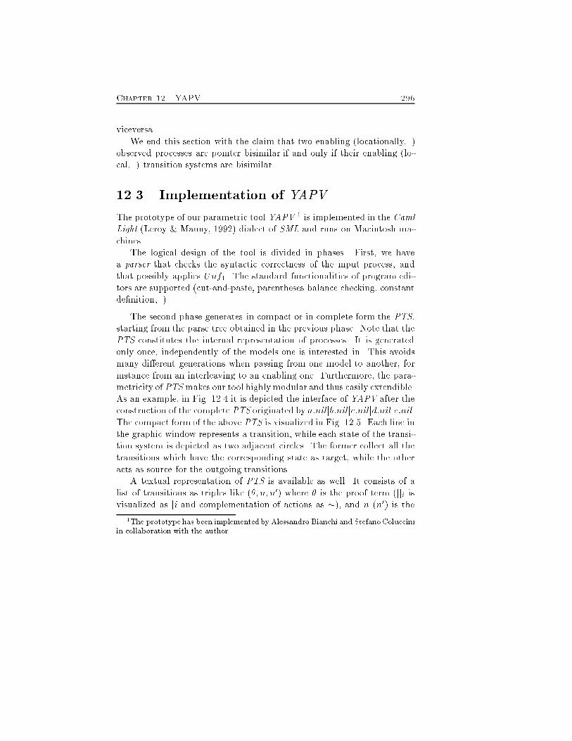
Chapter 12. YAPV 296viceversa.We end this section with the claim that two enabling (locationally,..)observed processes are pointer bisimilar if and only if their enabling (lo-cal,..) transition systems are bisimilar.12.3 Implementation of YAPVThe prototype of our parametric tool YAPV 1 is implemented in the CamlLight (Leroy & Mauny, 1992) dialect of SML and runs on Macintosh ma-chines.The logical design of the tool is divided in phases. First, we havea parser that checks the syntactic correctness of the input process, andthat possibly applies Unf1. The standard functionalities of program edi-tors are supported (cut-and-paste, parentheses balance checking, constantde�nition,..).The second phase generates in compact or in complete form the PTS,starting from the parse tree obtained in the previous phase. Note that thePTS constitutes the internal representation of processes. It is generatedonly once, independently of the models one is interested in. This avoidsmany di�erent generations when passing from one model to another, forinstance from an interleaving to an enabling one. Furthermore, the para-metricity of PTSmakes our tool highlymodular and thus easily extendible.As an example, in Fig. 12.4 it is depicted the interface of YAPV after theconstruction of the complete PTS originated by a:niljb:niljc:niljd:nilje:nil.The compact form of the above PTS is visualized in Fig. 12.5. Each line inthe graphic window represents a transition, while each state of the transi-tion system is depicted as two adjacent circles. The former collect all thetransitions which have the corresponding state as target, while the otheracts as source for the outgoing transitions.A textual representation of PTS is available as well. It consists of alist of transitions as triples like (�; n; n0) where � is the proof term (jji isvisualized as ji and complementation of actions as �), and n (n0) is the1The prototype has been implemented by Alessandro Bianchi and Stefano Colucciniin collaboration with the author.

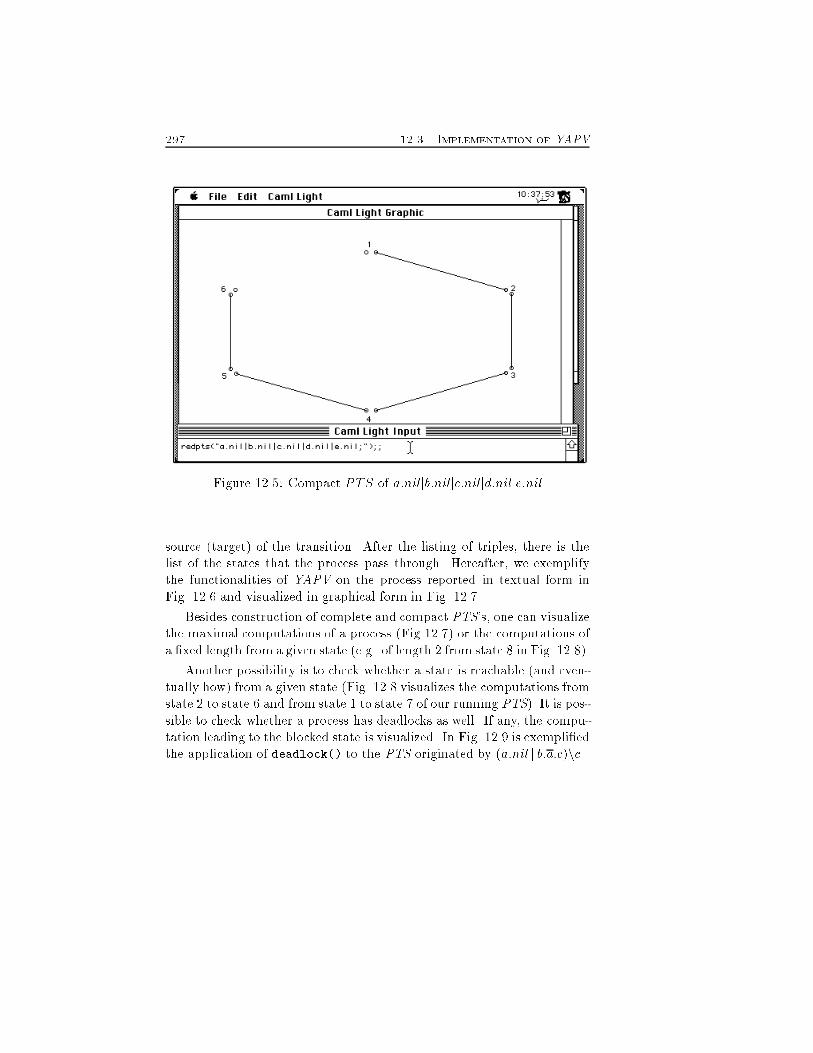
297 12.3. Implementation of YAPVFigure 12.5: Compact PTS of a:niljb:niljc:niljd:nilje:nilsource (target) of the transition. After the listing of triples, there is thelist of the states that the process pass through. Hereafter, we exemplifythe functionalities of YAPV on the process reported in textual form inFig. 12.6 and visualized in graphical form in Fig. 12.7.Besides construction of complete and compact PTS's, one can visualizethe maximal computations of a process (Fig 12.7) or the computations ofa �xed length from a given state (e.g. of length 2 from state 8 in Fig. 12.8).Another possibility is to check whether a state is reachable (and even-tually how) from a given state (Fig. 12.8 visualizes the computations fromstate 2 to state 6 and from state 1 to state 7 of our running PTS). It is pos-sible to check whether a process has deadlocks as well. If any, the compu-tation leading to the blocked state is visualized. In Fig. 12.9 is exempli�edthe application of deadlock() to the PTS originated by (a:nil j b:a:c)nc.

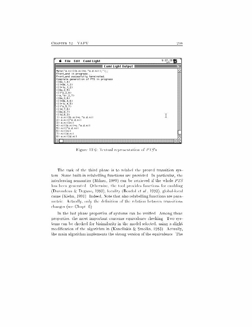
Chapter 12. YAPV 298Figure 12.6: Textual representation of PTS's.The task of the third phase is to relabel the proved transition sys-tem. Some built-in relabelling functions are provided. In particular, theinterleaving semantics (Milner, 1989) can be retrieved if the whole PTShas been generated. Otherwise, the tool provides functions for enabling(Darondeau & Degano, 1989), locality (Boudol et al., 1992), global-localcause (Kiehn, 1991). Indeed, Note that also relabelling functions are para-metric. Actually, only the de�nition of the relation between transitionschanges (see Chapt. 6).In the last phase properties of systems can be veri�ed. Among theseproperties, the most important concerns equivalence checking. Two sys-tems can be checked for bisimilarity in the model selected, using a slightmodi�cation of the algorithm in (Kanellakis & Smolka, 1983). Actually,the main algorithm implements the strong version of the equivalence. The

299 12.3. Implementation of YAPVFigure 12.7: Maximal computations.weak bisimulation which abstracts from internal moves may be obtainedby � -saturation. In Fig. 12.10 is shown the application of the bisimulationin the interleaving model, while Fig. 12.11 shows the bisimulation checkin a causal model.We now give some rough information on the storing space and the timeperformance of our implementation. Consider a process P made up of noccurrences of actions (note that Unf1(P ) may have 2�O(n) occurrencesof actions). Its compact representation has in average O(n) transitionsand O(n) states. States are internally represented as numbers, and arcsas tuples hunique name, source state, target state, labeli. Since each archas at most n � 1 pointers, the class of dependencies of P is encoded byat most O(n) integers. We have only few experimental data on the actualspace needed by our prototype for storing processes. A very preliminary

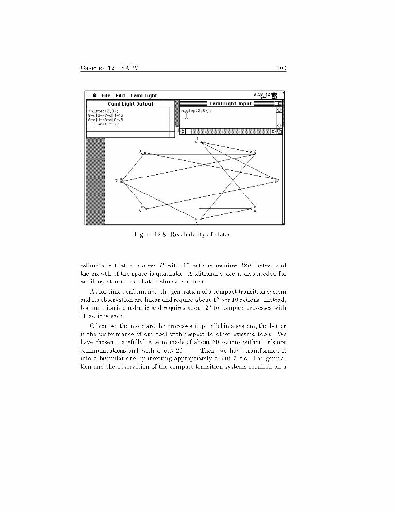
Chapter 12. YAPV 300Figure 12.8: Reachability of states.estimate is that a process P with 10 actions requires 32K bytes, andthe growth of the space is quadratic. Additional space is also needed forauxiliary structures, that is almost constant.As for time performance, the generation of a compact transition systemand its observation are linear and require about 100 per 10 actions. Instead,bisimulation is quadratic and requires about 200 to compare processes with10 actions each.Of course, the more are the processes in parallel in a system, the betteris the performance of our tool with respect to other existing tools. Wehave chosen \carefully" a term made of about 30 actions without � 's norcommunications and with about 20 \j". Then, we have transformed itinto a bisimilar one by inserting appropriately about 7 � 's. The genera-tion and the observation of the compact transition systems required on a

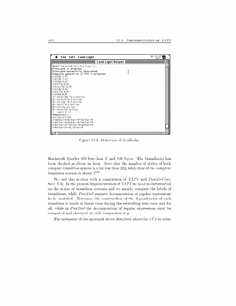
301 12.3. Implementation of YAPVFigure 12.9: Detection of deadlocks.Macintosh Quadra 950 less than 40 and 8M bytes. The bisimilarity hasbeen checked in about an hour. Note that the number of states of bothcompact transition system is a bit less than 200, while that of the completetransition system is about 2200.We end this section with a comparison of YAPV and PisaTool (seeSect. 9.3). In the present implementation ofYAPV we need no informationon the states of transition systems and we simply compare the labels oftransitions, while PisaTool requires decomposition of regular expressionsto be matched. Moreover, the construction of the dependencies of eachtransition is made in linear time during the relabelling step once and forall, while in PisaTool the decomposition of regular expressions must becomputed and observed at each comparison step.The extension of the approach above described above for CCS to other

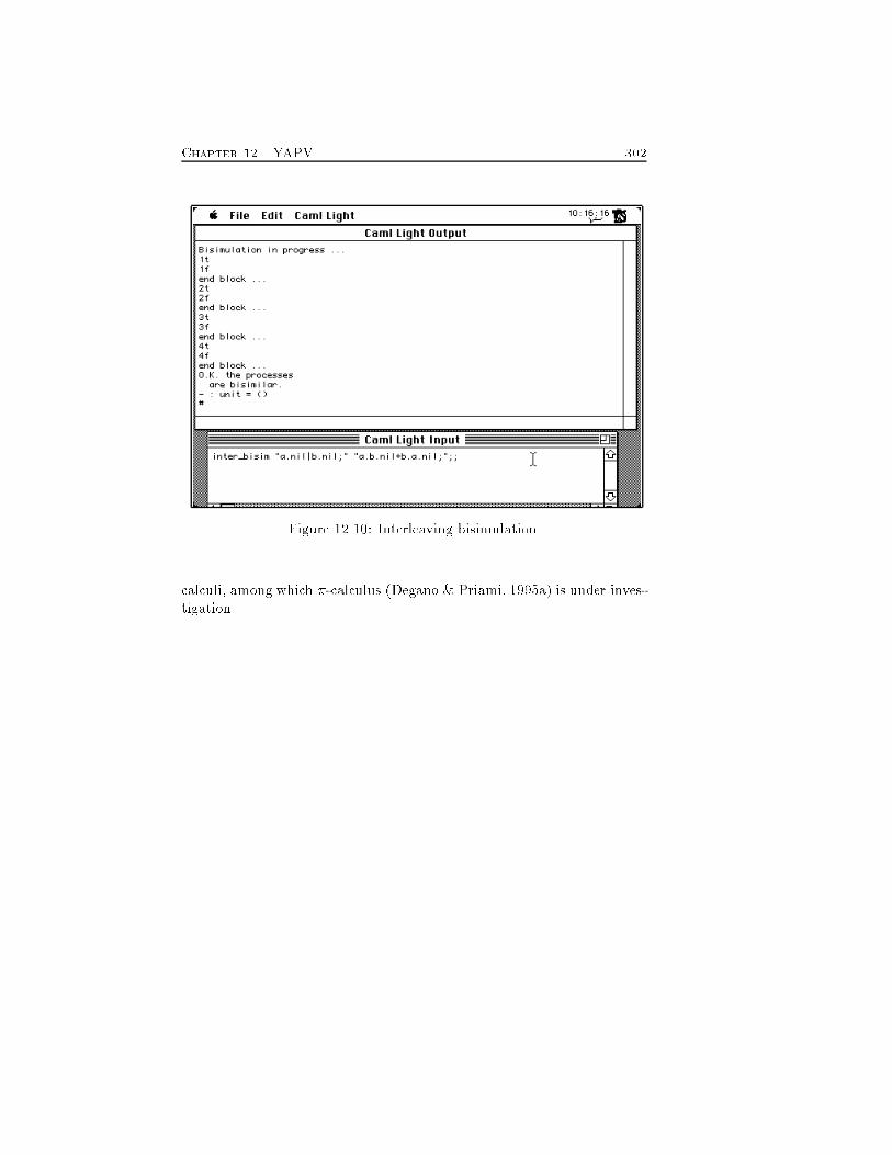
Chapter 12. YAPV 302Figure 12.10: Interleaving bisimulation.calculi, among which �-calculus (Degano & Priami, 1995a) is under inves-tigation.

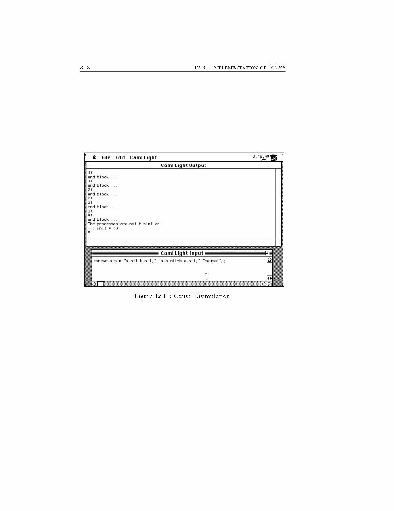
303 12.3. Implementation of YAPV

Figure 12.11: Causal bisimulation.

Chapter 12. YAPV 304

Part IVTowardsImplementations305

Chapter 13Stochastic �-calculusWe extend �-calculus to cope with performance modelling. The new lan-guage is called stochastic �-calculus (S�). We obtain a more expressivelanguage than classical stochastic process algebras because S� allows oneto describe dynamically recon�gurable or mobile networks. The semanticsof S� is given in SOS style. In order to e�ectively compute performancemeasures, we use the strati�ed transition system that is �nitely branch-ing introduced in Sect. 5.3. We give a transition rule to directly yield acontinuous time Markov chain from an S� speci�cation, with no transi-tion system manipulation. Finally, semantic descriptions are enriched toencode topology information. Hence, performance measures are derivedaccording to a given architecture.13.1 The stochastic extensionWe de�ne the syntax of stochastic �-calculus (S� for short), and we reportits informal and structural operational semantics. We annotate pre�xesof �-calculus with an exponential distribution represented by its uniqueparameter, as usual. Thus, the atomic components of processes are pairs(�; r), where � is the action and r is its rate. We let r range over IR+because we consider here only active activities. Passive and immediate307

Chapter 13. Stochastic �-calculus 308activities are dealt with in the last section. Note that the same actionmay exhibit di�erent rates.De�nition 13.1.1 Let r 2 IR+. Processes of stochastic �-calculus arebuilt according to Def. 4.1.1, where (�; r):P replaces �:P .Notation, conventions on names, variants of transitions and the structuralcongruence introduced for �-calculus are extended to S� in the obviousway.In the next subsection we give the informal semantics of S�. We alsodiscuss how to extract probability information from an S� speci�cationand how to de�ne the rate of a synchronization starting from the rates ofits components. To carry out the above programme we need the notion ofapparent rate of transitions (i.e., the rate which is captured by an externalobserver of the system) which may di�er from the actual rate. As a con-sequence, we must keep track of the multiplicity of activities between twostates. Finally, we introduce a notion of parametricity for the representa-tion of processes based on rich labels of transitions. A simple relabellingretrieves many semantic models presented in the literature.For the sake of presentation, we then de�ne the SOS semantics byextending the standard early proved semantics of �-calculus, and by as-suming implicitly that it is turned into a �nite branching transition systemby the de�nitions in Sect. 5.3.13.1.1 Informal semanticsThe activity described by a pre�x (�; r) waits for a delay �t taken from theexponential distribution r before its actual completion. In other words,�t is the time needed to complete the activity. The duration (or delay)of an activity is modelled by a random variable which is exponentiallydistributed. According to (Hillston, 1994a), activities always need someimplicit resource. Thus, the time elapsed before activity completion rep-resents the use of this resource.Summation models two processes which are competing for the sameimplicit resource. The process Q+R denotes a system which may behave

309 13.1. The stochastic extensioneither as Q or R. The �rst action completed determines the componentselected and the other is discarded. The di�erence with the same operatorof classical process algebras is that the selection mechanism is probabilisticrather than nondeterministic (see below the race condition).The process QjR either can execute asynchronous activities in Q orR or can perform invisible transitions when the two components com-municate. The rate of a communication re ects the one of the slowerparticipant. Note that we use a parallel composition in the CCS-likestyle rather than a CSP -like one, as done by almost all existing stochasticprocess algebras.The dynamic behaviour of processes is driven by a race condition. Allactivities enabled attempt to proceed, but only the fastest one succeeds.The fastest activity is di�erent on successive attempts because durationsare random variables. The continuity of the probabilistic distribution en-sures that the probability of two activities ending simultaneously is zero.Furthermore, exponential distributions enjoy the memoryless property.Roughly speaking, the time at which a transition occurs is independent ofthe time at which the last transition occurred. Thus, the elapsed time ofan activity in a state in which another one is the fastest is useless.Probabilities and rates of transitionsIn this subsection we assume that each activity has multiplicity one. Wealways ensure this condition with suitable labels (see Sect. 13.1.1). We alsoassume that transition systems are �nite branching. This is not the case ifP can perform a free input or a bound output because rules Ein and Opengenerate an in�nite branching (for �niteness conditions see Sect. 5.3).The race condition originates probabilistic choices. In fact, the prob-ability of a transition P (�;r)�! P 0 is the ratio between its rate and the exitrate of P , i.e., the sum of the rates of all activities enabled in Pr(P ) = XP (�j ;rj)�! Pj2Ts(P ) rjwhere Ts(P ) is the set of transitions enabled in P .

Chapter 13. Stochastic �-calculus 310We assume that synchronizations are equipped with their own rates(see below for their computation) in the following proposition.Proposition 13.1.2 Let P (�i;ri)�! Pi 2 Ts(P ). Then, the occurrenceprobability of P (�i;ri)�! Pi is ri=r(P ).For example, the probability that process (a; 3) + (b; 4) completes ac-tivity a is 3=7.To compute r(P ), we need the rate of synchronizations. First, we recallsome notions from (Hillston, 1994a), and we adapt them to our framework.The apparent rate ra(P ) of an action a in a given process P is the sumof the rates of all activities with action a that are enabled in Pra(P ) = XP (a;rj )�! Pj2Ts(P ) rjNote that ra(P ) coincides with the actual rate r of P (a;r)�! P 0, if it is theonly a-activity enabled in P . For instance, the apparent rate of action ain process (a; 3)+ (a; 4) is 7. Since the apparent rate of a synchronizationbetween two activities (a; r0) in P and (a; r1) in Q must re ect the one ofthe slower participant, we de�ne it asmin(ra(P ); ra(Q))Apparent rate allows us to compute conditional probabilities, as well.In fact, the probability of a transition P (a;r)�! P 0, given that an action aoccurs, is the ratio between its rate and the apparent rate of action a.Under the same assumptions of Proposition 13.1.2, we have the following.Proposition 13.1.3 Let P (a;ri)�! Pi 2 Ts(P ). Then, given that an actiona occurs, the conditional occurrence probability of P (a;ri)�! Pi is ri=ra(P ).For example, the probability of transition(a; 3) j (a; 2) + (b; 1) (a;3)�! 0 j (a; 2) + (b; 1);

311 13.1. The stochastic extensiongiven that an a occurs, is 3=5.Propositions 13.1.2 and 13.1.3 allow us to relate the rate of a transitionwith its occurrence probability and the apparent rate of its action.Corollary 13.1.4 Let P (a;ri)�! Pi 2 Ts(P ) and let p be its occurrenceprobability. Then, ri = p� ra(P ).The above corollary suggests us how to compute the rate of synchro-nizations. We obtain the rate by multiplying their occurrence probabilityand apparent rate.As usual, assume that parallel processes independently decide whichactions �re. Therefore, if P �res (a; r0) and Q �res (a; r1) in P jQ, theprobability that the two activities originate a communication isr0=ra(P ) � r1=ra(Q):Finally, the rate of synchronizations isR(P; a;Q; a; r0; r1) = r0=ra(P ) � r1=ra(Q)� (13.1)min(ra(P ); ra(Q))If there is a single a-activity enabled in P and a single a-activity enabledin Q, the right-hand side of the above equation is reduced to min(r0; r1).Instead of equation (13.1), any function f can be used, provided thatit is commutative to ensure compositionality (see (Hillston, 1994b)).Multiple instances of the same activityThe rate of an activity may di�er from the one captured by an externalobserver of the system. The observer only sees the action made availableby the system and registers its frequency, thus yielding its apparent rate.If transitions are only labelled by activities, processes (a; r)+(a; r) and(a; r) generate the same transition system. But the two are not equivalentwhen performance is analyzed. The �rst process shows an a at doublespeed than the second one. In fact, the apparent rate of the �rst processis 2r, while that of the other is r.

Chapter 13. Stochastic �-calculus 312Processes as those above are distinguished in PEPA with the intro-duction of multisets and multitransition systems. We prefer to use tags inthe style of proved transition systems to keep distinct transitions with thesame action between the same two states as in TIPP (G�otz et al., 1992)and MPA (Bernardo et al., 1994). We also record here each application ofrules Sum with tags +0 and +1 in the labels of transitions, during theirderivation. According to this convention, the �rst of the two processesabove originates two transitions that lead to the same state 0 and thatare labelled +0(a; r) and +1(a; r). Instead the second process originates asingle transition that leads to 0 and that is labelled (a; r). This approachis also used in (Hermanns & Rettelbach, 1994).13.1.2 Structural operational semanticsWe de�ne a semantics which satis�es all requirements of the previoussubsection.Labels of transitions are proof terms with actions enriched with rates.We also de�ne an auxiliary function { to extract rates from proof terms asfollows {(#(�; r)) = r and {((#hjj0#0�0; jj1#1�1i; r)) = r.The early proved transition system of S� is generated by the SOSrules in Tab. 13.1. The rate of communications (rules Com0 and Close0)is de�ned according to equation (13.1) in the previous subsection. Thesymmetric version of rules Com0 and Close0 are not reported, but theyshould be obvious.13.2 Performance measuresWe show how to turn an S� process into a CTMC. Since we have a �nitebranching semantics, Theorem 13.2.1 is a straightforward adaptation of acorresponding statement given for PEPA in (Hillston, 1994a). Its prooffollows the same pattern as well.Theorem 13.2.1 Let P be a �nite control S� process and let d(P ) =fPi jP s7�!� Pig be the set of all derivatives of P . Then, the stochasticprocess fX(t); t � 0g where X(ti) = Pj means that process P at time ti

313 13.2. Performance measuresbehaves as process Pj, is a continuous time Markov chain with state spaced(P ) and with stationary transition probabilities.We now de�ne the one-step transition probability at the level of tran-sition system. Recall that the transitions enabled in a process cannot bedisabled by ow of time. Hence, the CTMC associated with S� processesare homogeneous in time. Therefore, the one-step transition probabilityfrom Pi to Pj is the exit rate of Pi given that state Pj is reached. Moreformally, we have the following proposition.Proposition 13.2.2 Let TSfb(P ) = hP;�; 7�!; P i be the �nite statetransition system originated by P . Let Pi; Pj states of TSfb(P ) and letn be the number of states reachable from P . Then, the transition matrixof the CTMC associated to TSfb(P ) is a square matrix n � n Pij whoseelements pij are de�ned aspij = XPi �n7�!Pj2Ts(Pi) {(�n)= XPi �l7�!Pl2Ts(Pi) {(�l) (13.2)Note that the second summation in equation (13.2) coincides with r(Pi).Since equation (13.2) de�nes the one-step transition probability fromPi to Pj in terms of the transitions of Pi, and since our semantics is�nite branching, we can de�ne in SOS style the CTMC associated witha system. More precisely, we de�ne a strati�ed transition system whosetransition relation �!M is de�ned in terms of 7�!. We let the CTMC ofan S� process Pi (written CTMC(Pi)) be the minimal transition graphde�ned by rule CTMC : Pi �7�! PjPi pij�!M Pjwhere pij is de�ned according to equation (13.2).Performance analysis of process P can be performed on the transitionmatrix Pij of CTMC(P ). Since performance measures concern systemson long-run term, they are usually derived by using the equilibrium orstationary probability distribution of Markov chains (see Sect. 2.8).

Chapter 13. Stochastic �-calculus 314Following (Hillston, 1994a), we give a necessary condition for S� pro-cesses to originate Markov chains with stationary distributions. Since thechains we consider have a �nite state space, we are left to identify transi-tion systems that guarantee the irreducibility of the corresponding Markovchains. If we call cyclic a state of a transition system that can be reachedby any of its derivatives through a �nite sequence of transitions, we havethe following theorem.Theorem 13.2.3 Let hP;�; 7�!; P i be a transition system with P cyclic.Then, CTMC(P ) is irreducible.In order to get performance measures associated to process P , we as-sociate a reward to each action a and we denote it as �a, according to(Howard, 1971; Hillston, 1994a). Then, the reward of process P is thesum of the rewards of the actions it enables. The total reward of a com-ponent P is computed on the basis of an equilibrium distribution � asR(P ) = XP �i7�!Pi2Ts(P ) �`(�i)�(Pi)In the next section we report an example of performance evaluation.13.3 An exampleConsider a distributed system (Sys) made up of two resources (R1 and R2)each one specialized to perform an operation (op1 and op2, respectively).A user of the system (Q) performs operations of both kinds, but it doesnot know which resource to contact. Therefore, there is another node Dwhich waits for questions from the user and provides it with the link toaccess the right resource. Sometimes Sys may fail due to bad addressingof resources. Its speci�cation in S� is below.Q = hx 1; r1i:had(ch); r2i:hch1; r3i:Qe+hx2; r4i:had(ch); r5i:hch 2; r6i:QeQe = hok; r7i:Q+ hfail; r8i:Q

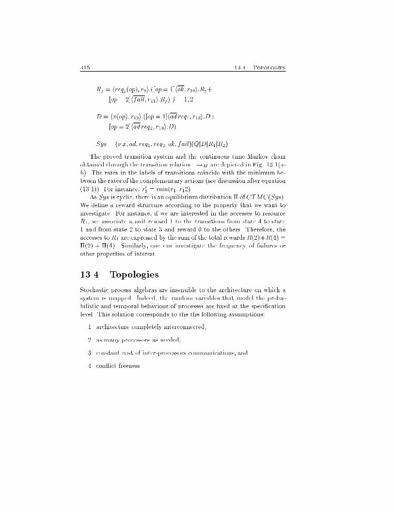
315 13.4. TopologiesRj = hreqj(op); r9i:([op = 1]hok; r10i:Rj+[op = 2]hfail; r11i:Rj) j = 1; 2D = hx(op); r12i:([op = 1]hadreq1; r13i:D+[op = 2]hadreq2; r14i:D)Sys = (� x; ad; req1; req2; ok; fail)(QjDjR1jR2)The proved transition system and the continuous time Markov chainobtained through the transition relation �!M are depicted in Fig. 13.1(a-b). The rates in the labels of transitions coincide with the minimum be-tween the rates of the complementary actions (see discussion after equation(13.1)). For instance, r01 = min(r1; r12).As Sys is cyclic, there is an equilibrium distribution � ofCTMC(Sys).We de�ne a reward structure according to the property that we want toinvestigate. For instance, if we are interested in the accesses to resourceR1, we associate a unit reward 1 to the transitions from state 4 to state1 and from state 2 to state 3 and reward 0 to the others. Therefore, theaccesses to R1 are expressed by the sum of the total rewards R(2)+R(4) =�(2) + �(4). Similarly, one can investigate the frequency of failures orother properties of interest.13.4 TopologiesStochastic process algebras are insensible to the architecture on which asystem is mapped. Indeed, the random variables that model the proba-bilistic and temporal behaviour of processes are �xed at the speci�cationlevel. This solution corresponds to the the following assumptions:1. architecture completely interconnected,2. as many processors as needed,3. constant cost of inter-processors communications, and4. con ict freeness.

Chapter 13. Stochastic �-calculus 3161 12 5 2 53 6 3 64 7 4 7(a) (b)�1�2�3 �4 �5�6�7 �8�9 �10 r01r02r03 r04 r05r06r07+r09 r08+r010�1 = (jj0jj0hjj0 +0 x 1; jj1x1i; r01)�2 = (jj0jj0hjj0ad(req1); jj1+0 ad(req1)i; r02)�3 = (jj0hjj0jj0ch1; ch1i; r03)�4 = (jj0jj0hjj0 +1 x 2; jj1x2i; r04)�5 = (jj0jj0hjj0ad(req2); jj1+1 ad(req2)i; r05)�6 = (hjj0jj0jj0ch(2); jj1ch 2i; r06)�7 = (jj0hjj0jj0 +0 ok;+0oki; r07)�8 = (hjj0jj0jj0 +0 ok; jj1+0 oki; r08)�9 = (jj0hjj0jj0 +1 fail;+1faili; r09)�10 = (hjj0jj0jj0 +0 fail; jj1 +1 faili; r010)Figure 13.1: Transition system (a) and CTMC (b) of Sys.

317 13.4. TopologiesAssumption 2 means that any process of the system at hand may beallocated on a di�erent processor. Assumption 4 means that any processmay access shared resources as soon as it need with no delay.The above assumptions limit the quality of the performance measureand the comparison of these measures with respect to di�erent allocations.In this section we release the above assumptions by slightly modifying theSOS semantics of S�.In order to have a uniform framework to specify systems and to studythe impact of their allocation on a given architecture, we describe topolo-gies in the same formalism used for the description of systems. Since thebehaviour of processes is described by transition systems in SOS style,we describe topologies by a set of axioms, and we include them in thesemantic description of S�.A topology is a labelled graph whose nodes are the processors of thearchitecture and whose arcs are the available physical links. Labels expressinformation on the communication along the link such as the expectedduration for the transmission of a unitary size datum, the frequency ofcon icts in accessing a given link and so on. We use as labels randomvariables taken from a suitable probabilistic distribution (for simplicity,we assume in this section the exponential distribution).The next step is the allocation of processes on the nodes of the architec-ture. For the sake of simplicity, we assume a static allocation of sequentialcomponents of the system on di�erent nodes (if available). Moreover, weassume that all concurrent sub-processes of a sequential component allo-cated on a node n run on n.The number of sequential components of a system is given by functionSc : P ! IN de�ned by structural induction as followsSc(0) = Sc((�; r):Q) = Sc(Q +Q) =Sc((�x)Q) = Sc([x = y]Q) = 1Sc(Q(y1; : : : ; yn)) = Sc(Q) (13.3)Sc(Q1 jQ2) = Sc(Q1) + Sc(Q2)Note that the number of sequential components can be computed syntac-tically because it depends on the parallel structure of processes.

Chapter 13. Stochastic �-calculus 318A system Q 2 P needs as many virtual nodes as the number of itssequential components Sc(Q). Recall that the parallel structure of pro-cesses is recorded by proof terms on the labels of transitions. Therefore,assuming that the parallel composition is left associative, we can uniquelyidentify the virtual nodes of a process Q as follows (when Sc(Q) � 1)NV = fjj1g [ f(jj0)i�1jj1 j 1 � i < Sc(Q)g[f(jj0)Sc(Q)g (13.4)where (jj0)i stands for the string originated by the concatenation of i jj0's.Consider the processQ = (((Q1 jQ2) jQ3) jQ4) (13.5)with Sc(Qi) = 1, i 2 f1; : : : ; 4g. The virtual nodes of Q are identi�edthrough the strings jj0jj0jj0 for Q1, jj0jj0jj1 for Q2, jj0jj1 for Q3, jj1 forQ4. The string associated to Qi corresponds to the proof term of actionsenabled in Qi derived through the rules of S�, once +i constructors areerased.We write NP = f1; : : : ; ng for the physical nodes of an architecture.Then, the mapping is expressed by a function M : NV ! NP such that� jNV j � jNP j ) M is surjective� jNV j � jNP j ) M is injectivewhere jSj denotes the cardinality of set S. The above characterizationimplies that M is bijective if and only if jNV j = jNP j.If a network is not completely interconnected, it is necessary a routing.Consider the topology in Fig. 13.2, and assume that process Q in (13.5)has been mapped onto the topology as followsM(jj1) = 4 M(jj0jj1) = 5M(jj0jj0jj1) = 2 M(jj0jj0jj0) = 1Roughly, Q1 is allocated on node 1, Q2 on 2, Q3 on 5, and Q4 is mappedonto node 4. A communication between Q1 and Q4 needs a routing

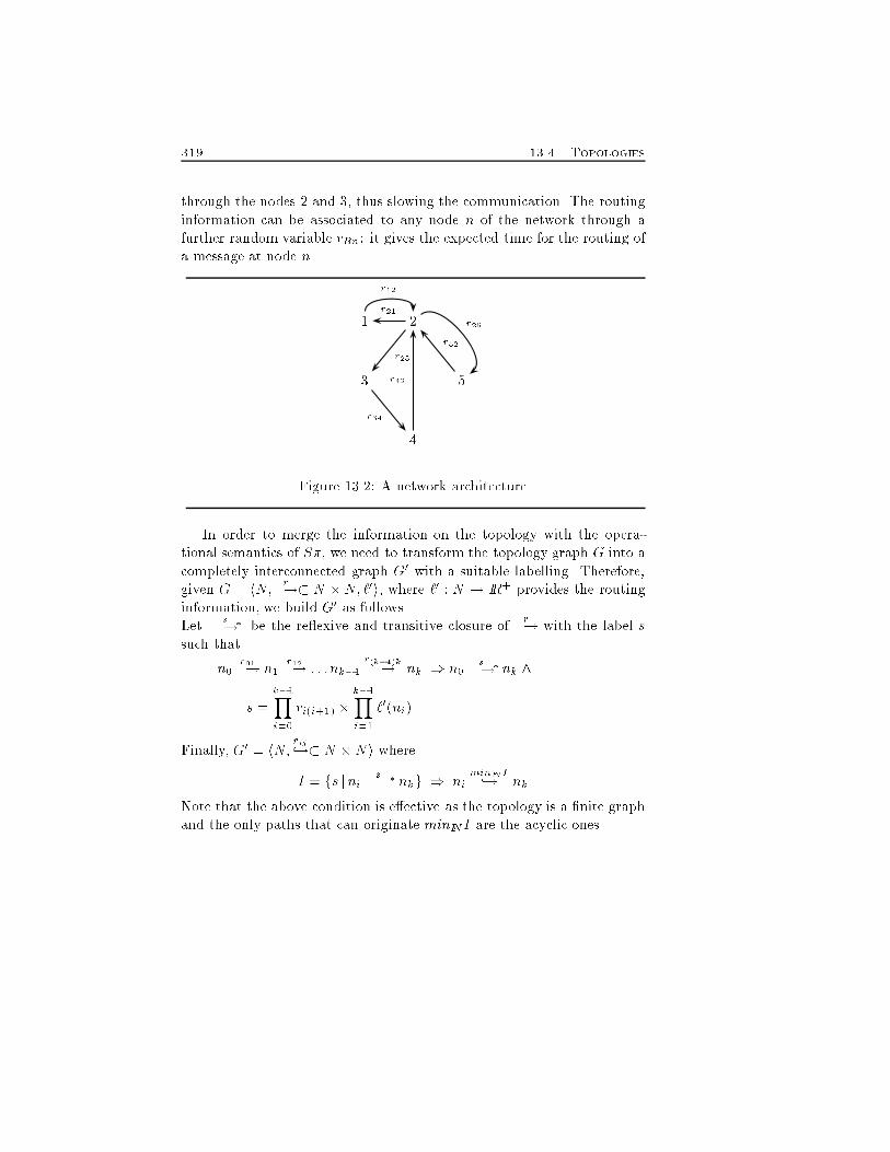
319 13.4. Topologiesthrough the nodes 2 and 3, thus slowing the communication. The routinginformation can be associated to any node n of the network through afurther random variable rRn: it gives the expected time for the routing ofa message at node n. 1 23 54r12r21r23r34 r42 r25r52Figure 13.2: A network architectureIn order to merge the information on the topology with the opera-tional semantics of S�, we need to transform the topology graph G into acompletely interconnected graph G0 with a suitable labelling. Therefore,given G = hN; r�!� N �N; `0i, where `0 : N ! IR+ provides the routinginformation, we build G0 as follows.Let s�!� be the re exive and transitive closure of r�! with the label ssuch thatn0 r01�! n1 r12�! : : :nk�1 r(k�1)k�! nk ) n0 s�!� nk ^s = k�1Yi=0 ri(i+1) � k�1Yi=1 `0(ni)Finally, G0 = hN; rij,!� N � N i whereI = fs jni s�!� nkg ) ni minIN I,! nkNote that the above condition is e�ective as the topology is a �nite graphand the only paths that can originate minINI are the acyclic ones.

Chapter 13. Stochastic �-calculus 320We are left to deal with the case of two communicating processes whichare allocated on the same physical node. For instance, the processes Q1and Q2 of �:(Q1 jQ2).Since we are considering distributed architectures, intra-node commu-nications are much less expensive than inter-node ones. Thus, the ex-pected time of intra-node communications must be smaller than that ofinter-node communications. To this purpose, we assume that each node ofthe topology graph has a self-loop labelled with r = 1. This labelling isreminiscent of immediate actions of stochastic process algebras like MPA(Bernardo et al., 1994): the duration of such actions is neglectable withrespect to the duration of the others.All the information we need to take the allocation of processes intoaccount during the performance evaluation is contained in the extendedtopology graph. The only change to the operational semantics of S� isthe substitution of the rules for communications with those in Tab. 13.2.There we use an auxiliary function ? to determine the node on which areallocated the partners of the communication. In order to de�ne ? we needto erase +i tags from proof terms as node identi�ers are strings over thealphabet fjj0; jj1g. To this purpose we use the function F+ de�ned asF+(+i#) = F+(#) F+(jji#) = jjiF+(#):Now we de�ne ?(#) =M(#0)where #0 is the longest pre�x of F+(#) such that #0 ,!, i.e., #0 is a nodeidenti�er of the considered topology. Note that such a #0 always existsdue to the way in which proof terms are built. In fact, the proof termidentifying a sequential component (a node identi�er) is a pre�x of theproof terms of all transitions originated by its sub-components (once +ihave been removed).We only need to modify equation (13.1) which computes the durationof synchronizations to consider the new parameter r. For example, we canchooseR(P; a;Q; a; rp; rq; r) = rp=ra(P )�rq=ra(Q) � min(ra(P ); ra(Q)) � r

321 13.5. Some remarksAssume that processes Q1 and Q4 in (13.5) are de�ned asQ1 = (a; 1=2) + (b; 1=3) j (a; 2=3)and Q4 = (a; 1=3) j (c; 1=4):Furthermore, let rR2 = 2=3; rR3 = 1=2 and r12 = 2; r23 = 2=3; r34 = 3=2.We compute the rate of the synchronization � between the �rst a in Q1and a in Q4 assuming the topology in Fig. 13.2 and the mappingM above.The apparent rate of a in Q1 is 7=6 and the apparent rate of a in Q4 is1=3. Therefore, the apparent rate of the synchronization ismin(7=6; 1=3) =1=3. The occurrence probability of theta is 3=7. Without consideringtopology information, the rate of � would be 1=7.The probability information attached to physical links originates thefactor 1=2 = r12 � r23 � r34. The factor of routing is 1=3 = rR2 � rR3.Finally, the rate of the synchronization considered is 2=21. Note thatthe rate is in uenced by the mapping. In fact, assume that Q4 is allo-cated on node 3. The factor due to topology is changed to 8=63. Thisexample shows that topology information can be used to compare di�erentallocation of processes with respect to e�ciency of synchronizations.13.5 Some remarksTo model passive and immediate activities, we let rate r range over IR+ [f1w jw 2 INg [ f0w jw 2 INg, where w is a weight that discriminatesbetween activities simultaneously enabled. Immediate activities have rate1w and their duration is 0, while passive activities have rate 0w and theirduration is unspeci�ed. Immediate activities are the ones selected �rstbecause they have zero duration, then active activities are considered,and �nally the passive ones. This is formally expressed by the relation1w < q < 0w with q 2 IR+. If there are more than one immediate orpassive activities enabled in the same state, we de�ne their occurrenceprobability according to their weights. We need the following relationsxw1 < xw2 , w1 < w2

Chapter 13. Stochastic �-calculus 322xw1 + xw2 = w1 + w2xw1=xw2 = w1=w2where x 2 f1; 0g. For instance, if n immediate activities (ai;1wi) areenabled in P , the occurrence probability of (aj ;1wj) is wj=(Pi=1::nwi).The occurrence probability of passive actions is computed similarly.The introduction of immediate and passive activities imposes the def-inition of a strati�ed transition system for the semantics of S� to avoidthat transitions with di�erent priority levels exit from the same state.The memoryless property of exponential distributions allows the ac-tivities enabled and not selected to forget their spent lifetime and to starta new one in the state reached (if they are still enabled). Assume thatthe activities suspended will continue from the point in which they werestopped. In this case, the causal and the concurrency relation betweentransitions de�ned in Chapt. 6 might help. Given an S� computation, todetermine the time spent by a transition � one needs to sum the time spentby all its concurrent transitions occurred between its immediate cause and�. Consider the computation P0 �0�! : : : �n�! Pn+1, and assume that the�ring of transition �i from process Pi takes �ti. Moreover, assume thattransition �n is caused by �i and all transitions between �i and �n areconcurrent with �n. This means that �n is enabled for the �rst time inPi+1, it is still enabled in Pj , i + 2 � j < n, and it is �red in Pn. Thus,the lifetime of �n starts in Pi+1 and expires in Pn+1. Finally, the delay of�n is Xj=i+1::n�tj:A solution for dealing with general distributions is presented in (G�otzet al., 1992) as well.

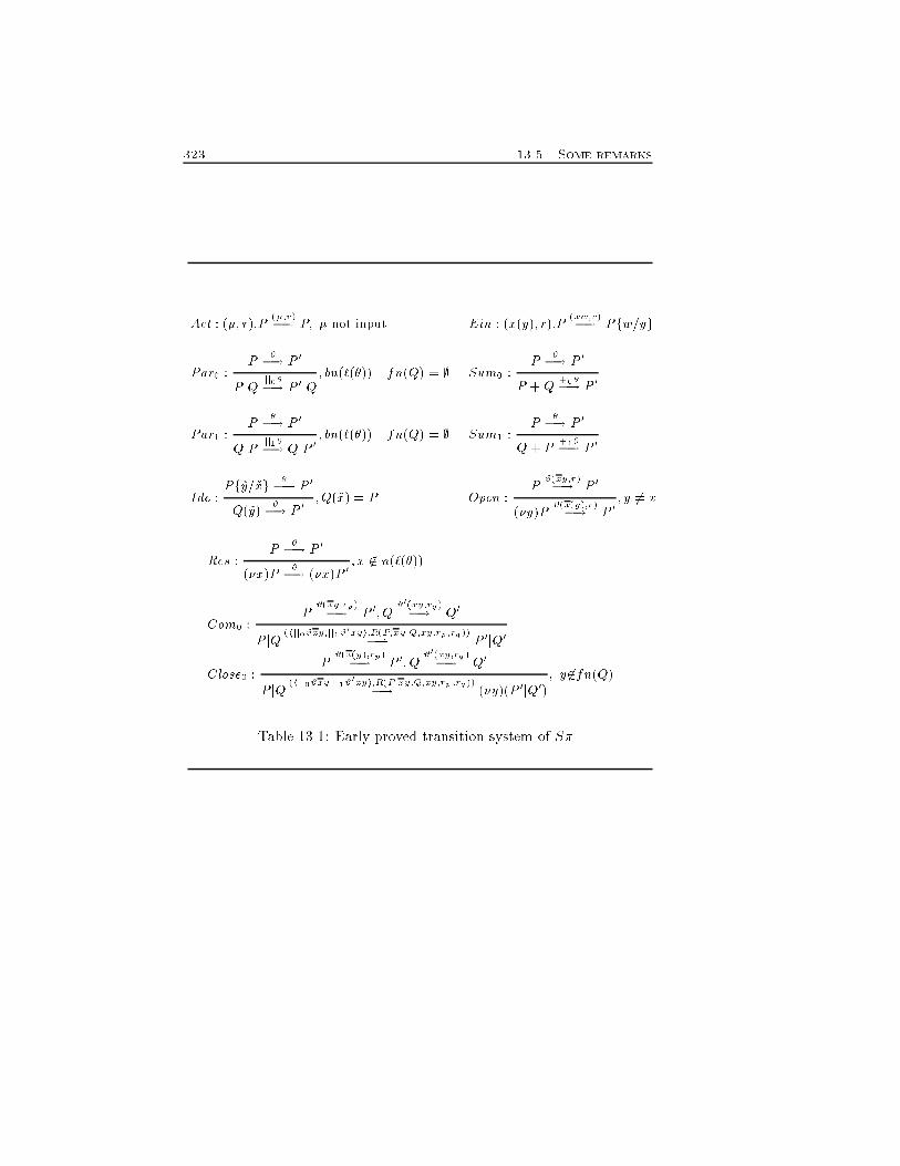
323 13.5. Some remarksAct : (�; r):P (�;r)�! P; � not input Ein : (x(y); r):P (xw;r)�! Pfw=ygPar0 : P ��! P 0P jQ jj0��! P 0jQ; bn(`(�)) \ fn(Q) = ; Sum0 : P ��! P 0P +Q +0��! P 0Par1 : P ��! P 0QjP jj1��! QjP 0 ; bn(`(�)) \ fn(Q) = ; Sum1 : P ��! P 0Q+ P +1��! P 0Ide : Pf~y=~xg ��! P 0Q(~y) ��! P 0 ;Q(~x) = P Open : P #(xy;r)�! P 0(�y)P #(x(y);r)�! P 0 ; y 6= xRes : P ��! P 0(�x)P ��! (�x)P 0 ; x 62 n(`(�))Com0 : P #(xy;rp)�! P 0;Q #0(xy;rq)�! Q0P jQ (hjj0#xy;jj1#0xyi;R(P;xy;Q;xy;rp ;rq))�! P 0jQ0Close0 : P #(x(y);rp)�! P 0;Q #0(xy;rq )�! Q0P jQ (hjj0#xy;jj1#0xyi;R(P;xy;Q;xy;rp ;rq))�! (�y)(P 0jQ0) ; y 62fn(Q)Table 13.1: Early proved transition system of S�.

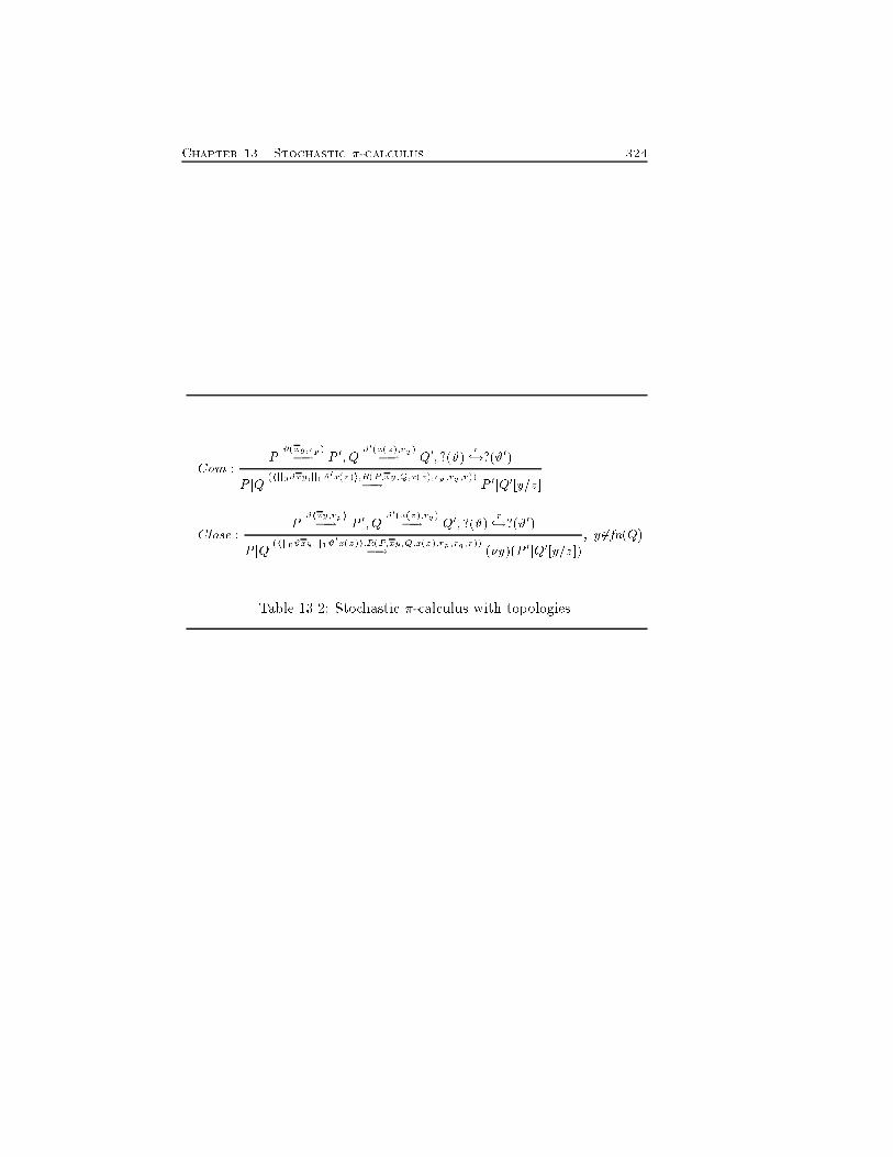
Chapter 13. Stochastic �-calculus 324Com : P #(xy;rp)�! P 0; Q #0(x(z);rq )�! Q0; ?(#) r,!?(#0)P jQ (hjj0#xy;jj1#0x(z)i;R(P;xy;Q;x(z);rp ;rq ;r))�! P 0jQ0[y=z]Close : P #hxy;rpi�! P 0;Q #0(x(z);rq)�! Q0; ?(#) r,!?(#0)P jQ (hjj0#xy;jj1#0x(z)i;R(P;xy;Q;x(z);rp ;rq ;r))�! (�y)(P 0jQ0[y=z]) ; y 62fn(Q)Table 13.2: Stochastic �-calculus with topologies

Chapter 14A Distributed NameManagerWe introduce an SOS semantics of �-calculus in which environment isdistributed. Essentially, each sequential components handles its names lo-cally. Comparison of names is performed through an equivalence relationwhich keep tracks of the relative addresses of the processes which ownthe names to be compared. Extrusions and communications a�ect theenvironments of the involved processes only. The semantic de�nitions arebased on a router factorized out of the semantics. Therefore, it can bere-de�ned to take into account peculiar characteristic of a given intercon-nection topology without a�ecting our operational semantics.14.1 Handling namesConsider for a while the parallel composition as the primary operator of �-calculus, insisting that it is not commutative. Then, build abstract syntaxtrees of processes as binary trees whose nodes are j operators and whoseleaves are the sequential components (notion made precise later) of thewhole process. Call them trees of (sequential) processes (see Fig. 14.1).325

Chapter 14. A Distributed Name Manager 326Assume that their left (right) branches denote the left (right) componentof parallel compositions, and label their arcs as jj0 (jj1). Therefore, anysequential component of a process is uniquely identi�ed by a string overfjj0; jj1g�. The string corresponds to a path from the root, the top-levelj of the whole process, to a leaf. Intuitively, the string is the address ofthe sequential component relative to the root. We will make use of thisinformation to specify a distributed name manager that handles nameslocally to sequential processes. Of course, a distributed environment rulesout the equations that handle restrictions globally, e.g. (� x)(P jQ) �(� x)P jQ if x 62 fn(Q).Although the distinction is not so sharp, in �-calculus names can bedivided in free or bound. Bound names may become free through eitherinput actions or extrusions. When a bound name becomes free, an ex-pensive �-conversion may be needed to avoid captures of free names (see(Milner et al., 1992a) for a detailed discussion).To avoid a global management of fresh names, we have to solve twoproblems. Names have to be generated locally and to be brandly new inthat local environment. Furthermore, when a name is exported to otherlocal environments via communications or extrusions, we must guaranteethat it captures no other free name around.First, we introduce a new indexed set of localized names (for simplic-ity, natural numbers), and we associate a counter with every sequentialprocess. When needed, the �rst name not in use is taken and the counteris increased. If �ring a pre�x originates new sequential processes, thecounter is distributed to them all. Clearly, this mechanism guaranteesthat a newly generated name is unique in its scope and does not captureother names therein.The second problem arises when two di�erent sequential processes, sayG and R, have generated two names syntactically equal, say n, that arealthough semantically distinct. Suppose now that G sends to R its n. Todistinguish between the two di�erent instances of n in the local environ-ment of R, the name generated by G will be enriched with the address ofG relative to R. The relative address can be decomposed into two partsaccording to the minimal common predecessor P of G and R. Hence, a rel-ative address is a string #�#0 2 fjj0; jj1g��fjj0; jj1g�, where # represents the

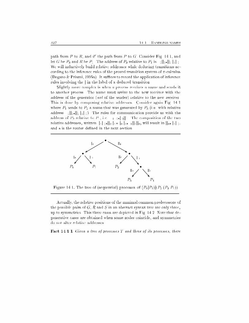
327 14.1. Handling namespath from P to R, and #0 the path from P to G. Consider Fig. 14.1, andlet G be P3 and R be P1. The address of P3 relative to P1 is jj0jj1�jj1jj1jj0.We will inductively build relative addresses while deducing transitions ac-cording to the inference rules of the proved transition system of �-calculus(Degano & Priami, 1995a). It su�ces to record the application of inferencerules involving the j in the label of a deduced transition.Slightly more complex is when a process receives a name and sends itto another process. The name must arrive to the new receiver with theaddress of the generator (not of the sender) relative to the new receiver.This is done by composing relative addresses. Consider again Fig. 14.1where P1 sends to P2 a name that was generated by P3 (i.e. with relativeaddress jj0jj1�jj1jj1jj0). The rules for communication provide us with theaddress of P2 relative to P1, i.e. jj1jj0�jj0jj1. The composition of the tworelative addresses, written jj1jj0�jj0jj1? jj0jj1�jj1jj1jj0, will result in jj0�jj1jj0,and ? is the router de�ned in the next section.�� �P0 P1 P2 �P3 P4jj0 jj1jj0 jj1 jj0 jj1jj0 jj1Figure 14.1: The tree of (sequential) processes of (P0jP1)j(P2j(P3jP4))Actually, the relative positions of the minimal common predecessors ofthe possible pairs of G, R and S in an abstract syntax tree are only three,up to symmetries. This three cases are depicted in Fig. 14.2. Note that de-generative cases are obtained when some nodes coincide, and symmetriesdo not alter relative addresses.Fact 14.1.1 Given a tree of processes T and three of its processes, there

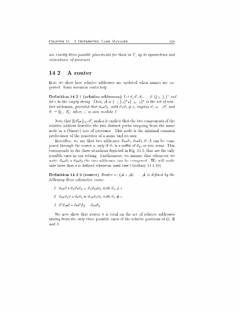
Chapter 14. A Distributed Name Manager 328are exactly three possible placements for them in T , up to symmetries andcoincidence of processes.14.2 A routerHere we show how relative addresses are updated when names are ex-ported. Some notation could help.De�nition 14.2.1 (relative addresses) Let #; #0; #i; : : : 2 fjj0; jj1g� andlet � be the empty string. Then, A = fjj0; jj1g��fjj0; jj1g� is the set of rela-tive addresses, provided that #0�#1, with #0#1 6= �, implies #0 = jji#00 and#1 = jji�1#01, where � is sum modulo 2.Note that jji#00�jji�1#01 makes it explicit that the two components of therelative address describe the two distinct paths outgoing from the samenode in a (binary) tree of processes. This node is the minimal commonpredecessor of the generator of a name and its user.Hereafter, we say that two addresses #0�#1; #2�#3 2 A can be com-posed through the router ?, only if #1 is a su�x of #2, or vice versa. Thiscorresponds to the three situations depicted in Fig. 14.2, that are the onlypossible ones in our setting. Furthermore, we assume that whenever wewrite #0�#1 ? #2�#3 the two addresses can be composed. We will makesure later that ? is de�ned whenever used (see Corollary 14.3.10).De�nition 14.2.2 (router) Router ? : (A � A) �! A is de�ned by thefollowing three exhaustive cases:1. #0�# ? #2#�#3 = #2#0�#3 with #2 6= �2. #0�#1# ? #�#3 = #0�#1#3 with #1 6= �3. #0#0�# ? #�#0#3 = #0�#3We now show that router ? is total on the set of relative addressesarising from the only three possible cases of the relative positions of G, Rand S.

329 14.2. A routerTheorem 14.2.3 Router ? is total on the possible relative addresses aris-ing in our setting.Proof. We prove the statement on the three only possible cases illustrated inFig. 14.2. Let G be the generator of a name, and let S send it to R.Consider tree (1). The name which is exported from S to R in the local envi-ronment of S is enriched with #2#�#3 which is the address of G relative to S.The communication between S and R originates the address of R relative to S,i.e. #0�#. The composition of the two addresses is #0�# ? #2#�#3 that resultsin #2#0�#3, by item 1 of Def. 14.2.2. Note that the case #2 = � originates thedegenerative case in which the root coincides with the common predecessor ofR and S. This originates two further cases: either #3 = #0 (G=R) or #3 = #(G=S). Consider the �rst one. The composition becomes #0�# ? #�#0 = ��� byitem 3 of Def. 14.2.2. (In fact a name generated by G is returned to G itselfand thus there is no pointer to the generator). The second case originates thecomposition #0�# ? #�# = #0�# by item 3 of Def. 14.2.2.The case of tree (2) is similar and is proved by applying item 2 of Def. 14.2.2.Consider tree (3). The name which is exported is enriched with #�#0#3 (theaddress of G relative to S). The address of R relative to S is #0#0�#. Then,#0#0�#?#�#0#3 = #0�#3 by item 3 of Def. 14.2.2. Degenerative cases are handledas done above. 2The above theorem also says that router ? correctly computes theaddress of R relative to G. Pictorially, ? discards the dashed paths in Fig.14.2.We prove below a few properties of ? that will be useful later. Theystate that hA � A; ?i would be a group, if ? were total. This is quite anatural property of routers: given a space of addresses and an intercon-nection topology, a router must always connect two sites in both ways,provided that there is a path between them. The �rst property says that? has a neutral element and an inverse on A � A. Its proof is immediatefrom Def. 14.2.2.Proposition 14.2.4 8#i�#j 2 A we have that1. ��� ? #i�#j = #i�#j ? ��� = #i�#j, i.e. ��� is the neutral element of ?;

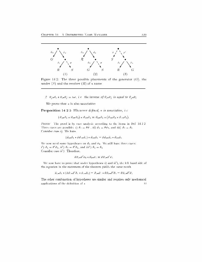
Chapter 14. A Distributed Name Manager 330� � �G � R � S �R S G S R G(1) (2) (3)#3 #2#0 # #0 #1#3 # # #0#0 #3Figure 14.2: The three possible placements of the generator (G), thesender (S) and the receiver (R) of a name.2. #j�#i ? #i�#j = ���, i.e. the inverse of #i�#j is equal to #j�#iWe prove that ? is also associative.Proposition 14.2.5 Whenever de�ned, ? is associative, i.e.(#0�#1 ? #2�#3) ? #4�#5 = #0�#1 ? (#2�#3 ? #4�#5):Proof. The proof is by case analysis according to the items in Def. 14.2.2.Three cases are possible: i) #2 = ##1, ii) #1 = ##2, and iii) #2 = #1.Consider case i). We have(#0�#1 ? ##1�#3) ? #4�#5 = ##0�#3 ? #4�#5We now need some hypotheses on #3 and #4. We still have three cases:i0) #4 = #0#3, ii0) #3 = #0#4, and iii0) #4 = #4.Consider case ii0). Therefore,##0�#0#4 ? #4�#5 = ##0�#0#5. We now have to prove that under hypotheses i) and ii0), the left hand side ofthe equation in the statement of the theorem yields the same result.#0�#1 ? (##1�#0#4 ? #4�#5) = #0�#1 ? ##1�#0#5 = ##0�#0#5The other combination of hypotheses are similar and requires only mechanicalapplications of the de�nition of ?. 2

331 14.3. Operational semanticsIdentity of names is not lost during exportation, because a name alwaysencodes a pointer to its generator. More formally, sending a name froma process S to R, and then sending the same name from R to S is aninvolution. Again, this is mandatory for a router.Proposition 14.2.6 #1�#0 ? (#0�#1 ? #2�#3) = #2�#3.Proof. By applying associativity, inverse and neutral element of ?, we have#1�#0 ? (#0�#1 ? #2�#3) = (#1�#0 ? #0�#1) ? #2�#3 = ��� ? #2�#3 = #2�#3: 214.3 Operational semanticsWe de�ne a late operational semantics of �-calculus that originates andhandles names locally according to the discussion in the previous sections.We start with the set of names.De�nition 14.3.1 (localized names) Let N 0 = AfN [INg be a count-able set of names, ranged over by r; s; u; : : :, with N 0\f�g = ;. We assumethat 8a 2 N : #�#0a �N 0 a.The new syntax of �-calculus is the one in Def. 4.1.1, with r, s and si inplace of x, y and yi. In particular, � can be either r(x) or rs or � .The standard notions on actions (still ranged over by �) and on names(subject, object, free, bound), as well as the structural congruence onprocesses, are extended to the new syntax in the obvious way.Following the ideas of (Degano & Priami, 1992; Degano & Priami,1995a), we encode in the labels of transitions the parallel structure ofprocesses to identify the sequential component that �res the action. Ac-tually, these labels encode a portion of the proof of the transitions, so wecall them proof terms as in (Degano & Priami, 1995a).De�nition 14.3.2 (labels) Labels of transitions (with metavariable �)are de�ned as �@#. The set of proof terms is denoted by �.

Chapter 14. A Distributed Name Manager 332As discussed above, to handle names locally, we enrich processes witha counter implemented as a family of operators n ) in the style of thecausal transition system of (Darondeau & Degano, 1989). The intuitivemeaning of n) P is that P has generated n� 1 new names and the nextone will be n. This extended processes are ranged over by t and we assumeon them the least structural congruence �t that satis�es the followingclauses� n) 0 �t 1) 0� n) (�r)P �t (�r)n) P� n) (P jQ) �t (n) P )j(n) Q)If the axioms are oriented from left to right, we obtain a terminating andcon uent rewriting system. Hereafter, we feel free to consider processesin normal form whenever convenient.We now start considering the problem of sending names. This requiresthe composition via ? of the address of the name itself with the addressof the sender relative to the receiver, as intuitively discussed in Sect. 14.1.We now lift composition of addresses to exportation of names. Recall thata �N 0 ���a.De�nition 14.3.3 (exporting names) Let r = (#r�#0r)n (resp. a) be aname.Name r exported at the relative address #�#0 is #�#0 ? r = (#�#0 ? #r�#0r)n(resp. a).Note that #�#0 is the address of the sender relative to the receiver. Recallthat names also encode a pointer to their generator.The following three auxiliary de�nitions are used in the operationalsemantics. We start with a selector of the sequential components of aprocess t at address #, denoted by t@#. Then, when considering processt, we will write r@# to say that the local environment where r is de�nedis the one of t@#.De�nition 14.3.4 (selector @) Let t@# be the sub-process at depth #de�ned inducing on the syntax as

333 14.3. Operational semantics� t@# = t if # = � or t is either of 0; �:t; t+ t0; (�x)t; [r = s]t; t(y);� (t0jt1)@jji# = ti@#, where i is either 0 or 1.Also, if r 2 n(t) then r@# implies r 2 n(t@#).Now, we introduce an equivalence relation on names. Intuitively, twonames of two sequential processes are equivalent if they coincide whenboth are sent to the same process. For simplicity, we check equivalenceof names by sending them to a common predecessor of the sequentialprocesses.De�nition 14.3.5 (equivalence of names)Given r 2 n(t@#) and s 2 n(t@#0), letr@# ' r@# ' s@#0 ' s@#0 , ��# ? r = ��#0 ? s:Note that ' is an equivalence relation, where re exivity, symmetry andtransitivity come out from the corresponding properties of =. Further-more, two equivalent names must have the same action part because ourrouter does not a�ect actions, but only addresses. The following theoremshows that if two names are equivalent in a node of a tree of processes,then they are equivalent everywhere.Theorem 14.3.6 Let r 2 n(t@#r) and s 2 n(t@#s). Then, r@# ' s@#0i� 8#�#r; #�#s relative addresses, #�#r ?r 2 n(t@#) and #�#s ?s 2 n(t@#)and #�#r ? r = #�#s ? s:Proof. (() Replace # with �.()) Since #�#r and #�#s are relative addresses, # share no pre�x either with #ror with #s. Therefore, #�#r ? r = #�� ? (��#r ? r) = #�� ? (��#s ? s) = #�#s ? s. 2The following theorem suggests us how names may be computed whenthey will be exported in the operational semantics de�nitions. It obviouslyrelies on router ?.Theorem 14.3.7 Given r, r@# ' s@#0 i� s = #0�# ? r.

Chapter 14. A Distributed Name Manager 334Proof. When r = a, trivial. When r = #r�#0rn, from Def. 14.3.5,r@# ' s@#0 , ��# ? r = ��#0 ? s , (��# ? #r�#0r)n = ��#0 ? s ,��# ? #r�#0r = ��#0 ? #s�#0sfor some #s�#0s. We now prove that #s�#0s can be only #0�# ? #r�#0r.First, #0�# ? #r�#0r is a solution of the last equation above because composingit with the relative address ��#0, we have ��#0 ? #0�# ? #r�#0r = ��# ? #r�#0r byassociativity of ? and by item 3 of Def. 14.2.2. The solution is unique, as well.Assume that there is another solution #0�#00 such that ��#0?#r�#0r = ��#0?#0�#00.Then, compose both with the same relative address #0��:#0�� ? (��#0 ? #r�#0r) = #0�� ? (��#0 ? #0�#00) , #r�#0r = #0�#00by Proposition 14.2.6. 2A few auxiliary de�nitions follow. We extend standard substitution ofone name for another so that the new substitution updates the involvednames while descending a tree of processes. In this way the names receivethe right address at every node of the tree.De�nition 14.3.8 (routed substitution) Let f�=�g be the standardsubstitution. Then the routed substitution fj � = � jg is de�ned inducingon the syntax as follows:� 0fju0=ujg = 0� (n) P )fju0=ujg = nfu0=ug ) Pfju0=ujg� (rs:P )fju0=ujg = (rs)fu0=ug:Pfju0=ujg� (r(a):P )fju0=ujg = � rfu0=ug(a):P if a 2 fu; u0g(r(a))fu0=ug:(Pfju0=ujg) otherwise� (P + Q)fju0=ujg = Pfju0=ujg+ Qfju0=ujg� ((� r)P )fju0=ujg = � (� r)P if r 2 fu; u0g(� r)(Pfju0=ujg) otherwise

335 14.3. Operational semantics� P (r)fju0=ujg = Pfju0=ujg(rfu0=ug)� (t0jt1)fjr=sjg = t0fjr0=s0jgjt1fjr1=s1jg where ri@jji ' r and si@jji ' sWe de�ne also tfj=jg@#, that applies the substitution to t@#, as� tfjr=sjg@# = tfjr=sjg if # = � or t has either form 0; �:t; t+ t0; (�x)t;[r = s]t; t(y)� (t0jt1)fjr=sjg@# = � t0fjr=sjg@#0 jt1 if # = jj0#0t0jt1fjr=sjg@#0 if # = jj1#0 if # 6= �Hereafter, in the routed substitutions, and in selectors t@# or r@#, wewill omit @�.Consider for instance(2) xy:w(z):z j 2) x(z):(� x)wx:(x(y) jxz))fj�1=xjgthat yields(2) xy:w(z):zfjjj0�1=xjg) j (2) x(z):(� x)wx:(x(y) jxz)fjjj1�1=xjg) =(2) jj0�1y:w(z):z) j (2) jj1�1(z):[(� x)wx:(x(y) jxz)]fjjj1�1=xjg) =(2) jj0�1y:w(z):z) j (2) jj1�1(z):(� x)wx:(x(y) jxz))Note that name x to be substituted is not enriched with a relative addressby fj � = � jg in the case of parallel composition because #�#0x �N 0 x.Furthermore the substitution takes the binders of names into account cor-rectly. In fact, the distribution of fj�1=xjg stops when the new binder (� x)is encountered. Another example of routed substitution is3) (� x)wx:(x(y) jxjj1�2)fjy=�2jg =3) (� x)wx:(x(y)fjy=jj0�2jg jxjj1�2fjy=jj1�2jg) =3) (� x)wx:(x(y) jxy)Again, the name replacing �2 is not enriched with a relative address be-cause of �N 0 . Note that placeholder y in the input x(y) is substituted.The routed substitutions exempli�ed above will be used in the examplebefore Theorem 14.3.11.

Chapter 14. A Distributed Name Manager 336Our version of the late proved transition system for �-calculus is re-ported in Tab. 14.1. Some comments are in order. We omit @� from labelsof transitions. Rules In and Open generate a new name �n and incrementthe counter of the sequential components that move. In the case of In,the new name is distributed to the residual through substitution fj�n=xjgthat enriches �n with the correct relative addresses. As for Open, thenew name must be distributed to t, the whole process under restriction.Thus, we use the name �#n as it is known at t. The rules for communi-cation locally check if the channel is the same, through the equivalence ofnames r0@jj0#0 ' r1@jj1#1. Then, the receiver distributes the value readto the sequential component ti@#i (which �red the input) by using theinformation encoded in the proof term of the transition. The applicationof rule In in the premises of a Com=Close introduces a new name thatwill never be used later. Collecting these useless names is easy: it su�cesto decrement the relevant counter while applying rule for communication.(We omit garbage of names for brevity.) Note that Close introduces thecorrect restriction by relying on the equivalence of names. Finally, theindex x in the transition relation is needed in the case of rule Res. In fact,we must ensure that the placeholder x replaced in rule In by �n was notrestricted.We remark that all side conditions of our rules are simply needed tocompute the names through our router ? and that they involve no globalcondition on names. In particular, we drop the classical side conditions of�-calculus on free and bound names. The only rule which applies substitu-tions to a context larger than a single process is Open. However, only theoperand of � is a�ected. This larger information is the minimum neededto advice the owners of a name that it is no more private to them.We now report an example of derivation of a transition. Consider theprocess 2) w(z):z j 3) (� x)wx:(x(y) jxy):

337 14.3. Operational semanticsWe deduce a communication between w(z) and wx, by using rule Close.The derived transition will be used in the example before Theorem 14.3.11.2) w(z):z w(�2)�!z 3) �2; 3) wx:(x(y) jxy) wx�!� (3) x(y) j3) xy)(�x)(3) wx:(x(y) jxy) w(�3)�!� (�x)(4) jj0�3(y) j4) jj1�3y)2) w(z):z j3) (� x)wx:(x(y) jxy) ��!� (� �jj13)(3) jj1�jj03 j (4) jj0�3(y) j 4) jj1�3y)Consider the target of the transition above, in whichjj0�3@jj1jj0 ' jj1�3@jj1jj1 ' �jj13:Thus (� �jj13) enforces communication between the rightmost processes.The following theorem ensures that no name in Tab. 14.1 is left un-known.Theorem 14.3.9 All names in the conclusions and conditions in Tab. 14.1are de�ned.Proof. When names are in N , the proof is obvious. Otherwise, start with thethe side condition of rule Res. By Theorem 14.3.7 and Def. 14.2.2 we havesbj(�)@# ' r ) r = ��# ? sbj(�) and sbj(�) = #�#0n ) r = �#0nThe case for s in the same rule is similar.Consider s1 in the side condition of rule Com0. By Theorem 14.3.7 it iss0@jj0#0 ' s1@jj1#1 ) s1 = jj1#1�jj0#0 ? s0Since s0 encodes the address of t0 relative to the generator G, we distinguishtwo cases: the common predecessor of G and t0 can be either above or below thecommon predecessor of t0 and t1. Consider the �rst case (the other is similar).The form of s0 is (#jj0#0�#0)n. Thus, by Def. 14.2.2 we obtain s1 = (#jj1#1�#0)n.The other cases of Com and Close are similar.The last case concerns name u in the conclusion of Open. Condition s@# ' urewrites as u = ��# ? s. Name s = (#�#0)n encodes the address of t relative toits generator. Then, by Def. 14.2.2, u = �#0n. 2The proof above guarantees also that every call to router ? is wellde�ned.

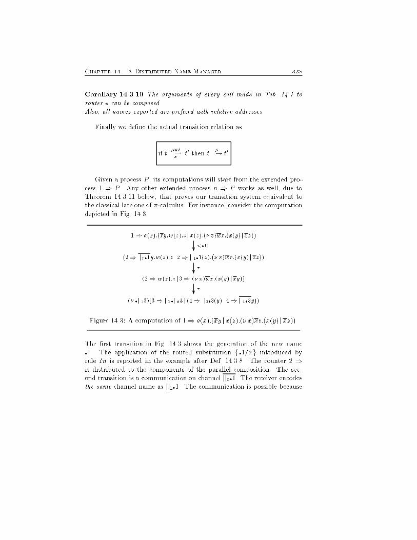
Chapter 14. A Distributed Name Manager 338Corollary 14.3.10 The arguments of every call made in Tab. 14.1 torouter ? can be composed.Also, all names exported are pre�xed with relative addresses.Finally we de�ne the actual transition relation asif t �@#�!x t0 then t ��! t0Given a process P , its computations will start from the extended pro-cess 1 ) P . Any other extended process n ) P works as well, due toTheorem 14.3.11 below, that proves our transition system equivalent tothe classical late one of �-calculus. For instance, consider the computationdepicted in Fig. 14.3.1) a(x):(xy:w(z):z jx(z):(� x)wx:(x(y) jxz))(2) jj0�1y:w(z):z j 2) jj1�1(z):(� x)wx:(x(y) j xz))(2) w(z):z j 3) (� x)wx:(x(y) jxy))(� �jj13)(3) jj1�jj03 j (4) jj0�3(y) j 4) jj1�3y))a(�1)��Figure 14.3: A computation of 1) a(x):(xy jx(z):(� x)xv:(x(y) jxz)).The �rst transition in Fig. 14.3 shows the generation of the new name�1. The application of the routed substitution fj�1=xjg introduced byrule In is reported in the example after Def. 14.3.8. The counter 2 )is distributed to the components of the parallel composition. The sec-ond transition is a communication on channel jj0�1. The receiver encodesthe same channel name as jj1�1. The communication is possible because

339 14.3. Operational semanticsjj0�1@jj0 ' jj1�1@jj1. Also, the counter of the residual of the receiver is in-creased because rule In generates a new name �2 that will be replaced withy by substitution fjy=�2jg in the conclusion of rule Com0 (see the exam-ple after Def. 14.3.8). The derivation of the last transition is exempli�edbefore Theorem 14.3.9, and uses a Close rule.The following theorem says that our transition system is a more con-crete version of the original one. In its statement, we use an auxiliaryfunction FC that erases counters from extended processes. Its de�nitionby structural induction should be obvious.Theorem 14.3.11 Let �!L the late transition relation of �-calculus.Then, P0 ��!L P1 i� t �0�! t0 and FC(t) = P �0�!L P 0 = FC(t0) is avariant of P0 ��!L P1.Proof. (Sketch.) The proof is by induction on the rules de�ning the transi-tion relations, by noting that ours and the standard ones are in a one-to-onecorrespondence. We start with the axiom In:P0 x(y)�!L P1 i� P0 x(�n)�! L P1f�n=yg; �n 62 fn(P1)Theorem 14.3.6 says that we can enrich name �n in the above transition withthe relative address of its generator with no capture of names. Thus we obtainP0 x(�n)�! L P1fj�n=yjg; �n 62 fn(P1) i� n) P0 x(�n)�! n+ 1) P1fj�n=yjgIn the leftmost transition we do not need the side condition �n 62 fn(P1) becausecounter n) ensures that n is a locally new name.The case of Open is almost the same of input.Consider the rule Pari. We have to show only that our management of namesmakes true the side condition of �-calculus bn(�)\fn(Pi) = ;. This immediatelyfollows by noting that rules In and Open (the only two that have labels withsome bound name) generates each time a new name that is di�erent from allother names in the system because it encodes the address of the generator.In the rule of communications the substitution of names is done only in thesequential components of the reader, because substitutions are routed.The only relevant remark about rule Res is that the name possibly read through

Chapter 14. A Distributed Name Manager 340an input is recorded in the auxiliary index of �@#�!x . 2We end this section with some remark. The management of local envi-ronments relies on the speci�cation of a router that shows how to exportnames. The de�nition of our router is factorized out of the semantic de-scriptions. Therefore, it can be changed according to the informationavailable on the interconnection network. This suggests us a possible hi-erarchy of descriptions, closer and closer to the actual implementation.Our approach can be easily extended to cover real distributed program-ming language like Facile that already has a proved operational semantics(Borgia, 1995).Our description of the name manager uses a family of operators n )that extends the syntax of the language. These operators are exactly thesame used to de�ne causal trees (Darondeau & Degano, 1989) and thecausal and locational semantics of �-calculus (Sangiorgi, 1994; Boreale &Sangiorgi, 1995). Therefore, we can apply as it is the technique presentedthere to encode our name handler into pure �-calculus.Finally, we admit that our extended names are quite unreadable. How-ever, they are to be used as internal names for speci�cations closer toe�cient implementations, rather than in high-level speci�cations, where aglobal space of names and global checks are acceptable.

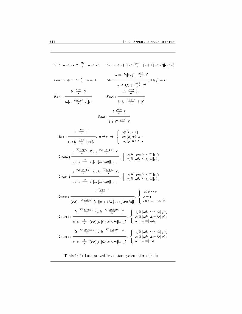
341 14.3. Operational semanticsOut : n) rs:P rs�!� n) P In : n) r(x):P r(�n)�!x (n+ 1)) Pfj�n=xjgTau : n) �:P ��!� n) P Ide : n) Pfjr=yjg �@#�!x t0n) Q(r) �@#�!x P 0 ; Q(y) = PPar0 : t0 �@#�!x t00t0jt1 �@jj0#�!x t00jt1 Par1 : t1 �@#�!x t01t0jt1 �@jj1#�!x t0jt01Sum : t �@#�!x t0t+ t00 �@#�!x t0Res : t �@#�!x t0(�u)t �@#�!x (�u)t0 ; � 6= � ) 8<: u62fr; s; xgsbj(�)@# ' robj(�)@# ' sCom0 : t0 r0s0@#0�!x t00; t1 r1(�m)@#1�!y t01t0jt1 ��!� t00jt01fjs1=�mjg@#1 ; � s0@jj0#0 ' s1@jj1#1r0@jj0#0 ' r1@jj1#1Com1 : t1 r1(�m)@#1�!x t01; t0 r0s0@#0�!y t00t1jt0 ��!� t01jt00fjs1=�mjg@#1 ; � s0@jj0#0 ' s1@jj1#1r0@jj0#0 ' r1@jj1#1Open : t rs@#�!x t0(�u)t r(�n)@#�!x (t0fjn+ 1=njg@#)fj�#n=ujg ; 8<: s@# ' ur 6= st@# = n) PClose0 : t0 r0(s0)@#0�!x t00; t1 r1(�m)@#1�!x t01t0jt1 ��!� (�u)(t00jt01fjs1=�mjg@#1) ; 8<: s0@jj0#0 ' s1@jj1#1r0@jj0#0 ' r1@jj1#1u ' s0@jj0#0Close1 : t1 r1(�m)@#1�!x t01; t0 r0(s0)@#0�!x t00t1jt0 ��!� (�u)(t01jt00fjs1=�mjg@#1) ; 8<: s0@jj0#0 ' s1@jj1#1r0@jj0#0 ' r1@jj1#1u ' s0@jj1#1Table 14.1: Late proved transition system of �-calculus.

Chapter 14. A Distributed Name Manager 342

Part VConclusions343

345We have presented a general framework for enhancing the structuraloperational semantics of concurrent distributed systems. The developmentof the thesis follows two main streams. The former is concerned with para-metricity. This feature permits to save time and e�orts in the descriptionof di�erent views of the same system and in the implementation of toolsfor computer aided veri�cation.Parametricity is implemented through the proved transition systemthat allows us to retrieve many semantic models (in particular the truly-concurrent ones) presented in the literature through simple relabellingfunctions. Also, the rich labelling of transitions permits us to de�ne acompact representation of processes that is used as internal representationof parametric veri�cation tools.The other line of evolution is concerned with a possible hierarchy ofsemantic de�nitions that are closer and closer to implementations. As acase study, we enrich the proved transition system with probabilistic dis-tributions to derive stochastic models of the system at hand. Then, per-formance measures are carried out with standard numerical techniques.Another implementation issue that we have dealt with is the speci�cationof a distributed name manager for �-calculus. The idea is to use the in-formation encoded in the labels of proved transitions to attach a uniquelocalized address to each name. As a consequence, we speci�ed a dis-tributed environment for �-calculus, already equipped with a distributedoperational semantics.Some work still has to be done. We want to investigate the use ofnon-interleaving semantics in the stochastic extensions of process calculi.In particular, a causal relation should allow us to use general distributionprobabilities that do not enjoy the memory less property.As far as the hierarchy of semantic descriptions is concerned, we needto further study the existence of mapping functions from a level to another.Furthermore, we need to identify the property of system descriptions thatthese semantics must preserve.A more long-term goal concerns the extension of the present approachto in�nite transition systems to study safety and liveness properties. Apossible solution is the extension of SOS semantics to G1SOS that can

346express also in�nite behaviours. Then, the use of abstract interpretations(Cousot & Cousot, 1992) could allow one to pass from one model to an-other and to study properties of in�nite systems.

ReferencesAceto, L. 1992. A Static View of Localities. Formal Aspects of Computing.Ahamad, M., Neiger, G., Burns, J.E., Kohli, P., & Hutto, P.W. 1995. Causalmemory: de�nitions, implementation and programming. Distributed Com-puting, 9, 37{49.Ahlers, K., Breen, D. E., Crampton, C., Rose, E., Tucheryan, M., Whitaker, R.,& Greer, D. 1994 (October). An augmented vision system for industrialapplications. In: SPIE Photonics for Industrial Applications ConferenceProceedings.Allen, A.A. 1978. Probability, Statistics, and Queueing Theory with ComputerScience Applications. Academic Press.Amadio, R., Leth, L., & Thomsen, B. 1995. From a Concurrent �-calculus tothe �-calculus. In: Proceedings of FCT'95.Amadio, R.M., & Prasad, S. 1994. Localities and failures. Tech. rept. 94-18.ECRC.Badrinath, B.R., & Ramamritham, K. 1992. Semantics-Based ConcurrencyControl: Beyond Commutativity. ACM TODS, 17(1), 163{199.Bates, P. 1990. MEC: a system for constructing and analysing transition sys-tems. In: Work. on Automatic Veri�cation Methods for Finite State Sys-tems, LNCS 407. Springer-Verlag.Bednarczyk, M.A. 1988. Categories of Asynchronous Transition Systems. Ph.D.thesis, University of Sussex.Bell, J.L., & Machover, M. 1977. A Course in Mathematical Logic. Elsevier.347

REFERENCES 348Bernardo, M., Donatiello, L., & Gorrieri, R. 1994. MPA: a stochastic processalgebra. Tech. rept. UBLCS-94-10. University of Bologna, Laboratory forComputer Science.Best, E., & Devillers, R. 1987. Sequential and concurrent behaviour in Petri nettheory. Theoretical Computer Science, 55(1), 87{136.Bianchi, A., Coluccini, S., Degano, P., & Priami, C. 1995. An E�cient Veri-�er of Truly Concurrent Properties. Pages 36{50 of: Malyshkin, V. (ed),Proceedings of PaCT'95, LNCS 964. Springer-Verlag.Bloom, B. 1995. Structural operational semantics as a speci�cation language.Pages 107{117 of: Proceedings of POPL'95. San Francisco, California:ACM.Bodei, C., Degano, P., & Priami, C. 1996. Mobile Processes with a DistributedEnvironment. In: Proceedings of ICALP'96, LNCS. Springer-Verlag.Bolognesi, T., & Caneve, M. 1989. Squiggles - A Tool for the Analysis of LOTOSSpeci�cations. Pages 201{216 of: Turner, K. (ed), Formal DescriptionTechniques. North-Holland.Boreale, M., & Sangiorgi, D. 1995. A fully abstract semantics of causality in the�-calculus. In: Proceedings of STACS'95, LNCS. Springer Verlag.Borgia, R. 1995. Semantiche causali per FACILE. M.Phil. thesis, Dipartimentodi Informatica, Universit�a di Pisa.Bouali, A., & de Simone, R. 1992. Symbolic Bisimulation Minimisation. In:Proceedings of CAV'92.Bouali, A., Gnesi, S., & Larosa, S. 1994. The Integration Project for the JACKEnvironment. In: Bullettin of the EATCS.Boudol, G. 1990. Flow event structures and ow nets. s�emantique du paral-lelisme, I. Guessarian (ed.), LNCS 469, 1990. In: Guessarian, I. (ed), Se-mantics of systems of concurrent processes, Proc. 18�eme �ecole de printempsd' informatique th�eorique, LNCS 469. Springer Verlag.Boudol, G., & Castellani, I. 1988. A Non-Interleaving Semantics for CCS basedon Proved Transitions. Fundamenta Informaticae, XI(4), 433{452.Boudol, G., de Simone, R., Roy, V., & Vergamini, D. 1990. Process Calculi,from Theory to Practice: Veri�cation Tools. In: Work. on AutomaticVeri�cationMethods for Finite State Systems, LNCS 407. Springer-Verlag.

349 REFERENCESBoudol, G., Castellani, I., Hennessy, M., & Kiehn, A. 1992. A Theory of Pro-cesses with Localities. Pages 108{122 of: Proceedings of CONCUR'92,LNCS 630. Springer-Verlag.Boudol, G., Castellani, I., Hennessy, M., & Kiehn, A. 1993. A Theory of Pro-cesses with Localities. Theoretical Computer Science, 114.Bowen, J.P., & Hinchey, M.G. 1994a. Formal Methods and Safety-Critical Stan-dards. IEEE Computer, August.Bowen, J.P., & Hinchey, M.G. 1994b. Seven more myths of formal methods: dis-pelling industrial prejudices. Pages 105{117 of: In Proceedings of FME'94(Industrial Bene�ts of formal Methods), LNCS 873. Springer-Verlag.Bowen, J.P., & Hinchey, M.G. 1995. Ten Commandaments of formal methods.IEEE Computer, 28(4), 56{63.Boyer, R.S., & Moore, J.S. 1979. A Computational Logic. Academic Press, NY.Brookes, S.D., Hoare, C.A.R., & Roscoe, A.D. 1984. A Theory of Communicat-ing Sequential Processes. Journal of ACM, 31(4), 560{599.Bryant, E. R. 1986. Graph-Based Algorithms for Boolean Function Manipula-tion. IEEE Transactions on Computers, C-36(8), 677{691.Buchholz, P. 1994. On a Markovian Process Algebra. Tech. rept. Informatik IV,University of Dortmund.Busi, N., & Gorrieri, R. 1995. A Petri net semantics for �-calculus. Pages145{159 of: Lee, I., & Smolka, S.A. (eds), In Proceedings of CONCUR'95,LNCS 962. Springer-Verlag.Christiansen, H., & Jones, N.D. 1983. Control- ow treatment in a simplesemantics-directed compiler generator. In: Bj�orner, D. (ed), IFIP WG2.2:Formal description of programming concepts II. North-Holland.Clarke, E.M., Emerson, E.A., & Sistla, A.P. 1986. Automatic Veri�cation ofFinite State Concurrent Systems using Temporal Logic Speci�cation. ACMTOPLAS, 8(2), 244 { 263.Cleaveland, R., & Madelaine, E. 1992. Automated Generation of Veri�cationTools. In: Proceedings of ERCIM Workshop on Theory and Practice inVeri�cation.Cleaveland, R., & Yankelevich, D. 1994. An Operational Framework for Value-Passing Processes. Pages 326{338 of: Proceedings of POPL'94.

REFERENCES 350Cleaveland, R., Parrow, J., & Ste�en, B. 1993. The Concurrency Workbench:A Semantics-Based Tool for the Veri�cation of Concurrent Systems. ACMTransaction on Programming Languages and Systems, 36{72.Clegg, M., & Valmari, A. 1991. Reduced Labelled Transition Systems SaveVeri�cation E�ort. In: Proceedings of CONCUR'91, LNCS 527. Springer-Verlag.Cleveland, R., Jain, S., & Trehan, V. 1993. GCCS: A graphical language fornetwork design. Tech. rept. N-C State University.Conte, P. 1991. Confronti tra semantiche ad ordinamento parziale per sistemiconcorrenti. M.Phil. thesis, Dipartimento di Informatica, Universit�a diPisa.Cousot, P., & Cousot, R. 1992. Inductive de�nitions, Semantics and AbstractInterpretation. Pages 83{94 of: Proceedings of POPL'92.Craigen, D., Gerhart, S., & Ralston, T. 1993. An International Survey of Indus-trial Application of Formal Methods. Tech. rept. NITGCR 93/626. AtomicEnergy Control Board of Canada, U.S. National Institute of Standardsand Technology, and U.S. Naval Research Laboratories, National TechnicalInformation Service, 5285 Port Royal Road, Spring�eld, VA 22161, USA.Darondeau, Ph., & Degano, P. 1989. Causal Trees. Pages 234{248 of: Proceed-ings of ICALP'89, LNCS 372. Springer-Verlag.de Bakker, J.W., & de Roever, W.P. 1972. A calculus for recursive programschemes. Pages 167{196 of: Proceedings of ICALP'72. North-Holland.De Nicola, R., Inverardi, P., & Nesi, M. 1991. Equational Reasoning aboutLOTOS Speci�cations: A Rewriting Approach. In: Proceedings of SixthInternational Workshop on Software Speci�cation and Design. IEEE.de Simone, R., & Vergamini, D. 1989. Aboard AUTO. Tech. rept. 111. INRIASophia-Antipolis.Degano, P., & Priami, C. 1992. Proved Trees. Pages 629{640 of: Proceedingsof ICALP'92, LNCS 623. Springer-Verlag.Degano, P., & Priami, C. 1994. A Compact Representation of Finite-StateProcesses. In: Proceddings of Workshop on Describing and PrescriptingProgram Behaviour.Degano, P., & Priami, C. 1995a. Causality for mobile processes. Pages 660{671of: Proceedings of ICALP'95, LNCS 944. Springer-Verlag.

351 REFERENCESDegano, P., & Priami, C. 1995b. Non Interleaving Semantics for Mobile Pro-cesses. In: Proceddings of Workshop on Tools for Analysis of Programs andSystems.Degano, P., & Priami, C. 1995c. Partial Ordering Semantics for �-calculus.Degano, P., & Priami, C. 1995d. Transitional Semantics of Full Prolog. Pages511{520 of: Alpuente, M., & Sessa, M.I. (eds), Proceedings of Joint Con-ference on Declarative Programming GULP-PRODE95.Degano, P., & Priami, C. 1996. Enhanced Operational Semantics. ACM Com-puting Surveys.Degano, P., De Nicola, R., & Montanari, U. 1985. Partial Ordering Derivationsfor CCS. Pages 520{533 of: Proceedings of FCT, LNCS 199. Springer-Verlag.Degano, P., De Nicola, R., & Montanari, U. 1987. Observational Congruencesfor Concurrency Models. Pages 105{132 of: Wirsing, M. (ed), FormalDescription of Programming Concepts III. North-Holland.Degano, P., De Nicola, R., & Montanari, U. 1990. A Partial Ordering Semanticsfor CCS. Theoretical Computer Science, 75, 223{262.Degano, P., Meseguer, J., & Montanari, U. 1992. Axiomatizing the Algebra ofNet Computations and processes. Acta Informatica.Degano, P., De Nicola, R., & Montanari, U. 1993. Universal Axioms for Bisim-ulation. Theoretical Computer Science, 114, 63{91.Enders, R., Filkorn, T., & Taubner, D. 1992. Generating BDDs for SymbolicModel Checking in CCS. In: Proceedings of CAV'91, LNCS 575. Springer-Verlag.Estenfeld, K., Schneider, H-A., Taubner, D., & Tiden, E. 1991. Computer AidedVeri�cation of Parallel Processes. Pages 208{226 of: Proceedings of VIS'91,Darmstadt Informatik Fachberichte Vol. 271.Fernandez, J.C., & Mounier, L. 1991. A Tool Set for Deciding BehaviouralEquivalences. In: Proceedings of CONCUR'91, LNCS 527.Ferrari, G. 1990. Unifying Models of Concurrency. Ph.D. thesis, Dipartimentodi Informatica, Universit�a di Pisa.Ferrari, G., Gorrieri, R., &Montanari, U. 1991. An extended expansion theorem.Pages 162{176 of: Proceedings of TAPSOFT'91, LNCS 431. Springer-Verlag.

REFERENCES 352Ferrari, G., Modoni, G., & Quaglia, P. 1995. Towards a Semantic-based Ver-i�cation Environment for the �-calculus. In: Proceedings of Fifth ItalianConference on Theoretical Computer Science.Ferrari, G., Montanari, U., & Mowbray, M. 1996. Structured Transition Systemswith Parametric Observations: Observational Congruences and MinimalRealizations. International Journal of Mathematical Structures in Com-puter Science.Gallo, Felix. 1994 (Dec.). Agent-Tcl: A White Paper. Posted to thesafe-tcl@cs.utk.edumailing list.Giacalone, A., Mishra, P., & Prasad, S. 1989. Facile: A Symmetric Integration ofConcurrent and Functional Programming. International Journal of ParallelProgramming, 18, 121{160.Giacalone, A., Mishra, P., & Prasad, S. 1990. Operational and Algebraic Seman-tics for Facile: A Symmetric Integration of Concurrent and Functional Pro-gramming. Pages 765{780 of: Proceedings ICALP'90, LNCS 443. Springer-Verlag.Gilmore, S., & Hillston, J. 1994. The PEPA Workbench: A Tool to Supporta Process Algebra-based Approach to Performance Modelling. In: G.,Harring (ed), Proceedings of Int. Conference on Modelling Techniques andTools For Computer Performance Evaluation.Godefroid, P. 1990. Using Partial Orders to Improve Automatic Veri�cationMethods. In: Proceedings of CAV'90.Godefroid, P., & Wolper, P. 1991. Using Partial Orders for the E�cient Ver-i�cation of Deadlock Freedom and Safety Properties. Pages 332{342 of:Proceedings of CAV'91, LNCS 575. Springer-Verlag.Godskesen, J.C., Larsen, K.G., & Zeeberg, M. 1989. TAV Users Manual. Tech.rept. Aalborg University Center, Denmark.Goltz, U., & Reisig, W. 1983. The Non-Sequential Behaviour of Petri Nets.Information and Computation, 57, 125{147.Gosling, James, & McGilton, Henry. 1995 (May). The Java Language Environ-ment. White paper.G�otz, N., Herzog, U., & Rettelbach, M. 1992. TIPP- A Language for TimedProcesses and Performance Evaluation. Tech. rept. 4/92. IMMD VII, Uni-versity of Erlangen-Nurnberg.

353 REFERENCESGraf, S., & Ste�en, B. 1990. Compositional Minimization of Finite State Pro-cesses. In: Proceedings of CAV'90.Groote, J. F., & Vaandrager, F. W. 1990. An E�cient Algorithm for BranchingBisimulation andStuttering Equivalence. In: S., Paterson M. (ed), Pro-ceedings of ICALP'90, LNCS 443. Springer-Verlag.Guessarian, I. 1981. Algebraic Semantics. In: LNCS 99. Springer Verlag.Gunter, C.A., & Scott, D.S. 1990. Semantic Domains. Handbook of TheoreticalComputer Science. Elsevier. Chap. 12, pages 634{674.Hall, J.A. 1990. Seven myths of formal methods. IEEE Software, 7(5), 11{19.Harvey, C. 1986. Performance Engineering as an Integral Part of System Design.BT Technology Journal, 4(3), 143{147.Hennessy, M. 1988. Algebraic Theory of Processes. MIT Press.Hennessy, M. 1990. The Semantics of Programming Languages - An ElementaryIntroduction using Structural Operational Semantics. Wiley.Hennessy, M., & Milner, R. 1985. Algebraic Laws for Nondeterminism andConcurrency. Journal of ACM, 32, 137{161.Hermanns, H., & Rettelbach, M. 1994. Syntax, Semantics, Equivalences andAxioms for MTIPP. In: Herzog, U., & Rettelbach, M. (eds), Proceedingsof PAPM'94.Hillston, J. 1994a. A Compositional Approach to Performance Modelling. Ph.D.thesis, University of Edinburgh, Department of Computer Science.Hillston, J. 1994b. The Nature of Synchronization. In: Herzog, U., & Rettelbach,M. (eds), Proceedings of PAPM'94.Hinchey, M.G., & Bowen, J.P. (eds). 1995. Application of formal Methods.Prentice Hall Series in Computer Science.Hoare, C.A.R. 1985. Communicating Sequential Processes. Prentice-Hall.Hoare, C.A.R., & Lauer, P.E. 1974. Consistent and complementary formaltheories of the semantics of programming languages. Acta Informatica, 3,135{153.Houston, I.S.C., & King, S. 1991. CICS Project Report: Experiences and Resultsfrom the use of Z in IBM. Pages 588{596 of: Prehn, S., & Toetenel,W.J. (eds), Proceedings of VDM'91:Formal Software DevelopmentMethods,LNCS 551. Springer-Verlag.

REFERENCES 354Howard, R. 1971. Dynamic Probabilistic Systems:Semi-Markov and DecisionSystems. Vol. II. Wiley.Inverardi, P., & Priami, C. 1991 (October). Evaluation of Tools for the Analysisof Communicating Systems. EATCS Bulletin, 45.Inverardi, P., & Priami, C. 1996. Automatic Veri�cation of Distributed Systems:The Process Algebras Approach. Formal Methods in System Design, 8(1),1{37.Inverardi, P., Priami, C., & Yankelevich, D. 1992a. A Parametric Veri�cationTool for Distributed Concurrent Systems. Pages 31{44 of: Proceedings ofERCIM Workshop on Theory and Practice in Veri�cation.Inverardi, P., Priami, C., & Yankelevich, D. 1992b. Veri�cation of Concur-rent Systems in SML. Pages 169{174 of: Proceedings of ACM SIGPLANWorkshop on ML and its Applications.Inverardi, P., Priami, C., & Yankelevich, D. 1993. Extended Transition Systemsfor Parametric Bisimulation. Pages 558{569 of: Lingas, A., Karlsson, R., &Carlsson, S. (eds), Proceedings of ICALP'93, LNCS 700. Springer-Verlag.Inverardi, P., Priami, C., & Yankelevich, D. 1994. Automatizing ParametricReasoning on Distributed Concurrent Systems. Formal Aspects of Com-puting, 6(6), 676{695.Janicki, R., & Koutny, M. 1990. Net Implementation of Optimal Simulations.Pages 295{314 of: Proceedings of Application and Theory of Petri Nets '90.Jategaonkar, L. 1993. Observing "True" Concurrency. Ph.D. thesis, MIT.Jategaonkar Jagadeesan, L., & Jagadeesan, R. 1995. Causality and True Con-currency: A Data- ow Analysis of the �-Calculus. Pages 277{291 of: Pro-ceedings of AMAST'95, LNCS 936. Springer-Verlag.Joyal, A., Nielsen, M., & Winskel, G. 1994. Bisimulation from Open Maps.Tech. rept. BRICS RS-94-7.Kanellakis, P. C., & Smolka, S. C. 1983. CCS Expressions, Finite State Processesand Three Problems of Equivalence. In: Proceedings of the Second ACMSymposium on Principles of Distributed Computing.Kiehn, A. 1991. Local and Global Causes. Tech. rept. TUM 342/23/91.Langerak, R. 1992. Transformations and semantics for LOTOS. Ph.D. thesis,Twente University.

355 REFERENCESLarsen, K. G. 1986. Context-dependent Bisimulation between Processes. Ph.D.thesis, University of Edimburgh.Larsen, K.G., & Skou, A. 1992. Compositional Veri�cation of ProbabilisticProcesses. In: Proceedings of CONCUR'92. LNCS, vol. 630. Springer-Verlag.Leroy, X., & Mauny, M. 1992. The Caml Light System, Release 0.5. Documen-tation and User's Manual.Leth, L. 1991. Functional Programs as Recon�gurable Networks of Communi-cating Processes. Ph.D. thesis, Imperial College - University of London.Leth, L., & Thomsen, B. 1995. Some Facile Chemistry. Formal Aspects ofComputing, Volume 7, Number 3, 314{328.Lin, H. 1991. PAM: A Process Algebra Manipulator. Tech. rept. 2/91. Universityof Sussex.Lucas, P. 1973. On program correctness and the stepwise development of im-plementations. Pages 219{251 of: Proceedings of Convegno di InformaticaTeorica.Madeleine, E., & Vergamini, D. 1992. Finiteness Conditions and StructuralConstruction of Automata for all Process Algebras. In: Kurshan, R., &Clarke, E. M. (eds), Proceedings of CAV'90, LNCS. Springer-Verlag.Malhotra, J., Smolka, S. A., Giacalone, A., & Shapiro, R. 1988. Winston, A Toolfor Hierarchical Design and Simulation of Concurrent Systems. In: Pro-ceedings of of the Workshop on Speci�cation and Veri�cation of ConcurrentSystems.Mauw, S., & Veltink, G.J. 1991. A Proof Assistant for PSF. In: Proceedings ofCAV'91, LNCS. Springer-Verlag.May, D., Barrett, G., & Shepherd, D. 1992. Designing Chips that Work. In:Hoare, C.A.R., & Gordon, M.J.C. (eds), Mechanized Reasoning and Hard-ware Design. Prentice Hall International Series in Computer Science.McCarthy, J. 1963. Towards a mathematical science of computation. Pages21{28 of: Popplewell, C.M. (ed), Information Processing 1962.McMillan, K.L. 1992. Using Unfoldings to Avoid the State Explosion Problemin the Veri�cation of Asynchronous Circuits. In: Proceedings of CAV'92.Meseguer, Jos�e, & Montanari, Ugo. 1990. Petri Nets Are Monoids. Informationand Computation, 88(2), 105{155.

REFERENCES 356Milne, G. 1991. The formal description and veri�cation of hardware timing.IEEE Trans. on Computers, 40(7).Milner, R. 1989. Communication and Concurrency. Prentice-Hall, London.Milner, R. 1991. The polyadic �-calculus: a tutorial. Tech. rept. ECS-LFCS-91-180. University of Edinburgh.Milner, R. 1992a. Action structures. Tech. rept. ECS-LFCS-92-249. Universityof Edinburgh.Milner, R. 1992b. Functions as processes. Mathematical Structures in ComputerScience, 2(2), 119{141.Milner, R., Parrow, J., & Walker, D. 1992a. A Calculus of Mobile Processes (Iand II). Information and Computation, 100(1), 1{77.Milner, R., Berry, D., & Turner, D. 1992b. A semantics for ML concurrencyprimitives. In: Proceedings of POPL'92.Montanari, U., & Pistore, M. 1995a. Checking Bisimilarity for �nitary �-calculus. Pages 42{56 of: Lee, I., & Smolka, S.A. (eds), Proceedings ofCONCUR'95, LNCS 962. Springer-Verlag.Montanari, U., & Pistore, M. 1995b. Concurrent semantics for the �-calculus.In: Electronic Notes in Computer Science. Elsevier.Montanari, U., & Yankelevich, D. 1992. A Parametric Approach to Localities.Pages 617{628 of: Proceedings of ICALP'92, LNCS 623. Springer-Verlag.Mycroft, A., Degano, P., & Priami, C. 1995. Complexity as a basis to compareconcurrency models. Pages 141{155 of: K. Kanchanasut, J.-J. L�evy (ed),Algorithms, Concurrency and Knowledge { Proceedings of Asian Comput-ing Science Conference, LNCS 1023. Springer-Verlag.Nicollin, X., & Sifakis, J. 1991. An Overview and Synthesis on Timed ProcessAlgebras. Pages 526{548 of: Real Time: Theory in Practice, LNCS 600.Springer-Verlag.Nielsen, M., Plotkin, G., & Winskel, G. 1981. Petri Nets, Event Structures andDomains. Theoretical Computer Science, 85{108.Nielson, F., & Nielson, H.R. 1992. Semantics with applications: a formal intro-duction. Wiley.Nielson, F., & Nielson, H.R. 1993. From CML to Process Algebras. Tech. rept.DAIMI PB-433. Computer Science Department - Aarhus University.

357 REFERENCESOrava, F. 1994. On the Formal Analysis of Telecommunications Protocols. Ph.D.thesis, Dept. of Computer Systems, Uppsala University and SICS.Orava, F., & Parrow, J. 1992. An algebraic veri�cation of a mobile network.Formal Aspects of Computing, 497{543.Paige, R., & Tarjan, R. 1987. Three Partition Re�nement Algorithms. SIAMJournal on Computing, 16(6), 973{989.Park, D. 1981. Concurrency and Automata on In�nite Sequences. Pages 167{183 of: Proceedings of GI, LNCS 104. Springer-Verlag.Peled, D. 1993. All from One, One from All: On Model Checking Using Repre-sentatives. Pages 409{423 of: Proceedings of CAV'93, LNCS 697. Springer-Verlag.Pierce, B.C., & Turner, D.N. 1995. PICT: A Programming Language Based onthe Pi-Calculus.Plotkin, G. 1981. A Structural Approach to Operational Semantics. Tech. rept.DAIMI FN-19. Aarhus University, Denmark.Pratt, V. 1986. Modelling Concurrency with Partial Orders. InternationalJournal of Parallel Programming, 15, 33{71.Priami, C. 1995a. Interleaving-based Partial Odering Semantics. In: Proceedingsof ICTCS95.Priami, C. 1995b. Stochastic �-calculus. The Computer Journal, 38(6).Priami, C. 1996. Integrating Behavioural and Performance Analysis with Topol-ogy Information. In: Proceedings of 29th Hawaian International Conferenceon System Sciences. Maui, Hawaii: IEEE.Priami, C., & Yankelevich, D. 1993. A Formal Paradigm for Multiview Dis-tributed Debugging Environments. In: Proceedings of AADEBUG'93 (International Workshop on Automated and Algorithmic Debugging).Priami, C., & Yankelevich, D. 1994. Read-Write causality. Pages 567{576 of:Proceedings of MFCS'94, LNCS 841. Springer-Verlag.Probst, D.K., & Li, H.F. 1990. Using Partial Order Semantics to Avoid the StateExplosion Problem in Asynchronous Systems. In: Proceedings of CAV'90.Rabinovich, A., & Trakhtenbrot, B. 1988. Nets of Processes. FundamentaInformaticae, XI(4), 357{404.Reisig, W. 1985. Petri Nets: An Introduction. In: EATCS Monographs.Springer-Verlag.

REFERENCES 358Reppy, J. 1992. Higher order concurrency. Ph.D. thesis, Cornell University, TR92-1285.Rosca, J.P. 1995. Genetic Programming Exploratory Power and the Discoveryof Functions. Pages 719{736 of: McDonnel, J.R., Reynolds, R.G., & Fogel,D.B. (eds), Proceedings of the Fourth Annual Conference on EvolutionaryProgramming. MIT Press.Rosca, J.P., & Ballard, D.H. 1995. Causality in Genetic Programming. In:Proceedings of the Fifth International Conference on Genetic Algorithms.Roy, V., & de Simone, R. 1989. An AUTOGRAPH Primer. Tech. rept. 112.INRIA Technical Report.Sangiorgi, D. 1992. Expressing Mobility in Process Algebras: First-Order andHigher-Order Paradigms. Ph.D. thesis, University of Edinburgh.Sangiorgi, D. 1994. Locality and non-interleaving semantics in calculi for mobileprocesses. In: Proceedings of TACS'94, LNCS 789. Springer-Verlag.Scott, D. 1970. Outline of a mathematical theory of computation. Pages 169{176 of: Proceedings of 4th Annual Princeton Conference on InformationScience and Systems.Shields, M.W. 1985. Concurrent Machines. Computer Journal, 449{465.Stark, A. 1989. Concurrent Transition Systems. Theoretical Computer Science,221{269.Talpin, J.-P. 1994. The Calumet Experiment in Facile - A Model for GroupCommunication and Interaction Control in Cooperative Applications. Tech.rept. ECRC-94-26. European Computer-Industry Research Centre.Talpin, J.-P., Marchal, P., & Ahlers, K.:. 1994. Calumet - A Reference Manual.Tech. rept. ECRC-94-30. European Computer-Industry Research Centre.Tarjan, R. 1981a. Fast Algorithms for Solving Path Problems. Journal of ACM,28(3), 594 { 614.Tarjan, R. 1981b. A Uni�ed Approach to Path Problems. Journal of ACM,28(3), 577 { 593.Thomsen, B. 1990. Calculi for Higher Order Communicating Systems. Ph.D.thesis, Imperial College - University of London.Thomsen, B. 1993. Plain CHOCS: a second generation calculus for higher orderprocesses. Acta Informatica, 30(1), 1{59.

359 REFERENCESThomsen, B., Leth, L., & Giacalone, A. 1992. Some Issues in the Semantics ofFacile Distributed Programming. In: Proceedings of the 1992 REX Work-shop on \Semantics: Foundations and Applications". LNCS 666. Springer-Verlag.Thomsen, B., Leth, L., Prasad, S., Kuo, T.-M., Kramer, A., Knabe, F., &Giacalone, A. 1993. Facile Antigua Release Programming Guide. Tech.rept. ECRC-93-20. European Computer-Industry Research Centre.Thomsen, B., Leth., L., Knabe, F., & Chevalier, P.-Y. 1995a. Mobile Agents.Tech. rept. ECRC-95-21. European Computer-Industry Research Centre.Thomsen, B., Knabe, F., Leth, L., & Chevalier, P.-Y. 1995b. Mobile Agents SetTo Work. Communications International, July.Valmari, A. 1990. A Stubborn Attack on State Explosion. In: Proceedings ofCAV'90.Valmari, A., & Tienari, M. 1991 (June). An Improved Failure Equivalence forFinite-State Systems with a Reduction Algorithm. In: Proceedings of IFIPWG6.1 Protocol Speci�cation, Testing and Veri�cation.van Glabbeek, R.J., & Goltz, U. 1989. Equivalence notions for concurrent sys-tems and re�nement of actions. In: Proceedings of MFCS'89, LNCS 379.Springer-Verlag.van Glabbeek, R.J., Smolka, S.A., Ste�en, B., & Tofts, C.M.N. 1990. Reactive,Generative and Strati�ed Models of Probabilistic Processes. Pages 130 {141 of: Proceedings of LICS'90.Victor, B., & Moller, F. 1994. The Mobility Workbench: A Tool for the �-calculus. In: Proceedings of CAV'94, LNCS 818. Springer-Verlag.Walker, D. 1994. Objects in the �-calculus. Information and Computation.White, James E. 1994. Telescript Technology: The Foundation for the ElectronicMarketplace. General Magic white paper, 2465 Latham Street, MountainView, CA 94040.Winskel, G. 1982. Event Structures for CCS and Related Languages. Pages561{576 of: Proceedings of ICALP'82, LNCS 140. Springer-Verlag.Winskel, G. 1987. Petri Nets, Algebras, Morphisms and Compositionality. In-formation and Computation, 72, 197{238.Winskel, G., & Nielsen, M. 1992. Models for concurrency. Tech. rept. DAIMI-PB-429. Computer Science Dept., Aarhus University.

REFERENCES 360Yankelevich, D. 1993. Parametric Views of Process Description Languages.Ph.D. thesis, Dipartimento di Informatica, Universit�a di Pisa.Zuidweg, H. 1989. Veri�cation by Abstraction and Bisimulation. In: WorkshopOn Automatic Veri�cation Methods for Finite State Systems.