Embed Size (px)
Citation preview

LSE Research Online Article (refereed)
Per G. Fredriksson, Eric Neumayer, Richard Damania and Scott Gates
Environmentalism, democracy, and pollution control
Originally published in Journal of environmental economics and management, 49 (2). 343 -365 © 2005 Elsevier Inc. You may cite this version as: Fredriksson, Per G. and Neumayer, Eric and Damania, Richard and Gates, Scott (2005). Environmentalism, democracy, and pollution control [online]. London: LSE Research Online. Available at: http://eprints.lse.ac.uk/archive/00000630 Available online: February 2006 LSE has developed LSE Research Online so that users may access research output of the School. Copyright © and Moral Rights for the papers on this site are retained by the individual authors and/or other copyright owners. Users may download and/or print one copy of any article(s) in LSE Research Online to facilitate their private study or for non-commercial research. You may not engage in further distribution of the material or use it for any profit-making activities or any commercial gain. You may freely distribute the URL (http://eprints.lse.ac.uk) of the LSE Research Online website. This document is the author’s final manuscript version of the journal article, incorporating any revisions agreed during the peer review process. Some differences between this version and the publisher’s version remain. You are advised to consult the publisher’s version if you wish to cite from it.
http://eprints.lse.ac.uk Contact LSE Research Online at: [email protected]

Environmentalism, Democracy, and Pollution Control
FINAL VERSION
MS#13136
Per G. Fredriksson
Department of Economics, Southern Methodist University, PO Box 750496, Dallas, TX 75275-0496,
USA
Eric Neumayer*
Centre for Environmental Policy and Governance, London School of Economics, Houghton Street,
London WC2A 2AE, UK
Richard Damania
School of Economics, University of Adelaide, Australia 5005
Scott Gates
Norwegian University of Science and Technology &
International Peace Research Institute Oslo, Fuglehauggata 11, 0260 Oslo, Norway
* Corresponding author. Fax: +44-207-955-7412. E-mail address: [email protected] (E. Neumayer).
1

Abstract
This paper makes two empirical contributions to the literature, based on predictions generated by a
lobby group model. First, we investigate how environmental lobby groups affect the determination of
environmental policy in rich and developing countries. Second, we explore the interaction between
democratic participation and political (electoral) competition. The empirical findings suggest that
environmental lobby groups tend to positively affect the stringency of environmental policy. Moreover,
political competition tends to raise policy stringency, in particular where citizens’ participation in the
democratic process is widespread.
Keywords: Environmentalism, democracy, environmental regulations, policy.
2

1. Introduction
This paper investigates how environmental lobby groups, citizens’ participation in the democratic
process, and the degree of electoral competition affect the determination of environmental policy in
rich and developing countries.
A prominent feature of the political landscape in the last few decades is the emergence of various
environmental lobby groups (Wapner [61]). Their impact appears to be rising. On fishing, for example,
Todd and Ritchie [57, p. 148] argue that “the tide is slowly turning in favour of the ENGOs on fisheries
issues.”1 However, surprisingly little research has examined the impact of environmental lobby groups
on environmental policy. Hillman and Ursprung [27], Fredriksson [19], Aidt [1], and Conconi [6,7]
study the theoretical effects of environmental lobby groups on environmental policy outcomes.2 The
empirical literature includes Kalt and Zupan [32], Durden et al. [14], Fowler and Shaiko [18], Cropper
et al. [9], VanGrasstek [59], and more recently, Riddel [54].3 These empirical studies have focused on
only one single country. No study exists of the effects of environmental lobbying on policy outcomes
1 ENGO is here an acronym for environmental non-governmental organization.
2 Smith [57] uses club theory to explain individuals’ decision to join an environmental lobby group.
3 Kalt and Zupan [32] and Durden et al. [14] examine the impact of environmental groups on coal strip-mining regulation.
Fowler and Shaiko [18] investigate the role of grass-roots environmental lobbying efforts in the US Senate. Both Kalt and
Zupan [32] and Fowler and Shaiko [18] report weak and inconsistent relationships between lobbying efforts of interest
groups and roll call votes. Durden et al. [14] report that environmentalists had below average impact on coal strip-mining
legislation. VanGrasstek [59] finds an effect of environmental lobby groups’ political action during the NAFTA
negotiations in the US Senate, Cropper et al. [9] finds that intervention by environmental advocacy groups raise the
probability that the USEPA cancelled a pesticide registration, and Riddel [54] shows that the Sierra Club and the League of
Conservation Voters have been successful in influencing US Senate election outcomes using campaign contributions (via
political action committees). Note that Jackson and Kingdon [31] demonstrate that using an index of other roll call votes as
a proxy for members’ ideology produces inconsistent estimates of the coefficients (see also Smith [55]).
3

across countries. Moreover, no study examines the environmental policy impacts of environmental
lobbying across different political regimes.
Our first main objective is to fill these gaps in the literature. One additional aim is to contribute to
the ongoing policy debate on how to improve local and global environmental policymaking. Can
foreign donors and international organizations expect to contribute to improved local and global
environmental quality by supporting local environmental lobby groups (non-governmental
organizations (NGOs)) in developing countries as currently done by the World Bank, among others?4
The second main objective of the paper is to contribute with a novel perspective to the small but
growing literature on the relationship between democracy and environmental policy making (see, e.g.,
[8], [44], [13]).5 We argue that an important interaction effect on environmental policy exists between
4 For example, the stated objectives of the Critical Ecosystem Partnership Fund (a joint initiative of Conservation
International, the Global Environment Facility, the Government of Japan, the MacArthur Foundation, and the World Bank)
are to serve as a catalyst to create strategic working alliances among diverse groups, to combine capacities and eliminating
duplication of efforts for a comprehensive and coordinated approach to conservation challenges, to encourage local dialogue
with extractive industries, and to strengthen indigenous organizations and facilitating partnerships. See
www.cepf.net/xp/cepf/about_cepf/index.xml (visited May 5, 2003) for further details.
5 In his theoretical work, Congleton [8] examines how environmental regulations are set to maximize the utility by (i) the
median voter in a democratic system, and by (ii) an authoritarian ruler in a non-democratic system. Two forces drive
Congleton’s theoretical results (Deacon [13] provides related arguments). First, a shorter time horizon of the policy maker
leads to less stringent environmental regulations, because of the long-term nature of many environmental problems. Arguing
that authoritarian rulers tend to have a shorter time horizons, Congleton’s model predicts that democracies have stricter
environmental regulations than non-democracies due to this effect. Second, the authoritarian ruler appropriates a larger
share of economy’s income, which has an ambiguous effect on the strictness of environmental regulations. On the one hand,
Congleton [8, p. 416] argues that for an autocrat, ‘An increase in the fraction of national income going to the individual of
interest increases the marginal cost of environmental standards faced by him, since he will now bear a larger fraction of
associated reductions in national income’ (see also [38]). On the other hand, appropriation of a larger share of the national
income might also lead to stricter environmental standards if we assume that environmental quality is a normal, if not a
4

(i) the level of democratic participation by the general population, and (ii) the degree of electoral
competition.6,7
We start by developing a theoretical model that provides guidance for our empirical work. First, the
environmentalists organize their lobbying effort by forming lobby groups with identical environmental
objectives. The number of environmental lobby groups that emerges depends on their collective action
costs. We assume that the environmentalists face collective action costs that are increasing in group
size, possibly due to their geographical dispersion or because of the administration and enforcement
costs of large groups (see [49]). A single industry group with negligible collective action costs opposes
their efforts.8
luxury good. Congleton [8] finds that more democratic countries are more likely to sign or enact national legislation
supporting the Montreal Protocol on chlorofluorocarbon (CFCs) emissions. Further empirical evidence is provided by
Murdoch and Sandler [44] and Murdoch et al. [45], who show that more democratic countries cut back more on
chlorofluorocarbon and sulphur oxide emissions. Deacon [13] reports that more democratic countries tend to provide greater
levels of public goods (including greater access to safe water and sanitation). Democratic countries ratified faster the United
Nations Framework on Climate Change (Fredriksson and Gaston [20]), the Convention on Biological Diversity and the
Convention on International Trade in Endangered Species (Neumayer [47]). Neumayer [46] and Neumayer et al. [48] also
find that more democratic countries put a higher percentage of land area under protection status and comply better with
reporting requirements of multilateral environmental agreements. However, this existing empirical literature has ignored the
level of democratic participation.
6 The democratic participation variable is calculated as the percentage of the total population participating in elections. The
electoral competition variable is calculated by subtracting the percentage of votes won by the largest party from 100.
7 Mueller and Stratmann [43] find that high levels of democratic participation are associated with more equal income
distribution, larger government sectors, and lower growth rates (see also [39] and [34]). The interaction between democratic
participation and political competition is ignored in their paper.
8 The industry owners are considerably fewer and more concentrated, and are therefore assumed to face relatively small
collective action costs.
5

Each lobby group seeks to influence the same policymaker (in the same legislature) with the help of
prospective campaign contributions (Grossman and Helpman [25]). The government values campaign
contributions and aggregate social welfare. However, social welfare is taken into consideration only to
the extent that (i) the average voter is expected to participate in the next election (implicitly modeled),
and (ii) the next election is competitive.9 Thus, the greater the number of disenfranchised citizens and
the lower the level of political competition expected by the government, the greater is the relative
weight that the government places on the political contributions from the environmental and industry
lobby groups. Essentially, where the level of democratic participation (political competition) is
expected to be relatively high, the policy maker’s ability to deviate from the welfare maximizing policy
is more restricted, given the degree of political competition (democratic participation rate).10
The predictions that emerge are that (i) an increase in the number of environmental lobby groups
leads to a more stringent environmental policy, (ii) a greater degree of democratic participation leads to
a more stringent environmental policy, (iii) greater political competition yields a stricter environmental
policy, and (iv) the effect of democratic participation (political competition) is conditional on the level
of political competition (democratic participation).
We test these predictions using cross-country data from 82 developing and 22 OECD countries on
the regulation of lead content in gasoline. The empirical findings are largely consistent with the
predictions of the model. First, we find evidence that an increase in the number of environmental lobby
groups tends to lower the lead content of gasoline. This empirical result may have policy implications.
The support of environmental lobby groups in developing countries may be a channel through which
international donors can help improve local and global environmental policymaking. This may
9 The democratic participation part of our model is reminiscent of Deacon’s [13] model of an uncontested minority political
elite, although in our model the franchise may range from close to the entire population to a small minority.
10 In Baron [2] and Grossman and Helpman [25] campaign contributions may be used to enlighten voters about the positions
of candidates, or purchase impressionable voters’ support.
6

facilitate compliance with global international environmental agreements such as the Kyoto Protocol on
CO2 emissions.
Second, whereas citizens’ democratic participation has no environmental policy effect by itself,
greater political competition tends to lower lead content in gasoline, in particular where the level of
political participation is high. However, democratic participation affects environmental policy
stringency only in countries with sufficiently high degree of political competition. Thus, democratic
participation has no effect in pure dictatorships. We believe these are new findings in the literature.
While these results are true in our full sample, the developing country results suggest that
democratic participation has never any effect in this group of countries, possibly due to threshold
effects or to different policy preferences among the very poor. In our view, compared with previous
studies in the literature, the results suggest a more detailed channel through which various aspects of
democracy (participation and competition) affect environmental policies.
The paper is organized as follows. Section 2 sets up the model, and Section 3 analyses the effects of
the number of environmental lobby groups and democratic participation rates. Section 4 presents our
empirical work. Section 5 concludes.
2. The Model
A small open economy has a “clean” sector producing a numeraire good z, and a polluting
sector producing a good x. The economy has consumers and firms, where the population is normalized
to 1. A share of the consumers derive disutility from pollution associated with the local
production of good z, and become environmentalists. A consumer has utility given by
1<Eα
11
, (1) Xcu+c=U exz θδ−)(
11 Corner solutions may result with quasi-linear preferences. Interior solutions are assumed.
7

where cz and cx are consumption of the numeraire good z and good x, with world and domestic prices
equal to 1 and p*, respectively.12 u(cx ) is a strictly concave and differentiable sub-utility function.
Production of x by each of the identical firms is given by x1≥n i, where nxi = X. is an indicator
variable that takes a value of one if the consumer suffers disutility from pollution (i.e., if she is an
environmentalist), and zero otherwise. θ is the per-unit damage from pollution, which depends on the
amount h
eδ
i spent by the firm on pollution control per unit of output, where 0<hθ , and .0>hhθ Thus,
Xθ represents aggregate emissions. The negative externality is regulated by the government which
employs a pollution tax t∈T, T∈R, on per unit of damage from production of good x.
Good z is produced with constant marginal cost equal to one. The cost of producing good x is given
by where we assume , , and that , but “negligible”.
Given the pollution tax, the profit function of each firm is given by
),,( ii hxv 0>xv ,0>hv 0>xxv ,0>hhv 0>hxv
,)(),()( *iiiiii xhthxvxpt θπ −−= (2)
which yields the first-order conditions
,0* =−−=∂∂
θπ
tvpx x
i
i (3.1)
.0=−−=∂∂
ihhi
i xtvh
θπ
(3.2)
Whereas equation (3.1) states that firm i will produce up to the point where the price is equal to the net-
of-tax marginal cost, equation (3.2) equalizes the marginal cost of reducing pollution (by increasing
pollution control costs) with the marginal gain (i.e., lower pollution taxes). Equations (3.1) and (3.2)
implicitly define the equilibrium values of xi and hi as functions of t: x(t) and h(t). Applying the implicit
function theorem to (3.1) and (3.2) yields 0<∂∂ txi and ;0>∂∂ thi i.e., an increase in the pollution
tax reduces output and increases pollution control expenditures.
12 The world market price p* is exogenously given as the country is a price taker.
8

Aggregate pollution tax revenues equal
),()( tXt=t θτ (4)
where X(t) = nx(t). We assume that tax revenues are distributed equally to all individuals (this
assumption does not drive our results).13
The model defines a three-stage game. The timing assumptions are as follows.
Stage 1. The consumers with environmental concerns each join one of k environmental lobby
groups. Similarly, the firms independently and simultaneously form their own lobby group.
Stage 2. The lobby groups offer the incumbent government a political contribution schedule each,
denoted by Λi, i=F,Ej, j=1,..., k. A lobby’s strategy consists of a continuous function i.e.,
it offers a specific political contribution for selecting a policy t.
;:)( ℜ→Λ Tti
Stage 3. The government proceeds to set its optimal environmental policy, given the lobby groups’
strategies and the expected levels of democratic participation and political competition in the next
election (only implicitly modeled). The government collects the associated contribution from the
lobbies. When the pollution tax has been set, the firms set output and pollution control levels.
The profits obtained by the n firms depend on the pollution tax rate. The n firms are sufficiently few
that lobby group organization costs are negligible. They are assumed able to organize into one single
lobby group i=F that coordinates a prospective political contribution offer to the government. On the
other hand, the environmentalists are many and dispersed. Thus, while the benefits of polluting are
concentrated among a relatively small number of firms, the pollution costs are thinly and widely spread
13 Let Y denote income of the representative consumer. Maximizing (1) subject to the budget constraint Y = cz + p*cx yields
consumption functions cx = d(p*) = uc-1 and cz = Y - p*d(p*). The indirect utility function of a consumer can then be expressed
as V(p*,t,Y) = Y + δ(p*) - θX, where δ(p*) = u[d(p*)] - p*d(p*) is the consumer surplus derived from consumption of good x.
Consumption of good z yields no consumer surplus.
9

across a larger number of individuals. Hence, as suggested by Olson [49], environmental groups are
likely to face greater difficulties and costs in forming lobby groups.
To capture this we assume that each environmental lobby group j confronts organizational costs
(e.g., negotiation, communication, collection, and monitoring costs) that are increasing in the number
of members, Nj(we drop the lobby specific notation j where redundant).14 For simplicity, we follow
Moe [42] and assume convex lobby group collective action costs. As discussed by Potters and Sloof
[52], a large number of potential participants to collective action is usually thought to raise the free
riding problem, and thus collective action costs. For example, Miller [40] and Trefler [58] report
negative effects of higher potential membership numbers on the degree of political influence. The
collective action costs are assumed to take the form Individuals affected by pollution
may each make voluntary contributions S to one single environmental lobby group, which organizes
collective action. It offers the government political contributions in an attempt to obtain more stringent
environmental controls.
.)( 2CNNC =
15
Let us consider a marginal consumer who suffers disutility from pollution. In particular, we focus on
her problem of how much to contribute to an environmental lobby group (zero contribution implies no
membership). Let t-e be the pollution tax set in the absence of this single member’s contribution to her
environmental group. Define t as the tax set by the government when the member contributes to her
environmental lobby. Analogously, define and )())(()( eee tXth=tD −−− −θ )())(()( tXth=tD θ− as the
levels of pollution damage suffered by each environmentalist with pollution tax policies t-e and t,
14 See Hamilton [26] for a study of communities’ anticipated ability to undertake collective action and the siting of
hazardous waste treatment facilities.
15 It is important to note that all our results go through if environmental groups face higher lobbying costs than the firm
lobby. To make the analysis transparent we consider the limiting case where the lobbying costs of the firms is normalized to
zero.
10

respectively. Then the payoff to the individual e from joining an environmental lobby group j is given
by
,)( ee StB=U − (5)
where B(t) = D(t-e) – D(t). Maximizing (5) with respect to yields the first-order condition eS
.01)(=−
∂∂
∂∂
−∂∂
ee
e
St
ttD=
SU (6)
Observe that ttD
∂∂ )( <0, hence an interior solution to (6) exists only if eS
t∂∂ >0. Thus, by the inverse
function theorem, (6) can be rearranged into
tS
ttD e
∂∂
=∂
∂−
)( . (7)
Equation (7) reveals that each individual pays contributions up to the point where the marginal
benefits from a policy change (in the form of reduced pollution) equals the marginal cost (comprising
the membership fee that is channeled into a greater potential political contribution to the government).
Thus, political contributions are locally truthful in the sense that they reflect the benefits of a policy
change.
Consider the group’s optimal membership size (see also [56]). The contributions received by
environmental lobby group j are used to cover the costs associated with organizing the group, CN2, and
to offer the government a contribution of size The optimal size N.1
2∑=
−=ΛN
e
eEj CNS * of each
environmental group j is determined by maximizing the group’s payoff:
.))(()( 2CNStBNt eEj −−=Ω (8)
Maximization of (8) yields the optimal size of each lobby group, defined by
.2)(*
CStBN
e−= (9)
11
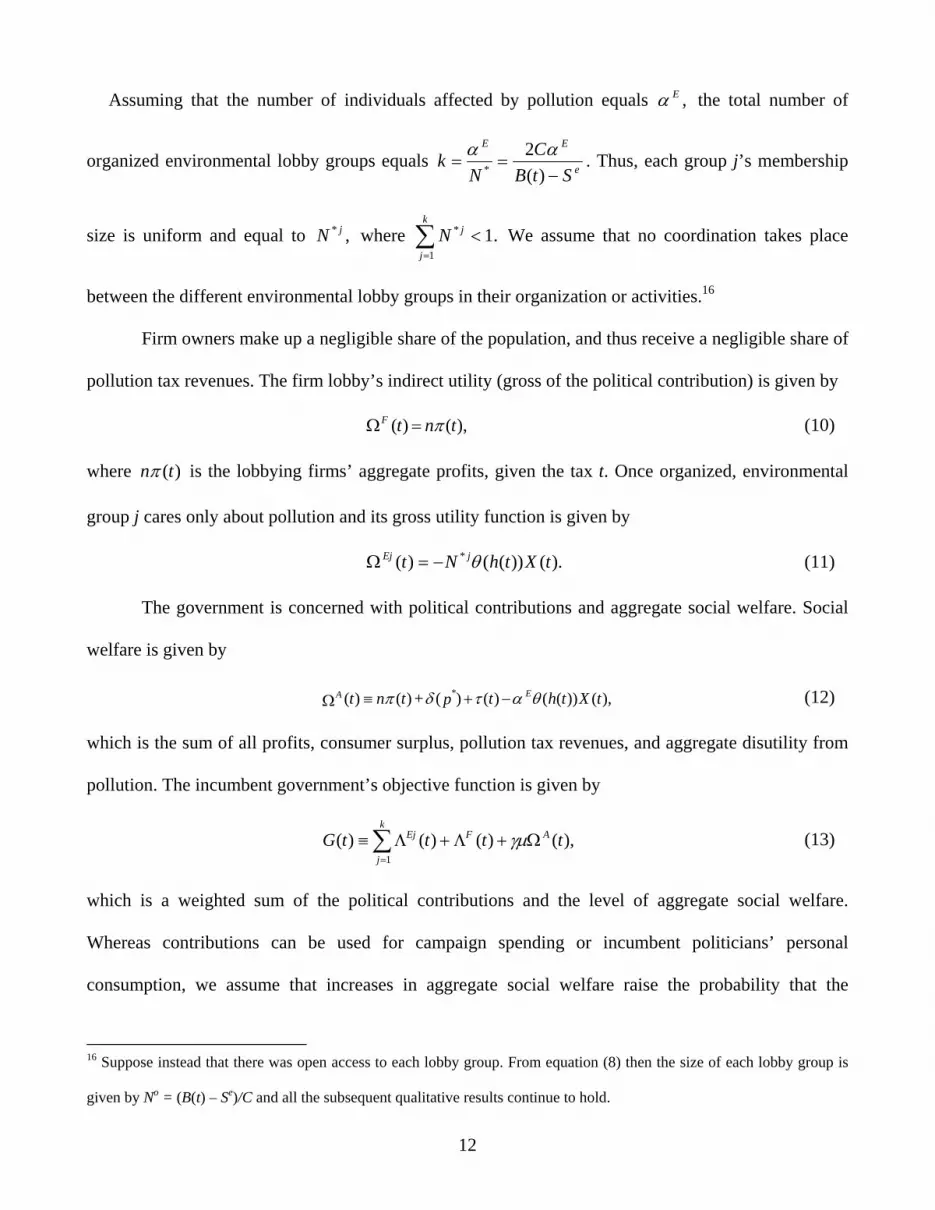
Assuming that the number of individuals affected by pollution equals the total number of
organized environmental lobby groups equals
,Eα
e
EE
StBC
Nk
−==
)(2
*
αα . Thus, each group j’s membership
size is uniform and equal to where We assume that no coordination takes place
between the different environmental lobby groups in their organization or activities.
,* jN ∑=
<k
j
jN1
* .1
16
Firm owners make up a negligible share of the population, and thus receive a negligible share of
pollution tax revenues. The firm lobby’s indirect utility (gross of the political contribution) is given by
),()( tntF π=Ω (10)
where )(tnπ is the lobbying firms’ aggregate profits, given the tax t. Once organized, environmental
group j cares only about pollution and its gross utility function is given by
).())(()( * tXthNt jEj θ−=Ω (11)
The government is concerned with political contributions and aggregate social welfare. Social
welfare is given by
),())(()()()()( * tXthtp+tnt EA θατδπ −+≡Ω (12)
which is the sum of all profits, consumer surplus, pollution tax revenues, and aggregate disutility from
pollution. The incumbent government’s objective function is given by
),()()()(1
ttttG AFk
j
Ej Ω+Λ+Λ≡ ∑=
γµ (13)
which is a weighted sum of the political contributions and the level of aggregate social welfare.
Whereas contributions can be used for campaign spending or incumbent politicians’ personal
consumption, we assume that increases in aggregate social welfare raise the probability that the
16 Suppose instead that there was open access to each lobby group. From equation (8) then the size of each lobby group is
given by No = (B(t) – Se)/C and all the subsequent qualitative results continue to hold.
12

government remains in power (not explicitly modeled).17 The relative weight on aggregate social
welfare in (13) adjusted by two factors: γ represents the (exogenous) expected democratic
participation rate in the next (implicitly modeled) upcoming election, and µ is the (exogenous)
expected degree of political competition in this election. We thus follow Dahl [10] and Vanhanen [60],
who regard both political participation and political competition as necessary requirements for
democracy.
Moreover, we take the view that only future levels of γ and µ are of importance to the incumbent,
elections already passed are of little importance for the government’s re-election efforts. Government
politicians will therefore need to form expectations about future democratic participation and electoral
competition levels. We assume that these expectations are correct.18
Note that a share )1( γ− of the consumers is disenfranchised in the policy process. This is
reminiscent of the formulation by Deacon [13] who studies the effects of democracy on the provision
of public goods. Deacon captures democratic “inclusiveness” by using a measure of the size of the elite
relative to the whole population. He argues that this variable measures “the degree to which
government policy incorporates, or fails to incorporate, the interests of the entire population.” (Deacon
[13, p. 10]). Note that in our framework every citizen’s welfare is indeed taken into consideration, but
the relative weights are (possibly severely) distorted by campaign contributions and democratic
participation rates below unity.
Note that γ is only a partial measure of the degree of democracy, because if all citizens are
essentially forced (by an incumbent autocrat) to vote on only one available choice, policy makers are
17 In the context of democratic societies this is perhaps obvious since it increases the probability that the median voter is
made better off. In non-democratic systems higher welfare will also lower the expected benefits from a regime change.
18 With regard to the application of rational expectations models to voting and elections, see MacKuen et al. [37] and
Erikson et al. [16].
13

unlikely to put a large weight on social welfare. In this case the electoral process places no pressure on
the incumbent politician to alter policies. Hence, the effect of democratic participation depends on the
expected level of political competition, .µ High levels of political participation have little positive
policy impact without effective choice, e.g. elections in single party dictatorships (Persson and
Tabellini [51]). Nearly all studies of democracy include some notion of competition in their definition
of democracy. Dahl’s [10] definition of democracy, indeed, is expressed purely in terms of
participation and electoral competition (or contestation).
The equilibrium in the common agency model by Bernheim and Whinston [3] maximizes the joint
surplus of all parties, as discussed by Grossman and Helpman [25]. In order to conserve space, we do
not derive the equilibrium condition here, but instead refer the reader to the earlier literature (see, for
example, [25]). The policy outcome maximizes the joint welfare of each lobby and the government,
given the other lobbies’ strategies. In our set-up, the characterization of the equilibrium pollution tax,
is given by ,*t
.0)()()( **
1
* =Ω+Ω+Ω∑=
ttt At
Ft
k
j
Ejt γµ (14)
Differentiation of (10), (11), and (12) with respect to the pollution tax yields (using the envelope
theorem):
),())(()( tXthtFt θ−=Ω (15)
⎟⎠⎞
⎜⎝⎛
∂∂
∂∂
+∂∂
−=Ωth
hX
tXtht EEj
tθθα ))(()( , (16)
and
.)()())(()()())(()1()( ⎟⎟
⎠
⎞⎜⎜⎝
⎛∂
∂∂
∂+
∂∂
−=Ωtth
ththtX
ttXthttA
tθθ (17)
Note that the Pigouvian tax is found by setting equation (17) equal to zero. This yields , since the
terms in brackets are all negative.
1=t
14

Note that with a uniform size of each environmental lobby, Summing (16) over all j,
substituting the resulting expression together with (15) and (17) into equation (14), and rearranging, we
find an expression for the equilibrium characterization given by
.1
jk
j
j kNN =∑=
( ) .0)()())(()()())(()()())((
)()(
*
)(
=⎟⎟⎠
⎞⎜⎜⎝
⎛∂
∂∂
∂+
∂∂
−−+−
−−− 4444444 34444444 21444 3444 21
444 3444 214434421 tth
ththtX
ttXthkNttXth
A
jE θθαγµθ (18)
We know that term A in (18) must be negative, because the remaining two terms in (18) are negative.
However, the equilibrium tax rate is indeterminate in size relative to the Pigouvian tax, .* Et α<> Two
forces push the tax rate in opposite directions. The industry lobby pushes the tax down, whereas the k
environmental groups all push it upwards. The industry group’s pressure is captured by the first term in
(18), and reflects the amount at stake (total pollution).
3. Environmental Lobbying, Participation, and Competition
In this section we analyze the effects of environmental lobby groups and the two components of
democracy on environmental policy making. The aim is to derive testable hypotheses for our empirical
work. We first investigate the effect of the number of environmental groups on environmental policy.
Total differentiation of equation (18) with respect to k yields
,0
)()())(()()())((*
>⎟⎟⎠
⎞⎜⎜⎝
⎛∂
∂∂
∂+
∂∂
=∂
∂
Dtth
ththtX
ttXthN
kt
j θθ (19)
where 0<D represents the second-order condition of the government’s maximization with respect to
t, and can be derived from equation (11). D is required to be negative for a maximum. Since the
numerator is negative, equation (19) is positive. We find the following prediction.
15
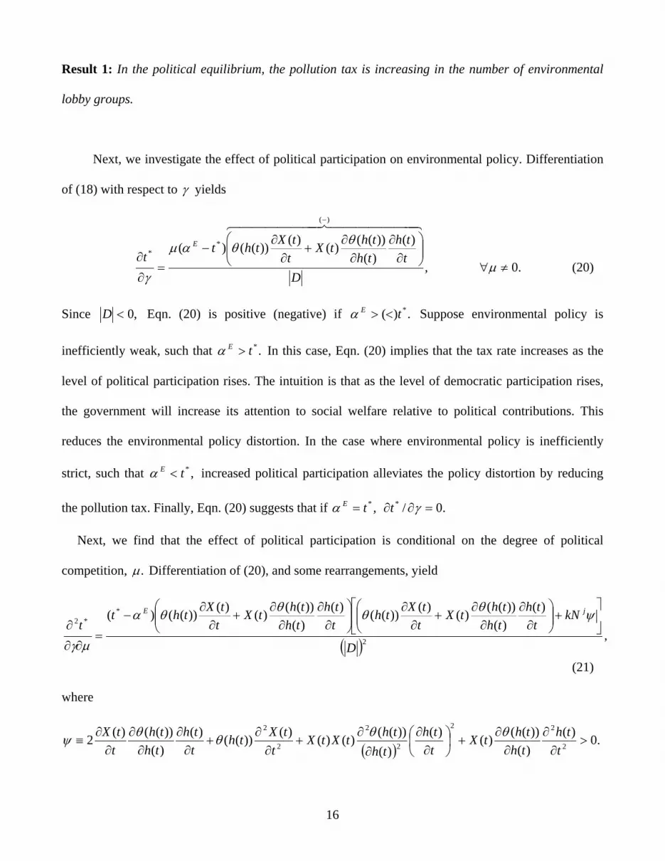
Result 1: In the political equilibrium, the pollution tax is increasing in the number of environmental
lobby groups.
Next, we investigate the effect of political participation on environmental policy. Differentiation
of (18) with respect to γ yields
,
)()())(()()())(()(
)(
**
Dtth
ththtX
ttXtht
tE
4444444 84444444 76 −
⎟⎟⎠
⎞⎜⎜⎝
⎛∂
∂∂
∂+
∂∂
−=
∂
∂θθαµ
γ .0≠∀µ (20)
Since ,0<D Eqn. (20) is positive (negative) if Suppose environmental policy is
inefficiently weak, such that In this case, Eqn. (20) implies that the tax rate increases as the
level of political participation rises. The intuition is that as the level of democratic participation rises,
the government will increase its attention to social welfare relative to political contributions. This
reduces the environmental policy distortion. In the case where environmental policy is inefficiently
strict, such that increased political participation alleviates the policy distortion by reducing
the pollution tax. Finally, Eqn. (20) suggests that if
.)( *tE <>α
.*tE >α
,*tE <α
,*tE =α .0/* =∂∂ γt
Next, we find that the effect of political participation is conditional on the degree of political
competition, .µ Differentiation of (20), and some rearrangements, yield
( ),
)()())(()()())(()(
)())(()()())(()(
2
**2
D
kNtth
ththtX
ttXth
tth
ththtX
ttXtht
tjE⎥⎦
⎤⎢⎣
⎡+⎟⎟
⎠
⎞⎜⎜⎝
⎛∂
∂∂
∂+
∂∂
⎟⎟⎠
⎞⎜⎜⎝
⎛∂
∂∂
∂+
∂∂
−
=∂∂
∂ψθθθθα
µγ
(21)
where
( ).0)(
)())(()()(
)())(()()()())(()(
)())(()(2 2
22
2
2
2
2
>∂
∂∂
∂+⎟
⎠⎞
⎜⎝⎛
∂∂
∂∂
+∂
∂+
∂∂
∂∂
∂∂
≡t
thththtX
tth
ththtXtX
ttXth
tth
thth
ttX θθθθψ
16

Suppose Eqn. (21) is positive (negative) for high (low) values of k, the number of
environmental lobby groups, in particular when
.*tE >α
.)()())(()()())(()( ψθθ jN
tth
ththtX
ttXthk ⎟⎟
⎠
⎞⎜⎜⎝
⎛∂
∂∂
∂+
∂∂
−<>
If instead Eqn. (21) is negative (positive) for high (low) values of k. ,*tE <α
Expressions (20) and (21) yield the following prediction.
Result 2: In the political equilibrium, if the pollution tax is inefficiently weak (strict), the pollution tax
is increasing (decreasing) with the expected democratic participation rate. The effect increases
(decreases) with the expected level of political competition, given that the number of environmental
lobby groups is large (small).
Result 2 shows that the effect of democratic participation depends on the equilibrium pollution tax
relative to the efficient level. Result 2 also suggests that an interaction effect exists between the
democratic participation rate and the degree of political competition. Since the number of
environmental lobby groups provides a condition for the direction of the interaction effect, it may be
expected to differ between rich and developing countries. We will return to this issue in our empirical
work.
Next, we investigate the effect of the degree of political competition on environmental policy.
Differentiation of (18) with respect to µ yields
,
)()())(()()())(()(
)(
**
Dtth
ththtX
ttXtht
tE
4444444 84444444 76 −
⎟⎟⎠
⎞⎜⎜⎝
⎛∂
∂∂
∂+
∂∂
−=
∂
∂θθαγ
µ ,0≠∀γ (22)
17
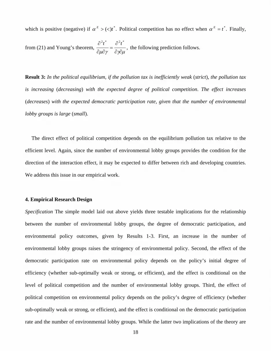
which is positive (negative) if Political competition has no effect when Finally,
from (21) and Young’s theorem,
.)( *tE <>α .*tE =α
,*2*2
µγγµ ∂∂
∂=
∂∂
∂ tt the following prediction follows.
Result 3: In the political equilibrium, if the pollution tax is inefficiently weak (strict), the pollution tax
is increasing (decreasing) with the expected degree of political competition. The effect increases
(decreases) with the expected democratic participation rate, given that the number of environmental
lobby groups is large (small).
The direct effect of political competition depends on the equilibrium pollution tax relative to the
efficient level. Again, since the number of environmental lobby groups provides the condition for the
direction of the interaction effect, it may be expected to differ between rich and developing countries.
We address this issue in our empirical work.
4. Empirical Research Design
Specification The simple model laid out above yields three testable implications for the relationship
between the number of environmental lobby groups, the degree of democratic participation, and
environmental policy outcomes, given by Results 1-3. First, an increase in the number of
environmental lobby groups raises the stringency of environmental policy. Second, the effect of the
democratic participation rate on environmental policy depends on the policy’s initial degree of
efficiency (whether sub-optimally weak or strong, or efficient), and the effect is conditional on the
level of political competition and the number of environmental lobby groups. Third, the effect of
political competition on environmental policy depends on the policy’s degree of efficiency (whether
sub-optimally weak or strong, or efficient), and the effect is conditional on the democratic participation
rate and the number of environmental lobby groups. While the latter two implications of the theory are
18

ambiguous (without further assumptions), they offer our empirical work the opportunity to bring some
empirical clarity to the identified interaction effects.
We aim to test these implications using cross-country data on the lead content of gasoline, using
(i) a data set from OECD and developing countries, and (ii) a developing country only sample.
The test can be formulated as follows,
ti = x′iβx + βkki + βssi + βcci +βscsici + εi, (23)
where ti is the environmental policy stringency in country i, xi is a vector of controls, ki is the number
of environmental lobby groups in country i, si is the democratic participation rate, ci is the degree of
political competition, and εi is a zero mean error term. βk, βs, βc, and βsc are coefficient scalars, and βx
is a coefficient vector. Equation (23) allows the effect of the democratic participation rate (political
competition) on environmental policy to be conditional on the degree of political competition
(democratic participation rate).
The formulation in (23) does not condition the interaction effects on the number of
environmental lobby groups, as specified in Results 2 and 3. However, we take this constraint into
consideration by running our regressions for the developing country sample separately.19 It is not a
priori clear whether the simple linear specification in (23) is the appropriate functional form for testing
our hypotheses. However, we tested for functional form misspecification with Ramsey’s [53] Reset test
and failed to reject the hypothesis that our linear specification is appropriate. In addition, we have
tested whether any higher order terms of the explanatory variables assume statistical significance if
added to the estimated model, but failed to find such evidence.
19 In the full sample (104 obs.), the mean number of environmental lobby groups is 16.9 (std.dev. is 32.9), and in the
developing country sample (82 obs.) the mean is 10.3 (std.dev. is 14.1) (data taken from the 2001 edition of Europa
Publications [17]). See Table I for other years.
19

Dependent Variable. The stringency of environmental policy is measured by the lead content of
gasoline in 1996, reported by Lovei [36]. LEADCONTENT measures the maximum allowed lead
content in gasoline in grams per liter (see also Hilton and Levinson [28]; Deacon [13]). This is equal to
zero in those countries that have completely banned leaded petrol. Unlike many other measures of the
stringency of environmental policy, LEADCONTENT is a non-subjective indicator.20 LEADCONTENT
takes a value of zero grams in 15 of the countries in our sample, among them Argentina, Austria,
Bolivia, and the United States. Spain and Kuwait have the highest values in the sample at 35.11 and
37.14 grams per liter, respectively. It should be noted that countries with identical lead content
legislation may have implemented these pieces of legislation at widely different points in time.21 While
it is widely known that the US has been a frontrunner in reducing and eliminating lead from gasoline
dating back to the 1970s, lead content policy changes in other countries are largely unknown, in
particular in developing countries. Fortunately, our main (political) explanatory variables are strongly
correlated over time (see Table I.C). Note also that our developing country models are likely to exclude
early lead content reformers such as the U.S. and the timing of policy initiation should be of minor
concern in these models.
20 Damania et al. [11] provide evidence that this index is closely correlated with a number of other measures of
environmental performance which are available for more restricted lists of countries.
21 We thank a thoughtful referee for bringing this issue to our attention. However, we note that countries remain free to
reverse their lead content legislation, i.e. most countries in our sample (except the ones having banned lead in gasoline) may
alter their lead content in either direction at any point in time. With only cross-country data available, we feel justified to
follow the previous cross-country empirical literature on the political economy of environmental policy. This literature
appears to favor using political pressure variables from the same (or close) year as the dependent variable, abstracting from
the year of policy reform (see, for example, [11] and the references therein). For similar (cross-sectional and cross-country)
approaches on the empirical political economy of trade policy, see Goldberg and Maggi [22], Gawande and Bandyopadhyay
[21], and Dutt and Mitra [15].
20

Independent variables. Turning to the independent variables, we use three sets of observations from
three different years for several of our variables. ENVIROGROUPSj, j=1993, 1996, 2000, measures the
number of environmental lobby groups in year j, as proxied by the number of non-governmental
organizations (NGOs) with an environmental interest per country. This data is reported by the
Environment Encyclopedia and Directory, and published by Europa Publications [17], respectively.
The three existing editions differ in their coverage, with the later editions becoming increasingly
comprehensive. ENVIROGROUPS1996 is the primary year of observation. Moreover,
ENVIROGROUPS1993 is used to explore whether political pressure three years prior influenced the
observed level of LEADCONTENT in 1996. For example (although not discussed in our theory), there
may be lags involved with the implementation of policy reforms. ENVIROGROUPS2000 (from Europa
Publications [17]) is included because it (in our view) appears to have the most comprehensive
coverage of environmental lobby groups, particularly for developing countries. However, some groups
were founded after 1996. We therefore deleted all such groups from the 2000 data. In the 2000 data,
the highest values in the sample are 65 (Poland), 190 (United Kingdom), and 250 (United States).22 The
number of environmental lobby groups equals zero in seven countries, among them Comoros, Malawi
and Oman. Among the developing countries, 24 out of 82 countries have at least ten active
environmental groups.
Our theory also contains political pressure from the industry group (see (18)). In a survey by
Potters and Sloof [52], it is reported that the greater a lobby’s stake, the greater its success. We use the
number of passenger and commercial vehicle cars per capita in year h, h=1993, 1996 (reported by
International Road Federation, various years), multiplied by the market share of leaded gasoline in
1996 (Lovei [36]) as a measure of industry lobby group pressure.23 This resulted in the variable
22 ENVIROGROUPS is not scaled by population, since we assume that lead regulation is determined by a central
government influenced by all existing lobby groups.
23 Unfortunately, to create VEHICLES1993 we were forced to use the 1996 value of the market share of leaded gasoline,
21

VEHICLESh, h=1993, 1996, which is intended to account for the number of leaded vehicles normalized
by population.24
Our theory highlights the roles of democratic participation and political competition in the
determination of environmental policy. This makes Vanhanen’s [60] index particularly useful for our
purposes. Vanhanen’s democracy index consists of two variables that are not based on expert
evaluations: (i) a PARTICIPATION variable, calculated as the percentage of the total population
participating in elections, and (ii) a COMPETITION variable, which is calculated by subtracting the
percentage of votes won by the largest party from 100. The variable
PARTICIPATION*COMPETITION captures the interaction discussed by our theory. Dictatorships that
do not commonly hold elections such as Libya have PARTICIPATION and COMPETITION scores of
0. Most democracies have participation rates above 50. Autocracies that hold fake elections such as
Cuba can also have high participation rates, but only democracies also have high competition rates,
usually above 50.
In our theory, the government formulates its policy choice with a view of the next election,
anticipating future rates of electoral participation and competition levels. We take the theory seriously
and use for all three sets of (year-based) regressions the latest available data point for the two variables
of concern, which is 1998.25 We thus assume that politicians formulating lead content policies in 1996
were able to (reasonably) forecast the participation rate and the level of political competition.
As an additional control, the logarithm of per capita income for year h, h=1993, 1996,
(lnGDPPCh) is included and can be expected to have a positive impact if environmental quality is a
since the 1993 value is unavailable.
24 We also tested (commercial vehicles per capita)*(market share of leaded gasoline). This indicator also produced
statistically significant results.
25 This PARTICIPATION and COMPETITION data will refer to elections held 1998 or the last election held before that
year. In case of a coup d'etat after the last election, both PARTICIPATION and COMPETITION are coded zero.
22

normal good, as discussed by the literature on the environmental Kuznets curve (see, e.g., [28], [41]).
Our GDP data for year h, h=1993, 1996, comes from World Bank [62]. As further proxy variables for
industry group lobby strength we also tested whether car production and oil production as a share of
GDP might impact upon our dependent variable. Both were highly insignificant throughout. To save
degrees of freedom, these were not included in the estimation results reported below. In order to
capture structural differences between groups of countries that might influence the stringency of
environmental regulation (Congleton [8]; Murdoch and Sandler [44]), we estimate our model for a
developing country only sample.
Data We have cross-country data from 82 developing countries and 22 OECD countries. Table I
provides summary statistics together with bivariate correlation matrices for the full and developing
country samples, respectively.
< Insert Table I about here >
Estimation Strategy In our main estimation we use OLS with heteroscedasticity robust standard
errors due to the simple cross-national character of our sample. The dependent variable is zero for some
observations. An estimation technique such as Tobit may therefore be appropriate, and we report Tobit
estimation results for the full sample. However, we prefer the OLS estimator for three reasons. First,
the share of zero values of the dependent variable is small (around 14 % in the full sample and 10 % in
the developing country sample). Second, the Tobit estimator becomes inconsistent in the presence of
heteroscedasticity and is generally more vulnerable to violations of the underlying distributional and
functional specification assumptions than OLS (Greene [23]). Third, the small sample properties of
maximum likelihood (ML) estimators such as Tobit are largely unknown. For example, Long and
Freese [35] consider ML estimation in samples of less than 100 observations as ‘risky’ and recommend
samples over 500 for use of ML, which is considerably above our sample size.
The endogeneity and measurement errors of ENVIROGROUPSj and VEHICLESh may potentially
be a problem. We tested the consistency of the OLS estimations using the Durbin-Wu-Hausman
23

(DWH) test (Davidson and MacKinnon [12]), but failed to reject the null of consistent OLS estimates.
However, for completeness we also include a set of IV results. As instruments, we use population size
(World Bank [62]), the percentage of Muslims in the population (Parker [50]), a dummy variable for a
country’s legal origin (La Porta et al. [33]), as well as a dummy variable for countries with a Confucian
tradition (Huntington [29]). Our instruments are partially correlated with ENVIROGROUPSj and
VEHICLESh in the sense that the correlation persists after all other exogenous variables are controlled
for. Since we have over-identifying restrictions, we can also test for the exogeneity of our
instruments.26 The tests suggest that our instruments are valid.
We tested whether different slope coefficients for our two lobby group variables,
ENVIROGROUPSj and VEHICLESh, are warranted. To do so, we grouped countries into those with (i)
high and low PARTICIPATION, (ii) high and low COMPETITION, and whether or not they are (iii) car
producing, or (iv) oil producing countries. We found no evidence of statistically significant differences
in the slope coefficients across any of these groups of countries. In addition, in our robustness analysis
we explored whether our results are sensitive to a number of countries having zero or extremely low
values (possibly due to measurement errors) for ENVIROGROUPSj by excluding all observations in
the lowest quartile for this variables.
5. Results
Table II reports our empirical estimates for our various specifications, with LEADCONTENT as the
dependent variable and explanatory variables from year 1996 (where applicable). Models 1 and 2
report full sample OLS and Tobit results, respectively. Model 3 reports OLS for the developing country
sample only, and Model 4 shows the full sample 2SLS results. The Sargan test fails to reject the over-
26 The test of over-identifying restrictions compares the IV estimation results for the just-identified to the over-identified
equation.
24

identification restrictions, suggesting that our instruments are truly exogenous and therefore valid
instruments.
< Insert Table II about here >
ENVIROGROUPS1996 is associated with lower lead content only in Model 1. This may be due to
an incomplete (in our view) count of environmental lobby groups reported for year 1996. The results
are mixed for the two variables measuring the two different aspects of democracy of interest. Whereas
PARTICIPATION is insignificant in Models 1-4, COMPETITION is significant at least at the 5% level
in these models. Moreover, consistent with our theory, an interaction exists between PARTICIPATION
and COMPETITION. The significant negative coefficient for PARTICIPATION*COMPETITION in
Models 1, 2 and 4 suggest that increased political competition raises the stringency of environmental
policy, in particular where the level of democratic participation is high. Model 1 suggests that at the
mean of PARTICIPATION, ∂LEADCONTENT/∂COMPETITION = -0.68 (= -0.368 - 0.009*34.85)
grams, and at one standard deviation above the mean the effect equals -0.85 (= -0.368 -
0.009*(34.85 + 18.87)) grams. Moreover, although democratic participation has no independent effect
on environmental policy stringency, PARTICIPATION does raise policy stringency conditional on the
level of political competition being non-zero. Thus, in all pure dictatorships with a value of
COMPETITION equal to zero (such as Iraq in the 1990s), PARTICIPATION has no effect on
LEADCONTENT. Using the estimated coefficients in Model 1 we find that at the mean value for
COMPETITION, ∂LEADCONTENT/∂PARTICIPATION = -0.37 (= -0.009*40.68) grams. We also find
that vehicle owners form a powerful lobby opposing the environmental lobby groups. VEHICLES is
positively associated with lead content in Models 1-4, lending further support to our theoretical
model.27 Moreover, lnGDPPC1996 is highly significant in these models, with the expected negative
sign.
27 In additional analysis we broke the VEHICLES variable into its two components to see whether vehicles per capita or the
25

Models 5-7 present an outlier analysis. It would be of concern if a few observations drove our
results. While Model 5 excludes the quartile of observations with the lowest values for
ENVIROGROUPS1996, Models 6 and 7 exclude outliers from the full- and developing country
samples, respectively. Belsley et al. [4] suggest that observations with both high residuals and a high
leverage deserve special attention. We exclude an observation from the sample if its DFITS is greater
in absolute terms than twice the square root of (k/n), where k is the number of independent variables
and n the number of observations, and where DFITS is defined as the square root of (hi/(1-hi)), where hi
is an observation’s leverage, multiplied by its studentized residual. In Models 5 and 6,
ENVIROGROUPS1996 is significant at the 5% level. This is consistent with the full sample OLS result
in Model 1, which thus appears not to be merely driven by influential outliers. However,
ENVIROGROUPS1996 is insignificant in Model 7 in the developing country sample (as in Model 3),
possibly due to insufficient variation. VEHICLES1996 and lnGDPPC1996 remain significant in
Models 5-7.
Models 3 and 7 suggest that PARTICIPATION has no significant effect in developing countries. A
reason for why the interaction effect differs in this group of countries is suggested by our theory, which
conditions the interaction effect on the number on environmental lobby groups. Whereas in the full
sample the number of groups (the level of environmentalism) appears sufficiently great to yield a
negative interaction effect, this is not the case in the developing country sample, and the coefficient
becomes insignificant (corresponding to (21) being approximately zero). A related issue is why
PARTICIPATION has no direct effect on environmental policy in even the full sample, in contrast to,
e.g., the results presented by Mueller and Stratmann [43] for income distribution? One reason may be
that the very poor tend to be the most disenfranchised in developing countries. The very poor may put a
market share of unleaded gasoline exerts the main effect on the dependent variable. We found that the market share is more
important than the extent of car ownership in a country.
26

low value on environmental quality (especially if lower lead content is associated with higher gasoline
prices), and an increase in the democratic participation rate by the very poor may therefore reduce the
average participant’s preference for stricter environmental policy, blurring the overall results. There
may also be threshold effects, over which PARTICIPATION has not reached in our sample of primarily
developing countries.
Table III reports similar models as in Table II, but using ENVIROGROUPS1993, VEHICLES1993,
and lnGDPPC1993, which seek to capture earlier (political) pressures that may affect LEADCONTENT
in 1996.
<Insert Table III here >
Whereas VEHICLES1993 and lnGDPPC1993 remain significant in all models,
ENVIROGROUPS1993 affects 1996 lead content only in Models 1, 6 and 7. COMPETITION also
preserves its significant negative sign in all models, but its interaction with PARTICIPATION is now
significant only in the 2SLS regression (Model 4) and in two models that are part of the outlier analysis
(Models 5 and 6). As before, PARTICIPATION is never significant.
Table IV reports results using ENVIROGROUPS2000 (which we believe provides a superior
coverage of the environmental lobby groups active in 1996, particularly for developing countries). This
variable is now significant in five of the seven models. In particular, ENVIROGROUPS2000 is
significant in both models focussing exclusively on developing countries (Models 3 and 7), and the
coefficient sizes are relatively large. This suggests that the support given by international donor
organizations such as the World Bank to environmental advocacy groups in developing countries may
have a measurable effect on environmental policy outcomes. COMPETITION is significant in all
models, and its interaction with PARTICIPATION is significant in a majority of the models.28 No major
changes occur for VEHICLES1996 or lnGDPPC1996.
28 In Model 2, PARTICIPATION* COMPETITION is only marginally insignificant with a p-value equal to 0.103.
27

< Insert Table IV here >
6. Conclusion
This paper seeks to determine whether the number of environmental lobby groups, the democratic
participation rate, and the degree of electoral competition have discernable impacts on environmental
policymaking. In particular, we present a novel theory: the effect of democratic participation (electoral
competition) is conditional on the level of electoral competition (democratic participation).
We find empirical support for the interaction effect suggested by our theory. Greater political
competition raises the stringency of environmental policies, and this tends to be the case particularly in
countries with a high level of democratic participation by citizens. However, democratic participation
affects environmental policy stringency only in countries with sufficiently high degree of political
competition. Thus, democratic participation has no environmental policy effect in pure dictatorships.
We believe these are new findings in the literature.
Our empirical results also suggest that lobbying on environmental issues may have policy effects. In
particular, we find some evidence that the number of environmental groups affect policy stringency.29
It may therefore be worthwhile for international donor organizations to provide support for
environmental non-governmental organizations worldwide. Such support may for example facilitate
compliance with the Kyoto Protocol.
Acknowledgements
We would like to thank two very helpful referees, Nils Petter Gleditsch, Angeliki Kourelis, Bob
Lowry, and Håvard Strand for many insightful comments, Tatu Vanhanen for a discussion and
29 We cannot make any inferences about the importance of the (average) size of the environmental lobbies. However, the
total number of environmentalists appears important, given the organization costs.
28

clarifications, and Seth Binder for his help in collecting the data. This paper was written while
Fredriksson visited the Department of Economics at the University of Gothenburg and he is grateful for
its hospitality. The usual disclaimers apply.
29
References
[1] T.S. Aidt, Political Internalization of Economic Externalities and Environmental Policy, J. Public
Econ. 69 (1998) 1-16.
[2] D.P. Baron, Electoral Competition with Informed and Uninformed Voters, Amer. Polit. Sci. Rev.
88 (1994) 33-47.
[3] B.D. Bernheim, M.D. Whinston, Menu Auctions, Resource Allocation, and Economic Influence,
Quart. J. Econ. 101 (1986) 1-31.
[4] D.A. Belsley, E. Kuh, R.E. Welsch, Regression Diagnostics, John Wiley, New York, 1980.
[5] K.A. Bollen, Liberal Democracy: Validity and Method Factors in Cross-National Measures,
Amer. J. Polit. Sci. 37 (1993) 1207–1230.
[6] P. Conconi, Green and Producer Lobbies: Competition or Alliance? in: S.M. Murshed (Ed.),
Issues in Positive Political Economy, Routledge, London, 2000.
[7] P. Conconi, Green Lobbies and Transboundary Pollution in Large Open Economies, J. Internat.
Econ. 59 (2003) 399–422.
[8] R.D. Congleton, Political Institutions and Pollution Control, Rev. Econ. Statist. 74 (1992) 412–
421.
[9] M.L. Cropper, W.L. Evans, S.J. Berardi, M.M. Ducla-Soares, P.R. Portney, The Determinants of
Pesticide Regulation: A Statistical Analysis of EPA Decision Making, J. Polit. Economy 100
(1992) 175-97.
[10] R.A. Dahl, Polyarchy: Participation and Opposition, Yale University Press, New Haven, CT &
London, 1971.
[11] R. Damania, P.G. Fredriksson, J.A. List, Trade Liberalization, Corruption, and Environmental
Policy Formation: Theory and Evidence, J. Environ. Econ. Manage. 46 (2003) 490-512.
30

[12] R. Davidsson, J.G. MacKinnon, Estimation and Inference in Econometrics, Oxford University
Press, New York, 1993.
[13] R.T. Deacon, The Political Economy of Environment-Development Relationships: A Preliminary
Framework. University of California at Santa Barbara Economics Working Paper 11-99, 1999,
www.econ.ucsb.edu/papers/WP11-99.pdf, last visited 8 May 2004.
[14] G.C. Durden, J.F. Shogren, J.I. Silberman, The Effects of Interest Group Pressure on Coal Strip-
Mining Legislation, Soc. Sc. Quart. 72 (1991), 239-250.
[15] P. Dutt, D. Mitra, Endogenous Trade Policy Through Majority Voting: An Empirical
Investigation, J. Internat. Econ. 58 (2002) 107-33.
[16] R.S. Erikson, M. MacKuen, J. Stimson, The Macro Polity. Cambridge University Press,
Cambridge, 2002.
[17] Europa Publications, The Environment Encyclopedia and Directory. Europa Publications Limited,
London, 1994, 1997, 2001.
[18] L.L. Fowler, R.G. Shaiko, The Grass Roots Connection: Environmental Activists and Senate Roll
Calls, Amer. J. Polit. Sci. 31 (1987) 484-510.
[19] P.G. Fredriksson, The Political Economy of Pollution Taxes in a Small Open Economy, J.
Environ. Econ. Manage. 33 (1997), 44-58.
[20] P.G. Fredriksson, N. Gaston, Ratification of the 1992 Climate Change Convention: What
Determines Legislative Delay?, Publ. Choice, 104 (2000) 345-368.
[21] K. Gawande, U. Bandyopadhyay, Is Protection for Sale? Evidence on the Grossman-Helpman
Theory of Endogenous Protection, Rev. Econ. Statist. 82 (2000) 139-152.
[22] P.K. Goldberg, G. Maggi, Protection for Sale: An Empirical Investigation, Amer. Econ. Rev. 89
(1999) 1135-1155.
31

[23] W.H. Greene, Econometric Analysis. Prentice Hall, Upper Saddle River, N.J, 2003.
[24] G.M. Grossman, E. Helpman, E., Protection for Sale, Amer. Econ. Rev. 84 (1994) 833-50.
[25] G.M. Grossman, E. Helpman, Electoral Competition and Special Interest Politics, Rev. Econ.
Studies 63 (1996) 265-86.
[26] J.T. Hamilton, Political and Social Costs: Estimating the Impact of Collective Action on
Hazardous Waste Facilities, RAND J. Econ. 24 (1993) 101-25.
[27] A.L. Hillman, H. Ursprung, The Influence of Environmental Concerns on the Political
Determination of Trade Policy, in: K. Anderson, R. Blackhurst (Eds), The Greening of World
Trade Issues, Harvester Wheatsheaf, New York, 1992.
[28] F.G.H. Hilton, A. Levinson, Factoring the Environmental Kuznets Curve: Evidence from
Automotive Lead Emissions, J. Environ. Econ. Manage. 35 (1998) 126- 41.
[29] S.P. Huntington, The Clash of Civilizations?, Foreign Aff. 72 (1993) 22-50.
[30] International Road Federation, World Road Statistics, IRF, Geneva, various years.
[31] J.E. Jackson, J.W. Kingdon, Ideology, Interest Groups Scores, and Legislative Votes, Amer. J.
Polit. Sci. 36 (1992) 805-823.
[32] J.P. Kalt, M.A. Zupan, Capture and Ideology in the Economic Theory of Politics, Amer. Econ.
Rev. 74 (1994) 279-300.
[33] R. La Porta, F. Lopez-de-Silanes, A. Shleifer, R. Vishny, The Quality of Government. J. Law,
Econ., Organ. 15 (1999) 222–79.
[34] A. Lijphart, Unequal Participation: Democracys Unresolved Dilemma, Amer. Polit. Sci. Rev. 91
(1997) 1-14.
32

[35] J.S. Long, J. Freese, Regression Models for Categorical Dependent Variables Using Stata, Stata
Corporation, College Station, 2001.
[36] M. Lovei, Phasing Out Lead from Gasoline – Worldwide Experience and Policy Implications,
World Bank Technical Paper No. 397, World Bank, Washington, DC, 1997.
[37] M. MacKuen, R. Erikson, J. Stimson, Macropartisanship, Amer. Polit. Sci. Rev. 83 (1989) 1125-
42.
[38] M.C. McGuire, M. Olson, Jr., The Economics of Autocracy and Majority Rule: The invisible
Hand and the Use of Force, J. Econ. Lit. 34 (1996) 72-96.
[39] J.S. Mill, Considerations of Representative Government, Bobbs-Merrill, New York, 1958 (first
published 1861).
[40] T.C. Miller, Agricultural Price Policies and Political Interest Groups Competition, J. Policy
Modell. 13 (1991) 489-513.
[41] D.L. Millimet, J.A. List, T. Stengos, The Environmental Kuznets Curve: Real Progress or
Misspecified Models?, Rev. Econ. Statist. 85 (2003) 1038-47.
[42] T.M. Moe, A Calculus of Group Membership, Amer. J. Polit. Sci. 24 (1980) 593-632.
[43] D.C. Mueller, T. Stratmann, The Economic Effects of Democratic Participation, J. Public Econ.
87 (2003) 2129-55.
[44] J.C. Murdoch, T. Sandler, The Voluntary Provision of a Public Good: The Case of Reduced CFC
Emissions and the Montreal Protocol, J. Public Econ. 63 (1997) 331-49.
[45] J.C. Murdoch, T. Sandler, T., K. Sargent, A Tale of Two Collectives: Sulphur versus Nitrogen
Oxides Emission Reduction in Europe, Economica 64 (1997) 281-301.
[46] E. Neumayer, Do Democracies Exhibit Stronger International Environmental Commitment? A
Cross-Country Analysis, J. Peace Res. 39 (2002) 139-64.
33

[47] E. Neumayer, Does Trade Openness Promote Multilateral Environmental Cooperation?, World
Economy 25 (2002) 815-32.
[48] E. Neumayer, S.G. Gates, N.P. Gleditsch, Environmental Commitment, Democracy and
Inequality. Background Paper, World Development Report 2003. World Bank, Washington, DC,
2002.
[49] M. Olson, The Logic of Collective Action, Harvard University Press, Cambridge, MA, 1965.
[50] P.M. Parker, National cultures of the world – a statistical reference, Greenwood Press, Westport,
1997.
[51] T. Persson, G. Tabellini, Political Economics. Explaining Economic Policy, MIT Press,
Cambridge, MA, 2002.
[52] J. Potters, R. Sloof, Interest Groups: A Survey of Empirical Models That Try to Assess Their
Influence, Europ. J. Polit. Economy 12 (1996) 403-442.
[53] J.B. Ramsey, Tests for specification errors in classical linear least squares regression analysis,
Journal of the Royal Statistical Society, Series B 31 (1969) 350-71.
[54] M. Riddel, Candidate Eco-labeling and Senate Campaign Contributions. J. Environ. Econ.
Manage. 45 (2003) 177-94.
[55] R.A. Smith, Interest Group Influence in the U.S. Congress, Legisl. Studies Quart. 20 (1995) 89-
139.
[56] V.K. Smith, A Theoretical Analysis of the “Green Lobby”, Amer. Polit. Sci. Rev. 79 (1985) 132-
47.
[57] E. Todd, E. Ritchie, Environmental Non-Governmental Organizations and the Common Fisheries
Policy, Aquatic Conservation: Marine and Freshwater Ecosystems 10 (2000) 141-49.
34

[58] D. Trefler, Trade Liberalization and the Theory of Endogenous Protection: An Econometric Study
of U.S. Import Policy, J. Polit. Economy 101 (1993) 138-60.
[59] C. VanGrasstek, The political economy of trade and the environment in the United States Senate,
in: P. Low (Ed.), Trade and the Environment, Discussion Paper #159, World Bank, Washington
DC, 1992.
[60] T. Vanhanen, A New Dataset for Measuring Democracy, 1810–1998, J. Peace Res. 37 (2000)
251–65.
[61] P. Wapner, Environmental Activism and World Civic Politics, SUNY, New York, 1995.
[62] World Bank, World Development Indicators 2001, World Bank, Washington, DC, 2001.
35

Table 1.A Descriptive statistics and bivariate correlation matrix: full sample Variable Obs Mean Std. Dev. Min Max ENVIROGROUPS2000 104 16.93 32.92 0 250 ENVIROGROUPS1996 104 17.26 34.75 0 261 ENVIROGROUPS1993 104 14.99 34.69 0 272 lnGDPPC1996 104 7.96 1.66 4.70 10.72 lnGDPPC1993 104 8.51 1.11 6.17 10.28 LEADCONTENT 104 40.10 28.87 0 85 PARTICIPATION 104 34.85 18.87 0 67.9 COMPETITION 104 40.68 23.47 0 70 VEHICLES1996 104 7.30 9.51 0 40.84 VEHICLES1993 104 6.84 9.49 0 47.43 Table 1.B Descriptive statistics and bivariate correlation matrix: developing countries Variable Obs Mean Std. Dev. Min Max ENVIROGROUPS2000 82 10.34 14.10 0 65 ENVIROGROUPS1996 82 9.88 11.63 0 55 ENVIROGROUPS1993 82 7.87 10.15 0 50 lnGDPPC1996 82 7.37 1.35 4.70 10.12 lnGDPPC1993 82 8.15 1.11 6.17 10.28 LEADCONTENT 82 47.32 27.70 0 85 PARTICIPATION 82 29.66 17.26 0 67.9 COMPETITION 82 34.70 22.82 0 70 VEHICLES1996 82 6.45 8.67 0 40.84 VEHICLES1993 82 6.04 8.93 0 47.43 Table 1.C Correlation matrix: full sample (N=104) (1) (2) (3) (4) (5) (6) (7) (8) (9) (10) (1) ENVIROGROUPS2000 1.00 (2) ENVIROGROUPS1996 0.96 1.00(3) ENVIROGROUPS1993 0.94 0.99 1.00(4) lnGDPPC1996 0.31 0.31 0.30 1.00(5) lnGDPPC1993 0.33 0.32 0.30 0.98 1.00(6) LEADCONTENT -0.33 -0.32 -0.30 -0.54 -0.57 1.00(7) PARTICIPATION 0.26 0.23 0.18 0.40 0.40 -0.35 1.00(8) COMPETITION 0.29 0.28 0.24 0.38 0.39 -0.47 0.67 1.00(9) VEHICLES1996 0.01 -0.02 -0.02 0.44 0.47 0.00 0.03 0.01 1.00(10) VEHICLES1993 0.00 -0.03 -0.02 0.44 0.47 -0.01 -0.02 -0.01 0.99 1.00
36

Table 2 Environmental Policy Stringency Equations (1) (2) (3) (4) (5) (6) (7)
OLS TOBIT Full sample Full sample
OLS Dev. countries
2SLS Full sample
OLS Excl. lower quartile
ENVIROGROUPS1996
OLS Excl. outliers
OLS Dev. Countries Excl. outliers
ENVIROGROUPS1996 -0.074** -0.119 -0.346 -0.188 -0.067** -0.068** -0.216 (0.032)
(0.089) (0.307) (0.118) (0.029) (0.029) (0.250)PARTICIPATION 0.021 0.020 0.086 0.013 0.215 0.138 0.075 (0.156) (0.189) (0.222) (0.154) (0.181) (0.146) (0.213)COMPETITION -0.368*** -0.408*** -0.318** -0.339** -0.652*** -0.513*** -0.402** (0.134) (0.140) (0.160) (0.133) (0.139) (0.151) (0.173)PARTICIPATION* -0.009* -0.011* -0.007 -0.010* -0.012** -0.013** -0.009COMPETITION (0.005) (0.006) (0.006) (0.005) (0.005) (0.005) (0.006)VEHICLES1996 0.794*** 1.152*** 0.819* 0.797*** 0.652** 0.749*** 1.123*** (0.226) (0.309) (0.448) (0.297) (0.261) (0.158) (0.349)lnGDPPC1996
-8.260*** -9.772*** -8.410*** -7.565*** -7.285*** -8.287*** -11.081***(1.603) (2.069) (2.839) (1.431) (1.954) (1.518) (2.376)
Constant 104.629*** 112.997*** 108.257*** 101.255*** 99.343*** 107.597*** 123.568***(11.647) (14.759) (17.600) (10.753) (15.034)
(10.848) (15.136)
N 104 104 82 104 78 98 74Adjusted R-squared .44 .19 .45 .49 .31 Pseudo R-squared .07 Ramsey Reset test .27
(.8494) .99
(.4002) .27
(.8467) .08
(.9726) .60
(.6152) DWH test 1.23 .50 2.85 1.70 .05
(.5417) (.7778) (.2403) (.4277) (.9734)Robust Sargan test
3.67 (.5986)
Notes: Dependent variable is LEADCONTENT. Heteroscedasticity robust standard errors in parentheses. *, **, *** represents significance at the 10, 5, 1
% levels, respectively. Ramsey Reset test is asymptotically F distributed under the null of no omitted variables, with p-values reported in brackets. DWH
test is asymptotically chi-sq distributed under the null of exogeneity, with p-values reported in brackets. Robust Sargan test is overidentification test of all
instruments and is asymptotically chi-sq distributed under the null of exogeneity of instruments, with p-values reported in brackets.
37

Table 3 Environmental Policy Stringency Equations: Robustness Analysis I (1) (2) (3) (4) (5) (6) (7)
OLS TOBIT Full sample Full sample
OLS Developing
countries
2SLS Full sample
OLS Excl. lower quartile
ENVIROGROUPS1993
OLS Excl.
outliers
OLS Dev. Countries Excl. outliers
ENVIROGROUPS1993 -0.060* -0.121 -0.368 -0.150 -0.047 -0.093* -0.512* (0.032)
(0.092) (0.322) (0.115) (0.029) (0.056) (0.265)PARTICIPATION 0.086 0.104 0.184 0.086 0.176 0.137 0.254 (0.153) (0.185) (0.218) (0.153) (0.162) (0.124) (0.202)COMPETITION -0.349*** -0.385*** -0.291* -0.316** -0.502*** -0.502*** -0.341** (0.131) (0.137) (0.152) (0.128) (0.130) (0.115) (0.141)PARTICIPATION* -0.007 -0.008 -0.004 -0.008* -0.011** -0.010** -0.002COMPETITION (0.005) (0.006) (0.006) (0.005) (0.005) (0.004) (0.006)VEHICLES1993 0.899*** 1.233*** 0.908** 1.164*** 1.129*** 0.825*** 1.079*** (0.198) (0.307) (0.364) (0.331) (0.263) (0.181) (0.344)lnGDPPC1993
-14.636*** -16.848*** -14.581*** -14.879***
-15.023*** -13.197*** -16.248***(2.400) (3.148) (3.708) (2.277) (2.761) (2.258) (3.184)
Constant 161.942*** 177.431*** 164.009*** 164.031*** 165.391*** 153.136*** 177.100***(18.968) (24.836) (27.094) (18.247) (22.346)
(17.803)
(23.375)
N 104 104 82 104 80 98 79Adjusted R-squared .44 .24 .51 .48 .33 Pseudo R-squared .08Ramsey Reset test .69
(.5607) 1.88
(.1414) .67
(.5741) .07
(.9749) .31
(.8187) DWH test 1.18 .02 1.21 1.29 .12
(.5538) (.9896) (5452) (.5246) (.9399)Robust Sargan test
4.449 (.4867)
Notes: Dependent variable is LEADCONTENT. Heteroscedasticity robust standard errors in parentheses. *, **, *** represents significance at the 10, 5, 1
percent levels, respectively. Ramsey Reset test is asymptotically F distributed under the null of no omitted variables, with p-values reported in brackets.
DWH test is asymptotically chi-sq distributed under the null of exogeneity, with p-values reported in brackets. Robust Sargan test is overidentification
test of all instruments and is asymptotically chi-sq distributed under the null of exogeneity of instruments, with p-values reported in brackets.
38

Table 4 Environmental Policy Stringency Equations: Robustness Analysis II (1) (2) (3) (4) (5) (6) (7)
OLS TOBIT Full sample Full sample
OLS Dev. countries
2SLS Full sample
OLS Excl. lower quartile
ENVIROGROUPS2000
OLS Excl. outliers
OLS Dev. Countries Excl. outliers
ENVIROGROUPS2000 -0.095** -0.159 -0.435* -0.234* -0.105** -0.112 -0.371* (0.041)
(0.099) (0.237) (0.137) (0.044) (0.069) (0.216)PARTICIPATION 0.035 0.047 0.220 0.048 0.167 0.163 0.231 (0.156) (0.190) (0.238) (0.160) (0.180) (0.149) (0.245)COMPETITION -0.367*** -0.403*** -0.311** -0.332** -0.518*** -0.507*** -0.451** (0.135) (0.139) (0.154) (0.134) (0.140) (0.151) (0.178)PARTICIPATION* -0.009* -0.010 -0.004 -0.009* -0.013** -0.012** -0.007COMPETITION (0.005) (0.006) (0.007) (0.005) (0.005) (0.005) (0.007)VEHICLES1996 0.798*** 1.161*** 0.872** 0.877*** 0.799*** 0.761*** 0.959*** (0.224) (0.307) (0.414) (0.311) (0.288) (0.162) (0.355)lnGDPPC1996
-8.277*** -9.845*** -8.767*** -7.804*** -8.394*** -8.360*** -9.347***(1.594) (2.035) (2.678) (1.501) (1.739) (1.522) (2.658)
Constant 104.945*** 113.867*** 111.310*** 103.105*** 109.122*** 108.496*** 114.069***(11.608) (14.615) (16.993) (11.358) (12.916)
(11.005)
(16.862)
N 104 104 82 104 78 97 76Adjusted R-squared .41 .21 .49 .45 .27 Pseudo R-squared .07 Ramsey Reset test .30
(.8259) .38
(.7676) .37
(.7779) .06
(.9812) .85
(.4719) DWH test 1.66 .49 5.59 1.41 .59
(.4357) (.7818) (.0611) (.4943) (.7442)Robust Sargan test
3.86 (.5694)
Notes: Dependent variable is LEADCONTENT. Heteroscedasticity robust standard errors in parentheses. *, **, *** represents significance at the 10, 5, 1
percent levels, respectively. Ramsey Reset test is asymptotically F distributed under the null of no omitted variables, with p-values reported in brackets.
DWH test is asymptotically chi-sq distributed under the null of exogeneity, with p-values reported in brackets. Robust Sargan test is overidentification
test of all instruments and is asymptotically chi-sq distributed under the null of exogeneity of instruments, with p-values reported in brackets.
39


