Embed Size (px)
Citation preview
Equal-order Finite Elements of
Hydrostatic Flow Problems
Dissertationzur Erlangung des Doktorgrades
der Mathematisch-Naturwissenschaftlichen Fakultatder Christian-Albrechts-Universitat zu Kiel
vorgelegt von
Madlen Kimmritz
Kiel, 2013

Erster Gutachter: Prof. Dr. Malte Braack
Zweiter Gutachter: Prof. Dr. Steffen Borm
Tag der mundlichen Prufung: 08.02.2013
Zum Druck genehmigt: 14.03.2013
gez. Dekan Prof. Dr. Wolfgang J. Duschl
Abstract
Subject of this thesis is the issue of equal-order finite element discretization of hydro-static flow problems. These flow problems typically arise in geophysical fluid dynamicson large scales and in flat domains. This small aspect ratio between the depth and thehorizontal extents of the considered domain allows to efficiently reduce the complexityof the incompressible three dimensional Navier-Stokes equations, which form the basisof geophysical flows. In the resulting set of equations, the vertical momentum equa-tion is replaced by the hydrostatic balance, which thus decouples the vertical pressurevariations from the dynamic system, and the dynamically relevant pressure becomestwo dimensional. Moreover, the vertical velocity component can be explicitely deter-mined by the horizontal velocity components. Concomitant with this reduction is thereplacement of the divergence constraint by a suitably modified version of it. As in theclassical framework, it is known that these hydrostatic flow problems also show a saddlepoint structure, and there is a similar uncertainty concerning existence and uniquenessof solutions as is apparent for the classical case.Although the variational framework has been intensively treated, the issue of the dis-cretization, in particular the finite element discretization of hydrostatic problems hashardly been considered yet. The present work dedicates to this topic. We indicate thetight relation between a finite element discretized hydrostatic flow problem and its twodimensional counterpart with respect to inf-sup stability.Moreover, we elaborate stabilization techniques in order to result to inf-sup stableschemes and to suitably treat the case of dominant advection. For each of these caseswe can draw on classical stabilization schemes. For the isotropic hydrostatic Stokesproblem we thus derive and examine residual-based as well as symmetric stabilizationschemes. In the appropriate Oseen case we restrict to symmetric stabilization schemes.Beside the isotropic case, we also consider hydrostatic problems on vertical anisotropicmeshes, i.e. although the mesh may be anisotropic, the surface mesh still showsisotropic structure. Therefore we derive an interpolation operator, which has suit-able projection and stability properties in three dimensions. An appropriate operatorfor the two dimensional case for bilinear finite element spaces has been developedin [Bra06]. In this vertical anisotropic context we restrict to symmetric stabilizationschemes for both problems, the hydrostatic Stokes and the hydrostatic Oseen problem.Further, we also examine the hydrostatic Stokes problem on meshes with anisotropyoccurring also in the surface mesh. This may be necessary in regions with strong flowsin one horizontal direction, e.g. in the Bering strait or along coastlines.In a following chapter we shortly discuss on the time discretization approach, particu-larly on the issue of pressure correction schemes. These schemes are discussed alreadyin a couple of works for classical flow problems. But a proper analysis is still missing.Finally, after considering algorithmic aspects, which also includes the topic of par-allelization, we numerically validate our theoretical results and numerically illustrateapparent physical phenomena occurring in ocean circulation regimes.
Zusammenfassung
Die vorliegende Arbeit widmet sich der Thematik der Diskretisierung von hydrostatis-chen Stromungsproblemen mittels Finiter Elemente gleicher Ordnung. HydrostatischeStromungsprobleme treten typischerweise im Bereich der geophysikalischen Fluiddy-namik auf grossen Skalen und in flachen Gebieten auf. Mathematische Grundlagebilden die inkompressiblen dreidimensionalen (3D) Navier-Stokes Gleichungen. Daskleine Aspektverhaltnis zwischen der Gebietstiefe und der horizontalen Ausdehnungdes Gebietes erlaubt es, die Komplexitat der inkompressiblen 3D Navier-Stokes Gle-ichungen merkbar zu reduzieren. Anwendung der sogenannten hydrostatischen Ap-proximation, welches das kleine Aspektverhaltnis ausnutzt, fuhrt dazu, dass die ver-tikale Gleichung der Impulserhaltung durch die hydrostatische Balance ersetzt wird.Dadurch wird der dynamisch relevante Druck zweidimensional (2D) und die vertikaleGeschwindigkeit bestimmt sich direkt aus den horizontalen. Einhergehend mit dieserReduktion ist eine Modifikation der Bedingung der Divergenzfreiheit. Das resultierendehydrostatische Stromungsproblem weist bekanntermaßen eine Sattelpunktstruktur auf,ahnlich dem klassischen Problem. Desweiteren herrscht auch im hydrostatischen Kon-text eine ahnliche Unsicherheit bezuglich Existenz und Eindeutigkeit von Losungenvor, wie sie auch in der klassischen Navier-Stokes-Thematik anzutreffen ist.Obwohl hydrostatische Probleme im variationellen Rahmen intensiv untersucht wor-den sind und werden, ist das Feld der Diskretisierung dieser Probleme, insbesonderedie Finite-Elemente-Diskretisierung, großtenteils unbearbeitet. Die vorliegende Arbeitwidmet sich dieser Thematik. Wir zeigen die enge Beziehung auf, die bezuglich der Inf-sup-Stabilitat zwischen dem diskreten hydrostatischen Stromungsproblem und seinem2D Pendant existiert. Desweiteren erarbeiten wir Stabilisierungsverfahren, um Inf-sup-Stabilitat zu erlangen und den Fall der dominanten Advektion adaquat zu behandeln.Hierbei konnen wir auf klassische Stabilisierungsverfahren zuruckgreifen.Neben dem isotropen Fall betrachten wir hydrostatische Probleme auf anisotropenGittern. Fur die Analyse entwickeln wir einen Interpolationsoperator, der passendeProjektions- und Stabilitatseigenschaften in 3D besitzt. Ein entsprechender Operatorfur den 2D Fall fur bilineare Finite Elemente wurde in [Bra06] entwickelt. Fur die Sta-bilisierung beschranken wir uns auf symmetrische Verfahren. Die Druckstabilisierungbleibt aufgrund der Dimension des Drucks auf vertikal anisotropen Gitter, d.h. obwohlGitteranisotropie auftreten kann ist das Oberflachengitter isotrop, isotrop. Im Fallauftretender Gitteranisotropie auch im Horizontalen greifen wir auf anisotrope Druck-stabilisierung zuruck.Desweitern diskutieren wir kurz die Thematik der Zeitdiskretisierung. Insbesonderegehen wir auf Druckkorrektur-Verfahren ein. Diese Verfahren wurden bereits fur klas-sische Stromungsprobleme diskutiert. Jedoch fehlt bislang eine Analyse dieser The-matik im hydrostatischen Kontext.Anschließend betrachten wir algorithmische Aspekte und gehen dabei auch auf dieThematik der Parallelisierung ein. Wir schließen die Arbeit mit einer numerischenValidierung der theoretischen Ergebnisse ab und illustrieren einige Phanomene derOzeanzirkulation.

Table of Contents
1 Introduction. . . . . . . . . . . . . . . . . . . . . . . . . . . . . . . . . . . . . . . . . . . . . . . . . . . . . . . 1
2 The Primitive Equations of the Ocean . . . . . . . . . . . . . . . . . . . . . . . . . . . . . 7
2.1 Preliminaries . . . . . . . . . . . . . . . . . . . . . . . . . . . . . . . . . . . . . . . . . . . . . . . . . . . 8
2.2 Scales. . . . . . . . . . . . . . . . . . . . . . . . . . . . . . . . . . . . . . . . . . . . . . . . . . . . . . . . . . 9
2.3 Conservation laws and equation of state . . . . . . . . . . . . . . . . . . . . . . . . . . . . 10
2.3.1 Conservation laws . . . . . . . . . . . . . . . . . . . . . . . . . . . . . . . . . . . . . . . . . 11
2.3.2 Mass budget . . . . . . . . . . . . . . . . . . . . . . . . . . . . . . . . . . . . . . . . . . . . . . 11
2.3.3 Momentum budget. . . . . . . . . . . . . . . . . . . . . . . . . . . . . . . . . . . . . . . . . 12
2.3.4 Equation of state . . . . . . . . . . . . . . . . . . . . . . . . . . . . . . . . . . . . . . . . . . 12
2.3.5 Energy and salt budget . . . . . . . . . . . . . . . . . . . . . . . . . . . . . . . . . . . . . 13
2.4 Approximations . . . . . . . . . . . . . . . . . . . . . . . . . . . . . . . . . . . . . . . . . . . . . . . . . 13
2.4.1 Boussinesq approximation . . . . . . . . . . . . . . . . . . . . . . . . . . . . . . . . . . 14
2.4.2 Reynolds average and parameterization of turbulence . . . . . . . . . . . 15
2.4.3 Hydrostatic approximation . . . . . . . . . . . . . . . . . . . . . . . . . . . . . . . . . . 16
2.5 Initial and boundary conditions. . . . . . . . . . . . . . . . . . . . . . . . . . . . . . . . . . . . 18
2.5.1 Initial conditions . . . . . . . . . . . . . . . . . . . . . . . . . . . . . . . . . . . . . . . . . . 18
2.5.2 Boundary conditions . . . . . . . . . . . . . . . . . . . . . . . . . . . . . . . . . . . . . . . 19
2.6 Governing set of equations . . . . . . . . . . . . . . . . . . . . . . . . . . . . . . . . . . . . . . . . 20
2.6.1 Primitive Equations. . . . . . . . . . . . . . . . . . . . . . . . . . . . . . . . . . . . . . . . 20
2.6.2 Evolutionary 2.5D Navier-Stokes equations . . . . . . . . . . . . . . . . . . . . 21
2.6.3 Dimensionless quantities . . . . . . . . . . . . . . . . . . . . . . . . . . . . . . . . . . . . 22
3 Variational Formulation of Hydrostatic Flow Problems . . . . . . . . . . . . . 25
3.1 Fundamentals . . . . . . . . . . . . . . . . . . . . . . . . . . . . . . . . . . . . . . . . . . . . . . . . . . . 26
3.1.1 Domain and space definitions. . . . . . . . . . . . . . . . . . . . . . . . . . . . . . . . 26
3.1.2 Methods . . . . . . . . . . . . . . . . . . . . . . . . . . . . . . . . . . . . . . . . . . . . . . . . . 29
i
TABLE OF CONTENTS
3.1.3 Hydrostatic issues . . . . . . . . . . . . . . . . . . . . . . . . . . . . . . . . . . . . . . . . . 36
3.2 Variational stationary systems. . . . . . . . . . . . . . . . . . . . . . . . . . . . . . . . . . . . . 38
3.2.1 Hydrostatic Stokes problem . . . . . . . . . . . . . . . . . . . . . . . . . . . . . . . . . 39
3.2.2 Hydrostatic Oseen problem . . . . . . . . . . . . . . . . . . . . . . . . . . . . . . . . . 40
3.2.3 Hydrostatic Navier-Stokes problem . . . . . . . . . . . . . . . . . . . . . . . . . . . 41
3.3 Variational evolutionary systems. . . . . . . . . . . . . . . . . . . . . . . . . . . . . . . . . . . 42
3.3.1 Hydrostatic Stokes problem . . . . . . . . . . . . . . . . . . . . . . . . . . . . . . . . . 42
3.3.2 Hydrostatic Navier-Stokes problem . . . . . . . . . . . . . . . . . . . . . . . . . . . 43
3.4 Regularity effect of the hydrostatic approximation. . . . . . . . . . . . . . . . . . . . 44
3.4.1 Regularity statements of non hydrostatic flow problems . . . . . . . . . 44
3.4.2 Comparison of the non hydrostatic and the hydrostatic results . . . 45
4 Equal-Order Finite Element Discretization of Stationary Systems. . . 47
4.1 Fundamentals . . . . . . . . . . . . . . . . . . . . . . . . . . . . . . . . . . . . . . . . . . . . . . . . . . . 49
4.1.1 Triangulations and Finite Element spaces . . . . . . . . . . . . . . . . . . . . . 49
4.1.2 Interpolation operators . . . . . . . . . . . . . . . . . . . . . . . . . . . . . . . . . . . . . 52
4.1.3 Hydrostatic Issues . . . . . . . . . . . . . . . . . . . . . . . . . . . . . . . . . . . . . . . . . 53
4.2 2D Stokes problem. . . . . . . . . . . . . . . . . . . . . . . . . . . . . . . . . . . . . . . . . . . . . . . 57
4.2.1 Galerkin formulation . . . . . . . . . . . . . . . . . . . . . . . . . . . . . . . . . . . . . . . 57
4.2.2 Stabilization of the problem . . . . . . . . . . . . . . . . . . . . . . . . . . . . . . . . . 57
4.2.3 A priori error estimates . . . . . . . . . . . . . . . . . . . . . . . . . . . . . . . . . . . . 62
4.3 3D Oseen problem . . . . . . . . . . . . . . . . . . . . . . . . . . . . . . . . . . . . . . . . . . . . . . . 62
4.3.1 Galerkin formulation . . . . . . . . . . . . . . . . . . . . . . . . . . . . . . . . . . . . . . . 62
4.3.2 Symmetric stabilization schemes . . . . . . . . . . . . . . . . . . . . . . . . . . . . . 63
4.3.3 A priori estimates . . . . . . . . . . . . . . . . . . . . . . . . . . . . . . . . . . . . . . . . . 64
4.4 Hydrostatic Stokes problem . . . . . . . . . . . . . . . . . . . . . . . . . . . . . . . . . . . . . . . 65
4.4.1 Galerkin formulation . . . . . . . . . . . . . . . . . . . . . . . . . . . . . . . . . . . . . . . 65
4.4.2 Stabilization of the problem . . . . . . . . . . . . . . . . . . . . . . . . . . . . . . . . . 66
4.4.3 A priori error estimates . . . . . . . . . . . . . . . . . . . . . . . . . . . . . . . . . . . . 69
4.5 Hydrostatic Oseen problem . . . . . . . . . . . . . . . . . . . . . . . . . . . . . . . . . . . . . . . 71
4.5.1 Galerkin formulation . . . . . . . . . . . . . . . . . . . . . . . . . . . . . . . . . . . . . . . 72
4.5.2 Stabilization of the problem . . . . . . . . . . . . . . . . . . . . . . . . . . . . . . . . . 73
4.5.3 A priori error estimates . . . . . . . . . . . . . . . . . . . . . . . . . . . . . . . . . . . . 76
4.5.4 The vertical velocity component . . . . . . . . . . . . . . . . . . . . . . . . . . . . . 85
ii
TABLE OF CONTENTS
5 Equal-Order Finite Element Discretization of Stationary Systemson Anisotropic Meshes . . . . . . . . . . . . . . . . . . . . . . . . . . . . . . . . . . . . . . . . . . . . 87
5.1 Preliminaries . . . . . . . . . . . . . . . . . . . . . . . . . . . . . . . . . . . . . . . . . . . . . . . . . . . 88
5.1.1 Anisotropic meshes . . . . . . . . . . . . . . . . . . . . . . . . . . . . . . . . . . . . . . . . 88
5.1.2 Interpolation operators . . . . . . . . . . . . . . . . . . . . . . . . . . . . . . . . . . . . . 95
5.1.3 Hydrostatic Issues . . . . . . . . . . . . . . . . . . . . . . . . . . . . . . . . . . . . . . . . . 104
5.2 Hydrostatic Stokes problem on vertical anisotropic meshes. . . . . . . . . . . . . 105
5.2.1 Galerkin formulation . . . . . . . . . . . . . . . . . . . . . . . . . . . . . . . . . . . . . . . 105
5.2.2 Stabilization of the problem . . . . . . . . . . . . . . . . . . . . . . . . . . . . . . . . . 106
5.2.3 A priori error estimates . . . . . . . . . . . . . . . . . . . . . . . . . . . . . . . . . . . . 108
5.2.4 Conclusions. . . . . . . . . . . . . . . . . . . . . . . . . . . . . . . . . . . . . . . . . . . . . . . 109
5.3 Hydrostatic Oseen problem on vertical anisotropic meshes . . . . . . . . . . . . . 111
5.3.1 Galerkin formulation . . . . . . . . . . . . . . . . . . . . . . . . . . . . . . . . . . . . . . . 111
5.3.2 Stabilization of the 2D pressure. . . . . . . . . . . . . . . . . . . . . . . . . . . . . . 112
5.3.3 Stabilization of 3D velocity dependent terms . . . . . . . . . . . . . . . . . . 113
5.3.4 Stability analysis . . . . . . . . . . . . . . . . . . . . . . . . . . . . . . . . . . . . . . . . . . 116
5.3.5 A priori error estimates . . . . . . . . . . . . . . . . . . . . . . . . . . . . . . . . . . . . 117
5.3.6 The vertical velocity component . . . . . . . . . . . . . . . . . . . . . . . . . . . . . 123
5.3.7 Conclusions. . . . . . . . . . . . . . . . . . . . . . . . . . . . . . . . . . . . . . . . . . . . . . . 123
5.4 Hydrostatic Stokes problem on horizontal anisotropic meshes . . . . . . . . . . 124
5.4.1 Galerkin formulation . . . . . . . . . . . . . . . . . . . . . . . . . . . . . . . . . . . . . . . 124
5.4.2 Stabilization of the problem . . . . . . . . . . . . . . . . . . . . . . . . . . . . . . . . . 125
5.4.3 A priori error estimates . . . . . . . . . . . . . . . . . . . . . . . . . . . . . . . . . . . . 126
5.4.4 Prospects for the hydrostatic Oseen problem. . . . . . . . . . . . . . . . . . . 127
6 Discretization of Evolutionary Hydrostatic Systems . . . . . . . . . . . . . . . . 129
6.1 Principles of splitting schemes . . . . . . . . . . . . . . . . . . . . . . . . . . . . . . . . . . . . . 130
6.2 Pressure correction methods for non hydrostatic problems . . . . . . . . . . . . . 131
6.2.1 Chorin-Temam scheme . . . . . . . . . . . . . . . . . . . . . . . . . . . . . . . . . . . . . 134
6.2.2 Van Kan scheme. . . . . . . . . . . . . . . . . . . . . . . . . . . . . . . . . . . . . . . . . . . 135
6.2.3 Rotational Van Kan scheme . . . . . . . . . . . . . . . . . . . . . . . . . . . . . . . . . 136
6.2.4 Applicability of different BDFk-SEr schemes . . . . . . . . . . . . . . . . . . 137
6.3 Pressure correction methods for hydrostatic problems . . . . . . . . . . . . . . . . . 138
6.3.1 Interaction between 2D and 3D . . . . . . . . . . . . . . . . . . . . . . . . . . . . . . 138
6.3.2 Hydrostatic issues . . . . . . . . . . . . . . . . . . . . . . . . . . . . . . . . . . . . . . . . . 139
iii
TABLE OF CONTENTS
7 Algorithmic Issues. . . . . . . . . . . . . . . . . . . . . . . . . . . . . . . . . . . . . . . . . . . . . . . . . 147
7.1 Uzawa approach. . . . . . . . . . . . . . . . . . . . . . . . . . . . . . . . . . . . . . . . . . . . . . . . . 147
7.2 Application of pressure correction schemes . . . . . . . . . . . . . . . . . . . . . . . . . . 149
7.3 Parallelization . . . . . . . . . . . . . . . . . . . . . . . . . . . . . . . . . . . . . . . . . . . . . . . . . . 149
8 Numerical Examples. . . . . . . . . . . . . . . . . . . . . . . . . . . . . . . . . . . . . . . . . . . . . . . 151
8.1 Stationary hydrostatic Stokes problem on isotropic meshes . . . . . . . . . . . . 151
8.1.1 Algorithm . . . . . . . . . . . . . . . . . . . . . . . . . . . . . . . . . . . . . . . . . . . . . . . . 152
8.1.2 Example 1: Convergence rates . . . . . . . . . . . . . . . . . . . . . . . . . . . . . . . 152
8.1.3 Example 2: Effect of the hydrostatic approximation . . . . . . . . . . . . 153
8.2 Stationary hydrostatic Oseen problem on isotropic meshes . . . . . . . . . . . . . 156
8.2.1 Algorithm . . . . . . . . . . . . . . . . . . . . . . . . . . . . . . . . . . . . . . . . . . . . . . . . 156
8.2.2 Example 1: Convergence rates in the linear case. . . . . . . . . . . . . . . . 157
8.2.3 Example 2: Convergence rates in the nonlinear case . . . . . . . . . . . . 158
8.3 Stationary hydrostatic Stokes problem on vertical anisotropic meshes . . . 159
8.3.1 Algorithm . . . . . . . . . . . . . . . . . . . . . . . . . . . . . . . . . . . . . . . . . . . . . . . . 160
8.3.2 Example: Convergence rates . . . . . . . . . . . . . . . . . . . . . . . . . . . . . . . . 161
8.4 Evolutionary hydrostatic flow problems . . . . . . . . . . . . . . . . . . . . . . . . . . . . . 164
8.4.1 Considered set of equations . . . . . . . . . . . . . . . . . . . . . . . . . . . . . . . . . 164
8.4.2 Algorithm . . . . . . . . . . . . . . . . . . . . . . . . . . . . . . . . . . . . . . . . . . . . . . . . 164
8.4.3 Example 1: Inertial oscillations . . . . . . . . . . . . . . . . . . . . . . . . . . . . . . 165
8.4.4 Example 2: Ekman transport. . . . . . . . . . . . . . . . . . . . . . . . . . . . . . . . 168
8.4.5 Example 3: Ekman pumping . . . . . . . . . . . . . . . . . . . . . . . . . . . . . . . . 175
8.4.6 Example 4: Inflow and wind stress induced flow. . . . . . . . . . . . . . . . 179
9 Conclusions and Perspectives . . . . . . . . . . . . . . . . . . . . . . . . . . . . . . . . . . . . . . 187
Appendices . . . . . . . . . . . . . . . . . . . . . . . . . . . . . . . . . . . . . . . . . . . . . . . . . . . . . . . . . . . 188
A Discretization Schemes for Evolutionary Systems. . . . . . . . . . . . . . . . . . . 189
A.1 Time discretization schemes. . . . . . . . . . . . . . . . . . . . . . . . . . . . . . . . . . . . . . . 189
A.2 Splitting schemes for nonhydrostatic problems . . . . . . . . . . . . . . . . . . . . . . . 191
B Algorithmic Principles. . . . . . . . . . . . . . . . . . . . . . . . . . . . . . . . . . . . . . . . . . . . . 201
B.1 Preliminaries . . . . . . . . . . . . . . . . . . . . . . . . . . . . . . . . . . . . . . . . . . . . . . . . . . . 202
B.2 Direct and linear iterative methods. . . . . . . . . . . . . . . . . . . . . . . . . . . . . . . . . 204
B.3 Preconditioning . . . . . . . . . . . . . . . . . . . . . . . . . . . . . . . . . . . . . . . . . . . . . . . . . 207
iv
TABLE OF CONTENTS
B.4 Krylov subspace methods . . . . . . . . . . . . . . . . . . . . . . . . . . . . . . . . . . . . . . . . . 209
C Published and Submitted Articles . . . . . . . . . . . . . . . . . . . . . . . . . . . . . . . . . 215
Index. . . . . . . . . . . . . . . . . . . . . . . . . . . . . . . . . . . . . . . . . . . . . . . . . . . . . . . . . . . . . . . . . 243
Bibliography. . . . . . . . . . . . . . . . . . . . . . . . . . . . . . . . . . . . . . . . . . . . . . . . . . . . . . . . . . 246
Acknowledgements. . . . . . . . . . . . . . . . . . . . . . . . . . . . . . . . . . . . . . . . . . . . . . . . . . . . 258
v

TABLE OF CONTENTS
vi
Chapter 1
Introduction
This work is devoted to the issue of stabilization of equal-order finite element dis-cretized hydrostatic flow problems. The set of equations which is largely applied inocean circulation models is a prominent example of hydrostatic flow problems, such aree.g. the finite difference models MOM3 [GHPR07] and SPEEDO [SH09] or the finiteelement ocean model described by Danilov et al. [DKS04]. Let me open this topic withthe words of the internationally recognized German climate researcher Mojib Latif:
”Twentieth century climate exhibits a strong warming trend. There is a broadscientific consensus that the warming contains a significant contribution fromenhanced atmospheric greenhouse gas (GHG) concentrations due to anthro-pogenic emissions. The climate will continue to warm during the 21st century[...], but by how much remains highly uncertain. This is mainly due to threefactors: natural variability, model uncertainty, and GHG emission scenario un-certainty. [...] Model uncertainty is important at all lead times. Furthermore,our understanding of the Earth System dynamics is incomplete. Potentiallyimportant feedbacks [...] are not well understood and not even taken into ac-count in many model projections. Yet the scientific evidence is overwhelmingthat global mean surface temperature will exceed a level toward the end of the21st century that will be unprecedented during the history of mankind, even ifstrong measures are taken to reduce global GHG emissions. It is this long-termperspective that demands immediate political action.” [Lat11]
We observe the following from this illustrative example of application: There is aneminent interest in reliable predictions concerning the developments in climate, inwhich the oceanic behavior plays a crucial role. However there is also a variety ofuncertainties concerning the (numerical) results of global circulation models. Theseuncertainties range from the lack of knowledge of the underlying physics to uncertaintieswith respect to the applied numerical models, e.g. stemming from the parameterizationof the scale processes, which are not resolved by the model. To go a step further into thefield of uncertainties, the Clay Mathematics Institute put out a reward of one millionUS$ on ”considerable progresses” in the context of existence and uniqueness resultsof a solution of the 3D Navier-Stokes equations, see also [Son09, Fef], which form the
1
1. Introduction
mathematical fundament of hydrostatic flow equations and are tightly related to thehydrostatic equations occurring in climate and oceanic circulation models. Thus, itis advisable to keep in mind, that results of ocean circulation and climate models arean attempt to describe the behavior of the nature as good as possible. Regarding thequality of such models we refer to e.g. [MSB+04, RJ08]. In this work we restrict ourattention to the oceanic case and to simplifications of it.
The 3D Navier-Stokes equations with additional diffusion-convection equations for po-tential temperature and salinity are assumed to describe ocean circulations sufficientlyaccurate. However, these set of equations are extremely expensive due to the varietyof scales in oceanic regimes. Several millions of degrees of freedom are necessary ifrelevant scales are aimed to be adequately resolved. For oceanic flows, an establishedapproach to reduce this vast amount of degrees of freedom while taking maintainableerror is the application of the hydrostatic approximation. This leads to the widelyused set of primitive equations, see Pedlosky [Ped86]. Due to the assumption of alarge aspect ratio between horizontal and vertical scales (which applies to relativelyflat domains), the hydrostatic balance, i.e. the effects of gravity, dominates all othercomponents occurring in the vertical part of the momentum balance. Two effects canbe observed. First, the vertical velocity component can be eliminated from the dynam-ical system, demanding the horizontal velocity field to be divergence free in verticalmean. Second, the three dimensional pressure field decomposes into a hydrostatic anda two dimensional hydrodynamic one. The hydrostatic pressure compensates gravita-tional forces. In hydrostatic equilibrium, it varies only vertically and is dynamicallyirrelevant. The vertical velocity component can be determined by a set of ordinarydifferential equations.
Once the set of equations is formulated, the issue of numerical realization arises. Fre-quently, the finite different approach is applied in ocean circulation models, whichmainly is reasoned historically and by their low computational costs. However, thefinite element approach enjoys increasing popularity due to its robustness with respectto irregular and rough boundaries of the underlying domain. Moreover, the possibil-ity to use stabilized equal-order finite elements is attractive in terms of higher-orderschemes. Up to now, little work has been published on the analysis of such discreteproblems. The publications concerning the finite element approach of hydrostatic flowproblems known to the author are the following: In the context of inf-sup stable finiteelements, in [GR05b] Guillen and Rodriguez designed and analyzed a consistent finiteelement method for the primitive equations of the ocean. Analysis of stabilized finiteelement schemes for the hydrostatic approximation of flow problems is done in [CGS12],where the authors considered the orthogonal sub-scales VMS method applied to thehydrostatic approximation of the Oseen problem. Moreover, in [KB12] we constructedseveral stabilization schemes for the hydrostatic Stokes system and studied them withrespect to stability and error estimates. In [Kim12], we dealt the construction andanalysis of symmetric stabilization schemes for the hydrostatic Oseen system, whichare attractive as they do not exhibit surplus coupling like residual-based schemes.
As already mentioned, the hydrostatic approximation is justified due to the thinness ofthe domain. In the context of discretization this means, that the applied decomposition
2
of the domain (grid) either has a very fine resolution in each direction, which cellwiseare of similar magnitude, or the resolution is much larger in the horizontal extendsthan in the vertical one. In the former case we call such a grid isotropic. In the latter(anisotropic) case, which is the recommendable approach in order to prevent numericaloverheads, application of the deductions and the stabilizations of the isotropic case tothe anisotropic does not lead to optimal results. Moreover, the applied interpolationoperators come up against their limitations. In [Bec95] Becker introduced an interpola-tion operator for the 2D anisotropic case and bilinear finite element spaces. In [Ape98],Apel dedicated to the field of anisotropic interpolation operators in 2D and 3D for fi-nite elements of arbitrary polynomial order. The issue of inf-sup stable finite elementsin the anisotropic framework has been treated in [AM08, AR01, AC00, SSS99, SS98],extensively for the 2D case. Analysis in the anisotropic framework of a linear (nonhydrostatic, i.e. classical) flow problem in two dimensions, which already shows im-portant characteristics of the Navier-Stokes problem, i.e. the Stokes problem, has beendone by [AM08, AR01, AC00, Ric05, BT06a, MPP02]. The appropriate Oseen problemin two dimensions has been treated in [Bra08a], the authors of [LAK06] also treated thethree dimensional case. To the authors knowledge, appropriate analysis of stabilizedequal-order finite element discretized problems in the hydrostatic framework has notbeen published yet. We start to close this gap in this work.
In order to algorithmically treat the discretized hydrostatic problems, one can takeadvantage of the differing dimensions of the three dimensional velocity field and thedynamically relevant hydrodynamic two dimensional pressure. On the one hand, anUzawa approach can be used or splitting schemes can be applied. These schemes havebeen invented by [Cho68, Tem68] as time stepping schemes. Several splitting schemeshave been invented and analyzed since then, see e.g. [BC08, GMS06, Pro97, Ran92,NP05] in the classical (i.e. non hydrostatic) framework. An analytical extend to thehydrostatic case is not known to the author. In this work, we give an intention ofthe applicability of a suitable class of splitting schemes in the hydrostatic context. Anextensive analysis on this issue however still seems to be missing. A different approachis the coupled solving, which has been done in [CGS12].
Another important issue we touch in this work is the thematic of parallelization, whichprovides the possibility to handle the vast complexity by distributing the problem toseveral computing units.
In the following we introduce the structure of the thesis by presenting a short surveyof the remaining chapters.
The Primitive Equations of the Ocean
In Chapter 2 we introduce basic notations, such as the definition of the domain orrelevant operators, which we apply throughout the work. Starting from a short discus-sion on our spatial and temporal window of interest, we then introduce the governingequations of hydrodynamics. Afterwards, we present common and important approxi-mations of the oceanic geophysical fluid dynamics regime, which lower the complexity
3
1. Introduction
of the underlying set of equations, one effective approximation being the hydrostaticapproximation. We give appropriate initial and boundary conditions and collect im-portant dimensionless numbers, which are used to characterize geophysical flows. Theconsiderations and deductions concerning the primitive equations are collections fromthe textbooks [Ped86, CRB11, OWE12].
Variational Formulation of Hydrostatic Flow Problems
In Chapter 3 we turn to the variational formulation of the resulting set of equations. Weintroduce basic notations in the variational context. We consider different hydrostaticproblems of different complexity, starting with the stationary Stokes system, turningover to the stationary hydrostatic Oseen problem and to the stationary Navier-Stokesproblem and finally consider the appropriate evolutionary cases.Moreover, we sketch known mechanisms to validate existence and uniqueness in theclassical framework and indicate appropriate proving mechanisms for the hydrostaticframework. Within this context we collect regularity results of the appropriate hydro-static problems and compare those statements to the classical problems. This surveyhas been done due to two reasons: On the one hand the effect of the hydrostatic ap-proximation on the regularity of the problems is figured out. On the other hand theseexistence and uniqueness results form the basis in the argumentation in the discreteframework, particularly in the field of error estimates.The collection of propositions and statements is taken from textbooks and appropriatearticles, see the referenced literature in the respective sections. Besides, in Section 3.1.3we examine and prove relevant properties of the averaging operator and the modifiedinf-sup constraint, and argue on the impact of the domain anisotropy on the inf-supconstant. The appropriate propositions and remarks are a generalization of the propo-sitions and proofs we did in [KB12] to the common Sobolev spaces of order p. In [KB12]we validated existence and uniqueness of the stationary hydrostatic Stokes problem forp = 2 in a classical manner. In the present work we join the results to the results alsoknown from literature.Moreover, we validate a generalization of the classical Poincare – Friedrichs inequalityto the W1,p
0 (Ω). We apply this in the Oseen framework.
Equal-Order Finite Element Discretization of Stationary Systems
Chapters 4 and 5 form the heart of this work. In Chapter 4 we start with an intro-duction of fundamental notations in the finite element framework, ranging from thenotions of triangulations and finite element spaces to suitable interpolation operators,which are essential in the proofs of a priori error estimates. We describe the meshrestrictions in the hydrostatic framework. Similar to the variational case we examinethe discrete counterparts of the averaging operator and the modified inf-sup constraint,both being analyzed in [KB12] and here being generalized to the case of Sobolev spacesof order p ∈ (1,∞), which has been done due to the regularity demands in the Oseenframework.
4
In Sections 4.2 and 4.3 we give an introduction of the stabilization of the 2D Stokesand the 3D Oseen problem, collecting relevant estimates and elaborating propositions,which are applied in the hydrostatic case. Sections 4.4 and 4.5 are devoted to thehydrostatic Stokes and hydrostatic Oseen problem. In each of these cases we intro-duce the appropriate Galerkin formulation, consider the inf-sup stability property ofthe equal-order finite element discretization, introduce suitable stabilizations, validatestability and prove optimal a priori error estimates. The deductions concerning thehydrostatic Oseen problem is the core of the submitted article [Kim12].
Equal-Order Finite Element Discretization of Stationary Systems on Aniso-tropic Meshes
Chapter 5 treats the hydrostatic problems formulated on (vertical) anisotropic meshes.As already indicated, these examinations and elaborations demand application of dif-ferent interpolation operators and stabilization schemes. Section 5.1.1 introduces thenotion of anisotropic meshes. In particular, we elaborate an inverse estimate foranisotropic tensor product type meshes, which we apply in the construction of anH1-stable projection operator in 3D. Section 5.1.2 presents important interpolationoperators in the anisotropic framework. In the context of the anisotropic Scott-Zhanginterpolation operator we present the 2D anisotropic H1-stable projection operator forbilinear finite element spaces as developed in [Bra06] and transfer the deductions tothe 3D case on finite element spaces of arbitrary polynomial order r on tensor producttype meshes. These deductions use the results and proofs of [Ape98]. In Section 5.1.3we once again turn to the examination of the vertical averaging operator and the mod-ified inf-sup condition. Section 5.2 and 5.3 then treat the hydrostatic Stokes and thehydrostatic Oseen problem in the vertical anisotropic framework. This means, that wepresume an isotropic surface mesh and allow for anisotropy in the vertical direction.
Discretization of Evolutionary Hydrostatic Systems
Chapter 6 examines the algorithmic treatment of evolutionary flow problems. We in-troduce the topic of splitting schemes, as they provide an approach to deal with thedifferent dimensions occurring in hydrostatic flow problems. Due to their suitability inthe hydrostatic framework, we go further into the topic of pressure correction schemes.In Section 6.3 we examine the adaption of pressure correction schemes to the hydro-static framework. We introduce the treatment of the modified inf-sup constraint andexamine the questions, whether the ideas and functionalities of pressure correctionsschemes (designed for classical flow problems) are transferable to the hydrostatic case.We finally introduce a suitable adaption of the pressure correction schemes to stabilizedhydrostatic problems.
5
1. Introduction
Algorithmic Issues
In Chapter 7 we recall the algorithmic realization of the deduced problems, introducingthe Uzawa approach as well as the possibility to resort to the concept of pressure cor-rection schemes. The fundamentals of the appropriate sections are given in AppendixB, which in turn are based on the textbooks [Mei11, Hac93, BBC+94, Saa03].
We also consider concepts of parallelization in the hydrostatic framework. A furtherbackground on the topic of parallelization can be found in [KR11], where we discuss theparallel multigrid smoother and prove the smoothing property of the parallel iterationfor a simple model example.
Numerical Examples
In Chapter 8 we validate the theoretical results of Chapter 4, consider physical phe-nomena, which are apparent in ocean circulation and use one of the schemes deducedin Chapter 6. Finally, a presentation of an application of the parallelization to thehydrostatic framework can be found in [KR11], where we adapted the concept of par-allelization to a hydrostatic flow problem.
Conclusions and Perspectives
This work closes with Chapter 9, in which we summarize the core results of the thesisand discuss open questions and show possible future work on this topic.
6
Chapter 2
The Primitive Equations of theOcean
The basic equations of hydrodynamics suitably describe the flows in the air, the oceanand on land, each regime having its own special features. Moreover, dependent on thearea of interest, different characteristics of the considered flow come to the fore, whileothers take a back seat. Before starting to model the set of equations we thus have toclarify our focus of interest. Regarding the underlying scheme, appropriate, relevantprocesses then can be figured out.
This chapter is structured as follows: Preliminary, we introduce basic notations, such asthe definition of the domain or relevant operators. Starting from a short discussion onour spatial and temporal window of interest, we then introduce the governing equationsof hydrodynamics. Afterwards, we present common and important approximationsof the oceanic geophysical fluid dynamics regime, which lower the complexity of theunderlying set of equations. We give appropriate initial and boundary conditions andcollect important dimensionless numbers, which are used to characterize geophysicalflows.
The following deductions are based on the text books [Ped86, CRB11, OWE12]. Aswe do not aim to go too deep into details, we refer to the cited literature for deeperinsights into this topic.
Without loss of generality we use the Eulerian representation, i.e. alterations of fluidparticles are observed from a fix point in space, instead of following that particle (La-grangian representation). For ease of simplified argumentation, we apply Cartesiancoordinates, which corresponds to mapping the problem onto a plane. This is suf-ficiently accurate, if the dimension of the considered domain is much less than theradius of the earth. Due to [CRB11], this approach is maintainable for domains withdimension up to about 1000 km.
7
2. The Primitive Equations of the Ocean
2.1 Preliminaries
Throughout this work we consider the domain
Ω := x = (x, y, z) ∈ R3 | (x, y) ∈ ω and z ∈ (−d(x, y), 0)with the 2D surface domain ω ⊂ R2and a positive depth function d : ω → R≥0. Theminimal depth of Ω is denoted as
δmin := mind(x, y) | (x, y) ∈ ω ,the maximal depth as
δmax := maxd(x, y) | (x, y) ∈ ω .If diamω/δmax 1, we denote Ω as flat . We classify the following boundary parts:
(a) the upper surface Γu := ω × 0,(b) side walls Γs := x ∈ R3 | (x, y) ∈ ∂ω and z ∈ [−d(x, y), 0] and
(c) the bottom Γb := x ∈ R3 | (x, y) ∈ ω and z = −d(x, y) .
The latter two boundary parts are united to Γw = Γs∪Γb. In particular, the changes inthe sea surface height are not considered in the definition of Ω. For ease of simplicity,these are completely neglected in the upcoming and the approximation of a rigid lidis applied. For a more differentiated approach, the reader is referred to [CRB11].Moreover, we assume a basin, which has no influx and no out flux, i.e. the side wallsΓs are assumed to be rigid.
The time span of interest is denoted as (0, T ).
The gradient of a scalar field v ∈ C1(Ω,R) is denoted as ∇v := (∂xv, ∂yv, ∂zv). Givena vector field v ∈ C1(Ω,R3) with components v1, v2 and v3, the divergence operator isdefined as div v := ∂xv1 +∂yv2 +∂zv3. For any scalar field v ∈ C2(Ω,R3), the Laplacianoperator ∆ is given as ∆v := div∇v.
We introduce a different notation for the two dimensional (2D) case: Given a scalarfield w ∈ C1(ω,R), the gradient is given by ∇′w := (∂xw, ∂yw). The 2D divergenceoperator is denoted as div ′w := ∂xw1 + ∂yw2for any w ∈ C1(ω,R2) with componentsw1 and w2. Appropriately, the 2D Laplacian is defined as ∆′w := div ′∇′w for anyw ∈ C2(ω,R2).
Given a vector α := (α1, α2, α3)>, αi ≥ 0 for i ∈ 1, 2, 3, and a vector valued,sufficiently regular ϕ := (ϕ1, ϕ2, ϕ3)>, the modified divergence operator div α· and thegradient operator ∇α·are given by
div αϕ := ∂x(α1/21 ϕ1) + ∂y(α
1/22 ϕ2) + ∂z(α
1/23 ϕ3) (2.1)
∇αϕ := (α1/21 ∂xϕ, α
1/22 ∂yϕ, α
1/23 ∂zϕ)> . (2.2)
8
2.2 Scales
The modified Laplacian is defined as
∆αϕ := div α∇αϕ , (2.3)
imposing sufficient regularity for ϕ. The vector valued modified Laplacian is alsodenoted by ∆α.
Moreover, we abbreviate the pointwise vertical integration as M : C(Ω)→ C(ω), whichis defined by
M v (x, y) :=
0∫−d(x,y)
v (x, y, z) dz . (2.4)
The vector-valued operator is also denoted as M.
2.2 Scales
The ocean exhibits a wide range of processes, which show very different temporaland spatial variating behavior. In order to describe them, the notion of scales isapplied. Scales of motions are dimensional quantities, which represent the quantitativemagnitude of the variable of interest. They are rather estimates, than precisely defined.
In [CRB11], the notion of scales is given as follows: For a given variable v, the timescale T is the time period, in which v changes significantly by a typical value V . Thespatial scale L is denoted similarly. E.g. considering an oceanic gyre, we could fix Tas the time, a particle in this gyre needs to carry out one cycle, V as the mean velocityof that particle and L as the diameter of that cycle. In [SDT06], the authors presenta more sophisticated approach via spatio-temporal correlation functions.
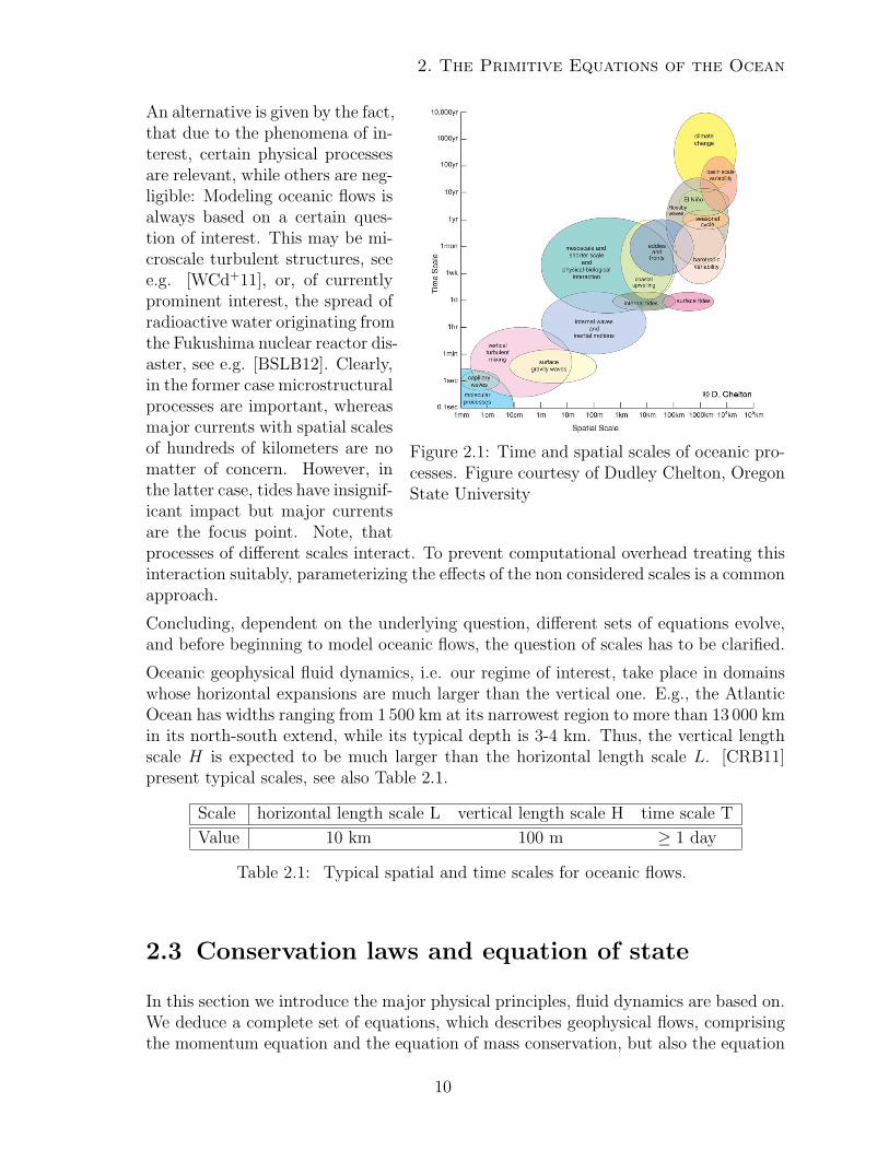
Figure 2.1 illustrates the vast amount of different acting processes occurring in theocean. Such are e.g. turbulent eddies, which last from seconds to minutes and varycentimeterwise, and the oceanic conveyor belt, which acts over thousands of kilometersand exhibit temporal cycles, which may span centuries.
No model can include all these processes. This can be highlighted by the following:Assume a set of equations, which describes ocean physics down to a minimal lengthscale of 1 cm with appropriate initial value. The earth’s surface is about 5, 1×10⁸km2,the ocean covers 70.8%, i.e. 361 × 1016cm2. Thus, already the storage of one single2D variable at a particular time necessitates 28.8 PB memory on a 64 bit architecture.Compare this to the memory capacity of the NASA Columbia Supercomputer 1, whichcurrently has a filesystem capacity of 9.3 PB 2. The attempt to model all physicsfrom small to large scale over centuries in order to gain suitable climate forecast isimpracticable.
1see http://www.nas.nasa.gov/hecc/resources/columbia.html2see http://www.nas.nasa.gov/assets/pdf/papers/2011 NAS User Survey Results.pdf
9
2. The Primitive Equations of the Ocean
Figure 2.1: Time and spatial scales of oceanic pro-cesses. Figure courtesy of Dudley Chelton, OregonState University
An alternative is given by the fact,that due to the phenomena of in-terest, certain physical processesare relevant, while others are neg-ligible: Modeling oceanic flows isalways based on a certain ques-tion of interest. This may be mi-croscale turbulent structures, seee.g. [WCd+11], or, of currentlyprominent interest, the spread ofradioactive water originating fromthe Fukushima nuclear reactor dis-aster, see e.g. [BSLB12]. Clearly,in the former case microstructuralprocesses are important, whereasmajor currents with spatial scalesof hundreds of kilometers are nomatter of concern. However, inthe latter case, tides have insignif-icant impact but major currentsare the focus point. Note, thatprocesses of different scales interact. To prevent computational overhead treating thisinteraction suitably, parameterizing the effects of the non considered scales is a commonapproach.
Concluding, dependent on the underlying question, different sets of equations evolve,and before beginning to model oceanic flows, the question of scales has to be clarified.
Oceanic geophysical fluid dynamics, i.e. our regime of interest, take place in domainswhose horizontal expansions are much larger than the vertical one. E.g., the AtlanticOcean has widths ranging from 1 500 km at its narrowest region to more than 13 000 kmin its north-south extend, while its typical depth is 3-4 km. Thus, the vertical lengthscale H is expected to be much larger than the horizontal length scale L. [CRB11]present typical scales, see also Table 2.1.
Scale horizontal length scale L vertical length scale H time scale T
Value 10 km 100 m ≥ 1 day
Table 2.1: Typical spatial and time scales for oceanic flows.
2.3 Conservation laws and equation of state
In this section we introduce the major physical principles, fluid dynamics are based on.We deduce a complete set of equations, which describes geophysical flows, comprisingthe momentum equation and the equation of mass conservation, but also the equation
10
2.3 Conservation laws and equation of state
of state, which determines the density and involves two further equations for salinityand temperature.
2.3.1 Conservation laws
Oceanic flows are covered by two major physical principles, conservation of mass andconservation of momentum. Conservation laws are of the following structure: Let ψ bea (conservative) property of interest. Given a mass element of arbitrary but fix volumeV of the fluid, the time variation, i.e. the total derivative (Dt· := ∂t ·+(v · ∇)·), of ψ∫
V
Dt(ρψ)dV =
∫V
(∂t(ρψ) + (v · ∇)(ρψ)) dV (per volume V ) and (2.5)∫V
DtψdV =∫V
(∂tψ + (v · ∇)ψ) dV (per mass∫VρdV ) (2.6)
can either vary due to
1. transport∫V−div (ρψv + Jψ)dV (per volume) and
∫V−div (ψv + Jψ)dV
(per mass), or
2. sources and sinks∫VCψdV .
The terms ρψv and ψv denote advective fluxes and Jψ the non-advective one. Thus,changes in the total amount of ψ can be described by
∂t
∫V
ρψdV =
∫V
(−div (ρψv + Jψ) + Cψ) dV and (2.7)
∂t
∫V
ψdV =
∫V
(−div (ψv + Jψ) + Cψ) dV,
respectively. As V is arbitrarily chosen, equations (2.5) and (2.6) can be replaced in alimiting process by the conservation laws
∂tρψ = −div (ρψv + Jψ) + Cψ and ∂tψ = −div (ψv + Jψ) + Cψ, (2.8)
respectively.
2.3.2 Mass budget
In the ocean, the only mass exchange takes place at boundaries, e.g. at the air-seainterface, where precipitation and evaporation take place, and boundaries with in- andoutflows, e.g. due to rivers. Thus, in the inner part of the ocean no mass sinks, sourcesor non-advective fluxes are apparent and the conservation law (per volume) for massbecomes
∂tρ = −div (ρv).
11
2. The Primitive Equations of the Ocean
2.3.3 Momentum budget
Momentum is defined as mass × velocity. Due to Newton’s 2nd law of motion (force =mass × acceleration), the conservation law (per mass) of momentum can be describedas
Dt(ρv) = f ,
whereas f collects volume and surface forces. In the scale ranges of ocean circulationmodels, the volume force is governed by gravity and rotation, i.e. we set
f v = −ρg −Θ× v
with acceleration of gravity g = (0, 0, g )>ms−2 and an angular velocity of the earthΘ = (0 , 0 , f )>s−1. The constant of gravity acceleration is given by g = −9.81, theCoriolis parameter by f = 7.29× 10⁻⁴ sinϕ with latitude ϕ. Note, that both, g and Θ,are approximately given.
The surface force occurs due to deformation of the mass element and is given byf s = div Π with symmetric stress tensor Π. The mean normal force per area is givenby p = −1
3trace(Π), i.e. the pressure. The tangential stresses are denoted by the
friction tensor Σ. For Newtonian fluids, such as the ocean, the friction force can besufficiently accurate formulated as
div Σ = div (µ∇v) +µ
3∇(divv)
with molecular viscosity µ. Thus, the equation for conservation of momentum finallyreads
Dt(ρv) = −ρg −Θ× v −∇p+ div (µ∇v) +µ
3∇(divv).
Remark 2.1. In [CRB11] it is anticipated, that the rotation of the earth has to betaken into account, only if the motion of the fluid evolves on a time scale T , which islarger than the time of one rotation, i.e. if T ≥ 2π/|θ| ≈ 24h.
2.3.4 Equation of state
For completeness of the given problem, an equation for the density field ρ is stillmissing, the equation of state. In the ocean, ρ varies due to fluctuations of pressurep, temperature T and salinity S, i.e. ρ = ρ(p, T, S), see [Gil82]. However, as water isalmost incompressible, ρ = ρ(T, S) is assumed for most applications with
ρ = ρ0
1− α(T − T0) + β(S − S0)
.
The coefficients and reference values are the thermal expansion coefficient α = 1.7 ×10⁻⁴K−1, the saline contraction coefficient β = 7.6 × 10⁻⁴ psu−1 and reference valuesρ0 = 1028kg m−3, T0 = 10C = 283K and S0 = 35 psu.
12
2.4 Approximations
2.3.5 Energy and salt budget
The temperature equation is based on the principle of energy conservation, i.e. the1st law of thermodynamics. It states, that the internal energy e of an element is thedifference between the received heat Q and the mechanical work W performed by theelement onto the ambient fluid, i.e.
Dte = Q−W.The relation between e and T is given by e = cV T with heat capacity cV = 3990J kg−1K−1
at constant volume.
In oceanic regimes no internal heat sources are apparent, i.e. the received heat Q solelyconsists of that heat, the considered element gains from its ambience by dissipativeprocesses, i.e. Q = kTρ
−1∆T with thermal conductivity constant kT .
As seawater is almost incompressible, the mechanical work W , performed by the con-sidered element, is neglected, i.e. the temperature equation becomes
ρcVDtT = kT∆T.
For the derivation of an equation for the salt budget, it is assumed, that seawaterelements conserve their salt budgets, except for diffusive transport, i.e.
DtS = κS∆S
with coefficient κs of salt diffusion.
2.4 Approximations
In this section we introduce the most relevant approximations, applied in the frameworkof geophysical fluid dynamics. These are first, the Boussinesq approximation, wherethe ”almost incompressibility” of the fluid is of advantage. Second, the Reynolds av-erage and parameterization of turbulence are applied, where small-scale processes arefiltered out of the governing set of equations (Reynolds averaging) and the impact ofthe processes of the unresolved scales on the resolved processes are modeled (param-eterization of turbulence). Third, the hydrostatic approximation is applied, in whichthe vertical momentum equation reduces to the equation of the hydrostatic balance,which adjusts, when the fluid is in equilibrium. This approximation effects, that thedynamically relevant pressure and the vertical velocity field become diagnostical, i.e.can be determined by the remaining ones. Under the assumption of a constant density(note, that the oceanic flow is almost incompressible), this approximation even effects,that the pressure becomes completely 2D.
Note, that there are lots of approximations, which are not mentioned in this chapter,such as the plane approximation or the representation of the different potentials oc-curring in the body forces of the momentum equations. For more detailed informationon these issues we refer to [Ped86, CRB11, OWE12].
13
2. The Primitive Equations of the Ocean
2.4.1 Boussinesq approximation
In the ocean, the variations of the density ρ are small compared to its constant meanvalue ρ0:
ρ = ρ0 + ρ with ρ0 = 1028 kg m−3 and |ρ| ≤ 3 kg m−3.
Note, that ρ0 is supposed to be the density, which adjusts, if the fluid is in equilibriumstate, also called the state of rest. Applicating the Boussinesq approximation meansto replace each occurrence of ρ by its approximative mean ρ0, unless ρ is dynamicallyrelevant. A first application converts the equation for the mass budget,
Dtρ+ ρ(div v) + ρ0(div v) = 0 , (2.9)
into volume conservation: The total derivative Dtρ is observed to be smaller than thesecond term on the left hand side of (2.9), see [CRB11], which again is of the order10−3 times smaller than the last term, due to ρ/ρ0 being of order 10−3. Thus, the firsttwo terms of (2.9) can be neglected and the velocity field can be regarded as divergencefree (or volume conserving):
div v = 0 . (2.10)
This equation is also called continuity equation in the mathematical framework. Con-sidering the total derivative Dt(ρ v) = ρDt v+(Dtρ) v of the momentum equation, thelatter term can be neglected, using the scaling arguments for Dtρ as presented above,and the equation of volume conservation (2.10). Approximating ρDt v by ρ0Dt v andrecalling volume conservation results in
ρ0Dt v = −ρg −Θ× v−∇p+ div (µ∇v).
Due to g = (0 , 0, g )>ms−2, the remaining impact of the non constant density ρ = ρ0+ρon the momentum solely acts on the vertical momentum equation by the terms ρ0g+ρg.The former term, ρ0g, accompanies a pressure p0, that, in the state of rest, adjusts dueto the gravity force, and is given by
p0(z) = P0 − ρ0gz (2.11)
with surface pressure P0 and p = p0 + p. The pressure p0 is called hydrostatic and phydrodynamic. The relation between ρ0 and p0 becomes comprehensive, if the momen-tum equation is considered in the state of rest, in which the velocity field is v0 = 0.Thus, the momentum equation becomes
Dt v = − ρ
ρ0
g − 1
ρ0
Θ× v− 1
ρ0
∇p+ div (ν∇v)
with kinematic viscosity ν := µρ−10 .
In a similar fashion, the temperature equation can be approximated as
DtT = κT∆T
14
2.4 Approximations
with heat kinematic diffusivity κT = kT (ρ0cV )−1. Note, that the equation of salt con-servation resulted from a conservation law, formulated per mass. Thus, the Boussinesqapproximation is not applied for this equation. For the choice of appropriate valuesfor κS and κT , the authors of [CRB11] state, that molecular diffusion mainly effectssmall-scale processes. The authors suggest to account for the apparency of turbulenceand to set the diffusivity coefficients κS and κT to the frequently applied larger valueκS = κT = κ := 10−2m2s−1.
2.4.2 Reynolds average and parameterization of turbulence
Recall that, on the one hand, oceanic flows contain a broad and interacting spectrumof scales of motion, and that on the other hand, the focus of oceanic fluid dynamicsis clearly on large scale behavior, not on small-scale ones. In contrast, the deductionof the present set of equations occasionally resulted from considerations on molecularscale.
Two tasks arise: a) to filter out the small-scale processes of the present set of equationsand b) to parameterize the impact of those small-scale processes, which are relevantfor the large-scale scenario.
To meet the first task, a given field u is decomposed, such that
u = 〈u〉 + u′ with 〈〈u〉〉 = 〈u〉 and 〈u′〉 = 0 (2.12)
applies, whereas 〈u〉 denotes a mean, e.g. the temporal average with sufficiently largeand small enough time interval, and fluctuations u′ from that mean value. Quantity〈u〉 is called Reynolds average of u and is the quantity of interest in the upcomingmodel. For different common averaging techniques see [SDT06].
Due to (2.12), Reynolds averaging the linear terms results in swapping the involvedquantity φ by 〈φ〉. Applying the averaging to the nonlinear terms results in
〈φψ〉 = 〈φ〉 〈ψ〉+ 〈φ′ψ′〉 .
Thus, the Reynolds-averaged set of equation is
div 〈v〉 = 0
∂t〈v〉+ (〈v〉 · ∇)〈v〉+∇〈v′ v′〉 = −〈ρ〉ρ0
g − 1
ρ0
Θ× 〈v〉 − 1
ρ0
∇〈p〉+ div (ν∇〈v〉)∂t〈T 〉+ (〈v〉 · ∇)〈T 〉+ div 〈v′ T ′〉 = κ∆〈T 〉∂t〈S〉+ (〈v〉 · ∇)〈S〉+ div 〈v′ S ′〉 = κ∆〈S〉
〈ρ〉 = ρ0
β(〈S〉 − S0)− α(〈T 〉 − T0)
,
which basically coincides with the non-averaged set, except for the additional terms∇〈v′ v′〉, div 〈v′ T ′〉 and div 〈v′ S ′〉. These terms represent the effect of the turbulent,
15
2. The Primitive Equations of the Ocean
unresolved scales on the resolved ones. The term ∇〈v′ v′〉 is given by
∇〈v′ v′〉 =
∂x〈u′u′〉+ ∂y〈v′u′〉+ ∂z〈w′u′〉∂x〈u′v′〉+ ∂y〈v′v′〉+ ∂z〈w′v′〉∂x〈u′w′〉+ ∂y〈v′w′〉+ ∂z〈w′w′〉
.
At this point, the second task, i.e. parameterizing the unresolved but relevant small-scale processes, is imposed. This task opens the challenging field of turbulence param-eterization. A survey of and insight into this topic is given by [SDT06]. A frequentlyused approach is proposed by Smagorinsky. We do not discuss this approach here, butrefer to [Sma63].
We apply the approach of replacing the terms ∇〈v′ v′〉, div 〈v′ T ′〉 and div 〈v′ S ′〉 withthe primary turbulent effect, diffusion (or dissipation) of the resolved quantities, seealso [Ped86, CRB11]. Due to the anisotropic behavior of large-scale oceanic flows, theappropriate eddy viscosity coefficients are distinguished between horizonal and verticalones. Both are considered to be much larger than the kinematic viscosity ν. [CRB11]suggests to assume one common horizontal eddy viscosity Ah for each of the horizontalsmall-scale parameterizations. Due to the different turbulent behavior of salinity andtemperature on the one hand and velocity on the other hand, a vertical eddy diffusivityκE is introduced for the former state variables, and a vertical eddy viscosity νE for thevelocity. Both, κE and νE are much smaller than Ah, i.e. κ, νE Ah. [Ped86] suggeststhe estimates 105 − 108cm2s−1 for Ah and 1− 103cm2s−1 for νE.
For ease of presentation, we skip the brackets of the Reynolds averaging in the up-coming and denote the Reynolds averaged quantities as v, p, T, S, ρ. Defining the eddyviscosity vector Aν := (Ah, Ah, νE)> and the diffusivity vector Aκ := (Ah, Ah, κE)>,we apply the notation (2.3). The Reynolds averaged set of equations with the intro-duced parameterization of unresolved small-scale processes is given by:
div v = 0
∂t v+(v ·∇)v = − ρ
ρ0
g − 1
ρ0
Θ× v− 1
ρ0
∇p+ ∆Aνv
∂tT + (v ·∇)T = ∆AκT
∂tS + (v ·∇)S = ∆AκS
ρ = ρ0
β(S − S0)− α(T − T0)
.
2.4.3 Hydrostatic approximation
The set of equations received at the end of the preceding section is also known as the3D incompressible Navier-Stokes equations, here formulated in a rotating frame, withanisotropic viscosities and coupled with convection - diffusion equations for temperatureand salinity, which in turn couple to the Navier-Stokes equations via the forcing ofthe momentum equations. Although this set of equations already went through alot of approximations (lots of them not being mentioned here), this set is still toocomplex for applications in geophysical fluid dynamics. In order to reduce this system
16
2.4 Approximations
noticeably while maintaining the basic physical structure we do some scale analysis,see also [Ped86, CRB11], and, at the end of this section, end up in the hydrostaticapproximation of the 3D incompressible Navier-Stokes equations.
As introduced in Section 2.2, the ratio between vertical and horizontal length scales issmall, i.e. a := HL−1 1. For oceanic flow scenarios a is of order 10−2 to 10−3. Aconsequence of this ratio results if the continuity equation is considered:
∂v1
∂x+∂v2
∂y+∂v3
∂z= 0.
Let U be the scale of the horizontal velocities v1 and v2, W be the scale of the verticalvelocity v3 and L and H be the horizontal and vertical length scales, respectively.Moreover, P denotes the scale of the pressure p. The first two terms are both of orderU/L. The last one is of order W/H, which in turn is of order U/L. Due to the smallaspect ratio we observe
W = aU .
Furthermore, let T be the time scale and have a look at the momentum equations.Each term in momentum equations we assign the appropriate scale in a subsequentline:
∂v1
∂t+v1
∂v1
∂x+v2
∂v1
∂y+v3
∂v1
∂z−Ah∂
2v1
∂x2−Ah∂
2v1
∂y2−νE ∂
2v1
∂z2− f v2 +
1
ρ0
∂p
∂x= 0
U
T
U2
L
U2
L
UW
HAh U
L2Ah U
L2νE
U
H2f U
P
ρ0L
∂v2
∂t+v1
∂v2
∂x+v2
∂v2
∂y+v3
∂v2
∂z−Ah∂
2v2
∂x2−Ah∂
2v2
∂y2−νE ∂
2v2
∂z2+ f v1 +
1
ρ0
∂p
∂y= 0
U
T
U2
L
U2
L
UW
HAh U
L2Ah U
L2νE
U
H2f U
P
ρ0L
∂v3
∂t+v1
∂v3
∂x+v2
∂v3
∂y+v3
∂v3
∂z−Ah∂
2v3
∂x2−Ah∂
2v3
∂y2−νE ∂
2v3
∂z2+
1
ρ0
∂p
∂z=
ρ
ρ0
g
W
T
UW
L
UW
L
W 2
HAhW
L2AhW
L2νE
W
H2
P
ρ0H
with ρ−10 Θ × v ≈ f(−v, u, 0)> and Coriolis parameter f = 2Θ sin θ ≈ 10−4s−1, see e.g.
[Ped86], with latitude θ and rotation of the earth Θ. Due to the order of W we deduce,that UW/H is of order U2/L. Considering the horizontal momentum equations thusleads to
P = ρ0U max
L
T, U, AhL−1, νEH
−2L, f L
Anticipating, see also Section 2.6.3, we reformulate the terms AhL−1 and νEH
−2Lby use of the horizontal and vertical Ekman numbers, Ekh = Ah(f L2)−1 and Ekv =
17
2. The Primitive Equations of the Ocean
νE(f H2)−1:
AhL−1 = Ekh L f, νEH−2L = Ekv L f .
In oceanic flows, i.e. for the presumed parameter setting of the Coriolis force theviscosities, the Ekman numbers are less than 1. I.e., the diffusive terms subordinatethe Coriolis terms and we have
P = ρ0U max
L
T, U, f L
.
Thus, the pressure dependent term in the vertical momentum equation is of order
P
ρ0H=U max
LT, U, f L
H
=UL
Hmax
1
T,U
L, f
.
The remaining terms on the left hand side of the vertical momentum equation are, intotal, of order
W max
1
T,U
L,W
H,Ekh f, Ekv f
and, due to the order of W , the ratio between the latter two terms is
W max
1T, UL, WH, Ekh f, Ekv f
ULH
max
1T, UL, f = a2 max
1T, UL, Ekh f, Ekv f
max
1T, UL, f ,
which is of order a2. As the aspect ratio a is small the vertical momentum equationfinally can be approximated by the hydrostatic balance
∂p
∂z= ρg .
2.5 Initial and boundary conditions
In this section we collect the still missing initial and boundary conditions. Note,that these conditions are attempts to model the behavior at initial time and on theboundaries, and are no physical principles. Moreover, if we assume, that the domainof interest is not surrounded by land, but by other flow regimes, different conditionshave to be applied.
2.5.1 Initial conditions
State variables are the horizonal velocity components v1, v2, the temperature T andsalinity S. The remaining variables are diagnostic, i.e. can be determined via the statevariables. No initial data are necessary for those.
18
2.5 Initial and boundary conditions
Initial values may be given by monthly mean values, based on a data record, whichcontains observational data, see e.g. [LBC+98].
Let (v1,0, v2,0, T0, S0) be the given the initial data such that
v1(x, y, z, 0) = v1,0(x, y, z), v2(x, y, z, 0) = v2,0(x, y, z),
T (x, y, z, 0) = T0(x, y, z), and S(x, y, z, 0) = S0(x, y, z)
apply for all (x, y, z) ∈ Ω.
2.5.2 Boundary conditions
On the bottom of the domain Γb, and on the side walls Γs, no-slip boundary conditionsare presumed for the horizontal velocity components v1 and v2, i.e.
v1 = v2 = 0 on (Γb ∪ Γs)× (0, T ) .
This approach has the disadvantage, that a boundary layer is imposed. Alternatively,slip boundary conditions can be imposed, i.e.
∂n(v1, v2) = 0 on (Γb ∪ Γs)× (0, T ) ,
as well as suitable inflow or outflow conditions with transient boundaries. We restrictto homogeneous Dirichlet boundary conditions.On the surface of the domain, the crucial impact, the wind stress, is modeled by
∂z(v1, v2) = (ρ0νE)−1τ on Γu × (0, T )
with wind stress τ . Due to the rigid lid approximation on the surface,
v3 = 0 on Γu × (0, T )
is indicated for the vertical velocity component v3. Moreover, as the fluid is assumedto be incompressible, we have
v3 = 0 on Γb × (0, T ) (2.13)
v3 = −z∫
−d(x,y)
(∂xv1 + ∂yv2) dz on Γs × (0, T ) . (2.14)
Similar to the horizontal velocity field, the boundary conditions for temperature andsalinity are given by
−κ∂zT = θT −κ∂zS = θS on Γu × (0, T )
T = 0 S = 0 on (Γs ∪ Γb)× (0, T )
with functions θT and θS, which depend on the wind speed, the moisture, cloudinessetc.
19
2. The Primitive Equations of the Ocean
2.6 Governing set of equations
The governing set of oceanic circulation models is called primitive equations. In thissection we introduce this set, collecting all previous considerations. Moreover, weassume full incompressibility and end up in the hydrostatic Navier-Stokes equations,which are the central set of equations of this work. We finish the section with aconsideration of relevant dimensionless numbers, which describe the characteristics ofthe considered fluid. Such are the Rossby, the Ekman and the Reynolds number.
2.6.1 Primitive Equations
Before assembling the set of primitive equations, we reformulate the continuity equa-tion. Using the boundary conditions for the vertical velocity component (2.13) and(2.14), the equation of volume conservation can be reformulated as
0∫−d(x,y)
(∂xv1 + ∂yv2) dz = 0 in ω × (0, T ).
In the upcoming let v := (v1, v2). Applying the abbreviation M for the vertical inte-gration as defined in (2.4) and the Leibniz integration rule, the continuity equation isgiven by
div ′(Mv) = 0 in Ω× (0, T ).
Recall the approximation ρ−10 Θ×v ≈ f v⊥ with v⊥ = (−v2, v1)> and Coriolis parameter
f = 10−4s−1, see e.g. [Ped86]. Moreover, we set ρ := ρ/ρ0 and p = p/ρ0. The primitive
20
2.6 Governing set of equations
equations finally are given by:
div ′(Mv) = 0 in Ω× (0, T ) (2.15)
v3(t, x, y, z) = −z∫
−d(x,y)
div ′ v dz in Ω× (0, T ) (2.16)
Dt v−∆Aνv + f v⊥ +∇′p = 0 in Ω× (0, T ) (2.17)
∂zp = −ρg in Ω× (0, T ) (2.18)
DtT −∆AκT = 0 in Ω× (0, T ) (2.19)
DtS −∆AκS = 0 in Ω× (0, T ) (2.20)
ρ = β(S − S0)− α(T − T0) in Ω× (0, T ) (2.21)
v, T, S = 0 on (Γb ∪ Γs)× (0, T ) (2.22)
∂zv = (ρ0νE)−1τ on Γu × (0, T ) (2.23)
−κ∂zT = θT on Γu × (0, T ) (2.24)
−κ∂zS = θS on Γu × (0, T ) (2.25)
v(x, y, z, 0) = v0(x, y, z) in Ω× 0 (2.26)
T (x, y, z, 0) = T0(x, y, z) in Ω× 0 (2.27)
S(x, y, z, 0) = S0(x, y, z) in Ω× 0 (2.28)
2.6.2 Evolutionary 2.5D Navier-Stokes equations
In the following we apply a further simplification: Under the assumption of absent strat-ification, i.e. ρ = 0, [CRB11] conclude, that p can be considered to be z-independentand geophysical flows tend to be hydrostatic, even if significant movement is apparent.The only remnant of the primary vertical momentum balance is thus given by the hy-drostatic balance, p0(z) = P0 − ρ0gz, which has already been retrieved in the contextof the Boussinesq approximation. As the variations of the density completely vanishfrom the system, we can also neglect the equations for the temperature and salinity, asthey are no longer dynamically relevant. Recalling, that we introduced the horizontal
21
2. The Primitive Equations of the Ocean
velocity field v := (v1, v2) we end up in the problem set:
div ′(Mv) = 0 in Ω× (0, T ) (2.29)
v3(t, x, y, z) = −z∫
−d(x,y)
div ′ v dz in Ω× (0, T ) (2.30)
∂t v+((v, v3) · ∇)v −∆Aνv + f v⊥ +∇′p = 0 in Ω× (0, T ) (2.31)
v = 0 on Γw × (0, T ) (2.32)
∂zv = (ρ0νE)−1τ on Γu × (0, T ) (2.33)
v(x, y, z, 0) = v0(x, y, z) in Ω× 0 . (2.34)
Note, that the vertical variations of the pressure field has already been described in thehydrostatic balance equation. Thus, the dynamically relevant pressure p becomes 2D,but still is embedded in a 3D problem. Moreover, we emphasize, that the originally3D divergence constraint is now vertically averaged and thus corresponds to the 2Dpressure, and vice versa. Thirdly, we only consider the horizontal momentum equations.Due to these reasons, we call this set the set of (incompressible) 2.5D Navier-Stokesequations. In the upcoming, this set is also called hydrostatic Navier-Stokes equations.
2.6.3 Dimensionless quantities
In Section 2.2 we already sketched, that different scenarios lead to different behaviorsof the considered fluid. Characteristics of such geophysical flows correlate with cer-tain, typical dimensionless key quantities, such as the Ekman number or the Reynoldsnumber. To retrieve these quantities, the hydrostatic Navier-Stokes equations are nor-malized.
Let L, H, T , U and W be the characteristic scales for horizontal length, vertical length,time, horizontal and vertical velocity, respectively. Note, that T = L/U . We considerthe normalized quantities
t∗ =t
T, x∗ =
x
L, y∗ =
y
L, z∗ =
z
H, v∗ =
v
U, v∗3 =
v3
W, p∗ =
1
U2p .
For ease of clarity, we use the full 3D divergence constraint div (v, v3) = 0 in theformulation of the normalized hydrostatic Navier-Stokes equations. Note, that thisequation with the appropriate boundary conditions (which we assumed) is equivalentto (2.29) – (2.30).
22
2.6 Governing set of equations
The term div (v, v3) = 0 and the terms occurring in (2.31) become
div ∗(v∗, v∗3) =L
Udiv ′ v+
H
W∂zv3 ,
∂t∗ v∗ =
L
U2∂t v,
((v∗, v∗3) · ∇∗)v∗ =
((L
U2v,
H
U Wv3
)· ∇)v,
∇′∗p∗ =L
U2∇′p ,
∆∗Aνv∗ =
L2
UAh∂xx v+
L2
UAh∂yy v+
H2
UνE∂zz v ,
the maximal time is T ∗ = T−1T and the domain is given by
Ω∗ :=x∗ ∈ R3 | (Lx∗, Ly∗) ∈ ω and z∗ ∈ (−d∗(Lx∗, Ly∗), 0)
with depth function d∗(Lx∗, Ly∗) = H−1d(x, y). The normalized hydrostatic Navier-Stokes equations in Ω∗ × (0, T ∗) are given by
div ′∗ v∗ +WL
UH∂z∗v
∗3 = 0
∂t∗ v∗+
((v∗,
WL
UHv∗3
)· ∇∗
)v∗+
f L
Uv∗⊥ +∇′∗p∗
−(AhUL
∂x∗x∗ v∗+AhUL
∂y∗y∗ v∗+
LνEUH2
∂z∗z∗ v∗)
= 0
The initial and boundary conditions are given appropriately. Following [CRB11], theratio WL(UH)−1, occurring twice in the normalized context, is on the order of theRossby number
Ro :=U
f L.
It compares the advection to the Coriolis force and is a fundamental number in thecontext of geophysical fluid dynamics. Due to the scales of the underlying regime,Ro ≤ 1 applies. Cushman-Roisin and Beckers emphasize, that the characteristicsof oceanic flows are highly sensitively related to the Rossby number. The secondimportant dimensionless number is the Reynolds number, which is defined as
Re :=UL
νE.
It is an important number for non rotating fluids and describes the relation betweeninertia forces and friction. Oceanic regimes show very large Reynolds numbers up tothe order 1011, if molecular viscosity has been used in the definition of the Reynoldsnumber. Large values of Re are reflected in turbulent behavior.
Note, that for flows with large Reynolds number, special attention has to be payednear boundaries with a no slip condition, where strong gradients of the velocity mightoccur, as v is of order U in the inner part of the domain and zero on the boundary.
23
2. The Primitive Equations of the Ocean
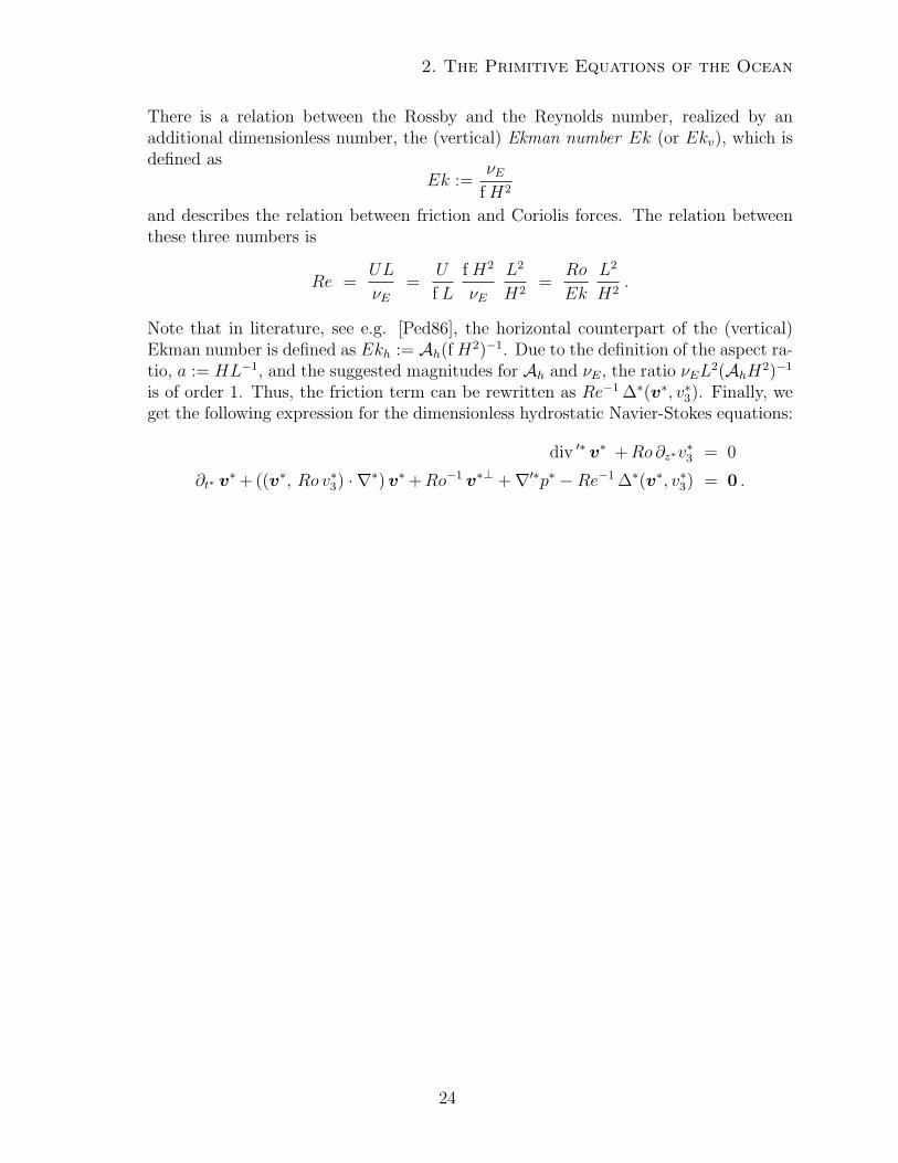
There is a relation between the Rossby and the Reynolds number, realized by anadditional dimensionless number, the (vertical) Ekman number Ek (or Ekv), which isdefined as
Ek :=νE
f H2
and describes the relation between friction and Coriolis forces. The relation betweenthese three numbers is
Re =UL
νE=
U
f L
f H2
νE
L2
H2=
Ro
Ek
L2
H2.
Note that in literature, see e.g. [Ped86], the horizontal counterpart of the (vertical)Ekman number is defined as Ekh := Ah(f H2)−1. Due to the definition of the aspect ra-tio, a := HL−1, and the suggested magnitudes for Ah and νE, the ratio νEL
2(AhH2)−1
is of order 1. Thus, the friction term can be rewritten as Re−1 ∆∗(v∗, v∗3). Finally, weget the following expression for the dimensionless hydrostatic Navier-Stokes equations:
div ′∗ v∗ +Ro∂z∗v∗3 = 0
∂t∗ v∗+ ((v∗, Ro v∗3) · ∇∗)v∗+Ro−1 v∗⊥ +∇′∗p∗ −Re−1 ∆∗(v∗, v∗3) = 0 .
24
Chapter 3
Variational Formulation ofHydrostatic Flow Problems
The variational framework on the one hand enables the discussions on existence,uniqueness and regularity of a solution of the underlying problem, especially in thecontext of complex flow problems, where a solution in the continuous framework isoften not known (recall the seventh millennium problem of the Clay institute). Onthe other hand, it provides a suitable approach to the formulation and analysis of thediscretized problems, which form the basis of numerical simulations.
Preliminary, we present basic notations in the variational context, which accompanyus through the remaining of this work. We then introduce methods for the proofs ofexistence and uniqueness of solutions for classical, non hydrostatic problems. Thesetechniques apply also in the hydrostatic framework in a similar fashion. The point ofthat survey is to recall the proving techniques and to get an impression, where theregularity results, collected later in this chapter, stem from.
After the presentation of these methods, we turn to the hydrostatic framework, particu-larly, analyze the variational averaging operator and the inf-sup constraint, formulatedin Sobolev spaces of arbitrary regularity p ∈ (1,∞). In this context, we also exam-ine the δmin-dependence of the appropriate inf-sup constant and find out, that thisinf-sup constant behaves as the classical counterpart. In [KB12], we developed thesestatements for the case p = 2.
In the Sections 3.2 and 3.2, we present the variational formulations of hydrostaticflow problems and give an overview over existence and uniqueness results, known fromliterature. We start from the less complex problem: the stationary hydrostatic Stokesproblem, add advection to the system, i.e. consider the Oseen case, and turn to theappropriate nonlinear case. Afterwards we treat the evolutionary case, beginning withthe linear problem and then turning to the nonlinear problem, i.e. the evolutionaryhydrostatic Navier-Stokes equations (2.29) – (2.34). The collection of the regularitystatements is not only interesting in the context of existence and uniqueness theory,but is also rather important for error estimates, in which the regularity of the solutiondetermines the order of convergence. In the majority of the literature, the impact of
25
3. Variational Formulation of Hydrostatic Flow Problems
temperature and salinity is neglected. We also do not present regularity results forthese variables, but refer to [Zia97] for the stationary hydrostatic Stokes system andto [LTW92, CT07] for the evolutionary hydrostatic Navier-Stokes problem.
In order to understand the regularity impact of the hydrostatic approximation withrespect to existence and uniqueness theory, we close the chapter with a comparisonof the regularity results of the non hydrostatic flow problems with their hydrostaticcounterpart. Note, that the majority of the available analysis on the non hydrostaticpart is settled in the framework of Dirichlet boundary conditions, whereas in mostof the literature for the hydrostatic problems a mixture of Dirichlet and Neumannboundary conditions is imposed. As the main emphasis is not put on the topic of nonhydrostatic problems, we present a rather rough collection of the main propositions.For more detailed informations, the reader is referred to the cited literature.
3.1 Fundamentals
We start this section with a presentation of basic notations, also broadening thePoincare–Friedrichs inequality to the case of Sobolev spaces with arbitrary regular-ity p ∈ (1,∞). Then, we consider the variational formulation of the averaging operatorwith respect to well-posedness, linearity, continuity and surjectivity in Sobolev spaceswith arbitrary regularity p ∈ (1,∞). We finish the section with the consideration ofthe modified inf-sup constraint, formulated in the Sobolev framework with arbitraryregularity p ∈ (1,∞).
3.1.1 Domain and space definitions
Let n ∈ 2, 3. Given an simply connected, open, bounded surface domain ω ⊂ Rn−1
and a positive depth function d : ω → R≥0, the underlying domain Ω ⊂ Rn is definedas
Ω := x = (x, y, z) ∈ Rn | (x, y) ∈ ω and z ∈ (−d(x, y), 0) ,
see also Section 2.1 for the 3D case. We take over the boundary notations, defined inthat section.
Let δmin > 0, unless noted differently.The domain Ω is a Lipschitz domain, if ∂Ω is partially Lipschitz, see also [Bra07]. Fora given p ≥ 1, we call Ω a Cp– domain, if the boundary ∂Ω is a 2D manifold of classCp. Throughout this work, we consider Ω to be a Lipschitz domain. In particular, it issimply connected.
For any p ∈ N, we denote the space of Lebesgue-integrable functions v with∫
Ω|v|p dx <
26
3.1 Fundamentals
∞ as Lp(Ω). Equipped with the norm
||v||p,Ω :=
(∫
Ω|v|p dx)1/p
, if p <∞ess supx∈Ω ||v(x)||, else,
Lp(Ω) forms a Banach space. We set
Lp0(Ω) :=
v ∈ Lp(Ω) | ∫Ω
v dx = 0
.
The Sobolev spaces Wk,p(Ω)consist of those functions v ∈ Lp(Ω) with distributionalderivatives Dαv ∈ Lp(Ω)d for all |α| ≤ k. Provided with the norm
||v||k,p,Ω :=
( ∑|α|≤k
∫Ω|Dαv|p dx
)1/p
, if p <∞
max|α|≤k||Dαv||0,∞,Ω else,
Wk,p(Ω) is a Banach space. For p < ∞, Wk,p(Ω) is separable. The appropriate seminorms are given by
|v|k,p,Ω :=
( ∑|α|=k
∫Ω|Dαv|p dx
)1/p
, if p <∞
||Dαv||0,∞,Ω else.
For p = 2, the spaces L2(Ω) and Hk(Ω) := Wk,2(Ω) are Hilbert spaces, if equipped withthe norm-inducing scalar products
(u, v)Ω :=
∫Ω
uv dx and (u, v)Ω,k :=∑|α|≤k
(Dαu,Dαv)Ω ,
respectively. We abbreviate | · |k,Ω := | · |k,2,Ω, || · ||Ω := || · ||2,Ωand || · ||k,Ω := || · ||k,2,Ω.Note, that there is an overlap in the definition of || · ||k,Ω with the definition of thenorm of Lp(Ω). If the application of that expression is ambiguous, we will denotethe underlying notion explicitely. Due to the existence of a continuous trace operatorγ : H1(Ω)→ L2(∂Ω) with γ(v) = v|∂Ω and due to the Sobolev embedding theorem, thespaces
H10(Ω) := v ∈ H1(Ω) | v|∂Ω = 0 and H1
b(Ω) := v ∈ H1(Ω) | v|Γs∪Γb = 0 ,W1,p
0 (Ω) := v ∈W1,p(Ω) | v|∂Ω = 0 and W1,pb (Ω) := v ∈W1,p(Ω) | v|Γs∪Γb = 0
for p ≥ 2 are well-defined. Considering the Poincare – Friedrichs inequality, ||v||Ω ≤cΩ|v|1,Ω for all v ∈ H1
0(Ω), the semi norm | · |1,Ω defines a norm on H10(Ω). Due to
the structure of the appropriate proof, see e.g. [Bra07], this inequality also holds forv ∈ H1
b(Ω). The following lemma, which is a generalization of the Poincare – Friedrichsinequality, states, that the semi norm | · |1,p,Ω also defines a norm on W1,p
0 (Ω).
27
3. Variational Formulation of Hydrostatic Flow Problems
Lemma 3.1. Let Ω ⊂ Rn, n ∈ N, be contained in an n-dimensional cube of side lengths ∈ R. Then,
||v ||0,p,Ω ≤ s1/q|v |1,p,Ω ∀v ∈W1,p0 (Ω)
applies for any p ∈ (1,∞) and q with 1/p+ 1/q = 1.
Proof. The proof is similar to the proof of the classical Poincare – Friedrichs inequality,see [Bra07]. As C∞0 (Ω) is dense in W1,p
0 (Ω), it suffices to prove the proposition forv ∈ C∞0 (Ω). Supposing Ω ⊂ C := (x1, . . . , xn) | 0 < xi < s ∀i ∈ 1, . . . , n and v = 0for x ∈ C \ Ω, we get
v(x1, . . . , xn) = v(0, x2, . . . , xn) +
∫ x1
0
∂x1 v(t, x2, . . . , xn) dt.
Application of the Holder inequality and gives
|v(x)|p ≤ sp/q∫ s
0
|∂x1 v(t, x2, . . . , xn)|p dt.
Integration along x1 and along the remaining coordinates finally assures
||v ||p0,p,Ω ≤ sp/q|v |p1,p,Ω .
Constant cω := s1/q is called Poincare–Friedrichs constant.
For a given Lebesgue space Lp(Ω), the appropriate dual space [Lp(Ω)]′ is given byLq(Ω) with 1/p + 1/q = 1 (q = ∞ if p = 1). For a given Sobolev space Wk,p
0 (Ω),the appropriate dual space is defined as [Wk,p
0 (Ω)]′ := W−k,q(Ω), for p = 2 we set[Hk
0(Ω)]′ = H−k(Ω). Dependent on the underlying space Wk,p0 (Ω), let 〈·, ·〉 denote the
duality between W−k,q(Ω) and Wk,p0 (Ω). If we attempt to emphasize the underlying
domain D, we write 〈·, ·〉D. Given a Hilbert space H, we can interprete each elementf ∈ H′ as a suitable element y ∈ H, due to the following theorem.
Theorem 3.2 (Riesz representation Theorem). Let H be a Hilbert space, equipped withscalar product (·, ·)H, norm || · ||H and dual space H′. For any f ∈ H′, there is a uniqueyf ∈ H with ||f ||H = ||yf ||H, s.t.
f(x) = (x, yf )H ∀x ∈ H .
Conversely, for any y ∈ H, there is a fy ∈ H′ with ||fy||H = ||y||H s. t.
fy(x) = (x, y)H ∀x ∈ H .
Proof. See [Yos80].
28
3.1 Fundamentals
Note, that this theorem is applied when theoretical results concerning existence anduniqueness of a solution (see e.g. Theorem 3.3 of Lax-Milgram) are used to validateexistence and uniqueness results of problems whose right hand sides are formulatedas (f ,ϕ)Ω instead of f(ϕ). A suitable interpretation is thus provided by the Rieszrepresentation Theorem.
Vector-valued spaces are denoted bold-faced, e.g. L2(Ω),H10(Ω), etc. The norms are
interpreted appropriately.
For an interval [0, T ], Banach space B and 1 ≤ p ≤ ∞, Lp(0, T ;B) denotes the spaceof Lp-integrable functions mapping from [0, T ] to B. Equipped with the norm
||f ||Lp(0,T ;B) :=
( T∫
0
||f(t)||pB dt
)1/p
, if p <∞
ess sup0≤t≤T ||f(t)||B, else ,
it forms a Banach space, see e.g. [Tem79]. If B denotes a Hilbert space with scalarproduct (·, ·)B, then Lp(0, T ;B) also denotes a Hilbert space with norm-inducing scalar
product∫ T
0(·, ·)B dt.
3.1.2 Methods
We present fundamental theorems and methods for the existence and uniqueness anal-ysis of incompressible flow problems and outline the proofs, in order to show basicconcepts, which also find application in the hydrostatic context.
For sake of brevity we assume homogeneous Dirichlet boundary conditions on ∂Ω.Moreover, let V := H1
0(Ω) and Q := L20(Ω) be the variational spaces for the velocity
and the pressure. Without loss of generality, we assume an isotropic viscosity, i.e.ν = Ah = νE > 0.
Stationary linear problems
Incompressible flow problems show a saddle point structure, which reveals due to the di-vergence constraint and the pressure gradient. Given Hilbert spaces V and Q, equippedwith the norms ||·||V and ||·||Q, with dual spaces V′ and Q′, as well as continuous bilinearforms
a : V×V→ R, a(v,ϕ) := ν(∇v,∇ϕ)Ω + f(v⊥,ϕ)Ω and (3.1)
b : Q×V→ R, b(ξ,v) := (div v, ξ)Ω , (3.2)
with viscosity ν > 0 and Coriolis force f ≥ 0, the saddle point problem is defined as
Given f ∈ V′, find (v, q) ∈ V×Q s. t.
a(v,ϕ) − b(q,ϕ) = 〈f ,ϕ〉 ∀ϕ ∈ Vb(ξ,v) = 0 ∀ξ ∈ Q (3.3)
29
3. Variational Formulation of Hydrostatic Flow Problems
The element q ∈ Q, i.e. the pressure, plays the role of the Lagrangian multiplier of thesecond equation,
b(ξ,v) = 0 ∀ξ ∈ Q ,the divergence constraint. Incorporating this condition into the variational space V,i.e. restricting V to J1 := v ∈ V | b(q,v) = 0 ∀q ∈ Q, results in the elliptic problem
Given f ∈ V′, find v ∈ J1 s. t. a(v,ϕ) = 〈f ,ϕ〉 ∀ϕ ∈ J1 . (3.4)
For the present flow problem, the space J1 is defined as the space of divergence freefunctions, i.e.
J1 := v ∈ V | div v = 0 . (3.5)
Unique solvability of this problem can be validated due the following considerations.
Theorem 3.3 (Lax Milgram Lemma). Let H be a Hilbert space equipped with norm|| · || and dual space H′. If the bilinear form a : H×H→ R is continuous, i.e.
a(v,ϕ) ≤ α1||v || ||ϕ || ∀ v,ϕ ∈ H ,
and coercive (or H – elliptic), i.e.
a(v,v) ≥ α2||v ||2 ∀ v ∈ H ,
then for any f ∈ H′ there is a unique solution v ∈ H of
a(v,ϕ) = f(ϕ) ∀ϕ ∈ H .
Proof. See [Pet65].
Assuming a continuous and coercive bilinear form a : J1×J1 → R, let v ∈ J1 be the(unique) solution of problem (3.4). In order to assure a solution (v, q) ∈ V×Q of (3.3),the element q ∈ Q has to fulfill
b(q,ϕ) = a(v,ϕ)− 〈f ,ϕ〉 ∀ϕ ∈ V . (3.6)
Let the operator B : Q→ V′ and the linear operator l ∈ V′ be defined as
〈Bq,ϕ〉 := b(q,ϕ) and l(ϕ) := a(v,ϕ)− 〈f ,ϕ〉 ∀ϕ ∈ V .
Note, that the functional l is element of the annihilator of J1 in V′, i.e. J1 := l ∈V′ | l(ϕ) = 0 ∀ϕ ∈ J1. Thus, the question of existence and uniqueness of an elementq ∈ Q that satisfies (3.6) can be formulated as the search for a (unique) q ∈ Q, suchthat Bq = l applies for an arbitrarily given l ∈ J1. For a suitably determined constantγ > 0, Braess proves the equivalence of the following two statements, [Bra07]:
(a) The operator B : Q → J1 ⊂ V ′ is an isomorphism with ||Bq||V′ ≥ γ||q||Q for anyq ∈ Q.
30
3.1 Fundamentals
(b) The inf-sup condition applies:
infq∈Q
supv∈V
b(q,v)
||v ||V||q||Q ≥ γ . (3.7)
In the context of non hydrostatic flow problems, the element q ∈ Q represents thepressure, v ∈ V the velocity field. The variational spaces are given by Q := L2
0(Ω)and V := H1
0(Ω) (assuming homogeneous Dirichlet conditions on ∂Ω). Bilinear formb : V×Q → R is defined as b(v, q) := (div v, q)Ω . The authors of [AG94] presentedthe validity of (3.7), proceeding on De Rham Lemma, i.e.
Theorem 3.4 (De Rham Lemma). Let Ω ⊂ Rn, n ≥ 2 be an open set and V = v ∈D(Ω) | div v = 0. If the distribution l ∈ D(Ω) satisfies 〈l,ϕ〉 = 0 for any ϕ ∈ V,then there is a distribution p ∈ D′(Ω) with l = ∇p.
Proof. See [dR60].
Stationary nonlinear problems
The nonlinear case distinguishes oneself by the additional nonlinear advection term
c(v,v,ϕ) := ((v · ∇)v,ϕ)Ω . (3.8)
We observe c(b,v,v) = 0 for any b ∈ J1 and any v ∈ V. As in the linear case,the pressure can be decoupled from the governing system and be retrieved by themomentum equation and a velocity, which has been determined beforehand. Due tothe nonlinearity of the problem, the previously introduced mechanisms can not beapplied. Instead, the construction of a Galerkin approximation, as well as applicationof the Brouwer’s fixed point Theorem and appropriate compactness results, provide asuitable handling of the problem.
Theorem 3.5 (Brouwer’s fixed point Theorem). Let B be a closed n-dimensional unitball, n ∈ N, and f : B → B be continuous. Then there is a x∗ ∈ B, such thatf(x∗) = x∗
Proof. See e.g. [Sca67].
Theorem 3.6 (Sobolev Embedding Theorem). Let Ω ⊂ Rn, n ∈ N, be a Lipschitzdomain, m ≥ 1 and p ∈ [1,∞).
(a) If mp > n or m = n and p = 1, then Wm,p(Ω) → Lq(Ω) for p ≤ q ≤ ∞.
(b) If mp = n, then Wm,p(Ω) → Lq(Ω) for p ≤ q <∞.
(c) If mp < n, then Wm,p(Ω) → Lq(Ω) for p ≤ q ≤ np/(n−mp).
(d) Propositions (a) and (b) are valid for arbitrary domains Ω, if homogeneous Dirich-let boundary conditions are implied on ∂Ω.
31
3. Variational Formulation of Hydrostatic Flow Problems
(e) If mp > n, then Wm,p(Ω) → C(Ω).
Proof. See e.g. [AF03, Wer05, Jos98].
Lemma 3.7 (Generalized Holder Inequality). Let p, q, r ∈ (1,∞), and f ∈ Lp(Ω),g ∈ Lq(Ω), h ∈ Lr(Ω), such that 1/p+ 1/q + 1/r = 1. Then fg h ∈ L1(Ω) and
||fg h||0,1,Ω ≤ ||f ||0,p,Ω ||g||0,q,Ω ||h||0,r,Ω .
Proof. The proof is an easy exercise, based on the common Holder inequality:
If 1/s+ 1/t = 1, f ∈ Ls(Ω) and g ∈ Lt(Ω), (3.9)
then fg ∈ L1(Ω) with ||fg||0,1,Ω ≤ ||f ||0,s,Ω ||g||0,t,Ω .We first validate an altered version:
If 1/p+ 1/q = 1/r′, f ∈ Lp(Ω) and g ∈ Lq(Ω),
then fg ∈ Lr′(Ω) with ||fg||r′,0,Ω ≤ ||f ||p,0,Ω||g||q,0,Ω .
Defining s = p/r′ and t = q/r′, we can apply (3.9) and get
||fg||0,r′,Ω =
(∫Ω
|f |r′|g|r′dx)1/r′
≤(||f ||p/s0,p,Ω ||g||q/t0,q,Ω
)1/r′
= ||f ||0,p,Ω ||g||0,q,Ω.
Let r′ be chosen, such that 1/r′ + 1/r = 1. We thus get
||fg h||0,1,Ω ≤ ||fg||0,r′,Ω ||h||0,r,Ω ≤ ||f ||0,p,Ω ||g||0,q,Ω ||h||0,r,Ω .
Theorem 3.8 (Rellich – Kondrachov). Let Ω ⊂ Rn, n ∈ N, be an open, boundedLipschitz domain. For p ∈ [1, n) and p∗ := np/(n− p), W1,p(Ω) is
(a) continuously embedded in Lq(Ω) with q ∈ [1, p∗] and
(b) compactly embedded in Lq(Ω) with q ∈ [1, p∗).
Proof. See [HK00].
The argumentation for existence of a solution is as follows, see also [Tem79]: As V0
is a subspace of H1(Ω), J1 is separable and we can assume finite-dimensional subsetsVm ⊂ J1, such that ∪m∈N Vm is dense in J1. We denote Vm := spanw1, . . . ,wm withbasis functionsw1, . . . ,wm. Thus, any v ∈ V0 can be represented as v =
∑∞m=1 αmwm
with suitable constants αm.
In the Galerkin approximation of the nonlinear problem, J1 is approximated by Vm,i.e. we get:
Find vm ∈ Vm s. t. a(vm,ϕ) + c(vm,vm,ϕ) = 〈f ,ϕ〉 ∀ϕ ∈ Vm . (3.10)
32
3.1 Fundamentals
In order to elaborate unique existence of (3.10), we linearize the problem by introduc-tion of the mapping Qm : Vm → Vm, which, for a given vm ∈ Vm, is defined as thesolution of
a(Qm(vm),ϕ) + c(vm, Qm(vm),ϕ) = 〈f ,ϕ〉 ∀ϕ ∈ Vm (3.11)
Lipschitz continuity of a(·, ·)+c(vm, ·, ·), and thus continuity, can be guaranteed by The-orem 3.6 and Lemma 3.7. Coercivity results from a(Qm(vm), Qm(vm)) = ν|Qm(vm)|21,Ωand c(vm, Qm(vm), Qm(vm)) = 0. Application of Theorem 3.3 assures a unique solu-tion, i.e. Qm(vm) is uniquely determined.Obviously, Qm : Bm → Bm, whereas Bm := v ∈ Vm | |v |1,Ω ≤ ν−1||f ||−1. Moreover,Qm : Bm → Bm is continuous, which can be validated by diagonal testing (3.11) andrecalling c(vm, Qm(vm), Qm(vm)) = 0, which leads to |Qm(vm)|1,Ω ≤ ν−1||f ||−1. Thenorm || · ||−1 is defined with respect to | · |1,Ω, i.e.
||f ||−1 := supϕ∈V
〈f ,ϕ〉|ϕ |1,Ω .
Thus, we have
||Qm|| := supvm∈Bm
|Qm(vm)|1,Ω|vm |1,Ω ≤ 1.
By means of a suitable transformation from the unit ball B ⊂ J1 to Bm, Brouwer’sfixed point Theorem 3.5 assures existence of a solution of (3.10), see also [Ist01]. Thus,the solutions vm, m ∈ N, define a bounded sequence in J1. Moreover, J1 is compactlyembedded in
J0 := v ∈ L2(Ω) | div v = 0 and v ·n|∂Ω = 0 , (3.12)
whereas v ·n|∂Ω is meant in the H−1/2(∂Ω)-sense, see also Theorem 3.8. Thus, thesequence (vm)m∈N is relatively compact, i.e. there is a subsequence (vmk)k∈N which isconvergent. I.e. existence of a solution of the nonlinear, infinite dimensional problemis assured. The pressure can be recovered as in the linear case.
For uniqueness, assume two solutions, v1,v2 ∈ B := v ∈ V | |v |1,Ω ≤ ν−1||f ||−1.Application of Lemma 3.7 and the observation, that c(b,v,v) = 0 for any b ∈ J1 andany v ∈ V, leads to the estimate |v1−v2 |21,Ω (1 − c2
Ων−2||f ||−1) ≤ 0. Thus, the
solution is unique, if c2Ων−2||f ||−1 ≤ 1.
Evolutionary problems
We now expand the stationary (nonlinear) problem to the evolutionary case, i.e. weadd the term (∂t v,ϕ)Ω, demand suitable initial conditions v(0) = v0 and consider theset of equations in a time interval (0, T ). The evolutionary problem is given by
Find v ∈ L∞(0, T ; J0) ∩ L2(0, T ; J1) (3.13)
s. t. (∂t v,ϕ)Ω + a(v,ϕ) + c(v,v,ϕ) = 〈f ,ϕ〉 ∀ϕ ∈ J1 .
Solutions of (3.13) are subdivided with respect to their regularity properties:
33
3. Variational Formulation of Hydrostatic Flow Problems
Definition 3.9. Let T > 0 be given. A solution v of problem (3.13) is called
(a) local weak solution, if v ∈ L∞(0, T ; J0) ∩ L2(0, T ; J1),
(b) local strong solution, if v ∈ L∞(0, T ; J1) ∩ L2(0, T ; J1 ∩H2(Ω)) and
∂t v ∈ L2(0, T ; J0).
If (a) or (b) applies for arbitrary T > 0, the solution is called (global) weak or (global)strong solution, respectively.
The analysis of existence and uniqueness of solutions is based on the ideas of thestationary case. The Galerkin approximation of the evolutionary set of equations canbe considered as a finite dimensional system of ordinary differential equations (ODE).Therefore, we can use the techniques of the ODE framework. The most importanttheorems are presented in the following.
Theorem 3.10 (Picard - Lindelof). Let y0 ∈ Rn and B := y ∈ Rn | ||y − y0|| ≤ β,f : [t0 − α, t0 + α] × B → Rn be continuous, bounded by M and Lipschitz continuousin its second component. Then, the ordinary differential equation (ODE)
y′(t) = f(t,y(t)), y(t0) = y0
has a unique solution within [t0 − ε, t0 + ε] for ε = minα, β/M.
Proof. See [Har02].
Theorem 3.11 (Gronwall). Let I := [t0, t0 + α] with α > 0, such that f and g arecontinuous functions with f(t), g(t) ≥ 0 in I and
f(t) ≤ c1
∫ t
t0
g(s)f(s) ds+ c2 ∀t ∈ I
for constants c1, c2 > 0. Then,
f(t) ≤ c2 exp
(c1
∫ t
t0
g(s) ds
)∀t ∈ I .
Proof. See [Ver00].
We start with an outline of an existence analysis for local weak solutions. For anyt ∈ (0, T ), the Galerkin approximated evolutionary problem is given by
Find vm(t) ∈ Vm (3.14)
s. t. (∂t vm(t),ϕ)Ω + a(vm(t),ϕ) + c(vm(t),vm(t),ϕ) = 〈f ,ϕ〉 ∀ϕ ∈ Vm .
Application of Theorem 3.10 assures existence of local solutions of (3.14). For valida-tion of the appropriate premises we refer to the stationary case and assume suitable
34
3.1 Fundamentals
regularity of the forcing f . If we diagonally test and temporally integrate problem(3.14), we result in a total energy budget, which is uniformly bounded in time, i.e.
||vm(t)||20,Ω + ν||∇vm ||2L2(0,t,L2(Ω)) ≤ ||v0 ||20,Ω + ν−1||f ||2L2(0,t,−1) , (3.15)
whereas the operator norm ||f ||L2(0,t,−1) is defined as
||f ||L2(0,t,−1) := (
∫ t
0
||f(s)||2−1ds)1/2 .
Application of Theorem 3.11 then assures a global Lipschitz condition, such that theapplication of Theorem 3.10 assures (global) existence of solutions of (3.14). Theinequality of Leray (3.15) applies for any m ∈ N, such that (vm)m∈N is bounded inL∞(0, T ; J0) ∩ L2(0, T ; J1). Thus, (vm)m∈N has a subsequence (vm′)m′∈N, which isweakly convergent in L2(0, T ; J1) and which is weakly-* convergent in L∞(0, T ; J0).The limes is denoted as v ∈ L2(0, T ; J1), which is the solution of (3.13).
Due to the missing regularity control of the solution, uniqueness of weak solutions ismost difficult of access in concerns of regularity analysis of incompressible flow prob-lems, see also [DG04]. An approach to assure the necessary regularity is provided bythe increase of the regularity demands on the solution v. This can be achieved by in-creased regularity of the data, i.e. the initial data and the forcing, and the underlyingdomain, see also Section 3.4.1, which also leads to increased regularity of the solution.
Given a solution v, suppose sufficient regularity of v. In particular, let ||∇v ||∞,Ω <∞. Consider the estimate (3.15) formulated in J1, instead of Vm. In order to proveuniqueness of v, assume another solution v of (3.13), take the difference of (3.13)formulated with v and with v and test with w := v−v. Then, the resulting energyevolution equation for w is, see also [DG04],
1
2∂t||w ||20,Ω + ((w ·∇)v,w)Ω = −ν||∇w ||20,Ω. (3.16)
The authors of [DG04] further deduce, that if there is a sufficient estimate for thenonlinear term, such that
((w ·∇)v,w)Ω ≤ ||∇v ||∞,Ω||w ||20,Ωwith finite expression ||∇v ||∞,Ω, then (3.16) can be recasted as an ODE. ApplicatingTheorem 3.11, we deduce
||w ||20,Ω ≤ ||w(0)||20,Ω exp
(c+
∫ t
0
||∇v ||∞,Ωds). (3.17)
The term ||w(0)||0,Ω is equal to zero, as we assumed v and v to be solutions of thesame problem, in particular v(0) = v(0) = v0, which states uniqueness.
A similar approach is applied for the validation of existence of strong solutions. Here,the exponential term in (3.17) enforces smallness conditions on the data, unless suitableregularity constraints are presumed.
35
3. Variational Formulation of Hydrostatic Flow Problems
3.1.3 Hydrostatic issues
In [AG94], Amrouche and Girault developed an analysis for the stationary, linear,non hydrostatic problem in a broader frame, i.e. for V = W1,p
0 (Ω) and Q := Lq0(Ω),p ∈ (1,∞) and 1/p + 1/q = 1, and thus deviated from the Hilbert space frame-work. Theorem 3.3 was circumvented by application of a Helmholtz-like decompo-sition and the isomorphism properties of ∇ : W−m,q(Ω)/R → Vm+1,p and div :
Wm+1,p0 (Ω)/Vm+1,p →Wm,p
0 (Ω)∩Lp0(Ω). Here, constant m is an arbitrary nonnegativeinteger. The space Vm+1,p is defined as closure of V , see Theorem 3.4, in Wm,p(Ω) andVm+1,p denotes the polar space of Vm+1,p.
As it turns out in the upcoming, the analysis of hydrostatic problems involving suit-able advection, necessitates a non Hilbertian approach. The article [AG94] supplies abasis for the discussions in that context. In particular, it assures, that a suitably mod-ified hydrostatic inf-sup constraint leads to a unique hydrostatic pressure, if a suitablesolution of the hydrostatic momentum equation, i.e. the horizontal velocity field, isdetermined in a div ′(M ·) - free variational horizontal velocity space. In the upcoming,we will validate this modified inf-sup condition for Sobolev spaces with arbitrary orderp ∈ (1,∞). Beforehand, we collect some relevant properties of the averaging operator,which is part of the inf-sup constraint.
Averaging operator
The variational version of the averaging operator (2.4) is given by
M : W1,pb (Ω)→W1,p
0 (ω),
(Mv−
∫ 0
−d(·)v(·, z) dz,ϕ
)ω
= 0 ∀ ϕ ∈W1,q(ω) .
(3.18)
We validated the following properties of the averaging operator in [KB12] for p = 2.In the upcoming subsections it turns out, that different kind of problems necessitatedifferent choices of the variational spaces. In order to take that issue into account, webroaden the scope to the case p ∈ (1,∞).
Lemma 3.12. Let p ∈ (1,∞), Ω be a flat domain and V = W1,p0 (Ω) or V = W1,p
b (Ω).The operator M : V→W1,p
0 (ω) is linear, continuous and surjective. Furthermore, foreach w ∈W1,p
0 (ω) there exists v ∈ V, so that Mv = w and
|v |1,p,Ω ≤ cωδ(1−2p)/pmin |w |1,p,ω .
cω is proportional to the Poincare-Friedrichs constant related to ω.
Proof. Operator M : V→W1,p0 (ω) is defined by equation (3.18). Let v ∈ V be chosen
arbitrarily. Applicating Leibniz integration rule and the Holder inequality leads to thebound
|Mv |1,p,ω ≤ δ1/qmax|v |1,p,Ω ∀v ∈ V . (3.19)
36
3.1 Fundamentals
Thus, M is continuous. Let ζ ∈ C(R) be defined by
ζ(z) :=
−z if − δmin/2 ≤ z ≤ 0,z + δmin if − δmin < z < −δmin/2,0 else.
Due to this construction, we obtain∫ 0
−d(x,y)ζ(z) dz = δ2
min/4. Hence, for arbitrary
w ∈W1,p0 (ω) the function v(x, y, z) := 4δ−2
minw(x, y)ζ(z) is element of V and Mv = w.In other words, M is surjective. By elementary calculus and Lemma 3.1 we obtain
|v |1,p,Ω =4
δ2min
(||ζ||0,p,R|w |1,p,ω + |ζ|1,p,R||w ||0,p,ω)
≤ 4
δ2min
(||ζ||0,p,R + cF |ζ|1,p,R)|w |1,p,ω ,
with the Poincare-Friedrichs constant cF . Finally, due to the estimates ||ζ||0,p,R ≤cδ
(p+1)/pmin and |ζ|1,p,R ≤ cδ
1/pmin, the flatness of Ω, which leads to 2cF (p + 1)−1/pδmin,
we arrive at the desired estimate.
Modified inf-sup constraint
In [KB12], we proved the following proposition for the case p = 2.
Proposition 3.13. Let Ω be a flat domain and p ∈ (1,∞). Then
supv∈V \0
(div ′Mv, q)ω|v |1,p,Ω ≥ γΩ,ω||q||0,q,ω ∀q ∈ Lq0(ω)
applies.
Proof. Based on the De Rham Lemma, see [dR60], the authors of [AG94] proved themodified inf-sup constraint, presented here for 2D domains,
supw∈W1,p
0 (ω)\0
(div ′w, q)ω|w |1,p,ω ≥ γω||q||0,q,ω ∀q ∈ Lq0(ω) .
Let q ∈ Lq0(ω) be given and w ∈ W1,p0 (ω) a corresponding 2D velocity field with
|w |1,p,ω = 1 and
(div ′w, q)ω ≥ γω||q||0,q,ω .
Due to Lemma 3.12 we find a v ∈ V with Mv = w and |v |1,p,Ω ≤ cωδ(1−2p)/pmin |w |1,p,ω.
By construction we obtain
(div ′Mv, q)ω ≥ γω||q||0,q,ω ≥ γωδ(2p−1)/pmin c−1
ω ||q||0,q,ω|v |1,p,Ω .
The assertion follows with γΩ,ω := γωδ(2p−1)/pmin c−1
ω .
37
3. Variational Formulation of Hydrostatic Flow Problems
Remark 3.14. As already mentioned in [KB12] for the case p = 2, the δmin-dependenceof the previously defined inf-sup constant γΩ,ω indicates a decrease of stability for flatdomains Ω. In order to qualitatively understand this dependence, let us consider thesurface ω := (0, d1) × (0, d2). According to Dobrowolski [Dob03], the inf-sup constantfor ω is to be found in the following range:
sin(π/8)
max(d1/d2, d2/d1)≤ γω ≤ π/
√12
max(d1/d2, d2/d1).
Hence, if the directional diameters are similar, d1 ≈ d2, we observe γω ≈ 1. Further,for flat domains Ω := ω × (0, d3), i.e. a := d1/d3 > 1, the inf-sup constant for the 3DStokes problem in Ω is of order
γΩ ∼ a−1.
On the other hand, let us consider the inf-sup constant of the discrete 2.5D problem.Since δmin = d3 and cω ∼ d1, we have
γΩ,ω = γωδ(2p−1)/pmin c−1
ω ∼ d1/q3 a−1 .
It seems reasonable to draw the conclusion, that the magnitude of the inf-sup constantof the hydrostatic problem can be adjusted to the depth of Ω, i.e. the scaling of d
1/q3 .
But, this conclusion is misleading due to the fact, that the pressure and the bilinear termin the hydrostatic case are 2D, instead of 3D. The factor d
1/q3 accounts for the different
scaling of ||p||0,q,ω (hydrostatic pressure in the Lq-norm) and ||q||0,Ω (3D pressure in theL2-norm). Thus, the anisotropic effects in the hydrostatic case and in the 3D casequalitatively match.
3.2 Variational stationary systems
In this section we consider stationary, hydrostatic problems. We start with the simplestcase, the 2.5D Stokes problem, then add an advection term with fix advection to theproblem, i.e. consider the 2.5D Oseen problem, which already shows some difficultiesof the nonlinear case. More precisely, due to the construction of diagnostical verticalvelocity component, the advection term shows less regularity than known from the full3D problem. This results in a non symmetric choice of variational spaces and to a nonstandard regularity argumentation. We end with a treatment of the nonlinear case, i.e.we consider the 2.5D Navier-Stokes problem.
For each of the introduced problems we collect main regularity results, given in lit-erature. Note, that the techniques to establish these regularity statements either aresimilar to the classical, non hydrostatic case as introduced in Section 3.1.2, or are re-trieved in a limiting process by consideration of anisotropic versions of the classicalproblem in vertical anisotropic domains.
38
3.2 Variational stationary systems
3.2.1 Hydrostatic Stokes problem
We neglect time derivatives, as well as the advection term in (2.31) and start with theappropriate stationary, linear problem, the stationary hydrostatic Stokes problem. Asthe vertical velocity v3 thus has no further dynamical impact, we neglect this variableand skip equation (2.30) in this case.
Assuming low regularity on the data, i.e.
f ∈ H−1b (Ω) and g ∈ H−1/2(Γu) , (3.20)
the stationary hydrostatic Stokes problem reads:
Given (3.20), find u := (v, p) ∈ H1b(Ω)× L2
0(ω) s. t. (3.21)
a(v,ϕ)− b(p,ϕ) + b(ξ,v) = l(ϕ) ∀(ϕ, ξ) ∈ H1b(Ω)× L2
0(ω)
with
a(v,ϕ) := (∇Aν v,∇Aν ϕ)Ω + (f v⊥,ϕ)Ω (3.22)
b(p,ϕ) := (p, div ′Mϕ)ω (3.23)
l(ϕ) := 〈f ,ϕ〉Ω + 〈g,ϕ〉Γu . (3.24)
The forcing term f denotes a suitable body force, whereas g describes the wind stressacting on Γu.
Similar to the full 3D Stokes problem, the Lagrangian multiplier of the nonlocal con-tinuity constraint is given by the pressure, see e.g. [LTW92]. Recall the definitions(3.12) and (3.5) of J0 and J1, respectively. The hydrostatic analogon is given by
J0 := v ∈ L2(Ω) | div ′(Mv) = 0 and Mv ·n|∂ω = 0 (3.25)
J1 := v ∈ H1b(Ω) | div ′(Mv) = 0 , (3.26)
Mv ·n|∂ω is meant in the H−1/2(∂ω)-sense. The reformulated problem in div ′(M ·)-freevelocity spaces reads
Given (3.20), find a (weak) solution v ∈ J1 s. t.
a(v,ϕ) = l(ϕ) ∀ϕ ∈ J1 (3.27)
Given a solution v ∈ J1 of (3.27), the pressure can be determined by
(p, div ′(Mϕ))ω = l(ϕ)− a(v,ϕ) ∀ϕ ∈ H1b(Ω) ,
using a suitably adapted De Rham Lemma, see Theorem 3.4 and Section 3.1.3. Thisapproach of div ′(M ·)- free spaces can be applied in each of the following hydrostaticproblems, leading to a pressure-free set of equations.
39
3. Variational Formulation of Hydrostatic Flow Problems
Regularity statements
Unique existence of a weak solution of problem (3.27) was proven by [BL92, CG00]. In[KB12], we similarly validated unique existence of weak solutions, imposing Dirichletdata on the entire boundary.
Ziane established unique existence of a strong solution v ∈ J1 ∩H2(Ω) in domains witha C3– depth function d ∈ C3(ω), assuming additional regularity on the data, i.e.
f ∈ L2(Ω) and g ∈ H1/2+ε0 (Γu) , ε > 0 , (3.28)
see [Zia97]. In [Zia95], the author also revealed unique existence of a strong solutionin the case of homogeneous Dirichlet boundary conditions, as well as periodic Dirichletboundary conditions in a domain with a C3– depth function, assuming f = 0.
The pressure has L2-regularity, see [CR04]. Assuming (3.28), Ziane proved H1-regularityfor the pressure in a domain with C3– depth function.
3.2.2 Hydrostatic Oseen problem
Turning to the stationary limit of (2.29) - (2.34), we are faced with the choice of thevariational spaces:For a given horizontal velocity field v ∈ H1
b(Ω), the appropriate vertical velocity com-ponent v3, determined by (2.30), generally has lower regularity than its horizontalcounterpart, i.e. v3 ∈ L2(Ω) and ∂zv3 ∈ L2(Ω). Thus, in general v3 6∈ H1(Ω) andthe entire 3D velocity field (v1, v2, v3) is element of the following set of div ′(M ·)- freefunctions
Ha :=b = (b1, b2, b3) ∈ H1
b(Ω)× L2(Ω) | (3.29)
b3(x, y, z) = −∫ z
−d(x,y)
(∂xb1(x, y, z) + ∂yb2(x, y, z)) dz , b3|Γu = 0
,
Thus, for any b ∈ Ha and v ∈ H1b(Ω), the advection term is given by
(b · ∇)v ∈ [W1,3(Ω)]′ with 〈(b · ∇)v,ϕ〉 := −((b · ∇)ϕ,v)Ω ∀ϕ ∈W1,3b (Ω) ,
(3.30)
see also [CG00]. This missing H−1-regularity of the advection term effects the nonHilbertian choice of a suitable trial space, X, and test space, Y:
X := V×Q with V := H1b(Ω) and Q := L
3/20 (ω), (3.31)
Y := V × Q with V := W1,3b (Ω) and Q := L2
0(ω). (3.32)
The justification of these choices is the following: Due to (3.30), the test space of thevelocity field has to be chosen as W1,3(Ω). Due to the pressure gradient term, thiseffects W1,3/2(ω)-regularity for the pressure gradient, i.e. ∇′p ∈ W1,3/2(ω), which in
40
3.2 Variational stationary systems
turn means p ∈ L3/20 (ω). As the trial space of the velocity field is H1
b(Ω) and due tothe divergence constraint, the test space for the pressure is L2
0(ω).Given an advection b ∈ Ha, the hydrostatic Oseen problem is:
Given (3.20), find a (weak) solution u := (v, p) ∈ X s. t.
A(b; u;φ) = l(ϕ) ∀φ := (ϕ, ξ) ∈ Y(3.33)
with
A(b; u;φ) := a(v,ϕ) + c(b,v,ϕ)− b(p,ϕ) + b(ξ,v) (3.34)
c(b,v,ϕ) := 〈(b · ∇)v,ϕ〉 . (3.35)
Regularity statements
Due to the tight connection of the hydrostatic Oseen problem to the hydrostatic Navier-Stokes problem, we refer to the next section and note, that if existence of a solutionis assured in the nonlinear context, existence of a solution accompanies uniqueness inthe Oseen case, due to linearity of the problem.
3.2.3 Hydrostatic Navier-Stokes problem
Applying the considerations from the preceding section, the variational formulation ofthe hydrostatic Navier-Stokes problem (2.29) – (2.34) is given by:
Given (3.20), find a (weak) solution u := (v, p) ∈ X s. t. (3.36)
A((v, v3); u;φ) = l(ϕ) ∀φ := (ϕ, ξ) ∈ Y
The operator A and the forcing l are given by (3.34) and (3.24), respectively. Thevertical velocity component v3 ∈ L2(Ω) is deduced by (2.30).
Regularity statements
Existence of a weak solution was validated in [BL92], presuming f = 0 and g ∈H1/2(Γu). Under the more extensive regularity assumption (3.20), the same resultswere obtained in [CG00, CLC00].
Uniqueness of weak solutions is still an open problem. The crux lies in the lack ofregularity of the third velocity component v3, given by (2.30), which is responsible forthe lack of regularity of the advection term (3.30) and thus for the non standard nonHilbertian variational approach (3.36), see also [CLC00].
However, under smallness assumptions on f and g with respect to the norms L2(Ω) and
H1/2+ε0 (Γu), ε > 0, respectively, unique existence of a strong solution v ∈ J1 ∩H2(Ω)
of the nonlinear problem was proven in [GMR01].
41
3. Variational Formulation of Hydrostatic Flow Problems
Due to [CR04], the pressure has L2-regularity, unless the domain definition is relaxedto the case d(x, y) ≥ 0 for (x, y) ∈ ∂ω. In this case, the pressure shows only L3/2-regularity. However, the authors of [CR04] point out, that the pressure converges inL2(ω′) for any interior subdomain ω′ of ω with d(x, y) ≥ δ∗ for all (x, y) ∈ ω′ and someδ∗ > 0.
3.3 Variational evolutionary systems
In this section we turn to the time-dependent problems. We start with the linear Stokescase. As the main task of the Oseen problem, i.e. explaining the non symmetric choiceof the variational spaces, has already been clarified in the stationary case, we do notconsider the evolutionary counterpart, but immediately turn over to the nonlinear case,i.e. the Navier-Stokes problem. For both problems, we collect regularity statements,given in literature. The notions weak and strong solutions carry over from the classicalframework as introduced in Section 3.1.2. As in the stationary case, the techniques toestablish regularity statements either are similar to the classical, non hydrostatic case,see Section 3.1.2, or are retrieved in a limiting process by consideration of anisotropicversions of the classical problem.
3.3.1 Hydrostatic Stokes problem
We neglect the nonlinear advection term in (2.31) of the hydrostatic Navier-Stokesproblem. Let T > 0. Under the assumption of low regularity on the data, i.e.
v0 ∈ J0 , f ∈ L2(0, T ; H−1b (Ω)) and g ∈ L2(0, T ; H−1(Γu)) (3.37)
the variational formulation of the resulting evolutionary hydrostatic Stokes problem isgiven by
Given (3.37), find a (weak) solution v ∈ L∞(0, T ; J0) ∩ L2(0, T ; J1) s. t. (3.38)∫ T0
−(v, ∂tϕ)Ω + a(v;ϕ) dt = −(v0,ϕ(0))Ω +
∫ T0
l(ϕ) dt
∀ϕ ∈ ξ ∈ H1(0, T ; J1) | ξ(T ) = 0.
Bilinear form a and forcing l are given by (3.22) and (3.24), respectively.
Regularity statements
Global unique existence of a weak solution with ∂t v ∈ L2(0, T ,J1) was established in[CLC00] assuming
v0 ∈ J1 , f ∈ L2(0, T ,J0), (3.39)
g ∈ L2(0, T ; H−1/2(Γu)) and ∂tg ∈ L2(0, T ; H−1/2(Γu)) .
42
3.3 Variational evolutionary systems
Based on the regularity assumptions
v0 ∈ J1 , f ∈ L2(0, T ; J0) , (3.40)
g ∈ L2(0, T ; H1/2+ε0 (Γu)) , ε > 0 and ∂tg ∈ L2(0, T ; H−1/2(Γu)) ,
global unique existence of a strong solution was deduced in [GR05a] for C3– domainsΩ ⊂ Rn with n ∈ 2, 3.Unique existence of a pressure p ∈ L2(0, T ; L2
0(Γu)) was established in [CLC00].
3.3.2 Hydrostatic Navier-Stokes problem
The variational formulation of the evolutionary nonlinear problem (2.29)–(2.34) is givenby
Given (3.37), find a (weak) solution v ∈ L∞(0, T ; J0) ∩ L2(0, T ; J1) s. t. (3.41)∫ T0
−(v, ∂tϕ)Ω + a(v;ϕ) + c((v, v3),v;ϕ) dt = −(v0,ϕ(0))Ω +
∫ T0
l(ϕ) dt
∀ϕ ∈ ξ ∈ H1(0, T ; J1) | ξ(T ) = 0 and ∂z ϕ ∈ L∞(0, T ; L3(Ω)).
The vertical velocity component v3 ∈ L2(Ω) is deduced by (2.30). Bilinear forms a andc and the forcing l are given by (3.22), (3.35) and (3.24), respectively.
Regularity statements
Global existence of weak solutions was proven in [PTW04] for Ω ⊂ R2, assumingv0 ∈ J0 and f ∈ L∞(0, T ; L2(Ω)). The authors also validated unique existence ofsolutions up to C∞-regularity. On the premise of (3.37), global existence for weaksolutions in Ω ⊂ R3 was established in [LTW92]. Global existence of weak solutions indomains with δmin ≥ 0 has been derived by [AG01].
Global uniqueness of weak solutions was proven in [GR04], demanding
∂z v ∈ L∞(0, T ; L2(Ω)) ∩ L2(0, T ; H1(Ω)) . (3.42)
This proposition also holds for domains with δmin ≥ 0. Note, that smallness conditionsare negligible.
For the case of strong solutions let Ω be a C3-domain. Assuming (3.40) and sufficientlysmall data, global unique existence of strong solutions in Ω ⊂ R2 have been establishedin [GR02]. The appropriate results for 3D domains were deduced in [GMR01] underthe assumption of sufficiently small data, v0 ∈ J1, f = f 1 + f 2 and g = g1 + g2 with(f 1, g1) fulfilling the regularity (3.40), and
f 2 ∈ L∞(0, T ; L2(Ω)),
g2 ∈ L∞(0, T ; H1/2+ε0 (Γu)) , ε > 0 and ∂tg2 ∈ L∞(0, T ; H−1/2(Γu))
43
3. Variational Formulation of Hydrostatic Flow Problems
In [GR04], the authors were able to release the smallness assumption in the proof ofuniqueness of strong solutions. Beside suitable regularity on the data, i.e.
f ∈ L2(0, T ; L2(Ω)) , g ∈ L2(0, T ; H1/2+ε0 (Γu)) ∩ L∞(0, T ; H−1/2(Γu)) , ε > 0,
∂tg ∈ L2(0, T ; H−3/2(Γu)) and g(0) ∈ H−1/2(Γu) ,
the sufficient condition (3.42) was imposed. In [CT07], Cao and Titi proved globalunique existence of a strong solution, for cylindric domains, assuming
v0 ∈ J1, f ∈ L∞(0, T ; H1(Ω)), g = 0 .
The authors note, that global unique existence of a strong solution also holds forinhomogeneous boundary conditions.
Applying a suitably adapted version of the lemma of De Rham, see Theorem 3.4, andrecalling the regularity results of the stationary case, unique existence of a pressurep ∈ W−1,∞(0, T ; L2(ω)) can be assured. If δmin ≥ 0, the regularity of the pressuredecreases to W−1,∞(0, T ; L3/2(ω)), see [AG01].
3.4 Regularity effect of the hydrostatic approxima-
tion
This section devotes the regularity impact of the hydrostatic approximation. We startwith a rough collection of regularity results for non hydrostatic flow problems andcompare these to the regularity statements, we collected in the preceding sections.
3.4.1 Regularity statements of non hydrostatic flow problems
In [Tem79], Temam validated unique existence of a solution of the stationary Stokesproblem. Literature on regularity of the solution is given by [Cat61, Sol68, JM86]. Thelatter of these articles states the relation between regularity of the solution and theregularity of the problem data and the domain, i.e. given a forcing term in Hm(Ω),m ≥ −1, and a Cr-domain Ω with r ≥ m + 2, then the solution v has regularityHm+1(Ω).
Existence of weak solutions of the steady-state Navier-Stokes equations was establishedin [Ler33]. The author figured out, that uniqueness can only be assured for sufficientlysmall data or for an appropriate short time interval. As in the linear case, the relationbetween the regularity of the solution and the regularities of the problem data applies.
In [FS02], Serenikov validated global unique existence of weak and strong solutions ofthe evolutionary Stokes problem.
In 2D, global unique existence of weak and strong solutions of the evolutionary Navier-Stokes equations is validated, see [Soh01]. In [Tem00], Temam states, that the regu-larity of the solution increases with the increase of the regularity of the data. Global
44
3.4 Regularity effect of the hydrostatic approximation
existence of a 3D weak solution was assured in [LR02]. Uniqueness and regularity ofweak solutions in 3D domains still are open problems, see e.g. [CT08].
Existence of 3D strong solutions is assured in a short time interval (0, T ), whereasT > 0 depends on the problem data, see e.g. [FS02]. Cao and Titi elaborated ex-istence of strong 3D solutions in (0, T ), imposing suitable regularity on the verticalvelocity or on the pressure, respectively, whereas T > 0 depends on the appropriateregularity constraint, see [CT08]. Due to [Ser63], there is no other weak solution in(0, T ).
Global existence of strong solutions in 3D is still an open problem, see [CT08]. Unique-ness of such a strong solution was established in [Lad69, Con95].
3.4.2 Comparison of the non hydrostatic and the hydrostaticresults
Due to the relations between a given incompressible fluid problem and its hydrostaticapproximation, the assumption of similar regularity results seems reasonable. We ob-serve the following:
For the stationary, linear problems, unique existence applies in the non hydrostaticsystem and in its hydrostatic approximation. This adjusts due to the continuity andcoercivity property of the bilinear form a and due to fact, that an altered version ofthe De Rham lemma also applies for the hydrostatic problem.
In the stationary nonlinear case, existence of weak solutions as well as unique existenceof strong solutions could be proved for the non hydrostatic problem and for its hydro-static approximation. Uniqueness of a weak solution of the non hydrostatic problemcould be assured in Ω = Rn for sufficiently small data. However, uniqueness of a weaksolution for the hydrostatic problem is an open problem. The difficulty lies in the lossof regularity of the advection term.
Turning to the evolutionary Stokes case, unique existence of weak and strong solutionsevolved for both, the non hydrostatic and the hydrostatic problem.
However, there is a gap between the evolutionary non hydrostatic Navier-Stokes prob-lem and its hydrostatic approximation. Whereas unique existence of weak solutions ofthe 2D problem is assured, this proposition for the appropriate hydrostatic problem ismissing. In 3D, existence of weak solutions is still an unresolved problem in both cases.
Note, that global uniqueness results for the weak and for the strong solutions of theevolutionary hydrostatic Navier-Stokes problem are known, where additional regularityon the solution or on the data, but no smallness assumptions on the data are imposed.A similar result for the appropriate non hydrostatic problem is not known to the au-thor.
Concluding, there are a lot of similarities with respect to existence and uniquenessresults. In the nonlinear case, the regularity loss in the advection term of the hydro-static problem leads to still unresolved difficulties in the proof of uniqueness of weak
45
3. Variational Formulation of Hydrostatic Flow Problems
solutions. The appropriate non hydrostatic problems show less troublesome properties,especially in the evolutionary case.
However, the work [GR04] of Guillen Gonzalez and Rodrıguez Bellido, as well as [CT08]from Cao and Titi, show valuable results, as global uniqueness of strong solutions doesnot necessitate smallness conditions on the data. Note, that Cao and Titi even wereable to release additional regularity on the solution. Comparable results for the nonhydrostatic problem are not known to the author.
46
Chapter 4
Equal-Order Finite ElementDiscretization of Stationary
Systems
Finite difference models enjoy frequent application in the context of ocean circulation,which is reasoned by their low costs. However, the finite element approach is alsoattractive due to its robustness with respect to the irregular and rough boundaries of theoceanic basins. While analysis of existence and uniqueness of a solution of the primitiveequations ripened noticeably in the past decades, see e.g. [BL92, CT07, CRM03],the analysis of the discretized schemes of the primitive equations, particularly thefinite element approach, however seems to be in its infancy. Note, that especially thepossibility to use stabilized equal-order finite elements for this system is attractive interms of higher-order schemes.The publications concerning the finite element approach of hydrostatic flow problemsknown to the author are the following: In the context of inf-sup stable finite elements,Guillen and Rodriguez published [GR05b], where the authors designed and analyzed aconsistent finite element method for the primitive equations of the ocean. Analysis ofstabilized finite element schemes for the hydrostatic approximation of flow problems isdone in [CGS12], where the authors considered the orthogonal sub-scales VMS methodapplied to the hydrostatic approximation of the Oseen problem. Moreover, in [KB12]we constructed several stabilization schemes for the hydrostatic Stokes system andstudied them with respect to stability and error estimates. In [Kim12], we dealt theconstruction and analysis of symmetric stabilization schemes for the hydrostatic Oseensystem, which are attractive as they do not exhibit surplus coupling like residual-basedschemes.
Due to the structure of the problem we use a 2D trial space for the pressure and a 3Done for the velocity with suitable interaction between these two spaces. However, thisnecessitates a certain class of underlying meshes, such that the interaction betweenthese problems of different dimensions are effective and enable sufficient stability anderror estimates. Moreover, as we figured out in Chapter 2, the relation between thediameter of the surface ω and the depth of Ω is supposed to be very large in oceanic
47
4. Equal-Order Finite Element Discretization of Stationary Systems
flow regimes. In this case, the use of isotropic triangulations can not be recommended.Rather, anisotropic elements with large compression into the vertical coordinate direc-tion are more appropriate. However, as anisotropic stabilization is not the focus of thischapter, we treat the case of isotropic meshes and give a glimpse on the treatment ofthe anisotropic case whenever necessary.
We observe the following stationary hydrostatic flow problems: First, we consider theproblem with the lowest structure, which shows the crux of the hydrostatic approxi-mation, i.e. the 2.5D Stokes problem. Second, we turn to the problems, which comeinto play, when dominant advection is entered into the problem. For ease of clarity, wedo not consider the nonlinear problem, but restrict to its linearized version, the 2.5DOseen problem.Similar to the standard flow problems, equal-order interpolation for pressure and veloc-ity suffer from the absence of a discrete (modified) inf-sup condition. Hence, existenceand uniqueness of a discrete pressure are not given for the pure Galerkin formulation.However, a suitable pressure stabilization can be achieved by introducing additionalterms in the corresponding bilinear form, which are based on stabilization terms of the2D Stokes problem.If the system additionally shows oscillations due to dominant advection, preventionis given by an adaptive use of stabilization schemes of the 3D Oseen problem. Theintroduction and analysis of these schemes is the subject of this chapter.
It is structured as follows: We start with fundamental definitions of the underlyingmeshes and spaces, and figure out their necessary properties. We then turn to thehydrostatic issues, where we determine relevant properties of the discrete averaging op-erator and the discrete modified inf-sup constraint. Subsequently, we recall well-knownstabilization schemes for the equal-order finite element discretized 2D Stokes and 3DOseen problem. For both problems, we review some stabilized finite element methodsand provide some basic properties which are needed for transferring the different kindsof stability to the 2.5D case. The following two sections treat the hydrostatic Stokesand the hydrostatic Oseen problem, introducing and analyzing the discrete problem,and applying suitable stabilization schemes. In both problems, we face the numeri-cal oscillations in the pressure field by application of pressure stabilization operators,stemming from the 2D Stokes problem. In the 2.5D Oseen case, the additional problemof dominant advection is treated by appropriate adaption of the stabilization schemesof the 3D Oseen problem.
Note, that the sections concerning the Stokes problem, i.e. Sections 4.2 and 4.4, as wellas the basic definitions of the mesh (see Section 4.1.1) and, for p = 2, the properties ofthe discrete averaging operator and the discrete modified inf-sup constraint, see Section4.1.3, are to be found in [KB12]. Moreover, the Oseen concerns, i.e. Section 4.5, aswell as the generalizations in Section 4.1.3 to the Sobolev spaces of arbitrary regularityp ∈ (1,∞), are part of [Kim12].
48
4.1 Fundamentals
4.1 Fundamentals
In this section we start with the description of triangulations of given domains Ω ⊂ R3,and of appropriate surface domains ω ⊂ R2. For ease of simplicity, we restrict topolyhedral domains. For domains with polygonal, not fitting in this framework, andnon polygonal boundary we refer to [Bra07]. Special focus is set on the requirementsfor the 3D triangulation, in order to handle the different dimensions of the pressureand the velocity field. We then examine the discrete averaging operator and turn tothe discrete counterpart of the modified inf-sup constraint, again elaborating a tightrelation between the non hydrodynamic version and the hydrodynamic counterpart.
4.1.1 Triangulations and Finite Element spaces
Let Kh be a decomposition (triangulation) of the 2D surface ω into open quadrilaterals(cells) K. The set Kh = K is also denoted as mesh. Given a cell K ∈ Kh, straightparts of ∂K are called edges and are indicated by e, nodes of a cell K are denoted asx. Constant ρK describes the radius of largest circle contained in K. The diameter ofK is denoted by hK and the global mesh size is defined as hω := maxhK : K ∈ Kh.Appropriately, let Th be a decomposition of the 3D domain Ω into hexahedrals (cells)T . For a given cell T ∈ Th, the straight parts of the boundary ∂T are called facesand are denoted as f . As in the 2D case, edges of T are indicated by e. As well,nodes are represented by x. Constant ρT describes the diameter of the largest ballcontained in T . The diameter of T is given by hT and the global mesh size is definedas hΩ := maxhT : T ∈ Th.A given (2D or 3D) mesh T is called admissible, see [Bra07], if the following propertiesare satisfied:
(i) ω = ∪T∈T T .
(ii) For any Ti, Tj ∈ T , Ti ∩ Tj = ∅ or Ti = Tj, applies.
(iii) Any edge/face of any Ti of a 2D/3D mesh T , respectively, is either part of ∂Ω,or edge/face of another cell Ti ∈ T .
In order to enable local mesh refinement without application of additional, connectingelements, we weaken the last demand and allow for hanging nodes, i.e. we admit cellswith nodes, that lie on midpoints of faces of neighboring cells. Each face is allowed tohave at most one hanging node, see also Figure 4.1.
A family of meshes T is called shape-regular , see [Bra07], if there is a constant c > 0,such that for all meshes T of that family
hTρT≤ c ∀T ∈ T (4.1)
49
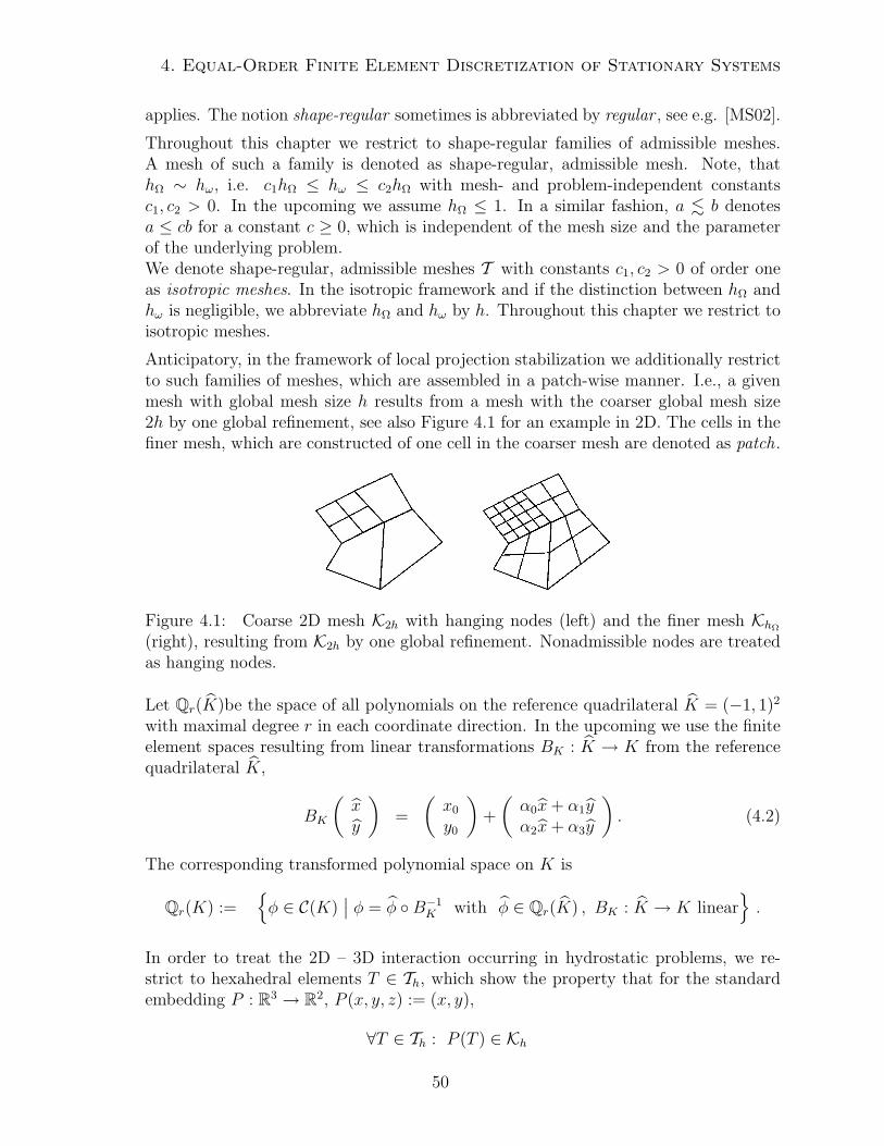
4. Equal-Order Finite Element Discretization of Stationary Systems
applies. The notion shape-regular sometimes is abbreviated by regular , see e.g. [MS02].
Throughout this chapter we restrict to shape-regular families of admissible meshes.A mesh of such a family is denoted as shape-regular, admissible mesh. Note, thathΩ ∼ hω, i.e. c1hΩ ≤ hω ≤ c2hΩ with mesh- and problem-independent constantsc1, c2 > 0. In the upcoming we assume hΩ ≤ 1. In a similar fashion, a . b denotesa ≤ cb for a constant c ≥ 0, which is independent of the mesh size and the parameterof the underlying problem.We denote shape-regular, admissible meshes T with constants c1, c2 > 0 of order oneas isotropic meshes. In the isotropic framework and if the distinction between hΩ andhω is negligible, we abbreviate hΩ and hω by h. Throughout this chapter we restrict toisotropic meshes.
Anticipatory, in the framework of local projection stabilization we additionally restrictto such families of meshes, which are assembled in a patch-wise manner. I.e., a givenmesh with global mesh size h results from a mesh with the coarser global mesh size2h by one global refinement, see also Figure 4.1 for an example in 2D. The cells in thefiner mesh, which are constructed of one cell in the coarser mesh are denoted as patch.
Figure 4.1: Coarse 2D mesh K2h with hanging nodes (left) and the finer mesh KhΩ
(right), resulting from K2h by one global refinement. Nonadmissible nodes are treatedas hanging nodes.
Let Qr(K)be the space of all polynomials on the reference quadrilateral K = (−1, 1)2
with maximal degree r in each coordinate direction. In the upcoming we use the finiteelement spaces resulting from linear transformations BK : K → K from the referencequadrilateral K,
BK
(xy
)=
(x0
y0
)+
(α0x+ α1yα2x+ α3y
). (4.2)
The corresponding transformed polynomial space on K is
Qr(K) :=φ ∈ C(K)
∣∣ φ = φ B−1K with φ ∈ Qr(K) , BK : K → K linear
.
In order to treat the 2D – 3D interaction occurring in hydrostatic problems, we re-strict to hexahedral elements T ∈ Th, which show the property that for the standardembedding P : R3 → R2, P (x, y, z) := (x, y),
∀T ∈ Th : P (T ) ∈ Kh
50
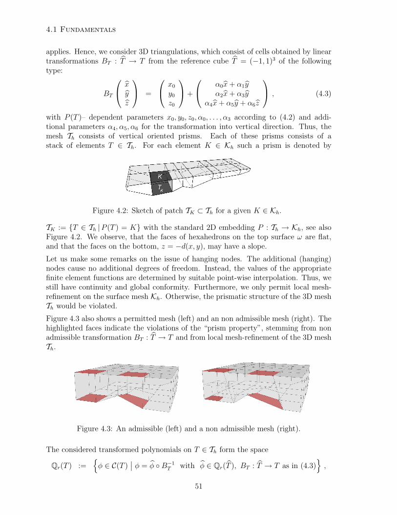
4.1 Fundamentals
applies. Hence, we consider 3D triangulations, which consist of cells obtained by lineartransformations BT : T → T from the reference cube T = (−1, 1)3 of the followingtype:
BT
xyz
=
x0
y0
z0
+
α0x+ α1yα2x+ α3y
α4x+ α5y + α6z
, (4.3)
with P (T )– dependent parameters x0, y0, z0, α0, . . . , α3 according to (4.2) and addi-tional parameters α4, α5, α6 for the transformation into vertical direction. Thus, themesh Th consists of vertical oriented prisms. Each of these prisms consists of astack of elements T ∈ Th. For each element K ∈ Kh such a prism is denoted by
Figure 4.2: Sketch of patch TK ⊂ Th for a given K ∈ Kh.TK := T ∈ Th |P (T ) = K with the standard 2D embedding P : Th → Kh, see alsoFigure 4.2. We observe, that the faces of hexahedrons on the top surface ω are flat,and that the faces on the bottom, z = −d(x, y), may have a slope.
Let us make some remarks on the issue of hanging nodes. The additional (hanging)nodes cause no additional degrees of freedom. Instead, the values of the appropriatefinite element functions are determined by suitable point-wise interpolation. Thus, westill have continuity and global conformity. Furthermore, we only permit local mesh-refinement on the surface mesh Kh. Otherwise, the prismatic structure of the 3D meshTh would be violated.
Figure 4.3 also shows a permitted mesh (left) and an non admissible mesh (right). Thehighlighted faces indicate the violations of the “prism property”, stemming from nonadmissible transformation BT : T → T and from local mesh-refinement of the 3D meshTh.
Figure 4.3: An admissible (left) and a non admissible mesh (right).
The considered transformed polynomials on T ∈ Th form the space
Qr(T ) :=φ ∈ C(T )
∣∣ φ = φ B−1T with φ ∈ Qr(T ), BT : T → T as in (4.3)
,
51
4. Equal-Order Finite Element Discretization of Stationary Systems
with polynomial space Qr(T ) on the reference element T of degree up to r in eachvariable.
Let Q, W and V be the variational spaces for the 2D pressure, the 2D velocity field andthe 3D velocity field, respectively, and r ≥ 1. The appropriate finite element spacesare given by
Qh := qh ∈ Q ∩ C(ω)∣∣ qh|K ∈ Qr(K), ∀K ∈ Kh , (4.4)
Wh := wh ∈W∩C(ω)2∣∣ vh,i |K ∈ Qr(K), i ∈ 1, 2, ∀K ∈ Kh , (4.5)
Vh := vh ∈ V∩C(Ω)2∣∣ vh,i |T ∈ Qr(T ), i ∈ 1, 2, ∀T ∈ Th . (4.6)
4.1.2 Interpolation operators
Suppose a variational space Hm(Ω). The quality of the finite element approximation ofan element v ∈ Hm(Ω) can be estimated due to approximation properties of a suitableinterpolation operator. Let Vh ⊂ Hm(Ω) be the space of finite elements of order r.
(a) Lagrangian interpolation operator
The Lagrangian interpolation operator ih : C(Ω)→ Vh provides the following estimatefor arbitrary T ∈ Th on isotropic meshes, see e.g. [Bra07]:
|v − ihv|k,2,T ≤ chm−k|v|m,2,T ∀v ∈ Hm(Ω) ∀m ∈ [2, r + 1] ∀ k ∈ [0,m]
Stability is achieved by setting k = m.
(b) Clement interpolation operator
An operator, which assures similar estimates as the Lagrangian interpolation operator,but allows v to be less regular, is given by the Clement interpolation operator ch :L1(Ω)→ Vh with p ∈ [1,∞), see e.g. [EG04]:
|v − chv|k,p,T ≤ chm−k|v|m,p,ωT ∀v ∈Wm,p(Ω) ∀m ∈ [0, r + 1] ∀ k ∈ [0,m] ,
whereas ωT denotes a suitable surrounding of T ∈ Th. The authors of [EG04] providethe following stability statement for r ∈ [1,∞) and k ∈ [0, 1]:
||chv||k,p,Ω ≤ c||v||k,p,Ω ∀v ∈Wk,p(Ω).
(c) Scott-Zhang interpolation operator
The disadvantages of the Clement interpolation operator are, that it does not preserveboundary conditions (which can be rectified by suitable modifications of the nodalvalues along the boundaries, see also [Bec95]), and second, that it is not a projection.
52
4.1 Fundamentals
Let us therefore introduce the Scott-Zhang interpolation operator zh : Wm,p(Ω) →Vh, which does not show these undesired properties, see e.g. [EG04], and allows thefollowing estimates:
|v − zhv|k,p,T ≤ chm−k|v|m,p,ωT ∀v ∈Wm,p(Ω) ∀m ∈ [m, r + 1] ∀ k ∈ [0,m] ,
whereas ωT denotes a suitable surrounding of T ∈ Th. The lower bound for m isgiven by m = 1, if p = 1, and m = p−1 + ε for arbitrary ε > 0, else. Assumingk ∈ [0,min1,m], the Scott-Zhang operator provides the stability property, see also[EG04]:
||zhv||k,p,Ω ≤ c||v||m,p,Ω ∀v ∈Wk,p(Ω).
(d) L2-orthogonal interpolation operator
In the case of local projection stabilization of the hydrostatic Oseen problem, a suitableorthogonality property is demanded in order to obtain optimal error estimates. Thisis assured by the interpolation operator ih,3d : V→ Vh, which has been introduced in[BB06] and fulfills the following properties:
(v−ih,3d v, ξ)Ω = 0 ∀v ∈ V , ∀ξ ∈ [Qr−12h (Ω)]2
(4.7)
||v−ih,3d v ||0,Ω + h|v−ih,3d v |1,Ω . hk+1||v ||k+1,Ω ∀v ∈ Hk+1(Ω) , 0 ≤ k ≤ r(4.8)
||ih,3d v ||1,Ω . ||v ||1,Ω ∀v ∈ H1(Ω) .(4.9)
The appropriate operator ih,2d : Q → Qh for the 2D pressure field shows similarproperties, i.e.
(p− ih,2dp, ϕ)ω = 0 ∀p ∈ Q ,∀ϕ ∈ Qr−12h (ω) (4.10)
||p− ih,2dp||0,ω + h|p− ih,2dp|1,ω . hk+1||p||k+1,ω ∀p ∈ Hk+1(ω) , 0 ≤ k ≤ r (4.11)
||ih,2dp||1,ω . ||p||1,ω ∀p ∈ H1(ω) . (4.12)
4.1.3 Hydrostatic Issues
As in the infinite dimensional case, i.e. Chapter 3, the divergence constraint is the keyissue in the analysis of existence and uniqueness. Due to that reasons, we examinethe properties of the discrete modified inf-sup constraint. Necessary properties of thediscrete version of the averaging operator are treated beforehand. The appropriatedeductions are found in [KB12] for p = 2. An extension for arbitrary p ∈ (1,∞) isindicated in [Kim12] and is presented in the following.
53
4. Equal-Order Finite Element Discretization of Stationary Systems
Discrete averaging operator
The following statement figures out, that the discrete averaging operator can be iden-tified by its counterpart as given in Chapter 3.
Lemma 4.1. Let p ∈ (1,∞). Moreover, let V := W1,p0 (Ω) or V := W1,p
b (Ω), p ≥ 1,and Vh ⊂ Vbe given by (4.6). For any vh ∈ Vh the integration operator M, given by(3.18), satisfies:
Mvh ∈Wh and Mvh =
∫ 0
−d(·)vh(·, z) dz .
Proof. Given the definition of Th recall that Th consists of prismatic hexahedrons. LetK ∈ Kh be given. We denote TK as the set of all T ∈ Th, that belong to such a prismwith top surface K. Note that the (x, y)-parts of the transformations BT : T → Tare characterized by BK as given by (4.2) and therefore identical for each T ∈ TK .Due to the construction of BT , the determinant of the Jacobian of BT is constant,cT := | det J(BT )| = α6(α0α3 − α1α2). Let vT ∈ Qr(T )2 such that vh |T = vT B−1
T .As vh is cell-wise polynomial, for each (x, y) ∈ K we derive
wh(x, y) :=
∫ 0
−d(x,y)
vh(x, y, z)dz =∑T∈TK
cT
1∫−1
vT (x, y, z)dz.
As vT ∈ Qr(T )2, the function cT1∫−1
vT (·, ·, z)dz is an element of Qr(K)2. Hence, it
follows wh |K ∈ Qr(K)2 and wh ∈Wh. Thus, we have
0 =(
Mvh−0∫
−d(·)
vh(·, z)dz,ϕ)ω
= (Mvh−wh,ϕ)ω ∀ϕ ∈Wq0(ω)
with q ≥ 1 such that 1/p+ 1/q = 1.
For upcoming proofs, among others, we need surjectivity of M. This property is appliedif the following assumption holds:
Assumption 4.2. Let p ∈ (1,∞). Each Th consists of cells obtained by a transforma-
tion of type (4.3) and there is an element ζh ∈W1,p(Ω)∩ C(Ω), which only depends on
z, i.e. ζh(x, y, z) = ζh(z), with supp(ξh) ⊂ [−δmin, 0], ζh|T ∈ Qr(T ) for all T ∈ Th and∫ 0
−δminζh dz = 1 , (4.13)
||ζh||0,p,R ≤ c δ(1−p)/pmin and |ζh|1,R ≤ c δ
(1−2p)/pmin , (4.14)
with h-independent constant c ≥ 0.
54
4.1 Fundamentals
Remark 4.3. Let us briefly examine this assumption with respect to admissible meshesfor Q1-elements (r = 1). Beside the previously discussed prismatic structure of Th, letthe mesh contain two straight layers of mesh points being parallel to the e1, e2-plane,at z-coordinates z1, z2 with −δmin ≤ z1 < z2 < 0. The function ζh, occurring inAssumption 4.2, can be constructed as follows:
ζh(z) :=
α(z − z1) if z1 ≤ z ≤ z2,α(1− z1/z2)z if z2 ≤ z ≤ 0,0 else.
Setting α = 2/[z1(z1 − z2)] assures the mean value property (4.13). By elementarycalculus we obtain ||ζh||0,p,R = 2(p + 1)−1/p|z1|(1−p)/p and |ζh|1,p,R ≤ 2|z1|−1/p(|z2|(z2 −z1))(1−p)/p. This ensures the bounds (4.14) where the constant c depends on the reg-ularity p of the underlying Sobolev space W1,p(Ω), and on the ratios δmin/|z1| andδmin/|z2 − z1| (but independent of h). For r ≥ 2 an even simpler construction is pos-sible with only one straight line at z1, with −δmin ≤ z1 < 0. Thus, Assumption 4.2 isless restrictive than an assumption to have a tensor mesh.
Lemma 4.4. Let V := W1,p0 (Ω) or V := W1,p
b (Ω) and W := W1,p0 (ω), p ∈ (1,∞).
Moreover, consider Vh ⊂ V, Wh ⊂W given by (4.6), and (4.5), respectively. Let Ωbe a flat domain.If Assumption 4.2 is valid, the operator M |Vh
: Vh →Wh is surjective. In particular,for each wh ∈Wh there exists a vh ∈ Vh, so that Mvh = wh,
||vh ||0,p,Ω ≤ cωδ(1−p)/pmin ||wh ||0,p,ω and |vh|1,p,Ω ≤ cωδ
(1−2p)/pmin |wh|1,p,ω . (4.15)
Proof. Let wh ∈ Wh be given. The construction of vh ∈ Vh with Mvh = wh issimilar to the proof of the continuous version (Lemma 3.12) with the difference thatwe need the piecewise linear function ζh ∈ C(R) from Assumption 4.2. Now, forvh(x, y, z) := wh(x, y) · ζh(z) we obtain vh ∈ Vh by construction and∫ 0
−d(x,y)
vh(x, y, z) dz = wh(x, y)
∫ 0
−d(x,y)
ζh(z) dz = wh(x, y) .
Hence, M is surjective. As Wh ⊂ W and Vh ⊂ V, the bounds (4.15) are obtainedsimilar to the bound in Lemma 3.12 by using the bounds of ||ξh||0,p,R and |ξh|1,p,R inAssumption 4.2.
Discrete modified inf-sup constraint
Dependent on the underlying problem we either consider (V, Q) := (H10(Ω),L2
0(ω)) or(V, Q) := (W1,p
b (Ω),Lq0(ω)), p, q ∈ (1,∞) such that p−1 + q−1 = 1. The 2D velocityspace is given by W := H1
0(ω) or W := W1,p0 (ω), respectively. The appropriate discrete
spaces Qh ⊂ Q, Vh ⊂ V and Wh ⊂W are given by (4.4) – (4.6). To assure existenceof a solution of a finite element discretized hydrostatic problem, the discrete modified
55
4. Equal-Order Finite Element Discretization of Stationary Systems
inf-sup condition
∃γ > 0 supvh∈Vh \0
(div ′Mvh, qh)Ω
||vh ||1,p,Ω ≥ γ||qh||0,q,ω ∀qh ∈ Qh, (4.16)
i.e. a sufficient upper bound for the pressure, has to apply. The following propositionstates the tight connection between the hydrostatic issue and the classical, non hy-drostatic case. Restricting this proposition to the Stokes case for a symmetric choiceof variational spaces and to the Oseen problem, which necessitates a non symmetricchoice of variational spaces, the appropriate Propositions can be found in [KB12] and[Kim12], respectively.
Proposition 4.5. Let p ∈ (1,∞), Ω be a flat domain and Th be a triangulation of Ωfulfilling Assumption 4.2. The lack as well as the validity of the inf-sup condition
∃γω > 0 supwh∈Wh \0
(div ′wh, qh)ω||wh ||1,p,ω ≥ γω||qh||0,q,ω ∀qh ∈ Qh, (4.17)
carries over to (4.16).
Proof. Throughout this proof, cΩ > 0 is a suitable, Ω – dependent constant. Let(4.17) be violated such that there is a pressure ph ∈ Qh \ 0 with (div ′wh, ph)ω =0 for all wh ∈ Wh. Due to the surjectivity of M : Vh → Wh, see Lemma 4.4,(div ′Mvh, ph)ω = 0 applies for all vh ∈ Vh. Moreover, we have ||Mvh ||1,p,ω ≤cΩ||vh ||1,p,Ω. Repeated application of Lemma 4.4 leads to
0 = supwh∈Wh
(div ′wh, qh)ω||wh ||1,p,ω ≥ cΩ sup
vh∈Vh
(div ′Mvh, qh)ω||vh ||1,p,Ω ≥ 0.
The second kind of instability, i.e.
∃qh ∈ Qh \ 0 ∀wh ∈Wh \0 (div ′wh, qh)ω||qh||0,q,ω||wh ||1,p,ω ≥ γh
with inf-sup constant γh → 0 for h→ 0, transfers to the hydrostatic case by applicationof M(Vh) = Wh and the estimate of Lemma 4.4.
On the other hand, let (4.17) be fulfilled. Recall the relation 1/p + 1/q = 1 . Lemma4.4 leads to (4.16) with constant
γ := δ1/qmin(1 + δpmin)1/pc−1
ω γω .
Remark 4.6. The argumentation on the δmin-dependence of the inf-sup constant γΩ,ω,see Remark 3.14, also applies in the discrete case.
56
4.2 2D Stokes problem
4.2 2D Stokes problem
In this section we consider the discrete 2D Stokes problem. We start with the Galerkinformulation, indicating, that an equal-order finite element approach does not lead toa stable problem. We then introduce several stabilization techniques, known fromliterature and present and validate estimates, which are applicable in the hydrostaticframe. We close the section with the presentation of a priori estimates for the appliedstabilization. The results and considerations of this sections can also be found in[KB12].
4.2.1 Galerkin formulation
Througout this section we consider velocity fields with imposed homogeneous Dirichletdata, i.e. the underlying variational spaces are W := H1
0(ω) and Q := L20(ω) and the
appropriate discrete spaces are given by (4.4) and (4.5). Without loss of generality weassume isotropic viscosities. In particular, we set ν = Aν = νE = 1. The equal-orderfinite element formulated 2D Stokes problem is given by
Find (wh, ph) ∈Wh×Qh s. t. Aω(wh, ph;ϕ, ξ) = 〈f ,ϕ〉 ∀(ϕ, ξ) ∈Wh×Qh
(4.18)
with
Aω(wh, ph;ϕ, ξ) := (∇′wh,∇′ϕ)ω − (ph, div ′ ϕ)ω + (div ′ wh, ξ)ω .
The validation of existence and uniqueness of a solution of this problem can be carriedout as in the infinite dimensional case, see also Section 3.1.2. As we apply conformfinite element spaces, i.e. Wh ⊂W, continuity and coercivity of the Laplacian inheritsfrom the infinite dimensional problem. However, the inf-sup constraint (3.7) does notapply in equal-order finite element spaces, see e.g. Braess [Bra07], and unique existenceof a discrete pressure ph cannot be assured. Introducing additional stabilization termsinto this Galerkin formulation with maintainable error properties may circumvent thisproblem, i.e. the given problem is stabilized, which gives the method its name.
4.2.2 Stabilization of the problem
In the following we introduce and examine stabilization terms which are known fromliterature and stabilize the 2D Stokes problem. We first treat symmetric stabilizationschemes, which only depent on Qh, and then turn to residual based stabilizations,which also depend on the velocities.
57
4. Equal-Order Finite Element Discretization of Stationary Systems
Symmetric pressure dependent stabilized methods
The bilinear operator for the 2D Stokes problem with inherent symmetric pressurestabilization is given by
Aωh(wh, ph;ϕ, ξ) := Aω(wh, ph;ϕ, ξ) + sh(ph, ξ) .
The entire discrete problem is of the form
Find (wh, ph) ∈Wh×Qh s. t. Aωh(wh, ph;ϕ, ξ) = 〈f ,ϕ〉 ∀(ϕ, ξ) ∈Wh×Qh .(4.19)
In the upcoming we concentrate on the following established stabilization techniques,whose application results in an inf-sup stabilization of the problem (4.19):
(P-i) Brezzi and Pitkaranta [BP84] for linear elements r = 1:
sh(p, ξ) :=∑K∈Kh
h2K(∇′p, ∇′ξ)K .
(P-ii) Local projection stabilization (LPS) [BB01],
sh(ph, ξ) :=∑K∈Kh
h2K(κh(∇′ph), κh(∇′ξ))K ,
with κh := id−π and L2-projection π : L20(ω)→ Qr−1
2h (ω) onto the ’discontinuous’space
Qr−12h (ω) := φ ∈ L2(ω)
∣∣ φ|K ∈ Qr−1(K) ∀K ∈ K2h .
(P-iii) Continuous interior penalty stabilization (CIP) of Burman and Hansbo [BH06]for r = 1,
sh(ph, ξ) :=∑e∈Eh
h3e
∫e
[∇′ph · n]e · [∇′ξ · n]eds,
where n denotes the outward normal to edge e and [φ]e the jump of φ across e.
(P-iv) Pressure projection of Dohrmann & Bochev [DB04]:
sh(ph, ξ) := −(ph − Pr−1ph, ξ − Pr−1ξ)ω,
with local L2-projection Pr−1 : L2(ω)→ Qr−1h (ω).
More detailed informations on stability and error estimates of these techniques are tobe found in the cited literature. In the upcoming we collect properties, which all ofthe schemes (P-i)-(P-iv) have in common. We start with a first, simple observation:
58
4.2 2D Stokes problem
Lemma 4.7. The stabilizations (P-i)–(P-iv) are bilinear forms and satisfy
sh(p, p) ≥ 0 , (4.20)
sh(p, q) ≤ sh(p, p)1/2sh(q, q)
1/2 (4.21)
for any p, q ∈ Qh.
Proof. Trivial to validate.
Let us anticipate, that application of the introduced stabilization schemes in the hydro-static framework leads to an appropriate stabilized hydrostatic problem. Preparatoryfor an appropriate proof we elaborate suitable propositions in the 2D non hydrostaticframework. Therefore, we define a norm ||| · |||ω and validate, that the stabilized 2DStokes problem is inf-sup stable with respect to that norm. As (4.20) applies and dueto bilinearity of sh,
|||(wh, ph)|||ω :=(||∇wh ||20,ω + ||ph||20,ω + sh(ph, ph)
)1/2(4.22)
defines a norm on Wh×Qh. Moreover, let
Bωh := (wh, ph) ∈Wh×Qh | |||(wh, ph)|||ω = 1
be the unit sphere on Wh×Qh with respect to ||| · |||ω.
Application of the results in [BB01, BP84, BH06, DB04] we can easily prove, thatapplication of each of the schemes (P-i)–(P-iv) to the 2D equal order finite elementdiscretized Stokes problem leads to appropriate inf-sup stable schemes. I.e., there isan inf-sup constant γω > 0, indepenent on the mesh size h, such that
inf(wh,ph)∈Bωh
sup(ϕ,ξ)∈Bωh
Aωh(wh, ph;ϕ, ξ) ≥ γω . (4.23)
We reformulate this inf-sup constraint into the following property, which is more suit-able in the hydrostatic framework:
Lemma 4.8. Application of one of the schemes (P-i)–(P-iv) to the discrete 2D Stokesproblem (4.18) leads to the following property: For any ph ∈ Qh there is an elementϕ ∈Wh such that
||∇′ϕ ||0,ω ≤ ||ph||0,ω and − (div ′ϕ, ph)ω ≥ γω4||ph||20,ω −
1
γωsh(ph, ph).
Proof. Let ph ∈ Qh be arbitrarily given, wh := 0 ∈Wh and an arbitrary stabilizationfrom (P-i) – (P-iv) be applied. Due to the inf-sup stability of the stabilized 2D Stokesproblem, there is a (ψ, ξ) ∈ Bω
h such that
Aωh(0, ph;ψ, ξ) = −(div ′ψ, ph)ω + sh(ph, ξ) ≥ γω|||(0, ph)|||ω|||(ψ, ξ)|||ω .
59
4. Equal-Order Finite Element Discretization of Stationary Systems
Due to the definition of the triple norm and |||(ψ, ξ)|||ω = 1 we can further deduce
−(div ′ψ, ph)ω ≥ 1
2γω||ph||0,ω +
1
2γωsh(ph, ph)
1/2 − sh(ph, ξ) .
Applying (4.21) and sh(ξ, ξ)1/2 ≤ |||(ψ, ξ)|||ω = 1 we get
−(div ′ψ, ph)ω ≥ 1
2γω||ph||0,ω − (1− γω/2)sh(ph, ph)
1/2
≥ 1
2γω||ph||0,ω − sh(ph, ph)1/2.
Suitable scaling of ψ, i.e. setting ϕ := ||ph||0,ω ψ, results in ||∇′ϕ ||0,ω ≤ ||ph||0,ω suchthat we finish the proof with the following estimate, where we apply Young’s inequality:
−(div ′ϕ, ph)ω ≥ γω2||ph||20,ω − sh(ph, ph)1/2||ph||0,ω
≥ γω4||ph||20,ω −
1
γωsh(ph, ph) .
Remark 4.9. We restrict our considerations on the stabilizations (P-i) – (P-iv). How-ever, the preceding lemma only requires application of inf-sup stable pressure dependentstabilizations, which fulfill the estimates of Lemma 4.7. Thus, our considerations alsoapply for any other pressure dependent stabilization, which inherits these properties.
Residual based stabilization
Literature also provides residual based stabilization schemes, which also depent on thevelocity components. In these cases, the stabilization also enters the forcing and theentire stabilized problem is given as:
Find (wh, ph) ∈Wh×Qh s. t. Aωh(wh, ph;ϕ, ξ) = 〈fh,ϕ〉 ∀(ϕ, ξ) ∈W×Q(4.24)
with stabilized bilinear form
Aωh(wh, ph;φ, ξ) := (∇′wh,∇′φ)ω − (ph, div ′ φ)ω + (div ′ wh, ξ)ω + sωh(wh, ph;φ, ξ) ,
and suitably modified linear form fh : Wh×Qh → R. Note, that we applied thesubscript ω in the definition of the stablization. This is done, as we can not directlyapply this stabilization in the hydrostatic context, but a slight modification of it. Inthe upcoming, we consider the following residual based schemes:
(P-v) Pressure Stabilization Petrov-Galerkin (PSPG) method [HFB86]:
sωh(w, p; ξ) := α0
∑K∈Kh
h2K(−∆′w+∇′p,∇′ξ)K ,
〈fh;ϕ, ξ〉 := (f ,ϕ)ω + α0
∑K∈Kh
h2K(f ,∇′ξ)K .
60
4.2 2D Stokes problem
(P-vi) Galerkin-Least-Squares (GLS) method for Stokes, introduced by Hughes, Francaand Stenberg [FHS93]:
sωh(w, p;ϕ, ξ) := α0
∑K∈Kh
h2K(−∆′w+∇′p,−∆′ϕ+∇′ξ)K ,
〈fh;ϕ, ξ〉 := (f ,ϕ)ω + α0
∑K∈Kh
h2K(f ,−∆′ϕ+∇′ξ)K .
(P-vii) Combination of GLS and penalization of pressure jumps across cell edges fordiscontinuous discrete pressures, introduced by Douglas and Wang [DW89] :
sωh(w, p;ϕ, ξ) := α0
∑K∈Kh
h2K(−∆′w+∇′p,−∆′ϕ+∇′ξ)K +
∑e∈Eh
he
∫e
[p][ξ] ds ,
〈fh;ϕ, ξ〉 := (f ,ϕ)ω + α0
∑K∈Kh
h2K(f ,−∆′ϕ+∇′ξ)K .
The stabilization coefficient α0 > 0, which occurs in the stabilization schemes (P-v)- (P-vii), is to be chosen in a suitable range. In particular, the coefficient has to bechosen suitably small in order to allow for the estimates in the upcoming lemma.
In the following section, we present a general stability proof for the appropriatelystabilized hydrostatic Stokes problem, which is, most extensively, independent of theparticular choice and structure of the stabilizations of avail. Further note, that the termsωh , chosen from (P-v) – (P-vii), does not fulfill the (appropriately adapted) estimatesof Lemma 4.10 and even may lead to negative expressions. Thus, the straightforwarddefinition of the triple norm ||| · |||ω in the residual based case may not lead to a norm.Thus, we introduce
sh(p, ξ) := sωh(0, ph; 0, ξ) . (4.25)
Lemma 4.10. Let sωh be arbitrarily chosen from (P-v)–(P-vii) and α0 > 0 be sufficientlysmall. Given the reduced form (4.25) and arbitrary p, ξ ∈ Qh and wh,ϕ ∈ Wh, thereduced term sh satisfies
sh(p, p) ≥ 0 , (4.26)
|sωh(w, p;ϕ, ξ)| ≤ (|w |21,ω + sh(p, p))1/2|||(ϕ, ξ)|||ω . (4.27)
The bilinear form Aωh is inf-sup stable and thus (4.23) applies.
Proof. The estimates are trivial to validate by an inverse estimate. For the proof ofthe inf-sup condition we refer to the cited literature.
Lemma 4.11. Let sωh be arbitrarily chosen from (P-v) – (P-vii) and sh be given by(4.25). For any ph ∈ Qh there is an element ψ ∈ Wh such that ||∇ψ ||0,ω ≤ ||ph||0,ωand
− (div ′ψ, ph)ω ≥ γω4||ph||20,ω −
1
2γωsh(ph, ph). (4.28)
61
4. Equal-Order Finite Element Discretization of Stationary Systems
Proof. We chose an arbitrary ph ∈ Qh and consider (0, ph) ∈Wh×Qh. Due to Lemma4.10, the inf-sup constraint (4.23) applies and existence of an element (ϕ, ξ) ∈ Bω
h isassured, which fulfills
Aωh(0, ph;ϕ, ξ) = −(div ′ϕ, ph)ω + sωh(0, ph;ϕ, ξ) ≥ γω|||(0, ph)|||ω.As well, application of Lemma 4.10 assures sωh(0, ph;ϕ, ξ) ≤ sh(ph, ph)
1/2. Thereforeand due to the definition of the triple norm ||| · |||ω,
−(div ′ϕ, ph)ω ≥ 1
2γω||ph||0,ω − 1
2sh(ph, ph)
1/2
applies. Suitable scaling of ϕ, i.e. setting ψ := ||ph||0,ω ϕ, results in the estimate||∇′ψ ||0,ω ≤ ||ph||0,ω. Similarly to the symmetric pressure stabilization, application ofthe inequality of Young finishes the proof:
−(div ′ψ, ph)ω ≥ γω2||ph||20,ω −
1
2sh(ph, ph)
1/2||ph||0,ω
≥ γω4||ph||20,ω −
1
2γωsh(ph, ph) .
4.2.3 A priori error estimates
Lemma 4.12. The symmetric stabilizations schemes (P-i)–(P-iv) as well as the re-duced terms (4.25) of the residual based stabilization schemes (P-v)–(P-vii) provide thefollowing a priori bound for every 1 ≤ k ≤ r:
sh(p, p)1/2 ≤ chkω||p||k,ω ∀p ∈ Hk(ω) .
Proof. The estimates for the schemes (P-i) – (P-iv) are to be found in [BP84, BB01,BH06, DB04]. For the schemes (P-v)–(P-vii) we refer to [HFB86, FHS93, DW89].
4.3 3D Oseen problem
In this section we introduce the discrete 3D Oseen problem. After mentioning thelack of the inf-sup constraint for equal-order finite elements, we collect some of sym-metric stabilization techniques and present important bounds. We close the sectionwith a presentation of suitable a priori error estimates, which find application in thehydrostatic framework.
4.3.1 Galerkin formulation
We consider the wind-driven 3D Oseen problem, neglecting Coriolis forces. Withoutloss of generality we assume isotropic viscosities and set ν = Aν = νE. I.e., let
62
4.3 3D Oseen problem
U := H1b(Ω) × H1
0(Ω) and P := L20(Ω). The dual space of U is denoted as U−1. The
appropriate finite dimensional spaces Uh and Ph are defined in a similar fashion as(4.4) and (4.6), respectively, on the spaces of piecewise polynomials of order r. Theequal-order finite element formulation of the 3D Oseen problem is given by:
Given bh ∈ Uh, div bh = 0, f ∈ U−1, g ∈ H−1/2(Γs)× 0,find yh = (uh, ph) ∈ Uh×Ph s.t.
AΩ(bh; yh;φ) = lΩ(ϕ) ∀φ = (ϕ, ξ) ∈ U×P(4.29)
with
AΩ(bh; yh;φ) = (σ uh,ϕ)Ω + ((bh · ∇) uh,ϕ)Ω
+ (ν∇uh,∇ϕ)Ω − (ph, div ϕ)Ω + (ξ, div uh)Ω ,
lΩ(ϕ) = (f ,ϕ)Ω + (g,ϕ)Γu .
As in the 2D Stokes case, the inf-sup constraint (3.7) is not assured for the equal-orderfinite element approach and suitable stabilization of the pressure has to be applied.Moreover, the problem shows oscillations, that occur due to dominant advection, seealso [RST08], which also have to be controlled.
4.3.2 Symmetric stabilization schemes
To circumvent the mentioned undesired properties, we add stabilizing terms to thesystem. Regarding suitable adaption of the stabilization for the appropriate hydrostaticproblem, we restrict to the presentation of symmetric stabilizations:
sΩh (uh, ph;ϕ, ξ) := sΩ
h,p(ph, ξ) + sΩh,v(uh,ϕ) ∀(uh, ph), (ϕ, ξ) ∈ Uh×Ph ,
whereas the term sΩh,p(·, ·) stabilizes the oscillations in the pressure and the term sΩ
h,v(·, ·)controls the undesired effect of the dominant advection. The stabilized problem thenis given by:
Given bh ∈ Uh, div bh = 0,f ∈ U−1, g ∈ H−1/2(Γs)× 0,find (uh, ph) ∈ Uh×Ph
s.t. AΩ(bh; uh, ph;ϕ, ξ) + sΩh (bh; uh, ph;ϕ, ξ) = lΩ(ϕ) ∀(ϕ, ξ) ∈ Uh×Ph .
In the upcoming we consider the following schemes:
(V-i) LPS [BL09]:
sΩh,p(ph, ξ) :=
∑M∈T2h
hM(κh,Ω(∇ph ),κh,Ω(∇ξ))
M,
63
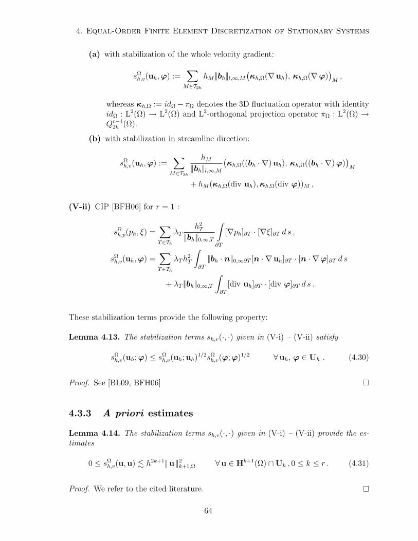
4. Equal-Order Finite Element Discretization of Stationary Systems
(a) with stabilization of the whole velocity gradient:
sΩh,v(uh,ϕ) :=
∑M∈T2h
hM ||bh||l,∞,M(κh,Ω(∇uh), κh,Ω(∇ϕ)
)M,
whereas κh,Ω := idΩ− πΩ denotes the 3D fluctuation operator with identityidΩ : L2(Ω) → L2(Ω) and L2-orthogonal projection operator πΩ : L2(Ω) →Qr−1
2h (Ω).
(b) with stabilization in streamline direction:
sΩh,v(uh,ϕ) :=
∑M∈T2h
hM||bh||l,∞,M
(κh,Ω((bh · ∇) uh), κh,Ω((bh · ∇)ϕ)
)M
+ hM(κh,Ω(div uh),κh,Ω(div ϕ))M ,
(V-ii) CIP [BFH06] for r = 1 :
sΩh,p(ph, ξ) =
∑T∈Th
λTh2T
||bh||0,∞,T
∫∂T
[∇ph]∂T · [∇ξ]∂T d s ,
sΩh,v(uh,ϕ) =
∑T∈Th
λTh2T
∫∂T
||bh · n||0,∞∂T [n · ∇uh]∂T · [n · ∇ϕ]∂T d s
+ λT ||bh||0,∞,T∫∂T
[div uh]∂T · [div ϕ]∂T d s .
These stabilization terms provide the following property:
Lemma 4.13. The stabilization terms sh,v(·, ·) given in (V-i) – (V-ii) satisfy
sΩh,v(uh;ϕ) ≤ sΩ
h,v(uh; uh)1/2sΩ
h,v(ϕ;ϕ)1/2 ∀uh, ϕ ∈ Uh . (4.30)
Proof. See [BL09, BFH06]
4.3.3 A priori estimates
Lemma 4.14. The stabilization terms sh,v(·, ·) given in (V-i) – (V-ii) provide the es-timates
0 ≤ sΩh,v(u,u) . h2k+1||u ||2k+1,Ω ∀u ∈ Hk+1(Ω) ∩Uh , 0 ≤ k ≤ r . (4.31)
Proof. We refer to the cited literature.
64
4.4 Hydrostatic Stokes problem
4.4 Hydrostatic Stokes problem
This section aims to introduce the equal-order finite element discretization of hydro-static flow problems, which has hardly been analyzed yet, see e.g. [CGS12, KB12,Kim12]. We restrict our view to the minimal system, which shows characteristic prop-erties of hydrostatic flows: we consider the stationary, linear hydrostatic Stokes problemin a non rotating frame, i.e. we neglect Coriolis forces. Moreover, we impose Dirichletdata on the entire domain, assume isotropic viscosities, i.e. ν = Aν = νE > 0, andnorm the problem, such that ν = 1.
We start with the Galerkin formulation, validating the tight relation between the 2Dand the 2.5D Stokes problem regarding inf-sup stability. Afterwards, we turn to sta-bilization methods, stemming from the already introduced stabilization techniques forthe 2D Stokes problem. We validate stability and elaborate optimal a priori errorestimates. The results of this section constitutes the heart of [KB12]. Note, that wefurthermore have a closer look at the residual based stabilizations of the hydrostaticStokes problem than has been done in [KB12] and elaborate some domain dependencies,which have been withhold in [KB12].
4.4.1 Galerkin formulation
Let V := H10(Ω) and Q := L2
0(ω) be the underlying variational spaces. The dualspace of V is denoted as V−1. The standard Galerkin formulation of the introducedhydrostatic Stokes problem by conforming finite elements in the finite dimensionalspace Xh := Vh×Qh is given by:
Given f ∈ V−1, find (vh, ph) ∈ Xh (4.32)
s. t. a(vh,ϕ)− b(ph,ϕ) + b(ξ,vh) = (f ,ϕ)Ω ∀(ϕ, ξ) ∈ Xh
with bilinear forms a(vh,ϕ) := (∇vh,∇ϕ)Ω and b(ph,ϕ) := (ph, div ′Mϕ)ω. Ifwe replace Xh by the space X := V×Q in problem (4.32), the system becomes thevariational formulation of the underlying hydrostatic Stokes problem.
Note, that we restrict to the case of homogeneous Dirichlet data for the velocity field.However, each problem with inhomogenous Dirichlet data can be reformulated intoa problem with homogeneous Dirichlet data by alteration of the right hand side into〈f , ϕ〉 := (f , ϕ)−a(v0, ϕ). The element v0 ∈ H1(Ω) is an extension of the appropriateboundary data to the entire domain Ω and is divergence-free in vertical mean.The next proposition states the tight relation between the 2D and the 2.5D Stokesproblem. Throughout this proposition we therefore broaden our attention to a widerrange of possible discrete spaces:
Proposition 4.15. Let Ω be a flat domain and Th be a triangulation of Ω fulfillingAssumption 4.2. The hydrostatic Stokes problem (4.32) formulated on the finite element
65
4. Equal-Order Finite Element Discretization of Stationary Systems
spaces Xh := Vh×Qh with
Qh := qh ∈ Q ∩ C(ω)∣∣ qh|K ∈ Qr(K), ∀K ∈ Kh ,
Vh := vh ∈ V∩C(Ω)2∣∣ vh,i |T ∈ Qs(T ), i ∈ 1, 2, ∀T ∈ Th
has a unique solution, if the 2D Stokes problem (4.18) formulated on the finite elementspaces Wh×Qh with
Qh := qh ∈ Q ∩ C(ω)∣∣ qh|K ∈ Qr(K), ∀K ∈ Kh ,
Wh := wh ∈W∩C(ω)2∣∣ vh,i |K ∈ Qs(K), i ∈ 1, 2, ∀K ∈ Kh
has a unique solution. Moreover, if the 2D Stokes problem is not inf-sup stable, thesame applies for the hydrostatic Stokes problem.
Proof. We apply the techniques, introduced in Section 3.1.2. First note, that thecontinuous bilinear form a : V×V → R is V-elliptic and Vh ⊂ V. It thus sufficesto assure, that the hydrostatic problem (4.32) satisfies the modified inf-sup condition(4.16), if the appropriate inf-sup condition (4.17) of the 2D Stokes problem is fulfilled.We already proved this statement in Proposition 4.5, restricting to p = 2.
Thus, due to the relation M(Vh) = Wh, see Lemma 4.4, and as equal-order finiteelements do not lead to an inf-sup stable 2D Stokes problem, see e.g. [Bra07], thediscrete hydrostatic Stokes problem (4.32) is not inf-sup stable. As introduced for the2D case, we avoid this problem by adding suitable stabilization terms to the system.
4.4.2 Stabilization of the problem
We adapt the introduced stabilization schemes for the 2D Stokes problem to the hy-drostatic case. As in the 2D case, the stabilized hydrostatic Stokes problem is givenby
Find (vh, ph) ∈ Xh s. t. Ah(vh, ph;ϕ, ξ) = (fh,φ)Ω ∀φ := (ϕ, ξ) ∈ Xh (4.33)
with Xh = Vh×Qh. The bilinear form Ah is defined due to the chosen stabilizationscheme. In the case of symmetric pressure stabilization, see Section 4.2.2, we set
Ah(vh, ph;ϕ, ξ) := a(vh,ϕ)− b(ph,ϕ) + b(ξ,vh) + sh(ph, ξ) (4.34)
and the forcing fh equals f . If a residual based stabilization term is applied, seeSection 4.2.2, the bilinear form is given by
Ah(vh, ph;ϕ, ξ) := a(vh,ϕ)− b(ph,ϕ) + b(ξ,vh) + sh(vh, ph;ϕ, ξ) . (4.35)
The stabilization term sh(·, ·; ·, ·) and the forcing fh are the hydrostatic 3D analogs ofthe 2D stabilization terms sωh(·, ·; ·, ·) and fh as introduced in Section 4.2.2. E.g., in
66
4.4 Hydrostatic Stokes problem
the GLS case the stabilization is given by
sh(vh, ph; ξ) := α0
∑K∈Kh
h2K(−M(∆vh) +∇′p,−M(∆ϕ) +∇′ξ)K ,
〈fh;ϕ, ξ〉 := (f ,ϕ)Ω + α0
∑K∈Kh
h2K(Mf ,−M(∆ϕ) +∇′ξ)K .
Thus, in the case of residual based stabilization we observe global couplings of thevelocity field and of the forcing, which in turn leads to a numerically more expensivescheme as in the case of symmetric pressure stabilization.
Remark 4.16. Note, that it is also possible to adapt the 2D residual based stabilizations(P-v) – (P-vii) in a 3D manner. I.e. in the case of GLS we can also treat
sh(vh, ph; ξ) := α0
∑T∈Th
h2T (−∆vh +∇′p,−∆ϕ+∇′ξ)T ,
〈fh;ϕ, ξ〉 := (f ,ϕ)Ω + α0
∑T∈Th
h2T (f ,−∆ϕ+∇′ξ)T .
The upcoming considerations basically are the same. But, the constants may dependon the depth of the domain in a slightly different way. Anticipatory, such a differenceoccurs in Lemma 4.17, in the estimate of sh(vh, ph, vh, 0) of the proof of Proposition4.18. The appropriate estimates are to be found in [KB12]. Moreover, the estimate ofsh((zh v−v), zhp− p;ϕ, ξ) in Proposition 4.21 alters to
sh((zh v−v), zhp− p;ϕ, ξ) ≤ c(hm||v ||m+1,Ω + hmω δmax||p||m,ω) ,
whereas we applied the property hT ≤ hK for any element T whose projection onto ωis the 2D cell K.
Similar to the 2D case the triple norm on Xh is given by
|||(v, p)||| := (||∇v ||20,Ω + ||p||20,ω + sh(p, p))1/2
. (4.36)
The term sh(·, ·) coincides with the entire stabilization in the case of symmetric pressurestabilization. If a residual based scheme is applied, it is given similar to (4.25):
sh(p, ξ) := sh(0, ph; 0, ξ) .
The residual based stabilization terms fulfill the following estimates, which are anadaption of Lemma 4.10:
Lemma 4.17. The hydrostatically adapted versions of the stabilization schemes (P-v),(P-vi) and (P-vii), as defined in Section 4.2.2, fulfill
sh(vh, ph;vh, ph) ≥ 1
2
(sh(ph, ph)− δmax|vh |21,Ω
) ∀(vh, ph) ∈ Xh ,
|sh(vh, ph;ϕ, ξ)| ≤ c(δmax|vh |21,Ω + sh(ph, ph))1/2|||(ϕ, ξ)||| ∀(vh, ph), (ϕ, ξ) ∈ Xh .
67
4. Equal-Order Finite Element Discretization of Stationary Systems
Proof. Under the constraint 0 < α0 < c−2inv, with constant cinv of the inverse estimate,
the validation of the estimates can be easily done by application of an inverse estimate,see e.g. [Bra07], of Young’s inequality as well as of the estimate (3.19).
Given these preparatory estimates, we now turn to the proof of inf-sup stability of asuitably stabilized hydrostatic Stokes problem. Therefore, let
Bh := (vh, ph) ∈ Xh | |||(vh, ph)||| = 1 .
Proposition 4.18. The underlying domain Ω is assumed to be a flat basin. Thetriangulation of Ω is given by Th and is presumed to fulfill Assumption 4.2. Let thehydrostatic Stokes problem be stabilized either by a symmetric pressure stabilizationof (P-i)–(P-iv) or by a residual based stabilization chosen from the list (P-v)–(P-vii).Then, the stabilized 2.5D Stokes bilinear form (4.34) or (4.35), respectively, is inf-supstable:
inf(vh,ph)∈Bh
sup(ϕ,ξ)∈Bh
Ah(vh, ph;ϕ, ξ) ≥ γΩ,ω .
Proof. We assume an arbitrary yh := (vh, ph) ∈ Xh. The authors of [BS11] introducedan abstract criterion for the inf-sup condition. We also apply it here. I.e. we considerthe following decomposition of the triple norm:
|||yh|||2 = |yh|2a + |yh|2b with
|yh|2a := |vh |21,Ω + sh(ph, ph) and |yh|2b := ||ph||20,ω.
In the case of symmetric pressure stabilization, we get Ah(yh;yh) = |yh|2a. In thecase of residual based stabilization, we apply Lemma 4.17, and estimate at leastAh(yh;yh) ≥ 1
2|yh|2a.
In order to prove the inf-sup condition, we construct an element vh ∈ Vh with|||(vh, 0)||| ≤ |||yh||| and
Ah(vh, ph; vh, 0) ≥ c1|uh |2b − c2|uh |2a .
Constant c1 has to be strictly positive, i.e. c1 > 0. Constant c2 is no further restricted.For the construction, we chose a ϕ ∈Wh, such that the element (ϕ, ph) fulfills (4.28).As M is surjective, see also Lemma 4.4, an element vh ∈ Vh is assured with ϕ = M vh.Setting wh := Mvh ∈Wh and applicating Lemma 4.8 leads to
Ah(yh; vh, 0) = (∇vh,∇vh)Ω − (ph, div ′ wh)ω + sh(vh, ph; vh, 0)
≥ −|vh |1,Ω|vh|1,Ω +γω4||ph||20,ω −
1
γωsh(ph, ph) + sh(vh, ph; vh, 0)
in the case of residual based stabilization. If a symmetric pressure stabilization isapplied, we can deduce the same estimate without the last term on the right hand side.
68
4.4 Hydrostatic Stokes problem
We further estimate the first term, |vh |1,Ω|vh|1,Ω, on the right hand side:
|vh |1,Ω|vh|1,Ω ≤ cωδ−3/2min |vh |1,Ω|ϕ |1,ω
≤ 4
γωc2ωδ−3min|vh |21,Ω +
γω16|ϕ |21,ω
≤ 4
γωc2ωδ−3min|vh |21,Ω +
γω16||ph||20,ω .
In the case of residual cased stabilization we apply the estimates (3.19) and (4.27):
|sh(vh, ph; vh, 0)| ≤ cδmax(|vh |21,Ω + sh(ph, ph))1/2|vh|1,Ω
≤ cδmax(‖vh |21,Ω + sh(ph, ph))1/2δ−3/2
max ||ph||0,ω≤ ccωδ
−1/2max |yh|a||ph||0,ω
≤ cc2ω
γωδmax|yh|2a +
γω16||ph||20,ω .
Thus, we entirely get the following bound:
Ah(yh; vh, 0) ≥ − c
γωc2ωδ−1min|vh |21,Ω +
γω8||ph||20,ω −
1
γωsh(ph, ph)
≥ − 1
γω
(1 + cc2
ωδ−1min
) |yh|2a +γω8|yh|2b .
4.4.3 A priori error estimates
In this section we analyze the a priori errors for the hydrostatic Stokes problem. Inappropriate deductions we apply the estimates, which we already collected for the 2DStokes problem. Moreover, we apply the following lemma, which states the strongconsistency of residual based stabilization schemes.
Lemma 4.19. Let sh be chosen from (P-v)–(P-vii). The solution (v, p) ∈ X :=(V×Q) of (4.32) fulfills
sh(v, p;ϕ, ξ) = 〈fh;ϕ, ξ〉 − (f ,ϕ)Ω ∀(ϕ, ξ) ∈ Xh . (4.37)
Proof. As we apply conforming finite elements, we can validate proposition (4.32) asfollows. First, we insert the solution (v, p) ∈ X into the stabilized hydrostatic Stokesproblem (4.33), then test the variational problem with elements (ϕ, ξ) from the discretespace Xh and finally formulate the difference of these two equations.
Before we turn to the main proposition of this section, we validate a simple estimate ofthe divergence constraint. We anticipatory add it here in order to accent the differentdemands on the estimate between the hydrostatic Stokes problem and the hydrostaticOseen problem. These differences necessitate more endeavors in the hydrostatic Oseencase than for the present hydrostatic Stokes problem.
69
4. Equal-Order Finite Element Discretization of Stationary Systems
Lemma 4.20. Let Th be a triangulation of Ω fulfilling Assumption 4.2, zh : V → Vh
be the Scott-Zhang interpolant, v ∈ Hk+1(Ω) ∩ V, 0 ≤ k ≤ r, and ξ ∈ Qh. Then,the divergence constraint of the interpolation error ηv = v−zh v supplies the a priorierror estimate:
(div ′Mηv, ξ)ω . hm||v ||m+1,Ω |||(0, ξ)||| (4.38)
with m = minr, k.
Proof. Partial integration of the divergence term in (4.38) leads to
|(div ′Mηv, ξ)ω| = |(Mηv,∇′ξ)ω| = |(ηv,∇′ξ)Ω| .
When we go over to the 3D expression |(ηv,∇′ξ)Ω| we constantly continue ∇′ξ invertical direction, i.e. use ∇′ξ(x, y, z) := ∇′ξ(x, y) for any (x, y, z) ∈ Ω. The latterterm on the right hand side can be estimated as
|(ηv,∇′ξ)Ω| ≤ cω||ηv||Ω||∇′ξ||ω .
which finishes the proof due to the definition of the triple norm (4.36), application ofan inverse estimate and the interpolation properties of the Scott-Zhang operator.
Proposition 4.21. Let Assumption 4.2 be valid and the continuous solution (v, p) ∈X := (V×Q) of (4.32) be sufficiently regular, (v, p) ∈ Hk+1(Ω)×Hk(ω). The discretesolution (vh, ph) of (4.33), stabilized by any of the stabilization schemes (P-i)–(P-iv)and (P-v)–(P-vii) fulfills the a priori error estimate
||v−vh ||1,Ω + ||p− ph||0,ω ≤ c(hm||v ||m+1,Ω + hmω ||p||m,ω
). (4.39)
Value m is given by m = minr, k and c is a constant, which does not depend on hand hω.
Proof. We proceed as usual and partition the error into an interpolation and a projec-tion part, applying the Scott-Zhang interpolants zh v and zhp. Due to the interpolationproperties of the Scott-Zhang interpolation operator, see also Section 4.1.2, it sufficesto examine the projection errors ||zh v−vh ||1,Ω and ||zhp − ph||0,ω. As we validated inProposition 4.18, the stabilized discrete problem is inf-sup stable and thus an element(ϕ, ξ) ∈ Xh with |||(ϕ, ξ)||| = 1 is assured, such that
γΩ,ω|||(zh v−vh, zhp− ph)||| ≤ Ah(zh v−vh, zhp− ph;ϕ, ξ)
is fulfilled. In the case of symmetric pressure stabilization, i.e. for the schemes (P-i)–(P-iv), we argue by application of the perturbed Galerkin orthogonality:
γΩ,ω|||(zh v−vh, zhp− ph)||| ≤ Ah(zh v−v, zhp− p;ϕ, ξ) + sh(p, ξ)
= a(zh v−v,ϕ)− b(zhp− p,ϕ) + b(ξ, zh v−v)− sh(zhp, ξ) .
70
4.5 Hydrostatic Oseen problem
If one of the residual based stabilization schemes (P-v)-(P-vii) is applied we deduce
γΩ,ω|||(zh v−vh, zhp− ph)||| ≤ Ah(zh v−v, zhp− p;ϕ, ξ)= a(zh v−v,ϕ)− b(zhp− p,ϕ) + b(ξ, zh v−v)
−sh(zh v−v, zhp− p;ϕ, ξ) .The Galerkin terms can be estimated as, see also Lemma 4.20,
a(zh v−v,ϕ) ≤ ||zh v−v ||1,Ω|||(ϕ, 0)||| ≤ chm||v ||m+1,Ω
− b(zhp− p,ϕ) ≤ ||zhp− p||0,ω|||(ϕ, 0)||| ≤ chmω ||p||m,ωb(ξ, zh v−v) ≤ ||div ′M(zh v−v)||0,ω|||(0, ξ)||| ≤ chm||v ||m+1,Ω .
The remaining stabilization terms for the schemes (P-i)–(P-iv) fulfill the followingupper bound
sh(zhp, ξ) = sh(p, ξ) + sh(zhp− p, ξ)≤ (sh(p, p)
1/2 + sh(zhp− p, zhp− p)1/2)sh(ξ, ξ)1/2
≤ (sh(p, p)1/2 + sh(zhp− p, zhp− p)1/2)|||(0, ξ)|||
≤ chmω ||p||m,ω + chmω |zhp− p|1,ω≤ chmω ||p||m,ω .
The remaining estimate for the residual based schemes reads:
sh((zh v−v), zhp− p;ϕ, ξ) ≤ c(δmax|zh v−v |21,Ω + sh(zhp− p, zhp− p))1/2
≤ c(hmδmax||v ||m+1,Ω + hmω ||p||m,ω)
The parts involving the pressure can be bounded as shown before. In sum, we arriveat the following estimate which implies the assertion:
γΩ,ω|||(zh v−vh, zhp− ph)||| ≤ c(hm||v ||m+1,Ω + hmω ||p||m,ω)
with a constant c, which is independent of h and hω.
4.5 Hydrostatic Oseen problem
In this section we broaden our attention to the discrete wind-driven hydrostatic Oseenproblem (3.33), also considering the impact of Coriolis forces. We begin with theintroduction of a suitable Galerkin formulation and recover regularity propositions. Asin the preceeding hydrostatic Stokes case, additional stabilization of the pressure isnecessary, and, additionally, suitable control over the advection has to be imposed. Werealize the appropriate stabilizations by application of symmetric terms, which stemfrom appropriate classical, non hydrostatic problems and are adapted suitably. Theperformed analysis includes stability concerns and a priori error estimates.
The results of this section constitutes the crucial part of [Kim12].
71
4. Equal-Order Finite Element Discretization of Stationary Systems
4.5.1 Galerkin formulation
We approximate both, the variational spaces X and Y by Xh := Vh×Qh as definedby (4.4) and (4.6). Similarly, we discretize the advection space Ha, see (3.29), as
Ha,h :=bh ∈ Ha
∣∣ bh,i|T ∈ Qr, i ∈ 1, 2, 3, ∀T ∈ Th. (4.40)
The space Ha,h is non trivial due to the following observations: Let (u2d, v2d) ∈ Wbe horizontal velocities, which are vertically invariant, i.e. u2d = u2d(x, y) and v2d =v2d(x, y). Moreover, let cu(x, y) := ∂xu2d(x, y) and cv(x, y) := ∂vv2d(x, y) for all (x, y) ∈ω. Due to Assumption 4.2 and Remark 4.3, the underlying 3D mesh Th has at least onehorizontally oriented inner node layer. Thus, we can define piecewise linear functionsuz and vz, such that the velocities u := u2d ·uz and v := v2d ·vz vanish at the bottom ofΩ and M(∂xu + ∂yv) = 0 applies. The appropriate vertical velocity w can be exactlydetermined by w(x, y, z) := − ∫ z−d(x,y)
(∂xu(x, y, z) + ∂yv(x, y, z))d z.
Note, that due to the regularity of the advection (b · ∇)v ∈ W−1,3/2b (Ω) with b ∈
Ha, v ∈ V, and due to the embedding from H1(Ω) to L6(Ω), see Theorem 3.6, we
have ((b · ∇)v,ϕ) . ||b||0,3,Ω|v|1,Ω|ϕ|1,Ω. In order to be able to suitably estimate theadvection term we thus restrict to the following approximation of b:
Assumption 4.22. For 0 ≤ k ≤ r and any b ∈ Ha ∩Hk+1(Ω) let bh ∈ Ha,h fulfill
||b− bh||0,3,Ω . hk ||b||k+1,Ω.
The Galerkin formulation of the 2.5D Oseen problem is given by:
Given bh ∈ Ha,h, f ∈ H−1b (Ω) and g ∈ H
−1/2b (Γs), find yh := (vh, ph) ∈ Xh s. t.
A(bh;yh;φ) = l(ϕ) ∀φ := (ϕ, ξ) ∈ Xh ,
(4.41)
whereas A is defined as in (3.34). Similar to the Stokes case we find a tight relationbetween the 2D and the 2.5D case. Again, we therefore broaden our attention to awider range of possible discrete spaces throughout this proposition:
Proposition 4.23. Let Ω be a flat domain and Th be a triangulation of Ω fulfillingAssumption 4.2. The 2.5D Oseen problem (4.41) formulated on the finite elementspaces Xh := Vh×Qh with
Qh := qh ∈ Q ∩ C(ω)∣∣ qh|K ∈ Qr(K), ∀K ∈ Kh ,
Vh := vh ∈ V∩C(Ω)2∣∣ vh,i |T ∈ Qs(T ), i ∈ 1, 2, ∀T ∈ Th
fulfills the modified inf-sup condition and thus assures stability of the discrete pressure,if the appropriate discrete 2D non hydrostatic Oseen problem (4.29) formulated on thefinite element spaces Wh×Qh with
Qh := qh ∈ Q ∩ C(ω)∣∣ qh|K ∈ Qr(K), ∀K ∈ Kh ,
Wh := wh ∈ H10(ω) ∩ C(ω)2
∣∣ vh,i |K ∈ Qs(K), i ∈ 1, 2, ∀K ∈ Khis inf-sup stable.
72
4.5 Hydrostatic Oseen problem
Proof. We already proved this statement in Proposition 4.5.
Similar to the case of the full 3D Stokes problem an approach of equal order finiteelements does not lead to an inf-sup stable discretization (4.41). As in the 2.5D Stokescase, we avoid this problem by adding suitable stabilization terms to the system. More-over, as turns out later in this work, the advection term has to be bounded suitably.This is not realized in problem (4.41).
4.5.2 Stabilization of the problem
We circumvent the loss of stability by adding suitable terms to the system (4.41). First,we introduce suitable stabilization schemes, that stabilize the pressure, then turn tothe stabilization of the velocity. We close this subsection with a stability analysis ofthe entire, stabilized problem.
Symmetric stabilization of the 2D pressure
In [KB12], the stabilization of the hydrodynamic 2D pressure has already been analyzedfor the 2.5D Stokes case, i.e. bh = 0, σ, f = 0 and ν = 1. To account for the Stokeslimit in the Oseen context we apply the 2D adapted local Peclet number PeK :=max||bh||0,∞,ThK/ν |T ∈ TK for any cell K ∈ Kh. Similarly, for each 2D cell K ∈Kh we interprete ||bh||0,∞,K as ||bh||0,∞,K := max||bh||0,∞,T |T ∈ KT. For ease ofpresentation we set λK := min1, P eK and λ := maxλK |K ∈ Kh.We consider the solely pressure dependent, symmetric stabilization techniques (P-ii)and (P-iii), introduced in Section 4.2.2 for the Stokes limit. Here, we present thepressure stabilization schemes in a more common frame, which also covers the Oseencase. The differences concern the parameter choices.
(P’-ii) Local projection stabilization (LPS) [BL09]:
sh,p(ph, ξ) :=∑L∈K2h
λLhL(κh,ω(∇′ph), κh,ω(∇′ξ))L ,
with fluctuation operator κh,ω := idω−πω, the 2D identity operator idω : L2(ω)→L2(ω) and the L2-projection πω : L2
0(ω) → Qr−12h (ω) onto a ’discontinuous’ space
on the patch mesh K2h,
Qr−12h (ω) := ϕ ∈ L2(ω) | ϕ|L ∈ Qr−1(L) ∀L ∈ K2h ,
(P’-iii) Continuous interior penalty stabilization (CIP) [BFH06] for r = 1:
sh,p(ph, ξ) =∑K∈Kh
λKh2K
||bh||0,∞,K
∫∂K
[∇′ph]∂K · [∇′ξ]∂K d s ,
where [ϕ]e denotes the jump of ϕ across the interior edge e and is set to zero ife ⊂ ∂ω.
73
4. Equal-Order Finite Element Discretization of Stationary Systems
Due to [BB06, BFH06] and the choice of the stabilization parameter, the followingbounds apply for the schemes (P’-iI) and (P’-iii):
sh,p(ph, ξ) ≤ sh,p(ph, ph)1/2sh,p(ξ, ξ)
1/2 ∀ph, ξ ∈ Qh , (4.42)
0 ≤ sh,p(ph, ph) . λh2l+1||ph||2l+1,ω ∀ph ∈ Qh ∩ Hl+1(ω), 0 ≤ l ≤ r . (4.43)
The propositions of the following lemma are crucial for the stability of the Oseenproblem and are similar to Lemma 4.8, which we applied in the 2.5D Stokes case.However, due to the differing parameter choice, we have to examine these statementsagain for the Oseen case.
Lemma 4.24. Let sh,p(·, ·) be chosen from the list (P’-ii) and (P’-iii). There areconstants c1, c2 > 0 such that for arbitrary ph ∈ Qh there is a ϕ ∈ Vh such that
|ϕ |1,Ω ≤ c||ph||0,ω and − (div ′Mϕ, ph)ω ≥ c1||ph||20,ω − c2sh,p(ph, ph) . (4.44)
Proof. Due to [MST07, BFH06] we have unique existence of the discrete 2D Oseenproblem for these cases (with different parameter settings than in the Stokes case).The proposition (4.44) thus can be proven as in the hydrostatic Stokes case.
Symmetric stabilization of the 3D velocity dependent terms
As known from the 3D Oseen problem, the divergence constraint and, in the case0 ≤ ν 1, the advection term have to be controlled, [BBJL07]. We apply an adaptionof known symmetric stabilizations for the 3D problem. The adaption is as follows:Starting from the 3D stabilizations and accounting for the reduction of dimension in the2.5D case, the vertical components occurring in the 3D terms are set to zero. Moreover,the stabilization concerning the divergence constraint only treats the horizontal velocitycomponents. Preventing numerical overhead, this divergence term is not considered asan average over the height, but controlled cellwise without vertical integration. In thecontext of error estimates it turns out, that the Coriolis force has to be controlled aswell. Therefore we add a suitable stabilization of order zero to the discrete system.
In the upcoming we consider the following stabilizing terms sh,v(·, ·):(V’-i) LPS:
(a) with stabilization of the entire velocity gradient:
sh,v(vh,ϕ) :=∑M∈T2h
hM ||bh||l,∞,M(κh,Ω(∇vh), κh,Ω(∇ϕ)
)M
+ f2 hM(κh,Ω vh, κh,Ωϕ
)M,
(b) with stabilization in streamline direction:
sh,v(vh,ϕ) :=∑M∈T2h
hM||bh||l,∞,M
(κh,Ω((bh · ∇)vh), κh,Ω((bh · ∇)ϕ)
)M
+ hM(κh,Ω(div ′ vh),κh,Ω(div ′ϕ))
+ f2 hM(κh,Ω vh, κh,Ωϕ
)M,
74
4.5 Hydrostatic Oseen problem
(V’-ii) CIP for r = 1:
sh,v(vh,ϕ) :=∑T∈Th
λTh2T
∫∂T
||bh · n||0,∞∂T [n · ∇vh]∂T · [n · ∇ϕ]∂T d s
+ λT ||bh||0,∞,T∫∂T
[div ′ vh]∂T · [div ′ϕ]∂T d s
+
∫∂T
f2[vh]∂T · [ϕ]∂T d s .
We collect some estimates, which are used to validate stability and to prove errorestimates.
Lemma 4.25. The stabilization terms sh,v(·, ·) given in (V’-i) – (V’-ii) provide theestimates
sh,v(vh;ϕ) ≤ sh,v(vh;vh)1/2sh,v(ϕ;ϕ)1/2 ∀vh, ϕ ∈ Vh ,
(4.45)
0 ≤ sh,v(v,v) .(f2 h2 + ||bh||0,∞,Ω
)h2k+1||v ||2k+1,Ω ∀v ∈ Hk+1(Ω) ∩Vh , 0 ≤ k ≤ r .
(4.46)
Proof. Estimate (4.45) and the lower bound of (4.46) are trivial. The estimates of theadvection stabilizing terms pass on from the 3D case, see Lemmata 4.13 and 4.14. Theterms concerning the Coriolis force can be evaluated as follows: In the LPS case theestimate applies due to the approximation property of the fluctuation operator, see e.g.[BL09]:
||κh,Ω(ϕ)||0,M ≤ hsM |ϕ |s,M ∀ϕ ∈ Hs(M), 0 ≤ s ≤ k + 1 . (4.47)
In the case of CIP stabilization, as is standard, the application of the trace inequalityand of an inverse estimate results in the desired estimate, see e.g. [BFH06].
Stability analysis
Collecting the results from the preceeding sections, the stabilized hydrostatic Oseenproblem reads:
Given bh ∈ Ha,h, f ∈ H−1b (Ω), g ∈ H
−1/2b (Γu), find yh := (vh, ph) ∈ Xh s. t.
Ah(bh;yh;φ) = l(ϕ) ∀φ := (ϕ, ξ) ∈ Xh
(4.48)
withAh(bh;yh;φ) := A(bh;yh;φ) + sh,p(ph, ξ) + sh,v(vh,ϕ) .
The stabilization terms sh,p and sh,v are chosen from (P’-i) – (P’-iii) and (V’-i) – (V’-ii).Note, that bh ∈ Ha,h is divergence free and thus 〈(bh · ∇)vh,vh〉 = 0 applies for anyvh ∈ Vh. For ease of presentation we use the notations
Ah(bh;vh, ph;ϕ, ξ) := a(bh;vh,ϕ) + b(ph,ϕ)− b(ξ,vh) + sh,v(vh,ϕ) + sh,p(ph, ξ)
75
4. Equal-Order Finite Element Discretization of Stationary Systems
with bilinear forms a(bh;vh,ϕ) := ν(∇vh,∇ϕ)Ω + σ(vh,ϕ)Ω + ((bh · ∇)vh,ϕ)Ω +f (v⊥h ,ϕ)Ω and b(vh; ξ) := (ξ, div ′Mvh)ω, whenever suitable.
We prove stability of problem (4.48) with respect to the mesh-dependent norm ||| · ||| :Xh → R+,
|||yh||| :=(Ah(bh;yh;yh) + (ν + σ)||qh||20,Ω
)1/2 ∀yh := (vh, qh) ∈ Xh . (4.49)
The unit sphere on Xh w.r.t. that norm is denoted by Bh.
Proposition 4.26. Let Assumption 4.2 be valid and ν, σ, f, ||bh||0,∞,Ω ≤ C. The stabi-lized 2.5D Oseen bilinear form (4.48) is inf-sup stable:
∃ γΩ,ω > 0 : infyh∈Bh
supφ∈Bh
Ah(bh;yh;φ) ≥ γΩ,ω .
Proof. Let (vh, ph) ∈ V h×Qh. We use the criterion for inf-sup conditions proposed in[BS11]: We split the triple norm into two parts
|||yh||| :=(|yh|2a + |yh|2b
)1/2with
|yh|2a := Ah(bh;yh;yh) and |yh|2b := (ν + σ)||qh||20,Ω .Crucial of this proof is the existence of a ϕ ∈ Vh fulfilling
|ϕ |1,Ω . ||ph||0,ω and − (div ′Mϕ, ph) ≥ c1||ph||20,ω − c2sh,p(ph, ph)
with h- and ν- independent constants c1, c2 > 0, see [KB12]. Given this ϕ ∈ Vh, wecan estimate
Ah(bh;vh, ph;ϕ, 0) ≥ c1||ph||20,ω − c2sh,p(ph, ph)
− C(ν1/2|vh|1,Ω + (1 + cF )||vh||0,Ω)||ph||0,ω + sh,v(vh,ϕ) .
Constant cF denotes the constant of the inequality of Poincare - Friedrichs. Due toLemma 4.25 we get sh,v(vh,ϕ) . sh,v(vh,vh)
1/2|ϕ |1,Ω. Scaling the element (ϕ, 0)produces
Ah(bh;vh, ph; (ν + σ)ϕ, 0) ≥ c1|(vh, ph)|2b − c2|(vh, ph)|2a .Diagonal testing leads to Ah(bh;vh, ph;vh, ph) = |vh, ph|2a, which finishes the proof.
4.5.3 A priori error estimates
In this section we deduce error estimates of the symmetric stabilized 2.5D Oseen prob-lem (4.48) with respect to a suitable mesh dependent triple norm. As already indicatedin the Stokes case, the involved triple norm of the Stokes problem enables a comfortableapproach to the divergence estimate, see Lemma 4.20. However, in the present case,the gradient of the pressure is multiplied by a factor of (ν + σ)−1/2, which disturbs theadaption of the proof of Lemma 4.20 to the Oseen case. Instead, we need appropriaterelations between the 2D and the 3D fluctuation operator, in the case of LPS, andbetween the 2D and 3D jump terms across cell boundaries, in the case of CIP. In theupcoming we treat both stabilization techniques separately.
76
4.5 Hydrostatic Oseen problem
Estimates in the LPS framework
Lemma 4.27. Let Assumption 4.2 be valid. The following estimate applies∑M∈T2h
||κh,Ωϕ ||20,M ≤ cΩ
∑L∈K2h
||κh,ω ϕ ||20,L ∀ϕ ∈ [L2(ω)]2 .
The occurence of ϕ on the left hand side denotes the constant continuation of ϕ invertical direction, i.e. we set ϕ(x, y, z) := ϕ(x, y) for all (x, y, z) ∈ Ω.
Proof. Let L be an element of the 2D patch mesh K2h and TL be given as defined inSection 4.2.2.
Note that the standard embedded πω ϕ is element of [Qr−12h (Ω)]2. Using the orthog-
onality property of πΩ and applying the Holder inequality as well as the weightedinequality of the geometric and arithmetic average, see e.g. [Bra07], we get:∑
M∈T2h||κh,Ωϕ ||20,M =
∑M∈T2h
(κh,Ωϕ,ϕ−πω ϕ)M
=∑M∈T2h
(κh,Ωϕ,κh,ω ϕ)M
≤( ∑M∈T2h
||κh,Ωϕ||20,M)1/2( ∑
L∈K2h
∑M∈TL
||κh,ω ϕ ||20,M)1/2
For a given cell M ∈ TL let δmin,M and δmax,M be the minimal and the maximal z-valueof M , respectively. As κh,ω ϕ is vertically invariant, we can further estimate∑
M∈TL||κh,ω ϕ ||20,M ≤
∑M∈TL
(δmax,M − δmin,M)||κh,ω ϕ ||20,L ≤ c δmax||κh,ω ϕ ||20,L ,
whereas the constant c depends on the maximal vertical shearing of the cells M ∈ TLand thus on the shape-regularity of the isotropic mesh, i.e. on maxM∈TLhM/ρM.Thus, we get
∑M∈T2h
||κh,Ωϕ ||20,M ≤ δ1/2max
( ∑M∈T2h
||κh,Ωϕ||20,M)1/2( ∑
L∈K2h
||κh,ω ϕ ||20,L)1/2
,
which finishes the proof.
Lemma 4.28. Let Assumption 4.2 be valid. The following estimate applies∑L∈K2h
||κh,ω(Mϕ)||20,L ≤ cΩ
∑M∈T2h
||κh,Ωϕ||20,M ∀ϕ ∈ [L2(Ω)]2 ,
Proof. Let L be an element of the 2D patch mesh K2h. Consider TK as already definedin Section 4.2.2. Note that πΩϕ ∈ Qr−1
2h (Ω) and M(πΩϕ) ∈ Qr−12h (ω). Using the
77
4. Equal-Order Finite Element Discretization of Stationary Systems
orthogonality properties of πω and πΩ we get:
||κh,ω(Mϕ)||20,L = (κh,ω(Mϕ),Mϕ)L
= (κh,ω(Mϕ),Mϕ−M(πΩϕ))L
≤ ||κh,ω(Mϕ)||0,L||M(κh,Ωϕ)||0,L .Finally, the following estimate applies
||M(κh,Ωϕ)||20,L ≤ δmax∑T∈TL
||κh,Ωϕ||20,T .
Given the L2-orthogonal interpolation operator ih,3d, let ηv = v−ih,3d v be the inter-polation error of the velocity field. The following lemma aims to provide an optimal apriori error estimate for the divergence term (div ′Mηv, ξ)ω. We validated a similarproposition for the Stokes case, see Lemma 4.20. Recall, that the triple norms ||| · |||applied in the Stokes case and in the present Oseen case differ. This effects a simpleestimate in the Stokes case, as the pressure ξ simply enters the triple norm. In thepresent Oseen case, we would catch a factor of (ν + σ)−1/2, see (4.49). Thus the Oseencase necessitates a more elaborative approach in order to avoid this undesired factor.
Lemma 4.29. Let Th be a triangulation of Ω fulfilling Assumption 4.2, ih,3d : V→ Vh
be the L2-orthogonal interpolation operator of Section 4.1.2(d), v ∈ Hk+1(Ω) ∩ V,0 ≤ k ≤ r, and ξ ∈ Qh.
The local projection stabilization sh,p(·, ·) of (P’-ii) supplies an optimal estimate of thedivergence constraint:
(div ′Mηv, ξ)ω . hk+1/2 maxK∈Kh
λ−1/2K ||v ||k+1,Ω sh,p(ξ, ξ)
1/2 . (4.50)
Proof. Applying the orthogonality property of the interpolation operator as well asLemma 4.27 we deduce
(div ′Mηv, ξ)ω ≤ |(Mηv,∇′ξ)ω|= |(ηv,∇′ξ)Ω|
=
∣∣∣∣∣ ∑M∈T2h
(ηv,κh,Ω∇′ξ)M∣∣∣∣∣
≤ ||ηv||0,Ω( ∑M∈T2h
||κh,Ω∇′ξ||20,M)1/2
. ||ηv||0,Ω( ∑L∈K2h
||κh,ω∇′ξ||20,L)1/2
≤ h−1/2 maxK∈Kh
λ−1/2K ||ηv||0,Ω
( ∑L∈K2h
λLhL||κh,ω∇′ξ||20,L)1/2
.
78
4.5 Hydrostatic Oseen problem
Due to the interpolation properties of the L2-orthogonal interpolation operator theproof is finished.
The following lemma considers the remaining problematic terms in the a priori errorestimate.
Lemma 4.30. Let Assumption 4.2 be valid, ih,3d : V→ Vh and ih,2d : Q→ Qh be theL2-orthogonal interpolation operators of Section 4.1.2(d). Assume (v, p) ∈ Hk+1
b (Ω)×Hl+1(ω), 0 ≤ k, l ≤ r, and (ϕ, ξ) ∈ Vh×Qh. The local projection stabilization termssh,v(·, ·) of (V’-i) allow the estimates:
〈(bh · ∇)(v−ih,3d v),ϕ〉+ f((v−ih,3d v)⊥,ϕ)Ω . hk+1/2||v ||k+1,Ωsh,v(ϕ,ϕ)1/2 ,(4.51)
(div ′Mϕ, p− ih,2dp)ω . hl+1/2||p||l+1,ωsh,v(ϕ,ϕ)1/2 .(4.52)
Proof. Estimate (4.51) applies via common LPS arguments. For the derivation of(4.52) we use Lemma 4.28:
(div ′Mϕ, p− ih,2dp)ω = (M(div ′ϕ), p− ih,2dp)ω=∑L∈K2h
(κh,ω(M(div ′ϕ)), p− ih,2dp)L
.
( ∑L∈K2h
(∑M∈TL
χM ||κh,Ω(div ′ϕ)||20,M)h2l+1||p||2l+1,L
)1/2
. sh,v(ϕ,ϕ)1/2hl+1/2||p||l+1,ω ,
Constant χM is set to χM := hM ||bh||l,∞,M in the case (V-ia) and to χM := hM in thecase (V-ib).
Proposition 4.31. Let Assumptions 4.2 and 4.22 be valid. Moreover, let the stabi-lization terms be sh,v(·, ·) and sh,p(·, ·) be chosen from (V’-i) and (P’-ii), respectively.If the continuous solution of (3.33) is sufficiently regular, u := (v, p) ∈ Hk+1(Ω) ×Hl+1(ω), 0 ≤ k, l ≤ r, and if b ∈ Ha ∩Hk+1(Ω), the following estimate for the discretesolution uh := (vh, ph) of (4.48) applies:
|||u−uh ||| . Cv hk ||v ||k+1,Ω + Cp h
l ||p||l+1,Ω
with
Cv := ν1/2 + (σ1/2 + f h+ ||bh||1/20,∞,Ω)h+ h1/2 + ν−1/2||b||k+1,Ω
Cp := (ν + σ)1/2h+ h1/2 .
Proof. As usual, we split the triple norm into an interpolation and a projection part:
|||u−uh ||| ≤ |||η|||+ |||ς||| .
79
4. Equal-Order Finite Element Discretization of Stationary Systems
with interpolation error η = u−ih u and projection error ς = ih u−uh. The involvedinterpolation operators are given by the L2-orthogonal ones as introduced in Section4.1.2(d).
Considering estimates (4.7) - (4.9), (4.42), (4.43) and Lemma 4.25, |||η||| can be esti-mated as
|||η||| .hk(ν1/2 + (σ1/2 + f h+ ||bh||1/20,∞,Ω)h+ h1/2
)||v ||k+1,Ω
+ hl((ν + σ)1/2h+ h1/2
) ||p||l+1,ω .
For the estimate of |||ς||| we apply the discrete stability result of Proposition 4.26. Wechose a test function φ := (ϕ, ξ) ∈ Bh, i.e. φ ∈Xh and |||φ ||| = 1, such that
Ah(bh; ς,φ) ≥ γΩ,ω|||ς||| .Note, that the solutions u ∈ X of problem (3.33) and uh ∈ Xh of (4.48) fulfill theequality
Ah(bh; uh;φ) = 〈f ,ϕ〉 = A(b; u;φ) = A(bh; u;φ) + 〈((b− bh) · ∇)v;ϕ〉 .Thus, it suffices to analyze the terms on the right hand side of
Ah(bh; ς;φ) = A(bh;η;φ) + sh,v(ih,3d v,ϕ) + sh,p(ih,2dp, ξ)− 〈((b− bh) · ∇)v;ϕ〉 .For the estimate of bilinear form A(bh;η;φ) we apply Lemmata 4.29 and 4.30 andbound the remaining terms as
ν(∇(ih,3d v−v),∇ϕ)Ω + σ(ih,3d v−v,ϕ)Ω ≤ (ν1/2 + σ1/2h ) hk||v ||k+1,Ω .
Using the estimates (4.42) and (4.43), the results of Lemma 4.25 and H1-regularity ofthe interpolation operators, the stabilization terms fulfill
sh,v(ih,3d v,ϕ) + sh,p(ih,2dp, ξ) .(
f h+ ||bh||1/20,∞,Ω)hk+1/2||v ||k+1,Ω + hl+1/2||p||l+1,ω .
The remaining term is the problematic one. Due to Assumption 4.22 we result in theestimate
〈((b− bh) · ∇)v,ϕ〉 ≤ ||b− bh||0,3,Ω|v |1,Ω||ϕ ||0,6,Ω (4.53)
. hk||b||k+1,Ω|v |1,Ω|ϕ |1,Ω≤ hkν−1/2||b||k+1,Ω||v ||k+1,Ω.
Remark 4.32. In the context of approximation theory, Assumption 4.22 is a suggestiveassumption. However this premise leads to a suboptimal error estimate. Unfortunately,we can not apply the introduced stabilization terms to properly bound the problematicterm. In the article [BL09], which treats the classical Oseen problem in the local projec-tion stabilization context, there is no distinction between b and bh and bh ∈W1,∞(Ω)is presumed. Thus, the suboptimal term vanishes. If we proceed similarly in the hydro-static framework, the estimate is optimal as well.
80
4.5 Hydrostatic Oseen problem
Estimates in the CIP framework
In order to derive error estimates for the CIP stabilized problem, we present a differentapproach, which follows the ideas of [BFH06]: we first present necessary tools and thenelaborate estimates for the error in the velocity field and afterwards turn to the errorconcerning the pressure. As in [BFH06] we restrict to the case σ > 0, and assumebh = b ∈W1,∞(Ω).
A crucial tool in the derivation of error estimates in the CIP case is the existence of aquasi-interpolant π∗h,r, which is given by
π∗h,r v(xi) :=1
ni
∑T :xi∈T
v |T (xi) ∀v ∈ H2(Ω)
for any node xi and number ni of elements, which contain xi as a node. For the 2Dpressure case it is defined appropriately. It allows the following estimates, see [BFH06]:
||h1/2((b · ∇)vh−π∗h,r(b · ∇)vh)||20,Ω .∑T∈Th
∫∂T
h2T |b · n|2|∇vhn|2d s (4.54)
||φ1/2(div ′ vh−π∗h,rdiv ′ vh)||20,Ω .∑T∈Th
∫∂T
φhT [div ′ vh]2 d s (4.55)
||φ1/2(∇′ph − π∗h,r∇′ph)||20,Ω .∑T∈Th
∫∂T
φhT |[∇ph]|2 d s (4.56)
for a function φ, constant per element.We derive estimates for the velocity error with respect to the following mesh-dependentnorm:
||vh ||vel := |||(vh, 0)||| .
The error concerning the velocity field with respect to this norm can be estimated as:
Proposition 4.33. Let Assumptions 4.2 and 4.22 be valid. Moreover, let the stabi-lization terms be sh,v(·, ·) and sh,p(·, ·) be given by (V’-ii) and (P’-iii).If the continuous solution of (3.33) is sufficiently regular, u := (v, p) ∈ Hk+1(Ω) ×Hl+1(ω), 1 ≤ k ≤ r and 0 ≤ l ≤ r, the error of the velocity of the discrete solutionuh := (vh, ph) of (4.48) can be estimated as:
||v − vh ||2vel .∑T∈Th
((σ + f)h
2(k+1)T + maxν, ||bh||0,∞,ThTh2k
T
)||v ||2k+1,T
+ maxT∈Thσ−1/2|b|1,∞,Thk+1
T 2||v ||2k+1,Ω +∑K∈Kk
h2lK ||p||2l+1,K
∑T∈TK
min||b||−10,∞,T , hTν
−1
Proof. We follow the ideas of [BFH06] and decompose the velocity error as
||v−vh ||vel ≤ ||v−πh,r v ||vel + ||πh,r v−vh ||vel .
81
4. Equal-Order Finite Element Discretization of Stationary Systems
The operator πh,r denotes the L2-projection πh,r : L2(Ω) → Qrh(Ω) and supplies the
estimates ∑|α|≤l||φDα(v − πh,rv)||20,Ω ≤
∑T∈Th||φ||20,∞,Th2k||v||2k+1,Ω (4.57)
for any v ∈ Hk+1(Ω), 0 ≤ l ≤ k + 1 and φ ∈ Qrh(Ω) fulfilling φ > 0 and |∇φ(x)| ≤
ch−1T φ(x) for all x ∈ T and T ∈ Th, see [BFH06].
A suitable estimate of ||v−πh,r v ||vel is assured by
||v−πh,r v ||2vel .∑T∈Th
((σ + f)h
2(k+1)T + maxν, ||bh||0,∞,ThTh2k
T
)||v ||2k+1,T
for any v ∈ Hk+1(Ω), see [BFH06]. Here, the Coriolis term is treated similar as thereaction term.
We set ηv := πh,r v−vh and ηp := πh,rp − ph. The estimate of the term ||ηv||vel usesthe coercivity property
Ah(b;ϕ, 0; vh, 0) & ||ϕ ||2vel ∀ϕ ∈ [Qrh(Ω)]2 ,
as well as the modified Galerkin orthogonality
A(b;v−vh, p− ph;ϕ, ξ) + sh,v(v−vh,ϕ)− sh,p(ph, ξ) = 0 (4.58)
for all (ϕ, ξ) ∈ [Qrh(Ω)]2 ×Qr
h(ω). Thus, the authors of [BFH06] get
||ηv||2vel + sh,p(ηp, ηp) . a(b;v−πh,r vh,ηv) + b(p− πh,rp,ηv)− b(ηp,v−πh,r v)
+ sh,v(v−πh,r v,ηv)− sh,p(πh,rp, ηp)We estimate each of the terms on the right hand side separately. The estimate of theterm a(b;v−vh,ηv) is standard, see [BFH06] and leads to
a(b;v−πh,r v,ηv) . ||v−πh,r v ||vel||ηv||vel + maxT∈Thσ−1/2|b|1,∞,Thk+1
T ||v ||k+1,Ω||ηv||vel
+
(∑T∈Th
max||b||0,∞,ThT , νh2kT ||v ||2k+1,T
)1/2
||ηv||vel .
The estimate of the second term, i.e. b(p−πh,rp,ηv), slightly differs from [BFH06] dueto the different dimensions of the pressure and the velocity field:
b(p− πh,rp,ηv) = (∇′(p− πh,rp),Mηv)ω = (∇′(p− πh,rp),ηv)Ω
= −(p− πh,rp, div ′ηv)Ω = −(p− πh,rp, div ′ηv − π∗h,rdiv ′ηv)Ω
. ||φ1(p− πh,rp)||0,Ω||φ−11 (div ′ηv − π∗h,rdiv ′ηv)||0,Ω
with piecewise constant function φ1 := ν−1/2 minPe−1/2T , 1. The latter one can be
estimated as
||φ−11 (div ′ηv − π∗h,rdiv ′ηv)||0,Ω . sh,v(ηv,ηv)
1/2
82
4.5 Hydrostatic Oseen problem
using (4.55), see also [BFH06]. The former one can be cellwise estimated as ||φ1||0,∞,T ≤min||b||−1
0,∞,T , hTν−11/2, such that
||φ1(p− πh,rp)||20,Ω . δmax∑K∈Kh
h2lK ||p||2l+1,K
∑T∈TK
min||b||−10,∞,T , hTν
−1
applies. In the latter estimate we used the prism property of the underlying mesh.
For the estimate of the third term, i.e. b(ηp,v−πh,r v), we argue in the 3D framework,and follow [BFH06]. Therefore we use the orthogonality property of πh,r and note,that π∗h,r(∇′ηp) ∈ [Qr
h(Ω)]2 applies:
b(ηp,v−πh,r v) = (∇′ηp,v−πh,r v)Ω = (∇′ηp − π∗h,r(∇′ηp),v−πh,r v)Ω
≤ ||φ−13 (∇′ηp − π∗h,r(∇′ηp))||0,Ω||πh,1φ3(v−πh,r v)||0,Ω
with φ3 := h−1/2T ||b||1/20,∞,Tλ
−1/2T with λT := minPeT , 1. Using (4.56) and (4.57), and
recalling the definition of the coefficients of the 2D pressure stabilization term, wefurther get
||φ−13 (∇′ηp − π∗h,r(∇′ηp))||0,Ω||πh,1φ3(v−πh,r v)||0,Ω
≤ c δmaxsh,p(ηp, ηp)1/2
(∑T∈Th
max||b||0,∞,ThT , νh2kT ||v ||2k+1,T
)1/2
,
see also [BFH06].The estimate of sh,v(v−πh,r v,ηv) is straight forward:
sh,v(v−πh,r v,ηv) ≤ sh,v(v−πh,r v,v−πh,r v)1/2sh,v(ηv,ηv)1/2
≤ ||v−πh,r v ||vel||ηv||vel .
The estimate of the pressure stabilization term can be done in 2D and be directly takenfrom [BFH06] for dimension 2, noting the adapted choice of the pressure stabilizationparameter:
sh,p(πh,rp, ηp) . sh,p(ηp, ηp)1/2
(∑K∈Kh
hk||b||−10,∞,KλKh
2lK ||p||2l+1,K
)1/2
,
which finishes the proof. For more detailed information we refer to the cited literature.
An estimate of the error of the pressure is given in the L2-norm. Again, we follow[BFH06]:
Proposition 4.34. Let Assumptions 4.2 and 4.22 be valid. Moreover, let the stabi-lization terms be sh,v(·, ·) and sh,p(·, ·) be given by (V’-ii) and (P’-iii).If the continuous solution of (3.33) is sufficiently regular, u := (v, p) ∈ Hk+1(Ω) ×
83
4. Equal-Order Finite Element Discretization of Stationary Systems
Hl+1(ω), 1 ≤ k ≤ r and 0 ≤ l ≤ r, the error of the pressure of the discrete solutionuh := (vh, ph) of (4.48) can be estimated as:
||p− ph||0,ω . Cu
(maxT∈ThhT ||b||0,∞,T , ν1/2 + σ1/2 + σ−1/2||b||0,∞,Ω
)with
Cu :=∑T∈Th
((σ + f)h
2(k+1)T + maxν, ||bh||0,∞,ThTh2k
T
)||v ||2k+1,T
+ maxT∈Thσ−1/2|b|1,∞,Thk+1
T 2||v ||2k+1,Ω +∑K∈Kk
h2lK ||p||2l+1,K
∑T∈TK
min||b||−10,∞,T , hTν
−1 .
Proof. We follow the ideas given in [BFH06]. Therefore we present the mechanisms ofthe cited literature and present specifics of the hydrostatic case.Given p− ph, Burman et al. provide a wp ∈ H1
0(ω) such that
div ′wp = p− ph, ||wp ||0,ω + |wp |1,ω . ||p− ph||0,ωapply, see [BFH06]. Taking advantage of the operator M, see Section 4.1.3, an elementvp ∈ V can be assured with Mvp = wp and
div ′Mvp = p− ph, ||vp ||0,Ω + |vp |1,Ω . ||p− ph||0,ω . (4.59)
Using the modified Galerkin orthogonality (4.58), applied with (ϕ, ξ) := (πh,r vp, 0),leads to
||p− ph||20,ω = (p− ph, div ′Mvp)ω
= (p− ph, div ′M(vp−πh,r vp))ω + a(bh,v−vh,πh,r vp)+ sh,v(v−vh,πh,r vp) ,
see also [BFH06]. We treat the first term on the right hand side in the 3D framework,noting, that πh,r∇′p, π∗h,r∇′p ∈ Qr
h(Ω) and applying the orthogonality property of πh,r,as well as (4.57), (4.59) we derive:
(p− ph, div ′M(vp−πh,r vp))ω ≤ |((∇′p− πh,r∇′p) + (π∗h,r∇′p−∇′ph),vp−πh,r vp)Ω|≤ |(∇′p− πh,r∇′p,vp−πh,r vp)Ω + (π∗h,r∇′p−∇′ph,vp−πh,r vp)Ω|. δ1/2
max(hl−1/2ω ||p||l+1,ω + max
T∈ThhT ||b||0,∞,T , ν1/2sh,p(ph, ph)
1/2)||p− ph||0,ω ,
see also [BFH06]. Note, that the estimate of the term (π∗h,r∇′p − ∇′ph,vp−πh,r vp)Ω
differs from the deductions in [BFH06]. As π∗h,r∇′p is vertically invariant we deduce inthe hydrostatic framework, using (4.56), (4.57) and (4.59):
(π∗h,r∇′p−∇′ph,vp−πh,r vp)Ω = (π∗h,r∇′p−∇′ph,M(vp−πh,r vp))ω≤ ||φ−1(π∗h,r∇′p−∇′ph)||0,ω||φM(vp−πh,r vp)||0,ω. δ1/2
max sh,p(ph, ph)1/2 max
K∈KhhK ||b||0,∞,K max1, P e−1
K 1/2||p− ph||0,ω
84
4.5 Hydrostatic Oseen problem
with φ2 := h−1K λ−1
K ||b||0,∞,K . Moreover note, that
maxK∈Kh
hK ||b||0,∞,K max1, P e−1K 1/2 ≤ max
T∈ThhT ||b||0,∞,T , ν1/2
applies. The remaining terms can be estimated in a straight forward manner, usingH1-stability of πh,r, (4.59) and considering the definition of the norm || · ||vel:a(b,v−vh,πh,r vp) + sh,v(v−vh,πh,r vp) ≤ ||v−vh ||vel||πh,r vp ||vel
+ (v−vh, bh · ∇πh,r vp). (σ1/2 + max
T∈Th||b||0,∞,ThT , ν1/2)||p− ph||0,ω + σ−1/2||b||0,∞,Ω||v−vh ||vel||p− ph||0,Ω .
Collecting the estimates and recalling the velocity error estimate of Proposition 4.33finishes the proof.
Thus, we result in similar estimates for the CIP stabilization of the hydrostatic Oseenproblem as given for the classical, 3D Oseen problem.
4.5.4 The vertical velocity component
Given the horizontal velocity field v ∈ V, the vertical velocity v3 can be (uniquely)determined by (2.30). Assuming v to have Hk+1(Ω)- regularity, we only get v3 ∈ Hk(Ω).Turning to the finite element formulation we observe for v3,h ∈ ϕ ∈ C(Ω) |ϕ|Γb =0 and ϕ|T ∈ Qr, ∀T ∈ Th:
||v3 − v3,h||20,Ω =
∣∣∣∣∣∣∣∣∫ z
−d(x,y)
div ′(v−vh) dz∣∣∣∣∣∣∣∣2
0,Ω
≤ δ2max|v−vh |21,Ω .
Recalling Proposition 4.31 and the definition of ||| · ||| we thus get the L2 estimate forthe vertical velocity in the LPS framework:
δ−1maxν
1/2||v3 − v3,h||0,Ω ≤ ν1/2|v−vh |1,Ω ≤ Cvhk||v ||k+1,Ω . (4.60)
In the CIP framework, we get
δ−1maxν
1/2||v3 − v3,h||0,Ω ≤ ν1/2|v−vh |1,Ω ≤ Cu
with Cu being defined as in Proposition 4.34.If we consider the a priori error estimates for vh, estimate (4.60) and recall, that wederived the Oseen problem from linearizing the nonlinear problem (3.36), the questionof aptness of Assumption 4.22 arises. Unfortunately, due to the embedding theory, atthis point we are not able to use the error estimates of Proposition 4.31 and (4.60) inthe W1,2-context to get statements in the W1,3-frame, as Assumption 4.22 suggests.Also, the estimate in Assumption 4.22 could not be relaxed to the W1,2-frame due tothe argumentation preceeding that Assumption.
If we consider the 2.5D Oseen problem as an independent problem, w.l.o.g. we canpremise Assumption 4.22 and do not get into troublesome argumentation while derivingH1- and L2-errors for the solution (vh, ph) of the discrete problem and the appropriatevertical velocity v3,h.
85
4. Equal-Order Finite Element Discretization of Stationary Systems
86
Chapter 5
Equal-Order Finite ElementDiscretization of Stationary
Systems on Anisotropic Meshes
In the preceding we tacitly assumed a sufficiently small cellwise aspect ratio. Recallthat we consider hydrostatic flow problems in flat and horizontally stretched domains.Application of isotropic meshes leads to similar resolutions in horizontal and verticaldirections, which effects a too costly horizontal resolution at least in the case of oceancirculation models. Moreover, (comparative) strong vertical gradients are assumedto be apparent near the surface layer. In order to prevent numerical overhead it isadvisable to apply triangulations whose cells are horizontally stretched. For an exampleof an applied grid we refer to [BMP+06], in which the global ORCA025 model isintroduced with a resolution of 0.25 at the equator, i.e. 27 km, and a vertical resolutionvarying between 6 m near the surface and 250 m near the bottom. Such a grid for suredoes not have small cellwise aspect ratios with strong anisotropy in vertical direction.Due to that reason, the notion of anisotropic meshes is used. In particular, we definethe notion of vertical anisotropic meshes. Along coastlines a finer mesh resolution inone horizontal direction may be necessary, i.e. we thus not only have horizontallystretched cells, but anisotropic mesh structure may also be apparent in horizontaldirection. Appropriately we introduce the notion of horizontal anisotropic meshes.
In the finite element context, application of equal-order finite elements still leads toa violation of the inf-sup constraint under the presumption of anisotropic meshes.Furthermore, depending on the finite element spaces, the inf-sup condition may sufferfrom small inf-sup constants due to the large aspect ratio, such that the entire discreteproblem is numerically instable. Moreover, the application of the interpolation operatoras introduced in the preceding chapter is questionable in the anisotropic context.In the framework of anisotropic interpolation operators, let us mention the followingpublications: First, the work [Bec95] of Becker, in which the author introduces firstexaminations of interpolation operators and stabilizations in the anisotropic contextin 2D and for bilinear finite elements. Further and more extensive analysison theissue of anisotropic interpolation operators in 2D and 3D has been done by Apel in
87
5. Equal-Order Finite Element Discretization of Stationary Systems onAnisotropic Meshes
[Ape98, Ape99].The issue of inf-sup stable finite elements has been treated in [AM08, AR01, AC00,SSS99, SS98]. The topic of anisotropic stabilization of the 2D Stokes problem has beentreated in [AM08, AR01, AC00, Ric05, BT06a, MPP02] and of the 2D Oseen problemin [Bra08a], the authors of [LAK06] also treated the three dimensional case. Numericalvalidation of 2D Oseen problem is treated in [Bla08, Bra08b].
In this chapter we adapt and develop suitable results to the 2.5D, i.e. hydrostatic,case. We start with an introduction of anisotropic meshes and appropriate restrictionsof those due to the requirements of the applied anisotropic interpolation operators. Af-terwards, we present the interpolation operatorators, developped in [Ape98], which arethe basis of our analysis. Anticipatory, we apply anisotropic local projection stabiliza-tion, which necessitates the application of projection operators with suitable properties.In [Bra08b], Braack develops an appropriate H1-stable projection operator in 2D forbilinear finite elements with suitable interpolation properties. Based on this work,we use the derivations in [Ape98] to deduce an appropriate 3D H1-stable projectionoperator for finite elements Qr(Ω) on flat tensor product type meshes. We then turnto the issue of the discrete inf-sup constraint in the hydrostatic framework. It turnsout, that isotroptic pressure stabilization may be applied as long as the surface meshis isotropic. Presuming such meshes we then analyze the hydrostatic Stokes problemand the hydrostatic Oseen problem. The treatment of 3D meshes with anisotropy inthe surface mesh is finally introduced. Unlike the former case we apply anisotropicpressure stabilization, which has been developped in [Bec95, Ric05, BT06a] for the 2DStokes problem.
5.1 Preliminaries
5.1.1 Anisotropic meshes
We recall, that for shape-regular families of (admissible) meshes T the overall cellwiseaspect ratio is bounded above by a suitable constant c ∈ R>0:
hTρT
=: cT ≤ c ∀T ∈ T (5.1)
with diameter hT of the smallest ball containing T and diameter ρT of the largest ballcontained in T , see constraint (4.1) Section 4.1.1.If the smallest constant c∗ ∈ R>0 satisfying (5.1) is small, i.e. of order O(1), then thecells of each mesh show a similar moderate aspect ratio (of order O(1)) and we denoteT as isotropic. Similar to the notion of a shape-regular mesh, a mesh of such a meshfamily is denoted as isotropic mesh. Contrary, if c∗ is large or if the family of meshesis not shape-regular, i.e.
supT∈T
cT =∞, (5.2)
88
5.1 Preliminaries
then T is called anisotropic, see e.g. [Bla07], in which anisotropic meshes are char-acterized by apparency of a large c∗, or [Ape99], in which the author puts the mainemphasis on (5.2).Recall, that in Section 4.1.1 we introduced the local characteristic mesh sizes hK andhT for cells K and T of 2D and 3D mesh Kh and Th, respectively. However, these meshsizes carry too little information in the framework of anisotropic meshes to characterizethe partly highly distorted cells. We introduce the more adequate mesh sizes h1,T , h2,T ,h3,T :For any quadrilateral E and any hexahedral T let
• meas2(E) be the surface area of E and
• meas3(T ) be the volume of T .
Given a cell T ∈ Th, let E be one of the longest edges of T . Moreover, let ΓE be thelargest of the two faces of T such that E ⊆ ΓE. Then,
• h1,T denotes the length of E,
• h2,T := meas2(ΓE)/h1,T and
• h3,T := meas3(T )/(h1,Th2,T ),
see also [Ape98]. We abbreviate hT := (h1,T , h2,T , h3,T ). On Cartesian meshes Th, i.e.Th consists of bricks T aligned with the coordinate axes, hi,T , i ∈ 1, 2, 3, simply aregiven by the different edge lengths of T . Note, that each Cartesian mesh with at leasttwo subjacent vertical layers (which we presume) fulfill Assumption 4.2.
Vertical anisotropic meshes
In order to account for the crucial presumption of hydrostatic problems, i.e. a flatdomain with large extents in horizontal directions, we introduce the notion of verticalanisotropic meshes:
Definition 5.1 (Vertical anisotropy). Let Th be a family of anisotropic meshes Thand let Kh be the appropriate family of surface meshes Kh of Th. Each mesh Th ispresumed to fulfill Assumption 4.2. If Kh is isotropic and h1,T = c2,T h2,T = c3,Th3,T
for each T ∈ Th with 1 ∼ c2 c3 , then Th is denoted as vertical anisotropic.
Horizontal anisotropic meshes
Moreover, in the case of strong currents, as e.g. are apparent in the Bering strait, theapplication of meshes which show also horizontal anisotropy may be useful.Due to concerns of application we orient ourself towards to [BT06a], in which theauthors discussed the local projection stabilization of the 2D Stokes problem on thefollowing 2D anisotropic meshes:
89
5. Equal-Order Finite Element Discretization of Stationary Systems onAnisotropic Meshes
Let Kh be a 2D mesh which can be representable via affine mappings GK from K :=[0, 1]2 onto K of the following type. For each K ∈ Kh we assume a cell wise shearingparameter σK ∈ R, a cell wise angle of rotation θK ∈ [0, 2π) and stretching parameters
h1,K and h2,K in x- and y-direction such that for all (x, y) ∈ K
GK
(x
y
)=
(x0,K
y0,K
)+
(cos θK − sin θKsin θK cos θK
)[(h1,K σKh2,K
0 h2,K
)(x
y
)+
(αK xy
βK xy
)]applies. Constant |σK | is supposed to be bounded by a constant σ0 ≥ 0. ParametersαK and βK are assumed to satisfy
|αK | ≤ h1,K
4and |βK | ≤ 1
4min
h2,K ,
h1,K
σ0
.
Moreover neighboring cells are required to be of similar size. Without loss of generalitywe assume h1,T ≥ h2,T . Restricting to these type of meshes we introduce the notion ofhorizontal anisotropic meshes:
Definition 5.2 (Horizontal anisotropy). Let Th be a family of anisotropic meshesTh and let Kh be the appropriate family of surface meshes Kh of Th. Each mesh This presumed to fulfill Assumption 4.2.
If each 2D surface mesh Kh fulfills the preceding demands and if each appropriate Thhas a global vertical mesh size h3 and if
h1,T & h3 & h2,T ∀T ∈ Thwith h3,T := cTh3, cT = O(1), then Th is denoted as horizontal anisotropic.
(a) Mesh restrictions for the anisotropic Lagrangian interpolation operator
First of all, let us note, that each of the considered triangulation of Ω is assumed tohave a prismatic structure, see Section 4.1.1.
Given an anisotropic mesh and a finite element space defined on this mesh, it is offhandnot clear, which approximation properties apply for these discrete spaces. Usually,these properties are indicated by knowledge of the approximation properties of suitableinterpolation operators. In [Ape98, Ape99] Apel examined the issue of interpolationoperators defined on finite element spaces which are based on anisotropic meshes. Inthe upcoming we denote these operators as anisotropic interpolation operators . Apel’sconsiderations in [Ape98, Ape99] are based on the following assumptions on the mesh(we present them for the 3D case):
Interior angle condition (iac) For any T ∈ Th let
• γF be the maximal interior angle of the six faces of T ,
• γT be the maximal angle between two faces of T .
90
5.1 Preliminaries
There is a constant 0 < γ∗ < π such that for any T ∈ Th: γ∗ ≤ γF , γT ≤ π − γ∗ .Coordinate system condition (csc) For any T ∈ Th let E and ΓE be denoted as
given above. Consider the origin Cartesian coordinate system (e1, e2, e3) and theCartesian coordinate system (e1,T , e2,T , e3,T ), which is constructed as follows:
• E is part of the e1,T -axis,
• ΓE is part of the e1,T , e2,T -plane,
• (0, 0, 0) is a node of the reference element T .
The mapping from (e1,T , e2,T , e3,T ) into (e1, e2, e3) consists of
• a translation,
• three rotations around ei,T by angles θi with
| sin θ1| ≤ Ch3,T/h2,T , | sin θ2| ≤ Ch3,T/h1,T , | sin θ3| ≤ Ch2,T/h1,T .
Remark 5.3. We comment on these conditions in the hydrostatic framework and startwith the examination of a (globally refined) vertical anisotropic mesh Th. I.e. the 2Dsurface mesh Kh of Th is isotropic. Further note, that Kh is parallel to the e1, e2-plane,and that Th fulfills the prism property, see Section 4.1.1, with vertical oriented edgesbeing parallel to the e3-axis. Thus, if the mesh is vertical anisotropic, the angle γ∗ ofthe iac can be assumed to be fairly close to π/2 for horizontally stretched cells, see alsothe red highlighting in Figure 5.1. Else, γ∗ is restricted by the depth of the domain andto the angles occurring in the coarsest mesh. If the considered T ∈ Th has isotropiccharacter, γ∗ may decrease down to about π/4.
Second, let us turn to the csc. For an isotropic cell this condition is not problematic dueto h1,T ∼ h3,T ∼ h3,T . For any stretched cell the longest edge E of T is almost horizon-tally oriented, whereas the degree of the skewness depends on the coarsest mesh. Due tothe flatness of Ω and as ω is part of the e1, e2-plane, the angles of the rotations arounde1,T and e2,T are small, see also Figure 5.1). The constraint on the remaining rota-tion is fairly unrestrictive as h2,T/h1,T ≈ 1. Concluding, regular, vertical anisotropicmeshes in the hydrostatic frame fulfill both requirements, the interior angle conditionand the coordinate system condition.If Th is constructed by (partly) local mesh refinement in the sense that (some) verticaloriented edges and faces are halved, the same argumentation applies.
If the 2D surface mesh also is anisotropic, it is not clear offhand, which edge is thelongest and thus the csc does not apply naturally. As well, the iap may be disturbeddue to the 2D mesh and also due to the possible degeneration of γT , if stronger meshrefinement is applied on Kh than on the resolution of the depth. In this case, the iacand the csc have to be enforced explicitely.
Presuming that Th provides the aic and the csc, Apel was able to derive suitableinterpolation estimates for cells T , which are parallelepipeds with
F T (x) = x0 +BT x with | detBT | = h1,Th2,Th3,T ,
91
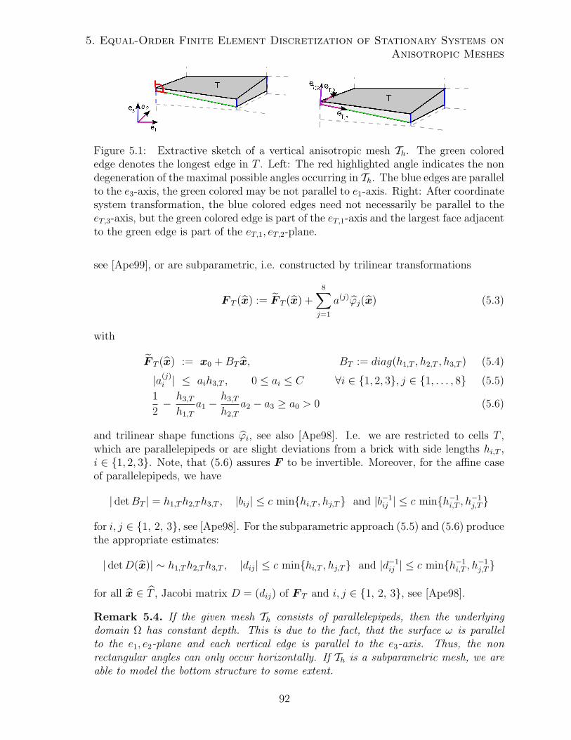
5. Equal-Order Finite Element Discretization of Stationary Systems onAnisotropic Meshes
Figure 5.1: Extractive sketch of a vertical anisotropic mesh Th. The green colorededge denotes the longest edge in T . Left: The red highlighted angle indicates the nondegeneration of the maximal possible angles occurring in Th. The blue edges are parallelto the e3-axis, the green colored may be not parallel to e1-axis. Right: After coordinatesystem transformation, the blue colored edges need not necessarily be parallel to theeT,3-axis, but the green colored edge is part of the eT,1-axis and the largest face adjacentto the green edge is part of the eT,1, eT,2-plane.
see [Ape99], or are subparametric, i.e. constructed by trilinear transformations
F T (x) := F T (x) +8∑j=1
a(j)ϕj(x) (5.3)
with
F T (x) := x0 +BT x, BT := diag(h1,T , h2,T , h3,T ) (5.4)
|a(j)i | ≤ aih3,T , 0 ≤ ai ≤ C ∀i ∈ 1, 2, 3, j ∈ 1, . . . , 8 (5.5)
1
2− h3,T
h1,T
a1 − h3,T
h2,T
a2 − a3 ≥ a0 > 0 (5.6)
and trilinear shape functions ϕi, see also [Ape98]. I.e. we are restricted to cells T ,which are parallelepipeds or are slight deviations from a brick with side lengths hi,T ,i ∈ 1, 2, 3. Note, that (5.6) assures F to be invertible. Moreover, for the affine caseof parallelepipeds, we have
| detBT | = h1,Th2,Th3,T , |bij| ≤ c minhi,T , hj,T and |b−1ij | ≤ c minh−1
i,T , h−1j,T
for i, j ∈ 1, 2, 3, see [Ape98]. For the subparametric approach (5.5) and (5.6) producethe appropriate estimates:
| detD(x)| ∼ h1,Th2,Th3,T , |dij| ≤ c minhi,T , hj,T and |d−1ij | ≤ c minh−1
i,T , h−1j,T
for all x ∈ T , Jacobi matrix D = (dij) of F T and i, j ∈ 1, 2, 3, see [Ape98].
Remark 5.4. If the given mesh Th consists of parallelepipeds, then the underlyingdomain Ω has constant depth. This is due to the fact, that the surface ω is parallelto the e1, e2-plane and each vertical edge is parallel to the e3-axis. Thus, the nonrectangular angles can only occur horizontally. If Th is a subparametric mesh, we areable to model the bottom structure to some extent.
92
5.1 Preliminaries
(b) Mesh restrictions for the anisotropic Scott-Zhang interpolation operator
In order to derive an interpolation operator, which is based on the Scott-Zhang operatorfor isotropic meshes and shows suitable interpolation estimates, Apel [Ape99] restrictsto meshes of tensor product type. Supposing flat cells, i.e. h1,T ∼ h2,T h3,T thecellwise transformations are given as
F T (x) = x0 +Bx with B =
(BT 00 ±h3,T
)(5.7)
such that | detBT | ∼ h21,T , ||BT || ∼ h1,T , and ||B−1
T || ∼ h−11,T , see [Ape99]. Moreover, in
order to treat the missing continuity of the underlying functions v, abrupt changes inthe element sizes are forbidden, i.e. hi,T ∼ hi,T ′ shall apply for all T, T ′ with T ∩T ′ 6= ∅.Speaking of which, the patch of T is denoted as
ST = int
( ⋃T ′∈Th
T ′ | T ∩ T ′ 6= ∅) .
Note, that the aip and the csc, as well as Assumption 4.2 obviously are fulfilled.
Lemma 5.5 (Inverse estimate). Let T be a cell of a vertical anisotropic tensor producttype mesh Th, vh ∈ Hk(T ) ∩Qr(T ) and 0 ≤ m ≤ k ≤ r. Then, the following estimateapplies:
|vh |k,T ≤ hm1,T h−k3,T |vh |m,T .
Proof. We collect some properties of the transformation F T (x) = x0 +Bx as given in(5.7). As Th is vertical anisotropic we have h3,T h1,T ∼ h2,T . Due to the constructionof F we have ||B|| . hT ∼ h1,T and ||B−1|| . ρ−1
T ∼ h−13,T , see also Section 4.1.1 on page
49 for the notations hT and ρT , and [Bra07]. Applicating the transformation theoremand suitable estimates on the reference element (both can be found in [Bra07]), wededuce for any T ∈ Th:
|vh |k,T . ||B−1||k | detB−1|−1/2 |vh|m,bT . ||B−1||k ||B||m |vh |m,T .
However, this estimate is too rough for the upcoming issues, as the scalings of thedifferent directional derivates are not distinguished. On Cartesian meshes we observethe following improved estimate for first derivatives, which is expandable to tensorproduct type meshes:
Lemma 5.6 (Inverse estimate for brick elements). Given a brick cell T of a mesh Thwith side lengths h1,T , h2,T , h3,T , for any vh ∈ H1(T )∩Qr(T ) and partial derivation ∂xi,i ∈ 1, 2, 3, the following inverse estimate applies:
||∂xi vh ||0,T . h−1i,T ||vh ||0,T .
93
5. Equal-Order Finite Element Discretization of Stationary Systems onAnisotropic Meshes
Proof. We set xj := xjh−1j,T , j ∈ 1, 2, 3 and consider the transformed brick element
T with side lengths 1, i.e. the transformation FT : T → T is given by FT (x) := BT x
with BT = diag(h1, h2, h3). We consider ξ := ∂xi vh(x) and ξ := ∂bxivh(x), and observe∂bxi(FT )j(x) = hiδij as well as ∂xi(F
−1T )j(x) = h−1
i,T δij. Thus the relation
|∂bxivh(x)| = |∂bxi(vh FT )(x)| =
∣∣∣∣∣3∑j=1
∂xj vh(x) · ∂bxi(FT )j(x)
∣∣∣∣∣ = hi,T |∂xi vh(x)|
(5.8)
applies and, using the transformation formula, see also [Bra07], we get
||∂xi vh ||20,T =
∫T
|∂xi vh(x)|2 dx = h−2i,T
∫T
∣∣∂bxivh(F−1T (x))
∣∣2 dx= h−2
i,T | detB−1T |−1
∫bT |∂bxivh(x)|2 dx = h−2
i,T | detB−1T |−1||∂bxivh||20,bT .
On the cubic element T we can apply the isotropic version of the inverse estimate ofLemma 5.5, see e.g. [Bra07],
||∂bxivh||20,bT ≤ |vh|21,bT . ||vh||20,bT .Again, applying the transformation formula we finally get
||∂xi vh ||20,T . h−2i,T | detB−1
T |−1||vh||20,bT . h−2i,T ||vh ||20,T .
Remark 5.7. Consider a vertical anisotropic tensor product type mesh Th, i.e. wehave hω,T := h1,T ∼ h2,T h3,T and a cellwise transformation F T as given in (5.7).The validation of the proposition of Lemma 5.6 for ∂x3 vh for any T ∈ Th is completelythe same. Considering either ∂x1 vh or ∂x2 vh, the proof of Lemma 5.6 alters in (5.8)to
|∂bxivh(x)| = |∂bxi(vh FT )(x)| =
∣∣∣∣∣3∑j=1
∂xj vh(x) · ∂bxi(FT )j(x)
∣∣∣∣∣. hω,T
2∑j=1
∣∣∂xj vh(x)∣∣ .
The remaining deductions remain. Thus we finally observe on vertical anisotropic,tensor product type meshes:
||∂xi vh ||0,T . h−1ω,T ||vh ||0,T ∀i ∈ 1, 2 ,∀T ∈ Th ,
||∂x3 vh ||0,T . h−13,T ||vh ||0,T .
Remark 5.8. The inverse estimates also apply for the 2D case with h1,K h2,K ontensor product meshes.
94
5.1 Preliminaries
5.1.2 Interpolation operators
We use the following notations: Given a multi index α := (α1, α2, α3), let |α| :=∑i αi, cα := (cα1, cα2, cα3), xα := xα1
1 xα22 x
α33 and Dα := ∂|α|/(∂xα1
1 ∂xα22 ∂x
α33 ) for any
α1, α1, α2, α3 ∈ N and c ∈ R>0. Moreover recall that we apply the space of polynomialsof order r in each coordinate direction.
(a) Lagrangian interpolation operator
The operator i(r) : C(T ) → Qr(T ) denotes the Lagrangian interpolation operator. Weset (i(r) v)(x) = i(r)v(x) with v(x) := v(F (x)). Provided the considered mesh showsthe aic and the csc, and T is a parallelepiped or the cellwise transformations are givenby (5.3), Apel [Ape98, Ape99] elaborates the estimate
||v−i(r) v ||20,T ≤ c∑|α|=r+1
h2αT ||Dα v ||20,T ∀v ∈ Hr+1(T ) ∩ C(T ) ∀T ∈ Th .
The estimates for v−i(r) v in the Sobolev spaces Hm(T ) are as follows. Provided, Thfulfills the aic and the csc, T is a parallelepiped and m ∈ 0, . . . , r, Apel [Ape99]further derives
|v−i(r) v |2m,T ≤ c∑
r+1−m≤|α|≤r+2−mh2αT ||Dα v ||2m,T ∀v ∈ Hr+2(T ) ∀T ∈ Th .
For the subparametric case and m = 1 the same estimate is given in [Ape98].
(b) Scott-Zhang interpolation operator
In order to refrain from the high regularity demands of the Lagrangian interpolationoperator on v, a resort is given by application of the Scott-Zhang approach. Apel[Ape99] introduced Scott-Zhang operators for cells of different stretching, in particularfor flat cells, which occur in the case of vertical anisotropic meshes. Apel restricts to(unions of) meshes of tensor product type. See also Subsection 5.1.1 (b) for appropriatenotions and further restrictions.Let z(r) denote this anisotropic Scott-Zhang interpolation operator, mapping on Qr.Given a cell T ∈ Th with h1,T , h2,T ≥ h3,T in ST , Apel derived the following estimates
|z(r) v |m,T ≤ c|v |m,ST ∀v ∈ Hl(ST ) (5.9)
|v−z(r) v |m,T ≤ c∑|α|=l−m
hαT |Dα v |m,ST ∀v ∈ Hl(ST ) (5.10)
with 0 ≤ m ≤ l and 1 ≤ l ≤ r + 1, which are also valid for the 2D case.For our purposes, the given estimates are not sufficient in order to get optimal a priorierror estimates (in the vertical anisotropic hydrostatic Oseen case). Due to that reason,we examine the estimation properties a little further than has been done in [Ape99]:
95
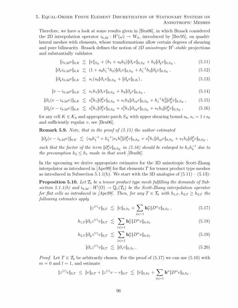
5. Equal-Order Finite Element Discretization of Stationary Systems onAnisotropic Meshes
Therefore, we have a look at some results given in [Bra06], in which Braack consideredthe 2D interpolation operator ih,2d : H1(ω) → Wh, introduced by [Bec95], on quadri-lateral meshes with elements, whose transformations allow certain degrees of shearingand pure bilinearity. Braack defines the notion of 2D anisotropic H1-stable projectionsand substantially validates
||ih,2dv||0,K . ||v||SK + (h1 + s0h2)||∂xv||0,SK + h2||∂yv||0,SK , (5.11)
||∂xih,2dv||0,K . (1 + s0h−11 h2)||∂xv||0,SK + h−1
1 h2||∂yv||0,SK , (5.12)
||∂yih,2dv||0,K . s1(s0||∂xv||0,SK + ||∂yv||0,K) , (5.13)
||v − ih,2dv||0,K . s1h1||∂xv||0,SK + h2||∂yv||0,SK , (5.14)
||∂x(v − ih,2dv)||0,K . s21h1||∂2
xv||0,SK + s1h2||∂xyv||0,SK + h−11 h2
2||∂2yv||0,SK , (5.15)
||∂y(v − ih,2dv)||0,K . s21h1||∂2
xv||0,SK + s21h1||∂xyv||0,SK + s1h2||∂2
yv||0,SK , (5.16)
for any cell K ∈ Kh and appropriate patch SK with upper shearing bound s0, s1 = 1+s0
and sufficiently regular v, see [Bra06].
Remark 5.9. Note, that in the proof of (5.15) the author estimated
||∂y(v − ih,2dv)||0,K . (s0h−11 + h−1
2 )s1h21||∂2
xv||0,SK + s21h1||∂xyv||0,SK + s1h2||∂2
yv||0,SK ,such that the factor of the term ||∂2
xv||0,SK in (5.16) should be enlarged to h1h−12 due to
the presumption h2 ≤ h1 made in that work [Bra06].
In the upcoming we derive appropriate estimates for the 3D anisotropic Scott-Zhanginterpolator as introduced in [Ape99] for flat elements T for tensor product type meshesas introduced in Subsection 5.1.1(b). We start with the 3D analogies of (5.11) – (5.13):
Proposition 5.10. Let Th be a tensor product type mesh fulfilling the demands of Sub-section 5.1.1(b) and ih,3d : H1(Ω) → Qr(Th) be the Scott-Zhang interpolation operatorfor flat cells as introduced in [Ape99]. Then, for any T ∈ Th with h1,T , h2,T ≥ h3,T thefollowing estimates apply
||z(r)v||0,T . ||v||0,ST +∑|α|=1
hαT ||Dαv||0,ST , (5.17)
h1,T ||∂xz(r)v||0,T .∑|α|=1
hαT ||Dαv||0,ST (5.18)
h2,T ||∂yz(r)v||0,T .∑|α|=1
hαT ||Dαv||0,ST (5.19)
||∂zz(r)v||0,T . ||∂zv||0,ST . (5.20)
Proof. Let T ∈ Th be arbitrarily chosen. For the proof of (5.17) we can use (5.10) withm = 0 and l = 1, and estimate
||z(r)v||0,T ≤ ||v||0,T + ||z(r)v − v||0,T . ||v||0,ST +∑|α|=1
hα||Dαv||0,ST .
96
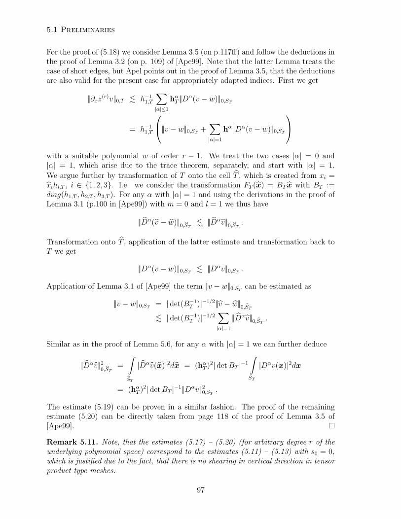
5.1 Preliminaries
For the proof of (5.18) we consider Lemma 3.5 (on p.117ff) and follow the deductions inthe proof of Lemma 3.2 (on p. 109) of [Ape99]. Note that the latter Lemma treats thecase of short edges, but Apel points out in the proof of Lemma 3.5, that the deductionsare also valid for the present case for appropriately adapted indices. First we get
||∂xz(r)v||0,T . h−11,T
∑|α|≤1
hαT ||Dα(v − w)||0,ST
= h−11,T
||v − w||0,ST +∑|α|=1
hα||Dα(v − w)||0,ST
with a suitable polynomial w of order r − 1. We treat the two cases |α| = 0 and|α| = 1, which arise due to the trace theorem, separately, and start with |α| = 1.
We argue further by transformation of T onto the cell T , which is created from xi =xihi,T , i ∈ 1, 2, 3. I.e. we consider the transformation FT (x) = BT x with BT :=diag(h1,T , h2,T , h3,T ). For any α with |α| = 1 and using the derivations in the proof ofLemma 3.1 (p.100 in [Ape99]) with m = 0 and l = 1 we thus have
||Dα(v − w)||0,bST . ||Dαv||0,bST .Transformation onto T , application of the latter estimate and transformation back toT we get
||Dα(v − w)||0,ST . ||Dαv||0,ST .
Application of Lemma 3.1 of [Ape99] the term ||v − w||0,ST can be estimated as
||v − w||0,ST = | det(B−1T )|−1/2||v − w||0,bST
. | det(B−1T )|−1/2
∑|α|=1
||Dαv||0,bST .
Similar as in the proof of Lemma 5.6, for any α with |α| = 1 we can further deduce
||Dαv||20,bST =
∫bST|Dαv(x)|2dx = (hαT )2| detBT |−1
∫ST
|Dαv(x)|2dx
= (hαT )2| detBT |−1||Dαv||20,ST .
The estimate (5.19) can be proven in a similar fashion. The proof of the remainingestimate (5.20) can be directly taken from page 118 of the proof of Lemma 3.5 of[Ape99].
Remark 5.11. Note, that the estimates (5.17) – (5.20) (for arbitrary degree r of theunderlying polynomial space) correspond to the estimates (5.11) – (5.13) with s0 = 0,which is justified due to the fact, that there is no shearing in vertical direction in tensorproduct type meshes.
97
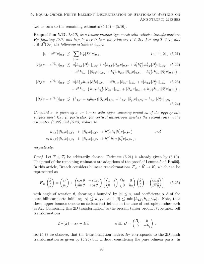
5. Equal-Order Finite Element Discretization of Stationary Systems onAnisotropic Meshes
Let us turn to the remaining estimates (5.14) – (5.16).
Proposition 5.12. Let Th be a tensor product type mesh with cellwise transformationsF T fulfilling (5.7) and h1,T ≥ h2,T ≥ h3,T for arbitrary T ∈ Th. For any T ∈ Th andv ∈ H2(ST ) the following estimates apply:
||v − z(r)v||0,T .∑|α|=i
hαT ||Dαv||0,ST i ∈ 1, 2, (5.21)
||∂x(v − z(r)v)||0,T . s21h1,T ||∂2
xv||0,ST + s21h2,T ||∂xyv||0,ST + s2
1h−11,Th
22,T ||∂2
yv||0,ST (5.22)
+ s21 h3,T
(||∂xzv||0,ST + h−11,T h2,T ||∂yzv||0,ST + h−1
1,T h3,T ||∂2zv||0,ST
),
||∂y(v − z(r)v)||0,T . s21h
21,Th
−12,T ||∂2
xv||0,ST + s21h1,T ||∂xyv||0,ST + s2
1h2,T ||∂2yv||0,ST (5.23)
+ s21 h3,T
(h1,T h
−12,T ||∂xzv||0,ST + ||∂yzv||0,ST + h−1
2,Th3,T ||∂2zv||0,ST
),
||∂z(v − z(r)v)||0,T . (h1,T + s0h2,T )||∂xzv||0,ST + h2,T ||∂yzv||0,ST + h3,T ||∂2zv||0,ST .
(5.24)
Constant s1 is given by s1 := 1 + s0 with upper shearing bound s0 of the appropriatesurface mesh Kh. In particular, for vertical anisotropic meshes the second rows in theestimates (5.22) and (5.23) reduce to
h3,T (||∂xzv||0,ST + ||∂yzv||0,ST + h−11,Th3||∂2
zv||0,ST ) and
s1 h3,T (||∂xzv||0,ST + ||∂yzv||0,ST + h−11 h3,T ||∂2
zv||0,ST ) ,
respectively.
Proof. Let T ∈ Th be arbitrarily chosen. Estimate (5.21) is already given by (5.10).The proof of the remaining estimates are adaptions of the proof of Lemma 5 of [Bra06].
In this article, Braack considers bilinear transformations FK : K → K, which can berepresented as
FK
(xy
)=
(x0
y0
)+
(cos θ − sin θsin θ cos θ
)[(1 s0 1
)(h1 00 h2
)(xy
)+
(αxyβxy
)](5.25)
with angle of rotation θ, shearing s bounded by |s| ≤ s0 and coefficients α, β of thepure bilinear parts fulfilling |α| ≤ h1,T/4 and |β| ≤ minh2,T , h1,T/s0. Note, thatthese upper bounds denote no serious restrictions in the case of isotropic meshes suchas Kh. Comparing this 2D transformation to the present tensor product type mesh celltransformations
F T (x) = x0 +Bx with B =
(BT 00 ±h3
),
see (5.7) we observe, that the transformation matrix BT corresponds to the 2D meshtransformation as given by (5.25) but without considering the pure bilinear parts. In
98
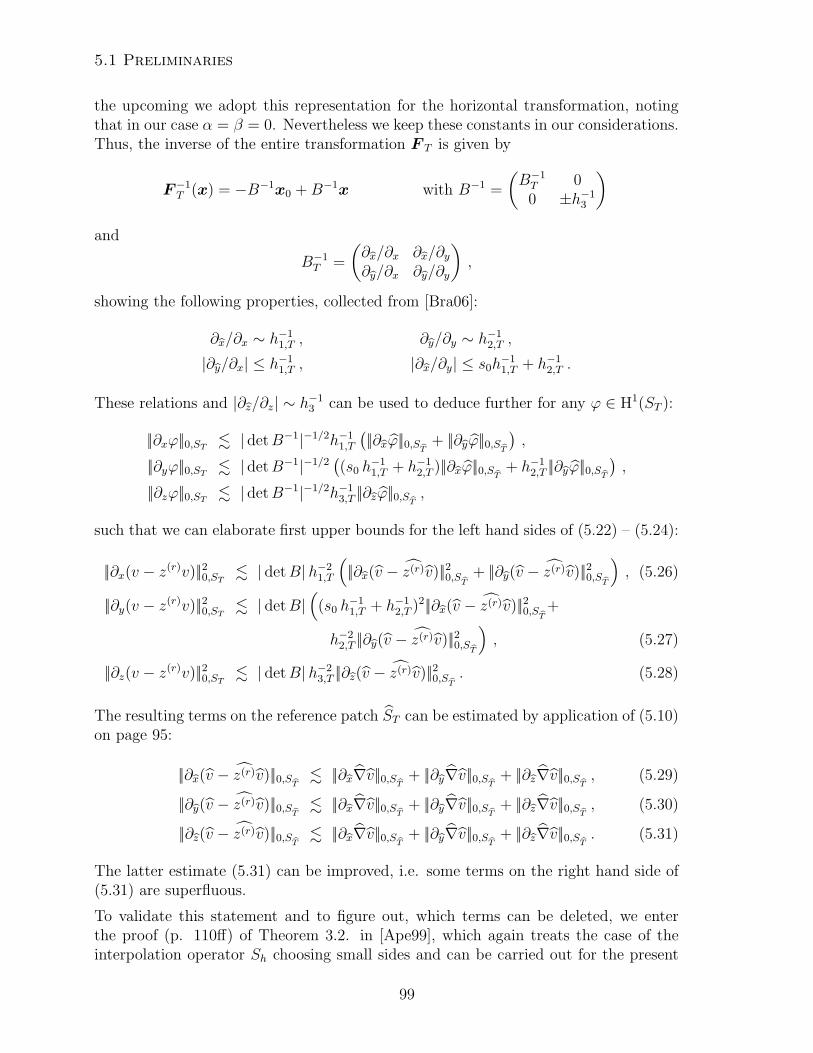
5.1 Preliminaries
the upcoming we adopt this representation for the horizontal transformation, notingthat in our case α = β = 0. Nevertheless we keep these constants in our considerations.Thus, the inverse of the entire transformation F T is given by
F−1T (x) = −B−1x0 +B−1x with B−1 =
(B−1T 00 ±h−1
3
)and
B−1T =
(∂bx/∂x ∂bx/∂y∂by/∂x ∂by/∂y
),
showing the following properties, collected from [Bra06]:
∂bx/∂x ∼ h−11,T , ∂by/∂y ∼ h−1
2,T ,
|∂by/∂x| ≤ h−11,T , |∂bx/∂y| ≤ s0h
−11,T + h−1
2,T .
These relations and |∂bz/∂z| ∼ h−13 can be used to deduce further for any ϕ ∈ H1(ST ):
||∂xϕ||0,ST . | detB−1|−1/2h−11,T
(||∂bxϕ||0,S bT + ||∂byϕ||0,S bT),
||∂yϕ||0,ST . | detB−1|−1/2((s0 h
−11,T + h−1
2,T )||∂bxϕ||0,S bT + h−12,T ||∂byϕ||0,S bT
),
||∂zϕ||0,ST . | detB−1|−1/2h−13,T ||∂bzϕ||0,S bT ,
such that we can elaborate first upper bounds for the left hand sides of (5.22) – (5.24):
||∂x(v − z(r)v)||20,ST . | detB|h−21,T
(||∂bx(v − z(r)v)||20,S bT + ||∂by(v − z(r)v)||20,S bT
), (5.26)
||∂y(v − z(r)v)||20,ST . | detB|(
(s0 h−11,T + h−1
2,T )2||∂bx(v − z(r)v)||20,S bT+
h−22,T ||∂by(v − z(r)v)||20,S bT
), (5.27)
||∂z(v − z(r)v)||20,ST . | detB|h−23,T ||∂bz(v − z(r)v)||20,S bT . (5.28)
The resulting terms on the reference patch ST can be estimated by application of (5.10)on page 95:
||∂bx(v − z(r)v)||0,S bT . ||∂bx∇v||0,S bT + ||∂by∇v||0,S bT + ||∂bz∇v||0,S bT , (5.29)
||∂by(v − z(r)v)||0,S bT . ||∂bx∇v||0,S bT + ||∂by∇v||0,S bT + ||∂bz∇v||0,S bT , (5.30)
||∂bz(v − z(r)v)||0,S bT . ||∂bx∇v||0,S bT + ||∂by∇v||0,S bT + ||∂bz∇v||0,S bT . (5.31)
The latter estimate (5.31) can be improved, i.e. some terms on the right hand side of(5.31) are superfluous.
To validate this statement and to figure out, which terms can be deleted, we enterthe proof (p. 110ff) of Theorem 3.2. in [Ape99], which again treats the case of theinterpolation operator Sh choosing small sides and can be carried out for the present
99
5. Equal-Order Finite Element Discretization of Stationary Systems onAnisotropic Meshes
operator, see also the proof of Theorem 3.3 in [Ape99]. For a given γ with |γ| = 1 andv ∈ H2(SbT ) we thus have
||Dγ(v − z(r)v)||0,S bT ≤ ||Dγ(v − w)||0,S bT + ||Dγ z(r)(w − v)||0,S bTfor any constant w. Due to the argumentation (on the reference element) in p.118in [Ape99] for the estimate (5.20), as well as for the horizontal cases, this estimatebecomes
||Dγ(v − z(r)v)||0,S bT . ||Dγ(v − w)||0,S bT , if Dγ = ∂z ,
||Dγ(v − z(r)v)||0,S bT . ||Dγ(v − w)||0,S bT + ||∇(v − w)||0,S bT ,. ||∇(v − w)||0,S bT else.
The last term in the latter estimate can not be neglected due to the application ofthe trace theorem (3.21) of [Ape99] in the deduction of the appropriate estimates (seeLemma 3.2 on page 109 in [Ape99]).
Using the proof (see p.101) of Lemma 3.1 on page of [Ape99] we deduce further
||Dγ(v − w)||0,S bT .∑|β|=1
||Dγ+β v||0,S bT .
Thus, we do not end up in an improvement of (5.29) – (5.30), but estimate (5.31) canbe replaced by
||∂bz(v − z(r)v)||0,bST . ||∂bz∇v||0,bST . (5.32)
Now, it essentially remains to estimate the terms on the right hand sides of (5.29),(5.30) and (5.32), and to assemble the entire informations elaborated above. Thereforewe collect the following estimates of the second derivatives. As also figured out in[Bra06] for the horizontal parts we observe the estimates:
|∂2bxv| . h21,T |∂2
xv| + h1,T h2,T |∂xyv| + h22,T |∂2
yv| ,|∂by∂bxv| = |∂by∂bxv| . (s0 h2,T + α)h1,T |∂2
xv| + (s0 h2,T + α)h2,T |∂xyv| + h22,T |∂2
yv| ,|∂bz∂bxv| = |∂bx∂bzv| . h3,T h1,T |∂xzv| + h3,T h2,T |∂yzv| ,
|∂2by v| . (s0 h2,T + α)2 |∂2xv| + (s0 h2,T + α)h2,T |∂xyv| + h2
2,T |∂2yv| ,
|∂bz∂byv| = |∂by∂bzv| . h3,T (s0 h2,T + α) |∂xzv| + h3,T h2,T |∂yzv| ,|∂2bz v| . h2
3,T |∂2zv| .
Assembling these estimates as well as using the limitations for α and h2,T ≤ h1,T we
100
5.1 Preliminaries
get
||∂bx∇v||0,bST . | detB|−1/2(h2
1,T ||∂2xv||0,ST + h1,T h2,T ||∂xyv||0,ST + h2
2,T ||∂2yv||0,ST+
h1,T h3,T ||∂xzv||0,ST + h2,T h3,T ||∂yzv||0,ST ) , (5.33)
||∂by∇v||0,bST . | detB|−1/2(s1 h
21,T ||∂2
xv||0,ST + s1 h1,T h2,T ||∂xyv||0,ST + h22,T ||∂2
yv||0,ST+
s1 h1,T h3,T ||∂xzv||0,ST + h2,T h3,T ||∂yzv||0,ST ) , (5.34)
||∂bz∇v||0,bST . | detB|−1/2h3,T ((h1,T + s0h2,T )||∂xzv||0,ST+ (5.35)
h2,T ||∂yzv||0,ST + h3,T ||∂2zv||0,ST
).
Combining (5.26) – (5.35) and suitable upper bounding finally lead to the desiredestimates.
Corollary 5.13. Let γ = (γ1, γ2, γ3) and γ = (γ1, γ2, 0) be multi-indices. For verticalanisotropic meshes the results of Proposition 5.12 can also be described as
||∂x(v − z(r)v)||0,T . hω∑|bγ|=2
||Dbγv||0,ST + h−1ω h3,T
∑|γ|=1
hγT ||∂zDγv||0,ST , (5.36)
||∂y(v − z(r)v)||0,T . hω∑|bγ|=2
||Dbγv||0,ST + h−1ω h3,T
∑|γ|=1
hγT ||∂zDγv||0,ST , (5.37)
||∂z(v − z(r)v)||0,T .∑|γ|=1
hγT ||∂zDγv||0,ST . (5.38)
Remark 5.14. Comparing the results of Proposition 5.12 we see, that the 3D Scott-Zhang interpolation operator maintains the results as introduced in [Bra06] as well inthree dimensions.
However, some further studies on the proofs of the propositions in [Ape99] reveal, thatthe estimates of Proposition 5.12 can be extended to the more common case of arbi-trary polynomial order r of the underlying finite element space on tensor product typemeshes. Due to our field of examination we restrict to the case of vertical anisotropicmeshes.
Proposition 5.15. Let Th be a vertical anisotropic tensor product type mesh withcellwise transformations F T fulfilling (5.7) and h1,T ≥ h2,T ≥ h3,T . For any T ∈ Th,v ∈ Hk+1(ST ), k ≤ r and γ with |γ| = 1 the following estimates apply:
||Dγ(v − z(r)v)||0,T . h−γT∑|α|≤k+1
hαT ||Dα v ||0,ST (5.39)
Proof. The proof uses the deductions of Lemma 3.5 in [Ape99], which are explicitelyformulated in Lemmata 3.1 and 3.2 in [Ape99]. We first observe for any polynomial wof order r − 1:
||Dγ(v − z(r)v)||0,T ≤ ||Dγ(v − w)||0,T + ||Dγz(r)(v − w)||0,T .
101
5. Equal-Order Finite Element Discretization of Stationary Systems onAnisotropic Meshes
Lemma 3.1 [Ape99] with m = 0 and l = k + 1 gives
hγT ||Dγ(v − w)||0,T ≤∑|α|=k+1
hαT |Dαv|0,ST
for a suitably chosen w. Existence of such a polynomial is assured due to Lemma 3.1.Let γ = (1, 0, 0) or γ = (0, 1, 0). Then, the term ||Dγz(r)(v − w)||0,T can be suitablyestimated as in the proof of Lemma 3.2, which supplies the estimate
||Dγz(r)(v − w)||0,T ≤ h−γT
||v − w||0,ST +∑|α|=1
hα||Dα(v − w)||0,ST
.
Again, applicating the estimates of Lemma 3.1 [Ape99] and noting, that hα ≤ hγ forany multi index α with |α| = 1 we get
||Dγz(r)(v − w)||0,T . h−γT∑|α|=k+1
hαT ||v||0,ST .
For the first order vertical derivative it suffices to consider the estimate (5.10) forl = k + 1 and m = 1:
||∂z(v−z(r) v)||0,T .∑|α|=k
hαT |Dα v |1,ST . h−13,T
∑|α|=k+1
hαT ||Dα v ||0,ST .
(c) L2-orthogonal interpolation operator
In the case of local projection stabilization of the hydrostatic Oseen problem in theanisotropic framework, it pays to have an interpolation operator, which not only ex-hibits suitable interpolation error estimates and stability properties, but also is L2-orthogonal with respect to a certain discrete space. Recall also Section 4.5.
Proposition 5.16. Assuming a vertical anisotropic tensor product type triangulationTh of Ω, such that the requirements of Subsection 5.1.1(b) for the Scott-Zhang interpo-lation operator are fulfilled. Let 0 ≤ k ≤ r. Then, there is an interpolation operatorih,3d : V→ Vh such that
(v−ih,3d v, ξ)Ω = 0 ∀v ∈ V ,∀ξ ∈ Qr−12h (Ω) , (5.40)
Moreover, for any v ∈ V and arbitrary T ∈ Th the following estimates apply:
||∂xih,3d v ||0,T + ||∂yih,3d v ||0,T . h−1ω
∑|α|=1
hαT ||Dα v ||0,ST (5.41)
||∂zih,3d v ||0,T . h−13,T
∑|α|=1
hαT ||Dα v ||0,ST . (5.42)
102
5.1 Preliminaries
The horizontal mesh size of the isotropic mesh Kh is given globally, i.e. by hω.For any v ∈ Hk+1(Ω) and T ∈ Th the interpolation operator ih,3d fulfills
||v−ih,3d v ||0,T +∑|γ|=1
hγT ||Dγ(v−ih,3d v)||0,T .∑|α|=k+1
hαT ||Dα v ||0,ST . (5.43)
Proof. The proof is an adaption the proof of the isotropic version as given in Lemma 4.5of [BB06] to the vertical anisotropic case. The operator ih,3d : V → Vh is constructedas ih,3d = z(r) +mh , with the anisotropic Scott-Zhang interpolant z(r) as introduced inSection 5.1.2(b). Due to (5.10), the operator z(r) fulfills the estimate (5.43). Moreover(5.41) and (5.42) apply for z(r), due to (5.18) –(5.20).
But the orthogonality property (5.40) is not assured, which has to be realized by theinvolvement of mh. Operator mh denotes the local projection from V onto Vh and isuniquely defined via
(mh v, ξ)M = (v−z(r) v, ξ)M ∀ξ ∈ Qr−12h (M) ,∀M ∈ T2h . (5.44)
Thus, ih,3d fulfills the orthogonality property (5.40). To reassure properties (5.41) –(5.43) note that due to (5.44) and the inverse estimate ||Dγ vh ||0,T ≤ h−γT ||vh ||0,Tfor any T ∈ Th and multi index γ with |γ| = 1, see Lemma 5.6 and Remark 5.7, theestimates
||mh v ||20,T =
∫T
(v−z(r) v)mh v dx . ||v−z(r) v ||0,T ||mh v ||0,T ,||Dγmh v ||20,T ≤ h−2γ
T ||mh v ||20,T . h−2γT ||v−z(r) v ||0,T ||mh v ||0,T
apply. Using the estimate of ||mh v ||0,T , the term ||Dγmh v ||0,T can be further estimatedas
||Dγmh v ||0,T ≤ h−γT ||v−z(r) v ||0,T ≤ h−γT∑|α|=k+1
hα1+α2ω hα3
3,T ||Dα v ||0,T .
Due to (5.10) and Proposition 5.15, z(r) provides property (5.43), and this estimate isfulfilled for the entire interpolation operator. The remaining estimates (5.41) and (5.42)for the common case are assured due to the improved inverse estimate, see Remark5.7, the estimate
||Dγmh v ||20,T . h−2γT ||mh v ||20,T . h−2γ
T ||v−z(r) v ||20,Tfor any T ∈ Th and multi-index γ with |γ| = 1, as well as the observation
||Dγ(ih,3d v)||0,T ≤ ||Dγ(z(r) v)||0,T + ||Dγ(mh v)||0,T .
Remark 5.17. Note, that the estimates (5.41) and (5.42) (for arbitrary r on verticalanisotropic tensor product type meshes) correspond to the results of the L2-orthogonal
103
5. Equal-Order Finite Element Discretization of Stationary Systems onAnisotropic Meshes
2D interpolation operator of [Bra08a] on Cartesian meshes for r = 1. The L2-estimatein (5.43) can be coarsened to
||v−ih,3d v ||0,T . h2ω (||∂x∇v ||0,ST + ||∂y∇v ||0,ST ) + h2
3,T ||∂z∇v ||0,ST ,
which corresponds to the appropriate L2-estimate of [Bra08a] on 2D Cartesian meshesfor r = 1. The same argumentation applies for the estimate of the first order deriva-tives.
5.1.3 Hydrostatic Issues
Discrete averaging operator on anisotropic meshes
The deductions and results of Subsection 4.1.3 on the discrete averaging operator areunaffected by the application of anisotropic meshes.
Discrete modified inf-sup constraint on anisotropic meshes
Let us recall the considerations of Section 4.1.3 on the discrete modified inf-sup con-straint. Given the discrete 3D velocity space Vh ⊂ V with V := H1
0(Ω) or V :=W1,p
b (Ω), chosen with respect to the underlying problem, and the discrete 2D pressurespace Qh ⊂ Q with Q := L2
0(ω) or Q := Lq0(ω), respectively, the discrete modifiedinf-sup constraint is given by
∃γ > 0 supvh∈Vh \0
(div ′Mvh, qh)Ω
||vh ||1,p,Ω ≥ γ||qh||0,q,ω ∀qh ∈ Qh . (5.45)
Proposition 5.18. The statements in Proposition 4.5 carry over to the case, whenvertical anisotropic or horizontal anisotropic meshes are applied.
Proof. As the results of the discrete averaging operator M : Vh → Wh are unaf-fected when anisotropic meshes are applied, the proof can directly be adapted from theisotropic case to the cases of vertical and horizontal anisotropic meshes.
Recalling the notions vertical anisotropic and horizontal anisotropic meshes, as well asProposition 5.18, we observe the following:
(a) If the underlying 3D mesh Th is vertical anisotropic, then the appropriate 2Dproblem is defined on a 2D isotropic mesh Kh. For those meshes we alreadyknow that e.g. equal-order finite elements are not suggestible without any furtherstabilization on the pressure.
(b) If the underlying 3D mesh is horizontal anisotropic, i.e. the 2D surface mesh isanisotropic, we have to fall back on hydrostatic finite element spaces Vh and Qh,such that Wh := M(Vh) and Qh are 2D inf-sup stable on anisotropic meshes.
104
5.2 Hydrostatic Stokes problem on vertical anisotropic meshes
In the framework of conforming finite elements, the authors of [AR01] presented anoverview of inf-sup stable pairs in the anisotropic context. We give some notes on theinf-sup stability results of [Bec95] and give an account of the survey in [AR01]:
Becker in [Bec95] validated inf-sup stability for stabilized elements Q1 −Q0 and Q1 −Q1, where he added suitably anisotropically adapted pressure stabilization terms ofcontinuous interior penalty type (see also (P-iii) on page 58 for the isotropic case) andof type (P-i) to the 2D Stokes problem. Moreover note, that Becker paves the wayfor the LPS approach in an anisotropic framework on Q1 elements using L2 projectionon the constants. The LPS approach for bilinear elements on 2D finally was proposedin [Ric05]. In [SS98, SSS99], Schotzau, Schwab and Stenberg examined the elementsQr −Qr−2 and Pr − Pr−2, r ≥ 2. It turned out, that that this approach is aspect ratioindependent inf-sup stable on 2D Cartesian meshes with thin layers along 2 oppositesides. Problems are supposed to arise near corners. The authors of [AC00] validatedfor the 2D case for the finite element space choice Qr+maxµr,1,r − Pr−1 for arbitrarybut fix µ, that the inf-sup constant is bounded away from zero and independent on theaspect ratio. In this case, the inf-sup constant depends on µ. Aspect ratio independentinf-sup stability for the 3D case for Qr − Qr−2 elements on meshes with refinementstowards faces has been proven by [TS01]. Apel and Randrianarivony figure out, thatQr − Qr−2 and the Taylor–Hood pair P2 − P1 is (experimentally) inf-sup stable onlayered meshes, which is not the rule for arbitrary anisotropic meshes. Moreover, themini element is observed to be not inf-sup stable.
5.2 Hydrostatic Stokes problem on vertical aniso-
tropic meshes
In this section we consider the hydrostatic Stokes problem in the vertical anisotropicframework. We start with a stability analysis of the Galerkin formulation of the prob-lem on vertical anisotropic meshes. As in the isotropic case it turns out, that theequal-order finite element approach we use does not lead to an inf-sup stable problem.Motivated by this lack, we consider the symmetric stabilization schemes (P-i) – (P-iv)of the isotropic hydrostatic Stokes problem in the vertical anisotropic framework. Weelaborate stability and optimal error estimates of the stabilized problem. Finally wecompare the results with the results of the appropriate isotropic problem and withsome results given in literature for the anisotropic 2D Stokes problem.
5.2.1 Galerkin formulation
Let Th be a vertical anisotropic triangulation fulfilling Assumption 4.2. Based on thismesh we define the discrete velocity space Vh ⊂ V := H1
0(Ω) and the pressure spaceQh ⊂ Q := L2
0(ω) as given in (4.6) and (4.4), and set Xh := Vh×Qh. As in the case of
105
5. Equal-Order Finite Element Discretization of Stationary Systems onAnisotropic Meshes
isotropic meshes the hydrostatic Stokes problem reads
Given f ∈ V−1, find (vh, ph) ∈ Xh (5.46)
s. t. a(vh,ϕ)− b(ph,ϕ) + b(ξ,vh) = (f ,ϕ)Ω ∀(ϕ, ξ) ∈ Xh
with bilinear forms a(vh,ϕ) := (∇vh,∇ϕ)Ω and b(ph,ϕ) := (ph, div ′Mϕ)ω.
As indicated in the preceding subsection (see note (a) on page 104) the elaboratedproperties for the hydrostatic Stokes problem on isotropic meshes are recovered in thecase of vertical anisotropic meshes:
Proposition 5.19. Let Ω be a flat domain and Th be a vertical anisotropic triangulationof Ω fulfilling Assumption 4.2. The 2.5D Stokes problem (5.46) has a unique solution,if the 2D Stokes problem (4.18) has a unique solution.
Proof. We argue as in the proof of Proposition 4.15. First, the continuous bilinearform a : V×V → R is still V-elliptic, and we still have conforming finite elements,i.e. Vh ⊂ V. Moreover, due to Proposition 5.18, the 2.5D problem (5.46) fulfills thediscrete modified inf-sup condition (5.45), if the appropriate inf-sup condition (4.17)of the 2D Stokes problem is fulfilled.
Due to consideration (a) on page 104, the equal-order finite element discretized hydro-static Stokes problem (5.46) on vertical anisotropic meshes is not inf-sup stable. Asintroduced for the case of isotropic meshes we avoid this problem by adding suitablestabilization terms to the system.
Remark 5.20. Anticipatory we note, that the discrete hydrostatic Stokes problem inthe vertical anisotropic context, i.e. problem (5.46), is formulated for a large class oftriangulations (and domains).In order to derive suitable error estimates we split the entire error into an interpolationand a projection error. Restrictively, suitable interpolation results, see also Section5.1.2, are only known (to the author) for a quite small class of triangulations (andthus of Ω).
5.2.2 Stabilization of the problem
As the inf-sup stability is a 2D concern, the solely pressure dependent stabilizationschemes for the hydrostatic Stokes case on isotropic meshes are expected to be easilyadaptable. The deductions and estimates concerning the pressure are anticipated to betransferable in a straightforward matter. The velocity field concerning parts howeverare expected to need some altered treatment as this field is defined on an anisotropicmesh, unlike the 2D pressure.The appropriately stabilized 2.5D Stokes problem is given as in the isotropic case:
Find (vh, ph) ∈ Xh s. t.
Ah(vh, ph;ϕ, ξ) = (f ,φ)Ω ∀φ := (ϕ, ξ) ∈ Xh
(5.47)
with Ah(vh, ph;ϕ, ξ) := a(vh,ϕ)− b(ph,ϕ) + b(ξ,vh) + sh(ph, ξ) . (5.48)
106
5.2 Hydrostatic Stokes problem on vertical anisotropic meshes
The applied stability term is chosen from the list (P-i) – (P-iv) of Section 4.2.2.
We define the triple norm on Xh as in (4.36),
|||(v, p)||| := (||∇v ||20,Ω + ||p||20,ω + sh(p, p))1/2
, (5.49)
as well as Bh:
Bh := (vh, ph) ∈ Xh | |||(vh, ph)||| = 1 .The following proposition shows that adding an arbitrary stabilization term of themethods (P-i)–(P-iv) leads to an inf-sup stable discretization of the 2.5D Stokes prob-lem on vertical anisotropic meshes.
Proposition 5.21. Let Ω be a flat basin and Th be a vertical anisotropic triangulationof Ω fulfilling Assumption 4.2. We consider the symmetric stabilizations (P-i)–(P-iv)of Section 4.2.2. The resulting 2.5D Stokes bilinear form (5.48) is also inf-sup stable:
inf(vh,ph)∈Bh
sup(ϕ,ξ)∈Bh
Ah(vh, ph;ϕ, ξ) ≥ γΩ,ω .
Proof. The proof can be accomplished as the proof of Proposition 4.18. We collect thecorner stones of that proof which are relevant for the present class of stabilizations:Let yh := (vh, ph) ∈ Xh be arbitrarily chosen. Splitting the triple norm into two parts
|||yh|||2 = |yh|2a + |yh|2b ,|yh|2a := |vh |21,Ω + sh(ph, ph) ,
|yh|2b := ||ph||20,ω ,and diagonal testing of the bilinear form (5.48) gives Ah(yh;yh) = |yh|2a. The inf-supcondition follows if a vh ∈ Vh exists such that |||(vh, 0)||| ≤ |||yh||| and
Ah(vh, ph; vh, 0) ≥ c1|uh |2b − c2|uh |2a ,with suitable constants c1 > 0 and c2. In order to find such vh ∈ Vh let ϕ ∈Wh be cho-sen, so that (ϕ, ph) satisfies estimate (4.28). Using the surjectivity of M (Lemma 4.4)we choose a vh ∈ Vh with ϕ = M vh, such that we can apply Lemma 4.8.Thus, the crucial argumentation passes on to a 2D argumentation on an isotropic meshand we can further argue as in the proof of Proposition 4.18: With wh := Mvh ∈Wh
and due to Lemma 4.8 we obtain
Ah(yh; vh, 0) = (∇vh,∇vh)Ω − (ph, div ′ wh)ω + sh(ph; 0)
≥ −|vh |1,Ω|vh|1,Ω +γω4||ph||20,ω −
1
γωsh(ph, ph)
≥ −(
4
γωc2ωδ−3min|vh |21,Ω +
γω16||ph||20,ω
)+γω4||ph||20,ω −
1
γωsh(ph, ph)
≥ − c
γωc2ωδ−3min|vh |21,Ω +
γω8||ph||20,ω −
1
γωsh(ph, ph)
≥ − 1
γω
(1 + cc2
ωδ−3min
) |yh|2a +γω8|yh|2b .
107
5. Equal-Order Finite Element Discretization of Stationary Systems onAnisotropic Meshes
5.2.3 A priori error estimates
The deduction of a priori error estimates for the stabilized 2.5D Stokes problem isbased on the estimates of the stabilization terms for the 2D Stokes problem. As in theisotropic case, the (perturbed) 2D Galerkin orthogonality,
Aωh(w−wh, p− ph;ϕ, ξ) = sh(p, ξ) ∀(ϕ, ξ) ∈Wh×Qh ,
plays a crucial role in the derivation of suitable error estimates.
Proposition 5.22. Let Ω be chosen such that there is a vertical anisotropic triangula-tion Th of Ω, fulfilling the restrictions of Subsection 5.1.1(b). If the continuous solutionof (4.32) formulated in X := (V×Q) is sufficiently regular, (v, p) ∈ Hr+1(Ω)×Hr(ω),we obtain the following estimate for the discrete solutions (vh, ph) of (5.47) for themethods (P-i)–(P-iv):
|||(v−vh, p− ph)||| .∑T∈Th
∑|α|=r
hαT |Dα v |1,ST +∑K∈Kh
hrK ||p||r,SK (5.50)
with patches ST and SK for any T ∈ Th and K ∈ Kh.
Proof. As usual we split the error into an interpolation error and a projection error.Note that the pressure is defined on an isotropic mesh. Let zhp be the Scott-Zhanginterpolant as given in the isotropic case, and zh v be the Scott-Zhang interpolant foranisotropic meshes of tensor product type as introduced in Subsection 5.1.2. (Note thatthe latter interpolation operator is responsible for the restrictive choice of Th.) Withthese interpolants and Lemma 4.12 we already get estimate (5.50) for |||(v−zh vh, p−zhph)|||.Thus it remains to bound the projection errors ||zh v−vh ||1,Ω and ||zhp− ph||0,ω by theright hand side of (5.50). Due to the discrete inf-sup condition there is a test function(ϕ, ξ) ∈ Xh with |||(ϕ, ξ)||| = 1 and
γΩ,ω|||(zh v−vh, zhp− ph)||| ≤ Ah(zh v−vh, zhp− ph;ϕ, ξ) .Using the (perturbed) Galerkin orthogonality we obtain
γΩ,ω|||(zh v−vh, zhp− ph)||| ≤ Ah(zh v−v, zhp− p;ϕ, ξ) + sh(p, ξ)
= a(zh v−v,ϕ)− b(zhp− p,ϕ)
+ b(ξ, zh v−v)− sh(zhp, ξ) .The Galerkin terms on the right hand side can be bounded by
a(zh v−v,ϕ) ≤ |zh v−v |1,Ω|||(ϕ, 0)||| ≤ c∑T∈Th
∑|α|=r
hαT |Dα v |1,ST
− b(zhp− p,ϕ) ≤ ||zhp− p||0,ω|||(ϕ, 0)||| ≤ chrω||p||r,ωb(ξ, zh v−v) ≤ ||div ′M(zh v−v)||0,ω|||(0, ξ)||| ≤ cω
∑T∈Th
∑|α|=r
hαT |Dα v |1,ST .
108
5.2 Hydrostatic Stokes problem on vertical anisotropic meshes
The stabilization term is 2D. Particularly it is defined on an isotropic mesh, and canbe bounded as in the proof of Proposition 4.21 by
sh(zhp, ξ) ≤ chrω||p||r,ω ,see page 71. In sum we arrive at the following estimate which implies the assertion:
γΩ,ω|||(zh v−vh, zhp− ph)||| . hrω||p||r,ω +∑|α|=r
hαT |Dα v |1,ST .
In the proof of Proposition 5.22 we used the anisotropic Scott-Zhang interpolation op-erator for the velocity, which forced us to restrict to tensor product type meshes. Arelaxation of this constraint is given by the anisotropic Lagrangian interpolation oper-ator, which has the lack of higher regularity demands on the solution of the problem:
Proposition 5.23. Let Th be a vertical anisotropic triangulation of Ω fulfilling As-sumption 4.2 and the demands of Subsection 5.1.1(a). If the continuous solution of(4.32) formulated in X := (V×Q) is sufficiently regular, (v, p) ∈ Hr+2(Ω) × Hr(ω),we obtain the following estimate for the discrete solutions (vh, ph) of (5.47) with stabi-lization scheme chosen from (P-i)–(P-iv):
|||(v−vh, p− ph)||| .∑T∈Th
∑|α|=r
hαT |Dα v |1,ST + hrω ||p||r,ω , (5.51)
with meshsize independent constant c.
Proof. The proof is the same as the proof of Proposition 5.22 with the difference, thatwe now apply the anisotropic Lagrangian interpolation operator. For the appropriateregularity constraints and differing estimates see Subsection 5.1.2(a).
Remark 5.24. Let r ≥ 1. For ease of an upcoming comparison with appropriateresults given in literature, the estimates of Propositions 5.22 and 5.23 can easily bereformulated as
|||(v−vh, p− ph)||| .∑T∈Th
(h1,T
∑|α|=r−1
hαT |∂xDα v |1,ST + h2,T
∑|α|=r−1
hαT |∂yDα v |1,ST)
+ h3,T
∑|α|=r−1
hαT |∂zDα v |1,ST)
+ hrω ||p||r,ω .
5.2.4 Conclusions
Application of the symmetric pressure stabilization applied in the isotropic case alsoleads to stabilization of the hydrostatic Stokes problem in the vertical anisotropicframework. The reason is the isotropic structure of Kh and the fact, that the pressure
109
5. Equal-Order Finite Element Discretization of Stationary Systems onAnisotropic Meshes
is defined on that 2D mesh.Comparing the present results to the isotropic case we end up in similar a priori errorestimates. But, in the anisotropic framework we are able to account for the anisotropyof the mesh and get suitably weighted results. However, the price to be paid is eitherthe restriction on the mesh and on the underlying domain, or weaker restrictions onthe mesh than in the former (Scott-Zhang) case but higher regularity demands for thesolution of the variational problem.
Comparing the present results to the results of the anisotropic 2D Stokes problem,see e.g. [Bec95, MPP02, BT06a, AM08, Bla08], we observe the following: The mostconspicuous difference to the anisotropic 2D Stokes problem is, that we do not haveto alter the stabilization of the scheme, neither the scheme itself nor the stabilizationparameters, although the mesh shows (certain) anisotropic behavior. This is owed tothe fact, that the (hydrostatic) pressure is only 2D and lives on an isotropic mesh. Thisenables the successful application of appropriate symmetric stabilizations in the verti-cal anisotropic framework, and a choice of the polynomial degree r as in the isotropicframework.Comparing the present results with the results of the non conforming approach theauthors of [AM08] (for the 2D Stokes problem) we get similar estimates but withoutcatching an additional term due to the non conformity. Moreover, the results in [AM08]apply for suitably constructed, inf-sup stable finite element spaces of order r ≥ 3 forthe velocity and pressure finite element spaces of order r− 1 on rectangular triangula-tions. I.e. the authors do not have to apply an extra stabilization to the scheme, buthave rather costly finite elements.The authors of [MPP02, Bla08] apply the residual-based approach of GLS stabilization,in which the overall shape of the stabilization does not alter from its isotropic coun-terpart, but the stabilization parameters are set in order to account for the anisotropy.The results (for H2−H1 regularity of the solution) are comparable to the results wederived above.Similar results for H2−H1 regular solutions of the Stokes problem in 2D were elabo-rated in [Bec95] for symmetric pressure stabilization on meshes with rectangular ele-ments and [BT06a] for local projection stabilization on parallelograms.
Concluding, we elaborated a priori error estimates of similar quality as to be found inliterature for the 2D Stokes problem. However, the structure of the hydrostatic problemon vertical anisotropic meshes enables the application of the Lagrangian interpolationoperator for which approximation properties are available not only on parallelogramsand rectangular elements, but also on quadrilaterals and hexahedrals, which are (slight)deviances from rectangular and brick elements. Moreover, the analytical approach ofthe hydrostatic Stokes problem for different choices of finite element spaces is quitecomfortable as argumentation ascribes either to the isotropic 2D case or can be directlydone by application of a suitable anisotropic 3D interpolation operator.
110
5.3 Hydrostatic Oseen problem on vertical anisotropic meshes
5.3 Hydrostatic Oseen problem on vertical aniso-
tropic meshes
In this section we analyze the hydrostatic Oseen problem in the vertical anisotropicframework. We proceed as before by analyzing the Galerkin formulation of the prob-lem on vertical anisotropic meshes, but restrict to meshes of tensor product type. Thelatter restriction is due to the availability of an appropriate L2-orthogonal interpolationoperator, being defined on such meshes. As expected it turns out to be not inf-supstable for equal-order finite elements. The canonical treatment follows: application ofsuitable stabilization schemes. We restrict our considerations to the case of local pro-jection stabilization. For the stabilization of the velocity in the anisotopic frameworkwe adapt the local projection stabilization of the entire velocity gradient on anisotropicmeshes as introduced and analyzed in [Bra08a]. We validate stability of the appropri-ately stabilized hydrostatic Oseen problem and elaborate a priori error estimates. Wefinish the section with conclusive words, collecting the main results of this section andcomparing these with results known from literature and sketching the treatment forthe non hydrostatic 3D Stokes and Oseen problem, which (to the authors knowledge)has not been analyzed yet.
5.3.1 Galerkin formulation
We recall and adapt the notions and propositions from Section 4.5.1. We approximateboth, the variational spaces X and Y by Xh := Vh×Qh as defined by (4.4) and (4.6).Recall the definitions (3.29) and (4.40) of the advection space Ha and its discretecounterpart Ha,h.
In order to be able to suitably estimate the advection term we restrict to approximationsof b, which fulfill the following anisotropic version of Assumption 4.22:
Assumption 5.25. For 0 ≤ k ≤ r and any b ∈ Ha ∩Hk+1(Ω) let bh ∈ Ha,h fulfill
||b− bh||0,3,Ω .∑T∈Th
h−13,T
∑|α|=k+1
hαT ||Dαb||0,T .
Recall the Galerkin formulation of the 2.5D Oseen problem:
Given bh ∈ Ha,h, f ∈ H−1b (Ω) and g ∈ H
−1/2b (Γs), find yh := (vh, ph) ∈ Xh s. t.
A(bh;yh;φ) = l(ϕ) ∀φ := (ϕ, ξ) ∈ Xh ,
(5.52)
whereas A is defined as in (3.34). Similar to the Stokes case we find a tight relationbetween the 2D and the 2.5D case:
Proposition 5.26. Let Ω be a flat domain and Th be a triangulation of Ω fulfillingAssumption 4.2. The 2.5D Oseen problem (5.52) fulfills the modified inf-sup condition
111
5. Equal-Order Finite Element Discretization of Stationary Systems onAnisotropic Meshes
and thus assures stability of the discrete pressure, if the appropriate discrete non hy-drostatic Oseen problem (4.29) in 2D with homogeneous Dirichlet boundary conditionson ∂ω is inf-sup stable.
Proof. We already proved this statement in Proposition (5.18).
Due to consideration (a) on page 104, the equal-order finite element discretized hydro-static Oseen problem (5.52) on vertical anisotropic meshes is not inf-sup stable. Weavoid this problem by adding suitable stabilization terms to the system. As in theisotropic case we suitably stabilize the advection term in order to derive appropriatebounds for that term.
5.3.2 Stabilization of the 2D pressure
We apply the local projection pressure stabilization scheme (P’-ii) as presented inSection 4.5.2, which acts on the isotropic surface mesh Kh:
(P’-ii) Local projection stabilization (LPS) [BL09]:
sh,p(ph, ξ) :=∑L∈K2h
σLhL||bh||0,∞,L (κh,ω(∇′ph), κh,ω(∇′ξ))L ,
with fluctuation operator κh,ω := idω−πω, the 2D identity operator idω : L2(ω)→L2(ω) and the L2-projection πω : L2
0(ω) → Qr−12h (ω) onto a ’discontinuous’ space
on the patch mesh K2h,
Qr−12h (ω) := ϕ ∈ L2(ω) | ϕ|L ∈ Qr−1(L) ∀L ∈ K2h ,
For any L ∈ K2h constant σL is given as σL := min1, P eL with 2D, hydrostaticallyadapted local Peclet number
PeL := maxL∈K2h
||bh||0,∞,LhL/ν with ||bh||0,∞,L := maxM∈TL
||bh||0,∞,M .
Note, that due to the definition of vertical anisotropic meshes we have hL ∼ h1,L ∼ h2,L.
Let us recall the properties of these stabilization schemes and suitably adapt themfor the vertical anisotropic case whenever necessary: The stabilization scheme (P’-ii)fulfills the estimates :
sh,p(ph, ξ) ≤ sh,p(ph, ph)1/2sh,p(ξ, ξ)
1/2 ∀ph, ξ ∈ Qh , (5.53)
0 ≤ sh,p(ph, ph) .∑L∈K2h
σL ||bh||−10,∞,L h
2l+1ω ||ph||2l+1,L ∀ph ∈ Qh ∩ Hl+1(ω) (5.54)
for 0 ≤ l ≤ r. Moreover, for the purpose of stability we need the result of Lemma4.24: For arbitrary ph ∈ Qh there is a ϕ ∈ Vh such that
|ϕ |1,Ω ≤ c||ph||0,ω and − (div ′Mϕ, ph)ω ≥ c1||ph||20,ω − c2sh,p(ph, ph) (5.55)
112
5.3 Hydrostatic Oseen problem on vertical anisotropic meshes
with suitable constants c1, c2 > 0.
In order to treat the anisotropy and the properties of local projection stabilizationappropriately we apply the interpolation operator introduced in Section 5.1.2(c).
Similar to the isotropic case the demands on the estimate of the modified divergenceterm (div ′M(v−ih,3d v), ξ)ω are stronger for the Oseen case than for the Stokes prob-lem. The following lemma aims to provide suitable a priori error estimates for thisdivergence term, see also the discussion on page 78.
Lemma 5.27. Let Th be a vertical anisotropic tensor product type triangulation of Ω,such that the requirements of Subsection 5.1.1(b) are fulfilled. Moreover, let ih,3d : V→Vh be taken from Lemma 5.16, v ∈ Hk+1(Ω) ∩V, 0 ≤ k ≤ r, and ξ ∈ Qh.Abbreviating the interpolation error as ηv = v−ih,3d v, the stabilization sh,p(·, ·) sup-plies the following estimate:
(Mηv,∇′ξ)L . δ1/2max(hω σL)−1/2 ||bh||1/20,∞,L
∑|α|=k+1
∑M∈TL
hαM ||Dα v ||0,M sh,p(ξ, ξ)1/2.
(5.56)
with σL := min1, P eL, any L ∈ K2h and TL := M ∈ T2h |P (M) = L as defined onpage 51.
Proof. The proof is similar to the proof of Lemma 4.29. Given an element L ∈ K2h
and applying the orthogonality property of the interpolation operator, we deduce
(M(v−ih,3d v),∇′ξ)L . ||M(v−ih,3d v)||0,L||κh,ω∇′ξ||0,L .≤ α
−1/2L ||Mηv||0,L α1/2
L ||κh,ω∇′ξ||0,L. δ1/2
max(hωσL)−1/2||bh||1/20,∞,L∑T∈TL
∑|α|=k+1
hαT ||Dα v ||0,T sh,p(ξ, ξ)1/2
with αL := σLhL||bh||−10,∞,L, L ∈ K2h.
5.3.3 Stabilization of 3D velocity dependent terms
Recall, that a suitable stabilization of the 3D velocity field should control the diver-gence constraint and, in the case 0 ≤ ν 1, the advection term. In Section 4.5 wealready obtained (inter alia) that the local projection stabilization of the entire velocitygradient performs that task satisfactorily. A slightly altered version of this stabilizationaccompanies us in the vertical anisotropic framework.An analysis of a local projection stabilized 2D Oseen problem for r = 1 and primarilyon anisotropic Cartesian meshes has been done in [Bra08a]. We take a bearing on thatlocal projection stabilization (of the entire velocity gradient) introduced in that workin order to find a suitable stabilization for the hydrostatic Oseen problem.
113
5. Equal-Order Finite Element Discretization of Stationary Systems onAnisotropic Meshes
To account for the mesh anisotropy we define the local minimal Peclet number, seealso [Bra08a] for the 2D case:
Pemin,T :=minh1,T , h2,T , h3,T||b||0,∞,T
ν.
As we consider the case of vertical anisotropic meshes, Pemin,T := h3,T ||b||0,∞,Tν−1
applies. Moreover, we use stabilization parameters, which depend on the direction ofthe appropriate derivative. Therfore, we introduce the following stabilization matrix:
Sδ := diag(δ1/21 , δ
1/22 , δ
1/23 )
with suitable directional stabilization parameters δ1, δ2, δ3.
Noting the construction in [Bra08a] and using the ideas of Section 3.4 of [Ric05], weconsider the following local projection stabilization of the 3D velocity field:
(V”) LPS with stabilization of the entire velocity gradient:
sh,v(vh,ϕ) :=∑M∈T2h
(SδM∇(κh,Ω vh), SδM∇(κh,Ωϕ)
)M
+ γM(κh,Ω vh, κh,Ωϕ
)M
with coefficients
δi,M := h2i,MλM , i ∈ 1, 2, 3 , λM := min1, P e−1
min,M ν−1 ||bh||20,∞,M ,
γM := f2 λM ||bh||−20,∞,Mh
21,M .
The fluctuation operator is given by κh,Ω := idΩ−πΩ with πΩ := i2h,3d, as definedin Lemma 5.16 but on the coarser mesh T2h. In particular, we have
(vh−i2h,3d vh, ξ)Ω = 0 ∀vh ∈ Vh ,∀ξ ∈ Qr2h(Ω) .
Compared to the stabilization as presented and analyzed in [Bra08a] we switched theorder of gradient and fluctuation operator. I.e. we directly apply the fluctuationoperator to the element vh and then treat the gradient of this element κh,Ω vh.We collect some estimates, which are used to validate stability and to prove errorestimates.
Lemma 5.28. Let ih,3d be the interpolation operator of Lemma 5.16, the verticalanisotropic tensor product type mesh Th fulfill the demands of Lemma 5.16 and k ∈ Nwith 0 ≤ k ≤ r. Then, for any v ∈ V∩Hk+1(Ω) the following estimate applies:
sh,v(ih,3d v−v, ih,3d v−v) .∑M∈T2h
[λM + γM ]∑|α|=k+1
h2αT ||Dα v ||20,SM .
Proof. Abbreviating ηv := v−ih,3d v, recalling the definition of κh,Ω := idΩ− i2h,3d andusing the estimate (5.43) and we observe for any M ∈ T2h and multi index γ with|γ| = 1
||Dγκh,Ωηv||0,M = ||Dγ(ηv − i2h,3dηv)||0,M . h−γM∑|α|=1
hαM ||Dαηv||0,SM .
114
5.3 Hydrostatic Oseen problem on vertical anisotropic meshes
Thus, we observe
||SδM∇(κh,Ωηv)||0,M . λ1/2M
∑|α|=1
hαM ||Dαηv||0,SM ,
recalling the definition of Sδ,M := diag(δ1/21,M , δ
1/22,M , δ
1/23,M) with δi,M := h2
i,MλM . Restrict-ing sh,v(ηv, ηv) to a patch cell M ∈ T2h and applying the estimate (5.43), we get
sh,v(ηv, ηv)|M = ||SδM∇(κh,Ωηv)||20,M + γM ||κh,Ωηv||20,M. λM
∑|γ|=1
h2γM ||Dγηv||20,SM + γM
∑|α|=k+1
h2αM ||Dα v ||20,SM
. (λM + γM)∑|α|=k+1
h2αM ||Dα v ||20,SM .
Lemma 5.29. Let ih,3d be the interpolation operator of Lemma 5.16, the verticalanisotropic tensor product type mesh Th fulfill the demands of Lemma 5.16 and k ∈ Nwith 0 ≤ k ≤ r.For any vh, ϕ ∈ Vh and any v ∈ Hk+1(Ω) the stabilization term sh,v(·, ·) given in (V”)provides
0 ≤ sh,v(vh;vh) (5.57)
sh,v(vh;ϕ) ≤ sh,v(vh;vh)1/2sh,v(ϕ;ϕ)1/2 (5.58)
sh,v(ih,3d v,ϕ) .∑M∈T2h
(λ1/2M + γ
1/2M )
∑|α|=k+1
hαM ||Dα v ||0,M sh,v(ϕ,ϕ)1/2 . (5.59)
Proof. Estimates (5.57) and (5.58) are trivial. We deduce estimate (5.59) following theargumentation in Section 3.4. of [Ric05]:
sh,v(ih,3d v,ϕ) ≤ sh,v(ih,3d v, ih,3d v)1/2 sh,v(ϕ,ϕ)1/2
≤ ∑M∈T2h
γM ||κh,Ω(ih,3d v)||20,M +∑
i∈1,2,3δi,M ||∇(κh,Ωih,3d v)||20,M
1/2
sh,v(ϕ,ϕ)1/2 .
Recalling κh,Ω := idΩ − i2h,3d and the properties of i2h,3d as given in Lemma 5.16 onQr
2h(Ω) instead of Qrh(Ω) we deduce further for any M ∈ T2h
||Sδ,M∇(κh,Ωih,3d v)||20,M ≤ ||Sδ,M∇(v−ih,3d v)||20,M + ||Sδ,M∇(κh,Ω v)||20,M. ||Sδ,M∇(v−i2h,3d v)||20,M .
Let γ be a multi index with |γ| = 1. Application of (5.43), see Lemma 5.16, and thedefinition of δi,M then results in
||hγMλ1/2M Dγ(v−i2h,3d v)||0,M . λ
1/2M
∑|α|=k+1
hαM ||Dα v ||0,SM ,
115
5. Equal-Order Finite Element Discretization of Stationary Systems onAnisotropic Meshes
which in turn leads to
||SδM∇(v−i2h,3d v)||0,M . λ1/2M
∑|α|=k+1
hαM ||Dα v ||0,SM .
The estimate of the Coriolis term results in a similar fashion:
γM ||κh,Ω(ih,3d v)||20,M . γM ||v−i2h,3d v ||20,M . γM∑|α|=k+1
h2αM ||Dα v ||20,M .
5.3.4 Stability analysis
The stabilized version of the (not inf-sup stable) discrete problem (5.52) is given by:
Given bh ∈ Ha,h, f ∈ H−1b (Ω), g ∈ H
−1/2b (Γu), find yh := (vh, ph) ∈ Xh s. t.
Ah(bh;yh;φ) = l(ϕ) ∀φ := (ϕ, ξ) ∈ Xh
(5.60)
with
Ah(bh;yh;φ) := A(bh;yh;φ) + sh,p(ph, ξ) + sh,v(vh,ϕ) .
Recall, that bh ∈ Ha,h is divergence free and thus 〈(bh · ∇)vh,vh〉 = 0 applies for anyvh ∈ Vh.
We prove stability of problem (5.60) with respect to the mesh-dependent norm ||| · ||| :Xh → R+,
|||yh||| :=(Ah(bh;yh;yh) + (ν + σ)||qh||20,Ω
)1/2 ∀yh := (vh, qh) ∈ Xh . (5.61)
The unit sphere on Xh w.r.t. that norm is denoted by Bh.
Proposition 5.30. Let Th be a vertical anisotropic tensor product type mesh fulfillingthe demands of Lemma 5.16, and ν, σ, f, ||bh||0,∞,Ω ≤ C. The stabilized 2.5D Oseenbilinear form (5.60) is inf-sup stable:
∃ γΩ,ω > 0 : infyh∈Bh
supφ∈Bh
Ah(bh;yh;φ) ≥ γΩ,ω .
Proof. The proof is similar to the proof of Proposition 4.26. Let (vh, ph) ∈ V h × Qh.We use the criterion for inf-sup conditions proposed in [BS11]: We split the triple norminto two parts
|||yh||| :=(|yh|2a + |yh|2b
)1/2with
|yh|2a := Ah(bh;yh;yh) and |yh|2b := (ν + σ)||qh||20,Ω .
116
5.3 Hydrostatic Oseen problem on vertical anisotropic meshes
Crucial of this proof is the existence of a ϕ ∈ Vh fulfilling
|ϕ |1,Ω . ||ph||0,ω and − (div ′Mϕ, ph) ≥ c1||ph||20,ω − c2sh,p(ph, ph)
with h- and ν- independent constants c1, c2 > 0, see [KB12]. Given this ϕ ∈ Vh, wecan estimate
Ah(bh;vh, ph;ϕ, 0) ≥ c1||ph||20,ω − c2sh,p(ph, ph)
− C(ν1/2|vh|1,Ω + (1 + cF )||vh||0,Ω)||ph||0,ω + sh,v(vh,ϕ) .
Constant cF denotes the constant of the inequality of Poincare - Friedrichs. Moreoverwe have sh,v(vh,ϕ) . sh,v(vh,vh)
1/2sh,v(ϕ,ϕ)1/2. Applying the estimate (5.43), aswell as bounding the stabilization parameter and the Poincare-Friedrichs inequalitywith constant cF we get
sh,v(ϕ,ϕ) =∑M∈T2h
||SδM∇(κh,Ωϕ)||20,M + γM ||κh,Ωϕ ||20,M
. |ϕ−i2h,3dϕ |21,Ω + ||ϕ−i2h,3dϕ ||20,Ω
. |ϕ |21,Ω + |i2h,3dϕ |21,Ω + |ϕ |21,Ω≤ (2 + cF )||ph||20,ω .
Scaling the element (ϕ, 0) with the factor ν + σ produces
Ah(bh;vh, ph; (ν + σ)ϕ, 0) ≥ c1|(vh, ph)|2b − c2|(vh, ph)|2a .Diagonal testing leads to Ah(bh;vh, ph;vh, ph) = |vh, ph|2a, which finishes the proof.
5.3.5 A priori error estimates
In this section we deduce error estimates of the symmetric stabilized 2.5D Oseen prob-lem (4.48). We start with some preparatory considerations.
Lemma 5.31. Let Th be a vertical anisotropic tensor product type mesh. The op-erator ih,3d is chosen from Lemma 5.16 and ih,2d : Q → Qh denotes the isotropic2D version concerning the pressure space. Moreover, let ||bh||0,∞,Ω ≤ C. Assume(v, p) ∈ Hk+1
b (Ω) × Hl+1(ω), 0 ≤ k, l ≤ r, and let (ϕ, ξ) ∈ Vh×Qh arbitrarily bechosen. The term sh,v(·, ·) defined by (V”) permits the estimates:
〈(bh · ∇)(v−ih,3d v),ϕ〉M . ||bh||0,∞,M ρ1/2M
∑|α|=k+1
hαM ||Dα v ||0,M |||(ϕ, ξ)||| , (5.62)
f((v−ih,3d v)⊥,ϕ)M . γ−1/2M f
∑|α|=k+1
hαM ||Dα v ||0,Msh,v(ϕ,ϕ)1/2 (5.63)
(div ′Mϕ, p− ih,2dp)L . δ1/2max ρ
1/2TL h
l+1ω ||p||l+1,L|||(ϕ, ξ)||| , (5.64)
for any M ∈ T2h, arbitrary L ∈ K2h, with ρTL := minmaxM∈TL
δ−13,M, ν−1, ρM :=
minδ−13,M , ν
−1.
117
5. Equal-Order Finite Element Discretization of Stationary Systems onAnisotropic Meshes
Proof. We start with the validation of estimate (5.62). Let v ∈ Hk+1b (Ω) and ϕ ∈ Vh
be arbitrarily given. Using the L2-orthogonality of ih,3d on Qrh(Ω), see (5.40), and the
observation that ∇(i2h,3dϕ) ∈ Qrh(Ω), the advection term then can be estimated as:
|〈(bh · ∇)(v−ih,3d v),ϕ〉M | ≤ ||bh||0,∞,M |(v−ih,3d v,∇ϕ)0,M |≤ ||bh||0,∞,T |(v−ih,3d v,∇(κh,Ωϕ))0,M |≤ ||bh||0,∞,T δ−1/2
3,M ||v−ih,3d v ||0,M ||SδM∇(κh,Ωϕ)||0,M. ||bh||0,∞,T δ−1/2
3,M
∑|α|=k+1
hα||Dα v ||0,Msh,v(ϕ,ϕ)1/2 .
Moreover, we have
|〈(bh · ∇)(v−ih,3d v),ϕ〉M | ≤ ||bh||0,∞,M ||v−ih,3d v ||0,M |ϕ |1,M≤ ||bh||0,∞,M ν−1/2
∑|α|=k+1
hαM ||Dα v ||0,M(ν1/2|ϕ |1,M) .
In a similar fashion, the Coriolis term can be estimated as
| f((v−ih,3d v)⊥,ϕ)M | ≤ ||v−ih,3d v ||0,M f ||κh,Ωϕ ||0,M. γ
−1/2M f
∑|α|=k+1
hαM ||Dα v ||0,Msh,v(ϕ,ϕ)1/2 .
For the derivation of (5.64) we observe for any ϕ ∈ Vh and any p ∈ Hl+1(ω):
|(div ′M(i2h,3dϕ), p− ih,2dp)L| = 0 ,
due to i2h,3dϕ ∈ Qr2h(Ω) and M : Qr
2h(Ω) → Qr2h(ω) (see Lemma 4.4), and due to the
L2-orthogonality of ih,2d. Denoting ei, i ∈ 1, 2, 3, as the unit vectors aligned to thecoordinate axes we thus deduce further
(div ′Mϕ, p− ih,2dp)L = (M div ′(κh,Ωϕ), p− ih,2dp)L. ||M div ′(κh,Ωϕ)||0,L hl+1
ω ||p||l+1,L
. δ1/2max
(∑M∈TL
||div ′(κh,Ωϕ)||20,M)1/2
hl+1ω ||p||l+1,L
. δ1/2max
∑M∈TL
δ−13,M
∑i∈1,2,3
δi,M ||∂ei(κh,Ωϕ)||20,M
1/2
hl+1ω ||p||l+1,L
≤ δ1/2max max
M∈TLδ−1/2
3,M sh,v(ϕ,ϕ)1/2hl+1ω ||p||l+1,L .
Moreover, we can estimate
(div ′Mϕ, p− ih,2dp)L ≤ ||div ′Mϕ ||0,L||p− ih,2dp||0,L≤ δ1/2
maxν−1/2(ν1/2||∇ϕ ||0,L)hl+1
ω ||p||l+1,L .
118
5.3 Hydrostatic Oseen problem on vertical anisotropic meshes
Before we turn to the a priori error estimates of the stabilized hydrostatic Oseenproblem on vertical anisotropic tensor product type grids, we consider the coefficientsof the relevant estimates, i.e. (5.54), Lemmata 5.27, 5.28, 5.29 and 5.31:
Lemma 5.32. For any M ∈ T2h and any L ∈ K2h the following estimates apply:
min1, P eL minM∈TL
||bh||−10,∞,M . max
M∈TL
σM ||bh||−1
0,∞,Mhωh
−13,M (5.65)
δ1/2max(σLhω)−1/2 max
M∈TL||bh||1/20,∞,M . δ1/2
maxh−1/2ω min
M∈TL
maxν h−1
3,M , ||bh||0,∞,M σM1/2
(5.66)
λM + γM ∼ σMh−13,Mh
2ω
(||bh||0,∞,M + h2ω f2 ||bh||−1
0,∞,M)
(5.67)
λ1/2M + γ
1/2M ∼ σ
1/2M h
−1/23,M (||bh||1/20,∞,M + hω f ||bh||−1/2
0,∞,M) (5.68)
minδ−1
3,M , ν−11/2 ||bh||0,∞,M ∼ (σM ||bh||0,∞,Mh−1
3,M)1/2 (5.69)
δ1/2max min
maxM∈TL
δ−13,M, ν−1
1/2
∼ δ1/2max max
M∈TLσM ||bh||−1
0,∞,Mh−13,M1/2 (5.70)
γ−1/2M f ∼ maxνh−1
3 , σM ||bh||0,∞,M1/2h1/23,M (5.71)
with 2D parameters PeL := max||bh||0,∞,LhLν−1 and σL := maxσM |M ∈ TL,and 3D parameters λM = σMh
−13,M ||bh||0,∞,M , σM := minPemin,M , 1, and γM :=
f2 λM ||bh||−20,∞,Mh
21,M .
Proof. The estimates (5.67) and (5.68) are obvious.For the derivation of estimate (5.69) we use the deductions in the proof of Lemma 4.6in [Bra08a]: We define χ := ν−1 min1, P e−1
min,Mh2M,1 = minν−1, h−1
3,M ||bh||−10,∞,Mh2
1,M .According to δ3,M = h3,M ||bh||0,∞,MσM , we can further deduce
χ = minν−1, δ−13,MσMh2
1,M
= minν−1, δ−13,M , P emin,Mδ
−13,Mh2
1,M (5.72)
= minν−1, δ−13,Mh2
1,M
and get
minδ−1
3,M , ν−11/2 ||bh||0,∞,M = ν−1/2 min1, P e−1/2
min,M||bh||0,∞,M= (σM ||bh||0,∞,Mh−1
3,M)1/2 .
In order to estimate the left hand side of 5.70 we observe the following:
min
maxM∈TL
δ−13,M, ν−1
1/2
= maxM∈TL
minδ−1/2
3,M , ν−1/2.
Applicating (5.72), see also [Bra08a], we get
minδ−1/23,M , ν−1/2 = χ1/2h−1
1,M = minν−1/2, h−1/23,M ||bh||−1/2
0,∞,M = (σM ||bh||−10,∞,Mh
−13,M)1/2 ,
119
5. Equal-Order Finite Element Discretization of Stationary Systems onAnisotropic Meshes
which finishes the proof of (5.70). The estimate (5.66) can be validated in a similarfashion. We deduce
(σLhω)−1/2 maxfM∈TL||bh||1/2
0,∞,fM
= h−1/2ω
[maxM∈TL
σM]−1/2
maxfM∈TL||bh||1/2
0,∞,fM
= h−1/2ω
[minM∈TL
maxνh−1
3,M ||bh||−10,∞,M , 1]1/2
maxfM∈TL||bh||1/2
0,∞,fM
= h−1/2ω
[minM∈TL
||bh||−1
0,∞,M maxνh−13,M , ||bh||0,∞,M maxfM∈TL
||bh||0,∞,fM
]1/2
≤ h−1/2ω
[minM∈TL
maxνh−1
3,M , ||bh||0,∞,M]1/2
= h−1/2ω
[minM∈TL
h−1
3,M maxν, ||bh||0,∞,Mh3,M]1/2
= h−1/2ω
[maxM∈TL
h3,M minν−1, ||bh||−1
0,∞,Mh−13,M
]−1/2
.
Using the definition of χ and (5.72), the equality
minν−1, ||bh||−10,∞,Mh
−13,M = minν−1, δ−1
3,M
applies, such that we get
(σLhω)−1/2 maxfM∈TL||bh||1/2
0,∞,fM≤ h−1/2
ω
[maxM∈TL
h3,M minν−1, δ−1
3,M]−1/2
= h−1/2ω
[minM∈TL
maxν h−1
3,M , δ3,M h−13,M
]1/2
= h−1/2ω
[minM∈TL
maxν h−1
3,M , ||bh||0,∞,M σM]1/2
.
Similar to the preceding case, the estimate (5.65) results due to the following deduction:
min1, P eL minfM∈TL||bh||−1
0,∞,fM = min
1, max
M∈TLν−1hω||bh||0,∞,M
minfM∈TL||bh||
−1
0,∞,fM= max
M∈TL
min1, ν−1hω||bh||0,∞,M
minfM∈TL||bh||
−1
0,∞,fM≤ max
M∈TL
min||bh||−1
0,∞,M , ν−1hω
≤ max
M∈TL
hων
−1 min||bh||−10,∞,Mh
−13,Mν, 1
∼ max
M∈TL
χh−1
ω
∼ max
M∈TL
σM ||bh||−1
0,∞,Mhωh−13
.
120
5.3 Hydrostatic Oseen problem on vertical anisotropic meshes
The remaining estimate (5.71) can be deduced by γ−1/2M f = (σ−1
M h3,M ||bh||0,∞,M)1/2 andthe application of (5.72):
σ−1M h3,M ||bh||0,∞,M = maxh3,M ||bh||0,∞,M , ν
=[minh−1
3,M ||bh||−10,∞,M , ν
−1]−1
=[minν−1, δ−1
3,M]−1
= maxν, δ3,M= maxν, σMh3,M ||bh||0,∞,M= maxν h−1
3,M , σM ||bh||0,∞,Mh3,M ,
which finishes the entire proof.
Proposition 5.33. Let Th be a vertical anisotropic tensor product type mesh fulfillingthe demands of Subsection 5.1.1(b). Moreover, let Assumption 5.25 be valid.If the continuous solution of (3.33) is sufficiently regular, u := (v, p) ∈ Hk+1(Ω) ×Hl+1(ω), 0 ≤ k, l ≤ r, the following estimate for the discrete solution uh := (vh, ph) of(5.60) applies:
|||u−uh ||| .∑M∈T2h
Cv,M h−1/23,M
∑|α|=k+1
hαM ||Dα v ||0,M +∑L∈K2h
Cp,Lh−1/23,∗ hl+1
L ||p||l+1,L
with C2v,M := ν h−1
3,M + σ h3,M + ||bh||0,∞,M + h2ω f2 σM ||bh||−1
0,∞,MC2p,L := ν + σ + max
M∈TL
σM ||bh||−1
0,∞,M
and h3,∗ := minh3,T |T ∈ Th.
Proof. We split the triple norm of u−uh := (v−vh, p− ph) into an interpolation anda projection part:
|||u−uh ||| ≤ |||η|||+ |||ς||| .with interpolation error η = u−ih u and projection error ς = ih u−uh. The in-terpolation operator ih consists of velocity interpolation operator ih,3d : V → Vh,which is taken from Proposition 5.16, and of the 2D pressure interpolation operatorih,2d : Q → Qh, which is taken from the isotropic 2D case. I.e. the latter one denotesthe 2D version of the L2-orthogonal interpolation operator as defined in Subsection4.1.2(d). Considering (5.54), Proposition 5.16 as well as Lemmata 5.28 and 5.32, |||η|||can thus be estimated as
|||η|||2 := ν||∇(v−ih,3d v)||20,Ω + σ||v−ih,3d v ||20,Ω + sh,v(v−ih,3d v,v−ih,3d v)
+ (ν + σ)||p− ih,2dp||20,Ω + sh,p(p− ih,2dp, p− ih,2dp)
.∑M∈T2h
(νh−23,M + σ + σMh
−13,M(||bh||0,∞,M + h2
ω f2 ||bh||−10,∞,M))
∑|α|=k+1
h2αM ||Dα v ||20,M
+∑L∈K2h
h2l+1L ((ν + σ)hL + max
M∈TL
σM ||bh||−1
0,∞,MhLh
−13,∗)||p||2l+1,L .
121
5. Equal-Order Finite Element Discretization of Stationary Systems onAnisotropic Meshes
For the estimate of |||ς||| we apply the discrete stability result of Proposition 5.30. Wechose a test function φ := (ϕ, ξ) ∈ Bh, i.e. φ ∈Xh and |||φ ||| = 1, such that
Ah(bh; ς,φ) ≥ γΩ,ω|||ς||| .
Note, that the solutions u ∈ X of problem (3.33) and uh ∈ Xh of (5.60) fulfill
Ah(bh; uh;φ) = 〈f ,ϕ〉 = A(b; u;φ) = A(bh; u;φ) + 〈((b− bh) · ∇)v;ϕ〉 .
Thus, it suffices to analyze the terms on the right hand side of
Ah(bh; ς;φ) = A(bh;η;φ) + sh,v(ih,3d v,ϕ) + sh,p(ih,2dp, ξ)− 〈((b− bh) · ∇)v;ϕ〉 .
In order to estimate of the bilinear form A(bh;η;φ) we apply Lemmata 5.27 and 5.31,as well as 5.32 and the property σM ≤ 1 for any M ∈ TL:
(div ′Mηv, ξ)ω ≤ |(Mηv,∇′ξ)ω|. δ1/2
max
∑L∈K2h
(hLσL)−1/2||bh||1/20,∞,L∑|α|=k+1
∑M∈TL
hαM ||Dα v ||0,M
. δ1/2max
∑L∈K2h
minM∈TL
maxνh−13,M , σM ||bh||0,∞,M1/2h−1/2
ω
∑|α|=k+1
∑M∈TL
hαM ||Dα v ||0,M
. δ1/2max
∑M∈T2h
maxνh−13,M , ||bh||0,∞,M1/2h−1/2
ω
∑|α|=k+1
hαM ||Dα v ||0,M
〈(bh · ∇)ηv,ϕ〉 .∑M∈T2h
||bh||0,∞,M minδ−1/23,M , ν−1/2
∑|α|=k+1
hαM ||Dα v ||0,M
.∑M∈T2h
(||bh||0,∞,Mh−13,M)1/2
∑|α|=k+1
hαM ||Dα v ||0,M
f(η⊥v ,ϕ)Ω .∑M∈T2h
γ−1/2M f
∑|α|=k+1
hαM ||Dα v ||0,M
.∑M∈T2h
maxνh−13,M , ||bh||0,∞,M1/2h
1/23,M
∑|α|=k+1
hαM ||Dα v ||0,M ,
(div ′Mϕ, ηp)ω . δ1/2max
∑L∈K2h
minmaxM∈TL
δ−1/23,M , ν−1/2hl+1
ω ||p||l+1,L
. δ1/2max
∑L∈K2h
maxM∈TL
σM ||bh||−10,∞,Mh
−13,M1/2hl+1
ω ||p||l+1,L
and bound the remaining terms canonically as
ν(∇ηv,∇ϕ)Ω + σ(ηv,ϕ)Ω ≤∑T∈Th
(ν1/2(h−1ω + h−1
3,T ) + σ1/2 )∑|α|=k+1
hαT ||Dα v ||0,T .
Using the estimates (5.53) and (5.54), and applying the results of Lemmata 5.29 and
122
5.3 Hydrostatic Oseen problem on vertical anisotropic meshes
5.32 we get
sh,p(ih,2dp, ξ) .∑L∈K2h
σ1/2L ||bh||−1/2
0,∞,Lhl+1/2L ||p||l+1,L ,
sh,v(ih,3d v,ϕ) .∑M∈T2h
(λ1/2M + γ
1/2M )
∑|α|=k+1
hαM ||Dα v ||0,M
.∑M∈T2h
σ1/2M (||bh||1/20,∞,M + hω f ||bh||−1/2
0,∞,M)h−1/23,M
∑|α|=k+1
hαM ||Dα v ||0,M .
Due to Assumption 5.25 the remaining term can be estimated as
〈((b− bh) · ∇)v,ϕ〉 ≤∑T∈Th||b− bh||0,3,T |v |1,T ||ϕ ||0,6,T
.∑T∈Th
h−13,T
∑|α|=k+1
hαT |v |1,T |ϕ |1,T (5.73)
≤ ν−1/2∑T∈Th
h−13,T
∑|α|=k+1
hα||v ||k+1,T .
Combining the resulting estimates finishes the proof.
5.3.6 The vertical velocity component
As in the isotropic case we examine the a priori error estimates of the vertical velocitycomponent. Recall, that the vertical velocity v3 can be (uniquely) determined by (2.30)for a given horizontal velocity field v ∈ V. The finite element discretized verticalvelocity v3,h ∈ ϕ ∈ C(Ω) | v3,h|Γb = 0 and v3,h|T ∈ Qr, ∀T ∈ Th thus fulfills:
||v3 − v3,h||20,Ω =
∣∣∣∣∣∣∣∣∫ z
−d(x,y)
div ′(v−vh) dz∣∣∣∣∣∣∣∣2
0,Ω
≤ δ2max|v−vh |21,Ω .
Assuming sufficient regularity of v and recalling the results of Proposition 5.33, as wellas the definition of ||| · ||| we get:
δ−1maxν
1/2||v3 − v3,h||0,Ω ≤ ν1/2|v−vh |1,Ω.
∑M∈T2h
ν1/2Cv,Mh−1/23,M
∑|α|=k+1
hαM ||Dα v ||0,M .
For further argumentation we refer to the isotropic case.
5.3.7 Conclusions
We concentrated on the case of local projection stabilization for the velocity stabi-lization and developed a stabilization scheme, which assures inf-sup stability of theproblem, as well as derived suitable a priori error estimates.
123
5. Equal-Order Finite Element Discretization of Stationary Systems onAnisotropic Meshes
Note, that the estimate of the divergence constraint (5.64) evokes a nonlocal depen-dence on the vertical mesh sizes h3,M for all elements M of a prism TK , which enters inthe a priori estimate of Proposition 5.33 of the pressure as h3,∗ := minh3,T |T ∈ Th.Thus, if non regular meshes Th are apparent, these estimates may become large andeffect the entire prism with surface cell L ∈ Kh. However note, that such a term is alsopart of the estimate of the non hydrostatic case, see e.g. [Bra08a] for the 2D Oseenproblem. Entirely, we qualitatively resulted in the same results for the 2.5D problemas derived in [Bra08a] for the 2D case.
If we would aim to transfer the present results to the 3D non hydrostatic case, we needto assure existence of a suitable 3D anisotopic pressure stabilization, such that inf-supstability is guaranteed, independent on the aspect ratio. In the case of local projectionstabilization, this means, that we need an inf-sup stable finite element pair in 3D asprojected space. Recalling the considerations of Section 5.1.3 the choice Qr −Qr−2 isan option for layered meshes and the 3D pressure stabilization then reads
sh,p(p, ξ) :=∑T∈Th
αT (κΩh (∇p), κΩ
h (∇ξ))T
with κΩh = idΩ − π and L2-projection π : L2
0(Ω) → Qr−22h (Ω), constructed as in Section
5.1.1(d). The stabilization of the velocity field in the Oseen case is the adaption of sh,vpresented beforehand. The error estimates for the pressure and the velocity part thenare similar to the hydrostatic case, but a little simpler, as the vertical integration isnot apparent in the divergence constraint.
5.4 Hydrostatic Stokes problem on horizontal aniso-
tropic meshes
In this section we examine the hydrostatic Stokes problem on horizontal anisotropicCartesian meshes. We proceed as in the previous cases by introducing the discreteproblem, analysis of its stability property. We then introduce suitable stabilizationschemes, validate the desired stability property and turn to the estimates of the apriori error.
5.4.1 Galerkin formulation
Let Th be a horizontal anisotropic mesh fulfilling Assumption 4.2. The appropriatediscrete spaces are given by Vh ⊂ V := H1
0(Ω) and Qh ⊂ Q := L20(ω) as defined in
(4.6) and (4.4) for r = 1. We set Xh := Vh×Qh. As in the case of vertical anisotropicmeshes the hydrostatic Stokes problem reads
Given f ∈ V−1, find (vh, ph) ∈ Xh (5.74)
s. t. a(vh,ϕ)− b(ph,ϕ) + b(ξ,vh) = (f ,ϕ)Ω ∀(ϕ, ξ) ∈ Xh
124
5.4 Hydrostatic Stokes problem on horizontal anisotropic meshes
with bilinear forms a(vh,ϕ) := (∇vh,∇ϕ)Ω and b(ph,ϕ) := (ph, div ′Mϕ)ω.
Similar to the vertical anisotropic case we recover the following stability result:
Proposition 5.34. Let Ω be a flat domain and Th be a horizontal anisotropic trian-gulation of Ω fulfilling Assumption 4.2. The 2.5D Stokes problem (5.46) has a uniquesolution, if the 2D Stokes problem (4.18) has a unique solution.
Proof. The proof coincides with the vertical anisotropic analogue.
Referring to the discussions in Section 5.1.3, stabilization of the problem (5.74) isnecessary in order to result in an inf-sup stable scheme. In the upcoming we restrictto the case of bilinear finite elements.
5.4.2 Stabilization of the problem
For sake of brevity we restrict to Cartesian meshes and refer to the cited literature.We consider the stabilization schemes of the equal-order finite element discretized 2DStokes problem on anisotropic meshes as introduced and analyzed in [Bec95, Ric05,BT06a]:
(Paniso-i) Becker [Bec95] for linear elements r = 1:
sh(p, ξ) :=∑K∈Kh
h21,K(∂xp, ∂xξ)K + h2
2,K(∂yp, ∂yξ)K .
(Paniso-ii) Local projection stabilization (LPS) [Ric05],
sh(ph, ξ) := δ0
∑K∈Kh
h21,K(∂x(κhph), ∂x(κhph))K + h2
2,K(∂y(κhph), ∂y(κhph))K
with κh := id−π and L2-projection π : L20(ω)→ Q1
2h(ω) onto the ’discontinuous’space Q1
2h(ω).
(Paniso-iii) Local projection stabilization (LPS) [BT06a],
sh(ph, ξ) := δ0
∑K∈Kh
(κh(∂xph), κh(∂xph))K + h22,K(κh(∂yph), κh(∂yph))K ,
with κh := id − π, L2-projection π : L20(ω) → Q1
2h(ω) onto the ’discontinuous’space Q1
2h(ω).
Using one of these stabilization schemes, the stabilized problem is given by
Find (vh, ph) ∈ Xh s. t.
Ah(vh, ph;ϕ, ξ) = (f ,φ)Ω ∀φ := (ϕ, ξ) ∈ Xh
(5.75)
with Ah(vh, ph;ϕ, ξ) := a(vh,ϕ)− b(ph,ϕ) + b(ξ,vh) + sh(ph, ξ) . (5.76)
125
5. Equal-Order Finite Element Discretization of Stationary Systems onAnisotropic Meshes
For the upcoming proofs we apply the triple norm ||| · ||| as given in (5.49) and theappropriate sphere Bh.
The inf-sup stability property,
inf(vh,ph)∈Bh
sup(ϕ,ξ)∈Bh
Ah(vh, ph;ϕ, ξ) ≥ γΩ,ω .
can be validated in the same way as in the case of vertical anisotropic meshes, i.e.Proposition 5.21, applying the inf-sup stability results on anisotropic meshes Kh asproven in [Bec95, Ric05, BT06a]. We omit an additional proposition and proof hereand refer to Proposition 5.21.
5.4.3 A priori error estimates
In order to suitable establish a priori error estimates, we collect some estimates of theintroduced stabilization schemes.
Lemma 5.35. The Cartesian mesh Kh is assumed to fulfill the demands of Section5.1.1 for the surface mesh of a horizontal anisotropic mesh. Let ih,2d be the modi-fied Scott-Zhang interpolation operator as constructed in [BT06a]. The stabilizationschemes (Paniso-i) – (Paniso-iii) allow the estimates
sh,p(ih,2dp, ih,2dp) .∑L∈K2h
h21,L||∂xp||20,L + h2
2,L||∂yp||20,L ∀p ∈ H1(ω) , (5.77)
sh,p(ih,2dp− p, ih,2dp− p) .∑L∈K2h
h21,L||∂xp||20,L + h2
2,L||∂yp||20,L ∀p ∈ H1(ω) . (5.78)
Proof. The estimates are to be found in [Bec95, Ric05, BT06a] or simple consequencesof the estimates in the cited literature.
Note, that in the case of Cartesian meshes fulfilling Assumption 4.2 we have hi,K = hi,T ,i = 1, 2 for any T ∈ Th whose 2D projection onto the surface mesh Kh is K.Applying the above estimates of the stabilization schemes we can prove the followinga priori error estimates:
Proposition 5.36. Let Ω be chosen such that there is a horizontal anisotropic Carte-sian triangulation Th of Ω. If the continuous solution of (4.32) formulated in X :=(V×Q) is sufficiently regular, (v, p) ∈ H2(Ω)×H1(ω), we obtain the following estimatefor the discrete solutions (vh, ph) of (5.75) for the methods (Paniso-i)–(Paniso-iii):
|||(v−vh, p− ph)||| .∑T∈Th
∑|α|=1
hαT |Dα v |1,ST (5.79)
+∑
K∈Khh1,K ||∂xp||0,SK + h2,K ||∂yp||0,SK
with patches ST and SK for any T ∈ Th and K ∈ Kh.
126
5.4 Hydrostatic Stokes problem on horizontal anisotropic meshes
Proof. We split the error into an interpolation and a projection part. As in the case ofvertical anisotropic meshes, we apply different interpolation operators for the velocityand the pressure. The interpolation operator for the pressure, ih,2d, is given by themodified Scott-Zhang interpolation operator as introduced in [BT06a], see also Section5.1.2. The interpolation operator for the velocity, ih,3d, is given by the Scott-Zhanginterpolant for anisotropic meshes of tensor product type as introduced in [Ape99] forneedle cells (see p.123f in [Ape99]), which also has the desired interpolation properties,see Section 5.1.2.Due to the interpolation properties of these operators, it remains to examine the pro-jection error. This estimate can be done as in the proof of Proposition 5.50 using theestimates of Lemma 5.35.
5.4.4 Prospects for the hydrostatic Oseen problem
The introduced anisotropic pressure stabilization schemes can be used in order to con-struct suitable stabilizations for the hydrostatic Oseen problem on horizontal anisotropicmeshes. The argumentation remains as in the vertical anisotropic case with a suitablyaltered anisotropic stabilization, as e.g. is introduced in [Bra08a] for the 2D case. Butnote, that the stabilization parameters differ as h3,T generally is not the smallest meshsize characteristic. Thus, the local Peclet number has to be altered, see e.g. [Bra08a],not only in the velocity stabilization but also in the pressure stabilization. However,due to the modified inf-sup constraint, the coupling within a (vertical oriented) prismof the considered mesh still remains.
127
5. Equal-Order Finite Element Discretization of Stationary Systems onAnisotropic Meshes
128
Chapter 6
Discretization of EvolutionaryHydrostatic Systems
Based on the results of the discretization of stationary problems we now broaden ourattention to the discretization of the evolutionary problems, i.e. beside the space dis-cretization we also have to treat time dependencies.In [CR02], Chacon Rebollo and Rodriguez Gomez treat the Rothe approach for hy-drostatic flow problems and solve the problem. However in the context of ocean cir-culation modeling this approach is far too expensive. The reason is, that due to theincompressibility constraint coupled numerical solution of ocean circulation problemsshow a coupling of the velocity and pressure field.In the context of nonhydrostatic flow problems, a popular resort is provided by theclass of pressure segregation (or splitting) schemes, which have been invented in thelate 1960’s by Chorin [Cho68] and Temam [Tem68]. Several splitting schemes havebeen invented and analyzed since then, see e.g. [BC08, GMS06, Pro97, Ran92, NP05].These schemes commonly consist of two subproblems, one for the pressure and one forthe velocity, such that standard solvers for the appropriate subproblems can be ap-plied. Analysis of splitting schemes in the context of stabilized flow problems has beenstudied in [BC08]. The authors treated the case of OSS stabilization. For a couple ofschemes they observed improved stability properties, which do not break down whenthe time step goes to zero.The tight relation between hydrostatic and nonhydrostatic problems suggests the ap-plication of these splitting schemes in the hydrostatic framework. Moreover, one mightsuspect a further computing time advantage, as the pressure problem has to be solvedsolely in 2D, whereas the horizontal velocity problem remains a 3D problem. Recall,that this was the original impetus for the application of the hydrostatic approximation.Due to that reason, we restrict our attention to the field of splitting schemes. Note thatdue to the authors knowledge application of splitting schemes to hydrostatic problemsis a widely undealt field and appropriate analysis is still missing.
The chapter is structured as follows: In Section 6.1 we present the basic ideas of split-ting schemes. Due to the suitability of pressure correction schemes for hydrostaticissues we restrict to this class of splitting schemes in Section 6.2. We also present im-
129
6. Discretization of Evolutionary Hydrostatic Systems
portant examples of this class. For further interest note, that in Appendix A.2 we give asurvey of further common schemes and consider the treatment for stabilized problems.In Section 6.3 we turn to the application of pressure correction schemes to hydrostaticproblems. We start this section with notes on the interaction between the 2D pressureand the 3D velocity field. Justifying the applicability of pressure correction schemes tohydrostatic problems we draw observations of the transferability of properties in thenonhydrostatic framework to the hydrostatic case. Such are the projection property,which is crucial in this context, the restriction on velocity boundary conditions and thepossibility of improving the artificial boundary conditions on the pressure. We finallypresent a pressure correction algorithm for hydrostatic flow problems. As we applyequal order finite elements, we consider stabilized problems.
6.1 Principles of splitting schemes
In this section we collect main aspects of splitting schemes as given in literature, suchas [GMS06, BC08, Pro08, Pro97]. The majority of publications in this field focuses onnonhydrostatic flow problems with homogeneous Dirichlet data on the whole boundaryof Ω. Recall, that we assume Ω to be a bounded, simply connected Lipschitz domain,see Section 3.1.1. Corresponding to these boundary conditions, the L2-orthogonalHelmholtz decomposition
L2(Ω) = J0⊕J0⊥ ,
see also [GR86], plays a crucial role in the analysis of the class of projection methods,such as the henceforth introduced pressure correction and velocity correction schemes.For the definition of J0 see (3.12) on page 33. The space J0
⊥ can be identified by
J0⊥ := ∇p | p ∈ H1(Ω) ,
which, anticipating, indicates the role of the pressure. In the case of open boundaryconditions on parts Γ1 6= ∅ of ∂Ω, the decomposition of L2(Ω) differs, i.e. we have aHodge decomposition,
L2(Ω) = J⊕ J with (6.1)
J := v ∈ L2(Ω) | div v = 0 and v ·n|Γ1 = 0 and
J := ∇p ∈ L2(Ω) | p ∈ H1(Ω) and p|∂Ω\Γ1 = 0 .
This effects a different boundary setting for the pressure in the occurring pressure Pois-son problem, see [GMS06]. This case as well as the case of differing velocity boundaryconditions but homogeneous Dirichlet data on ∂Ω have been rarely discussed in liter-ature.Provided a Helmholtz decomposition of L2(Ω), the appropriate L2-orthogonal projec-tion operator P maps a given element v ∈ L2(Ω) onto v = v + ∇q with ∇q ∈ J0
⊥
and v ∈ J0, or ∇q ∈ J⊥ and v ∈ J, respectively. This projection plays an essential
130
6.2 Pressure correction methods for non hydrostatic problems
role in the context of pressure and velocity correction schemes and justifies the notionprojection schemes, which is occasionally used. Under the presumption that Ω is aCr+1-domain, r ≥ 1, this projection operator is Hr(Ω)-stable, see [Tem68], i.e.
||Pv||0,Ω ≤ Cr,Ω||v||r,Ω .
This projection is embedded in a time discretization process, using established time-discretization schemes, see e.g. Section A.1. In order to announce accuracy statementsof the splitting schemes, we denote the following: For a given time step ∆t > 0 andti = i∆t with i ∈ 0, . . . , imax = T /∆t, let
ϕ∆t := (ϕi)imaxi=0
be a sequence in a Hilbert space V . We use the discrete norms
||ϕ∆t||l2(V ) :=
(∆t
imax∑i=0
||ϕi||2V)1/2
, ||ϕ∆t||l∞(V ) := maxi∈0,...,imax
||ϕi||V .
In the upcoming we distinguish and introduce the classes of pressure-correction schemes,velocity-correction schemes and consistent splitting schemes.
As the nonlinearity of the Navier-Stokes equations does not effect the splitting error, see[GMS06], we restrict to the 3D Stokes equations (3.3). Moreover we set f = 0, applyisotropic viscosity, i.e. consider only one viscosity ν > 0 for all space dimensions,and, being guided by the literature at hand, demand homogeneous Dirichlet boundaryconditions on ∂Ω. I.e. given a sufficiently smooth forcing f and initial conditionv0 ∈ J1 ∩H1
0(Ω) we consider the problem
Find (v, p) s. t. ∂t v−ν∆v+∇p = f in Ω× [0, T ]div v = 0 in Ω× [0, T ]v |∂Ω = 0 in [0, T ]v |t=0 = v0 in Ω .
(6.2)
6.2 Pressure correction methods for non hydrostatic
problems
The idea of pressure correction schemes is to apply established time-discretizations, seee.g. Section A.1, to use an explicite, extrapolated pressure in the momentum equation,and to treat the momentum and the continuity equation separately.Let pi−(l−1), . . . , pi, i ≥ l − 1, be the approximations of the pressure at time steps(i − l + 1)∆t, . . . , i∆t. The l-th order extrapolation of the pressure at time (i + 1)∆tis given by
pi+1,∗ :=l−1∑n=0
γnpi−n (6.3)
131
6. Discretization of Evolutionary Hydrostatic Systems
with constant γ0, . . . , γl−1 ∈ R. For n = 0, 1, 2, appropriate parameter settings are givenon the right hand side of Table A.1. Moreover, we apply the following approximationfor a given time derivative, see (A.1):
Dkyi+1 = α0y
i+1 +Dk,1yi+1 := α0y
i+1 +k∑j=1
αjyi−j+1 . (6.4)
Thus, the class of pressure correction schemes is given by
Algorithm 6.1 (Pressure correction scheme). Let χ ∈ 0, 1, k, l ∈ N, and, for anyi ≥ maxk, l − 1, initial values vi−k+1, . . . ,vi and pi−l+1, . . . , pi be given.
The i-th step of the scheme is given by:
(i) Velocity predictor step Find the velocity predictor vi+1 s.t.
∆t−1(α0vi+1 +Dk,1 v
i+1)− ν∆vi+1 +∇pi+1,∗ = f(ti+1) in Ω, (6.5)
vi+1 = 0 on ∂Ω (6.6)
(ii) Velocity corrector and pressure predictor stepDetermine a pressure qi+1 and the appropriate corrected (divergence free) velocityvi+1, s. t.
∆t−1α0(vi+1−vi+1) +∇qi+1 = 0 in Ω (6.7)
div vi+1 = 0 in Ω (6.8)
vi+1 ·n = 0 on ∂Ω (6.9)
(iii) Pressure corrector step Update the pressure due to
pi+1 = qi+1 + pi+1,∗ − χνdiv vi+1 in Ω (6.10)
In step (i) of the algorithm, an established time discretization, see Section A.1, is ap-plied, whereas the yet undetermined velocity with (consistent) boundary conditions isdenoted by vi+1. This velocity is not divergence free. As well, the pressure is treatedexplicitely by the extrapolation pi+1,∗. In step (ii), the swap of vi+1 by vi+1 in step(i) is corrected with the help of a predictive pressure qi+1, demanding correct bound-ary conditions on vi+1 only in normal direction. Step (iii) of the pressure correctionalgorithm gathers the remaining ”inconsistencies” evoked in steps (i) and (ii), i.e. theintroductions of the pressure extrapolation in step (i) and the artificial pressure of step(ii) are corrected. The additional term χνdiv vi+1 in step (iii) accounts for the accuracyof the pressure boundary conditions. If χ = 0, the schemes are called standard pres-sure correction schemes , if χ = 1 they are denoted as rotational pressure correctionschemes.
132
6.2 Pressure correction methods for non hydrostatic problems
The numerical realization of step (ii) draws on the following: Applying the divergenceoperator on (6.7) and noting (6.8) as well as the appropriate boundary condition (6.9)produces the Poisson equation
−∆qi+1 = −α0
∆tdiv vi+1 in Ω , (6.11)
∂nqi+1 = 0 on ∂Ω . (6.12)
Note, that in the case of open boundaries on a part Γ1 6= ∅ of the boundary, thecondition qi+1|∂Ω\Γ1 = 0 has to be imposed and boundary condition (6.12) only applieson Γ1, recall also the Hodge decomposition (6.1), the appropriate projection operatorand see [GMS06].Given this artificial pressure qi+1, the projection of vi+1 onto the space of divergencefree velocity functions can be realized by making use of relation (6.7):
vi+1 = vi+1 − ∆t
α0
∇qi+1 in Ω . (6.13)
Thus, this second step can be understood as the application of the projection operatorP , P (vi+1) = vi+1, whereas the (weighted) gradient of the artificial pressure acts asthe projector. Note, that P 2(vi+1) = P (vi+1), as there is no update for P (v) withdivP (v) = 0.
The effect of the additional term χνdiv vi+1 in step (iii) is the following: Note, thatthe relation
∇×∇× vi+1 = ∇×∇× vi+1 ( = ∇×∇× vi+1 −∇divvi+1 = −∆vi+1)(6.14)
applies. Supposing the rotational case, i.e. χ = 1, we thus observe the following (forthe Stokes problem consistent) boundary condition for the pressure
∂npi+1|∂Ω = (f(ti+1)− ν∇×∇× vi+1) · n|∂Ω . (6.15)
This can be understood by adding steps (i) and (ii), as well as considering step (iii) andthe relation (6.14). Instead, if χ = 0, the pressure correction step (iii) can be insertedin step (ii), yielding the altered version of (6.7):
∆t−1α0(vi+1−vi+1) +∇(pi+1 − pi+1,∗) = 0 in Ω ,
which in turn implies ∇(pi+1 − pi+1,∗) · n|∂Ω = 0 and thus gives
∇pi+1 · n|∂Ω = ∇pi+1,∗ · n|∂Ω .
For the frequently used pressure extrapolations of orders 0 and 1 we observe: Consid-ering the 0-th order pressure extrapolation we get
∇pi · n|∂Ω = 0
133
6. Discretization of Evolutionary Hydrostatic Systems
for any i ∈ N. Using the 1-st order extrapolation of the pressure causes
∇pi · n|∂Ω = ∇p0 · n|∂Ω
for any i ∈ N, with initially given pressure p0. These artificial boundary conditionsenforce numerical boundary layers, which spoil the order of the splitting error.
Implementations of Algorithm 6.1 commonly use the velocity predictor step as given instep (i). Step (ii) however is realized by first determining the predictive pressure as thesolution of the Poisson equation (6.11), and second projecting the predicted velocityvi+1 onto the space of divergence free functions, which is represented in equation (6.13).We postpone the determination of the initial values to the appropriate schemes.
Frequent discussions are held on the question which velocity is the right one. Whereasvi shows correct boundary conditions but is not divergence free, the updated velocityvi has incorrect boundary conditions but is divergence free. Error analysis shows, thatboth velocities show similar accuracies, such that both can be used.
Let us consider the extention to the nonlinear case by adding the nonlinear advectionterm to the Stokes problem. In [GMS06] it is stated that application of the uncondition-ally stable semi-implicit skew-symmetric, 1
2(v ·∇v+(div v)v), divergence, div (v⊗v),
and rotational, (∇× v)× v, forms of the convections term enables the application ofnon divergence free velocities as (approximate) advection, i.e. v can be applied as ad-vection. In [BC08], Badia and Codina follow this approach and use a skew symmetricform of the advection term. In [Pro97], Prohl applies the divergence free velocity, vn,in the standard form of the advection term at time iteration step n+ 1.
For stability aspects and the treatment of stabilized problems we refer to Section A.2.4.
6.2.1 Chorin-Temam scheme
The pioneering splitting scheme is also known as the Chorin scheme. As this scheme hascontemporaneously been invented by Chorin [Cho68] and Temam [Tem69], we denotethis scheme Chorin-Temam scheme. It uses backward Euler (i.e. BDF1) and neglectsthe pressure in the momentum equation , as well as the additional term νdiv vi+1, i.e.χ = 0. The equation in the velocity predictor step is given by
∆t−1(vi+1 − vhi )− ν∆vi+1 = f(ti+1) in Ω, (6.16)
with boundary conditions (6.6), see also Table A.1. Equation (6.7) of the velocitycorrector step reads
∆t−1(vi+1−vi+1) +∇pi+1 = 0 in Ω . (6.17)
As the extrapolation is of order 0 and χ = 0, step (iii) is neglected. The alreadymentioned loss of accuracy due to the artificial boundary conditions can be found inthe error estimates:
134
6.2 Pressure correction methods for non hydrostatic problems
Let (v, p) be the (sufficiently smooth) solution of problem (6.2) and vi, vi and pi,i ∈ 0, . . . , imax, be the solution of the Chorin-Temam scheme. Shen [She92] andRannacher [Ran92] proposed the following estimates:
||v∆t − v∆t ||l∞(L2(Ω)) + ||v∆t − v∆t||l∞(L2(Ω)) ≤ c∆t (6.18)
||p∆t − p∆t||l∞(L2(Ω)) + ||v∆t − v∆t||l∞(H1(Ω)) ≤ c∆t1/2 , (6.19)
whereas constant c > 0 depends on v, p and on the upper bound of the consideredtime interval T . Thus, the Chorin-Temam scheme has an irreducible splitting errorof order O(∆t). Moreover, the scheme does not assure first order convergence forthe velocity with respect to the H1-norm and for the pressure in the L2-norm. Fur-ther, Rannacher [Ran92] conjectures, that the artificial boundary condition enforces anumerical boundary layer of width O(
√ν∆t).
Finally, let us comment, that higher order time stepping schemes do not improve theoverall convergence and 1-st order time stepping schemes are sufficient, such as theapplied Euler backward scheme. Badia and Codina [BC08] also denote this scheme asBDF1-SE1, pointing out the orders of the underlying BDF scheme and of the splittingerror.
Characteristics for the Chorin-Temam scheme are, that (a) even for smooth initial datathe algorithm breaks down for T → 0, see [HR82, Pro08], and (b) due to the neglectionof the pressure in the momentum equation, the pressure undergoes a stabilization, suchthat this scheme is applicable also for finite element spaces which are not inf-sup stablewithout any further stabilizing modifications, see also [Pro08].
6.2.2 Van Kan scheme
One option to improve the Chorin-Temam scheme is the application of an improvedextrapolation of the pressure and (to account for the improved splitting error) the useof a higher order time discretization scheme. Goda in [God79] suggested the use of aformerly determined pressure in the momentum equation followed by a suitably adaptedvelocity update. In [vK86] Van Kan finally introduced the appropriate second order(standard) pressure correction scheme, the Van Kan scheme, using a second ordertime discretization and a first order pressure extrapolation. When a BDF2 schemeis applied, the splitting scheme is also denoted as BDF2-SE2 in terms of Badia andCodina [BC08]. The appropriate shape of the momentum equation (6.5) in the velocitypredictor step (i) is given by
∆t−1
(3
2vi+1 − 2vi +vi−1
)− ν∆vi+1 +∇phi = f(ti+1) in Ω, (6.20)
imposing the homogenous Dirichlet boundary conditions (6.6) on vi+1. As we do notconsider the rotational form, i.e. χ = 0, we can simplify the algorithm by incorporationthe pressure corrector step (iii) into step (ii) and get
3
2∆t
(vi+1−vi+1
)+∇(pi+1 − pi) = 0 in Ω
135
6. Discretization of Evolutionary Hydrostatic Systems
Suppose a (sufficiently smooth) solution v and p of problem (6.2). Under the assump-tion of suitable estimates of the initially given iterates v1, v1 and p1, i.e.
||v(∆t)− v1||0,Ω ≤ c∆t2 , ||v(∆t)− v1||1,Ω ≤ c∆t3/2 , ||p(∆t)− p1||1,Ω ≤ c∆t ,(6.21)
the Van Kan scheme fulfills the following error estimate, see also [GMS06]:
||v∆t − v∆t ||l2(L2(Ω)) + ||v∆t − v∆t||l2(L2(Ω)) ≤ c∆t2 , (6.22)
||p∆t − p∆t||l∞(L2(Ω)) + ||v∆t − v∆t||l∞(H1(Ω)) ≤ c∆t (6.23)
with constant c being dependent on v, p and T . An appropriate proof has been givenin [She96] for the Crank-Nicolson time-discretization scheme, and in [Gue99] for theBDF2 scheme. The authors in [GMS06] also note, that the error estimates hold forany A-stable second order time discretization scheme.
Thus the Van Kan scheme has a splitting error of O(∆t2), but the L2-error of thepressure as well as the H1-error of the velocity is not second order. The inducednumerical boundary layer has a width of O(
√ν∆t).
The requirements (6.21) are fulfilled, if v0 is set to the initial value v0 and p0 isdetermined by setting t = 0 and determining p(0) in (6.2). The values v1, v1 and p1
are then determined by a BDF1-SE1 scheme, i.e. using the Euler backward schemeand applicate the same extrapolation of the pressure as in the Van Kan scheme, seealso [GMS06].
6.2.3 Rotational Van Kan scheme
As indicated several times, the application of the rotational form aims to improve theerror estimates by improving the boundary conditions for the pressure. The idea touse the term νdiv vi+1 in step (iii) of Algorithm 6.1 stems from Timmermans, Minevand Van der Vosse [TMV96]. Using BDF2 for time discretization and first order pres-sure extrapolation, the algorithm is given as in the Van Kan scheme: the momentumequation of step (i) of the algorithm is given by (6.20). Due to the differing pressureupdate, steps (ii) and (iii) can not be assembled, i.e. the velocity corrector equation ofstep (ii) of the algorithm by
3
2∆t
(vi+1−vi+1
)+∇qi+1 = 0 in Ω
and the pressure update reads
pi+1 = qi+1 + pi − νdiv vi+1 in Ω
At the beginning of this subsection we already explained, that this equation imposesthe improved boundary condition (6.15) on the pressure. However, due to the boundarycondition (6.9) in step (ii) of the algorithm (which is also imposed here), the splitting
136
6.2 Pressure correction methods for non hydrostatic problems
causes an inexact velocity boundary condition. This finds expression in the error esti-mates, see also [GS04, GMS06]:Given a (sufficiently smooth) solution v and p of problem (6.2) and first iteratesv1, v1, p1 fulfilling Assumption (6.21), the iterates of the BDF2-SE1 scheme in ro-tational form show the following estimates:
||v∆t − v∆t ||l2(L2(Ω)) + ||v∆t − v∆t||l2(L2(Ω)) ≤ c∆t2 (6.24)
||v∆t − v∆t ||l2(H1(Ω)) + ||v∆t − v∆t||l2(H1(Ω)) + ||p∆t − p∆t||l2(L2(Ω)) ≤ c∆t3/2 , (6.25)
again constant c > 0 depends on v, p and on T . We observe a splitting error of O(∆t2),as well as improved H1-errors of the velocities and an L2-error of the pressure.Recall, that the determination of the initial values as presented for the Van Kan schemeleads to the estimates (6.21) and thus can also be applied here.
6.2.4 Applicability of different BDFk-SEr schemes
Let the pressure correction schemes be constructed with a BDFk scheme and a pressureextrapolation of r-th order in rotational form, i.e. χ = 1. Anticipating, the authorsin [GMS06] propose, that inf-sup stability of the space discretized problem has to beassured for each of the following schemes.
We first consider applications to problem (6.2), see also [GMS06]. The appropriate caseincluding open boundary is considered afterwards. The authors of [GMS06] indicatethat choosing r = k − 1 leads to a consistency error of the velocity with respect tothe H1-norm of order k and to a consistency error of the pressure with respect to theL2-norm of order r.However, stability and convergence could only be validated for (k, r) = (1, 0) and(k, r) = (2, 1). In nonrotational form, these are the already introduced Chorin-Temamscheme and the Van Kan scheme, respectively.The case (k, r) = (3, 2) is also discussed in [GMS06]. The authors claim, that thevelocity is third order accurate for ∆t being not too small. The scheme is supposed tobecome unstable if ∆t < ch2 using the finite element approach. This is troublesome, ifthe scheme is applied to nonlinear problems, due to the CFL criterion. The appropriate(numerically validated) orders of the errors are: third order for the L2-velocity errorand 5/2-th order for the H1-velocity error and the L2-pressure error.
If k = r, the appropriate consistency errors have the same order, but stability andconvergence could only be validated for k = r = 1. The velocity error in the L2-norm,as well as in the H1-norm, and the L2-error of the pressure could be proven to be of firstorder. Considering the scheme with k = r = 2, numerical experiments suggest secondorder accuracies for these errors. Applying finite element approximations, ch2 ≤ ∆tseems to be necessary for stability of the scheme. An appropriate proof is missing.
In the case of open boundaries, the authors of [GMS06] considered the cases k = r = 1and k = 2 and r = 1. For the first case they depict convergence order better than 3/4for the L2-error of the velocity and the pressure as well as for the H1-error of the velocity.For the second case the same estimates apply, except for the L2-error of the velocity,
137
6. Discretization of Evolutionary Hydrostatic Systems
where better than 5/4 order of convergence could be proven. The improvements ofthese 3/4 and 5/4 convergence orders are determined by the properties of the Stokesoperator. Moreover, considering finite element discretizations, the authors numericallyobserve stability for the case k = r = 2 only if h2 ∼ ∆t, which is impracticable.
In [BC08] Badia and Codina conjecture, that pressure correction schemes of order threeand higher are unstable. The reason behind however is still unclear.
6.3 Pressure correction methods for hydrostatic prob-
lems
In this section we turn to the hydrostatic framework. We start with the operators,which enable the combination of the 2D pressure and the 3D velocity problems. After-wards we face the questions which arise, if we aim to adopt the schemes to hydrostaticproblems. The section closes with the representation of a splitting scheme for the LPSstabilized hydrostatic Navier-Stokes problem.
Hydrostatic flow problems show the characteristics, that the velocity field and thepressure live in spaces of different dimensions. Moreover, the divergence constraint isalso 2D instead of 3D. In the context of pressure correction schemes, the divergenceconstraint is part of the pressure Poisson problem, which would also be 2D in the hy-drostatic case. In a (3D) velocity prediction step the pressure is treated explicitely andthus does not have to be solved coupled with the velocity. Thus, the class of pressurecorrection methods suits well in the hydrostatic context.The characteristics of hydrostatic problems do not benefit in the context of velocity cor-rection schemes. Moreover, the class of consistent splitting schemes could be appliedin the hydrostatic context. As the analysis of pressure correction schemes is more sub-stantial than the latter one, we concentrate on the idea of pressure correction schemes.Note that due to the author’s knowledge, at present no analysis of the splitting schemesapplied to hydrostatic flow problems is available.
6.3.1 Interaction between 2D and 3D
To account for the interaction between the occurring 2D and 3D subproblems we denotethe operator P3D. It embeds a 2D pressure ph ∈ Qh, which is defined on the surfacemesh Kh, into the appropriate 3D discrete pressure space Ph, see also Section 4.3.1.Due to the prismatic structure of the 3D mesh Th, see definition (4.3) and Figure 4.3,each node in Th with 3D coordinates (x, y, z) can be assigned to a node in the surfacemesh Kh with 2D coordinates (x, y). Thus, the embedding passes on each pressurevalue of a given node to its spatial subjacent nodes of Th.Another aspect is the implementation of the vertical integration operator. If we aimto adapt Algorithm 6.1 to the hydrostatic case, we have to algorithmically realize the
138
6.3 Pressure correction methods for hydrostatic problems
vertical integration operator in step (ii) of the Algorithm, i.e. we have to discretize
Mwh :=
∫ 0
−d(x,y)
wh dz ∀(x, y) ∈ ω (6.26)
for a given scalar element wh of an appropriate finite element space. The transfor-mation (4.3) shows the following property: Consider the reference element T and thevertically oriented line with end points (x, y, 0) and (x, y, 1). Under the transformation
BT : T → T , see (4.3), these line remains vertically oriented. This implicates, thatall degrees of freedom, which lie on top of each other, remain lieing on top of eachother after the transformation. Due to the spatial ordering of the degrees of freedom(dofs) it suffices to evaluate (6.26) only for each dof, with coordinates (x, y), on thesurface mesh. Assuming wh = 0 on the bottom of the domain, we can reformulate thedetermination of (6.26) as a set of ODEs by
∂zφ(x, y, z) = ∂z
(∫ z
−d(x,y)
wh(x, y, t) dt
)= wh(x, y, z) ∀ dofs (x, y) ∈ ω . (6.27)
Thus, determining φ(x, y, 0) corresponds the evaluation of Mwh, which can be dis-cretized by one of the established time discretization schemes, see Section A.1.In the upcoming algorithm wh will be div ′vn+1
h . Thus, solving (6.27) corresponds tothe determination of the appropriate vertical velocity component, recall (2.30).
Note, that these considerations also apply for stabilized pressure correction schemes,see Algorithm A.4.
6.3.2 Hydrostatic issues
As motivated in the introductory words of this section we consider the class of pressurecorrection schemes and apply the ideas to the time discretization of the evolutionaryhydrostatic Navier-Stokes problem (3.36). Due to the properties of pressure correctionschemes and available analysis, several questions arise in the context of hydrostaticproblems:
(a) ”Do the mechanisms of the pressure correction schemes transfer to the hydrostaticcase? In particular, based on the ideas of pressure correction schemes and ahydrostatic flow problem, is it possible to construct a suitable projection scheme?”
(b) ”Does the application of rotational pressure correction schemes lead to superiorpressure boundary conditions compared to the standard form? ”
(c) ”Do we have to restrict to homogeneous velocity boundary conditions on the en-tire boundary in order to make (fairly) sure to apply correct boundary conditionson the pressure Poisson problem?”
In the henceforth subsections we discuss on these points. For ease of simplicity werestrict to the hydrostatic Stokes problem (3.21) with f = 0 and add some notes on thenonlinear case, where suitable.
139
6. Discretization of Evolutionary Hydrostatic Systems
Projection property of pressure correction schemes
Consider Algorithm 6.1. In step (ii) of the algorithm the non divergence free velocityis Helmholtz projected onto the space of divergence free velocities by determination ofa suitable pressure. This is the crucial step in projection schemes.Adapting the ideas of pressure correction schemes to the treatment of problem (3.21)a suitable algorithm should guarantee, that the predicted velocity v is projected ontothe space of velocities, which fulfill the modified divergence constraint
div ′Mv = 0 . (6.28)
Due to the construction of pressure correction schemes, this projection should be re-alized by application of the gradient of a suitable pressure to the predictor velocityv. Thus, question (a) is related to the question whether L2(Ω) has a Helmholtz-likedecomposition in the sense:
L2(Ω) (= [L2(Ω)]2) = J ⊕G with
J :=v ∈ L2(Ω) | v |Γs = 0 and div ′Mv = 0
and (6.29)
G := P3D(d−1∇′q) ∈ L2(Ω) | q ∈ L20(ω) . (6.30)
Function d : ω → R>0 denotes the bounded depth function of the domain.
Lemma 6.2 (Helmholtz-like decomposition of L2(Ω)). Let Ω be simply connected andbounded with depth function d > 0 in ω, and J and G be as given in (6.29) and (6.30),respectively. Then J ∪G denotes an orthogonal decomposition of L2(Ω), i.e.
L2(Ω) = J ⊕G ,
whereas the orthogonality property applies with respect to the scalar product 〈·, ·〉d :=(d·, ·)Ω
Proof. First note that J is a closed subset L2(Ω). Let v ∈ L2(Ω) be arbitrarily given.Due to Lemma 3.12 we get an element w ∈ L2(ω) with Mv = w. The space L2(ω)has a Helmholtz decomposition,
L2(ω) = Jω ⊕Gω with
Jω := w ∈ L2(ω) | w |∂ω = 0 and div ′w = 0Gω := ∇′p ∈ L2(ω) | p ∈ L2
0(ω) ,see e.g. [AG94]. Thus, there are uniquely determined w1 ∈ Jω and ∇′p ∈ Gω suchthat Mv = w = w1 +∇′p. We set v2 = P3D(d−1∇′p) and v1 = v−v2. Thus, we havev = v1 +v2. Obviously, v2 ∈ G, and v1 ∈ J due to
div ′Mv1 = div ′M(v−P3D
(d−1∇′p))
= div ′(w1 +∇′p)− div ′(∇′p)= 0 .
140
6.3 Pressure correction methods for hydrostatic problems
Moreover, for any v1 ∈ J and v2 = P3D(d−1∇′p) ∈ G, we observe
(d v1, P3D(d−1∇′p))Ω = (Mv1,∇′p)ω = −(div ′(Mv1), p)ω = 0 ,
i.e. J and G are orthogonal with respect to the scalar product 〈·, ·〉d := (d·, ·)Ω.
As Gω can also be considered as a rotation free vector field, see e.g. [Wan10], the spaceL2(Ω) is decomposable into a height-averaged divergence free field and a 3D projectedand height weighted 2D rotational free field.The choice of this decomposition wises up due to the following considerations: Letv be a velocity, which does not fulfill the constraint (6.28) and let the (2D) artificialpressure q be solution of the Poisson equation
−∆q = −α0 ∆t−1 div ′M v in ω ,∂nq = 0 on ∂ω .
(6.31)
Then, v := v + ∆t α−10 P3D(d−1∇′q) fulfills the condition (6.28):
div ′Mv = div ′M v + div ′(∆t α−1
0 M(1) d−1∇′q)= div ′M v + ∆t α−1
0 ∆′q ,
which equals zero due to (6.31).
Concluding, we answer question (a) as follows: As we assumed the underlying domainto fulfill δmin > 0, there is a Helmholtz-like decomposition of L2(Ω) which enables theapplication of the projection in step (ii) of Algorithm 6.1 to the hydrostatic case. I.e.,for any given velocity v, there is a (unique) pressure p and a (unique) velocity v, whichfulfills (6.28), such that v = v + d−1∇p. Thus, the projection property applies also inthe hydrostatic context, even though in a modified fashion. However, the involvementof the scalar product 〈·, ·〉d effects the pressure and thus entire system. We discuss thatissue in the following subsection.
Remark 6.3. This Helmholtz-like decomposition of the L2(Ω) suggests an appropriateadaption of pressure correction schemes in the hydrostatic framework with domainsshowing the property δmin > 0. However it is not clear how to proceed in the case whenthe minimal depth of the domain is allowed to be zero, i.e. δmin ≥ 0.
For appropriate discussions on the Oseen and on the Navier-Stokes case recall Chapter3: As we assumed the minimal depth of the domain to be strictly positive, δmin >0, the pressure part of the appropriate solution belongs to L2
0(ω). As the velocityspaces of the Stokes, the Oseen and the Navier-Stokes problems coincide, the precedingargumentation also applies for the Oseen and the Navier-Stokes case.
Pressure Update
In the preceding subsection we elaborated a projection of a velocity, which does notsatisfy the modified divergence constraint, onto the space J by a depth weighted hori-zontal gradient of a 2D artificial pressure. Let us figure out this effect on the pressure,
141
6. Discretization of Evolutionary Hydrostatic Systems
updated in step (iii) of Algorithm 6.1. We consider the standard case, i.e. χ = 0,and adapt the equations of Algorithm 6.1 to the hydrostatic Stokes problem. We in-corporate the considerations of the preceding subsection. Equation (6.5) then is givenby
∆t−1(α0vi+1 +Dk,1 v
i+1)− ν∆vi+1 + P3D(∇′pi+1,∗) = f(ti+1) in Ω . (6.32)
Considering the precedingly considered, altered projection properties for hydrostaticproblems, the equations in step (ii) then turns out to be
∆t−1α0(vi+1−vi+1) + P3D(d−1∇′qi+1) = 0 in Ω (6.33)
div ′Mvi+1 = 0 in ω (6.34)
vi+1 ·n = 0 on Γs (6.35)
Inserting equation (6.33) into (6.32) leads to
∆t−1Dk vi+1−ν∆vi+1 + P3D(d−1∇′qi+1 +∇′pi+1,∗) = f(ti+1) in Ω . (6.36)
Thus the updated pressure pi+1 shall
∇′pi+1 = d−1∇′qi+1 +∇′pi+1,∗ .
For constant depth, d ≡ cd > 0, the update is similar as in the nonhydrostatic case:
pi+1 = d−1 qi+1 + pi+1,∗ . (6.37)
However, in the case of nonconstant depth, the task to find an appropriate pressureupdate is not that obvious. Due to ∇′(d−1qi+1) = d−1∇′qi+1 + qi+1∇′d−1, applicatingan update of kind (6.37) leads to the relation
∇′pi+1 = d−1∇′qi+1 +∇′pi+1,∗ + (∇′d−1) qi+1
= d−1∇′qi+1 +∇′pi+1,∗ + d (∇′d−1) (pi+1 − pi+1,∗) ,
and thus (6.36) becomes
∆t−1Dk vi+1−ν∆vi+1 + P3D
(∇′pi+1 − d (∇′d−1) (pi+1 − pi+1,∗))
= f(ti+1) in Ω ,
i.e. beside the disturbance due to the viscous term of the predictor velocity we haveto face the additional error due to the term
(∇′d−1) qn+1 = (∇′d−1) d(pi+1 − pi+1,∗) . (6.38)
Obviously, its contribution decreases with the increase of the order of pressure extrap-olation. As this additional term does not occur in the nonhydrostatic case, the overallimpact of this term is not known. But, as (6.38) is an additional term of 0-th orderwith unknown sign, it is suggestive that the imposed additional term has no additionalstability but rather disturbing impact on the system. Therfore, we aim to correctit by extrapolating qn+1 by qi+1,∗, and adding the term P3D ((∇′d−1)qi+1,∗) to the lefthand side of (6.32).
142
6.3 Pressure correction methods for hydrostatic problems
Pressure correction schemes - in standard or in rotational form?
Let us now ponder on the use of the rotational variant of a pressure correction scheme.For ease of simplicity we restrict on the case of constant depth function d with d ≡ 1.Thus, no additional impact due to the artificial pressure in step (i) has to be considered.Due to the preceding discussions we consider the modified pressure update (6.37) andadd an adapted variant of νdiv vn+1, which is responsible for an improvement of thepressure boundary conditions in the nonhydrostatic case. I.e., we consider the update
pn+1 = d−1 qn+1 + pn+1,∗ − νdiv ′M vn+1 . (6.39)
As in the preceding subsection the momentum equation can be reformulated as
∆t−1Dk vi+1−ν∆vi+1 + P3D
(∇′pi+1 − ν∇′div ′M vn+1)
= f(ti+1) in Ω ,
which leads to the following boundary condition for the pressure:
∇′(P3pn+1) · n = f(tn+1) · n+ ν
(∆vn+1 + P3(∇′div ′M vn+1)
) · n− δΓu∆t−1Dk v
i+1 ·n on ∂Ω ,
whereas δΓu equals 1 on Γu and is zero else.The first conspicuousness is that Neumann boundary conditions are only imposed on theside walls Γs (due to the verticality of those boundary parts), which coincides with thedomain of definition of the pressure. Attempting to analyze this boundary condition wenote, that the rotation operator is not defined for our 3D two-componential horizontalvelocity field. Thus, we evade this lack by application of the approach done withthe Coriolis term, see (2.31), which resulted by neglecting the vertical component ofthe vector field (which indeed is not apparent) as well as the third component of therotation operator (which could be determined). Instead of ∇ × ∇ × (v, v3) we nowhave −(∂zzv1, ∂zzv2). Moreover,
∇′div ′Mv = (∂xx M v1 + ∂xy M v2 , ∂yx M v1 + ∂yy M v2)
applies, such that
∂zzv1 + P3(∇′div ′Mv)1 = ∂zzv1 + ∂xx M v1 + ∂xy M v2 ,
∂zzv2 + P3(∇′div ′Mv)2 = ∂zzv2 + ∂yx M v1 + ∂yy M v2 .
Contrary to (6.14) we do not observe the relation (∂zzv1, ∂zzv2) + P3(∇′div ′Mv) =∆v. Thus and to answer question (b), it is not clear, whether the rotational approachleads to an improved approximation of the pressure boundary condition or if it worsensit, which is the more likely suggestion. In order to avoid these uncertainties, and likelysources of errors, it is suggestible to rather apply the pressure correction scheme instandard form.
143
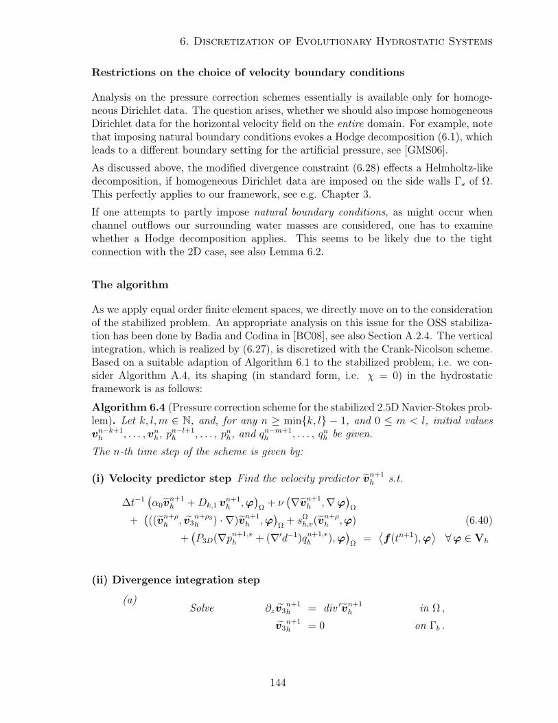
6. Discretization of Evolutionary Hydrostatic Systems
Restrictions on the choice of velocity boundary conditions
Analysis on the pressure correction schemes essentially is available only for homoge-neous Dirichlet data. The question arises, whether we should also impose homogeneousDirichlet data for the horizontal velocity field on the entire domain. For example, notethat imposing natural boundary conditions evokes a Hodge decomposition (6.1), whichleads to a different boundary setting for the artificial pressure, see [GMS06].
As discussed above, the modified divergence constraint (6.28) effects a Helmholtz-likedecomposition, if homogeneous Dirichlet data are imposed on the side walls Γs of Ω.This perfectly applies to our framework, see e.g. Chapter 3.
If one attempts to partly impose natural boundary conditions, as might occur whenchannel outflows our surrounding water masses are considered, one has to examinewhether a Hodge decomposition applies. This seems to be likely due to the tightconnection with the 2D case, see also Lemma 6.2.
The algorithm
As we apply equal order finite element spaces, we directly move on to the considerationof the stabilized problem. An appropriate analysis on this issue for the OSS stabiliza-tion has been done by Badia and Codina in [BC08], see also Section A.2.4. The verticalintegration, which is realized by (6.27), is discretized with the Crank-Nicolson scheme.Based on a suitable adaption of Algorithm 6.1 to the stabilized problem, i.e. we con-sider Algorithm A.4, its shaping (in standard form, i.e. χ = 0) in the hydrostaticframework is as follows:
Algorithm 6.4 (Pressure correction scheme for the stabilized 2.5D Navier-Stokes prob-lem). Let k, l,m ∈ N, and, for any n ≥ mink, l − 1, and 0 ≤ m < l, initial valuesvn−k+1h , . . . ,vnh, pn−l+1
h , . . . , pnh, and qn−m+1h , . . . , qnh be given.
The n-th time step of the scheme is given by:
(i) Velocity predictor step Find the velocity predictor vn+1h s.t.
∆t−1(α0v
n+1h +Dk,1 v
n+1h ,ϕ
)Ω
+ ν(∇vn+1
h ,∇ϕ)Ω
+(((vn+ρ
h , v3n+ρ3
h ) · ∇)vn+1h ,ϕ
)Ω
+ sΩh,v(v
n+ρh ,ϕ) (6.40)
+(P3D(∇pn+1,∗
h + (∇′d−1)qn+1,∗h ),ϕ
)Ω
=⟨f(tn+1),ϕ
⟩ ∀ϕ ∈ Vh
(ii) Divergence integration step
(a)Solve ∂zv3
n+1h = div ′vn+1
h in Ω ,
v3n+1h = 0 on Γb .
144
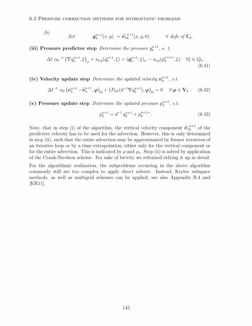
6.3 Pressure correction methods for hydrostatic problems
(b)Set gn+1
h (x, y) = v3n+1h (x, y, 0) ∀ dofs of Kh .
(iii) Pressure predictor step Determine the pressure qn+1h , s. t.
∆t α0−1(∇qn+1
h , ξ)ω
+ sh,p(qn+1h , ξ) = (gn+1
h , ξ)ω − sh,p(pn+1,∗h , ξ) ∀ξ ∈ Qh .
(6.41)
(iv) Velocity update step Determine the updated velocity vn+1h , s.t.
∆t−1 α0
(vn+1h −vn+1
h ,ϕ)
Ω+(P3D(d−1∇qn+1
h ),ϕ)
Ω= 0 ∀ϕ ∈ Vh . (6.42)
(v) Pressure update step Determine the updated pressure pn+1h , s.t.
pn+1h = d−1 qn+1
h + pn+1,∗h . (6.43)
Note, that in step (i) of the algorithm, the vertical velocity component v3n+1h of the
predictive velocity has to be used for the advection. However, this is only determinedin step (ii), such that the entire advection may be approximated by former iteratives ofan iterative loop or by a time extrapolation, either only for the vertical component orfor the entire advection. This is indicated by ρ and ρ3. Step (ii) is solved by applicationof the Crank-Nicolson scheme. For sake of brevity we refrained tidying it up in detail.
For the algorithmic realization, the subproblems occurring in the above algorithmcommonly still are too complex to apply direct solvers. Instead, Krylov subspacemethods, as well as multigrid schemes can be applied, see also Appendix B.4 and[KR11].
145
6. Discretization of Evolutionary Hydrostatic Systems
146
Chapter 7
Algorithmic Issues
In the preceding chapters we derived the set of governing equations, considered ex-istence, uniqueness and regularity properties of possible solutions, and analyzed itsequal-order finite element discretization. But, unless we are not able to derive solu-tions of these discretized problems, the preceding considerations are practically futile.
The main observation we make is, that in hydrostatic problems the velocity field andthe pressure are defined in domains of different dimensions. Thus, common approachesto solve such problems, such as direct iterative methods, see also Appendix B, cannot be adapted offhand. The task of this chapter is to show possible accesses toalgorithmically treat hydrostatic problems.
In the context of evolutionary hydrostatic flow problems, we already treated one pos-sibility to deal with the different dimensions for the evolutionary case. For the algo-rithmic treatment of the resulting subproblems we refer to the Appendix B. Thus itremains to consider stationary hydrostatic flow problems.We consider two possibilities to algorithmically treat the stationary hydrostatic prob-lems. On the one hand, this is the idea of pressure correction schemes. On the otherhand, we can apply the idea of Uzawa algorithms. These two issues are content ofSections 7.1 and 7.2. After having dealt these two approaches we turn to the issue ofparallelization in Section 7.3. For a closer look into this topic we refer to [KR11], inwhich we introduced issues on parallelization in detail, particularly in the context ofmultigrid schemes.
7.1 Uzawa approach
We figured out in Chapter 3 and frequently applied in Chapters 4 and 5 the saddlepoint structure of hydrostatic flow problems. When we attempt to solve such problems,we again can make use of this property.
We consider the discretized stationary problem
A(uh)(φ) = f(φ) ∀φ ∈ Xh ,
147
7. Algorithmic Issues
whereas uh denotes the discrete solution of the problem, A : Xh ×Xh → R denotesthe bilinear form and f the forcing. Let
Φh := ϕih, i = 1, . . . ,m and Ξh := ξih, i = 1, . . . , nbe the common Lagrange basis systems of Vh and Qh with ϕi(xj) = δij and ξi(yj) = δij,where xj are the m dofs of the velocity field and yj the n dofs of the pressure field.Thus, we end up in the following algebraic system
Mz :=
(A BT
−B D
)(xy
)=
(f0
)with nonsingular matrix A ∈ Rm×m, matrix D ∈ Rn×n of the pressure stabilizationand matrix B ∈ Rm×n, accounting for the modified inf-sup constraint. The expressionf on the right hand side is to be interpreted elementwisely.
If we apply the idea of the Schur complement and apply the (simple) Richardsoniteration to the resulting pressure problem, see also Sections B.1.2 and B.2.3, we getthe following algorithm:
Algorithm 7.1. Let y(0) ∈ Rn and θ be a sufficiently small damping parameter. Thei-th step, i ≥ 1, of the algorithm is given by:
(i) Ax(i) = f − P (BTy(i)),
(ii) y(i+1) = y(i) + θ(Bx(i) +Dy(i)) ,
whereas P denotes the embedding from 2D to 3D. Thus, once we have determined the2D pressure gradient BTy(i), we can embed it to 3D and are thus able to determine thenext velocity iterative, x(i), in step (i) of the algorithm. Given this x(i), the modifieddivergence constraint, Bx(i), can be determined, see also Section 6.3, which enable tosolve the 2D subproblem (ii).For a suitable preconditioning for the non hydrostatic case we refer to B.3.4. For anappropriate argumentation in the hydrostatic case, let us assume D = 0. Then, thetask of the preconditioning of the hydrostatic Schur complement is to find a suitableapproximation of S−1 = (BA−1BT )−1. Given the hydrostatic Stokes problem we haveB = div ′M, A = ∆, BT = P∇′ and thus
S = div ′M ∆−1 P∇′ ∼ id ,
such that the inverse mass matrix of the pressure space, i.e. M−1p , can be applied as
preconditioner for the pressure problem.
In order to accelerate the iterative process, the search directions can be chosen moresophisticatedly. For symmetric problems, such as evolve for the hydrostatic Stokesproblem, we can apply the conjugate gradient approach, see also Section B.4.3. Therealization can be done in a similar fashion as described above. For non symmetricproblems, such as the hydrostatic Oseen problem, suitable schemes, such as biconjugategradient schemes have to be applied. However, numerical tests for the hydrostatic
148
7.2 Application of pressure correction schemes
Oseen problem revealed, that a good performance is only observed for problems withsmall magnitudes of the advection field. For the case of stronger advection, suitablepreconditioners have to be applied.
The resulting subproblems commonly still are too complex to apply a direct solver.Instead, Krylov subspace methods, as well as multigrid schemes can be applied, seealso Appendix B.4 and [KR11].
7.2 Application of pressure correction schemes
Another approach to solve a stationary hydrostatic flow problem is the application ofa pressure correction scheme. We already introduced this issue in Chapter 6. In thischapter we also noted, that an appropriate convergence analysis is still missing. Givena hydrostatic flow problem, which is assumed to have a stationary solution, i.e.
Find (vh, ph) ∈ Xh s. t.
a(vh,ϕ)− b(ph,ϕ) + b(ξ,vh) = (f ,ϕ)Ω∀(ϕ, ξ) ∈ Xh ,
we add the time derivative terms (∂t vh,ϕ)Ω to the system and proceed as in theevolutionary case. If two consecutive solutions only differ in a negligible manner, westop the iterative process.This approach may be quite expensive, as the evolution to the steady state may takesome time. Thus, if suitable and efficient Uzawa methods are at hand, this approachshould be preferred, such as the Uzawa-CG-scheme in the case of the hydrostatic Stokesproblem.A different possibility was applied in [CGS12], where the authors used a coupled solverimplemented with the finite element solver FreeFem++, see also [DHP03].
7.3 Parallelization
Given complex hydrostatic fluid problems, a feasible approach to handle the appro-priate immense algebraic system is the parallelization of the problem. In the formerchapter, as well as in the two preceding sections we followed an approach, in which sub-problems of different dimensions are to be solved. Whereas the pressure problem is 2D,the (altered) momentum equation still is 3D, which causes the main effort. Moreover,the vertical integration has to be realized in order to determine the vertical velocity onthe one hand, and the modified divergence constraint on the other hand.
The benefit of parallelizing the 2D pressure Poisson problem is marginal, see also[KR11], and it suffices to parallelize the 3D subproblems. For the parallelization ofthe 3D momentum equation we refer to Section 3 of [KR11]. In order to efficientlyparallelize the vertical integration, the mesh distribution should be done in such way,that as less communication as possible takes places. Indeed it can be done without
149
7. Algorithmic Issues
communication, if the mesh distribution takes care of the prismatic structure of the3D mesh, i.e. only the x y plane is decomposed, see also Figure 8 in [KR11].
150
Chapter 8
Numerical Examples
This chapter aims to illustrate and validate the analytical results and deductions ofthe preceding chapters. We start with the case of the stationary hydrostatic Stokesproblem on isotropic meshes, demonstrating the proven convergence results and illus-trating the effect of the hydrostatic approximation. We then turn to the stationaryhydrostatic Oseen problem on isotropic meshes, showing numerical results for the lin-ear case as well as the nonlinear case. The numerical results for the hydrostatic Stokescase are also to be found in [KB12]. The results for the hydrostatic Oseen problemare also presented in [Kim12]. Afterwards, we turn to the case of vertical anisotropicmeshes in the framework of the hydrostatic Stokes problem. Further, we examine theevolutionary case, more precise, we consider physical phenomena, which are apparentin oceanic regimes.Another topic is the issue of parallelization. This has been numerically treated in[KR11] and is given in Appendix C. In order to avoid redundancy we skip the repre-sentation of those tests and results, and refer to to appended article.
For the implementation of the hydrostatic problems we use different splitting schemes,as presented in the respective sections, see also Chapter 6. We apply the finite elementspace Q1−Q1. For the stabilization of the schemes we use local projection stabilizationschemes.
8.1 Stationary hydrostatic Stokes problem on iso-
tropic meshes
In this section we numerically validate the results of Section 4.4 for the local projectionstabilization method as one choice of the presented stabilization methods. Moreover,we give an intuition of the quality of the hydrostatic approximation for domains withdifferent aspect ratios.
151
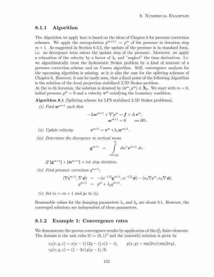
8. Numerical Examples
8.1.1 Algorithm
The Algorithm we apply here is based on the ideas of Chapter 6 for pressure correctionschemes. We apply the extrapolation pm+1,∗ := pm of the pressure in iteration stepm + 1. As suggested in Section 6.3.2, the update of the pressure is in standard form,i.e. no divergence term enters the update step of the pressure. Moreover, we applya relaxation of the velocity by a factor of λv and ”neglect” the time derivatives. I.e.we algorithmically treat the hydrostatic Stokes problem by a kind of mixture of apressure correction scheme and an Uzawa algorithm. Still, convergence analysis forthe upcoming algorithm is missing, as it is also the case for the splitting schemes ofChapter 6. However, it can be easily seen, that a fixed point of the following Algorithmis the solution of the local projection stabilized 2.5D Stokes problem.At the m-th iteration, the solution is denoted by (vm, pm) ∈ Xh. We start with m = 0,initial pressure pm = 0 and a velocity vm satisfying the boundary condition.
Algorithm 8.1 (Splitting scheme for LPS stabilized 2.5D Stokes problems).
(i) Find wm+1 such that
−∆wm+1 +∇′pm = f + ∆vm,
wm+1 = 0 on ∂Ω .
(ii) Update velocity: vm+1 = vm +λvwm+1 .
(iii) Determine the divergence in vertical mean
gm+1 =
0∫−d(x,y)
div ′ vm+1 dz .
If ||gm+1||+ ||wm+1|| < tol stop iteration.
(iv) Find pressure correction qm+1:
(∇qm+1,∇φ) = −(α−1/2gm+1, α−1/2φ)− (κh∇pm, κh∇φ)
pm+1 = pm + λpqm+1 .
(v) Set m := m+ 1 and go to (i).
Reasonable values for the damping parameters λv and λp are about 0.1. However, theconverged solutions are independent of these parameters.
8.1.2 Example 1: Convergence rates
We demonstrate the proven convergence results by application of the Q1 finite elements.The domain is the unit cube Ω := (0, 1)3 and the (smooth) solution is given by
v1(x, y, z) = x(x− 1) (2y − 1) z(1− z), p(x, y) = sin(2πx) sin(2πy),
v2(x, y, z) = (1− 2x) y(y − 1) /6.
152
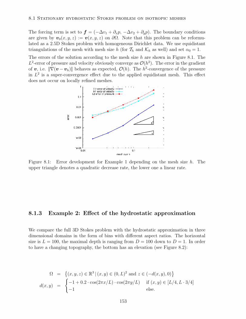
8.1 Stationary hydrostatic Stokes problem on isotropic meshes
The forcing term is set to f = (−∆v1 + ∂xp, −∆v2 + ∂yp). The boundary conditionsare given by v0(x, y, z) := v(x, y, z) on ∂Ω. Note that this problem can be reformu-lated as a 2.5D Stokes problem with homogeneous Dirichlet data. We use equidistanttriangulations of the mesh with mesh size h (for Th and Kh as well) and set α0 = 1.
The errors of the solution according to the mesh size h are shown in Figure 8.1. TheL2-error of pressure and velocity obviously converge as O(h2). The error in the gradientof v, i.e. ||∇(v−vh)|| behaves as expected, O(h). The h2-convergence of the pressurein L2 is a super-convergence effect due to the applied equidistant mesh. This effectdoes not occur on locally refined meshes.
Figure 8.1: Error development for Example 1 depending on the mesh size h. Theupper triangle denotes a quadratic decrease rate, the lower one a linear rate.
8.1.3 Example 2: Effect of the hydrostatic approximation
We compare the full 3D Stokes problem with the hydrostatic approximation in threedimensional domains in the form of bins with different aspect ratios. The horizontalsize is L = 100, the maximal depth is ranging from D = 100 down to D = 1. In orderto have a changing topography, the bottom has an elevation (see Figure 8.2):
Ω =
(x, y, z) ∈ R3 | (x, y) ∈ (0, L)2 and z ∈ (−d(x, y), 0)
d(x, y) =
−1 + 0.2 · cos(2πx/L) · cos(2πy/L) if (x, y) ∈ [L/4, L · 3/4]
−1 else.
153
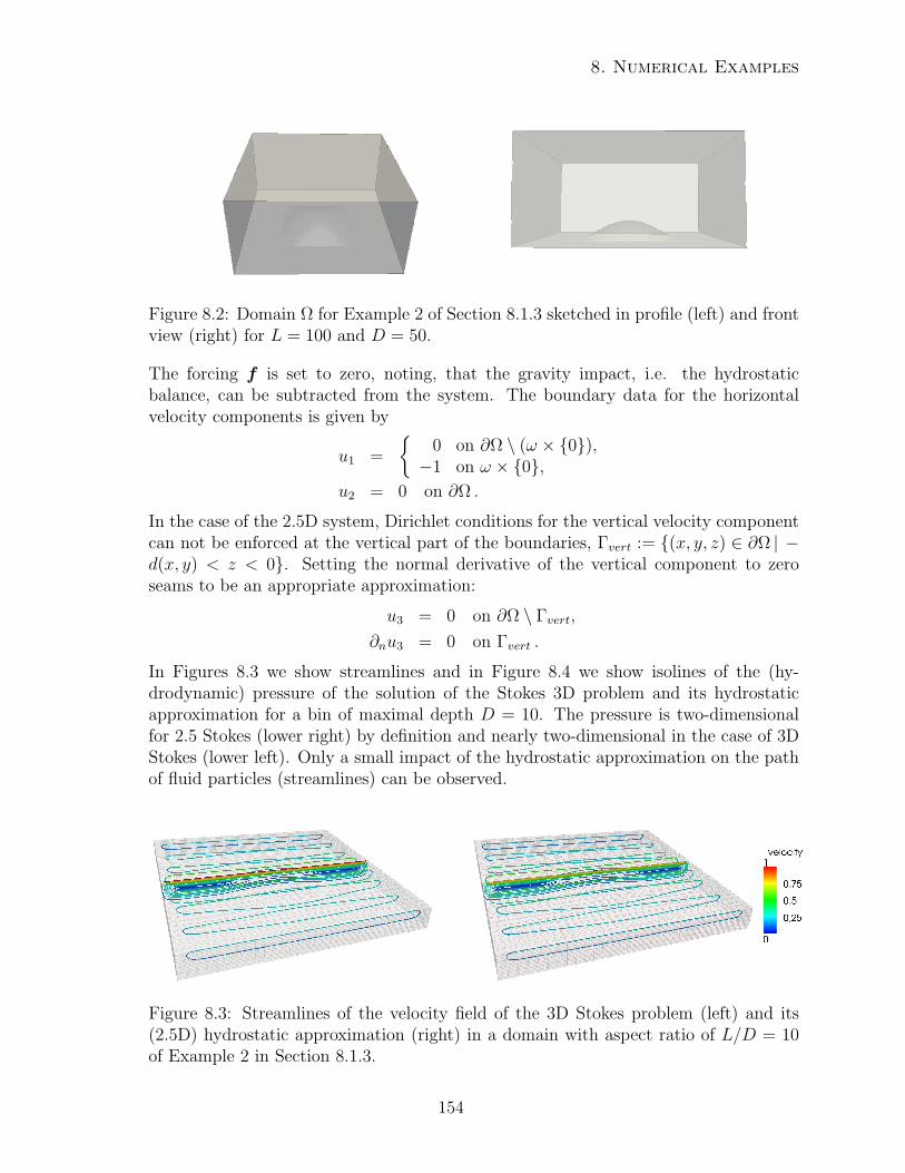
8. Numerical Examples
Figure 8.2: Domain Ω for Example 2 of Section 8.1.3 sketched in profile (left) and frontview (right) for L = 100 and D = 50.
The forcing f is set to zero, noting, that the gravity impact, i.e. the hydrostaticbalance, can be subtracted from the system. The boundary data for the horizontalvelocity components is given by
u1 =
0 on ∂Ω \ (ω × 0),−1 on ω × 0,
u2 = 0 on ∂Ω .
In the case of the 2.5D system, Dirichlet conditions for the vertical velocity componentcan not be enforced at the vertical part of the boundaries, Γvert := (x, y, z) ∈ ∂Ω | −d(x, y) < z < 0. Setting the normal derivative of the vertical component to zeroseams to be an appropriate approximation:
u3 = 0 on ∂Ω \ Γvert,
∂nu3 = 0 on Γvert .
In Figures 8.3 we show streamlines and in Figure 8.4 we show isolines of the (hy-drodynamic) pressure of the solution of the Stokes 3D problem and its hydrostaticapproximation for a bin of maximal depth D = 10. The pressure is two-dimensionalfor 2.5 Stokes (lower right) by definition and nearly two-dimensional in the case of 3DStokes (lower left). Only a small impact of the hydrostatic approximation on the pathof fluid particles (streamlines) can be observed.
Figure 8.3: Streamlines of the velocity field of the 3D Stokes problem (left) and its(2.5D) hydrostatic approximation (right) in a domain with aspect ratio of L/D = 10of Example 2 in Section 8.1.3.
154
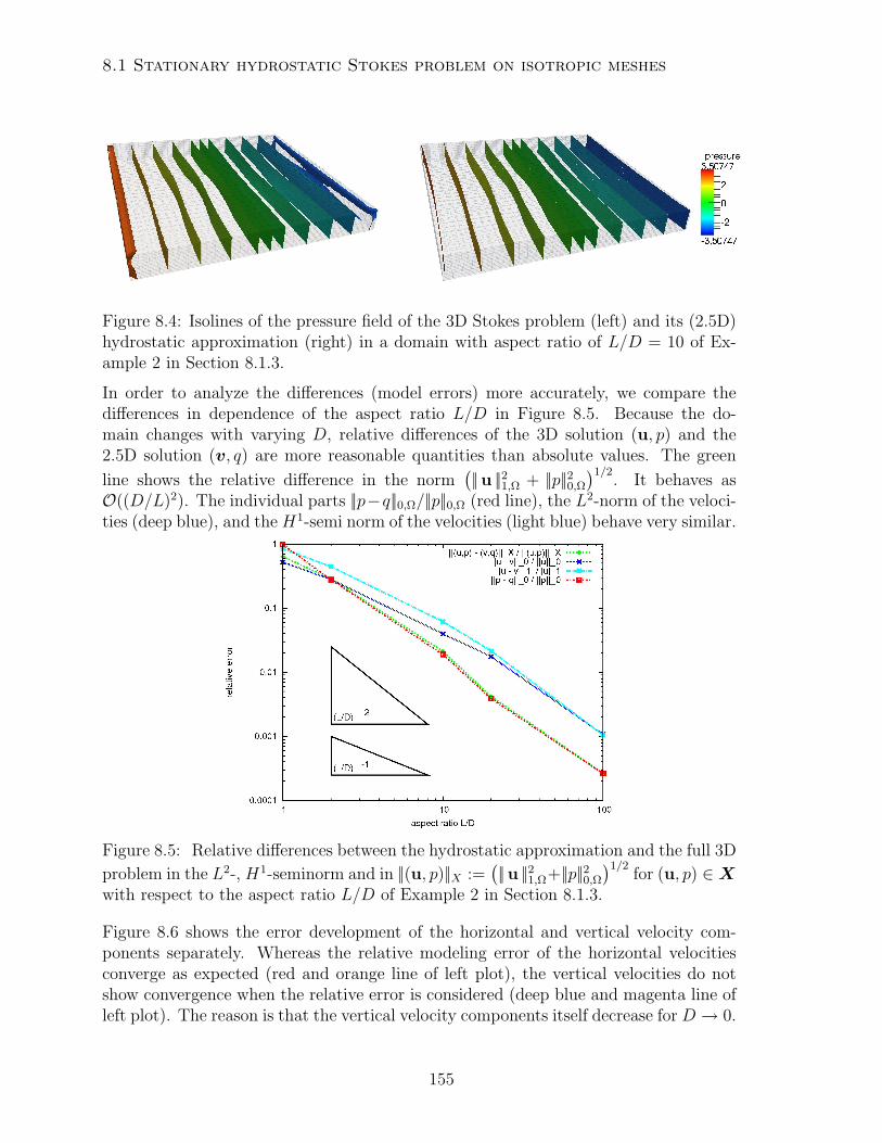
8.1 Stationary hydrostatic Stokes problem on isotropic meshes
Figure 8.4: Isolines of the pressure field of the 3D Stokes problem (left) and its (2.5D)hydrostatic approximation (right) in a domain with aspect ratio of L/D = 10 of Ex-ample 2 in Section 8.1.3.
In order to analyze the differences (model errors) more accurately, we compare thedifferences in dependence of the aspect ratio L/D in Figure 8.5. Because the do-main changes with varying D, relative differences of the 3D solution (u, p) and the2.5D solution (v, q) are more reasonable quantities than absolute values. The green
line shows the relative difference in the norm(||u ||21,Ω + ||p||20,Ω
)1/2. It behaves as
O((D/L)2). The individual parts ||p−q||0,Ω/||p||0,Ω (red line), the L2-norm of the veloci-ties (deep blue), and the H1-semi norm of the velocities (light blue) behave very similar.
Figure 8.5: Relative differences between the hydrostatic approximation and the full 3D
problem in the L2-, H1-seminorm and in ||(u, p)||X :=(||u ||21,Ω+||p||20,Ω
)1/2for (u, p) ∈X
with respect to the aspect ratio L/D of Example 2 in Section 8.1.3.
Figure 8.6 shows the error development of the horizontal and vertical velocity com-ponents separately. Whereas the relative modeling error of the horizontal velocitiesconverge as expected (red and orange line of left plot), the vertical velocities do notshow convergence when the relative error is considered (deep blue and magenta line ofleft plot). The reason is that the vertical velocity components itself decrease for D → 0.
155
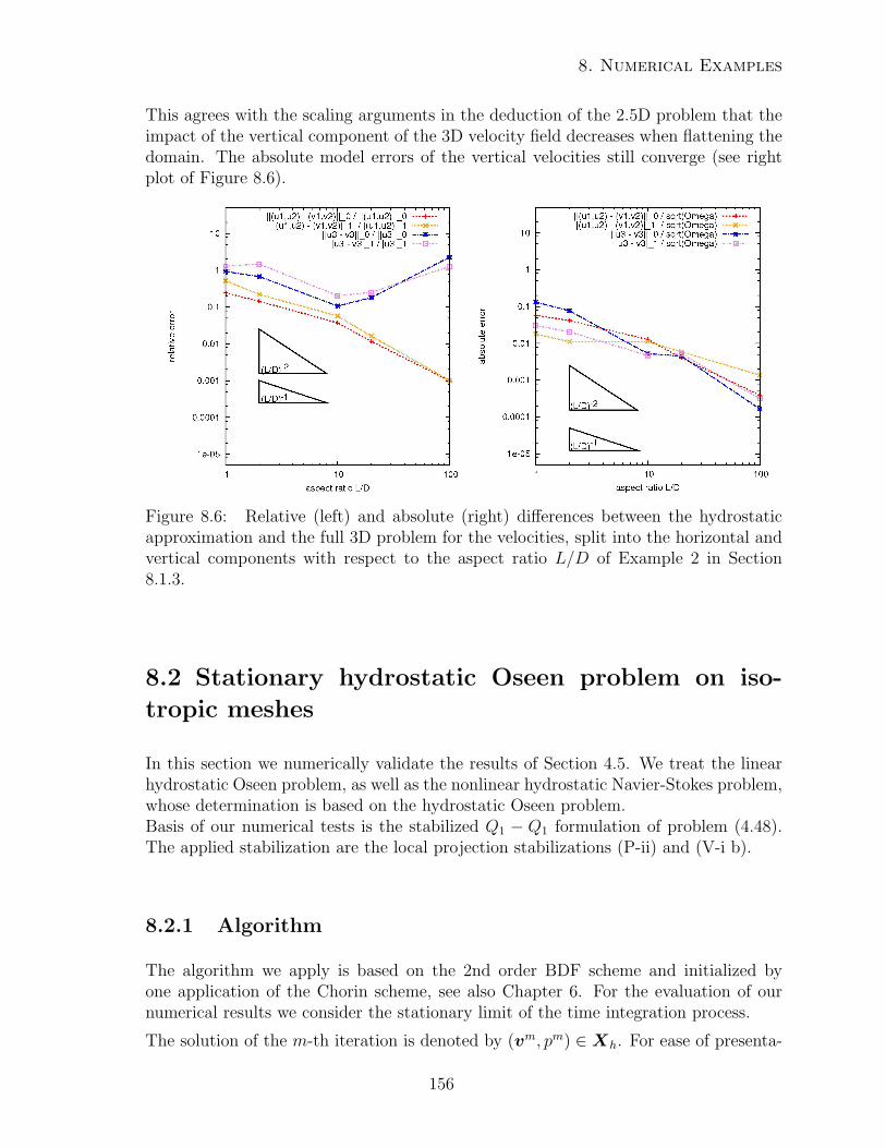
8. Numerical Examples
This agrees with the scaling arguments in the deduction of the 2.5D problem that theimpact of the vertical component of the 3D velocity field decreases when flattening thedomain. The absolute model errors of the vertical velocities still converge (see rightplot of Figure 8.6).
Figure 8.6: Relative (left) and absolute (right) differences between the hydrostaticapproximation and the full 3D problem for the velocities, split into the horizontal andvertical components with respect to the aspect ratio L/D of Example 2 in Section8.1.3.
8.2 Stationary hydrostatic Oseen problem on iso-
tropic meshes
In this section we numerically validate the results of Section 4.5. We treat the linearhydrostatic Oseen problem, as well as the nonlinear hydrostatic Navier-Stokes problem,whose determination is based on the hydrostatic Oseen problem.Basis of our numerical tests is the stabilized Q1 − Q1 formulation of problem (4.48).The applied stabilization are the local projection stabilizations (P-ii) and (V-i b).
8.2.1 Algorithm
The algorithm we apply is based on the 2nd order BDF scheme and initialized byone application of the Chorin scheme, see also Chapter 6. For the evaluation of ournumerical results we consider the stationary limit of the time integration process.
The solution of the m-th iteration is denoted by (vm, pm) ∈Xh. For ease of presenta-
156
8.2 Stationary hydrostatic Oseen problem on isotropic meshes
tion let
as(bh;v;ϕ) := (ν∇v,∇ϕ)Ω + (σv,ϕ)Ω +((bh · ∇)v+f v⊥,ϕ
)Ω
+ sh,v(v;ϕ).
We use an Oseen linearization of the advection term. For a presumed v0 = v0, thealgorithm is thus given by:
Algorithm 8.2 (Pressure correction scheme based on BDF2 for the local projectionstabilized hydrostatic Navier-Stokes problem). Let m = 1.
(i) If m = 1 set λ = (δt)−1, χ = 0 and vm = vm,else set λ = 3 (2δt)−1, χ = 1 and vm = (2vm − 1
2vm−1).
(ii) Find wm+1 such that(λwm+1,ϕ
)Ω
+ as(vm;wm+1;ϕ)− χ(pm, div ′ϕ)Ω = lm+1(ϕ) + (δt)−1 (vm,ϕ)Ω
(ii) Determine the divergence in vertical mean
gm+1 =
0∫−d(x,y)
div ′wm+1 dz .
(iii) Find pressure correction qm+1:
λ−1(∇′qm+1,∇′ξ)ω + sh,p(qm+1, ξ) = −(gm+1, ξ)ω − sh,p(pm; ξ)
If ||q||0,ω < tol stop iteration.
(iv) Update pressure: pm+1 = χ pm + d−1 qm+1 .
(v) Update velocity: vm+1 = wm+1−λ−1∇′qm+1 and v3m+1 =
z∫−d(x,y)
div ′vm+1 dz .
(vi) Set m := m+ 1 and go to (i).
It is claimed in[GMS06], that the splitting error of the introduced scheme affects therate of timal convergence and pointed out, that spatial convergence tests with fixedtime steps δt may lead to false results. Due to that we set δt = h in our computations.
8.2.2 Example 1: Convergence rates in the linear case
We start with the examination of the linear problem. For bilinear elements and σ, ν ∼ 1,Proposition 4.31 anticipates a decrease of ||ν1/2∇(v−vh)||0,Ω and ||(ν+σ)1/2(p−ph)||0,Ωof orders O(h) and O(h3/2), respectively. We thus expect linear convergence of ||∇(v−vh)||0,Ω and convergence of order O(h3/2) for ||p − ph||0,Ω. Applying standard dualityarguments, the observed convergence of the velocity error in the L2-norm shall be oforder O(h2).
157
8. Numerical Examples
In the case ν h and σ ∼ 1, Proposition 4.31 suggests a decrease of ||ν1/2∇(v−vh)||0,Ωand ||(ν + σ)1/2(p − ph)||0,Ω both of order O(h3/2). Thus we shall observe convergencerates for ||∇(v− vh)||0,Ω, ||p− ph||0,Ω and ||v− vh||0,Ω as in the former case. If ν, σ h,the convergence of ||p − ph||0,Ω is supposed to be at least of order O(h). Note, thatdue to Section 4.5.4, the L2-error of the vertical velocity component is supposed toconverge linearly.
The underlying domain for all test cases is the unit cube Ω := (0, 1)3. We use equidis-tant triangulations of Ω and ω with mesh size h for both. In each case we set the righthand side f and the forcing g according to the solution
v(x, y, z) =
(e−x sin(πx)2∂y (sin(πy)2) sin(z)
−∂x (e−x sin(πx)2) sin(πy)2 2(1− cos(1))z
)p(x, y) = ex − (e1 − 1) .
Moreover, the advection term b is set to (1, 1, 0) in each of these three tests. Toaccount for the mentioned, different cases, we examine three scenarios. The accordingparameter setting is to be found in Table 8.1.
ν σ f
Test case 1 1 1 1Test case 2 10−4 1 10−1
Test case 3 10−4 0 10−1
Table 8.1: Parameter settings for the test cases of the linear problem.
The errors of the solution w.r.t. the H1-semi- and L2-norm according to the mesh sizeh are shown in Fig. 8.7, on the top left for the first test case, on the top right for thesecond. The results for the third test case are presented in the lower left figure.
Considering the depicted graphs we see, that in each of the test cases 1 – 3, the H1-errors of the velocity are of order 1. The L2-errors of the velocity converge quadratically,as expected. Moreover, the L2-errors of the pressure converge at least with orderO(h1.5). As well, the L2-error of the vertical velocity component subordinates a linearconvergence behavior.
8.2.3 Example 2: Convergence rates in the nonlinear case
We consider the solution of Example 1. The advection term b is set to the velocitydetermined in the former iteration step. For ease of stationarity of the solution we setν = 1. The remaining parameters are set to σ = f = 1. We pass on the considerationsfrom Example 1 to the present example. The observed convergence rates are depictedin the lower right graph of Fig. 8.7. As in Example 1 we recover the theoretical resultsin the numerical computations.
158
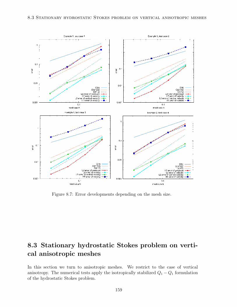
8.3 Stationary hydrostatic Stokes problem on vertical anisotropic meshes
Figure 8.7: Error developments depending on the mesh size.
8.3 Stationary hydrostatic Stokes problem on verti-
cal anisotropic meshes
In this section we turn to anisotropic meshes. We restrict to the case of verticalanisotropy. The numerical tests apply the isotropically stabilized Q1−Q1 formulationof the hydrostatic Stokes problem.
159
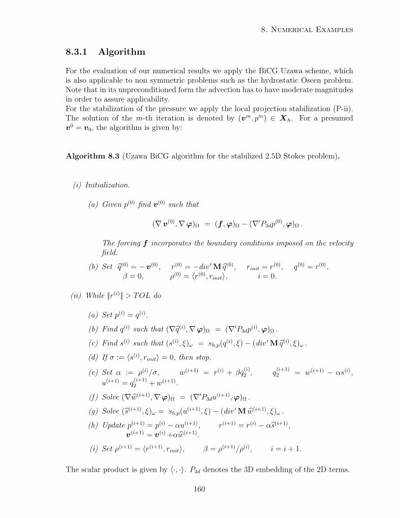
8. Numerical Examples
8.3.1 Algorithm
For the evaluation of our numerical results we apply the BiCG Uzawa scheme, whichis also applicable to non symmetric problems such as the hydrostatic Oseen problem.Note that in its unpreconditioned form the advection has to have moderate magnitudesin order to assure applicability.For the stabilization of the pressure we apply the local projection stabilization (P-ii).The solution of the m-th iteration is denoted by (vm, pm) ∈ Xh. For a presumedv0 = v0, the algorithm is given by:
Algorithm 8.3 (Uzawa BiCG algorithm for the stabilized 2.5D Stokes problem).
(i) Initialization.
(a) Given p(0) find v(0) such that
(∇v(0),∇ϕ)Ω = (f ,ϕ)Ω − (∇′P3dp(0),ϕ)Ω .
The forcing f incorporates the boundary conditions imposed on the velocityfield.
(b) Set q(0) = −v(0), r(0) = −div ′M q(0), rinit = r(0), q(0) = r(0),β = 0, ρ(0) = 〈r(0), rinit〉, i = 0.
(ii) While ||r(i)|| > TOL do
(a) Set p(i) = q(i).
(b) Find q(i) such that (∇q(i),∇ϕ)Ω = (∇′P3dp(i),ϕ)Ω .
(c) Find s(i) such that (s(i), ξ)ω = sh,p(q(i), ξ)− (div ′M q(i), ξ)ω .
(d) If σ := 〈s(i), rinit〉 = 0, then stop.
(e) Set α := ρ(i)/σ, w(i+1) = r(i) + βq(i)2 , q
(i+1)2 = w(i+1) − αs(i),
u(i+1) = q(i+1)2 + w(i+1).
(f) Solve (∇w(i+1),∇ϕ)Ω = (∇′P3du(i+1),ϕ)Ω .
(g) Solve (s(i+1), ξ)ω = sh,p(u(i+1), ξ)− (div ′M w(i+1), ξ)ω .
(h) Update p(i+1) = p(i) − αu(i+1), r(i+1) = r(i) − αs(i+1),v(i+1) = v(i) +αw(i+1).
(i) Set ρ(i+1) = 〈r(i+1), rinit〉, β = ρ(i+1)/ρ(i), i = i+ 1.
The scalar product is given by 〈·, ·〉. P3d denotes the 3D embedding of the 2D terms.
160
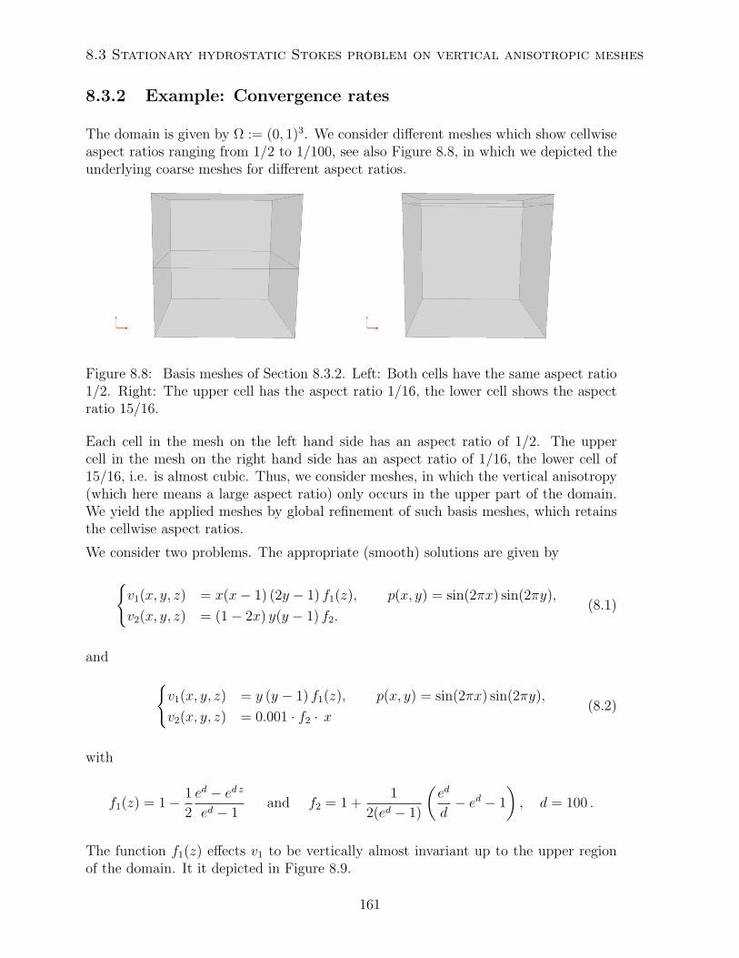
8.3 Stationary hydrostatic Stokes problem on vertical anisotropic meshes
8.3.2 Example: Convergence rates
The domain is given by Ω := (0, 1)3. We consider different meshes which show cellwiseaspect ratios ranging from 1/2 to 1/100, see also Figure 8.8, in which we depicted theunderlying coarse meshes for different aspect ratios.
Figure 8.8: Basis meshes of Section 8.3.2. Left: Both cells have the same aspect ratio1/2. Right: The upper cell has the aspect ratio 1/16, the lower cell shows the aspectratio 15/16.
Each cell in the mesh on the left hand side has an aspect ratio of 1/2. The uppercell in the mesh on the right hand side has an aspect ratio of 1/16, the lower cell of15/16, i.e. is almost cubic. Thus, we consider meshes, in which the vertical anisotropy(which here means a large aspect ratio) only occurs in the upper part of the domain.We yield the applied meshes by global refinement of such basis meshes, which retainsthe cellwise aspect ratios.
We consider two problems. The appropriate (smooth) solutions are given by
v1(x, y, z) = x(x− 1) (2y − 1) f1(z), p(x, y) = sin(2πx) sin(2πy),
v2(x, y, z) = (1− 2x) y(y − 1) f2.(8.1)
and v1(x, y, z) = y (y − 1) f1(z), p(x, y) = sin(2πx) sin(2πy),
v2(x, y, z) = 0.001 · f2 · x(8.2)
with
f1(z) = 1− 1
2
ed − ed zed − 1
and f2 = 1 +1
2(ed − 1)
(ed
d− ed − 1
), d = 100 .
The function f1(z) effects v1 to be vertically almost invariant up to the upper regionof the domain. It it depicted in Figure 8.9.
161
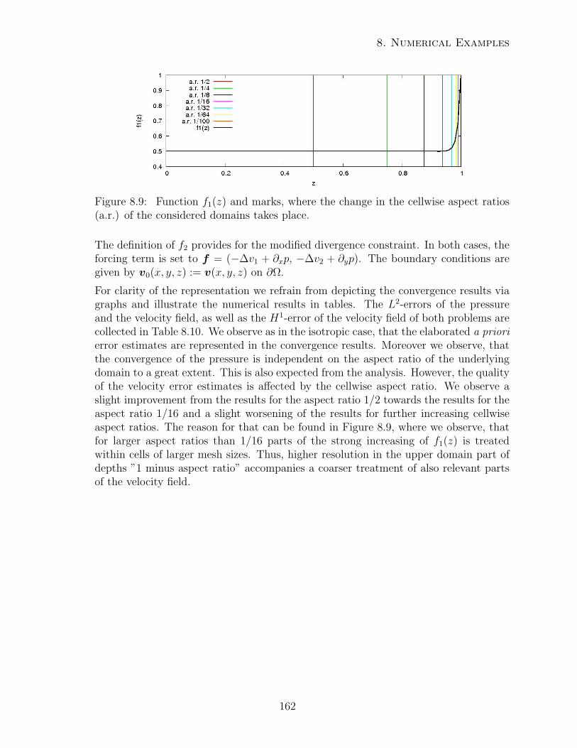
8. Numerical Examples
Figure 8.9: Function f1(z) and marks, where the change in the cellwise aspect ratios(a.r.) of the considered domains takes place.
The definition of f2 provides for the modified divergence constraint. In both cases, theforcing term is set to f = (−∆v1 + ∂xp, −∆v2 + ∂yp). The boundary conditions aregiven by v0(x, y, z) := v(x, y, z) on ∂Ω.
For clarity of the representation we refrain from depicting the convergence results viagraphs and illustrate the numerical results in tables. The L2-errors of the pressureand the velocity field, as well as the H1-error of the velocity field of both problems arecollected in Table 8.10. We observe as in the isotropic case, that the elaborated a priorierror estimates are represented in the convergence results. Moreover we observe, thatthe convergence of the pressure is independent on the aspect ratio of the underlyingdomain to a great extent. This is also expected from the analysis. However, the qualityof the velocity error estimates is affected by the cellwise aspect ratio. We observe aslight improvement from the results for the aspect ratio 1/2 towards the results for theaspect ratio 1/16 and a slight worsening of the results for further increasing cellwiseaspect ratios. The reason for that can be found in Figure 8.9, where we observe, thatfor larger aspect ratios than 1/16 parts of the strong increasing of f1(z) is treatedwithin cells of larger mesh sizes. Thus, higher resolution in the upper domain part ofdepths ”1 minus aspect ratio” accompanies a coarser treatment of also relevant partsof the velocity field.
162
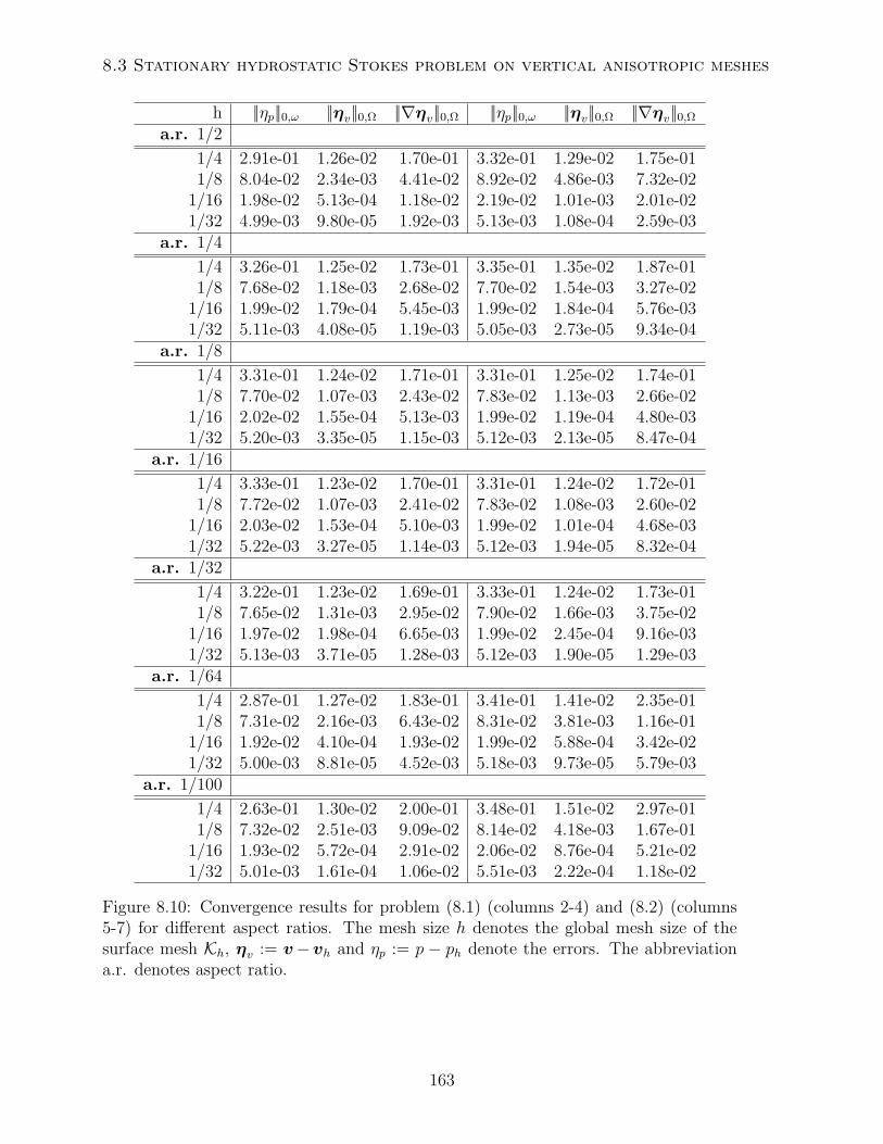
8.3 Stationary hydrostatic Stokes problem on vertical anisotropic meshes
h ||ηp||0,ω ||ηv||0,Ω ||∇ηv||0,Ω ||ηp||0,ω ||ηv||0,Ω ||∇ηv||0,Ωa.r. 1/2
1/4 2.91e-01 1.26e-02 1.70e-01 3.32e-01 1.29e-02 1.75e-011/8 8.04e-02 2.34e-03 4.41e-02 8.92e-02 4.86e-03 7.32e-02
1/16 1.98e-02 5.13e-04 1.18e-02 2.19e-02 1.01e-03 2.01e-021/32 4.99e-03 9.80e-05 1.92e-03 5.13e-03 1.08e-04 2.59e-03
a.r. 1/4
1/4 3.26e-01 1.25e-02 1.73e-01 3.35e-01 1.35e-02 1.87e-011/8 7.68e-02 1.18e-03 2.68e-02 7.70e-02 1.54e-03 3.27e-02
1/16 1.99e-02 1.79e-04 5.45e-03 1.99e-02 1.84e-04 5.76e-031/32 5.11e-03 4.08e-05 1.19e-03 5.05e-03 2.73e-05 9.34e-04
a.r. 1/8
1/4 3.31e-01 1.24e-02 1.71e-01 3.31e-01 1.25e-02 1.74e-011/8 7.70e-02 1.07e-03 2.43e-02 7.83e-02 1.13e-03 2.66e-02
1/16 2.02e-02 1.55e-04 5.13e-03 1.99e-02 1.19e-04 4.80e-031/32 5.20e-03 3.35e-05 1.15e-03 5.12e-03 2.13e-05 8.47e-04
a.r. 1/16
1/4 3.33e-01 1.23e-02 1.70e-01 3.31e-01 1.24e-02 1.72e-011/8 7.72e-02 1.07e-03 2.41e-02 7.83e-02 1.08e-03 2.60e-02
1/16 2.03e-02 1.53e-04 5.10e-03 1.99e-02 1.01e-04 4.68e-031/32 5.22e-03 3.27e-05 1.14e-03 5.12e-03 1.94e-05 8.32e-04
a.r. 1/32
1/4 3.22e-01 1.23e-02 1.69e-01 3.33e-01 1.24e-02 1.73e-011/8 7.65e-02 1.31e-03 2.95e-02 7.90e-02 1.66e-03 3.75e-02
1/16 1.97e-02 1.98e-04 6.65e-03 1.99e-02 2.45e-04 9.16e-031/32 5.13e-03 3.71e-05 1.28e-03 5.12e-03 1.90e-05 1.29e-03
a.r. 1/64
1/4 2.87e-01 1.27e-02 1.83e-01 3.41e-01 1.41e-02 2.35e-011/8 7.31e-02 2.16e-03 6.43e-02 8.31e-02 3.81e-03 1.16e-01
1/16 1.92e-02 4.10e-04 1.93e-02 1.99e-02 5.88e-04 3.42e-021/32 5.00e-03 8.81e-05 4.52e-03 5.18e-03 9.73e-05 5.79e-03
a.r. 1/100
1/4 2.63e-01 1.30e-02 2.00e-01 3.48e-01 1.51e-02 2.97e-011/8 7.32e-02 2.51e-03 9.09e-02 8.14e-02 4.18e-03 1.67e-01
1/16 1.93e-02 5.72e-04 2.91e-02 2.06e-02 8.76e-04 5.21e-021/32 5.01e-03 1.61e-04 1.06e-02 5.51e-03 2.22e-04 1.18e-02
Figure 8.10: Convergence results for problem (8.1) (columns 2-4) and (8.2) (columns5-7) for different aspect ratios. The mesh size h denotes the global mesh size of thesurface mesh Kh, ηv := v−vh and ηp := p − ph denote the errors. The abbreviationa.r. denotes aspect ratio.
163
8. Numerical Examples
8.4 Evolutionary hydrostatic flow problems
In this section we treat the evolutionary case and consider physical phenomena, whichapparent in oceanic regimes. We start with the impact of the Coriolis force on itsown, where we observe an oscillation of the solution, which is imposed due to therotation of the earth. We then turn to the Ekman transport, which occurs due tothe Coriolis force when wind stress is imposed on the surface of the domain. Weobserve, that the thus induced surface velocity field is turned southwards by 45 fromthe direction of the wind stress. Moreover we observe the Ekman layer, which adjustsnear the upper surface and where the so called Ekman spirals of the velocity field canbe observed. Further, we consider the case of a sheared wind stress, which effects theEkman pumping, which is an important mechanism of the ocean, as it transports thewater masses and nutrients from deeper regions to the surface. For this examples wetook our cue from [Ped86, CR02, Cha, CRB11]. We close this section with an flowexample, where we imposed a sheared wind stress, induced an inflow region and openeda part of the wall, such that an outflow is possible.
8.4.1 Considered set of equations
We consider the evolutionary hydrostatic Navier Stokes equations. I.e. we considerthe system (2.29) – (2.34). To account for the unresolved scales, we assume (constant)turbulent viscosity, Aν . For ease of presentation we denote the entire velocity field asu and the horizontal velocity field as v. The vertical velocity field is given by v3.
The entire set of equations thus becomes
div ′(Mv) = 0
v3 = −∫ z
−d(x,y)
div ′ v dz
∂t v+u · ∇v−∆Aν v+ f v⊥+∇′p = 0
v |t=0 = v0 ,
v |Γb∪Γs = 0 , νE∂z v |Γu = τ ,
Proper initial and boundary conditions, as well as domain and time interval specifica-tions are given in the appropriate examples.
8.4.2 Algorithm
We apply a similar algorithm as in Section 8.2 for the stationary hydrostatic Oseenproblem. The solution of the m-th iteration is denoted by (vm, pm) ∈ Xh. Again, weabbreviate
as(bh;v;ϕ) := (Aν∇v,∇ϕ)Ω + (σv,ϕ)Ω +((bh · ∇)v+f v⊥,ϕ
)Ω
+ sh,v(v;ϕ)
164
8.4 Evolutionary hydrostatic flow problems
with anisotropic velocity stabilization (V”) as examined in Section 5.3. The appliedpressure stabilization sh,p is chosen as (P’-ii), see also Section 5.3. We use an Oseenlinearization of the advection term. For a presumed v0 = v0, the algorithm is thusgiven by:
Algorithm 8.4 (Pressure correction scheme based on BDF2 for the evolutionary localprojection stabilized hydrostatic Navier-Stokes problem). Let m = 1.
(i) If m = 1 set λ = (δt)−1, χ = 0 and vm = vm,else set λ = 3 (2δt)−1, χ = 1 and vm = (2vm − 1
2vm−1).
(ii) Find wm+1 such that(λwm+1,ϕ
)Ω
+ as(vm;wm+1;ϕ)− χ(pm, div ′ϕ)Ω = lm+1(ϕ)
+ (δt)−1 (vm,ϕ)Ω
(iii) Determine the divergence in vertical mean
gm+1 =
0∫−d(x,y)
div ′wm+1 dz .
(iv) Find pressure correction qm+1:
λ−1(∇′qm+1,∇′ξ)ω + sh,p(qm+1, ξ) = −(gm+1, ξ)ω − sh,p(pm; ξ)
If ||q||0,ω < tol stop iteration.
(v) Update pressure: pm+1 = χ pm + d−1 qm+1 .
(vi) Update velocity: vm+1 = wm+1 − λ−1∇′qm+1 and
v3m+1 =
z∫−d(x,y)
div ′vm+1 dz .
(vii) Set m := m+ 1 and go to (i).
8.4.3 Example 1: Inertial oscillations
Phenomenom of interest: Inertial frequency
We start with a phenomenom, which is caused by the Coriolis force. (For the deductionswe refer to [CRB11].) Therefore we consider the set of equations, in which no additionalforces and no viscous terms are apparent, as well pressure variations are neglected, i.e.we consider the system
∂tu− f v = 0 , ∂tv + f u = 0 .
165
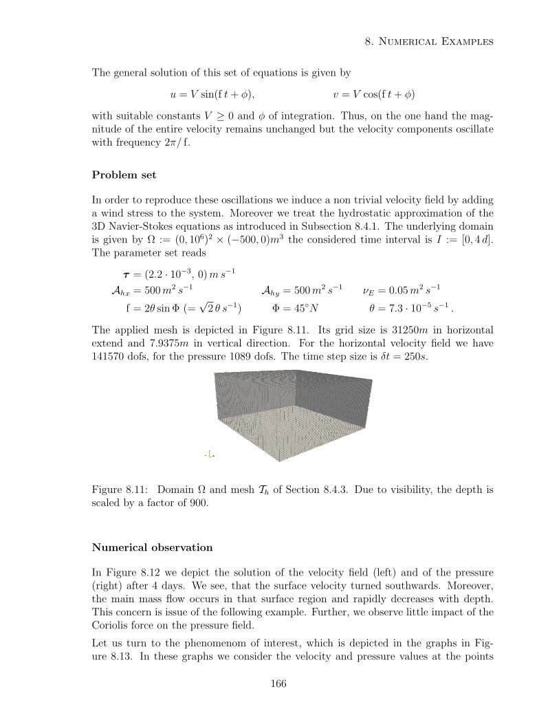
8. Numerical Examples
The general solution of this set of equations is given by
u = V sin(f t+ φ), v = V cos(f t+ φ)
with suitable constants V ≥ 0 and φ of integration. Thus, on the one hand the mag-nitude of the entire velocity remains unchanged but the velocity components oscillatewith frequency 2π/ f.
Problem set
In order to reproduce these oscillations we induce a non trivial velocity field by addinga wind stress to the system. Moreover we treat the hydrostatic approximation of the3D Navier-Stokes equations as introduced in Subsection 8.4.1. The underlying domainis given by Ω := (0, 106)2 × (−500, 0)m3 the considered time interval is I := [0, 4 d].The parameter set reads
τ = (2.2 · 10−3, 0)ms−1
Ahx = 500m2 s−1 Ahy = 500m2 s−1 νE = 0.05m2 s−1
f = 2θ sin Φ (=√
2 θ s−1) Φ = 45N θ = 7.3 · 10−5 s−1 .
The applied mesh is depicted in Figure 8.11. Its grid size is 31250m in horizontalextend and 7.9375m in vertical direction. For the horizontal velocity field we have141570 dofs, for the pressure 1089 dofs. The time step size is δt = 250s.
Figure 8.11: Domain Ω and mesh Th of Section 8.4.3. Due to visibility, the depth isscaled by a factor of 900.
Numerical observation
In Figure 8.12 we depict the solution of the velocity field (left) and of the pressure(right) after 4 days. We see, that the surface velocity turned southwards. Moreover,the main mass flow occurs in that surface region and rapidly decreases with depth.This concern is issue of the following example. Further, we observe little impact of theCoriolis force on the pressure field.
Let us turn to the phenomenom of interest, which is depicted in the graphs in Fig-ure 8.13. In these graphs we consider the velocity and pressure values at the points
166
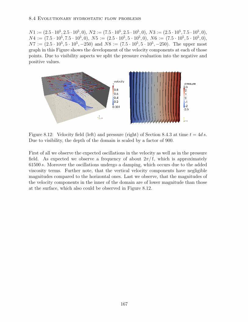
8.4 Evolutionary hydrostatic flow problems
N1 := (2.5 · 105, 2.5 · 105, 0), N2 := (7.5 · 105, 2.5 · 105, 0), N3 := (2.5 · 105, 7.5 · 105, 0),N4 := (7.5 · 105, 7.5 · 105, 0), N5 := (2.5 · 105, 5 · 105, 0), N6 := (7.5 · 105, 5 · 105, 0),N7 := (2.5 · 105, 5 · 105,−250) and N8 := (7.5 · 105, 5 · 105,−250). The upper mostgraph in this Figure shows the development of the velocity components at each of thosepoints. Due to visibility aspects we split the pressure evaluation into the negative andpositive values.
Figure 8.12: Velocity field (left) and pressure (right) of Section 8.4.3 at time t = 4d s.Due to visibility, the depth of the domain is scaled by a factor of 900.
First of all we observe the expected oscillations in the velocity as well as in the pressurefield. As expected we observe a frequency of about 2π/ f, which is approximately61500 s. Moreover the oscillations undergo a damping, which occurs due to the addedviscosity terms. Further note, that the vertical velocity components have negligiblemagnitudes compared to the horizontal ones. Last we observe, that the magnitudes ofthe velocity components in the inner of the domain are of lower magnitude than thoseat the surface, which also could be observed in Figure 8.12.
167
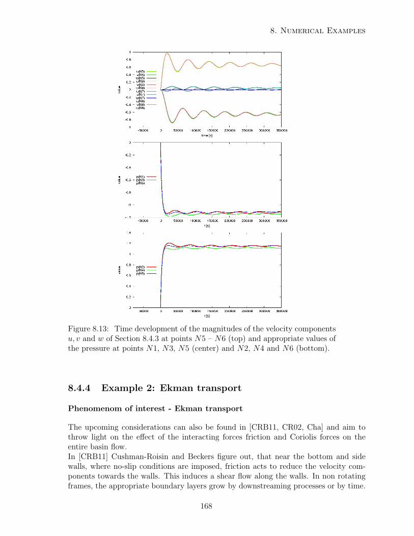
8. Numerical Examples
Figure 8.13: Time development of the magnitudes of the velocity componentsu, v and w of Section 8.4.3 at points N5 – N6 (top) and appropriate values ofthe pressure at points N1, N3, N5 (center) and N2, N4 and N6 (bottom).
8.4.4 Example 2: Ekman transport
Phenomenom of interest - Ekman transport
The upcoming considerations can also be found in [CRB11, CR02, Cha] and aim tothrow light on the effect of the interacting forces friction and Coriolis forces on theentire basin flow.In [CRB11] Cushman-Roisin and Beckers figure out, that near the bottom and sidewalls, where no-slip conditions are imposed, friction acts to reduce the velocity com-ponents towards the walls. This induces a shear flow along the walls. In non rotatingframes, the appropriate boundary layers grow by downstreaming processes or by time.
168
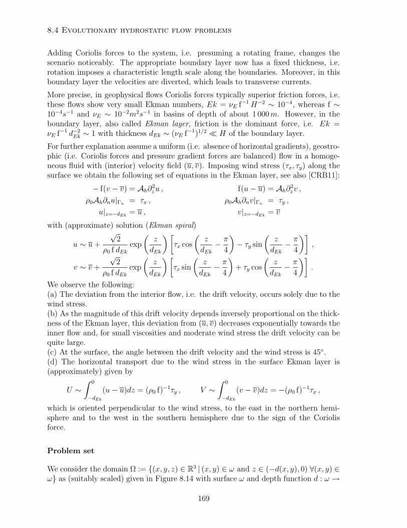
8.4 Evolutionary hydrostatic flow problems
Adding Coriolis forces to the system, i.e. presuming a rotating frame, changes thescenario noticeably. The appropriate boundary layer now has a fixed thickness, i.e.rotation imposes a characteristic length scale along the boundaries. Moreover, in thisboundary layer the velocities are diverted, which leads to transverse currents.
More precise, in geophysical flows Coriolis forces typically superior friction forces, i.e.these flows show very small Ekman numbers, Ek = νE f−1H−2 ∼ 10−4, whereas f ∼10−4s−1 and νE ∼ 10−2m2s−1 in basins of depth of about 1 000m. However, in theboundary layer, also called Ekman layer, friction is the dominant force, i.e. Ek =νE f−1 d−2
Ek ∼ 1 with thickness dEk ∼ (νE f−1)1/2 H of the boundary layer.
For further explanation assume a uniform (i.e. absence of horizontal gradients), geostro-phic (i.e. Coriolis forces and pressure gradient forces are balanced) flow in a homoge-neous fluid with (interior) velocity field (u, v). Imposing wind stress (τx, τy) along thesurface we obtain the following set of equations in the Ekman layer, see also [CRB11]:
− f(v − v) = Ah∂2zu , f(u− u) = Ah∂2
zv ,
ρ0Ah∂nu|Γu = τx , ρ0Ah∂nv|Γu = τy ,
u|z=−dEk = u , v|z=−dEk = v
with (approximate) solution (Ekman spiral)
u ∼ u+
√2
ρ0 f dEkexp
(z
dEk
)[τx cos
(z
dEk− π
4
)− τy sin
(z
dEk− π
4
)],
v ∼ v +
√2
ρ0 f dEkexp
(z
dEk
)[τx sin
(z
dEk− π
4
)+ τy cos
(z
dEk− π
4
)].
We observe the following:(a) The deviation from the interior flow, i.e. the drift velocity, occurs solely due to thewind stress.(b) As the magnitude of this drift velocity depends inversely proportional on the thick-ness of the Ekman layer, this deviation from (u, v) decreases exponentially towards theinner flow and, for small viscosities and moderate wind stress the drift velocity can bequite large.(c) At the surface, the angle between the drift velocity and the wind stress is 45.(d) The horizontal transport due to the wind stress in the surface Ekman layer is(approximately) given by
U ∼∫ 0
−dEk(u− u)dz = (ρ0 f)−1τy , V ∼
∫ 0
−dEk(v − v)dz = −(ρ0 f)−1τx ,
which is oriented perpendicular to the wind stress, to the east in the northern hemi-sphere and to the west in the southern hemisphere due to the sign of the Coriolisforce.
Problem set
We consider the domain Ω := (x, y, z) ∈ R3 | (x, y) ∈ ω and z ∈ (−d(x, y), 0) ∀(x, y) ∈ω as (suitably scaled) given in Figure 8.14 with surface ω and depth function d : ω →
169
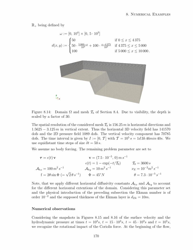
8. Numerical Examples
R+ being defined by
ω := [0, 104]× [0, 5 · 103]
d(x, y) :=
50 if 0 ≤ x ≤ 4 375
50 · 5 000−x103 + 100 · x−4 375
103 if 4 375 ≤ x ≤ 5 000
100 if 5 000 ≤ x ≤ 10 000 .
Figure 8.14: Domain Ω and mesh Th of Section 8.4. Due to visibility, the depth isscaled by a factor of 30.
The spatial resolution of the considered mesh Th is 156.25m is horizontal directions and1.5625 − 3.125m in vertical extent. Thus the horizontal 3D velocity field has 141570dofs and the 2D pressure field 1089 dofs. The vertical velocity component has 70785dofs. The time interval is given by I := [0, T ] with T = 105 s = 1d 3h 46min 40s. Weuse equidistant time steps of size δt = 50 s.
We assume no body forcing. The remaining problem parameter are set to
τ = ε(t) v v = (7.5 · 10−5, 0)ms−1
ε(t) = 1− exp(−t/T0) T0 = 3600 s
Ahx = 100m2 s−1 Ahy = 10m2 s−1 νE = 10−2m2 s−1
f = 2θ sin Φ (=√
2 θ s−1) Φ = 45N θ = 7.3 · 10−5 s−1
Note, that we apply different horizontal diffusivity constants Ahx and Ahy to accountfor the different horizontal extentions of the domain. Considering this parameter setand the physical introduction of the preceding subsection the Ekman number is oforder 10−2 and the supposed thickness of the Ekman layer is dEk = 10m.
Numerical observations
Considering the snapshots in Figures 8.15 and 8.16 of the surface velocity and thehydrodynamic pressure at times t = 103s, t = 15 · 103s, t = 45 · 103s and t = 105s,we recognize the rotational impact of the Coriolis force. At the beginning of the flow,
170
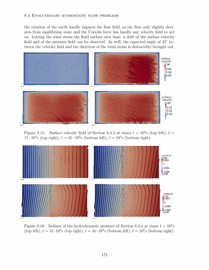
8.4 Evolutionary hydrostatic flow problems
the rotation of the earth hardly impacts the flow field, as the flow only slightly devi-ates from equilibrium state and the Coriolis force has hardly any velocity field to acton. Letting the wind stress the fluid surface over time, a drift of the surface velocityfield and of the pressure field can be observed. As well, the expected angle of 45 be-tween the velocity field and the direction of the wind stress is distinctibly brought out.
Figure 8.15: Surface velocity field of Section 8.4.4 at times t = 103s (top left), t =15 · 103s (top right), t = 45 · 103s (bottom left), t = 105s (bottom right).
Figure 8.16: Isolines of the hydrodynamic pressure of Section 8.4.4 at times t = 103s(top left), t = 15 · 103s (top right), t = 45 · 103s (bottom left), t = 105s (bottom right).
171
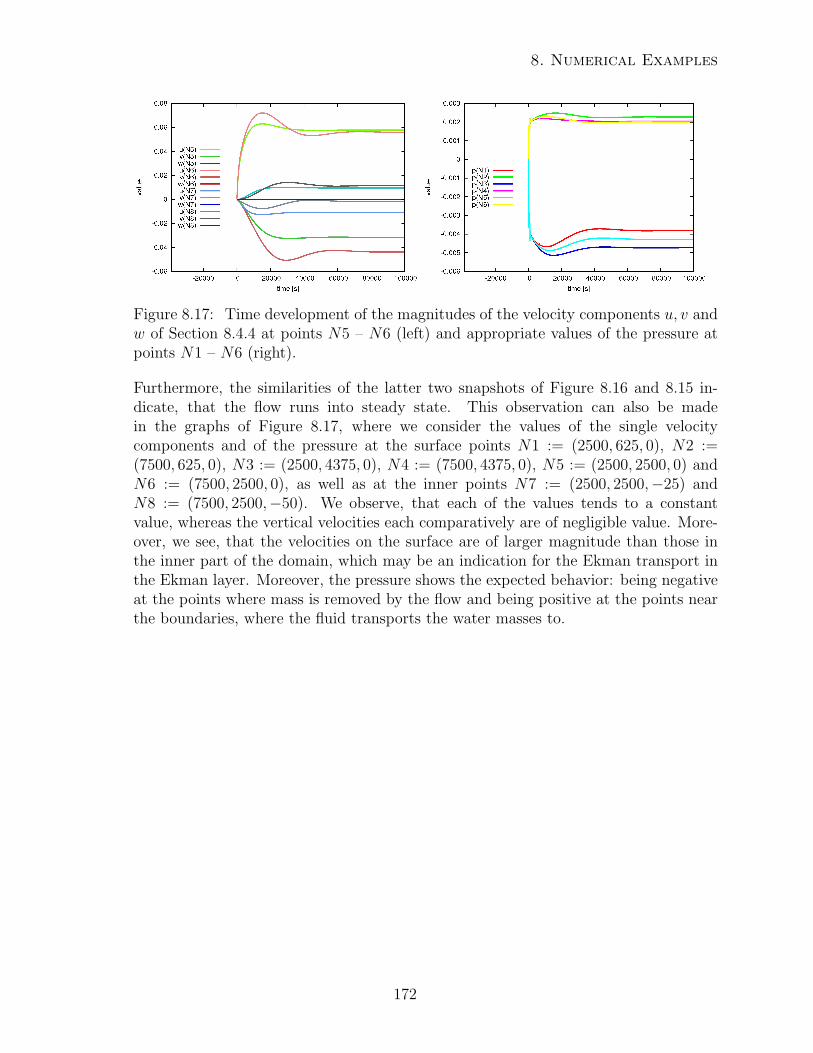
8. Numerical Examples
Figure 8.17: Time development of the magnitudes of the velocity components u, v andw of Section 8.4.4 at points N5 – N6 (left) and appropriate values of the pressure atpoints N1 – N6 (right).
Furthermore, the similarities of the latter two snapshots of Figure 8.16 and 8.15 in-dicate, that the flow runs into steady state. This observation can also be madein the graphs of Figure 8.17, where we consider the values of the single velocitycomponents and of the pressure at the surface points N1 := (2500, 625, 0), N2 :=(7500, 625, 0), N3 := (2500, 4375, 0), N4 := (7500, 4375, 0), N5 := (2500, 2500, 0) andN6 := (7500, 2500, 0), as well as at the inner points N7 := (2500, 2500,−25) andN8 := (7500, 2500,−50). We observe, that each of the values tends to a constantvalue, whereas the vertical velocities each comparatively are of negligible value. More-over, we see, that the velocities on the surface are of larger magnitude than those inthe inner part of the domain, which may be an indication for the Ekman transport inthe Ekman layer. Moreover, the pressure shows the expected behavior: being negativeat the points where mass is removed by the flow and being positive at the points nearthe boundaries, where the fluid transports the water masses to.
172
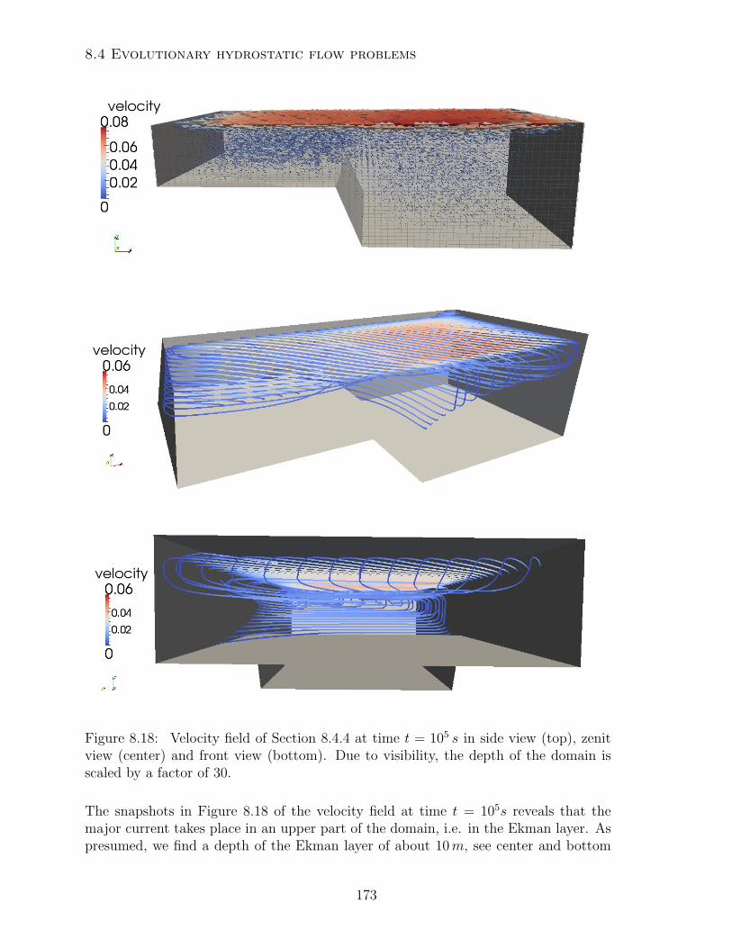
8.4 Evolutionary hydrostatic flow problems
Figure 8.18: Velocity field of Section 8.4.4 at time t = 105 s in side view (top), zenitview (center) and front view (bottom). Due to visibility, the depth of the domain isscaled by a factor of 30.
The snapshots in Figure 8.18 of the velocity field at time t = 105s reveals that themajor current takes place in an upper part of the domain, i.e. in the Ekman layer. Aspresumed, we find a depth of the Ekman layer of about 10m, see center and bottom
173
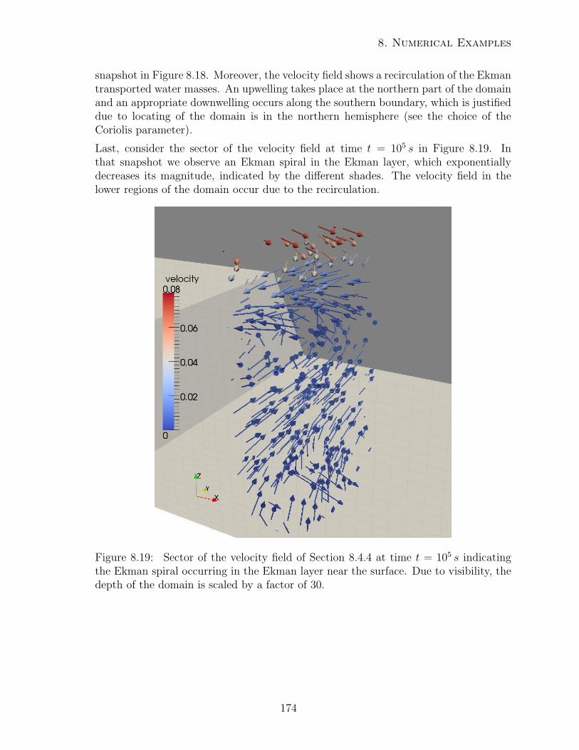
8. Numerical Examples
snapshot in Figure 8.18. Moreover, the velocity field shows a recirculation of the Ekmantransported water masses. An upwelling takes place at the northern part of the domainand an appropriate downwelling occurs along the southern boundary, which is justifieddue to locating of the domain is in the northern hemisphere (see the choice of theCoriolis parameter).
Last, consider the sector of the velocity field at time t = 105 s in Figure 8.19. Inthat snapshot we observe an Ekman spiral in the Ekman layer, which exponentiallydecreases its magnitude, indicated by the different shades. The velocity field in thelower regions of the domain occur due to the recirculation.
Figure 8.19: Sector of the velocity field of Section 8.4.4 at time t = 105 s indicatingthe Ekman spiral occurring in the Ekman layer near the surface. Due to visibility, thedepth of the domain is scaled by a factor of 30.
174
8.4 Evolutionary hydrostatic flow problems
8.4.5 Example 3: Ekman pumping
Phenomenom of interest: Ekman pumping
We resume to the considerations of Example 1 and start our argumentation from theEkman transport in the surface Ekman layer. As figured out in the former section,the eastwards directed wind stress and the Coriolis forces, acting on the moving fluid,imposes a south–easternwards water mass transport in the Ekman layer (in the northernhemisphere). The numerical test of Example 1 reveals, that the Ekman transportinvokes circulation with an upwelling at the northern boundary and a downwelling atthe southern boundary. However, this resulting circulation in the upper flow regionoccurs due to the imposed Dirichlet boundary conditions along the side and bottomwalls of the velocity field.In oceanic flows, wind stress induced water mass exchanges from deeper regions, whichare abundant in nutrients, is an important mechanism and takes place, when the windstress is not rotation free, see also [CRB11].Let us explain this more involved up- and downwelling, also called Ekman pumpingand Ekman suction, respectively.
Therefore, let w be the vertical velocity in the interior, defined by the divergenceconstraint
w =
∫ ∞0
(∂xu+ ∂yv) dz = (ρ0 f)−1 (∂xτy − ∂yτx) .
I.e. if the curl of the imposed wind stress does not vanish, the appropriate spatial vari-ations in the wind drive vertical currents, which in turn drive the interior circulationof the ocean.Moreover, the drift velocities in the Ekman layer along the bottom wall are (approxi-mately) given by
u ≈ u− exp
(−(d+ z)
dEk
)[u cos
(z + d
dEk
)+ v sin
(z + d
dEk
)],
v ≈ v + exp
(−(d+ z)
dEk
)[u sin
(z + d
dEk
)− v cos
(z + d
dEk
)],
with depth function d and resulting vertical drift velocity w = wd + wpump with wd =−u∂xd−v∂yd, accounting for the bottom structure, and an Ekman pumping or suctioncontribution wpump = dEk(∂xv − ∂yu)/2, see also [CRB11]. I.e. at the lower Ekmanboundary an upwelling/downwelling takes place due to the vorticity of the interiorvelocity field, which has been imposed by the wind stress.
175
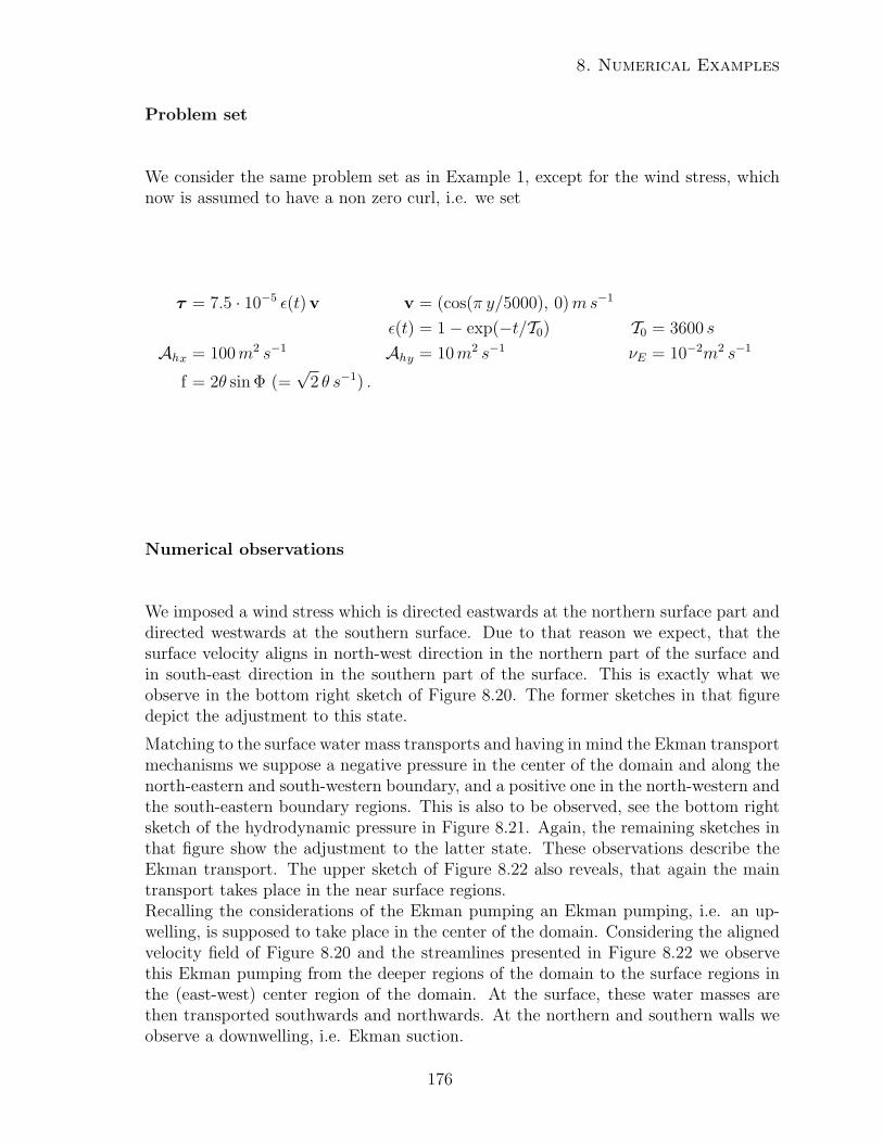
8. Numerical Examples
Problem set
We consider the same problem set as in Example 1, except for the wind stress, whichnow is assumed to have a non zero curl, i.e. we set
τ = 7.5 · 10−5 ε(t) v v = (cos(π y/5000), 0)ms−1
ε(t) = 1− exp(−t/T0) T0 = 3600 s
Ahx = 100m2 s−1 Ahy = 10m2 s−1 νE = 10−2m2 s−1
f = 2θ sin Φ (=√
2 θ s−1) .
Numerical observations
We imposed a wind stress which is directed eastwards at the northern surface part anddirected westwards at the southern surface. Due to that reason we expect, that thesurface velocity aligns in north-west direction in the northern part of the surface andin south-east direction in the southern part of the surface. This is exactly what weobserve in the bottom right sketch of Figure 8.20. The former sketches in that figuredepict the adjustment to this state.
Matching to the surface water mass transports and having in mind the Ekman transportmechanisms we suppose a negative pressure in the center of the domain and along thenorth-eastern and south-western boundary, and a positive one in the north-western andthe south-eastern boundary regions. This is also to be observed, see the bottom rightsketch of the hydrodynamic pressure in Figure 8.21. Again, the remaining sketches inthat figure show the adjustment to the latter state. These observations describe theEkman transport. The upper sketch of Figure 8.22 also reveals, that again the maintransport takes place in the near surface regions.Recalling the considerations of the Ekman pumping an Ekman pumping, i.e. an up-welling, is supposed to take place in the center of the domain. Considering the alignedvelocity field of Figure 8.20 and the streamlines presented in Figure 8.22 we observethis Ekman pumping from the deeper regions of the domain to the surface regions inthe (east-west) center region of the domain. At the surface, these water masses arethen transported southwards and northwards. At the northern and southern walls weobserve a downwelling, i.e. Ekman suction.
176
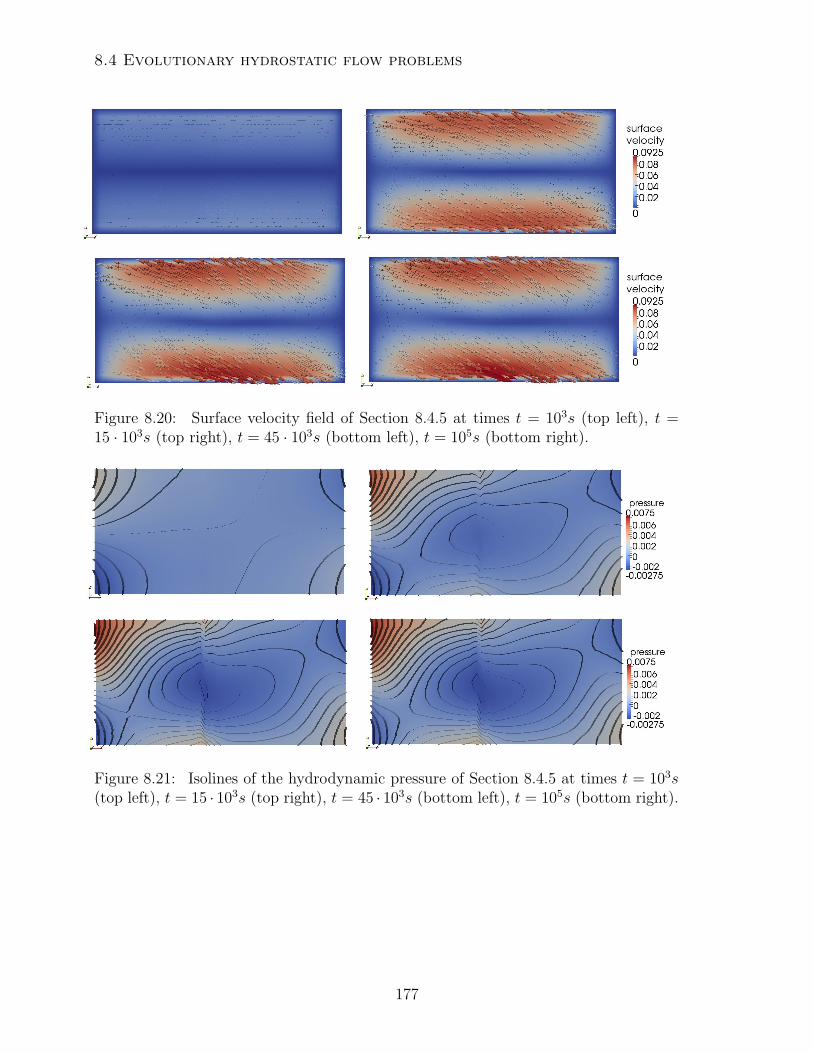
8.4 Evolutionary hydrostatic flow problems
Figure 8.20: Surface velocity field of Section 8.4.5 at times t = 103s (top left), t =15 · 103s (top right), t = 45 · 103s (bottom left), t = 105s (bottom right).
Figure 8.21: Isolines of the hydrodynamic pressure of Section 8.4.5 at times t = 103s(top left), t = 15 · 103s (top right), t = 45 · 103s (bottom left), t = 105s (bottom right).
177
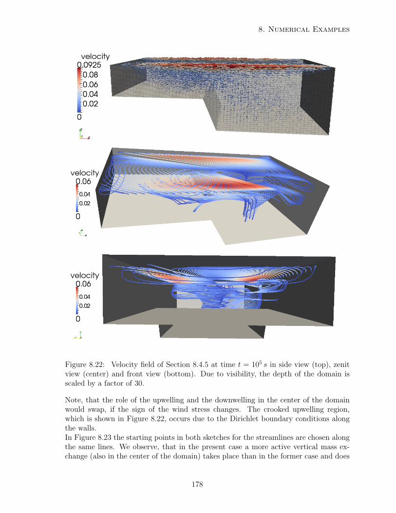
8. Numerical Examples
Figure 8.22: Velocity field of Section 8.4.5 at time t = 105 s in side view (top), zenitview (center) and front view (bottom). Due to visibility, the depth of the domain isscaled by a factor of 30.
Note, that the role of the upwelling and the downwelling in the center of the domainwould swap, if the sign of the wind stress changes. The crooked upwelling region,which is shown in Figure 8.22, occurs due to the Dirichlet boundary conditions alongthe walls.In Figure 8.23 the starting points in both sketches for the streamlines are chosen alongthe same lines. We observe, that in the present case a more active vertical mass ex-change (also in the center of the domain) takes place than in the former case and does
178
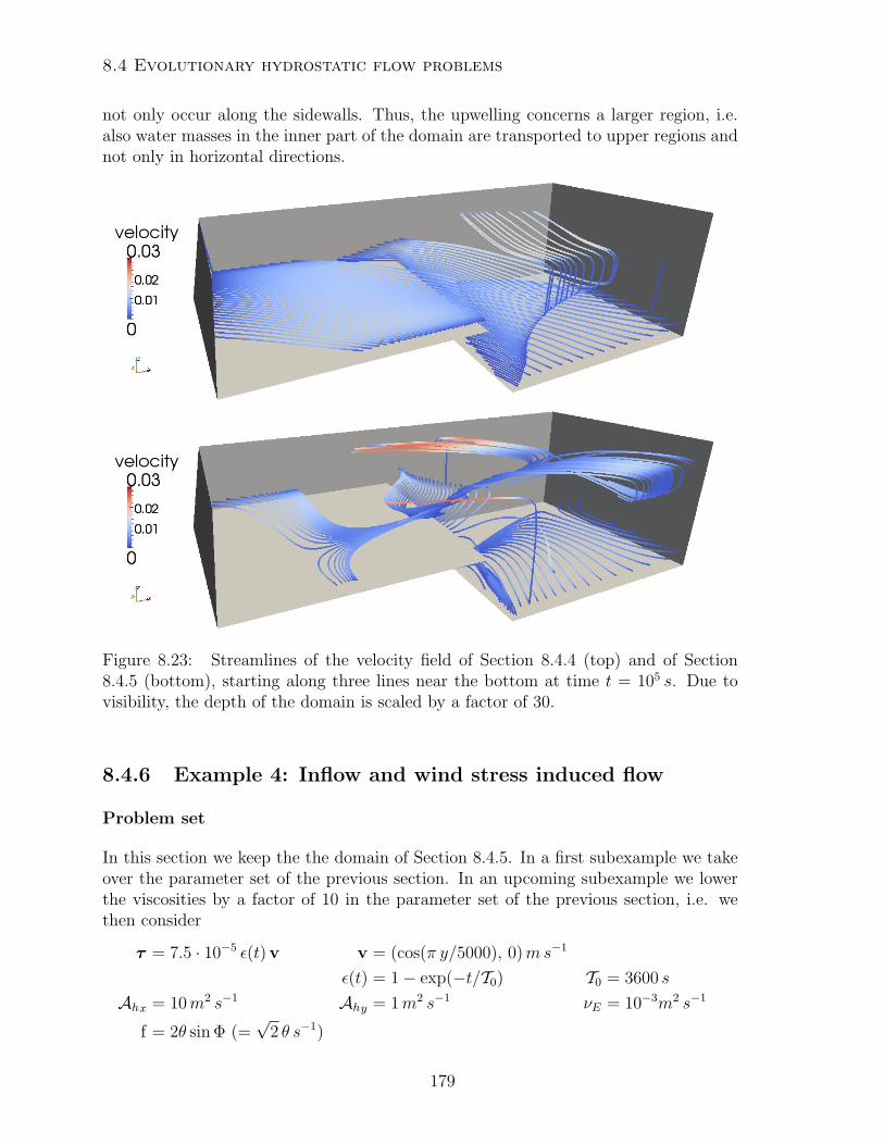
8.4 Evolutionary hydrostatic flow problems
not only occur along the sidewalls. Thus, the upwelling concerns a larger region, i.e.also water masses in the inner part of the domain are transported to upper regions andnot only in horizontal directions.
Figure 8.23: Streamlines of the velocity field of Section 8.4.4 (top) and of Section8.4.5 (bottom), starting along three lines near the bottom at time t = 105 s. Due tovisibility, the depth of the domain is scaled by a factor of 30.
8.4.6 Example 4: Inflow and wind stress induced flow
Problem set
In this section we keep the the domain of Section 8.4.5. In a first subexample we takeover the parameter set of the previous section. In an upcoming subexample we lowerthe viscosities by a factor of 10 in the parameter set of the previous section, i.e. wethen consider
τ = 7.5 · 10−5 ε(t) v v = (cos(π y/5000), 0)ms−1
ε(t) = 1− exp(−t/T0) T0 = 3600 s
Ahx = 10m2 s−1 Ahy = 1m2 s−1 νE = 10−3m2 s−1
f = 2θ sin Φ (=√
2 θ s−1)
179
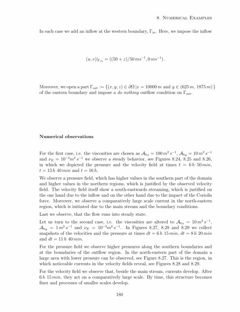
8. Numerical Examples
In each case we add an inflow at the western boundary, Γin. Here, we impose the inflow
(u, v)|Γin = ((50 + z)/50ms−1, 0ms−1) .
Moreover, we open a part Γout := (x, y, z) ∈ ∂Ω |x = 10000m and y ∈ (625m, 1875m) of the eastern boundary and impose a do nothing outflow condition on Γout.
Numerical observations
For the first case, i.e. the viscosities are chosen as Ahx = 100m2 s−1, Ahy = 10m2 s−1
and νE = 10−2m2 s−1 we observe a steady behavior, see Figures 8.24, 8.25 and 8.26,in which we depicted the pressure and the velocity field at times t = 6h 50min,t = 13h 40min and t = 16h.
We observe a pressure field, which has higher values in the southern part of the domainand higher values in the northern regions, which is justified by the observed velocityfield. The velocity field itself show a south-eastwards streaming, which is justified onthe one hand due to the inflow and on the other hand due to the impact of the Coriolisforce. Moreover, we observe a comparatively large scale current in the north-easternregion, which is initiated due to the main stream and the boundary conditions.
Last we observe, that the flow runs into steady state.
Let us turn to the second case, i.e. the viscosities are altered to Ahx = 10m2 s−1,Ahy = 1m2 s−1 and νE = 10−3m2 s−1. In Figures 8.27, 8.28 and 8.29 we collectsnapshots of the velocities and the pressure at times dt = 6h 15min, dt = 8h 20minand dt = 11h 40min.
For the pressure field we observe higher pressures along the southern boundaries andat the boundaries of the outflow region. In the north-eastern part of the domain alarge area with lower pressure can be observed, see Figure 8.27. This is the region, inwhich noticeable currents in the velocity fields reveal, see Figures 8.28 and 8.29.
For the velocity field we observe that, beside the main stream, currents develop. After6h 15min, they act on a comparatively large scale. By time, this structure becomesfiner and processes of smaller scales develop.
180
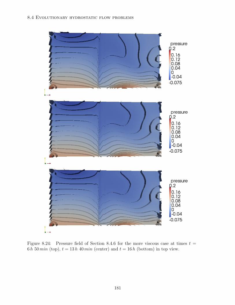
8.4 Evolutionary hydrostatic flow problems
Figure 8.24: Pressure field of Section 8.4.6 for the more viscous case at times t =6h 50min (top), t = 13h 40min (center) and t = 16h (bottom) in top view.
181
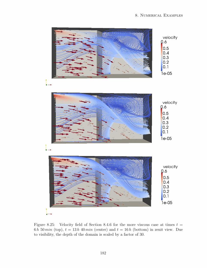
8. Numerical Examples
Figure 8.25: Velocity field of Section 8.4.6 for the more viscous case at times t =6h 50min (top), t = 13h 40min (center) and t = 16h (bottom) in zenit view. Dueto visibility, the depth of the domain is scaled by a factor of 30.
182
8.4 Evolutionary hydrostatic flow problems
Figure 8.26: Velocity field of Section 8.4.6 for the more viscous case at times t =6h 50min (top), t = 13h 40min (center) and t = 16h (bottom) in zenit view. Dueto visibility, the depth of the domain is scaled by a factor of 30.
183
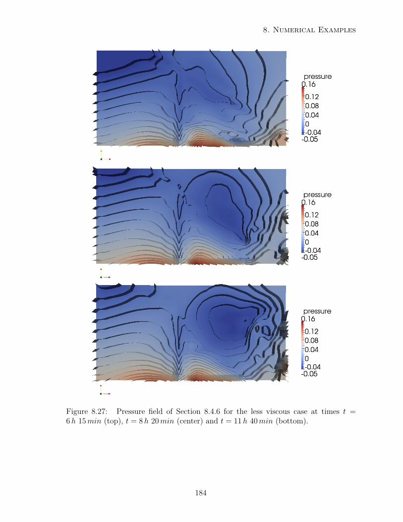
8. Numerical Examples
Figure 8.27: Pressure field of Section 8.4.6 for the less viscous case at times t =6h 15min (top), t = 8h 20min (center) and t = 11h 40min (bottom).
184
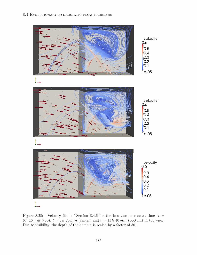
8.4 Evolutionary hydrostatic flow problems
Figure 8.28: Velocity field of Section 8.4.6 for the less viscous case at times t =6h 15min (top), t = 8h 20min (center) and t = 11h 40min (bottom) in top view.Due to visibility, the depth of the domain is scaled by a factor of 30.
185
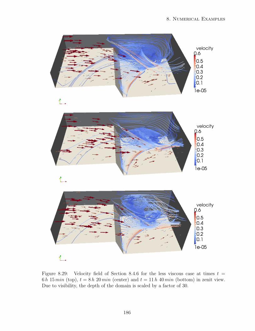
8. Numerical Examples
Figure 8.29: Velocity field of Section 8.4.6 for the less viscous case at times t =6h 15min (top), t = 8h 20min (center) and t = 11h 40min (bottom) in zenit view.Due to visibility, the depth of the domain is scaled by a factor of 30.
186
Chapter 9
Conclusions and Perspectives
We started this thesis with an introduction of the topic of hydrostatic flow problemsranging from the physical background to the variational context. The main issue ofthis work was the analysis of equal-order finite element discretized hydrostatic flowproblems. We analyzed the equal-order finite element discretization of the hydrostaticStokes and the hydrostatic Oseen problem on isotropic and on vertical anisotropicmeshes. Within this context we developed suitable stabilization schemes, which ensurethe modified inf-sup constraint and, in the Oseen case, also stabilizes the oscillationsoccurring due to dominant advection. These stabilization schemes are based on estab-lished schemes for the classical, i.e. non hydrostatic, case. We elaborated, that thesestabilization schemes lead to optimal a priori error estimates. Within the anisotropicframework we elaborated suitable error estimates, which are based on [Ape98] and[Bra06]. As well, we developed a suitable H1-stable, 3D projection operator, whichopened the possibility of anisotropic local projection stabilization of the 3D velocityfield. Closing the chapter on anisotropy we treated the hydrostatic Stokes problemon meshes, where anisotropy also is allowed to occur on the surface mesh. We ex-amined the stability property of the unstabilized scheme. As in the former cases,suitable stabilization turned out to be necessary. Unlike the former cases, we had toapply anisotropic pressure stabilization schemes. We applied anisotropic stabilizationschemes, which are given by [Bec95, Ric05, BT06a], and elaborated inf-sup stability aswell as optimal a priori error estimates, which are comparable with the results knownfor the 2D standard problem.Turning to the evolutionary problems, we introduced splitting schemes, which are es-tablished in the classical framework. Due to their structure, i.e. splitting the entireproblem into a pressure and a velocity problem, these schemes seemed to be a goodchoice for the algorithmic treatment of the evolutionary, but also for the stationary hy-drostatic problems. Within this context we explained how to adapt these schemes to thehydrostatic case. This is not straightforward due to the modified inf-sup constraint. Inparticular we dedicated to the questions, whether the hydrostatically adapted schemesin turn are projection schemes, whether to use the rotational or the standard approachand we shortly discussed on the choice of boundary conditions.The quality of the stabilization schemes on isotropic meshes has been numerically testedin Chapter 8. In this chapter we also numerically portrayed different phenomena found
187
9. Conclusions and Perspectives
in oceanic regimes, which are primarily induced by the rotation of the earth, i.e. theCoriolis force. Further, we presented parallel efficiency of a partly parallelized prob-lem. Here, the parallelization was applied to the numerically expensive 3D momentumequation and to the 3D equation for salinity and temperature, whereas the 2D pressureproblem remained unchanged.
Throughout the entire work we presumed the domain to have a depth, which is strictlybounded away from zero. However, there is analysis for the variational problem in adomain with δmin = 0, see e.g.[BL92]. The extention to the discretized problem, aswell to the issue of splitting schemes is still missing.
The issue of pressure correction schemes itself in the hydrostatic framework also seemsto be undealt to the most extent. We gave an intention in the present work, but aproper convergence analysis is still missing in the hydrostatic framework, quite apartfrom appropriately stabilized schemes. Moreover, the authors of [BC08] examinedstabilized version of pressure correction schemes in the classical context for symmetricstabilization schemes. How to apply splitting schemes to non symmetric stabilizedproblems is also an open question.
In the present work we did not deal with the topic of non conforming finite elementsin the hydrostatic framework. As well, we did not treat the issue of local mesh re-finement and adaptivity, being accompanied with that topic, the field of a posteriorierror estimates for hydrostatic flow problems is still missing. Moreover, the treatmentof corners and edges in the anisotropic, hydrostatic case is still undone.
With respect to the numerical realization of the given hydrostatic problem it has tobe noted, that the splitting approach is suitable in the context of evolutionary prob-lem. However, it revealed to be numerically too expensive in the context of stationaryproblems. A coupled solver, such as applied in [CGS12] in the toolbox FreeFem++,see [DHP03], is more suggestible.
Broadening the attention also to the energy equations, which effects a varying densityand thus dynamically couples to the hydrostatic Navier-Stokes equations, a suitableanalysis of the discrete problem still is missing. Within this context, the authors of[BB02] already considered this issue in the classical, compressible framework. Moreoverin the context of constant density in the classical framework, the authors of [AL94]considered the case of convection-diffusion problems.
Finally let us mention, that we presumed a fixed set of equations, including all thesimplifications and approximations, see also Chapter 2. Within this context, param-eterizations were applied in order to present unresolved but important processes inthe resolved range. Within this context, huge uncertainties are apparent, e.g. in thecontext of turbulent parameterization. We applied a quite simple parameterization,the Smagorinsky approach. However, the suitability of this approach is doubtful andimproved parameterizations are eagerly desired.
188
Appendix A
Discretization Schemes forEvolutionary Systems
We start with the introduction of classical time stepping schemes, which form a basiselement in the construction of splitting schemes. The presented schemes and theirproperties are a taken from classical textbooks, e.g. [Her01]. Considering nonhydro-static flow problems, we then turn to the field of splitting schemes. Note, that thebasic ideas of splitting schemes have already been introduced in Section 6.1. As wellwe already treated the class of pressure correction schemes in Section 6.2. We neglectboth topics here and refer to the appropriate sections whenever necessary. Instead,we introduce further established approaches to suitably split flow problems: penaltyprojection schemes, velocity correction schemes and consistent splitting schemes. Wedeal with convergence and stability aspects and present the application of splittingschemes in the context of stabilized problems at the example of pressure correctionschemes. This sections is a summary of [GMS06, GS04, Pro97, Pro08, BC08]. It in-troduces the main aspects, stressing on the topics which may profit in the deductionof the hydrostatic case.
A.1 Time discretization schemes
In this section we shortly collect common time discretization schemes, focusing on A-stable schemes as given in textbooks, such as [Her01]. We do not consider the caseof step size control and thus restrict to the case of one step size for the entire timediscretization. For further informations we refer to the cited literature.
Given a time interval I := [0, T ] we consider the ODE
y′(t) = f(t, y), y(0) = y0 ∀t ∈ Iwith sufficiently regular function f . There are a couple of commonly used methods,such as Runge-Kutta schemes, Adams-Bashforth formulas, Adams-Moulton schemesor backward differentiation formulas (BDF schemes). In the following we use thegeneralized θ-scheme and the BDFk scheme.
189
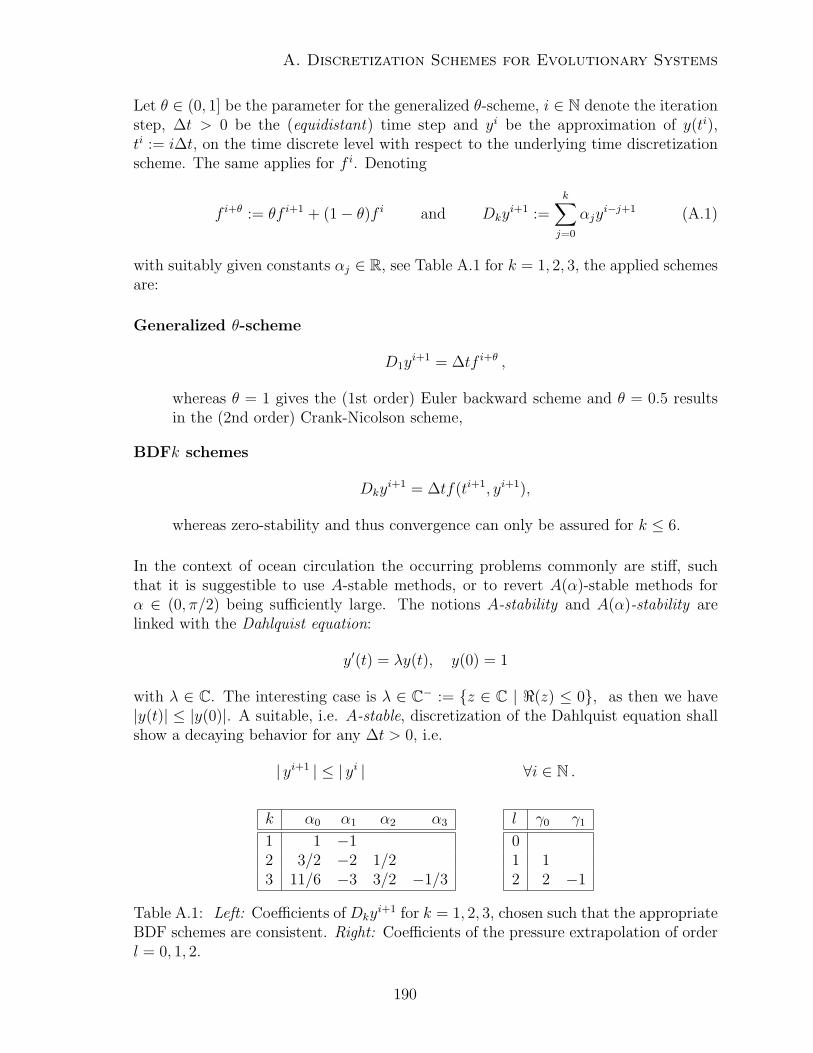
A. Discretization Schemes for Evolutionary Systems
Let θ ∈ (0, 1] be the parameter for the generalized θ-scheme, i ∈ N denote the iterationstep, ∆t > 0 be the (equidistant) time step and yi be the approximation of y(ti),ti := i∆t, on the time discrete level with respect to the underlying time discretizationscheme. The same applies for f i. Denoting
f i+θ := θf i+1 + (1− θ)f i and Dkyi+1 :=
k∑j=0
αjyi−j+1 (A.1)
with suitably given constants αj ∈ R, see Table A.1 for k = 1, 2, 3, the applied schemesare:
Generalized θ-scheme
D1yi+1 = ∆tf i+θ ,
whereas θ = 1 gives the (1st order) Euler backward scheme and θ = 0.5 resultsin the (2nd order) Crank-Nicolson scheme,
BDFk schemes
Dkyi+1 = ∆tf(ti+1, yi+1),
whereas zero-stability and thus convergence can only be assured for k ≤ 6.
In the context of ocean circulation the occurring problems commonly are stiff, suchthat it is suggestible to use A-stable methods, or to revert A(α)-stable methods forα ∈ (0, π/2) being sufficiently large. The notions A-stability and A(α)-stability arelinked with the Dahlquist equation:
y′(t) = λy(t), y(0) = 1
with λ ∈ C. The interesting case is λ ∈ C− := z ∈ C | <(z) ≤ 0, as then we have|y(t)| ≤ |y(0)|. A suitable, i.e. A-stable, discretization of the Dahlquist equation shallshow a decaying behavior for any ∆t > 0, i.e.
| yi+1 | ≤ | yi | ∀i ∈ N .
k α0 α1 α2 α3
1 1 −12 3/2 −2 1/23 11/6 −3 3/2 −1/3
l γ0 γ1
01 12 2 −1
Table A.1: Left: Coefficients of Dkyi+1 for k = 1, 2, 3, chosen such that the appropriate
BDF schemes are consistent. Right: Coefficients of the pressure extrapolation of orderl = 0, 1, 2.
190
A.2 Splitting schemes for nonhydrostatic problems
If this decay does not apply for all λ ∈ C−, but for all λ ∈ C− with∣∣∣∣arctan
(<(λ)
=(λ)
)∣∣∣∣ ≤ α
for a fixed α ∈ (0, π/2), the numerical scheme is called A(α)-stable. For some ap-plications it is sufficient to apply (convergent) A(α)-stable schemes, provided α to besuitably large.
The Euler backward scheme is A-stable. Due to the 2nd Dahlquist barrier, see also[Her01], the BDF1 scheme and the BDF2 schemes are A-stable and the (A-stable andimplicit) trapezoidal formula (θ-scheme with θ = 1/2) has convergence order of 2.Moreover, the BDF3 scheme is A(α)-stable with α = 86.
A.2 Splitting schemes for nonhydrostatic problems
This section provides a summary of different classes of splitting schemes, besides thealready introduced class of pressure correction schemes, see Section 6.2. The deductionsare collected from [GMS06, BC08, Pro08, Pro97].
A.2.1 Penalty projection schemes
Based on the Chorin-Temam scheme as introduced in Section 6.3, Prohl [Pro08] choosesthe following approach: Consider the parameter setting of the Chorin-Temam scheme,which reflects in Dk,1 v
i+1 = vi and pi+1,∗ = 0. Prohl adds (6.16) at time (i + 1)∆tto (6.17) at time i∆t, exploiting the reformulation (6.11) of the latter equation. Theresulting set of equations is given by
∆t−1(vi+1 − vi)− ν∆vi+1 +∇pi = f(ti+1) in Ω
div vi+1 −∆t∆pi+1 = 0 in Ω
∂npi+1 = 0 on ∂Ω .
Prohl postulates the following drawbacks, which we partly already have faced: (a) theapparent velocity vi+1 satisfies the divergence constraint only up to a penalty term, (b)artificial pressure boundary conditions are imposed, (c) due to the explicit treatment ofthe pressure in the momentum equation the discrete energy law is violated. In order totackle the artificial boundary layer, he suggests the introduction of a modified pressureextrapolation and a divergence concerning term in the momentum equation as wellas application of a pressure update, which calls the pressure updates of the precedingrotational schemes to mind, see also [Pro08]:
191
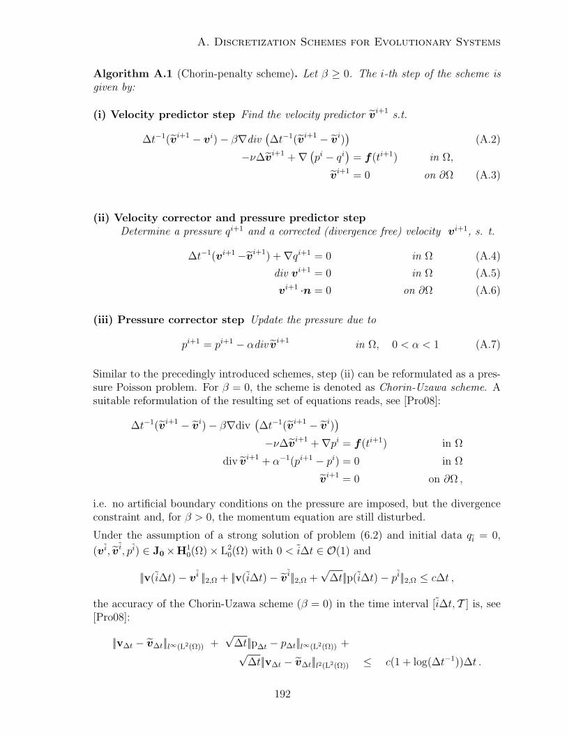
A. Discretization Schemes for Evolutionary Systems
Algorithm A.1 (Chorin-penalty scheme). Let β ≥ 0. The i-th step of the scheme isgiven by:
(i) Velocity predictor step Find the velocity predictor vi+1 s.t.
∆t−1(vi+1 − vi)− β∇div(∆t−1(vi+1 − vi)) (A.2)
−ν∆vi+1 +∇ (pi − qi) = f(ti+1) in Ω,
vi+1 = 0 on ∂Ω (A.3)
(ii) Velocity corrector and pressure predictor stepDetermine a pressure qi+1 and a corrected (divergence free) velocity vi+1, s. t.
∆t−1(vi+1−vi+1) +∇qi+1 = 0 in Ω (A.4)
div vi+1 = 0 in Ω (A.5)
vi+1 ·n = 0 on ∂Ω (A.6)
(iii) Pressure corrector step Update the pressure due to
pi+1 = pi+1 − αdiv vi+1 in Ω, 0 < α < 1 (A.7)
Similar to the precedingly introduced schemes, step (ii) can be reformulated as a pres-sure Poisson problem. For β = 0, the scheme is denoted as Chorin-Uzawa scheme. Asuitable reformulation of the resulting set of equations reads, see [Pro08]:
∆t−1(vi+1 − vi)− β∇div(∆t−1(vi+1 − vi))−ν∆vi+1 +∇pi = f(ti+1) in Ω
div vi+1 + α−1(pi+1 − pi) = 0 in Ω
vi+1 = 0 on ∂Ω ,
i.e. no artificial boundary conditions on the pressure are imposed, but the divergenceconstraint and, for β > 0, the momentum equation are still disturbed.
Under the assumption of a strong solution of problem (6.2) and initial data qi = 0,
(v i, v i, pi) ∈ J0×H10(Ω)× L2
0(Ω) with 0 < i∆t ∈ O(1) and
||v(i∆t)− v i ||2,Ω + ||v(i∆t)− v i||2,Ω +√
∆t||p(i∆t)− pi||2,Ω ≤ c∆t ,
the accuracy of the Chorin-Uzawa scheme (β = 0) in the time interval [i∆t, T ] is, see[Pro08]:
||v∆t − v∆t||l∞(L2(Ω)) +√
∆t||p∆t − p∆t||l∞(L2(Ω)) +√∆t||v∆t − v∆t||l2(L2(Ω)) ≤ c(1 + log(∆t−1))∆t .
192
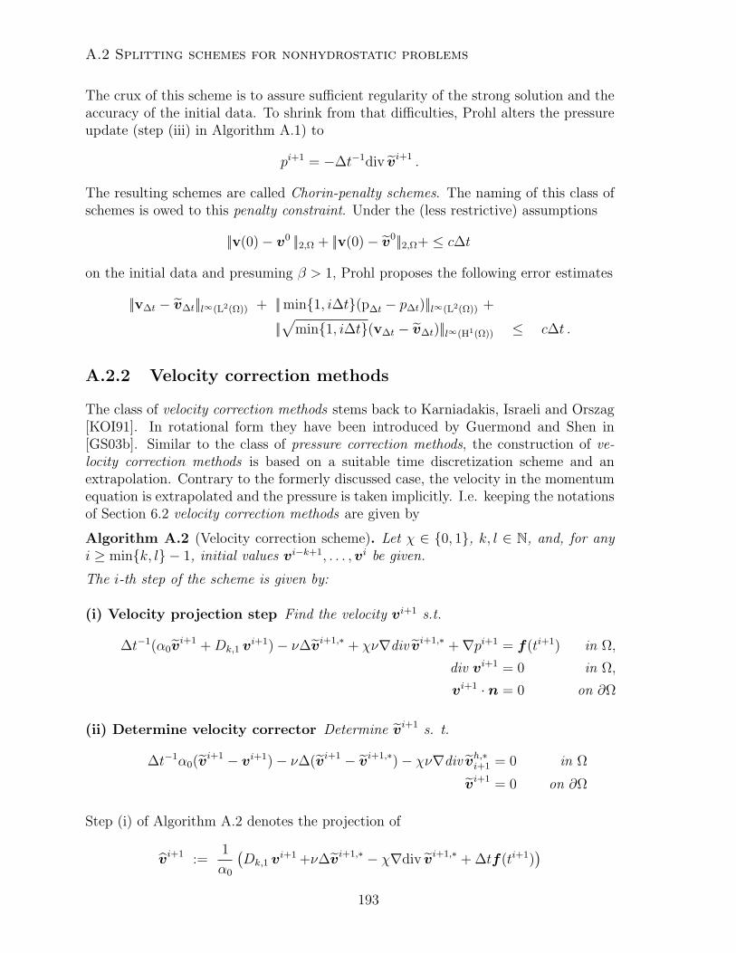
A.2 Splitting schemes for nonhydrostatic problems
The crux of this scheme is to assure sufficient regularity of the strong solution and theaccuracy of the initial data. To shrink from that difficulties, Prohl alters the pressureupdate (step (iii) in Algorithm A.1) to
pi+1 = −∆t−1div vi+1 .
The resulting schemes are called Chorin-penalty schemes. The naming of this class ofschemes is owed to this penalty constraint. Under the (less restrictive) assumptions
||v(0)− v0 ||2,Ω + ||v(0)− v0||2,Ω+ ≤ c∆t
on the initial data and presuming β > 1, Prohl proposes the following error estimates
||v∆t − v∆t||l∞(L2(Ω)) + ||min1, i∆t(p∆t − p∆t)||l∞(L2(Ω)) +
||√
min1, i∆t(v∆t − v∆t)||l∞(H1(Ω)) ≤ c∆t .
A.2.2 Velocity correction methods
The class of velocity correction methods stems back to Karniadakis, Israeli and Orszag[KOI91]. In rotational form they have been introduced by Guermond and Shen in[GS03b]. Similar to the class of pressure correction methods, the construction of ve-locity correction methods is based on a suitable time discretization scheme and anextrapolation. Contrary to the formerly discussed case, the velocity in the momentumequation is extrapolated and the pressure is taken implicitly. I.e. keeping the notationsof Section 6.2 velocity correction methods are given by
Algorithm A.2 (Velocity correction scheme). Let χ ∈ 0, 1, k, l ∈ N, and, for anyi ≥ mink, l − 1, initial values vi−k+1, . . . ,vi be given.
The i-th step of the scheme is given by:
(i) Velocity projection step Find the velocity vi+1 s.t.
∆t−1(α0vi+1 +Dk,1 v
i+1)− ν∆vi+1,∗ + χν∇div vi+1,∗ +∇pi+1 = f(ti+1) in Ω,
div vi+1 = 0 in Ω,
vi+1 · n = 0 on ∂Ω
(ii) Determine velocity corrector Determine vi+1 s. t.
∆t−1α0(vi+1 − vi+1)− ν∆(vi+1 − vi+1,∗)− χν∇div vh,∗i+1 = 0 in Ω
vi+1 = 0 on ∂Ω
Step (i) of Algorithm A.2 denotes the projection of
vi+1 :=1
α0
(Dk,1 v
i+1 +ν∆vi+1,∗ − χ∇div vi+1,∗ + ∆tf(ti+1))
193
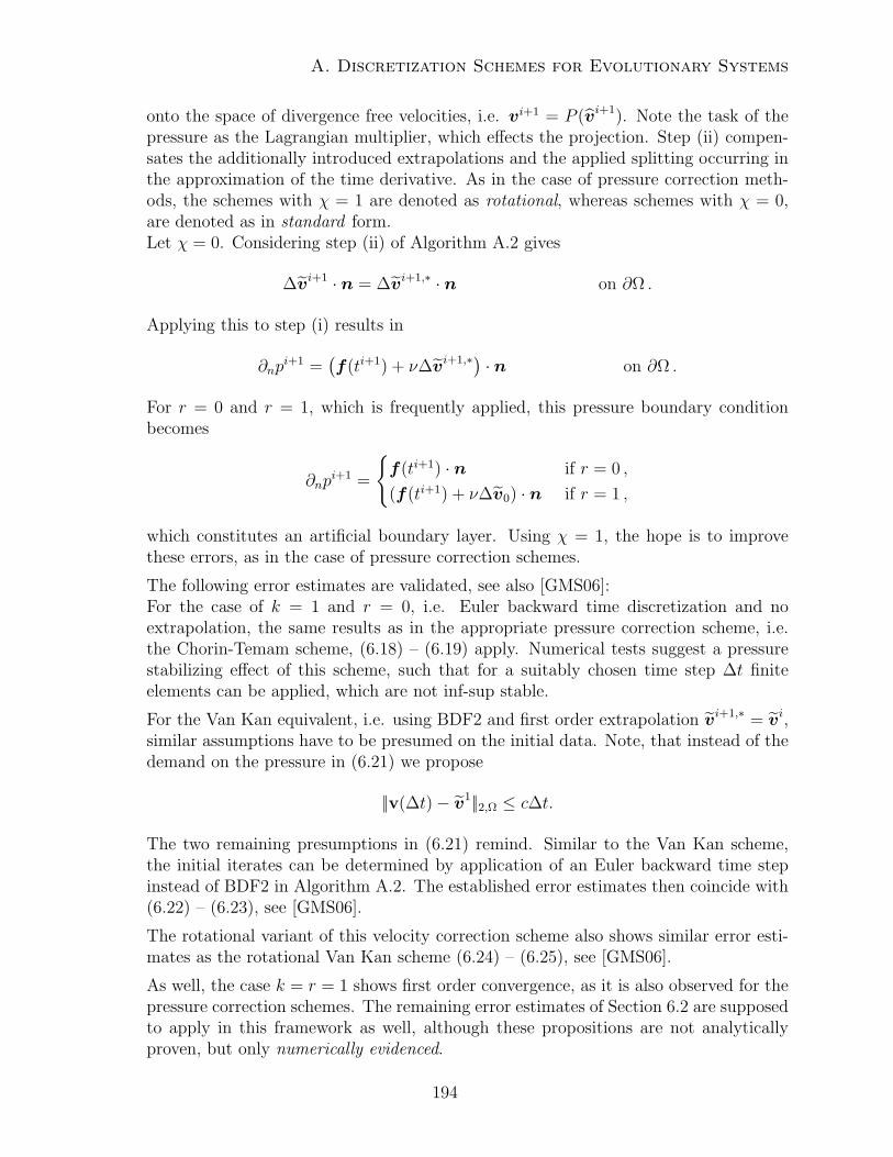
A. Discretization Schemes for Evolutionary Systems
onto the space of divergence free velocities, i.e. vi+1 = P (vi+1). Note the task of thepressure as the Lagrangian multiplier, which effects the projection. Step (ii) compen-sates the additionally introduced extrapolations and the applied splitting occurring inthe approximation of the time derivative. As in the case of pressure correction meth-ods, the schemes with χ = 1 are denoted as rotational, whereas schemes with χ = 0,are denoted as in standard form.Let χ = 0. Considering step (ii) of Algorithm A.2 gives
∆vi+1 · n = ∆vi+1,∗ · n on ∂Ω .
Applying this to step (i) results in
∂npi+1 =
(f(ti+1) + ν∆vi+1,∗) · n on ∂Ω .
For r = 0 and r = 1, which is frequently applied, this pressure boundary conditionbecomes
∂npi+1 =
f(ti+1) · n if r = 0 ,
(f(ti+1) + ν∆v0) · n if r = 1 ,
which constitutes an artificial boundary layer. Using χ = 1, the hope is to improvethese errors, as in the case of pressure correction schemes.
The following error estimates are validated, see also [GMS06]:For the case of k = 1 and r = 0, i.e. Euler backward time discretization and noextrapolation, the same results as in the appropriate pressure correction scheme, i.e.the Chorin-Temam scheme, (6.18) – (6.19) apply. Numerical tests suggest a pressurestabilizing effect of this scheme, such that for a suitably chosen time step ∆t finiteelements can be applied, which are not inf-sup stable.
For the Van Kan equivalent, i.e. using BDF2 and first order extrapolation vi+1,∗ = vi,similar assumptions have to be presumed on the initial data. Note, that instead of thedemand on the pressure in (6.21) we propose
||v(∆t)− v1||2,Ω ≤ c∆t.
The two remaining presumptions in (6.21) remind. Similar to the Van Kan scheme,the initial iterates can be determined by application of an Euler backward time stepinstead of BDF2 in Algorithm A.2. The established error estimates then coincide with(6.22) – (6.23), see [GMS06].
The rotational variant of this velocity correction scheme also shows similar error esti-mates as the rotational Van Kan scheme (6.24) – (6.25), see [GMS06].
As well, the case k = r = 1 shows first order convergence, as it is also observed for thepressure correction schemes. The remaining error estimates of Section 6.2 are supposedto apply in this framework as well, although these propositions are not analyticallyproven, but only numerically evidenced.
194
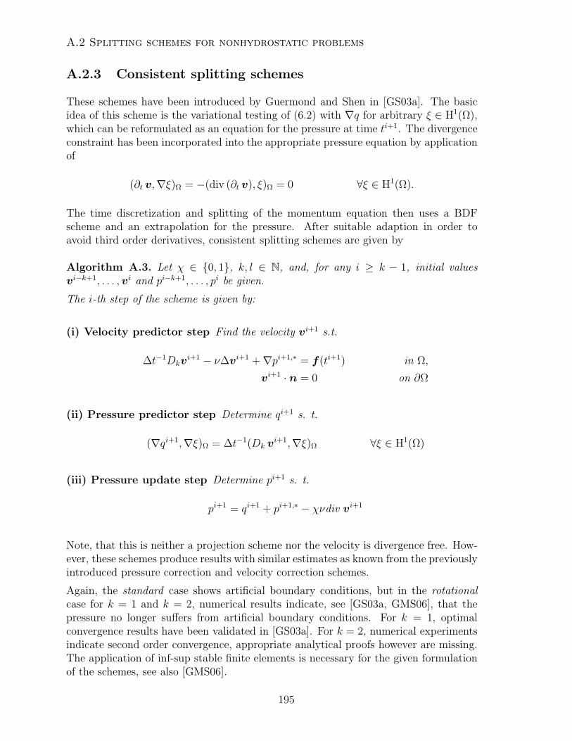
A.2 Splitting schemes for nonhydrostatic problems
A.2.3 Consistent splitting schemes
These schemes have been introduced by Guermond and Shen in [GS03a]. The basicidea of this scheme is the variational testing of (6.2) with ∇q for arbitrary ξ ∈ H1(Ω),which can be reformulated as an equation for the pressure at time ti+1. The divergenceconstraint has been incorporated into the appropriate pressure equation by applicationof
(∂t v,∇ξ)Ω = −(div (∂t v), ξ)Ω = 0 ∀ξ ∈ H1(Ω).
The time discretization and splitting of the momentum equation then uses a BDFscheme and an extrapolation for the pressure. After suitable adaption in order toavoid third order derivatives, consistent splitting schemes are given by
Algorithm A.3. Let χ ∈ 0, 1, k, l ∈ N, and, for any i ≥ k − 1, initial valuesvi−k+1, . . . ,vi and pi−k+1, . . . , pi be given.
The i-th step of the scheme is given by:
(i) Velocity predictor step Find the velocity vi+1 s.t.
∆t−1Dkvi+1 − ν∆vi+1 +∇pi+1,∗ = f(ti+1) in Ω,
vi+1 · n = 0 on ∂Ω
(ii) Pressure predictor step Determine qi+1 s. t.
(∇qi+1,∇ξ)Ω = ∆t−1(Dk vi+1,∇ξ)Ω ∀ξ ∈ H1(Ω)
(iii) Pressure update step Determine pi+1 s. t.
pi+1 = qi+1 + pi+1,∗ − χνdiv vi+1
Note, that this is neither a projection scheme nor the velocity is divergence free. How-ever, these schemes produce results with similar estimates as known from the previouslyintroduced pressure correction and velocity correction schemes.
Again, the standard case shows artificial boundary conditions, but in the rotationalcase for k = 1 and k = 2, numerical results indicate, see [GS03a, GMS06], that thepressure no longer suffers from artificial boundary conditions. For k = 1, optimalconvergence results have been validated in [GS03a]. For k = 2, numerical experimentsindicate second order convergence, appropriate analytical proofs however are missing.The application of inf-sup stable finite elements is necessary for the given formulationof the schemes, see also [GMS06].
195
A. Discretization Schemes for Evolutionary Systems
A.2.4 Stability aspects
As indicated in Section 6.2 for the Chorin-Temam scheme, some of the introducedschemes (for certain time steps ∆t) allow the application of finite element spaces, whichare not inf-sup stable. However it is stated in [GMS06], that this is not the rule. Onthe contrary, the authors suggest that, generally, the inf-sup condition is necessary andsufficient for the well-posedness of the fully discretized problem. Thus, either inf-supstable finite elements are to be chosen, or an appropriate stabilization has to be incorpo-rated into the splitting scheme. In [BC08] Badia and Codina collected known stabilityresults for the unstabilized problems, and introduced and analyzed the application ofsplitting schemes to stabilized finite element approximations of nonhydrostatic flowproblems, i.e. the fully discretized problem is analyzed. Due to applicability for hydro-static problems we restrict our attention to the results concerning pressure correctionschemes, given in [BC08]. For further informations we refer to the cited literature.
Beforehand, we introduce some notations, see also [BC08]. Let d ∈ N denote thedimension of the problem. Considering the finite element spaces Vh and Qh based onpolynomials of order rv and rq, respectively, let
φi,ji∈Nv ,j∈1,...,d ⊕ φi,ji∈Nd,j∈1,...,d and ξii∈Np
be Lagrangian bases of Vh and Qh, respectively. The set Nd denotes the fixed nodalvelocity values due to the boundary conditions. The remaining nodes of the velocityspace are given by Nv, the nodes of the pressure space are represented by Np. Basedon the evolutionary 3D Navier-Stokes problem
Find (v, p) s. t. ∂t v+(v ·∇)v−ν∆v+∇p = f in Ω× [0, T ]div v = 0 in Ω× [0, T ]v |∂Ω = 0 in [0, T ]v |t=0 = v0 in Ω ,
(A.8)
let (vn+1h , pn+1
h ) be the solution of the discretized problem at time (n + 1)∆t. Thesolution is determined using one of the introduced splitting schemes with an appropriatetime discretization scheme, and applying the introduced finite element spaces for thespatial discretization. Thus, vi+1
h and pi+1h can be represented by
vn+1h (x) =
∑i∈Nv
(Un+1)iφi(x) +∑i∈Nd
(Un+1d )iφi(x) ∀x ∈ Ω
pn+1h (x) =
∑i∈Nq
(Pn+1)iξi(x) ∀x ∈ Ω
with vectors Un+1 and Pn+1 containing the nodal values of vn+1h and pn+1
h . VectorUn+1d contains the fixed data of the velocity.
Recall the definitions (3.1), (3.2) and (3.8) of the forms a, b and c, and set f = 0.
196
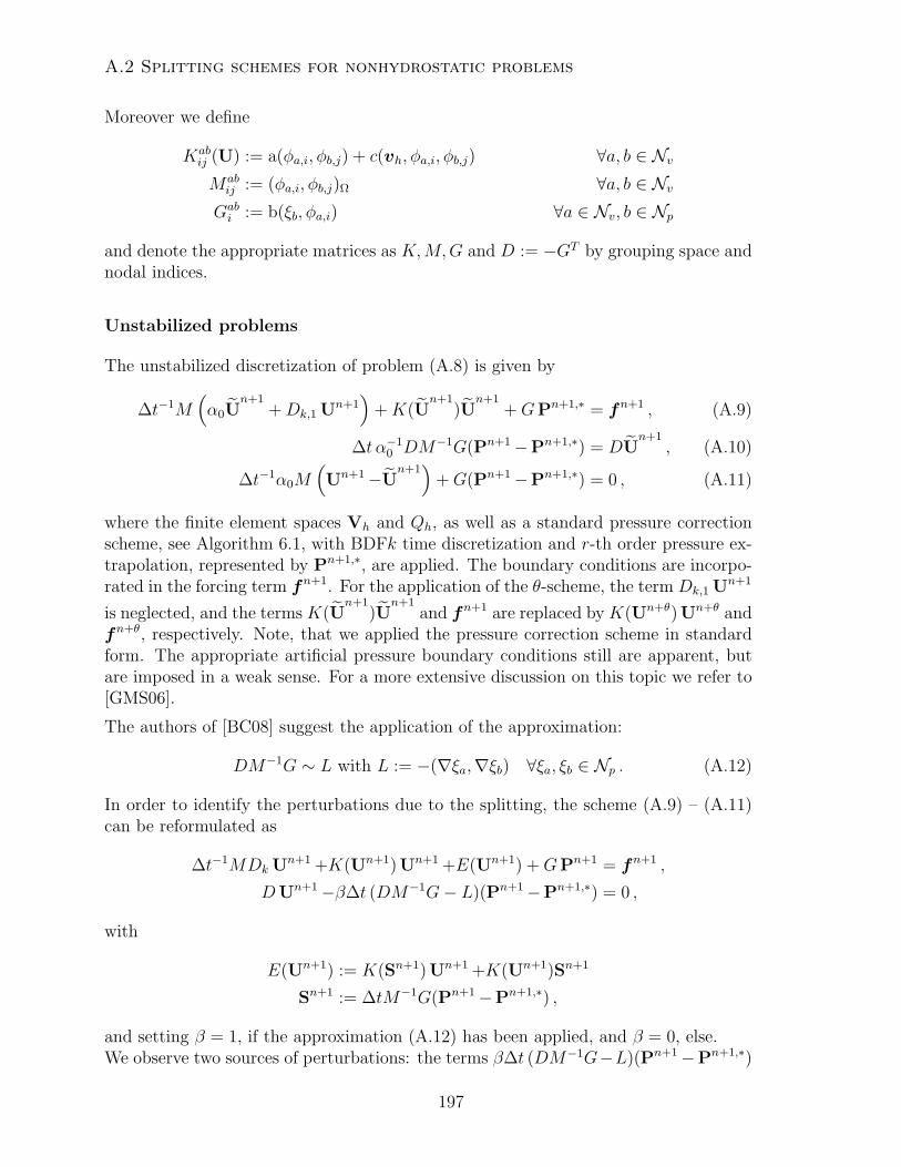
A.2 Splitting schemes for nonhydrostatic problems
Moreover we define
Kabij (U) := a(φa,i, φb,j) + c(vh, φa,i, φb,j) ∀a, b ∈ NvMab
ij := (φa,i, φb,j)Ω ∀a, b ∈ NvGabi := b(ξb, φa,i) ∀a ∈ Nv, b ∈ Np
and denote the appropriate matrices as K,M,G and D := −GT by grouping space andnodal indices.
Unstabilized problems
The unstabilized discretization of problem (A.8) is given by
∆t−1M(α0U
n+1+Dk,1 Un+1
)+K(U
n+1)U
n+1+GPn+1,∗ = fn+1 , (A.9)
∆t α−10 DM−1G(Pn+1−Pn+1,∗) = DU
n+1, (A.10)
∆t−1α0M(Un+1−U
n+1)
+G(Pn+1−Pn+1,∗) = 0 , (A.11)
where the finite element spaces Vh and Qh, as well as a standard pressure correctionscheme, see Algorithm 6.1, with BDFk time discretization and r-th order pressure ex-trapolation, represented by Pn+1,∗, are applied. The boundary conditions are incorpo-rated in the forcing term fn+1. For the application of the θ-scheme, the term Dk,1 Un+1
is neglected, and the terms K(Un+1
)Un+1
and fn+1 are replaced by K(Un+θ) Un+θ andfn+θ, respectively. Note, that we applied the pressure correction scheme in standardform. The appropriate artificial pressure boundary conditions still are apparent, butare imposed in a weak sense. For a more extensive discussion on this topic we refer to[GMS06].
The authors of [BC08] suggest the application of the approximation:
DM−1G ∼ L with L := −(∇ξa,∇ξb) ∀ξa, ξb ∈ Np . (A.12)
In order to identify the perturbations due to the splitting, the scheme (A.9) – (A.11)can be reformulated as
∆t−1MDk Un+1 +K(Un+1) Un+1 +E(Un+1) +GPn+1 = fn+1 ,
DUn+1−β∆t (DM−1G− L)(Pn+1−Pn+1,∗) = 0 ,
with
E(Un+1) := K(Sn+1) Un+1 +K(Un+1)Sn+1
Sn+1 := ∆tM−1G(Pn+1−Pn+1,∗) ,
and setting β = 1, if the approximation (A.12) has been applied, and β = 0, else.We observe two sources of perturbations: the terms β∆t (DM−1G−L)(Pn+1−Pn+1,∗)
197
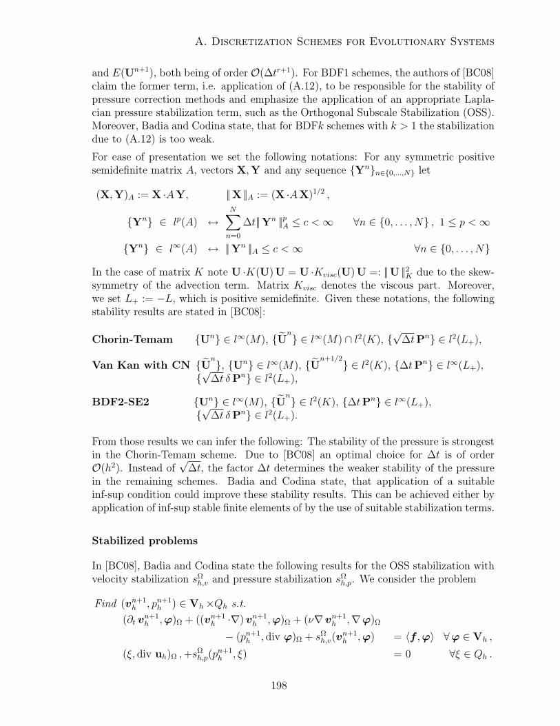
A. Discretization Schemes for Evolutionary Systems
and E(Un+1), both being of order O(∆tr+1). For BDF1 schemes, the authors of [BC08]claim the former term, i.e. application of (A.12), to be responsible for the stability ofpressure correction methods and emphasize the application of an appropriate Lapla-cian pressure stabilization term, such as the Orthogonal Subscale Stabilization (OSS).Moreover, Badia and Codina state, that for BDFk schemes with k > 1 the stabilizationdue to (A.12) is too weak.
For ease of presentation we set the following notations: For any symmetric positivesemidefinite matrix A, vectors X,Y and any sequence Ynn∈0,...,N let
(X,Y)A := X ·AY, ||X ||A := (X ·AX)1/2 ,
Yn ∈ lp(A) ↔N∑n=0
∆t||Yn ||pA ≤ c <∞ ∀n ∈ 0, . . . , N , 1 ≤ p <∞
Yn ∈ l∞(A) ↔ ||Yn ||A ≤ c <∞ ∀n ∈ 0, . . . , NIn the case of matrix K note U ·K(U) U = U ·Kvisc(U) U =: ||U ||2K due to the skew-symmetry of the advection term. Matrix Kvisc denotes the viscous part. Moreover,we set L+ := −L, which is positive semidefinite. Given these notations, the followingstability results are stated in [BC08]:
Chorin-Temam Un ∈ l∞(M), Un ∈ l∞(M) ∩ l2(K), √∆tPn ∈ l2(L+),
Van Kan with CN Un, Un ∈ l∞(M), Un+1/2 ∈ l2(K), ∆tPn ∈ l∞(L+),√∆t δPn ∈ l2(L+),
BDF2-SE2 Un ∈ l∞(M), Un ∈ l2(K), ∆tPn ∈ l∞(L+),√∆t δPn ∈ l2(L+).
From those results we can infer the following: The stability of the pressure is strongestin the Chorin-Temam scheme. Due to [BC08] an optimal choice for ∆t is of orderO(h2). Instead of
√∆t, the factor ∆t determines the weaker stability of the pressure
in the remaining schemes. Badia and Codina state, that application of a suitableinf-sup condition could improve these stability results. This can be achieved either byapplication of inf-sup stable finite elements of by the use of suitable stabilization terms.
Stabilized problems
In [BC08], Badia and Codina state the following results for the OSS stabilization withvelocity stabilization sΩ
h,v and pressure stabilization sΩh,p. We consider the problem
Find (vn+1h , pn+1
h ) ∈ Vh×Qh s.t.
(∂t vn+1h ,ϕ)Ω + ((vn+1
h ·∇)vn+1h ,ϕ)Ω + (ν∇vn+1
h ,∇ϕ)Ω
− (pn+1h , div ϕ)Ω + sΩ
h,v(vn+1h ,ϕ) = 〈f ,ϕ〉 ∀ϕ ∈ Vh ,
(ξ, div uh)Ω ,+sΩh,p(p
n+1h , ξ) = 0 ∀ξ ∈ Qh .
198
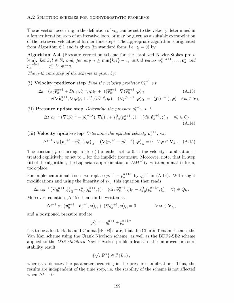
A.2 Splitting schemes for nonhydrostatic problems
The advection occurring in the definition of sh,v can be set to the velocity determined ina former iteration step of an iterative loop, or may be given as a suitable extrapolationof the retrieved velocities of former time steps. The appropriate algorithm is originatedfrom Algorithm 6.1 and is given (in standard form, i.e. χ = 0) by
Algorithm A.4 (Pressure correction scheme for the stabilized Navier-Stokes prob-lem). Let k, l ∈ N, and, for any n ≥ mink, l − 1, initial values vn−k+1
h , . . . ,vnh andpn−l+1h , . . . , pnh be given.
The n-th time step of the scheme is given by:
(i) Velocity predictor step Find the velocity predictor vn+1h s.t.
∆t−1(α0vn+1h +Dk,1 v
n+1h ,ϕ)Ω + ((vn+1
h · ∇)vn+1h ,ϕ)Ω (A.13)
+ν(∇vn+1h ,∇ϕ)Ω + sΩ
h,v(vn+ρh ,ϕ) + (∇pn+1,∗
h ,ϕ)Ω = 〈f(tn+1),ϕ〉 ∀ϕ ∈ Vh
(ii) Pressure update step Determine the pressure pn+1h , s. t.
∆t α0−1(∇(pn+1
h − pn+1,∗h ),∇ξ)
Ω+ sΩ
h,p(pn+1h , ξ) = (div vn+1
h , ξ)Ω ∀ξ ∈ Qh
(A.14)
(iii) Velocity update step Determine the updated velocity vn+1h , s.t.
∆t−1 α0
(vn+1h −vn+1
h ,ϕ)
Ω+(∇(pn+1
h − pn+1,∗h ),ϕ
)Ω
= 0 ∀ϕ ∈ Vh . (A.15)
The constant ρ occurring in step (i) is either set to 0, if the velocity stabilization istreated explicitely, or set to 1 for the implicit treatment. Moreover, note, that in step(ii) of the algorithm, the Laplacian approximation of DM−1G, written in matrix form,took place.
For implementational issues we replace pn+1h − pn+1,∗
h by qn+1h in (A.14). With slight
modifications and using the linearity of sh,p this equation then reads
∆t α0−1(∇qn+1
h , ξ)
Ω+ sΩ
h,p(qn+1h , ξ) = (div vn+1
h , ξ)Ω − sΩh,p(p
n+1,∗h , ξ) ∀ξ ∈ Qh .
Moreover, equation (A.15) then can be written as
∆t−1 α0
(vn+1h −vn+1
h ,ϕ)
Ω+(∇qn+1
h ,ϕ)
Ω= 0 ∀ϕ ∈ Vh ,
and a postponed pressure update,
pn+1h = qn+1
h + pn+1,∗h
has to be added. Badia and Codina [BC08] state, that the Chorin-Temam scheme, theVan Kan scheme using the Crank Nicolson scheme, as well as the BDF2-SE2 schemeapplied to the OSS stabilized Navier-Stokes problem leads to the improved pressurestability result
√τ Pn ∈ l1(L+) ,
whereas τ denotes the parameter occurring in the pressure stabilization. Thus, theresults are independent of the time step, i.e. the stability of the scheme is not affectedwhen ∆t→ 0.
199

A. Discretization Schemes for Evolutionary Systems
200
Appendix B
Algorithmic Principles
The field of discrete mathematics shows a large variety of methods to algorithmicallytreat flow problems, such as Newton iteration, direct methods, linear iterative schemes,Krylov subspace methods, multigrid methods, or the idea of preconditioning, whichaims to increase the performance of the iteration by solving an equivalent problemwith improved matrix properties.
For large systems, direct methods and linear iterative schemes are far too expensive.However, they are often used as a preconditioner in iterative methods or as smoothingoperators in multigrid schemes in an incomplete form, and find application as solversfor small subproblems.With the Krylov subspace methods a class of efficient methods is given, which assuresthe determination of the exact solution of a linear problem after maximal n iterationsteps for underlying (nonsingular) matrices of dimension n× n.The computational costs of each of the previously mentioned schemes depend on thecondition number of the underlying matrix. Due to the computational costs of solvingone iterative and due to the amount of sufficient iterations, these procedures are im-practicable for large linear systems. Multigrid schemes are efficient schemes, which areindependent on the condition number, and still have a simple structure.A large variety of scales inheres ocean circulation. A major difficulty is the strongstiffness. Without implicit and very robust solution methods it is a difficult task tosolve such systems at all. To sufficiently reduce the complexity of the problems differenttechniques can be combined: adaptive local mesh refinement [BR01] to resolve reactionfronts and singularities, special storage techniques [BT06b], implicit methods to allowfor large time steps, splitting and approximation of equations [Pro97] for a reductionof the dimension. Still, the remaining systems may be so large that parallelization isnecessary.
Following these considerations the chapter is structured as follows: We start withan introduction of essential notations and short derivation of a suitable linear system,which can be treated by appropriate schemes for linear problems, such as linear iterativemethods or Krylov subspace methods. Moreover, we have a glimpse on the treatmentof problems showing a saddle point structure. We then present an overview oversimple algorithms, such as direct and linear iterative schemes, to solve linear systems.
201
B. Algorithmic Principles
Due to the dimensions of the underlying problems, they are not used as solvers forthese problems on their own, but serve as preconditioners, smoothers or as solver forsuitably small subproblems. The following section, Section B.3, introduces the field ofpreconditioning and presents a few preconditioners. For a closer look into that topicthe reader is referred to [BBC+94, Hac93]. Section B.4 considers the class of Krylovsubspace methods, which assure convergence of the iteration after a fixed, but (for ourapplications) commonly large amount of iterations. Similar to the formerly introducedmethods, they are solely applied for subproblems occurring in the multigrid frameworkwhen direct and linear iterative methods are not applicable. The topic of multigridmethods is already treated in Appendix C. We skip an additional treatment here.
The topics can be found in textbooks such as [Mei11, Hac93, BBC+94, Saa03].
B.1 Preliminaries
In this section we present basic notations used in this chapter. Moreover, we accountfor the special structure of the present problems, i.e. the saddle point structure, whichallows us to draw on algorithms for linear algebraic problems and split the given prob-lem in order to reduce the computational costs. Each of the reducing subproblems canbe solved with the methods introduced in the upcoming sections.
B.1.1 Basic notations
We relax the definition of the underlying domain, see Section 3.1.1, and consider opendomains Ω ⊂ R3. In particular we do not consider the 2D case here. Let u ∈ V be thesolution of a system of partial differential equations (not necessarily a flow problem)given in the weak formulation on Ω:
u ∈ V : a(u)(φ) = 0 ∀φ ∈ V, (B.1)
where a(·)(·) is a semi-linear form, linear in the second argument. Let a(·)(·) describea system of Nc equations and u : Ω → RNc have Nc solution components. E.g., for3D (nonhydrostatic) Navier-Stokes flows we have Nc = 4 with three velocity and onepressure component.
Recall the notions of Section 4.1.1 on triangulations and finite element spaces. I.e.note, that a triangulation Th of the domain Ω is assumed to be regular, and that weapply the concept of hanging nodes in order to allow for locally refined meshes. Nodes,faces and edges of Th are denoted as x, f and e, respectively.The argumentations in this chapter are not only valid for finite element spaces, whichare based on linear transformations BT : T → T of type (4.3), but also apply for
arbitrary affine mappings from the reference element T to the computational elementT . We denote the appropriate conforming finite element space as Vh ⊂ V. Let
Ψh := φih, i = 1, . . . ,Nh,
202
B.1 Preliminaries
be the common Lagrange basis system of Vh with φi(xj) = δij, where xj are the Nhdegrees of freedom. With Nh we identify the size of the problem to be solved.
To approximate the partial differential equation in this discrete space Vh we associatethe finite element function uh ∈ [Vh]
Nc with a coefficient vector uh ∈ RNh×Nc given by
(uh)j = uh(xj) ∈ RNc , uh =
Nh∑j=1
(uh)jφjh(x). (B.2)
We solve the partial differential equation (B.1) with a Newton method yielding iteratesuth by:
a′(uth)(ut+1h − uth, φh) = −a(uth)(φh) ∀φh ∈ [Vh]
Nc ,
where a′(uh)(wh, φh) is the directional derivative of the form a(·)(·) in direction of theupdate wh evaluated in the last approximation uh. The discrete solution of the partialdifferential is then characterized by the solution of the linear equations
Ahuh = bh,
where the system matrix Ah and the load vector bh are given by:
(Ah)ij = a′(uth)(φjh, φ
ih), i, j = 1, . . . ,Nh,
(bh)j = −a(uth)(φjh), j = 1, . . . ,Nh.
Remark B.1. We store the matrix and the vectors in a block-wise sense: every entryof the matrix (Ah)ij ∈ RNc×Nc is a matrix itself, gathering all couplings between the Ncequation components and every entry of the vectors (bh)i ∈ RNc is a vector. Thus, allalgebraic algorithms can be presented independent of the number of solution componentsNc.Anticipating, the block-wise storage technique clusters local dependencies of the differentsolution components and is crucial to obtain an efficient parallel method.
B.1.2 Saddle point problems
The following considerations are based on [Car86, LQ86, Bra07]. As already discussedin Chapter 3, hydrostatic flow problems show a saddle point structure, which, in steadystate, is also apparent in their appropriate (conforming) finite element discretization,see also Chapter 4. This can be explored in order to reduce computational costs by asuitable splitting of the fully discrete problem. The commonly applied Uzawa algorithmoriginates from the framework of linear algebraic problems and finds its appropriatealgorithmical realization due to the properties of the underlying problem matrix.As examined in Chapter 6, evolutionary flow problems are also numerically tackled withsplitting schemes. These schemes may also show the structure of an Uzawa algorithm,which moved some authors to suitably name the appropriate splitting schemes.
We consider the linear algebraic system
Mx :=
(A BT
B D
)(vp
)=
(fg
)(B.3)
203
B. Algorithmic Principles
with nonsingular matrix A ∈ Rm×m, matrix D ∈ Rn×n and matrix B ∈ Rm×n. Apply-ing blockwise Gauss elimination leads to
(BA−1BT −D)p = BA−1f − g , (B.4)
v = A−1f − A−1BTp (B.5)
with Schur complement S := BA−1BT − D. [Oue81, Car86] provide the followingregularity statements:
(i) Let ρ(M) be the rank of M . ρ(M) = ρ(A) + ρ(S). I.e. if M is nonsingular, so isS.
(ii) Let M be symmetric and A be nonsingular and positive definite.
(ii-a) M is positive definite if and only if S is positive definite,
(ii-b) M is positive semidefinite if and only if S is positive semidefinite.
(iii) If M is nonsingular and Hermitean, then S is nonsingular and Hermitean.
Thus, the nonsingularity property of the entire matrix M carries over to its Schurcomplement S. If problem (B.3) has a uniqie solution, the same applies for (B.4) –(B.5). In particular, some properties of the underlying entire problem inherit to thereduced problem (B.4) – (B.5).
The basic idea of an Uzawa algorithm is to solve equation (B.4) for p iteratively andcontemporeaneously update v due to (B.5), at best in an efficient way.Dependent on the properties of S, different schemes offer, such as the motivativeRichardson iteration or the (faster) BiConjugate Gradient scheme for nonsymmetricproblems, or the Conjugate Gradient Scheme for symmetric matrices.
B.2 Direct and linear iterative methods
In this section we present an overview over simple algorithms for linear systems, start-ing with the class of direct methods. These methods assure, that at the end of the(expensive) procedure, the solution x of the linear system Ax = b is known (up to errorsdue to machine inaccuracy). Due to their high costs this approach is not manageablefor large systems, but can be used to handle subproblems of suitable size. Henceforthwe introduce the still expensive linear iterative methods . Schemes of these classes canbe used - in an inexact manner - in the construction of preconditioners. We treat thisissue in Section B.3. Throughout this section we consider the linear problem
Ax = b (B.6)
with nonsingular matrix A ∈ Rn×n.
204
B.2 Direct and linear iterative methods
B.2.1 Direct methods
The simplest approach to determine the solution x of the linear problem (B.6) is theapplication of a suitable factorization of matrix A, i.e. A = A1A2, such that theresulting subproblem are to be solved easily.
LU factorization
The procedure of LU factorization decomposes matrix A into an upper triangularmatrix L and a lower triangular matrix U . Conveniently, in order to assure existenceof such a decomposition, partial pivoting is applied. Based on the Gaussian algorithm,the factorization with partial pivoting can be described with suitable permutationmatrices Pk, concentrated in the matrix P , and Gaussian transformations, given byFrobenius matrices Lk. The LU scheme with partial pivoting is as follows:
1. Determine PA = LU .
2. Solve Lz = Pb.
3. Solve Ux = z.
In order to solve the linear problem with this approach, O(n3) floating point operations(flops) are necessary, i.e. this approach is quite expensive. The approach for symmet-ric, positive-definite matrices, i.e. the Cholesky scheme, does not lead to a considerableimprovement, even if a more economical storage is possible exploiting symmetry. How-ever, the effort of the LU decomposition (step 1) and solving the forward and backwardsubstitution (steps 2 and 3) for tridiagonal matrices A becomes linear.
QR factorization
The QR decomposition of matrix A consists of a unitary matrix Q and an uppertriangular matrix R, which has the same norm and condition number as A. As thecolumns of Q denote an orthonormal basis of Rn, it is suggestible to apply knownorthogonalization strategies for the construction of the factorization A = QR, suchas the Gram-Schmidt scheme, the Givens scheme or the Householder scheme. Due tothe numerical instability of the Gram-Schmidt method, it is customary to apply eitherthe Givens, the Householder scheme, or a modified Gram-Schmidt scheme. UsingQ∗ = Q−1, the QR factorization for solving the problem (B.6) is given by
1. Determine A = QR.
2. Solve Rx = Q∗b.
The algorithmic complexity is as large as in the LU factorization, O(n3).
205
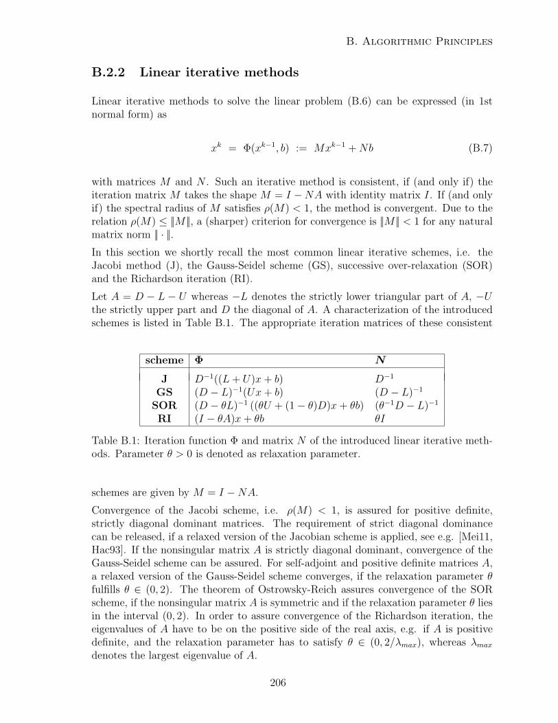
B. Algorithmic Principles
B.2.2 Linear iterative methods
Linear iterative methods to solve the linear problem (B.6) can be expressed (in 1stnormal form) as
xk = Φ(xk−1, b) := Mxk−1 +Nb (B.7)
with matrices M and N . Such an iterative method is consistent, if (and only if) theiteration matrix M takes the shape M = I −NA with identity matrix I. If (and onlyif) the spectral radius of M satisfies ρ(M) < 1, the method is convergent. Due to therelation ρ(M) ≤ ||M ||, a (sharper) criterion for convergence is ||M || < 1 for any naturalmatrix norm || · ||.In this section we shortly recall the most common linear iterative schemes, i.e. theJacobi method (J), the Gauss-Seidel scheme (GS), successive over-relaxation (SOR)and the Richardson iteration (RI).
Let A = D − L − U whereas −L denotes the strictly lower triangular part of A, −Uthe strictly upper part and D the diagonal of A. A characterization of the introducedschemes is listed in Table B.1. The appropriate iteration matrices of these consistent
scheme Φ N
J D−1((L+ U)x+ b) D−1
GS (D − L)−1(Ux+ b) (D − L)−1
SOR (D − θL)−1 ((θU + (1− θ)D)x+ θb) (θ−1D − L)−1
RI (I − θA)x+ θb θI
Table B.1: Iteration function Φ and matrix N of the introduced linear iterative meth-ods. Parameter θ > 0 is denoted as relaxation parameter.
schemes are given by M = I −NA.
Convergence of the Jacobi scheme, i.e. ρ(M) < 1, is assured for positive definite,strictly diagonal dominant matrices. The requirement of strict diagonal dominancecan be released, if a relaxed version of the Jacobian scheme is applied, see e.g. [Mei11,Hac93]. If the nonsingular matrix A is strictly diagonal dominant, convergence of theGauss-Seidel scheme can be assured. For self-adjoint and positive definite matrices A,a relaxed version of the Gauss-Seidel scheme converges, if the relaxation parameter θfulfills θ ∈ (0, 2). The theorem of Ostrowsky-Reich assures convergence of the SORscheme, if the nonsingular matrix A is symmetric and if the relaxation parameter θ liesin the interval (0, 2). In order to assure convergence of the Richardson iteration, theeigenvalues of A have to be on the positive side of the real axis, e.g. if A is positivedefinite, and the relaxation parameter has to satisfy θ ∈ (0, 2/λmax), whereas λmaxdenotes the largest eigenvalue of A.
206
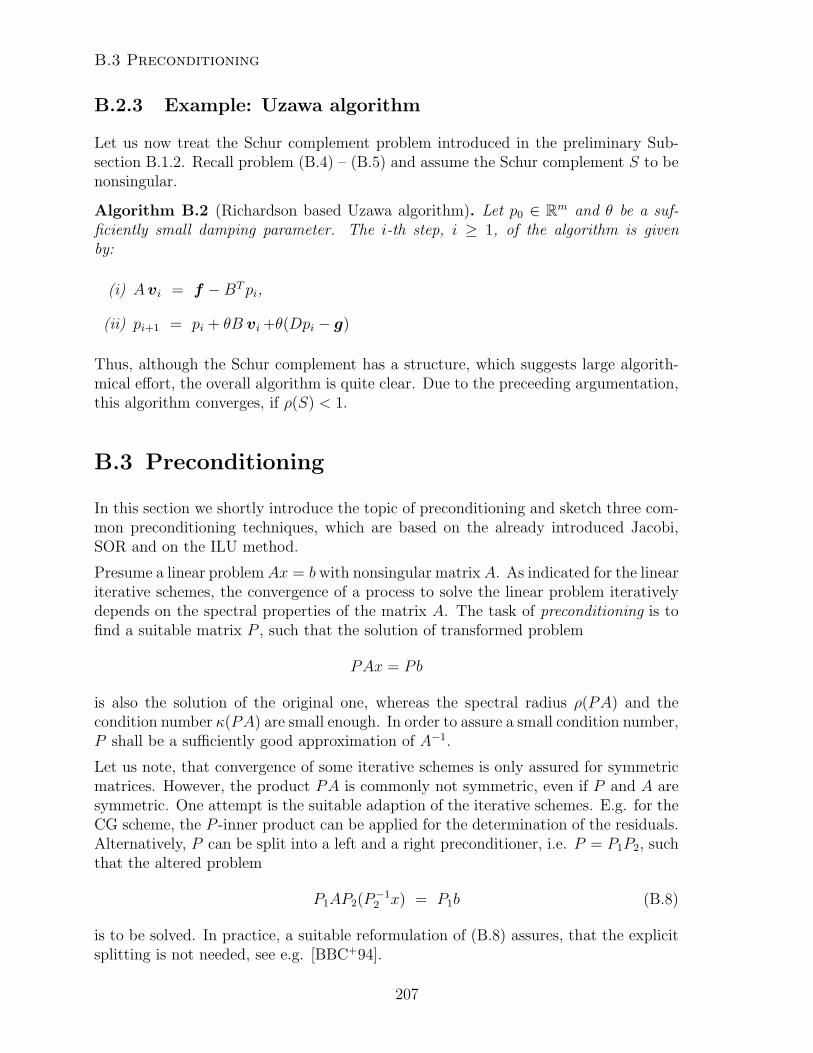
B.3 Preconditioning
B.2.3 Example: Uzawa algorithm
Let us now treat the Schur complement problem introduced in the preliminary Sub-section B.1.2. Recall problem (B.4) – (B.5) and assume the Schur complement S to benonsingular.
Algorithm B.2 (Richardson based Uzawa algorithm). Let p0 ∈ Rm and θ be a suf-ficiently small damping parameter. The i-th step, i ≥ 1, of the algorithm is givenby:
(i) Avi = f −BTpi,
(ii) pi+1 = pi + θB vi +θ(Dpi − g)
Thus, although the Schur complement has a structure, which suggests large algorith-mical effort, the overall algorithm is quite clear. Due to the preceeding argumentation,this algorithm converges, if ρ(S) < 1.
B.3 Preconditioning
In this section we shortly introduce the topic of preconditioning and sketch three com-mon preconditioning techniques, which are based on the already introduced Jacobi,SOR and on the ILU method.
Presume a linear problemAx = b with nonsingular matrixA. As indicated for the lineariterative schemes, the convergence of a process to solve the linear problem iterativelydepends on the spectral properties of the matrix A. The task of preconditioning is tofind a suitable matrix P , such that the solution of transformed problem
PAx = Pb
is also the solution of the original one, whereas the spectral radius ρ(PA) and thecondition number κ(PA) are small enough. In order to assure a small condition number,P shall be a sufficiently good approximation of A−1.
Let us note, that convergence of some iterative schemes is only assured for symmetricmatrices. However, the product PA is commonly not symmetric, even if P and A aresymmetric. One attempt is the suitable adaption of the iterative schemes. E.g. for theCG scheme, the P -inner product can be applied for the determination of the residuals.Alternatively, P can be split into a left and a right preconditioner, i.e. P = P1P2, suchthat the altered problem
P1AP2(P−12 x) = P1b (B.8)
is to be solved. In practice, a suitable reformulation of (B.8) assures, that the explicitsplitting is not needed, see e.g. [BBC+94].
207
B. Algorithmic Principles
B.3.1 Jacobi preconditioner
We recall the fixed point scheme (B.7) and reformulate the Jacobi iteration as
xk+1 = xk −D−1(Ax− b)
with D as a simple approximation of A. The Jacobi preconditioner uses the sameapproximation, i.e. P = D−1. This simple approach is easy to implement and doesnot lead to particular problems in the context of parallel computing. However, moresophisticated preconditioners lead to larger improvements of the convergence behavior,see [BBC+94].
B.3.2 Symmetric SOR preconditioner
Assuming a symmetric matrix A with A = D − L − L>, the preconditioner, which isbased on a symmetric version of the SOR scheme is given by P−1 = (2− θ)−1(θ−1D−L)(θ−1D)−1(θ−1D − L)> with a similar approach as in the Jacobian case. An optimalchoice of the relaxation parameter leads to an improved decrease of the iteration steps.Note, that the application of this preconditioner in parallelized computations neces-sitates a suitable ordering of the variables. Again, we refer to [BBC+94] for furtherinformations.
B.3.3 ILU preconditioners
ILU preconditioners are based on incomplete LU factorization. A common approachis to consider the set S of nontrivial matrix positions (i, j), i.e. aij 6= 0. Let B be amatrix of same dimensions as A. The positions (i, j) 6∈ S with bij 6= 0 are called fill-ins.The idea of ILU factorization is to ignore (certain) fill-ins in the matrices occurring inthe LU factorization process of A, such that the matrices occurring in the factorizationprocess are almost as sparse as the problem matrix A and P ≈ A−1.
Such a preconditioner P may be given by P−1 = LPUP with nonsingular, lower and up-per triangular matrices LP and UP , or, more frequently, by P−1 = (DP +LP )D−1
P (DP +UP ) = (DP + LP )(I + D−1
P UP ). In the latter case DP denotes a diagonal matrix, andLP and UP are strictly lower and upper triangular matrices. For further informationon the construction of preconditioners we refer to [BBC+94, Hac93].
Due to the incompleteness of the factorization of a given matrix, zero pivots or indefinitematrices (due to occurrences of negative pivot elements) may lead to a break down inthe creating step of the preconditioner. However, there are mechanisms, e.g. suitablereplacing of the pivot elements, such that the break down is intercepted. Moreover weobserve higher construction costs compared to the formerly introduced preconditioners.These costs can be amortized, if the same preconditioner is used repeatedly, e.g. intime or Newton iterations. The authors of [BBC+94] note a poor efficiency in theparallel context.
208
B.4 Krylov subspace methods
B.3.4 Example: Preconditioned Uzawa algorithm
Again, we consider the reformulated saddle point problem (B.4) – (B.5). [Bra07] in-dicates, that the condition number of the Schur complement (at least for D = 0) isunevenly. Thus, it offers to apply a suitable preconditioning of the Schur complement.We build up our argumentation on the Richardson based Uzawa algorithm B.2 and ona stable finite element discretization of the nonhydrostatic Stokes problem formulatedon shape regular meshes.
Given the Schur complement S = BTA−1B (with D = 0), the task is to find a suitableapproximation of S−1. Given the nonhydrostatic Stokes problem we have BT = div ,A = ∆, B = ∇ and thus
S = div ∆−1 ∇ ∼ id ,
see also [BC08]. As the Schur complement is defined on the pressure space, we thuscan apply the inverse of the mass matrix on the pressure space, M−1
p . The resultingscheme is given by:
Algorithm B.3 (Preconditioned Richardson based Uzawa algorithm). Let p0 ∈ Rm
and θ be a sufficiently small damping parameter. The i-th step, i ≥ 1, of the algorithmis given by:
(i) Avi = f −BTpi,
(ii) Mppi+1 = Mppi + θB vi
Step (i) of the origin Uzawa algorithm B.2 remains unchanged, as it is the update of thevelocity, which also can be determined at the end of the overall Richardson iterationof the Schur complement problem. However, in step (ii), the preconditioner M−1
p wasapplied to S, which is incorporated in the iteration function Φ.
B.4 Krylov subspace methods
In this section we introduce the idea of Krylov subspace methods. Corresponding onthe type of the underlying matrices, different optimizations can be applied, which leadsto different classes of methods. We present one method for symmetric matrices, the CGmethod, and one for common nonsingular matrices, the method of generalized minimalresiduals (GMRES).
Again, we consider the linear problem
Ax = b (B.9)
with nonsingular matrix A ∈ Rn×n, and a suitable initial element y ∈ Rn. Krylovsubspace methods are based on the spaces
Km(A, y) := spany, Ay, A2y, . . . , Am−1y= v ∈ Rn | v = p(A)y , p is polynomial of degree deg p ≤ m− 1 ,
209
B. Algorithmic Principles
the Krylov subspaces. Obviously, Km−1(A, y) ⊆ Km(A, y), m ≥ 1. The numbergrade(y) denotes the degree of the polynomial p with minimal degree, such thatp(A)y = 0. Due to the Cayley-Hamilton theorem, we have grade(y) ≤ n. The sety, Ay, . . . , Am−1y denotes a basis of Km(A, y), if the only polynomial p of degreedeg p ≤ m− 1 with p(A)y = 0 is the trivial polynom p ≡ 0, which leads to
dim(Km(A, y)) = minm, grade(y) ≤ n .
For a given initial guess x(0) we set y = r(0) := b − Ax(0). The preceding assuresexistence of a polynom p of (minimal) degree deg p := n ≤ n− 1, such that
p(A)r(0) =n∑i=0
αiAir(0) = 0 (B.10)
applies with suitable constants αi ∈ R. As r(0), Ar(0), . . . , Anr(0) are linearly indepen-dent, at least α0 and αn are non-trivial, i.e. α0, αn 6= 0. Thus, we get
A−1r(0) = −n∑i=1
αiα0
Ai−1r(0) ∈ Kn−1(A, r(0)) . (B.11)
Recalling the underlying problem (B.9) and the definition of the initial residual, r(0) :=b− Ax(0), we thus get
x = A−1b = x(0) + A−1r(0) , (B.12)
whereas x(0) is initially given and A−1r(0) has to be determined in an iterative but finiteprocess.
Considering the representations (B.11) and (B.12), the successive approximation ofA−1r(0) by suitable elements of Km(A, r(0)) in order to construct an approximationx(m) ∈ x(0) + Km(A, r(0)) for 0 ≤ m ≤ n, suggests itself. Indeed, the approach inthe Krylov subspace methods is to construct a sequence of elements x(m) ∈ x(0) +Km(A, r(0)), such that
(a) x(m) is the best approximation of x in x(0) +Km(A, r(0)) and
(b) the sequence (x(m))0≤m≤n converges sufficiently fast to the solution x = A−1b.
Note, that due toKi(A, r(0)) ⊂ Kj(A, r(0)) for i < j ≤ n andKn(A, r(0)) = Kn+k(A, r(0))
for any k ∈ N, requirement (a) assures convergence of the sequence (x(i))i∈N. In orderto assure (a) and (b), it is useful to glance at the theory of projection methods, seee.g. [Saa03]:
Let K and L be two m-dimensional subspaces of Rn. We set the space K as Km(A, r(0)).The definition of L is postponed. The appropriate projection method with respect toour linear problem (B.9) and due to these m-dimensional spaces is given by
Find x(m) ∈ x(0) +Km(A, r(0)) , such that b− Ax(m) ⊥ L . (B.13)
210
B.4 Krylov subspace methods
Denoting x(m) = x(0) + δ(m), problem (B.13) can be reformulated as
Find δ(m) ∈ Km(A, r(0)) , such that (r(0) − Aδ(m), ϕ) = 0 ∀ϕ ∈ L , (B.14)
whereas (·, ·) denotes the Euclidean scalar product. Let Bk := [b1, . . . , bm] and Bl :=[b1, . . . , bm] be the n × m- matrices, whose column vectors are the basis elements ofKm(A, r(0)) and L, respectively. Problem (B.14) then can be formulated as
Find C(m) ∈ Rn, such that B>l ABkC(m) = B>l r
(0) . (B.15)
I.e. x(m) = x(0) + Bk(B>l ABk)
−1B>l r(0). Now, to justify the latter deductions, note
that the matrix B>l ABk is nonsingular, if (see also [Saa03]):
(a1) A is positive definite and L = Km(A, r(0)), or
(b1) A is nonsingular and L = AKm(A, r(0)).
In particular, assuming (a1) or (b1), respectively, the solution x(m) of (B.13) fulfillsone of the following best approximations:
(a2) if A is symmetric and positive definite, and L = Km(A, r(0)), then
(A(x− x(m)), (x− x(m))) = miny∈x(0)+Km(A,r(0))
(A(x− y), (x− y)) , or
(b2) if A is nonsingular and L = AKm(A, r(0)), then
||b− Ax(m)||2 = miny∈x(0)+Km(A,r(0))
||b− Ay||2 ,
whereas || · ||2 denotes the Euclidean norm.
Thus, depending on the choice of L, we end up in two different classes of Krylovsubspace schemes, one class for symmetric positive definite matrices, such as the CGmethod, and one class for nonsingular matrices. Members of that class are the GMRESscheme or the BiCG iteration.
Concluding, Krylov subspace methods consist in the determination of successive ap-proximations x(m) ∈ x(0) + Km(A, r(0)), which are the best approximations of x inx(0) +Km(A, r(0)), see (a2) and (b2), and are orthogonal to an m-dimensional space L,which either is the space Km(A, r(0)) itself or AKm(A, r(0)). For large n, the orthogo-nalization process is quite expensive. In practice, n is large. Commonly, the solutionx is only determined approximately, i.e. the iterative process is stopped after m niterations, and a restarting of the algorithm with x′(0) = x(m) takes place.
In the upcoming we present one method of each class, the CG scheme for symmetricpositive definite matrices A, and the GMRES scheme of nonsingular matrices A. Westart with the GMRES scheme, as the CG scheme can be introduced via simplificationof some sub-algorithms occurring in the GMRES scheme.
211
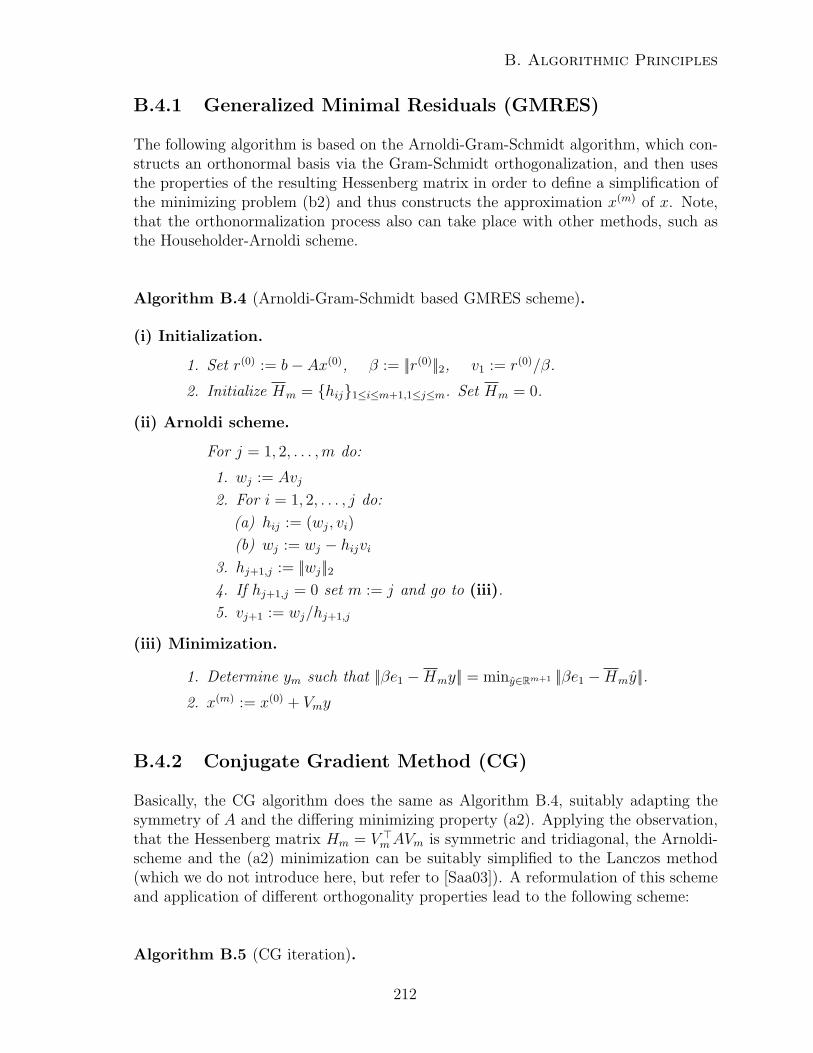
B. Algorithmic Principles
B.4.1 Generalized Minimal Residuals (GMRES)
The following algorithm is based on the Arnoldi-Gram-Schmidt algorithm, which con-structs an orthonormal basis via the Gram-Schmidt orthogonalization, and then usesthe properties of the resulting Hessenberg matrix in order to define a simplification ofthe minimizing problem (b2) and thus constructs the approximation x(m) of x. Note,that the orthonormalization process also can take place with other methods, such asthe Householder-Arnoldi scheme.
Algorithm B.4 (Arnoldi-Gram-Schmidt based GMRES scheme).
(i) Initialization.
1. Set r(0) := b− Ax(0), β := ||r(0)||2, v1 := r(0)/β.
2. Initialize Hm = hij1≤i≤m+1,1≤j≤m. Set Hm = 0.
(ii) Arnoldi scheme.
For j = 1, 2, . . . ,m do:
1. wj := Avj
2. For i = 1, 2, . . . , j do:
(a) hij := (wj, vi)
(b) wj := wj − hijvi3. hj+1,j := ||wj||24. If hj+1,j = 0 set m := j and go to (iii).
5. vj+1 := wj/hj+1,j
(iii) Minimization.
1. Determine ym such that ||βe1 −Hmy|| = miny∈Rm+1 ||βe1 −Hmy||.2. x(m) := x(0) + Vmy
B.4.2 Conjugate Gradient Method (CG)
Basically, the CG algorithm does the same as Algorithm B.4, suitably adapting thesymmetry of A and the differing minimizing property (a2). Applying the observation,that the Hessenberg matrix Hm = V >mAVm is symmetric and tridiagonal, the Arnoldi-scheme and the (a2) minimization can be suitably simplified to the Lanczos method(which we do not introduce here, but refer to [Saa03]). A reformulation of this schemeand application of different orthogonality properties lead to the following scheme:
Algorithm B.5 (CG iteration).
212
B.4 Krylov subspace methods
(i) Initialization. Set r(0) := b− Ax(0), p(0) := r(0).
(ii) Orthogonalization and minimization.
For j = 1, 2, . . . , until convergence do:
1. αj := ||r(j)||22/(Ap(j), p(j))
2. x(j+1) := x(j) + αjp(j)
3. r(j+1) := r(j) − αjAp(j)
4. βj := ||r(j+1)||22/||r(j)||225. p(j+1) := r(j+1) + βjp
(j)
Note, that the CG scheme can also be retrieved starting from the gradient schemewith steepest descent d(m) and assuring, that not only two neighboring residuals areorthogonal, i.e. (r(m), r(m+1)) = 0, m ≥ 0, but each, i.e. (r(i), r(j)) = 0 for i 6= j. This,again leads to a Galerkin system of kind (a2).
B.4.3 Example: CG-Uzawa algorithm
Considering the Schur complement problem (B.4)–(B.5), we solve equation (B.5) by ap-plication of the conjugate gradient method. As already mentioned before, this scheme isonly applicable to problems with symmetric matrices, such as the symmetric stabilizedfinite element discretized Stokes problem.
Algorithm B.6 (CG Uzawa iteration).
(i) Initialization.
1. Determine h(0) due to Ah(0) = f −BTp(0).
2. Set r(0) := Bh(0) +Dp(0) − g, q(0) := r(0).
(ii) Orthogonalization and minimization.
For j = 1, 2, . . . , until convergence do:
1. Solve Ah(k) = (BT q(j))
2. αj := ||r(j)||22/(Bh(j) −Dq(j), q(j))
3. p(j+1) := p(j) + αjq(j)
4. v(j+1) := v(j)−αjh(j)
5. r(j+1) := r(j) − αj(Bh(j) −Dq(j))
6. βj := ||r(j+1)||22/||r(j)||227. q(j+1) := r(j+1) + βjq
(j)
The structure of the Schur complement comes into effect repeately in (ii) step 4, wherethe velocity is updated by use of the already determined variable h(j).
213
B. Algorithmic Principles
Note, that in the case of the (stabilized) Stokes problem, the main effort of this algo-rithm consists in solving Poisson problems in the initialization step and in (ii) step 1.For unsymmetric problems, a Krylov subspace method for problems with unsymmetricmatrices can be applied. However, inverting matrix A is much more expensive. Thusit is suggestable to solve the entire, coupled problem, e.g. with a multigrid scheme.
214
Appendix C
Published and Submitted Articles
Abstract of the Article
”Equal-order finite elements for the hydrostatic Stokes
problem”
Simulation of flow phenomena in the ocean and in other large but relatively flat basinsare typically based on the so-called primitive equations, which, among oth- ers, resultfrom application of the hydrostatic approximation. The crucial premise for this ap-proximation is the dominance of the hydrostatic balance over remaining vertical flowphenomena in large but flat domains, which leads to a decomposition of the three-dimensional (3D) pressure field into a hydrostatic part and an only two-dimensional(2D) hydrodynamic part. The former pressure can be obtained by solving OrdinaryDifferential Equations. The latter one is determined by a 2D elliptic problem whichcan be solved quite efficiently. The velocity field remains three dimensional. How-ever, its vertical component can be eliminated from the dynamic system. In this work,we analyze such 2.5-dimensional (2.5D) Stokes systems and formulate stabilized fi-nite element schemes with equal-order interpolation. The absence of a discrete inf-supcondition is compensated by introducing additional terms into the discrete variationalform. We show stability and give an a priori error estimate for several established sta-bilized equal-order schemes, as pressure-stabilized Petrov-Galerkin (PSPG), Galerkinleast squares (GLS) and local projection schemes (LPS) which are extended here tothe hydrostatic approximation. The basic assumption we need is a certain property ofthe underlying 3D mesh. We illustrate the order of convergence of the 2.5D problemby numerical examples and demonstrate the effect of the hydrostatic approximation incomparison to the full 3D problem.
215
C. Published and Submitted Articles
Abstract of the Article
”Symmetric Stabilization of Equal-order Finite Ele-
ment Discretized Hydrostatic Flow Problems”
Simulation of flow phenomena in the ocean and in other large but relatively flat basinsare typically based on the so-called primitive equations, which, among others, resultfrom application of the hydrostatic approximation. The crucial premise for this ap-proximation is the dominance of the hydrostatic balance over remaining vertical flowphenomena in large but flat domains, which leads to a decomposition of the three-dimensional (3D) pressure field into a hydrostatic part and an only two-dimensional(2D) hydrodynamic part. The former pressure can be obtained by solving OrdinaryDifferential Equations. The latter one is determined by a 2D elliptic problem whichcan be solved quite efficiently. The velocity field remains 3D. However, its verticalcomponent can be eliminated from the dynamic system. In this work, we analyzesuch ”2.5-dimensional” (2.5D) Oseen systems and formulate symmetric stabilized fi-nite element schemes with equal-order interpolation. The absence of a discrete inf-supcondition as well as problems due to dominating advection are compensated by intro-ducing suitable stabilizing terms into the discrete variational form. We show stability,give an a priori error estimate for several established symmetric stabilization schemesand illustrate the order of convergence of the 2.5D problem by numerical examples.
216
Parallel multigrid method for finite element simulations ofcomplex flow problems on locally refined meshes
Madlen Kimmritz1, Thomas Richter2,∗
1 University of Kiel2 University of Heidelberg
SUMMARY
We present a parallel multigrid solver on locally refined meshes for solving very complex threedimensional flow problems. Besides describing the parallel implementation in detail, we proof thesmoothing property of the suggested iteration for a simple model problem. For demonstration of theefficiency and feasibility of the solver, we show a chemically reactive flow simulation for a Methaneburner using detailed chemical reaction modeling. Further, we give results of a ocean flow simulation.All described methods are implemented in the finite element toolbox Gascoigne. Copyright c© 2009John Wiley & Sons, Ltd.
key words: adaptive finite elements, multigrid, parallelization, flow simulation, reactive flows,
computation hydrodynamics
1. Introduction
In this paper we describe a parallel solution method for very complex three dimensionalflow problems given as large systems of partial differential equations. We present two diverseapplications: first the simulation of a Methane burner using detailed modeling of the chemicalreactions. Second, the simulation of ocean flows. Both problems are described by verylarge systems of partial differential equations based on the Navier-Stokes equations. For thesimulation of the Methane burner besides the four flow variables velocity and pressure, thetemperature as well as the concentrations of all chemical species have to be considered. Herewe use a chemical reaction system involving 39 chemical species leading to a coupled systemof 43 solution components. For modeling ocean flows we at least have to consider the velocity,the pressure, the temperature, and the salinary saturation. Further solution components arerequired, if chemical reactions are to be modeled.
The complexity of the numerical problem grows quadratically with the number of solutioncomponents, thus the resulting algebraic systems are immense. Further, both problems are
∗Correspondence to: Institute of Applied Mathematics, INF 294, 69120 Heidelberg, [email protected])
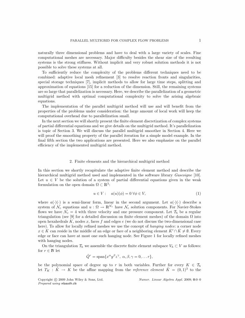
PARALLEL MULTIGRID FOR COMPLEX FLOW PROBLEMS 1
naturally three dimensional problems and have to deal with a large variety of scales. Finecomputational meshes are necessary. Major difficulty besides the shear size of the resultingsystems is the strong stiffness. Without implicit and very robust solution methods it is notpossible to solve these systems at all.
To sufficiently reduce the complexity of the problems different techniques need to becombined: adaptive local mesh refinement [3] to resolve reaction fronts and singularities,special storage techniques [7], implicit methods to allow for large time steps, splitting andapproximation of equations [15] for a reduction of the dimension. Still, the remaining systemsare so large that parallelization is necessary. Here, we describe the parallelization of a geometricmultigrid method with optimal computational complexity to solve the arising algebraicequations.
The implementation of the parallel multigrid method will use and will benefit from theproperties of the problems under consideration: the large amount of local work will keep thecomputational overhead due to parallelization small.
In the next section we will shortly present the finite element discretization of complex systemsof partial differential equations and we give details on the multigrid method. It’s parallelizationis topic of Section 3. We will discuss the parallel multigrid smoother in Section 4. Here wewill proof the smoothing property of the parallel iteration for a simple model example. In thefinal fifth section the two applications are presented. Here we also emphasize on the parallelefficiency of the implemented multigrid method.
2. Finite elements and the hierarchical multigrid method
In this section we shortly recapitulate the adaptive finite element method and describe thehierarchical multigrid method used and implemented in the software library Gascoigne [10].Let u ∈ V be the solution of a system of partial differential equations given in the weakformulation on the open domain Ω ⊂ R3:
u ∈ V : a(u)(φ) = 0 ∀φ ∈ V, (1)
where a(·)(·) is a semi-linear form, linear in the second argument. Let a(·)(·) describe asystem of Nc equations and u : Ω → RNc have Nc solution components. For Navier-Stokesflows we have Nc = 4 with three velocity and one pressure component. Let Th be a regulartriangulation (see [9] for a detailed discussion on finite element meshes) of the domain Ω intoopen hexahedrals K, nodes x, faces f and edges e (we do not discuss the two-dimensional casehere). To allow for locally refined meshes we use the concept of hanging nodes: a corner nodex ∈ K can reside in the middle of an edge or face of a neighboring element K ′ ∩ K 6= ∅. Everyedge or face can have at most one such hanging node. See Figure 1 for locally refined mesheswith hanging nodes.
On the triangulation Th we assemble the discrete finite element subspace Vh ⊂ V as follows:for r ∈ N let
Qr = spanxαyβzγ , α, β, γ = 0, . . . r,be the polynomial space of degree up to r in both variables. Further for every K ∈ Thlet TK : K → K be the affine mapping from the reference element K = (0, 1)3 to the
Copyright c© 2009 John Wiley & Sons, Ltd. Numer. Linear Algebra Appl. 2009; 0:0–0Prepared using nlaauth.cls
2 M. KIMMRITZ, T. RICHTER
4
7 4T T
01T
2T
L
55
55 20
13 34
Figure 1. Top row: adaptive refinement of meshes. Bottom row: global coarsening for the generationof a multigrid hierarchy. The numbers indicate the number of elements in every mesh.
computational element K. Then, we define the finite element space:
Vh := φ ∈ V : φ∣∣∣K
= φh T−1K , φh ∈ Qr.
LetΨh := φih, i = 1, . . . ,Nh,
be the common Lagrange basis system of the finite element space Vh with φi(xj) = δij , wherexj are the Nh degrees of freedom. With Nh we will identify the size of the problem to besolved.
To approximate the partial differential equation in this discrete space Vh we associate thefinite element function uh ∈ [Vh]Nc with a coefficient vector uh ∈ RNh×Nc given by
(uh)j = uh(xj) ∈ RNc , uh =Nh∑j=1
(uh)jφjh(x). (2)
We solve the partial differential equation (1) with a Newton method yielding iterates uth by:
a′(uth)(ut+1h − uth, φh) = −a(uth)(φh) ∀φh ∈ [Vh]Nc ,
where a′(uh)(wh, φh) is the directional derivative of the form a(·)(·) in direction of the updatewh evaluated in the last approximation uh. The discrete solution of the partial differential isthen characterized by the solution of the linear equations
Ahuh = bh,
where the system matrix Ah and the load vector bh are given by:
(Ah)ij = a′(uth)(φjh, φih), i, j = 1, . . . ,Nh,
(bh)j = −a(uth)(φjh), j = 1, . . . ,Nh.
Copyright c© 2009 John Wiley & Sons, Ltd. Numer. Linear Algebra Appl. 2009; 0:0–0Prepared using nlaauth.cls
PARALLEL MULTIGRID FOR COMPLEX FLOW PROBLEMS 3
3
hH
1Φ
H
xH
1Φ
h
2Φ
1
2
3Φ
h
hx
xhx
h
1
2
1
h
12
Figure 2. Nested function spaces between refined meshes: Φ1H = 1
2Φ1
h + Φ2h + 1
2Φ3
h.
We store the matrix and the vectors in a block-wise sense: every entry of the matrix (Ah)ij ∈RNc×Nc is a matrix itself, gathering all couplings between the Nc equation components andevery entry of the vectors (bh)i ∈ RNc is a vector. This storage technique clusters localdependencies of the different solution components and will be crucial to obtain an efficientparallel method. Further, all algebraic algorithms can be presented independent of the numberof solution components Nc. We use an adaptive algorithm for obtaining a good approximationuh to u:
Algorithm 1. Adaptive finite element algorithmLet TOL be a prescribed error tolerance, Th an initial triangulation of the domain Ω.
1. On the triangulation Th define the finite element space Vh.2. Solve the partial differential equation
a(uh)(φh) = 0 ∀φh ∈ Vh.3. Estimate the error ηh(uh)4. If |ηh(uh)| < TOL break5. Refine the mesh using the estimate: Th → Th′ . Restart at 1. using Th′ .
By this algorithm a sequence of locally refined meshes T1, . . . , TL = Th is generated. (See thetop row of Figure 1). In step 5. of the algorithm, certain elements K of Th are split into eightnew hexahedrals. For a review of advanced error estimation and mesh refinement techniquesused in these calculations see [3] or [6].
This hierarchy of finite element meshes calls for geometric multigrid methods as solverfor the linear systems. Here we briefly describe the multiplicative multigrid method. Let Tl,l = 0, . . . , L be a hierarchy of finite element meshes with TL = Th being the finest mesh. Thecoarser meshes are generated by the process of global coarsening (see [2]). Instead of usingthe mesh sequence as produced in the adaptive algorithm 1, we start with the finest meshTL := Th and produce coarse meshes by successively coarsening the mesh as much as possible.This way we have Nl Nl−1 for large l and obtain optimal complexity for the multigridmethod for most meshes Th. See [2] for details and the lower row of Figure 1 for an example.Here, in this simple example, the ratios are NL/N2 ≈ 2.9 and N2/N1 ≈ 2.9 instead of 1.6 and2.6 if one would use the meshes produced by the adaptive algorithm in reverse order. In [2]the mesh nesting is studied in detail. Opposed to most multigrid methods on locally refinedmeshes, every mesh level Tl covers the whole domain Ω. This will simplify the construction ofan efficient parallel multigrid method.
By this construction the function spaces Vl on Tl are nested Vl−1 ⊂ Vl and every basisfunction φil−1 ∈ Ψl−1 can be linearly combined by adequate basis functions of Ψl. By
Copyright c© 2009 John Wiley & Sons, Ltd. Numer. Linear Algebra Appl. 2009; 0:0–0Prepared using nlaauth.cls
4 M. KIMMRITZ, T. RICHTER
Pl ∈ RNl×Nl−1 we denote the prolongation of the coefficient vector ul−1 to ul so that
ul = Plul−1,
Nl∑j=1
(ul)jφjl (x) =
Nl−1∑j=1
(ul−1)jφjl−1(x) ∀x ∈ Tl.
See Figure 2 for a one-dimensional example. By Rl := PTl we denote the restriction operator.These two operators will also be used as restriction and prolongation operators between thefunction spaces Vl and Vl−1.
On the sequence of meshes Tl and spaces Vl for l = 0, . . . , L we can now give the hierarchicalmultigrid method to solve Ahuh = bh:
Algorithm 2. Hierarchical Multigrid Method on level lIf l = 0 solve A0u0 = b0. Otherwise,
1. Pre-smooth: u′l = Sprel (Al,bl,ul)
2. Compute the residual rl = bl −Alu′l3. Restrict the residual rl−1 = Rlrl4. Solve Al−1wl−1 = rl−1 with the multigrid algorithm on level l − 1.5. Prolongate the coarse mesh solution: wl = Plwl−1.6. Update: u′′l = u′l + wl
7. Post-smooth: ul = Spostl (Al,bl,u′′l ).
In step 4. the algorithm itself is called in a recursive way. The multigrid method consists of3 parts: first, solution of the coarse mesh problem. second, the prolongation and restrictionoperation and third, the smoothing. The smoothing process is an approximate solution processwith the goal of reducing the high frequent error contributions. Usually very easy iterativeschemes like Jacobi, Gauss-Seidel or SOR are used. Having flow applications in mind we usea Richardson iteration (with approximately 5 steps) preconditioned by an ILU as smoother:
u′l = Sl(Al,bl,ul) = ul + (LlUl)−1(bl −Alul),
where LlUl ≈ Al is an incomplete decomposition of Al with zero fill in.The prolongation and restriction operators are as described before. For the coarse mesh
solution we use a direct solver if the size of the coarse mesh T0 permits it. Otherwise we use aGMRES iteration, preconditioned with an ILU.
3. Parallel multigrid on locally refined meshes
Parallel multigrid methods for the solution of linear systems are well established, see [8]. Thebasic outline is as follows. Let Mcpu be the number of subdomains to be used for splittingthe problem. This can be the number of cpu’s on a cluster system or the number of coreson a shared memory system. The vertical hierarchy of multigrid meshes Tl for l = 0, . . . , L ishorizontally partitioned into subdomains
Tl = ∪p=1,...,MlT pl , Ml ≤Mcpu,
in the following non-overlapping sense: every element K ∈ Tl is uniquely allotted to onesubdomain K ∈ T pl . Nodes x ∈ Tl, edges e ∈ Tl and faces f ∈ Tl can belong to more than one
Copyright c© 2009 John Wiley & Sons, Ltd. Numer. Linear Algebra Appl. 2009; 0:0–0Prepared using nlaauth.cls
PARALLEL MULTIGRID FOR COMPLEX FLOW PROBLEMS 5
subdomain. The set of nodes x ∈ T pl also belonging to other subdomains is called the interfaceIpl of T pl :
Ipl := x ∈ T pl : ∃q 6= p : x ∈ T ql .On every T pl we define the finite element space V pl in the usual way.
Let Rpl ∈ RNpl ×Nl be the restriction of Tl to T pl . It holds (Rpl )ij = 1 if φpj corresponds to
the same basis function in V pl as φi in Vl. All other entries of Rpl are zero. By Ppl := (Rpl )T wedenote the prolongation from T pl to Tl. Then, for a coefficient vector (2) xl ∈ RNl we definethe local distributed vector xpl ∈ RN
pl by
xpl := Rpl xl.The system matrix Al is assembled locally by
(Apl )ij = a′(uth)(φjl , φ
il), i, j = 0, . . . ,N p
l .
This results in an additive distribution. The local matrices Apl are not point-wise restrictions
of Al but given by
Al =Ml∑p=1
Ppl AplRpl .
The matrix-vector product yl = Alxl can be split into two steps:
Algorithm 3. Parallel matrix vector product yl = Alxl
1. On p = 1, . . . ,Ml compute ypl = Alxpl
2. Balance values on the interface ypl = Rpl∑Ml
q=1 Pql yqlWhile the first step can be done in parallel, the second step requires communication on theinterface nodes. This interface balancing operator will be used again and is indeed the mostimportant ingredient to the parallel multilevel method.
Parallel multigrid can now be regarded as a subspace correction method with a twodimensional splitting, vertically into mesh levels T0, . . . , TL and horizontally into subdomainsT 1l , . . . , TMl
l , see [21] for this concept. Parallelization aims at implementing the existingalgorithm in a most efficient way on a distributed memory machine. As far as possible, thealgorithm itself shall not be changed. In the following paragraphs we will discuss the differentsteps of Algorithm 2 with respect to the parallelization.
3.1. The parallel multigrid smoother
In Steps 1. and 7. of Algorithm 2, the multigrid smoother is applied as a Richardson iteration.Every step t = 0, 1, . . . of this iteration yields an update:
LlUlytl = rtl := bl −Alutl , ut+1l = utl + ytl .
The assembly of the ILU decomposition is a globally coupled process and not easy to parallelize.We alter the smoothing process in order to get an algorithm better suitable for parallelization.Instead of computing the global ILU of Al we simply construct local ILU’s on every subdomain:
LplUpl ≈ A
p
l , (3)
Copyright c© 2009 John Wiley & Sons, Ltd. Numer. Linear Algebra Appl. 2009; 0:0–0Prepared using nlaauth.cls
6 M. KIMMRITZ, T. RICHTER
and replace the smoothing operation by local updates:
LplUpl y
p,(t)l = rp,(t)l , yp,(t)l = Rpl
Ml∑q=1
Pql yql .
The first step can be done in parallel while in second step the application of the interfacebalancing operator is necessary.
Since the matrix Al is distributed in an additive sense to the subdomains, the localmatrices Ap
l correspond to Neumann problems which in general are not regular. For the ILU-construction in (3) we construct local Dirichlet versions A
p
l of Apl by summing up all values
on the interface:
Ap
l := RplAlPpl = Rpl(∑
q
Pql AqlRql
)Ppl .
Here, we need to exchange all matrix rows belonging to interface nodes. This procedure doesnot represent the original smoothing process from the sequential algorithm, but it yields arobust smoothing operator. Solving the local problems exactly
Ap
l ypl = rpl ,
the parallel smoother would correspond to an additive Schwarz iteration with overlap h (onelayer of cells) with homogeneous Dirichlet values. In Section 4 we will show, that this minimaloverlap is sufficient to obtain a fixed reduction rate for high frequent error parts in a multigridcontext applied to the Laplace equation.
Algorithm 4. Parallel Smoothing IterationOn p ∈ 1, . . . ,Ml, given up,(0)
l for t = 0, 1, . . .
1. Local residual: rp,(t)l = bpl −Apl u
p,(t)l
2. Exchange on interface: rp,(t)l = Rpl∑Pql rq,(t)l
3. Local update: LplUpl y
p,(t)l = rp,(t)l
4. Update: up,(t+1)l = up,(t)l +Rpl
∑Pql yq,(t)l
Steps 2. and 4. require communication along the interface, all other steps can be done inparallel. To get an efficient algorithm all domains have to be of the same size and the interfaceshave to be as small as possible:
(M1) Create balanced partitionings
N pl ≈ N q
l , ∀p, q ∈ 1, . . . ,Ml, ∀l ∈ 0, . . . , L (4)
(M2) Minimize the size of the interfaces
max1≤p≤P
#Ipl → min! (5)
Copyright c© 2009 John Wiley & Sons, Ltd. Numer. Linear Algebra Appl. 2009; 0:0–0Prepared using nlaauth.cls
PARALLEL MULTIGRID FOR COMPLEX FLOW PROBLEMS 7
3.2. Mesh transfer operators
The second important ingredient to geometric multigrid methods is the mesh transfer operator:the restriction in step 3. of Algorithm 2 and the prolongation in step 5. Here, both hierarchiesget involved. To process the prolongation to node x1
H of the coarse mesh TH in Figure 2, nodesx1h, x
2h and x3
h from the fine mesh Th are necessary. In the parallel version all four involvednodes can rest in different subdomains making communication necessary. We split the meshtransfer into two parts: first we process the vector to be prolongated on the fine mesh Th.Then, we carry the contributions of Th to the corresponding nodes on the coarse mesh TH .With respect to the situation in Figure 2, for a vector uh to be prolongated to uH the algorithmis as follows:
1. Collect the contributions on Th:
uh(x2h) =
12uh(x1
h) + uh(x2h) +
12uh(x3
h).
2. Copy the entries to the corresponding nodes on THuH(x1
H) = uh(x2h).
The communication pattern for the first step is the same as the usual exchange of values onthe interfaces. In the second step there is no communication required, if the distribution ofthe meshes is nested and the nodes x1
H = x2h are distributed to the same subdomain p. For
the parallel mesh transfer to be efficient we demand the mesh distribution to be as nested aspossible:
(M3) Create nested partitionings of the triangulations:
x ∈ T pl−1 ⇒ x ∈ T pl . (6)
This demand is usually not feasible: The efficiency of multigrid methods relies on smallcoarse meshes. Often, the number of elements in the coarse mesh is smaller than the numberof subdomains Mcpu. Furthermore, using locally refined meshes the claim for a nestedpartitioning contravenes the claim for a balanced partitioning of every level. In Section 3.4we will explain our approach to fulfill the three mesh demands (M1), (M2) and (M3) asgood as possible.
3.3. The interface exchange operator
One of the basic operators in the parallel multigrid method is the exchange of node valuesacross the interfaces. E.g. to guarantee the overlapping partitioning of vectors after the matrix-vector product:
ypl = RplMl∑q=1
Pql yql .
For a node xil on the interface Ipl , this operator adds all the values uql (xil) from adjacent
subdomains q with xil ∈ T ql :(upl )i =
∑xq
j∈T ql : xq
j =xpi
(uql )j .
Copyright c© 2009 John Wiley & Sons, Ltd. Numer. Linear Algebra Appl. 2009; 0:0–0Prepared using nlaauth.cls
8 M. KIMMRITZ, T. RICHTER
In the worst case, if every subdomain touches every other subdomain, this is an all-to-allcommunication. Usually however every subdomain has a common interface only with a smallnumber of neighboring domains. For every node xil on the interface between at least twosubdomains, let Ml(xil) ⊂ 1, . . . ,Ml be the set of subdomains containing the node and let#Ml(x) be bounded by:
#Ml(x) ≤ Cnei, ∀x ∈ Tl, ∀l = 0, . . . , L.
In [17] an algorithm is described which creates a communication network to process as manyinterface in parallel as possible. The overall communication effort depends on
Wint(Tl) = O(Cnei · maxq∈1,...,Ml
(#Iql )),
the product of the maximum interface size and the maximum number of neighbors a subdomaincan have.
3.4. Partitioning of the meshes
This section is devoted to the partitioning of the mesh hierarchy. In the previous discussion wehave collected the three objectives (M1)-(M3), see (4), (5), (6) for the mesh partitioningto yield an efficient parallel algorithm. The first two objectives (M1) and (M2) can betransformed into a standard graph partitioning problem: create a balanced partitioning withminimal edge-cut. The third task, the generation of a nested partitioning is harder toaccomplish. On structured meshes, one could just partition the coarse mesh T0 and carryover this partitioning to all the finer meshes Tl in the following way: If the element K ∈ Tl−1
belongs to subdomain p ∈ 1, . . . ,Ml−1, all the children Ki ∈ Tl are assigned to subdomainT pl . All the partitionings would be nested and (M3) would be fulfilled perfectly.
This easy algorithm does not work, if the coarse mesh is too coarse to make a balancedpartitioning possible, e.g. if N0 <Mcpu. With respect to locally refined meshes this algorithmis not optimal, since it is possible, that the finer meshes TL are mostly refined in certain regionsall belonging to the same subdomain in the coarse mesh. A non-balanced partitioning of thefine meshes, where most of the work happens would be the result.
In Bastian [1] a dynamic load balancing scheme for local multigrid methods on adaptivelyrefined meshes is described. Prior to distributing the multigrid meshes, elements are gatheredin clusters combining neighboring elements in both directions, neighbors on one level as wellas neighbors across the mesh levels. If all elements in one cluster stay together on the samecpu, no communication will be necessary, neither for the mesh transfer nor for balancing onany interface. Schupp [18] used a similar setting for a parallel multigrid solver with dynamicload balancing. The main problem of this partitioning procedure is the setup of the clusters.These clusters can be considered as cones K with some element K ∈ Tl as the cone end. Thecones then widen up with all descendents of K in finer meshes Tl+1, . . . , TL.
The method of global coarsening simplifies the generation of a balanced, yet nestedpartitioning. For every fixed mesh level k ∈ 0, . . . , L we can build a set of cones C(k) whichconsists of all cones K ∈ C(k) with the elements K ∈ Tk as ends and widening up to the finestmesh TL. If we partition these cones to Mcpu parts, we get a nested partitioning of all finemeshes Tk, . . . , TL. On locally refined meshes we introduce weighted cones. The cone-weight ofK is the number of elements K ∈ K that are fine-mesh elements in TL. A balanced partitioningof the weighted cones then results in balanced fine meshes. The mesh level k has to be chosen
Copyright c© 2009 John Wiley & Sons, Ltd. Numer. Linear Algebra Appl. 2009; 0:0–0Prepared using nlaauth.cls
PARALLEL MULTIGRID FOR COMPLEX FLOW PROBLEMS 9
large enough to get a sufficient number of cones to produce a balanced partition. The lowerthe mesh level k is chosen, the more meshes are distributed in a nested way:
Algorithm 5. Distribution of the fine meshes
1. Get smallest number k ∈ 0, . . . , L with #Tk ≥ Cminpart · Mcpu.2. Construct set of cones C(k).3. Construct weighted graph G(k) with nodes K ∈ C(k), node-weights ω(K) = #K and edges
(K,K′) ∈ G(k) if elements K and K ′ in Tk are adjacent. The edge-weight ω(K,K′) is thenumber of contacts between elements K ∈ K and K ′ ∈ K′.
4. Partition the graph G(k) → G(k)1, . . . ,G(k)Mcpu to yield a partitioning with balanced node-weights and minimal edge-cut.
5. Carry the partitioning to Tk, . . . , TL: for l = k, . . . , L assign element K ∈ Tl to subdomain T ql ,if K ∈ K ∈ G(k)q.
Once the set of cones C(k) is distributed, we get a distribution of the meshes Tk, . . . , TL. Ina second step, this distribution has to be carried over to all coarse meshes T0, . . . , Tk−1:
Algorithm 6. Distribution of the coarse meshesFor l = k − 1, . . . , 0:
1. For K ∈ Tl, let Ki ∈ Tl+1 be the children. Assign K to T pl , where p is the subdomain T pl+1
containing the most children Ki.2. If #T ql < Cminpart, combine T ql and T q′l , where q′ is the index of the next-smallest subdomain.
The first step assures that the partitioning is as nested as possible. The second step is calledthe coarse mesh agglomeration and assures that the meshes are not too small.
The process of mesh partitioning is not implemented in parallel. Further, we do not usedynamic load balancing and redistribution of partitionings. The mesh partitioning is carriedout sequentially and the partitioned meshes are afterwards transferred to the different cpu’s.For the simulation of small pde systems, this procedure will not result in a scalable parallelalgorithm. Since we only consider complex multi-component flow problems, this approach isjustifiable, see the numerical examples.
3.5. Distribution of locally refined meshes
To correctly and efficiently deal with hanging nodes some small variations of the meshpartitioning algorithms from the preceding sections are necessary. In the finite elementsimulation, hanging nodes are no real degrees of freedom. Instead the values are interpolatedusing neighboring degrees of freedom. To avoid additional communication here, we change theassemble of cones in Algorithm 5 in a way, that all information needed to handle hangingnodes are clustered in the cones. In [17] we explain details on this modification.
In Figure 3 we show the partitioning process in detail for the mesh hierarchy given inFigure 1. Let Mcpu = 2 and Cminpart = 8 for this example. The mesh T2 is the smallest meshstill large enough to satisfy McpuCminpart ≥ N2. These cones then need to be clustered tocombine hanging nodes information. The weighted graph has four nodes and six edges. Finallythis graph is distributed into two subdomains with weights 28 and 24. This describes steps 1.to 4. of Algorithm 5. It remains to carry this partitioning to the meshes of the hierarchy.This is demonstrated in Figure 4: The two fine meshes TL and T2 are large enough to satisfy
Copyright c© 2009 John Wiley & Sons, Ltd. Numer. Linear Algebra Appl. 2009; 0:0–0Prepared using nlaauth.cls

10 M. KIMMRITZ, T. RICHTER
16 28
441 1
4
4
1 4
1
4
1
1 1
4
4
4
4
16 16
4 4
28
3 5
3
5
1 1
28
4 4
16
Figure 3. From left to right: the smallest mesh T2 with N2 ≥ CminpartMcpu, clustering of hangingnodes constraints, transformation to a corresponding weighted graph, partitioning of the graph.
Figure 4. Partitioning of the complete mesh hierarchy. The partitioning of the left two meshes iscarried over from Figure 3, the right two meshes are to small to satisfy Nl ≥ CminpartMcpu.
N pl ≥ Cminpart and the partitioning can be directly carried over. The two coarse meshes are
too small and coarse mesh agglomeration is applied: just one subdomain is used.
3.6. Parallel efficiency
Losses in efficiency are either due to non-optimality of the parallelized algorithm or due to workand communication overhead produced by the parallelization. The used parallel algorithm onlydiffers in the choice of the multigrid smoother, having a Schwarz type decomposition as basis.
Overhead is mainly communication overhead for exchange of values across the interface andfor communication during the mesh transfer. In the following, we assume, that N := NL = Nhis the problem-size and that N Mcpu · Cminpart. Then let Tk with Nk ≥Mcpu · Cminpart bethe set of cones used for the decomposition and Cminpart large enough to produce a balancedpartitioning with local problem sizes:
N pl ≈
NlMcpu
, l ≥ k, p = 1, . . . ,Ml.
First we discuss the parallel overhead on the fine meshes l = k, . . . , L where the partitioningis balanced and P = Mcpu cpu’s are used. The overhead emerges from communication inthe interface exchange operator (Section 3.3) and in the mesh-transfer (Section 3.2). For finemeshes with a nested partitioning l ≥ k, all additional work is due to exchange of values alongthe interface. The set of nodes on the interface of a subdomain T pl is a lower-dimensionalentity,
#Ipl = O(
(N pl )
d−1d
),
where d is the spatial dimension. Considering systems of Nc coupled partial differentialequations, every subdomain has to exchange O(Nc · #Ipl ) values with adjacent subdomains.Using the distributed communication network mentioned in Section 3.3 this communication is
Copyright c© 2009 John Wiley & Sons, Ltd. Numer. Linear Algebra Appl. 2009; 0:0–0Prepared using nlaauth.cls
PARALLEL MULTIGRID FOR COMPLEX FLOW PROBLEMS 11
done in at most Cnei steps leading to an overall communication work for the interface exchangeoperator of
W commint (Tl, P ) = ccommO
(Nc · Cnei
(NlP
) d−1d
)
3.6.1. Parallel efficiency of the matrix-vector product For a system of Nc partial differentialequations, the block-matrix on mesh level Tl has Nl rows, each with Crow entries (dependingon the finite element space). The matrix entries are matrices of size Aij ∈ RNc×Nc . Usuallywe have Crow ≈ (2r + 1)d, where d is the spatial dimension and r is the polynomial degree.The numerical work for a matrix-vector product is O(C2
rowN 2cNl). In the parallel version, the
numerical work is equally split to P cpu’s and the overall effort is given by:
Wm-v(Tl, P ) = O
(cnumC
2rowN 2
c
NlP
+ ccommNc · Cnei
(NlP
) d−1d
).
and the parallel efficiency by:
Em-v(Tl, P ) =1
1 + ccommcnum
· CneiC2
rowNc
(PNl
) 1d
.
Usually – depending on the architecture of the computer system – we have ccomm cnum.All the other constants however are in favor of efficiency for complex systems. For threedimensional problems using quadratic finite elements, we have Cnei ≈ 6 and Crow ≈ 125. Forthe Navier-Stokes equations it is Ncomp = 4 and for the chemical reactive flow example inSection 5.1, we have Nc = 43. Thus, we have for Navier-Stokes equations (NS) and for thereactive flow equations (RF)
CNSm-v =
Cnei
C2rowNc
=6
12524≈ 10−4, CRF
m-v =Cnei
C2rowNc
=6
125243≈ 10−5,
and we get a good scalability if the ratio of problem size and number of CPU’s is constant.
3.6.2. Parallel efficiency of matrix and residual assembly Besides the linear algebra part,finite element applications spend a large share of time for the assembly of the system matrixand for the integration of nonlinear residuals. Here we only analyze the integration of residuals,which is the harder task in terms of parallelization since the amount of sequential numericalwork to be done is less. On a mesh Tl we have to compute
(rl)j = a(uh)(φjl ), ∀j = 1, . . . , Nl.
The numerical integration is done locally on every element K ∈ Tl by a Gauss-rule. For finiteelements of degree r in d space dimensions, Gauss-rules with
Cgauss = (2r)d
integration points per element are used. The evaluation of the bi-linear form a(·)(·) in everyGauss-point takes Cform operations, where Cform can vary between 5 for the simple Laplace-equation and 1000 for complicated nonlinear equations (like the reactive flow equation in
Copyright c© 2009 John Wiley & Sons, Ltd. Numer. Linear Algebra Appl. 2009; 0:0–0Prepared using nlaauth.cls
12 M. KIMMRITZ, T. RICHTER
Section 5.1). For a coupled system of Nc equations, the sequential work for the assemble ofthe residual is given by
Wresidual(Tl) = O(cnumCgaussCformN 2
cNl).
In the parallel version the local numerical work is again distributed in an optimal sense.The communication overhead is due to exchange of interface values. We thus get as parallelefficiency:
Eresidual(Tl, P ) =1
1 + ccommcnum
CneiCgaussCformNc
(PNl
) 1d
.
For quadratic finite elements in three dimensions we have Cgauss = 64. For the Navier-Stokesequations it is Cform ≈ 20 for the reactive flow system (RF) Cform ≈ 5 000:
CNSresidual =
Cnei
CgaussCformNc ≈ 10−3, CRFresidual =
Cnei
CgaussCformNc ≈ 10−7.
3.6.3. Parallel efficiency on the coarse meshes and the full multigrid method In the caseof balanced partitioning, all numerical algorithms based on local calculations followed by anexchange of interface values show a parallel efficiency of
E(Tl, P ) =1
1 + c(PNl
) 1d
,
with a small constant c. On coarse meshes Tl with l < k we use a lower number of cpu’s thanon the fine meshes, thus Pl < P =Mcpu, and the parallel efficiency is limited by:
E(Tl, Pl, P ) =1
PPl
(1 + c
(PNl
) 1d
) ≤ PlP
The overall sequential work for the multigrid method on L levels is given by
Wmg(T0, . . . , TL) = c
L∑l=0
Nl ≈ CmgNL.
where Cmg is a constant depending on the growth ratio between two consecutive meshes Nland Nl+1. In the parallel version we get
Wmg(P0, . . . , PL, T0, . . . TL) =L∑l=0
(NlPl
+ c
(NlPl
) d−1d
)and by using Nl/Pl = Cminpart for all coarse meshes l < k we get
Wmg(P, T0, . . . , TL) ≈ CαCminpart + Cα
(N
P+ Cα
(N
P
) d−1d
),
to get the overall parallel efficiency
Emg(P, T0, . . . , TL) ≈ 1
1 + CminpartPN + c
(PN
) 1d
.
For N/P Cminpart we get a good parallel efficiency of the overall multigrid scheme.
Copyright c© 2009 John Wiley & Sons, Ltd. Numer. Linear Algebra Appl. 2009; 0:0–0Prepared using nlaauth.cls
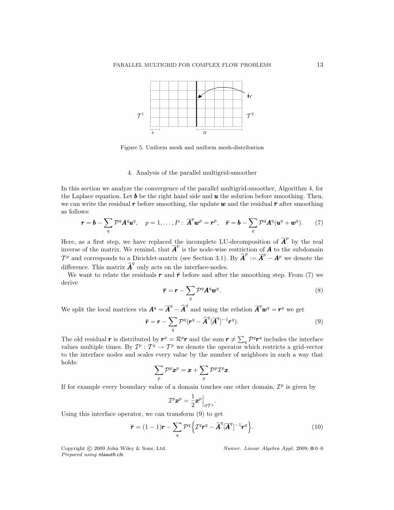
PARALLEL MULTIGRID FOR COMPLEX FLOW PROBLEMS 13
h H
T 1
iiiΓ
T 2
Figure 5. Uniform mesh and uniform mesh-distribution
4. Analysis of the parallel multigrid-smoother
In this section we analyze the convergence of the parallel multigrid-smoother, Algorithm 4, forthe Laplace equation. Let bbb be the right hand side and uuu the solution before smoothing. Then,we can write the residual rrr before smoothing, the update www and the residual rrr after smoothingas follows:
rrr = bbb−∑q
PqAAAquuuq, p = 1, . . . , P : AAApwwwp = rrrp, rrr = bbb−
∑q
PqAAAq(uuuq +wwwq). (7)
Here, as a first step, we have replaced the incomplete LU-decomposition of AAAp
by the realinverse of the matrix. We remind, that AAA
pis the node-wise restriction of AAA to the subdomain
T p and corresponds to a Dirichlet-matrix (see Section 3.1). By AAAp
:= AAAp −AAAp we denote the
difference. This matrix AAAq
only acts on the interface-nodes.We want to relate the residuals rrr and rrr before and after the smoothing step. From (7) we
deriverrr = rrr −
∑q
PqAAAqwwwq. (8)
We split the local matrices via AAAq = AAAq − AAAq and using the relation AAA
qwwwq = rrrq we get
rrr = rrr −∑q
Pq(rrrq − AAAq[AAAq]−1rrrq). (9)
The old residual rrr is distributed by rrrp = Rprrr and the sum rrr 6= ∑q Pqrrrq includes the interfacevalues multiple times. By Ip : T q → T p we denote the operator which restricts a grid-vectorto the interface nodes and scales every value by the number of neighbors in such a way thatholds: ∑
p
Ppxxxp = xxx+∑p
PpIpxxx.
If for example every boundary value of a domain touches one other domain, Ip is given by
Ipxxxp =12xxxp∣∣∣∂T q
.
Using this interface operator, we can transform (9) to get
rrr = (1− 1)rrr −∑q
PqIqrrrq − AAAq[AAAq]−1rrrq
. (10)
Copyright c© 2009 John Wiley & Sons, Ltd. Numer. Linear Algebra Appl. 2009; 0:0–0Prepared using nlaauth.cls
14 M. KIMMRITZ, T. RICHTER
The first term in rrr is zero. The second term only contains values in interface-nodes, since thematrices AAA
qand the interface operator Iq only act here and are zero elsewhere.
To analyze these remaining terms, we introduce a discrete Fourier basis of the subdomainsT p. We assume, that T p = (0, H)2 has N2
p nodes with local mesh-size h = H/(Np − 1). SeeFigure 5 for an easy example with only two subdomains. For θθθ = (θx, θy) ∈ 1, . . . , Np2 wedefine the discrete Fourier grid-functions:
Φp(θθθ)(iii) = sin(πθx(ix − 1)Np + 1
)sin(πθy(iy − 1)Np + 1
), iii = (ix, iy) ∈ 0, . . . , Np + 12.
These functions are zero for ix, iy ∈ 0, Np + 1 which corresponds to the boundary of thedomain ∂[−h,H+h]2, one layer of elements across the interface to the neighboring subdomain.Using this notation, a finite element vector vvvp on T p can be written as
vvvp =∑θθθ
vpθθθΦp(θθθ), vpθθθ ∈ R with θθθ ∈ 1, . . . , Np2. (11)
On these uniform meshes, the matrix AAAp
for the Laplace equation discretized with piecewisebilinear finite elements in stencil notation reads:
AAAp
=13
−1 −1 −1−1 8 −1−1 −1 −1
.Using the basic principles of trigonometric functions, the action ofAAA
pon a Fourier grid-function
Φp(θθθ) can by calculated as
AAApΦp(θθθ) = λ(θθθ)Φp(θθθ),
λ(θθθ) :=13
8− 2 cos
(πθx
Np + 1
)− 2 cos
(πθy
Np + 1
)− 4 cos
(πθx
Np + 1
)cos(
πθyNp + 1
)(12)
Writing the residual rrr before smoothing like (11) in the Fourier basis and by using (12) we getan explicit presentation of the local update wwwp:
rrrp =∑θθθ
rθθθΦp(θθθ) ⇒ wwwp =
∑θθθ
rθθθλ(θθθ)
Φp(θθθ). (13)
To estimate the remaining term in (10) we need to describe the action of the difference-matrix AAA
p= AAA
p −AAAp. Let iiiΓ ∈ T p be a point on a vertical interface touching one neighbor(see Figure 5). Here, the matrix AAA
pin stencil notation is given by (as seen from the left
subdomain):
AAAp(iiiΓ) =
13
0 − 12
0 40 − 1
2
∣∣∣∣∣∣ ,Like (12) we get for each Fourier component Φp(θθθ):
AAAp(iiiΓ)Φp(θθθ) = µ(θθθ)Φp(θθθ), µ(θθθ) :=
13
4− cos
(πθy
Np + 1
). (14)
Copyright c© 2009 John Wiley & Sons, Ltd. Numer. Linear Algebra Appl. 2009; 0:0–0Prepared using nlaauth.cls
PARALLEL MULTIGRID FOR COMPLEX FLOW PROBLEMS 15
Hence, we can combine (11), (12), (13) and (14) to get for the Fourier components rθθθ of thenew residual (assuming the interface is touched by two subdomains)
Iqrrrq − AAAq[AAAq]−1rrrq =∑θθθ
(12− µ(θθθ)λ(θθθ)
)rqθθθΦ
q(θθθ).
For all high frequencies we get by simple estimation:∣∣∣∣12 − µ(θθθ)λ(θθθ)
∣∣∣∣ ≤ 18
for θθθ ∈ Np/2, . . . , Np2.
Finally, for the overall residual combining both sides of the interface, the residual is reducedby the factor 4
|rpθθθ| ≤14|rpθθθ |, (15)
which yields a fixed convergence rate for all high frequencies. This estimate does not dependon the mesh-size h or the size of the subdomains H and is always valid for this minimal-overlapconfiguration.
At last, we discuss the case, where the local update wwwq is not computed exactly, but by anincomplete LU-iteration:
wwwq,(ν) = Sν(AAAq)rrrq.
Then, we introduce the additional error term
wwwq,(ν) = wwwq + (Sν(AAAq)− [AAA
q]−1)rrrq.
This local ILU-iteration does not depend on the partitioning of the domain, or the overlap,and thus there exists a ν0 ∈ N, such that:
‖(Sν(AAAq)− [AAA
q]−1)rrrq‖ ≤ 1
4‖rrrq‖ for ν ≥ ν0.
Combining this estimate with (15), the parallel multigrid smoother applied to the Laplaceequation exhibits a reduction rate smaller than 1
2 for all high frequent error contributions.
5. Numerical examples
5.1. Simulation of chemically reactive flows
In this section we present the simulation of a Methane burner under consideration of a detailedchemical reaction system involving NCS = 39 chemical species and 302 elementary chemicalreactions. The equations for modeling reactive flows are the Navier-Stokes equations with anenergy equation for the temperature and one diffusion-reaction-transport equation for everychemical species. Since the flow is comparatively slow, and changes in the density are mainlydue to temperature changes, the equations are written in the Low-Mach-Number limit splittingthe pressure into a hydrodynamical phyd and into a thermodynamical pth part p = pth + phyd,
Copyright c© 2009 John Wiley & Sons, Ltd. Numer. Linear Algebra Appl. 2009; 0:0–0Prepared using nlaauth.cls
16 M. KIMMRITZ, T. RICHTER
see [5]:
∇ · v +1m
v · ∇m− 1T
v · ∇T = 0,
ρ∂tv + ρv · ∇v −∇ · (µ∇v) +∇phyd = ρg,
ρcp∂tT + ρcpv · ∇T −∇ · λ∇T = fT (T,w),ρ∂twk + ρv · ∇wk +∇ · Fk = fk(T,w), k = 1 . . . , NCS − 1,
ρ =pm
RT.
Here, v is the velocity, T the temperature, wk, k = 1, . . . , NCS are the mass fractions of thespecies mixture, m the mean molecular weight of the mixture and ρ the mixtures density. Alltogether the system includes Nc = 43 coupled solution components. The chemical productionterms fk are given by
fK(T,w) := mk
NCR∑r=1
(νrk − νrk)kr(T )NCS∏j=1
cνrj(w)j
,
where for every reaction r = 1, . . . , NCR, νrk are the stoichiometric indices of species k and cjis the concentration and mj the molecular weight of species j. The reaction rate is given byan Arrhenius law
kr(T ) = ArTβr exp
−EarRT
.
The values Ar, Ear and βr are read from tables. For evaluating the residual of the equations inone point, for every of the NCS species every of the NCR reactions has to be evaluated whereall species can couple. Reactive flow calculations thus show an enormous local computationaleffort. Our example uses a 39 species reaction model considering 302 chemical reactions. Thereaction system is usually very sparse (not all species appear in every reaction, usually only 4).Here, the average numerical effort to evaluate the complete reaction system in every Gauss-point is 39 · 302 · 4 ≈ 50 000.
In Figure 6 we show the model of the Methane burner under consideration. On the right sideof the figure the reduced three dimensional computational domain is shown. With the threedifferent lamella, the cooling pipe it features the characteristic properties of the geometry.
In [17, 7] a numerical study of this Methane burner has been performed. In particular ithas been found out, that considering the full three dimensional geometry is compulsive. Forobtaining results with an estimated error tolerance of ≤ 5% locally refined meshes with about300 000 mesh elements where necessary. For storing the system matrix more than 30GB ofmemory was used. The calculations have been done in 2005 on a Linux-Cluster with 32 nodes,running at 2.4 GHz each and connected with a standard Gigabit Ethernet network.
In Table I results from the calculations are given. Due to the very large memory consumptionsystematical studies on the parallel efficiency are not possible. We thus show results from theprogress of the adaptive algorithm, using different numbers of cpu’s. In the last column wegive an index for the parallel efficiency which measures the efficiency compared to the first rowof the table:
Ei(P ) :=PS
TS
NS
P TP
NP
,
Copyright c© 2009 John Wiley & Sons, Ltd. Numer. Linear Algebra Appl. 2009; 0:0–0Prepared using nlaauth.cls
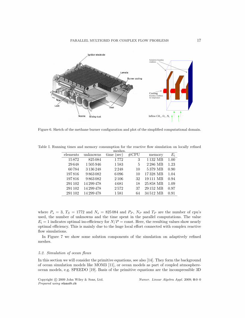
PARALLEL MULTIGRID FOR COMPLEX FLOW PROBLEMS 17
Inflow CH , O , N2 24
boundary conditionfor temperature
Cooling
Symmetric boundarycondition
Figure 6. Sketch of the methane burner configuration and plot of the simplified computational domain.
Table I. Running times and memory consumption for the reactive flow simulation on locally refinedmeshes.
elements unknowns time (sec) #CPU memory Ei
15 872 825 084 1 772 3 1 132 MB 1.0029 648 1 505 946 1 583 5 2 286 MB 1.2360 784 3 136 248 2 248 10 5 379 MB 0.90
197 816 9 863 082 6 096 10 17 328 MB 1.04197 816 9 863 082 2 106 32 19 111 MB 0.94291 102 14 299 478 4 681 18 25 858 MB 1.09291 102 14 299 478 2 572 37 29 152 MB 0.97291 102 14 299 478 1 581 64 34 512 MB 0.91
where Ps = 3, TS = 1772 and Ns = 825 084 and PP , NP and TP are the number of cpu’sused, the number of unknowns and the time spent in the parallel computations. The valueEi = 1 indicates optimal iso-efficiency for N/P = const. Here, the resulting values show nearlyoptimal efficiency. This is mainly due to the huge local effort connected with complex reactiveflow simulations.
In Figure 7 we show some solution components of the simulation on adaptively refinedmeshes.
5.2. Simulation of ocean flows
In this section we will consider the primitive equations, see also [14]. They form the backgroundof ocean simulation models like MOM3 [11], or ocean models as part of coupled atmosphere-ocean models, e.g. SPEEDO [19]. Basis of the primitive equations are the incompressible 3D
Copyright c© 2009 John Wiley & Sons, Ltd. Numer. Linear Algebra Appl. 2009; 0:0–0Prepared using nlaauth.cls
18 M. KIMMRITZ, T. RICHTER
Figure 7. Velocity (left), temperature (middle) and concentration for Formaldehyde (right) for theMethane burner simulation.
Navier-Stokes equations in a rotating frame:
∇ · v = 0ρc∂tv + ρcv · ∇v −∇ · (µ∇v)− f i3 × v +∇p = ρg + Φ
ρ = G(p).
State variables are velocity v, pressure p and density ρ. Model parameters are viscosity µ, meandensity ρc, Coriolis parameter f and gravity g, given as g := (0, 0,−g)> with gravity constantg. The vector i3 denotes the vertical unit vector. We will neglect large scale effects like tidaland centrifugal forces Φ and Coriolis forces, i.e. we set Φ = 0 and disregard the term f i3×v.Density ρ is determined in an equation of state. In ocean modeling lots of different approximateformulae for this equation are applied [14]. We will employ a polynomial approach.An observed feature of large-scale motions in the ocean is its small aspect ratio. This means,that the characteristic vertical length scale D is much smaller than the horizontal, L, one, i.e.δ := D/L 1. Scaling arguments lead to a neglection of vertical acceleration, see [13]. Thusthe third momentum equation becomes
∂zp = −ρg,the hydrostatic balance. We denote the pressure occurring due to gravitational acceleration ashydrostatic pressure phs.Furthermore we enrich the given set of equations by conservation equations for potentialtemperature θ and salinity S, both being important for the (thermo-) dynamic behavior ofoceanic systems.As we are not able to resolve motions of all appearing scales, we have to parameterizethe smallest ones, which have an important impact on larger, resolvable scales. Forparameterization of this turbulent behavior we use a simplified Smagorinsky model, see [4].
Copyright c© 2009 John Wiley & Sons, Ltd. Numer. Linear Algebra Appl. 2009; 0:0–0Prepared using nlaauth.cls
PARALLEL MULTIGRID FOR COMPLEX FLOW PROBLEMS 19
I.e. we add the diffusive term ∇· (νturb∇v) to the horizontal momentum equations. The valueνturb is the parameter of turbulent viscosity and v := (v1, v2)> denotes the horizontal velocityfield. The vertical velocity field is given by v3. As kinematic viscosity is much smaller thanthe turbulent one, we neglect the former. Analogously we proceed with equations of potentialtemperature and salinity. The entire set of equations thus becomes
∇ · v = 0
ρc∂tv + ρcv · ∇v −∇ · (µturb∇v) + ∇p = 0∂zphs = −ρg
ρc∂tθ + ρcv · ∇θ −∇ · (κturb∇θ) = 0ρc∂tS + ρcv · ∇S −∇ · (ζturb∇S) = 0
ρ = G(p, θ, S).
(16)
Here, ∇ is defined as ∇φ := (∂xφ, ∂yφ)> for scalar field φ : Ω ⊂ R3 → R. The equation ofstate will be given by a linearized equation for buoyancy:
ρ = α(θ − θc)− β(S − Sc)with positive constant coefficients α and β of thermal and haline expansion and referencevalues for potential temperature, θc, and salinity, Sc. We consider domains Ω ⊂ R3, that canbe formulated as
Ω := x ∈ R3 |(x, y) ∈ Ω and z ∈ (−D(x, y), 0),for 2D domains Ω and functions D : Ω → R+. Due to the small aspect ratio, δ 1, domainΩ and function D have to satisfy max(x,y)∈ΩD(x, y) diam(Ω). In particular we neglectvariations from plain sea surface due to wave formation (rigid lid approximation). We resultin a natural boundary condition for v3:
v3 = 0 on x ∈ ∂Ω | z ∈ −D(x, y), 0 .Together with the incompressibility constraint and the assumption of continuousdifferentiability in z-direction of v3 we have
0∫z=−D(x,y)
∇ · v dz = 0, ∀(x, y) ∈ Ω.
This demand is an auxiliary tool for development of an efficient algorithm for the givenproblem.To solve the introduced problem, a standard incremental pressure-correction projection schemehas been implemented. Projection schemes, as invented in the late 1960’s, see also [12], [15],[16], aim to overcome the computational difficulties and decouple the pressure from the velocityfield, which are interdependent due to the incompressibility constraint. The resulting set ofdecoupled elliptic problems is supposed to be very efficient for large scale problems, see [12].
We suppose an equidistant decomposition of the given time interval [0, T ] with time stepsof size k. The (m + 1)-rst iteration of the implemented algorithm is as follows: Let(vm, pm, θm, Sm, ρm) be solution of the m-th iteration. Then
Copyright c© 2009 John Wiley & Sons, Ltd. Numer. Linear Algebra Appl. 2009; 0:0–0Prepared using nlaauth.cls
20 M. KIMMRITZ, T. RICHTER
Algorithm 7. Splitting scheme for the hydrostatic approximation
(i) find wm+1 := (wm+11 , wm+1
2 )> such that
k−1(wm+1 − vm) + (vm · ∇)wm+1 −∇ · (µturbρc∇wm+1) +
1ρc∇ pm = 0,
with appropriate boundary conditions for wm+1,(ii) determine fm+1
q such that
fm+1q =
0∫z=−D(x,y)
∇ · wm+1 dz
(iii) update horizontal velocities
−∆qm+1 = fm+1q , ∂nq
m+1|∂Ω = 0
vm+1 = wm+1 − ∇π3d(qm+1)
(iv) find vm+13 such that
−∂zvm+13 = ∇ · vm+1, vm+1
3 |∂Ωbot= 0
(v) identify θm+1 and Sm+1 such that
k−1(θm+1 − θm) + (vm+1 · ∇)θm+1 − κturbρc
∆θm+1 = 0,
k−1(Sm+1 − Sm) + (vm+1 · ∇)Sm+1 − ζturbρc
∆Sm+1 = 0,
with appropriate boundary conditions for θm+1 and Sm+1,(vi) u pdate pressure
ρm+1 = α(θm+1 − θc)− β(Sm+1 − Sc),∂zp
m+1hs = −gρm+1, pm+1
hs |∂Ωtop= 0,
pm+1 = pm+1hs + π3d(qm+1).
The operator π3d, used in steps (iii) and (vi) of algorithm, is given by
π3d(φ)(x) := D−1(x, y)φ(x, y), ∀φ : Ω→ R ∀x ∈ Ω.
In (i) we compute vertical velocities, which are not divergence-free in vertical mean. In thesecond step we determine the right hand side fm+1
q of the equation for the artificial pressureqm+1. This pressure is used to update the horizontal velocities vm+1 in (iii). In step (iv) thevertical velocity vm+1
3 is determined, such that the entire velocity field vm+1 is divergence free.Potential temperature and salinity are computed in (v), which are used in (vi) to determinethe density ρm+1 and to update the pressure pm+1.Standard schemes for the instationary, incompressible three dimensional Navier-Stokesequations including equations for potential temperature and salinity use one system of threedimensional equations with six unknowns. Instead, the presented algorithm solves problemsin three dimensions with two components each, one scalar three dimensional ode and twodimensional scalar Poisson-equations.
Copyright c© 2009 John Wiley & Sons, Ltd. Numer. Linear Algebra Appl. 2009; 0:0–0Prepared using nlaauth.cls
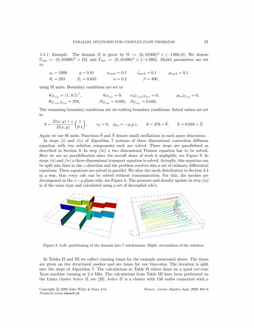
PARALLEL MULTIGRID FOR COMPLEX FLOW PROBLEMS 21
5.2.1. Example. The domain Ω is given by Ω := (0, 10 000)2 × (−1 000, 0). We denoteΓtop := (0, 10 000)2 × 0 and Γbot := (0, 10 000)2 × −1.000. Model parameters are setto
ρc = 1000 g = 9.81 κturb = 0.1 ζturb = 0.1 µturb = 0.1θc = 283 Sc = 0.035 α = 0.2 β = 400,
using SI units. Boundary conditions are set to
v|Γtop= (1, 0.1)>, v|Γbot
= 0, v3|Γtop∪Γbot= 0, phs|Γtop
= 0,θ|Γtop∪Γbot
= 278, S|Γtop= 0.035, S|Γbot
= 0.033.
The remaining boundary conditions are do-nothing boundary conditions. Initial values are setto
v =D(x, y) + z
D(x, y)
(1
0.1
), v3 = 0, phs = −ρcg z, θ = 278 + θ, S = 0.033 + S.
Again we use SI units. Functions θ and S denote small oscillations in each space dimension.In steps (i) and (iv) of Algorithm 7 systems of three dimensional convection diffusion
equation with two solution components each are solved. These steps are parallelized asdescribed in Section 3. In step (iii) a two dimensional Poisson equation has to be solved.Here we use no parallelization since the overall share of work is negligible, see Figure 9. Insteps (ii) and (iv) a three-dimensional transport equation is solved. Actually, this equation canbe split into lines in the z-direction and the problem resolves into a set of ordinary differentialequations. These equations are solved in parallel. We alter the mesh distribution in Section 3.4in a way, that every ode can be solved without communication. For this, the meshes aredecomposed in the x−y plane only, see Figure 8. The pressure and density update in step (vi)is of the same type and calculated using a set of decoupled ode’s.
Figure 8. Left: partitioning of the domain into 7 subdomains. Right: streamlines of the solution.
In Tables II and III we collect running times for the example mentioned above. The timesare given on two structured meshes and are times for one time-step. The iteration is splitinto the steps of Algorithm 7. The calculations in Table II where done on a quad oct-coreXeon machine running at 2.4 Mhz. The calculations from Table III have been performed onthe Linux cluster helics II, see [20]. helics II is a cluster with 156 nodes connected with a
Copyright c© 2009 John Wiley & Sons, Ltd. Numer. Linear Algebra Appl. 2009; 0:0–0Prepared using nlaauth.cls
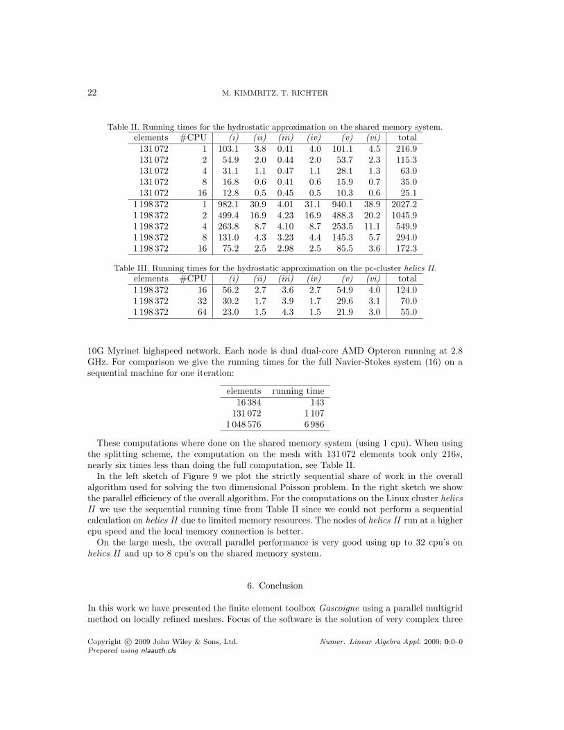
22 M. KIMMRITZ, T. RICHTER
Table II. Running times for the hydrostatic approximation on the shared memory system.
elements #CPU (i) (ii) (iii) (iv) (v) (vi) total131 072 1 103.1 3.8 0.41 4.0 101.1 4.5 216.9131 072 2 54.9 2.0 0.44 2.0 53.7 2.3 115.3131 072 4 31.1 1.1 0.47 1.1 28.1 1.3 63.0131 072 8 16.8 0.6 0.41 0.6 15.9 0.7 35.0131 072 16 12.8 0.5 0.45 0.5 10.3 0.6 25.1
1 198 372 1 982.1 30.9 4.01 31.1 940.1 38.9 2027.21 198 372 2 499.4 16.9 4.23 16.9 488.3 20.2 1045.91 198 372 4 263.8 8.7 4.10 8.7 253.5 11.1 549.91 198 372 8 131.0 4.3 3.23 4.4 145.3 5.7 294.01 198 372 16 75.2 2.5 2.98 2.5 85.5 3.6 172.3
Table III. Running times for the hydrostatic approximation on the pc-cluster helics II.
elements #CPU (i) (ii) (iii) (iv) (v) (vi) total1 198 372 16 56.2 2.7 3.6 2.7 54.9 4.0 124.01 198 372 32 30.2 1.7 3.9 1.7 29.6 3.1 70.01 198 372 64 23.0 1.5 4.3 1.5 21.9 3.0 55.0
10G Myrinet highspeed network. Each node is dual dual-core AMD Opteron running at 2.8GHz. For comparison we give the running times for the full Navier-Stokes system (16) on asequential machine for one iteration:
elements running time16 384 143
131 072 1 1071 048 576 6 986
These computations where done on the shared memory system (using 1 cpu). When usingthe splitting scheme, the computation on the mesh with 131 072 elements took only 216s,nearly six times less than doing the full computation, see Table II.
In the left sketch of Figure 9 we plot the strictly sequential share of work in the overallalgorithm used for solving the two dimensional Poisson problem. In the right sketch we showthe parallel efficiency of the overall algorithm. For the computations on the Linux cluster helicsII we use the sequential running time from Table II since we could not perform a sequentialcalculation on helics II due to limited memory resources. The nodes of helics II run at a highercpu speed and the local memory connection is better.
On the large mesh, the overall parallel performance is very good using up to 32 cpu’s onhelics II and up to 8 cpu’s on the shared memory system.
6. Conclusion
In this work we have presented the finite element toolbox Gascoigne using a parallel multigridmethod on locally refined meshes. Focus of the software is the solution of very complex three
Copyright c© 2009 John Wiley & Sons, Ltd. Numer. Linear Algebra Appl. 2009; 0:0–0Prepared using nlaauth.cls
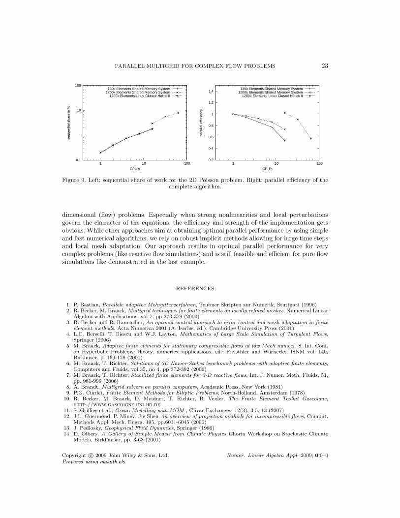
PARALLEL MULTIGRID FOR COMPLEX FLOW PROBLEMS 23
0.1
1
10
100
1 10 100
sequ
entia
l sha
re in
%
CPU’s
130k Elements Shared Memory System1200k Elements Shared Memory System
1200k Elements Linux Cluster Helics II
0.2
0.4
0.6
0.8
1
1.2
1.4
1 10 100
para
llel e
ffici
ency
CPU’s
130k Elements Shared Memory System1200k Elements Shared Memory System
1200k Elements Linux Cluster Helics II
Figure 9. Left: sequential share of work for the 2D Poisson problem. Right: parallel efficiency of thecomplete algorithm.
dimensional (flow) problems. Especially when strong nonlinearities and local perturbationsgovern the character of the equations, the efficiency and strength of the implementation getsobvious. While other approaches aim at obtaining optimal parallel performance by using simpleand fast numerical algorithms, we rely on robust implicit methods allowing for large time stepsand local mesh adaptation. Our approach results in optimal parallel performance for verycomplex problems (like reactive flow simulations) and is still feasible and efficient for pure flowsimulations like demonstrated in the last example.
REFERENCES
1. P. Bastian, Parallele adaptive Mehrgitterverfahren, Teubner Skripten zur Numerik, Stuttgart (1996)2. R. Becker, M. Braack, Multigrid techniques for finite elements on locally refined meshes, Numerical Linear
Algebra with Applications, vol 7, pp 373-379 (2000)3. R. Becker and R. Rannacher, An optimal control approach to error control and mesh adaptation in finite
element methods, Acta Numerica 2001 (A. Iserles, ed.), Cambridge University Press (2001)4. L.C. Berselli, T. Iliescu and W.J. Layton, Mathematics of Large Scale Simulation of Turbulent Flows,
Springer (2006)5. M. Braack, Adaptive finite elements for stationary compressible flows at low Mach number, 8. Int. Conf.
on Hyperbolic Problems: theory, numerics, applications, ed.: Freisthler and Warnecke, ISNM vol. 140,Birkhuser, p. 169-178 (2001)
6. M. Braack, T. Richter, Solutions of 3D Navier-Stokes benchmark problems with adaptive finite elements,Computers and Fluids, vol 35, no 4, pp 372-392 (2006)
7. M. Braack, T. Richter, Stabilized finite elements for 3-D reactive flows, Int. J. Numer. Meth. Fluids, 51,pp. 981-999 (2006)
8. A. Brandt, Multigrid solvers on parallel computers, Academic Press, New York (1981)9. P.G. Ciarlet, Finite Element Methods for Elliptic Problems, North-Holland, Amsterdam (1978)
10. R. Becker, M. Braack, D. Meidner, T. Richter, B. Vexler, The Finite Element Toolkit Gascoigne,http://www.gascoigne.uni-hd.de
11. S. Griffies et al., Ocean Modelling with MOM , Clivar Exchanges, 12(3), 3-5, 13 (2007)12. J.L. Guermond, P. Minev, Jie Shen An overview of projection methods for incompressible flows, Comput.
Methods Appl. Mech. Engrg. 195, pp.6011-6045 (2006)13. J. Pedlosky, Geophysical Fluid Dynamics, Springer (1986)14. D. Olbers, A Gallery of Simple Models from Climate Physics Chorin Workshop on Stochastic Climate
Models, Birkhauser, pp. 3-63 (2001)
Copyright c© 2009 John Wiley & Sons, Ltd. Numer. Linear Algebra Appl. 2009; 0:0–0Prepared using nlaauth.cls
24 M. KIMMRITZ, T. RICHTER
15. A. Prohl, Projection and Quasi-Compressibility Methods for Solving the Incompressible Navier-StokesEquations, B.G. Teubner Stuttgart (1997)
16. R. Rannacher, On Chorin’s projection method for the incompressible Navier-Stokes Equations, in TheNavier-Stokes Equations II - Theory and Numerical Methods, pp.167-183, Springer Berlin/Heidelberg(1992)
17. T. Richter, Parallel Multigrid Method for Adaptive Finite Elements with Application to 3D Flow Problems,Doctoral Dissertation, University of Heidelberg (2005)
18. B. Schupp, Entwicklung eines effizienten Verfahrens zur Simulation kompressibler Stromungen in 3D aufParallelrechnern, Doctoral Dissertation, University of Freiburg (1999)
19. C.A. Severijns, W. Hazeleger, The efficient global primitive equation climate model SPEEDO , Geosci.Model Dev. Discuss., 2. pp. 1115 - 1155 (2009)
20. Helics, HEidelberg LInux Cluster System II, http://helics.iwr.uni-heidelberg.de, 200721. J. Xu, Iterative methods by space decomposition and subspace correction, SIAM Review, vol 34, no 4, pp.
581 - 613 (1992)
Copyright c© 2009 John Wiley & Sons, Ltd. Numer. Linear Algebra Appl. 2009; 0:0–0Prepared using nlaauth.cls

C. Published and Submitted Articles
242
Index
Pe, Peclet numberhydrostatic, on a 2D mesh, 112on a 3D mesh, 114
Re, Peclet number, 23, 24local discrete, 72
Ha, advection space, 40discrete, 71
., 50∼, 502nd Dahlquist barrier, 191
A(α)-stability, 190|| · ||p,Ω, norm of Lp(Ω), 26|| · ||k,p,Ω, norm of Wk,p(Ω), 27| · |k,p,Ω, semi norm of Wk,p(Ω), 27|| · ||Ω, norm of L2(Ω), 27|| · ||k,Ω, norm of Hk(Ω), 27| · |k,Ω, semi norm of Hk(Ω), 27||| · |||ω, 59||| · |||, 67, 75, 106, 117(·, ·)Ω, scalar product in L2(Ω), 27(·, ·)Ω,k, scalar product in Hk(Ω), 27a, aspect ratio, 24A-stability, 190
BDFk schemes, 190BDFk-SEr scheme, 137BDF1-SE1, see Chorin-Temam schemeBDF1-SE1 scheme, 136BDF2-SE1
rotational, 137BDF2-SE2, 135, 199Bh, 67, 75, 106, 117Bωh , 59
boundaryΓb, 8Γs, 8
Γu, 8Γw, 8
C−, 190Chorin scheme, see Chorin-Temam schemeChorin-penalty scheme, 192, 193Chorin-Temam scheme, 134, 137, 194, 199Chorin-Uzawa scheme, 192coercive, 30Conjugate Gradient Scheme, 204consistency error, 137consistent splitting scheme
rotational, 195standard, 195
continuity equation, 14continuous, 30convergence, 137coordinate system condition, 91Crank-Nicolson scheme, 190csc,
see coordinate system condition91
Dahlquist equation, 190δij, Kronecker delta, 203d, depth function, 8, 26direct method, 204div′·, 2D divergence, 8div·, 3D divergence, 8divα·, anisotropic 3D divergence, 8dof, degree of freedom, 139domain
ω, 8, 26Ω, 8, 26Lipschitz, 26Cp– , 26flat, 8, 36
Ek, Ekman number, 24
243
INDEX
Ekman pumping, 175Ekman spiral, 169Ekman suction, 175Ekman transport, 168elliptic, 30Euclidean norm, 211Euclidean scalar product, 211Euler backward scheme, 135, 136, 190
fill-in, 208flops, 205
Galerkin approximation, 32Gauss-Seidel iteration, 206Generalized Holder Inequality, 31GMRES, 212∇′·, 2D gradient, 8∇·, 3D gradient, 8∇α·, anisotropic 3D gradient, 8grade(y), 210
hanging nodes, 49Helmholtz decomposition, 130Hodge decomposition, 130, 133
iac,see interior angle condition90
ILU factorization, 208ILU preconditioner, 208=(z) imaginary part of z ∈ C, 191inf-sup condition
2D, 56, 59hydrostatic, 68, 75, 107, 117, 127modified discrete, 56, 104modified, , 37common, 30
interior angle condition, 90interpolation operator
anisotropic, 90Clement, 52, 103point-wise, 52Scott-Zhang, 53, 69, 70, 108
Jacobi iteration, 206, 208Jacobi preconditioner, 208
Lagrangian multiplier, 29
∆′, 2D Laplacian , 8∆, 3D Laplacian , 8∆α·, anisotropic 3D Laplacian , 9Lebesgue
Lp0(Ω), 27Lp(Ω), Lebesgue space, 26linear iterative method
consistent, 206linear iterative method, 206linear iterative methods, 204LU factorization, 205
M, vertical integration operatorcontinuous, 9discrete, 54variational, 36
meas2(E), surface area of E, 89meas3(T ), volume of T , 89mesh, 49
admissible, 49anisotropic, 89Cartesian, 89K, quadrilateral (cell) of Kh, 49T , hexahedral (cell) of Th, 49e, edge of a cell, 49f , face of a cell, 49h, global mesh size, 50hω, global mesh size of Kh, 49hΩ, global mesh size of Th, 49horizontal anisotropic, 90isotropic, 50, 88Kh, 2D surface mesh, 49Th, 3D mesh, 49, 54x, node of a cell, 49patch, 50TK , prism of Th, 51reference element, 50–52, 202regular, 50shape-regular, 49vertical anisotropic, 89
δmin, 8, 26, 54T , 8
natural matrix norm, 206Nc, 203Nh, 203
244
INDEX
ODE, 34, 189
penalty constraint, 193Poincare – Friedrichs inequality, 27
generalized, 27preconditioning, 207pressure correction scheme
rotational, 132standard, 132
pressure corrector step, 132, 134–136, 192pressure prediction step, 145pressure predictor step, 132, 192, 195pressure update step, 145, 195, 199projection scheme, 131
Qh, discrete 2D pressure space, 52, 65, 66,72
QR factorization, 205Qr(K), 2D polynomials on K, 50Qr(T ), 3D polynomials on T , 51, 52
<(z) real part of z ∈ C, 190Richardson iteration, 204, 206Ro, Rossby number, 23, 24
saddle point problem, 29scale, 9
L, length scale, 9T , time scale, 9V , velocity scale, 9
Schur complement, 204Sobolev space
Wk,p(Ω), 27Hp(Ω), 27H1
0(Ω), 27W1,p
0 (Ω), 27W1,p
b (Ω), 27SOR, 206stabilization
Brezzi and Pitkaranta, 58, 112CIP, 58, 64, 73, 74, 112Douglas and Wang, 61GLS, 61LPS, 58, 63, 73, 74, 112, 115pressure projection, 58PSPG, 60
strong solutionglobal, 34local, 34
Symmetric SOR preconditioner, 208
TheoremBrouwer’s fixed point, 31De Rham, 31Gronwall, 34Lax Milgram, 30Picard - Lindelof, 34Rellich – Kondrachov, 32Riesz representation, 28Sobolev Embedding, 31
Uzawa algorithm, 203, 204, 207, 209
V, 3D velocity space, 54Van Kan scheme, 135–137, 199variable
diagnostic, 18state, 18
velocity correction schemerotational, 194standard, 194
velocity corrector step, 132, 134, 192, 193velocity predictor step, 132, 134–136, 144,
192, 195, 199velocity projection step, 193velocity update step, 145, 199Vh, discrete 3D velocity space, 52, 54, 65,
72
weak solutionglobal, 34local, 33
Wh, discrete 2D velocity space, 52, 66, 72
245

INDEX
246
Bibliography
[AC00] M. Ainsworth and P. Coggins. The stability of mixed hp-finite elementmethods for Stokes flow on high aspect ratio elements. SIAM J. Numer.Anal., 38:1721–1761, 2000.
[AF03] R.A. Adams and J.J. Fournier. Sobolev spaces. Pure and Apllied Mathe-matics. Academic Press, New York, 2003.
[AG94] C. Amrouche and V. Girault. Decomposition of Vector Spaces and Appli-cation to the Stokes problem in arbitrary dimension. Csechoslovak Math.Journ., 44(119):109 – 140, 1994.
[AG01] P. Azerad and F. Guillen Gonzalez. Mathematical justification of the hy-drostatic approximation in the primitive equations of geophysical fluid dy-namics. SIAM J. Math. Anal., 33(4):847 – 859, 2001.
[AL94] T. Apel and G. Lube. Local inequalities for anisotropic finite elements andtheir applications to convection-diffusion problems, 1994. Preprint SPC94-26, TU Chemnitz-Zwickau.
[AM08] Th. Apel and G. Matthies. Non-conforming, anisotropic, rectangular finiteelements of arbitrary order for the Stokes problem. SIAM J. Numer. Anal.,46:1867–1891, 2008.
[Ape98] Th. Apel. Anisotropic Interpolation Error Estimates for IsoparametricQuadrilateral Finite Elements, 1998.
[Ape99] Th. Apel. Anisotropic finite elements: local estimates and applications,1999.
[AR01] Thomas Apel and H. M. Randrianarivony. Stability of discretizations ofthe Stokes problem on anisotropic meshes, 2001.
[BB01] R. Becker and M. Braack. A finite element pressure gradient stabilizationfor the Stokes equations based on local projections. CALCOLO, 60(2):173– 199, 2001.
[BB02] R. Becker and M. Braack. Solution of a stationary benchmark problem fornatural convection with large temperature difference. Int. J. Therm. Sci.,41:428–439, 2002.
247
BIBLIOGRAPHY
[BB06] M. Braack and E. Burman. Local Projection Stabilization for the OseenProblem and its Interpretation as a Variational Multiscale Method. SIAMJ. Numer. Anal., 43:2544–2566, January 2006.
[BBC+94] R. Barrett, M. Berry, T. F. Chan, J. Demmel, J. Donato, J. Dongarra,V. Eijkhout, R. Pozo, C. Romine, and H. Van der Vorst. Templates forthe Solution of Linear Systems: Building Blocks for Iterative Methods, 2ndEdition. SIAM, Philadelphia, PA, 1994.
[BBJL07] M. Braack, E. Burman, V. John, and G. Lube. Stabilized finite elementmethods for the generalized Oseen problem. Comput. Methods Appl. Mech.Eng., 196:853 – 866, 2007.
[BC08] S. Badia and R. Codina. Algebraic pressure segregation methods for the in-compressible Navier-Stokes equations. Archives of Computational Methodsin Engineering, 15:343–369, 2008.
[Bec95] R. Becker. An Adaptive Finite Element Method for the IncompressibleNavier-Stokes Equations on Time-dependent Domains, 1995.
[BFH06] E. Burman, M.A. Fernandez, and P. Hansbo. Continuous Interior PenaltyFinite Element Method for Oseen’s Equations. SIAM J. Numer. Anal.,44:1248–1274, March 2006.
[BH06] E. Burman and P. Hansbo. Edge stabilization for the generalized Stokesproblem: a continuous interior penalty method. Comput. Methods Appl.Mech. Eng., 195(19-22):2393–2410, 2006.
[BL92] O. Besson and M.R. Laydi. Some estimates for the anisotropic Navier-Stokes equations and for the hydrostatic approximation. Math. Modellingand Num. Anal. 26, 7:855–865, 1992.
[BL09] M. Braack and G. Lube. Finite elements with local projection stabilizationfor incompressible flow problems. Journal of Comput. Math., 27(2-3):116 –147, 2009.
[Bla07] Jordi Blasco. An anisotropic pressure-stabilized finite element method forincompressible flow problems. Computers and Mathematics with Applica-tions, 53(6):895 – 909, 2007.
[Bla08] Jordi Blasco. An anisotropic gls-stabilized finite element method for in-compressible flow problems. Comput. Meth. Appl. Mesh. Engrg., 197:3712– 3723, 2008.
[BMP+06] Barnier B., G. Madec, T. Penduff, J.-M. Molines, A.-M. Treguier, J. LeSommer, A. Beckmann, A. Biastoch, C. Boning, J. Dengg, C. Derval,E. Durand, S. Gulev, E. Remy, C. Talandier, S. Theetten, M. Maltrud,J. McClean, and B. De Cuevas. Impact of partial steps and momentum
248
BIBLIOGRAPHY
advection schemes in a global ocean circulation model at eddy permittingresolution. Ocean Dynamics, 4, 2006.
[BP84] F. Brezzi and J. Pitkaranta. On the stabilization of finite element approxi-mations of the Stokes equations. W. Hackbusch (ed.), Notes on NumericalFluid Mechanics: Efficient Solutions of Elliptic Systems, 10, 1984.
[BR01] R. Becker and R. Rannacher. An optimal control approach to error controland mesh adaptation in finite element methods. Acta Numerica 2001 (A.Iserles, ed.), Cambridge University Press, 2001.
[Bra06] M. Braack. Anisotropic H1-stable projections on quadrilateral meshes. Enu-math 2005 Proc., eds.: Bermudez de Castro et al., Springer, pages 495–503,2006.
[Bra07] D. Braess. Finite elements. Theory, fast solvers and applications in solidmechanics. Cambridge: Cambridge University Press, 2007.
[Bra08a] M. Braack. A stabilized finite element scheme for the Navier-Stokes equa-tions on quadrilateral anisotropic meshes. ESAIM: Mathematical Modellingand Numerical Analysis, pages 903–924, 2008.
[Bra08b] M. Braack. Local Projection Stabilization for the Oseen System onAnisotropic Cartesian Meshes. Springer Heidelberg, pages 441 – 448, 2008.
[BS11] M. Braack and F. Schieweck. Equal-order fininte elements with local pro-jection stabilization for the Darcy-Brinkman equations. Comp. Meth. Appl.Mech. Eng., 200:1126 – 1136, 2011.
[BSLB12] E. Behrens, F. U. Schwarzkopf, J. F. Lubbecke, and C. W. Boning. Modelsimulations on the long-term dispersal of 137 Cs released into the PacificOcean off Fukushima. Environmental Research Letters, 7(3):034004, 2012.
[BT06a] M. Braack and T.Richter. Local projection stabilization for the Stokessystem on anisotropic quadrilateral meshes. Enumath Proc. 2005, eds.:Bermudez de Castro et al., Springer, 27(2-3):770 – 778, 2006.
[BT06b] M. Braack and T.Richter. Stabilized finite element for 3D reactive flows.Intern. Journal for Numerical Methods in Fluids, 51, Issue 9-10:981 – 999,2006.
[Car86] D. Carlson. What are Schur Complements, Anyway? Linear Algebra andits Applications, 74(0):257 – 275, 1986.
[Cat61] L Cattabriga. Su un problema al contoro relativo al sistema di equazionidi Stokes. Rend. Sem. Mat. Univ. Padova, 31:308–340, 1961.
249
BIBLIOGRAPHY
[CG00] T. Chacon Rebollo and F. Guillen Gonzalez. An intrinsic analysis of exis-tence of solutions for the hydrostatic approximation of Navier-Stokes equa-tions. Comptes Rendus de l’Academie des Sciences - Series I - Mathematics,330(9):841 – 846, 2000.
[CGS12] T. Chacon Rebollo, M. Gomez Marmol, and I. Sanchez Munoz. Numericalsolution of the Primitive Equations of the ocean by the Orthogonal Sub-Scales VMS method. Applied Numerical Mathematics, 62(4):342 – 359,2012. Third Chilean Workshop on Numerical Analysis of Partial DifferentialEquations (WONAPDE 2010).
[Cha] T. Chacon Rebollo. Numerical Approximation of Hydrodynamic Geophys-ical Flows.
[Cho68] A.J. Chorin. Numerical Solution of the Navier-Stokes Equations. Mathe-matics of Computation, 22(104):pp. 745–762, 1968.
[CLC00] T. Chacon Rebollo, R. Lewandowski, and E. Chacon Vera. Analy-sis of the hydrostatic approximation in oceanography with compressionterm. ESAIM: Mathematical Modelling and Numerical Analysis, 34:525–537, 2000.
[Con95] P. Constantin. A few results and open problems regarding incompressiblefluids. Notices Amer. Math. Soc., 42:658–663, 1995.
[CR02] T. Chacon Rebollo and D. Rodriguez Gomez. Prismatic finite element so-lution of the primitive equations of the ocean. Cours CEA-EDF-INRIAProblemes Non Lineaires Appliques Ecoulements peu profond a surface li-bre, 2002.
[CR04] T. Chacon Rebollo and D. Rodriguez Gomez. Numerical investigation of theregularity of the pressure for the primitve equations of the ocean. Comput.Methods Appl. Mech. Engrg., 193:4457–4474, 2004.
[CRB11] B. Cushman-Roisin and J.-M. Beckers. Introduction to Geophysical FluidDynamics. Physical and Numerical Aspects. Academic Press, 2011.
[CRM03] C.Hu, R.Temam, and M.Ziane. The primitive equations on the large scaleocean under the small depth hypothesis. Discrete and Contin. Dynam.Systems 9, 1:97–131, 2003.
[CT07] C. Cao and E. Titi. Global Well-Posedness of 3D Primitive Equations.Ann. Math. 166, 1:245–267, 2007.
[CT08] C. Cao and E. Titi. Regularity Criteria for the three-dimensional Navier–Stokes Equations. Indiana Univers. Mathem. J., 57(6):2643–2661, 2008.
[DB04] C. R. Dohrmann and P. B. Bochev. A stabilized finite element method forthe Stokes problem based on polynomial pressure projections. InternationalJournal for Numerical Methods in Fluids, 46:183 – 201, 2004.
250
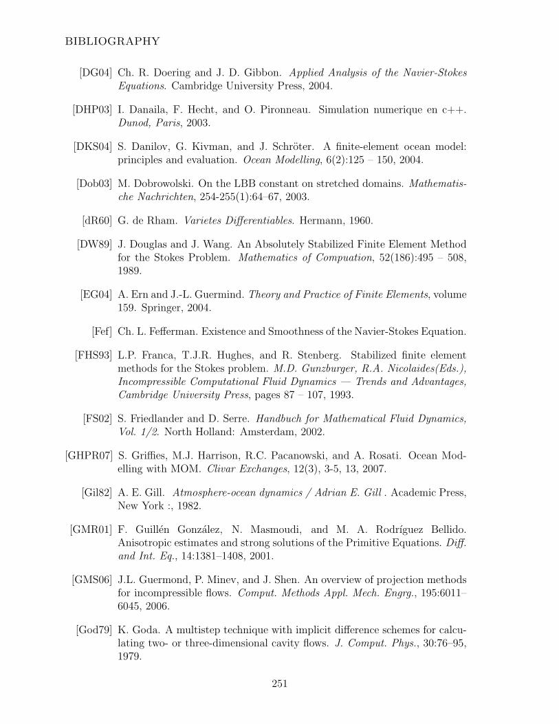
BIBLIOGRAPHY
[DG04] Ch. R. Doering and J. D. Gibbon. Applied Analysis of the Navier-StokesEquations. Cambridge University Press, 2004.
[DHP03] I. Danaila, F. Hecht, and O. Pironneau. Simulation numerique en c++.Dunod, Paris, 2003.
[DKS04] S. Danilov, G. Kivman, and J. Schroter. A finite-element ocean model:principles and evaluation. Ocean Modelling, 6(2):125 – 150, 2004.
[Dob03] M. Dobrowolski. On the LBB constant on stretched domains. Mathematis-che Nachrichten, 254-255(1):64–67, 2003.
[dR60] G. de Rham. Varietes Differentiables. Hermann, 1960.
[DW89] J. Douglas and J. Wang. An Absolutely Stabilized Finite Element Methodfor the Stokes Problem. Mathematics of Compuation, 52(186):495 – 508,1989.
[EG04] A. Ern and J.-L. Guermind. Theory and Practice of Finite Elements, volume159. Springer, 2004.
[Fef] Ch. L. Fefferman. Existence and Smoothness of the Navier-Stokes Equation.
[FHS93] L.P. Franca, T.J.R. Hughes, and R. Stenberg. Stabilized finite elementmethods for the Stokes problem. M.D. Gunzburger, R.A. Nicolaides(Eds.),Incompressible Computational Fluid Dynamics — Trends and Advantages,Cambridge University Press, pages 87 – 107, 1993.
[FS02] S. Friedlander and D. Serre. Handbuch for Mathematical Fluid Dynamics,Vol. 1/2. North Holland: Amsterdam, 2002.
[GHPR07] S. Griffies, M.J. Harrison, R.C. Pacanowski, and A. Rosati. Ocean Mod-elling with MOM. Clivar Exchanges, 12(3), 3-5, 13, 2007.
[Gil82] A. E. Gill. Atmosphere-ocean dynamics / Adrian E. Gill . Academic Press,New York :, 1982.
[GMR01] F. Guillen Gonzalez, N. Masmoudi, and M. A. Rodrıguez Bellido.Anisotropic estimates and strong solutions of the Primitive Equations. Diff.and Int. Eq., 14:1381–1408, 2001.
[GMS06] J.L. Guermond, P. Minev, and J. Shen. An overview of projection methodsfor incompressible flows. Comput. Methods Appl. Mech. Engrg., 195:6011–6045, 2006.
[God79] K. Goda. A multistep technique with implicit difference schemes for calcu-lating two- or three-dimensional cavity flows. J. Comput. Phys., 30:76–95,1979.
251
BIBLIOGRAPHY
[GR86] V. Girault and P.-A. Raviart. Finite Elements for the Navier Stokes Equa-tions. Springer Berlin, 1986.
[GR02] F. Guillen Gonzalez and M.A. Rodrıguez Bellido. On the strong solutionsof the 2D Primitive Equations problem. Nonlinear Analysis, 50:621–646,2002.
[GR04] F. Guillen Gonzalez and M.A. Rodrıguez Bellido. On the uniqueness andregularity of the Primitive Equations imposing additional anisotropic reg-ularity. Applied Mathematics Letters, 18:783 – 789, 2004.
[GR05a] F. Guillen Gonzalez and M.A. Rodrıguez Bellido. A review on the improvedregularity for the Primitive Equations. Banach Center Publications, 70:85– 103, 2005.
[GR05b] F. Guillen Gonzalez and D. Rodrıguez Gomez. Bubble finite elements forthe primitive equations of the ocean. Numer. Math, 2005.
[GS03a] J. L. Guermond and J. Shen. A new class of truly consistent splittingschemes for incompressible flows. J. Comput. Phys., 192:262–276, 2003.
[GS03b] J. L. Guermond and J. Shen. Velocity-correction projectin methods forincompressible flows. SIAM J. Numer. Anal., 41(1):112–134, 2003.
[GS04] J. L. Guermond and J. Shen. On the error estimates for the rotationalpressure-correction projection methods. Math. Comput., 73(248):1719–1737, 2004.
[Gue99] J. L. Guermond. Un resultat de convergence d’ordre deux en temps pourl’approximation des equations de Navier-Stokes par une technique de pro-jection incrementale. M2AN Math. Model. Numer. Anal., 30(1):169–189,1999.
[Hac93] W. Hackbusch. Iterative Losung grosser schwachbesetzter Gleichungssys-teme. Teubner Verlag, 1993.
[Har02] Ph. Hartmann. Ordinary Differential Equations. Society for Industr. andAppl. Math., 2002.
[Her01] M. Hermann. Numerische Mathematik. Oldenbourg, 2001.
[HFB86] T. Hughes, L. Franca, and M. Balestra. A new finite element formula-tion for computational fluid dynamics: V. circumvent the Babuska-Brezzicondition: A stable Petrov-Galerkin formulation for the Stokes problemaccommodating equal order interpolation. Comput. Methods Appl. Mech.Engrg., 59:89–99, 1986.
[HK00] P. Hajlasz and P. Koskela. Sobolev met Poincare. Number 688. Memoirs ofthe American Mathematical Society, 2000.
252
BIBLIOGRAPHY
[HR82] J.G. Heywood and R. Rannacher. Finite element approximation of thenonstationary Navier-Stokes problem. I. Regularity of solutions and sec-ond order error estimates for statial discretization. SIAM J. Num. Anal.,19:275–311, 1982.
[Ist01] I.V. Istratescu. Fixed Point Theory: An Introduction. D. Reidel PublichingCompany, 2001.
[JM86] J.-M.Ghidalaglia. On the fractal dimension of attractors for viscous incom-pressible fluid flows. SIAM J. Math. Anal., 17(5):1139–1157, 1986.
[Jos98] J. Jost. Partielle Differentialgleichungen: Elliptische (und parabolische)Gleichungen. Springer, 1998.
[KB12] M. Kimmritz and M. Braack. Equal-order finite elements for the hydrostaticStokes problem. Computational Methods in Applied Mathematics, 12:306–329, 2012.
[Kim12] M. Kimmritz. Symmetric Stabilization of Equal-Order Finite Element Dis-cretized Hydrostatic Flow Problems. submitted, 2012.
[KOI91] G.E. Karniadakis, S.A. Orszag, and M. Israeli. High-order splitting methodsfor the incompressible Navier-Stokes equations. J. Comput. Phys., 97:414–43, 1991.
[KR11] M. Kimmritz and Th. Richter. Parallel multigrid method for finite elementsimulations of complex flow problems on locally refined meshes. NumericalLinear Algebra with Applications, 18(4):615–636, 2011.
[Lad69] O.A. Ladyzhenskaya. Mathematical Theory of Viscous Incompressible Flow.Gordon and Breach, New York, 2nd, english translation edition, 1969.
[LAK06] G. Lube, Th. Apel, and T. Knopp. Stabilized Finite Element Methods withAnisotropic Mesh Refinement for the Oseen problem. Int. Conference onBoundary and Interior Layers BAIL, 2006.
[Lat11] Mojib Latif. Uncertainty in climate change projections. Journal of Geo-chemical Exploration, 110: Sustainability of Geochemical Cycling, 19th In-ternational Symposium on Environmental Biogeochemistry ”EnvironmentalChanges and Sustainability of Biogeochemical Cycling”(1):1–7, 2011.
[LBC+98] S. Levitus, T.P. Boyer, M.E. Conkright, T. O’ Brien, C. StephensJ. Antonov and, L. Stathoplos, D. Johnson, and R. Gelfeld. NOAA At-las NESDIS 18, World Ocean Database 1998: VOLUME 1: INTRODUC-TION. U.S. Gov. Printing Office, Wash., D.C., 1998.
[Ler33] J. Leray. Etude de diverses quations intgrales non linaires et de quelquesproblmes que pose l’hydrodynamique. J. Math. Pures Appl., 12:1–82, 1933.
253
BIBLIOGRAPHY
[LQ86] U. Langer and W. Queck. On the convergence factor of Uzawa’s algorithm.Journal of Computational and Applied Mathematics, 15(2):191 – 202, 1986.
[LR02] P.G. Lemarie-Rieusset. Recent Developments in the Navier-Stoeks problem.Chapman & Hall, 2002.
[LTW92] J.L. Lions, R. Temam, and S. Wang. On the equations of the large scaleocean. Nonlinearity, 5:1007–1053, 1992.
[Mei11] A. Meister. Numerik linearer Gleichungssysteme: Eine Einfuhrung in mod-erne Verfahren. Vieweg + Teubner Verlag, 4 edition, 2011.
[MPP02] St. Micheletti, S. Perotto, and M. Picasso. Some remarks on the stabilitycoefficients and bubble stabilization of FEM on anisotropic meshes, 2002.
[MS02] P. Ming and Z.-C. Shi. Quadrilateral mesh revisited. Comput. MethodsAppl. Mech. Engrg., 191:5671–5682, 2002.
[MSB+04] J. M. Murphy, D. M. H. Sexton, D. N. Barnett, G. S. Jones, M. J. Webb,M. Collins, and D. A. Stainforth. Quantification of modelling uncertaintiesin a large ensemble of climate change simulations. Nature, 430:768 – 772,2004.
[MST07] G. Matthies, P. Skrzypacz, and L. Tobiska. A unified convergence analysisfor local projection stabilizations applied to the Oseen problem. M2ANMath. Model. Numer. Anal., 41:713–742, 2007.
[NP05] R.H. Nochetto and J.-H. Pyo. The Gauge-Uzawa Finite Element Method.Part I: The Navier-Stokes Equations. SIAM J. Numer. Anal., 43:1043–1068,March 2005.
[Oue81] D. V. Ouellette. Schur complements and statistics. Linear Algebra and itsApplications, 36(0):187 – 295, 1981.
[OWE12] D. Olbers, J. Willebrand, and C. Eden. Ocean Dynamics. Springer, 2012.
[Ped86] J. Pedlosky. Geophysical Fluid Dynamics. Springer, 1986.
[Pet65] W.V. Petryshyn. Constructional proof of Lax-Milgram Lemma and ItsApplication to Non-K-P.D. Abstract and Differential Operator Equations.J.SIAM Numer. Anal. Ser. B, 2(3):404 – 420, 1965.
[Pro97] A. Prohl. Projection and Quasi-Compressibility Methods for Solving theIncompressible Navier-Stokes Equations. B.G. Teubner Stuttgart, 1997.
[Pro08] Andreas Prohl. On Pressure Approximation via Projection Methods forNonstationary Incompressible Navier-Stokes Equations. SIAM J. Numer.Anal., 47(1):158–180, October 2008.
254
BIBLIOGRAPHY
[PTW04] M. Petcu, R. Temam, and D. Wirosoetisno. Existence and regularity resultsfor the primitive equations in two space dimensions. Communications onPure and Applied Analysis (CPAA), 3:115 – 131, 2004.
[Ran92] R. Rannacher. On Chorin’s projection method for the incompressibleNavier-Stokes Equations. The Navier-Stokes Equations II - Theory andNumerical Methods, Springer Berlin/Heidelberg, pages 167 – 183, 1992.
[Ric05] T. Richter. Parallel Multigrid Method for Adaptive Finite Elements withApplication to 3D Flow Problems. Doctoral Dissertation, University ofHeidelberg, 2005.
[RJ08] T. Reichler and K. Junsu. How Well Do Coupled Models Simulate Today’sClimate? Bulletin of the American Meteorological Society, 89(3):303–311,03/2008 2008.
[RST08] H.-G. Roos, M. Stynes, and L. Tobiska. Robust Numerical Methods for Sin-gularly Perturbed Differential Equations – Convection-Diffusion-Reactionand Flow Problems, volume 24. Springer Series in Computational Mathe-matics, 2nd edition, 2008.
[Saa03] Y. Saad. Iterative methods for sparse linear systems. SIAM, 2003.
[Sca67] H. Scarf. The Approximation of Fixed Points of a Continuous Mapping.SIAM J. Appl. Math., 15(5):1328 – 1343, 1967.
[SDT06] P. Sagaut, S. Deck, and M. Terracol. Multiscale and Multiresolution Ap-proaches in Turbulence. Imperial College Press, 2006.
[Ser63] J. Serrin. The initial value problem for the Navier-Stokes equations. Non-linear Problems, R.E. Langer ed., pages 69–98, 1963.
[SH09] C.A. Severijns and W. Hazeleger. The efficient global primitive equationclimate model SPEEDO. Geosci. Model Dev. Discuss., 2:1115 – 1155, 2009.
[She92] J. Shen. On error estimates of the projection methods for the Navier-Stokesequations: first-order schemes. SIAM J. Numer. Anal, 29:57–77, 1992.
[She96] J. Shen. On error estimates of the projection methods for the Navier-Stokesequations: second-order schemes. Math. Comp., 65(215):1039 – 1065, 1996.
[Sma63] J. Smagorinsky. General circulation experiments with the primitive equa-tions. i. the basic experiment. Mon. Wea. Rev., 91:99 – 164, 1963.
[Soh01] H. Sohr. The Navier-Stokes equations. An Elementary Functional AnalyticApproach. Birkhauser Verlag, Basel, 2001.
[Sol68] V.A. Solonnikov. Estimates for solutions of a non-stationary linearizedsystem of Navier-Stokes equations. A.M.S. Translations, 75:1–116, 1968.
255
BIBLIOGRAPHY
[Son09] T. Sonar. Turbulenzen um die Fluidmeshanik. Spektrum der WissenschaftVerlagsgesellschaft mbH, 2009.
[SS98] D. Schotzau and C. Schwab. Mixed hp-FEM on anisotropic meshes. Math.Models Methods Appl. Sci., 8:787–820, 1998.
[SSS99] D. Schotzau, C. Schwab, and R. Stenberg. Mixed hp-FEM on anisotropicmeshes II: Hanging nodes and tensor products of boundary layer meshes.Numer. Math., 83:667 – 697, 1999.
[Tem68] R. Temam. Une methode d’approximation de la solution des equations deNavier-Stokes. Bulletin de la S.M.F., 96:115–152, 1968.
[Tem69] R. Temam. Sur L’approximation de la solution des equations de Navier-Stokes par la methode des pas fractionaires ii. Arch. Rat. Mech. Anal.,33:377–385, 1969.
[Tem79] R. Temam. Navier-Stokes Equations. Theory and Numerical Analysis.North Holland, 1979.
[Tem00] R. Temam. Some developments on Navier-Stokes equations in the sec-ond half of the 20th century. Development of Mathematics 1950-2000,Birkhauser, Basel, pages 1049–1106, 2000.
[TMV96] L.J.P. Timmermans, P.D. Minev, and F.N. Van De Vosse. An approximateprojection scheme for incompressible flow using spectral elements. Int. J.Numer. Methods Fluids, 22:673–688, 1996.
[TS01] A. Toselli and C. Schwab. Mixed hp-finite element approximations on geo-metric edge and boundary layer meshes in three dimensions. SAM Report2001-02, ETH Zurich, 2001.
[Ver00] F. Verhulst. Nonlinear Differential Equations and Dynamical Systems.Springer, 2000.
[vK86] J. van Kan. A second-order accurate pressure-correction scheme for viscousincompressible flow. SIAM J. Sci. Stat. Comput., 7:870–891, 1986.
[Wan10] K. Wannert. Stabilie Algorithmem fur die Magnetotomographi anBrennstoffzellen. Forschumszentrum Julich, 2010.
[WCd+11] M. Wade, G. Caniaux, Y. duPenhoat, M. Dengler, H. Giordani, andR. Hummels. A one-dimensional modeling study of the diurnal cycle in theequatorial Atlantic at the PIRATA buoys during the EGEE-3 campaign.Ocean Dynamics, 61:1–20, 2011.
[Wer05] D. Werner. Funktionalanalysis. Springer, 5th, extended edition, 2005.
[Yos80] K. Yoshida. Functional Analysis. Springer, 1980.
256
BIBLIOGRAPHY
[Zia95] M. Ziane. Regularity results for Stokes type systems. Applicable Analysis,58:263–292, 1995.
[Zia97] M. Ziane. Regularity results for the stationary primitive equations of theatmosphere and the ocean. Nonlinear Anal., 28(2):289–313, January 1997.
257
Acknowledgements
This work has partially been supported by the DFG Excellence Cluster ”Future Ocean”within the mini-proposal CP0721.
First of all I’d like to thank Prof. Dr. Malte Braack for the possibility to work on thisinteresting topic belonging to the challenging field of climate research, as well as forenabling the participations in conferences in Kiel and abroad, not forgetting for theassured financing throughout the entire time. Regarding the financial support I’d liketo mention the great opportunity to give lessons in different fields of mathematics.
Further, I’d like express deep gratidute to Thomas Richter for always being welcomewith my questions, the engaged answering of those, and the reading of my manuscript.
As well, my thanks are addressed to Prof. Dr. Steffen Borm for helpful discussionsand to his team for the possibility to participate in students research activities takingplace in this group.
Moreover, I’d like to thank Benjamin and Nico for the possibility of discussions.
The numerical examples have been implemented using the software library gascoigne.Thanks to Malte Braack, Roland Becker, Dominik Meidner, Thomas Richter and BorisVexler for development, maintenance and enabling the work with this library.
Thomas Apel, Francisco Guillen, Isabel Munoz and Edriss Titi are thanked for thewilling answering of my inquiries. I’d moreover like to thank Dudley Chelton for thekind permission to use his figure on the scales of oceanic processes.
For their great offering of the vast variety of courses not only concerning the oceanicissue I’d like to thank the organizors of the Integrated School of Ocean Sciences (ISOS).
In addition, I heartly thank the team of ”Ocean circulation and climate dynamics” atthe IfM Geomar for always being a welcome guest. In particular, I express my gratitudeto Erik Behrens for lots of talks on physical issues, for the enduring answering myquestions and for reading the physical concerns of this work.
For well-meaningness and carefree talks, also in stressing times, I’d like to thank Martinand Stephan. As well, my thanks are addressed to Ulrike Zander for the brighteninglittle somethings.
Enabling nice times beside university I’d like to thank Petra for the nice coffee breaks,Gerhard for being there, anytime, Franziska and Erik inter alia for the refreshingmornings, Thorsten and Frank for the refreshing evenings, Olav for the enlightning ina dark moment, Daniel for the encouragements, as well as the Uni BigBand Kiel fortheir colorful notes. Claudia, Thomas, Stef, Barbara and Andre I would like to thankfor being friends and family.Last but not least, I heartfelty thank Tom and Doreen Rother for their inspirings,confidences and lots more.
Eidesstattliche Erklarung
Hiermit bestatige ich, dass die Abhandlung - abgesehen von der Beratung durch denBetreuer Prof. Dr. M. Braack - nach Form und Inhalt meine eigene Arbeit ist.
Die vorliegende Arbeit hat keiner anderen Stelle im Rahmen eines Prufungsverfahrensvorgelegen. Teile der Arbeit sind wie folgt veroffentlicht beziehungsweise eingereicht:
• Equal-order finite elements for the hydrostatic Stokes problemAutoren: Madlen Kimmritz, Malte BraackJournal: Computational Methods in Applied Mathematics 12(3)Jahr: 2012 (veroffentlicht)
• Parallel multigrid method for finite element simulations of complex flow problemson locally refined meshesAutoren: Madlen Kimmritz, Thomas RichterJournal: Numerical Linear Algebra with Applications 18 (4)Jahr: 2011 (veroffentlicht)
• Symmetric Stabilization of Equal-Order Finite Element Discretized HydrostaticFlow ProblemsAutor: Madlen KimmritzJournal: Computer Methods in Applied Mechanics and Engineering(eingereicht)
Die vorliegende Arbeit ist unter Einhaltung der Regeln guter wissenschaftlicher Praxisder Deutschen Forschungsgemeinschaft entstanden.
Ort, Datum Madlen Kimmritz


![[7] Equal Employment and Child Welfare](https://img.pdfslide.net/doc/110x75/6319c020c51d6b41aa048bc4/7-equal-employment-and-child-welfare.jpg)


