Equalization and Fiscal Competition: Theoryand Evidence

Leonzio RizzoSTICERD-LSE, Houghton Street, London WC2A 2AE,University of Ferrara, Ferrara Corso Ercole I d�Este, 44

andCatholic University of Milan, Largo Gemelli 1, Milano

l.rizzo@lse.ac.uk

5 May 2001

Abstract

We develop a model with two countries, producing two goods: onemobile and the other not. The mobile good is taxed according to theorigin principle. People decide to buy the good where the price is moreconvenient for them. The two countries engage in Þscal competition. Theintroduction of an equalization transfer decreases the Þscal externality dueto the tax-base mobility: some of the lost tax �comes back�. We test thetheoretical results by using tax data from Canada, where an equalizationtransfer holds, and United States. We Þnd that tax-competition is lowerbetween canadian provinces, than between a canadian province and a USstate.

Keywords: Þscal competition, equalization, transfer, externality, tax-rate.

JEL classification: H21, H23.

1

1 Introduction1

Fiscal decentralization is normally justiÞed by two factors. Firstly, local taxesreßect citizens� preferences much more than central taxes. Secondly, the man-agement of local public expenditure would be more efficient than it would be iftaxes were centralized.However, in a federation the geographical subset, where regional Government

taxes, can not coincide with the subset where the tax-base of the residents ofeach region is distributed. In this case with free mobility of persons, goods andcapital each region Þxes its tax rate without taking into account the beneÞtsin revenue and/or social welfare to the other regions (Mintz and Tulkens 1986;Wilson, 1991; Wildasin, 1988; Kanbur and Keen 1993).Normally transfers are needed to avoid these inefficiencies (Wildasin1991;

Dahlby, 1996). This is a key issue inside the European Community. In factthe CockÞeld White Paper (Commission, 1985) and subsequent Commissionproposals recommended with the implementation of a VAT origin system (whichshould symplify a lot the life to the traders because they would deal with onlyone Þscal administration) the adoptions of two important measures to avoidthe Þscal administrations to lose revenue and indeed starting competing bydecreasing their tax-rates: harmonization of the tax rates and a clearing housemechanism.The approval of a clearing mechanism would ensure each nationhas the same revenue it would have in a destination system. Moreover it shouldeliminate the incentive for each nation to decrease its taxes. This last statementis what the Coase theorem forecasts: the welfare of an inefficient equilibrium canbe improved by using appropriate side payments. Is this working in a federationwhere states compete by Þxing taxes?In the paper we test the efficacy in welfare terms of a transfer system by

looking at a particular federal reality: Canada, where an equalization systemamong the provinces holds. According to this transfer system each provincereceives (gives) a quota of its revenue, according to an equalization rate if itstax-base is lower (higher) than a standard tax-base.In the theoretical part we suppose to deal with a federation where the en-

forcement problem of the transfer has already been solved (Bordignon et al.2000;Dhillon et al. 1999): each country reveals its true type in its tax-rate decisionand the transfer has already been optimally designed (Dahlby and Wilson, 1994;Dahlby, 1996; Boadway and Keen, 1996). We analyse the welfare properties ofan equalization transfer, based on differences on Þscal capacities, and show thatit is equivalent to a compensation transfer. The intuition is the following: ifcountry j loses a quota of its tax-base bacause some other country decreases itstax, with an equalization mechanism country j recovers part of it because thereceived (given) transfer will be higher (lower) than it was before the mentioned

1 I wish to thank Tim Besley, Valentino Larcinese, Imran Rasul and all the participants tothe EOPP-STICERD seminar, PET conference (the Second International Conference of theAssociation of Public Economic Theory - Warwick 2000) and to seminars at IFS (23 February2001), University of Ferrara and Catholic University of Milan for helpful comments. The usualdisclaimer applies.

2

change.We highlight the process which leads the equalization transfer to improve the

efficiency of a federal Þscal system, by using a simple model with two countries,producing one good. The good is taxed according to the origin principle. So thetax-base can move from one country to the other according to the advantageof the consumers, which, given the production price, is determined by the tax-decision of the Þscal authorities and a transport or transaction cost. The reasonof the tax-base mobility can be twofold: Þrst people, given a tax-differential,can cross the border and buy elsewhere the product, second tax-differentials canincentivate smuggling from the low tax-country to the high-tax country. Thisis equivalent in terms of loss in revenue for the high-tax country to a cross-border shopping phenomenon. This situation, if we assume that the prevailingeffect determining the externality level is the public consumption effect (Mintz,Tulkens, 1986; Kanbur and Keen, 1993), leads to too low tax rates with respectto a Pareto-optimal tax decision. We show that, by inserting an equalizationtransfer based on Þscal capacity, one of the determinants of the coefficient of thetax best reply function, given the tax rate of the other country, is lower thanin the case without the transfer. This means that the level of tax-competitiondecreases.This result has been tested by using data of two federal countries: Canada

and United States. The reason for the choice of Canada and United States isthat both are federal countries where each province or state has decision poweron taxes, especially on sales taxes or speciÞc taxes on goods. Moreover in USthere is no equalization system among the states, Canada has an equalizationsystem based on Þscal capacity. In Canada the transfer is calculated for 30types of taxes. We test the theoretical model by using sales taxes and cigarettesspeciÞc taxes for the period 1984-1994. The test looks at how a Canadianprovince replies to a tax-change of a neighbouring province/state, accordingto the nation (Canada or US) the neighbouring province/state belongs. Thetheoretical intuition is conÞrmed by the empirical test: in fact a change in taxrate of the Canadian provinces is inßuenced more by a change in tax-rate of aUS neighboring state, than by a change in tax-rate of a Canadian neighbouringprovince. The reason of that is the following. If a Canadian province losestaxes because a neighboring Canadian province decreases its tax-rate, some ofthe lost tax �comes back� because of the equalization transfer. If a Canadianprovince loses taxes because a neighbouring US state decreases its tax-rate, theCanadian province will not recover anything because no equalization systemholds. Indeed it will react more heavily if the change in tax-rate is coming froma US neighboring state than if it is coming from a Canadian province.It is interesting to notice that this can be thought as a test of the �Coase

Theorem�. Each province, in fact, is given a transfer, which in the theoreticalpart is shown to be partially equivalent to a compensation transfer, linked tothe difference between its tax-base and a Canadian standard tax-base. Weshow that this transfer inßuences the negative Þscal externality, related to theinterprovincial tax-base mobility, but not the negative externality related to theinternational tax-base mobility.

3

It is interesting to note that in the speciÞc geographical area we have chosenthe way how provinces and/or states relates in their tax-decisions on cigarettesseems to be quite important according to the last report of the World Health Or-ganization (1999) on tobacco control. The report put the attention on the factthat �differential in the price of tobacco products among neighbouring countriesmay lead to both casual cross-border shopping and illegal bootlegging. Cross-border sales may even occur within countries, such as Canada and United States,given the intracountry price differences among Canadian provinces and stateswithin the United States�. If the states and/or provinces are aware of that,they will choose their tax-rates by looking at the nighbouring choice. This iswhat seems to be happened between the 80�s and 90�s when the cigarettes smug-gling between the States and Canada became a huger and huger problem andculminates with the �92-94 smuggling crises�. Smugglers proÞt of the differ-ence in sales and cigarettes taxes among provinces. �Cigarettes are smuggledfrom ...Alberta to British Columbia....by road through mail order operators, bycommercial couriers and airline baggage� (The Globe and Mail, July 28, 1997).Inspector Ferguson of the RCMP�s economic crime unit in British Columbiadeclared in an interview (The Globe and Mail, July 28, 1997) in 1997: �Inter-provincial smuggling is costing millions and millions of dollars in lost taxes. It�sa huge problem. People don�t realize how serious it is.� Similar problems aresupposed to hold among other provinces. Difference in cigarettes tax amongbordering provinces sometimes is really huge. Take for example the westernpart of the country: in 92 Newfoundland has a tax per pack which is more thanhalf the bordering PEI, Quebec and New Brunswik.The paper is organized as follows. The second section develops the theo-

retical model. The third section discusses the impact in welfare terms of anequalization transfer. In the forth section the model is tested. Section 5 con-cludes.

2 The model

Consider an economy with two countries. In each country there is an identicalnumber of residents. Two goods are produced: a mobile good x and an immobilegood z. The two goods are produced by means of a constant return to scaleproduction function, with labour l as the only input. Each resident can decidewhere to buy the consumption good x, according to the post-tax price anda transport or transaction cost. This action can be legal or illegal. In theformer case we talk about cross-border shopping, whose level is constrained bythe distance from the border and so the transport cost. In the latter case thetax-base mobility is due to smuggling and each resident bears an ethical cost.2

Another way to interpret the cost linked to the illegal tax-base mobility is theremuneration of risk, the smugglers bear to be discovered from the police, whichis higher, the higher the number of residents to be provided is. If the residents

2One can think of an imaginary line where people are uniformly distributed according totheir observance level of the law.

4

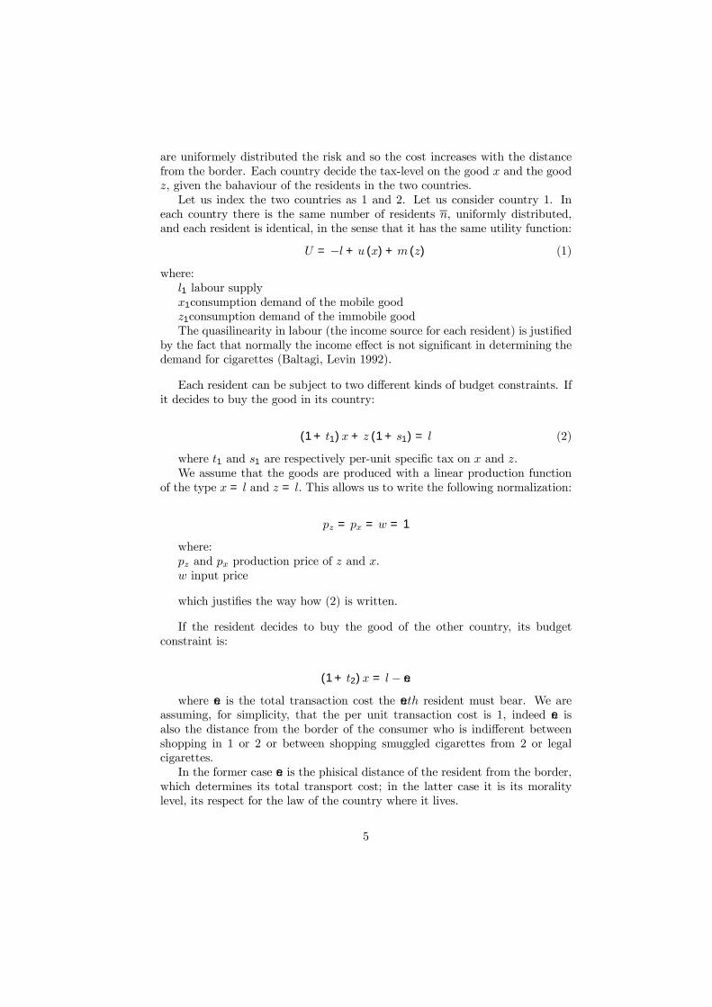
are uniformely distributed the risk and so the cost increases with the distancefrom the border. Each country decide the tax-level on the good x and the goodz, given the bahaviour of the residents in the two countries.Let us index the two countries as 1 and 2. Let us consider country 1. In

each country there is the same number of residents n, uniformly distributed,and each resident is identical, in the sense that it has the same utility function:

U = −l + u (x) +m (z) (1)

where:l1 labour supplyx1consumption demand of the mobile goodz1consumption demand of the immobile goodThe quasilinearity in labour (the income source for each resident) is justiÞed

by the fact that normally the income effect is not signiÞcant in determining thedemand for cigarettes (Baltagi, Levin 1992).

Each resident can be subject to two different kinds of budget constraints. Ifit decides to buy the good in its country:

(1 + t1)x+ z (1 + s1) = l (2)

where t1 and s1 are respectively per-unit speciÞc tax on x and z.We assume that the goods are produced with a linear production function

of the type x = l and z = l. This allows us to write the following normalization:

pz = px = w = 1

where:pz and px production price of z and x.w input price

which justiÞes the way how (2) is written.

If the resident decides to buy the good of the other country, its budgetconstraint is:

(1 + t2)x = l − enwhere en is the total transaction cost the enth resident must bear. We are

assuming, for simplicity, that the per unit transaction cost is 1, indeed en isalso the distance from the border of the consumer who is indifferent betweenshopping in 1 or 2 or between shopping smuggled cigarettes from 2 or legalcigarettes.In the former case en is the phisical distance of the resident from the border,

which determines its total transport cost; in the latter case it is its moralitylevel, its respect for the law of the country where it lives.

5

2.1 The second stage

If the consumer decides to buy the good x sold and taxed in its country it willsolve the following problem:

maxl,xU − λ [(1 + t1)x+ (1 + s1)z − l]

from which we obtain:

x = (u0)−1 (1 + t1) (3)

z = (m0)−1(1 + s1) (4)

l = (1 + t1)x(t1) (5)

Substituting (3), (4) and (5) in (1):

V 11 = −(1 + t1)x (t1) + u (x (t1)) +m (z (s1)) (6)

If the consumer decides to buy the good from the other country it will solvethe following problem:

maxl,xU − λ [(1 + t2)x+ (1 + s1)z − (l1 − en)]

obtaining:

x = (u0)−1 (1 + t2) (7)

z = (m0)−1(1 + s1) (8)

l = (1 + t2)x(t2) + en (9)

Substituting (7), (8) and (9) in (1):

V 12 = −(1 + t2)x (t2)− en+ u (x (t2)) +m (z (s1)) (10)

6

Each resident decides if to buy in 1 or 2, by comparing (6) and (10). Aresident in 1 will be willing to buy x in 2 or the good x illegally coming from 2as far as:

V 12 > V

11 (11)

If we take (11) as an equality it is possible to obtain the number of residents,en, buying x in 2 or smuggled from 2, given that t2 < t1. Moreover, totallydifferentiating and using Roy�s identity:

dendt1

= x (t1)

and:

dendt2

= −x (t2)

When t1 increases, given t2, the number of people which decides to buy thegood from 2 increases, and vice-versa when t2 increases, given t1.

2.2 The first stage

By using the informations from the second stage we can build up the tax-basesof the two countries. Take, without loss of generality, t2 < t1:

B1 = (n− en)x (t1) + nz(s1)

and the total tax-base in 2:

B2 = nx(t2) + enx (t2) + nz(s1)

By using the informations from the second stage we can also build up thewelfare functions in the two countries:

W1 = (n− en)V 11 (·) + enV 1

2 (·)This is a utilitarian indirect welfare function: the sum of the indirect utilities

of all the residents: the ones buying in 1 and the ones buying in 2 or buying thesmuggled good from 2.3

3The welfare function of 2 is:

W2 = nV 22

7

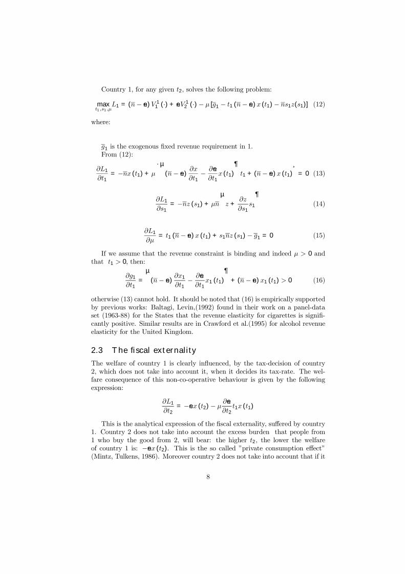
Country 1, for any given t2, solves the following problem:

maxt1,s1,µ

L1 = (n− en)V 11 (·) + enV 1

2 (·)− µ [g1 − t1 (n− en)x (t1)− ns1z(s1)] (12)

where:

g1 is the exogenous Þxed revenue requirement in 1.From (12):

∂L1

∂t1= −nx (t1) + µ

·µ(n− en)

∂x

∂t1− ∂en∂t1x (t1)

¶t1 + (n− en)x (t1)

¸= 0 (13)

∂L1

∂s1= −nz (s1) + µn

µz +

∂z

∂s1s1

¶(14)

∂L1

∂µ= t1 (n− en)x (t1) + s1nz (s1)− g1 = 0 (15)

If we assume that the revenue constraint is binding and indeed µ > 0 andthat t1 > 0, then:

∂g1

∂t1=

µ(n− en)

∂x1

∂t1− ∂en∂t1x1 (t1)

¶+ (n− en)x1 (t1) > 0 (16)

otherwise (13) cannot hold. It should be noted that (16) is empirically supportedby previous works: Baltagi, Levin,(1992) found in their work on a panel-dataset (1963-88) for the States that the revenue elasticity for cigarettes is signiÞ-cantly positive. Similar results are in Crawford et al.(1995) for alcohol revenueelasticity for the United Kingdom.

2.3 The fiscal externality

The welfare of country 1 is clearly inßuenced, by the tax-decision of country2, which does not take into account it, when it decides its tax-rate. The wel-fare consequence of this non-co-operative behaviour is given by the followingexpression:

∂L1

∂t2= −enx (t2)− µ ∂en

∂t2t1x (t1)

This is the analytical expression of the Þscal externality, suffered by country1. Country 2 does not take into account the excess burden that people from1 who buy the good from 2, will bear: the higher t2, the lower the welfareof country 1 is: −enx (t2). This is the so called �private consumption effect�(Mintz, Tulkens, 1986). Moreover country 2 does not take into account that if it

8

increases t2, it gives back to 1 a quota of revenue: −µ ∂en∂t2t1x (t1) ≥ 0. This is the

�public consumption effect� (Mintz, Tulkens, 1986). The higher the sensitivityof n to a change in t2, the higher this last effect is. If −µ ∂en

∂t2t1x (t1) > −enx (t2)

country 2 chooses too low a tax-rate from the point of view of country 1.4 In thiscase it is important to introduce some mechanism to incentivate the countriesnot to decrease their tax-rates. This is what the EU wants to do by trying toimplement a compensation mechanism togheter with a VAT origin tax-system.

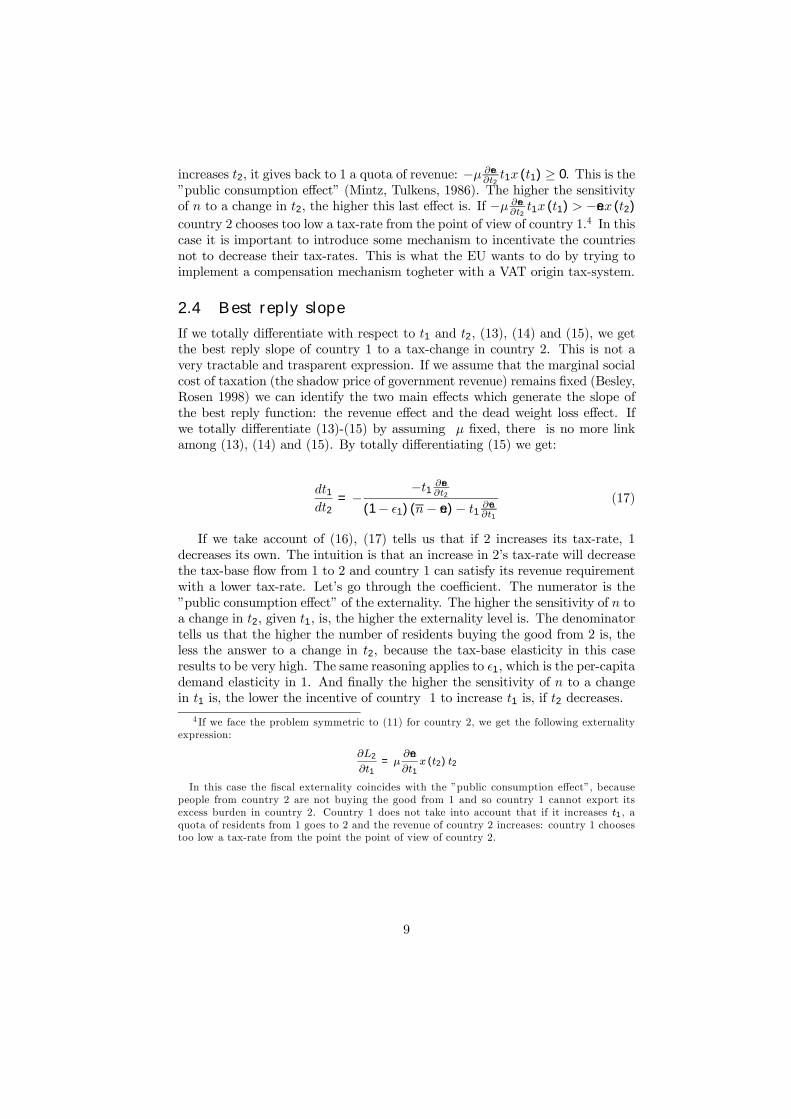
2.4 Best reply slope

If we totally differentiate with respect to t1 and t2, (13), (14) and (15), we getthe best reply slope of country 1 to a tax-change in country 2. This is not avery tractable and trasparent expression. If we assume that the marginal socialcost of taxation (the shadow price of government revenue) remains Þxed (Besley,Rosen 1998) we can identify the two main effects which generate the slope ofthe best reply function: the revenue effect and the dead weight loss effect. Ifwe totally differentiate (13)-(15) by assuming µ Þxed, there is no more linkamong (13), (14) and (15). By totally differentiating (15) we get:

dt1dt2

= − −t1 ∂en∂t2

(1− ²1) (n− en)− t1 ∂en∂t1

(17)

If we take account of (16), (17) tells us that if 2 increases its tax-rate, 1decreases its own. The intuition is that an increase in 2�s tax-rate will decreasethe tax-base ßow from 1 to 2 and country 1 can satisfy its revenue requirementwith a lower tax-rate. Let�s go through the coefficient. The numerator is the�public consumption effect� of the externality. The higher the sensitivity of n toa change in t2, given t1, is, the higher the externality level is. The denominatortells us that the higher the number of residents buying the good from 2 is, theless the answer to a change in t2, because the tax-base elasticity in this caseresults to be very high. The same reasoning applies to ²1, which is the per-capitademand elasticity in 1. And Þnally the higher the sensitivity of n to a changein t1 is, the lower the incentive of country 1 to increase t1 is, if t2 decreases.

4 If we face the problem symmetric to (11) for country 2, we get the following externalityexpression:

∂L2

∂t1= µ

∂en∂t1

x (t2) t2

In this case the Þscal externality coincides with the �public consumption effect�, becausepeople from country 2 are not buying the good from 1 and so country 1 cannot export itsexcess burden in country 2. Country 1 does not take into account that if it increases t1, aquota of residents from 1 goes to 2 and the revenue of country 2 increases: country 1 choosestoo low a tax-rate from the point the point of view of country 2.

9

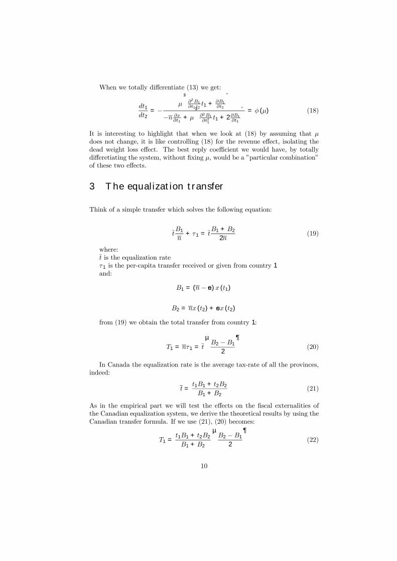
When we totally differentiate (13) we get:

dt1dt2

= −µ

³∂2B1

∂t1t2t1 + ∂B1

∂t2

´−n ∂x∂t1 + µ

³∂2B1

∂t21t1 + 2∂B1

∂t1

´ = φ (µ) (18)

It is interesting to highlight that when we look at (18) by assuming that µdoes not change, it is like controlling (18) for the revenue effect, isolating thedead weight loss effect. The best reply coefficient we would have, by totallydifferetiating the system, without Þxing µ, would be a �particular combination�of these two effects.

3 The equalization transfer

Think of a simple transfer which solves the following equation:

tB1

n+ τ1 = t

B1 +B2

2n(19)

where:t is the equalization rateτ1 is the per-capita transfer received or given from country 1and:

B1 = (n− en)x (t1)

B2 = nx (t2) + enx (t2)

from (19) we obtain the total transfer from country 1:

T1 = nτ1 = t

µB2 −B1

2

¶(20)

In Canada the equalization rate is the average tax-rate of all the provinces,indeed:

t =t1B1 + t2B2

B1 +B2(21)

As in the empirical part we will test the effects on the Þscal externalities ofthe Canadian equalization system, we derive the theoretical results by using theCanadian transfer formula. If we use (21), (20) becomes:

T1 =t1B1 + t2B2

B1 +B2

µB2 −B1

2

¶(22)

10

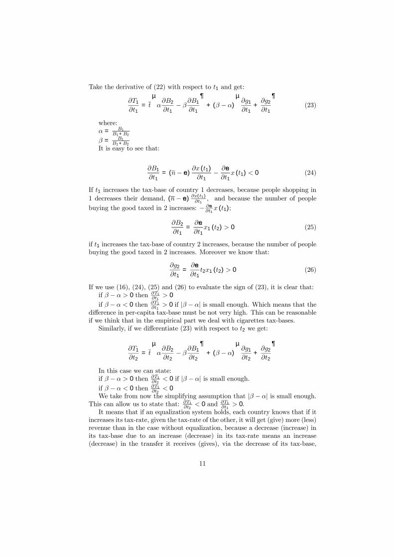
Take the derivative of (22) with respect to t1 and get:

∂T1

∂t1= t

µα∂B2

∂t1− β∂B1

∂t1

¶+ (β − α)

µ∂g1

∂t1+∂g2

∂t1

¶(23)

where:α = B1

B1+B2

β = B1

B1+B2

It is easy to see that:

∂B1

∂t1= (n− en)

∂x (t1)

∂t1− ∂en∂t1x (t1) < 0 (24)

If t1 increases the tax-base of country 1 decreases, because people shopping in1 decreases their demand, (n− en) ∂x(t1)

∂t1, and because the number of people

buying the good taxed in 2 increases: − ∂en∂t1x (t1);

∂B2

∂t1=∂en∂t1x1 (t2) > 0 (25)

if t1 increases the tax-base of country 2 increases, because the number of peoplebuying the good taxed in 2 increases. Moreover we know that:

∂g2

∂t1=∂en∂t1t2x1 (t2) > 0 (26)

If we use (16), (24), (25) and (26) to evaluate the sign of (23), it is clear that:if β − α > 0 then ∂T1

∂t1> 0

if β − α < 0 then ∂T1

∂t1> 0 if |β − α| is small enough. Which means that the

difference in per-capita tax-base must be not very high. This can be reasonableif we think that in the empirical part we deal with cigarettes tax-bases.Similarly, if we differentiate (23) with respect to t2 we get:

∂T1

∂t2= t

µα∂B2

∂t2− β∂B1

∂t2

¶+ (β − α)

µ∂g1

∂t2+∂g2

∂t2

¶In this case we can state:if β − α > 0 then ∂T1

∂t2< 0 if |β − α| is small enough.

if β − α < 0 then ∂T1

∂t2< 0

We take from now the simplifying assumption that |β − α| is small enough.This can allow us to state that: ∂T1

∂t2< 0 and ∂T1

∂t1> 0.

It means that if an equalization system holds, each country knows that if itincreases its tax-rate, given the tax-rate of the other, it will get (give) more (less)revenue than in the case without equalization, because a decrease (increase) inits tax-base due to an increase (decrease) in its tax-rate means an increase(decrease) in the transfer it receives (gives), via the decrease of its tax-base,

11

∂B1

∂t1= (n− en) ∂x(t1)

∂t1− ∂en

∂t1x (t1), and the increase of the tax-base of the other

country: ∂B2

∂t1= ∂en

∂t1x (t2) . Each country in this case takes into account that an

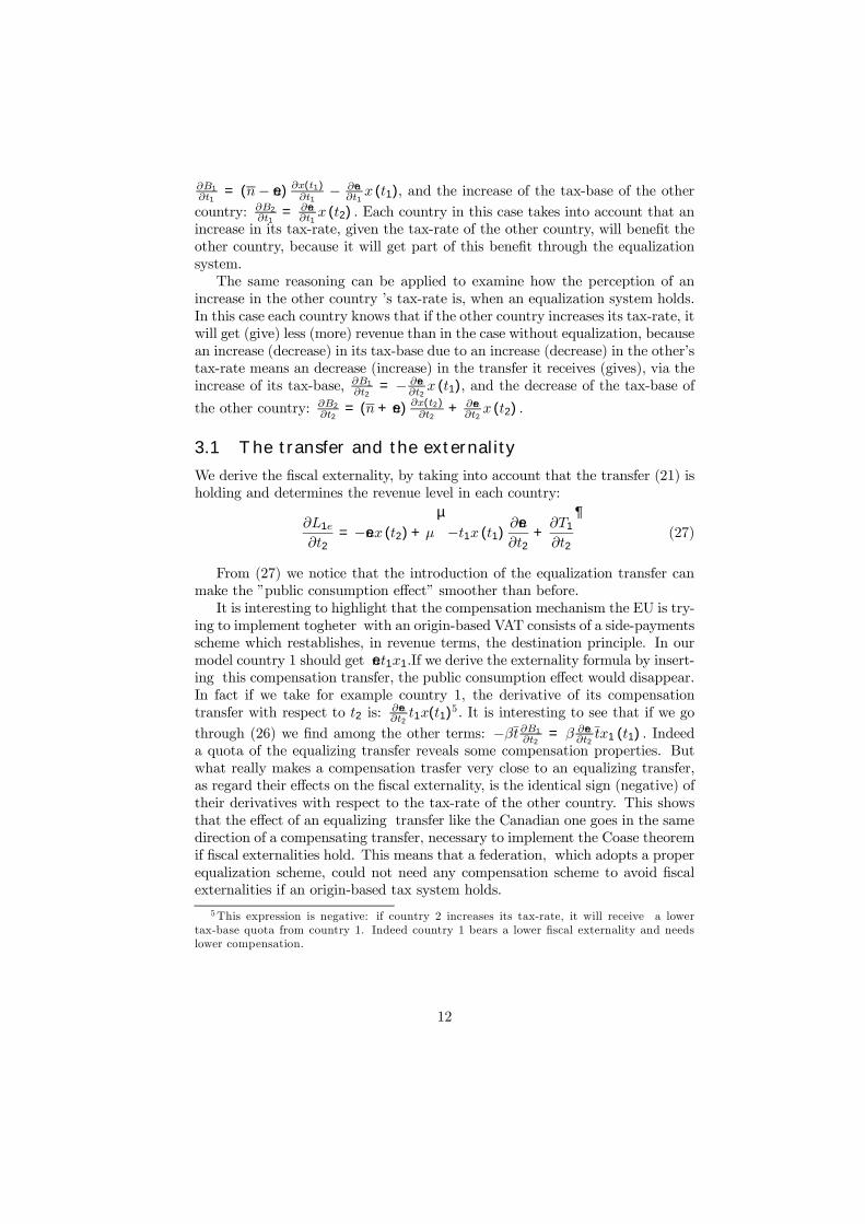
increase in its tax-rate, given the tax-rate of the other country, will beneÞt theother country, because it will get part of this beneÞt through the equalizationsystem.The same reasoning can be applied to examine how the perception of an

increase in the other country �s tax-rate is, when an equalization system holds.In this case each country knows that if the other country increases its tax-rate, itwill get (give) less (more) revenue than in the case without equalization, becausean increase (decrease) in its tax-base due to an increase (decrease) in the other�stax-rate means an decrease (increase) in the transfer it receives (gives), via theincrease of its tax-base, ∂B1

∂t2= − ∂en

∂t2x (t1), and the decrease of the tax-base of

the other country: ∂B2

∂t2= (n+ en) ∂x(t2)

∂t2+ ∂en

∂t2x (t2) .

3.1 The transfer and the externality

We derive the Þscal externality, by taking into account that the transfer (21) isholding and determines the revenue level in each country:

∂L1e

∂t2= −enx (t2) + µ

µ−t1x (t1)

∂en∂t2

+∂T1

∂t2

¶(27)

From (27) we notice that the introduction of the equalization transfer canmake the �public consumption effect� smoother than before.It is interesting to highlight that the compensation mechanism the EU is try-

ing to implement togheter with an origin-based VAT consists of a side-paymentsscheme which restablishes, in revenue terms, the destination principle. In ourmodel country 1 should get ent1x1.If we derive the externality formula by insert-ing this compensation transfer, the public consumption effect would disappear.In fact if we take for example country 1, the derivative of its compensationtransfer with respect to t2 is: ∂en

∂t2t1x(t1)5 . It is interesting to see that if we go

through (26) we Þnd among the other terms: −βt∂B1

∂t2= β ∂en

∂t2tx1 (t1) . Indeed

a quota of the equalizing transfer reveals some compensation properties. Butwhat really makes a compensation trasfer very close to an equalizing transfer,as regard their effects on the Þscal externality, is the identical sign (negative) oftheir derivatives with respect to the tax-rate of the other country. This showsthat the effect of an equalizing transfer like the Canadian one goes in the samedirection of a compensating transfer, necessary to implement the Coase theoremif Þscal externalities hold. This means that a federation, which adopts a properequalization scheme, could not need any compensation scheme to avoid Þscalexternalities if an origin-based tax system holds.

5This expression is negative: if country 2 increases its tax-rate, it will receive a lowertax-base quota from country 1. Indeed country 1 bears a lower Þscal externality and needslower compensation.

12

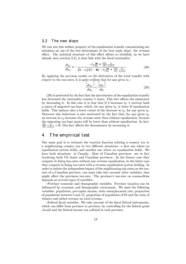
3.2 The new slope

We can test this welfare property of the equalization transfer concentrating ourattention on one of the two determinats of the best reply slope: the revenueeffect. The anlytical structure of this effect allows to establish, as we havealready seen (section 2.4), a clear link with the Þscal externality:

dt1edt2e

= −−t1 ∂en

∂t2+ ∂T1

∂t21

x1(t1)

(1− ²1) (n− en)− t1 ∂en∂t1

+ ∂T1

∂t11

x1(t1)

(28)

By applying the previous results on the derivatives of the total transfer withrespect to the tax-rates, it is quite evident that for any given t2 :¯̄̄̄

dt1edt2e

¯̄̄̄<

¯̄̄̄dt1dt2

¯̄̄̄(29)

(29) is motivated by the fact that the introduction of the equalization transferhas decreased the externality country 1 bears. This fact affects the numeratorby decreasing it. In this case it is true that if 2 increases t2, 1 receives backa quota of migrated tax-base, which, for any given t2, is lower if equalizationholds. This induces also a lower extent of the decrease in t1, for any given t2.Moreover this behaviour is also motivated by the fact that, for any given t2,an increase in t1 increases the revenue more than without equalization, becausethe migrating tax-base quota will be lower than without equalization. In fact:∂T1

∂t11

x1(t1) > 0. This fact affects the denominator by increasing it.

4 The empirical test

Our main goal is to estimate the reaction function relating a country tax toa neighbouring country tax in two different situations: a Þrst one where anequalization system holds, and another one where no equalization holds. Wehave both situations in Canada. Most of Canadian provinces are in factbordering both US states and Canadian provinces. In the former case theycompete in Þxing tax-rates without any revenue equalization, in the latter casethey compete in Þxing tax-rates with a revenue equalization system holding. Inorder to isolate the independent impact of the neighbouring tax-rates on the tax-rate of a Canadian province, one must take into account other variables, thatmight affect the provinces tax-rate. The province�s tax-rate on commoditiesdepends on several types of variables:-Province economic and demographic variables. Province taxation can be

inßuenced by economic and demographic enviroment. We used the followingvariables: population, per-capita income, state unemployment rate, proportionof population between 5 and 17, proportion of population of 65 and the ratio oftobacco and alchol revenue on total revenue.-Federal Þscal variables. We take account of the Þscal federal instruments,

which can differ from province to province, by controlling for the federal grant-in-aid and the federal income tax colleted in each province.

13

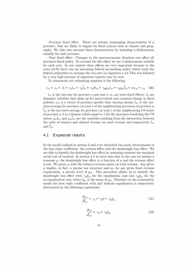
-Province Þxed effect. There are certain unchanging characteristics of aprovince, that are likely to impact its Þscal system such as climate and geog-raphy. We take into account these characteristics by including a dichotomousvariable for each province.-Year Þxed effect. Changes in the macroeconomic situation can affect all

provinces Þscal policy. To account for this effect we use a dichotomous variablefor each year. In our context these effects are very important because in theyears 84-94 there was an increasing federal no-smoking policy which leads thefederal authorities to increase the tax-rate on cigarettes a lot.This was followedby a very high increase of cigarettes exports year by year.To summarize our estimating equation is the following:

tst = αs + βt + γ1tst + γ2tst + γ3δtst + γ4gsttst + γ5gsttst + φxst + ²st (30)

tst is the tax-rate for province s and year t; αs are state Þxed effects; βt aredummies variables that picks up for macro-shock and common change in Þscalpolicies; xst is a vector of province speciÞc time varying shocks; tst is the tax-rates average for province s in year t of the neighbouring provinces of province s;tst is the tax-rates average for province s in year t of the neighbouring US statesof province s; δ is a dummy which equal to 1 for the provinces bordering the USstates; gsttst and gsttst are the variables resulting from the interaction betweenthe ratio of tobacco and alchool revenue on total revenue and respectively tstand tst.

4.1 Expected results

In the model oulined in section 2 and 3 we described two main determinants ofthe best reply coefficient: the revenue effect and the deadweight loss effect. Weare able to identify the deadweight loss effect by assuming constant the marginalsocial cost of taxation. In section 2.4 we have seen that in the case we assume aconstant µ, the deadweight loss effect is a function of µ and the revenue effectis not. We proxy µ with the tobacco revenue quota on total revenue. Any givenµ implies, in fact, a precise tax structure and so, for any given Þxed revenuerequirement, a precise level of gst. This procedure allows us to identify thedeadweight loss effect with γ4gst for the equalization case and γ5gst for theno-equalization case, where gst is the mean of gst. Therefore in the econometricmodel the best reply coefficient with and without equalization is respectivelydetermined by the following expressions:

dtstdtst

= γ1 + γ3δ + γ4gst (31)

dtst

dtst= γ2 + γ5gst (32)

14

In (31) the revenue effect is further splitted to account for the US bordereffect. It is, in fact well known that the great part of the population of theprovinces bordering the US states lives near the border. In this situation it theprovincial authority normally cares much more of a US neighbouring state tax-change, than of a neighbouring Canadian province tax-change. One can arguethat this fact can explain the difference between dtst

dtstand dtst

dtst

. As we want to

know if this difference can be explained by the equalization system, we identifythe quota of the coefficient due to this effect by using the variable δtst. Theleft coefficient quotas are γ1 and γ2. Both could be respectively reßected by aformula as (28) and (17), which does not include the deadweight loss effect. γ1

reßects (28) depurated by the particular behaviour of the provinces borderingthe United States. Therefore we can think of γ1 and γ2 as proxing the revenueeffect and we expect from theory:

|γ1| < |γ2|

4.2 Data description

4.2.1 Tax-rates

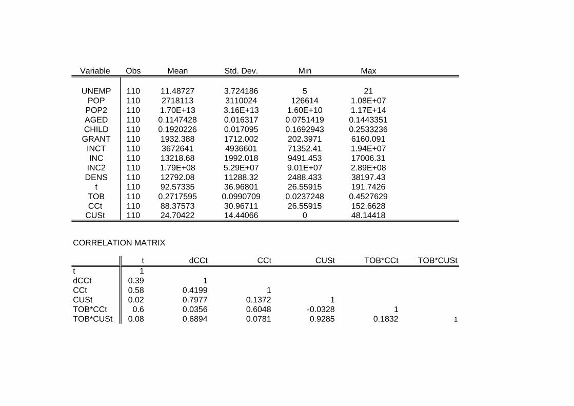
We used annual data on the provinces and US bordering states for the years1984 to 1994, inclusive. Cigarettes in Canada and United States are normallysubject to ad valorem general sales taxes as well as unit taxes. We compute atotal real unit tax-rate, by taking the unit-tax equivalent of the general sales tax(calculated by multiplying the general sales tax-rate by the price), adding thisto the unit tax-rate, and then dividing by the CPI to adjust for inßation. Wecalculate these total taxes for US by using tax-rates from ACIR annual reports.We took them from the web site of the National Clearinghouse on Tobacco andHealth for Canada.6 The idea is that when setting unit taxes on cigarettes,provinces take into account the general sales taxes levied on these commodities.These last taxes also inßuence the tax-inclusive prices.Taxes on cigarettes vary among Canadian provinces. In 1991, as an example,

PEI provincial taxes on 20 cigarettes were 1.80$ (in Canadian dollars), NewBrunswick 2.50$, Nova Scotia 1.85$, Québec 1.52$, Ontario 1.66$, Newfondland1.97$, Saskatchewn 1.66$, Manitoba 1.94$, Alberta 1.40$, British Columbia1.60$.As noted above our main focus is on the different relationship between

province cigarettes tax-rate and the Canadian neighbouring tax-rate and theUS neighbouring tax-rate. We estimate the neighbouring tax-rates by doingthe mean of the neighbouring Canadian provinces tax-rates (CCtst) and/or USstates tax-rates (CUStst) and dividing the former for the Canadian CPI andthe latter for the US CPI. The Canadian tax-rates are further divided by thePPP index.7

6www.cctc.ca7The PPP index for Canada-US was downloaded by the OECD web site

15

4.2.2 Other variables

There is a set of time varying variables characterizing the province�s economicand demographic situation: province population (POPst), population density(DENSst), province per-capita income in 89 US$ (INCst), province unem-ployment rate (UNEMPst), proportion of individuals in the province who arebetween 5 and 17 (CHILDst) and proportion of individuals who are over 65(AGEDst). As a rough measure of cigarettes tax-base elasticity we use the ratioof tobacco and alchool revenue8 on total revenue (PTOBst). we take account ofthe federal policy inßuence, speciÞc for each province by controlling for federalgrant-in-aid in 89 US$ (GRANTst) and federal tax-revenue in each province in89 US$ (INCTst).9

4.2.3 Results

All the results of the regressions in table 1 are with years and provinces ef-fects. Column (1) reports the results relative to the regression with the controls.Column (2) reports the results of the regression with only the indepedendentvariables. In column (3) we have the results for the estimated equation (30)not instrumented. In column (4) we have the results for the estimated equa-tion with instrumentation. We instrumented the neighbouring tax-rates withtheir economic and demographic variables, which are signiÞcantly related to theneighbouring tax-rates, but not related to the considered province tax-rate. Weinstrument the neighbouring tax-rates because we assume (as standard theorydoes) that tax-rates are simultaneosly determined by all the provinces (Mintz,Tulkens 1986; Kanbur and Keen 1993; Besley, Case, 1995). In this case tst andtst are functions of tst, so the independent variables, tst and tst, of (30) are cor-related with the disturbance term ²st and the forth Gauss-Markov condition isviolated. As a consequence the estimates of the standard errors will be invalidand the coefficients will be biased. To avoid this problem we instrument theendogenous variables by using the Two-Stage Least Squares method.The regression with only the Þxed effects explains the 77% of variance of tst.

As we already mentioned, in Canada during the last 80s and the Þrst 90s, thefederal tax-rate increased, because of a strong anti-smoking federal governmentpolicy: in 1988 the total federal tax (federal speciÞc + sales tax) on 20 cigaretteswas 0.76 $ (Canadian dollars); in 1993 it arrived at 1.93 $. This federal behaviour

8Canadian Statistics do not offer a disaggregated measure of tobacco provincial revenue. Bytaking the aggregated measure we assume that tobacco and alchool revenue are not correlatedand that the quota of alchool on total revenue does not explain the choice of the cigarettestax-rate. In this case the bias introduced by not considering only the tobacco revenue shouldbe very small

9All the socio-economic variables for the USA have been collected by using the followingweb sites:www.census.govwww.bea.doc.govwww.stats.bls.govThe socio-economic variables for Canada have been bought from Canadian Statistics

(www.statcan.ca)

16

is incorporated in the year effect and it inßuences positively the province tax-rate, conferming a recent result on vertical externalities (Besley, Rosen, 1998). Ifwe look at column (1) we see that it explains 87% of the variance but almost allthe control are not signiÞcative. In column (2) we have the regression with thedependent variables. Almost all of them are signiÞcative and the R2 increases(0.93). In column (3) we use both the dependent variables and the controlsand the R2 increases further (0.97), making almost all the controls signiÞcative.This means that the depent variables are really essential in the economy of theregression. Putting in other words the bias on the controls, if we omit, thedependent variables is much higher, than the bias on the dependent variablesif we omit the controls. This tells us that the only year effects cannot explainthe variance of tst and the high R2. In this case in fact the values of the controlsin column (3) would not change a lot from the ones in column (1), which arealready controlled for the years and province effects. Moreover the standarddeviations of tst and tst are not so small to allow only the year effects to explainthe variance of tst.The coefficient γ3 = 0.84 shows the role of the provinces bordering the US in

making not signiÞcant the part of the coefficient due to the revenue effect (linkedto the externality level). The reason is that the great part of the populationlives near the US border. In fact, if we estimate the regression without thiscoefficient control, we get a very small γ1 (-0.064), which is not signiÞcative(col.5). In the regression in column 3 γ1 = −0.41 and signiÞcative at 5%. Thisis the revenue effect in the equalization case, depurated from the border effect.The robustness of this interpretation is also conÞrmed by the fact that if wereplicate the regression with only the provinces bordering the US, γ1 is verysmall and again negative (col.6).The econometric results conÞrm the theory in fact:

|γ1| < |γ2|So the existence of the equalizing transfer offsets the externality which drives

the extent of γ1,determining the above inequality.When we instrument, our results do not change. γ1 and γ2 increase in

absolute value and also their difference increases. (col.4)

5 Conclusion

In the second section we derive optimality conditions and the slope of the bestreply function of one country, given the tax rate of the other. We show thatthe tax rate choice is inefficiently low because the consumer of one country canbuy the good produced in the other country (Þscal externality). Moreover wediscuss how the the Þscal externality is reßected in the slope of the best replyfunction.In the third section we then study how the introduction of an equalization

system, based on Þscal capacity, can affect the Þrst order conditions, by changingthe extent of the Þscal externality. We show that a Pareto improvement occurs:

17

each country, given the tax rate of the other, chooses a higher tax-rate. We lookÞnally at how the effect of the equalization system is reßected in the best replyfunction slope.We Þnd that the best reply function is less steep if we introduce equalization.

This is because the Þscal externality is partially offset by the existence of thetransfer and the slope of the best reply function depends on the extent of theÞscal externality.So in our case raising welfare by decreasing the Þscal externality level means

decreasing the best reply function slope.We are interested in the best reply function slope because this is the link with

the empirical test. If we are able to understand the entity of the welfare effectsdue to the introduction of an equalization system, by analysing the changes inthe best reply function slopes we are able to test what the theory predicts, inwelfare terms, if the equalization system is introduced.The second part of the paper develops a test of the theoretical result by using

a data-set Canada-US 1984-1994 with sales taxes and speciÞc cigarettes taxes.The test conÞrms the theoretical result that the introduction of an equalizationsystem decreases the Þscal externality due to tax-base mobility.

6 References

Baltagi, B. H. and Levin D. (1992), Cigarettes Taxation: Raising Revenues andReducing Consumption, Structural Change and Economic Dynamics 2, 321-336.Besley, T. and H. S. Rosen (1998), Vertical externalities in tax setting: evi-

dence from gasoline and cigarettes, Journal of Public Economics 70, 383-398.Besley, T. and A. Case (1995), Incumbent Behavior: Vote Seeking, Tax

Setting and Yardstick Competition, American Economic Review 85, 25-45.Besley, T. and Coate S. (2000), Elected versus Appointed Regulators: The-

ory and Evidence, mimeo, STICERD-LSE, London.Bird, R. M. and E. Slack (1990), Equalization: the Representative Tax Sys-

tem Revisited, Canadian Tax Journal 38, 913-927.Boadway, R. and M. Keen (1996), Efficiency and The Optimal Direction of

Federal-State Transfers, International Tax and Public Finance 3, 137-155Bordignon M., Manasse P., Tabellini G. (2000), Optimal Regional Redis-

tribution under Asymmetric Information, forthcoming in American EconomicReviewCommission of the European Communities (1985), Completing the Internal

Market, COM(85) 310, Brussels.Commission of the European Communities (1996), A Common System of

VAT: A Program for the Single Market, COM(96) 328 Final, Brussels.Dhillon A., Perroni C., Scharf K. A. (1999) Implementing Tax Coordination,

Journal Public Economics 72, 243-268.Dahlby, B. and S. Wilson (1994), Fiscal Capacity, Tax Effort and Optimal

Equalization Grants, Canadian Journal of Economics 27, 657-672.

18

Dalbhy, B. (1996), Fiscal Externalities and the Design of IntergovernmentalGrants, International Tax and Public Finance 3, 397-412.Kanbur, R. and M. Keen, (1993), Jeux sans Frontiers: Tax Competition and

Tax Coordination when Countries Differ in Size, American Economic Review,83, 887-892.Keen, M. (1989), Pareto Improving Indirect Tax Harmonization, European

Economic Review 33, 1-12.Keen, M. and S. Smith (1996), The Future of VAT in the European Union,

Economic Policy 23, 373-411Larcinese, V. (2000), Information Acquisition and Electoral Turnout: The-

ory and Evidence from Britain, mimeo, STICERD-LSE, London.Lee, C., M. Pearson and S. Smith (1988) Fiscal Harmonization: an Analysis

of the European Commission�s Proposals, Institute for Fiscal Studies Reportseries n.28, Institute for Fiscal Studies, LondonLockwood, B. (1993), Commodity Tax Competition under Destination and

Origin Principles, Journal of Public Economics 32, 141-162.Lockwood, B. (2000), Tax Competition and Tax Co-ordination under Des-

tiantion and Origin Principle: a Synthesis, mimeo, University of Warwick, War-wick.Mintz, J. and Tulkens, H. (1986), Commodity Tax Competition between

Member Sstates of a Federation: Equilibrium and Efficiency, Journal of PublicEconomics 29, 133-172.Rasul, I. (2000), Ethnicity and Learning from Test Scores in Education:

Theory and Evidence, mimeo, STICERD-LSE, London.Scharf, K. A. (1999) Scale Economies in Cross-Border Shopping and Com-

modity Taxation, International Tax and Public Finance 6, 89-99Wildasin, D. E. (1988), Nash Equilibria in Models of Fiscal Competition,

Journal of Public Economics 35, 229-240.Wildasin, D. E. (1991), Income Redistribution in a Common Market, Amer-

ican Economic Review 81, 757-774.Wilson, J. D. (1991), Tax Competition with Interregional Differences in

Factor Endowments, Journal of Urban Economics 21, 423-451.

19

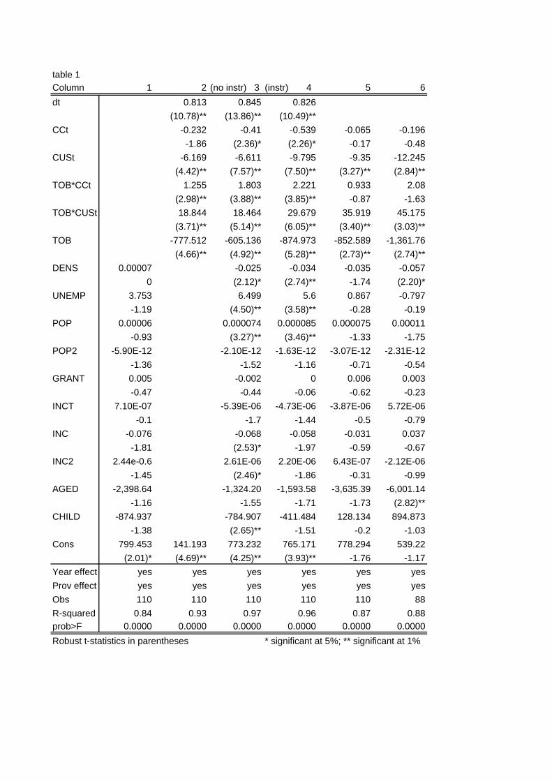
table 1Column 1 2 (no instr) 3 (instr) 4 5 6dt 0.813 0.845 0.826

(10.78)** (13.86)** (10.49)**CCt -0.232 -0.41 -0.539 -0.065 -0.196

-1.86 (2.36)* (2.26)* -0.17 -0.48CUSt -6.169 -6.611 -9.795 -9.35 -12.245

(4.42)** (7.57)** (7.50)** (3.27)** (2.84)**TOB*CCt 1.255 1.803 2.221 0.933 2.08

(2.98)** (3.88)** (3.85)** -0.87 -1.63TOB*CUSt 18.844 18.464 29.679 35.919 45.175

(3.71)** (5.14)** (6.05)** (3.40)** (3.03)**TOB -777.512 -605.136 -874.973 -852.589 -1,361.76

(4.66)** (4.92)** (5.28)** (2.73)** (2.74)**DENS 0.00007 -0.025 -0.034 -0.035 -0.057

0 (2.12)* (2.74)** -1.74 (2.20)*UNEMP 3.753 6.499 5.6 0.867 -0.797

-1.19 (4.50)** (3.58)** -0.28 -0.19POP 0.00006 0.000074 0.000085 0.000075 0.00011

-0.93 (3.27)** (3.46)** -1.33 -1.75POP2 -5.90E-12 -2.10E-12 -1.63E-12 -3.07E-12 -2.31E-12

-1.36 -1.52 -1.16 -0.71 -0.54GRANT 0.005 -0.002 0 0.006 0.003

-0.47 -0.44 -0.06 -0.62 -0.23INCT 7.10E-07 -5.39E-06 -4.73E-06 -3.87E-06 5.72E-06

-0.1 -1.7 -1.44 -0.5 -0.79INC -0.076 -0.068 -0.058 -0.031 0.037

-1.81 (2.53)* -1.97 -0.59 -0.67INC2 2.44e-0.6 2.61E-06 2.20E-06 6.43E-07 -2.12E-06

-1.45 (2.46)* -1.86 -0.31 -0.99AGED -2,398.64 -1,324.20 -1,593.58 -3,635.39 -6,001.14

-1.16 -1.55 -1.71 -1.73 (2.82)**CHILD -874.937 -784.907 -411.484 128.134 894.873

-1.38 (2.65)** -1.51 -0.2 -1.03Cons 799.453 141.193 773.232 765.171 778.294 539.22

(2.01)* (4.69)** (4.25)** (3.93)** -1.76 -1.17Year effect yes yes yes yes yes yesProv effect yes yes yes yes yes yesObs 110 110 110 110 110 88R-squared 0.84 0.93 0.97 0.96 0.87 0.88prob>F 0.0000 0.0000 0.0000 0.0000 0.0000 0.0000Robust t-statistics in parentheses * significant at 5%; ** significant at 1%

Variable Obs Mean Std. Dev. Min Max

UNEMP 110 11.48727 3.724186 5 21POP 110 2718113 3110024 126614 1.08E+07

POP2 110 1.70E+13 3.16E+13 1.60E+10 1.17E+14AGED 110 0.1147428 0.016317 0.0751419 0.1443351CHILD 110 0.1920226 0.017095 0.1692943 0.2533236GRANT 110 1932.388 1712.002 202.3971 6160.091

INCT 110 3672641 4936601 71352.41 1.94E+07INC 110 13218.68 1992.018 9491.453 17006.31

INC2 110 1.79E+08 5.29E+07 9.01E+07 2.89E+08DENS 110 12792.08 11288.32 2488.433 38197.43

t 110 92.57335 36.96801 26.55915 191.7426TOB 110 0.2717595 0.0990709 0.0237248 0.4527629CCt 110 88.37573 30.96711 26.55915 152.6628

CUSt 110 24.70422 14.44066 0 48.14418

CORRELATION MATRIX

t dCCt CCt CUSt TOB*CCt TOB*CUStt 1dCCt 0.39 1CCt 0.58 0.4199 1CUSt 0.02 0.7977 0.1372 1TOB*CCt 0.6 0.0356 0.6048 -0.0328 1TOB*CUSt 0.08 0.6894 0.0781 0.9285 0.1832 1