Embed Size (px)
Citation preview
Communications inCommun. Math. Phys. 72, 55-76 (1980) Mathematical
Physics© by Springer-Verlag 1980
Equilibrium Statesfor a Plane Incompressible Perfect Fluid
Carlo Boldrighini* and Sandro Frigio**Istituto Matematico, Universita di Camerino, Camerino, Italy
Abstract. We associate to the plane incompressible Euler equation withperiodic conditions the corresponding Hopf equation, as an equation formeasures on the space of solenoidal distributions. We define equilibrium statesas the solutions of the stationary Hopf equation. We find a class of equilibriumstates which corresponds to a class of infinitely divisible distributions, andinvestigate the properties of gaussian and poissonian states. Equilibriumdynamics for a class of poissonian states is constructed by means of theOnsager vortex equations.
1. Introduction
The purpose of this paper is to exhibit a class of equilibrium states for a plane fluidwhich moves according to the incompressible Euler equation, and to study theirmain properties. Our treatment will be limited to the case of periodic boundaryconditions, which allows an explicit use of Fourier methods.
Equilibrium states for the plane incompressible Euler fluid have been studiedby physicists for a long time. Among the most significant contributions we maymention a paper by Lee [1] in which a class of gaussian states were introduced asmacrocanonical equilibrium states corresponding to energy and enstrophy con-servation, and a paper by Novikov [2] in which equilibrium states correspondingto poissonian distribution of vortices are studied.
The mathematical definition of equilibrium state which we give is based on theHopf equation associated to the plane incompressible Euler equation, namely wedefine equilibrium states as solutions of the stationary Hopf equation. We recallthat the Hopf equation describes the evolution of measures on phase spaceassociated to the point evolution, and is written in terms of the characteristicfunctionals.
* Research partially supported by C.N.R., G.N.F.M.** C.N.R. fellowship, G.N.F.M.
0010-3616/80/0072/0055/S04.40
56 C. Boldrighini and S. Frigio
The Hopf equation plays here a role similar to that of the B-B-K-G-Yhierarchy equations in statistical mechanics (which is not surprising since the latteris nothing else than the evolution equation for the generating functional). In fact,although in mechanics there is an independent notion of equilibrium state (that ofGibbs state), it turns out that the class of Gibbs states corresponds to the class ofstationary solutions of the B-B-K-G-Y hierarchy equations [3].
Our main result consists in exhibiting solutions of the stationary Hopfequation which are associated to the law of vorticity conservation along thetrajectory of fluid particles, which is a characteristic feature of the plane Eulerfluid. The corresponding measures are weak limits of some natural latticemeasures with "Gibbs factor" associated to the constants of the motion of theEuler flow, energy excluded. Such equilibrium states are in one to one cor-respondence with a family of infinitely divisible distribution laws, and arecharacterized by the fact that vorticity is distributed as a generalized random fieldwith independent values at each point. The vorticity distribution can be in-terpreted as a superposition of a gaussian distribution and a finite or infinitenumber of Poisson distributions.
We give an analysis of the main properties of the gaussian and poissonianstates: we establish in particular that square summable velocity fields have zeromeasure in both cases. We also construct a further class of gaussian equilibriumstates, associated to energy and enstrophy conservation, which are just theequilibrium states introduced by Lee [1]. They turn out to be absolutelycontinuous with respect to the gaussian measures previously considered.
If an equilibrium state is physically significant, it should be possible to showthat it is the limit of the evolution of some class of physically reasonable states.This problem is similar to that of founding the Gibbs postulate in statisticalmechanics (see for example [4]) and is probably of comparable mathematicaldifficulty. There are physical grounds which suggest that such a problem isreasonable at least for poissonian states (cf. [2]), and for gaussian states (see forinstance [5] where results of computer experiments are provided, and referencestherein). In order to formulate the problem at a mathematical level one should firstconstruct "nonequilibrium dynamics", which in our case amounts to extending theexistence theorem for the Euler equation to a set of initial data which is largeenough to contain the support of the states the evolution of which is to be studied(including equilibrium states). In statistical mechanics this problem has beensolved only for one-dimensional and two-dimensional system [6, 7]. In our case,we believe that one should, for the moment, be content with the construction of"equilibrium dynamics", that is, of time evolution for a set of full measure withrespect to a fixed equilibrium state (in statistical mechanics this problem hasalready found a satisfactory solution, see [8] and references therein). We succeededin constructing equilibrium dynamics for a class of poissonian equilibrium states,by showing that the solution of the Onsager vortex equations gives a (generalized)solution of the Euler equation.
The plan of the paper is the following. In Sect. 2 we expose the main facts onthe plane Euler equation, with particular attention to the periodic case. In Sect. 3we introduce the Hopf equation in a way which is convenient for measures ongeneralized function spaces (usually it is defined for measures on spaces of square
States for an Incompressible Fluid 57
summable functions, which are too small for our purposed). In Sect. 4 weintroduce the main class of equilibrium states, and show than they are solutions ofthe stationary Hopf equation. In Sect. 5 we study gaussian and poissonianequilibrium states and construct gaussian equilibrium states associated to energyand enstrophy conservation. In Sect. 6 we construct the equilibrium dynamics fora class of poissonian states. Section 7 is devoted to a conclusive discussion.
2. The Plane Incompressible Euler Equation
a. Generalities
Let Ω denote an open set of the plane, and dΩ its boundary, which we suppose atleast of class C1. The plane incompressible Euler equation for the velocity fieldu(χ, ί) = (w1(χ j t), u2(x, t)) and the pressure field p(x, ί), ((x, ί)eί2 x IR1), in absence ofexternal forces, is
— u + (u F)u= — Vp (2.1)
divu-0 (2.2)
V=\ , 1 is the gradient, and divu= Y —u . Equations (2.1) and (2.2) are\dx1 dxj ^ ^ ffi dXi
accompanied by the initial condition
u(x,0) = u0(x) (2.3)
and the boundary condition
u n|ao = 0, (2.4)
n being the outer normal on dΩ. We recall that the solenoidality condition (2.2)expresses incompressibility, and the boundary condition (2.4) means that theliquid cannot flow out of Ω.
Equations (2.1) and (2.2) can be written in terms of the vorticity field ω(x, t)
ω(x, ί) = rotu(x, ί)= —ox1 ox2
(ω is a scalar in dimension 2). Defining, following Kato [9], the rotation of a scalarfield φ(x) as the vector
(2.5,x2 x
we have
τotrotφ=-Δφ. (2.6)
It is easily seen that a differentiable solenoidal vector field in Ω, v(x), satisfyingthe boundary condition v n|5β = 0 can be uniquely reconstructed in terms of itsrotation:
v(x) = rotG(rotv) (2.7)
58 C. Boldrighini and S. Frigio
G being the inverse of ( — A) with zero boundary conditions on dΩ [i.e. G(φ) is thesolution of the equation Aιp= — φ, t/;|aβ = 0].
In place of Eqs. (2.1) and (2.2) we can write
)ω = 0 (2.8)ot
u = rotG(ω). (2.9)
Equation (2.8) expresses the law of "vorticity conservation for any fluid particle",i.e. it says that the "total derivative" of the vorticity is zero.
b. Existence, Uniqueness and Constants of the Motion
Existence, uniqueness [with p(x, ί) determined up to an arbitrary function of time]and regularity for solutions of the problem (2.1)-(2.4) have been proved in variousframeworks. For classical solutions (i.e. such that all the derivatives involved existand are continuous), it is assumed that dΩ is at least of class C2 + δ, (<5>0) and themain tool of the proof is Schauder's fixed point theorem (see for example [9]). For"weak solutions", [i.e. solutions which are not necessarily differentiable and satisfy(2.1) and (2.2) in a "weak sense", that is, in some space of functional] an existenceand uniqueness result has been proved under the assumption that u0 is a squaresummable function with square summable gradient, and that dΩ is of class C2 (cf.[10]). The proof is based on compactness arguments, and the solution is acontinuous function of t with values in the space of square summable vectorfunctions (L2(Ω))2. All results for classical as well as for weak solutions hold for alltimes.
We now recall some well-known properties of the Euler equations. (We limitour considerations to classical solutions only.)
By "constant of the motion" we mean a functional of u, which is unchanged asu evolves according to the Euler equation. We have:
Proposition 2.1. The energy
Ω
does not depend on t if u(x, t) is a classical solution of the problem (2.1)-(2.4) (by"dx" we denote the Lebesgue measure on R2j.
Proof. From the existence and uniqueness theorem for classical solutions we havethat E(t) exists and is differentiable in t for any t. We have
-E(t)=- f u-(u-F)udx=- J(u F)||u|2ώc=-| J |u|2u nώc = 0.dt Ω Q QQ
There are many other constants of the motion, as a consequence of the "law ofvorticity conservation" (2.8):
Proposition 2.2. For any continuous function /e C(IR) the functional
If=\f(ω(x,t)dx (2.10)Ω
is a constant of the motion if u is a classical solution of problem (2.1)-(2.4).
States for an Incompressible Fluid 59
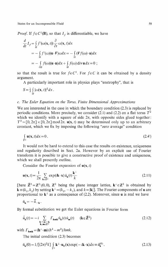
Proof. If /eC^IR), so that If is differentiable, we have
-If=$f'(ω(x,t))-ω(x,t)dx
- - j /'(ω)(u F)ωdx = - J (F/(ω) u)dxΩ β
n)dx+ f /(
so that the result is true for feC1. For /eC it can be obtained by a densityargument.
A particularly important role in physics plays "enstrophy", that is
c. The Euler Equation on the Torus. Finite Dimensional Approximations
We are interested in the case in which the boundary condition (2.3) is replaced byperiodic conditions. More precisely, we consider (2.1) and (2.2) on a flat torus T2
which we identify with a square of side 2π, with opposite sides glued together :T2 = [0, 2π] x [0, 2π] mod2π. u(x, t) may be determined only up to an arbitraryconstant, which we fix by imposing the following "zero average" condition
J u(x,ί)dx = 0. (2.4')Γ2
It would not be hard to extend to this case the results on existence, uniquenessand regularity described in Sect. 2a. However by an explicit use of Fouriertransform it is possible to give a constructive proof of existence and uniqueness,which we shall presently outline.
Consider the Fourier expansion of u(x, ί)
u(x, *)=-- Σ expίfk x)^) (2.11)2π kez2 /c
[here Z2 = Z2\(0,0), Z2 being the plane integer lattice, k1eZ2 is obtained byk = (fe 1,fe 2)by setting k1 = (fe2, — fej, and fe = |k|]. The Fourier components of u areproportional to k1 as a consequence of (2.2). Moreover, since u is real we have
By formal substitution we get the Euler equations in Fourier form
M')=-i Σ Γhmkύh(t)ύm(t) (keZ2) (2.12)
with Γhmk - (h1 - m) (h2 - m2)/hmk.
The initial condition (2.3) becomes
ik'X)dx = ύ(^. (2.13)Γ2
60 C. Boldrighini and S. Frigio
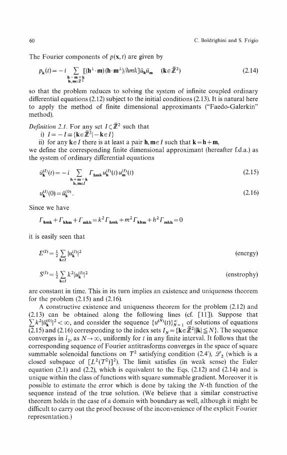
The Fourier components of p(x,ί) are given by
Λ(0=-ΐ Σ L(^ m)(li'm^/hmk-]ύhύm (keZ2) (2.14)
so that the problem reduces to solving the system of infinite coupled ordinarydifferential equations (2.12) subject to the initial conditions (2.13). It is natural hereto apply the method of finite dimensional approximants ("Faedo-Galerkin"method).
Definition 2.ί. For any set /C^2 such that
ii) for any ke / there is at least a pair h, me / such that k = h + m,we define the corresponding finite dimensional approximant (hereafter f.d.a.) asthe system of ordinary differential equations
ώ<"(ί)=-ί £ rhmkuV(t)u£(l) (2.15)h + m = k
h,me/
"ί/)(0) = fiΓ (2.16)
Since we have
it is easily seen that
£(/) = έ Σ W T (energy)ke/
ke/
(enstrophy)
are constant in time. This in its turn implies an existence and uniqueness theoremfor the problem (2.15) and (2.16).
A constructive existence and uniqueness theorem for the problem (2.12) and(2.13) can be obtained along the following lines (cf. [11]). Suppose that^/c2 |wk
0) |2<oo, and consider the sequence {t/(Λ°(£)}^=1 of solutions of equations(2.15) and (2.16) corresponding to the index sets IN = {keZ2||k| ̂ N}. The sequenceconverges in /2, as JV-»oo, uniformly for t in any finite interval. It follows that thecorresponding sequence of Fourier antitrasforms converges in the space of squaresummable solenoidal functions on T2 satisfying condition (2.4'), j§?2 (which is aclosed subspace of \_L2(T2}~\2}. The limit satisfies (in weak sense) the Eulerequation (2.1) and (2.2), which is equivalent to the Eqs. (2.12) and (2.14) and isunique within the class of functions with square summable gradient. Moreover it ispossible to estimate the error which is done by taking the Λ/-th function of thesequence instead of the true solution. (We believe that a similar constructivetheorem holds in the case of a domain with boundary as well, although it might bedifficult to carry out the proof because of the inconvenience of the explicit Fourierrepresentation.)
States for an Incompressible Fluid 61
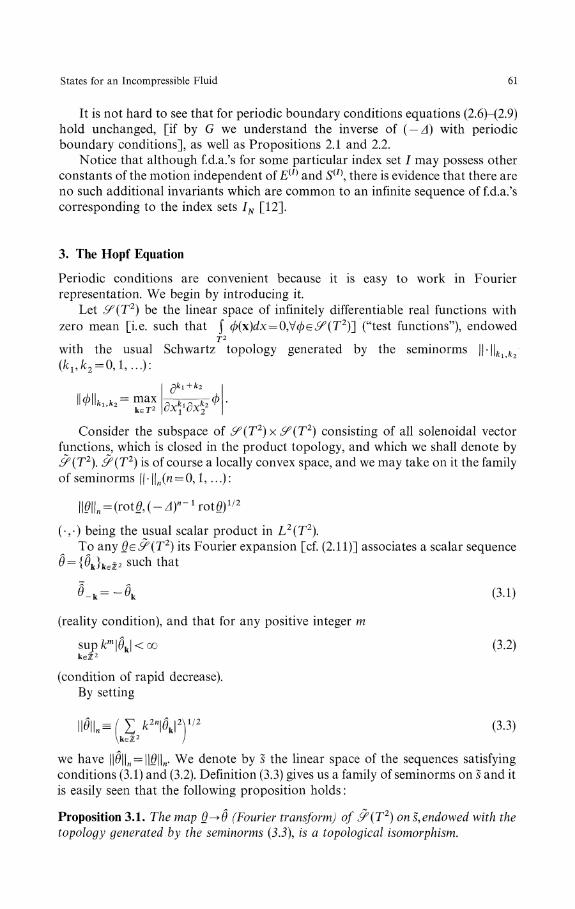
It is not hard to see that for periodic boundary conditions equations (2.6)-(2.9)hold unchanged, [if by G we understand the inverse of ( — A) with periodicboundary conditions], as well as Propositions 2.1 and 2.2.
Notice that although f.d.a.'s for some particular index set / may possess otherconstants of the motion independent of E(I} and S(I\ there is evidence that there areno such additional invariants which are common to an infinite sequence of f.d.a.'scorresponding to the index sets IN [12].
3. The Hopf Equation
Periodic conditions are convenient because it is easy to work in Fourierrepresentation. We begin by introducing it.
Let ^(T2) be the linear space of infinitely differentiable real functions withzero mean [i.e. such that J φ(x)dx = Q,\/φe<?(T2)~] ("test functions"), endowed
T2
with the usual Schwartz topology generated by the seminorms INI*! &2
= max2 keT2
Consider the subspace of £f (T2) x <? (T2) consisting of all solenoidal vectorfunctions, which is closed in the product topology, and which we shall denote by^(T2). &(T2) is of course a locally convex space, and we may take on it the familyof seminorms || ||n(n = 0, 1, ...):
(v) being the usual scalar product in L2(Γ2).To any θe&(T2) its Fourier expansion [cf. (2.11)] associates a scalar sequence
θ = {θk}k^2 such that
S-k=-3k (3-1)
(reality condition), and that for any positive integer m
sup/cm |0k |<oo (3.2)keZ2
(condition of rapid decrease).By setting
Λ=f Σ fc2Ί3\keZ2
we have ||Θ||M = ||Θ||Π. We denote by s the linear space of the sequences satisfyingconditions (3.1) and (3.2). Definition (3.3) gives us a family of seminorms on s and itis easily seen that the following proposition holds :
Proposition 3.1. The map θ->θ (Fourier transform) of &(T2) ons.endowed with thetopology generated by the semmorms (3.3), is a topologίcal isomorphism.
62 C. Boldrighini and S. Frigio
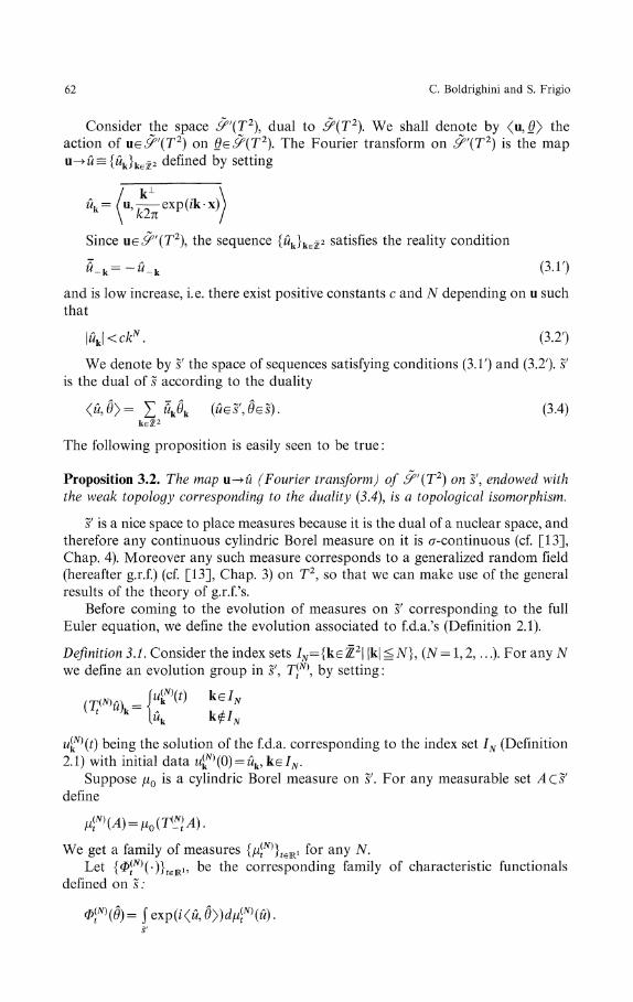
Consider the space &'(T2\ dual to &(T2\ We shall denote by <u,θ> theaction of ue^'(T2) on θe&(T2). The Fourier transform on &'(T2) is the mapu-»tίΞΞ{/2k}ke^2 defined by setting
Since UE^'(T2), the sequence {uk}ke^2 satisfies the reality condition
u_k=-u_k (3.1')
and is low increase, i.e. there exist positive constants c and N depending on u suchthat
\ύk\<ckN. (3.2')
We denote by s' the space of sequences satisfying conditions (3.Γ) and (3.2'). s'is the dual of s according to the duality
< f i , > = £ 5kθk (ύes\θes). (3.4)keZ2
The following proposition is easily seen to be true :
Proposition 3.2. The map u-»w (Fourier transform) of &'(T2) on s', endowed withthe weak topology corresponding to the duality (3.4\ is a topologίcal isomorphism.
s' is a nice space to place measures because it is the dual of a nuclear space, andtherefore any continuous cylindric Borel measure on it is σ-continuous (cf. [13],Chap. 4). Moreover any such measure corresponds to a generalized random field(hereafter g.r.f.) (cf. [13], Chap. 3) on T2, so that we can make use of the generalresults of the theory of g.r.f.'s.
Before coming to the evolution of measures on s' corresponding to the fullEuler equation, we define the evolution associated to f.d.a.'s (Definition 2.1).
Definition 3.1. Consider the index sets /N={kG^2| |k| gjΛΓ}, (N = 1, 2, . . .). For any Nwe define an evolution group in s', Ί*N\ by setting :
u (
k
} ( t ) being the solution of the f.d.a. corresponding to the index set IN (Definition2.1) with initial data ι4N)(0) = "k,ke/ ίV.
Suppose μ0 is a cylindric Borel measure on s'. For any measurable set A C s'define
We get a family of measures {μ^JfeR1 f°r
Let {Φ^ίOlίeRij be the corresponding family of characteristic functionalsdefined on 5;
States for an Incompressible Fluid 63
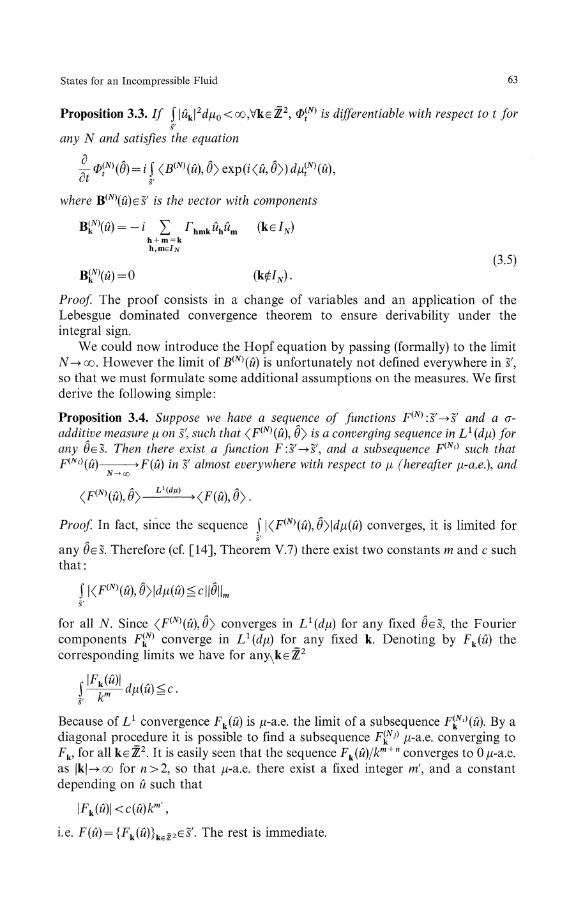
Proposition 3.3. // J |ί/k|2dμ0<oo,VkeZ2, Φ|N) is differ entiable with respect to t for
s'any N and satisfies the equation
|- ΦW(Θ) = i ί <5^(ώ), Θy exp(ί<fi, 0» d/Γ(Λ),CT §/
where B(JV)(M)ES' is ffte vector with components
BH«) = -ί Σ ^mk«h«m (ke/N)h + m = kh,me/ιv
(3.5)
Proo/ The proof consists in a change of variables and an application of theLebesgue dominated convergence theorem to ensure derivability under theintegral sign.
We could now introduce the Hopf equation by passing (formally) to the limitJV-KX). However the limit of B(N}(ύ) is unfortunately not defined everywhere in s',so that we must formulate some additional assumptions on the measures. We firstderive the following simple:
Proposition 3.4. Suppose we have a sequence of functions F(]V):s'— »s' and a σ-additive measure μ on s', such that (F(N}(ύ\ θy is a converging sequence in L1 (dμ) forany θes. Then there exist a function F:s'—>s', and a subsequence F(]Vί) such thatF(Ni\u) - >F(ύ) in sf almost everywhere with respect to μ (hereafter μ-a.e.), and
N-* oo
Lί(dμ}
Proof. In fact, since the sequence J |<F(]V)(w), θy\dμ(ύ) converges, it is limited fors'
any θes. Therefore (cf. [14], Theorem V.7) there exist two constants m and c suchthat:
for all N. Since (F(N}(u),θy converges in ^(dμ) for any fixed θes, the Fouriercomponents F^ converge in Ll(άμ) for_ any fixed k. Denoting by Fk(ύ) thecorresponding limits we have for
Because of L1 convergence Fk(ff) is μ-a.e. the limit of a subsequence F^l)(ύ). By adiagonal procedure it is possible to find a subsequence F^j) μ-a.e. converging toFk, for all keZ2. It is easily seen that the sequence Fk(ύ)/km+n converges to Oμ-a.e.as |k|->oo for π>2, so that μ-a.e. there exist a fixed integer m', and a constantdepending on ύ such that
i.e. F(u) = {Fk(u)}kef2es'. The rest is immediate.
64 C. Boldrighini and S. Frigio
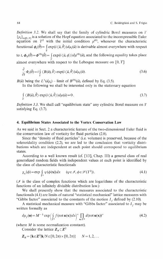
Definition 3.2. We shall say that the family of cylindric Borel measures on s'{μjίe[0 Γ] is a solution of the Hopf equation associated to the incompressible Eulerequation on T2 with the initial condition μ(0), whenever the characteristic
functional Φt(θ) = J exp(i<w, θy)dμt(ύ) is derivable almost everywhere with respects'
to ί, Φ0(θ) = φ(0}(θ)= J exp(i<w, φy)dμ(0}(ύ\ and the following equality takes places'
almost everywhere with respect to the Lebesgue measure on [0, T]
Φt(θ) = i j <β(ώ), θy exp(ΐ<ώ, 0»dft(ώ) . (3.6)<7Γ s/
5(ώ) being the Ll(dμt) - limit of £(JV)(w), defined by Eq. (3.5).In the following we shall be interested only in the stationary equation
J <£?(«), θ> exp(i<«, θy)dμ(ΰ) = Q. (3.7)s'
Definition 3.3. We shall call "equilibrium state" any cylindric Borel measure on s'satisfying Eq. (3.7).
4. Equilibrium States Associated to the Vortex Conservation Law
As we said in Sect. 2 a characteristic feature of the two-dimensional Euler fluid isthe conservation law of vorticity for fluid particles (2.8).
Since the "density of fluid particles" (i.e. volumes) is preserved, because of thesolenoidality condition (2.2), we are led to the conclusion that vorticity distri-butions which are independent at each point should correspond to equilibriumstates.
According to a well known result (cf. [13], Chap. Ill) a general class of realgeneralized random fields with independent values at each point is identified bythe class of characteristic functionals
χv(0) = exp J ιp(φ(x))dx (ψe^,φe^(T2)). (4.1)T2
(J> is the class of complex functions which are logarithms of the characteristicfunctions of an infinitely divisible distribution law.)
We shall presently show that the measures associated to the characteristicfunctionals (4.1) are limits of natural "statistical mechanical" lattice measures with"Gibbs factor" associated to the constants of the motion If defined by (2.10).
A statistical mechanical measure with "Gibbs factor" associated to If may bewritten formally as
dμf(u) = M~1 exp/ J /(rot u(\))dx\" Π <*(rot u(x))" (4.2)\T2 / xeΓ2
(where M is some normalization constant).Consider the lattice ZNC%2
ZΛr = {keZ2 |k/Λ/ re[0,2π)x[0,2π)} ΛΓ = 1,2,...
States for an Incompressible Fluid 65
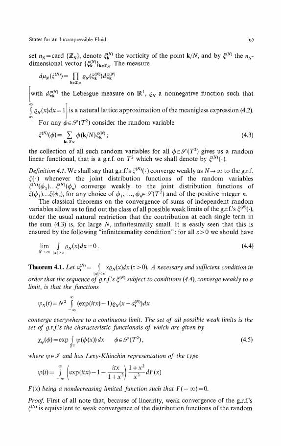
set nN = carά {ZN}, denote ξ^} the vorticity of the point k/ΛΓ, and by ξ(N) the nN-dimensional vector { ζ - The measure
with dξ^ the Lebesgue measure on R1, ρ^ a nonnegative function such that
J ρN(x)dx = 1 is a natural lattice approximation of the meanigless expression (4.2).00 J
For any φe^(T2) consider the random variable
ξm(Φ)= Σ ΦWWIW , (4.3)
the collection of all such random variables for all φe^(T2) gives us a randomlinear functional, that is a g.r.f. on T2 which we shall denote by
Definition 4.1. We shall say that g.r.f.'s ξ(N)(-) converge weakly as N-+ oo to the g.r.f.ξ( ) whenever the joint distribution functions of the random variablesξ(N)(φί)...ξ(N)(φn) converge weakly to the joint distribution functions ofξ(φ1)...ξ(φn)9 for any choice of φl9 ..., φne^(T2) and of the positive integer n.
The classical theorems on the convergence of sums of independent randomvariables allow us to find out the class of all possible weak limits of the g.r.f.'s ξ(N\-),under the usual natural restriction that the contribution at each single term inthe sum (4.3) is, for large N, infinitesimally small. It is easily seen that this isensured by the following "infinitesimality condition": for all e>0 we should have
lim J ρN(x)dx = Q. (4.4)N-+CQ \χ\>ε
Theorem 4.1. Let a^} = j xρN(x)dx (τ >0). A necessary and sufficient condition in\x\<τ
order that the sequence of g.r.f.'s ξ(N) subject to conditions (4.4), converge weakly to alimit, is that the functions
ψN(t) = N2 ] (exp(Jίx)-l)ρjv(x + α<NVx— 00
converge everywhere to a continuous limit. The set of all possible weak limits is theset of g.r.f.'s the characteristic functional^ of which are given by
χψ(φ) = πp J ψ(φ(x))dx 0e^(T2), (4.5)Γ2
where φe./ and has Levy-Khinchin representation of the type
itx --2
ψ(t)= j exp(itx)-l---oo \ -1- "Γ^
F(x) being a nondecreasing limited function such that F(— oo) = 0.
Proof. First of all note that, because of linearity, weak convergence of the g.r.f.'sξ(N) is equivalent to weak convergence of the distribution functions of the random
66 C. Boldrighini and S. Frigio
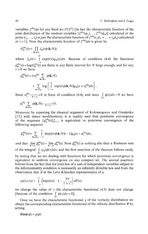
variables ζ(N\φ) for any fixed φe^(T2) [in fact the characteristic function of thejoint distribution of the random variables {ζ(N)(φι\ ...,ξ(N}(φN)} calculated at thepoint (tl9 .. ., ίj is just the characteristic function of ξ(N\t1φί + . . . + tnφn) calculatedat t= 1]. Now the characteristic function of ξ(N}(φ) is given by
GΓ(0= Π f*(tΦWN))keZN
00
where fN(t)= j exp(itx)ρN(x)dx. Because of condition (4.4) the functions— 00
are finite in any finite interval for N large enough, and for anyτ>0 we have
<>(ί) = /tα<N) £ φ(k/N)
+ Σ l o g ί jkeZίv I — oo
Since a(^} - »0 in force of condition (4.4), and since j φ(x)dx = 0 we have^
Moreover by repeating the classical argument of Kolomogorov and Gnedenko[15] with minor modifications, it is readily seen that pointwise convergenceof the sequence {g(φ\t)}^=1 is equivalent to pointwise convergence of thefollowing sequence
0f(0= Σ ϊ (™p(itφWN))-l)ρ^x + aW)dx,keZjί ~~ °o
and that lim g(^\t) = lira gψ\t). Now gψ\t) is nothing else than a Riemann sumJV-+00 ^ N^oo ψ ψ
of the integral J ψN(φ(x))dx, and the first assertion of the theorem follows easilyΓ2
by noting that we are dealing with functions for which pointwise convergence isequivalent to uniform convergence on any compact set. The second assertionfollows from the fact that the limit law of a sum of independent variables subject tothe infinitesimality condition is necessarily an infinitely divisible law and from theobservation that if in the Levy-Khinchin representation of ψ
ίtxJ exp(ifx)-l-—-Ί )dF(x)
no V i +x /
we change the value of y the characteristic functional (4.5) does not change[because of the condition J φ(x)dx = 0].
T2
Once we have the characteristic functional χ of the vorticity distribution weobtain the corresponding characteristic functional of the velocity distribution Φ bysetting
States for an Incompressible Fluid 67
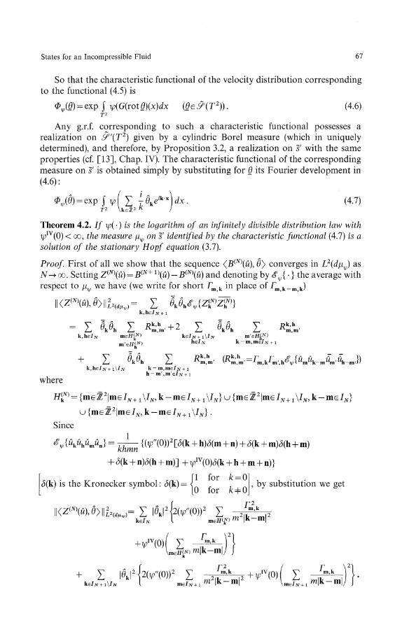
So that the characteristic functional of the velocity distribution correspondingto the functional (4.5) is
Φv,(θ) = exp f v>(G(rotθ)(x)dx (θe^(T2)) . (4.6)Γ2
Any g.r.f. corresponding to such a characteristic functional possesses arealization on ^'(T2) given by a cylindric Borel measure (which in uniquelydetermined), and therefore, by Proposition 3.2, a realization on s' with the sameproperties (cf. [13], Chap. IV). The characteristic functional of the correspondingmeasure on s' is obtained simply by substituting for θ its Fourier development in(4.6):
. (4.7)
Theorem 4.2. If ψ( ) is the logarithm of an infinitely divisible distribution law withφlv(0)< oo, the measure μψ on s1 identified by the characteristic functional (4.7) is asolution of the stationary Hopf equation (3.7).
Proof. First of all we show that the sequence (B(N\ύ\ θ> converges in L2(dμψ) asN-+ oo. Setting Z(N\ύ) = B(N+ l\u) - B(N\ύ) and denoting by £ψ{ } the average withrespect to μψ we have (we write for short Γm k in place of Γm k _ m k)
k,heIN+ i
/?k'h
k, he/^
/?k»hKm,m'
where
+ Σ Mh Σk,h6/ίv+ iVΓzv k-m,me/Λr+ i
h — m',m'e/ίVH- 1
Since
m)
+ δ(k + n)(5(h + m)] + tpιv(0)^(k + h + m + n)}
u5(k) is the Kronecker symbol: δ(k)= < , by substitution we getlor
+vιv(θ) Σ) » ι-m
+ k / Σ / I0J2 {2(v"(0))2 Σ m2^m]2 + ΆO) ( Σ : —m
68 C. Boldrighini and S. Frigio
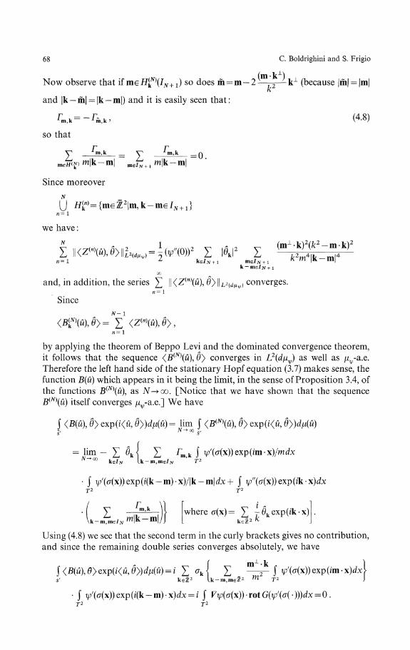
Now observe that if meH(^\IN+1) so does m = m — 2 — -̂ — k1 (because |m| = |m|/C
and |k — ίh| = |k — m|) and it is easily seen that:
rm,*=-r^, (4.8)so that
y Γ™Λ = y Γ™>* =Qm6SN, m|k - m| me^ + , m|k - m|
Since moreover
we have :
N
Σ
and, in addition, the series Σ IKZ(lf)(w), 0>||L2(dMv) converges.«= i
Since
by applying the theorem of Beppo Levi and the dominated convergence theorem,it follows that the sequence <J3(Λ°(w), θy converges in L2(dμψ) as well as μv-a.e.Therefore the left hand side of the stationary Hopf equation (3.7) makes sense, thefunction B(ύ) which appears in it being the limit, in the sense of Proposition 3.4, ofthe functions B(N\ύ\ as JV-»oo. [Notice that we have shown that the sequenceB(N\ύ) itself converges μv-a.e.] We have
B(ύ\ θy exp(i<w, θy)dμ(ύ) = lim J (B(N\ύ), θy exp(i<w, θy}dμ(ύ]s'
= lip ~ Σ 0k| Σ Γm,k ί t//(σ(x))exp(im x)/mdx~^°° ke/jv Ik —m,me/^ T2
• J ψf(σ(x))exp(ί(lί-m)'X)/\'k-m\dx+ J t/;r/((7(x))exp(ik x)dxT2 Γ2
where σ(x) = Σ T ̂ k exP (^'x) •
Using (4.8) we see that the second term in the curly brackets gives no contribution,and since the remaining double series converges absolutely, we have
J <β(M), Θy exp(ι<M, θy)dμ(ύ) = / Σ σk Ί Σ —2~ ί V'M*))exp(ίm x)cs' keZ 2 lk-m,meZ2 m T2
T2 T2
States for an Incompressible Fluid 69
5. Properties of the Gaussian and Poissonian States
a. Gaussian States
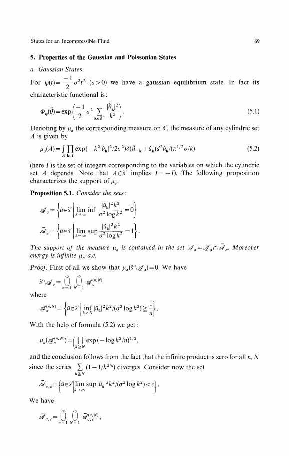
For ψ(t)= - σ2t2 (<τ>0) we have a gaussian equilibrium state. In fact its
characteristic functional is :
(5.1)κ
Denoting by μσ the corresponding measure on s', the measure of any cylindric setA is given by
}= ί ΠA ke/
(5.2)
(here / is the set of integers corresponding to the variables on which the cylindricset A depends. Note that Acs' implies /=—/). The following propositioncharacterizes the support of μσ.
Proposition 5.1. Consider the sets:
\1J.\2k2
lim inf -
= <UGS'lu |2/c2
lim sup —^—ry = 1L/c-oo σ 2log/c 2
support of the measure μσ is contained in the set £#σ = ^energy is infinite μΰ-a.e.
Proof. First of all we show that μσ(s'\^σ) = Q. We have00 00
\ — σ \J \J — σ
. Moreover
w = l N=l
where
mf |uk
With the help of formula (5.2) we get:
and the conclusion follows from the fact that the infinite product is zero for all n, N
since the series £ (1 — l/7c2/") diverges. Consider now the setk>N
c = ίues' lim sup|t/J2/c2/(σ2log/c2)<cl .Jfe^oo
We have
_ oo oo
•*-.«= u. u^r,
70 C. Boldrighini and S. Frigio
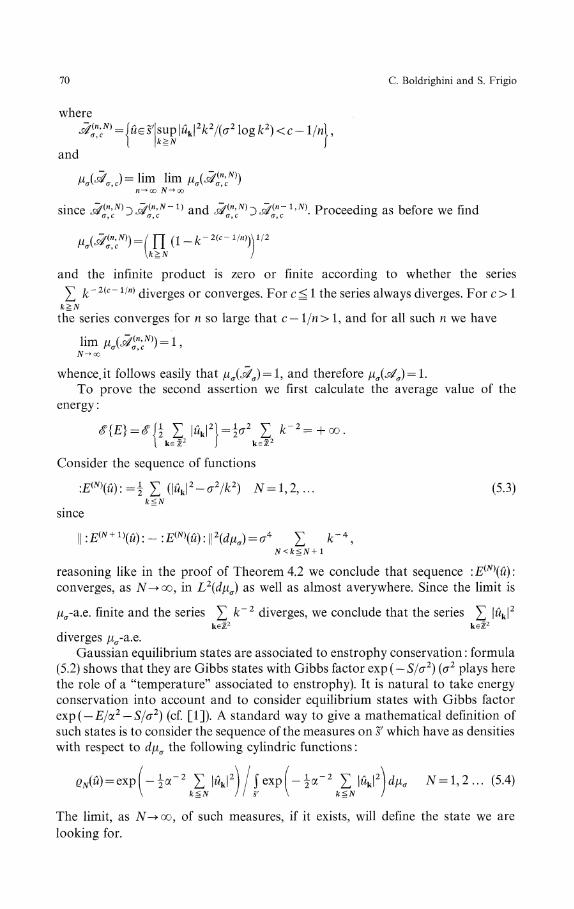
where^c
N} = ίύESfsup\uk\2k2/(σ2logk2)<c-l/n\,
and
n—>• oo N—>• oo
since S/£ C
N) 3 jtfff ~ ̂ and ^"^b^"c~1>N). Proceeding as before we findC
and the infinite product is zero or finite according to whether the series
Σ k~2(c~ 1/n) diverges or converges. For c ̂ 1 the series always diverges. For c> 1/c^N
the series converges for n so large that c— l/n> 1, and for all such n we have
- *>) = !,
whence.it follows easily that μσ(jtfσ) = l, and therefore μσ(eβ/<y) = l.To prove the second assertion we first calculate the average value of the
energy :
keZ 2
Consider the sequence of functions
:E^(ύ):=^(\ύk
2-σ2/k2) N = l,2,... (5.3)fc^IV
since
reasoning like in the proof of Theorem 4.2 we conclude that sequence :E(N\ύ):converges, as JV->oo, in L2(dμσ) as well as almost averywhere. Since the limit is
μσ-a.e. finite and the series ^ k~2 diverges, we conclude that the series ]Γ \ύk\2
keZ2 keZ2
diverges μσ-a.e.Gaussian equilibrium states are associated to enstrophy conservation : formula
(5.2) shows that they are Gibbs states with Gibbs factor exp( — S/σ2) (σ2 plays herethe role of a "temperature" associated to enstrophy). It is natural to take energyconservation into account and to consider equilibrium states with Gibbs factorexp( — E/a2 — S/σ2) (cf. [1]). A standard way to give a mathematical definition ofsuch states is to consider the sequence of the measures on s' which have as densitieswith respect to dμσ the following cylindric functions :
f exp(- ^oΓ2 Σ |ώJ2W N=l,2 . . . (5.4)k^N I s ' \ k^N I
The limit, as 7V-^oo, of such measures, if it exists, will define the state we arelooking for.
States for an Incompressible Fluid 71
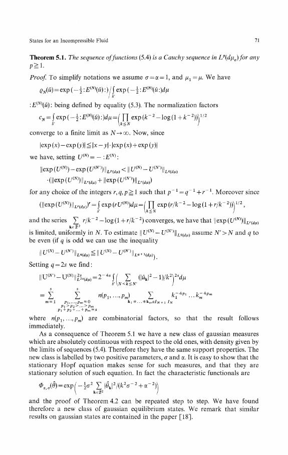
Theorem 5.1. The sequence of functions (5.4) is a Cauchy sequence in Lp(dμσ)for any
P^l.
Proof. To simplify notations we assume σ — α = l, and μί=μ. We have
:E(N\ύ): being defined by equality (5.3). The normalization factors
5'
converge to a finite limit as JV-κx). Now, since
|exp (x) - exp (y)\ ^\x-y\ |exp (x) + exp (y)\
we have, setting U(N}= - :E(N}:
for any choice of the integers r,q,p^l such that p"1 = q~1 +r~l. Moreover since
and the series ]Γ r/k~2 — log(l + r//c~2) converges, we have that ||exp(17(]V))||Lr(dμ)
keZ 2
is limited, uniformly in N. To estimate || t/(N) — U(N>)\\Lq(dμ) assume N'>N and q tobe even (if q is odd we can use the inequality
) _ TT(N') || < || ττ(N) _U \\mdμ)=\\U
Setting q = 2s we find :
Σm = l Pι,...,pm = 0
Pl>P2> >Pm
where n(p1? ...,pm) are combinatorial factors, so that the result followsimmediately.
As a consequence of Theorem 5.1 we have a new class of gaussian measureswhich are absolutely continuous with respect to the old ones, with density given bythe limits of sequences (5.4). Therefore they have the same support properties. Thenew class is labelled by two positive parameters, σ and α. It is easy to show that thestationary Hopf equation makes sense for such measures, and that they arestationary solution of such equation. In fact the characteristic functionals are
and the proof of Theorem 4.2 can be repeated step to step. We have foundtherefore a new class of gaussian equilibrium states. We remark that similarresults on gaussian states are contained in the paper [18].
72 C. Boldrighini and S. Frigio
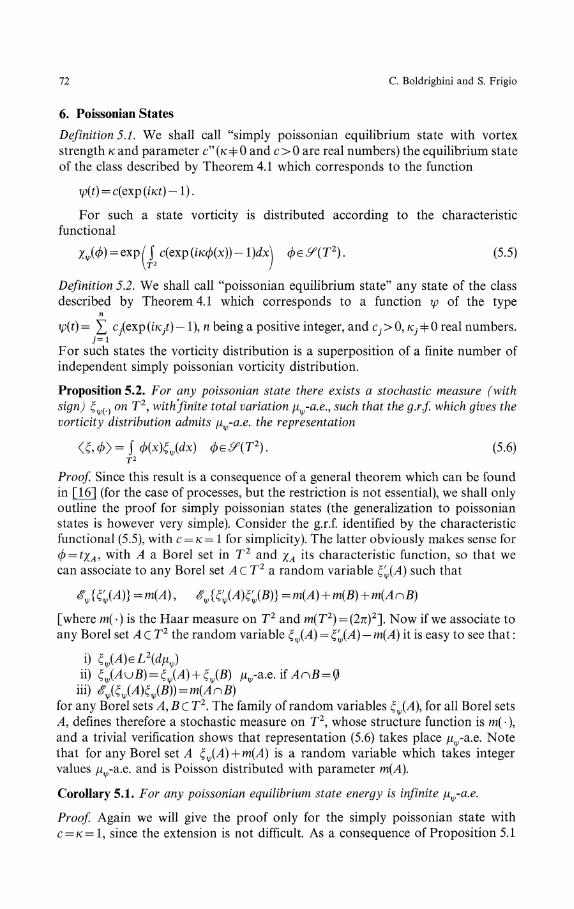
6. Poissonian States
Definition 5.1. We shall call "simply poissonian equilibrium state with vortexstrength K and parameter c" (K Φ 0 and c> 0 are real numbers) the equilibrium stateof the class described by Theorem 4.1 which corresponds to the function
V>(ί) = c(exp(iιcί)-l).
For such a state vorticity is distributed according to the characteristicfunctional
c(εxp(ίκφ(x))-l)dx\ φe^(T2). (5.5)2 /Definition 5.2. We shall call "poissonian equilibrium state" any state of the classdescribed by Theorem 4.1 which corresponds to a function ψ of the type
n
ψ(t) = Σ c/exp (iKjt) —l),n being a positive integer, and c. > 0, κj Φ 0 real numbers.7=1
For such states the vorticity distribution is a superposition of a finite number ofindependent simply poissonian vorticity distribution.
Proposition 5.2. For any poissonian state there exists a stochastic measure (withsign) ξv(ι) on T2, with'finite total variation μψ-a.e., such that the g.r.f. which gives thevorticity distribution admits μψ-a.e. the representation
<ξ,φy=SΦ(x)ξψ(dx) φe^(T2). (5.6)T2
Proof. Since this result is a consequence of a general theorem which can be foundin [16] (for the case of processes, but the restriction is not essential), we shall onlyoutline the proof for simply poissonian states (the generalization to poissonianstates is however very simple). Consider the g.r.f. identified by the characteristicfunctional (5.5), with c = κ—l for simplicity). The latter obviously makes sense forφ = tχA, with A a Borel set in T2 and χA its characteristic function, so that wecan associate to any Borel set A C T2 a random variable ξ'ψ(A) such that
[where m( ) is the Haar measure on T2 and m(T2) = (2π)2]. Now if we associate toany Borel set A C T2 the random variable ξψ(A) = ξf
ψ(A) — m(A) it is easy to see that :
i) ξψ(A)eL2(dμψ)ii) ξψ(AuB) = ξψ(A) + ξψ(B) μψ-z.e.ifAπB = φ
iii) Λψ(ξψ(A)ξψ(B)) = m(AnB)for any Borel sets A, B C T2. The family of random variables ξ (A), for all Borel setsA, defines therefore a stochastic measure on T2, whose structure function is m( ),and a trivial verification shows that representation (5.6) takes place μv-a.e. Notethat for any Borel set A ξψ(A) + m(A) is a random variable which takes integervalues μv-a.e. and is Poisson distributed with parameter m(A).
Corollary 5.1. For any poissonian equilibrium state energy is infinite μψ-a.e.
Proof. Again we will give the proof only for the simply poissonian state withc = κ=l, since the extension is not difficult. As a consequence of Proposition 5.1
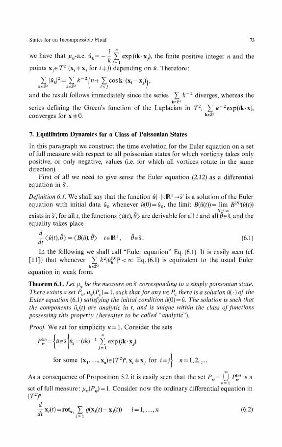
States for an Incompressible Fluid 73
i n
we have that μv-a.e. wk= - -r Σ expίik x^), the finite positive integer n and thekj=1
points Xj eT2 (x^φX; for z'Φj) depending on ύ. Therefore:
and the result follows immediately since the series Σ k~2 diverges, whereas thekeZ2
series defining the Green's function of the Laplacian in T2, Σ AΓ2exp(/k x),converges for x Φ 0. ke^2
7. Equilibrium Dynamics for a Class of Poissonian States
In this paragraph we construct the time evolution for the Euler equation on a setof full measure with respect to all poissonian states for which vorticity takes onlypositive, or only negative, values (i.e. for which all vortices rotate in the samedirection).
First of all we need to give sense the Euler equation (2.12) as a differentialequation in 5'.
Definition 6.1. We shall say that the function ύ( •) IR1 -»s' is a solution of the Eulerequation with initial data ύ0 whenever M(()) = MO, the limit B(ύ(t))= lim B(N\ύ(t))
N^ooexists in s', for all t, the functions <w(ί), θ> are derivable for all t and all ΘES, and theequality takes place
d,0> feIR 1 , ΘES. (6.1),
In the following we shall call "Euler equation" Eq. (6.1). It is easily seen (cf.[11]) that whenever Σ /c2 |w(
k
0) |2< oo Eq. (6.1) is equivalent to the usual EulerkeZ2
equation in weak form.
Theorem 6.1. Let μψ be the measure on sf corresponding to a simply poissonian state.There exists a set Pψ, μψ(Pψ) = 1, such that for any we Pψ there is a solution ύ(-)of theEuler equation (6.1) satisfying the initial condition ύ(0) = ύ. The solution is such thatthe components ύk(t) are analytic in ί, and is unique within the class of functionspossessing this property (hereafter to be called "analytic").
Proof. We set for simplicity κ=ί. Consider the sets
j=ι
for some (x1? ...,xn)e(T2)n,χ.φx7 for ϊφj i n=l,2,. . .
00
As a consequence of Proposition 5.2 it is easily seen that the set Pψ = (J P(^ is an= 1
set of full measure : μψ(Pψ) = 1. Consider now the ordinary differential equation in(T2)"
-̂ Xi(ί) = rotxί X g(xi(t) - x (ί)) i = l,...,n (6.2)at j φ l
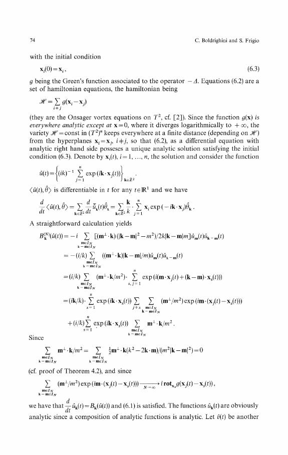
74 C. Boldrighini and S. Frigio
with the initial condition
x,(0) = X i , (6.3)
g being the Green's function associated to the operator —A. Equations (6.2) are aset of hamiltonian equations, the hamiltonian being
(they are the Onsager vortex equations on T2, cf. [2]). Since the function g(x) iseverywhere analytic except at x = 0, where it diverges logarithmically to + oo, thevariety j^ = const in (T2)" keeps everywhere at a finite distance (depending on jj?)from the hyperplanes Xj = Xj, z'ΦΛ so that (6.2), as a differential equation withanalytic right hand side posseses a unique analytic solution satisfying the initialcondition (6.3). Denote by xf(ί), i= 1, ..., n, the solution and consider the function
Γ1 Σ exp(ίk x/ί))j=l
(ύ(t\βy is differentiable in t for any ίeR1 and we have
~<ύ(t),θy = Σ 4A(f)θk = Σ Γ Σ x (exp(-ik xj)θk.dt keZ2" f keZ 2 / C j = l
A straightforward calculation yields
<'("(i))=-i Σ [(m
Σ ((m± k)lk - m|/m)Mm(ίK _ m(ί)e/ίvmeljv
(mx k/m2). Σ expWm^ s, j = 1ljv
exp (ik - xs(ί)) Σ Σ (m±K) exP (ίm 's = l j Φ s me/jv
k- me/jvn
+ (i/k) Σ exp (ft xs(ί)) Σ m1 k/m2 .'s = 1
0 . k -Since
X m1-k/m2= X |m1 k(/c2-2k m)/(m2|k-m|2) = 0me/]v meljv
k — me/ΛΓ k — me/iv
(cf. proof of Theorem 4.2), and since
X (mλ/m2) exp (im (x/ί) - xs(ί))) ̂ 7̂ i rotXs6f(x/ί) - xs(ί)) ,
we have that — ύk(t) = Bk(ύ(t}) and (6. 1) is satisfied. The functions flk(f) are obviously
analytic since a composition of analytic functions is analytic. Let v(t) be another
States for an Incompressible Fluid 75
analytic solution satisfying the same initial condition at ί = 0; the functions vk
coincide with the functions ύk and so do all their derivatives, which may calculatedwith the help of Eq. (6.2) in terms of the initial data. Since the function vk(t) andwk(ί) are analytic and have all derivaties equal at ί = 0, they must coincide.
Actually a stronger result is true, which we give as a corollary.
Corollary 6.1. There exists a set P in sf such that for any ύeP there is a uniqueanalytic solution M( ) of the Euler equation (6.1) satisfying the initial conditionw(0) = ύ, and, moreover, μψ(P) = 1 for any measure μψ corresponding to a simplypoissonίan state or to a poissonian state for which all vortex strengths κ are of thesame sign.
Proof. Consider the sets
7 = 1
for some (x^ ...,xn)E(T2)n,κs,κj>Oandxjή=xs for
The set P(n} corresponds to all possible configurations of n vortices with vortexstrengths of the same sign (i.e. all vortices rotate in the same direction). It is not
GO
hard to see (cf. Proposition 5.2) that the set P = (J P(π) is a set of full measure forn= 1
any poissonian state satisfying the conditions of the corollary. Now, by repeating,with small modifications, the proof of Theorem 6.1 it is seen that existence ofdynamics on the set P follows from the existence of a unique solution for finitesystems of vortices rotating in the same direction.
Notice that for poissonian states with vortex strengths of both signs thetheorem does not hold, since finite configurations of vortices of both signs may becatastriphic, i.e. two vortices may collapse in a finite time [17].
Conclusions
Equilibrium dynamics for poissonian states admitting only positive (or negative)vorticity has been easily obtained via the Onsager vortex equations. The problemis more complicated for the other physically interesting cases. For poissonianstates with vorticity of both signs equilibrium dynamics can be constructed, bymeans of the Onsager vortex equations, only of the set of the catastrophic con-figurations which we mentioned at the end of the preceding paragraph is shownto be of zero equilibrium measure, as it is reasonable to expect. For this, however,one should wait until a sufficiently complete characterization of the catastrophicset is given (which seems to be a hard task). For gaussian states there are somepreliminary results [18], however the problem is essentially open.
Once equilibrium dynamics have been constructed we can investigate theevolution of initial states which are absolutely continuous with respect to theequilibrium measure. Convergence to equilibrium for such states is strictlyconnected to the ergodic properties of the corresponding "equilibrium dynamicalsystem" (which is the dynamical system on phase space given by equilibriummeasure and time evolution). The investigation of the ergodic properties of the
76 C. Boldrighini and S. Frigio
equilibrium states is probably as difficult a problem as it is in statistical mechanics(cf. [19]).
For poissonian states we can say for sure that ergodicity does not hold, sincethere are invariants of the motion (at least the vortex number, the hamiltonian and
n
the vorticity center x= £ Xi(fX) Even on the manifolds identified by suchi = l
integrals of the motion the system is in general nonergodic and apparently avariant of the Kolmogorov-ArnoΓd-Moser theorem holds [20]. The situation issimilar to that of finite particle systems.
Acknowledgements. We are indepted first of all to G. Gallavotti who stimulated our interest in thesubject. We thank also R. L. Dobrushin, E. A. Novikov, A. Pellegrinotti, Ya. G. Sinai, D. Surgailis,L. Triolo and A. M. Yaglom for many useful conversations and comments.
References
1. Lee, T.D.: Quart. Appl. Math. 10, 69 (1952)2. Novikov, E.A.: Sov. Phys. JETP 41, 937 (1976)3. Gurievich, B.M., Suhov, Ju.M.: Commun. Math. Phys. 49, 63 (1976)4. Dobrushin, R.L., Suhov, Ju.M.: Lecture notes in physics, Vol. 80, p. 325. Berlin, Heidelberg, New
York: Springer 19785. Fox, D.G.,Orszag, S.A.: Phys. Rev. Lett. 16, 169 (1973)6. Lanford, O.E. Ill, Commun. Math. Phys. 9, 169 (1968); 11, 257 (1969)7. Fritz, J., Dobrushin, R.L.: Commun. Math. Phys. 57, 67 (1977)8. Lanford, O.E.Ill: Lecture notes in physics, Vol. 38, p. 1. Berlin, Heidelberg, New York: Springer
19759. Kato, T.: Arch. Rat. Anal. 25, 188 (1967)
10. Bardos, C.: I. Math. An. Appl. 40, 769 (1972)11. Boldrighini, C.: Introduzione alia Fluidodinamica, Quaderni del C.N.R., Roma., 197912. Lee, J.: Phys. Fluids 20, 1250 (1977)13. Gelfand, I.M., Vilenkin, M.Y.: Generalized functions, Vol. IV. New York: Academic Press 196414. Reed, M., Simon, B.: Functional analysis, Vol. 1. New York: Academic Press 197215. Gnedenko, B.V., Kolmogorov, A.M.: Limit distributions for sums of independent random
variables. Cambridge: Addison Wesley 195416. Skorokhod, A.V.: Stochastic processes with independent increments. Moscow: Nauka 196417. Novikov, E.A.: Teoreticeskaja i Matematiceskaja Fizika. To appear18. Albeverio, S., Ribeiro de Faria, M., H0egh-Krohn, R.: Centre de Physique Teorique, CNRS
Marseille Universite d'Aix, Marseille II, Uer Scientifique di Luminy, preprint, 197819. Goldstein, S., Lebowitz, J.L., Aizenman, M.: Lecture notes in physics, Vol. 38, pp. 112. Berlin,
Heidelberg, New York: Springer 197520. Sinai, Ya.G.: Private communication
Communicated by J. L. Lebowitz
Received May 21, 1979


