Ergodicity of one-dimensional resource sharing systems

Stochastic Processes and their Applications 98 (2002) 1–22www.elsevier.com/locate/spa

Ergodicity of one-dimensional resource sharingsystems�

Enrique Andjela ; ∗, F. Javier L*opezb, Gerardo SanzbaLaboratoire D’Analyse, Topologie et Probabilit�es, Universit�e de Provence, 39, rue Joliot, Curie 13453

Marseille Cedex 13, FrancebDepartmento de M�etodos Estad�'sticos, Universidad de Zaragoza, C=Pedro Cerbuna, 12,

50009 Zaragoza, Spain

Received 7 February 2001; received in revised form 20 September 2001; accepted 3 October 2001

Abstract

We study one-dimensional resource sharing systems which can be seen as interacting particlesystems taking values in ({0; 1; : : : ; C}M )Z. We 5rst get, by coupling techniques, an estimate oftheir invariant measures. Then, for processes having a reversible measure, we show the unique-ness of the invariant measure and conclude that they are ergodic. As a consequence, we provethat every loss network on Z with calls of bounded length is ergodic. c© 2001 Elsevier ScienceB.V. All rights reserved.

MSC: primary: 60K35; secondary 90B15

Keywords: Resource sharing systems; Loss networks; Ergodicity; Relative entropy; Coupling

1. Introduction

Resource sharing systems appear when several servers must complete jobs usingsome resources which must be shared with other servers. Such situations are commonin many 5elds, and their applications to computer and communication networks haveattracted much attention in the past 20 years, both in a deterministic context (see, e.g.,Courcoubetis et al., 1987; Fujishige et al., 1988; Langston and Morford, 1990; Moodyand Antsaklis, 1998) where an e@cient way to redistribute the jobs and the resources

� Partial funding provided by Projects BFM 2000-1060 of MCYT, CONSI+D P062=99-C of DGA, andProgram EUROPA of CAI-CONSI+D.

∗ Corresponding author. Fax: +33-491-11-35-52.E-mail addresses: [email protected] (E. Andjel), [email protected] (F.J. L*opez),

[email protected] (G. Sanz).

0304-4149/01/$ - see front matter c© 2001 Elsevier Science B.V. All rights reserved.PII: S0304 -4149(01)00138 -7

2 E. Andjel et al. / Stochastic Processes and their Applications 98 (2002) 1–22

is sought, and in a stochastic context (see, e.g., Bolch et al., 1998; Courcoubetis et al.,1984; Forbes et al., 1996; Graham and Meleard, 1994; Hunt and Kurtz, 1994; Kelly,1985; Sidhu and Wijesinha, 1998) where there are some random quantities involvedand the long term behavior of the system is studied.We consider a stochastic version of these systems. At each point of a graph G

there is a server who can do diKerent types of jobs. Jobs arrive at a server followingPoisson processes whose rates depend on his state and the state of the rest of theservers. The times of completion of a job by a server are exponentially distributedwith rates depending on the type of job and on the state of that server and of the otherservers who share some resources with him. All the random times are assumed to beindependent. If each server has a 5nite buKer (that is, there is a maximum number ofjobs which can be handled by the server and any job arriving when the buKer is full isnot accepted), the state space of each server is {0; 1; : : : ; C}M where M is the numberof diKerent types of job and C is the maximum capacity.When the graph G is 5nite, the process is a continuous-time Markov chain with

a 5nite state space and is therefore ergodic (i.e., it has a unique invariant mea-sure and the process converges to it from every initial measure) if and only if itis irreducible. However, for general in5nite G, the ergodicity of the process is notguaranteed.In this paper, we study the case where the graph G is Z, that is, the servers are

placed along an in5nite line. Our model can be seen as an interacting particle sys-tem and we refer the reader to Liggett (1985) from where we borrow the de5nitionsand notations for these processes. We will assume that the rates of our processes aretranslation invariant (the behavior of each server is the same, regardless of his sit-uation in Z) and 5nite range (the rates of arrival and completion of jobs at eachserver depend only of a 5nite number of “neighbors”). These assumptions are ratherstandard in interacting particle systems and assure that any of these processes is awell de5ned Feller process (in particular, this implies that is has at least one in-variant measure). From a practical point of view, it is logical to suppose that theservers will not share their resources with servers who are arbitrarily far away fromthem.Among other interesting systems, the processes we study include loss networks.

Loss networks play an important role in the modeling and analysis of systems suchas telephone networks, database structures and communication networks (see Kelly(1991)). In one of the simplest versions, a loss network can be seen as a cable onwhich K stations are placed and calls may be made from some station to another one.Each call uses a fraction C−1 of the section of the cable lying between the two stationsand is lost if some part of that section of the cable is already carrying C calls. Thetimes of arrivals and completions of calls follow independent Poisson processes. Inthis case, the state space of the network is 5nite and a rather complete description ofits invariant measure is given in Kelly (1987). When there is a countable number ofstations arranged on Z and the calls are of bounded length, loss networks can be seenas resource sharing systems as described above.The goal of this work is to study the ergodicity of a general class of resource

sharing systems (those having a reversible measure). There are few known results on

E. Andjel et al. / Stochastic Processes and their Applications 98 (2002) 1–22 3

this subject. Ycart (1993) showed, using the monotonicity of a related process, theergodicity of the philosophers’ process on Z, a resource sharing system where serverscan handle only one job and share one resource with their left and right neighbor (inTheorem 4:1 of Forbes et al. (1996), using similar arguments, this result was extendedunder some domination conditions on the rates, to the case where the servers can handletwo jobs); Ferrari and Garcia (1998) showed, by a percolation argument, the ergodicityof one-dimensional loss networks when the rate of arrivals of calls is su@ciently small(actually, they work in R instead of Z, but point out that their argument can be alsoapplied in Z). The main di@culty for getting ergodicity results in general resourcesharing systems is that they are not attractive processes and the usual technique ofstochastic comparison does not work.To get the ergodicity of the processes under study, we 5rst give an estimate of

their invariant measures. We will be interested in the probability, under the invariantmeasure, of a server x being idle conditioned to the value of the servers in the segment{x+1; : : : ; x+ n}. Under some general hypotheses on the rates, we will show that thisprobability can be uniformly (i.e. not depending on x or n) bounded below by somepositive constant. This will be done in Section 2 by the construction of a suitablecoupling.Section 3 is devoted to the proof of the ergodicity of resource sharing systems with a

reversible measure. We 5rst give some positivity conditions on the rates which ensurethat the reversible measure is unique and then show that this measure is the uniqueinvariant measure of the process. For doing that, we use the relative entropy technique,which has been widely applied for interacting particle systems with reversible measuresand was 5rst used in this context as early as 1971 in Holley (1971). As the rates of ourprocesses are not strictly positive, we need some estimates of the invariant measuresof the processes which we get from the results in Section 2. Once we have shownthe uniqueness of the invariant measure, we just have to refer to Mountford (1995) toconclude that our processes are ergodic.We 5nish the paper with an application of our results to loss networks (Section 4).

As pointed out before, loss networks on Z whose calls are of bounded length can beseen as resource sharing systems. We will see that they satisfy the conditions on therates imposed in Sections 2 and 3 and have a reversible measure. Therefore, applyingthe results proved in these sections, we conclude that they are ergodic. We point outthat, unlike in previous papers, here we do not require the arrival rates to be small toprove the ergodicity of the process.

2. Invariant measures of resource sharing systems

2.1. De9nitions and main theorem

Our resource sharing systems will be interacting particle systems on X =W Z, withW = {0; 1; : : : ; C}M . The state of a site x∈Z for a con5guration �∈X (denoted by�(x)) will be a M -tuple whose ith component (denoted by �(x; i)) is the number ofjobs of type i the particle at x has under the con5guration �. The generator of the


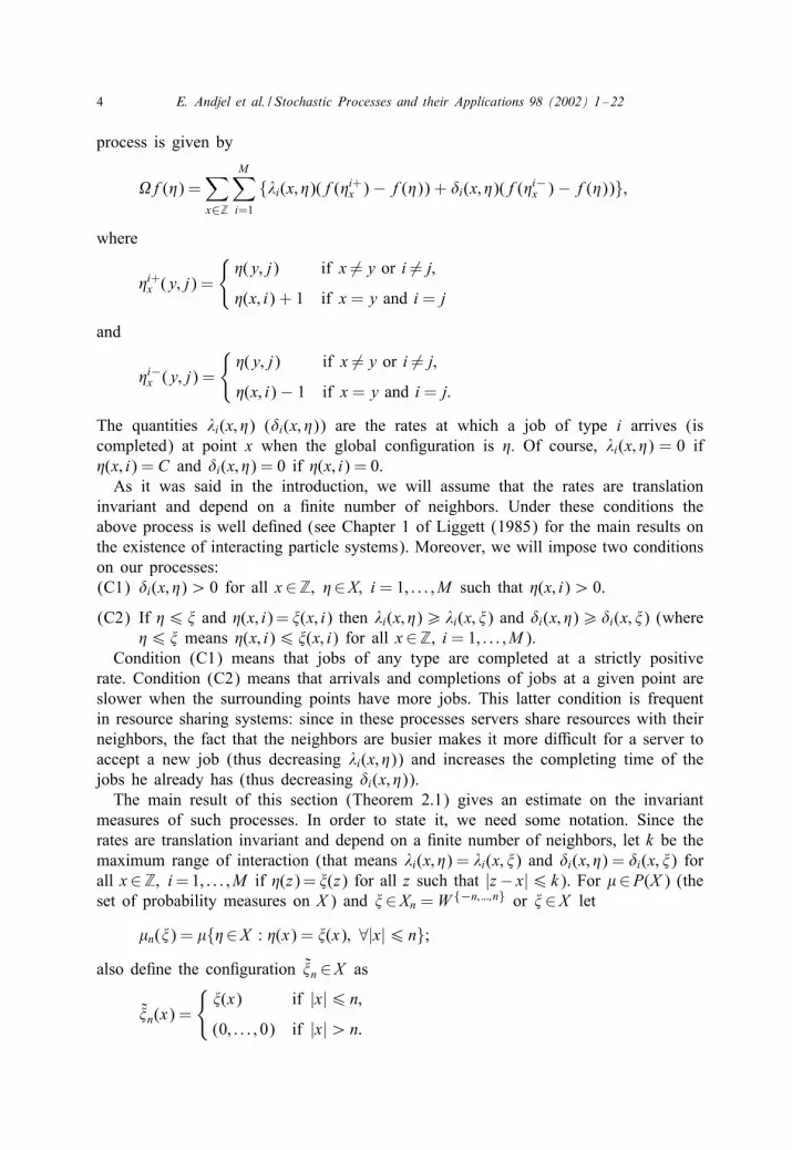
process is given by

�f(�) =∑x∈Z

M∑i=1

{�i(x; �)(f(�i+x )− f(�)) + �i(x; �)(f(�i−x )− f(�))};

where

�i+x (y; j) =

{�(y; j) if x �=y or i �= j;�(x; i) + 1 if x = y and i = j

and

�i−x (y; j) =

{�(y; j) if x �=y or i �= j;�(x; i)− 1 if x = y and i = j:

The quantities �i(x; �) (�i(x; �)) are the rates at which a job of type i arrives (iscompleted) at point x when the global con5guration is �. Of course, �i(x; �) = 0 if�(x; i) = C and �i(x; �) = 0 if �(x; i) = 0.As it was said in the introduction, we will assume that the rates are translation

invariant and depend on a 5nite number of neighbors. Under these conditions theabove process is well de5ned (see Chapter 1 of Liggett (1985) for the main results onthe existence of interacting particle systems). Moreover, we will impose two conditionson our processes:(C1) �i(x; �)¿ 0 for all x∈Z; �∈X; i = 1; : : : ; M such that �(x; i)¿ 0.

(C2) If �6 � and �(x; i)= �(x; i) then �i(x; �)¿ �i(x; �) and �i(x; �)¿ �i(x; �) (where�6 � means �(x; i)6 �(x; i) for all x∈Z, i = 1; : : : ; M).

Condition (C1) means that jobs of any type are completed at a strictly positiverate. Condition (C2) means that arrivals and completions of jobs at a given point areslower when the surrounding points have more jobs. This latter condition is frequentin resource sharing systems: since in these processes servers share resources with theirneighbors, the fact that the neighbors are busier makes it more di@cult for a server toaccept a new job (thus decreasing �i(x; �)) and increases the completing time of thejobs he already has (thus decreasing �i(x; �)).The main result of this section (Theorem 2.1) gives an estimate on the invariant

measures of such processes. In order to state it, we need some notation. Since therates are translation invariant and depend on a 5nite number of neighbors, let k be themaximum range of interaction (that means �i(x; �) = �i(x; �) and �i(x; �) = �i(x; �) forall x∈Z; i=1; : : : ; M if �(z)= �(z) for all z such that |z− x|6 k). For �∈P(X ) (theset of probability measures on X ) and �∈Xn =W {−n; :::; n} or �∈X let

�n(�) = �{�∈X : �(x) = �(x); ∀|x|6 n};also de5ne the con5guration �n ∈X as

�n(x) =

{�(x) if |x|6 n;

(0; : : : ; 0) if |x|¿n:


Finally, for �∈Xn or �∈X , de5ne:

5n�(�) ={

1 if �(x) = �(x) ∀x∈{−n; : : : ; n};0 otherwise:

The main result of this section is

Theorem 2.1. Let �i(x; �); �i(x; �) be the rates of a resource sharing system satisfying(C1) and (C2); k the maximum range of interaction and � an invariant measure forthe process. Then; for each m¿ 1; there exists �(=�(m))¿ 0 such that

�n+m(�n)¿ ��n(�) (2.1)

for all n¿ k and �∈Xn.

2.2. Proof of Theorem 2.1

We 5rst consider the case m= 1; the general case will follow by an easy inductionargument. To prove Theorem 2.1 for m = 1, we will construct a coupling which willshow the existence of �¿ 0 such that, for all n¿ k; �∈Xn and all �0 ∈X ,

P�0{5n+1�n

(�1) = 1}¿ �P�0{5n�(�1) = 1}; (2.2)

where P�0 stands for the probability when the initial con5guration of the process is�0, and �1 represents the process at time t = 1. To see that this su@ces to proveTheorem 2.1, note that (2.2) can be written as

S(1)5n+1�n

(�0)¿ �S(1)5n�(�0);

where S is the semigroup of the process. As the inequality holds for all �0 ∈X , wehave ∫

S(1)5n+1�n

d�¿ �∫S(1)5n� d�

which, if � is invariant, is equivalent to (2.1).Let, from now on, n¿ k; �0 ∈X and �∈Xn be 5xed. To prove (2.2) we construct

a coupled process (denoted (�t ; �′t)) with the following properties:(a) the two components (�t and �′t) are versions of the process we are studying,(b) starting from (�0; �0) the conditional probability of {5n+1

�n(�′1)=1} given {5n�(�1)=1}

is bounded below by a constant �.The idea behind this construction is to let the coordinates �(x) and �′(x) evolve

together as much as possible if −n6 x6 n and evolve independently in appropri-ately chosen time intervals if |x| = n + 1. To achieve this we will use the graphicalrepresentation of the process (see, e.g., Harris, 1974).We begin with the 5rst component of the coupled process. For each point x∈Z, each

i=1; : : : ; M and each possible value of (�(x−k); : : : ; �(x+k)), let B(i; x; �) be a Poisson


process with rate �i(x; �). Then, let � = min{i; x;�:�i(x;�)¿0}�i(x; �) (note that, since therates are 5nite range and translation invariant, the set over which the minimum istaken is 5nite, so � is well de5ned and strictly positive) and at each point x∈Z andeach i = 1; : : : ; M let D1(i; x) be a Poisson process with rate � and, 5nally, for eachx∈Z; i=1; : : : ; M and each possible value of (�(x−k); : : : ; �(x+k)), let D2(i; x; �) be aPoisson process with rate �i(x; �)− �. Assume that all the above Poisson processes areindependent. The 5rst component of the coupling (starting from �0) will be de5nedas follows: a new job of type i will arrive at point x in the con5guration � at thetimes given by the jumps of B(i; x; �); a job of type i will be 5nished at point x in thecon5guration � at the times of D1(i; x) and at the times of D2(i; x; �). It is clear that�t evolves as the process with rates �i(x; �) and �i(x; �) starting from �0.

The de5nition of the second component of the process is more complicated andrequires some extra notation and a lemma. Divide Z in 5ve disjoint subsets Z=!1 ∪!2 ∪!3 ∪!4 ∪!5 where !1 = {x: |x|¿n+ k +1}, !2 = {x: n+1¡ |x|6 n+ k +1};!3 = {−n− 1; n+ 1}, !4 = {x: n− k ¡ |x|6 n} and !5 = {x: |x|6 n− k}. Let F =!3 × {1; : : : ; M} × {0; : : : ; C − 1} and de5ne the random set A as

A={(x; i; r)∈F : D1(i; x)

(r + 1C

)− D1(i; x)

( rC

)= 0

};

where D1(i; x)(t) represents the number of jumps of the Poisson process D1(i; x)between time 0 and t.

Lemma 2.1. There exists a deterministic set A ⊆ F (depending on n; �0 and �) suchthat

P�0{5n�(�1) = 1; A= A}¿ 122MC

P�0{5n�(�1) = 1};where �1 is the 9rst component of the coupled process at time t = 1.

Proof. It follows directly from the total probability theorem; since

P�0{5n�(�1) = 1}=∑A⊆F

P�0{5n�(�1) = 1; A= A}

and; as the cardinal of F is 2MC; there must be (at least) one set A satisfying thestatement of the lemma.

We are now ready to give the evolution of the second component of the coupling.The following construction is valid as long as �t¿ �′t and �t(x) = �

′t(x) for all x �∈ !3

(which, as will become clear, is enough for our purposes). If these conditions failat some t0 ∈ [0; 1], then we let the second component of the coupled process evolveindependently of �t for t ¿ t0.

De5ne the following Poisson processes:• for x∈!2 ∪ !4; i = 1; : : : ; M and each value of ((�(x − k); �′(x − k)); : : : ; (�(x +k); �′(x + k))) with �¿ �′ and �(x) = �′(x), the Poisson process B′(i; x; �; �′) withrate �i(x; �′)− �i(x; �) (¿ 0 by (C2)) and the Poisson process D′(i; x; �; �′) with rate�i(x; �′)− �i(x; �) (¿ 0 by (C2)).


• for x∈!3, i = 1; : : : ; M , and each value of (�′(x − k); : : : ; �′(x + k)), the Poissonprocess B′(i; x; �′) with rate �i(x; �′). De5ne also, for x∈!3, i=1; : : : ; M the Poissonprocess D′

1(i; x) with rate �; for each value of (�′(x− k); : : : ; �′(x+ k)), the Poissonprocess D′

2(i; x; �′) with rate �i(x; �′) − � and, for each value of ((�(x − k); �′(x −

k)); : : : ; (�(x + k); �′(x + k))) with �¿ �′ and �(x; i) = �′(x; i), the Poisson processD′

3(i; x; �; �′) with rate �i(x; �′)− �i(x; �) (¿ 0 by (C2)).

All these processes are taken to be independent and independent from those de5ningthe 5rst component of the coupled process.The evolution of the second component of the coupled process �′t (as long as �t¿ �′t

and �t(x) = �′t(x) for x �∈ !3; otherwise it evolves independently of �t) is de5ned bythe following Poisson processes:• for x∈!1 ∪ !5, jobs of type i arrive at point x in the con5guration �′ at the time

jumps of B(i; x; �) and are completed at the time jumps of D1(i; x) and of D2(i; x; �),• for x∈!2 ∪ !4, jobs of type i arrive at x when the con5guration of the coupledprocess is (�; �′) following the processes B(i; x; �) and B′(i; x; �; �′) and are completedfollowing the processes D1(i; x), D2(i; x; �) and D′(i; x; �; �′);

• for x∈!3, jobs of type i arrive at x when the con5guration of �′t is �′ following the

process B′(i; x; �′). Last, to de5ne the times at which jobs of type i are completedat x∈!3, recall the de5nition of A in Lemma 2.1 and for t ∈ [0; 1] let r(0) = 0,r(t)= r ∈{0; 1; : : : ; C−1} if r=C ¡ t6 (r+1)=C. Then for each x∈!3, i=1; : : : ; Mconsider the following cases:◦ t such that (x; i; r(t)) �∈ A and �t(x; i)¿�′t(x; i). In this case, jobs are completedfollowing D1(i; x) and D′

2(i; x; �′),

◦ t such that (x; i; r(t))∈ A and �t(x; i)¿�′t(x; i): jobs are completed following D′1(i; x)

and D′2(i; x; �

′),◦ t such that (x; i; r(t)) �∈ A and �t(x; i) = �′t(x; i): jobs are completed followingD1(i; x), D2(i; x; �) and D′

3(i; x; �; �′) and

◦ t such that (x; i; r(t))∈ A and �t(x; i) = �′t(x; i): jobs are completed followingD′

1(i; x), D2(i; x; �) and D′3(i; x; �; �

′).It is direct to check that �′t is a copy of the process with rates �i(x; �) and �i(x; �)

starting from �0.De5ne the following events:

E1 = {5n+1�n

(�′1) = 1};

E2 = {5n�(�1) = 1; A= A};

E3 =

{B′(i; x; �′)(1) = 0 ∀x∈!3; i = 1; : : : ; M; �′;

B′(i; x; �; �′)(1) = D′(i; x; �; �′)(1) = 0 ∀x∈!2 ∪ !4; i = 1; : : : ; M; �; �′;

D′1(i; x)

(r + 1C

)− D′

1(i; x)( rC

)¿ 1 ∀(x; i; r)∈ A

}:


Proposition 2.1. The events E2 and E3 are independent and E2 ∩ E3 ⊆ E1.

Proof. The independence of E2 and E3 is clear since they are de5ned throughindependent processes.To prove that E2∩E3 ⊆ E1, we start showing that under E2∩E3, �t(x)=�′t(x) for all

x �∈ !3, t ∈ [0; 1] and �t(x)¿ �′t(x) for x∈!3, t ∈ [0; 1]. First note that, as the coupledprocess starts with (�0; �0), under E3 the only discrepancies between the processes (aslong as �t¿ �′t) can occur in !3. Then note that the inequality �t(x)¿ �′t(x) for x∈!3,t ∈ [0; 1], is a consequence of the following two observations:(1) Under E3, there are no arrivals of jobs at x∈!3 in �′t .(2) Under E2, if �t(x; i) = �′t(x; i), and a job of type i is completed at x∈!3 at time

t in the 5rst component then:• either (x; i; r(t)) �∈ A and D1(i; x) or D2(i; x; �) have a jump at time t• or (x; i; r(t))∈ A and the completion is due to a jump of D2(i; x; �).

In both cases the job is also completed for the second component.To complete the proof of the proposition, note that for each x∈!3; i = 1; : : : ; M ,

under E3 there are no arrivals of new jobs in �′(t) and, under E2 ∩ E3, there is atleast one (attempt of) completion of job in �′(t) for each interval [r=C; r + 1=C) forr=0; : : : ; C− 1 due to D′

1(i; x) (if (x; i; r)∈ A) or D1(i; x) (if (x; i; r) �∈ A). Therefore,we get �′1(x; i) = 0 for x∈!3, i = 1; : : : ; M .

We can now complete the proof of (2.2). Since E3 depends on a 5xed number(not depending on n) of Poisson processes, there exists '¿ 0 such that P(E3)¿ '. ByProposition 2.1 and Lemma 2.1, we get

P�0 (E1)¿P�0 (E2 ∩ E3) = P�0 (E2)P(E3)¿ 122MC

P�0 (5n�(�1) = 1)';

taking �= '=22MC , we get (2.2) and Theorem 2.1 is proved for m= 1. Now, applyingm times the proved inequality, the result follows for m¿ 1, with �(m) = �m.

Remark 2.1. Theorem 2.1 and its proof can be extended in a straightforward way toyield: for each m¿ 1; there exists �(=�(m))¿ 0 such that

�n−m;n′+m(�n;n′)¿ ��n;n′(�)

for all n; n′ ∈Z such that n′¿ n+ 2k and �∈Xn;n′ ; where Xn;n′ =W {n; :::; n′};

�n;n′(�) = �(�: �(x) = �(x) ∀x∈{n; : : : ; n′});and �n;n′(x) = �(x) for all x∈{n; : : : ; n′}; �n;n′(x) = 0 otherwise.

3. Ergodicity of reversible processes

3.1. Notations and 9rst results

In this section we will show that, under certain positivity conditions, interactingparticle systems on Z having a reversible measure are ergodic. Recall that a measure


� is reversible for the process with semigroup S if∫fS(t)g d� =

∫gS(t)f d� ∀f; g∈C(X ):

(De5nition II:5:1 of Liggett, 1985).For spin systems (i.e., when particles can take only two values and only one par-

ticle changes its value at each transition) having a reversible measure and translationinvariant strictly positive rates, depending on a 5nite number of neighbors, ergodicitywas proved in Holley and Stroock (1989). Their proof requires the strict positivity ofthe rates. For processes with some null rates having a reversible measure, there areno general results on ergodicity and only some particular cases, as the philosophers’process (Ycart, 1993) have been studied.This section is organized as follows: we 5rst state the positivity conditions we will

impose on our processes (note that some positivity conditions are necessary for er-godicity because, otherwise, our process may have more than one reversible measure)and give some general properties of the processes satisfying these positivity conditions.In Subsection 3.2 we will show that the reversible measure (if it exists) of a processsatisfying these positivity conditions is unique. Finally, in Subsection 3.3 we will seethat, if all the invariant measures of such processes verify a certain condition, then theprocesses are ergodic. This condition will be implied, for example, by (C1) and (C2)of Section 2.As in Section 2, the state space of our processes will be a subset of X=W Z, with W=

{0; 1; : : : ; C}M . In this section, we will not restrict our processes to be resource sharingsystems, having rates �i(x; �) and �i(x; �), but will consider general rates cab(x; �),representing the rate of change of particle x from a∈W to b∈W if �(x) = a or fromb to a if �(x) = b. Note that the rates are really de5ned twice (for ab and for ba);in order to avoid this, we will endow W with a total order and de5ne the rates cabonly for a¡b in this order. As in Section 2, the rates cab(x; �) will be translationinvariant and depend on a 5nite number of neighbors. The generator of the processcan be written as follows:

�f(�) =∑x∈Z

∑a¡b

cab(x; �)(f(�xab)− f(�));

where

�xab(y) =

�(y) if y �= x;�(x) if y = x; �(x) �= a and �(x) �= b;b if y = x and �(x) = a;

a if y = x and �(x) = b:

In order to state the positivity conditions we will impose on the rates of our pro-cesses, we 5rst de5ne the set E ⊆ X of admissible con5gurations, that is, the con5gu-rations of X which are not forbidden for our processes. Recall that k is the maximumrange of interaction.


De"nition 3.1. Let R∈N; w(r; y; i)¿ 0 for r = 1; : : : ; R; y= 0; : : : ; k; i= 1; : : : ; M andC(r)¿ 0 for r = 1; : : : ; R. The set E of admissible con5gurations is de5ned as

E =

�∈X

∣∣∣∣∣∣k∑y=0

M∑i=1

w(r; y; i)�(x + y; i)6C(r); ∀r = 1; : : : ; R; x∈Z : (3.1)

Note that E �= ∅ since the con5guration � ≡ 0 is in E.

The idea behind De5nition 3.1 is that our processes have some capacity restrictions(set for every segment of length k in Z). The quantity w(r; y; i) is the weight thatthe ith coordinate of the particle x + y (with y = 0; : : : ; k) has in the rth restrictionassociated to particle x. The de5nition of E is general enough to include many subsetsof X (and, of course, X itself) as the set of admissible con5gurations of the process.The main constraint is that if �∈E and �′6 � (with the natural partial order), then�′ ∈E. For instance, for resource sharing systems, this is a natural de5nition, since it isreasonable to assume that if the system admits a certain load of jobs, it surely admitsa smaller one. As we will see in Section 4, in the case of loss networks, the set E isformed by those con5gurations where the total number of calls past any point is lessthan or equal to a 5xed capacity C.We will suppose that our process evolves inside E; that is, if �∈E and �xab �∈ E,

then cab(x; �) = 0 (that is, E is closed for the evolution of �t). For completeness, weshould say something on the evolution of the process when �t �∈ E (this can onlyhappen if �0 �∈ E). In that case, we assume that the transition rates are as follows: foreach x∈Z and x′ = x − k; : : : ; x such that

k∑y=0

M∑i=1

w(r; y; i)�(x′ + y; i)¿C(r)

with w(r; x− x′; i)�(x; i)¿ 0 for some i (that is, the value �(x; i) is contributing to theviolation of a constraint) then the only allowed change for these ith coordinates of x isto �(x; i)− 1 at a 5xed rate .¿ 0. This . can be arbitrary; however for Theorem 3.1below, where our processes will be assumed to verify (C1) and (C2) of Section 2, .must be taken smaller than or equal to the value of � de5ned in the proof of Theorem2.1 in order that the new rates do not violate condition (C2) so, for simplicity, we take. = �. For the rest of values of i and x (those which do not contribute to violate anyconstraint), the transition rates are the same as in the case where �∈E. This form ofthe rates for � �∈ E keeps the translation invariance and 5nite (k) range assumptions wehave made. Moreover, it is easy to see that all the invariant measures of the processconcentrate on E.For x∈Z; n¿ 3k − 1 and a1; : : : ; ak ; b1; : : : ; bk ∈W such that the con5gurations �

de5ned by

�(x) =

{ax if 16 x6 k;

0 otherwise


and �, de5ned as � changing a by b, are in E, de5ne the set

E(x; x + n; a1; : : : ; ak ; b1; : : : ; bk) = {�∈W {x+k; :::; x+n−k}|�∗ ∈E};

where �∗ is obtained from � by setting the values of the particles at y¡x or y¿x+nequal to 0, those at x; : : : ; x+k−1 equal to a1; : : : ; ak , respectively, and those at x+n−k+1; : : : ; x+n equal to b1; : : : ; bk , respectively. Note that E(x; x+n; a1; : : : ; ak ; b1; : : : ; bk) �= ∅since it contains at least � ≡ 0.

Since the change rates of a particle depend at most of its k left and right neighborswe can de5ne a continuous-time Markov chain on E(x; x+n; a1; : : : ; ak ; b1; : : : ; bk), withthe same rates as the process on E and boundary values equal to a1; : : : ; ak to the leftof x + k and equal to b1; : : : ; bk to the right of x + n − k. The positivity conditionwill be:PC The continuous-time Markov chains on E(x; x + n; a1; : : : ; ak ; b1; : : : ; bk) de5ned

above are irreducible, for all x∈Z; n¿ 3k − 1 and a1; : : : ; ak ; b1; : : : ; bk .In other words, this positivity condition means that even if not all con5gurations

are allowed in the process, the conditional processes de5ned on 5nite subintervals areirreducible on the set of admissible con5gurations.Although we have de5ned the process (and condition PC) for any k¿ 1, we may

study only the case where the rates at x depend on the values of the con5gurationat x − 1, x and x + 1 without loss of generality. Otherwise, if the rates depend onk ¿ 1 neighbors to the left and to the right of each particle, we can de5ne an equiv-alent process by considering k-dimensional particles with space state Wk , each onecorresponding to k adjacent particles of the original process (that is, particle x of thecollapsed process will be the k tuple of particles (kx; kx + 1; : : : ; kx + (k − 1)) in theoriginal process). It is clear that the rates of the collapsed process depend only onthe left and right neighbors of the particle and, since these two processes are equiv-alent, they have the same invariant measures, reversible measures and either both areergodic or both are non-ergodic. Moreover, for this collapsed process, the set W isof the form {0; 1; : : : ; C}Mk and the set of admissible con5gurations is de5ned like theoriginal process, with suitable R, w and C(r). It is also easy to see that if a processwith range k veri5es PC, then the range 1 collapsed process also veri5es PC.Therefore, from now on, we will assume that the rates cab(x; �) depend only on

�(x − 1); �(x) and �(x + 1). In some occasions throughout this section, instead ofusing the notation cab(x; �) for the rates, we will use the notation �ac(b; b′), which willbe the rate of change of a particle from b to b′ when its left neighbor has the valuea and its right neighbor has the value c.Note that, depending on the values of w(r; y; i) and C(r), there may be values of W

which cannot be attained by the particles of our processes. We de5ne the set W ⊆ Was the set of points a∈W such that the con5guration � given by

�(x) =

{a if x = 0;

0 if x �=0

is in E.


In the rest of this section En will be the restriction of E to {−n; : : : ; n} that is

En = {�∈W {−n; :::; n} | ∃�∈E s:t: 5n�(�) = 1}:

Due to the form of E in (3.1), the set En can be equivalently de5ned as

En = {�∈W {−n; :::; n} | �n ∈E};

where �n is de5ned in Section 2.To 5nish this part, we give a result which shows that although our process may

have null rates, the positivity conditions force the invariant measures to give positiveprobability to every admissible cylinder of E.

Lemma 3.1. Let � be invariant for the process verifying PC; then �n(�)¿ 0 for all�∈E; n¿ 0. On the other hand; if �∈W {−n; :::; n} \ En; then �n(�) = 0.

Proof. The proof is simple and we omit the details. For the 5rst part; note that; forany n¿ 0; there must be some �∈E such that �n(�)¿ 0. From here; changing acoordinate each time; due to the irreducibility imposed by PC it is possible to showthat the con5guration 0 veri5es �n(0)¿ 0; for all n¿ 0. Then; from the con5guration 0;changing a coordinate each time; we can attain any con5guration (between −n and n)� in E; again by irreducibility; and show that �n(�)¿ 0. The second assertion followsdirectly from the fact that the invariant measures concentrate on E.

3.2. Uniqueness of the reversible measure

In this subsection, we show that, under PC, if the process has a reversible measure,it is unique. We need the following characterization of a reversible measure.

Lemma 3.2. A probability measure � is reversible for the process with rates cab(x; �)if and only if

cab(x; �)�n(�) = cab(x; �xab)�n(�xab) ∀�∈En; a¡b; |x|¡n (3.2)

for all n¿ 1.

Proof. It is a direct extension of Lemma 11:18 of Chen (1992) from spin systems tothe case where particles can take more than two values. Actually; the result in Chen(1992) is given for �∈Xn; but for �∈Xn \ En both sides of (3.2) are zero (by theassumption on the rates and the last assertion of Lemma 3.1).

We introduce some notation: for a; b∈ W , de5ne F(a; b) as follows. If b = 0, thenF(a; b) = 1 for all a. When b �=0, consider the set E(−1; 1; a; 0); if the con5guration(with only one particle) with value b at 0 is not in E(−1; 1; a; 0), then F(a; b) = 0.Otherwise, as the process (with only one particle) is irreducible on E(−1; 1; a; 0), therewill be a 5nite sequence of values in W : b0 =0; b1; : : : ; bl=b from 0 to b with positive


rates of change. De5ne, then

F(a; b) =

∏lj=1 �a0(bj−1; bj)∏lj=1 �a0(bj; bj−1)

:

The value of F(a; b) may depend on the particular sequences of states chosen; supposethen that we are given a way to chose these sequences (this is always possible sincethe state space of E(−1; 1; a; 0) is 5nite). Note that, if the process has a reversiblemeasure,

�ac(b; b′)¿ 0 ⇔ �ac(b′; b)¿ 0

whenever (a; b; c); (a; b′; c)∈E(−2; 2; 0; 0). Therefore the denominator in the de5nitionof F is never 0.If � is a reversible measure for the process satisfying PC, then, by Lemma 3.2,

the marginal measure �n satis5es (3.2). Therefore, it can be shown (using Kolmogorovcriteria for continuous-time Markov chains, see Theorem 1:8 of Kelly, 1979) that � is aGibbs measure, as de5ned in De5nition 1:5 of Ruelle (1978), relative to the interaction1{x;x+1}(a; b) =−logF(a; b). Since Gibbs measures in one dimension are unique (seeCorollary 5:6 of Ruelle (1978)) when the interaction is 5nite range and mixing (theinteraction in our case is mixing since F is irreducible and aperiodic), we conclude:

Proposition 3.1. If a process satis9es PC; then it has at most one reversible measure.

3.3. Uniqueness of the invariant measure and ergodicity

In Subsection 3.2 we have shown that the reversible measure of a process satisfyingPC, when it exists, is unique. We now show, under an additional condition to be statedbelow, that this reversible measure is the unique invariant measure of the process.The technique we use is relative entropy and our approach is similar to Holley andStroock (1977), where it was implemented to study the invariant measures of thestochastic Ising model (that is, a spin system with strictly positive rates and a reversiblemeasure); we follow the scheme of Section IV:5 in Liggett (1985). The fact that ourprocesses have null rates and non-admissible con5gurations makes some calculationsmore involved.Given a¡b∈ W , �∈E and x∈Z de5ne the sets:

Aab� = {y∈Z | cab(y; �)¿ 0}; Aabx = {�∈E | cab(x; �)¿ 0}:

For �∈E, the generator of the process can be written as

�f(�) =∑a¡b

∑x∈Aab�

cab(x; �)(f(�xab)− f(�))

since cab(x; �)=0 for x �∈ Aab� . With this formulation, all rates cab(x; �) in the generatorare non-zero; however, the summation on x depends on the particular con5guration �.


The sets Aab� and Aabx can also be de5ned on {−n; : : : ; n} and En, respectively, asfollows: given a¡b∈ W ; |x|6 n and �∈En:

Aabn� = {y∈{−n; : : : ; n} | ∃�′ ∈E s:t: 5n�(�′) = 1; cab(y; �′)¿ 0};

Aabnx = {�∈En | ∃�′ ∈E s:t: 5n�(�′) = 1; cab(x; �′)¿ 0}:

Let n¿ 0 and �∈En. For � probability measure on E and a¡b∈ W , |x|6 n, de5ne

2nab(x; �) =∫cab(x; �)5n�(�) d�:

From the de5nition of reversible measure, it is easy to see that � is reversible forthe process if and only if

2nab(x; �) = 2nab(x; �xab) ∀|x|6 n; a¡b∈ W ; �∈En

for all n¿ 0. The next lemma gives some properties of the functions 2nab.

Lemma 3.3. If the process veri9es PC and; for all a¡b∈ W and �∈E; cab(x; �)¿ 0implies cab(x; �xab)¿ 0; then(i) ∫

�5n� d� =∑a¡b

∑x∈Aabn�

(2nab(x; �xab)− 2nab(x; �))

for all n¿ 0; �∈P(E) and �∈En.(ii) Let � be invariant for the process, n¿ 0; �∈En; a¡b∈ W and x∈Aabn�, then

2nab(x; �)¿ 0 and 2nab(x; �xab)¿ 0.

Proof. (i) A direct calculation yields:∫�5n� d� =−

∑a¡b

∑x∈Aabn�

2nab(x; �) +∑a¡b

∑x∈Aabn�xab

2nab(x; �xab):

Since our hypotheses on the rates imply that Aabn� = Aabn�xab

this proves part (i).(ii) Let us see that 2nab(x; �)¿ 0. If |x|¡n, it is immediate from the de5nition of

2nab(x; �) and Lemma 3.1. If |x| = n, it may happen that cab(x; �) = 0 for some �∈Esuch that 5n�(�) = 1. Suppose that 2nab(x; �) = 0, then

0 =∫cab(x; �)5n� d� =

∫{�∈E|cab(x;�)¿0;5n�(�)=1}

cab(x; �) d�

and we get∫{�∈E|cab(x;�)¿0;5n�(�)=1}

d� = 0:


This implies �n+1(�′) = 0 for some �′ ∈En+1, contradicting Lemma 3.1. The positivityof 2nab(x; �xab) is proved analogously (since, by the hypotheses of the lemma, x∈Aabn�implies x∈Aabn�xab).

From now on, we assume that our process satis5es PC and has a (unique) reversiblemeasure 3. The existence of such a measure implies that cab(x; �xab)¿ 0 whenevercab(x; �)¿ 0. To show that 3 is the only invariant measure of the process, we willtake � invariant for the process and show that � = 3, by using the relative entropyof the marginals of � respect to those of 3. Given a 5nite set S and two probabilitymeasures � and 3 such that 3(x)¿ 0 for all x∈ S, the entropy of � relative to 3 isde5ned (De5nition II:4:1 of Liggett, 1985) as

H (�) =∑x∈S

�(x) log�(x)3(x)

with the convention 0 log 0 = 0.By Lemma 3.1, 3n is strictly positive on En and we can de5ne the relative entropy

of � relative to 3 on {−n; : : : ; n} as

Hn(�) =∑�∈En

�n(�) log(�n(�))−∑�∈En

�n(�) log(3n(�)):

The following result uses Hn to show an important relationship between 3 and �.

Proposition 3.2. Let � be invariant for the process with reversible measure 3; thenfor all n¿ 0;

∑a¡b

∑�∈En

∑x∈Aabn�

(2nab(x; �)− 2nab(x; �xab)) log2nab(x; �)2nab(x; �xab)

=∑a¡b

∑�∈En

∑x∈Aabn�

(2nab(x; �)− 2nab(x; �xab))

×(log

3n(�)3n(�xab)

+ log2nab(x; �)�n(�)

− log2nab(x; �xab)�n(�xab)

):

Proof. Let us compute

ddtHn(�t)

∣∣∣∣t=0

=ddt

∑�∈En

(�t)n(�) log((�t)n(�))

∣∣∣∣∣∣t=0

− ddt

∑�∈En

(�t)n(�) log(3n(�))

∣∣∣∣∣∣t=0

:

Since (�t)n(�) =∫5n� d�S(t) =

∫S(t)5n� d�; we get d=dt(�t)n(�) =

∫S(t)�5n� d�.


Thus,

ddt

∑�∈En

(�t)n(�) log ((�t)n(�))

∣∣∣∣∣∣t=0

=∑�∈En

(1 + log �n(�))ddt(�t)n(�)

∣∣∣∣t=0

=∑�∈En

log �n(�)∑a¡b

∑x∈Aabn�

(2nab(x; �xab)− 2nab(x; �))

by part (i) of Lemma 3.3. Since

ddt

∑�∈En

(�t)n(�) (log 3n(�))

∣∣∣∣∣∣t=0

=∑�∈En

log 3n(�)∑a¡b

∑x∈Aabn�

(2nab(x; �xab)− 2nab(x; �));

we get:

ddtHn(�t)

∣∣∣∣t=0

=∑�∈En

(log �n(�)− log 3n(�))∑a¡b

∑x∈Aabn�

(2nab(x; �xab)− 2nab(x; �)):

As the process has a reversible measure, x∈Aabn� is equivalent to x∈Aabn�xab , therefore,changing the variable � into �xab in the right-hand side above we also get:

ddtHn(�t)

∣∣∣∣t=0

=∑�∈En

∑a¡b

∑x∈Aabn�

(log �n(�xab)− log 3n(�xab))(2nab(x; �)− 2nab(x; �xab)):

Now we add the last two equalities and noting that by part (ii) of Lemma 3.3,2nab(x; �) and 2

nab(x; �xab) are strictly positive for a¡b∈ W , �∈En and x∈Aabn�, we add

and subtract to the right-hand side the expression (2nab(x; �)−2nab(x; �xab)) log2nab(x; �)=2nab(x; �xab) to obtain

2ddtHn(�t)

∣∣∣∣t=0

=−∑a¡b

∑�∈En

∑x∈Aabn�


+∑a¡b

∑�∈En

∑x∈Aabn�

(2nab(x; �)− 2nab(x; �xab))

×(log

3n(�)3n(�xab)



):

As � is invariant, (d=dt)Hn(�t) = 0 and the result is proved.

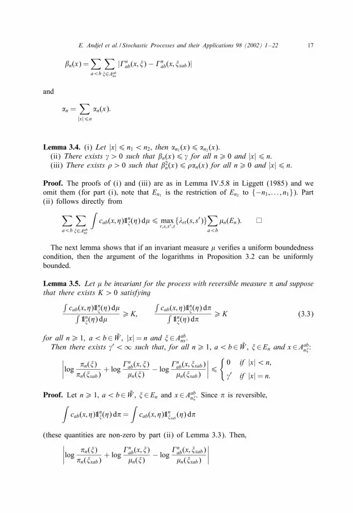
For n¿ 0 and |x|6 n, de5ne

�n(x) =∑a¡b

∑�∈Aabnx


;


5n(x) =∑a¡b

∑�∈Aabnx

|2nab(x; �)− 2nab(x; �xab)|

and

�n =∑|x|6n

�n(x):

Lemma 3.4. (i) Let |x|6 n1¡n2; then �n1 (x)6 �n2 (x).(ii) There exists '¿ 0 such that 5n(x)6 ' for all n¿ 0 and |x|6 n.(iii) There exists 6¿ 0 such that 52n(x)6 6�n(x) for all n¿ 0 and |x|6 n.

Proof. The proofs of (i) and (iii) are as in Lemma IV:5:8 in Liggett (1985) and weomit them (for part (i); note that En1 is the restriction of En2 to {−n1; : : : ; n1}). Part(ii) follows directly from

∑a¡b

∑�∈Aabnx

∫cab(x; �)5n�(�) d�6 max

r; s; s′ ; t{�rt(s; s′)}

∑a¡b

�n(En):

The next lemma shows that if an invariant measure � veri5es a uniform boundednesscondition, then the argument of the logarithms in Proposition 3.2 can be uniformlybounded.

Lemma 3.5. Let � be invariant for the process with reversible measure 3 and supposethat there exists K ¿ 0 satisfying∫

cab(x; �)5n�(�) d�∫5n�(�) d�

¿K;

∫cab(x; �)5n�(�) d3∫

5n�(�) d3¿K (3.3)

for all n¿ 1; a¡b∈ W ; |x|= n and �∈Aabnx .Then there exists '′¡∞ such that, for all n¿ 1, a¡b∈ W , �∈En and x∈Aabn�:∣∣∣∣log 3n(�)

3n(�xab)+ log

2nab(x; �)�n(�)


∣∣∣∣6{

0 if |x|¡n;

'′ if |x|= n:

Proof. Let n¿ 1; a¡b∈ W ; �∈En and x∈Aabn�. Since 3 is reversible;∫cab(x; �)5n�(�) d3=

∫cab(x; �)5n�xab(�) d3

(these quantities are non-zero by part (ii) of Lemma 3.3). Then;∣∣∣∣log 3n(�)3n(�xab)



∣∣∣∣


6

∣∣∣∣∣log∫5n�(�) d3∫

cab(x; �)5n�(�) d3

∫cab(x; �)5n�(�) d�∫

5n�(�) d�

∣∣∣∣∣+

∣∣∣∣∣log∫5n�xab(�) d3∫

cab(x; �)5n�xab(�) d3

∫cab(x; �)5n�xab(�) d�∫

5n�xab(�) d�

∣∣∣∣∣ :Let us bound the 5rst term. If −n¡x¡n, then cab(x; �) = cab(x; �n) if � is such

that 5n�(�) = 1. Thus∫5n�(�) d3∫

cab(x; �)5n�(�) d3

∫cab(x; �)5n�(�) d�∫

5n�(�) d�= 1:

Let now x=−n. We need lower and upper bounds for the argument of the logarithm.Suppose �(−n)=a (the case �(−n)=b is analogous) and de5ne mab=maxc;d{�cd(a; b)}.By condition (3.3) for 3 we get∫

5n�(�) d3∫cab(x; �)5n�(�) d3

∫cab(x; �)5n�(�) d�∫

5n�(�) d�6mabK

and, by condition (3.3) for �,∫5n�(�) d3∫

cab(x; �)5n�(�) d3

∫cab(x; �)5n�(�) d�∫

5n�(�) d�¿

Kmab

:

Therefore, the 5rst summation, for x =−n, is bounded by

max{∣∣∣∣log Kmab

∣∣∣∣ ;∣∣∣logmab

K

∣∣∣}= logmabK;

which, in turn, can be bounded by a constant not depending on n; �; a or b. A boundfor x = n is obtained in a similar way. The second term is bounded analogously.

Lemma 3.6. Under the conditions of Lemma 3.5; �n6 '′∑

|x|=n 5n(x); for all n¿ 1.

Proof. It is a direct consequence of Proposition 3.2 and Lemma 3.5.

The next proposition shows, under conditions PC and (3.3), the uniqueness of theinvariant measure.

Proposition 3.3. Consider a process verifying PC and having a reversible measure 3.If � is invariant for the process and � and 3 satisfy (3:3); then � = 3.

Proof. By part (ii) of Lemma 3.4 and Lemma 3.6; we know that for n¿ 1; �n6 2''′:By part (i) of Lemma 3.4 we have

n∑k=1

(�k(−k) + �k(k))6∑|x|6n

�n(x) = �n:


Writing �′k = �k(−k) + �k(k) for k¿ 1; we getn∑k=1

�′k6 �n6 2''′

for all n¿ 1; so the series above converges and �′k → 0 as k → ∞.Now, by part (iii) of Lemma 3.4 and Lemma 3.6, �n6 '′

√6∑

|x|=n√�n(x),

therefore,n∑k=1

�′k6 �n6 '′√6(√�n(−n) +

√�n(n)):

Since �′n converges to 0 so does the right-hand side above, therefore �k(−k)=�k(k)=0, for k¿ 1, and we conclude �n(x) = 0 for all n¿ 1 and |x|6 n. This implies that,for all n¿ 1

2nab(x; �) = 2nab(x; �xab) ∀a¡b∈ W ; �∈En; x∈Aabn�;

which implies that � is reversible for the process. By Proposition 3.1, the reversiblemeasure is unique, and the proposition is proved.

Corollary 3.1. Suppose that a process satis9es PC and admits a reversible measure.If (3:3) holds for all its invariant measures; then the process is ergodic.

Proof. Proposition 3.3 shows the uniqueness of the invariant measure of the pro-cess. This; together with Theorem 2 of Mountford (1995); which asserts that everyone-dimensional process with 5nite range; translation invariant rates having a uniqueinvariant measure is ergodic; completes the proof.

In Section 2, we have shown property (2.1) for the invariant measures of resourcesharing systems. In the next result, we use Corollary 3.1 to show that if these processesverify PC and have a reversible measure, they are ergodic.

Theorem 3.1. Consider a resource sharing system (de9ned in Section 2) verifying PC;(C1) and (C2). If it has a reversible measure; then it is ergodic.

Proof. By Theorem 2.1 and Corollary 3.1; we just have to see that property (2.1) forevery invariant measure of the resource sharing system implies condition (3.3) for thecorresponding invariant measure of the collapsed process de5ned in Subsection 3.1. Tosee this; note that since (2.1) holds; a similar inequality (with a diKerent value of �)holds for any invariant measure of the collapsed process. Therefore; for some �¿ 0we have

�n+1(�n)¿ ��n(�)

for all n¿ 1 and �∈Xn. Now; if a¡b∈ W ; �∈En and x∈Aabn�; de5ningm′ab = minc;d {�cd(a; b) : �cd(a; b)¿ 0} (which is well de5ned because x∈Aabn�);


we have∫cab(x; �)5n�(�) d�

=∫{�|cab(x;�)¿0;5n+1

�n(�)=1}

cab(x; �) d� +∫{�|5n�(�)=1;5n+1

�n(�)=0}

cab(x; �) d�

¿m′ab

∫5n+1�n

(�) d�¿m′ab�

∫5n�(�) d�;

which is (3.3) and completes the proof.

Remark 3.1. The approach followed in this paper for showing the ergodicity of re-source sharing systems is essentially one-dimensional. For a higher dimensional setting;some additional conditions seem to be necessary for the uniqueness of the reversiblemeasure. The coupling in Section 2 has a direct extension to Zd; however; the boundin (2.1) is not independent of n and the entropy technique of Subsection 3.3 should bemodi5ed to take this di@culty into account. Moreover; even if the uniqueness of theinvariant measure could be shown; it is not known if Mountford’s result (Theorem 2in Mountford (1995)) still holds for dimensions greater than one.

4. Application to loss networks

In this section we apply Theorem 3.1 to one-dimensional loss networks. Consider acountable number of stations arranged on the integers. Each call between stations x andx+ i requests a fraction C−1 of the cable between these two points and at each pointx∈Z, a request of a call from x to x+ i (with i=1; : : : ; k) arrives after an exponentialtime with parameter �i. The call is rejected if past any point x; : : : ; x+i there are alreadyC calls in progress. If the call is rejected, it is lost; otherwise it lasts an exponentialtime with parameter �i. All the exponential times are taken to be independent. Thisevolution corresponds to a resource sharing system as de5ned in Section 2. The statespace of each particle is given by W = {1; : : : ; C}k and �(x; i) represents the numberof calls from x to x + i. The rates of the process are �i(x; �) = �i if the arrival of thenew call does not break the previous rule and 0 otherwise, and �i(x; �) = �i�(x; i).It is clear that this process veri5es (C1) and (C2) since (C1) is equivalent to �i ¿ 0

for all i and (C2) follows from the fact that if �6 � and �(x; i) = �(x; i), then either�i(x; �)=0 and �i(x; �)=0, or �i(x; �)=�i and �i(x; �)=0; �i. Moreover, the state spaceof the loss network is not W Z but E as in De5nition 3.1; to see this, pick R= 1,

w(1; y; i) =

{0 if y + i¡ k;

1 otherwise

and C(1) = C (note that the restriction at x takes account for the number of calls inprogress past the point x + k). Finally, note that condition PC in Section 3, namely


the irreducibility of the 5nite conditional processes, is satis5ed since every admissiblecon5guration communicates with (0; : : : ; 0).With all this in mind, to apply Theorem 3.1, we just have to see that the loss network

has a reversible measure.

Lemma 4.1. The loss network de9ned above has a reversible measure.

Proof. We prove the existence of the reversible measure for the collapsed process; asdescribed at the beginning of Section 3 (the original and the collapsed processes havethe same reversible measures). For the collapsed process; let us study the 5nite processon E(−n; n; 0; 0) (recall that in the collapsed process W = {0; 1; : : : ; C}k2 since eachparticle corresponds to k particles of the original process). If; for the 5nite process; weremove the restriction on the number of calls (but keep �(x; i)6C for all x; i); thenthe k2 coordinates of each particle perform bounded birth and death processes whichare independent of each other and independent of the processes associated to othersites. Therefore; this process is reversible. If we recover now the restriction on thenumber of calls; by the truncature Lemma (Lemma 1:5 of Kelly; 1979); the collapsedloss network on E(−n; n; 0; 0) is reversible with unique (by irreducibility) reversiblemeasure 8n. By setting all the coordinates outside {−n; : : : ; n} equal to 0; the measures8n can be seen as measures on X . As X is compact; there is a subsequence (8nk )of (8n) which converges weakly to a measure 8. Now; since the measures 8nk arereversible for the 5nite processes; by the de5nition of weak convergence; it followsthat 8 veri5es condition (3.2) and is; therefore; reversible for the collapsed loss network.

We have just proved.

Theorem 4.1. Every 9nite range translation invariant loss network on Z isergodic.

Remark 4.1. Although we have considered a network with a simple restriction (nomore than C calls past any point); Theorem 4.1; with a very similar proof; also holdsfor more general one-dimensional networks. This includes; for instance; the case wherethere are diKerent types of calls which use diKerent cables (r = 1; : : : ; R) each onehaving capacity Cr and there are also some global restrictions (e.g.; no more thanC¡C1 + · · · + CR calls past any point); or the case where a call of type r needs afraction fr of the section of the cable.

Acknowledgements

Part of this work was carried out while the second author was invited at the LATP ofthe Universit*e de Provence. The authors are grateful to the anonymous referees for theirvery careful reading and useful suggestions which resulted in an overall improvementof the paper.


References

Bolch, G., Greine, S., de Meer, H., Trivedi, K.S., 1998. Queuing Networks and Markov Chains. Wiley,New York.

Chen, M.F., 1992. From Markov Chains to Non-equilibrium Particle Systems. World Scienti5c, Singapore.Courcoubetis, C.A., Reiman, M.I., Simon, B., 1987. Stability of a queueing system with concurrent service

and locking. SIAM J. Comput. 16, 169–178.Courcoubetis, C.A., Varaiya, P., Walrand, J., 1984. Invariance in resource-sharing systems. J. Appl. Probab.

21, 777–785.Ferrari, P.A., Garcia, N.L., 1998. One-dimensional loss networks and conditioned M=G=∞ queues. J. Appl.

Probab. 35, 963–975.Forbes, F., FranTcois, O., Ycart, B., 1996. Stochastic comparison for resource sharing models. Markov

Processes Rel. Fields 2, 581–606.Fujishige, S., Katoh, N., Ichimori, T., 1988. The fair resource allocation problem with submodular constraints.

Math. Oper. Res. 13, 164–173.Graham, C., Meleard, S., 1994. Fluctuations for a fully connected loss network with alternate routing.

Stochastic Proc. Appl. 53, 97–115.Harris, T.E., 1974. Contact interactions on a lattice. Ann. Probab. 2, 969–988.Holley, R.A., 1971. Free energy in a Markovian model of a lattice spin system. Comm. Math. Phys. 23,

87–99.Holley, R.A., Stroock, D.W., 1977. In one and two dimensions, every stationary measure for a stochastic

Ising model is a Gibbs state. Comm. Math. Phys. 55, 37–45.Holley, R.A., Stroock, D.W., 1989. Uniform and L2 convergence in one dimensional stochastic Ising models.

Comm. Math. Phys. 123, 85–93.Hunt, P.J., Kurtz, T.G., 1994. Large loss networks. Stochastic Proc. Appl. 53, 363–378.Kelly, F.P., 1979. Reversibility and Stochastic Networks. Wiley, New York.Kelly, F.P., 1985. Stochastic models of computer communication systems. J. Roy. Statist. Soc. Ser. B 85,

379–395.Kelly, F.P., 1987. One-dimensional circuit-switched networks. Ann. Probab. 15, 1166–1179.Kelly, F.P., 1991. Loss networks. Ann. Appl. Probab. 1, 319–378.Langston, M.A., Morford, M.P., 1990. Resource allocation under limited sharing. Discrete Appl. Math. 28,

135–147.Liggett, T.M., 1985. Interacting Particle Systems. Springer, New York.Moody, J.O., Antsaklis, P.J., 1998. Supervisory Control of Discrete Event Systems Using Petri Nets. Kluwer

Academic Publishers, Boston.Mountford, T.S., 1995. A coupling of in5nite particle systems. J. Math. Kyoto Univ. 35, 43–52.Ruelle, D., 1978. Thermodynamic Formalism. Addison-Wesley Publishing, Reading, MA.Sidhu, D.P., Wijesinha, A.L., 1998. Performance analysis of a constrained resource sharing system. Queuing

Systems Theory Appl. 29, 293–311.Ycart, B., 1993. The philosopher’s process: an ergodic reversible nearest particle system. Ann. Appl. Probab.

3, 356–363.

Documents

Ergodicity of one-dimensional resource sharing systems