AN INTRODUCTION TO QUANTUM FIELD THEORY

Erik Verlinde

Theory Division, CERN, CH-1211 Geneva 23, Switzerland

Abstract

The basic concepts and ideas underlying quantum �eld theory

are presented, together with a brief discussion of Lagrangian �eld

theory, symmetries and gauge invariance. The use of the Feyn-

man rules to calculate scattering amplitudes and cross sections is

illustrated in the context of quantum electro dynamics.

1. INTRODUCTION

Quantum �eld theory provides a successful theoretical framework for describing

elementary particles and their interactions. It combines the theory of special relativity

and quantum mechanics and leads to a set of rules that allows one to compute physical

quantities that can be compared with high energy experiments. The physical quantity of

most interest in high energy experiments is the cross-section �. It determines directly the

number of events that an experimentalist will be able to see, and also is in a direct way

related to the quantum mechanical probabilities that can be computed with the help of

�eld theory.

In these notes I will present the basic concepts and ideas underlying quantum �eld

theory. Starting from the quantum mechanics of relativistic particles I will introduce

quantum �eld operators and explain how these are used to describe the interactions among

elementary particles. These notes also contain a brief discussion of Lagrangian �eld theory,

symmetries and gauge invariance. Finally, after presenting a heuristic derivation of the

Feynman rules, I'll illustrate in the context of quantum electro dynamics how to calculate

the amplitude that determines the cross section for a simple scattering process. But before

we turn to the quantum mechanics, let us �rst discuss the meaning of the cross section in

more familiar classical terms.

1.1 From Events to Cross Sections

For concreteness, let us consider an experiment with two colliding particle beams in

which one beam consists of, say, electrons and the other beam of positrons. An experimen-

talist can now collect and count the events in which an electron and a positron collide and

produce several other particles. The number of events N that occur in a certain amount

of time depends on various experimental details, in particular the densities �1 and �2 of

the particles inside the beams and of course the particle velocities ~v1 and ~v2.

To �nd out how these parameters a�ect the number of events, let us �rst consider

the probability that an event occurs inside a a small volume �V and within a time

interval �t. In this case we can assume that the densities and velocities are constant.

Now imagine that one of the particles, say the electron, has a �nite cross-section � as seen

from the perspective of the other particle, the positron. After a time �t each electron

has moved with respect to the positrons over a distance j~v1 � ~v2j�t, where ~v1 � ~v2 is the

relative velocity, and in this way it has swept out a part of space with a volume equal to

�j~v1 � ~v2j�t. The probability that in this time the electron has collided with a positron

is equal to the number of positrons inside this volume, which is �2�j~v1 � ~v2j�t. Finally,

to obtain the total number �N of collisions we have to multiply this with the number

of electrons inside the volume �V ; this number is �1�V . In this way we �nd that the

number of events that occur in �V and �t is

�N = ��1�2j~v1 � ~v2j�V�t (1)

In a realistic situation the densities �i(~x; t) of the particles and their velocities are not

constant in space and time. Instead of the velocity ~v it is also more appropriate to use

the current density ~j that describes the ux of the particles per unit of area. It is de�ned

by ~j = �~v where ~v is the local velocity at a certain point in space and time. By repeating

the above argumentation we can express the number of events in an in�nitesimal volume

dV and time interval dt as dN = �j�2~j1 � �1~j2jd3~xdt. Then by integrating of space and

time we obtain the following expression for the total number of events N

N = �

ZdtL(t); (2)

where1)

L(t) =

Zd3xj�1(~x; t)~j2(~x; t)� �2(~x; t)~j1(~x; t)j: (3)

All experimental details that in uence the number of events are combined in the time

integral of L(t), which is called the integrated luminosity. The integrated luminosity does

not depend on the kind of process that one is interested in, and so it can be measured by

looking at a reference process for which the cross section � is accurately known. With this

knowledge one can then determine the cross sections for all other processes. These cross-

sections � are independent of the experimental details, and thus can be used to compare

the data that come from di�erent experiments. They are also the relevant quantities that

one wishes to compute using quantum �eld theory.

1.2 Quantum Mechanical Probabilities

Just to give an idea of how the cross section � is related to a quantum mechanical

amplitude, let us assume that before the collision the densities and velocities of the par-

ticles inside the beams are accurately known. In terms of quantum mechanics this means

1) A more careful analysis shows that the integrand has an additional relativistic con-

tribution 1cj~j1 � ~j2j. This term can be dropped in a situation where ~j1 and ~j2 are

(approximately) parallel.

that one has speci�ed the initial quantum state jii of the colliding particles. Similarly,

by measuring the energies and directions of the particles that are being produced by the

collisions one selects a certain �nal wave-function jfi that describes the state of the

out-going particles. According to the rules of quantum mechanics the probablity W for

this event to happen is given by the absolute valued squared of the overlap between the

�nal state and the initial state

Wi!f = jhijfij2

Quantum �eld theory provides the tools to compute the amplitudes hijf i, and hence

determine the quantum mechanical probabilities W . In fact, the quantity that is most

directly computed is the probability W that a collision takes place per unit of volume

and time for a situation with constant particle densities �1 and �2. For this situation W

may be identi�ed with the ratio �N=�V�t, which according to equation (1) gives the

cross section � times the product of the densities and relative velocity. All this will be

explained in more detail in the following sections.

2. RELATIVITY AND QUANTUM MECHANICS

The elementary particles that are used in high energy experiments have velocities

close to the speed of light, and should therefore be described by the theory of special

relativity. For relativistic particles it is convenient to specify their motion, instead by

their velocity ~v, in terms of their momentum

~p =m~vq

1 � (~vc)2

(4)

An important reason for this is that during collision the total momentum of the particles

will be conserved. The total energy of the particles will also be conserved. In special

relativity the energy of a particle with momentum ~p is given by

E =q~p2c2 +m2c4 (5)

For a particle at rest this becomes Einstein's famous relation E = mc2.

2.1 Relativistic Wave Functions

In quantum mechanics the energy E becomes identi�ed with the Hamiltonian oper-

ator H. The time evolution of the wave function for a single particle is, as usual, governed

by the Schr�odinger equation in which the Hamiltonian H acts as a di�erential operator.

The form of this di�erential operator can be read of from (5) by replacing the momentum

~p by the operator ~p = �i�h~r. This gives

i�h@t (~x; t) = H (~x; t) (6)

with

H =

q��h2~r2 +m2c4: (7)

An important di�erence with the non-relativistic case is, however, that the Hamiltonian

involves a square root. Still the Schr�odinger equation can easily be solved by expanding

the wave-function in terms of plane waves

~k(~x; t) = ei~k�~x�i!(~k)t:

These plane waves are the eigenfunctions of the momentum operators ~p with eigenvalue

~p = �h~k and are also energy eigenstates with eigenvalue E = �h!(~k). The most general

solution to the Schr�odinger equation can now be written as2)

(~x; t) =1

(2�)3

Zd3~k

2!(~k)ei~k�~x�i!(~k)t (~k); (8)

where

!(~k) =

q~k2 +m2: (9)

To simplify the formulas we put here and in the following �h = c = 1. When the momentum

~p is well speci�ed the wave-function (~k) will be strongly peaked near ~k = ~p. The position

of the particle will in this case not be very precisely determined due to the uncertainty

principle. So the wave function gives us only a probability �(~x; t) for �nding a particle at

a position ~x at a certain time t. Because probabilities have to be conserved, there must

also exist a probability current density ~j(~x; t) that obeys the conservation law

@t�(~x; t) = ~r �~j(~x; t) (10)

For the relativistic wave function the probability density and current density are given by

the expressions

�=i

2m( �@t � @t

�)

~j=�i

2m( �~r � ~r �) (11)

These densities can in fact be identi�ed with the particle densities � and ~j inside the

beam. Notice that for a plane wave ~k these densities are given by � = !mand ~j =

~km. To

verify that these expressions indeed satisfy the conservation law (10) one has to use the

`square' of the Schr�odinger equation (6)

(@2t �~r2 +m2) (~x; t) = 0 (12)

This equation is called the Klein-Gordon equation. We note, however, that the Klein-

Gordon equation allows more general solutions than the original Schr�odinger equation.

Namely, if we change the sign of the time frequency !(~k)! �!(~k) in the expression (8)

it would still be a solution of (12). These negative frequency solutions are not physically

acceptable as wave functions because they would correspond to particles with negative

energy.

2.2 The Dirac Equation

For particles with spin the wave function not only carries information about the

momentum and energy but also specify the polarization of the particle. An electron has

spin 1=2, and so its wave function has two independent components �"(~x; t), for spin up,

2) Here the normalization factor 2!(~k) is chosen so that the function (~k) has a relativistic

invariant meaning.

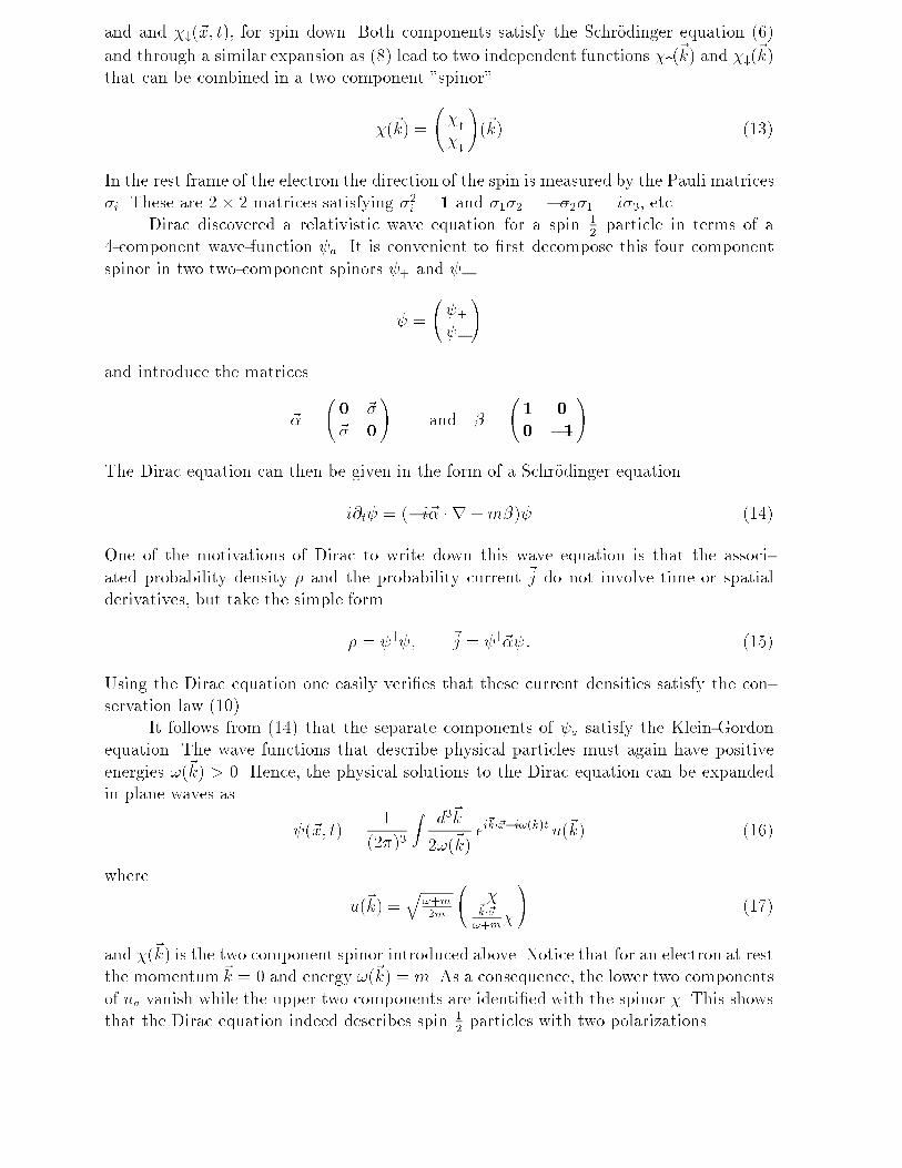
and and �#(~x; t), for spin down. Both components satisfy the Schr�odinger equation (6)

and through a similar expansion as (8) lead to two independent functions �"(~k) and �#(~k)

that can be combined in a two component "spinor"

�(~k) =

�

"

�#

!(~k) (13)

In the rest frame of the electron the direction of the spin is measured by the Pauli matrices

�i. These are 2 � 2 matrices satisfying �2i = 1 and �1�2 = ��2�1 = i�3, etc.

Dirac discovered a relativistic wave equation for a spin 12particle in terms of a

4-component wave-function a. It is convenient to �rst decompose this four component

spinor in two two-component spinors + and �.

=

+ �

!

and introduce the matrices

~� =

0 ~�

~� 0

!and � =

1 0

0 �1

!

The Dirac equation can then be given in the form of a Schr�odinger equation

i@t = (�i~� � r+m�) (14)

One of the motivations of Dirac to write down this wave equation is that the associ-

ated probability density � and the probability current ~j do not involve time or spatial

derivatives, but take the simple form

� = y ; ~j = y~� : (15)

Using the Dirac equation one easily veri�es that these current densities satisfy the con-

servation law (10).

It follows from (14) that the separate components of a satisfy the Klein-Gordon

equation. The wave functions that describe physical particles must again have positive

energies !(~k) > 0. Hence, the physical solutions to the Dirac equation can be expanded

in plane waves as

(~x; t) =1

(2�)3

Zd3~k

2!(~k)ei~k�~x�i!(k)t u(~k) (16)

where

u(~k) =q

!+m2m

�

~k�~�!+m

�

!(17)

and �(~k) is the two component spinor introduced above. Notice that for an electron at rest

the momentum~k = 0 and energy !(~k) = m. As a consequence, the lower two components

of ua vanish while the upper two components are identi�ed with the spinor �. This shows

that the Dirac equation indeed describes spin 12particles with two polarizations.

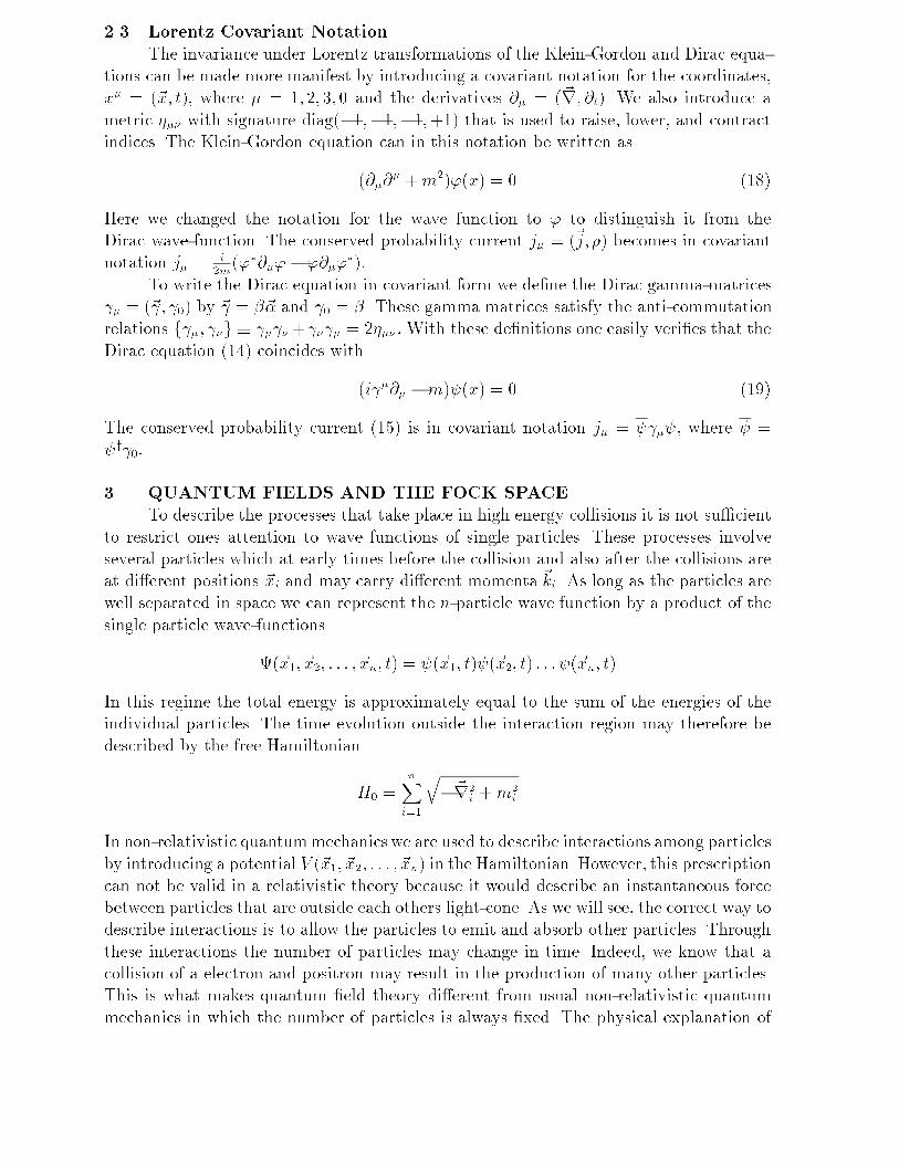
2.3 Lorentz Covariant Notation

The invariance under Lorentz transformations of the Klein-Gordon and Dirac equa-

tions can be made more manifest by introducing a covariant notation for the coordinates,

x� = (~x; t), where � = 1; 2; 3; 0 and the derivatives @� = (~r; @t). We also introduce a

metric ��� with signature diag(�1;�1;�1;+1) that is used to raise, lower, and contract

indices. The Klein-Gordon equation can in this notation be written as

(@�@� +m2)'(x) = 0 (18)

Here we changed the notation for the wave function to ' to distinguish it from the

Dirac wave-function. The conserved probability current j� = (~j; �) becomes in covariant

notation j� =i

2m('�@�'� '@�'

�):

To write the Dirac equation in covariant form we de�ne the Dirac gamma-matrices

� = (~ ; 0) by ~ = �~� and 0 = �. These gamma matrices satisfy the anti-commutation

relations f �; �g � � � + � � = 2��� :With these de�nitions one easily veri�es that the

Dirac equation (14) coincides with

(i �@� �m) (x) = 0 (19)

The conserved probability current (15) is in covariant notation j� = � ; where =

y 0:

3. QUANTUM FIELDS AND THE FOCK SPACE

To describe the processes that take place in high energy collisions it is not su�cient

to restrict ones attention to wave functions of single particles. These processes involve

several particles which at early times before the collision and also after the collisions are

at di�erent positions ~xi and may carry di�erent momenta ~ki. As long as the particles are

well separated in space we can represent the n-particle wave function by a product of the

single particle wave-functions

(~x1; ~x2; : : : ; ~xn; t) = (~x1; t) (~x2; t) : : : (~xn; t)

In this regime the total energy is approximately equal to the sum of the energies of the

individual particles. The time evolution outside the interaction region may therefore be

described by the free Hamiltonian

H0 =nXi=1

q�~r2

i +m2i

In non-relativistic quantummechanics we are used to describe interactions among particles

by introducing a potential V (~x1; ~x2; : : : ; ~xn) in the Hamiltonian. However, this prescription

can not be valid in a relativistic theory because it would describe an instantaneous force

between particles that are outside each others light-cone. As we will see, the correct way to

describe interactions is to allow the particles to emit and absorb other particles. Through

these interactions the number of particles may change in time. Indeed, we know that a

collision of a electron and positron may result in the production of many other particles.

This is what makes quantum �eld theory di�erent from usual non-relativistic quantum

mechanics in which the number of particles is always �xed. The physical explanation of

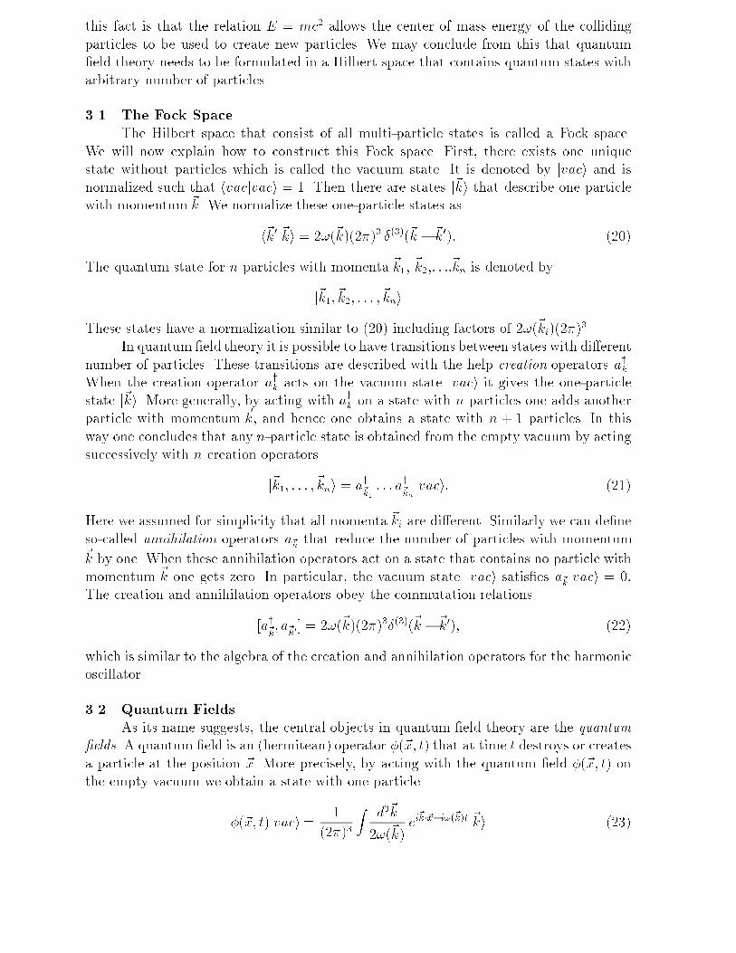
this fact is that the relation E = mc2 allows the center of mass energy of the colliding

particles to be used to create new particles. We may conclude from this that quantum

�eld theory needs to be formulated in a Hilbert space that contains quantum states with

arbitrary number of particles.

3.1 The Fock Space

The Hilbert space that consist of all multi-particle states is called a Fock space.

We will now explain how to construct this Fock space. First, there exists one unique

state without particles which is called the vacuum state. It is denoted by jvaci and is

normalized such that hvacjvaci = 1. Then there are states j~ki that describe one particle

with momentum ~k. We normalize these one-particle states as

h~k0j~ki = 2!(~k)(2�)3 �(3)(~k � ~k0): (20)

The quantum state for n particles with momenta ~k1, ~k2,: : :,~kn is denoted by

j~k1; ~k2; : : : ; ~kni

These states have a normalization similar to (20) including factors of 2!(~ki)(2�)3.

In quantum �eld theory it is possible to have transitions between states with di�erent

number of particles. These transitions are described with the help creation operators ayk.

When the creation operator ayk acts on the vacuum state jvaci it gives the one-particle

state j~ki. More generally, by acting with ayk on a state with n particles one adds another

particle with momentum ~k, and hence one obtains a state with n + 1 particles. In this

way one concludes that any n-particle state is obtained from the empty vacuum by acting

successively with n creation operators

j~k1; : : : ; ~kni = ay~k1: : : a

y~knjvaci: (21)

Here we assumed for simplicity that all momenta ~ki are di�erent. Similarly we can de�ne

so-called annihilation operators a~k that reduce the number of particles with momentum~k by one. When these annihilation operators act on a state that contains no particle with

momentum ~k one gets zero. In particular, the vacuum state jvaci satis�es a~kjvaci = 0:

The creation and annihilation operators obey the commutation relations

[ay~k; a~k0] = 2!(~k)(2�)3�(3)(~k � ~k0); (22)

which is similar to the algebra of the creation and annihilation operators for the harmonic

oscillator.

3.2 Quantum Fields

As its name suggests, the central objects in quantum �eld theory are the quantum

�elds. A quantum �eld is an (hermitean) operator �(~x; t) that at time t destroys or creates

a particle at the position ~x. More precisely, by acting with the quantum �eld �(~x; t) on

the empty vacuum we obtain a state with one particle

�(~x; t)jvaci =1

(2�)3

Zd3~k

2!(~k)ei~k�~x�i!(~k)t

j~ki (23)

Here we notice the similarity with the expression (8) for the single particle wave function.

But it should be clear that quantum �eld �(~x; t) has quite a di�erent interpretation than

the wave function (~x; t). By expanding the �eld �(x; t) in terms of plane waves as

�(~x; t) =1

(2�)3

Zd3~k

2!(~k)

�ay~kei~k�~x�i!(k)t + a~ke

�i~k�~x+i!(k)t�

(24)

one obtains the creation and annihilation operators ay~k and a~k that we introduced before.

Notice that the quantum �eld �(x; t) satis�es the Klein-Gordon equation (12), but that

unlike the wave-function (~x; t) it contains in its expansion plane waves with negative

time frequency �!(~k).

The canonical commutation relations between the creation and annihilation oper-

ators imply that the quantum �eld �(~x; t) does not necessarily commute with the �eld

�(~y; t0) at some other point in space and time. However, two operators that act at the

same time t0 = t but at di�erent points in space should commute. Otherwise there would

be a contradiction with one of the postulates of relativity that no signal can travel faster

than light. Indeed one can show that

[�(~y; t); �(~x; t)] = �i�(3)(~x� ~y) (25)

where �(~y; t) = @t�(~y; t) is called the canonically conjugate �eld of �(~x; t) because their

relation is similar to that of the momentum ~p and the coordinate ~x. We remark that by

expanding the �eld � and � in plane waves one recovers from (25) all the commutation

relations (22) of the creation and annihilation operators.

3.3 Quantum Fields for Particles with Charge and Spin

The �eld that we just described is the simplest example of a relativistic quantum

�eld. It describes an uncharged particle with zero spin such as the pion �0. We will now

brie y describe the quantum �elds for particles with charge and spin. An important fact

about Nature is that all charged particle have an associated anti-particle with an identical

mass and spin but with opposite charge. For example, the anti-particle for the �+ pion is

the negatively charged pion ��, and the positron is the anti-particle associated with the

electron. The quantum �eld for the charged pions is a complex scalar with expansion

'(~x; t) =1

(2�)3

Zd3~k

2!(~k)

�ay~kei~k�~x�i!(k)t + b~ke

�i~k�~x+i!(k)t�

(26)

where ay~kcreates a �+ while b~k annihilates a ��. The other operators b

y~kand a~k are

contained in the hermitean conjugate �eld 'y. The electron and positron are described

by a complex Dirac spinor which has four components satisfying the Dirac equation. The

creation and annihilation operators are again found by expanding the Dirac �eld in Fourier

modes

(~x; t) =1

(2�)3

Zd3~k

2!(~k)

�cy~k;au

a(~k)ei~k�~x�i!(k)t + d~k;bv

b(~k)e�i~k�~x+i!(k)t

�(27)

where ua(~k) is de�ned in (17), with a = " or #, and vb(~k) is given by a similar expression

with the upper and lower components interchanged. The �rst term gives the creation

operators cy~k;a for the electron and the last term describes the annihilation operators d~k;bfor the positron. Again the hermitean conjugate �eld gives the other operators. Because

the electron and positron are fermions the creation and annihilation operators satisfy

canonical anti-commutation rulesncy~k;a; c~k0;a0

o= �aa02!(k)(2�)

3�(3)(~k � ~k0) (28)

This will incorporate the Pauli exclusion principle, and leads, as we will see, to some slight

di�erences in the Feynman rules for fermions compared to bosons.

3.4 The Feynman Propagator

The forces between elementary particles are often described by the mediation of

another particle which is created at one point (~x; t) in space and time and then annihi-

lated at another point (~x0; t0) with t0 > t. The quantum mechanical amplitude for such a

successive creation and annihilation is given by the propagator

�(~x� ~x0; t� t0) = hvacj�(~x0; t0)�(~x; t)jvaci for t0 > t (29)

For t > t0 one has to change the order of the two �elds, because the operator that

corresponds to the earliest point in time must also acts �rst on the vacuum. So in this

case the particle is �rst created at the position (~x0; t0) and than annihilated at (~x; t).

The propagator will play an important role in the Feynman rules. But just as a

preparation, we will describe here how to evaluate it. First we insert the equation (23)

and then use the normalization (20). In this way we obtain

�(~x� ~x0; t� t0) =1

(2�)3

Zd3k

2!(~k)ei~k�(~x�~x0)�i!(~k)jt�t0j (30)

Notice that the propagators only depends on the di�erences in the coordinates. We can

use this to put ~x0 and t0 equal to zero. The above expression is a direct generalization of

the familiar Yukawa potential e�jmjj~xj=j~xj to which it would reduce in the static limit. We

can rewrite the propagator in a manifestly Lorentz invariant form by using the identity

i

2�

Z +1

�1dk0

e�ik0t

k20 � !2 + i�=e�i!jtj

2!

which is proven by a complex contour deformation. The Feynman propagator can thus be

written in covariant notation as

�(x) =Z

d4k

(2�)4e�ik�x�(k) (31)

with

�(k) =i

k2 �m2 + i�(32)

and k� = (~k; k0) and x� = (~x; t). In a similar way one can derive the Feynman propagator

for the Dirac �eld. The only di�erence is that we have a sum over polarization states of

the electron. From the normalization of the spinor ua(~k) given in section 2.2 one �nds

that as a result the integrand contains an additional factorXa

ua(~k)ua(~k) = (k� �+m) (33)

where � are the gamma matrices introduced in section 2.3.

4. AMPLITUDES AND CROSS SECTIONS

In this section we will explain how the cross section is related to quantummechanical

amplitude, and we will describe how these amplitudes are represented in quantum �eld

theory

4.1 From Amplitudes to Cross Sections

Consider an event where two particles with momenta ~p1 and ~p2 collide and produce

n particles with momenta ~k1, : : :, ~kn. Before the collision we can represent the wave

functions of both particles by planes waves ~p1, and ~p2. We will denote this two-particle

state by j~p1; ~p2ii. Similarly, after the collision we have n particles with wave functions

given by plane waves. The corresponding n-particle state is j~k1; : : : ; ~knif . The quantum

mechanical probability for this process is determined by the transition amplitude

Ai!f (p1; p2; ki) =ih~p1; ~p2j~k1; : : : ; ~kni

f(34)

These transition amplitudes are the objects that one would like to compute with quantum

�eld theory. But before we discuss that in some detail, let us �rst explain in what way

these amplitudes are related to the cross section, which after all is the observable that

can be measured.

During a collision there are various physical quantities that are conserved. In par-

ticular, the total energy and momentum before and after the collision must be the same.

This tells us that the transition amplitude A will vanish unless

nXi=1

!i(ki)=!1(p1) + !1(p2)

nXi=1

~ki=~p1 + ~p2

Examples of other conserved quantities are charge, lepton number etc. Now according

to the standard rules, we can now calculate the probability by taking the square of the

amplitude. Notice, however, since we have �xed the momentum of the produced particles,

we are only calculation a partial probability for producing particles with momenta between~ki and ~ki + d~ki. This transition probability is

dW (~p1; ~p2;~ki) = (2�)4jA(~p1; ~p2;~ki)j2Yi

d3ki

(2�)32!(~ki)(35)

To obtain the full probability one has to integrate of the �nal momenta ~ki. Implicit in the

expression (35) are the delta-functions for momentum and energy conservation. To make

them explicit one should multiply the right hand side by

(2�)4 �(3)�P

i~ki�~p1�~p2

���P

i !(~ki)�!1�!2�

This transition rate dW depends on the normalization of the wave functions of the two

incoming particles. Because these wave-functions are represented by planes waves the

associated particle densities are �i =!i(~pi)mi

and ~ji =~pimi

. Now, to go from the transition

probability to the di�erential cross-section d� we can follow the same steps of section 1.1.

The luminosity is given by the integral of j~j1�2�~j2�1j = j~p1!2�~p2!1j=m1m2. If we divide

the transition rate dW by this factor we obtain the cross section. Thus we obtain

d� =m1m2

j~p1!2 � ~p2!1jdW (p1; p2; ki) (36)

This expression is valid in the center of mass frame. To extend it to general Lorentz frames

we simply note that numerator can be written in covariant form asq(p1 � p2)2 �m2

1m22.

In the following we will not really be concerned with calculating explicitly these cross sec-

tions. Instead we will focus on the quantum mechanical amplitudesA and the probability

rate dW .

4.2 The Interaction Hamiltonian

In quantum mechanics the time evolution of a quantum state is described by a

Schr�odinger equation. For the situation of our interest the Hamiltonian H is an operator

that acts in the Fock space of many particles, and can be written a sum of the free

Hamiltonian H0 and an additional term Hint that represent the interactions among the

particles. What can we say about Hint? Because the interactions may change the number

of particles the Hamiltonian will contain operators that can create or destruct particles.

Furthermore, the interactions should be consistent with causality, which means that the

presence of a particle can be felt by another particle only when they have been in causal

contact. This is guaranteed when the interactions that are contained in the Hamiltonian

only occur between particles that are at the same point in space and time.

To make a long story short, the appropriate way to construct a Hamiltonian that

satis�es all the required properties is to express the interaction Hamiltonian as an integral

over space of a density H(~x; t). This Hamiltonian density H must be given in terms of

a product of the quantum �elds � and � and, possibly, the �rst order spatial derivatives~r�.

HI(t) =

Zd3xHint

��; ~r�; �

�(37)

In fact, also the free Hamiltonian is of this form with an integrand that is quadratic in

the quantum �elds

H0 =Zd3x

��2 + (r�)2

�(38)

This is what distinguishes the free Hamiltonian from the interaction Hamiltonian, which is

an higher order operator. A typical example of an interaction term isHint(~x; t) = ��4(~x; t).

In modern approaches to quantum �eld theory one does not often use the Hamilto-

nian density H, but instead one formulates the theory in terms of a Lagrangian density

L(~x; t). It is related to the Hamiltonian density by

H(�; �)=� _�� L(�; _�)

�=@L

@ _�(39)

The advantage of using the Lagrangian instead of the Hamiltonian formalism is that all

symmetries, like Lorentz invariance, are manifest. This is because, instead of the Hamil-

tonian H which is an integral over space, one works with an action S that is written as

an integral over space and time of the Lagrangian density L. In the next section we will

discuss the Lagrangian formulation in more detail.

4.3 The S-Matrix

We will now describe how the quantum mechanical probability amplitudes

A(~pi; ~p2;~kj) =ih~p1; : : : ; ~pmj~k1; : : : ; ~kni

f

are represented in terms of quantum �eld theory. The idea is as follows. We consider a

quantum state j(t)i which at the time t = �1 coincides with the initial state. Then

by studying its time evolution we can in principle �nd out what this state looks like at

t = +1. The probability for �nding the n particles in the �nal state j(1)i is then

determined by the overlap of the n-particle state with this �nal state.

So, once we know the Hamiltonian density Hint in principle all we have to do is to

solve the Schr�odinger equation

i@tj(t)iS = (H0 +Hint) j(t)iS (40)

Without interaction this would have been easy, because the free Hamiltonian just evolves

each of the particles according to the usual one particle Schr�odinger equation. In partic-

ular, it doesn't change the number of particles.

The non-trivial part of the time evolution is contained in the interaction Hamilto-

nian. One can describe the quantum states in a di�erent representation which only sees

the interactions by undoing the time evolution that is generated by the free Hamiltonian.

So we introduce a new quantum state by

j(t)iI= eitH0

j(t)iS: (41)

The time evolution of this state is generated only by the interaction Hamiltonian

i@tjiI = Hint(t)jiI (42)

The interaction Hamiltonian Hint(t) is expressed as in (37). Note, however, that in this

picture the �elds �(~x; t) and hence Hint(t) are time dependent. This time dependence

simply means that the �elds �(~x; t) satisfy the Klein-Gordon, or Dirac, or some other

linear wave equation. Formally we can write down the solution to the Schr�odinger equation

(40) as

j(tf)iI = Texp

��i

Z tf

ti

dtHI (t)

�j(ti)iI (43)

where the time ordening symbol T implies that the operators HI (t) must act successively

on the state j(ti)i in the order of the time t in their argument. More explicitly,

T exp

��i

Z tf

ti

dtHI (t)

��

1Xn=0

(�i)nZti<t1<t2<:::<tn<t

f

dt1dt2 : : : dtn HI(tn) : : :HI

(t2)HI(t1) (44)

Next we insert the expression (37) for the interaction Hamiltonian and send ti ! �1

and tf !1 to get

j(1)iI= Texp

��i

Zd4xHint(x)

�j(�1)i

I(45)

where d4x = dtd3x and x = (~x; t). This exponential operator on the right-hand-side is

called the S-matrix. Its matrix elements give the probability amplitude that for an initial

n-particle state jp1; : : : ; pni the outgoing state is given by them-particle state jk1; : : : ; kmi.

This amplitude is

A(pi; kj) = hk1; : : : ; kmjTexp

��i

Zd4xHint(x)

�jp1; : : : ; pni (46)

From this expression it is straightforward to derive the Feynman rules for a given Hamil-

tonian densite Hint(x).

4.4 Feynman Rules

To evaluate these amplitudes one has to use perturbation theory. One expands the

exponent, taking in to account the time ordening, and than one inserts the explicit expres-

sion of the interaction Hamiltonian in terms of the �elds. As mentioned, the Hamiltonian

density is some polynomial in the �elds � and its derivatives. These �elds create or destroy

particles at a certain position (~x; t) in space and time. The power of the �elds tells us how

many particles are destroyed or annihilated at one point.

The various contributions to the scattering amplitude can be represented graphically

in terms of Feynman diagrams. Given a diagram there is a very precise prescription to

write down the expression for the contribution in terms of the propagators and vertices of

a given quantum �eld theory. Here we will here just sketch the basic idea. Each Feynman

diagram has a number of external lines that represent the incoming and outgoing particles.

For the above amplitude the number of lines would be m incoming and n outgoing. We

label these lines by the associated momenta ki and pi. According to the Feynman rules

one has to write down for each of the lines the appropriate single particle wave functions

describing a particle with external momentum ~ki or ~pi. Next, the external lines come

together at vertices. These vertices are in one to one correspondence with the various

terms in the interaction Hamiltonian. For a simple situation in which Hint has just one

term ��4 there is just one type of vertex where 4 lines come together. For each vertex one

has to write down one power of the coupling constant � times an i that comes from the i

in front of the Hamiltonian.

Further, the sum of all momenta that ow towards a vertex must vanish. It is not

necessary that all lines that come together in one vertex correspond to external lines. A

Feynman diagram has also internal lines that correspond to the propagators. Just like the

external lines, the internal lines also carry momentum. For each propagator one has to

write down a factor that depends on its momentum. The precise form of this propagator

depends on the type of �eld. For the Klein Gordon scalar �eld that we considered so far

the propagator is

�(k) =i

k2 �m2 + i�(47)

where k = (~k; k0) and k2 = k20 �

~k2. We have already explained in section 3.4 how this

expression is derived. For diagrams without closed loops the condition that momentum is

conserved at each vertex determines the momenta for all the internal lines in terms of the

external momenta ki. But for diagrams with ` closed loops there will be ` undetermined

momenta that have to be integrated over. Fermion loops have an additional factor of

(�1) because of fermi statistics. Finally, one has to sum over all inequivalent ways that

the external lines can be connected through propagators and vertices. What I have just

given is only a rough sketch of the Feynman rules. The precise rules depend of course on

the quantum �eld theory that one considers and, unfortunately, also on conventions.

5. LAGRANGIAN FIELD THEORY

We will leave aside the quantum �elds for while, and consider classical �eld theory

in its Lagrangian formulation.

5.1 The Action Principle

A classical �eld theory may be de�ned in terms of an action S that is given as an

integral over space and time of a Lagrangian density L. This Lagrangian density L is a

Lorentz invariant function of the �eld � and its derivative @��. Thus in general the action

S takes the form

S =

Zd4xL(�(x); @��(x)): (48)

According to the action principle one obtains the classical �eld equations by requiring

that the action is stationary, that means it does not change under in�nitesimal variations

of the �elds �! �+ ��. For general values of the �eld � the the action S changes under

such a variation by a small amount �S given by

�S=

Zd4x

@L

@���(x) +

@L

@(@��)@�(��)

!

Zd4x

"@L

@�� @�

@L

@(@��)

!#�� (49)

where we dropped a surface terms after the partial integration. In this way we �nd that

the variation of the action vanishes provided the �eld �(x) satis�es the Euler-Lagrange

equation

@�

@L

@(@��)

!�@L

@�= 0 (50)

Note that to obtain a linear Euler-Lagrange equation the Lagrangian must be quadratic

in the �elds � and its derivatives. But in general one can write down Lagrangians that ,

besides a quadratic terms, involve higher order powers. These Lagrangians will give rise

to non-linear �eld equations. It is in this way that interactions are introduced in the

Lagrangian formalism.

We have seen that the �elds � and associated with particles with spin zero and

spin 1=2 satisfy the Klein-Gordon and Dirac equation. These wave equations can in fact be

derived from an action principle. Because the wave equations are linear it is not di�cult to

construct the corresponding Lagrangrians L. For the Klein Gordon �eld the Lagrangian

is

L� =12@��@

��� 12m2�2; (51)

One easily checks that �L��

= m2� and �L�@��

= �@�� and thus the Euler-Lagrange equa-

tion indeed reproduces the Klein-Gordon equation. In a similar way one can �nd the

Lagrangian for the Dirac �eld

L = (i �@� �m) (52)

where = y 0.

5.2 Noether's Theorem: An Example

Charged particles with spin, such as the �� pions, are described by a complex scalar

�eld '. For this �eld the Lagrangian is

L' = @�'�@�'�m2'�'; (53)

Notice that the Lagrangian is real, despite of the fact that ' is complex. Moreover, when

we multiply the �eld ' by a complex phase factor

'! ei�' (54)

the Lagrangian L' will remain the same because (ei�)�ei� = 1. This has an important

consequence. Namely, suppose that � is a function of the space and time coordinate x�.

In that case the transformation (54) is not a symmetry of the Lagrangian or the action.

Yet, when the �elds satisfy the equation of motion, we know that the action should be

invariant under in�nitesimal transformations ' ! ' + �'. For an in�nitesimal phase

rotation (54) with a small parameter �� the �eld ' varies with �' = i��'. After inserting

this variation in the action one can easily see that all terms without derivatives on ��

cancel. The terms that are left over are

�S = ie

Zd4x@�(��) ('�@�'� '@�'

�)

From the action principle we know that this variation should vanish, and therefore we

conclude that the expression

j�e = ie('�@�'� '@�'�) (55)

must satisfy the conservation law

@�j�e = 0: (56)

This can also be checked directly from the equation of motion. The current je� = (~je; �e)

represents the electric current and charge density. The fact that the presence of a conserved

current is associated with a symmetry of the Lagrangian is known as Noether's theorem.

For a complex Dirac �eld, which describes the electron and positron, one can in a similar

way determine the expression for the electric current density. It is

j�e = e � (57)

This current will play an important role in describing the interactions with the electro-

magnetic �eld.

5.3 Photons and the Electro Magnetic Field

The photon is a particle with spin one, and is described by a vector �eldA� = ( ~A; V ).

These �elds ~A and V are in fact the vector and scalar potential for the electric �eld~E = @t ~A� ~rV and magnetic �eld ~B = ~r� ~A. Already in the previous century Maxwell

wrote down the �eld equations for ~E and ~B

~r� ~B � @t ~E=~je

~r � ~E=�e (58)

where �e and ~je are the electric charge and current densities. The fact that these equations

are Lorentz invariant was discovered only later, and led to the development of special

relativity. Nowadays, we write often the Maxwell equations directly in a covariant form

in terms of the electromagnetic �eld strength

F�� = @�A� � @�A� (59)

which combines the electric and magnetic �eld: F0i = Ei, Fij = �ijkBk. The equation (58)

can be combined as

@�F�� = je� (60)

Notice that this equation only has solutions when the current je� satis�es the conservation

law (56), because for the left-hand-side of this equation we automically have @�@�F�� = 0.

The Maxwell equations can again be derived from an action principle. The Lagrangian is

given as a function of A�(x) by

LA = �14(@�A� � @�A�)

2 +A�j�e (61)

It is not di�cult to verify that the Euler-Lagrange equations give the equation (60). For

example, the linear term in A� directly leads to the right hand side in terms of the electric

current.

6. QUANTUM ELECTRO DYNAMICS

Quantum Electro Dynamics (QED) describes the electro-magnetic interactions be-

tween electrons and positrons. By combining the results of the previous section we can

easily construct an action for the electron and positron �eld together with the electro-

magnetic �eld. Namely, we simply take the sum of the Lagrangians(52) and (61)

LQED = LA + L

and identify the electric current with the Noether current (57), that is j�e = e � .

Combining these ingredients we can write the Lagrangian of quantum electro dynamics

as

LQED = �1

4F 2�� � (i �D� �m) (62)

where

D� = (@� � ieA�): (63)

is called the covariant derivative.

6.1 Gauge Invariance of the Lagrangian

A very important property of this Lagrangian is that it is invariant under local

gauge transformations. These tranformations act on the �eld A� as

A� ! A� +1e@��: (64)

and simultaneously on the fermion �eld and as complex phase rotations

! ei� ;

! e�i� (65)

First, one easily checks that the �eld strength is invariant: F�� ! F��+1e(@�@���@�@��) =

F�� . Next, the fact that the derivative @� on the fermion �eld is replaced by the `covariant

derivative' D� guarantees the invariance of the kinetic term of the fermions because it

follows from (63) and (64) that under a gauge transformation D� ! ei�D�e�i� and so

D� ! ei�D� (66)

This phase factor cancels against the one of . The signi�cance of the gauge invariance is

that it ensures that the photon only has two physical polarizations and remains massless.

6.2 The Feynman Rules of QED

Given the form of the Lagrangian one can read of the Feynman rules in a simple

manner by writing the action in terms of Fourier modes. The quadratic terms in the �elds

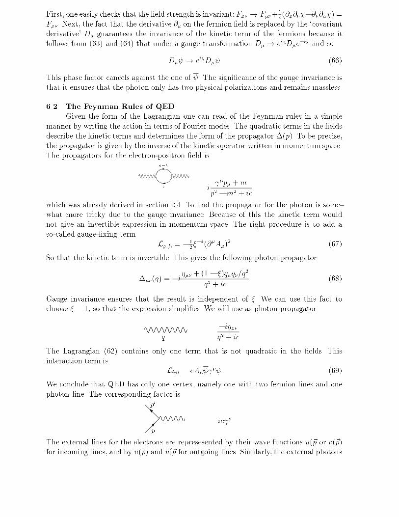
describe the kinetic terms and determines the form of the propagator �(p). To be precise,

the propagator is given by the inverse of the kinetic operator written in momentum space.

The propagators for the electron-positron �eld is

k

q + k

i �p� +m

p2 �m2 + i�

which was already derived in section 2.4. To �nd the propagator for the photon is some-

what more tricky due to the gauge invariance. Because of this the kinetic term would

not give an invertible expression in momentum space. The right procedure is to add a

so-called gauge-�xing term

Lg:f: = �12��1(@�A�)

2 (67)

So that the kinetic term is invertible. This gives the following photon propagator

���(q) = �i��� + (1 � �)q�q�=q

2

q2 + i�(68)

Gauge invariance ensures that the result is independent of �. We can use this fact to

choose � = 1, so that the expression simpli�es. We will use as photon propagator

q

�i���

q2 + i�

The Lagrangian (62) contains only one term that is not quadratic in the �elds. This

interaction term is

Lint = eA� � (69)

We conclude that QED has only one vertex, namely one with two fermion lines and one

photon line. The corresponding factor is

p

p0

ie �

The external lines for the electrons are represesented by their wave functions u(~p or v(~p)

for incoming lines, and by u(p) and v(~p for outgoing lines. Similarly, the external photons

have a factor ��(k) that describes their polarization. The physical polarization satisfy

k��� = 0. Furthermore, due to the gauge invariance the Feynman amplitudes must be

invariant under �� � �� + �k�. This implies that longitudinal photons with �� = �k�decouple, and hence the photon has only two physical polarizations. Finally, each loop

momentum integral has a normalization factor (2�)�4.

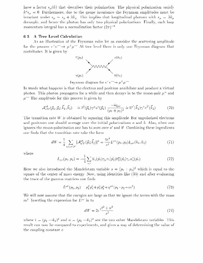
6.3 A Tree Level Calculation

As an illustration of the Feynman rules let us consider the scattering amplitude

for the process e+e� ! �+��. At tree level there is only one Feynman diagram that

contributes. It is given by

u(p1)

v(p2)

u(k1)

v(k1)

Feynman diagram for e+e� ! �+��

In words what happens is that the electron and positron annihilate and produce a virtual

photon. This photon propagates for a while and then decays in to the muon-pair �+ and

��. The amplitude for this process is given by

Aaba0b0(~p1; ~p2;

~k1; ~k2) = ie vb(~p1) �ua(~p1)

�i���

(p1 + p2)2ie ua

0

(~k1) �vb

0

(~k2) (70)

The transition rate W is obtained by squaring this amplitude. For unpolarized electrons

and positrons one should average over the initial polarizations a and b. Also, when one

ignores the muon-polarization one has to sum over a0 and b0. Combining these ingredients

one �nds that the transition rate take the form

dW =1

4

Xa;b;a0;b0

jAaba0b0(~pi;

~kj)j2 =

4e4

s2L��(p1; p2)L��(k1; k2) (71)

where

L��(p1; p2) = �1

4

Xa;b

ua(~p1) �vb(~p2)v�b(~p2) �u

�a(~p1) (72)

Here we also introduced the Mandelstam variable s = (p1 + p2)2 which is equal to the

square of the center of mass energy. Now, using identities like (33) and after evaluating

the trace of the gamma matrices one �nds

L��(p1; p2) = p�1p�2+p

�1p

�2+�

��(p1 � p2+m2) (73)

We will now assume that the energies are large so that we ignore the terms with the mass

m2. Inserting the expression for L�� in to

dW = 2e4t2 + u2

s2(74)

where t = (p1 � k1)2 and u = (p1 � k2)

2 are the two other Mandelstam variables. This

result can now be compared to experiments, and gives a way of determining the value of

the coupling constant e.

6.4 Loop Corrections

At one loop there are four kinds of Feynman diagrams that give corrections to the

tree level result. First there is the possibility that the electron emits a photon which it

again re-absorbs before it annihilates with the positron. This gives the electron self-energy.

Then there is a so-called vertex correction where a photon is emitted by the electron and

absorbed by the positron before both annihilate. Another possibility is that the emitted

photon is absorbed only later by one of the produced muons.

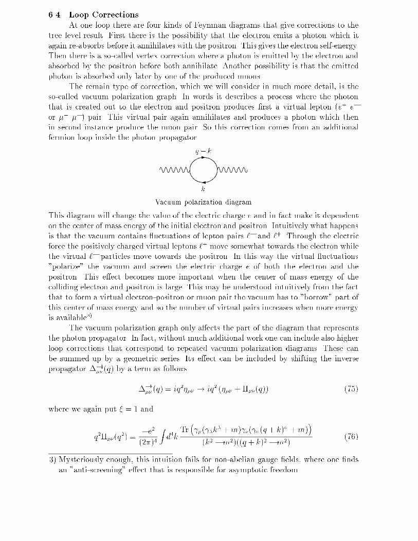
The remain type of correction, which we will consider in much more detail, is the

so-called vacuum polarization graph. In words it describes a process where the photon

that is created out to the electron and positron produces �rst a virtual lepton (e+ e�

or �+ ��) pair. This virtual pair again annihilates and produces a photon which then

in second instance produce the muon pair. So this correction comes from an additional

fermion loop inside the photon propagator.

k

q + k

Vacuum polarization diagram

This diagram will change the value of the electric charge e and in fact make it dependent

on the center of mass energy of the initial electron and positron. Intuitively what happens

is that the vacuum contains uctuations of lepton pairs `� and `+. Through the electric

force the positively charged virtual leptons `+ move somewhat towards the electron while

the virtual `� particles move towards the positron. In this way the virtual uctuations

"polarize" the vacuum and screen the electric charge e of both the electron and the

positron. This e�ect becomes more important when the center of mass energy of the

colliding electron and positron is large. This may be understood intuitively from the fact

that to form a virtual electron-positron or muon pair the vacuum has to "borrow" part of

this center of mass energy and so the number of virtual pairs increases when more energy

is available3).

The vacuum polarization graph only a�ects the part of the diagram that represents

the photon propagator. In fact, without much additional work one can include also higher

loop corrections that correspond to repeated vacuum polarization diagrams. These can

be summed up by a geometric series. Its e�ect can be included by shifting the inverse

propagator ��1�� (q) by a term as follows

��1�� (q) = iq2��� ! iq2 (��� +���(q)) (75)

where we again put � = 1 and

q2���(q2) =

�e2

(2�)4

Zd4k

Tr� �( �k

� +m) �( �(q + k)� +m)�

(k2 �m2)((q + k)2 �m2)(76)

3) Mysteriously enough, this intuition fails for non-abelian gauge �elds, where one �nds

an "anti-screening" e�ect that is responsible for asymptotic freedom.

It follows from Lorentz invariance and gauge invariance (decoupling of the longitudinal

polarization of the photon) that this expression must be of the form

���(q2) = (q2��� � q�q�)�(q2) (77)

This can be veri�ed explicitely by evaluating the gamma trace and doing some manipula-

tions in the integral. Fruther, we will again assume that the energy carried by the photon

is much larger that the electron mass, and so we drop the terms depending on m. In this

way one �nds

�(q2) =�e2

(2�)4

Zd4k

1

k2(q + k)2(78)

This integral is in�nite. This is of course rather disturbing result, but fortunately there is

still a way to extract a sensible answer. First one has to regulate the integral so that it is

�nite, and then apply a so-called renormalization procedure. Here we will not go in too

much detail, but we just want make clear what the essential idea behind renormalization.

6.5 Regularization and Renormalization

There are various way to regulate the above integral expression. The simplest fashion

is to analytically continue to euclidean space and to introduce a momentum cut o� � by

restricting the integral over k to values with jkj < �. Again omitting some details, one

gets

�(q2)=�e2

12�2

Z �2

q2

d(k2)

k2

=e2

12�2ln

q2

�2

!(79)

This one-loop correction can now be inserted in the Feynman graph for the full process,

and in this way added to the tree-level result. Because it only corrects the photon propa-

gator the result is of the same form as the tree-level, but with an additional s dependent

factor. This eventually leads to

dW = 2e4t2 + u2

s2

1�

e2

12�2ln

�s

�2

�!�2(80)

Now there appears to be a problem with this expression. Namely, it depends on the cut-o�

�, which was chosen arbitrarily. In particular, when we would send the cut-o� � ! 1

we would again �nd a divergent answer, at least when we keep e �xed. The solution to

this problem is that the coupling constant e that appears in this expression should not

really be identi�ed with the physical value of the electric charge that we measure in the

laboratory. Therefore, we are allowed to make this `bare' coupling e = e0(�) dependent

on the cut-o� � in such a way that the physical observables like dW are independent of

�.

Suppose we �rst do the experiment at a certain center of mass energy s = �2. Then

at this value of s we can now use the tree-level expression (74) to de�ne the physical

coupling constant e(�) by

dWjs=�2

= 2e4(�)t2 + u2

s2(81)

Comparing this to the one loop result (80) one concludes that

e2(�) = e20(�)

1 �

e20(�)

12�2ln

�2

�2

!!�1(82)

where we made explicit that the bare coupling e20(�) depends on the cut-o�. This equation

now tells us what e20(�) is in terms of the physical coupling e(�). Next we can re-express

the result for the physical observable dW at other values for s in terms of the physical

coupling e(�). In this way one �nds that cut-o� � disappears from the expression for dW ,

because it follows from (82) that

e20(�)

1�

e20(�)

12�2ln

�s

�2

�!�1= e2(�)

1 �

e2(�)

12�2ln

s

�2

!!�1(83)

and so we can write the transition probability in terms of the physical coupling constant

as

dW = 2e4(�)t2 + u2

s2

1�

e2(�)

12�2ln

s

�2

!!�2(84)

This expression is identical to (80) but now the cut-o� � is replaced by the mass scale �,

which is called the renormalization scale. Still there appears to be the problem that the

answer for dW depends on the arbitrary scale �, while we know that the physical value

of dW must be independent of �. However, this condition precisely determines the way

that e(�) depends on �. So �nally, we conclude that the e�ect of the one-loop vacuum

polarization can be summarized by equation (81) with a running coupling constant e(�).

Given the value of e(�) at low energies, say at �0 � a few eV , we can determine its value

at other values from the condition that value of dW remains unchanged. This gives

e2(�) = e2(�0)

1�

e2(�0)

12�2ln

�2

�20

!!�1(85)

At low energies we know the value of the coupling constant very well: we have �(�0) =

e2(�0)=4� = 1=137. The value at higher energies follows from the above relation which

may be rewritten in terms of the �ne structure constant �(�) = e2(�)=4� as

1

�(�)=

1

�(�0)�

1

3�ln(

�2

�20): (86)

In fact, at high energies one also has to take in to account the contribution to the vacuum

polarization of other charged particles, in particular the muon. This leads to additional

contributions that change the coe�cient 13�

somewhat. This running of the �ne structure

constant has been con�rmed by high energy experiments, in particular at LEP.