Error Estimates for Approximate Solutions of the Riccati Equation with Real or Complex Potentials

arX

iv:0

807.

4406

v2 [

mat

h-ph

] 2

3 N

ov 2

009

ERROR ESTIMATES FOR APPROXIMATE SOLUTIONS OF THE

RICCATI EQUATION WITH REAL OR COMPLEX POTENTIALS

FELIX FINSTER AND JOEL SMOLLER

JULY 2008

Abstract. A method is presented for obtaining rigorous error estimates for approx-imate solutions of the Riccati equation, with real or complex potentials. Our maintool is to derive invariant region estimates for complex solutions of the Riccati equa-tion. We explain the general strategy for applying these estimates and illustrate themethod in typical examples, where the approximate solutions are obtained by glue-ing together WKB and Airy solutions of corresponding one-dimensional Schrodingerequations. Our method is motivated by and has applications to the analysis of linearwave equations in the geometry of a rotating black hole.

1. Introduction

The time-independent one-dimensional Schrodinger equation plays an importantrole in both mathematics and physics. Except in special situations, it is impossibleto find exact solutions, and thus one resorts to approximation techniques. The mostcommon method is to take the WKB wave functions away from the zeros of the poten-tial, and to glue them together with Airy functions, which approximate the solutionsnear the zeros (see for example the textbook [9, Section 2.4] or the book [5]). Usually,the potential in the Schrodinger equation is real-valued. However, there are situations(like systems with dissipation) where the Schrodinger potential is complex.

The shortcoming of most approximation procedures is that they do not give errorestimates. To quote Froman and Froman [5, page 3] (1965),

“In spite of the abundant literature there is still lacking a convenientmethod for obtaining definite limits of error. . . The problem of obtain-ing such limits of error is not only of academic or mathematical interestbut is especially important in some physical applications. . . ”

Unfortunately, such a convenient method for obtaining definite limits of error is stilllacking today. Indeed, to our knowledge, despite the vast literature on WKB methods(see [4] and the references therein), only a few papers are concerned with rigorouserror estimates. As typical examples see [7, 8], where L2-estimates are derived in thetime-dependent setting for short times, as well as [6], where estimates are obtainedin the setting of multiple tunneling. Here we shall develop a general method forobtaining rigorous pointwise error estimates for any given approximate solution in thetime-independent setting, even in the case when the Schrodinger potential is complex.

We were led to the study of error estimates for solutions of one-dimensional Schrodin-ger equations from problems arising in general relativity. In particular, when analyzing

F.F. is supported in part by the Deutsche Forschungsgemeinschaft.J.S. is supported in part by the Humboldt Foundation and the National Science Foundation, Grant

No. DMS-0603754.1

http://arxiv.org/abs/0807.4406v2

https://www.researchgate.net/publication/268307494_The_Schrodinger_and_Riccati_Equations?el=1_x_8&enrichId=rgreq-ad1defab-1e22-4ae2-9f99-74c95345114c&enrichSource=Y292ZXJQYWdlOzIyNTEwMzkzNTtBUzoxMDQxOTY4ODgwNzIyMDVAMTQwMTg1Mzg4MjQ3Ng==

2 F. FINSTER AND J. SMOLLER

the scalar wave equation in the Kerr geometry, Carter’s remarkable separation ofvariables [1] gives rise to a radial and angular ODE. These equations can both betransformed into the Schrodinger form, which are coupled through two parameters ωand λ. For estimating the global behavior of the solutions uniformly in ω and λ, wewere led to the idea of using invariant disk estimates [3, 2]. When attempting to extendour analysis to gravitational waves in the framework of the Teukolsky equation [10],one of the difficulties that arises is that the potentials in the separated equations turnout to be complex. In the present paper, we obtain invariant disk estimates in ageneral setting, which are applicable to one-dimensional Schrodinger equations with areal or complex potential. The previous estimates in [3, 2] will arise as special cases.In particular, our method gives rigorous pointwise error estimates for the standardapproximations by WKB and Airy functions. But the method works just as well forany other approximate solutions. The aim of the present paper is to introduce themethod from a general point of view, and to illustrate it in typical examples. For anapplication to eigenvalue and gap estimates as well as to problems involving parameterswe refer to [3] and [2].

We now set up the framework and fix our notation. The one-dimensional Schrodingerequation reads

[

− d2

dx2+ V(x)

]

φ(x) = λφ(x) .

Absorbing the parameter λ into the potential, we rewrite the Schrodinger equation as

d2

dx2φ = V (x)φ(x) , (1.1)

where the new potential V = V − λ may depend on additional parameters. This isa linear second order ODE. Thus the general solution φ can be written as a linearcombination of two linearly independent fundamental solutions φ1 and φ2,

φ = a φ1 + b φ2 . (1.2)

By choosing the coefficients a and b appropriately, one can then satisfy suitable bound-ary conditions, if so desired. Setting

y =φ′

φ, (1.3)

the function y satisfies the Riccati equation

y′ = V − y2 . (1.4)

Our strategy is to estimate y in the complex plane. This requires a brief explanation,because in the case when V is real it is natural to also choose φ, and thus y, tobe real. This real function φ will in general have zeros, and y will be singular ateach of these zeros. These divergences make it difficult to estimate y. We avoidthis problem by considering a linear combination φ = φ1 + iφ2 with real fundamentalsolutions φ1 and φ2. Then, since the zeros of the fundamental solutions never coincide,the function φ never vanishes, and thus the corresponding function y is globally well-defined.

In the more general case when the potential V is complex, the situation is moredifficult because complex solutions of the Riccati equation (1.4) may “blow up in finitetime”. Nevertheless, we can hope to avoid singularities of the Riccati equation bychoosing the initial condition y(0) suitably.

https://www.researchgate.net/publication/2091466_Spectral_Estimates_and_Non-Selfadjoint_Perturbations_of_Spheroidal_Wave_Operators?el=1_x_8&enrichId=rgreq-ad1defab-1e22-4ae2-9f99-74c95345114c&enrichSource=Y292ZXJQYWdlOzIyNTEwMzkzNTtBUzoxMDQxOTY4ODgwNzIyMDVAMTQwMTg1Mzg4MjQ3Ng==



https://www.researchgate.net/publication/30847266_Decay_of_Solutions_of_the_Wave_Equation_in_the_Kerr_Geometry?el=1_x_8&enrichId=rgreq-ad1defab-1e22-4ae2-9f99-74c95345114c&enrichSource=Y292ZXJQYWdlOzIyNTEwMzkzNTtBUzoxMDQxOTY4ODgwNzIyMDVAMTQwMTg1Mzg4MjQ3Ng==



ERROR ESTIMATES FOR THE RICCATI EQUATION 3

In this paper, we focus on the analysis of solutions of the Riccati equation forspecific initial conditions y(0). This is justified because our estimates also give riseto corresponding estimates for general approximate Schrodinger wave functions, usingthe following procedure. Suppose that a specific y is known, up to a small error term.Then integrating (1.3), one obtains one fundamental solution φ1(x) = exp(

∫ xy) of

the Schrodinger equation. The other fundamental solution can readily be obtainedby integrating the Wronskian equation φ′

1φ2 − φ1φ′2 = const. We thus obtain the

general solution (1.2). Keeping track of the error in this procedure, one can deriveerror estimates for any Schrodinger wave function.

2. The Flow of Circles for a Constant Potential

In this section we consider the special case of a constant potential. This case caneasily be analyzed in closed form, and the resulting flow in the complex plane will behelpful for the geometric understanding of the invariant disk estimates. Thus assumethat V is a non-zero complex constant. We set ζ =

√V . Then the general solution of

the Schrodinger equation (1.1) is

φ(x) = aeζx + be−ζx , x ∈ R

with a, b ∈ C. The corresponding solution of the Riccati equation is

y(x) = ζaeζx − be−ζx

aeζx + be−ζx= ζ

(a − b) cosh(ζx) + (a + b) sinh(ζx)

(a + b) cosh(ζx) + (a − b) sinh(ζx)

= ζ(a − b) + τ(x) (a + b)

(a + b) + τ(x) (a − b),

where τ(x) := tanh(ζx). Setting y0 = y(0),

y0 = ζa − b

a + b,

we can express y in terms of y0,

y(x) = ζy0 + τ(x) ζ

τ(x) y0 + ζ.

Note that the mapping y0 → y is a fractional linear transformation. It has the fixedpoints y = ±ζ corresponding to the two solutions φ = e±ζx, respectively. Furthermore,we see that circles are mapped onto circles or straight lines. Thus by varying x, weobtain a flow of circles in the complex plane. To analyze this flow, let us assume that y0

lies on a circle of radius R0 around m0, i.e.

y0 = m0 + z with z = R0 eiϕ .

Then for any fixed x,

y = ζz + m0 + τζ

τz + τm0 + ζ.

Thus for any m ∈ C, we can write

y − m =(ζ − τm)R0e

iϕ + ζm0 + τζ2 − τmm0 − mζ

τR0eiϕ + τm0 + ζ=

c

eiϕ

(

eiϕ + γ

e−iϕ + δ

)

,

where the introduced quantities

c =(ζ − τm)R0

τm0 + ζ, γ =

ζm0 + τζ2 − τmm0 − mζ

(ζ − τm)R0, δ =

τR0

τm0 + ζ


are independent of ϕ. For m to be the center of the new circle, the resulting expressionfor |y−m| must be independent of ϕ. This gives the condition γ = δ. We thus concludethat

|y − m| = R ,

where the center and radius are given by

m = ζ(m0 + τζ)(τm0 + ζ) − R2

0 τ

|τm0 + ζ|2 − R20|τ |2

, R =R0 |τ2 − 1| |ζ|2

|τm0 + ζ|2 − R20 |τ |2

.

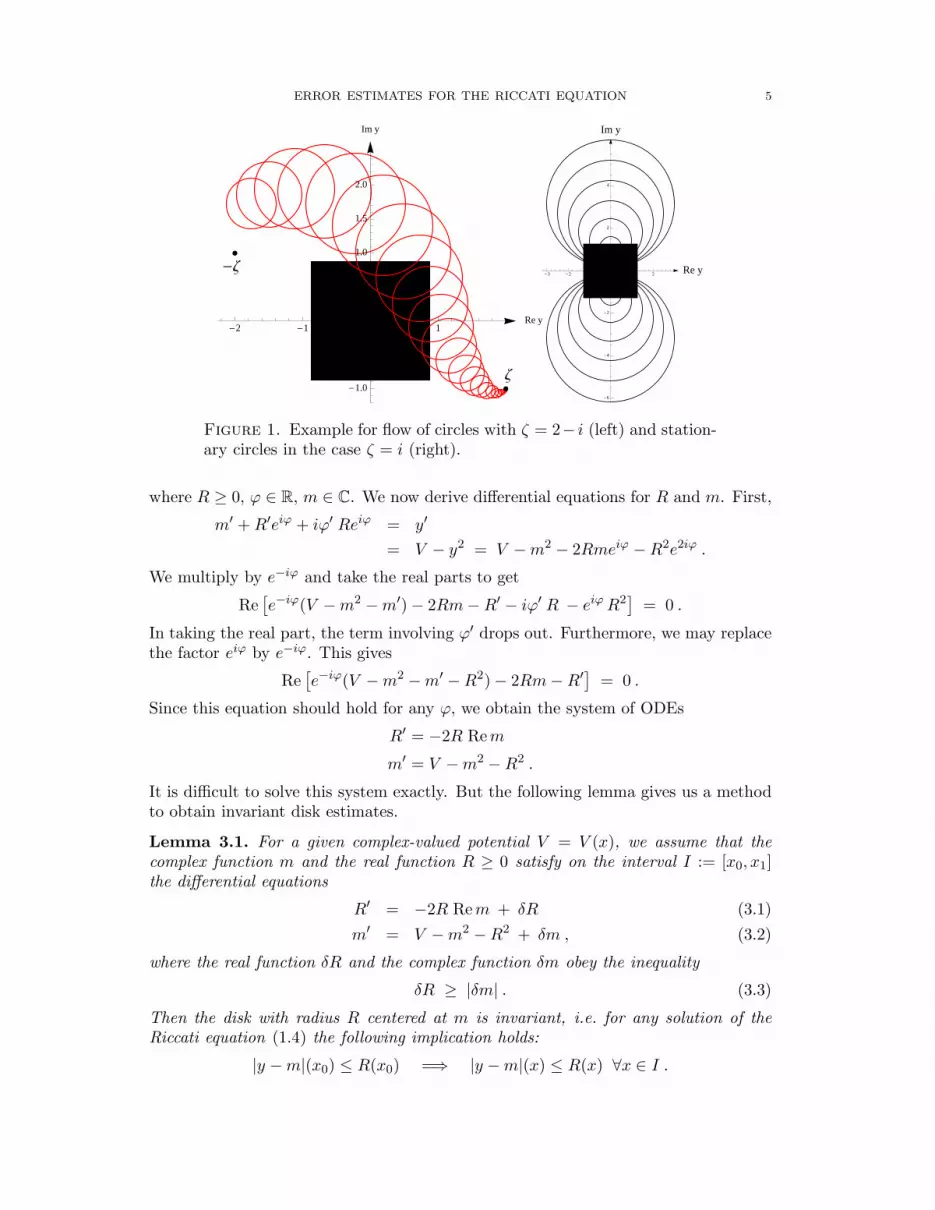
The denominator can have zeros, in which case the circle degenerates to a straightline. Whenever the denominator has no zeros, we can take the limit x → ∞ to findthat in the case Re ζ > 0, the circle asymptotically approaches the fixed point y = ζ,unless if we start at m0 = −ζ with R0 = 0. Thus we can say that y = ζ is the stableand y = −ζ the unstable fixed point. Conversely, in the case Re ζ < 0, the fixedpoint y = ζ is unstable, whereas y = −ζ is stable. The flow of circles is illustrated inFigure 1 (left).

In the remaining case Re ζ = 0, we clarify the situation by computing the stationarycircles. In this case, ζ and τ are purely imaginary, and thus the above formula for Rbecomes

R = R0 ζ2 τ2 − 1

τ2(R20 − |m0|2) − 2τ ζ Re(m0) − ζ2

.

For a stationary circle, R must equal R0, for all imaginary τ (because the range ofthe function tanh(ζx) is iR). Multiplying by the denominator, we get a quadraticpolynomial in τ , and comparing the coefficients, we obtain the conditions

Rem0 = 0 and |m0|2 − R20 = |ζ|2 .

We thus obtain for any R0 ≥ 0 the two circles with centers

m0 = ±i√

R20 + |ζ|2 , (2.1)

and an easy computation shows that these circles are indeed stationary under the flow.Since these circles enclose the fixed points (see Figure 1 (right)), both fixed points arecenters.

This simple analysis gives rise to a useful concept. Namely, the above flow of circlesunder the Riccati equation defines an invariant region consisting of the interior of thecircles together with their boundary. In the next section we shall implement this pointof view in the case of a non-constant potential V .

3. Invariant Disk Estimates for the Riccati Equation

We now turn our attention to solutions y ∈ C of the Riccati equation (1.4) for ageneral complex-valued potential V (x). Our goal is to derive inequalities of the form

|y(x) − m(x)| ≤ R(x)

for explicit functions m and R. Geometrically, this means that the exact solution ystays inside the disk of radius R centered at m. Thus we can interpret m as anapproximate solution, with R giving a rigorous bound on the error.

In preparation, we show that the the flow given by the Riccati equation maps circlesinto circles. At the same time, we derive differential equations describing the motionof these circles. Let us assume that y lies on a circle of radius R centered at m, i.e.

y = m + R eiϕ ,


-Ζ

Ζ

-2 -1 1Re y

-1.0

-0.5

0.5

1.0

1.5

2.0

Im y

-3 -2 -1 1 2 Re y

-6

-4

-2

2

4

Im y

Figure 1. Example for flow of circles with ζ = 2− i (left) and station-ary circles in the case ζ = i (right).

where R ≥ 0, ϕ ∈ R, m ∈ C. We now derive differential equations for R and m. First,

m′ + R′eiϕ + iϕ′ Reiϕ = y′

= V − y2 = V − m2 − 2Rmeiϕ − R2e2iϕ .

We multiply by e−iϕ and take the real parts to get

Re[

e−iϕ(V − m2 − m′) − 2Rm − R′ − iϕ′ R − eiϕ R2]

= 0 .

In taking the real part, the term involving ϕ′ drops out. Furthermore, we may replacethe factor eiϕ by e−iϕ. This gives

Re[

e−iϕ(V − m2 − m′ − R2) − 2Rm − R′]

= 0 .

Since this equation should hold for any ϕ, we obtain the system of ODEs

R′ = −2R Rem

m′ = V − m2 − R2 .

It is difficult to solve this system exactly. But the following lemma gives us a methodto obtain invariant disk estimates.

Lemma 3.1. For a given complex-valued potential V = V (x), we assume that thecomplex function m and the real function R ≥ 0 satisfy on the interval I := [x0, x1]the differential equations

R′ = −2R Rem + δR (3.1)

m′ = V − m2 − R2 + δm , (3.2)

where the real function δR and the complex function δm obey the inequality

δR ≥ |δm| . (3.3)

Then the disk with radius R centered at m is invariant, i.e. for any solution of theRiccati equation (1.4) the following implication holds:

|y − m|(x0) ≤ R(x0) =⇒ |y − m|(x) ≤ R(x) ∀x ∈ I .


Proof. We first prove the lemma in the case of strict inequality in (3.3). If the lemmawere false, there would be an x ∈ I such that |y − m|(x) > R(x). Let x ∈ [x0, x1) bethe infimum of all such x. Then |y−m|(x) = R(x). Using (1.4) and (3.2), we find at x

d

dx|y − m| = Re

(y′ − m′)(y − m)

|y − m| = Re(V − y2 − V + m2 + R2 − δm)(y − m)

|y − m|

≤ R Re(y − m) + |δm| − Re(y2 − m2)(y − m)

|y − m|= R Re(y − m) + |δm| − R Re(y + m) = −2R Rem + |δm| .

Combining this with (3.1) and the strict inequality in (3.3), we obtain

d

dx|y − m|(x) <

d

dxR(x) .

Hence there is a δ > 0 such that on the interval (x, x + δ) the inequality |y − m| < Rholds. This is a contradiction.

To prove the general case of non-strict inequality in (3.3), we introduce the new

radius R by

R = R + εeL(x−x1) ,

where ε > 0 and

L > maxI

(

−2Re m + 2R − εeL(x−x1))

. (3.4)

Then R and m satisfy again the differential equations (3.1) and (3.2), where R is

replaced by R, and δR and δm are replaced by

δR = δR + εeL(x−x1) (L + 2Re m)

δm = δm + εeL(x−x1)(

2R − εeL(x−x1))

.

Using (3.3) and (3.4), we see that |δm| < δR for sufficiently small ε, and thus the circle

with radius R and center m is invariant. Letting ε ց 0 completes the proof. �

In what follows, it is convenient to write m = α+iβ with real α and β, and similarlywe write δm = δα + i δβ. Then the equations (3.1) and (3.2) become

R′ = −2αR + δR (3.5)

α′ = Re V − α2 + β2 − R2 + δα (3.6)

β′ = Im V − 2αβ + δβ . (3.7)

In our first theorem we satisfy the conditions of Lemma 3.1 by employing a specialansatz where the invariant disks are centered on the real axis (so that β ≡ 0). Weintroduce the abbreviation

U = Re V − α2 − α′ . (3.8)

Theorem 3.2. Suppose that on an interval I ⊂ R, we are given the real func-tions α,W ∈ C1(I). Assume furthermore that W > 0 and that

2αW +W ′

2−

√W

(

|W − U | + |Im V |)

≥ 0 . (3.9)

Then the circle with radius R centered at m with

R =√

W , m = α (3.10)


is invariant on I under the Riccati flow (1.4).

Proof. We shall verify the conditions of Lemma 3.1. Using the ansatz (3.10) in theequations (3.5), (3.6) and (3.7), we get

δR =W ′

2√

W+ 2α

√W , δα = W − U , δβ = −ImV .

The sufficient condition δR ≥ |δα| + |δβ| reduces to (3.9). �

In our next theorem we will not prescribe β. For convenience, we now replace (3.3)by the sufficient condition

δR = |δα| + |δβ| . (3.11)

Thus our task is to find six functions R, α, β, δR, δα and δβ which satisfy theequations (3.5), (3.6) and (3.7) together with the condition (3.11). Thus we expectthat we can freely assign two functions, and then the remaining four functions willbe determined. To explain which functions are to be preassigned, we note that theequations (3.5) and (3.7) are both linear, so that the only nonlinearity appears in theα-equation (3.6). Thus we can get rid of the nonlinear differential equation by takingthe functions

α and W := R2 − β2 (3.12)

as a-priori given. Then (3.6) becomes the defining equation for δα; namely,

δα = −ReV + α2 + α′ + W .

Using these definitions, we are left with the system of equations

R′ = −2αR + |δα| + |δβ| (3.13)

β′ = Im V − 2αβ + δβ (3.14)

R2 − β2 = W (3.15)

for the three unknown functions R, β and δβ. This system consists of two lineardifferential equations and one nonlinear algebraic equation. Of course, we must alsoensure that 0 ≤ R < ∞.

To analyze these equations, we consider the two cases δβ ≥ 0 and δβ < 0 separately.

Case (A) δβ ≥ 0: Subtracting (3.14) from (3.13) we get

(R − β)′ = −2α (R − β) − ImV + |δα| . (3.16)

Furthermore, differentiating (3.15) gives

2RR′ − 2ββ′ = W ′ . (3.17)

We consider (3.16) and (3.17) as a system of two linear algebraic equations inthe unknowns R′ and β′. Solving for β′ and substituting into (3.14), we find

(R − β) δβ = −R |δα| + 2Wα + ImV β +W ′

2. (3.18)

Since we assumed δβ to be positive, we get the consistency condition

(R − β)

[

2αW +W ′

2− R |δα| + β ImV

]

≥ 0 . (3.19)

Provided that this consistency condition holds, we can use (3.16) to solvefor R − β. Then using (3.15), we conclude that R + β = W/(R − β).


Case (B) δβ < 0: Adding (3.13) and (3.14) gives

(R + β)′ = −2α (R + β) + ImV + |δα| . (3.20)

Solving (3.20) and (3.17) for β′ and substituting the result into (3.14), weobtain

(R + β) δβ = R |δα| − 2Wα − ImV β − W ′

2,

giving rise in this case to the consistency condition

(R + β)

[

2αW +W ′

2− R |δα| + β ImV

]

≥ 0 . (3.21)

Provided that this consistency condition holds, R + β is determined by (3.20),and R − β = W/(R + β).

Since the bracket in (3.19) and (3.21) will appear often, it is convenient to introducethe abbreviation

D = 2αW +W ′

2− R |δα| + β ImV . (3.22)

We refer to D as the determinator. Then the following invariant disk estimate holds.

Theorem 3.3. Suppose that on an interval I ⊂ R, we are given the real func-tions α,W ∈ C1(I). We set

σ(x) = exp

(∫ x

2α

)

. (3.23)

Then the following statements hold.

(A) Define real functions R and β on I by

(R − β)(x) =1

σ

∫ x

σ (−ImV + |W − U |) (3.24)

(R + β)(x) =W (x)

(R − β)(x)(3.25)

(with U as defined by (3.8)). Assume that the function R − β has no zeros,R ≥ 0, and that

(R − β) D ≥ 0 (3.26)

(with D according to (3.22)). Then the circle centered at m(x) = α + iβ withradius R(x) is invariant on I under the Riccati flow (1.4).

(B) Define real functions R and β on I by

(R + β)(x) =1

σ

∫ x

σ (Im V + |W − U |) (3.27)

(R − β)(x) =W (x)

(R + β)(x). (3.28)

Assume that the function R + β has no zeros, R ≥ 0, and that

(R + β) D ≥ 0 . (3.29)

Then the circle centered at m(x) = α + iβ with radius R(x) is invariant on Iunder the Riccati flow (1.4).


Proof. We only prove the first part, as the proof of the second part is similar. Since (3.26)holds, we are consistently in Case (A) above. Integrating the differential equation (3.16)gives (3.24), whereas (3.25) follows from (3.12). We thus have a solution of the systemof equations (3.13), (3.14) and (3.15) with δβ given by (3.18). Applying Lemma 3.1completes the proof. �

We next outline the general strategy for applying the last theorem. Suppose thatan approximate solution y of the Riccati equation is given. Setting V = y′ + y2, wecan consider y as a solution of a Riccati equation

y′ = V − y2 (3.30)

with an “approximate” potential V . Since y approximates y, an obvious idea wouldbe to consider circles centered at m = y. In the estimates of Theorem 3.3, however,we only need to prescribe the function α = Rem, whereas the imaginary part of mwill then be determined. Therefore, it is natural to choose

α = Re y . (3.31)

A natural choice for W is to set

W = U (3.32)

(with U according to (3.8)), because then the term |W − U | in (3.24) and (3.27)vanishes1. Then Theorem 3.3 gives us invariant disk estimates. The center m of thisdisk can be viewed as an improved approximate solution, and its error, measured asthe distance from the exact solution, is at most R. The invariant disk estimate dependscrucially on the sign of the determinator D. Thus in applications it is important toknow the sign of D. It can even be useful to modify y so as to give D a desired sign(this will be illustrated in Section 5 in a few examples). For this purpose, it is usefulto bring the determinator into a more convenient form.

Lemma 3.4. Suppose that, for a given solution y of an approximate Riccati equa-tion (3.30), α and W are chosen according to (3.31) and (3.32). Then the determinatoris given by

D = 2α Re(V − V ) +1

2Re(V − V )′ − β Im V + β Im V , (3.33)

where β = Im y.

Proof. Writing the Riccati equation (3.30) as

α′ = Re V − α2 + β2 , β′ = Im V − 2αβ ,

we can use (3.32) and (3.8) to obtain

W = U = Re(V − V ) − β2 .

Applying these identities in (3.22) gives

D = 2α Re(V − V ) +1

2Re(V − V )′ − 2αβ2 − ββ′ + β Im V .

Using the β′-equation finishes the proof. �

1Other choices of W might be useful, but we will not consider them in this paper.


4. Error Estimates for Real Potentials and Examples

In this section we shall illustrate our error estimates in examples for a real poten-tial V and explain how the previous results from [3, 2] fit into our framework. Wefirst mention an additional structural relation which appears only for a real potential.Namely, suppose that φ is a complex solution of the Schrodinger equation (1.1). De-composing it into its real and imaginary parts, φ = φ1+iφ2, the functions φ1 and φ2 arereal solutions of the Schrodinger equation forming a fundamental set. Thus their Wron-skian w = φ1φ

′2 − φ′

1φ2 is a constant. It can be expressed as w = Im (φ φ′) = |φ|2 Im y,giving rise to the relation

|φ|2 =w

Im y,

which is useful for estimating the amplitude of φ. Moreover, this relation shows thatthe imaginary part of y can never change sign, and thus the upper and lower halfplanes must be invariant regions for y.

To illustrate how our estimates apply, we begin with a simple example.

Example 4.1. (negative, increasing potential) Suppose that the potential satis-fies on the interval I = [x0, x1] the conditions

V (x) ≤ 0 , V ′(x) ≥ 0 .

The simplest (but certainly not the best) choice is to set α ≡ 0. Furthermore, set-ting W = U , we see from (3.23) that σ is a constant. According to (3.8), we findthat W = V . The determinator (3.22) simplifies to

D =V ′

2≥ 0 . (4.1)

We want to apply part (B) of Theorem 3.3 (part (A) is similar if one flips the signof β). From (3.27) we see that R+β is a constant, which according to (3.29) and (4.1)must be positive. We thus obtain

β + R = c > 0 , β − R =|V |c

. (4.2)

The condition R ≥ 0 gives the constraint

c2 ≥ maxI

|V | = |V (x0)| .

If the potential is constant, we recover the stationary circles of Section 2 (as is easilyverified by comparing (4.2) and (2.1)). If the potential is non-constant, we get anincreasing family of invariant disks in the upper half plane centered on the imaginaryaxis whose highest point is fixed at ic, and whose lowest point varies like i|V |/c; seeFigure 2. ♦

We next consider the situation for a general real potential V and a general choiceof α, again setting W = U . Then the determinator becomes

D = 2αU +U ′

2=

U

2

(σ2U)′

σ2U(4.3)

(with σ defined by (3.23)). The main simplification is that now D is an a-priori givenfunction. In the case when R − β and R + β have opposite signs, we see from (3.26)and (3.29) that, depending on the sign of D, either part (A) or part (B) of Theorem 3.3applies. In this case, we can combine parts (A) and (B) to obtain a statement whichcan be used even if D changes sign infinitely often. In view of (3.15), the condition


c

Im y

Re y

|V |c

Figure 2. A simple invariant disk estimate for a negative, increasing potential.

that R−β and R+β should have opposite signs is equivalent to the simpler conditionthat U < 0; it means that the invariant disk either lies in the upper half plane or in thelower half plane, without intersecting the real line. By continuity, the invariant diskcannot move from the upper to the lower half plane. Thus we can assume withoutloss of generality that the invariant disk lies in the upper half plane. This meansthat R + β > 0 and R − β < 0. It is convenient to satisfy the equation (3.15) (andthus also (3.25) and (3.28)) by making the ansatz

β =

√

|U |2

(

T +1

T

)

, R =

√

|U |2

(

T − 1

T

)

(4.4)

with a free function T > 1. If D is negative, we apply Theorem 3.3 (A) to obtain

T = −√

|U |R − β

= −σ√

|U |c

with c an integration constant. Diffentiating gives

T ′

T=

(σ√

|U |)′

σ√

|U |=

1

2

(σ2|U |)′σ2|U | =

1

2

(σ2U)′

σ2U=

1

2

∣

∣

∣

∣

(σ2U)′

σ2U

∣

∣

∣

∣

,

where in the last two steps we used that U is negative, and that in the consideredcase D < 0, the term (σ2U)′/(σ2U) is positive according to (4.3). If D is positive, weapply Theorem 3.3 (B) to get

T =R + β√

|U |=

c

σ√

|U |.

Now differentiating gives

T ′

T= −(σ

√

|U |)′

σ√

|U |= −1

2

(σ2U)′

σ2U=

1

2

∣

∣

∣

∣

(σ2U)′

σ2U

∣

∣

∣

∣

,

where in the last step we used that now (σ2U)′/(σ2U) < 0. We conclude that, inde-pendent of the sign of D, we obtain the differential equation

T ′

T=

1

2

∣

∣

∣

∣

(σ2U)′

σ2U

∣

∣

∣

∣

.


R

Im y

Re y

m√

|U |T

√

|U |T

Figure 3. Invariant disk estimate for U < 0.

Integrating both sides, we can rewrite T as a total variation,

T (x) = T0 exp

(

1

2TV[x0,x) log |σ2U |

)

. (4.5)

In this way, we recover the invariant disk estimate which was first obtained in [3,Lemma 4.1]; see Figure 3.

Lemma 4.2. Let α be a real function on [x0, x1] which is continuous and piecewiseC1. Suppose that the function U := V −α2−α′ is negative on [x0, x1]. Using the abovedefinitions (4.5) and (4.4), the disks of radius R centered at m = α + iβ are invariantunder the Riccati flow (1.4), on [x0, x1].

We now illustrate in two examples how this lemma can be applied (for other ap-plications see [3, Theorems 4.2 and 4.3] and [2, Lemmas 4.10 and 4.12]). In the firstexample, we consider the case that the potential V is negative. We recall that theWKB wave functions are given by (see for example [9, Section 2.4] or [5])

φWKB(x) = |V (x)|− 1

4 exp

(

±i

∫ x√

|V |)

. (4.6)

A short calculation shows that these functions satisfy the equation

d2

dx2φWKB − V φWKB =

(

5

16

|V |′2|V |2 − 1

4

|V |′′|V |

)

φWKB .

Interpreting the right side as an error term, one sees that the WKB wave functionsare expected to be a good approximation to φ provided that

∣

∣

∣

∣

V ′′

V 2

∣

∣

∣

∣

+

∣

∣

∣

∣

V ′2

V 3

∣

∣

∣

∣

≪ 1 . (4.7)

For definiteness, we consider the plus sign in (4.6) (the minus sign can be obtained bycomplex conjugation). Then the corresponding approximate Riccati solution is givenby

yWKB =φ′

WKB

φWKB

= i√

|V | − V ′

4V.


Following the general strategy described after Theorem 3.3, we thus choose

α = Re yWKB = − V ′

4V. (4.8)

An easy computation gives

α′ = −V ′′

4V+

V ′2

4 V 2(4.9)

U = V

(

1 +V ′′

4V 2+

5 V ′2

16 |V |3)

(4.10)

σ = exp

(

−1

2

∫ x V ′

V

)

=c

√

|V |(4.11)

σ2U = −c2

(

1 +V ′′

4V 2+

5 V ′2

16 |V |3)

. (4.12)

In view of (4.10), the condition (4.7) and the fact that V < 0, we see that U is negative.Thus Lemma 4.2 applies, giving the following estimate.

Example 4.3. (error estimate for WKB wave function, V < 0)Suppose that V is negative and

− V ′′

4V 2− 5 V ′2

16 |V |3 < 1 .

Then the disks of radius R centered at m = α + iβ as given by (4.8), (4.4) and

T (x) = T0 exp

(

1

2TV[x0,x) log

[

1 +V ′′

4V 2+

5 V ′2

16 |V |3])

(4.13)

are invariant under the Riccati flow (1.4), on [x0, x1].

In our setting, the semiclassical limit can be described by scaling the potentialaccording to V → λV and considering the behavior as λ → ∞. In this limit, the squarebracket in (4.13) converges to one, so that the logarithm vanishes. As a consequence,T becomes a constant. Choosing T0 = 1, we find that the radius R(x) as given by (4.4)vanishes identically in the semiclassical limit, in agreement with the fact that the WKBwave function goes over to the exact solution.

The next estimate even applies near a zero of the potential.

Example 4.4. (invariant disk estimate with exponential bound)Choose a constant α,

α = c + supx∈[x0,x1]

√

max(0, V (x)) (4.14)

with c ≥ 0. Then

U = V − α2 < −c2 ≤ 0

σ = C e2αx

σ2U = C2 e4αx(

V − α2)

with an integration constant C. Hence Lemma 4.2 yields that the disks of radius Rcentered at m = α + iβ as given by (4.14), (4.4) and

T (x) = T0 exp

(

1

2TV[x0,x) log

[

e4αx(

V − α2)]

)


Uσ

c1

α −√

U

c2

σ

−c1

σ

−Uσ

c2

Im y

Re y

α +√

U

Figure 4. Invariant lens-shaped region estimate for U > 0.

are invariant under the Riccati flow (1.4), on [x0, x1].

Clearly, due to the exponential factor e4αx, this estimate gets weaker as the size ofthe interval increases. We shall below see a much better estimate using Airy functions(see Example 5.1).

We next consider how Theorem 3.3 applies in the case U ≥ 0 (where we againchoose W = U). Then, according to (3.15), the functions R − β and R + β have thesame sign, which must be positive because R ≥ 0. Inspection of (3.26) and (3.29)yields that the determinator must be positive, i.e.

U ′ + 4αU ≥ 0 . (4.15)

Provided that this condition holds, we may apply both parts (A) and (B) of Theo-rem 3.3. Taking the intersection of the corresponding invariant disks gives the followingresult, which generalizes [2, Lemma 4.2].

Lemma 4.5. Let α be a real function on [x0, x1] which is continuous and piecewiseC1. Suppose that the function U := V − α2 − α′ is positive on [x0, x1] and that thecondition (4.15) holds. For any positive constants ck, k = 1, 2, we introduce the twodisks of radii Rk centered at mk = α + iβk with

R1 =1

2

(

Uσ

c1+

c1

σ

)

, β1 =1

2

(

Uσ

c1− c1

σ

)

R2 =1

2

(

Uσ

c2+

c2

σ

)

, β2 = −1

2

(

Uσ

c2− c2

σ

)

.

Then the two disks as well as the lens-shaped region obtained as their intersection areinvariant under the Riccati flow (1.4).

As is easily verified, the boundaries of both disks intersect the real axis at the pointsα ±

√U , and thus their intersection is non-void; see Figure 4.


In our next example we shall apply Lemma 4.5 to the WKB wave function fora positive potential. We thus assume that V > 0 and that (4.7) is again satisfied.Considering the WKB wave function

φWKB(x) = V (x)−1

4 exp

(∫ x √

V

)

, (4.16)

an easy computation shows that

yWKB(x) =φ′

WKB

φWKB

=√

V − V ′

4V

α = Re yWKB(x) =√

V − V ′

4V

U = V − α2 − α′ = − 5

16

V ′2

V 2+

V ′′

4V.

Unfortunately, in contrast to our previous example (4.10), now U need not have a fixedsign, and thus one cannot apply the above lemmas. Our method for getting aroundthis problem is to consider in the WKB ansatz another potential VWKB, and to set

φWKB(x) = VWKB(x)−1

4 exp

(∫ x

√

VWKB

)

.

Then

α = Reφ′

WKB

φWKB

=√

VWKB − V ′WKB

4VWKB

(4.17)

U = V − α2 − α′ = V − VWKB − 5

16

V ′2WKB

V 2WKB

+V ′′

WKB

4VWKB

. (4.18)

By arranging that U has a definite sign, we may apply either Lemma 4.2 or Lemma 4.5.To give a simple example, we choose

VWKB =V

4.

Then U is positive because V is positive and (4.7) holds. Furthermore, a direct com-putation gives

σ = exp

(∫ x

2α

)

=1√V

exp

(∫ x √

V

)

(4.19)

2

VU =

3

2+

[

−5

8

V ′2

V 3+

V ′′

2V 2

]

(4.20)

2

3V3

2

(

U ′ + 4αU)

= 1 +

[

− 5

12

V ′2

V 3+

5

8

V ′3

V9

2

+V ′′

3V 2− 3V ′V ′′

4V7

2

+V ′′′

6V5

2

]

. (4.21)

We are now in a position to apply Theorem 3.3.

Example 4.6. (error estimate for WKB wave function, V > 0)Suppose that V is positive and that the square brackets in (4.20) and (4.21) are bothgreater than minus one. Then choosing U and σ according to (4.20) and (4.19),the lens-shaped region from Lemma 4.5 (see Figure 4) is invariant under the Riccatiflow (1.4), on [x0, x1].


It is worth noting that from (4.19), we see that σ grows exponentially. Hence thelens-shaped region gets thinner, improving the estimate exponentially fast.

The previous estimates using Lemma 4.2 and Lemma 4.5 have the disadvantage thatif U changes sign, different kinds of estimates must be pasted together. This makes itnecessary to match invariant disks (see [2, Lemma 4.4]). In the next section we explaina more convenient method in the more general context of a complex potential (butalso working for real potentials) which makes it possible for the invariant disks to flowcontinuously across the real line.

5. Error Estimates for Approximate WKB/Airy Solutions for Real orComplex Potentials

In this section we illustrate the general technique for applying Theorem 3.2 andTheorem 3.3 by discussing typical examples. Based on Theorems 3.2 and 3.3, we willderive rigorous error estimates for the standard approximate solutions obtained byglueing together WKB and Airy wave functions.

For a given potential (real or complex), one can usually distinguish regions where |V |is large, so that the solutions of the Schrodinger equation are well-approximated byWKB wave functions. In the remaining regions, one can approximate the potential bya linear potential, so that the Schrodinger equation can be solved explicitly in terms ofAiry functions. To be more flexible, in the WKB region we consider the approximatesolutions

φWKB(x) = VWKB(x)−1

4 exp

(∫ x

±√

VWKB

)

(5.1)

with a potential VWKB ≈ V , which will be determined later. Likewise, in the Airyregion, our approximate wave functions are solutions of the Schrodinger equation

φ′′A(x) = VA φA , (5.2)

where VA ≈ V is a linear function, also to be determined later. By the standard C1-glueing of the WKB and Airy functions, we obtain an approximate wave function φ.The wave function φ is a weak solution of a Schrodinger equation

φ′′ = V φ , (5.3)

where V in the Airy region coincides with VA, whereas in the WKB region a shortcalculation gives

V = VWKB +5

16

V ′2WKB

V 2WKB

− V ′′WKB

4VWKB

. (5.4)

Note that V is piecewise smooth, but in general has discontinuities. Following thestrategy explained after Theorem 3.3, we introduce the function y = φ′/φ, which iscontinuous and piecewise smooth, satisfying the Riccati equation

y′ = V − y2 . (5.5)

We again introduce the (continuous, but only piecewise smooth) function α by

α = Re y , (5.6)

define U by (3.8) and (again for simplicity) choose W = U . We choose startingvalues for the functions β and R which are compatible with (3.15). We can thenapply Theorem 3.3 in various ways. If U < 0, i.e. R + β and R − β have oppositesigns, depending on the sign of the determinator D, we can apply either part (A)


or part (B). If however U ≥ 0, the functions R + β and R − β are both positive,and thus Theorem 3.3 applies only if D is positive, and in this case we can applyboth part (A) and part (B). If β becomes zero, it may be preferable to switch to thesimpler estimate of Theorem 3.2, provided that the inequality (3.9) holds. In this way,we have different possibilities to obtain invariant disk estimates, and by taking theirintersection one gets even sharper estimates involving lens-shaped invariant regions.Observe that on the boundaries between the WKB and Airy regions, the functions Vand α′, and consequently also U , may have discontinuities. In order to satisfy (3.15),either R + β or R − β must “jump” discontinuously, in such a way that the new diskcontains the old one.

The crucial point for making this procedure work is that one must be able to pre-scribe the sign of D or to satisfy the inequality (3.9). One method to achieve this isto modify the potentials VWKB and VA in (5.1) and (5.2). The effect on D of modify-ing the potentials can be seen most easily from Lemma 3.4. More specifically, in theWKB region, the term 2α Re(V − V ) in (3.33) can be suitably changed by modifying

the real part of VWKB, whereas the imaginary part of VWKB affects the term −β Im V .Note that the derivative term in (3.33) as well as the derivative terms in (5.4) onlygive rise to small corrections. In the Airy region, on the other hand, we can changethe coefficients in the linear function VA(x) to modify the suitable terms in (3.33). Inorder to satisfy the condition (3.9), it may be useful to apply the identity

(3.9) = 2α Re(V − V ) +1

2Re(V − V )′ − β Im V − |ImV |

√

Re(V − V ) − β2

(keeping in mind that in this case, β ≡ 0, and thus β should be small), or else one canmodify α, without respecting the relation (5.6).

We now give two concrete examples to illustrate this method. In the first example,the imaginary part of the potential is so small that the method works just as well fora real potential.

Example 5.1. We consider the potential (inspired by the spheroidal wave operator [3])

V = 10000

(

−1

2+ (1 + 0.05 i) sin2 x

)

, (5.7)

on the interval [0, π2 ]. Due to the large prefactor, the WKB condition (4.7) is satisfied

except in a small neighborhood of the point x = π4 , where |V | is small. Thus we divide

our interval into three regions:

(a) The “classically allowed” WKB region [0, 0.715](b) The Airy region [0.715, 0.83] near the “classical turning point”(c) The “classically forbidden” WKB region [0.83, π

2 ]

(The precise choice of the boundary points is arbitrary and has no major effect. More-over, since the factor 0.05 is so small, we simply adopted the terminology from quantummechanics, disregarding the effect of the imaginary part of the potential.) In the Airyregion we approximate the potential by its linear Taylor series around the point x = π

4 .We glue together the corresponding WKB and Airy functions, starting at x = 0 withthe WKB wave function (5.1) with VWKB = V and choosing the plus sign. In the

region (c) we also choose VWKB = V . This gives the approximate wave function φ,

and we define the corresponding approximate Riccati solution by y = φ′/φ. Followingthe general procedure described earlier in this section, we choose α according to (5.6)and set W = U . To better illustrate our estimates, we choose the radius R of the


Β+RΒ-R

0.0 0.2 0.4 0.6 0.8 1.0 1.2 1.4x0

10

20

30

40

50

60

Im y

Α+RΑ-R

0.2 0.4 0.6 0.8 1.0 1.2 1.4x0

20

40

60

Re y

Figure 5. Upper and lower bounds for the imaginary (left) and real(right) parts of the Riccati solution in Example 5.1.

initial disk to be 2.5, although choosing it equal to zero would give a better estimate.In Figure 5 (left), the imaginary part of an exact numerical solution y starting onthe boundary of the initial circle is plotted together with the upper bound β + R andthe lower bound β − R. Likewise, in Figure 5 (right), the real part of the solution aswell as the upper bound α + R and the lower bound α − R are given. On sees thatthe invariant disks jump discontinuously at the glueing points, such that the new diskcontains the old disk. In Figure 6,

the invariant disks are plotted for discrete values of x, and the black dots denotethe exact solution at these values of x. We point out that the invariant disk alwaysstays in the upper half plane. In region (c), the determinator is negative, so that part(A) of Theorem 3.3 applies. This means geometrically that the lower bound β − Rapproaches the exact solution exponentially fast, whereas the upper bound β + R isnot as good an approximation.

In order to get a better upper bound, we changed the WKB potential in region (c)to

VWKB = 0.9 V . (5.8)

This makes the determinator negative, so that part (B) of Theorem 3.3 applies.Since VWKB in (5.8) deviates considerably from V , we cannot expect that our ap-proximation will be good in region (c). This is reflected in Figure 7 by the fact that Rbecomes large if x approaches π

2 . Nevertheless, this estimate is still useful because theupper bound β +R approaches the exact solution exponentially fast. Taking the inter-section of the invariant disks with those from Figure 6, one gets lens-shaped invariantregions, thus estimating the exact solution up to exponentially decaying errors (seeFigure 8). This exponential shrinkage of the invariant region can be understood bythe fact that the the potential is slowly varying, and that for a constant potential thesolutions would tend exponentially fast to the stable fixed point

√V (see Section 2).

Finally, in Figure 9 we show invariant disk estimates, where in region (c) we appliedTheorem 3.2 and chose β ≡ 0. This estimate is not as good as the previous estimate,but on the other hand Theorem 3.2 is easier to apply, and the coarser estimate mightbe sufficient for some applications. ♦

In the previous example, the semi-classical approximation was very good becauseof the large prefactor in (5.7). In our next example, the WKB/Airy wave function isnot such a good approximation, making the error estimates more subtle. Moreover,


10 20 30 40 50 60Re y

10

20

30

40

50

60

70

Im y

Figure 6. Invariant disks for the Riccati solution in Example 5.1.

Β+RΒ-R

0.2 0.4 0.6 0.8 1.0 1.2 1.4x

-40

-20

0

20

40

60

Im y

Α+R Α-R

0.2 0.4 0.6 0.8 1.0 1.2 1.4x0

20

40

60

80

100

Re y

Figure 7. Upper and lower bounds after flipping the sign of D in Example 5.1.

35 40 45Re y

4.0

4.5

5.0

Im y

Figure 8. Lens-shaped region estimates for the Riccati equation in Example 5.1.

the imaginary part of V has the opposite sign, thereby forcing the Riccati solution tocross the real axis. By suitably adjusting the sign of the determinator, we will arrangethat the invariant disks also move from one half plane to the other.


20 40 60Re y

20

40

60

Im y

Figure 9. Invariant disk estimate applying Theorem 3.2 in Example 5.1.

Example 5.2. We consider on the interval [0, π2 ] the potential

V = 500

(

−1

2+ (1 − 0.2 i) sin2 x

)

.

We choose the WKB regions to be [0, 0.52] (region (a)) and [0.83, π2 ] (region (c)),

and the intermediate region [0.52, 0.83] (region (b)) is the Airy region. In Figures 10and 11 upper and lower bounds are given. In Figure 12 we plot the correspondinginvariant disk estimates as well as lens-shaped invariant regions obtained by takingthe intersection of the disks of Figures 10 and 11.

Note that now the invariant disks cross the real axis. When this happens, one mustensure when applying Theorem 3.3 that the denominator in (3.25) or (3.28) neverbecomes zero, because otherwise we would lose control of the estimates. This meansthat if the function R−β vanishes, we must arrange the sign of the determinator suchthat case (A) applies, whereas R+β may vanish only when we are in case (B). To thisend, the potentials VWKB and VA are chosen as follows:

Β+R

Β-R

0.2 0.4 0.6 0.8 1.0 1.2 1.4x

-10

-5

0

5

10

15

Im y

Α+R

Α-R

0.2 0.4 0.6 0.8 1.0 1.2 1.4x0

5

10

15

Re y

Figure 10. Upper and lower bounds for the imaginary (left) and real(right) parts of the Riccati solution in Example 5.2.


Β+R

Β-R

0.2 0.4 0.6 0.8 1.0 1.2 1.4x

-10

-5

0

5

10

Im y

Α+R

Α-R

0.2 0.4 0.6 0.8 1.0 1.2 1.4x0

5

10

15

Re y

Figure 11. Upper and lower bounds after flipping the sign of D in Example 5.2.

5 10 15Re y

-5

5

10

15

Im y

Figure 12. Invariant disk (red) and lens-shaped region estimates(blue) for the Riccati equation in Example 5.2.

In region (a), we choose VWKB = V . In region (b), for VA we took the linear Taylorpolynomial and decreased the real part of the linear term so as to make D positive.Then we are in case (B) of Theorem 3.3, in which the function β−R can cross smoothlyacross the real line. Shortly after β −R has become negative, we switch to case (A) ofTheorem 3.3, so that β + R can smoothly flip sign. For the estimates of Figure 10 wechoose the potential VWKB = V in region (c) such that D is always positive. Then β−Ris a good approximation. For the estimates of Figure 11, however, we modified VWKB


Re V�-V

Im V�-V

0.5 1.0x

-10

-5

5

V�- V

Re V�-V

Im V�-V

0.5 1.0x

-5

5

10

15

20

V�- V

Figure 13. The potential V −V as used for the estimates in Figure 10(left) and Figure 11 (right).

in region (c) such as to arrange that D becomes negative, with the result that β + Ris a good approximation.

Our choice of the approximate potentials is shown in Figure 13, where we plot thereal and imaginary parts of V −V , with V as in (5.3) and (5.5). We point out that thescale in these plots is one order of magnitude smaller than the scale of V ∼ 250. Thisillustrates that slight modifications of the approximate potentials suffice to arrange theappropriate sign of D. The detailed form of the choice of the approximate potentialsaffects the function β + R in Figure 10 (left) or the function β −R in Figure 11 (left),as well as the functions α±R on the right of these figures. However, the correspondinglens-shaped invariant regions are insensitive to the detailed choice of V ; see Figure 12.

♦

Acknowledgments: We would like to thank the referees for valuable comments. We aregrateful to the Alexander-von-Humboldt Foundation as well as the Vielberth Founda-tion, Regensburg, for their generous support.

References

[1] B. Carter, “Black hole equilibrium states,” in Black holes/Les astres occlus, Ecole d’ ete Phys.Theor., Les Houches (1972)

[2] F. Finster, N. Kamran, J. Smoller and S.-T. Yau, “Decay of solutions of the wave equation in theKerr geometry,” gr-qc/0504047, Commun. Math. Phys. 264 (2006) 465-503

[3] F. Finster, H. Schmid, “Spectral estimates and non-selfadjoint perturbations of spheroidal waveoperators,” math-ph/0405010, J. Reine Angew. Math. 601 (2006) 71-107

[4] S. Fraga, J.M. Garcıa de la Vega, E.S. Fraga, “The Schrodinger and Riccati Equations,” LectureNotes in Chemistry 70, Springer Verlag (1999)

[5] N. Froman, P.O. Froman, “JWKB Approximation, Contributions to the Theory,” North-HollandPublishing Company, Amsterdam (1965)

[6] G. Jona-Lasinio, F. Martinelli, E. Scoppola, “New approach to the semiclassical limit of quantummechanics, I. Multiple tunnelings in one dimension,” Commun. Math. Phys. 80 (1981) 223-254

[7] V.P. Maslov, M.V. Fedoriuk, “Semiclassical Analysis in Quantum Mechanics,” Reidel, Dordrecht(1981)

[8] F.H. Molzahn, “A quantum WKB approximation without classical trajectories,” J. Math. Phys.29 (1988) 2256-2267

[9] J.J. Sakurai, “Modern Quantum Mechanics,” Addison-Wesley Publishing Company (1985)[10] S. Teukolsky, W.H. Press, “Perturbations of a rotating black hole. III. Interaction of the hole with

gravitational and electromagnetic radiation,” Astrophys. J. 193 (1974), 443–461.


NWF I - Mathematik, Universitat Regensburg, D-93040 Regensburg, GermanyE-mail address: [email protected]

Mathematics Department, The University of Michigan, Ann Arbor, MI 48109, USAE-mail address: [email protected]

Documents

Error Estimates for Approximate Solutions of the Riccati Equation with Real or Complex Potentials