Embed Size (px)
Citation preview

HAL Id: tel-00814711https://tel.archives-ouvertes.fr/tel-00814711
Submitted on 27 Nov 2014
HAL is a multi-disciplinary open accessarchive for the deposit and dissemination of sci-entific research documents, whether they are pub-lished or not. The documents may come fromteaching and research institutions in France orabroad, or from public or private research centers.
L’archive ouverte pluridisciplinaire HAL, estdestinée au dépôt et à la diffusion de documentsscientifiques de niveau recherche, publiés ou non,émanant des établissements d’enseignement et derecherche français ou étrangers, des laboratoirespublics ou privés.
Finance immobilière : Essais sur la gestion deportefeuille et des risques : Une mesure du risque de
l’immobilier directCharles-Olivier Amédée-Manesme
To cite this version:Charles-Olivier Amédée-Manesme. Finance immobilière : Essais sur la gestion de portefeuille et desrisques : Une mesure du risque de l’immobilier direct. Economies et finances. Université de CergyPontoise, 2012. Français. �NNT : 2012CERG0595�. �tel-00814711�

UNIVERSITÉ DE CERGY-PONTOISE
E.D. ÉCONOMIE, MANAGEMENT, MATHÉMATIQUES CERGY
LABORATOIRE DE RECHERCHE THEMA
Thèse pour obtenir le grade de
Docteur en Sciences de Gestion de l’Université de Cergy-Pontoise
Finance immobilière
Essais sur la gestion de portefeuille et des risques
Une mesure du risque de l'immobilier direct
Version finale
Charles-Olivier AMÉDÉE-MANESME
Soutenance publique le lundi 12 Novembre 2012
à l’Université de Cergy-Pontoise
Sous la direction de Monsieur Fabrice Barthélémy
(THEMA - Université de Cergy-Pontoise)
Jury de thèse
Directeur de recherche (Cergy-Pontoise): Fabrice Barthélémy (Univ. Cergy-Pontoise)
Rapporteur (externe): Patrice Poncet (Univ. Paris I)
Rapporteur (externe): Alain Coën (ESG - UQAM)
Examinateur (Cergy-Pontoise): Jean-Luc Prigent (Univ. Cergy-Pontoise)
Examinateur (externe): Arnaud Simon (Univ. Paris Dauphine)
Examinateur (externe): Olivier Scaillet (HEC Genève)
Examinateur (externe): Christophe Pineau (BNP Paribas immobilier)
Examinateur (externe): Michel Baroni (Essec Business School)


UNIVERSITY OF CERGY-PONTOISE
E.D. ÉCONOMIE, MANAGEMENT, MATHÉMATIQUES CERGY
LABORATOIRE DE RECHERCHE THEMA
Dissertation to obtain the degree of
Docteur en Sciences de Gestion de l’Université de Cergy-Pontoise
Real Estate Finance
Essays in Portfolio and Risk Management A valuation of risk for direct real estate
Final version
by
Charles-Olivier AMÉDÉE-MANESME
Defended on the 12 November 2012 in the University of Cergy-Pontoise
under the supervision of
Fabrice Barthélémy (Université de Cergy-Pontoise)
Doctoral Jury
Supervisor (Cergy-Pontoise): Fabrice Barthélémy (Univ. Cergy-Pontoise)
Reviewer (external): Patrice Poncet (Univ. Paris I)
Reviewer (external): Alain Coën (ESG - UQAM)
Suffragan (Cergy-Pontoise): Jean-Luc Prigent (Univ. Cergy-Pontoise)
Suffragan (external): Arnaud Simon (Univ. Paris Dauphine)
Suffragan (external): Olivier Scaillet (HEC Genève)
Suffragan (external): Christophe Pineau (BNP Paribas Real Estate)
Suffragan (external): Michel Baroni (Essec Business School)


Real estate risk and portfolio management PhD Thesis - October 2012
Charles-Olivier Amédée-Manesme i
Avertissements / Warnings
Cette thèse a été réalisée dans le cadre d’une Convention Industrielle de Formation par la
Recherche (CIFRE) entre l’Université Cergy-Pontoise et la société BNP Paribas Real
Estate Investment Services.
L’Université Cergy-Pontoise et la société BNP Paribas Real Estate Investment Services
n’entendent donner aucune approbation ou improbation aux opinions émises dans cette
thèse.
Ces opinions et résultats doivent être considérés comme propres à leurs auteurs. Il en
assume seul l’entière responsabilité et ne saurait engager la responsabilité d’un tiers.
*
* *
This thesis was conducted within the framework of a French contract (CIFRE) between
the University of Cergy-Pontoise and BNP Paribas Real Estate Investment Services.
The University of Cergy-Pontoise and BNP Paribas Real Estate Investment Services will
not be responsible for any approval or disapproval opinions expressed in the thesis.
These opinions and results should be considered those of the authors.

Real estate risk and portfolio management PhD Thesis - October 2012
Charles-Olivier Amédée-Manesme ii
Wisdom means to have sufficiently big dreams so as not to
lose sight of them while pursuing them.
*
* *
La Sagesse, c'est d'avoir des rêves suffisamment grands pour
ne pas les perdre de vue lorsqu'on les poursuit.
O. Wilde

Real estate risk and portfolio management PhD Thesis - October 2012
Charles-Olivier Amédée-Manesme iii
This thesis was supported by Fondation Palladio,
a French Foundation that supports real estate research and education
under the aegis of Fondation de France.
-
The views expressed herein are those of the authors and are not
necessarily those of BNP Paribas Real Estate, Essec Business School,
Fondation Palladio and University and Cergy-Pontoise.
Real estate risk and portfolio management PhD Thesis - October 2012
Charles-Olivier Amédée-Manesme iv
Summary
The academic contribution of this thesis is in providing an estimate of the risk for managing commercial real estate investment. Property investment is subject to numerous specificities including location, liquidity, investment size or obsolescence, requiring active management. These particularities make traditional approaches to risk measurement difficult to apply. We present our work in the form of four papers on real estate portfolios and risk management. This research is built on extant literature, and relies on previous research, examining first the implication of the option of the tenant to vacate embedded in leases and the implication of this for portfolio value, risk and management. The thesis then concentrates on valuation of Value at Risk measurements through two new approaches developed especially for real estate.
In the first paper, we consider options to vacate embedded in continental Europe
leases in order to better assess commercial real estate portfolio value and risk, conducted through Monte Carlo simulations and options theory. The second paper considers the optimal holding period of a real estate portfolio when options to break the lease are considered. It relies directly from the first article, which has already treated this kind of option. The third paper proposes a model to determine the Value at Risk of commercial real estate investments, considering non-normality of real estate returns. This is conducted through a Cornish-Fisher expansion and rearrangement procedure. In the fourth paper, we present a model developed for real estate Value at Risk valuation. This model accounts for the most important parameters and specifications influencing property risk and returns.
Keywords: real estate, lease structure, portfolio management, risk management, Value at Risk, Cornish-Fisher expansion, Monte Carlo simulation, rearrangement procedure.
* * *

Real estate risk and portfolio management PhD Thesis - October 2012
Charles-Olivier Amédée-Manesme v
Résumé
Cette thèse contribue à la recherche académique en immobilier par l’apport d’une estimation du risque pour la gestion d’immobilier commercial d’investissement. L’investissement immobilier compte de nombreuses particularités parmi lesquelles la localisation, la liquidité, la taille d’investissement ou l’obsolescence et requiert une gestion active. Ces spécificités rendent les approches traditionnelles de mesure du risque difficile à appliquer. Ce travail de recherche se présente sous la forme de quatre articles académiques traitant de la gestion de portefeuille et du risque en immobilier. Ce travail est construit sur la littérature académique existante et s’appuie sur les publications antérieures. Il s’attache d’abord à analyser les options de départ des locataires contenues dans les baux commerciaux en Europe continental et en étudie les impacts sur la valeur, la gestion et le risque des portefeuilles. Ensuite, la thèse étudie l’évaluation d’un outil de mesure du risque en finance, la Value at Risk au travers de deux approches innovantes spécialement développées pour l’immobilier.
Dans le premier article, nous prenons en considérations les options de départ des
locataires inclus dans les baux en Europe continental pour mieux évaluer la valeur et le risque d’un portefeuille de biens d’immobilier commercial. Ceci est obtenu par l’utilisation simultanée de simulations de Monte Carlo et de la théorie des options. Le second article traite de la durée de détention optimale d’un portefeuille immobilier lorsque sont prises en compte les options contenues dans les baux. Le troisième article s’intéresse à la Value at Risk et propose un modèle qui tient compte de la non-normalité des rendements en immobilier. Ceci est obtenu par la combinaison de l’utilisation du développement de Cornish-Fisher et de procédures de réarrangement. Enfin dans un dernier article, nous présentons un modèle spécialement développé pour le calcul de Value at Risk en immobilier. Ce modèle présente l’avantage de prendre en compte les spécificités de l’immobilier et les paramètres qui ont une forte influence sur la valeur des actifs.
Mots clefs : immobilier, structure des baux, gestion de portefeuilles, gestion du risque, Value at Risk, développement de Cornish-Fisher, méthodes numériques, procédures de réarrangement.
* * *

Real estate risk and portfolio management PhD Thesis - October 2012
Charles-Olivier Amédée-Manesme vi
Résumé long de thèse
Cette thèse se place dans le cadre de la recherche en finance immobilière. Elle
cherche en particulier à mieux comprendre, appréhender et mesurer les risques liés
spécifiquement au secteur immobilier et plus particulièrement à l’immobilier
d’investissement : l’immobilier commercial (commercial real estate). Ce travail a été
réalisé dans le cadre d’un contrat CIFRE avec BNP Paribas Real Estate.
La thèse se divise en trois parties liées par le fil commun de la mesure du risque
immobilier. Chaque partie compte deux chapitres ce qui fait un total de 6 chapitres. La
thèse est rédigée en anglais et présente 4 articles de recherche originaux. Le premier
chapitre présente le marché immobilier, son fonctionnement et les principaux véhicules
d’investissement. Le second chapitre est une revue de la littérature. Cette revue de la
littérature n’a pas prétention à être exhaustive mais est suffisamment large pour couvrir
une très grande partie des sujets traités ou abordés dans cette thèse. Le but est d’exposer
les principaux résultats de la recherche en finance immobilière. La seconde partie
s’intéresse à la mesure et à la prise en compte du risque en immobilier (risque de marché
et risque spécifique). Cette partie se concentre particulièrement sur le risque lié aux
baux. Le troisième chapitre présente le premier article qui traite de l’évaluation
immobilière et de l’analyse des risques par la combinaison de simulations de Monte Carlo
et l’introduction de la théorie des options. Le quatrième chapitre offre une application
directe du premier article. Il étudie la durée de détention optimale d’un portefeuille
immobilier en fonction des baux des actifs immobiliers. Ce quatrième chapitre constitue
le second article de cette thèse. La troisième partie se concentre précisément sur la Value
at Risk en tant que mesure du risque financier. Cette mesure a été choisie par un certain
nombre de règlementations récentes1 pour le calcul du capital requis des banques et
assureurs européens. Le cinquième chapitre propose un modèle de calcul de la Value at
Risk (VaR) en immobilier prenant en compte la non-normalité des rendements de
l’immobilier commercial. Ce modèle repose sur le développement de Cornish Fisher et
1 Solvency II, réglementation qui concerne les assureurs européens, est en cours de mise en
place à l’heure ou cette thèse est écrite. Cette règlementation a choisi la VaR à 0.5% pour le calcul du capital requis et conservé par les assureurs.
Bâle II, réglementation qui concerne les banques dans le monde entier est en vigueur depuis 2007. Cette réglementation base sur la VaR à 1% le calcul des risques de marché.
Bâle III est la révision de la norme Bâle II. Principalement cette réforme touche à la liquidité. La réforme propose en outre l’utilisation de la Value at Risk Conditionnelle (ou Expected Shortfall) pour le calcul du capital requis. A l’heure ou cette thèse est écrite, la réglementation n’est pas publiée et le débat sur le choix de la mesure la plus adaptée n’est pas arrêté.

Real estate risk and portfolio management PhD Thesis - October 2012
Charles-Olivier Amédée-Manesme vii
une procédure de réarrangement. Il a fait l’objet de la rédaction d’un article. Le sixième
et dernier chapitre expose un modèle de calcul de la VaR qui prend en compte les
principaux risques spécifiques liés à l’immobilier et qui de suite permet un calcul de la
VaR qui tient compte des spécificités du portefeuille. Ce modèle présente l’avantage de
différencier les portefeuilles immobiliers sur le critère de la VaR.
L’immobilier requiert des connaissances multidisciplinaires alliant entres autres
l’architecture, la construction, l’urbanisme, l’économie ou la finance. Ainsi, l’immobilier
rentre dans de nombreuses disciplines académiques et dans de nombreux pays,
l’immobilier fait l’objet de chaires spécifiques. Dans cette présentation, on va d’abord
s’attacher à définir l’immobilier, puis on présentera succinctement le marché de
l’immobilier et en particulier l’immobilier en tant que classe d’actifs et enfin, on
s’attachera à donner certains des principaux canaux d’investissement en immobilier.
Dans son sens large, l’immobilier concerne tout ce qui touche à la Terre. Sur cette
base, l’immobilier représente un quart de la surface de la planète. Dans une définition
plus restreinte, l’immobilier représente l’ensemble des espaces construits ou exploitables
de la planète. En ce sens, l’immobilier recouvre un certain nombre de sous-actifs qui ont
des propriétés, classifications et caractéristiques différentes. Les principaux sous-actifs
sont : les terrains, les bureaux, les propriétés résidentielles, les commerces, les espaces
industriels, ou encore les hôtels. La plupart des acteurs se sont spécialisés dans un des
sous-actifs avec une palette de métiers eux-mêmes spécialisés tels que la promotion
immobilière, le développement, la construction, la gestion, l’investissement etc.
L’immobilier est donc tout ce qui est lié au terrain, son développement, sa construction,
sa vente, son achat et sa gestion.
Le marché de l’immobilier est un marché local. On distingue deux marchés : le
marché de l’immobilier résidentiel (housing) et le marché de l’immobilier commercial.
Dans cette thèse, on ne s’est intéressé qu’à l’immobilier commercial et même plus
précisément à l’immobilier commercial d’investissement2, soit les actifs achetés dans le
but d’en retirer un rendement. En tant que classe d’actif, l’immobilier est une classe
distincte des autres. Elle représente 50% de la richesse mondiale (source : The
Economist), c’est la première classe d’actifs des investisseurs individuels, la plus vieille
classe d’actifs, et elle est souvent présentée comme une classe d’actifs qui devrait être
incluse dans tous les portefeuilles diversifiés. Cette classe d’actifs montre aussi des
spécificités uniques : illiquidité, localisation, taille d’investissement ou encore
2 La terminologie anglo-saxonne est plus précise sur le sujet car elle différencie
l’immobilier détenu par les entreprises, corporate real estate, et l’immobilier utilisé par les entreprises, commercial real estate.

Real estate risk and portfolio management PhD Thesis - October 2012
Charles-Olivier Amédée-Manesme viii
l’obsolescence. Depuis le début des années 90, le secteur de l’immobilier s’est financiarisé
dans le monde entier créant de fait la finance immobilière. En Europe, on compte
aujourd’hui une taille du marché de l’immobilier commercial presque comparable à celle
des marchés obligataires ou actions (5 000 Mds€ versus 7 000 Mds€). Comme dans tous
les domaines financiers, l’objectif est d’évaluer les principaux facteurs de risques et de
rendements : l’état du marché immobilier locatif, l’état du marché immobilier
d’investissement, les coûts opérationnels et de maintenance, les possibles coûts de
vacance, la liquidité, les baux, les problématiques de financement etc. L’investissement
dans cette classe d’actifs attire généralement des investisseurs en quête de diversification
et de rendement récurrent mais aussi des investisseurs opportunistes recherchant des
gains en capitaux. Comme annoncé précédemment, le marché immobilier est un marché
local mais à capitaux internationaux. Le nombre d’investisseurs internationaux et de
transactions transfrontalières croit fortement depuis le début des années 2000. Les acteurs
du marché expliquent que cette augmentation est largement due à la transparence du
marché qui s’est nettement améliorée depuis les années 90, en particulier avec
l’émergence de fournisseurs de données spécialisés en immobilier. Cette
internationalisation s’est aussi accompagnée d’une augmentation de la corrélation entre
les marchés.
L’investissement en immobilier peut revêtir deux grandes formes : l’investissement
direct ou indirect. Dans le cas de l’investissement direct, l’immobilier est détenu
physiquement par les investisseurs. Ils sont donc en charge de gérer leurs actifs (location,
travaux, mise aux normes etc.), éventuellement par un contrat de prestations de service.
Dans le cas de l’investissement indirect, l’immobilier est détenu par le biais de véhicules
d’investissement. Ces véhicules peuvent être cotés (foncières, REITs) ou pas ; règlementé
(OPCI, fonds ouverts allemands) ou pas (fonds luxembourgeois). L’avantage de l’indirect
est d’obtenir plus rapidement une diversification et de pouvoir profiter des compétences
de spécialistes de l’investissement et de la gestion immobilière. Son inconvénient est son
coût (frais de gestion).
La littérature en immobilier n’est relativement pas très large en comparaison avec
d’autres classes d’actifs. Principalement, cette littérature est anglo-saxonne, en grande
partie pour des questions d’accessibilité aux données. Elle est construite autour de quatre
grandes thématiques : la gestion de portefeuille, les baux, la distribution des rendements
et la Value at Risk. Sans prétendre être exhaustive, notre revue de la littérature aborde
les principaux articles et souligne les résultats les plus intéressants relatifs à la thèse.
Dans le cadre de la gestion de portefeuille, la littérature en finance immobilière
étudie différents aspects tel que l’allocation optimale en actifs immobiliers, la

Real estate risk and portfolio management PhD Thesis - October 2012
Charles-Olivier Amédée-Manesme ix
diversification d’un portefeuille immobilier par régions ou par type d’actifs, le nombre
d’actifs ou de baux nécessaires à la diversification d’un portefeuille immobilier, la
couverture contre l’inflation, le niveau optimal de dette ou encore l’étude du marché
naissant des dérivés immobiliers. La littérature forme un consensus sur l’apport de
l’immobilier dans un portefeuille. Tout portefeuille diversifié devrait posséder de
l’immobilier. Les proportions varient selon les études et les pays entre 15 et 25%
(Chaudhry et al., 1999 ; Hoesli et al., 2004 ; Bekkers et al., 2009 ; MacKinnon et Zaman,
2009). Cependant, les investisseurs institutionnels allouent une part beaucoup plus faible
que celle recommandée par la littérature (Chun et al., 2004 ; Geltner et al. 2006 ;
Clayton, 2007) : entre 5 et 10%. De nombreuses études se sont alors interrogées sur les
raisons de cette faible part allouée à l’immobilier en contradiction avec les
recommandations des modèles d’allocations. Les principaux résultats et articles sur le
sujet sont ceux de Chun et al. (2004), Geltner et al. (2006) ou Bond et al. (2008). Il n’y a
pas de consensus parmi les académiques pour expliquer la faible allocation des
institutionnels en immobilier. Cependant, la littérature s’accorde sur la difficulté
rencontrée par les investisseurs pour évaluer le risque en immobilier. En effet, un certain
nombre de particularités propres à l’immobilier rendent cette classe d’actifs plus
singulière que les classes d’actifs traditionnelles (actions ou obligations). Deux effets sont
spécifiques à l’immobilier : d’abord la diversification d’un portefeuille d’actifs immobiliers
requiert un nombre très important d’actifs (> 200) car le risque spécifique est très
difficile à éliminer. En effet, la littérature montre que la diminution marginale du risque
est quasiment nulle après 10 actifs en immobilier (Brown, 1991 ; Byrne et Lee, 2001,
Callender et al., 2007). Ensuite la gestion immobilière requiert une gestion active, le
gérant étant responsable de l’exécution des transactions, de la sélection des actifs et de la
gestion du risque mais aussi de l’exécution de la stratégie qu’il souhaite mettre en place
pour chacun des actifs. Contrairement aux gérants actions ou obligations qui sélectionne
des entreprises (ou des pays) et qui gère les probabilités qu’elles n’exécutent pas les
stratégies qu’elles annoncent, le gérant immobilier doit comprendre les fondamentaux du
marché et être capable d’évaluer les risques de chacun des actifs et au niveau du
portefeuille, pour décider et exécuter une stratégie. Le gérant immobilier doit donc être
en mesure de suivre la vie de l’actif et d’en mesurer les risques à chaque instant. C’est en
ce sens que cette thèse a été écrite. Cette thèse se concentre sur la compréhension des
spécificités de l’immobilier et en particulier sur la mesure du risque en immobilier lorsque
ses particularités sont prises en considération. En effet, il n’existe pas de modèles
spécifiques d’évaluation du risque en immobilier ou qui prend en compte les risques de
l’immobilier. C’est en partie pour ces raisons que le marché de l’immobilier n’a jamais vu
se développer réellement dans le marché de produits dérivés (c’est pourtant aussi un

Real estate risk and portfolio management PhD Thesis - October 2012
Charles-Olivier Amédée-Manesme x
champ de recherches académiques large). Deux autres domaines de recherche ont fait
l’objet d’un fort intérêt de la part de la communauté des chercheurs en immobilier : il
s’agit de la couverture (supposée) contre l’inflation et du niveau optimal de dette dans un
portefeuille immobilier. Ces deux domaines ont fait l’objet de papiers de recherche qui ne
font pas partie de cette thèse.
Le bail est un élément essentiel de l’immobilier. Le bail est un contrat de location
lié à l’actif immobilier. Il est essentiel en finance immobilière car il est à la base des
échanges de flux. Outre la définition juridique de jouissance d’une chose immobilière pour
une durée donnée, le contrat de bail stipule le montant du loyer, son mode d’ajustement,
la durée du bail et les éventuelles conditions de rupture. Les baux ont fait l’objet d’un
grand nombre de recherches dans la littérature en finance immobilière mais aussi en
économie immobilière. De nombreux articles s’intéressent à la valorisation financière des
baux et à l’influence qu’ils ont sur la structure des loyers. Dans cette thèse, nous nous
intéressons particulièrement à l’influence de la structure des baux sur le risque immobilier
et sur l’évaluation immobilière. En effet les baux commerciaux (européens en particulier)
sont en général signés sur des durées longues avec des options de départ anticipées
possibles en faveur du locataire en cours de contrat à des dates données. On s’intéresse
dans cette thèse à l’analogie qu’il y a entre les options financières et les options de départ
des locataires dans les baux commerciaux.
La distribution des rendements immobiliers est un sujet récurrent dans la
littérature en finance immobilière. La littérature sur le sujet est principalement anglo-
saxonne et fait l’objet d’un consensus : les rendements immobiliers ne suivent pas une
distribution normale. Les articles sur le sujet sont basés soit sur l’immobilier direct, soit
sur l’immobilier coté. Les travaux de Young (1995, 2006, 2008) sont une référence dans le
domaine. Dans cette thèse, on s’intéresse à l’immobilier direct et la non-normalité des
rendements nous amène à utiliser des techniques qui prennent en compte cette non-
normalité pour déterminer la Value at Risk.
La Value at Risk est une mesure de risque relativement récente (années 90) qui a
connu un fort essor à la lumière des diverses régulations qui se sont imposées aux acteurs
de la finance. L’objet de la thèse n’est pas de discuter la pertinence de la VaR comme
mesure de risque ou de dénoncer ses limites. Les régulateurs de nombreux pays (entre
autres, ceux concernés par Bâle II, Bâle III et Solvency II) ont choisi la VaR comme
mesure de risque (pour le calcul entre autre du capital requis) et de fait, s’intéresser à la
VaR est essentiel même s’il faut rester conscient de ses limites. La VaR a fait l’objet de
travaux très nombreux. Les travaux fondateurs sur la mesure de la VaR sont, entre
autres, ceux de Jorion (1996), Linsmeier et Pearson (2000), Duffie et Pan (1997) ou
Engle et Manganelli (1999). Les propriétés théoriques ont été abordées par Artzner et al.

Real estate risk and portfolio management PhD Thesis - October 2012
Charles-Olivier Amédée-Manesme xi
(1999), Cvitanic et Karatzas (1999) ou encore Wang (1999). L’article d’Artzner et al.
(1999) est essentiel dans la littérature. De nombreux articles se sont aussi intéressés à la
meilleure méthode pour calculer la VaR, entre autres, ceux de Pichler et Selitsch (1999)
et Mina et Ulmer (1999) s’intéressent à la décomposition de Cornish Fisher pour le calcul
de la VaR. La littérature relative à la VaR spécifique à l’immobilier est pratiquement
inexistante. L’immobilier indirect coté n’a pas fait l’objet de recherches spécifiques car les
outils et méthodologies que l’on peut appliquer sont ceux qui ont été développés pour les
autres classes d’actifs. Pour l’immobilier direct, la littérature est pratiquement
inexistante. Pourtant le besoin de méthodes et outils spécifiques se fait fortement
ressentir. Ceci est souligné dans le rapport pour IPF (Investment Property Forum) écrit
par Booth et al. (2002) et qui revoit l’ensemble des méthodes de mesure et de gestion du
risque. Le seul article spécifique sur la VaR est l’article de Gordon et Wai Kuen Tse
(2003) qui considère la Value at Risk comme une mesure de risque pour prendre en
compte l’effet de levier. C’est en particulier cette absence de recherche sur la VaR en
immobilier qui a motivé le travail de thèse sur la VaR immobilière.
Le troisième chapitre (premier article)3 Combining Monte Carlo Simulations and
Options to manage Risk of Real Estate Portfolio se concentre sur l’analogie qui existe
entre les baux en immobilier commercial et les options financières. Un bail donne
généralement au locataire le droit mais pas l’obligation de partir avant la fin du contrat à
des échéances données (traditionnellement un bail est signé pour une durée donnée avec
une ou plusieurs options de départ en faveur du locataire au cours de la durée du bail).
De la même façon, une option européenne donne le droit mais pas l’obligation à son
détenteur de vendre ou acheter un sous-jacent financier à une date donnée. Si l’on fait
l’hypothèse que les acteurs sont rationnels, ces options ne seront exercées que si elles sont
dites « dans la monnaie ». Par analogie, on peut envisager que sous l’hypothèse d’un
comportement rationnel des acteurs, une option de départ en faveur d’un locataire sera
exercée si la valeur des loyers de marché est inférieure au loyer payé actuellement (le loyer
payé devenant la valeur du strike et l’option de départ étant « dans le monnaie » dans le
cas où le locataire rationnel doit l’exercer). C’est sur la base de cette analogie que ce
chapitre est construit. De la même façon qu’une option financière est exercée, le chapitre
3 Ce chapitre a fait l’objet d’un article de recherche accepté pour publication dans le
Journal of Property Investment and Finance. Cet article a été coécrit avec Michel Baroni, Fabrice Barthélemy et Etienne Dupuy. L’article a fait l’objet de présentations dans de nombreuses conférences telles que celle de l’American Real Estate Society en 2010, l’European Real Estate Society en 2010, l’American Real Estate Urban Economic Association (American Economic Association) en 2012 et l’AFFI en 2012.

Real estate risk and portfolio management PhD Thesis - October 2012
Charles-Olivier Amédée-Manesme xii
intègre les options de départs des locataires dans un modèle d’évaluation qui prend ainsi
en compte les risques liés aux baux. Ces options de départ contenues dans les baux sont
l’une des principales préoccupations des investisseurs. En effet, les investisseurs en
immobilier sont majoritairement attirés par deux choses : d’une part les flux récurrents et
indexés que procurent l’immobilier et d’autre part les potentielles plus-values
immobilières liées à la corrélation entre cet actif et le niveau d’inflation. Cependant, les
options contenues dans les baux ont une grande influence sur la récurrence des flux mais
aussi sur la valeur des actifs4. C’est pourquoi il est fondamental de les prendre en
considération lors de l’évaluation d’un actif et dans le cadre de la gestion de portefeuilles
immobiliers. En effet, les modèles traditionnels de gestion et d’évaluation prennent mal
en compte cette spécificité immobilière : soit un revenu moyen récurrent est considéré,
soit deux ou trois (en général : cas de base, optimiste ou pessimiste) sont pris en compte
auxquels on affecte éventuellement une probabilité d’occurrence.
La nécessité d’une approche qui tient compte des risques spécifiques provient
d’une part de la mauvaise appréciation du risque lié aux baux et d’autre part des
difficultés à faire disparaitre le risque spécifique des portefeuilles immobiliers. En effet,
comme présenté dans la revue de la littérature, un portefeuille immobilier diversifié
nécessite un très grand nombre d’actifs. Ce nombre d’actifs est rarement atteint par les
investisseurs. Par suite, le risque spécifique demeure dans le portefeuille et il est donc
nécessaire de le prendre en compte dans les modèles d’évaluation. C’est là l’idée de base
de ce premier chapitre. C’est justement de proposer un modèle qui pallie aux défauts des
modèles plus traditionnels importés de la finance. Notre approche suggère de combiner
l’utilisation de méthodes numériques (Monte Carlo) et de la théorie des options
(cependant l’objet n’est pas de valoriser la prime d’option mais seulement d’utiliser la
théorie des options : exercice ou pas). L’idée est d’utiliser des simulations de Monte Carlo
pour les valeurs locatives de marché et pour le prix du portefeuille (en prenant en compte
la corrélation entre les différents facteurs de risques estimés) puis, aux dates déterminées,
de comparer le loyer payé avec le loyer disponible (simulé) sur le marché pour un bien
identique et considérer la décision la plus rationnelle du locataire. Ainsi, si face à une
option de départ, si le loyer payé est supérieur (à la constante #5 près) au loyer de marché,
le locataire quitte l’immeuble et le propriétaire fait face à une période de vacance et donc
à un vide dans ses revenus. Eventuellement, selon les situations et les marchés, cette
période peut générer des coûts de vacance. La durée de la vacance est modélisée par une
4 Particulièrement en immobilier commercial où un bien loué se vend plus cher et plus
vite qu’un bien vacant par opposition au marché résidentiel. 5 La constante # peut être interprétée comme des coûts de transactions, de
déménagements ou de frictions.

Real estate risk and portfolio management PhD Thesis - October 2012
Charles-Olivier Amédée-Manesme xiii
loi de Poisson. Dans notre cas et pour simplifier la présentation, nous prenons
l’hypothèse qu’à la fin d’un bail, les deux acteurs ayant une option (de départ ou de
reprendre son bien), ils négocient un nouveau bail à la valeur locative de marché. La
figure 1 présente le cas sur un bail type français, soit un bail de 9 ans avec deux
possibilités de départ pour le locataire en année 3 et 6 (dit le bail 3/6/9). Cette figure
illustre le cas ou à la fin de l’année 3, le loyer de marché (MRV) est inférieur au loyer
payé et le locataire quitte l’immeuble. Le propriétaire fait face à 4 années de vacance et
un nouveau bail est contracté jusqu’à la fin de la simulation.
Figure 1 - Illustration du modèle sur un bail type français (3/6/9) avec 3 = 0 pour 1
simulation
Ensuite, cette action est répétée de très nombreuses fois et on peut obtenir la
moyenne des flux reçus sur un bail. Le résultat est présenté dans la figure 2. On observe
une forte baisse des loyers générés par le bail type aux années ou le locataire à une
possibilité de départ.
Figure 2 - Moyenne des loyers générés et des valeurs locatives de marché d’un bail type
français (3/6/9) avec 3 = 0 pour 10 000 simulations
Real estate risk and portfolio management PhD Thesis - October 2012
Charles-Olivier Amédée-Manesme xiv
L’intérêt de cette méthode en plus d’une meilleure prise en compte des risques
spécifiques dans la valorisation d’un portefeuille immobilier est aussi de mieux
appréhender et évaluer les risques immobiliers. En effet, l’utilisation des méthodes
numériques permet d’évaluer avec plus de pertinence les risques du portefeuille, en
particulier, la distribution des loyers ou la distribution des valeurs possibles de
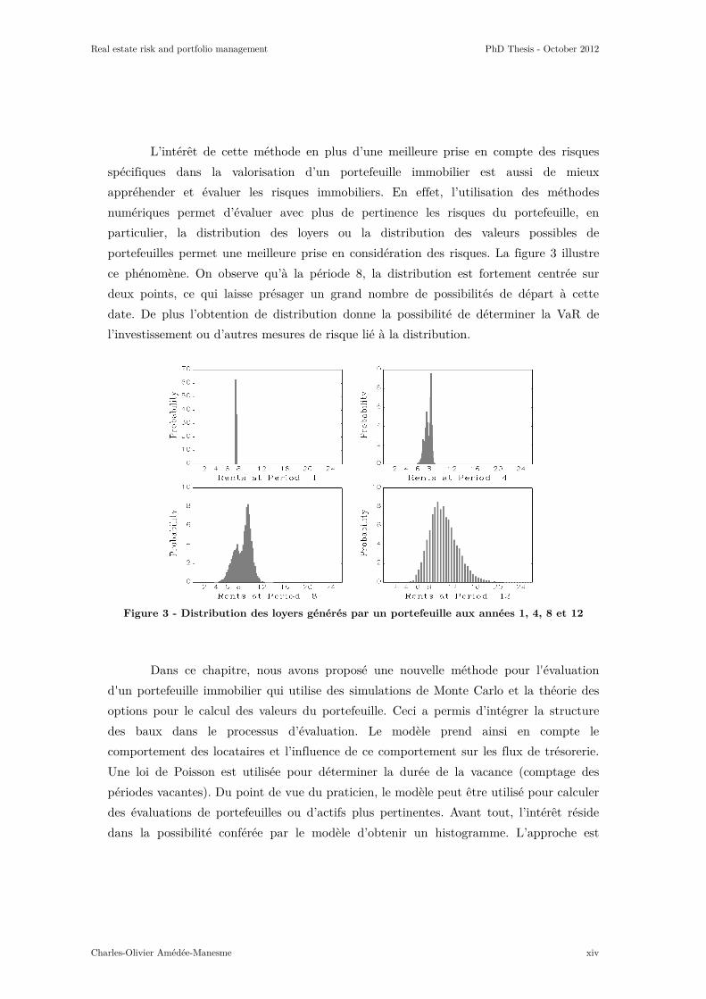
portefeuilles permet une meilleure prise en considération des risques. La figure 3 illustre
ce phénomène. On observe qu’à la période 8, la distribution est fortement centrée sur
deux points, ce qui laisse présager un grand nombre de possibilités de départ à cette
date. De plus l’obtention de distribution donne la possibilité de déterminer la VaR de
l’investissement ou d’autres mesures de risque lié à la distribution.
Figure 3 - Distribution des loyers générés par un portefeuille aux années 1, 4, 8 et 12
Dans ce chapitre, nous avons proposé une nouvelle méthode pour l'évaluation
d'un portefeuille immobilier qui utilise des simulations de Monte Carlo et la théorie des
options pour le calcul des valeurs du portefeuille. Ceci a permis d’intégrer la structure
des baux dans le processus d’évaluation. Le modèle prend ainsi en compte le
comportement des locataires et l’influence de ce comportement sur les flux de trésorerie.
Une loi de Poisson est utilisée pour déterminer la durée de la vacance (comptage des
périodes vacantes). Du point de vue du praticien, le modèle peut être utilisé pour calculer
des évaluations de portefeuilles ou d’actifs plus pertinentes. Avant tout, l’intérêt réside
dans la possibilité conférée par le modèle d’obtenir un histogramme. L’approche est

Real estate risk and portfolio management PhD Thesis - October 2012
Charles-Olivier Amédée-Manesme xv
flexible et permet de rajouter et de modifier de nombreux paramètres en fonction des
besoins inhérents à chaque marché et à chaque investisseur.
Ce travail ouvre la voie à de nombreux autres domaines de la finance
immobilière, la gestion des risques en particulier. La connaissance des flux de trésorerie
est une aide précieuse pour la mesure des risques et dans les négociations entre
propriétaire et locataire. En utilisant des méthodes de Monte Carlo, on obtient aussi un
ensemble de résultats au lieu d'un résultat unique ce qui présente un intérêt évident pour
la gestion des risques car les régulateurs comme les investisseurs ont de plus en plus
besoin de mesures de risque. Le développement de notre démarche va dans ce sens.
Le quatrième chapitre (second article)6 de cette thèse est une application
directe du modèle précédent. L’article présenté dans ce chapitre se concentre sur un
problème traditionnel de la Finance : la durée de détention. La littérature sur le sujet a
créé un consensus : des coûts de transaction élevés impliquent une durée de détention
plus longue et une forte volatilité implique une durée de détention plus courte. A ce
sujet, on peut se reporter aux travaux de Demsetz (1968), Tinic (1972), Amihud et
Mendelson (1986) ou encore Atkin et Dyl (1997). L’immobilier qui présente une forte
volatilité et des coûts de transactions élevés est un cas à part sur lequel la littérature n’a
pas su trouver un consensus. De plus, le caractère local et les spécificités pays de
l’immobilier créent de grandes différences. Par suite, il convient de considérer les
spécificités de l’immobilier pour déterminer la durée de détention optimale. Dans ce
contexte, le second article se propose de prendre en compte les baux inclus dans le
portefeuille pour déterminer la durée de détention optimale du portefeuille. Ceci est
rendu possible grâce à l’utilisation du modèle développé précédemment7.
Ce travail fait suite à un travail précédent publié par Baroni et al. (2007b)
et qui donne une formule fermée qui permet d’obtenir la durée de détention optimale
d’un portefeuille immobilier par l’utilisation de méthodes de simulations de Monte Carlo.
Notre objectif est d’utiliser une méthodologie proche mais pas similaire. L’idée est de
6 Cet article a fait l’objet d’un article présenté à la conférence annuelle de l’American
Real Estate Society en 2012. Sa rédaction a été finalisée avec l’écriture de cette thèse et il est maintenant en révision au Journal of Property Investment and Finance.
7 Peu de recherches examinent les périodes de détention optimales pour les
portefeuilles immobiliers. Toutefois, récemment, ce sujet a fait l'objet de quelques
publications : Barthélémy et Prigent (2009, 2011) ou Cheng et al (2010a, 2010b, 2010c). A ce
jour et à notre connaissance, aucune recherche ne prend en compte la structure des baux
dans l’évaluation de la durée de détention optimale. Cet article cherche à combler cette
lacune.
Real estate risk and portfolio management
Charles-Olivier Amédée-Manesme
rajouter la structure des baux et donc de prendre en compte les options incluses dans les
baux (au lieu d’un loyer moyen tel que utilisé dans Baroni et al., 2007b). Ces
modifient la distribution des valeurs et par suite la durée de détention optimale. Ce
chapitre démontre les différences qui se produisent lorsque les options
accordées aux locataires sont prises en considération. Nous démontrons comment l
objectifs de détention peuvent être modifiés par la prise en considération de la structure
des baux du portefeuille. L
mais d'analyser l'effet des paramètres sur la durée de détention optim
sont illustrés sur les deux figures 4 et 5.
Figure 4 - Durée de détention optimal
est simulée (cas Baroni et al, 2007b)
Figure 5 - Durée de détention optimal
terminale, des valeurs locatives de marché, et de la structure des baux (ici
ferme
risk and portfolio management PhD Thesis
rajouter la structure des baux et donc de prendre en compte les options incluses dans les
baux (au lieu d’un loyer moyen tel que utilisé dans Baroni et al., 2007b). Ces
modifient la distribution des valeurs et par suite la durée de détention optimale. Ce
chapitre démontre les différences qui se produisent lorsque les options
accordées aux locataires sont prises en considération. Nous démontrons comment l
objectifs de détention peuvent être modifiés par la prise en considération de la structure
L’objectif n'est pas de prédire la période de détention optimale,
des paramètres sur la durée de détention optimale. Les résultats
sont illustrés sur les deux figures 4 et 5.
Durée de détention optimale d’un portefeuille lorsque seule la valeur terminal
est simulée (cas Baroni et al, 2007b)
Durée de détention optimale d’un portefeuille avec simulations de la valeur
terminale, des valeurs locatives de marché, et de la structure des baux (ici
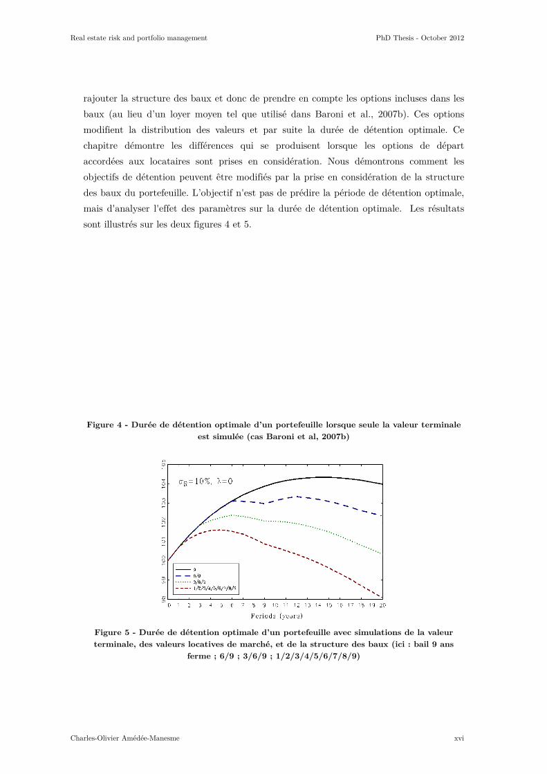
ferme ; 6/9 ; 3/6/9 ; 1/2/3/4/5/6/7/8/9)
PhD Thesis - October 2012
xvi
rajouter la structure des baux et donc de prendre en compte les options incluses dans les
baux (au lieu d’un loyer moyen tel que utilisé dans Baroni et al., 2007b). Ces options
modifient la distribution des valeurs et par suite la durée de détention optimale. Ce
chapitre démontre les différences qui se produisent lorsque les options de départ
accordées aux locataires sont prises en considération. Nous démontrons comment les
objectifs de détention peuvent être modifiés par la prise en considération de la structure
période de détention optimale,
ale. Les résultats
la valeur terminale
avec simulations de la valeur
terminale, des valeurs locatives de marché, et de la structure des baux (ici : bail 9 ans

Real estate risk and portfolio management PhD Thesis - October 2012
Charles-Olivier Amédée-Manesme xvii
Dans ce chapitre, nous avons donc proposé de tenir compte de la structure des
baux dans le calcul de la durée de détention optimale d’un portefeuille de biens
immobiliers en utilisant le modèle proposé au chapitre précédent. En grande partie, le
meilleur moment pour vendre un portefeuille immobilier dépend des flux futurs de
trésorerie. Nos principaux résultats sont les suivants : d’abord la volatilité des valeurs
locatives de marché a une très forte influence sur la période de détention (plus la
volatilité augmente, plus la durée de détention diminue), ensuite, le nombre d’options a
un effet très fort sur la durée de détention. En somme, prendre en compte la structure
des baux et par suite les possibilités de rupture données aux locataires permet d’obtenir
une meilleur évaluation et analyse de la durée de détention optimale.
Le chapitre 5 (troisième article)8 traite de la mesure de la Value at Risk lorsque
la non-normalité des rendements est prise en compte. Pour ce faire, ce chapitre propose
l’utilisation du développement de Cornish-Fisher qui permet d’approcher les quantiles
d’une distribution lorsque celle-ci ne satisfait pas l’hypothèse de normalité.
Comme présenté dans la revue de la littérature, la distribution des rendements en
immobilier ne peut pas être décrite par une loi normale. La littérature sur le sujet est
relativement large et crée un consensus. C’est pourquoi, on ne peut faire l’hypothèse
d’une distribution Gaussienne pour le calcul de la VaR. Traditionnellement, cette
hypothèse est acceptée car elle permet de calculer très rapidement la VaR avec comme
seule information la moyenne et la variance. Ce chapitre propose de mesurer la VaR en
utilisant les 4 premiers moments de la distribution (moyenne, variance, coefficient
d’asymétrie et Kurtosis). Pour ce faire, le développement de Cornish-Fisher est introduit.
Ce développement permet d’approximer le quantile d’une distribution.
Si l’on note zα le quantile gaussien et ,CFz α le quantile de Cornish Fisher, # le
niveau de probabilité, S le coefficient d’asymétrie et K le Kurtosis, le développement de
Cornish-Fisher prend la forme suivante :
2 3 3 2,
1 1 10,1 , 1 3 ( 3) 2 56 3624CF
z z z S z z K z z Sα α α α α ααα ∀ ∈ + − + − − − −≃
On peut ainsi en déduire le quantile modifié de Cornish-Fisher :
, ,0,1 ,
CF CFq zα αα µ σ ∀ ∈ = +
8 Ce chapitre a fait l’objet de la rédaction d’un papier de recherche qui a été présenté
en 2012 à la conférence annuelle de l’European Real Estate Society dans la session doctorale. L’article a été plébiscité et a reçu le prix du papier de recherche le plus recommandé de la session doctorant (Most Commended Paper). L’article est en cours de soumission au Journal of Real Estate Finance and Economics.

Real estate risk and portfolio management PhD Thesis - October 2012
Charles-Olivier Amédée-Manesme xviii
Ce développement de Cornish-Fisher permet donc de calculer rapidement le
quantile d’une fonction en prenant en compte les moments d’ordre supérieur à 2. Bien
que cette approximation soit un outil utile et puissant, il est peu utilisé en finance. Ceci
provient d’une des limites du développement de Cornish-Fisher, il ne conserve pas la
monotonie, pourtant condition nécessaire pour les fonctions de répartition : l’ordre des
quantiles de la distribution n’est pas conservé par la transformation. Le développement
de Cornish-Fisher viole donc une des conditions de base des fonctions de répartition.9
Une condition nécessaire et suffisante pour conserver la monotonie est que la dérivée de
α,CFz
par rapport à αz ne soit pas nulle. Cela peut se traduire par :
2 2 23 3 54 1 09 8 6 8 36S K S K S
− −− − − − ≤
Il faut donc que S et K respecte les conditions permettant de satisfaire
l’inéquation précédente.
En pratique, cette condition n’est que rarement vérifiée ce qui rend l’utilisation
du développement de Cornish-Fisher compliquée. Cette difficulté a été résolue par
Chernozuhov et al. (2010). Il propose d’introduire une procédure de réarrangement pour
résoudre le problème de la non-monotonie. Le réarrangement consiste à classer par ordre
croissant ou décroissant l’ensemble des éléments d’une base de données. Cet article,
Chernozuhov et al. (2010), démontre que l’utilisation d’une procédure de réarrangement
permet d’une part de résoudre le problème de la non-monotonie dans l’utilisation de
l’approximation de Cornish Fisher et d’autre part d’obtenir une meilleure estimation des
quantiles. La figure 6 illustre ce principe.
Figure 6 - Illustration de la procédure de réarrangement
9 Ce point est largement débattu dans la littérature académique (Barton et Dennis, 1952 ; Draper et
Tierney, 1971 et Spiring, 2011).
Real estate risk and portfolio management PhD Thesis - October 2012
Charles-Olivier Amédée-Manesme xix
Dans ce chapitre, nous proposons d’estimer les quantiles des rendements
immobiliers en utilisant cette combinaison (développement de Cornish Fisher et
réarrangement) afin de déterminer la Value at Risk de l’immobilier lorsque les moments
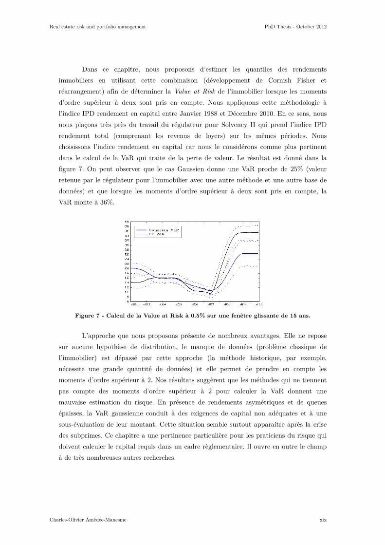
d’ordre supérieur à deux sont pris en compte. Nous appliquons cette méthodologie à
l’indice IPD rendement en capital entre Janvier 1988 et Décembre 2010. En ce sens, nous
nous plaçons très près du travail du régulateur pour Solvency II qui prend l’indice IPD
rendement total (comprenant les revenus de loyers) sur les mêmes périodes. Nous
choisissons l’indice rendement en capital car nous le considérons comme plus pertinent
dans le calcul de la VaR qui traite de la perte de valeur. Le résultat est donné dans la
figure 7. On peut observer que le cas Gaussien donne une VaR proche de 25% (valeur
retenue par le régulateur pour l’immobilier avec une autre méthode et une autre base de
données) et que lorsque les moments d’ordre supérieur à deux sont pris en compte, la
VaR monte à 36%.
Figure 7 - Calcul de la Value at Risk à 0.5% sur une fenêtre glissante de 15 ans.
L’approche que nous proposons présente de nombreux avantages. Elle ne repose
sur aucune hypothèse de distribution, le manque de données (problème classique de
l’immobilier) est dépassé par cette approche (la méthode historique, par exemple,
nécessite une grande quantité de données) et elle permet de prendre en compte les
moments d’ordre supérieur à 2. Nos résultats suggèrent que les méthodes qui ne tiennent
pas compte des moments d’ordre supérieur à 2 pour calculer la VaR donnent une
mauvaise estimation du risque. En présence de rendements asymétriques et de queues
épaisses, la VaR gaussienne conduit à des exigences de capital non adéquates et à une
sous-évaluation de leur montant. Cette situation semble surtout apparaitre après la crise
des subprimes. Ce chapitre a une pertinence particulière pour les praticiens du risque qui
doivent calculer le capital requis dans un cadre règlementaire. Il ouvre en outre le champ
à de très nombreuses autres recherches.

Real estate risk and portfolio management PhD Thesis - October 2012
Charles-Olivier Amédée-Manesme xx
Le dernier chapitre (quatrième article)10 de la thèse traite aussi de la Value at
Risk. L’idée de base de ce chapitre repose sur une observation simple : les méthodes
traditionnelles d’analyse et de mesure du risque ne permettent généralement pas de
discriminer entre les stratégies ou entre les portefeuilles sur le critère de la Value at Risk.
En effet, les méthodes traditionnelle, historique, Monte Carlo ou paramétrique sont
basées sur des indices ou des bases de données qui concentrent et agrègent les
informations de l’ensemble du marché. La VaR calculée avec ces méthodologies donne la
VaR du marché ou à défaut la VaR correspondant aux données du marché (si l’ensemble
du marché n’est pas observable) et par suite ces méthodologies ne donne pas la VaR du
portefeuille ou de l’allocation spécifique de l’investisseur. Cette observation revêt une
importance particulière en immobilier ou le risque de marché est difficilement isolable et
les portefeuilles rarement correctement diversifiés, comme cela a été évoqué dans la revue
de la littérature et dans l’introduction de la thèse ou de ce résumé. Pourtant deux
portefeuilles d’actifs immobiliers qui ont des stratégies différentes ne devraient pas avoir
la même VaR et par suite le même capital requis.
La méthodologie proposée repose sur des techniques de simulation et la prise en
compte d’un certain nombre de spécificités de l’immobilier. Encore une fois, l’idée sous-
jacente de ce chapitre repose sur une des particularités de l’immobilier, le risque
spécifique est difficile à diversifier et il convient donc de considérer les risques qui
proviennent des spécificités. Les risques spécifiques pris en compte dans cet article sont
les structures de baux, l’obsolescence et son influence sur la durée de vacance entre deux
locataires et sur la probabilité de vacance, le cout de la vacance et l’effet de levier. De
plus, le risque de marché est pris en compte par des méthodes numériques.
Dans ce chapitre, la méthode numérique que nous retenons pour la prise en
compte du risque de marché est le bootstrapping. Cette méthode présente l’avantage de
ne pas requérir d’hypothèse sur la distribution des séries utilisées (mais on peut aussi
utiliser des simulations de Monte Carlo si l’on peut aisément faire une hypothèse ou une
estimation sur la distribution des rendements). La structure des baux est prise en compte
par le modèle présenté dans le troisième chapitre de cette thèse (premier article) : si un
bail est loué à un loyer différent du prix du marché, le locataire, rationnel, quitte le
bâtiment et le propriétaire fait alors face à de la vacance. Il peut cependant exister une
10 Cet article a été présenté à de nombreuses conférences. Entre autre, à la conférence
annuelle de l’European Real Estate Society, en 2011 en session doctorale (poster) et en 2012 lors de la session plénière. Il a aussi été présenté lors de la session doctorale de la conférence annuelle de l’American Real Estate Society en 2012. En 2011, cet article a reçu le prix du meilleur poster de la session doctorale (Best Poster Presentation) à la conférence annuelle de l’European Real Estate Society.

Real estate risk and portfolio management PhD Thesis - October 2012
Charles-Olivier Amédée-Manesme xxi
certaine latitude entre le prix du marché et le prix payé. La durée de la vacance est prise
en compte par une loi de Poisson qui compte le nombre de périodes vacantes. Le loyer est
donné par contrat et les valeurs locatives de marché sont simulées (bootstrapping). Si
plusieurs marchés doivent être pris en compte, on utilise une méthode de moving block-
bootstraping (la taille des blocs peut varier). L’obsolescence de l’actif est prise en compte
par un taux d’obsolescence (ou d’usure) de l’actif immobilier. Ce taux influe sur le risque
de devenir vacant comme sur la durée de la vacance. Enfin on considère l’effet de levier
car c’est un des facteurs qui différencie les stratégies. On propose dans ce modèle de se
baser sur le critère de la loan to value (LTV), avec une possibilité pour l’emprunteur de
s’écarter un peu de la LTV initiale mais en considérant une rupture du contrat de prêt
avec exercice de l’hypothèque sur le bien dans le cas où l’écart avec la valeur initiale est
supérieur à un certain pourcentage négocié. Au regard des différences de stratégies
possibles, on n’a pas considéré dans ce modèle le service de la dette (DSCR ou ICR) :
ceci se justifie par le fait que les stratégies opportunistes peuvent ne pas générer de flux
pendant un grand nombre de périodes et pourtant générer un fort rendement par des
gains en capitaux d’où un rendement supérieur.
Le modèle est illustré sur 2 portefeuilles qui ont des stratégies radicalement
différentes. Un portefeuille core (sécurisé) et un portefeuille opportuniste. Le portefeuille
core investit dans des immeubles neufs ou récents, loués sur de longues périodes (baux
fermes supérieurs à 6 ans) avec peu d’effet de levier (30%) et sur la base d’un taux de
rendement initial proche de 6%. Le portefeuille opportuniste investit dans des actifs
obsolètes ou anciens qui peuvent soit être loués sur des durées relativement courtes, soit
être vacants avec un effet de levier conséquent (70%) et sur la base d’un taux de
rendement initial de l’ordre de 8%. Les figures 8 et 9 présentent les résultats pour les
deux portefeuilles, dans le cas d’abord (figure 8) où seuls sont pris en compte les risques
de prix, de valeurs locatives et de baux, puis (figure 9) où sont ajoutés les risques liés à
l’obsolescence, à la vacance et à la dette.

Real estate risk and portfolio management PhD Thesis - October 2012
Charles-Olivier Amédée-Manesme xxii
a. Core (VaR0.5% = 34.7%) b. Opportuniste (VaR0.5% = 41.8%)
Figure 8 - Cas où l’on considère le risque de prix et de valeur locative de marché et la
structure des baux
a. Core (VaR0.5% = 54.1%) b. Opportuniste (VaR0.5% = 94.4%)
Figure 9 - Cas où l’on considère le risque de prix et de valeur locative de marché, la
structure des baux, l’obsolescence et son influence sur la probabilité de devenir vacant et
sur la durée de la vacance, le coût de la vacance et l’effet de levier
Le but de cet article est de contribuer à la littérature sur la VaR en proposant
une méthode d’évaluation qui prenne en compte les spécificités de l’immobilier. Les
modèles traditionnels de calcul de la VaR souffrent en immobilier d’une difficulté : ils
s'appuient sur des indices de marché ou de données, et donc fournissent le même résultat
indépendamment du portefeuille. Pourtant, les investissements immobiliers sont
caractérisés par l'hétérogénéité des actifs et donc les indices boursiers ne reflètent
généralement pas le risque du portefeuille de l’investisseur. Contrairement aux approches
traditionnelles, notre approche permet de discriminer parmi les stratégies sur le critère de
la VaR. Ceci peut être autant utile aux académiques qu’aux praticiens. Le modèle
proposé ouvre la porte à de nombreuses études futures : l’impact de la dette, ou
l’influence de la stratégie sur le capital requis. Le modèle est particulièrement pertinent,
car il est le premier qui permet de calculer des VaR différentes pour différents

Real estate risk and portfolio management PhD Thesis - October 2012
Charles-Olivier Amédée-Manesme xxiii
portefeuilles, même si les portefeuilles ne diffèrent que sur leurs stratégies en termes de
durée des baux.
*
* *
Finalement, cette thèse a abordé la problématique du risque dans les
investissements immobiliers et en particulier des spécificités de l’actif immobilier. Ce
travail a grandement été motivé par d’une part le fait que la réduction marginale du
risque idiosyncrasique diminue rapidement après 10 actifs et d’autre part par le fait que
le risque spécifique est très difficile à diversifier, même en présence d’un portefeuille très
large. Il est donc nécessaire de prendre en considération ces risques dans l’évaluation, la
gestion et l’allocation de portefeuilles immobiliers. Le manque de travaux universitaires
dans le domaine de l’immobilier direct et la taille de cette classe d’actifs dans le monde
ont aussi été de grandes motivations dans l’écriture de cette thèse.
A plusieurs égards, la thèse répond à la problématique du risque spécifique en
immobilier : elle propose de nouveaux modèles qui prennent en compte les
caractéristiques spécifiques de l’investissement immobilier en termes de particularités
comme dans les distributions de rendement. L’originalité réside en partie dans ces
spécificités prises en compte et en partie dans l’approche pratique des méthodes
proposées. Ce travail a un intérêt à la fois pour les praticiens et les académiques. Ces
nombreuses applications pratiques ont été permises grâce au contrat doctoral (CIFRE)
dans lequel cette thèse a été écrite.

Real estate risk and portfolio management PhD Thesis - October 2012
Charles-Olivier Amédée-Manesme xxiv
Acknowledgements
This thesis is the culmination of my maturation as an applied real estate financial
analyst. I would not have completed this thesis without the contributions of a number of
individuals who helped in a variety of ways and made this thesis possible.
I started this thesis to expand my knowledge of real estate, particularly in
Finance. With hindsight, I can say these 3 years at the University of Cergy-Pontoise not
only expanded my knowledge of real estate but also expanded my horizon of life. Overall,
the experience was gratifying in terms of insights gained and skills developed.
I express gratitude to my supervisor, Fabrice Barthélémy; I am highly indebted to
him. His knowledge and personality contributed to my development as a researcher. For
continuous support of my thesis study and research, for his motivation, enthusiasm, and
immense patience, I thank him greatly. I cannot imagine having a better advisor and
mentor for my thesis study. His guidance helped me during the times of researching and
writing this thesis. He opened the world of academic research to me, guided me, and
helped me with my first steps into this world. For all these, thank you very much,
Fabrice.
The genesis for this project derives from Michel Baroni at Essec Business School.
He was at the origin of my initiation into real estate finance, and he advised me during
the course of my thesis. His advice, networking and experiments helped me design this
thesis, and he was invaluable. I offer him many thanks.
I also have particular sentiment for Jean-Luc Prigent for enlightening me on my
first glance at research and the academician’s world, and advising me during many
stimulating discussions. I am heavily indebted to Jean-Luc for his valuable advice in
science and math discussions.
To Michel and Jean-Luc I am grateful in every possible way, and I hope to keep
up our collaborations in the future.
My greatest professional debt is owed to Etienne Dupuy of BNP Paribas Real
Estate and AREIM (French real estate research association). I thank Etienne for offering
me the opportunity to fund my PhD through a French contract (CIFRE) in BNP Paribas
Real Estate Investment Services team. I benefited greatly from outstanding work and

Real estate risk and portfolio management PhD Thesis - October 2012
Charles-Olivier Amédée-Manesme xxv
ideas from Etienne; he is a great manager and mentor who become a friend and source of
amazement, admiration and fun.
I gratefully thank Patrice Poncet and Alain Coën for accepting to refer this
thesis. I am thankful that in the midst of all their activities, they accepted to be
members of the reading committee. I realize how lucky I am to have both serving as
referees.
I am extraordinarily fortunate to have Arnaud Simon, Michel, Baroni, Fabrice
Barthélémy, Christophe Pineau, Jean-Luc Prigent and Olivier Scaillet as suffragan on my
Jury. I thank the jury for its willingness to participate and take time to review this work.
Its advice and remarks benefitted this dissertation greatly. I could never imagine a better
Jury. Thank you.
At the University of Cergy-Pontoise and at Essec Business School, I was deeply
influenced and assisted by numerous magnificent scholars, including Jocelyn Martel,
Mathieu Martin, Patrice Poncet, Rolland Portait or François Longin. I thank particularly
another Cergy-Pontoise lab-mate, Donald Keenan, a real estate (but not only) academic
expert, for inciting me to work on diverse, exciting projects that I am convinced will lead
to more research and publications. I hope to continue to share with you these two
passions: real estate and wine.
Excellent advices, comments and reviews were offered by BNP Paribas Real
Estate colleagues Victoria Bauchart, Evelyne Simon, Alessandro di Cino, Vincent Esnard,
Laurent Boissin, Dung Pham, Jean-Philippe Fouilleron, Karl Delattre, Richard Malle,
Christophe Pineau, Assia Taibi, Yves Gourdin, Eric Vu Anh Tran, Samuel Duah, Souad
Cherfouh, Eugène Agossou Voyeme, Valérie Deveau, Véronique Dubuis, Sophie Baillet,
Vincent Chevallier, Anais Leroux, Béatrice Perrot and Simona Montanaro among others.
My many friends in the real estate industry unalterably changed my thought
process. I never ceased to learn from their creativity, drive and ingenuity. While it is
impossible to identify all of these influences, AREIM’s11 members merit special thanks:
Ardoingt Albanel, Mahdi Mokrane, Attila Ballaton, Christian de Kerangal, Kan Baccam,
Pierre Schoeffler and Cécile Hickel.
I have fond thoughts of my lab mates: Nasser Naguez, Abdallah Ben Saida,
Nourdine Letifi, Rim Ayadi, Sami Zouairi, Emeline Limon, Roxane Bricet, Louis
11 French real estate research association

Real estate risk and portfolio management PhD Thesis - October 2012
Charles-Olivier Amédée-Manesme xxvi
Chauveau, Davide Romelli, Andreoli Francesco, Romain Legrand, Mi lim Kim, Inoa Pena
Ignacio augusto, Huang Sainan, Letifi Nourdine, Samia Badji, Wafa Sayeh and Songlin
Zeng. I have a particular though for Emeline Limon who spend time explaining me the
basis of LATEX sorfware.
I convey special acknowledgement to Cecile Moncelon, Lisa Colin and Stephanie
Richard Edmond for indispensable help in dealing with travel funds, administration and
bureaucratic matters during my stay in University of Cergy Pontoise. I have also a
though for Malika Badache for her patience.
The Fondation Palladio, a French Foundation that supports real estate research
and education under the aegis of Fondation de France, supported this work. I especially
acknowledge Philippe Richard and Mathieu Garro for their help and contributions.
I apologize to the students who suffered in my classes. I hope that they have
forgiven my ignorance. I salute Michel Baroni again and Patrice Noisette who offered me
the opportunity to teach finance and real estate finance lectures and assistance at the
Essec Business School.
Special thanks go to John Garger. Without him, this thesis would be
unintelligible due to my imperfect English.
Never least, but too often last in my focus are both my family and friends for
supporting me. They suffered for well over 4 years my grumpiness and impatience.
Finally, I thank everybody who was important to the realization of this thesis,
and express my apologies that I could not mention him or her personally.
My apologies to anyone I missed inadvertently. I assume responsibility for any
remaining errors.
Charles-Olivier Amédée-Manesme

Real estate risk and portfolio management PhD Thesis - October 2012
Charles-Olivier Amédée-Manesme xxvii
Table of contents
Avertissements / Warnings ........................................................................ i
Summary .................................................................................................. iv
Résumé ...................................................................................................... v
Résumé long de thèse ............................................................................... vi
Acknowledgements ............................................................................... xxiv
Table of content .................................................................................. xxvii
List of Tables ....................................................................................... xxxi
List of Graphs ..................................................................................... xxxii
List of abbreviations ............................................................................xxxv
GENERAL INTRODUCTION ........................................................................ 1
PART I – REAL ESTATE MARKET AND LITERATURE ......................... 13
Chapter I. A brief review of real estate market ................................................................ 13
I. The real estate market ...................................................................................... 19
II. The financial activity: direct and indirect investment .................................. 22
A. Direct Real Estate ........................................................................................ 22
B. Indirect Investment in Real Estate .............................................................. 25
Chapter II. Review of the literature and recent research developments ........................ 28
I. Real estate portfolio allocation and portfolio management .............................. 29
A. Real estate as a portfolio diversifier ............................................................. 30
B. Sector versus region ...................................................................................... 33
C. Number of assets versus number of leases .................................................... 36
D. Inflation hedging .......................................................................................... 37
E. Optimal debt level ........................................................................................ 39
F. Note on real estate derivatives ..................................................................... 39
II. Lease structure ............................................................................................. 41
A. Presentation of leases ................................................................................... 42
1. Type of rent change in leases ....................................................................... 43

Real estate risk and portfolio management PhD Thesis - October 2012
Charles-Olivier Amédée-Manesme xxviii
2. Break options (or break clauses) ................................................................. 43
B. Literature on lease structure ........................................................................ 44
III. Distribution of returns .................................................................................. 47
A. Direct real estate .......................................................................................... 48
B. Indirect real estate ....................................................................................... 49
IV. Value at Risk ................................................................................................ 51
A. Introduction and definition .......................................................................... 51
B. Literature review .......................................................................................... 55
C. VaR limitations and Conditional VaR ......................................................... 58
PART II – REAL ESTATE PORTFOLIO AND RISK MANAGEMENT ..... 61
Chapter III. Combining Monte Carlo Simulations and Options to Manage Risk of Real
Estate Portfolio Management (2012) ....................................................................................... 64
I. Introduction ...................................................................................................... 66
II. The basic model ............................................................................................ 72
A. Cash Inflows ................................................................................................. 72
B. Cash outflows ............................................................................................... 76
C. Free cash flows ............................................................................................. 77
D. Discount Rate Choice ................................................................................... 78
III. Applying a Monte Carlo simulation: simulating prices, market rental values
and rent 78
A. Terminal value ............................................................................................. 79
B. Market rental values (MRV) ........................................................................ 80
C. Simulation of the rent .................................................................................. 82
D. Simulation of rent and market rental value ................................................. 84
E. Distribution of rent ...................................................................................... 87
F. Simulation of free cash flows ........................................................................ 87
IV. Application of the model .............................................................................. 88
A. Valuation of a portfolio ................................................................................ 88
B. Sensitivity analysis and model limitations ................................................... 93
V. Conclusion .................................................................................................... 97
Appendices of chapter 1 ........................................................................... 98

Real estate risk and portfolio management PhD Thesis - October 2012
Charles-Olivier Amédée-Manesme xxix
Chapter IV. Optimal Holding Periods of a Real Estate Portfolio according to the Leases
103
I. Introduction .................................................................................................... 105
II. Literature .................................................................................................... 107
III. Optimal holding period with traditional discounted cash flow (DCF) ....... 109
IV. Optimal holding period incorporating risk in the terminal value (Baroni,
Barthélémy and Mokrane, 2007b) ...................................................................................... 112
V. The break-option: optimal holding period incorporating risk in terminal
value and lease structure (Amédée-Manesme, Baroni, Barthélémy and Dupuy, 2012) ...... 113
A. The model .................................................................................................. 115
B. Optimal holding period .............................................................................. 117
VI. Conclusion .................................................................................................. 123
PART III – REAL ESTATE RISK MANAGEMENT: VALUE AT RISK ... 127
Chapter V. Cornish-Fisher Expansion for Real Estate Value at Risk .......................... 129
I. Introduction .................................................................................................... 130
II. Variance-Covariance Value at Risk and Cornish-Fisher adjustment .......... 135
A. VaR with Normal assumption: ................................................................... 135
B. VaR with quasi-normal assumption: Cornish-Fisher expansion ................. 137
III. Application ................................................................................................. 141
IV. Conclusion .................................................................................................. 149
Appendices for chapter 3 ....................................................................... 151
Chapter VI. Value at Risk: a Specific Real Estate Model .............................................. 152
I. Introduction .................................................................................................... 153
II. The model ................................................................................................... 158
A. Discounted cash flow .................................................................................. 159
B. Quantitative methods in discounted cash flow ........................................... 160
C. Lease structure ........................................................................................... 162
D. Length and cost of vacancy ........................................................................ 163
E. Obsolescence (depreciation) ....................................................................... 165
F. Probability of vacancy according to obsolescence ...................................... 166
G. Length of vacancy according to obsolescence ............................................ 167

Real estate risk and portfolio management PhD Thesis - October 2012
Charles-Olivier Amédée-Manesme xxx
H. Debt ........................................................................................................... 167
III. Application ................................................................................................. 169
A. Data and presentation of the portfolios ..................................................... 169
B. Implementation of the model and results ................................................... 177
IV. Limitations and hurdles .............................................................................. 185
V. Conclusion .................................................................................................. 186
Appendix of chapter 4 ........................................................................... 188
GENERAL CONCLUSION ......................................................................... 189
Conferences and publications ................................................................. 193
References .............................................................................................. 195

Real estate risk and portfolio management PhD Thesis - October 2012
Charles-Olivier Amédée-Manesme xxxi
List of Tables
Table I-1 - Correlation matrix between some real estate markets over two periods ................ 17
Table I-2 - Estimated size of total market (M€) ...................................................................... 21
Table I-3 - Basic statistics of FTSE and IPD U.K. .................................................................. 24
Table I-4 - Basic statistics of CAC and IPD France ................................................................ 25
Table I-5 - Comparison of volatility and returns between REITs and Eurostoxx 50 ............... 27
Table III-1 – Dynamics between two consecutive periods ........................................................ 76
Table III-2 - Passing rent produced and rental values of the 16 premises................................ 90
Table III-3 - Current lease structure of the portfolio ............................................................... 91
Table III-4 - Lease structures of all premises in the portfolio for cases of re-letting ................ 92
Table V-1 - 0.5% quantile and VaR for a Gaussian distribution as a function of andµ σ ..... 137
Table V-2 - Real estate monthly returns pdf and cdf according to the period ...................... 143
Table VI-1 - Market rental values, rent and lease structures of units in the portfolio. .......... 171
Table VI-2 - Correlation matrix market rental values and prices in Munich and Paris ......... 173
Table VI-3 - Possible state of properties ................................................................................ 175
Table VI-4 - Moving criteria decision associated with state of the property ......................... 175
Table VI-5 - Average vacancy length associated with state of the property .......................... 176
Table VI-6 - Comparisons of the portfolios ............................................................................ 177
Table VI-7 - Portfolios and cities’ returns .............................................................................. 178
Table VI-8 - Value at Risk using the parametric approach .................................................... 179
Table VI-9 – VaR with Monte Carlo simulations ................................................................... 180
Table VI-10 – All possible scenarios of the two portfolios and their computed VaRs ............ 188
Real estate risk and portfolio management PhD Thesis - October 2012
Charles-Olivier Amédée-Manesme xxxii
List of Graphs
Graph I-1 - Market sector value ............................................................................................... 14
Graph I-2 – European commercial property market size ......................................................... 15
Graph I-3 - Direct real estate investment volume, M€, Europe, 2007 ..................................... 18
Graph I-4 - Source of capital invested in European real estate, 2007, percentage of the total 18
Graph I-5 - European Investment Volume ............................................................................... 22
Graph I-6 - FTSE return versus IPD U.K. total return ........................................................... 23
Graph I-7 - CAC return versus IPD France total return ......................................................... 24
Graph I-8 - Listed European real estate (Eurozone) versus Eurostoxx 50 ............................... 26
Graph III-1 - Illustrations of Poisson’s law for average vacancy lengths of 1, 2 and 3 periods 76
Graph III-2 - Five simulated price paths .................................................................................. 80
Graph III-3 - Estimated density function for prices at time t = 15 ......................................... 80
Graph III-4 - Four possible cases of a French lease .................................................................. 83
Graph III-5 - Six illustrations of our method used in a French lease ....................................... 84
Graph III-6 - Three paths for market rental value and for rent in a French lease. .................. 86
Graph III-7 - Average of 10,000 scenarios for rent and market rental values in a French lease
.................................................................................................................................................. 86
Graph III-8 - Average rent and market rental value produced by the portfolio ....................... 93
Graph III-9 - Expectation and standard error of rent in the portfolio as a function of the
moving criterion decision (α) and expected length of vacancy (λ)........................................... 94
Graph III-10 - Expectation of rent in the portfolio as a function of either the moving criterion
decision (α) or expected length of vacancy (λ). ....................................................................... 95
Graph III-11 - Standard error of rent in the portfolio as a function of either the moving
criterion decision (α) or expected length of vacancy (λ). ......................................................... 95
Graph III-12 - Expectation and standard error of price of the portfolio as a function of the
moving criterion decision (α) and expected length of vacancy (λ)........................................... 95
Graph III-13 - Illustration of the paths’ behaviors when correlation is considered for price &
market rental value ................................................................................................................... 98
Graph III-14 - Histogram of rent in a French lease for t = 1, …,15. ........................................ 99
Graph III-15 - Leases during the holding period of the portfolio ........................................... 100
Graph III-16 - Histogram of rent produced by the portfolio annually over 15 years. ............ 101
Graph IV-1 - Increase of the portfolio present value with the DCF approach ( g g∞> ) ........ 110
Graph IV-2 - Constant present value of a portfolio with the DCF approach ( g g∞= ) ......... 111
Graph IV-3 - Decrease of the portfolio present value with the DCF approach ( g g∞< ) ....... 111

Real estate risk and portfolio management PhD Thesis - October 2012
Charles-Olivier Amédée-Manesme xxxiii
Graph IV-4 - Optimal holding period of the portfolio value when a terminal value is
simulated ................................................................................................................................ 113
Graph IV-5 - Optimal holding period without volatility of market rental values .................. 118
Graph IV-6 - Optimal holding period with market rent volatility ......................................... 119
Graph IV-7 - Optimal holding period with increasing vacancy length .................................. 120
Graph IV-8 - Optimal holding period with various lease structures ...................................... 121
Graph IV-9 - Optimal holding period with rent growth rate lower than market rental value
trend ....................................................................................................................................... 122
Graph IV-10 - Optimal holding period with rent growth rate higher than the market rental
value trend .............................................................................................................................. 123
Graph V-1 - Quantile function and VaR for a Gaussian distribution as a function of
andµ σ ................................................................................................................................ 137
Graph V-2 - Rearrangement procedure ( )0.25α < ................................................................... 139
Graph V-3 - Cornish-Fisher and normal quantiles according to the skewness coefficient ...... 140
Graph V-4 - Cornish-Fisher and normal quantiles according to the kurtosis coefficient ....... 141
Graph V-5 - Real estate index and returns from January 1988 to December 2010 ............... 142
Graph V-6 - Real estate returns pdf and cdf according to a 15-year period .......................... 143
Graph V-7 - mean, standard deviation, skewness and kurtosis according to the 15-year period,
and their 95% bootstrap confidence interval .......................................................................... 144
Graph V-8 - Skewness and kurtosis belonging to the domain of validity (D ). The represented
function equals 0 if ( , ) and 1 if ( , )S K D S K D∉ ∈ . .................................................................. 145
Graph V-9 - 5%, 1%, 0.5% and 0.1% quantiles of the real estate returns distribution
according to the 15-year period .............................................................................................. 146
Graph V-10 - 5%, 1%, 0.5% and 0.1% Gaussian and corrected Cornish-Fisher VaR in base
100 according to a 15-year period, and their corresponding 95% bootstrap confidence interval
................................................................................................................................................ 147
Graph V-11 - Gaussian and Cornish-Fisher corrected VaR for various window lengths ........ 148
Graph V-12 - Cornish-Fisher quantiles, left-skewed and leptokurtic distribution, 1.5, 6S K=− =
................................................................................................................................................ 151
Graph V-13 - Differences among Cornish-Fisher VaRs for various window lengths .............. 151
Graph VI-1 - Market capital growth (1991 to 100) ................................................................ 172
Graph VI-2 - Market rental growth (1991 to 100) ................................................................. 173
Graph VI-3 – Distribution of Monte Carlo results for the VaR computation ........................ 180
Graph VI-4 - Approach combining bootstrapping for market rental values, and property
prices and lease structure ....................................................................................................... 181
Graph VI-5 - Approach combining bootstrapping for market rental values, and properties
prices, lease structure and cost of vacancy ............................................................................. 182

Real estate risk and portfolio management PhD Thesis - October 2012
Charles-Olivier Amédée-Manesme xxxiv
Graph VI-6 - Approach combining bootstrapping for market rental values, and properties
prices, lease structure, cost of vacancy and length of vacancy ............................................... 182
Graph VI-7 - Approach combining bootstrapping for market rental values, and properties
prices and lease structures considering obsolescence in the cost of vacancy and length of
vacancy ................................................................................................................................... 183
Graph VI-8 - Approach combining bootstrapping for market rental values, and properties
prices, lease structure and debt considering obsolescence in the cost of vacancy and length of
vacancy ................................................................................................................................... 184

Real estate risk and portfolio management PhD Thesis - October 2012
Charles-Olivier Amédée-Manesme xxxv
List of abbreviations
BNPPRE BNP Paribas Real Estate
CBRE Coldwell Banker Richard Ellis
EPRA European Public Real Estate Association
PMA Property Market Analysis
CAPM Capital asset pricing model
INREV European Association for Investors in Non-listed Real Estate Vehicles
IPD Investment Property Databank
NCREIF National Council of Real Estate Investment Fiduciaries
NOI Net operating income
REITS Real estate investments trusts
UCITs Undertakings for Collective Investment in Transferable Securities
0.5% VaR Value at Risk, 0.5% percentile
EU European Union
US United States
GAV Gross Asset Value
NAV Net Asset Value
LTV Loan To Value
EIOPA European Insurance and Occupational Pensions Authority (formerly
CEIOPS)
CEIOPS Committee of European Insurance and Occupational Pensions
Supervisors
MRV Market Rental Values
FCF Free Cash Flows

Real estate risk and portfolio management PhD Thesis - October 2012
Charles-Olivier Amédée-Manesme 1
GENERAL INTRODUCTION
Real estate is about land, and in that sense, real estate is a quarter of the
earth’s surface on which 6 billion humans live. Real estate is about built space - the
space in which we live, work, walk and play - that design and define modern cities.
Real estate represents a half of the value of all capital assets in the world1 (source: The
Economist, 20022). No matter how real estate is defined, it cannot be ignored; real
estate is fundamental.
Real estate is called real for a reason. Real estate is real, a topic of interest to
everyone. It is built of concrete, steel and brick, and sometimes wood and straw. It has
a strong influence on the lives of everyone, and it is of concern to everyone.
Real estate can be studied academically from many perspectives:
- Esthetic and functional (architecture)
- Physical structures (civil engineering)
- Ecologic (sustainable development)
- Urbanism (city construction and development)
- Legal (rights and duties associated with ownership)
- Sociologic (spacial and social phenomena)
- Economics (urban economics and civilization history)
- Finance (investment, portfolio management and risk valuation)
Even if not exhaustive, this list of disciplines is a good review of all topics
spread out over the real estate arena. Real estate research appeals to multidisciplinary
approaches, and encompasses numerous fields and researchers. This may explain why
real estate faces difficulties when entering academic areas.
This thesis does not ignore these subjects, but is not intended to represent
multidisciplinary research. Not only is contemporary real estate a crucial link to global
capital markets and risk management, it is a critical resource in developed and
developing economies. This resource requires expert analyses through academic and
empirical research in all aspects of the topic. In this thesis, we connect, directly or
indirectly, to: finance, economics, urban development, wealth accumulation,
demography, environmental sustainability (linked to obsolescence) and public policies.
1 In France, in 2011, and according to Trésor Public, real estate accounted for 60% of the country’s wealth. 2 The Economist 2002 was the only reliable reference we found. We faced difficulties finding recent valuations of wealth worldwide with emphasis on real estate. Research published by McKinsey exists, but we were unable to obtain it free.
Real estate risk and portfolio management PhD Thesis - October 2012
Charles-Olivier Amédée-Manesme 2
To provide sufficient depth and rigor, we concentrate on one of the major disciplines in
studying real estate: real estate finance. Real estate is a distinct asset class;3 it is the
major asset class for individual investors, the oldest asset class in history and is often
presented as a fundamental asset class that should be included in every diversified
portfolio (see Chaudhry et al., 1999; Hoesli et al., 2004; or Bekkers et al., 2009). In
medieval times, land was the sole asset class considered important. Kings, Queens,
Lords and Dukes measured wealth by the amount of land they held, and their names
were often associated with the land they owned. Society changed in the last 400 years
from one based on agriculture to one based on industry. Goods and services became
new sources of wealth and power, so property wealth evolved with concentration on
location. The question was decreasingly how much and increasingly where.
Real estate was an asset class long before all others. Stocks and bonds are
modern investment innovations, created to support the needs of financial and
industrial sectors, and more recently governments. It seems stocks and bonds became
primary choices for investment instead of the classic choice of real estate.4 It is often
forgotten that real estate was society’s primary asset class.
Before discussing analysis of real estate investments, portfolio and risk
management, it is essential to gain understanding of land spaces and real estate. All of
us have been involved with real estate our entire lives, but most of the time this
involvement was unconscious. Real estate is comprised of two words, real and estate.
Etymologically,5 the word real refers to a thing in opposition to a person. This comes
from the Latin word res, which means matter or thing (réel in Old French). The
conceptual difference is between immovable property whose title transfers with the
land, and movable property whose title can be removed from land. The word estate
comes from the Old French word estat (état in modern French), which means position,
condition, health or status. Etymology of the word makes a strong link between the
tangibility of an asset and its condition. A more modern definition of real estate is the
one from online dictionary Investorwords: real estate is “a piece of land, including the
air above it and the ground below it, and any buildings or structures on it. Real estate
can include business and/or residential properties, and are generally sold either by a
realtor or directly by the individual who owns the property. In most situations […], real
estate is a legal designation, and is subject to legislation.” According to this definition,
real estate is a piece of land, possibly with something on it.
3 See Anson (2002). 4 Now an alternative one. 5 Source: http://www.etymonline.com/

Real estate risk and portfolio management PhD Thesis - October 2012
Charles-Olivier Amédée-Manesme 3
Real estate covers a large number of assets with various property
classifications, designs and features. Major real estate assets are land, retail properties,
warehouses and industrial properties, office properties, hotels and residential
properties.
- Land is the most basic type of real estate. Land can be used for
farm, pastures or development. The size and location of a
parcel of land are important in determining its value,
developability and potential;
- Retail properties are properties used for a store, shopping
center or service business. Some retail properties are downtown
shops, owned individually. The primary difference with a
shopping center is that each shop is interested in maximizing
its own profit rather than maximizing profit for the entire retail
environment. In contrast, a shopping center attempts to
maximize the entire shopping experience through
complementary tenancy, design, attractive features etc.;
- Warehouse and industrial properties are used for storage. They
are generally simple physical structures, but they may have
demanding specifications (floor slope, cooling, humidity, etc.).
They are usually simple structures to allow easy
reconfiguration;
- Office properties are buildings in which people work. Office
properties can be located in central business districts or in
suburban areas, and sometimes in the middle of nowhere.
Central business districts are located in a city center near
transportation networks and historic nodes. Suburban
properties are located outside the city, and can generally be
rented cheaply. They are usually assembled in parks of office
building, with buildings sharing common amenities like a
campus. In Europe, property location plays a larger role in
determining not only value, but also category in comparison
with states where design, age or amenities are key;
- Hotels are a niche. The category can provide full services such
as restaurants and convention services or shopping, or can be
limited. A hotel is an operating business with design and
location components. Success depends on how well the property
is operated;

Real estate risk and portfolio management PhD Thesis - October 2012
Charles-Olivier Amédée-Manesme 4
- Residential properties are places for people to live. Types of
housing include owner occupancy, tenancy, housing
cooperatives, condominiums etc.
Varying property types serve different users, and require different leases,
marketing, design and engineering. This is why real estate professionals are
increasingly specializing in a particular property type. The industry evolved into
numerous areas and jobs, and a non-exhaustive list of specialties includes: appraisal,
brokerages, development, property management, real estate marketing, real estate
investing, corporate real estate (managing the real estate held or used by a
corporation) etc. Each field can be specialized into a type of property such as
residential, office or retail.
Real estate became a major financial sector and investment asset over the past
30 years, referred to as commercial real estate. The financiarization of the sector in the
1980s in the United States and in the 1990s in Europe developed real estate quickly
into a financial asset, creating real estate finance as a field itself.6 Real estate finance is
all about risk and opportunity. Property value is fundamentally an assessment of
associated risk and opportunities. The primary risks faced in real estate investment
are:
- Operating cost: operating cost is specific real estate risk.
Utilities, property taxes, maintenance salaries, insurances etc.
fluctuate during holding periods.
- Vacancy cost: a property may face periods of vacancy.
Vacancies are one of the most important risks faced by real
estate investors. A vacant property generates costs and becomes
obsolete more quickly than a rented one.
- Obsolescence: a building does not keep its level of efficiency
over time, requiring investment and maintenance.
- Leasing: a lease is a contract between a holder of property
rights and a consumer or user holding at least some of those
rights, covering a specific period. At the end of the contract,
the space may become vacant. Leases may concede options to
terminate the lease before the end of the contract (the option
can be mutual or asymmetric).
- Liquidity: a building is less liquid than a government bond.
6 France is an exception; real estate is often considered an external sector.

Real estate risk and portfolio management PhD Thesis - October 2012
Charles-Olivier Amédée-Manesme 5
- Market risk: real estate suffers from two market risks: price risk
(fluctuation of assets’ prices) and user risk (consumption of
space from tenants)
The primary opportunity in holding real estate is cash flow. While there are no
cash flows opportunity associated with holding a 10-year AAA government bonds,
there may be opportunities to generate cash flows from a building. Principally, these
opportunities include:
- Operating costs: operating-cost synergies or expertise
- Terminal value: The value of the building at the end of a lease
appreciates because of economic growth or inflation, allowing
resell for profit. The property may be re-leased for a more
favorable price to another tenant at the end of the contract.
- Rental growth: the lease provides a mechanism to increase total
payments during the course of a lease.
A property therefore has greater advantages but also greater disadvantages
than a 10-year AAA government bond, so an investor must adjust the discount rate -
and risk valuation - accordingly.
To summarize this tentative definition, real estate is all things connected to
land, its development, sale, purchase, construction, renting, and leasing; it includes
everything that deals with properties.
Real estate investment involves the purchase, ownership, management and
rental of real estate for profit. Real estate is an asset with limited liquidity relative to
other investments. It is also capital intensive and highly cash-flow dependent. If an
investor does not understand or manage these factors well, real estate is a risky
investment. The primary cause of real estate investment failure occurs when the
investment goes into negative cash flows for a period that is not sustainable, often
forcing an investor to sell the property at a loss or risk insolvency. Investors add
physical real estate to portfolios for many reasons. Some investors look for a hedge
against inflation. Indeed, a portfolio of stocks and bonds suffers under inflation.7 On
the contrary, real estate and commodities are traditional hedges against inflation since
their prices follow - or are even part of - inflation. Other investors add real estate to
their portfolios for diversification. It has long been documented that a well-diversified
portfolio lowers risk because it contains various asset classes that do not move in the
7 This point raises various comments and it is not a subject of consensus among researchers. The literature review (part I.2) offers more details.

Real estate risk and portfolio management PhD Thesis - October 2012
Charles-Olivier Amédée-Manesme 6
same direction at the same time. Real estate8 offers investors the benefit of
diversification, and this diversification produces regular income while other markets
such as stocks decrease and pay small or no dividends. Lastly, investors seek real estate
assets for decorrelation. Some argue real estate assets are decorrelated from traditional
investment instruments. This assertion is controversial in real estate finance, and no
consensus has emerged. There is no purpose to discussing it here, though real estate
does not link perfectly to capital markets.9
In this thesis, the primary emphasis is financial economic aspects of real estate,
and the most important aspect is to understand commercial property from an
investment viewpoint. The central question when considering real estate investment is
how and whether the asset will generate future cash flows. Academicians question real
estate finance issues pertaining to the recurrence, magnitude, timing, security and
nature of these cash flows. Cash flows are thus the most important drivers of real
estate investment. Whatever the importance of cash flows and their nature, the
fundamental question in real estate finance is risk, particularly with respect to cash-
flow risk. This thesis concentrates on global risk: cash-flow risk, leasing risk, volatility,
distribution and Value at Risk. More precisely, this thesis concentrates on one of the
major - perhaps the most important - topic in finance: risk in real estate finance and
how to estimate it reliably. Finance is all about risk, and real estate finance does not
stray from this paradigm.
Over the years, finance has been controversial. Originally, finance determined
opportunity costs and the value of investments, and allocated a flow of capital to and
among underlying physical assets. Nevertheless, lack of regulations, increased debt
burdens (overleveraging), financial innovations and complexities, and most importantly
inaccurate pricing of risk steered the financial sector from its original purpose. This
drift created controversies and criticisms within finance. Many economists consider the
latest financial crisis to be the worst since the Great Depression of the 1930s, resulting
in the collapse of large financial institutions, bank bailouts by national governments,
and downturns in stock markets worldwide. In many areas,10 the housing market
suffered, resulting in evictions, foreclosures and prolonged unemployment. The crisis
played a role in the failure of key businesses, declines in consumer wealth estimated in
trillions of U.S. dollars, and a downturn in economic activity, leading to the 2008 to
2012 global recession and contributing to the European sovereign-debt crisis. Many
causes of the financial crisis have been suggested, with varying weights assigned by
8 We differentiate between physical real estate and listed real estate. 9 See more discussions in the literature review. 10 France is an exception.

Real estate risk and portfolio management PhD Thesis - October 2012
Charles-Olivier Amédée-Manesme 7
experts, but the primary cause of the crisis was real estate. Bursting of the U.S.
housing bubble, which peaked in February 2007, caused security values tied to U.S.
real estate pricing to plummet, damaging financial institutions globally. Since then,
finance has been the scapegoat.11 Despite this irritation, we believe in the importance
of finance in real estate. Physical structures and aesthetic characteristics studied by
engineers and architects cannot exist without financial capital that commands and
finances the resources to produce them. Therefore, the academic disciplines that study
financial capital are of vital importance to real estate professionals.
Real estate finance is a mixture of corporate finance and investments, both
relevant to analyzing commercial real estate assets. Before discussing the core of real
estate finance and risk, it is necessary to address a few features specific to real estate.
These topics were mentioned above but have not been defined. Real estate harbors
nearly all problems encountered in the practice of finance, while at the same time they
are traditionally part of more predictable assets. Methodologists argue there are two
routes to understanding a phenomenon. The first consists of examining the general,
the regular, and the ordinary, excluding the unusual. The second consists of examining
problems and abnormal cases, excluding the ordinary. Both are useful in real estate.
For those proceeding scientifically, real estate is an interesting asset since each
possesses its own intricacies, subtleties and specifications:
- Location is the first exception. While a security is abstract - a
simple balance-sheet entry - a property’s location makes
arbitrage arduous and comparisons difficult.12
- Temporality. A real estate asset is severely illiquid. Buying and
selling are hardly unpredictable in real estate since they are
grounded heavily to physical assets. Buying and selling spans
months or years in comparison to securities that can be traded
in seconds. A real estate investment is a long-term investment
in comparison to traditional asset classes.
- Investment size. Real Estate assets are large, non-divisible
assets. Investing in real estate is capital intensive, though
capital can be gained through leverage. The minimum
investment in real estate is larger than in other asset classes.
- Obsolescence. A building does not preserve efficiency. Thus, a
building requires regular improvements and regular expenses to
11 French translation: bouc émissaire 12 A dictum in real estate: “the primary real estate drivers are location, location and location”.

Real estate risk and portfolio management PhD Thesis - October 2012
Charles-Olivier Amédée-Manesme 8
remain usable and current. A building is subject to legal
restrictions in terms of external and internal changes. This
point is essential since a building is a service provider: the
higher the level of service, the higher the price paid for the
service.
Real estate is a real asset on which specific financial tools must be built,
developed and studied.
Even considering all of these points, academicians and researchers ask why a
thesis in real estate contributes to the field. Although this question provokes and
mocks, it is clear the research has to be motivated. Especially in France, real estate
management appears to be a kind of loose canon of the academic research; it is part of
economics and at the same time part of finance. Studying real estate leads to research
in either economics or finance, so the traditional French differentiation between the
two does not hold. Here, the objective is to motivate and justify real estate as a field
and then to highlight the sub-areas of research in real estate finance tackle in this
thesis. Finally, this section introduces and underlines areas that have not been subject
to sufficient research and that can be examined more deeply.
Real estate is an academic discipline. Real estate and its sub-area commercial
real estate are mature asset classes with identified investors and a relatively deep
market. Certainly, real estate is an asset, but contrary to stocks and bonds, it requires
physical management from owners or users. The tangibility of the asset attracts
professional to work in this area. Second, following integration of physical commercial
properties in institutional portfolios in the late 1980s in the United States, real estate
became an academic discipline itself. Prior to that time, property research linked to
geography and urban research. Now property research is a recognized, mature
discipline with particular emphasis and interest on empirical and theoretical research.
Third, real estate business and education are internationalizing. For a long time, real
estate business was regional business, and so followed real estate education. Today,
many real estate topics are treated from an international perspective, and
academicians are increasingly interested in real estate markets abroad. The way an
asset is surveyed, an investment opportunity approached and institutional investors
diversify from home countries are of interest to academicians. Fourth, real estate assets
account for 50% of worldwide wealth; that alone is a reason to conduct research on the
topic. Fifth, particularly obvious in France and partially true elsewhere, real estate is
not a purely academic discipline as are labor economics, industrial economics,
derivatives pricing, quantitative finance and econometric theory. However, real estate

Real estate risk and portfolio management PhD Thesis - October 2012
Charles-Olivier Amédée-Manesme 9
research is developing, and that growth and a need for data help develop recognition
for the field.
Extant real estate research focuses primarily on market modeling and
forecasting, investment strategies, REITs,13 appraisals, property development, urban
economics, market theory equilibrium and indices. Like many other areas, the property
sector has been affected by financiarization. Internationally, the real estate market has
a profound effect on equity (pointed out later in this thesis); the subprime crisis of
2007 is one example. The market undergoes great fluctuations that spans months or
years. Today, the real estate investing concept is undergoing change; from market-
driven by owners and users, the market recently became an investor-driven asset, and
financiarization in the industry is undergoing positive changes. Particularly, the
emerging real estate derivatives market and the commercial real estate debt market
attract new investors, and may lead to considerable changes in market structures.
There is an area neglected: the underlying asset itself. Research focusing on the asset
itself and its characteristics is scarce, due primarily to a lack of reliable data.
Many other research areas have not been the subject of sufficient research.
This paragraph does not list all questions that can be addressed, but identifies three
real estate domains that will require researches on in the future. First, there are
opportunities for researchers interested in property risk management to provide
descriptions, analyses and evaluations using contemporary approaches. The
performance of standard methodologies in real estate is poor due to small databases
and liquidity than in traditional investment sectors. This implicitly leads researchers to
identify the best models to determine real estate risk. We present two new approaches
for real estate VaR estimation. Second, published research on property derivatives,
options and indices forget the portfolio insurance sector. Since producing pricing
methodologies and indices in real estate represents a significant challenge, portfolio
insurance is likely to be of interest to both academicians and professionals. This is an
area absent of research in real estate finance. Third, real options are the subject of
many papers, particularly in the context of property development. However, there is
still a place for publication in this field for portfolio and property management. Many
possibilities to use real options skills exist at the asset-management level, but there is
still a large gap for development. Clearly, there is a strong scope of future research
available.
13 Real Estate Investment Trusts (REITs) are listed real estate vehicles.

Real estate risk and portfolio management PhD Thesis - October 2012
Charles-Olivier Amédée-Manesme 10
One central issue we point out again is a lack of data in real estate finance
research.14 Some argue real estate is too complex and suffers heavily from a lack of
relevant data to study the subject scientifically. Real estate research becomes more art
than science. Real estate is complex, data are imperfect and decision-making is often a
kind of art, but this state drives investment decision-making processes for half of the
world’s asset. At least for this half, studying real estate scientifically with available
data is a sufficient reason.
This doctoral thesis focuses on commercial real estate finance risk, and is
written in English. The basic problematic is how to better understand and better
assess real estate risk. Another question can be: how to better value risk
measurements? This thesis attempts to propose new models for risk valuation. It is
thus a thesis based on models (by opposition to thesis based on empirical research and
database). The proposed models seek to improve real estate risk understanding and
valuation. This thesis is cumulative and consists of four papers:
1. Combining Monte Carlo Simulation and Options to Manage Risk of
Real Estate Portfolio, chapter III;
2. Optimal Holding Periods of a Real Estate Portfolio according to the
Leases, chapter IV;
3. Cornish-Fisher Expansion for Real Estate Value at Risk, chapter V;
4. Value at Risk: a Specific Real Estate Model, chapter VI;
In this introduction, we introduced and defined the real estate sector, and we
motivated the topic of this thesis. Particularly, we partially answer the traditional
question why real estate. The remainder of this dissertation is divided into three parts:
Part I - This part is an introduction to the remainder of the thesis. The first
chapter describes briefly the real estate market, with an emphasis on the European
real estate market.15 The market description is introductory and not intended to be
exhaustive. The second chapter presents an account of what has been published in real
estate finance by scholars and researchers. The objective of the chapter is not to detail
all publications, but convey established knowledge and ideas of interest to this
research.
14 Much real estate data come from private operators. As a result, data are infrequent, elusive, fragmented and expensive. In particular, data are difficult to standardize, very localized, confidential and often unavailable. 15 Data were more easily available in Europe.

Real estate risk and portfolio management PhD Thesis - October 2012
Charles-Olivier Amédée-Manesme 11
Part II - This part focuses on real estate portfolio and risk management, with
emphasis on both options embedded in real estate leasing structures and market risk.
We determine how lease structures influence portfolio valuation, portfolio risk and
portfolio management. The first section introduces real estate portfolio management
and explores issues arising from traditional methodologies. Then we present a model
that integrates break clauses offered to tenants. This is done with simultaneously use
of Monte Carlo simulations and options theory. The third section turns to holding-
period strategy in a real estate portfolio when options embedded in leases are
considered. This work relies on the first article presented in chapter three, and is a
continuation of a previous article by Baroni et al. (2007b). The problems, objectives,
methodologies and scientific contributions of the two chapters are presented.
Part III - This part deals with risk and, more specifically, Value at Risk
measurement. Value at Risk is a risk measurement whose computation is now
mandatory for regulatory purpose (Bale II, Bale III, Solvency II and NAIC).16 In real
estate, no model has been proposed to compute Value at Risk reliably. Nevertheless,
real estate includes specification data that are considered better when evaluating
investment Value at Risk. This part proposes a chapter that concentrates on Value at
Risk computations using Cornish-Fisher and a rearrangement procedure. The
traditional assumption of normality can be overtaken. A second chapter (chapter VI)
presents a model of Value at Risk assessment that considers primary real estate
specifications. Scientific contributions and methodologies are explained.
Both papers presented in these two chapters were lauded by the European Real
Estate Society conference during the PhD session.
16 The National Association of Insurance Commissioners (NAIC) is the U.S. standard-setting and regulatory support organization created and governed by the chief insurance regulators for all 50 states (equivalent to the European Insurance and Occupational Pensions Authority—the EIOPA—for Europe, which promotes Solvency II regulations.

Real estate risk and portfolio management PhD Thesis - October 2012
Charles-Olivier Amédée-Manesme 12

Real estate risk and portfolio management PhD Thesis - October 2012
Charles-Olivier Amédée-Manesme 13
PART I – REAL ESTATE MARKET
AND LITERATURE
Chapter I. A brief
review of real estate
market
A review of the real estate market is challenging, but useful for researchers to
understand the market in which they evolve. This is particularly true because the real
estate market is neither observable nor transparent. The countries included in this
market presentation are fixed technically by the availability of information. The
following information comes primarily from BNP Paribas Real Estate, CBRE, INREV,
EPRA, PMA, IPD, and other sources. A book by Suarez (2008), reviewing European
real estate markets, was great help.
This market presentation covers two topics: a description of the real estate
market and the financial activity linked to real estate investment.
Real estate is one of the primary activity sectors worldwide. Property markets
have many impacts on various players, from individuals to investors. A large part of an
individual’s wealth in the world is invested in real estate assets. In France, according
to the state agency,17 real estate represents 61% of wealth in the country. Worldwide,
real estate assets represent 54% of wealth and financial assets represent 46%. These
numbers appeared in The Economist newspapers. Developed economy assets at the
end of 2002 were:
17 Direction du Trésor

Real estate risk and portfolio management PhD Thesis - October 2012
Charles-Olivier Amédée-Manesme 14
• Residential property: $48 trillion
• Commercial property: $14 trillion
• Equities: $20 trillion
• Government bonds: $20 trillion
• Corporate bonds: $13 trillion
• Total: $115 trillion18
Graph I-1 - Market sector value Source: The Economist, 2002
The real estate sector influences activities in financial institutions. A simple
look at what happened during the second half of 2007 in the financial market when
U.S. real estate markets started to collapse demonstrates a strong relationship between
real estate and other financial sectors, and more generally other economic sectors. The
financial crisis was triggered primarily by subprime mortgage loans. A large portion of
financial institutions’ balance sheets is made up of mortgage and property-related
loans. These loans had experienced huge growth worldwide until 2007, and some
European countries such as Spain experienced this growth until 2008. Today,
companies are still clearing balance sheets of loans and mortgages that collapsed since
then.
The real estate industry also contributes to activities in financial markets in
new ways, with the real estate derivatives market a notable example. Derivatives on
property assets are a recent innovation and may play a role in the management of real
estate investment risk in the future. In addition, many financial products deriving from
real estate are booming. For example, commercial real estate debt (as opposition to
corporate debt) is an old product, but with recent interest coming from institutional
investors. The volume invested by institutions increased considerably in recent years,
particularly in light of Solvency II regulations for insurers.19 However, rapid growth of
new securities, vehicles and products, and their complexities, led many investors to
take positions they did not fully understand, with risk management systems that do
not cover all scenarios. New risk management systems and measurements, especially
built on the real estate sector, are needed. This thesis attempts to fill this gap.
Commercial real estate plays a role in business, accounting for a large portion
of companies’ investments and expenses. Above all, it is one of the primary
18 Assets not counted include bank deposits, insurance "reserve" assets, natural resources and human assets. 19 Contrarily, due to capital requirements, banks are reducing exposure to real estate.

Real estate risk and portfolio management PhD Thesis - October 2012
Charles-Olivier Amédée-Manesme 15
investments of professional and institutional investors in real estate. For illustration,
EPRA/INREV20 computed the size of European real estate, displayed in Graph I-2.
Graph I-2 – European commercial property market size
Source: EPRA/INREEV research, 2012
Commercial property other than residential (shops and retail, offices,
industrial) plays a vital role in Europe’s business, industry and social life. Its market
value in 2011 was approximately € 5 trillion, comparable to the value of plant and
machinery in Europe’s businesses and close to the size of European stock and
government bond markets. According to EPRA, the value of housing (residential) at €
22.5 trillion far exceeds other property or investment sectors.
During the past 15 years (20 years in the U.K.), a large dissemination of
information concerning real estate transactions and information boosted the confidence
and transparency of the property sector as a whole throughout Europe. This
information takes the form of investment and rental reports from brokers, asset
managers and business associations. This dissemination was further helped by the
creation of property benchmarks such as INREV, IPD and PMA.21 One consequence22
of the growth of transparency and available information was the number of investors
20 EPRA is the European Public Real Estate Association, and INREV is the European Association for Investors in Non-listed Real Estate Vehicles. 21 IPD is the Investment Property Database, and PMA is the Property Market Analysis. 22 Another consequence of real estate transparency improvement is growth in required management of properties, projects and assets. Property investors must hire real estate specialists to accomplish tasks required for preservation of an asset.
€
1 000 €
2 000 €
3 000 €
4 000 €
5 000 €
6 000 €
7 000 €
8 000 €
Commercial property
Stock markets Government bonds
€billion, 2011

Real estate risk and portfolio management PhD Thesis - October 2012
Charles-Olivier Amédée-Manesme 16
who crossed frontiers. With improvements in market transparency, foreign investments
in all countries emerged.
Real estate is viewed historically as a local phenomenon. Over many years,
builders and developers relied on themselves to find the best land and property. This
belief was based on local knowledge. Combined with the fact that real estate assets are
unmovable physically, the real estate industry was one of the last to globalize.23 Until
the 1990s and despite occasional deals, the business itself remained largely local. In the
last decade, globalization increasingly involved internationalization of services sectors,
among which lays the real estate industry. Builders, brokerage firms, consulting and
services firms, real estate finance firms and investors extended their areas of operation
beyond local markets to a worldwide base. This point is fundamental at the time of
the writing of this thesis. One obvious signal of this growing globalization is growth of
cross-country investment. In France in 2011,24 42% of investments came from foreign
investors. Another sign of globalization is the growing number of companies in the real
estate sector crossing the frontier to conduct international business operations, such as
various American or Qataris funds, and other pension funds. Although increasing
internationalization is standardizing practices - and to some extent returns - low
correlation is observable in investment returns in various countries. This is illustrated
below by the correlation matrix of European countries using PMA Database.
23 Some economists still argue the real estate industry is local. 24 Source: BNP Paribas Real Estate.

Real estate risk and portfolio management PhD Thesis - October 2012
Charles-Olivier Amédée-Manesme 17
a. 1989 to 2010
b. 2000 to 2010
Table I-1 - Correlation matrix between some real estate markets over two periods
In addition to globalization, regulation of numerous activities is converging
across countries, particularly in Europe, and the real estate investment trust (REIT) is
an example of this convergence. REITs began in the 1960s in the United States and
are now present in nearly all developed countries. They were introduced in France in
2003 and in the U.K., Germany and Italy in 2007. Another example is growth of real
estate companies and funds, particularly growth of assets managed by fund or portfolio
managers. They require geographic diversification to meet growth and diversification
goals. Graph I-3 and Graph I-4 illustrate this growth for European countries. Thus,
many factors drive growing internationalization.
Bru
ssel
s
Par
is: C
BD
Ber
lin
Fra
nkfu
rt:
Cit
y
Milan
Lon
don:
Cen
tral
Lon
don:
Wes
t E
nd
and
Mid
tow
n
Brussels 100% 60% -38% -22% 81% 58% 58%Paris: CBD 100% 7% 19% 41% 87% 85%Berlin 100% 88% -40% -9% -17%Frankfurt: City 100% -8% 0% -10%Milan 100% 40% 41%London: Central 100% 99%London: West End and Midtown 100%Source: PMA Database, 2000-2010
Bru
ssel
s
Par
is: C
BD
Ber
lin
Fra
nkfu
rt:
Cit
y
Milan
Lon
don:
Cen
tral
Lon
don:
Wes
t E
nd
and
Mid
tow
n
Brussels 100% 70% -23% 17% 93% 70% 76%Paris: CBD 100% -11% 40% 78% 76% 75%Berlin 100% 59% -30% -58% -58%Frankfurt: City 100% 24% -4% -6%Milan 100% 71% 75%London: Central 100% 99%London: West End and Midtown 100%Source: PMA Database, 1989-2010

Real estate risk and portfolio management
Charles-Olivier Amédée-Manesme
Graph I-3 - Direct real estate investment volume
Source
Graph I-4 - Source of capital invested in European real estate, 2007, percentage of the
Source
Globalization has parti
already operate in more than one country
euro. In addition, practices and procedures are becoming
European regulation (UCITs
Institutions on other continent
Europe. American real estate companies and
development of commercial real estate business
Germany
12%
risk and portfolio management PhD Thesis
Direct real estate investment volume, M€, Europe, 2007
Source: Jones Lang Lasalle (2007) & Suarez (2008)
Source of capital invested in European real estate, 2007, percentage of the
total
Source: Jones Lang Lasalle (2007) & Suarez (2008)
has particularly appeared in Europe where many companies
operate in more than one country, helped greatly by the common
In addition, practices and procedures are becoming increasingly similar
European regulation (UCITs for instance).
other continents also contributed to internationalization in
Europe. American real estate companies and gulf countries played a
commercial real estate businesses, strategy and development
Other
31%
UK
26%
Global
15%
Germany
12%
France
4%
USA
6%
Rep of
Ireland
6%
PhD Thesis - October 2012
18
Europe, 2007
Source of capital invested in European real estate, 2007, percentage of the
many companies
the common money: the
similar following
also contributed to internationalization in
layed a role in the
and development in Europe.

Real estate risk and portfolio management PhD Thesis - October 2012
Charles-Olivier Amédée-Manesme 19
I. The real estate market
Real estate is classified generally into three main areas:
- Owner-occupied houses;
- Commercial real estate;
- Special real estate assets25
We focus on commercial real estate. This thesis is driven primarily by
institutional investors, and commercial real estate is nearly the only sector of
investment in real estate for professional investors due to size, competition and
returns. Commercial real estate includes many types of assets. The main properties by
value and transactions include offices, retail, industrial and logistics, but this category
also includes hotels, apartment blocks, parking lots, retirement homes, student homes,
etc. Due to availability of data,26 we define three sectors: offices, shopping centers and
industrial/logistics.
- Offices are the most typical investment assets in commercial
real estate. It is the largest sector and the most liquid. They
are easier to manage, usually requiring relatively little effort to
rent and attract quality tenants. Graph I-5 shows offices as the
predominant sector in commercial real estate.
- Shopping centers are retail properties that are planned, built
and managed as a single entity, comprising units and communal
areas with a minimum gross rentable area of 5,000 sqm
(International Council of Shopping Centers reports, 2005).
Shopping centers can be a general shopping center or a
specialized one. They can be classified by size or other criteria
such as outlets, themes etc.
- Industrial/logistic properties are built for the management of
resources, between a point of origin and a point of destination
for the logistic sector, and for transformation and management
of the resource itself for the industrial sector. The industrial
and logistic markets are influenced by economic activity in each
25 Special real estate includes churches, public buildings and facilities. It is an emerging market, and we did not find conclusive data on this point. Particularly in France, public real estate holdings or management - among which include universities - is incipient and will certainly rise in coming years. 26 Commercial real estate information is normally presented by city instead of country.

Real estate risk and portfolio management PhD Thesis - October 2012
Charles-Olivier Amédée-Manesme 20
geographic area, and by adjacent areas, particularly with
regard to production and international commerce.
When considering commercial real estate, one should first establish the size of
stock, then the rental market and its principal economic variables (take-up,27 rent and
occupancy), and finally the investment market (transactions, prices and yield).28 These
data are not presented here for simplicity of presentation. However, interested readers
can find this information easily and freely on brokers or asset managers’ websites
(CBRE, BNP Paribas Real Estate, ING and Jones Lang Lasalle etc.) for all major
cities worldwide.
Existing property stock can be measured by size (square meters/feet) or
investment value. After deciding on size or investment value, either total stock
constructed and extant or investible stock can be considered. In 2012, Europe was the
continent with the second largest real estate stock29 after North America, and as
expected, the majority of this stock is located in Western Europe. The largest markets
in terms of country are the United States and Japan. As shown in Table I-2, since the
mid-1990s, investment volumes and stocks increased in European real estate markets.
Among other reasons, this was due to the industry’s recurring income (rent) and, as
mentioned above, low correlation of direct real estate with equity and fixed-income
investments. Improved market accessibility also encouraged many investors to invest in
real estate assets. All of these factors led institutional investors to increase the weights
of real estate assets in investment portfolios.
27 Take-up represents the amount of sqm let over a past period (quarter, year etc.). 28 Yield is immediate profitability from a property, measured as the ratio of net income to property price; net income is rent minus expenses incurred. 29 We did not find consistent data concerning Chinese and Indian markets.

Real estate risk and portfolio management PhD Thesis - October 2012
Charles-Olivier Amédée-Manesme 21
Table I-2 - Estimated size of total market (M€)
Source: IPD, 2012
Stated earlier, in dealing with commercial real estate, there are two markets:
rental markets (take-up) and investment markets, and investors usually consider both.
First, they consider take-up - the square meters let during the past year or quarter -
and they compare it to available vacant stock (or soon vacant). Second, they consider
the investment in the sector and compare it to other transactions. It is essential for an
investor to buy property that can be let, and to buy it at a price comparable to the
market.30
30 In real estate, one or two transactions can represent 20% to 30% of the market, and are not necessarily representative of the market as a whole. This is why comparables are difficult to find and analyze.
Country 1998 2006 2011
Australia 96 271 153 895 182 509
Austria - 17 387 22 786
Belgium - 29 765 47 610
Canada - 98 619 139 822
Czech Republic - 12 411 11 152
Denmark - 26 890 34 425
Finland (KTI) 25 736 27 550 42 900
France 112 499 181 830 236 332
Germany 317 948 278 139 270 341
Ireland 2 888 7 177 2 522
Italy - 62 845 79 475
Japan - 207 244 595 735
Korea - 13 776 38 149
Netherlands 55 998 81 645 117 220
Norway - 27 677 40 237
Poland - 11 357 16 224
Portugal - 13 028 15 073
South Africa 14 921 18 344 30 875
Spain - 31 877 40 984
Sweden 55 241 80 352 107 345
Switzerland - 97 604 140 231
UK 277 533 486 182 284 085
US - 1 193 535 1 516 190

Real estate risk and portfolio management PhD Thesis - October 2012
Charles-Olivier Amédée-Manesme 22
Graph I-5 - European Investment Volume
Source: Real Capital Analytics, February 2011
Three countries dominate European real estate: Germany, France and the U.K.
The largest European market is the U.K. (Table I-2 and Graph I-5). Graph I-5 shows
some other related facts. Investment volumes have reduced greatly since 2007, with
opportunistic investments nearly inexistent (Dev Site on the Graph I-5). In terms of
investment, the big three European markets dominate European investments. In term
of sectors, office31 and retail lead the market with more than 65% of transactions since
2007. Financial turmoil has had a strong impact on the property market; the volume
invested reduced to half since 2007.
II. The financial activity: direct and indirect investment
A. Direct Real Estate
Direct real estate involves the purchase, ownership, management, rental and/or
sale of real estate for profit. Improvements, redevelopments and repositionings are part
of real estate investing. Direct real estate is a specific investment typology that
31 The office sector is more liquid and easier in which to invest.

Real estate risk and portfolio management
Charles-Olivier Amédée-Manesme
involves limited liquidity relative to other investments
highly cash-flow dependent.
direct real estate becomes
real estate investment is low liquidity; property is not a readily marketable asset like
equities or bonds. Direct real estate returns are much less
returns: property is a less volatile asset.
and Tirolle, 2001 or Danielsen et al., 2010
investment is the price paid for greater liquidity. This assertion is true for all direct
real estate markets except in the U
markets, or nearly so. However
risk-return profiles of the direct real estate market in the U
equity markets, if computed without liquidity premium
Graph I-6
risk and portfolio management PhD Thesis
limited liquidity relative to other investments. It is capital inten
flow dependent. If all specifications are not understood and managed
s a risky investment. The most distinct characteristic of direct
real estate investment is low liquidity; property is not a readily marketable asset like
irect real estate returns are much less convertible
s a less volatile asset. Some real estate academicians
and Tirolle, 2001 or Danielsen et al., 2010) argue that the high volatility of equity
investment is the price paid for greater liquidity. This assertion is true for all direct
except in the U.K. where real estate assets are as volatile as equity
. However, volatility is paid for by a higher return
of the direct real estate market in the U.K. is better than those
if computed without liquidity premiums.
6 - FTSE return versus IPD U.K. total return
PhD Thesis - October 2012
23
t is capital intensive and
are not understood and managed well,
a risky investment. The most distinct characteristic of direct
real estate investment is low liquidity; property is not a readily marketable asset like
convertible than equity
Some real estate academicians (Holmstrom
that the high volatility of equity
investment is the price paid for greater liquidity. This assertion is true for all direct
ere real estate assets are as volatile as equity
, and therefore
is better than those in

Real estate risk and portfolio management PhD Thesis - October 2012
Charles-Olivier Amédée-Manesme 24
Graph I-7 - CAC return versus IPD France total return
One of the first drivers of direct real estate investors is a search for higher
returns. Between 1998 and 2011, the average real estate return was 8% in the U.K. and
10% in France, while the average annual return was 1% for the FSTE and -0.1% for
the CAC. In terms of volatility, it is clear that real estate is less volatile in France than
the stock market (5% versus 25%), as illustrated in Table I-3. Direct real estate
exhibits higher returns, lower volatility and low correlation, which makes it one of the
best portfolio diversifiers. It is important to understand that we do not consider
premiums for liquidity issues, though many researchers argue that institutional
investors account for this liquidity issue by underweighting real estate assets in
portfolios (Garlappi et al., 2007; Bond and Slezak, 2010).
Table I-3 - Basic statistics of FTSE and IPD U.K.
-60%
-50%
-40%
-30%
-20%
-10%
0%
10%
20%
30%
40%
19
98
19
99
20
00
20
01
20
02
20
03
20
04
20
05
20
06
20
07
20
08
20
09
20
10
20
11
CAC 40 total return (divident reinvested) IPD France total return
FTSE 100 IPD UK Total return
1985-2006 7,4% 11,8%
1985-2011 5,6% 9,3%
1985-2006 14,7% 14,1%
1985-2011 16,2% 16,8%
1985-2006
1985-2011
Return
Volatility
8,7%
38,6%Correlations

Real estate risk and portfolio management PhD Thesis - October 2012
Charles-Olivier Amédée-Manesme 25
Table I-4 - Basic statistics of CAC and IPD France
Direct real estate investment is also characterized by high transaction costs,
both for the buyer and seller, and high administrative and management costs. In
addition to disparate taxes, change in ownership normally implies legal and brokerage
expenses. Also, real estate assets are heterogeneous: one asset is not interchangeable
with another. Traditionally, direct real estate is driven by three factors: location,
location and location. However, the industry is becoming more complex, and location
is no longer the only factor in property returns. For example, the benefits of leverage
and tax deductions, given complex-structured products, allow higher returns.
Direct real estate is a distinct asset requiring active management and
competencies (technical, legal and financial) from investors. These points are
counterbalanced with better returns and lower volatility, except in the U.K. according
to available data.
B. Indirect Investment in Real Estate
There are two primary vehicles for indirect investment in real estate: real
estate investment funds and listed real estate companies, commonly called REITs.
Indirect investments offer many advantages over direct investments. Indirect investors
benefit from scale effects (indirect investments allow for smaller investment),
diversification (an investment in an indirect vehicle generally leads to a share of many
properties) and professional management that help investors choose suitable
properties.
Listed real estate offers advantages in comparison to direct real estate, but
these benefits apply to other indirect real estate vehicles, among them funds.32 The
most important benefit is tax advantages for an investor; in most countries, listed real
32 except SCPI and OPCI in France
FTSE 100 IPD France Total return
Return 1998-2006 6,3% 11,8%
1998-2011 -0,1% 10,0%
Volatility 1998-2006 25,5% 5,0%
1998-2011 26,8% 6,5%
1998-2006
1998-2011Correlation
18,1%
21,9%

Real estate risk and portfolio management PhD Thesis - October 2012
Charles-Olivier Amédée-Manesme 26
estate is a flow-through vehicle for tax purposes,33 and legislation usually requires
distribution of between 75% to 90% of profit and a minimum investment in property
greater than 60%. In addition, listed real estate is a flexible investment; changing
sectors or regional weights span months in direct or funds investment, and may take
only a few days in a listed portfolio. There are also disadvantages to indirect real
estate. For example, stock market movements affect listed real estate, and they
generally exhibit greater volatility. Some argue confidentiality of fund management and
opacity of decisions are other issues.
Real estate stock performance has two components, one related to the stock
markets and the other to evolution of property markets. Graph I-8 shows the
performance of European real estate stocks juxtaposed to stock markets, represented
by the Eurostoxx 50. The returns and volatilities of real estate are computed in Table
I-5. Listed real estate is a very risky (volatile) asset in comparison to direct real estate.
Graph I-8 - Listed European real estate (Eurozone) versus Eurostoxx 50
Source: IEIF
33 Avoiding double taxation make REITs (listed real estate) tax-efficient investments.
0
500
1000
1500
2000
2500
3000
3500
De
c-0
2
Jun
-03
De
c-0
3
Jun
-04
De
c-0
4
Jun
-05
De
c-0
5
Jun
-06
De
c-0
6
Jun
-07
De
c-0
7
Jun
-08
De
c-0
8
Jun
-09
De
c-0
9
Jun
-10
De
c-1
0
Jun
-11
De
c-1
1
Jun
-12
Dow Jones Euro
Stoxx 50

Real estate risk and portfolio management PhD Thesis - October 2012
Charles-Olivier Amédée-Manesme 27
Table I-5 - Comparison of volatility and returns between REITs and Eurostoxx 50
Source: IEIF
In this thesis, we do not compare direct and indirect real estate performance.
This subject is a thesis in itself, and has been the focus of much research. We focus on
direct real estate investments even if results can be applied and generalized to listed
real estate.
Return
5 years
REIT Europe -5,44%
REIT Continental Europe -5,94%
Dow Jones Euro Stoxx 50 -8,51%
1 year 3 years
REIT Europe 26,06% 16,69%
REIT Continental Europe 106,42% 16,38%
Dow Jones Euro Stoxx 50 30,78% 18,75%
31/07/2012
31/07/2012Volatility

Real estate risk and portfolio management PhD Thesis - October 2012
Charles-Olivier Amédée-Manesme 28
Chapter II. Review of the literature and recent
research developments
A researcher cannot perform significant research without first
understanding the literature in the field
Boote and Beile (2005)
A literature review is a review of what has been published on a topic by
academicians, researchers and sometimes practitioners. This literature review takes a
place in the introduction of the thesis. The intention in writing this literature review is
more to convey knowledge and ideas established in real estate finance than to conduct
an exhaustive literature review. The real estate finance literature is sparse and
relatively recent.1 The real estate finance industry emerged in the 1980s, and
academicians in the field started about the same time; in Europe, the real estate
finance industry emerged later in the 1990s.
Before starting this literature review, it is fundamental to cite four books on
which the fundaments of this thesis rely. These books can be seen as the bedside books
of this dissertation. Without these books, the thesis would have been more difficult to
write. The books are those of Portrait and Poncet (2011), Vernimmen et al. (2013),
Poncet and Aftalion (2003) and Prigent et al. (2007).2
The purpose of the literature review is not to provide a descriptive list of
available research or create summaries and presentations of the concepts and work on
topics we explore here. We organize this review around topics related directly to the
research question. We synthesize primary results and highlight the most important
research. We nearly avoid controversial areas in the literature because our research
1 In comparison to other financial sectors, in which the literature started in the 1950s. 2 See also Bertrand and Prigent (2012), in French.

Real estate risk and portfolio management PhD Thesis - October 2012
Charles-Olivier Amédée-Manesme 29
area is not controversial with respect to results.3 Whenever possible, we formulate
questions that require further attention in the future for researchers and practitioners.
This literature review attempts to be broad, describing numerous fields of real
estate finance and economics. We particularly concentrate on the topic we address now
and conclude on later in the thesis. For this reason, some repetition occurs between
this literature review and the literature review concerning the other papers. We
minimize the number of repeated studies and academic works, but some researchers
and papers are fundamental and are mentioned two or three times in the thesis. In
advance, we ask the reader to forgive these repetitions.
The review is built around four parts. First, we present literature related to
real estate portfolio management. We introduce numerous studies but concentrate on
real estate as a portfolio diversifier, the traditional debate on sector versus regional
diversification in the context of a real estate portfolio, inflation hedging properties of
real estate and optimal debt in a real estate fund. We complete this presentation with
an introduction to real estate derivatives research. Second, we introduce lease and lease
structures, and present research conducted in this field. We particularly highlight
terms and various types of leases. Third, we review distributions in real estate,
particularly of return distributions. We present all primary contributions from real
estate academicians in the field. Unfortunately, these contributions come primarily
from the United States and U.K. markets, likely based on data availability. Finally, we
concentrate on Value at Risk. We present the sparse research on the topic conducted in
real estate fields, and those in general finance fields. All missing references or mistakes
- if any - are those of the authors.
I. Real estate portfolio allocation and portfolio management
Most extant studies agree on the importance of strategic asset allocation as a
fundamental parameter of investment returns. Brinson et al. (1986) reveal that 93% of
performance differences can be explained with assets allocation, implying strategic
asset allocation is far more important than market timing and security selection.
Portfolio diversification and allocation have long been of interest to real estate
academicians. The most important authors in this area are, among others: Byrne and
Lee (1996, 1997, 1998, 2000, 2011) and Hoesli et al. (2000, 2004, 2012). The literature
3 For a controversial area, see research concerning copulas.

Real estate risk and portfolio management PhD Thesis - October 2012
Charles-Olivier Amédée-Manesme 30
in this field is large, and presentation is restricted to only three of the primary trends.
These trends are the role of real estate as a portfolio diversifier, the tradeoff between
region or sector diversification and the debate involving number of leases versus
number of assets in portfolio diversification. We discuss briefly inflation hedging
characteristics of real estate, and optimal debt level in a fund. We conclude this review
with a note on real estate derivatives.
A. Real estate as a portfolio diversifier
Traditionally, real estate assets are regarded as safe investments, with inflation-
hedging properties that offer diversification potential and high absolute returns.
Nevertheless, there exists no consensus on its role in an investment context. Many
papers focus on the benefits of including real estate assets in mixed-asset portfolios.4
Real estate has long been proven an effective portfolio diversifier at both domestic and
international levels. Optimal allocation to real estate is generally found - according to
authors, countries and databases - to stand from 15% to 25%. This level remains stable
when the standard deviation varies. Optimal allocation of an institutional portfolio
among various asset classes is of primary importance. In fact, it has a critical impact
on portfolio risk and performance.
The positive role of real estate in a mixed-asset portfolio supposes real estate
returns have low correlations with stocks and bonds. Using co-integration techniques,
Chaudhry et al. (1999) demonstrate stocks correlate negatively with real estate in the
long-term. They also show that stocks have a weaker impact on real estate assets than
on bonds and T-bills. Concentrating on risk reductions brought on by real estate,
Hoesli et al. (2004) analyze the impact of including direct real estate in portfolios of
financial assets for seven countries at domestic and international levels.5 They address
data-quality issues: appraisal-based indices and mean returns. Findings suggest adding
real estate at the domestic level leads to a 5% to 10% risk reduction, and at the
international level, the reduction is 10% to 20%. Surprisingly, the authors found a
quasi-constant, optimal real estate allocation: 15% to 25%. They found nearly the
same results whether currencies are hedged. Recently Bekkers et al. (2009) explore
which asset classes add value to a traditional portfolio of stocks, bonds and cash, and
determine optimal weights. Results recommend adding real estate, commodities and
4 See also Hudson et al. (2003) 5 They particularly consider currency hedging issues.

Real estate risk and portfolio management PhD Thesis - October 2012
Charles-Olivier Amédée-Manesme 31
high yield bonds to the traditional asset mix of corporate and government bonds and
stocks. MacKinnon and Zaman (2009) examine the diversification properties of real
estate according investor time horizons, and consider return predictability. Results
demonstrate the risk of real estate returns is much less for long-term investors than for
short-term investors because of mean-reversion properties of real estate returns.
However, from their findings, long-term risk characteristics of direct real estate are
close to those of stocks. They conclude that diversification benefits of real estate come
from correlations that decrease on a long horizon. In addition to these papers using
correlations and traditional portfolio allocation, Brounen et al. (2010) consider
liabilities of investors in portfolio allocation. They demonstrate direct real estate assets
should be included in a portfolio when investors consider liabilities for diversification
potential and not for inflation-hedging properties. Brounen et al. (op. cit.) determine
an optimal portfolio allocation for real estate ranges from 16% to 35% according to the
expected return utility and depending on the level of risk tolerance. Rehring (2012)
compares portfolio choice results for alternative asset allocation approaches,
considering marketing period risk, returns predictability and transaction costs.6 The
paper introduces an asset allocation approach developed by Campbell and Viceira
(2002) to estimate the term structure of risk. The author highlights differences among
short, medium and long-term investments, concluding by showing that the usual mean-
variance analysis can be misleading because it ignores returns predictability,
transaction costs and marketing period risk; it overweighs real estate in portfolio
allocation.
Some researchers concentrate on international diversification. Strong evidence
suggests international diversification is useful for real estate (as shown in the market
review, decorrelation is more important). One of the first papers in this field was
Eicholtz (1996). Eicholtz showed how international diversification works better for real
estate (indirect) than for stocks and bonds. In the same trend, Gordon et al. (1998)
found that the efficient frontier containing international listed real estate dominates
the frontier with international stocks and indirect real estate in a U.S. context. Case et
al. (2000) show how international direct real estate diversification is useful to U.S.
investors. Professional real estate companies that aimed to justify suggested allocations
largely published numerous recent studies on the topic.
Diversification using listed real estate (REITs) as a direct real estate proxy is a
traditional question in portfolio allocation. Are REITs real estate or stocks? Many
6 Transaction costs are important for the weight assigned to real estate in the short to medium term.

Real estate risk and portfolio management PhD Thesis - October 2012
Charles-Olivier Amédée-Manesme 32
studies examine the question of whether securitized real estate returns reflect direct
real estate returns of general stocks market returns. Direct real estate has shown to
provide diversification benefits. However, it exhibits several disadvantages such as low
liquidity, high transaction costs and lumpiness, particularly when investment exists
across a fund. Securitized and direct real estate might be driven by common real estate
factors over long horizon; therefore listed real estate is expected to provide the same
diversification benefits as the direct one. The question of whether real estate securities
behave as real estate or equities is old and fundamental for a large number of
investors. The answer is not conclusive in extant literature. Among others, the primary
contributions to the field include Goetzmann and Ibbotson (1990), Ross and Zisler
(1991), Myer and Webb (1994), Mei and Lee (1994), Mueller and Mueller (2003),
Brounen and Eicholtz (2001), Schätz and Sebastian (2009), Yunus (2009), Pavlov and
Wachter (2011) and more recently Hoesli and Oikarinen (2012).
Even with all this research, institutional investors allocate lower weights to real
estate than those suggested by literature. Clayton (2007) estimates allocation to real
estate by institutional investors is 7.3% in the United States and 8.5% in the United
Kingdom. Chun et al. (2004)7 underlines how real estate researchers can question
differences between suggested allocations and low actual allocations to real estate in
portfolios of institutional investors. According to Chun et al. (op. cit.), it seems
institutional investors are not solely in search of maximum returns; they might
consider risk relative to liabilities, and consider risk-adjusted measurements. Numerous
extant studies are unable to solve this contradiction, and demonstrate inefficiency in
understanding why. Among others, Chun et al. (2000), Bond et al. (2008) and Geltner
et al. (2006) highlight the difference between suggested and real allocation, but do not
explain it. Some studies try to explain this observation. Kallberg et al. (1996) and
Chun et al. (2000) proposed explanations earlier. Chun et al. (op. cit.) supposed that
institutional investors do not use asset optimization but asset liability optimization to
determine weights in a portfolio. Their work focuses on indirect listed real estate only
(REITs). Kallberg, et al. (1996) argue institutional investors consider real estate
specifications and difficulties when determining portfolio allocation, such as indivisible
assets, illiquidity,8 no possibility of short-selling and local specificities. More recent
research confirms the intuition of Chun et al. (2000). Brounen et al. (2010)9 show that
the weight that should be allocated to real estate is in line with actual institutional
7 See also Chun et al. (2008) 8 See Cao and Teiletche (2007) for ways to deal with estimation problems of illiquid assets. 9 See also Brounen et al. (2009).

Real estate risk and portfolio management PhD Thesis - October 2012
Charles-Olivier Amédée-Manesme 33
weights if an asset-liability management framework is used rather than traditional
models. Second, the same group of authors, Chun et al. (2004), suggests traditional,
modern portfolio theory is difficult to apply in real estate because returns are
dependent and are not distributed identically.
B. Sector versus region
A large number of papers, written largely in the 1990s, took an interest in
diversification in real estate, more precisely on sector versus regional diversification
issues, from a number of perspectives. Today, when real estate investors want to
diversify portfolios, it is still done through a process of naïve sector versus region
diversification. From this comes the problem of whether investors should confine
investments to one region and seek diversification by real estate sector within the
region, or diversify across regions while remaining within a real estate sector.10
One of the first papers focusing on this area was Eichholtz et al. (1995) in
which the authors examine the benefits of sector versus regional diversification in the
U.S. and U.K. They use various methods including correlation analysis, principal
components and mean-variance analysis. For the U.S., they find that retail investment
should be diversified across regions and that industrial and office investment should be
diversified across real estate types. For the U.K., the opposite was true. Retail should
be diversified across sector, and office and industrial should be diversified across both
real estate sector and region. In 1998, 2000 and 2011, Lee and Byrne published three
papers about region versus sector diversification in real estate. Their work is one of the
fundamental contributions to the field. Lee and Byrne (1998) examine diversification
using mean absolute deviation in the U.K., comparing numerous efficient frontiers
using annual returns from 392 locations in the IPD Key Centres report (1981 to 1997).
They concentrate on sector diversification using a mean absolute deviation model
against three types of regional portfolios. In line with previous results, they found
sector portfolios dominate regional portfolios. Byrne and Lee (2000) investigate risk
reduction achieved across sectors and regions in the U.K., finding the greatest
percentage reduction in total risk from naïve diversification across the three sectors
(retail, office and industrial) and four regions (London, the South East, the South
West and the North) occurred within regional portfolios spread across the three
sectors. In contrast, sector portfolios spread across the four regions showed only minor
10 A related issue is diversification by both sector and region.

Real estate risk and portfolio management PhD Thesis - October 2012
Charles-Olivier Amédée-Manesme 34
risk reductions, with the office sector showing the worst performance. They explain
this with correlations lower within a region than across sectors. Byrne and Lee (2011)
study whether it is more advantageous to diversify by sector or region in terms of risk
reduction using a recent database (1981 to 2007). They extend previous work by Byrne
and Lee (1998). In line with previous research, the authors conclude property market
sectors dominate regions. In these studies, Byrne and Lee (1998, 2011) apply the mean
absolute deviation portfolio method from Konno (1988, 1990).11 This approach
overcomes numerous issues arising from the Markovitz approach.12 Another study using
a different approach but with comparable conclusions is Fisher and Liang (2000) in the
U.S. market. They apply a dummy-variable method developed by Heston and
Rouwenhorst (1994), dividing U.S. real estate into four sectors and four regions.
Returns from real estate corresponded to variables that identify sector and regional
affiliations. The authors argue that the NCREIF environment in the period 1977 to
1999 had better sector diversification than the regional one. Lee (2001) uses the same
Heston and Rouwenhorst model for the U.K., decomposing total returns from the IPD
Key Centres series into sector and regional influences. Results show sector effects
account for most of the variation in property returns, accounting for more than three
times the variability of real estate returns over regional factors. Results also
demonstrate that two properties in the same sector are likely to be closer substitutes
than two properties in the same region. Therefore, portfolio risk reduction was greater
with a sector than a regional diversification. Using the same Heston and Rouwenhorst
(1994) method, Andrew et al. (2003) found that for the U.K., the sector effect had a
greater influence on property returns than regional factors using IPD annual data from
1981 to 2002, no matter the difference in specifications of sectors and regions.
Alternative to afore-mentioned papers that focus on traditional approaches,
one can avoid classic portfolio theory or dummy variable method by using cluster
techniques on return data from individual property markets. The method essentially
holds in towns and cities, but large amounts of data are required. The objective is to
cluster data by sector or region. If the regional dimension plays a role in return
determination, property markets will cluster by location. This technique was used by
11 Konno and Yamazaki (1991) demonstrate this procedure offers several useful properties in comparison to the Markowitz approach (see also Byrne and Lee (1997)). 12 The traditional approach to investigating allocation problems has been to study correlations within real estate sectors and regions, and to use the classic mean-variance analysis from Markowitz. The primary criticism of a model based on correlation matrices is that only one dimension of diversification is considered. One must investigate the benefits of individual property risk. Another criticism is assumptions underlying the model such as the return distributions or investor utility functions. Assumption of return normality is generally invalid; see part 3 of the literature review.

Real estate risk and portfolio management PhD Thesis - October 2012
Charles-Olivier Amédée-Manesme 35
Cullen (1991) on 5500 properties extracted from the IPD database in the U.K. Results
suggest industrial assets are homogenous across the country, while retail spread more
on ownership and lease terms and structure than on any regional basis. In contrast,
the office sector displayed a distinct geographic structure, with city offices showing the
greatest difference in comparison to the rest of the U.K. Two other groups of authors
used this method: Hoesli et al. (1997) and Hamelink et al. (2000). They found similar
results using quarterly IPD data (1977 to 1995). Office and industrial assets displayed
strong geographic dimensions, but retail did not exhibit any geographic dimensions.
The central London office market in particular, and especially the city office market,
behaved differently from the rest of the U.K. Eichholtz et al. (1995) already obtained
this same conclusion. More recently and using the same approach, Jackson and White
(2005) found retail showed evidence of London clusters, but no evidence of any other
references. It is important to point out that contrary to extant papers, Jackson and
White use rental growth IPD data (1981 to 2000). In a recent paper, Hess and
Ruggiero (2009) tried to determine whether recent changes in market conditions
(subprime crisis) influenced the traditional market structure. Their finding was that
the cluster technique works in the long-term, but is disturbed by extreme events such
as abnormal risk levels.
Few studies deviate from this general trend of results. Among the few is Newell
and Keng (2003) study of quarterly data in Australia for three sectors and three
regions over the period 1995 to 2002 using the Heston and Rouwenhorst method. They
show differences in sector and regional diversification were not as substantive as
elsewhere, with regional diversification delivering slightly greater benefits than sector
diversification. Importantly, they demonstrate both sector and region offer
diversification benefits. Particularly relevant in this study is the more significant
regional contribution to property diversification in Australia in comparison to the U.S.
and U.K. Smith et al. (2005) also study diversification issues, starting with the
assumption that real estate is essentially a local investment. They demonstrate that
the major part of institutional real estate lays in the largest cities in the U.S.,
concluding the major markets are size-driven, not only geographic or sector driven.

Real estate risk and portfolio management PhD Thesis - October 2012
Charles-Olivier Amédée-Manesme 36
C. Number of assets versus number of leases
In contemporary finance, portfolio diversification is studied by considering
returns, variances and correlations of individual asset returns. In real estate,
diversification uses another method, referred to as number of leases (or tenants).
Most academic literature suggests the number of assets required in a real estate
portfolio is much larger than that held by most institutional portfolios. Brown (1988,
1991), Byrne and Lee (2000) and Callender et al. (2007) discuss this point. Real estate
assets are indivisible by nature; holding a large number of assets requires a large
amount of capital. Brown (1988) demonstrates most risk reduction can be achieved
with relatively small numbers of properties. The marginal decrease in risk diminished
rapidly after 10 properties. Other papers obtain similar results. Jones, Lang Wootton13
(1986) argue nearly all possible risk reductions were achieved after 20 properties.
Barber (1991) found that the majority of diversification was achieved once 40 to 45
properties were held in a portfolio. All of these results demonstrate that high levels of
reduction in the variability of portfolio returns are possible with modest property
numbers. However, these findings are based on averaging results across many
portfolios; any particular portfolio may have a much higher level of risk. Many papers
concentrate on portfolio return volatility versus diversification because reducing
portfolio return variability does not mean good diversification. Brown (1988) shows
that good diversification requires 200 assets to replicate the market at a 95% level.
Brown’s observation derives from a paradox: real estate assets display low correlation;
a low number of assets allow rapid risk reductions, but because the market accounts
for only a small part of the return for each asset, a large portfolio is required to obtain
good diversification. Cullen (1991) and Byrne and Lee (2001) obtain 400 to 500 assets
to achieve an acceptable level of diversification.14 Callender at al. (2007) confirm
previous results, finding that 30 to 50 properties are sufficient to achieve a high level of
risk reduction, but full diversification requires very large portfolios. Other papers seek
explanations to the small numbers of assets held by investors in comparison to
academicians’ recommendations. For example, Lee (2005) argues investors are rational
holding small portfolios because marginal benefits of diversification are poor.
Regardless of portfolio size, various methods of portfolio construction may offer
more efficient diversification strategies. In the context of multi-let properties or in
13 Former name of Jones Lang Lasalle 14 See Devaney and Lee (2005), who demonstrate benefits of increasing the number of properties to decrease downside risk.

Real estate risk and portfolio management PhD Thesis - October 2012
Charles-Olivier Amédée-Manesme 37
portfolios containing a large number of assets (and possibly a larger number of tenant),
one of the most important objectives of diversification is to reduce risk of income
shortfalls. Mitchell (2012) argues real estate assets behave like the market but suggests
lease events are the most important source of specific risk.15 Income shortfall is central
when considering loan covenants and ratios, and evokes the question of how many
leases are necessary to decrease income shortfall risk. The number of leases sufficient
to decrease risk of income shortfall has long been of concern to academicians and
practitioners because income is the critical variable in most circumstance.16 Mitchell
(2012) considers the variability of returns based on income returns, not only total
returns as is traditionally the case in much research. The approach examines income
shortfall during the holding period of the asset or portfolio. Also focusing on cash
flows, Robinson (2012) uses simulation techniques to isolate the impact of variables
such as void periods, free rent and lease lengths. Simulation techniques have long been
used to examine options embedded in leases such as break clauses, turnover and
renewals (Booth and Walsh 2001a, 2001b; Amede-Manesme et al. 2012). Robinson (op.
cit.) focuses on multi-let industrial properties, and concentrates not on valuation of
leases, but on changes of cash flow. This research considers the number of leases
required in a portfolio of multi-let assets to obtain the correct level of diversification,
and the study uses Monte Carlo simulation to address the question. Robinson finds
that 240 leases are the minimum to diversify a portfolio. Literature focusing on leases
in the context of portfolio management and income is sparse, and largely influenced
our choice to work in this area.
D. Inflation17 hedging
Despite recent focus on commodities and gold, real estate remains an excellent
inflation-hedging tool. Properties are a large part of individual expense, and their
prices influence movements of inflation measures. Similar to other real assets, values of
physical real estate relate positively to inflation. Particularly, underlying materials
(concrete and steel) used for construction link to inflation. Contrarily, inflationary
15 This thesis is written in this sense. 16 For leveraged portfolios, expected income is more important since the lender had an interest in various debt ratios and loan covenants. 17 Inflation is a measure of changes in the cost of living. Inflation is measured using a weighted basket of goods and observing price changes. In practice, there are many difficulties involved in measuring inflation. For this reason, inflation measurement is a conflicting measure among economists. We do not solve the debate here, but underline the issue.

Real estate risk and portfolio management PhD Thesis - October 2012
Charles-Olivier Amédée-Manesme 38
pressures affect numerous financial assets like stocks and bonds adversely. In this
section, literature and theories on inflation-hedging characteristics of commercial real
estate (and briefly for housing) are discussed. There exists no consensus across
countries concerning results and properties, but general results suggest direct real
estate investment provides a hedge against inflation in the short and long terms, while
securitized real estate investment affects only the long-term. Studies do not agree on
this point, and we do not reopen the debate here.
For listed real estate, Hoesli et al. (2008) found there is some inflation
protection in investing in indirect (and direct) real estate assets in the U.S. and U.K.
Chatrath and Liang (1998) analyze the U.S. securitized sector and demonstrate some
long-term but no short-term inflation-hedging properties. Using Fama and Schwert’s
(1977) model, Bahram et al. (2004) demonstrate REITs offer poor inflation-hedging
properties in the long-term (evidence suggests REITs are coupled with the stock
market).
The inflation-hedging capabilities of direct real estate investment are examined
in real estate literature with mixed results. Hoesli et al. (1997) demonstrate in the
U.K. that real estate is a good short-term inflation-hedging tool in comparison to
bonds, but found stocks are a better inflation-hedging tool than real estate. In
addition to this previous research (1997 focusing on direct real estate and 2006
focusing on both types), Hoesli et al. (2008) consider the short-term, inflation-hedging
properties of U.K. real estate in comparison to other U.K. investments. The authors
conclude real estate has poorer short-term hedging properties than stocks, but better
than bonds. Simultaneously, Liu et al. (1997) obtained similar results, demonstrating
stocks provide a better hedge against inflation than direct real estate in some countries
and comparable hedging in others.
On inflation-hedging characteristics, two studies are particularly interesting.
Sing and Low (2000) test inflation-hedging characteristics of real estate in Singapore,
arguing industrial property is the most effective hedge against both expected and
unexpected inflation (their work differentiates properties sectors). Bond and Seiler
(1998) focus on the housing sector and suggest residential properties in the U.S.
provide inflation-hedging capabilities. They use regression for the period 1969 to 1994.
Little research deviates from this trend of inflation-hedging properties of real
estate. Stevenson and Murray (1999)18 use causality tests to show real estate led
inflation for Irish real estate, but did not find evidence that real estate is an inflation
18 See Stevenson (2000) for interesting comments concerning real estate diversification and inflation-hedging using indices.

Real estate risk and portfolio management PhD Thesis - October 2012
Charles-Olivier Amédée-Manesme 39
hedge. Glascock et al. (2002) conclude a non-significant correlation between inflation
and real estate returns. It is important to note that most of the studies presented here
do not differentiate property sectors: offices, residential properties and retail.
E. Optimal debt level
Over the last thirty years, use of debt increased substantially, with a peak in
the years 2005 to 2007. Highly leveraged real estate funds, their impact on the
economy and the risk undertaken by this kind of fund have been the subject of many
publications. Today, the trend is driven by low-leveraged funds, and the new problem
is more determining the optimal level of debt than maximizing debt.
Literature on debt does not provide a practical guide on how or why19 to use
leverage, and what is the optimal debt level for a fund or property. The widely
accepted and taught theory comes from Modigliani and Miller (1958), who
demonstrate company value does not depend on debt structure or level unless the debt
provides tax benefits; tax advantage is the only reason for debt.
Smith and Boyd (1998) support Modigliani and Miller by analyzing the impact
of debt on a mixed-asset portfolio both with and without leverage, and demonstrate an
optimal debt level of between 20% and 75%.
In real estate context, Cannaday and Yang (1996) and McDonald (1999) show
the existence of an optimal debt level for a real estate fund. These papers demonstrate
optimal debt increases with tax rate. Tyrell and Bostwick (2005) support optimal
leverage by considering rises in interest rates when debt increases. More recently, van
der Spek and Hoorenman (2011) argue 40% is the maximum debt level, offering 3
reasons: high cost of distress, asymmetric performance fees, and impact of interest
rates. Optimal debt has long been questioned by academicians, and the debate
continues. Results and trends change widely with economic environments (and also
with investor risk aversion).
F. Note on real estate derivatives
A derivative asset is an asset whose value derives from the value of another.
The most salient are those associated with stocks and interest rates. Recent
19 Anson and Hudson-Wilson (2003) list advantages and disadvantages of leverage, highlighting the stop-loss quality of debt. They discuss better diversification offered by leverage.

Real estate risk and portfolio management PhD Thesis - October 2012
Charles-Olivier Amédée-Manesme 40
developments in derivative products have been made on the property market:
derivatives contracts written on real estate performance indices such as the IPD index
in the U.K. or the NCREIF index in the United States. In theory, derivatives provide
important benefits to real estate investment management. In practice, many real estate
derivatives emerge, and investor appetite is large, but at the time this thesis is written
(2012), no market or index has taken a leadership position or created consensus. Direct
real estate derivative products are essentially futures and swap contracts. Generally, no
cash is exchanged at the time of the trade. However, an amount called the notional is
traded (fictively: no flow), and then cash is exchanged according to performance of the
real estate index. Investors can either buy or sell the real estate index, taking a long or
short position.
The derivatives market has not yet caught on, but in theory, this market could
greatly improve the efficiency of the real estate investment market. Real estate
derivatives should be preferred to insurance-type contracts because of their direct
settlement and liquidity. Case et al. (1993) point out liquidity can only be obtained if
banks participate more actively in real estate index futures and options.
Academic research on real estate derivatives are relatively recent, and focus
generally on indices. Hinkelman and Swidler (2008) show that housing price risk
cannot be hedged with existing derivatives on commodities and financial indices. This
comes from the incompleteness of the property market. Academicians agree on one
point: it is unlikely individuals will use property derivatives to hedge house prices.
Property derivatives are therefore for institutional investors because banks and other
investors have an interest in hedging portfolios of loans based on property prices or
hedging this illiquid investment. This topic is the primary area of research developed
by Case and Shiller (1996) and Fisher (2005),20 among others. Shiller (2008) provides a
fundamental study in which he highlights barriers that need to be passed for
establishment of a real estate derivatives market. Fabozzi et al. (2010) survey
instruments available for real estate risk management, discussing limitations of this
kind of product.
To complete this note on real estate derivatives, Geltner and Fisher (2007)
focus on commercial real estate derivatives, proposing a review of key characteristics of
property price indices (particularly differences between appraisal and transaction-based
indices) and of all derivatives theories in light of commercial property derivatives.
They examine derivatives pricing from both classic arbitrage and broader equilibrium
20 In the French market, Gouriéroux and Laferrère (2009) published research on hedonic housing prices indices, highlighting growing demand for reliable indices and proposing a new index unexplored in light of real estate derivatives.

Real estate risk and portfolio management PhD Thesis - October 2012
Charles-Olivier Amédée-Manesme 41
perspectives. Their paper is a reference for commercial property derivatives since many
points are addressed (equilibrium pricing, risk, index knowledge, difference between
real estate index and underlying markets).
Improvement in derivatives markets is fundamental for the real estate industry.
It may improve efficiency in spot markets and price discovery, and it may remove
barriers arising from transaction costs. It can also attract new investors to this asset
class, especially those interested in the low correlation of real estate with other asset
classes, and liquidity.
*
* *
In sum, these studies demonstrate that for a real estate fund manager, the first
level of top-down analysis is global allocation to a portfolio because this weighting
offers the greatest potential for risk reductions. Many papers show that real estate
provides diversification benefits in a portfolio containing stocks and bonds. Subdivided
allocations show superiority of a sector diversification strategy over the conventional
regional approach (albeit without consensus). This led professionals and academicians
to ask what is a region, and there is still research to be done on this topic. Number of
leases provides diversification benefits, and is of interest to investors. In addition, debt
and inflation hedging are unsolved issues; further research is needed. Beside these, the
effect of break options and lease structures on portfolio management and/or on
markets is an area that has not been researched sufficiently. Therefore, there are still
large gaps in portfolio management and allocation literature concerning real estate.
II. Lease structure
Evolution of the commercial properties market in the 1990s was accompanied
by a market evolution in leasing and occupational practices, with an abundance of
short leases and break clauses. This created various investment characteristics for
investors. In this section, we present leasing terms, characteristics and types, and
introduce literature on the topic. We largely rely on Geltner et al. (2006)

Real estate risk and portfolio management PhD Thesis - October 2012
Charles-Olivier Amédée-Manesme 42
A. Presentation of leases
The operating cash flow on which the value of commercial properties is based
derives from the space market. More directly, leases moderate this operating cash flow,
at least according to revenue. For residential properties, leases are short-term, typically
a year.21 In most other types of commercial property, long-term leases of various types
are the norm. In all cases, the nature of leases and the major considerations in leasing
strategy are key elements for management of commercial properties and are important
determinants of investment performance and value of such assets. Without being
comprehensive in treating commercial property leases, we introduce some basic terms
and strategic considerations important from an economic perspective regarding
commercial property leases and leasing. A number of characteristics influence the value
of a property, and one of the most fundamental is the lease (location is first).
A lease involves a contract between a holder of property rights and a consumer
or user holding at least some of those rights, covering a specified period. The property
owner is the landlord. Generally, leases give possession and use rights but not
development or redevelopment rights (an exception to this may occur in the case of
very long leases). The holder of the lease is called the tenant, and the price of the lease
is called the rent, typically paid periodically. In addition to possessory rights, the lease
specifies other rights and duties on the part of the tenant and landlord. We do not
expand here on lease law. Lease law is an extensive branch of the law, and commercial
leases are usually complex legal documents. In addition, lease laws are country-specific.
Commercial property leases vary in how building expenses are treated. Some
leases require the landlord to pay these expenses, some leases require the tenant to
pay, and others provide a share of operating expense. The landlord has the advantage
of giving the tenant operating expenses, offering protection against inflation of those
expenses. It allows therefore a transfer of building operating risk to the tenant. There
are numerous kinds of leases, the most popular of which include:
- Gross lease. The landlord pays operating expenses. This kind of
lease is also called a full-service lease (such as Regus or
Multiburo).
- Net lease. The tenant is responsible for operating expenses.
Sometimes this kind of lease is referred to as triple net; the
21 The exception is France among others.
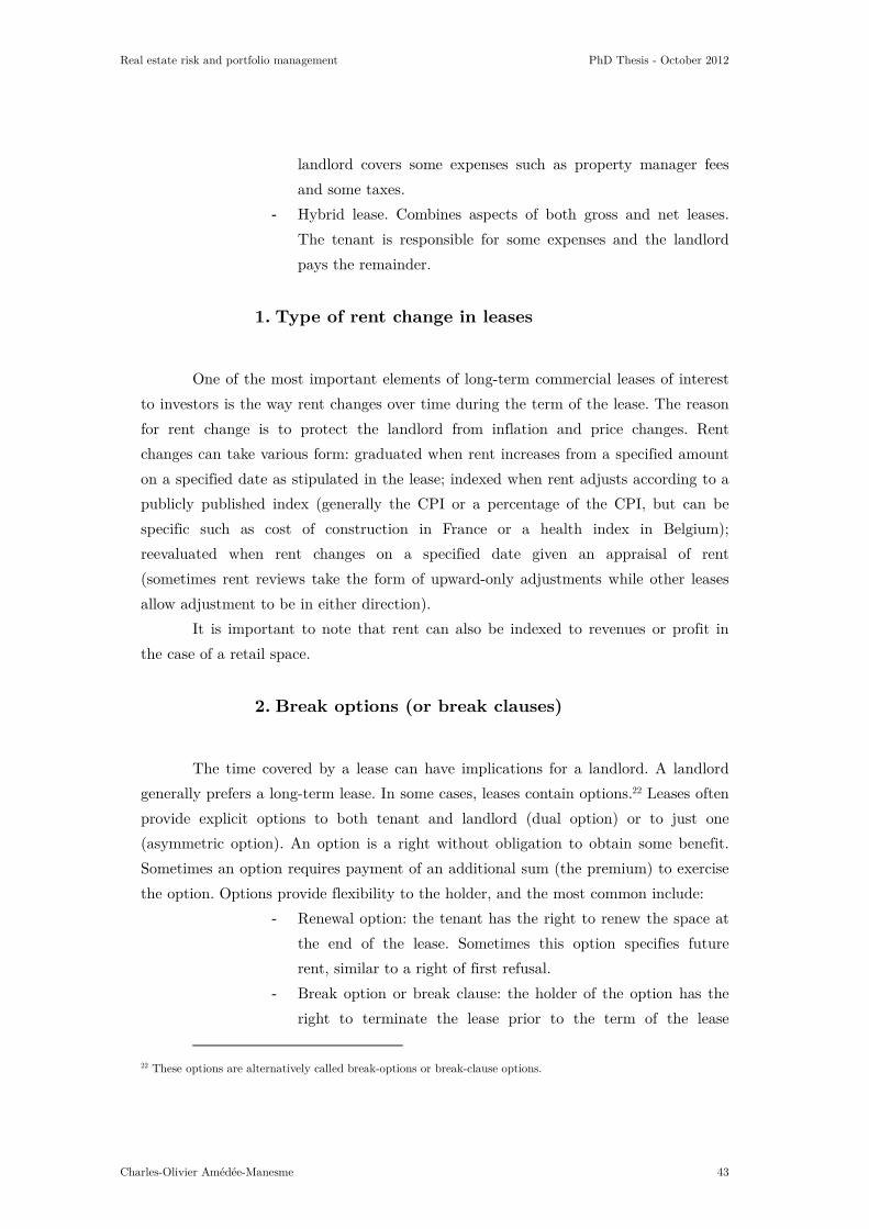
Real estate risk and portfolio management PhD Thesis - October 2012
Charles-Olivier Amédée-Manesme 43
landlord covers some expenses such as property manager fees
and some taxes.
- Hybrid lease. Combines aspects of both gross and net leases.
The tenant is responsible for some expenses and the landlord
pays the remainder.
1. Type of rent change in leases
One of the most important elements of long-term commercial leases of interest
to investors is the way rent changes over time during the term of the lease. The reason
for rent change is to protect the landlord from inflation and price changes. Rent
changes can take various form: graduated when rent increases from a specified amount
on a specified date as stipulated in the lease; indexed when rent adjusts according to a
publicly published index (generally the CPI or a percentage of the CPI, but can be
specific such as cost of construction in France or a health index in Belgium);
reevaluated when rent changes on a specified date given an appraisal of rent
(sometimes rent reviews take the form of upward-only adjustments while other leases
allow adjustment to be in either direction).
It is important to note that rent can also be indexed to revenues or profit in
the case of a retail space.
2. Break options (or break clauses)
The time covered by a lease can have implications for a landlord. A landlord
generally prefers a long-term lease. In some cases, leases contain options.22 Leases often
provide explicit options to both tenant and landlord (dual option) or to just one
(asymmetric option). An option is a right without obligation to obtain some benefit.
Sometimes an option requires payment of an additional sum (the premium) to exercise
the option. Options provide flexibility to the holder, and the most common include:
- Renewal option: the tenant has the right to renew the space at
the end of the lease. Sometimes this option specifies future
rent, similar to a right of first refusal.
- Break option or break clause: the holder of the option has the
right to terminate the lease prior to the term of the lease
22 These options are alternatively called break-options or break-clause options.

Real estate risk and portfolio management PhD Thesis - October 2012
Charles-Olivier Amédée-Manesme 44
within a specified notice period. The option may be written
either for the tenant or the landlord. Break clauses can take
many forms; there is no universal form or type of break clause.
Issues related to drafting, timing, beneficiaries, penalties and
frequency vary. This point is exacerbated further by the
diversity of break clauses and letting circumstances, which
produce diversity for financial implications.
- Expansion option: this option takes the form of a right of first
refusal for the tenant for a space adjacent to leased space. The
option can also take the form of offering the tenant the right to
rent space at a specified price during a specified period. These
break-options are found particularly in continental Europe
leases, and motivated this thesis.
B. Literature on lease structure
Numerous papers examine the effect of commercial property leases on market
structures and investor behavior. The same authors or group of authors largely write
these papers. The implications for investment strategy of a short or long lease, pricing
of leased property, cost of vacancy, probability of vacancy and global influences of all
these factors on market rental value volatility have been the subjects of many papers.
From our viewpoint, this is not sufficient, and many points have not been questioned.
This is due primarily to the specificity of lease structures and regulations among
countries. Leases are country-specific, and comparison is difficult due to discrepancies
in lease lengths, indexations, options, renewals etc. Particularly, pricing of a lease
structure is a risk factor, more an asset-specific risk factor than market or portfolio
risk, and therefore it is a more difficult risk to study. However, lack of reliable data on
patterns arising from lease terminations and lack of reliable time series of historic
property performance limit the efficacy of research in the field. We present here
primarily contributions to the field. We first discuss research on the pricing of lease
structures, and then research on options applied to leases.
In research of pricing lease terms and structure variation, the traditional
assumption of lease pricing models is that real estate investors extract the same value
from a property regardless of lease structure. One of the most significant papers on
lease pricing is Grenadier’s (1995) analysis of a range of lease options. Grenadier

Real estate risk and portfolio management PhD Thesis - October 2012
Charles-Olivier Amédée-Manesme 45
studies parallelism of varying lease lengths with bonds that have comparable
maturities. He determines rent equilibrium for any lease length and the term structure
of lease rates analogous to a term structure of interest rates. Grenadier proposes
numerous assumptions concerning patterns of lease lengths given various market
conditions. Following the method used for the term structure of interest rates, he
describes three possible term structure shapes—downward-sloping, upward-sloping and
single-humped—driven by landlord expectations. He also demonstrates that short lease
terms do not mechanically produce higher rent, and justifies why some owners, under
certain market conditions, prefer short leases or fixed rent.23 However, his work is
based on many hypotheses. Among them, the model does not consider transaction
costs, vacancies, taxes and landlord behaviors. Other contributions to the field come
from McAllister and Tarbert (1999), McAllister (2001), Mcallister and Roarty (1998,
1999), McAllister (2008) and McAllister and Fuerst (2008). They examine growth of
short leases (or the growth of break clauses) and implications of both shorter leases
and break options in commercial property investments. McAllister identifies many
critical variables influencing the effects of short leases on risk and return. In terms of
valuation, no general rule can be applied to account for break-options. This was also
the argument of Herd and Lizieri (1994), who found valuers tend to use ad hoc
adjustments to reflect the effects of break clauses.24 These authors highlight a strong
lack of consistency among valuers. They build a simulation approach to account for the
possibility that tenants exercise the option to leave. They also found evidence of
inconsistency in application of yield adjustments as a remedy for the impact of break
options on value. Their models fail to incorporate additional risks inherent in break
clauses and short leases or the possibility of downward rent reviews or free rent.
Another field related to lease options raises considerable interest among
researchers: the application of option pricing techniques to property investment and
development decisions. The choice to vacate can be viewed like a typical option. The
first work on this topic are those of Grenadier (1995), Ward (1997), Ward et al. (1998),
Patel and Sing (1998), Rowland (1999) and Baum (2003). More recent research25 on
these topics come from Booth and Walsh (2001a, 2001b), Ambrose et al. (2002),
23 If they expect market conditions to improve, they should regard short leases more favorably. 24 This is due both to difficulty in assessing the effect of a break-option on the market (the effect may be different from one asset to another and from one location to another) and difficulty in finding comparable transactions to apply comparable models. 25 These works concentrate on U.K. and U.S. real estate markets, but are interesting.

Real estate risk and portfolio management PhD Thesis - October 2012
Charles-Olivier Amédée-Manesme 46
Hendershott and Ward (2003) and Stanton and Wallace (2009).26 A paper by McCann
and Ward (2004) is particularly appealing; they study optimal lease lengths from the
tenant’s viewpoint and question applicability of a term structure. Results suggest that
from the tenant’s perspective, the cost of space changes with the length of a lease
independently from the term structure of rental rates. Occupancy value is a function of
tenants’ specifications such as legal costs, search costs, moving costs, double rent,
repairing costs and opportunity costs. They develop a model that, given assumptions,
prices the range of lease lengths for individual tenants. The conclusion is that business
reasons dominate the term structure of rent, not financials. It is clear that researchers
are unable to identify an expected term structure of rent (Clapham et al. 2006; Bond
et al. 2008).
Some limitations appear in these works, the source of which is differences
between real estate assets and other products. In a typical option, an investor acquires
the right to buy (call option) or sell (put option) an underlying asset before or on a
pre-defined date. In real estate, our concern is the option to vacate conceded to a
tenant. It is possible to find an analogy with European options and, more precisely, a
European put option where the tenant has the right to sell the lease (to vacate) on an
agreed date. The option’s value is a function of movement in the price of the
underlying asset. In theory, the higher the volatility of the underlying asset, the higher
the option’s price. In the option-pricing model, the key variable is volatility due
primarily to the fact that volatility is the only factor estimated (historically or implied
in a volatility model). Even in deep real estate markets, volatility is misestimated. This
derives from a well-known real estate issue discussed already in this thesis: lack of
reliable historic time series and/or adequate transaction data. Many academicians
(Hodges 1990; Hamill et al. 2006, 2008, 2011) have long highlighted this point on
volatility and options. Today, it is still an issue for lease options pricing.
A further field that have raised a large amount of academic research is the
financial and economic theories that suggest lease and debt are substitutes. An
increase in one leads to a decrease in the other according to a potential substitution
coefficient. The basic idea behind this comes from the analogy between cash flows from
the lease obligations and cash flows from debt cash flows. One of the most
fundamental researches in this field27 is Ang and Peterson (1984) who conduct a series
of empirical tests. The authors demonstrate that leases and debt are complements
instead of substitutes. This idea has been the primary one in the literature since today.
26 Clapham and Gunnelin (2003) discuss the limitations of options theory in property options. 27 See also Franks and Hodges (1978) and Mukherjee (1991). In addition to that, Myers et al. (1976) derived a formula for evaluating financial lease contract.
Real estate risk and portfolio management PhD Thesis - October 2012
Charles-Olivier Amédée-Manesme 47
Recently, this filed has been the subject of some papers. Among others, Eisfeldt and
Rampini (2009) studies the financing role of leasing. They argue that the benefit of
leasing is that repossession of a leased asset is easier than foreclosure on the
collateral of a secured loan. This suggests that leasing preserves capital.
An issue appearing in all of these studies is ignorance of the impact of
heterogeneity, even though this shortcut is mentioned systematically. For example,
decisions to move are driven by rational factors, but more on a volunteer basis than
from management.28 In addition, landlord behavior is unclear and largely dependent on
strategy. Researchers such as Miceli and Sirmans (1999) demonstrate that landlords
attempt to minimize vacancy and turnover costs by offering discounts to long-term
tenants. Landlords may minimize the number of possible break-options conceded to
tenants by giving discounts or free rent.
Leases, therefore, are important factors in property returns and for the market.
They influence volatility and distribution because they play a role in global market
risk. In that sense, we discuss research of returns distribution in the next section.
III. Distribution of returns
Many practitioners optimize portfolio risk and diversification using the
traditional Markovitz (1952, 1968) mean-variance model and its corollary, the Capital
Asset Pricing Model, developed by Sharpe (1964), adapting the model to commercial
real estate. Literature related to these models in real estate was presented in the first
section of this literature review. The relevancy of the modern portfolio theory model is
not discussed here, but we raise strong doubts concerning assumptions, and review
literature on the topic. Nevertheless, the traditional approach is justified if the assets
are both traded in frictionless liquid markets and asset returns are independently and
identically distributed over time. In this context, the solution to the long-term asset
allocation dilemma is similar to the short-term one. Nobel Samuelson (1969) and
Merton (1969) demonstrate this. In real estate, assumptions underlying the classic
results of Samuelson and Merton are likely violated.29 It is widely assumed that returns
28 There exists heterogeneity in the probability of exercise in the real estate market. In a typical European option, the rational investor always exercises an option if it is in the money. In real estate, each break option is unique in terms of structure of the option and tenant attitudes to exercise. 29 Transaction costs and lack of liquidity are obvious market frictions.

Real estate risk and portfolio management PhD Thesis - October 2012
Charles-Olivier Amédée-Manesme 48
from real estate are not normal, and thus not independently and identically
distributed. Many academicians have started to examine real estate return
distributions. However, estimating returns over long periods is an arduous task in real
estate, particularly in direct real estate. Many empirical tests in the real estate
literature support how important it is to assume non-normality of property returns.
Non-normality of real estate returns has soon intrigued academicians, and has been a
strong debate in the literature. Young et al. (1995, 2006, 2008) and Lee et al. (1997,
2002, 2006) published numerous papers on the topic. One of the key points in direct
real estate is lack of data, and all traditional models require high frequencies of data
for correct estimation of the distribution. The papers discussed below concern U.K.
and U.S. data, once more based on availability. We share the following presentation
between direct and indirect real estate.
A. Direct real estate
In direct real estate, the frequency and reliability of data is particularly
critical. Nevertheless, many researchers publish papers on return distributions. Among
the first papers on the topic, Miles and McCue (1984) or Hartzell et al. (1986) found
evidence of non-normality by focusing on skewness and kurtosis coefficients. Similarly,
Myer and Webb (1994) confirm evidence of non-normality using kurtosis, and
demonstrate autocorrelation in private real estate returns. The most fundamental
empirical research on the Gaussian distribution assumption comes from Young and
Graff (1995). Using the NCREIF database (1980 to 1992), they characterize non-
normality of U.S. institutional private real estate distributions, demonstrating how an
infinite variance model provides better descriptions of distributions of returns in the
property sector. They particularly discuss how the diminution of risk from
diversification is less effective in the non-normal context. Byrne and Lee (1997)
examine quarterly returns for sectors and regions using the NCREIF (1983 to 1994).
The Jarque Bera test rejects normality for 10 of 16 sub-sectors, consistent with earlier
findings because they find positive kurtosis and demonstrate how real estate returns
exhibit negative skewness. They point out how portfolio allocation, using volatility as a
risk measurement, is unsuitable. Graff et al. (1997) examine the distribution
characteristics of Australian real estate based on the Property Council of Australia’s
Performance Index, a short time series (1984 to 1996). The study highlights problems
of a direct real estate database (low frequency of data, small number of assets,
valuation). They conclude an abnormal shape of the distribution for Australian

Real estate risk and portfolio management PhD Thesis - October 2012
Charles-Olivier Amédée-Manesme 49
property returns. The shape of the distribution is nearly the same as the one for the
United States. Australian real estate investment is therefore heteroscedatic. In terms of
portfolio management, this shows that models that rely on finite variance statistics are
inefficient in the Australian real estate context. Lizieri and Ward (2000) also examine
the distribution of returns in the commercial real estate market, focusing on direct real
estate in the U.K. They concentrate on office, retail and industrial properties to
discriminate commercial real estate from private residential markets. They highlight
the non-normality of property returns based on the IPD monthly index database. The
logistic distribution is only one of possible distributions. Implications of distributions
for asset allocation are examined. Lizieri and Ward contradicted two received ideas.
First, they do not attribute aberrant behavior of real estate returns to appraisal or
smoothing issues. Second, they suggest real estate returns produce better results in less
frequent database, returns being easier to model. According to the authors, these
points come from real estate characteristics such as heterogeneity, indivisibility,
valuations versus transactions data or high transaction costs. Young et al. (2006)
support previous results, emphasizing how unsafe it is to assume normality in real
estate returns using annual IPD data (1981 to 2003). They analyze subsectors and
reject the normality assumption at the sub-sector level. Analysis demonstrates how the
skewness coefficient and the magnitude of real estate assets change over time. More
recently, Young (2008) extends previous results to a more recent database based on
NCREIF (1980 to 2003). In this updated empirical analysis, the authors find evidence
of non-normality, and show how differences among property types appear salient. Real
estate risk is shown to be heteroscedastic. Once again, the paper demonstrates asset
diversification is less effective than expected. Outside English-speaking countries,
Richter et al. (2011) question the normality of German property returns based on IPD
Database. Using quantile-based estimation, they examine distributions of income,
capital growth and total returns, revealing that the assumption of normality in return
distributions can be rejected for all subsamples of all property types.
B. Indirect real estate
Many studies concentrate on indirect real estate return distributions. For listed
real estate, more data are available, and it is easier to determine a distribution. These
returns provide evidence of skewed, peaked distributions and fat tails. The distribution
of listed real estate has long been questioned in the literature, and many papers

Real estate risk and portfolio management PhD Thesis - October 2012
Charles-Olivier Amédée-Manesme 50
concerning nearly all countries are available. We only present a general survey of this
literature because we do not focus on listed real estate (REITs) in this thesis.
A paper by Lizieri and Satchell (1997) examines the distribution of monthly
property company (as opposed to REITs) returns in the U.K. between 1972 and 1992,
demonstrating strong evidence for non-normality. The Jarque-Bera test rejects the
hypothesis of normality, and returns exhibited positive skewness and kurtosis
coefficients and were fat-tailed.
For purely listed real estate (REITs), Seiler et al. (1999) investigate the return
distributions of equity real estate investment trusts (EREITs) from a quarterly
database (1986 to 1996). In spite of the size of database, the Kolmogorov-Smirnov,
Shapiro-Wilks and Lilliefors tests rejected normality. They conduct the study on a
sector basis and expose results sector by sector. For example, office REITs returns
were less normal while industrial REITs returns did not reject the tests. They highlight
that offices exhibit high volatility and are skewed positively. More recent research
confirms these results. Lizieri et al. (2007) identify and model excess kurtosis in REITs
returns. Cotter and Stevenson (2007) demonstrate for REITs returns that conditional
heteroskedasticity and volatility can be modeled with many GARCH models. Cotter
and Roll (2011) also provide elements for REITs return characteristics. They compare
it to the S&P500, and REITs exhibited lower market risk (beta) but comparable total
volatility. Return distributions displayed negative skewness and very high kurtosis,
implying REITs returns are non-normal.
Another classic question when considering listed real estate returns remains
unsolved; are REITs stock or property? This question was discussed in the portfolio
allocation part of the literature review, and has been the subject of numerous studies.
Today, no consensus emerges, leaving considerable work for academicians. Here, we
mention studies that discuss it in light of distributions. Many researchers note that
REIT and property companies sharing returns have much closer contemporaneous
correlations with the stock market than with the underlying real estate market. These
results hold even when researchers correct the distribution for appraisal smoothing in
the direct property market and for gearing (leverage) in the indirect market as
demonstrated by Barkham and Geltner (1995). We highlight the fact that information
about REITs return distributions does not necessarily offer information on direct real
estate returns. Interest in this field is reported to MacKinnon and Al Zaman (2009)
and Hoesli and Oikarinen (2012).
Studies suggest that the normality of real estate asset returns is sensitive to
data frequency. Using conventional statistical approaches on monthly data, Lee (2002)
demonstrates positive skewness in nearly all markets. Booth et al. (2002) show
Real estate risk and portfolio management PhD Thesis - October 2012
Charles-Olivier Amédée-Manesme 51
evidence of kurtosis, with tails particularly fat. Contrarily, Maurer et al. (2004) find no
evidence of either skewness or kurtosis using quarterly data from the U.K. Lizieri and
Ward (2000) partially contradict Maurer et al. (op. cit); monthly returns were non-
normal, and normality was not rejected at the sub-sector level for quarterly returns in
2 of 5 subsectors. As discussed, Young et al. (2006) used the IPD U.K. annual data
(1981 to 2003), rejecting the normality of distributions of real estate returns. There
exists no consensus on the optimum data frequency, and the debate on normality
continues. As we show in part three of this thesis concerning Value at Risk using
Cornish-Fisher expansion, the assumption of normality collapsed after the 2007
subprime crisis (lack of recent researches from the best of our knowledge).
Few studies in real estate consider non-normality in portfolio management and
allocation, and in risk management. It is partially the objective of this thesis to
consider non-normality, particularly in the case of risk management. Non-normality
has huge effects on Value at Risk assessment and more generally on risk management.
This is why we concentrate part of this thesis on Value at Risk.
IV. Value at Risk
A. Introduction and definition30
Risk measurements have changed remarkably since Markovitz (1952) developed
his theory in the 1950s. At that time, standard deviation was the risk measure of an
efficient portfolio, but this measure was not relevant for only one security. For a single
security, risk is computed using covariance between the security and the market. A
security’s standard deviation is comprised of risk that can be mitigated by
diversification and risk that cannot be diversified, yet only the risk that cannot be
diversified is remunerated. Risk theories that followed concentrated primarily on
factors that determine security risk and capital market equilibrium. When considering
a portfolio comprised of N securities, Markowitz’s model requires the estimation of N
variances and2
2N N−
covariances. When N becomes large, estimation of the variance-
covariance matrix becomes arduous, and the possibilities for errors increase, which can
lead to misleading decision. During the 1960s, Sharpe (1964) developed the Capital
30 This introduction largely takes a leaf out of Racicot et al. (2006).

Real estate risk and portfolio management PhD Thesis - October 2012
Charles-Olivier Amédée-Manesme 52
Asset Pricing Model, a mono-factor model that considers covariance between a security
and a market as the only risk factor. Risk is represented by the beta (β) and is called
the systematic risk, but it cannot be mitigated by diversification. Contrarily, specific
(non-systematic) risk inherent to a company can be mitigated by diversification. Then,
Ross (1976) developed the Asset Pricing Theory in the 1970s, a multifactor model that
identifies the multidimensional effects of risk. One of the weaknesses of this model is
that it does not explain factors that determine security returns.
Value at Risk did not appear before the late 1980s. In 1987, the stock market
crashed, a triggering event for development of new risk measures. This was the first
major financial crisis in which practitioners and academicians were afraid of global
bankruptcy of the entire system. The crash was so improbable given standard statistics
models, that many quantitative analysts cast doubts and began to question the
models. Many academicians claimed the crisis would recur and called for reconsidering
the models. Considering extreme events became necessary. Limitations of traditional
risk measures were recognized, and measuring risk of falling asset values was becoming
urgent. The necessity of relying on a risk measurement that considers the entire
distribution of returns of a portfolio was obvious. Throughout the 1990s, a new risk
measurement was developed: Value at Risk (VaR).31
VaR was developed and adopted by practitioners and regulators. Jorion (2006)
defines VaR as “a method of assessing risk that uses standard statistical techniques
used routinely in other technical fields. Loosely, VaR summarizes the worst look over a
target horizon that will not be exceeded with a given level of confidence.” In financial
risk management, VaR is a risk measure of loss on a portfolio of financial assets. For a
given portfolio, probability and time horizon, VaR is a threshold value such that the
probability that the mark-to-market loss on the portfolio over the given period exceeds
this value (assuming no trading in the portfolio) is the probability level. For portfolio
value at time t, tV , for one period and for threshold α , this can be expressed as:
( )1 ,, 0
t t t tt V V VaR
αα
+∀ Ρ − + < =
Considering a centered and reduced random variable U with cumulative
distribution function UF and uα , the quantile at thresholdα , we have:32
{ }( ) sup | ( )U
VaR U u F u uα α
α= − < = −
31 For this thesis, VaR is assumed to be computed for a static portfolio, with no change in its structure and no trading or arbitrage.
32 Some choose to count effective loss positively: { }( ) inf | ( )U
VaR U u F uα
α= > , which is equal to uα if the
distribution is symmetric.

Real estate risk and portfolio management PhD Thesis - October 2012
Charles-Olivier Amédée-Manesme 53
This measure is becoming increasingly popular to value risk of institutional
and individual portfolios. VaR is an easy to understand method for quantifying market
risk. Today, VaR is used by many regulators as a risk measurement reference for Basel
I, Basel II, Solvency II and NAIC, among others.
Worldwide adoption of the Basel II Accord in 1999 and near completion in
2012 (Basel III must be applied for 2019) offers further motivation for VaR. The Basle
committee required that banks compute their VaR periodically and maintain sufficient
capital to pay eventual losses projected by VaR. Unfortunately, there is no single
measure of VaR because volatility, a fundamental component, is latent. Banks must
use many VaR models to compute a range of prospective losses. More recently, the
Solvency II regulation for insurers in Europe proposed VaR as a reference measure to
determine required capital. Like Basel II, it proposes either use of a standard model or
an internal model. The standard model for real estate VaR leads to required capital of
25% for real estate investments. This calculation was made based on IPD U.K., all
properties total return index (this index is a reliable commercial monthly index in
Europe).33 The committee recognizes the non-normality of real estate returns, but did
not try to estimate real estate required capital. It recommends an historic VaR of 25%,
leaving further research for internal model.
VaR computations are complex because distributions of returns are generally
unknown. The primary uses of VaR in finance are risk management, risk analysis,
financial control, financial reporting and computing regulatory capital. Methods and
risk measurements such as stress testing, expected shortfalls, and tail VaR have
become more popular because they focus particularly on expected severity of failure.
VaR is slowly replacing standard deviation (or volatility) as the most widely used
measure of risk34 because of the need for a single risk measure for calculation of capital
adequacy limits for financial institutions such as banks and insurers. VaR allows
regulators and bank managers to put a single number on a predefined worst-case
scenario, at a predefined confidence level.
The three traditional methods of calculating VaR are the historic, the
parametric and the Monte Carlo methods.
- The historical method involves taking empirical profit and loss
history and ordering them, assuming history repeats. The main
33 From the Solvency II report, referenced as CEIOPS-DOC-40/09 (2009): - 3.160: “One of the most challenging factors of this specific calibration is the lack of long time series across most European markets.” - 3.169 & 3.171: “All distributions of property returns are characterized by long left fat-tails and excess kurtosis signifying disparity from normal distribution.” 34 This point is subject to debate.

Real estate risk and portfolio management PhD Thesis - October 2012
Charles-Olivier Amédée-Manesme 54
benefit of the method is that it does not require assumptions
concerning the nature of the distribution of returns. A
drawback is that this method assumes the shape of future
returns will be the same as those in the past. To make this
approach statistically reliable, one needs to ensure that a
sufficient number of observations are available and they are
representative of all possible states for the portfolio. Data must
incorporate observations from both bull and bear markets. In
real estate, since we rarely have enough history (more generally
in almost all non-listed markets), the method is not as accurate
as either the parametric or simulation methods.
- The parametric method (sometimes called variance-covariance
method) requires an assumption concerning the statistical
distribution (normal, log-normal etc.) from which the data are
drawn. Parametric approaches are comparable to fitting curves
through data and then reading off VaR from the fitted curve
(unfortunately, for many sophisticated models, analytical
solutions do not exist). The parametric VaR is one of the more
popular methods. The attraction of parametric or analytic VaR
is that relatively little information is needed to compute it. A
weakness is that the distribution chosen may not reflect all
possible states of the market and may under or overestimate
risk. This problem is particularly acute when using VaR to
assess risk of asymmetric distributions (left skewed distribution
or one for a particular portfolio containing options). In such
cases, higher statistical moments of skewness and kurtosis,
which contribute to more extreme losses (fat tails), need to be
considered. Although some level of statistical sophistication is
necessary, parametric methods exist for a wide variety of
distributions.
- The Monte Carlo approach has become increasingly popular in
recent years, due to improvements in computer and software
power. Monte Carlo methods rely on repeated random
generations from a probability distribution of inputs that are
used to compute model results. Simulation-based VaR generates
many scenarios drawn from either a parametric assumption
about the shape of the distribution (Monte Carlo) or re-

Real estate risk and portfolio management PhD Thesis - October 2012
Charles-Olivier Amédée-Manesme 55
sampling (bootstrap) the empirical history and generating
sufficient data to be statistically significant. VaR is deduced by
reading the desired percentile as with the historic method.
After defining VaR and a presentation of the primary methods of computing
VaR, we review the literature on the subject and introduce the sparse literature that
concentrates on real estate VaR.
B. Literature review
VaR has been the subject of broad research among academicians. All methods
proposed to compute VaR or a distribution quantile have been subject to academic
research after development of VaR. A large portion of the literature focuses on ways to
measure VaR. For example, Linsmeier and Pearson (2000), Duffie and Pan (1997) and
Engle and Manganelli (1999) published general papers on measuring VaR. More
specific research was published on primary methods, among them Monte Carlo
simulation from Pritsker (1997), Johnson transformations from Zangari (1996a),
Cornish-Fisher expansions from Zangari (1996b) and Fallon (1996), Solomon-Stephens
approximation from Britton-Jones and Schaefer (1999), saddle-point approximations
from Feuerverger and Wong (2000), Fourier-inversion from Frolov and Kitaev (1998)
and extreme value theory from Longin (2000). Theoretical properties of VaR
evaluation is reported by Artzner et al. (1999), Cvitanic and Karatzas (1999) and
Wang (1999).
Other attention is given to VaR optimization for portfolio or risk reductions.
Roy (1952), Telser (1967) and Kataoka (1963), who focus on portfolio constraints
called safety-first approaches at the time, started these works. Emmer et al. (2001),
Alexander and Baptista (2002, 2003), Embrechts et al. (1999) and Kast et al. (1999)
extended research on VaR. Also, the work of Gourieroux et al. (2000) about the
sensitivity of Value at Risk is appealing.35
In addition to all these methods, many works concentrate on the best methods
to compute VaR or on the pros and cons of VaR. Jorion (1996) explains that the
benefits of VaR should not mask its shortcomings because any VaR number is itself
measured with error or estimation risk. Jorion recommends reporting a confidence
interval with the VaR number to be more relevant. The author highlights that the
35 the authors derive analytical expressions for and second derivatives of the VaR.

Real estate risk and portfolio management PhD Thesis - October 2012
Charles-Olivier Amédée-Manesme 56
greatest advantage of VaR computation is to think globally and critically about risk.
Pichler and Selitsch (1999) compare five VaR methods in the context of portfolios that
include options using Johnson transformations, variance-covariance, and three Cornish-
Fisher-approximations for the second, fourth and sixth orders. They conclude that the
sixth-order Cornish-Fisher approximation is the best approach. Mina and Ulmer
(1999) compare Johnson transformations, Fourier inversion, Cornish-Fisher
approximations and Monte Carlo simulation. Their conclusions include the following:
Johnson transformations are not a robust choice. Monte Carlo and Fourier inversion
are robust, and Cornish-Fisher is extremely fast but less robust than the two previous
approaches, particularly when the distribution is far from normal. Feuerverger and
Wong (2000) focus on when to use Cornish-Fisher in comparison to Fourier inversion,
saddle point methods, and Monte Carlo. The paper concludes with an extension of the
method, which includes higher-order terms. Candelon et al. (2011) propose a method
to backtest VaR models using a duration-based backtesting procedure derived from the
GMM test introduced by Bontemps (2008). This allows testing distribution
assumptions using an easy approach. Thus, the authors introduce a new way to
backtest VaR estimation and forecasts. Other academicians such as Longin (2005)
suggest taking interest in extreme events—and therefore extreme value theory—only
when appraising extreme risk such as VaR.
The sub-additivity issue of VaR has recently36 been the subject of a few papers,
particularly after the subprime crisis in 2007 when the non-normality of returns was
rediscovered. A description of the underlying issues and further references can be
found in McNeil et al. (2005). Other research on the subject includes Rootzén and
Klüppelberg (1999), Dhaene et al. (2009) and Daníelsson et al. (2012). Heyde et al.
(2006) discuss robustness of risk measures, suggesting replacement of tail conditional
expectations (sub-additive risk measure) with a more robust tail conditional median,
which is simply VaR at a higher confidence level.
The debate concerning VaR relevancy is old and not the purpose of this thesis.
We accept the choice of VaR by regulators without discussion, and try to develop a
better VaR valuation model.
Research of risk focusing on direct real estate or unlisted vehicles is scarce in
spite of increasing interest. Again, this is probably partially due to the paucity of
available data. Either invest in listed real estate, real estate data is quoted daily and
36 Artzner et al. (1999) discuss strengths and weaknesses of VaR as a risk measure.

Real estate risk and portfolio management PhD Thesis - October 2012
Charles-Olivier Amédée-Manesme 57
sufficient data are available to compute VaR for a portfolio, or invest in direct real
estate and deal with small datasets. This is particularly true in commercial real estate
in which institutional investors largely invest, and where VaR computation is
mandatory for capital adequacy. The real estate market is comparable to the private
equity market where indices are built on smaller numbers of transactions. A real estate
property index aggregates real estate market information to provide a representation of
underlying performance. However, this is conducted monthly in the best of cases
(U.K., U.S. and Australia), quarterly or semi-annually occasionally but generally
yearly, largely linked to sector. The residential field, in which many transactions can
be observed, exhibits a monthly index frequently. Contrarily, commercial real estate
faces more difficulties to deliver indices with larger periodicities.
Research of VaR in real estate focuses on REITs or securitized real estate. VaR
for listed real estate relies on methods for stocks or bonds. Zhou and Anderson (2012)
concentrate on extreme risks and the behavior of REITs in abnormal market
conditions, arguing no universal method can be recommended for VaR in listed real
estate. They note estimation of risk for stocks and REITs requires disparate
approaches. Cotter and Roll (2011) study REIT behavior over 40 years, highlighting
non-normality of REIT returns. They compute VaR for the index following three
methods that do not rely on Gaussian assumptions: Efficient Maximization algorithm,
Generalized Pareto Distribution and a GARCH model. The authors highlight that
reality is much worse than that depicted by an assumption of normally distributed
returns. Liow (2008) uses extreme value theory to assess VaR dynamics of ten major
securitized real estate markets. Extreme value theory allows the author to consider the
stochastic behavior of the tail. Using this tool, extreme market risks are better
assessed than with traditional standard deviation measures, and real estate forecasts
are more accurate.
Literature focusing on VaR in the context of direct real estate investment is
sparse. However, numerous studies concentrate on risk management and assessment in
real estate. Booth et al. (2002) examine risk measurement and management for real
estate portfolios, explaining that practical issues force real estate investors to treat
them differently from other assets classes. They particularly espouse that direct real
estate is an area for further research. The report is a complete review of the range of
risk measures that can be used to measure real estate risk. It focuses on the difference
between symmetric measures such as standard deviation and downside risk measures
such as VaR. The authors conclude by recommending use of risk measures “that
properly reflect their subjective risk preferences and do not use standard deviation of
investment returns for the sake of simplicity. […] Different risk measures measure

Real estate risk and portfolio management PhD Thesis - October 2012
Charles-Olivier Amédée-Manesme 58
different aspects of risk.” Their work concentrates on all risk measures usable in real
estate. They do not conclude with one perfect risk measure, but propose adapting risk
measures to needs. Gordon and Wai Kuen Tse (2003) consider VaR a tool to measure
leverage risk in a real estate portfolio. Debt in a real estate portfolio is a traditional
issue in real estate finance. The paper demonstrates VaR allows better assessment of
risk. Traditional risk-adjusted measures (Sharpe ratio, Treynor’s and Jensen’s alpha)
suffer from the leverage paradox; leverage adds risk along with the potential for higher
returns per unit of higher risk. Therefore, the risk/return ratio does not change
noticeably and is not an accurate tool to measure risk inherent to debt. They conclude
VaR is good tool for leverage risk. Farelly (2012) focuses on measuring risk of unlisted
property funds using a forward-looking approach. Among other results, the author
considers moments measures of orders greater than two (asymmetry considered) using
Cornish-Fisher expansion.
Recommending other risk measures, Brown and Young (2011) focus on a new
way to measure real estate investment risk. They refute the assumption of normally
distributed returns that flaws forecasts and decisions, and the nature of risk and how
it should be measured is discussed. Interestingly, VaR is not retained, and the expected
shortfall is recommended more. The authors then focus on spectral measures, which
represent their final recommendation.
Following these authors, we motivate the third part of this thesis with needs
for better VaR assessment in direct real estate.
C. VaR limitations and Conditional VaR
VaR is not the maximum loss an investor can realize; it is the lowest loss at
thresholdα . Even if exact in theory, it works only within a specified confidence level.
There is always a higher level of loss for a lower confidence level.37 Despite its
popularity among practitioners, regulators and academicians, VaR is subject to many
criticisms. It has been controversial since it moved from trading desks into public
awareness in 1994. A common complaint among academicians is that VaR is not sub-
additive; VaR does not systematically satisfy the property of convexity as illustrated
by Danielson et al. (2005). The VaR of a combined portfolio can be larger than the
sum of the VaR of its components. This was demonstrated by Artzner et al. (1999).
Except in some special cases (among which normal distribution), VaR does not satisfy
37 Kerviel’s event happened only once in Societé Générale history.

Real estate risk and portfolio management PhD Thesis - October 2012
Charles-Olivier Amédée-Manesme 59
the sub-additivity requirement for mathematical coherence and for simple, practical
use. Assessing plausible losses is difficult using VaR theory. Losses can be extremely
large and sometimes impossible to determine once an investment goes beyond the VaR
point. From a practitioner’s viewpoint, VaR is more the level of losses at which an
investor stops trying to imagine what worse can happen next.
VaR is a risk measure that only considers the probability of being below a
threshold level; it does not consider values below this level or their averages. This is
why other risk measures have been proposed. Among them, expected shortfall as
defined by Acerbi et al. (2001) (also called conditional VaR: CVaR) or the TailVaR
from Artzner et al. (1999). Applications of CVaR in real estate finance are nearly non-
existent, and applications and research on the topic are currently in preparation.
Mentioned above, the objective of this thesis is not to discuss the quality of
VaR as a risk estimator or its adequacy for risk-budgeting purposes. Regulators chose
VaR for a required economic capital calculation, and its computation is now
mandatory for all regulated practitioners. Therefore, academic research on the topic is
now also mandatory.
*
* *
This literature review was designed as prose. The writing tries to avoid
providing a list describing or summarizing one piece of literature after another. The
literature review is organized into sections that present themes or identify trends,
including relevant and irrelevant theories. It cites the most relevant published papers,
and synthesizes and evaluates the papers in light of this study. We apologize for
missing references and inaccuracies.

Real estate risk and portfolio management PhD Thesis - October 2012
Charles-Olivier Amédée-Manesme 60

Real estate risk and portfolio management PhD Thesis - October 2012
Charles-Olivier Amédée-Manesme 61
PART II – REAL ESTATE
PORTFOLIO AND RISK
MANAGEMENT
This part focuses on real estate portfolio and risk management, concentrating
particularly on a topic that has not been the subject of sufficient academic or
professional research: break options. Another title could have been how break clauses
can be considered in real estate portfolio management. Break options are options
embedded in leases in favor of the tenant, comparable to financial options. These
options are a continental Europe lease specificities, but this kind of option is
standardizing, and they are sometimes used in the U.K. or the U.S. (even if their use is
in a state of infancy in these countries). The break options are one of the most
important risk real estate finance must deal with and we introduce in this part a
model that allows including them rationally in cash flows. This way, this real estate
specific risk can be considered.
Real estate portfolio (or fund) management differs radically from managing
equity, bond or mutual funds in that real estate managers are not only responsible for
asset allocation, risk management and transaction supervision, but also managing
execution of asset strategy. Unlike equity managers who research companies and
manage probabilities that they can execute strategies, real estate managers must define
and execute strategies at the property and portfolio levels. Therefore, real estate asset
management - contrary to traditional asset management of stocks and bonds - requires
experienced individuals who optimize the value of properties through superior
transaction services, information and management execution. Real estate portfolio
managers conduct asset allocation and asset selection not only by understanding
fundamentals of the market and/or of locations, but also by being experts in real
estate property, generally within local regions and within a specific commercial real
estate sector (office, industrial or retail).
Real estate portfolio managers also deal with the life of the property. In
addition to creating and approving budgets and expenses, asset managers increase
value by managing the leasing of properties managed. Leasing is one of the more

Real estate risk and portfolio management PhD Thesis - October 2012
Charles-Olivier Amédée-Manesme 62
complex functions, and has a strong effect on portfolio value. Success in leasing is not
only attained by finding and executing the highest possible leasing opportunities of
each unit, but also by conducting a leasing program aligned with portfolio strategy
while maintaining good relationships with existing tenants. For example, during
periods of rising rent rates, long-term leases may be locked in to income-oriented
properties, while for strategies focused on capital appreciation, lease terms may be
shortened to take advantage of higher expected rates in the future or for property-
repositioning programs.
Mentioned above, break-options have not been the subject of many studies.
The reason is simple: questions center on continental Europe. In the U.K. and United
States where the majority academic research (particularly real estate) is conducted and
published, options are not the same and sometimes do not exist. Options to leave in
favor of the tenant (an asymmetric option) are not the way Anglo-Saxon culture
thinks. In that context, an option must be dual: both the tenant and the landlord have
the possibility to decide what to do about the space. Some argue tenants are too
protected by law in France. However, the concept of break-options similar to that
known in continental Europe is slowly emerging, especially for large tenants that have
bargaining power. This is why this kind of option has not been the subject of many
studies. Notwithstanding, the importance of this kind of option and the ways they can
be analyzed is a fundamental issue that could be the subject of much research. They
have a strong influence on investors’ decisions and on the structure of the market.
They can be used by tenant to manage expenses and by contrast, they can be used by
investors to attract tenants who are uncertain of their business plan or to negotiate
higher rent. These options offer many possibilities that should be explored.
Commercial real estate investment is often analyzed in light of the length of
secured cash flows, and long-term leases offer numerous advantages to investors. First,
secured properties are easier to price since no assumptions have to be considered for
future tenant decisions. Second, short leases raise many questions for the investor.
Price if vacant, level of rent achievable, length of potential vacancy and financial
incentives to concede to the tenant are questions raised only in cases of vacancy. That
makes the decision more arduous. Third, strategies are more difficult to determine
with short-term leases. Fourth, long-term leased properties are more liquid and can be
sold more quickly. We focus on the way break-options can be considered to manage a
real estate portfolio. We concentrate on the way break-options can be included in cash
flows and the influence they have on portfolio management. Research of this topic is
potentially large; covering it is not possible in a thesis.

Real estate risk and portfolio management PhD Thesis - October 2012
Charles-Olivier Amédée-Manesme 63
We propose a new approach that considers options embedded in leases. The
model can be used for valuation, portfolio management and risk management. This is
the subject of the first chapter in this part. The second chapter concentrates on
portfolio management when these kinds of options are considered, and questions the
optimal holding period (optimal time to sell) of a real estate portfolio that accounts
for break-clauses. This second article involves not only aspects arising from portfolio
management, but also investigates property risk management and addresses cash-flow
modeling perspectives.
The two papers presented in this part along the two chapters are:
Chapter III: Paper 1: Combining Monte Carlo Simulation and Options to
Manage Risk of Real estate Portfolio
Chapter IV: Paper 2: Optimal Holding Periods of a Real Estate Portfolio
according to the Leases;

Real estate risk and portfolio management PhD Thesis - October 2012
Charles-Olivier Amédée-Manesme 64
Chapter III. Combining Monte Carlo Simulations
and Options to Manage
Risk of Real Estate
Portfolio Management
(2012)1
This study examines options embedded in leases to better account for them in
the investment process, which includes acquisition, portfolio management and risk
management. The third chapter of this thesis examines break clauses conceded to
tenants embedded in leases contracts. We investigate inclusion of these kinds of option
in a cash flow model and their effect on investment management, risk management and
investment decisions. Break options are options in favor of a tenant that offer the right
but not the obligation to vacate the property on a predefined date. Break options can
be interpreted in various ways, but in this chapter, we analyze them exactly as
financial options except we do not determine the premium of the option but explore
the possibility of exercising the option. The problem with break options in real estate
finance is how to determine their exercisability and how to account for them during
cash flow modeling. Often, fund or asset managers consider two or three scenarios
1 This study led to a paper that is under consideration at the Journal of Property Investment and Finance (Emerald), and we are waiting for reviews. The article was written with Michel Baroni (Essec Business School), Fabrice Barthélémy (University of Cergy-Pontoise) and Etienne Dupuy (BNP Paribas Real Estate). The article has been presented at many conferences, and has been the subject of many modifications since the first presentation. It was presented in draft state in 2010 at the American Real Estate Society’s annual conference in Naples, Florida. The study garnered numerous positive comments. It was then presented in the same year at the European Real Estate Society’s annual conference in Milan. The paper received many recommendations, particularly a few concerning distributions of returns. Next, we presented the paper at the American Real Estate Urban Economics Association’s annual conference in 2012. The paper was refereed by Jacque Gordon from Wharton University and senior researcher for Jones Lang Lasalle in Chicago during a session chaired by Austin Jaffe from the University of State Pennsylvania. The paper received many comments and recommendations. The range of possible cash flows and returns and apprehension of break risk was appreciated. The referee recommended focusing more on risk management. Finally, the paper was presented at the French Financial Association (Association Française de Finance, AFFI) in 2011. The general topic of real estate received excellent feedback, and attendees appreciated the model. The author would like to thank participants of all these conferences for their helpful comments.

Real estate risk and portfolio management PhD Thesis - October 2012
Charles-Olivier Amédée-Manesme 65
where tenants either stay or leave the property, and determine returns in two other
cases.2 They consider the possibility of a tenant leaving. Even if it accounts for
multiple scenarios, this method does not consider all possibilities. During some market
events, rental values rise quickly, and the tenant will not move to a more expensive
space. In other cases, rental values decline dramatically, but since the rent is not high,
the tenant is again not tempted to move. The problem is to determine reliably how to
account for break options and determine whether an option is exercised (given rational
behavior). We propose a model that addresses the break option issue and
simultaneously accounts for general market risk. Our approach considers both market
and idiosyncratic risk, specific risk in real estate that is a large part of leasing. Specific
risk is difficult to diversify in real estate as discussed in the literature review because a
large number of assets is needed. Accounting for specific risk is essential when valuing
or managing a portfolio.
This chapter’s method relies on combining Monte Carlo simulation with option
theory. The model is comprised of a traditional discounted cash flow model that
accounts for all incomes and outcomes of a real estate portfolio investment. Incomes
are rent and terminal values and outcomes are expenses related to properties, if any,
according to lease structures (see part I. chap. 2). On this basic model, market risk is
added using Monte Carlo simulation on both prices of the portfolio and market rental
values. Correlations among all simulated parameters are considered. In this way, both
price and market rental value market risks are considered in cash flows. However, in
real estate finance, usual income is not commensurate with market rental values.
Inflows come from rent, and rent is rarely equal to market rental values (i.e., only
when a lease is contracted in a rational world). In addition, units might become vacant
for a period if a tenant vacates, so using option theory, we include the possibility of a
change in cash flow. At the time of a break option, a let space is vacated if rent is too
high in comparison to market rental values of comparable spaces. We account for such
vacancies. Vacancy length is modeled using Poisson’s law, a parameter that represents
average vacancy length in the market. This analysis follows option theory in the sense
that we analyze the possibility of a tenant exercising an option to leave exactly as a
financial option. The option is exercised if at the predefined date, rent paid (passing
rent) is higher than the market rental value of similar space.3 This is combined with
methods that repeat scenarios thousands of times, so the possibility of exercising an
2 Usually referred to as a base, opportunistic or pessimistic case. 3 This analysis is only partially true because it ignores friction and agency costs such as moving costs, broker fees etc. This point is discussed later.

Real estate risk and portfolio management PhD Thesis - October 2012
Charles-Olivier Amédée-Manesme 66
option similarly repeats. Monte Carlo simulation in real estate cash flow forecasting is
common, even if few papers concentrate on this point (French and Gabrielly, 2005;
Baroni et al., 2007a or Hoesli et al., 2006). For each Monte Carlo scenario, we obtain a
price of the portfolio, and the action is repeated thousands of times to obtain a range
of possible scenarios. We use option theory to account for specific risk of a property in
the portfolio, and we use Monte Carlo simulations for market risk: prices and market
rental values. We thus account for both market and specific risk.
Without rationality, typical real estate cash flow models do consider options
embedded in leases, and often it is only a fund manager’s perception that prevails. In
addition, lease structures and contracts vary widely from country to country. We
demonstrate that simultaneous use of Monte Carlo simulation and option theory
improves real estate portfolio management, risk management and real estate valuation.
Our work contributes to extant research in several ways. First, we consider options
embedded in a lease. Second, we use Monte Carlo simulation for prices and market
rental values to incorporate risk in cash flow modeling. Third, we combine the two
ideas to obtain a better valuation and risk management model. Our method accounts
for both market and specific risk, fundamental for managing real estate portfolios
because specific risk is difficult to diversify and generally persists except in very large
portfolios.
Our study allows future model improvements and provides directions for use of
our approach in risk management. This method is beneficial for examining difficulties
investors have meeting loan payments. A model that considers options embedded in a
lease has not appeared in the literature. This approach encourages investors to
consider options not only as risk, but also as opportunity.
I. Introduction
Since real estate asset transactions are relatively infrequent, there is a lack of
market valuations by means of which value can be estimated. Real estate portfolios are
largely assessed using valuation models. Investors must add their own perceptions of
risk to these models to arrive at a decision to buy or sell an asset. The most frequent
financial risks they face relate to operating costs, vacancy rates, leases and liquidity.
Principal opportunities for improving performance arise from operating costs, terminal
values and rental income growth since leases provide mechanisms to increase payments
Real estate risk and portfolio management PhD Thesis - October 2012
Charles-Olivier Amédée-Manesme 67
over a lease’s life. The need for appraisal in real estate business arises from the
heterogeneous nature of properties; all properties differ at least in terms of location,
and this is one of the most important determinants of value. A centralized Walrasian
price cannot be set for trading property assets as is common for capital market
securities. Absence of a market-based pricing mechanism prompts a need to improve
valuation methods so they more accurately reflect risks involved in real estate.
Real estate valuation includes appraisal of the prospective price of a property.
Real estate can involve nearly all of the problems encountered in the practice of
valuation, though it is a more predictable asset. Following Nassim Taleb, who in his
foreword to Geman (2005) emphasizes the specific nature of commodities, we
emphasize some specificities of real estate assets. The first characteristic is unique
location. While a security is abstract with no location and existing only as a balance
sheet entry, properties possess location characteristics that make arbitrage arduous and
comparison difficult. Second is temporal; a real estate asset is illiquid. Buying and
selling is quite predictable in real estate, rooted in its physical nature. Buying and
selling spans months in comparison to securities traded twice in seconds. Third is the
size of the investment; real estate assets are large, indivisible assets. Fourth is
obsolescence; a building deteriorates and does not keep its level of efficiency. Fifth is
cash flow; small cash flows occur while the asset is held, and large flows occur at the
time of sale. Considering all of these characteristics, the difficulties of real estate
valuation are obvious.
Accepted widely by practitioners and academicians, traditional valuation
methods include construction costs, comparisons with similar assets, yield
capitalizations, discounted cash flows, and asset present values. These methods suffer
from many limitations, particularly two inherent disadvantages: they do not consider
risk and they are sensitive to parameters such as infinite growth rates of cash flows.
These limitations are discussed by Fama and French (1989), Ferson and Harvey (1991),
French and Gabrielli (2004) and Myers (1974), who favor the present-value approach.4
Traditional valuation methods do not meet basic requirements such as probability
distributions, standard error calculations and confidence intervals. Such limitations are
problematic so we overcome these issues by suggesting a new valuation method that,
using Monte Carlo simulation and options, incorporates uncertainty into the valuation
process. The Monte Carlo method has long been applied to incorporate risk into
simulations of many scenarios. Adding an option element to cash flows allows us to
4 The APV approach was used in real estate finance, among others, by Hoesli et al. (2006)

Real estate risk and portfolio management PhD Thesis - October 2012
Charles-Olivier Amédée-Manesme 68
consider risk borne by the lease. Simulation enables us to derive a broad range of
applications and metrics such as VaR.
The first use of simulation in real estate appraisal can be found in Pyhrr
(1973), who analyzes risks of real estate investments. Quantitiative methods5 are used
by Wofford (1978), Li (2000), Kelliher and Mahoney (2000), Dupuy (2003, 2004),
French and Gabrielly (2004, 2005, 2006), Hoesli et al. (2006) and Baroni et al. (2007a,
2007b). The idea introduced by Pyhrr (1973) renders risk assessment explicit, and
makes better use of modern financial theories and computer resources. In 1973, Pyhrr
emphasized that it is possible to use quantitative methods to develop models that help
investment decision-makers account for three dimensions: degree of uncertainty, time
dependence and complexity. This model forms the basis for all modern models that use
Monte Carlo simulation in real estate. Monte Carlo methods are computer intensive,
but as early as Jaffe (1985), extensive and increasing use of the computer for real
estate valuation purposes is noted. We believe a revolution is occurring in real estate
risk assessment, with quantitative and probabilistic approaches employed increasingly
in the computation of risk measurement and management of investment risks. Monte
Carlo simulations were used extensively recently for risk management and stress
testing in many financial fields. In real estate finance, Follain and Giertz (2011)
develop a model that estimates the severity of low-probability events in house price
movements. Following Follain and Giertz (2011), our model can be used for stress
testing or risk valuation in commercial real estate.
This work builds principally on four sources: French and Gabrielli (2005),
Hoesli et al. (2006), Baroni et al. (2007a) and Dupuy (2003). These papers
demonstrate and present the first practical uses of Monte Carlo simulations.
French and Gabrielli (2005) propose a standardized approach, suggesting a
generic forecasting software package such as Crystal Ball6 to incorporate uncertainty
into valuation (cash flows). Their article is based on the discounted cash flow model,
and its authors emphasize that uncertainty comes from both lack of knowledge and
imperfect information concerning inputs usually used in analysis. They particularly
propose assigning a probability distribution to uncertain input variables, and are able
to determine both a range of outcomes and valuations. They also argue the
possibilities this approach offers such as client information on valuation uncertainty
and risks involved in assessments. In conclusion, they emphasize a need to establish a
standard approach.
5 A presentation of real estate quantitative methods is reported in Jaffe and Sirmans (1994), chapter 13. 6 Other software such as @Risk exists.

Real estate risk and portfolio management PhD Thesis - October 2012
Charles-Olivier Amédée-Manesme 69
Hoesli et al. (2006) add uncertainty to the valuation process, and solve the
problem of a constantly weighted average cost of capital using Monte Carlo simulations
in the discount rate. They simulate a risk-free rate using Cox et al.’s (1985) dynamic
model, incorporating variations into the risk-free interest rate. Moreover, the model
supports the inclusion of building-specific characteristics in the risk premium, achieved
by rating market states and assessing property-specific hedonic characteristics that are
translated into building-specific risk premiums. The approach is similar to the scoring
method used by the hedge-fund industry, and overcomes some of the most salient
limitations of the discounted cash flow model. It also incorporates risk into cash flows
using a time-varying weighted average cost of capital. The method does not require
knowledge of an asset’s value, which is normally necessary to determine the weighted
average cost of capital, at least from an academic viewpoint.
Baroni et al. (2007a) propose a real estate portfolio valuation method that uses
Monte Carlo simulations, simulating both rental value and price of an asset. The
model is innovative by introducing uncertainty not only into cash flows, but also into
asset price. Furthermore, they model vacancy rate using a uniform law, and thus
incorporate the possibility of vacancy changes in the portfolio. Among other things,
their approach permits elimination of one of the most profound issues in valuation; the
terminal value calculation is simulated rather than being dependent on a dubiously
infinite growth rate. Empirical tests using an index constructed by Baroni et al. (2005)
suggest just how robust the method is in comparison to the traditional discounted cash
flow approach. The approach permits measurement of risk with a given distribution of
outcomes. VaR is particularly easy to compute. The paper also opens many
applications for portfolio management. For example, Baroni et al. (2007b) and
Barthélémy and Prigent (2009) derive optimal holding periods for a real estate
portfolio, a well-known issue in finance.
Dupuy (op.cit.) introduced a combination of Monte Carlo simulations and
options for real estate valuation in 2003. He considers risk borne by the real estate
owner, focusing on options granted to a tenant in a lease. Dupuy concentrates on
market rental values, and combines Monte Carlo simulations for these market rental
values with options to demonstrate that a lease structure incorporating break clauses
transforms normally distributed market rental values into a reduced set of income
paths. More precisely, the author derives tenant behaviors by comparing expectations
of tenant cash flows and market rental value cash flows for each simulated scenario. In
addition, Dupuy derives many applications and measures regarding average time on
premises and probabilities of a tenant vacating. This is not, however, incorporated in
the asset’s price at the end of a period.

Real estate risk and portfolio management PhD Thesis - October 2012
Charles-Olivier Amédée-Manesme 70
Following Dupuy (2003), French and Gabrielli (2005) and Baroni et al. (2007a),
we improve existing commercial real estate valuation methods by introducing
uncertainty and risk into the valuation process. The essential contribution is that we
consider the option to vacate in the lease as a financial option. We consider
uncertainty in the input parameters of the model, but also uncertainty deriving from a
tenant’s behavior with respect to the right to vacate. Therefore, we consider both
market and idiosyncratic risk. This is especially fundamental in real estate portfolios
since it has long been argued that such portfolios require a large number of assets to
diversify (Brown, 1988, 1991; Byrne and Lee, 2000; Callender et al., 2007). Given the
difficulty of maintaining such a quantity of assets, specific risk is often not diversified
well. Considering specific risks - and among them, leasing risk is one of the most
important - is a key issue when managing or valuing real estate portfolios. We achieve
this by combining Monte Carlo simulations and option theory.
We focus on one of the most essential determinants of the commercial lease:
the lease and its structure. A lease is a rental agreement between a landlord and
tenant. In Europe, lease structures vary from country to country, and are different in
the U.K.7 in comparison to the rest of continental Europe. Information concerning
lease structure is an essential component of any cash-flow model because the lease
provides information about expected cash flows in subsequent years. A lease usually
specifies starting date, initial rent, expiry date, indexation rules and the option of the
tenant to vacate the premises before expiry. These last options are called break
(sometimes renewal) options (clauses). They are a particular feature of a continental
European lease, and one of the greatest risks faced by European real estate investors.
A break option is an asymmetric right in favor of the tenant. At the time of a break
option, the tenant has the right without obligation to terminate the lease. A tenant
may leave at the time of a break option, so break options are likely to cause vacancies
and a hiatus of cash flows, representing the principal cash flow risk investors face. A
void incurs costs and gives rise to no revenue. Premises may deteriorate and outdate
more quickly, representing increased risk of capital loss. Extant rental contracts
research - Miceli and Sirmans (1999) - suggests landlords attempt to minimize vacancy
and turnover costs by offering discounts to long-term tenants. Landlords try to
minimize the number of possible break-options conceded to tenants by offering
discounts and rent-free periods.
7 U.K. leases are usually long leases without break clauses, and only involve upward revisions of rent. However, use is changing, and options to leave (asymmetric or dual) are appearing slowly.

Real estate risk and portfolio management PhD Thesis - October 2012
Charles-Olivier Amédée-Manesme 71
The proposed model considers risks underlying the lease structure in relation
to market rental values, agency costs, and current rent paid in the portfolio as a whole.
We use Monte Carlo simulation and apply basic option theory:
- We use Monte Carlo simulations to price a portfolio and for all
market rental values of all rental spaces in a portfolio;
- We apply basic option theory to break options granted a
tenant.
Each Monte Carlo scenario generates a value on every lease, achieved through
three factors: simulated state of market rental value, lease structure, and tenant
decisions, all according to current rent and assuming rational behavior. The model
incorporates uncertainty with regard to cash flow in relation to the state of market
rental values, and also incorporates it into a price component. We claim this method is
more accurate and reliable than traditional methods. The method offers the possibility
to compute a number of risk metrics, including a range of forward return outcomes
and VaR. This makes the approach relevant to risk management purpose and
reporting.
Section 2 develops the model as we focus on risks that must be considered,
including vacancy, which we model with options. Section 3 describes and illustrates
simulations applied to a lease. Section 4 provides applications and illustrations of the
model based on a case study in which we conduct sensitivity analysis to measure the
model’s robustness. Section 5 summarizes conclusions.8
8 Prerequisite: We state here assumptions we make throughout paper and the terms we use. We assume investors are rational and use net present value to decide on favorable investments. We assume a real estate portfolio comprised of many commercial properties. These properties are so many spaces that can be rented. The portfolio is acquired or sold as a whole during one period, and the properties in the portfolio are not acquired gradually. At the time of acquisition, the spaces comprising the portfolio can be let or not; if not, they are vacant. The space leased at acquisition may have been contracted at different dates before acquisition, and therefore have different break option and maturity dates. For simplification, we consider all leases are already contracted or may be contracted, have been signed or will be signed on January 1st. All cash flows occur on January 1st, and we do not consider quarterly payments. A 9-year lease that begins in the 1st period has its first payment during the 1st period and the last payment during the 9th period. A lease that has its first break option at year 3 may only be vacant during the 4th period, so it produces at least three cash inflows. Rent is paid one period after acquisition or the signing of a lease. Rent decided at time t is received one period after at time t +1.

Real estate risk and portfolio management PhD Thesis - October 2012
Charles-Olivier Amédée-Manesme 72
II. The basic model
Our model is based on the non-deterministic (stochastic) approach taken as the
classic discounted cash flow method.9 Our objective is to determine, as accurately as
possible, all future cash flows generated by a portfolio. Integrating risk into each cash
flow enables us to compute global risk of a real estate portfolio. Our approach
considers tenant behavior with respect to the lease structure of a portfolio in
commercial real estate. The model estimates both risks included in cash flows
generated by assets in the portfolio and risks associated with the market: prices and
market rental values.
To describe these risks more precisely, we consider five sources of risk:
- indexation risk of rental value (i);
- evolution of market rental value prices (ii);
- potential vacancy rate of the portfolio (iii);
- variation of expenses over time (iv);
- market price risk (v).
Conjunction of these risk sources enables us to decompose risks related to a
portfolio’s cash flows. We analyze cash inflows relative to rent and then cash outflows
so we can construct a valuation model for the portfolio.
Our model considers the specificity of each sub-market and each lease structure
within the portfolio. We also consider n assets (or n properties) to be invested in m
sub-markets. We assume( )m n≤ .
A. Cash Inflows
Cash flows generated by a real estate investment are comprised of rental
payments. To compute future rent, three factors must be considered:
- rent evolution, or the way rent is revised in leases (i);
- evolution of market rental value for the sub-market
corresponding to the asset (ii);
- evolution of possible vacancies for each lease (iii).
9 Baroni et al. (2007a) report a clear and developed description of the traditional DCF method in comparison to a stochastic model.
Real estate risk and portfolio management PhD Thesis - October 2012
Charles-Olivier Amédée-Manesme 73
For 1, , ,i n∀ = …iS is the subset of dates in which the option to leave can be
exercised for space i. We analyze rent for a space i belonging to a sub-market 1,j m ∈
. Its rent at time t ( 0, , )t T= ⋯ is ,t i
Rent , its corresponding market rental value is
,j
t iMRV , and the index (when applicable) mentioned in the lease for rent revision is
,
,t iRent
t jI .
The space may be let or not let. If let, the tenant has or does not have the
possibility of leaving at a predetermined date before the term of the lease (i.e., the
break option). When the lease terminates, both tenant and landlord can decide to
continue with the lease or not, with some limitations we consider irrelevant here. The
end of the lease also represents a break option but is symmetric since both tenant and
landlord can exercise it, even if often at varying costs. Thus, uncertainty regarding
changes in rent over time arise primarily from possibilities that the break option will
be exercised,10 and the length of any vacancy periods. This is precisely what we
investigate in our model. We examine risk presented by break options and the length
of vacancy in terms of cash flows and portfolio valuation. At a break option point, a
tenant has two possible choices: staying or leaving. From the owner’s perspective, this
is translated into continuity of cash flows versus a void period, or even negative cash
flow. Given an assumption of rational behaviors, the model determines choices open to
a tenant, incorporating consequences in cash flows. Faced with a break option, both
tenant and landlord wish to increase wealth. The landlord wants to hedge revenues
and increase building value. The tenant wants to minimize both current rent paid and
expenses related to the premises. Assuming rational behavior, when faced with a break
option, the tenant stays on the premises only if rent is not too high in comparison to
current market rental values available for similar spaces on the market, plus relevant
transaction or agency costs.11 We model vacancy length using a random discrete
10 We do not consider bankruptcy even though the risk is relevant. 11 There is an analogy in classic financial derivatives. The break option works as a valuable European option. In finance, a European option is a contract between a buyer and a seller that gives the buyer the right without obligation to buy or sell an underlying asset at a later predefined date at an agreed price. In return for the option, the seller collects a premium from the buyer. In a capital market, a rational player exercises a European option at maturity as soon as it terminates if the sum of money (i.e., its underlying price) is above a predefined point. By analogy, at the time of a break option, the tenant has the right without obligation to terminate the lease. A rational tenant terminates the lease only if its option to leave—its break option—is in the money (i.e., if the market rental value is below rent). In contrast to traditional financial analysis, we do not value the option’s premium. In our model, the tenant is tempted to leave as soon as the market rental value for available identical space is much less than current rent. Note: A call option is in the money if its underlying price is above a predefined price: St > K. A rational player exercises the call to buy the underlying asset at a cheaper price. A call option is at the money if the price of the

Real estate risk and portfolio management PhD Thesis - October 2012
Charles-Olivier Amédée-Manesme 74
distribution: Poisson’s law. In this way, the prospects of a vacant space being let or
remaining vacant are considered.
At each period, there exist three outcomes of modeled ,t i
Rent :
- If a lease has just been contracted, at period t, the lease is
around market price.
, ,, 0j
t i t i iRent MRV tε= + ∀ ≥ , with ( ) ( ) 2E 0 and V
i i iε ε σ= =
Noise i
ε arises from market incompleteness and inefficiencies (e.g.,
information regarding real estate transactions is never fully available.
- For current lease, the rent at period t is: ,
, 1, ,( , ), 0, ,t iRent
t i t i t jRent f Rent I t i j−= ∆ ∀ ≥ ∀ ∀ ,
,
,t iRent
t jI represents the index to which the rent has been fixed from the
beginning of the lease. This case remains valid even for the first period
of the lease (t = 0). In this case, the lease has already been contracted
at the time the portfolio is purchased. The beginning of analysis does
not usually correspond to beginning of leases in the portfolio since the
tenant may be in place before acquisition.
- At period t, the premises may be vacant. In this case, no rent is
paid:
,0, ,
t iRent t i= ∀ ∀
Hence, the model for rent at period t of premises i may be summarized as:
( ) ( ),
2,
, 1, ,
, with E 0 and V (a)
, , , ( , ) (b)
0 (c)
t i
j
t i i i i i
Rent
t i t i t j
MRV
t i j Rent f Rent I
ε ε ε σ
−
+ = =∀ ∀ ∀ = ∆
The essential characteristic of each space is to be let or vacant at period t. The
model focuses on dynamics between two consecutive periods; for example, period t and
period t+1:
- Does a let space remain let or not?
- Does a vacant space remain vacant or not?
Determining the way a current or potential tenant will behave is difficult. In
our context, it means determining if a vacant space attracts a tenant and if a let space
underlying asset it is written on equals the strike price: St = K. A call option is out of the money if its underlying price is below a predefined price: St < K.

Real estate risk and portfolio management PhD Thesis - October 2012
Charles-Olivier Amédée-Manesme 75
keeps its tenant on the premises. The purpose is to find a rule or principle that can be
used as a standard for two predefined cases, (i) and (ii), which can be used rationally
in the context of real estate portfolio management and valuation. We propose two
rules, one to decide if a let space remains let when facing a break option (i) and the
other to determine how long a vacant space remains vacant (ii).
- (i) The first rule is based on a comparison between current rent
and market rental value available for similar space in the same
market. Under the assumption of rational behavior, the option
to leave is exercised by the tenant only if it is the time of a
break option ( )tt S∈ and if rent currently paid is too high in
comparison to current market value.12 Mathematically, this can
be written as:
1, , ,i n∀ = … 1, , ,i m∀ = … ,i
t S∀ ∈ if
,
1,
,
1 , then 0t i
t ij
t i
RentRent
MRVα +≥ + = , for 0α > .
If there is no possible break option at period t (i
t S∉ ), the
space remains let by contract at period t+1. It also remains let
when there is a possible option to leave (i
t S∈ ) that goes
unexercised.
- (ii) The second issue faced by the landlord is length of vacancy.
Once a vacant space exists in a portfolio, it is difficult to
rationally infer the length of time the space remains vacant.
Length of vacancy may be months or years, varying widely
from one space to another depending on the state of the sub-
market, location, and state and quality of the premises. To
model these possibilities in vacancy length, we define a random
variable X as the number of periods during which the premises
remain vacant. Poisson’s law is used to model vacancy length:
~ ( )!
keX P X k
k
λλ −
= =
where k is the length of vacancy and λ is a positive real number
equal to the expected number of occurrences during an interval.
In our case, the expected number of occurrences equals average
12 In practice, various events can occur. Landlords may concede a revision of the rental level to prevent a void situation; at the same time, tenants may prefer to stay on the premises to save transaction costs. Negotiations are common.

Real estate risk and portfolio management PhD Thesis - October 2012
Charles-Olivier Amédée-Manesme 76
vacancy length in the sub-market. We illustrate Poisson’s law in
Graph III-1.
X ~ P(1) X ~ P(2) X ~ P(3)
Graph III-1 - Illustrations of Poisson’s law for average vacancy lengths of 1, 2 and 3
periods
This representation determines vacancy length - and its underlying associated
probability - independently of the last vacancy period as soon as a known average
vacancy length ( λ ) for each sub-market is available. This way, length of vacancy is
modeled as a random variable that can take a different value for each simulation,
instead of a chance, fixed value.
The dynamic between two consecutives periods is summarized in Table III-1.
t+1
t Let Vacant
Let
No break option
,
,
Break option
1t i
t i
Rent
MRVα
≤ +
,
,
Break option
1t i
t i
Rent
MRVα
≥ +
Vacant Let (a tenant was found) Vacant Table III-1 – Dynamics between two consecutive periods
B. Cash outflows
Cash outflows represent various expenses related to a building arising for the
landlord, and they are threefold:

Real estate risk and portfolio management PhD Thesis - October 2012
Charles-Olivier Amédée-Manesme 77
- Current expenses link to regular expenses such as insurance,
repairs and maintenance. Let *,t i
Exp be the expected current
expenses during period t for space i and ,t i
ν the probability of
realizing those expenses. Expected current expenses at period t
for premises i can be expressed as: *
, , ,1, , , ,
t i t i t ii n t Exp Expν∀ = ∀ = ×…
- Capital expenses are expenses related to maintenance or
refurbishment, which have direct influence on the value of the
asset or its marketability (e.g., roof repairs, ventilation or
elevator replacement). Let ,t iWk be the expected potential work
(capital expenditure) at period t for premises i and ,t i
κ the
probability of such work being necessary. Expected capital
expenses during period t can be formulated as: *
, , ,1, , , ,
t i t i t ii n t Wk Wkκ∀ = ∀ = ×…
- Vacancy charges correspond to expenses arising only during
vacancy such as land or local taxes, heating, cooling, security or
marketing expenses (e.g., billboards). Let *,t i
Cv be expected
vacancy expenses during t for premises i and ,t iv the probability
that such expenses will arise. Expected vacancy charges during
period t can be formulated as: *
, , ,1, , , ,
t i t i t ii n t Cv v Cv∀ = ∀ = ×…
C. Free cash flows
We are now able to determine the free cash flows we use to compute the
present value of a real estate portfolio. These cash flows incorporate simulations of rent
and the behavioral model of tenant choice. The free cash flows generated by the
portfolio are comprised principally of cash inflows from rent and tax reductions due to
depreciation, cash outflows associated with expenses, a terminal value and capital
gains tax, if any. The terminal value - and capital gains tax - arises only when the
portfolio is sold at the end of the holding period. Through assumption and for
simplification, we treat the entire portfolio as sold at the end of the period (t = T).

Real estate risk and portfolio management PhD Thesis - October 2012
Charles-Olivier Amédée-Manesme 78
- Free cash flows of space i at period t from period t ( 1, -1t T ∈
), where the portfolio is sold at period T, are expressed as:
1, , , 1, , - 1i n t T∀ = ∀ = …… ,
( ) ( ), , , , , ,1
t i t i t i t i t i t iFCF Rent Exp Wk Cv Depτ τ= − − − − +
where ,t i
Dep is the element of depreciation at time t
corresponding to space i, and τ is the tax rate.
- Free cash flows for period 1, , - 1t T= … , of a portfolio
comprised of n spaces to let is evaluated as:
1, , 1, , 1i n t T∀ = ∀ = −… … ,
( ) ( ) ( ), , , , ,1 1
1n n
t t i t i t i t i t ii i
FCF Rent Exp Wk Cv Depτ τ= =
= − − − − +∑ ∑
- Free cash flows at time T at the end of the holding period is:
1,..., ,i n∀ =
( ) ( ) ( ), , , , ,1 1
1n n
T T i T i T i T i T i Ti i
FCF Rent Exp Wk Cv Dep P PVτ τ τ= =
= − − − − + + − ×∑ ∑
where TP is the expected portfolio terminal value at the end of
the holding period and PV the capital gain (plus value) at the
end of the investment.
D. Discount Rate Choice
The choice that must be made between cost of equity and cost of capital when
discounting cash flows is an issue in itself, and extends beyond this thesis. Since we do
not include debt cash flows in our model, a classic weighted average cost of capital is
used, and the investor is assumed to be in a situation where this is relevant. We denote
k as the weighted average cost of capital, used as the discount rate.
III. Applying a Monte Carlo simulation: simulating prices,
market rental values and rent
To elaborate the on model, terminal value, market rental values and rent,
including indexation, must be simulated.

Real estate risk and portfolio management PhD Thesis - October 2012
Charles-Olivier Amédée-Manesme 79
A. Terminal value
Following Baroni et al. (2007a), our model simulates the price of a portfolio.
Terminal value impacts significantly portfolio valuation, and incorporation of
uncertainty in the terminal value is one of the major strengths of the model.13 We
suppose the following geometric Brownian motion governs asset prices.
Pt
P P t
t
dP= dt + W
Pµ σ
This equation assumes commercial real estate returns can be modeled as a
simple diffusion process, where parameters P
µ and
Pσ correspond to trend and
volatility. As an example, we present paths of the price for 00P = , and of the
histogram of possible prices, with various values for P
µ and
Pσ .
As an illustration, Graph III-2 uses 5 simulated paths to show two price
dynamics with different volatilities, the trend being the same:
- Case 1: 0.02 0.05 Pt
t
t
dP= dt + dW
P
- Case 2: 0.02 0.10 Pt
t
t
dP= dt + dW
P
For each case, an estimated density function of random variable tP is
represented for t=15 and 5,000 paths in Graph III-3.
13 Terminal values are sensitive to the leasing status of properties in the portfolio. The value of a vacant property suffers from its leasing status (liquidity and attractiveness). To clarify and simplify the presentation here, we do not considier vacancies in terminal values. Vacancy is nonetheless considered in current cash flows. This issue could be solved with an indicative function (1vacant) that affects the value of vacant properties.

Real estate risk and portfolio management PhD Thesis - October 2012
Charles-Olivier Amédée-Manesme 80
Case 1: 0.05P
σ =
Case 2: 0.10P
σ =
Graph III-2 - Five simulated price paths
Graph III-3 - Estimated density function for prices at time t = 15
B. Market rental values (MRV)
We consider the sub-market of each asset since sub-market specifications are
fundamental. The dictum location, location, location is not tired as Bourassa et al.
(1999, 2003) argues, but is a necessary condition for accurate estimates of portfolios.
Following the authors mentioned previously, we consider sub-markets to model market
rental values indices; we use an index per sub-market.
Each space i that is part of the portfolio generates a rent ,t i
Rent (rent can be
0) during period t. Each space i also has a market rental value at time t, denoted
,j
t iMRV . This market rental value follows a dynamic based on the index of its sub-

Real estate risk and portfolio management PhD Thesis - October 2012
Charles-Olivier Amédée-Manesme 81
market. Two spaces located in the same sub-market have the same market rental value
dynamic, though divergences in values occur due to differences in size, floor level or
any similar specification. We assume two spaces in the same sub-market with varying
characteristics, following the same dynamics but possibly with different values. We
define ,
jMRV
t jI as the index of the market rental value in sub-market j during period t.
We assume in the same way for price that the following geometric Brownian motion
governs all indices of market rental values:
1, , ,j m∀ = … ,
, ,
,
,
jj
MRV
t j
j jj MRV MRV
t j t j
MRV
It j
tMRVI I
t j
dIdt dW
Iµ σ= +
Indices representing development of market rental value in all sub-markets are
defined by their trends and volatilities. Various market rental values can be simulated
to represent a diversified portfolio invested in various sub-markets. To simulate them,
estimation of all parameters ,MRVt jI
µ and ,MRVt jI
σ for all sub-markets j is necessary. The
market rental value of space i in sub-market j at time t is:
1, , ,i n∀ = … 1, , , ,j m t∀ = ∀…, 1, ,
( , )jMRVj j
t i t i t jMRV f MRV I−= ∆
The last equation shows the need to start with initial market rental value
0,iMRV , 1,...,i n∀ = . This is why the initial market rental value must be estimated.14
Given the dependence (i.e., correlation) between the price of a real estate
portfolio and market rental values of which this portfolio is comprised, it is not
possible to simulate processes independently. It is necessary not only to consider
correlations between indices of market rental values and price, but between market
rental value indices themselves. Simulation requires estimation of correlations between
price and all market rental value indices, and between indices themselves. It is
therefore necessary to estimate all ,/ MRVt jP I
ρ and all , , '/MRV MRVt j t jI I
ρ :
1, , ,j m∀ = …,
,/
MRVjt j
MRVjt j
IP
t tP I
dW dWρ =
1, , ,j m∀ = … ' 1, , ,j m∀ = … 'j j≠ , , '
, , '/
MRVMRV jjt j t j
MRVMRV jjt j t j
I I
t tI I
dW dWρ =
Graph III-13 shows an illustration.
14 Market rental values are available freely for nearly all markets (i.e., on brokers’ websites).

Real estate risk and portfolio management PhD Thesis - October 2012
Charles-Olivier Amédée-Manesme 82
C. Simulation of the rent
As detailed in section 2, the lease structure must be considered when
simulating rent. For each lease and at break dates (i
t S∈ , 1, , ,i n∀ = … ), the market
rental value of each space is compared to current rent, and the model demonstrates
whether the option to leave should be exercised.
For illustrative purposes, we present in Graph III-4 all possible cases that
occur for a classic French commercial lease in the case where vacancy length is fixed
for one year. This lease takes the form of a 9-year contract with two break options: to
leave the premises before the end of the contract at the end of years 3 and 6. Consider
a periodic indexation set to 2.5%. The market rental value is fixed at 100 during the
lease. The lease begins at period t = 1, and four cases occur in Graph III-4:
a) The space remains let during the lease and no break options are
exercised;
b) The first break option (end of period 3) is exercised. After one year of
vacancy, a new tenant enters the premises and stays until the end of
the new lease;
c) The second break option (end of 6th period) is exercised. A new tenant
enters the space after one year of vacancy;
d) Each current tenant exercises the first break option each time the
option arises, and the landlord faces two years of vacancy during the 4th
and 8th periods.

Real estate risk and portfolio management PhD Thesis - October 2012
Charles-Olivier Amédée-Manesme 83
(a) (b)
(c) (d)
Graph III-4 - Four possible cases of a French lease
In all cases, rent returns to the market rental value after each break option is
exercised. Consequently, a break option represents opportunity for the tenant or risk
for the landlord.

Real estate risk and portfolio management PhD Thesis - October 2012
Charles-Olivier Amédée-Manesme 84
D. Simulation of rent and market rental value
(a) (b)
(c) (d)
(e) (f)
Graph III-515 - Six illustrations of our method used in a French lease
15 Comments to Graph III-5: The cases represented in Graph III-5 form a panel for all cases generated through simulation.

Real estate risk and portfolio management PhD Thesis - October 2012
Charles-Olivier Amédée-Manesme 85
We introduce market rental value and rent received by considering the
dynamics represented by vacancy length. Graph III-5 presents rent resulting from six
simulated cases for a French lease (9-year lease with break options at years 3 and 6)
over 15 years. The bold line represents rent paid and the lighter line represents market
rental value. In these graphs, rent is indexed annually at 2.5%, and the average
vacancy length is 2 years ( 2λ = ). We assume a tenant decides to move as soon as rent
is higher than the market rental value at the date of a break option ( 0α = ). The
market rental value index follows N(0.02; 0.1), and Graph III-5(f) is a case in which no
rent is paid during initial periods.
The Monte Carlo method creates a large number of scenarios, and each
presents rent paid by one space during a simulation. By repeating this hundreds of
times, we calculate the average of all simulations and obtain rent expected during the
period. Graph III-6 represents three paths for rent, market rental value and their
combinations for a French lease. Graph III-7 represents the averages of rent and
market rental values for the lease (3/6/9). As before, market rental values are
represented by N(0.02; 0.10) and rent is indexed at 2.5% per annum. The average
vacancy length is 2 years ( 2λ = ) and we assume 0α = . We obtain the expectation of
the Brownian market rental value (determined analytically) and expected rent. As
predicted, rent is below market rental value.
(a) - None of the break options are exercised by the first tenant during the course of its lease until period 9. However, the space is vacated when the lease terminates, but the landlord does not face vacancy because a new tenant enters the space immediately, so there is no void period. After three years on the premises, the second tenant leaves the space and, once more, a tenant immediately enters the premises without void. (b) - At the end of year 3, the tenant finds a cheaper place elsewhere, and the space is vacated. The vacancy lasts 4 years until the 8th period when a new tenant is found. (c) - The first tenant stays on the property until the end of the contract, leaving after nine years. At that time, a new tenant enters the space for higher rent and leaves the property after three years since the market rental value has hence fallen. The space remains vacant until the end of the simulation. (d) - The first tenant leaves the property at its first break option, and the space remains vacant for 5 years. After 3 years on the premises, the second tenant decides to leave and the space has two years of void before a third tenant enters the property. (e) - The first tenant stays 6 years. After one year of vacancy, a second tenant lets the space. Three years later, the second tenant leaves and the space is vacant for 4 years. (f) - The property is vacant at the beginning of the simulation, and remains vacant for three years. The first tenant enters the property at period 4 and stays six years. The space remains vacant for two years and then a second tenant lets the space and leaves after three years.

Real estate risk and portfolio management PhD Thesis - October 2012
Charles-Olivier Amédée-Manesme 86
Graph III-6 - Three paths for market rental value and for rent in a French lease.
Graph III-7 - Average of 10,000 scenarios for rent and market rental values in a French
lease

Real estate risk and portfolio management PhD Thesis - October 2012
Charles-Olivier Amédée-Manesme 87
E. Distribution of rent
To illustrate the relevance of the model, we present a histogram of rent paid in
a French lease for each period. The lease is assumed to have been signed initially for 9
years with 2 break options at years 3 and 6. When broken and after the vacancy
period, the new lease is contracted under the same terms (3/6/9). Graph III-14 in
Appendix 2 shows the change from the lease structure, and highlights the importance
of taking options offered to a tenant.
F. Simulation of free cash flows
In this section, simulations both of rent and terminal value of the portfolio are
combined. The classic discounted cash flow model is used to price net present value of
the real estate portfolio. All future free cash flows are discounted at discount rate k.
This enables us to attach a value to the portfolio. The distribution obtained from all
scenarios can be used for risk management. 1
01 (1 ) (1 )
Tt T
T
FCF FCFP
k kθθ
−
=
= ++ +∑
or more precisely:
( ) ( ) ( ), , , , ,1 1
01
1
(1 ) (1 )
n n
t i t i t i t i t iTi i T
T
Rent Exp Wk Cv DepP PV
Pk kθ
θ
τ τ τ= =
=
− − − − + − ×= +
+ +
∑ ∑∑
Applying the Monte Carlo method, the process is repeated hundreds of times,
and we obtain a large number of prices for the portfolio. The average estimates the
portfolio’s value.
The parameters that must be estimated to implement the model include:
- trend and volatility of price: P
µ and P
σ;
- trends and volatilities of all market rental value indices ,MRVt jI
µ
and ,MRVt jI
σ , 1, ,j m∀ = … ;
- correlations between all simulated processes.
The lease structures of each space, initial rent and indexations for each lease
are known in the contract. The initial market rental values, initial market price and

Real estate risk and portfolio management PhD Thesis - October 2012
Charles-Olivier Amédée-Manesme 88
tax rate are observable or can be estimated. Discount rate k corresponds to the
weighted average cost of capital, and the depreciation rate and its impact on cash
flows are country-specific and observable. For simplification, expenditure growth is
constant but if necessary and if sufficient information is available, it could be
simulated. The next section deals with valuation of a portfolio and provides detail on
free cash flow simulations.
IV. Application of the model
A. Valuation of a portfolio
Using the framework, we simulate both cash flows generated by leases and the
terminal value of a commercial real estate portfolio. The method is based on the
modeling of rent, expenditures and price dynamics. We provide a model that investors
can use to analyze portfolio risk associated with lease structures. We also test
robustness of the model using a sample.
The model preserves a degree of freedom for all variables and possible
relationships/correlations. Modeling allows incorporation of experiences from real
estate portfolio managers and local agencies. For example, an asset manager might
possess empirical knowledge of a portfolio’s ability to maintain tenants or may be an
especially skilled negotiator, and use these in a simulation.16 The greater the
experience, the better the model should prove in simulations in the sense that the
dynamics represented in the model should be closer to reality.
We take one example to compute the value of annual inflows from a portfolio
over a 15-year period. We show in Graph III-16 the histogram of possible rent
produced by the portfolio each year. We focus particularly on parameters that have
the greatest impact on both a tenant’s behavior and valuation of the portfolio: vacancy
length (λ) and the difference between market rental values and rent whose level
prompts a tenant to move (α).
The commercial real estate portfolio we consider is a real portfolio comprised
of 16 lettable spaces. The portfolio holds 6 properties, acquired during construction
16 An experienced asset manager can increase or decrease the decision factor to criteria.

Real estate risk and portfolio management PhD Thesis - October 2012
Charles-Olivier Amédée-Manesme 89
between 2005 and 2009 (the last completion of a building). The portfolio was sold in
2010 for 100 M€. All spaces are located in the suburbs of Paris, France, driven by the
same sub-market index. Therefore, j = 1 (the number of sub-markets for market rental
value index ,
jMRV
t jI ). The sub-market index follows normal law N(0.04; 0.08) and market
rental values of the spaces follow N(0.04; 0.08). 1
,1, ~ (0.04; 0.08)tMRV
tt I N∀
where j is unique in our case (same sub-market). Regarding annual rent review,
we consider a fixed increase of 2.5% per annum. In practice, differences often occur
with maximum indexation: a cap, fixed indexation, or upward revision only. ,
,1, , 2.5%t iRent
tt i I∀ ∀ =
Passing rent and rental values of all premises at the time of acquisition are
displayed in Table III-2. One space identified with lease 14 is initially vacant, some are
under-let (initial rent is below market price) as is the cases for leases 8, 9, 10, 11. Some
are over-let (initial rent is above market price) as is the cases for leases 1, 2, 4, 5, 13,
16. The remaining portfolio is let at market price: leases 3, 6, 7, 12, 15. Simply and
without simulation, we predict which tenants are more difficult to maintain. Holders of
over-let leases are more tempted to move to cheaper places.

Real estate risk and portfolio management PhD Thesis - October 2012
Charles-Olivier Amédée-Manesme 90
Table III-2 - Passing rent produced and rental values of the 16 premises
The portfolio is purchased entirely in one period, so the buyer acquires a
portfolio that exists and is under management. Properties have been marketed and let
for various periods, and the leases are running with various maturity dates and lease
structures. The current lease structure is shown in Table III-3.
(in €)
Market rental values
of the spaces at
acquisition
Passing rents at
acquisition
Lease 1 1 000 000 1 100 000
Lease 2 500 000 550 000
Lease 3 300 000 300 000
Lease 4 500 000 550 000
Lease 5 600 000 620 000
Lease 6 150 000 150 000
Lease 7 600 000 600 000
Lease 8 700 000 650 000
Lease 9 600 000 550 000
Lease 10 500 000 450 000
Lease 11 600 000 550 000
Lease 12 300 000 300 000
Lease 13 300 000 330 000
Lease 14 150 000 0
Lease 15 500 000 500 000
Lease 16 200 000 220 000
TOTAL 7 500 000 7 420 000

Real estate risk and portfolio management PhD Thesis - October 2012
Charles-Olivier Amédée-Manesme 91
Table III-3 - Current lease structure of the portfolio
Among leases in the portfolio, some have just been contracted, some terminate
within a short period and some are longer-term and include numerous break options.
All leases began prior to the purchase date of the portfolio. The seller waited to hold a
secure portfolio (nearly fully let) to market it. Period 1 corresponds to the period
between date 0 (t = 0) and 1 (t = 1). A tenant who has a break option in year 1 will
pay rent once and can then break the lease at the end of the first year. This is
illustrated in the Graph III-15 in Appendix 3.
If a space becomes vacant, a new lease must be drawn up. This can be done
under a predefined lease structure after a period of vacancy, or immediately after the
lease terminates. Lease structures depend on size and configuration of the premises to
let and on targeted tenants. The lease structures applicable to the successor tenant are
shown in Table III-4. For example, if lease 10 is broken, the subsequent tenant enters
the property under a traditional French leasing contract (3/6/9).
period of
acquisition
First period of
break option
Second period of
break option
Third period of
break optionEnd of lease
Lease 1 6 9
Lease 2 3 6
Lease 3 4 7
Lease 4 3
Lease 5 1 4
Lease 6 2 5 8 11
Lease 7 6
Lease 8 1 7
Lease 9 2
Lease 10 8
Lease 11 1 4
Lease 12 5
Lease 13 6 9
Lease 14
Lease 15 5 8
Lease 16 2 5 8 11
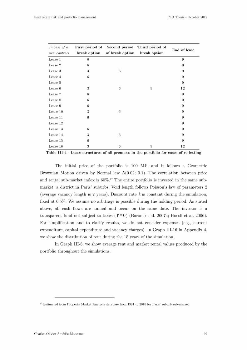
Real estate risk and portfolio management PhD Thesis - October 2012
Charles-Olivier Amédée-Manesme 92
Table III-4 - Lease structures of all premises in the portfolio for cases of re-letting
The initial price of the portfolio is 100 M€, and it follows a Geometric
Brownian Motion driven by Normal law N(0.02; 0.1). The correlation between price
and rental sub-market index is 60%.17 The entire portfolio is invested in the same sub-
market, a district in Paris’ suburbs. Void length follows Poisson’s law of parameters 2
(average vacancy length is 2 years). Discount rate k is constant during the simulation,
fixed at 6.5%. We assume no arbitrage is possible during the holding period. As stated
above, all cash flows are annual and occur on the same date. The investor is a
transparent fund not subject to taxes ( 0τ = ) (Baroni et al. 2007a; Hoesli et al. 2006).
For simplification and to clarify results, we do not consider expenses (e.g., current
expenditure, capital expenditure and vacancy charges). In Graph III-16 in Appendix 4,
we show the distribution of rent during the 15 years of the simulation.
In Graph III-8, we show average rent and market rental values produced by the
portfolio throughout the simulations.
17 Estimated from Property Market Analysis database from 1981 to 2010 for Paris’ suburb sub-market.
In case of a
new contract
First period of
break option
Second period
of break option
Third period of
break optionEnd of lease
Lease 1 6 9
Lease 2 6 9
Lease 3 3 6 9
Lease 4 6 9
Lease 5 9
Lease 6 3 6 9 12
Lease 7 6 9
Lease 8 6 9
Lease 9 6 9
Lease 10 3 6 9
Lease 11 6 9
Lease 12 9
Lease 13 6 9
Lease 14 3 6 9
Lease 15 6 9
Lease 16 3 6 9 12

Real estate risk and portfolio management PhD Thesis - October 2012
Charles-Olivier Amédée-Manesme 93
Graph III-8 - Average rent and market rental value produced by the portfolio
The model also displays average rent paid for each lease, so risky leases can be
forecasted and analyzed, which assist decision-making.
B. Sensitivity analysis and model limitations
We analyze sensitivity of the model to length of vacancy (λ) and criteria for the
decision to move, the moving criteria decision (α). We highlight the robustness of the
model, but note some of its limitations. Sensitivity analysis is conducted using the
previous portfolio under the same initial conditions; the only changes are λ and α.
Both parameters impact vacancies (on vacancy probability or length). The
criterion for the decision to move increases or decreases the number of break options
exercised and therefore must have a large impact on vacancies. Average length of
vacancy determines how long a space remains vacant and therefore how long it
generates costs instead of revenues. Graphs represent the sum of expected rent (Graph
III-9, Graph III-10 and Graph III-11), portfolio value (Graph III-12) and associated
standard errors.
As predicted, expected rent decreases when length of vacancy increases. At the
same time, rent decreases when the moving criteria decision applies more strictly (α =
0, for example). It is interesting to note that rent produced by the portfolio is affected
more strongly by length of vacancy over time than by moving criteria. This is due to
the lease structure. Once a tenant signs a new lease at rent close to the market rental

Real estate risk and portfolio management PhD Thesis - October 2012
Charles-Olivier Amédée-Manesme 94
value, predictable income is usually secured for some years, and the impact on cash
flow is far less. Risk associated with these two parameters is represented by standard
errors. The graph demonstrates that these two parameters have a large influence on
the risk of portfolio value and also on risk associated with resulting cash flows. This
result is consistent with investor fear concerning risk of vacancy. They usually
understand this vacancy consists of costs it generates and the time it takes to re-let.
Results strengthen evidence that vacancy is the most important factor influencing the
value of a classic asset (for high-yield assets, vacancy has a higher impact with respect
to cash flow volatility than low-yield assets). At the same time, volatility of the cash
flow is barely influenced by length of vacancy when costs of moving are high. This
highlights the interest investors have in making improvements chargeable to tenants so
enhanced future cash flows are secured. According to this framework, landlords should
pay for maintenance or refurbishment in exchange for surrender of break options.
Graph III-9 - Expectation and standard error of rent in the portfolio as a function of
the moving criterion decision (α) and expected length of vacancy (λ).

Real estate risk and portfolio management PhD Thesis - October 2012
Charles-Olivier Amédée-Manesme 95
Graph III-10 - Expectation of rent in the portfolio as a function of either the moving
criterion decision (α) or expected length of vacancy (λ).
Graph III-11 - Standard error of rent in the portfolio as a function of either the moving
criterion decision (α) or expected length of vacancy (λ).
Graph III-12 - Expectation and standard error of price of the portfolio as a function of
the moving criterion decision (α) and expected length of vacancy (λ).

Real estate risk and portfolio management PhD Thesis - October 2012
Charles-Olivier Amédée-Manesme 96
One of the most obvious limitations of the model is the assumption of tenant
rational behavior. Although this assumption is classic, it is not always verified.
Tenants do not always behave rationally in the sense of being driven only by financial
considerations, though commercial real estate is a factor of production. Many factors
influence a decision to move such as availability of space, social impact, routine,
communication, mergers and acquisitions. In some rare cases, the landlord is tempted
to give a discount to short-term tenants according to elasticity of demand. Barker
(2003) develops a model in which landlords consider both turnover and demand
elasticity.
Even if this assumption is questionable, we do not believe it represents a major
issue. Particularly in continental Europe, rent is usually in line with market rental
values available for similar premises, and this is precisely because of the prospects of a
break option being open to tenants. Negotiations over rent are common when break
options approach. A landlord concedes financial incentives (free rent or improvements)
or even rent reduction so vacancy or movement to a new, longer lease is avoided.
Further research that includes utility functions would elucidate this limitation.
Another limitation is inherent to real estate as an asset class, due largely to
lack of data. We implicitly suppose a normal law drives both market rental values and
terminal values of the portfolio in absence of data that define a more specific law. This
assumption is weak but common, but does not affect the relevance of the model. The
model can be adapted by using another law or other simulation method (e.g.,
bootstrapping, neuronal methods, introducing extreme values etc.). The difficulty lies
in a lack of data for all periods. In continental Europe, indices are generally annual
(sometimes biannual), and do not cover all sub-markets in which portfolios are
invested. Thus, it is difficult to calibrate a model with sparse data. The U.K. is an
exception in that it provides monthly indices, but U.K. leases are characterized by
length and lack break options (generally an upward-only rent review every five years).
Our model is less applicable to this country even if standard leases in the U.K. change.
Another limitation is the possibility of negotiation, which is not considered in
our proposal. Practitioners often negotiate when they anticipate lease breaks. Their
objectives include securing future cash flows and maximizing value of the properties
managed. They usually try to maintain tenants on the premises to prevent vacancy by
negotiating long before a break-option. We envisage solutions to this issue. These
include utility functions for a tenant or a negotiation model used in labor economics
fields, modified slightly for real estate investment management. Practitioners (tenants
or landlords) can also use our model as an aid to negotiation to determine the impact
of a future break-option on the value of a portfolio or to determine the range of

Real estate risk and portfolio management PhD Thesis - October 2012
Charles-Olivier Amédée-Manesme 97
possibilities in rent negotiation, from which rent reduction is better than vacancy. We
hope to propose negotiation as an addition to the model in a future research.
V. Conclusion
We propose a new method for valuation of a real estate portfolio using Monte
Carlo simulation and options to compute price. We suggest a way of incorporating
lease structure risk into the valuation process. The principal improvement in our
proposal is considering break options offered to tenants in various lease structures. The
model considers tenant behavior with regard to cash flows, and shows its impact on
portfolio value by combining Monte Carlo methods for portfolio price under various
market rental values. For each simulated scenario and for each lease at the time of a
break option, we compare current rent with market rental value available for similar
spaces, and assume financial rationality to decide whether the tenant moves. Poisson’s
law determines length of vacancy. From a practitioner’s viewpoint, the model can be
used to compute more robust valuations of a real estate portfolio, but reporting and
risk assessment above all. Practitioners should find interesting the possibility that the
model confers on displaying a histogram or a distribution function instead of a fixed
value. A need for fair value of real estate portfolios remains. The problem in
application is finding the inputs the model requires such as trends and volatilities of
each sub-market. Our approach is flexible; many parameters can be introduced and
applied to suit assumptions and needs of each investor.
This study opens the way to many other fields of real estate finance, risk
management particularly. Using sensitivity analysis, we demonstrate the extent to
which cash flow knowledge is of valuable assistance to risk measurement and in
negotiations between landlord and tenant. Using Monte Carlo methods, we obtain a
range of outcomes instead of a fixed result. Risk associated with a portfolio or a
specific asset is thereby estimated better. The model, along with the distribution of its
results, allows us to compute a portfolio’s VaR. Both regulators and investors
increasingly require such risk measures. Developing our approach in this direction -
and providing robust tools for management and assessment of risk - is the objective of
future research.
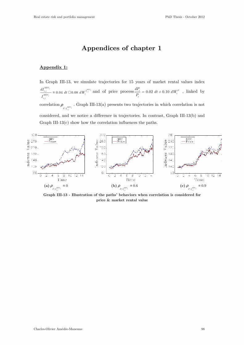
Real estate risk and portfolio management PhD Thesis - October 2012
Charles-Olivier Amédée-Manesme 98
Appendices of chapter 1
Appendix 1:
In Graph III-13, we simulate trajectories for 15 years of market rental values index
,,
,
0.04 0.08j
MRVjt j
j
MRV
It j
tMRV
t j
dIdt dW
I= + and of price process 0.02 0.10 Pt
t
t
dP= dt + dW
P , linked by
correlation,/MRVjt jP I
ρ . Graph III-13(a) presents two trajectories in which correlation is not
considered, and we notice a difference in trajectories. In contrast, Graph III-13(b) and
Graph III-13(c) show how the correlation influences the paths.
(a),/
0MRVjt jP I
ρ = (b),/
0.6MRVjt jP I
ρ = (c),/
0.9MRVjt jP I
ρ =
Graph III-13 - Illustration of the paths’ behaviors when correlation is considered for
price & market rental value

Real estate risk and portfolio management PhD Thesis - October 2012
Charles-Olivier Amédée-Manesme 99
Appendix 2:
(a) - Histogram of rent after period 1 (b) - Histogram of rent after period 4
(c) - Histogram of rent after period 8 (d) - Histogram of rent after period 14
Graph III-14 - Histogram of rent in a French lease for t = 1, …,15.
Note: In the histograms, rent is not discounted, and values on the abscissas do not have to be compared. The distribution of values remains relevant.
Graph III-14 shows the transformation of the distribution throughout a
traditional French lease. It illustrates the importance of considering a break option.
These options influence the distribution of values rent takes.
(a) - Until period 3, all rent produced are equal, and therefore the distribution
concentrates at one point;
(b) - After the first break option (period 4) values primarily concentrate two
points, including point 0 for all premises vacant after the exercise of the first break
option, and 107.6 = 100 x (1+2.5%)3 when the tenants stay on the property. Some
other points appear in the distribution, attributed to scenarios where the premises find
a new tenant immediately. Thus, the transformation is visible after year 3 (at year 4).
At this point, a significant part of rent is 0, representing the simulated state of the
market when the space became vacant. This highlights the extent to which vacancy
influences the distribution of cash flows. During the two following periods, no break
options can be exercised.

Real estate risk and portfolio management PhD Thesis - October 2012
Charles-Olivier Amédée-Manesme 100
(c) - This point occurs after the second break-option, if the first was not
exercised. We observe an increase in the number of vacant spaces, which demonstrates
some tenants exercised the option. This period exhibits the break options of tenants
who contracted a lease after departure of the first tenants. The small number of
tenants involved is not obvious.
(d) - The distribution distorts after the end of the lease (year 9) when the
landlord negotiates rent equal to market rental value. After year 9, all states of the
market are possible because the landlord and tenant are supposed—under our
assumption of rational behavior—to conclude a contract at market value.
Appendix 3
Graph III-15 - Leases during the holding period of the portfolio
t=0Lease #
Lease 12
Lease 13
-3 -2 -1
t = 1
t = 1
6 8 9
t = 8 = 11t = 5
t = 4
t = 3
t = 6
t = 4
Lease 15
10 11 121 2 3 4 5Periods
t = 6 t = 9
t = 6
7
t = 4 t = 7
t = 5
Lease 16
Lease 1
Lease 2
Lease 3
Lease 4
Lease 5
Lease 6
Lease 8
Lease 9
Lease 10
Lease 11
Lease 7
Lease 14
t = 2
t = 3
t = 2
Time 0
Acquisition of the
portfolio
t = 5 t = 8
t = 8 = 11t = 5
t = 7t = 1
t = 2
t = 8
t = 9t = 6

Real estate risk and portfolio management PhD Thesis - October 2012
Charles-Olivier Amédée-Manesme 101
Appendix 4
(a) (b) (c)
(d) (e) (f)
(g) (h) (i)
(j) (k) (l)
(m) (n) (o)
Graph III-16 - Histogram of rent produced by the portfolio annually over 15 years.

Real estate risk and portfolio management PhD Thesis - October 2012
Charles-Olivier Amédée-Manesme 102
Comments on Graph III-16:
(a) - This is just after the first-period differences appear, due to the vacant
space that can be let, or not, during the first period.
(g) - The distribution of rent produced at year 7 is noticeable and shows that
this year is especially risky for the portfolio. This can be translated into action for
portfolio management. For example, knowing risk, the decision could be to secure cash
flows for this year either by buying portfolio insurance or renegotiating the lease in
advance, selling one risky asset, or buying another one to mitigate risk in the same
year. Letting and vacancy risk are therefore valued.
(o) - The distribution of rent is spread, and possibilities are multiple. It is
possible to compute the probability of loss in rental level or the probability of rent
falling below a specified amount.

Real estate risk and portfolio management PhD Thesis - October 2012
Charles-Olivier Amédée-Manesme 103
Chapter IV. Optimal Holding Periods of a
Real Estate Portfolio
according to the Leases1
The idea for this study came from a previous paper written by Baroni et al.
(2007b). That paper proposes a closed formula to obtain the optimal time to sell a real
estate portfolio. Using a similar approach, we compute the optimal holding period, but
we improve the previous model by adding options included in a lease. Options modify
income distributions and therefore the value distribution. This work is in line with
Baroni et al. (2007b) and is a companion article for the paper presented in chapter III.
This chapter deals with the holding period of a fund or portfolio; the question
is a traditional one in finance. In real estate finance, this issue is not often addressed
correctly since free cash flows come primarily from rent, and break-options are not
usually considered. A portfolio replicates market income globally, but it has long been
demonstrated that specific risk requires a very large number of assets2 to be
diversified, which is generally not attainable. Considering options to vacate in a real
estate portfolio is thus fundamental. Since a diversified portfolio is difficult to obtain,
idiosyncratic risk is never diversified correctly, and thus it is important to account for
break options, which are one off - if not the - most important specific risks faced by
real estate investors. We propose a model to determine the optimal holding period of a
real estate portfolio that integrates real estate specific risk such as break options. We
do not interpret the holding period as the point where value is maximized; we also
consider when cash flow risks are minimized. Investors and real estate fund managers
might be interested in this interpretation of optimal time to sell, which not only
1 This article was written with Michel Baroni (Essec Business School) and Fabrice Barthélémy (University of
Cergy-Pontoise). At the time, this thesis is written, the paper has been submitted to the Journal of Property
investment and Finance, Emerald. In 2012, this paper was presented at an international conference, the American
Real Estate Society. We received positive comments from attendees and improved the paper by following some
recommendations. The author would like to thank the participants of the ARES conference who give their views
and comments about the paper. 2 See literature review part I chap. 2.

Real estate risk and portfolio management PhD Thesis - October 2012
Charles-Olivier Amédée-Manesme 104
considers price risk, but also cash flow risk. Contrary to bonds that deliver recurrent
cash flows, properties can be vacant (at least some units), and consequently, they
generate more costs than revenues during a period. They become competitive again
when the unit(s) is (are) relet (a bond that stops its debt service payment generally
harbors problems), and will never reimburse the owner. The purpose of this chapter is
to account for break-options in the holding period decision using our previously
proposed model (chapter III of this thesis). The chapter follows extant studies Baroni
et al. (2007a, 2007b), which introduce risk in the holding period decision, but do not
consider break clauses included in leases.
This chapter relies on both the previously presented method and another
model developed by Baroni et al. (2007b). The model proposed by Baroni et al. (op.
cit.) determines the optimal holding period of a real estate portfolio. However, the
model does not consider options in a lease. They use binomial law that accounts for
changes in the occupancy rate of properties, and therefore considers changes in rent
(the inflows). We combine option theory and Monte Carlo simulation to account for
both specific and market risks, and determine the optimal time to sell a real estate
portfolio. For each scenario, we determine the time that maximizes price of the
portfolio while considering breaks. We then take the average of all simulated scenarios
and obtain the optimal holding period. The method analyzes essential parameters that
influence the holding period and determine the best lease structure for the holding
period desired or given expected future market conditions.
Little research examines holding periods for real estate portfolios. However,
recently, this topic was the subject of a few publications (Barthélémy and Prigent,
2009, 2011; Cheng et al., 2010a, 2010b, 2010c), but none consider vacancies in holding
period decisions even if they are essential to account for specific risk. This article fills
this gap by studying the effect of break-options on optimal holding period. It considers
vacancies and especially concentrates on the effect of these vacancies on cash flows.
This chapter involves comparison with an extant article in real estate portfolio
management, Baroni et al. (2007b), which uses a similar method but does not consider
options. The chapter demonstrates differences that occur when options are considered.
It is demonstrated that accomplishable objectives in terms of returns and portfolio
management are modified with these specifications considered. The purpose is not to
predict optimal holding period, but to analyze the effect regarding its impact on the
holding period of market parameters. Results of this study provide advice to real
estate investors and strategists.

Real estate risk and portfolio management PhD Thesis - October 2012
Charles-Olivier Amédée-Manesme 105
I. Introduction
Optimal holding period in real estate portfolio management is a recent issue.
Institutional investors realized recently the importance of holding period for managing
the risk of real estate assets or, more generally, real estate portfolios. For many years,
real estate portfolio investment was a passive investment in which investors were
buying real estate, mature asset that generated recurring cash flows (rent). The
traditional strategy was to hold real estate over many years, corroborated by large
transaction costs and limited liquidity of real estate investments. Few institutional
investors bought opportunistic or value-added assets held for shorter periods. This
typology of assets was reserved for developers, some opportunistic funds and
specialized REITs. Given the specialization and sophistication of the real estate
practice and industry, investors now examine the holding period of a real estate asset
or portfolio as a parameter to consider when investing. The holding period is still
regarded as only one parameter, dependent on either lease structure or length life of a
fund instead of based on a result computed from expectations of the economy or real
estate market (e.g., initial yields, future developments and rental values evolutions).
Underneath this reasoning lays the criterion of liquidity, a key issue for investors. An
asset leased for a long period is more liquid than a short-term leased asset, even in a
bull market. Many investors look for long-term leases without break-options because
they do not want to bear leasing risk. According to the local market, they look for
long-term leases (e.g., 10-year leases) and sell the asset after a few years (e.g., 5 years)
to an investor interested in asset management challenges, negotiations and marketing.
They adapt the holding period strategy to lease structure.
Investors adjust holding period strategies in real estate based on lease
structure. This can be explained through the various kinds of investors in real estate.
Often for purely technical reasons, a finite holding period (conventionally 10 years in
corporate finance) is used in cash flow projections to avoid an infinitely long (>30
years) cash flow series. The choice of holding period in cash flow projections must fit
either the exit strategy or investors’ intentions (some close-ended funds have finite lives
and constrain the initial strategy). If the predefined holding period is short, the weight
of terminal value in net present value is more important, and risk expected from
calculation of this value is also more important. From our viewpoint, investors project
to sell a property for three reasons:
- The property was managed intensively and no further asset
management is envisioned. Asset managers often argue that

Real estate risk and portfolio management PhD Thesis - October 2012
Charles-Olivier Amédée-Manesme 106
their work consists of managing a property by securing tenants
(lease and relation) and conducting work on the property such
as change in property use, energy consumption, security,
parking, cleaning etc).
- The asset belongs to a portfolio for which an exit strategy was
defined. Depending on the strategy of portfolio management
chosen by the investor, the policy regarding resale may be
different. Core investors were once interested only in long-term
leases without break-options, and sold all properties when the
lease lengths were below a certain duration (e.g., 5 years). An
opportunistic investor who seeks large capital returns might be
interested only in properties that require huge asset
management such as repositioning or refurbishment. The
investor sells properties as soon as they are secured.
- The asset does not accurately fit the portfolio. This might be
the case when too many leasing risks are concentrated on the
same period or when market rental values are far lower than
current rent.
All of these cases have a common point; the property is sold when the
remaining lease duration is long enough to make the property attractive and liquid.
Selling an obsolete, vacant property is never a goal in a business plan that optimizes
portfolio value. An investor has to solve this opportunity, which occurs during the
holding period. The buyer must bear vacancy and redevelopment risks, and thus might
state a price that incorporates this risk (such as a large discount).
Our purpose is to consider risk linked to lease structure in future cash flows
and determine how considering lease structure of a property modifies the optimal
duration of a real estate portfolio. Given the behavior of a landlord in terms of holding
period is driven primarily by lease structure, we model changes in holding period due
to lease structure. This is achieved through a combination of Monte Carlo simulations
for evolutions of terminal values and market rental values and option theory to
simulate the exercising of break-options.
One of the improvements of this article is consideration of idiosyncratic risk,
essential because real estate portfolios require a very large number of assets to
diversify specific risk (Brown, 1998; Byrne and Lee, 2001; Callender et al., 2007).
Generally, investors do not hold sufficient assets to diversify specific risk. Considering
specific risk improves real estate portfolio management and, particularly, the holding
period. If the market is replicated, the optimal holding period can be computed using

Real estate risk and portfolio management PhD Thesis - October 2012
Charles-Olivier Amédée-Manesme 107
market data alone. If the market is not replicated (generally the case in real estate),
the optimal holding period must consider specific risk of the portfolio, including
leasing risk as a fundamental risk.
The structure of the chapter is as follows. After a section dedicated to
literature, Section 3 provides a survey concerning lease structure, with focus on
European lease structures, and presents a model in which lease structure is considered
in cash flows. This section serves as a brief reminder of the previous model (chapter 3).
Section 4 demonstrates that the classic DCF method does not allow computing
optimal holding period. Results from extant research, in which a trend is incorporated
in terminal values, are also presented. Section 5 shows that the optimal holding period
reacts to changes in some parameters and lease structures. Section 6 is a conclusion.
II. Literature
Real estate holding period has been an issue for real estate academicians and
practitioners for a long time. It is an essential component of investment in commercial
real estate portfolios. However, results concerning optimality of a holding period are
nearly exclusively empirical. Presumably, it depends on many factors, including market
conditions, transactions costs, types of property, lease length, strategy and others.
Holding period is a classic issue in finance and has been the subject of many studies.
The issue has been studied for a long time in stock literature. Demsetz (1968)
and Tinic (1972) notice transaction costs influence holding periods. Amihud and
Mendelson (1986) show that assets with high bid-ask spreads (a proxy for high
transaction costs) are held at equilibrium by investors who expect to hold assets for a
long time. Atkin and Dyl (1997) in an empirical research consider the effects of firm
size, bid-ask spread and volatility of returns on holding periods of stocks for a sample
of 2000 NASDAQ firms and 500 to 1100 NYSE firms from 1981 to 1993. They
demonstrate a positive correlation between holding period and transaction costs and
firm size, and a negative one between holding period and price variability. Two
assertions are generally accepted in stock literature: large transaction costs drive
investors to hold assets for a long time and substantial volatility drives investors to
hold an asset for a shorter period. Real estate assets exhibit these two features: high
transaction costs and large volatility, the reason optimal holding period represents a
challenge for real estate academicians and practitioners.

Real estate risk and portfolio management PhD Thesis - October 2012
Charles-Olivier Amédée-Manesme 108
Real estate holding periods are the topic of many empirical studies, but no
consensus emerges and the literature is sparse. For the U.S., Hendershott and Ling
(1984), Gau and Wang (1994) and Fisher and Young (2000) argue holding durations
are conditioned by tax laws. For the U.K., the relationship between returns and
holding periods appears complex. In a study using investor interviews, Rowley et al.
(1998) show investors and new property developers have a holding period in mind from
the beginning. They conclude that for offices, a holding period decision links to
depreciation and obsolescence factors. For retail property, the decision is empirical,
depending on active management and the state of the market. In a more recent article,
Collett et al. (2003) highlight knowledge of a holding period is important in a decision
to invest in commercial real estate portfolios. Investment appraisal requires specifying
an analysis period, and asset allocation depends on variances and covariances of assets
influenced by a reference interval or analysis. Using the database of properties
provided by IPD in the U.K. over an 18-year period, they conclude the median holding
period is about seven years. Sales rates vary across the holding period (probably due
to rent cycles and lease structures), and the holding period varies by property type.
The larger and more expensive the properties, the longer the holding periods. If the
return is greater, the holding period is shorter. However, they are unable to propose
conclusions about a link between volatility and holding period because of absence of a
proxy to measure the relationship. For small residential investments, Brown and
Geurts (2005) offer an empirical response to the following questions: how long does an
investor own an apartment building and why do investors sell some property more
frequently than others do? Through a sample of apartment buildings of between 5 and
20 units over the period 1970 to 1990 in San Diego, they found the average holding
period is approximately five years. They propose investors sell property sooner when
values rise faster than rent. Brown (2004) shows that considering risk peculiar to real
estate investments explains the reason for owning real estate by private investors and
their buy-sell behaviors. Applying the CAPM for individuals to understand portfolio
management does not drive relevant results as demonstrated by Geltner et al. (2006).
For residential real estate, Cheng et al. (2010c) demonstrate higher illiquidity and
transaction costs lead to longer holding periods, while higher return volatility implies
shorter holding periods. These results are consistent with previous articles regarding
financial assets.
Following a different approach, Baroni et al. (2007a) propose using dynamic
cash flows for rent inflows and terminal values in a real estate portfolio. These
dynamics are simple diffusion processes in which corresponding parameters are the
trend and volatility for rent and price, respectively. These parameters are estimated

Real estate risk and portfolio management PhD Thesis - October 2012
Charles-Olivier Amédée-Manesme 109
from a rent index and a real estate index using Paris data, considering the correlation
between these two indices. This approach suggests an interesting role played by the
holding duration in the determination of asset value. Baroni et al. (2007b) determine
optimal holding period when chosen initially. They model terminal values as diffusion
processes, and derive a closed formula for optimal holding period under conditions of
parameters. Barthélémy and Prigent (2009) also examine determination of optimal
holding period (optimal time to sell in a real estate portfolio), considering knowledge
the investor holds concerning the probability distribution of the real estate index.
Barthélémy and Prigent (2011) provide another study on the holding period topic in
real estate when risk aversion is considered.
To our knowledge, the existing academic literature on holding periods does not
consider lease structure an essential decision factor. However, many investors
determine a strategy as a function of the lease and not of the market or state of the
economy. We propose considering the lease structure to determine the optimal holding
period for a fund. The next sections introduce the optimization model and the model
on which we rely to consider the leases. We start with a review of extant models for
real estate portfolio holding periods.
III. Optimal holding period with traditional discounted cash
flow (DCF)
Most investors originally used the DCF framework to evaluate portfolios. We
demonstrate this framework is inappropriate to compute an optimal holding period for
a portfolio of real estate assets. The traditional, deterministic DCF model calculates
net present value that is the sum of all the future cash flows generated by the asset
discounted by a discount rate. Denote 0,TP the net present value of the asset sold at
date T.
( ) ( )0,1 1 1
Tt T
T t Tt
FCF TVP
k k=
= ++ +
∑
where k is usually the weighted average cost of capital (WACC) used to
discount the various free cash flows t
FCF , and T
TV is the terminal value computed as:
(1 )=
- T
T
FCF gTV
k g∞
∞
+

Real estate risk and portfolio management PhD Thesis - October 2012
Charles-Olivier Amédée-Manesme 110
where free cash flow (FCF) after time T grows infinitely at constant rate g∞ .
If we denote g the growth rate of the free cash flows before time T, the equation
becomes:
( )( )
( ) ( )( ) ( )
1 1
1 1
0,1
1 1 1
1 1
t TT
T t Tt
FCF g FCF g gP
k k g k
− −
∞
=∞
+ + += +
+ − +∑
Baroni et al. (2007b) demonstrate the behavior of price can be studied by
computing 0, 1 0,T TP P+ − .
( )( )
1
0, 1 0, 1
1
1
T
T T T
g g gP P FCF
k gk
−
∞+
∞
+ −− = − +
The sign on the right part of equation corresponds to the sign of g g∞− . We
then have the following states:
If g g∞> then 0, 1 0,
0T T
P P+ − > and the price grows infinitely;
If g g∞= then 0, 1 0,
0T T
P P+ − = and the price does not move;
If g g∞< then 0, 1 0,
0T T
P P+ − < and the price decreases infinitely.
With 8.40%k = , 4%g = , 3%g∞ = and 11FCF = , Graph IV-1 illustrates the
monotonous character of the function with the DCF approach. Graph IV-2
corresponds to a case where a loss in terminal value is balanced by a gain in cash flow:
g g∞= . Graph IV-3 is obtained with 4.5%g∞ = .
Graph IV-1 - Increase of the portfolio present value with the DCF approach ( g g∞> )
18
18,5
19
19,5
20
20,5
21
21,5
22
0 5 10 15 20 25 30
P(0
,T)
Holding period (T)
Portfolio(0,T)

Real estate risk and portfolio management PhD Thesis - October 2012
Charles-Olivier Amédée-Manesme 111
Graph IV-2 - Constant present value of a portfolio with the DCF approach ( g g∞= )
Graph IV-3 - Decrease of the portfolio present value with the DCF approach ( g g∞< )
The traditional DCF framework cannot allow an optimal holding period for a
portfolio, according to the asset present value, whatever the rates of expected growth
are.
We now introduce a model developed by Baroni et al. (2007b) that leads to a
closed formula.
02468
101214161820
0 5 10 15 20 25 30
P(0
,T)
Holding period (T)
Sum_(t<=T) FCF(0,t) TV(0,T)
23,5
24
24,5
25
25,5
26
0 5 10 15 20 25 30
P(0
,T)
Holding period (T)
Portfolio(0,T)
Portfolio(0,T)

Real estate risk and portfolio management PhD Thesis - October 2012
Charles-Olivier Amédée-Manesme 112
IV. Optimal holding period incorporating risk in the terminal
value (Baroni, Barthélémy and Mokrane, 2007b)
Baroni et al. (2007a) propose Monte Carlo simulation in valuation, and their
contribution is modeling terminal value. They consider the real estate price of the
assets follows geometric Brownian motion (versus an infinite growth rate with
traditional DCF):
t
P P t
t
dPdt dW
Pµ σ= +
This equation assumes real estate returns can be modeled as a simple diffusion
process where parameters P
µ and P
σ are the trend and volatility. They propose this
modeling to improve the DCF method to allow an optimal detention period. They
then compare this new approach with the discrete case derived in the previous section.
Following Baroni et al. (2007b), the expected present value of the asset sold at
date T is:
( )( ) ( )0,
1
E1 1
Tt T
T t Tt
FCF PP
k k=
= ++ +
∑
with TP
computed using Brownian process ( , )µ σ and
( )0( ) 1
T
TE P P µ= +
The expected growth rate of the price is:
( )( )
( ) ( ) ( )0, 1 0, 1 01
1E 1 1
1
T T
T T TP P FCF g P k
kµ µ+ +
− = + + + − +
They conclude two cases be considered:
- kµ = , hence, there is no optimal holding period;
- kµ ≠ , an optimal sell date (under existing conditions) may
exist and is obtained by a closed formula3:
( )1
0*
ln
1ln
1
FCF
P kT
g
µ
µ
− = + +
3 The optimal holding period does not depend on the standard deviation parameter (
Pσ )

Real estate risk and portfolio management PhD Thesis - October 2012
Charles-Olivier Amédée-Manesme 113
This formula determines the conditions under which an optimal solution exists.
The conditions can be summarized by:
1
0
max ,FCF
g k kP
µ
− < <
An optimal holding period for a real estate portfolio can be thus derived.
Using the same example but simply adding a trend that fills conditions
8.40%k = , 3%g = , 4.5%P
µ = , σP = 5%, 021P = and 1
1FCF = , we derive an optimal
holding period of about 13.81 years. Here, the free cash flows periodicity corresponds
to one year.
Graph IV-4 - Optimal holding period of the portfolio value when a terminal value is
simulated
Similarly, we consider risk from a terminal value and market rental value, but
add a fundamental risk factor: one related to lease structure. This is possible from
previous paper (chapter 3).
V. The break-option: optimal holding period incorporating risk
in terminal value and lease structure (Amédée-Manesme, Baroni,
Barthélémy and Dupuy, 2012)
For core investors, real estate assets are cash flow-generating assets and
properties, purchased primarily for the rent they generate. One of the most essential
determinants of cash flow in real estate investment (particularly commercial real
20,8
21
21,2
21,4
21,6
21,8
22
22,2
0 5 10 15 20 25 30
P(0
,T)
Holding period (T)

Real estate risk and portfolio management PhD Thesis - October 2012
Charles-Olivier Amédée-Manesme 114
estate) is the lease that stipulates the conditions under which the property is let.
Regulating rights and obligations of the landlord and the tenant, the lease provides
information concerning expected cash flows for years ahead. A lease specifies a starting
date, initial rent, lease expiration date, indexation rules, and options available to the
tenant to leave the premises before the lease expires. These last options are called
break (sometimes renewal) options. They are a particular feature of continental Europe
leases, and one of the most important risks European real estate investors face. In
Europe, lease structures vary from country to country, and are even more different in
the U.K. Information on lease structure is thus an essential component of any cash
flow model. However, a property may be vacant (sometimes partially) and may
generate more costs4 than revenue. Vacancy is an essential issue for real estate
investment, particularly for cash flow forecasting. Departure of a tenant is essential
when valuing future cash flows.
A break option is an asymmetric right in favor of the tenant: at the time of a
break option (usually fixed in the lease), the tenant has the right, but not the
obligation to terminate the lease. For various reasons, a tenant may leave at the time
of a break option. Therefore, break options cause vacancy and a hiatus in cash flows,
and this represents the principal cash flow risk borne by investors. A vacant space
incurs costs and offers no revenue. In addition, the premises may become outdated or
more quickly obsolete, and thus also involves increased risk of capital loss. Previous
academic studies of rental contracts such as Miceli and Sirmans (1999) suggest
landlords attempt to minimize vacancy and turnover costs by offering discounts to
long-term tenants. Landlords often try to dissuade a tenant from leaving at the dates
fixed by the lease by offering discounts or free rent. In this way, they minimize the
number of break-options (again, information concerning break clauses is reported in
the general introduction to this thesis).
Lease structure risk is crucial when considering real estate investment,
particularly in the context of optimal holding period. A property with a short-term
lease bears more leasing risk, and therefore may be less liquid. When future cash flows
are projected, considering a tenant may leave is essential, and it may have a huge
impact on terminal value and the holding period. In the following model, the impact
4 As any commodity or product traded in a free market, supply and demand control rent. If a rental property is priced above current market value, competitively priced properties rent while overpriced properties sit vacant. A property does not keep efficiency without a minimum investment. A vacant property requires substantial investment in addition to recurrent costs (e.g., local taxes, security, technical control etc.). Vacancy cost is therefore the money estimated in consequence to vacancy.

Real estate risk and portfolio management PhD Thesis - October 2012
Charles-Olivier Amédée-Manesme 115
on holding period is considered by assuming terminal value is subject to systematic
risk only.
A. The model
In the previous chapter (paper), we present a model that we briefly remind
here. Chapter III presenting Amédée-Manesme et al. (2012) develop a model that
considers lease structures (and therefore break-options) of a real estate portfolio. We
improve existing commercial real estate valuation methods by introducing uncertainty
and risk into the valuation process. The problem is modeling the exercise of the break-
option, and in case of exercise, to determine how long a vacant space can remain
vacant.5 The model offers answers to these questions by considering risk underlying the
lease structure, the risk the rent on the exercise date of the break-option is greater
than the market rental value. Obviously, agency costs (e.g., moving costs, transaction
costs etc.) also must be considered. Both Monte Carlo simulation and option theory to
model a tenant’s decision are combined to simulate future cash flows. The model
incorporates uncertainty in the determination of terminal value. Both the price of the
portfolio (P) and market rental values (MRV) are simulated as diffusion processes:
Pt
P P t
t
dPdt dW
Pµ σ= +
MRVt
MRV MRVt t
MRVIt
tMRV I I
t
dIdt dW
Iµ σ= +
These equations assume real estate prices and real estate rental values can be
modeled as Brownian diffusion process where parameters P
µ and ,
jMRV
t jI
µ are the price
and market rental value index trends and P
σ and
,
jMRV
t jI
σ the price and market rental
value index volatilities. The correlation between market rental values and terminal
value is also considered. Market rental value is modeled as index MRV
tI , but the size of
the spaces and other characteristics can be considered. Generally, two spaces located in
the same property follow the same index, but differ by rent, size and specifications
5 The space may be let or not. If let, depending on the terms of the contract, the tenant enjoys the possibility of leaving at a predetermined date during the length of the lease (the break option). When the lease terminates, both tenant and landlord decide to either continue with the lease or not, eventually with some limitations. The end of the lease is also a break option, but symmetric since both tenant and landlord can exercise it even if it implies costs. Uncertainty regarding changes in rent over time arises from the possibilities a break option will be exercised, and the length of vacancy periods

Real estate risk and portfolio management PhD Thesis - October 2012
Charles-Olivier Amédée-Manesme 116
(e.g., floors, A/C system, orientation etc.). However, rent is not necessarily equal to
market rental value, so the model compares rent currently paid to simulated rental
values. A rational tenant exercises a break-option as soon as the rent currently paid is
too high in comparison with the market rental values available for similar spaces.
Therefore, the tenant leaves the space at the time of a break-option when rent is much
higher than market rental value. This is written as:
,
1,
,
1 , then 0t i
t i
t i
RentRent
MRVα +≥ + =
where α is a decision criteria (≥ 0 if the tenant is rational, including possible
moving costs, for example), ,t iRent is rent of the space i at time t, and is ,t i
MRV the
market rental value of space i at time t.
The model considers differences that arise between evolution of market rent
and rent contracted years before a break-option. Three factors are thus considered:
evolution of rent (or the ways they are revised), evolution of market rental values and
evolution of possible vacancies. As soon as a tenant vacates a space, the landlord faces
a void period. Length of vacancy (of the void period) is modeled using Poisson’s law.
( )!
keX P X k
k
λλ −
= =∼
where k is length of vacancy and λ is a positive real number equal to expected
number of occurrences during a given interval. In this case, it is equal to average
length of vacancy.
For each simulated scenario, we simulate a path of portfolio price and all paths
for each market rental value of each unit in the portfolio (all of them being correlated).
Simulated portfolio price is used in the discounted cash flow model as terminal value.
For each let unit and at the time of a break-option (if any), the current rent paid
(passing rent) is compared with simulated market rental value available for similar
spaces. In cases where rent paid is too high in comparison to market rental value, a
tenant vacates and the landlord might face a void in cash flows for the unit. Length of
vacancy is determined randomly following Poisson’s law, a parameter equal to average
vacancy length in the market. If a space is vacant initially, length of vacancy is also
determined using Poison’s law. Through an assumption of player rationality (tenants
and landlords), new leases are contracted at the market rental value of the unit. At
each period, we calculate the price of the portfolio (simulated) and the cash flows
produced by the units (some cash flows are 0 for vacant spaces). The price of the
portfolio can then be computed for each holding period. We replicate the procedure
thousands times and obtain a portfolio price for various holding periods. We thus

Real estate risk and portfolio management PhD Thesis - October 2012
Charles-Olivier Amédée-Manesme 117
obtain both averages of all scenarios and a distribution of prices for each holding
period.
For clarity of presentation and assuming rational behavior of the players, we
assume a new lease without vacancy at the end of a lease. In this sense, we assume
landlords and tenants negotiate and conclude a new lease at the MRV.
The model is based on a stochastic approach of the classic discounted cash flow
method, and incorporates both systematic (through simulation of price) and specific
(structure of lease) risk for each cash flow. This approach considers a tenant’s behavior
regarding break options included in a lease,6 and can be tailored to real portfolio
managers to manage portfolio risk. Managing portfolio risk is also useful to determine
the best time to sell a portfolio. We do this in the next section where we apply the
model to determine an optimal holding period.
B. Optimal holding period
Determining an analytic formula for optimal holding period of a real estate
portfolio when options embedded in the lease are considered is not possible. Following
Amédée-Manesme et al. (2012), we estimate optimal holding period of a real estate
fund when lease structures are considered. We consider the optimal holding period as
the one that maximizes portfolio value. The model differs from the model presented by
Baroni et al. (2007b) since numerous leases and introduction of break options are
considered. We simulate portfolio price and incorporate risk, but rent also incorporates
risk in the sense that the possibility of vacancy is considered lease by lease.
Nevertheless, rent is not simulated; only market rental values are simulated.
To demonstrate relevancy of the proposal and changes undergone by the
optimal holding period when the lease structure is examined, we consider for a
quantitative example the same parameters as do Baroni et al. (2007b); P0 = 100, FCF0
= 4.8, µP = 4.5% , σP = 5% , k = 8.4%, g = 3%. We consider one lease structure for
illustration purposes and for better understanding of the model. The portfolio holds
6 A space may be let or not. If let, the tenant has or does not have the possibility of leaving at a predetermined date during the term of the lease (the break option). When the lease terminates, both tenant and landlord can decide to either continue with the lease or not (with some limitations, which we consider irrelevant here). The end of the lease is therefore a break option, but symmetric since both tenant and landlord can exercise it even if often with varying costs. Uncertainty regarding changes in rent over time arises from possibilities that the break option will be exercised, and length of vacancy periods.

Real estate risk and portfolio management PhD Thesis - October 2012
Charles-Olivier Amédée-Manesme 118
one property (value = 100), which itself holds one lease ( 0 0= = 4.8Rent MRV ). In a
work-in-process article, numerous properties and leases are considered. To clarify this
section, we only take a simple case: 1 asset with 1 lease, otherwise the effect of the
model is not easily observed. For simplicity, we consider the lease starts in the first
period. We add the following parameters that refer to market rental values and the
lease: MRV0 = 4.8 (= FCF0), µR = 3% (= g), σR = 0 and λ = 07 and the lease
structure = 3/6/9 years (nine-year lease with options at years 3 and 6). Finally, we
consider the portfolio as a whole, and do not allow rebalancing or arbitrage.
We first simulate the base case and then change parameter by parameter to
demonstrate the influence of lease structures. Underlined parameters are those changed
from the base case or that must be noticed.
Base case: σR = 0: P0 = 100, FCF0 = 4.8, µP = 4.5%, σP = 5%, k = 8.4%, g = 3%,
MRV0 = FCF0, µR = 3%, n = 5 000, σR = 0, λ = 0, lease structure = 3/6/9, α = 0
Graph IV-5 - Optimal holding period without volatility of market rental values
In this base case, we obtain the same results as Baroni et al. (2007b) in which
rent follows a deterministic process. This is consistent with assumptions taken in this
base case where there is no volatility in the evolution of the MRV:
0 0
0R t t
R
MRV Rent
g MRV Rentµσ
=
= ==
7 Average lease length.

Real estate risk and portfolio management PhD Thesis - October 2012
Charles-Olivier Amédée-Manesme 119
The combination of the absence of volatility and the trend of the market rental
value equal to indexation leads to the same rent at each period. Therefore, no break-
options are exercised since rent is never higher than market rental value. This leads to
the same rent produced by Baroni et al. (2007b), and thus the same free cash flows.
We obtain the same optimal holding period of 14 years. A model without volatility can
be translated in a model where rent is indexed and price alone bears volatility. It is
important to note that absence of options exercised makes average vacancy length
meaningless.
Case 1: P0 = 100, FCF0 = 4.8, µP = 4.5%, σP = 5%, k = 8.4%, g = 3%, MRV0 =
FCF0, µR = 3%, n = 5 000, σR varies, λ = 0, lease structure = 3/6/9, α = 0
Graph IV-6 - Optimal holding period with market rent volatility
When the volatility of market rental values increases, optimal holding period
decreases. The market rental value does not follow rent, and in some paths, break-
options are exercised. We thus observe a decline in portfolio value due to the number
of break-options exercised. At each option exercised, rent is revised to a lower value
and the holding period decreases. We conclude that the optimal holding period
decreases when volatility of the market rental value increases. *
0R
dT
dσ<
This result follows the literature concerning stocks and bonds in which holding
period decreases when volatility of returns increases.

Real estate risk and portfolio management PhD Thesis - October 2012
Charles-Olivier Amédée-Manesme 120
Case 2: P0 = 100, FCF0 = 4.8, µP = 4.5%, σP = 5%, k = 8.4%, g = 3%, MRV0 =
FCF0, µR = 3%, n = 5 000, σR = 0.1%, λ varies, lease structure = 3/6/9, α = 0
Graph IV-7 - Optimal holding period with increasing vacancy length
In the presence of low volatility and when average length of vacancy increases,
the optimal holding period decreases. Length of vacancy has a huge impact on optimal
holding period. This demonstrates that it is important to consider length of vacancy
due to the void periods considered. These periods influence cash flows generated by
the property, particularly when break-options are multiple or when the length of
secured cash flows is short. *
0dT
dλ<
Note that the presence of a minimum volatility is mandatory. Without
volatility, no options are exercised and we are back to the deterministic case presented
above.

Real estate risk and portfolio management PhD Thesis - October 2012
Charles-Olivier Amédée-Manesme 121
Case 3: P0 = 100, FCF0 = 4.8, µP = 4.5%, σP = 5%, k = 8.4%, g = 3%, MRV0 =
FCF0, µR = 3%, n = 5 000, σR = 0.1, λ = 0, lease structure varies, α = 0
Graph IV-8 - Optimal holding period with various lease structures
The number of possible break options also has a huge impact on optimal time
to sell. Length of secured cash flow makes the optimal holding period increase.
Investors with a short-term lease bear more risk of void from cash flows and therefore
less cash flows on average, corroborating observed behavior of contemporary investors.
Generally, investors who invest in short-term, leased properties resell quickly as soon
as they have released it, based on a longer lease. Contrarily, long-term leased
properties are of more interest to long-term investors seeking more recurrent cash flows
and minimum risk.

Real estate risk and portfolio management PhD Thesis - October 2012
Charles-Olivier Amédée-Manesme 122
Case 4: g < µR: P0 = 100, FCF0 = 4.8, µP = 4.5%, σP = 5%, k = 8.4%, g = 2%, MRV0
= FCF0, µR = 4%, n = 5 000, σR = 0.1, λ = 0, lease structure varies, α = 0
Graph IV-9 - Optimal holding period with rent growth rate lower than market rental
value trend
If current rent increases at a lower average rate than the MRV, a tenant is
rarely tempted to leave the premises. If rent grows slower than the market rental value,
the tenant, on average, is not tempted to move. Simulation was conducted under the
assumption of null average vacancy length, and therefore the few options exercised are
immediately released based on lower rent. The pits observed in Graph IV-9 correspond
to renegotiations at the end of each lease when the tenant and landlord concede to
market rental value as rent (this is an assumption of the ABBD’s model that can be
modified).
A rent growth rate that is lower than the market rental value trend drives a
longer holding period due to few break-options exercised.

Real estate risk and portfolio management PhD Thesis - October 2012
Charles-Olivier Amédée-Manesme 123
Case 5: g > µR: P0 = 100, FCF0 = 4.8, µP = 4.5%, σP = 5%, k = 8.4%, g = 4%, MRV0
= FCF0, µR = 2%, n = 5 000, σR = 0.1, λ = 0, lease structure varies, α = 0
Graph IV-10 - Optimal holding period with rent growth rate higher than the market
rental value trend
If current rent increases at a higher rate than the market rental value, tenants
exercise many break-options. The investor faces many void periods, and the optimal
time to sell decreases due to lower cash flows generated, on average. The market rent
available, on average, is lower than rent currently paid. The tenant is therefore
tempted to leave and break-options are exercised more frequently. This is consistent
with observations in a bear market in which tenants move more often to reduce fixed
costs, including rent.
Rental growth higher than market rental value growth drives a lower optimal
holding period, due primarily to the break-options exercised.
VI. Conclusion
In this article, we compute optimal holding period of a real estate portfolio by
considering possible break-options for leases in a portfolio. This is possible by relying
on a model that combines Monte Carlo simulation and option theory. Obviously,
market risk is considered using Monte Carlo simulation that simulates market rental
value and portfolio price paths. Specific risk is considered using option theory. Options

Real estate risk and portfolio management PhD Thesis - October 2012
Charles-Olivier Amédée-Manesme 124
to vacate are analyzed like financial options in which the premium is not computed.
We incorporate risk for cash flow (rent) and terminal value.
We conclude options embedded in leases influence optimal holding periods. The
optimal time to sell a real estate portfolio depends largely on future cash flows,
particularly on the security of future cash flows. We illustrate the effects of various
parameters on optimal holding period. The most obvious results include: the volatility
of market rental value links negatively to holding period (the more volatility, the
shorter the holding period); average vacancy length links negatively to optimal holding
period (the more vacancies, the shorter the holding period); the number of break
options link negatively to holding period; rent growth and market rental value growth
rates can be considered; rent growing faster than market rental value has more chance
to be broken when possible, and this translates into a shorter holding period.
In sum, accounting for break clauses when managing a holding period of a real
estate portfolio is essential. Break-options are a primary specific risk faced by portfolio
managers because investors incur lack of cash flows, making optimal holding period
more difficult to determine.
Many studies can be imagined following this one. One of the most important is
to consider properties independently instead of the entire portfolio, and to allow selling
properties at different dates to maximize returns. The portfolio may be managed
actively and may sell or arbitrate properties given risks or expected risks. This may be
conducted through aversion options. In addition, consideration of time on the market
(properties are not liquid assets and may take months to sell) is a factor that could be
the subject of research. Adding a utility function in the tenant’s decision may also
improve the model.8
8 See for instance, Barthélémy and Prigent (2009, 2011)

Real estate risk and portfolio management PhD Thesis - October 2012
Charles-Olivier Amédée-Manesme 125
*
* *
Our objective was to introduce the structure of leases and associated break-
options in real estate cash flows to improve real estate portfolio management. These
options are essential when a real estate portfolio is considered because specific risk
cannot be diversified easily. We do this through simultaneous use of Monte Carlo
simulations and option theory. Our approach considers options embedded in
continental European leases drawn up with tenants who may move before the end of
the contract. We combine Monte Carlo simulation for both market prices and rental
values with an options model that considers a rational tenant’s behavior when facing a
break-option. Our findings suggest simulated cash flows that consider options are more
reliable that those computed using traditional discounted cash flow methods. An
inherent limitation of our model is the assumption of rationality in tenant decisions.
We analyze how options influence owners’ income. Practitioners can use this
model to check relevancy of an investment or determine portfolio risks. Debt service
issues can be addressed using this approach particularly concerning distribution of
outcomes. The model allows us to analyze the effects of break-options on optimal
holding period. We improve on an extant study from Baroni et al. (2007b) by
incorporating break clauses in the decision process, which is both essential for
reliability and in line with practice.
Given many recent regulations and growth in investor interest, risk of loss is
again considered. A real estate portfolio cannot be managed correctly without
estimating extreme losses. These possible losses are now considered when an
investment decision must be made. Now, VaR must be computed for capital adequacy,
a topic we address in the next part.
* *
*

Real estate risk and portfolio management PhD Thesis - October 2012
Charles-Olivier Amédée-Manesme 126

Real estate risk and portfolio management PhD Thesis - October 2012
Charles-Olivier Amédée-Manesme 127
PART III – REAL ESTATE RISK
MANAGEMENT: VALUE AT RISK
The third part of the thesis focuses on risk management, and we concentrate
on risk measurement: Value at Risk (VaR). Risk management is the process of
identifying and analyzing uncertainty in investment decisions over the life of an
investment. This last part - the life of the investment - is particularly important in real
estate. Property investment is not passive; it is active in which decisions must be
made, sometimes taking time to apply. It consists of quantifying potential losses and
taking appropriate action given investment objectives and risk tolerance. Poor risk
management results in losses for both companies and individuals involved in the
investment.9 The risk management process requires first determining what risks exist
in an investment, and second handling those risks to fulfill investment objectives. Risk
management is an essential part of financial management. It is mandated by
regulation, and in practice, risk measures such as VaR are ways to gauge risk.
We pay particular attention to VaR in this part of the thesis. VaR is a
technique used to estimate the probability of losses and is based on statistical analysis
of historic prices or returns. Banks, insurance companies, security firms and other
companies involved in investment management use VaR. Its calculus is now standard
in all annual reports. Until recently, this calculus was not standard in real estate
finance, and its computation is still infrequent due primarily to sectors that are
complex and opaque.
Traditional methods to compute VaR are presented in the introduction of this
thesis, but these methods suffer from many constraints when applied to real estate
finance. Lack of reliable data makes it difficult to determine distributions of returns
and estimate parameters required by models. Characteristics of property investments
such as limited liquidity, tangibility, location, obsolescence and investment size yield
VaR models created for stocks and bonds inadequate for real estate investments. This
is why we concentrate on real estate VaR in this part of the thesis.
9 For example, loose credit risk management by financial firms largely caused a recession that began in 2008.

Real estate risk and portfolio management PhD Thesis - October 2012
Charles-Olivier Amédée-Manesme 128
The first chapter concentrates on a VaR model for non-normal distributions by
mixing two methods: Cornish-Fisher expansion and rearrangement procedure. This
way, the quantile function of the distribution can be determined reliably and VaR
computed quickly. The second chapter concentrates on a VaR model that considers
characteristics of property investment. Specific and market risks are used to compute
VaR specific to a portfolio.
The two chapters presented in this part of the thesis have led to two papers:
Chapter V: Paper 3: Cornish-Fisher expansion for real estate Value at Risk
Chapter VI: Paper 4: Value at Risk: a specific real estate model

Real estate risk and portfolio management PhD Thesis - October 2012
Charles-Olivier Amédée-Manesme 129
Chapter V. Cornish-Fisher1 Expansion for
Real Estate Value at
Risk2
This study was initiated following a conference hosted by the INREV
association (a real estate business association) concerning the ways Solvency II treats
real estate. Non-normality of real estate returns was not considered in VaR
computations, piquing our interest. We faced an issue of validity and realized Cornish-
Fisher was rarely applied to real estate finance. However, we searched for solutions and
found a paper from Chernozhukov et al. (2010) that demonstrates how rearrangement
procedures solve the issue.
Real estate returns are known to be distributed non-normally. Available
databases are less than sufficient; better markets exhibit more than 250 data points.
This is highlighted in the introduction of this thesis. For these reasons, traditional
models used to compute VaR are unsuitable. These models suffer either from strong
assumptions such as normality of returns for Monte Carlo and parametric methods or
from lack of data from the real estate sector. Computation of VaR at the 0.5% level as
requested by the Solvency II framework requires a minimum of 200 values. Even with
200 values, the minimum of the series might be an outlier. Therefore, it is necessary to
rely on other models to compute VaR. Problems include difficulty in identifying the
distribution of a series and dealing with lack of data from the real estate sector. We
propose a model that neither relies on strong assumptions nor requires too much data.
1 See Cornish and Fisher (1938) 2 Fabrice Barthélémy (University of Cergy-Pontoise) and I started the initial work. Donald Keenan (University of Cergy-Pontoise) joined the team to give a final hand. The paper has international interest even if the application is in the U.K., and we hope to submit it to a good journal such as Journal of Real Estate Finance and Economics or Real Estate Economics, two American-ranked journals. We will submit it in the weeks following the defense. In 2012, the paper was presented at the European Real Estate Society’s annual conference in the PhD paper session category and was awarded most commended paper. We received strong positive comments to continue research in this area. The authors would like to thank participants of the ERES conference and in particular Peter Byrne for their comments and advices.

Real estate risk and portfolio management PhD Thesis - October 2012
Charles-Olivier Amédée-Manesme 130
Cornish-Fisher combines with rearrangement procedures well because it requires
neither assumptions on return distributions nor large data sets.
The primary innovation of this method is in mixing two extant theories:
Cornish-Fisher expansion and rearrangement procedures. Cornish-Fisher expansion
suffers from a significant issue; it does not preserve monotony of a distribution,
particularly for the lowest quantiles where quantiles are necessary for VaR
computation. We apply a regulating procedure called rearrangement to monotonize
Cornish-Fisher expansions, an approach Chernozhukov et al. (2010) develop and
demonstrate. Following this idea, we propose a new way to compute VaR for real
estate distributions. The technique is robust for many distributions and allows us to
determine more reliably the quantile function of distributions. We apply the method to
a number of distributions that differ from a Gaussian distribution, and illustrate it. We
also illustrate our method using the U.K. IPD all-property capital returns database
and compare results with those obtained from regulators of the Solvency II framework,
calibrated using the U.K. IPD all-property, total-return database for the standard
model.
We examine the benefits of a VaR computation model that considers non-
normal distributions. This kind of model has not been used in direct commercial real
estate finance even though the literature highlights non-normality of return
distributions. We contribute to extant literature by adding a new method to compute
VaR in real estate. Our approach is possible due to a combination of rearrangement
procedure and Cornish-Fisher expansion. We apply this model to the IPD U.K.
database and demonstrate that standard approaches underestimate VaR in the U.K.
market. The purpose of this article is not to predict VaR in a real estate market, but
to compare the proposed approach with the standard normal-assumption method.
Results of this study demonstrate that Solvency II regulations calibrated by the IPD
U.K. database do not assess risk taken on by real estate investors correctly. The results
provide insights into the realities of risk undertaken by property investors and
information concerning the reliability of standard models created by regulators.
I. Introduction
The stock market crashed in 1987, triggering new risk-measures development.
This was the first major financial crisis in which practitioners and academicians were
concerned about global bankruptcy. The crash was so improbable to happen given

Real estate risk and portfolio management PhD Thesis - October 2012
Charles-Olivier Amédée-Manesme 131
standard statistical models that all quantitative analysts cast doubts and began to
question the models. Many academicians claimed the crisis would recur and called for
reconsidering models. Considering extreme events had become obvious. Limitations of
traditional risk measures were recognized, and measuring the risk of falling asset values
was becoming urgent. Relying on a risk measure that considered the entire return
distribution of a portfolio was necessary. Throughout the 1990s, a new risk measure
was developed: Value at Risk, with acronym VaR.3
The first step of VaR was worldwide adoption of the Basel II Accord in 1999,
with near completion today (Basel III must be applied by 2019). The Basle committee
requires banks to compute VaR periodically and maintain sufficient capital to pay
losses projected by VaR. Unfortunately, there is more than one measure of VaR since
volatility, a fundamental component of VaR, is latent. Therefore, banks must use many
VaR models to compute a range of prospective losses. More recently, Solvency II
regulations (for insurers in Europe) proposed VaR as a reference measure to determine
required capital.
In this chapter, we discuss neither VaR quality as a risk estimator nor
adequacy of the measure for risk budgeting purpose. Regulators chose VaR for required
economic capital calculations, and its computation is mandatory for all regulated
practitioners. VaR is an essential research field that should be of interest to
academicians.
Many studies concentrate on the best methods to compute VaR. We point out
three articles presented in the literature review and highlight other articles focusing on
Cornish-Fisher. Pichler and Selitsch (1999) compare five VaR methods in the context
of portfolios that include options: Johnson transformations, Variance-Covariance, and
three Cornish-Fisher-approximations for the second, fourth and sixth orders. They
conclude that a sixth-order Cornish-Fisher approximation is best approaches compared
to the other approaches. Mina and Ulmer (1999) compare Johnson transformations,
Fourier inversion, Cornish-Fisher approximations, and Monte Carlo simulation,
concluding Johnson transformations are not a robust choice. Monte Carlo and Fourier
inversion are robust, and Cornish-Fisher is fast but a bit less robust, particularly when
the distribution is far from normal due to non-monotony of a Cornish-Fisher
expansion. Feuerverger and Wong (2000) focus on when to use Cornish-Fisher in
comparison to Fourier inversion, saddle point methods, and Monte Carlo. The paper
concludes with an extension of the method, which includes higher-order terms. Jaschke
3 In our context, VaR is computed for a static portfolio with no changes in structure, and no trading or arbitrage.

Real estate risk and portfolio management PhD Thesis - October 2012
Charles-Olivier Amédée-Manesme 132
(1999)4 concentrates on Cornish-Fisher properties and underlying assumptions in the
context of VaR, with particular focus on monotony of the distribution function and
convergences that are not guaranteed. Jaschke discusses how these assumptions make
Cornish-Fisher appear undesirable and difficult to use. However, he demonstrates that
when a dataset fits required assumptions, accuracy of Cornish-Fisher expansion is
generally more than sufficient, in addition to being faster.
Proper use of Cornish-Fisher expansion should avoid one important pitfall; the
formula is valid only if skewness and kurtosis coefficients belong to a particular set. In
practice, this constraint is not verified often (e.g., when the excess of kurtosis is
negative). Chernozhukov et al. (2010) propose a procedure called increasing
rearrangement to remedy the issue, and we apply this method to the real estate sector.
VaR has been the subject of some articles, but these papers focus on listed real
estate and not direct real estate. VaR for listed real estate relies on the same methods
as that used for stocks or bonds. Zhou and Anderson (2012) concentrate on extreme
risks and behavior of REITs in abnormal market conditions. They found no universal
method for VaR in listed real estate and estimation of the risk for stocks and REITs
requires different methods. Cotter and Roll (2011) study REIT behavior over the past
40 years, highlighting the non-normality of REIT returns. They compute VaR of the
index following three methods that do not rely on Gaussian assumptions, including the
Efficient Maximization algorithm, the Generalized Pareto Distribution and a GARCH
model. Liow (2008) uses extreme value theory to assess VaR dynamics of ten major
securitized real estate markets. Extreme value theory allows the author to consider
stochastic behavior of the tail. Extreme market risks are assessed better than when
using traditional standard deviation measures, and real estate forecasts are more
accurate.
Literature focusing on VaR in the context of direct real estate investment (or
funds) is sparse. Numerous studies concentrate on risk management and assessment in
real estate. Booth et al. (2002) examine risk measurement and management of real
estate portfolios, suggesting practical issues force real estate investors to treat real
estate differently from other asset classes. They particularly highlight that direct real
estate may be an area for further research. The report is a complete review of the
range of risk measures used to assess real estate risk. It focuses on the difference
between symmetric measures such as standard deviation and downside risk measures
such as VaR. Their work concentrates on all risk measures usable in real estate, and
their purpose is not to propose innovation, but to convey a survey of real estate risk
4 See also the chapter (by Jaschke and Jiang) of Härdle et al. (2008) for a detailed presentation.

Real estate risk and portfolio management PhD Thesis - October 2012
Charles-Olivier Amédée-Manesme 133
measures. Gordon and Wai Kuen Tse (2003) consider VaR a tool to measure leveraged
risk in the case of a real estate portfolio. Debt in a real estate portfolio is a traditional
issue studied in real estate finance. The paper demonstrates that VaR allows better
assessment of risk. Particularly, traditional risk-adjusted measures (e.g., Sharpe ratio,
Treynor’s and Jensen’s alpha) suffer from a leverage paradox. Leverage adds risk along
with potential for higher returns per unit of higher risk. Therefore, the risk/return
ratio does not change noticeably and is not an accurate tool to measure risk inherent
in debt. Contrarily, VaR is a good tool for leveraged risk. Brown and Young (2011)
focus on a new way to measure real estate investment risk called spectral measures.
They begin by refuting the assumption of normally distributed returns that flaw
forecasts and decisions. The nature of risk and how it should be measured is discussed.
Interestingly, VaR is not retained, and expected shortfall is recommended more highly.
The authors focus on spectral measures, their recommendation.
From our knowledge, the use of Cornish-Fisher expansion to determine VaR in
real estate has not been a subject in much literature. No study focuses solely on
Cornish-Fisher in a real estate context. Lee and Higgins (2009) use Cornish-Fisher
expansion in a real estate context, arguing that the Sharpe performance formula
neglects two important characteristics of real estate returns: non-normality and
autocorrelation. They apply Cornish-Fisher expansion to adjust Sharpe ratio
performance to non-normality. Farelly (2012) presents a study that focuses on
measuring risk of an unlisted property fund using a forward-looking approach. Among
other relevant results, the author considers moments’ measurements of orders higher
than two (asymmetry considered) using Cornish-Fisher expansion. Following these
authors, we motivate our research on needs of better VaR assessments in the direct
real estate field.
Research on risk focusing on direct real estate or unlisted vehicles is scarce in
spite of increasing interest, due likely to both lack of data from the commercial real
estate sector and issues arising from non-normality of returns. Limited data from the
sector is one of the primary obstacles of reliable VaR computations. Either you invest
in listed real estate and it is quoted daily and sufficient data are available to compute
VaR for your portfolio, or you invest in direct real estate and you deal with small
datasets. This is particularly true in commercial real estate in which institutional
investors largely invest. The real estate market is comparable to the private equity
market where indices are created from small numbers of transactions. A real estate
property index attempts to aggregate real estate market information to provide a
representation of underlying real estate performance. However, this is generally
conducted monthly in the best cases, quarterly or semi-annually, or sometimes
Real estate risk and portfolio management PhD Thesis - October 2012
Charles-Olivier Amédée-Manesme 134
annually. This links largely to sector. The residential field, where many transactions
are observable, exhibits a monthly index frequently. Commercial real estate (e.g.,
offices, shopping centers etc.) faces more difficulties to deliver indices, with large
periodicity. To determine VaR of a real estate portfolio at threshold 0.5% (as requested
by Solvency II framework) using the historic approach, a minimum of 200 values is
needed, which represents 17 years of a monthly index. With that number of
observations, VaR is irrelevant since it corresponds to the minimum of a series. Hence,
it is necessary to use other methods to determine VaR for direct commercial real
estate.
The non-normality of real estate return distributions is a perplexing issue for
VaR computation. This point has long been demonstrated by Myer and Webb (1994),
Young and Graff (1995) and Byrne and Lee (1997). Recent studies such as Lizieri and
Ward (2000), Young et al. (2006) and Young (2008) show that real estate returns
usually exhibit non-normal returns. These works focus mainly on Anglo-Saxon
economies, but similarities in real estate return distributions are assessed. Real estate
returns skew left and exhibit fat tails. The distribution used to estimate VaR of a
portfolio is determined from returns distribution or corresponding sector indices.
Nevertheless, the normality assumption is adopted regularly to determine VaR because
it allows quick and easy computation.
Both lack of data and non-normality issues must be considered when
determining real estate VaR and this motivate our study. The case of Solvency II
regulation (European regulation for insurers) is particularly interesting. They base
capital requirements on VaR estimation, and propose either a standard or an internal
model. The standard model for real estate VaR leads to required capital of 25% for
real estate investments. This calculation was made on IPD U.K. all properties total
return index, which applies to the U.K. only even if the regulation concerns all of
Europe. This index is one of the only reliable commercial monthly indices in Europe.
The committee recognizes the non-normality of real estate returns, but do not estimate
real estate required capital. They also identify lack of data and the difficulties of
computing VaR. In the absence of better datasets and indices, they recognize
imperfections in their recommendations. Nevertheless, they admit an historic VaR of
25% for all European countries computed using a U.K. monthly total return index,
leaving further research for internal models. Their result, as they highlight, is similar
to the one obtained with a Gaussian assumption. Following these observations, we seek
VaR methods that consider non-normality of real estate returns in VaR computations,
without relying on large datasets. This is what Cornish-Fisher expansion combined
with rearrangement procedures does. The expansion uses moments of orders higher

Real estate risk and portfolio management PhD Thesis - October 2012
Charles-Olivier Amédée-Manesme 135
than two, and therefore deals with non-normal distributions. The Cornish-Fisher
approximation transforms a Gaussian quantile according to skewness and kurtosis
coefficients.
In spite of growing needs for better VaR assessment, due to regulatory
requirements and extreme risk estimations, research on the topic remains scarce. To
estimate VaR of direct real estate and unlisted property funds, we use Cornish-Fisher
expansion and a rearrangement procedure (Chernozhukov et al. 2010). This method
explicitly accounts for asymmetry and fat-tail characteristics of direct real estate
returns.5 We improve both traditional and regulators’ model (i.e., standard models).
This research contributes to extant literature by employing a method that is not based
solely on the first two statistical moments, and has pertinence given the current
regulatory environment; recent regulations base capital requirements on VaR.
The remainder of the chapter is organized as follows. Section 2 introduces the
Cornish-Fisher expansion and discusses technical points, and Section 3 implements the
model. Section 4 discusses limitations, and section 5 concludes.
II. Variance-Covariance Value at Risk and Cornish-Fisher
adjustment
After a brief review of VaR in the Gaussian case, we analyze Cornish-Fisher
expansion and its implications on VaR computations.
A. VaR with Normal assumption:
If the returns are supposed to be normal, we would know the quantiles of a
distribution. Let X be a random variable that models return value ( )2,X N µ σ∼ . This
random variable can be written as a function of standard normal variable Z as
follows: X Zµ σ= + . We define zα , the standardized Gaussian quantile, at threshold
α , which verifies ( )ZF zα α= . Corresponding quantile qα for X, which corresponds to
( )XF qα α= , can be written as:
5 VaR calculated using Cornish-Fisher expansion modifies multiplicity associated with normal law to consider moments of orders higher than two for the return distribution.

Real estate risk and portfolio management PhD Thesis - October 2012
Charles-Olivier Amédée-Manesme 136
0,1 , q zα αα µ σ ∀ ∈ = + (1)
Suppose zα and qα are quantile functions. The VaR at threshold α for
investment 0I is equal to6
( ) 0 00, , ( )
ZF VaR I q Iµ
α ασα − ∀ ∈ = − ×
(2)
qα may be interpreted as the VaR in percentage, that is relative to investment:
0 01
0 0
( ) 100% 100 % 100 %
VaR I q Iq q
I Iα α
α α−
× − ×= = − = (3)
To analyze whether both µ and σ influence VaR, consider three sets of
parameters for a Gaussian distribution: ( )21
0.02,0.05X N∼ , ( )22
0.08,0.05X N∼ and
( )23
0.08,0.10X N∼ . The first two graphs on Graph V-1 represent both cumulative
distribution functions for these three cases, with focus on probabilities lower than 5%.
The increase of the expectation from case 1 to 2 (from 0.02 to 0.08) leads to a higher
0.5% quantile (i.e., less negative); -0.0488 instead of -0.1088. This implies a lower VaR,
around 73.19 instead 163.19, for the same initial investment of 1,500. An increase of
the standard deviation from case 2 to 3 (from 0.08 to 0.10) leads to a lower 0.5%
quantile (i.e., more negative); -0.1776 instead of -0.1088. This implies a higher VaR,
around 266.37 instead 163.19, for the same initial investment of 1,500. As shown in
relation (3) and presented in Table V-1, the computation of the VaR relative to the
investment is simply the quantile in percentage.
6 Since
1q q
α α−= − , we have
0 1 0( )VaR I q I
α α−= × . Since VaR is a loss, this concept exists for a given α if and only if
qα
is negative. Hence, ( )0 0Z
q z Fµ
α α σµ σ α −< ⇔ + < ⇔ < .

Real estate risk and portfolio management PhD Thesis - October 2012
Charles-Olivier Amédée-Manesme 137
Graph V-1 - Quantile function and VaR for a Gaussian distribution as a function of
andµ σ
Case 1 Case 2 Case 3
µ 2% 8% 8%
σ 5% 5% 10%
q0.005 -0.1088 -0.0488 -0.1776
VaR0.005(I0=1500) 163.19 73.19 266.37
VaR0.005(I0=1) 10.88% 4.88% 17.76%
Table V-1 - 0.5% quantile and VaR for a Gaussian distribution as a function of andµ σ
B. VaR with quasi-normal assumption: Cornish-Fisher
expansion
Cornish and Fisher (1937) developed the Cornish-Fisher expansion. In a case of
independent and identically distributed random variables, it is possible to obtain
explicit expansions for standardized quantiles as functions of corresponding quantiles
of a unit’s normal distribution. The terms of these expansions are polynomial functions
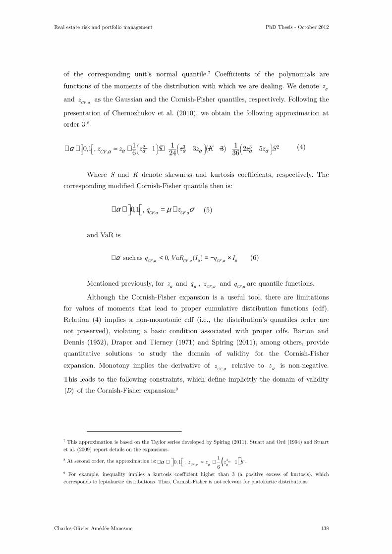
Real estate risk and portfolio management PhD Thesis - October 2012
Charles-Olivier Amédée-Manesme 138
of the corresponding unit’s normal quantile.7 Coefficients of the polynomials are
functions of the moments of the distribution with which we are dealing. We denote zα
and ,CF
z α as the Gaussian and the Cornish-Fisher quantiles, respectively. Following the
presentation of Chernozhukov et al. (2010), we obtain the following approximation at
order 3:8
2 3 3 2,
1 1 10,1 , 1 3 ( 3) 2 56 3624CF
z z z S z z K z z Sα α α α α ααα ∀ ∈ + − + − − − −≃ (4)
Where S and K denote skewness and kurtosis coefficients, respectively. The
corresponding modified Cornish-Fisher quantile then is:
, ,0,1 ,
CF CFq zα αα µ σ ∀ ∈ = + (5)
and VaR is
, , 0 , 0
suchas 0, ( )CF CF CFq VaR I q Iα α αα∀ < = − × (6)
Mentioned previously, for zα and qα , ,CF
z α and ,CF
q α are quantile functions.
Although the Cornish-Fisher expansion is a useful tool, there are limitations
for values of moments that lead to proper cumulative distribution functions (cdf).
Relation (4) implies a non-monotonic cdf (i.e., the distribution’s quantiles order are
not preserved), violating a basic condition associated with proper cdfs. Barton and
Dennis (1952), Draper and Tierney (1971) and Spiring (2011), among others, provide
quantitative solutions to study the domain of validity for the Cornish-Fisher
expansion. Monotony implies the derivative of α,CF
z relative to αz is non-negative.
This leads to the following constraints, which define implicitly the domain of validity
( )D of the Cornish-Fisher expansion:9
7 This approximation is based on the Taylor series developed by Spiring (2011). Stuart and Ord (1994) and Stuart et al. (2009) report details on the expansions.
8 At second order, the approximation is: ( )2
,
10,1 , 1
6CFz z z S
α α αα∀ ∈ + − ≃ .
9 For example, inequality implies a kurtosis coefficient higher than 3 (a positive excess of kurtosis), which corresponds to leptokurtic distributions. Thus, Cornish-Fisher is not relevant for platokurtic distributions.

Real estate risk and portfolio management PhD Thesis - October 2012
Charles-Olivier Amédée-Manesme 139
2 2 23 3 54 1 09 8 6 8 36S K S K S
− −− − − − ≤ (7)
If ( , )S K D∈ , then the quantile function is monotonic. If not, the Cornish-
Fisher expansion is irrelevant. Nevertheless, Chernozhukov et al. (2010) propose a
procedure called rearrangement to restore monotonicity. The procedure corresponds to
a sort of the function of interest. As they mention and demonstrate, rearrangement
pushes non-monotone approximations closer to the true monotone target function. In
our problem, it corresponds to ascending sort of the quantile function α,CFq .
Consider skewness of 0.8 and kurtosis of 2, excess kurtosis equal to -1. These
parameters correspond to a platokurtic and right-skewed distribution function. Since
these parameters do not belong to the domain of validity, the ,CF
z α quantile function is
not monotonic. Applying rearrangement procedure to this quantile function, we obtain
αɶ
,CFz , the corrected Cornish-Fisher transformation of the Gaussian quantiles. Focusing
on probabilities less than 25%, Graph V-2 shows the impact of this procedure.
Graph V-2 - Rearrangement procedure ( )0.25α <
Discrepancy between the two quantile functions is noticeable for the smallest
probabilities, which are the most important ones for VaR computation. The non-
rearranged quantile function may be more severely non-monotone (and therefore could
provide poorer approximations of the distribution function) in comparison to the one
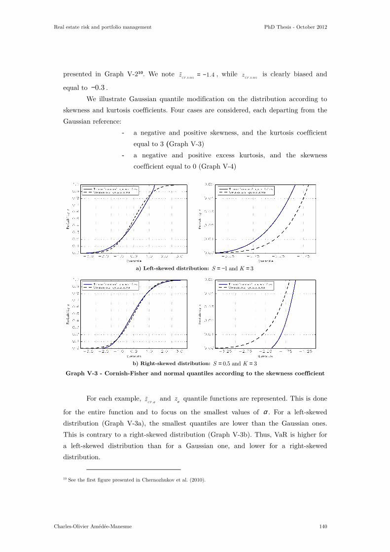
Real estate risk and portfolio management PhD Thesis - October 2012
Charles-Olivier Amédée-Manesme 140
presented in Graph V-210. We note ,0.001
1.4CFz = −ɶ , while
,0.001CFz is clearly biased and
equal to 0.3− .
We illustrate Gaussian quantile modification on the distribution according to
skewness and kurtosis coefficients. Four cases are considered, each departing from the
Gaussian reference:
- a negative and positive skewness, and the kurtosis coefficient
equal to 3 (Graph V-3)
- a negative and positive excess kurtosis, and the skewness
coefficient equal to 0 (Graph V-4)
a) Left-skewed distribution: 1 and 3S K= − =
b) Right-skewed distribution: 0.5 and 3S K= =
Graph V-3 - Cornish-Fisher and normal quantiles according to the skewness coefficient
For each example, ,CF
zα
ɶ and zα quantile functions are represented. This is done
for the entire function and to focus on the smallest values of α . For a left-skewed
distribution (Graph V-3a), the smallest quantiles are lower than the Gaussian ones.
This is contrary to a right-skewed distribution (Graph V-3b). Thus, VaR is higher for
a left-skewed distribution than for a Gaussian one, and lower for a right-skewed
distribution.
10 See the first figure presented in Chernozhukov et al. (2010).

Real estate risk and portfolio management PhD Thesis - October 2012
Charles-Olivier Amédée-Manesme 141
For instance, a skewness coefficient of -1 leads to ,0.05
1.9103CFz = −ɶ , while
0.051.6449z = − ;
,0.0013.3049
CFz = −ɶ and
0.0013.0902z = − . With skewness equal to 0.5, we
obtain ,0.05
1.4980CFz = −ɶ . A leptokurtic (platokurtic) distribution implies lower (higher)
smallest quantiles as shown in Graph V-4a (Graph V-4b). The highest correction for
the VaR occurs in the case of a left-skewed and leptokurtic distribution. This situation
is presented in appendix Graph V-12.
a) Platokurtocic distribution: 0 and 2.5S K= =
b) Leptokurtocic distribution: 0 and 4S K= =
Graph V-4 - Cornish-Fisher and normal quantiles according to the kurtosis coefficient
III. Application
We study monthly IPD U.K. real estate capital returns all properties index
from January 1988 to December 2010, which is 276 observations.11 The index is
valuation-based. The pitfalls of this specific index (i.e., valuation-based index, smooth,
reliability) are discussed in Solvency II calibration paper CEIOPS-SEC-40-10, but are
11 Solvency II regulation is based on U.K. IPD total return indices spanning 1987 to the end of 2008, totaling 259 monthly returns.

Real estate risk and portfolio management PhD Thesis - October 2012
Charles-Olivier Amédée-Manesme 142
not the purpose of this chapter. Our objective in the following is to apply Cornish-
Fisher expansion to compute the VaR of real estate UK capital return and to
underline the shortcuts and simplifications made be the regulators who do not consider
the asymmetry of returns (more generally the non-normality). The regulator however
underlines the shortcuts it was taken but do not provide any solutions or answers:
“The figures below demonstrate the standardized distribution (i.e., mean is zero and
unit standard deviation) of annual property returns across alternative property market
sectors. All distributions of property returns are characterized by long left fat-tails and
excess kurtosis signifying disparity from normal distribution. […], albeit the methods
do not eliminate the inherent bias. We find […] left tail […] whilst the volatility of the
adjusted de-smoothed index is much lower than the volatility of the MSCI developed
total return index”. The committee recognizes its conservatism in using the total
return index, which inherently assumes rental yield earned is re-invested. We chose the
IPD capital return index to avoid the shortcut. The committee recognizes the
shortcuts, but in absence of better datasets and because of the low proportion of real
estate portfolios for insurers in Europe, it did not improve its work.
We study the database and determine quantiles and VaR at thresholds of 5%,
1%, 0.5% and 0.1%. The 0.5% threshold is required by solvency II regulation. The
values are annualized monthly returns. The index and corresponding returns are
presented in Graph V-5, clearly exhibiting both the 1990s overproduction crisis and
subprime periods.
Graph V-5 - Real estate index and returns from January 1988 to December 2010
We use bandwidth to obtain VaR evolution. The length of the bandwidth is
not determined, neither statistically nor from a real estate viewpoint (e.g., economic
analysis, regulators etc.). Statistically, length has to be large enough to enable moment
computation. Standard valuation models use a 10-year cash flow period, but it could
be longer. For example, the Solvency II standard model for real estate required capital

Real estate risk and portfolio management PhD Thesis - October 2012
Charles-Olivier Amédée-Manesme 143
is based on all observations. Since the purpose of our analysis is VaR for non-Gaussian
distributions and not the impact of window length, we do not study this point. A 15-
year period is used, a compromise between sufficient data and obtaining VaR analysis
over time.
Distributions of returns differ across periods as illustrated in Graph V-6.
Various curves correspond to the entire period and three 15-year periods: the first 15-
year period (January 1988 to December 2002), the middle 15 years (December 1991 to
November 2006) and the last 15 years (December 1995 to December 2010).
Graph V-6 - Real estate returns pdf and cdf according to a 15-year period
The middle 15-year period distribution is the more concentrated one, and the
high returns from the end of the 1980s and the lower returns from the subprime crises
are not considered. The distribution for the last 15-year period is left-skewed, with
high negative returns (subprime crises).12 These negative returns lead to a different
analysis of risk when analyzing descriptive statistics presented in Table V-2.
Periods Mean S.D. Min Max S K Q1 Q2 Q3
1988-01 / 2010-12 0.0213 0.1132 -0.3154 0.2439 -0.7502 3.7849 -0.0438 0.0305 0.1001
1988-01 / 2002-12 0.0286 0.0903 -0.1396 0.2439 0.4854 2.8450 -0.0407 0.0248 0.0706
1991-12 / 2006-11 0.0357 0.0633 -0.0849 0.1600 0.0363 2.3219 -0.0045 0.0314 0.0732
1996-01 / 2010-12 0.0169 0.1095 -0.3154 0.1543 -1.5666 5.0540 -0.0022 0.0332 0.0770
Table V-2 - Real estate monthly returns pdf and cdf according to the period
12 This raises a question concerning the window length of the dataset chosen by regulators. A shorter dataset that comes back to today leads to higher skewness and kurtosis coefficients. The subprime and sovereign debt crisis had more important weights.

Real estate risk and portfolio management PhD Thesis - October 2012
Charles-Olivier Amédée-Manesme 144
Mentioned previously, a long dataset is recommended to compute VaR, and we
remind here that we decide to compute the following results based on 15 years (i.e.,
180 returns). In addition to allowing us to consider more than one cycle, this choice
enables obtaining results that are not too erratic, which is the case with small
windows. We thus use a 15-year rolling period to compute moments of the returns.
Each of the 97 computations contains 180 observations.13
Graph V-7 shows the 95% bootstrap confidence interval of the mean, the
standard deviation, the skewness coefficients and the kurtosis coefficients. The means
and standard deviations are unstable. The returns increase from December 1999 to the
subprime crises (during the normal increase and the bubble), and are falling.
Graph V-7 - mean, standard deviation, skewness and kurtosis according to the 15-year
period, and their 95% bootstrap confidence interval
Evolution of the standard deviation appears opposite. Evolutions of S and K
are much more dichotomous: i) nearly stable around 0 and 3, the Gaussian values
before the subprime crises, ii) highly left-skewed ( 0S < ) and leptokurtic ( 3K > )
afterwards. Until December 2001, the distribution is platokurtic (the kurtosis
coefficients are different from 3). From December 2002 to December 2007, the skewness
is either null or positive (right-skewed due to high returns as during the bubble period,
for example).
Mentioned in Section 2 of this chapter, Cornish-Fisher expansion was
subordinated to the monotonic condition. The latter is verified when skewness and
kurtosis coefficients belong to the domain of validity, defined as inequality (7). The
validity condition is not verified each time kurtosis is lower than 3. Moreover, the
combination of skewness and kurtosis coefficients leads to a larger invalidity period.
Without Chernozhukov et al. (2010), Cornish-Fisher expansion would be possible only
13 For example, estimation of the distribution in December 2002 was made using returns from January 1988 to December 2002.

Real estate risk and portfolio management PhD Thesis - October 2012
Charles-Olivier Amédée-Manesme 145
in two relatively small periods: from November 2003 to April 2004 and from March
2008 to November 2008 (shown in Graph V-8).
Graph V-8 - Skewness and kurtosis belonging to the domain of validity (D ). The
represented function equals 0 if ( , ) and 1 if ( , )S K D S K D∉ ∈ .
Given S and K for each 15-year rolling period, we compute Cornish-Fisher
correction of Gaussian quantiles. Graph V-9 presents results for the 5%, 1%, 0.5% and
0.1% quantiles of the real estate returns distribution. Approximation is conducted at
both orders 2 and 3. The modified quantile at order 3 is, by construction, more precise
than the one obtained at order 2. Nonetheless, the latter offers a good approximation
of the correction, which must be made for Gaussian quantiles. Whatever the order, the
discrepancy between modified quantiles ,CF
zα
ɶ and the Gaussian ones zα is high. The
dotted lines correspond to Gaussian quantiles. The correction is noticeable during the
first months (from December 2002), during the bubble period and largely after the
market collapse in December 2007. It is now clear how important this correction is
when the threshold of VaR decreases. This correction is especially relevant when
considering lower quantiles (e.g., for the 0.5% threshold of Solvency II quantile).

Real estate risk and portfolio management PhD Thesis - October 2012
Charles-Olivier Amédée-Manesme 146
5%α = 1%α =
0.5%α = 0.1%α =
Graph V-9 - 5%, 1%, 0.5% and 0.1% quantiles of the real estate returns distribution
according to the 15-year period
The Gaussian quantile is constant whatever the period since S and K are fixed
to 0 and 3, respectively. The quantile modification induced by the Cornish-Fisher
expansion comes from the fact that the skewness and kurtosis coefficients are not
constant over time, as indicated in Graph V-7. This is particularly obvious for the
0.5% and 0.1% quantiles, which are the more interesting quantiles for VaR
computation. Thus:
- In December 2002, the modified quantile is less negative than
the Gaussian one (i.e., less risky);
- During 2003, the quantile decreases to reach the Gaussian one
in the middle of 2004;
- From the middle of 2004 to December 2007 (bubble period), we
again obtain less negative quantiles than the Gaussian one for
thresholds lower than 5%;
- From 2007 to 2008, a fall in market value leads to higher
modified quantiles in absolute value;
- From 2008 to 2009, the modified quantile increases slightly but
remains below the Gaussian value (i.e., pronounced for the
lowest quantiles).

Real estate risk and portfolio management PhD Thesis - October 2012
Charles-Olivier Amédée-Manesme 147
We now compute VaR given the same threshold with the same 15-year
window. The interesting point is to compare results with those obtained from the
regulators. Solvency II regulation requires 25% of required capital for real estate
investments. Its valuation is based on U.K. all properties total return database with a
threshold of 0.5%. Valuation by regulators is close to that obtained with the Gaussian
assumption at 0.5% threshold level. However, considering moments of orders higher
than 2 leads to higher VaR, and therefore higher required capital. This result
demonstrates how essential it is to consider skewness and kurtosis to better estimate
real estate VaR.
5%α = 1%α =
0.5%α = 0.1%α =
Graph V-10 - 5%, 1%, 0.5% and 0.1% Gaussian and corrected Cornish-Fisher VaR in
base 100 according to a 15-year period, and their corresponding 95% bootstrap
confidence interval
There are two sources of risk in the confidence interval computation for
Gaussian VaR: randomness of mean and variance. Adding to these randomness of the
skewness and kurtosis coefficients, we obtain four elements entering the calculus of the
corrected VaR. The 95% confidence interval of the corrected VaR is often lower than
the Gaussian one. There are more sources of randomness, but since the random
variables correlate, the standard deviation of the VaR estimator is lower. Hence, we
observe two improvements in VaR:

Real estate risk and portfolio management PhD Thesis - October 2012
Charles-Olivier Amédée-Manesme 148
- The expectation (i.e., value required by regulators) is more
reliable; the Gaussian VaR is biased in any case where
normality is rejected;
- The precision of expectation is enhanced, which reinforces the
previous calculus.
Graph V-10 highlights the corrected VaR (denoted CF VaR on the graph for
the Cornish-Fisher VaR) is different from the Gaussian one. The VaR discrepancy is
low only for the 2004/2006 to 2007/2012 periods, which was stressed previously
concerning quantile analysis (Graph V-9). For lower thresholds (0.5% and 0.1%), there
is a difference between the two VaRs during the bubble period; the corrected one is
lower. For other periods, correction is high. For example, in December 2010, we obtain
about 25% of required capital at the 5% threshold, while the corrected VaR is about
35%, an increase of 40%.
To conclude this analysis, we revisit length of window choice. In Graph V-11,
VaR of the 10, 11, 12.5, 14 and 15-year periods are represented simultaneously for the
same period. Before the middle of 2008, the longer the window, the higher the VaR.
After that date, we observe the opposite effect. Modifications created by the window
length are qualitatively the same for the Gaussian and Cornish-Fisher VaRs.
a) Gaussian VaR b) Cornish-Fisher VaR
Graph V-11 - Gaussian and Cornish-Fisher corrected VaR for various window lengths
The difference between these two VaRs is stable whatever the windows as
highlighted in appendix Graph V-13. This illustrates window length is not relative to
the Cornish-Fisher expansion but to the VaR computation, and more generally to
distribution estimation. As mentioned previously, regulators could fix the length
exogenously.14
14 Many financial areas use a 10-year window.

Real estate risk and portfolio management PhD Thesis - October 2012
Charles-Olivier Amédée-Manesme 149
As all methods proposed for VaR estimation, Cornish-Fisher methods suffer
from limitations, and we discuss some limitations briefly.
IV. Conclusion
We propose a VaR computation model that combines Cornish-Fisher expansion
and rearrangement procedures. This combination was necessary since Cornish-Fisher
expansion suffers from an important pitfall; the cumulative distribution function could
be non-monotonic, which makes it inapplicable to many practical situations. The mix
of these two methodologies - Cornish-Fisher and rearrangement - allows determining
the quantile function and VaR more reliably. This approach bypasses models relying on
Gaussian15 assumptions or other distribution assumptions (e.g., Monte Carlo and
parametric method). Our approach does not rely on any distribution assumptions, so
we account for non-normality of returns in real estate. In addition, traditional lack of
data is overtaken using this approach (historic method,16 for example, requires a large
amount of data).
The objective of the chapter is to compute VaR for a direct commercial real
estate investment such as requested by many recent regulations. Results show methods
that do not consider skewness and kurtosis to compute VaR lead toworse estimation of
risk. In the presence of skewed returns and fat tails, the Gaussian VaR leads to non-
adequate capital requirements and under-evaluation. This situation appears especially
after the subprime crises.
This article contributes to the existing literature by employing a method based
only on the first four statistical moments and has relevance given current regulatory
environments. There are good reasons for real estate practitioners, banks and insurers
to implement it alongside other models in a real estate context where datasets are
modest. When faced with lack of data, no methods provide accurate outputs.
Professionals also find here an internal model to determine required capital.
The method is particularly robust for distributions that are non-normal, and
therefore applies to hedge funds and private equity sectors, among others. Further
studies should be conducted in those two financial fields. VaR is a risk measure that
only considers the probability of being below a threshold. It does not consider values
15 For simplicity, the Gaussian distribution is used, which enables dealing with small datasets. 16 The traditional, historic VaR is usually not possible or relevant.

Real estate risk and portfolio management PhD Thesis - October 2012
Charles-Olivier Amédée-Manesme 150
below this level or their average. In this sense, researches focusing on measures that
consider the entire distribution such as Conditional Value at Risk or expected shortfall
should be explored, especially methods relying on Cornish-Fisher expansion. Also,
bandwidth size is another issue that requires further study.

Real estate risk and portfolio management PhD Thesis - October 2012
Charles-Olivier Amédée-Manesme 151
Appendices for chapter 3
Appendix 1: Left-skewed and leptokurtic distribution
Graph V-12 - Cornish-Fisher quantiles, left-skewed and leptokurtic distribution,
1.5, 6S K=− =
Appendix 2: Comparison of Cornish-Fisher VaR for various window lengths
Graph V-13 - Differences among Cornish-Fisher VaRs for various window lengths

Real estate risk and portfolio management PhD Thesis - October 2012
Charles-Olivier Amédée-Manesme 152
Chapter VI. Value at Risk: a Specific Real
Estate Model1
In this chapter, we incorporate real estate portfolio specifications in a real
estate VaR model. The idea is the following: two portfolios must exhibit different
VaRs. However, the traditional methods presented in the introduction of this thesis
offer the same VaR whether the portfolio is risky (opportunistic strategy) or secured
(core strategy). Even if the approach is acceptable from a risk management viewpoint,
results are not ideal. Since real estate investment is difficult to diversify, it is extremely
complicated to eradicate specific risk, and therefore specific risk exists in the majority
of real estate investor’s portfolios. It follows that risk of the entire market does not
correspond to risk an investor bears. Our objective is to contribute to real estate risk
VaR model by proposing a new model that incorporates all risks borne by real estate
investors. The proposed model must be able to discriminate between risky and secured
investments.
The approach of this paper derives partially from this thesis’s first paper. We
improve the VaR computation model by considering characteristics of real estate
portfolios. The characteristics considered include lease structures, obsolescence,
vacancy costs, vacancy probabilities given an obsolescence rate, rent, market rental
values and market prices. We use a method close to the one used in the first paper. We
simulate numerous paths of market rental values in a portfolio and prices of each
property using bootstrapping. We use bootstrapping instead of Monte Carlo simulation
because of the difficulty to determine the distribution of returns reliably;
1 This study was started by Charles-Olivier Amédée-Manesme who was joined quickly by Fabrice Barthélémy (University of Cergy-Pontoise). The genesis was a presentation at the French Real Estate Research association concerning Solvency II. Numerous people asked how to differentiate risky and non-risky investments given the approach offered by regulators of required capital. We realized no method existed, and so projected to develop one. In 2011, a version of this paper was presented at the European Real Estate Society’s annual conference in Eindhoven during a PhD student poster session, and was awarded most commended poster. Stephen Pyhrr (University of Texas) and Nick French (Oxford Brookes University) offered excellent recommendations and comments for improvement of the work. In 2012, an advanced version was presented at the European Real Estate Society’s annual conference in a parallel session. Once again, we received excellent comments, especially concerning ways to account for leverage in this kind of model from people at Reading University (Kieran Farelly, among others). The authors wish to thank all the participants of these conferences for the helpful comments.

Real estate risk and portfolio management PhD Thesis - October 2012
Charles-Olivier Amédée-Manesme 153
bootstrapping offers the advantage of not requiring assumptions of the distribution in
a series. We consider correlations among variables using the block bootstrap method
proposed by Politis et al. (2004, 2009). Then we incorporate specific risk at the
property level. We account for lease structure risk following rational behavior; a
rational tenant vacates the property at the time of a break option if the property’s
rent is too high in comparison to market rental values of similar space. We account for
length of vacancy following Poisson’s law, and link the parameter of the Poisson’s law
to obsolescence of the property; the higher the obsolescence, the higher the length of
vacancy. We determine the obsolescence function of the property (or the way the
property becomes vacant in time), and link obsolescence to the vacancy probability.
Finally, we integrate the leverage at the portfolio level and include the possibility to
breach LTV covenants. The approach considers many criteria that enter property
investments and portfolio management. Limitations of this approach reside in the
number of parameters estimated and the difficulty of finding reliable databases for the
effects we examine.
The primary contribution of this paper lays in assessing VaR by incorporating
characteristics of real estate investments. No methods have been developed especially
for real estate. Nevertheless, real estate investments harbor many characteristics
discussed in the introduction of this thesis that must be considered when computing
VaR measures. The results and approach developed in this article provide useful ideas
for risk managers and academicians. Research of obsolescence effects on value, tenant
behavior, vacancy length and property itself must be conducted to determine the
precise effects of all parameters on VaR. The method developed in this paper should
be of the interest to professional risk managers willing to construct internal models for
capital adequacy purposes. The approach could be adapted - with a few changes - to
nearly all asset classes not traded regularly such as art, wine, private equity venture
funds, hedge funds etc.
I. Introduction
VaR is one of the most well-known and accepted measures of risk of loss for a
portfolio of financial assets. It is recognized as a powerful and efficient risk measure.
VaR is appealing because it conveys market risk of the entire portfolio in one metric.
Moreover, VaR focuses directly and in local currency terms on a major reason for
assessing risk: loss of portfolio value. It offers the advantage of representing investment

Real estate risk and portfolio management PhD Thesis - October 2012
Charles-Olivier Amédée-Manesme 154
risk with one number, expressed as a value or percentage. Until recently, VaR was not
popular in real estate industry and research, contrary to other financial sectors such as
stocks and bonds in which VaR computation is standard. This is due to a lack of data
in the real estate industry, particularly commercial real estate data in which
transactions are often undisclosed and less frequent. Computing VaR requires reliable
and frequent data; this measure is only relevant if a large amount of data is accessible.
Recently, VaR became more popular in real estate in light of recent regulations
that require it. Recent2 regulations such as Bale II, Bale III and Solvency II reinforce
bank and insurance capital structures. They require computation of VaR for all
investments, including real estate. Practitioners, risk managers and even academicians
must consider the VaR of a portfolio before investing or studying. Consideration of
return per capital invested is no longer sufficient; return per capital employed (invested
and required) is now considered. Thus, VaR is slowly becoming a fundamental risk
measure for commercial real estate investments.
Nearly all - if not all – contemporary financial sectors are subject to recent
regulations. These regulations are not easily comparable, but they all follow the same
objective: assessing the risks borne by financial institutions more accurately with
required capital. All of these regulations use either a standard or user-specific, internal
model. Calculation methods and assumptions of the standard model are public
information: databases, assumptions and methods are available. Standard models
propose for each asset class (e.g., stocks, bonds, indirect investments, real estate etc.)
standard required capital. Nevertheless, all major institutional investors opt for an
internal model. They argue required capital computed with the standard model does
not represent the risks they bear. They also argue that the standard model maximizes
required capital, and so construct internal valuation models to determine the VaR of
their investments.
In real estate, VaR has been the topic of some research. Research of risk
focusing on direct real estate or unlisted vehicles is scarce in spite of increasing
interest, due partially to the paucity of available data. Either invest in listed real
estate and real estate is quoted daily and enough data are available to compute
portfolio VaR, or invest in direct real estate and deal with small datasets. This is
particularly true in commercial real estate in which institutional investors invest
largely and VaR computation is mandatory for capital adequacy. The real estate
market is comparable to the private equity market in which indices are constructed
2 The impetus to use VaR comes from international adoption of the Basel Accord (nearing completion in 2012) in 1999.

Real estate risk and portfolio management PhD Thesis - October 2012
Charles-Olivier Amédée-Manesme 155
from small numbers of transactions. Real estate property indices aggregate real estate
market information to provide a representation of underlying real estate performance.
However, this is conducted monthly in the best cases, quarterly or semi-annually and
sometimes annually, linked largely to sector. The residential field, in which many
transactions are observable, generates a monthly index frequently. Commercial real
estate faces more difficulties delivering indices with a large periodicity.
Research of VaR in real estate focuses on REITs or securitized real estate, due
primarily to data availability. VaR for listed real estate relies on methods for stocks
and bonds. Zhou and Anderson (2012) concentrate on extreme risks and the behavior
of REITs in abnormal market conditions, suggesting no universal method can be
recommended for VaR in listed real estate. They note that estimation of risk for stocks
and REITs requires disparate approaches. Cotter and Roll (2011) study REIT behavior
over the past 40 years. They particularly highlight the non-normality of REIT returns.
They compute VaR for the index following three methods that do not rely on Gaussian
assumptions: Efficient Maximization algorithm, the Generalized Pareto Distribution
and a GARCH model. The authors highlight that reality is much worse than that
depicted by an assumption of normally distributed returns. Liow (2008) uses extreme
value theory to assess VaR dynamics of ten major securitized real estate markets.
Extreme value theory allows the author to consider the stochastic behavior of the tail.
An extreme market assesses risk better than traditional standard deviation measures,
and real estate forecasts are more accurate.
Literature focusing on VaR in the context of direct real estate investment (or
funds) is sparse and similar to the previous chapter. However, numerous papers
concentrate on risk management and assessment in real estate. Booth et al. (2002)
study risk measurement and management in the context of real estate portfolios. They
argue practical issues force real estate investors to treat it differently than other assets
classes. They particularly highlight that direct real estate is a topic for future research.
The report is a complete review of the range of risk measures that measure real estate
risk, focusing on the difference between symmetric measures such as standard
deviation and downside risk measures such as VaR. Their work concentrates on all risk
measures appropriate for real estate. They do not conclude with one ideal risk
measure, but propose adapting risk measures to needs. Gordon and Wai Kuen Tse
(2003) consider VaR a tool for measuring leveraged risk in a real estate portfolio. Debt
in a real estate portfolio is a traditional issue in real estate finance. The paper
demonstrates VaR offers better assessment of risk. Traditional risk-adjusted measures
(e.g., Sharpe ratio, Treynor’s and Jensen’s alpha) suffer from the leverage paradox.
Leverage adds risk along with potential for higher returns per unit of higher risk.

Real estate risk and portfolio management PhD Thesis - October 2012
Charles-Olivier Amédée-Manesme 156
Therefore, the risk/return ratio does not change noticeably and is not an accurate tool
for measuring risk inherent in debt. VaR is good tool for leveraged risk. Brown and
Young (2011) focus on a new way to measure real estate investment risk. They begin
by refuting the assumption of normally distributed returns that flaw forecasts and
decisions. The nature of risk and how it should be measured is discussed. Interestingly,
VaR is not retained, and expected shortfall is recommended more highly. The authors
focus on spectral measures, their final recommendation. Farelly (2012) measures risk of
unlisted property funds using a forward-looking approach. Among other results, the
author considers moment measurements of orders higher than two (asymmetry
considered) using Cornish-Fisher expansion. Following these authors, we focus our
paper on the need for better VaR assessments in the direct real estate field.
In real estate investment, no VaR model dominates. Even worse, we do not
find a model constructed especially for real estate portfolios or investments. Property
investments harbor many characteristics and discrepancies that must be considered
when assessing risk. Among them are illiquidity (buying and selling may span months),
location (property is immovable), obsolescence (property does not preserve efficiency),
lease structures and break clauses (property may be leased long or short-term, possibly
with break clauses). VaR has long been applied exclusively to liquid portfolios; that is,
portfolios that can reasonably be marketed regularly.
Recent regulations urge methods of computing VaR more reliably. Lack of data
is one of the primary motivations to implement traditional VaR methods (e.g., historic,
Monte Carlo and parametric) in real estate. However, all methods suffer at least from
one limitation; they do not consider the characteristics of the real estate portfolios
analyzed. Computing VaR using market data gives the market VaR, not portfolio VaR,
VaR. Real estate portfolio characteristics are so different that it is fundamental to
consider them in any risk calculation. Few investors argue they replicate the real estate
market. They have preferences and invest in one type of risk according to their
required return. Some investors invest only in core assets (newly delivered or
refurbished properties with a long-term lease); others invest only in risky assets (old
buildings to be refurbished or vacant properties). Real estate VaR must therefore
consider characteristics and intricacies of a portfolio. This point is particularly obvious
for property investments since two investors who invest in the same area but under
disparate strategies cannot arrive at the same VaR.3 Two portfolios that compute VaR
3 In the same vein, two different portfolios cannot display the same Value at Risk and two identical portfolios with two different strategies cannot display the same VaR.

Real estate risk and portfolio management PhD Thesis - October 2012
Charles-Olivier Amédée-Manesme 157
using the same index or data arrive at the same value if they consider only location
and not the characteristics of the investment.
We propose a model that considers characteristics of real estate investments,
and the purpose resides in characteristics of the real estate portfolio. We focus on lease
structure, state of the properties, possible vacancies, tenant decisions and leverage. We
propose a method that considers all characteristics and particularities of a portfolio
and incorporate it into a VaR calculation. The objectives are to construct a model that
discriminates risky and non-risky investments and obtain a VaR specific to a portfolio.
Before discussing analysis and presentation of the model, we point out
assumptions taken in this article. We assume rational investors and players make
decisions based on discounted cash flows and returns. We do not consider asset
management fees in portfolio management. For clarity, we suppose an optimal world
without taxes (Hoesli et al., 2006; Baroni et al., 2007a). We consider neither
depreciation nor capital gain tax. We consider leverage in the model and account for
the LTV ratio only.4 Finally, we do not consider arbitrage or investment during a
simulation. Therefore, the portfolio is an asset itself, sold entirely at the end of a
simulation. These restrictions can be removed easily, but we assume them to keep this
article clear and to a reasonable length.
This article chapter is laid out as follows. The next section presents the model.
All parameters included in the model are explained and described, and their functions
and effects are also discussed. In section 3, we introduce an example based on two
portfolios that differ on only a few points. This example illustrates the model well. The
parameters and functions presented in the previous sections are estimated or
stipulated. Results demonstrate both the impact of each parameter and its relevancy.
Section 4 concludes and discusses future research.
Important note: The model developed below considers all primary
factors that influence property values and returns, but more
importantly, it accounts for factors that generate risk. We consider
parameters that either have a traditional impact on a property’s
return (i.e., leverage, lease structure, and break options) or are
widely regarded as important by investors (i.e., state of property,
vacancy costs, probability of vacancy etc.). To do this properly, it
would have been necessary to determine both parameters and their
4 The importance of leverage in the Value at Risk assessment has been studied in Gordon and Wai Kuen Tse (2003).

Real estate risk and portfolio management PhD Thesis - October 2012
Charles-Olivier Amédée-Manesme 158
functions using a database. This was not possible at the time this
thesis was written. Databases are scarce and we were not able to
obtain them (IPD and PMA refused and Costar is currently studying
our idea). For these reasons, we do not determine precisely
parameters and their functions, but we do speculate on their
functions logically. We hope to obtain a database to determine
reliably functions and parameters, and make this part of the thesis
publishable.
II. The model
The model we propose was constructed to consider the primary characteristics
of real estate investments that influence value and expected returns in the portfolio.
These characteristics were chosen because they are points of attention for investors
(e.g., length of vacancy). Length of vacancy represents market data, but it is not
market data according to property obsolescence, and must be considered in models. At
the time a property is purchased, it may be in a good state, but after a few years, the
previous state changes (e.g., if spaces are vacated, if a new standard appears or simply
because of time etc.), affecting vacancy length.
The model is based on two papers: Baroni et al. (2007a) and Amédée-Manesme
et al. (2012). Our proposal relies on these two papers by adopting their ideas: Monte
Carlo simulations for terminal and market rental values and option theory for leases.
We add numerous factors that affect values or returns of portfolios. Particularly, we
are interested in factors that affect portfolio value negatively. Assessing VaR, we assess
losses and therefore focus only on factors that affect values or returns.
As already stated, many of the hypotheses offered in this paper are not
confirmed through database estimation and cannot rely on extant research. Principally,
this comes from poverty of real estate data. Some of the functions stated in this article
are purely speculative and are assessed neither statistically nor econometrically.
However, the model allows a large degree of freedom and was constructed as a toolbox
from which one can chose which functions or factors to incorporate. Estimated
functions can be replaced with better ones if and when available.

Real estate risk and portfolio management PhD Thesis - October 2012
Charles-Olivier Amédée-Manesme 159
A. Discounted cash flow
The basis of our proposal is a traditional discounted cash flow model. The
present value model is used commonly and accepted widely in real estate and
corporate finance. Real estate assets are income-producing investments. We determine
price of a portfolio 0P as the discounted sum of all future free cash flows (FCF; positive
or negative) generated by a portfolio, discounted at discount rate k:
( )01
,1
Tt
tt
FCFt P
k=
∀ =+
∑
In real estate, FCFs are comprised of two parts: recurrent cash flows coming
from exploitation of properties (i.e., rent and expenses)5 and terminal values when
properties are sold. Terminal values of a portfolio are only involved at the conclusion
of cash flows. It is fundamental to know that by assumption and for simplification, no
arbitrage is possible before the end of cash flows and the portfolio itself is sold at the
end of a holding period. The two components of the FCFs are:
- Rent and expenses generated by the properties in the portfolio.
o The FCFs of unique space (or unit) i of property j at
time 1; 1t t ∈ − gives:
( )1
1, , , 1, , - 1,n
i i i i i
t t t t ti
i n t T FCF Rent Exp Wk Cv=
∀ = ∀ = … = − − −∑…
where, as defined by Amédée-Manesme et al. (2012), i
tRent is
the rent of space i over period t-1 to t, i
tExp are common (or
recurrent) expenses of space i over period t-1,t, i
tWk are
capital expenses related to space i over period t-1,t and i
tCv
are vacancy costs of space i over period t-1,t.
o FCFs for all spaces in the portfolio comprised of n
spaces at time t are: 1, , , 1, , - 1i n t T∀ = ∀ = ……
( ) ( )1 1
n ni i i i i
t t t t t ti i
FCF FCF Rent Exp Wk Cv= =
= = − − −∑ ∑
- The terminal values of all properties.
5 Expenses can be recurrent or infrequent.
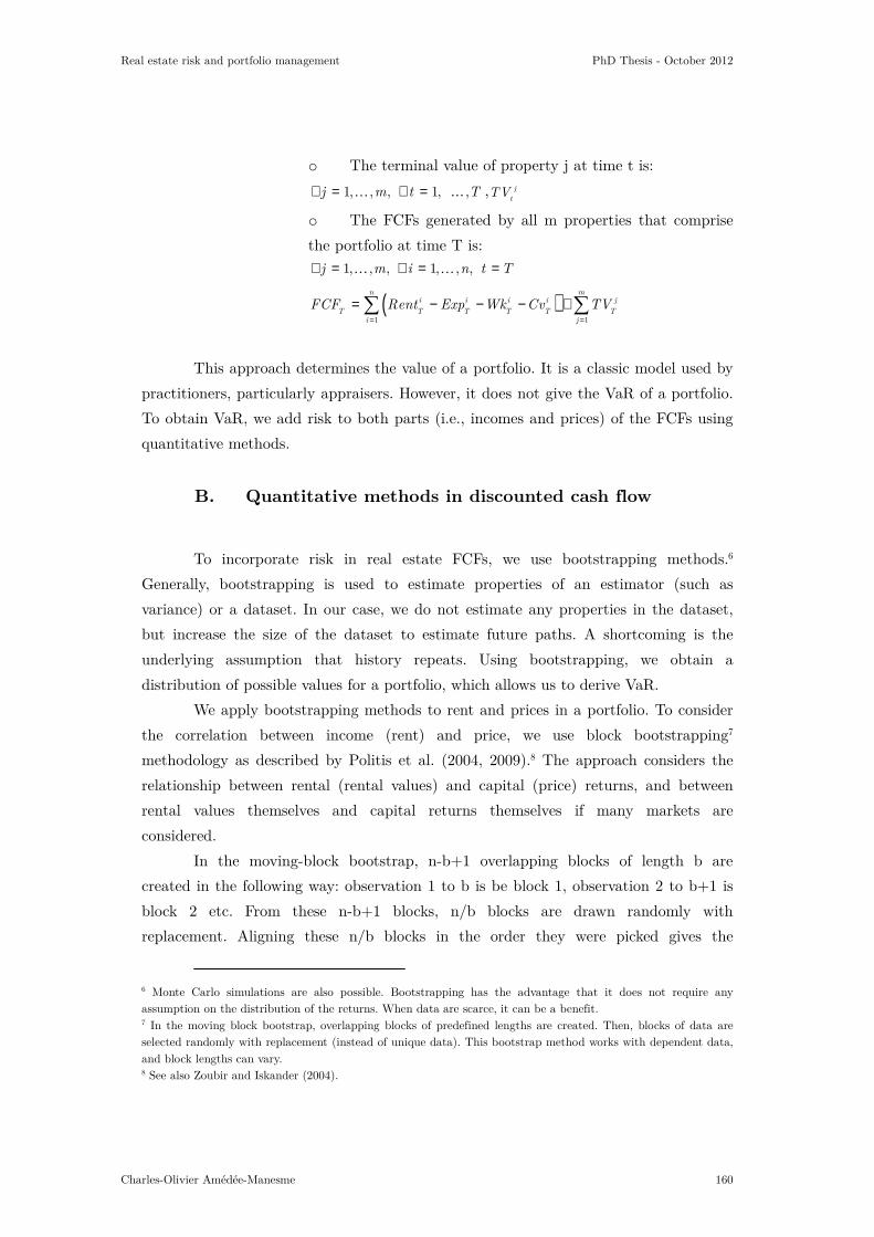
Real estate risk and portfolio management PhD Thesis - October 2012
Charles-Olivier Amédée-Manesme 160
o The terminal value of property j at time t is:
1, , , 1, ,j m t T∀ = ∀ = …… , j
tTV
o The FCFs generated by all m properties that comprise
the portfolio at time T is:
1, , , 1, , ,j m i n t T∀ = ∀ = =… …
( )1 1
n mi i i i j
T T T T T Ti j
FCF Rent Exp Wk Cv TV= =
= − − − +∑ ∑
This approach determines the value of a portfolio. It is a classic model used by
practitioners, particularly appraisers. However, it does not give the VaR of a portfolio.
To obtain VaR, we add risk to both parts (i.e., incomes and prices) of the FCFs using
quantitative methods.
B. Quantitative methods in discounted cash flow
To incorporate risk in real estate FCFs, we use bootstrapping methods.6
Generally, bootstrapping is used to estimate properties of an estimator (such as
variance) or a dataset. In our case, we do not estimate any properties in the dataset,
but increase the size of the dataset to estimate future paths. A shortcoming is the
underlying assumption that history repeats. Using bootstrapping, we obtain a
distribution of possible values for a portfolio, which allows us to derive VaR.
We apply bootstrapping methods to rent and prices in a portfolio. To consider
the correlation between income (rent) and price, we use block bootstrapping7
methodology as described by Politis et al. (2004, 2009).8 The approach considers the
relationship between rental (rental values) and capital (price) returns, and between
rental values themselves and capital returns themselves if many markets are
considered.
In the moving-block bootstrap, n-b+1 overlapping blocks of length b are
created in the following way: observation 1 to b is be block 1, observation 2 to b+1 is
block 2 etc. From these n-b+1 blocks, n/b blocks are drawn randomly with
replacement. Aligning these n/b blocks in the order they were picked gives the
6 Monte Carlo simulations are also possible. Bootstrapping has the advantage that it does not require any assumption on the distribution of the returns. When data are scarce, it can be a benefit. 7 In the moving block bootstrap, overlapping blocks of predefined lengths are created. Then, blocks of data are selected randomly with replacement (instead of unique data). This bootstrap method works with dependent data, and block lengths can vary. 8 See also Zoubir and Iskander (2004).
Real estate risk and portfolio management PhD Thesis - October 2012
Charles-Olivier Amédée-Manesme 161
bootstrapped observations. Bootstrapping works with dependent data, however the
bootstrapped observations are not stationary by construction. But it is shown that
varying block length avoids this problem
For each asset in a portfolio, we use bootstrapping to model both terminal
values and all income from all spaces of properties. This action is done at the portfolio
level considering correlations among all simulated variables. We repeat this procedure
thousands of times and obtain a distribution for all values obtained.
Incorporation of quantitative methods in the discounted cash flow of real estate
finance is not new. It has already been proposed by numerous academicians, including
Pyhrr (1973) (the first introduction of quantitative methods in real estate), French and
Gabrielli (2004, 2005, 2006), Hoesli et al. (2006) and Baroni et al. (2007a, 2007b).
Following these authors, we account for uncertainty using quantitative methods
(bootstrapping). This allows us to consider risk in income returns and prices. Thus, we
consider market risk when computing the value of a portfolio. In theory and according
to traditional Markovitz (1952) portfolio theory, specific risk can be diversified so only
market risk remains. In real estate, specific risk is difficult (nearly impossible) to
diversify, and an incredibly large number of asset is necessary to diversify specific risk.
This has long been demonstrated by a number of articles, including Brown (1988,
1991), Barber (1991), Cullen (1991), Byrne and Lee (2001), Callender et al. (2007) and
Mitchell (2012). This is why it is fundamental to account for specific risk.
Risk in income returns depends on not only market risk, but also specific risk
(or idiosyncratic risk). Market rental value is not income a landlord receives for a unit;
the landlord receives rent, and rent rarely equals market rental value. This is due to a
lease. Rent is usually indexed over time, and thus increases gradually given a specified
index (except in the U.K. where rent is based on an upward-only review of market
rental values). Given a market, rent currently paid by a tenant may deviate strongly
from market rental value, and thus create risk.9 This is one of the most important risks
borne by a landlord: leasing risk (i.e., when a space becomes vacant). Considering lease
structure is fundamental when uncertainty of cash flows is also considered. It allows
considering one of the most essential specific risks. To incorporate this risk, we use a
model presented in the next sections.
9 This case occurred often in 2010; many leases contracted in 2007 were outside the market. Between 2007 and 2010, market rental values collapsed in major European cities, given the PMA database.

Real estate risk and portfolio management PhD Thesis - October 2012
Charles-Olivier Amédée-Manesme 162
C. Lease structure
In a parent paper presented in the 3rd chapter of this thesis, Amédée-Manesme
et al. (2012) explain how rent is indexed (in most countries, rent is revised regularly
based on indices such as inflation and market value) and how lease structures influence
cash flows. We focus on the option conceded to a tenant in a lease and the behavior of
the tenant facing this option. The possibility to vacate is one of the primary drivers of
real estate portfolio return, particularly in the case of a falling market of rental values.
We point out some essential features of the model. Rent is generally indexed during
the course of the contract (with exception in the U.K.). Contracts are written with
clauses in favor of the tenant to terminate the contract before the end of the lease.10
These options are called break-options (or break-clauses). Facing a break-option (or at
exercise time), we assume a rational tenant leaves if the difference between rent
currently paid and rental value available on the market for a similar space is not too
high. This decision is rational in the sense that the tenant decides to move to a
cheaper place if the possibility to do so is available.11 In a falling market, property can
be over-rented (i.e., tenants pay more than the market level). In this case, rent
reversions are not always welcome by landlords.12 Break-clauses represent opportunities
for a tenant to spend less, and a rational tenant may exercise this opportunity.
Mathematically, the decision to move for a tenant facing a break-option can be
expressed as:
1 , 0i
it
i
t
MRV
Rentα α> + >
where iα is the moving criteria decision for space i and MRVt is the market
rental value at time t for space i. Quantity α represents bargaining power of the
tenant, which can include moving, agency (the cost of a consulting business that helps
the company in its decision or the cost of the broker) and human resource costs.13
Instead of using bootstrapping for rent and price, we use it for all market
rental values and prices (the portfolio is comprised of m properties and n spaces). At
relevant dates, simulated market rental values are compared to rent paid, and the most
rational decision is taken. If a space is let too much above current market value at the
10 Options embedded in a lease are asymmetric because only the tenant can exercise the option. 11 Moving or agency costs may be considered. 12 Owners or asset managers may be tempted to negotiate, grant free rent, upgrade or offer financial incentives to maintain a tenant. These are not considered in the model, but could be an improvement of this approach and of Amédée-Manesme et al.’s (2012) recommendations. 13 The company may face defection of some workers due to location changes.

Real estate risk and portfolio management PhD Thesis - October 2012
Charles-Olivier Amédée-Manesme 163
time of a break option, the tenant vacates and the landlord faces a void. We now have
a model that considers both vacancy and a tenant breaking a lease before the end of
the contract. A difference here lays in the way rent is estimated.
We take two hypotheses that can be relaxed in the model, but that are
necessary for clarity of presentation. After a period of vacancy (or after a break-option
is exercised), a property is relet at market rental value. At the end of a lease when the
option is a dual option, both tenant and landlord can make a decision; the tenant and
the landlord decide to renew the contract at market rental value.14 This follows the
idea of rational behavior (the landlord wants to increase revenue and avoid vacancy,
and the tenant avoids moving and agency costs).
Therefore, this paper introduces the possibility of vacancy. It is essential in any
real estate cash flow model to consider leases, particularly lease structures and
vacancies incurred by those structures. Disparities that occur due to a lease structure
have a colossal impact on future cash flows and on risk of the investment. When
calculating VaR, the risk profile of the portfolio, with or without leasing or property
risk, is important. A VaR computed for a real estate portfolio that faces many break-
options in the near future (and therefore many leasing risks) must be higher than a
VaR computed for a core portfolio without leasing risks, even if both investors - core
and opportunist - have sufficient assets to diversify specific risk. A VaR valuation
model must incorporate leasing and property risks. This is why we incorporate lease
structure risk in the VaR model. Now we consider two issues arising from vacancy:
length of vacancy and cost of vacancy. Vacancy costs influence property value
according to the length a unit or property remains vacant.
D. Length and cost of vacancy
Vacancy is one of the greater risks investors bear. A vacant space generates
costs and obsolesces more quickly. We face two issues: how long a space remains vacant
and how much vacancy costs. We propose a solution for each and suggest
incorporating them into our VaR model.
Following Amédée-Manesme et al. (2012), we model vacancy length using
Poison’s law. Therefore, length of vacancy follows:
( ) ( )!
k
ip k P X k ek
λ λ−= = =
14 This decision is financially rational for both tenant and landlord. The tenant minimizes expenses (no moving costs, broker fees etc.) and the landlord maximizes revenues because vacancy is avoided.

Real estate risk and portfolio management PhD Thesis - October 2012
Charles-Olivier Amédée-Manesme 164
with λ a positive real number equal to the average vacancy length and k the
number of occurrences of the event. Average vacancy length in a market is available
easily from databases or brokers. These data can be segmented by sub-markets and
sometimes sub-sub-markets (e.g., new versus second-hand premises).
Vacancy costs represent spending estimated to be paid due to vacancy. This
arises because in most rental contracts, a tenant pays current expenses and only large
capital expenses are paid by the landlord. Estimation of vacancy costs is difficult
because expenses in cases of vacancy vary widely by property and location. Technical
characteristics, tenants, services and location of a property influence the types of
charges faced during void periods. Costs faced by a landlord during vacancy come from
various sources. Landlords may have to spend marketing expenses or broker fees. Some
local taxes usually charged to a tenant must be paid by a landlord during vacancies.15
A landlord may also need to keep heating or air-conditioning to keep the spaces in a
good state. In addition, landlords often must maintain services for other tenants on the
property.16 These costs are part of common expenses charged proportionally to the
sizes let, and therefore the landlord must pay the parts arising from vacant spaces.
Estimating cost of vacancy is complicated, requiring much information and
many parameters. However, an experienced real estate asset manager can determine
vacancy costs of a real estate asset. It only remains to count these costs in cash flows
when a space is vacant.
To model them, we propose a percentage of estimated market rental value.
The percentage must be estimated using a database. In absence of a database, a
percentage can be fixed to an arbitrary value or estimated through experience or
valuation. Therefore, vacancy cost at time t for space i is:
1 ( , )i i
t vacant tCv t i MRVξ= × ×
with ( , )t iξ a function representing vacancy charges for asset i at time t. 1vacant
is the indicatory function and i
tCv is the amount of vacancy cost defined in II.A of this
chapter.
Thus, each time a space becomes vacant, vacancy cost and length of vacancy
are considered. However, many factors influence vacancy length and the probability of
vacancy. One primary factor is the obsolescence rate of the property (or the state of
the property). In commercial real estate, after location—which largely defines rent—
the state of the property influences a tenant’s decision strongly.
15 Properties such as towers and service offices face particular charges. 16 This is often the case in a half-let property in which a landlord faces higher vacancy costs than with an empty property. A landlord pays half of reception-desk costs, half of security and half of canteen subscriptions.

Real estate risk and portfolio management PhD Thesis - October 2012
Charles-Olivier Amédée-Manesme 165
E. Obsolescence (depreciation)
There exists some confusion surrounding the terms depreciation and
obsolescence. The two are often used interchangeably, as we do. However, it is clear
depreciation has several recognized and major impacts on property that obsolescence
does not have, particularly when considering accounting and taxation. Only one
discernible academic development of a body of knowledge and theory defines and
classifies these concepts: Baum (1991). Nevertheless, much literature exists in
accounting that concentrates on techniques used in the application of depreciation to
profit and loss accounts. In addition, RICS Asset Valuation Standards Committee
guidelines offer partial definitions for depreciation and obsolescence for property
sectors. For our purposes, we consider obsolescence a cause and depreciation an effect.
Since our objective is not to define or redefine terms, we use one comprehensible
concept: obsolescence.
Obsolescence represents a decline in competitiveness, usefulness and/or value of
a property. Obsolescence occurs due to availability of alternatives that perform better,
cheaper or both, or changes in user preferences, requirements or style. Property
obsolescence affects value in two ways: physical deterioration and functional decline.
Salways (1986) and Baum (1991, 1994)17 describe categories of building obsolescence,
including aesthetics (outdated appearance), functional (technological progress that
changes an occupier’s requirements), legal (safety or environmental) and social
(demands for a secure environment). Obsolescence is a highly complex topic that is
difficult to evaluate reliably and credibly. We do not model obsolescence rate or
propose an obsolescence function18 because those could be topics of an entire thesis,
but we do consider obsolescence in the VaR model. In the application section, we
assume linear decline of property competitiveness.
A property does not preserve efficiency over time due to normal use, changes
and environment. To account for obsolescence, we introduce function ( ),t jθ , assuming
property efficiency decreases over time. By reciprocity, obsolescence of a property
increases during its life. Therefore:
( ),, , 0
d t jt j
dt
θ∀ ∀ >
17 See also: Barras and Clarck (1996). 18 An obsolescence model can be found in Baum (1991).

Real estate risk and portfolio management PhD Thesis - October 2012
Charles-Olivier Amédée-Manesme 166
Obsolescence is represented by a percentage of the total value of the property.
Note that property preserves residual value even when obsolete; this value can come
from location or attractiveness of the shape of the building (e.g., historic façade).
Obsolescence thus has a strong, direct influence on value, but also indirectly on asset
management. An obsolete property faces difficulties attracting and retaining tenants.
F. Probability of vacancy according to obsolescence
The state of a property is a fundamental part of its value, and essential to
remain attractiveness to a tenant. Maintaining a tenant in an old or obsolete asset can
be difficult. Leasing an old or obsolete property is more difficult than leasing a new
one, even for a cheaper price.
Formalizing and quantifying risk of vacancy is essential to obtain a good
understanding of real estate risk. We consider the probability of vacancy increases with
obsolescence. We incorporate probability of vacancy in moving criteria decision α. This
criterion may have a huge impact on a tenant’s decision, positive or negative (in cases
of extremely obsolete properties), and therefore influence a decision taken by a tenant
strongly when facing a break option. Therefore:
( ) ( )( )
,, ,, 0 , 0
,
i j
td t j d t
t tdt d t j
θ α θ
θ∀ > ⇒ ∀ <
where θ is the obsolescence function depending on time t and property j, a
function that increases over time, and ,i jt
α is the moving criteria for space i of property
j at time t. The moving criterion is a function that influences the probability of
vacancy according to the state of the property. Since the more a property is obsolete,
lower are the moving decision criteria, and the probability of vacancy increases. Ideally,
the moving criteria decision is estimated using a complete database. However, this was
not possible, and a credible function is assumed during application. We thus include
the probability of vacancy more rapidly given property obsolescence. To influence the
decision of the current tenant, the obsolescence rate has a strong influence on the
length a property remains vacant.

Real estate risk and portfolio management PhD Thesis - October 2012
Charles-Olivier Amédée-Manesme 167
G. Length of vacancy according to obsolescence
The state of a property influences attractiveness strongly. Therefore, an
obsolete or out-of-date property remains vacant longer than a newer one,19 even if rent
is lower. Average vacancy length in our model is market average (or sub-market
average), and therefore, some properties remain vacant longer than others do. We
hypothesize that obsolescence influences expected length of vacancy positively.20
Mathematically, this is expressed as:
( )( ), ,
, , 0,
d t it i
d t j
λ θ
θ∀ ∀ >
where ( )λ θ, ,t i is the average length of vacancy function for space i at time t.
Again, a database estimates this function better, but this was not possible for this
paper. We modify average length of vacancy by incorporating a portion that varies
according to obsolescence rate.
H. Debt
Debt is the last element influencing risk of a real estate portfolio. Debt affects
returns but also investment risk in light of extreme events such as those estimated in a
VaR model. Leveraged investments offer better returns in cases of favorable situations.
In cases of bad situations, investors may not recover anything, and can lose all invested
capital. Leverage adds risk in addition to potential higher returns. However, common
risk-adjustment measures have serious limitations when applied to leveraged portfolios.
The Sharpe ratio and other risk-adjustment measures (e.g., Treynor’s or Jensen’s
alpha) does not allow differentiation between risky and non-risky investments because,
by definition, it results in comparable levels. Thus, risk/return ratio does not change
appreciably with leverage. VaR offers better consideration of leveraged risk. In our
model, debt is not considered at the portfolio level, but it is considered at the property
level. This is often the case in real estate finance because property is viewed as a
covenant of a loan and landlords do not often accept cross-collateral to remain free
19 An obsolete property located in an area where all properties are obsolete does not suffer from the obsolescence rate. A refurbished property in an area where all properties are obsolete either attracts tenants more easily as the best property in a market or is too expensive or beautiful for tenants in the market. 20 This is true assuming tenants are rational and assuming spaces are priced at market rental values.

Real estate risk and portfolio management PhD Thesis - October 2012
Charles-Olivier Amédée-Manesme 168
from decisions (cross-collateral blocks management decisions). Covenants are the terms
or clauses in a loan agreement.
Given limited benefits, lenders must focus on limiting their downside. As a
result, a secured lender underwrites loans based on many ratios. The four most
common are loan-to-value (LTV), debt-service coverage, interest coverage and fixed-
charge. While these ratios are important, covenants are far more important and
contentious. To limit disadvantages of a risk profile, lenders demand as many loan
covenants (or securities) as possible.
We concentrate21 solely on the LTV, and more precisely on the covenants
attached to the ratio. LTV represents the ratio of the first mortgage lien as a
percentage of the total appraised value of real property. For example, if an investor
borrows 50 M€ to purchase a property worth 100M€ at relative valuation, the LTV
ratio is 50/100 or 50%. Risk of default is always at the forefront of lending decisions,
and likelihood of a lender absorbing a loss in a foreclosure process increases as the
amount of equity decreases. Therefore, as the LTV ratio of a loan increases, the
qualification guidelines for loans become increasingly severe. In addition, cost of debt
(margin) depends on LTV; low LTV ratios often accompany low debt margins.
The agreement generally allows the LTV to vary from a percentage (δ) of the
initial LTV due to market movements (and appraisals). We assume loan conditions are
breached if property value is lower than the minimum accepted by (or negotiated in) a
loan agreement.
For property j at time t, if 0, , j j
tt j LTV LTV δ∀ ∀ > + the loan is breached. δ
represents permitted variation of the initial LTV. Since breach of LTV covenant is a
default, the lender demands immediate repayment of the loan22 or preempted of the
property.
We consider leverage risk in our VaR model. As soon as the simulated value of
the property moves too far from initial LTV ( j
tLTV ), the value of the property falls to
0 (because it is preempted), and no further income is generated by the property. Other
loan risks, especially those related to income, are more complicated to model.
21 Other ratios are also fundamental for lenders, but differ from market to market, and are subject to negotiation. 22 If the lender decides not to call in the loan, the lender usually requires the loan to be renegotiated in terms less favorable to the borrower, including higher interest rates and substantial fees. Some loans require a borrower to provide a deposit as further security in the event of a breach of the LTV ratio, thus increasing the financial burden of the borrower. There are indications that lenders are increasingly willing to renegotiate a loan instead of calling it in, given they want to limit bad debts. It is in their interest to agree to a solution that works for both parties.
Real estate risk and portfolio management PhD Thesis - October 2012
Charles-Olivier Amédée-Manesme 169
Particularly, opportunistic loans often do not cover income ratios, but pay debt service
with equity. This is why we do not account for it.
III. Application
A. Data and presentation of the portfolios
To illustrate the relevancy of our model, we consider two portfolios that differ
only by investment type. One is a core (secured) portfolio and the other is an
opportunistic (risky) portfolio. The portfolios are comprised of 10 properties invested
in Europe in two markets: France (Central Paris, outside Golden Triangle) and
Germany (Central Munich). The properties of the portfolios are located in the same
market and sub-market. They differ only in size, leasing and state of properties. Five
properties have been acquired in each city. The French part of the portfolio holds 7
units (two properties have two spaces to let, the others are mono-tenant properties),
and the German part holds 6 units (one property divided into two spaces).23 More
information on strategy includes:
- The core portfolio is invested only in new developments or
recently refurbished properties with long-term leases. Its
objective is to distribute recurrent cash flows to an investor. It
does not consider leasing or property risk. Leverage is limited
and equal to 30%. This investor has long-term investment
objectives (i.e., greater than 8 years).
- The opportunist investor acquires only empty (with lease risk)
new developments or old, obsolete properties with short-term
leases or vacancies. This investor bears obsolescence and leasing
risks, and the objective is to realize capital gains. The portfolio
is leveraged at 60%, and the investment objective is short (i.e.,
fewer than 6 years).
The two portfolios have the same initial acquisition price of 1,000 M€, but
initial yields are different. They were acquired on the same date. Our model requires
certain inputs. In addition, some parameters must be estimated if data are available.
Required inputs include:
23 We assume a space cannot be divided. In practice, units are divided frequently as a function of tenant wishes.
Real estate risk and portfolio management PhD Thesis - October 2012
Charles-Olivier Amédée-Manesme 170
i. Price of each property;
ii. Rent for all units in the portfolios (rent can be 0);
iii. Market rental values for each unit;
iv. Leases of all let spaces and expected leases in case of breaks;
v. Indexation of each unit;
vi. Evolution of the two markets in terms of market rental values and prices;
vii. Average vacancy length for each sub-market (only two sub-markets are
considered: Paris and Munich);
viii. Cost of capital
ix. Vacancy cost of each unit;
x. State of each property and how this state is expected to evolve
(obsolescence function of each property);
xi. Moving criteria decision for each market and its evolution (probability of
vacancy);
xii. Length of vacancy function (dependant on state of the properties);
xiii. General information such as portfolio LTV, debt margin etc.
Inputs i to v: Inputs i. to v. are available in the annual report of each fund. In
Table VI-1, we show information concerning these inputs. For simplicity, each property
has a price of 100 M€ for a portfolio value of 1,000 M€. All new leases are expected to
be contracted according to 6/9-year contracts in France and 5/10-year contracts in
Germany. We assume all leases are indexed at 2% per year (in practice, discrepancies24
can occur; Germany and France do not use the same index or a similar indexation).
Market rental values, passing rent at the time of acquisition and the lease structure of
each space are displayed in Table VI-1.
24 Rent is indexed annually at 2%. In practice, indexation can be negotiated according to many rules. French leases are indexed annually on a specific index (Cost of Construction Index), and German leases are indexed each time cumulated national inflation reaches 10%.

Real estate risk and portfolio management PhD Thesis - October 2012
Charles-Olivier Amédée-Manesme 171
Table VI-1 - Market rental values, rent and lease structures of units in the portfolio.
The acquisition price of each property is the same, but their initial yields are
not. The core portfolio is acquired for a net initial yield of 6.2%25 and the
opportunistic portfolio for 8.7%. The riskier portfolio is thus bought for a higher yield,
representing higher risk borne by the investor (258 bp). The core portfolio is fully let
and has no financial vacancy. The opportunistic portfolio has 8 vacant spaces,
representing 66% financial vacancy. Both portfolios are slightly over-let (passing rent >
MRV). The let spaces of the core purchaser are slightly over-let by 2.5%. The
opportunist purchaser acquired the portfolio over-let by just 1% (on the let part).
Differences between passing rent and market rental values are globally low. These
differences can be explained by indexation: some rent was indexed positively through
years when market rental values were descending.26
The two portfolios have existed a number of years, and spaces have thus been
marketed and let at various dates and periods. Some have been running for many years
and are close to the end of the contract; others have just been signed and will produce
income for many years. Leases that have just been signed are signed at market rental
value, given the assumption of rationality. Other leases exhibit differences from market
25 Based on market rental values and to make numbers comparable, net initial yield = market rental values/portfolio value. 26 This occurred often after the 2007 financial crisis when rent was indexed positively and market rental values collapsed.
Property # CityUnit
#
Lease structure
in case of break
Core Opportu
nistic
Core Opportu
nistic
Core Opportun
isticProperty 1 Paris Unit 1 3.1 4.1 3.2 4.1 9 4
Unit 2 3.1 4.6 3.2 - 7 -
Property 2 Paris Unit 3 3 4.3 3.5 4.5 9/12 5
Unit 4 3 5 3 - 9 -
Property 3 Paris Unit 5 6.3 9.5 6.3 - 8 -
Property 4 Paris Unit 6 6 8.2 6 8.3 9 2/5
Property 5 Paris Unit 7 6.4 8.9 6.3 - 6/9 -
Property 6 Munich Unit 8 6 7 6.1 - 10 -
Property 7 Munich Unit 9 6.1 8.9 6.3 9 10 4
Property 8 Munich Unit 10 6.1 9.7 6.1 - 8 -
Property 9 Munich Unit 11 6 7.9 6.5 - 7 -
Property 10 Munich Unit 12 3.4 4.5 3.1 4 9 6
Unit 13 3.1 4.8 3.3 - 7 -
Total / Average 61.6 M€ 87.4 M€ 62.9 M€ 29.9 M€ 8.36 years 1.5 years
Financial Vacancy 0% 66%
Rents (M€)Market rental
values (M€)
6/9
5/10
Current lease
structure

Real estate risk and portfolio management
Charles-Olivier Amédée-Manesme
rental value; some are over
leases are shown in Table
secured cash flows and the opportunistic portfolio has only 1.5 years.
Input vi: Evolution of the two markets is public information displayed by data
providers or brokers. We rely on
(1991-2010), which covers
we were able to access and where cit
and price evolution given
VI-1 and Graph VI-2. Obviously,
Strategy serves investors interested
to construct a VaR model that differentiates the two investments.
Graph
27 PMA is a data provider specializing in real estate markets28 A prime market is characterized by location. Prime assets are located in the best areas of a city, let under a long-term lease to grade-A tenants (i.e., rating > AA).
risk and portfolio management PhD Thesis
some are over-let and some are under-let. Future break options of all
Table VI-1. Note that the core portfolio has more than 1 year of
secured cash flows and the opportunistic portfolio has only 1.5 years.
ution of the two markets is public information displayed by data
e rely on the Property Market Analysis (PMA
s the prime market.28 This database is not best
we were able to access and where city data were available. We use market rental values
the PMA database. The two evolutions are shown in
. Obviously, market evolution does not depend
trategy serves investors interested in various risk/return frameworks. O
a VaR model that differentiates the two investments.
Graph VI-1 - Market capital growth (1991 to 100)
Source: PMA Database
PMA is a data provider specializing in real estate markets. A prime market is characterized by location. Prime assets are located in the best areas of a city, let under a
A tenants (i.e., rating > AA).
PhD Thesis - October 2012
172
uture break options of all
ote that the core portfolio has more than 1 year of
ution of the two markets is public information displayed by data
Property Market Analysis (PMA27) database
best, but it is one
data were available. We use market rental values
shown in Graph
evolution does not depend on strategy.
. Our objective is
A prime market is characterized by location. Prime assets are located in the best areas of a city, let under a

Real estate risk and portfolio management
Charles-Olivier Amédée-Manesme
Graph
As shown in Graph
first from 1991 to 2000 and the second from 2001 to 2007.
do rental growth and capital growth. The lowest correlation is between capital returns
of Munich and rental growth of Paris. The correlation matrix is
Table VI-2 - Correlation matrix market rental values and prices in Munich and Paris
Input vii: Average vacancy lengths are also market data. For Paris
an average vacancy length of 2 years
Input viii: Cost of capital in absence of debt (unleveraged fund)
5.5%. This number represents a premium of 150bp on average 10
from 2001 to 2010 (4% for France and 3.9% for Germany). The risk premium used here
is based on the assumption that property should have a risk premium over government
Paris Central (capital returns)
Munich City (capital returns)
Paris Central (rental growth)
Munich City (rental growth)
risk and portfolio management PhD Thesis
Graph VI-2 - Market rental growth (1991 to 100)
Source: PMA Database
Graph VI-1 and Graph VI-2, the series considers two cycles: the
from 1991 to 2000 and the second from 2001 to 2007. The two cities correlate
capital growth. The lowest correlation is between capital returns
of Munich and rental growth of Paris. The correlation matrix is shown in
Correlation matrix market rental values and prices in Munich and Paris
Source: PMA Database
verage vacancy lengths are also market data. For Paris
an average vacancy length of 2 years, and 2.5 years for Munich.
ost of capital in absence of debt (unleveraged fund)
5.5%. This number represents a premium of 150bp on average 10-year Sovereign debt
% for France and 3.9% for Germany). The risk premium used here
is based on the assumption that property should have a risk premium over government
Paris Central
(capital returns)
Munich City
(capital returns)
Paris Central
(rental growth)
Munich City
Paris Central (capital returns) 100%
Munich City (capital returns) 56% 100%
Paris Central (rental growth) 74% 19% 100%
Munich City (rental growth) 68% 62% 73%
PhD Thesis - October 2012
173
two cycles: the
he two cities correlate as
capital growth. The lowest correlation is between capital returns
in Table VI-2.
Correlation matrix market rental values and prices in Munich and Paris
verage vacancy lengths are also market data. For Paris, we obtain
ost of capital in absence of debt (unleveraged fund) is equal to
year Sovereign debt
% for France and 3.9% for Germany). The risk premium used here
is based on the assumption that property should have a risk premium over government
Munich City
(rental growth)
100%

Real estate risk and portfolio management PhD Thesis - October 2012
Charles-Olivier Amédée-Manesme 174
bonds. Factors influencing the premium include volatility, liquidity and transparency.29
Following the PMA database recommendation, we use 150bp for both markets.
As already addressed during this chapter and more generally during
this chapter, we were unable to find a reliable database with state of
properties, and therefore unable to determine functions and inputs
required in such databases such as obsolescence, moving criteria
decision and length of vacancy according to obsolescence rate. To
illustrate the relevancy of our approach and the impact of parameters
in the model, we make reasonable assumptions about the shapes of
these functions. This does not change the relevancy of the model
because these assumptions can be changed and relaxed across
markets or countries and the model was constructed like a toolbox in
which an analyst can decide which parameters to include.
Input ix: Vacancy costs can change across properties and locations. Without
accurate data for each property, it is difficult to estimate cost of vacancy per unit. For
this reason, we chose a common rule for all spaces in the properties. Cost of vacancy
equals 15% of market rental value whatever the state or number of tenants. Thus, the
cost of vacancy for space i is:
1 0.15i i
t vacant tCv MRV= × ×
Input x: The initial states of properties are known, usually available in the last
appraisal report. However, the way states evolve is unknown. Therefore, it is the
obsolescence function (and not the obsolescence rate itself) that must be estimated.
Given lack of data concerning real estate markets, we once again assume the
obsolescence function. We use a simple rule: obsolescence rate of a property increases
gradually over 30 years. After 30 years, a property is obsolete (without works or
capital expenses). Note that obsolescence is a loss in the real, existing use value in
comparison to the market. Our obsolescence assumption is not calculated using land
value; an obsolete asset preserves remaining market value due to land and letting
values.
We define 6 states of properties presented in Table VI-3. Following our
assumption of a 30-year life before obsolescence, a property remains in each state 5
years. For a 10-year discounted cash flow model, the state of the property changes
29 See Jones Lang LaSalle Transparency index.

Real estate risk and portfolio management PhD Thesis - October 2012
Charles-Olivier Amédée-Manesme 175
twice. Assumption of linear erosion (excepting land) is probably incorrect. Reality lays
between accelerated (quicker at the beginning) or reduced erosions (quicker at the
end).
Table VI-3 - Possible state of properties
Input xi: Probability of vacancy considered in light of a moving criteria
decision is a difficult parameter to assess. It depends on each tenant, and can be
modified given business characteristics. We assume a moving criteria decision that
changes gradually from one market state to another. A newly developed property has a
moving criteria decision equal to 1.25 and an obsolete one equal to 0.75 as shown in
Table VI-4.
Table VI-4 - Moving criteria decision associated with state of the property
In the absence of property states, the moving criteria decision is fixed
arbitrarily to 1.05.
Input xii: Length of vacancy is a function of state of the property; the more a
property is obsolete, the longer it remains vacant.
Possible state of a property
- 1: New or completely refurbished - Labelled
- 2: very Good state
- 3: Good condition
- 4: In need of some attention
- 5: Old
- 6: To be refurbished / obsolete
Possible state of a property Moving criteria decision
- 1: New or completely refurbished - Labelled
- 2: very Good state
- 3: Good condition
- 4: In need of some attention
- 5: Old
- 6: To be refurbished / obsolete
1.25
1.15
1.05
0.95
0.85
0.75

Real estate risk and portfolio management PhD Thesis - October 2012
Charles-Olivier Amédée-Manesme 176
Table VI-5 - Average vacancy length associated with state of the property
Input xii: In our model, leverage is considered explicitly, driven by the LTV
ratio. LTV is debt compared to appraised value of a property. Given market
movements, LTV ratio moves over time, and debt agreements allow movement around
the initial LTV (�). In this application, the core portfolio has an LTV ratio of 30% and
the opportunistic one has an LTV of 60%. The swap rate operates independent of
strategy and is fixed to 3.5% (the average of the past 10 years of swap rates from 2000
to 2010). However, the margins are different from one strategy to another, with a
margin of 130bp for the core portfolio and 250bp for the opportunistic one. Thus, cost
of debt equals 4.8% for the core portfolio and 6% for the opportunistic portfolio.
Now we come to negotiated LTV. The core portfolio has low initial debt and
can negotiate greater movements in the market. Thus, � = 0.4 (LTV = 70%). The
opportunistic portfolio has lower power of negotiation and can only negotiate low
movements in the market: � = 0.25 (a total LTV of 85%). Since market movement
might be temporary, we assume the lender exercises its option only if the covenant is
breached during two consecutive periods (one period equals one year). After two
periods of LTV covenant breach, the property is preempted by the lender and the
value falls to 0. In addition, it no longer generates rent.
According to debt, the cost of capital changes following the weighted average
cost of capital. We consider a cost of equity (required return) of 8.5% and 20% for the
core and the opportunistic portfolio, respectively.
We thus have all inputs, the parameters and functions necessary to compute
VaR, and implement the model for the two portfolios. Table VI-6 shows a comparative
summary of the two portfolios. The opportunistic properties exhibit a higher rate of
vacancy and a stronger obsolescence rate.
Possible state of a propertyAverage vacancy
length Munich
Average vacancy
length Paris
- 1: New or completely refurbished - Labelled
- 2: very Good state
- 3: Good condition
- 4: In need of some attention
- 5: Old
- 6: To be refurbished / obsolete
2.00
2.50
3.00
3.50
4.00
4.50
1.50
2.00
2.50
3.00
3.50
4.00

Real estate risk and portfolio management PhD Thesis - October 2012
Charles-Olivier Amédée-Manesme 177
Table VI-6 - Comparisons of the portfolios
B. Implementation of the model and results
Using a traditional VaR model, we begin implementation by computing VaR
for the two portfolios. The computation is conducted using thresholds of 5.0%, 1.0%
and 0.5%. We then progressively add each source of risk and observe the effects on
VaR.
• Historic approach (total returns30)
30 Total returns represent combined returns from rent and prices, similar to a reinvested dividend index.
Portfolio # 1 Portfolio # 2
Strategy Core Opportunistic
Nb properties
Nb spaces
Portfolio Value
Market rental value 60.3 80.0
Passing rent 60.0 29.5
Vacancy rate 0% 63%
Nb vacant space 0 8
Weighted average
lease length8.36 years 1.5 years
Lease structure in
case of BO
Average state of
property1.3 4.3
WACC
LTV 0.3 0.6
Swap rate 350 bp 350 bp
Margin 130 bp 250 bp
Covenant breach 70% 85%
Cost of equity 8.5% 20.0%
WACC 7.3% 11.6%
10
- 5 in France
- 5 in Germany
13
- 7 in France
- 6 in Germany
1,000
- France: 6/9
- Germany: 5/10
5.5%

Real estate risk and portfolio management PhD Thesis - October 2012
Charles-Olivier Amédée-Manesme 178
The historic method involves taking empirical profit and loss histories and
ordering them, assuming history repeats. To compute historic VaR for a portfolio, we
consider yearly total returns of the two countries and compute historic total returns for
the two portfolios by weighting (50% for each) the cities’ indices. Due to the small
number of available data, we were only able to compute 5% VaR. We obtained an
historic VaR at 5% of 18% (0.05
0.18historicalVaR = ). The historic31 method offers the same
result whatever the risk or portfolio.
Table VI-7 - Portfolios and cities’ returns
• Parametric approach (total returns)
The parametric32 approach is based on an assumption concerning a statistical
distribution (normal, log-normal etc.) from which data are drawn. In this paper, we
31 To make this approach statistically reliable, ensure a sufficient number of observations is available and that they are representative of all possible states for the portfolio. 32 The distribution may not reflect all possible market states accurately and may under or overestimate risk. With only 20 data points, choice of distribution is a huge dilemma.
Years Munich + Paris Munich Paris
1990 16% 4% 29%
1991 -1% -13% 10%
1992 -15% -14% -17%
1993 -7% -4% -10%
1994 -3% -9% 3%
1995 -10% -10% -10%
1996 1% -2% 3%
1997 15% 27% 3%
1998 14% 16% 12%
1999 13% 18% 8%
2000 34% 41% 26%
2001 0% -3% 2%
2002 -11% -8% -15%
2003 -2% 0% -4%
2004 -1% 7% -8%
2005 12% 16% 7%
2006 27% 27% 27%
2007 18% 22% 13%
2008 -18% -28% -9%
2009 -5% -5% -6%
2010 17% 26% 9%
Portfolio total return Cities total return

Real estate risk and portfolio management PhD Thesis - October 2012
Charles-Olivier Amédée-Manesme 179
assume a normal distribution of returns. Thus, portfolio returns follow 2(0.04;0.14 )N . If
we define zα , the standardized Gaussian quantile at threshold α , which verifies
( )ZF zα α= , the corresponding quantile qα of the distribution is:
0,1 , q zα αα µ σ ∀ ∈ = +
The VaR at threshold α for an investment is:
( ) 0 00, , ( )
ZF VaR I q Iµ
α ασα − ∀ ∈ = − ×
Results are presented in percentage (in absolute term) in Table VI-8. Once
again, this method does not allow discriminating risky and core investments.
Table VI-8 - Value at Risk using the parametric approach
• Monte Carlo simulation (total returns)
Monte Carlo methods rely on repeated random generation from a probability
distribution of inputs that are then used to compute model results. The approach
requires an assumption on the distribution of returns. In this paper, we again assume a
normal distribution. Thus, portfolio returns follow 2(0.04;0.14 )N . We simulate 10,000
paths over one year and compute VaR for the portfolio. Results are shown in Table
VI-9.
α zα qα VaR (%)
5% -1.645 -0.188 19%
1% -2.326 -0.285 28%
0,5% -2.576 -0.320 32%

Real estate risk and portfolio management PhD Thesis - October 2012
Charles-Olivier Amédée-Manesme 180
Graph VI-3 – Distribution of Monte Carlo results for the VaR computation
Table VI-9 – VaR with Monte Carlo simulations
• Bootstrapping (market rental values + properties
prices) + leases structures (length of vacancy unaffected by
obsolescence)
Now we present the model we propose. We add each risk one at a time that we
suggest considering. We only present a few cases, but all possible cases and their
results are presented in appendix 1. We only consider leases structure when the length
of vacancy is unaffected by obsolescence rate of the property. Here, vacancy length
equals, on average, the market mean.
0 200 400 600 800 1000 1200 1400 1600 1800 2000 22000
200
400
600
800
1000
1200
Portfolio values
Pro
babi
lity
Histogram of portfolio values & 0.5% VaR
α VaR (%) VaRα
5% 18.7 812.57
1% 27.5 724.51
0.5% 30.7 692.31

Real estate risk and portfolio management PhD Thesis - October 2012
Charles-Olivier Amédée-Manesme 181
a. Core (VaR0.5% = 34.7%) b. Opportunist (VaR0.5% = 41.8%)
Graph VI-4 - Approach combining bootstrapping for market rental values, and property
prices and lease structure
This model allows differentiating between strategies in computation of VaR,
obtained by considering characteristics of real estate investments. Note the difference
between the two strategies: 7% in absolute terms and 17% in nominal difference. This
demonstrates the relevancy of our approach, which considers the specifications that
drive differences between the strategies.
• Bootstrapping (market rental values + properties
prices) + leases structures (length of vacancy not affected by
obsolescence) + cost of vacancy
Now we add cost of vacancy (15% of MRV). We consider costs incurred by the
vacancy of a unit. Obviously, this parameter influences the opportunistic portfolio
profoundly. None of the units in the core portfolio was vacant, and the assumption of
rationality led us to consider a negotiation to market rent at the end of the lease,
thereby avoiding vacancy. The parameter has thus a small impact on the core
portfolio. The risky portfolio is affected by vacancy costs. It increases VaR by 4%
(7.6% in absolute terms) in comparison with the case where this cost is not considered.
This result justifies considering this factor.

Real estate risk and portfolio management PhD Thesis - October 2012
Charles-Olivier Amédée-Manesme 182
a. Core (VaR0.5% = 34.5%) b. Opportunist (VaR0.5% = 45.0%)
Graph VI-5 - Approach combining bootstrapping for market rental values, and
properties prices, lease structure and cost of vacancy
• Bootstrapping (market rental values + properties
prices) + leases structures + cost of vacancy + length of
vacancy (affected by obsolescence)
We now consider obsolescence rate of a property in length of vacancy. A recent
property remains vacant for a shorter period and an obsolete one for a longer period.
This has nearly no effect on the core portfolio, which has no (or almost no) vacant
units during simulation. The opportunistic portfolio, however, is affected slightly by
this parameter; its VaR at 0.5% threshold increases by 4% in comparison to the value
obtained when cost of vacancy and lease structure are considered.
a. Core (VaR0.5% = 34.8%) b. Opportunist (VaR0.5% = 48.7%)
Graph VI-6 - Approach combining bootstrapping for market rental values, and
properties prices, lease structure, cost of vacancy and length of vacancy

Real estate risk and portfolio management PhD Thesis - October 2012
Charles-Olivier Amédée-Manesme 183
Note that the impact of obsolescence on length of vacancy is also strong.
Therefore, the effects of obsolescence on length of vacancy must be considered when
computing real estate VaR.
• Bootstrapping (market rental values + properties
prices) + leases structures + cost of vacancy + length of
vacancy (affected by obsolescence) + probability of vacancy
(affected by obsolescence)
The probability of being vacant in this application will not show a strong
effect. The core portfolio is comprised primarily of recent properties let under long-
term leases, and therefore the expected impact of this parameter is low. For the
opportunistic portfolio, the impact will again be weak because the units are already
vacant and thus will be relet under longer leases.
a. Core (VaR0.5% = 34.9%) b. Opportunist (VaR0.5% = 48.9%)
Graph VI-7 - Approach combining bootstrapping for market rental values, and
properties prices and lease structures considering obsolescence in the cost of vacancy
and length of vacancy
Note that probability of being vacant is relatively low in this application.
Either the few number of leases that present break-options33 (already vacant for the
opportunistic portfolio and long-term leases for the core portfolio) or the few number
of properties that are old in the core portfolio explain this result.
• Bootstrapping (market rental values + properties
prices) + leases structures + cost of vacancy + length of
33 The hypothesis of renewal at the end of the lease is also one of the reason.

Real estate risk and portfolio management PhD Thesis - October 2012
Charles-Olivier Amédée-Manesme 184
vacancy (affected by obsolescence) + probability of vacancy
(affected by obsolescence) + Debt level
Finally, we add debt to the model. Level and cost of debt is higher for the
opportunistic portfolio. In addition, the opportunistic portfolio has a lower freedom for
the LTV covenant. This is why the expected impact on VaR is higher for the risky
portfolio. This portfolio may be affected more by cost of debt because all vacant spaces
are affected negatively by debt during the time they remain vacant. Note that the
distribution changes when debt is considered; the distribution of the opportunistic
portfolio becomes particularly left-skewed.
a. Core (VaR0.5% = 54.1%) b. Opportunist (VaR0.5% = 94.4%)
Graph VI-8 - Approach combining bootstrapping for market rental values, and
properties prices, lease structure and debt considering obsolescence in the cost of
vacancy and length of vacancy
Again, the model enables us to discriminate between core and opportunistic
investments. We note a strong increase in VaR incurred by debt. For the opportunistic
portfolio, this leads to a VaR of about 90%. This result is challenging for supporters of
high debt, but we justify the result with the following: the period includes two strong
declines in property value (mid-1990s and beginning of the century), and lenders in
these periods faced covenant breaches. Lenders avoided these issues with linear
amortization of a loan or other covenants (e.g., deposits or other properties). These
parameters can be added easily to the model, but are not presented here to keep the
model understandable.

Real estate risk and portfolio management PhD Thesis - October 2012
Charles-Olivier Amédée-Manesme 185
IV. Limitations and hurdles
There are obvious limitations to our approach we would like to underline. The
purpose of this section is to provide ideas for improvement of the model rather than
explaining method inadequacies.
Using bootstrapping methods, our model implicitly assumes the past repeats.
Obviously, this is false. However, in absence of relevant databases, it is nearly
impossible to determine the distributions of returns reliably. We suggest bootstrap
methods to avoid assumptions concerning returns distributions. This assumption can
be easily overridden with any other distribution according to market data. Another
issue arising from bootstrapping is that past data does not necessarily account for
improvements in an area or future developments. External events are frequent in real
estate such as political decisions, changes to local taxes and public transportation
improvements. This can be corrected case by case with an additional factor
representing future attractiveness (or ugliness) of a market or sub-market.
Incentive and negotiation strategies are not considered correctly in this model.
Landlords generally maintain tenants on a property by offering free rent and financial
incentives. Our model, which considers rational behavior, does not replicate the
market. The bargaining power of landlords and tenants can be considered in threshold
level α (the moving criteria decision may include a utility function that considers
tenant preferences), but even with that threshold, decisions are not necessarily rational
and other external or emotional factors enter the decision process.
Capital expenses are not considered in the model. We do not find any rational
rule that allows incorporating capital expenses. In fact, large capital expenses occur
only when a property is vacant and the property is in need of improvements.
Therefore, we do not include capital expenses in the VaR model. Nevertheless, we are
conscious that opportunistic strategies in real estate finance focus primarily on capital
expenses and repositioning strategies; the objective is to buy an obsolete property,
refurbish it and relet it at higher rent in a long term-lease (core). This limitation is a
challenge for future research that concentrates on opportunistic strategies.
The way debt is considered is questionable. The debt-service coverage and
interest coverage ratios are not considered in our model. However, we know these two
ratios are important to lenders. How ratios based on income can be included in our
model is unclear. It is difficult to include them rationally with a rule common to all
strategies. For example, opportunistic portfolios do not generate sufficient cash flows
when debt is issued, and therefore covenants are breached immediately. Core strategies

Real estate risk and portfolio management PhD Thesis - October 2012
Charles-Olivier Amédée-Manesme 186
do not leverage many investments, and usually do not have trouble with these ratios.
This is why we concentrate solely on LTV. Once again, this can be the subject of
future research. Debt and leveraged risk have not been subjects of sufficient research in
real estate finance, but recent attention of European insurers on commercial real estate
debt (following Solvency II regulation) will probably enhance research in the field.
We emphasize again lack of data in a real estate context. Writing this article
(and this thesis), our primary difficulty was lack of data for many aspects of the
model. Functions proposed in this study were not estimated, and thus rely on logic
alone. The model remains nevertheless reliable. The general idea is consistent and
functions certainly vary across markets. Publication of this paper is uncertain without
a credible database that allows justifying functions assumed. The model is trustworthy,
but requires estimated functions.
V. Conclusion
The purpose of this article is to contribute to VaR method development in real
estate finance. Traditional VaR models suffer from a problem in real estate investment:
they rely on market indices or data, and therefore provide the same result regardless of
portfolio. Yet real estate investments are characterized by heterogeneity of assets and
thus market indices generally do not reflect portfolio risk. Contrary to traditional
approaches, our approach allows discriminating strategies from VaR results. This is
useful to both academicians who want to increase real estate understanding and
professionals who need to consider all risks they bear when investing in real estate, and
who must now compute VaR for capital requirements (principally given Solvency II
regulations).
The method incorporates real estate characteristics in the VaR model. Above
all, they are required due to difficulties of diversifying idiosyncratic risk in real estate
finance. This is why we consider leasing, vacancy, cost of vacancy, obsolescence and
leverage risks. Besides these, we also account for market risk by including it in
property prices and in market rental values using bootstrapping; we construct a VaR
model that accounts for market and specific risk. The method is applied to two real
estate portfolios, and we illustrate the relevancy of the model and show that the model
can be used to compute VaR for a portfolio. We especially demonstrate that our
approach returns disparate VaRs for various portfolios.
The model opens doors to numerous future studies. Debt, strategy and rational
behavior should be subjects in future research. Obsolescence of a property and its

Real estate risk and portfolio management PhD Thesis - October 2012
Charles-Olivier Amédée-Manesme 187
effects should be particularly questioned, primarily in the context of environmental
impact.
To the best of our knowledge, this is the first attempt to consider real estate
characteristics when computing VaR for real estate finance. The model is particularly
relevant because it is the first that permits different VaRs for various portfolios even if
the portfolios differ only with respect to leasing strategy. However, limitations remain
and future research is planned. Rationality of players in a market should be examined,
especially using a utility function.

Real estate risk and portfolio management PhD Thesis - October 2012
Charles-Olivier Amédée-Manesme 188
Appendix of chapter 4
Table VI-10 – All possible scenarios of the two portfolios and their computed VaRs
Core
strategy
Opportunistic
strategy
Cost of
vacancy
Probability of
vacancy
Length of
vacancyDebt Level 0.5% VaR 1% VaR 5% VaR
X - - - - 0% 34,7% 32,9% 27,3%
X - - - - 30% 54,2% 49,3% 37,1%
X - - - X 0% 34,6% 33,0% 27,4%
X - - - X 30% 54,1% 48,2% 36,4%
X - - X - 0% 34,8% 33,0% 27,5%
X - - X - 30% 54,1% 49,1% 38,0%
X - - X X 0% 34,3% 33,0% 27,5%
X - - X X 30% 54,2% 50,8% 37,4%
X - X - - 0% 34,5% 33,0% 27,4%
X - X - - 30% 54,2% 50,0% 37,6%
X - X - X 0% 34,8% 33,2% 27,2%
X - X - X 30% 54,2% 50,8% 37,1%
X - X X - 0% 34,2% 33,0% 27,0%
X - X X - 30% 54,2% 50,8% 37,8%
X - X X X 0% 34,9% 32,7% 27,1%
X - X X X 30% 54,1% 48,3% 36,4%
- X - - - 0% 41,8% 39,4% 30,5%
- X - - - 60% 92,5% 91,3% 84,8%
- X - - X 0% 45,0% 43,0% 35,6%
- X - - X 60% 93,1% 92,4% 87,3%
- X - X - 0% 42,6% 39,7% 31,2%
- X - X - 60% 93,1% 92,5% 84,7%
- X - X X 0% 45,7% 43,2% 35,6%
- X - X X 60% 92,6% 92,0% 87,0%
- X X - - 0% 45,0% 41,9% 32,8%
- X X - - 60% 94,4% 93,5% 87,0%
- X X - X 0% 48,7% 46,3% 37,7%
- X X - X 60% 94,4% 93,8% 89,7%
- X X X - 0% 44,2% 42,2% 32,9%
- X X X - 60% 94,3% 93,1% 86,4%
- X X X X 0% 48,9% 47,0% 38,3%
- X X X X 60% 94,4% 93,4% 89,0%

Real estate risk and portfolio management PhD Thesis - October 2012
Charles-Olivier Amédée-Manesme 189
GENERAL CONCLUSION
This thesis has addressed the question of risk in real estate investments: the
asset’s uniqueness and specifications in returns distributions. This was motivated by
the fact that the marginal reduction of idiosyncratic risk decreases rapidly after 10
properties;34 it is why the thesis concentrate on specific risk in real estate. The original
question of the thesis: how to account for specific risk in real estate is answered in
several ways. The thesis constructs new models that account for specifications of real
estate investments, and proposes new ways to estimate VaR that incorporate
characteristics of real estate distributions. This work is significant in the sense that
contrary to many recent studies of real estate, which concentrate primarily on
empirical databases, this dissertation proposes new approaches that both improve
traditional approaches and are useable by practitioners. Originality lays in part in
consideration of real estate characteristics and in a practical approach to proposed
methods. This work should be interesting to both practitioners and academicians.
Motivations for writing this thesis are highlighted in the general introduction.
Motivation primarily came from lack of academic research in the real estate field,
particularly from continental Europe, and because real estate accounts for half of the
world’s wealth. The thesis improves comprehension of general real estate and specific
risk. It particularly develops the literature review to offer a global representation of the
current state of research in the area. This allowed to present findings and facts on
which this dissertation is constructed. One of the primary conclusions of the literature
review is this observation: real estate exhibits many features missing in other assets
and that make this area distinct. One peculiarity caught attention: specific risk cannot
be diversified properly without a very large number of assets. The purpose was to
incorporate characteristics of real estate assets in portfolio management and in risk
valuation and management. The thesis considers property features (e.g., lease
structures, heterogeneity, liquidity, obsolescence etc.) and characteristics of real estate
returns distributions (i.e., peaked and left-skewed). This was done across four papers
34 Most literature suggests the number of assets required in a real estate portfolio is much larger than that held in most institutional portfolios.

Real estate risk and portfolio management PhD Thesis - October 2012
Charles-Olivier Amédée-Manesme 190
that treat real estate portfolio management and risk valuation with particular
emphasis on lease structures and VaR measures, respectively.
In terms of methods, the thesis either constructs new models that account for
asset specifications or applies recently developed mathematical models to those
specifications. The thesis combines quantitative methods and option theory to account
for leasing risk and to obtain estimation of cash flow risk across a classic discounted
cash flow model. Other factors can be included in the model (e.g., bargaining power).
This first model is constructed and complicated to determine the optimal holding
period of a real estate portfolio and compute real estate VaR. Second the research
combines Cornish-Fisher expansion and rearrangement procedure to compute the
quantile function of the returns distribution. This allows fulfilling the thesis’s
objectives: accounting for abnormal distribution risk and an asset’s features.
Findings of this thesis are twofold. First, still today, the specific risk is not
evaluated appropriately in real estate, and in this sense; the current work can improve
comprehension of idiosyncratic property risk, especially leasing risk. Second, the two
new approaches that allow better valuation of VaR in real estate improve the practice
of risk management and capital requirements. Paper 3 demonstrates that accounting
for non-normality of returns augments required capital in comparison to a standard
model. Again, this highlights a need for more research. Globally, this thesis suggests
real estate risk is not estimated correctly.
This thesis implies numerous practical applications, partially because it was
written during a French doctoral contract (CIFRE) that allows theses in the private
sector (BNP Paribas Real Estate) and therefore allows exploration of real business
issues. The model developed in the first paper, which accounts for leasing risk, can be
used in practice for multiple purposes such as optimal holding period (presented
throughout paper 2), debt level and risk (Amédée-Manesme and Dupuy, 2010),
inflation hedging and more generally portfolio management. Risk can be estimated
more reliably. Similarly, the two VaR models can be used by regulators to improve
internal models or by professionals for risk valuation and capital requirement
adequacy. In addition, use of VaR for portfolio allocation has become popular. This
thesis can therefore have a huge impact on risk assessment in real estate businesses,
particularly if regulators understand and adopt this approach.
This work has - of course - some limitations, highlighted throughout the thesis
(even if it is not the case in classical papers written for publication). None are
irremediable. This conclusion does not list all limitations, but does mention the most

Real estate risk and portfolio management PhD Thesis - October 2012
Charles-Olivier Amédée-Manesme 191
salient. The main limitations are the rationality assumption and lack of data, which
are discussed thoroughly in this thesis.
This thesis does not claim to be exhaustive, but presents a comprehensive
treatment of real estate risk. It combines basic quantitative and qualitative methods,
but above all, it opens a way to many future studies. Below is a list of some questions
to address (and answer) in the future. First, the term structure of rent according to
break-options can be questioned. Break-options have a huge impact on a landlord’s
cash flows, but also on the way rent can be estimated. Second, implied volatility of real
estate has not been given much attention even if volatility, unfortunately, is a common
risk measure in finance. Implied volatility of real estate can be estimated using the
break-options contained in leases by comparing rent level and incentives conceded to
tenants with rent and incentives when no breaks are included in the lease. The method
implicitly links the premium paid for an option and the rent and incentives negotiated.
Third is tenant behavior. This study assumes rational behavior of players in a real
estate market, but this assumption can be questioned. Many decisions in real estate
are not driven purely by rational factors, but also by sentiment, and using utility
functions allows considering irrational player behaviors. Fourth is liquidity. In real
estate, time on the market plays an important role in decisions, and can be a bad
decision when marketing an asset. This point was recently the subject of some papers,
particularly in the United States where liquidity of residential real estate assets was
questioned after the subprime crisis. There exists a huge line of future research in this
area, with liquidity being nowadays a recurring issue for investors and academicians.
Fifth are risk measures. Regulators chose VaR to manage financial institutional risk,
but this measure faces many criticisms, and further research can be envisioned,
particularly of risk measures such as expected shortfall and fractals. Sixth are the
distributions of real estate returns and the possible use of co-skewness techniques in
order to better understand the real estate returns (see for example: Carmichael and
Coën, 2011). Last is portfolio management. Portfolio allocation and management are
covered largely in literature (specialized or not in real estate). Nevertheless, something
is lacking in literature: managing real estate risk exposures using a risk budgeting
approach. Over the last fifty years, mean-variance optimization was used widely to
manage asset portfolios and build strategic asset allocation. Today, given required
capital computations, the risk budgeting approach may become a popular method of
allocating portfolios.
Developments made in this thesis demonstrate a need for more real estate
research. The approaches incorporate specific features found in real estate portfolios
and risk management. The significance of these articles relies primarily on

Real estate risk and portfolio management PhD Thesis - October 2012
Charles-Olivier Amédée-Manesme 192
idiosyncratic risk. Success depends on dissemination, and thus on publication. The
importance and relevancy of this work have been identified. An early version of the
fourth paper presented in the PhD session at the ERES35 conference in Eindhoven in
2011 was awarded most commended poster by the ERES committee. The third paper
was awarded most commended paper during the PhD session in Edinburgh in 2012 at
the ERES conference.
*
* *
There is no doubt real estate practice and knowledge will grow, even designing
models, software, methods and enhanced databases for future generations. More
research will be devoted to make these data and tools easier to use in industry
discussions. “Learn from yesterday, live for today, hope for tomorrow. The important
thing is not to stop questioning,” said Albert Einstein. I hope to continue reflecting on
and conducting research, no matter how hard it is as long as I never stop questioning.
35 European Real Estate Society.

Real estate risk and portfolio management PhD Thesis - October 2012
Charles-Olivier Amédée-Manesme 193
Conferences and publications
2010:
• American Real Estate Society annual conference in Naples, FL
Paper presentation: Combining Monte Carlo Simulations and
Options to Manage Risk of Real Estate Portfolio; with M.
Baroni, F. Barthélémy and E. Dupuy;
• European Real Estate Society annual conference in Milan, Italy
Paper presentation: Combining Monte Carlo Simulations and
Options to Manage Risk of Real Estate Portfolio; with M.
Baroni, F. Barthélémy and E. Dupuy;
Research presentation: Real Estate Portfolio Optimal Debt
Structure: A pan-European Approach; with E. Dupuy.
2011:
• American Real Estate Society annual conference in Seattle, WA
Research Presentation: Long-term inflation hedging properties
of direct real estate investment: a methodology to study
inflation’s protection given the lease structure and the
indexation uses; with M. Baroni;
• European Real Estate Society annual conference in Eindhoven,
Netherlands
Poster presentation: A model to compute Value at Risk for
direct real estate investments;
Received ERES doctoral price: Best poster presentation.

Real estate risk and portfolio management PhD Thesis - October 2012
Charles-Olivier Amédée-Manesme 194
2012:
• The American Urban Real Estate and Urban Economics
Association in Chigago, IL
Paper presentation: Combining Monte Carlo Simulations and
Options to Manage Risk of Real Estate Portfolio; with M.
Baroni, F. Barthélémy and E. Dupuy;
• American Real Estate Society annual conference in St Pete, FL
Paper presentation PhD session: Value at Risk: a specific real
estate model;
Paper presentation: Optimal holding period for real estate
portfolio; with M. Baroni and F. Barthélémy;
• Association Française de Finance annual conference in
Strasbourg, France
Paper presentation: Combining Monte Carlo Simulations and
Options to Manage Risk of Real Estate Portfolio. With M.
Baroni, F. Barthélémy and E. Dupuy;
• European Real Estate Society annual conference in Edinburgh,
Scotland
Paper presentation: Value at Risk: a specific real estate model.
Paper presentation PhD session: Cornish-Fisher for real estate
Value at Risk. With F. Barthélémy;
Received ERES doctoral price: highly commended paper;

Real estate risk and portfolio management PhD Thesis - October 2012
Charles-Olivier Amédée-Manesme 195
References
Academic references:
Acerbi, C., Nordio, C., Sirtori, C., 2001. Expected Shortfall as a Tool for Financial
Risk Management. working paper, http://arxiv.org/abs/cond-mat/0102304.
Aftalion, F., Poncet, P., 2003. Les Techniques de mesure de performance.
Economica.
Alexander, G.J., Baptista, A.M., 2002. Economic implications of using a mean-VaR
model for portfolio selection: A comparison with mean-variance analysis. Journal of
Economic Dynamics and Control 26, 1159–1193.
Alexander, G.J., Baptista, A.M., 2003. Portfolio Performance Evaluation Using
Value at Risk. The Journal of Portfolio Management 29, 93–102.
Ambrose, B., Hendershott, P., Kłosek, M., 2002. Pricing Upward-Only Adjusting
Leases. The Journal of Real Estate Finance and Economics 25, 33–49.
Amédée-Manesme, C.-O., Baroni, M., Barthélémy, F., Dupuy, E., 2012. Combining
Monte Carlo Simulations and Options to Manage the Risk of Real Estate Portfolios
(ESSEC Working Paper No. WP1115). ESSEC Research Center, ESSEC Business School.
Amédée-Manesme, C.-O., Dupuy, E., 2010. Real estate portfolio optimal debt
structure: a pan-european approach. Eres presentation,
http://www.libsearch.com/view/650885.
Amihud, Y., Mendelson, H., 1986. Asset pricing and the bid-ask spread. Journal of
Financial Economics 17, 223–249.
Andrew, M., Devaney, S., Lee, S., 2003. Another Look at the Relative Importance
of Sectors and Regions in Determining Property Returns (Real Estate & Planning Working
Paper No. rep-wp2003-14). Henley Business School, Reading University.
Ang, J., Peterson, P.P., 1984. The Leasing Puzzle. The Journal of Finance 39,
1055–1065.
Anson, M.J.., Hudson-Wilson, S., 2003. Should One Use Leverage in a Private
Equity Real Estate Portfolio? The Journal of Portfolio Management 29, 54–61.
Artzner, P., Delbaen, F., Eber, J.-M., Heath, D., 1999. Coherent Measures of Risk.
Mathematical Finance 9, 203–228.
Atkins, A.B., Dyl, E.A., 1997. Transactions Costs and Holding Periods for
Common Stocks. The Journal of Finance 52, 309–325.
Bahram, A., Arjun, C., Kambiz, R., 2004. REIT Investments and Hedging Against
Inflation. Journal of Real Estate Portfolio Management 10, 97–112.

Real estate risk and portfolio management PhD Thesis - October 2012
Charles-Olivier Amédée-Manesme 196
Barker, D., 2003. Length of residence discounts, turnover, and demand elasticity.
Should long-term tenants pay less than new tenants? Journal of Housing Economics 12, 1–
11.
Barkham, R., Geltner, D., 1995. Price Discovery in American and British Property
Markets. Real Estate Economics 23, 21–44.
Baroni, M., Barthélémy, F., Mokrane, M., 2005. Real Estate Prices: A Paris
Repeat Sales Residential Index. Journal of Real Estate Literature 13, 303–322.
Baroni, M., Barthélémy, F., Mokrane, M., 2007a. Using rents and price dynamics
in real estate portfolio valuation. Property Management 25, 462–486.
Baroni, M., Barthélémy, F., Mokrane, M., 2007b. Optimal holding period for a real
estate portfolio. Journal of Property Investment & Finance 25, 603–625.
Barras, R., Clark, P., 1996. Obsolescence and performance in the Central London
office market. Journal of Property Valuation and Investment 14, 63–78.
Barthelemy, F., Prigent, J.-L., 2011. Real Estate Portfolio Managementq:
Optimization under Risk Aversion (Thema Working Paper No. 2011-12).
Barthélémy, F., Prigent, J.-L., 2009. Optimal Time to Sell in Real Estate Portfolio
Management. The Journal of Real Estate Finance and Economics 38, 59–87.
Barton, D.E., Dennis, K.E., 1952. The conditions under which Gram-Charlier and
Edgeworth curves are positive definite and unimodal. Biometrika 39, 425–427.
Baum, A., 1991. Property Investment Depreciation and Obsolescence. Cengage
Learning EMEA.
Baum, A., 1994. Quality and Property Performance. Journal of Property Valuation
and Investment 12, 31–46.
Baum, A., 2003. Pricing the options inherent in leased commercial property: a UK
case study.
Bekkers, N., Doeswijk, R.Q., Lam, T.W., 2009. Strategic Asset Allocation:
Determining the Optimal Portfolio with Ten Asset Classes. SSRN eLibrary.
Bertrand, P., Prigent, J.-L., 2012. Gestion de Portefeuille - Analyse quantitative et
gestion structurée, 2 Ed. ed. Economica.
Bond, M., Seiler, M., 1998. Real Estate Returns and Inflation: An Added Variable
Approach. Journal of Real Estate Research 15, 327–338.
Bond, S., Loizou, P., McAllister, P., 2008. Lease Maturity and Initial Rent: Is
There a Term Structure for UK Commercial Property Leases? The Journal of Real Estate
Finance and Economics 36, 451–469.
Bond, S.A., Slezak, S.L., 2010. The Optimal Portfolio Weight for Real Estate with
Liquidity Risk and Uncertainty Aversion. SSRN eLibrary.
Bontemps, C., 2008. Moment-based tests for discrete distributions.
Real estate risk and portfolio management PhD Thesis - October 2012
Charles-Olivier Amédée-Manesme 197
Boote, D.N., Beile, P., 2005. Scholars Before Researchers: On the Centrality of the
Dissertation Literature Review in Research Preparation. Educational Researcher 34, 3–15.
Booth, P., Walsh, D., 2001a. An option pricing approach to valuing upward only
rent review properties with multiple reviews. Insurance: Mathematics and Economics 28,
151–171.
Booth, P., Walsh, D., 2001b. The application of financial theory to the pricing of
upward-only rent reviews. Journal of Property Research 18, 69–83.
Bourassa, S.C., Hamelink, F., Hoesli, M., MacGregor, B.D., 1999. Defining Housing
Submarkets. Journal of Housing Economics 8, 160–183.
Bourassa, S.C., Hoesli, M., Peng, V.S., 2003. Do housing submarkets really matter?
Journal of Housing Economics 12, 12–28.
Brinson, G.P., Hood, L.R., Beebower, G.L., 1986. Determinants of Portfolio
Performance. Financial Analysts Journal 42, 39–44.
Britten-Jones, M., Schaefer, S.M., 1999. Non-Linear Value-at-Risk. European
Finance Review 2, 161–187.
Brounen, D., Eichholtz, P., Ling, D., 2009. The Liquidity of Property Shares: An
International Comparison. Real Estate Economics 37, 413–445.
Brounen, D., Eichholtz, P.M.A., 2001. Capital Structure Theory: Evidence from
European Property Companies’ Capital Offerings. Real Estate Economics 29, 615–632.
Brounen, D., Prado, M.P., Verbeek, M., 2010. Real Estate in an ALM Framework:
The Case of Fair Value Accounting. Real Estate Economics 38, 775–804.
Brown, G.R., 1988. Reducing the dispersion of returns in UK real estate portfolios.
Journal of Property Valuation and Investment 6, 127–147.
Brown, G.R., 1991. Property investment and the capital markets. E & FN Spon.
Brown, R., 2004. Risk and Private Real Estate Investments. Journal of Real Estate
Portfolio Management 10, 113–127.
Brown, R., Geurts, T., 2005. Private Investor Holding Period. Journal of Real
Estate Portfolio Management 11, 93–104.
Brown, R., Young, M., 2011. Coherent risk measures in real estate investment.
Journal of Property Investment & Finance 29, 479–493.
Byrne, P., Lee, S., 1997. Real Estate Portfolio Analysis under Conditions of Non-
Normality: The Case of NCREIF. Journal of Real Estate Portfolio Management 3, 37–46.
Byrne, P., Lee, S., 2000. Risk reduction in the United Kingdom property market.
Journal of Property Research 17, 23–46.
Byrne, P.J., Lee, S., 2001. Risk reduction and real estate portfolio size. Managerial
and Decision Economics 22, 369–379.

Real estate risk and portfolio management PhD Thesis - October 2012
Charles-Olivier Amédée-Manesme 198
Callender, M., Devaney, S., Sheahan, A., Key, T., 2007. Risk Reduction and
Diversification in UK Commercial Property Portfolios. Journal of Property Research 24,
355–375.
Campbell, J.Y., Viceira, L.M., 2002. Strategic Asset Allocation, 1st ed. Oxford
University Press, USA.
Candelon, B., Colletaz, G., Hurlin, C., Tokpavi, S., 2011. Backtesting Value-at-
Risk: A GMM Duration-Based Test. Journal of Financial Econometrics 9, 314–343.
Cannaday, R.E., Yang, T.T., 1996. Optimal leverage strategy: Capital structure in
real estate investments. The Journal of Real Estate Finance and Economics 13, 263–271.
Cao, D., Teïletche, J., 2007. Reconsidering asset allocation involving illiquid assets.
Journal of Asset Management 8, 267–282.
Carmichael, B., Coën, A., 2011. Asset Pricing with Skewed Returns_. working
paper.
Case, B., Goetzmann, W.N., Rouwenhorst, K.G., 2000. Global Real Estate Markets
- Cycles and Fundamentals. SSRN eLibrary.
Case, K.E., Shiller, R.J., 1996. Default Risk and Real Estate Prices: The Use of
Index- Based Futures and Options in Real Estate. SSRN eLibrary.
Case, K.E., Shiller, R.J., Weiss, A.N., 1993. Index- Based Futures And Options
Markets In Real Estate. The Journal of Portfolio Management 19, 83–92.
CFA, M.J.A.P., Anson, M., 2002. The Handbook of Alternative Assets, 1st ed.
Wiley.
Chatrath, A., Liang, Y., 1998. REITs and Inflation: A Long-Run Perspective.
Journal of Real Estate Research 16, 311–326.
Chaudhry, M.K., Myer, F.C.N., Webb, J.R., 1999. Stationarity and Cointegration
in Systems with Real Estate and Financial Assets. The Journal of Real Estate Finance and
Economics 18, 339–49.
Cheng, P., Lin, Z., Liu, Y., 2010a. Illiquidity, transaction cost, and optimal holding
period for real estate: Theory and application. Journal of Housing Economics 19, 109–118.
Cheng, P., Lin, Z., Liu, Y., 2010b. Home Price, Time-on-Market, and Seller
Heterogeneity Under Changing Market Conditions. The Journal of Real Estate Finance
and Economics 41, 272–293.
Cheng, P., Lin, Z., Liu, Y., 2010c. Illiquidity and Portfolio Risk of Thinly Traded
Assets. The Journal of Portfolio Management 36, 126–138.
Chernozhukov, V., Fernández-Val, I., Galichon, A., 2010. Rearranging Edgeworth–
Cornish–Fisher expansions. Economic Theory 42, 419–435.
Chun, G., Shilling, J., 2008. Real Estate Asset Allocations and International Real
Estate Markets. Journal of the Asian Real Estate Society 1, 17–44.

Real estate risk and portfolio management PhD Thesis - October 2012
Charles-Olivier Amédée-Manesme 199
Chun, G.H., Ciochetti, B.A., Shilling, J.D., 2000. Pension-Plan Real Estate
Investment in an Asset–Liability Framework. Real Estate Economics 28, 467–491.
Chun, G.H., Sa-Aadu, J., Shilling, J.D., 2004. The Role of Real Estate in an
Institutional Investor’s Portfolio Revisited. The Journal of Real Estate Finance and
Economics 29, 295–320.
Clapham, E., Englund, P., Quigley, J.M., Redfearn, C.L., 2006. Revisiting the Past
and Settling the Score: Index Revision for House Price Derivatives. Real Estate Economics
34, 275–302.
Clapham, E., Gunnelin, Å., 2003. Rental Expectations and the Term Structure of
Lease Rates. Real Estate Economics 31, 647–670.
Clayton, J., 2007. Commercial real estate derivatives: the developing U.S. market.
The Counselors of Real Estate 32.
Collett, D., Lizieri, C., Ward, C., 2003. Timing and the Holding Periods of
Institutional Real Estate. Real Estate Economics 31, 205–222.
Cornish, E.A., Fisher, R.A., 1938. Moments and Cumulants in the Specification of
Distributions. Revue de l’Institut International de Statistique / Review of the International
Statistical Institute 5, 307.
Cotter, J., Roll, R., 2011. A Comparative Anatomy of REITs and Residential Real
Estate Indexes: Returns, Risks and Distributional Characteristics (Working Paper No.
201008). Geary Institute, University College Dublin.
Cotter, J., Stevenson, S., 2007. Modeling Long Memory in REITs (MPRA Paper
No. 3500). University Library of Munich, Germany.
Cox, J.C., Ingersoll, J.E., Ross, S.A., 1985. A Theory of the Term Structure of
Interest Rates. Econometrica 53, 385–407.
Cvitanić, J., Karatzas, I., 1999. On dynamic measures of risk. Finance and
Stochastics 3, 451–482.
Danielsen, B., Harrison, D., Van Ness, R., 2010. Liquidity, Accounting
Transparency, and the Cost of Capital: Evidence from Real Estate Investment Trusts.
working paper, ncsu.edu.
Danielsson, J., de Vries, C.G., Jorgensen, B., Samorodnitsky, G., Mandira, S.,
2012. Fat tails, VaR and subadditivity. working paper.
Danielsson, J., Vries, C.G. de, Samorodnitsky, G., Jorgensen, B.N., Mandira, S.,
2005. Subadditivity Re–Examined: the Case for Value-at-Risk (working paper No. dp549).
Financial Markets Group.
Demsetz, H., 1968. The Cost of Transacting. The Quarterly Journal of Economics
82, 33–53.
Devaney, S., Lee, S.L., 2005. Real estate portfolio size and risk reduction. working
paper.

Real estate risk and portfolio management PhD Thesis - October 2012
Charles-Olivier Amédée-Manesme 200
Dhaene, J., Kaas, R., Goovaerts, M., Denuit, M., 2009. Modern Actuarial Risk
Theory: Using R. Springer.
Draper, N.R., Tierney, D.E., 1971. Exact Formulas for Additional Terms in Some
Important Series Expansions. Defense Technical Information Center.
Duffie, D., Pan, J., 1997. An Overview of Value at Risk. The Journal of Derivatives
4, 7–49.
Dupuy, E.M.M., 2004. The Form of Real Estate Risk: an Application to French
Commercial Property Portfolios. 11th European Real Estate Society Conference (2-5 June
2004) Milano, Italy.
Dupuy, E.S.A., 2003. Real Estate Options: taking real Estate Risk Analysis
Forward. 10th European Real Estate Society Conference (10-13 June 2003) Helsinki,
Finland.
Eichholtz, P.M.A., 1996. Does international diversification work better for real
estate than for stocks and bonds? (Open Access publications from Maastricht University
No. urn:nbn:nl:ui:27-14004). Maastricht University.
Eichholtz, P.M.A., Hoesli, M., MacGregor, B.D., Nanthakumaran, N., 1995. Real
estate portfolio diversification by property type and region. Journal of Property Finance 6,
39–59.
Eisfeldt, A.L., Rampini, A.A., 2009. Leasing, Ability to Repossess, and Debt
Capacity. Rev. Financ. Stud. 22, 1621–1657.
Embrechts, P., Resnick, S.I., Samorodnitsky, G., 1999. Extreme value theory as a
risk management tool. North American Actuarial Journal 30–41.
Emmer, S., Klüppelberg, C., Korn, R., 2001. Optimal Portfolios with Bounded
Capital at Risk. Mathematical Finance 11, 365–384.
Engle, R.F., Manganelli, S., 2001. Value at Risk Models in Finance. SSRN
eLibrary.
Fabozzi, F.J., Shiller, R.J., Tunaru, R.S., 2010. Property Derivatives for Managing
European Real-Estate Risk. European Financial Management 16, 8–26.
Fallon, W., 1996. Calculating Value-at-risk. Wharton School, University of
Pennsylvania.
Fama, E.F., French, K.R., 1989. Business conditions and expected returns on
stocks and bonds. Journal of Financial Economics 25, 23–49.
Fama, E.F., Schwert, G.W., 1977. Asset returns and inflation. Journal of Financial
Economics 5, 115–146.
Farrelly, K., 2012. Measuring the risk of unlisted property funds - A forward
looking analysis. Eres 2012 annual conference.
Ferson, W.E., Harvey, C.R., 1991. The Variation of Economic Risk Premiums.
Journal of Political Economy 99, 385–415.

Real estate risk and portfolio management PhD Thesis - October 2012
Charles-Olivier Amédée-Manesme 201
Feuerverger, A., Wong, A., 2000. Computation of value-at-risk for nonlinear
portfolios. Journal of Risk 3, 37–55.
Fisher, J.D., 2005. New Strategies for Commercial Real Estate Investment and
Risk Management. The Journal of Portfolio Management 31, 154–161.
Fisher, J.D., Liang, Y., 2000. Is Sector Diversification More Important Than
Regional Diversification? Real Estate Finance 17, 35–40.
Fisher, J.D., Young, M.S., 2000. Holding Periods for Institutional Real Estate n
the NCREIF Database. Real Estate Finance 17, 27–34.
Follain, J.R., Giertz, S.H., 2011. Using Monte Carlo simulations to establish a new
house price stress test. Journal of Housing Economics 20, 101–119.
Franks, J.R., Hodges, S.D., 1978. Valuation of Financial Lease Contract: a Note.
The Journal of Finance 33, 657–669.
French, N., Gabrielli, L., 2004. The uncertainty of valuation. Journal of Property
Investment & Finance 22, 484–500.
French, N., Gabrielli, L., 2005. Discounted cash flow: accounting for uncertainty.
Journal of Property Investment & Finance 23, 75–89.
French, N., Gabrielli, L., 2006. Uncertainty and feasibility studies: an Italian case
study. Journal of Property Investment & Finance 24, 49–67.
Frolov, G.A., Kitaev, M.Y., 1998. A problem of numerical inversion of implicitly
defined Laplace transforms. Computers & Mathematics with Applications 36, 35–44.
Fuerst, F., McAllister, P., 2011. Green Noise or Green Value? Measuring the
Effects of Environmental Certification on Office Values. Real Estate Economics 39, 45–69.
Garlappi, L., Uppal, R., Wang, T., 2007. Portfolio Selection with Parameter and
Model Uncertainty: A Multi-Prior Approach. Rev. Financ. Stud. 20, 41–81.
Gau, G.W., Wang, K., 1994. The Tax-Induced Holding Periods of Real Estate
Investors: Theory and Empirical Evidence. The Journal of Real Estate Finance and
Economics 8, 71–85.
Geltner, D., Fisher, J.D., 2007. Pricing and Index Considerations in Commercial
Real Estate Derivatives. The Journal of Portfolio Management 33, 99–118.
Geltner, D.M., Miller, N.G., Clayton, J., Eichholtz, P., 2006. Commercial Real
Estate Analysis and Investments, 2nd ed. South-Western Educational Pub.
Geman, H., 2005. Commodities and Commodity Derivatives: Modeling and Pricing
for Agriculturals, Metals and Energy. John Wiley & Sons.
Glascock, J.L., Lu, C., So, R.W., 2002. REIT Returns and Inflation: Perverse or
Reverse Causality Effects? The Journal of Real Estate Finance and Economics 24, 301–317.
Goetzmann, W.N., Ibbotson, R.G., 1990. The performance of real estate as an
asset class. Journal of Applied Corporate Finance 3, 65–76.

Real estate risk and portfolio management PhD Thesis - October 2012
Charles-Olivier Amédée-Manesme 202
Gordon, J., Canter, T., Webb, J., 1998. The Effect of International Real Estate
Securities on Portfolio Diversification. Journal of Real Estate Portfolio Management 4, 83–
91.
Gordon, J.N., Tse, E.W.K., 2003. VaR. The Journal of Portfolio Management 29,
62–65.
Gouriéroux, C., Laferrère, A., 2009. Managing hedonic housing price indexes: The
French experience. Journal of Housing Economics 18, 206–213.
Gourieroux, C., Laurent, J.P., Scaillet, O., 2000. Sensitivity analysis of Values at
Risk. Journal of Empirical Finance 7, 225–245.
Graff, R.A., Harrington, A., Young, M.S., 1997. The Shape of Australian Real
Estate Return Distributions and Comparisons to the United States. Journal of Real Estate
Research 14, 291–308.
Grenadier, S.R., 1995. Valuing lease contracts A real-options approach. Journal of
Financial Economics 38, 297–331.
Hamelink, F., Hoesli, M., Lizieri, C., MacGregor, B.D., 2000. Homogeneous
commercial property market groupings and portfolio construction in the United Kingdom.
Environment and Planning A 32, 323 – 344.
Hamill, J.R.H., Sternberg, J., White, C.G., 2011. Valuation Of The Embedded
Option In A Non-Cancelable Lease: Theory And Application. Journal of Applied Business
Research (JABR) 22.
Hamill, P., He, X.-Z., Li, Y., 2008. Can Trend Followers Survive in the Long-Run:
Insights from Agent-Based Modeling, in: Brabazon, A., O’Neill, M. (Eds.), Natural
Computing in Computational Finance. Springer Berlin Heidelberg, Berlin, Heidelberg, pp.
253–269.
Härdle, W.K., Hautsch, N., Overbeck, L., 2008. Applied Quantitative Finance.
Springer.
Hartzell, D., Hekman, J., Miles, M., 1986. Diversification Categories in Investment
Real Estate. Real Estate Economics 14, 230–254.
Hendershott, P.H., Ling, D.C., 1984. Prospective Changes in Tax Law and the
Value of Depreciable Real Estate. Real Estate Economics 12, 297–317.
Hendershott, P.H., Ward, C.W.R., 2003. Valuing and Pricing Retail Leases with
Renewal and Overage Options. The Journal of Real Estate Finance and Economics 26,
223–240.
Heston, S.L., Rouwenhorst, K.G., 1994. Does industrial structure explain the
benefits of international diversification? Journal of Financial Economics 36, 3–27.
Heyde, C.C., Kou, S.G., Peng, X.H., 2006. What is a good risk measure: bridging
the gaps between data, coherent risk measures, and insurance risk measures.

Real estate risk and portfolio management PhD Thesis - October 2012
Charles-Olivier Amédée-Manesme 203
Hinkelmann, C., Swidler, S., 2008. Trading House Price Risk with Existing Futures
Contracts. The Journal of Real Estate Finance and Economics 36, 37–52.
Hodge, D., 1990. Geography and the political economy of urban transportation.
Urban Geography 11, 87–100.
Hoesli, D.M., Macgregor, P.B., 2000. Property Investment: Principles and Practice
of Portfolio Management, 1st ed. Longman.
Hoesli, M., Jani, E., Bender, A., 2006. Monte Carlo simulations for real estate
valuation. Journal of Property Investment & Finance 24, 102–122.
Hoesli, M., Lekander, J., Witkiewicz, W., 2004. International Evidence on Real
Estate as a Portfolio Diversifier. Journal of Real Estate Research 26, 161–206.
Hoesli, M., Liljeblom, E., Löflund, A., 2012. The Effect of Lock-Ups on the
Suggested Real Estate Portfolio Weight. SSRN eLibrary.
Hoesli, M., Lizieri, C., MacGregor, B., 1997. The Spatial Dimensions of the
Investment Performance of UK Commercial Property. Urban Stud 34, 1475–1494.
Hoesli, M., Lizieri, C., MacGregor, B., 2008. The Inflation Hedging Characteristics
of US and UK Investments: A Multi-Factor Error Correction Approach. The Journal of
Real Estate Finance and Economics 36, 183–206.
Hoesli, M., MacGregor, B.D., Matysiak, G., Nanthakumaran, N., 1997. The Short-
Term Inflation-Hedging Characteristics of U.K. Real Estate. The Journal of Real Estate
Finance and Economics 15, 27–57.
Hoesli, M., Oikarinen, E., 2012. Are REITs Real Estate? Evidence from
International Sector Level Data. SSRN eLibrary.
Holmström, B., Tirole, J., 2001. LAPM: A Liquidity-Based Asset Pricing Model.
The Journal of Finance 56, 1837–1867.
Hudson-Wilson, S., Fabozzi, F.J., Gordon, J.N., 2003. Why Real Estate? The
Journal of Portfolio Management 29, 12–25.
Jackson, C., White, M., 2005. Challenging Traditional Real Estate Market
Classifications for Investment Diversification. Journal of Real Estate Portfolio Management
11, 307–321.
Jaffe, A.J., 1985. The Future of Appraising. Appraisal Journal 53, 621.
Jaffe, A.J., Sirmans, C.F., 1994. Fundamentals of Real Estate Investment, 3rd ed.
Prentice Hall College Div.
Jaschke, S., 1999. The Cornish-Fisher-Expansion in the Context of Delta - Gamma
- Normal Approximations (Working Paper). Humboldt University, Sonderforschungsbereich
373.
Jones Lang Wootton, 1986. Risk and Asset Allocation Implications of Portfolio
Strategy. (Jones Lang Wooton is now Jones Lang Lasalle).

Real estate risk and portfolio management PhD Thesis - October 2012
Charles-Olivier Amédée-Manesme 204
Jorion, P., 1996. Risk 2: Measuring the Risk in Value at Risk. Financial Analysts
Journal 52, 47–56.
Jorion, P., 2006. Value at Risk: The New Benchmark for Managing Financial Risk,
3rd Edition, 3rd ed. McGraw-Hill.
Kallberg, J.G., Liu, C.H., Greig, D.W., 1996. The Role of Real Estate in the
Portfolio Allocation Process. Real Estate Economics 24, 359–377.
Kast, R. et al., 2001. Évaluation de risques controversés par la théorie des options
réelles. Economie & prévision no 149, 51–63.
Kataoka, S., 1963. A Stochastic Programming Model. Econometrica 31, 181–196.
Kelliher, C.F., Mahoney, L.S., 2000. Using Monte Carlo Simulation to Improve
Long-Term Investment Decisions. Appraisal Journal 68, 44.
Konno, H., 1990. Piecewise linear risk function and portfolio optimization. Journal
of the Operations Research Society of Japan 33, 139–156.
Konno, H., Yamazaki, H., 1991. Mean-Absolute Deviation Portfolio Optimization
Model and Its Applications to Tokyo Stock Market. Management Science 37, 519–531.
Lee, S., 2001. The Relative Importance of Property Type and Regional Factors in
Real Estate Returns. Journal of Real Estate Portfolio Management 7, 159–167.
Lee, S., 2002. Volatility persistence and time-varying betas in the UK real estate
market. working paper.
Lee, S., Byrne, P., 1998. Diversification by sector, region or function? A mean
absolute deviation optimisation. Journal of Property Valuation and Investment 16, 38–56.
Lee, S., Byrne, P., French, N., 1996. Assessing the future of property in the
multi‐asset portfolio: The case of UK pension funds. Journal of Property Research 13, 197–
209.
Lee, S., Higgins, D., 2009. Evaluating the Sharpe performance of the Australian
property investment markets. Pacific Rim Property Research Journal 15, 358–370.
Lee, S.L., 2005. The marginal benefit of diversification in commercial real estate
portfolios.
Li, L.H., 2000. Simple Computer Applications Improve the Versatility of
Discounted Cash Flow Analysis. Appraisal Journal 68, 86.
Linsmeier, T.J., Pearson, N.D., 2000. Value at Risk. Financial Analysts Journal 56,
47–67.
Liow, K.H., 2008. Extreme returns and value at risk in international securitized
real estate markets. Journal of Property Investment & Finance 26, 418–446.
Liu, C.H., Hartzell, D.J., Hoesli, M.E., 1997. International Evidence on Real Estate
Securities as an Inflation Hedge. Real Estate Economics 25, 193–221.

Real estate risk and portfolio management PhD Thesis - October 2012
Charles-Olivier Amédée-Manesme 205
Lizieri, C., Satchell, S., 1997. Interactions Between Property and Equity Markets:
An Investigation of Linkages in the United Kingdom 1972–1992. The Journal of Real
Estate Finance and Economics 15, 11–26.
Lizieri, C., Satchell, S., Zhang, Q., 2007. The Underlying Return-Generating
Factors for REIT Returns: An Application of Independent Component Analysis. Real
Estate Economics 35, 569–598.
Lizieri, C., Ward, C.W.R., 2000. Commercial Real Estate Return Distributions: A
Review of Literature and Empirical Evidence. SSRN eLibrary.
Longin, F., 2005. The choice of the distribution of asset returns: How extreme
value theory can help? Journal of Banking & Finance 29, 1017–1035.
Longin, F.M., 2000. From value at risk to stress testing: The extreme value
approach. Journal of Banking & Finance 24, 1097–1130.
MacKinnon, G.H., Zaman, A.A., 2009. Real Estate for the Long Term: The Effect
of Return Predictability on Long-Horizon Allocations. Real Estate Economics 37, 117–153.
Markowitz, H., 1952. Portfolio Selection. The Journal of Finance 7, 77.
Markowitz, H.M., 1968. Portfolio Selection: Efficient Diversification of Investments.
Yale University Press.
Maurer, R., Reiner, F., Sebastian, S., 2004. Characteristics of German Real Estate
Return Distribution: Evidence from Germany and Comparison to the U.S. and the U.K.
Journal of Real Estate Portfolio Management 10, 59–76.
McAllister, P., 2001. Pricing short leases and break clauses using simulation
methodology. Journal of Property Investment & Finance 19, 361–374.
McAllister, P., Tarbert, H., 1999. Bargaining, utility and rents: Analysing the effect
of potential lease termination on rent negotiation outcomes. Journal of Property
Investment & Finance 17, 353–364.
McCann, P., Ward, C., 2004. Real Estate Rental Payments: Application of Stock-
Inventory Modeling. The Journal of Real Estate Finance and Economics 28, 273–292.
Mcdonald, J.F., 1999. Optimal Leverage in Real Estate Investment. The Journal of
Real Estate Finance and Economics 18, 239–252.
McNeil, A.J., Frey, R., Embrechts, P., 2005. Quantitative Risk Management:
Concepts, Techniques, and Tools. Princeton University Press.
Mei, J., Lee, A., 1994. Is there a real estate factor premium? The Journal of Real
Estate Finance and Economics 9, 113–126.
Merton, R.C., 1969. Lifetime Portfolio Selection under Uncertainty: The
Continuous-Time Case. The Review of Economics and Statistics 51, 247–57.
Miceli, T.J., Sirmans, C.F., 1999. Tenant Turnover, Rental Contracts, and Self-
Selection. Journal of Housing Economics 8, 301–311.

Real estate risk and portfolio management PhD Thesis - October 2012
Charles-Olivier Amédée-Manesme 206
Miles, M., McCue, T., 1984. Commercial Real Estate Returns. Real Estate
Economics 12, 355–377.
Modigliani, F., Miller, M.H., 1958. The Cost of Capital, Corporation Finance and
the Theory of Investment. The American Economic Review 48, 261–297.
Mueller, A., Mueller, G., 2003. Public and Private Real Estate in a Mixed-Asset
Portfolio. Journal of Real Estate Portfolio Management 9, 193–203.
Mukherjee, T.K., 1991. A Survey of Corporate Leasing Analysis. Financial
Management 20, 96.
Myer, F.C.N., Webb, J.R., 1994. Statistical Properties of Returns: Financial Assets
versus Commercial Real Estate. The Journal of Real Estate Finance and Economics 8,
267–82.
Myers, S.C., 1974. Interactions of Corporate Financing and Investment Decisions-
Implications for Capital Budgeting. Journal of Finance 29, 1–25.
Myers, S.C., Dill, D.A., Bautista, A.J., 1976. Valuation of Financial Lease
Contract. The Journal of Finance 31, 799–819.
Newell, G., Keng, T.Y., 2003. The Significance of Property Sector and Geographic
Diversification in Australian Institutional Property. Pacific Rim Property Research Journal
9, 248–264.
Pavlov, A., Wachter, S., 2011. Subprime Lending and Real Estate Prices. Real
Estate Economics 39, 1–17.
Pearson, N.D., 2002. What’s new in value at risk? A selective survey. International
Finance Review 3, 15–37.
Pichler, S., Selitsch, K., 1999. A comparison of analytical VaR methodologies for
portfolios that include options.
Politis, D.N., Patton, A., White, H., 2009. Correction to “Automatic Block-Length
Selection for the Dependent Bootstrap” by D. Politis and H. White. Econometric Reviews
28, 372–375.
Politis, D.N., White, H., 2004. Automatic Block-Length Selection for the
Dependent Bootstrap. Econometric Reviews 23, 53–70.
Portrait, R., Poncet, P., 2011. Finance de marché 2012q: Instruments de base,
produits dérivés, portefeuilles et risques, 3e édition. ed. Dalloz-Sirey.
Prigent, J.-L., Cont, R., Madan, D.B., Dempster, M.A.H., 2007. Portfolio
Optimization And Performance Analysis, 1st ed. Chapman & Hall/CRC.
Pritsker, M., 1997. Evaluating Value at Risk Methodologies: Accuracy versus
Computational Time. Journal of Financial Services Research 12, 201–242.
Pyhrr, S.A., 1973. A Computer Simulation Model to Measure the Risk in Real
Estate Investment. Real Estate Economics 1, 48–78.

Real estate risk and portfolio management PhD Thesis - October 2012
Charles-Olivier Amédée-Manesme 207
Racicot, F.-E., Théoret, R., Calmes, C., Salazar, J., 2006. Finance
computationnelle et gestion des risquesq: Ingénierie financière avec applications Excel
(Visual Basic) et Matlab. Presses de l’Université du Québec.
Rehring, C., 2012. Real Estate in a Mixed-Asset Portfolio: The Role of the
Investment Horizon. Real Estate Economics 40, 65–95.
Richter, J., Thomas, M., Füss, R., 2011. German Real Estate Return Distributions:
Is There Anything Normal? Journal of Real Estate Portfolio Management 17, 161–179.
Robinson, B.L., 2012. How many leases are enough to diversify a portfolio of multi-
let industrial properties? working paper, presented at the 2012 eres annual conference.
Rootzen, H., Kluppelberg, C., 1999. A single number can’t hedge against Economic
Catastophes. Ambio 28, 550–555.
Ross, S., Zisler, R., 1991. Risk and return in real estate. The Journal of Real
Estate Finance and Economics 4.
Ross, S.A., 1976. The arbitrage theory of capital asset pricing. Journal of Economic
Theory 13, 341–360.
Rowley, A., 1998. Private‐property decision makers and the quality of urban
design. Journal of Urban Design 3, 151–173.
Roy, A.D., 1952. Safety First and the Holding of Assets. Econometrica 20, 431–449.
Samuelson, P.A., 1969. Lifetime Portfolio Selection by Dynamic Stochastic
Programming. The Review of Economics and Statistics 51, 239–46.
Schätz, A., Sebastian, S., 2009. The links between property and the economy –
evidence from the British and German markets. Journal of Property Research 26, 171–191.
Seiler, M., Webb, J., Neil Myer, F., 1999. Are EREITs Real Estate? Journal of
Real Estate Portfolio Management 5, 171–181.
Sharpe, W.F., 1964. Capital Asset Prices: A Theory of Market Equilibrium under
Conditions of Risk. The Journal of Finance 19, 425.
Shiller, R.J., 2008. Derivatives Markets for Home Prices (Working Paper No.
13962). National Bureau of Economic Research.
Sing, T.-F., Low, S.-H., 2000. The Inflation-Hedging Characteristics of Real Estate
and Financial Assets in Singapore. Journal of Real Estate Portfolio Management 6, 373–
385.
Smith, A., Hess, R., Liang, Y., 2005. Point of View Clustering the U.S. Real Estate
Markets. Journal of Real Estate Portfolio Management 11, 197–209.
Smith, B.D., Boyd, J.H., 1998. The evolution of debt and equity markets in
economic development. Economic Theory 12, 519–560.
Spiring, F., 2011. The Refined Positive Definite and Unimodal Regions for the
Gram-Charlier and Edgeworth Series Expansion. Advances in Decision Sciences 2011, 1–18.

Real estate risk and portfolio management PhD Thesis - October 2012
Charles-Olivier Amédée-Manesme 208
Stanton, R., Wallace, N., 2009. An Empirical Test of a Contingent Claims Lease
Valuation Model. Journal of Real Estate Research 31, 1–26.
Stevenson, S., 2000. International Real Estate Diversification: Empirical Tests
using Hedged Indices. Journal of Real Estate Research 19, 105–131.
Stevenson, S., Murray, L., 1999. An Examination of the Inflation Hedging Ability
of Irish Real Estate. Journal of Real Estate Portfolio Management 5, 59–69.
Stuart, A., Ord, K., 1994. Kendall’s Advanced Theory of Statistics, Distribution
Theory, Volume 1. ed. Wiley.
Stuart, A., Ord, K., Arnold, S., 2009. Kendall’s Advanced Theory of Statistics,
Classical Inference and the Linear Model, Volume 2A. ed. Wiley.
Suárez, J.L., 2008. European Real Estate Markets, First ed. Palgrave Macmillan.
Telser, L.G., 1967. A Critique of Some Recent Empirical Research on the
Explanation of the Term Structure of Interest Rates. Journal of Political Economy 75, 546–
561.
Tinic, S.M., 1972. The Economics of Liquidity Services. The Quarterly Journal of
Economics 86, 79–93.
Tyrrell, N., Bostwick, J., 2005. Leverage in real estate investments: an optimization
approach. Briefings in Real Estate Finance 5, 143–154.
Van der Spek, M., Hoorenman, C., 2011. Leverage: Please Use Responsibly.
Journal of Real Estate Portfolio Management 17, 75–88.
Vernimmen, P., Quiry, P., Fur, Y.L., 2012. Finance d’entreprise, Edition 2013. ed.
Dalloz-Sirey.
Wang, T., 1999. A Class of Dynamic Risk Measures. working paper,
http://web.cenet.org.cn/upfile/57263.pdf.
Ward, C., Hendershott, P.H., French, N., 1998. Pricing upwards-only rent review
clauses: An international perspective. Journal of Property Valuation and Investment 16,
447–454.
Wofford L.E., 1978. A Simulation Approach to the Appraisal of Income Producing
Real Estate. Real Estate Economics 6, 370–394.
Young, M., 2008. Revisiting Non-normal Real Estate Return Distributions by
Property Type in the U.S. The Journal of Real Estate Finance and Economics 36, 233–248.
Young, M.S., Graff, R.A., 1995. Real Estate Is Not Normal: A Fresh Look at Real
Estate Return Distributions. The Journal of Real Estate Finance and Economics 10, 225–
59.
Young, M.S., Lee, S.L., Devaney, S.P., 2006. Non‐Normal Real Estate Return
Distributions by Property Type in the UK. Journal of Property Research 23, 109–133.

Real estate risk and portfolio management PhD Thesis - October 2012
Charles-Olivier Amédée-Manesme 209
Yunus, N., 2009. Increasing Convergence Between U.S. and International
Securitized Property Markets: Evidence Based on Cointegration Tests. Real Estate
Economics 37, 383–411.
Zhou, J., Anderson, R., 2012. Extreme Risk Measures for International REIT
Markets. The Journal of Real Estate Finance and Economics 45, 152–170.
Zoubir, A.M., Iskander, D.R., 2004. Bootstrap Techniques for Signal Processing.
Cambridge University Press.
Professional publications:
Barber, C., 1991. Modern Portfolio Theory; Fact and Fantasy. A Paper presented
as part of the seminar series organized by the Society of Property Researchers and the
RICS, entitled Property in a Portfolio Context.
Booth, P., Matysiak, G. and Ormerod, P., 2002. Risk Measurement and
Management for Real Estate Portfolios, Report for the Investment Property Forum,
London: IPF.
Cullen, I., 1991. Risk Management in Investment Property Portfolios. A Paper
presented as part of the seminar series organised by the Society of Property Researchers
and the RICS, entitled Property in a Portfolio Context.
Hess, R., and Ruggiero, A., 2009. Size Tiered Economic Geography: 2009 Update,
Pramerica Real Estate Investors, www. Pramericarei.com/prei
Herd, G., and Lizieri, C., 1994. Valuing and appraising new lease forms: the case of
break clauses in office markets, Proceedings of RICS The Cutting Edge property research
conference, September, 1994.
McAllister, P., and O’Roarty, B., 1998. The legal and valuation implications of
break clauses: a behavourial perspective, Paper delivered at RICS Cutting Edge conference,
de Montfort University, 1998.
McAllister P., and O’Roarty, B., 1999. Pricing break clauses: a fundamental
approach, Paper delivered at the RICS Cutting Edge conference, Cambridge.
Mina, J., and Ulmer, A., 1999. Delta-gamma four ways, RiskMetrics Group, Credit
Metrics Monitor, RMG Journal, Volume 1, 5-16. (http://www.texnology.com/risk.pdf)
Mitchell, P., 2012. The magnitude and nature of individual property risk and
implications for investment processes. Paper presented at SPR Research seminar, London.
Patel, K., and Sing, T.F., 1998. Application of Contingent Claim Valuation (Real
Option) Model for Property Investment Analysis, Paper delivered at RICS Cutting Edge
Conference, Montfort University, 1998.
Real estate risk and portfolio management PhD Thesis - October 2012
Charles-Olivier Amédée-Manesme 210
Rowland, P., 1999. Pricing lease covenants: turning theory into practice, Paper
delivered at PRRES conference, Kuala Lumpur, 1999.
Salway, F. W., 1986. Depreciation of Commercial Property, Reading: CALUS.
Ward, C., 1997. Risk neutrality and the pricing of specific financial aspects of UK
leases, Paper delivered at RICS Cutting Edge Research Conferences, Dublin, 1997.
Zangari, P., 1996b. A VaR methodology for portfolios that include options,
RiskMetrics Monitor 1996, (4th quarter), 4-12.
(http://www.indiceperu.com/smartfolio/refer23.pdf)
Zangari, P., 1996a. How accurate is the delta-gamma methodology? RiskMetrics
Monitor 1996, (3rd quarter), 12-29. (http://www.msci.com/products/riskmetrics.html).
Websites:
Wikipedia
Investopedia
Yahoo
Etymonline
Direction du Trésor (French treasury ministry)
RICS (Cobra)
CoStar
Newspaper:
The Economist
Les Echos
Database:
IEIF
IPD
PMA
Datastream (from Essec Business School)
BNP Paribas Real Estate
CBRE
INREV

Real estate risk and portfolio management PhD Thesis - October 2012
Charles-Olivier Amédée-Manesme 211
EPRA
Jones Lang Lasalle
ING
RICS
EIOPA
CEIOPS
CoStar
Regulations:
CEIOPS-DOC-40/09, 2009. CEIOPS, Advice for Level 2 Implementing Measures
on Solvency II, European commission, Solvency II.
QIS5 Technical Specifications, 2010. Annex to Call for Advice from CEIOPS on
QIS5, European commission, Solvency II.
CEIOPS-SEC-40-10, 2010. QIS5 Calibration Paper, European commission,
Solvency II.
The IPD Solvency II Review, 2011. Informing a new regulatory framework for real
estate, (http://www.abi.org.uk/Publications/55864.pdf).
International Council of Shopping Centers report, 2005, European Service Charge
Guide, http://www.icsc.org/


Summary
The academic contribution of this thesis is in providing an estimate of the risk for managing commercial real estate investment. Property investment is subject to numerous specificities including location, liquidity, investment size or obsolescence, requiring active management. These particularities make traditional approaches to risk measurement difficult to apply. We present our work in the form of four papers on real estate portfolios and risk management. This research is built on extant literature, and relies on previous research, examining first the implication of the option of the tenant to vacate embedded in leases and the implication of this for portfolio value, risk and management. The thesis then concentrates on valuation of Value at Risk measurements through two new approaches developed especially for real estate. In the first paper, we consider options to vacate embedded in continental Europe leases in order to better assess commercial real estate portfolio value and risk, conducted through Monte Carlo simulations and options theory. The second paper considers the optimal holding period of a real estate portfolio when options to break the lease are considered. It relies directly from the first article, which has already treated this kind of option. The third paper proposes a model to determine the Value at Risk of commercial real estate investments, considering non-normality of real estate returns. This is conducted through a Cornish-Fisher expansion and rearrangement procedure. In the fourth paper, we present a model developed for real estate Value at Risk valuation. This model accounts for the most important parameters and specifications influencing property risk and returns.
Résumé
Cette thèse contribue à la recherche académique en immobilier par l’apport d’une estimation du risque pour la gestion d’immobilier commercial d’investissement. L’investissement immobilier compte de nombreuses particularités parmi lesquelles la localisation, la liquidité, la taille d’investissement ou l’obsolescence et requiert une gestion active. Ces spécificités rendent les approches traditionnelles de mesure du risque difficile à appliquer. Ce travail de recherche se présente sous la forme de quatre articles académiques traitant de la gestion de portefeuille et du risque en immobilier. Ce travail est construit sur la littérature académique existante et s’appuie sur les publications antérieures. Il s’attache d’abord à analyser les options de départ des locataires contenues dans les baux commerciaux en Europe continental et en étudie les impacts sur la valeur, la gestion et le risque des portefeuilles. Ensuite, la thèse étudie l’évaluation d’un outil de mesure du risque en finance, la Value at Risk au travers de deux approches innovantes spécialement développées pour l’immobilier. Dans le premier article, nous prenons en considérations les options de départ des locataires inclus dans les baux en Europe continental pour mieux évaluer la valeur et le risque d’un portefeuille de biens d’immobilier commercial. Ceci est obtenu par l’utilisation simultanée de simulations de Monte Carlo et de la théorie des options. Le second article traite de la durée de détention optimale d’un portefeuille immobilier lorsque sont prises en compte les options contenues dans les baux. Le troisième article s’intéresse à la Value at Risk et propose un modèle qui tient compte de la non-normalité des rendements en immobilier. Ceci est obtenu par la combinaison de l’utilisation du développement de Cornish-Fisher et de procédures de réarrangement. Enfin dans un dernier article, nous présentons un modèle spécialement développé pour le calcul de Value at Risk en immobilier. Ce modèle présente l’avantage de prendre en compte les spécificités de l’immobilier et les paramètres qui ont une forte influence sur la valeur des actifs.


