Estimation of all-terminal network reliability using an artificial neural network

Estimation of All-Terminal Network Reliability Using an Artificial Neural Network

Chat Srivaree-ratana and Alice E. SmithDepartment of Industrial and Systems Engineering

206 Dunstan HallAuburn University

Auburn University, AL 36849-5346334-844-1400

334-844-1381 (fax)[email protected] (will be forwarded)

Submitted to Computers & Operations Research

June 1999

1


STATEMENT OF SCOPE AND PURPOSE

When designing computer or communications network topologies, a commonreliability measure is all-terminal reliability, the probability that all nodes (computersor terminals) can communicate with all others. Exact calculation of all-terminalreliability is an NP-hard problem, precluding its use during optimal network topologydesign, where this calculation must be made thousands or millions of times. Thispaper presents a novel method for estimating all-terminal network reliability that iscomputationally practical. We show how a neural network can be used to estimateall-terminal network reliability by using the network topology, the link reliabilitiesand an upperbound on all-terminal network reliability as inputs. The neural networkis trained and validated on a very minute fraction of possible network topologies, andonce trained, it can be used without restriction during network design for a topologyof a fixed number of nodes. The trained neural network is extremely fastcomputationally and can accommodate a variety of network design problems.

2


ABSTRACT

The exact calculation of all-terminal network reliability is an NP-hard problem, withcomputational effort growing exponentially with the number of nodes and links in thenetwork. During optimal network design, a huge number of candidate topologies aretypically examined with each requiring a network reliability calculation. Because ofthe impracticality of calculating all-terminal network reliability for networks ofmoderate to large size, Monte Carlo simulation methods to estimate networkreliability and upper and lower bounds to bound reliability have been used asalternatives. This paper puts forth another alternative to the estimation of all-terminalnetwork reliability – that of artificial neural network (ANN) predictive models.Neural networks are constructed, trained and validated using the network topologies,the link reliabilities, and a network reliability upperbound as inputs and the exactnetwork reliability as the target. A hierarchical approach is used: a general neuralnetwork screens all network topologies for reliability followed by a specialized neuralnetwork for highly reliable network designs. Both networks with identical linkreliability and networks with varying link reliability are studied. Results, using agrouped cross validation approach, show that the ANN approach yields more preciseestimates than the upperbound, especially in the worst cases.

Keywords: neural network, network reliability, network design.

3


1. INTRODUCTION TO THE PROBLEM

Reliability and cost are two important considerations when designing communications

networks, especially backbone telecommunications networks, wide area networks, local area

networks and data communications networks located in industrial facilities. If the nodes (stations,

terminals or computer sites) of the network are fixed, the main design decisions are selection of the

type and routing of links (cables or lines) of the network to ensure proper and reliable operation

while meeting cost objectives. The following typically define the problem assumptions:

1. The location of each network node is given.

2. Nodes are perfectly reliable.

3. Link costs and reliabilities are fixed and known.

4. Each link is bi-directional.

5. There are no redundant links in the network.

6. Links are either operational or failed.

7. The failures of links are independent.

8. No repair is considered.

Mathematically, the design optimization problem can be expressed as:

Minimize Z(x) =i

N

j i

N

=

−

= +∑ ∑

1

1

1

cij xij

s.t. R(x) ≥ Ro

where:

N number of nodes

(i,j) a link between nodes i and j

4

xij decision variable, e.g., xij∈{0,1} for networks with identical link reliability

x a link topology of x12, ... , xij, ... , xN-1,N

R(x) reliability of x

Ro network reliability requirement

Z objective function

cij cost of (i,j)

The network topology design problem has been studied in the literature with both

enumerative based methods (usually a variation of branch-and-bound) [18] and heuristic methods [1,

6, 8, 9, 10, 11, 24]. A common aspect of these optimization methods is that network reliability must

be calculated for each and every candidate topology identified, usually running to millions or

greater. The search space size of possible network topologies is:

( )( )

kNN

2

1−×

(1)

where k is the number of choices for the links (assuming the links have the same number of choices).

For example, a ten node network (N=10) with links of identical reliability (k=2) has 3.5×1013

possible designs. A ten node network with five alternative link cost/reliability choices has 1035

possible designs. Clearly for networks of realistic size, a computationally expedient alternative to

the exact network reliability calculation must be found to use during the design optimization

procedure.

The network design problem is especially difficult when considering all-terminal network

reliability (also called uniform or overall network reliability), defined as the probability that all

nodes can communicate with all other nodes. (This is equivalent to all-terminal stationary

availability when a mission time is not implicitly assumed.) The difficulty arises because the exact

calculation of all-terminal network reliability is NP-hard, that is, computational effort increases

5

exponentially with network size [14]. One way to calculate the exact network reliability is to

enumerate all possible minimal cut sets of a network as in [3]. Other similar approaches to exactly

calculating network reliability are given in [2, 4, 22]. These methods are not computationally

practical for large networks since the fundamental step of enumeration of minimal cutsets is NP-hard

[21]. Monte Carlo stochastic simulation methods can estimate network reliability very precisely [12,

27], however, simulation must be repeated numerous times to ensure a good estimate. Therefore, the

simulation approach also incurs significant computational effort when estimating the reliability of

the network, especially for highly reliable networks where failures are rare.

2. NEURAL NETWORKS FOR RELIABILITY ESTIMATION

Neural networks were inspired by the power, flexibility and robustness of the biological

brain. They are computational (mathematical) analogs of the basic biological components of a brain

neurons, synapses and dendrites. Artificial neural networks (hereafter referred to as ANN)

consist of many simple computational elements (summing units neurons and weighted

connections weights) that work together in parallel and in series. Neural networks begin in a

random state and “learn” using repeated processing of a training set, that is, a set of inputs with

target outputs. Learning occurs because the error between the ANN output and the target output is

calculated and used to adjust the weighted synapses. This continues until errors are small enough or

no more weight changes are occurring. The ANN is then trained and the weights are fixed. The

trained ANN can be used for new inputs to perform function approximation or classification tasks.

While the original inspiration was the biological brain, an ANN can also be regarded as a

statistic, and there are many strong and important parallels between the field of statistics and the

field of ANN [5, 15]. The process of training the ANN using a data set is an analog to computing a

vector valued statistic from that data set. Just as a regression equation’s coefficients (viz., slopes and

6

intercepts) are calculated by minimizing squared error over the data set, ANN weights are

determined by minimizing error over the data set. However, there are also important dissimilarities

between statistics and ANN. ANN have many free parameters (i.e., weighted connections). An

ANN with five inputs, an intermediate (hidden) layer of five neurons and a single output has 36

trainable weights, where a simple multiple linear regression would have six (five slopes and an

intercept). ANN can accommodate redundant free parameters rather well, but there is significant

danger in overfitting an ANN model [15]. An overfitted ANN would be strongly dependent on the

data set (sample) used to build it, and may poorly reflect the underlying relationship (population).

Therefore, thorough validation of ANN using data not used in training is essential.

An important property of ANN, under certain conditions, is that they are universal

approximators [13, 16, 26]. This means that the bias associated with choosing a functional form, as

is done in regression analysis when a linear relationship is selected, is minimized. This is a

substantial advantage over traditional statistical prediction models, as the relationship between

network topology and all-terminal reliability is highly non-linear with significant, but complex,

interactions among the links.

In this paper, ANN are developed, or trained, based on the all-terminal reliability of a very

small set of possible network topologies and link reliabilities for a given number of nodes. The

resulting ANN is used to estimate network reliability as a function of the link reliabilities and the

topology during the search for the optimal topology. In this way, estimates of the reliability of

numerous topologies are available without costly calculation or simulation. A disadvantage of using

ANN as a reliability evaluator is that the reliability prediction is only an estimate that may be subject

to bias and/or variance depending on the adequacy of the ANN. A similar approach was used for

design of series-parallel systems when considering cost and reliability [7], however it had less

7

practical utility because reliability of series-parallel systems can be exactly calculated quite easily

with closed form mathematical expressions.

3. TRAINING AND VALIDATING THE NEURAL NETWORKS

A backpropagation training algorithm [25] was selected because of its powerful

approximation capacity and it applicability to both binary and continuous inputs. The number of

nodes in the network, and thus the number of possible links

−

2)1(NN , for a given ANN was fixed.

3.1 Networks with Identical Link Reliability

Limiting the links chosen to be in a network topology to those with the same reliability (i.e.,

k=2) simplifies the problem of estimating network reliability because the number of possible

topologies grows exponentially with an increase in k (see equation 1). In this case, if xij = 1, the link

is chosen for the network topology and if xij = 0, no link is present. However, to make the ANN

more applicable to a variety of design problems, five different values of link reliability were chosen

to be included in a single ANN. For the problems studied, these link reliability values are 0.80, 0.85,

0.90, 0.95 and 0.99. To clarify, the ANN in this section would be appropriate for network design

problems using any of these five link reliabilities, however, for a given design problem all links must

have the same reliability. This is relaxed in the next section where networks with varying link

reliabilities are considered.

The inputs to the ANN were:

1. The architecture of the network as indicated by a series of binary variables (xij).

The length of the string of 0’s and 1’s is equal to 2

)1( −NN .

2. The link reliability (0.80, 0.85, 0.90, 0.95, 0.99).

3. The calculated upperbound using the method of [19, 20].

The upperbound calculation, while adding computational effort of O(N3), significantly improved the

8

estimation precision of the ANN. Without the upperbound as an input, the errors of the ANN

reported in section 4 were nearly doubled. Any upperbound could be used, such as that in [17],

however the one chosen is rather unique in that it is applicable to networks with links with different

reliability values, and it has been shown to more precise than other bounds that could accommodate

links of different reliabilities [19, 20]. This property of accommodating links with different

reliabilities will be important for the ANN described in the next section. The bound used is:

−

−

−⋅

−−≤ ∑ ∏

∏∏

=

−

=

∈

∈

N

i

i

j ki

Ekkj

Ekki p

p

p j

i1

1

1 )1(

)1(

1)1(1)(R x (2)

where p is reliability of a given link and E is the set of links connected to a given node.

The output of the ANN was the estimated all-terminal network reliability. For the training

and validation sets, the target network reliability was the exact value as calculated using the

backtracking technique of [3]. This procedure essentially enumerates the cutsets and calculates the

network unreliablity, (1-R(x)), as detailed below:

Step 0: (Initialization). Mark all links as free; create a stack that is initially empty.

Step 1: (Generate modified cutset)

(a) Find a set of free links that together with all inoperative links will form a

network-cut.

(b) Mark all the links found in 1(a) inoperative and add them to the stack.

(c) The stack now represents a modified cutset; add its probability to a

cumulative sum.

Step 2: (Backtrack)

(a) If the stack is empty, end.

9

(b) Take a link off the top of the stack.

(c) If the link is inoperative and if when made operative, a spanning tree of

operative links exists, then mark it free and go to 2(a).

(d) If the link is inoperative and the condition tested in 2(c) does not hold,

then mark it operative, put it back on the stack and go to Step 1.

(e) If the link is operative, then mark it free and go to 2(a).

A node size of ten was chosen to investigate the approach of this paper. A set of 750

network topologies were randomly generated (ensuring each network formed at least a spanning tree,

i.e., R(x) > 0) with 150 observations of each link reliability. Remembering that the total number of

network designs that could be handled by this ANN is 5 × 245 or 1.7 × 1014, 750 is an exceedingly

small sample indeed. The upperbound of each network topology and the exact network reliability

were calculated to use as an input and as the target output, respectively. After preliminary

experiments, a network architecture of 47 inputs (45 possible arcs, the link reliability and the

network upperbound), 47 hidden neurons in one hidden layer and a single output was used.

The data set was divided using a five-fold cross validation technique so that five validation

ANN were trained and one final application ANN was trained. The five validation ANN used 4/5’s

of the data set for training (600 observations) and the remaining 1/5 (150 observations) as testing,

where the testing set changed with each validation ANN. Each training and testing set had equal

proportions of each link reliability. The final application ANN was trained using all 750 members of

the data set and its validation is inferred using the cross validation ANN. This cross validation

approach provides an unbiased and quite precise estimate of ANN performance on the population of

network topologies. The grouped cross validation estimate of root mean squared error (RMSE) for

the application ANN is:

10

[ ]( )∑∑= =

+−+− −5

1

150

1

2

150)1()(150)1( ,Tˆ 750

1= RMSE

g hhgghg fy x (3)

where g indexes the group left out, h indexes the observations in the left out group, and the sample

T(g)

={(x1,y

1), (x

2,y

2), ..., (x

(g-1)150,y

(g-1)150), (x

(g)151,y

(g)151),... , (x

750,y

750)} is used to construct the ANN

[ ]hggf +5011)-( ,Tˆ x . (For a full presentation on the cross validation approach as applied to ANN, see

[23].)

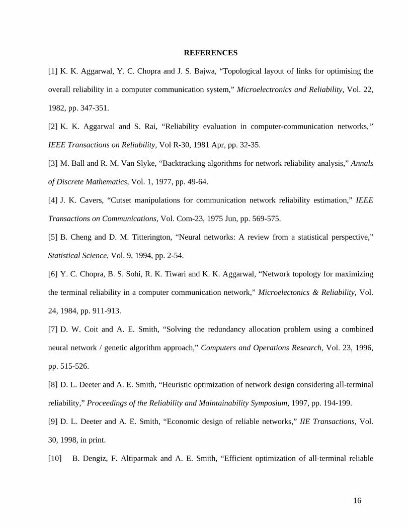
A second strategy using a specialized ANN for highly reliable networks was also employed.

Because most actual network topology designs will be highly reliable, it is important that the

reliability estimation be precise when R(x) ≥ 0.90. If the first ANN (just described) estimated a

reliability of 0.90 or greater, the network topology, the link reliability and the upperbound were input

to the second, specialized ANN, as shown in Figure 1. This ANN was trained on 250 randomly

generated topologies (using the same five link reliabilities) that had actual all-terminal reliabilities of

0.90 or greater. As in the general ANN, there were equal number (50) observations of each link

reliability in the data set. Also as in the general ANN, a five-fold grouped cross validation

procedure was used for ANN training and validation. The ANN architecture was the same as the

first network. Using the network reliability estimate from the first ANN as an additional input to the

specialized ANN was tried, but this did not improve predictive performance of the specialized ANN.

INSERT FIGURE 1 HERE

3.2 Networks with Varying Link Reliability

Allowing links of different reliability within a single network topology is an important real

world consideration. It does greatly expand the number of possible network topologies,

complicating both the network design problem and the estimation of all-terminal network reliability.

Using the same set of five link reliabilities from section 3.1, networks with mixes of these were

11

randomly generated (using equal probability on each link type). For these networks, k=6 (i.e., one of

the five reliability values or 0, which indicates the link is not present in the network topology). To

clarify, the ANN in this section would be appropriate for network design problems using any of

these five link reliabilities in any combination. The binary topology inputs of section 3.1 are no

longer applicable. Instead, the reliability value of each link is input (0, 0.80, 0.85, 0.90. 0.95, 0.99)

and the input of the single link reliability from section 3.1 is eliminated, leaving 46 inputs for a ten

node network.

The inputs to the ANN were:

1. The architecture of the network as indicated by a series of real valued variables

(xij). The length of the string is equal to 2

)1( −NN .

2. The calculated upperbound using the method of [19, 20] of the network.

As in section 3.1, 750 randomly generated network topologies were used for training and validating

the ANN and the exact all-terminal network reliability using backtracking [3] was used as the target.

The ANN architecture used 46 hidden neurons in a single hidden layer and a single output.

Also, as in section 3.1, the strategy of a general ANN for all network topologies and a

specialized ANN for highly reliable (≥ 0.90) networks was used. The specialized networks were

trained and validated using a set of 250 randomly generated topologies. Again, there were 46 inputs

to the neural network, a single output and 46 hidden neurons in one hidden layer.

4. COMPUTATIONAL RESULTS

4.1 Networks with Identical Link Reliability

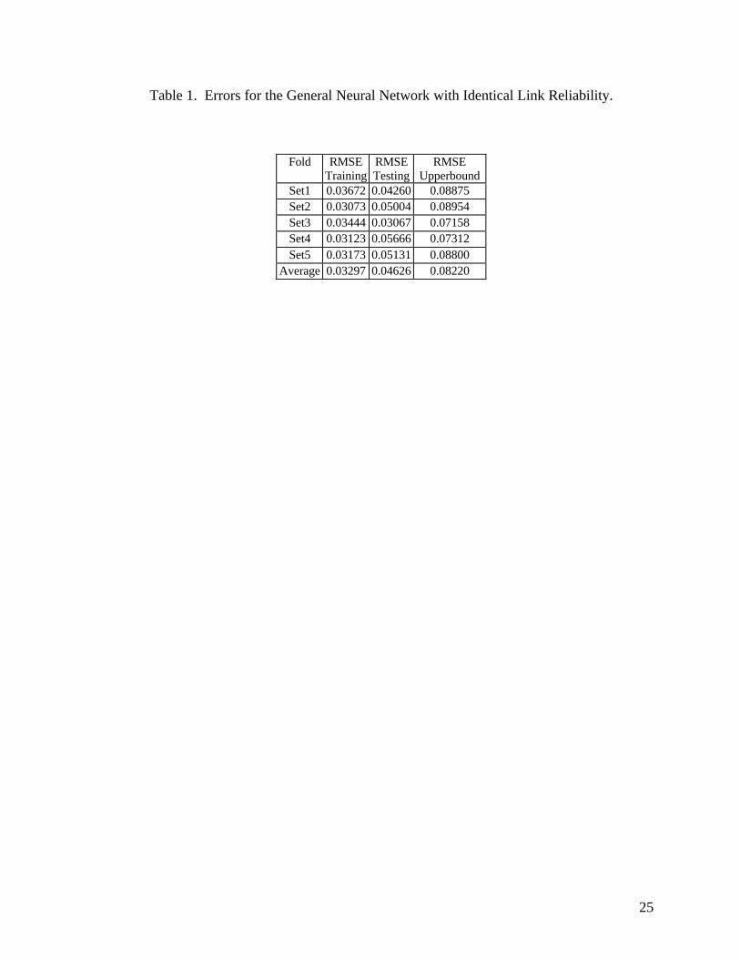
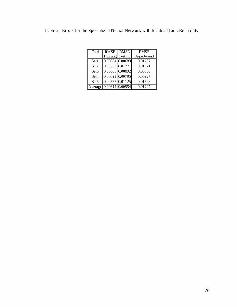
Tables 1 and 2 give the five-fold results in root mean squared error (RMSE) for the general

ANN and the specialized ANN, respectively, for networks with identical link reliability (those

described in section 3.1). It can be seen that the ANN estimations always improve upon the

12

upperbound estimates, sometimes significantly. Furthermore, the errors of the specialized ANN are

much less than that of the general ANN, allowing a more precise network reliability estimation for

those topologies that are likely to be considered the best.

INSERT TABLES 1 AND 2 HERE

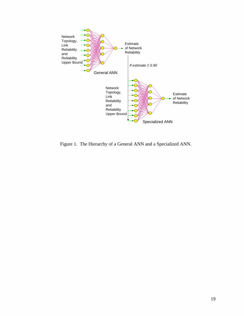
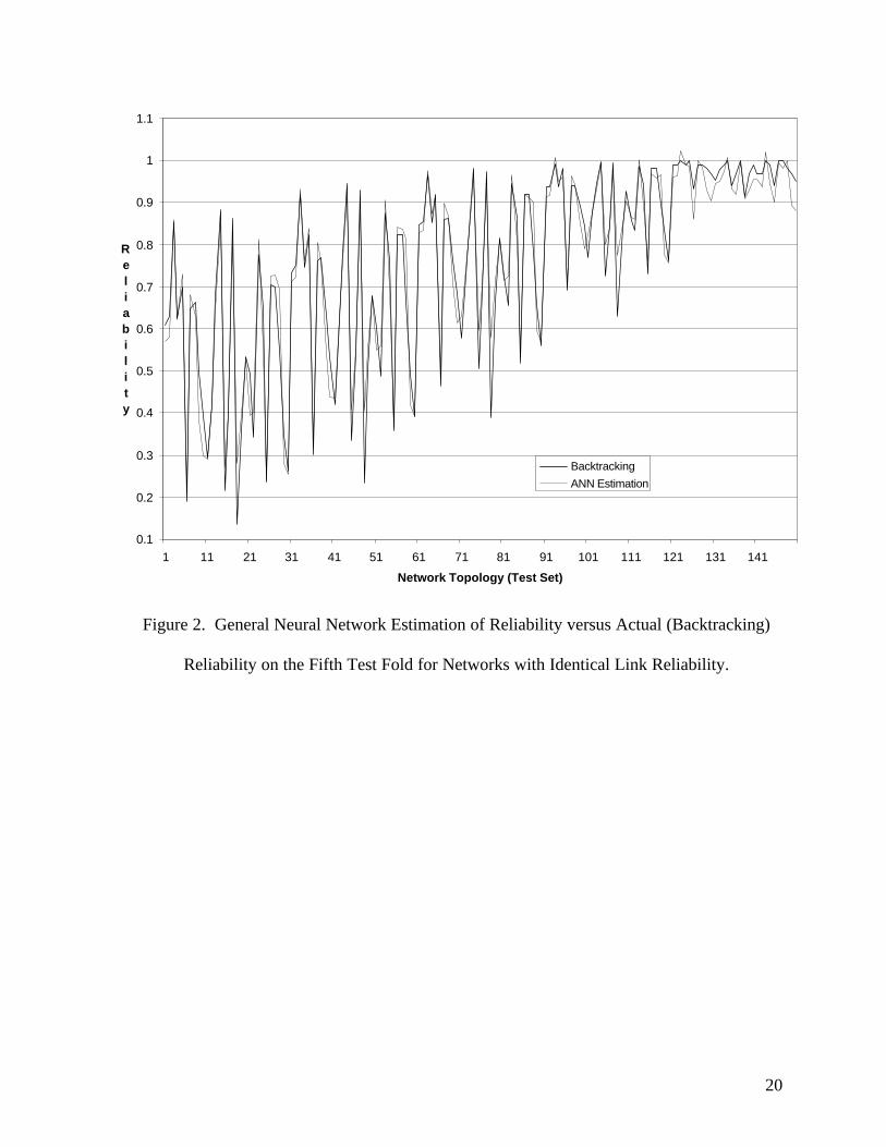
Figure 2 shows an example of one of the five-fold validations comparing the estimation of

the ANN on the test set with the actual reliability while Figure 3 shows the same for the specialized

ANN. It can be seen that the predictions of the ANN are unbiased and are quite precise. Where the

general ANN is less precise (at R(x) ≥ 0.90), the specialized ANN does a much better job. The mean

absolute error (MAE) of the application general ANN is 0.036 and the MAE of the application

specialized ANN is 0.007. Of course, these errors may be positive or negative since an ANN is an

unbiased estimator while the upperbound errors will always be positive.

INSERT FIGURES 2 AND 3 HERE

A statistical analysis of the estimations of the ANN and the upperbound with the exact

network reliability showed that the ANN was statistically closer to the exact value. Specifically, an

ANOVA for the general ANN over the 750 test observations was significant with a p value of

< 0.0000. A Tukey test for mean differences at α=0.05 resulted in the exact reliability from

backtracking and the ANN in the same statistical group while the upperbound formed a second

group. A paired t test between the exact value and the ANN had a p value of 0.0183 with a mean

difference of –0.0041 while a paired t test between the exact value and the upperbound had a p value

of < 0.0000 and a mean difference of -0.0515. For the specialized ANN using the 250 test

observations, the ANOVA had a p value of 0.0019 and the ANN and the exact values were again in

one statistical group using the Tukey test at α=0.05, while the upperbound formed a second group.

The paired t test between the exact reliability and the ANN estimation had a p value of 0.0527 with a

13

mean difference of –0.0012 while the paired t test between the exact value and the upperbound had a

p value of < 0.0000 with a mean difference of –0.0082.

4.2 Networks with Varying Link Reliability

This problem is much harder than that described in the preceding section, however the ANN

prediction performed well. Table 3 gives the results over the five fold cross validation for the

general purpose ANN while Table 4 gives the same results for the specialized ANN. It can be seen

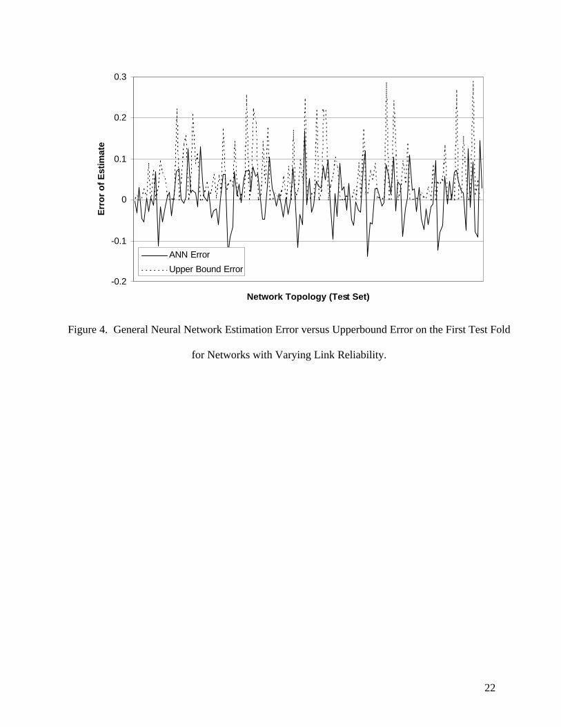
that the RMS error of the ANN is still significantly less than that of the upperbound. A graphic view

shows that the ANN estimate is unbiased while the upperbound estimate is biased upwards, of

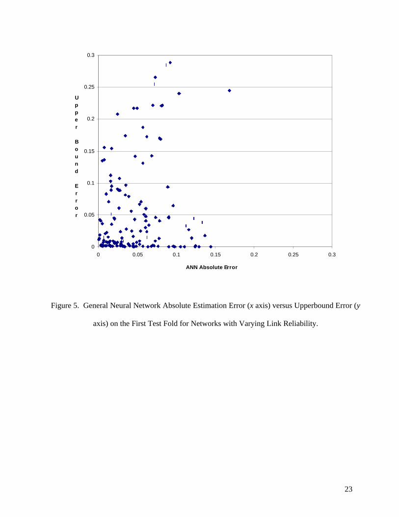
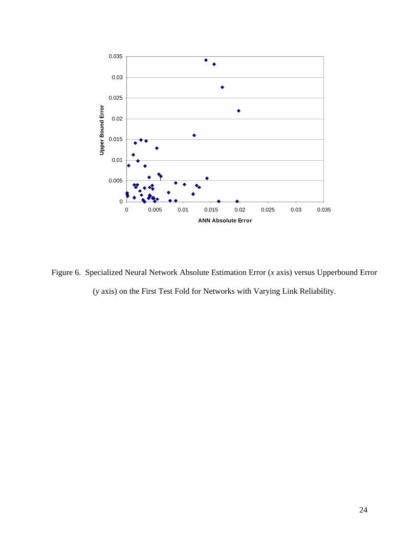
course (Figure 4). Figures 5 and 6 show the absolute error of the ANN versus the error of the

upperbound for the first fold of the test set for the general and specialized ANN, respectively. It can

be easily seen that while the upperbound sometimes performs better than the ANN, the maximum

errors of the ANN are much less. That is, the worst cases of the ANN are much better estimates than

the worst cases of the upperbound. This has practical importance since a large error may badly

mislead the optimization search where small errors will not. Therefore, the ANN can engender a

more reliable search than the upperbound.

INSERT TABLES 3 AND 4 HERE

INSERT FIGURES 4, 5 and 6 HERE

As in the preceding section, a statistical analysis of the estimations of the ANN and the

upperbound with the exact network reliability showed that the ANN was statistically closer to the

exact value. The ANOVA for the general ANN over the 750 test observations was significant with a

p value of < 0.0000. A Tukey test for mean differences at α=0.05 grouped the exact reliability from

backtracking and the ANN together while the upperbound formed a separate group. A paired t test

between the exact value and the ANN had a p value of 0.0195 with a mean difference of –0.0054

14

while a paired t test between the exact value and the upperbound had a p value of < 0.0000 and a

mean difference of -0.0511. For the specialized ANN using the 250 test observations, the ANOVA

had a p value of 0.0032 and the ANN and the exact values were again in one statistical group using

the Tukey test at α=0.05, while the upperbound formed another. The paired t test between the exact

value and the ANN had a p value of 0.6682 (not statistically different) with a mean difference of

–0.00027 while the paired t test between the exact value and the upperbound had a p value of

< 0.0000 with a mean difference of –0.00746.

4.3 General Remarks

Considering the relatively minute training set used for each ANN, the computational benefits

of the approach become apparent. The ANN approach can now be used for any network design

problem of ten nodes with these five link reliabilities, in either an identical manner (sections 3.1 and

4.1) or in a mixed manner (sections 3.2 and 4.2). Considering the vast search spaces of each ten

node reliability design problem, an optimization procedure that examined only a very small fraction

of possible designs would still require millions of network reliability calculations. The tiny number

of network topologies needed for ANN training and validation gives an indication of the power of

the method. Increasing the training and validation set size will almost certainly improve the

estimation accuracy of the ANN while a decrease in size will worsen the estimates. For networks of

larger size, where target (actual) reliabilities using backtracking or another exact method are not

practical, Monte Carlo simulation could be substituted. Network reliability could be accurately

estimated by using many replications of Monte Carlo simulation for each network topology in the

data set available for training/testing. While this is still computationally burdensome, it is feasible,

and need only be done for the relatively small training/testing data set.

15

5. CONCLUSIONS AND DISCUSSION

The ANN approach to estimating all-terminal reliability worked well. Using an extremely

small fraction of the possible network topologies for a ten node problem, a general ANN and a

specialized ANN were trained and validated. Subsequent use of the ANN during network design

optimization will be basically computationally “free”. The recommended approach is to use the

ANN estimation during the optimization for all topologies considered and then exactly calculate1 the

network reliability on only the optimal topology, or the few best topologies. In this way, almost all

of the computational effort of reliability calculation is eliminated while maintaining a workable

design optimization method.

It is likely that confining the ANN for networks with identical link reliability to only a single

link reliability would further improve its precision, however this would reduce flexibility during the

design phase. Another alteration is to not randomly generate the network topologies for training and

validation, but use a design of experiments to obtain a balance of topologies with different number

of links, node degrees, reliabilities, etc. As a further extension, this methodology may work using

function approximation methods other than neural networks, such as regression or spline fitting.

Finally, this approach of substituting a computationally expedient approximation for the exact

objective function calculation in iterative optimization can be feasible and effective for many

problems. The important issues are to develop an approximation that is precise enough, especially in

the search space regions of greatest interest, and saves sufficient computational effort to make the

sacrifice of the exact objective function calculation worthwhile.

1 Or, alternatively, estimate it accurately with Monte Carlo simulation.

16

REFERENCES

[1] K. K. Aggarwal, Y. C. Chopra and J. S. Bajwa, “Topological layout of links for optimising the

overall reliability in a computer communication system,” Microelectronics and Reliability, Vol. 22,

1982, pp. 347-351.

[2] K. K. Aggarwal and S. Rai, “Reliability evaluation in computer-communication networks,”

IEEE Transactions on Reliability, Vol R-30, 1981 Apr, pp. 32-35.

[3] M. Ball and R. M. Van Slyke, “Backtracking algorithms for network reliability analysis,” Annals

of Discrete Mathematics, Vol. 1, 1977, pp. 49-64.

[4] J. K. Cavers, “Cutset manipulations for communication network reliability estimation,” IEEE

Transactions on Communications, Vol. Com-23, 1975 Jun, pp. 569-575.

[5] B. Cheng and D. M. Titterington, “Neural networks: A review from a statistical perspective,”

Statistical Science, Vol. 9, 1994, pp. 2-54.

[6] Y. C. Chopra, B. S. Sohi, R. K. Tiwari and K. K. Aggarwal, “Network topology for maximizing

the terminal reliability in a computer communication network,” Microelectonics & Reliability, Vol.

24, 1984, pp. 911-913.

[7] D. W. Coit and A. E. Smith, “Solving the redundancy allocation problem using a combined

neural network / genetic algorithm approach,” Computers and Operations Research, Vol. 23, 1996,

pp. 515-526.

[8] D. L. Deeter and A. E. Smith, “Heuristic optimization of network design considering all-terminal

reliability,” Proceedings of the Reliability and Maintainability Symposium, 1997, pp. 194-199.

[9] D. L. Deeter and A. E. Smith, “Economic design of reliable networks,” IIE Transactions, Vol.

30, 1998, in print.

[10] B. Dengiz, F. Altiparmak and A. E. Smith, “Efficient optimization of all-terminal reliable

17

networks using an evolutionary approach,” IEEE Transactions on Reliability, Vol. 46, 1997, pp. 18-

26.

[11] B. Dengiz, F. Altiparmak and A. E. Smith, “Local search genetic algorithm for optimal

design of reliable networks,” IEEE Transactions on Evolutionary Computation, Vol. 1, 1997, pp.

179-188.

[12] G. S. Fishman, “A Monte Carlo sampling plan for estimating network reliability,”

Operations Research, Vol. 34, 1986, pp. 581-594.

[13] K. Funahashi, “On the approximate realization of continuous mappings by neural networks,”

Neural Networks, Vol. 2, 1989, pp. 183-192.

[14] M. R. Garey and D. S. Johnson, Computers and Intractability: A Guide to the Theory of NP-

Completeness, W. H. Freeman and Co., San Francisco, 1979.

[15] S. Geman, E. Bienenstock and R. Doursat “Neural networks and the bias/variance dilemma,”

Neural Computation, Vol. 4, 1992, pp. 1-58.

[16] K. Hornik, M. Stinchcombe and H. White, “Multilayer feedforward networks are universal

approximators,” Neural Networks, Vol. 2, 1989, pp. 359-366.

[17] R.-H. Jan, “Design of reliable networks,” Computers and Operations Research, Vol. 20,

1993, pp. 25-34.

[18] R.-H. Jan, F.-J. Hwang, and S.-T. Chen, “Topological optimization of a communication

network subject to a reliability constraint,” IEEE Transactions on Reliability, Vol. 42, 1993, pp. 63-

70.

[19] A. Konak and A. E. Smith, “A general upperbound for all-terminal network reliability and its

uses,” Proceedings of the Industrial Engineering Research Conference, Banff, Canada, May 1998,

CD Rom format.

18

[20] A. Konak and A. E. Smith, “An improved general upperbound for all-terminal network

reliability,” in revision at IIE Transactions.

[21] J. S. Provan and M. O. Ball, “The complexity of counting cuts and of computing the

probability that a graph is connected,” SIAM Journal of Computing, Vol. 12, 1983 Nov., pp. 777-

788.

[22] S. Rai, “A cutset approach to reliability evaluation in communication networks,” IEEE

Transactions on Reliability, Vol. R-31, 1982 Dec, pp. 428-431.

[23] J. M. Twomey and A. E. Smith, “Bias and variance of validation methods for function

approximation neural networks under conditions of sparse data,” IEEE Transactions on Systems,

Man, and Cybernetics, Part C, Vol. 28, August 1998, 417-430.

[24] A. N. Venetsanopoulos and I. Singh, “Topological optimization of communication networks

subject to reliability constraints,” Problem of Control and Information Theory, Vol. 15, 1986, pp.

63-78.

[25] Paul J. Werbos, Beyond Regression: New Tools for Prediction and Analysis in the

Behavioral Sciences, unpublished Ph.D. Thesis, Harvard University, 1974.

[26] H. White, “Connectionist nonparametric regression: Multilayer feedforward networks can

learn arbitrary mappings,” Neural Networks, Vol. 3, 1990, pp. 535-549.

[27] M.-S. Yeh, J.-S. Lin and W.-C. Yeh, “A new Monte Carlo method for estimating network

reliability,” Proceedings of the 16th International Conference on Computers & Industrial

Engineering, 1994, pp. 723-726.

19

If estimate ≥ 0.90

General ANN

NetworkTopology,LinkReliabilityandReliabilityUpper Bound

Estimateof NetworkReliability

Specialized ANN

Estimateof NetworkReliability

NetworkTopology,LinkReliabilityandReliabilityUpper Bound

Figure 1. The Hierarchy of a General ANN and a Specialized ANN.

20

0.1

0.2

0.3

0.4

0.5

0.6

0.7

0.8

0.9

1

1.1

1 11 21 31 41 51 61 71 81 91 101 111 121 131 141

Network Topology (Test Set)

Reliability

Backtracking

ANN Estimation

Figure 2. General Neural Network Estimation of Reliability versus Actual (Backtracking)

Reliability on the Fifth Test Fold for Networks with Identical Link Reliability.

21

0.9

0.92

0.94

0.96

0.98

1

1 11 21 31 41 51Network Topology (Test Set)

Reliability

Exact Reliability

Neural NetworkEstimation

Figure 3. Specialized Neural Network Estimation of Reliability versus Actual Reliability on the

First Test Fold for Networks with Identical Link Reliability.

22

-0.2

-0.1

0

0.1

0.2

0.3

Network Topology (Test Set)

Err

or

of

Est

imat

e

ANN Error

Upper Bound Error

Figure 4. General Neural Network Estimation Error versus Upperbound Error on the First Test Fold

for Networks with Varying Link Reliability.

23

0

0.05

0.1

0.15

0.2

0.25

0.3

0 0.05 0.1 0.15 0.2 0.25 0.3

Upper Bound Error

ANN Absolute Error

Figure 5. General Neural Network Absolute Estimation Error (x axis) versus Upperbound Error (y

axis) on the First Test Fold for Networks with Varying Link Reliability.

24

0

0.005

0.01

0.015

0.02

0.025

0.03

0.035

0 0.005 0.01 0.015 0.02 0.025 0.03 0.035

ANN Absolute Error

Up

per

Bo

un

d E

rro

r

Figure 6. Specialized Neural Network Absolute Estimation Error (x axis) versus Upperbound Error

(y axis) on the First Test Fold for Networks with Varying Link Reliability.

25

Table 1. Errors for the General Neural Network with Identical Link Reliability.

Fold RMSETraining

RMSETesting

RMSEUpperbound

Set1 0.03672 0.04260 0.08875Set2 0.03073 0.05004 0.08954Set3 0.03444 0.03067 0.07158Set4 0.03123 0.05666 0.07312Set5 0.03173 0.05131 0.08800

Average 0.03297 0.04626 0.08220

26

Table 2. Errors for the Specialized Neural Network with Identical Link Reliability.

Fold RMSETraining

RMSETesting

RMSEUpperbound


Average 0.00612 0.00954 0.01207

27

Table 3. Errors for the General Neural Network with Varying Link Reliability.

Fold RMSETraining

RMSETesting

RMSEUpperbound


Average 0.04504 0.06260 0.08698

28

Table 4. Errors for the Specialized Neural Network with Varying Link Reliability.

Fold RMSETraining

RMSETesting

RMSEUpperbound


Average 0.00776 0.00980 0.01277

Documents

Estimation of all-terminal network reliability using an artificial neural network