ESTIMATION OF HYDRAULIC DIFFUSIVITY IN

STREAM-AQUIFER SYSTEM

By Govinda C. Mishra1 and Sharad K. Jain2

ABSTRACT: The Laplace transform of convolution equation, which relates aquifer response to boundary per-turbation, expresses explicitly the hydraulic diffusivity in terms of the Laplace transform parameter, changes instream stage, and fluctuations of piezometric level at a point near the stream. Hydraulic diffusivity has beenestimated using the Laplace transform approach. The diffusivity has also been determined from observed re-sponse of an aquifer and the boundary perturbation using the Marquardt method, a least-squares optimizationtechnique. If the observed data are free from random error, the diffusivity can be estimated accurately using theLaplace transform approach. Unlike the least-squares optimization method, the Laplace transform techniqueautomatically gives less weight to the latter part of the aquifer response and thereby to the random error containedin it. Discrete kernel coefficients have been derived, using which the water level rise in an aquifer that can bepredicted for any variation in stream stage.

INTRODUCTION

The estimation of hydraulic diffusivity from the observationof stream stage and consequent water table fluctuations in anadjacent aquifer is an inverse problem. An inverse problemcannot be solved unless the corresponding direct problem hasbeen solved a priori. The stream-aquifer interaction problemhas been solved by several investigators (Todd 1955; Rowe1960; Cooper and Rorabaugh 1963; Hall and Moench 1972;Morel-Seytoux and Daly 1975; Halek and Svec 1979), and thestream-aquifer equations have been applied by various otherinvestigators to estimate the aquifer diffusivity (Rowe 1960;Ferris 1962; Pinder et al. 1969; Brown et al. 1972; Singh andSagar 1977). An alternate approach is presented here to deter-mine the diffusivity using the measurements of stream stageduring passage of a flood wave and the consequent water levelfluctuations in a piezometer in the vicinity of the stream.

ANALYTICAL DEVELOPMENT

Discrete Kernel for Piezometric Rise

The unit step response function that relates rise in piezo-metric surface in an initially steady-state semiinfinite homo-geneous and isotropic confined aquifer, bounded by a fullypenetrating straight stream, to a step rise in stream stage hasbeen derived by Carslaw and Jaeger (1959) for an analogousheat conduction problem. The unit step response function is

K(x, t) = erfc{x/ (4bt)} (1)Ï

where x = distance from the bank of the stream; t = timemeasured since the onset of change in stream stage; b = hy-draulic diffusivity of the aquifer defined as ratio of transmis-sivity to storage coefficient or as ratio of saturated hydraulicconductivity to specific storage; and erfc{?} = complementaryerror function.

In nature, a stream partially penetrates an aquifer. For apartially penetrating stream, the flow is 2D near the stream.To use (1) in such a case, it is necessary to install two obser-vation wells on one side of the stream in a line perpendicularto the stream. The first one should be installed from the stream

1Sci. F, Nat. Inst. of Hydro., Roorkee 247667, U.P., India.2Sci. E, Nat. Inst. of Hydro., Roorkee 247667, U.P., India.Note. Discussion open until September 1, 1999. To extend the closing

date one month, a written request must be filed with the ASCE Managerof Journals. The manuscript for this paper was submitted for review andpossible publication on May 15, 1997. This paper is part of the Journalof Irrigation and Drainage Engineering, Vol. 125, No. 2, March/April,1999. qASCE, ISSN 0733-9437/99/0002-0074–0081/$8.00 1 $.50 perpage. Paper No. 15783.

74 / JOURNAL OF IRRIGATION AND DRAINAGE ENGINEERING / MARC

bank at a distance equal to the thickness of the aquifer belowthe streambed beyond which the flow is 1D (Streltsova 1974).Thickness of the aquifer below the streambed can be ascer-tained from the study of lithologs in the vicinity of the stream.The water level fluctuations in this well can be considered torepresent fluctuations in a fully penetrating stream (Reynolds1987). The water level fluctuations in the other well representthe aquifer response. Eq. (1) is a good approximation for anunconfined aquifer if the changes in water level are small incomparison to the saturated thickness of the aquifer (Cooperand Rorabaugh 1963).

For varying stream stage, s(t), the rise in piezometric sur-face, s(x, t), according to Duhamel’s integral (Thomson 1950)is given by

tds(t)

s(x, t) = s K(x, t) 1 K(x, t 2 t) dt (2)0 E dt0

where s0 = initial sudden rise in the stream stage; and t =time variable. Duhamel’s integral, which can be expressed intwo different forms (Thomson 1950), has been used exten-sively for solving stream-aquifer interaction problems (Pinderet al. 1969; Venetis 1970; Hall and Moench 1972; Abdulrazzakand Morel-Seytoux 1983; Morel-Seytoux 1988).

Let the time span be discretized into uniform time steps ofsize Dt. Let the rate of change of stream stage, ds(t)/dt, be aconstant within a time step; however, ds(t)/dt may vary fromone time step to the next. Eq. (2) can be rewritten as

xs(x, nDt) = s erfc0 F G

(4bnDt)ÏgDtn

s 2 s xg g211 erfc dtO F E H J GDt (4b(nDt 2 t))g=1 Ï(g21)Dt (3)

where sg = rise in stream stage at t = gDt.Let, for computation of rise in piezometric surface, a dis-

crete kernel coefficient, dr(x, Dt, m), be defined asDt

1 xd (x, Dt, m) = erfc dt (4)r E H JDt 4b(mDt 2 t)Ï0

where m = integer. Using a substitution t = Dtv, and dt =Dtdv, where v is a dimensionless dummy variable, (4) is sim-plified to

1x

d (x, Dt, m) = erfc dv (5)r E H J4bDt(m 2 v)Ï0

Performing the integration (see Appendix I)

H/APRIL 1999

d (x, Dt, m) = 1 1 {(m 2 1)r

21 x /(2bDt)}erf[x/ {4bDt(m 2 1)}] 2 {mÏ21 x /(2bDt)}erf{x/ (4bDtm)} 1 x {(m 2 1)/(bDtp)}Ï Ï

2?exp[2x /{4bDt(m 2 1)}]

22 x {m/(bDtp)}exp{2x /(4bDtm)}Ï (6)

Discrete kernel coefficients for return flow and cumulativereturn flow for the stream-aquifer system have been derivedby Morel-Seytoux (1988). In the current definition of the dis-crete kernel, the time step Dt appears explicitly and the dis-crete kernel coefficient is dimensionless.

The rise in piezometric surface at the end of nth unit timestep given by (3) is expressed in terms of discrete kernel co-efficient as

nx

s(x, nDt) = s erfc 10 H J O(4bnDt) g=1Ï

? [(s 2 s )d (x, Dt, n 2 g 1 1)]g g21 r (7)

The fluctuations in piezometric surface at different locationsfor a single or several flood events can be determined using(6) and (7).

DETERMINATION OF HYDRAULIC DIFFUSIVITY

The hydraulic diffusivity can be determined using the fluc-tuations in stream stage during the passage of a flood and theconsequent changes in water level recorded in a piezometernear the stream either by applying a Laplace transform tech-nique or using a least-squares optimization method. Thesemethods are discussed below.

Laplace Transform Method

The Laplace transform, which transforms one class of func-tion into another, has the advantage that, under certain circum-stances, it replaces complicated functions by simpler ones(Widder 1961). An approach based on Laplace transform fordetermining the hydraulic diffusivity is described below.

Taking the Laplace transform of the terms on both sides of(2)

` `

2at 2ats(x, t)e dt = s K(x, t)e dt0E E0 0

` tds(t) 2at1 K(x, t 2 t) dt e dtE FE Gdt0 0 (8)

where a = Laplace transform parameter. Applying Faltung the-orem, that is,

t

L F (t 2 t)F (t) dt = L[F (t)]L[F (t)]1 2 1 2FE G0

Eq. (8) reduces to`

ds2ats(x, t)e dt = s L[K(x, t)] 1 L L[K(x, t)] (9)0E F Gdt0

Substituting the Laplace transform of the complementary errorfunction, K(x, t), into (9) (Abramowitz and Stegun 1970)

`

ds2at 2s(x, t)e dt = s 1 L exp[2 (ax /b)]/a (10)Ï0E F S DGdt0

Discretizing the time domain in steps of uniform size Dt,and assuming that the rate of change of stream stage is a con-stant within a time step, (10) is expressed as (Gustav 1961)

JOURNAL OF IR

gDtn n

0 2ats e dt = s 1g21/2 0O F E G F Og=1 g=1(g21)Dtn ` n `→ →

gDts 2 sg g21 2at 2? e dt exp {2 (al /b)}/aÏH E JGDt (g21)Dt (11)

where = 1 and = observed water level0 0 0 0s [s s ]/2; sg21/2 g21 g g

rise at time gDt in a piezometer located at a distance l fromthe stream bank. Integrating, (11) reduces to

n n2a(g21)Dt 2agDt{e 2 e }0s = s 1g21/2 0O F G F Oag=1 g=1n ` n `→ →

2alexp 2H Î Jb

2a(g21)Dt 2agDt(s 2 s ) (e 2 e )g g21? GDt a a (12)

or

2exp{2 (al /b)}Ïn

0 2a(g21)Dt 2agDt[s {e 2 e }]g21/2Og=1n `→= n 2a(g21)Dt 2agDts 2 s e 2 eg g21

s 10F O HS D S DJGDt ag=1n `→ (13)

Taking the natural logarithm of terms on either side and solv-ing for b yields

n 2

0 2a(g21)Dt 2agDt[s (e 2 e )]g21/2Og=1n `2 →b = al ln n 2a(g21)Dt 2agDts 2 s e 2 eg g21YF Gs 10 OHS DS DJDt ag=1

n `→

(14)

In practice, an observation period is always finite. There-fore, the summations can be truncated beyond a finite obser-vation period. Introducing truncation errors in the summationsof the series, (14) is modified to

n2

0 2a(g21)Dt 2agDt{s (e 2 e )} 1 εg21/2 1Og=12b = al ln n 2a(g21)Dt 2agDts 2 s e 2 eg g21YF G

s 1 1 ε0 2O HS D S DJDt ag=1

(15)

The two series containing the average water level rise at thepiezometer, and the change in stream stage will converge asthey contain exponentials of negative terms. The rate of con-vergence will depend upon the value of a and Dt. For example,for a step rise in water level in the observation well, for a =0.06 h21, Dt = 1 h, and n = 240, the truncation error ε1 willbe ;5%. Moreover, the stream stage and the water level riseat the piezometer after some lag will become smaller afterrecession of the flood wave. The truncation errors, ε1 and ε2,would, therefore, tend to zero with increasing observation pe-riod. Hence, the hydraulic diffusivity, b, can be computed withreasonable accuracy using (15).

If a flood wave follows a definite equation, the computationof b can be further simplified. For example, let s0 be equal tozero and let the flood wave follow the damped sinusoidalequation proposed by Cooper and Rorabough (1963)

RIGATION AND DRAINAGE ENGINEERING / MARCH/APRIL 1999 / 75

2dtNH (1 2 cos vt)e for 0 # t # t0 ds(t) = (16)H0 for t > td

where s(t) = rise above initial water level in the stream; H0 =height of peak flood stage above initial water level; td = periodof the flood wave; tc = time of flood peak; v = 2p/td, thefrequency of oscillation; N = exp(dtc)/(1 2 cos vtc); and d =v cot(0.5vtc). The function s(t) has an ordinary discontinuityat t = td, and the finite jump at t = td is equal to NH0(1 2 cosvtd)exp(2dtd). The Laplace transform of the derivative ds(t)/dt, in which s(t) has an ordinary discontinuity at t = td, isgiven by (Kreyszig 1989)

ds(t)L = aL[s(t)] 2 s(0) 2 [s(t 1 ε)dF Gdt

2 s(t 2 ε)]exp(2at )], ε → 0d d (17)

The Laplace transform of s(t), which has an ordinary discon-tinuity at t = td, is given by

` t `d

2at 2at 2atL{s(t)} = s(t)e dt = s(t)e dt 1 s(t)e dtE E E0 0 td

td

2dt 2at= {NH (1 2 cos vt)e }e dt0E0 (18)

Incorporating the Laplace transform of s(t) in (17), the La-place transform of the derivative is

L{ds(t)/dt} = NH a exp{2(d 1 a)t }[d/{a(d 1 a)}0 d

2 (1/a)cos vt 1 {(d 1 a)cos vt 2 v sin vt }d d d

2 2/{d 1 a) 1 v }] 1 NH a[1/(d 1 a) 2 (d 1 a)0

2 2/{(d 1 a) 1 v }] (19)

This analytical expression of the Laplace transform of ds/dtis an alternate substitute for the denominator in the logarithmicterm in (15) only if the flood wave follows (16).

Least-Squares Optimization Method

The hydraulic diffusivity, b, can be determined minimizingthe objective function

2N­s(l, nDt)0s 2 s(l, nDt)u 1 Dbn b*O F H U JG

­bn=1 b*

with respect to Db, where N = number of observations; b* =initial guess of the hydraulic diffusivity; and Db = incrementin b. Following a numerical method, the derivative ­s(1, nDt)/­b at b = b* can be computed from (7). The derivative couldbe derived analytically as well. The well known Marquardtalgorithm (Marquardt 1963) is a technique of estimation ofnonlinear parameters by linearization and minimization of theleast squares. The Marquardt algorithm has been applied byseveral investigators to determine transmissivity and storagecoefficient of a confined aquifer from pumping test data(Chander et al. 1981; Johns et al. 1992).

RESULTS AND DISCUSSION

The proposed methods for determining the aquifer param-eter from the response of the stream-aquifer system have beentested using synthetic data. The water level rise in a piezometerwas generated for different values of b, for the following floodwave that follows (16):

• Time of flood peak, tc: 24 h• Duration of flood wave, td: 120 h

76 / JOURNAL OF IRRIGATION AND DRAINAGE ENGINEERING / MARC

• Maximum rise in stream stage, H0: 2 m• Time-step size or sampling period, Dt: 1, 0.5, and 0.25 h• Duration of observation, nDt: 120, 240, 360, and 600 h• Distance of piezometer from stream, l: 50 and 200 m• Hydraulic diffusivity, b: 25.0 and 50,000.0 m2/h

The standard deviation, sd, of the error free set of rises inwater level in a piezometer was computed. Random errorswith zero mean and a prescribed percentage of sd as standarddeviation have been added to the piezometric levels. Thesepiezometric levels containing random errors have been re-garded as observed piezometric levels and have been used fortesting the proposed methods of identification of parameter.

Laplace Transform Technique

The expression of hydraulic diffusivity [(15)], which hasbeen derived using Laplace transform technique, contains allthe inherent problems of the Laplace transform method. Theperturbation and the response differ from each other at smallas well as large values of t depending upon the distance of thepiezometer from the stream bank and aquifer diffusivity. Thewater level may continue to rise in a piezometer even thoughthe flood wave might have started receding. In the Laplacetransform technique, the perturbation and the response areweighted by the factor exp(2at) and their variations at largevalues of t can only be seen in the transform near the origin(i.e., a is small) (Hamming 1973). In other words, delayedresponse can be accounted for by selecting a small value ofa. Conversely, the parameter a must be sufficiently large tomake the integral convergent. Thus, there is a conflict in theselection of the parameter a. While selecting a, one has tocheck the lower limit for which the Laplace transforms of theinput and output functions exist. For example, if the input oroutput function is of exponential form [exp(at)], the parametera should be greater than a (Rainville 1963). The Laplace trans-forms for a damped sinusoidal continuous function, and itsderivative, exist for a greater than zero (Rainville 1963). Asseen from (19), this is also true for a damped sinusoidal func-tion with ordinary discontinuity. The output function corre-sponding to a sinusoidal input will also be sinusoidal. There-fore, for the present input and output functions, the Laplaceparameter a should be greater than zero.

The fundamental trouble with the Laplace transform hasbeen discussed by Hamming (1973). For solving a problemby Laplace transformation, measurements of input and outputare made in the time domain. There is a limit on how fine aspacing one can take near the origin, and there is also a limiton how long a time one can make a measurement. Thus thetransform is not as well determined as one would wish. How-ever, in practice, the transform is applied. Gustav (1961) hassuggested an approach for choosing the time step size. Ac-cording to him, selection of time step should be based uponthe fact that both the perturbation and the response shouldchange on average by ;10% of their maximum values withinsuccessive intervals of the chosen time step.

The error in the estimated diffusivity is linked to the dura-tion of observation, time step size, value of Laplace transformparameter a, error due to numerical integration, and the ran-dom error in the observation.

The diffusivity evaluated by the Laplace transform tech-nique is presented in Tables 1 and 2 for different durations ofobservation and Laplace transform parameter a. A time stepsize of 1 h, which satisfies Gustav’s condition, has been cho-sen. For the assumed flood wave and sampling period of 1 h,the changes in flood stage and piezometric level within twosuccessive sampling periods are contained within 6.9 and 6.4%of their respective maximum fluctuations. Two sets of obser-vations containing normally distributed random errors with 5

H/APRIL 1999

TABLE 1. Estimation of Hydraulic Diffusivity by LaplaceTransform Technique (Time to Peak = 24 h, Duration of FloodWave = 120 h, Maximum Rise in Stream Stage = 2 m and Dis-tance of Observation Well from Stream = 50 m, Sampling Period= 1 h)

b assumedfor genera-

tion ofsynthetic

data(m2/h)

(1)

Duration ofobservation

(h)(2)

Laplaceparameter a

(h)21

(3)

Standarddeviation of

random error/standard

deviation oferror free

data(%)(4)

Computed b(m2/h)

(5)

25 120 0.01 0 18.65 18.8

10 19.00.05 0 24.9

5 25.310 25.6

0.10 0 25.05 26.4

10 27.7240 0.01 0 24.1

5 24.310 24.5

0.05 0 25.05 25.3

10 25.70.10 0 25.0

5 26.310 27.5

360 0.01 0 24.85 25.0

10 25.20.05 0 25.0

5 25.310 25.6

0.10 0 25.05 25.2

10 27.4600 0.01 0 25.0

5 25.210 25.4

0.05 0 25.05 25.3

10 25.60.10 0 25.0

5 26.110 27.2

and 10% of sd as standard deviation have been considered.Table 1 shows that when the duration of observation equalsthe duration of flood wave, the error in estimation of hydraulicdiffusivity is 26%. Table 2 shows that for high hydraulic dif-fusivity, the error is 13%. When the duration of observationis twice the duration of flood wave, the error is <4%. Thusthe duration of observation should be at least twice the dura-tion of flood wave. From data containing random error, whosestandard deviation is 10% of sd, low hydraulic diffusivity canbe computed with 98.5% accuracy if the duration of obser-vation is twice the duration of flood. The corresponding ac-curacy for higher diffusivity, when the data contain randomerror at 10% of sd, is 84%. The accuracy can be further im-proved using a smaller time step.

Considering the duration of observation as five times theduration of flood wave, the sensitivity of the computation ofhydraulic diffusivity to the time step size Dt, Laplace trans-form parameter a, and the random error in the observation ispresented in Fig. 1. These have been obtained using the syn-thetic data at a piezometer located at a distance of 200 m fromthe stream bank in an aquifer having hydraulic diffusivity of50,000 m2/h. From Fig. 1 it is seen that if the observed data

JOURNAL OF I

TABLE 2. Estimation of Hydraulic Diffusivity by LaplaceTransform Technique (Time to Peak = 24 h, Duration of FloodWave = 120 h, Maximum Rise in Stream Stage = 2 m and Dis-tance of Observation Well from Stream = 200 m, Sampling Pe-riod = 1 h)

b assumedfor genera-

tion ofsynthetic

data(m2/h)

(1)

Duration ofobservation

(h)(2)

Laplaceparameter

(h)21

(3)

Standarddeviation of

random error/standard

deviation oferror free

data(%)(4)

Computed b(m2/h)

(5)

50,000 120 0.01 0 43,4185 51,106

10 60,9490.05 0 50,182

5 54,44810 59,243

0.10 0 50,5995 57,877

10 66,667240 0.01 0 49,215

5 56,00110 64,241

0.05 0 50,2105 53,879

10 57,9360.10 0 50,599

5 56,82210 64,142

360 0.01 0 49,8805 56,105

10 63,5350.05 0 50,210

5 53,35510 56,782

0.10 0 50,5995 55,910

10 62,013600 0.01 0 50,014

5 55,09310 60,963

0.05 0 50,2105 52,727

10 55,4250.10 0 50,599

5 54,82810 59,556

are free from random error, the error in estimated diffusivityvaries linearly with Laplace parameter a. The error is attrib-uted to the time step size because for smaller time step sizethe graph tends to coincide with the a-axis. Thus, for errorfree data, any value of a greater than zero can be used fortime step Dt < 1 h. For observed data containing error, a par-abolic relationship exists between the percentage of error inthe estimated diffusivity and the Laplace parameter a. Withsmaller time step, the error in the estimation decreases. Theerror attains a minimum at some value of a. In particular forDt = 1 h, and standard deviation of random error = 10% sd,the error is minimum at a = 0.04 h21 and the minimum erroris 10.1%. For Dt = 0.25 h, the minimum occurs at a = 0.04h21 and the minimum error is 6%. For the time step size of0.25 h, the changes in flood stage and piezometric level withintwo successive time steps are contained within 1.7 and 1.6%of their respective maximum fluctuations. Thus, for determin-ing the hydraulic diffusivity, a time step size for which themaximum change in the perturbation within two successivetime steps does not exceed by 2% of the maximum streamstage rise is preferable. Once the time step size is selected, ashould be assigned a value such that 0.02 < aDt < 0.06. With

RRIGATION AND DRAINAGE ENGINEERING / MARCH/APRIL 1999 / 77

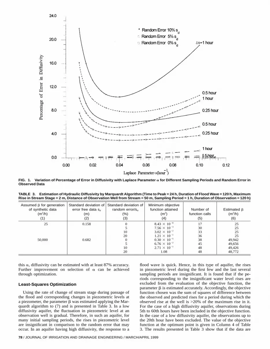
FIG. 1. Variation of Percentage of Error in Diffusivity with Laplace Parameter a for Different Sampling Periods and Random Error inObserved Data

TABLE 3. Estimation of Hydraulic Diffusivity by Marquardt Algorithm (Time to Peak = 24 h, Duration of Flood Wave = 120 h, MaximumRise in Stream Stage = 2 m, Distance of Observation Well from Stream = 50 m, Sampling Period = 1 h, Duration of Observation = 120 h)

Assumed b for generationof synthetic data

(m2/h)(1)

Standard deviation oferror free data sd

(m)(2)

Standard deviation ofrandom error/sd

(%)(3)

Minimum objectivefunction attained

(m2)(4)

Number offunction calls

(5)

Estimated b(m2/h)

(6)

25 0.158 0 8.43 3 1028 17 255 7.56 3 1023 30 25

10 3.02 3 1022 33 2520 1.21 3 1021 36 25

50,000 0.682 0 0.30 3 1025 38 49,9425 6.76 3 1022 45 49,656

10 2.71 3 1021 48 49,42620 1.08 48 48,772

this a, diffusivity can be estimated with at least 87% accuracy.Further improvement on selection of a can be achievedthrough optimization.

Least-Squares Optimization

Using the rate of change of stream stage during passage ofthe flood and corresponding changes in piezometric levels ata piezometer, the parameter b was estimated applying the Mar-quardt algorithm to (7) and is presented in Table 3. In a lowdiffusivity aquifer, the fluctuation in piezometric level at anobservation well is gradual. Therefore, in such an aquifer, formany initial sampling periods, the rises in piezometric levelare insignificant in comparison to the random error that mayoccur. In an aquifer having high diffusivity, the response to a

78 / JOURNAL OF IRRIGATION AND DRAINAGE ENGINEERING / MARCH

flood wave is quick. Hence, in this type of aquifer, the risesin piezometric level during the first few and the last severalsampling periods are insignificant. It is found that if the pe-riods corresponding to the insignificant water level rises areexcluded from the evaluation of the objective function, theparameter b is estimated accurately. Accordingly, the objectivefunction chosen was the sum of squares of difference betweenthe observed and predicted rises for a period during which theobserved rise at the well is >20% of the maximum rise in it.For the case of a high diffusivity aquifer, observations during5th to 60th hours have been included in the objective function.In the case of a low diffusivity aquifer, the observations up tothe 20th hour have been excluded. The value of the objectivefunction at the optimum point is given in Column 4 of Table3. The results presented in Table 3 show that if the data are

/APRIL 1999

free from random error, high hydraulic diffusivity of severalthousand m2/h magnitude as well as low hydraulic diffusivityof the order of 25 m2/h can be estimated with 99.99% accu-racy. If the data contain random error with a standard deviationof 20% sd, low hydraulic diffusivity is computed with 99.5%accuracy. The accuracy for high diffusivity is 97.5%. The hy-draulic diffusivity can thus be estimated very accurately usingthe Marquardt algorithm using a selected part of the observeddata.

Both the transmissivity and storage coefficient control theunsteady state response of an aquifer to any boundary pertur-bation whereas the transmissivity alone controls the nearsteady-state response of an aquifer. Therefore, for determiningthe aquifer diffusivity, the unsteady response of an aquifershould be given more weight than the steady-state response.The weighting factor in Laplace transform is Thus, the2ate .Laplace transform technique automatically gives more weightto the unsteady response (fluctuating part) of the aquifer thatoccurs earlier than to the near steady-state response that occurslater. This is the major strength and motivation for using theLaplace transform approach.

The least-squares optimization gives equal weight to all in-put data and thereby also to the random error contained in it.When the response of the aquifer over a threshold level wasconsidered, the results improved. Thus, this approach requirescareful screening of the input data.

FIELD VERIFICATION

Reynolds (1987) has estimated aquifer diffusivity for threesites in a finite glacial-outwash aquifer near Cortland, N.Y., bymatching the theoretical head response to a flood wave withcorresponding observed water level rise in the aquifer. Duha-mel’s formula has been used by Reynolds to generate the the-oretical head response. Prior processing of the field data isrequired for using them in solving the inverse problem. Theantecedent trends of the observation well hydrographs prior to

JOURNAL OF I

the onset of the particular flood wave should be extrapolatedfor the duration of the flood wave, and the observed datashould be corrected. Such a practice has been recommendedfor analyzing aquifer test data (Brown et al. 1972). Each an-tecedent trend may approximate a straight line when waterlevel changes are plotted in a semilog plot. Extrapolation ofan antecedent hydrograph becomes easy in such a case. Proc-essed field data reported by Reynolds (1987) have been usedto compute the hydraulic diffusivity by the present methods.

The response data at Site 1 (Elm Street) are suitable forsolving the inverse problem as an almost complete responseof the aquifer to a single flood wave in the stream is available.Also at this site the aquifer boundary is at a large distancefrom the observation well, and the assumption of infinite aq-uifer is valid.

The water table fluctuations at the first observation well Aadjacent to stream and at the second observation well B, lo-cated at a distance of 152 m from the first observation well,are presented in Fig. 2. As suggested by Reynolds, the waterlevels in the observation well A are substituted for streamstage. The water level rise at the observation well A consistsof two parts: (1) A step rise of 0.457 m; and (2) a sinusoidalpart. The step rise part is ascertained from the recession partof flood hydrograph. For a time step size of 1 h, the changesin flood stage and piezometric level within two successive timesteps are contained within 6.6 and 6.9% of their respectivemaximum fluctuations. Therefore, accoding to the Gustav con-dition, a time step size of 1 h can be adopted. For Dt = 1 h,the trial value of a should lie in the range 0.04–0.06 h21. Witha = 0.05 h21, the computed diffusivity corresponding to theobserved piezometric level at well B is 1,560 m2/h, and forthis diffusivity the sum of the squares of error between ob-served and simulated piezometric rise is minimum. Applyingthe Marquardt algorithm to (7), the hydraulic diffusivity wasfound to be 1,550 m2/h. The water level fluctuations at obser-vation well B computed by (7) with b = 1,560 m2/h are shown

FIG. 2. Comparison of Simulated Flood Wave Response to Observed Flood Wave Response

RRIGATION AND DRAINAGE ENGINEERING / MARCH/APRIL 1999 / 79

in Fig. 2. The simulated hydrograph matches well with theobserved hydrograph, and the peak has an error of ;8.2%.

Reynolds, using a method based on Duhamel’s principle,has reported the hydraulic diffusivity at this site to be 2,200m2/h and has simulated the fluctuations at observation well B.When Reynolds’ well B simulated data are used as observeddata, the hydraulic diffusivity is found to be 2,390 m2/h byboth the Laplace transform technique and Marquardt algo-rithm.

CONCLUSIONS

Unit step response function coefficients have been derivedand using these coefficients, the piezometric rise in an aquifercan be computed consequent to any flood wave in a fully pen-etrating stream.

The Laplace transform of the convolution equation, whichrelates aquifer response to boundary perturbation, explicitlyexpresses the hydraulic diffusivity in terms of the Laplacetransform parameter, changes in stream stage, and correspond-ing fluctuations of piezometric surface in the aquifer. The hy-draulic diffusivity can be estimated using the Laplace trans-form approach with reasonable accuracy.

If the observed data are free from random error, the diffu-sivity can be estimated accurately by both the Laplace trans-form and the least-square approach. The Marquardt methodcan be used to determine diffusivity from data containing ran-dom error by selecting observed data over a threshold value.Though such selection of observed data is not applicable inthe case of Laplace transform method, the method automati-cally gives less weight to the latter part of the observation andthereby to the random error contained in them. The Laplacetransform method gives more weight to the early part of theaquifer response that is governed by the hydraulic diffusivityand less weight to the latter part of the response that is gov-erned by transmissivity of the aquifer.

The computation of hydraulic diffusivity by the Laplacetransform method is straightforward and simple as comparedto the Marquardt method.

APPENDIX I. INTEGRATION OF STEPRESPONSE FUNCTION

Substituting v = m 2 x 2/(4bDtu2), dv = x 2/(2bDtu3) in (5)1

xd (x, Dt, m) = erfc dvr E H J

4bDt(m 2 v)Ï0

x/ 4bDt(m21)Ï2x 23= [u {1 2 erf(u)}] duE2bDt x/ 4bDtmÏ (20)

Integrating by parts

23 22[u {1 2 erf(u)}] du = 2u /2{1 2 erf(u)}E22 2 222 u exp(2u )/ p du = 2u /2{1 2 erf(u)}ÏE

21 21 u exp(2u )/ p 1 erf(u)Ï

Putting the limits and simplifying

d (x, Dt, m) = 1 1 {(m 2 1)r

21 x /(2bDt)}erf[x/ {4bDt(m 2 1)}]Ï22 {m 1 x /(2bDt)}erf{x/ (4bDtm)}Ï

21 x {(m 2 1)/(bDtp)}exp[2x /{4bDt(m 2 1)}]Ï22 x {m/(bDtp)}exp{2x /(4bDtm)}Ï

80 / JOURNAL OF IRRIGATION AND DRAINAGE ENGINEERING / MARC

ACKNOWLEDGMENTS

The writers are thankful to the anonymous reviewers whose commentsand suggestions have significantly improved the manuscript.

APPENDIX II. REFERENCES

Abdulrazzak, M. J., and Morel-Seytoux, H. J. (1983). ‘‘Recharge fromephemeral stream following wetting front arrival to water table.’’ WaterResour. Res., 19(1), 194–200.

Abramowitz, M., and Stegun, I. A., eds. (1970). Handbook of mathe-matical functions. Dover, New York.

Brown, R. N., Konoplyantsev, A. A., Ineson, J., and Kovalevsky, V. S.(1972). ‘‘Ground-water studies, an international guide for research andpractice.’’ Studies and Rep. in Hydro., No. 7, UNESCO, Paris.

Carslaw, H. S., and Jaeger, J. C. (1959). Conduction of heat in solids,2nd Ed., Oxford University Press, London, 305.

Chander, S., Kapoor, P. N., and Goyal, S. K. (1981). ‘‘Analysis of pump-ing test data using Marquardt algorithm.’’ Ground Water, 19(3), 275–278.

Cooper, H. H., Jr., and Rorabough, M. I. (1963). ‘‘Groundwater move-ments and bank storage due to flood stages in surface streams.’’ WaterSupply Paper 1536-J, U.S. Geological Survey, Washington, D.C.

Ferris, J. G. (1962). ‘‘Cyclic fluctuations of water levels as a basis fordetermining aquifer transmissibility.’’ Groundwater Note 1, U.S. Ge-ological Survey, Washington, D.C.

Gustav, D. (1961). Guide to the application of Laplace transform. VanNostrand Reinhold, New York.

Halek, V., and Svec, J. (1979). Groundwater hydraulics. Elsevier Science,New York, 478.

Hall, F. R., and Moench, A. F. (1972). ‘‘Application of convolution equa-tion to stream-aquifer relationships.’’ Water Resour. Res., 8(2), 487–493.

Hamming, R. W. (1973). Numerical methods for scientists and engineers.McGraw-Hill, New York, 633.

Johns, R. A., Semprini, L., and Roberts, P. V. (1992). ‘‘Estimating aquiferproperties by nonlinear least-squares analysis of pump test response.’’Ground Water, 30(1), 68–77.

Kreyszig, E. (1989). Advanced engineering mathematics, 5th Ed., WileyEastern Ltd., New Delhi, 208.

Marquardt, D. W. (1963). ‘‘An algorithm for least squares estimation ofnonlinear parameters.’’ J. Soc. Industrial and Appl. Mathematics,11(2), 431–441.

Morel-Seytoux, H. J. (1988). ‘‘Soil-aquifer-stream interactions—A re-ductionist attempt toward physical-stochastic integration.’’ J. Hydro.,Amsterdam, 102, 355–379.

Morel-Seytoux, H. J., and Daly, C. J. (1975). ‘‘A discrete kernel generatorfor stream-aquifer studies.’’ Water Resour. Res., 11(2), 253–260.

Pinder, G. F., Bredehoeft, J. D., and Cooper, H. H. (1969). ‘‘Determina-tion of aquifer diffusivity from aquifer response to fluctuations in riverstage.’’ Water Resour. Res., 4(5), 850–855.

Rainville, E. D. (1963). The Laplace transform: An introduction. Mac-millan, New York, 3.

Reynolds, R. J. (1987). ‘‘Diffusivity of a glacial-outwash aquifer by thefloodwave-response technique.’’ Ground Water, 25(3), 290–299.

Rowe, P. P. (1960). ‘‘An equation for estimating transmissibility and co-efficient of storage from river level fluctuations.’’ J. Geophys. Res.,65(10), 3419–3424.

Singh, S. R., and Sagar, B. (1977). ‘‘Estimation of aquifer diffusivity instream-aquifer systems.’’ J. Hydr. Div., ASCE, 103(11). 1293–1302.

Streltsova, T. (1974). ‘‘Method of additional seepage resistances—The-ory and applications.’’ J. Hydr. Div., ASCE, 100(8), 1119–1131.

Thomson, W. T. (1950). Laplace transformation theory and engineeringapplications. Prentice-Hall, Englewood Cliffs, N.J., 37.

Todd, D. K. (1955). ‘‘Groundwater flow in relation to a flooding stream.’’Proc., ASCE, Reston, Va., 81, 20.

Venetis, C. (1970). ‘‘Finite aquifers: Characteristic responses and appli-cations.’’ J. Hydro., Amsterdam, 12, 53–62.

Widder, D. V. (1961). Advanced calculus. Prentice-Hall, EnglewoodCliffs, N.J., 436.

APPENDIX III. NOTATION

The following symbols are used in this paper:

H0 = maximum rise in stream stage;K(x, t) = unit step response function;

L = Laplace transform operator;

H/APRIL 1999

l = distance of piezometer from stream;m, n = integer;

N = number of observations;sd = standard deviation of error free set of rises in wa-

ter level in piezometer;s(x, t) = rise in piezometric surface;

0s g = observed water level rise during time gDt;0s g21/2 = average of observed water level rise during time

(g 2 1)Dt and gDt;t = time;

tc = time of flood peak;td = duration of flood wave;x = horizontal coordinate measured from stream bank;a = Laplace transform parameter;

JOURNAL OF IRR

b = hydraulic diffusivity of aquifer defined as ratio oftransmissivity to storage coefficient or as ratio ofsaturated hydraulic conductivity to specific stor-age;

b* = initial guess of hydraulic diffusivity;g = integer;

Dt = time step size or sampling period;dr(x, Dt, m) = discrete kernel coefficient for computation of

s(x, t);ε = small quantity;

ε1, ε2 = truncation errors;sr = rise in stream stage at t = gDt;s0 = initial sudden rise in stream stage; andv = frequency of oscillation.

IGATION AND DRAINAGE ENGINEERING / MARCH/APRIL 1999 / 81