Embed Size (px)
Citation preview
UNIVERSITY OF PORT HARCOURT
STATISTICS HAS IT THAT…
An Inaugural Lecture
BY
ETHELBERT, CHINAKA NDUKA Professor of Statistics
INAUGURAL LECTURE SERIES
NO. 57
22 NOVEMBER, 2007.
ii
University of Port Harcourt Press
University of Port Harcourt,
Port Harcourt,
Nigeria.
Email: [email protected]
© ETHELBERT CHINAKA NDUKA
ISSN: 1119-9849
INAUGURAL LECTURE SERIES. No. 57
DELIVERED: 22 NOVEMBER, 2007
All Rights Reserved
Designed, Printed and Bound by UPPL

iii
Acknowledgements
I express my gratitude to the following:
- My Parents Mr. & Mrs. Eugene Nduka who toiled to
see me through my academic pursuits particularly primary,
secondary and undergraduate studies.
- Sir T.U Asawalam, late Chief (Sir) C. N. Anyamkpa
and late Chief V.N. Munahawu for cajoling my parents into
sending me to secondary school.
- C.O.C. Chijioke who introduced us to statistics in
the secondary school.
- My Lecturers at the University of Nigeria, Nsukka
who imparted a lot in me in academics and integrity:
particularly Professors I.B. Onukogu, P.I. Uche, C.C.
Agunwamba (now based in USA) and W.I.E. Chukwu.
- Professor E. O. Anosike who is my Counsellor and a
source of inspiration.
- My Supervisor at the University of Ibadan,
Professor T.A. Bamiduro whose relationship with me has
grown beyond that of student and his supervisor. Indeed,
my exposure to and interaction with colleagues beyond the
shores of Nigeria is due to him.
- The University of Port Harcourt whose staff
development programme enabled me to obtain higher
degrees.
- The Academic Officer and Personnel Officer
(Academic) for providing relevant data on the list of
Inaugural Lecturers and their promotion dates respectively.

iv
- To the Vice-Chancellor; for giving me the
opportunity to deliver this lecture barely two years of
attaining the rank of professor. I consider myself lucky to
have a waiting time of two years.
- Our children, Ogadinma, Izuchika, Uzoamaka and
Chiamaka for appreciating the dictum that “it is not enough
for father, mother to be all and for you to be nothing”.
Finally, I am without words to thank my wife, Flo for all
she is to me.
v
Contents
Acknowledgements ..................................................... iii
Preamble ....................................................................... 2
Introduction .................................................................. 3
Rationale for Title ........................................................ 5
Concept of Statistics ..................................................... 5
Some Statistical Distributions ...................................... 7
Ladder of Activity in Life .......................................... 10
What Has Three Got to do with this? ......................... 12
Outliers ..................................................................... .15
Statisticians Dilemma Versus Outliers ...................... .16
My Contributions To Statistics ................................. .16
- Research ……………………………………..17
- Teaching……………………………………..30
- Consulting……………………………………30
Challenges Facing Statistics and
Statisticians………………………………………….31
- use, abuse and mis-use………………………31
- poor record keeping………………………....31
- dearth of statisticians……………...………...31
- mis-use and abuse of statistical
methods……………………………………...33
Random Thoughts on National Issues………………36
- population census…………………................36
- minimum wage……………………................41
- academic planning offices…………………...42
Concluding Remarks………………………………...43
References……………………...................................45
1
TITLE: Statistics Has It that…
Vice-Chancellor,
Deputy Vice-Chancellors
Members of Governing Council
Principal Officers
Provost, College of Health Sciences
Dean, School of Graduate Studies
Deans of Faculties
Professors, Directors and Heads of Departments
Distinguished Colleagues
Our Unique Students
Distinguished Audience
Ladies and Gentlemen.
2
Preamble
I welcome you all to the 57th
inaugural lecture of our
Unique University, the 12th
in the Faculty of Science and of
course the maiden entry by the Department of Mathematics
and Statistics into the roll call of inaugural lecturers. It is
really an honour, a privilege and a challenge for a Professor
to be accorded the opportunity to stand before you to face
“this public hearing conducted on a Professor” otherwise
called inaugural lecture.
It is however, a greater challenge and problem for a
Professor in the Mathematical Sciences to address this
heterogeneous audience without luring them to sleep with
much of mathematical expressions. I will therefore try as
much as possible to make this presentation less
mathematical, while at the same time urging you to up your
residual appreciation of at least mathematical symbols and
the impressions they convey. Indeed, in all the inaugural
lectures I have come across in the mathematical sciences,
none is found wanting in mathematical expressions; I am as
such following a tradition.
3
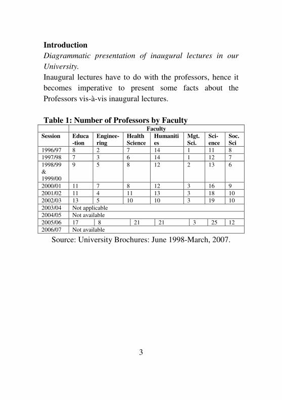
Introduction
Diagrammatic presentation of inaugural lectures in our
University.
Inaugural lectures have to do with the professors, hence it
becomes imperative to present some facts about the
Professors vis-à-vis inaugural lectures.
Table 1: Number of Professors by Faculty Faculty
Session Educa
-tion
Enginee-
ring
Health
Science
Humaniti
es
Mgt.
Sci.
Sci-
ence
Soc.
Sci
1996/97 8 2 7 14 1 11 8
1997/98 7 3 6 14 1 12 7
1998/99
&
1999/00
9 5 8 12 2 13 6
2000/01 11 7 8 12 3 16 9
2001/02 11 4 11 13 3 18 10
2002/03 13 5 10 10 3 19 10
2003/04 Not applicable
2004/05 Not available
2005/06 17 8 21 21 3 25 12
2006/07 Not available
Source: University Brochures: June 1998-March, 2007.
4
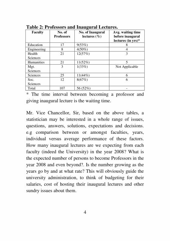
Table 2: Professors and Inaugural Lectures. Faculty No. of
Professors
No. of Inaugural
lectures (%)
Avg. waiting time
before inaugural
lectures (in yrs)*
Education 17 9(53%) 8
Engineering 8 4(50%) 4
Health
Sciences
21 12(57%) 3
Humanities 21 11(52%) 5
Mgt.
Sciences
3 1(33%) Not Applicable
Sciences 25 11(44%) 6
Soc.
Sciences
12 8(67%) 6
Total 107 56 (52%) -
* The time interval between becoming a professor and
giving inaugural lecture is the waiting time.
Mr. Vice Chancellor, Sir, based on the above tables, a
statistician may be interested in a whole range of issues,
questions, answers, solutions, expectations and decisions.
e.g comparison between or amongst faculties, years,
individual versus average performance of these factors.
How many inaugural lectures are we expecting from each
faculty (indeed the University) in the year 2008? What is
the expected number of persons to become Professors in the
year 2008 and even beyond?. Is the number growing as the
years go by and at what rate? This will obviously guide the
university administration, to think of budgeting for their
salaries, cost of hosting their inaugural lectures and other
sundry issues about them.
5
Mr. Vice-Chancellor, Sir, distinguished audience you will
appreciate that for instance there may be a difference
between the expected number of Professors and the actual
number of Professors come 2008. The difference between
this expected number and the actual number is the margin
of error in our estimation. It is this error that the statistician
is expected to minimize in order to arrive at optimal
decisions.
Rationale For Title
Very often, we hear or read the statements: statistics has it
that… or according to statistics, some events were observed
to happen. These statements are made when we want to
assert our positions with “facts and figures”. For instance, it
is said that Nigeria is the most populous black nation in the
world. This is driven home with the assertion that statistics
has it or according to statistics, one out of every four black
Africans is a Nigerian. It gives you a clearer picture and
quantifies how populous Nigeria is among the comity of
black nations. However, we need to appreciate that in an
attempt to present “facts and figures” a third component
falsehood or error creeps in. It is this falsehood or error
(which may be unintentional) that the statistician is
expected to minimize.
Concept of Statistics
To the layman statistics connotes the collection, tabulation
and presentation of information in numerical form-figures.
6
However, beyond this classical concept of statistics being
the collection, collation, and presentation of data, it is put
succinctly as the science of decision making in the face of
uncertainty. Therefore, statisticians reason and take
decisions in the realm of uncertainty Oyejola (2006). It is
this uncertainty (error) which occurs in every day human
activity, physical experiments, businesses, politics etc
which is to be minimized. The smaller your error the better
your decisions. Minimal errors imply improved efficiency
and cost reduction in any system. These are the hallmarks
of statistical activities. Statistics is therefore the science
(pure and applied) of creating, developing and applying
techniques such that uncertainty of inductive inferences
may be evaluated, Torrie (1998). It is the whole enterprise
of use and development of theory and methods applied in
design, analysis and interpretation of information,
Bamiduro (2005).
A proper design, analysis and interpretation of data lead to
better decision making (policy making and
implementation), hence, none of these should be missing in
the link; because in any experiment
Wrong Design + Right Analysis ⇔ Biased Results
Right Design + Wrong Analysis ⇔ Biased Result
Right Design + Right Analysis ⇔ Unbiased Results
Nduka (1997)
7
Some Statistical Distributions
Certain experiments are associated with certain
distributions.
(i) If an experiment consists of two possible
outcomes say success or failure (like in exams),
fertile or infertile (human or animal
reproduction), yes or no (opinion polls), etc,
independent and identical trials of such an
experiment is described by the binomial
distribution P(x = k] =
k
np
kq
n-k, k = 0, 1, … n.
(ii) If in successive trials, the first probability of
success after several failures (like students trials
in an examination before success), it is described
by the geometric distribution P(x = k) = qk-1
p,
k=0,1, …
(iii) Very many distributions abound describing
events e.g. Poisson, Exponential (arrival and
departure at airports within time interval,
queuing models like modeling traffic flows), etc.
However, the most popular and plausible of all distributions
is the normal or Gaussian distribution after its founder
Gaussian (1777-1855). This bell shaped distribution is
associated with many activities in life. This distribution is
characterized by two parameters – the mean and variance.
Above all, every other distribution tends to the normal
distribution as the number of sample observations becomes
large (as large as 30). In other words, regardless of the
8
nature of your experiment if the number of independent
trials is at least thirty, it can conveniently be described by
the normal distribution. This position has been proved by
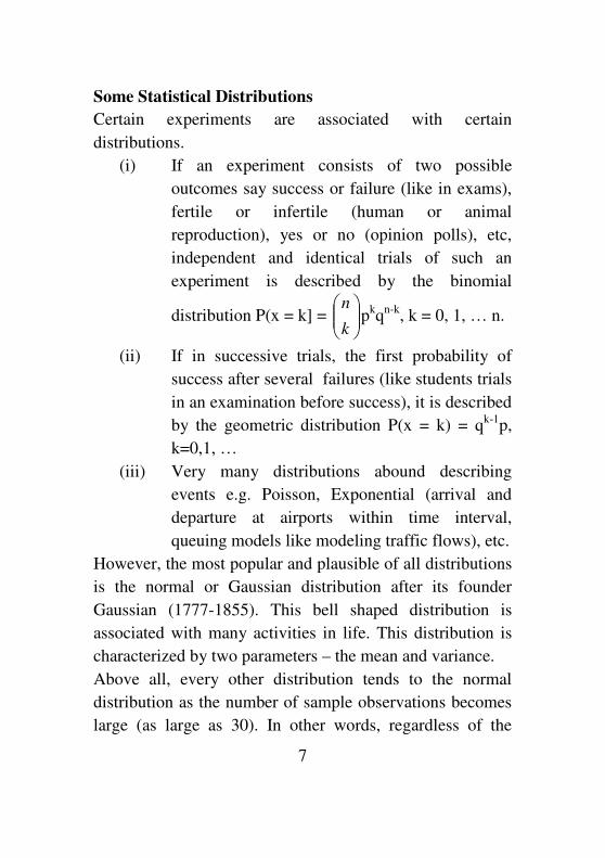
the Central Limit Theorem, Srinivasan and Mehata (1981).
The figure (1), below represents the shape of the normal
distribution.
Figure 1: Normal Curve
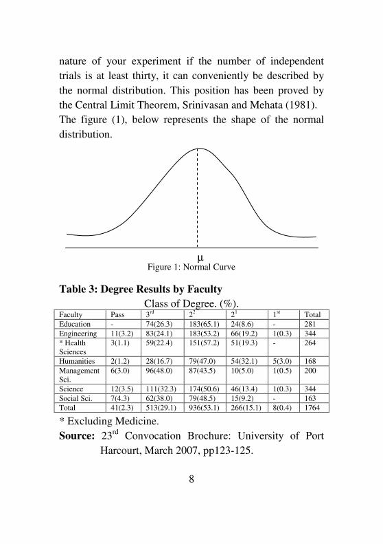
Table 3: Degree Results by Faculty
Class of Degree. (%). Faculty Pass 3
rd 2
2 2
1 1
st Total
Education - 74(26.3) 183(65.1) 24(8.6) - 281
Engineering 11(3.2) 83(24.1) 183(53.2) 66(19.2) 1(0.3) 344
* Health
Sciences
3(1.1) 59(22.4) 151(57.2) 51(19.3) - 264
Humanities 2(1.2) 28(16.7) 79(47.0) 54(32.1) 5(3.0) 168
Management
Sci.
6(3.0) 96(48.0) 87(43.5) 10(5.0) 1(0.5) 200
Science 12(3.5) 111(32.3) 174(50.6) 46(13.4) 1(0.3) 344
Social Sci. 7(4.3) 62(38.0) 79(48.5) 15(9.2) - 163
Total 41(2.3) 513(29.1) 936(53.1) 266(15.1) 8(0.4) 1764
* Excluding Medicine.
Source: 23rd
Convocation Brochure: University of Port
Harcourt, March 2007, pp123-125.
µ
9
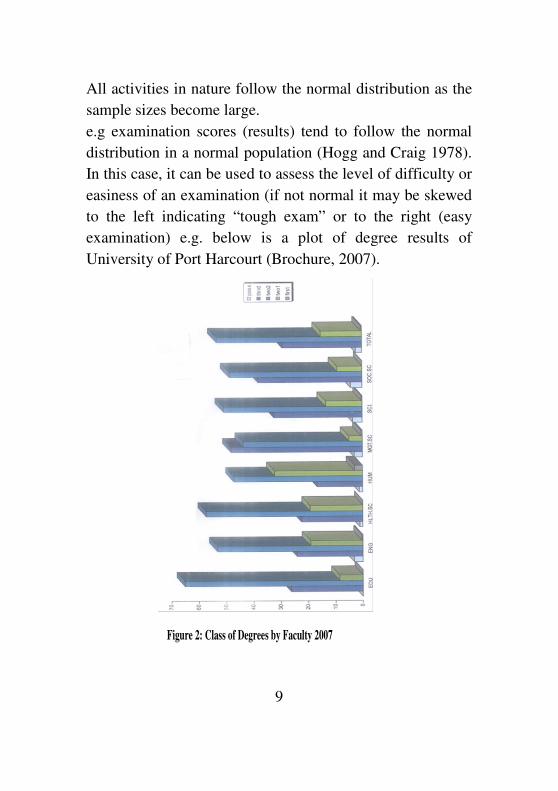
All activities in nature follow the normal distribution as the
sample sizes become large.
e.g examination scores (results) tend to follow the normal
distribution in a normal population (Hogg and Craig 1978).
In this case, it can be used to assess the level of difficulty or
easiness of an examination (if not normal it may be skewed
to the left indicating “tough exam” or to the right (easy
examination) e.g. below is a plot of degree results of
University of Port Harcourt (Brochure, 2007).
Figure 2: Class of Degrees by Faculty 2007
10
It has to be stated that in a normally distributed scores, it is
peaked at 2nd
class lower division; the difference between
the number of 2nd
upper and 3rd
class should not be
significantly different, the difference in the number of 1st
class and pass degrees should also not be significantly
different.
Again, in a large class, for a standard exam, the scores peak
at C with the difference between the number with maximum
score (A) and minimum score (F) not being significant.
Ladder of Activity in Life
The normal curve can be used to demonstrate man’s activity
in his ladder of life.
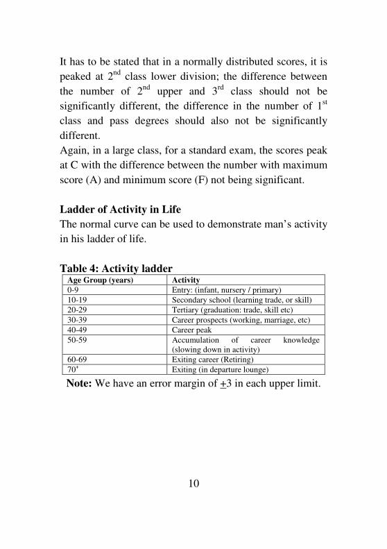
Table 4: Activity ladder Age Group (years) Activity
0-9 Entry: (infant, nursery / primary)
10-19 Secondary school (learning trade, or skill)
20-29 Tertiary (graduation: trade, skill etc)
30-39 Career prospects (working, marriage, etc)
40-49 Career peak
50-59 Accumulation of career knowledge
(slowing down in activity)
60-69 Exiting career (Retiring)
70+ Exiting (in departure lounge)
Note: We have an error margin of +3 in each upper limit.
11
Fig. 3: Normal Distribution Curve.
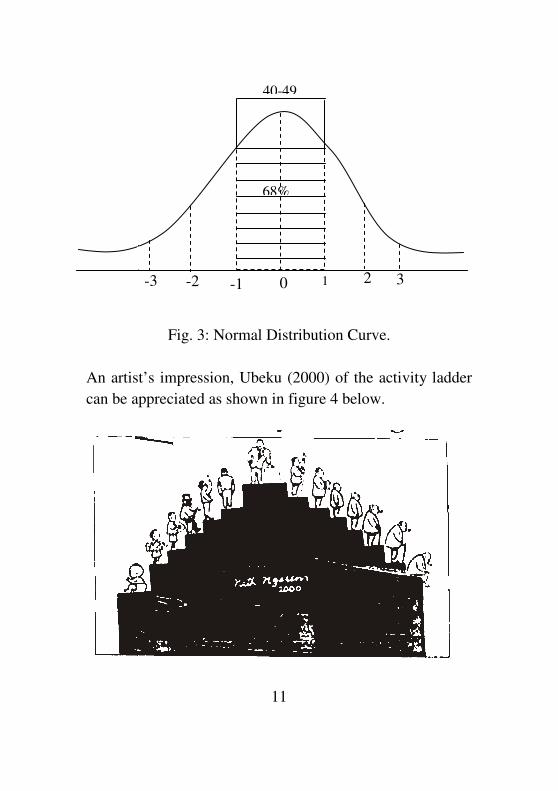
An artist’s impression, Ubeku (2000) of the activity ladder
can be appreciated as shown in figure 4 below.
0
40-49
68%
-1 -2 -3 3 2 1 -3
12
Fig 4: Activity curve
Mr. Vice-Chancellor sir, we can now appreciate in the
lighter mood, the maxim that a fool at forty is a fool
forever. However, from the statistician’s point of view, this
statement is not absolute, rather it is probabilistic, and this
probability is 0.68. In other words, that a fool, has 32%
chance of pulling himself / herself out of foolery.
The above table can therefore be condensed into three, say
0-29 (learning process)
30-59 (working process)
60 and above (retiring process)
What Has Three Got to do with this?
Permit me sir, to demonstrate the usefulness of the number
three in the affairs of statistics and man in general.
1. The statistician divides the study of data into three parts:
- collecting data
- processing data
- drawing inference from data
2. We notice that the statistical tables of standard normal
distribution is tabulated for values between -3 and 3 (i.e
+3) Kanji (1993), Meyer (1977), Nwobi and Nduka
(2003).
3. If we exclude the children and adolescents, life’s major
activities are concentrated in three age groups; namely
20-39 (Youth).
40-59 (Adulthood)
60 and above (Old Age).

13
These age groups have some interesting features:
Knowing scientists. (Vollmann, 1985, Fischof 2007, Vasey
2007) have identified the different temperaments and blood
radiations. For the youth, it is melancholic (i.e dreaming
and longing for the ideal), for adulthood it is choleric
(urging to action), and for the old age it is phlegmatic (quiet
reflection). Again some knowing ones and philosophers,
Malchow (2007) associated the quest for knowledge in
these groups. Youth as the whence in life (i.e where do I
come from?).
Adulthood as the why in life (i.e what is the purpose of life
and existence?).
Old age as the whiter in life (i.e where do I go to from here?
Life beyond the earthly existence).
There is therefore an urge in man to know who he is
and his purpose in creation. This is because, man is not just
the physical body we see. It is the body and his inner core
(the spirit) that make the man. (Genesis 2:7, James 2:26).
And the Lord God formed man out of the dust of the ground
and breathed into his nostrils the breath of life and man
became a living soul. Just as we care for the body we
should equally care for the spirit, hence the need for him to
discover or indeed re-discover himself. We recognize the
concept of Trinity (God the father, the Son and Holy Spirit),
body, soul, spirit, triangle, etc.
4. There is also the role of three in holding the balance
of governance (the executive, judiciary and

14
legislature) and social stratification (upper class,
middle class and lower class).
5. The computer has three main devices input,
processing unit and output.
6. Let me personally say that our country enjoyed
healthier economy and politics under the three
regional structure than what we have today; in terms
of GDP, per capita income and quality of leadership.
7. Above all, three basic natural laws regulate the
activities of man in creation (Vollmann, 1985,
Huemar 2006, 2007).
i) The law of sowing and reaping or reciprocal action
or karma or cause and effect etc. (Galatians 6:7).
Be not deceived, God is not mocked; for whatsoever
a man soweth, that shall he reap. Again, three basic
ways of sowing; through our three abilities; thinking
(thoughts), talking (words) and action (deeds).
ii) The law of Attraction of Homogenous species or
birds of the same feather flock together, like father
like son, tell me your friend, and I will tell you who
you are, etc.
iii) The law of gravity (density) made popular by
physicists; that light objects float, while heavy
objects sink e.g cork immersed in water floats, while
stone sinks. If we do something right and noble we
feel light, if otherwise we feel heavy and dense.
An understanding and conscious living of these laws, will
make us appreciate the import of the admonitions by our
15
Lord Jesus Christ that we should lay our treasures in heaven
and that what does it profit a man if he gains the whole
world at the expense of his soul.
The import of this is that even if one is not a fool at forty
(indeed has reached his peak there) it is a waste if he has
not led a spiritual life (i.e not worshiped God in truth and
spirit).
In this wise, I associate myself to some extent the call by
Okoh (2005) enjoining man in the Delphic maxim to “know
himself” because we are plagued by the problem of “mis-
education” caused by the absence of a philosophical base.
Indeed Keller (1880-1968) put it more succinctly
“the best educated human being is one who understands
most about life he is placed in”.
Outliers
Whatever deviates from that which is normal (i.e expected)
be it in conduct (behavior), business, measurements etc, we
commonly say it is abnormal or unexpected. In statistics,
such observation(s) that fall(s) outside the pattern exhibited
by the rest of the data set is called an outlier or wild shot
(Barnett and Levis (1990).
In accordance, with our number three, the simplest method
of identifying an outlier is x +3s ( x – sample mean, s-
sample standard deviation). In other words, any value that
lies outside the above interval is an outlier. Let me illustrate
this with these simple scores of two students in a sessional
examination.
16
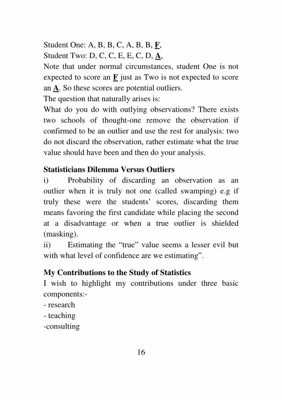
Student One: A, B, B, C, A, B, B, F,
Student Two: D, C, C, E, E, C, D, A,
Note that under normal circumstances, student One is not
expected to score an F just as Two is not expected to score
an A. So these scores are potential outliers.
The question that naturally arises is:
What do you do with outlying observations? There exists
two schools of thought-one remove the observation if
confirmed to be an outlier and use the rest for analysis: two
do not discard the observation, rather estimate what the true
value should have been and then do your analysis.
Statisticians Dilemma Versus Outliers
i) Probability of discarding an observation as an
outlier when it is truly not one (called swamping) e.g if
truly these were the students’ scores, discarding them
means favoring the first candidate while placing the second
at a disadvantage or when a true outlier is shielded
(masking).
ii) Estimating the “true” value seems a lesser evil but
with what level of confidence are we estimating”.
My Contributions to the Study of Statistics
I wish to highlight my contributions under three basic
components:-
- research
- teaching
-consulting
17
Statistics was a novel subject introduced as a course in class
IV in our secondary school. We were about 15 students who
sat for it in the WASC exams that year before WAEC
scrapped it later. This marked my attachment to the
discipline. I did my National Youth Service at the Institute
of Agricultural Research – Samaru Zaria as a “Statistical
Research Officer” in the Data Processing and Field
Experiments Unit in 1980-81.
This marked the beginning of my interest in statistical
modeling with bias in Biometrics (application of statistical
methods and principles in biological, agricultural, medical
and allied disciplines) particularly in the later part of my
career.
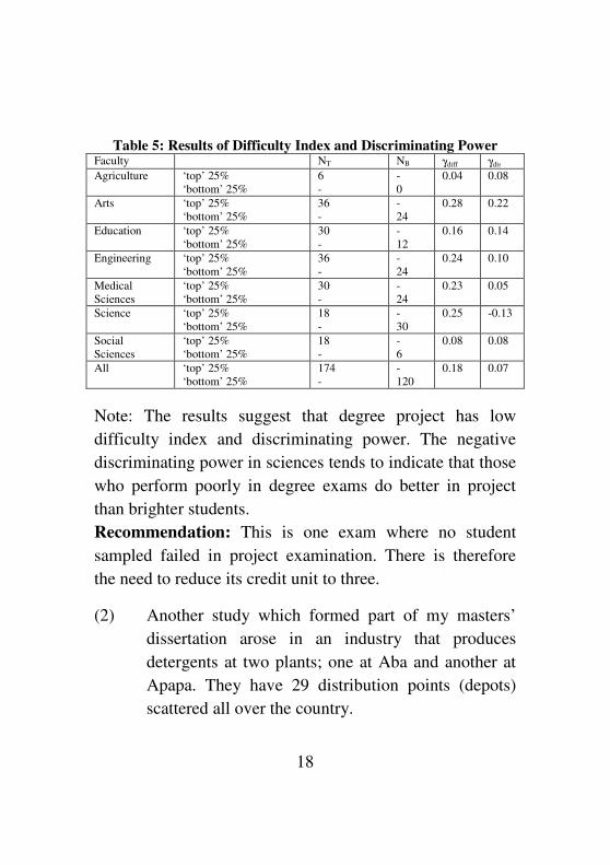
Research – (1) My first research effort arose from part of
my undergraduate project (Nduka, 1991) which was to find
out how efficient students’ degree project discriminates
among students of varying abilities – which is the sole aim
of any exam. This is because the degree project has six
credit units in almost all the Nigerian Universities and
consumes a lot of resources and time.
The difficulty index 10,)(2
<≤
+= diff
BT
diffN
NNγγ
and the discriminating power
≤≤−−= 11
%25""%25""dis
BT
disbottom
N
top
Nγγ . Results of updated
data collected from the University of Nigeria, Nsukka over
the period 1985-1989 are shown below. I was able to prove
the theorem that If γdiff ∈[0.4, 0.6], then γdis → 1.
18
Table 5: Results of Difficulty Index and Discriminating Power Faculty NT NB γdiff γdis
Agriculture ‘top’ 25%
‘bottom’ 25%
6
-
-
0
0.04 0.08
Arts ‘top’ 25%
‘bottom’ 25%
36
-
-
24
0.28 0.22
Education ‘top’ 25%
‘bottom’ 25%
30
-
-
12
0.16 0.14
Engineering ‘top’ 25%
‘bottom’ 25%
36
-
-
24
0.24 0.10
Medical
Sciences
‘top’ 25%
‘bottom’ 25%
30
-
-
24
0.23 0.05
Science ‘top’ 25%
‘bottom’ 25%
18
-
-
30
0.25 -0.13
Social
Sciences
‘top’ 25%
‘bottom’ 25%
18
-
-
6
0.08 0.08
All ‘top’ 25%
‘bottom’ 25%
174
-
-
120
0.18 0.07
Note: The results suggest that degree project has low
difficulty index and discriminating power. The negative
discriminating power in sciences tends to indicate that those
who perform poorly in degree exams do better in project
than brighter students.
Recommendation: This is one exam where no student
sampled failed in project examination. There is therefore
the need to reduce its credit unit to three.
(2) Another study which formed part of my masters’
dissertation arose in an industry that produces
detergents at two plants; one at Aba and another at
Apapa. They have 29 distribution points (depots)
scattered all over the country.

19
The problem is: how do we optimally allocate these
commodities to these depots at a minimal cost?
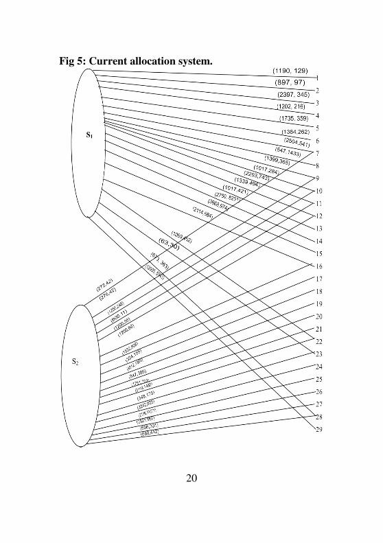
20
Fig 5: Current allocation system.
21
The desire was to construct an optimal network flow f(ni, nj)
from production points (Si , i = 1, 2) to the depots such that
the total flow cost (transportation).
∑∑=i j
jiji nnfnnf ),(),()( γγ is minimal and the total
flow capacity (quantity of goods),
∑∑=i j
jiji nnfnncfc ),(),()( is maximal.
We proposed an algorithm (Chukwu and Nduka 1993)
which iteratively searches the route for the maximal
allocation of commodity flows from their restricted or
relaxed production points to their corresponding depots at a
minimal cost.
The total cost of distributing 66,413 cases of detergents is
(in Nm) N17,701.00). In applying the algorithm to their
own distribution schedule the same quantity could be
distributed to the various depots at N15,245.00 (13.87%
cost reduction) i.e (N2456). Applying the proposed
algorithm and suggesting alternative distribution schedule,
the same quantity could be distributed at a cost of
N14,486.00 (18.16% cost reduction).
The merits: Our algorithm has been proved optimal in
solving restricted and relaxed multi-commodity flow
problem without intermediate routes; with efficient results.
If distribution cost is equal to zero, the algorithm solves the
maximal flow problem of Ford and Fulkerson (1962).
(3) These papers (Erondu & Nduka, 1993a, 1993
b) were
based on water samples experiment conducted by
22
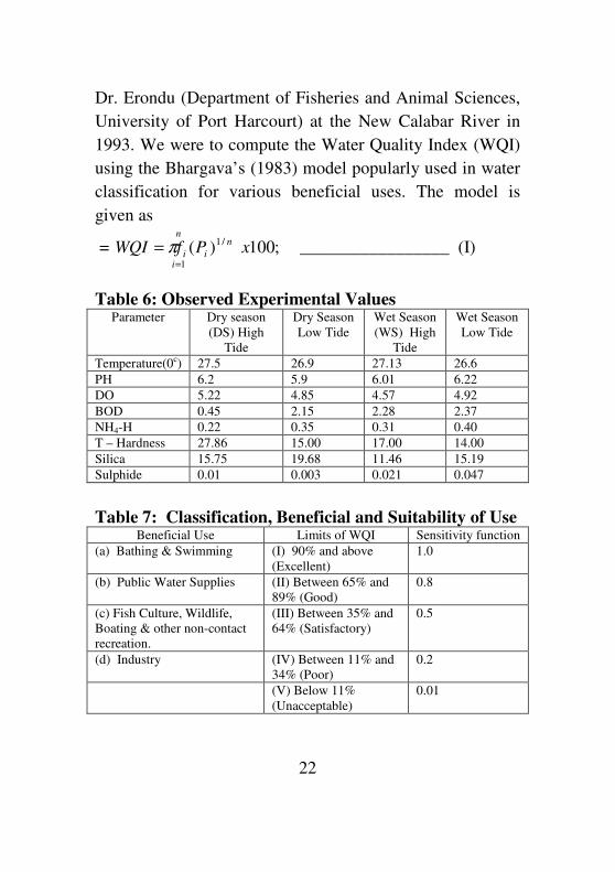
Dr. Erondu (Department of Fisheries and Animal Sciences,
University of Port Harcourt) at the New Calabar River in
1993. We were to compute the Water Quality Index (WQI)
using the Bhargava’s (1983) model popularly used in water
classification for various beneficial uses. The model is
given as
= ;100)( /1
1
xPfWQIn
i
n
ii
=
= π _________________ (I)
Table 6: Observed Experimental Values Parameter Dry season
(DS) High
Tide
Dry Season
Low Tide
Wet Season
(WS) High
Tide
Wet Season
Low Tide
Temperature(0c) 27.5 26.9 27.13 26.6
PH 6.2 5.9 6.01 6.22
DO 5.22 4.85 4.57 4.92
BOD 0.45 2.15 2.28 2.37
NH4-H 0.22 0.35 0.31 0.40
T – Hardness 27.86 15.00 17.00 14.00
Silica 15.75 19.68 11.46 15.19
Sulphide 0.01 0.003 0.021 0.047
Table 7: Classification, Beneficial and Suitability of Use Beneficial Use Limits of WQI Sensitivity function
(a) Bathing & Swimming (I) 90% and above
(Excellent)
1.0
(b) Public Water Supplies (II) Between 65% and
89% (Good)
0.8
(c) Fish Culture, Wildlife,
Boating & other non-contact
recreation.
(III) Between 35% and
64% (Satisfactory)
0.5
(d) Industry (IV) Between 11% and
34% (Poor)
0.2
(V) Below 11%
(Unacceptable)
0.01
23
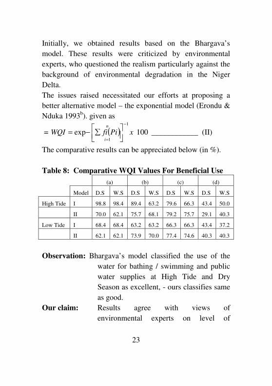
Initially, we obtained results based on the Bhargava’s
model. These results were criticized by environmental
experts, who questioned the realism particularly against the
background of environmental degradation in the Niger
Delta.
The issues raised necessitated our efforts at proposing a
better alternative model – the exponential model (Erondu &
Nduka 1993b). given as
= ( ) 100exp
1
1
xPifiWQIn
i
−
=
∑−= ____________ (II)
The comparative results can be appreciated below (in %).
Table 8: Comparative WQI Values For Beneficial Use
(a) (b) (c) (d)
Model D.S W.S D.S W.S D.S W.S D.S W.S
High Tide I 98.8 98.4 89.4 63.2 79.6 66.3 43.4 50.0
II 70.0 62.1 75.7 68.1 79.2 75.7 29.1 40.3
Low Tide I 68.4 68.4 63.2 63.2 66.3 66.3 43.4 37.2
II 62.1 62.1 73.9 70.0 77.4 74.6 40.3 40.3
Observation: Bhargava’s model classified the use of the
water for bathing / swimming and public
water supplies at High Tide and Dry
Season as excellent, - ours classifies same
as good.
Our claim: Results agree with views of
environmental experts on level of
24
pollution. It builds more realism to the
data.
Benefits: A useful tool for the monitoring,
evaluation of the quality of water body,
and for the control of water pollution (i.e.
abatement programme).
Further modification and applications of the model have
also evolved over the years. (Onuoha and Nduka, 2004:
2005).
(4) Mr. Vice Chancellor sir, permit me to discuss briefly
my research efforts as a Ph.D candidate. My thesis
was in the area of biometrics, specifically response
surface methodology using inverse polynomials.
Sometimes, the primary aim of an experimenter is to
determine the treatment or factor combinations
which will give the best response.
The multifactor response is called the response surface; the
experiment usually a factorial design used in describing the
surface is called the response surface experiment, while the
statistical method of exploring this surface to obtain the
optimum response (yield) is the response surface
methodology (RSM). In other words, if we have the
response model
Y = f(x, β) + e
x = vector of design variables
β = vector of parameters
e = experimental random error
e ∼ IID (0, δe2).
25
which is within experimental region of operation or interest,
then the surface represented by E(y) = f(x, β̂ ) is defined as
the response surface. The fundamental issue is at what
design points do you explore to obtain the optimum
response. This is the concept of RSM.
The fundamental applications of RSM in any experimental
design are in approximating the true models (known or
unknown), discriminating between (among) models, and the
exploration of response surfaces.
Though my study was in the latter, we have traversed the
others.
The ordinary polynomials, particularly the second order
(quadratic) have been popularly used in exploring response
surfaces because of their conceptual and computational
simplicity, and easy location of the optimum. However,
they exhibit the undesirable problem of unboundedness,
symmetry about the optimum, thereby making nonsense of
extrapolation if prediction is one of the experimental
objectives, Morton (1983), Mead & Pike (1975).
On the other hand, inverse polynomials have the desirable
properties of boundedness, asymptotics, distribution free,
invariance and speedy convergence.
Awareness in the use of inverse polynomials increased
following Nelder’s (1966) multi-factor experiment on
Bermuda-grass for parameter estimation. This he called
generalized inverse polynomial. The major area of
application of inverse polynomials has been in agronomy,
26
growth studies in plant yield relationships and inverse linear
regression methods of calibration (Zemroch (1986).
However, recent studies show applications in the “other
biometrics” chemotherapy, finger-printing and forensic
science (Biometric Bulletins 2006).
The major limitations of Nelder’s generalized inverse
polynomial are:-
(a) it does not establish a common relationship among
the various models.
(b) It is not widened in scope by permitting powers of
the factorial experiment.
(c) The above observations can be appreciated from his
model (Nelder 1966) expressed as
k
ik
i xxxinpolynomialy
x.,........., 211 =−π …(4.1)
A new generalized inverse polynomial was justifiably
proposed Nduka (1994) which
(a) synthesizes the common relationship among the
family of inverse models
(b) has a multi-parametric form that unified the variants
of growth models.
The new generalized inverse polynomial (Nduka, 1994)
that takes care of inverse polynomial of order p in k-factor
experiments is expressed as
( )1
,1
2
210111
..........−
−==
+++=p
iipiiii
k
i
ik
ixxx
y
xββββππ …(4.2)
27
Applications
(a) The new generalized inversed polynomial Nduka
and Bamiduro (1997) has been applied in response surface
design giving a clearer insight to Nelder’s (1968), and
Meads (1971) yield-density relationship as follows:
(i) In a single factor experiment
where k = 1, p = 1
y-1
= β11 + β01x-1
…(4.3)
(which is a simple inverse regression model). This
(equation 4.3) can be equivalently stated as
y-θ
= β11 + β01ρ-1
...(4.4)
as a general case
y is yield per plant, ρ is number of plants per unit area
(plant-density)
ρ11, ρ01, θ, φ are parameters such that θ/φ ≤ 1, θ >0, φ = 1, 0
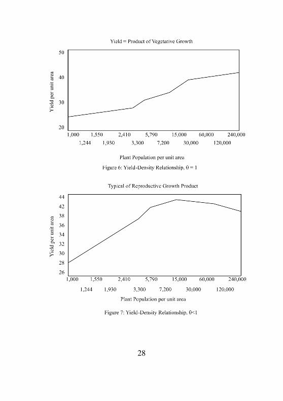
< θ ≤ 1. So θ becomes a competitive index. W = ρy (yield
per unit area) attains asymptotic maximum at ρ = ∞ only for
θ = 1 and this is typical of vegetative plant growth (see
fig.6.)
28
29
In attains a definite maximum at ρ <∞ if θ < 1 (which is
estimable) and this is typical of reproductive plant growth
(see fig5). Taking the exponential of equation (1.0) gives
the Gompertz model (Winsor, 1982; Ferrante, et al 2000)
used in actuarial studies, while the reciprocal gives the
logistic model used in dose-response studies in clinical
trials (Sugar, et al 2007).
(ii) for a polynomial of order 2, 1-factor experiment gives
x/y = β0 + β1x + β1x2 (inverse quadratic model) …(4.5)
(iii) for 22 – factorial experiment i.e. 2 factors at 2 levels,
this transforms to
y-1
= B11 + B01x1-1
+ B10x2-1
+ B00(x1x2)-1
…(4.6)
This is a variant of Berry’s (1968) model if y = yθ ; used in
crop-yield density involving intra (x1) and integer (x2) row
spacing and density at ρ = (x1 x2)-1
.
(b) when the maximum is not attainable, Nduka et al,
(1998), contributed expression for the density at which
specific proportions of the maximum is obtained.
(c) In (b) above, where it is not feasible to obtain full yield
at harvest time because it is unattainable or simply
unavoidable; Nduka & Bamiduro (2002) combined methods
of calculus of variation and maximum likelihood estimates
to obtain a proportion of this yield. This was obtained for
both known desired and unknown (estimable) proportions
of the maximum yield on rectangular and square plot
formations. The analytical results (using SAS – Gauss
Newton) method of iterative nonlinear least square on
soyabean experiment Wiggans,(1984) gives.
30
W -0.86216
= 0.0164 – 0.00426x1-1
– 0.06832x2-1
+
0.00543(x1x2)-1
…(4.7)
In the circumstance described above where the
experimenter may be forced to seek some proportion
λ(say), 0 < λ < 1 of this maximum; this can be obtained
from the equation
W′′ = λwmax …(4.8)
Therefore, for known λ
W" = ( )
1001
111
BB
B))
))θλ −−
…(4.9)
For unknown (estimable) λ, we infer that since max(W′′) = 1
Then ( )θ
λ−−
=11
1001
1 B
BB)
))
…4.10)
Therefore, from the above, for known λ, W′′ 5.068λ and for
λ unknown λ)
= 0.197.
This implies that we will obtain a yield growth rate of 5.068
for λ known and 19.7% of optimum yield for λ unknown.
The ordinary implication is that premature harvest in this
(or similar) experiment will not be profitable or desirable.
Benefits: An experimenter (agriculturist) is now better
guided to know what proportion of his full yield is
obtainable before full harvest time.
The new generalized inverse polynomial has also been
applied as methods for discriminating between models
Nduka (1997), for testing the goodness of approximation of
model variants Nduka (1995) and model comparisons
Nduka (1999).
31
Teaching
I have been teaching statistics in this University to
undergraduate and post graduate students in our department
and also as service course to students in biological sciences.
The courses include Regression Analysis and Model
Building; Design and Analysis of Experiments, Multivariate
Analysis, Linear Models, Probability Theory and Statistics
for Biological and Agricultural Sciences. I have also
supervised and continue to supervise B.Sc projects, M.Sc
Theses and Ph.D dissertations. I persuade my graduate
students to have their works published in journals and at
worst conference proceedings (Nduka and Ijomah 2004,
Nduka and Igabari 2006, 2007, Nduka and Consul 2007,
John and Nduka 2007).
Consulting
I have been doing some statistical consulting to post
graduate students, staff and researchers who apply statistical
methods in their studies. My interaction with some
colleagues at this level enhanced an appreciation for
collaborative studies (Erondu and Nduka, 1993 (a, b),
Nduka and Kalu (2001, 2002), Onuoha and Nduka (1994,
2004, 2005), Owate and Nduka (2001), Didia and Nduka
(2007). My interaction too has exposed me to some
misconceptions or shall I say poor perception of statistics
and statisticians. There is little awareness on the need to
involve the statistician at all stages of experimentation i.e
designing, monitoring (evaluating), data collection,
32
analysis, interpretation and presentation of research results.
A good number of researchers come with finished
experimental data, demanding analysis that should conform
to their expected results, and could express disappointment
if otherwise. Some simply want “certified P-value”, while
others even come for interpretation of already analysed data
(at times wrongly analysed). My personal experience with
researchers is that over 70% come with finished
experimental data. Little thought is ever given at the
experimental stage of a possible analysis sketch that would
be suitable to the form of the experimental design, to avoid
undue statistical complications during proper analysis.
Above all, basic knowledge of statistical principles like
randomizations, sampling techniques, questionnaire design
and procedures for research experimentations are lacking.
Challenges facing Statistics and Statisticians
Mr. Vice-Chancellor, Sir, statistics is the most widely used,
misused and abused of all disciplines, because everybody
needs the services of statistics and statisticians. The
challenges are (a) use, abuse and misuse (b) poor record
keeping (c) dearth of statisticians (among others).
(a) Use, Abuse and Misuse
Statistics is used by all and sundry ranging from the grocery
shop owner (who takes stock of daily or weekly sales in
order to guide her in the quantity of goods to buy and
monitor profit) to large complex organizations (in their
policy formulations and planning).
33
The use can be summarized into
(a) Evaluation of existing conditions
(b) Provision of information for programme formulation
and development,
(c) Monitoring of system progress.
(d) Guiding research, decisions making and forecasting.
Today, we talk about biometrics/biostatistics (statistics in
biology, agriculture, and medicine), econometrics (statistics
in economics), psychometrics (statistics in education and
psychology), technometrics (statistics in chemical sciences
and engineering), geostatistics (statistics in geosciences)
and business statistics, etc.
The basic statistical principles and methodologies in these –
metrics are the same. They only differ in applications and
details. This implies that no scientific investigation (indeed
any investigation in any discipline) is capable of proving
anything valid without the aid of statistics. Indeed, it is now
a maxim that serious research requires serious statistics –
that statistical package goes by the name SYSTAT (2005).
No journal worth its name now accepts any publications
without statistical input even in the humanities.
Misuse and Abuse
It does seem to me that misuse and abuse of statistics are
inseparable. For instance drawing wrong inferences from
data constitute misuse and abuse at the same time, hence
permit me to treat them as same.
34
The first thing that strikes me in this is what a foremost
professor of statistics, Biyi Afonja (1985) called the fa-fi-fal
syndrome (I call it AIDS Version of Statistics). This is the
willful and deliberate falsification of facts and figures to
gain some advantage. We need not go far to appreciate this.
Our electoral system (voter registration and voter turn out)
defies all known electoral behaviours and demographic
features, our conduct of census and results, results of
opinion polls, etc. These falsifications are mostly borne out
of selfish desires, to mask what betrays our dishonesty or to
protect what is called “sensitive statistics” particularly in
government circles. Masking of important information is a
bane of our environment right from organizations to
individuals. e.g data on age are defective in our system.
Misuse and Abuse of Statistical Methods
I have chosen to discuss the simplest of methods known to
every literate person and that is the ‘average’, called
arithmetic mean, also known popularly as the mean.
Appreciating the misuse, abuse or even over-use makes it
unnecessary to discuss any other statistical methods
suffering the same fate (and there are quite a lot). This only
shows how serious the problem is.
(i) The most important rule is that only like objects
should be included in mean calculations so as to ensure that
there is some approximate relationship between the mean
and all the individual values.
35
(ii) When comparing means of separate data sets, users
do not often ensure that the sets are themselves comparable
before attempting to compare statistics derived from or even
do the desirable thing by transforming the data set into
terms of common dimension, say the use of percentages
often called “percentage persuasion” ,Reichmann(1983).
For instance, when government justifies frequent fuel price
increases (hikes) by quoting international prices or prices in
developed economies (ignoring the prices in developing
countries that belong to OPEC like Nigeria and their wage
structures).
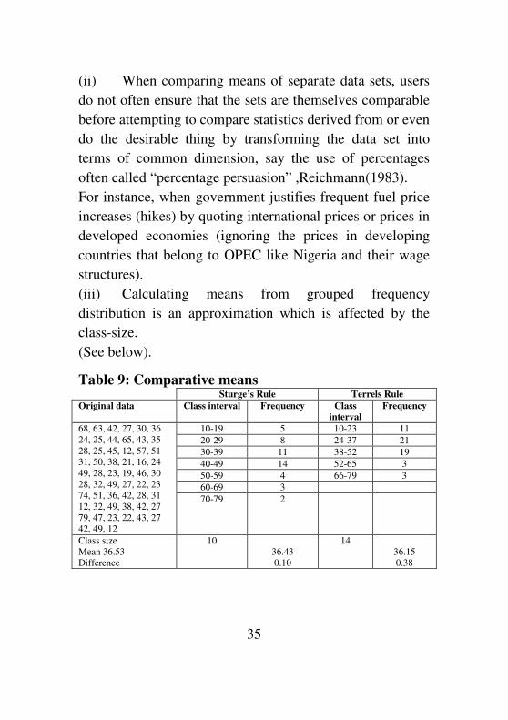
(iii) Calculating means from grouped frequency
distribution is an approximation which is affected by the
class-size.
(See below).
Table 9: Comparative means Sturge’s Rule Terrels Rule
Original data Class interval Frequency Class
interval
Frequency
68, 63, 42, 27, 30, 36
24, 25, 44, 65, 43, 35
28, 25, 45, 12, 57, 51
31, 50, 38, 21, 16, 24
49, 28, 23, 19, 46, 30
28, 32, 49, 27, 22, 23
74, 51, 36, 42, 28, 31
12, 32, 49, 38, 42, 27
79, 47, 23, 22, 43, 27
42, 49, 12
10-19 5 10-23 11
20-29 8 24-37 21
30-39 11 38-52 19
40-49 14 52-65 3
50-59 4 66-79 3
60-69 3
70-79 2
Class size
Mean 36.53
Difference
10
36.43
0.10
14
36.15
0.38
36
(iv) Other means and their uses exist apart from the
arithmetic mean e.g the harmonic mean and the geometric
mean.
This is because the arithmetic mean cannot be suitably used
for all sets of data. It is not appropriate for use in
calculating average rates of speed or sales or growth. If a
man cycled to a point 1km away at 2km/hr and returned to
the same distance at 6km/hr. You may say he averaged
4km/hr, but this is wrong. It took him 30 minutes to do the
first journey and 10mins to return, so he cycled 2kms in 40
minutes, his average speed is therefore 3km/hr
We use harmonic mean to deal with rates which are not
dependent upon each other, and the geometric mean rates
dependent on each other (e.g population growth over a
period of time).
(b) Poor Record Keeping
We as a country and at individual levels have very poor
record keeping habits. I may not go far here. How many of
us can present our one year pay slip on short notice without
searching all the corners of our houses? Even where records
are available, most often they are incomplete records.
(c) Dearth of statisticians – the acute shortage of
statisticians has made many of us jack of all trades. There
are about twenty three professors of statistics in Nigeria,
only two are available in the south-south – one at University
of Benin and another at the University of Port Harcourt (the
two only became professors barely two years ago). Six are
retired and three are abroad.
37
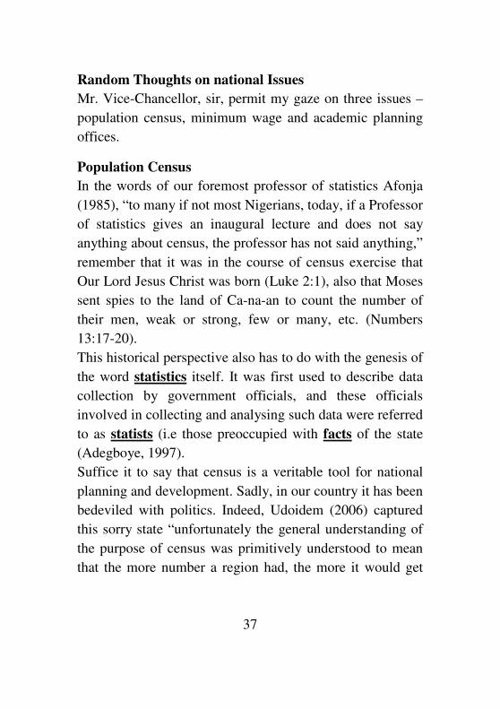
Random Thoughts on national Issues
Mr. Vice-Chancellor, sir, permit my gaze on three issues –
population census, minimum wage and academic planning
offices.
Population Census
In the words of our foremost professor of statistics Afonja
(1985), “to many if not most Nigerians, today, if a Professor
of statistics gives an inaugural lecture and does not say
anything about census, the professor has not said anything,”
remember that it was in the course of census exercise that
Our Lord Jesus Christ was born (Luke 2:1), also that Moses
sent spies to the land of Ca-na-an to count the number of
their men, weak or strong, few or many, etc. (Numbers
13:17-20).
This historical perspective also has to do with the genesis of
the word statistics itself. It was first used to describe data
collection by government officials, and these officials
involved in collecting and analysing such data were referred
to as statists (i.e those preoccupied with facts of the state
(Adegboye, 1997).
Suffice it to say that census is a veritable tool for national
planning and development. Sadly, in our country it has been
bedeviled with politics. Indeed, Udoidem (2006) captured
this sorry state “unfortunately the general understanding of
the purpose of census was primitively understood to mean
that the more number a region had, the more it would get
38
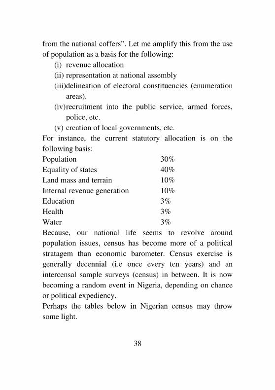
from the national coffers”. Let me amplify this from the use
of population as a basis for the following:
(i) revenue allocation
(ii) representation at national assembly
(iii)delineation of electoral constituencies (enumeration
areas).
(iv) recruitment into the public service, armed forces,
police, etc.
(v) creation of local governments, etc.
For instance, the current statutory allocation is on the
following basis:
Population 30%
Equality of states 40%
Land mass and terrain 10%
Internal revenue generation 10%
Education 3%
Health 3%
Water 3%
Because, our national life seems to revolve around
population issues, census has become more of a political
stratagem than economic barometer. Census exercise is
generally decennial (i.e once every ten years) and an
intercensal sample surveys (census) in between. It is now
becoming a random event in Nigeria, depending on chance
or political expediency.
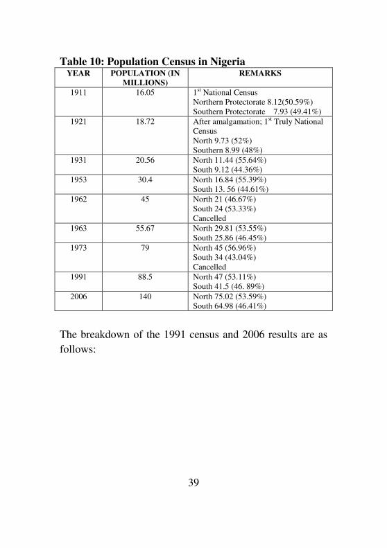
Perhaps the tables below in Nigerian census may throw
some light.
39
Table 10: Population Census in Nigeria YEAR POPULATION (IN
MILLIONS)
REMARKS
1911 16.05 1st National Census
Northern Protectorate 8.12(50.59%)
Southern Protectorate 7.93 (49.41%)
1921 18.72 After amalgamation; 1st Truly National
Census
North 9.73 (52%)
Southern 8.99 (48%)
1931 20.56 North 11.44 (55.64%)
South 9.12 (44.36%)
1953 30.4 North 16.84 (55.39%)
South 13. 56 (44.61%)
1962 45 North 21 (46.67%)
South 24 (53.33%)
Cancelled
1963 55.67 North 29.81 (53.55%)
South 25.86 (46.45%)
1973 79 North 45 (56.96%)
South 34 (43.04%)
Cancelled
1991 88.5 North 47 (53.11%)
South 41.5 (46. 89%)
2006 140 North 75.02 (53.59%)
South 64.98 (46.41%)
The breakdown of the 1991 census and 2006 results are as
follows:
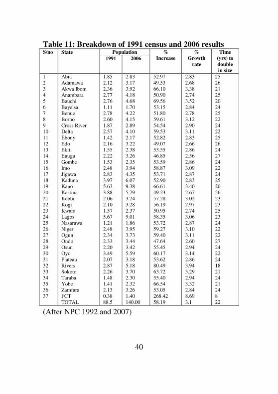
40
Table 11: Breakdown of 1991 census and 2006 results S/no State Population %
Increase
%
Growth
rate
Time
(yrs) to
double
in size
1991 2006
1
2
3
4
5
6
7
8
9
10
11
12
13
14
15
16
17
18
19
20
21
22
23
24
25
26
27
28
29
30
31
32
33
34
35
36
37
Abia
Adamawa
Akwa Ibom
Anambara
Bauchi
Bayelsa
Benue
Borno
Cross River
Delta
Ebony
Edo
Ekiti
Enugu
Gombe
Imo
Jigawa
Kaduna
Kano
Kastina
Kebbi
Kogi
Kwara
Lagos
Nasarawa
Niger
Ogun
Ondo
Osun
Oyo
Plateau
Rivers
Sokoto
Taraba
Yobe
Zamfara
FCT
TOTAL
1.85
2.12
2.36
2.77
2.76
1.11
2.78
2.60
1.87
2.57
1.42
2.16
1.55
2.22
1.53
2.48
2.83
3.97
5.63
3.88
2.06
2.10
1.57
5.67
1.21
2.48
2.34
2.33
2.20
3.49
2.07
2.87
2.26
1.48
1.41
2.13
0.38
88.5
2.83
3.17
3.92
4.18
4.68
1.70
4.22
4.15
2.89
4.10
2.17
3.22
2.38
3.26
2.35
3.94
4.35
6.07
9.38
5.79
3.24
3.28
2.37
9.01
1.86
3.95
3.73
3.44
3.42
5.59
3.18
5.18
3.70
2.30
2.32
3.26
1.40
140.00
52.97
49.53
66.10
50.90
69.56
53.15
51.80
59.61
54.54
59.53
52.82
49.07
53.55
46.85
53.59
58.87
53.71
52.90
66.61
49.23
57.28
56.19
50.95
58.35
53.72
59.27
59.40
47.64
55.45
60.17
53.62
80.49
63.72
55.40
66.54
53.05
268.42
58.19
2.83
2.68
3.38
2.74
3.52
2.84
2.78
3.12
2.90
3.11
2.83
2.66
2.86
2.56
2.86
3.09
2.87
2.83
3.40
2.67
3.02
2.97
2.74
3.06
2.87
3.10
3.11
2.60
2.94
3.14
2.86
3.94
3.29
2.94
3.32
2.84
8.69
3.1
25
26
21
25
20
24
25
22
24
22
25
26
24
27
24
22
24
25
20
26
23
23
25
23
24
22
22
27
24
22
24
18
21
24
21
24
8
22
(After NPC 1992 and 2007)
41
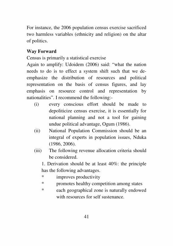
For instance, the 2006 population census exercise sacrificed
two harmless variables (ethnicity and religion) on the altar
of politics.
Way Forward
Census is primarily a statistical exercise
Again to amplify: Udoidem (2006) said: “what the nation
needs to do is to effect a system shift such that we de-
emphasize the distribution of resources and political
representation on the basis of census figures, and lay
emphasis on resource control and representation by
nationalities”. I recommend the following:-
(i) every conscious effort should be made to
depoliticize census exercise, it is essentially for
national planning and not a tool for gaining
undue political advantage, Ogum (1986).
(ii) National Population Commission should be an
integral of experts in population issues, Nduka
(1986, 2006).
(iii) The following revenue allocation criteria should
be considered.
1. Derivation should be at least 40%: the principle
has the following advantages.
* improves productivity
* promotes healthy competition among states
* each geographical zone is naturally endowed
with resources for self sustenance.
42
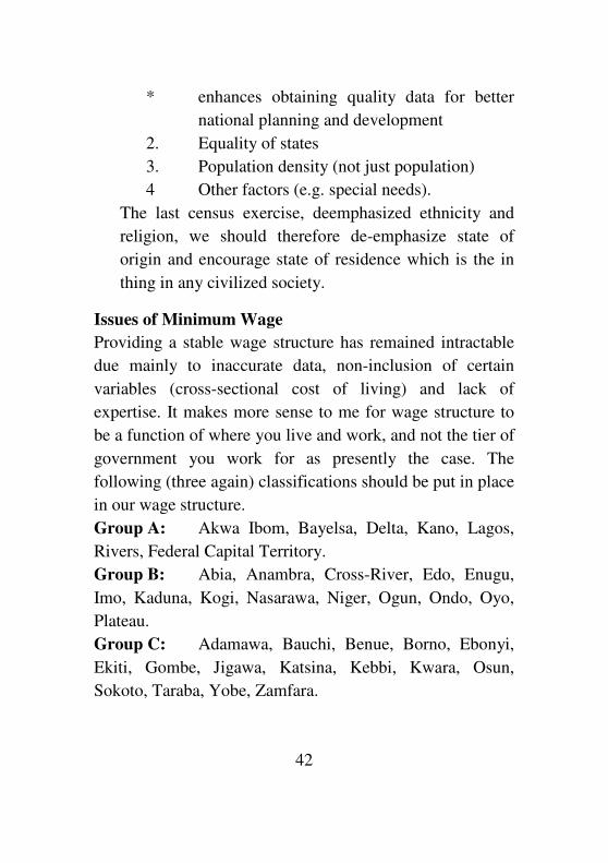
* enhances obtaining quality data for better
national planning and development
2. Equality of states
3. Population density (not just population)
4 Other factors (e.g. special needs).
The last census exercise, deemphasized ethnicity and
religion, we should therefore de-emphasize state of
origin and encourage state of residence which is the in
thing in any civilized society.
Issues of Minimum Wage
Providing a stable wage structure has remained intractable
due mainly to inaccurate data, non-inclusion of certain
variables (cross-sectional cost of living) and lack of
expertise. It makes more sense to me for wage structure to
be a function of where you live and work, and not the tier of
government you work for as presently the case. The
following (three again) classifications should be put in place
in our wage structure.
Group A: Akwa Ibom, Bayelsa, Delta, Kano, Lagos,
Rivers, Federal Capital Territory.
Group B: Abia, Anambra, Cross-River, Edo, Enugu,
Imo, Kaduna, Kogi, Nasarawa, Niger, Ogun, Ondo, Oyo,
Plateau.
Group C: Adamawa, Bauchi, Benue, Borno, Ebonyi,
Ekiti, Gombe, Jigawa, Katsina, Kebbi, Kwara, Osun,
Sokoto, Taraba, Yobe, Zamfara.
43
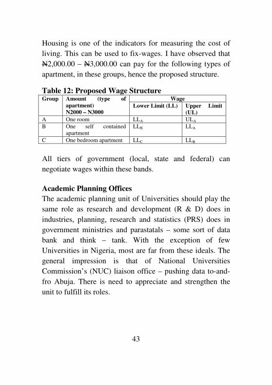
Housing is one of the indicators for measuring the cost of
living. This can be used to fix-wages. I have observed that
N2,000.00 – N3,000.00 can pay for the following types of
apartment, in these groups, hence the proposed structure.
Table 12: Proposed Wage Structure Group Amount (type of
apartment)
N2000 – N3000
Wage
Lower Limit (LL) Upper Limit
(UL)
A One room LLA ULA
B One self contained
apartment
LLB LLA
C One bedroom apartment LLC LLB
All tiers of government (local, state and federal) can
negotiate wages within these bands.
Academic Planning Offices
The academic planning unit of Universities should play the
same role as research and development (R & D) does in
industries, planning, research and statistics (PRS) does in
government ministries and parastatals – some sort of data
bank and think – tank. With the exception of few
Universities in Nigeria, most are far from these ideals. The
general impression is that of National Universities
Commission’s (NUC) liaison office – pushing data to-and-
fro Abuja. There is need to appreciate and strengthen the
unit to fulfill its roles.
44
Concluding Remarks
Mr. Vice-Chancellor sir, in the last few hours of my
presentation, I have made efforts to highlight the following:
(a) the distribution of inaugural lectures in our
university
(b) the relevance of the number three (3) in statistics
and in life.
(c) My modest contributions to statistics in teaching,
research, consultancy and training.
(d) Some misuses and abuses which statistics can be
subjected to.
(e) The need for a depoliticized census exercise.
(f) Restructured differential minimum wage regime that
reflects cost of living in the work place.
Statistics is the power house or the engine room of any
establishment in the society. The engine of a car is masked
(i.e hidden) by the entire body which is more elegant to
behold. The performance and elegance of the car are
determined by the engine which is tucked under the bonnet.
None of us will like to drive a car that has its engine
exposed, but that in reality is the car. So also statisticians
are the backbone in any establishment, they are the
background people for policy formulation and
implementation by the authorities.
Therefore, the right attitude, appreciation and recognition
must be accorded the statistician and the data system (all
men and materials involved at all stages of experimental
design, data collection and analysis) to minimize the ‘fal’ in

45
the ‘fa-fi-fal’ syndrome in the society. This is the only
panacea for successes in industrial and government policies
and programmes like NEEDS, Vision 2020, UBE, NEPAD,
MDG, etc.
It is only in this sense that we can say with high degree of
confidence that statistics has it that… according to
statistics… and it will be so.
Let me thank you Mr. Vice-Chancellor and distinguished
listeners by exhorting in the words of Florence Nightingale
(1820-1910) “an administrator would be more successful if
he had statistical knowledge” Nay she went further to say
“the universe evolved in accordance with God’s plan. But to
understand God’s plan you need statistics” (in Nabugoomu,
2005, Encarta Online).
Finally, no work is exhaustive or free from errors, and this
is no exception. If any thing displeases, I therefore plead
your understanding and forgiveness for such shortcomings
are of the head and not of the heart. I willingly accept five
percentage error margin; for in the words of Chaucer (1960)
“ask any scholar of discerning, he will say the schools are
filled with altercations…”.
Thank you.
46
References
Adegboye, O. O. (1997). The Magicians, the Prophets and the
Statisticians. Inaugural Lecture 1997, University of Ilorin.
Afonja, B.(1985). Facts, Figures and Falsehood Syndrome in
Society. Inaugural Lecture 1985, University of Ibadan.
Bamiduro, T. A.(2005). Statistics and Search for the Truth: A
Biometrician’s View. Inaugural Lecture 2005 University of
Ibadan.
Barnett, V. and Lewis, T.(1996)3rd
Ed. Outliers in Statistical
Data. John Wiley New York.
Berry G.(1967). A Mathematical Model Relating Plant Yield
with Arrangement for Regularly Spaced Crops. Biometrics,
23, 505-515.
Bhargava, D.C.(1983). Use of a Water Quality Index for River
Classification and Zoning of Ganga River. Environmental
Pollution, Series B; 6,51-57.
Biometrics Bulletin of the International Biometric Society,
23,3,2006.
Brochure of 23rd
Convocation: University of Port Harcourt, 2007
pp123-125
Chaucer, G.(1960). The Canterbury Tales. Penguin Books Ltd.
England, p. 243.
47
Chukwu, W.I.E. and Nduka, E.C. (1993). Optimal Search
Method in Multi-commodity Flow Problem. Discovery and
Innovation, Academy of Science, Kenya. 5,3,2
Davies, O.L. and Goldsmith, P.L(1980)Ed. Statistical Methods
in Research and Production. Longman Group Ltd. London,
4th Ed.
Didia, B.C. and Nduka. E.C. (2007). Stature Estimation Formulae
of Nigerians. J. Forensic Science (in Press).
Encarta online – 2006 : Florence Nightingale; Keller Helen.
Erondu, E.S. and Nduka, E.C. (1993a). Computation of Water
Quality Index (WQI) for Beneficial Uses: Studies on Water
Samples From the New Calabar River. Nig. J. Biotech.
11,63-68
Erondu, E.S. and Nduka, E.C.(1993 b). A Model for Determining
Water Quality Index for Classification of the New Calabar
River at Aluu Port Harcourt Nigeria. Int. J. Env. Stud.
44,131-134.
Ferrante, L. Bompardre, S. Possati, L. and Leone, L.(2000).
Parameter Estimation in a Gompertzian Stochastic Model for
Tumor Growth, Biometrics 56, 1076-1081.
Fischof, P. (2007). Greater Self-Awareness Through the
Temperaments. Grail World Magazine pp. 9-11.
Ford, L.R. and Fulkerson (1962). Flows in Network. Princeton,
N.J. Princeton University Press.
48
Gaussian R (1777-1855). A History of Mathematical Statistics
(in Hald, A. 1998). Wiley- Interscience pp331-380.
Heumer,W.(2006). Fate and Justice. Grail World Magazine.
Stiftung Gralsbotschaft, Publishing Coy. Stuggart, pp. 28-34.
Heumer,W.(2007). A Path to the Recognition of God. Grail
World Magazine. Stiftung Gralsbtschaft Publishing Coy.
Stuggart. Pp18-19
Hogg R.V. and Craig, A.T.(1978). Introduction to Mathematical
Statistics. Collier Macmillan International Edition. P.112.
John, O.O. and Nduka E.C.(2007). Quantile Regression Analysis
As a Robust Alternative to Ordinary Least Squares. 31st
Ann.Conf. Nig. Stat. Assoc.
Kanji, G.K. (1993). 100 Statistical Tests. Sage Publications,
London pp159-160.
King James Version of the Bible (Genesis 2: 7; James 2;26;
Luke 2:1 Numbers 13: 17-20; Galatians 6.7)
Malchow, D.(2007). Genes: The Core of Life? Grail World
Magazine. Pp12-14.
Mead, R.(1971). Plant Density and Crop Yield. Appl. Statist. 19,
64-81.
Mead, R. and Pike, D.J.(1975). A Review of Response Surface
Methodology from a Biometric View Point, Biometrics 31,
803-851.
49
Meyer, P.L.(1977). 2nd
Ed. Introductory Probability and
Statistical Applications. Addision- Welsey Pub.Coy.
London. Pp.342-343.
Nabugoomu, F.(2005). Statistics for Food Product Development
Processes. 9th Bi-annual Conf. Sub-saharan African Network,
Addis-Ababa Ethiopia.
Nduka, E.C. (1986). The Interaction Between Politics and
Population Census in Nigeria: A Statistical Problem: 10th
Ann. Conf. Nig. Stat. Assoc.
Nduka, E.C. (1991). Students’ Degree Project as an Efficient Test
Discriminator. Int. J. Math. Ed. Sci. Tech. 22, 3, 395-401.
Nduka, E.C. (1994). Inverse Polynomials in the Exploration of
Response Surfaces. Unpublished Ph.D. Thesis Submitted to
the University of Ibadan.
Nduka,E.C. (1995) Testing the Goodness of Approximation of
the Mitscherlich Model via its Variants. Int. J. Math. Ed.
Sci. Tech. 26,2,213-217.
Nduka, E.C. (1997). Methods for Discriminating Between
Models. Int. J. Math. Ed. Sci. Tech. 28,3,317-32.
Nduka E.C. (1997). Statistics in Agricultural Research: The
Nigerian Environment, 12th Ann. Conf. Farm Mgt. Assoc.
Nig. Pp.129-133.
Nduka, E.C. (1999). Principles of Applied Statistics: Regression
and Correlation Analyses. Crystal Publishers, Owerri.
50
Nduka, E.C. (1999). Model Comparisons in Plant-Yield
Relationships. Global J. Pure and Appl. Sci. 5,3,417-419.
Nduka, E.C. (2007). 2006 Nigerian Population Census:
Preliminary Analysis of Facts and Figures: Paper Presented
at The School of Graduate Studies Forum, University of Port
Harcourt.
Nduka,E.C. (2002). Obtaining Proportion of Optimum Yield
when Full Yield is Unattainable Global J. Math. Sci. 1, 1 &
2, 21-25.
Nduka, E.C. and Bamiduro, T.A. (1997). A New Generalized
Inverse Polynomial for Response Surface Designs. J. Nig.
Stat. Assoc. 11, 1, 41-48.
Nduka, E.C. Bamiduro, T.A. and Atobatele,J.T. (1998).
Obtaining Proportion of Optimum Yield Under An Inverse
Polynomial Yield-Density Relationship. J.Sci. Res. 4, 1, 1-2.
Nduka, E. C. and Consul, J. I. (2007). The Effects of Outliers In a
Regression Model. 31st Ann. Conf. Nig. Stat. Assoc.
Nduka, E.C. and Igabari, J. N. (2007). A Modified Generalized
Generating Function. Global J. Math. Sci. (In Press).
Nduka, E.C. and Igabari, J.N. (2006) On the Existence,
Uniqueness and Uniform Continuity of the Generalized
Generating Function (ggf). 25th Ann. Conf. Nig. Math. Soc.
Nduka, E.C. and Ijomah, M.A. (2004). The Effects of Some
Economic Indicators on Nigeria’s Balance of Payment
Regime. 28th Ann. Conf. Nig. Stat. Assoc.
51
Nduka, E.C. and Kalu, I. E. (2001). Strategies for Cost-Effective
Disposal of Solid Wastes in Nigeria. J. Agric. Sci. Env. Mgt.
5, 3, 5-8.
Nduka, E.C. and Kalu, I. E. (2002). Economic Analysis of
Wastes Management in Nigeria. J. Agric. Sci. Env. Mgt. 6,
1, 64-68.
Nelder, J.A. (1966). Inverse Polynomials, a Useful Group of
Multi-Factor Response Functions. Biometrics 22, 128-141.
Nelder, J.A. (1968). Regression, Model Building and Invariance
(with Discussion). J.R. Stat. Soc. A 131, 303-315.
Nwobi, F.N. and Nduka, E.C. (2003) 2nd
Ed. Statistical Notes
and Tables for Research. Alphabet Nig. Publishers, Owerri.
Pp.43-51.
Ogum, G.E.O. (1986). The Hide-and-Seek of Nigerian Census.
10th Ann. Conf. Nig. Stat. Assoc.
Okoh, J.D. (2005). The Risk of An Educational System Without
a Philosophical Base. Inaugural Lecture Series, No. 38.
University of Port Harcourt.
Onuoha, G.C., Adoki, A. Erondu, E.S. and Nduka, E.C. (1994).
Microbial Profile of Organically Enriched Freshwater Ponds
in South Eastern Nigeria. Int. J. Env. Stud. 48, 275-282.
Onuoha, G.C. and Nduka, E.C. (2005). Simple Models for
Determining Water Quality: Studies on Water Samples from
Aba River – Nigeria 9th Bi-annual Conf. Sub-sahara African
52
Network of International Biometric Society held in Addis-
Ababa. Ethiopia.
Onuoha, G.C. and Nduka, E.C. (2004). Application of Water
Quality Indices for the Classification of the Bonny River-
Nigeria. Scientia Africana 3, 2, 23-32.
Owate, I.O and Nduka,E.C. (2001). Essentials of Research
Methods and Technical Writing. Minson Publishers, Port
Harcourt.
Oyejola, B.A. (2006). Reasoning in the Realm of Uncertainty.
Inaugural Lecture No. 80 University of Ilorin.
Reichmann, W.J. (1983). Use and Abuse of Statistics. Penguin
Books, U.K. p. 73.
Srinivansan, S.K. and Mehata, K.M. (1981). Probability and
Random Processes. Tata McGraw-Hill Pub. Coy. Ltd.
Pp.250-252.
Sugar, E.A., Wang, C.Y. and Prentice, R.L. (2007). Logistic
Regression With Exposure Biomarkers and Flexible
Measurement Error, Biometrics, 63, 1, 143-151.
SYSTAT (2005). SSC Statistical Resources Handbook; The
University of Reading, UK.
Torrie, J.H. (1998). Principles and Procedures of Statistics: A
Biometrical Approach. 8th Ed. McGraw Hill International
Book Coy. London. P.2.
53
Ubeku, A. (2000). The Ladder of Life. How Old Are You and
What Are You Doing? Sunday Vanguard June 18, 2000
p.19.
Udoidem, S.I. (2006). The Philosopher in the Market Place:
Reflections on the Future of Nigeria. Inaugural Lecture
Series No. 49. University of Port Harcourt.
Vasey C. (2007). Temperament and Health. Grail World
Magazine. Stiftung Gralsbotschaft Publishing Coy. Stuttgart.
Pp.6-8.
Vollmann, H. (1985). A Gate Opens. Stiftung Gralsbotschaft,
Publishers Coy. Stuttgart.
www.SAS.com/software.
Wiggans, R.G.(1989). The Influence of Space and Arrangement
on the Production of Soybean Plants. J. Amer.Soc. Agron.
31, 314-321.
Winsor, C.P. (1982). The Gompertz Curve as a Growth Curve.
Proc.Nat.Acad.Sci. 18, 1-18.
Zemroch, J.P. (1986). Cluster Analysis as an Experimental
Design Generator, with Application to Gasoline Blending
Experiments. Technometrics. 28, 39-49.


