Embed Size (px)
Citation preview
Eurasian Journal of
Agricultural Research
Volume 4, Issue 2, November 2020
ISSN: 2636 – 8226
https://dergipark.org.tr/en/pub/ejar
EDITORIAL BOARD
Chief Editor: M. Cüneyt BAĞDATLI, Nevşehir Hacı Bektaş Veli University, Turkey
Co - Editor: İlknur BAĞDATLI, Niğde Ömer Halisdemir University, Turkey
Eleni TSANTILI, Agricultural University of Athens, Greece
Joseph HELLA, Sokoine University of Agriculture, Tanzania
Pradeep SHRIVASTA, Barkatullah University, Applied Aquaculture, India
Mirza Barjees BAIG, King Saud University, Kingdom of Saudi Arabia
Andrey FILINKOV, Agricultural Academy, Russia
Alessandro PICCOLO, University of Naples Federico II, Agricultural Chemistry, Italy
Aurel CALINA (Vice-Rector), Faculty of Agronomy, Univerity of Craiova, Romanian
Noreddine KACEM CHAOUCHE, Université frères Mentouri constantine, Algeria
Ayhan CEYHAN, Nigde Omer Halisdemir University, Turkey
Ahmad-Ur-Rahman SALJOGI, The University of Agriculture, Pakistan
Vilda GRYBAUSKIENE (Vice Dean), Lithuanian University, Lithuanian
Mirela Mariana NICULESCU (Vice-Dean) Univerity of Craiova, Romania
Markovic NEBOJSA Univerrsity of Belgrade, Serbia
Liviu Aurel OLARU, Faculty of Agronomy, Univerity of Craiova, Romania
Hamed Doulati BANEH, Agricultural Research Center, Iran
Jenica CALINA, Faculty of Agronomy, Univerity of Craiova, Romania
Zoran PRZIC, Univerrsity of Belgrade, Serbia
Gokhan Onder ERGUVEN, Munzur University, Turkey
Biljana KIPROVSKI, Institute of Field and Vegetable Crops, Serbia
Mina SHIDFAR, Urmia University, Faculty of Agriculture, Iran
Abdul Majeed KUMBHAR, Sindh Agriculture University, Tandojam
Ilie Silvestru NUTA, Forestry Division Dolj, Craiova, Romania
Mounira KARA ALI, FSNV, Univ. Frères Mentouri, Constantine
Korkmaz BELLITURK, Tekirdag Namık Kemal University, Turkey
Asma AIT KAKI, Université M'hamed Bougara Boumerdes, Algeria
Sema YAMAN, Nigde Omer Halisdemir University, Turkey
Sajid MAQSOOD, United Arab Emirates University, United Arab Emirates
Osman GOKDOGAN, Nevsehir Hacı Bektas Veli University, Turkey
Jiban SHRESTHA, Nepal Agricultural Research Council, Nepal
Hafiz Qaisar YASIN, Department of Punjab Agriculture, Pakistan
Erhan GOCMEN, Tekirdağ Namık Kemal University, Turkey
Marko PETEK, University of Zagreb, Croatia
Ali Beyhan UÇAK, Siirt University, Turkey
INTERNATIONAL INDEXING
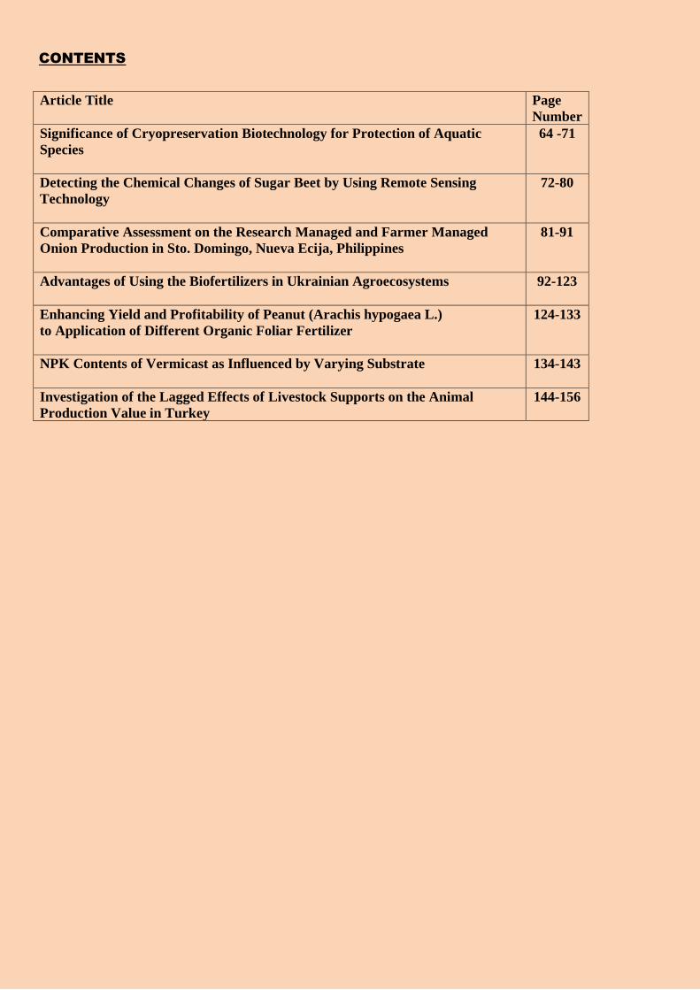
CONTENTS
Article Title Page
Number
Significance of Cryopreservation Biotechnology for Protection of Aquatic
Species
64 -71
Detecting the Chemical Changes of Sugar Beet by Using Remote Sensing
Technology
72-80
Comparative Assessment on the Research Managed and Farmer Managed
Onion Production in Sto. Domingo, Nueva Ecija, Philippines
81-91
Advantages of Using the Biofertilizers in Ukrainian Agroecosystems
92-123
Enhancing Yield and Profitability of Peanut (Arachis hypogaea L.)
to Application of Different Organic Foliar Fertilizer
124-133
NPK Contents of Vermicast as Influenced by Varying Substrate 134-143
Investigation of the Lagged Effects of Livestock Supports on the Animal
Production Value in Turkey
144-156
Eurasian Journal of Agricultural Research 2020; Vol: 4, Issue: 2, pp: 64-71
64
Significance of Cryopreservation Biotechnology for Protection of
Aquatic Species
Maliha Afreen1* and İlknur Uçak2
Nigde Omer Halisdemir University, Faculty of Agricultural Sciences and Technologies, Nigde, Turkey
* Corresponding author: [email protected]
Abstract
Cryopreservation is a method of long term storage of living cells at very low temperature mostly
at the temperature of liquid nitrogen that is -196oC. These cells are stored in those conditions in
which their capabilities of movement, regeneration and reproduction should not disturb. This
process is very helpful for the fish farming as preserved sperm, oocytes can be used for the off
season fertilization of fish species. Cryopreservation is helpful for conservation of specific genetic
traits and to extant endangered species. By cryobanking transportation of gemplasm from one farm
to another farm is also become easy. In this process some chemicals are used as cryoprotectant
agents like DMSO (dimethyl sulfoxide). In this review we describe both advantages and
disadvantages of cryopreservation.
Keywords: Cryopreservation, Conservation, Dimethyl sulfoxide, Fertilization, Germplasm
Rewiev article
Received Date:21 November 2019
Accepted Date:30 November 2020
Eurasian Journal of Agricultural Research 2020; Vol: 4, Issue: 2, pp: 64-71
65
INTRODUCTION
Cryopreservation is defined as the long time storage of Individual living cells and
biological tissues at very low temperatures, like the temperature of liquid nitrogen, usually at -
196oC (Bakhach, 2009). At this temperature, the cellular activities are temporarily prevented and
cells can be genetically stable for a long time until needed. This procedure is very important for
biomedical, clinical, species conservation and biotechnology research areas. It is a best method for
preserving living tissues for long time because it’s a cheap method as compared to other
procedures.
Cryoinjury is the most important area of research for checking the response of cell changes
according to inner and outer environment (Mazur, 1984). It also considered the properties of
freezing and defrosting. Important parameters which involve in these research areas are diffusion,
osmosis, Cryoprotectants, cooling and thawing process.
Cryopreservation method comprises conversion of cell maintenance media to culture media
which have cryopreservation agent, like dimethyl sulfoxide (DMSO). Then Cells are cooled at
temperature of -80°C in specific cooling container. After cooling cells are transferred to very low
temperature storage of below -135°C. Liquid nitrogen is commonly used for this extreme low
temperature.
Cryopreservation has many applied uses in fisheries and aquaculture. They are:
1. Wider transfer of gametes from one point to another point
2. Male progeny fish numbers reduced
3. Provide more time for progeny availability
4. large number of families should be conserved through Selective propagation
5. genetic resources preservation
Fish population is in alarming condition due to water pollution and overfishing.
Endangered species can be preserved by cryopreservation of aquatic germplasm, and by fish
farming. By these strategies genetically important characteristics can be conserved and saved from
loss occur through diseases and natural disasters.
Many fish species has been preserved completely by cryopreservation of semen for
propagation of many wild and domestic species. Researchers did many efforts from more than last
three decades for cryopreservation of fish embryos but still they are unsuccessful (Streit et al.,
2014). Successful cryopreservation of gametes, eggs, and embryos will provide a new way of
completely limitless production of more vigorous and healthy generations of fish species as needed
(Godoy, 2013). Genetic biodiversity of aquatic resources can be maintained by saving the
Genomes of endangered species (Rana, 1995).
Cryopreservation of sperm from aquatic species
According to IUCN 5,161 aquatic species are in endangered condition and these can be
recovering by using the cryopreservation methods in farming of naturally present species (IUCN
Red List, 2015). Researchers are focusing on aquatic animals species for the purpose of life
maintenance in controlled condition and for checking the effect of environmental pollution for
future maintenance. This environmental pollution become a great risk for Killer whales (Orcinus
orca) and dangerous for movement, production and strength of sperm. As a result it can create the
infertility in Killer whales.
Eurasian Journal of Agricultural Research 2020; Vol: 4, Issue: 2, pp: 64-71
66
This problem was recovered by directional solidification technology and by using
cryprotectant agents and glycerol (Robeck et al., 2011). This method also used for cryobanking of
gametes to maintain the population of sea aquariums.
Androgenesis
Cryopreservation also used for the purpose of changing in chromosome set by stopping
activity of the oocyte genome through irradiation or stop fertilization by using cold, heat or
pressure shock at the first stage of mitotic division. This complete process of inactivation is called
Androgenesis (Dunham, 2004; Komen & Thorgaard, 2007). This procedure is helpful for the
recovery of specific species which sperms were cryopreserved by fertilizing with eggs of relevant
species. This technique was successfully applied on rainbow trout (Babiak et al., 2002; Scheerer
et al., 1991), sturgeon species (Grunina et al., 2006), and between fertilization of common carp
and goldfish (Bercsényi et al., 1998).
Germplasm Cryobanking of aquatic species
Cryobanking of fish germplasm involve many types of cells, like sperm, eggs, oocytes,
embryos, somatic cells, spermatogonia and primordial germ cells. Endangered natural reservoirs
of fish species also can be saved by using Germplasm cryopreservation. The first successful
cryopreservation process was done on bull semen to save and reproduce the threatened species
(Polge et al., 1949). In fish Aquaculture sperm is mostly common for the propagation and
administration of related species involving cyprinids, silurids, salmonid (Magyary et al., 1996;
Tsvetkova et al., 1996). Cryopreservation of embryos and oocytes in aquatic species is only
successful for eastern oyster eggs (Crassostrea virginica) (Tervit et al., 2005), and for larvae of
sea urchin and eastern oyster (Paniagua-Chavez & Tiersch, 2001; Adams et al., 2006).
Fish genome is small in size, so it is best model for studying the human genetic diseases
(Barbazuk et al., 2000). More than 200 fish species sperm was successfully manage and
cryopreserved from marine and fresh water (Kopeika et al., 2007; Tsai et al., 2010) including carp,
salmonids, catfish, cichlids, medakas, white-fish, pike, milkfish, grouper, cod, and zebrafish (Scott
& Baynes, 1980; Harvey & Ashwood-Smith 1982; Stoss & Donaldson 1983; Babiak et al., 1995;
Suquet et al., 2000; Van et al., 2006; Bokor et al., 2007; Tsai et al., 2010). Frozen-thawed
spermatozoa have more fertility and survival power than freshwater species (Drokin, 1993; Gwo,
2000).
Tissue collection and cryopreservation
Tissue culture is necessary for getting the more tissues before cryopreservation or it is also
required for reproduction of fish. It is difficult to manage all samples collectively at the time of
tissue collection so these are cryopreserved as soon as possible after harvesting of tissues (Moritz
& Labbe, 2008). Fish sperms and somatic cells can be saved in cryobank by collecting them in
straws and cryovials. Procedures of tissue collection, culturing them and cryopreservation have
been designed for different aquatic species (Lakra et al., 2011), but their response can be varied
from specie to specie (Chenais et al., 2014).
Eurasian Journal of Agricultural Research 2020; Vol: 4, Issue: 2, pp: 64-71
67
Pros and Cons of Cryopreservation in Fisheries Science
Biological material can be preserved for thousands of years without damage.
Total volume of sperm can be used without any wastage.
Off-season fertilization can be done by using preserved sperms.
Transportation of germplasm is easy for farming system as compared to transport of fish.
Conservation of genetic resources of specific required traits (Cabrita et al., 2010).
Conservation of genetic material of threatened species which become very important model
specie in biomedical research (Tsai, 2003; Iwai et al., 2009).
Fish gametes can be preserved from both parents for maintenance of genetic biodiversity.
Fish embryo and oocytes cannot be cryopreserved because of damage by very low
temperature (Tsai & Lin, C, 2012).
Cryopreservation Quality
For getting the best results of cryopreservation evaluation of every step is necessary. This
process has different steps for the quality checking is following:
• Checking the movement of sperm after collection
• After putting in extender solution
• After storage at low temperature
• After addition of cryoprotectant
• After melting of sample
• Fish quality sperm can also be checked by using software “computer-assisted sperm
analysis”
• Flow cytometry and comet assay also used for checking cell characteristics and DNA
quality (Daly & Tiersch, 2011).
Cryoprotectants
Cryoprotectants used to prevent damage of cells from the crystallization and
recrystallization process during storage at freezing temperature. Chemicals which used as
cryoprotectants are following (Meryman, 1966).
• Methanol
• Dimethyl sulfoxide (DMSO)
• Sucrose
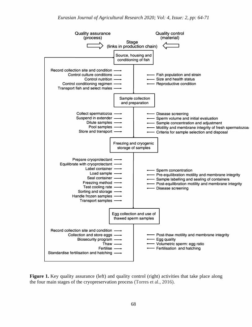
Evaluation strategies used in cryopreservation:
There are four main stages in the cryopreservation process including condition of fish at
the time of collection, preparation, cryostorage and thaw conditions of sperm at the time of usage.
All these steps are given in fig 1.
Eurasian Journal of Agricultural Research 2020; Vol: 4, Issue: 2, pp: 64-71
68
Figure 1. Key quality assurance (left) and quality control (right) activities that take place along
the four main stages of the cryopreservation process (Torres et al., 2016).
Eurasian Journal of Agricultural Research 2020; Vol: 4, Issue: 2, pp: 64-71
69
Difficulties in Cryopreservation
Sometime cells are not able to use after cryopreservation due to damage of cell membrane
(Kim et al., 2015; Chaytor et al., 2012). During cryopreservation two methods can create problem
are slow-freezing and vitrification (Fahy et al., 1984). These processes can create crystallization,
recrystallization and formation of glass solid instead of crystals inside and outside of the cell and
causes the injury of cell even cryoprotectants also not enough to solve this problem (Fahy et al.,
1984). Anti-freezing proteins are used to solve this problem by preventing the ice recrystallization,
so it can improve the process of cryopreservation (Zilli et al., 2014).
New Trends and Future Works in the Area
Researchers are trying to find out solutions for the preservation of fish embryos and ovarian
tissues. Genetic and behavioral changes of cells should be checked in Larvae and juveniles stages
and even in adult form when they are exposed to cryo-solutions. Scientists are trying to find out
new solutions for overcome the problems of cell damage produced by ice crystallization.
REFERENCES
Adams S. L., Hessian P. A. & Mladenov P. V. 2006. The potential for cryopreserving larvae of
the sea urchin, Evechinuschloroticus, Cryobiology, 52(1), 139-145.
Barbazuk W, B., Korf I., Kadavi C., Heyen J., Tate S. & Wun E. 2000. The syntenic relationship
of the zebrafish and human genomes, Genome Research, 10, 1351-1358.
Bakhach J. 2009. The cryopreservation of composite tissues: principles and recent advancement
on cryopreservation of different type of tissues, Organogenesis, 5(3), 119-126.
Babiak I., Dobosz S., Goryczko K., Kuzminski H., Brzuzan P. & Ciesielski S. 2002. Androgenesis
in rainbow trout using cryopreserved spermatozoa: the effect of processing and biological
factors, Theriogenology, 57, 1229–1249.
Bercsényi M., Magyary I., Urbányi B., Orbán L. & Horváth L. 1998. Hatching out goldfish from
common carp eggs: interspecific androgenesis between two cyprinid species, Genome, 41,
573–579.
Babiak I., Glogowsky., Brzuska J. E., Szumiec J. & Adamek J. 1995. Cryopreservation of sperm
of common carp Cyprinus carpio, Aquaculture Research, 28, 567- 571.
Bokor Z., Müller T., Bercsényi M., Horváth L., Urbányi B. & Horváth A. 2007. Cryopreservation
of sperm of two European percid species, the pikeperch (Sander lucioperca) and the Volga
pikeperch (S. volgensis), Acta. Biologica. Hungarica, 58(2), 199-20.
Cabrita E., Sarasquete C., Martínez‐Páramo S., Robles V., Beirao J., Pérez‐Cerezales S. & Herráez
M. P. 2010. Cryopreservation of fish sperm: applications and perspectives, Journal of
Applied Ichthyology, 26(5), 623-635.
Chenais N., Depince A., Le Bail P.Y. & Labbe C. 2014. Fin cell cryopreservation and fish
reconstruction by nuclear transfer stand as promising technologies for preservation of
finfish genetic resources, Aquaculture International, 22, 63–76.
Chaytor J. L., Tokarew J. M., Wu L. K., Leclre M., Tam R. Y., Capicciotti C. J., Guolla L., Von
Moos E., Findlay C. S. & Allan D. S. 2012. Inhibiting ice recrystallization and optimization
of cell viability after Cryopreservation, Glycobiology, 22, 123–133.
Daly J. & Tiersch T. R. 2011. Flow cytometry for the assessment of sperm quality in aquatic
species, Cryopreservation in Aquatic Species, 201-207.
Eurasian Journal of Agricultural Research 2020; Vol: 4, Issue: 2, pp: 64-71
70
Dunham R. A. 2004. Gynogenesis, androgenesis, cloned populations and nuclear transplantation,
Aquaculture and fisheries biotechnology: genetic approaches, 54-61.
Drokin S. I. 1993. Phospholipid distribution and fatty acid composition of phosphatidylcholine
and phosphatidyl ethanolamine in sperm of some freshwater and marine species of fish,
Aquatic Living Resources, 6, 49-56.
Drokin S. I. 1993. Phospholipid distribution and fatty acid composition of phosphatidylcholine
and phosphatidyl ethanolamine in sperm of some freshwater and marine species of fish,
Aquatic Living Resources, 6, 49-56.
Fahy G. M., MacFarlane D. R., Angell C. A. & Meryman H. T. 1984. Vitrification as an approach
to cryopreservation, Cryobiology, 21, 407–426.
Grunina A.S., Recoubratsky A. V., Tsvetkova L. I. & Barmintsev V. A. 2006. Investigation on
dispermic androgenesis in sturgeon fish. The first successful production of androgenetic
sturgeons with cryopreserved sperm. Issue with Special Emphasis on Cryobiology,
International Jornal of Refrigeration, 29, 379–386.
Godoy L. C., Streit Jr. D. P., Zampolla T., Bos-Mikich A. & Zhang T. 2013. A study on the
vitrification of stage III stage zebrafish (Danio rerio) ovarian follicles, Cryobiology; 67(3),
347-354.
Gwo J. C. 2000. Cryopreservation of aquatic invertebrate seman, Aquaculture Research, 31, 259-
271.
Harvey B. & Ashwood-Smith M. J. 1982. Cryopretectant penetration and supercooling in the eggs
of salmonid fishes, Cryobiology, 19, 29-40.
Iwai T., Inowe S., Kotani T. & Yamashita M. 2009, Production of transgenic medaka fish carrying
fluorescent nuclei and chromosomes, Zoological Science, 26, 9–16.
IUCN. IUCN Red List of Threatened Species, 2015.
Komen H. & Thorgaard G. H. 2007. Androgenesis, gynogenesis and the production of clones in
fishes, Aquaculture, 269, 150–173.
Kim H. J., Shim H. E., Lee J. H., Kang Y. C. & Hur Y. B. 2015. Ice-binding protein derived from
Glaciozyma can improve the viability of cryopreserved mammalian cells, Journal of
Microbiology and Biotechnology, 25, 1989–1996.
Kopeika E., Kopeika J. & Zhang T. 2007. Cryopreservation of fish sperm, Methods in Molecular
Biology, 368, 203-17.
Lakra W. S., Swaminathan T. R. & Joy K. P. 2011. Development, characterization, conservation
and storage of fish cell lines, Fish Physiology and Biochemistry, 37, 1–20.
Moritz C. & Labbe C. 2008. Cryopreservation of goldfish fins and optimization for field scale
cryobanking, Cryobiology, 56, 181–188.
Meryman H. T. 1966. Review of biological freezing, Cryobiology, 1-114.
Mazur P. 1984. Freezing of living cells: mechanisms and implications. American journal of
physiology-cell physiology, 247(3), 125-142.
O’Brien J. K. & Robeck T. R. 2010. The value of ex situ cetacean populations in understanding
reproductive physiology and developing assisted reproductive technology for ex situ and
in situ species management and conservation efforts, International journal of comparative
psychology, 23, 227–248.
Polge C, Smith A. U. & Parkes A. S. 1949. Revival of spermatozoa after vitrification and
dehydration at low temperatures, Nature, 164, 666.
Paniagua-Chavez C. G. & Tiersch T. R. 2001. Laboratory studies of cryopreservation of sperm
and trochophore larvae of the eastern oyster, Cryobiology, 43(3), 211- 223.
Eurasian Journal of Agricultural Research 2020; Vol: 4, Issue: 2, pp: 64-71
71
Robeck T. R., Steinman K. J., Gearhart S., Reidarson T. R., McBain J. F. & Monfort S. L. 2004.
Reproductive physiology and development of artificial insemination technology in killer
whales (Orcinus orca), Biology of Reproduction, 71, 650–660.
Robeck T. R., Gearhart S. A., Steinman K. J., Katsumata E., Loureiro J. D. & O’Brien J. K. 2011.
In vitro sperm characterization and development of a sperm cryopreservation method using
directional solidification in the killer whale (Orcinus orca), Theriogenology, 76, 267–279.
Robeck T. R., Montano G. A., Steinman K. J., Smolensky P., Sweeney J., Osborn S. & O’Brien J.
K. 2013. Development and evaluation of deep intra-uterine artificial insemination using
cryopreserved sexed spermatozoa in bottlenose dolphins (Tursiops truncatus), Animal
Reproduction Science, 139, 168–181.
Rana K. 1995. Preservation of gametes. Broodstock management and egg and larval quality,
Cambridge: Blackwell Science, 53-75.
Scheerer P. D., Thorgaard G. H. & Allendorf F. W. 1991. Genetic analysis of androgenetic rainbow
trout, Journal of Experimental Zoology, 260, 382–390.
Streit Jr. D. P., Godoy L. D., Ribeiro R. P., Fornari D. C., Digmayer M. & Zhang T. 2014.
Cryopreservation of embryos and oocytes of South American fish species.
Scott A. P. & Baynes S. M. 1980. A review of the biology, handing and storage of salmonid
spermatozoa, Journal of Fish Biology, 17, 707-739.
Stoss J. & Donaldson EM. 1983. Studies on cryopreservation of eggs from rainbow trout (Salmo
gairdneri) and coho salmon (Oncorhynchus Kisutch), Aquaculture, 31, 51-65.
Suquet M., Dreanno C., Fauvel C., Cosson J. & Billard R. 2000. Cryopreservation of sperm in
marine fish, Aquaculture Research, 31(3), 231-243.
Torres L., Hu E. & Tiersch T. R. 2016. Cryopreservation in fish: current status and pathways to
quality assurance and quality control in repository development, Reproduction, Fertility
and Development, 28(8), 1105-1115.
Tsai S. & Lin C. 2012. Advantages and applications of cryopreservation in fisheries
science, Brazilian archives of biology and technology, 55(3), 425-434.
Tsvetkova L. I., Cosson J., Linhart O. & Billard R. 1996. Motility and fertilizing capacity of fresh
and frozen-thawed spermatozoa in sturgeons Acipenser baeri and A. ruthenus, Journal of
Applied Ichthyology, 12, 107-112.
Tervit H. R., Adams S. L., Roberts R. D., McGowan L. T., Pugh P. A. & Smith J. F. 2005.
Successful cryopreservation of Pacific oyster (Crassostrea gigas) oocytes, Cryobiology,
51(2), 142-151.
Tiersch T. R., Yang H., Jenkins J. A. & Dong Q. 2007. Sperm cryopreservation in fish and
shellfish, Society for Reproduction and Fertility, 65, 493-508.
Tsai S., Spikings E. & Lin C. 2010. Effects of the controlled slow cooling procedure on freezing
parameters and ultrastructural morphology of Taiwan shoveljaw carp (Varicorhinus
barbatulus) sperm, Aquatic Living Resources, 23, 119-124.
Tsai H. J. 2003. Transgenic Fish: researches and Applications, Journal of the Fisheries Society of
Taiwan, 30, 263–277.
Van der Straten K. M., Leung L. K., Rossini R. & Johnston S. D. 2006. Cryopreservation of
spermatozoa of black marlin, Makaira indica (Teleostei: Istiophoridae),
International journal for low temperature science and technology, 27(4), 203-209.
Zilli L., Beirão J., Schiavone R., Herraez M. P., Gnoni A. & Vilella S. 2014. Comparative
proteome analysis of cryopreserved flagella and head plasma membrane proteins from sea
bream spermatozoa: Effect of antifreeze proteins, Plos One, 9(6), e99992.
Eurasian Journal of Agricultural Research 2020; Vol: 4, Issue: 2, pp: 72-80
72
Detecting the Chemical Changes of Sugar Beet
by Using Remote Sensing Technology
Rutkay ATUN*, Önder GÜRSOY
Sivas Cumhuriyet University, Engineering Faculty, Department of Geomatics, Sivas / Turkey
* Corresponding author: [email protected]
Abstract
The changes in spectral behavior of plants against chemical effects were investigated by using
remote sensing and its terrestrial spectral data, in this study. Sugar beet plant was selected
as test plants. The study area was split into 3 sections for the sugar beet plant and three
different phosphorus fertilization were treated to these sections (300 kg P ha-1, 150 kg P ha-1 and
0 kg P ha-1). Terrestrial spectral measurements were carried out on the leaves of the sugar beets,
after the development of them. The reflectance values obtained by terrestrial spectral measurement
data were used as an end member in order to run spectral classification and Sentinel 2A satellite
image was used for spectral classification. Vegetation indices also were produced in order to
support the spectral classification results. As a result of the study, remote sensing and its terrestrial
components' usability have been shown in order to prevent wrong fertilization, to increase product
yield, to protect the health of the plant and soil.
Keywords: Spectroradiometer measurements, Spectral classification, Sugar beet
Research article
Received Date: 11 February 2020
Accepted Date:30 November 2020
Eurasian Journal of Agricultural Research 2020; Vol: 4, Issue: 2, pp: 72-80
73
INTRODUCTION
Remote sensing basically means that the information of an object is obtained without direct
contact to that object. The science of remote sensing has also shown great improvement since the
1800s (Gibson, 2000). In addition, today there are many free satellite images available for remote
sensing and it provides speed, practicality, and convenience in accessing the information (Gürsoy
et. al., 2017; Gürsoy & Atun, 2019a; Canbaz et. al., 2018). Nowadays, the use of remote sensing
has increased and the usage areas have varied with the developing technology. One of these areas
is agricultural applications. Thanks to remote sensing, it has been possible to perform applications
such as tracing, irrigation, fertilization, and product health quickly and effectively (Ramoelo et.
al., 2015; He et al., 2016; Birdal et al., 2017).
There are many studies on agriculture by using remote sensing in today. In the study
conducted by Özelkan et al. (2015), the vineyard areas in the Trakya region in Turkey were
investigated by remote sensing and geographical information systems. In this context, using the
remote sensing and GIS, the vineyard areas in the area of Trakya region, Tekirdağ and Tekirdağ
Department of Viticulture Research Station were examined. The geographical location of the
existing vineyard was determined by satellite image for this purpose. In addition, water stress and
photosynthesis conditions of plants were investigated with the help of terrestrial hyperspectral
remote sensing techniques and the most suitable areas for viticulture were evaluated in a GIS
environment by considering various criteria.
The study carried out in 2017 by Gürsoy et al, it was treated various doses of cadmium and
zinc to sugar beet plants grown in a greenhouse environment. Zinc was applied as 0 and 5.0 mg
Zn / kg doses and cadmium doses were treated 0, 2.5, 5.0 and 10.0 mg Cd / kg (CuSO4). As a
result of the study, the wavelength ranges in which the spectral signatures change in the
electromagnetic spectrum according to the doses and the elements applied to the plants were
determined.
The study conducted Yousfi et al. in 2016, wheat and bread wheat in different irrigation
conditions of vegetation indices and canopy temperatures were compared to different
methodological approaches. The plants were periodically observed for two years, the
spectrophotometry of the plants was examined and the images were taken with traditional cameras.
Canopy temperatures were measured between 12.00 and 14.00 at noon simultaneously with
spectroradiometer measurements. The GA, GGA and NDVI vegetation indices were produced to
investigate the status of plants. The GA and GGA vegetation indices were calculated by the images
taken from the camera. NDVI index was calculated by reflectance obtained from
spectroradiometer. As a result of the study, the vegetation indices obtained by traditional cameras
(GA, GGA) showed a significant correlation with the NDVI calculated by the reflectance obtained
by the spectroradiometer.
In this study, unlike the experiments conducted in the literature, plants treated differently
doses of fertilization were classified by spectral classification algorithms by using remote sensing
and its terrestrial spectral components. Subsequently, different vegetation indices were utilized in
order to support the classification results and the relationships between these indices were
examined. As a result, differences in the amount of fertilizer in plants could be detected by remote
sensing and its terrestrial spectral components.
Eurasian Journal of Agricultural Research 2020; Vol: 4, Issue: 2, pp: 72-80
74
MATERIAL and METHODS
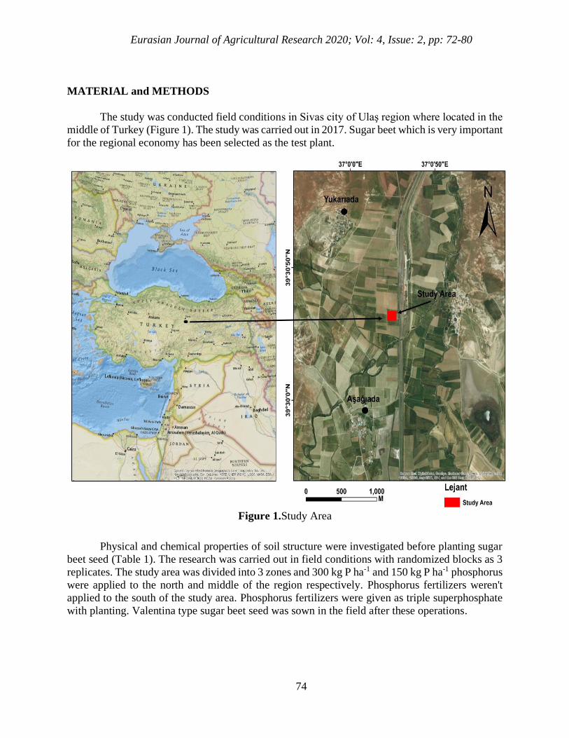
The study was conducted field conditions in Sivas city of Ulaş region where located in the
middle of Turkey (Figure 1). The study was carried out in 2017. Sugar beet which is very important
for the regional economy has been selected as the test plant.
Figure 1.Study Area
Physical and chemical properties of soil structure were investigated before planting sugar
beet seed (Table 1). The research was carried out in field conditions with randomized blocks as 3
replicates. The study area was divided into 3 zones and 300 kg P ha-1 and 150 kg P ha-1 phosphorus
were applied to the north and middle of the region respectively. Phosphorus fertilizers weren't
applied to the south of the study area. Phosphorus fertilizers were given as triple superphosphate
with planting. Valentina type sugar beet seed was sown in the field after these operations.
Eurasian Journal of Agricultural Research 2020; Vol: 4, Issue: 2, pp: 72-80
75
Table 1. Physical and Chemical Properties of Soil Structure (Gürsoy & Atun, 2019b)
Soil Property Depth (0-30 cm)
pH (H2O) 7.42
Lime (%) 14.30
Salt (dS m-1) 0.41
Organic Matter (%) 1.30
Texture CL
Total N (%) 0.10
Available P (kg ha-1) 53.50
Available K (kg ha-1) 948.10
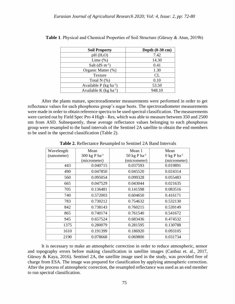
After the plants mature, spectroradiometer measurements were performed in order to get
reflectance values for each phosphorus group’s sugar beets. The spectroradiometer measurements
were made in order to obtain reference spectra to be used spectral classification. The measurements
were carried out by Field Spec Pro 4 High - Res, which was able to measure between 350 and 2500
nm from ASD. Subsequently, these average reflectance values belonging to each phosphorus
group were resampled to the band intervals of the Sentinel 2A satellite to obtain the end members
to be used in the spectral classification (Table 2).
Table 2. Reflectance Resampled to Sentinel 2A Band Intervals
It is necessary to make an atmospheric correction in order to reduce atmospheric, sensor
and topography errors before making classification in satellite images (Canbaz et. al., 2017,
Gürsoy & Kaya, 2016). Sentinel 2A, the satellite image used in the study, was provided free of
charge from ESA. The image was prepared for classification by applying atmospheric correction.
After the process of atmospheric correction, the resampled reflectance was used as an end member
to run spectral classification.
Wavelength
(nanometer)
Mean
300 kg P ha-1
(micrometer)
Mean 1
50 kg P ha-1
(micrometer)
Mean
0 kg P ha-1
(micrometer)
443 0.040715 0.037593 0.019891
490 0.047850 0.045520 0.024314
560 0.095054 0.099328 0.055483
665 0.047529 0.043044 0.021635
705 0.136481 0.141598 0.083516
740 0.572003 0.604650 0.416171
783 0.730212 0.754632 0.532130
842 0.738143 0.760215 0.539149
865 0.740174 0.761540 0.541672
945 0.657524 0.683436 0.474532
1375 0.280079 0.281595 0.130788
1610 0.191399 0.186920 0.093105
2190 0.078668 0.069800 0.031734
Eurasian Journal of Agricultural Research 2020; Vol: 4, Issue: 2, pp: 72-80
76
Matched filtering, one of the most frequently used algorithm in classification has been
chosen as a spectral classification algorithm. The matched filtering has been derived to remove the
signal to noise ratio of a disturbed signal by noise. This algorithm is also used as the best method
for detecting primary users of the transmitted signal is known (Harsanyi & Chang, 1994; Gürsoy
& Atun, 2018; Gürsoy et. al., 2017).
Various vegetation indices were also used in order to support the result of the classification
study. The indices were generated using spectral reflectance differences of the Sentinel 2A
satellite. Vegetation indices used in the study were NDVI, CIgreen and CIrededge.
The most common vegetation index for determining plant status and vegetation is NDVI.
In the NDVI index, the near infrared and red regions of the electromagnetic spectrum are used.
The red and near-infrared region is a region sensitive to plants and dense vegetation (Rouse et. al.,
1974; Welmann et. al., 2018; Gandhi et. al., 2015). It was produced to detect different phosphorus
doses, in the scope of the study.
Green and near-infrared regions of the spectrum are used in CIgreen, which is called the
green chlorophyll index (Clevers & Gitelson, 2013; Peng et. al., 2011). CIgreen was also used to
display phosphorus fertilization at different doses in sugar beet.
The red region of the spectrum is utilized to generate the CIred-edge index used to estimate
the amount of fertilizer and chlorophyll in plants (Clevers & Kooistra, 2012; Vina et. al., 2011). It
was also utilized to monitor phosphorus fertilization at different doses in sugar beet plants.
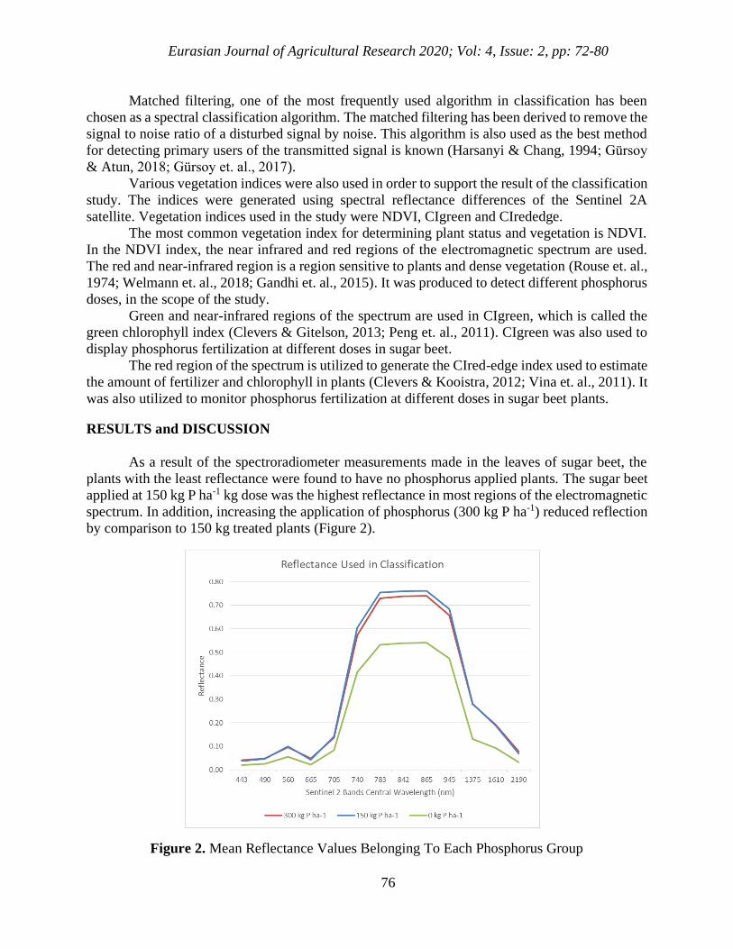
RESULTS and DISCUSSION
As a result of the spectroradiometer measurements made in the leaves of sugar beet, the
plants with the least reflectance were found to have no phosphorus applied plants. The sugar beet
applied at 150 kg P ha-1 kg dose was the highest reflectance in most regions of the electromagnetic
spectrum. In addition, increasing the application of phosphorus (300 kg P ha-1) reduced reflection
by comparison to 150 kg treated plants (Figure 2).
Figure 2. Mean Reflectance Values Belonging To Each Phosphorus Group
Eurasian Journal of Agricultural Research 2020; Vol: 4, Issue: 2, pp: 72-80
77
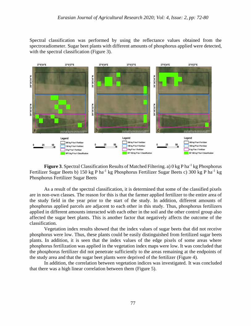
Spectral classification was performed by using the reflectance values obtained from the
spectroradiometer. Sugar beet plants with different amounts of phosphorus applied were detected,
with the spectral classification (Figure 3).
Figure 3. Spectral Classification Results of Matched Filtering. a) 0 kg P ha-1 kg Phosphorus
Fertilizer Sugar Beets b) 150 kg P ha-1 kg Phosphorus Fertilizer Sugar Beets c) 300 kg P ha-1 kg
Phosphorus Fertilizer Sugar Beets
As a result of the spectral classification, it is determined that some of the classified pixels
are in non-own classes. The reason for this is that the farmer applied fertilizer to the entire area of
the study field in the year prior to the start of the study. In addition, different amounts of
phosphorus applied parcels are adjacent to each other in this study. Thus, phosphorus fertilizers
applied in different amounts interacted with each other in the soil and the other control group also
affected the sugar beet plants. This is another factor that negatively affects the outcome of the
classification.
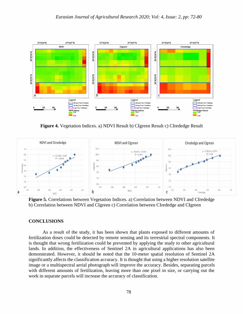
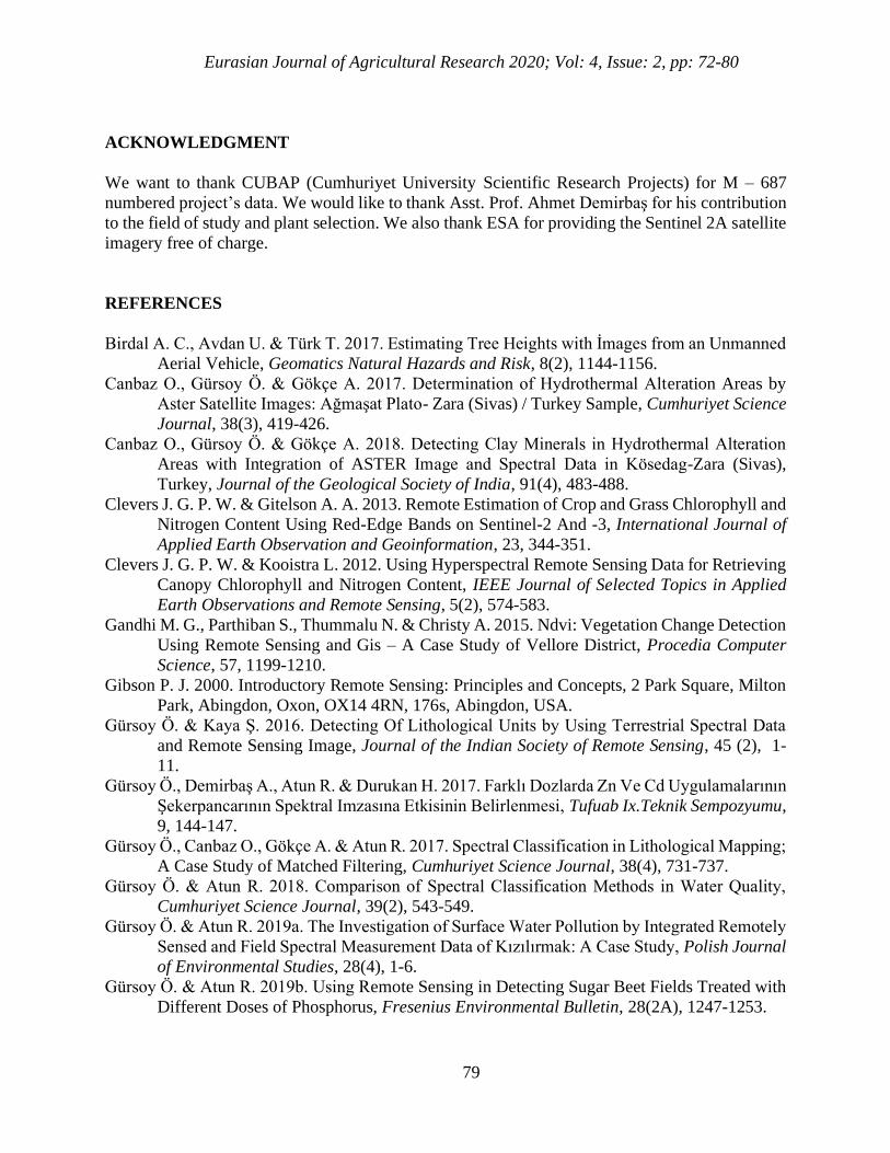
Vegetation index results showed that the index values of sugar beets that did not receive
phosphorus were low. Thus, these plants could be easily distinguished from fertilized sugar beets
plants. In addition, it is seen that the index values of the edge pixels of some areas where
phosphorus fertilization was applied in the vegetation index maps were low. It was concluded that
the phosphorus fertilizer did not penetrate sufficiently to the areas remaining at the endpoints of
the study area and that the sugar beet plants were deprived of the fertilizer (Figure 4).
In addition, the correlation between vegetation indices was investigated. It was concluded
that there was a high linear correlation between them (Figure 5).
Eurasian Journal of Agricultural Research 2020; Vol: 4, Issue: 2, pp: 72-80
78
Figure 4. Vegetation Indices. a) NDVI Result b) CIgreen Result c) CIrededge Result
Figure 5. Correlations between Vegetation Indices. a) Correlation between NDVI and CIrededge
b) Correlation between NDVI and CIgreen c) Correlation between CIrededge and CIgreen
CONCLUSIONS
As a result of the study, it has been shown that plants exposed to different amounts of
fertilization doses could be detected by remote sensing and its terrestrial spectral components. It
is thought that wrong fertilization could be prevented by applying the study to other agricultural
lands. In addition, the effectiveness of Sentinel 2A in agricultural applications has also been
demonstrated. However, it should be noted that the 10-meter spatial resolution of Sentinel 2A
significantly affects the classification accuracy. It is thought that using a higher resolution satellite
image or a multispectral aerial photograph will improve the accuracy. Besides, separating parcels
with different amounts of fertilization, leaving more than one pixel in size, or carrying out the
work in separate parcels will increase the accuracy of classification.
Eurasian Journal of Agricultural Research 2020; Vol: 4, Issue: 2, pp: 72-80
79
ACKNOWLEDGMENT
We want to thank CUBAP (Cumhuriyet University Scientific Research Projects) for M – 687
numbered project’s data. We would like to thank Asst. Prof. Ahmet Demirbaş for his contribution
to the field of study and plant selection. We also thank ESA for providing the Sentinel 2A satellite
imagery free of charge.
REFERENCES
Birdal A. C., Avdan U. & Türk T. 2017. Estimating Tree Heights with İmages from an Unmanned
Aerial Vehicle, Geomatics Natural Hazards and Risk, 8(2), 1144-1156.
Canbaz O., Gürsoy Ö. & Gökçe A. 2017. Determination of Hydrothermal Alteration Areas by
Aster Satellite Images: Ağmaşat Plato- Zara (Sivas) / Turkey Sample, Cumhuriyet Science
Journal, 38(3), 419-426.
Canbaz O., Gürsoy Ö. & Gökçe A. 2018. Detecting Clay Minerals in Hydrothermal Alteration
Areas with Integration of ASTER Image and Spectral Data in Kösedag-Zara (Sivas),
Turkey, Journal of the Geological Society of India, 91(4), 483-488.
Clevers J. G. P. W. & Gitelson A. A. 2013. Remote Estimation of Crop and Grass Chlorophyll and
Nitrogen Content Using Red-Edge Bands on Sentinel-2 And -3, International Journal of
Applied Earth Observation and Geoinformation, 23, 344-351.
Clevers J. G. P. W. & Kooistra L. 2012. Using Hyperspectral Remote Sensing Data for Retrieving
Canopy Chlorophyll and Nitrogen Content, IEEE Journal of Selected Topics in Applied
Earth Observations and Remote Sensing, 5(2), 574-583.
Gandhi M. G., Parthiban S., Thummalu N. & Christy A. 2015. Ndvi: Vegetation Change Detection
Using Remote Sensing and Gis – A Case Study of Vellore District, Procedia Computer
Science, 57, 1199-1210.
Gibson P. J. 2000. Introductory Remote Sensing: Principles and Concepts, 2 Park Square, Milton
Park, Abingdon, Oxon, OX14 4RN, 176s, Abingdon, USA.
Gürsoy Ö. & Kaya Ş. 2016. Detecting Of Lithological Units by Using Terrestrial Spectral Data
and Remote Sensing Image, Journal of the Indian Society of Remote Sensing, 45 (2), 1-
11.
Gürsoy Ö., Demirbaş A., Atun R. & Durukan H. 2017. Farklı Dozlarda Zn Ve Cd Uygulamalarının
Şekerpancarının Spektral Imzasına Etkisinin Belirlenmesi, Tufuab Ix.Teknik Sempozyumu,
9, 144-147.
Gürsoy Ö., Canbaz O., Gökçe A. & Atun R. 2017. Spectral Classification in Lithological Mapping;
A Case Study of Matched Filtering, Cumhuriyet Science Journal, 38(4), 731-737.
Gürsoy Ö. & Atun R. 2018. Comparison of Spectral Classification Methods in Water Quality,
Cumhuriyet Science Journal, 39(2), 543-549.
Gürsoy Ö. & Atun R. 2019a. The Investigation of Surface Water Pollution by Integrated Remotely
Sensed and Field Spectral Measurement Data of Kızılırmak: A Case Study, Polish Journal
of Environmental Studies, 28(4), 1-6.
Gürsoy Ö. & Atun R. 2019b. Using Remote Sensing in Detecting Sugar Beet Fields Treated with
Different Doses of Phosphorus, Fresenius Environmental Bulletin, 28(2A), 1247-1253.
Eurasian Journal of Agricultural Research 2020; Vol: 4, Issue: 2, pp: 72-80
80
Harsanyi J. C. & Chang C. I. 1994. Hyperspectral Image Classification and Dimensionality
Reduction: An Orthogonal Subspace Projection Approach, IEEE Transactions on
Geoscience and Remote Sensing, 32(4), 779-785.
He L., Zhang H. Y. Zhang Y. S., Song X., Feng W., Kang G. Z., Wang C. Y. & Guo T.C. 2016.
Estimation Canopy Leaf Nitrogen Concentration in Winter Wheat Based On Multiangular
Hyperspectral Remote Sensing, European Journal of Agronomy, 73, 170-185.
Özelkan E., Karaman M., Candar S., Coşkun Z. & Örmeci C., 2015. Investigation of Grapevine
Photosynthesis Using Hyperspectral Techniques and Development of Hyperspectral Band
Ratio Indices Sensitive to Photosynthesis, Journal of Environmental Biology, 36, 91-100.
Peng Y., Gitelson A. A., Keydan G., Rundquist D. C. & Moses W., 2011. Remote Estimation of
Gross Primary Production in Maize and Support for a New Paradigm Based on Total Crop
Chlorophyll Content, Remote Sensing of Environment, 115, 978-989.
Ramoelo A., Dzikiti S., Deventer H. V., Maherry A., Cho M. A. & Gush M. 2015. Potential to
Monitor Plant Stress Using Remote Sensing Tools, Journal of Arid Environments, 113,
134-144.
Rouse J. W., Haas R. H., Schell J. A. & Deering D.W. 1974. Monitoring Vegetation Systems in
the Great Plains with ERTS, NASA SP-351, Third ERTS-1 Symposium NASA, 3, 309-317.
Vina A., Gitelson A. A., Robertson A. N. L. & Peng Y. 2011. Comparison of Different Vegetation
Indices for the Remote Assessment of Green Leaf Area Index of Crops, Remote Sensing of
Environment, 115, 3468-3478.
Welmann T., Haase D., Knapp S., Salbach C., Selsam P. & Lausch A. 2018. Urban Land Use
Intensity Assessment: The Potential of Spatio-Temporal Spectral Traits with Remote
Sensing, Ecological Indicators, 85, 190-203.
Yousfi S., Kellas N., Saidi L., Benlakehal Z., Chaou L., Siad D., Herda F., Karrou M., Vergara O.,
Gracia A., Araus J. L. & Serret M. D. 2016. Comparative Performance of Remote Sensing
Methods in Assessing Wheat Performance under Mediterranean Conditions, Agricultural
Water Management, 164(1), 137-147.
Eurasian Journal of Agricultural Research 2020; Vol: 4, Issue: 2, pp: 81-91
81
Comparative Assessment of the Researcher-Managed and Farmer-Managed
Onion (Allium cepa L.) Production in Sto. Domingo, Nueva Ecija, Philippines
Ulysses A. Cagasan
Department of Agronomy, Visayas State University, Visca, Baybay City, Leyte 6521-A, Philippines
Corresponding Author: [email protected]
Abstract
A comparative assessment is a vital tool in the farmer's practice on their farm and compares the
researcher's practice on how it varies in terms of its operation and productivity. It is also a good
idea to assess it in a commercial scope of production. This study aimed to assess, compare, and
give the farmers the recommended commercial onion production practice. This was possible
through a survey conducted, assess, and compare the two management practices of growing onion
crops by the researcher and the farmer-managed onion production. A survey of onion growing areas
in Brgy. San Fransisco in Sto. Domingo, Nueva Ecija was done to determine the differences
between the researcher-managed and farmer-managed in its farm management and operations. The
survey results revealed that the researcher's technologies have done for a long time; therefore, it
needs some verification to update the information. However, it is still useful to have a guide to
improve the technology either on the farmers` side and to the researcher's end. Therefore, for
successful adoption of the technology, it should be tested first in the specific locality before
recommending it to the farmers, or the farmer should experiment on a small portion of their farm
before doing it in a commercial plantation. The farmer's practiced also reveals some innovative way
of doing farm activities practically and proven effective for productivity and income.
Keywords: Onion production, research, farmer's managed, net income
Research article
Received Date: 16 November 2020
Accepted Date:30 November 2020
Eurasian Journal of Agricultural Research 2020; Vol: 4, Issue: 2, pp: 81-91
82
INTRODUCTION
Bulb onion (Allium cepa L.), locally known as sibuyas, is probably the most indispensable
culinary ingredient not only in the Philippines but probably in the world. It is a favorite seasoning,
and its pungent aroma and sharp taste make it ideal for spicing up meat, salads, and vegetable dishes
(https://businessdiary.com.ph/6051/onion-production-guide). It is also used to cure various
physiological disorders such as cough, obesity, insomnia, hemorrhoid, and constipation. In 2019,
the volume of onions produced in the Philippines was approximately 222.1 thousand metric tons.
In 2018, the production value of onions in the country was about 6.7 billion Philippine pesos (Onion
Production in the Philippines 2019). In Central Luzon, the top producer of red onion at 19.74
thousand metric tons accounted for 51.9 percent of the country's total production. MIMAROPA
followed this with 42.4 percent, and Ilocos Region, 2.6 percent. However, the production of onion
in Nueva Ecija, particularly in the municipality of Bongabon (the leading producer of onion in the
Philippines and probably in Southeast Asia), is expected to increase following the introduction
newer and pest-resistant varieties. Onion production fits very well in the rice farming system in
selected regions of the country. These are usually grown after rice towards the dry season when
water is not sufficient for another rice crop. Farmers utilize the rice straw from the previous
cropping as mulching materials in allium production. They consider onion and garlic as good cash
crops with high returns to investment, Lopez, and Anit (1994).
A survey and field visitation was done in Sto. Domingo being one of the onions producing
areas in Nueva Ecija, to conduct a survey and focus group discussion (FGD) with the vegetable
farmer leaders. The FGD group was led by a model farmer named Ging Gamboa, an Engineer who
ventured into the vegetable farming business in Sto Domingo, Nueva Ecija. We interviewed two
researchers from the Central Luzon State University, Science City of Munoz, Nueva Ecija, to verify
their practice and ask the guide on the cultural management practices they developed for onion bulb
production. A comparative assessment is an essential tool in knowing the condition of the farmer's
practice in their farm and to compare the researcher's practice on how it varies in terms of its
operation and management. This study aimed to assess, compare, and give the farmer's
recommendations, the best practice of commercial onion production.
METHODOLOGY
The method used in the study was done by gathering ten onion farmer leaders through focus
group discussion (FGD). All the information asked the farmers were guided with standard cultural
management practices for onion production published by the onion researchers (Abon et al. 2015).
The area was visited, and the farmers were interviewed and observed for their activities on the farm.
Eurasian Journal of Agricultural Research 2020; Vol: 4, Issue: 2, pp: 81-91
83
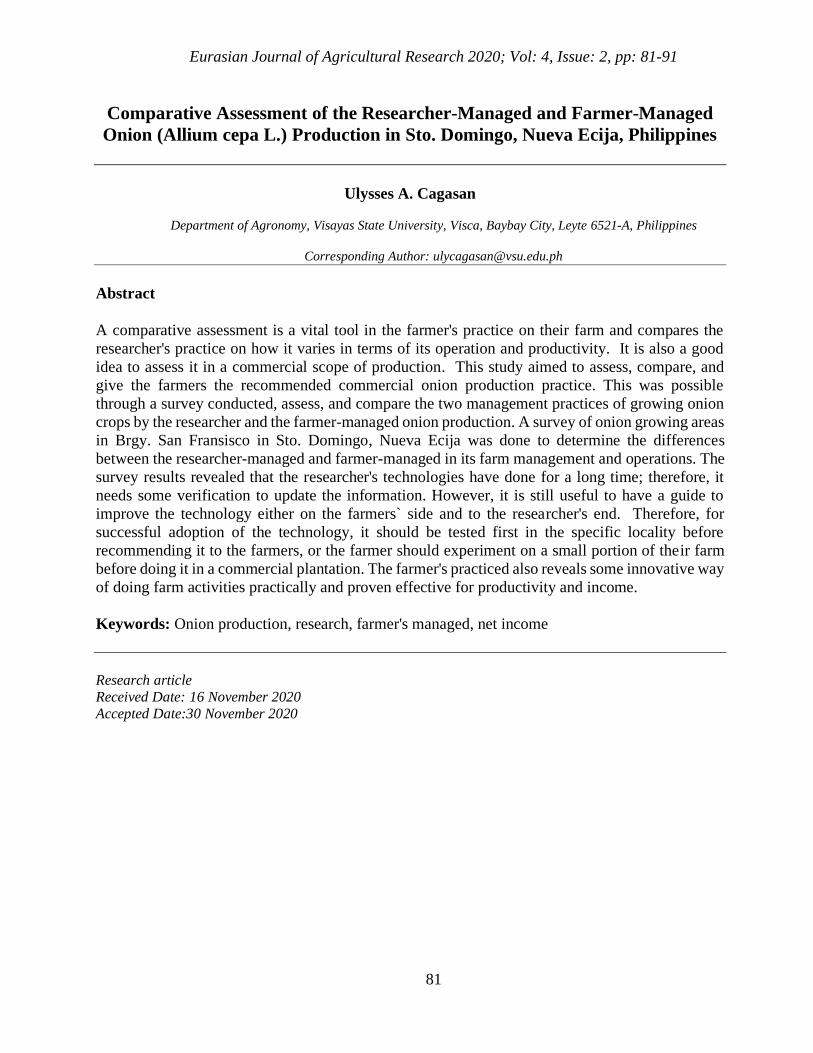
Figure 1. Area planted with onions one month after planting
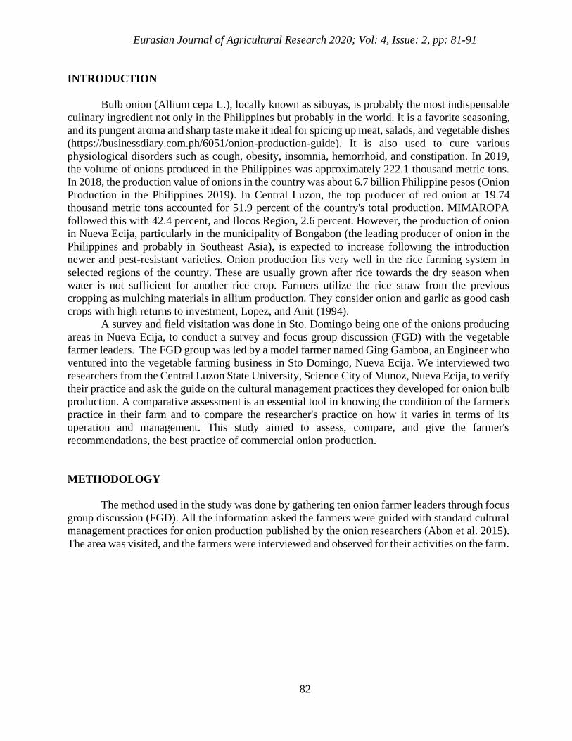
Figure 2. Onions production using double rows planting
Eurasian Journal of Agricultural Research 2020; Vol: 4, Issue: 2, pp: 81-91
84
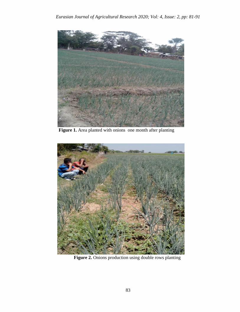
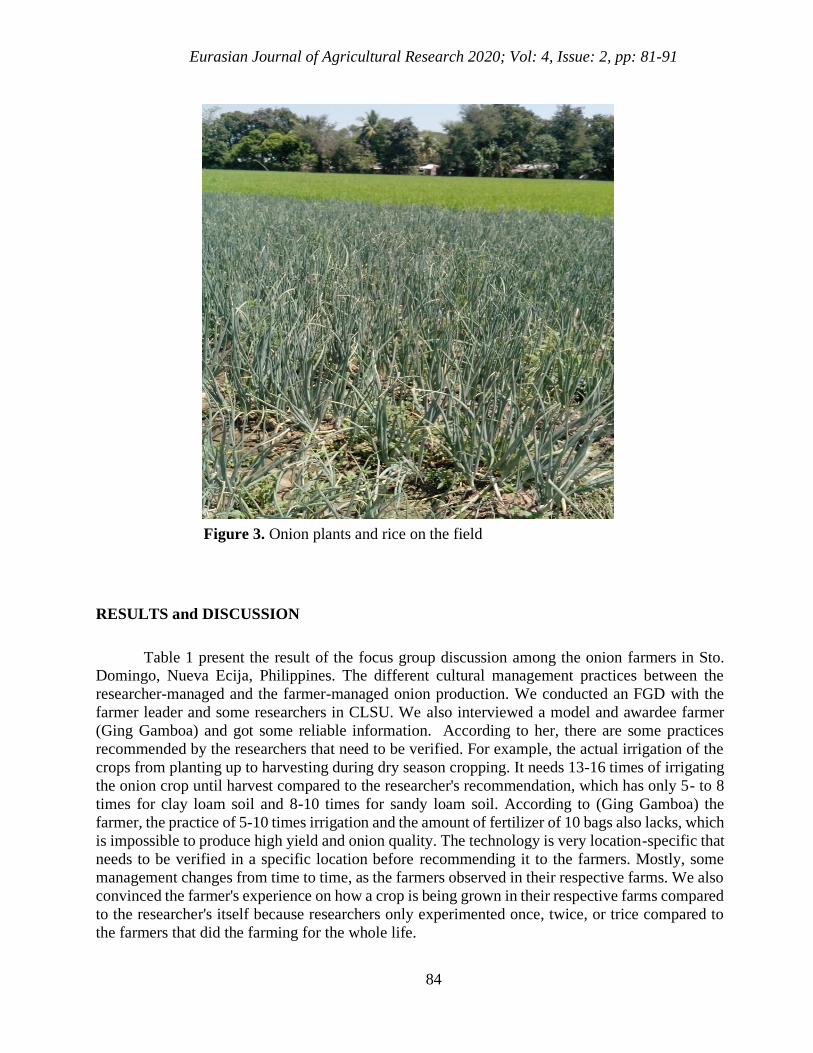
Figure 3. Onion plants and rice on the field
RESULTS and DISCUSSION
Table 1 present the result of the focus group discussion among the onion farmers in Sto. Domingo, Nueva Ecija, Philippines. The different cultural management practices between the
researcher-managed and the farmer-managed onion production. We conducted an FGD with the
farmer leader and some researchers in CLSU. We also interviewed a model and awardee farmer
(Ging Gamboa) and got some reliable information. According to her, there are some practices
recommended by the researchers that need to be verified. For example, the actual irrigation of the
crops from planting up to harvesting during dry season cropping. It needs 13-16 times of irrigating
the onion crop until harvest compared to the researcher's recommendation, which has only 5- to 8
times for clay loam soil and 8-10 times for sandy loam soil. According to (Ging Gamboa) the
farmer, the practice of 5-10 times irrigation and the amount of fertilizer of 10 bags also lacks, which
is impossible to produce high yield and onion quality. The technology is very location-specific that
needs to be verified in a specific location before recommending it to the farmers. Mostly, some
management changes from time to time, as the farmers observed in their respective farms. We also
convinced the farmer's experience on how a crop is being grown in their respective farms compared
to the researcher's itself because researchers only experimented once, twice, or trice compared to
the farmers that did the farming for the whole life.
Eurasian Journal of Agricultural Research 2020; Vol: 4, Issue: 2, pp: 81-91
85
Also, the researcher's technologies have done for a long time; therefore, it needs some
verification to update the technology's information. However, it is still useful to have a guide to
improve the technology either on the farmers` side and to the researcher's end. Therefore, it must
be tested first in the specific locality before recommending it to the farmers for successful adoption
of the technology. The farmer should experiment on a small portion of the farm before doing it on
a commercial plantation.
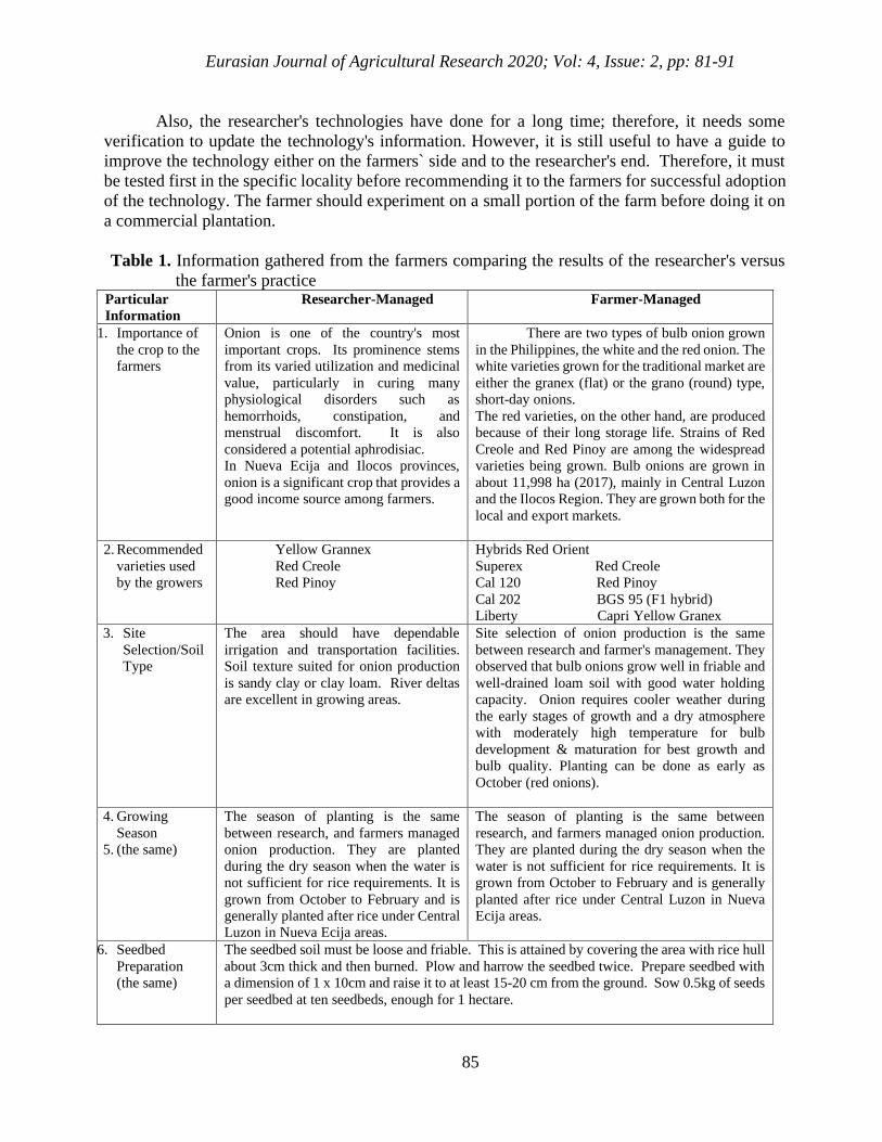
Table 1. Information gathered from the farmers comparing the results of the researcher's versus
the farmer's practice Particular
Information
Researcher-Managed Farmer-Managed
1. Importance of
the crop to the
farmers
Onion is one of the country's most
important crops. Its prominence stems
from its varied utilization and medicinal
value, particularly in curing many
physiological disorders such as
hemorrhoids, constipation, and
menstrual discomfort. It is also
considered a potential aphrodisiac.
In Nueva Ecija and Ilocos provinces,
onion is a significant crop that provides a
good income source among farmers.
There are two types of bulb onion grown
in the Philippines, the white and the red onion. The
white varieties grown for the traditional market are
either the granex (flat) or the grano (round) type,
short-day onions.
The red varieties, on the other hand, are produced
because of their long storage life. Strains of Red
Creole and Red Pinoy are among the widespread
varieties being grown. Bulb onions are grown in
about 11,998 ha (2017), mainly in Central Luzon
and the Ilocos Region. They are grown both for the
local and export markets.
2. Recommended
varieties used
by the growers
Yellow Grannex
Red Creole
Red Pinoy
Hybrids Red Orient
Superex Red Creole
Cal 120 Red Pinoy
Cal 202 BGS 95 (F1 hybrid)
Liberty Capri Yellow Granex
3. Site
Selection/Soil
Type
The area should have dependable
irrigation and transportation facilities.
Soil texture suited for onion production
is sandy clay or clay loam. River deltas
are excellent in growing areas.
Site selection of onion production is the same
between research and farmer's management. They
observed that bulb onions grow well in friable and
well-drained loam soil with good water holding
capacity. Onion requires cooler weather during
the early stages of growth and a dry atmosphere
with moderately high temperature for bulb
development & maturation for best growth and
bulb quality. Planting can be done as early as
October (red onions).
4. Growing
Season
5. (the same)
The season of planting is the same
between research, and farmers managed
onion production. They are planted
during the dry season when the water is
not sufficient for rice requirements. It is
grown from October to February and is
generally planted after rice under Central
Luzon in Nueva Ecija areas.
The season of planting is the same between
research, and farmers managed onion production.
They are planted during the dry season when the
water is not sufficient for rice requirements. It is
grown from October to February and is generally
planted after rice under Central Luzon in Nueva
Ecija areas.
6. Seedbed
Preparation
(the same)
The seedbed soil must be loose and friable. This is attained by covering the area with rice hull
about 3cm thick and then burned. Plow and harrow the seedbed twice. Prepare seedbed with
a dimension of 1 x 10cm and raise it to at least 15-20 cm from the ground. Sow 0.5kg of seeds
per seedbed at ten seedbeds, enough for 1 hectare.
Eurasian Journal of Agricultural Research 2020; Vol: 4, Issue: 2, pp: 81-91
86
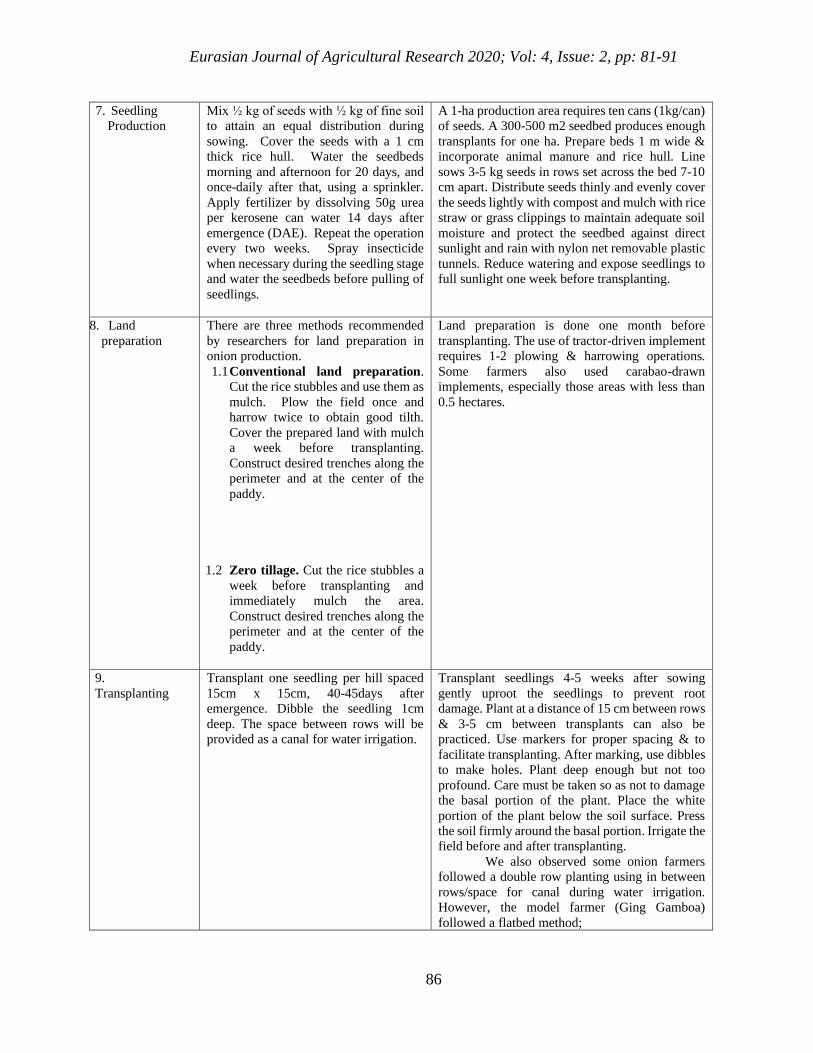
7. Seedling
Production
Mix ½ kg of seeds with ½ kg of fine soil
to attain an equal distribution during
sowing. Cover the seeds with a 1 cm
thick rice hull. Water the seedbeds
morning and afternoon for 20 days, and
once-daily after that, using a sprinkler.
Apply fertilizer by dissolving 50g urea
per kerosene can water 14 days after
emergence (DAE). Repeat the operation
every two weeks. Spray insecticide
when necessary during the seedling stage
and water the seedbeds before pulling of
seedlings.
A 1-ha production area requires ten cans (1kg/can)
of seeds. A 300-500 m2 seedbed produces enough
transplants for one ha. Prepare beds 1 m wide &
incorporate animal manure and rice hull. Line
sows 3-5 kg seeds in rows set across the bed 7-10
cm apart. Distribute seeds thinly and evenly cover
the seeds lightly with compost and mulch with rice
straw or grass clippings to maintain adequate soil
moisture and protect the seedbed against direct
sunlight and rain with nylon net removable plastic
tunnels. Reduce watering and expose seedlings to
full sunlight one week before transplanting.
8. Land
preparation
There are three methods recommended
by researchers for land preparation in
onion production.
1.1 Conventional land preparation.
Cut the rice stubbles and use them as
mulch. Plow the field once and
harrow twice to obtain good tilth.
Cover the prepared land with mulch
a week before transplanting.
Construct desired trenches along the
perimeter and at the center of the
paddy.
1.2 Zero tillage. Cut the rice stubbles a
week before transplanting and
immediately mulch the area.
Construct desired trenches along the
perimeter and at the center of the
paddy.
Land preparation is done one month before
transplanting. The use of tractor-driven implement
requires 1-2 plowing & harrowing operations.
Some farmers also used carabao-drawn
implements, especially those areas with less than
0.5 hectares.
9.
Transplanting
Transplant one seedling per hill spaced
15cm x 15cm, 40-45days after
emergence. Dibble the seedling 1cm
deep. The space between rows will be
provided as a canal for water irrigation.
Transplant seedlings 4-5 weeks after sowing
gently uproot the seedlings to prevent root
damage. Plant at a distance of 15 cm between rows
& 3-5 cm between transplants can also be
practiced. Use markers for proper spacing & to
facilitate transplanting. After marking, use dibbles
to make holes. Plant deep enough but not too
profound. Care must be taken so as not to damage
the basal portion of the plant. Place the white
portion of the plant below the soil surface. Press
the soil firmly around the basal portion. Irrigate the
field before and after transplanting.
We also observed some onion farmers
followed a double row planting using in between
rows/space for canal during water irrigation.
However, the model farmer (Ging Gamboa)
followed a flatbed method;
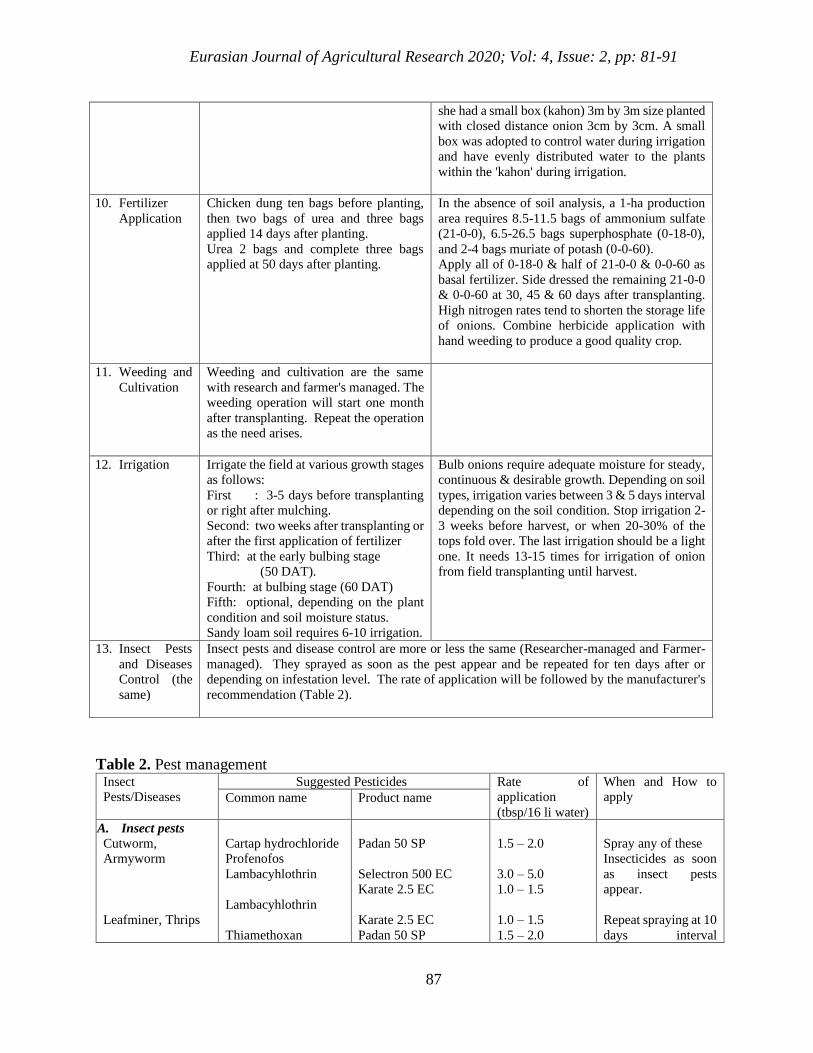
Eurasian Journal of Agricultural Research 2020; Vol: 4, Issue: 2, pp: 81-91
87
she had a small box (kahon) 3m by 3m size planted
with closed distance onion 3cm by 3cm. A small
box was adopted to control water during irrigation
and have evenly distributed water to the plants
within the 'kahon' during irrigation.
10. Fertilizer
Application
Chicken dung ten bags before planting,
then two bags of urea and three bags
applied 14 days after planting.
Urea 2 bags and complete three bags
applied at 50 days after planting.
In the absence of soil analysis, a 1-ha production
area requires 8.5-11.5 bags of ammonium sulfate
(21-0-0), 6.5-26.5 bags superphosphate (0-18-0),
and 2-4 bags muriate of potash (0-0-60).
Apply all of 0-18-0 & half of 21-0-0 & 0-0-60 as
basal fertilizer. Side dressed the remaining 21-0-0
& 0-0-60 at 30, 45 & 60 days after transplanting.
High nitrogen rates tend to shorten the storage life
of onions. Combine herbicide application with
hand weeding to produce a good quality crop.
11. Weeding and
Cultivation
Weeding and cultivation are the same
with research and farmer's managed. The
weeding operation will start one month
after transplanting. Repeat the operation
as the need arises.
12. Irrigation
Irrigate the field at various growth stages
as follows:
First : 3-5 days before transplanting
or right after mulching.
Second: two weeks after transplanting or
after the first application of fertilizer
Third: at the early bulbing stage
(50 DAT).
Fourth: at bulbing stage (60 DAT)
Fifth: optional, depending on the plant
condition and soil moisture status.
Sandy loam soil requires 6-10 irrigation.
Bulb onions require adequate moisture for steady,
continuous & desirable growth. Depending on soil
types, irrigation varies between 3 & 5 days interval
depending on the soil condition. Stop irrigation 2-
3 weeks before harvest, or when 20-30% of the
tops fold over. The last irrigation should be a light
one. It needs 13-15 times for irrigation of onion
from field transplanting until harvest.
13. Insect Pests
and Diseases
Control (the
same)
Insect pests and disease control are more or less the same (Researcher-managed and Farmer-
managed). They sprayed as soon as the pest appear and be repeated for ten days after or
depending on infestation level. The rate of application will be followed by the manufacturer's
recommendation (Table 2).
Table 2. Pest management Insect
Pests/Diseases
Suggested Pesticides Rate of
application
(tbsp/16 li water)
When and How to
apply Common name Product name
A. Insect pests
Cutworm,
Armyworm
Leafminer, Thrips
Cartap hydrochloride
Profenofos
Lambacyhlothrin
Lambacyhlothrin
Thiamethoxan
Padan 50 SP
Selectron 500 EC
Karate 2.5 EC
Karate 2.5 EC
Padan 50 SP
1.5 – 2.0
3.0 – 5.0
1.0 – 1.5
1.0 – 1.5
1.5 – 2.0
Spray any of these
Insecticides as soon
as insect pests
appear.
Repeat spraying at 10
days interval
Eurasian Journal of Agricultural Research 2020; Vol: 4, Issue: 2, pp: 81-91
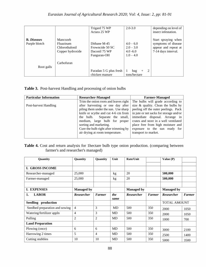
88
B. Diseases
Purple blotch
Root galls
Mancozeb
Fluazinam
Chlorothalonil
Copper hydroxide
Carbofuran
Trigard 75 WP
Actara 25 WP
Dithane M-45
Frowncide 50 SC
Daconil 75 WP
Funguran-OH
Furadan 5 G plus fresh
chicken manure
2.0-3.0
4.0 – 6.0
2.0 – 3.0
4.0 -6.0
1.0 – 4.0
1 bag + 2
tons/hectare
depending on level of
insect infestation.
Start spraying when
symptoms of disease
appear and repeat at
7-14 days interval.
Table 3. Post-harvest Handling and processing of onion bulbs
Particular Information Researcher-Managed Farmer-Managed
Post-harvest Handling
Trim the onion roots and leaves right
after harvesting or one day after
piling them under the sun. Use sharp
knife or scythe and cut 4-6 cm from
the bulb. Separate the small,
medium, large bulb for proper
sorting and marketing.
Cure the bulb right after trimming by
air drying at room temperature.
The bulbs will grade according to
size & quality. Clean the bulbs by
peeling off the outer peelings. Pack
in jute or net sacks for storage and/or
immediate disposal. Arrange in
crates and store in a well ventilated
place free from high moisture and
exposure to the sun ready for
transport to market.
Table 4. Cost and return analysis for 1hectare bulb type onion production. (comparing between
farmer's and researcher's managed)
Quantity Quantity Quantity Unit Rate/Unit
Value (P)
I. GROSS INCOME
Researcher-managed 25,000
kg 20
500,000
Farmer-managed 25,000
kg 20 500,000
I. EXPENSES Managed by
Managed by Managed by
1. LABOR Researcher Farmer the
same
Researcher Farmer Researcher Farmer
Seedling production
TOTAL AMOUNT
Seedbed preparation and sowing 4 3 MD 500 350 2000 1050
Watering/fertilizer appln 4 3 MD 500 350 2000 1050
Pulling 2 2 MD 500 350 1000 700
Land Preparation
Plowing (once) 6 6 MD 500 350 3000 2100
Harrowing 2 times 5 4 MD 500 350 2500 1400
Cutting stubbles 10 10 MD 500 350 5000 3500
Eurasian Journal of Agricultural Research 2020; Vol: 4, Issue: 2, pp: 81-91
89
Construction of trenches 5 5 MD 500 350 2500 1750
Mulching 6 0 MD 500 350 3000 0
Planting 25 25 MD 500 350 12500 8750
Care of plants
Weeding 20 20 MD 500 350 10000 7000
Controlling of insect pests 4 5 MD 500 350 2000 1750
Fertilizer application 5 5 MD 500 350 2500 1750
Irrigation 10 15 MD 500 350 5000 5250
Harvesting 25 25 MD 500 350 12500 8750
Trimming/curing/drying 5 5 MD 500 350 2500 1750
Sorting 5 5 MD 500 350 2500 1750
Hauling 2 2 MD 500 350 1000 700
Cleaning/sorting
/packaging
10 10 MD 500 350 5000
3500
SUB-TOTAL
78,500 52,150
1.MATERIAL INPUTS
Seeds 5 5 kg 1500 1500 7500 7500
Fertilizer
Complete 6 6 bags 1500 1500 9000 9000
Urea 3 5 bags 1500 1500 4500 7500
Amm sulfate 0 3 bags 0 700 0 2100
Muriate of potash 0 3 bags 0 705 0 2115
Chemicals
Karate 1 1 li 1500 1500 1500 1500
Selecron 500 EC 1 1 li 750 750 750 750
Padan 50 SP 1 1 kg 750 750 750 750
Dithane 1 1 box 450 450 450 450
Gasoline 35 35 li 60 60 2100 2100
Oil 8 8 li 200 200 1600 1600
Jute sacks 1000 1000 pcs 15 15 15000 15000
SUB-TOTAL
43150 50365
TOTAL ON LABOR & INPUTS
121,650 102,515
Overhead Expenses
Research (Land charge 1/)
10,000 10,000
Interest on capital 2/
17234 17234
TOTAL EXPENSES
148,884 129,749
NET INCOME per
Hectare
351,116 370,251
1/ Land charge is based on payment to Riceland, computed at 15 cavans/ha at 46kg/cavan at P15/kg 2/ Capital is based on labor and inputs. Interest rate is 28 % per annum. Onion (Bulb type) production and marketing
covers six months.
Eurasian Journal of Agricultural Research 2020; Vol: 4, Issue: 2, pp: 81-91
90
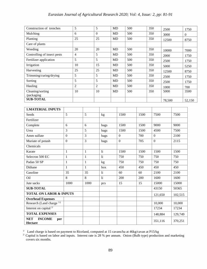
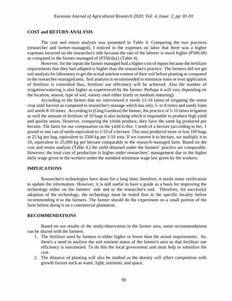
COST and RETURN ANALYSIS
The cost and return analysis was presented in Table 4. Comparing the two practices
(researcher and farmer-managed), I noticed in the expenses on labor that there was a higher
expenses incurred on the researcher's side because the rate of the laborer is much higher (P500.00)
as compared in the farmer-managed of (P350/day) (Table 4).
However, for the inputs the farmer managed had a higher cost of inputs because the fertilizer
requirements that they had adopted is higher than the researcher's practice. The farmers did not get
soil analysis for laboratory to get the actual nutrient content of their soil before planting as compared
to the researcher-managed area. Soil analysis is recommended to minimize loses or over application
of fertilizer is controlled thus, fertilizer use efficiency will be achieved. Also the number of
irrigation/watering is also higher as experienced by the farmer. Perhaps it will vary depending on
the location, season, type of soil, variety used either (early or medium maturing).
According to the farmer that we interviewed it needs 13-16 times of irrigating the onion
crop until harvest as compared to researcher's manage which has only 5- to 8 times and sandy loam
soil needs 8-10 times. According to (Ging Gamboa) the farmer, the practice of 5-10 times irrigation
as well the amount of fertilizer of 10 bags is also lacking which is impossible to produce high yield
and quality onion. However, comparing the yields produce, they have the same kg produced per
hectare. The basis for our computation on the yield is this: 1 tenth of a hectare (according to her, 1
pound or one can of seeds equivalent to 1/10 of a hectare. This area produced more or less 100 bags
at 25 kg per bag, equivalent to 2500 kg per 1/10 area. If we convert it to hectare, we multiply it to
10, equivalent to 25,000 kg per hectare comparable to the research-managed farm. Based on the
cost and return analysis (Table 4.) the yield obtained under the farmers` practice are comparable.
However, the total cost of production is higher under researchers` management due to the higher
daily wage given to the workers under the standard minimum wage law given by the workers.
IMPLICATIONS
Researcher's technologies have done for a long time; therefore, it needs some verification
to update the information. However, it is still useful to have a guide as a basis for improving the
technology either on the farmers` side and to the researcher's end. Therefore, for successful
adoption of the technology, the technology must be tested first in the specific locality before
recommending it to the farmers. The farmer should do the experiment on a small portion of the
farm before doing it on a commercial plantation.
RECOMMENDATIONS
Based on our results of the study/observation in the farmer area, some recommendations
can be shared with the farmers.
1. The fertilizer used by farmers is either higher or lower than the actual requirements. So,
there's a need to analyze the soil nutrient status of the farmer's area so that fertilizer use
efficiency is maximized. To do this the local government unit must help or subsidize the
cost.
2. The distance of planting will also be studied as the density will affect competition with
growth factors such as water, light, nutrients, and space.
Eurasian Journal of Agricultural Research 2020; Vol: 4, Issue: 2, pp: 81-91
91
3. The program of planting and crop rotation is encouraged to minimize build-ups of pests and
diseases in the area; also, the soil's organic content be improved by using leguminous crops.
4. Adopt integrated pest management to minimize the use of harmful chemical pesticides,
which is very harmful to the environment and animals and human beings.
5. For successful adoption of the technology, it is essential that it be tested first in the specific
locality before recommending it to the farmers. The farmer should experiment with a small
portion of the farm before doing it on a commercial plantation.
6. If possible, the Department of Agriculture (DA) will assist not only on the technology but
also on the financial aspects, especially those farmers who have no enough money to provide
during crop production.
7. The government will also consider the concern of the farmers, especially during the
marketing of their produce.
REFERENCES
Abon C C Jr., Legaspi B.V. & Patricio M.G. Technology for Onion Production
Chang K., 2004. Introduction to Geographic Information Systems. McGraw-Hill Companies Inc.
New York, New York. CIA. 2003. Visited: 08/27/2003. The World Factbook: Bolivia
http://www.cia.gov/cia/publications/factbook/geos/bl.html Crivelli, C. 1911. modified:
2003, visited: 09/16/03. The Catholic Encyclopedia, Volume XII.
http://www.newadvent.org/cathen/12140a.htm
Lopez, E.L. and Anit, E.A. (1994). ALLIUM PRODUCTION IN THE PHILIPPINES. Acta Hortic.
358, 61-70. DOI: 10.17660/ActaHortic.1994.358.8.
https://doi.org/10.17660/ActaHortic.1994.358.8
Rivas E., 2001. Descripcion Gral de la Cadena de la Cebolla en los Valles de Bolivia.
Unpublished. Given to me by Marcos Moreno of FDTA-Valles June 2002.
Rivas E., 2002. Plan de Comercializacion de Cebolla Seca. Unpublished. Given to me by Marcos
Moreno of FDTA-Valles June 2002. Production, Technoguide for all Agronomic crops,
Research Division, CLSU, Munoz, Nueva Ecija.
Pcarrd-Da., 2000. Bulb Onion Production Guide. Los Banos Laguna, www.openacademy.ph;
Photos: Wikimedia, ttps://www.agriculture.com.ph/2019/08/07/a-promising-new-red-
onion-variety/
Onion Production in the Philippines. (2019). Grades, Fixer. Retrieved December 5, 2020, from
https://gradesfixer.com/free-essay-examples/onion-production-in-the-philippines/
Onion Production Guide. https://businessdiary.com.ph/6051/onion-production-guide/ Retrieved
December, 2019.
https://www.google.com/search?client=firefox-b-d&q=onion+production+in+the+Philippines,
Retrieved 2020.
Eurasian Journal of Agricultural Research 2020; Vol: 4, Issue: 2, pp: 92-123
92
Advantages of Using the Biofertilizers in Ukrainian Agroecosystems
Hasrat Arjjumend*1, 2, Konstantia Koutouki1, 2, Olga Donets3
1Faculty of Law, Université de Montréal, Montreal (Quebec) H3T 1J7, Canada 2Centre for International Sustainable Development Law, Montreal (Quebec) H3A 1X1, Canada
3Department of Environmental Law, Yaroslav Mudryi National Law University,
61024, Pushkins'ka St, 77, Kharkiv, Ukraine
*Corresponding author : [email protected]
Hasrat Arjjumend ORCID: https://orcid.org/0000-0002-4419-2791
Abstract
Amid growing problems of excessive application of chemical fertilizers, biofertilizers hold the
potential to increase farmers’ current agricultural productivity, while at the same time contributing
to the soil’s ability to produce more in the future. This article is part of a larger study conducted
by the Université de Montréal in Ukraine with the support of Mitacs and Earth Alive Clean
Technologies. The responses of user farmers and non-user farmers of biofertilizers, manufacturers
or suppliers of biofertilizers, government officers and research scientists are captured to build
understandings of how microbial products (biofertilizers) prove to be advantageous when applied
in food crops. The agronomic advantage of biofertilizers compared to conventional chemical
fertilizers is well proved biologically and in economic terms. The farmers surveyed showed
interests in using biofertilizers in the future, however, both manufacturing and supply of
biofertilizers are inadequate compared to the demand of microbial biofertilizers in the country.
Yet, the farmers are concerned for supply of quality products have better effectiveness, longer
shelf life and lesser costs.
Keywords: Biofertilizers; Biologicals; Fertilizers; Farmers’ Preference; Soil Health
Research article
Received Date: 30 September 2020 Accepted Date:30 November 2020
Eurasian Journal of Agricultural Research 2020; Vol: 4, Issue: 2, pp: 92-123
93
INTRODUCTION
To accomplish high productivity of crops and soil, the unsustainable application of
chemical fertilizers and plant protection chemicals have resulted in steady declines in soil and crop
productivities the world over. Hence, agricultural practices need to evolve to sustainably meet the
growing global demand for food without irreversibly damaging the world’s natural resources
(especially soil) while maintaining food security. Investing in sustainable agriculture is one of the
most effective ways to simultaneously achieve the Sustainable Development Goals (SDGs) related
to poverty and hunger, nutrition and health, education, economic and social growth, peace and
security, and preserving the world’s environment (Earth Alive, 2017). Amid growing problems of
excessive application of chemical fertilizers, biofertilizers hold the potential to increase farmers’
current agricultural productivity, while at the same time contributing to the soil’s ability to produce
more in the future. Several countries, such as Canada, Argentina, South Africa, Australia, USA,
India and Brazil, have embraced these technologies. The list of potential commercial biofertilizer
products that promise increased yield for the farmer continues to grow (Simiyu et al., 2013).
A biofertilizer is a substance containing living microorganisms that are applied to seed,
plant surfaces, or soil, and that colonize the rhizosphere or the interior of the plant and promotes
growth by increasing the supply or availability of primary nutrients to the host plant (Weyens et
al., 2009; Xiang et al., 2012). Some common agents in biofertilizers include Rhizobium,
Azotobacter, Azospirillum, Phosphorus solubilizing bacteria (PSB) and Mycorrhizae. The
microbial biofertilizers have been developed to recover the soil biology and sustainability of
agroecosystems. The biofertilizers contribute to the soil’s ability to produce more in the future
(Arjjumend et al., 2017). The benefits of biofertilizers have been cited as cost-effective, providing
up to 25-30% of chemical fertilizer equivalent of nitrogen, providing phosphorous and potassium,
increasing water absorption and keeping soil biologically active (Arjjumend, Konstantia and
Warrren, 2020). The agronomic potential of plant–microbial symbioses proceeds from the analysis
of their ecological impacts, which have been best studied for N-fixing (Franche, Lindstrom and
Elmerich, 2009). In the soil or rhizosphere, biofertilizers generate plant nutrients such as nitrogen
and phosphorous through their activities or make them available to the plants (Rajendra, Singh and
Sharma, 1998).
The biofertilizers market is segmented by microorganisms into rhizobium, azotobacter,
azospirillum, blue-green algae, phosphate solubilizing bacteria, mycorrhiza, and other
microorganisms, by technology type into carrier enriched biofertilizers, liquid biofertilizers, and
other technology types, by application into seed treatment and soil treatment, and by crop type into
cereals, legumes, fruits and vegetables, plantations, and others (Arjjumend, Konstantia and
Warrren, 2020). Ukraine has limited production of biofertilizer products. As the Ukrainian
economy generally declined beginning in 1991, many production units were shut down, and have
not been restored (Stefanovska, Pidlisnyuk and Kaya, 2006). The existing poor status of
biofertilizer production and distribution, which is largely government-sponsored, indicates that the
country has huge gaps between demand and supply. In Ukraine, the majority of plant nutrients,
including biofertilizers and organic fertilizers, are imported, especially from China.
Eurasian Journal of Agricultural Research 2020; Vol: 4, Issue: 2, pp: 92-123
94
This article is an outcome of a larger study conducted between September 2017 and
February 2020 by the authors from the Faculté de droit, Université de Montréal with the financial
support from Mitacs and Earth Alive Clean Technologies. Field data collection support was
provided by Department of Environmental Law, Yaroslav Mudriy National Law University of
Ukraine and by several community workers in their individual capacities. The present paper
focuses on advantages of using biofertilizers vis-à-vis chemical fertilizers in Ukraine. Four
different groups of respondents were surveyed between April 2018 and March 2019 using methods
of semi-structured interviews, structured interviews, informal discussions, and observation. The
responses of user farmers and non-user farmers of biofertilizers, manufacturers or suppliers of
biofertilizers, and scientists are reviewed to build cases of how microbial products (biologicals)
prove to be advantageous when applied in field crops. The agronomic advantage of biofertilizers
compared to conventional chemical fertilizers is biologically and economically well proven. The
respondent farmers have shown their preference of biofertilizers over chemical fertilizers and have
expressed willingness to adopt biofertilizers to revive their soil biology and health along with
better crop yields.
MATERIALS and METHODS
The present study was conducted in Ukraine to understand scientific advantages of using
biofertilizers. Several types of respondents were interviewed and observations were made in the
field, apart from reviewing the pertinent literature.
Sampling and Sample Techniques
Different four respondent groups were chosen to conduct the study: Group 1 – research and
development (R&D) Scientists; Group 2 – Manufacturers and Suppliers; Group 3 – User & Non-
User Farmers; and Group 4 – Government Officers. Group 1 involves respondents from R&D of
biofertilizers and scientists conducting research on microbial agents. These scientists were
important for the study because they had explained the microbiology, biotechnology,
agrochemistry of the microbial biofertilizers. Group 2 respondents include those from the
manufacturing, trade and supply chain of biologicals and agrochemicals. Group 3 respondents are
the farmers/cultivators/growers using or not using the biofertilizers. These farmers are direct
stakeholders of this study on biofertilizers. In absence of biologicals, they may be suffering from
adverse effects of chemical fertilizers. Alternatively, in event of using biologicals in their farming
practices, these respondents will have experiences and opinions about various aspects of
biofertilizers. Group 4 respondents included government officers involved in policy/law
implementation/enforcement, some of which was informally shared by the officers, as they cannot
share such information in writing or formally.
Table 1 contains the total sample size of each of the respondent groups. Names of Ukrainian
oblasts are also mentioned in Table 1 for all respondent groups. In Table 2, distribution of surveyed
farmers or growers is highlighted. All the proposed participants (respondents) were first contacted
through telephone and/or email in order to make an appointment. Following the pre-appointments,
the participants were physically visited and interviewed or interacted with.
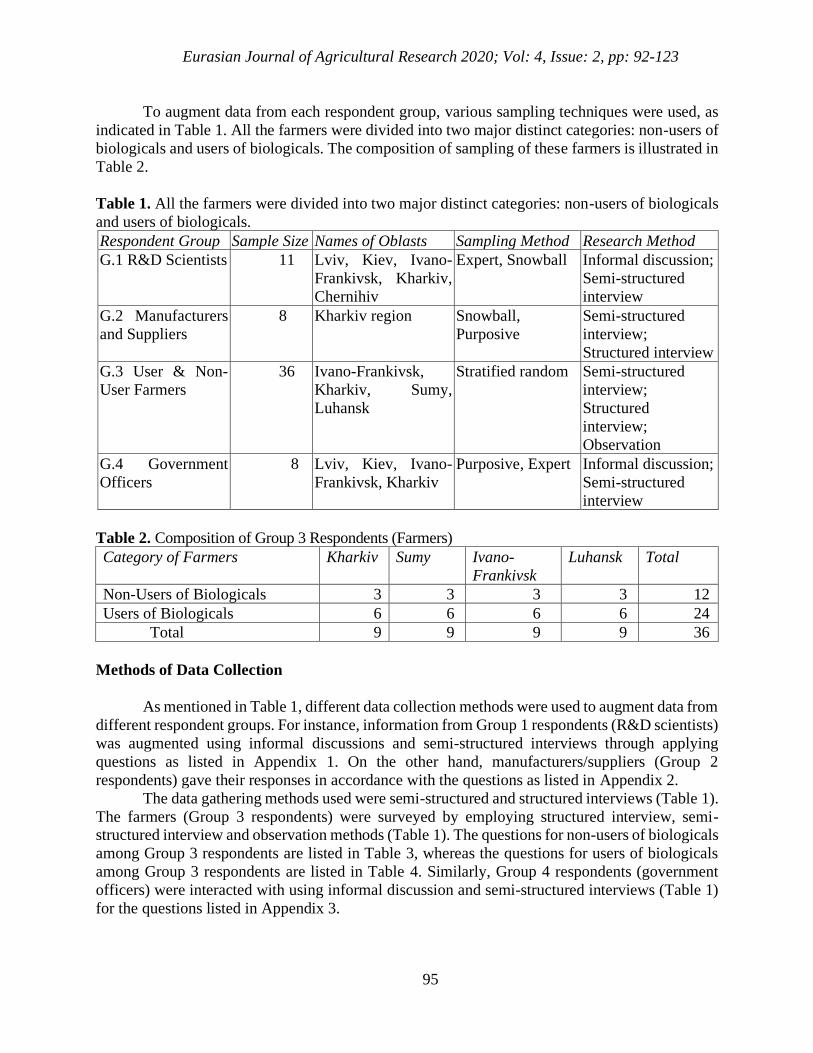
Eurasian Journal of Agricultural Research 2020; Vol: 4, Issue: 2, pp: 92-123
95
To augment data from each respondent group, various sampling techniques were used, as
indicated in Table 1. All the farmers were divided into two major distinct categories: non-users of
biologicals and users of biologicals. The composition of sampling of these farmers is illustrated in
Table 2.
Table 1. All the farmers were divided into two major distinct categories: non-users of biologicals
and users of biologicals.
Respondent Group Sample Size Names of Oblasts Sampling Method Research Method
G.1 R&D Scientists 11 Lviv, Kiev, Ivano-
Frankivsk, Kharkiv,
Chernihiv
Expert, Snowball Informal discussion;
Semi-structured
interview
G.2 Manufacturers
and Suppliers
8 Kharkiv region Snowball,
Purposive
Semi-structured
interview;
Structured interview
G.3 User & Non-
User Farmers
36 Ivano-Frankivsk,
Kharkiv, Sumy,
Luhansk
Stratified random Semi-structured
interview;
Structured
interview;
Observation
G.4 Government
Officers
8 Lviv, Kiev, Ivano-
Frankivsk, Kharkiv
Purposive, Expert Informal discussion;
Semi-structured
interview
Table 2. Composition of Group 3 Respondents (Farmers)
Category of Farmers Kharkiv Sumy Ivano-
Frankivsk
Luhansk Total
Non-Users of Biologicals 3 3 3 3 12
Users of Biologicals 6 6 6 6 24
Total 9 9 9 9 36
Methods of Data Collection
As mentioned in Table 1, different data collection methods were used to augment data from
different respondent groups. For instance, information from Group 1 respondents (R&D scientists)
was augmented using informal discussions and semi-structured interviews through applying
questions as listed in Appendix 1. On the other hand, manufacturers/suppliers (Group 2
respondents) gave their responses in accordance with the questions as listed in Appendix 2.
The data gathering methods used were semi-structured and structured interviews (Table 1).
The farmers (Group 3 respondents) were surveyed by employing structured interview, semi-structured interview and observation methods (Table 1). The questions for non-users of biologicals
among Group 3 respondents are listed in Table 3, whereas the questions for users of biologicals
among Group 3 respondents are listed in Table 4. Similarly, Group 4 respondents (government
officers) were interacted with using informal discussion and semi-structured interviews (Table 1)
for the questions listed in Appendix 3.
Eurasian Journal of Agricultural Research 2020; Vol: 4, Issue: 2, pp: 92-123
96
Certificat D’approbation Éthique (Ethical Approval Certificate) and its Compliance
The Multi-Faculty Committee on Research Ethics (Comité plurifacultaire d’éthique de la
recherche - CPER) of Université de Montréal issued Ethical Approval Certificate (no. CPER‐17‐
114‐P) to the study project. During the field data collection from all four respondent groups, the
conditions of the Ethics Certificate were fulfilled and complied with. In compliance of the Ethical
Certificate, the Consent Form was presented to each of the individual respondents in Ukrainian.
Depending on participant preference, the appropriate Consent Form was used and signed by both
the respondent and field researcher. Before conducting the interview or discussion with the
respondents/participants, each individual was told the objectives of the research through an
Information Sheet containing what was expected from respondent, the benefit of sharing
information, confidentiality details, and the participant’s right to withdraw. After adequate
explanations about the research and freely given consent of the respondent/participant, the desired
information was augmented from the respondent/participant.
RESULTS
The information gathered from all the respondents has been analyzed and presented to build
cases of how microbial products (biologicals) prove to be advantageous when applied in field
crops. Sampling of 12 farmers (3 farmers in each of 4 oblasts) using chemical fertilizers was done
in Ukraine and their responses were recorded on several parameters (Table 3). The questions were
chiefly regarding the disadvantages of using chemical fertilizers and the impacts they observed on
their agroecosystems and human health and domestic animals from chemical fertilizers used.
Likewise, 24 farmers (3 farmers using biofertilizers and 3 using biopesticides or using both in each
of 4 oblasts) in Ukraine were interviewed and their answers were recorded in Table 4.
1. Soil performance under chemical fertilizers
The respondent farmers using chemical fertilizers were asked for their views on how
chemical fertilizers affect the soil, plants, ecosystem and human health (Table 3). Most of these
farmers gave favorable views about chemical fertilizers by stating that the chemicals improve
production as the plants need nutrition and crops cannot be grown without nutrition (Table 3).
Respondent scientists and officers argued that mineral fertilizers replenish the availability of
nutrients in soil and maintain fertility of soil. The suppliers/manufacturers articulated that the
impact of chemical fertilizers on soil depends on the quantum of chemicals being used. According
to farmers, if chemical fertilizer is used in the right proportion in accordance with moisture, it is
harmless to soil (Table 3).
However, other respondent farmers narrated how chemical fertilizers deteriorate the
conditions of the soil. These respondents observed that, after the introduction of mineral fertilizers,
the intensity of the natural conversion of atmospheric nitrogen to the compounds that can be
assimilated by plants is reduced (Table 3). The mineral salt solutions are harmful to soil
microorganisms that form a layer on the fertile soil, and hence the formation of humus slows down
(Table 3).
Eurasian Journal of Agricultural Research 2020; Vol: 4, Issue: 2, pp: 92-123
97
Another question posed to the respondent farmers was “how does the soil get affected after
application of chemical fertilizers?” (Table 3). Ukrainian farmers using chemicals advocated in
favour of the fertilizers, saying that the soil restores deficient nutrients once fertilizers are applied
and that only excesses of mineral fertilizers cause harmful effects on soil (Table 3). These
respondent farmers noted that they use chemicals in right quantities, hence negative effects are not
visible (Table 3). According to them, soil is not affected if chemical fertilizer is applied wisely in
appropriate quantity as the correct dosage of fertilizers minimize the ecological footprint on the
soil (Table 3). However, some respondent farmers using chemical fertilizers shared their
experiences that chemical fertilizers can increase the radioactive lead Pb (204Pb, 206Pb, 207Pb, 208Pb), which causes accumulation of heavy metals in soil and plant bodies (Table 3). The influence
of chemical fertilizers on atmospheric air and water is mainly due to excessive nitrogen release.
Apparently, mineral fertilizers have a negative impact on plants and on the quality of products, as
well as on organisms that use it, the farmers claimed (Table 3).
2. Health and ecological risks from chemical fertilizers
In Ukraine’s four oblasts, respondent farmers using chemical fertilizers listed the common
health effects of chemical fertilizers, especially on children and women (Table 3), including
gastrointestinal problems, poisoning, vomiting, cancer (if residues persist), phlegm of the upper
respiratory tract, rhinitis, laryngitis, bronchitis, and pneumoconiosis (Table 3). The respondent
scientists explained that the enzyme system is poorly developed in children, making nitrates more
dangerous for them, especially as nitrates and nitrites are carcinogens. Moreover, nitrozoamines,
which have hepatotoxic properties, cause hepatitis. Some suppliers and surveyed farmers using
chemical fertilizers highlighted that nitrites lead to chronic intoxication of the body, weaken the
immune system, reduce mental and physical capacity, exhibit mutagenic and embryotoxic
properties (Table 3). The respondent farmers using chemical fertilizers explained the ecological
effects of chemical fertilizers (Table 3). They replied that chemicals take path in the human food
chain. The mineral fertilizers accelerate leaching of calcium, magnesium, zinc and copper, from
the soil, which affects the processes of photosynthesis and reduces the resistance of plants to
diseases (Table 3). Mineral fertilizers lead to reducing soil porosity and granular aggregates and,
finally, to acidification of the soil (Table 3).
Regarding the health effects of chemical fertilizers, Ukrainian farmers using biofertilizers
and biopesticides suggested a list of associated sicknesses, such as asthma, skin diseases,
gastrointestinal problems, toxicity among children, and miscarriages of pregnant women (Table
4). Some respondent farmers explained that mineral fertilizers are used everywhere in Ukraine and
that no health issue is observed if fertilizer is used in appropriate quantity (Table 4). However,
scientists, officers and other farmers explained that many chemical elements enter plants through
biological processes, and that they are transformed into toxic elements. Nitrogenous fertilizers
pose the greatest danger to humans and agroecosystems (Table 4).
Nitrates are especially dangerous for infants, because their enzyme base is imperfect, and
recovery of methemoglobin into hemoglobin is slow (Table 4).
The question “Do you think that biofertilizers are safer compared to chemical fertilizers?”
was addressed by farmers using biofertilizers and biopesticides (Table 4), who affirmed this
observation. The respondent farmers reiterated that biofertilizers do not cause harm to the soil or
plants (Table 4). Several respondent farmers also reported that biofertilizers remove ions of heavy
metals from soil and clean the contaminated soil (Table 4).
Eurasian Journal of Agricultural Research 2020; Vol: 4, Issue: 2, pp: 92-123
98
The respondent farmers then described the comparative ecological advantage of
biofertilizers, including that they are relatively safer to ecosystems as they trigger oxidation of soil
(Table 4). Some of the respondents said that biofertilizers contribute to the neutralization of salts
of heavy metals. These respondents compared chemical fertilizers by stating that chemicals store
in soil and plant body, hence the mineral fertilizers need to be used as per strict technical
prescriptions if used along with biofertilizers (Table 4).
3. Soil performance under biofertilizers
Respondent Ukrainian farmers using biofertilizers in crops were asked how the
biofertilizers benefit the soil, plants, ecosystem and human health (Table 4). In the respondents’
views, biofertilizers do not harm humans, plants or ecosystems. According to the surveyed
government officers, biofertilizers benefit and enrich the soil as fertility increases. According to
the farmers interviewed, biofertilizers stimulate plant growth and mobilize the minerals (e.g. N,
Fl) to become accessible to plants and nourish soil (Table 4). The respondent manufacturers and
scientists expressed their views that the chemicalization process of soil reduces because the
biofertilizers are safer and have no negative impact on soil. Biofertilizers are also reported to
increase plant and soil immunity while improving quality of produce (Table 4). The respondent
farmers shared their observations that resistance to various diseases and to climatic variability
increases following the application of microbial biofertilizers (Table 4). The farmers and
government officers also explained how microorganisms deliver functions in the soil. They
described that atmospheric nitrogen is fixed by microbes and transferred to plants, as microbes
also synthesize a wide range of substances in soil (Table 4). According to respondent scientists,
humus is increased several times because microbes of biofertilizers positively impact the
enzymatic activity in the soil. Finally, the farmers indicated that biofertilizers solve salinity
problems in the soil (Table 4).
The question of how the attributes of the soil change once biofertilizers are used was
answered by the surveyed farmers using biofertilizers and biopesticides (Table 4). The respondent
farmers expressed their views that the bacteria of biofertilizers stimulate root growth and solubilize
the nutrients or minerals like phosphorus, which the plants easily digest. Plant root systems enlarge
and are nourished because the microbes fix nutrients to make them accessible to plant roots (Table
4). The biofertilizers increase soil temperature by 2-5oC which enhances root formation and
germination of seeds. Fruiting, blooming, germination, and root formation are supported by the
bacteria that feed on root secretions and release growth metabolites (Table 4). The rational use of
biofertilizers contributes to obtaining environmentally friendly products, the accumulation of
humus, reducing soil fatigue, improving soil structure and fertility (Table 4). According to the
surveyed farmers using them, due to their biological properties, biofertilizers are absorbed by plants
at a rate of almost 100 per cent, while the content of nitrates in farm produce remains minimal
(Table 4).
The manufacturers/suppliers said that with prolonged use and strict application of
biofertilizers, soil can improve. Farmers also stated that the bacteria feed on secretions of the root
system in rhizosphere (Table 4). The respondent farmers using biofertilizers and respondent
scientists articulated that biofertilizers work on a synergistic basis or on antagonism principles and,
as a result, the fermentation process makes leaves and fruits of plants inedible to the pathogenic
microbes.
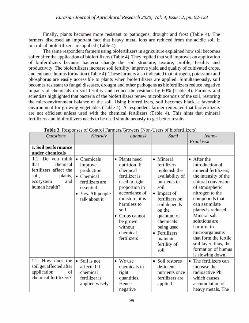
Eurasian Journal of Agricultural Research 2020; Vol: 4, Issue: 2, pp: 92-123
99
Finally, plants becomes more resistant to pathogens, drought and frost (Table 4). The
farmers disclosed an important fact that heavy metal ions are reduced from the acidic soil if
microbial biofertilizers are applied (Table 4).
The same respondent farmers using biofertilizers in agriculture explained how soil becomes
softer after the application of biofertilizers (Table 4). They replied that soil improves on application
of biofertilizers because bacteria change the soil structure, texture, profile, fertility and
productivity. The biofertilizers increase soil fertility, improve yield and quality of cultivated crops,
and enhance humus formation (Table 4). These farmers also indicated that nitrogen, potassium and
phosphorus are easily accessible to plants when biofertilizers are applied. Simultaneously, soil
becomes resistant to fungal diseases, drought and other pathogens as biofertilizers reduce negative
impacts of chemicals on soil fertility and reduce the residues by 60% (Table 4). Farmers and
scientists highlighted that bacteria of the biofertilizers renew microbiocenosis of the soil, restoring
the microenvironment balance of the soil. Using biofertilizers, soil becomes black, a favorable
environment for growing vegetables (Table 4). A respondent farmer reiterated that biofertilizers
are not efficient unless used with the chemical fertilizers (Table 4). This hints that mineral
fertilizers and biofertilizers needs to be used simultaneously to get better results.
Table 3. Responses of Control Farmers/Growers (Non-Users of biofertilizers)
Questions Kharkiv Luhansk Sumi Ivano-
Frankivsk
1. Soil performance
under chemicals
1.1. Do you think
that chemical
fertilizers affect the
soil, plants,
ecosystem and
human health?
• Chemicals
improve
production
• Chemical
fertilizers are
essential
• Yes. All people
talk about it
• Plants need
nutrition. If
chemical
fertilizer is
used in right
proportion in
accordance of
moisture, it is
harmless to
soil.
• Crops cannot
be grown
without
chemical
fertilizers
• Mineral
fertilizers
replenish the
availability of
nutrients in
soil
• Impact of
fertilizers on
soil depends
on the
quantum of
chemicals
being used
• Fertilizers
maintain
fertility of
soil
• After the
introduction of
mineral fertilizers,
the intensity of the
natural conversion
of atmospheric
nitrogen to the
compounds that
can assimilate
plants is reduced.
Mineral salt
solutions are
harmful to
microorganisms
that form the fertile
soil layer; thus, the
formation of humus
is slowing down.
1.2. How does the
soil get affected after
application of
chemical fertilizers?
• Soil is not
affected if
chemical
fertilizer is
applied wisely
• We use
chemicals in
right
quantities.
Hence
negative
• Soil restores
deficient
nutrients once
fertilizers are
applied
• The fertilizers can
increase the
radioactive Pb
which causes
accumulation of
heavy metals. The
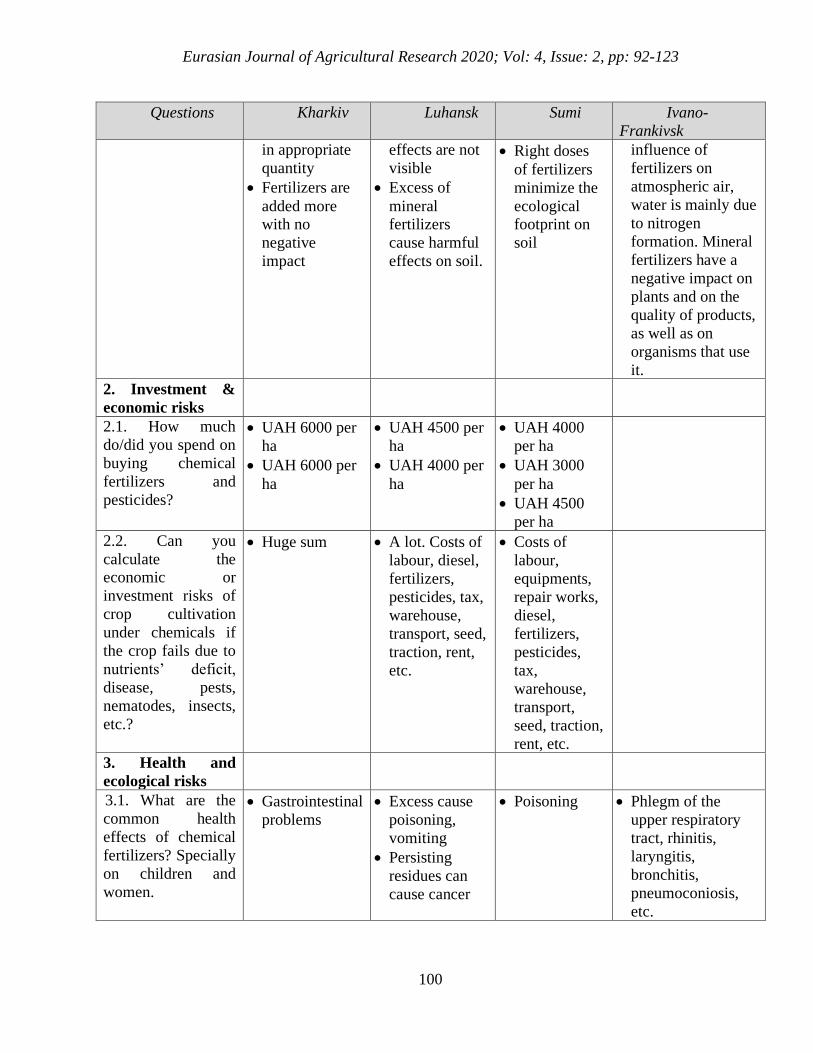
Eurasian Journal of Agricultural Research 2020; Vol: 4, Issue: 2, pp: 92-123
100
Questions Kharkiv Luhansk Sumi Ivano-
Frankivsk
in appropriate
quantity
• Fertilizers are
added more with no
negative
impact
effects are not
visible
• Excess of
mineral fertilizers
cause harmful
effects on soil.
• Right doses
of fertilizers
minimize the
ecological footprint on
soil
influence of
fertilizers on
atmospheric air,
water is mainly due
to nitrogen
formation. Mineral
fertilizers have a
negative impact on
plants and on the
quality of products,
as well as on
organisms that use
it.
2. Investment &
economic risks
2.1. How much
do/did you spend on
buying chemical
fertilizers and
pesticides?
• UAH 6000 per
ha
• UAH 6000 per
ha
• UAH 4500 per
ha
• UAH 4000 per
ha
• UAH 4000
per ha
• UAH 3000
per ha
• UAH 4500
per ha
2.2. Can you
calculate the economic or
investment risks of
crop cultivation
under chemicals if
the crop fails due to
nutrients’ deficit,
disease, pests,
nematodes, insects,
etc.?
• Huge sum
• A lot. Costs of
labour, diesel,
fertilizers,
pesticides, tax,
warehouse,
transport, seed,
traction, rent,
etc.
• Costs of
labour,
equipments,
repair works,
diesel,
fertilizers,
pesticides,
tax,
warehouse,
transport,
seed, traction,
rent, etc.
3. Health and
ecological risks
3.1. What are the
common health
effects of chemical
fertilizers? Specially
on children and
women.
• Gastrointestinal
problems
• Excess cause
poisoning,
vomiting
• Persisting
residues can
cause cancer
• Poisoning • Phlegm of the
upper respiratory
tract, rhinitis,
laryngitis,
bronchitis,
pneumoconiosis,
etc.
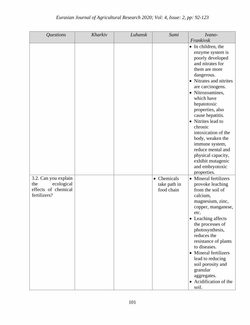
Eurasian Journal of Agricultural Research 2020; Vol: 4, Issue: 2, pp: 92-123
101
Questions Kharkiv Luhansk Sumi Ivano-
Frankivsk
• In children, the
enzyme system is
poorly developed
and nitrates for them are more
dangerous.
• Nitrates and nitrites
are carcinogens.
• Nitrozoamines,
which have
hepatotoxic
properties, also
cause hepatitis.
• Nitrites lead to
chronic
intoxication of the
body, weaken the
immune system,
reduce mental and
physical capacity,
exhibit mutagenic
and embryotoxic
properties.
3.2. Can you explain
the ecological
effects of chemical
fertilizers?
• Chemicals
take path in
food chain
• Mineral fertilizers
provoke leaching
from the soil of
calcium,
magnesium, zinc,
copper, manganese,
etc.
• Leaching affects
the processes of
photosynthesis,
reduces the
resistance of plants
to diseases.
• Mineral fertilizers
lead to reducing
soil porosity and
granular
aggregates.
• Acidification of the
soil.
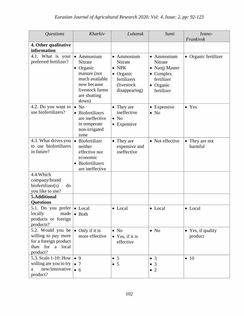
Eurasian Journal of Agricultural Research 2020; Vol: 4, Issue: 2, pp: 92-123
102
Questions Kharkiv Luhansk Sumi Ivano-
Frankivsk
4. Other qualitative
information
4.1. What is your
preferred fertilizer? • Ammonium
Nitrate
• Organic
manure (not
much available
now because
livestock farms
are shutting
down)
• Ammonium
Nitrate
• NPK
• Organic
fertilizers
(livestock
disappearing)
• Ammonium
Nitrate
• Nanjj Master
• Complex
fertilizer
• Organic
fertilizer
• Organic fertilizer
4.2. Do you want to
use biofertilizers? • No
• Biofertilizers
are ineffective
in temperate
non-irrigated
zone
• They are
ineffective
• No
• Expensive
• Expensive
• No
• Yes
4.3. What drives you
to use biofertilizers
in future?
• Biofertilizer
neither
effective nor
economic
• Biofertilizers
are ineffective
• They are
expensive and
ineffective
• Not effective • They are not
harmful
4.4.Which
company/brand
biofertilizer(s) do
you like to use?
5.Additional
Questions
5.1. Do you prefer
locally made
products or foreign
products?
• Local
• Both
• Local • Local • Local
5.2. Would you be
willing to pay more
for a foreign product
than for a local
product?
• Only if it is
more effective
• No
• Yes, if it is
effective
• No • Yes, if quality
product
5.3. Scale 1-10: How
willing are you to try
a new/innovative
product?
• 9
• 7
• 6
• 5
• 5
• 3
• 3
• 2
• 10
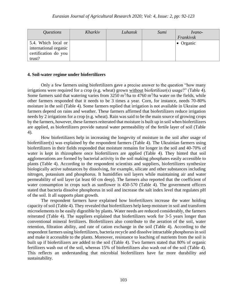
Eurasian Journal of Agricultural Research 2020; Vol: 4, Issue: 2, pp: 92-123
103
Questions Kharkiv Luhansk Sumi Ivano-
Frankivsk
5.4. Which local or
international organic
certification do you
trust?
• Organic
4. Soil-water regime under biofertilizers
Only a few farmers using biofertilizers gave a precise answer to the question “how many
irrigations were required for a crop (e.g. wheat) grown without biofertilizer(s) usage?” (Table 4).
Some farmers said that watering varies from 3250 m3/ha to 4760 m3/ha water on the fields, while
other farmers responded that it needs to be 3 times a year. Corn, for instance, needs 70-80%
moisture in the soil (Table 4). Some farmers replied that irrigation is not available in Ukraine and
farmers depend on rains and weather. These farmers affirmed that biofertilizers reduce irrigation
needs by 2 irrigations for a crop (e.g. wheat). Rain was said to be the main source of growing crops
by the farmers, however, these farmers reiterated that moisture is built up in soil when biofertilizers
are applied, as biofertilizers provide natural water permeability of the fertile layer of soil (Table
4).
How biofertilizers help in increasing the longevity of moisture in the soil after usage of
biofertilizer(s) was explained by the respondent farmers (Table 4). The Ukrainian farmers using
biofertilizers in their fields responded that moisture remains for longer in the soil and 40-70% of
water is kept in rhizosphere once biofertilizers are applied (Table 4). They hinted that soil
agglomerations are formed by bacterial activity in the soil making phosphates easily accessible to
plants (Table 4). According to the respondent scientists and suppliers, biofertilizers synthesize
biologically active substances by dissolving, for example, silicate and other substances including
nitrogen, potassium and phosphorus. It humidifies soil layers while maintaining air and water
permeability of soil layer (at least 60 cm deep). The farmers also reported that the coefficient of
water consumption in crops such as sunflower is 450-570 (Table 4). The government officers
stated that bacteria dissolve phosphorus in soil and increase the salt index level that regulates pH
of the soil. It all supports plant growth.
The respondent farmers have explained how biofertilizers increase the water holding
capacity of soil (Table 4). They revealed that biofertilizers help keep moisture in soil and transform
microelements to be easily digestible by plants. Water needs are reduced considerably, the farmers
reiterated (Table 4). The suppliers explained that biofertilizers work for 3-5 years longer than
conventional mineral fertilizers. Biofertilizers also contribute to the aeration of the soil, water
retention, filtration ability, and rate of cation exchange in the soil (Table 4). According to the
respondent farmers using biofertilizers, bacteria recycle and dissolve intractable phosphorus in soil and make it accessible to the plants. Moreover, resistance to leaching of nutrients from the soil is
built up if biofertilizers are added to the soil (Table 4). Two farmers stated that 80% of organic
fertilizers wash out of the soil, whereas 15% of biofertilizers also wash out of the soil (Table 4).
This reflects an understanding that microbial biofertilizers have far more durability and
sustainability.
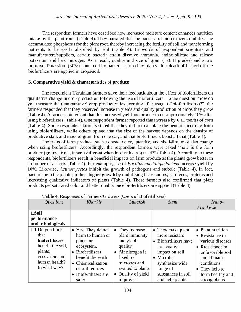
Eurasian Journal of Agricultural Research 2020; Vol: 4, Issue: 2, pp: 92-123
104
The respondent farmers have described how increased moisture content enhances nutrition
intake by the plant roots (Table 4). They narrated that the bacteria of biofertilizers mobilize the
accumulated phosphorus for the plant root, thereby increasing the fertility of soil and transforming
nutrients to be easily absorbed by soil (Table 4). In words of respondent scientists and
manufacturers/suppliers, certain bacteria strain dissolve ammonia, amino-silicate and release
potassium and hard nitrogen. As a result, quality and size of grain (I & II grades) and straw
improve. Potassium (30%) contained by bacteria is used by plants after death of bacteria if the
biofertilizers are applied in crops/soil.
5. Comparative yield & characteristics of produce
The respondent Ukrainian farmers gave their feedback about the effect of biofertilizers on
qualitative change in crop production following the use of biofertilizers. To the question “how do
you measure the (comparative) crop productivities accruing after usage of biofertilizer(s)?”, the
farmers responded that they observed increase in yields and quality production of crops they grow
(Table 4). A farmer pointed out that this increased yield and production is approximately 10% after
using biofertilizers (Table 4). One respondent farmer reported this increase by 6.11 ton/ha of corn
(Table 4). Some respondent farmers stated that they did not calculate the benefits accruing from
using biofertilizers, while others opined that the size of the harvest depends on the density of
productive stalk and mass of grain from one ear, and that biofertilizers boost all that (Table 4).
The traits of farm produce, such as taste, color, quantity, and shelf-life, may also change
when using biofertilizers. Accordingly, the respondent farmers were asked “how is the farm
produce (grains, fruits, tubers) different when biofertilizer(s) used?” (Table 4). According to these
respondents, biofertilizers result in beneficial impacts on farm produce as the plants grow better in
a number of aspects (Table 4). For example, use of Bacillus amyloliquefaciens increase yield by
10%. Likewise, Actinomycetes inhibit the growth of pathogens and stubble (Table 4). In fact,
bacteria help the plants produce higher growth by mobilizing the vitamins, carotenes, proteins and
increasing qualitative indicators of plants (Table 4). These farmers also confirmed that plant
products get saturated color and better quality once biofertilizers are applied (Table 4).
Table 4. Responses of Farmers/Growers (Users of Biofertilizers)
Questions Kharkiv Luhansk Sumi Ivano-
Frankivsk
1.Soil
performance
under biologicals
1.1 Do you think
that
biofertilizers benefit the soil,
plants,
ecosystem and
human health?
In what way?
• Yes. They do not
harm to human or
plants or
ecosystem.
• Biofertilizers
benefit the earth
• Chemicalization
of soil reduces
• Biofertilizers are
safer
• They increase
plant immunity
and yield
quality
• Air nitrogen is
fixed by
microbes and
availed to plants
• Quality of yield
improves
• They make plant
more resistant
• Biofertilizers have
no negative
impact on soil
• Microbes
synthesize wide
range of
substances in soil
and help plants
• Plant nutrition
• Resistance to
various diseases
• Rresistance to
unfavorable soil
and climatic
conditions.
• They help to
form healthy and
strong plants
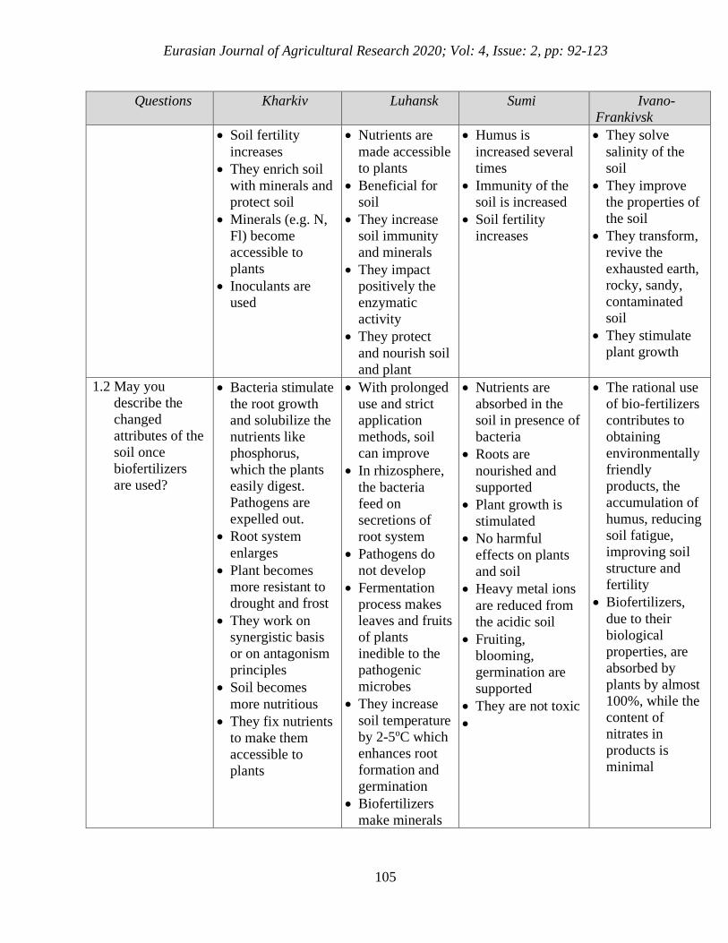
Eurasian Journal of Agricultural Research 2020; Vol: 4, Issue: 2, pp: 92-123
105
Questions Kharkiv Luhansk Sumi Ivano-
Frankivsk
• Soil fertility
increases
• They enrich soil
with minerals and
protect soil
• Minerals (e.g. N,
Fl) become
accessible to
plants
• Inoculants are
used
• Nutrients are
made accessible
to plants
• Beneficial for
soil
• They increase
soil immunity
and minerals
• They impact
positively the
enzymatic
activity
• They protect
and nourish soil
and plant
• Humus is
increased several
times
• Immunity of the
soil is increased
• Soil fertility
increases
• They solve
salinity of the
soil
• They improve
the properties of
the soil
• They transform,
revive the
exhausted earth,
rocky, sandy,
contaminated
soil
• They stimulate
plant growth
1.2 May you
describe the
changed
attributes of the
soil once
biofertilizers
are used?
• Bacteria stimulate
the root growth
and solubilize the
nutrients like
phosphorus,
which the plants
easily digest.
Pathogens are
expelled out.
• Root system
enlarges
• Plant becomes
more resistant to
drought and frost
• They work on
synergistic basis
or on antagonism
principles
• Soil becomes
more nutritious
• They fix nutrients
to make them
accessible to
plants
• With prolonged
use and strict
application
methods, soil
can improve
• In rhizosphere,
the bacteria
feed on
secretions of
root system
• Pathogens do
not develop
• Fermentation
process makes
leaves and fruits
of plants
inedible to the
pathogenic
microbes
• They increase
soil temperature
by 2-5oC which
enhances root
formation and
germination
• Biofertilizers
make minerals
• Nutrients are
absorbed in the
soil in presence of
bacteria
• Roots are
nourished and
supported
• Plant growth is
stimulated
• No harmful
effects on plants
and soil
• Heavy metal ions
are reduced from
the acidic soil
• Fruiting,
blooming,
germination are
supported
• They are not toxic
•
• The rational use
of bio-fertilizers
contributes to
obtaining
environmentally
friendly
products, the
accumulation of
humus, reducing
soil fatigue,
improving soil
structure and
fertility
• Biofertilizers,
due to their
biological
properties, are
absorbed by
plants by almost
100%, while the
content of
nitrates in
products is
minimal
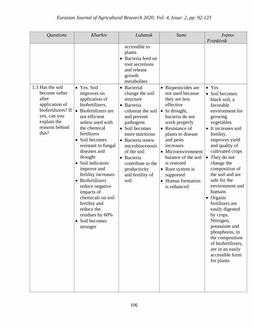
Eurasian Journal of Agricultural Research 2020; Vol: 4, Issue: 2, pp: 92-123
106
Questions Kharkiv Luhansk Sumi Ivano-
Frankivsk
accessible to
plants
• Bacteria feed on
root secretions and release
growth
metabolites
1.3 Has the soil
become softer
after
application of
biofertilizers? If
yes, can you
explain the
reasons behind
this?
• Yes. Soil
improves on
application of
biofertilizers.
• Biofertilizers are
not efficient
unless used with
the chemical
fertilizers
• Soil becomes
resistant to fungal
diseases and
drought
• Soil indicators
improve and
fertility increases
• Biofertilizers
reduce negative
impacts of
chemicals on soil
fertility and
reduce the
residues by 60%
• Soil becomes
stronger
• Bacterial
change the soil
structure
• Bacteria
colonize the soil
and prevent
pathogens
• Soil becomes
more nutritious
• Bacteria renew
microbiocenosis
of the soil
• Bacteria
contribute to the
productivity
and fertility of
soil
• Biopesticides are
not used because
they are less
effective
• In drought,
bacteria do not
work properly
• Resistance of
plants to disease
and pests
increases
• Microenvironment
balance of the soil
is restored
• Root system is
supported
• Humus formation
is enhanced
• Yes
• Soil becomes
black soil, a
favorable
environment for
growing
vegetables
• It increases soil
fertility,
improves yield
and quality of
cultivated crops
• They do not
change the
composition of
the soil and are
safe for the
environment and
humans
• Organic
fertilizers are
easily digested
by crops.
Nitrogen,
potassium and
phosphorus, in
the composition
of biofertilizers,
are in an easily
accessible form
for plants
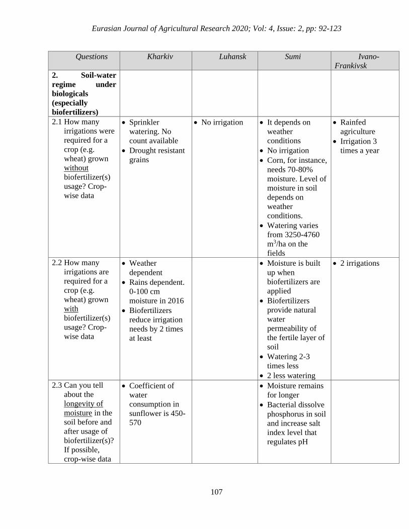
Eurasian Journal of Agricultural Research 2020; Vol: 4, Issue: 2, pp: 92-123
107
Questions Kharkiv Luhansk Sumi Ivano-
Frankivsk
2. Soil-water
regime under
biologicals
(especially
biofertilizers)
2.1 How many
irrigations were
required for a
crop (e.g.
wheat) grown
without
biofertilizer(s)
usage? Crop-
wise data
• Sprinkler
watering. No
count available
• Drought resistant
grains
• No irrigation • It depends on
weather
conditions
• No irrigation
• Corn, for instance,
needs 70-80%
moisture. Level of
moisture in soil
depends on
weather
conditions.
• Watering varies
from 3250-4760
m3/ha on the
fields
• Rainfed
agriculture
• Irrigation 3
times a year
2.2 How many
irrigations are
required for a
crop (e.g.
wheat) grown
with
biofertilizer(s)
usage? Crop-
wise data
• Weather
dependent
• Rains dependent.
0-100 cm
moisture in 2016
• Biofertilizers
reduce irrigation
needs by 2 times
at least
• Moisture is built
up when
biofertilizers are
applied
• Biofertilizers
provide natural
water
permeability of
the fertile layer of
soil
• Watering 2-3
times less
• 2 less watering
• 2 irrigations
2.3 Can you tell
about the
longevity of
moisture in the
soil before and
after usage of
biofertilizer(s)?
If possible,
crop-wise data
• Coefficient of
water
consumption in
sunflower is 450-
570
• Moisture remains
for longer
• Bacterial dissolve
phosphorus in soil
and increase salt
index level that
regulates pH
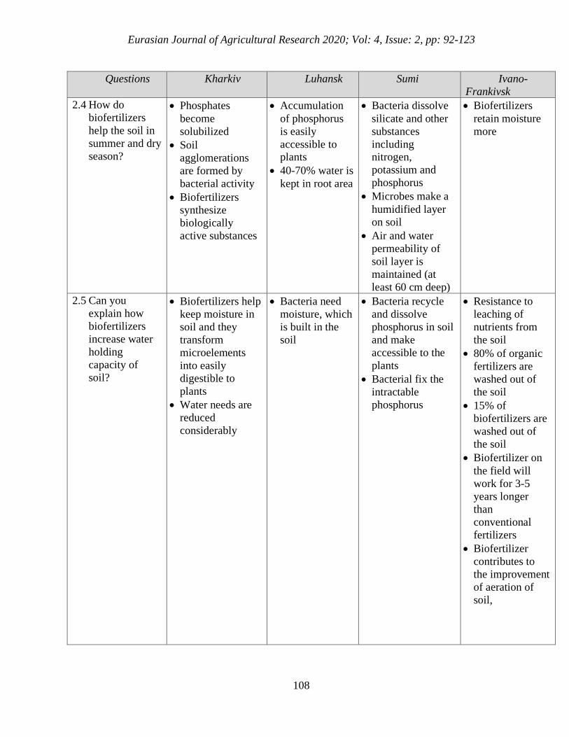
Eurasian Journal of Agricultural Research 2020; Vol: 4, Issue: 2, pp: 92-123
108
Questions Kharkiv Luhansk Sumi Ivano-
Frankivsk
2.4 How do
biofertilizers
help the soil in
summer and dry
season?
• Phosphates
become
solubilized
• Soil
agglomerations
are formed by
bacterial activity
• Biofertilizers
synthesize
biologically
active substances
• Accumulation
of phosphorus
is easily
accessible to plants
• 40-70% water is
kept in root area
• Bacteria dissolve
silicate and other
substances
including nitrogen,
potassium and
phosphorus
• Microbes make a
humidified layer
on soil
• Air and water
permeability of
soil layer is
maintained (at
least 60 cm deep)
• Biofertilizers
retain moisture
more
2.5 Can you
explain how
biofertilizers
increase water
holding
capacity of
soil?
• Biofertilizers help
keep moisture in
soil and they
transform
microelements
into easily
digestible to
plants
• Water needs are
reduced
considerably
• Bacteria need
moisture, which
is built in the
soil
• Bacteria recycle
and dissolve
phosphorus in soil
and make
accessible to the
plants
• Bacterial fix the
intractable
phosphorus
• Resistance to
leaching of
nutrients from
the soil
• 80% of organic
fertilizers are
washed out of
the soil
• 15% of
biofertilizers are
washed out of
the soil
• Biofertilizer on
the field will
work for 3-5
years longer
than
conventional
fertilizers
• Biofertilizer
contributes to
the improvement
of aeration of
soil,
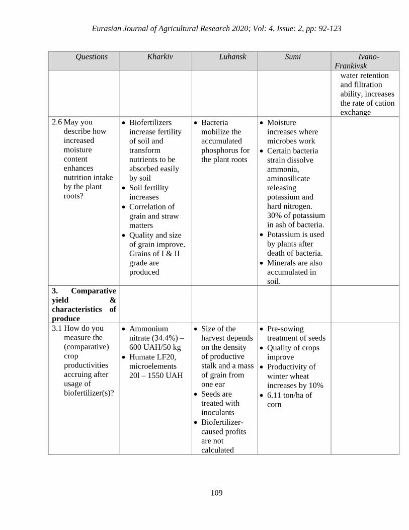
Eurasian Journal of Agricultural Research 2020; Vol: 4, Issue: 2, pp: 92-123
109
Questions Kharkiv Luhansk Sumi Ivano-
Frankivsk
water retention
and filtration
ability, increases
the rate of cation
exchange
2.6 May you
describe how
increased
moisture
content
enhances
nutrition intake
by the plant
roots?
• Biofertilizers
increase fertility
of soil and
transform
nutrients to be
absorbed easily
by soil
• Soil fertility
increases
• Correlation of
grain and straw
matters
• Quality and size
of grain improve.
Grains of I & II
grade are
produced
• Bacteria
mobilize the
accumulated
phosphorus for
the plant roots
• Moisture
increases where
microbes work
• Certain bacteria
strain dissolve
ammonia,
aminosilicate
releasing
potassium and
hard nitrogen.
30% of potassium
in ash of bacteria.
• Potassium is used
by plants after
death of bacteria.
• Minerals are also
accumulated in
soil.
3. Comparative
yield &
characteristics of
produce
3.1 How do you
measure the
(comparative)
crop
productivities
accruing after
usage of
biofertilizer(s)?
• Ammonium
nitrate (34.4%) –
600 UAH/50 kg
• Humate LF20,
microelements
20l – 1550 UAH
• Size of the
harvest depends
on the density
of productive
stalk and a mass
of grain from
one ear
• Seeds are
treated with
inoculants
• Biofertilizer-
caused profits
are not
calculated
• Pre-sowing
treatment of seeds
• Quality of crops
improve
• Productivity of
winter wheat
increases by 10%
• 6.11 ton/ha of
corn
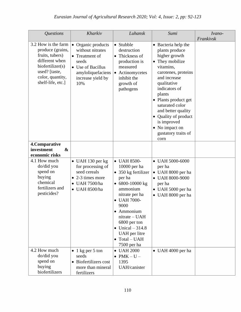
Eurasian Journal of Agricultural Research 2020; Vol: 4, Issue: 2, pp: 92-123
110
Questions Kharkiv Luhansk Sumi Ivano-
Frankivsk
3.2 How is the farm
produce (grains,
fruits, tubers)
different when
biofertilizer(s)
used? [taste,
color, quantity,
shelf-life, etc.]
• Organic products
without nitrates
• Treatment of
seeds
• Use of Bacillus
amyloliquefaciens
increase yield by
10%
• Stubble
destruction
• Thickness of
production is
measured
• Actinomycetes
inhibit the
growth of
pathogens
• Bacteria help the
plants produce
higher growth
• They mobilize
vitamins,
carotenes, proteins
and increase
qualitative
indicators of
plants
• Plants product get
saturated color
and better quality
• Quality of product
is improved
• No impact on
gustatory traits of
corn
4.Comparative
investment &
economic risks
4.1 How much
do/did you
spend on
buying
chemical
fertilizers and
pesticides?
• UAH 130 per kg
for processing of
seed cereals
• 2-3 times more
• UAH 7500/ha
• UAH 8500/ha
• UAH 8500-
10000 per ha
• 350 kg fertilizer
per ha
• 6800-10000 kg
ammonium
nitrate per ha
• UAH 7000-
9000
• Ammonium
nitrate – UAH
6800 per ton
• Unical – 314.8
UAH per litre
• Total – UAH
7500 per ha
• UAH 5000-6000
per ha
• UAH 8000 per ha
• UAH 8000-9000
per ha
• UAH 5000 per ha
• UAH 8000 per ha
4.2 How much
do/did you
spend on
buying
biofertilizers
• 1 kg per 5 ton
seeds
• Biofertilizers cost
more than mineral
fertilizers
• UAH 2000
• PMK – U –
1395
UAH/canister
• UAH 4000 per ha
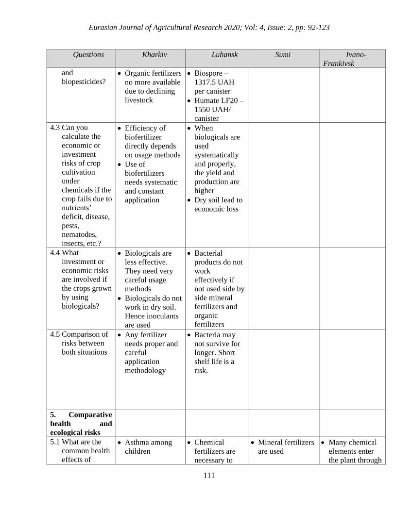
Eurasian Journal of Agricultural Research 2020; Vol: 4, Issue: 2, pp: 92-123
111
Questions Kharkiv Luhansk Sumi Ivano-
Frankivsk
and
biopesticides? • Organic fertilizers
no more available
due to declining
livestock
• Biospore –
1317.5 UAH
per canister
• Humate LF20 –
1550 UAH/
canister
4.3 Can you
calculate the
economic or
investment
risks of crop
cultivation
under
chemicals if the
crop fails due to
nutrients’
deficit, disease,
pests,
nematodes,
insects, etc.?
• Efficiency of
biofertilizer
directly depends
on usage methods
• Use of
biofertilizers
needs systematic
and constant
application
• When
biologicals are
used
systematically
and properly,
the yield and
production are
higher
• Dry soil lead to
economic loss
4.4 What
investment or
economic risks
are involved if
the crops grown
by using
biologicals?
• Biologicals are
less effective.
They need very
careful usage
methods
• Biologicals do not
work in dry soil.
Hence inoculants
are used
• Bacterial
products do not
work
effectively if
not used side by
side mineral
fertilizers and
organic
fertilizers
4.5 Comparison of
risks between
both situations
• Any fertilizer
needs proper and
careful
application
methodology
• Bacteria may
not survive for
longer. Short
shelf life is a
risk.
5. Comparative
health and
ecological risks
5.1 What are the
common health
effects of
• Asthma among
children
• Chemical
fertilizers are
necessary to
• Mineral fertilizers
are used
• Many chemical
elements enter
the plant through
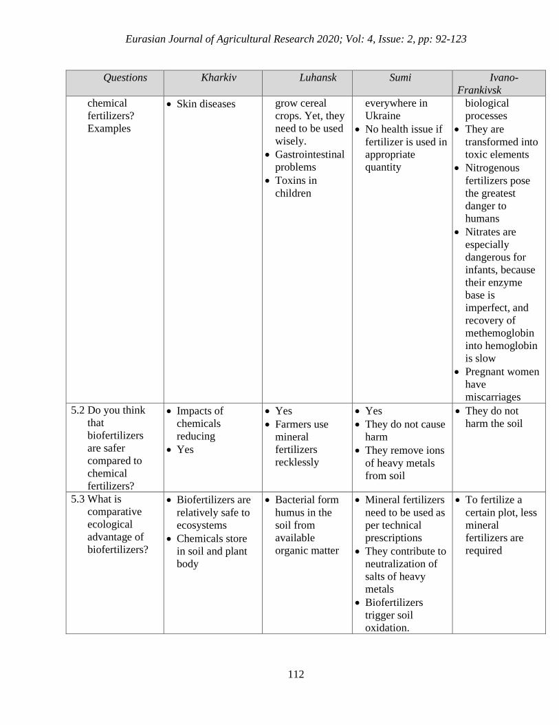
Eurasian Journal of Agricultural Research 2020; Vol: 4, Issue: 2, pp: 92-123
112
Questions Kharkiv Luhansk Sumi Ivano-
Frankivsk
chemical
fertilizers?
Examples
• Skin diseases grow cereal
crops. Yet, they
need to be used
wisely.
• Gastrointestinal
problems
• Toxins in
children
everywhere in
Ukraine
• No health issue if
fertilizer is used in appropriate
quantity
biological
processes
• They are
transformed into toxic elements
• Nitrogenous
fertilizers pose
the greatest
danger to
humans
• Nitrates are
especially
dangerous for
infants, because
their enzyme
base is
imperfect, and
recovery of
methemoglobin
into hemoglobin
is slow
• Pregnant women
have
miscarriages
5.2 Do you think
that
biofertilizers
are safer
compared to
chemical
fertilizers?
• Impacts of
chemicals
reducing
• Yes
• Yes
• Farmers use
mineral
fertilizers
recklessly
• Yes
• They do not cause
harm
• They remove ions
of heavy metals
from soil
• They do not
harm the soil
5.3 What is
comparative
ecological
advantage of
biofertilizers?
• Biofertilizers are
relatively safe to
ecosystems
• Chemicals store
in soil and plant
body
• Bacterial form
humus in the
soil from
available
organic matter
• Mineral fertilizers
need to be used as
per technical
prescriptions
• They contribute to
neutralization of
salts of heavy
metals
• Biofertilizers
trigger soil
oxidation.
• To fertilize a
certain plot, less
mineral
fertilizers are
required
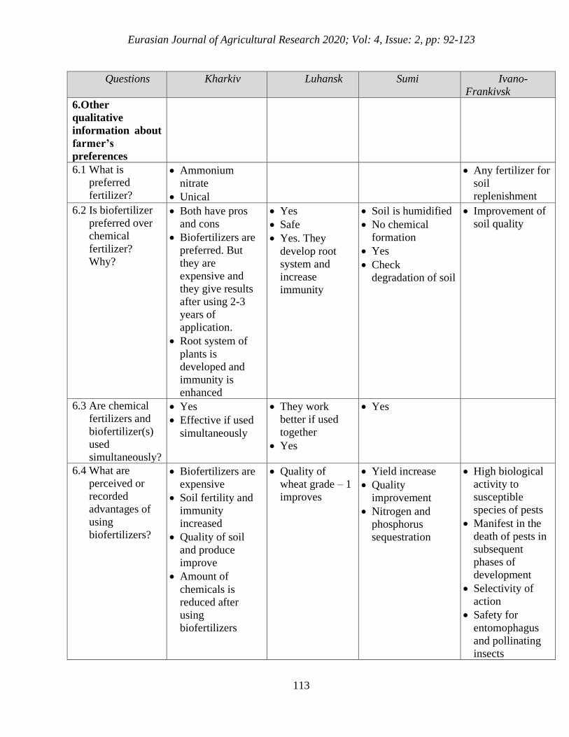
Eurasian Journal of Agricultural Research 2020; Vol: 4, Issue: 2, pp: 92-123
113
Questions Kharkiv Luhansk Sumi Ivano-
Frankivsk
6.Other
qualitative
information about
farmer’s
preferences
6.1 What is
preferred
fertilizer?
• Ammonium
nitrate
• Unical
• Any fertilizer for
soil
replenishment
6.2 Is biofertilizer
preferred over
chemical
fertilizer?
Why?
• Both have pros
and cons
• Biofertilizers are
preferred. But
they are
expensive and
they give results
after using 2-3
years of
application.
• Root system of
plants is
developed and
immunity is
enhanced
• Yes
• Safe
• Yes. They
develop root
system and
increase
immunity
• Soil is humidified
• No chemical
formation
• Yes
• Check
degradation of soil
• Improvement of
soil quality
6.3 Are chemical
fertilizers and
biofertilizer(s)
used
simultaneously?
• Yes
• Effective if used
simultaneously
• They work
better if used
together
• Yes
• Yes
6.4 What are
perceived or
recorded
advantages of
using
biofertilizers?
• Biofertilizers are
expensive
• Soil fertility and
immunity
increased
• Quality of soil
and produce
improve
• Amount of
chemicals is
reduced after
using
biofertilizers
• Quality of
wheat grade – 1
improves
• Yield increase
• Quality
improvement
• Nitrogen and
phosphorus
sequestration
• High biological
activity to
susceptible
species of pests
• Manifest in the
death of pests in
subsequent
phases of
development
• Selectivity of
action
• Safety for
entomophagus
and pollinating
insects
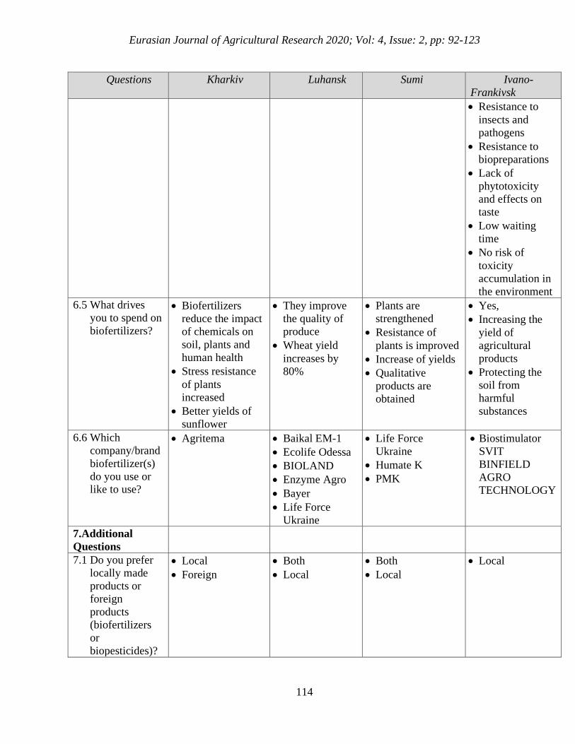
Eurasian Journal of Agricultural Research 2020; Vol: 4, Issue: 2, pp: 92-123
114
Questions Kharkiv Luhansk Sumi Ivano-
Frankivsk
• Resistance to
insects and
pathogens
• Resistance to
biopreparations
• Lack of
phytotoxicity
and effects on
taste
• Low waiting
time
• No risk of
toxicity
accumulation in
the environment
6.5 What drives
you to spend on
biofertilizers?
• Biofertilizers
reduce the impact
of chemicals on
soil, plants and
human health
• Stress resistance
of plants
increased
• Better yields of
sunflower
• They improve
the quality of
produce
• Wheat yield
increases by
80%
• Plants are
strengthened
• Resistance of
plants is improved
• Increase of yields
• Qualitative
products are
obtained
• Yes,
• Increasing the
yield of
agricultural
products
• Protecting the
soil from
harmful
substances
6.6 Which
company/brand
biofertilizer(s)
do you use or like to use?
• Agritema
• Baikal EM-1
• Ecolife Odessa
• BIOLAND
• Enzyme Agro
• Bayer
• Life Force
Ukraine
• Life Force
Ukraine
• Humate K
• PMK
• Biostimulator
SVIT
BINFIELD
AGRO
TECHNOLOGY
7.Additional
Questions
7.1 Do you prefer
locally made
products or
foreign
products
(biofertilizers
or
biopesticides)?
• Local
• Foreign
• Both
• Local
• Both
• Local
• Local
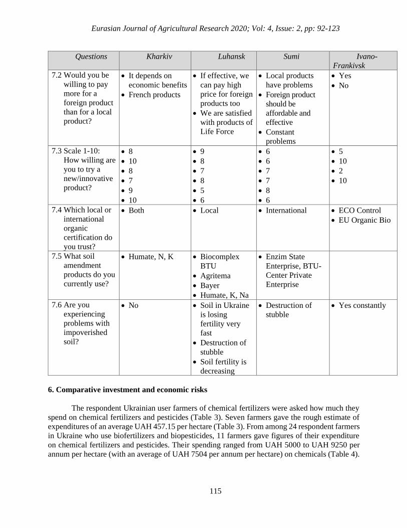
Eurasian Journal of Agricultural Research 2020; Vol: 4, Issue: 2, pp: 92-123
115
Questions Kharkiv Luhansk Sumi Ivano-
Frankivsk
7.2 Would you be
willing to pay
more for a
foreign product
than for a local
product?
• It depends on
economic benefits
• French products
• If effective, we
can pay high
price for foreign
products too
• We are satisfied
with products of
Life Force
• Local products
have problems
• Foreign product
should be
affordable and
effective
• Constant
problems
• Yes
• No
7.3 Scale 1-10:
How willing are
you to try a
new/innovative
product?
• 8
• 10
• 8
• 7
• 9
• 10
• 9
• 8
• 7
• 8
• 5
• 6
• 6
• 6
• 7
• 7
• 8
• 6
• 5
• 10
• 2
• 10
7.4 Which local or
international
organic
certification do
you trust?
• Both • Local • International • ECO Control
• EU Organic Bio
7.5 What soil
amendment
products do you
currently use?
• Humate, N, K • Biocomplex
BTU
• Agritema
• Bayer
• Humate, K, Na
• Enzim State
Enterprise, BTU-
Center Private
Enterprise
7.6 Are you
experiencing
problems with
impoverished
soil?
• No • Soil in Ukraine
is losing
fertility very
fast
• Destruction of
stubble
• Soil fertility is
decreasing
• Destruction of
stubble
• Yes constantly
6. Comparative investment and economic risks
The respondent Ukrainian user farmers of chemical fertilizers were asked how much they
spend on chemical fertilizers and pesticides (Table 3). Seven farmers gave the rough estimate of
expenditures of an average UAH 457.15 per hectare (Table 3). From among 24 respondent farmers
in Ukraine who use biofertilizers and biopesticides, 11 farmers gave figures of their expenditure
on chemical fertilizers and pesticides. Their spending ranged from UAH 5000 to UAH 9250 per
annum per hectare (with an average of UAH 7504 per annum per hectare) on chemicals (Table 4).
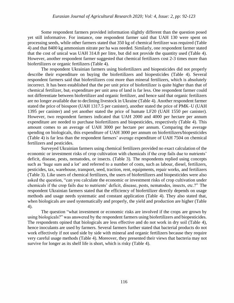
Eurasian Journal of Agricultural Research 2020; Vol: 4, Issue: 2, pp: 92-123
116
Some respondent farmers provided information slightly different than the question posed
yet still informative. For instance, one respondent farmer said that UAH 130 were spent on
processing seeds, while other farmers stated that 350 kg of chemical fertilizer was required (Table
4) and that 8400 kg ammonium nitrate per ha was needed. Similarly, one respondent farmer stated
that the cost of unical was UAH 314.8 per litre, but did not provide the quantity used (Table 4).
However, another respondent farmer suggested that chemical fertilizers cost 2-3 times more than
biofertilizers or organic fertilizers (Table 4).
The respondent Ukrainian farmers using biofertilizers and biopesticides did not properly
describe their expenditure on buying the biofertilizers and biopesticides (Table 4). Several
respondent farmers said that biofertilizers cost more than mineral fertilizers, which is absolutely
incorrect. It has been established that the per unit price of biofertilizer is quite higher than that of
chemical fertilizer, but, expenditure per unit area of land is far less. One respondent farmer could
not differentiate between biofertilizer and organic fertilizer, and hence said that organic fertilizers
are no longer available due to declining livestock in Ukraine (Table 4). Another respondent farmer
stated the price of biospore (UAH 1317.5 per canister), another stated the price of PMK–U (UAH
1395 per canister) and yet another stated the price of humate LF20 (UAH 1550 per canister).
However, two respondent farmers indicated that UAH 2000 and 4000 per hectare per annum
expenditure are needed to purchase biofertilizers and biopesticides, respectively (Table 4). This
amount comes to an average of UAH 3000 per hectare per annum. Comparing the average
spending on biologicals, this expenditure of UAH 3000 per annum on biofertilizers/biopesticides
(Table 4) is far less than the respondent farmers’ average expenditure of UAH 7504 on chemical
fertilizers and pesticides.
Surveyed Ukrainian farmers using chemical fertilizers provided no exact calculation of the
economic or investment risks of crop cultivation with chemicals if the crop fails due to nutrients’
deficit, disease, pests, nematodes, or insects. (Table 3). The respondents replied using concepts
such as ‘huge sum and a lot’ and referred to a number of costs, such as labour, diesel, fertilizers,
pesticides, tax, warehouse, transport, seed, traction, rent, equipments, repair works, and fertilizers
(Table 3). Like users of chemical fertilizers, the users of biofertilizers and biopesticides were also
asked the question, “can you calculate the economic or investment risks of crop cultivation under
chemicals if the crop fails due to nutrients’ deficit, disease, pests, nematodes, insects, etc.?” The
respondent Ukrainian farmers stated that the efficiency of biofertilizer directly depends on usage
methods and usage needs systematic and constant application (Table 4). They also stated that,
when biologicals are used systematically and properly, the yield and production are higher (Table
4).
The question “what investment or economic risks are involved if the crops are grown by
using biologicals?” was answered by the respondent farmers using biofertilizers and biopesticides.
The respondents opined that biologicals are less effective and do not work in dry soil (Table 4),
hence inoculants are used by farmers. Several farmers further stated that bacterial products do not
work effectively if not used side by side with mineral and organic fertilizers because they require
very careful usage methods (Table 4). Moreover, they presented their views that bacteria may not
survive for longer as its shelf life is short, which is risky (Table 4).
Eurasian Journal of Agricultural Research 2020; Vol: 4, Issue: 2, pp: 92-123
117
7. Farmers’ preferences for fertilizers and biofertilizers
The respondent farmers who were users of chemicals fertilizers were asked for their
preferences of using fertilizers and their potential preferences should biofertilizers be offered to
them (Table 3). Similarly, respondent users of biofertilizers also expressed their preferences (Table
4). Usage of chemicals in crops indicates that most of the nutrients are nitrogen, phosphorus and
potash. Ammonium nitrate, unical and complex fertilizer are reported as major sources of nitrogen
(Table 3; Table 4). Micronutrients and calcium or magnesium attained least priority. However,
organic manure and organic fertilizer are two reported sources of humus content for the soil (Table
3). According to government officers, however, not much humus is available in Ukraine now
because livestock farms are shutting down and livestock are disappearing fast.
Through the question, “do you want to use biofertilizers?”, the willingness of respondent
farmers to use biofertilizers was understood. With the exception of 1-2 respondent farmers,
respondents failed to demonstrate a firm willingness to use biofertilizers. Some respondents argued
that biofertilizers are ineffective in temperate and non-irrigated zones, while others simply stated
it was too expensive to use (Table 3). What would drive them to use biofertilizers in the future also
generated negative responses by Ukrainian farmers using chemical fertilizers (Table 3). Their
answers were the same – biofertilizers are neither effective nor economic. However, several
respondent farmers argued that biofertilizers are not harmful and can be beneficial (Table 3).
The reasons for preferring biofertilizers over chemical fertilizers were explored with the
respondent farmers using biofertilizers (Table 4). They responded that the root system of plants is
developed, and immunity is enhanced, once biofertilizers are used (Table 4), and that the
biofertilizers check the degradation of soil and improve quality of soil as well as plants (Table 4).
Chemicalization of the soil does not take place. However, one respondent farmer expressed the
view that both chemical fertilizer and biofertilizer are expensive and they give results after using
2-3 years of application (Table 4). The respondent farmers also confirmed that they use chemical
fertilizers and biofertilizer(s) simultaneously (Table 4). Biofertilizers give effective results if used
simultaneously (Table 4).
The respondent Ukrainian farmers using biofertilizers disclosed the perceived or recorded
advantages of using biofertilizers (Table 4). According to the respondent farmers, soil
fertility/quality and plant immunity/yield increased with improved quality of wheat grade-I (Table
4). They also reported that the amount of chemicals needed is reduced after using biofertilizers,
which promote nitrogen and phosphorus sequestration. Moreover, plant protection functions are
also delivered by biofertilizers, which trigger high biological activity to susceptible species of pests
(Table 4). This manifests in the death of pests in subsequent phases of development, while ensuring
safety for entomophagus and pollinating insects. After all, biofertilizers build resistance to insects
and pathogens with lack of phytotoxicity and no risk of toxicity accumulation in the environment
(Table 4).
The factors which drive respondent user farmers to purchase biofertilizers include their
being economically cheaper, poison free, and ecologically safe. The farmers using biofertilizers
suggested that plants are strengthened with increased resistance through using biofertilizers.
Moreover, biofertilizers reduce the impact of chemicals on soil, plants and human health (Table
4). These respondent farmers stated that crops, like sunflower, produce better yields (80%
increase) and better quality of grains, fruits and tubers, and forage (Table 4).
Eurasian Journal of Agricultural Research 2020; Vol: 4, Issue: 2, pp: 92-123
118
The surveyed farmers using biofertilizers provided the names of some manufacturers of
biofertilizers which they prefer, including Agritema, Baikal EM-1, Ecolife Odessa, BIOLAND,
Enzyme Agro, Bayer, Life Force Ukraine, Humate K, PMK, Biostimulator and SVIT Binfield
Agro Technology (Table 4).
Potential preferences of respondent farmers regarding the use of local or foreign products
(biofertilizers) were identified through interview questions. Most of the respondent farmers
showed preferences for using local biofertilizers (Table 3). Only a few respondent farmers
preferred both local and foreign made products (Table 3). Similarly, respondent user farmers of
biofertilizers gave their preferences as to both local and international products (Table 4). However,
many respondent farmers have shown no preference to pay more for a foreign product rather than
for a local product (Table 3). Yet, majority of respondent farmers stated that they could pay more
for foreign products if they are relatively more effective and their quality is better (Table 3). In the
same fashion, respondent farmers using biofertilizers were asked the question, “would you be
willing to pay more for a foreign product than for a local product?” There was a mixed response
on this issue. The majority of respondent farmers using biofertilizers showed willingness to use a
foreign product (Table 4), although many of them stated that this willingness was conditional.
They expressed that preference for biofertilizers depends on economic benefits, effectiveness,
affordability, and other qualitative traits (Table 4). One respondent farmer refused to accept foreign
products due to satisfaction with products of Life Force company (Table 4).
The respondent farmers’ willingness scale to try a new/innovative product was probed as
well. Out of 12 surveyed farmers, 9 farmers opted to share their willingness on a total 10-point
scale (Table 3), with the average of 5.55 out of 10-point scale (Table 3). It is significant that more
than half of the respondent farmers have a willingness to use biofertilizers in the future. Likewise,
all 21 respondent farmers from the 4 different oblasts of Ukraine shared their willingness to try a
new/innovative product on 10-point scale (Table 4). Their average score on this scale was 7.3
(Table 4). This score is higher than the respondent farmers using only chemical fertilizers, which
may be because the users of biofertilizers have already adopted new products and innovations and
thus are more willing to try another set of innovations.
As certification and standards are key to the acceptance and preference of biofertilizers,
respondent farmers using chemical fertilizers were surveyed, but they did not provide responses
(Table 3). The same was true of respondent farmers using biofertilizers (Table 4). Together, they
have equal trust in both kinds of certifications and standards. They noted the names of the two
trusted certifications – ECO Control (Ukrainian) and EU Organic Bio (international) (Table 4).
Respondent Ukrainian users of biofertilizers informed that they exclusively use soil amendment
products such as Humate, Biocomplex BTU, Agritema products, Bayer products, K, Na, and
Enzim (Table 4). The respondent farmers using biofertilizers shared their experiences concerning
problems they are facing with impoverished soil (Table 4). Some respondent farmers answered
negatively, while others stated that soil in Ukraine is losing fertility very fast and they are
constantly facing difficulties (Table 4).
Eurasian Journal of Agricultural Research 2020; Vol: 4, Issue: 2, pp: 92-123
119
DISCUSSION
1. Soil performance under chemical fertilizers
Chemical fertilizers affect soil, plants, ecosystems and human health. When using chemical
fertilizers, the soil becomes drought-prone, water-deficit, hard, compact, water-scarce, infertile,
polluted and less productive. After the introduction of mineral fertilizers, the intensity of the
natural conversion of atmospheric nitrogen to the compounds that can be assimilated by plants is
reduced. The mineral salt solutions are harmful to soil microorganisms that form a layer on the
fertile soil, and hence the formation of humus slows down. Chemical fertilizers can increase the
radioactive lead (204Pb, 206Pb, 207Pb, 208Pb), which causes accumulation of heavy metals in soil and
plant bodies. A few respondent Ukrainian farmers stated that the impact of chemical fertilizers on
soil depends on the quantum of chemicals being used and that only excess of mineral fertilizers
cause harmful effects on soil.
2. Health and ecological risks from chemical fertilizers
The common diseases that can be attributed to usage of chemical fertilizers are: skin
diseases, kidney problems, respiratory diseases, indigestion, memory loss, lung ailments, mental
and physical weakness, menstrual disorders, loss of immunity, loss of work efficiency, eyesight
weakness, gastrointestinal problems, poisoning, vomiting, cancer (if residues persist), phlegm of
the upper respiratory tract, rhinitis, laryngitis, bronchitis, pneumoconiosis, hepatitis, chronic
intoxication of the body, asthma, weakened immune system, miscarriages of pregnant women, and
mutagenic and embryotoxic effects. Mineral fertilizers accelerate leaching of calcium, magnesium,
zinc, copper, and manganese from the soil. Leaching affects the processes of photosynthesis and
reduces the resistance of plants to diseases. Mineral fertilizers lead to reducing soil porosity and
granular aggregates, and finally leads to acidification of the soil. Nitrogenous fertilizers pose the
greatest danger to humans and agroecosystems. Nitrates are especially dangerous for infants,
because their enzyme base is imperfect, and recovery of methemoglobin into hemoglobin is slow.
Biofertilizers, on the other hand, are safer compared to chemical fertilizers. Biofertilizers do not
pollute water and air and keep the environment clean as they trigger oxidation of soil. Biofertilizers
remove ions of heavy metals from soil and clean the contaminated soil.
3. Soil performance under biofertilizers
Biofertilizers are confirmed to improve the soil texture and profile, while enhancing soil
fertility. Another significant advantage of using biofertilizers is that they are toxin-free, non-
poisonous, harmless to soil, environment friendly, and disease resistant. Biofertilizers are also
claimed to support plants and human health, reducing carbon footprints, while helping plants grow
better and more safely. The microbes of biofertilizers solubilize nutrients (micronutrients too) of
the soil and make them available to plant roots. Another aspect of microbes acting in the soil is
their ability to enhance soil’s water retention capacity, enabling the soil to retain moisture in which
nutrients dissolve and become available to plants. Biofertilizers increase soil temperature by 2-5oC
which enhances root formation and germination of seeds. Fruiting, blooming, germination, and
root formation are supported by the bacteria that feed on root secretions and release growth
metabolites.
Eurasian Journal of Agricultural Research 2020; Vol: 4, Issue: 2, pp: 92-123
120
The bacteria feed on secretions of root system in rhizosphere. Some biofertilizers have
additional strength to defy enemy insects and pests, thereby reducing the use of plant protection
chemicals. Biofertilizers are also reported as increasing plant and soil immunity while improving
quality of produce. Biofertilizers work on a synergistic basis or on antagonism principles and, as a
result, fermentation process makes leaves and fruits of plants inedible to the pathogenic microbes.
Finally, plants becomes more resistant to pathogens, drought and frost. As a result, soil becomes
resistant to fungal diseases, drought and other pathogens since biofertilizers reduce negative
impacts of chemicals on soil fertility and reduce the residues by 60%. The respondent farmers also
indicated that biofertilizers solve salinity problems in the soil.
4. Soil-water regime under biofertilizers
Biofertilizers reduce irrigation needs by 2 times at least for a crop (e.g. wheat) grown with
biofertilizer(s) usage. The moisture is built up in soil when biofertilizers are applied, as the
biofertilizers provide natural water permeability of the fertile layer of soil. Moisture remains for
longer in the soil and 40-70% of water is kept in rhizosphere once biofertilizers are applied.
Biofertilizers synthesize biologically active substances by dissolving, for example, silicate and
other substances including nitrogen, potassium and phosphorus. They humidify soil layers and
maintain air and water permeability of soil layer (at least 60 cm deep). Biofertilizers transform
microelements to become easily digestible by plants and also contribute to the aeration of the soil,
water retention, filtration ability, rate of cation exchange in the soil. Moreover, humus that causes
plant growth is formed, aiding in resistance to drought and water holding capacity of the soil.
Consequently, moisture solubilizes nutrients and enhances uptake by plant roots and hence
nutrients intake is facilitated by moisture. Therefore, the effect of dry spell is minimized. Some
farmers stated that the bacteria dissolve phosphorus in soil and increase salt index level that
regulates pH of the soil. This all supports plant growth. The bacteria recycle and dissolve
intractable phosphorus in soil and make it accessible to the plants. Certain bacteria strain dissolve
ammonia, amino-silicate and release potassium and hard nitrogen. As a result, quality and size of
grain (I & II grades) and straw improve.
5. Comparative yield & characteristics of produce
There is a reported 10-15% increase in yield and production after using biofertilizers. For
example, the use of Bacillus amyloliquefaciens increases yield by 10%. The tubers, grains and
fruits have better taste, size, quality, production, shelf-life, and color after biofertilizers are used.
Noticeably, the size of the harvest depends on the density of productive stalk and mass of grain
from one ear, and biofertilizers boost all these entities. Likewise, Actinomycetes inhibit the growth
of pathogens and stubble. In fact, bacteria help the plants produce higher growth by mobilizing the
vitamins, carotenes, proteins and increasing qualitative indicators of plants. The respondent
farmers also confirmed that plant products get saturated color and better quality once biofertilizers
are applied.
Eurasian Journal of Agricultural Research 2020; Vol: 4, Issue: 2, pp: 92-123
121
6. Comparative investment and economic risks
Expenditures per unit area of land on buying chemical pesticides/fertilizers and
biofertilizers/biopesticides were compared. Ukrainian farmers stated that it costs more than 2-3
times the price of chemical fertilizers/pesticides when compared to biofertilizers or organic
fertilizers and biopesticides. In Ukraine, the average spending on biologicals was UAH 3000 per
annum versus average spending of UAH 7504 on chemical fertilizers and pesticides. An
investment or economic risk if the crops grown by using biologicals exists. When the risk of the
losses was quite high (60-70%) with the chemically grown crops, the risk of losses reduces to
average 33% if crops grown by using biologicals. Therefore, risks reduce considerably if
biologicals are used.
7. Farmers’ preferences for fertilizers and biofertilizers
Nitrogen, phosphorus and potash are the main nutrients used in crops. Micronutrients and
calcium or magnesium attained least priority. Common fertilizers include NPK (nitrogen,
phosphorus, potassium), calcium nitrate, DAP (diammonium phosphate), MoP (molybdenum
phosphate), ammonium nitrate, unical and complex fertilizer. Among the micronutrients, only the
molybdenum was found being used by some farmers. How are biofertilizers applied? The
respondent farmers confirmed that they use chemical fertilizers and biofertilizer(s) simultaneously.
What drives respondent user farmers to purchase biofertilizers? Some advantages of using
biofertilizers were stated to be production sustainability, input cost reduction, cheaper prices,
ecologically safe, organic status, health and safety.
The respondent farmers’ average willingness to adopt biofertilizers was measured. The
respondent Ukrainian non-user of biofertilizers showed an average willingness of 5.55 out of 10-
point scale (nearly 55%). On the other hand, the average willingness score of users of biofertilizers
is 7.3 (i.e. 73%). This reflects that users of biofertilizers express greater willingness to adopt
biofertilizers, yet the willingness of non-users of biofertilizers is not less. These respondent farmers
showed preferences for using both local and foreign made biofertilizers. Moreover, they also trust
both local and international organic certification.
CONCLUSION
A biofertilizer contains living microorganisms that are applied to seed, plant surfaces, or
soil, and that colonize the rhizosphere or the interior of the plant and promotes growth by
increasing the supply or availability of primary nutrients to the host plant. Some common agents
in biofertilizers include Rhizobium, Azotobacter, Azospirillum, phosphorus solubilizing bacteria
(PSB) and Mycorrhizae. The agronomic advantage of biofertilizers compared to conventional
chemical fertilizers is well proved biologically and in economic terms. The biofertilizers are safer
ecologically and in context of public health. The biofertilizer is broad spectrum efficient inoculum
tested to boost production, soil biology and agroecosystem sustainability. In the study, two
important economic angles are highlighted by the respondents: 1) reduced risks of crop failure if
using the biofertilizers; and 2) comparatively lesser inputs and investment are needed to grow
crops if biofertilizers are added. Such economic and scientific advantages of using biofertilizers
ultimately mobilize the respondent farmers preferring biofertilizers over the chemical fertilizers.
Eurasian Journal of Agricultural Research 2020; Vol: 4, Issue: 2, pp: 92-123
122
A problem lies with the production and supply of biofertilizers in Ukraine. Both the
production and distribution are inadequate compared to the demand for microbial biofertilizers.
However, a dozen companies are operational in Ukraine trading and supplying biofertilizers and
other soil nutrients. The farmers using biofertilizers prefer using the microbial products, with
certain reservations about quality of products, effectiveness and shelf life of microorganisms. The
findings of this study revealed the scientific and practical advantages of using biofertilizers,
however, studies need to be pursued to understand reasons of such trade gaps and slow growth of
biofertilizers in agriculture sector of Ukraine.
REFERENCES
Arjjumend H., Koutouki K., & Neufeld, S. 2020. Comparative Advantage of Using the
Biofertilizers in Indian Agroecosystems. In press.
Arjjumend, H., Neufeld, S., Yargeu, V. & Warren, M. 2017. Reviving Soil Biology and Crop
Productivity through New Biofertilizer: Agroecological Performance of Pseudomonas
monteilli in Tropical Environments. International Journal of Tropical Agriculture, 35(4),
1235-1247. ISSN: 0254-8755. Available online:
https://serialsjournals.com/abstract/34617_63-.pdf
Earth Alive 2017. Earth Alive’s Commitment to Sustainable Development. Available online:
http://earthalivect.com/about-us/sustainability/. Accessed on 18 January 2017.
Franche, C., Lindstrom, K. & Elmerich, C. 2009. Nitrogen fixing bacteria associated with
leguminous and non-leguminous plants. Plant and Soil, 321, 35–59.
Rajendra, P., Singh, S. & Sharma, S. N. 1998. Interrelationship of fertilizers use and other
agricultural inputs for higher crop yields. Fertilizers News, 43, 35-40.
Simiyu, N.S.W., Tarus, D., Watiti, J., Nang’ayo, F. 2013. Effective regulation of bio-fertilizers
and bio-pesticides: A potential avenue to increase agricultural productivity, Compro II
Policy Series, No. 1, 2013, International Institute of Tropical Agriculture.
Stefanovska, T.R., Pidlisnyuk, V.V. & Kaya, H.K. 2006. Biological control of pests in Ukraine:
legacy from the past and challenges for the future. In, Perspectives in Agriculture, Veterinary
Science, Nutrition and Natural Resources. CAB Reviews.
Weyens, N., van der Lelie, D., Taghavi, S., Newman, L. & Vangronsveld, J. 2009. Exploiting
plant-microbe partnerships to improve biomass production and remediation. Trends in
Biotechnology, 27(10), 591-598.
Xiang, W., Zhao, L., Xu, X., Qin, Y. & Yu, G. 2012. Mutual Information Flow between Beneficial
Microorganisms and the Roots of Host Plants Determined the Bio-Functions of
Biofertilizers. American Journal of Plant Sciences, 3, 1115-1120. Doi: http://dx.doi.org/10
.4236/ajps.2012.38134
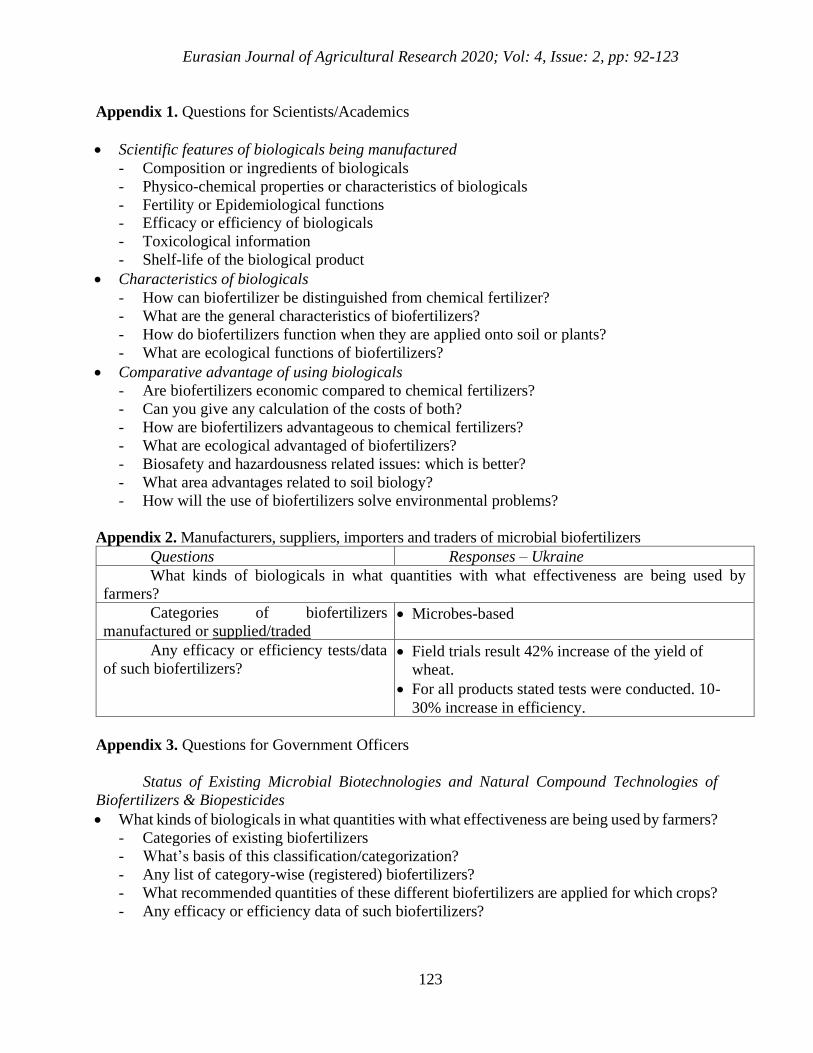
Eurasian Journal of Agricultural Research 2020; Vol: 4, Issue: 2, pp: 92-123
123
Appendix 1. Questions for Scientists/Academics
• Scientific features of biologicals being manufactured
- Composition or ingredients of biologicals
- Physico-chemical properties or characteristics of biologicals
- Fertility or Epidemiological functions - Efficacy or efficiency of biologicals
- Toxicological information
- Shelf-life of the biological product
• Characteristics of biologicals
- How can biofertilizer be distinguished from chemical fertilizer?
- What are the general characteristics of biofertilizers?
- How do biofertilizers function when they are applied onto soil or plants?
- What are ecological functions of biofertilizers?
• Comparative advantage of using biologicals
- Are biofertilizers economic compared to chemical fertilizers?
- Can you give any calculation of the costs of both?
- How are biofertilizers advantageous to chemical fertilizers?
- What are ecological advantaged of biofertilizers?
- Biosafety and hazardousness related issues: which is better?
- What area advantages related to soil biology?
- How will the use of biofertilizers solve environmental problems?
Appendix 2. Manufacturers, suppliers, importers and traders of microbial biofertilizers
Questions Responses – Ukraine
What kinds of biologicals in what quantities with what effectiveness are being used by
farmers?
Categories of biofertilizers
manufactured or supplied/traded • Microbes-based
Any efficacy or efficiency tests/data
of such biofertilizers? • Field trials result 42% increase of the yield of
wheat.
• For all products stated tests were conducted. 10-
30% increase in efficiency.
Appendix 3. Questions for Government Officers
Status of Existing Microbial Biotechnologies and Natural Compound Technologies of
Biofertilizers & Biopesticides
• What kinds of biologicals in what quantities with what effectiveness are being used by farmers?
- Categories of existing biofertilizers
- What’s basis of this classification/categorization?
- Any list of category-wise (registered) biofertilizers?
- What recommended quantities of these different biofertilizers are applied for which crops?
- Any efficacy or efficiency data of such biofertilizers?
Eurasian Journal of Agricultural Research 2020; Vol: 4, Issue:2, pp:124-133
124
Enhancing the Yield and Profitability of Peanut (Arachis hypogaea L.)
to Application of Different Organic Foliar Fertilizers
Heneroso R. Orbeta1 Ulysses A. Cagasan2*
1,2Department of Agronomy, Visayas State University, Visca, Baybay City, Leyte 6521-A, Philippines
*Corresponding Author: [email protected]
Abstract
One strategy to produce enough, healthy, and safer products is to apply the best practices by using
locally produced organic bio-fertilizer as nutrients for the crops. This study aimed to evaluate the
effects, determine the appropriate, and assess the profitability of using locally produced organic
foliar fertilizers on peanut production. The treatments designated as follows: T1 - Control (no
application), T2- Power grow 100 ml/16li H2O, T3 - Vermi tea 100 ml/16li H2O, T4 - Poultry litter
tea100 ml/16li H2O, and T5 - Wood vinegar 100 ml/16li H2O. The experiment was laid out in
Randomized Complete Block Design (RCBD) with three replications. Each replication was
divided into five (5) treatment plots measuring twelve (12) m2 separated by 1 m alleyways between
replications and treatment plots to facilitate farm operations and data gathering. The treatment
plants were sprayed with foliar fertilizer six times at weekly intervals, starting two weeks up to
the pick of the peanut plants' last flowering. Results showed that peanut plants flowered early
when applied with poultry litter tea. Likewise, highest leaf area index (LAI) and weight of 1,000
seeds (g) when applied with Power grow foliar fertilizer. Application of poultry litter tea, power
grow and wood vinegar obtained the highest seed yield of 1.31-1.470 t ha-1 and achieved the
highest grain yield tha-1. Thus, gave the high gross margin of PhP36,723-48,965.00 ha-1 among
the treatments. In terms of pest incidence, no serious presence of insects and diseases were noted;
thus, a high to moderate resistance rating was obtained in all treatment plants.
Keywords: Best practices, local organic produced, sustainable, productivity and income
Research article
Received Date: 16 November 2020 Accepted Date: 30 November 2020
Eurasian Journal of Agricultural Research 2020; Vol: 4, Issue:2, pp:124-133
125
INTRODUCTION
INTRODUCTION
Peanut (Arachis hypogaea L.) is also named groundnut, which belongs to the family
Leguminosae that produces underground fruits called pods (Aboelill et al., 2012). The Philippines
is consumed as boiled peanut, peanut oil, peanut butter, roasted peanuts, peanut bars, and candies.
Groundnuts are considered a vital source of nutrients, calories, minerals, and antioxidants, vitamins
essential for optimum health. It is one of the legumes considered as an excellent intercrop to corn,
sorghum, sugarcane. Planting peanut help enrich the soil nutrients due to its ability to fix
atmospheric nitrogen. Peanut, as a legume, needs only a small amount of N because of its ability to
fix nitrogen from the atmosphere (Jordan et al., 2017). Organic substances can be used as fertilizer
because it contains essential nutrients like nitrogen, phosphorus, potassium, calcium, iron,
manganese, zinc, copper, magnesium, and protein substances that stimulate plant metabolism.
Organic fertilizers are an excellent substitute for inorganic fertilizer in crops that require less
nutrients for their growth and development. The use of organic foliar fertilizer is beneficial. It
contains microorganisms such as bacteria that hastens organic materials' mineralization and makes
it available to plants through the foliar spray (Yansong et al., 2009).
Foliar application of nutrients is a feasible, economically viable, and environmentally
friendly approach to nutrient management. It is often the most effective and economical way to
correct plant nutrient deficiencies at critical growth stages. Reports indicated that foliar application
promoted root absorption of the same nutrient or other nutrients by improving root growth and
increasing nutrients' uptake (Meena et al., 2007). The foliar application also overcomes the
physiological disturbances caused by adverse soil conditions that hamper mobility and nutrient
absorption. Foliar spraying of N, Mn, Cu, and B on several crops indicated beneficial effects.
Kalinova, et al. (2014) indicated that foliar application of 1% KCl obtained the best results
in groundnuts. Manure tea as foliar fertilizer corrects the plant's deficiencies because the nutrients
enter the plant through the stomata and cuticle. Foliar application of fertilizer is an effective way
of correcting soil nutrient deficiency when plants cannot absorb directly from the soil (Jordan et
al., 2017). The foliar application provides a quicker response and more effective for some nutrients
like NPK than soil-applied fertilizer (Brandenburg, et al., 2019). Foliar feeding is often the most
effective and economical way to correct plant nutrient deficiencies. It has become an established
procedure in crop production to increase yield and improve the product's quality. Since there is a
need to look for cheap and ecologically safe plant growth enhancers as a supplement to inorganic
fertilizer for peanut production, Power grows, vermi tea, poultry litter tea, and wood vinegar can
be used for this purpose. Hence, this study was conducted to evaluate the effects of different organic
foliar fertilizers on peanut growth and yield.
MATERIALS and METHODS
Experimental Area, Design, and Soil Sampling
An area of 226.0 m2 Umingan clay loam soil (FAO, 2016) is located at the Agronomy
Experimental Area College of Agriculture and Food Science, Visayas State University, Baybay
City, Leyte. The experimental area has a GPS coordinates of 10o44' 59.8668" N, 124o47' 38.1264"
E. This was plowed and harrowed twice using a tractor-drawn implement at weekly intervals.
Eurasian Journal of Agricultural Research 2020; Vol: 4, Issue:2, pp:124-133
126
These were done to allow the weeds to decompose, pulverize the soil, level the field, and
provide time for weed seeds to germinate and incorporate them into the soil. Furrows were
constructed at a distance of 0.5 m apart.
Soil samples were collected randomly from the experimental area before plowing. These
were composited, air-dried, pulverized, sieved (2 mm wire mesh) and submitted to the Central
Analytical Service Laboratory (CASL), PhilRootcrops, Visayas State University, Visca, Baybay
City, Leyte. The soil samples were analyzed to determine the soil pH Potentiometric method (1:2.5
soil water ratio), % organic matter (Modified Walkley-Black method), total N by (micro Kjeldal
method), extractable P, and exchangeable K (ammonium acetate extraction method). For the final
soil analysis, three samples were collected from each treatment plot after peanut harvest. Collected
soil samples were air-dried, composited, and processed to determine the same soil parameters
mentioned above. The experiment was laid out in an RCBD (Randomized Complete Block
Design) with three replications. Each replication was divided into five treatment plots, measuring
3 m × 4 m with 1 m alleyways between replications and 0.50 m between treatment plots to facilitate
farm operations and data gathering. The different treatments are as follows: T1- Control (no
application), T2 -100ml/16li H2O Power Grow, T3 - 100ml/16li H2O Vermi tea, T4 -100ml/16li
H2O Poultry litter tea, T5 -100ml/16li H2O Wood vinegar.
Organic Foliar Fertilizer Preparation
Vermicast was purchased at the Eco FARMI, and Poultry litter at the Department of Animal Science, both from Visayas State University, Baybay City, Leyte. While Wood vinegar was
procured at Balinsasayao Research Station, Balinsasayao, Abuyog, Leyte. Vermitea, and Poultry
litter tea were prepared through fermentation for three (3) weeks. The mixture of 1:1 ratio was
prepared by mixing 1 liter of unchlorinated water and 1 kg of Vermicast in a clean bucket, covered
with cheesecloth to prevent insects and other organisms' entry while allowing air circulation inside
of the bucket and was mixed thoroughly and was fermented for 3 weeks. The mixture was then
filtered, and the filtrates were placed in clean containers and stored under ambient conditions.
(Krawczyk, 2018). All organic foliar fertilizer samples were collected and brought to the Central
Analytical Service Laboratory (CASL), PhilRootcrops, Visayas State University, Visca, Baybay
City, Leyte for the analysis of NPK contents.
Organic Foliar Fertilizer Application
Spraying of foliar fertilizers (100 ml of fermented organic foliar fertilizers per 16 liters of
water) was done six (6) times at weekly intervals starting two (2) weeks after sowing (DAS) up to
the peak of the last flowering of peanut plants.
Spraying of organic foliar fertilizers was done when the wind is expected, and an enclosure
was provided around the treatment plants to avoid contamination of other treatments.
Harvesting was done when 90% of the plants reached maturity. The pods became firm at this
stage, and the crop exhibited yellowing to brown of matured leaves. One row on each side and
two end hills served as border plants leaving two border rows in each treatment plot. Extra care
was observed to minimize the damage of pods. After this, peanut pods were handpicked, washed,
and sundried to attain a moisture content of 14% using a moisture meter.
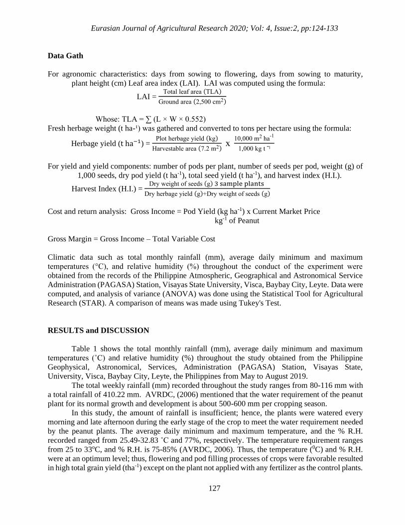
Eurasian Journal of Agricultural Research 2020; Vol: 4, Issue:2, pp:124-133
127
Data Gath
For agronomic characteristics: days from sowing to flowering, days from sowing to maturity,
plant height (cm) Leaf area index (LAI). LAI was computed using the formula:
LAI = Total leaf area (TLA)
Ground area (2,500 cm2)
Whose: TLA = ∑ (L × W × 0.552)
Fresh herbage weight (t ha-¹) was gathered and converted to tons per hectare using the formula:
Herbage yield (t ha−1) = Plot herbage yield (kg)
Harvestable area (7.2 m2) x
10,000 m2 ha-1
1,000 kg t ˉˡ
For yield and yield components: number of pods per plant, number of seeds per pod, weight (g) of
1,000 seeds, dry pod yield (t ha-1), total seed yield (t ha-1), and harvest index (H.I.).
Harvest Index (H.I.) = Dry weight of seeds (g) 3 sample plants
Dry herbage yield (g)+Dry weight of seeds (g)
Cost and return analysis: Gross Income = Pod Yield (kg ha-1) x Current Market Price
kg-1 of Peanut
Gross Margin = Gross Income – Total Variable Cost
Climatic data such as total monthly rainfall (mm), average daily minimum and maximum
temperatures (°C), and relative humidity (%) throughout the conduct of the experiment were
obtained from the records of the Philippine Atmospheric, Geographical and Astronomical Service
Administration (PAGASA) Station, Visayas State University, Visca, Baybay City, Leyte. Data were
computed, and analysis of variance (ANOVA) was done using the Statistical Tool for Agricultural
Research (STAR). A comparison of means was made using Tukey's Test.
RESULTS and DISCUSSION
Climatic Data
Table 1 shows the total monthly rainfall (mm), average daily minimum and maximum
temperatures (˚C) and relative humidity (%) throughout the study obtained from the Philippine
Geophysical, Astronomical, Services, Administration (PAGASA) Station, Visayas State,
University, Visca, Baybay City, Leyte, the Philippines from May to August 2019.
The total weekly rainfall (mm) recorded throughout the study ranges from 80-116 mm with
a total rainfall of 410.22 mm. AVRDC, (2006) mentioned that the water requirement of the peanut
plant for its normal growth and development is about 500-600 mm per cropping season.
In this study, the amount of rainfall is insufficient; hence, the plants were watered every
morning and late afternoon during the early stage of the crop to meet the water requirement needed
by the peanut plants. The average daily minimum and maximum temperature, and the % R.H.
recorded ranged from 25.49-32.83 ˚C and 77%, respectively. The temperature requirement ranges
from 25 to 33oC, and % R.H. is 75-85% (AVRDC, 2006). Thus, the temperature (0C) and % R.H.
were at an optimum level; thus, flowering and pod filling processes of crops were favorable resulted
in high total grain yield (tha-1) except on the plant not applied with any fertilizer as the control plants.
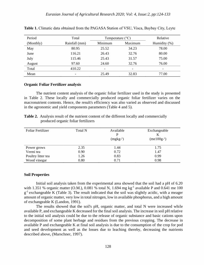
Eurasian Journal of Agricultural Research 2020; Vol: 4, Issue:2, pp:124-133
128
Table 1. Climatic data obtained from the PAGASA Station of VSU, Visca, Baybay City, Leyte
Period Total Temperature (°C) Relative
(Monthly) Rainfall (mm) Minimum Maximum Humidity (%)
May 80.95 25.52 34.23 78.00
June 116.21 26.43 32.76 80.00
July 115.46 25.43 31.57 75.00
August 97.60 24.60 32.76 76.00
Total 410.22 - - -
Mean - 25.49 32.83 77.00
Organic Foliar Fertilizer analysis
The nutrient content analysis of the organic foliar fertilizer used in the study is presented
in Table 2. These locally and commercially produced organic foliar fertilizer varies on the
macronutrient contents. Hence, the result's efficiency was also varied as observed and discussed
in the agronomic and yield components parameters (Table 4 and 5).
Table 2. Analysis result of the nutrient content of the different locally and commercially
produced organic foliar fertilizers
Foliar Fertilizer Total N Available
P
(mgkg-¹)
Exchangeable
K
(me100g-¹)
Power grows 2.35 1.44 1.75
Vermi tea 0.90 0.72 1.47
Poultry litter tea 1.26 0.83 0.99
Wood vinegar 0.80 0.71 0.98
Soil Properties
Initial soil analysis taken from the experimental area showed that the soil had a pH of 6.20
with 1.351 % organic matter (O.M.), 0.081 % total N, 1.694 mg kg-1 available P and 0.641 me 100
g-1 exchangeable K (Table 3). The result indicated that the soil was slightly acidic, with a meager
amount of organic matter, very low in total nitrogen, low in available phosphorus, and a high amount
of exchangeable K (Landon, 1991).
The results showed that the soil's pH, organic matter, and total N were increased while
available P, and exchangeable K decreased for the final soil analysis. The increase in soil pH relative
to the initial soil analysis could be due to the release of organic substance and basic cations upon
decomposition of some plant herbage and residues from the previous cropping. The decrease in
available P and exchangeable K at final soil analysis is due to the consumption of the crop for pod
and seed development as well as the losses due to leaching thereby, decreasing the nutrients
described above, (Marschner, 1997).
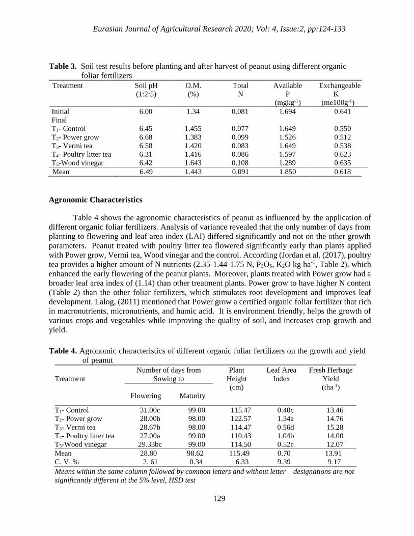
Eurasian Journal of Agricultural Research 2020; Vol: 4, Issue:2, pp:124-133
129
Table 3. Soil test results before planting and after harvest of peanut using different organic
foliar fertilizers
Treatment Soil pH
(1:2:5)
O.M.
(%)
Total
N
Available
P
(mgkg-1)
Exchangeable
K
(me100g-1)
Initial 6.00 1.34 0.081 1.694 0.641
Final
T1- Control 6.45 1.455 0.077 1.649 0.550
T2- Power grow 6.68 1.383 0.099 1.526 0.512
T3- Vermi tea 6.58 1.420 0.083 1.649 0.538
T4- Poultry litter tea 6.31 1.416 0.086 1.597 0.623
T5-Wood vinegar 6.42 1.643 0.108 1.289 0.635
Mean 6.49 1.443 0.091 1.850 0.618
Agronomic Characteristics
Table 4 shows the agronomic characteristics of peanut as influenced by the application of
different organic foliar fertilizers. Analysis of variance revealed that the only number of days from
planting to flowering and leaf area index (LAI) differed significantly and not on the other growth
parameters. Peanut treated with poultry litter tea flowered significantly early than plants applied
with Power grow, Vermi tea, Wood vinegar and the control. According (Jordan et al. (2017), poultry
tea provides a higher amount of N nutrients (2.35-1.44-1.75 N, P2O5, K2O kg ha-1, Table 2), which
enhanced the early flowering of the peanut plants. Moreover, plants treated with Power grow had a
broader leaf area index of (1.14) than other treatment plants. Power grow to have higher N content
(Table 2) than the other foliar fertilizers, which stimulates root development and improves leaf
development. Lalog, (2011) mentioned that Power grow a certified organic foliar fertilizer that rich
in macronutrients, micronutrients, and humic acid. It is environment friendly, helps the growth of
various crops and vegetables while improving the quality of soil, and increases crop growth and
yield.
Table 4. Agronomic characteristics of different organic foliar fertilizers on the growth and yield
of peanut
Treatment
Number of days from
Sowing to
Plant
Height
(cm)
Leaf Area
Index
Fresh Herbage
Yield
(tha-1)
Flowering Maturity
T1- Control 31.00c 99.00 115.47 0.40c 13.46
T2- Power grow 28.00b 98.00 122.57 1.34a 14.76
T3- Vermi tea 28.67b 98.00 114.47 0.56d 15.28
T4- Poultry litter tea 27.00a 99.00 110.43 1.04b 14.00
T5-Wood vinegar 29.33bc 99.00 114.50 0.52c 12.07
Mean 28.80 98.62 115.49 0.70 13.91
C. V. % 2. 61 0.34 6.33 9.39 9.17
Means within the same column followed by common letters and without letter designations are not
significantly different at the 5% level, HSD test
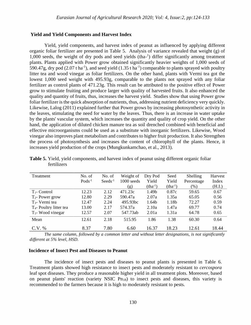
Eurasian Journal of Agricultural Research 2020; Vol: 4, Issue:2, pp:124-133
130
Yield and Yield Components and Harvest Index
Yield, yield components, and harvest index of peanut as influenced by applying different
organic foliar fertilizer are presented in Table 5. Analysis of variance revealed that weight (g) of
1,000 seeds, the weight of dry pods and seed yields (tha-1) differ significantly among treatment
plants. Plants applied with Power grow obtained significantly heavier weights of 1,000 seeds of
590.47g, dry pod (2.07 t ha-1), and seed yield (1.35 t ha-1) comparable to plants sprayed with poultry
litter tea and wood vinegar as foliar fertilizers. On the other hand, plants with Vermi tea got the
lowest 1,000 seed weight with 495.93g, comparable to the plants not sprayed with any foliar
fertilizer as control plants of 471.23g. This result can be attributed to the positive effect of Power
grow to stimulate fruiting and produce larger with quality of harvested fruits. It also enhanced the
quality and quantity of fruits, thus, increases the harvest yield. Studies show that using Power grow
foliar fertilizer is the quick absorption of nutrients, thus, addressing nutrient deficiency very quickly.
Likewise, Lalog (2011) explained further that Power grows by increasing photosynthetic activity in
the leaves, stimulating the need for water by the leaves. Thus, there is an increase in water uptake
by the plants' vascular system, which increases the quantity and quality of crop yield. On the other
hand, the application of diluted chicken manure tea as soil drenched combined with beneficial and
effective microorganisms could be used as a substitute with inorganic fertilizers. Likewise, Wood
vinegar also improves plant metabolism and contributes to higher fruit production. It also Strengthen
the process of photosynthesis and increases the content of chlorophyll of the plants. Hence, it
increases yield production of the crops (Mungkunkamchao, et al., 2013).
Table 5. Yield, yield components, and harvest index of peanut using different organic foliar
fertilizers
Treatment No. of
Pods-1
No. of
Seeds-1
Weight of
1000 seeds
(g)
Dry Pod
Yield
(tha-1)
Seed
Yield
(tha-1)
Shelling
Percentage
(%)
Harvest
Index
(H.I.)
T1- Control 12.23 2.12 471.23c 1.49b 0.87c 59.65 0.67
T2- Power grow 12.80 2.29 590.47a 2.07a 1.35a 65.05 0.56
T3- Vermi tea 12.47 2.24 495.93bc 1.64b 1.18b 72.27 0.59
T4- Poultry litter tea 13.00 2.17 574.37a 2.10a 1.47a 69.77 0.74
T5- Wood vinegar 12.57 2.07 547.73ab 2.01a 1.31a 64.78 0.65
Mean 12.61 2.18 515.95 1.86 1.38 60.30 0.64
C.V. % 8.37 7.80 6.60 16.37 18.23 12.61 18.44
The same column, followed by a common letter and without letter designations, is not significantly
different at 5% level, HSD.
Incidence of Insect Pest and Diseases to Peanut
The incidence of insect pests and diseases to peanut plants is presented in Table 6.
Treatment plants showed high resistance to insect pests and moderately resistant to cercospora
leaf spot diseases. They produce a reasonable higher yield in all treatment plots. Moreover, based
on peanut plants' reaction (variety NSIC Pn18) to insect pests and diseases, this variety is
recommended to the farmers because it is high to moderately resistant to pests.
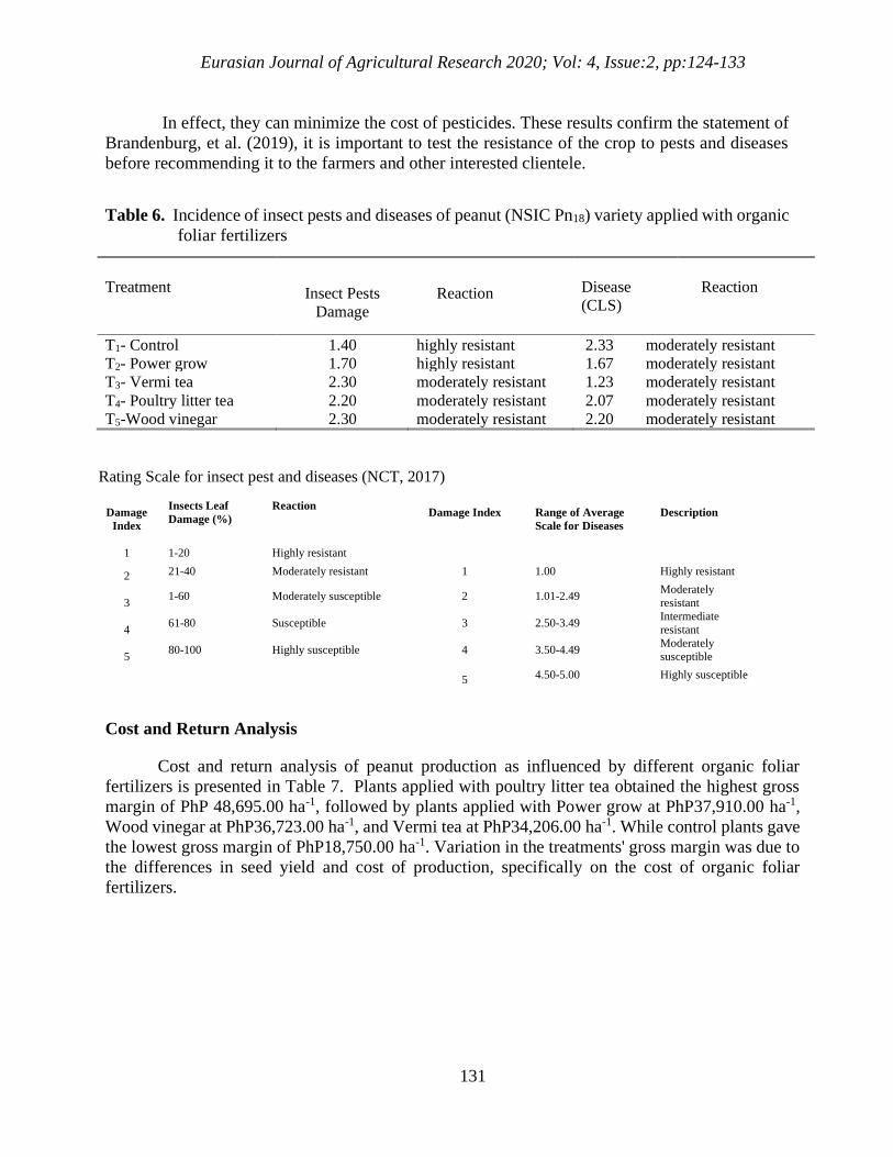
Eurasian Journal of Agricultural Research 2020; Vol: 4, Issue:2, pp:124-133
131
In effect, they can minimize the cost of pesticides. These results confirm the statement of
Brandenburg, et al. (2019), it is important to test the resistance of the crop to pests and diseases
before recommending it to the farmers and other interested clientele.
Table 6. Incidence of insect pests and diseases of peanut (NSIC Pn18) variety applied with organic
foliar fertilizers
Treatment
Disease
(CLS)
Reaction
Insect Pests
Damage
Reaction
T1- Control 1.40 highly resistant 2.33 moderately resistant T2- Power grow 1.70 highly resistant 1.67 moderately resistant T3- Vermi tea 2.30 moderately resistant 1.23 moderately resistant T4- Poultry litter tea 2.20 moderately resistant 2.07 moderately resistant T5-Wood vinegar 2.30 moderately resistant 2.20 moderately resistant
Rating Scale for insect pest and diseases (NCT, 2017)
Damage
Index
Insects Leaf
Damage (%)
Reaction Damage Index
Range of Average
Scale for Diseases
Description
1
1-20
Highly resistant
2 21-40 Moderately resistant 1 1.00 Highly resistant
3 1-60 Moderately susceptible 2 1.01-2.49
Moderately
resistant
4 61-80 Susceptible 3 2.50-3.49
Intermediate
resistant
5 80-100 Highly susceptible 4 3.50-4.49
Moderately
susceptible
5 4.50-5.00 Highly susceptible
Cost and Return Analysis
Cost and return analysis of peanut production as influenced by different organic foliar
fertilizers is presented in Table 7. Plants applied with poultry litter tea obtained the highest gross
margin of PhP 48,695.00 ha-1, followed by plants applied with Power grow at PhP37,910.00 ha-1,
Wood vinegar at PhP36,723.00 ha-1, and Vermi tea at PhP34,206.00 ha-1. While control plants gave
the lowest gross margin of PhP18,750.00 ha-1. Variation in the treatments' gross margin was due to
the differences in seed yield and cost of production, specifically on the cost of organic foliar
fertilizers.
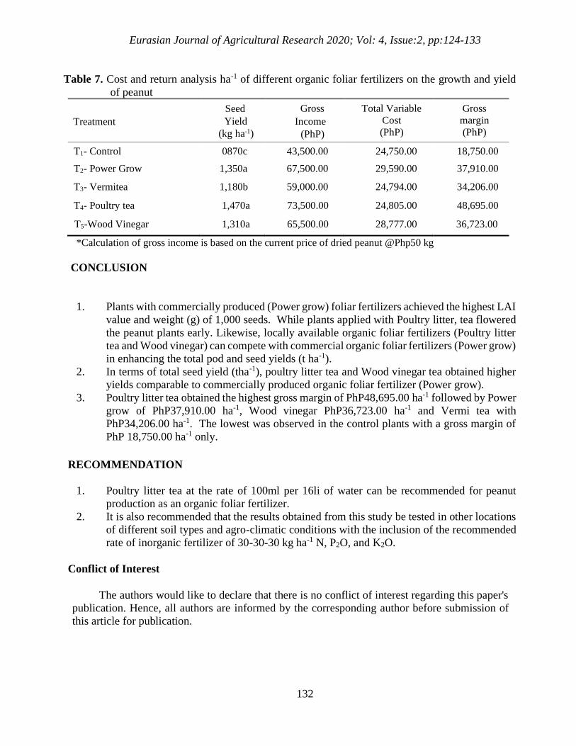
Eurasian Journal of Agricultural Research 2020; Vol: 4, Issue:2, pp:124-133
132
Table 7. Cost and return analysis ha-1 of different organic foliar fertilizers on the growth and yield
of peanut
Treatment
Seed
Yield
(kg ha-1)
Gross
Income
(PhP)
Total Variable
Cost
(PhP)
Gross
margin
(PhP)
T1- Control 0870c 43,500.00 24,750.00 18,750.00
T2- Power Grow 1,350a 67,500.00 29,590.00 37,910.00
T3- Vermitea 1,180b 59,000.00 24,794.00 34,206.00
T4- Poultry tea 1,470a 73,500.00 24,805.00 48,695.00
T5-Wood Vinegar 1,310a 65,500.00 28,777.00 36,723.00
*Calculation of gross income is based on the current price of dried peanut @Php50 kg
CONCLUSION
1. Plants with commercially produced (Power grow) foliar fertilizers achieved the highest LAI
value and weight (g) of 1,000 seeds. While plants applied with Poultry litter, tea flowered
the peanut plants early. Likewise, locally available organic foliar fertilizers (Poultry litter
tea and Wood vinegar) can compete with commercial organic foliar fertilizers (Power grow)
in enhancing the total pod and seed yields (t ha-1).
2. In terms of total seed yield (tha-1), poultry litter tea and Wood vinegar tea obtained higher
yields comparable to commercially produced organic foliar fertilizer (Power grow).
3. Poultry litter tea obtained the highest gross margin of PhP48,695.00 ha-1 followed by Power
grow of PhP37,910.00 ha-1, Wood vinegar PhP36,723.00 ha-1 and Vermi tea with
PhP34,206.00 ha-1. The lowest was observed in the control plants with a gross margin of
PhP 18,750.00 ha-1 only.
RECOMMENDATION
1. Poultry litter tea at the rate of 100ml per 16li of water can be recommended for peanut
production as an organic foliar fertilizer.
2. It is also recommended that the results obtained from this study be tested in other locations
of different soil types and agro-climatic conditions with the inclusion of the recommended
rate of inorganic fertilizer of 30-30-30 kg ha-1 N, P2O, and K2O.
Conflict of Interest
The authors would like to declare that there is no conflict of interest regarding this paper's
publication. Hence, all authors are informed by the corresponding author before submission of
this article for publication.
Eurasian Journal of Agricultural Research 2020; Vol: 4, Issue:2, pp:124-133
133
Authors' Contribution
This work was carried out in collaboration between the senior and junior authors. Both
authors contributed to the conduct of the study up the final editing of the article before
submission for publication.
REFERENCES
Aboelill A.A., Mehanna H.M., Kassab OM., & Abdallah EF. 2012. The Response of Peanut to
Foliar Spraying with Potassium Under Water Stress Conditions. Australian Journal of
Basic and Applied Sciences, 6(8): 626-634.
AVRDC, 2006. Association of International Research and Development Centers for Agriculture
Conference. ACIAR; Australia. 7:27-46pp.
Brandenburg R.L., Jordan D.L., Royals B.R., Mahoney D.J. & Johnson P.D. 2019. Utilization of
Imidacloprid to Control Pests in Peanut in North Carolina. Peanut Science 46:1, 8-13.
Online publication date: 24-Apr-2019.
FAO, 2016. Food and Agriculture Organization of the United Nations, Rome, Italy.
Jordan D.L., Brandenburg R., Brown B., Bullen G., Roberson G. & Shew B., 2017. Peanut
Information. North Carolina Cooperative Extension Service Pub. AG-331. 172 pages.
Kalinova S., Kostadinova S. & Hristoskov A. 2014. Nitrogen use efficiency and maize yield
response to nitrogen rate and foliar fertilizing. Bulgarian Journal of Agricultural
Science, No. 20, pp.
Krawczyk M. L., 2018. Make Your Own Liquid Garden Fertilizer, URL:
http://goo.gl/k80xwW,Date Retrieved: May 16, 2018
Lalog J.T. 2011. Dynapharm Company Incorporation, Quezon City, Philippines
Landon J.R. 1991. Booker Tropical Soil Manual. Longman Scientific and Technical/Ezzex,
England p.474
Marschner H.I. 1997. Mineral nutrition of higher plants. 2nd ed. San Diego: Academic Press,
889p.
Meena S., Malarkodi M. & Senthilvalavan P. 2007. Secondary and micronutrients for groundnut.
A review. Agric. Rev., 28(4):295- 300
Mungkunkamchao T., Kesmala T., Pimratch S., Toomsan B. & Jothityangkoon D. 2013. Wood
vinegar and fermented bioextracts: Natural products to enhance growth and yield of
tomato. Sci. Hortic-Amsterdam. 154, 66-72.
NCT Manual for Legumes. Revised. 2017. Guidelines in conducting National Cooperative
Testing in Field Legumes. Field legumes Technical Working Group. Bureau of Plant
Industry. Diliman, Quezon City. Revised 2017.
Travero J.T. & Mihara M. 2016. Effects of pyroligneous acid to growth and yield of soybean
(glycine max L.). International Journal of Environmental and Rural Development.7,50-
54.
Eurasian Journal of Agricultural Research 2020; Vol: 4, Issue: 2, pp: 134-143
134
NPK Contents of Vermicast as Influenced by Varying Substrates
Christian Ulysses G. Cagasan*, Malvin B. Datan and Warren Kim Siarot
Visayas State University, Visca, Baybay City, Leyte 6521-A, Philippines
* Corresponding author: [email protected]
Abstract
Vermicomposting has been practiced for many years by several researchers for its positive
outcomes toward sustainable agriculture. This study was conducted to assess the N, P, K content
of vermicast as influenced by different substrates. Approximately, four (4) samples in each
substrate as initial sample and vermicast as final sample were collected in the study. Varying
substrates include the use of cow manure, mudpress, banana peelings, some leguminous plants
namely kudzu and kakawate. Substrates and vermicasts among all treatments range from slightly
acidic to slightly alkaline condition. There were considerably decreased in terms of pH, total N,
K from its initial sample (substrate) to its final sample (vermicast) except for total P. Thus, this
could be attributed to the nature and properties of varying substrates fed to the earthworms.
Keywords: Vermicast, organic substrates, total N, P, K
Research article
Received Date: 18 November 2020
Accepted Date:30 November 2020
Eurasian Journal of Agricultural Research 2020; Vol: 4, Issue: 2, pp: 134-143
135
INTRODUCTION
In today’s generation, organic fertilizer had gained more attention due to heavy doses of
chemical fertilizers and pesticides are being used by the farmers to get a better yield of various
crops. These chemical fertilizers and pesticides decreased soil fertility and caused health problems
to the consumers. Due to adverse effects of chemical fertilizers, interest has been stimulated for
the use of organic manures. The Philippine Organic Agriculture Act (RA 10068) was approved to
promote and implement the practice of organic agriculture in the Philippines that will
cumulatively condition and enrich the fertility of the soil, increase farm productivity, reduce
pollution and destruction of the environment. Organic fertilizers are effective in improving soil
fertility and agricultural production by providing essential elements (N, P, K). Nevertheless,
effectiveness of organic fertilizer requires time but its effects are sustainable in the long run. The
release of nutrients from organic fertilizer is gradual and as microorganisms in the soil breakdown
and decomposes the organic matter and makes the nutrients available for plants (Mencide, 2011).
Organic agriculture includes the practices of vermiculture and vermicomposting.
Basically, vermiculture is the science of breeding and raising earthworms. According to
Entre Pinoys (2010), it defines the growing potential for waste reduction, fertilizer production, as
well as an assortment of possible outcomes for the future use.
Vermicomposting is the process of producing organic fertilizer or the vermicompost
derived from different substrates or biodegradable materials that are processed by earthworms.
Composting with earthworms lessens the disposal of agricultural wastes and increases the benefits
of high quality compost (Rogayan, 2010). Furthermore, vermicomposting is a simple
biotechnological process of composting in which certain species of earthworms are used to
enhance the process of waste conversion and produce a better product. The resulting product of
vermicomposting is commonly known as ‘vermicast’. Vermicast is an organic fertilizer which is
of high quality and it is very useful in enriching the soil as soil conditioner. Moreover, vermicast
which is high in microbial enzymes and plant growth regulators and is also fortified with pest
repellence attributes (Vermi Co. 2001 as cited by Ranin, 2015). According to Vasanthi and
Kumaraswamy (1999) vermicast contains essential nutrients essential for plant growth, thus
minimizing the application of chemical fertilizers.
This study was conducted to assess the nutrient content (NPK) of vermicast produce by E.
eugeniae when fed with different mixtures of substrates. This research also aims to identify the
changes of nutrient content of the different substrates after the vermicast production.
MATERIALS and METHODS
Treatments and Experimental Design
The experiment was laid out in a Randomized Complete Block Design (RCBD) with three
replications. T1= 1:1:1 cow manure, mud press, and banana peelings; T2= 1:1:1:1 cow manure,
mud press, banana peelings, and rice straw; T3= 1:1:1:1 cow manure, mud press, banana peelings,
and kudzu; T4= 1:1:1:1 cow manure, mud press, banana peelings, and kakawate.
Eurasian Journal of Agricultural Research 2020; Vol: 4, Issue: 2, pp: 134-143
136
Preparation of Organic Materials and Vermicomposting Process
The use of plastic containers was provided with wire holes at the bottom for drainage. The
substrates such as kudzu, kakawate, rice straw, banana peelings, mudpress and cow manure were
collected in the field. These materials were shredded and mixed into the dried and compounded
cow manure.
Vermi worms used in the study were cultured and collected at Eco-FARMI, VSU, Baybay
City, Leyte. These vermi worms are identified as ‘African night crawler’ or scientifically known
as Eudrilus eugeniae. A total of 500 g of earthworms was introduced into each treatment. The
containers were placed in a cool dark place. Water was applied over the container to prevent from
drying. Casts were collected after 6 weeks after the introduction of the earthworms and nutrient
content was analyzed for pH, N, P, and K.
Data Gathered
Physical properties of vermicompost
This was done by weighing 5 to 10 grams of freshly harvested vermicompost from each
treatment. Samples were oven-dried at 70 degrees Celsius for 24 hours. Moisture content was
calculated using the formula:
%MC = (FW - ODW) / FW x 100
Where:
MC= moisture content
FW= fresh weight of vermicompost (g)
ODW= overn-dry weight of vermicompost (g)
Chemical properties of vermicompost
Vermicast from each treatment was analysed for the following parameters: pH was
determined using potentiometric method (PCARR,1980). Organic Matter (OM) was determined
following the walkley-black method (Nelson and Sommers, 1982). Total Nitrogen (N) was derived
using the equation:
Total N (%) = % OM x 0.05
Total Phosphorus (P) was determined by using the extract from total K analysis, 2 ml aliquot of
the extract from each treatment was placed in test tubes and was added with mixed reagent and
stand for one hour to develop the molybdenum blue color. The sample was measured using B-L
spectronic 20 at 880 nm and computed using the formula:
Total P (%)= ODS x K x (100/0.05) x (1/1000) x dilution
Where:
ODS = optical density
K = slope of standard curve
100 = dilution of digested sample
1/10000 = to express result in % basis
Total Potassium (K) was determined suing Aqua Regia method (Chen and Lena, 2001).
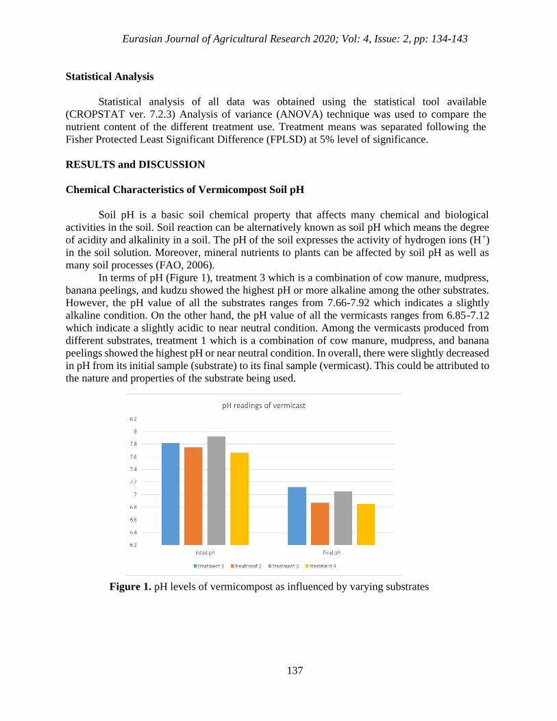
Eurasian Journal of Agricultural Research 2020; Vol: 4, Issue: 2, pp: 134-143
137
Statistical Analysis
Statistical analysis of all data was obtained using the statistical tool available
(CROPSTAT ver. 7.2.3) Analysis of variance (ANOVA) technique was used to compare the
nutrient content of the different treatment use. Treatment means was separated following the
Fisher Protected Least Significant Difference (FPLSD) at 5% level of significance.
RESULTS and DISCUSSION
Chemical Characteristics of Vermicompost Soil pH
Soil pH is a basic soil chemical property that affects many chemical and biological
activities in the soil. Soil reaction can be alternatively known as soil pH which means the degree
of acidity and alkalinity in a soil. The pH of the soil expresses the activity of hydrogen ions (H+)
in the soil solution. Moreover, mineral nutrients to plants can be affected by soil pH as well as
many soil processes (FAO, 2006).
In terms of pH (Figure 1), treatment 3 which is a combination of cow manure, mudpress,
banana peelings, and kudzu showed the highest pH or more alkaline among the other substrates.
However, the pH value of all the substrates ranges from 7.66-7.92 which indicates a slightly
alkaline condition. On the other hand, the pH value of all the vermicasts ranges from 6.85-7.12
which indicate a slightly acidic to near neutral condition. Among the vermicasts produced from
different substrates, treatment 1 which is a combination of cow manure, mudpress, and banana
peelings showed the highest pH or near neutral condition. In overall, there were slightly decreased
in pH from its initial sample (substrate) to its final sample (vermicast). This could be attributed to
the nature and properties of the substrate being used.
Figure 1. pH levels of vermicompost as influenced by varying substrates
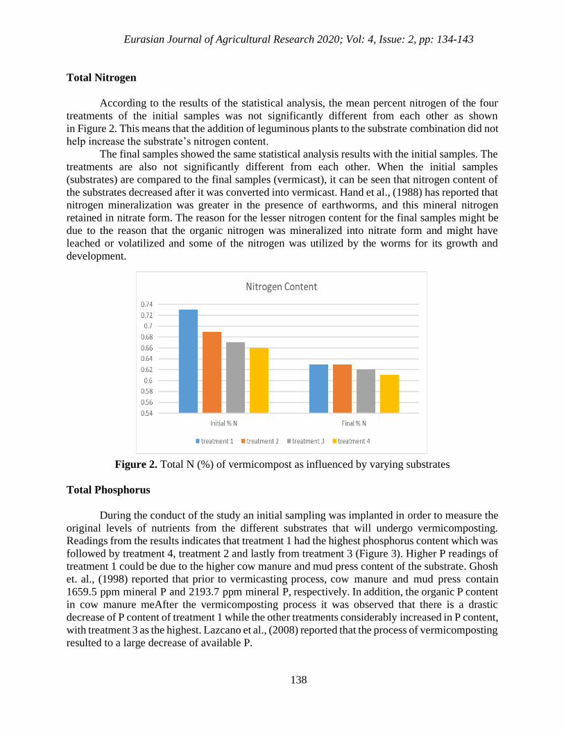
Eurasian Journal of Agricultural Research 2020; Vol: 4, Issue: 2, pp: 134-143
138
Total Nitrogen
According to the results of the statistical analysis, the mean percent nitrogen of the four
treatments of the initial samples was not significantly different from each other as shown
in Figure 2. This means that the addition of leguminous plants to the substrate combination did not
help increase the substrate’s nitrogen content.
The final samples showed the same statistical analysis results with the initial samples. The
treatments are also not significantly different from each other. When the initial samples
(substrates) are compared to the final samples (vermicast), it can be seen that nitrogen content of
the substrates decreased after it was converted into vermicast. Hand et al., (1988) has reported that
nitrogen mineralization was greater in the presence of earthworms, and this mineral nitrogen
retained in nitrate form. The reason for the lesser nitrogen content for the final samples might be
due to the reason that the organic nitrogen was mineralized into nitrate form and might have
leached or volatilized and some of the nitrogen was utilized by the worms for its growth and
development.
Figure 2. Total N (%) of vermicompost as influenced by varying substrates
Total Phosphorus
During the conduct of the study an initial sampling was implanted in order to measure the
original levels of nutrients from the different substrates that will undergo vermicomposting.
Readings from the results indicates that treatment 1 had the highest phosphorus content which was
followed by treatment 4, treatment 2 and lastly from treatment 3 (Figure 3). Higher P readings of
treatment 1 could be due to the higher cow manure and mud press content of the substrate. Ghosh
et. al., (1998) reported that prior to vermicasting process, cow manure and mud press contain
1659.5 ppm mineral P and 2193.7 ppm mineral P, respectively. In addition, the organic P content
in cow manure meAfter the vermicomposting process it was observed that there is a drastic
decrease of P content of treatment 1 while the other treatments considerably increased in P content,
with treatment 3 as the highest. Lazcano et al., (2008) reported that the process of vermicomposting
resulted to a large decrease of available P.

Eurasian Journal of Agricultural Research 2020; Vol: 4, Issue: 2, pp: 134-143
139
The decrease of P of treatment 1 could be due to in growth and multiplication rate of the
earthworms in the organic wastes, which resulted in a differential pattern of uptake of the nutrient
for their body synthesis which caused a lesser release of the remaining P (Ghosh et al., 1998).
Leguminous plants such as kakawate have P levels that ranges from 0.19 to 0.25 based on
the findings of Budelman (1989). Moreover, Kudzu appears to be largely dependent on
mycorrhizal relationships. Plants from Alabama were found to develop 70% root colonization with
mycorrhizal fungi, although only 10% of root tissues showed arbuscule development (Greipsson
and DiTommaso, 2006). Inoculation of vesicular arbuscular mycorrhizal species resulted in higher
tropical kudzu yields and greater magnesium and phosphorus uptake (Dodd et al. 1990). With
these findings, it implies that both these leguminous plant species may contain high amounts of P.
Increased P levels of treatments 3 and 4 may have been caused by the action of earthworms, which
released higher amounts of phosphorus from the organic form and, at the same time, reduced
fixation in different inorganically bound forms. Such effects of earthworms in mineralizing wide
ranges of organic materials with the help of various bacteria and enzymes in the intestine has been
described in detail by Edward and Lofty (1972). Mansell et al. (1981) showed that plant litter
contained more available P after ingestion by earthworms and they attributed this increase to
physical breakdown of the plant material by the worms. Satchell and Martin (1984) found an
increase of 25% in total P of paper-waste sludge, after worm activity.
They attributed this increase in Total P to direct action of worm gut enzymes and indirectly
by stimulation of the microflora. According to Lee (1992) the passage of organic residue through
the gut of earthworm to the plant the released of phosphorus in available form is performed partly
by earthworm gut phosphatases and further released of phosphorus might be attribute to
phosphorus solubilizing microorganism present in worm cast.
After the vermicomposting process it was observed that there is a drastic decrease of P
content of treatment 1 while the other treatments considerably increased in P content, with
treatment 3 as the highest. Lazcano et al., (2008) reported that the process of vermicomposting
resulted to a large decrease of available P. The decrease of P of treatment 1 could be due to in
growth and multiplication rate of the earthworms in the organic wastes, which resulted in a
differential pattern of uptake of the nutrient for their body synthesis which caused a lesser release
of the remaining P (Ghosh et al., 1998).
Leguminous plants such as kakawate have P levels that ranges from 0.19 to 0.25 based on
the findings of Budelman (1989). Moreover, Kudzu appears to be largely dependent on
mycorrhizal relationships. Plants from Alabama were found to develop 70% root colonization with
mycorrhizal fungi, although only 10% of root tissues showed arbuscule development (Greipsson
and DiTommaso, 2006). Inoculation of vesicular arbuscular mycorrhizal species resulted in higher
tropical kudzu yields and greater magnesium and phosphorus uptake (Dodd et al. 1990). With
these findings, it implies that both these leguminous plant species may contain high amounts of P.
Increased P levels of treatments 3 and 4 may have been caused by the action of earthworms, which
released higher amounts of phosphorus from the organic form and, at the same time, reduced
fixation in different inorganically bound forms. Such effects of earthworms in mineralizing wide
ranges of organic materials with the help of various bacteria and enzymes in the intestine has
been described in detail by Edward and Lofty (1972).
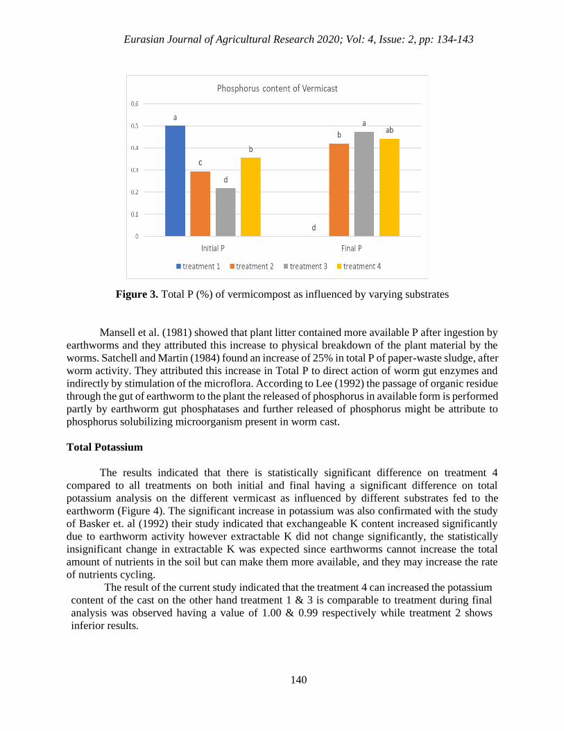
Eurasian Journal of Agricultural Research 2020; Vol: 4, Issue: 2, pp: 134-143
140
Figure 3. Total P (%) of vermicompost as influenced by varying substrates
Mansell et al. (1981) showed that plant litter contained more available P after ingestion by
earthworms and they attributed this increase to physical breakdown of the plant material by the
worms. Satchell and Martin (1984) found an increase of 25% in total P of paper-waste sludge, after
worm activity. They attributed this increase in Total P to direct action of worm gut enzymes and
indirectly by stimulation of the microflora. According to Lee (1992) the passage of organic residue
through the gut of earthworm to the plant the released of phosphorus in available form is performed
partly by earthworm gut phosphatases and further released of phosphorus might be attribute to
phosphorus solubilizing microorganism present in worm cast.
Total Potassium
The results indicated that there is statistically significant difference on treatment 4
compared to all treatments on both initial and final having a significant difference on total
potassium analysis on the different vermicast as influenced by different substrates fed to the
earthworm (Figure 4). The significant increase in potassium was also confirmated with the study
of Basker et. al (1992) their study indicated that exchangeable K content increased significantly
due to earthworm activity however extractable K did not change significantly, the statistically
insignificant change in extractable K was expected since earthworms cannot increase the total
amount of nutrients in the soil but can make them more available, and they may increase the rate
of nutrients cycling.
The result of the current study indicated that the treatment 4 can increased the potassium
content of the cast on the other hand treatment 1 & 3 is comparable to treatment during final
analysis was observed having a value of 1.00 & 0.99 respectively while treatment 2 shows
inferior results.
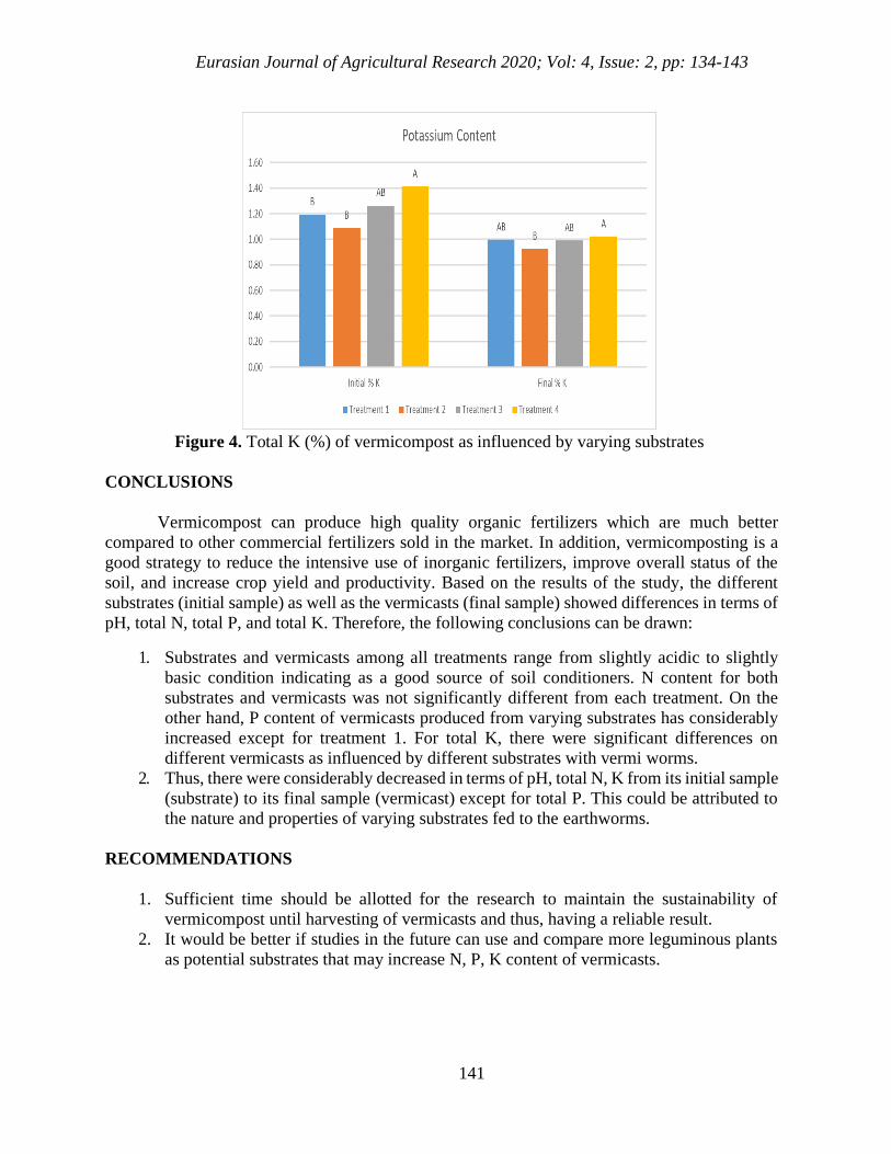
Eurasian Journal of Agricultural Research 2020; Vol: 4, Issue: 2, pp: 134-143
141
Figure 4. Total K (%) of vermicompost as influenced by varying substrates
CONCLUSIONS
Vermicompost can produce high quality organic fertilizers which are much better
compared to other commercial fertilizers sold in the market. In addition, vermicomposting is a
good strategy to reduce the intensive use of inorganic fertilizers, improve overall status of the
soil, and increase crop yield and productivity. Based on the results of the study, the different
substrates (initial sample) as well as the vermicasts (final sample) showed differences in terms of
pH, total N, total P, and total K. Therefore, the following conclusions can be drawn:
1. Substrates and vermicasts among all treatments range from slightly acidic to slightly
basic condition indicating as a good source of soil conditioners. N content for both
substrates and vermicasts was not significantly different from each treatment. On the
other hand, P content of vermicasts produced from varying substrates has considerably
increased except for treatment 1. For total K, there were significant differences on
different vermicasts as influenced by different substrates with vermi worms.
2. Thus, there were considerably decreased in terms of pH, total N, K from its initial sample
(substrate) to its final sample (vermicast) except for total P. This could be attributed to
the nature and properties of varying substrates fed to the earthworms.
RECOMMENDATIONS
1. Sufficient time should be allotted for the research to maintain the sustainability of
vermicompost until harvesting of vermicasts and thus, having a reliable result.
2. It would be better if studies in the future can use and compare more leguminous plants
as potential substrates that may increase N, P, K content of vermicasts.
Eurasian Journal of Agricultural Research 2020; Vol: 4, Issue: 2, pp: 134-143
142
Conflict of Interest
The authors would like to declare that there is no conflict of interests regarding this paper's
publication. Hence, all authors are informed by the corresponding author before submission of this
article for publication.
Authors’ Contribution
This work was carried out in collaboration between the senior and junior authors. Both
authors contributed to the conduct of the study up the final editing of the article before submission
for publication.
REFERENCES
Basker A., Macgregor A.N. & Kirkman J.H. 1992. Influence of soil ingestion by earthworms
on the availability of potassium in soil: An incubation experiment. Department of Soil
Science, Massey University, Palmerston North, New Zealand. 14: 300-303.
Budelman A. 1989. Nutrient composition of the leaf biomass of three selected woody
leguminous species. Agroforestry Systems 8:39-51.
Chen J.H. & Lena. 2001. Effect of substrate concentration on bioleaching of metal-contaminated
sediment, J. Haard. Mat. 82, 77-89 pp.
Dodd J., Arias I., Koomen I. & Hayman D. 1990. The management of populations of vesicular-
arbuscular mycorrhizal fungi in acid-infertile soils of a savanna ecosystem. Plant Soil,122:
229-240.
Edward C.A. & Lofty J.R. 1972. Biology of Earthworms. Chapman and Hall, London.
Entre Pinoys. 2010. Retrieved on September 29, 2010 from
http://www.mixph.com/2006/12/vermiculture-the-management-of-worms.html.
Food and Agriculture Organization of the United Nations (FAO), 2006. Guidelines for soil
description (4th ed.). Rome, Italy.
Ghosh M., Chattopadhyay G N. & Baral K. 1998. Transformation of phosphorus during
vermicomposting. Bioresource Technology, 69 (1999) 149-154.
Greipsson S. & Ditommaso A. 2006. Invasive non-native plants alter the occurrence of
arbuscular mycorrhizal fungi and benefit from this association. Ecol. Restor. 24: 236-241.
Hand P., Hayes W.A., Frankland J.C. & Satchell J.E. 1988. Vermicomposting of cow slurry.
Pedobiologia. 31. 199-209.
Lazcano C., Gómez-Brandón, M. & Domínguez J. 2008. Comparison of the effectiveness of
composting and vermicomposting for the biological stabilization of cattle manure.
Chemosphere 72 (2008) 1013–1019.
Lee K.E. 1992. Some trends opportunities earthworm research or Darwin children. The future of
our discipline. Soil Biol. Biochem., 24: 1765-1771.
Mansell G.P., Syers J.K. & Gregg P.E.H.1981. Plant availability of phosphorus in dead herbage ingested by surface-casting earthworms. Soil Biol. Biochem. 13, 163–167.
Eurasian Journal of Agricultural Research 2020; Vol: 4, Issue: 2, pp: 134-143
143
Mencide B.S. 2011. Effects of guano and inorganic fertilizer on the growth and yield of lowland
rice. Undergrad. Thesis, VSU, Baybay, Leyte. 40 pp.
Nelson D.W. & Sommers L.E. 1982. Total carbon, organic, and organic matter. Pp 539-579.
In: A.L. Page, R.H. Miller and D.R Reeney (eds). Methods of soil analsysis Part2:
Chemical and microbiological properties. American society of Agronomy, Inc., Madison,
Wisconsin USA.
PCARR, 1980. Standard methods of analysis for soil, plant tissue, water and fertilizer. Farm and
systems res. Div. Philippine Council for Agriculture and Resources Research, Los. Banos.
164 pp.
Ranin L.A. 2015. Physical and chemical characteristics of vermicompost as affected by different
feed formulations. Thesis, VSU, Philippines.
Rogayan D. Jr. 2010. Vermiculture and vermicompost.
SatchelL J.E. & Martin, K. 1984. Phosphate activity in earthworm faeces. Soil Biol. Biochem.
16, 191–1.
Vasanthi D. & Kumaraswamy K. 1999. Efficacy of Vermicompost to Improve Soil Fertility and
Rice Yield.
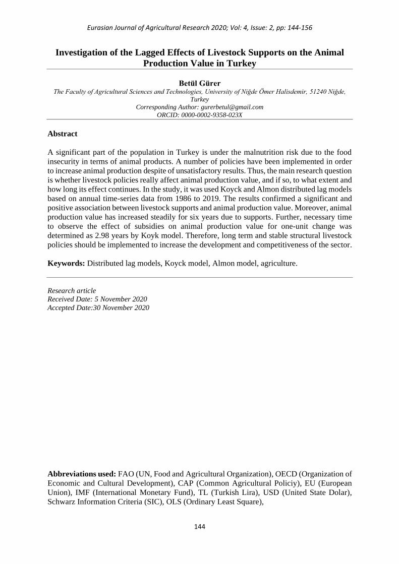
Eurasian Journal of Agricultural Research 2020; Vol: 4, Issue: 2, pp: 144-156
144
Investigation of the Lagged Effects of Livestock Supports on the Animal
Production Value in Turkey
Betül Gürer The Faculty of Agricultural Sciences and Technologies, University of Niğde Ömer Halisdemir, 51240 Niğde,
Turkey
Corresponding Author: [email protected]
ORCID: 0000-0002-9358-023X
Abstract
A significant part of the population in Turkey is under the malnutrition risk due to the food
insecurity in terms of animal products. A number of policies have been implemented in order
to increase animal production despite of unsatisfactory results. Thus, the main research question
is whether livestock policies really affect animal production value, and if so, to what extent and
how long its effect continues. In the study, it was used Koyck and Almon distributed lag models
based on annual time-series data from 1986 to 2019. The results confirmed a significant and
positive association between livestock supports and animal production value. Moreover, animal
production value has increased steadily for six years due to supports. Further, necessary time
to observe the effect of subsidies on animal production value for one-unit change was
determined as 2.98 years by Koyk model. Therefore, long term and stable structural livestock
policies should be implemented to increase the development and competitiveness of the sector.
Keywords: Distributed lag models, Koyck model, Almon model, agriculture.
Research article
Received Date: 5 November 2020
Accepted Date:30 November 2020
Abbreviations used: FAO (UN, Food and Agricultural Organization), OECD (Organization of
Economic and Cultural Development), CAP (Common Agricultural Policiy), EU (European
Union), IMF (International Monetary Fund), TL (Turkish Lira), USD (United State Dolar),
Schwarz Information Criteria (SIC), OLS (Ordinary Least Square),
Eurasian Journal of Agricultural Research 2020; Vol: 4, Issue: 2, pp: 144-156
145
INTRODUCTION
Animal production has been significantly decreased in Turkey per capita, which was
much faster especially in recent years. Per capita daily protein and energy production from
animal origin can be considered as an important indicator to show relationship between animal
production and nutrients. When this indicator is taken into consideration, it can be said that
although energy and protein production level of foodstuff in Turkey is adequate, production of
foods from animal origin is not at the sufficient level to ensure adequate nutrition. According
to FAO data, per capita total energy supply in 2017 was 3720 kcal/day, while per capita energy
supply from animal products was 567 kcal/day. Similarly, per capita total protein consumption
quantity was 102.2 gr/day, while per capita animal protein supply was 35.6 gr/day. Experts
suggest that the average protein requirement of the individuals for healthy and balanced
nutrition should be average 1 gr for each kilogram of body weight per day, of which at least
42% (about 35-40 gr) should be provided from animal source foods (Saçlı, 2007). Compared
to developed countries, a considerable part of the population in the country is under the
malnutrition risk due to problems in terms of availability and accessibility of animal products.
For example, daily per capita total protein supply and animal protein supply were 103.85 gr and
60.38 gr in EU, 109.6 gr and 69.78 gr in USA, respectively (FAO, 2020).
Livestock sector has faced many challenges in Turkey. Some of these challenges are
small scale and dispersed enterprises, low productivity, insufficient livestock policies and the
lack of sufficient support.
Livestock policy is one of the basic policies of every country regardless of development
level. Although it is not sufficient, livestock sector has been supported by the different
agriculture policy measures since the establishment of the republic in Turkey. The main
purposes of the support policies are to provide sufficient nutrient for the society, to reach self-
sufficiency in the animal production, to increase the productivity of holdings, to increase
income of livestock farmers and to ensure rural development.
In Turkey, there has been a positive relationship between livestock supports and animal
production value by the years. Increasing animal production supports increase animal
production value. According to the Ministry of Agriculture and Forestry data, livestock support
amount reached to 3 million TL in 2000s. Last ten years, livestock supports have increased
more than 100% and the share of that in agricultural subsidies reached to 34.6% in 2019. The
value of animal production was also reached to 259 billion TL by increasing 22 times in the
same period (TurkStat, 2020).
In recent years, the number of studies about the effects of agricultural subsidies on
various indicators such as production, farm income, and economic growth are increasing. In
line with the diversity of agricultural policy programmes, empirical studies analysed different
aspects of government subsidies in agriculture. Vozarova and Kotulic (2015), for instance,
found that there was a strong correlation between amount of gross agricultural production and
the volume of subsidies granted in Slovakia. Malan et al. (2016) found that price distortions
had a strong, significant impact on cocoa and cotton yields in Africa. Skreli et al. (2015) found
that government subsidy had a clear, positive impact on the area planted with olives and
vineyards in Albania. Minviel and Latruffe (2014) found that targeted investment subsidies
were positively associated with farm’s technical efficiency, while Bojnec and Latruffe (2013)
found that agricultural subsidies reduced the technical efficiency of Slovenian farms but
improved their profitability. Brady et al. (2009) analysed the impact of decoupled direct
payments on biodiversity and landscape and found that eliminating the link between support
payments and production had only limited negative consequences for the landscape. Semerci
and Çelik (2017) examined the utilisation level of subsidies in dairy cattle enterprises in Hatay
Eurasian Journal of Agricultural Research 2020; Vol: 4, Issue: 2, pp: 144-156
146
province of Turkey and found that livestock subsidies were decreasing the production costs and
increasing farmers’ income significantly.
The various policy support mechanisms may affect production decisions in the
agriculture sector. One of the critical issues in analysing the impact of subsidies in agriculture
is to recognise the long lags involved. Especially, this situation is very crucial in livestock
because the sector has the high investment cost. Supports on livestock sector today might result
with investment of new enterprises and improvement of current enterprises in the sector in the
future. Unlike crop production, one or more years is necessary to see the effect of supports on
animal production sector. When taking into consideration the lag between the production of
animal products and marketing, it would be seen that the length of lag of that is longer than that
of crop production.
In order to determine the appropriate policy settings in the livestock, a necessary
condition is to understand the relationship between livestock subsidies and the value of animal
production. Therefore, the objective of this study was to investigate the role of subsidies in
livestock production value. However, as well as the impacts of the subsidies are quite extensive,
the study only focused on the reflection of subsidies on production value. In particular, the
paper examines the short- and long-run pass-through of subsidies to animal production value in
Turkey. Thus, the aim was not only to examine any relationship between subsidies payments
and animal production value but also to investigate the scope and time span of this relationship.
Investigating the time effect of livestock subsidies has substantial importance, as it offers us
with the knowledge related whether subsidies payments cause future benefits and increase
livestock value in the long run. There is no empirical evidence showing the association between
livestock supports and animal production value from long lags perspective. In this context, this
is the first study examining the long-term effect of subsidies on animal production value of
livestock sector by using distributed lag models. Within this scope, analyses were conducted to
see whether livestock policies really affect the production value of the sector and if so, to what
extent and how long its effect continues.
MATERIAL and METHODS
Data
The data of the study were collected from records of Turkish Statistical Institute
(TurkStat), Ministry of Agriculture and Forestry (MAF), and OECD (Producer Support
Estimates database). The data related to the value of livestock production and livestock supports
were put yearly from 1990 to 2019. Deflated values of animal production and supports
according to producer price index were used in study. All series have been transformed in
natural logarithms, because otherwise, with trending data, the relative error might decline over
time and this is inappropriate (Tiffin and Dawson, 2000). In the models, total animal production
value was represented as AVt variable and total livestock supports amount was presented as
Subt variable.
Figure 1 gives animal production value and livestock supports by the years in Turkey.
Between 1990-2019 years, while total livestock supports with constant price has increased by
3.7 times, total animal production value with constant price has increased by 6.0 times.
Theoretical Framework
Distributed lag models have a specific place in literature of economics because it allows
us to analyse the behaviour of economic units (consumer, producers, etc.) based on appropriate
dynamic models.
Eurasian Journal of Agricultural Research 2020; Vol: 4, Issue: 2, pp: 144-156
147
Studied and used for the first time by Irving Fisher (Isyar, 1999), distributed lag models
take into account not only the present year value but also the previous year values of defining
variable (Erdal et al., 2009). If the length of lags for explanatory variable is not determined, this
type of model is called an as “infinite lag model” and shown as follows: Yt = α + β0 Xt + β 1 Xt-1 + β2 Xt-2 + …+ ut (1)
On the other hand, if length of lags for explanatory variable is defined as k, this type
model is called “finite distributed lag model” and can be written as: Yt = α + β0Xt + β1Xt-1 + β 2Xt-2 +…+β kXt-k +ut (2) Mostly, dependent variable (Y) responds to the explanatory variable (X) after some time
which is called as “lag period”. Unknown parameters (α, β0, …, βk) in these models can be
estimated by the ordinary least square method (OLS). But this estimation has certain drawbacks
about the lack of information on maximum length of lags and decline of degrees of freedom.
Besides, the most important problem is about multicollinearity between explanatory variables
(Gujarati, 2004) that leads to biased results. To overcome these challenges in distributed lag
models, Koyck (1954) has developed one of the distributed lag models. Koyck’s method
assumes that effects of lags of explanatory variable on dependent variable decrease
geometrically: βk= β0λk k=0,1,… (3)
Where λ ( 0<λ<1) is known as the rate of decline of the distributed lag. Besides, 1−λ is
defined as the speed of adjustment. In other words, each estimated β coefficient is less than the
previous β coefficient. The value of lag coefficient, βk, depends on the value of λ. The closer
the value of λ to one, the slower the rate of decline in βk is. Whereas, the closer the value of λ
to zero, the quicker the decline in βk is. Mean lag is the weighted average of all lags involved
and can be formulated as (Gujarati, 2004): Mean lag = λ / (1-λ) (4) Mean lag provides the summary information of the speed with which the dependent
variable (Y) responds to the explanatory variable (X). For instance, assume that it is used annual
data, and mean lag is found as “6,” this means that it takes “6” years’ for the effects of changes
in explanatory variable (X) to be perceived on dependent variable (Y). The features of Koyck
scheme assumes nonnegative values for λ and λ<1 and finite of the sum of β’s (Gujarati, 2004).
As a result, Koyck method on the infinite model can be formed as: Yt = α + β0Xt + β0 λ Xt-1 + β0 λ 2Xt-2 +…+ut (5)
In this form, linear regression method cannot be applied to this form of model (Equation
5), since there are large number of parameters to be estimated and λ coefficients are highly
nonlinear form. As a solution, Koyck suggests to take lag by one period back to obtain following
form: Yt-1 = α + β0Xt-1 + β0 λ Xt-2 + β0 λ2Xt-3 +…+ut-1 (6)
Thereafter, the equation (7) is obtained as a result of equation (6) multiplied by λ. λ Yt-1 = α + λ β0Xt-1 + β0 λ2 Xt-2 + β0 λ3Xt-3 +…+ λ ut-1 (7)
The equation (8) is got by subtracting equation (7) from equation (5): Yt - λ Yt-1 = α (1- λ )+ β0Xt +( ut-λut-1) (8)
Afterwards, the model can be rearranged as: Yt = α (1- λ )+ β0Xt + λ Yt-1 + vt (9)
where vt in Equation (9) is equal to ut-λut-1 and the moving average of ut, ut–1. This procedure
just described is known as Koyck transformation and Equation (9) is also called as Koyck
model. In Koyck model, lag values of explanatory variable (X) are not defined to solve
multicollineratiy problem. Therefore, Koyck model needs to estimate α, β and λ only to solve
the distributed lag model (Gujarati, 2004).
Eurasian Journal of Agricultural Research 2020; Vol: 4, Issue: 2, pp: 144-156
148
Another model of distributed lag models is the Almon model. Since the β parameters of
the Koyck model are continuously decreasing, many other situations that may be different can
be ignored. For these reasons, in the case of the Almon model, β 's may increase first, then
decrease, or decrease first and then increase.
Shirley Almon (1965) follows the “Weierstrass Theorem” in Mathematics and assumes
that βi can be approximated by a suitable-degree polynomial in i, the length of the lag. There
are two basic equations that generates the cruxes of Almon model (Gujarati, 2004); Yt = α + β0Xt + β1Xt-1 + β 2Xt-2 +…+β kXt-k +ut (10) βi = a0 + a1 i + a2i2 +…+anin (11)
βi is an nth-degree polynominal in i . It is assumed that n (the degree of the polynomial)
is less than k (the maximum length of the lag).
In the stage of modeling, firstly suitable time lag is acquired by using Schawarz Information
Criteria (SIC) or Akaike Information Criteria (AIC).
In the model, the lag that makes AIC and SIC value the minimum value is considered
to be the suitable time lag (Kutlar, 2000). The notations related to AIC and SIC values are
defined in Equation 12 and Equation 13; AIC= T ln +2n (12) SIC= T lnσ2 + n ln(T) (13) T = Number of usable observations, n = Number of parameters estimated, σ2 = KKT /Tn
=the highest probability estimation or error variance related to the model and KKT = Residual
sum of squares (RSS).
After the determination of the suitable time lag, the polynomial degree needs to be
determined. Polynomial degree is at least one more than the number of each flection (maximum
or minimum points). The determination of the polynomial degree is mostly subjective. Thus, to
determine these criteria is up to the researcher’s forecasting (Akın, 2002). In this study, based
on SIC the most suitable time lag has been determined as “X-6” season and polynomial degree
has been determined as second-degree polynomial by forecasting. After the determination of
the polynomial degree, the suitable “Z” values are acquired. In the acquisition of “Z” values,
The Equations 14, 15 and 16 can be used;
Z0t= ∑ Xt-i
k
i=0
(14)
𝑍1𝑡 = ∑ 𝑖𝑋𝑡−𝑖 (15)
𝑘
𝑖=0
𝑍2𝑡 = ∑ 𝑖2𝑋𝑡−𝑖
𝑘
𝑖=0
⋯ … … … … … … … … … … … … … … … (16)
In the Almon scheme, Y is regressed according to “Z” variables that have been
generated, not according to “X”. The equation (17) can be estimated by usual OLS method. So,
the forecast of α and ai (a0, a1 and a2) would provide all the statistical conditions required, on
condition that possibility disturbance term fulfils the forecast of classical linear regression
Model (Gujarati, 2004).
Yt=α+α0Z0t+α1Z1t+α2Z2t+ut (17)
Moreover, when the “a” coefficients are obtained from equation (17), the original βi’s
are estimated from equation (11) as follows in the Equations 18, 19, 20 and 21.
Eurasian Journal of Agricultural Research 2020; Vol: 4, Issue: 2, pp: 144-156
149
β0 = a0 (18) β1 = a0+ a1 + a2 (19) β2 = a0+ 2a1+ 4a2 (20) β3 = a0+ 3a1+ 9a2 (21) ……………………….. βk = a0+ ka1+ k2a2 Thus, the distributed lag model can be interpreted in according to equation (10) by
putting into their places of the obtained βi values.
Although there are studies using Distributed Lag Models in agriculture sector, none of
these studies is from subsidies perspective. For instance, several authors studied the relationship
between production and price in buffalo milk (Çelik, 2015a), in sheep milk (Çelik, 2015b) and
cow milk (Özsayın, 2017). Within this context, this study has the potential to add benefit to
agricultural policy aspect of the sector by using this methodology.
RESULTS and DISCUSSION
An Overview of the Livestock Sector in Turkey
Livestock sector has a significant potential in Turkey. The sector's contribution to farm
income is substantial, and livestock production and marketing activities are important for the
economic development of rural areas in Turkey (Yurdakul et al., 1999). Animal production
including meat, milk, eggs, honey, wool, and hides constituted approximately 32.2% of total
agricultural production value in 2019 (TurkStat, 2020). However, this value is comparatively
fairly low than that in developed countries, which is about 60-70%. In recent years, Turkey's
livestock sector has displayed an increasing trend in terms of productivity but a decreasing trend
for per capita consumption of animal products (Akbay and Boz, 2005).
Historically, according to livestock inventory data, the number of bovine and small
ruminant animals were increasing until the early 1980s but it has decreased after this date.
Between 1980-2009 years, the number of bovine animals decreased by 36.1% (about 6 million
heads) and the number of small ruminants decreased by 60.3% (about 41 million head). As
from 2009, it has been observed an increase in the number of livestock due to the increasing
supports. Thus, the number of cattle and buffaloes in Turkey reached to 17.9 million heads with
an increase of 65.3% in 2017 compared to 2009. The number of sheep and goat in Turkey
reached to 48.5 million heads with an increase of 80.4% in 2019 compared to 2009 (TurkStat,
2020).
In contrast to the red meat sector, the numbers of poultry and beehives have steadily
increased during the same period. Poultry products are gaining importance and account for a
major share of animal products in human diets in Turkey as in many other countries (Akbay
and Boz, 2005). By 2019, Turkey had 348.8 million head of poultry and 8.1 million beehives,
almost 6 times higher for poultry and 3.7 times higher for beehives than those numbers in 1980.
Considering the animal number and production, the level of yields per animal in Turkey
are considerable low in comparison with the developed countries. Despite the significant
growth in carcass and milk yields, the productivity increases have not been sufficient to prevent
reduction in output potential caused by declining animal inventories, particularly in the sheep
sector (Koc et al., 2001).
For the past 100 years, Turkish government has implemented a number of policies
aimed to improve production of animal production but the outcomes have been dissatisfactory.
The supports for plant production was substantial within the agricultural policies in Turkey,
while supports for animal production had been remained at a more limited level. As a result of
this, important problems had begun to be experienced in livestock sector.
Eurasian Journal of Agricultural Research 2020; Vol: 4, Issue: 2, pp: 144-156
150
Implemented policies in this period had adversely affected both the quality and quantity
of animal production. This situation had also caused the ambivalent in product prices and
producers’ incomes. In consequence of these adverse developments, in 1987, the government
introduced “Agricultural Packet” measures, which particularly concerned livestock sector. As
a part of this measure, subsidy payments for import of breeding animal, mixed feed sales and
incentive premium payment for milk were initiated. Incentive premium payments for red and
poultry meat were implemented periodically, but these subsidies were terminated in 1995. In
addition, incentive premium was paid to private sector in order to support artificial
insemination. Medicines used for animal health had been reimbursed at a rate of 20% over the
drug price. However, these measures had not been sufficient, and as a result livestock had
declined and Turkey’s food imports have gradually increased after the 1980s (Aral and Cevger,
2000; Sayın, 2001).
In consequence of internal dynamics and external factors, the comprehensive
agricultural reform had been added to agenda since 2000. One of the main reasons of
agricultural policy reforms was the reducing the burden of agriculture on the economy
especially after the economic crises in these years. Besides this internally factor, internationally
binding and non-binding pressures played an important role in the reform initiatives. These
were the Uruguay Round agreement on agricultural trade, the accession negotiations with the
EU which put ‘adjusting to the CAP’ on political agenda, the 1999 agreement with the IMF
reforming agricultural policy, and the agreement with the World Bank as an important financial
supporter for the Agricultural Reform Implementation Project (ARIP) (Köse, 2012).
Therefore, after 2000, the aims of agricultural policies within the context of the
agriculture reform had been changed considerably. The direct income support based on land
(decoupled from type or quantity of production) had put into force as the main policy instrument
instead of almost all input and output price subsidies and grants in various forms. In 2000,
Decree of Supporting Livestock numbered as 2000/467 under “The Project of Supporting and
Improving Livestock” was initiated for following five-year period in order to develop livestock
and increase animal production. Along with this decree, incentives were brought for artificial
insemination, calves born by artificial insemination, equipment to use for artificial
insemination, animals with breeding certificate, and keeping the stud book records in order to
bring the genetic breeding more efficient and common. Furthermore, supports such as breeding
heifer support, beekeeping and honey support, support of incentive pay for meat and milk,
forage crops support, and fisheries were implemented (Anonymous, 2000; Ertürk et al., 2015).
In 2005, new decree numbered as 2005/8053 had been entered into force but it was withdrawn
after one year. In the scope of this new decree, the supports of “payment per animal” were
implemented as livestock policy instruments and artificial insemination supports were
terminated (Saçlı, 2012).
In 2006, a legal framework was formed for supports via The Law of Agriculture entered
into force (Ertürk et.al., 2015). The purpose of this law was to determine necessary policies and
make regulations in order to be developed and supported of agriculture sector and rural area in
line with development plans and strategies. Within this scope, main objectives of the support
instruments for livestock were to increasing of coarse fodder production and animal breeding,
increasing productivity, specialisation of animal enterprises, providing of animal health and
welfare, ensuring the hygiene conditions in the enterprises, incentive of animal identification
system, processing and marketing of animal products and their control, monitoring and
improvement of standards, supporting of aquaculture (Anonymous, 2006).
Since 2017, Turkey has been initiated to implement a new subsidy program, which is
called as “National Agriculture Project”. This project covers a new subsidy allocation system
for agricultural products.
Eurasian Journal of Agricultural Research 2020; Vol: 4, Issue: 2, pp: 144-156
151
The project was built on 941 agricultural basins based on climate and soil to subsidize
specific crops for each zone. One of the important components of the project is “Domestic
Production Support Model in Livestock”. The main objective of this component is to eliminate
import-based husbandry and to increase the livestock inventory in Turkey. The sub-components
of the livestock subsidies are the establishing areas for grazing animals, the establishing
breeding pregnant heifers’ production centers, the establishing breeding ram and male goat
production centers in order to produce high quality male stock for the other herds, the
establishing buffalo production centers, the establishing resting and control/inspection stations
in order to reduce the number of animal deaths and diseases from rough transport conditions
(MAF, 2020).
In sum, especially from 2000s, Turkey has made enormous strides in terms of livestock
policies. In this period, both the amount of new regulations in livestock supports and the share
of livestock subsidies in total agricultural supports increased. As in recent years, many of the
subsidies were given to livestock. While the share of livestock subsidies in total support was
0.02% in 1990, it reached 0.5% in 2000, 9.6% in 2005, 20.3% in 2010 and 34.6% in 2019
(MAF, 2020). Roughly 4.2 billion TL (0.5 billion USD) support was provided for the livestock
sector in 2019, with 12 percent increase compared to the previous year.
The Results of Almon and Koyck Models
Almon and Koyck models, which are distributed lag models, were used to investigate
the association between livestock support payments and animal production value in this study.
In order to determine whether or not it was appropriate to distributed lag models of the
relationship between these two variables at the studied period, a correlation analysis was
performed. A correlation coefficient of 0.97 was found, indicating a strong relationship between
the two variables. This result indicated that animal production value and livestock subsidies
relationship could be studied using distributed lag models.
In order to form Koyck and Almon model, it was necessary to determine lag length of
livestock subsidies series. For this purpose, it was used Schwarz Information Criteria (SIC).
The lag length is found by determining value making the smallest to Schwarz value (Acquah
2010). At this stage, it was started with a very great k value (lag length) without making any
restriction for the form of distributed lag (Özsayın, 2017). There is no general rule for
determining the maximum lag length, so researchers usually determine this length by
themselves subjectively. In the literature, the maximum lag length for monthly series is
determined as 12 or 24, while this number can be set as 4, 8 or 12 for seasonal series (Kadılar
2000). In this study, maximum lag length was taken as “8” since dataset was yearly. In
accordance with schwarz criterion value, which was determined for different lag lengths in
Table 1, the smallest value of SIC was obtained as “6”.
As it is seen in Table 1, the effect of livestock subsidies on animal production value
would disappear after six years. After determining the lag length, the Koyck model was
estimated to deal with multicollineratiy problems. The Koyck model estimation result was
reported in Table 2. According to the results, livestock subsidies (Sub) had positive significant
effect on animal production value (AV) with adjusted R2 of 0.83 in value.
To investigate necessary time period for one-unit change in subsidies to have a
perceptible effect on animal production value, it was calculated mean lags using Koyck model.
According to the results, it took 2.98 years for subsidies to be felt on production value for
livestock sector. (Table 2).
Considering that βk = β0λk, it can be reached regression equation (22) by using β0 and λ
derived from Koyck model. Yt = α+β0Xt+β1Xt−1+β2Xt−2+…..+υt and βk = β0λk k = 0,1,… (22)
Eurasian Journal of Agricultural Research 2020; Vol: 4, Issue: 2, pp: 144-156
152
AV=1.630+0.054Subt+0.040Subt-1+0.030Subt-2+0.023Subt-3+0.017Subt-4+0.013Subt-5 + 0.010Subt-6 (23)
Calculation of the coefficients reported in equation (23) are as follows: β0 = (λ0 β0)= 0.054; β1 = (λ1 β0 )= 0.040 ; β2 = (λ2 β0 )= 0.030; β3 =(λ3 β0 )= 0.023;
β4=(λ4β0)=0.017; β5 = (λ5 β0 )= 0.013; β6 = (λ6 β0 )= 0.010 The effect of subsidy expenses on production value are geometrically declining as seen
in equation (23), since λ is between 0 and 1.
However, while Koyck model suggests that lag coefficients undergo geometric decay,
that is, the values of the lag coefficients decline in the pattern of a geometric progression, Almon
model assumes that a polynomial of a fairly low degree can represent the lag coefficients
(Watson & Teelucksingh 2002). For this reason, The Almon model is more flexible than the
Koyck model in that it allows the effect of X on Y to change over time.
In the Almon model, “βk = α0 + kα1 + k2 α2 “assumption is used instead of βk = β0λk
assumption. It must be calculated α0, α1, α2 values in order to be able to apply this assumption.
In the Almon sequence that is created, the regression of dependent variable is acquired
according to “Z” variables that have been generated, not according to “explanatory variable”.
Since polynomial model degree was determined as second, the empirical equation considering
Z values can be written as follows (equation 24) according to results of the model in Table 3. Yt= α+ α0Z0t + α1Z1t + α2Z2t +ut Yt= 6.425 + 0.087Z0t + 0.012Z1t -0.013Z2t + ut (24) The result in Table 3 showed that the overall model was statistically significant with
having relatively high the adjusted R-squared value (87%). Yt= α + β0 Subt +β1 Subt-1 +β2 Subt-2 +β3 Subt-3+β4 Subt-4 +β5 Subt-5+ β6 Subt-6 + β7 Subt-7
Yt= 6.425 – 0.062 Subt + 0.013Subt-1 + 0.063Subt-2 + 0.087Subt-3+ 0.086Subt-4 + 0.060Subt-
5 + 0.008Subt-6
According to Almon model results in Table 4, livestock support payments seemed to
have a negative effect on animal production value in the current year, but after one year, this
affect changed the sign and became positive. However, the parameters of supports “t-0” and
from “t-2” to”t-5” found statistically significant. One unit increase for previous year in the
livestock subsidies caused an increasing on current animal production value by 0.013 unit, this
value fallowed an increase of animal production value for “t-2” period by 0.063, for “t-3” period
by 0.087 and for “t-4” period by 0.086. After 5 years, the subsidies effect on production value
decreased but impact was the positive.
CONCLUSION
Since the beginning of 2000s, agricultural policies related to livestock have changed
rapidly and continuously. Besides, the share of that in total agricultural supports has also
increased. Therefore, it has been necessary to carry out a study on determination of the effect
of these changing supports on the value of animal production considering the lagged values.
For this purpose, this study investigated that the existence and the effect of long-term
relationship between animal production and subsidies in Turkey which has the problem of
inadequate animal food production for many years. According to results, support payments for
animal production came out as an important factor that would affect the farmer’s production
process. The results confirmed the expectations that subsidy payments could increase the
attractiveness of livestock investments and accordingly, increase producer supply for the animal
production. Besides, relatively high the adjusted R-squared value from Almon model indicated
that 87% of the changes in animal production value could be explained by the support payments
and lagged values of that.
Eurasian Journal of Agricultural Research 2020; Vol: 4, Issue: 2, pp: 144-156
153
Moreover, there was an increase in the value of animal production in the following years
by means of the supports provided to livestock. According to the results provided by Almon
model, the effect of this increase continued until the fourth year. After fourth year, this effect
went on increase decreasingly. The Koyck model result showed that a 10% increase in subsidies
would lead to an increase in animal production of 0.54% in current year, 0.40% in the following
year, 0.30% in three years and 0.23% in the fourth year. This effect remained decreasingly until
sixth year. According to Koyck model results, necessary time period for being felt on animal
production value of one-unit change in subsidies took 2.98 years. As it could be seen in this
study, livestock support payments could not only increase the value of animal production for
current year, but also could increase the production value of the following years. In sum, animal
production value was sensitive to the livestock subsidies of past periods. Supports had effect
positively on farmers’ decision and this effect remained 6 years.
In the last 100 years, the supports for plant production were substantial within the
agricultural policies in Turkey, while supports for animal production has been remained at a
more limited level. As a result of this, important problems have begun to be experienced in
livestock sector. Implemented policies in this period have adversely affected both the quality
and quantity of animal production. This situation had also caused the ambivalent in product
prices and producers’ incomes. The major problems of animal production in Turkey are low
productivity and high production costs. This is closely related to the race characteristics of
existing animals as well as animal husbandry and feeding. Besides that, some factors such as
the high cost of animal feed, which is the important cost factor in animal breeding, small-scale
production, unorganized and inadequacy of marketing infrastructures affects adversely the
competitiveness of the sector. According to these results, animal production problem in Turkey
should be solved by long term and stable structural livestock policies to be provided for
livestock and the sector’s competitiveness can be increased.
The study only aimed to focus on the investigation of the link between livestock
subsides and livestock production value. However, further research is needed to the
investigation of the effects of these subsidies from the various aspects such as socio-economic
and productivity on the sector by based on comprehensive survey data.
REFERENCES
Acquah H.D. 2010. Comparison of Akaike Information Criterion (AIC) and Bayesian
Information Criterion (BIC) in selection of an asymmetric price relationship. J. Dev.
Agric. Econ., 2(1):1-6.
Akbay C. & Boz İ. 2005. Turkey's livestock sector: production, consumption and policies.
Livestock Research for Rural Development. 17, Article105.
Akın F. 2002. Ekonometri, Ekin Kitabevi, Bursa,Turkey.
Almon S. 1965. The Distributed Lag between Capital Appropriations and Expenditures.
Econometrica, 33(1):178 – 196.
Anonymous. 2000. Council of ministers’ decision on supporting of livestock no. 2000/467(in
Turkish).10.05.2000 date and number 24045 Official Newspaper, Ankara (Turkey).
Anonymous. 2006. Agricultural Law (number: 5488). (in Turkish). 25.04.2006 date and
number 26148, Official Newspaper, Prime Ministry, Ankara (Turkey).
Aral S. & Cevger Y. 2000. Türkiye’de Cumhuriyetten Bugüne Izlenen Hayvancılık Politikaları.
Proceeding Türkiye 2000 Hayvancılık Kongresi, 35:68. Ankara (Turkey).
Bojnec Š. & Latruffe L. 2013. Farm Size, Agricultural Subsidies and Farm Performance in
Slovenia. Land Use Policy, 32: 207-217.
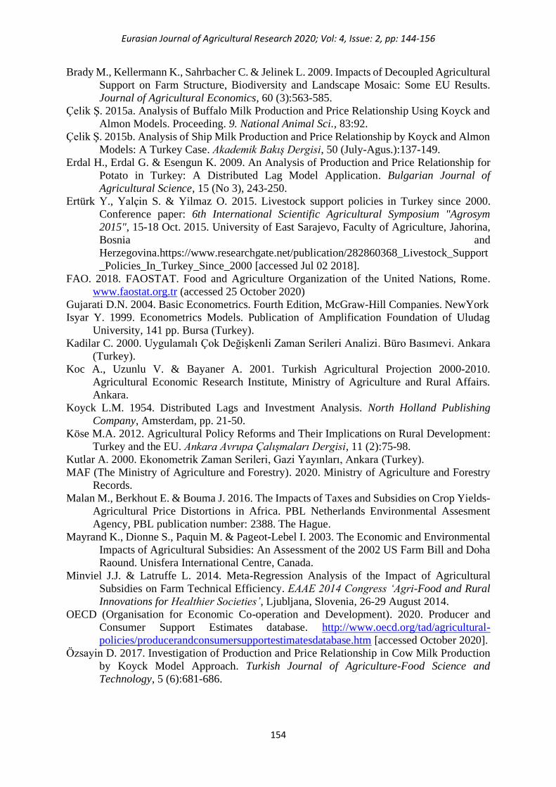
Eurasian Journal of Agricultural Research 2020; Vol: 4, Issue: 2, pp: 144-156
154
Brady M., Kellermann K., Sahrbacher C. & Jelinek L. 2009. Impacts of Decoupled Agricultural
Support on Farm Structure, Biodiversity and Landscape Mosaic: Some EU Results.
Journal of Agricultural Economics, 60 (3):563-585.
Çelik Ş. 2015a. Analysis of Buffalo Milk Production and Price Relationship Using Koyck and
Almon Models. Proceeding. 9. National Animal Sci., 83:92.
Çelik Ş. 2015b. Analysis of Ship Milk Production and Price Relationship by Koyck and Almon
Models: A Turkey Case. Akademik Bakış Dergisi, 50 (July-Agus.):137-149.
Erdal H., Erdal G. & Esengun K. 2009. An Analysis of Production and Price Relationship for
Potato in Turkey: A Distributed Lag Model Application. Bulgarian Journal of
Agricultural Science, 15 (No 3), 243-250.
Ertürk Y., Yalçin S. & Yilmaz O. 2015. Livestock support policies in Turkey since 2000.
Conference paper: 6th International Scientific Agricultural Symposium "Agrosym
2015", 15-18 Oct. 2015. University of East Sarajevo, Faculty of Agriculture, Jahorina,
Bosnia and
Herzegovina.https://www.researchgate.net/publication/282860368_Livestock_Support
_Policies_In_Turkey_Since_2000 [accessed Jul 02 2018].
FAO. 2018. FAOSTAT. Food and Agriculture Organization of the United Nations, Rome.
www.faostat.org.tr (accessed 25 October 2020)
Gujarati D.N. 2004. Basic Econometrics. Fourth Edition, McGraw-Hill Companies. NewYork
Isyar Y. 1999. Econometrics Models. Publication of Amplification Foundation of Uludag
University, 141 pp. Bursa (Turkey).
Kadilar C. 2000. Uygulamalı Çok Değişkenli Zaman Serileri Analizi. Büro Basımevi. Ankara
(Turkey).
Koc A., Uzunlu V. & Bayaner A. 2001. Turkish Agricultural Projection 2000-2010.
Agricultural Economic Research Institute, Ministry of Agriculture and Rural Affairs.
Ankara.
Koyck L.M. 1954. Distributed Lags and Investment Analysis. North Holland Publishing
Company, Amsterdam, pp. 21-50.
Köse M.A. 2012. Agricultural Policy Reforms and Their Implications on Rural Development:
Turkey and the EU. Ankara Avrupa Çalışmaları Dergisi, 11 (2):75-98.
Kutlar A. 2000. Ekonometrik Zaman Serileri, Gazi Yayınları, Ankara (Turkey).
MAF (The Ministry of Agriculture and Forestry). 2020. Ministry of Agriculture and Forestry
Records.
Malan M., Berkhout E. & Bouma J. 2016. The Impacts of Taxes and Subsidies on Crop Yields-
Agricultural Price Distortions in Africa. PBL Netherlands Environmental Assesment
Agency, PBL publication number: 2388. The Hague.
Mayrand K., Dionne S., Paquin M. & Pageot-Lebel I. 2003. The Economic and Environmental
Impacts of Agricultural Subsidies: An Assessment of the 2002 US Farm Bill and Doha
Raound. Unisfera International Centre, Canada.
Minviel J.J. & Latruffe L. 2014. Meta-Regression Analysis of the Impact of Agricultural
Subsidies on Farm Technical Efficiency. EAAE 2014 Congress ‘Agri-Food and Rural
Innovations for Healthier Societies’, Ljubljana, Slovenia, 26-29 August 2014.
OECD (Organisation for Economic Co-operation and Development). 2020. Producer and
Consumer Support Estimates database. http://www.oecd.org/tad/agricultural-
policies/producerandconsumersupportestimatesdatabase.htm [accessed October 2020].
Özsayin D. 2017. Investigation of Production and Price Relationship in Cow Milk Production
by Koyck Model Approach. Turkish Journal of Agriculture-Food Science and
Technology, 5 (6):681-686.
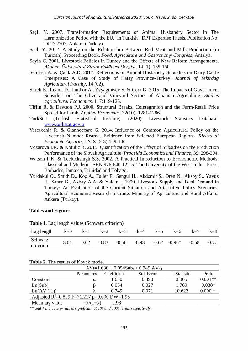
Eurasian Journal of Agricultural Research 2020; Vol: 4, Issue: 2, pp: 144-156
155
Saçli Y. 2007. Transformation Requirements of Animal Husbandry Sector in The
Harmonization Period with the EU. [In Turkish]. DPT Expertise Thesis, Publication No:
DPT: 2707, Ankara (Turkey).
Sacli Y. 2012. A Study on the Relationship Between Red Meat and Milk Production (in
Turkish). Proceeding Book, Food, Agriculture and Gastronomy Congress, Antalya.
Sayin C. 2001. Livestock Policies in Turkey and the Effects of New Reform Arrangements.
Akdeniz Üniversitesi Ziraat Fakültesi Dergisi, 14 (1): 139-150.
Semerci A. & Çelik A.D. 2017. Reflections of Animal Husbandry Subsidies on Dairy Cattle
Enterprises: A Case of Study of Hatay Province-Turkey. Journal of Tekirdag
Agricultural Faculty, 14 (02).
Skreli E., Imami D., Jambor A., Zvyagintsev S. & Çera G. 2015. The Impacts of Government
Subsidies on The Olive and Vineyard Sectors of Albanian Agriculture. Studies
agricultural Economics. 117:119-125.
Tiffin R. & Dawson P.J. 2000. Structural Breaks, Cointegration and the Farm-Retail Price
Spread for Lamb. Applied Economics, 32(10): 1281-1286
TurkStat (Turkish Statistical Institute). (2020). Livestock Statistics Database.
www.turkstat.gov.tr
Viscecchia R. & Giannoccaro G. 2014. Influence of Common Agricultural Policy on the
Livestock Number Reared. Evidence from Selected European Regions. Rivista di
Economia Agraria, LXIX (2-3):129-140.
Vozarova I.K. & Kotulic R. 2015. Quantification of the Effect of Subsidies on the Production
Performance of the Slovak Agriculture. Proceida Economics and Finance, 39: 298-304.
Watson P.K. & Teelucksingh S.S. 2002. A Practical Introduction to Econometric Methods:
Classical and Modern. ISBN:976-640-122-5. The University of the West Indies Press,
Barbados, Jamaica, Trinidad and Tobago.
Yurdakul O., Smith D., Koç A., Fuller F., Sengul H., Akdemir Ş., Oren N., Aksoy S., Yavuz
F., Saner G., Akbay A.A. & Yalcin I. 1999. Livestock Supply and Feed Demand in
Turkey: An Evaluation of the Current Situation and Alternative Policy Scenarios.
Agricultural Economic Research Institute, Ministry of Agriculture and Rural Affairs.
Ankara (Turkey).
Tables and Figures
Table 1. Lag length values (Schwarz criterion)
Lag length k=0 k=1 k=2 k=3 k=4 k=5 k=6 k=7 k=8
Schwarz
criterion 3.01 0.02 -0.83 -0.56 -0.93 -0.62 -0.96* -0.58 -0.77
Table 2. The results of Koyck model
AVt=1.630 + 0.054Subt + 0.749 AVt-1 Parametres Coefficient Std. Error t-Statistic Prob.
Constant α 1.630 0.398 3.365 0.001**
Ln(Sub) β 0.054 0.027 1.769 0.088*
Ln(AV (-1)) λ 0.749 0.071 10.622 0.000**
Adjusted R2=0.829 F=71.217 p=0.000 DW=1.95
Mean lag value =λ/(1−λ) 2.98 ** and * indicate p-values significant at 1% and 10% levels respectively.
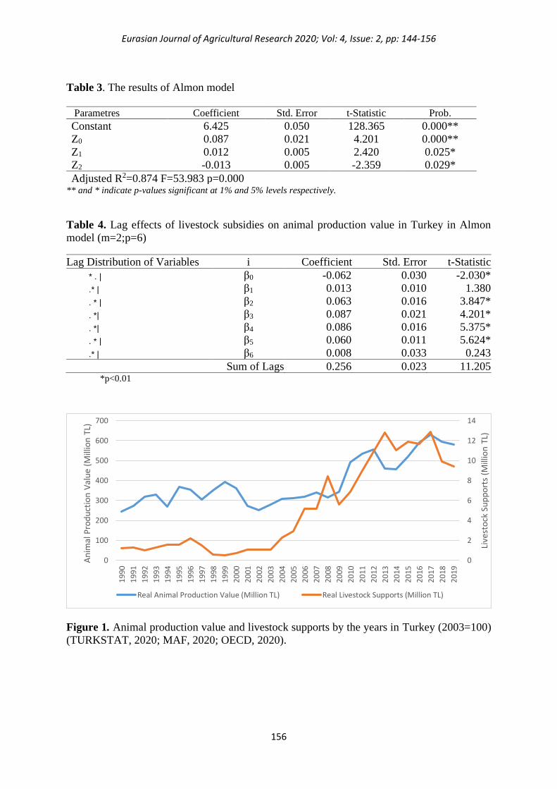
Eurasian Journal of Agricultural Research 2020; Vol: 4, Issue: 2, pp: 144-156
156
Table 3. The results of Almon model
Parametres Coefficient Std. Error t-Statistic Prob.
Constant 6.425 0.050 128.365 0.000**
Z0 0.087 0.021 4.201 0.000**
Z1 0.012 0.005 2.420 0.025*
Z2 -0.013 0.005 -2.359 0.029*
Adjusted R2=0.874 F=53.983 p=0.000 ** and * indicate p-values significant at 1% and 5% levels respectively.
Table 4. Lag effects of livestock subsidies on animal production value in Turkey in Almon
model (m=2;p=6)
Lag Distribution of Variables i Coefficient Std. Error t-Statistic
* . | β0 -0.062 0.030 -2.030*
.* | β1 0.013 0.010 1.380
. * | β2 0.063 0.016 3.847*
. *| β3 0.087 0.021 4.201*
. *| β4 0.086 0.016 5.375*
. * | β5 0.060 0.011 5.624*
.* | β6 0.008 0.033 0.243
Sum of Lags 0.256 0.023 11.205 *p<0.01
Figure 1. Animal production value and livestock supports by the years in Turkey (2003=100)
(TURKSTAT, 2020; MAF, 2020; OECD, 2020).
0
2
4
6
8
10
12
14
0
100
200
300
400
500
600
700
19
90
19
91
19
92
19
93
19
94
19
95
19
96
19
97
19
98
19
99
20
00
20
01
20
02
20
03
20
04
20
05
20
06
20
07
20
08
20
09
20
10
20
11
20
12
20
13
20
14
20
15
20
16
20
17
20
18
20
19
Live
sto
ck S
up
po
rts
(Mill
ion
TL)
An
imal
Pro
du
ctio
n V
alu
e (M
illio
n T
L)
Real Animal Production Value (Million TL) Real Livestock Supports (Million TL)


