Evaluating Tools for Performance Modeling of

Grid Applications

Mariela Curiel?, Gustavo Alvarez, and Leonardo Flores

Universidad Simon Bolıvar,Departamento de Computacion y Tecnologıa de la Informacion,

Apartado 89000, Caracas 1080-A, Venezuelamcuriel@ldc.usb.ve,{gjalvarez, floresm.leonardo}@gmail.com

Abstract. A Grid is a collection of heterogeneous distributed comput-ing resources for solving large-scale computational and data intensiveproblems. It is a dynamic environment where resources attributes -suchas load- change constantly hindering performance evaluation activities.Performance models could be a solution to this problem because theyprovide a way of performing repeatable and controllable experiments.Several tools have been developed for modeling scheduling algorithms inGrids. We believe, however, that if these tools are to be used for mod-eling application performance they should be improved by adding someparticular features. In this paper, we identify such features and evalu-ate two modeling tools based on those features. These tools are used torepresent the execution of applications in the Grid SUMA.

1 Introduction

A Grid is a collection of heterogeneous and geographically-dispersed computingresources connected by a network, possibly at different sites and organizations.The Grid middleware provides transparent access to resources, and in general itdeals with the physical characteristics of the Grid. Grids have dynamic nature,i.e., some performance characteristics, such as load, may change over time dueto the fact that resources are shared by other applications. This behavior causesperformance degradation and makes it difficult to evaluate performance. Applica-tion performance analysis is crucial to obtain high performance. Although somefactors such as network load or bad scheduling decisions may cause problems,one of the main source of poor performance comes from wrong design decisions.One can repair the problems after finishing the application development (tun-ing) or during the software development process. In the first case, one modifiesalgorithms, data structures, compiler options, etc. and then, observe the results.Additional runs should be done in similar conditions in order to evaluate theeffects of each change. However, it is impossible to get repeatable results in Gridexperiments. Fortunately, modeling allows us to count on a controllable experi-mentation environment. Additionally, one can use a model to design applications

? This work is partially supported by FONACIT, project S1-2002000560

2 Curiel, Alvarez, Flores

whose performance is tailored to the dynamic Grid nature. To construct a rep-resentative application model may imply modeling the Grid middleware. Somesimulation packages have been developed for modeling Grid scheduling strate-gies. The objective of this research is to evaluate different tools for modeling Gridapplications. The idea is to show drawbacks and strengths that can be useful toimprove existing tools or to develop new ones. In this work we start by choosingtools from both Client/Server, distributed applications domain (LQNM analyti-cal [1] and simulation solvers [2]) and Grid domain (GridSim [3]). The tools willbe used to model sequential and parallel applications of the Grid SUMA ([4]).

2 Desirable Characteristics in a Modeling Tool

In this Section we present a list of desirable features to support applicationperformance modeling and analysis. This is not an exhaustive list, and it can beenriched along the research. We claim that Grid modeling tools should:

1. Offer capabilities for constructing a representative Grid model:It means to provide facilities for modeling basic Grid elements: (a) Networktopology, which includes different graphs, bandwidth and latencies. (b) Computeresources, memories, storage resources and other kind of resources. (c) Aspectsrelated to the dynamic nature of the Grid, i.e. load and unavailability of theresources. (d) Middleware layers. (e) Other particular Grid characteristics suchas reservation of resources or location in any time zone.

2. Offer capabilities for easily constructing a representative appli-

cation model: It includes the possibility of modeling: (a) Simple sequentialapplications that only need especial resources or services. (b) Different mod-els of distributed and parallel applications. (c) Stochastic behavior. In regardsto (b), [5] classifies parallel Grid applications in four groups: loosely coupled(compute intensive with low memory requirements, small amount of data pertask and little communication between tasks), pipelined (very memory and dataintensive, with coarse-grained inter-task communication), tightly synchronized(frequent inter-task synchronization, significant computation and memory/datausage) and widely distributed (update and/or unify distributed data bases, theyhave small computational, data and memory requirements)

3. Offer enough metrics for performance analysis: It includes clas-sical metrics such as response times, waiting times, number of I/O operations,number of network communications, bytes transferred in I/O or network commu-nications, residency times, resource utilizations and new Grid metrics. Resultantdata should be provided in text format and by means of graphical tools.

4. Be easy to use: Tools should offer wide and clear documentation, usersupport and user-friendly interfaces. Additionally, it could be interesting to pro-vide high level models closer to the application developers (UML diagrams, MSC,etc.) as well as the algorithms to transform them into performance models.

5. Be efficient: The dynamics of a Grid is complex. It is possible to findNP-complete problems in, for example, routing or scheduling strategies thatcannot be treated by analytical techniques. However, diverse kind of programs

Evaluating Tools for Performance Modeling of Grid Applications 3

run on the Grid. Some of them could be very simple, as for example to requesta cluster for running a parallel rigid application. In these cases an analyticalmodel could be enough. So, it is recommendable to provide diverse methods tosolve a variety of problems. When simulation is the only option, solutions suchas parallel simulations should be explored.

3 Selected Tools

Our final goal is to discover the presence or absence of the mentioned charac-teristics in an important number of modeling tools (mainly oriented to Gridand distributed systems modeling). In order to review each tool exhaustively, itis necessary its installation and use. Due to a lack of time, we start by evalu-ating a reduced number of tools. BeoSim, Bricks, SimGrid, GridSim, ChicSimand OptorSim are popular simulation tools frequently referenced in Grid relatedbibliography (see references in [6]). BeoSim, Bricks, ChicSim were discarded be-cause they are not currently available for users. For the time being, we ruledOptorSim out because it is designed for data Grid modeling and we want tomodel a computational Grid. Although LQNM analytical and simulation solversare oriented to Client/Server applications they were chose by the possibility ofdoing analytical models. Between GridSim and SimGrid we first took Gridsimfor two main reasons: GridSim is Java based and it apparently has more capac-ities for Grid modeling. SimGrid, OptorSim and other simulation tools will besubsequently evaluated. The next paragraphs explain in detail characteristics ofLQNM solvers and GridSim.

Layered Queuing Network Models are QNM extended to reflect interac-tions between client and server processes. We choose LQNM (lqns version 3) bythe following reasons : 1) The application model can be easily constructed by nonexperts in performance evaluation: the tools are embedded in a SPE method-ology that derives Layered Queuing Network Models (LQNM) from systemsscenarios described by means of Use Case Maps (UCM); free software packagesare available for process automation under this methodology. 2) Models can besolved by simulation or analytical techniques: The Layered Queuing NetworkSolver (LQNS) solves the model analytically, whereas the ParaSol StochasticRendez-Vous Network Simulator (ParaSRVN) use the simulation technique.

An LQNM can be represented by a graph with nodes for Tasks and Devices,and arrows for service requests. A Task (parallelograms in figure 1) is a soft-ware object that has its own thread of execution. Tasks are divided into threecategories: Client Tasks (only send requests), Active Server Tasks (can receiveand send requests) and Pure Server Tasks (only receive requests). There arethree types of interactions between Tasks: asynchronous messages, synchronousinteractions and forwarding messages. In a forward call, the sending Client Taskmakes a synchronous call and blocks until it receives a reply. The receiving Taskpartially processes the call and then forwards it to another server, which be-comes responsible for sending a reply to the blocked Client Task. Tasks receiveany kind of request message in points called Entries (smaller parallelograms in

4 Curiel, Alvarez, Flores

figure 1). A Task has a different Entry for every kind of service it provides.Internally, an Entry could be composed by sequences of smaller computationalblocks called Activities (rectangles), which are related in sequence, loop, parallelconfigurations, etc.

GridSim [3] is a toolkit for modeling and simulation of heterogeneous re-sources, users, applications, brokers and schedulers in a Grid computing envi-ronment. GridSim was chosen because of the following reasons: 1) It is one ofthe most popular simulation tool for Grid research. 2) It is based on Java, whichis a popular language. 3) GridSim is an active project. 4) According to the doc-umentation GridSim has interesting features for modeling Grid environments,for example: (a) it allows modeling of heterogeneous types of resources operat-ing under space- or time-shared mode; (b) resources can be located in any timezone and booked for in advance; (c) different parallel application models can besimulated.

GridSim adopts the multi-layered design architecture. The first bottom layeris the Java interface and the JVM. The second layer is SimJava, which providesan event-driven discrete event simulation package on top of JVM to drive thesimulation for GridSim. The third layer is the GridSim toolkit that provides themodeling and simulation of Core Grid entities, such as resources and Grid Infor-mation Services, using the events of the second layer. The simulation of resourceaggregators called Grid brokers or schedulers is provided by the fourth layer.The top layer focuses on application and resource modeling with different sce-narios to evaluate scheduling and resource management policies, heuristics andalgorithms. Applications in GridSim are modeled as a number of work packetsthat are called Gridlets. A Gridlet is a package that contains all the informationrelated to the job and its execution management details, such as job length ex-pressed in MIPS (or SPECs), disk I/O operations, the size of input and outputfiles, and the job originator. Grid resources, users and brokers are modeled as En-tities, and they communicate via messaging events using the advanced networkfeatures. Synchronous and asynchronous messages are allowed.

4 SUMA

SUMA (Scientific Ubiquitous Metacomputing Architecture) [4] is a computa-tional Grid that transparently executes Java bytecode on remote machines, withadditional support for scientific computing development. SUMA provides accessto both single-process (possibly multi-threaded) and parallel execution agents,according to the JVM and mpiJava execution model. A user invokes the execu-tion of a program in SUMA through the services suma Execute (on-line executionmode) or suma Submit (off-line execution). We modeled only scenarios associ-ated to suma execute. The steps of the suma execute services follow: When aClient wants to send an execution request to SUMA, it firstly must find a Proxy,by invoking the findProxy method in Scheduler. The Scheduler finds an appro-priate Proxy and returns a CORBA reference to the Client. Then the Clientinvokes the execute method in its Proxy, passing the name of the main class as a

Evaluating Tools for Performance Modeling of Grid Applications 5

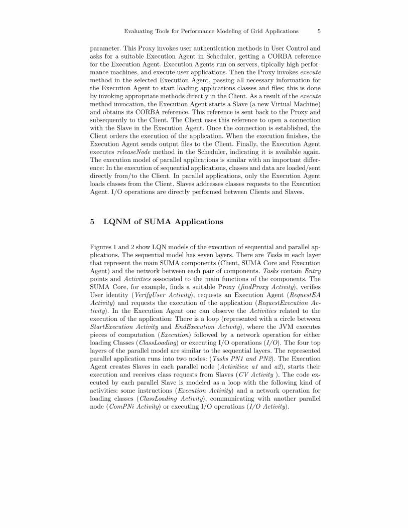
parameter. This Proxy invokes user authentication methods in User Control andasks for a suitable Execution Agent in Scheduler, getting a CORBA referencefor the Execution Agent. Execution Agents run on servers, tipically high perfor-mance machines, and execute user applications. Then the Proxy invokes executemethod in the selected Execution Agent, passing all necessary information forthe Execution Agent to start loading applications classes and files; this is doneby invoking appropriate methods directly in the Client. As a result of the executemethod invocation, the Execution Agent starts a Slave (a new Virtual Machine)and obtains its CORBA reference. This reference is sent back to the Proxy andsubsequently to the Client. The Client uses this reference to open a connectionwith the Slave in the Execution Agent. Once the connection is established, theClient orders the execution of the application. When the execution finishes, theExecution Agent sends output files to the Client. Finally, the Execution Agentexecutes releaseNode method in the Scheduler, indicating it is available again.The execution model of parallel applications is similar with an important differ-ence: In the execution of sequential applications, classes and data are loaded/sentdirectly from/to the Client. In parallel applications, only the Execution Agentloads classes from the Client. Slaves addresses classes requests to the ExecutionAgent. I/O operations are directly performed between Clients and Slaves.

5 LQNM of SUMA Applications

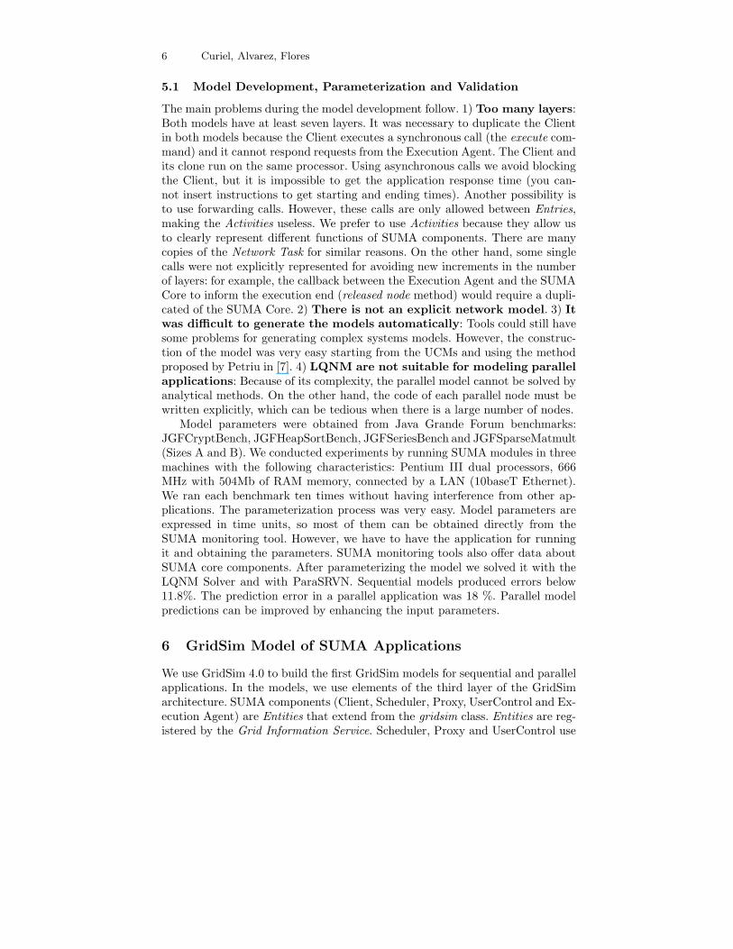
Figures 1 and 2 show LQN models of the execution of sequential and parallel ap-plications. The sequential model has seven layers. There are Tasks in each layerthat represent the main SUMA components (Client, SUMA Core and ExecutionAgent) and the network between each pair of components. Tasks contain Entrypoints and Activities associated to the main functions of the components. TheSUMA Core, for example, finds a suitable Proxy (findProxy Activity), verifiesUser identity (VerifyUser Activity), requests an Execution Agent (RequestEAActivity) and requests the execution of the application (RequestExecution Ac-tivity). In the Execution Agent one can observe the Activities related to theexecution of the application: There is a loop (represented with a circle betweenStartExecution Activity and EndExecution Activity), where the JVM executespieces of computation (Execution) followed by a network operation for eitherloading Classes (ClassLoading) or executing I/O operations (I/O). The four toplayers of the parallel model are similar to the sequential layers. The representedparallel application runs into two nodes: (Tasks PN1 and PN2). The ExecutionAgent creates Slaves in each parallel node (Activities: a1 and a2), starts theirexecution and receives class requests from Slaves (CV Activity ). The code ex-ecuted by each parallel Slave is modeled as a loop with the following kind ofactivities: some instructions (Execution Activity) and a network operation forloading classes (ClassLoading Activity), communicating with another parallelnode (ComPNi Activity) or executing I/O operations (I/O Activity).

6 Curiel, Alvarez, Flores

5.1 Model Development, Parameterization and Validation

The main problems during the model development follow. 1) Too many layers:Both models have at least seven layers. It was necessary to duplicate the Clientin both models because the Client executes a synchronous call (the execute com-mand) and it cannot respond requests from the Execution Agent. The Client andits clone run on the same processor. Using asynchronous calls we avoid blockingthe Client, but it is impossible to get the application response time (you can-not insert instructions to get starting and ending times). Another possibility isto use forwarding calls. However, these calls are only allowed between Entries,making the Activities useless. We prefer to use Activities because they allow usto clearly represent different functions of SUMA components. There are manycopies of the Network Task for similar reasons. On the other hand, some singlecalls were not explicitly represented for avoiding new increments in the numberof layers: for example, the callback between the Execution Agent and the SUMACore to inform the execution end (released node method) would require a dupli-cated of the SUMA Core. 2) There is not an explicit network model. 3) It

was difficult to generate the models automatically: Tools could still havesome problems for generating complex systems models. However, the construc-tion of the model was very easy starting from the UCMs and using the methodproposed by Petriu in [7]. 4) LQNM are not suitable for modeling parallel

applications: Because of its complexity, the parallel model cannot be solved byanalytical methods. On the other hand, the code of each parallel node must bewritten explicitly, which can be tedious when there is a large number of nodes.

Model parameters were obtained from Java Grande Forum benchmarks:JGFCryptBench, JGFHeapSortBench, JGFSeriesBench and JGFSparseMatmult(Sizes A and B). We conducted experiments by running SUMA modules in threemachines with the following characteristics: Pentium III dual processors, 666MHz with 504Mb of RAM memory, connected by a LAN (10baseT Ethernet).We ran each benchmark ten times without having interference from other ap-plications. The parameterization process was very easy. Model parameters areexpressed in time units, so most of them can be obtained directly from theSUMA monitoring tool. However, we have to have the application for runningit and obtaining the parameters. SUMA monitoring tools also offer data aboutSUMA core components. After parameterizing the model we solved it with theLQNM Solver and with ParaSRVN. Sequential models produced errors below11.8%. The prediction error in a parallel application was 18 %. Parallel modelpredictions can be improved by enhancing the input parameters.

6 GridSim Model of SUMA Applications

We use GridSim 4.0 to build the first GridSim models for sequential and parallelapplications. In the models, we use elements of the third layer of the GridSimarchitecture. SUMA components (Client, Scheduler, Proxy, UserControl and Ex-ecution Agent) are Entities that extend from the gridsim class. Entities are reg-istered by the Grid Information Service. Scheduler, Proxy and UserControl use

Evaluating Tools for Performance Modeling of Grid Applications 7

Fig. 1. Sequential LQNM Fig. 2. Parallel LQNM

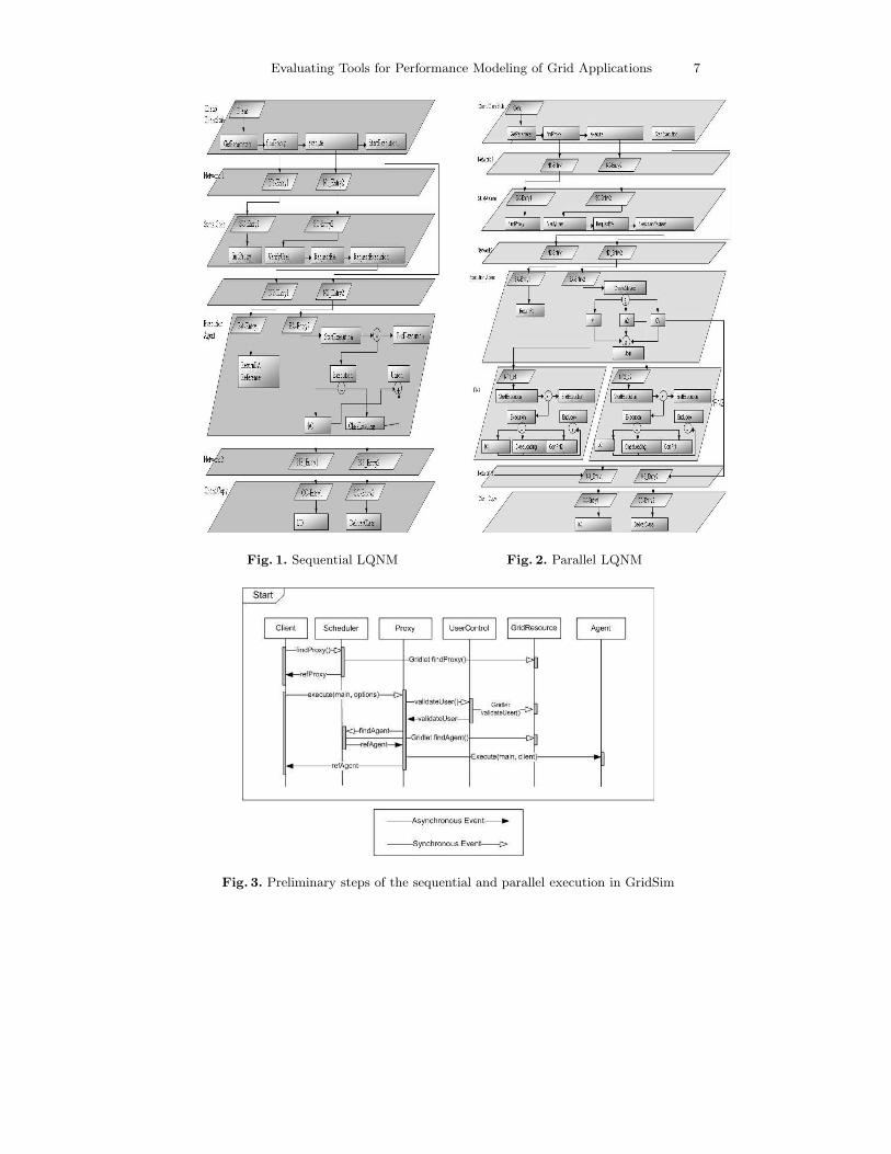
Fig. 3. Preliminary steps of the sequential and parallel execution in GridSim

8 Curiel, Alvarez, Flores

a GridResource Entity to simulate their processing tasks (i.e., to find a Proxy,to validate Users, etc.). The process of creating a GridResource is as follows:First, Processing elements (PE) objects are created with a suitable MIPS rating.PE are assembled together to create a Machine. GridSim Machine class repre-sents an uniprocessor or shared memory multiprocessor machine. One or moremachines form a GridResource. SUMA Core components submit Gridlets to theGridResource SumaCore (figure 3). In the sequential model, a GridResource witha single machine and one or more PEs is bound to the Execution Agent. The exe-cution of one application is modeled by means of a loop where some instructions(simulated by a Gridlet submitted to a GridResource) are followed by messagesto the Client Entity to either load classes or execute I/O operations. A networktopology was created to allow the Entities to communicate. Each Entity definesan instance of the Link class. An instance of Router class is created to forwarddata from one Entity to another. Figure 3 shows the sequence of messages amongSUMA Core Entities before executing the application. In the parallel model eachSlave has associated its own GridResource. Each GridResource has a Machineobject and a PE.

6.1 Model Development, Parameterization and Validation

The modeling process was a bit difficult despite the programmers experience inJava. The learning curve of GridSim is slow. Knowledge of object oriented andJava programming is required. On the other hand, once GridSim architecture andphilosophy is understood, it was very easy to construct the models because thereis a direct correspondence between SUMA components and GridSim Entities.The use of asynchronous messages allows us to make calls between Entitiesin both directions: call and callbacks, without copying components. Since themodel is a Java program, one can insert special instructions in any place toobtain execution times. Many identical parallel nodes can be added by changinga single parameter.

We execute the benchmarks used to parameterize the LQNM in five ma-chines with the following characteristics: AMD Athlon 64 3800 1GB RAM (runsthe Client), Pentium IV 3.4 GHz, 512 RAM (for the Scheduler, the User Con-trol, the Proxy and the Execution Agent); machines are connected by a LAN(10baseT Ethernet). The main GridResource static parameters were architec-ture, operating system, MIPS, number of machines and number of PE. The firsttwo parameters were obtained from OS commands. The SiSoftware Sandra Lite2007 (http://www.sisoftware.co.uk) was used to compute the MIPS rating permachine. The number of machines and PE depend on the particular Grid ar-chitecture. The main parameters of the Link class are: delay (ping command),MTU (standard Ethernet) and the bandwidth (obtained from router specifica-tions). The main drawback was to obtain the gridletLength value for each SUMAcomponent. The gridletLength is expressed in MI (Millions Instruction) and it isdifficult to know the value of this parameter in a Java Program. The solution wasto measure the program, to obtain the execution times and to convert measuredtimes into MI. Prediction errors were below 7.9%

Evaluating Tools for Performance Modeling of Grid Applications 9

7 Comparison of Tools

After using the selected tools for developing the SUMA models, it is possible tocompare them based on the “desirable characteristics”:

1. Capabilities for constructing a representative Grid model: In thisaspect GridSim is so far one of the most complete tool. Some aspects that couldbe included are: (a) New classes that allow to model new software components(middleware, operating systems, etc.). (b) Improvements to hardware resourcesmodels (more complex network topologies, different network protocols, mem-ory models, etc.) (c) Background load of processors with probabilistic behavior.LQNM tools were not designed for modeling Grid systems. They could be usefulfor modeling small Grids (for example intra-organizational Grids) or other kindof distributed systems, such as clusters with simple application models. Somefeatures could be added to improve distributed systems models, for example:network models.

2. Capabilities for easily constructing a representative model of

the application: With respect to this characteristic, GridSim also has manyadvantages: it allow us to model diverse models of parallel and distributed ap-plications. [8] describes GridSim extensions for simulating data Grids. GridSimis based on deterministic simulation where no random events occur. This is adrawback because it limits the type of application to be modeled. However,GridSimRandom class and eduni.simjava.distributions package can be used forincorporating randomness in data. This randomness would require new outputsprocessing. LQNM tools seem suitable for modeling sequential and some kindof distributed applications. Stochastic behavior can be included in analytical andsimulation models by indicating means and variances.

3. Metrics for performance analysis: GridSim provides a small set ofmetrics. Metrics about gridlet processing are: CPU time, wall clock time andwaiting time. There are not explicit metrics about throughput or resource uti-lization. There are, however, a variety of metrics in the new network models.GridSim output should be improved by incorporating new metrics. LQNM

tools offer diverse metrics to evaluate the application performance (responsetimes, waiting times, devices utilizations, etc) and simulation results (confidenceintervals).

4. Ease to use: The learning curve of GridSim is slow. [9] describes a Java-based Graphical User Interface (GUI) tool for GridSim, which aims to reduce thelearning process and enables fast creation of simulation models. Future researchprojects could be oriented to provide higher level models and methodologies totransform them in GridSim models. Higher level parameters that can be inter-nally transformed should also be included. These features would help applicationdesigners and application developers without experience in performance evalu-ation or Java programming. GridSim documentation is good. LQNM could beeasily constructed from Use Case Maps, so application developers/designers notneed to be queuing network experts.

5. Efficiency: GridSim uses serial simulation. Techniques to reduce sim-ulation times should be incorporated to Grid modeling tools: parallel simula-

10 Curiel, Alvarez, Flores

tions and to combine analytical and simulation approaches. Analytical LQNM

meaningfully reduces model execution times. However, approximated analyticaltechniques only can be used in very simple application models.

8 Conclusions

The aim of our research is to evaluate simulation tools for performance modelingof Grid applications. We have used two set of tools for modeling applications thatrun in the Java-based computational Grid SUMA. One set of tools solve LQNMs.They were not designed to model Grid environments but offer some advantagesfor modeling sequential and distributed applications (especially Client/Serverapplications). These advantages are: 1) Possibility of obtaining analytical andsimulation results. 2) LQNM can be derived from Use Case Maps. 3) The toolsprovide several metrics for evaluating application performance and quality ofsimulation results. On the other hand, tools like GridSim allow us to modelin detail diverse aspects of Grid platforms and a variety of parallel applicationmodels. They have many of the “desirable characteristics”, but three aspectsneed to be improved: efficiency, the set of metrics and the ease of use. Thesefeatures will help designers and application developers construct right modelsand obtain results in very short times. Future research includes the evaluationof different tools and the modeling of different kinds of Grid applications.

References

1. Franks, G.: Performance Analysis of Distributed Server Systems. PhD thesis, Car-leton University (2000)

2. Mascarenhas, E.: A System for Multithreaded Parallel Simulation with MigrantThread and Objects. PhD thesis, Purdue University (1996)

3. Sulistio, A., Poduval, G., Buyya, R., Tham, C.: Constructing a grid simulationwith differentiated network service using gridsim. In: Proc. of the 6th. InternationalConference on Internet Computing (ICOMP’ 05). (2005)

4. Cardinale, Y., Curiel, M., Figueira, C., Garcıa, P., Hernandez, E.: Implementationof a corba-based metacomputing system. In: Proc. of Workshop on Java for HighPerformance Computing.LNCS. (2001)

5. Snavely, A., Chun, G., Casanova, H., der Wijngaart, R.V., Frumkin, M.: Bench-marks for grid computing: A review of ongoing efforts and fututre directions. Sig-metrics Perfor. Eval. Rev 30(4) (2003) 27–32

6. Quetier, B., Capello, F.: A survey of grid research tools: simulators, emulators andreal life platforms. In: Proc. of 17th IMACS World Congress (IMAC 2005), France.(2005)

7. Petriu, D.C., Woodside, C.: Software performance models from systems scenariosin use case maps. Proc. of TOOLS, Springer Verlag, LNCS 794 (2002) 159–177

8. A.Sulistio, Cibej, U., Robic, B., Buyya, R.: A Toolkit for Modeling and Simulationof Data Grids with Integration of Data Storage, Replication and Analysis. TechnicalReport GRIS-TR-2005-13, University of Melbourne (2005)

9. Sulistio, A., Yeo, C.S., Buyya, R.: Visual modeler for grid modeling and simulation(gridsim) toolkit. In: Proc. of the 3rd. International Conference on ComputationalScience (ICCS 2003), Springer Verlag Publications (LCNS Series) (2003)