Embed Size (px)
Citation preview
FINAL REPORT
North Carolina Department of Transportation Research Project No. HWY-2002-12
Evaluation of Bridge Analysis Vis-à-vis Performance
By
Janos Gergely Principal Investigator
Timothy O. Lawrence
Graduate Research Assistant
Claudia I. Prado Graduate Research Assistant
Chad T. Ritter
Graduate Research Assistant
William B. Stiller Graduate Research Assistant
Department of Civil Engineering University of North Carolina at Charlotte
9201 University City Boulevard Charlotte, NC 28223
December 15, 2004
2
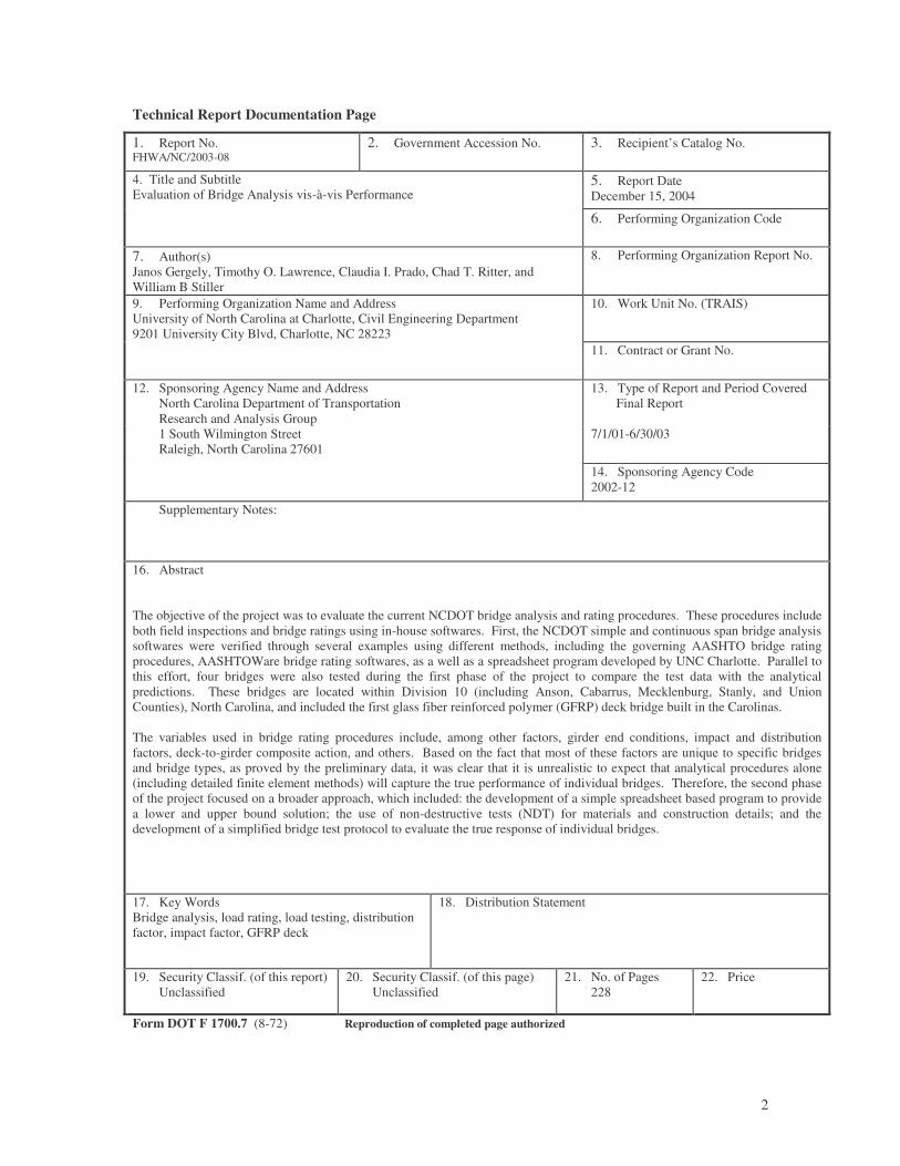
Technical Report Documentation Page
1. Report No. FHWA/NC/2003-08
2. Government Accession No.
3. Recipient’s Catalog No.
4. Title and Subtitle Evaluation of Bridge Analysis vis-à-vis Performance
5. Report Date December 15, 2004
6. Performing Organization Code
7. Author(s) Janos Gergely, Timothy O. Lawrence, Claudia I. Prado, Chad T. Ritter, and William B Stiller
8. Performing Organization Report No.
9. Performing Organization Name and Address University of North Carolina at Charlotte, Civil Engineering Department 9201 University City Blvd, Charlotte, NC 28223
10. Work Unit No. (TRAIS)
11. Contract or Grant No.
12. Sponsoring Agency Name and Address North Carolina Department of Transportation Research and Analysis Group
13. Type of Report and Period Covered Final Report
1 South Wilmington Street Raleigh, North Carolina 27601
7/1/01-6/30/03
14. Sponsoring Agency Code 2002-12
Supplementary Notes:
16. Abstract The objective of the project was to evaluate the current NCDOT bridge analysis and rating procedures. These procedures include both field inspections and bridge ratings using in-house softwares. First, the NCDOT simple and continuous span bridge analysis softwares were verified through several examples using different methods, including the governing AASHTO bridge rating procedures, AASHTOWare bridge rating softwares, as a well as a spreadsheet program developed by UNC Charlotte. Parallel to this effort, four bridges were also tested during the first phase of the project to compare the test data with the analytical predictions. These bridges are located within Division 10 (including Anson, Cabarrus, Mecklenburg, Stanly, and Union Counties), North Carolina, and included the first glass fiber reinforced polymer (GFRP) deck bridge built in the Carolinas. The variables used in bridge rating procedures include, among other factors, girder end conditions, impact and distribution factors, deck-to-girder composite action, and others. Based on the fact that most of these factors are unique to specific bridges and bridge types, as proved by the preliminary data, it was clear that it is unrealistic to expect that analytical procedures alone (including detailed finite element methods) will capture the true performance of individual bridges. Therefore, the second phase of the project focused on a broader approach, which included: the development of a simple spreadsheet based program to provide a lower and upper bound solution; the use of non-destructive tests (NDT) for materials and construction details; and the development of a simplified bridge test protocol to evaluate the true response of individual bridges.
17. Key Words Bridge analysis, load rating, load testing, distribution factor, impact factor, GFRP deck
18. Distribution Statement
19. Security Classif. (of this report) Unclassified
20. Security Classif. (of this page) Unclassified
21. No. of Pages 228
22. Price
Form DOT F 1700.7 (8-72) Reproduction of completed page authorized

3
DISCLAIMER
The contents of this report reflect the views of the authors and not necessarily the
views of the University. The authors are responsible for the facts and the accuracy of the
data presented herein. The contents do not necessarily reflect the official views or
policies of either the North Carolina Department of Transportation or the Federal
Highway Administration at the time of publication. This report does not constitute a
standard, specification, or regulation.

4
ACKNOWLEDGEMENTS
The research documented in this report was sponsored by the North Carolina
Department of Transportation (NCDOT) and the Federal Highway Administration’s
(FHWA) Innovative Bridge Research and Construction (IBRC) program. A Technical
Advisory Committee (TAC) composed of representatives of the two agencies provided
valuable guidance and technical support for this research project. The project TAC
Committee included Lin Wiggins (Chair), Henry Black, Rodger Rochelle, Rick Lakata,
Tom Koch, Cecil Jones, and Greg Perfetti of NCDOT, and Paul Simon of FHWA.
The authors would like to thank Garland Haywood, Ronald Lee and the Division
10 Bridge Maintenance Unit for their technical and material assistance throughout the
project. Their assistance included bridge identification, site preparation, traffic control,
loading truck, access to snooper truck, and other materials and supplies for the seven
bridge tests. Concrete Supply of Charlotte, N.C. provided the use of their truck to load
two of the bridges, Vulcraft of Florence, S.C. supplied the work platform for one of the
bridges, and Zapata Engineering of Charlotte, N.C. provided additional instruments to the
last two bridge tests. Their contributions are greatly appreciated.
The authors are also thankful to the UNC Charlotte research team, including Mike
Moss and Dan Rowe of the College of Engineering, and the undergraduate research
assistants working on the project, including Jennifer Carroll, Peter Foster, Chris Frank,
Drew Lyerly, Brad McConnell, Logan Smith, Avery Turner, Jeremy Wallace, and Brian
Zapata. Their help is gratefully acknowledged.

5
EXTENDED SUMMARY
The objective of the project was to evaluate the current NCDOT bridge analysis
and rating procedures. These procedures include both field inspections and bridge ratings
using in-house softwares. First, the NCDOT simple and continuous span bridge analysis
softwares were verified through several examples using different methods, including the
governing AASHTO bridge rating procedures, AASHTOWare bridge rating softwares, as
a well as a spreadsheet program developed by UNC Charlotte. Parallel to this effort, four
bridges (one with a GFRP deck) were also tested during the first phase of the project;
bridges located within Division 10 (including Anson, Cabarrus, Mecklenburg, Stanly, and
Union Counties), North Carolina, to compare the test data with the analytical predictions.
The first phase of the project proved that the NCDOT bridge rating software
directly follows the latest AASHTO requirements (with one small exception), providing a
safe and conservative approach to assess the existing bridges. Furthermore, the
experimental results also showed that the analytical predictions can not, in most cases,
provide an accurate estimate of the true behavior of these (especially older concrete)
bridges. Significant strength reserves were identified due to several factors, including
girder/deck composite action, impact and distribution factors, material strength,
contribution of non-structural elements, girder end conditions, etc...
Based on the fact that most of these factors are unique to specific bridges and
bridge types, as proved by these preliminary data, it was concluded that it is unrealistic to
expect that analytical procedures alone will capture the true performance of individual
bridges. Therefore, the second phase of the project focused on a broader approach, which

6
included: the development of a simple spreadsheet based program to provide a lower and
upper bound solution; the use of non-destructive tests (NDT) for materials and
construction details; and the development of a simplified bridge test protocol to evaluate
the true response of individual bridges.
The spreadsheet program allows the user to input a range of values for most of the
above-mentioned influencing factors, and when combined with more realistic material
properties from NDT tests, the output provides a lower and upper bound bridge response
(i.e. strain, deformation, bridge rating and posting).
During the development of the simplified testing protocol, three additional
bridges were tested. Similarly to the previous four bridges, this experimental phase of the
project involved the instrumentation (using up to 102 instruments) and the load testing of
these bridges using static, slow and dynamic load cases using truck weights close to the
operating rating. However, in addition to this large setup, an independent data
acquisition system was also used with a small number of additional instruments.
The purpose of this parallel (and much smaller) setup was to investigate whether a
scaled down instrumentation will provide realistic information on impact and distribution
factors, support conditions, composite actions and non-structural elements. Based on the
last three bridges tested, it was concluded, that a relatively simple instrumentation setup
can be effective in the load rating of bridges through testing. These diagnostic tests are
also included in the “Manual for Bridge Rating Through Load Testing”, a document
published by NCHRP.
The specific recommendations that are suggested by the authors based on the
seven bridges analyzed and tested can be summarized as:

7
Ø Reconsider the use of PercEffective in the NCDOT bridge rating software,
especially for concrete girder bridges with only minor hairline cracks in tension zone.
It is also recommended to use actual concrete strength values determined by NDT.
Ø Consider reducing or eliminating the impact factor for existing bridges with
“healthy” approach slabs and deck joints. This would increase most bridge ratings by
20-30%
Ø Consider the use of UNC Charlotte’s spreadsheet program (properly tested) to
allow the analysis to include simple span girder end restraint. This could be as high
as 30% for semi-integral and integral end walls.
Ø Consider the composite action (up to a certain horizontal shear level) between
steel girders and concrete decks for older bridges with certain construction details.
Ø Expand the bridge files to include non-destructive tests and damage extent and
propagation (cracks, spallings, and corrosion signs).
Ø Use bridge load testing (based on fully developed and detailed testing protocols)
to verify transverse load distribution, impact factor, and member strain levels.
Ø Revise and expand the current NCDOT analysis software to allow for parametric
studies, upgrade inspection field reports to include specific information on materials,
and damage/corrosion details, and combine the analysis with selected bridge tests.
In conclusion, the current NCDOT analysis software provides safe and
conservative bridge rating in accordance with the latest AASHTO requirements.
However, parametric studies in combination with properly planned load tests can
provide a more realistic estimate of bridge performance at the load level investigated,
and will result (in most cases) in higher load ratings for existing bridges.
8
TABLE OF CONTENTS
DISCLAIMER ...........................................................................................................3 ACKNOWLEDGEMENTS.......................................................................................4 EXTENDED SUMMARY.........................................................................................5 1. INTRODUCTION .........................................................................................10 1.1 Background ........................................................................................10 1.2 Literature Review...............................................................................12 2. PROJECT OVERVIEW ................................................................................17 2.1 Objectives ..........................................................................................17 2.2 Significance of Work .........................................................................18 3. LOAD RATING ............................................................................................20 3.1 Bridge Condition Evaluation .............................................................20 3.2 AASHTO Load Rating Guidelines ....................................................22 3.3 NCDOT Bridge Rating Procedures ...................................................23 3.4 Sample Analysis.................................................................................26 3.5 AASHTOWare...................................................................................33 3.6 UNCC Bridge Analysis Software ......................................................36 4. BRIDGE SELECTION..................................................................................38 4.1 Selection Criteria ...............................................................................38 4.2 GFRP Deck Bridge ............................................................................39 4.3 Concrete Deck Girder Bridges...........................................................39 4.4 Steel Girder Bridges...........................................................................43 4.5 Crutch Bent Bridge ............................................................................50 4.6 Summary of Bridge Selection............................................................52 5. EXPERIMENTAL RESULTS.......................................................................54 5.1 Bridge 89-0022 ................................................................................54 5.2 Bridge 59-0361 ................................................................................63 5.3 Bridge 12-0271 ................................................................................68 5.4 Bridge 59-0038 ................................................................................78 5.5 Bridge 12-0227 ................................................................................86 5.6 Bridge 59-0841 ................................................................................96 5.7 Bridge 89-0219 ................................................................................102
9
6. ANALYTICAL STUDIES AND COMPARISONS .....................................108 6.1 Bridge Rating .....................................................................................108 6.2 Distribution Factors ...........................................................................110 6.3 Impact Factors....................................................................................112 6.4 Composite Action ..............................................................................114 6.5 Girder End Conditions .......................................................................117 6.6 Strain Levels ......................................................................................119 6.7 Crutch Bent Retrofit...........................................................................121 7. NCDOT BRIDGE ANALYSIS SOFTWARES ............................................124 7.1 Simple Span Analysis Software.........................................................124 7.2 Continuous Span Analysis Software..................................................130 7.3 Conclusions........................................................................................134 8. BRIDGE RATING THROUGH LOAD TESTING ......................................135 8.1 Rating Procedure................................................................................136 8.2 Personnel and Equipment Needs .......................................................138 9. SUMMARY AND CONCLUSIONS ............................................................140 9.1 General Conclusions ..........................................................................140 9.2 Concrete Girder Bridges ....................................................................142 9.3 Steel Girder Bridges...........................................................................142 9.4 GFRP Deck Bridge ............................................................................143 9.5 Crutch Bent Repair ............................................................................143 10. RECOMMENDATIONS AND IMPLEMENTATION ................................144 11. REFERENCES ..............................................................................................146 12. APPENDICES ...............................................................................................148 A – UNC Charlotte Bridge Analysis Software Instruction Manual ..............148 B – GFRP Deck Bridge Construction Report ................................................166 C – Instrumentation and Load Testing...........................................................196 D – Load Paths...............................................................................................222

10
1. INTRODUCTION
1.1 Background
Over 50% of the nation’s bridges are either structurally deficient or functionally
obsolete. So, why don’t we see a lot of structural collapses and closed bridges? First,
most of the problems are identified during the scheduled bridge inspection. Based on the
inspection report, structural analyses and rating are performed. Bridge postings prompt
actions, and regular maintenance needs are issued as necessary.
The second reason is the actual bridge capacity and performance may be far
superior to the performance shown by current rating procedures. Similarly to engineering
practices in other fields, safety factors are included in bridge design and analysis as well.
Furthermore, bridges often exhibit inherent strength reserves from various factors, such
as higher composite action, girder end restraints, contributions from secondary elements,
etc... Therefore, in order to assess the bridge capacity more realistically, for bridge
posting or for special permits, the results from actual load tests may improve/supplement
the current analytical procedures.
In 1968, the Federal Highway Act created the National Bridge Inspection
Program (NBIP) which required state agencies to track and catalogue the conditions of
bridges on principal highways. This program was later changed by the Surface
Transportation Assistance Act of 1978 to include all bridges on public roads. Each year,
State highway agencies are required to comply with the National Bridge Inspections
Standards (NBIS), which contains five major provisions: inspection procedures,

11
frequency of inspections, qualifications for individuals performing inspection, inspection
reports, and inventories.
The evaluation of the load carrying capacity of bridges is an important process,
and it is essential in alerting motorists of any load carrying deficiencies by posting load
restrictions. The inspection information of each bridge in the State is then submitted to
the Federal Highway Administration (FHWA), and stored in the National Bridge
Inventory (NBI) database. The information stored is used by the FHWA to allocate state
funding for the Highway Bridge Replacement Program (HBRP).
It is believed that the current rating process may underestimate the load carrying
capacity of some of the bridges, resulting in unwarranted load posting. In 2003, North
Carolina DOT reported 2,400 National Highway System (NHS) bridges and 14,422 non-
NHS bridges. Of the 2,400 NHS bridges, 18.7% and 28.9% were designated deficient
with ADT>50,000 and ADT<50,000, respectively (NBI 2003). The numbers were 32.1%
and 33.9% for non-NHS bridges with ADT>10,000 and ADT<10,000, respectively.
Load-restricting postings create difficulties for shipping goods. Routes have to be
changed and special permits need to be approved. School bus routes have to be changed
(school busses require an SV-16 ton posting, or better), resulting in increased commuting
time for the students. Postings reduce the service level of a road, which in turn, has an
economic impact on the geographical area served by the particular bridge. In some cases,
trucks are not able to deliver products to certain areas due to bridge postings. On the
other hand, it is difficult to enforce these postings, especially in rural areas. The reality
may be however, that the analysis procedures are overly conservative, and they might
unnecessarily result in a bridge posting.

12
The University of North Carolina at Charlotte (UNC Charlotte), in collaboration
with the North Carolina Department of Transportation (NCDOT), developed a research
project to evaluate the current analysis procedures used to determine the load rating of
North Carolina bridges.
The project was divided into three phases and was projected to take two years to
complete. The first phase focused on the testing of a glass fiber reinforced polymer
(GFRP) deck, a new type of decking system never used before in the state of North
Carolina. The second phase required the evaluation of the current bridge rating
procedures used by NCDOT, and the testing of three bridges. In the third and final
phase, the findings of phase two are analyzed, and improvements are suggested to the
existing procedure to better predict the response of the bridges to service conditions.
1.2 Literature Review
The true strength of existing bridges puzzled DOT officials, engineers and
researchers for a long time. It has been observed very early on that standard analytical
procedures do not and can not accurately predict all the factors influencing a bridge’s
load carrying capacity. Among these factors, one must mention the distribution and
impact factors, unintended composite actions and girder end fixities, strength increase
due to non-structural elements, etc…
NCHRP Report 301 (Moses, 1987) makes recommended revisions concerning
steel girder bridges for the AASHTO “Manual for Condition Evaluation of Bridges”.
These recommendations were included in the 2nd Edition of the AASHTO manual
(AASHTO, 2000) which was used for this report. Another important resource in this
13
field is the “Guide Specifications for the Strength Evaluation of Existing Steel and
Concrete Bridges”, (AASHTO, 1988).
NCHRP Report 306 (Burdette and Goodpasture, 1988) discusses several topics
concerning unintended composite action between the deck and girders of a bridge
designed to have no composite action. Other topics covered in this report were the
stiffening affect of railings and the unintended continuity that occurs within simple span
bridges.
The effects that railings (especially concrete railings) and curbs have on bridges
have been known for some time. Sartwell (1976) analyzes this behavior for a simple-
span bridge. His theoretical results based on the interaction of the rail and curb for a
concrete deck bridge closely matched what was seen through experimental analysis. He
concluded that the parapet and curb increase the strength of the bridge when loads are
applied adjacent to the curb.
However, theoretical analyses can only provide a (sometimes too) conservative
bridge rating, often resulting in unnecessarily low postings which are nearly impossible
to enforce. These analyses can be complemented by sound bridge load tests to evaluate
the true capacity of a structure. Currently, the “Manual for Bridge Rating Through Load
Testing” (NCHRP Project 12-28(13)A, Lichtenstein and Associates, 1990), provides the
most comprehensive load rating available. The authors distinguish between diagnostic
and proof load tests.
For the diagnostic test a selected load is positioned on the structure, and its effects
are analyzed and compared to analytical predictions. Any discrepancy is rationalized,
and the improved model included in future analyses. During proof load testing, the

14
bridge is incrementally increased, while its members monitored throughout the test. The
test is aborted as soon as a predetermined target load is achieved, or the bridge members
reached their elastic limit. In this project, diagnostic load tests were performed on seven
North Carolina bridges in a two-year period.
Bakht and Jaeger (1990) discuss some of the surprises associated with bridge
testing and their affect on the underestimation of the bridge’s strength, resulting from
enhanced flexural stiffness due to end conditions and the composite action in non-
compositely designed bridges.
A study performed by Nowak and Kim (1998) looked into the strain distribution
between girders for an existing bridge. They found strain levels less than predicted in the
girders at the midspan of the structure. This was partially attributed to a rotational
stiffness at the end bents. Strain gages placed near the supports of the bridge yielded
some compression in the bottom flange of the girder, which supported the theory that
rotational stiffness is present at the support. They also made the conclusion that the
AASHTO Standard Specification distribution factors were an overestimate of the
distribution measured for single truck loading.
In the field of steel bridges, two publications are highlighted here: one on short
span steel bridges (Stallings and Yoo, 1993), and the other on curved steel girder bridges
(Galambos et al., 2000). Two papers by Aktan et al. (1997 and 1998) discuss the
analytical (modal analysis) and experimental aspects of bridge structural identification.
The authors emphasize the as-built bridge information and on finite element analysis.
Gergely et al. (2000), and Pantelides and Gergely (2002) performed detailed
analytical studies on several Interstate bridges in the Salt Lake Valley in order to assess
15
the capacity of these structures for gravity and lateral loads. These analyses included
finite element non-linear pushover analyses, a method that studies the behavior of
structures well beyond their service load conditions.
Furthermore, to evaluate the increase in bridge capacity by composite retrofit,
three bridge bents were tested as well. The composite repair and retrofit significantly
improved the bridge’s ductility and lateral load capacity (Pantelides and Gergely, 2002).
It is important to mention that the bridge retained its gravity load capacity even when its
lateral load capacity dropped significantly – an important life safety issue in regions with
high seismic demands.
An experimental study is currently under way in South Carolina (Schiff and
Philbrick, 1999), with the primary objective to assess and rate highway bridges by load
testing. In the first phase, the investigators provided a detailed review of current
technologies and practices, followed by the development of a bridge testing protocol, and
the field test of this new method.
The present project also includes the analysis and load testing of the first glass
fiber reinforced polymer deck bridge in the Carolinas. This new decking material has
been extensively researched by the Delaware Center for Composite Materials (2000).
The focus of the research was on the connection between the deck panels and the
supporting structure, the connection between the deck panels, and the service life of the
deck material. It was found that the connection of the deck panel to the girder was best
accomplished by grouting three shear studs spaced at 24”, with each shear stud being
surrounded with a spiral to confine the concrete around the shear stud. With this
16
arrangement, laboratory testing found composite action to occur between the deck and
the girder.
Another study done on a bridge improvement published by Alampalli and Kunin
(2001) involved replacement of the concrete deck of a truss bridge with a GFRP deck
system. When the GFRP was tested, the system showed no composite action with the
supporting floor beams. In addition to the lack of composite action, there was also no
transfer of shear between adjacent panels. The panels however, lacked the mechanical
connections used in the previous study, and were simply butt connected with epoxy.
In a similar study Bridge Diagnostics, Inc. (2000) field-tested a GFRP deck on a
truss bridge in Warrensburg, NY. The GFRP was being used to replace the heavier
concrete deck slab. The bridge used a beam and stringer system to support the deck and
live load. They found the deck to act compositely with the stringers and beams.
Similarly to the Delaware study, the panel to steel connection was made with studs, but
the details of the connection were unclear. One noteworthy finding was the localized
cupping of the top flange when the axle load passed over a strain gage.

17
2. PROJECT OVERVIEW
2.1 Objectives
The objective of the project was to evaluate the current NCDOT bridge analysis
and rating procedures. These procedures include both field inspections and bridge ratings
using in-house softwares. First, the NCDOT simple and continuous span bridge analysis
softwares were verified through several examples using different methods, including the
governing AASHTO bridge rating procedures, AASHTOWare bridge rating softwares, as
a well as a spreadsheet program developed by UNC Charlotte.
Parallel to this effort, four bridges (one with a GFRP deck) were also tested
during the first phase of the project; bridges located within Division 10 (including Anson,
Cabarrus, Mecklenburg, Stanly, and Union Counties), North Carolina, to compare the test
data with the analytical predictions.
The second phase of the project focused on a broader approach, which included:
the development of a simple spreadsheet based program to provide a lower and upper
bound solution; the use of non-destructive tests (NDT) for materials and construction
details; and the development of a simplified bridge test protocol to evaluate the true
response of individual bridges.
The UNC Charlotte spreadsheet program allows the user to input a range of
values for most of the above-mentioned influencing factors, and when combined with
more realistic material properties from NDT tests, the output provides a lower and upper
bound bridge response (i.e. strain, deformation, bridge rating and posting).

18
During the development of the simplified testing protocol, three additional
bridges were tested. Similarly to the previous four bridges, this experimental phase of the
project involved the instrumentation (using up to 102 instruments) and the load testing of
these bridges using static, slow and dynamic load cases using truck weights close to the
operating rating. However, in addition to this large setup, an independent data
acquisition system was also used with a small number of additional instruments.
The purpose of this parallel (and much smaller) setup was to investigate whether a
scaled down instrumentation will provide realistic information on impact and distribution
factors, support conditions, composite actions and non-structural elements. Based on the
last three bridges tested, it was concluded, that a relatively simple instrumentation setup
can be effective in the load rating of bridges through testing. These diagnostic tests are
also included in the “Manual for Bridge Rating Through Load Testing”, a document
published by NCHRP.
The proposed project was performed in close collaboration with NCDOT and
FHWA engineers and personnel at both divisional and State level. Both the AASHTO
Standard Specifications (1992 and interims) and the North Carolina requirements were
considered in the load tests and bridge analyses. The project provided valuable
information on the correlation between predicted and actual bridge behavior under a
specific truck loading, and under a typical day’s traffic conditions.
2.2 Significance of Work
This project provided a unique opportunity to monitor the construction of the first
glass fiber reinforced polymer (GFRP) deck bridge in North Carolina. A construction

19
report has been prepared, recording every step of the construction process. Once the
bridge was completed, using close to a hundred instruments, the behavior of the bridge
was monitored while loaded with a moving concrete truck.
Furthermore, five conventional bridges were also analyzed and tested. The results
revealed important strength reserves in these bridges (ranging from 1 month to 55 years
of age), attributed to girder end restraints, composite action between girders and decks,
and contribution from secondary elements, among other factors. To analyze these
bridges, analysis procedures developed by NCDOT, as well as commercially available
software and in-house spreadsheet programs were used.
Also, the last bridge studied in this project was a bridge with timber deck on steel
girder. The bridge was retrofitted using a crutch bent installed in one of the spans. This
investigation proved the effectiveness of this relatively simple retrofit method.
And finally, this project provided a great opportunity for UNC Charlotte graduate
and undergraduate students to become more familiar with bridge analysis and testing
procedures, and to interact with NCDOT personnel at both State and Division 10 level.
Overall, the authors hope that this research will benefit the NCDOT Bridge
Maintenance Unit in future bridge analysis and testing procedures.

20
3. LOAD RATING
3.1 Bridge Condition Evaluation
The Manual for Condition Evaluation of Bridges (AASHTO, 2000) provides
detailed procedures on the inspection, material testing, and load rating of bridges. This
manual includes specific requirements for bridge records, including the following
information: construction, shop, and as-built drawings; specifications, material
certification and tests; load test data, maintenance and repair history, accident records,
postings, inspection history and requirements. It also requires a detailed inventory data
with complete geometric and component descriptions, inspection information, and bridge
condition and load rating data.
All public bridges are subject to a biannual bridge inspection program. Routine
inspections (the most common inspection type – others are initial, damage, in-depth, and
special inspections) closely follow the requirements of the National Bridge Inspection
Standards. These inspections are conducted by qualified inspection personnel and the
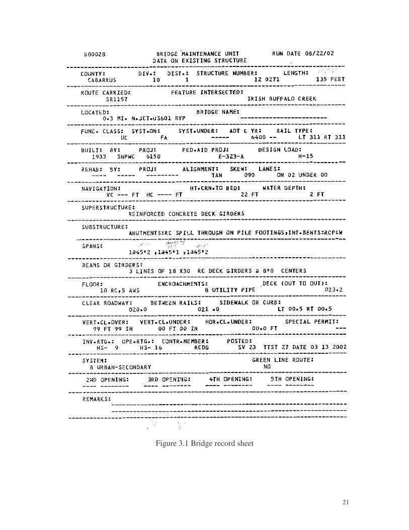
results are recorded in standard inspection forms and bridge records (see Figure 3.1).
21
Figure 3.1 Bridge record sheet

22
In order to learn more about the inspection procedures, the UNC Charlotte
research team joined the Division 10 bridge inspection crew to several bridges scheduled
for routine inspection. During this process, the two-man crew performed several field
measurements on the superstructure, the substructure, and the channel profile (where
applicable). The inspectors also noted the condition and the grade of deterioration (where
applicable) for all structural and non-structural elements, and took digital pictures of
selected bridge details. All of this information was included in the inspection report and
sent to the Analysis Team of the Bridge Maintenance Unit.
As a part of the bridge condition evaluation, the AASHTO (2000) manual
provides guidelines on material testing, including both field and laboratory tests. These
tests are aimed, using destructive and non-destructive methods, at the in-situ or laboratory
assessment of strength and condition of concrete, steel, and timber materials.
3.2 AASHTO Load Rating Guidelines
As part of the condition assessment of bridges, the above-mentioned manual
(AASHTO, 2000) also provides detailed bridge load rating procedures. These
calculations are performed in order to evaluate the safe load carrying capacity of bridges,
and are performed or updated following each bridge inspection.
Highway bridges are rated at two levels, inventory and operating levels. The
inventory rating (IR) represents “a load level which can safely utilize the structure for an
indefinite period of time.” This rating uses a large safety factor, since this day-to-day use
will imply the largest amount of traffic passing over the bridge. The operating rating
(OR) represents “the absolute maximum permissible load level to which the structure

23
may be subjected.” This rating uses a smaller safety factor in order to maximize the
capabilities of the bridge for the occasional special case. Therefore, the OR is not
intended for everyday use.
The rating can use either the allowable stress (AS) method, or the load factor (LF)
method. The selection of the method will change the load factors and the member
capacity values used in Equation 3.1:
)1(2
1
ILADAC
RF+××
×−= 3.1
where: RF – rating factor for live load; C – capacity of the member; A1 – factor for dead
loads; D – dead load effect; A2 – factor for live loads; L – live load effect; and I – impact
factor.
This rating factor can also be used to determine the bridge rating in tons (using
Equation 3.2). The overall bridge rating will be governed by the member with the lowest
rating factor.
WRFRT ×= )( 3.2
where: RT – bridge member rating in tons; and W – weight of nominal truck used to
determine live load effects.
3.3 NCDOT Bridge Rating Procedures
The computer analysis programs currently used by the NCDOT are MS-DOS
based programs, and are based on equations recommended by AASHTO (2000) for
bridge superstructures.

24
The input files for these programs are generated using bridge records and the most
current inspection reports. These files include general bridge data, such as bridge
number, county number, date inspected, and date of analysis; geometric information,
including span length, size of members, bridge dead loads; material properties from as-
built drawings, or from AASHTO recommended values when no other data is available.
In addition, the programs prompt the user to input the percentage of the girder that
is still effective. This is where the inspection process ties in with the computer program.
From the notes and photographs of a particular component the bridge inspectors provided
in their report, the analyzing engineer estimates the percent effective of the cross-section.
Obviously, this is a subjective estimate, and it is intended to result in a conservative load
rating.
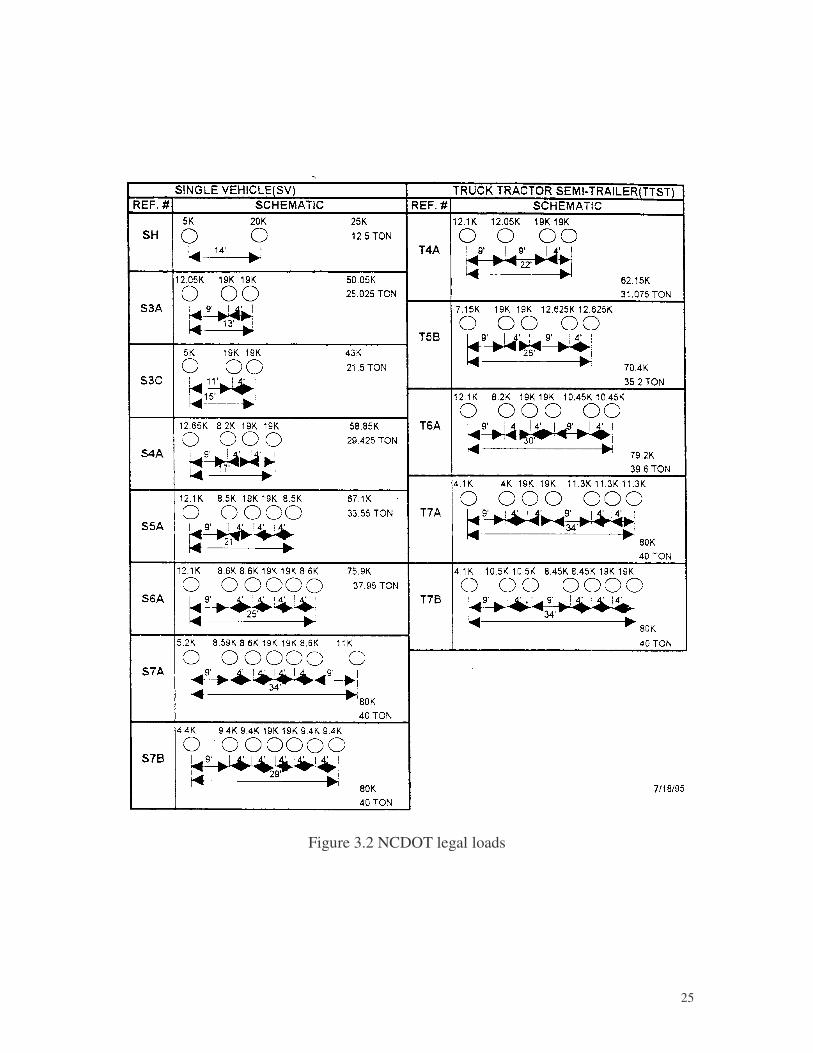
After all the information is input into the program, the computer calculates the
dead load moment, girder capacity, and live load moments. The program computes live
load moments by positioning different types of legal truck loads to determine critical
elements on the bridge. The schematics shown on Figure 3.2 are used by the programs to
model real vehicle axle spacing and axle loads. Each of these trucks are identified by a
reference number and is placed into one of two categories: single vehicles (SV), and
truck tractor semi-trailer (TTST).
25
Figure 3.2 NCDOT legal loads

26
Using these live load moments the program calculates two rating factors,
inventory and operating. These factors are then multiplied by the weight of the truck, and
then divided by the distribution factor to develop a rating for that girder. To calculate the
rating factors, the program utilizes Equation 3.3.
( )2100
2
1
����
�
�
����
�
�
××
×−��
���
� ×=
IMomentLLA
MomentDLAPercEff
MRF
i
n
i 3.3
where: Mn – moment capacity of the girder; PercEff – percent of girder resisting loading;
MomentDL – moment due to dead load; MomentLL – moment due to live load; I –
impact factor; A1 = 1.3 (dead load factor); A2 = 1.3 for operating, 2.17 for inventory (live
load factor); and i – indicates this value varies with each truck.
To convert this rating factor into a rating, Equation 3.4 is used:
( )DistFactor
RFtTruckWeighRating ii
i
×= 3.4
where: Truck Weight – weight of vehicle; RF – rating factor; and DistFactor –
distribution factor (based on AASHTO or user input).
3.4 Sample Analysis
This section outlines a sample computer analysis first by hand calculations, then
by using the NCDOT computer output. For simplicity, the hand calculations will be
limited to the S3C truck. The same process can be repeated for all the remaining loading
trucks. The structure being analyzed is a simple-span reinforced concrete deck girder
(RCDG) bridge. The process is similar for steel girder bridges with a few exceptions,
such as, serviceability requirements, compact section requirements, etc.
27
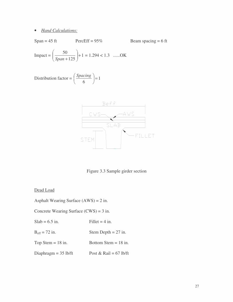
• Hand Calculations:
Span = 45 ft PercEff = 95% Beam spacing = 6 ft
Impact = 1125
50 +���
����
�
+Span = 1.294 < 1.3 ......OK
Distribution factor = 16
=��
���
� Spacing
Figure 3.3 Sample girder section
Dead Load
Asphalt Wearing Surface (AWS) = 2 in.
Concrete Wearing Surface (CWS) = 3 in.
Slab = 6.5 in. Fillet = 4 in.
Beff = 72 in. Stem Depth = 27 in.
Top Stem = 18 in. Bottom Stem = 18 in.
Diaphragm = 35 lb/ft Post & Rail = 67 lb/ft

28
��
���
�×+×��
�
���
���
�+×=12150
12150
12 SlabSpacingSpacingCWSAWSDLSlab
[ ] ftlbDiapragmRailPostDLFilletTopStemStemDepthDL Slab /1481&1441502 =+++�
�
���
�+×=
ftkSpan
DLMomentDL −=���
����
�= 375
8000
2
Live Load
Truck = S3C
MomentLLS3C = 418.31 k-ft
Girder Capacity Calculation
f’c = 2500 psi fy = 33000 psi �1 = 0.85 � = 0.9
d = 27.46 in. Beff = 72 in. As = 16.974 in2 t = Slab – ¼ in.
=��
�
�
��
�
�
×××
=effc
ys
Bf
fAa '85.0
3.661 in. < t = 6.25 in. .......... Rectangular Compression Zone
ftka
dfAMn ys −=��
���
���
�
���
���
� −××= 107712000
12
φ
Rating Factor
A1 = 1.3 A2 = 1.3 for operating, 2.17 for inventory
913.02100
32
1
=����
�
�
����
�
�
××
×−��
���
�×=
IMomentLLA
MomentDLAPercEff
MRF
CSinv
n
inv
29
524.12100
32
1
=����
�
�
����
�
�
××
×−��
���
�×=
IMomentLLA
MomentDLAPercEff
MRF
CSoperoper
Load Rating
tonsDistFactor
RFtTruckWeighRating invCS
inv 6.193 =��
���
� ×=
tonsDistFactor
RFtTruckWeighRating operCS
oper 8.323 =���
����
� ×=
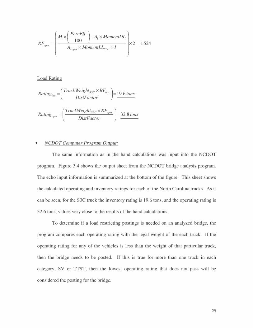
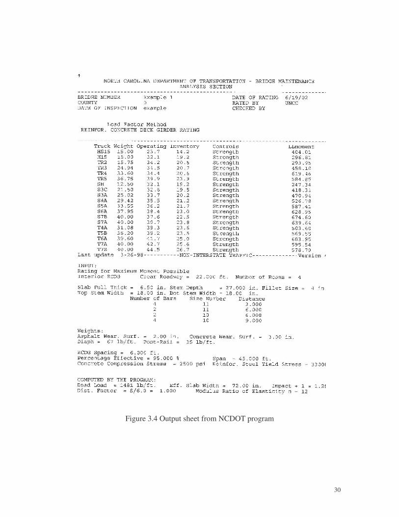
• NCDOT Computer Program Output:
The same information as in the hand calculations was input into the NCDOT
program. Figure 3.4 shows the output sheet from the NCDOT bridge analysis program.
The echo input information is summarized at the bottom of the figure. This sheet shows
the calculated operating and inventory ratings for each of the North Carolina trucks. As it
can be seen, for the S3C truck the inventory rating is 19.6 tons, and the operating rating is
32.6 tons, values very close to the results of the hand calculations.
To determine if a load restricting postings is needed on an analyzed bridge, the
program compares each operating rating with the legal weight of the each truck. If the
operating rating for any of the vehicles is less than the weight of that particular truck,
then the bridge needs to be posted. If this is true for more than one truck in each
category, SV or TTST, then the lowest operating rating that does not pass will be
considered the posting for the bridge.
30
Figure 3.4 Output sheet from NCDOT program
31
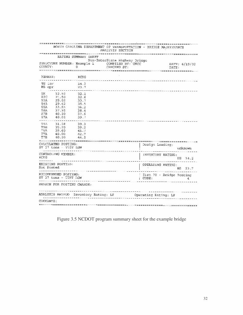
This is done for both SV and TTST separately; therefore, if a bridge is posted, it
will be posted for both SV and TTST, as needed. TTST are generally longer vehicles
with wider axle spacing, so the ratings are generally larger. Figure 3.5 is a summary
sheet for the bridge analysis. The three columns near the center of the page, from left to
right, are the trucks reference numbers, truck weight in tons, and operating rating for each
particular truck.
For the SV, each one of the operating ratings is larger than the legal weights,
except for S7B and S7A. The lower of these two ratings is rounded down to the closest
whole number and governs the load-restricting posting. In this case, S7B governs the SV
category with 37 tons. For the TTST, none of the operating ratings are lower than the
legal weights. Therefore, the bridge is not restricted for TTST.
The result of these comparisons is noted on the summary sheet:
SV-37 tons TTST-Legal gross weight
32
Figure 3.5 NCDOT program summary sheet for the example bridge
33
3.5 AASTHOWare
The AASHTOWare software package consists of three programs: Opis, Virtis and
Pontis. These three programs allow for the exchange of data between the programs. This
enables the user to input data for the structure only once, and then share it between the
programs to carry out each program’s specific functions. Therefore, a user can design a
bridge with Opis, which is design software that was not evaluated during this research.
Then export the data to Virtis, a load rating software to determine the Inventory and
Operating Ratings, and finally, export that data to Pontis, a bridge management system
that generates data for the National Bridge Inventory (NBI).
The Virtis and Pontis programs were developed by AASHTOWare to implement
the NCHRP 12-50 methods (Transportation Research Board, 2003). This 1998 project
concluded in 2002 with the development of a methodology for bridge-design software
validation. From this, "Process 12-50", a systematic method of comparing and evaluating
bridge design and analysis software, was generated. Process 12-50 provides a
standardized report format for presenting and comparing results for a specific bridge
design and a powerful method for formally reviewing specification changes.
The demonstration copies of Virtis and Pontis were evaluated for ninety days,
during this project. This time limitation only allowed for the analysis of one of the
scheduled test bridges. The outputs were compared with the current NCDOT load rating
software.

34
Virtis
The software Virtis Version 4.1 was developed by AAHSTO in 2001. It is a
bridge load rating software with the capability of using either LFD or LRFD. The
demonstration copy used during this research employed the 1996 AASHTO Standard
Specifications for Load Factor Design and the 1998 AASHTO LRFD Specifications.
However, full versions of this product allow for code updates (interim revisions) as
required.
Virtis allows the user to input all design data for the bridge, or import it from
Opis, including shear reinforcement. The user input option allows the user to define
different beam shapes, end conditions, and material properties. The program can
evaluate steel, timber, or reinforced and prestressed concrete members. The bridge can
be defined as a simple beam or continuous, or a combination of both for multiple spans
with the end conditions defined as pinned-pinned, fixed-fixed, or a combination.
For steel girder bridges, this program allows the user to detail information
concerning the deterioration of the beam. A deterioration profile can be created for the
web, top and bottom flanges, and top and bottom cover plates. This profile can be
generated based on field inspection notes, and will greatly affect the load rating of the
bridge.
The program will also consider percent effective of the bridge member’s section.
However, adjusting the percent effective from the default 100% created a controlling
Ultimate Shear Capacity versus Ultimate Moment Capacity. While this may realistically
be the controlling factor, there is a known problem with the software in this regard. The
modification of the percent effective does not allow the user to ignore shear.
35
The program can evaluate the entire bridge, a selected span, or a single girder. It
will report the calculated load ratings for the controlling load vehicle. It will also
generate graphs and tables for moment, shear, and displacement. This program however,
will not generate load postings. It generates inventory and operating ratings that are used
in determining the required posting. These ratings were used to compare and evaluate the
current NCDOT load rating software.
Pontis
The software Pontis Version 4.1 was developed by AASHTOWare as a bridge
management system. It allows the user to either create or import data from Virtis and
determine the sufficiency ratings of the bridge. Pontis is currently used by most states.
Missouri and Florida Departments of Transportation have utilized the program since
1998.
The sufficiency rating calculations follow the items described by NBI (USDOT,
1995). These rating are based on inspection details, which are entered into the program
from the field inspection notes. The program transfers the field inspection ratings into
NBI Coding. This is then used to determine the bridge sufficiency rating. The Federal
Highway Administration (FHWA) considers a bridge structurally deficient when the
sufficiency rating is below 50.
The software’s management system also entails the ability of project planning,
programming, and preservation of the structure. For the purposes of this research
however, only the inspection function was used.

36
3.6 UNCC Bridge Analysis Software
In order to perform some of the lower and upper bound analyses on several
bridges, the researchers developed a simple-span bridge analysis (Excel based) software.
For reference, the file is attached to this report, and a detailed instruction manual is
provided in Appendix A.
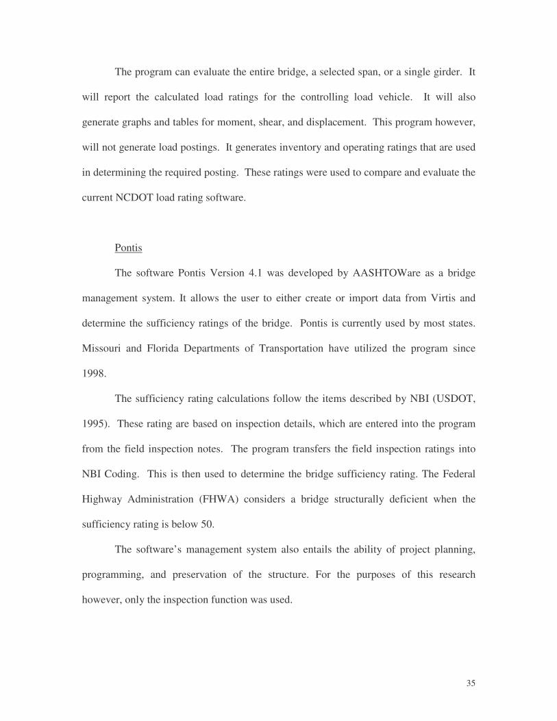
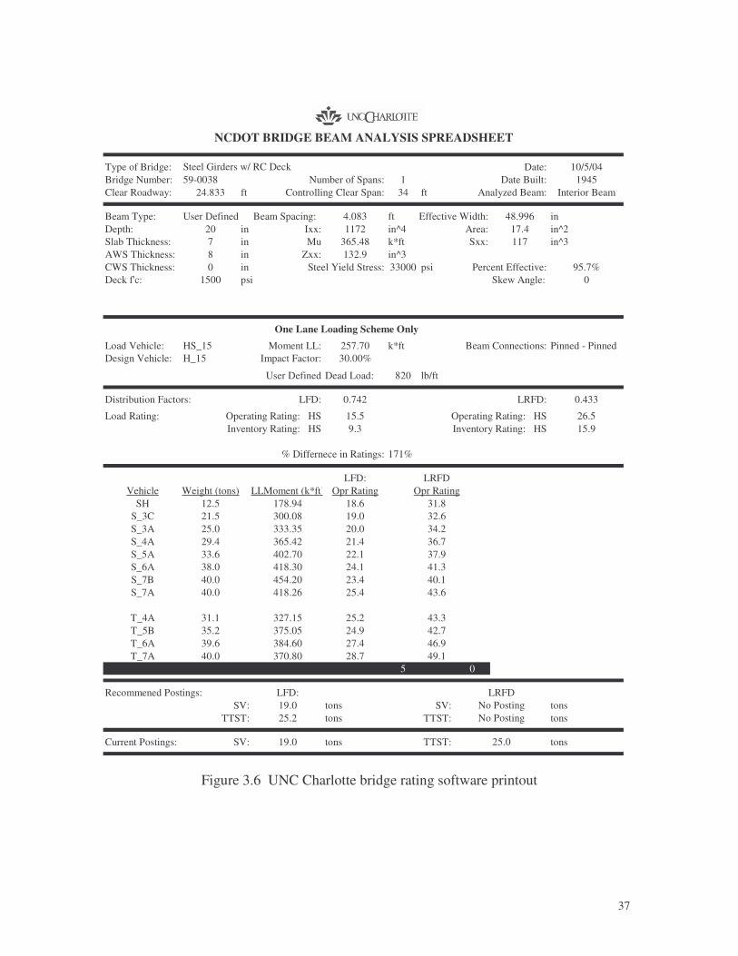
An output example is shown in Figure 3.6, illustrating the ratings for 59-0038. As
it can be seen, the software evaluates the bridge rating using both LFD and LRFD
methods. Furthermore, it is possible to input pinned, fixed, and partially fixed girder end
connections. Even though the software does not have continuous span capabilities, this
feature allows the user to investigate the effect partial fixity has on the bridge rating.
The software also allows the engineer to input calculated or user definer
distribution factors and impact factors for both concrete and steel girder bridges. For
RCDG bridges, cracked section properties are used, as needed. In order to allow a more
direct comparison between analytical rating and load test results, an added feature allows
for the calculation of strains and stresses in the bridge girders.
Another feature for this software is the capability to save the input and output files
electronically. This allows the user to store the bridge data between two inspections,
reducing the time needed to re-run the program.
The intent of the development of this program was not to replace the existing
NCDOT bridge analysis software, only to complement its capabilities with added features
that allow for a lower and upper bound analysis. However, if there is a need expressed
by NCDOT, the software can be further developed to include continuous span girders, as
well as a variety of other customized features.
37
Figure 3.6 UNC Charlotte bridge rating software printout
Type of Bridge: Date: 10/5/04Bridge Number: 59-0038 Number of Spans: 1 Date Built: 1945Clear Roadway: 24.833 ft Controlling Clear Span: 34 ft Analyzed Beam: Interior Beam
Beam Type: User Defined Beam Spacing: 4.083 ft Effective Width: 48.996 inDepth: 20 in Ixx: 1172 in^4 Area: 17.4 in^2Slab Thickness: 7 in Mu 365.48 k*ft Sxx: 117 in^3AWS Thickness: 8 in Zxx: 132.9 in^3CWS Thickness: 0 in Steel Yield Stress: 33000 psi Percent Effective: 95.7%Deck f'c: 1500 psi Beam f'c: psi Skew Angle: 0
Calculated Area of Steel: 16.96 in^2effective depth excluding CWS, d: 28.08 in
Load Vehicle: HS_15 Moment LL: 257.70 k*ft Beam Connections: Pinned - PinnedDesign Vehicle: H_15 Impact Factor: 30.00% % of Partial Fixity Assumed: 50.0%
User Defined Dead Load: 820 lb/ft
Distribution Factors: LFD: 0.742 LRFD: 0.433
Load Rating: Operating Rating: HS 15.5 Operating Rating: HS 26.5Inventory Rating: HS 9.3 Inventory Rating: HS 15.9
% Differnece in Ratings: 171%
LFD: LRFDVehicle Weight (tons) LLMoment (k*ft) Opr Rating Opr Rating
SH 12.5 178.94 18.6 0 31.8 0S_3C 21.5 300.08 19.0 1 32.6 0S_3A 25.0 333.35 20.0 2 34.2 0S_4A 29.4 365.42 21.4 3 36.7 0S_5A 33.6 402.70 22.1 4 37.9 0S_6A 38.0 418.30 24.1 5 41.3 0S_7B 40.0 454.20 23.4 6 40.1 0S_7A 40.0 418.26 25.4 7 43.6 0
T_4A 31.1 327.15 25.2 1 43.3 0T_5B 35.2 375.05 24.9 2 42.7 0T_6A 39.6 384.60 27.4 3 46.9 0T_7A 40.0 370.80 28.7 4 49.1 0T_7B 40.0 312.50 34.0 5 58.3 0
Recommened Postings: LFD:SV: 19.0 tons SV: tons
TTST: 25.2 tons TTST: tons
Current Postings: SV: 19.0 tons TTST: tons25.0
NCDOT BRIDGE BEAM ANALYSIS SPREADSHEET
Steel Girders w/ RC Deck
No PostingNo Posting
LRFD
One Lane Loading Scheme Only

38
4. BRIDGE SELECTION
4.1 Selection Criteria
The criterions for selecting appropriate bridges for this project were created to
ensure a true representation of typical bridges, especially those with higher maintenance
needs. The selection and prioritization was coordinated with the NCDOT Bridge
Maintenance Unit using the available computer database. Each selection was based on
the following criteria (not in order of importance):
• Importance and traffic – to minimize commuter inconvenience the NCDOT
suggested that only bridges on the secondary system should be considered, with
adequate possibilities for traffic detours.
• Load ratings – the selected bridges had a wide range of load ratings, anywhere
from bridges posted for SV-14 tons, to bridges with no postings.
• Bridge condition and estimated remaining life – only bridges with a reasonable
life expectancy were considered.
• Bridge superstructure system – both concrete and steel girder bridges were
selected, with simply supported and continuous systems.
• Site access – to allow the research team to prepare bridges for testing, only
structures with reasonable foot and vehicular access were considered.
• Location of bridges – in order to avoid long travel times for the research team,
only bridges within Division 10 were considered.

39
4.2 GFRP Deck Bridge
This project provided a unique opportunity to the researchers at UNC Charlotte to
monitor the construction, instrumentation and field testing of the first glass fiber
reinforced polymer (GFRP) deck bridge in North Carolina. The original Bridge 89-022
was built in 1944, and replaced in September 2001.
The original steel girder and concrete deck system superstructure was replaced
with 7 – W24x94 steel girders and a composite deck supplied by Martin Marietta
Composites. As it was mentioned earlier, this deck replacement project was funded with
a discretionary grant from the Federal Highway Administration’s (FHWA) Innovative
Bridge Research and Construction (IBRC) program. Table 4.1 at the end of this chapter
provides more specific details for Bridge 89-022. In addition, a detailed, phase-by-phase
construction report and structural description for this composite deck bridge is included
in Appendix B.
4.3 Concrete Deck Girder Bridges
During this project, two reinforced concrete deck girder (RCDG) bridges were
analyzed, instrumented and tested. The first RCDG structure was Bridge 59-361, a rural
two-lane bridge located in western Mecklenburg County, North Carolina on Bellhaven
Blvd. (SR 2373). The bridge consists of three simple spans of approximately 40 ft each.
The deck is supported by four reinforced concrete girders spaced at 6 ft-8 in. on center.
Construction of bridge 59-361 was completed in 1935; since that time, there have not
been any structural modifications made to either the substructure or the superstructure.
Figure 4.1 shows an elevation view of bridge 59-361, and Figure 4.2 shows a typical

40
cross section of the bridge superstructure.
Figure 4.1 Side view of Bridge 59-361
Figure 4.2 Typical cross-section of the superstructure for Bridge 59-361
The steel reinforcement is not shown in Figure 4.2 for clarity. The deck is
reinforced with #4 bars at 6 in. o.c. in the bottom of the deck and #4 bars at 16 in. o.c. in
the top of the deck longitudinal to the direction of traffic. In the transverse direction, #5
bars at a varying spacing were used. The girders were reinforced with (4) - #11 bars 3 in.
from the bottom of the girder, (2) - #11 and (2) - #10 bars 6 in. from the bottom of the

41
girder, and (4) - #10 bars 9 in. from the bottom of the girder. For shear reinforcing, #4
bars at an unknown spacing were used.
The most recent three bridge inspection reports covering a span of five years have
been reviewed. According to these reports, bridge 59-361 has isolated, minor hairline
cracks in the girders and the piers. Each of these girders was rated as either good or fair.
Furthermore, each report stated the same observed condition of the girders. Therefore, it
is fair to assume that the cracks did not widen over this five-year period. In order to
monitor changing conditions of concrete girders, it is recommended to mark the extent of
these cracks, properly identifying the date of the last inspection and markings.
Although the apparent beam conditions have remained the same, the bridge load-
restricting posting has been decreased after each report. Until 1999, the bridge was not
posted. At the time of inspection, bridge 59-361 was posted at 35 tons for single
vehicles, due to a change in material properties specified by AASHTO. The compressive
strength of concrete for bridges constructed before 1959 was increased from 2,500 psi to
2,700 psi and the yield strength of steel for bridges constructed before 1954 was
decreased from 33,000 psi to 30,000 psi. Obviously, these changes had an impact on the
bridge posting.
Since the load testing in November 2001, the bridge has been reposted at 32 tons
for single vehicles (SV) and 38 tons for truck tractor semi-trailers (TTST). This change
was due to the resurfacing of SR 2373, resulting in an addition of 2.5 in. of asphalt
wearing surface for a total of 9” of asphalt.
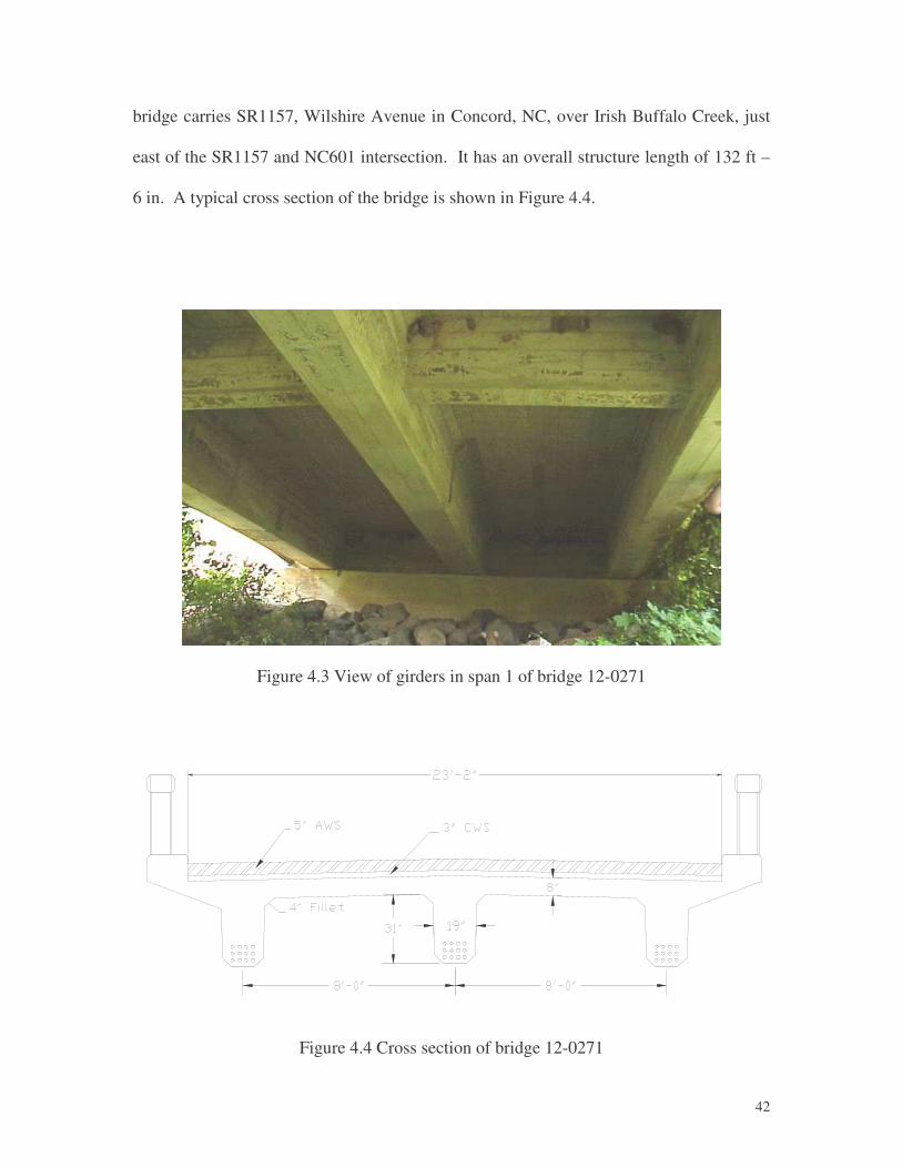
The second RCDG structure tested was Bridge 12-0271 (Figure 4.3), a three-span
reinforced concrete deck girder bridge with three girders. This two-lane secondary route
42
bridge carries SR1157, Wilshire Avenue in Concord, NC, over Irish Buffalo Creek, just
east of the SR1157 and NC601 intersection. It has an overall structure length of 132 ft –
6 in. A typical cross section of the bridge is shown in Figure 4.4.
Figure 4.3 View of girders in span 1 of bridge 12-0271
Figure 4.4 Cross section of bridge 12-0271

43
The bridge was designed for a load vehicle of H-15. It is currently posted for SV
at 23 tons and TTST at 27 tons. This posting occurred on March 13, 2002, which
represents a reduction from the previous posting of 32 tons. This change in posting
occurred due to a change in allowable stresses for concrete and steel. The prior posting
was based on unknown material strengths governed by the year of construction.
However, a recent NCDOT memorandum mandates the use of reinforcing steel
and concrete allowable stresses from the original plans, whenever the information is
available. Based on the original plans, the concrete compressive strength was established
as 1,950 psi, and the yield strength of the reinforcing steel was computed as 30 ksi.
The last inspection of this bridge occurred on January 29, 2002. In this report, the
bridge inspectors noted that, there were vertical and horizontal cracks on the sides face of
the girders at midspan, which led to a decision to use a 95% effectiveness for the girder
sections (PercEff in Equation 3.3). The current load ratings are Inventory HS-9.9 and
Operating HS-16.5, resulting in a sufficiency rating of 48.1%, which gives the bridge an
NBI status of structurally deficient.
4.4 Steel Girder Bridges
Three steel girder bridges were analyzed and tested during the two-year period of
this project. The first was Bridge 59-0038, a rural two-lane bridge located in
southeastern Mecklenburg County, North Carolina on Sam Newell Road (SR 3168). The
bridge consists of one simple span of approximately 36 ft. The original superstructure of
the bridge consisted of a reinforced concrete deck supported by five steel girders spaced
at 4 ft – 1 in. on center. Construction on this bridge was completed in 1945. Since that
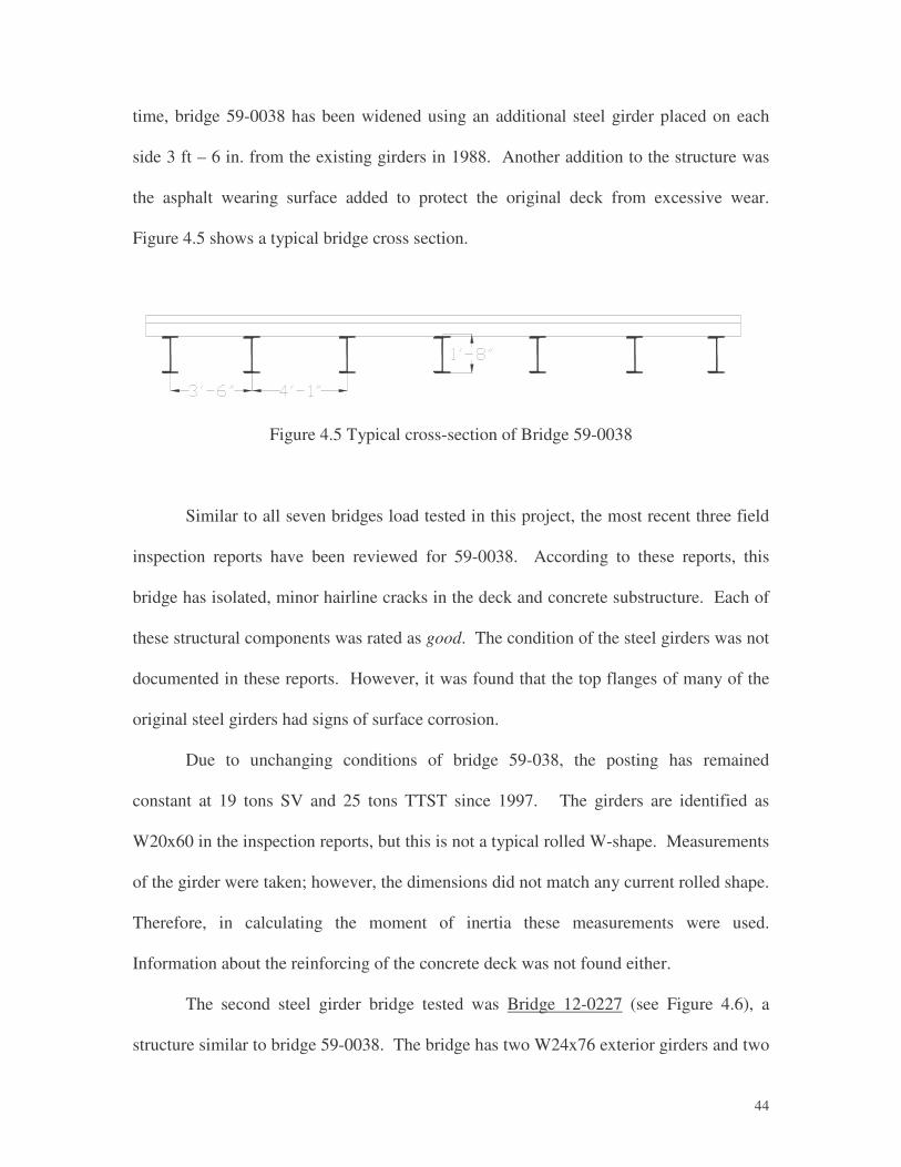
44
time, bridge 59-0038 has been widened using an additional steel girder placed on each
side 3 ft – 6 in. from the existing girders in 1988. Another addition to the structure was
the asphalt wearing surface added to protect the original deck from excessive wear.
Figure 4.5 shows a typical bridge cross section.
Figure 4.5 Typical cross-section of Bridge 59-0038
Similar to all seven bridges load tested in this project, the most recent three field
inspection reports have been reviewed for 59-0038. According to these reports, this
bridge has isolated, minor hairline cracks in the deck and concrete substructure. Each of
these structural components was rated as good. The condition of the steel girders was not
documented in these reports. However, it was found that the top flanges of many of the
original steel girders had signs of surface corrosion.
Due to unchanging conditions of bridge 59-038, the posting has remained
constant at 19 tons SV and 25 tons TTST since 1997. The girders are identified as
W20x60 in the inspection reports, but this is not a typical rolled W-shape. Measurements
of the girder were taken; however, the dimensions did not match any current rolled shape.
Therefore, in calculating the moment of inertia these measurements were used.
Information about the reinforcing of the concrete deck was not found either.
The second steel girder bridge tested was Bridge 12-0227 (see Figure 4.6), a
structure similar to bridge 59-0038. The bridge has two W24x76 exterior girders and two

45
W27x94 interior girders. The reinforced concrete deck has an epoxy-wearing surface. It
carries state route SR1006 (Mt. Pleasant Road) over Rocky River.
As it can be seen in Figure 4.7, significant debris was present at the time of the
bridge instrumentation and testing. Also, it is evident from Figure 4.8 that the add-on
timber bent has been repaired in the past. An additional timber post has been installed
between the first and second posts, unloading the gravity loads from one of the severely
decayed original posts.
Figure 4.6 View of bridge 12-0227
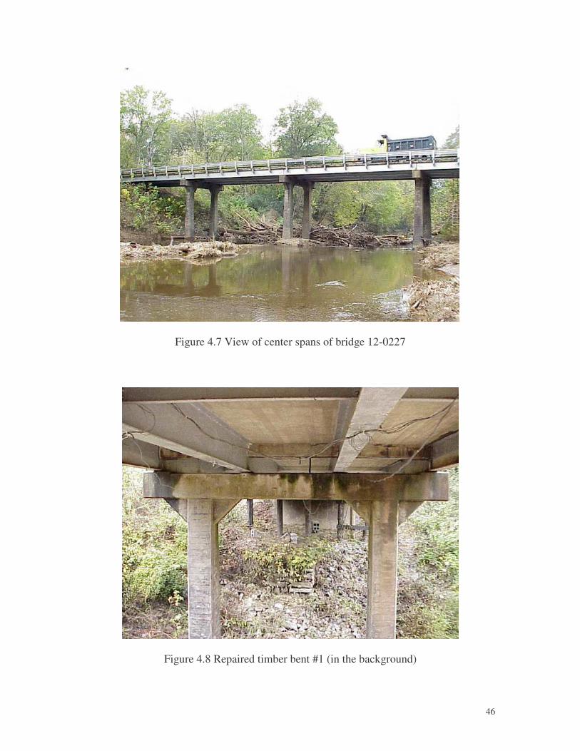
46
Figure 4.7 View of center spans of bridge 12-0227
Figure 4.8 Repaired timber bent #1 (in the background)
47
This bridge has a current posting of an SV at 24 tons and TTST at 28 tons,
established on July 24, 1995. The bridge provided easy work access on two of the five
spans with a ladder, while a snooper truck was required to complete the scheduled tasks
only on the third (middle) span.
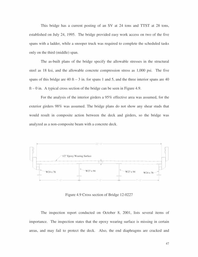
The as-built plans of the bridge specify the allowable stresses in the structural
steel as 18 ksi, and the allowable concrete compression stress as 1,000 psi. The five
spans of this bridge are 40 ft – 3 in. for spans 1 and 5, and the three interior spans are 40
ft – 0 in. A typical cross section of the bridge can be seen in Figure 4.9.
For the analysis of the interior girders a 95% effective area was assumed, for the
exterior girders 98% was assumed. The bridge plans do not show any shear studs that
would result in composite action between the deck and girders, so the bridge was
analyzed as a non-composite beam with a concrete deck.
1/2" Epoxy Wearing Surface
W24 x 76 W27 x 94W24 x 76W27 x 94
Figure 4.9 Cross section of Bridge 12-0227
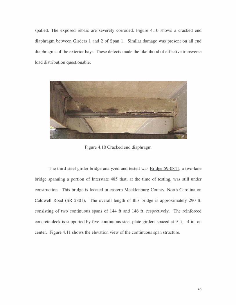
The inspection report conducted on October 8, 2001, lists several items of
importance. The inspection states that the epoxy wearing surface is missing in certain
areas, and may fail to protect the deck. Also, the end diaphragms are cracked and
48
spalled. The exposed rebars are severely corroded. Figure 4.10 shows a cracked end
diaphragm between Girders 1 and 2 of Span 1. Similar damage was present on all end
diaphragms of the exterior bays. These defects made the likelihood of effective transverse
load distribution questionable.
Figure 4.10 Cracked end diaphragm
The third steel girder bridge analyzed and tested was Bridge 59-0841, a two-lane
bridge spanning a portion of Interstate 485 that, at the time of testing, was still under
construction. This bridge is located in eastern Mecklenburg County, North Carolina on
Caldwell Road (SR 2801). The overall length of this bridge is approximately 290 ft,
consisting of two continuous spans of 144 ft and 146 ft, respectively. The reinforced
concrete deck is supported by five continuous steel plate girders spaced at 9 ft – 4 in. on
center. Figure 4.11 shows the elevation view of the continuous span structure.
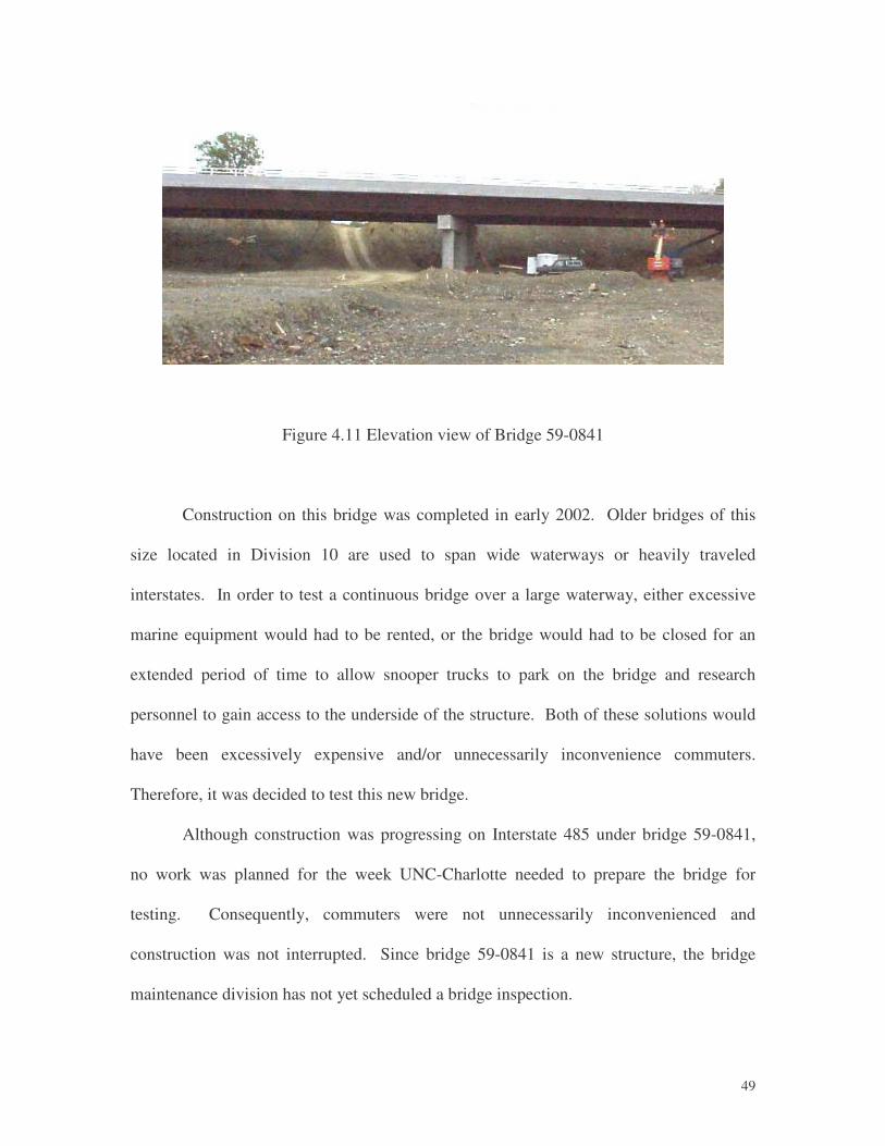
49
Figure 4.11 Elevation view of Bridge 59-0841
Construction on this bridge was completed in early 2002. Older bridges of this
size located in Division 10 are used to span wide waterways or heavily traveled
interstates. In order to test a continuous bridge over a large waterway, either excessive
marine equipment would had to be rented, or the bridge would had to be closed for an
extended period of time to allow snooper trucks to park on the bridge and research
personnel to gain access to the underside of the structure. Both of these solutions would
have been excessively expensive and/or unnecessarily inconvenience commuters.
Therefore, it was decided to test this new bridge.
Although construction was progressing on Interstate 485 under bridge 59-0841,
no work was planned for the week UNC-Charlotte needed to prepare the bridge for
testing. Consequently, commuters were not unnecessarily inconvenienced and
construction was not interrupted. Since bridge 59-0841 is a new structure, the bridge
maintenance division has not yet scheduled a bridge inspection.
50
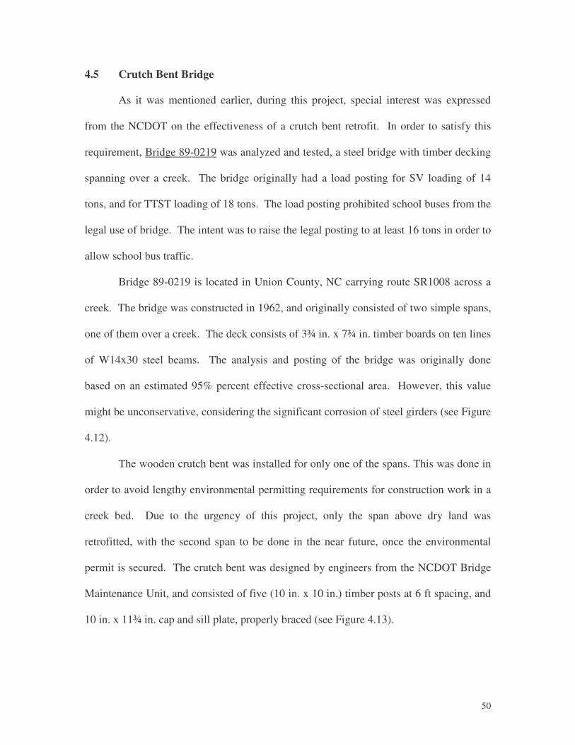
4.5 Crutch Bent Bridge
As it was mentioned earlier, during this project, special interest was expressed
from the NCDOT on the effectiveness of a crutch bent retrofit. In order to satisfy this
requirement, Bridge 89-0219 was analyzed and tested, a steel bridge with timber decking
spanning over a creek. The bridge originally had a load posting for SV loading of 14
tons, and for TTST loading of 18 tons. The load posting prohibited school buses from the
legal use of bridge. The intent was to raise the legal posting to at least 16 tons in order to
allow school bus traffic.
Bridge 89-0219 is located in Union County, NC carrying route SR1008 across a
creek. The bridge was constructed in 1962, and originally consisted of two simple spans,
one of them over a creek. The deck consists of 3¾ in. x 7¾ in. timber boards on ten lines
of W14x30 steel beams. The analysis and posting of the bridge was originally done
based on an estimated 95% percent effective cross-sectional area. However, this value
might be unconservative, considering the significant corrosion of steel girders (see Figure
4.12).
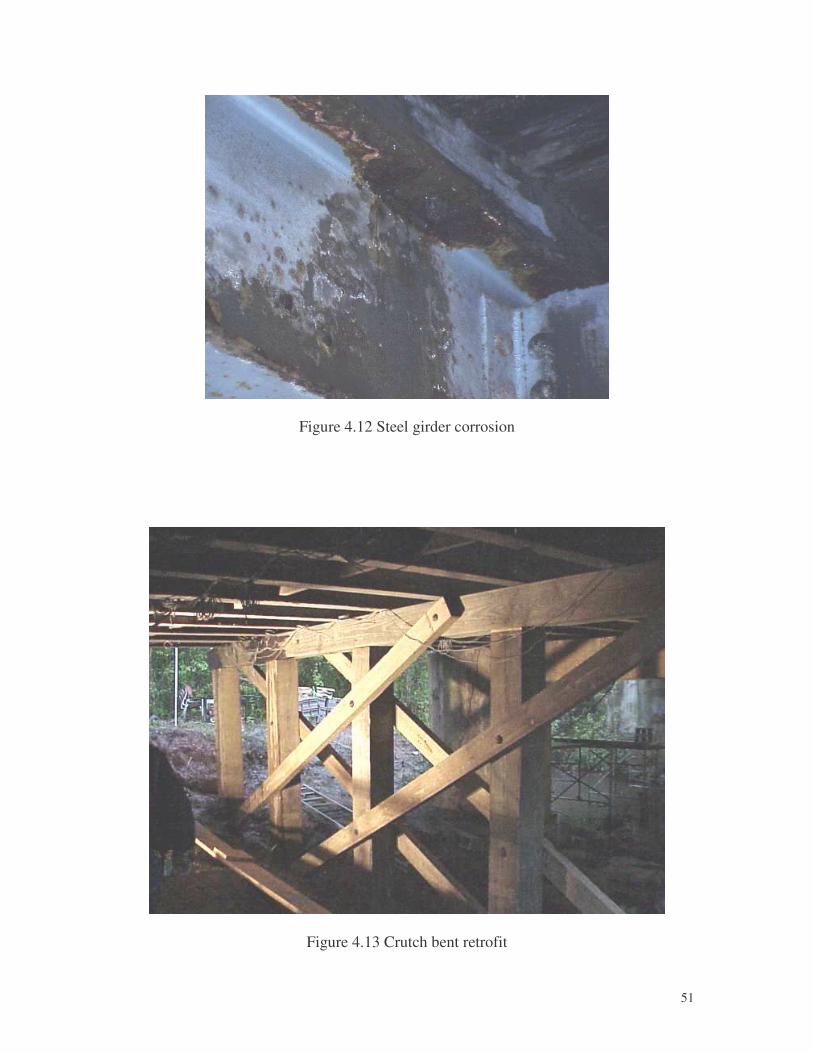
The wooden crutch bent was installed for only one of the spans. This was done in
order to avoid lengthy environmental permitting requirements for construction work in a
creek bed. Due to the urgency of this project, only the span above dry land was
retrofitted, with the second span to be done in the near future, once the environmental
permit is secured. The crutch bent was designed by engineers from the NCDOT Bridge
Maintenance Unit, and consisted of five (10 in. x 10 in.) timber posts at 6 ft spacing, and
10 in. x 11¾ in. cap and sill plate, properly braced (see Figure 4.13).
51
Figure 4.12 Steel girder corrosion
Figure 4.13 Crutch bent retrofit

4.6 Summary of Bridge Selection
As it can be seen from the previous sections, a large variety of bridges have been
analyzed and tested. In order to allow quick referencing of these structures, Table 4.1
shows a summary of all the bridges tested in this project. In this table only the most
important details are provided.
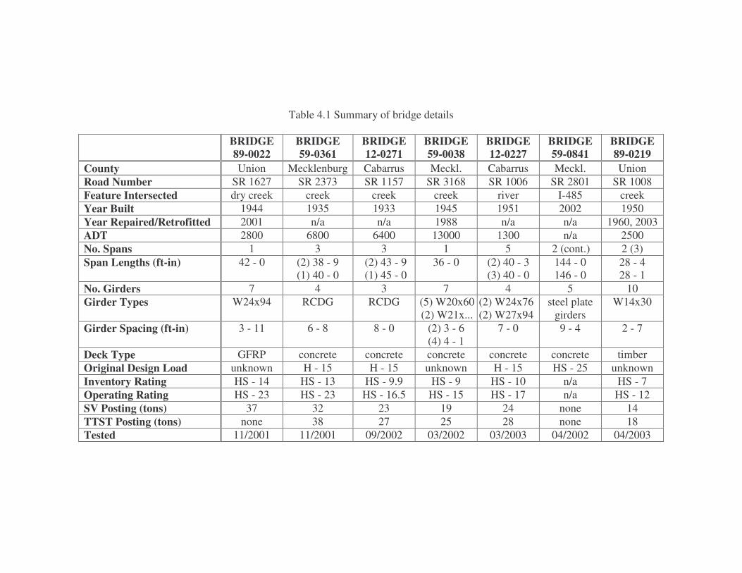
Table 4.1 Summary of bridge details
BRIDGE 89-0022
BRIDGE 59-0361
BRIDGE 12-0271
BRIDGE 59-0038
BRIDGE 12-0227
BRIDGE 59-0841
BRIDGE 89-0219
County Union Mecklenburg Cabarrus Meckl. Cabarrus Meckl. Union Road Number SR 1627 SR 2373 SR 1157 SR 3168 SR 1006 SR 2801 SR 1008 Feature Intersected dry creek creek creek creek river I-485 creek Year Built 1944 1935 1933 1945 1951 2002 1950 Year Repaired/Retrofitted 2001 n/a n/a 1988 n/a n/a 1960, 2003 ADT 2800 6800 6400 13000 1300 n/a 2500 No. Spans 1 3 3 1 5 2 (cont.) 2 (3) Span Lengths (ft-in) 42 - 0 (2) 38 - 9
(1) 40 - 0 (2) 43 - 9 (1) 45 - 0
36 - 0 (2) 40 - 3 (3) 40 - 0
144 - 0 146 - 0
28 - 4 28 - 1
No. Girders 7 4 3 7 4 5 10 Girder Types W24x94 RCDG RCDG (5) W20x60
(2) W21x... (2) W24x76 (2) W27x94
steel plate girders
W14x30
Girder Spacing (ft-in) 3 - 11 6 - 8 8 - 0 (2) 3 - 6 (4) 4 - 1
7 - 0 9 - 4 2 - 7
Deck Type GFRP concrete concrete concrete concrete concrete timber Original Design Load unknown H - 15 H - 15 unknown H - 15 HS - 25 unknown Inventory Rating HS - 14 HS - 13 HS - 9.9 HS - 9 HS - 10 n/a HS - 7 Operating Rating HS - 23 HS - 23 HS - 16.5 HS - 15 HS - 17 n/a HS - 12 SV Posting (tons) 37 32 23 19 24 none 14 TTST Posting (tons) none 38 27 25 28 none 18 Tested 11/2001 11/2001 09/2002 03/2002 03/2003 04/2002 04/2003

�
54
5. EXPERIMENTAL RESULTS
Throughout this project, seven bridges were analyzed, instrumented and tested.
Hundreds of experimental data files were generated from recordings of up to a hundred of
instruments during static, slow and dynamic loading, focusing on the behavior of structural and
non-structural components. The following sections describe the most important findings for
each bridge, and their relevance to the project objectives.
5.1 Bridge 89-0022
Strain level and composite action
One method to prove composite or non-composite action in the bridge would be to locate
the neutral axis of the girders. With no composite action, the strain in the girders would change
from compression to tension at a location near the center of mass of the girder (for this bridge
that would be 12.16 in.). The midspan of girders 2 and 4 were instrumented with strain gages on
the top and bottom flanges. These instruments were used to help locate the position of the
neutral axis. Assuming the strain in the girder remains linear, which should be the case for
girder stresses lower than the yield level, the position of the neutral axis (NA) from the bottom of
the steel girders can be calculated using Equation 5.1:
( )TB
BftdNA
εεε+
−= 5.1
where: d = 24.31 in. – girder depth; tf = 0.875 in. – flange thickness; εB – bottom flange strain
(in/in); εT – top flange strain (in/in).

�
55
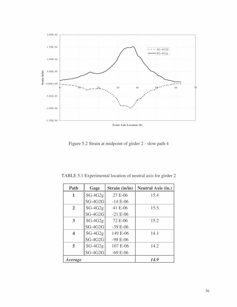
The calculations for the experimental neutral axis location are demonstrated using the
readings from the top and bottom flange strain at the midpoint of girder 2 for path 4. Both static
(see Figure 5.1) and slow (see Figure 5.2) readings were analyzed. For both cases, the maximum
bottom flange tensile strain was measured around 149 µε, and the maximum top flange strain
was approximately -98 µε. Using Equation 6.1, the neutral axis was computed as 14.1 in.
When the neutral axis at the midpoint of girder 2 was computed for all five load paths
(shown in Table 5.1), the position of the neutral axis was computed to be an average of 14.9 in.
above the bottom flange of the girder. Similar result (14.5 in.) was recorder for girder 4 at
midspan. With the center of mass of the girder being located at 12.16 in., it is clear that there
was some composite action taking place. This result will be further analyzed in Chapter 6.
Figure 5.1 Strain at midpoint of girder 2 - static path 4
-1.50E-04
-1.00E-04
-5.00E-05
0.00E+00
5.00E-05
1.00E-04
1.50E-04
2.00E-04
Load Location
Stra
in (i
n/in
)
SG-4G2gSG-4G2G
b
a
�
56
Figure 5.2 Strain at midpoint of girder 2 - slow path 4
TABLE 5.1 Experimental location of neutral axis for girder 2
Path Gage Strain (in/in) Neutral Axis (in.) 1 SG-4G2g 27 E-06 15.4 SG-4G2G -14 E-06 2 SG-4G2g 41 E-06 15.5 SG-4G2G -21 E-06 3 SG-4G2g 72 E-06 15.2 SG-4G2G -39 E-06 4 SG-4G2g 149 E-06 14.1 SG-4G2G -98 E-06 5 SG-4G2g 107 E-06 14.2 SG-4G2G -69 E-06
Average 14.9
-1.50E-04
-1.00E-04
-5.00E-05
0.00E+00
5.00E-05
1.00E-04
1.50E-04
2.00E-04
0 10 20 30 40 50 60 70
Front Axle Location (ft)
Stra
in (i
n/in
)
SG-4G2GSG-4G2g

�
57
Being the first GFRP deck bridge in the Carolinas, special attention was paid to
the strain levels in the GFRP deck. Composite materials are linear; therefore, in order to
avoid brittle material failure, it is important that at service level, adequate safety factors
are used.
Being comprised of glass fiber laminas with various orientations, the strain in the
fibers of the panels was not evaluated, and there was no allowable strain given by the
panel manufacturer for the laminas themselves. Martin Marietta Composites provided
designers only an overall allowable strain on the bottom of the deck panel for
compression (-0.26%) and tension (0.26%). The ultimate strain levels should be at least
six to eight times higher.
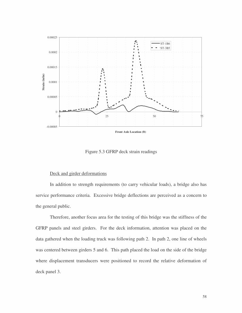
The strain readings in Bays 5 and 6 are plotted for load path 2 in Figure 6.5. The
maximum tensile strain was observed in Bay 5, and it was approximately 0.024%
(0.00024 in/in, or 240 µε). Therefore, the allowable strain in the material is over ten
times larger than the strain experienced in the panel.
The maximum negative strain (compression) was recorded in bay 6. The strain at
this location reached -0.002%. Once again, the strain induced in the material did not
even come close to reaching the strain allowed in the material. In this case the allowable
strain in the material was –0.26%, or roughly 130 times the strain present in the deck
panel.
Indeed, from these data, one can conclude that the bridge deck is performing well
within the manufacturer’s specifications. In the future, it will be possible to increase the
efficiency of FRP bridge decks significantly.
�
58
Figure 5.3 GFRP deck strain readings
Deck and girder deformations
In addition to strength requirements (to carry vehicular loads), a bridge also has
service performance criteria. Excessive bridge deflections are perceived as a concern to
the general public.
Therefore, another focus area for the testing of this bridge was the stiffness of the
GFRP panels and steel girders. For the deck information, attention was placed on the
data gathered when the loading truck was following path 2. In path 2, one line of wheels
was centered between girders 5 and 6. This path placed the load on the side of the bridge
where displacement transducers were positioned to record the relative deformation of
deck panel 3.
-0.00005
0
0.00005
0.0001
0.00015
0.0002
0.00025
0 25 50 75
Front Axle Location (ft)
Stra
in (i
n/in
)ST-1B6ST-3B5

�
59
The deflection of the bays is shown in Figure 5.4. From this graph, one can see
the maximum deflection of the panel to be 0.017 in. It was also noted that the panel
seemed to camber up slightly in bay 6. This camber reached a maximum value of 0.008
in. With the girders spaced at 47 in. o.c., the 0.017 in. deflection, as a ratio to the girder
spacing, is L/2800. Presently, AASHTO does not have a requirement for the deflection
of the composite deck. However, when comparing the deck deflection ratio to the
tolerances established for girders, this structure is well within the L/800 live load criteria
established for bridges (AASHTO Standard Specifications 10.6.2).
Midspan deflections were recorded for girders 1, 4, 5, 6, and 7. These deflections
were plotted for all the slow load paths. The deflections for slow path 1 are shown in
Figure 5.5. The corresponding maximum deflection for this loading condition occurred
at girder 6, and had a magnitude of 0.183 in. This value represents approximately
L/2600, which is well within the live load limit established by AASHTO.
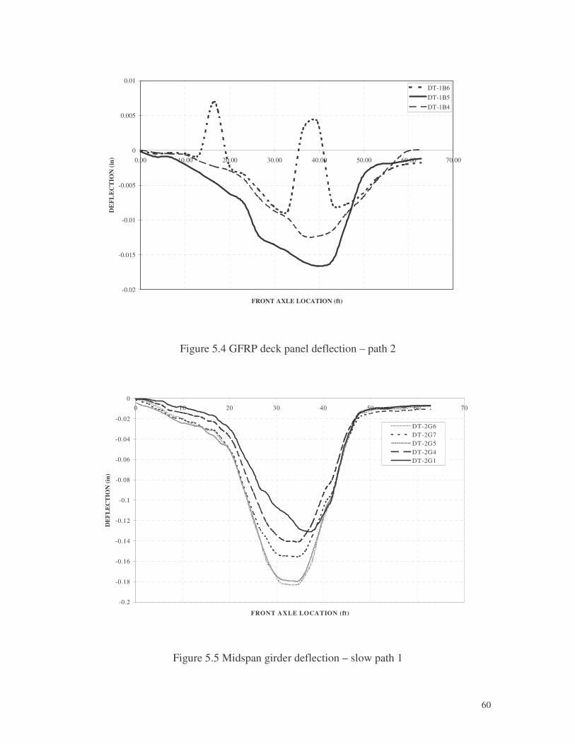
�
60
Figure 5.4 GFRP deck panel deflection – path 2
Figure 5.5 Midspan girder deflection – slow path 1
-0.02
-0.015
-0.01
-0.005
0
0.005
0.01
0.00 10.00 20.00 30.00 40.00 50.00 60.00 70.00
FRONT AXLE LOCATION (ft)
DE
FLE
CT
ION
(in)
DT-1B6DT-1B5DT-1B4
-0.2
-0.18
-0.16
-0.14
-0.12
-0.1
-0.08
-0.06
-0.04
-0.02
00 10 20 30 40 50 60 70
FRONT AXLE LOCATION (ft)
DE
FLE
CT
ION
(in)
DT-2G6DT-2G7DT-2G5DT-2G4DT-2G1
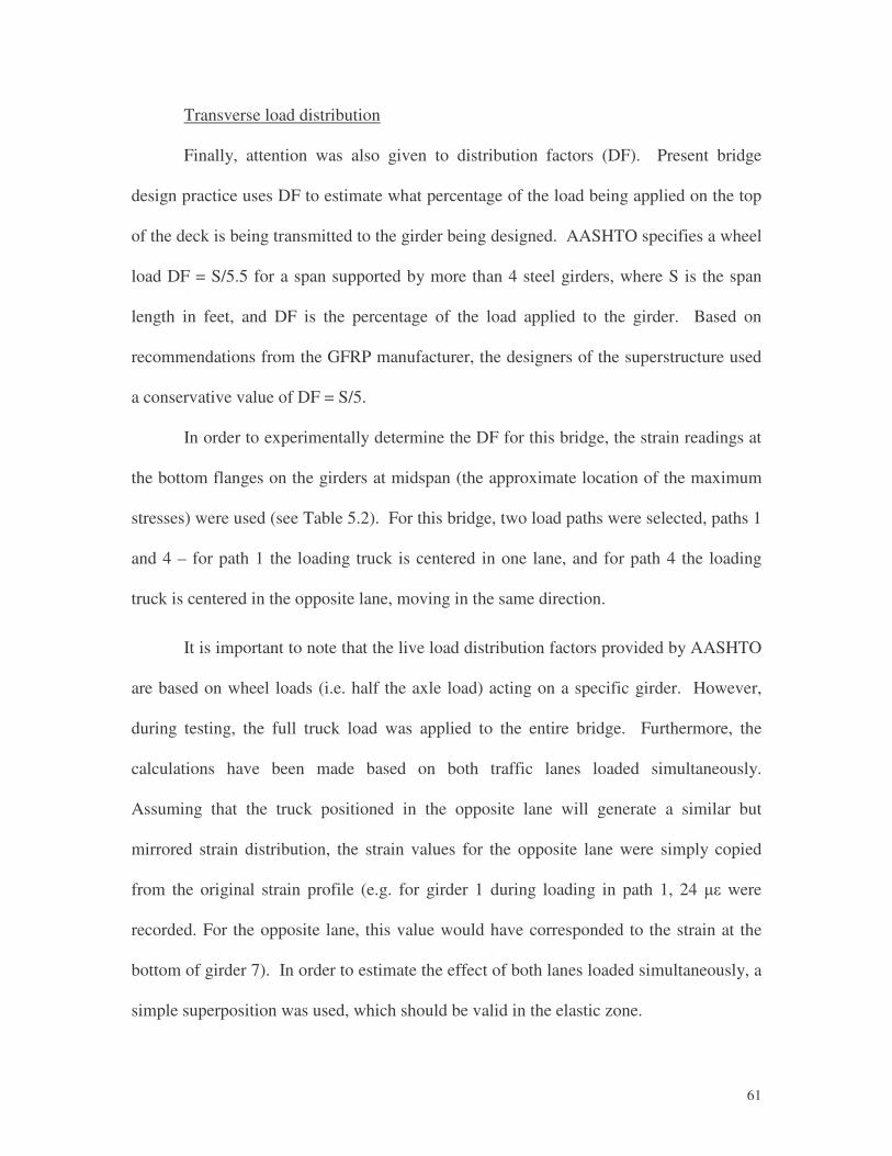
�
61
Transverse load distribution
Finally, attention was also given to distribution factors (DF). Present bridge
design practice uses DF to estimate what percentage of the load being applied on the top
of the deck is being transmitted to the girder being designed. AASHTO specifies a wheel
load DF = S/5.5 for a span supported by more than 4 steel girders, where S is the span
length in feet, and DF is the percentage of the load applied to the girder. Based on
recommendations from the GFRP manufacturer, the designers of the superstructure used
a conservative value of DF = S/5.
In order to experimentally determine the DF for this bridge, the strain readings at
the bottom flanges on the girders at midspan (the approximate location of the maximum
stresses) were used (see Table 5.2). For this bridge, two load paths were selected, paths 1
and 4 – for path 1 the loading truck is centered in one lane, and for path 4 the loading
truck is centered in the opposite lane, moving in the same direction.
It is important to note that the live load distribution factors provided by AASHTO
are based on wheel loads (i.e. half the axle load) acting on a specific girder. However,
during testing, the full truck load was applied to the entire bridge. Furthermore, the
calculations have been made based on both traffic lanes loaded simultaneously.
Assuming that the truck positioned in the opposite lane will generate a similar but
mirrored strain distribution, the strain values for the opposite lane were simply copied
from the original strain profile (e.g. for girder 1 during loading in path 1, 24 �� were
recorded. For the opposite lane, this value would have corresponded to the strain at the
bottom of girder 7). In order to estimate the effect of both lanes loaded simultaneously, a
simple superposition was used, which should be valid in the elastic zone.
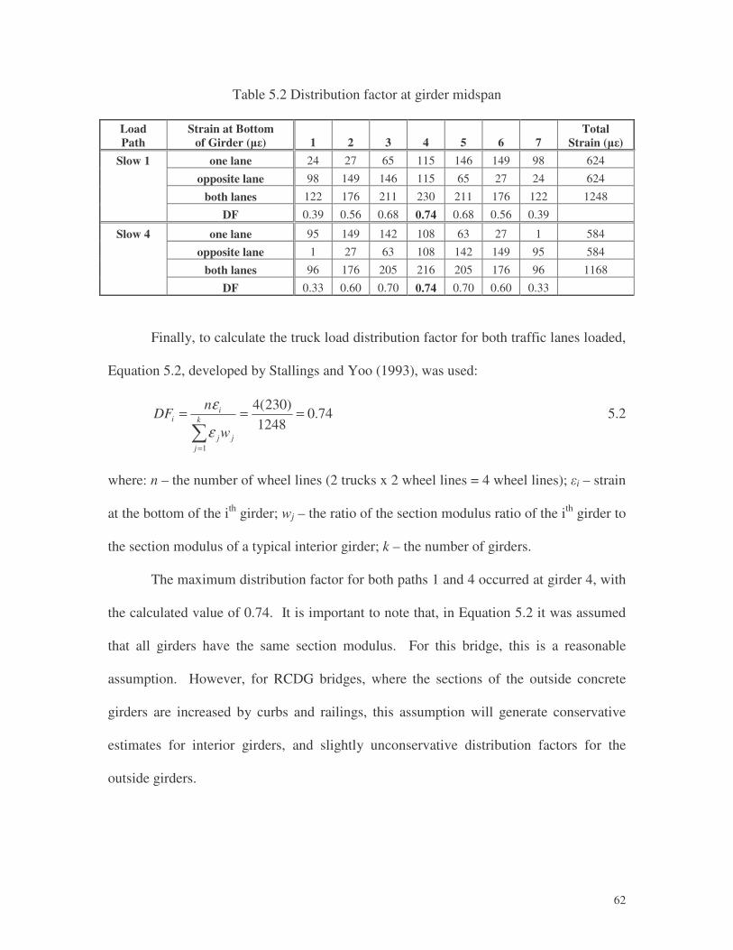
�
62
Table 5.2 Distribution factor at girder midspan
Load Path
Strain at Bottom of Girder (��) 1 2 3 4 5 6 7
Total Strain (��)
Slow 1 one lane 24 27 65 115 146 149 98 624
opposite lane 98 149 146 115 65 27 24 624
both lanes 122 176 211 230 211 176 122 1248
DF 0.39 0.56 0.68 0.74 0.68 0.56 0.39
Slow 4 one lane 95 149 142 108 63 27 1 584
opposite lane 1 27 63 108 142 149 95 584
both lanes 96 176 205 216 205 176 96 1168
DF 0.33 0.60 0.70 0.74 0.70 0.60 0.33 Finally, to calculate the truck load distribution factor for both traffic lanes loaded,
Equation 5.2, developed by Stallings and Yoo (1993), was used:
74.01248
)230(4
1
===
=
k
jjj
ii
w
nDF
ε
ε 5.2
where: n – the number of wheel lines (2 trucks x 2 wheel lines = 4 wheel lines); �i – strain
at the bottom of the ith girder; wj – the ratio of the section modulus ratio of the ith girder to
the section modulus of a typical interior girder; k – the number of girders.
The maximum distribution factor for both paths 1 and 4 occurred at girder 4, with
the calculated value of 0.74. It is important to note that, in Equation 5.2 it was assumed
that all girders have the same section modulus. For this bridge, this is a reasonable
assumption. However, for RCDG bridges, where the sections of the outside concrete
girders are increased by curbs and railings, this assumption will generate conservative
estimates for interior girders, and slightly unconservative distribution factors for the
outside girders.
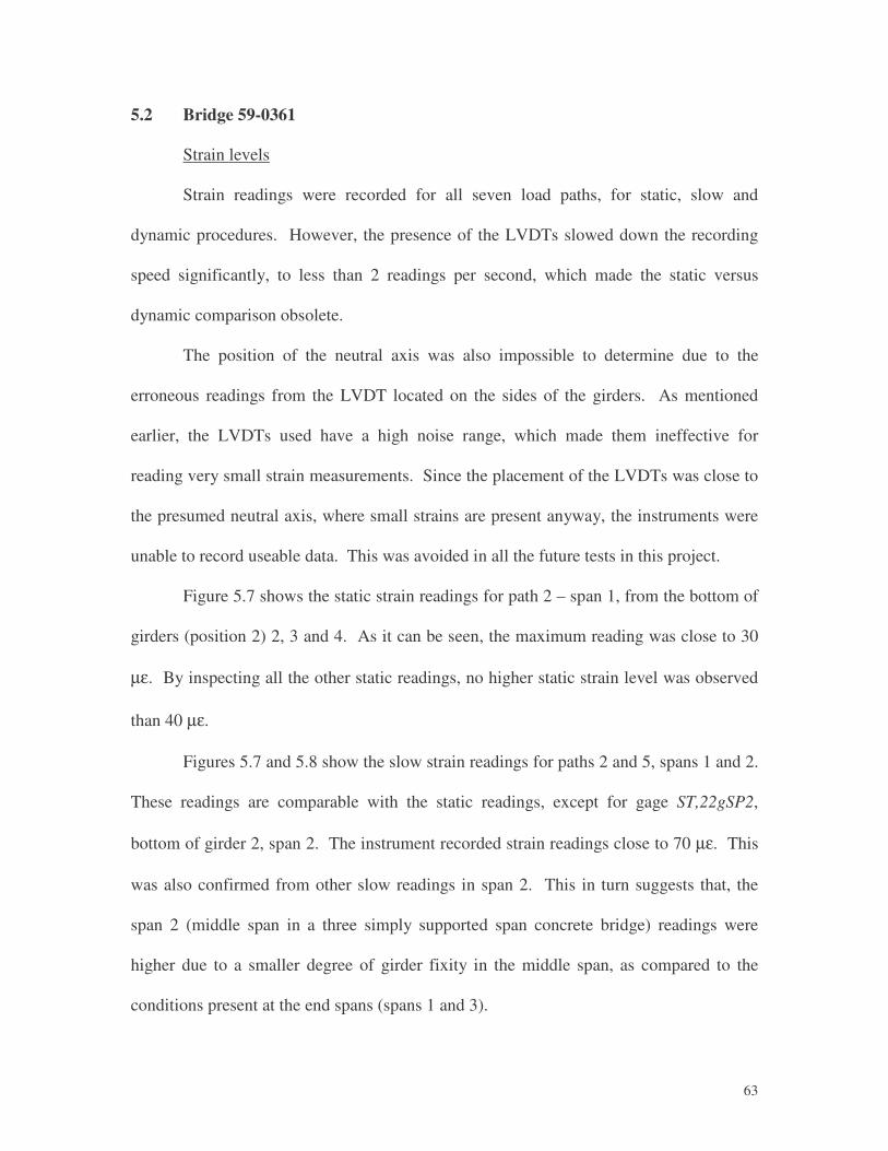
�
63
5.2 Bridge 59-0361
Strain levels
Strain readings were recorded for all seven load paths, for static, slow and
dynamic procedures. However, the presence of the LVDTs slowed down the recording
speed significantly, to less than 2 readings per second, which made the static versus
dynamic comparison obsolete.
The position of the neutral axis was also impossible to determine due to the
erroneous readings from the LVDT located on the sides of the girders. As mentioned
earlier, the LVDTs used have a high noise range, which made them ineffective for
reading very small strain measurements. Since the placement of the LVDTs was close to
the presumed neutral axis, where small strains are present anyway, the instruments were
unable to record useable data. This was avoided in all the future tests in this project.
Figure 5.7 shows the static strain readings for path 2 – span 1, from the bottom of
girders (position 2) 2, 3 and 4. As it can be seen, the maximum reading was close to 30
µε. By inspecting all the other static readings, no higher static strain level was observed
than 40 µε.
Figures 5.7 and 5.8 show the slow strain readings for paths 2 and 5, spans 1 and 2.
These readings are comparable with the static readings, except for gage ST,22gSP2,
bottom of girder 2, span 2. The instrument recorded strain readings close to 70 µε. This
was also confirmed from other slow readings in span 2. This in turn suggests that, the
span 2 (middle span in a three simply supported span concrete bridge) readings were
higher due to a smaller degree of girder fixity in the middle span, as compared to the
conditions present at the end spans (spans 1 and 3).
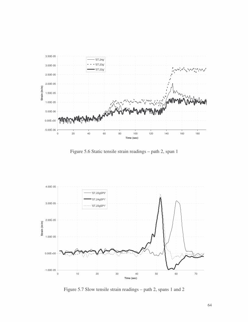
�
64
-5.00E-06
0.00E+00
5.00E-06
1.00E-05
1.50E-05
2.00E-05
2.50E-05
3.00E-05
3.50E-05
0 20 40 60 80 100 120 140 160 180
Time (sec)
Str
ain
(in/in
)
'ST,24g'
'ST,23g'
'ST,22g'
Figure 5.6 Static tensile strain readings – path 2, span 1
-1.00E-05
0.00E+00
1.00E-05
2.00E-05
3.00E-05
4.00E-05
0 10 20 30 40 50 60 70
Time (sec)
Str
ain
(in
/in)
'ST,22gSP2'
'ST,24gSP1'
'ST,23gSP1'
Figure 5.7 Slow tensile strain readings – path 2, spans 1 and 2
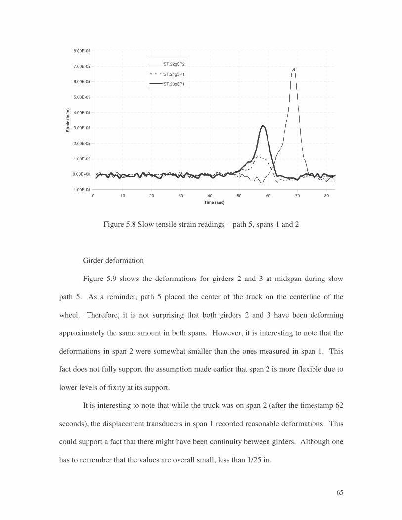
�
65
-1.00E-05
0.00E+00
1.00E-05
2.00E-05
3.00E-05
4.00E-05
5.00E-05
6.00E-05
7.00E-05
8.00E-05
0 10 20 30 40 50 60 70 80
Time (sec)
Str
ain
(in
/in)
'ST,22gSP2'
'ST,24gSP1'
'ST,23gSP1'
Figure 5.8 Slow tensile strain readings – path 5, spans 1 and 2
Girder deformation
Figure 5.9 shows the deformations for girders 2 and 3 at midspan during slow
path 5. As a reminder, path 5 placed the center of the truck on the centerline of the
wheel. Therefore, it is not surprising that both girders 2 and 3 have been deforming
approximately the same amount in both spans. However, it is interesting to note that the
deformations in span 2 were somewhat smaller than the ones measured in span 1. This
fact does not fully support the assumption made earlier that span 2 is more flexible due to
lower levels of fixity at its support.
It is interesting to note that while the truck was on span 2 (after the timestamp 62
seconds), the displacement transducers in span 1 recorded reasonable deformations. This
could support a fact that there might have been continuity between girders. Although one
has to remember that the values are overall small, less than 1/25 in.
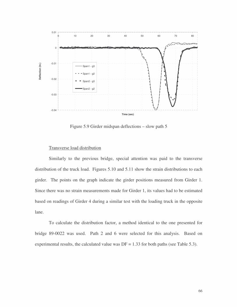
�
66
-0.04
-0.03
-0.02
-0.01
0
0.010 10 20 30 40 50 60 70 80
Time (sec)
Def
lect
ion
(in.)
Span1 - g3
Span1 - g2
Span2 - g3
Span2 - g2
Figure 5.9 Girder midspan deflections – slow path 5
Transverse load distribution
Similarly to the previous bridge, special attention was paid to the transverse
distribution of the truck load. Figures 5.10 and 5.11 show the strain distributions to each
girder. The points on the graph indicate the girder positions measured from Girder 1.
Since there was no strain measurements made for Girder 1, its values had to be estimated
based on readings of Girder 4 during a similar test with the loading truck in the opposite
lane.
To calculate the distribution factor, a method identical to the one presented for
bridge 89-0022 was used. Path 2 and 6 were selected for this analysis. Based on
experimental results, the calculated value was DF = 1.33 for both paths (see Table 5.3).
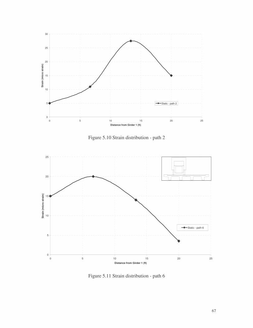
�
67
0
5
10
15
20
25
30
0 5 10 15 20 25
Distance from Girder 1 (ft)
Str
ain
(mic
ro s
trai
n)
Static - path 2
Figure 5.10 Strain distribution - path 2
0
5
10
15
20
25
0 5 10 15 20 25
Distance from Girder 1 (ft)
Str
ain
(mic
ro s
trai
n)
Static - path 6
Figure 5.11 Strain distribution - path 6
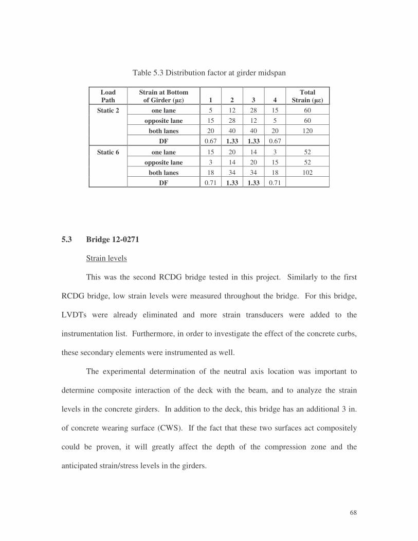
�
68
Table 5.3 Distribution factor at girder midspan
Load Path
Strain at Bottom of Girder (��) 1 2 3 4
Total Strain (��)
Static 2 one lane 5 12 28 15 60
opposite lane 15 28 12 5 60
both lanes 20 40 40 20 120
DF 0.67 1.33 1.33 0.67
Static 6 one lane 15 20 14 3 52
opposite lane 3 14 20 15 52
both lanes 18 34 34 18 102
DF 0.71 1.33 1.33 0.71
5.3 Bridge 12-0271
Strain levels
This was the second RCDG bridge tested in this project. Similarly to the first
RCDG bridge, low strain levels were measured throughout the bridge. For this bridge,
LVDTs were already eliminated and more strain transducers were added to the
instrumentation list. Furthermore, in order to investigate the effect of the concrete curbs,
these secondary elements were instrumented as well.
The experimental determination of the neutral axis location was important to
determine composite interaction of the deck with the beam, and to analyze the strain
levels in the concrete girders. In addition to the deck, this bridge has an additional 3 in.
of concrete wearing surface (CWS). If the fact that these two surfaces act compositely
could be proven, it will greatly affect the depth of the compression zone and the
anticipated strain/stress levels in the girders.
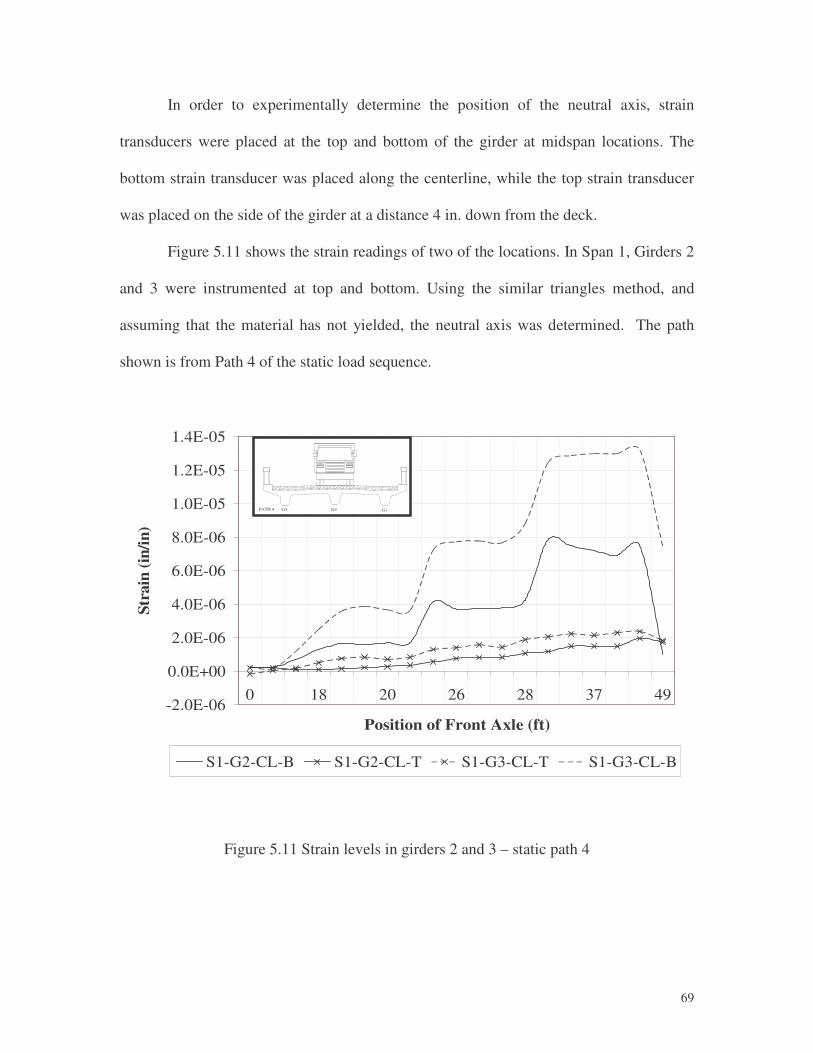
�
69
In order to experimentally determine the position of the neutral axis, strain
transducers were placed at the top and bottom of the girder at midspan locations. The
bottom strain transducer was placed along the centerline, while the top strain transducer
was placed on the side of the girder at a distance 4 in. down from the deck.
Figure 5.11 shows the strain readings of two of the locations. In Span 1, Girders 2
and 3 were instrumented at top and bottom. Using the similar triangles method, and
assuming that the material has not yielded, the neutral axis was determined. The path
shown is from Path 4 of the static load sequence.
-2.0E-06
0.0E+00
2.0E-06
4.0E-06
6.0E-06
8.0E-06
1.0E-05
1.2E-05
1.4E-05
0 18 20 26 28 37 49
Position of Front Axle (ft)
Stra
in (i
n/in
)
S1-G2-CL-B S1-G2-CL-T S1-G3-CL-T S1-G3-CL-B
G3PATH 4 G2 G1
Figure 5.11 Strain levels in girders 2 and 3 – static path 4
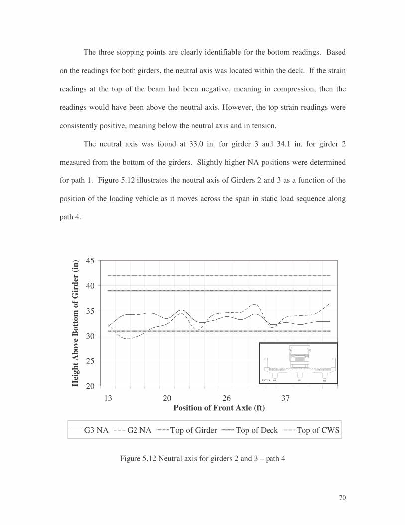
�
70
The three stopping points are clearly identifiable for the bottom readings. Based
on the readings for both girders, the neutral axis was located within the deck. If the strain
readings at the top of the beam had been negative, meaning in compression, then the
readings would have been above the neutral axis. However, the top strain readings were
consistently positive, meaning below the neutral axis and in tension.
The neutral axis was found at 33.0 in. for girder 3 and 34.1 in. for girder 2
measured from the bottom of the girders. Slightly higher NA positions were determined
for path 1. Figure 5.12 illustrates the neutral axis of Girders 2 and 3 as a function of the
position of the loading vehicle as it moves across the span in static load sequence along
path 4.
20
25
30
35
40
45
13 20 26 37Position of Front Axle (ft)
Hei
ght A
bove
Bot
tom
of G
irde
r (in
)
G3 NA G2 NA Top of Girder Top of Deck Top of CWS
G3PATH 4 G2 G1
Figure 5.12 Neutral axis for girders 2 and 3 – path 4

�
71
The shift of the neutral axis into the deck could also be attributed to the cracked
nature of each girder. Girder 2, throughout the length of the bridge, had more cracks in
the bottom face of the girder than the others did. There were also more longitudinal
cracks within the depth of Girder 2. Figure 5.13 shows some of the longitudinal cracks
near the centerline of Girder 2 in Span 1. Photo (a) shows a longitudinal crack
(highlighted) that is at an average distance of 14.5” from the bottom of the girder. Photo
(b) shows another longitudinal crack (highlighted) running along the bottom of the girder.
Figure 5.14 shows a representative vertical crack. These vertical cracks up to 9
in. are seen throughout the bridge. The image shown was taken at midspan of Girder 2 in
Span 1. The crack has been highlighted to aid its clarity. This type of crack is most
commonly a flexural crack; although no other sign of distress was visible.
(a) (b)
Figure 5.13 Cracked girder sections
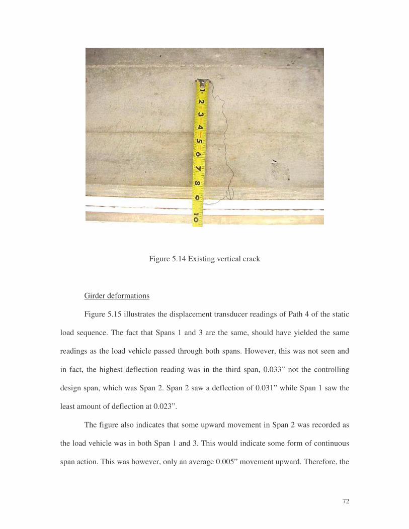
�
72
Figure 5.14 Existing vertical crack
Girder deformations
Figure 5.15 illustrates the displacement transducer readings of Path 4 of the static
load sequence. The fact that Spans 1 and 3 are the same, should have yielded the same
readings as the load vehicle passed through both spans. However, this was not seen and
in fact, the highest deflection reading was in the third span, 0.033” not the controlling
design span, which was Span 2. Span 2 saw a deflection of 0.031” while Span 1 saw the
least amount of deflection at 0.023”.
The figure also indicates that some upward movement in Span 2 was recorded as
the load vehicle was in both Span 1 and 3. This would indicate some form of continuous
span action. This was however, only an average 0.005” movement upward. Therefore, the
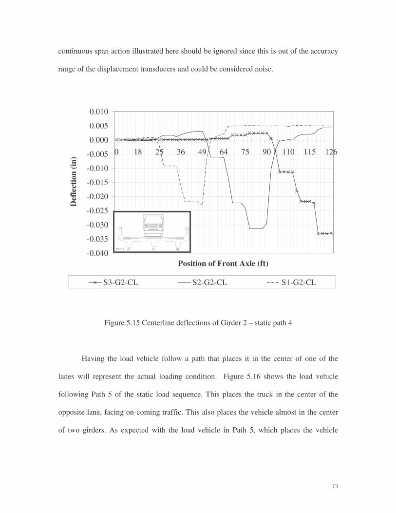
�
73
continuous span action illustrated here should be ignored since this is out of the accuracy
range of the displacement transducers and could be considered noise.
-0.040
-0.035
-0.030
-0.025
-0.020
-0.015
-0.010
-0.005
0.000
0.005
0.010
0 18 25 36 49 64 75 90 110 115 126
Position of Front Axle (ft)
Def
lect
ion
(in)
S3-G2-CL S2-G2-CL S1-G2-CL
G3PATH 4 G2 G1
Figure 5.15 Centerline deflections of Girder 2 – static path 4
Having the load vehicle follow a path that places it in the center of one of the
lanes will represent the actual loading condition. Figure 5.16 shows the load vehicle
following Path 5 of the static load sequence. This places the truck in the center of the
opposite lane, facing on-coming traffic. This also places the vehicle almost in the center
of two girders. As expected with the load vehicle in Path 5, which places the vehicle
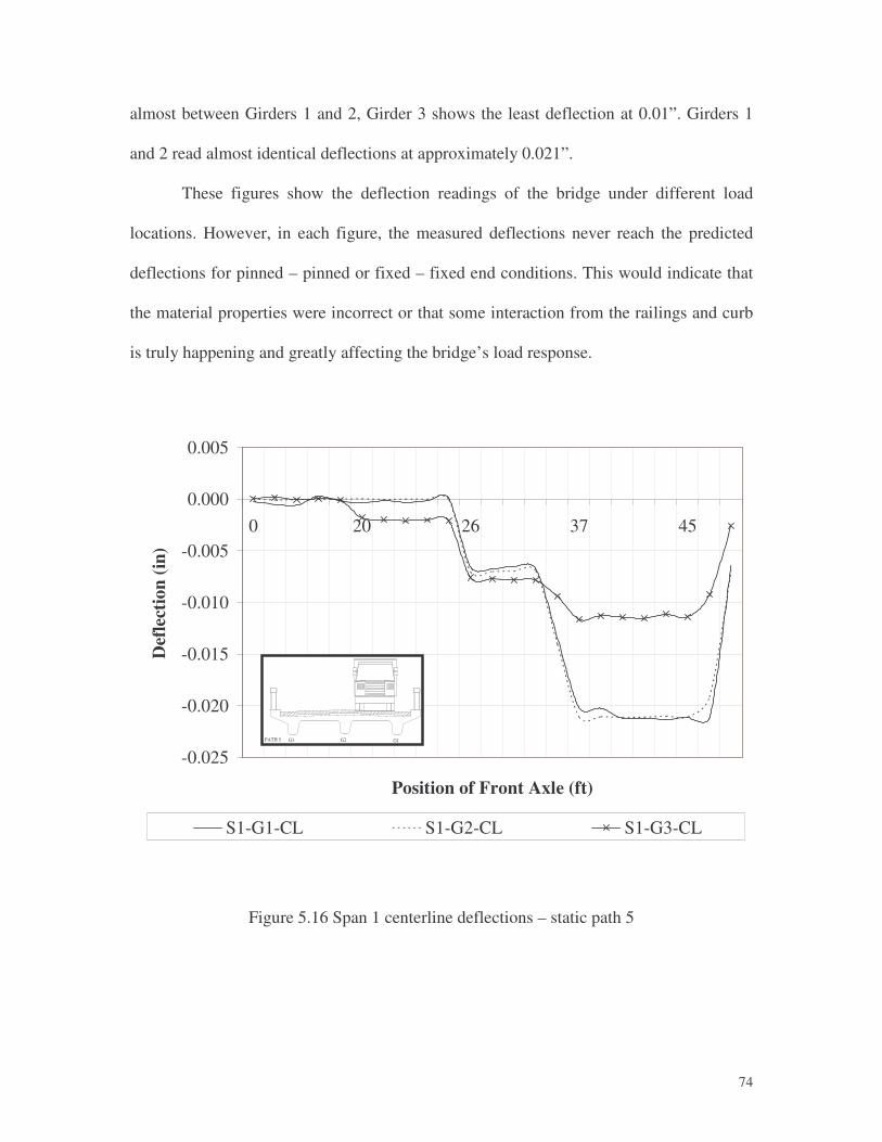
�
74
almost between Girders 1 and 2, Girder 3 shows the least deflection at 0.01”. Girders 1
and 2 read almost identical deflections at approximately 0.021”.
These figures show the deflection readings of the bridge under different load
locations. However, in each figure, the measured deflections never reach the predicted
deflections for pinned – pinned or fixed – fixed end conditions. This would indicate that
the material properties were incorrect or that some interaction from the railings and curb
is truly happening and greatly affecting the bridge’s load response.
-0.025
-0.020
-0.015
-0.010
-0.005
0.000
0.005
0 20 26 37 45
Position of Front Axle (ft)
Def
lect
ion
(in)
S1-G1-CL S1-G2-CL S1-G3-CL
G3PATH 5 G2 G1
Figure 5.16 Span 1 centerline deflections – static path 5

�
75
Transverse load distribution
The determination of the live load distribution to the girders was done using the
strain readings at the centerlines of the three girders. Here, two dynamic paths were
chosen for analysis. After these readings were compiled in a table format (shown in
Table 5.4), the truck load distribution factors were calculated. It is important to note, that
the DF = 1.44 calculated for this three-girder bridge is significantly higher than the values
established for a seven-girder bridge. Obviously, the demand on these three girders to
carry the truck load is substantially higher.
Table 5.4 Distribution factor at girder midspan
Load Path
Strain at Bottom of Girder (��) 1 2 3
Total Strain (��)
Dynamic 2 one lane 4 10 14 28
opposite lane 14 10 4 28
both lanes 18 20 18 56
DF 1.29 1.43 1.29
Dynamic B one lane 13 9 3 25
opposite lane 3 9 13 25
both lanes 16 18 16 50
DF 1.28 1.44 1.28
Dynamic effects
The measurement of strains induced by the impact of the load vehicle was
monitored during the dynamic load sequences. These dynamic strains were then
compared with those seen in the static and slow loading sequences to determine if impact
was occurring. These loading sequences only lasted for an approximate duration of 4
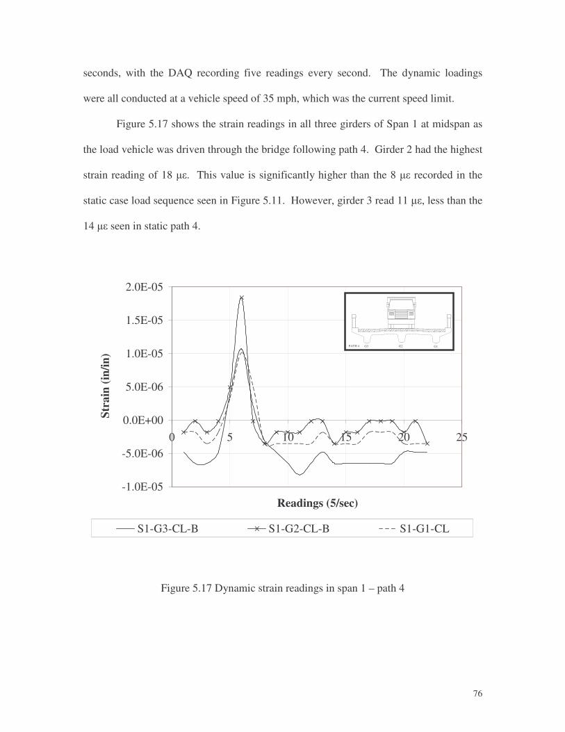
�
76
seconds, with the DAQ recording five readings every second. The dynamic loadings
were all conducted at a vehicle speed of 35 mph, which was the current speed limit.
Figure 5.17 shows the strain readings in all three girders of Span 1 at midspan as
the load vehicle was driven through the bridge following path 4. Girder 2 had the highest
strain reading of 18 ��. This value is significantly higher than the 8 �� recorded in the
static case load sequence seen in Figure 5.11. However, girder 3 read 11 ��, less than the
14 �� seen in static path 4.
-1.0E-05
-5.0E-06
0.0E+00
5.0E-06
1.0E-05
1.5E-05
2.0E-05
0 5 10 15 20 25
Readings (5/sec)
Stra
in (i
n/in
)
S1-G3-CL-B S1-G2-CL-B S1-G1-CL
G3PATH 4 G2 G1
Figure 5.17 Dynamic strain readings in span 1 – path 4

�
77
These two readings are at the two extremes measured during dynamic loading.
The vast majority of the dynamic readings were approximately equal to the static data.
The actual impact is greatly affected by the presence of bumps on the bridge approach
(Beal, 1998). It was noticed during the bridge test that some vehicular impact was
occurring as vehicles entered the bridge from the approaches. Some differences in the
asphalt overlay at the bridge abutments were noticeable at both ends of the bridge. This
caused the vehicles to “bounce” on to the bridge. Figure 5.18 shows one of the
approaches with the unevenness of the asphalt, which contributes to the bouncing effect.
Figure 5.18 Uneven asphalt at bridge approach
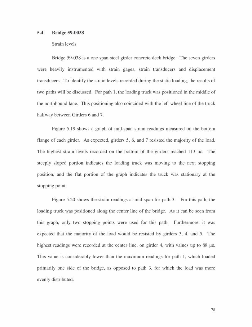
�
78
5.4 Bridge 59-0038
Strain levels
Bridge 59-038 is a one span steel girder concrete deck bridge. The seven girders
were heavily instrumented with strain gages, strain transducers and displacement
transducers. To identify the strain levels recorded during the static loading, the results of
two paths will be discussed. For path 1, the loading truck was positioned in the middle of
the northbound lane. This positioning also coincided with the left wheel line of the truck
halfway between Girders 6 and 7.
Figure 5.19 shows a graph of mid-span strain readings measured on the bottom
flange of each girder. As expected, girders 5, 6, and 7 resisted the majority of the load.
The highest strain levels recorded on the bottom of the girders reached 113 ��. The
steeply sloped portion indicates the loading truck was moving to the next stopping
position, and the flat portion of the graph indicates the truck was stationary at the
stopping point.
Figure 5.20 shows the strain readings at mid-span for path 3. For this path, the
loading truck was positioned along the center line of the bridge. As it can be seen from
this graph, only two stopping points were used for this path. Furthermore, it was
expected that the majority of the load would be resisted by girders 3, 4, and 5. The
highest readings were recorded at the center line, on girder 4, with values up to 88 ��.
This value is considerably lower than the maximum readings for path 1, which loaded
primarily one side of the bridge, as opposed to path 3, for which the load was more
evenly distributed.
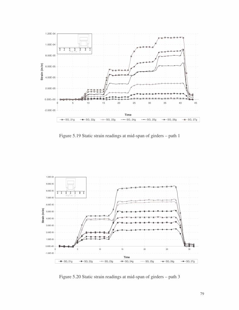
�
79
-2.00E-05
0.00E+00
2.00E-05
4.00E-05
6.00E-05
8.00E-05
1.00E-04
1.20E-04
0 5 10 15 20 25 30 35 40 45
Time
Str
ain
(in
/in)
SG, 21g SG, 22g SG, 23g SG, 24g SG, 25g SG, 26g SG, 27g
Figure 5.19 Static strain readings at mid-span of girders – path 1
-1.00E-05
0.00E+00
1.00E-05
2.00E-05
3.00E-05
4.00E-05
5.00E-05
6.00E-05
7.00E-05
8.00E-05
9.00E-05
1.00E-04
0 5 10 15 20 25 30
Time
Str
ain
(in/in
)
SG, 21g SG, 22g SG, 23g SG, 24g SG, 25g SG, 26g SG, 27g
Figure 5.20 Static strain readings at mid-span of girders – path 3

�
80
Figure 5.21 shows the mid-span strain readings measured on the top flanges of
each girder. This information along with data from Figure 5.19 allows for the
determination of the position of the neutral axis, which in turn, provided information as to
whether or not the girders and deck are acting compositely. At the time of construction
of bridge 59-038, the use of composite members was not a common practice. Although
the construction drawings of this bridge are not available, at the beginning of the analysis,
it was believed that shear studs were not used; therefore, the bridge should act non-
compositely (i.e. the experimental neutral axis should be located at the centroid of the
steel girder.
To calculate the neutral axis from test data, the girder was assumed to be in the
elastic range, and the strain slope was linear. Considering the small strain levels
measured during these tests, this assumption was reasonably accurate. The position of
the neutral axis was then determined using similar triangles. Table 5.5 shows the
calculated neutral axis for all girders at mid-span.
As it can be seen from this table, all erroneous readings were omitted (shaded
information) in this analysis. As shown in Table 5.5, the girders are acting as composite
members to some degree, because the position of the neutral axis was not located halfway
down the section, in this case 10 in. The average NA position was calculated as 5.28 in.,
well above the mid-height of the girder web. However, since only three readings were
used to come to this conclusion, caution must be used when a scientific trend is sought.
To confirm these findings, the results of path 3 were also analyzed, and
summarized in Table 5.6. As it can be seen, the instruments on girders 2, 3, 4, and 5
recorded valid data. The other three girders were either too far away from the loading to
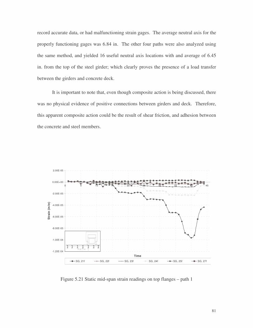
�
81
record accurate data, or had malfunctioning strain gages. The average neutral axis for the
properly functioning gages was 6.84 in. The other four paths were also analyzed using
the same method, and yielded 16 useful neutral axis locations with and average of 6.45
in. from the top of the steel girder; which clearly proves the presence of a load transfer
between the girders and concrete deck.
It is important to note that, even though composite action is being discussed, there
was no physical evidence of positive connections between girders and deck. Therefore,
this apparent composite action could be the result of shear friction, and adhesion between
the concrete and steel members.
-1.20E-04
-1.00E-04
-8.00E-05
-6.00E-05
-4.00E-05
-2.00E-05
0.00E+00
2.00E-05
0 5 10 15 20 25 30 35 40 45
Time
Str
ain
(in
/in)
SG, 21f SG, 22f SG, 23f SG, 24f SG, 25f SG, 27f
Figure 5.21 Static mid-span strain readings on top flanges – path 1
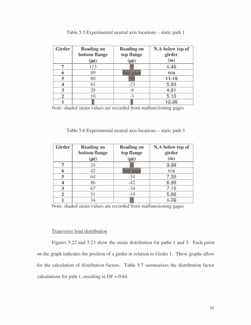
�
82
Table 5.5 Experimental neutral axis locations – static path 1
Girder Reading on bottom flange
(µµµµεεεε)
Reading on top flange
(µµµµεεεε)
N.A below top of girder
(in) 7 113 -5 1.45 6 89 Bad gage n/a 5 80 -96 11.19 4 61 -23 5.93 3 29 -8 4.81 2 10 -3 5.10 1 2 3 12.25
Note: shaded strain values are recorded from malfunctioning gages
Table 5.6 Experimental neutral axis locations – static path 3
Girder Reading on bottom flange
(µµµµεεεε)
Reading on top flange
(µµµµεεεε)
N.A below top of girder
(in) 7 24 -4 3.39 6 42 Bad gage n/a 5 64 -34 7.35 4 86 -42 6.98 3 67 -34 7.15 2 51 -19 5.88 1 34 -2 1.70
Note: shaded strain values are recorded from malfunctioning gages
Transverse load distribution
Figures 5.22 and 5.23 show the strain distribution for paths 1 and 3. Each point
on the graph indicates the position of a girder in relation to Girder 1. These graphs allow
for the calculation of distribution factors. Table 5.7 summarizes the distribution factor
calculations for path 1, resulting in DF = 0.64.
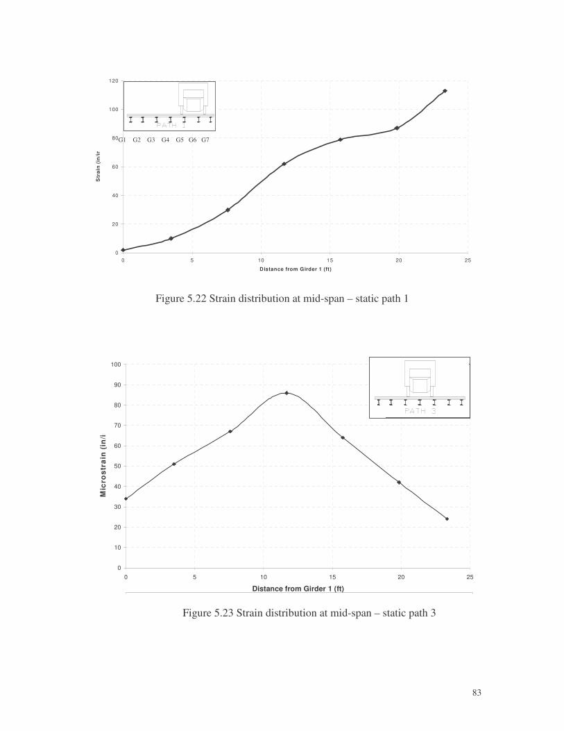
�
83
G1 G2 G3 G4 G5 G6 G7
0
20
40
60
80
100
120
0 5 10 15 20 25
Distance from Girder 1 (ft)
Str
ain
(in
/in
)
Figure 5.22 Strain distribution at mid-span – static path 1
0
10
20
30
40
50
60
70
80
90
100
0 5 10 15 20 25
Distance from Girder 1 (ft)
Mic
ros
tra
in (
in/i
n)
Figure 5.23 Strain distribution at mid-span – static path 3

�
84
Table 5.7 Distribution factor for bridge 59-0038
Load Path
Strain at Bottom of Girder (��) 1 2 3 4 5 6 7
Total Strain (��)
Static 1 one lane 2 10 29 61 80 89 113 384
opposite lane 113 89 80 61 29 10 2 384
both lanes 115 99 109 122 109 99 115 786
DF 0.60 0.52 0.57 0.64 0.57 0.52 0.60
It is important to note that the graph for path 3 the strain distribution is nearly
symmetrical. However, Figure 5.24 shows a discrepancy on the load distribution to
girders 2, 3, 5, and 6. The same discrepancy exists in the distribution factors in Table 5.7
– the load is not being transferred to the outside girders as smoothly.
So what is happening at this bridge? As it was outlined in Table 4.1, the bridge
built in 1945 was widened in 1988 by the addition of one steel wide flange girder on each
side. It is obvious from Figure 5.22 and Table 5.7, a discontinuity has been introduced at
the two exterior girders, which affected the transverse distribution of the truck load.
Dynamic effects
Figure 5.24 shows the dynamic strain readings for path 1. As anticipated, girders
6 and 7 recorded the highest levels, and girders 1 and 2 the lowest, respectively. Table
5.8 compares the data between static and dynamic tests for paths 1 and 3. It is clear from
this table that there is no significant increase in strain due to impact from the dynamic
test. All three dynamic runs have been analyzed for each path, and the results from the
highest reading runs were included in Table 5.8. Furthermore, no impact effect was
observed for any of the remaining five paths.
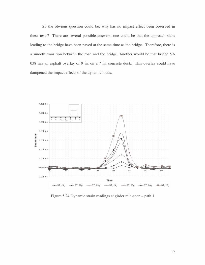
�
85
So the obvious question could be: why has no impact effect been observed in
these tests? There are several possible answers; one could be that the approach slabs
leading to the bridge have been paved at the same time as the bridge. Therefore, there is
a smooth transition between the road and the bridge. Another would be that bridge 59-
038 has an asphalt overlay of 9 in. on a 7 in. concrete deck. This overlay could have
dampened the impact effects of the dynamic loads.
-2.00E-05
0.00E+00
2.00E-05
4.00E-05
6.00E-05
8.00E-05
1.00E-04
1.20E-04
1.40E-04
130 132 134 136 138 140 142 144
Time
Str
ain
(in
/in)
ST, 21g ST, 22g ST, 23g ST, 24g ST, 25g ST, 26g ST, 27g
Figure 5.24 Dynamic strain readings at girder mid-span – path 1

�
86
Table 5.8 Strain comparisons for static and dynamic cases
Strain Readings – Path 1 (µµµµεεεε)
Strain Readings – Path 3 (µµµµεεεε)
Gage Position
Static Dynamic Static Dynamic 27g 113 114 24 28 26g 89 76 42 31 25g 80 63 64 60 24g 61 54 86 82 23g 29 28 67 62 22g 10 12 51 58 21g 2 4 34 33
5.5 Bridge 12-0227
Strain readings
For the tests conducted on this bridge, the 140 ft displacement transducer was not
used. There was an in-field problem with the device the day of testing. Unfortunately, it
could not be solved within the tight schedule of the required road closure. Therefore, all
the graphs were plotted versus the test time instead of the position of the front axle, as it
was done for all the other static tests.
Figure 5.25 shows the strain readings from girder 3 of Span 1. The readings are
from the static load sequence following path 2. The data from this path was selected
since it generated the highest strain readings in girder 3. The figure shows the readings
from both the primary DAQ and the portable DAQ. As it was mentioned earlier, for two
bridges a second DAQ system was used with six strain transducers to investigate the
possibility of using only a small number of instruments to evaluate a particular bridge. In
this figure, each of the instruments from the portable DAQ was designated with a
preceding ‘Z’.
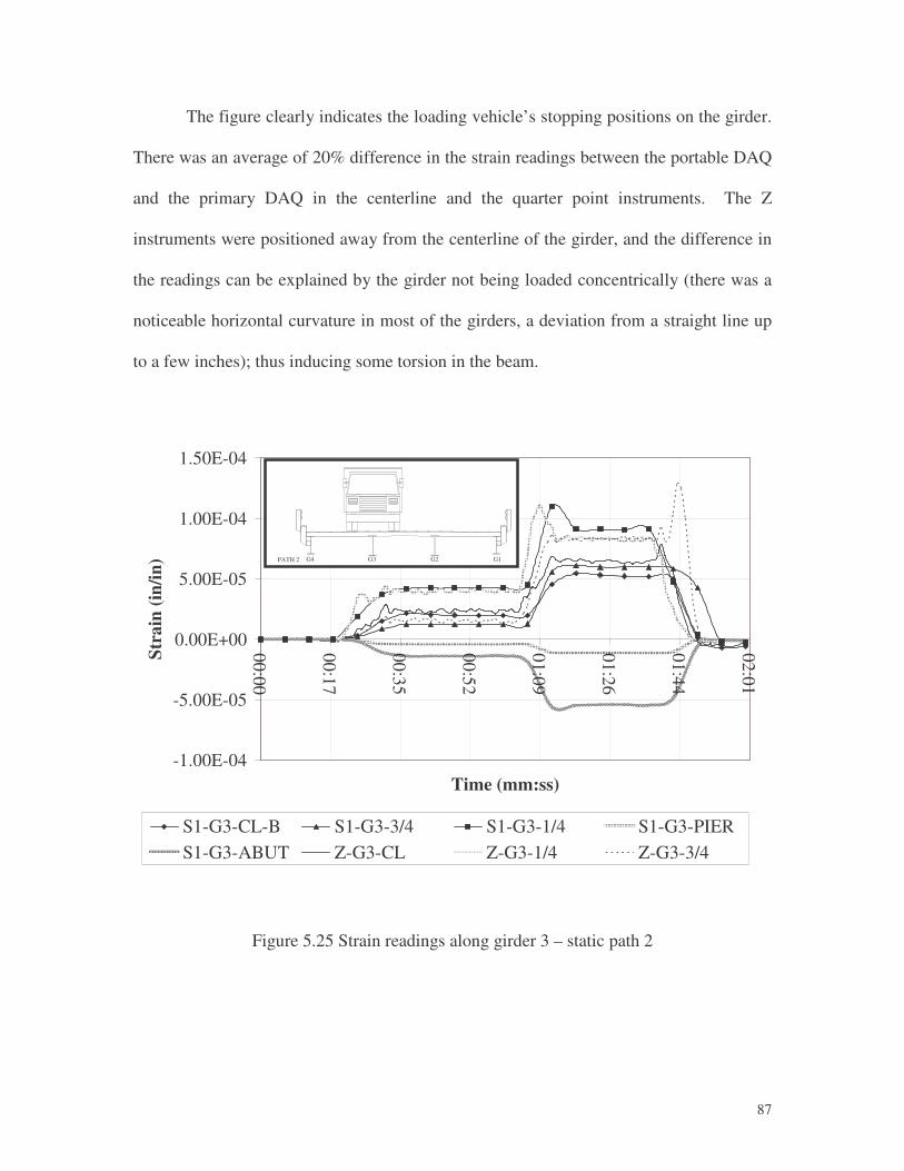
�
87
The figure clearly indicates the loading vehicle’s stopping positions on the girder.
There was an average of 20% difference in the strain readings between the portable DAQ
and the primary DAQ in the centerline and the quarter point instruments. The Z
instruments were positioned away from the centerline of the girder, and the difference in
the readings can be explained by the girder not being loaded concentrically (there was a
noticeable horizontal curvature in most of the girders, a deviation from a straight line up
to a few inches); thus inducing some torsion in the beam.
-1.00E-04
-5.00E-05
0.00E+00
5.00E-05
1.00E-04
1.50E-04
00:00
00:17
00:35
00:52
01:09
01:26
01:44
02:01
Time (mm:ss)
Stra
in (i
n/in
)
S1-G3-CL-B S1-G3-3/4 S1-G3-1/4 S1-G3-PIERS1-G3-ABUT Z-G3-CL Z-G3-1/4 Z-G3-3/4
PATH 2 G4 G3 G2 G1
Figure 5.25 Strain readings along girder 3 – static path 2
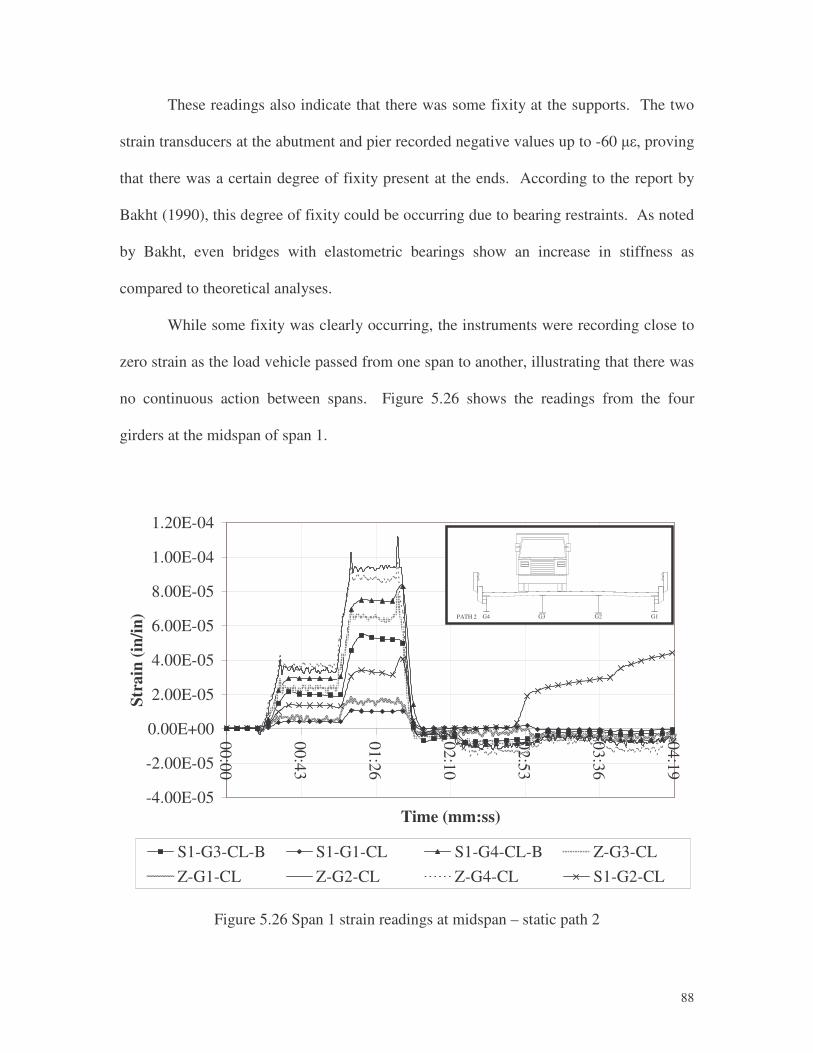
�
88
These readings also indicate that there was some fixity at the supports. The two
strain transducers at the abutment and pier recorded negative values up to -60 ��, proving
that there was a certain degree of fixity present at the ends. According to the report by
Bakht (1990), this degree of fixity could be occurring due to bearing restraints. As noted
by Bakht, even bridges with elastometric bearings show an increase in stiffness as
compared to theoretical analyses.
While some fixity was clearly occurring, the instruments were recording close to
zero strain as the load vehicle passed from one span to another, illustrating that there was
no continuous action between spans. Figure 5.26 shows the readings from the four
girders at the midspan of span 1.
-4.00E-05
-2.00E-05
0.00E+00
2.00E-05
4.00E-05
6.00E-05
8.00E-05
1.00E-04
1.20E-04
00:00
00:43
01:26
02:10
02:53
03:36
04:19
Time (mm:ss)
Stra
in (i
n/in
)
S1-G3-CL-B S1-G1-CL S1-G4-CL-B Z-G3-CLZ-G1-CL Z-G2-CL Z-G4-CL S1-G2-CL
PATH 2 G4 G3 G2 G1
Figure 5.26 Span 1 strain readings at midspan – static path 2
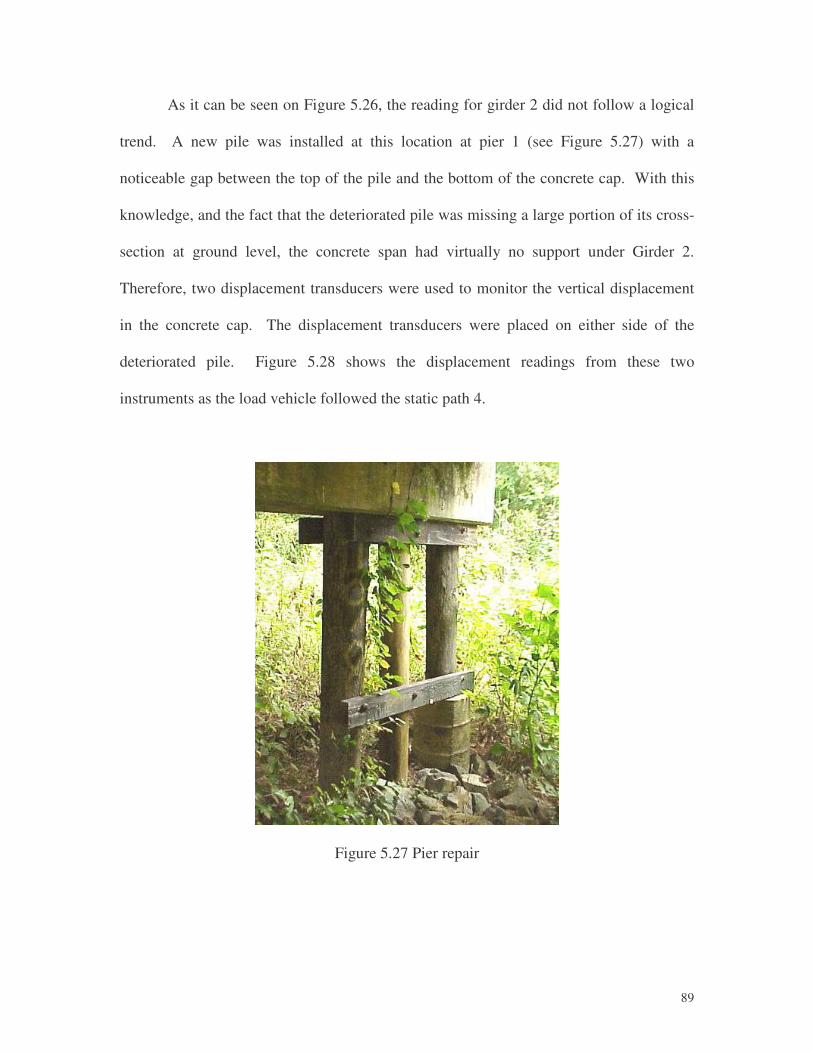
�
89
As it can be seen on Figure 5.26, the reading for girder 2 did not follow a logical
trend. A new pile was installed at this location at pier 1 (see Figure 5.27) with a
noticeable gap between the top of the pile and the bottom of the concrete cap. With this
knowledge, and the fact that the deteriorated pile was missing a large portion of its cross-
section at ground level, the concrete span had virtually no support under Girder 2.
Therefore, two displacement transducers were used to monitor the vertical displacement
in the concrete cap. The displacement transducers were placed on either side of the
deteriorated pile. Figure 5.28 shows the displacement readings from these two
instruments as the load vehicle followed the static path 4.
Figure 5.27 Pier repair
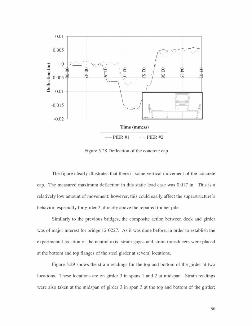
�
90
-0.02
-0.015
-0.01
-0.005
0
0.005
0.01
00:00
00:43
01:26
02:10
02:53
03:36
04:19
05:02
Time (mm:ss)
Def
lect
ion
(in)
PIER #1 PIER #2
PATH 4 G4 G3 G2 G1
Figure 5.28 Deflection of the concrete cap
The figure clearly illustrates that there is some vertical movement of the concrete
cap. The measured maximum deflection in this static load case was 0.017 in. This is a
relatively low amount of movement; however, this could easily affect the superstructure’s
behavior, especially for girder 2, directly above the repaired timber pile.
Similarly to the previous bridges, the composite action between deck and girder
was of major interest for bridge 12-0227. As it was done before, in order to establish the
experimental location of the neutral axis, strain gages and strain transducers were placed
at the bottom and top flanges of the steel girder at several locations.
Figure 5.29 shows the strain readings for the top and bottom of the girder at two
locations. These locations are on girder 3 in spans 1 and 2 at midspan. Strain readings
were also taken at the midspan of girder 3 in span 3 at the top and bottom of the girder;
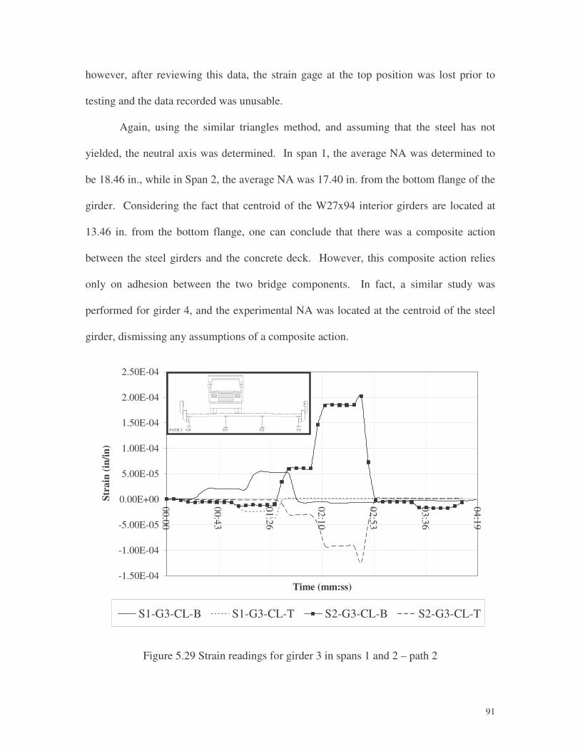
�
91
however, after reviewing this data, the strain gage at the top position was lost prior to
testing and the data recorded was unusable.
Again, using the similar triangles method, and assuming that the steel has not
yielded, the neutral axis was determined. In span 1, the average NA was determined to
be 18.46 in., while in Span 2, the average NA was 17.40 in. from the bottom flange of the
girder. Considering the fact that centroid of the W27x94 interior girders are located at
13.46 in. from the bottom flange, one can conclude that there was a composite action
between the steel girders and the concrete deck. However, this composite action relies
only on adhesion between the two bridge components. In fact, a similar study was
performed for girder 4, and the experimental NA was located at the centroid of the steel
girder, dismissing any assumptions of a composite action.
-1.50E-04
-1.00E-04
-5.00E-05
0.00E+00
5.00E-05
1.00E-04
1.50E-04
2.00E-04
2.50E-04
00:00
00:43
01:26
02:10
02:53
03:36
04:19
Time (mm:ss)
Stra
in (i
n/in
)
S1-G3-CL-B S1-G3-CL-T S2-G3-CL-B S2-G3-CL-T
PATH 2 G4 G3 G2 G1
Figure 5.29 Strain readings for girder 3 in spans 1 and 2 – path 2
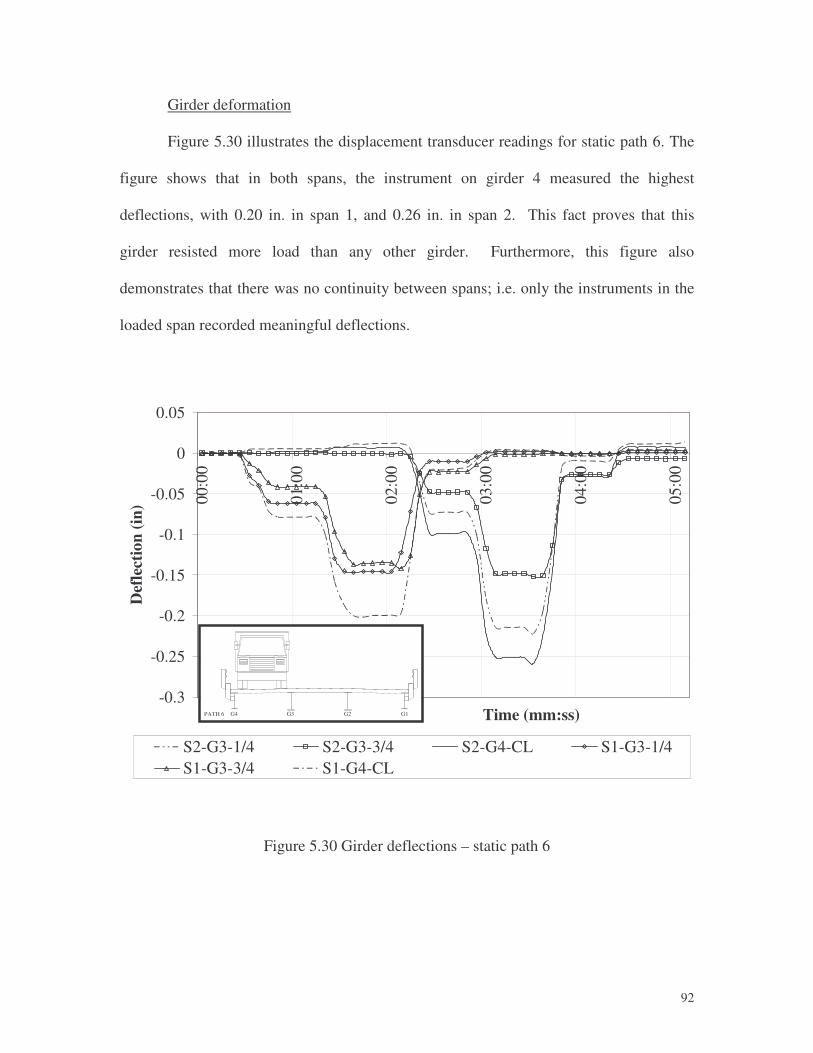
�
92
Girder deformation
Figure 5.30 illustrates the displacement transducer readings for static path 6. The
figure shows that in both spans, the instrument on girder 4 measured the highest
deflections, with 0.20 in. in span 1, and 0.26 in. in span 2. This fact proves that this
girder resisted more load than any other girder. Furthermore, this figure also
demonstrates that there was no continuity between spans; i.e. only the instruments in the
loaded span recorded meaningful deflections.
-0.3
-0.25
-0.2
-0.15
-0.1
-0.05
0
0.05
00:0
0
01:0
0
02:0
0
03:0
0
04:0
0
05:0
0
Time (mm:ss)
Def
lect
ion
(in)
S2-G3-1/4 S2-G3-3/4 S2-G4-CL S1-G3-1/4S1-G3-3/4 S1-G4-CL
PATH 6 G4 G3 G2 G1
Figure 5.30 Girder deflections – static path 6
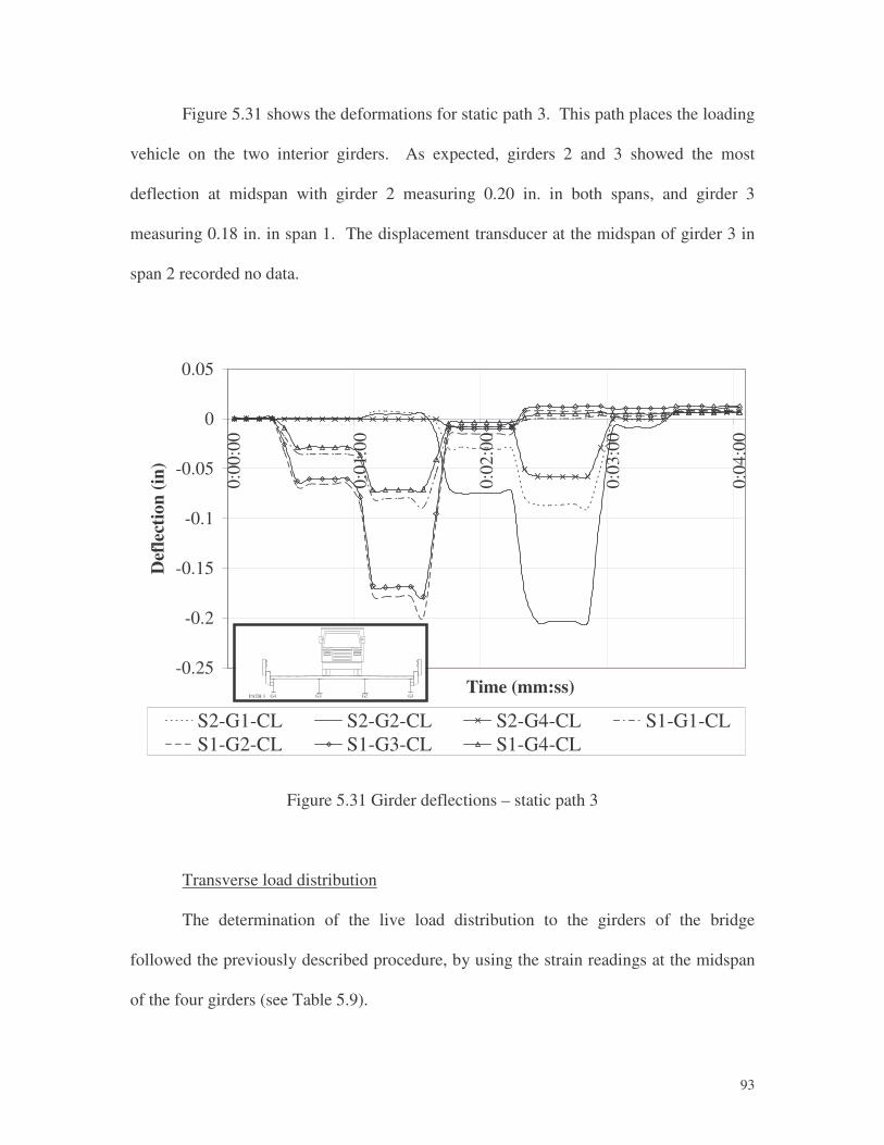
�
93
Figure 5.31 shows the deformations for static path 3. This path places the loading
vehicle on the two interior girders. As expected, girders 2 and 3 showed the most
deflection at midspan with girder 2 measuring 0.20 in. in both spans, and girder 3
measuring 0.18 in. in span 1. The displacement transducer at the midspan of girder 3 in
span 2 recorded no data.
-0.25
-0.2
-0.15
-0.1
-0.05
0
0.05
0:00
:00
0:01
:00
0:02
:00
0:03
:00
0:04
:00
Time (mm:ss)
Def
lect
ion
(in)
S2-G1-CL S2-G2-CL S2-G4-CL S1-G1-CLS1-G2-CL S1-G3-CL S1-G4-CL
PATH 3 G4 G3 G2 G1
Figure 5.31 Girder deflections – static path 3
Transverse load distribution
The determination of the live load distribution to the girders of the bridge
followed the previously described procedure, by using the strain readings at the midspan
of the four girders (see Table 5.9).
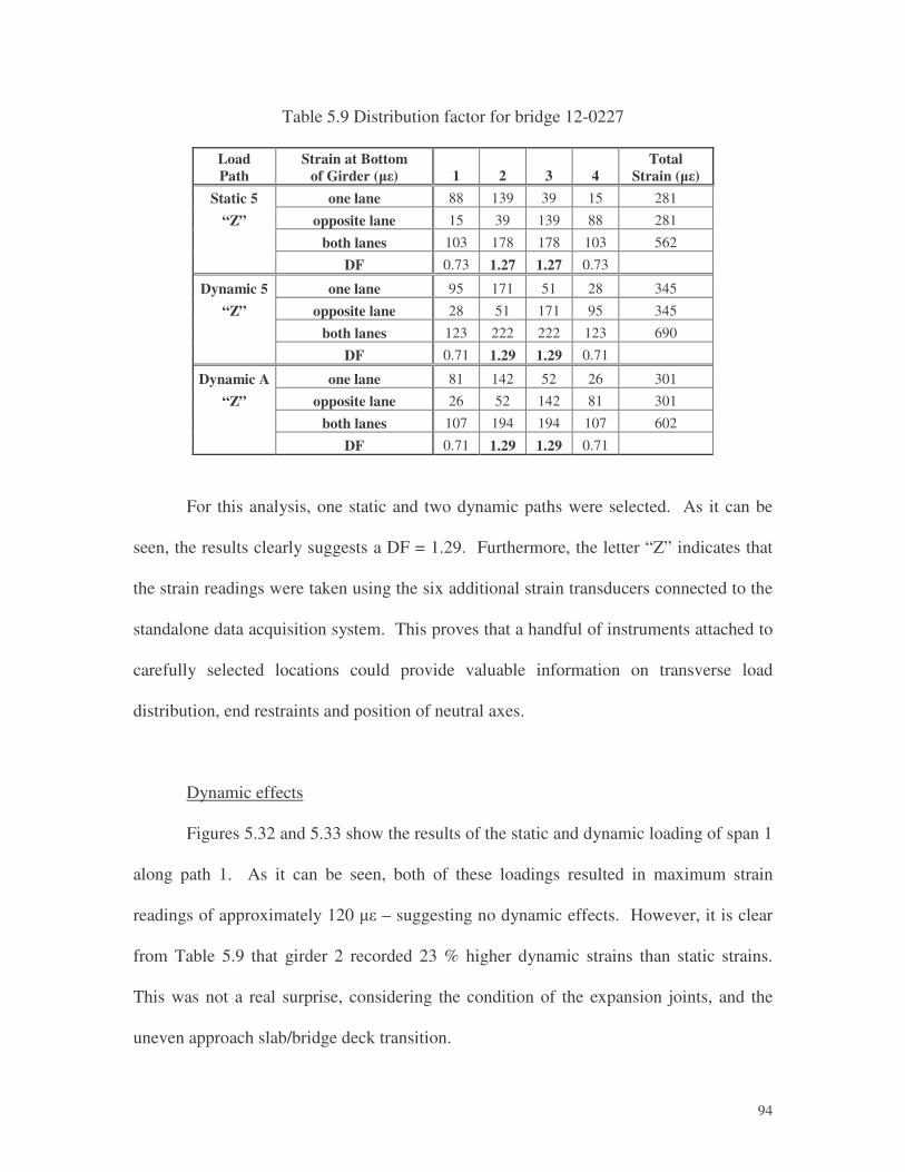
�
94
Table 5.9 Distribution factor for bridge 12-0227
Load Path
Strain at Bottom of Girder (��) 1 2 3 4
Total Strain (��)
Static 5 one lane 88 139 39 15 281
“Z” opposite lane 15 39 139 88 281
both lanes 103 178 178 103 562
DF 0.73 1.27 1.27 0.73
Dynamic 5 one lane 95 171 51 28 345
“Z” opposite lane 28 51 171 95 345
both lanes 123 222 222 123 690
DF 0.71 1.29 1.29 0.71
Dynamic A one lane 81 142 52 26 301
“Z” opposite lane 26 52 142 81 301
both lanes 107 194 194 107 602
DF 0.71 1.29 1.29 0.71
For this analysis, one static and two dynamic paths were selected. As it can be
seen, the results clearly suggests a DF = 1.29. Furthermore, the letter “Z” indicates that
the strain readings were taken using the six additional strain transducers connected to the
standalone data acquisition system. This proves that a handful of instruments attached to
carefully selected locations could provide valuable information on transverse load
distribution, end restraints and position of neutral axes.
Dynamic effects
Figures 5.32 and 5.33 show the results of the static and dynamic loading of span 1
along path 1. As it can be seen, both of these loadings resulted in maximum strain
readings of approximately 120 �� – suggesting no dynamic effects. However, it is clear
from Table 5.9 that girder 2 recorded 23 % higher dynamic strains than static strains.
This was not a real surprise, considering the condition of the expansion joints, and the
uneven approach slab/bridge deck transition.
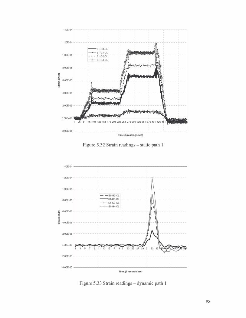
�
95
-2.00E-05
0.00E+00
2.00E-05
4.00E-05
6.00E-05
8.00E-05
1.00E-04
1.20E-04
1.40E-04
1 26 51 76 101 126 151 176 201 226 251 276 301 326 351 376 401 426 451 476 501 526 551
Time (5 readings/sec)
Str
ain
(in/
in)
S1-G3-CLS1-G1-CLS1-G2-CLS1-G4-CL
Figure 5.32 Strain readings – static path 1
-4.00E-05
-2.00E-05
0.00E+00
2.00E-05
4.00E-05
6.00E-05
8.00E-05
1.00E-04
1.20E-04
1.40E-04
1 3 5 7 9 11 13 15 17 19 21 23 25 27 29 31 33 35 37 39 41 43 45 47
Time (5 records/sec)
Str
ain
(in/in
)
S1-G3-CLS1-G1-CLS1-G2-CLS1-G4-CL
Figure 5.33 Strain readings – dynamic path 1
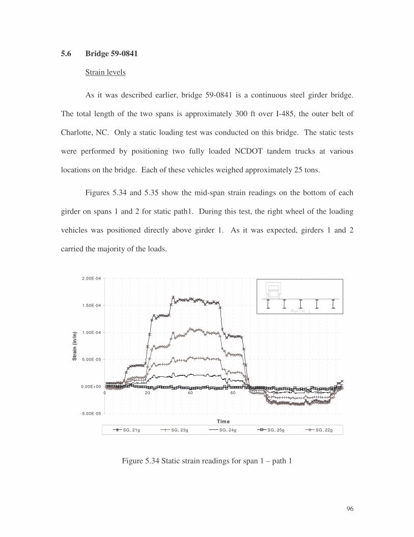
�
96
5.6 Bridge 59-0841
Strain levels
As it was described earlier, bridge 59-0841 is a continuous steel girder bridge.
The total length of the two spans is approximately 300 ft over I-485, the outer belt of
Charlotte, NC. Only a static loading test was conducted on this bridge. The static tests
were performed by positioning two fully loaded NCDOT tandem trucks at various
locations on the bridge. Each of these vehicles weighed approximately 25 tons.
Figures 5.34 and 5.35 show the mid-span strain readings on the bottom of each
girder on spans 1 and 2 for static path1. During this test, the right wheel of the loading
vehicles was positioned directly above girder 1. As it was expected, girders 1 and 2
carried the majority of the loads.
-5.00E-05
0.00E+00
5.00E-05
1.00E-04
1.50E-04
2.00E-04
0 20 40 60 80 100
Time
Str
ain
(in/in
)
SG, 21g SG, 23g SG, 24g SG, 25g SG, 22g
Figure 5.34 Static strain readings for span 1 – path 1
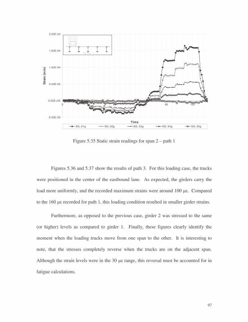
�
97
-5.00E-05
0.00E+00
5.00E-05
1.00E-04
1.50E-04
2.00E-04
0 20 40 60 80 100
Time
Str
ain
(in/in
)
SG, 61g SG, 62g SG, 63g SG, 64g SG, 65g
Figure 5.35 Static strain readings for span 2 – path 1
Figures 5.36 and 5.37 show the results of path 3. For this loading case, the trucks
were positioned in the center of the eastbound lane. As expected, the girders carry the
load more uniformly, and the recorded maximum strains were around 100 ��. Compared
to the 160 �� recorded for path 1, this loading condition resulted in smaller girder strains.
Furthermore, as opposed to the previous case, girder 2 was stressed to the same
(or higher) levels as compared to girder 1. Finally, these figures clearly identify the
moment when the loading trucks move from one span to the other. It is interesting to
note, that the stresses completely reverse when the trucks are on the adjacent span.
Although the strain levels were in the 30 �� range, this reversal must be accounted for in
fatigue calculations.
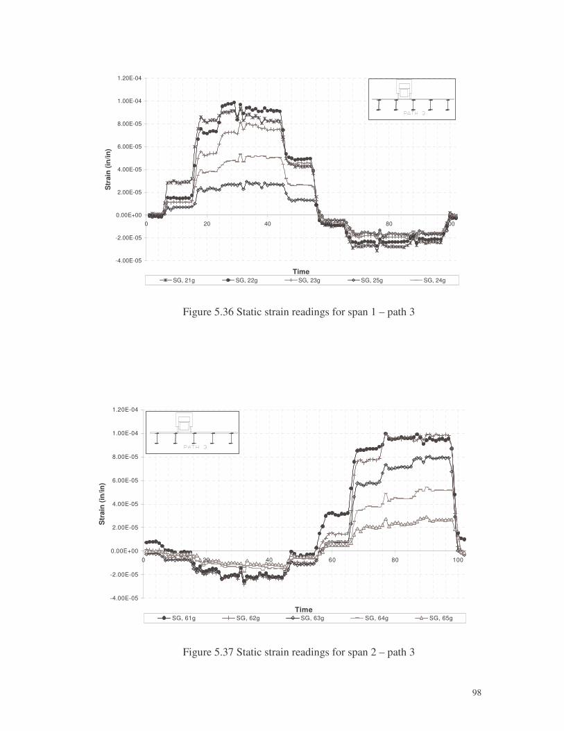
�
98
-4.00E-05
-2.00E-05
0.00E+00
2.00E-05
4.00E-05
6.00E-05
8.00E-05
1.00E-04
1.20E-04
0 20 40 60 80 100
Time
Str
ain
(in/in
)
SG, 21g SG, 22g SG, 23g SG, 25g SG, 24g
Figure 5.36 Static strain readings for span 1 – path 3
-4.00E-05
-2.00E-05
0.00E+00
2.00E-05
4.00E-05
6.00E-05
8.00E-05
1.00E-04
1.20E-04
0 20 40 60 80 100
Time
Str
ain
(in/in
)
SG, 61g SG, 62g SG, 63g SG, 64g SG, 65g
Figure 5.37 Static strain readings for span 2 – path 3

�
99
The girders of bridge 59-0841 were designed as composite sections. By using the
strain readings from the bottom flanges and readings from the top flanges, the location of
the neutral axis for a member was determined. Table 5.10 shows the calculated neutral
axis positions for each pair of strain gages at the mid-span of each span. Similar
comparisons were made for all pairs on strain gages on the bridge, and an average neutral
axis location of 58.25 in. above the bottom flange was calculated.
Considering the fact that these welded plate girders were more than 5 ft deep,
these calculations prove that the concrete deck and the steel plate girder were resisting
live loads as a composite section.
Table 5.10 Position of neutral axis
Span Girder Distance from bottom flange (in.)
1 1 61.46 2 59.18 3 56.79 4 55.86 5 58.26 2 1 Bad gage 2 60.04 3 58.18 4 55.58 5 57.71
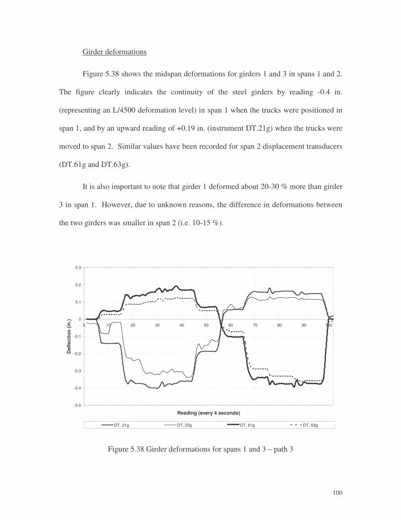
�
100
Girder deformations
Figure 5.38 shows the midspan deformations for girders 1 and 3 in spans 1 and 2.
The figure clearly indicates the continuity of the steel girders by reading -0.4 in.
(representing an L/4500 deformation level) in span 1 when the trucks were positioned in
span 1, and by an upward reading of +0.19 in. (instrument DT.21g) when the trucks were
moved to span 2. Similar values have been recorded for span 2 displacement transducers
(DT.61g and DT.63g).
It is also important to note that girder 1 deformed about 20-30 % more than girder
3 in span 1. However, due to unknown reasons, the difference in deformations between
the two girders was smaller in span 2 (i.e. 10-15 %).
-0.5
-0.4
-0.3
-0.2
-0.1
0
0.1
0.2
0.3
0 10 20 30 40 50 60 70 80 90 100
Reading (every 4 seconds)
Def
lect
ion
(in.)
DT, 21g DT, 23g DT, 61g DT, 63g
Figure 5.38 Girder deformations for spans 1 and 3 – path 3
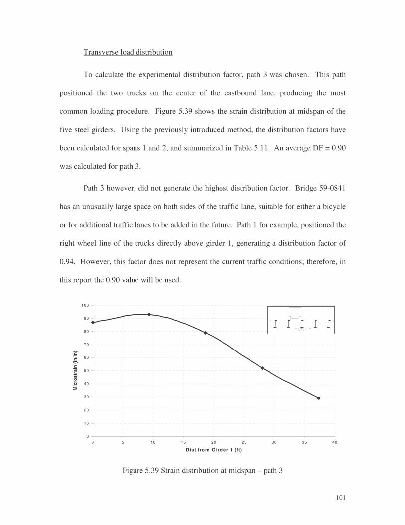
�
101
Transverse load distribution
To calculate the experimental distribution factor, path 3 was chosen. This path
positioned the two trucks on the center of the eastbound lane, producing the most
common loading procedure. Figure 5.39 shows the strain distribution at midspan of the
five steel girders. Using the previously introduced method, the distribution factors have
been calculated for spans 1 and 2, and summarized in Table 5.11. An average DF = 0.90
was calculated for path 3.
Path 3 however, did not generate the highest distribution factor. Bridge 59-0841
has an unusually large space on both sides of the traffic lane, suitable for either a bicycle
or for additional traffic lanes to be added in the future. Path 1 for example, positioned the
right wheel line of the trucks directly above girder 1, generating a distribution factor of
0.94. However, this factor does not represent the current traffic conditions; therefore, in
this report the 0.90 value will be used.
0
10
20
30
40
50
60
70
80
90
100
0 5 10 15 20 25 30 35 40
Dist from G irder 1 (ft)
Mic
rost
rain
(in/
in)
Figure 5.39 Strain distribution at midspan – path 3

�
102
Table 5.11 Distribution factor for bridge 59-0841
Load Path
Strain at Bottom of Girder (��) 1 2 3 4 5
Total Strain (��)
Static 3 one lane 91 97 73 48 27 337
Span 1 opposite lane 27 48 73 97 91 337
both lanes 118 145 146 145 118 674
DF 0.70 0.86 0.87 0.86 0.70
Static 3 one lane 87 93 79 52 29 340
Span 2 opposite lane 29 52 79 93 87 340
both lanes 116 145 158 145 116 680
DF 0.68 0.85 0.93 0.85 0.68
5.7 Bridge 89-0219
Strain levels
The instrumentation of this bridge consisted of over eighty instruments positioned
throughout the two spans of the bridge. Span 1 received the crutch bent retrofit,
therefore, the two half spans are designated spans 1A and 1B. Furthermore, girders 2 and
9 were instrumented on the full length, whereas the remainder of the girders received
instruments only at midspan, and a few additional locations.
Figure 5.40 shows the readings from selected strain gages and strain transducers.
As expected, girders 9 and 10 recorded the highest strain levels in span 2, reaching strain
values up to 180 ��. These values are significantly lower than the strain recorded in span
1 and at the crutch bent location, at which location the highest strain values were in the
70 �� range – clearly indicating the benefits offered by the crutch bent retrofit. This
relatively simple and fast repair method lowered the demand on the girders by 250%, a
significant reduction.
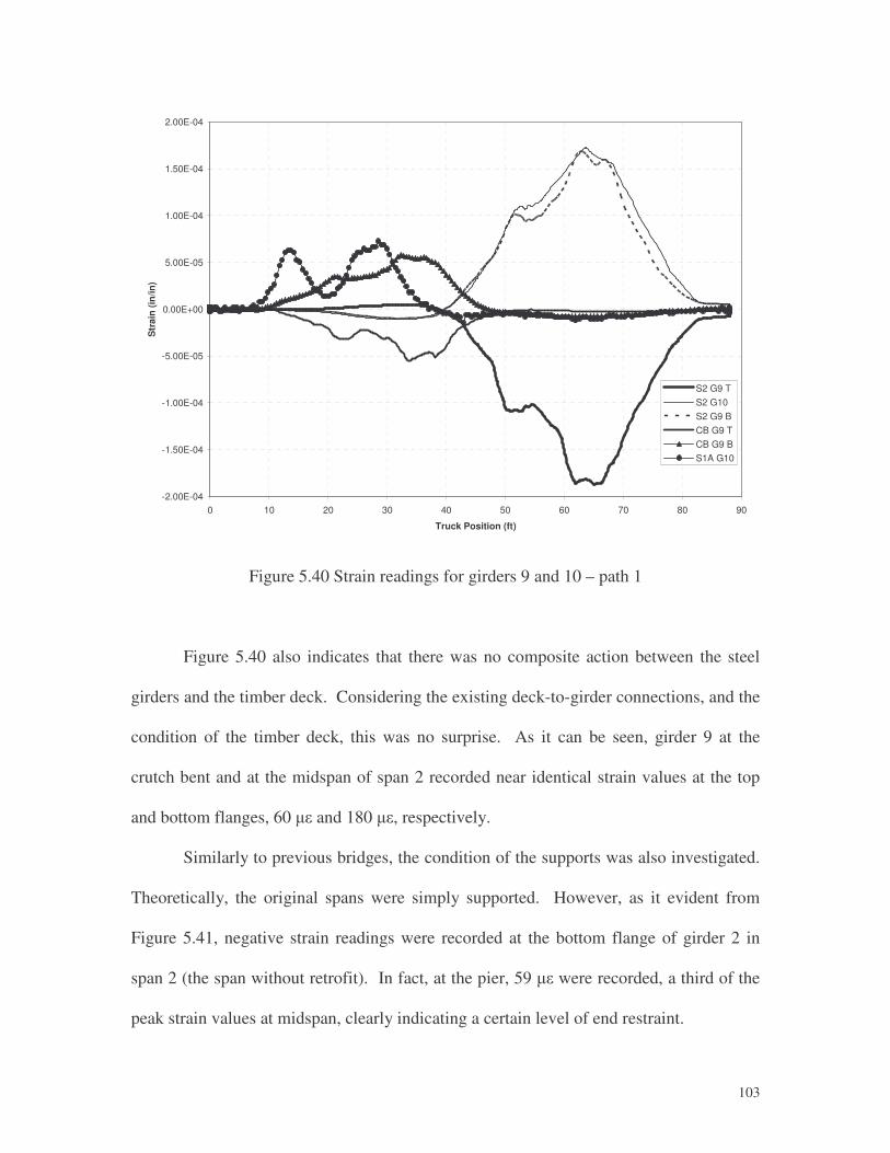
�
103
-2.00E-04
-1.50E-04
-1.00E-04
-5.00E-05
0.00E+00
5.00E-05
1.00E-04
1.50E-04
2.00E-04
0 10 20 30 40 50 60 70 80 90
Truck Position (ft)
Str
ain
(in/in
)
S2 G9 TS2 G10S2 G9 BCB G9 TCB G9 BS1A G10
Figure 5.40 Strain readings for girders 9 and 10 – path 1
Figure 5.40 also indicates that there was no composite action between the steel
girders and the timber deck. Considering the existing deck-to-girder connections, and the
condition of the timber deck, this was no surprise. As it can be seen, girder 9 at the
crutch bent and at the midspan of span 2 recorded near identical strain values at the top
and bottom flanges, 60 �� and 180 ��, respectively.
Similarly to previous bridges, the condition of the supports was also investigated.
Theoretically, the original spans were simply supported. However, as it evident from
Figure 5.41, negative strain readings were recorded at the bottom flange of girder 2 in
span 2 (the span without retrofit). In fact, at the pier, 59 �� were recorded, a third of the
peak strain values at midspan, clearly indicating a certain level of end restraint.
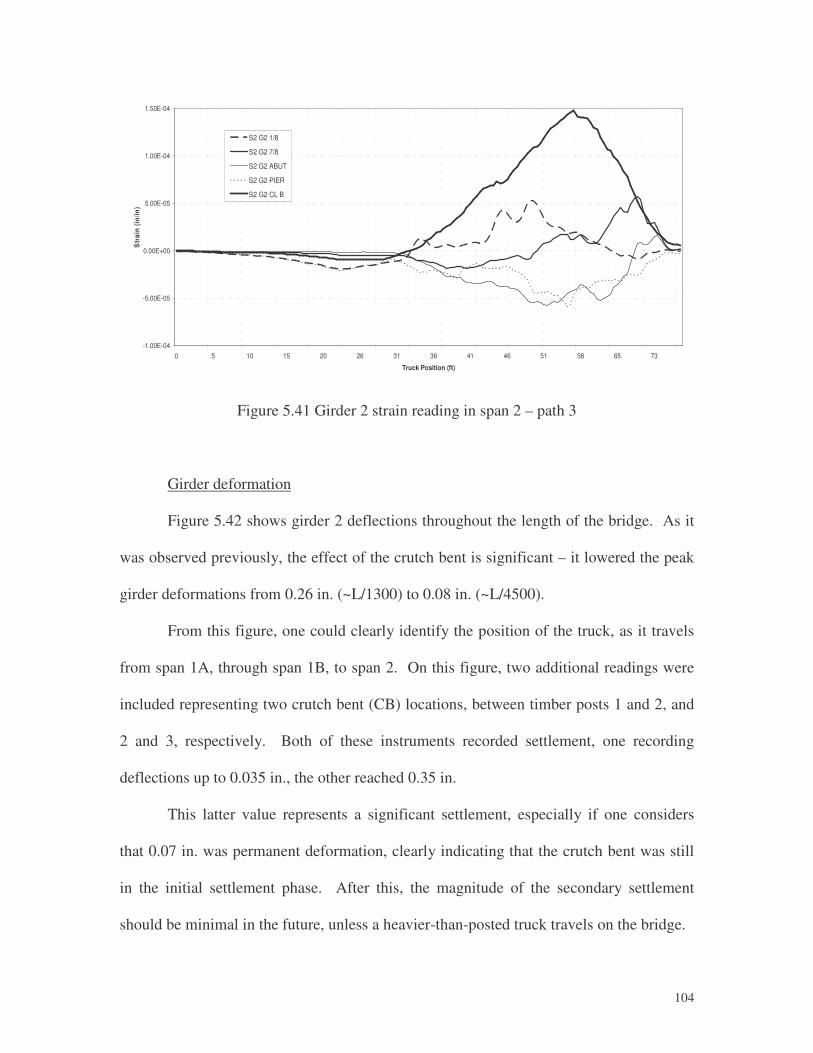
�
104
-1.00E-04
-5.00E-05
0.00E+00
5.00E-05
1.00E-04
1.50E-04
0 5 10 15 20 26 31 36 41 46 51 58 65 73
Truck Position (ft)
Str
ain
(in/in
)S2 G2 1/8
S2 G2 7/8
S2 G2 ABUT
S2 G2 PIER
S2 G2 CL B
Figure 5.41 Girder 2 strain reading in span 2 – path 3
Girder deformation
Figure 5.42 shows girder 2 deflections throughout the length of the bridge. As it
was observed previously, the effect of the crutch bent is significant – it lowered the peak
girder deformations from 0.26 in. (~L/1300) to 0.08 in. (~L/4500).
From this figure, one could clearly identify the position of the truck, as it travels
from span 1A, through span 1B, to span 2. On this figure, two additional readings were
included representing two crutch bent (CB) locations, between timber posts 1 and 2, and
2 and 3, respectively. Both of these instruments recorded settlement, one recording
deflections up to 0.035 in., the other reached 0.35 in.
This latter value represents a significant settlement, especially if one considers
that 0.07 in. was permanent deformation, clearly indicating that the crutch bent was still
in the initial settlement phase. After this, the magnitude of the secondary settlement
should be minimal in the future, unless a heavier-than-posted truck travels on the bridge.
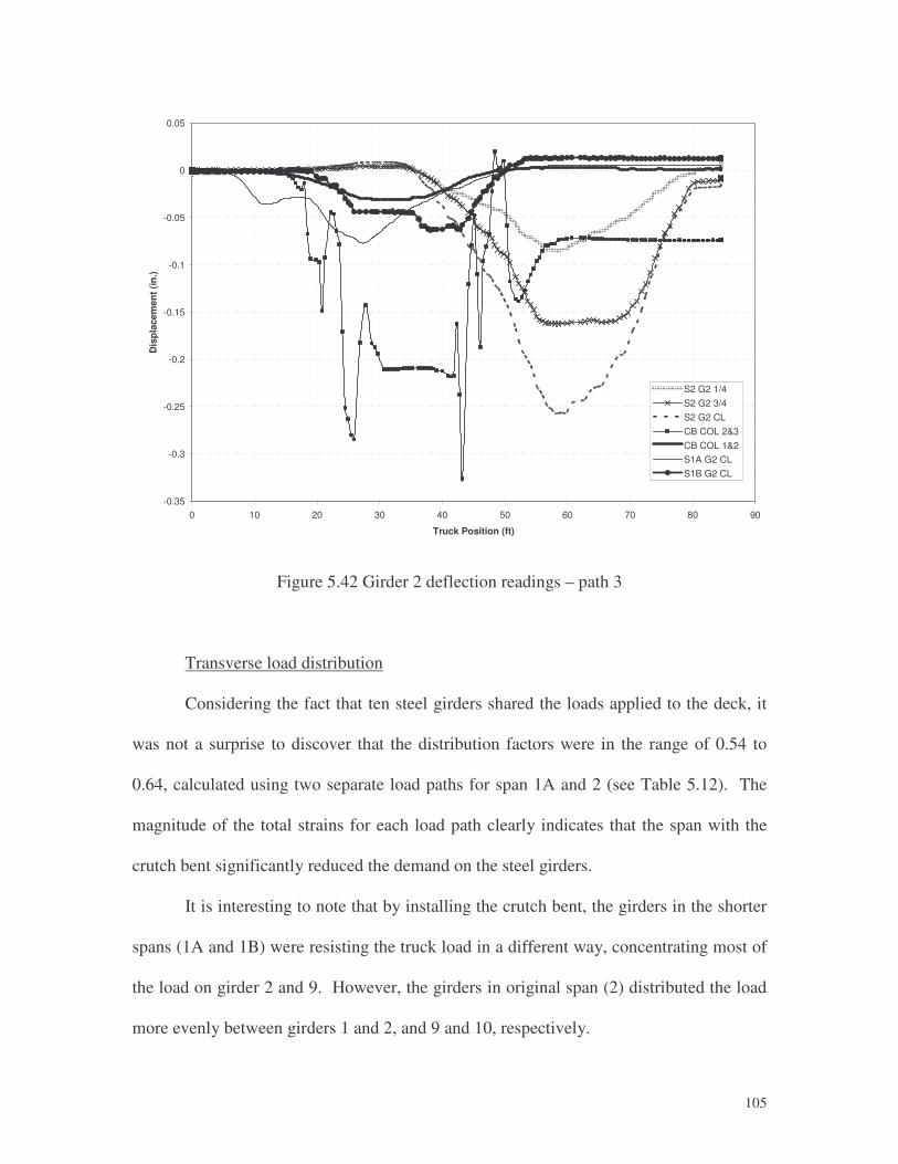
�
105
-0.35
-0.3
-0.25
-0.2
-0.15
-0.1
-0.05
0
0.05
0 10 20 30 40 50 60 70 80 90
Truck Position (ft)
Dis
plac
emen
t (in
.)
S2 G2 1/4S2 G2 3/4S2 G2 CLCB COL 2&3CB COL 1&2S1A G2 CLS1B G2 CL
Figure 5.42 Girder 2 deflection readings – path 3
Transverse load distribution
Considering the fact that ten steel girders shared the loads applied to the deck, it
was not a surprise to discover that the distribution factors were in the range of 0.54 to
0.64, calculated using two separate load paths for span 1A and 2 (see Table 5.12). The
magnitude of the total strains for each load path clearly indicates that the span with the
crutch bent significantly reduced the demand on the steel girders.
It is interesting to note that by installing the crutch bent, the girders in the shorter
spans (1A and 1B) were resisting the truck load in a different way, concentrating most of
the load on girder 2 and 9. However, the girders in original span (2) distributed the load
more evenly between girders 1 and 2, and 9 and 10, respectively.
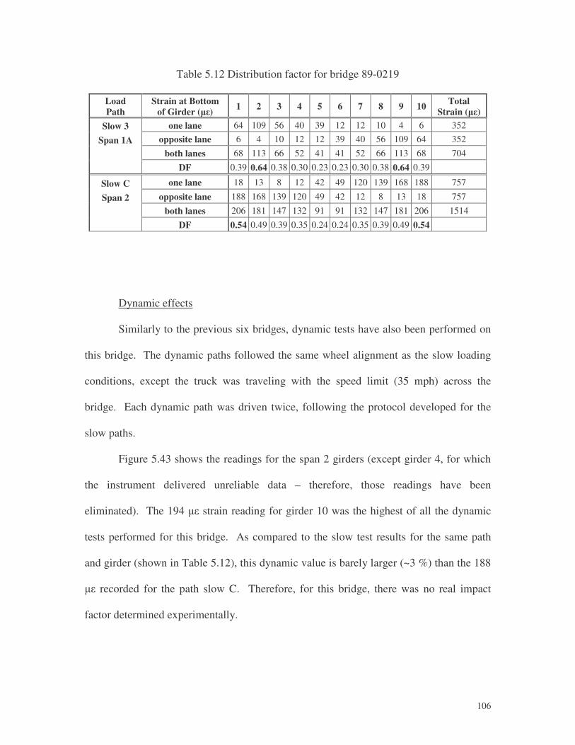
�
106
Table 5.12 Distribution factor for bridge 89-0219
Load Path
Strain at Bottom of Girder (��) 1 2 3 4 5 6 7 8 9 10 Total
Strain (��) Slow 3 one lane 64 109 56 40 39 12 12 10 4 6 352
Span 1A opposite lane 6 4 10 12 12 39 40 56 109 64 352
both lanes 68 113 66 52 41 41 52 66 113 68 704
DF 0.39 0.64 0.38 0.30 0.23 0.23 0.30 0.38 0.64 0.39
Slow C one lane 18 13 8 12 42 49 120 139 168 188 757
Span 2 opposite lane 188 168 139 120 49 42 12 8 13 18 757
both lanes 206 181 147 132 91 91 132 147 181 206 1514
DF 0.54 0.49 0.39 0.35 0.24 0.24 0.35 0.39 0.49 0.54
Dynamic effects
Similarly to the previous six bridges, dynamic tests have also been performed on
this bridge. The dynamic paths followed the same wheel alignment as the slow loading
conditions, except the truck was traveling with the speed limit (35 mph) across the
bridge. Each dynamic path was driven twice, following the protocol developed for the
slow paths.
Figure 5.43 shows the readings for the span 2 girders (except girder 4, for which
the instrument delivered unreliable data – therefore, those readings have been
eliminated). The 194 �� strain reading for girder 10 was the highest of all the dynamic
tests performed for this bridge. As compared to the slow test results for the same path
and girder (shown in Table 5.12), this dynamic value is barely larger (~3 %) than the 188
�� recorded for the path slow C. Therefore, for this bridge, there was no real impact
factor determined experimentally.
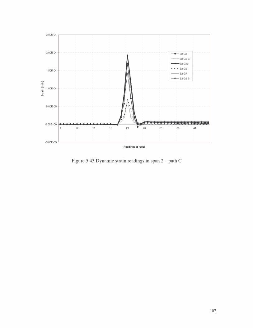
�
107
-5.00E-05
0.00E+00
5.00E-05
1.00E-04
1.50E-04
2.00E-04
2.50E-04
1 6 11 16 21 26 31 36 41
Readings (5 /sec)
Str
ain
(in
/in)
S2 G8
S2 G5 B
S2 G10
S2 G6
S2 G7
S2 G9 B
Figure 5.43 Dynamic strain readings in span 2 – path C
�
108
6. ANALYTICAL STUDIES AND COMPARISONS
During the first phase of the project, four bridges were tested and analyzed.
Based on these preliminary analyses, the loading truck and the instrumentation details
were determined. After the actual experiments, the test data was analyzed, and then the
results compared with the bridge ratings.
In the second phase, bridge testing was preceded by extensive analyses, including
a parametric study with variables, such as material property, girder end fixity, degree of
composite action, etc…. These analyses provided a bridge response envelope,
considering the combined effects of the above-mentioned factors. This phase was
followed by the bridge tests, and then a comparison was performed between the
analytical and experimental results.
In this section, nearly all variables involving bridge rating will be examined. As it
will be demonstrated, a number of these variables are bridge specific, and conclusions
could not be drawn for general use. Even more so, some of these bridge specific
variables are also condition specific, and they could easily be altered during routine
maintenance procedures.
6.1 Bridge Rating
In order to evaluate the NCDOT bridge rating software, the previously described
AASHTOWare software was used, in addition to an elaborate spreadsheet developed at
UNC Charlotte based on the AASHTO load rating equations discussed earlier. As
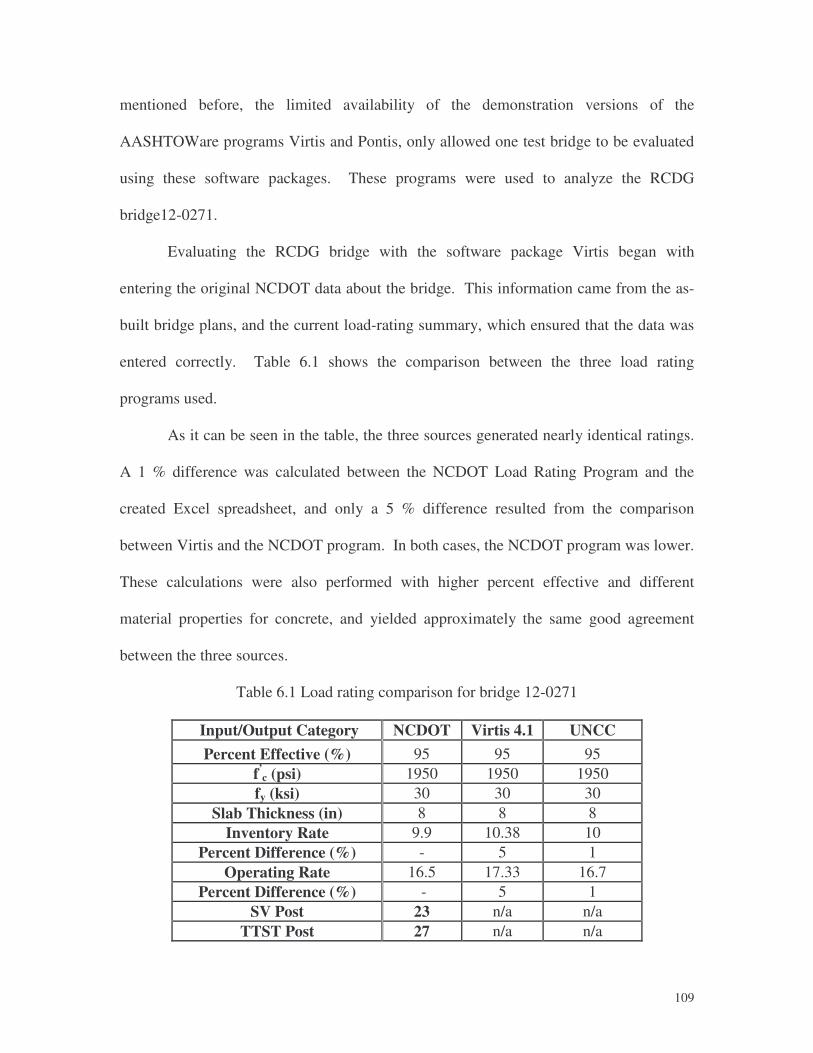
�
109
mentioned before, the limited availability of the demonstration versions of the
AASHTOWare programs Virtis and Pontis, only allowed one test bridge to be evaluated
using these software packages. These programs were used to analyze the RCDG
bridge12-0271.
Evaluating the RCDG bridge with the software package Virtis began with
entering the original NCDOT data about the bridge. This information came from the as-
built bridge plans, and the current load-rating summary, which ensured that the data was
entered correctly. Table 6.1 shows the comparison between the three load rating
programs used.
As it can be seen in the table, the three sources generated nearly identical ratings.
A 1 % difference was calculated between the NCDOT Load Rating Program and the
created Excel spreadsheet, and only a 5 % difference resulted from the comparison
between Virtis and the NCDOT program. In both cases, the NCDOT program was lower.
These calculations were also performed with higher percent effective and different
material properties for concrete, and yielded approximately the same good agreement
between the three sources.
Table 6.1 Load rating comparison for bridge 12-0271
Input/Output Category NCDOT Virtis 4.1 UNCC Percent Effective (%) 95 95 95
f’c (psi) 1950 1950 1950
fy (ksi) 30 30 30 Slab Thickness (in) 8 8 8
Inventory Rate 9.9 10.38 10 Percent Difference (%) - 5 1
Operating Rate 16.5 17.33 16.7 Percent Difference (%) - 5 1
SV Post 23 n/a n/a TTST Post 27 n/a n/a
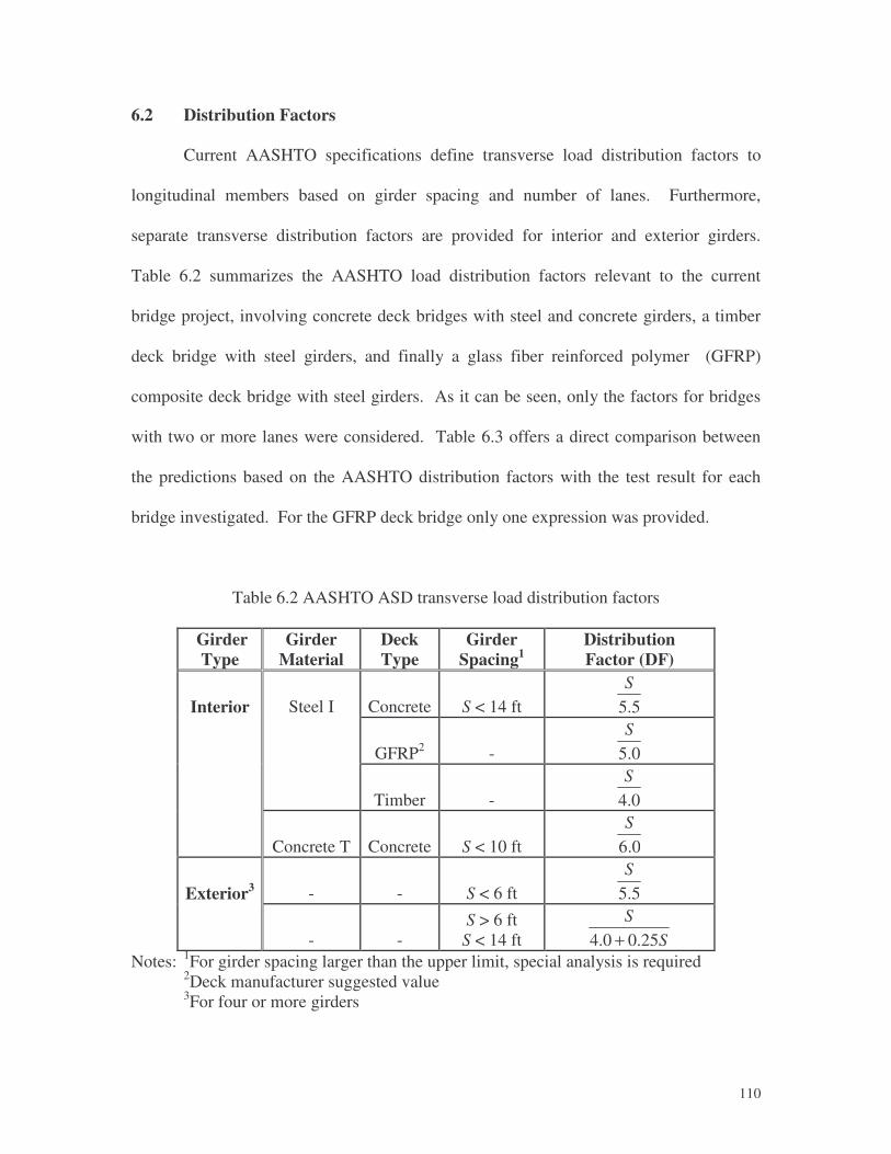
�
110
6.2 Distribution Factors
Current AASHTO specifications define transverse load distribution factors to
longitudinal members based on girder spacing and number of lanes. Furthermore,
separate transverse distribution factors are provided for interior and exterior girders.
Table 6.2 summarizes the AASHTO load distribution factors relevant to the current
bridge project, involving concrete deck bridges with steel and concrete girders, a timber
deck bridge with steel girders, and finally a glass fiber reinforced polymer (GFRP)
composite deck bridge with steel girders. As it can be seen, only the factors for bridges
with two or more lanes were considered. Table 6.3 offers a direct comparison between
the predictions based on the AASHTO distribution factors with the test result for each
bridge investigated. For the GFRP deck bridge only one expression was provided.
Table 6.2 AASHTO ASD transverse load distribution factors
Girder Type
Girder Material
Deck Type
Girder Spacing1
Distribution Factor (DF)
Interior Steel I Concrete S < 14 ft 5.5S
GFRP2 - 0.5S
Timber - 0.4S
Concrete T Concrete S < 10 ft 0.6S
Exterior3 - - S < 6 ft 5.5S
- - S > 6 ft S < 14 ft S
S25.00.4 +
Notes: 1For girder spacing larger than the upper limit, special analysis is required 2Deck manufacturer suggested value
3For four or more girders
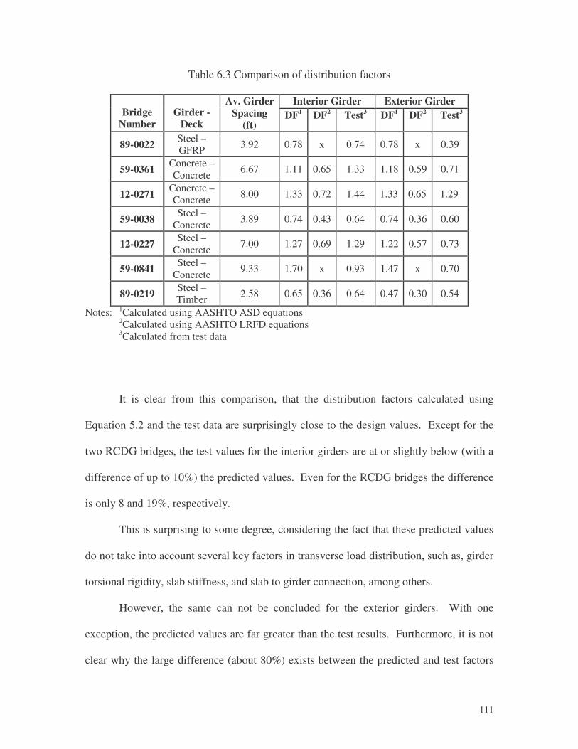
�
111
Table 6.3 Comparison of distribution factors
Interior Girder Exterior Girder Bridge
Number Girder -
Deck
Av. Girder Spacing
(ft) DF1 DF2 Test3 DF1 DF2 Test3
89-0022 Steel – GFRP 3.92 0.78 x 0.74 0.78 x 0.39
59-0361 Concrete – Concrete 6.67 1.11 0.65 1.33 1.18 0.59 0.71
12-0271 Concrete – Concrete 8.00 1.33 0.72 1.44 1.33 0.65 1.29
59-0038 Steel – Concrete 3.89 0.74 0.43 0.64 0.74 0.36 0.60
12-0227 Steel – Concrete 7.00 1.27 0.69 1.29 1.22 0.57 0.73
59-0841 Steel – Concrete 9.33 1.70 x 0.93 1.47 x 0.70
89-0219 Steel – Timber 2.58 0.65 0.36 0.64 0.47 0.30 0.54
Notes: 1Calculated using AASHTO ASD equations 2Calculated using AASHTO LRFD equations 3Calculated from test data
It is clear from this comparison, that the distribution factors calculated using
Equation 5.2 and the test data are surprisingly close to the design values. Except for the
two RCDG bridges, the test values for the interior girders are at or slightly below (with a
difference of up to 10%) the predicted values. Even for the RCDG bridges the difference
is only 8 and 19%, respectively.
This is surprising to some degree, considering the fact that these predicted values
do not take into account several key factors in transverse load distribution, such as, girder
torsional rigidity, slab stiffness, and slab to girder connection, among others.
However, the same can not be concluded for the exterior girders. With one
exception, the predicted values are far greater than the test results. Furthermore, it is not
clear why the large difference (about 80%) exists between the predicted and test factors

�
112
for the interior girders of bridge 59-0841 (the new continuous steel girder bridge with
spans close to 150 ft), the predicted values being far too conservative for most of the
tested bridges.
6.3 Impact Factors
In order to account for dynamic, vibratory and impact effects, for design
purposes, AASHTO specifies an impact factor that is used to increase the live load
effects on a bridge. As it can be seen from Equation 6.1, the formula for impact factor (I)
is based on the bridge span. The upper limit for this value is set for 0.30, representing a
30 % increase for the live loads applied.
12550+
=L
I 6.1
where: I – live load impact factor; and L – bridge span length (ft).
It is clear from this equation, that this equation will yield lower impact factors for
longer span bridges with possibly longer dynamic periods. This philosophy follows the
classical seismic design approach based on spectral accelerations, yielding higher seismic
forces for stiffer, and therefore, shorter period structures (all other aspects being equal).
Table 6.4 provides a comprehensive evaluation on the dynamic loadings. It is
clear from this table, that with the exception of one or two values, the vast majority of the
dynamic loadings did not result in any significant impact factors. Virtually all the
dynamic readings, with the exception of the first (1st) and maybe the second (2nd) highest
values, were lower than the corresponding static or slow experimental result.
By carefully reviewing all of the results it was obvious, that some of the spikes
resulting in a higher dynamic reading were erroneous, and could not be confirmed with
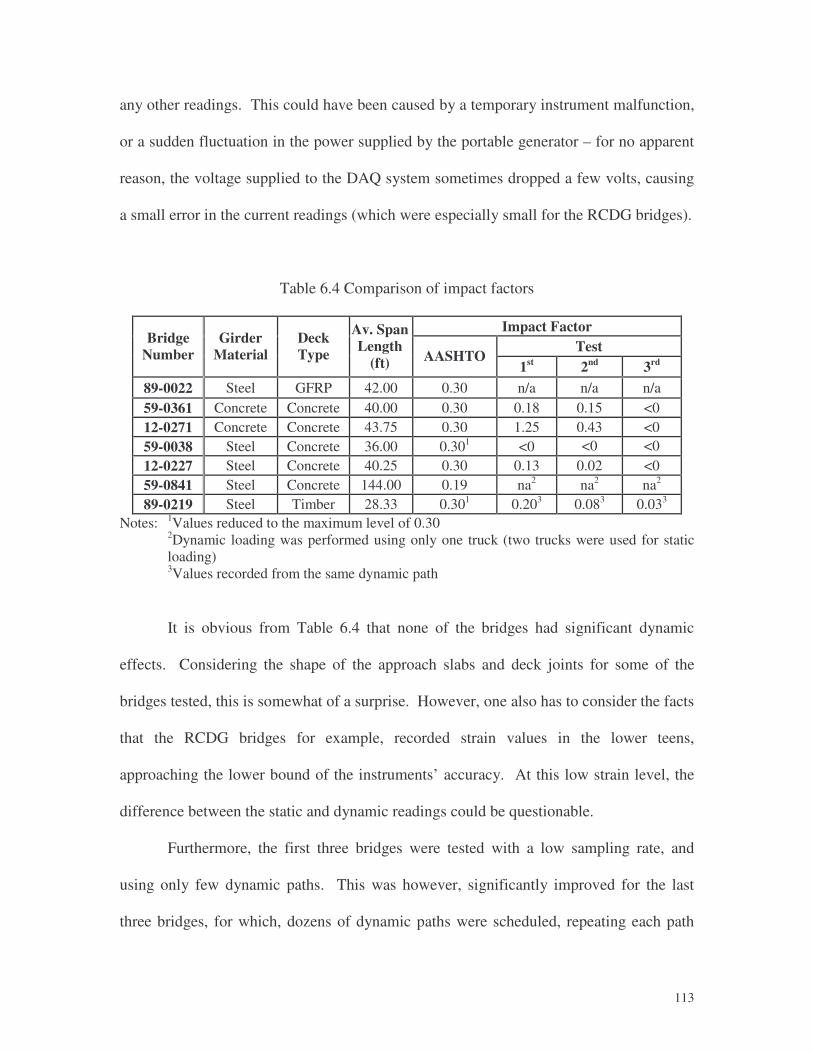
�
113
any other readings. This could have been caused by a temporary instrument malfunction,
or a sudden fluctuation in the power supplied by the portable generator – for no apparent
reason, the voltage supplied to the DAQ system sometimes dropped a few volts, causing
a small error in the current readings (which were especially small for the RCDG bridges).
Table 6.4 Comparison of impact factors
Impact Factor Test Bridge
Number Girder
Material Deck Type
Av. Span Length
(ft) AASHTO 1st 2nd 3rd
89-0022 Steel GFRP 42.00 0.30 n/a n/a n/a 59-0361 Concrete Concrete 40.00 0.30 0.18 0.15 <0 12-0271 Concrete Concrete 43.75 0.30 1.25 0.43 <0 59-0038 Steel Concrete 36.00 0.301 <0 <0 <0
12-0227 Steel Concrete 40.25 0.30 0.13 0.02 <0 59-0841 Steel Concrete 144.00 0.19 na2 na2 na2 89-0219 Steel Timber 28.33 0.301 0.203 0.083 0.033
Notes: 1Values reduced to the maximum level of 0.30 2Dynamic loading was performed using only one truck (two trucks were used for static
loading) 3Values recorded from the same dynamic path
It is obvious from Table 6.4 that none of the bridges had significant dynamic
effects. Considering the shape of the approach slabs and deck joints for some of the
bridges tested, this is somewhat of a surprise. However, one also has to consider the facts
that the RCDG bridges for example, recorded strain values in the lower teens,
approaching the lower bound of the instruments’ accuracy. At this low strain level, the
difference between the static and dynamic readings could be questionable.
Furthermore, the first three bridges were tested with a low sampling rate, and
using only few dynamic paths. This was however, significantly improved for the last
three bridges, for which, dozens of dynamic paths were scheduled, repeating each path

�
114
twice, to ensure repeatability.
6.4 Composite Action
A bridge girder’s flexural capacity is significantly increased if positive
connections are provided between the girder and the bridge deck. The connection in
contemporary construction is realized by shear studs welded to steel girders, and poured
integrally with the concrete deck. Shear studs however, have not always been used to
transfer the longitudinal shear loads between girders and deck.
For these older bridges, no composite action exists – at least theoretically. In
reality, out of the five steel girder bridges tested, only the timber deck bridge behaved as
expected. As it was shown in the previous chapter, the neutral axes of the superstructure
for the other four steel girder bridges was found to be well above the mid-height of the
girders, clearly indicating a certain level of composite action in most of the cases.
Bridge 89-0022
Traditionally, composite action was accounted for by using transformed sections,
where a homogeneous section was created from the two materials of the superstructure.
Based on the manufacturer’s recommendation, in the design of the GFRP deck
replacement, for structure 89-0022, no composite action was assumed. However, the
load testing clearly showed interaction between the steel girders and the GFRP deck.
To verify this result, an attempt was made to develop a transformed section. This
was done by using the modular ratio of the steel and the composite material. Using the
manufacturer’s information for the modulus of elasticity of the deck panels, and the steel

�
115
modulus of elasticity (see Table 6.5), the modular ratio (n) was computed using Equation
6.2.
6.11==c
s
EE
n 6.2
where: Es – modulus of elasticity of steel (psi); and Ec – modulus of elasticity of GFRP deck in
the transverse direction (psi).
Table 6.5 Steel girder and composite panel information
Steel Girder GFRP Deck
Es= 2.90E+07 psi EcL = 2.50E+06 psi
H= 24.31 in h= 7.66 in
Tsf= 0.875 in Tpf= 0.66 in
Ig= 2700 in4 W= 47 in
As= 27.7 in2 Ap= 31.02 in2
Sx= 222.1 in3
Using this information and the girder spacing as the tributary width, the effective
width of deck panel for the section was computed using Equation 6.3 to be 4.1 in.
nW
beff = 6.3
where: beff – effective section width (in.); and W – girder spacing (in.).
Using this effective area and the dimensions of the girder, the neutral axis was
computed using Equation 6.4, to be located at 14.98 in. above the bottom flange of the
girder.

�
116
( )
( ) iny
TbA
hHTb
HA
y
b
pfeffs
pfeffs
b
98.1466.0205.47.27
266.7
31.2466.0205.4231.24
7.27
22
22
=××+
��
�
���
���
� +×××+��
���
� ×=
××+
��
�
���
���
� +×××+��
���
� ×=
6.4
where: yb – transformed section neutral axis location (in.); As – area of steel girder (in2);
H – height of steel girder (in.); h – height of GFRP deck panel (in.); and Tpf – top flange
thickness (in.).
Using the location of the neutral axis, the composite section properties can be
found, such as the section modulus (273.03 in3), and the moment of inertia (4136.2 in4).
As it was shown in Table 5.1, the measured neutral axis position was nearly identical
with the value calculated using Equation 6.4, clearly proving that full composite action
exists between the steel girders and the GFRP deck.
Bridge 59-0038
As one more example of composite calculations, the results of bridge 59-0038
will also be presented, for which, the steel girder was embedded in the concrete deck.
Table 6.6 shows the calculations for the strains, the bending stresses and the deflections
based on non-composite and composite sections. As it can be seen, the composite section
results are much closer to the actual test data. There are some discrepancies, however,
and they can be the result of higher compressive strength for the concrete deck.
This would certainly affect the modular ratio, as well as the stiffness results for
the composite section. But would this automatically imply a composite action even at
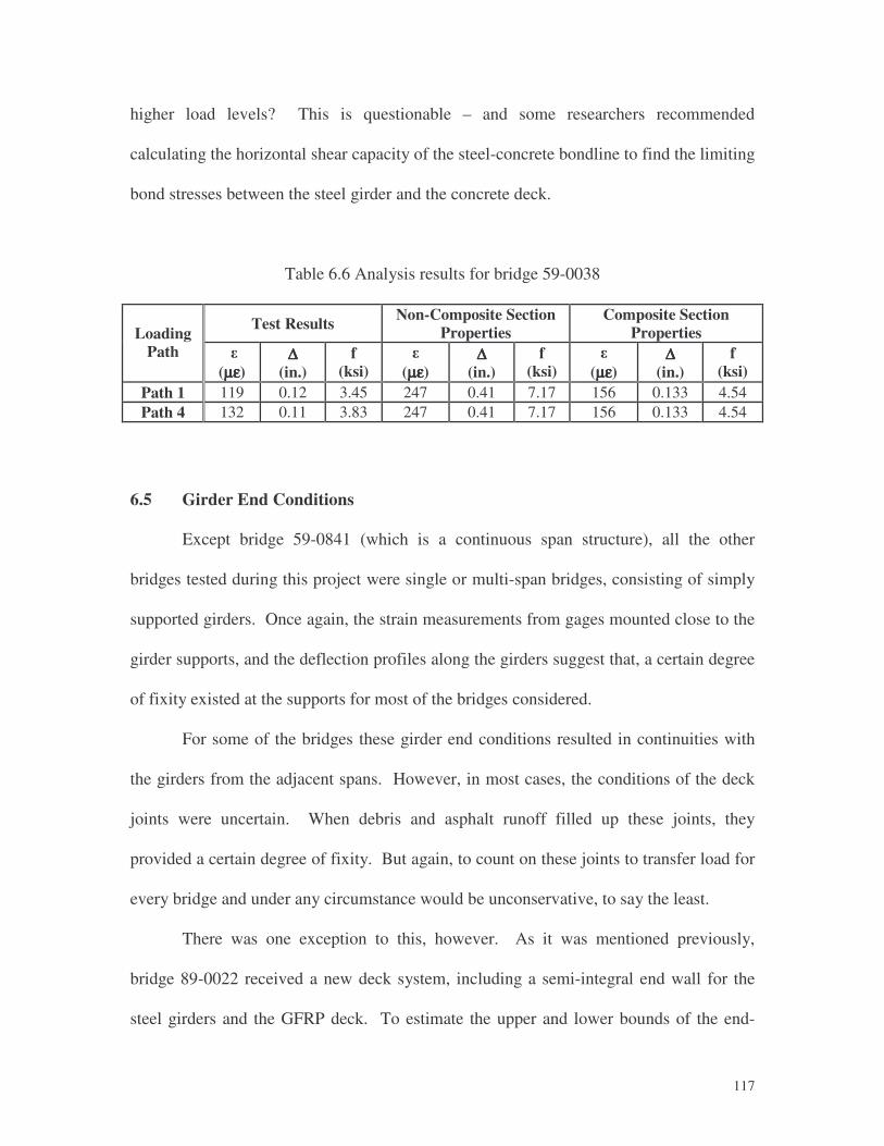
�
117
higher load levels? This is questionable – and some researchers recommended
calculating the horizontal shear capacity of the steel-concrete bondline to find the limiting
bond stresses between the steel girder and the concrete deck.
Table 6.6 Analysis results for bridge 59-0038
Test Results Non-Composite Section Properties
Composite Section Properties Loading
Path � (µµµµεεεε)
∆∆∆∆ (in.)
f (ksi)
� (µµµµεεεε)
∆∆∆∆ (in.)
f (ksi)
� (µµµµεεεε)
∆∆∆∆ (in.)
f (ksi)
Path 1 119 0.12 3.45 247 0.41 7.17 156 0.133 4.54 Path 4 132 0.11 3.83 247 0.41 7.17 156 0.133 4.54
6.5 Girder End Conditions
Except bridge 59-0841 (which is a continuous span structure), all the other
bridges tested during this project were single or multi-span bridges, consisting of simply
supported girders. Once again, the strain measurements from gages mounted close to the
girder supports, and the deflection profiles along the girders suggest that, a certain degree
of fixity existed at the supports for most of the bridges considered.
For some of the bridges these girder end conditions resulted in continuities with
the girders from the adjacent spans. However, in most cases, the conditions of the deck
joints were uncertain. When debris and asphalt runoff filled up these joints, they
provided a certain degree of fixity. But again, to count on these joints to transfer load for
every bridge and under any circumstance would be unconservative, to say the least.
There was one exception to this, however. As it was mentioned previously,
bridge 89-0022 received a new deck system, including a semi-integral end wall for the
steel girders and the GFRP deck. To estimate the upper and lower bounds of the end-
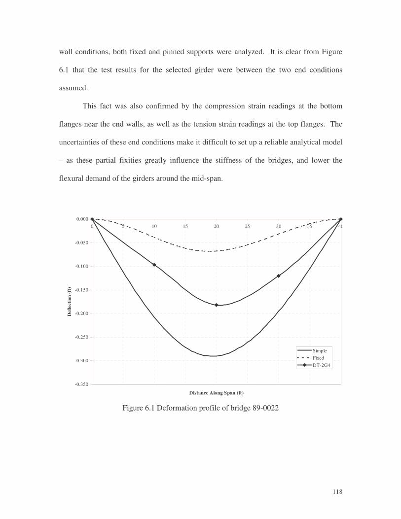
�
118
wall conditions, both fixed and pinned supports were analyzed. It is clear from Figure
6.1 that the test results for the selected girder were between the two end conditions
assumed.
This fact was also confirmed by the compression strain readings at the bottom
flanges near the end walls, as well as the tension strain readings at the top flanges. The
uncertainties of these end conditions make it difficult to set up a reliable analytical model
– as these partial fixities greatly influence the stiffness of the bridges, and lower the
flexural demand of the girders around the mid-span.
Figure 6.1 Deformation profile of bridge 89-0022
-0.350
-0.300
-0.250
-0.200
-0.150
-0.100
-0.050
0.0000 5 10 15 20 25 30 35 40
Distance Along Span (ft)
Def
lect
ion
(ft)
SimpleFixedDT-2G4

�
119
6.6 Strain Levels
In the second phase of this project, in order to estimate the expected strain levels
in the bridge girders, all of the factors mentioned in this chapter were considered in
different combinations. However, this created upper and lower bound strain values that
were so far apart, the range became too wide to be meaningful.
The largest differences between predicted and tested strains and stresses occurred
for the RCDG bridges. For these concrete girders, strains in the 200-300 µε levels were
predicted. This numbers were also confirmed with simpler finite element analyses.
Nevertheless, during testing, the strain levels recorded were well below 100 µε. Even the
deformations were in the few hundreds of an inch range, proving that these structures are
far stiffer and stronger than anticipated.
To find the reasons for this unexpected behavior, non-destructive tests (NDT)
were performed to verify the concrete compressive strength for the girders. As it was
mentioned earlier, AASHTO and NCDOT guidelines clearly specify the concrete
strength for older structures (for these two bridges the values were 1,950 and 2,500 psi,
respectively), when the original specifications are not clear, or they are no longer
available.
Schmidt hammer and Windsor probes were used in the NDT, and the results were
surprisingly high. Virtually all of the measurements for the two RCDG bridges resulted
in concrete strengths well above 6,000 psi. Indeed, one could argue that f’c has little or
no effect on the girder’s flexural capacity – when these values were used in the NCDOT
bridge rating software, the significantly higher concrete strength resulted in a difference
less than 10%.
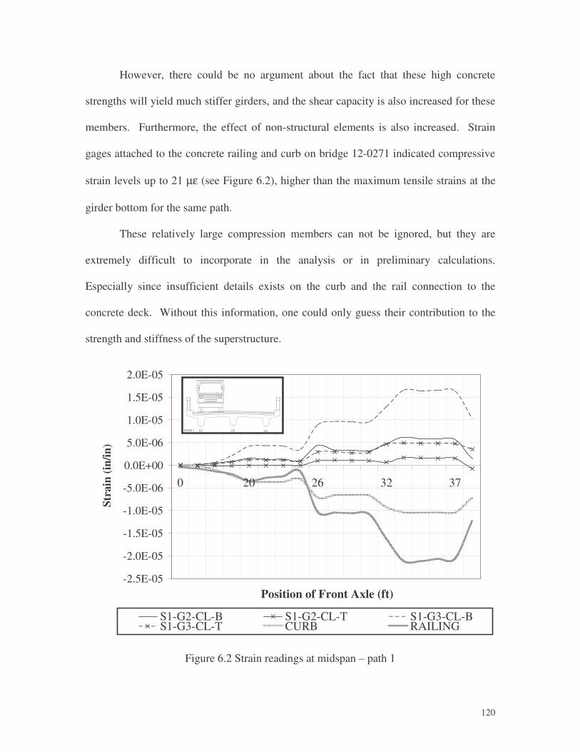
�
120
However, there could be no argument about the fact that these high concrete
strengths will yield much stiffer girders, and the shear capacity is also increased for these
members. Furthermore, the effect of non-structural elements is also increased. Strain
gages attached to the concrete railing and curb on bridge 12-0271 indicated compressive
strain levels up to 21 µε (see Figure 6.2), higher than the maximum tensile strains at the
girder bottom for the same path.
These relatively large compression members can not be ignored, but they are
extremely difficult to incorporate in the analysis or in preliminary calculations.
Especially since insufficient details exists on the curb and the rail connection to the
concrete deck. Without this information, one could only guess their contribution to the
strength and stiffness of the superstructure.
-2.5E-05
-2.0E-05
-1.5E-05
-1.0E-05
-5.0E-06
0.0E+00
5.0E-06
1.0E-05
1.5E-05
2.0E-05
0 20 26 32 37
Position of Front Axle (ft)
Stra
in (i
n/in
)
S1-G2-CL-B S1-G2-CL-T S1-G3-CL-BS1-G3-CL-T CURB RAILING
PATH 1 G3 G2 G1
Figure 6.2 Strain readings at midspan – path 1
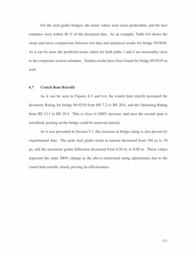
�
121
For the steel girder bridges, the strain values were more predictable, and the best
estimates were within 40 % of the measured data. As an example, Table 6.6 shows the
strain and stress comparisons between test data and analytical results for bridge 59-0038.
As it can be seen, the predicted strain values for both paths 1 and 4 are reasonably close
to the composite section estimates. Similar results have been found for bridge 89-0219 as
well.
6.7 Crutch Bent Retrofit
As it can be seen in Figures 6.3 and 6.4, the crutch bent retrofit increased the
Inventory Rating for bridge 89-0219 from HS 7.2 to HS 20.8, and the Operating Rating
from HS 12.1 to HS 29.4. This is close to 200% increase, and once the second span is
retrofitted, posting on the bridge could be removed entirely.
As it was presented in Section 5.7, this increase in bridge rating is also proven by
experimental data. The peak steel girder strain in tension decreased from 180 �� to 70
��, and the maximum girder deflection decreased from 0.26 in. to 0.08 in. These values
represent the same 200% change as the above-mentioned rating adjustments due to the
crutch bent retrofit, clearly proving its effectiveness.
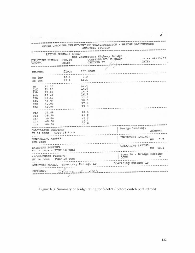
�
122
Figure 6.3 Summary of bridge rating for 89-0219 before crutch bent retrofit
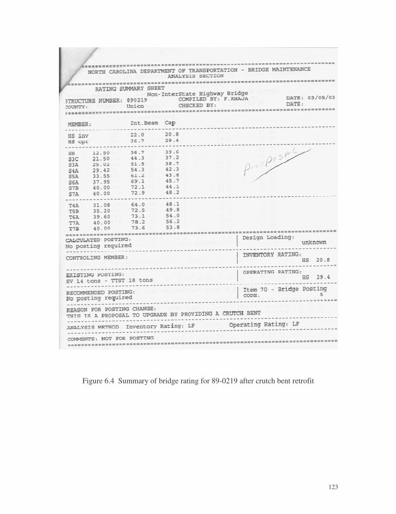
�
123
Figure 6.4 Summary of bridge rating for 89-0219 after crutch bent retrofit

�
124
7. NCDOT BRIDGE ANALYSIS SOFTWARES
7.1 Simple Span Analysis Software
During this research project, five of the bridges tested were also analyzed using
NCDOT’s simple span analysis software. As it was mentioned in Chapter 3 of this
report, the NCDOT analysis software directly follows the AASHTO (2000) bridge
condition evaluation procedures. The only added feature in the software is the use of an
effective girder cross section, a factor (smaller than one) that accounts for the loss of
effective area due to corrosion or vehicular damage. This feature adds an additional
safety factor to the already conservative AASHTO approach.
In addition, two other softwares have been used to verify the results of the
NCDOT analysis software. One is the Virtis program developed by AASHTOWare, the
other is an Excel-based spreadsheet developed by the UNC Charlotte research group.
Both of these programs verified the accuracy of the NCDOT program, and once again,
proved its safe and conservative approach to bridge evaluation.
In order to have a better appreciation of the accuracy of the NCDOT software, an
example calculation will be presented here. This example presents the findings of the
analysis and testing of bridge 59-0038.
Figures 7.1 and 7.2 are the output sheets from the NCDOT bridge analysis
program using the original data for Bridge 59-0038. For the original conditions, the S3C
single loading vehicle and the T4A - TTST loading vehicle govern the analysis, and
result in a bridge posting of 19 tons for SV, and 25 tons for TTST.
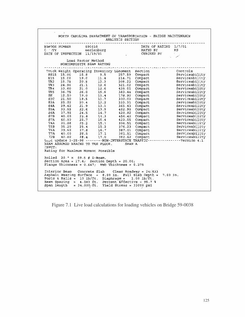
�
125
Figure 7.1 Live load calculations for loading vehicles on Bridge 59-0038
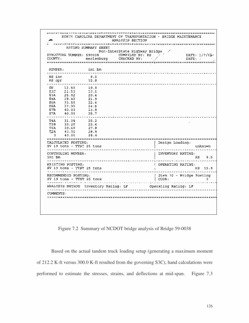
�
126
Figure 7.2 Summary of NCDOT bridge analysis of Bridge 59-0038
Based on the actual tandem truck loading setup (generating a maximum moment
of 212.2 K-ft versus 300.0 K-ft resulted from the governing S3C), hand calculations were
performed to estimate the stresses, strains, and deflections at mid-span. Figure 7.3
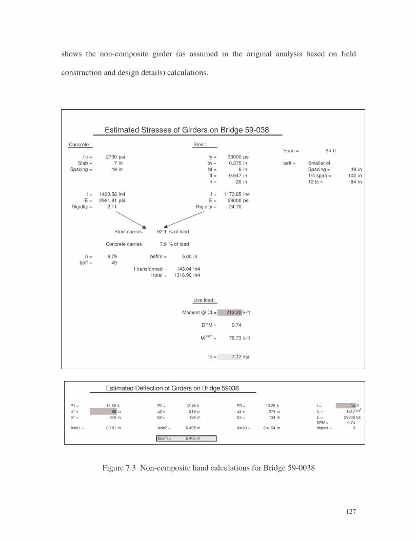
�
127
shows the non-composite girder (as assumed in the original analysis based on field
construction and design details) calculations.
Figure 7.3 Non-composite hand calculations for Bridge 59-0038
Concrete: Steel:Span = 34 ft
f'c = 2700 psi fy = 33000 psiSlab = 7 in tw = 0.375 in beff = Smaller of
Spacing = 49 in bf = 8 in Spacing = 49 intf = 0.647 in 1/4 span = 102 inh = 20 in 12 tc = 84 in
I = 1400.58 in4 I = 1173.85 in4E = 2961.81 psi E = 29000 psi
Rigidity = 2.11 Rigidity = 24.70
Steel carries 92.1 % of load
Concrete carries 7.9 % of load
n = 9.79 beff/n = 5.00 inbeff = 49
I transformed = 143.04 in4I total = 1316.90 in4
Live load:
Moment @ CL= 212.20 k-ft
DFM = 0.74
Mbeam = 78.73 k-ft
fb = 7.17 ksi
Estimated Stresses of Girders on Bridge 59-038
P1 = 11.66 k P2 = 13.46 k P3 = 13.28 k L= 34 ft a1 = 66 in a2 = 219 in a3 = 274 in IC = 1317 in4
b1 = 342 in b2 = 189 in b3 = 134 in E = 29000 ksiDFM = 0.74
Axle1 = 0.181 in Axle2 = 0.495 in Axle3 = 0.4194 in Impact = 0
Beam = 0.406 in
Estimated Deflection of Girders on Bridge 59038
�
128
After testing Bridge 59-0038, the results of the tests were compared to the hand
calculations to determine if the structure was performing as expected. Similar to other
bridges, Bridge 59-038 performed better than anticipated. Although the differences in
strain and deflection values were not as large, the steel girder bridge still experienced
only half the estimated strain and a quarter of the estimated deflection.
One of the reasons for these differences is a result of a possible composite action
between the girders and the bridge deck. The bridge was inspected and the top flange of
the girder is embedded into the concrete deck, bracing the compression flange and tying
the girder firmly to the deck. This connection was strong enough to allow the bridge to
act partially composite at the load level tested. Figure 7.4 shows the hand calculations
performed assuming full composite action in the bridge superstructure.
Table 7.1 compares the strain and deflection values at mid-span of one of the steel
girders from the loading tests, as well as the results from the non-composite and
composite hand calculations. From this table, it is clear that the test strains values are
slightly less than the composite values, whereas the deflections are practically identical.
However, one should remember that the horizontal shear capacity between the
girders and the deck could be exceeded if a significantly larger truckload was applied to
the bridge. This should need to be further investigated on a case-by-case basis.
Table 7.1 Strain and deflection values at mid-span for Bridge 59-0038
Test Values Analysis Based on Non-Composite Sections
Analysis Based on Composite Sections
Loading Path
µε ∆ (in) )(ksif µε ∆ (in) )(ksif µε ∆ (in) )(ksif 1 119 0.12 3.45 247 0.41 7.17 156 0.133 4.54 4 132 0.11 3.83 247 0.41 7.17 156 0.133 4.54
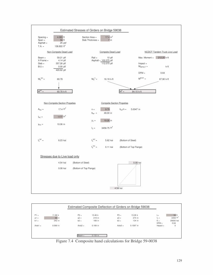
�
129
Figure 7.4 Composite hand calculations for Bridge 59-0038
Spacing = 4.083 ft Section Area = 17.4 in2
Span = 34 ft Slab Thickness = 7 inAsphalt = 25 psfT.A. = 138.822 ft2
Beam = 59.21 plf Rail = 10 plf Max. Moment = 212.20 k-ftX-Frame = 4.14 plf Asphalt = 102.075 plfSlab = 357.26 plf 112.075 plf Impact =B/U = 0.00 plf MIMPACT = k-ft
420.62 plfDFM = 0.64
MDNC = 60.78 MD
C = 16.19 k-ft Mbeam = 67.90 k-ft
MNC = 60.78 k-ft MC = 84.10 k-ft
ANC = 17.4 in2n = 9.79 beff/n = 5.0047 in
beff = 49.00 in
INC = 1177 in4
yC = 19.26 in
yNC = 10.06 in
IC = 3458.75 in4
fbNC = 6.23 ksi fb
NC = 5.62 ksi (Bottom of Steel)
fbNC = 0.11 ksi (Bottom of Top Flange)
4.54 ksi (Bottom of Steel) 0.08 ksi
0.08 ksi (Bottom of Top Flange)
4.54 ksi
Non-Compsite Section Propeties Compsite Section Propeties
Stresses due to Live load only
Estimated Stresses of Girders on Bridge 59038
Non-Compsite Dead Load Compsite Dead Load NCDOT Tandem Truck Live Load
Estimated Composite Deflection of Girders on Bridge 59038
P1 = 11.66 k P2 = 13.46 k P3 = 13.28 k L= 34 ft a1 = 66 in a2 = 219 in a3 = 274 in IC = 3459 in4
b1 = 342 in b2 = 189 in b3 = 134 in E = 29000 ksiDFM = 0.64
Axle1 = 0.069 in Axle2 = 0.189 in Axle3 = 0.1597 in Impact = 0
Beam = 0.133 in
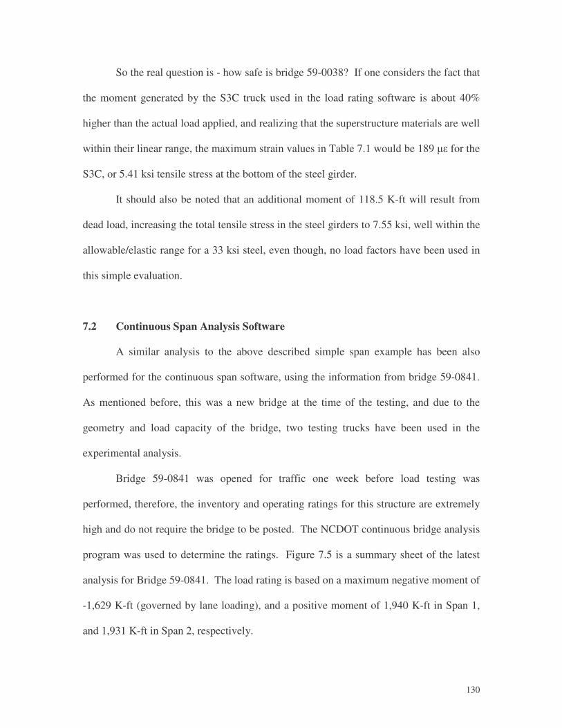
�
130
So the real question is - how safe is bridge 59-0038? If one considers the fact that
the moment generated by the S3C truck used in the load rating software is about 40%
higher than the actual load applied, and realizing that the superstructure materials are well
within their linear range, the maximum strain values in Table 7.1 would be 189 �� for the
S3C, or 5.41 ksi tensile stress at the bottom of the steel girder.
It should also be noted that an additional moment of 118.5 K-ft will result from
dead load, increasing the total tensile stress in the steel girders to 7.55 ksi, well within the
allowable/elastic range for a 33 ksi steel, even though, no load factors have been used in
this simple evaluation.
7.2 Continuous Span Analysis Software
A similar analysis to the above described simple span example has been also
performed for the continuous span software, using the information from bridge 59-0841.
As mentioned before, this was a new bridge at the time of the testing, and due to the
geometry and load capacity of the bridge, two testing trucks have been used in the
experimental analysis.
Bridge 59-0841 was opened for traffic one week before load testing was
performed, therefore, the inventory and operating ratings for this structure are extremely
high and do not require the bridge to be posted. The NCDOT continuous bridge analysis
program was used to determine the ratings. Figure 7.5 is a summary sheet of the latest
analysis for Bridge 59-0841. The load rating is based on a maximum negative moment of
-1,629 K-ft (governed by lane loading), and a positive moment of 1,940 K-ft in Span 1,
and 1,931 K-ft in Span 2, respectively.
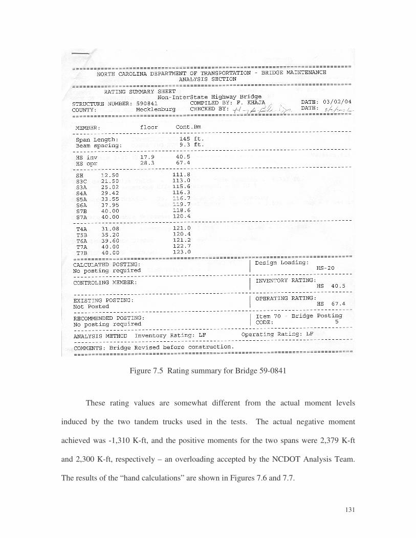
�
131
Figure 7.5 Rating summary for Bridge 59-0841
These rating values are somewhat different from the actual moment levels
induced by the two tandem trucks used in the tests. The actual negative moment
achieved was -1,310 K-ft, and the positive moments for the two spans were 2,379 K-ft
and 2,300 K-ft, respectively – an overloading accepted by the NCDOT Analysis Team.
The results of the “hand calculations” are shown in Figures 7.6 and 7.7.
�
132
Figure 7.6 Composite hand calculations for span 1 of Bridge 59-0841
Deck thickness = 8.75 in 20 inBeff = 105 in 1 inB/U = 2.5 in 22 inf'c = 3000 psi 1.125 inRa 0.5625 in
64 inSpacing = 9.33 ft
Max. Moment =2379.30 k-ft
Span = 146.5 ft Impact =MIMPACT = k-ft
Beff = Smaller ofSpacing = 112 in DFM = 0.931/4 span = 440 in
12 tc = 105 in Mbeam = 1106.37 k-ft
Section Area = 918.75 in2 80.75 in2I = 5861.81641 in4 I = 98726.37 in4E = 3155.92425 ksi E = 29000 ksi
ANC = 80.75 in2n = 9.19 beff/n deck = 11.43 in
beff/n B/U = 2.18 inytNC = 34.93 inybNC = 31.19 in AC = 186.17 in2
IC = 178341.2 in4
INC = 98726.373 in4 ytC = 22.67203 inybC = 54.70297 in
Stresses due to Live load only
0.78 ksi
4.07 ksi
Non-Compsite Section Propeties
NCDOT Tandem Truck Live Load
Compsite Section Propeties
Web thickness =Web height =
Section Area =
Top flange width =Top flange thickness =Bottom flange width =Bottom flange Thinkness =
Estimated Stresses of Girders on Bridge 59-0841
Span 1
Geomectric Properties of the Concrete Deck Geometric Properties of the Plate Girders
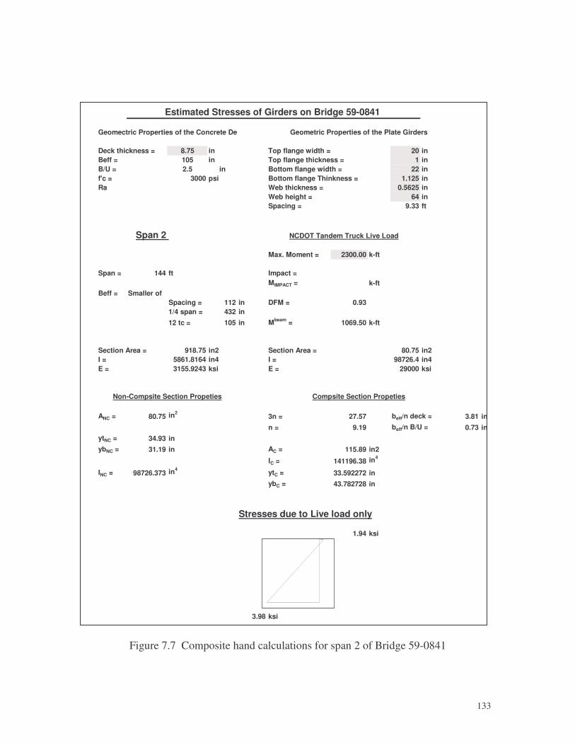
�
133
Figure 7.7 Composite hand calculations for span 2 of Bridge 59-0841
Deck thickness = 8.75 in 20 inBeff = 105 in 1 inB/U = 2.5 in 22 inf'c = 3000 psi 1.125 inRa 0.5625 in
64 inSpacing = 9.33 ft
Max. Moment = 2300.00 k-ft
Span = 144 ft Impact =MIMPACT = k-ft
Beff = Smaller ofSpacing = 112 in DFM = 0.931/4 span = 432 in12 tc = 105 in Mbeam = 1069.50 k-ft
Section Area = 918.75 in2 80.75 in2I = 5861.8164 in4 I = 98726.4 in4E = 3155.9243 ksi E = 29000 ksi
ANC = 80.75 in23n = 27.57 beff/n deck = 3.81 in
n = 9.19 beff/n B/U = 0.73 inytNC = 34.93 inybNC = 31.19 in AC = 115.89 in2
IC = 141196.38 in4
INC = 98726.373 in4 ytC = 33.592272 inybC = 43.782728 in
Stresses due to Live load only
1.94 ksi
3.98 ksi
NCDOT Tandem Truck Live Load
Non-Compsite Section Propeties Compsite Section Propeties
Web thickness =Web height =
Section Area =
Top flange width =Top flange thickness =Bottom flange width =Bottom flange Thinkness =
Estimated Stresses of Girders on Bridge 59-0841
Span 2
Geomectric Properties of the Concrete Deck Geometric Properties of the Plate Girders

�
134
After testing Bridge 59-0841, the results of the tests were compared to the hand
calculations to determine if the structure was performing as expected. Table 7.2 shows a
good agreement between anticipated and test live load values (considering only truck
loads). Once again, these values are far from the allowable stresses for the AASHTO
M270 Grade 50W steel, even though only live loads have been considered in this
example.
Table 7.2 Strain values at mid-span for Bridge 59-0841
Test Values Hand Calculations Loading Configuration µε )(ksif µε )(ksif
Path 1, Span 1 165 4.79 140 4.07 Path 5, Span 1 147 4.26 140 4.07 Path 1, Span 2 165 4.79 137 3.98 Path 5, Span 2 145 4.21 137 3.98
7.3 Conclusions
In conclusion, it is clear that based on the seven bridge tests and extensive
analytical work, the NCDOT simple and continuous span softwares directly follow the
AASHTO requirements (with one minor conservative exception) for bridge rating, and
provide a safe and conservative estimate for the load capacity of existing bridges. At this
point, improvement to these softwares could only be made if the bridge analysis program
results are complemented by bridge tests to allow for more realistic estimates of
important factors, such as transverse load distribution, impact, composite action, etc...

�
135
8. BRIDGE RATING THROUGH LOAD TESTING
It is clear from the discussions presented in the previous chapters that the true
behavior of each individual bridge largely depends on the specific conditions present at
the bridge being investigated. Would a full finite element analysis provide these factors
with confidence? Yes, for some of them (e.g. load distribution factors, contribution of
secondary elements); but even slight deviations from the design specifications, in
combination with the under- or over-estimation of the true condition of structural
elements (degree of corrosion and cracking), deck and girder joints, approach slabs and
material properties, would provide erroneous results.
Based on the data presented in this report, it is evident that some of the factors
that influence the true response of a bridge structure can be estimated with confidence.
However, a good number of other factors can only be evaluated through actual load
testing. The Manual for Bridge Rating Through Load Testing (1998) published by the
NCHRP Research Results Digest provides detailed information on factors influencing
bridge rating, load testing protocols, and guidelines for re-evaluating bridges based on
test data.
Would it make economical and engineering sense to test every single bridge in the
country? Probably not, these tests would be most feasible for posted bridges or structures
with questionable strength, damaged bridges, or bridges evaluated for special permits.
As sensor technology evolves in the near future, it would be beneficial to embed sensors

�
136
into several bridge components, and either monitor them continuously, or record their
data as a load testing is performed in the future.
8.1 Rating Procedure
As it was mentioned earlier, for the last three bridges tested in this research
project an additional portable data acquisitions system was also used to monitor the
bridges’ response. It was clear, that the handful of instruments used with this system
provided reliable data that could be used to re-rate these bridges based on test
information. These instruments allowed the more realistic evaluation of several factors,
including the load distribution and impact factors, the true strain levels in primary bridge
components, the presence of composite action, and the degree of fixity for simple span
superstructure components.
Although it is not anticipated to occur with frequency, the bridge testing might
reveal a weaker-than-expected structure. Experience shows that most bridges tested
exhibit significant load reserves. No matter what is the result, load testing will provide a
more realistic “picture”, well worth the effort. The actual procedure should include the
following steps:
1. Bridge inspection and evaluation – this step is already being done every other
year. Should also include material tests using NDT techniques, or tests on actual samples
collected from selected members.
2. Initial bridge load rating – based on real material properties and updated loading
information, perform an initial load rating of the bridge.
�
137
3. Design of instrumentation and loading protocol – based on the make-up,
geometry, size, ADT, and other factors, design an instrumentation plan. Select the
loading truck(s) sufficiently large to perform a diagnostic testing in function of the
current load rating of the bridge.
4. Instrumentation of bridge components – this step involves the preparation of the
bridge site, and the positioning of the instruments. These instruments (up to two dozens)
should include strain measuring devices, e.g. strain transducers, strain gages or LVDTs,
depending on the girder and deck material. If load testing will not immediately follow
the installation of the instruments, these devices must be protected against environmental
effects and vandalism.
5. Bridge load testing – during this phase, the bridge is partially or fully closed to
traffic. Then, following a predetermined loading protocol, the bridge is loaded with a
slow-moving truck. The load path is designed to provide maximum effect on the girders
and decks, as applicable. In order to provide a more realistic impact factor for the bridge
being evaluated, data would be recorded while the loading truck moves at the legal speed
limit.
6. Experimental data analysis – using simple hand calculations (or in-house
spreadsheet programs, or commercially available software), the test data is analyzed, and
compared with predicted values.
7. Update of initial bridge load rating – based on the experimental data, the bridge
is then re-rated, to provide a more realistic performance level for the structure being
analyzed. The above mentioned Manual for Bridge Rating Through Load Testing
provides detailed rating procedures using actual field test data.

�
138
8.2 Personnel and Equipment Needs
Bridge rating through load testing is not new. Several commercial entities exist
around the country specialized in this procedure. However, in order to provide a more
economical approach, with minimal training and a reasonable initial investment in
equipment, several testing crews could be established. Table 8.1 summarizes the
personnel and equipment needs to perform the 7 steps outlined in the previous section.
Table 8.1 Summary of bridge testing personnel and equipment needs
Step Task Description
Personnel Need
Personnel Training
Equipment Type Equipment Cost
Estimated Time
1 bridge inspection
existing inspection crew
minimal for NDT
NDT (if used)
depends on NDT type
1 hour for NDT
2 initial load rating
existing bridge analysis team
no change no change no change no change
3 design bridge test protocol
1-2 additions to bridge analysis
minimal to moderate
none none 2-3 hours
6-12 for strain $3k - $6k 4 bridge instrumentation
1 addition to inspection crew
minimal 4-6 for deformation $2k - $3k
2-3 hours
data acquisition ~$25k 5 bridge load testing
truck driver (from NCDOT yard)
minimal to moderate loading truck
traffic control minimal
1-2 hours
6 test data analysis
same as Step 3 moderate in-house or commercial software
~$5k for commercial
2-4 hours
7 update bridge load rating
same as Step 3 moderate same as Step 6 none 1-2 hours
As it can be seen, the majority of personnel are already in place, requiring only 1
additional inspection crew member trained to place instrumentation and conduct bridge
load testing. This crew member would travel with the testing equipment to bridge test
sites, and would be assisted by the local bridge maintenance and/or inspection team.
There would be a need for 1 or 2 additional bridge analysis personnel. The
training for these engineers would be relatively simple, including experimental stress

�
139
analysis, basic instrumentation, and test data interpretation.
The initial equipment cost is approximately $40k - $50k, not including
consumables such as clamps, ties, etc... This cost could be recovered within the first few
bridge tests by minimizing or eliminating some of the structural repair and strengthening
work otherwise required. These instruments are well documented and established within
the bridge testing community. Some of these firms also developed software programs
that directly import test data, and perform the necessary load rating calculations.
The actual field work (steps 4 and 5) requires 3-5 hours per bridge, depending on
the complexity of the project, access to the bridge site, etc… However, the bridge would
be closed for only an hour to perform the actual bridge testing. The instrumentation
placement and tear-down requires no special traffic control (bridge or lane closure), for
most of the bridges.
Table 8.1 only provides cost estimates for the initial equipment investment. The
objective of the project did not include a detailed cost analysis of per bridge testing and
analysis, however, it is safe to estimate this cost as $10k-$15k, depending on project
specifics. The same work can be also contracted to outside firms, in which case the cost
per bridge would probably be in the $30k to $45k range (estimated price for 2003).
Based on this information, is bridge testing worth the effort and the investment by
any DOT? Not for all the bridges, but if severe postings, expensive bridge repairs or
bridge replacements can be delayed or avoided, it is clear that a comprehensive bridge
testing program benefits the travelers both short term and long term. This project
provided only a pilot study on this topic. In order to develop a detailed test and analysis,
and to field test the entire procedure, further studies are required.

�
140
9. SUMMARY AND CONCLUSIONS
This project involved the analysis and testing of seven bridges in Division 10.
The list of bridges included two RCDG bridges, three steel girder bridges with concrete
deck, one steel girder bridge with GFRP deck, and finally, one steel girder bridge with
timber deck. The analysis included simple spreadsheet programs, NCDOT and
AASHTOWare bridge rating softwares, finite element analysis, and simple calculations.
The testing phase of the project involved the instrumentation (using up to 102
instruments, and two separate DAQ systems) and the load testing of these bridges using
static, slow and dynamic load cases. Two types of trucks were used in the experimental
phase, a 9 cy concrete mixer, and a standard NCDOT tandem dump truck, loaded to
generate stresses in the structures close to the operating rating load.
As it was mentioned earlier, only representative experimental data and analytical
results are provided in this report. More detailed information can be found in the theses
and project report of the co-author graduate research assistants involved in this project.
After analyzing and testing seven bridges, several conclusions can be drawn.
9.1 General Conclusions
• Considering the factors influencing the behavior of (especially older) bridges, it is
difficult to estimate their behavior. These factors included girder/deck composite action,
impact and distribution factors, material strength, contribution of non-structural elements,
girder end conditions, etc... Based on the load tests, significant capacity reserves were

�
141
found in every bridge, well beyond the analytical predictions.
• Properly planned load testing can provide valuable information on the true capacity of
a bridge for a service load test desired. However, some of the factors mentioned before,
are dependent of the load level. They include: (1) the composite action based only on
friction and bond; (2) the condition of the approach slabs as a contributor to the impact
factors; (3) the connections between structural and non-structural elements; etc...
• Based on the last three bridges tested, it was concluded, that a relatively simple
instrumentation setup can be effective in the load rating of bridges through testing. As it
was mentioned earlier, a second data acquisition system was used in the second phase of
this project, recording test data from six independent strain transducers. This setup was
successful in capturing valuable bridge-specific conditions. These findings were also
confirmed by the more elaborate DAQ and instrumentation system.
• Sixteen displacement transducers were used at each bridge; however, the data
recorded by these instruments was not as useful as anticipated. At the most, they proved
the existence of girder end conditions, and indicated the stiffness of the superstructure.
• The applicability and the reliability of the results from the strain transducers far
exceeded the expectations. Properly mounted, these instruments were superior to the
strain gages and LVDT-s considered in this project.
• After several bridge tests, it was concluded that the static loading sequences did not
provide results that complimented the data from the slow moving loading trucks.
Therefore, the time consuming static loadings were eliminated from the rest of the bridge
tests, reducing the bridge preparation and closure time.

�
142
9.2 Concrete Girder Bridges
• Current analysis procedures significantly underestimate the strength and stiffness of
reinforced concrete deck girder (RCDG) bridges.
• The concrete compressive strength in the RCDG bridges tested was much higher than
the initially assumed values.
• Both the assumed transverse distribution factors and the impact factors were off, as
compared to the test values.
• Concrete railings and curbs significantly contribute to the strength and stiffness of
these bridges, especially to the exterior girders.
• Besides minor hairline cracks, these bridges were in relatively good shape.
• It is very difficult to predict the girder end conditions (they depend on the condition
of the deck, the joint, etc…).
9.3 Steel Girder Bridges
• The predicted (AASHTO) distribution factors were surprisingly close to the test
results.
• Virtually no impact factors were experienced during the dynamic loading. This was
the case even for the bridge with poor approach slab and deck joint conditions.
• Composite action between steel girders and concrete deck was experienced for most
of the cases. However, it is difficult to predict its effectiveness at higher loads.
• It was difficult to quantify the effects of girder bearing plate and diaphragm
conditions. These certainly affected the transverse load distribution.

�
143
9.4 GFRP Deck Bridge
• Since this was a relatively new bridge system (the first in North Carolina), this bridge
received a lot of the attention, both experimentally and analytically.
• The results confirmed full composite action between the steel girders and the GFRP
deck.
• The recorded strain levels on the GFRP deck were significantly lower than the
allowable values recommended by the manufacturer.
• The semi-integral end walls provided a certain level of end fixities for the steel
girders.
9.5 Crutch Bent Repair
• Although this is a temporary safety measure, this relatively simple repair method
significantly improved the capacity and stiffness of one of the spans for the steel girder
timber deck bridge.
• As expected, the timber deck did not provide any composite action with the steel
girders.

�
144
10. RECOMMENDATIONS AND IMPLEMENTATION
Based on the finding of this project, several recommendations are being made.
Each of these recommendations is accompanied by a suggested method of
implementation, and the resources required for achieving them.
• Based on the seven bridges analyzed and tested (the authors do not suggest that the
number of bridges tested allows for a full statistical evaluation – the pool of bridges
considered only reflects representative bridges), the following recommendations can be
made on bridge analysis and rating:
Ø Reconsider the use of PercEffective in the NCDOT bridge rating software,
especially for concrete girder bridges with only minor hairline cracks in tension zone.
Ø Consider reducing or eliminating the impact factor for existing bridges with
“healthy” approach slabs and deck joints.
Ø Consider the use of UNC Charlotte’s spreadsheet program (properly tested) to
allow the analysis to include simple span girder end restraint. This could be as high
as 30% for semi-integral and integral end walls.
Ø Consider the composite action (up to a certain horizontal shear level) between
steel girders and concrete decks for older bridges with certain construction details.
• Expand the bridge files to include non-destructive tests and damage extent and
propagation (cracks, spallings, and corrosion signs). More accurate material properties
and reinforcing steel details are needed, at least once for each bridge with unknown or
unclear design and/or construction data.

�
145
Ø Implementation: Develop an NDT equipment list, equip and train the bridge
inspection crew to use the basic NDT kit for concrete and steel material evaluation.
• Use bridge load testing to verify transverse load distribution, impact factor, and
member strain levels. This will be particularly useful for posted bridges, or when issuing
special permits for a particular structure.
Ø Implementation: Develop a detailed standard bridge loading protocol. Train and
equip a bridge maintenance crew to perform relatively simple bridge tests, using only
a handful of instruments strategically located and applied in a short period of time,
and tested with well planned loading paths and a standard truck. The recorded test
information can be then forwarded to the analysis team for evaluation.
• Enforce bridge posting more effectively.
Ø Implementation: move the posting sign (or provide additional ones) further away
from the posted bridge. During this project, in several occasions, trucks with
significantly larger loads than the allowed were traveling over the posted bridge.
Special sensors could be embedded in the road surface to warn the driver of large
loads of possible detours and bridge postings.
• As the technology becomes more available and affordable, in the future remote
sensing could significantly increase the interaction between the inspection and analysis
(load rating procedures). This investment may streamline operations such as evacuation,
detour and construction zone management, etc...
• A revised and expanded analysis software, with an upgraded field report to include
specific information on materials and details, combined with selected testing would
enhance the bridge rating procedures allowing for a more accurate assessment.
�
146
11. REFERENCES
AASHTOWare. Pontis Version 4.1 User’s Manual. 2001. AASHTOWare. Virtis Version 4.1 User’s Manual. 2001. Advanced Composites Technology Transfer / Bridge Infrastructure Renewal Consortium (2000). “Advanced Composites for Bridge Infrastructure Renewal – Phase II.” Final Report. DARPA MDA972-94-3-0030 Volume IV Task 16 – Modular Composite Bridge. Defense Advanced Research Projects Agency. Aktan, A.E., Farhey, D.N., Helmicki, A.J., Brown, D.L., Hunt, V.J., Lee, K-H, and Levi, A., (1997) “Structural Identification for Condition Assessment: Experimental Arts.” Journal of Structural Engineering, ASCE, 123 (12), 1674-1684. Aktan, A.E., Catbas, N, Turer, A., and Zhang, Z., (1998) “Structural Identification: Analytical Aspects.” Journal of Structural Engineering, ASCE, 124 (7), 817-829. Alampalli, S. and Kunin, J. (2001). “Load Testing of An FRP Bridge Deck On A Truss Bridge.” Final Report, FHWA/NY/SR-01/137. American Association of State Highway and Transportation Officials. LRFD Bridge Design Specifications – US Units. Washington DC. 2001. American Association of State Highway and Transportation Officials. Manual for Condition Evaluation of Bridges, Second Edition (revised by 1995 to 2000 Interim Revisions). Washington DC. 2000. American Association of State Highway and Transportation Officials. Standard Specifications for Highway Bridges, Sixteenth Edition. Washington DC. 1998. Bakht, B., and Jaeger, L.G. “Bridge Testing – A Surprise Every Time.” Journal of Structural Engineering. Volume 116 Number 5. May 1990. Bridge Diagnostic, Inc. www.bridgetest.com. Feb 2003. Burdette, E.G., and Goodpasture, D.W. Correlation of Bridge Load Capacity Estimates with Test Data, NCHRP Report 306, National Research Council. Washington DC. June 1988.

�
147
Galambos, T.V, Hajjar, J.H., Huang, W-S, Pulver, B.E., Leon, R.T., and Rudie, B.J. (2000). “Comparison of Measured and Computed Stresses in a Steel Curved Girder Bridge.” Journal of Bridge Engineering, ASCE, 5(3), 191-199. Gergely, J., Pantelides, C.P., and Reaveley, L.D., (2000) “Shear Strengthening of R/C T-joints Using CFRP Composites.” Journal of Composites for Construction, ASCE, 4 (2). Moses F. and Verma D. Load Capacity Evaluation of Existing Bridges: NCHRP Report 301. National Research Council. Washington DC. December 1987. National Bridge Inventory. www.nationalbridgeinventory.com. Jan 2003. North Carolina Department of Transportation. Memorandum: Using Reinforcing Steel and Concrete Stress From the Plans. January 21, 2000. National Cooperative Highway Research Program: Manual for Bridge Rating Through Load Testing. Research Results Digest number 234. November 1998. Nowak, A. and Kim, S. (1998). “Development of a Guide for Evaluation of Existing Bridges Part I.” Michigan Department of Transportation, Project 97-0245 DIR. Pantelides, C.P., and Gergely, J. (2002) “Carbon Fiber Reinforced Polymer Seismic Retrofit of RC Bridge Bent: Design and In Situ Validation,” Journal of Composites for Construction, ASCE, 6(1) – Received the 2002 BEST APPLIED RESEARCH PAPER AWARD from the Journal of Composites for Construction, ASCE. Sartwell D, Heins CP, and Looney CTG. Analytical and Experimental Behavior of a Simple-Span Girder Bridge. Transportation Research Record Number 295. University of Maryland at College Park. 1976. Schiff, S. and Philbrick Jr., T. (1999). “Load Testing for Assessment and Rating of Highway Bridges: Phase I – Review of Current and Experimental Technologies and Practices.” Final Report, SCDOT Research Project No. 588. Stallings, JM and Yoo, CH. “Tests and Ratings of Short Span Steel Bridges.” Journal of Structural Engineering. ASCE Volume 119 Number 7. July 1993. United States Department of Transportation. Recording and Coding Guide for the Structure Inventory and Appraisal of the Nation’s Bridges. Report Number FHWA-PD-96-001. 1995.

�
148
APPENDIX A
UNC CHARLOTTE BRIDGE ANALYSIS SOFTWARE
-INSTRUCTION MANUAL-
A.1 Introduction This Bridge Analysis Spreadsheet was specifically designed to analyze North Carolina Department of Transportation (NCDOT) Bridges 12-0271 and 12-0227. The spreadsheet allowed for quick evaluation of the current NCDOT Load Rating software and in-field test results. This spreadsheet was also used to compare a few NCDOT bridges with their respective NCDOT load ratings and test results. This spreadsheet is limited to the bridge types of reinforced concrete deck girder (RCDG) and steel girder with concrete deck bridges that are simply supported. Although this spreadsheet was reviewed, tested, and verified with the current NCDOT load rating software, some errors in calculations and in software programming may have been overlooked. For this reason, this spreadsheet should not be used for load rating bridges until extensive comparative studies have been performed. It is designed to be used as a supplement to compare various factors that influence the load rating and posting of bridges. This spreadsheet has been protected to keep inadvertent changes from being made to the spreadsheet. Please note that the screen images shown within this report may vary slightly from the actual screen image that you see in the version you are using.
A.2 Start Up 1. Locate the file “Bridge Analysis v1.4.xls” and open. 2. This spreadsheet utilizes macros that must be enabled for proper function.
Therefore the macros must be enabled. 3. The spreadsheet opens up to a disclaimer that must be accepted to move on.
Declining the terms of the disclaimer will lead to Excel shutting down. The ‘Disclaimer’ screen can be seen in the following figure.

�
149
4. After accepting the disclaimer terms, the ‘Main Menu’ screen appears.
A.3 Bridge Type Selection 1. Select the bridge type, either RCDG or Steel Girders w/ Concrete Deck, from the
yellow cell which is a pull down list. The ‘Main Menu’ screen is seen below.
2. You will notice several key notes on this page that attention must be paid to. a. “This spreadsheet is designed for simply supported bridges only.”
This states that the analysis of continuous beams cannot be preformed by this spreadsheet at the present level of development.
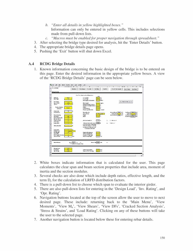
�
150
b. “Enter all details in yellow highlighted boxes.” Information can only be entered in yellow cells. This includes selections made from pull-down lists.
c. “Macros must be enabled for proper navigation through spreadsheet.” 3. After selecting the bridge type desired for analysis, hit the ‘Enter Details’ button. 4. The appropriate bridge details page opens. 5. Pushing the ‘Exit’ button will shut down Excel.
A.4 RCDG Bridge Details 1. Known information concerning the basic design of the bridge is to be entered on
this page. Enter the desired information in the appropriate yellow boxes. A view of the ‘RCDG Bridge Details’ page can be seen below.
2. White boxes indicate information that is calculated for the user. This page calculates the clear span and beam section properties that include area, moment of inertia and the section modulus.
3. Several checks are also done which include depth ratios, effective length, and the term De for the calculation of LRFD distribution factors.
4. There is a pull-down list to choose which span to evaluate the interior girder. 5. There are also pull-down lists for entering in the ‘Design Load’, ‘Inv. Rating’, and
‘Opr. Rating’. 6. Navigation buttons located at the top of the screen allow the user to move to next
desired page. These include: returning back to the ‘Main Menu’, ‘View Moments’, ‘View Mn’, ‘View Shears’, ‘View DFs’, ‘Cracked Section Analysis’, ‘Stress & Strains’, and ‘Load Rating’. Clicking on any of these buttons will take the user to the selected page.
7. Another navigation button is located below these for entering rebar details.
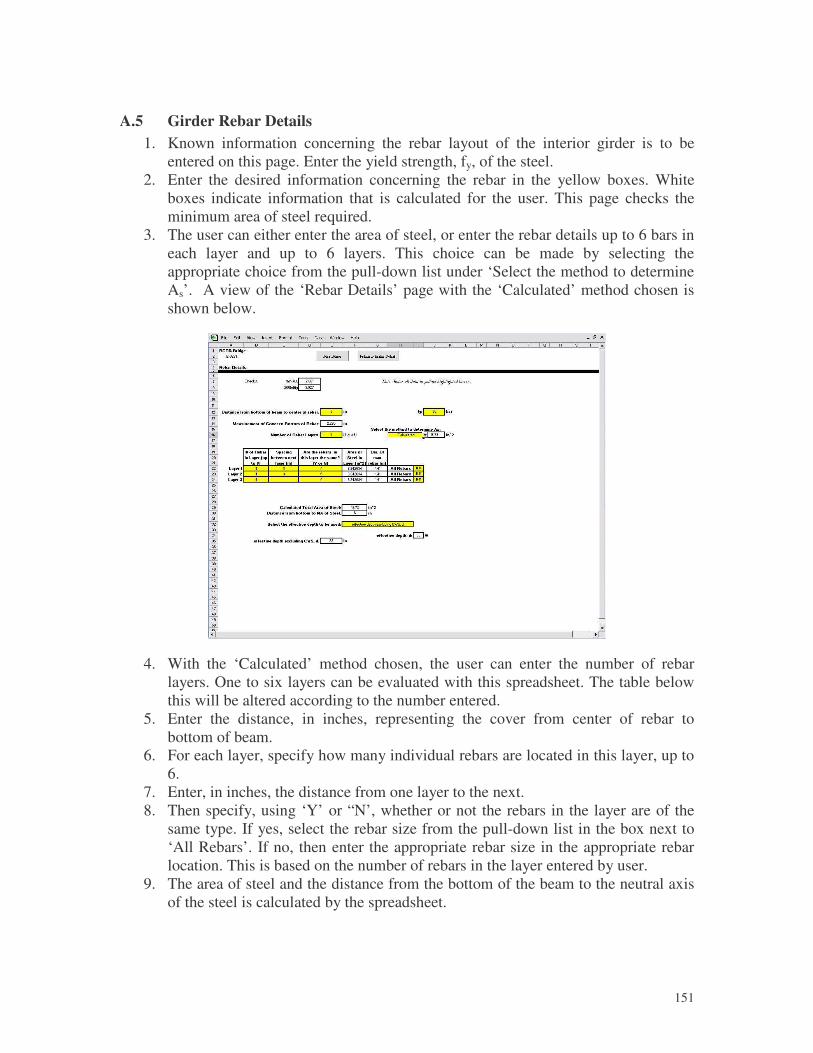
�
151
A.5 Girder Rebar Details 1. Known information concerning the rebar layout of the interior girder is to be
entered on this page. Enter the yield strength, fy, of the steel. 2. Enter the desired information concerning the rebar in the yellow boxes. White
boxes indicate information that is calculated for the user. This page checks the minimum area of steel required.
3. The user can either enter the area of steel, or enter the rebar details up to 6 bars in each layer and up to 6 layers. This choice can be made by selecting the appropriate choice from the pull-down list under ‘Select the method to determine As’. A view of the ‘Rebar Details’ page with the ‘Calculated’ method chosen is shown below.
4. With the ‘Calculated’ method chosen, the user can enter the number of rebar layers. One to six layers can be evaluated with this spreadsheet. The table below this will be altered according to the number entered.
5. Enter the distance, in inches, representing the cover from center of rebar to bottom of beam.
6. For each layer, specify how many individual rebars are located in this layer, up to 6.
7. Enter, in inches, the distance from one layer to the next. 8. Then specify, using ‘Y’ or “N’, whether or not the rebars in the layer are of the
same type. If yes, select the rebar size from the pull-down list in the box next to ‘All Rebars’. If no, then enter the appropriate rebar size in the appropriate rebar location. This is based on the number of rebars in the layer entered by user.
9. The area of steel and the distance from the bottom of the beam to the neutral axis of the steel is calculated by the spreadsheet.
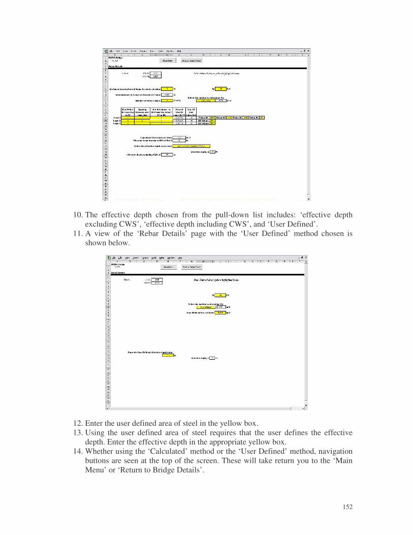
�
152
10. The effective depth chosen from the pull-down list includes: ‘effective depth excluding CWS’, ‘effective depth including CWS’, and ‘User Defined’.
11. A view of the ‘Rebar Details’ page with the ‘User Defined’ method chosen is shown below.
12. Enter the user defined area of steel in the yellow box. 13. Using the user defined area of steel requires that the user defines the effective
depth. Enter the effective depth in the appropriate yellow box. 14. Whether using the ‘Calculated’ method or the ‘User Defined’ method, navigation
buttons are seen at the top of the screen. These will take return you to the ‘Main Menu’ or ‘Return to Bridge Details’.
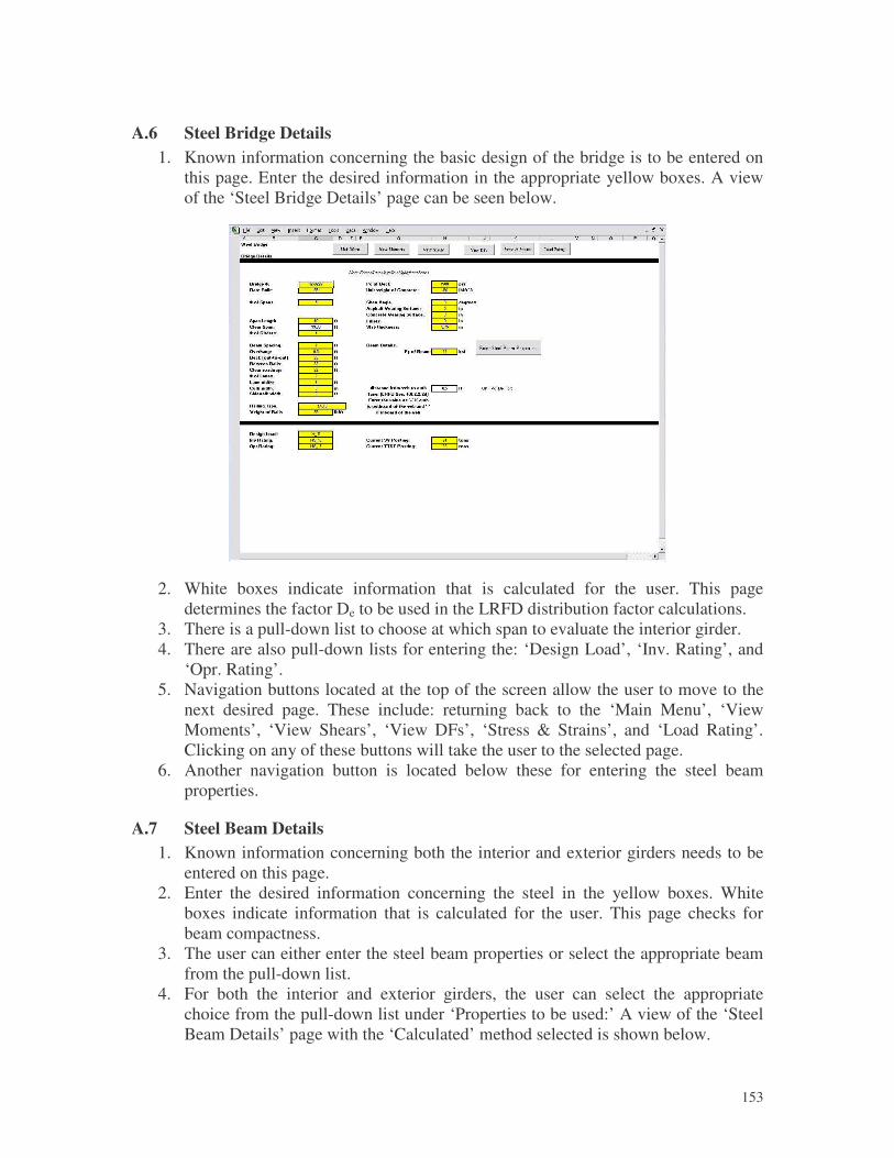
�
153
A.6 Steel Bridge Details 1. Known information concerning the basic design of the bridge is to be entered on
this page. Enter the desired information in the appropriate yellow boxes. A view of the ‘Steel Bridge Details’ page can be seen below.
2. White boxes indicate information that is calculated for the user. This page determines the factor De to be used in the LRFD distribution factor calculations.
3. There is a pull-down list to choose at which span to evaluate the interior girder. 4. There are also pull-down lists for entering the: ‘Design Load’, ‘Inv. Rating’, and
‘Opr. Rating’. 5. Navigation buttons located at the top of the screen allow the user to move to the
next desired page. These include: returning back to the ‘Main Menu’, ‘View Moments’, ‘View Shears’, ‘View DFs’, ‘Stress & Strains’, and ‘Load Rating’. Clicking on any of these buttons will take the user to the selected page.
6. Another navigation button is located below these for entering the steel beam properties.
A.7 Steel Beam Details 1. Known information concerning both the interior and exterior girders needs to be
entered on this page. 2. Enter the desired information concerning the steel in the yellow boxes. White
boxes indicate information that is calculated for the user. This page checks for beam compactness.
3. The user can either enter the steel beam properties or select the appropriate beam from the pull-down list.
4. For both the interior and exterior girders, the user can select the appropriate choice from the pull-down list under ‘Properties to be used:’ A view of the ‘Steel Beam Details’ page with the ‘Calculated’ method selected is shown below.
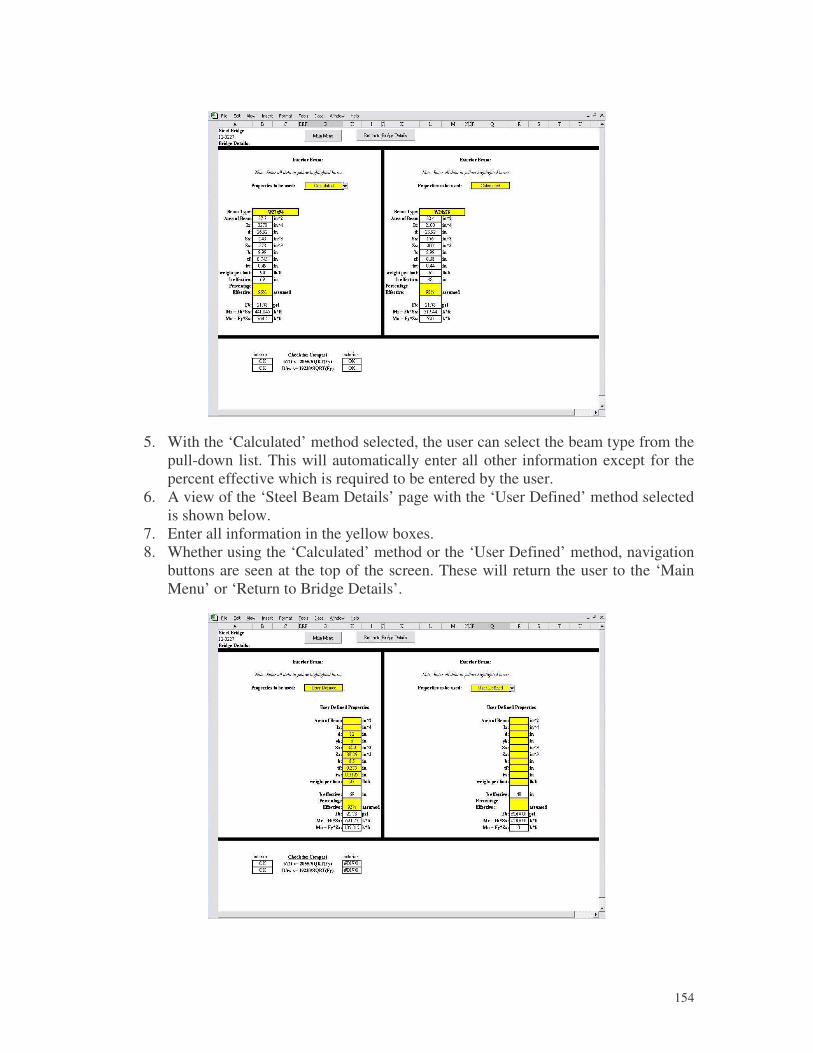
�
154
5. With the ‘Calculated’ method selected, the user can select the beam type from the pull-down list. This will automatically enter all other information except for the percent effective which is required to be entered by the user.
6. A view of the ‘Steel Beam Details’ page with the ‘User Defined’ method selected is shown below.
7. Enter all information in the yellow boxes. 8. Whether using the ‘Calculated’ method or the ‘User Defined’ method, navigation
buttons are seen at the top of the screen. These will return the user to the ‘Main Menu’ or ‘Return to Bridge Details’.
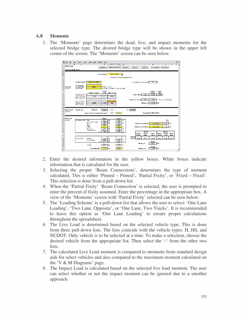
�
155
A.8 Moments 1. The ‘Moments’ page determines the dead, live, and impact moments for the
selected bridge type. The desired bridge type will be shown in the upper left corner of the screen. The ‘Moments’ screen can be seen below.
2. Enter the desired information in the yellow boxes. White boxes indicate information that is calculated for the user.
3. Selecting the proper ‘Beam Connections’, determines the type of moment calculated. This is either ‘Pinned – Pinned’, ‘Partial Fixity’, or ‘Fixed – Fixed’. This selection is done from a pull-down list.
4. When the ‘Partial Fixity’ ‘Beam Connection’ is selected, the user is prompted to enter the percent of fixity assumed. Enter the percentage in the appropriate box. A view of the ‘Moments’ screen with ‘Partial Fixity’ selected can be seen below.
5. The ‘Loading Scheme’ is a pull-down list that allows the user to select: ‘One Lane Loading’, ‘Two Lane, Opposite’, or ‘One Lane, Two Trucks’. It is recommended to leave this option as ‘One Lane Loading’ to ensure proper calculations throughout the spreadsheet.
6. The Live Load is determined based on the selected vehicle type. This is done from three pull-down lists. The lists coincide with the vehicle types: H, HS, and NCDOT. Only vehicle is to be selected at a time. To make a selection, choose the desired vehicle from the appropriate list. Then select the ‘-‘ from the other two lists.
7. The calculated Live Load moment is compared to moments from standard design aids for select vehicles and also compared to the maximum moment calculated on the ‘V & M Diagrams’ page.
8. The Impact Load is calculated based on the selected live load moment. The user can select whether or not the impact moment can be ignored due to a smother approach.
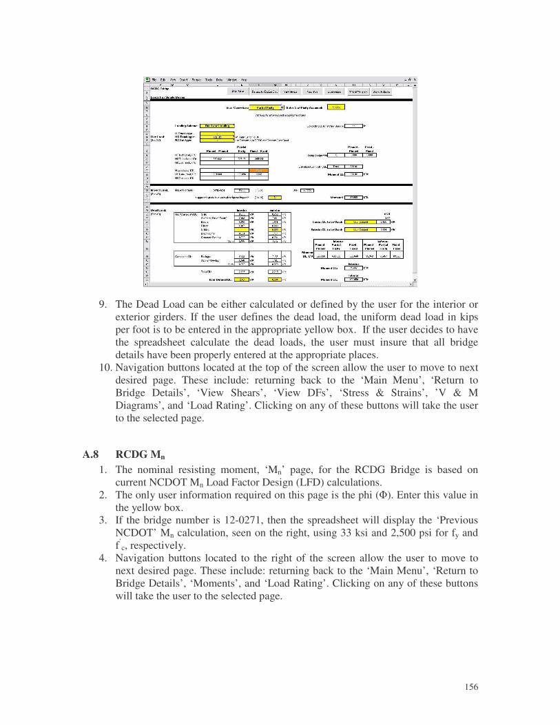
�
156
9. The Dead Load can be either calculated or defined by the user for the interior or
exterior girders. If the user defines the dead load, the uniform dead load in kips per foot is to be entered in the appropriate yellow box. If the user decides to have the spreadsheet calculate the dead loads, the user must insure that all bridge details have been properly entered at the appropriate places.
10. Navigation buttons located at the top of the screen allow the user to move to next desired page. These include: returning back to the ‘Main Menu’, ‘Return to Bridge Details’, ‘View Shears’, ‘View DFs’, ‘Stress & Strains’, ’V & M Diagrams’, and ‘Load Rating’. Clicking on any of these buttons will take the user to the selected page.
A.8 RCDG Mn 1. The nominal resisting moment, ‘Mn’ page, for the RCDG Bridge is based on
current NCDOT Mn Load Factor Design (LFD) calculations. 2. The only user information required on this page is the phi (�). Enter this value in
the yellow box. 3. If the bridge number is 12-0271, then the spreadsheet will display the ‘Previous
NCDOT’ Mn calculation, seen on the right, using 33 ksi and 2,500 psi for fy and f’
c, respectively. 4. Navigation buttons located to the right of the screen allow the user to move to
next desired page. These include: returning back to the ‘Main Menu’, ‘Return to Bridge Details’, ‘Moments’, and ‘Load Rating’. Clicking on any of these buttons will take the user to the selected page.
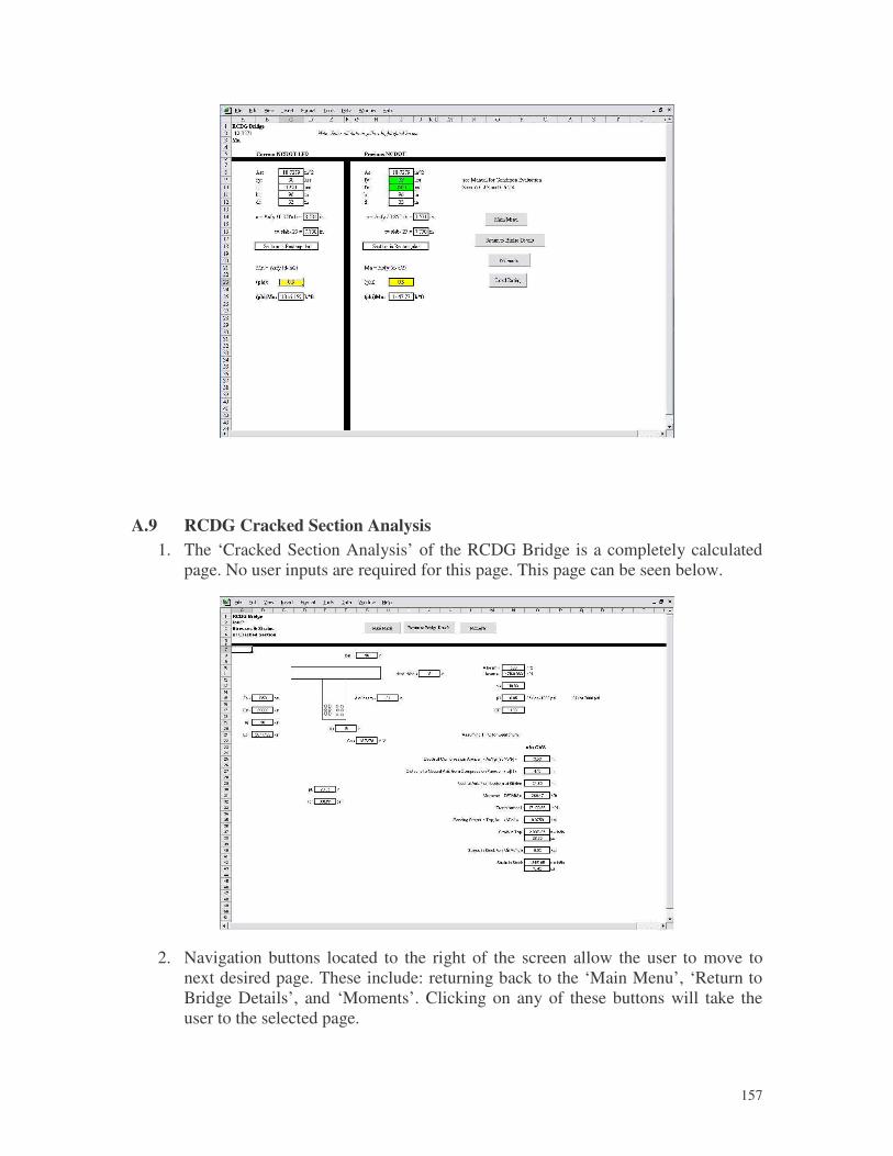
�
157
A.9 RCDG Cracked Section Analysis 1. The ‘Cracked Section Analysis’ of the RCDG Bridge is a completely calculated
page. No user inputs are required for this page. This page can be seen below.
2. Navigation buttons located to the right of the screen allow the user to move to
next desired page. These include: returning back to the ‘Main Menu’, ‘Return to Bridge Details’, and ‘Moments’. Clicking on any of these buttons will take the user to the selected page.
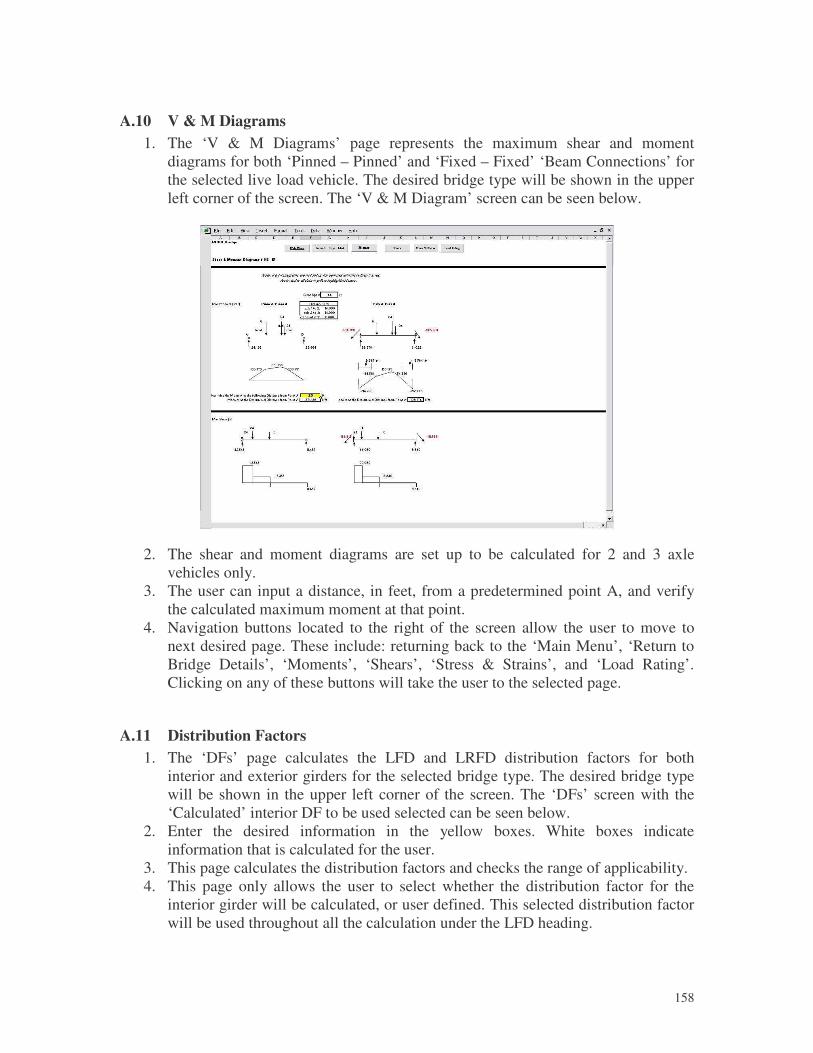
�
158
A.10 V & M Diagrams 1. The ‘V & M Diagrams’ page represents the maximum shear and moment
diagrams for both ‘Pinned – Pinned’ and ‘Fixed – Fixed’ ‘Beam Connections’ for the selected live load vehicle. The desired bridge type will be shown in the upper left corner of the screen. The ‘V & M Diagram’ screen can be seen below.
2. The shear and moment diagrams are set up to be calculated for 2 and 3 axle
vehicles only. 3. The user can input a distance, in feet, from a predetermined point A, and verify
the calculated maximum moment at that point. 4. Navigation buttons located to the right of the screen allow the user to move to
next desired page. These include: returning back to the ‘Main Menu’, ‘Return to Bridge Details’, ‘Moments’, ‘Shears’, ‘Stress & Strains’, and ‘Load Rating’. Clicking on any of these buttons will take the user to the selected page.
A.11 Distribution Factors 1. The ‘DFs’ page calculates the LFD and LRFD distribution factors for both
interior and exterior girders for the selected bridge type. The desired bridge type will be shown in the upper left corner of the screen. The ‘DFs’ screen with the ‘Calculated’ interior DF to be used selected can be seen below.
2. Enter the desired information in the yellow boxes. White boxes indicate information that is calculated for the user.
3. This page calculates the distribution factors and checks the range of applicability. 4. This page only allows the user to select whether the distribution factor for the
interior girder will be calculated, or user defined. This selected distribution factor will be used throughout all the calculation under the LFD heading.
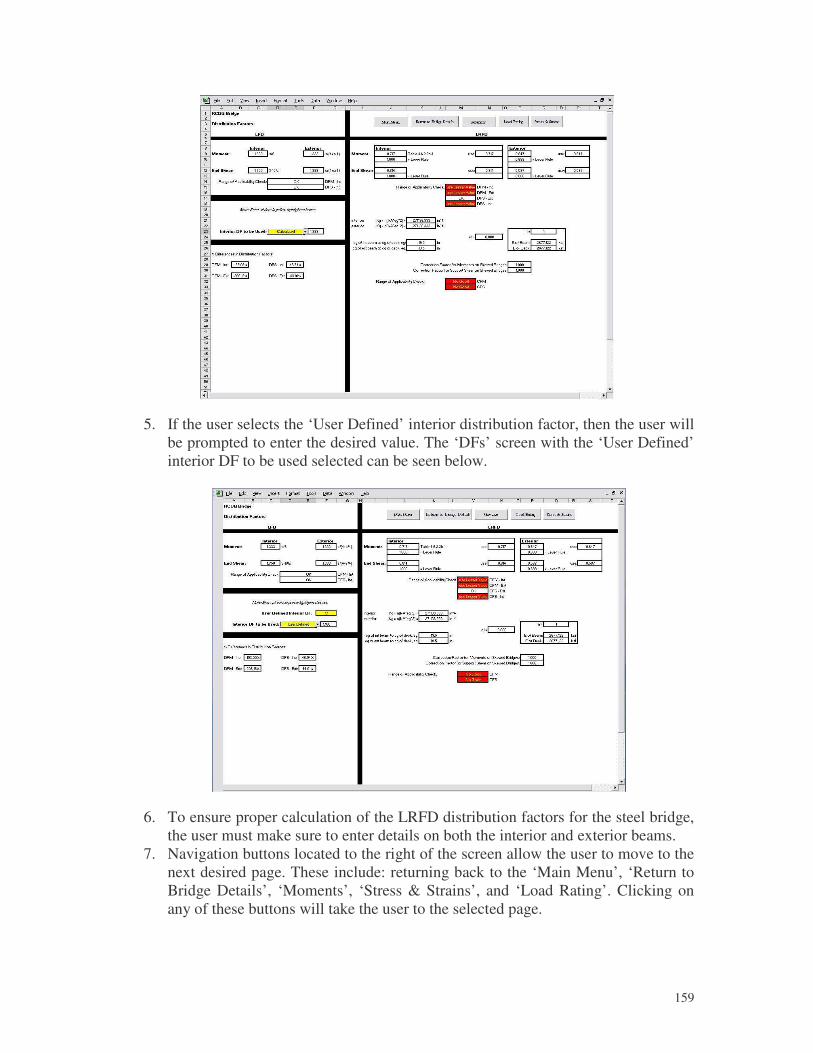
�
159
5. If the user selects the ‘User Defined’ interior distribution factor, then the user will be prompted to enter the desired value. The ‘DFs’ screen with the ‘User Defined’ interior DF to be used selected can be seen below.
6. To ensure proper calculation of the LRFD distribution factors for the steel bridge,
the user must make sure to enter details on both the interior and exterior beams. 7. Navigation buttons located to the right of the screen allow the user to move to the
next desired page. These include: returning back to the ‘Main Menu’, ‘Return to Bridge Details’, ‘Moments’, ‘Stress & Strains’, and ‘Load Rating’. Clicking on any of these buttons will take the user to the selected page.
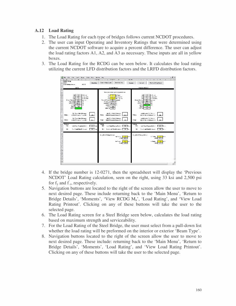
�
160
A.12 Load Rating 1. The Load Rating for each type of bridges follows current NCDOT procedures. 2. The user can input Operating and Inventory Ratings that were determined using
the current NCDOT software to acquire a percent difference. The user can adjust the load rating factors A1, A2, and A3 as necessary. These inputs are all in yellow boxes.
3. The Load Rating for the RCDG can be seen below. It calculates the load rating utilizing the current LFD distribution factors and the LRFD distribution factors.
4. If the bridge number is 12-0271, then the spreadsheet will display the ‘Previous
NCDOT’ Load Rating calculation, seen on the right, using 33 ksi and 2,500 psi for fy and f’
c, respectively. 5. Navigation buttons are located to the right of the screen allow the user to move to
next desired page. These include returning back to the ‘Main Menu’, ‘Return to Bridge Details’, ‘Moments’, ‘View RCDG Mn’, ‘Load Rating’, and ‘View Load Rating Printout’. Clicking on any of these buttons will take the user to the selected page.
6. The Load Rating screen for a Steel Bridge seen below, calculates the load rating based on maximum strength and serviceability.
7. For the Load Rating of the Steel Bridge, the user must select from a pull-down list whether the load rating will be preformed on the interior or exterior ‘Beam Type’.
8. Navigation buttons located to the right of the screen allow the user to move to next desired page. These include: returning back to the ‘Main Menu’, ‘Return to Bridge Details’, ‘Moments’, ‘Load Rating’, and ‘View Load Rating Printout’. Clicking on any of these buttons will take the user to the selected page.
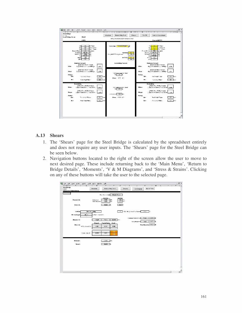
�
161
A.13 Shears 1. The ‘Shears’ page for the Steel Bridge is calculated by the spreadsheet entirely
and does not require any user inputs. The ‘Shears’ page for the Steel Bridge can be seen below.
2. Navigation buttons located to the right of the screen allow the user to move to next desired page. These include returning back to the ‘Main Menu’, ‘Return to Bridge Details’, ‘Moments’, ‘V & M Diagrams’, and ‘Stress & Strains’. Clicking on any of these buttons will take the user to the selected page.
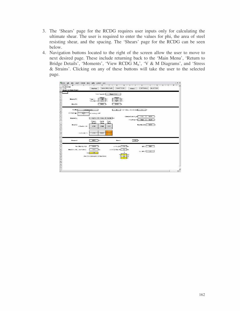
�
162
3. The ‘Shears’ page for the RCDG requires user inputs only for calculating the ultimate shear. The user is required to enter the values for phi, the area of steel resisting shear, and the spacing. The ‘Shears’ page for the RCDG can be seen below.
4. Navigation buttons located to the right of the screen allow the user to move to next desired page. These include returning back to the ‘Main Menu’, ‘Return to Bridge Details’, ‘Moments’, ‘View RCDG Mn’, ‘V & M Diagrams’, and ‘Stress & Strains’. Clicking on any of these buttons will take the user to the selected page.
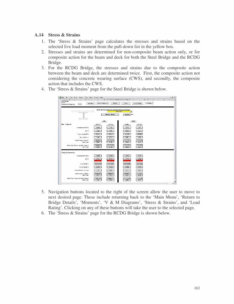
�
163
A.14 Stress & Strains 1. The ‘Stress & Strains’ page calculates the stresses and strains based on the
selected live load moment from the pull-down list in the yellow box. 2. Stresses and strains are determined for non-composite beam action only, or for
composite action for the beam and deck for both the Steel Bridge and the RCDG Bridge.
3. For the RCDG Bridge, the stresses and strains due to the composite action between the beam and deck are determined twice. First, the composite action not considering the concrete wearing surface (CWS), and secondly, the composite action that includes the CWS.
4. The ‘Stress & Strains’ page for the Steel Bridge is shown below.
5. Navigation buttons located to the right of the screen allow the user to move to next desired page. These include returning back to the ‘Main Menu’, ‘Return to Bridge Details’, ‘Moments’, ‘V & M Diagrams’, ‘Stress & Strains’, and ‘Load Rating’. Clicking on any of these buttons will take the user to the selected page.
6. The ‘Stress & Strains’ page for the RCDG Bridge is shown below.
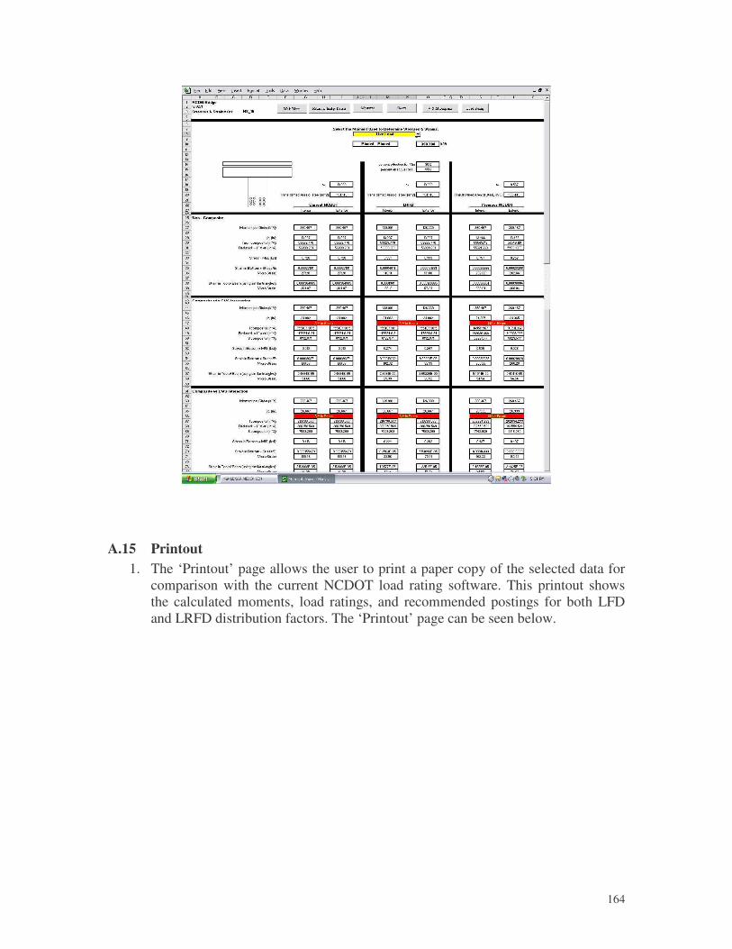
�
164
A.15 Printout 1. The ‘Printout’ page allows the user to print a paper copy of the selected data for
comparison with the current NCDOT load rating software. This printout shows the calculated moments, load ratings, and recommended postings for both LFD and LRFD distribution factors. The ‘Printout’ page can be seen below.
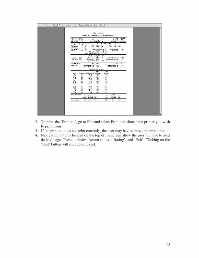
�
165
2. To print the ‘Printout’, go to File and select Print and choose the printer you wish to print from.
3. If the printout does not print correctly, the user may have to reset the print area. 4. Navigation buttons located on the top of the screen allow the user to move to next
desired page. These include: ‘Return to Load Rating’, and ‘Exit’. Clicking on the ‘Exit’ button will shut down Excel.
�
166
APPENDIX B
GFRP DECK BRIDGE CONSTRUCTION REPORT
B.1 Executive Summary
The 20th century brought about many innovative changes to the world of construction. While concrete and steel tend to be the materials of choice, technology has introduced a material, which may become the material of choice for future designs. This material is Fiber Reinforced Polymer (FRP). Composites being both light and strong, are being introduced to many applications, including bridge construction.
In an effort to speed construction and increase service life of a bridge, the North Carolina Department of Transportation (NCDOT) looked to composites. A deteriorating bridge in Union County presented the opportunity to test this new concept in bridge construction. Bridge #89-022 over Mill Creek on New Salem Road (SR1627) needed to be removed and rebuilt, so it was chosen to receive the first composite deck in the State of North Carolina. Martin Marietta Composites division, producer of the FRP DuraSpanTM system, was contracted to produce the panels required for the bridge replacement.
The construction of this bridge was funded in large part through a discretionary grant from the FHWA through the Innovative Bridge Research and Construction Program. Evaluation of this structure continues as a part of the NCDOT Research Project 2002-12 entitled “Evaluation of Bridge Analysis vis-à-vis Performance”. The results of this evaluation will therefore be contained in the final report for this research to be concluded in the summer of 2003.
First, the existing structure was removed, and the new steel girders were installed. Then, angles were welded to the girders to support the panel and to provide room for grout injection. After the angles were welded in place, the panels were placed in accordance with the Martin Marietta Installation Guide by NCDOT personnel, and under the supervision of Martin Marietta representatives. After the deck panels were placed, a combination of shear studs and grout were used to permanently attach the panels to the girders. Once this attachment was made, the rebar and forms for the endwalls were placed, and the concrete was poured. The asphalt overlay was then placed followed by the guardrail. The last item on the agenda was the load testing of the bridge. Once testing was completed, the bridge was opened to traffic.
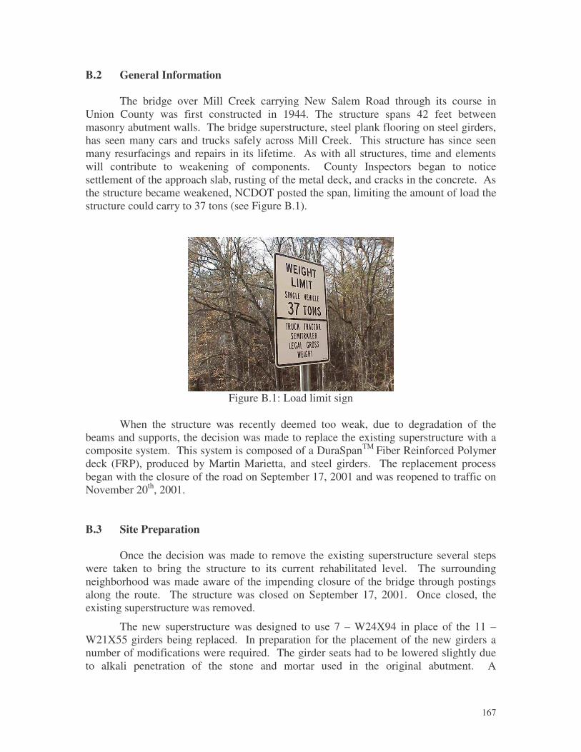
�
167
B.2 General Information
The bridge over Mill Creek carrying New Salem Road through its course in Union County was first constructed in 1944. The structure spans 42 feet between masonry abutment walls. The bridge superstructure, steel plank flooring on steel girders, has seen many cars and trucks safely across Mill Creek. This structure has since seen many resurfacings and repairs in its lifetime. As with all structures, time and elements will contribute to weakening of components. County Inspectors began to notice settlement of the approach slab, rusting of the metal deck, and cracks in the concrete. As the structure became weakened, NCDOT posted the span, limiting the amount of load the structure could carry to 37 tons (see Figure B.1).
Figure B.1: Load limit sign
When the structure was recently deemed too weak, due to degradation of the
beams and supports, the decision was made to replace the existing superstructure with a composite system. This system is composed of a DuraSpanTM Fiber Reinforced Polymer deck (FRP), produced by Martin Marietta, and steel girders. The replacement process began with the closure of the road on September 17, 2001 and was reopened to traffic on November 20th, 2001. B.3 Site Preparation
Once the decision was made to remove the existing superstructure several steps were taken to bring the structure to its current rehabilitated level. The surrounding neighborhood was made aware of the impending closure of the bridge through postings along the route. The structure was closed on September 17, 2001. Once closed, the existing superstructure was removed.
The new superstructure was designed to use 7 – W24X94 in place of the 11 – W21X55 girders being replaced. In preparation for the placement of the new girders a number of modifications were required. The girder seats had to be lowered slightly due to alkali penetration of the stone and mortar used in the original abutment. A
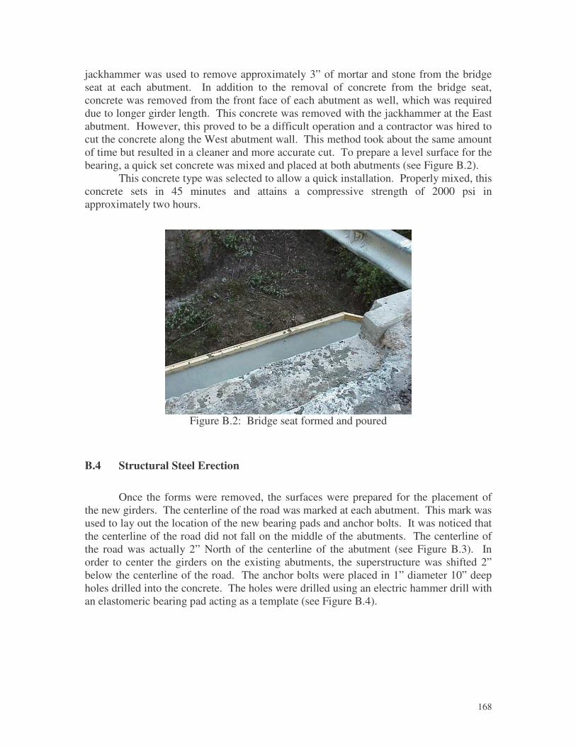
�
168
jackhammer was used to remove approximately 3” of mortar and stone from the bridge seat at each abutment. In addition to the removal of concrete from the bridge seat, concrete was removed from the front face of each abutment as well, which was required due to longer girder length. This concrete was removed with the jackhammer at the East abutment. However, this proved to be a difficult operation and a contractor was hired to cut the concrete along the West abutment wall. This method took about the same amount of time but resulted in a cleaner and more accurate cut. To prepare a level surface for the bearing, a quick set concrete was mixed and placed at both abutments (see Figure B.2).
This concrete type was selected to allow a quick installation. Properly mixed, this concrete sets in 45 minutes and attains a compressive strength of 2000 psi in approximately two hours.
Figure B.2: Bridge seat formed and poured
B.4 Structural Steel Erection
Once the forms were removed, the surfaces were prepared for the placement of
the new girders. The centerline of the road was marked at each abutment. This mark was used to lay out the location of the new bearing pads and anchor bolts. It was noticed that the centerline of the road did not fall on the middle of the abutments. The centerline of the road was actually 2” North of the centerline of the abutment (see Figure B.3). In order to center the girders on the existing abutments, the superstructure was shifted 2” below the centerline of the road. The anchor bolts were placed in 1” diameter 10” deep holes drilled into the concrete. The holes were drilled using an electric hammer drill with an elastomeric bearing pad acting as a template (see Figure B.4).
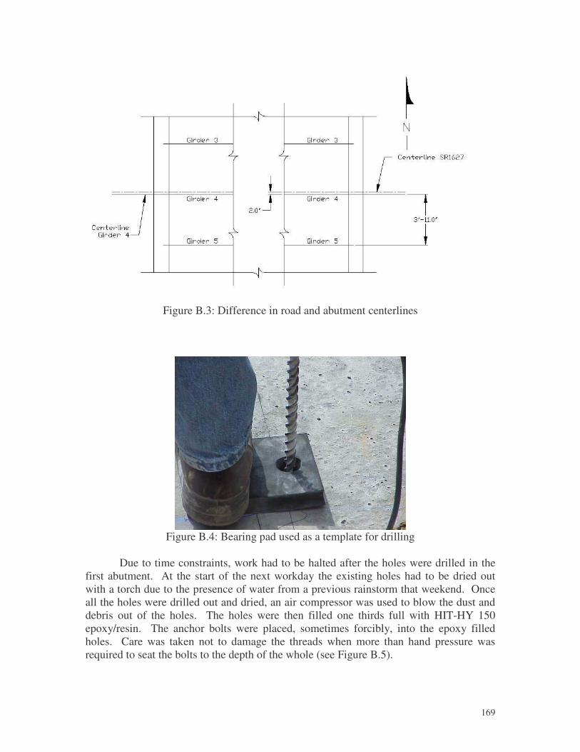
�
169
Figure B.3: Difference in road and abutment centerlines
Figure B.4: Bearing pad used as a template for drilling
Due to time constraints, work had to be halted after the holes were drilled in the
first abutment. At the start of the next workday the existing holes had to be dried out with a torch due to the presence of water from a previous rainstorm that weekend. Once all the holes were drilled out and dried, an air compressor was used to blow the dust and debris out of the holes. The holes were then filled one thirds full with HIT-HY 150 epoxy/resin. The anchor bolts were placed, sometimes forcibly, into the epoxy filled holes. Care was taken not to damage the threads when more than hand pressure was required to seat the bolts to the depth of the whole (see Figure B.5).
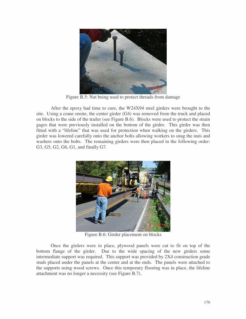
�
170
Figure B.5: Nut being used to protect threads from damage
After the epoxy had time to cure, the W24X94 steel girders were brought to the
site. Using a crane onsite, the center girder (G4) was removed from the truck and placed on blocks to the side of the trailer (see Figure B.6). Blocks were used to protect the strain gages that were previously installed on the bottom of the girder. This girder was then fitted with a “lifeline” that was used for protection when walking on the girders. This girder was lowered carefully onto the anchor bolts allowing workers to snug the nuts and washers onto the bolts. The remaining girders were then placed in the following order: G3, G5, G2, G6, G1, and finally G7.
Figure B.6: Girder placement on blocks
Once the girders were in place, plywood panels were cut to fit on top of the
bottom flange of the girder. Due to the wide spacing of the new girders some intermediate support was required. This support was provided by 2X4 construction grade studs placed under the panels at the center and at the ends. The panels were attached to the supports using wood screws. Once this temporary flooring was in place, the lifeline attachment was no longer a necessity (see Figure B.7).
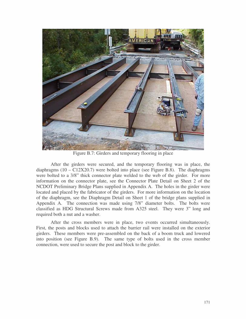
�
171
Figure B.7: Girders and temporary flooring in place
After the girders were secured, and the temporary flooring was in place, the
diaphragms (10 – C12X20.7) were bolted into place (see Figure B.8). The diaphragms were bolted to a 3/8” thick connector plate welded to the web of the girder. For more information on the connector plate, see the Connector Plate Detail on Sheet 2 of the NCDOT Preliminary Bridge Plans supplied in Appendix A. The holes in the girder were located and placed by the fabricator of the girders. For more information on the location of the diaphragm, see the Diaphragm Detail on Sheet 1 of the bridge plans supplied in Appendix A. The connection was made using 7/8” diameter bolts. The bolts were classified as HDG Structural Screws made from A325 steel. They were 3” long and required both a nut and a washer.
After the cross members were in place, two events occurred simultaneously. First, the posts and blocks used to attach the barrier rail were installed on the exterior girders. These members were pre-assembled on the back of a boom truck and lowered into position (see Figure B.9). The same type of bolts used in the cross member connection, were used to secure the post and block to the girder.

�
172
Figure B.8: Diaphragm bolted in place
Simultaneously, the angles (L2X2) used to separate the composite deck from the girder were installed. The angles were positioned so as to be level across the bridge transversely, and angled so as to follow the camber of the bridge along the longitudinal direction. The angles were welded to the girders top flange using a ¼” fillet weld placed every 12”. The next step in the process was the installation of the suspended scaffolding. This scaffolding was attached to the bottom flanges of two girders (G2 and G6). Once in place, this scaffold allowed access to the bottom of the bridge superstructure.
�
Figure B.9: Post and block assembly
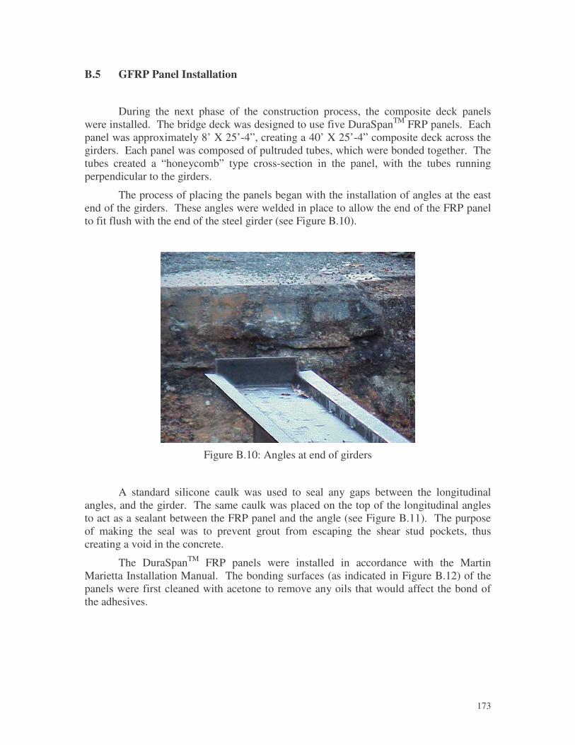
�
173
B.5 GFRP Panel Installation
During the next phase of the construction process, the composite deck panels were installed. The bridge deck was designed to use five DuraSpanTM FRP panels. Each panel was approximately 8’ X 25’-4”, creating a 40’ X 25’-4” composite deck across the girders. Each panel was composed of pultruded tubes, which were bonded together. The tubes created a “honeycomb” type cross-section in the panel, with the tubes running perpendicular to the girders.
The process of placing the panels began with the installation of angles at the east end of the girders. These angles were welded in place to allow the end of the FRP panel to fit flush with the end of the steel girder (see Figure B.10).
Figure B.10: Angles at end of girders
A standard silicone caulk was used to seal any gaps between the longitudinal angles, and the girder. The same caulk was placed on the top of the longitudinal angles to act as a sealant between the FRP panel and the angle (see Figure B.11). The purpose of making the seal was to prevent grout from escaping the shear stud pockets, thus creating a void in the concrete.
The DuraSpanTM FRP panels were installed in accordance with the Martin Marietta Installation Manual. The bonding surfaces (as indicated in Figure B.12) of the panels were first cleaned with acetone to remove any oils that would affect the bond of the adhesives.
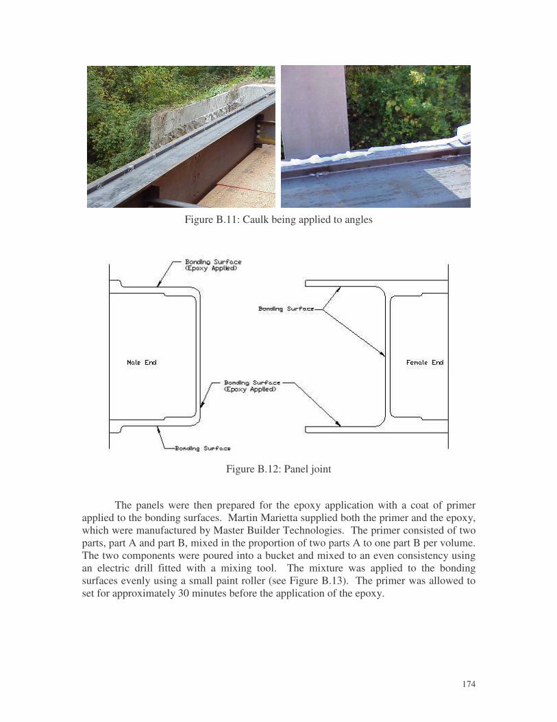
�
174
Figure B.11: Caulk being applied to angles
Figure B.12: Panel joint
The panels were then prepared for the epoxy application with a coat of primer applied to the bonding surfaces. Martin Marietta supplied both the primer and the epoxy, which were manufactured by Master Builder Technologies. The primer consisted of two parts, part A and part B, mixed in the proportion of two parts A to one part B per volume. The two components were poured into a bucket and mixed to an even consistency using an electric drill fitted with a mixing tool. The mixture was applied to the bonding surfaces evenly using a small paint roller (see Figure B.13). The primer was allowed to set for approximately 30 minutes before the application of the epoxy.
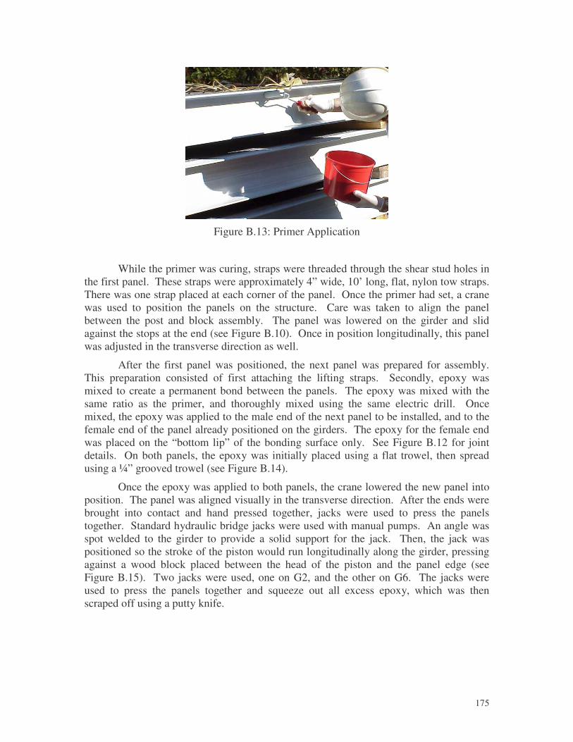
�
175
Figure B.13: Primer Application
While the primer was curing, straps were threaded through the shear stud holes in the first panel. These straps were approximately 4” wide, 10’ long, flat, nylon tow straps. There was one strap placed at each corner of the panel. Once the primer had set, a crane was used to position the panels on the structure. Care was taken to align the panel between the post and block assembly. The panel was lowered on the girder and slid against the stops at the end (see Figure B.10). Once in position longitudinally, this panel was adjusted in the transverse direction as well.
After the first panel was positioned, the next panel was prepared for assembly. This preparation consisted of first attaching the lifting straps. Secondly, epoxy was mixed to create a permanent bond between the panels. The epoxy was mixed with the same ratio as the primer, and thoroughly mixed using the same electric drill. Once mixed, the epoxy was applied to the male end of the next panel to be installed, and to the female end of the panel already positioned on the girders. The epoxy for the female end was placed on the “bottom lip” of the bonding surface only. See Figure B.12 for joint details. On both panels, the epoxy was initially placed using a flat trowel, then spread using a ¼” grooved trowel (see Figure B.14).
Once the epoxy was applied to both panels, the crane lowered the new panel into position. The panel was aligned visually in the transverse direction. After the ends were brought into contact and hand pressed together, jacks were used to press the panels together. Standard hydraulic bridge jacks were used with manual pumps. An angle was spot welded to the girder to provide a solid support for the jack. Then, the jack was positioned so the stroke of the piston would run longitudinally along the girder, pressing against a wood block placed between the head of the piston and the panel edge (see Figure B.15). Two jacks were used, one on G2, and the other on G6. The jacks were used to press the panels together and squeeze out all excess epoxy, which was then scraped off using a putty knife.
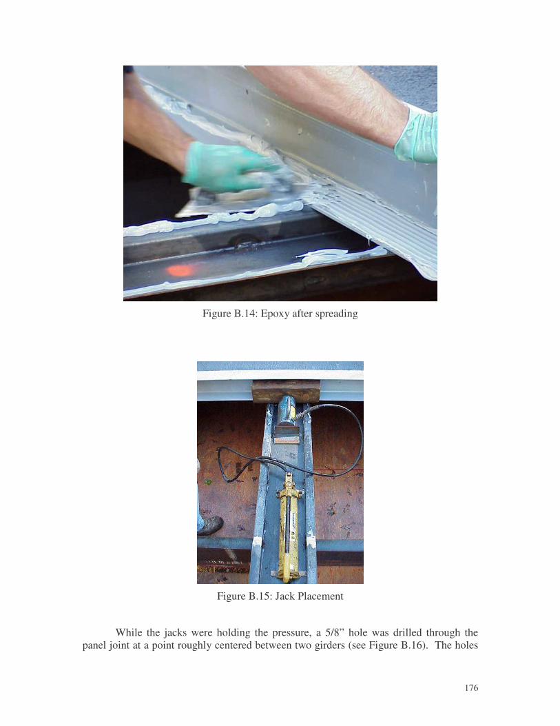
�
176
Figure B.14: Epoxy after spreading
Figure B.15: Jack Placement
While the jacks were holding the pressure, a 5/8” hole was drilled through the panel joint at a point roughly centered between two girders (see Figure B.16). The holes

�
177
were drilled between girders G1 & G2, and between G6 & G7. Then, an epoxy coated composite dowel was driven into the hole to secure the two FRP panels while the adhesive cured (see Figure B.16).
Figure B.16: Dowel Placement
Once the dowels were in place, the jacks were released and the temporary angle braces removed. This process of epoxy application, panel placement, jacking, drilling and doweling was repeated for all the remaining panels. The jacking of the last panel required some modification. The last panel covered the ends of the girders, so the jack brace could not be welded to them. A brace was made from scrap wood on-site to transfer the jacking force to the approach pavement (see Figure B.17).
Figure B.17: Jack Placement at End Panel
After being allowed to set and cure overnight, the panel joints were prepared for the joint tape. This preparation consisted of grinding away any excess epoxy that expanded out of the joint during the curing process. Once this was done, acetone was used to clean the top surface of the joints of any oils that would interfere with the bonding of the tape to the deck surface.
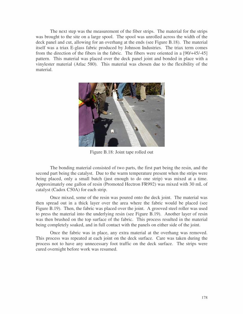
�
178
The next step was the measurement of the fiber strips. The material for the strips was brought to the site on a large spool. The spool was unrolled across the width of the deck panel and cut, allowing for an overhang at the ends (see Figure B.18). The material itself was a triax E-glass fabric produced by Johnson Industries. The triax term comes from the direction of the fibers in the fabric. The fibers were oriented in a [90/+45/-45] pattern. This material was placed over the deck panel joint and bonded in place with a vinylester material (Atlac 580). This material was chosen due to the flexibility of the material.
Figure B.18: Joint tape rolled out
The bonding material consisted of two parts, the first part being the resin, and the second part being the catalyst. Due to the warm temperature present when the strips were being placed, only a small batch (just enough to do one strip) was mixed at a time. Approximately one gallon of resin (Promoted Hectron FR992) was mixed with 30 mL of catalyst (Cadox C50A) for each strip.
Once mixed, some of the resin was poured onto the deck joint. The material was then spread out in a thick layer over the area where the fabric would be placed (see Figure B.19). Then, the fabric was placed over the joint. A grooved steel roller was used to press the material into the underlying resin (see Figure B.19). Another layer of resin was then brushed on the top surface of the fabric. This process resulted in the material being completely soaked, and in full contact with the panels on either side of the joint.
Once the fabric was in place, any extra material at the overhang was removed. This process was repeated at each joint on the deck surface. Care was taken during the process not to have any unnecessary foot traffic on the deck surface. The strips were cured overnight before work was resumed.
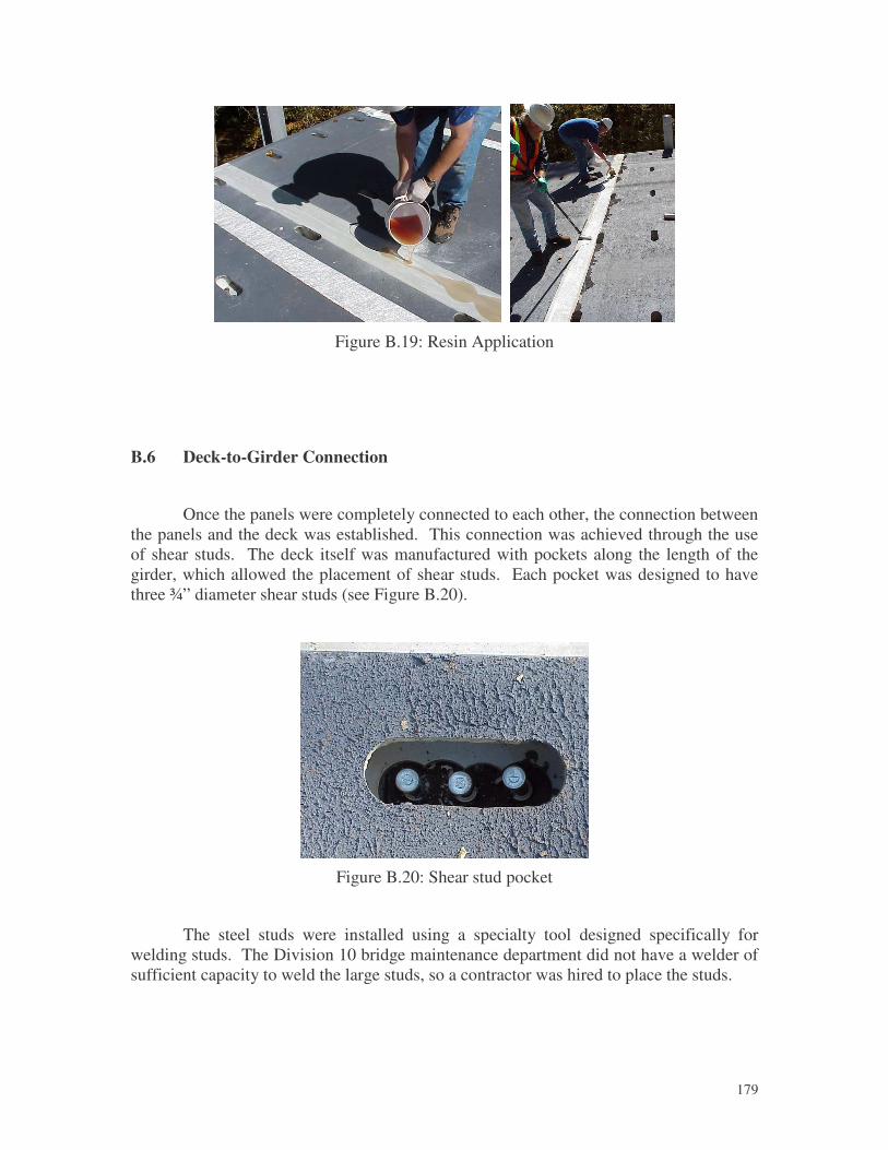
�
179
Figure B.19: Resin Application
B.6 Deck-to-Girder Connection
Once the panels were completely connected to each other, the connection between the panels and the deck was established. This connection was achieved through the use of shear studs. The deck itself was manufactured with pockets along the length of the girder, which allowed the placement of shear studs. Each pocket was designed to have three ¾” diameter shear studs (see Figure B.20).
Figure B.20: Shear stud pocket
The steel studs were installed using a specialty tool designed specifically for welding studs. The Division 10 bridge maintenance department did not have a welder of sufficient capacity to weld the large studs, so a contractor was hired to place the studs.
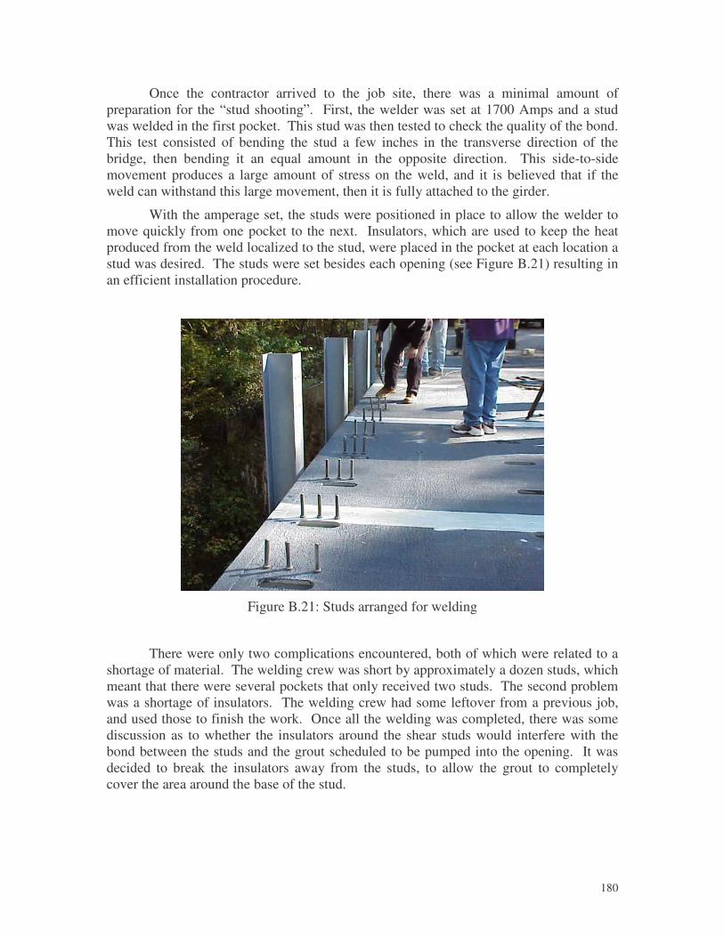
�
180
Once the contractor arrived to the job site, there was a minimal amount of preparation for the “stud shooting”. First, the welder was set at 1700 Amps and a stud was welded in the first pocket. This stud was then tested to check the quality of the bond. This test consisted of bending the stud a few inches in the transverse direction of the bridge, then bending it an equal amount in the opposite direction. This side-to-side movement produces a large amount of stress on the weld, and it is believed that if the weld can withstand this large movement, then it is fully attached to the girder.
With the amperage set, the studs were positioned in place to allow the welder to move quickly from one pocket to the next. Insulators, which are used to keep the heat produced from the weld localized to the stud, were placed in the pocket at each location a stud was desired. The studs were set besides each opening (see Figure B.21) resulting in an efficient installation procedure.
Figure B.21: Studs arranged for welding
There were only two complications encountered, both of which were related to a shortage of material. The welding crew was short by approximately a dozen studs, which meant that there were several pockets that only received two studs. The second problem was a shortage of insulators. The welding crew had some leftover from a previous job, and used those to finish the work. Once all the welding was completed, there was some discussion as to whether the insulators around the shear studs would interfere with the bond between the studs and the grout scheduled to be pumped into the opening. It was decided to break the insulators away from the studs, to allow the grout to completely cover the area around the base of the stud.
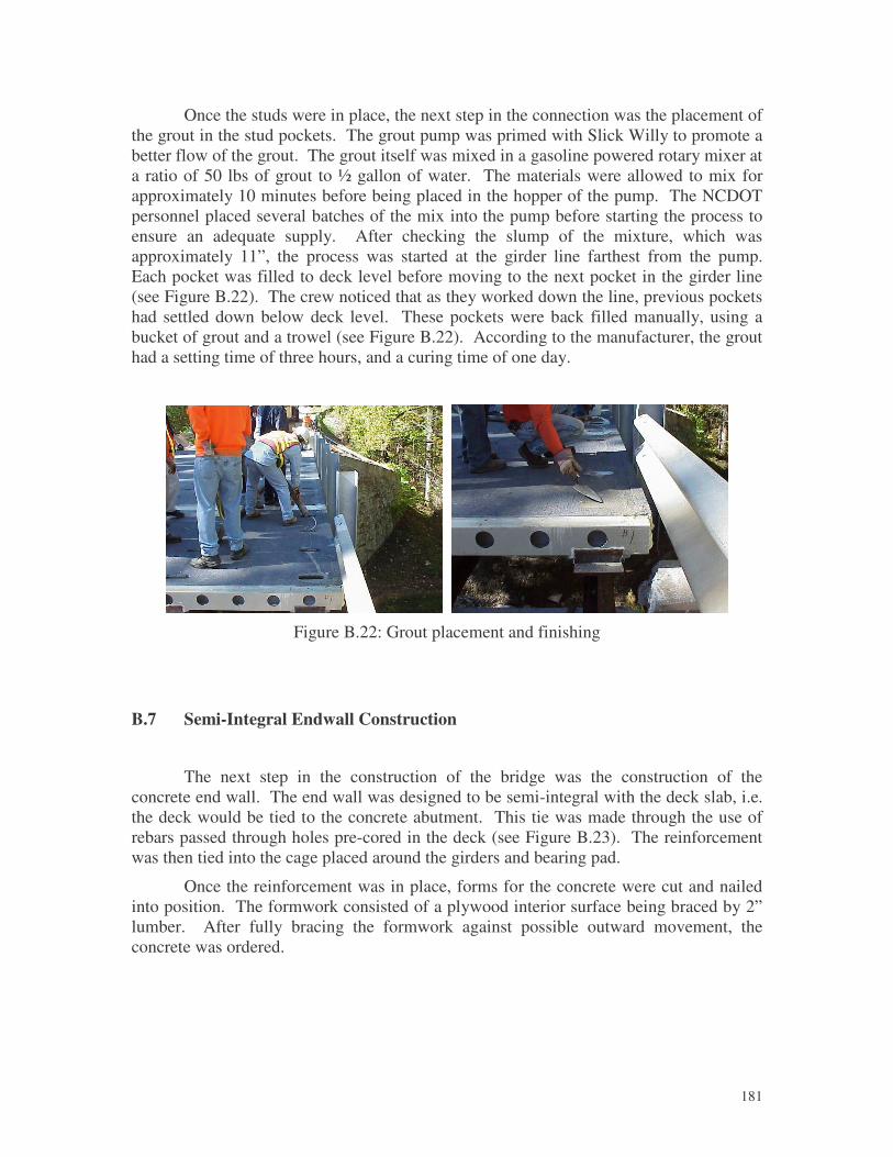
�
181
Once the studs were in place, the next step in the connection was the placement of the grout in the stud pockets. The grout pump was primed with Slick Willy to promote a better flow of the grout. The grout itself was mixed in a gasoline powered rotary mixer at a ratio of 50 lbs of grout to ½ gallon of water. The materials were allowed to mix for approximately 10 minutes before being placed in the hopper of the pump. The NCDOT personnel placed several batches of the mix into the pump before starting the process to ensure an adequate supply. After checking the slump of the mixture, which was approximately 11”, the process was started at the girder line farthest from the pump. Each pocket was filled to deck level before moving to the next pocket in the girder line (see Figure B.22). The crew noticed that as they worked down the line, previous pockets had settled down below deck level. These pockets were back filled manually, using a bucket of grout and a trowel (see Figure B.22). According to the manufacturer, the grout had a setting time of three hours, and a curing time of one day.
Figure B.22: Grout placement and finishing
B.7 Semi-Integral Endwall Construction
The next step in the construction of the bridge was the construction of the concrete end wall. The end wall was designed to be semi-integral with the deck slab, i.e. the deck would be tied to the concrete abutment. This tie was made through the use of rebars passed through holes pre-cored in the deck (see Figure B.23). The reinforcement was then tied into the cage placed around the girders and bearing pad.
Once the reinforcement was in place, forms for the concrete were cut and nailed into position. The formwork consisted of a plywood interior surface being braced by 2” lumber. After fully bracing the formwork against possible outward movement, the concrete was ordered.
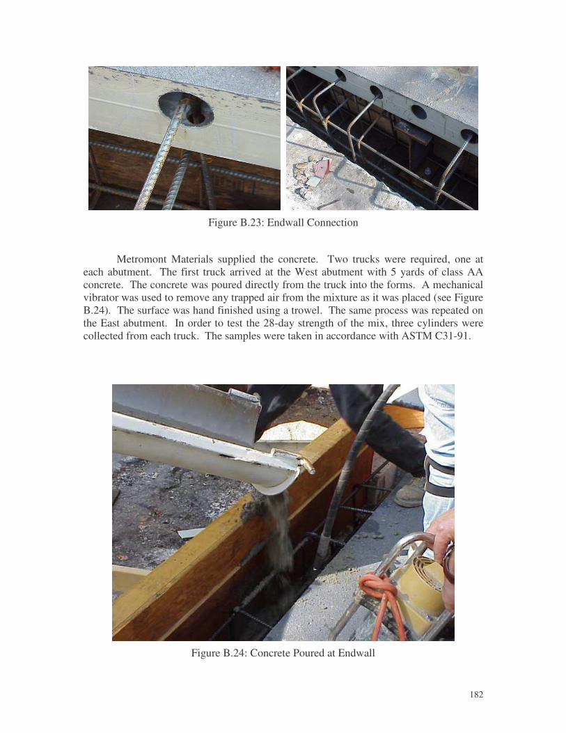
�
182
Figure B.23: Endwall Connection
Metromont Materials supplied the concrete. Two trucks were required, one at each abutment. The first truck arrived at the West abutment with 5 yards of class AA concrete. The concrete was poured directly from the truck into the forms. A mechanical vibrator was used to remove any trapped air from the mixture as it was placed (see Figure B.24). The surface was hand finished using a trowel. The same process was repeated on the East abutment. In order to test the 28-day strength of the mix, three cylinders were collected from each truck. The samples were taken in accordance with ASTM C31-91.
Figure B.24: Concrete Poured at Endwall
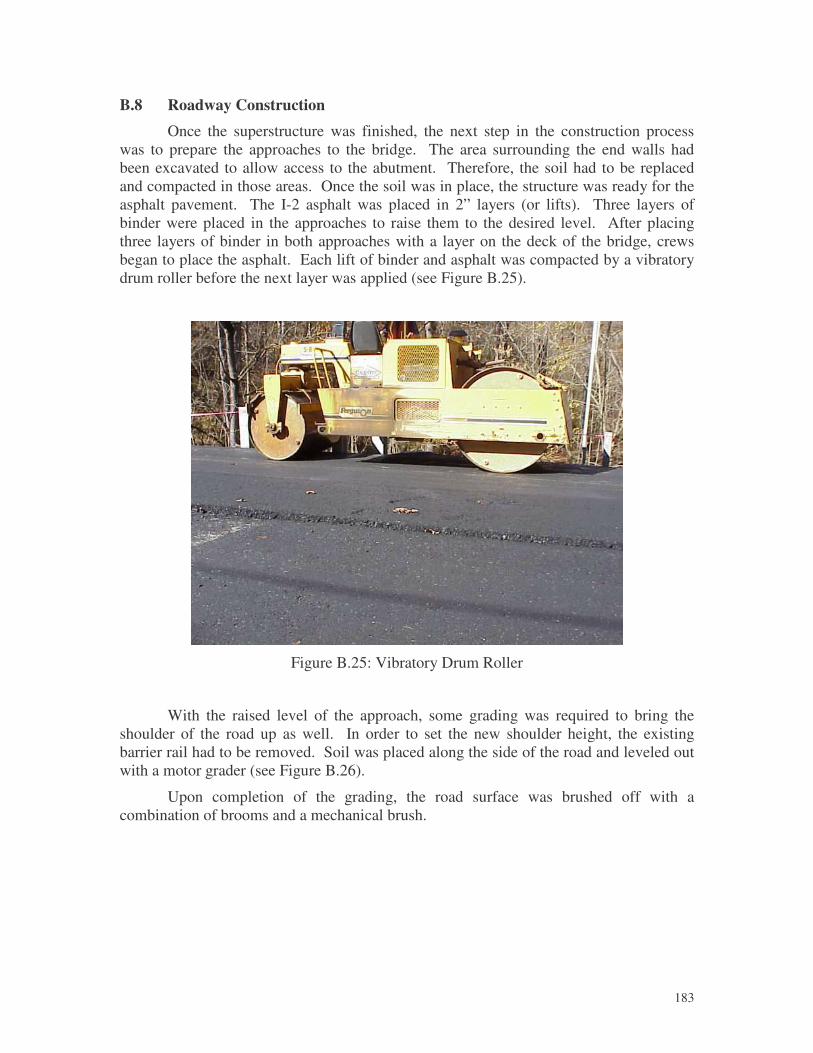
�
183
B.8 Roadway Construction
Once the superstructure was finished, the next step in the construction process was to prepare the approaches to the bridge. The area surrounding the end walls had been excavated to allow access to the abutment. Therefore, the soil had to be replaced and compacted in those areas. Once the soil was in place, the structure was ready for the asphalt pavement. The I-2 asphalt was placed in 2” layers (or lifts). Three layers of binder were placed in the approaches to raise them to the desired level. After placing three layers of binder in both approaches with a layer on the deck of the bridge, crews began to place the asphalt. Each lift of binder and asphalt was compacted by a vibratory drum roller before the next layer was applied (see Figure B.25).
Figure B.25: Vibratory Drum Roller
With the raised level of the approach, some grading was required to bring the shoulder of the road up as well. In order to set the new shoulder height, the existing barrier rail had to be removed. Soil was placed along the side of the road and leveled out with a motor grader (see Figure B.26).
Upon completion of the grading, the road surface was brushed off with a combination of brooms and a mechanical brush.
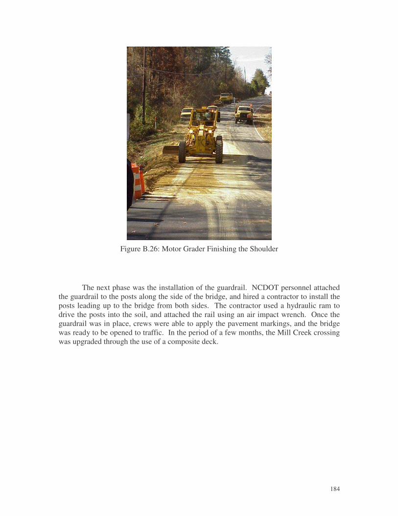
�
184
Figure B.26: Motor Grader Finishing the Shoulder
The next phase was the installation of the guardrail. NCDOT personnel attached the guardrail to the posts along the side of the bridge, and hired a contractor to install the posts leading up to the bridge from both sides. The contractor used a hydraulic ram to drive the posts into the soil, and attached the rail using an air impact wrench. Once the guardrail was in place, crews were able to apply the pavement markings, and the bridge was ready to be opened to traffic. In the period of a few months, the Mill Creek crossing was upgraded through the use of a composite deck.
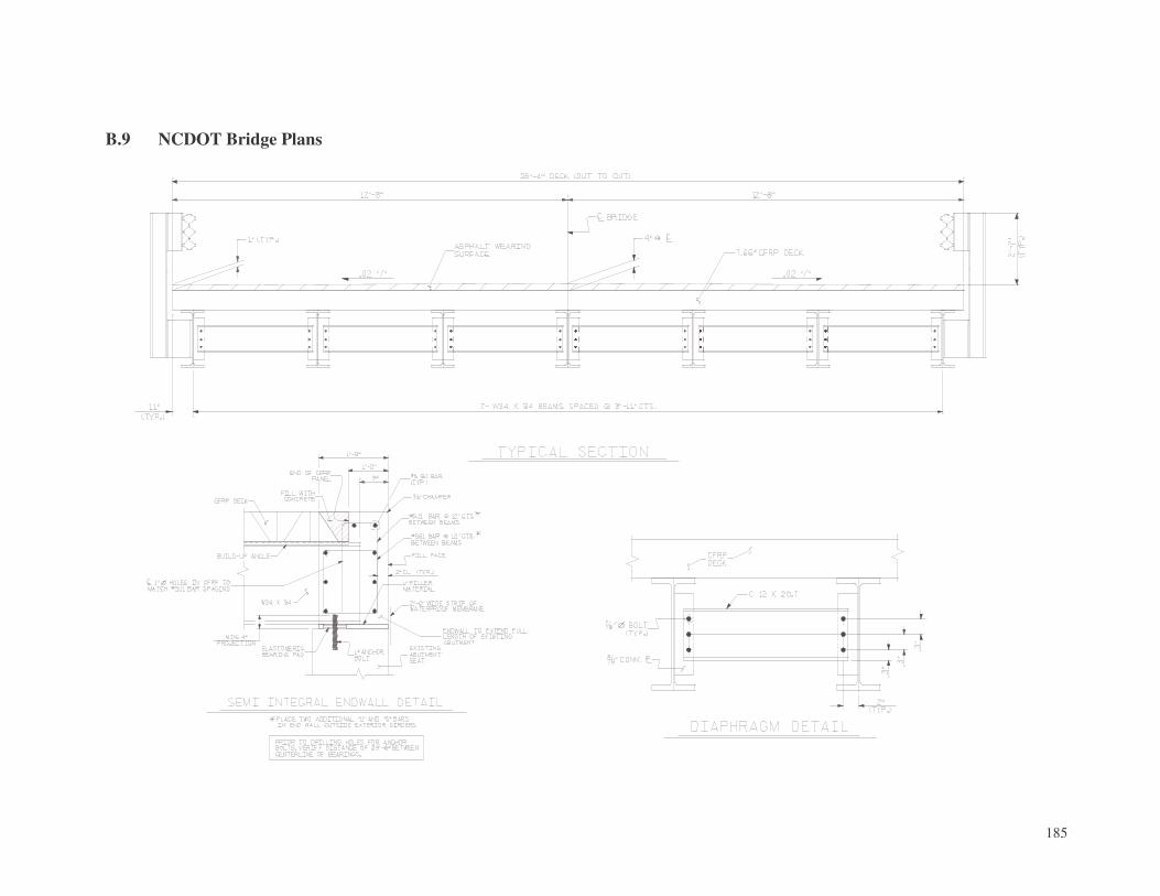
�
185
B.9 NCDOT Bridge Plans
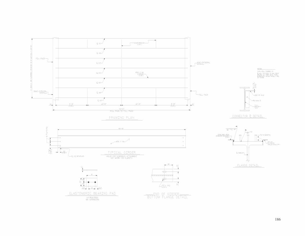
�
186
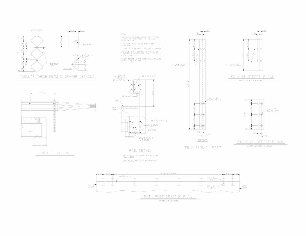
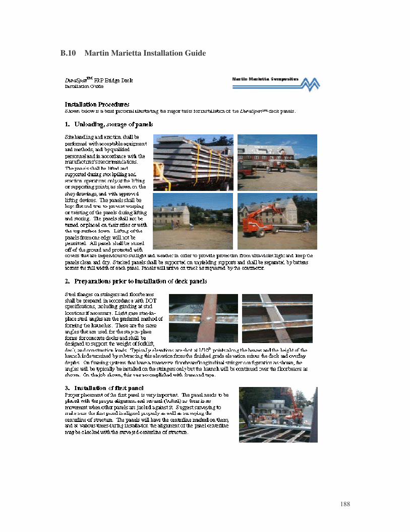
�
188
B.10 Martin Marietta Installation Guide

�
189
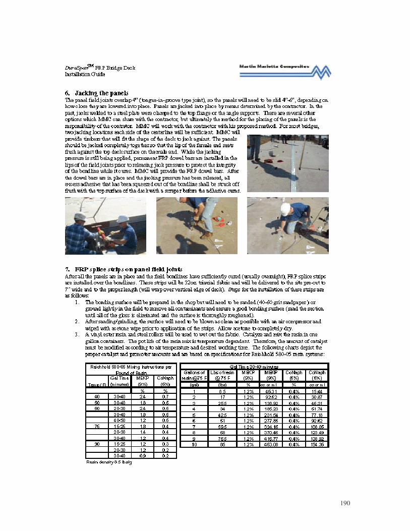
�
190

�
191

�
192

�
193

�
194
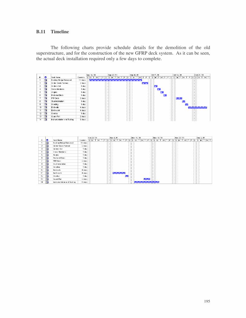
�
195
B.11 Timeline
The following charts provide schedule details for the demolition of the old superstructure, and for the construction of the new GFRP deck system. As it can be seen, the actual deck installation required only a few days to complete.
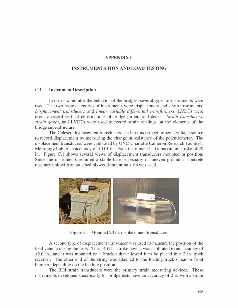
�
196
APPENDIX C
INSTRUMENTATION AND LOAD TESTING
C.1 Instrument Description
In order to monitor the behavior of the bridges, several types of instruments were used. The two basic categories of instruments were displacement and strain instruments. Displacement transducers and linear variable differential transformers (LVDT) were used to record vertical deformations of bridge girders and decks. Strain transducers, strain gages, and LVDTs were used to record strain readings on the elements of the bridge superstructure.
The Celesco displacement transducers used in this project utilize a voltage source to record displacement by measuring the change in resistance of the potentiometer. The displacement transducers were calibrated by UNC-Charlotte Cameron Research Facility’s Metrology Lab to an accuracy of ±0.01 in. Each instrument had a maximum stroke of 20 in. Figure C.1 shows several views of displacement transducers mounted in position. Since the instruments required a stable base, especially on uneven ground, a concrete masonry unit with an attached plywood-mounting strip was used.
Figure C.1 Mounted 20 in. displacement transducers
A second type of displacement transducer was used to measure the position of the load vehicle during the tests. This 140 ft – stroke device was calibrated to an accuracy of ±2.0 in., and it was mounted on a bracket that allowed it to be placed in a 2 in. truck receiver. The other end of the string was attached to the loading truck’s rear or front bumper, depending on the loading position.
The BDI strain transducers were the primary strain measuring devices. These instruments developed specifically for bridge tests have an accuracy of 2 % with a strain
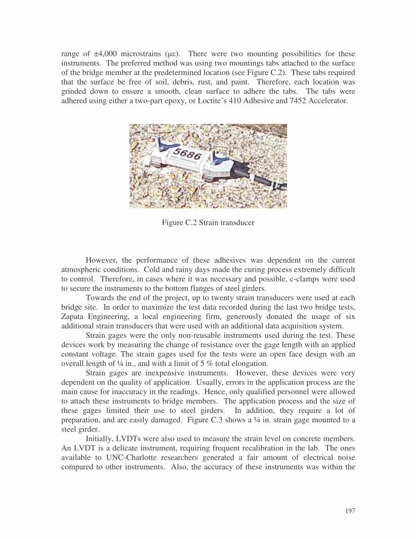
�
197
range of ±4,000 microstrains (��). There were two mounting possibilities for these instruments. The preferred method was using two mountings tabs attached to the surface of the bridge member at the predetermined location (see Figure C.2). These tabs required that the surface be free of soil, debris, rust, and paint. Therefore, each location was grinded down to ensure a smooth, clean surface to adhere the tabs. The tabs were adhered using either a two-part epoxy, or Loctite’s 410 Adhesive and 7452 Accelerator.
Figure C.2 Strain transducer
However, the performance of these adhesives was dependent on the current atmospheric conditions. Cold and rainy days made the curing process extremely difficult to control. Therefore, in cases where it was necessary and possible, c-clamps were used to secure the instruments to the bottom flanges of steel girders.
Towards the end of the project, up to twenty strain transducers were used at each bridge site. In order to maximize the test data recorded during the last two bridge tests, Zapata Engineering, a local engineering firm, generously donated the usage of six additional strain transducers that were used with an additional data acquisition system.
Strain gages were the only non-reusable instruments used during the test. These devices work by measuring the change of resistance over the gage length with an applied constant voltage. The strain gages used for the tests were an open face design with an overall length of ¼ in., and with a limit of 5 % total elongation.
Strain gages are inexpensive instruments. However, these devices were very dependent on the quality of application. Usually, errors in the application process are the main cause for inaccuracy in the readings. Hence, only qualified personnel were allowed to attach these instruments to bridge members. The application process and the size of these gages limited their use to steel girders. In addition, they require a lot of preparation, and are easily damaged. Figure C.3 shows a ¼ in. strain gage mounted to a steel girder.
Initially, LVDTs were also used to measure the strain level on concrete members. An LVDT is a delicate instrument, requiring frequent recalibration in the lab. The ones available to UNC-Charlotte researchers generated a fair amount of electrical noise compared to other instruments. Also, the accuracy of these instruments was within the
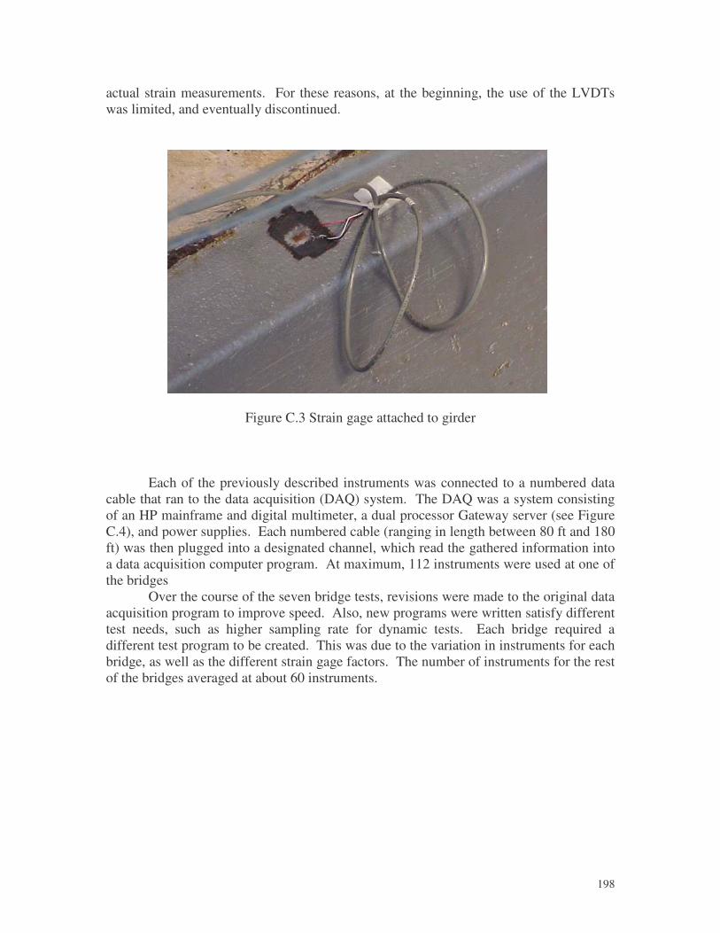
�
198
actual strain measurements. For these reasons, at the beginning, the use of the LVDTs was limited, and eventually discontinued.
Figure C.3 Strain gage attached to girder
Each of the previously described instruments was connected to a numbered data cable that ran to the data acquisition (DAQ) system. The DAQ was a system consisting of an HP mainframe and digital multimeter, a dual processor Gateway server (see Figure C.4), and power supplies. Each numbered cable (ranging in length between 80 ft and 180 ft) was then plugged into a designated channel, which read the gathered information into a data acquisition computer program. At maximum, 112 instruments were used at one of the bridges
Over the course of the seven bridge tests, revisions were made to the original data acquisition program to improve speed. Also, new programs were written satisfy different test needs, such as higher sampling rate for dynamic tests. Each bridge required a different test program to be created. This was due to the variation in instruments for each bridge, as well as the different strain gage factors. The number of instruments for the rest of the bridges averaged at about 60 instruments.
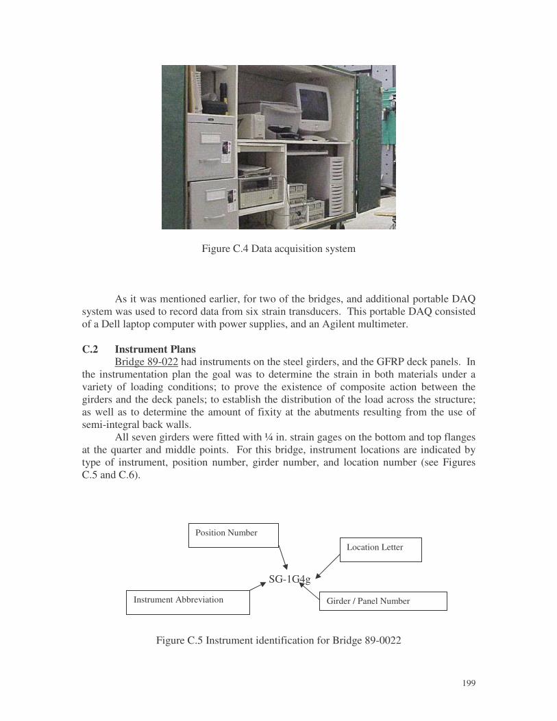
�
199
Figure C.4 Data acquisition system
As it was mentioned earlier, for two of the bridges, and additional portable DAQ system was used to record data from six strain transducers. This portable DAQ consisted of a Dell laptop computer with power supplies, and an Agilent multimeter. C.2 Instrument Plans
Bridge 89-022 had instruments on the steel girders, and the GFRP deck panels. In the instrumentation plan the goal was to determine the strain in both materials under a variety of loading conditions; to prove the existence of composite action between the girders and the deck panels; to establish the distribution of the load across the structure; as well as to determine the amount of fixity at the abutments resulting from the use of semi-integral back walls.
All seven girders were fitted with ¼ in. strain gages on the bottom and top flanges at the quarter and middle points. For this bridge, instrument locations are indicated by type of instrument, position number, girder number, and location number (see Figures C.5 and C.6).
SG-1G4g
Figure C.5 Instrument identification for Bridge 89-0022
Location Letter
Girder / Panel Number
Position Number
Instrument Abbreviation
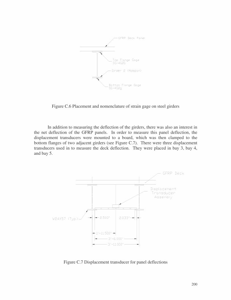
�
200
Figure C.6 Placement and nomenclature of strain gage on steel girders
In addition to measuring the deflection of the girders, there was also an interest in the net deflection of the GFRP panels. In order to measure this panel deflection, the displacement transducers were mounted to a board, which was then clamped to the bottom flanges of two adjacent girders (see Figure C.7). There were three displacement transducers used in to measure the deck deflection. They were placed in bay 3, bay 4, and bay 5.
Figure C.7 Displacement transducer for panel deflections
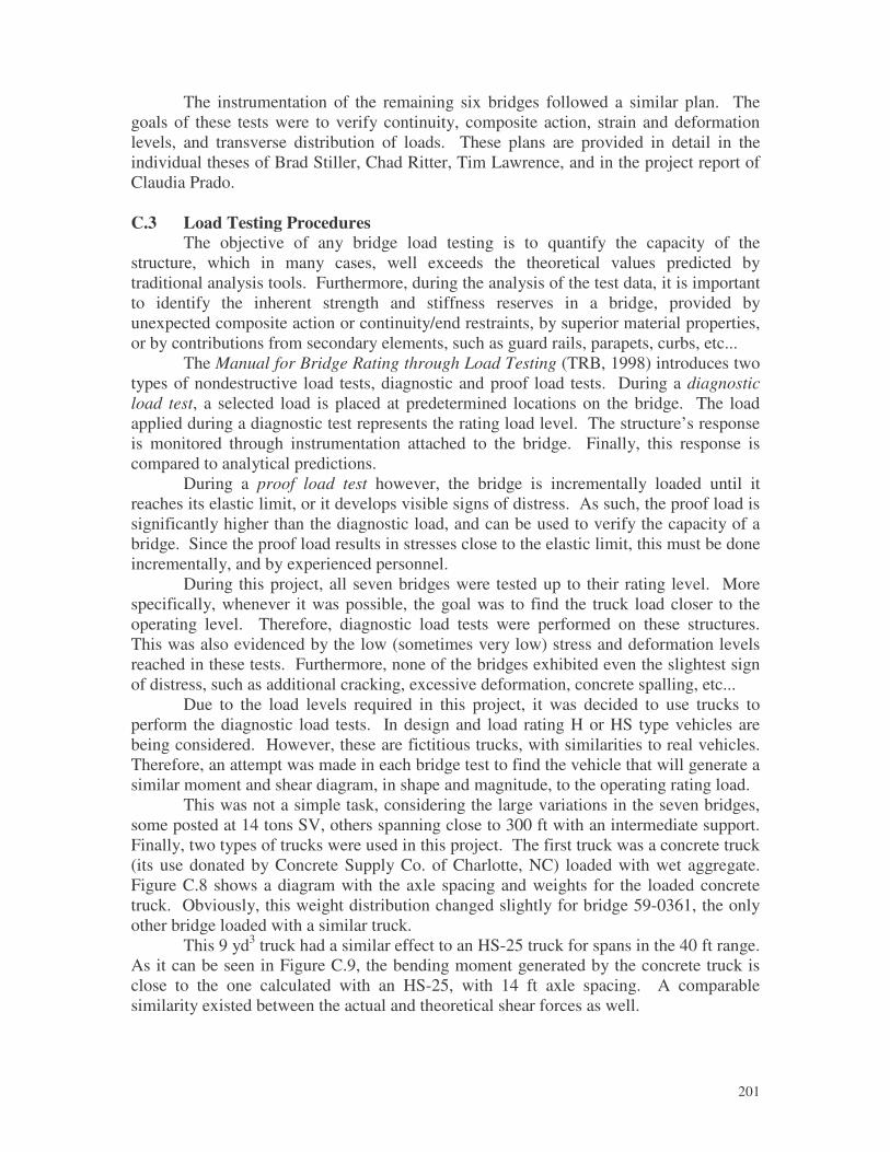
�
201
The instrumentation of the remaining six bridges followed a similar plan. The goals of these tests were to verify continuity, composite action, strain and deformation levels, and transverse distribution of loads. These plans are provided in detail in the individual theses of Brad Stiller, Chad Ritter, Tim Lawrence, and in the project report of Claudia Prado. C.3 Load Testing Procedures
The objective of any bridge load testing is to quantify the capacity of the structure, which in many cases, well exceeds the theoretical values predicted by traditional analysis tools. Furthermore, during the analysis of the test data, it is important to identify the inherent strength and stiffness reserves in a bridge, provided by unexpected composite action or continuity/end restraints, by superior material properties, or by contributions from secondary elements, such as guard rails, parapets, curbs, etc...
The Manual for Bridge Rating through Load Testing (TRB, 1998) introduces two types of nondestructive load tests, diagnostic and proof load tests. During a diagnostic load test, a selected load is placed at predetermined locations on the bridge. The load applied during a diagnostic test represents the rating load level. The structure’s response is monitored through instrumentation attached to the bridge. Finally, this response is compared to analytical predictions.
During a proof load test however, the bridge is incrementally loaded until it reaches its elastic limit, or it develops visible signs of distress. As such, the proof load is significantly higher than the diagnostic load, and can be used to verify the capacity of a bridge. Since the proof load results in stresses close to the elastic limit, this must be done incrementally, and by experienced personnel.
During this project, all seven bridges were tested up to their rating level. More specifically, whenever it was possible, the goal was to find the truck load closer to the operating level. Therefore, diagnostic load tests were performed on these structures. This was also evidenced by the low (sometimes very low) stress and deformation levels reached in these tests. Furthermore, none of the bridges exhibited even the slightest sign of distress, such as additional cracking, excessive deformation, concrete spalling, etc...
Due to the load levels required in this project, it was decided to use trucks to perform the diagnostic load tests. In design and load rating H or HS type vehicles are being considered. However, these are fictitious trucks, with similarities to real vehicles. Therefore, an attempt was made in each bridge test to find the vehicle that will generate a similar moment and shear diagram, in shape and magnitude, to the operating rating load.
This was not a simple task, considering the large variations in the seven bridges, some posted at 14 tons SV, others spanning close to 300 ft with an intermediate support. Finally, two types of trucks were used in this project. The first truck was a concrete truck (its use donated by Concrete Supply Co. of Charlotte, NC) loaded with wet aggregate. Figure C.8 shows a diagram with the axle spacing and weights for the loaded concrete truck. Obviously, this weight distribution changed slightly for bridge 59-0361, the only other bridge loaded with a similar truck.
This 9 yd3 truck had a similar effect to an HS-25 truck for spans in the 40 ft range. As it can be seen in Figure C.9, the bending moment generated by the concrete truck is close to the one calculated with an HS-25, with 14 ft axle spacing. A comparable similarity existed between the actual and theoretical shear forces as well.
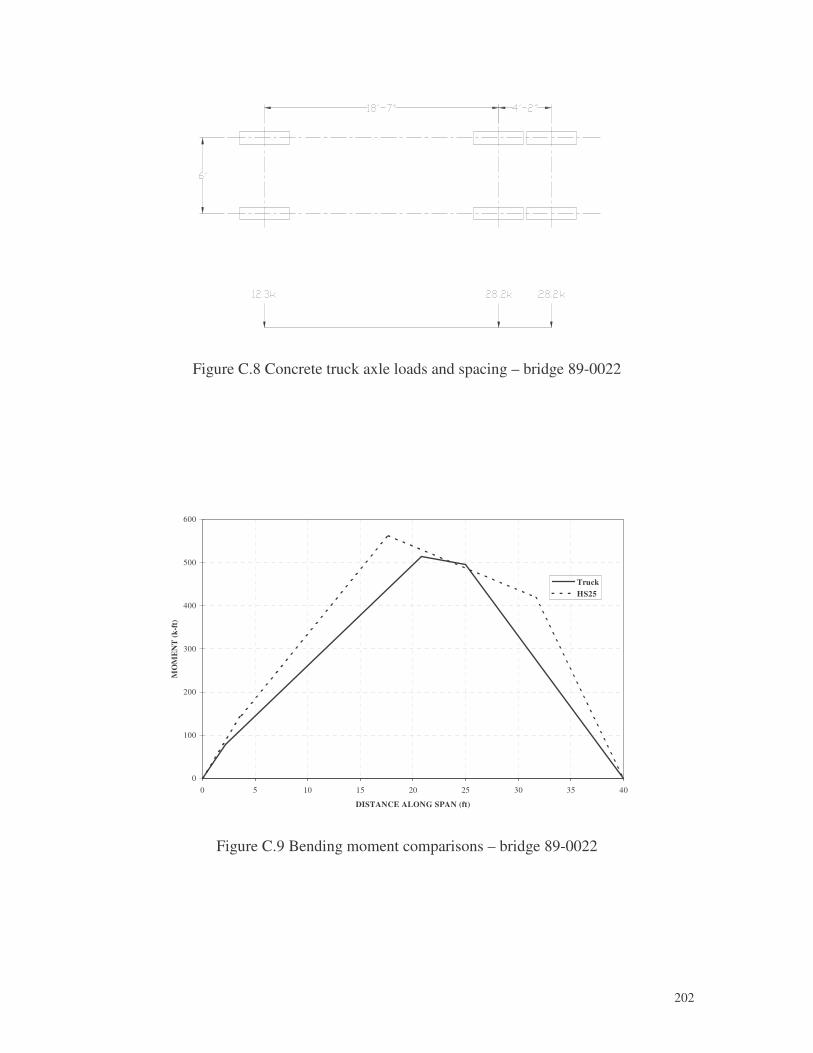
�
202
Figure C.8 Concrete truck axle loads and spacing – bridge 89-0022
Figure C.9 Bending moment comparisons – bridge 89-0022
0
100
200
300
400
500
600
0 5 10 15 20 25 30 35 40
DISTANCE ALONG SPAN (ft)
MO
ME
NT
(k-ft
)
TruckHS25

�
203
The second truck type was a NCDOT tandem truck loaded with aggregate at different levels (see Figure C.10). This loading system resulted in gross weights between 18 to 25 tons, close to most of the posting levels of the bridges considered. For bridge 59-0841 two of these trucks were used to simulate the effects of the governing lane load (for all of the other bridges truck loads governed the design and analysis).
Whenever it was possible, the trucks were weighed, axle by axle, by the Division of Motor Vehicles in the morning of the tests. Also, the axle spacing was verified in each case – this was necessary because there was a few feet difference in the tandem trucks available on a particular test date.
Figure C.10 Tandem truck loading bridge 89-0219
As it was mentioned earlier, a diagnostic load test requires the positioning of a loading vehicle at predetermined locations, while reading the bridge’s structural response. Based on this requirement, it makes sense to position the loading vehicle to locations on the bridge that would generate the largest shear and bending forces, and vertical deformations. In this project, four different loading protocols were followed: static, dynamic, and slow movements, and finally, ambient traffic loading.
The static load followed the above-mentioned recommendations for diagnostic testing. The trucks were positioned at dozens of locations throughout the bridges, loading all the lanes, one at the time, from both traffic directions. In order to confirm test repeatability, the most important locations were loaded twice, then the result compared.
For one of the early bridges, these same static “spots” were loaded again, but with a slow moving truck. The position of the truck along the bridge was recorded using the 146 ft displacement transducer. By comparing the result of the static and the slow loading procedures, no real differences were observed. Therefore, it was decided for the
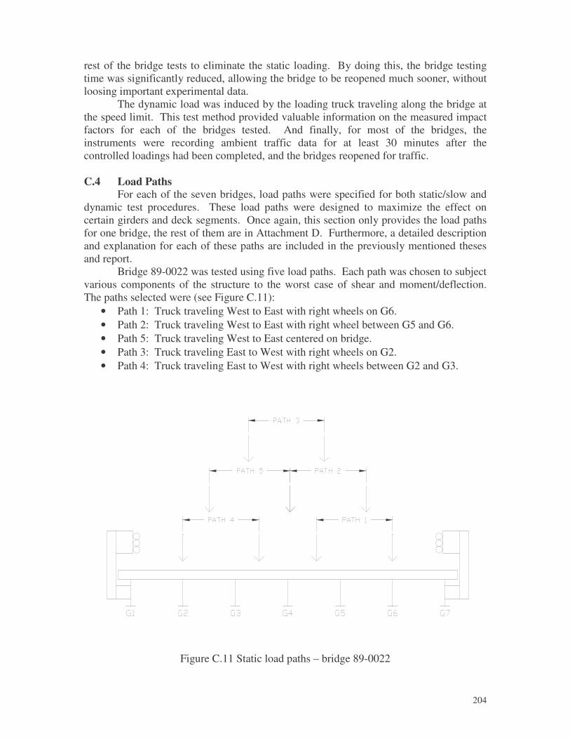
�
204
rest of the bridge tests to eliminate the static loading. By doing this, the bridge testing time was significantly reduced, allowing the bridge to be reopened much sooner, without loosing important experimental data.
The dynamic load was induced by the loading truck traveling along the bridge at the speed limit. This test method provided valuable information on the measured impact factors for each of the bridges tested. And finally, for most of the bridges, the instruments were recording ambient traffic data for at least 30 minutes after the controlled loadings had been completed, and the bridges reopened for traffic. C.4 Load Paths
For each of the seven bridges, load paths were specified for both static/slow and dynamic test procedures. These load paths were designed to maximize the effect on certain girders and deck segments. Once again, this section only provides the load paths for one bridge, the rest of them are in Attachment D. Furthermore, a detailed description and explanation for each of these paths are included in the previously mentioned theses and report.
Bridge 89-0022 was tested using five load paths. Each path was chosen to subject various components of the structure to the worst case of shear and moment/deflection. The paths selected were (see Figure C.11):
• Path 1: Truck traveling West to East with right wheels on G6. • Path 2: Truck traveling West to East with right wheel between G5 and G6. • Path 5: Truck traveling West to East centered on bridge. • Path 3: Truck traveling East to West with right wheels on G2. • Path 4: Truck traveling East to West with right wheels between G2 and G3.
Figure C.11 Static load paths – bridge 89-0022

�
205
The stopping points used in the static testing varied depending on the path. These stopping points are also summarized in Table C.1, and are shown in Figure C.12. The eight stopping points for this bridge were:
a) Back wheels located to produce maximum moment in span. b) Back wheels located to produce maximum shear in span. c) Back wheels centered in GFRP panel 1. d) Back wheels centered in GFRP panel 2. e) Back wheels centered in GFRP panel 3 f) Back wheels centered in GFRP panel 4. g) Back wheels centered in GFRP panel 5 h) Back wheels positioned over joint between panel 2 and panel 3.
The slow testing was performed along the same paths as the static testing. The location of the load path was measured and marked on the pavement with a chalk line. During the testing, there was a spotter just in front of the load truck guiding the driver along the proper path. The load was applied slowly across the span in order to avoid any dynamic effects.
Table C.1 Stopping points for testing
Static Path Number a b c d e f g h
1 X X 2 X X X X X X 3 X X 4 X X 5 X X X X X X
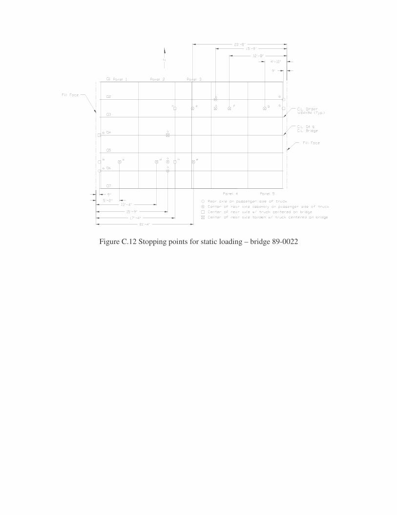
Figure C.12 Stopping points for static loading – bridge 89-0022
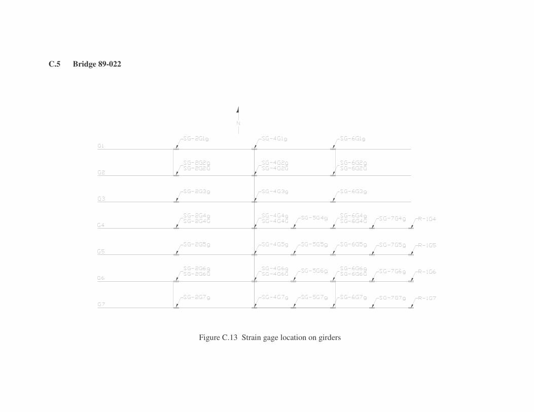
C.5 Bridge 89-022
Figure C.13 Strain gage location on girders
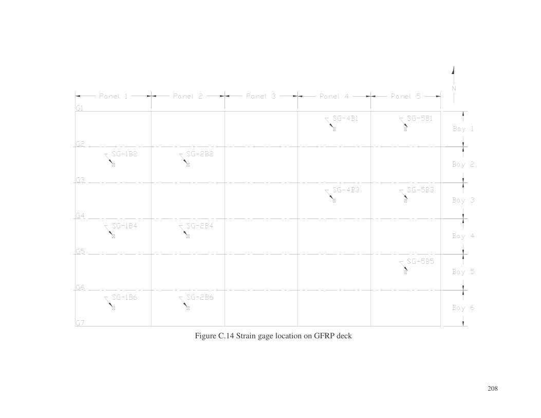
�
208
Figure C.14 Strain gage location on GFRP deck
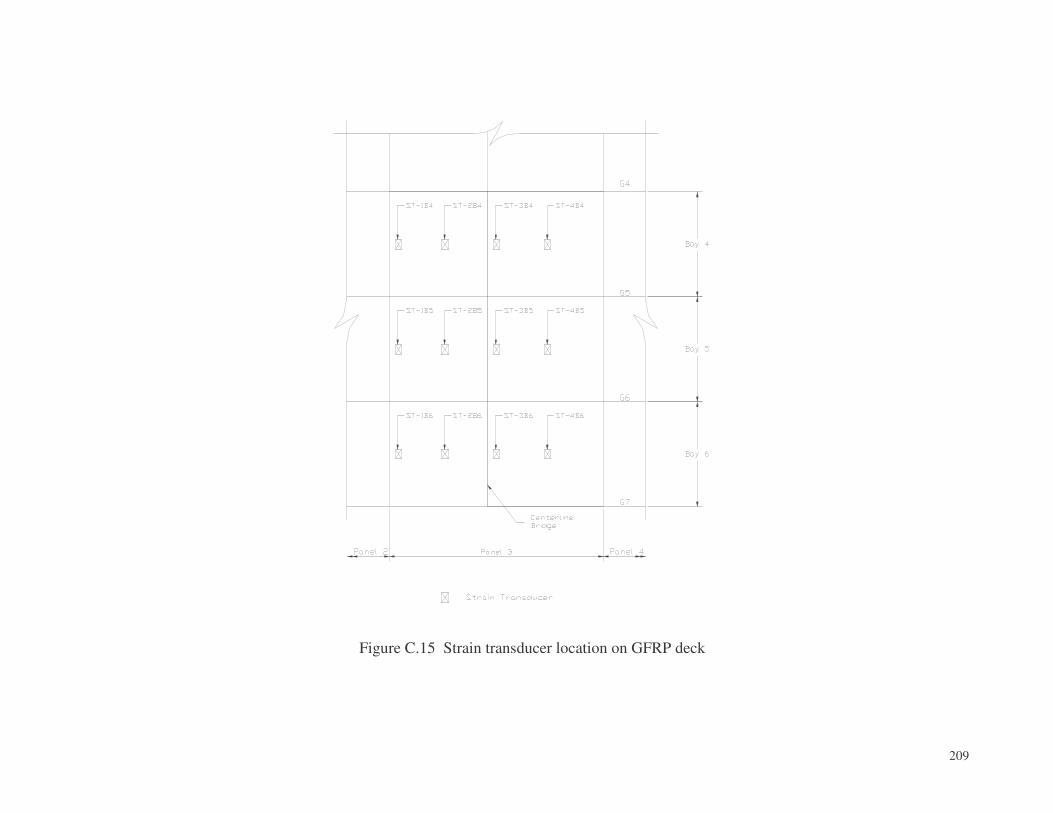
�
209
Figure C.15 Strain transducer location on GFRP deck
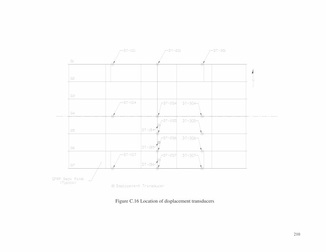
�
210
Figure C.16 Location of displacement transducers
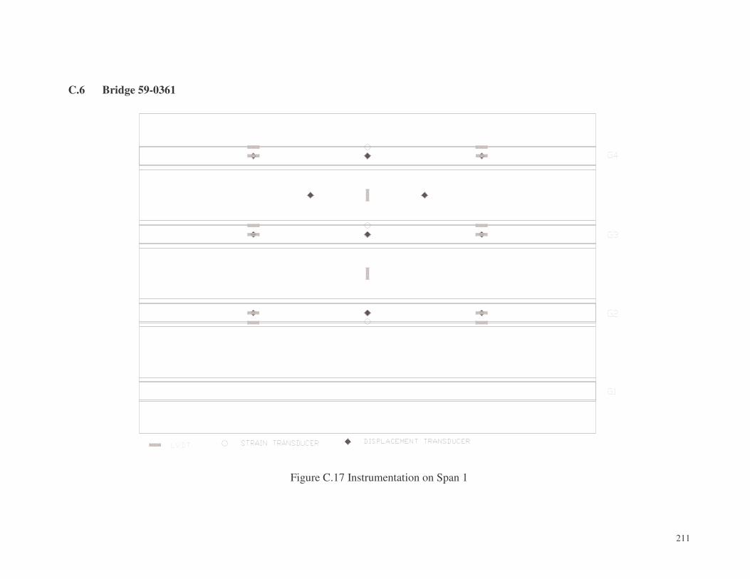
�
211
C.6 Bridge 59-0361
Figure C.17 Instrumentation on Span 1
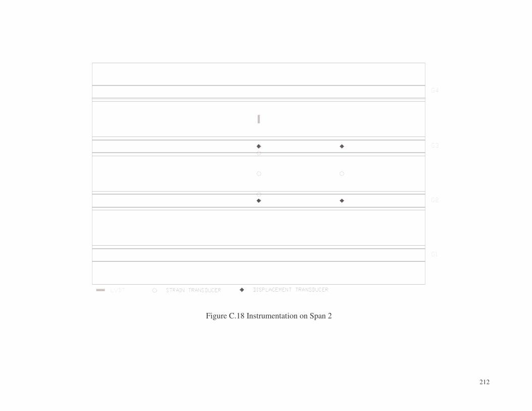
�
212
Figure C.18 Instrumentation on Span 2
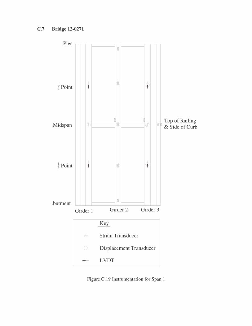
C.7 Bridge 12-0271
Girder 2
Key
Strain Transducer
Displacement Transducer
LVDT
Abutment
14 Point
Girder 1 Girder 3
34 Point
Midspan
Pier
Top of Railing & Side of Curb
Figure C.19 Instrumentation for Span 1
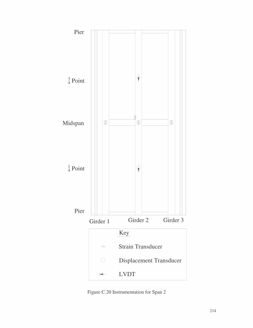
�
214
34 Point
Midspan
14 Point
Girder 3
Key
Strain Transducer
Displacement Transducer
LVDT
Girder 1
PierGirder 2
Pier
Figure C.20 Instrumentation for Span 2
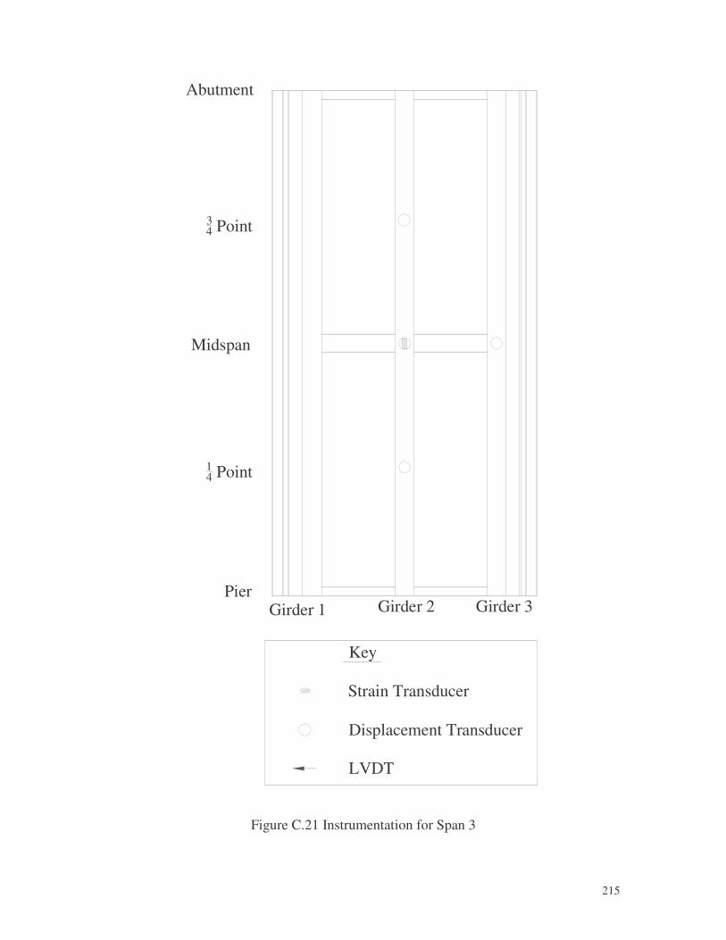
�
215
Girder 3
Key
Strain Transducer
Displacement Transducer
LVDT
PierGirder 1
14 Point
Girder 2
Abutment
Midspan
34 Point
Figure C.21 Instrumentation for Span 3
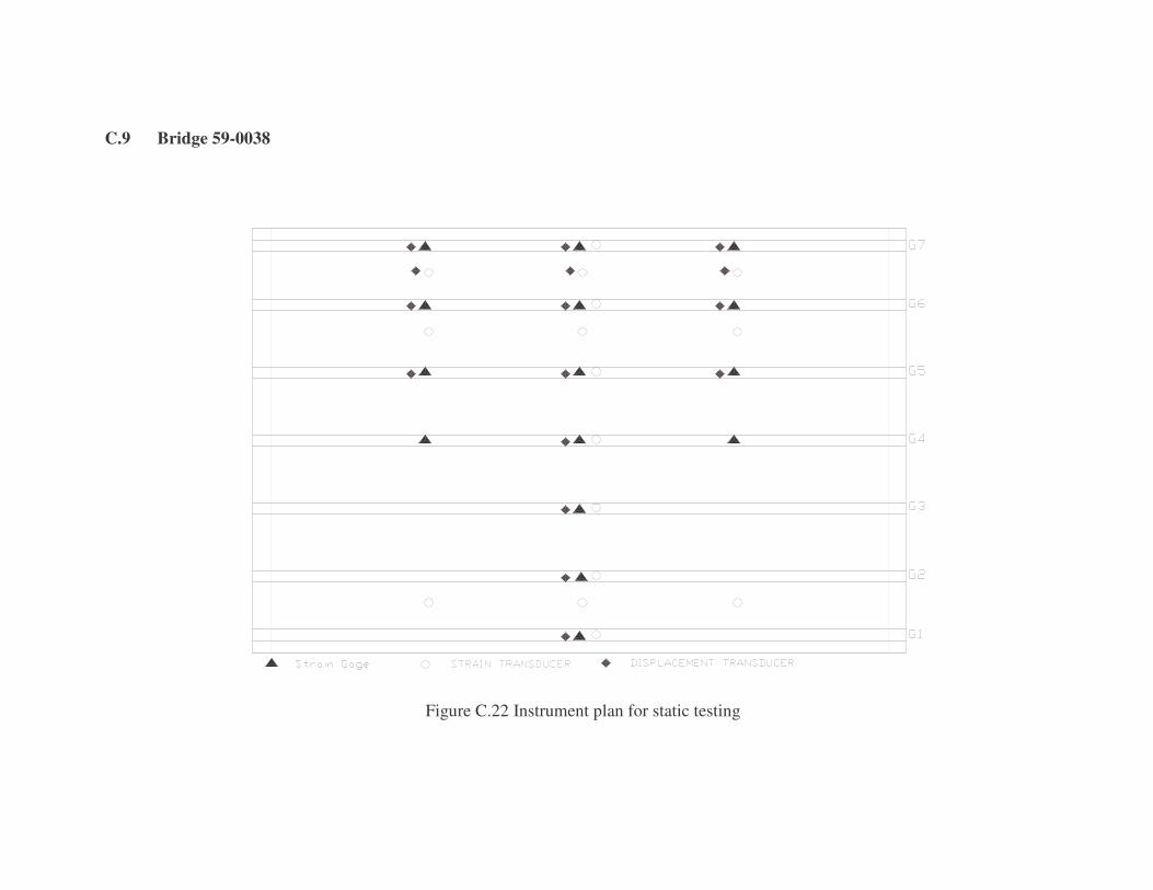
C.9 Bridge 59-0038
Figure C.22 Instrument plan for static testing
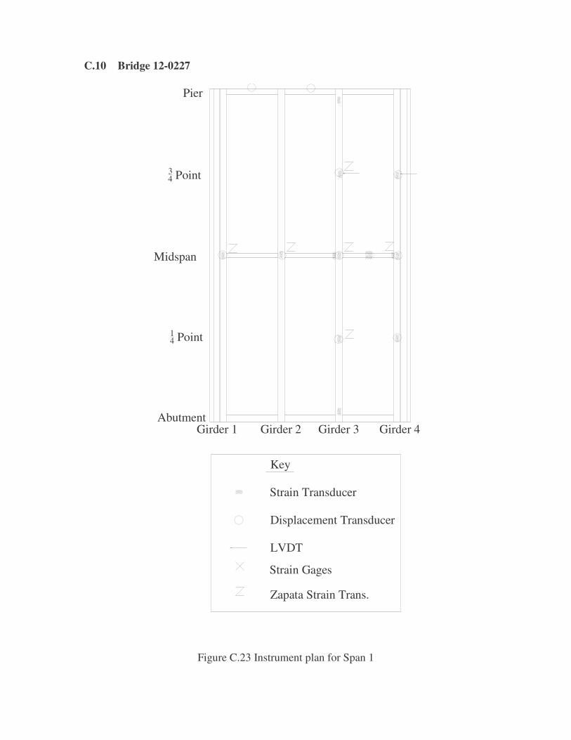
C.10 Bridge 12-0227
Key
Strain Transducer
Displacement Transducer
LVDT
Zapata Strain Trans.
Strain Gages
Girder 2
14 Point
AbutmentGirder 1
34 Point
Pier
Midspan
Girder 4Girder 3
SPAN 1
Figure C.23 Instrument plan for Span 1
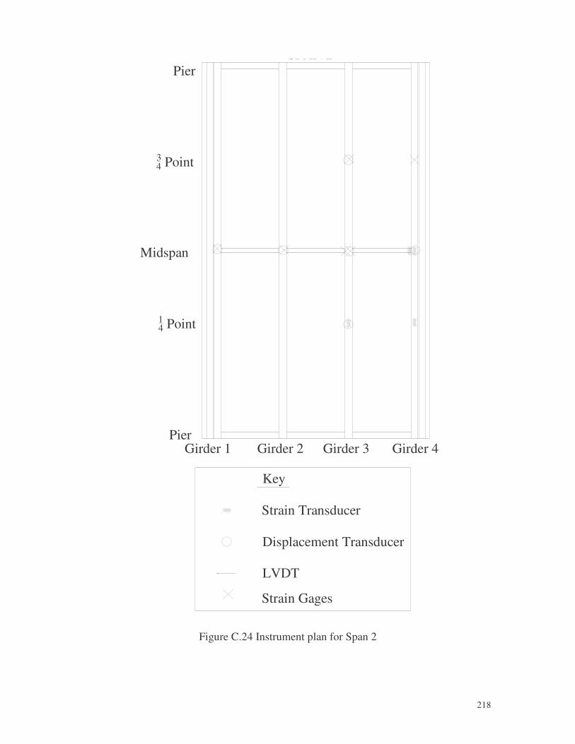
�
218
Midspan
Key
Strain Transducer
Displacement Transducer
LVDT
Strain Gages
Girder 2Girder 1Pier
14 Point
Girder 3
34 Point
PierSPAN 2
Girder 4
Figure C.24 Instrument plan for Span 2
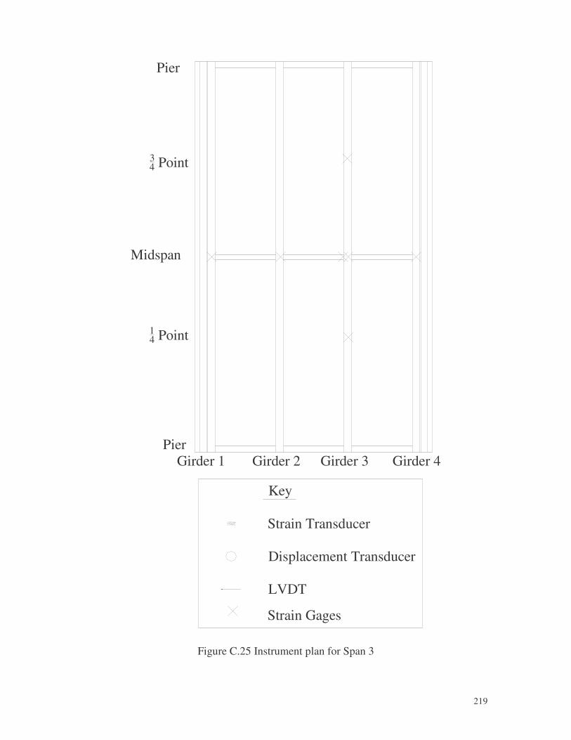
�
219
PierGirder 1
14 Point
34 Point
Midspan
Pier
Key
Strain Transducer
Displacement Transducer
LVDT
Strain Gages
Girder 3Girder 2 Girder 4
SPAN 3
Figure C.25 Instrument plan for Span 3
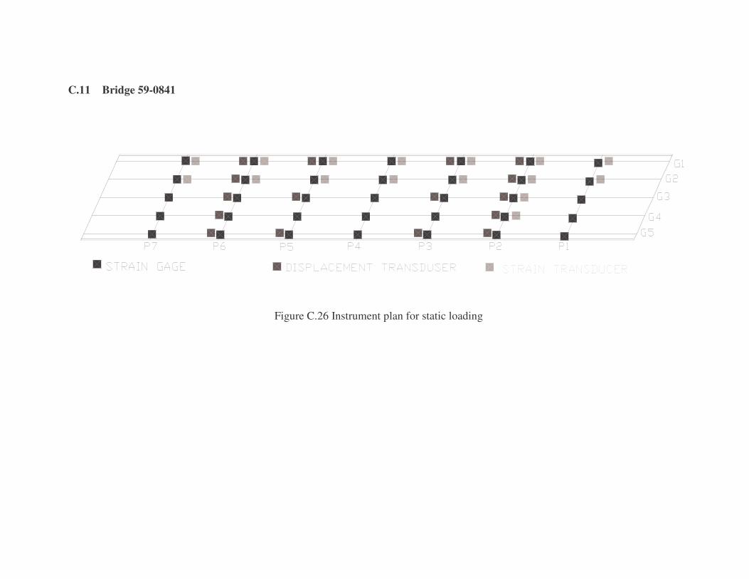
C.11 Bridge 59-0841
Figure C.26 Instrument plan for static loading
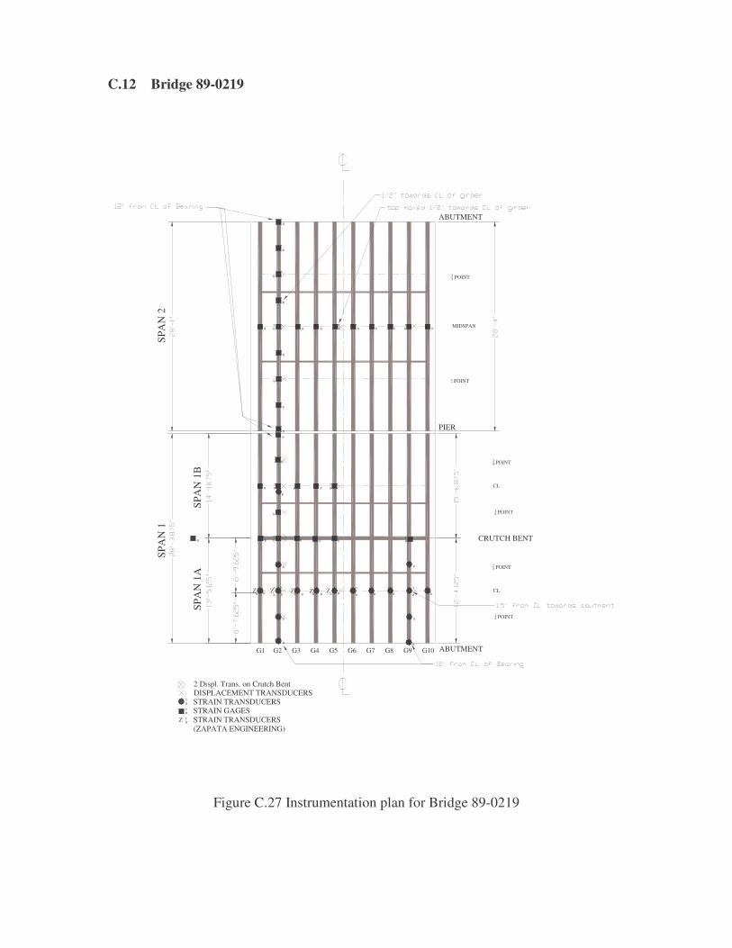
C.12 Bridge 89-0219
SPA
N 1
SPA
N 2
SPA
N 1
BSP
AN
1A
G1 G2 G3 G4 G5 G6 G7 G8 G9 G10
2 Displ. Trans. on Crutch BentDISPLACEMENT TRANSDUCERSSTRAIN TRANSDUCERSSTRAIN GAGESSTRAIN TRANSDUCERS (ZAPATA ENGINEERING)
TB
TB
ABUTMENT
ABUTMENT
PIER
CRUTCH BENT
B
B
B
B
TB
B
B
B
B
TB BB B BB
MIDSPAN
34 POINT
14 POINT
34 POINT
B
B
TB
B
TB
B
BB CL
14 POINT
BBB B
14 POINT
CL
34 POINT
B
BB
T
B BB B
TBZ
Z ZZB B
ZZT
B BB
T
B
B
BB
T
B
TB
B B
B
BTB
B
TB
B
B
B
Figure C.27 Instrumentation plan for Bridge 89-0219

�
222
APPENDIX D
LOAD PATHS

�
223
D.1 Bridge 59-0361
Static Path No.
Description of path a b c d e f g h
Slow Dynamic
1 Right wheel line over girder 4 x x x x x x x x x
2 Truck centered in southbound lane x x x x
3 Right wheel line between girders 3 and 4 x x x x x x x x x
4 Right wheel line over girder 1 x x x x
5 Truck center of yellow line on bridge x x x
6 Truck centered in northbound lane x x x x
7 Right wheel line between girders 1 and 2 x x x
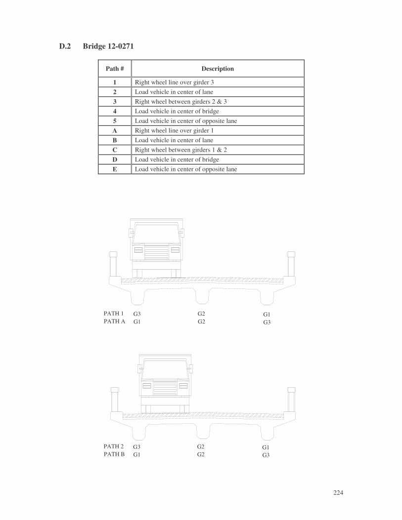
�
224
D.2 Bridge 12-0271
Path # Description
1 Right wheel line over girder 3 2 Load vehicle in center of lane 3 Right wheel between girders 2 & 3 4 Load vehicle in center of bridge 5 Load vehicle in center of opposite lane A Right wheel line over girder 1 B Load vehicle in center of lane C Right wheel between girders 1 & 2 D Load vehicle in center of bridge E Load vehicle in center of opposite lane
G1PATH AG3PATH 1
G3G2G2 G1
G1PATH BG3PATH 2
G3G2G2 G1
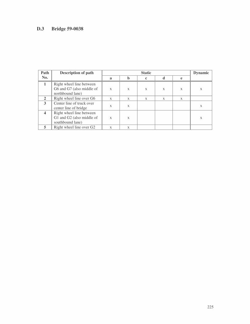
�
225
D.3 Bridge 59-0038
Static Path No.
Description of path a b c d e
Dynamic
1 Right wheel line between G6 and G7 (also middle of northbound lane)
x x x x x x
2 Right wheel line over G6 x x x x x 3 Center line of truck over
center line of bridge x x x
4 Right wheel line between G1 and G2 (also middle of southbound lane)
x x x
5 Right wheel line over G2 x x
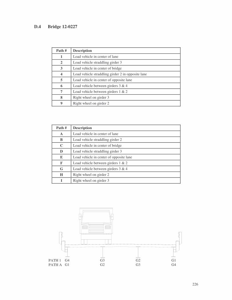
�
226
D.4 Bridge 12-0227
Path # Description
1 Load vehicle in center of lane
2 Load vehicle straddling girder 3
3 Load vehicle in center of bridge
4 Load vehicle straddling girder 2 in opposite lane
5 Load vehicle in center of opposite lane
6 Load vehicle between girders 3 & 4
7 Load vehicle between girders 1 & 2
8 Right wheel on girder 3
9 Right wheel on girder 2
Path # Description A Load vehicle in center of lane
B Load vehicle straddling girder 2
C Load vehicle in center of bridge
D Load vehicle straddling girder 3
E Load vehicle in center of opposite lane
F Load vehicle between girders 1 & 2
G Load vehicle between girders 3 & 4
H Right wheel on girder 2
I Right wheel on girder 3
PATH APATH 1
G1G4
G2G3
G3G2
G4G1
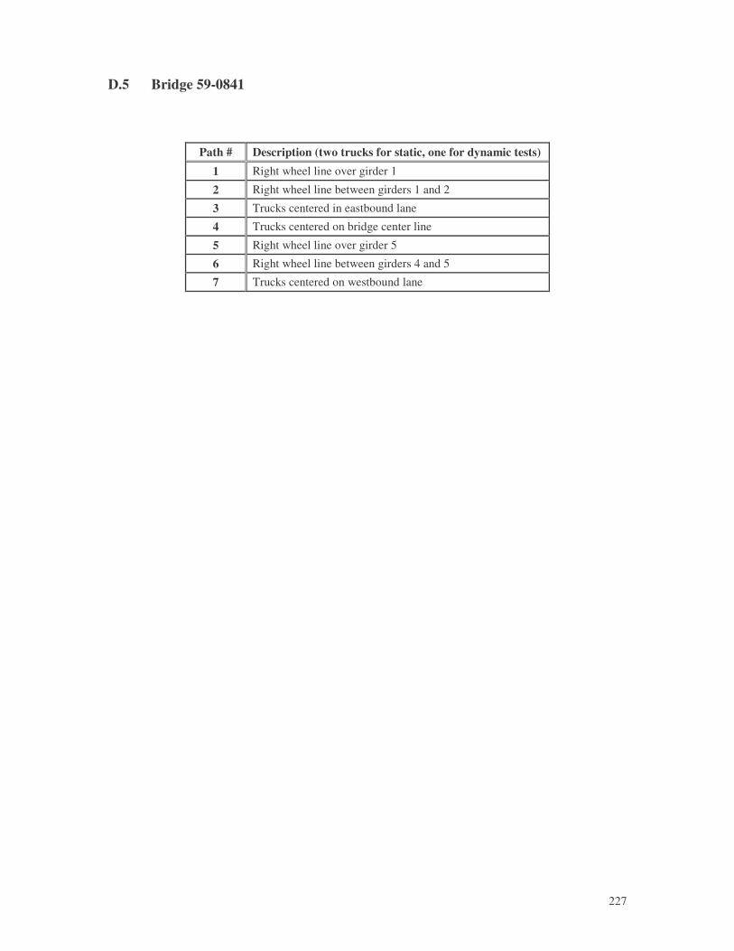
�
227
D.5 Bridge 59-0841
Path # Description (two trucks for static, one for dynamic tests) 1 Right wheel line over girder 1
2 Right wheel line between girders 1 and 2
3 Trucks centered in eastbound lane
4 Trucks centered on bridge center line
5 Right wheel line over girder 5
6 Right wheel line between girders 4 and 5
7 Trucks centered on westbound lane
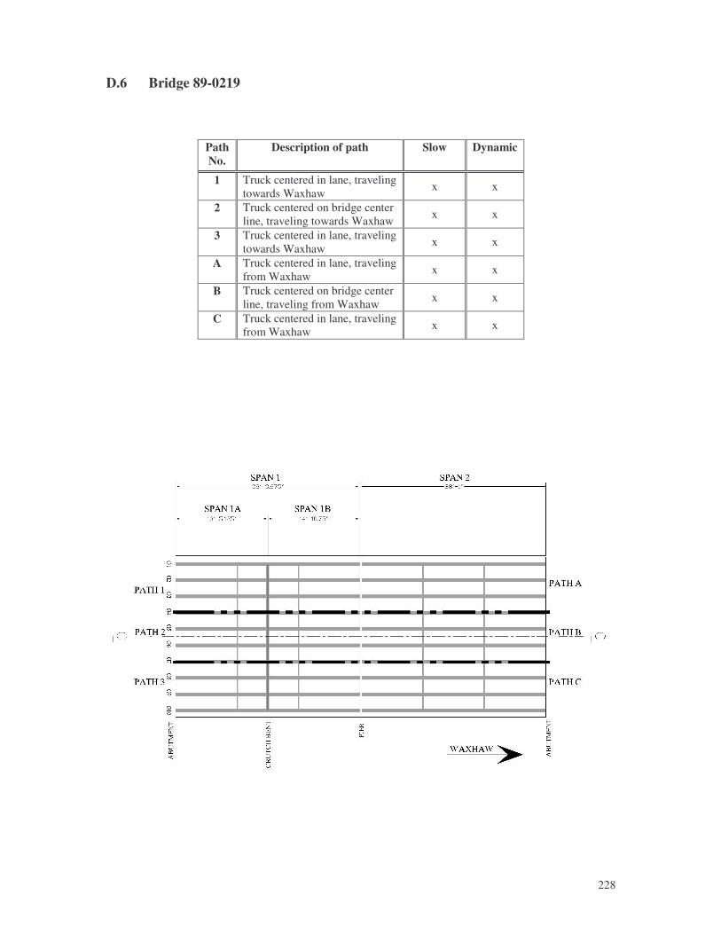
�
228
D.6 Bridge 89-0219
Path No.
Description of path Slow Dynamic
1 Truck centered in lane, traveling towards Waxhaw x x
2 Truck centered on bridge center line, traveling towards Waxhaw x x
3 Truck centered in lane, traveling towards Waxhaw x x
A Truck centered in lane, traveling from Waxhaw x x
B Truck centered on bridge center line, traveling from Waxhaw x x
C Truck centered in lane, traveling from Waxhaw x x