Evaluation of the DMS flux and its conversion to SO2 over the southern ocean

*Corresponding author. Fax: #1-404-894-1993.E-mail address: [email protected] (D. Davis).1Current address: Department of Environmental Engineer-

ing, Dong-Eui University, Pusan, South Korea.

Atmospheric Environment 35 (2001) 159}172

Evaluation of the DMS #ux and its conversion to SO2

over the southern ocean

Zang-Ho Shon!,1, D. Davis!,*, G. Chen!, G. Grodzinsky!, A. Bandy",D. Thornton", S. Sandholm!, J. Bradshaw!, R. Stickel!, W. Chameides!,

G. Kok#, L. Russell$, L. Mauldin#, D. Tanner#, F. Eisele#

!School of Earth and Atmospheric Sciences, Georgia Institute of Technology, Atlanta, USA"Department of Chemistry, Drexel University, Philadelphia, USA

#National Center for Atmospheric Research, Boulder, USA$Department of Chemical Engineering, Princeton University, Princeton, USA

Received 15 November 1999; accepted 23 February 2000

Abstract

A total of 16 boundary layer (BL) DMS #ux values were derived from #ights over the Southern Ocean. DMS #uxvalues were derived from airborne observations recorded during the Aerosol Characterization Experiment (ACE 1). Thelatitude range covered was 553S}403S. The method of evaluation was based on the mass-balance photochemical-modeling (MBPCM) approach. The estimated #ux for the above latitude range was 0.4}7.0lmolm~2d~1. The averagevalue from all data analyzed was 2.6$1.8lmolm~2d~1. A comparison of the MBPCM methodology with several otherDMS #ux methods (e.g., ship and airborne based) revealed reasonably good agreement in some cases and signi"cantdisagreement in other cases. Considering the limited number of cases compared and the fact that conditions for thecomparisons were far from ideal, it is not possible to conclude that major agreement or di!erences have been establishedbetween these methods. A major result from this study was the "nding that DMS oxidation is a major source of BL SO

2over the Southern Ocean. Model simulations suggest that, on average, the conversion e$ciency is 0.7 or higher, givena lifetime for SO

2of &1 d. A comparison of two sulfur case studies, one based on DMS}SO

2data generated on the

NCAR C-130 aircraft, the other based on data recorded on the NOAA ship Discoverer, revealed qualitative agreement in"nding that DMS was a major source of Southern Ocean SO

2.On the other hand, signi"cant disagreement was found

regarding the DMS/SO2

conversion e$ciency (e.g., 0.3}0.5 versus 0.7}0.9). Although yet unknown factors, such asvertical mixing, may be involved in reducing the level of disagreement, it does appear at this time that some signi"cantportion of this di!erence may be related to systematic di!erences in the two di!erent techniques employed to measureSO

2. It would seem prudent, therefore, that further instrument intercomparison SO

2studies be considered. It also would

be desirable to stage new intercomparison activity between the MBPCM #ux approach and the air-to-sea gradient aswell as other #ux methods, but under far more favorable conditions. ( 2000 Elsevier Science Ltd. All rights reserved.

Keywords: Marine; Sulfur; Chemistry; DMS; SO2; ACE1

1. Introduction

Oceanic emissions of dimethyl sul"de (DMS:CH

3SCH

3) are known to be a major primary source of

natural sulfur in the remote marine atmosphere (Andreaeand Raemdonck, 1983; Andreae, 1986; Bates et al., 1987).One of its oxidation products, SO

2, is also known to be

a major source of sulfate aerosol. Hence, via its formation

1352-2310/00/$ - see front matter ( 2000 Elsevier Science Ltd. All rights reserved.PII: S 1 3 5 2 - 2 3 1 0 ( 0 0 ) 0 0 1 6 6 - 7

Fig. 1. Southern Ocean C-130 #ight tracks during ACE 1. Thenumber next to each track is the "eld program mission number.

of CCN, sulfate aerosol derived from the oxidation ofDMS has the potential for in#uencing the Earth's radi-ative budget (Charlson et al., 1987). This suggests thatboth accurate assessments of the DMS #ux and its con-version e$ciency to SO

2and sulfate represent critical

inputs to climate models.At present, the e$ciency with which DMS forms SO

2is still problematic. Laboratory chamber type studieshave been qualitatively informative; but as pointed outin recent reviews of marine sulfur chemistry (e.g.,Berresheim et al., 1995 and references therein), because ofthe inability of these chambers to simulate actual marineconditions, the resulting product distributions still lackcredibility.

More surprising have been the con#icting results thathave emerged from marine sulfur "eld studies. Forexample, given that the typical boundary layer (BL)DMS lifetime with respect to OH is in the range of0.5}2d (e.g., Wine et al., 1981; Hynes et al., 1986), andthat for SO

2is typically less than 1 d (e.g., Berresheim

et al., 1995; Bonsang et al., 1987, and references therein),it follows that one should see a strong anticorrelationbetween these two species. This is particularly true if thesampling times are restricted to a temporal resolution ofmuch less than 1 d. However, in one of the earliest studiesin which both species were measured (Bandy et al., 1992),no anticorrelative behavior was observed. The resultingestimated conversion e$ciency was thus quite small, e.g.,)0.2. This ship study was carried out in the north-eastern Paci"c at 483N latitude. By contrast, in a laterground-based study near the equator, Bandy et al. (1996)reported a strong anticorrelation between DMS andSO

2. In this case the conversion e$ciency for DMS to

SO2

was estimated at 0.62$0.15. At the same site (i.e.,Christmas Island, 23N, 1573W), but using DMS}SO

2data collected from an airborne sampling platform,Davis et al. (1999) reported an analysis of sulfur datagathered again by Bandy and co-workers that also re-vealed a strong anticorrelation between DMS and SO

2.

These investigators estimated a conversion e$ciencyonly slightly higher than that reported by Bandy et al.,e.g., 0.72$0.15. Considerably at odds with the con-clusions of the previous two tropical studies, Yvon andSaltzman (1996) have reported shipboard data (i.e., 123S,1353W) that showed only a weak anticorrelation betweenDMS and SO

2. In this case the conversion e$ciency

dropped to 0.27}0.54. Huebert et al. (1993) also analyzedship data in the tropical Paci"c but in their study thesampling resolution for SO

2was a half day or longer.

Thus, under these conditions one might expect to seea positive correlation between DMS and SO

2. This was

a result not observed. Yet, at two other ground-basedsites, one at Amsterdam Island at 383S, 773E (Putaud etal., 1992) and the other at Cape Grim at 413S, 1443E(Ayers et al., 1997), `long-terma daily (Amsterdam) andweekly (Cape Grim) averaged DMS and SO

2data were

recorded that did result in positive correlations betweenDMS and SO

2. For the Amsterdam Island study the

reported conversion e$ciency was in the range of0.64}0.69 whereas that for Cape Grim was signi"cantlylower.

In this paper we present an analysis of airborne sulfurdata recorded during the First Aerosol CharacterizationExperiment (ACE 1) "eld study. Explored here is boththe issue of the con"dence level one can place in currentDMS #ux assessments and the issue of the e$ciency withwhich DMS is converted into SO

2.

2. Observational data

Data recorded during the ACE 1 "eld campaign arethe only data used in this study. The ACE 1 campaignwas carried out during the months of November andDecember 1995. Of the 31 marine #ights #own duringACE 1, 18 of these (#ights 11}28) were made over theSouthern Ocean between the dates of 17 November and12 December 1995. These #ights covered the latituderange of 403S}553S and a longitude range of1353E}1603E as shown in Fig. 1. The most commonlyemployed sampling strategy for the National Center forAtmospheric Research's (NCAR) C-130 aircraft consistedof #ying sequential circles (diameter &60 km) at 3 or4 constant altitudes (i.e., typically 30, 150, 300, 450, 600,and/or 900m) while moving with the wind "eld. Both BLand bu!er layer (BuL) altitudes were #own during each"eld mission. (Note, the bu!er layer is de"ned here as thetransition zone between the BL and free troposphere aspreviously described by Russell et al., 1998.) For the

160 Z.-H. Shon et al. / Atmospheric Environment 35 (2001) 159}172

Table 1Summary of model input conditions!

Flightno.

Sampling time(local)

Latitude(negative: S)

Longitude(negative: W)

T "

(3C)T

$"

(3C)[O

3]"

(ppbv)[CO]"(ppbv)

[NO]"(pptv)

[NOx]#

(pptv)BL h(km)

EMD(km)

11 12:45 !53.4 137.9 1.7 !2.7 24.9 72.0 4.4 11.6 0.5 0.812 10:49 !48.3 137.3 5.5 !2.9 26.4 71.2 3.1 9.4 1.1 1.214A 11:39 !40.7 144.2 10.6 3.3 24.7 79.6 4.7 13.5 0.8 2.114B 15:44 !43.6 150.8 13.3 3.5 24.6 71.6 4.8 13.4 0.5 1.615 11:39 !47.4 145.5 8.5 4.2 20.1 69.1 2.7 7.2 0.4 0.916 12:54 !54.1 159.2 2.2 !3.1 21.4 68.5 2.5 5.8 0.4 0.417 12:56 !41.0 143.6 10.9 3.7 23.4 66.5 5.2 14.2 0.6 1.318 05:58 !45.0 144.5 9.5 4.8 21.0 69.2 3.9 15.2 1.0 1.019A 14:27 !46.3 148.8 9.8 5.1 21.1 70.0 3.2 9.4 1.1 1.119B 18:04 !47.0 151.3 9.8 5.9 20.4 69.6 3.2 11.9 0.8 0.820 05:05 !51.0 157.0 6.1 4.1 21.8 68.0 3.6 27.5 0.8 1.121 04:34 !42.5 142.1 9.5 1.1 20.7 66.4 2.9 6.9 0.9 1.522 15:45 !41.4 139.3 10.5 1.6 18.4 64.8 2.0 4.7 1.0 1.024 10:15 !45.2 143.6 10.0 5.8 20.8 63.6 2.6 6.1 0.5 0.725 20:30 !46.0 145.7 9.9 5.8 20.2 62.1 2.2 5.1 0.6 0.826 09:29 !49.9 147.5 9.0 6.6 19.9 65.6 2.5 9.3 0.5 1.1

!T$

is the dew point temperature; for a detailed discussion on [NO], see the text."Median observations.#Model calculated quantity.

Lagrangian missions (#ights 18}20 and 23}26), a com-mon air mass was tracked in time using `smarta balloonslaunched from the NOAA research vessel Discoverer(Businger et al., 1999). For further detail on all aspects ofthe ACE 1 sampling strategy, the reader is directed to theACE 1 Òverviewa paper by Bates et al. (1998a).

The ACE 1 airborne "eld program included measure-ments of the sulfur species, DMS, SO

2, H

2SO

4, and

MSA as well as the aerosol species SO2~4

and methanesulfonate (MS). Other critical trace gas measurementsincluded OH, O

3, CO, CH

4, NO, H

2O

2, and CH

3OOH.

Meteorological parameters recorded included UV irra-diance (e.g., Eppley radiometer), T, P and the horizontaland vertical winds.

The C-130 DMS and SO2

measurements were madeusing gas chromatography/mass spectrometry (GC/MS)with isotopically labeled DMS and SO

2being used as

internal standards. The sampling resolution ranged from4 to 6min and the overall system had limits-of-detection(LOD) of &1 part per trillion by volume (pptv) for bothDMS and SO

2. For further details regarding this tech-

nique see Bandy et al. (1992, 1993). For details on themeasurements of other trace gases and aerosol species,the reader is directed to the ACE 1 Òverviewa paper byBates et al. (1998a).

During the Southern Ocean component of the ACE1 program, the C-130 aircraft sampled the BL 82 times.Of these, 66 sampling events were found acceptable forestimating DMS #uxes. Those runs rejected typically hadpoorly de"ned photochemical environments associated

with them. From the 66 acceptable events, 16 indepen-dent #ux values were estimated. The large reduction inthe number of independently de"ned #ux values re#ectsthe fact that typically four or more BL sampling eventswere used in determining one independent #ux value.

Median concentrations of the photochemical species,NO, CO, H

2O, O

3, H

2O

2, CH

3OOH, and CH

4formed

the basis for all input to the box model used to de"neboth the diel pro"les for OH and NO

3(see Table 1). In

the case of NO, most of the BL observations were at orbelow the 2 sigma detection limit of the chemilumines-cence NO sensor (e.g., typically 5}10 pptv). Hence, theNO input to the model involved bracketing a range ofvalues that encompassed a lower limit of 1 pptv and anupper limit de"ned by the 2 sigma uncertainty in the NOmeasurement. Using this approach, both upper andlower limiting values for OH were assigned. The bestestimate of the DMS #ux for these cases was that de"nedby the mean OH value.

3. Approach and model description

3.1. Approach

The method used in evaluating the DMS #ux (FDMS

)was based on the mass-balance photochemical-modeling(MBPCM) approach as described by Davis et al. (1999)and Chen et al. (1999). (Note, still earlier forms of thisapproach have been previously described by Saltzman

Z.-H. Shon et al. / Atmospheric Environment 35 (2001) 159}172 161

and Cooper, 1989; Davison and Hewitt, 1992; Thompsonet al., 1990, 1993.) As outlined by Chen et al., to achievethe most reliable results using the MBPCM approach,the region under investigation must have: (1) a reason-ably high degree of surface DMS homogeneity, and (2)gas-phase levels of DMS that re#ect photochemicalquasi-steady-state conditions. Given that the BL is wellmixed, the "nal form of the mass balance equation is asfollows:

d[DMS]

dt"

FDMS

EMD!(k

OH[OH]#k

NO3[NO

3])[DMS]

#

1

EMDPhB6L

hBL

wAL[DMS(z)]

Lz B dz. (1)

Here, EMD de"nes the DMS equivalent mixing depthwhich can best be represented by

EMD"

:[DMS(z)] dz

[DMS]BL

. (2)

In this equation the quantity [DMS]BL

represents theaverage DMS concentration in the marine BL. Thus, theequivalent mixing depth, EMD, is just the height of anatmospheric column that contains all DMS mass (includ-ing both BuL and BL) but at BL concentrations.Evaluation of the EMD was carried out from airborneobservations of DMS recorded during descents and as-cents to/from the BL. Although this quantity undoubted-ly varies in time, as suggested by Chen et al. (1999) toa "rst approximation one can assume a constant value.Our making this assumption in this study re#ects the factthat realistically only a very limited number of verticalDMS observations could be made during a typical #ight.

The remaining terms in Eq. (1) include kOH

and kNO3

,the reaction rate coe$cients for reaction with OH andNO

3; `wa, the mean vertical velocity; and L[DMS(z)]/Lz,

the vertical gradient of DMS in the BuL. From thisequation it can be seen that the "rst term on the right-hand side relates to the DMS sea-to-air #ux, the secondterm de"nes the loss of DMS due to oxidation by OHand NO

3, and the third term evaluates the e!ects of

large-scale mean vertical motion. The 24 h average valuefor `wa was that made available via NCEP meteorologi-cal data. The approach taken here was similar to thatused for evaluating EMD; we assumed that to a "rstapproximation the value of `wa was not time dependent.Note also that in Eq. (1) we have chosen not to assign anyloss of DMS to chlorine oxidation or oxidation fromother halogen species. Based on the recent results ofSingh et al. (1996), Davis et al. (1999), and Chen et al.(2000), it would appear that for remote open ocean areasthe impact from chlorine and bromine atoms is probably)15%. Obviously, if halogen atoms did make a measur-able contribution, the #ux reported here would representa lower limit value only.

From a practical point of view, the `best estimatea forFDMS

can be derived by adjusting the #ux value in Eq. (1)until the di!erence between the model-estimated and theobserved DMS pro"les is minimized. The minimizationroutine used here was `chi-squared testinga. Given thefact that several data points at di!erent times were avail-able to help de"ne the "t, as discussed by Chen et al.(1999), the resulting "t typically leads to #ux errors of lessthan 20%. Given a reasonable estimate of the DMS #ux,a diel pro"le for DMS was then generated from which theyield of SO

2was evaluated. The latter evaluation was

carried out using Eq. (3). This expression addresses theSO

2mass balance resulting from BL-oxidized DMS and

the loss of SO2

from all BL removal processes, i.e.,

d[SO2]BL DMS

dt"ck[OH][DMS]!¸[SO

2]BL DMS

. (3)

Note that `ca in this equation represents the overall SO2

conversion e$ciency from the OH/DMS reaction. Thus,it de"nes contributions from both abstraction and addi-tion channels. Similarly, the total "rst-order SO

2loss

parameter, L, includes both gas-phase chemical losses aswell as the physical removal processes de"ned by wet/dryocean deposition, scavenging by sea-salt aerosol andcloud droplets, as well as dilution by vertical transport.As discussed earlier in the text, given the limitations ofthe airborne sampling campaign, the time variability inthe value of L was assumed to be negligible over a 24 hperiod. Also, since the levels of NO

xwere typically quite

low, no e!ort was made here to include SO2

productionfrom the NO

3radical which typically was )5%.

As noted in the Ìntroductiona, results from previous"eld studies have led to a rather large range of DMS/SO

2conversion e$ciencies. In this analysis we have chosen touse only those results from previous studies by thisgroup, and thus, have initially limited ourselves to twoinitial values: 1.0 and 0.7. The "rst value obviously rep-resents an upper limit for SO

2production, and de"nes

a best-case scenario for DMS oxidation being the domi-nant source of BL SO

2levels. The second value of 0.7 is

quite close to several values recently derived from mar-ine-sulfur "eld-studies in which Bandy and co-workershave been the principal source of SO

2data. This value

has thus emerged as our `best estimatea of the conversione$ciency. It was arrived at by estimating the average `cavalue from the "eld study results of Davis et al. (1998,1999), Chen et al. (2000), and Bandy et al. (1996). A sim-ilar treatment was also adopted for the value of `La. Inthis case the range of values from "eld studies was thatcompiled by Grodzinsky et al. (2000). The recommenda-tion for SO

2gave a lifetime range for marine conditions

consisting of a low value of 0.25 d and a high of 2 d. Forpurposes of this work, we have taken values of `La thatcorrespond to SO

2lifetimes of 0.25, 1, and 2 d. Our

`standard modela has been de"ned using an SO2

lifetime


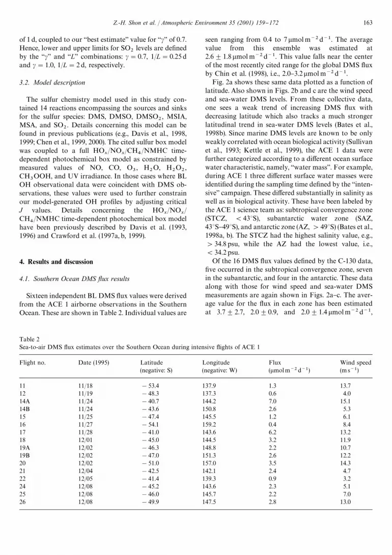
Table 2Sea-to-air DMS #ux estimates over the Southern Ocean during intensive #ights of ACE 1

Flight no. Date (1995) Latitude(negative: S)

Longitude(negative: W)

Flux(lmolm~2d~1)

Wind speed(ms~1)

11 11/18 !53.4 137.9 1.3 13.712 11/19 !48.3 137.3 0.6 4.014A 11/24 !40.7 144.2 7.0 15.114B 11/24 !43.6 150.8 2.6 5.315 11/25 !47.4 145.5 1.2 6.116 11/27 !54.1 159.2 0.4 8.417 11/28 !41.0 143.6 6.2 13.218 12/01 !45.0 144.5 3.2 11.919A 12/02 !46.3 148.8 2.2 10.719B 12/02 !47.0 151.3 2.6 12.220 12/02 !51.0 157.0 3.5 14.321 12/04 !42.5 142.1 2.4 4.722 12/05 !41.4 139.3 0.9 3.224 12/08 !45.2 143.6 2.3 5.125 12/08 !46.0 145.7 2.2 7.026 12/08 !49.9 147.5 2.8 13.0

of 1 d, coupled to our `best estimatea value for `ca of 0.7.Hence, lower and upper limits for SO

2levels are de"ned

by the `ca and `La combinations: c"0.7, 1/L"0.25 dand c"1.0, 1/L"2 d, respectively.

3.2. Model description

The sulfur chemistry model used in this study con-tained 14 reactions encompassing the sources and sinksfor the sulfur species: DMS, DMSO, DMSO

2, MSIA,

MSA, and SO2. Details concerning this model can be

found in previous publications (e.g., Davis et al., 1998,1999; Chen et al., 1999, 2000). The cited sulfur box modelwas coupled to a full HO

x/NO

x/CH

4/NMHC time-

dependent photochemical box model as constrained bymeasured values of NO, CO, O

3, H

2O, H

2O

2,

CH3OOH, and UV irradiance. In those cases where BL

OH observational data were coincident with DMS ob-servations, these values were used to further constrainour model-generated OH pro"les by adjusting criticalJ values. Details concerning the HO

x/NO

x/

CH4/NMHC time-dependent photochemical box model

have been previously described by Davis et al. (1993,1996) and Crawford et al. (1997a, b, 1999).

4. Results and discussion

4.1. Southern Ocean DMS yux results

Sixteen independent BL DMS #ux values were derivedfrom the ACE 1 airborne observations in the SouthernOcean. These are shown in Table 2. Individual values are

seen ranging from 0.4 to 7lmol m~2d~1. The averagevalue from this ensemble was estimated at2.6$1.8lmol m~2d~1. This value falls near the centerof the most recently cited range for the global DMS #uxby Chin et al. (1998), i.e., 2.0}3.2lmol m~2d~1.

Fig. 2a shows these same data plotted as a function oflatitude. Also shown in Figs. 2b and c are the wind speedand sea-water DMS levels. From these collective data,one sees a weak trend of increasing DMS #ux withdecreasing latitude which also tracks a much strongerlatitudinal trend in sea-water DMS levels (Bates et al.,1998b). Since marine DMS levels are known to be onlyweakly correlated with ocean biological activity (Sullivanet al., 1993; Kettle et al., 1999), the ACE 1 data werefurther categorized according to a di!erent ocean surfacewater characteristic, namely, `water massa. For example,during ACE 1 three di!erent surface water masses wereidenti"ed during the sampling time de"ned by the ìnten-sivea campaign. These di!ered substantially in salinity aswell as in biological activity. These have been labeled bythe ACE 1 science team as: subtropical convergence zone(STCZ, (433S), subantarctic water zone (SAZ,433S}493S), and antarctic zone (AZ, '493S) (Bates et al.,1998a, b). The STCZ had the highest salinity value, e.g.,'34.8 psu, while the AZ had the lowest value, i.e.,(34.2 psu.

Of the 16 DMS #ux values de"ned by the C-130 data,"ve occurred in the subtropical convergence zone, sevenin the subantarctic, and four in the antarctic. These dataalong with those for wind speed and sea-water DMSmeasurements are again shown in Figs. 2a}c. The aver-age value for the #ux in each zone has been estimatedat 3.7$2.7, 2.0$0.9, and 2.0$1.4lmolm~2d~1,


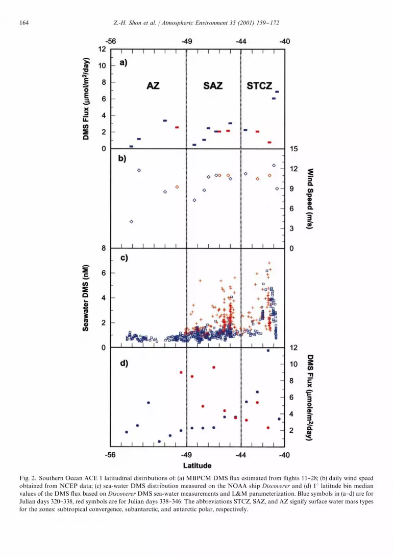
Fig. 2. Southern Ocean ACE 1 latitudinal distributions of: (a) MBPCM DMS #ux estimated from #ights 11}28; (b) daily wind speedobtained from NCEP data; (c) sea-water DMS distribution measured on the NOAA ship Discoverer and (d) 13 latitude bin medianvalues of the DMS #ux based on Discoverer DMS sea-water measurements and L&M parameterization. Blue symbols in (a}d) are forJulian days 320}338, red symbols are for Julian days 338}346. The abbreviations STCZ, SAZ, and AZ signify surface water mass typesfor the zones: subtropical convergence, subantarctic, and antarctic polar, respectively.


respectively. For comparison purposes, the comparableDMS #uxes derived from sea-water measurements areshown in Fig. 2d. In the latter plot we have used theestimated median value for each 13 of latitude by binningall individual values appearing within each degree oflatitude. (Note, the L&M parameterization was used inthis assessment.) For the STCZ, although the trends inNovember and December were similar to those for theaircraft, the average values estimated from the ship dataare seen as being nearly twice as large. This is also seen tobe true for the SAZ. For the AZ, the ship data areprimarily available for only the month of November andthese are seen as reasonably close to those estimatedfrom the aircraft data. Overall, the ship DMS #ux valuesare nearly 2 times higher than those derived from theaircraft observations, or a factor of 3.6 times higher if theparameterization by Wanninkhof (1992) is used. The factthat there is a large di!erence in the average #ux valuesbetween the two di!erent approaches does not necessar-ily extrapolate to there being a systematic di!erence inthe #ux evaluation methods. For example, as statedearlier, the aircraft values were quite limited in number;and, in addition, there can be seen considerable variabil-ity in the DMS #ux as well as a general lack of coordina-tion between many of the ship and aircraft tracks. Thus,it is not totally unreasonable that the two platformsmight have produced this large di!erence. At the sametime one cannot preclude this possibility (see discussionthat follows in Section 4.2).

4.2. Comparison of MBPCM and air}sea gradientyux methods

The air}sea gradient method is currently the mostextensively used method for determining the DMSsea-to-air #ux. Our current global DMS #ux picture ismostly based on values derived from this method. Itrequires both a measurement of sea-water DMS and theevaluation of the sea}air transfer e$ciency factor, i.e.,piston velocity. The piston velocity is believed to bea function of surface wind speed as well as sea-watertemperature. Once evaluated for a speci"c set of me-teorological conditions, more general forms of this`transfer velocitya can be developed via parameteriz-ation equations which take into account the dependencyof the #ux on wind speed. Currently, at least three di!er-ent versions of wind speed parameterization have beenemployed (Smethie et al., 1985; Liss and Merlivat, 1986;Wanninkhof, 1992). In fact, the range of results fromthese di!erent approaches has provided one basis forde"ning the uncertainty in our current estimates for theglobal DMS #ux which is estimated to be as large asa factor of two (Andreae, 1986; Bates et al., 1987; Andreaeand Crutzen, 1997). In the text that follows the sea}airDMS #ux derived from the Liss and Merlivat (e.g.,`Vp(L&M)a) and Wanninkhof parameterizations (e.g.,

`Vp(W)a) are compared to those estimated in this workusing the MBPCM approach.

Detailed #ux comparisons from the ACE 1 observa-tions were made possible as a result of two preplannedencounters between the NCAR C-130 and the NOAAship Discoverer. During both encounters the respectivesampling platforms were positioned at nearly the samelocation at the same time. The "rst of these cases involveddata collected during #ight 15, the second involved #ight22. As shown in Fig. 3a, during #ight 15, BL circularpatterns were #own in the very near vicinity of theDiscoverer's ship track, with two of the sampling circlesactually overlapping the ship track. We have set the areaof comparison to be the latitude range of 46.73S}47.93Swith corresponding longitude coordinates of 144.33E}146.23E. The ship and aircraft DMS #uxes measuredduring this encounter are those shown in Fig. 3b. Fromhere it can be seen that the MBPCM #ux is higher thanthe Vp(L&M) #ux but at some locations overlaps theVp(W) estimate. The average MBPCM #ux is1.2$0.5lmol m~2d~1, with the cited uncertainty re-#ecting the random error estimated from a propagationof error analysis. Values for the ship in the èncounterregiona averaged 0.7$0.08lmolm~2d~1 for Vp(L&M)and 1.2$0.13lmolm~2d~1 for Vp(W), where thestated uncertainties for these two values represent thestandard deviation of the mean (SDOM). Hence, allmethods appear to be consistent within the speci"eduncertainties, but numerically the MBPCM method iscloser to the Vp(W) #ux estimate.

Any further e!ort at a quantitative comparison ofthese #ux methods must re#ect on the fact that theMBPCM #ux method could have potentially been in-#uenced by several systematic errors. One of these couldhave resulted from the presence of a large gradient in thelocal DMS #ux "eld (see, for example, Mari et al., 1998).In the case of #ight 15, for example, an examination ofFig. 3b suggests that the DMS #ux may have been morethan a factor of 2 higher when the Discoverer was atlatitudes (473S. This #ux enhancement could have re-sulted from a combination of elevated sea-water DMSand wind speed increases, as shown in Fig. 3c. Given thewind direction reported, it is also quite possible thatthe C-130 sampled an air mass that originated from thenorthwest (i.e., lower latitudes). Assuming this air masshad equilibrated with the high #ux region and the photo-chemical and meteorological conditions there were sim-ilar to those observed during #ight 15, model simulationssuggest that the MBPCM #ux estimate might have beenshifted to values that were factors of 1.5}2 too high. Iftrue, in this one case the correction would tend to shiftthe estimated MBPCM #ux to values closer to theVp(L&M) estimate.

The second aircraft}ship DMS #ux comparison, #ight22, is shown in Fig. 3d. As before, it is quite apparent thatthere was considerable success in getting the C-130 BL


Fig. 3. ACE 1 #ux intercomparison between C-130 and the ship Discoverer for: (a) #ight track for C-130 #ight 15 } time between twosolid circles de"nes the intercomparison time; (b) DMS #ux based on C-130 #ight 15 data and those from the ship Discoverer } opencircles de"ne #ux values based on Liss and Merlivat (1986) parameterization, "lled circles are those based on Wanninkhof (1992)parameterization; (c) wind speed and sea-water DMS concentrations measured onboard Discoverer; (d) same as (a), but for #ight 22; (e)same as (b), but for #ight 22; and (f) same as (c), but for #ight 22.

#ight pattern to encompass a signi"cant portion ofthe Discoverer's ship track. For this comparison theMBPCM #ux is seen as 0.9$0.3lmolm~2d~1, whilethe average values derived from the ship data forVp(L&M) and Vp(W) are 0.5$0.2 and 1.5$0.3lmolm~2d~1, respectively. As before, the stated uncertaintyfor the MBPCM method represents the propagated errorwhile that for the ship-derived #uxes is de"ned by theSDOM. Although within the combined uncertainties all#uxes appear to be consistent, it is di$cult to ignore thelarge changes that occurred in both the Vp(L&M) andVp(W) #uxes during the encounter period. As shown inFig. 3f, shipboard observations of sea-water DMS appearto have undergone a smaller variation during the en-counter time period than did wind speed. Variations inthe latter parameter most likely are the main cause of thelarge variation in the sea-water DMS #uxes shown in

Fig. 3e. As discussed for #ight 15, the presence of largegradients in the DMS #ux "eld during #ight 22 alsocould have produced a signi"cant bias in the MBPCM#ux estimate. The wind direction measurements suggestthat the sampled air mass could have originated from thenorth. Unfortunately, there were no ship observations tothe north, making it impossible to even estimate the signof this potential error.

4.3. Comparison of MBPCM and TD}BU and DMS/aerosol budget yux approaches

Although it is of great interest to compare sea-water-based #ux determinations with the MBPCM approach, itis of equal importance to know just how well di!erentDMS #ux methodologies agree when all are based onatmospheric observations. In the case of ACE 1, the


Fig. 4. Intercomparison of DMS #ux methods during ACE1 based on atmospheric measurements of DMS: (a) C-130 #ighttracks during the Lagrangian #ight sequence 24, 25 and 26; and(b) DMS #uxes derived from the MBPCM approach and theTD}BU and AB methods.

opportunity for such a comparison arose during Lagran-gian #ight sequence 24, 25, and 26. For these #ightsthe MBPCM #ux was compared with two independentmethods, both reported by Russell et al. (1998).These two independent methods have been labeled bytheir authors top-down/bottom-up (TD}BU) andDMS/aerosol budget (AB). Detailed descriptions of bothapproaches can be found in Russell et al. (1998) andreferences therein. Fig. 4a shows the #ight tracks formissions 24, 25, and 26, while the corresponding #uxestimates are displayed in Fig. 4b. From these plots it canbe seen that with the exception of #ight 26 the MBPCM#uxes generally fall between the TD}BU and DMS/ABmethods. Although not shown, two independent #uxdeterminations, based on sea-water DMS measurements(Suhre et al., 1998; Bates et al., 1998b), gave #ux valuesthat were within a factor of 1.3}2 of the MBPCM ap-proach for #ights 24 and 25. For #ight 26, one methodwas larger by a factor of 2.5, the other by a factor greaterthan 5. Quite clearly, #ight 26 presented problems for allmethods, having a meteorological setting that was farmore complex than for the other two #ights (Wang et al.,

1999). In particular, the MBPCM #ux estimate for #ight26 most likely encompasses additional systematic erroras a result of there being present during the #ight mul-tiple layers of clouds (Davis et al., 2000).

As shown in Table 2, the MBPCM #ux estimates for#ights 24, 25, and 26 are 2.3$0.7, 2.2$0.5, and2.8$1.4lmol m~2d~1, respectively. For #ight 24, theaverage TD}BU #ux is seen as a factor of 2.6 higher thanMBPCM while that estimated from the AB approach isa factor of 1.9 lower. By contrast, for #ight 25, theMBPCM #ux is only 10% higher than the TD}BU #ux,but the AB value is more than a factor of 2 lower. In the"nal #ight, 26, both the TD}BU and AB methods areseen as factors of 2}3.5 higher. The uncertainties asso-ciated with both the TD}BU and AB approaches pre-dominantly re#ect the level of DMS inhomogeneity inthe air mass sampled. Unfortunately, this was a BLproperty that typically was not that well de"ned by thelimited measurements recorded during each #ight. Cur-rent estimates place this as high as a factor of 2. Consid-eration of all three #ights produced a mean value for theMBPCM approach of 2.4$0.5 and for the TD}BU andAB methods values of 5.5$1.3 and 3.0$1.3lmolm~2d~1, respectively. The stated uncertainties re#ect thecalculated SDOM. If restricted to just #ights 24 and 25,the three methods result in #ux values of 2.2$0.4,4.6$1.8, and 1.1$0.4, respectively. Thus, in all casesthe TD}BU method is higher than MBPCM by nearlya factor of two. On the hand, the AB method is somewhathigher when considering all three #ights but is nearlya factor of two lower when examining only #ights 24and 25. It must be reemphasized, however, that all #uxcomparisons during the ACE 1 ìntensivea period werelimited to rather small regions, typically involving signi"-cant gradients. In particular, the TD}BU method is quitesensitive to local gradient conditions, whereas the othertwo methods tend to average conditions over a largerregion. In summary, any conclusions drawn from theACE 1 data should be considered as only suggestive notconclusive.

5. Contribution of DMS oxidation to BL SO2

The contribution of oxidized DMS to the SouthernOcean BL SO

2budget was evaluated by comparing

observed SO2

levels to those derived from model simula-tions. As discussed in Section 3.1, the calculated value forSO

2, [SO

2]DMS

, was computed from Eq. (3). Recall, thisequation describes the mass balance between SO

2forma-

tion from DMS oxidation and its loss via both chemicaland physical processes. As per our earlier discussions, forall 16 BL sampling events in which the DMS #ux wasevaluated, [SO

2]DMS

values were also calculated. Simula-tions were run for our standard case with c"0.7 and1/L"1.0 d; the minimum case with c"0.7 and


Fig. 5. Comparison of observed SO2

with model simulatedvalues during the ACE 1 intensive period. The symbol `qade"nes the overall DMS-to-SO

2conversion e$ciency and q is

the SO2

lifetime. The top and bottom of the vertical lines withineach bar de"ne the upper and lower limit model estimates for themixing ratio of SO

2when produced from DMS. These limits

correspond to c and q values of 1.0 and 2 d versus 0.7 and 0.25d,respectively. The `best estimatea is de"ned by the top of the clearrectangular bars and corresponds to c"0.7 and q"1d. Thetop of the solid rectangular bars de"nes the observed mixingratios for the SO

2.

1/L"0.25d; and the maximum case with c"1.0 and1/L"2.0 d. The results are those shown in Fig. 5. Fromhere it can be seen that for 14 out of 16 runs, the standardcase values of [SO

2]DMS

are equal to or somewhat largerthan those observed. We interpret these results as strong-ly suggestive that DMS oxidation is the dominant sourceof SO

2in the remote Southern Ocean. This conclusion

was also supported by the observation that the BL versusBuL gradient in SO

2was primarily negative or neutral

when data were available for evaluation. It was alsofurther corroborated in a more detailed sulfur budgetanalysis reported by Davis et al. (2000). In the latterstudy, the authors carried out an analysis of the Lagran-gian #ight sequence 23, 24, and 25. In this case a stronganticorrelation was found between DMS and SO

2in

which systematic decreases in DMS were seen followingsunrise and concomitant increases were observed in SO

2.

In a totally independent ship-based study during ACE 1reported by De Bruyn et al. (1998), a similar conclusionwas reached. Finally, Mari et al. (1999), using sea-water-derived DMS #ux values and aircraft SO

2observations,

also arrived at the same conclusion.Quite interestingly, although the results reported

by De Bruyn et al. (1998) qualitatively are in goodagreement with those reported in this work, their `best

estimatea for the value of c was substantially lower,ranging from 0.3 to 0.5. Considering the similarities in thetemperature "eld for both studies as well as in the levelsof critical species like NO, it seems unlikely that the causeof this shift in c would be due to a major shift in the DMSoxidation mechanism for the two sampling platforms.Other possibilities would include: (a) systematic errors ineither the measurement of DMS or SO

2, (b) incorrect

estimates of the OH level, or (c) lack of appropriatecorrections for the e!ects of vertical mixing.

In the study by De Bruyn et al. (1998) the DMS-to-SO

2ratio was the principal basis upon which the value of

c was derived. The median value in their study for thisratio was &8. Corresponding median values for DMSand SO

2were 106 and 13 pptv, respectively. By contrast,

the median DMS : SO2

ratio estimated from the C-130data was &3. This ratio was based on median values forDMS and SO

2of 92 and 35 pptv, respectively.

The ship results of De Bruyn et al. can also be com-pared to the independent detailed sulfur budget study ofDavis et al. (2000), again using C-130 data. The De Bruynet al. study was performed on Julian days 338}340 where-as that by Davis et al. was based on results from theLagrangian B #ight sequence (#ight 24, 25, and 26) cover-ing Julian days 341}343. One of the interesting aspects ofthese two studies is the fact that although each occurredon slightly di!erent days and at a somewhat di!erentgeographical sites in the Southern Ocean, both arrived ata similar average value for the estimated lifetime for SO

2,

i.e., 12}14h (Davis et al., 2000), and 8}16h (De Bruyn etal., 1998). However, in contrast to the SO

2lifetime "nd-

ings, these two studies derived quite di!erent values for c.Davis et al. evaluated c at 0.7}0.9 as compared with thepreviously cited results of De Bruyn et al. of 0.3}0.5.Recall, the latter c value range is also similar to thatdiscussed earlier in the text involving the tropicalDMS}SO

2data reported by Yvon and Saltzman (1996).

Yvon and Saltzman's c values were also noted to besigni"cantly lower than those derived by Davis et al.(1999) and Chen et al. (2000) (e.g., 0.27}0.54 versus0.65$0.15) which also involved a tropical environment.

Of interest in each of the above studies is the questionwhether signi"cant di!erences existed in the respectivechemical and physical environments and what possibledi!erences existed in the types of instrumentation used tomake the sulfur observations. Possible di!erences in thevertical mixing properties of each BL environment areclearly one of the most di$cult issues to evaluate. Forexample, only in the case of the two airborne studiesreported by Davis et al. were vertical observations ofchemical and meteorological parameters su$cientlycomplete to evaluate the role of vertical mixing. Thus,one clearly cannot rule out the possibility that this wasa contributing factor in de"ning some of the di!erencesreported in c. Possible di!erences in the respective chem-ical environments can be more easily assessed. In the case


of NO levels, for example, observations recorded in therespective tropical and Southern Ocean environmentssuggest that in all cases the di!erences were quite small.(Note, signi"cant di!erences in the level of NO can bea basis for arguing that the DMS oxidation mechanismmight have been di!erent for the two studies even thoughthey took place in the same geographical region.) Asrelated to di!erences in the diurnal averaged OH level foreach study, an assessment of this critical quantity usinga common photochemical model, based on actual photo-chemical observational data recorded at each site orplatform, has revealed that for the tropical studies theYvon and Saltzman study produced the lowest value by&20% whereas for the Southern Ocean studies DeBruyn et al's study was &21% higher than that esti-mated at the site analyzed by Davis. Thus, these resultsdo not seem to provide a simple answer to the di!erencein the previously cited c values.

The third and "nal possibility listed above, namely,di!erences in the sulfur measuring instrumentation isaddressed in the text that follows. In this context it isworth noting that in the two case studies in the SouthernOcean (e.g., De Bruyn et al.'s results and those reportedby Davis et al. (2000)), the ratio of the median values ofmeasured DMS from the two studies was 1.05; however,that for SO

2was 2.2. As noted earlier, the di!erence in

the average level of OH for the two studies reduces theabove discrepancy slightly, but clearly is not the wholeanswer. Regarding the instrumentation employed, thatfor measuring DMS had much commonality in that bothwere GC based. Furthermore, both have previously beeninvolved in a common DMS "eld intercomparison study,the NASA CITE-3 program. This program compared sixdi!erent DMS techniques. Drexel "elded an isotopic-dilution gas-chromatography mass-spectrometric (ID-GC/MS) technique and U. Miami employed a gaschromatography-#ame photometric detection system.(Note, these same systems have been used in all studiesunder discussion.) The intercomparison was carried outo! the northeast coast of the USA and o! the easterncoast of Brazil (Gregory et al., 1993). The conclusionfrom this double-blind airborne intercomparison wasthat àlla methods were without any major systematicerrors and that even at DMS levels (50 pptv this spe-cies could be measured to within a few pptv.

Concerning the SO2

measurements, in the De Bruynet al. and Yvon and Saltzman's studies the HPLC/Fluorescence method was employed. In all analysisreported by Davis et al. and Chen et al., the SO

2data

were those recorded by Bandy and co-workers using theID-GC/MS method. The only SO

2intercomparison in-

volving both Drexel's ID-GC/MS and the U. Miami'sFluorescence}HPLC instrument was that carried out atLewes, Delaware (Stecher et al., 1997). Among the"ndings that can be extracted from this ground-basedstudy (i.e., GASIE } Gas Phase Sulfur Intercomparison

Experiment) are the following: (1) the ID-GC/MS andHPLC/Fluorescence instruments di!ered by &27% intheir measurement of a standard SO

2calibration source,

the ID-GC/MS system giving the higher reading; and(2) even with normalization of all data to account for thiscalibration di!erence, the ID-GC/MS system typicallywas found to measure 15}20% higher than theHPLC/Fluorescence instrument when measuring dilutedambient air samples. The resulting collective errorshowed up during many of the individual samplingperiods involving diluted ambient air samples with mix-ing ratios of less than 200 pptv. This di!erence was fre-quently as high as factors of 1.4}1.5.

Given the limited information available, we can drawno "nal conclusions concerning the accuracy of each ofthese measurement systems. However, the intercom-parison results would seem to suggest that there might bea signi"cant systematic di!erence between measurementsrecorded on these two di!erent systems when in the "eld.

6. Summary and conclusion

The MBPCM approach was used here to evaluatesea-to-air DMS #uxes for the Southern Ocean. Theseevaluations were based on 18 airborne #ights (i.e., #ights11}28) #own during the ACE 1 "eld study in Novemberand December 1995. From these 18 #ights, 16 indepen-dent BL DMS #ux values were de"ned. The latituderange covered by these was 553S}403S and encompassedthe #ux range of 0.4}7.0lmolm~2d~1. The averagevalue was 2.6$1.8lmolm~2d~1. For the same timeperiod, the average value derived from all sea-watermeasurements was approximately a factor of 2 larger,based on the L&M parameterization, or a factor of3 when using W's parameterization. That they coulddi!er by this amount is not totally unreasonable consid-ering the fact that a wide range of DMS #uxes presentedthemselves during the Southern Ocean study and that theDiscoverer's sampling track was frequently nonalignedwith that of the C-130's. Obviously, one can also not ruleout the possibility that there could have been a funda-mental di!erence in the techniques employed for estima-ting the #uxes.

E!orts to compare the MBPCM #ux method withother airborne-based approaches resulted in our "ndingsome cases which showed reasonably good agreementand other cases that were in signi"cant disagreement.Thus, we believe it would be premature at this time todraw any "nal conclusions from this intercomparison. Toa very large degree, these results re#ect the fact that thenumber of detailed comparisons was small, and thatthe conditions under which the comparisons were madewere far from ideal.

A major result from this study was the conclusion thatDMS oxidation is a major source of BL SO

2in the


Southern Ocean, in agreement with other ACE 1 investi-gators. Assuming that the sole source of reduced sulfur isDMS, our simulations suggest that, on average, the con-version of DMS to SO

2occurs with an e$ciency of

&0.7, given an assumed lifetime for SO2

of &1 d. On atleast one occasion, during the second ACE 1 Lagrangian,observations were recorded under nighttime conditionswhich led to a direct determination of the SO

2lifetime of

12}14h. Although meteorological and chemical condi-tions during Lagrangian B were not typical of the ACE1 "eld program overall, they still provided a basis forcomparison with an independent study on the ship Dis-coverer. This comparison revealed that although bothstudies point toward DMS as a major source of SO

2,

each arrived at a quite di!erent estimate for the DMS-to-SO

2conversion e$ciency (e.g., 0.3}0.5 versus 0.7}0.9).

It was further noted that a similar di!erence in c (SO2)

resulted when independent tropical studies (involvingtwo di!erent SO

2instruments) were compared. Al-

though yet unknown factors may still be involved whichare responsible for the di!erences noted in the conversione$ciency, the evidence now available suggests that thisdi!erence may be at least partially tied to systematicdi!erences in the SO

2calibrations and measurements. At

this time there is no basis for selecting one measurementover the other. It would seem prudent, however, to rec-ommend that a further e!ort be made to examine thisissue in that the results could have a major impact on ourinterpretation of the DMS oxidation mechanism. It isalso recommended that a further e!ort be made at inter-comparing the MBPCM #ux approach with the air-to-sea gradient as well as other #ux methods under morefavorable conditions. The location for the latter studyshould be one where the meteorology is relatively stable,DMS lifetimes are short, and the DMS #ux "eld isreasonably uniform. One such possibility would be thetrade wind regime in the central tropical Paci"c.

Acknowledgements

The authors D. Davis and G. Chen would like toacknowledge the partial support of this research by theNational Science Foundation under grant ATM-9617378. They would also like to thank Drs. Don Len-schow, Tim Bates, and Q. Wang for many informativediscussions. This research is a contribution to the Inter-national Global Atmospheric Chemistry (IGAC) CoreProject of the International Geosphere}Biosphere Pro-gram (IGBP) and is part of the IGAC Aerosol Character-ization Experiments (ACE).

References

Andreae, M.O., 1986. The ocean as a source of atmosphericsulfur compounds. In: Buat-Menard, P. (Ed.), The Role

of Air Sea Exchange in Geochemical Cycling. Reidel, D.,Netherlands, pp. 331}362.

Andreae, M.O., Raemdonck, H., 1983. Dimethyl sul"de in thesurface ocean and the marine atmosphere: a global view.Science 221, 744}747.

Andreae, M.O., Crutzen, P.J., 1997. Atmospheric aerosol: bio-geochemical sources and role in atmospheric chemistry.Science 276, 1052}1058.

Ayers, G.P., Cainey, J.M., Gillett, R.W., Saltzman, E.S., Hooper,M., 1997. Sulfur dioxide and dimethyl sul"de in marine air atCape Grim, Tasmania. Tellus B 49, 292}299.

Bandy, A.R., Scott, D.L., Blomquist, B.W., Chen, S.W., Thor-nton, D.C., 1992. Low yields of SO

2from dimethyl sul"de

oxidation in the marine boundary layer. GeophysicalResearch Letters 19, 1125}1127.

Bandy, A.R., Thornton, D.C., Driedger III, A.R., 1993. Airbornemeasurements of sulfur dioxide, dimethyl sul"de, carbondisul"de, and carbonyl sul"de by isotope dilution gaschromatography/mass spectrometry. Journal of Geophysi-cal Research 98, 23423}23433.

Bandy, A.R., Thornton, D.C., Blomquist, B.W., Chen, S., Wade,T.P., Ianni, J.C., Mitchell, G.M., Nadler, W., 1996. Chemistryof dimethyl sul"de in the equatorial Paci"c atmosphere.Geophysical Research Letters 23, 741}744.

Bates, T.S., Cline, J.D., Gammon, R.H., Kelly-Hansen, S.R.,1987. Regional and seasonal variations in the #ux of oceanicdimethylsul"de to the atmosphere. Journal of GeophysicalResearch 92, 2930}2938.

Bates, T.S., Huebert, B.J., Gras, J.L., Gri$ths, F.B., Durkee,P.A., 1998a. International Global Atmospheric Chemistry(IGAC) Project's First Aerosol Characterization Experiment(ACE 1): overview. Journal of Geophysical Research 103,16297}16318.

Bates, T.S., Kapustin, V.N., Quinn, P.K., Covert, D.S., Co!man,D.J., Mari, C., Durkee, P.A., De Bruyn, W.J., Saltzman, E.S.,1998b. Processes controlling the distribution of aerosol par-ticles in the lower marine boundary layer during the FirstAerosol Characterization Experiment (ACE 1). Journal ofGeophysical Research 103, 16369}16383.

Berresheim, H., Wine, P., Davis, D., 1995. Sulfur in the atmo-sphere. In: Singh, H.B. (Ed.), Composition, Chemistry, andClimate of the Atmosphere. Van Nostrand Reinhold, NewYork, pp. 251}307.

Bonsang, B., Nguyen, B.C., Lambert, G., 1987. Comment on`The Residence Time of Aerosols and SO

2in the Long-

Range Transport over the Oceana by Ito et al. Journal ofAtmospheric Chemistry 5, 367}369.

Businger, S., Johnson, R., Katzfey, J., Siems, S., Wang, Q.,1999. Smart tetroons for Lagrangian air}mass tracking dur-ing ACE 1. Journal of Geophysical Research 104,11709}11722.

Charlson, R.J., Lovelock, J.E., Andreae, M.O., Warren, S.G.,1987. Oceanic phytoplankton, atmospheric sulphur, cloudalbedo and climate. Nature 326, 655}661.

Chen, G., Davis, D., Kasibhatla, P., Bandy, A., Thornton, D.,Huebert, B.J., Clarke, A.D., 1999. A photochemical assess-ment of DMS sea-to-air #ux as inferred from PEM-WestA and B observations. Journal of Geophysical Research 104,5471}5482.

Chen, G., Davis, D. D., Kasibhatla, P., Bandy, A. R., Thornton,D. C., Huebert, B. J., Clarke, A. D., 2000. A study of DMS


oxidation in the tropics: comparison of Christmas Island"eld observations of DMS, SO

2, and DMSO with model

simulations. Journal of Geophysical Research, in press.Chin, M., Rood, R.B., Allen, D.J., Andreae, M.O., Thompson,

A.M., Lin, S.J., Atlas, R.M., Ardizzone, J.V., 1998. Processescontrolling dimethylsul"de over the ocean: case studies usinga 3-D model driven by assimilated meteorological "elds.Journal of Geophysical Research 103, 8341}8353.

Crawford, J.H., et al., 1997a. An assessment of ozone photo-chemistry in the extratropical western north Paci"c: impactof continental out#ow during the late winter/earlier spring.Journal of Geophysical Research 102, 28469}28488.

Crawford, J.H., et al., 1997b. Implications of large scale shifts intropospheric NO

xlevels in the remote tropical Paci"c. Jour-

nal of Geophysical Research 102, 28447}28468.Crawford, J.H., et al., 1999. Assessment of upper tropospheric

HOx

sources over the tropical Paci"c based on NASAGTE/PEM data: net e!ect on HO

xand other photochemical

parameters. Journal of Geophysical Research 104,16255}16273.

Davis, D.D., et al., 1993. Photostationary state analysis of theNO

2}NO system based on airborne observations from the

subtropical/tropical North and South Atlantic. Journal ofGeophysical Research 98, 23501}23523.

Davis, D.D., et al., 1996. Assessment of the ozone photochemis-try tendency in the western North Paci"c as inferred fromPEM-West A observations during the fall of 1991. Journal ofGeophysical Research 101, 2111}2134.

Davis, D.D., Chen, G., Kasibhatla, P., Je!erson, A., Tanner, D.,Eisele, F., Lenschow, D., Ne!, W., Berresheim, H., 1998.DMS oxidation in the Antarctic marine boundary layer:comparison of model simulations and "eld observations ofDMS, DMSO, DMSO

2, H

2SO

4(g), MSA(g), and MSA(p).

Journal of Geophysical Research 103, 1657}1678.Davis, D.D., Chen, G., Bandy, A., Thornton, D., Eisele, F.,

Mauldin, L., Tanner, D., Lenschow, D., Huebert, B.,Heath, J., Clarke, A., Blake, D., 1999. DMS oxidation inthe equatorial Paci"c: comparison of model simulationswith "eld observations for DMS, SO

2, H

2SO

4(g), MSA(g),

MS, and NSS. Journal of Geophysical Research 104,5675}5784.

Davis, D.D., Chen, G., Shon, Z., Bandy, A., Thornton, D., Eisele,F., Mauldin, L., Tanner, D., Huebert, B., Clarke, A., 2000.A boundary layer sulfur budget analysis of the SouthernOcean during late spring. Geophysical Research Letters, inpreparation.

Davison, B., Hewitt, C.N., 1992. Natural sulfur speciesfrom the north Atlantic and their contribution to the UnitedKingdom sulfur budget. Journal of Geophysical Research97, 2475.

De Bruyn, W.J., Bates, T.S., Cainey, J.M., Saltzman, E.S., 1998.Shipboard measurements of dimethyl sul"de and SO

2south-

west of Tasmania during the First Aerosol CharacterizationExperiment (ACE 1). Journal of Geophysical Research 103,16703}16711.

Gregory, G., Warren, L.S., Davis, D.D., Andreae, M.O., Bandy,A.R., Ferek, R.J., Johnson, J.E., Saltzman, E.S., Cooper, D.J.,1993. An intercomparison of instrumentation for tropos-pheric measurements of dimethyl sul"de: aircraft results forconcentrations at the parts-per-trillion level. Journal of Geo-physical Research 98, 23373}23388.

Grodzinsky et al., 2000. DMS #uxes during PEM-Tropics A:calculations based on the mass balance/photochemicalmodel (MBPCM) approach, in preparation.

Huebert, B.J., et al., 1993. Observations of the atmosphericsulfur cycle on SAGA-3. Journal of Geophysical Research98, 16985}16996.

Hynes, A.J., Wine, P.H., Semmes, D.H., 1986. Kinetics andmechanism of OH reactions with organic sul"des. Journal ofPhysical Chemistry 90, 4148}4156.

Kettle, A.J., et al., 1999. A global database of sea surfacedimethylsul"de (DMS) measurements and a procedure topredict sea surface DMS as a function of latitude, longitude,and month. Global Biogeochemical Cyccles 13, 399}444.

Liss, P.S., Merlivat, L., 1986. Air}sea gas exchange rates: intro-duction and synthesis. In: Buat-MeH nard, P. (Ed.), The Role ofAir}Sea Exchange in Geochemical Cycling. D. Reidel, Nor-well, MA, pp. 113}127.

Mari, C., Suhre, K., Bates, T.S., Johnson, J.E., Rosset, R., Bandy,A.R., Eisele, F.L., Mauldin, R.L., Thornton, D.C., 1998.Physico-chemical modeling of the First Aerosol Character-ization Experiment (ACE 1) Lagrangian B, 2. DMS emission,transport and oxidation at the mesoscale. Journal of Geo-physical Research 103, 16457}16473.

Mari, C., Suhre, K., Rosset, R., Bates, T., Huebert, B., Bandy, A.,Thornton, D., Businger, S., 1999. One}dimensional modelingof sulfur species during the First Aerosol CharacterizationExperiment (ACE 1) Lagrangian. Journal of GeophysicalResearch 104, 21733}21749.

Putaud, J.-P., Mihalopoulos, N., Nguyen, B.C., Campin, J.M.,Belviso, S., 1992. Seasonal variations of atmospheric sulfurdioxide and dimethyl-sul"de concentrations at AmsterdamIsland in the Southern Indian Ocean. Journal of Atmo-spheric Chemistry 15, 117}131.

Russell, L.M., Lenschow, D.H., Laursen, K.K., Krummel, P.B.,Siems, S.T., Bandy, A.R., Thornton, D.C., Bates, T.S., 1998.Bidirectional mixing in an ACE- marine boundary layeroverlain by a second turbulent layer. Journal of GeophysicalResearch 103, 16411}16432.

Saltzman, E.S., Cooper, W.J., 1989. Dimethyl sul"de and hy-drogen sul"de in marine air. In: Biogenic Sulfur in theEnvironment, ACS Symposium Series, American ChemistrySociety, Washington DC. Vol. 393, pp. 330}351.

Singh, H.B., et al., 1996. Low ozone in the marine boundarylayer of the tropical Paci"c Ocean: photochemical loss,chlorine atoms, and entrainment, in Paci"c ExploratoryMission-West, Phase A. Journal of Geophysical Research101, 1907}1917.

Smethie Jr., W.M., Takahashi, T., Chipman, D.W., Ledwell, J.R.,1985. Gas exchange and CO

2#ux in the tropical Atlantic

Ocean determined from 222Rn and pCO2

measurements.Journal of Geophysical Research 90, 7005}7022.

Stecher III, H.A. et al., 1997. Results of the gas-phase sulfurintercomparison experiment (GASIE): overview of experi-mental setup, results and general conclusions. Journal ofGeophysical Research 102, 16219}16236.

Suhre, K., et al., 1998. Physico-chemical modeling of ACE-1Lagrangian B. 1. A moving column approach. Journal ofGeophysical Research 103, 16433}16456.

Sullivan, C.W., Arrigo, K.R., McClain, C.R., 1993. Distributionof phytoplankton blooms in the Southern Ocean. Science262, 1832}1837.


Thompson, A.M., Esaias, W.E., Iverson, R.L., 1990. Twoapproaches to determining the sea-to-air #ux of dimethylsul"de-satellite ocean color and a photochemical model withatmospheric measurements. Journal of Geophysical Re-search 95, 551}558.

Thompson, A.M., et al., 1993. Ozone observations and a modelof marine boundary layer photo-chemistry during SAGA 3.Journal of Geophysical Research 98, 16955}16968.

Wang, Q., et al., 1999. Characteristics of the marine boundarylayers during two lagrangian measurement periods. Part I:general conditions and mean characteristics. Journal of Geo-physical Research 104, 21751}21765.

Wanninkhof, R., 1992. Relationship between wind speed and gasexchange over the ocean. Journal of Geophysical Research97, 7373}7382.

Wine, P.H., Kreutter, N.M., Gump, C.A., Ravishankara, A.R.,1981. Kinetics of OH reactions with the atmospheric sulfurcompounds H

2S, CH

3SH, CH

3SCH

3, and CH

3SSCH

3.

Journal of Physical Chemistry 85, 2660}2665.Yvon, S.A., Saltzman, E.S., 1996. Atmospheric sulfur

cycling in the tropical Paci"c marine boundary layer (123S,1353W): a comparison of "eld data and model results 2.Sulfur dioxide. Journal of Geophysical Research 101,6911}6918.


Documents

Evaluation of the DMS flux and its conversion to SO2 over the southern ocean