Embed Size (px)
Citation preview
Originaldokument gespeichert auf dem Dokumentenserver der Universität Basel edoc.unibas.ch
Evolutionary community ecology in the
cichlid species-flock of the East African
Lake Tanganyika
Inauguraldissertation
zur
Erlangung der Würde eines Doktors der Philosophie
vorgelegt der
Philosophisch-Naturwissenschaftlichen Fakultät
der Universität Basel
von
Lukas Benedikt Widmer
aus Mosnang (SG), Schweiz
Basel, 2021

Genehmigt von der Philosophisch-Naturwissenschaftlichen Fakultät
auf Antrag von
Prof. Dr. Walter Salzburger Prof. Dr. Christian Sturmbauer Zoologisches Institut, Universität Basel Institut für Biologie/Bereich Zoologie, Universität Graz
Basel, den 23.04.2019
Prof. Dr. Martin Spiess (Dekan, Philosophisch-Naturwissenschaftliche Fakultät, Universität Basel)


Table of Contents
Introduction ............................................................................................................................................ 7
Part One: Methodology ..................................................................................................................... 15
Chapter 1: Point-Combination Transect (PCT): Incorporation of small
underwater cameras to study fish communities ...................................................................... 17
1.1. Manuscript ........................................................................................................................ 19
1.2. Supplementary Information ............................................................................................ 31
Chapter 2:Does eDNA within sediments reflect local cichlid assemblages in Lake
Tanganyika? .................................................................................................................................... 47
2.1. Draft manuscript ............................................................................................................... 49
2.2. Supplementary Information ............................................................................................ 71
Part Two: Evolutionary Community Ecology ................................................................................. 79
Chapter 3: Community assembly patterns and niche evolution in the species-flock of
cichlid fishes from East African Lake Tanganyika .................................................................... 81
3.1. Manuscript ........................................................................................................................ 83
3.2. Supplementary Information .......................................................................................... 111
Chapter 4: Where Am I? Niche constraints due to morphological specialisation of two
Tanganyikan cichlid species ....................................................................................................... 143
4.1. Manuscript ...................................................................................................................... 145
4.2. Supplementary Information .......................................................................................... 155
Discussion .......................................................................................................................................... 169
Acknowledgements .......................................................................................................................... 177
Curriculum Vitae ............................................................................................................................... 181

Introduction
Water, a main source of all life on earth – covers over two thirds of our planets’ surface, yet
contains the most unexplored ecosystems (Webb, Vanden Berghe, & O’Dor, 2010). It is little
wonder that scientist around the globe are fascinated by the unknown that lies within the
depth of the blue world. Fresh waters such as rivers and lakes make up only a fraction, namely
0.01% of surface waters, still, a fourth of our planet’s aquatic biodiversity is found in
freshwater (Grosberg, Vermeij, & Wainwright, 2012). Although this is the equivalent to ‘only’
about 5% of the global biodiversity, we find therein an extraordinary variation of life forms.
“Almost every major mammalian clade has at least one transition event going back in the
water, except the primates. Then again, Homo sapiens is hairless and with a fatty layer beneath
the skin, traits often associated with living in water”
Prof. Dr. Heinrich Reichert, University of Basel
This particular statement made during my Bachelor degree, though meant as an amusing
anecdote rather than a scientific hypothesis, fanned my already kindling fascination with the
diversity and adaptation of life in the aquatic environment.
Since Darwin formulated his ‘mystery of mysteries’ of the origin of species (Darwin, 1859),
evolutionary biologist have been trying to solve his riddle and understand how and why
diversity of life emerged (e.g. Nosil, 2012). Darwin postulated the theory of natural selection
based on, among others, his study of the finches on Galapagos, which since then have been
studied extensively (Snow & Grant, 2006; Han et al., 2017). Speciation through natural
selection can be categorised into two general ways, either mutation-order or ecological driven
speciation. Ecological speciation, where divergent selection is driven by diverging
environmental conditions is thought by many to be a key trigger of speciation; it is, however, a
hotly debated topic, whether ecological speciation in itself can truly be a major force for
diversification of species (Schluter, 2000; Nosil, 2012). This is especially true in the case of
adaptive radiations – that is rapidly diversifying lineages that exploit a variety of habitats and
differ in traits to exploit these different niches, such as the Darwin finches or the Anolis Lizards
found in the Caribbean (Losos, 1990; Losos, Jackman, Larson, de Queiroz, & Rodriguez-
Schettino, 1998; Hertz et al., 2013).
Within teleost fish, the family Cichlidae sticks out because of particularly fast (‘explosive’)
speciation events bringing forth approximately 3’000-4’000 species (Turner, Seehausen,
Knight, Allender, & Robinson, 2001; Salzburger, 2018). This massive diversity makes Cichlidae
the champion of species-richness within the vertebrates (Sturmbauer, Husemann, & Danley,
2011; Berner & Salzburger, 2015). In particular, the enigmatic cichlids species-flock of the East
African Great Lakes exhibit diversity in morphology, behaviour, and ecology that is unrivalled,
making these a prime example of an adaptive radiation (Salzburger, 2018). The oldest of these,
Lake Tanganyika is home to approximately 250 endemic cichlid species belonging to 14
different lineages so-called tribes. Members of these lineages have diversified to occupy a
wide variety of habitats in the lake, but not in an equal manner. To better understand the
influence of the environment on the diversification within lineages, researchers began to
include ecological niche modelling (ENM) into the framework of phylogenetic studies on other
radiations (Knouft, Losos, Glor, & Kolbe, 2006; García-Navas & Westerman, 2018). Using ENM
can give us a better insight into the ecological niche of different species and how their niches
overlap. Considering that we seldom observe the fundamental niche, but rather the realized
niche; we should not rely solely on the information gained through the environmental
variables, but consider the community structure and co-occurrence patterns, as they influence
niche occupancy as well. Taking this into account, the information gained could help our

understanding of the underlying processes of speciation; as the ecological niche that is
occupied by a species will have had an apparent influence on the evolution of its
morphological, physiological or behaviour traits; so, the diversification of the niche can be
studied to understand the evolution of species diversity (Ackerly, Schwilk, & Webb, 2006;
Knouft et al., 2006).
To be able to study the cichlid community in its entirety we first had to develop a solid
approach to get reliable census data. In the first part of my thesis I tackled this challenge. In
Chapter 1 (‘Point-Combination Transect (PCT): Incorporation of small underwater cameras to
study fish communities’) we present a novel approach of a non-invasive method to study
underwater communities based on the use of small digital cameras together with a critical
assessment of its strength and flaws, including a comparison to long established underwater
visual census methods (UVC). Another approach to study and monitor natural communities is
the integration of genetic methods such as the use of environmental DNA (eDNA). Chapter 2
(‘Does eDNA within sediments reflect local cichlid assemblages in Lake Tanganyika?’) explores
the applicability of eDNA, particularly found in the sediment, being used to assess the cichlids
fish diversity at various sites at Lake Tanganyika. Compared with carefully compiled PCT data
following the methodology presented in Chapter 1, we compiled an ideal data set for proof of
concept of PCT and discuss the validity of eDNA as a tool for future community assessments
in cichlids.
In Part Two, with the robust methodology introduced in Chapter 1, we address questions
concerning the community structure and niche evolution of the adaptive radiation of
Tanganyikan cichlids in Chapter 3 (‘Community assembly patterns and niche evolution in the
species-flock of cichlid fishes from East African Lake Tanganyika’). In this Chapter, we describe
the extensive fieldwork and visual census survey we conducted at Lake Tanganyika and
analyse the community structure and patterns of assembly for the cichlid species-flock. Using
ecological niche modelling and the resulting niche overlap as a proxy, I explore the difference
between the tribes and their implication for the radiation of lineages. Lastly, using phylogenetic
tools, we reconstructed the niche tolerance of 94 cichlid species to study the evolution of the
niche within the adaptive radiation.
In my last chapter, Chapter 4 (‘Where Am I? Niche constraints due to morphological
specialisation of two Tanganyikan cichlid species’), we used reciprocal transplant experiments
in a semi-natural environment to examine how the performance of distinctly different species
is influenced when they are displaced from their natural niche into a “foreign” habitat. The
focus lies on the capacity to deal with a new environment by studying survival, growth and
phenotypic plasticity of the lower pharyngeal jaw (LPJ), a trophic structure used by cichlids for
mastication (Liem, 1973).
In summary, my thesis is structured into two parts, each containing two manuscripts. The first
part focuses on defining and thoroughly validating a new methodology to collect reliable
census data of the cichlid species-flock of Lake Tanganyika. The second part focuses on the
community structure and assembly patterns of the cichlids along the Zambian and Tanzanian
coast. Followed lastly by an examination of niche evolution, through the use of ecological niche
models (ENM) that are based on the cichlid census and environmental data collected during my
thesis.
References
Ackerly, D. D., Schwilk, D. W., & Webb, C. O. (2006). Niche evolution and adaptive radiation:
Testing the order of trait divergence. Ecology, 87(7 SUPPL.), 50–61. doi:10.1890/0012-
9658(2006)87[50:NEAART]2.0.CO;2
Berner, D., & Salzburger, W. (2015). The genomics of organismal diversification illuminated by
adaptive radiations. Trends in Genetics, 31(9), 491–499. doi:10.1016/j.tig.2015.07.002
Darwin, C. (1859). On the Origin of Species by Means of Natural Selection. D. Appleton and
Company. doi:10.1007/s11664-006-0098-9
García-Navas, V., & Westerman, M. (2018). Niche conservatism and phylogenetic clustering in
a tribe of arid-adapted marsupial mice, the Sminthopsini. Journal of Evolutionary Biology,
31(8), 1204–1215. doi:10.1111/jeb.13297
Grosberg, R. K., Vermeij, G. J., & Wainwright, P. C. (2012). Biodiversity in water and on land.
Current Biology, 22(21), R900–R903. doi:10.1016/j.cub.2012.09.050
Han, F., Lamichhaney, S., Rosemary Grant, B., Grant, P. R., Andersson, L., & Webster, M. T.
(2017). Gene flow, ancient polymorphism, and ecological adaptation shape the genomic
landscape of divergence among Darwin’s finches. Genome Research, 27(6), 1004–1015.
doi:10.1101/gr.212522.116
Hertz, P. E., Arima, Y., Harrison, A., Huey, R. B., Losos, J. B., & Glor, R. E. (2013). Asynchronous
Evolution Of Physiology And Morphology In Anolis Lizards. Evolution, 67(7), 2101–2113.
doi:10.1111/evo.12072
Knouft, J. H., Losos, J. B., Glor, R. E., & Kolbe, J. J. (2006). Phylogenetic analysis of the
evolution of the niche in lizards of the Anolis sagrei group. Ecology, 87, S29-38.
Liem, K. F. (1973). Evolutionary Strategies and Morphological Innovations: Cichlid Pharyngeal
Jaws. Systematic Zoology, 22(4), 425. doi:10.2307/2412950
Losos, J. B. (1990). A Phylogenetic Analysis of Character Displacement in Caribbean Anolis
Lizards. Evolution, 44(3), 558. doi:10.2307/2409435
Losos, J. B., Jackman, T. R., Larson, A., de Queiroz, K., & Rodriguez-Schettino, L. (1998).
Contingency and determinism in replicated adaptive radiations of island lizards. Science,
279(5359), 2115–2118. doi:10.1126/science.279.5359.2115
Nosil, P. (2012). Ecological Speciation. Oxford University Press.
doi:10.1093/acprof:osobl/9780199587100.001.0001
Salzburger, W. (2018). Understanding explosive diversification through cichlid fish genomics.
Nature Reviews Genetics. doi:10.1038/s41576-018-0043-9
Schluter, D. (2000). The Ecology of Adaptive Radiation. Oxford Series in Ecology and Evolution.
doi:10.2307/3558417
Snow, D. W., & Grant, P. R. (2006). Ecology and Evolution of Darwin’s Finches. The Journal of
Animal Ecology. doi:10.2307/4785
Sturmbauer, C., Husemann, M., & Danley, P. D. (2011). Explosive Speciation and Adaptive
Radiation of East African Cichlid Fishes. In Biodiversity Hotspots (pp. 333–362). Berlin,
Heidelberg: Springer Berlin Heidelberg. doi:10.1007/978-3-642-20992-5_18
Turner, G. F., Seehausen, O., Knight, M. E., Allender, C. J., & Robinson, R. L. (2001). How many
species of cichlid fishes are there in African lakes? Molecular Ecology, 10(3), 793–806.
Retrieved from http://www.ncbi.nlm.nih.gov/pubmed/11298988
Webb, T. J., Vanden Berghe, E., & O’Dor, R. (2010). Biodiversity’s Big Wet Secret: The Global
Distribution of Marine Biological Records Reveals Chronic Under-Exploration of the Deep
Pelagic Ocean. PLoS ONE, 5(8), e10223. doi:10.1371/journal.pone.0010223


Part One
Methodology

Chapter 1
Point-Combination Transect (PCT):
Incorporation of small underwater cameras to
study fish communities
Widmer L, Heule E, Colombo M, Rueegg A, Indermaur A, Ronco F, Salzburger W
Methods in Ecology and Evolution (2019)
DOI: 10.1111/2041-210X.13163
1.1 Manuscript pages 19 – 29
1.2 Supplementary Information pages 31 - 46

Methods Ecol Evol. 2019;1–11. wileyonlinelibrary.com/journal/mee3 | 1
1 | INTRODUCTION
Underwater visual census (UVC) methods such as line transect (Brock, 1954) or point count observation (Samoilys & Carlos, 1992,
2000) are widely applied in ecology and, today, represent a standard approach for the non- invasive assessment of underwater communi-ties, particularly of fish. In order to obtain UVC data the observation is typically performed directly by SCUBA divers (or snorkelers), who
Received:11August2018 | Accepted:22January2019DOI: 10.1111/2041-210X.13163
R E S E A R C H A R T I C L E
Point-CombinationTransect(PCT):Incorporationofsmallunderwatercamerastostudyfishcommunities
LukasWidmer |EliaHeule |MarcoColombo |AttilaRueegg |AdrianIndermaur | FabriziaRonco |WalterSalzburger
Department of Environmental Sciences, Zoological Institute, University of Basel, Basel, Switzerland
CorrespondenceLukas WidmerEmail: [email protected] and Walter Salzburger Email: [email protected]
FundinginformationH2020 European Research Council, Grant/Award Number: 617585; European Research Council
Handling Editor: Chris Sutherland
Abstract1. Available underwater visual census (UVC) methods such as line transects or point
count observations are widely used to obtain community data of underwater spe-cies assemblages, despite their known pit-falls. As interest in the community structure of aquatic life is growing, there is need for more standardized and repli-cable methods for acquiring underwater census data.
2. Here, we propose a novel approach, Point-Combination Transect (PCT), which makes use of automated image recording by small digital cameras to eliminate ob-server and identification biases associated with available UVC methods. We con-ducted a pilot study at Lake Tanganyika, demonstrating the applicability of PCT on a taxonomically and phenotypically highly diverse assemblage of fishes, the Tanganyikan cichlid species-flock.
3. We conducted 17 PCTs consisting of five GoPro cameras each and identified 22,867 individual cichlids belonging to 61 species on the recorded images. These data were then used to evaluate our method and to compare it to traditional line transect studies conducted in close proximity to our study site at Lake Tanganyika.
4. We show that the analysis of the second hour of PCT image recordings (equivalent to 360 images per camera) leads to reliable estimates of the benthic cichlid com-munity composition in Lake Tanganyika according to species accumulation curves, while minimizing the effect of disturbance of the fish through SCUBA divers. We further show that PCT is robust against observer biases and outperforms tradi-tional line transect methods.
K E Y WO RD S
cichlid fish, community ecology, comparative analysis, diversity, lake tanganyika, monitoring, sampling, underwater visual census
This is an open access article under the terms of the Creative Commons Attribution License, which permits use, distribution and reproduction in any medium, provided the original work is properly cited. © 2019 The Authors. Methods in Ecology and EvolutionpublishedbyJohnWiley&SonsLtdonbehalfofBritishEcologicalSociety.
2 | Methods in Ecology and Evolu!on WIDMER Et al.
record the presence and abundance of the species under investiga-tion following standardized procedures (Colvocoresses & Acosta, 2007; Dickens, Goatley, Tanner, & Bellwood, 2011; Whitfield et al., 2014). A major drawback of UVC applications involving human ob-servers is that these are subject to a number of biases, which are – depending on the strategy used – difficult or impossible to avoid. For example the presence of the observer can itself have a strong effect on the local fish community by altering fish behaviour (Dickens et al., 2011; Pais & Cabral, 2017). Observer swimming speed and distance to substratum have been reported as additional factors that can influ-ence the observational results of transect studies (Edgar, Barrett, & Morton, 2004). Another potential problem is observer expertise and subjectivity, typically resulting in data skewing towards well- known species (Thompson & Mapstone, 1997; Williams, Walsh, Tissot, & Hallacher, 2006). These problems can largely be overcome using dig-ital imaging technologies that are observer- independent and gener-ate underwater images or video footage that can subsequently be analysed (Pereira, Leal, & de Araújo, 2016). Using digital information has the additional advantage that the raw data can be stored and re- evaluated if desired, thus facilitating repeatability and reproducibility of the results.
The application of camera- based census methods in the aquatic realm is, however, much more challenging than in terrestrial ecosys-tems. For example aquatic habitats are typically much less accessi-ble, and light penetration and visibility are much lower in water than in air. Cameras for underwater use need to be specifically equipped and protected, which subsequently makes the handling, installation and recovery of cameras more difficult; standard procedures used in census surveys in terrestrial habitats cannot easily be applied underwater (e.g. the use of motion sensors would cause cameras to fire constantly due to water movement and/or suspended par-ticles, whereas the use of artificial or flash light would bias the ob-servations by attracting or scaring off certain individuals). Despite the general difficulties, several camera- based census methods are available to date specifically tailored towards underwater use. The STAVIRO method introduced by Pelletier et al. (2012), for instance, consists of an encased camera revolving about itself on a motor, taking images of a circular area in accordance with the principles of point observations. Although bias by observer presence is reduced or entirely eliminated, the moving object of the STAVIRO apparatus might still alter fish behaviour (Mallet, Wantiez, Lemouellic, Vigliola, & Pelletier, 2014). The often- used Baited- Remote Underwater Video (BRUV) technique involves video surveillance of bait, which is placed in a particular habitat (Lowry, Folpp, Gregson, & Mckenzie, 2011; Unsworth, Peters, McCloskey, & Hinder, 2014). The resulting foot-age is then used to estimate fish abundance. Although under certain circumstances this might be a valuable approach, it is not suitable for observing a community as a whole, as there is a species- specific bias through the bait used (Wraith, Lynch, Minchinton, Broad, & Davis, 2013).
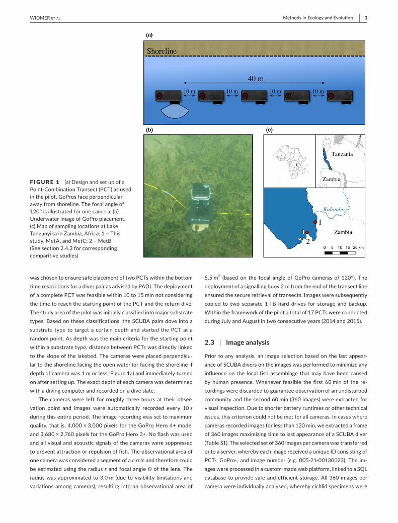
Here we introduce a novel approach, the Point- Combination Transect (PCT) method (Figure 1a,b), which incorporates elements of conventional UVC line and point transects with digital underwater
imaging tools. We demonstrate the wide applicability of PCT by employing it on a rather complex assemblage of fishes, the species flock of cichlid fishes from Lake Tanganyika in East Africa. This fish community is dominated by species that strongly interact with the substrate, exemplified through numerous substrate breeders or algae scrappers; but even highly mobile and pelagic species inter-act closely with the benthos, for example when predating others or during spawning (Konings, 1998). Our novel approach is based on small, automated digital cameras in underwater housings that are placed on the benthos and aligned along a given distance at a set depth level. The PCT method enables a researcher to observe sev-eral spatially close communities simultaneously by automatically re-cording images in a defined time lapse. Once the cameras are placed, there is no further disturbance by SCUBA divers and no interaction of the camera with its surroundings, including no movement and no visual or audible signalling. We show how with relatively little mon-etary and timely investment, valuable and robust data on fish com-munity structures can be collected, even at remote places and under demanding field conditions.
2 | MATERIALSANDMETHODS
2.1 | Studysite
The pilot was conducted at Lake Tanganyika, East Africa. The study site was restricted to the bay off Kalambo Falls Lodge located close tothemouthofKalamboRiver(8°37′36″S,31°12′2″E)innorthernZambia (Figure 1c). This bay was chosen for its diversity in habitats present within close proximity and its accessibility from Kalambo Falls Lodge. Furthermore, the bay is subjected to moderate fishing pressure only, primarily targeting non- cichlid fish species. Hence we assumed to observe a relatively undisturbed, local fish community bereft of extensive anthropogenic influences. The study area com-prises a diverse set of environments, such as predominantly rock- or sand- covered habitats; areas with an intermediate coverage of the lakebed; or vegetation dominated habitats. PCTs were conducted on a variety of depth levels, ranging from <1 m up to 21 m.
2.2 | Point-CombinationTransectsettings
The technical equipment for our PCT consisted of GoPro cameras (Hero 3+ Silver Edition, Hero 4+ Silver Edition, © GoPro, Inc.), each equipped with a 16 GB microSD card (ScanDisk) ensuring sufficient storage capacity for high- quality image storage. The protective housing provided by the supplier is waterproof to a depth of 40 m, making additional underwater housing unnecessary. The cameras were mounted in their housing on the supplied stand and fixed to a small rock (approximate dimensions: length = 15 cm, width = 15 cm, height = 5 cm) to provide negative buoyancy, immobility and stabil-ity once placed underwater on the lakebed (Figure 1b).
The setup for a PCT consists of five GoPro cameras positioned in a distance of 10 m of each other along a marked cord (total length of the transect: 40 m) (Figure 1a). The length of 40 m for one transect
| 3Methods in Ecology and Evolu!onWIDMER Et al.
was chosen to ensure safe placement of two PCTs within the bottom time restrictions for a diver pair as advised by PADI. The deployment of a complete PCT was feasible within 10 to 15 min not considering the time to reach the starting point of the PCT and the return dive. The study area of the pilot was initially classified into major substrate types. Based on these classifications, the SCUBA pairs dove into a substrate type to target a certain depth and started the PCT at a random point. As depth was the main criteria for the starting point within a substrate type, distance between PCTs was directly linked to the slope of the lakebed. The cameras were placed perpendicu-lar to the shoreline facing the open water (or facing the shoreline if depth of camera was 1 m or less; Figure 1a) and immediately turned on after setting up. The exact depth of each camera was determined with a diving computer and recorded on a dive slate.
The cameras were left for roughly three hours at their obser-vation point and images were automatically recorded every 10 s during this entire period. The image recording was set to maximum quality, that is, 4,000 × 3,000 pixels for the GoPro Hero 4+ model and 3,680 × 2,760 pixels for the GoPro Hero 3+. No flash was used and all visual and acoustic signals of the cameras were suppressed to prevent attraction or repulsion of fish. The observational area of one camera was considered a segment of a circle and therefore could be estimated using the radius r and focal angle ! of the lens. The radius was approximated to 3.0 m (due to visibility limitations and variations among cameras), resulting into an observational area of
5.5 m2 (based on the focal angle of GoPro cameras of 120°). The deployment of a signalling buoy 2 m from the end of the transect line ensured the secure retrieval of transects. Images were subsequently copied to two separate 1 TB hard drives for storage and backup. Within the framework of the pilot a total of 17 PCTs were conducted duringJulyandAugustintwoconsecutiveyears(2014and2015).
2.3 | Imageanalysis
Prior to any analysis, an image selection based on the last appear-ance of SCUBA divers on the images was performed to minimize any influence on the local fish assemblage that may have been caused by human presence. Whenever feasible the first 60 min of the re-cordings were discarded to guarantee observation of an undisturbed community and the second 60 min (360 images) were extracted for visual inspection. Due to shorter battery runtimes or other technical issues, this criterion could not be met for all cameras. In cases where cameras recorded images for less than 120 min, we extracted a frame of 360 images maximizing time to last appearance of a SCUBA diver (Table S1). The selected set of 360 images per camera was transferred onto a server, whereby each image received a unique ID consisting of PCT- , GoPro- , and image number (e.g. 005- 21- 00130023). The im-ages were processed in a custom- made web platform, linked to a SQL database to provide safe and efficient storage. All 360 images per camera were individually analysed, whereby cichlid specimens were
F IGURE 1 (a) Design and set up of a Point-Combination Transect (PCT) as used in the pilot. GoPros face perpendicular away from shoreline. The focal angle of 120° is illustrated for one camera. (b) Underwater image of GoPro placement. (c) Map of sampling locations at Lake Tanganyika in Zambia, Africa: 1 – This study, MetA, and MetC; 2 – MetB (See section 2.4.3 for corresponding comparitive studies)
4 | Methods in Ecology and Evolu!on WIDMER Et al.
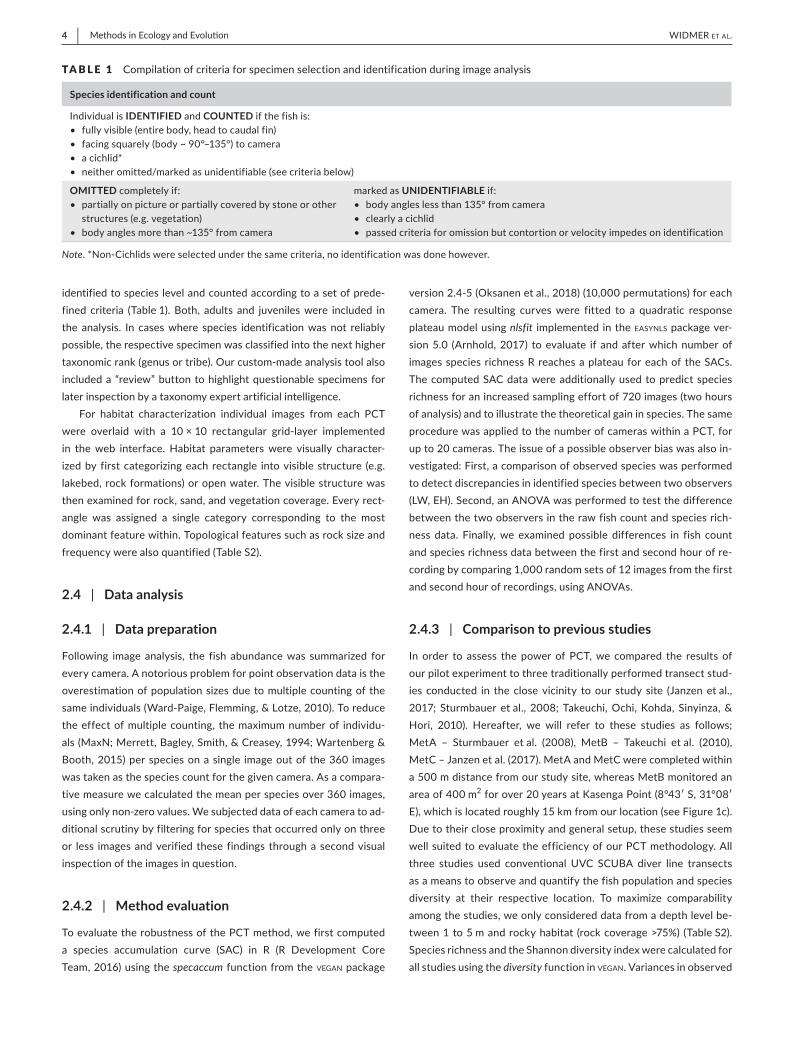
identified to species level and counted according to a set of prede-fined criteria (Table 1). Both, adults and juveniles were included in the analysis. In cases where species identification was not reliably possible, the respective specimen was classified into the next higher taxonomic rank (genus or tribe). Our custom- made analysis tool also included a “review” button to highlight questionable specimens for later inspection by a taxonomy expert artificial intelligence.
For habitat characterization individual images from each PCT were overlaid with a 10 × 10 rectangular grid- layer implemented in the web interface. Habitat parameters were visually character-ized by first categorizing each rectangle into visible structure (e.g. lakebed, rock formations) or open water. The visible structure was then examined for rock, sand, and vegetation coverage. Every rect-angle was assigned a single category corresponding to the most dominant feature within. Topological features such as rock size and frequency were also quantified (Table S2).
2.4 | Dataanalysis
2.4.1 | Datapreparation
Following image analysis, the fish abundance was summarized for every camera. A notorious problem for point observation data is the overestimation of population sizes due to multiple counting of the same individuals (Ward- Paige, Flemming, & Lotze, 2010). To reduce the effect of multiple counting, the maximum number of individu-als (MaxN; Merrett, Bagley, Smith, & Creasey, 1994; Wartenberg & Booth, 2015) per species on a single image out of the 360 images was taken as the species count for the given camera. As a compara-tive measure we calculated the mean per species over 360 images, using only non- zero values. We subjected data of each camera to ad-ditional scrutiny by filtering for species that occurred only on three or less images and verified these findings through a second visual inspection of the images in question.
2.4.2 | Methodevaluation
To evaluate the robustness of the PCT method, we first computed a species accumulation curve (SAC) in R (R Development Core Team, 2016) using the specaccum function from the vegan package
version 2.4- 5 (Oksanen et al., 2018) (10,000 permutations) for each camera. The resulting curves were fitted to a quadratic response plateau model using nlsfit implemented in the easynls package ver-sion 5.0 (Arnhold, 2017) to evaluate if and after which number of images species richness R reaches a plateau for each of the SACs. The computed SAC data were additionally used to predict species richness for an increased sampling effort of 720 images (two hours of analysis) and to illustrate the theoretical gain in species. The same procedure was applied to the number of cameras within a PCT, for up to 20 cameras. The issue of a possible observer bias was also in-vestigated: First, a comparison of observed species was performed to detect discrepancies in identified species between two observers (LW, EH). Second, an ANOVA was performed to test the difference between the two observers in the raw fish count and species rich-ness data. Finally, we examined possible differences in fish count and species richness data between the first and second hour of re-cording by comparing 1,000 random sets of 12 images from the first and second hour of recordings, using ANOVAs.
2.4.3 | Comparisontopreviousstudies
In order to assess the power of PCT, we compared the results of our pilot experiment to three traditionally performed transect stud-ies conducted in the closevicinity toour study site (Janzenetal.,2017; Sturmbauer et al., 2008; Takeuchi, Ochi, Kohda, Sinyinza, & Hori, 2010). Hereafter, we will refer to these studies as follows; MetA – Sturmbauer et al. (2008), MetB – Takeuchi et al. (2010), MetC–Janzenetal.(2017).MetAandMetCwerecompletedwithina 500 m distance from our study site, whereas MetB monitored an area of 400 m2forover20yearsatKasengaPoint(8°43′S,31°08′E), which is located roughly 15 km from our location (see Figure 1c). Due to their close proximity and general setup, these studies seem well suited to evaluate the efficiency of our PCT methodology. All three studies used conventional UVC SCUBA diver line transects as a means to observe and quantify the fish population and species diversity at their respective location. To maximize comparability among the studies, we only considered data from a depth level be-tween 1 to 5 m and rocky habitat (rock coverage >75%) (Table S2). Species richness and the Shannon diversity index were calculated for all studies using the diversity function in vegan. Variances in observed
TABLE 1 Compilation of criteria for specimen selection and identification during image analysis
Speciesidentificationandcount
Individual is IDENTIFIED and COUNTED if the fish is:• fully visible (entire body, head to caudal fin)• facing squarely (body ~ 90°–135°) to camera• a cichlid*• neither omitted/marked as unidentifiable (see criteria below)
OMITTED completely if:• partially on picture or partially covered by stone or other
structures (e.g. vegetation)• body angles more than ~135° from camera
marked as UNIDENTIFIABLE if:• body angles less than 135° from camera• clearly a cichlid• passed criteria for omission but contortion or velocity impedes on identification
Note. *Non- Cichlids were selected under the same criteria, no identification was done however.
| 5Methods in Ecology and Evolu!onWIDMER Et al.
fish density among the three studies were compared using a Mann–Whitney U test on the count data per species. MetA provided no actual counts for species observed three times or fewer, hence we assumed a value of three for these species in the above- mentioned analyses. As an additional evaluation of the appropriateness of the PCT approach, we tested for a size- dependent observation bias. To this end, we categorized the observed species into two size classes based on their standard length (SL). The mean SL of at least 10 speci-mens per species, extracted from the Tanganyika cichlid collection at the Zoological Institute of the University of Basel, was used for this comparison.
3 | RESULT
3.1 | Pilotstudy
The 17 PCTs of this study yielded data from 78 cameras, that is, 28,080 images for the subsequent analysis of the cichlid commu-nity at the study site (Exemplary images: Figure S3). The PCTs en-compass depths from 1 m to 21 m and three major habitat types: sandy, rocky and intermediate. 17,322 individual fish were identified to species level, 1,566 to genus level and 5,269 fish could not be identified on the images. The MaxN statistics of the raw count data resulted in 3,030 specimens at the species level (2,761 specimens if using the mean), 124 at the genus level and 324 at the tribe level. In total 61 cichlid species were recorded in the 2 years of this pilot on three different habitat types.
3.2 | Methodevaluation
The species accumulation curves (SACs) were calculated for 64 cam-eras (14 cameras were excluded from the analysis due to the small number of species recorded) (Table S4). The SACs of 53 cameras
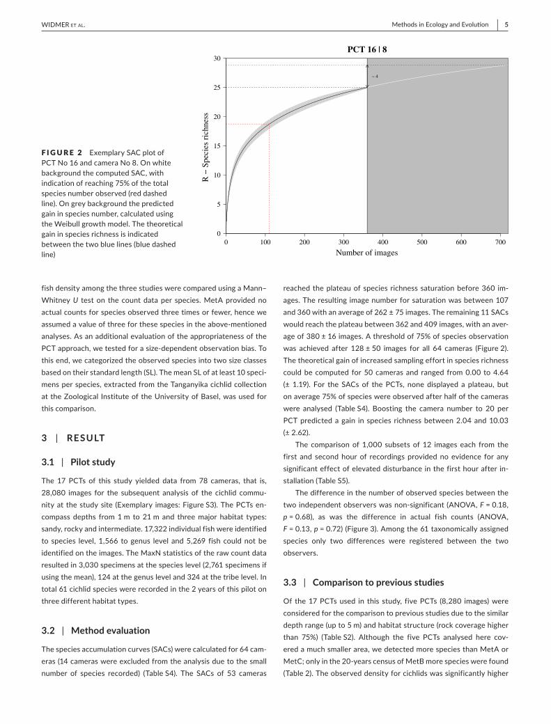
reached the plateau of species richness saturation before 360 im-ages. The resulting image number for saturation was between 107 and 360 with an average of 262 ± 75 images. The remaining 11 SACs would reach the plateau between 362 and 409 images, with an aver-age of 380 ± 16 images. A threshold of 75% of species observation was achieved after 128 ± 50 images for all 64 cameras (Figure 2). The theoretical gain of increased sampling effort in species richness could be computed for 50 cameras and ranged from 0.00 to 4.64 (± 1.19). For the SACs of the PCTs, none displayed a plateau, but on average 75% of species were observed after half of the cameras were analysed (Table S4). Boosting the camera number to 20 per PCT predicted a gain in species richness between 2.04 and 10.03 (± 2.62).
The comparison of 1,000 subsets of 12 images each from the first and second hour of recordings provided no evidence for any significant effect of elevated disturbance in the first hour after in-stallation (Table S5).
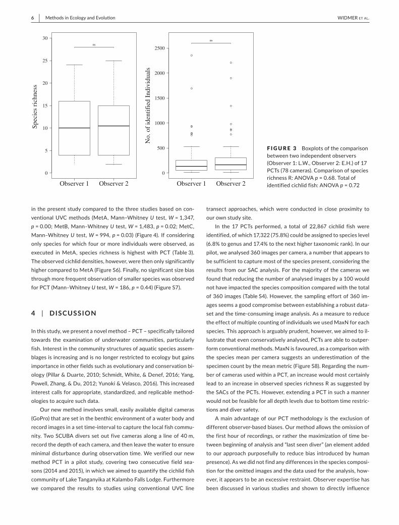
The difference in the number of observed species between the two independent observers was non- significant (ANOVA, F = 0.18, p = 0.68), as was the difference in actual fish counts (ANOVA, F = 0.13, p = 0.72) (Figure 3). Among the 61 taxonomically assigned species only two differences were registered between the two observers.
3.3 | Comparisontopreviousstudies
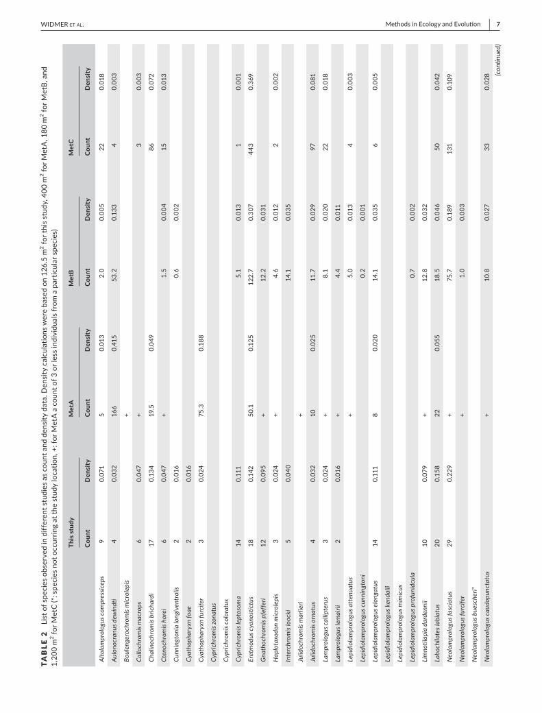
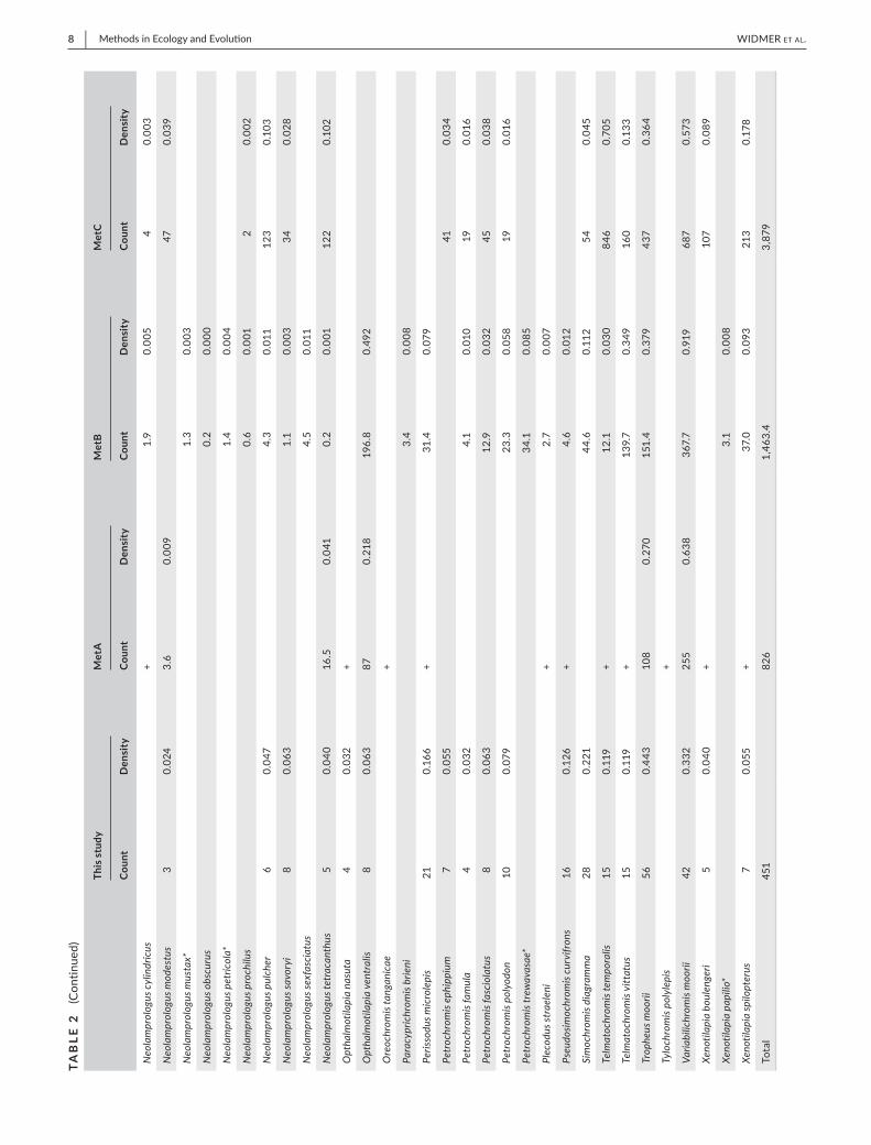
Of the 17 PCTs used in this study, five PCTs (8,280 images) were considered for the comparison to previous studies due to the similar depth range (up to 5 m) and habitat structure (rock coverage higher than 75%) (Table S2). Although the five PCTs analysed here cov-ered a much smaller area, we detected more species than MetA or MetC; only in the 20- years census of MetB more species were found (Table 2). The observed density for cichlids was significantly higher
F IGURE 2 Exemplary SAC plot of PCT No 16 and camera No 8. On white background the computed SAC, with indication of reaching 75% of the total species number observed (red dashed line ). On grey background the predicted gain in species number, calculated using the Weibull growth model. The theoretical gain in species richness is indicated between the two blue lines (blue dashed line)
0 100 200 300 400 500 600 7000
5
10
15
20
25
30PCT 16 | 8
Number of images
R !
Spe
cies
rich
ness
~ 4
6 | Methods in Ecology and Evolu!on WIDMER Et al.
in the present study compared to the three studies based on con-ventional UVC methods (MetA, Mann–Whitney U test, W = 1,347, p = 0.00; MetB, Mann–Whitney U test, W = 1,483, p = 0.02; MetC, Mann–Whitney U test, W = 994, p = 0.03) (Figure 4). If considering only species for which four or more individuals were observed, as executed in MetA, species richness is highest with PCT (Table 3). The observed cichlid densities, however, were then only significantly higher compared to MetA (Figure S6). Finally, no significant size bias through more frequent observation of smaller species was observed for PCT (Mann–Whitney U test, W = 186, p = 0.44) (Figure S7).
4 | DISCUSSION
In this study, we present a novel method – PCT – specifically tailored towards the examination of underwater communities, particularly fish. Interest in the community structures of aquatic species assem-blages is increasing and is no longer restricted to ecology but gains importance in other fields such as evolutionary and conservation bi-ology (Pillar & Duarte, 2010; Schmidt, White, & Denef, 2016; Yang, Powell, Zhang, & Du, 2012; Yunoki & Velasco, 2016). This increased interest calls for appropriate, standardized, and replicable method-ologies to acquire such data.
Our new method involves small, easily available digital cameras (GoPro) that are set in the benthic environment of a water body and record images in a set time- interval to capture the local fish commu-nity. Two SCUBA divers set out five cameras along a line of 40 m, record the depth of each camera, and then leave the water to ensure minimal disturbance during observation time. We verified our new method PCT in a pilot study, covering two consecutive field sea-sons (2014 and 2015), in which we aimed to quantify the cichlid fish community of Lake Tanganyika at Kalambo Falls Lodge. Furthermore we compared the results to studies using conventional UVC line
transect approaches, which were conducted in close proximity to our own study site.
In the 17 PCTs performed, a total of 22,867 cichlid fish were identified, of which 17,322 (75.8%) could be assigned to species level (6.8% to genus and 17.4% to the next higher taxonomic rank). In our pilot, we analysed 360 images per camera, a number that appears to be sufficient to capture most of the species present, considering the results from our SAC analysis. For the majority of the cameras we found that reducing the number of analysed images by a 100 would not have impacted the species composition compared with the total of 360 images (Table S4). However, the sampling effort of 360 im-ages seems a good compromise between establishing a robust data-set and the time- consuming image analysis. As a measure to reduce the effect of multiple counting of individuals we used MaxN for each species. This approach is arguably prudent, however, we aimed to il-lustrate that even conservatively analysed, PCTs are able to outper-form conventional methods. MaxN is favoured, as a comparison with the species mean per camera suggests an underestimation of the specimen count by the mean metric (Figure S8). Regarding the num-ber of cameras used within a PCT, an increase would most certainly lead to an increase in observed species richness R as suggested by the SACs of the PCTs. However, extending a PCT in such a manner would not be feasible for all depth levels due to bottom time restric-tions and diver safety.
A main advantage of our PCT methodology is the exclusion of different observer- based biases. Our method allows the omission of the first hour of recordings, or rather the maximization of time be-tween beginning of analysis and “last seen diver” (an element added to our approach purposefully to reduce bias introduced by human presence). As we did not find any differences in the species composi-tion for the omitted images and the data used for the analysis, how-ever, it appears to be an excessive restraint. Observer expertise has been discussed in various studies and shown to directly influence
F IGURE 3 Boxplots of the comparison between two independent observers (Observer 1: L.W., Observer 2: E.H.) of 17 PCTs (78 cameras). Comparison of species richness R: ANOVA p = 0.68. Total of identified cichlid fish: ANOVA p = 0.72
0
5
10
15
20
25
30
Observer 1 Observer 2
Spec
ies
rich
ness
ns
0
500
1000
1500
2000
2500
Observer 1 Observer 2
No.
of i
dent
ifie
d In
divi
dual
s
ns
| 7Methods in Ecology and Evolu!onWIDMER Et al.
TABLE 2
List
of s
peci
es o
bser
ved
in d
iffer
ent s
tudi
es a
s co
unt a
nd d
ensi
ty d
ata.
Den
sity
cal
cula
tions
wer
e ba
sed
on 1
26.5
m2 fo
r thi
s st
udy,
400
m2 fo
r Met
A, 1
80 m
2 for M
etB,
and
1,
200
m2 fo
r Met
C (*
: spe
cies
not
occ
urrin
g at
the
stud
y lo
catio
n, +
: for
Met
A a
cou
nt o
f 3 o
r les
s in
divi
dual
s fr
om a
par
ticul
ar s
peci
es)
Thisstudy
MetA
MetB
MetC
Count
Density
Count
Density
Count
Density
Count
Density
Alto
lam
prol
ogus
com
pres
sicep
s9
0.07
15
0.01
32.
00.
005
220.
018
Aulo
nocr
anus
dew
indt
i4
0.03
216
60.
415
53.2
0.13
34
0.00
3
Boul
enge
roch
rom
is m
icro
lepi
s+
Callo
chro
mis
mac
rops
60.
047
+3
0.00
3
Chal
inoc
hrom
is br
icha
rdi
170.
134
19.5
0.04
986
0.07
2
Cten
ochr
omis
hore
i6
0.04
7+
1.5
0.00
415
0.01
3
Cunn
ingt
onia
long
iven
tral
is2
0.01
60.
60.
002
Cyat
hoph
aryx
n fo
ae2
0.01
6
Cyat
hoph
aryx
n fu
rcife
r3
0.02
475
.30.
188
Cypr
ichr
omis
zona
tus
Cypr
ichr
omis
colo
ratu
s
Cypr
ichr
omis
lept
osom
a14
0.11
15.
10.
013
10.
001
Eret
mod
us c
yano
stic
tus
180.
142
50.1
0.12
512
2.7
0.30
744
30.
369
Gna
thoc
hrom
is pf
effe
ri12
0.09
5+
12.2
0.03
1
Hap
lota
xodo
n m
icro
lepi
s3
0.02
4+
4.6
0.01
22
0.00
2
Inte
rchr
omis
looc
ki5
0.04
014
.10.
035
Julid
ochr
omis
mar
lieri
+
Julid
ochr
omis
orna
tus
40.
032
100.
025
11.7
0.02
997
0.08
1
Lam
prol
ogus
cal
lipte
rus
30.
024
+8.
10.
020
220.
018
Lam
prol
ogus
lem
airii
20.
016
+4.
40.
011
Lepi
diol
ampr
olog
us a
tten
uatu
s+
5.0
0.01
34
0.00
3
Lepi
diol
ampr
olog
us c
unni
ngto
ni0.
20.
001
Lepi
diol
ampr
olog
us e
long
atus
140.
111
80.
020
14.1
0.03
56
0.00
5
Lepi
diol
ampr
olog
us k
enda
lli
Lepi
diol
ampr
olog
us m
imic
us
Lepi
diol
ampr
olog
us p
rofu
nidc
ula
0.7
0.00
2
Lim
notil
apia
dar
denn
ii10
0.07
9+
12.8
0.03
2
Lobo
chilo
tes l
abia
tus
200.
158
220.
055
18.5
0.04
650
0.04
2
Neo
lam
prol
ogus
fasc
iatu
s29
0.22
9+
75.7
0.18
913
10.
109
Neo
lam
prol
ogus
furc
ifer
+1.
00.
003
Neo
lam
prol
ogus
bue
sche
ri*
Neo
lam
prol
ogus
cau
dopu
ncta
tus
+10
.80.
027
330.
028 (continued)
8 | Methods in Ecology and Evolu!on WIDMER Et al.
Thisstudy
MetA
MetB
MetC
Count
Density
Count
Density
Count
Density
Count
Density
Neo
lam
prol
ogus
cyl
indr
icus
+1.
90.
005
40.
003
Neo
lam
prol
ogus
mod
estu
s3
0.02
43.
60.
009
470.
039
Neo
lam
prol
ogus
mus
tax*
1.3
0.00
3
Neo
lam
prol
ogus
obs
curu
s0.
20.
000
Neo
lam
prol
ogus
pet
ricol
a*1.
40.
004
Neo
lam
prol
ogus
pro
chilu
s0.
60.
001
20.
002
Neo
lam
prol
ogus
pul
cher
60.
047
4.3
0.01
112
30.
103
Neo
lam
prol
ogus
savo
ryi
80.
063
1.1
0.00
334
0.02
8
Neo
lam
prol
ogus
sexf
asci
atus
4.5
0.01
1
Neo
lam
prol
ogus
tetr
acan
thus
50.
040
16.5
0.04
10.
20.
001
122
0.10
2
Opt
halm
otila
pia
nasu
ta4
0.03
2+
Opt
halm
otila
pia
vent
ralis
80.
063
870.
218
196.
80.
492
Ore
ochr
omis
tang
anic
ae+
Para
cypr
ichr
omis
brie
ni3.
40.
008
Peris
sodu
s mic
role
pis
210.
166
+31
.40.
079
Petr
ochr
omis
ephi
ppiu
m7
0.05
541
0.03
4
Petr
ochr
omis
fam
ula
40.
032
4.1
0.01
019
0.01
6
Petr
ochr
omis
fasc
iola
tus
80.
063
12.9
0.03
245
0.03
8
Petr
ochr
omis
poly
odon
100.
079
23.3
0.05
819
0.01
6
Petr
ochr
omis
trew
avas
ae*
34.1
0.08
5
Plec
odus
stra
elen
i+
2.7
0.00
7
Pseu
dosim
ochr
omis
curv
ifron
s16
0.12
6+
4.6
0.01
2
Sim
ochr
omis
diag
ram
ma
280.
221
44.6
0.11
254
0.04
5
Telm
atoc
hrom
is te
mpo
ralis
150.
119
+12
.10.
030
846
0.70
5
Telm
atoc
hrom
is vi
ttat
us15
0.11
9+
139.
70.
349
160
0.13
3
Trop
heus
moo
rii56
0.44
310
80.
270
151.
40.
379
437
0.36
4
Tylo
chro
mis
poly
lepi
s+
Varia
bilic
hrom
is m
oorii
420.
332
255
0.63
836
7.7
0.91
968
70.
573
Xeno
tilap
ia b
oule
nger
i5
0.04
0+
107
0.08
9
Xeno
tilap
ia p
apili
o*3.
10.
008
Xeno
tilap
ia sp
ilopt
erus
70.
055
+37
.00.
093
213
0.17
8
Tota
l45
182
61,
463.
43,
879
TABLE2
(Con
tinue
d)
| 9Methods in Ecology and Evolu!onWIDMER Et al.
count data and identification efforts (Thompson & Mapstone, 1997; Williams et al., 2006). In the case of PCT, the difference between two independent observers proved to be insignificant (Figure 3). In 28,080 images and 61 cichlid species only two individuals were as-signed to different species by the two observers. Even count data were the same between the two observers, likely as a result of the highly standardized approach to identify and count the cichlid fishes on the images.
To compare directly with studies done in a similar location we stripped down our data to only five PCTs, which reduced the number of species observed in the full pilot (61 to 39 species, see Section 3.1). In terms of species richness, PCT outperformed the conven-tional UVC line- transect for both studies done in very close proxim-ity to our study location and is virtually tantamount to the 20- year census done by MetB. This result clearly indicates the power of the PCT in comparison with the conventional UVC line- transect meth-odology. Taking into account the difference in the area covered with UVC line- transect and PCT this impression is further strengthened: Even though our PCTs covered only a fraction of the area of obser-vation compared to the three comparative studies, they captured as many species as the average of the 20 year- census of MetB and more than double the species of MetA, suggesting that traditional UVC line transect approaches fail to record all species present at
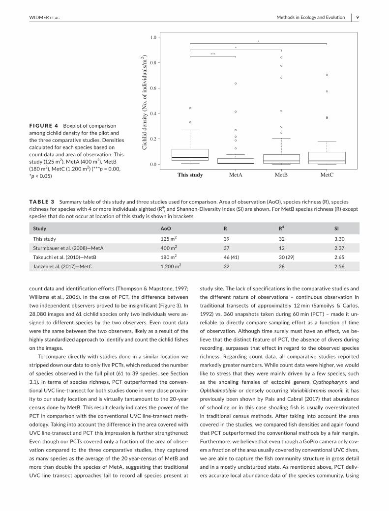
study site. The lack of specifications in the comparative studies and the different nature of observations – continuous observation in traditional transects of approximately 12 min (Samoilys & Carlos, 1992) vs. 360 snapshots taken during 60 min (PCT) – made it un-reliable to directly compare sampling effort as a function of time of observation. Although time surely must have an effect, we be-lieve that the distinct feature of PCT, the absence of divers during recording, surpasses that effect in regard to the observed species richness. Regarding count data, all comparative studies reported markedly greater numbers. While count data were higher, we would like to stress that they were mainly driven by a few species, such as the shoaling females of ectodini genera Cyathopharynx and Ophthalmotilpia or densely occurring Variabilichromis moorii; it has previously been shown by Pais and Cabral (2017) that abundance of schooling or in this case shoaling fish is usually overestimated in traditional census methods. After taking into account the area covered in the studies, we compared fish densities and again found that PCT outperformed the conventional methods by a fair margin. Furthermore, we believe that even though a GoPro camera only cov-ers a fraction of the area usually covered by conventional UVC dives, we are able to capture the fish community structure in gross detail and in a mostly undisturbed state. As mentioned above, PCT deliv-ers accurate local abundance data of the species community. Using
F IGURE 4 Boxplot of comparison among cichlid density for the pilot and the three comparative studies. Densities calculated for each species based on count data and area of observation: This study (125 m2), MetA (400 m2), MetB (180 m2), MetC (1,200 m2) (***p = 0.00, *p < 0.05)
0.0
0.2
0.4
0.6
0.8
1.0
Cic
hlid
den
sity
(No.
of i
ndiv
idua
ls/m
2 )
This study MetA MetB MetC
*
*
***
TABLE 3 Summary table of this study and three studies used for comparison. Area of observation (AoO), species richness (R), species richness for species with 4 or more individuals sighted (R4) and Shannon- Diversity Index (SI) are shown. For MetB species richness (R) except species that do not occur at location of this study is shown in brackets
Study AoO R R4 SI
This study 125 m2 39 32 3.30
Sturmbauer et al. (2008)—MetA 400 m2 37 12 2.37
Takeuchi et al. (2010)—MetB 180 m2 46 (41) 30 (29) 2.65
Janzenetal.(2017)—MetC 1,200 m2 32 28 2.56
10 | Methods in Ecology and Evolu!on WIDMER Et al.
abundance and standard length (SL), biomass may be approximated, although prior information on SL is necessary as no length measure-ments can be taken from non- stereo images (as performed on stereo images by Wilson, Graham, Holmes, MacNeil, & Ryan, 2018). An al-ternative approach could be the measuring of landmarks while set-ting up PCT to allow researchers to measure individuals a posteriori. As this was not the aim of this study, we are unable to provide more detailed information here.
Looking in depth at the species that were observed, we investi-gated if camera position biased our data to small and benthic spe-cies. We did, however, not find any evidence that would support this. When comparing this aspect directly with the other studies and the UVC strip transect, there was no evidence for a significant shift to-wards small species. The general set up of the PCT does suggest a focus on benthic communities; however, our method is able to cap-ture mobile and pelagic species as well (Figure S9). We thus see the advantage of the observational success not depending on the size or position in the water column of the fish, as illustrated within this study. However, it is advisable to select target species with a certain degree of dependence on the substrate.
To date, several approaches exist to incorporate the use of electronic equipment and therefore reduce a number of biases as-sociated with conventional UVC used for ecological observation of underwater communities. For example TOWed Video (TOWV) is used to monitor communities by recording footage as the cameras are pulled through the habitat (Mallet & Pelletier, 2014). However, regarding observer presence, the use of cameras would not have markedly benefited the quality of the collected data in this instance, as firstly, depending on the depth, heavy surface disturbance has to be considered, and more importantly the moving, baited object pulled through the fish community might selectively attract some fish species over others (Pais & Cabral, 2017; Pereira et al., 2016). Therefore, abundance and species richness data of the habitat in question might not reflect reality. A different approach was intro-duced in 2012 (STAVIRO; Pelletier et al., 2012) using stationary cameras that rotate to simulate a point transect, presumably elim-inating the bias of observer presence. This approach marginally failed to show its superiority to general UVC techniques and might still contain bias through its moving apparatus (Mallet et al., 2014). In contrast, an indication for the inconspicuousness of our outlined methodology (PCT) is that a number of species difficult to monitor could be captured on camera, for example pelagic predators such as Bathybates fasciatus and the African tigerfish Hydrocynus vittatus, the latter of which was never directly observed in this area (personal observation) in 10 years diving at this location, or the shy cichlid spe-cies Neolamprologus prochilus that usually remains under rocks and is therefore rarely seen (Konings, 1998).
Considering all approaches using cameras, including PCT, it is im-portant to note that the recording of the underwater image material is the smaller part of data collection, followed by a time intensive period of images analysis. The main advantages of PCT compared to other camera- based approaches are its compact design, its cost effectiveness, its standardized setup and handling, as well as its
ability to deliver robust digital data, making PCT well suited for the observation of underwater communities even under difficult field conditions.
ACKNOWLEGEMENTS
We thank Daniel Lüscher and the crew of Kalambo Falls Lodge for the support in logistics, the Lake Tanganyika Research Unit, Department of Fisheries, Republic of Zambia, for research permits, and two anonymous reviewers and the associate editor for valuable suggestions. This study was supported by the European Research Council (ERC, CoG ‘CICHLID~X’ to W.S.).
AUTHORS’CONTRIBUTIONS
L.W., E.H., M.C. and W.S. conceived and supervised the study, all co- authors conducted the fieldwork, L.W. constructed the image analysis tool and SQL database, L.W. and E.H. processed the images, with A.I. reviewing difficult cases. F.R. provided data on standard length, L.W. analysed the data, and wrote the manuscript with feed-back from all co- authors.
DATAACCCESSIBILTY
All raw count data used in this study including a separate species list are available from the Dryad Digital Repository https://doi.org/10.5061/dryad.1kr7759 (Widmer et al., 2019).
ORCID
Lukas Widmer http://orcid.org/0000-0003-2642-8163
REFERENCES
Arnhold, E. (2017). easynls: Easy nonlinear model. R Package Version 5.0, 1–9. Retrieved from https://cran.r-project.org/package=easynls
Brock, V. E. (1954). A preliminary report on a method of estimating reef fish populations. The Journal of Wildlife Management, 18(3), 297. https://doi.org/10.2307/3797016
Colvocoresses, J., & Acosta, A. (2007). A large-scale field comparisonof strip transect and stationary point count methods for conduct-ing length- based underwater visual surveys of reef fish populations. Fisheries Research, 85(1–2), 130–141. https://doi.org/10.1016/j.fishres.2007.01.012
Dickens,L.C.,Goatley,C.H.R.,Tanner,J.K.,&Bellwood,D.R.(2011).Quantifying relative diver effects in underwater visual censuses. PLoS ONE, 6(4), 6–8. https://doi.org/10.1371/journal.pone.0018965
Edgar, G. J., Barrett, N. S., &Morton, A. J. (2004). Biases associatedwith the use of underwater visual census techniques to quan-tify the density and size- structure of fish populations. Journal of Experimental Marine Biology and Ecology, 308(2), 269–290. https://doi.org/10.1016/j.jembe.2004.03.004
Janzen,T.,Alzate,A.,Muschick,M.,Maan,M.E.,vanderPlas,F.,&Etienne,R. S. (2017). Community assembly in Lake Tanganyika cichlid fish: Quantifying the contributions of both niche- based and neutral pro-cesses. Ecology and Evolution, 7(4), 1057–1067. https://doi.org/10.1002/ece3.2689
| 11Methods in Ecology and Evolu!onWIDMER Et al.
Konings, A. (1998). Tanganyika cichlids in their natural habitat (3rd ed.). El Paso, TX: Cichlid Press.
Lowry, M., Folpp, H., Gregson, M., & Mckenzie, R. (2011). A comparison of methods for estimating fish assemblages associated with estuarine arti-ficial reefs. Brazilian Journal of Oceanography, 59(Spec. Issue 1), 119–131. https://doi.org/10.1590/S1679-87592011000500014
Mallet, D., & Pelletier, D. (2014). Underwater video techniques for observ-ing coastal marine biodiversity: A review of sixty years of publications (1952- 2012). Fisheries Research, 154, 44–62. https://doi.org/10.1016/j.fishres.2014.01.019
Mallet, D., Wantiez, L., Lemouellic, S., Vigliola, L., & Pelletier, D. (2014). Complementarity of rotating video and underwater visual census for assessing species richness, frequency and density of reef fish on coral reef slopes. PLoS ONE, 9(1), e84344. https://doi.org/10.1371/journal.pone.0084344
Merrett, N. R., Bagley, P. M., Smith, A., & Creasey, S. (1994). Scavenging deep demersal fishes of the Porcupine Seabight, north- east Atlantic: Observations by baited camera, trap and trawl. Journal of the Marine Biological Association of the United Kingdom, 74(3), 481–498. https://doi.org/10.1017/S0025315400047615
Oksanen,J.,Blanchet,F.G.,Kindt,R.,Legendre,P.,Minchin,P.R.,O'hara,R.B.,…Oksanen,M.J.(2018).vegan: Community ecology package. R Package Version 2. 4-6. https://doi.org/10.1093/molbev/msv334
Pais, M. P., & Cabral, H. N. (2017). Fish behaviour effects on the accuracy and precision of underwater visual census surveys. A virtual ecologist approach using an individual- based model. Ecological Modelling, 346, 58–69. https://doi.org/10.1016/j.ecolmodel.2016.12.011
Pelletier, D., Leleu, K., Mallet, D., Mou-Tham, G., Hervé, G., Boureau, M., & Guilpart, N. (2012). Remote high- definition rotating video enables fast spatial survey of marine underwater macrofauna and habitats. PLoS ONE, 7(2), e30536. https://doi.org/10.1371/journal.pone.0030536
Pereira, P. H. C., Leal, I. C. S., & de Araújo, M. E. (2016). Observer presence may alter the behaviour of reef fishes associated with coral colonies. Marine Ecology, 37(4), 760–769. https://doi.org/10.1111/maec.12345
Pillar, V. D., & Duarte, L. d. S. (2010). A framework for metacommunity anal-ysis of phylogenetic structure. Ecology Letters, 13(5), 587–596. https://doi.org/10.1111/j.1461-0248.2010.01456.x
R Development Core Team. (2016). R: A language and environment for statis-tical computing. Vienna, Austria: R Foundation for Statistical Computing. https://doi.org/10.1038/sj.hdy.6800737
Samoilys, M., & Carlos, G. (1992). Development of an underwater visual census method for assessing shallow water reef fish stocks in the south west Pacific: Final report. Queensland: Queensland Dept. of Primary Industries. Retrieved from http://www.worldcat.org/title/develop-ment-of-an-underwater-visual-census-method-for-assessing-shal-low-water-reef-fish-stocks-in-the-south-west-pacific-final-report/oclc/32021136?referer=di&ht=edition
Samoilys, M. A., & Carlos, G. (2000). Determining methods of under-water visual census for estimating the abundance of coral reef fishes. Environmental Biology of Fishes, 57(3), 289–304. https://doi.org/10.1023/A:1007679109359
Schmidt,M.L.,White,J.D.,&Denef,V.J.(2016).Phylogeneticconserva-tion of freshwater lake habitat preference varies between abundant bacterioplankton phyla. Environmental Microbiology, 18(4), 1212–1226. https://doi.org/10.1111/1462-2920.13143
Sturmbauer, C., Fuchs, C., Harb, G., Damm, E., Duftner, N., Maderbacher, M., & Koblmüller, S. (2008). Abundance, distribution, and ter-ritory areas of rock- dwelling Lake Tanganyika cichlid fish spe-cies. Hydrobiologia, 615(1), 57–68. https://doi.org/10.1007/s10750-008-9557-z
Takeuchi, Y., Ochi, H., Kohda, M., Sinyinza, D., & Hori, M. (2010). A 20- year census of a rocky littoral fish community in Lake Tanganyika. Ecology of Freshwater Fish, 19(2), 239–248. https://doi.org/10.1111/j.1600-0633.2010.00408.x
Thompson, A. A., & Mapstone, B. D. (1997). Observer effects and training in underwater visual surveys of reef fishes. Marine Ecology Progress Series, 154, 53–63. https://doi.org/10.3354/meps154053
Unsworth,R.K.F.,Peters,J.R.,McCloskey,R.M.,&Hinder,S.L. (2014).Optimising stereo baited underwater video for sampling fish and in-vertebrates in temperate coastal habitats. Estuarine, Coastal and Shelf Science, 150(PB), 281–287. https://doi.org/10.1016/j.ecss.2014.03.020
Ward-Paige,C.,Flemming,J.M.,&Lotze,H.K.(2010).Overestimatingfishcounts by non- instantaneous visual censuses: Consequences for pop-ulation and community descriptions. PLoS ONE, 5(7), 1–9. https://doi.org/10.1371/journal.pone.0011722
Wartenberg,R.,&Booth,A.J.J.(2015).Videotransectsarethemostap-propriate underwater visual census method for surveying high- latitude coral reef fishes in the southwestern Indian Ocean. Marine Biodiversity, 45(4), 633–646. https://doi.org/10.1007/s12526-014-0262-z
Whitfield, P. E., Muñoz, R. C., Buckel, C. A., Degan, B. P., Freshwater, D. W., &Hare,J.A.(2014).NativefishcommunitystructureandIndo-Pacificlionfish Pterois volitans densities along a depth- temperature gradient in Onslow Bay, North Carolina, USA. Marine Ecology Progress Series, 509, 241–254. https://doi.org/10.3354/meps10882
Widmer, L., Heule, E., Colombo, M., Rueegg, A., Indermaur, A., Ronco, F., & Salzburger, W. (2019). Data from: Point- Combination Transect (PCT): Incorporation of small underwater cameras to study fish communities. Dryad Digital Repository, https://doi.org/10.5061/dryad.1kr7759
Williams,I.D.,Walsh,W.J.,Tissot,B.N.,&Hallacher,L.E.(2006).Impactof observers’ experience level on counts of fishes in underwater vi-sual surveys. Marine Ecology Progress Series, 310, 185–191. https://doi.org/10.3354/meps310185
Wilson,S.K.,Graham,N.A.J.,Holmes,T.H.,MacNeil,M.A.,&Ryan,N.M. (2018). Visual versus video methods for estimating reef fish bio-mass. Ecological Indicators, 85(October 2017), 146–152. https://doi.org/10.1016/j.ecolind.2017.10.038
Wraith,J.,Lynch,T.,Minchinton,T.E.,Broad,A.,&Davis,A.R.(2013).Baittype affects fish assemblages and feeding guilds observed at baited remote underwater video stations. Marine Ecology Progress Series, 477, 189–199. https://doi.org/10.3354/meps10137
Yang,Z.,Powell, J.R.,Zhang,C.,&Du,G. (2012).Theeffectofenviron-mental and phylogenetic drivers on community assembly in an al-pine meadow community. Ecology, 93(11), 2321–2328. https://doi.org/10.1890/11-2212.1
Yunoki, T., & Velasco, L. T. (2016). Fish metacommunity dynamics in the patchy heterogeneous habitats of varzea lakes, turbid river channels and transparent clear and black water bodies in the Amazonian Lowlands of Bolivia. Environmental Biology of Fishes, 99, 391–408. https://doi.org/10.1007/s10641-016-0481-1
SUPPORTINGINFORMATION
Additional supporting information may be found online in the Supporting Information section at the end of the article.
Howtocitethisarticle: Widmer L, Heule E, Colombo M, et al. Point- Combination Transect (PCT): Incorporation of small underwater cameras to study fish communities. Methods Ecol Evol. 2019;00:1–11. https://doi.org/10.1111/2041-210X.13163


Chapter 1
Supplementary Information
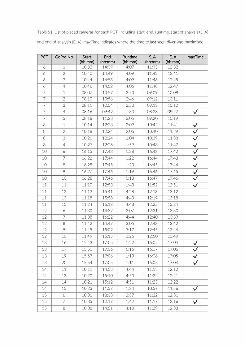
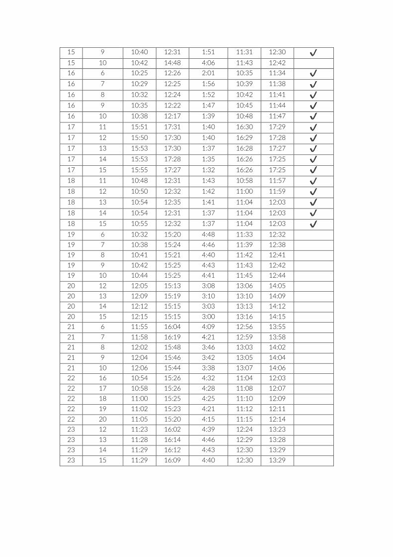
Table S1: List of placed cameras for each PCT, including start, end, runtime, start of analysis (S_A)
and end of analysis (E_A). maxTime indicates where the time to last seen diver was maximised.
PCT GoPro No Start
(hh:mm) End
(hh:mm) Runtime (hh:mm)
S_A (hh:mm)
E_A (hh:mm)
maxTime
6 1 10:32 14:39 4:07 11:33 12:32
6 2 10:40 14:49 4:09 11:42 12:41
6 3 10:44 14:53 4:09 11:46 12:45
6 4 10:46 14:52 4:06 11:48 12:47
7 1 08:07 10:57 2:50 09:09 10:08
7 2 08:10 10:56 2:46 09:12 10:11
7 3 08:11 12:04 3:53 09:13 10:12
7 4 08:16 09:49 1:33 08:28 09:27 ✔ 7 5 08:18 11:23 3:05 09:20 10:19
8 1 10:14 12:23 2:09 10:42 11:41 ✔ 8 2 10:18 12:24 2:06 10:40 11:39 ✔ 8 3 10:20 12:24 2:04 10:39 11:38 ✔ 8 4 10:27 12:26 1:59 10:48 11:47 ✔
10 6 16:15 17:43 1:28 16:43 17:42 ✔ 10 7 16:22 17:44 1:22 16:44 17:43 ✔ 10 8 16:25 17:45 1:20 16:45 17:44 ✔ 10 9 16:27 17:46 1:19 16:46 17:45 ✔ 10 10 16:28 17:46 1:18 16:47 17:46 ✔ 11 11 11:10 12:53 1:43 11:52 12:51 ✔ 11 12 11:13 15:41 4:28 12:13 13:12
11 13 11:18 15:58 4:40 12:19 13:18
11 15 11:24 16:12 4:48 12:25 13:24
12 6 11:30 14:37 3:07 12:31 13:30
12 7 11:38 16:22 4:44 12:40 13:39
12 8 11:42 14:47 3:05 12:43 13:42
12 9 11:45 15:02 3:17 12:45 13:44
12 10 11:49 15:15 3:26 12:50 13:49
13 16 15:43 17:05 1:22 16:05 17:04 ✔ 13 17 15:50 17:06 1:16 16:07 17:06 ✔ 13 19 15:53 17:06 1:13 16:06 17:05 ✔ 13 20 15:54 17:05 1:11 16:05 17:04 ✔ 14 11 10:11 14:55 4:44 11:13 12:12
14 13 10:20 15:10 4:50 11:22 12:21
14 14 10:21 15:12 4:51 11:23 12:22
14 15 10:23 11:57 1:34 10:57 11:56 ✔ 15 6 10:31 13:08 2:37 11:32 12:31
15 7 10:35 12:17 1:42 11:17 12:16 ✔ 15 8 10:38 14:51 4:13 11:39 12:38
15 9 10:40 12:31 1:51 11:31 12:30 ✔ 15 10 10:42 14:48 4:06 11:43 12:42
16 6 10:25 12:26 2:01 10:35 11:34 ✔ 16 7 10:29 12:25 1:56 10:39 11:38 ✔ 16 8 10:32 12:24 1:52 10:42 11:41 ✔ 16 9 10:35 12:22 1:47 10:45 11:44 ✔ 16 10 10:38 12:17 1:39 10:48 11:47 ✔ 17 11 15:51 17:31 1:40 16:30 17:29 ✔ 17 12 15:50 17:30 1:40 16:29 17:28 ✔ 17 13 15:53 17:30 1:37 16:28 17:27 ✔ 17 14 15:53 17:28 1:35 16:26 17:25 ✔ 17 15 15:55 17:27 1:32 16:26 17:25 ✔ 18 11 10:48 12:31 1:43 10:58 11:57 ✔ 18 12 10:50 12:32 1:42 11:00 11:59 ✔ 18 13 10:54 12:35 1:41 11:04 12:03 ✔ 18 14 10:54 12:31 1:37 11:04 12:03 ✔ 18 15 10:55 12:32 1:37 11:04 12:03 ✔ 19 6 10:32 15:20 4:48 11:33 12:32
19 7 10:38 15:24 4:46 11:39 12:38
19 8 10:41 15:21 4:40 11:42 12:41
19 9 10:42 15:25 4:43 11:43 12:42
19 10 10:44 15:25 4:41 11:45 12:44
20 12 12:05 15:13 3:08 13:06 14:05
20 13 12:09 15:19 3:10 13:10 14:09
20 14 12:12 15:15 3:03 13:13 14:12
20 15 12:15 15:15 3:00 13:16 14:15
21 6 11:55 16:04 4:09 12:56 13:55
21 7 11:58 16:19 4:21 12:59 13:58
21 8 12:02 15:48 3:46 13:03 14:02
21 9 12:04 15:46 3:42 13:05 14:04
21 10 12:06 15:44 3:38 13:07 14:06
22 16 10:54 15:26 4:32 11:04 12:03 22 17 10:58 15:26 4:28 11:08 12:07 22 18 11:00 15:25 4:25 11:10 12:09 22 19 11:02 15:23 4:21 11:12 12:11 22 20 11:05 15:20 4:15 11:15 12:14 23 12 11:23 16:02 4:39 12:24 13:23
23 13 11:28 16:14 4:46 12:29 13:28
23 14 11:29 16:12 4:43 12:30 13:29
23 15 11:29 16:09 4:40 12:30 13:29
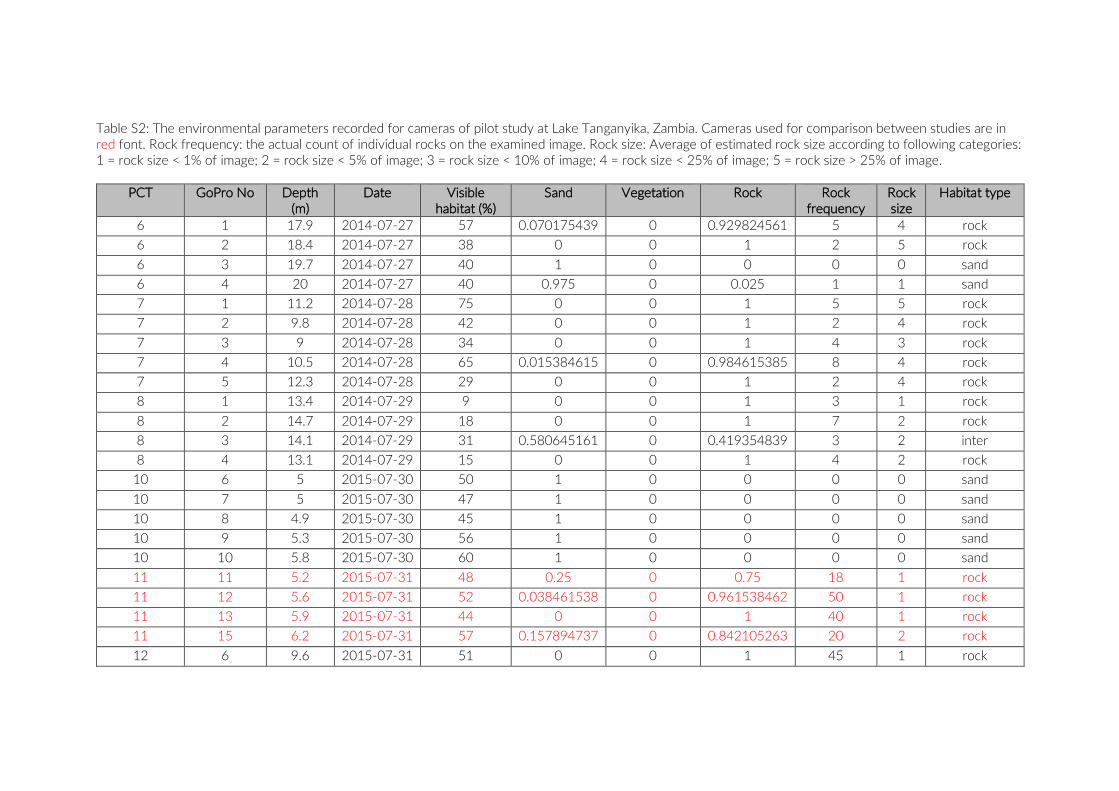
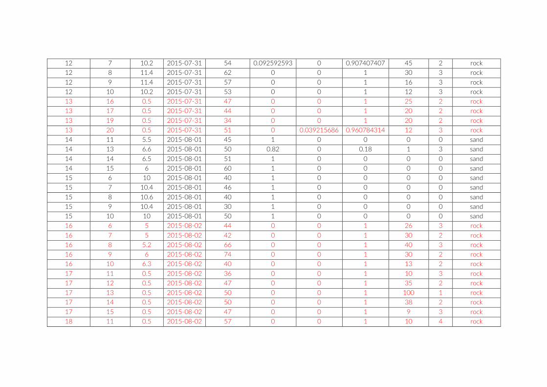
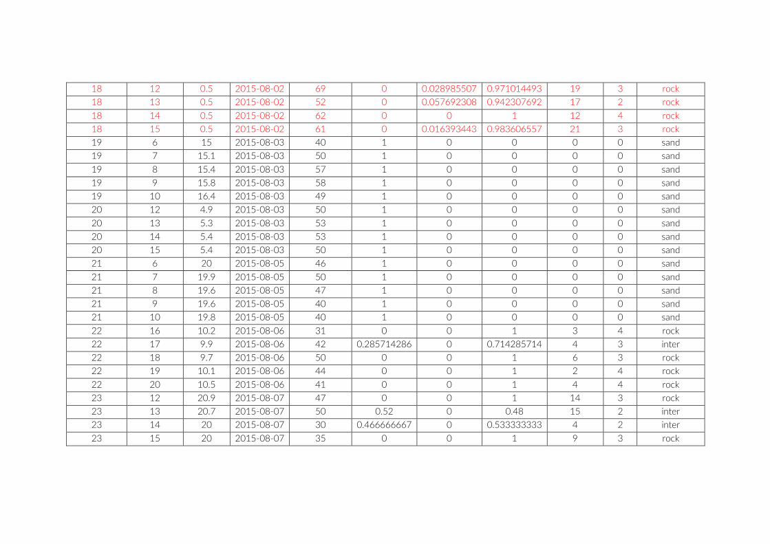
Table S2: The environmental parameters recorded for cameras of pilot study at Lake Tanganyika, Zambia. Cameras used for comparison between studies are in red font. Rock frequency: the actual count of individual rocks on the examined image. Rock size: Average of estimated rock size according to following categories: 1 = rock size < 1% of image; 2 = rock size < 5% of image; 3 = rock size < 10% of image; 4 = rock size < 25% of image; 5 = rock size > 25% of image.
PCT GoPro No Depth (m)
Date Visible habitat (%)
Sand Vegetation Rock Rock frequency
Rock size
Habitat type
6 1 17.9 2014-07-27 57 0.070175439 0 0.929824561 5 4 rock
6 2 18.4 2014-07-27 38 0 0 1 2 5 rock
6 3 19.7 2014-07-27 40 1 0 0 0 0 sand
6 4 20 2014-07-27 40 0.975 0 0.025 1 1 sand
7 1 11.2 2014-07-28 75 0 0 1 5 5 rock
7 2 9.8 2014-07-28 42 0 0 1 2 4 rock
7 3 9 2014-07-28 34 0 0 1 4 3 rock
7 4 10.5 2014-07-28 65 0.015384615 0 0.984615385 8 4 rock
7 5 12.3 2014-07-28 29 0 0 1 2 4 rock
8 1 13.4 2014-07-29 9 0 0 1 3 1 rock
8 2 14.7 2014-07-29 18 0 0 1 7 2 rock
8 3 14.1 2014-07-29 31 0.580645161 0 0.419354839 3 2 inter
8 4 13.1 2014-07-29 15 0 0 1 4 2 rock
10 6 5 2015-07-30 50 1 0 0 0 0 sand
10 7 5 2015-07-30 47 1 0 0 0 0 sand
10 8 4.9 2015-07-30 45 1 0 0 0 0 sand
10 9 5.3 2015-07-30 56 1 0 0 0 0 sand
10 10 5.8 2015-07-30 60 1 0 0 0 0 sand
11 11 5.2 2015-07-31 48 0.25 0 0.75 18 1 rock
11 12 5.6 2015-07-31 52 0.038461538 0 0.961538462 50 1 rock
11 13 5.9 2015-07-31 44 0 0 1 40 1 rock
11 15 6.2 2015-07-31 57 0.157894737 0 0.842105263 20 2 rock
12 6 9.6 2015-07-31 51 0 0 1 45 1 rock
12 7 10.2 2015-07-31 54 0.092592593 0 0.907407407 45 2 rock
12 8 11.4 2015-07-31 62 0 0 1 30 3 rock
12 9 11.4 2015-07-31 57 0 0 1 16 3 rock
12 10 10.2 2015-07-31 53 0 0 1 12 3 rock
13 16 0.5 2015-07-31 47 0 0 1 25 2 rock
13 17 0.5 2015-07-31 44 0 0 1 20 2 rock
13 19 0.5 2015-07-31 34 0 0 1 20 2 rock
13 20 0.5 2015-07-31 51 0 0.039215686 0.960784314 12 3 rock
14 11 5.5 2015-08-01 45 1 0 0 0 0 sand
14 13 6.6 2015-08-01 50 0.82 0 0.18 1 3 sand
14 14 6.5 2015-08-01 51 1 0 0 0 0 sand
14 15 6 2015-08-01 60 1 0 0 0 0 sand
15 6 10 2015-08-01 40 1 0 0 0 0 sand
15 7 10.4 2015-08-01 46 1 0 0 0 0 sand
15 8 10.6 2015-08-01 40 1 0 0 0 0 sand
15 9 10.4 2015-08-01 30 1 0 0 0 0 sand
15 10 10 2015-08-01 50 1 0 0 0 0 sand
16 6 5 2015-08-02 44 0 0 1 26 3 rock
16 7 5 2015-08-02 42 0 0 1 30 2 rock
16 8 5.2 2015-08-02 66 0 0 1 40 3 rock
16 9 6 2015-08-02 74 0 0 1 30 2 rock
16 10 6.3 2015-08-02 40 0 0 1 13 2 rock
17 11 0.5 2015-08-02 36 0 0 1 10 3 rock
17 12 0.5 2015-08-02 47 0 0 1 35 2 rock
17 13 0.5 2015-08-02 50 0 0 1 100 1 rock
17 14 0.5 2015-08-02 50 0 0 1 38 2 rock
17 15 0.5 2015-08-02 47 0 0 1 9 3 rock
18 11 0.5 2015-08-02 57 0 0 1 10 4 rock
18 12 0.5 2015-08-02 69 0 0.028985507 0.971014493 19 3 rock
18 13 0.5 2015-08-02 52 0 0.057692308 0.942307692 17 2 rock
18 14 0.5 2015-08-02 62 0 0 1 12 4 rock
18 15 0.5 2015-08-02 61 0 0.016393443 0.983606557 21 3 rock
19 6 15 2015-08-03 40 1 0 0 0 0 sand
19 7 15.1 2015-08-03 50 1 0 0 0 0 sand
19 8 15.4 2015-08-03 57 1 0 0 0 0 sand
19 9 15.8 2015-08-03 58 1 0 0 0 0 sand
19 10 16.4 2015-08-03 49 1 0 0 0 0 sand
20 12 4.9 2015-08-03 50 1 0 0 0 0 sand
20 13 5.3 2015-08-03 53 1 0 0 0 0 sand
20 14 5.4 2015-08-03 53 1 0 0 0 0 sand
20 15 5.4 2015-08-03 50 1 0 0 0 0 sand
21 6 20 2015-08-05 46 1 0 0 0 0 sand
21 7 19.9 2015-08-05 50 1 0 0 0 0 sand
21 8 19.6 2015-08-05 47 1 0 0 0 0 sand
21 9 19.6 2015-08-05 40 1 0 0 0 0 sand
21 10 19.8 2015-08-05 40 1 0 0 0 0 sand
22 16 10.2 2015-08-06 31 0 0 1 3 4 rock
22 17 9.9 2015-08-06 42 0.285714286 0 0.714285714 4 3 inter
22 18 9.7 2015-08-06 50 0 0 1 6 3 rock
22 19 10.1 2015-08-06 44 0 0 1 2 4 rock
22 20 10.5 2015-08-06 41 0 0 1 4 4 rock
23 12 20.9 2015-08-07 47 0 0 1 14 3 rock
23 13 20.7 2015-08-07 50 0.52 0 0.48 15 2 inter
23 14 20 2015-08-07 30 0.466666667 0 0.533333333 4 2 inter
23 15 20 2015-08-07 35 0 0 1 9 3 rock
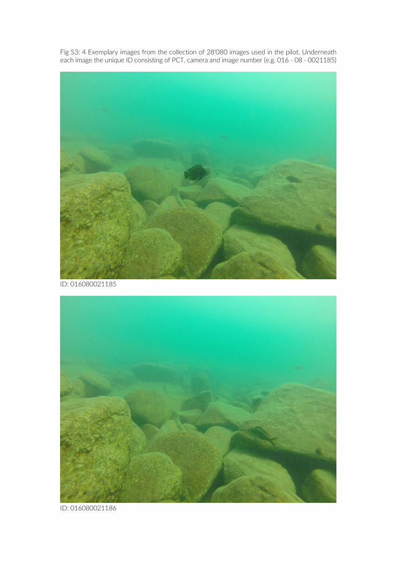
Fig S3: 4 Exemplary images from the collection of 28'080 images used in the pilot. Underneath each image the unique ID consisting of PCT, camera and image number (e.g. 016 - 08 - 0021185)
ID: 016080021185
ID: 016080021186
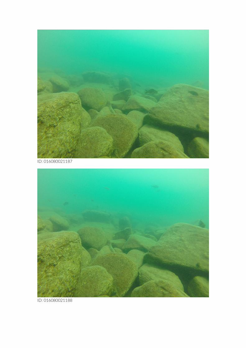
ID: 016080021187
ID: 016080021188
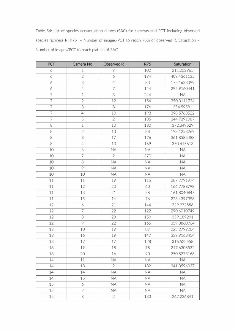
Table S4: List of species accumulation curves (SAC) for cameras and PCT including observed
species richness R. R75 = Number of images/PCT to reach 75% of observed R. Saturation =
Number of images/PCT to reach plateau of SAC
PCT Camera No Observed R R75 Saturation
6 1 9 102 211.232965 6 2 6 194 409.4361135 6 3 4 83 175.1633099 6 4 7 144 295.9160441 7 1 3 244 NA 7 2 12 154 350.3111734 7 3 8 176 354.59581 7 4 10 193 398.5763522 7 5 2 185 344.7391987 8 1 10 180 372.349529 8 2 13 88 198.1258269 8 3 17 176 361.8585488 8 4 13 169 350.415613
10 6 NA NA NA 10 7 2 270 NA 10 8 NA NA NA 10 9 NA NA NA 10 10 NA NA NA 11 11 19 115 287.7791974 11 12 20 60 166.7788798 11 13 21 58 161.8040847 11 15 14 76 223.4397398 12 6 21 144 329.972556 12 7 22 122 290.6010749 12 8 28 159 359.189291 12 9 22 165 359.8860764 12 10 19 87 223.2799204 13 16 19 147 339.9163454 13 17 17 128 316.522558 13 19 18 78 217.6308532 13 20 16 90 250.8273168 14 11 NA NA NA 14 13 2 182 341.3596037 14 14 NA NA NA 14 15 NA NA NA 15 6 NA NA NA 15 7 NA NA NA 15 8 2 133 267.236841
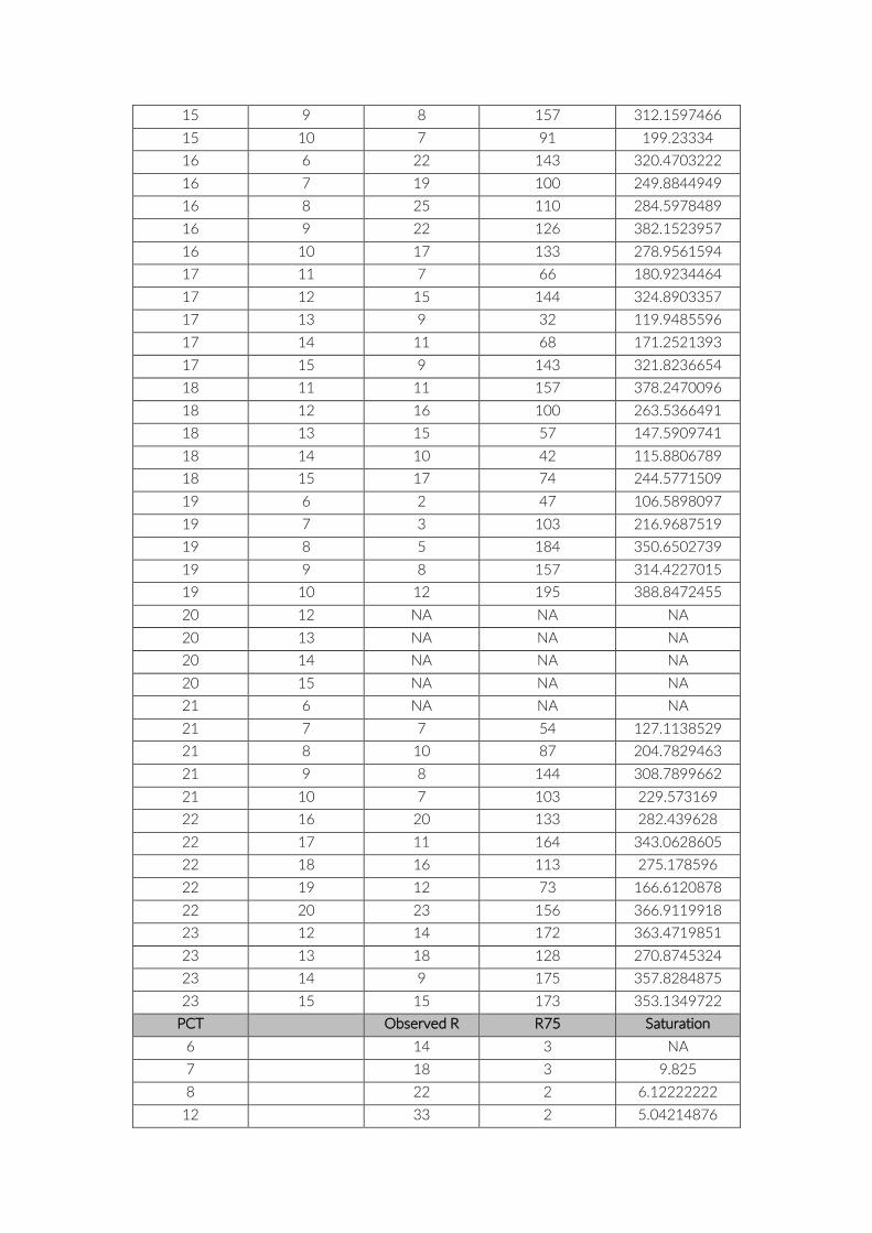
15 9 8 157 312.1597466 15 10 7 91 199.23334 16 6 22 143 320.4703222 16 7 19 100 249.8844949 16 8 25 110 284.5978489 16 9 22 126 382.1523957 16 10 17 133 278.9561594 17 11 7 66 180.9234464 17 12 15 144 324.8903357 17 13 9 32 119.9485596 17 14 11 68 171.2521393 17 15 9 143 321.8236654 18 11 11 157 378.2470096 18 12 16 100 263.5366491 18 13 15 57 147.5909741 18 14 10 42 115.8806789 18 15 17 74 244.5771509 19 6 2 47 106.5898097 19 7 3 103 216.9687519 19 8 5 184 350.6502739 19 9 8 157 314.4227015 19 10 12 195 388.8472455 20 12 NA NA NA 20 13 NA NA NA 20 14 NA NA NA 20 15 NA NA NA 21 6 NA NA NA 21 7 7 54 127.1138529 21 8 10 87 204.7829463 21 9 8 144 308.7899662 21 10 7 103 229.573169 22 16 20 133 282.439628 22 17 11 164 343.0628605 22 18 16 113 275.178596 22 19 12 73 166.6120878 22 20 23 156 366.9119918 23 12 14 172 363.4719851 23 13 18 128 270.8745324 23 14 9 175 357.8284875 23 15 15 173 353.1349722
PCT Observed R R75 Saturation 6 14 3 NA 7 18 3 9.825 8 22 2 6.12222222
12 33 2 5.04214876
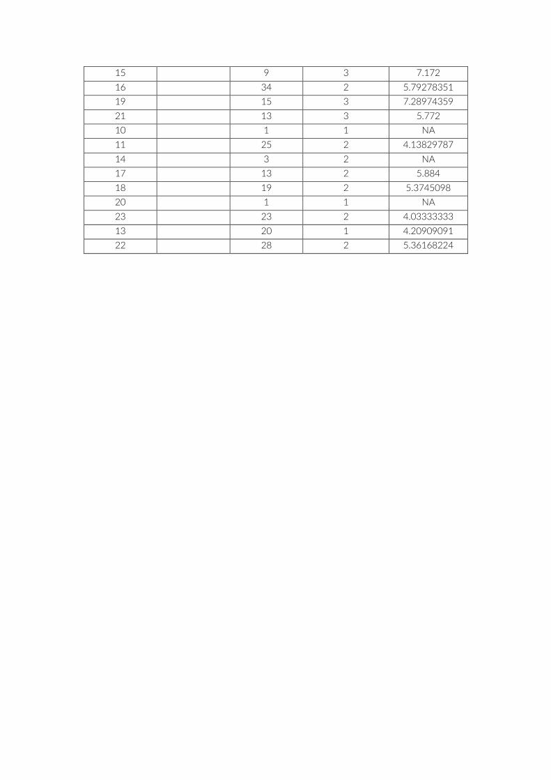
15 9 3 7.172 16 34 2 5.79278351 19 15 3 7.28974359 21 13 3 5.772 10 1 1 NA 11 25 2 4.13829787 14 3 2 NA 17 13 2 5.884 18 19 2 5.3745098 20 1 1 NA 23 23 2 4.03333333 13 20 1 4.20909091 22 28 2 5.36168224
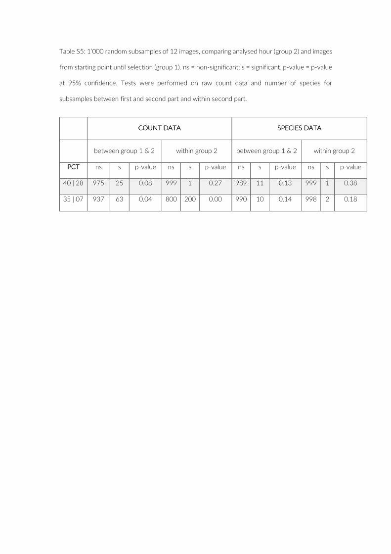
Table S5: 1’000 random subsamples of 12 images, comparing analysed hour (group 2) and images
from starting point until selection (group 1). ns = non-significant; s = significant, p-value = p-value
at 95% confidence. Tests were performed on raw count data and number of species for
subsamples between first and second part and within second part.
COUNT DATA SPECIES DATA
between group 1 & 2 within group 2 between group 1 & 2 within group 2
PCT ns s p-value ns s p-value ns s p-value ns s p-value
40 | 28 975 25 0.08 999 1 0.27 989 11 0.13 999 1 0.38
35 | 07 937 63 0.04 800 200 0.00 990 10 0.14 998 2 0.18
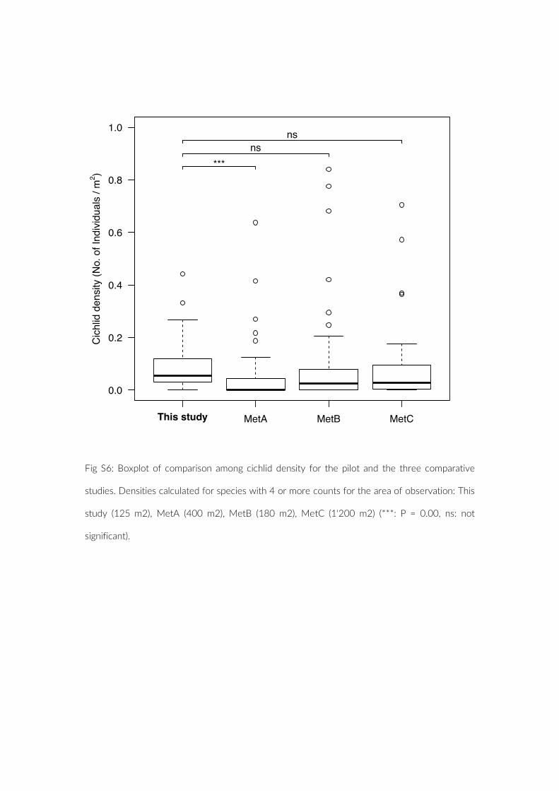
Fig S6: Boxplot of comparison among cichlid density for the pilot and the three comparative
studies. Densities calculated for species with 4 or more counts for the area of observation: This
study (125 m2), MetA (400 m2), MetB (180 m2), MetC (1'200 m2) (***: P = 0.00, ns: not
significant).
0.0
0.2
0.4
0.6
0.8
1.0
Cic
hlid
den
sity
(No.
of I
ndiv
idua
ls /
m2 )
This study MetA MetB MetC
nsns
***
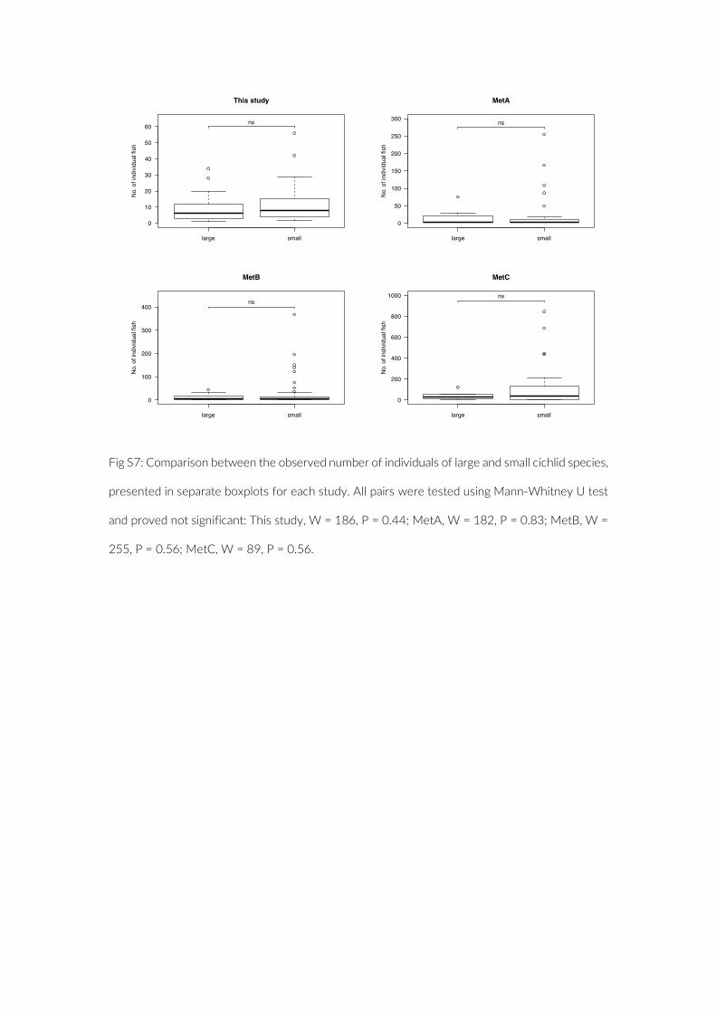
Fig S7: Comparison between the observed number of individuals of large and small cichlid species,
presented in separate boxplots for each study. All pairs were tested using Mann-Whitney U test
and proved not significant: This study, W = 186, P = 0.44; MetA, W = 182, P = 0.83; MetB, W =
255, P = 0.56; MetC, W = 89, P = 0.56.
0
10
20
30
40
50
60
This study
No.
of i
ndiv
idua
l fis
h
large small
ns
0
50
100
150
200
250
300
MetA
No.
of i
ndiv
idua
l fis
h
large small
ns
0
100
200
300
400
MetB
No.
of i
ndiv
idua
l fis
h
large small
ns
0
200
400
600
800
1000
MetC
No.
of i
ndiv
idua
l fis
h
large small
ns
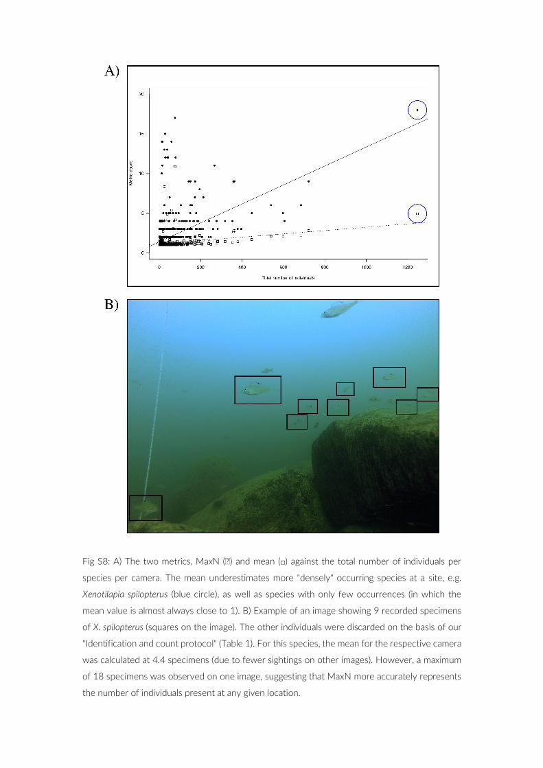
Fig S8: A) The two metrics, MaxN (�) and mean (☐) against the total number of individuals per
species per camera. The mean underestimates more "densely" occurring species at a site, e.g.
Xenotilapia spilopterus (blue circle), as well as species with only few occurrences (in which the
mean value is almost always close to 1). B) Example of an image showing 9 recorded specimens
of X. spilopterus (squares on the image). The other individuals were discarded on the basis of our
"Identification and count protocol" (Table 1). For this species, the mean for the respective camera
was calculated at 4.4 specimens (due to fewer sightings on other images). However, a maximum
of 18 specimens was observed on one image, suggesting that MaxN more accurately represents
the number of individuals present at any given location.
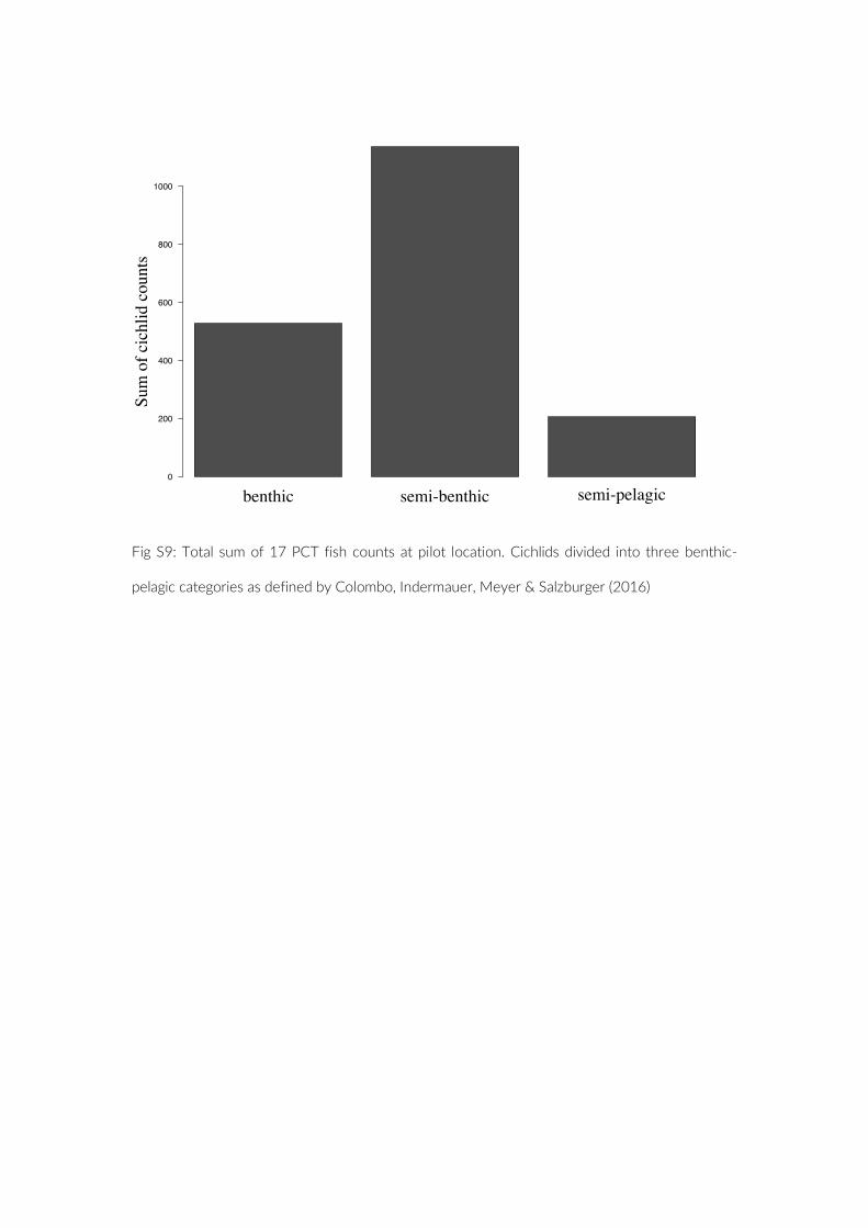
Fig S9: Total sum of 17 PCT fish counts at pilot location. Cichlids divided into three benthic-
pelagic categories as defined by Colombo, Indermauer, Meyer & Salzburger (2016)
0
200
400
600
800
1000
semi-benthicbenthic semi-pelagic
Sum
of c
ichl
id c
ount
s

Chapter 2
Does eDNA within sediments reflect local
cichlid assemblages in Lake Tanganyika?
Widmer L & El Taher E, Salzburger W
2.1 Manuscript pages 49 – 69
2.2 Supplementary Information pages 71 - 77

Does eDNA within sediments reflect local cichlid
assemblages in Lake Tanganyika? Lukas Widmer1 & Athimed El Taher1, Walter Salzburger1
1 Universität Basel, Zoologisches Institut, Vesalgasse 1, CH-4051 Basel
Abstract Environmental DNA (eDNA), that is DNA fragments stemming from an unknown composition of
organisms extracted from environmental samples, such as soil or water, are gaining in popularity in
the use for monitoring aquatic ecosystems. eDNA approaches are often based on sampling
surface water, but recent studies suggest a heightened concentration of eDNA in sediments. We
applied an eDNA metabarcoding approach to sediment samples from various sites at the East
African Lake Tanganyika. We compared the cichlid species richness derived from these sediment
samples to data obtained by a novel underwater visual census method, the Point-Combination
Transect (PCT). The diversity observed with the visual method was higher than then one detected
with the eDNA metabarcoding approach. However, the species observed by the two methods
proved to be mostly complementary. Taken together, our results indicate that PCT combined with
an eDNA approach could represent a robust tool to study underwater communities.
Introduction
Key components of nature conservation and biodiversity management are the monitoring and
understanding of species richness including gathering data on species distribution across a wider
landscape as well as determining their population densities (Rapport, Costanza, & McMichael, 1998;
Eros, 2007; Cianfrani et al., 2011). A major challenge in this field is the detection of rare or patchily
distributed species in fragmented environments. Traditional, non-invasive observational approaches
often fail to detect these rare species (or make their detection extremely elaborate) (Jerde, Mahon,
Chadderton, & Lodge, 2011; Wilcox et al., 2013). Such approaches have, however, long been the
only way to assess species richness and distribution in vulnerable ecosystems (Watson & Quinn,
1997; Colvocoresses & Acosta, 2007). In the aquatic environment, classic approaches to conduct
surveys are the underwater visual census methods such as line transects or points counts (M.
Samoilys & Carlos, 1992; M. A. Samoilys & Carlos, 2000), which through their biases associated with
diver presence, may fail to detect shy or rare species (Dickens, Goatley, Tanner, & Bellwood, 2011;
Pereira, Leal, & de Araújo, 2016; Pais & Cabral, 2017). Recently, more advanced survey methods
have been developed, such as the Point-Combination Transect (PCT) (Widmer et al., 2019), which
makes use of digital cameras in underwater housings placed within the benthic environment and set
to record digital images in a predefined time interval. The use of remote imaging eliminates biases
that are usually associated with traditional UVC methods, might improve the quality of census
surveys to a degree that they capture rare species when other methods fail.
Another approach is to use environmental DNA (eDNA), that is, DNA fragments collected from
environmental samples, such as soil or water, for monitoring the biodiversity in terrestrial as well as
in aquatic ecosystems (Thomsen & Willerslev, 2015; Klymus, Marshall, & Stepien, 2017; Lobo,
Shokralla, Costa, Hajibabaei, & Costa, 2017). eDNA has a long history in microbiology and other
fields focusing on terrestrial systems (Thomsen & Willerslev, 2015; Padgett-Stewart et al., 2016). Its
application in the aquatic environment, despite a growing number of studies, is still relatively new.
The most common methodology to obtain eDNA samples is either from surface water or to increase
eDNA concentration from the filtrate of several litres of water (McKee, Spear, & Pierson, 2015;
Catalunya, Velocimetry, & Correlation, 2016; Valentini et al., 2016). For prolonged fieldwork in
remote or not easily accessible locations, however, another issue could present itself by the required
equipment to filter and transport water samples. Nevertheless, the applicability of this approach has
been demonstrated in a variety of studies on different systems and its limitations (e.g. non-target
species detection) discussed (Catalunya et al., 2016; Hänfling et al., 2016; Valentini et al., 2016;
Klymus et al., 2017). As aquatic DNA particle is subjected to transport by water movement, it may
not reflect local communities sufficiently, in particular when focusing on benthic species (Turner,
Uy, & Everhart, 2015). Turner, Uy and Everhart (2015) proposed the use of surficial sediment
samples to extract eDNA, as the concentration is higher due to particle settling (Turner et al., 2014).
For example, a major source of aqueous macrofaunal eDNA are fecal particles, which are frequently
excreted and often contain high concentrations of DNA (Barnes et al., 2014; Turner et al., 2015).
Due to their size, these particles usually settle in the upper sediment layer rather than staying
suspended in the water column (Turner et al., 2014). The higher concentration of eDNA in
sediments, also reduces the logistical requirements in that minimum quantity per sample can be
reduced compared to 250 ml when using surface water (Olds et al., 2016). Therefore, an approach
using sediment samples, might facilitate broad scale surveys in difficult field conditions due to the
simplistic material requirements and easy handling.
Here we aimed to use a modified version of the approach by Turner et al. (2015) to first evaluate
its applicability under difficult field conditions and to provide proof-of-concept of the newly
introduced PCT method (Widmer et al., 2019). For several field season a PCT study was conducted
to observe the cichlid fish community in Lake Tanganyika along the coasts of Zambia and Tanzania
(Widmer et al. manuscript). In addition to collecting images with PCTs, we also sampled the upper
sediment layers from sites where PCTs were placed. DNA was then extracted from these sediment

samples and sequenced using next generation sequencing. The resulting sequences were then
assigned to cichlid species and species occurrence and distribution determined to enable a
comparison to data obtained through the PCT method.
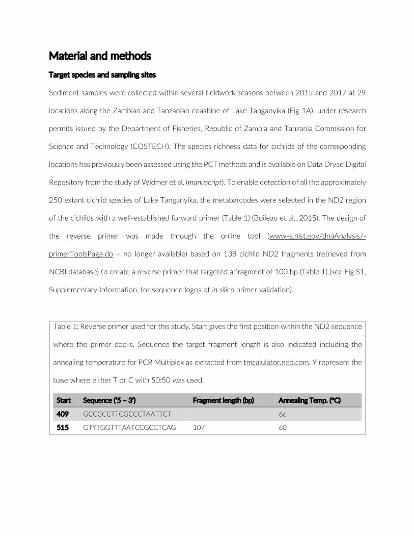
Material and methods
Target species and sampling sites
Sediment samples were collected within several fieldwork seasons between 2015 and 2017 at 29
locations along the Zambian and Tanzanian coastline of Lake Tanganyika (Fig 1A); under research
permits issued by the Department of Fisheries, Republic of Zambia and Tanzania Commission for
Science and Technology (COSTECH). The species richness data for cichlids of the corresponding
locations has previously been assessed using the PCT methods and is available on Data Dryad Digital
Repository from the study of Widmer et al. (manuscript). To enable detection of all the approximately
250 extant cichlid species of Lake Tanganyika, the metabarcodes were selected in the ND2 region
of the cichlids with a well-established forward primer (Table 1) (Boileau et al., 2015). The design of
the reverse primer was made through the online tool (www-s.nist.gov/dnaAnalysis/-
primerToolsPage.do – no longer available) based on 138 cichlid ND2 fragments (retrieved from
NCBI database) to create a reverse primer that targeted a fragment of 100 bp (Table 1) (see Fig S1,
Supplementary Information, for sequence logos of in silico primer validation).
Table 1: Reverse primer used for this study. Start gives the first position within the ND2 sequence
where the primer docks. Sequence the target fragment length is also indicated including the
annealing temperature for PCR Multiplex as extracted from tmcalulator.neb.com. Y represent the
base where either T or C with 50:50 was used.
Start Sequence (‘5 – 3’) Fragment length (bp) Annealing Temp. (°C)
409 GCCCCCTTCGCCCTAATTCT 66
515 GTYTGGTTTAATCCGCCTCAG 107 60
Sampling collection, preservation and storage
Sediment samples were collected using 50-mL centrifuge tubes (FalconTM
) during SCUBA dives of
PCT deployment. Prior to dives, the tubes were flooded with surface water, fish eDNA
concentration was assumed be negligible in the small amount of water (Fig 1B). Samples were
collected immediately after the placement of a camera to avoid excessive disturbance of the
sediment. The 50 mL tubes were gently pushed through the upper 2 cm of substrate until
approximately 10 ml wet sediment was collected. We collected three replicates of sediment at any
given location, which was within a 1 m radius of a randomly chosen camera of the deployed PCT.
This was usually done for two cameras per location. The excess water for each sample was removed
and the wet weight of the sample measured using a scale and approximately 10 ml of CTAB added
to each sample for DNA preservation (Chen, Rangasamy, Tan, Wang, & Siegfried, 2010;
Kiptantiyawati et al., 2014; Renshaw, Olds, Jerde, Mcveigh, & Lodge, 2015). At each location 10 ml
of CTAB was added to an empty tube as a collection control. All samples were stored at room
temperature until extraction.
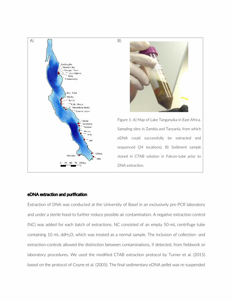
A)
B)
Figure 1: A) Map of Lake Tanganyika in East Africa.
Sampling sites in Zambia and Tanzania, from which
eDNA could successfully be extracted and
sequenced (24 locations). B) Sediment sample
stored in CTAB solution in Falcon-tube prior to
DNA extraction.
eDNA extraction and purification
Extraction of DNA was conducted at the University of Basel in an exclusively pre-PCR laboratory
and under a sterile hood to further reduce possible air contamination. A negative extraction control
(NC) was added for each batch of extractions. NC consisted of an empty 50-mL centrifuge tube
containing 10 mL ddH2O, which was treated as a normal sample. The inclusion of collection- and
extraction-controls allowed the distinction between contaminations, if detected, from fieldwork or
laboratory procedures. We used the modified CTAB extraction protocol by Turner et al. (2015)
based on the protocol of Coyne et al. (2005). The final sedimentary eDNA pellet was re-suspended
in 1 mL of 1X TE Low EDTA buffer. DNA concentration was measured using Thermo ScientificTM
NanoDropTM
2000. Ahead of the PCR, 100 μl of diluted eDNA extract from all 174 samples was
purified using a OneStep Inhibitor Removal Kit (Zymo Research, Irvine, California, USA). Each sample
was diluted to a concentration of 2.5 ng/μl, after pilot PCR reactions revealed this a promising
concentration for PCR reactions.
PCR and library preparation
PCR Master Mix was prepared under a UV sterilised hood in a laboratory where no fish tissue or
DNA samples are being handled to avoid contaminating the solutions. The entire preparation of the
PCR plates was done under a UV sterilised hood in the RNA lab again to avoid contamination
through cichlid DNA. We performed 10-μL reactions using 1 μL of eDNA extract with 5 μL of
QIAGEN Multiplex PCR Master Mix. Three technical replicates of the PCR were performed under
the following reaction conditions: 95 °C for 15 min and 40 3-step cycles of 94 °C for 30 s, 58 °C
for 90 s and 72 °C for 60 followed by the end step at 60 °C for 30 min. All PCR reactions were
conducted on a Veriti® 96-Well Thermal Cycler (Applied Biosystems). The three technical replicates
of each sample were pooled before quantifying amplicon length and concentration using 4200
TapeStation System (Agilent Technologies, Inc.). Samples with a concentration over 0.1 ng/μl of the
target amplicon were sent to D-BSSE (Genomic Center Basel, Switzerland) for library preparation
using KAPA Library Preparation Kit and sequencing on MiSeq Reagent Kit v3 (SR 150) in a single
run.
Bioinformatic analysis
Raw sequence reads were quality filtered and trimmed with Trimmomatic version 0.33 (Bolger,
Lohse, & Usadel, 2014) with a palindrome clip threshold of six, a simple clip threshold of one, a 10
bp window size, a required window quality of 20 and a read minimum length of 50 bp. We discarded
reads with an expected error higher than 0.75 at any nucleotide site with usearch version 7.0.1090

(Edgar, 2010). We also removed singletons and dereplicated reads with usearch version 5.2.236-
6.1.544 (Edgar, 2010). We used SAP (Statistical Assignment Package) (Munch, Boomsma,
Huelsenbeck, Willerslev, & Nielsen, 2008) to assignment our DNA sequence (similarity-threshold
0.97) to our taxonomic group of interest (ND2 from cichlids of Lake Tanganyika (Ronco et al. in
preparation)). Our bioinformatic pipeline was adapted from a published method from Olds et al. in
the Journal of Ecology and Evolution (Olds et al., 2016).
Results & Discussion
Here we used next-generation sequencing of environmental DNA (eDNA) to determine cichlid
distribution and species richness at various sites in Lake Tanganyika. Furthermore, we compared our
eDNA data set to the distribution and species richness data of a lake-wide census survey conducted
between 2014 and 2017, using the newly introduced underwater visual census method, Point-
Combination Transect (PCT) (Widmer et al., 2019). The eDNA metabarcode was selected from the
mitochondrial ND2 region to distinguish the diverse cichlid species-flock in Lake Tanganyika. The
eDNA metabarcoding approach missed to accurately reproduce the local cichlid assemblies
observed using PCT. Though it has previously been shown that eDNA approaches are able to
accurately capture fish communities in some instances (Turner et al., 2015), technical difficulties
during this study make a final conclusion about the applicability of eDNA to characterize local
communities of the Lake Tanganyika cichlid species-flock difficult.
In the course of this study, we collected 174 sediment samples (including collection field controls)
from 29 locations (which represent 51 different PCTs). Sediments were collected from an upper
depth limit of 2.9 m down to maximum depth of 31.8 m (Table S2, Supplementary Information). The
samples initially contained an average of 24.3 g (SD ±3.7) wet sediment and after DNA extraction
an average concentration of 43.0 ng/μl (SD ±30.4). We did not find a significant change in the
amount of extracted DNA per sample for different depths or substrate types (ANOVA: FDepth =
0.136, pDepth = 0.71; FSubstrate = 0.372, pSubstrate = 0.54). After quantifying amplicon length (target 107
bp) and concentration of PCR products, 78 samples with a concentration over 0.1 ng/μl of the target
amplicons were sent to D-BSSE for library preparation (Table S2, Supplementary Information).
Following the library preparation another 8 samples were removed, as the majority of libraries
corresponded to non-specific amplicons, resulting in 70 samples from 24 different locations being
sequenced on Illumina MiSeq (Table S2, Supplementary Information). The high loss of samples, was
mostly due to non-target amplification and incomplete primer ligation, resulting in ample primer
dimers, during PCR. Size selection, with an acceptable amount of product loss of the ~100 bp target
amplicon, was not feasible, as the size difference to primer dimers was minute.
Sequencing and species assignment
The single Illumina MiSeq run generated 18’589’697 sinlge-end reads for the 70 samples,
corresponding to a mean read count of ~265’567 per sample. After quality and error filtering, and
dereplication, we retained a total of 2’230’727 reads with an average of ~31’867 reads per sample
for the final species assignment (Fig 2) (Table S2, Supplementary Information). The complex length
profiles of libraries resulting from high concentration of primer dimers and other PCR by-products
lead to high loss of reads in the quality filtering step. To avoid such losses in future eDNA studies
of Lake Tanganyika cichlids, additional testing of primer pairs and DNA cleaning should be
performed.
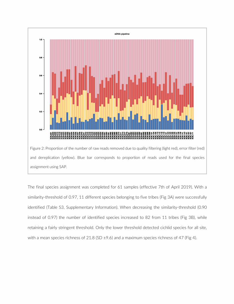
Figure 2: Proportion of the number of raw reads removed due to quality filtering (light red), error filter (red)
and dereplication (yellow). Blue bar corresponds to proportion of reads used for the final species
assignment using SAP.
The final species assignment was completed for 61 samples (effective 7th of April 2019). With a
similarity-threshold of 0.97, 11 different species belonging to five tribes (Fig 3A) were successfully
identified (Table S3, Supplementary Information). When decreasing the similarity-threshold (0.90
instead of 0.97) the number of identified species increased to 82 from 11 tribes (Fig 3B), while
retaining a fairly stringent threshold. Only the lower threshold detected cichlid species for all site,
with a mean species richness of 21.8 (SD ±9.6) and a maximum species richness of 47 (Fig 4).
SOIL001
SOIL003
SOIL006
SOIL015
SOIL018
SOIL022
SOIL023
SOIL024
SOIL025
SOIL027
SOIL030
SOIL034
SOIL035
SOIL037
SOIL038
SOIL040
SOIL041
SOIL042
SOIL045
SOIL046
SOIL049
SOIL050
SOIL052
SOIL053
SOIL054
SOIL055
SOIL057
SOIL060
SOIL061
SOIL062
SOIL063
SOIL065
SOIL066
SOIL070
SOIL071
SOIL073
SOIL077
SOIL079
SOIL081
SOIL082
SOIL083
SOIL084
SOIL085
SOIL086
SOIL091
SOIL092
SOIL095
SOIL096
SOIL098
SOIL101
SOIL104
SOIL105
SOIL113
SOIL115
SOIL118
SOIL119
SOIL121
SOIL124
SOIL125
SOIL129
SOIL135
SOIL137
SOIL138
SOIL139
SOIL141
SOIL143
SOIL151
SOIL157
SOIL167
SOIL171
eDNA pipeline
0.0
0.2
0.4
0.6
0.8
1.0
SOIL001
SOIL003
SOIL006
SOIL015
SOIL018
SOIL022
SOIL023
SOIL024
SOIL025
SOIL027
SOIL030
SOIL034
SOIL035
SOIL037
SOIL038
SOIL040
SOIL041
SOIL042
SOIL045
SOIL046
SOIL049
SOIL050
SOIL052
SOIL053
SOIL054
SOIL055
SOIL057
SOIL060
SOIL061
SOIL062
SOIL063
SOIL065
SOIL066
SOIL070
SOIL071
SOIL073
SOIL077
SOIL079
SOIL081
SOIL082
SOIL083
SOIL084
SOIL085
SOIL086
SOIL091
SOIL092
SOIL095
SOIL096
SOIL098
SOIL101
SOIL104
SOIL105
SOIL113
SOIL115
SOIL118
SOIL119
SOIL121
SOIL124
SOIL125
SOIL129
SOIL135
SOIL137
SOIL138
SOIL139
SOIL141
SOIL143
SOIL151
SOIL157
SOIL167
SOIL171
0.0
0.2
0.4
0.6
0.8
1.0
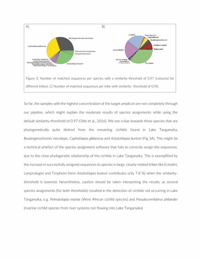
A)
B)
Figure 3: Number of matched sequences per species with a similarity-threshold of 0.97 (coloured for
different tribes). C) Number of matched sequences per tribe with similarity -threshold of 0.90.
So far, the samples with the highest concentration of the target amplicon are not completely through
our pipeline, which might explain the moderate results of species assignments while using the
default similarity-threshold of 0.97 (Olds et al., 2016). We see a bias towards three species that are
phylogenetically quite distinct from the remaining cichlids found in Lake Tanganyika,
Boulengerochromis microlepis, Cyphotilapia gibberosa and Astatotilapia burtoni (Fig 3A). This might be
a technical artefact of the species assignment software that fails to correctly assign the sequences,
due to the close phylogenetic relationship of the cichlids in Lake Tanganyika. This is exemplified by
the increase in successfully assigned sequences to species in large, closely related tribes like Ectodini,
Lamprologini and Tropheini (here Astatotilapia burtoni contributes only 7.8 %) when the similarity-
threshold is lowered. Nevertheless, caution should be taken interpreting the results, as several
species assignments (for both thresholds) resulted in the detection of cichlids not occurring in Lake
Tanganyika, e.g. Pelmatolapia mariae (West African cichlid species) and Pseudocrenilabrus philander
(riverine cichlid species from river systems not flowing into Lake Tanganyika)
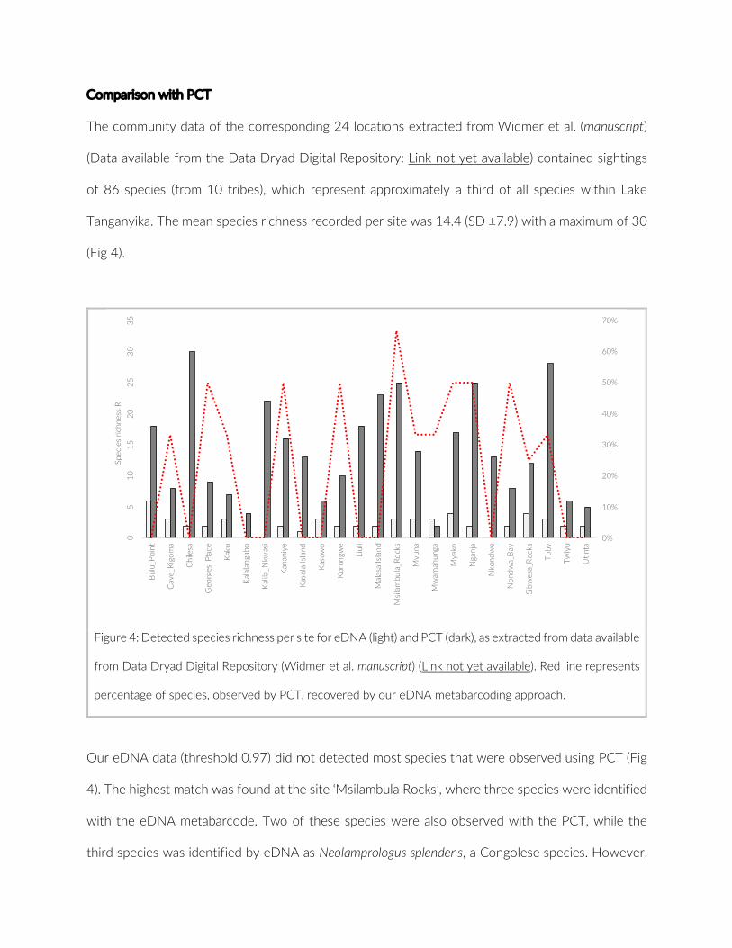
Comparison with PCT
The community data of the corresponding 24 locations extracted from Widmer et al. (manuscript)
(Data available from the Data Dryad Digital Repository: Link not yet available) contained sightings
of 86 species (from 10 tribes), which represent approximately a third of all species within Lake
Tanganyika. The mean species richness recorded per site was 14.4 (SD ±7.9) with a maximum of 30
(Fig 4).
Figure 4: Detected species richness per site for eDNA (light) and PCT (dark), as extracted from data available
from Data Dryad Digital Repository (Widmer et al. manuscript) (Link not yet available). Red line represents
percentage of species, observed by PCT, recovered by our eDNA metabarcoding approach.
Our eDNA data (threshold 0.97) did not detected most species that were observed using PCT (Fig
4). The highest match was found at the site ‘Msilambula Rocks’, where three species were identified
with the eDNA metabarcode. Two of these species were also observed with the PCT, while the
third species was identified by eDNA as Neolamprologus splendens, a Congolese species. However,
0%
10%
20%
30%
40%
50%
60%
70%
05
1015
2025
3035
Bul
u_Po
int
Cav
e_Ki
gom
a
Chi
lesa
Geo
rges
_Pla
ce
Kak
u
Kal
alan
gabo
Kal
ila_N
kwas
i
Kan
aniy
e
Kas
ola
Isla
nd
Kas
owo
Kor
ongw
e
Liul
i
Mal
asa
Isla
nd
Msi
lam
bula
_Roc
ks
Mvu
na
Mw
amah
unga
Mya
ko
Nga
nja
Nko
ndw
e
Non
dwa_
Bay
Sibw
esa_
Roc
ks
Toby
Twiy
u
Utin
ta
Spec
ies
richn
ess
R
Neolamprologus gracilis, a close relative of N. splendens was observed at the site using PCT. This again
illustrates the difficulties of using eDNA for species assignment on the cichlids of Lake Tanganyika,
as it is plausible that the sequence assigned to N. splendens is actually from N. gracilis. Reducing the
threshold of our eDNA pipeline increases the species richness observed by eDNA, but not the match
rate with PCT method, as one might expect. Meaning, the eDNA approach detects almost
exclusively additional species compared to the PCT data set.
Conclusion
Based on our current state of data analysis, we are unable to use eDNA to provide a proof of
concept for the novel method PCT. Nevertheless, in terms of species richness, we found that PCT
greatly outperformed the eDNA metabarcoding approach (if threshold 0.97 is used) and certainly
represent a robust tool to study underwater communities. At this point, no conclusion can be drawn
concerning the applicability of the eDNA approach for Lake Tanganyika, due to the quality of our
eDNA data; rather, it illustrates the issues that need to be resolved before further use: (1) re-
evaluation of the pipeline, (2) re-establishing reference database to increase certainty for taxonomic
assignment.

Acknowledgments
We thank Fabrizia Ronco, Adrian Indermaur, Heinz Büscher, the crew of Kalambo Falls Lodge and
George Kazumbe and his crew for the support in logistics and fieldwork, the Lake Tanganyika
Research Unit, Department of Fisheries, Republic of Zambia and the Tanzania Commission for
Science and Technology (COSTECH), for research permits. Further, we would like to thank Nicolas
Boileau for his support in the laboratory. This study was supported by the European Research
Council (ERC, CoG ‘CICHLID~X’ to WS).
Author’s contribution
LW and WS conceived and supervised the study, all co-authors conducted the fieldwork. LW was
responsible for lab work, analysed the data, and wrote the manuscript with feedback from all co-
authors. AT conducted the bioinformatic analysis.
References
Barnes, M. A., Turner, C. R., Jerde, C. L., Renshaw, M. A., Chadderton, W. L., & Lodge, D. M.
(2014). Environmental conditions influence eDNA persistence in aquatic systems.
Environmental Science and Technology, 48(3), 1819–1827. doi:10.1021/es404734p
Boileau, N., Cortesi, F., Egger, B., Muschick, M., Indermaur, A., Theis, A., … Salzburger, W. (2015).
A complex mode of aggressive mimicry in a scale-eating cichlid fish. Biology Letters, 11(9),
20150521. doi:10.1098/rsbl.2015.0521
Bolger, A. M., Lohse, M., & Usadel, B. (2014). Trimmomatic: a flexible trimmer for Illumina
sequence data. Bioinformatics, 30(15), 2114–2120. doi:10.1093/bioinformatics/btu170
Catalunya, U. P. De, Velocimetry, P. I., & Correlation, D. I. (2016). Fish community assessment with
eDNA metabarcoding: effects of sampling design and bioinformatic filtering. Canadian Journal
of Fisheries and Aquatic Sciences.
Chen, H., Rangasamy, M., Tan, S. Y., Wang, H., & Siegfried, B. D. (2010). Evaluation of five
methods for total DNA extraction from western corn rootworm beetles. PLoS ONE, 5(8).
doi:10.1371/journal.pone.0011963
Cianfrani, C., Le Lay, G., Maiorano, L., Satizábal, H. F., Loy, A., & Guisan, A. (2011). Adapting global
conservation strategies to climate change at the European scale: The otter as a flagship
species. Biological Conservation, 144(8), 2068–2080. doi:10.1016/j.biocon.2011.03.027
Colvocoresses, J., & Acosta, A. (2007). A large-scale field comparison of strip transect and
stationary point count methods for conducting length-based underwater visual surveys of
reef fish populations. Fisheries Research, 85(1–2), 130–141.
doi:10.1016/j.fishres.2007.01.012
Coyne, K. J., Handy, S. M., Demir, E., Whereat, E. B., Hutchins, D. A., Portune, K. J., … Cary, S. C.
(2005). Improved quantitative real-time PCR assays for enumeration of harmful algal species
in field samples using an exogenous DNA reference standard. Limnology and Oceanography:
Methods, 3(9), 381–391. doi:10.4319/lom.2005.3.381
Dickens, L. C., Goatley, C. H. R., Tanner, J. K., & Bellwood, D. R. (2011). Quantifying relative diver
effects in underwater visual censuses. PLoS ONE, 6(4), 6–8.
doi:10.1371/journal.pone.0018965
Edgar, R. C. (2010). Search and clustering orders of magnitude faster than BLAST. Bioinformatics,
26(19), 2460–2461. doi:10.1093/bioinformatics/btq461
Eros, T. (2007). Partitioning the diversity of riverine fish: The roles of habitat types and non-native
species. Freshwater Biology, 52(7), 1400–1415. doi:10.1111/j.1365-2427.2007.01777.x
Hänfling, B., Lawson Handley, L., Read, D. S., Hahn, C., Li, J., Nichols, P., … Winfield, I. J. (2016).
Environmental DNA metabarcoding of lake fish communities reflects long-term data from
established survey methods. Molecular Ecology, 25(13), 3101–3119. doi:10.1111/mec.13660
Jerde, C. L., Mahon, A. R., Chadderton, W. L., & Lodge, D. M. (2011). “Sight-unseen” detection of
rare aquatic species using environmental DNA. Conservation Letters, 4(2), 150–157.
doi:10.1111/j.1755-263X.2010.00158.x
Kiptantiyawati, N., Syarifah, N. L., Maulia, P., Sulistiyowati, E., Putra, M. R., Yudiansyah, … Ardie, S.
W. (2014). Sample preservation procedures and simple dna isolation protocols for the
tuberous crop, cassava (Manihot esculenta crantz.). Asia-Pacific Journal of Molecular Biology
and Biotechnology, 22(1), 164–170.
Klymus, K. E., Marshall, N. T., & Stepien, C. A. (2017). Environmental DNA (eDNA) metabarcoding
assays to detect invasive invertebrate species in the Great Lakes. PLoS ONE, 12(5), 1–24.
doi:10.1371/journal.pone.0177643
Lobo, J., Shokralla, S., Costa, M. H., Hajibabaei, M., & Costa, F. O. (2017). DNA metabarcoding for
high-throughput monitoring of estuarine macrobenthic communities. Scientific Reports, 7(1),
1–13. doi:10.1038/s41598-017-15823-6
McKee, A. M., Spear, S. F., & Pierson, T. W. (2015). The effect of dilution and the use of a post-

extraction nucleic acid purification column on the accuracy, precision, and inhibition of
environmental DNA samples. Biological Conservation, 183, 70–76.
doi:10.1016/j.biocon.2014.11.031
Munch, K., Boomsma, W., Huelsenbeck, J. P., Willerslev, E., & Nielsen, R. (2008). Statistical
Assignment of DNA Sequences Using Bayesian Phylogenetics. Systematic Biology, 57(5), 750–
757. doi:10.1080/10635150802422316
Olds, B. P., Jerde, C. L., Renshaw, M. A., Li, Y., Evans, N. T., Turner, C. R., … Lamberti, G. A. (2016).
Estimating species richness using environmental DNA. Ecology and Evolution, 6(12), 4214–
4226. doi:10.1002/ece3.2186
Padgett-Stewart, T. M., Wilcox, T. M., Carim, K. J., McKelvey, K. S., Young, M. K., & Schwartz, M.
K. (2016). An eDNA assay for river otter detection: a tool for surveying a semi-aquatic
mammal. Conservation Genetics Resources, 8(1), 5–7. doi:10.1007/s12686-015-0511-x
Pais, M. P., & Cabral, H. N. (2017). Fish behaviour effects on the accuracy and precision of
underwater visual census surveys. A virtual ecologist approach using an individual-based
model. Ecological Modelling, 346, 58–69. doi:10.1016/j.ecolmodel.2016.12.011
Pereira, P. H. C., Leal, I. C. S., & de Araújo, M. E. (2016). Observer presence may alter the
behaviour of reef fishes associated with coral colonies. Marine Ecology, 37(4), 760–769.
doi:10.1111/maec.12345
Rapport, D., Costanza, R., & McMichael, A. (1998). Assessing ecosystem health. Trends in Ecology &
Evolution, 13, 397–402. Retrieved from
http://www.sciencedirect.com/science/article/pii/S0169534798014499
Renshaw, M. A., Olds, B. P., Jerde, C. L., Mcveigh, M. M., & Lodge, D. M. (2015). The room
temperature preservation of filtered environmental DNA samples and assimilation into a
phenol-chloroform-isoamyl alcohol DNA extraction. Molecular Ecology Resources, 15(1), 168–
176. doi:10.1111/1755-0998.12281

Samoilys, M. A., & Carlos, G. (2000). Determining methods of underwater visual census for
estimating the abundance of coral reef fishes. Environmental Biology of Fishes, 57(3), 289–
304. doi:10.1023/A:1007679109359
Samoilys, M., & Carlos, G. (1992). Development of an Underwater Visual Census Method for Assessing
Shallow Water Reef Fish Stocks in the South West Pacific: Final Report. Queensland: Queensland
Dept. of Primary Industries. Retrieved from http://www.worldcat.org/title/development-of-
an-underwater-visual-census-method-for-assessing-shallow-water-reef-fish-stocks-in-the-
south-west-pacific-final-report/oclc/32021136?referer=di&ht=edition
Thomsen, P. F., & Willerslev, E. (2015). Environmental DNA - An emerging tool in conservation for
monitoring past and present biodiversity. Biological Conservation, 183, 4–18.
doi:10.1016/j.biocon.2014.11.019
Turner, C. R., Barnes, M. A., Xu, C. C. Y., Jones, S. E., Jerde, C. L., & Lodge, D. M. (2014). Particle
size distribution and optimal capture of aqueous macrobial eDNA. Methods in Ecology and
Evolution, 5(7), 676–684. doi:10.1111/2041-210X.12206
Turner, C. R., Uy, K. L., & Everhart, R. C. (2015). Fish environmental DNA is more concentrated in
aquatic sediments than surface water. Biological Conservation, 183, 93–102.
doi:10.1016/j.biocon.2014.11.017
Valentini, A., Taberlet, P., Miaud, C., Civade, R., Herder, J., Thomsen, P. F., … Dejean, T. (2016).
Next-generation monitoring of aquatic biodiversity using environmental DNA metabarcoding.
Molecular Ecology, 25(4), 929–942. doi:10.1111/mec.13428
Watson, R. A., & Quinn, T. J. (1997). Performance of transect and point count underwater visual
census methods. Ecological Modelling, 104(1), 103–112. doi:10.1016/S0304-3800(97)00117-
8
Widmer, L., Heule, E., Colombo, M., Rueegg, A., Indermaur, A., Ronco, F., & Salzburger, W. (2019).
Point-Combination Transect (PCT): Incorporation of small underwater cameras to study fish

communities. Methods in Ecology and Evolution, 2019(August 2018), 1–11.
doi:10.1111/2041-210X.13163
Wilcox, T. M., McKelvey, K. S., Young, M. K., Jane, S. F., Lowe, W. H., Whiteley, A. R., & Schwartz,
M. K. (2013). Robust Detection of Rare Species Using Environmental DNA: The Importance
of Primer Specificity. PLoS ONE, 8(3), e59520. doi:10.1371/journal.pone.0059520


Chapter 2
Supplementary Information
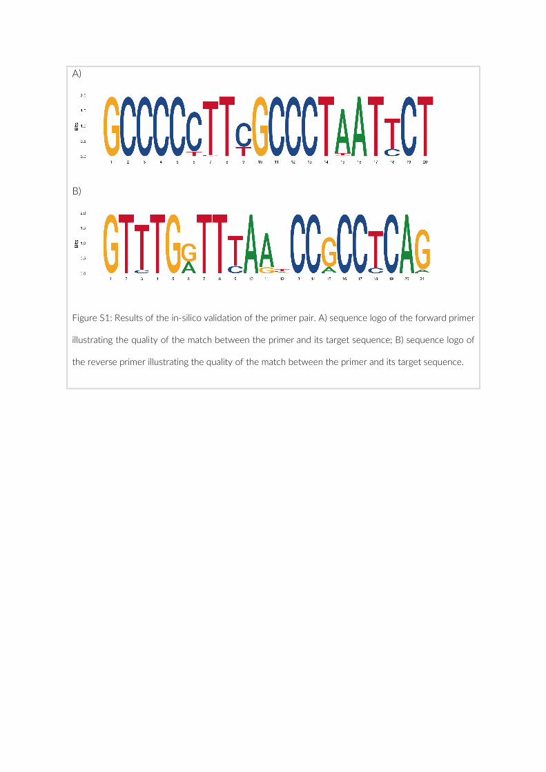
A)
B)
Figure S1: Results of the in-silico validation of the primer pair. A) sequence logo of the forward primer
illustrating the quality of the match between the primer and its target sequence; B) sequence logo of
the reverse primer illustrating the quality of the match between the primer and its target sequence.
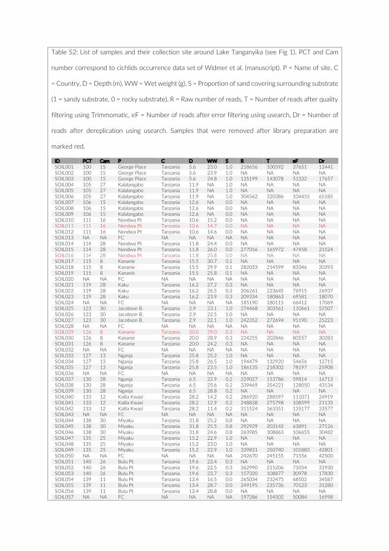
Table S2: List of samples and their collection site around Lake Tanganyika (see Fig 1). PCT and Cam
number correspond to cichlids occurrence data set of Widmer et al. (manuscript). P = Name of site, C
= Country, D = Depth (m), WW = Wet weight (g), S = Proportion of sand covering surrounding substrate
(1 = sandy substrate, 0 = rocky substrate), R = Raw number of reads, T = Number of reads after quality
filtering using Trimmomatic, eF = Number of reads after error filtering using usearch, Dr = Number of
reads after dereplication using usearch. Samples that were removed after library preparation are
marked red.
ID PCT Cam P C D WW S R T eF Dr SOIL001 100 15 George Place Tanzania 5.6 23.0 1.0 218656 100592 37651 11441 SOIL002 100 15 George Place Tanzania 5.6 23.9 1.0 NA NA NA NA SOIL003 100 15 George Place Tanzania 5.6 24.8 1.0 135199 143078 51332 17657 SOIL004 105 27 Kalalangabo Tanzania 11.9 NA 1.0 NA NA NA NA SOIL005 105 27 Kalalangabo Tanzania 11.9 NA 1.0 NA NA NA NA SOIL006 105 27 Kalalangabo Tanzania 11.9 NA 1.0 304562 320386 104455 65185 SOIL007 106 15 Kalalangabo Tanzania 12.6 NA 0.0 NA NA NA NA SOIL008 106 15 Kalalangabo Tanzania 12.6 NA 0.0 NA NA NA NA SOIL009 106 15 Kalalangabo Tanzania 12.6 NA 0.0 NA NA NA NA SOIL010 111 16 Nondwa Pt Tanzania 10.6 15.2 0.0 NA NA NA NA SOIL011 111 16 Nondwa Pt Tanzania 10.6 14.7 0.0 NA NA NA NA SOIL012 111 16 Nondwa Pt Tanzania 10.6 14.6 0.0 NA NA NA NA SOIL013 NA NA FC NA NA NA NA NA NA NA NA SOIL014 114 28 Nondwa Pt Tanzania 11.8 24.4 0.0 NA NA NA NA SOIL015 114 28 Nondwa Pt Tanzania 11.8 26.0 0.0 277056 165972 47458 21524 SOIL016 114 28 Nondwa Pt Tanzania 11.8 25.8 0.0 NA NA NA NA SOIL017 115 8 Kananie Tanzania 15.5 30.7 0.1 NA NA NA NA SOIL018 115 8 Kananie Tanzania 15.5 29.9 0.1 282033 214599 83346 20393 SOIL019 115 8 Kananie Tanzania 15.5 25.8 0.1 NA NA NA NA SOIL020 NA NA FC NA NA NA NA NA NA NA NA SOIL021 119 28 Kaku Tanzania 16.2 27.2 0.3 NA NA NA NA SOIL022 119 28 Kaku Tanzania 16.2 26.5 0.3 206261 223645 76915 26937 SOIL023 119 28 Kaku Tanzania 16.2 23.9 0.3 209334 180863 69581 18070 SOIL024 NA NA FC NA NA NA NA 185190 180115 66412 17069 SOIL025 123 30 Jacobson B. Tanzania 2.9 23.1 1.0 274468 303561 110661 52507 SOIL026 123 30 Jacobson B. Tanzania 2.9 22.5 1.0 NA NA NA NA SOIL027 123 30 Jacobson B. Tanzania 2.9 22.1 1.0 242352 272694 95190 25223 SOIL028 NA NA FC NA NA NA NA NA NA NA NA SOIL029 126 8 Kananie Tanzania 20.0 29.0 0.3 NA NA NA NA SOIL030 126 8 Kananie Tanzania 20.0 28.9 0.3 224255 202846 80557 30283 SOIL031 126 8 Kananie Tanzania 20.0 24.2 0.3 NA NA NA NA SOIL032 NA NA FC NA NA NA NA NA NA NA NA SOIL033 127 13 Nganja Tanzania 25.8 25.2 1.0 NA NA NA NA SOIL034 127 13 Nganja Tanzania 25.8 26.5 1.0 194479 132920 54656 12715 SOIL035 127 13 Nganja Tanzania 25.8 23.5 1.0 186135 218302 78197 25908 SOIL036 NA NA FC NA NA NA NA NA NA NA NA SOIL037 130 28 Nganja Tanzania 6.5 22.9 0.2 229027 153786 59814 16713 SOIL038 130 28 Nganja Tanzania 6.5 25.6 0.2 339469 354221 128050 43134 SOIL039 130 28 Nganja Tanzania 6.5 28.8 0.2 NA NA NA NA SOIL040 133 12 Kalila Kwasi Tanzania 28.2 14.2 0.2 286920 288597 111071 24919 SOIL041 133 12 Kalila Kwasi Tanzania 28.2 12.9 0.2 248838 275798 108599 21135 SOIL042 133 12 Kalila Kwasi Tanzania 28.2 11.4 0.2 311524 363351 135177 33577 SOIL043 NA NA FC NA NA NA NA NA NA NA NA SOIL044 138 30 Miyaku Tanzania 31.8 25.2 0.8 NA NA NA NA SOIL045 138 30 Miyaku Tanzania 31.8 25.5 0.8 292929 203142 63891 27126 SOIL046 138 30 Miyaku Tanzania 31.8 24.6 0.8 263985 308863 106655 30482 SOIL047 135 25 Miyaku Tanzania 15.2 22.9 1.0 NA NA NA NA SOIL048 135 25 Miyaku Tanzania 15.2 23.0 1.0 NA NA NA NA SOIL049 135 25 Miyaku Tanzania 15.2 22.9 1.0 339831 350740 101883 42801 SOIL050 NA NA FC NA NA NA NA 242670 245155 71556 42500 SOIL051 140 26 Bulu Pt Tanzania 19.6 22.4 0.3 NA NA NA NA SOIL052 140 26 Bulu Pt Tanzania 19.6 22.5 0.3 362990 215206 71054 31930 SOIL053 140 26 Bulu Pt Tanzania 19.6 23.7 0.3 157320 108877 30978 17830 SOIL054 139 11 Bulu Pt Tanzania 13.4 16.5 0.0 265034 232475 68502 34587 SOIL055 139 11 Bulu Pt Tanzania 13.4 28.7 0.0 249195 235736 70123 31280 SOIL056 139 11 Bulu Pt Tanzania 13.4 28.8 0.0 NA NA NA NA SOIL057 NA NA FC NA NA NA NA 197286 154502 50084 16998
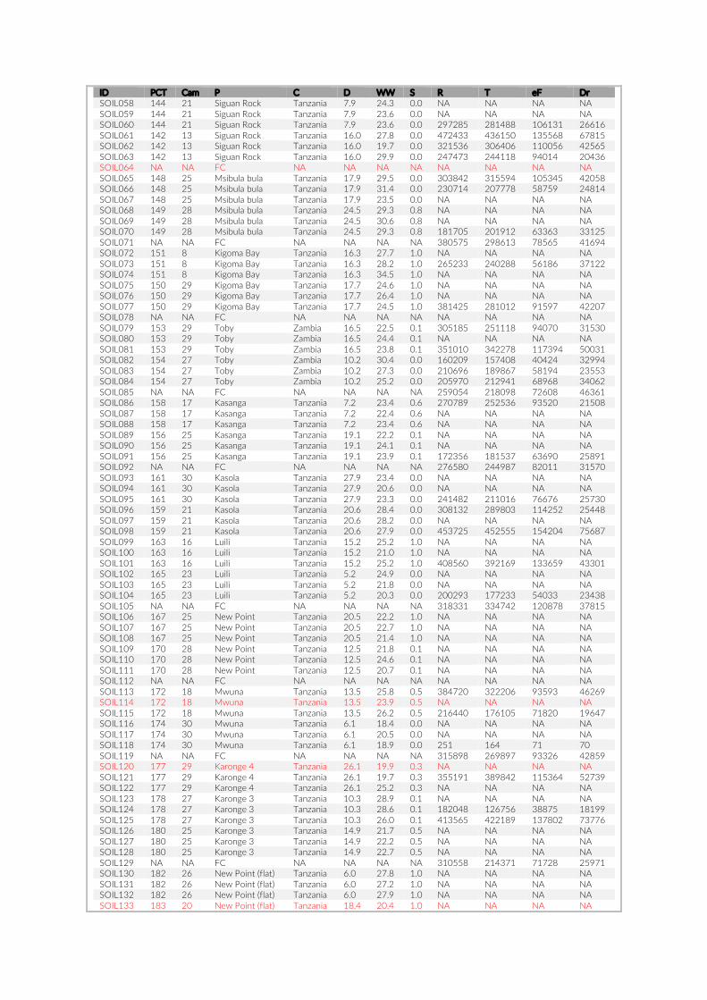
ID PCT Cam P C D WW S R T eF Dr SOIL058 144 21 Siguan Rock Tanzania 7.9 24.3 0.0 NA NA NA NA SOIL059 144 21 Siguan Rock Tanzania 7.9 23.6 0.0 NA NA NA NA SOIL060 144 21 Siguan Rock Tanzania 7.9 23.6 0.0 297285 281488 106131 26616 SOIL061 142 13 Siguan Rock Tanzania 16.0 27.8 0.0 472433 436150 135568 67815 SOIL062 142 13 Siguan Rock Tanzania 16.0 19.7 0.0 321536 306406 110056 42565 SOIL063 142 13 Siguan Rock Tanzania 16.0 29.9 0.0 247473 244118 94014 20436 SOIL064 NA NA FC NA NA NA NA NA NA NA NA SOIL065 148 25 Msibula bula Tanzania 17.9 29.5 0.0 303842 315594 105345 42058 SOIL066 148 25 Msibula bula Tanzania 17.9 31.4 0.0 230714 207778 58759 24814 SOIL067 148 25 Msibula bula Tanzania 17.9 23.5 0.0 NA NA NA NA SOIL068 149 28 Msibula bula Tanzania 24.5 29.3 0.8 NA NA NA NA SOIL069 149 28 Msibula bula Tanzania 24.5 30.6 0.8 NA NA NA NA SOIL070 149 28 Msibula bula Tanzania 24.5 29.3 0.8 181705 201912 63363 33125 SOIL071 NA NA FC NA NA NA NA 380575 298613 78565 41694 SOIL072 151 8 Kigoma Bay Tanzania 16.3 27.7 1.0 NA NA NA NA SOIL073 151 8 Kigoma Bay Tanzania 16.3 28.2 1.0 265233 240288 56186 37122 SOIL074 151 8 Kigoma Bay Tanzania 16.3 34.5 1.0 NA NA NA NA SOIL075 150 29 Kigoma Bay Tanzania 17.7 24.6 1.0 NA NA NA NA SOIL076 150 29 Kigoma Bay Tanzania 17.7 26.4 1.0 NA NA NA NA SOIL077 150 29 Kigoma Bay Tanzania 17.7 24.5 1.0 381425 281012 91597 42207 SOIL078 NA NA FC NA NA NA NA NA NA NA NA SOIL079 153 29 Toby Zambia 16.5 22.5 0.1 305185 251118 94070 31530 SOIL080 153 29 Toby Zambia 16.5 24.4 0.1 NA NA NA NA SOIL081 153 29 Toby Zambia 16.5 23.8 0.1 351010 342278 117394 50031 SOIL082 154 27 Toby Zambia 10.2 30.4 0.0 160209 157408 40424 32994 SOIL083 154 27 Toby Zambia 10.2 27.3 0.0 210696 189867 58194 23553 SOIL084 154 27 Toby Zambia 10.2 25.2 0.0 205970 212941 68968 34062 SOIL085 NA NA FC NA NA NA NA 259054 218098 72608 46361 SOIL086 158 17 Kasanga Tanzania 7.2 23.4 0.6 270789 252536 93520 21508 SOIL087 158 17 Kasanga Tanzania 7.2 22.4 0.6 NA NA NA NA SOIL088 158 17 Kasanga Tanzania 7.2 23.4 0.6 NA NA NA NA SOIL089 156 25 Kasanga Tanzania 19.1 22.2 0.1 NA NA NA NA SOIL090 156 25 Kasanga Tanzania 19.1 24.1 0.1 NA NA NA NA SOIL091 156 25 Kasanga Tanzania 19.1 23.9 0.1 172356 181537 63690 25891 SOIL092 NA NA FC NA NA NA NA 276580 244987 82011 31570 SOIL093 161 30 Kasola Tanzania 27.9 23.4 0.0 NA NA NA NA SOIL094 161 30 Kasola Tanzania 27.9 20.6 0.0 NA NA NA NA SOIL095 161 30 Kasola Tanzania 27.9 23.3 0.0 241482 211016 76676 25730 SOIL096 159 21 Kasola Tanzania 20.6 28.4 0.0 308132 289803 114252 25448 SOIL097 159 21 Kasola Tanzania 20.6 28.2 0.0 NA NA NA NA SOIL098 159 21 Kasola Tanzania 20.6 27.9 0.0 453725 452555 154204 75687 SOIL099 163 16 Luili Tanzania 15.2 25.2 1.0 NA NA NA NA SOIL100 163 16 Luili Tanzania 15.2 21.0 1.0 NA NA NA NA SOIL101 163 16 Luili Tanzania 15.2 25.2 1.0 408560 392169 133659 43301 SOIL102 165 23 Luili Tanzania 5.2 24.9 0.0 NA NA NA NA SOIL103 165 23 Luili Tanzania 5.2 21.8 0.0 NA NA NA NA SOIL104 165 23 Luili Tanzania 5.2 20.3 0.0 200293 177233 54033 23438 SOIL105 NA NA FC NA NA NA NA 318331 334742 120878 37815 SOIL106 167 25 New Point Tanzania 20.5 22.2 1.0 NA NA NA NA SOIL107 167 25 New Point Tanzania 20.5 22.7 1.0 NA NA NA NA SOIL108 167 25 New Point Tanzania 20.5 21.4 1.0 NA NA NA NA SOIL109 170 28 New Point Tanzania 12.5 21.8 0.1 NA NA NA NA SOIL110 170 28 New Point Tanzania 12.5 24.6 0.1 NA NA NA NA SOIL111 170 28 New Point Tanzania 12.5 20.7 0.1 NA NA NA NA SOIL112 NA NA FC NA NA NA NA NA NA NA NA SOIL113 172 18 Mwuna Tanzania 13.5 25.8 0.5 384720 322206 93593 46269 SOIL114 172 18 Mwuna Tanzania 13.5 23.9 0.5 NA NA NA NA SOIL115 172 18 Mwuna Tanzania 13.5 26.2 0.5 216440 176105 71820 19647 SOIL116 174 30 Mwuna Tanzania 6.1 18.4 0.0 NA NA NA NA SOIL117 174 30 Mwuna Tanzania 6.1 20.5 0.0 NA NA NA NA SOIL118 174 30 Mwuna Tanzania 6.1 18.9 0.0 251 164 71 70 SOIL119 NA NA FC NA NA NA NA 315898 269897 93326 42859 SOIL120 177 29 Karonge 4 Tanzania 26.1 19.9 0.3 NA NA NA NA SOIL121 177 29 Karonge 4 Tanzania 26.1 19.7 0.3 355191 389842 115364 52739 SOIL122 177 29 Karonge 4 Tanzania 26.1 25.2 0.3 NA NA NA NA SOIL123 178 27 Karonge 3 Tanzania 10.3 28.9 0.1 NA NA NA NA SOIL124 178 27 Karonge 3 Tanzania 10.3 28.6 0.1 182048 126756 38875 18199 SOIL125 178 27 Karonge 3 Tanzania 10.3 26.0 0.1 413565 422189 137802 73776 SOIL126 180 25 Karonge 3 Tanzania 14.9 21.7 0.5 NA NA NA NA SOIL127 180 25 Karonge 3 Tanzania 14.9 22.2 0.5 NA NA NA NA SOIL128 180 25 Karonge 3 Tanzania 14.9 22.7 0.5 NA NA NA NA SOIL129 NA NA FC NA NA NA NA 310558 214371 71728 25971 SOIL130 182 26 New Point (flat) Tanzania 6.0 27.8 1.0 NA NA NA NA SOIL131 182 26 New Point (flat) Tanzania 6.0 27.2 1.0 NA NA NA NA SOIL132 182 26 New Point (flat) Tanzania 6.0 27.9 1.0 NA NA NA NA SOIL133 183 20 New Point (flat) Tanzania 18.4 20.4 1.0 NA NA NA NA
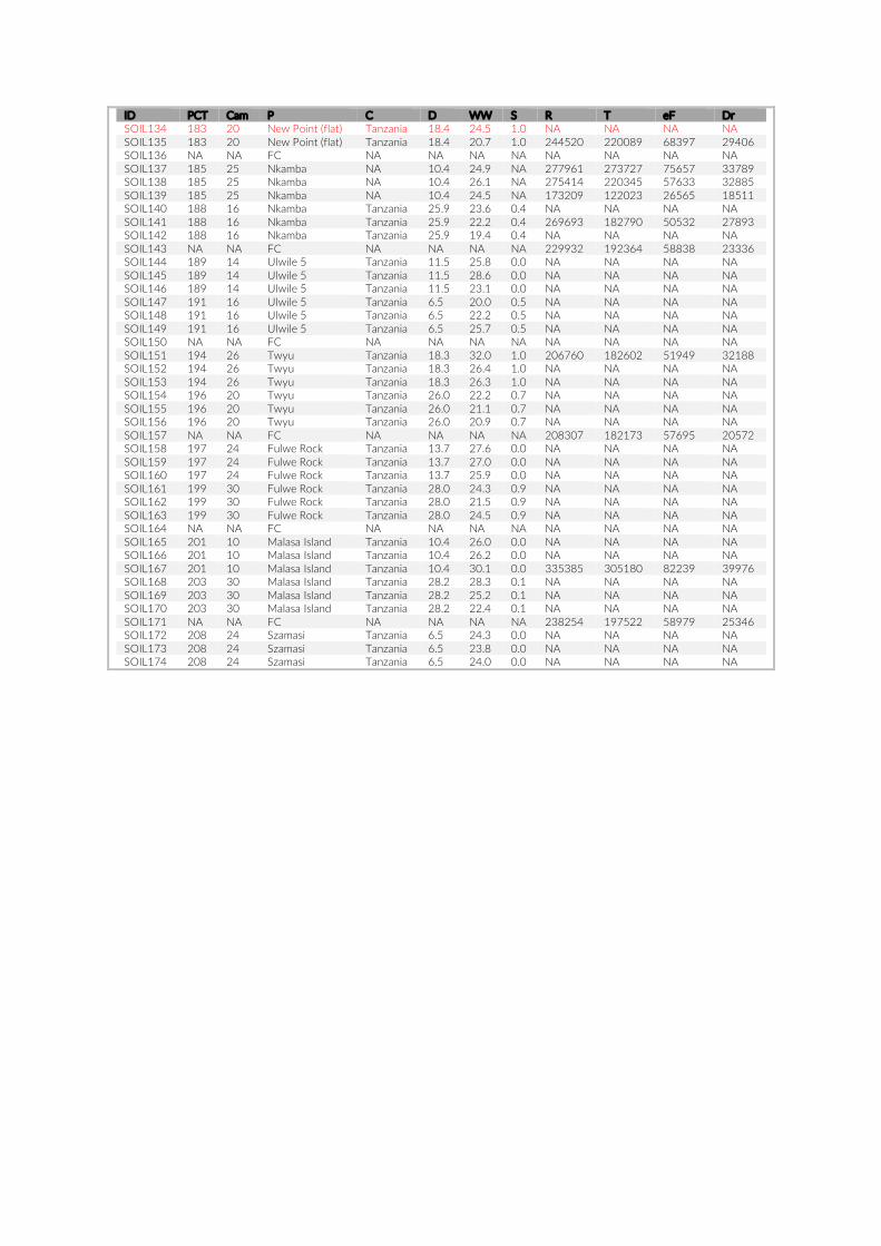
ID PCT Cam P C D WW S R T eF Dr SOIL134 183 20 New Point (flat) Tanzania 18.4 24.5 1.0 NA NA NA NA SOIL135 183 20 New Point (flat) Tanzania 18.4 20.7 1.0 244520 220089 68397 29406 SOIL136 NA NA FC NA NA NA NA NA NA NA NA SOIL137 185 25 Nkamba NA 10.4 24.9 NA 277961 273727 75657 33789 SOIL138 185 25 Nkamba NA 10.4 26.1 NA 275414 220345 57633 32885 SOIL139 185 25 Nkamba NA 10.4 24.5 NA 173209 122023 26565 18511 SOIL140 188 16 Nkamba Tanzania 25.9 23.6 0.4 NA NA NA NA SOIL141 188 16 Nkamba Tanzania 25.9 22.2 0.4 269693 182790 50532 27893 SOIL142 188 16 Nkamba Tanzania 25.9 19.4 0.4 NA NA NA NA SOIL143 NA NA FC NA NA NA NA 229932 192364 58838 23336 SOIL144 189 14 Ulwile 5 Tanzania 11.5 25.8 0.0 NA NA NA NA SOIL145 189 14 Ulwile 5 Tanzania 11.5 28.6 0.0 NA NA NA NA SOIL146 189 14 Ulwile 5 Tanzania 11.5 23.1 0.0 NA NA NA NA SOIL147 191 16 Ulwile 5 Tanzania 6.5 20.0 0.5 NA NA NA NA SOIL148 191 16 Ulwile 5 Tanzania 6.5 22.2 0.5 NA NA NA NA SOIL149 191 16 Ulwile 5 Tanzania 6.5 25.7 0.5 NA NA NA NA SOIL150 NA NA FC NA NA NA NA NA NA NA NA SOIL151 194 26 Twyu Tanzania 18.3 32.0 1.0 206760 182602 51949 32188 SOIL152 194 26 Twyu Tanzania 18.3 26.4 1.0 NA NA NA NA SOIL153 194 26 Twyu Tanzania 18.3 26.3 1.0 NA NA NA NA SOIL154 196 20 Twyu Tanzania 26.0 22.2 0.7 NA NA NA NA SOIL155 196 20 Twyu Tanzania 26.0 21.1 0.7 NA NA NA NA SOIL156 196 20 Twyu Tanzania 26.0 20.9 0.7 NA NA NA NA SOIL157 NA NA FC NA NA NA NA 208307 182173 57695 20572 SOIL158 197 24 Fulwe Rock Tanzania 13.7 27.6 0.0 NA NA NA NA SOIL159 197 24 Fulwe Rock Tanzania 13.7 27.0 0.0 NA NA NA NA SOIL160 197 24 Fulwe Rock Tanzania 13.7 25.9 0.0 NA NA NA NA SOIL161 199 30 Fulwe Rock Tanzania 28.0 24.3 0.9 NA NA NA NA SOIL162 199 30 Fulwe Rock Tanzania 28.0 21.5 0.9 NA NA NA NA SOIL163 199 30 Fulwe Rock Tanzania 28.0 24.5 0.9 NA NA NA NA SOIL164 NA NA FC NA NA NA NA NA NA NA NA SOIL165 201 10 Malasa Island Tanzania 10.4 26.0 0.0 NA NA NA NA SOIL166 201 10 Malasa Island Tanzania 10.4 26.2 0.0 NA NA NA NA SOIL167 201 10 Malasa Island Tanzania 10.4 30.1 0.0 335385 305180 82239 39976 SOIL168 203 30 Malasa Island Tanzania 28.2 28.3 0.1 NA NA NA NA SOIL169 203 30 Malasa Island Tanzania 28.2 25.2 0.1 NA NA NA NA SOIL170 203 30 Malasa Island Tanzania 28.2 22.4 0.1 NA NA NA NA SOIL171 NA NA FC NA NA NA NA 238254 197522 58979 25346 SOIL172 208 24 Szamasi Tanzania 6.5 24.3 0.0 NA NA NA NA SOIL173 208 24 Szamasi Tanzania 6.5 23.8 0.0 NA NA NA NA SOIL174 208 24 Szamasi Tanzania 6.5 24.0 0.0 NA NA NA NA
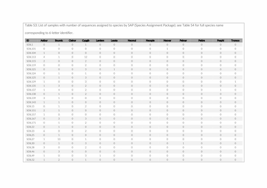
Table S3: List of samples with number of sequences assigned to species by SAP (Species Assignment Package); see Table S4 for full species name
corresponding to 6-letter identifier.
ID Astbur Boumic Ctehor Cypgib Lamlem Lessta Neomul Neosple Neovar Pelmar Pettre Psephi Tromoo
SOIL1 0 1 0 1 0 0 0 0 0 0 0 0 0
SOIL101 0 0 0 0 0 0 0 0 1 0 0 0 0
SOIL104 1 0 0 0 0 0 0 0 0 0 0 0 0
SOIL113 4 1 0 12 0 0 0 0 0 0 0 0 0
SOIL115 2 0 0 2 0 0 0 0 0 0 0 0 0
SOIL119 0 0 0 2 0 0 0 0 0 0 0 0 0
SOIL121 0 0 0 3 0 1 0 0 0 0 0 0 0
SOIL124 0 1 0 1 0 0 0 0 0 0 0 0 0
SOIL125 0 1 0 3 0 0 0 0 0 0 0 0 0
SOIL129 1 0 0 3 0 0 0 0 0 0 0 0 1
SOIL135 1 3 0 2 0 0 0 0 0 0 0 0 0
SOIL137 1 4 0 2 0 0 0 0 0 0 0 1 0
SOIL138 0 1 0 2 0 0 0 0 0 0 0 0 0
SOIL139 3 1 0 0 0 0 0 0 0 0 0 0 0
SOIL143 1 1 0 0 0 0 0 0 0 0 0 0 0
SOIL15 0 1 0 2 0 0 0 0 0 0 0 0 0
SOIL151 2 1 0 0 0 0 0 0 0 0 0 0 0
SOIL157 1 0 0 0 0 0 0 0 0 0 0 0 0
SOIL167 0 3 0 3 0 0 0 0 0 0 0 0 0
SOIL171 0 1 0 2 0 0 0 0 0 0 0 0 0
SOIL22 0 1 0 0 0 0 0 0 0 0 0 0 0
SOIL23 6 0 0 2 0 0 0 0 0 0 0 0 0
SOIL25 0 1 0 0 0 0 0 0 0 0 0 0 0
SOIL27 1 13 0 1 0 0 0 0 0 0 0 0 0
SOIL30 0 1 0 3 0 0 0 0 0 1 0 0 0
SOIL38 3 0 0 2 0 0 0 0 0 0 0 0 0
SOIL46 0 3 0 0 0 0 0 0 0 0 0 0 0
SOIL49 1 0 0 3 1 0 0 0 0 0 0 0 0
SOIL52 1 2 0 1 0 0 0 0 0 0 0 0 0
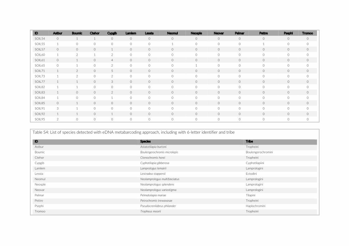
ID Astbur Boumic Ctehor Cypgib Lamlem Lessta Neomul Neosple Neovar Pelmar Pettre Psephi Tromoo
SOIL54 0 1 1 0 0 0 0 0 0 0 0 0 0
SOIL55 1 0 0 0 0 0 1 0 0 0 1 0 0
SOIL57 0 0 0 1 0 0 0 0 0 0 0 0 0
SOIL60 1 2 1 2 0 0 0 0 0 0 0 0 0
SOIL61 0 1 0 4 0 0 0 0 0 0 0 0 0
SOIL65 0 1 0 2 0 0 0 1 0 0 0 0 0
SOIL71 1 2 0 5 0 0 0 0 0 0 0 0 0
SOIL73 1 2 0 2 0 0 0 0 0 0 0 0 0
SOIL77 1 1 0 3 0 0 0 0 0 0 0 0 0
SOIL82 1 1 0 0 0 0 0 0 0 0 0 0 0
SOIL83 1 0 0 2 0 0 0 0 0 0 0 0 0
SOIL84 1 0 0 1 0 0 0 0 0 0 0 0 0
SOIL85 0 1 0 0 0 0 0 0 0 0 0 0 0
SOIL91 3 1 0 0 0 0 0 0 0 0 0 0 0
SOIL92 1 1 0 1 0 0 0 0 0 0 0 0 0
SOIL95 2 0 0 0 0 0 0 0 0 0 0 0 0
Table S4: List of species detected with eDNA metabarcoding approach, including with 6-letter identifier and tribe
ID Species Tribe
Astbur Astatotilapia burtoni Tropheini
Boumic Boulengerochromis microlepis Boulengerochromini
Ctehor Ctenochromis horei Tropheini
Cypgib Cyphotilapia gibberosa Cyphotilapiini
Lamlem Lamprologus lemairii Lamprologini
Lessta Lestradea stappersii Ectodini
Neomul Neolamprologus multifasciatus Lamprologini
Neosple Neolamprologus splendens Lamprologini
Neovar Neolamprologus variostigma Lamprologini
Pelmar Pelmatolapia mariae Tilapini
Pettre Petrochromis trewavasae Tropheini
Psephi Pseudocrenilabrus philander Haplochromini
Tromoo Tropheus moorii Tropheini


Part Two
Evolutionary Community Ecology


Chapter 3
Community assembly patterns and niche
evolution in the species-flock of cichlid fishes
from East African Lake Tanganyika
Widmer L, El Taher A, Indermaur A, Ronco F, Salzburger W
3.1 Manuscript pages 83 – 110
3.2 Supplementary Information pages 111 - 142

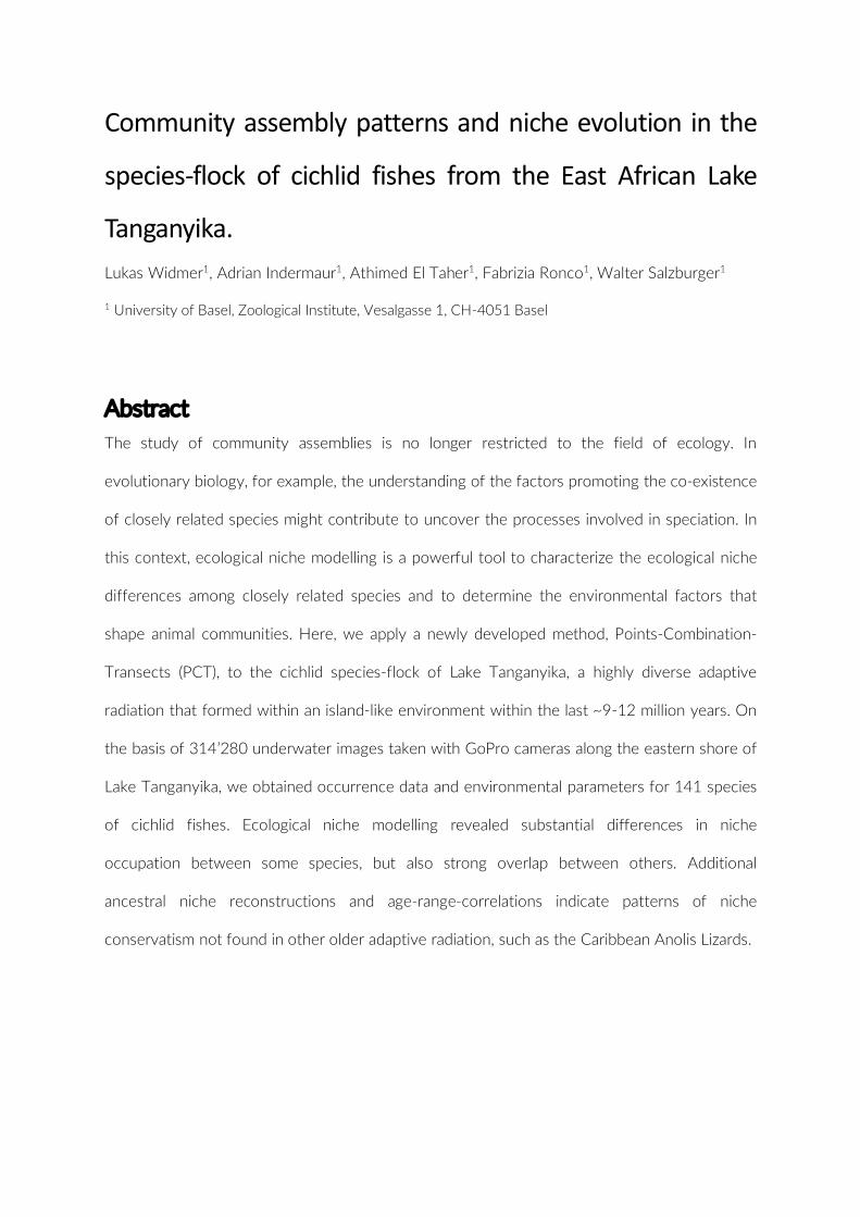
Community assembly patterns and niche evolution in the
species-flock of cichlid fishes from the East African Lake
Tanganyika. Lukas Widmer1, Adrian Indermaur1, Athimed El Taher1, Fabrizia Ronco1, Walter Salzburger1
1 University of Basel, Zoological Institute, Vesalgasse 1, CH-4051 Basel
Abstract
The study of community assemblies is no longer restricted to the field of ecology. In
evolutionary biology, for example, the understanding of the factors promoting the co-existence
of closely related species might contribute to uncover the processes involved in speciation. In
this context, ecological niche modelling is a powerful tool to characterize the ecological niche
differences among closely related species and to determine the environmental factors that
shape animal communities. Here, we apply a newly developed method, Points-Combination-
Transects (PCT), to the cichlid species-flock of Lake Tanganyika, a highly diverse adaptive
radiation that formed within an island-like environment within the last ~9-12 million years. On
the basis of 314’280 underwater images taken with GoPro cameras along the eastern shore of
Lake Tanganyika, we obtained occurrence data and environmental parameters for 141 species
of cichlid fishes. Ecological niche modelling revealed substantial differences in niche
occupation between some species, but also strong overlap between others. Additional
ancestral niche reconstructions and age-range-correlations indicate patterns of niche
conservatism not found in other older adaptive radiation, such as the Caribbean Anolis Lizards.
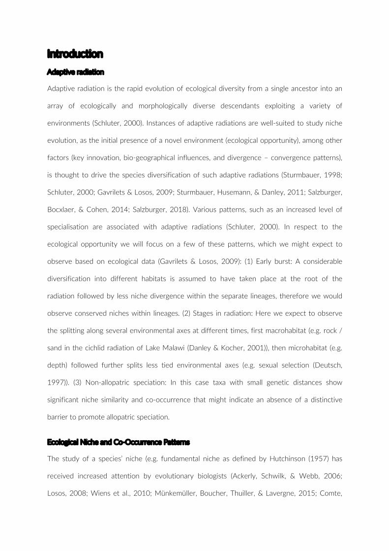
Introduction
Adaptive radiation
Adaptive radiation is the rapid evolution of ecological diversity from a single ancestor into an
array of ecologically and morphologically diverse descendants exploiting a variety of
environments (Schluter, 2000). Instances of adaptive radiations are well-suited to study niche
evolution, as the initial presence of a novel environment (ecological opportunity), among other
factors (key innovation, bio-geographical influences, and divergence – convergence patterns),
is thought to drive the species diversification of such adaptive radiations (Sturmbauer, 1998;
Schluter, 2000; Gavrilets & Losos, 2009; Sturmbauer, Husemann, & Danley, 2011; Salzburger,
Bocxlaer, & Cohen, 2014; Salzburger, 2018). Various patterns, such as an increased level of
specialisation are associated with adaptive radiations (Schluter, 2000). In respect to the
ecological opportunity we will focus on a few of these patterns, which we might expect to
observe based on ecological data (Gavrilets & Losos, 2009): (1) Early burst: A considerable
diversification into different habitats is assumed to have taken place at the root of the
radiation followed by less niche divergence within the separate lineages, therefore we would
observe conserved niches within lineages. (2) Stages in radiation: Here we expect to observe
the splitting along several environmental axes at different times, first macrohabitat (e.g. rock /
sand in the cichlid radiation of Lake Malawi (Danley & Kocher, 2001)), then microhabitat (e.g.
depth) followed further splits less tied environmental axes (e.g. sexual selection (Deutsch,
1997)). (3) Non-allopatric speciation: In this case taxa with small genetic distances show
significant niche similarity and co-occurrence that might indicate an absence of a distinctive
barrier to promote allopatric speciation.
Ecological Niche and Co-Occurrence Patterns
The study of a species’ niche (e.g. fundamental niche as defined by Hutchinson (1957) has
received increased attention by evolutionary biologists (Ackerly, Schwilk, & Webb, 2006;
Losos, 2008; Wiens et al., 2010; Münkemüller, Boucher, Thuiller, & Lavergne, 2015; Comte,
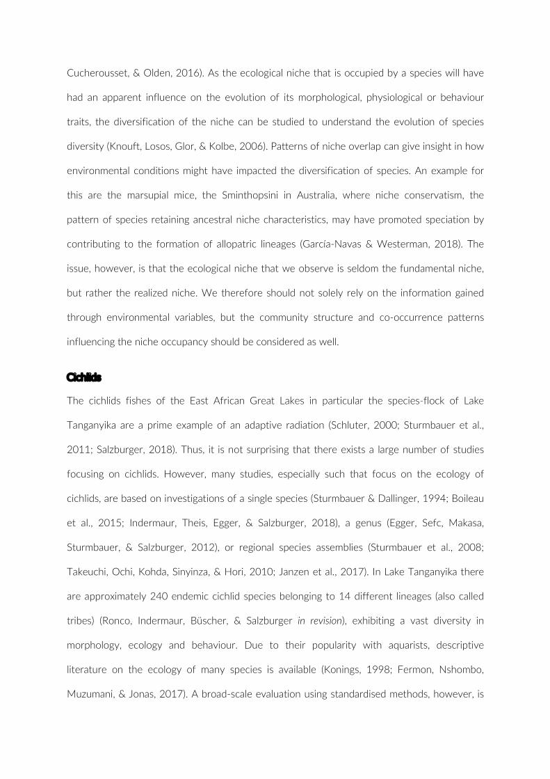
Cucherousset, & Olden, 2016). As the ecological niche that is occupied by a species will have
had an apparent influence on the evolution of its morphological, physiological or behaviour
traits, the diversification of the niche can be studied to understand the evolution of species
diversity (Knouft, Losos, Glor, & Kolbe, 2006). Patterns of niche overlap can give insight in how
environmental conditions might have impacted the diversification of species. An example for
this are the marsupial mice, the Sminthopsini in Australia, where niche conservatism, the
pattern of species retaining ancestral niche characteristics, may have promoted speciation by
contributing to the formation of allopatric lineages (García-Navas & Westerman, 2018). The
issue, however, is that the ecological niche that we observe is seldom the fundamental niche,
but rather the realized niche. We therefore should not solely rely on the information gained
through environmental variables, but the community structure and co-occurrence patterns
influencing the niche occupancy should be considered as well.
Cichlids
The cichlids fishes of the East African Great Lakes in particular the species-flock of Lake
Tanganyika are a prime example of an adaptive radiation (Schluter, 2000; Sturmbauer et al.,
2011; Salzburger, 2018). Thus, it is not surprising that there exists a large number of studies
focusing on cichlids. However, many studies, especially such that focus on the ecology of
cichlids, are based on investigations of a single species (Sturmbauer & Dallinger, 1994; Boileau
et al., 2015; Indermaur, Theis, Egger, & Salzburger, 2018), a genus (Egger, Sefc, Makasa,
Sturmbauer, & Salzburger, 2012), or regional species assemblies (Sturmbauer et al., 2008;
Takeuchi, Ochi, Kohda, Sinyinza, & Hori, 2010; Janzen et al., 2017). In Lake Tanganyika there
are approximately 240 endemic cichlid species belonging to 14 different lineages (also called
tribes) (Ronco, Indermaur, Büscher, & Salzburger in revision), exhibiting a vast diversity in
morphology, ecology and behaviour. Due to their popularity with aquarists, descriptive
literature on the ecology of many species is available (Konings, 1998; Fermon, Nshombo,
Muzumani, & Jonas, 2017). A broad-scale evaluation using standardised methods, however, is

lacking to date. The earliest broad-scale reports of the taxonomy of Lake Tanganyika’s cichlid
fauna, including a discussion about the ecology and diversity of the then known species, was
published over a century ago (Boulenger, 1898), the more recent one is still over 60 years old
(Poll, 1956). Therefore, an extensive exploration of the cichlid community and their ecological
niches seems due. To enable this primary investigation of niche evolution and community
assembly patterns within a strong phylogenetic framework, we make use of a recent and very
robust phylogeny based on whole genome sequencing of all Tanganyikan cichlids species
(Ronco et al. in preparation).
Aim
In this study we examine the extant cichlid species of Lake Tanganyika in respect to their
community structure, co-occurrences patterns and ecological niche in a uniquely broad-scale
and lake-wide context. We considered the entire cichlid species-flock of ~240 endemic species
from the along the coast of Lake Tanganyika (Ronco et al. in revision). Through extensive
fieldwork campaigns we collected a comprehensive data set of the occurrence, habitat
preferences and distribution of the primarily benthic cichlid fishes in Lake Tanganyika. With the
collected data we first explored the community structure and the underlying assembly
processes using co-occurrence data. We then constructed ecological niche models for each
species and examined, in a phylogenetic context, the patterns of niche diversification within
the Lake Tanganyika cichlid assembly.

Methods and Material
Cichlid visual census survey
Census data of cichlid fishes were collected between 2014 and 2017 at 45 locations along the
Zambian and Tanzanian coastline of Lake Tanganyika (Fig 1A) (total time in the field: three
months); under research permits issued by the Department of Fisheries, Republic of Zambia
and Tanzania Commission for Science and Technology (COSTECH). For data collection we
used a method we introduced recently, Point-Combination-Transects (PCTs), following the
strategy described in Widmer et al. (2019). In short, a PCT consists of five GoPro
cameras (Hero 3+ Silver Edition, Hero 4+ Silver Edition, © GoPro, Inc.) in underwater housings,
which are placed within the benthic environment in a standardized manner and equally spaced
along a transect line of 40 m, and set to record digital images in a time interval of 10 s for a
period of approximately 3 h (second hour of recordings was used for analysis, 360 images).
Each camera covered an area of approximately 5.5 m2 (Widmer et al., 2019). The sampling
locations were chosen to cover the three sub-basins of Lake Tanganyika and adequately
sample the different benthic habitat types in the littoral and sublittoral zone (up to a maximum
depth of 40 m). At each location, the target depths for three to four PCTs were defined a priori
and assigned to two SCUBA diver pairs. Each pair deployed up to two PCTs per dive; this
ensured safe installation and retrieval of PCTs under PADI safety regulations.
At the University of Basel, Switzerland, the resulting images were analysed as described in
Widmer et al. (2019). In brief, on each image only specimens that were fully visible and
their body facing the camera squarely (~ 90° – 135°) were counted and identified. To minimise
the effect of multiple counting of specimens we applied the MaxN count (maximum observed
number of specimens per species in a single image of a camera) (Merrett, Bagley, Smith, &
Creasey, 1994). Census data was either used in the form of each cameras’ MaxN value or as
the sum of MaxN values per PCT (five cameras), indicated from hereon as CAM- and PCT-data
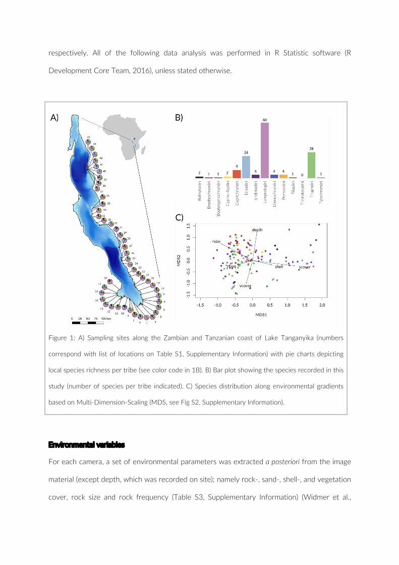
respectively. All of the following data analysis was performed in R Statistic software (R
Development Core Team, 2016), unless stated otherwise.
Figure 1: A) Sampling sites along the Zambian and Tanzanian coast of Lake Tanganyika (numbers
correspond with list of locations on Table S1, Supplementary Information) with pie charts depicting
local species richness per tribe (see color code in 1B). B) Bar plot showing the species recorded in this
study (number of species per tribe indicated). C) Species distribution along environmental gradients
based on Multi-Dimension-Scaling (MDS, see Fig S2, Supplementary Information).
Environmental variables
For each camera, a set of environmental parameters was extracted a posteriori from the image
material (except depth, which was recorded on site); namely rock-, sand-, shell-, and vegetation
cover, rock size and rock frequency (Table S3, Supplementary Information) (Widmer et al.,
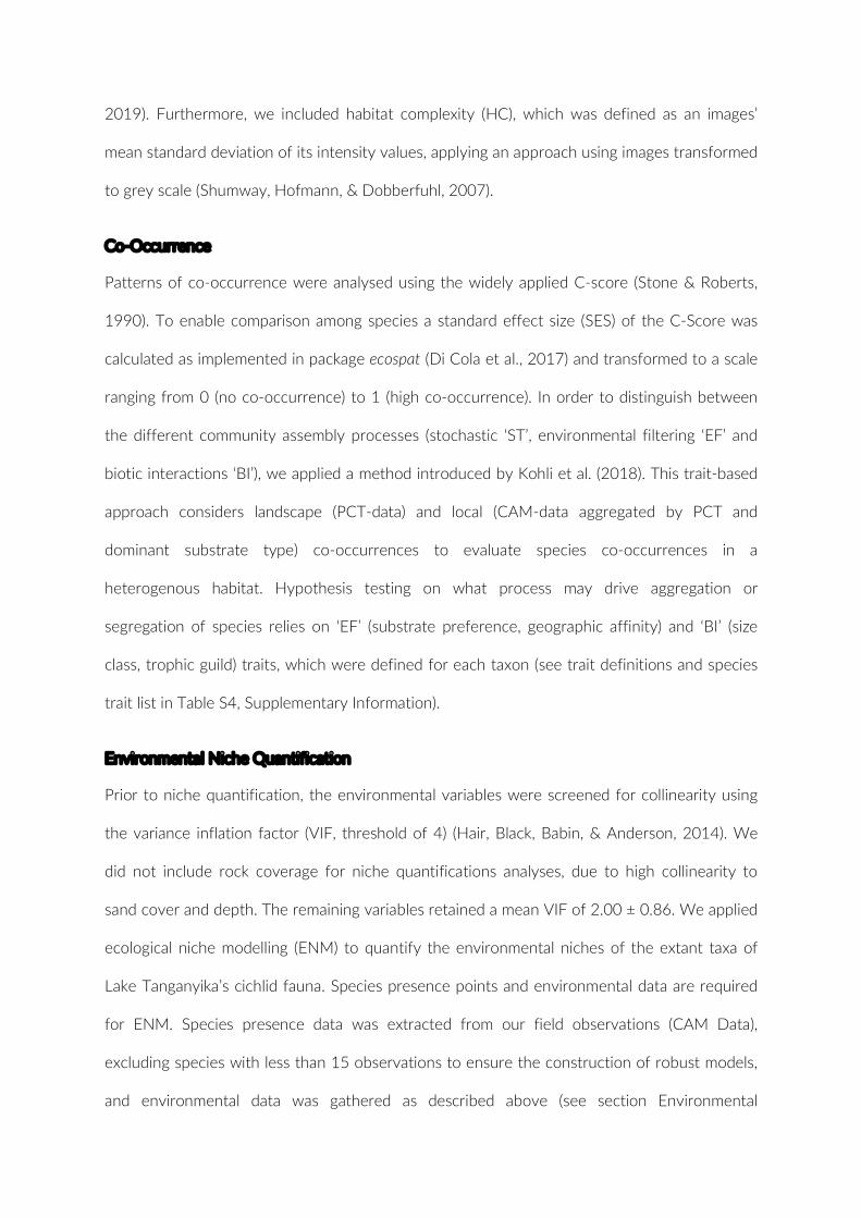
2019). Furthermore, we included habitat complexity (HC), which was defined as an images’
mean standard deviation of its intensity values, applying an approach using images transformed
to grey scale (Shumway, Hofmann, & Dobberfuhl, 2007).
Co-Occurrence
Patterns of co-occurrence were analysed using the widely applied C-score (Stone & Roberts,
1990). To enable comparison among species a standard effect size (SES) of the C-Score was
calculated as implemented in package ecospat (Di Cola et al., 2017) and transformed to a scale
ranging from 0 (no co-occurrence) to 1 (high co-occurrence). In order to distinguish between
the different community assembly processes (stochastic ‘ST’, environmental filtering ‘EF’ and
biotic interactions ‘BI’), we applied a method introduced by Kohli et al. (2018). This trait-based
approach considers landscape (PCT-data) and local (CAM-data aggregated by PCT and
dominant substrate type) co-occurrences to evaluate species co-occurrences in a
heterogenous habitat. Hypothesis testing on what process may drive aggregation or
segregation of species relies on ‘EF’ (substrate preference, geographic affinity) and ‘BI’ (size
class, trophic guild) traits, which were defined for each taxon (see trait definitions and species
trait list in Table S4, Supplementary Information).
Environmental Niche Quantification
Prior to niche quantification, the environmental variables were screened for collinearity using
the variance inflation factor (VIF, threshold of 4) (Hair, Black, Babin, & Anderson, 2014). We
did not include rock coverage for niche quantifications analyses, due to high collinearity to
sand cover and depth. The remaining variables retained a mean VIF of 2.00 ± 0.86. We applied
ecological niche modelling (ENM) to quantify the environmental niches of the extant taxa of
Lake Tanganyika’s cichlid fauna. Species presence points and environmental data are required
for ENM. Species presence data was extracted from our field observations (CAM Data),
excluding species with less than 15 observations to ensure the construction of robust models,
and environmental data was gathered as described above (see section Environmental
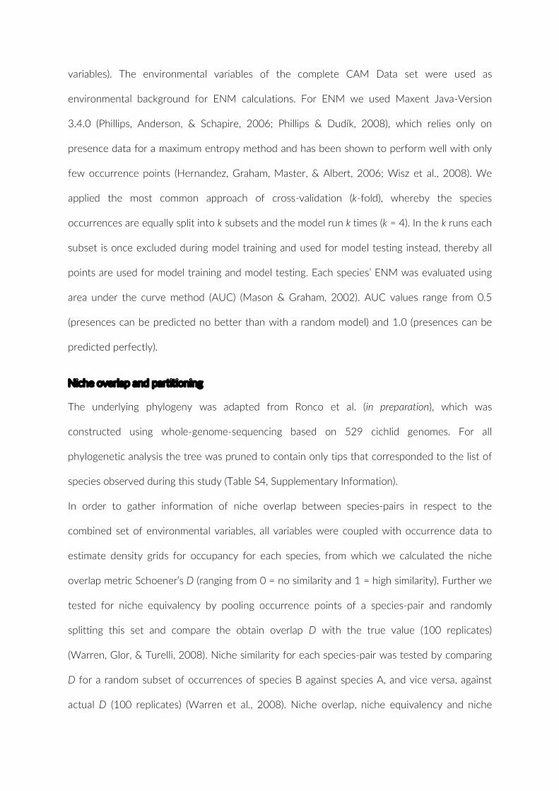
variables). The environmental variables of the complete CAM Data set were used as
environmental background for ENM calculations. For ENM we used Maxent Java-Version
3.4.0 (Phillips, Anderson, & Schapire, 2006; Phillips & Dudík, 2008), which relies only on
presence data for a maximum entropy method and has been shown to perform well with only
few occurrence points (Hernandez, Graham, Master, & Albert, 2006; Wisz et al., 2008). We
applied the most common approach of cross-validation (k-fold), whereby the species
occurrences are equally split into k subsets and the model run k times (k = 4). In the k runs each
subset is once excluded during model training and used for model testing instead, thereby all
points are used for model training and model testing. Each species’ ENM was evaluated using
area under the curve method (AUC) (Mason & Graham, 2002). AUC values range from 0.5
(presences can be predicted no better than with a random model) and 1.0 (presences can be
predicted perfectly).
Niche overlap and partitioning
The underlying phylogeny was adapted from Ronco et al. (in preparation), which was
constructed using whole-genome-sequencing based on 529 cichlid genomes. For all
phylogenetic analysis the tree was pruned to contain only tips that corresponded to the list of
species observed during this study (Table S4, Supplementary Information).
In order to gather information of niche overlap between species-pairs in respect to the
combined set of environmental variables, all variables were coupled with occurrence data to
estimate density grids for occupancy for each species, from which we calculated the niche
overlap metric Schoener’s D (ranging from 0 = no similarity and 1 = high similarity). Further we
tested for niche equivalency by pooling occurrence points of a species-pair and randomly
splitting this set and compare the obtain overlap D with the true value (100 replicates)
(Warren, Glor, & Turelli, 2008). Niche similarity for each species-pair was tested by comparing
D for a random subset of occurrences of species B against species A, and vice versa, against
actual D (100 replicates) (Warren et al., 2008). Niche overlap, niche equivalency and niche
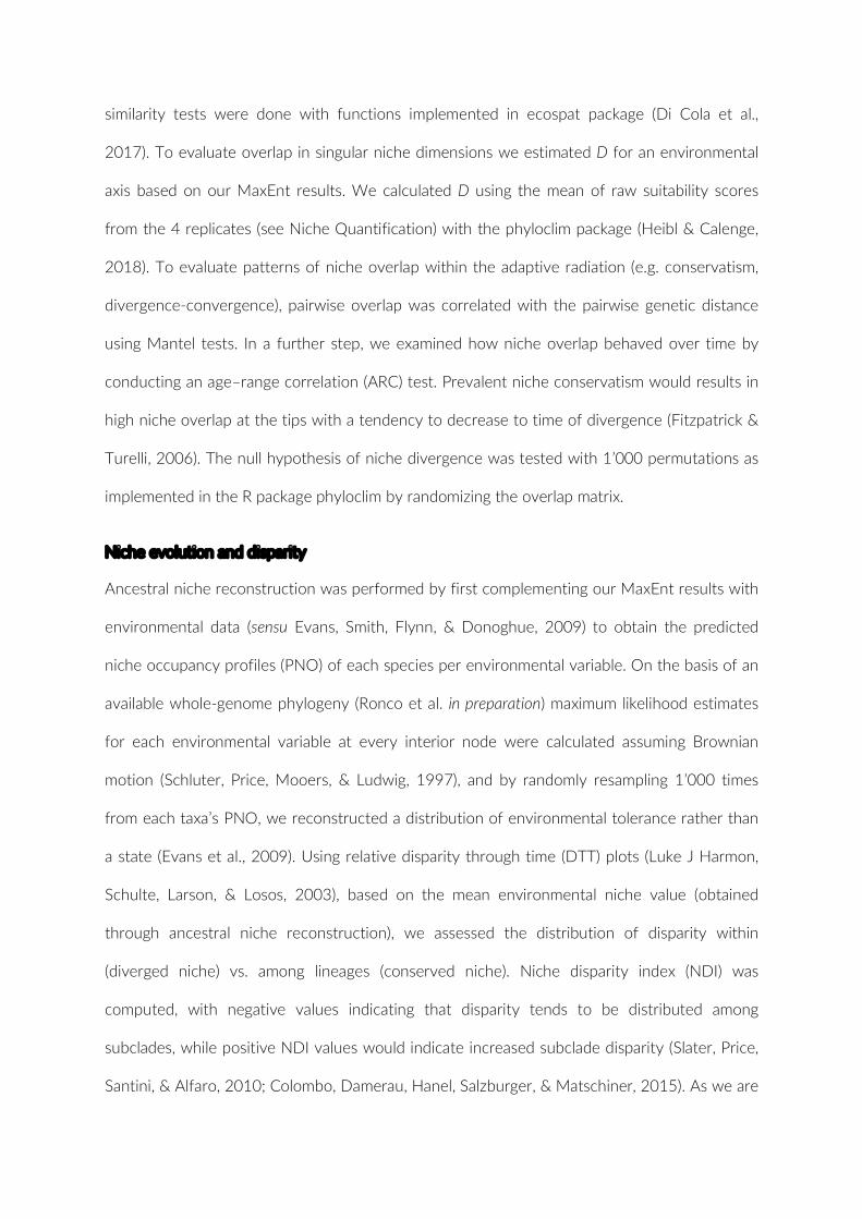
similarity tests were done with functions implemented in ecospat package (Di Cola et al.,
2017). To evaluate overlap in singular niche dimensions we estimated D for an environmental
axis based on our MaxEnt results. We calculated D using the mean of raw suitability scores
from the 4 replicates (see Niche Quantification) with the phyloclim package (Heibl & Calenge,
2018). To evaluate patterns of niche overlap within the adaptive radiation (e.g. conservatism,
divergence-convergence), pairwise overlap was correlated with the pairwise genetic distance
using Mantel tests. In a further step, we examined how niche overlap behaved over time by
conducting an age–range correlation (ARC) test. Prevalent niche conservatism would results in
high niche overlap at the tips with a tendency to decrease to time of divergence (Fitzpatrick &
Turelli, 2006). The null hypothesis of niche divergence was tested with 1’000 permutations as
implemented in the R package phyloclim by randomizing the overlap matrix.
Niche evolution and disparity
Ancestral niche reconstruction was performed by first complementing our MaxEnt results with
environmental data (sensu Evans, Smith, Flynn, & Donoghue, 2009) to obtain the predicted
niche occupancy profiles (PNO) of each species per environmental variable. On the basis of an
available whole-genome phylogeny (Ronco et al. in preparation) maximum likelihood estimates
for each environmental variable at every interior node were calculated assuming Brownian
motion (Schluter, Price, Mooers, & Ludwig, 1997), and by randomly resampling 1’000 times
from each taxa’s PNO, we reconstructed a distribution of environmental tolerance rather than
a state (Evans et al., 2009). Using relative disparity through time (DTT) plots (Luke J Harmon,
Schulte, Larson, & Losos, 2003), based on the mean environmental niche value (obtained
through ancestral niche reconstruction), we assessed the distribution of disparity within
(diverged niche) vs. among lineages (conserved niche). Niche disparity index (NDI) was
computed, with negative values indicating that disparity tends to be distributed among
subclades, while positive NDI values would indicate increased subclade disparity (Slater, Price,
Santini, & Alfaro, 2010; Colombo, Damerau, Hanel, Salzburger, & Matschiner, 2015). As we are

supplied with a robust phylogeny, we refrained from using posterior trees and simulated trait
behaviour under BM (replicates 1000). All functions are implemented in phyloclim (Heibl &
Calenge, 2018), APE (Paradis, Claude, & Strimmer, 2004) and GEIGER (L. J. Harmon, Weir,
Brock, Glor, & Challenger, 2008).
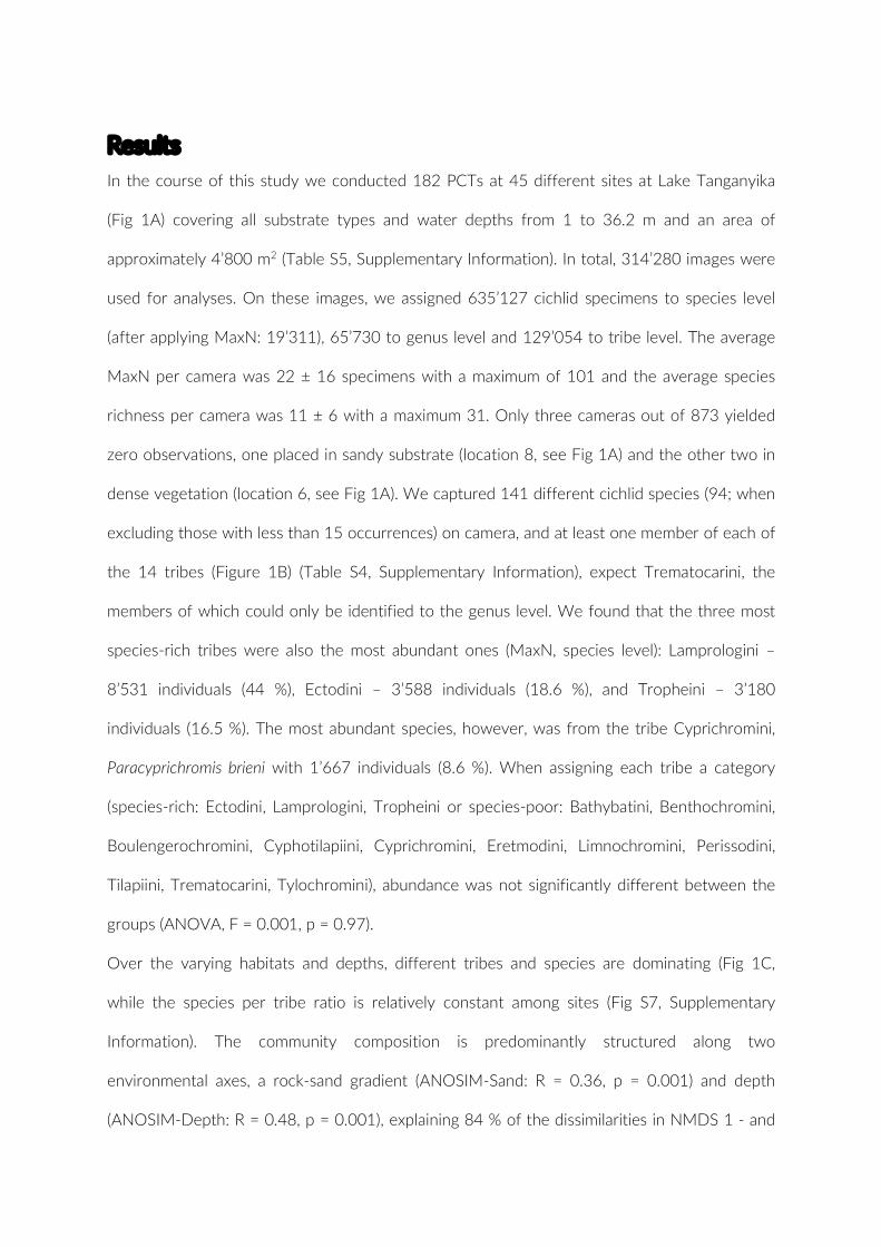
Results In the course of this study we conducted 182 PCTs at 45 different sites at Lake Tanganyika
(Fig 1A) covering all substrate types and water depths from 1 to 36.2 m and an area of
approximately 4’800 m2 (Table S5, Supplementary Information). In total, 314’280 images were
used for analyses. On these images, we assigned 635’127 cichlid specimens to species level
(after applying MaxN: 19’311), 65’730 to genus level and 129’054 to tribe level. The average
MaxN per camera was 22 ± 16 specimens with a maximum of 101 and the average species
richness per camera was 11 ± 6 with a maximum 31. Only three cameras out of 873 yielded
zero observations, one placed in sandy substrate (location 8, see Fig 1A) and the other two in
dense vegetation (location 6, see Fig 1A). We captured 141 different cichlid species (94; when
excluding those with less than 15 occurrences) on camera, and at least one member of each of
the 14 tribes (Figure 1B) (Table S4, Supplementary Information), expect Trematocarini, the
members of which could only be identified to the genus level. We found that the three most
species-rich tribes were also the most abundant ones (MaxN, species level): Lamprologini –
8’531 individuals (44 %), Ectodini – 3’588 individuals (18.6 %), and Tropheini – 3’180
individuals (16.5 %). The most abundant species, however, was from the tribe Cyprichromini,
Paracyprichromis brieni with 1’667 individuals (8.6 %). When assigning each tribe a category
(species-rich: Ectodini, Lamprologini, Tropheini or species-poor: Bathybatini, Benthochromini,
Boulengerochromini, Cyphotilapiini, Cyprichromini, Eretmodini, Limnochromini, Perissodini,
Tilapiini, Trematocarini, Tylochromini), abundance was not significantly different between the
groups (ANOVA, F = 0.001, p = 0.97).
Over the varying habitats and depths, different tribes and species are dominating (Fig 1C,
while the species per tribe ratio is relatively constant among sites (Fig S7, Supplementary
Information). The community composition is predominantly structured along two
environmental axes, a rock-sand gradient (ANOSIM-Sand: R = 0.36, p = 0.001) and depth
(ANOSIM-Depth: R = 0.48, p = 0.001), explaining 84 % of the dissimilarities in NMDS 1 - and
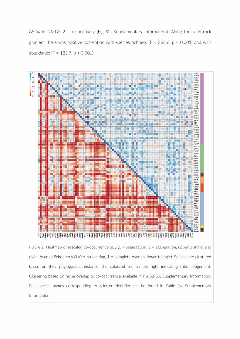
85 % in NMDS 2 – respectively (Fig S2, Supplementary Information). Along the sand-rock
gradient there was positive correlation with species richness (F = 383.6, p < 0.001) and with
abundance (F = 123.7, p < 0.001).
Figure 2: Heatmap of rescaled co-occurrence SES (0 = segregation, 1 = aggregation, upper triangle) and
niche overlap Schoener’s D (0 = no overlap, 1 = complete overlap, lower triangle). Species are clustered
based on their phylogenetic distance, the coloured bar on the right indicating tribe assignment.
Clustering based on niche overlap or co-occurrence available in Fig S8-S9, Supplementary Information.
Full species names corresponding to 6-letter identifier can be found in Table S4, Supplementary
Information.
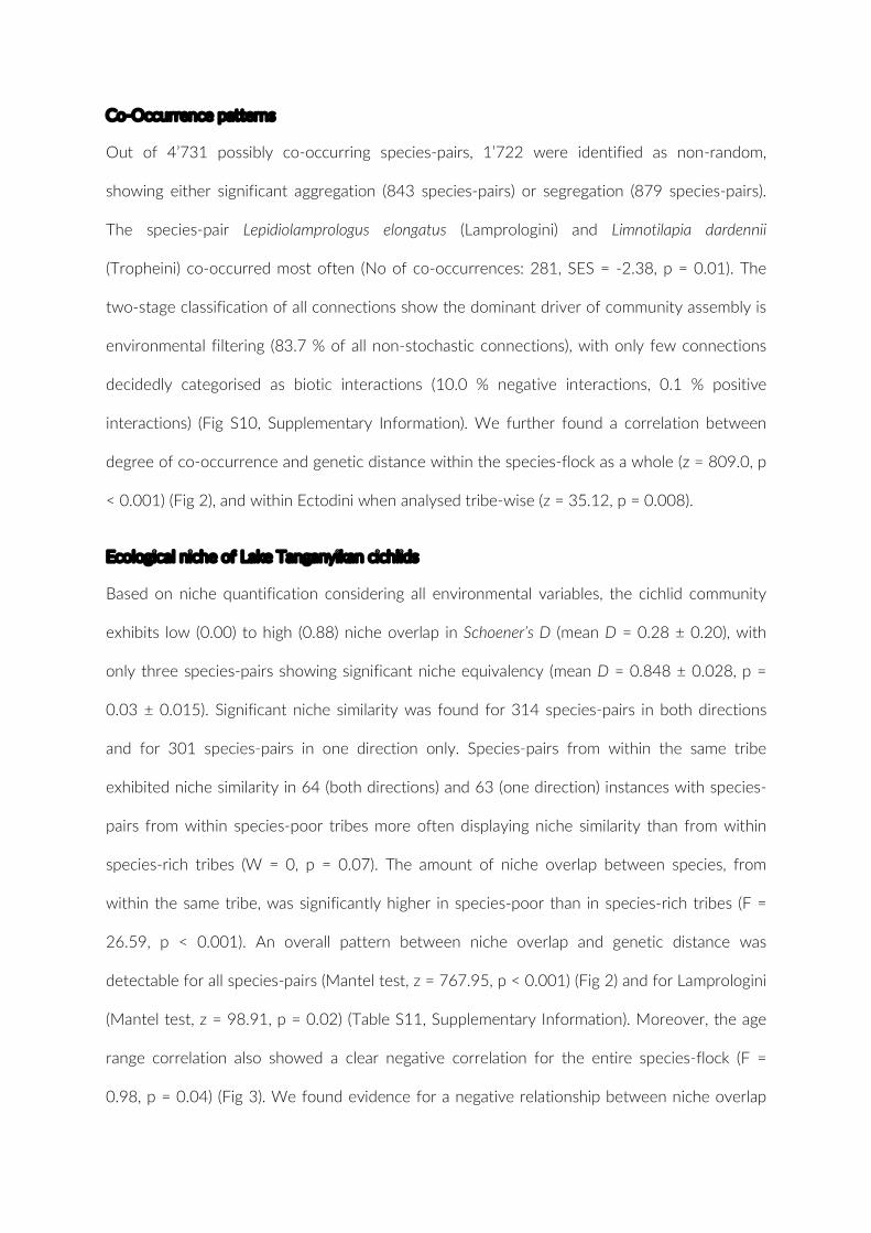
Co-Occurrence patterns
Out of 4’731 possibly co-occurring species-pairs, 1’722 were identified as non-random,
showing either significant aggregation (843 species-pairs) or segregation (879 species-pairs).
The species-pair Lepidiolamprologus elongatus (Lamprologini) and Limnotilapia dardennii
(Tropheini) co-occurred most often (No of co-occurrences: 281, SES = -2.38, p = 0.01). The
two-stage classification of all connections show the dominant driver of community assembly is
environmental filtering (83.7 % of all non-stochastic connections), with only few connections
decidedly categorised as biotic interactions (10.0 % negative interactions, 0.1 % positive
interactions) (Fig S10, Supplementary Information). We further found a correlation between
degree of co-occurrence and genetic distance within the species-flock as a whole (z = 809.0, p
< 0.001) (Fig 2), and within Ectodini when analysed tribe-wise (z = 35.12, p = 0.008).
Ecological niche of Lake Tanganyikan cichlids
Based on niche quantification considering all environmental variables, the cichlid community
exhibits low (0.00) to high (0.88) niche overlap in Schoener’s D (mean D = 0.28 ± 0.20), with
only three species-pairs showing significant niche equivalency (mean D = 0.848 ± 0.028, p =
0.03 ± 0.015). Significant niche similarity was found for 314 species-pairs in both directions
and for 301 species-pairs in one direction only. Species-pairs from within the same tribe
exhibited niche similarity in 64 (both directions) and 63 (one direction) instances with species-
pairs from within species-poor tribes more often displaying niche similarity than from within
species-rich tribes (W = 0, p = 0.07). The amount of niche overlap between species, from
within the same tribe, was significantly higher in species-poor than in species-rich tribes (F =
26.59, p < 0.001). An overall pattern between niche overlap and genetic distance was
detectable for all species-pairs (Mantel test, z = 767.95, p < 0.001) (Fig 2) and for Lamprologini
(Mantel test, z = 98.91, p = 0.02) (Table S11, Supplementary Information). Moreover, the age
range correlation also showed a clear negative correlation for the entire species-flock (F =
0.98, p = 0.04) (Fig 3). We found evidence for a negative relationship between niche overlap
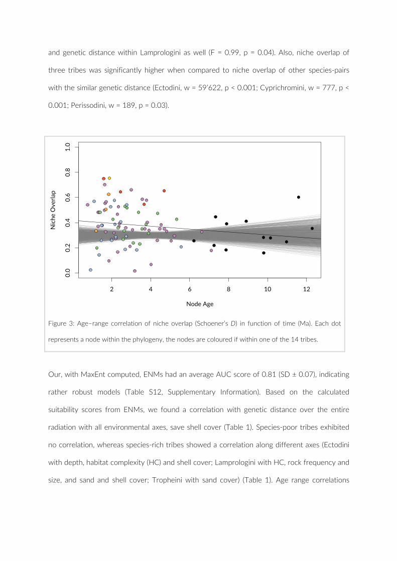
and genetic distance within Lamprologini as well (F = 0.99, p = 0.04). Also, niche overlap of
three tribes was significantly higher when compared to niche overlap of other species-pairs
with the similar genetic distance (Ectodini, w = 59’622, p < 0.001; Cyprichromini, w = 777, p <
0.001; Perissodini, w = 189, p = 0.03).
Figure 3: Age–range correlation of niche overlap (Schoener’s D) in function of time (Ma). Each dot
represents a node within the phylogeny, the nodes are coloured if within one of the 14 tribes.
Our, with MaxEnt computed, ENMs had an average AUC score of 0.81 (SD ± 0.07), indicating
rather robust models (Table S12, Supplementary Information). Based on the calculated
suitability scores from ENMs, we found a correlation with genetic distance over the entire
radiation with all environmental axes, save shell cover (Table 1). Species-poor tribes exhibited
no correlation, whereas species-rich tribes showed a correlation along different axes (Ectodini
with depth, habitat complexity (HC) and shell cover; Lamprologini with HC, rock frequency and
size, and sand and shell cover; Tropheini with sand cover) (Table 1). Age range correlations
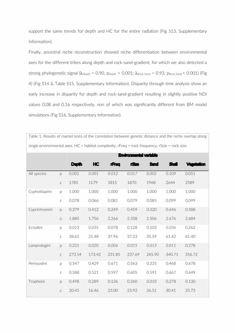
support the same trends for depth and HC for the entire radiation (Fig S13, Supplementary
Information).
Finally, ancestral niche reconstruction showed niche differentiation between environmental
axes for the different tribes along depth and rock-sand-gradient, for which we also detected a
strong phylogenetic signal (lDepth = 0.90, pDepth < 0.001; lRock-Sand = 0.93, pRock-Sand < 0.001) (Fig
4) (Fig S14 & Table S15, Supplementary Information). Disparity through time analysis show an
early increase in disparity for depth and rock-sand-gradient resulting in slightly positive NDI
values 0.08 and 0.16 respectively, non of which was significantly different from BM model
simulations (Fig S16, Supplementary Information).
Table 1: Results of mantel tests of the correlation between genetic distance and the niche overlap along
single environmental axes. HC = habitat complexity, rFreq = rock frequency, rSize = rock size.
Environmental variable
Depth HC rFreq rSize Sand Shell Vegetation
All species p 0.001 0.001 0.012 0.017 0.002 0.109 0.051
z 1785 1179 1815 1870 1968 2644 2589
Cyphotilapiini p 1.000 1.000 1.000 1.000 1.000 1.000 1.000
z 0.078 0.066 0.081 0.079 0.085 0.099 0.099
Cyprichromini p 0.379 0.412 0.249 0.459 0.320 0.646 0.588
z. 1.885 1.756 2.266 2.358 2.506 2.676 2.684
Ectodini p 0.013 0.035 0.078 0.128 0.103 0.036 0.262
z 38.61 21.48 37.96 37.23 35.59 61.42 61.40
Lamprologini p 0.221 0.020 0.006 0.015 0.013 0.011 0.278
z 273.54 173.42 231.85 237.69 265.90 340.71 356.72
Perissodini p 0.547 0.429 0.671 0.563 0.335 0.468 0.678
z 0.588 0.521 0.597 0.605 0.591 0.667 0.649
Tropheini p 0.498 0.289 0.136 0.260 0.010 0.278 0.130
z 20.45 16.46 23.00 23.92 26.51 30.41 25.73
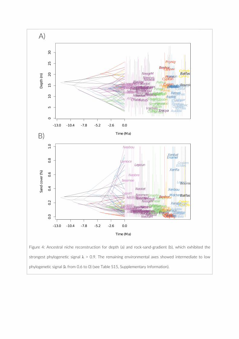
Figure 4: Ancestral niche reconstruction for depth (a) and rock-sand-gradient (b), which exhibited the
strongest phylogenetic signal l > 0.9. The remaining environmental axes showed intermediate to low
phylogenetic signal (l from 0.6 to 0) (see Table S15, Supplementary Information).
Discussion Here we present a substantial data set based on a non-invasive cichlid visual census survey,
which includes information on their environmental preferences along the Zambian and
Tanzanian shores of Lake Tanganyika. Data collection was conducted in a standardised manner
and provides a unique insight into the littoral and sublittoral community assembly of this most
diverse cichlid radiation. The consistently high tribal diversity across the lake, and its sub
basins, underlines our balanced sampling efforts (Fig 1). The predominantly endemic cichlids of
Lake Tanganyika were the dominating contributor to the local fish community and are found in
each of the vast number of diverse habitats within the lake (Konings, 1998; Sturmbauer et al.,
2011; Salzburger, 2018). Contemporary studies of evolutionary community ecology are often
limited by the fact that only closely related groups are studied, due to sampling and availablility
of phylogenetic framework for small groups (Mayfield & Levine, 2010; Clarke, Thomas, &
Freckleton, 2017). These factors, however, might hamper the power of studies of niche
evolution, as certainly interactions are not soley restricted to close relatives (Wilcox, Schwartz,
& Lowe, 2018). Nevertheless, exclusively examinig cichlids and the structuring of their
community shows that they follow general rules of fish assemblies, which are otherwise
comprised of many families. Thus, we believe that the focus on the cichlid community only,
does not hamper our conclusions. We explored the detailed structure and drivers of the cichlid
community and co-occurrence patterns, and assessed the evolution of the ecological niche in a
phylogenetic framework.
Community structure
High tribal diversity was found at all sites, nevertheless there are marked differences in the
contribution of each tribe to communities on different substrates and depths. The structuring
of the species assemblies along these two environmental gradients, depth and rock-sand, is
well documented (Danley & Kocher, 2001). Depth has a strong impact on fish communities in
the marine environment (Garrabou, Ballesteros, & Zabala, 2002; Smith & Brown, 2002) and as
such it is little surprising to observe a similar effect on the cichlid assembly that inhabits Lake
Tanganyika, which is the second deepest fresh water lake in the world (Salzburger et al., 2014).
The importance of substrate, in particular the sand-rock gradient, is also expected and its
implication on diversification has been reported for the cichlid radiation of Lake Malawi
(Danley & Kocher, 2001).
The two-step approach introduced by Kohli et al. (2018) identified the main force influencing
co-occurrences to be a stochastic process, with environmental filtering only being second. The
importance of environmental filtering is further supported by the highly significant structuring
of the community along environmental gradients (Fig S2, Supplementary Information). This is
congruous with previous findings on the community assembly of Tanganyikan cichlids in
localised study (Janzen et al., 2017). A prevalence of environmental filtering seems a general
pattern applying to cichlids communities in Lake Tanganyika on a larger scale. However, we
find little evidence for phylogenetic clustering, indicating that the different tribes converged on
the habitats with competition among members of different tribes not being of sufficient
strength to promote extensive phylogenetic clustering (Vamosi, Heard, Vamosi, & Webb, 2009;
Gerhold, Cahill, Winter, Bartish, & Prinzing, 2015). We do, however, observe some clustering
and potential niche conservatism within the tribes Tropheini and Cyprichromini (Fig 1C & 2).
The negative biotic interactions that were uncovered mostly refer to geographically separated
sister taxa (e.g. Telmatochromis vittatus & T. bifrenatus see Fig 2) or other geographical variants
restricted to a particular location. Although the ranges of these taxa often abut, it is difficult to
predict if these separations happened due to competition or a geographic barrier that is no
longer present. As it was shown for the Tropheini genus Tropheus, relatively small stretches of
sand can already function as effective barriers to promote reproductive isolation (Egger et al.,
2012).
Ecological Niche
The overall moderate niche overlap within the entire radiation illustrates the high degree of
specialisation and the vast diversity in ecological niche space occupied by the cichlids in Lake
Tanganyika. This impression is further strengthened by the scarce prevalence of niche
similarity among species. Considering the effect of niche-based processes (environmental
filtering) in community composition, the weak correlation of relatedness and niche overlap
suggests some importance of niche conservatism, supporting the niche-based process of
community assembly, as it was found in other adaptive radiations (Danley & Kocher, 2001).
Despite a lack of niche similarity between sister taxa, which is arguably a strong indication for
niche conservatism (Knouft et al., 2006; Warren et al., 2008), the age range correlation
confirmed the weak negative trend indicating a pattern of niche convservatism in the entire
cichlid-species flock. The contrasting levels of niche overlap might indicate the varying
relevance of niche conversatim for the different tribes. The variation among tribes is further
highlighted by the correlations of relatedness to differing environmental axes among the tribes.
The observation that not all clades (here tribes) within a radiation feature patterns of niche
convservatism is not uncommon (García-Navas & Westerman, 2018); several studies provdied
evidence for such asymmetries among species in terms of niche evolution at different scales
(geographic and taxonomic) (Blair, Sterling, Dusch, Raxworthy, & Pearson, 2013; Culumber &
Tobler, 2016). Coupled with the results from the ancestral niche reconstruction, wherein a
general patterns of narrow niche width of the species-poor tribes (Eretmodini, Limnochromini,
Cyphotilapiini, Cyprichromini, Perissodini) along at least either depth or sand-rock emerged
further strengthens this impression of variable niche conservatism among tribes. However, for
three of these tribes (Eretmodini, Limnochromini, Perissodini) we have a small number of
species records only, and therefore cannot weight these results to heavily.

Overall, these varying patterns of niche conservatism among tribes in combination with the
importance of niche-based community assembly could suggest that niche evolution and
diversification happened along different environmental axes for the different tribes. The
history of niche occupation estimated through ancestral niche reconstruction could further
indicate that the environmental diversifcation of the Lake Tanganyika cichlid species flock
happened in stages.

Acknowledgments We thank Heinz Büscher, the crew of Kalambo Falls Lodge and George Kazumbe and his crew
for the support in logistics and fieldwork, the Lake Tanganyika Research Unit, Department of
Fisheries, Republic of Zambia and the Tanzania Commission for Science and Technology
(COSTECH), for research permits. This study was supported by the European Research Council
(ERC, CoG ‘CICHLID~X’ to WS).
Author’s contribution LW and WS conceived and supervised the study, all co-authors conducted the fieldwork, LW
processed the images, analysed the data, and wrote the manuscript with feedback from all co-
authors.
Data accessibility All raw count data used in this study including a separate species list is available from the
Dryad Digital Repository (Link not yet available).
References Ackerly, D. D., Schwilk, D. W., & Webb, C. O. (2006). Niche evolution and adaptive radiation:
Testing the order of trait divergence. Ecology, 87(7 SUPPL.), 50–61. doi:10.1890/0012-
9658(2006)87[50:NEAART]2.0.CO;2
Blair, M. E., Sterling, E. J., Dusch, M., Raxworthy, C. J., & Pearson, R. G. (2013). Ecological
divergence and speciation between lemur (Eulemur) sister species in Madagascar. Journal
of Evolutionary Biology, 26(8), 1790–1801. doi:10.1111/jeb.12179
Boileau, N., Cortesi, F., Egger, B., Muschick, M., Indermaur, A., Theis, A., … Salzburger, W.
(2015). A complex mode of aggressive mimicry in a scale-eating cichlid fish. Biology
Letters, 11(9), 20150521. doi:10.1098/rsbl.2015.0521
Boulenger, G. A. (1898). Report on the fishes recently obtained by Mr. JES Moore in Lake
Tanganyika. Proceedings of the Zoological Society of London, 3.
Clarke, M., Thomas, G. H., & Freckleton, R. P. (2017). Trait Evolution in Adaptive Radiations:
Modeling and Measuring Interspecific Competition on Phylogenies. The American
Naturalist, 189(2), 121–137. doi:10.1086/689819
Colombo, M., Damerau, M., Hanel, R., Salzburger, W., & Matschiner, M. (2015). Diversity and
disparity through time in the adaptive radiation of Antarctic notothenioid fishes. Journal of
Evolutionary Biology, 28(2), 376–394. doi:10.1111/jeb.12570
Comte, L., Cucherousset, J., & Olden, J. D. (2016). Global test of Eltonian niche conservatism
of nonnative freshwater fish species between their native and introduced ranges.
Ecography, (February), 1–9. doi:10.1111/ecog.02007
Culumber, Z. W., & Tobler, M. (2016). Ecological divergence and conservatism: spatiotemporal
patterns of niche evolution in a genus of livebearing fishes (Poeciliidae: Xiphophorus).
BMC Evolutionary Biology, 16(1), 44. doi:10.1186/s12862-016-0593-4
Danley, P. D., & Kocher, T. D. (2001). Speciation in rapidly diverging systems: Lessons from
Lake Malawi. Molecular Ecology, 10(5), 1075–1086. doi:10.1046/j.1365-
294X.2001.01283.x
Deutsch, J. C. (1997). Colour diversification in Malawi cichlids: Evidence for adaptation,
reinforcement or sexual selection? Biological Journal of the Linnean Society, 62(1), 1–14.
doi:10.1006/bijl.1997.0135
Di Cola, V., Broennimann, O., Petitpierre, B., Breiner, F. T., D’Amen, M., Randin, C., … Guisan,
A. (2017). ecospat: an R package to support spatial analyses and modeling of species
niches and distributions. Ecography, 40(6), 774–787. doi:10.1111/ecog.02671
Egger, B., Sefc, K. M., Makasa, L., Sturmbauer, C., & Salzburger, W. (2012). Introgressive
hybridization between color morphs in a population of cichlid fishes twelve years after
human-induced secondary admixis. Journal of Heredity, 103(4), 515–522.
doi:10.1093/jhered/ess013
Evans, M. E. K., Smith, S. A., Flynn, R. S., & Donoghue, M. J. (2009). Climate, Niche Evolution,
and Diversification of the " Bird-Cage " Evening Primroses (Oenothera, Sections Anogra
and Kleinia). Am. Nat, 173(173), 0–0. doi:10.1086/595757
Fermon, Y., Nshombo, M., Muzumani, R., & Jonas, B. (2017). Lac Tanganyika – Guide de la faune
des poissons de la côte congolaise, d’Ubwari à la Ruzizi. AFC (Association France Cichlid).
Fitzpatrick, B. M., & Turelli, M. (2006). the Geography of Mammalian Speciation: Mixed Signals
From Phylogenies and Range Maps. Evolution, 60(3), 601. doi:10.1554/05-453.1
García-Navas, V., & Westerman, M. (2018). Niche conservatism and phylogenetic clustering in
a tribe of arid-adapted marsupial mice, the Sminthopsini. Journal of Evolutionary Biology,
31(8), 1204–1215. doi:10.1111/jeb.13297
Garrabou, J., Ballesteros, E., & Zabala, M. (2002). Structure and Dynamics of North-western
Mediterranean Rocky Benthic Communities along a Depth Gradient. Estuarine, Coastal and
Shelf Science, 55(3), 493–508. doi:10.1006/ecss.2001.0920
Gavrilets, S., & Losos, J. B. (2009). Adaptive radiation: Contrasting theory with data. Science.
doi:10.1126/science.1157966

Gerhold, P., Cahill, J. F., Winter, M., Bartish, I. V., & Prinzing, A. (2015). Phylogenetic patterns
are not proxies of community assembly mechanisms (they are far better). Functional
Ecology, 29(5), 600–614. doi:10.1111/1365-2435.12425
Hair, J. F., Black, W. C., Babin, J. B., & Anderson, R. E. (2014). Multivariate Data Analysis (7th
ed.). Pearson Education Limited.
Harmon, L. J., Schulte, J. A., Larson, A., & Losos, J. B. (2003). Tempo and mode of evolutionary
radiation in iguanian lizards. Science (New York, N.Y.), 301(5635), 961–4.
doi:10.1126/science.1084786
Harmon, L. J., Weir, J. T., Brock, C. D., Glor, R. E., & Challenger, W. (2008). GEIGER:
investigating evolutionary radiations. Bioinformatics, 24(1), 129–131.
doi:10.1093/bioinformatics/btm538
Heibl, C., & Calenge, C. (2018). R Package ‘phyloclim’: Integrating Phylogenetics and Climatic
Niche Modeling. Cran.
Hernandez, P. A., Graham, C. H., Master, L. L., & Albert, D. L. (2006). The effect of sample size
and species characteristics on performance of different species distribution modeling
methods. Ecography, 29(5), 773–785. doi:10.1111/j.0906-7590.2006.04700.x
Hutchinson, G. E. (1957). Concluding Remarks. Cold Spring Harbor Symposia on Quantitative
Biology, 22, 415–427. doi:10.1101/SQB.1957.022.01.039
Indermaur, A., Theis, A., Egger, B., & Salzburger, W. (2018). Mouth dimorphism in scale-eating
cichlid fish from Lake Tanganyika advances individual fitness. Evolution, 72(9), 1962–
1969. doi:10.1111/evo.13552
Janzen, T., Alzate, A., Muschick, M., Maan, M. E., van der Plas, F., & Etienne, R. S. (2017).
Community assembly in Lake Tanganyika cichlid fish: quantifying the contributions of
both niche-based and neutral processes. Ecology and Evolution, 7(4), 1057–1067.
doi:10.1002/ece3.2689
Knouft, J. H., Losos, J. B., Glor, R. E., & Kolbe, J. J. (2006). Phylogenetic analysis of the
evolution of the niche in lizards of the Anolis sagrei group. Ecology, 87, S29-38.
Kohli, B. A., Terry, R. C., & Rowe, R. J. (2018). A trait-based framework for discerning drivers of
species co-occurrence across heterogeneous landscapes. Ecography, 41(12), 1921–1933.
doi:10.1111/ecog.03747
Konings, A. (1998). Tanganyika cichlids in their natural habitat (3rd ed.). Cichlid Press, El Paso,
USA.
Losos, J. B. (2008). Phylogenetic niche conservatism, phylogenetic signal and the relationship
between phylogenetic relatedness and ecological similarity among species. Ecology Letters.
doi:10.1111/j.1461-0248.2008.01229.x
Mason, S. J., & Graham, N. E. (2002). Areas beneath the relative operating characteristics
(ROC) and relative operating levels (ROL) curves: Statistical significance and
interpretation. Quarterly Journal of the Royal Meteorological Society, 128(584), 2145–2166.
doi:10.1256/003590002320603584
Mayfield, M. M., & Levine, J. M. (2010). Opposing effects of competitive exclusion on the
phylogenetic structure of communities. Ecology Letters, 13(9), 1085–1093.
doi:10.1111/j.1461-0248.2010.01509.x
Merrett, N. R., Bagley, P. M., Smith, A., & Creasey, S. (1994). Scavenging Deep Demersal Fishes
of the Porcupine Seabight, North-East Atlantic: Observations by Baited Camera, Trap and
Trawl. Journal of the Marine Biological Association of the United Kingdom, 74(3), 481–498.
doi:10.1017/S0025315400047615
Münkemüller, T., Boucher, F. C., Thuiller, W., & Lavergne, S. (2015). Phylogenetic niche
conservatism - common pitfalls and ways forward. Functional Ecology, 29(5), 627–639.
doi:10.1111/1365-2435.12388
Paradis, E., Claude, J., & Strimmer, K. (2004). APE: Analyses of Phylogenetics and Evolution in
R language. Bioinformatics, 20(2), 289–290. doi:10.1093/bioinformatics/btg412
Phillips, S. J., Anderson, R. P., & Schapire, R. E. (2006). Maximum entropy modeling of species
geographic distributions. Ecological Modelling, 190(3–4), 231–259.
doi:10.1016/J.ECOLMODEL.2005.03.026
Phillips, S. J., & Dudík, M. (2008). Modeling of species distribution with Maxent: new
extensions and a comprehensive evalutation. Ecograpy, 31(December 2007), 161–175.
doi:10.1111/j.2007.0906-7590.05203.x
Poll, M. (1956). Exploration Hydrobiologique Du Lac Tanganyika (1946-1947) Volume III fascicule
5B: Poissons Cichlidae (Vol. 3). doi:10.2307/1439430
R Development Core Team. (2016). R: A Language and Environment for Statistical Computing.
R Foundation for Statistical Computing Vienna Austria. doi:10.1038/sj.hdy.6800737
Ronco, F., Indermaur, A., Büscher, H. H., & Salzburger, W. (n.d.). The taxonomic diversity of the
cichlid fish fauna of Lake Tanganyika. Journal of Great Lakes Research (in Revision), (SIAL
special issue).
Salzburger, W. (2018). Understanding explosive diversification through cichlid fish genomics.
Nature Reviews Genetics. doi:10.1038/s41576-018-0043-9
Salzburger, W., Bocxlaer, B. Van, & Cohen, A. S. (2014). Ecology and Evolution of the African
Great Lakes and Their Faunas. Annual Review of Ecology, Evolution and Systematics.
doi:10.1146/annurev-ecolsys-120213-091804
Schluter, D. (2000). The Ecology of Adaptive Radiation. Oxford Series in Ecology and Evolution.
doi:10.2307/3558417
Schluter, D., Price, T., Mooers, A. O., & Ludwig, D. (1997). Likelihood of Ancestor States in
Adaptive Radiation. Evolution, 51(6), 1699–1711.
Shumway, C. A., Hofmann, H. A., & Dobberfuhl, A. P. (2007). Quantifying habitat complexity in
aquatic ecosystems. Freshwater Biology, 52(6), 1065–1076. doi:10.1111/j.1365-
2427.2007.01754.x
Slater, G. J., Price, S. A., Santini, F., & Alfaro, M. E. (2010). Diversity versus disparity and the
radiation of modern cetaceans. Proceedings. Biological Sciences, 277(1697), 3097–104.
doi:10.1098/rspb.2010.0408
Smith, K. F., & Brown, J. H. (2002). Patterns of diversity, depth range and body size among
pelagic fishes along a gradient of depth. Global Ecology and Biogeography, 11(4), 313–322.
doi:10.1046/j.1466-822X.2002.00286.x
Stone, L., & Roberts, A. (1990). The checkerboard score and species distributions. Oecologia,
85(1), 74–79. doi:10.1007/BF00317345
Sturmbauer, C. (1998). Explosive speciation in cichlid fishes of the African Great Lakes: a
dynamic model of adaptive radiation. Journal of Fish Biology, 53(sa), 18–36.
doi:10.1111/j.1095-8649.1998.tb01015.x
Sturmbauer, C., & Dallinger, R. (1994). Diurnal Variation of Spacing and Foraging Behaviour in
Tropheus Moorii (Cichlidae) in Lake Tanganyika, Eastern Africa. Netherlands Journal of
Zoology, 45(3–4), 386–401. doi:10.1163/156854295X00375
Sturmbauer, C., Fuchs, C., Harb, G., Damm, E., Duftner, N., Maderbacher, M., … Koblmüller, S.
(2008). Abundance, distribution, and territory areas of rock-dwelling Lake Tanganyika
cichlid fish species. Hydrobiologia, 615(1), 57–68. doi:10.1007/s10750-008-9557-z
Sturmbauer, C., Husemann, M., & Danley, P. D. (2011). Explosive Speciation and Adaptive
Radiation of East African Cichlid Fishes. In Biodiversity Hotspots (pp. 333–362). Berlin,
Heidelberg: Springer Berlin Heidelberg. doi:10.1007/978-3-642-20992-5_18
Takeuchi, Y., Ochi, H., Kohda, M., Sinyinza, D., & Hori, M. (2010). A 20-year census of a rocky
littoral fish community in Lake Tanganyika. Ecology of Freshwater Fish, 19(2), 239–248.
doi:10.1111/j.1600-0633.2010.00408.x
Vamosi, S. M., Heard, S. B., Vamosi, J. C., & Webb, C. O. (2009). Emerging patterns in the
comparative analysis of phylogenetic community structure. Molecular Ecology, 18(4), 572–
592. doi:10.1111/j.1365-294X.2008.04001.x
Warren, D. L., Glor, R. E., & Turelli, M. (2008). Environmental niche equivalency versus
conservatism: Quantitative approaches to niche evolution. Evolution, 62(11), 2868–2883.
doi:10.1111/j.1558-5646.2008.00482.x
Widmer, L., Heule, E., Colombo, M., Rueegg, A., Indermaur, A., Ronco, F., & Salzburger, W.
(2019). Point-Combination Transect (PCT): Incorporation of small underwater cameras to
study fish communities. Methods in Ecology and Evolution, 2019(August 2018), 1–11.
doi:10.1111/2041-210X.13163
Wiens, J. J., Ackerly, D. D., Allen, A. P., Anacker, B. L., Buckley, L. B., Cornell, H. V., … Stephens,
P. R. (2010). Niche conservatism as an emerging principle in ecology and conservation
biology. Ecology Letters, 13(10), 1310–1324. doi:10.1111/j.1461-0248.2010.01515.x
Wilcox, T. M., Schwartz, M. K., & Lowe, W. H. (2018). Evolutionary Community Ecology: Time
to Think Outside the (Taxonomic) Box. Trends in Ecology and Evolution.
doi:10.1016/j.tree.2018.01.014
Wisz, M. S., Hijmans, R. J., Li, J., Peterson, A. T., Graham, C. H., Guisan, A., … Zimmermann, N.
E. (2008). Effects of sample size on the performance of species distribution models.
Diversity and Distributions, 14(5), 763–773. doi:10.1111/j.1472-4642.2008.00482.x

Chapter 3
Supplementary Information
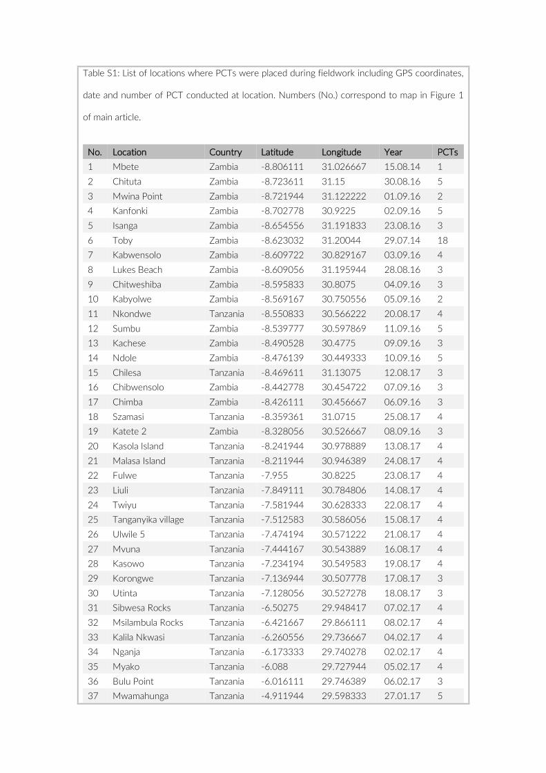
Table S1: List of locations where PCTs were placed during fieldwork including GPS coordinates,
date and number of PCT conducted at location. Numbers (No.) correspond to map in Figure 1
of main article.
No. Location Country Latitude Longitude Year PCTs
1 Mbete Zambia -8.806111 31.026667 15.08.14 1
2 Chituta Zambia -8.723611 31.15 30.08.16 5
3 Mwina Point Zambia -8.721944 31.122222 01.09.16 2
4 Kanfonki Zambia -8.702778 30.9225 02.09.16 5
5 Isanga Zambia -8.654556 31.191833 23.08.16 3
6 Toby Zambia -8.623032 31.20044 29.07.14 18
7 Kabwensolo Zambia -8.609722 30.829167 03.09.16 4
8 Lukes Beach Zambia -8.609056 31.195944 28.08.16 3
9 Chitweshiba Zambia -8.595833 30.8075 04.09.16 3
10 Kabyolwe Zambia -8.569167 30.750556 05.09.16 2
11 Nkondwe Tanzania -8.550833 30.566222 20.08.17 4
12 Sumbu Zambia -8.539777 30.597869 11.09.16 5
13 Kachese Zambia -8.490528 30.4775 09.09.16 3
14 Ndole Zambia -8.476139 30.449333 10.09.16 5
15 Chilesa Tanzania -8.469611 31.13075 12.08.17 3
16 Chibwensolo Zambia -8.442778 30.454722 07.09.16 3
17 Chimba Zambia -8.426111 30.456667 06.09.16 3
18 Szamasi Tanzania -8.359361 31.0715 25.08.17 4
19 Katete 2 Zambia -8.328056 30.526667 08.09.16 3
20 Kasola Island Tanzania -8.241944 30.978889 13.08.17 4
21 Malasa Island Tanzania -8.211944 30.946389 24.08.17 4
22 Fulwe Tanzania -7.955 30.8225 23.08.17 4
23 Liuli Tanzania -7.849111 30.784806 14.08.17 4
24 Twiyu Tanzania -7.581944 30.628333 22.08.17 4
25 Tanganyika village Tanzania -7.512583 30.586056 15.08.17 4
26 Ulwile 5 Tanzania -7.474194 30.571222 21.08.17 4
27 Mvuna Tanzania -7.444167 30.543889 16.08.17 4
28 Kasowo Tanzania -7.234194 30.549583 19.08.17 4
29 Korongwe Tanzania -7.136944 30.507778 17.08.17 3
30 Utinta Tanzania -7.128056 30.527278 18.08.17 3
31 Sibwesa Rocks Tanzania -6.50275 29.948417 07.02.17 4
32 Msilambula Rocks Tanzania -6.421667 29.866111 08.02.17 4
33 Kalila Nkwasi Tanzania -6.260556 29.736667 04.02.17 4
34 Nganja Tanzania -6.173333 29.740278 02.02.17 4
35 Myako Tanzania -6.088 29.727944 05.02.17 4
36 Bulu Point Tanzania -6.016111 29.746389 06.02.17 3
37 Mwamahunga Tanzania -4.911944 29.598333 27.01.17 5

No. Location Country Latitude Longitude Year PCTs
38 Mwamawimbi Tanzania -4.905 29.595556 23.01.17 3
39 Kaku Tanzania -4.896389 29.611667 26.01.17 7
40 Cave Kigoma Tanzania -4.886944 29.615833 10.02.17 3
41 Georges Place Tanzania -4.885 29.620833 19.01.17 3
42 Nondwa Point Tanzania -4.864167 29.607222 18.01.17 3
43 Nondwa Bay Tanzania -4.864111 29.609639 24.01.17 4
44 Kalalangabo Tanzania -4.843611 29.609444 21.01.17 4
45 Kananiye Tanzania -4.794167 29.599444 28.01.17 6
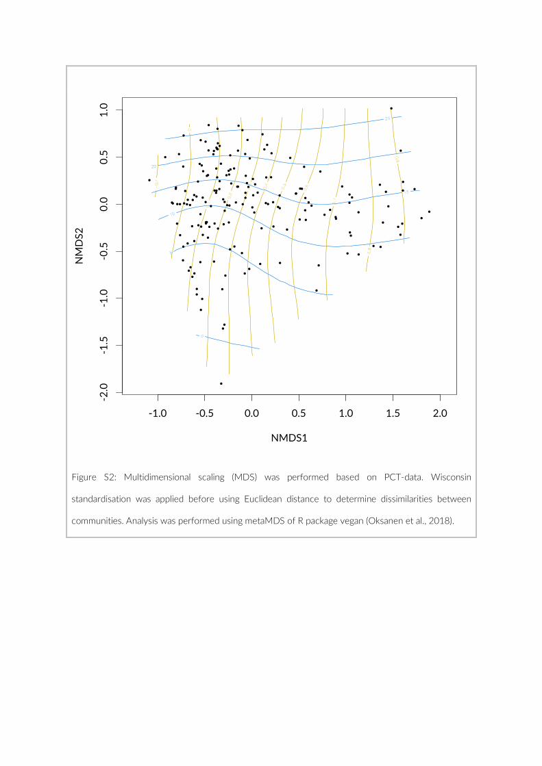
Figure S2: Multidimensional scaling (MDS) was performed based on PCT-data. Wisconsin
standardisation was applied before using Euclidean distance to determine dissimilarities between
communities. Analysis was performed using metaMDS of R package vegan (Oksanen et al., 2018).
-1.0 -0.5 0.0 0.5 1.0 1.5 2.0
-2.0
-1.5
-1.0
-0.5
0.0
0.5
1.0
NMDS1
NMDS2
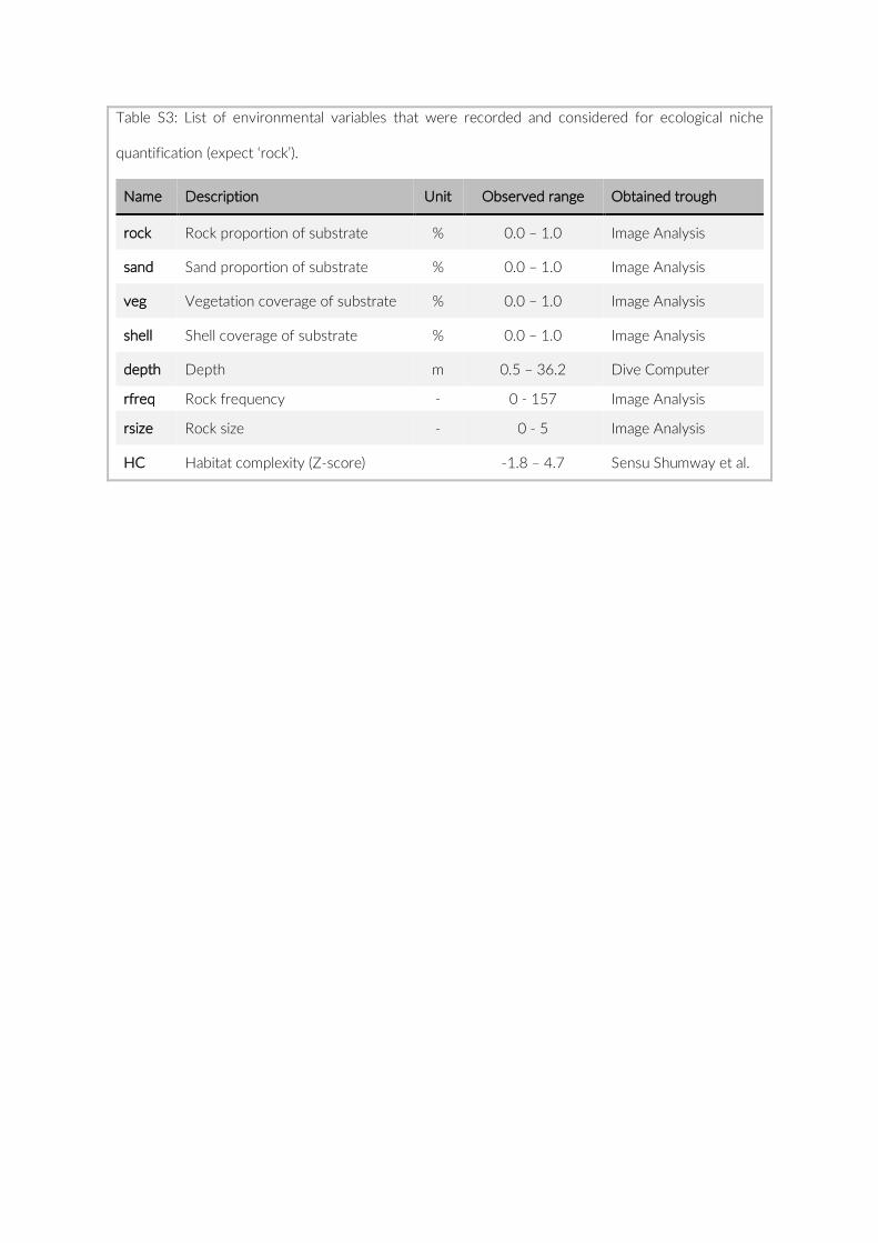
Table S3: List of environmental variables that were recorded and considered for ecological niche
quantification (expect ‘rock’).
Name Description Unit Observed range Obtained trough
rock Rock proportion of substrate % 0.0 – 1.0 Image Analysis
sand Sand proportion of substrate % 0.0 – 1.0 Image Analysis
veg Vegetation coverage of substrate % 0.0 – 1.0 Image Analysis
shell Shell coverage of substrate % 0.0 – 1.0 Image Analysis
depth Depth m 0.5 – 36.2 Dive Computer
rfreq Rock frequency - 0 - 157 Image Analysis
rsize Rock size - 0 - 5 Image Analysis
HC Habitat complexity (Z-score) -1.8 – 4.7 Sensu Shumway et al.
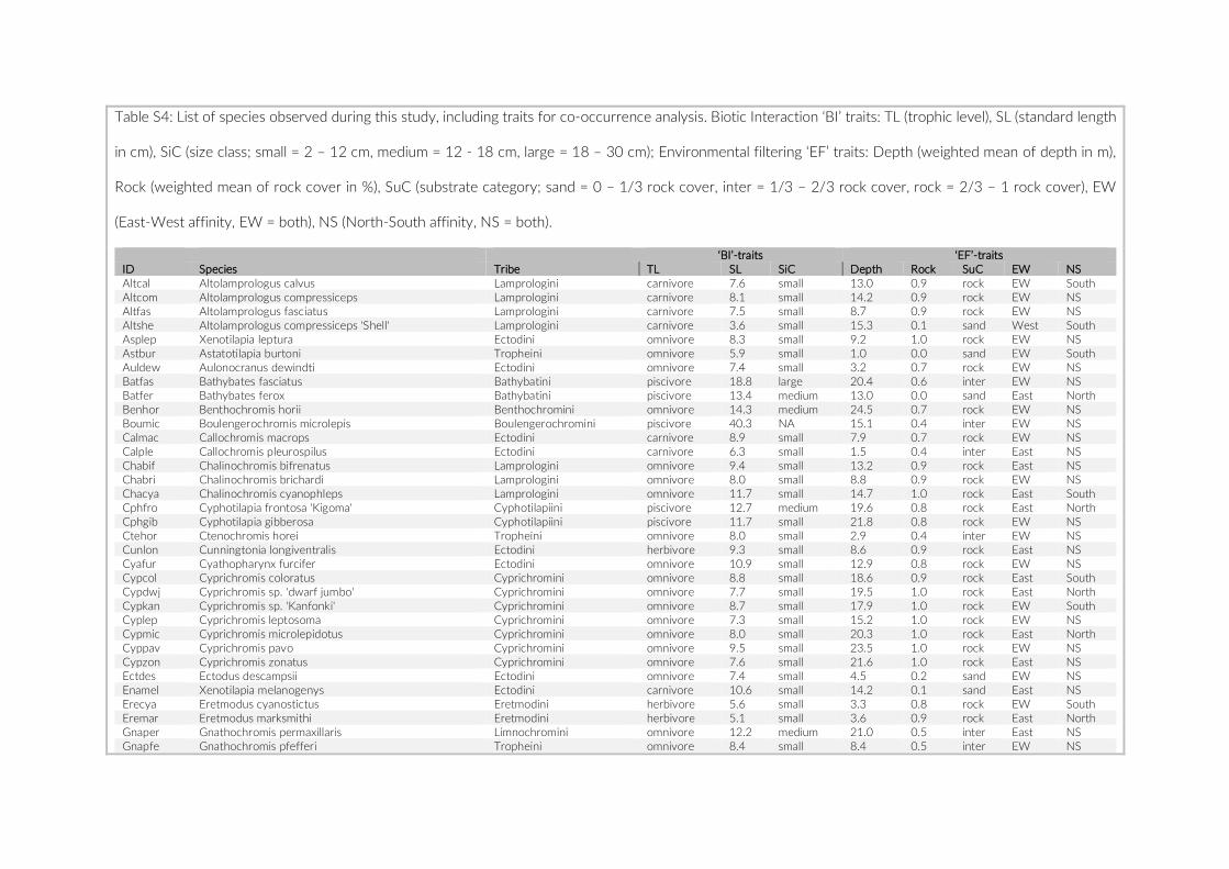
Table S4: List of species observed during this study, including traits for co-occurrence analysis. Biotic Interaction ‘BI’ traits: TL (trophic level), SL (standard length
in cm), SiC (size class; small = 2 – 12 cm, medium = 12 - 18 cm, large = 18 – 30 cm); Environmental filtering ‘EF’ traits: Depth (weighted mean of depth in m),
Rock (weighted mean of rock cover in %), SuC (substrate category; sand = 0 – 1/3 rock cover, inter = 1/3 – 2/3 rock cover, rock = 2/3 – 1 rock cover), EW
(East-West affinity, EW = both), NS (North-South affinity, NS = both).
‘BI’-traits ‘EF’-traits ID Species Tribe TL SL SiC Depth Rock SuC EW NS Altcal Altolamprologus calvus Lamprologini carnivore 7.6 small 13.0 0.9 rock EW South Altcom Altolamprologus compressiceps Lamprologini carnivore 8.1 small 14.2 0.9 rock EW NS Altfas Altolamprologus fasciatus Lamprologini carnivore 7.5 small 8.7 0.9 rock EW NS Altshe Altolamprologus compressiceps 'Shell' Lamprologini carnivore 3.6 small 15.3 0.1 sand West South Asplep Xenotilapia leptura Ectodini omnivore 8.3 small 9.2 1.0 rock EW NS Astbur Astatotilapia burtoni Tropheini omnivore 5.9 small 1.0 0.0 sand EW South Auldew Aulonocranus dewindti Ectodini omnivore 7.4 small 3.2 0.7 rock EW NS Batfas Bathybates fasciatus Bathybatini piscivore 18.8 large 20.4 0.6 inter EW NS Batfer Bathybates ferox Bathybatini piscivore 13.4 medium 13.0 0.0 sand East North Benhor Benthochromis horii Benthochromini omnivore 14.3 medium 24.5 0.7 rock EW NS Boumic Boulengerochromis microlepis Boulengerochromini piscivore 40.3 NA 15.1 0.4 inter EW NS Calmac Callochromis macrops Ectodini carnivore 8.9 small 7.9 0.7 rock EW NS Calple Callochromis pleurospilus Ectodini carnivore 6.3 small 1.5 0.4 inter East NS Chabif Chalinochromis bifrenatus Lamprologini omnivore 9.4 small 13.2 0.9 rock East NS Chabri Chalinochromis brichardi Lamprologini omnivore 8.0 small 8.8 0.9 rock EW NS Chacya Chalinochromis cyanophleps Lamprologini omnivore 11.7 small 14.7 1.0 rock East South Cphfro Cyphotilapia frontosa 'Kigoma' Cyphotilapiini piscivore 12.7 medium 19.6 0.8 rock East North Cphgib Cyphotilapia gibberosa Cyphotilapiini piscivore 11.7 small 21.8 0.8 rock EW NS Ctehor Ctenochromis horei Tropheini omnivore 8.0 small 2.9 0.4 inter EW NS Cunlon Cunningtonia longiventralis Ectodini herbivore 9.3 small 8.6 0.9 rock East NS Cyafur Cyathopharynx furcifer Ectodini omnivore 10.9 small 12.9 0.8 rock EW NS Cypcol Cyprichromis coloratus Cyprichromini omnivore 8.8 small 18.6 0.9 rock East South Cypdwj Cyprichromis sp. 'dwarf jumbo' Cyprichromini omnivore 7.7 small 19.5 1.0 rock East North Cypkan Cyprichromis sp. 'Kanfonki' Cyprichromini omnivore 8.7 small 17.9 1.0 rock EW South Cyplep Cyprichromis leptosoma Cyprichromini omnivore 7.3 small 15.2 1.0 rock EW NS Cypmic Cyprichromis microlepidotus Cyprichromini omnivore 8.0 small 20.3 1.0 rock East North Cyppav Cyprichromis pavo Cyprichromini omnivore 9.5 small 23.5 1.0 rock EW NS Cypzon Cyprichromis zonatus Cyprichromini omnivore 7.6 small 21.6 1.0 rock East NS Ectdes Ectodus descampsii Ectodini omnivore 7.4 small 4.5 0.2 sand EW NS Enamel Xenotilapia melanogenys Ectodini carnivore 10.6 small 14.2 0.1 sand East NS Erecya Eretmodus cyanostictus Eretmodini herbivore 5.6 small 3.3 0.8 rock EW South Eremar Eretmodus marksmithi Eretmodini herbivore 5.1 small 3.6 0.9 rock East North Gnaper Gnathochromis permaxillaris Limnochromini omnivore 12.2 medium 21.0 0.5 inter East NS Gnapfe Gnathochromis pfefferi Tropheini omnivore 8.4 small 8.4 0.5 inter EW NS
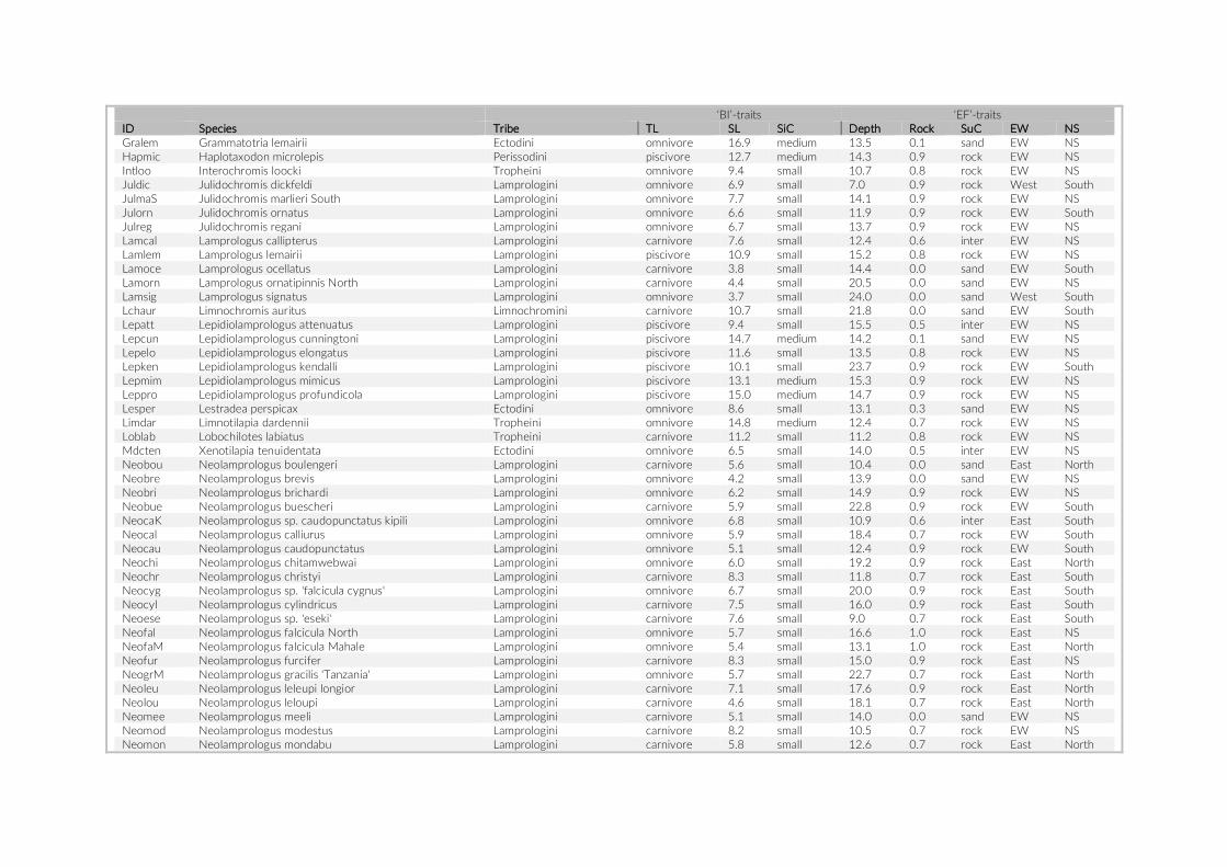
‘BI’-traits ‘EF’-traits ID Species Tribe TL SL SiC Depth Rock SuC EW NS Gralem Grammatotria lemairii Ectodini omnivore 16.9 medium 13.5 0.1 sand EW NS Hapmic Haplotaxodon microlepis Perissodini piscivore 12.7 medium 14.3 0.9 rock EW NS Intloo Interochromis loocki Tropheini omnivore 9.4 small 10.7 0.8 rock EW NS Juldic Julidochromis dickfeldi Lamprologini omnivore 6.9 small 7.0 0.9 rock West South JulmaS Julidochromis marlieri South Lamprologini omnivore 7.7 small 14.1 0.9 rock EW NS Julorn Julidochromis ornatus Lamprologini omnivore 6.6 small 11.9 0.9 rock EW South Julreg Julidochromis regani Lamprologini omnivore 6.7 small 13.7 0.9 rock EW NS Lamcal Lamprologus callipterus Lamprologini carnivore 7.6 small 12.4 0.6 inter EW NS Lamlem Lamprologus lemairii Lamprologini piscivore 10.9 small 15.2 0.8 rock EW NS Lamoce Lamprologus ocellatus Lamprologini carnivore 3.8 small 14.4 0.0 sand EW South Lamorn Lamprologus ornatipinnis North Lamprologini carnivore 4.4 small 20.5 0.0 sand EW NS Lamsig Lamprologus signatus Lamprologini omnivore 3.7 small 24.0 0.0 sand West South Lchaur Limnochromis auritus Limnochromini carnivore 10.7 small 21.8 0.0 sand EW South Lepatt Lepidiolamprologus attenuatus Lamprologini piscivore 9.4 small 15.5 0.5 inter EW NS Lepcun Lepidiolamprologus cunningtoni Lamprologini piscivore 14.7 medium 14.2 0.1 sand EW NS Lepelo Lepidiolamprologus elongatus Lamprologini piscivore 11.6 small 13.5 0.8 rock EW NS Lepken Lepidiolamprologus kendalli Lamprologini piscivore 10.1 small 23.7 0.9 rock EW South Lepmim Lepidiolamprologus mimicus Lamprologini piscivore 13.1 medium 15.3 0.9 rock EW NS Leppro Lepidiolamprologus profundicola Lamprologini piscivore 15.0 medium 14.7 0.9 rock EW NS Lesper Lestradea perspicax Ectodini omnivore 8.6 small 13.1 0.3 sand EW NS Limdar Limnotilapia dardennii Tropheini omnivore 14.8 medium 12.4 0.7 rock EW NS Loblab Lobochilotes labiatus Tropheini carnivore 11.2 small 11.2 0.8 rock EW NS Mdcten Xenotilapia tenuidentata Ectodini omnivore 6.5 small 14.0 0.5 inter EW NS Neobou Neolamprologus boulengeri Lamprologini carnivore 5.6 small 10.4 0.0 sand East North Neobre Neolamprologus brevis Lamprologini omnivore 4.2 small 13.9 0.0 sand EW NS Neobri Neolamprologus brichardi Lamprologini omnivore 6.2 small 14.9 0.9 rock EW NS Neobue Neolamprologus buescheri Lamprologini carnivore 5.9 small 22.8 0.9 rock EW South NeocaK Neolamprologus sp. caudopunctatus kipili Lamprologini omnivore 6.8 small 10.9 0.6 inter East South Neocal Neolamprologus calliurus Lamprologini omnivore 5.9 small 18.4 0.7 rock EW South Neocau Neolamprologus caudopunctatus Lamprologini omnivore 5.1 small 12.4 0.9 rock EW South Neochi Neolamprologus chitamwebwai Lamprologini omnivore 6.0 small 19.2 0.9 rock East North Neochr Neolamprologus christyi Lamprologini carnivore 8.3 small 11.8 0.7 rock East South Neocyg Neolamprologus sp. 'falcicula cygnus' Lamprologini omnivore 6.7 small 20.0 0.9 rock East South Neocyl Neolamprologus cylindricus Lamprologini carnivore 7.5 small 16.0 0.9 rock East South Neoese Neolamprologus sp. 'eseki' Lamprologini carnivore 7.6 small 9.0 0.7 rock East South Neofal Neolamprologus falcicula North Lamprologini omnivore 5.7 small 16.6 1.0 rock East NS NeofaM Neolamprologus falcicula Mahale Lamprologini omnivore 5.4 small 13.1 1.0 rock East North Neofur Neolamprologus furcifer Lamprologini carnivore 8.3 small 15.0 0.9 rock East NS NeogrM Neolamprologus gracilis 'Tanzania' Lamprologini omnivore 5.7 small 22.7 0.7 rock East North Neoleu Neolamprologus leleupi longior Lamprologini carnivore 7.1 small 17.6 0.9 rock East North Neolou Neolamprologus leloupi Lamprologini carnivore 4.6 small 18.1 0.7 rock East North Neomee Neolamprologus meeli Lamprologini carnivore 5.1 small 14.0 0.0 sand EW NS Neomod Neolamprologus modestus Lamprologini carnivore 8.2 small 10.5 0.7 rock EW NS Neomon Neolamprologus mondabu Lamprologini carnivore 5.8 small 12.6 0.7 rock East North
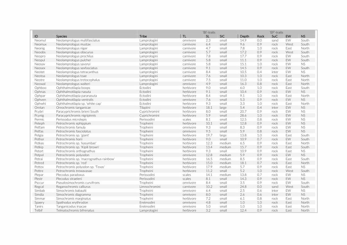
‘BI’-traits ‘EF’-traits ID Species Tribe TL SL SiC Depth Rock SuC EW NS Neomul Neolamprologus multifasciatus Lamprologini omnivore 2.3 small 14.9 0.0 sand EW South Neomux Neolamprologus mustax Lamprologini carnivore 6.4 small 9.6 0.9 rock West South Neonig Neolamprologus niger Lamprologini carnivore 4.7 small 7.8 1.0 rock East North Neoobs Neolamprologus obscurus Lamprologini carnivore 5.7 small 17.2 0.9 rock West South Neopro Neolamprologus prochilus Lamprologini carnivore 7.8 small 17.7 0.9 rock EW South Neopul Neolamprologus pulcher Lamprologini carnivore 5.8 small 11.1 0.9 rock EW South Neosav Neolamprologus savoryi Lamprologini carnivore 5.8 small 15.1 1.0 rock EW NS Neosex Neolamprologus sexfasciatus Lamprologini carnivore 9.1 small 14.5 0.9 rock EW South Neotet Neolamprologus tetracanthus Lamprologini carnivore 8.4 small 10.5 0.4 inter EW NS Neotoa Neolamprologus toae Lamprologini carnivore 7.6 small 10.3 1.0 rock East North Neotre Neolamprologus tretocephalus Lamprologini carnivore 7.5 small 11.0 1.0 rock East North Neowal Neolamprologus walteri Lamprologini omnivore 4.9 small 16.3 0.8 rock East North Ophboo Ophthalmotilapia boops Ectodini herbivore 9.0 small 6.0 1.0 rock East South Ophnas Ophthalmotilapia nasuta Ectodini herbivore 9.1 small 10.4 0.9 rock EW NS Ophpar Ophthalmotilapia paranasuta Ectodini herbivore 8.4 small 9.1 1.0 rock East North Ophven Ophthalmotilapia ventralis Ectodini omnivore 7.6 small 5.3 0.9 rock EW NS Ophwhi Ophthalmotilapia sp. 'white cap' Ectodini herbivore 9.3 small 3.3 1.0 rock East North Oretan Oreochromis tanganicae Tilapiini herbivore 18.1 large 5.4 0.4 inter EW NS Pcybri Paracyprichromis brieni South Cyprichromini herbivore 8.0 small 20.7 0.9 rock EW NS Pcynig Paracyprichromis nigripinnis Cyprichromini herbivore 5.9 small 28.6 1.0 rock EW NS Permic Perissodus microlepis Perissodini scales 8.1 small 12.5 0.8 rock EW NS Peteph Petrochromis ephippium Tropheini herbivore 10.1 small 12.8 0.9 rock EW NS Petfam Petrochromis famula Tropheini omnivore 9.3 small 8.3 0.9 rock EW NS Petfas Petrochromis fasciolatus Tropheini omnivore 9.5 small 5.9 0.8 rock EW NS Petgia Petrochromis sp. 'giant' Tropheini herbivore 19.7 large 13.8 1.0 rock East South Pethor Petrochromis horii Tropheini herbivore 9.0 small 10.9 0.7 rock EW South Petkas Petrochromis sp. 'kasumbae' Tropheini herbivore 12.3 medium 6.5 0.9 rock East North Petkip Petrochromis sp. 'Kipili brown' Tropheini herbivore 13.4 medium 15.7 0.9 rock East South Petort Petrochromis orthognathus Tropheini herbivore 9.3 small 10.9 0.9 rock East NS Petpol Petrochromis polyodon Tropheini omnivore 12.8 medium 5.9 0.9 rock EW NS Petrai Petrochromis sp. 'macrognathus rainbow' Tropheini herbivore 16.5 medium 8.5 0.9 rock East South Petred Petrochromis sp. 'red' Tropheini herbivore 15.0 medium 18.1 0.7 rock East North Pettex Petrochromis polyodon sp. 'Texas' Tropheini herbivore 17.9 medium 5.7 0.9 rock East NS Pettre Petrochromis trewavasae Tropheini herbivore 11.2 small 5.2 1.0 rock West South Plepar Plecodus paradoxus Perissodini scales 14.1 medium 13.8 0.7 rock EW NS Plestr Plecodus straeleni Perissodini scales 8.1 small 14.3 0.9 rock EW NS Psccur Pseudosimochromis curvifrons Tropheini omnivore 8.4 small 3.5 0.9 rock EW South Regcal Reganochromis calliurus Limnochromini carnivore 10.2 small 24.8 0.0 sand West South Simbab Simochromis babaulti Tropheini omnivore 6.4 small 2.5 0.6 inter EW NS Simdia Simochromis diagramma Tropheini omnivore 8.0 small 2.6 0.6 inter EW NS Simmar Simochromis marginatus Tropheini herbivore 7.2 small 6.1 0.8 rock East North Spaery Spathodus erythrodon Eretmodini omnivore 4.8 small 1.0 1.0 rock East North Tanirs Tanganicodus irsacae Eretmodini omnivore 5.0 small 1.0 1.0 rock East North Telbif Telmatochromis bifrenatus Lamprologini herbivore 3.2 small 12.4 0.9 rock East North
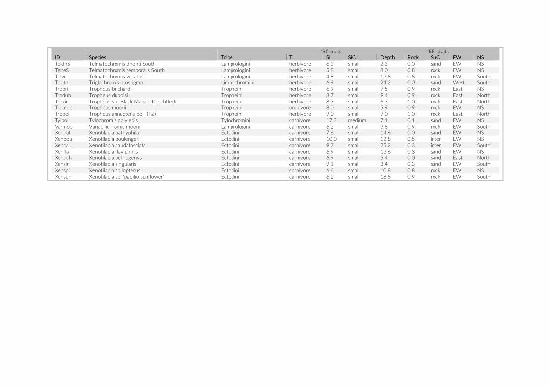
‘BI’-traits ‘EF’-traits ID Species Tribe TL SL SiC Depth Rock SuC EW NS TeldhS Telmatochromis dhonti South Lamprologini herbivore 6.2 small 2.3 0.0 sand EW NS TelteS Telmatochromis temporalis South Lamprologini herbivore 5.8 small 8.0 0.8 rock EW NS Telvit Telmatochromis vittatus Lamprologini herbivore 4.8 small 13.8 0.8 rock EW South Trioto Triglachromis otostigma Limnochromini herbivore 6.9 small 24.2 0.0 sand West South Trobri Tropheus brichardi Tropheini herbivore 6.9 small 7.5 0.9 rock East NS Trodub Tropheus duboisi Tropheini herbivore 8.7 small 9.4 0.9 rock East North Trokir Tropheus sp. 'Black Mahale Kirschfleck' Tropheini herbivore 8.3 small 6.7 1.0 rock East North Tromoo Tropheus moorii Tropheini omnivore 8.0 small 5.9 0.9 rock EW NS Tropol Tropheus annectens polli (TZ) Tropheini herbivore 9.0 small 7.0 1.0 rock East North Tylpol Tylochromis polylepis Tylochromini carnivore 17.3 medium 7.1 0.1 sand EW NS Varmoo Variabilichromis moorii Lamprologini carnivore 6.2 small 3.8 0.9 rock EW South Xenbat Xenotilapia bathyphila Ectodini carnivore 7.6 small 14.6 0.0 sand EW NS Xenbou Xenotilapia boulengeri Ectodini carnivore 10.0 small 12.8 0.5 inter EW NS Xencau Xenotilapia caudafasciata Ectodini carnivore 9.7 small 25.2 0.3 inter EW South Xenfla Xenotilapia flavipinnis Ectodini carnivore 6.9 small 13.6 0.3 sand EW NS Xenoch Xenotilapia ochrogenys Ectodini carnivore 6.9 small 5.4 0.0 sand East North Xensin Xenotilapia singularis Ectodini carnivore 9.1 small 3.4 0.3 sand EW South Xenspi Xenotilapia spilopterus Ectodini carnivore 6.6 small 10.8 0.8 rock EW NS Xensun Xenotilapia sp. 'papilio sunflower' Ectodini carnivore 6.2 small 18.8 0.9 rock EW South
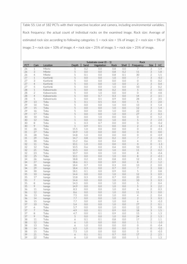
Table S5: List of 182 PCTs with their respective location and camera, including environmental variables.
Rock frequency: the actual count of individual rocks on the examined image. Rock size: Average of
estimated rock size according to following categories: 1 = rock size < 1% of image; 2 = rock size < 5% of
image; 3 = rock size < 10% of image; 4 = rock size < 25% of image; 5 = rock size > 25% of image.
Substrate cover (0 – 1) Rock PCT Cam Location Depth Sand Vegetation Rock Shell Frequency Size HC 26 1 Mbete 5 0.2 0.0 0.8 0.0 7 3 1.4 26 3 Mbete 5 0.0 0.0 0.8 0.2 11 3 1.8 26 4 Mbete 5 0.1 0.0 0.8 0.1 30 2 1.5 27 1 Kanfonki 5 0.0 0.0 1.0 0.0 7 3 -0.2 27 3 Kanfonki 5 0.0 0.0 0.0 0.0 0 0 0.2 27 4 Kanfonki 5 0.0 0.0 1.0 0.0 2 3 0.4 27 5 Kanfonki 5 0.0 0.0 1.0 0.0 10 2 0.2 28 1 Kabwensolo 5 0.0 0.8 0.2 0.0 5 2 3.0 28 2 Kabwensolo 5 0.0 1.0 0.0 0.0 0 0 4.8 28 4 Kabwensolo 5 0.0 0.7 0.3 0.0 14 2 3.1 28 5 Kabwensolo 5 0.0 0.1 0.9 0.0 28 2 3.5 29 13 Toby 5 0.1 0.5 0.4 0.0 5 3 2.0 29 14 Toby 5 0.0 0.0 1.0 0.0 13 3 1.4 29 15 Toby 5 0.0 0.0 1.0 0.0 12 3 1.4 29 16 Toby 5 0.0 0.0 1.0 0.0 22 2 0.6 29 17 Toby 5 0.0 0.0 1.0 0.0 27 2 0.3 30 10 Toby 1 0.0 1.0 0.0 0.0 0 0 1.2 30 12 Toby 1 0.0 0.0 1.0 0.0 5 2 2.4 30 8 Toby 1 0.3 0.7 0.0 0.0 0 0 -0.2 30 9 Toby 1 0.9 0.1 0.0 0.0 2 2 -1.4 31 26 Toby 15.5 1.0 0.0 0.0 0.0 0 0 -0.1 31 27 Toby 14.9 1.0 0.0 0.0 0.0 0 0 0.0 31 28 Toby 14.8 1.0 0.0 0.0 0.0 0 0 -0.9 31 29 Toby 14.7 0.8 0.0 0.2 0.0 7 2 -0.6 31 30 Toby 15.2 0.6 0.0 0.4 0.0 4 2 0.1 32 11 Toby 10.1 1.0 0.0 0.0 0.0 0 0 -1.3 32 12 Toby 10.5 0.6 0.0 0.4 0.0 10 2 -1.5 32 21 Toby 10.5 0.0 0.0 1.0 0.0 11 2 0.2 32 23 Toby 10.7 0.0 0.0 1.0 0.0 8 3 -0.4 32 25 Toby 10.1 0.0 0.0 1.0 0.0 8 2 -0.1 34 26 Isanga 18.8 0.2 0.0 0.8 0.0 12 2 0.3 34 27 Isanga 18.6 0.1 0.0 0.9 0.0 8 2 1.2 34 28 Isanga 18.4 0.7 0.0 0.3 0.0 13 2 0.0 34 29 Isanga 18.4 0.3 0.0 0.7 0.0 7 3 0.8 34 30 Isanga 18.1 0.1 0.0 0.9 0.0 5 2 0.8 35 10 Isanga 14.4 0.0 0.0 1.0 0.0 12 3 0.9 35 17 Isanga 13.8 0.3 0.0 0.7 0.0 20 2 0.4 35 7 Isanga 14.4 0.0 0.0 1.0 0.0 10 3 0.3 35 8 Isanga 14.3 0.0 0.0 1.0 0.0 5 2 0.4 35 9 Isanga 14.9 0.0 0.0 1.0 0.0 5 3 2.2 36 11 Isanga 8.3 0.0 0.0 1.0 0.0 6 2 0.3 36 12 Isanga 8.6 0.0 0.0 1.0 0.0 11 3 0.0 36 13 Isanga 7.5 0.0 0.0 1.0 0.0 4 2 0.4 36 14 Isanga 7.7 0.0 0.0 1.0 0.0 2 3 0.3 36 15 Isanga 7.7 0.0 0.0 1.0 0.0 6 3 -0.3 37 10 Toby 5.4 0.0 0.0 1.0 0.0 27 2 0.1 37 6 Toby 5.7 0.0 0.0 1.0 0.0 12 3 0.8 37 7 Toby 4.9 0.0 0.1 0.9 0.0 18 3 1.5 37 8 Toby 4.7 0.0 0.1 0.9 0.0 15 3 1.3 37 9 Toby 5 0.0 0.0 1.0 0.0 24 2 1.3 38 11 Toby 6 0.1 0.1 0.8 0.0 17 2 1.1 38 12 Toby 6 1.0 0.0 0.0 0.0 1 1 -1.0 38 13 Toby 6 1.0 0.0 0.0 0.0 0 0 -0.4 38 14 Toby 6.5 1.0 0.0 0.0 0.0 0 0 -0.2 38 15 Toby 7.5 1.0 0.0 0.0 0.0 0 0 -0.5 39 21 Toby 6 0.1 0.1 0.7 0.0 17 2 2.5 39 22 Toby 6 1.0 0.0 0.0 0.0 1 1 1.3
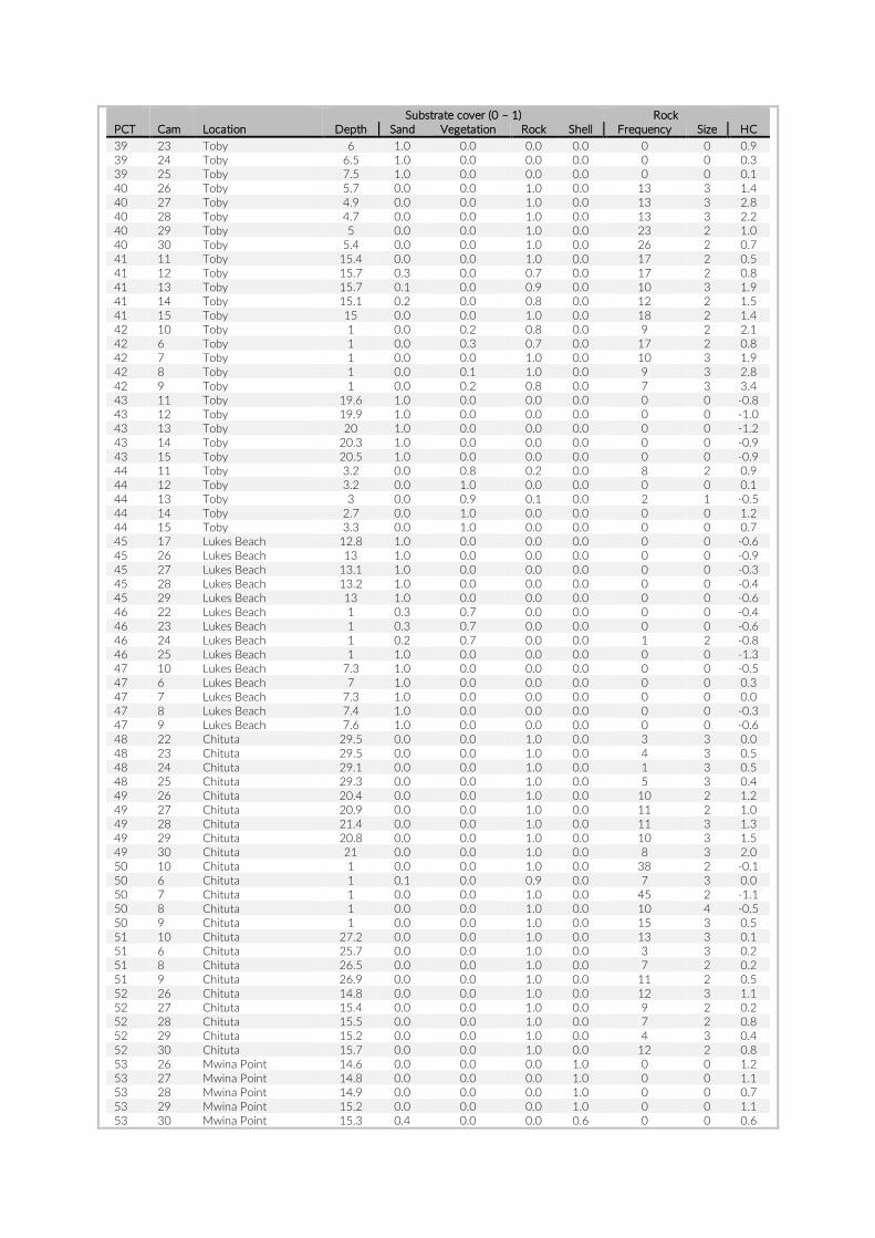
Substrate cover (0 – 1) Rock PCT Cam Location Depth Sand Vegetation Rock Shell Frequency Size HC 39 23 Toby 6 1.0 0.0 0.0 0.0 0 0 0.9 39 24 Toby 6.5 1.0 0.0 0.0 0.0 0 0 0.3 39 25 Toby 7.5 1.0 0.0 0.0 0.0 0 0 0.1 40 26 Toby 5.7 0.0 0.0 1.0 0.0 13 3 1.4 40 27 Toby 4.9 0.0 0.0 1.0 0.0 13 3 2.8 40 28 Toby 4.7 0.0 0.0 1.0 0.0 13 3 2.2 40 29 Toby 5 0.0 0.0 1.0 0.0 23 2 1.0 40 30 Toby 5.4 0.0 0.0 1.0 0.0 26 2 0.7 41 11 Toby 15.4 0.0 0.0 1.0 0.0 17 2 0.5 41 12 Toby 15.7 0.3 0.0 0.7 0.0 17 2 0.8 41 13 Toby 15.7 0.1 0.0 0.9 0.0 10 3 1.9 41 14 Toby 15.1 0.2 0.0 0.8 0.0 12 2 1.5 41 15 Toby 15 0.0 0.0 1.0 0.0 18 2 1.4 42 10 Toby 1 0.0 0.2 0.8 0.0 9 2 2.1 42 6 Toby 1 0.0 0.3 0.7 0.0 17 2 0.8 42 7 Toby 1 0.0 0.0 1.0 0.0 10 3 1.9 42 8 Toby 1 0.0 0.1 1.0 0.0 9 3 2.8 42 9 Toby 1 0.0 0.2 0.8 0.0 7 3 3.4 43 11 Toby 19.6 1.0 0.0 0.0 0.0 0 0 -0.8 43 12 Toby 19.9 1.0 0.0 0.0 0.0 0 0 -1.0 43 13 Toby 20 1.0 0.0 0.0 0.0 0 0 -1.2 43 14 Toby 20.3 1.0 0.0 0.0 0.0 0 0 -0.9 43 15 Toby 20.5 1.0 0.0 0.0 0.0 0 0 -0.9 44 11 Toby 3.2 0.0 0.8 0.2 0.0 8 2 0.9 44 12 Toby 3.2 0.0 1.0 0.0 0.0 0 0 0.1 44 13 Toby 3 0.0 0.9 0.1 0.0 2 1 -0.5 44 14 Toby 2.7 0.0 1.0 0.0 0.0 0 0 1.2 44 15 Toby 3.3 0.0 1.0 0.0 0.0 0 0 0.7 45 17 Lukes Beach 12.8 1.0 0.0 0.0 0.0 0 0 -0.6 45 26 Lukes Beach 13 1.0 0.0 0.0 0.0 0 0 -0.9 45 27 Lukes Beach 13.1 1.0 0.0 0.0 0.0 0 0 -0.3 45 28 Lukes Beach 13.2 1.0 0.0 0.0 0.0 0 0 -0.4 45 29 Lukes Beach 13 1.0 0.0 0.0 0.0 0 0 -0.6 46 22 Lukes Beach 1 0.3 0.7 0.0 0.0 0 0 -0.4 46 23 Lukes Beach 1 0.3 0.7 0.0 0.0 0 0 -0.6 46 24 Lukes Beach 1 0.2 0.7 0.0 0.0 1 2 -0.8 46 25 Lukes Beach 1 1.0 0.0 0.0 0.0 0 0 -1.3 47 10 Lukes Beach 7.3 1.0 0.0 0.0 0.0 0 0 -0.5 47 6 Lukes Beach 7 1.0 0.0 0.0 0.0 0 0 0.3 47 7 Lukes Beach 7.3 1.0 0.0 0.0 0.0 0 0 0.0 47 8 Lukes Beach 7.4 1.0 0.0 0.0 0.0 0 0 -0.3 47 9 Lukes Beach 7.6 1.0 0.0 0.0 0.0 0 0 -0.6 48 22 Chituta 29.5 0.0 0.0 1.0 0.0 3 3 0.0 48 23 Chituta 29.5 0.0 0.0 1.0 0.0 4 3 0.5 48 24 Chituta 29.1 0.0 0.0 1.0 0.0 1 3 0.5 48 25 Chituta 29.3 0.0 0.0 1.0 0.0 5 3 0.4 49 26 Chituta 20.4 0.0 0.0 1.0 0.0 10 2 1.2 49 27 Chituta 20.9 0.0 0.0 1.0 0.0 11 2 1.0 49 28 Chituta 21.4 0.0 0.0 1.0 0.0 11 3 1.3 49 29 Chituta 20.8 0.0 0.0 1.0 0.0 10 3 1.5 49 30 Chituta 21 0.0 0.0 1.0 0.0 8 3 2.0 50 10 Chituta 1 0.0 0.0 1.0 0.0 38 2 -0.1 50 6 Chituta 1 0.1 0.0 0.9 0.0 7 3 0.0 50 7 Chituta 1 0.0 0.0 1.0 0.0 45 2 -1.1 50 8 Chituta 1 0.0 0.0 1.0 0.0 10 4 -0.5 50 9 Chituta 1 0.0 0.0 1.0 0.0 15 3 0.5 51 10 Chituta 27.2 0.0 0.0 1.0 0.0 13 3 0.1 51 6 Chituta 25.7 0.0 0.0 1.0 0.0 3 3 0.2 51 8 Chituta 26.5 0.0 0.0 1.0 0.0 7 2 0.2 51 9 Chituta 26.9 0.0 0.0 1.0 0.0 11 2 0.5 52 26 Chituta 14.8 0.0 0.0 1.0 0.0 12 3 1.1 52 27 Chituta 15.4 0.0 0.0 1.0 0.0 9 2 0.2 52 28 Chituta 15.5 0.0 0.0 1.0 0.0 7 2 0.8 52 29 Chituta 15.2 0.0 0.0 1.0 0.0 4 3 0.4 52 30 Chituta 15.7 0.0 0.0 1.0 0.0 12 2 0.8 53 26 Mwina Point 14.6 0.0 0.0 0.0 1.0 0 0 1.2 53 27 Mwina Point 14.8 0.0 0.0 0.0 1.0 0 0 1.1 53 28 Mwina Point 14.9 0.0 0.0 0.0 1.0 0 0 0.7 53 29 Mwina Point 15.2 0.0 0.0 0.0 1.0 0 0 1.1 53 30 Mwina Point 15.3 0.4 0.0 0.0 0.6 0 0 0.6
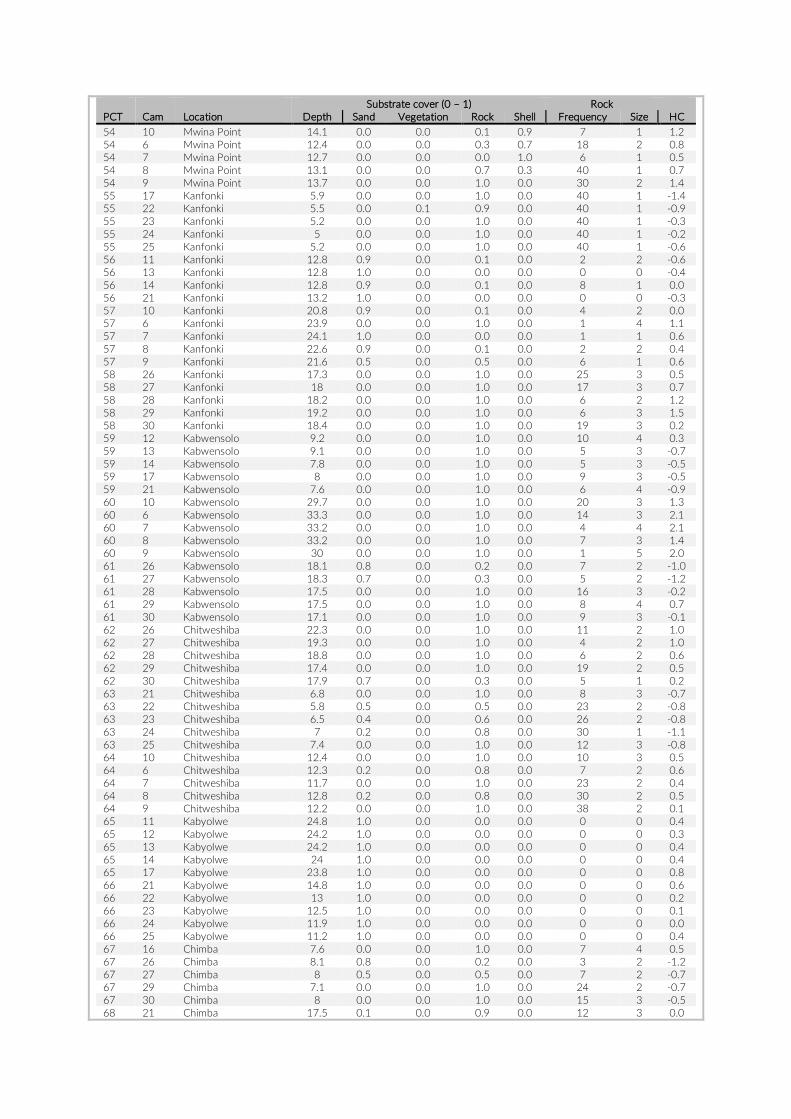
Substrate cover (0 – 1) Rock PCT Cam Location Depth Sand Vegetation Rock Shell Frequency Size HC 54 10 Mwina Point 14.1 0.0 0.0 0.1 0.9 7 1 1.2 54 6 Mwina Point 12.4 0.0 0.0 0.3 0.7 18 2 0.8 54 7 Mwina Point 12.7 0.0 0.0 0.0 1.0 6 1 0.5 54 8 Mwina Point 13.1 0.0 0.0 0.7 0.3 40 1 0.7 54 9 Mwina Point 13.7 0.0 0.0 1.0 0.0 30 2 1.4 55 17 Kanfonki 5.9 0.0 0.0 1.0 0.0 40 1 -1.4 55 22 Kanfonki 5.5 0.0 0.1 0.9 0.0 40 1 -0.9 55 23 Kanfonki 5.2 0.0 0.0 1.0 0.0 40 1 -0.3 55 24 Kanfonki 5 0.0 0.0 1.0 0.0 40 1 -0.2 55 25 Kanfonki 5.2 0.0 0.0 1.0 0.0 40 1 -0.6 56 11 Kanfonki 12.8 0.9 0.0 0.1 0.0 2 2 -0.6 56 13 Kanfonki 12.8 1.0 0.0 0.0 0.0 0 0 -0.4 56 14 Kanfonki 12.8 0.9 0.0 0.1 0.0 8 1 0.0 56 21 Kanfonki 13.2 1.0 0.0 0.0 0.0 0 0 -0.3 57 10 Kanfonki 20.8 0.9 0.0 0.1 0.0 4 2 0.0 57 6 Kanfonki 23.9 0.0 0.0 1.0 0.0 1 4 1.1 57 7 Kanfonki 24.1 1.0 0.0 0.0 0.0 1 1 0.6 57 8 Kanfonki 22.6 0.9 0.0 0.1 0.0 2 2 0.4 57 9 Kanfonki 21.6 0.5 0.0 0.5 0.0 6 1 0.6 58 26 Kanfonki 17.3 0.0 0.0 1.0 0.0 25 3 0.5 58 27 Kanfonki 18 0.0 0.0 1.0 0.0 17 3 0.7 58 28 Kanfonki 18.2 0.0 0.0 1.0 0.0 6 2 1.2 58 29 Kanfonki 19.2 0.0 0.0 1.0 0.0 6 3 1.5 58 30 Kanfonki 18.4 0.0 0.0 1.0 0.0 19 3 0.2 59 12 Kabwensolo 9.2 0.0 0.0 1.0 0.0 10 4 0.3 59 13 Kabwensolo 9.1 0.0 0.0 1.0 0.0 5 3 -0.7 59 14 Kabwensolo 7.8 0.0 0.0 1.0 0.0 5 3 -0.5 59 17 Kabwensolo 8 0.0 0.0 1.0 0.0 9 3 -0.5 59 21 Kabwensolo 7.6 0.0 0.0 1.0 0.0 6 4 -0.9 60 10 Kabwensolo 29.7 0.0 0.0 1.0 0.0 20 3 1.3 60 6 Kabwensolo 33.3 0.0 0.0 1.0 0.0 14 3 2.1 60 7 Kabwensolo 33.2 0.0 0.0 1.0 0.0 4 4 2.1 60 8 Kabwensolo 33.2 0.0 0.0 1.0 0.0 7 3 1.4 60 9 Kabwensolo 30 0.0 0.0 1.0 0.0 1 5 2.0 61 26 Kabwensolo 18.1 0.8 0.0 0.2 0.0 7 2 -1.0 61 27 Kabwensolo 18.3 0.7 0.0 0.3 0.0 5 2 -1.2 61 28 Kabwensolo 17.5 0.0 0.0 1.0 0.0 16 3 -0.2 61 29 Kabwensolo 17.5 0.0 0.0 1.0 0.0 8 4 0.7 61 30 Kabwensolo 17.1 0.0 0.0 1.0 0.0 9 3 -0.1 62 26 Chitweshiba 22.3 0.0 0.0 1.0 0.0 11 2 1.0 62 27 Chitweshiba 19.3 0.0 0.0 1.0 0.0 4 2 1.0 62 28 Chitweshiba 18.8 0.0 0.0 1.0 0.0 6 2 0.6 62 29 Chitweshiba 17.4 0.0 0.0 1.0 0.0 19 2 0.5 62 30 Chitweshiba 17.9 0.7 0.0 0.3 0.0 5 1 0.2 63 21 Chitweshiba 6.8 0.0 0.0 1.0 0.0 8 3 -0.7 63 22 Chitweshiba 5.8 0.5 0.0 0.5 0.0 23 2 -0.8 63 23 Chitweshiba 6.5 0.4 0.0 0.6 0.0 26 2 -0.8 63 24 Chitweshiba 7 0.2 0.0 0.8 0.0 30 1 -1.1 63 25 Chitweshiba 7.4 0.0 0.0 1.0 0.0 12 3 -0.8 64 10 Chitweshiba 12.4 0.0 0.0 1.0 0.0 10 3 0.5 64 6 Chitweshiba 12.3 0.2 0.0 0.8 0.0 7 2 0.6 64 7 Chitweshiba 11.7 0.0 0.0 1.0 0.0 23 2 0.4 64 8 Chitweshiba 12.8 0.2 0.0 0.8 0.0 30 2 0.5 64 9 Chitweshiba 12.2 0.0 0.0 1.0 0.0 38 2 0.1 65 11 Kabyolwe 24.8 1.0 0.0 0.0 0.0 0 0 0.4 65 12 Kabyolwe 24.2 1.0 0.0 0.0 0.0 0 0 0.3 65 13 Kabyolwe 24.2 1.0 0.0 0.0 0.0 0 0 0.4 65 14 Kabyolwe 24 1.0 0.0 0.0 0.0 0 0 0.4 65 17 Kabyolwe 23.8 1.0 0.0 0.0 0.0 0 0 0.8 66 21 Kabyolwe 14.8 1.0 0.0 0.0 0.0 0 0 0.6 66 22 Kabyolwe 13 1.0 0.0 0.0 0.0 0 0 0.2 66 23 Kabyolwe 12.5 1.0 0.0 0.0 0.0 0 0 0.1 66 24 Kabyolwe 11.9 1.0 0.0 0.0 0.0 0 0 0.0 66 25 Kabyolwe 11.2 1.0 0.0 0.0 0.0 0 0 0.4 67 16 Chimba 7.6 0.0 0.0 1.0 0.0 7 4 0.5 67 26 Chimba 8.1 0.8 0.0 0.2 0.0 3 2 -1.2 67 27 Chimba 8 0.5 0.0 0.5 0.0 7 2 -0.7 67 29 Chimba 7.1 0.0 0.0 1.0 0.0 24 2 -0.7 67 30 Chimba 8 0.0 0.0 1.0 0.0 15 3 -0.5 68 21 Chimba 17.5 0.1 0.0 0.9 0.0 12 3 0.0
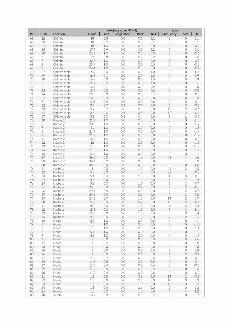
Substrate cover (0 – 1) Rock PCT Cam Location Depth Sand Vegetation Rock Shell Frequency Size HC 68 22 Chimba 18 0.8 0.0 0.0 0.2 0 0 0.1 68 23 Chimba 18 0.9 0.0 0.0 0.1 0 0 0.1 68 24 Chimba 18 1.0 0.0 0.0 0.0 0 0 -0.2 68 25 Chimba 17.9 0.9 0.0 0.0 0.2 0 0 0.0 69 10 Chimba 24.7 1.0 0.0 0.0 0.0 0 0 -0.6 69 6 Chimba 22 0.8 0.0 0.0 0.2 0 0 0.0 69 7 Chimba 22.7 1.0 0.0 0.0 0.0 0 0 -0.3 69 8 Chimba 23.7 1.0 0.0 0.0 0.0 0 0 -0.5 69 9 Chimba 24.4 1.0 0.0 0.0 0.0 0 0 -0.4 70 27 Chibwensolo 15.9 0.0 0.0 0.0 1.0 0 0 1.2 70 29 Chibwensolo 16.3 0.1 0.0 0.0 1.0 0 0 0.9 70 30 Chibwensolo 16.7 0.0 0.0 0.0 1.0 0 0 0.9 70 7 Chibwensolo 15.7 0.0 0.0 0.0 1.0 0 0 0.6 71 21 Chibwensolo 13.5 0.1 0.0 0.0 0.9 0 0 0.6 71 23 Chibwensolo 13.5 0.2 0.0 0.0 0.8 0 0 -0.1 71 24 Chibwensolo 13.5 0.3 0.0 0.0 0.7 0 0 -0.5 71 25 Chibwensolo 13.5 0.2 0.0 0.0 0.8 0 0 0.0 71 6 Chibwensolo 13.5 0.4 0.0 0.0 0.6 0 0 -0.4 72 12 Chibwensolo 3.9 0.0 0.3 0.7 0.0 6 3 -0.5 72 13 Chibwensolo 3.7 0.7 0.0 0.3 0.0 13 2 -0.6 72 14 Chibwensolo 3.5 0.0 0.5 0.5 0.0 12 2 -0.4 72 17 Chibwensolo 3.1 0.0 0.6 0.4 0.0 8 2 -0.9 73 10 Katete 2 21.1 1.0 0.0 0.0 0.0 0 0 -1.5 73 6 Katete 2 20.8 1.0 0.0 0.0 0.0 0 0 -1.7 73 7 Katete 2 21 1.0 0.0 0.0 0.0 0 0 -1.5 73 8 Katete 2 21.4 1.0 0.0 0.0 0.0 0 0 -1.7 73 9 Katete 2 21.2 1.0 0.0 0.0 0.0 0 0 -1.7 74 11 Katete 2 12.2 1.0 0.0 0.0 0.0 0 0 -0.8 74 12 Katete 2 12 1.0 0.0 0.0 0.0 0 0 -1.2 74 13 Katete 2 11.5 1.0 0.0 0.0 0.0 0 0 -1.2 74 14 Katete 2 11.5 1.0 0.0 0.0 0.0 0 0 -1.2 74 16 Katete 2 12.2 1.0 0.0 0.0 0.0 0 0 -1.4 75 27 Katete 2 36.2 0.0 0.0 1.0 0.0 23 1 0.6 75 29 Katete 2 34.1 0.2 0.0 0.8 0.0 35 1 0.0 75 30 Katete 2 35.5 0.0 0.0 0.0 0.0 0 0 1.0 76 21 Kachese 5 0.0 0.0 1.0 0.0 21 2 0.0 76 22 Kachese 5.2 0.0 0.0 1.0 0.0 32 1 -0.8 76 23 Kachese 5.4 0.0 0.0 1.0 0.0 4 3 -0.8 76 24 Kachese 4.8 0.0 0.0 1.0 0.0 7 4 0.4 76 25 Kachese 5.3 0.0 0.0 1.0 0.0 5 3 -0.7 77 17 Kachese 24.3 0.3 0.0 0.7 0.0 7 2 -0.3 77 26 Kachese 24.1 0.5 0.0 0.5 0.0 5 2 -0.6 77 27 Kachese 24.6 0.4 0.0 0.6 0.0 9 3 0.6 77 29 Kachese 24.3 0.0 0.0 1.0 0.0 14 2 0.0 77 30 Kachese 24.2 0.3 0.0 0.7 0.0 15 2 -0.1 78 11 Kachese 15.2 0.0 0.0 1.0 0.0 40 2 0.3 78 12 Kachese 15.5 0.0 0.0 1.0 0.0 8 3 1.1 78 13 Kachese 15.5 0.0 0.0 1.0 0.0 3 3 0.4 78 14 Kachese 15.6 0.0 0.0 1.0 0.0 26 2 0.6 79 10 Ndole 5.2 1.0 0.0 0.0 0.0 0 0 -1.4 79 6 Ndole 7.4 1.0 0.0 0.0 0.0 0 0 -1.0 79 7 Ndole 6 1.0 0.0 0.0 0.0 0 0 -1.4 79 8 Ndole 5.4 1.0 0.0 0.0 0.0 0 0 -1.8 79 9 Ndole 5.1 1.0 0.0 0.0 0.0 0 0 -1.8 80 11 Ndole 1 0.0 1.0 0.0 0.0 0 0 2.6 80 12 Ndole 1 0.0 1.0 0.0 0.0 0 0 0.8 80 13 Ndole 1 0.0 1.0 0.0 0.0 0 0 0.3 80 14 Ndole 1 0.0 1.0 0.0 0.0 0 0 0.8 80 16 Ndole 1 0.0 0.9 0.1 0.0 1 2 -0.1 81 17 Ndole 11.3 0.7 0.0 0.0 0.3 0 0 -0.8 81 26 Ndole 11.6 0.5 0.0 0.0 0.5 0 0 -0.4 81 27 Ndole 11.5 0.4 0.0 0.0 0.6 0 0 -0.3 81 29 Ndole 11.7 0.5 0.0 0.0 0.5 0 0 0.0 81 30 Ndole 11.9 0.4 0.0 0.0 0.6 0 0 -0.2 82 21 Ndole 1.5 0.5 0.0 0.5 0.0 14 2 -0.8 82 22 Ndole 1.5 0.3 0.0 0.8 0.0 10 3 0.3 82 23 Ndole 1.5 0.0 0.0 1.0 0.0 12 3 0.6 82 24 Ndole 1.5 0.4 0.0 0.6 0.0 0 0 0.3 82 25 Ndole 1.5 0.0 0.0 1.0 0.0 4 4 1.2 83 10 Sumbu 16.2 0.3 0.0 0.0 0.7 0 0 0.7
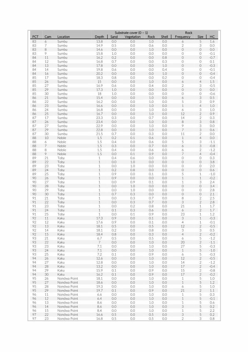
Substrate cover (0 – 1) Rock PCT Cam Location Depth Sand Vegetation Rock Shell Frequency Size HC 83 6 Sumbu 13.8 0.0 0.0 1.0 0.0 6 5 1.6 83 7 Sumbu 14.9 0.5 0.0 0.6 0.0 2 3 0.0 83 8 Sumbu 14.6 0.0 0.0 1.0 0.0 0 0 0.0 83 9 Sumbu 15.8 1.0 0.0 0.0 0.0 0 0 -0.1 84 11 Sumbu 16.2 0.2 0.0 0.0 0.8 0 0 -0.7 84 12 Sumbu 16.8 0.7 0.0 0.0 0.3 0 0 0.1 84 13 Sumbu 17.8 0.0 0.0 0.0 1.0 0 0 -0.3 84 14 Sumbu 19.8 0.6 0.0 0.0 0.4 0 0 -0.1 84 16 Sumbu 20.2 0.0 0.0 0.0 1.0 0 0 -0.4 85 17 Sumbu 18.3 0.8 0.0 0.0 0.2 0 0 -0.4 85 26 Sumbu 15 0.0 0.0 1.0 0.0 6 4 1.5 85 27 Sumbu 16.9 0.6 0.0 0.4 0.0 2 3 -0.5 85 29 Sumbu 17.3 1.0 0.0 0.0 0.0 0 0 0.0 85 30 Sumbu 18 1.0 0.0 0.0 0.0 0 0 -0.6 86 21 Sumbu 15.4 0.0 0.0 1.0 0.0 6 3 0.5 86 22 Sumbu 16.2 0.0 0.0 1.0 0.0 5 3 0.9 86 23 Sumbu 16.6 0.0 0.0 1.0 0.0 1 4 1.0 86 24 Sumbu 16.8 0.0 0.0 1.0 0.0 6 3 1.0 86 25 Sumbu 16.7 0.0 0.0 1.0 0.0 12 2 0.9 87 17 Sumbu 23.3 0.3 0.0 0.7 0.0 14 2 0.3 87 26 Sumbu 23.4 0.0 0.0 1.0 0.0 8 3 0.8 87 27 Sumbu 22.9 0.0 0.0 1.0 0.0 9 3 0.0 87 29 Sumbu 22.8 0.0 0.0 1.0 0.0 7 3 0.6 87 30 Sumbu 21.5 0.7 0.0 0.3 0.0 11 2 0.0 88 10 Ndole 1.5 0.2 0.1 0.6 0.0 1 4 0.0 88 6 Ndole 1.5 0.4 0.0 0.6 0.0 5 3 -1.1 88 7 Ndole 1.5 0.3 0.0 0.7 0.0 6 3 -0.8 88 8 Ndole 1.5 0.4 0.0 0.6 0.0 6 2 -1.2 88 9 Ndole 1.5 0.0 0.1 0.9 0.0 7 4 -0.4 89 21 Toby 1 0.4 0.6 0.0 0.0 0 0 0.3 89 22 Toby 1 0.0 1.0 0.0 0.0 0 0 3.8 89 23 Toby 1 0.0 1.0 0.0 0.0 0 0 2.0 89 24 Toby 1 0.2 0.8 0.0 0.0 0 0 0.6 89 25 Toby 1 0.9 0.0 0.1 0.0 5 1 -1.0 90 26 Toby 1 0.9 0.0 0.0 0.0 1 1 -0.2 90 27 Toby 1 0.0 0.9 0.1 0.0 1 3 2.4 90 28 Toby 1 0.0 1.0 0.0 0.0 0 0 3.4 90 29 Toby 1 0.0 1.0 0.0 0.0 0 0 2.8 90 30 Toby 1 0.7 0.3 0.0 0.0 0 0 2.1 91 21 Toby 1 0.0 0.3 0.7 0.0 8 2 2.5 91 22 Toby 1 0.0 0.3 0.7 0.0 3 2 2.8 91 23 Toby 1 0.0 0.2 0.8 0.0 21 1 1.7 91 24 Toby 1 0.1 0.3 0.6 0.0 6 2 1.7 91 25 Toby 1 0.0 0.1 0.9 0.0 23 1 1.2 92 11 Kaku 17.3 0.9 0.0 0.1 0.0 3 1 -0.3 92 12 Kaku 17.6 0.9 0.0 0.1 0.0 4 1 -0.1 92 13 Kaku 18.1 0.5 0.0 0.5 0.0 12 2 -0.5 92 14 Kaku 18.1 0.2 0.0 0.8 0.0 3 3 0.5 92 15 Kaku 18.4 0.8 0.0 0.3 0.0 4 2 -0.2 93 21 Kaku 6.7 0.5 0.0 0.5 0.0 6 5 -1.2 93 22 Kaku 7 0.0 0.0 1.0 0.0 20 2 -1.1 93 23 Kaku 7.1 0.0 0.0 1.0 0.0 27 5 -0.3 93 24 Kaku 7.1 0.0 0.0 1.0 0.0 1 5 -1.0 93 25 Kaku 7.2 0.1 0.0 0.9 0.0 6 5 -0.3 94 26 Kaku 12.6 0.0 0.0 1.0 0.0 12 2 -0.5 94 27 Kaku 12.8 0.0 0.0 1.0 0.0 14 2 -1.2 94 28 Kaku 13.2 0.0 0.0 1.0 0.0 17 2 -0.4 94 29 Kaku 15.9 0.1 0.0 0.9 0.0 15 2 -0.8 94 30 Kaku 16.2 0.1 0.0 0.9 0.0 17 2 -0.2 95 26 Nondwa Point 18.1 0.0 0.0 1.0 0.0 1 5 1.0 95 27 Nondwa Point 18.6 0.0 0.0 1.0 0.0 1 5 1.2 95 28 Nondwa Point 19.3 0.0 0.0 1.0 0.0 6 5 1.0 95 29 Nondwa Point 19.7 0.1 0.0 0.9 0.0 21 2 1.1 96 11 Nondwa Point 6.6 0.0 0.0 1.0 0.0 1 5 0.3 96 12 Nondwa Point 6.4 0.0 0.0 1.0 0.0 1 5 -0.1 96 13 Nondwa Point 8.6 0.0 0.0 1.0 0.0 1 5 0.6 96 14 Nondwa Point 8.6 0.0 0.0 1.0 0.0 3 5 0.2 96 15 Nondwa Point 8.4 0.0 0.0 1.0 0.0 1 5 2.2 97 22 Nondwa Point 16.6 0.5 0.0 0.5 0.0 3 5 0.2 97 23 Nondwa Point 16.8 0.5 0.0 0.5 0.0 2 3 0.8
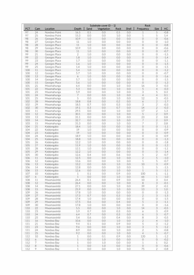
Substrate cover (0 – 1) Rock PCT Cam Location Depth Sand Vegetation Rock Shell Frequency Size HC 97 24 Nondwa Point 16.5 0.5 0.0 0.5 0.0 1 5 -0.8 97 25 Nondwa Point 15.3 0.0 0.0 1.0 0.0 1 5 1.4 98 26 Georges Place 10.9 1.0 0.0 0.0 0.0 0 0 -0.6 98 27 Georges Place 11 1.0 0.0 0.0 0.0 0 0 -1.0 98 28 Georges Place 11 1.0 0.0 0.0 0.0 0 0 -0.8 98 29 Georges Place 10.9 1.0 0.0 0.0 0.0 0 0 -0.6 98 30 Georges Place 11 1.0 0.0 0.0 0.0 0 0 -0.7 99 21 Georges Place 2 1.0 0.0 0.0 0.0 0 0 -1.5 99 22 Georges Place 1.8 1.0 0.0 0.0 0.0 0 0 -1.4 99 23 Georges Place 1.7 1.0 0.0 0.0 0.0 0 0 -1.1 99 24 Georges Place 1.6 1.0 0.0 0.0 0.0 0 0 -1.5 99 25 Georges Place 1.4 1.0 0.0 0.0 0.0 0 0 -1.5 100 11 Georges Place 5.4 1.0 0.0 0.0 0.0 0 0 -1.2 100 12 Georges Place 5.7 1.0 0.0 0.0 0.0 0 0 -0.7 100 13 Georges Place 6 1.0 0.0 0.0 0.0 0 0 -1.6 100 14 Georges Place 5.7 1.0 0.0 0.0 0.0 0 0 -1.5 100 15 Georges Place 5.6 1.0 0.0 0.0 0.0 0 0 -1.3 101 21 Mwamahunga 6.4 0.0 0.0 1.0 0.0 16 3 -0.3 101 22 Mwamahunga 5.3 0.0 0.0 1.0 0.0 5 4 -0.3 101 23 Mwamahunga 5.9 0.0 0.0 1.0 0.0 3 5 0.3 101 24 Mwamahunga 7 0.0 0.0 1.0 0.0 4 4 0.1 101 25 Mwamahunga 5 0.0 0.0 1.0 0.0 12 3 -0.5 102 28 Mwamahunga 18.8 0.8 0.0 0.2 0.0 6 2 -1.7 102 29 Mwamahunga 18.5 0.7 0.0 0.3 0.0 3 2 -0.3 102 30 Mwamahunga 19.1 0.3 0.0 0.7 0.0 14 2 -0.3 103 11 Mwamahunga 29.5 0.0 0.0 1.0 0.0 17 2 1.3 103 12 Mwamahunga 30.1 0.0 0.0 1.0 0.0 5 2 0.9 103 13 Mwamahunga 31.1 0.0 0.0 1.0 0.0 23 2 0.8 103 14 Mwamahunga 32.7 0.0 0.0 1.0 0.0 7 2 0.9 103 15 Mwamahunga 31.3 0.0 0.0 1.0 0.0 7 2 0.8 104 21 Kalalangabo 18.4 1.0 0.0 0.0 0.0 0 0 -1.1 104 22 Kalalangabo 19 1.0 0.0 0.0 0.0 0 0 -0.9 104 23 Kalalangabo 19 1.0 0.0 0.0 0.0 0 0 -0.9 104 24 Kalalangabo 18.9 1.0 0.0 0.0 0.0 0 0 -0.9 104 25 Kalalangabo 18.8 1.0 0.0 0.0 0.0 0 0 -1.3 105 26 Kalalangabo 12.2 1.0 0.0 0.0 0.0 0 0 -1.8 105 27 Kalalangabo 11.9 1.0 0.0 0.0 0.0 0 0 -1.2 105 28 Kalalangabo 12.1 1.0 0.0 0.0 0.0 0 0 -1.1 105 29 Kalalangabo 12.2 1.0 0.0 0.0 0.0 0 0 -1.4 105 30 Kalalangabo 12.6 0.4 0.0 0.6 0.0 5 2 -0.7 106 11 Kalalangabo 12.5 0.0 0.0 1.0 0.0 2 5 -1.0 106 12 Kalalangabo 13.6 0.0 0.0 1.0 0.0 1 5 -0.7 106 13 Kalalangabo 13.2 0.0 0.0 1.0 0.0 10 3 -0.9 106 14 Kalalangabo 12.8 0.0 0.0 1.0 0.0 1 5 -1.5 106 15 Kalalangabo 12.6 0.0 0.0 1.0 0.0 1 5 -1.1 107 10 Kalalangabo 1 0.1 0.0 0.9 0.0 100 1 -1.1 107 6 Kalalangabo 1 0.0 0.0 1.0 0.0 66 1 -1.0 108 11 Mwamawimbi 26.4 0.1 0.0 0.9 0.0 10 3 0.4 108 12 Mwamawimbi 26.4 0.0 0.0 1.0 0.0 8 3 -0.1 108 14 Mwamawimbi 27.1 0.0 0.0 1.0 0.0 39 2 -0.1 108 15 Mwamawimbi 25.9 0.0 0.0 1.0 0.0 13 3 1.0 109 26 Mwamawimbi 17.8 1.0 0.0 0.0 0.0 0 0 -1.3 109 27 Mwamawimbi 17.3 0.7 0.0 0.3 0.0 2 3 -1.5 109 28 Mwamawimbi 17.4 1.0 0.0 0.0 0.0 0 0 -1.5 109 29 Mwamawimbi 17.5 0.6 0.0 0.4 0.0 5 3 -1.1 109 30 Mwamawimbi 17.8 1.0 0.0 0.0 0.0 0 0 -1.6 110 22 Mwamawimbi 5.5 0.0 0.0 1.0 0.0 14 3 -0.5 110 23 Mwamawimbi 5.9 0.7 0.0 0.3 0.0 6 3 -0.9 110 24 Mwamawimbi 6.4 0.7 0.0 0.3 0.0 6 3 -0.7 110 25 Mwamawimbi 5.4 0.6 0.0 0.4 0.0 8 3 -0.5 111 16 Nondwa Bay 10.6 0.0 0.0 1.0 0.0 2 4 -1.0 111 21 Nondwa Bay 9.4 0.1 0.0 0.9 0.0 5 3 -1.2 111 23 Nondwa Bay 9.6 0.0 0.0 1.0 0.0 3 5 -1.2 111 24 Nondwa Bay 8.9 0.0 0.0 1.0 0.0 2 5 -0.8 111 25 Nondwa Bay 9.2 0.0 0.0 1.0 0.0 4 5 -0.7 112 10 Nondwa Bay 1 0.0 0.1 0.9 0.0 120 1 -1.2 112 6 Nondwa Bay 1 0.0 1.0 0.0 0.0 0 0 -0.2 112 7 Nondwa Bay 1 0.0 1.0 0.0 0.0 1 1 0.2 112 8 Nondwa Bay 1 0.0 1.0 0.0 0.0 0 0 -0.6 112 9 Nondwa Bay 1 0.0 0.0 1.0 0.0 75 2 -0.8
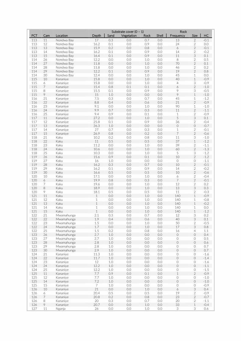
Substrate cover (0 – 1) Rock PCT Cam Location Depth Sand Vegetation Rock Shell Frequency Size HC 113 11 Nondwa Bay 17 0.3 0.0 0.7 0.0 13 2 -0.1 113 12 Nondwa Bay 16.2 0.1 0.0 0.9 0.0 24 2 0.0 113 13 Nondwa Bay 15.9 0.2 0.0 0.8 0.0 6 2 -0.1 113 14 Nondwa Bay 16.2 0.1 0.0 0.9 0.0 14 2 -0.2 113 15 Nondwa Bay 16.4 0.1 0.0 0.9 0.0 11 3 0.1 114 26 Nondwa Bay 12.2 0.0 0.0 1.0 0.0 8 2 0.5 114 27 Nondwa Bay 11.8 0.0 0.0 1.0 0.0 70 2 0.1 114 28 Nondwa Bay 11.8 0.0 0.0 1.0 0.0 46 2 0.2 114 29 Nondwa Bay 12.2 0.1 0.0 0.9 0.0 19 2 0.8 114 30 Nondwa Bay 12.4 0.0 0.0 1.0 0.0 45 1 0.0 115 10 Kananiye 15.8 0.0 0.0 1.0 0.0 40 1 -0.9 115 6 Kananiye 15.8 0.0 0.0 1.0 0.0 4 3 -0.9 115 7 Kananiye 15.4 0.8 0.1 0.1 0.0 6 2 -1.0 115 8 Kananiye 15.5 0.1 0.0 0.9 0.0 9 3 -0.5 115 9 Kananiye 15 1.0 0.0 0.0 0.0 9 1 -1.0 116 21 Kananiye 7.5 0.3 0.0 0.7 0.0 45 1 -1.2 116 22 Kananiye 8.8 0.4 0.0 0.6 0.0 21 2 -0.9 116 23 Kananiye 9.1 0.0 0.0 1.0 0.0 90 1 -1.0 116 24 Kananiye 9.9 0.7 0.0 0.3 0.0 11 2 -1.1 116 25 Kananiye 9.4 0.9 0.0 0.1 0.0 1 2 -0.9 117 11 Kananiye 27.2 0.0 0.0 1.0 0.0 5 3 0.1 117 12 Kananiye 25.8 0.1 0.0 0.9 0.0 36 2 -0.4 117 13 Kananiye 26.3 1.0 0.0 0.0 0.0 0 0 -0.7 117 14 Kananiye 27 0.7 0.0 0.3 0.0 1 2 -0.1 117 15 Kananiye 26.9 0.8 0.0 0.2 0.0 7 2 -0.6 118 21 Kaku 10.2 0.2 0.0 0.8 0.0 11 3 -1.0 118 22 Kaku 11 0.5 0.0 0.5 0.0 37 1 -1.2 118 23 Kaku 11.2 0.0 0.0 1.0 0.0 39 2 -1.1 118 24 Kaku 10.6 0.0 0.0 1.0 0.0 60 2 -1.3 118 25 Kaku 10.3 0.0 0.0 1.0 0.0 5 3 -1.2 119 26 Kaku 15.6 0.9 0.0 0.1 0.0 10 2 -1.2 119 27 Kaku 16 1.0 0.0 0.0 0.0 0 0 -1.1 119 28 Kaku 16.2 0.3 0.0 0.7 0.0 10 2 -0.1 119 29 Kaku 16.2 0.1 0.0 0.9 0.0 14 2 -0.2 119 30 Kaku 16.6 0.5 0.0 0.5 0.0 10 2 -0.6 120 10 Kaku 17.1 0.0 0.0 1.0 0.0 6 2 -0.4 120 6 Kaku 19.9 0.8 0.0 0.3 0.0 7 2 -0.1 120 7 Kaku 19.6 0.0 0.0 1.0 0.0 12 2 0.2 120 8 Kaku 18.9 0.0 0.0 1.0 0.0 13 3 0.3 120 9 Kaku 18.1 0.5 0.0 0.5 0.0 11 2 -0.3 121 11 Kaku 1 0.0 0.0 1.0 0.0 140 1 -0.9 121 12 Kaku 1 0.0 0.0 1.0 0.0 140 1 -0.8 121 13 Kaku 1 0.0 0.0 1.0 0.0 140 1 -0.2 121 14 Kaku 1 0.0 0.0 1.0 0.0 140 1 0.0 121 15 Kaku 1 0.0 0.0 1.0 0.0 140 1 -1.2 122 21 Mwamahunga 2.1 0.3 0.0 0.7 0.0 12 3 0.2 122 22 Mwamahunga 1.9 0.4 0.0 0.6 0.0 40 3 0.1 122 23 Mwamahunga 1.5 0.0 0.0 1.0 0.0 50 2 -0.5 122 24 Mwamahunga 1.7 0.0 0.0 1.0 0.0 17 3 0.8 122 25 Mwamahunga 1.5 0.2 0.0 0.8 0.0 16 4 1.1 123 26 Mwamahunga 2.7 1.0 0.0 0.0 0.0 0 0 0.4 123 27 Mwamahunga 2.7 1.0 0.0 0.0 0.0 0 0 0.5 123 28 Mwamahunga 2.8 1.0 0.0 0.0 0.0 0 0 0.6 123 29 Mwamahunga 2.8 1.0 0.0 0.0 0.0 0 0 0.7 123 30 Mwamahunga 2.9 1.0 0.0 0.0 0.0 0 0 0.7 124 21 Kananiye 11.3 1.0 0.0 0.0 0.0 0 0 -1.6 124 22 Kananiye 11.7 1.0 0.0 0.0 0.0 0 0 -1.4 124 23 Kananiye 12 1.0 0.0 0.0 0.0 0 0 -1.6 124 24 Kananiye 12.2 1.0 0.0 0.0 0.0 0 0 -1.1 124 25 Kananiye 12.2 1.0 0.0 0.0 0.0 0 0 -1.5 125 11 Kananiye 7.7 0.9 0.0 0.1 0.0 1 2 -0.9 125 12 Kananiye 7.7 1.0 0.0 0.0 0.0 0 0 -1.0 125 14 Kananiye 7.2 1.0 0.0 0.0 0.0 0 0 -1.0 125 15 Kananiye 7 1.0 0.0 0.0 0.0 0 0 -0.9 126 10 Kananiye 21 0.0 0.0 1.0 0.0 6 3 0.4 126 6 Kananiye 20.4 0.5 0.0 0.5 0.0 19 2 -0.9 126 7 Kananiye 20.8 0.2 0.0 0.8 0.0 23 2 -0.7 126 8 Kananiye 20 0.3 0.0 0.7 0.0 20 2 -1.1 126 9 Kananiye 20.7 0.0 0.0 1.0 0.0 33 1 -0.4 127 11 Nganja 26 0.0 0.0 1.0 0.0 3 3 0.6
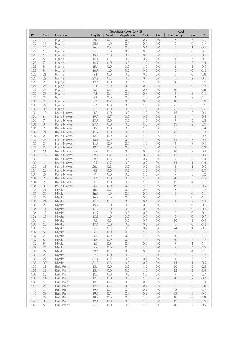
Substrate cover (0 – 1) Rock PCT Cam Location Depth Sand Vegetation Rock Shell Frequency Size HC 127 12 Nganja 25.7 0.1 0.0 0.9 0.0 8 3 1.1 127 13 Nganja 25.8 1.0 0.0 0.0 0.0 0 0 -1.6 127 14 Nganja 26.2 0.9 0.0 0.1 0.0 5 1 -0.7 127 15 Nganja 26.5 1.0 0.0 0.0 0.0 0 0 -0.8 128 10 Nganja 15.9 1.0 0.0 0.0 0.0 0 0 -0.9 128 6 Nganja 16.1 0.1 0.0 0.9 0.0 1 5 -0.3 128 7 Nganja 16.9 0.0 0.0 1.0 0.0 9 3 0.4 128 8 Nganja 15.4 0.0 0.0 1.0 0.0 1 5 -0.9 128 9 Nganja 16.7 1.0 0.0 0.0 0.0 0 0 -1.0 129 21 Nganja 21 0.0 0.0 0.0 0.0 0 0 0.8 129 22 Nganja 20.2 0.1 0.0 0.9 0.0 3 2 -0.3 129 23 Nganja 19.6 0.0 0.0 1.0 0.0 4 3 0.9 129 24 Nganja 21 1.0 0.0 0.0 0.0 0 0 -1.4 129 25 Nganja 20.2 0.2 0.0 0.8 0.0 10 2 0.6 130 26 Nganja 7.8 0.4 0.0 0.6 0.0 6 3 -1.0 130 27 Nganja 6.9 0.0 0.0 1.0 0.0 4 3 0.7 130 28 Nganja 6.5 0.2 0.0 0.8 0.0 10 3 1.0 130 29 Nganja 6.5 0.0 0.0 1.0 0.0 25 3 0.1 130 30 Nganja 6.1 0.0 0.0 1.0 0.0 22 3 0.0 131 10 Kalila Nkwasi 18 0.0 0.0 1.0 0.0 15 3 -0.1 131 6 Kalila Nkwasi 19.7 0.7 0.0 0.3 0.0 1 4 -0.5 131 7 Kalila Nkwasi 20.7 0.0 0.0 1.0 0.0 9 3 1.3 131 8 Kalila Nkwasi 20.4 0.0 0.0 1.0 0.0 13 2 1.0 131 9 Kalila Nkwasi 19 0.0 0.0 1.0 0.0 6 3 0.4 132 21 Kalila Nkwasi 11.7 0.0 0.0 1.0 0.0 22 3 -1.1 132 22 Kalila Nkwasi 12.3 0.0 0.0 1.0 0.0 7 3 -0.4 132 23 Kalila Nkwasi 13.1 0.0 0.0 1.0 0.0 11 3 -0.1 132 24 Kalila Nkwasi 11.6 0.0 0.0 1.0 0.0 6 3 -0.5 132 25 Kalila Nkwasi 12.6 0.0 0.0 1.0 0.0 2 2 0.3 133 11 Kalila Nkwasi 29 0.5 0.0 0.5 0.0 16 2 -0.4 133 12 Kalila Nkwasi 28.2 0.2 0.0 0.8 0.0 15 3 -0.2 133 13 Kalila Nkwasi 28.6 0.3 0.0 0.7 0.0 9 2 0.4 133 14 Kalila Nkwasi 29 0.7 0.0 0.3 0.0 14 1 0.4 133 15 Kalila Nkwasi 28.4 0.8 0.0 0.2 0.0 6 1 -0.2 134 26 Kalila Nkwasi 4.8 0.0 0.0 1.0 0.0 8 4 0.0 134 27 Kalila Nkwasi 4 0.0 0.0 1.0 0.0 9 5 0.2 134 28 Kalila Nkwasi 3.5 0.0 0.0 1.0 0.0 20 3 -1.2 134 29 Kalila Nkwasi 3.7 0.0 0.0 1.0 0.0 12 4 -1.3 134 30 Kalila Nkwasi 3.7 0.0 0.0 1.0 0.0 19 3 -0.9 135 21 Myako 16.4 0.7 0.0 0.3 0.0 3 2 -1.3 135 22 Myako 16.6 1.0 0.0 0.0 0.0 0 0 -1.4 135 23 Myako 16.9 1.0 0.0 0.0 0.0 0 0 -1.2 135 24 Myako 16.5 0.9 0.0 0.1 0.0 1 2 -1.4 135 25 Myako 15.2 1.0 0.0 0.0 0.0 0 0 -0.8 136 11 Myako 11.8 1.0 0.0 0.0 0.0 0 0 -0.4 136 12 Myako 11.9 1.0 0.0 0.0 0.0 0 0 -0.4 136 13 Myako 10.8 1.0 0.0 0.0 0.0 0 0 -0.7 136 14 Myako 9.2 0.3 0.0 0.7 0.0 10 2 -0.9 136 15 Myako 10.4 1.0 0.0 0.0 0.0 0 0 -1.1 137 10 Myako 5.6 0.3 0.0 0.7 0.0 24 1 -0.8 137 6 Myako 5.8 0.0 0.0 1.0 0.0 35 2 -1.0 137 7 Myako 5.8 0.0 0.0 1.0 0.0 50 2 -1.3 137 8 Myako 5.9 0.0 0.0 1.0 0.0 50 2 -1.3 137 9 Myako 5.7 0.8 0.0 0.2 0.0 7 1 -1.4 138 26 Myako 27 0.0 0.0 1.0 0.0 2 4 0.5 138 27 Myako 28.6 0.5 0.0 0.5 0.0 5 4 0.1 138 28 Myako 29.3 0.0 0.0 1.0 0.0 65 2 1.3 138 29 Myako 31.1 0.9 0.0 0.1 0.0 4 2 -1.0 138 30 Myako 31.8 0.8 0.0 0.2 0.0 14 1 -0.7 139 11 Bulu Point 13.4 0.0 0.0 1.0 0.0 10 2 0.3 139 12 Bulu Point 13.4 0.0 0.0 1.0 0.0 12 2 0.4 139 13 Bulu Point 11.9 0.0 0.0 1.0 0.0 9 3 0.7 139 14 Bulu Point 12.8 0.0 0.0 1.0 0.0 28 2 -0.6 139 15 Bulu Point 12.5 0.2 0.0 0.8 0.0 5 3 0.4 140 26 Bulu Point 19.6 0.3 0.0 0.7 0.0 8 3 0.8 140 27 Bulu Point 19.5 0.1 0.0 0.9 0.0 28 2 0.7 140 28 Bulu Point 19.6 0.1 0.0 0.9 0.0 32 2 -0.5 140 29 Bulu Point 19.9 0.0 0.0 1.0 0.0 10 2 0.9 140 30 Bulu Point 19.1 0.0 0.0 1.0 0.0 12 3 0.5 141 6 Bulu Point 6.7 0.0 0.0 1.0 0.0 40 2 -0.7
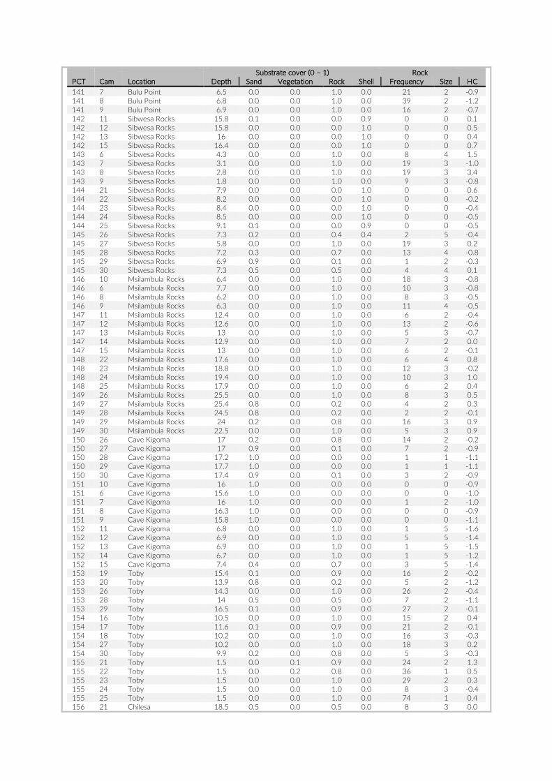
Substrate cover (0 – 1) Rock PCT Cam Location Depth Sand Vegetation Rock Shell Frequency Size HC 141 7 Bulu Point 6.5 0.0 0.0 1.0 0.0 21 2 -0.9 141 8 Bulu Point 6.8 0.0 0.0 1.0 0.0 39 2 -1.2 141 9 Bulu Point 6.9 0.0 0.0 1.0 0.0 16 2 -0.7 142 11 Sibwesa Rocks 15.8 0.1 0.0 0.0 0.9 0 0 0.1 142 12 Sibwesa Rocks 15.8 0.0 0.0 0.0 1.0 0 0 0.5 142 13 Sibwesa Rocks 16 0.0 0.0 0.0 1.0 0 0 0.4 142 15 Sibwesa Rocks 16.4 0.0 0.0 0.0 1.0 0 0 0.7 143 6 Sibwesa Rocks 4.3 0.0 0.0 1.0 0.0 8 4 1.5 143 7 Sibwesa Rocks 3.1 0.0 0.0 1.0 0.0 19 3 -1.0 143 8 Sibwesa Rocks 2.8 0.0 0.0 1.0 0.0 19 3 3.4 143 9 Sibwesa Rocks 1.8 0.0 0.0 1.0 0.0 9 3 -0.8 144 21 Sibwesa Rocks 7.9 0.0 0.0 0.0 1.0 0 0 0.6 144 22 Sibwesa Rocks 8.2 0.0 0.0 0.0 1.0 0 0 -0.2 144 23 Sibwesa Rocks 8.4 0.0 0.0 0.0 1.0 0 0 -0.4 144 24 Sibwesa Rocks 8.5 0.0 0.0 0.0 1.0 0 0 -0.5 144 25 Sibwesa Rocks 9.1 0.1 0.0 0.0 0.9 0 0 -0.5 145 26 Sibwesa Rocks 7.3 0.2 0.0 0.4 0.4 2 5 -0.4 145 27 Sibwesa Rocks 5.8 0.0 0.0 1.0 0.0 19 3 0.2 145 28 Sibwesa Rocks 7.2 0.3 0.0 0.7 0.0 13 4 -0.8 145 29 Sibwesa Rocks 6.9 0.9 0.0 0.1 0.0 1 2 -0.3 145 30 Sibwesa Rocks 7.3 0.5 0.0 0.5 0.0 4 4 0.1 146 10 Msilambula Rocks 6.4 0.0 0.0 1.0 0.0 18 3 -0.8 146 6 Msilambula Rocks 7.7 0.0 0.0 1.0 0.0 10 3 -0.8 146 8 Msilambula Rocks 6.2 0.0 0.0 1.0 0.0 8 3 -0.5 146 9 Msilambula Rocks 6.3 0.0 0.0 1.0 0.0 11 4 -0.5 147 11 Msilambula Rocks 12.4 0.0 0.0 1.0 0.0 6 2 -0.4 147 12 Msilambula Rocks 12.6 0.0 0.0 1.0 0.0 13 2 -0.6 147 13 Msilambula Rocks 13 0.0 0.0 1.0 0.0 5 3 -0.7 147 14 Msilambula Rocks 12.9 0.0 0.0 1.0 0.0 7 2 0.0 147 15 Msilambula Rocks 13 0.0 0.0 1.0 0.0 6 2 -0.1 148 22 Msilambula Rocks 17.6 0.0 0.0 1.0 0.0 6 4 0.8 148 23 Msilambula Rocks 18.8 0.0 0.0 1.0 0.0 12 3 -0.2 148 24 Msilambula Rocks 19.4 0.0 0.0 1.0 0.0 10 3 1.0 148 25 Msilambula Rocks 17.9 0.0 0.0 1.0 0.0 6 2 0.4 149 26 Msilambula Rocks 25.5 0.0 0.0 1.0 0.0 8 3 0.5 149 27 Msilambula Rocks 25.4 0.8 0.0 0.2 0.0 4 2 0.3 149 28 Msilambula Rocks 24.5 0.8 0.0 0.2 0.0 2 2 -0.1 149 29 Msilambula Rocks 24 0.2 0.0 0.8 0.0 16 3 0.9 149 30 Msilambula Rocks 22.5 0.0 0.0 1.0 0.0 5 3 0.9 150 26 Cave Kigoma 17 0.2 0.0 0.8 0.0 14 2 -0.2 150 27 Cave Kigoma 17 0.9 0.0 0.1 0.0 7 2 -0.9 150 28 Cave Kigoma 17.2 1.0 0.0 0.0 0.0 1 1 -1.1 150 29 Cave Kigoma 17.7 1.0 0.0 0.0 0.0 1 1 -1.1 150 30 Cave Kigoma 17.4 0.9 0.0 0.1 0.0 3 2 -0.9 151 10 Cave Kigoma 16 1.0 0.0 0.0 0.0 0 0 -0.9 151 6 Cave Kigoma 15.6 1.0 0.0 0.0 0.0 0 0 -1.0 151 7 Cave Kigoma 16 1.0 0.0 0.0 0.0 1 2 -1.0 151 8 Cave Kigoma 16.3 1.0 0.0 0.0 0.0 0 0 -0.9 151 9 Cave Kigoma 15.8 1.0 0.0 0.0 0.0 0 0 -1.1 152 11 Cave Kigoma 6.8 0.0 0.0 1.0 0.0 1 5 -1.6 152 12 Cave Kigoma 6.9 0.0 0.0 1.0 0.0 5 5 -1.4 152 13 Cave Kigoma 6.9 0.0 0.0 1.0 0.0 1 5 -1.5 152 14 Cave Kigoma 6.7 0.0 0.0 1.0 0.0 1 5 -1.2 152 15 Cave Kigoma 7.4 0.4 0.0 0.7 0.0 3 5 -1.4 153 19 Toby 15.4 0.1 0.0 0.9 0.0 16 2 -0.2 153 20 Toby 13.9 0.8 0.0 0.2 0.0 5 2 -1.2 153 26 Toby 14.3 0.0 0.0 1.0 0.0 26 2 -0.4 153 28 Toby 14 0.5 0.0 0.5 0.0 7 2 -1.1 153 29 Toby 16.5 0.1 0.0 0.9 0.0 27 2 -0.1 154 16 Toby 10.5 0.0 0.0 1.0 0.0 15 2 0.4 154 17 Toby 11.6 0.1 0.0 0.9 0.0 21 2 -0.1 154 18 Toby 10.2 0.0 0.0 1.0 0.0 16 3 -0.3 154 27 Toby 10.2 0.0 0.0 1.0 0.0 18 3 0.2 154 30 Toby 9.9 0.2 0.0 0.8 0.0 5 3 -0.3 155 21 Toby 1.5 0.0 0.1 0.9 0.0 24 2 1.3 155 22 Toby 1.5 0.0 0.2 0.8 0.0 36 1 0.5 155 23 Toby 1.5 0.0 0.0 1.0 0.0 29 2 0.3 155 24 Toby 1.5 0.0 0.0 1.0 0.0 8 3 -0.4 155 25 Toby 1.5 0.0 0.0 1.0 0.0 74 1 0.4 156 21 Chilesa 18.5 0.5 0.0 0.5 0.0 8 3 0.0
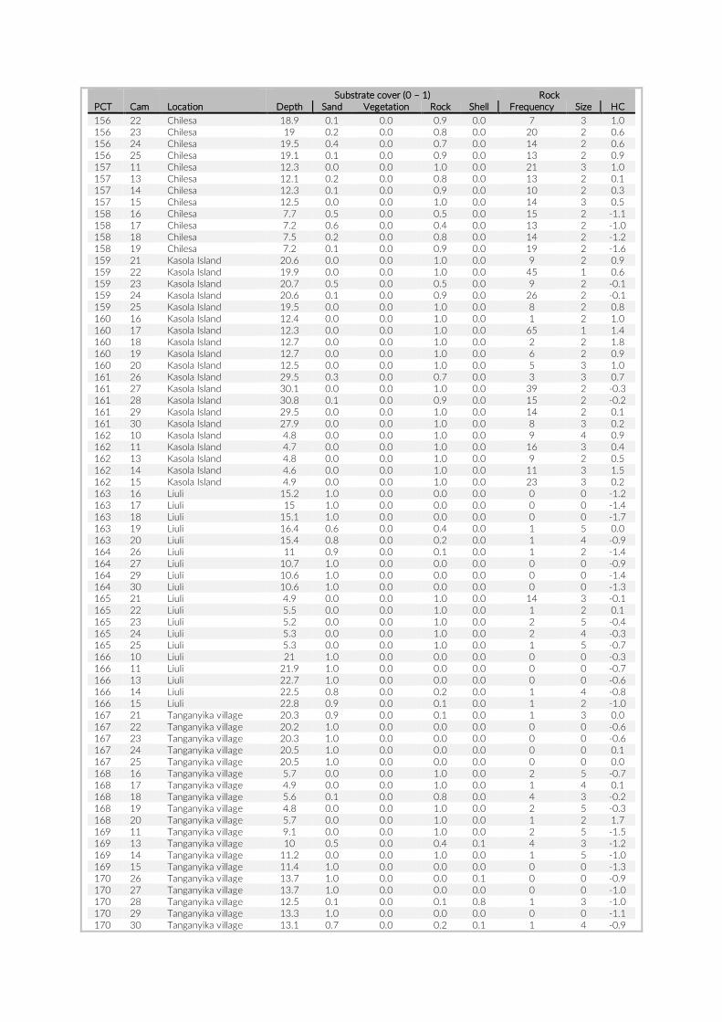
Substrate cover (0 – 1) Rock PCT Cam Location Depth Sand Vegetation Rock Shell Frequency Size HC 156 22 Chilesa 18.9 0.1 0.0 0.9 0.0 7 3 1.0 156 23 Chilesa 19 0.2 0.0 0.8 0.0 20 2 0.6 156 24 Chilesa 19.5 0.4 0.0 0.7 0.0 14 2 0.6 156 25 Chilesa 19.1 0.1 0.0 0.9 0.0 13 2 0.9 157 11 Chilesa 12.3 0.0 0.0 1.0 0.0 21 3 1.0 157 13 Chilesa 12.1 0.2 0.0 0.8 0.0 13 2 0.1 157 14 Chilesa 12.3 0.1 0.0 0.9 0.0 10 2 0.3 157 15 Chilesa 12.5 0.0 0.0 1.0 0.0 14 3 0.5 158 16 Chilesa 7.7 0.5 0.0 0.5 0.0 15 2 -1.1 158 17 Chilesa 7.2 0.6 0.0 0.4 0.0 13 2 -1.0 158 18 Chilesa 7.5 0.2 0.0 0.8 0.0 14 2 -1.2 158 19 Chilesa 7.2 0.1 0.0 0.9 0.0 19 2 -1.6 159 21 Kasola Island 20.6 0.0 0.0 1.0 0.0 9 2 0.9 159 22 Kasola Island 19.9 0.0 0.0 1.0 0.0 45 1 0.6 159 23 Kasola Island 20.7 0.5 0.0 0.5 0.0 9 2 -0.1 159 24 Kasola Island 20.6 0.1 0.0 0.9 0.0 26 2 -0.1 159 25 Kasola Island 19.5 0.0 0.0 1.0 0.0 8 2 0.8 160 16 Kasola Island 12.4 0.0 0.0 1.0 0.0 1 2 1.0 160 17 Kasola Island 12.3 0.0 0.0 1.0 0.0 65 1 1.4 160 18 Kasola Island 12.7 0.0 0.0 1.0 0.0 2 2 1.8 160 19 Kasola Island 12.7 0.0 0.0 1.0 0.0 6 2 0.9 160 20 Kasola Island 12.5 0.0 0.0 1.0 0.0 5 3 1.0 161 26 Kasola Island 29.5 0.3 0.0 0.7 0.0 3 3 0.7 161 27 Kasola Island 30.1 0.0 0.0 1.0 0.0 39 2 -0.3 161 28 Kasola Island 30.8 0.1 0.0 0.9 0.0 15 2 -0.2 161 29 Kasola Island 29.5 0.0 0.0 1.0 0.0 14 2 0.1 161 30 Kasola Island 27.9 0.0 0.0 1.0 0.0 8 3 0.2 162 10 Kasola Island 4.8 0.0 0.0 1.0 0.0 9 4 0.9 162 11 Kasola Island 4.7 0.0 0.0 1.0 0.0 16 3 0.4 162 13 Kasola Island 4.8 0.0 0.0 1.0 0.0 9 2 0.5 162 14 Kasola Island 4.6 0.0 0.0 1.0 0.0 11 3 1.5 162 15 Kasola Island 4.9 0.0 0.0 1.0 0.0 23 3 0.2 163 16 Liuli 15.2 1.0 0.0 0.0 0.0 0 0 -1.2 163 17 Liuli 15 1.0 0.0 0.0 0.0 0 0 -1.4 163 18 Liuli 15.1 1.0 0.0 0.0 0.0 0 0 -1.7 163 19 Liuli 16.4 0.6 0.0 0.4 0.0 1 5 0.0 163 20 Liuli 15.4 0.8 0.0 0.2 0.0 1 4 -0.9 164 26 Liuli 11 0.9 0.0 0.1 0.0 1 2 -1.4 164 27 Liuli 10.7 1.0 0.0 0.0 0.0 0 0 -0.9 164 29 Liuli 10.6 1.0 0.0 0.0 0.0 0 0 -1.4 164 30 Liuli 10.6 1.0 0.0 0.0 0.0 0 0 -1.3 165 21 Liuli 4.9 0.0 0.0 1.0 0.0 14 3 -0.1 165 22 Liuli 5.5 0.0 0.0 1.0 0.0 1 2 0.1 165 23 Liuli 5.2 0.0 0.0 1.0 0.0 2 5 -0.4 165 24 Liuli 5.3 0.0 0.0 1.0 0.0 2 4 -0.3 165 25 Liuli 5.3 0.0 0.0 1.0 0.0 1 5 -0.7 166 10 Liuli 21 1.0 0.0 0.0 0.0 0 0 -0.3 166 11 Liuli 21.9 1.0 0.0 0.0 0.0 0 0 -0.7 166 13 Liuli 22.7 1.0 0.0 0.0 0.0 0 0 -0.6 166 14 Liuli 22.5 0.8 0.0 0.2 0.0 1 4 -0.8 166 15 Liuli 22.8 0.9 0.0 0.1 0.0 1 2 -1.0 167 21 Tanganyika village 20.3 0.9 0.0 0.1 0.0 1 3 0.0 167 22 Tanganyika village 20.2 1.0 0.0 0.0 0.0 0 0 -0.6 167 23 Tanganyika village 20.3 1.0 0.0 0.0 0.0 0 0 -0.6 167 24 Tanganyika village 20.5 1.0 0.0 0.0 0.0 0 0 0.1 167 25 Tanganyika village 20.5 1.0 0.0 0.0 0.0 0 0 0.0 168 16 Tanganyika village 5.7 0.0 0.0 1.0 0.0 2 5 -0.7 168 17 Tanganyika village 4.9 0.0 0.0 1.0 0.0 1 4 0.1 168 18 Tanganyika village 5.6 0.1 0.0 0.8 0.0 4 3 -0.2 168 19 Tanganyika village 4.8 0.0 0.0 1.0 0.0 2 5 -0.3 168 20 Tanganyika village 5.7 0.0 0.0 1.0 0.0 1 2 1.7 169 11 Tanganyika village 9.1 0.0 0.0 1.0 0.0 2 5 -1.5 169 13 Tanganyika village 10 0.5 0.0 0.4 0.1 4 3 -1.2 169 14 Tanganyika village 11.2 0.0 0.0 1.0 0.0 1 5 -1.0 169 15 Tanganyika village 11.4 1.0 0.0 0.0 0.0 0 0 -1.3 170 26 Tanganyika village 13.7 1.0 0.0 0.0 0.1 0 0 -0.9 170 27 Tanganyika village 13.7 1.0 0.0 0.0 0.0 0 0 -1.0 170 28 Tanganyika village 12.5 0.1 0.0 0.1 0.8 1 3 -1.0 170 29 Tanganyika village 13.3 1.0 0.0 0.0 0.0 0 0 -1.1 170 30 Tanganyika village 13.1 0.7 0.0 0.2 0.1 1 4 -0.9
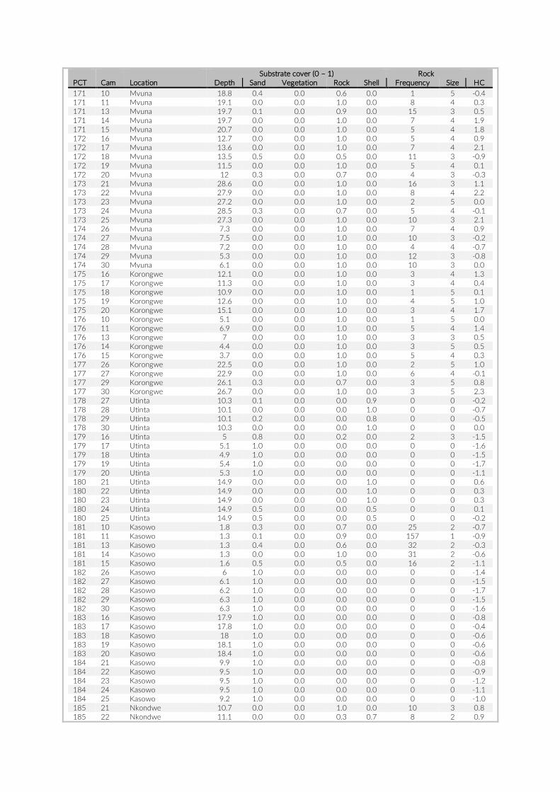
Substrate cover (0 – 1) Rock PCT Cam Location Depth Sand Vegetation Rock Shell Frequency Size HC 171 10 Mvuna 18.8 0.4 0.0 0.6 0.0 1 5 -0.4 171 11 Mvuna 19.1 0.0 0.0 1.0 0.0 8 4 0.3 171 13 Mvuna 19.7 0.1 0.0 0.9 0.0 15 3 0.5 171 14 Mvuna 19.7 0.0 0.0 1.0 0.0 7 4 1.9 171 15 Mvuna 20.7 0.0 0.0 1.0 0.0 5 4 1.8 172 16 Mvuna 12.7 0.0 0.0 1.0 0.0 5 4 0.9 172 17 Mvuna 13.6 0.0 0.0 1.0 0.0 7 4 2.1 172 18 Mvuna 13.5 0.5 0.0 0.5 0.0 11 3 -0.9 172 19 Mvuna 11.5 0.0 0.0 1.0 0.0 5 4 0.1 172 20 Mvuna 12 0.3 0.0 0.7 0.0 4 3 -0.3 173 21 Mvuna 28.6 0.0 0.0 1.0 0.0 16 3 1.1 173 22 Mvuna 27.9 0.0 0.0 1.0 0.0 8 4 2.2 173 23 Mvuna 27.2 0.0 0.0 1.0 0.0 2 5 0.0 173 24 Mvuna 28.5 0.3 0.0 0.7 0.0 5 4 -0.1 173 25 Mvuna 27.3 0.0 0.0 1.0 0.0 10 3 2.1 174 26 Mvuna 7.3 0.0 0.0 1.0 0.0 7 4 0.9 174 27 Mvuna 7.5 0.0 0.0 1.0 0.0 10 3 -0.2 174 28 Mvuna 7.2 0.0 0.0 1.0 0.0 4 4 -0.7 174 29 Mvuna 5.3 0.0 0.0 1.0 0.0 12 3 -0.8 174 30 Mvuna 6.1 0.0 0.0 1.0 0.0 10 3 0.0 175 16 Korongwe 12.1 0.0 0.0 1.0 0.0 3 4 1.3 175 17 Korongwe 11.3 0.0 0.0 1.0 0.0 3 4 0.4 175 18 Korongwe 10.9 0.0 0.0 1.0 0.0 1 5 0.1 175 19 Korongwe 12.6 0.0 0.0 1.0 0.0 4 5 1.0 175 20 Korongwe 15.1 0.0 0.0 1.0 0.0 3 4 1.7 176 10 Korongwe 5.1 0.0 0.0 1.0 0.0 1 5 0.0 176 11 Korongwe 6.9 0.0 0.0 1.0 0.0 5 4 1.4 176 13 Korongwe 7 0.0 0.0 1.0 0.0 3 3 0.5 176 14 Korongwe 4.4 0.0 0.0 1.0 0.0 3 5 0.5 176 15 Korongwe 3.7 0.0 0.0 1.0 0.0 5 4 0.3 177 26 Korongwe 22.5 0.0 0.0 1.0 0.0 2 5 1.0 177 27 Korongwe 22.9 0.0 0.0 1.0 0.0 6 4 -0.1 177 29 Korongwe 26.1 0.3 0.0 0.7 0.0 3 5 0.8 177 30 Korongwe 26.7 0.0 0.0 1.0 0.0 3 5 2.3 178 27 Utinta 10.3 0.1 0.0 0.0 0.9 0 0 -0.2 178 28 Utinta 10.1 0.0 0.0 0.0 1.0 0 0 -0.7 178 29 Utinta 10.1 0.2 0.0 0.0 0.8 0 0 -0.5 178 30 Utinta 10.3 0.0 0.0 0.0 1.0 0 0 0.0 179 16 Utinta 5 0.8 0.0 0.2 0.0 2 3 -1.5 179 17 Utinta 5.1 1.0 0.0 0.0 0.0 0 0 -1.6 179 18 Utinta 4.9 1.0 0.0 0.0 0.0 0 0 -1.5 179 19 Utinta 5.4 1.0 0.0 0.0 0.0 0 0 -1.7 179 20 Utinta 5.3 1.0 0.0 0.0 0.0 0 0 -1.1 180 21 Utinta 14.9 0.0 0.0 0.0 1.0 0 0 0.6 180 22 Utinta 14.9 0.0 0.0 0.0 1.0 0 0 0.3 180 23 Utinta 14.9 0.0 0.0 0.0 1.0 0 0 0.3 180 24 Utinta 14.9 0.5 0.0 0.0 0.5 0 0 0.1 180 25 Utinta 14.9 0.5 0.0 0.0 0.5 0 0 -0.2 181 10 Kasowo 1.8 0.3 0.0 0.7 0.0 25 2 -0.7 181 11 Kasowo 1.3 0.1 0.0 0.9 0.0 157 1 -0.9 181 13 Kasowo 1.3 0.4 0.0 0.6 0.0 32 2 -0.3 181 14 Kasowo 1.3 0.0 0.0 1.0 0.0 31 2 -0.6 181 15 Kasowo 1.6 0.5 0.0 0.5 0.0 16 2 -1.1 182 26 Kasowo 6 1.0 0.0 0.0 0.0 0 0 -1.4 182 27 Kasowo 6.1 1.0 0.0 0.0 0.0 0 0 -1.5 182 28 Kasowo 6.2 1.0 0.0 0.0 0.0 0 0 -1.7 182 29 Kasowo 6.3 1.0 0.0 0.0 0.0 0 0 -1.5 182 30 Kasowo 6.3 1.0 0.0 0.0 0.0 0 0 -1.6 183 16 Kasowo 17.9 1.0 0.0 0.0 0.0 0 0 -0.8 183 17 Kasowo 17.8 1.0 0.0 0.0 0.0 0 0 -0.4 183 18 Kasowo 18 1.0 0.0 0.0 0.0 0 0 -0.6 183 19 Kasowo 18.1 1.0 0.0 0.0 0.0 0 0 -0.6 183 20 Kasowo 18.4 1.0 0.0 0.0 0.0 0 0 -0.6 184 21 Kasowo 9.9 1.0 0.0 0.0 0.0 0 0 -0.8 184 22 Kasowo 9.5 1.0 0.0 0.0 0.0 0 0 -0.9 184 23 Kasowo 9.5 1.0 0.0 0.0 0.0 0 0 -1.2 184 24 Kasowo 9.5 1.0 0.0 0.0 0.0 0 0 -1.1 184 25 Kasowo 9.2 1.0 0.0 0.0 0.0 0 0 -1.0 185 21 Nkondwe 10.7 0.0 0.0 1.0 0.0 10 3 0.8 185 22 Nkondwe 11.1 0.0 0.0 0.3 0.7 8 2 0.9
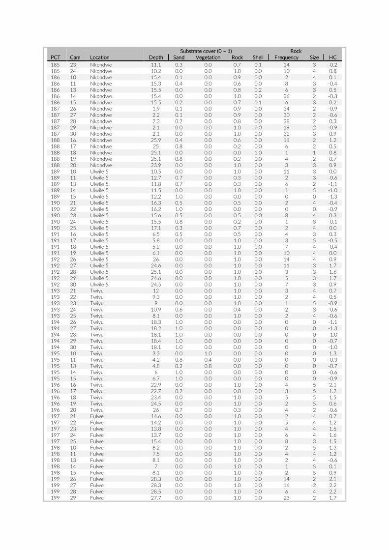
Substrate cover (0 – 1) Rock PCT Cam Location Depth Sand Vegetation Rock Shell Frequency Size HC 185 23 Nkondwe 11.1 0.3 0.0 0.7 0.1 14 3 -0.2 185 24 Nkondwe 10.2 0.0 0.0 1.0 0.0 10 4 0.8 186 10 Nkondwe 15.4 0.1 0.0 0.9 0.0 2 4 0.1 186 11 Nkondwe 15.3 0.4 0.0 0.6 0.0 8 3 -0.4 186 13 Nkondwe 15.5 0.0 0.0 0.8 0.2 6 3 0.5 186 14 Nkondwe 15.4 0.0 0.0 1.0 0.0 36 2 -0.3 186 15 Nkondwe 15.5 0.2 0.0 0.7 0.1 6 3 0.2 187 26 Nkondwe 1.9 0.1 0.0 0.9 0.0 34 2 -0.9 187 27 Nkondwe 2.2 0.1 0.0 0.9 0.0 30 2 -0.6 187 28 Nkondwe 2.3 0.2 0.0 0.8 0.0 38 2 0.3 187 29 Nkondwe 2.1 0.0 0.0 1.0 0.0 19 2 -0.9 187 30 Nkondwe 2.1 0.0 0.0 1.0 0.0 32 3 0.9 188 16 Nkondwe 25.9 0.4 0.0 0.6 0.0 11 2 1.2 188 17 Nkondwe 25 0.8 0.0 0.2 0.0 6 2 0.5 188 18 Nkondwe 25.1 0.0 0.0 0.0 1.0 1 1 0.8 188 19 Nkondwe 25.1 0.8 0.0 0.2 0.0 4 2 0.7 188 20 Nkondwe 23.9 0.0 0.0 1.0 0.0 3 3 0.9 189 10 Ulwile 5 10.5 0.0 0.0 1.0 0.0 11 3 0.0 189 11 Ulwile 5 12.7 0.7 0.0 0.3 0.0 2 3 -0.6 189 13 Ulwile 5 11.8 0.7 0.0 0.3 0.0 6 2 -1.1 189 14 Ulwile 5 11.5 0.0 0.0 1.0 0.0 1 5 -1.0 189 15 Ulwile 5 12.2 1.0 0.0 0.0 0.0 0 0 -1.3 190 21 Ulwile 5 16.3 0.5 0.0 0.5 0.0 2 4 -0.4 190 22 Ulwile 5 16.2 1.0 0.0 0.0 0.0 0 0 -0.9 190 23 Ulwile 5 15.6 0.5 0.0 0.5 0.0 8 4 0.3 190 24 Ulwile 5 15.5 0.8 0.0 0.2 0.0 1 3 -0.1 190 25 Ulwile 5 17.1 0.3 0.0 0.7 0.0 2 4 0.0 191 16 Ulwile 5 6.5 0.5 0.0 0.5 0.0 4 3 0.3 191 17 Ulwile 5 5.8 0.0 0.0 1.0 0.0 3 5 -0.5 191 18 Ulwile 5 5.2 0.0 0.0 1.0 0.0 7 4 -0.4 191 19 Ulwile 5 6.1 0.0 0.0 1.0 0.0 10 4 0.0 192 26 Ulwile 5 26 0.0 0.0 1.0 0.0 14 4 0.9 192 27 Ulwile 5 24.6 0.0 0.0 1.0 0.0 11 3 1.7 192 28 Ulwile 5 25.1 0.0 0.0 1.0 0.0 3 3 1.6 192 29 Ulwile 5 24.6 0.0 0.0 1.0 0.0 5 3 1.7 192 30 Ulwile 5 24.5 0.0 0.0 1.0 0.0 7 3 0.9 193 21 Twiyu 12 0.0 0.0 1.0 0.0 3 4 0.7 193 22 Twiyu 9.3 0.0 0.0 1.0 0.0 2 4 0.5 193 23 Twiyu 9 0.0 0.0 1.0 0.0 1 5 -0.9 193 24 Twiyu 10.9 0.6 0.0 0.4 0.0 2 3 -0.6 193 25 Twiyu 8.1 0.0 0.0 1.0 0.0 2 4 -0.6 194 26 Twiyu 18.3 1.0 0.0 0.0 0.0 0 0 -1.1 194 27 Twiyu 18.2 1.0 0.0 0.0 0.0 0 0 -1.3 194 28 Twiyu 18.1 1.0 0.0 0.0 0.0 0 0 -1.0 194 29 Twiyu 18.4 1.0 0.0 0.0 0.0 0 0 -0.7 194 30 Twiyu 18.1 1.0 0.0 0.0 0.0 0 0 -1.0 195 10 Twiyu 3.3 0.0 1.0 0.0 0.0 0 0 1.3 195 11 Twiyu 4.2 0.6 0.4 0.0 0.0 0 0 -0.3 195 13 Twiyu 4.8 0.2 0.8 0.0 0.0 0 0 -0.7 195 14 Twiyu 6 1.0 0.0 0.0 0.0 0 0 -0.6 195 15 Twiyu 6.7 1.0 0.0 0.0 0.0 0 0 -0.9 196 16 Twiyu 22.9 0.0 0.0 1.0 0.0 4 5 2.1 196 17 Twiyu 22.7 0.2 0.0 0.8 0.0 3 5 1.2 196 18 Twiyu 23.4 0.0 0.0 1.0 0.0 5 5 1.5 196 19 Twiyu 24.5 0.0 0.0 1.0 0.0 2 5 0.6 196 20 Twiyu 26 0.7 0.0 0.3 0.0 4 2 -0.6 197 21 Fulwe 14.6 0.0 0.0 1.0 0.0 2 4 0.7 197 22 Fulwe 14.2 0.0 0.0 1.0 0.0 5 4 1.2 197 23 Fulwe 13.8 0.0 0.0 1.0 0.0 4 4 1.5 197 24 Fulwe 13.7 0.0 0.0 1.0 0.0 6 4 1.6 197 25 Fulwe 15.4 0.0 0.0 1.0 0.0 8 3 1.5 198 10 Fulwe 8.2 0.0 0.0 1.0 0.0 2 5 1.3 198 11 Fulwe 7.5 0.0 0.0 1.0 0.0 4 4 1.2 198 13 Fulwe 8.1 0.0 0.0 1.0 0.0 2 4 -0.6 198 14 Fulwe 7 0.0 0.0 1.0 0.0 1 5 0.1 198 15 Fulwe 8.1 0.0 0.0 1.0 0.0 2 5 0.9 199 26 Fulwe 28.3 0.0 0.0 1.0 0.0 14 2 2.1 199 27 Fulwe 28.3 0.0 0.0 1.0 0.0 16 2 2.2 199 28 Fulwe 28.5 0.0 0.0 1.0 0.0 6 4 2.2 199 29 Fulwe 27.7 0.0 0.0 1.0 0.0 23 2 1.7
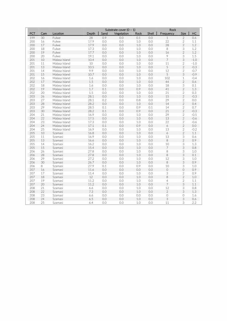
Substrate cover (0 – 1) Rock PCT Cam Location Depth Sand Vegetation Rock Shell Frequency Size HC 199 30 Fulwe 28 0.9 0.0 0.1 0.0 1 2 0.6 200 16 Fulwe 17.9 0.0 0.0 1.0 0.0 22 2 1.1 200 17 Fulwe 17.9 0.0 0.0 1.0 0.0 28 2 1.2 200 18 Fulwe 17.3 0.0 0.0 1.0 0.0 8 3 1.2 200 19 Fulwe 17.7 0.0 0.0 1.0 0.0 16 2 1.2 200 20 Fulwe 19.1 0.0 0.0 1.0 0.0 9 3 1.5 201 10 Malasa Island 10.4 0.0 0.0 1.0 0.0 7 3 -1.0 201 11 Malasa Island 10 0.0 0.0 1.0 0.0 11 2 -1.0 201 13 Malasa Island 10.5 0.0 0.0 1.0 0.0 5 2 -0.3 201 14 Malasa Island 9.9 0.0 0.0 1.0 0.0 12 2 -0.7 201 15 Malasa Island 10.7 0.0 0.0 1.0 0.0 5 3 -0.9 202 16 Malasa Island 1.6 0.0 0.0 1.0 0.0 102 1 -0.4 202 17 Malasa Island 1.5 0.0 0.0 1.0 0.0 44 2 0.6 202 18 Malasa Island 1.6 0.0 0.0 1.0 0.0 18 3 0.1 202 19 Malasa Island 1.7 0.1 0.0 0.9 0.0 41 2 1.3 202 20 Malasa Island 1.5 0.0 0.0 1.0 0.0 21 2 0.3 203 26 Malasa Island 28.1 0.0 0.0 1.0 0.0 15 2 -0.3 203 27 Malasa Island 28.1 0.2 0.0 0.8 0.0 29 2 0.0 203 28 Malasa Island 28.2 0.0 0.0 1.0 0.0 14 2 0.4 203 29 Malasa Island 28.5 0.1 0.0 0.9 0.1 14 2 0.7 203 30 Malasa Island 28.2 0.1 0.0 0.9 0.0 21 2 -0.3 204 21 Malasa Island 16.9 0.0 0.0 1.0 0.0 29 2 -0.5 204 22 Malasa Island 17.5 0.0 0.0 1.0 0.0 13 2 -0.6 204 23 Malasa Island 17.3 0.0 0.0 1.0 0.0 22 2 -0.6 204 24 Malasa Island 17.1 0.1 0.0 0.9 0.0 6 2 0.0 204 25 Malasa Island 16.9 0.0 0.0 1.0 0.0 13 2 -0.2 205 10 Szamasi 16.8 0.0 0.0 1.0 0.0 6 2 1.1 205 11 Szamasi 16.9 0.0 0.0 1.0 0.0 13 3 0.6 205 13 Szamasi 16.6 0.0 0.0 1.0 0.0 8 2 0.9 205 14 Szamasi 16.2 0.0 0.0 1.0 0.0 10 3 1.3 205 15 Szamasi 15.4 0.0 0.0 1.0 0.0 7 3 0.8 206 26 Szamasi 27.8 0.0 0.0 1.0 0.0 8 3 1.0 206 28 Szamasi 27.8 0.0 0.0 1.0 0.0 8 3 0.1 206 29 Szamasi 27.2 0.0 0.0 1.0 0.0 12 3 1.0 206 30 Szamasi 26.7 0.0 0.0 1.0 0.0 8 3 0.9 206 8 Szamasi 27.9 0.1 0.0 0.9 0.0 10 3 1.0 207 16 Szamasi 11.6 0.0 0.0 0.0 0.0 0 0 0.9 207 17 Szamasi 11.4 0.0 0.0 1.0 0.0 3 2 0.9 207 18 Szamasi 12 0.0 0.0 1.0 0.0 8 2 1.0 207 19 Szamasi 11.2 0.0 0.0 1.0 0.0 4 2 1.1 207 20 Szamasi 11.2 0.0 0.0 1.0 0.0 7 3 1.1 208 21 Szamasi 6.6 0.0 0.0 1.0 0.0 12 3 0.8 208 22 Szamasi 7.3 0.0 0.0 1.0 0.0 2 3 1.3 208 23 Szamasi 6.6 0.0 0.0 0.0 0.0 0 0 1.6 208 24 Szamasi 6.5 0.0 0.0 1.0 0.0 3 3 0.6 208 25 Szamasi 6.4 0.0 0.0 1.0 0.0 11 3 2.2
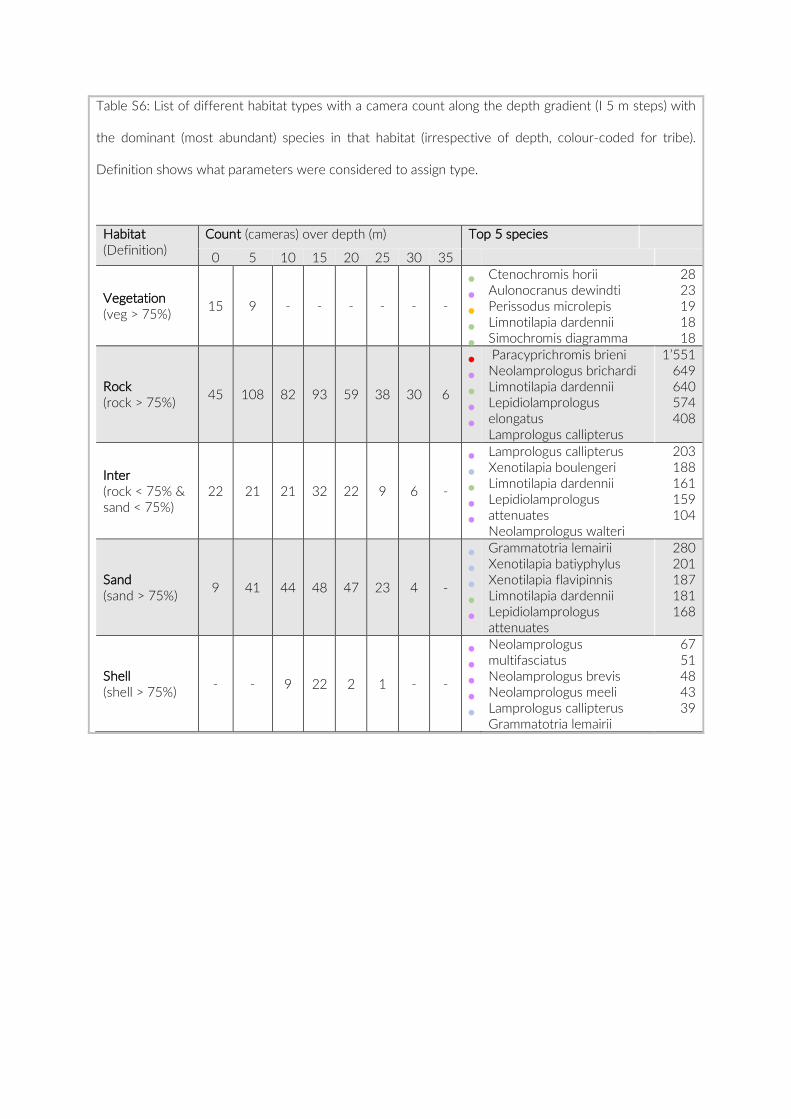
Table S6: List of different habitat types with a camera count along the depth gradient (I 5 m steps) with
the dominant (most abundant) species in that habitat (irrespective of depth, colour-coded for tribe).
Definition shows what parameters were considered to assign type.
Habitat (Definition)
Count (cameras) over depth (m) Top 5 species
0 5 10 15 20 25 30 35
Vegetation (veg > 75%) 15 9 - - - - - -
Ctenochromis horii Aulonocranus dewindti Perissodus microlepis Limnotilapia dardennii Simochromis diagramma
28 23 19 18 18
Rock (rock > 75%)
45 108 82 93 59 38 30 6
Paracyprichromis brieni Neolamprologus brichardi Limnotilapia dardennii Lepidiolamprologus elongatus Lamprologus callipterus
1’551 649 640 574 408
Inter (rock < 75% & sand < 75%)
22 21 21 32 22 9 6 -
Lamprologus callipterus Xenotilapia boulengeri Limnotilapia dardennii Lepidiolamprologus attenuates Neolamprologus walteri
203 188 161 159 104
Sand (sand > 75%)
9 41 44 48 47 23 4 -
Grammatotria lemairii Xenotilapia batiyphylus Xenotilapia flavipinnis Limnotilapia dardennii Lepidiolamprologus attenuates
280 201 187 181 168
Shell (shell > 75%)
- - 9 22 2 1 - -
Neolamprologus multifasciatus Neolamprologus brevis Neolamprologus meeli Lamprologus callipterus Grammatotria lemairii
67 51 48 43 39
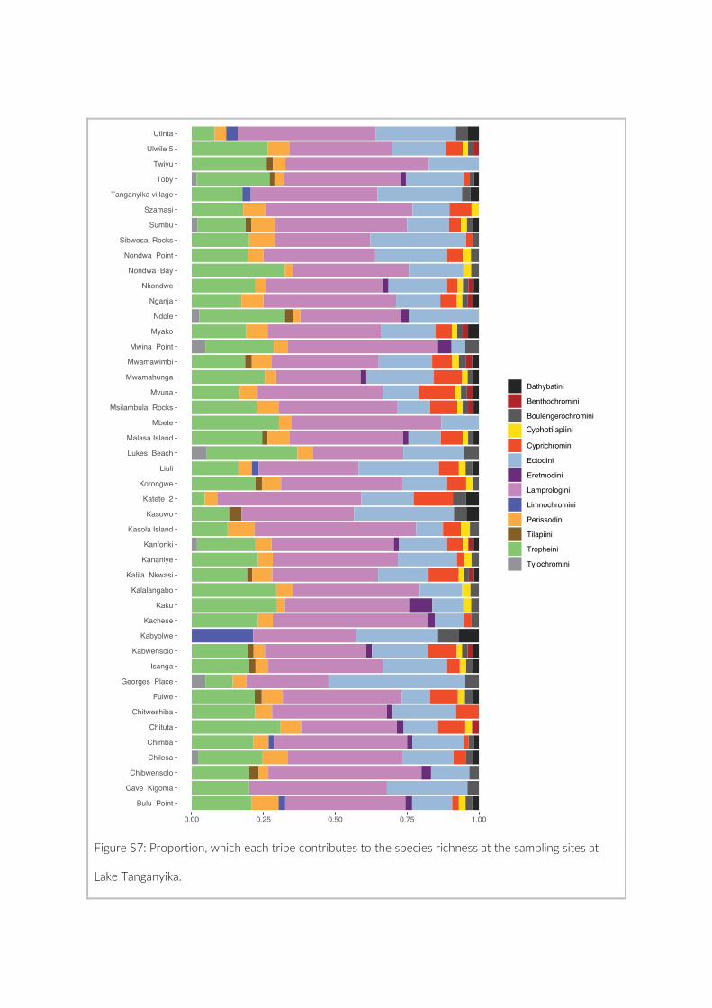
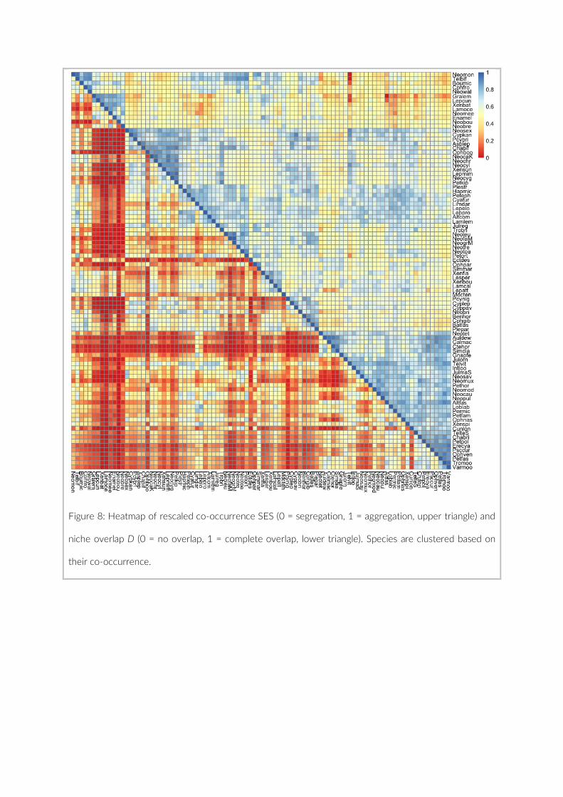
Figure 8: Heatmap of rescaled co-occurrence SES (0 = segregation, 1 = aggregation, upper triangle) and
niche overlap D (0 = no overlap, 1 = complete overlap, lower triangle). Species are clustered based on
their co-occurrence.
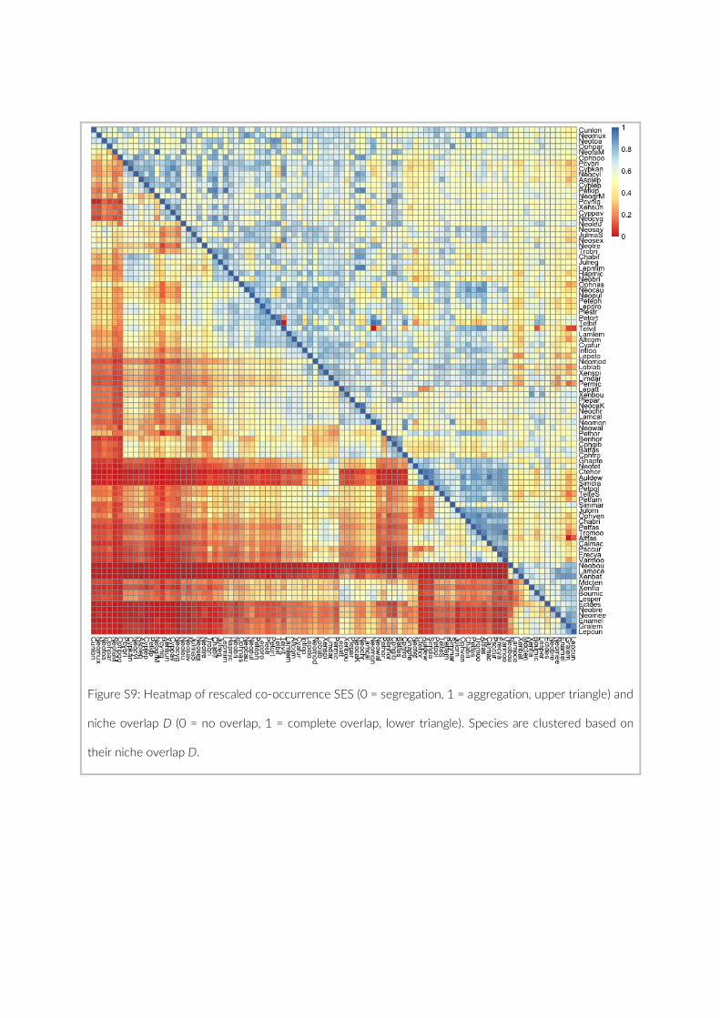
Figure S9: Heatmap of rescaled co-occurrence SES (0 = segregation, 1 = aggregation, upper triangle) and
niche overlap D (0 = no overlap, 1 = complete overlap, lower triangle). Species are clustered based on
their niche overlap D.
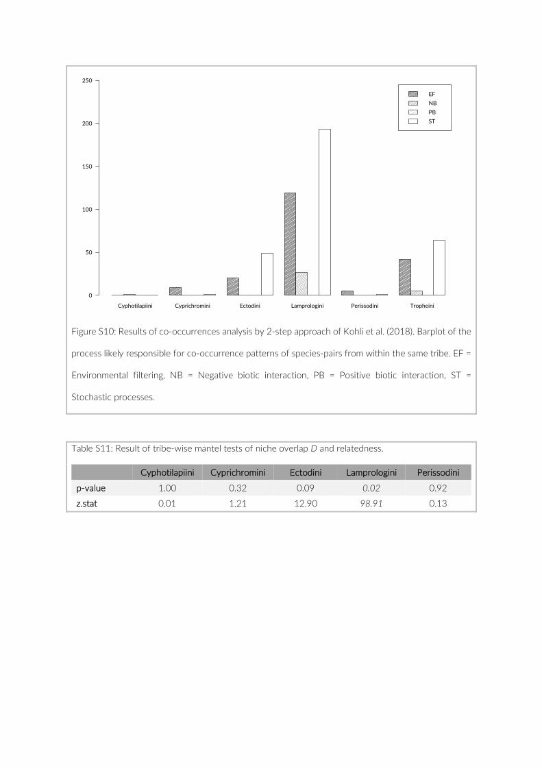
Figure S10: Results of co-occurrences analysis by 2-step approach of Kohli et al. (2018). Barplot of the
process likely responsible for co-occurrence patterns of species-pairs from within the same tribe. EF =
Environmental filtering, NB = Negative biotic interaction, PB = Positive biotic interaction, ST =
Stochastic processes.
Table S11: Result of tribe-wise mantel tests of niche overlap D and relatedness.
Cyphotilapiini Cyprichromini Ectodini Lamprologini Perissodini
p-value 1.00 0.32 0.09 0.02 0.92
z.stat 0.01 1.21 12.90 98.91 0.13
Cyphotilapiini Cyprichromini Ectodini Lamprologini Perissodini Tropheini
EFNBPBST
0
50
100
150
200
250
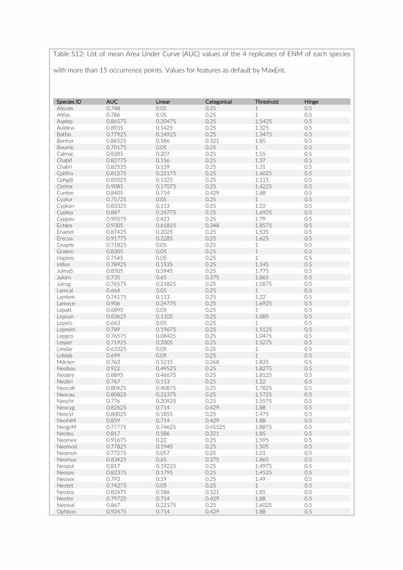
Table S12: List of mean Area Under Curve (AUC) values of the 4 replicates of ENM of each species
with more than 15 occurrence points. Values for features as default by MaxEnt.
Species ID AUC Linear Categorical Threshold Hinge Altcom 0.748 0.05 0.25 1 0.5 Altfas 0.786 0.05 0.25 1 0.5 Asplep 0.86575 0.20475 0.25 1.5425 0.5 Auldew 0.8935 0.1425 0.25 1.325 0.5 Batfas 0.77925 0.14925 0.25 1.3475 0.5 Benhor 0.86525 0.586 0.321 1.85 0.5 Boumic 0.70175 0.05 0.25 1 0.5 Calmac 0.8385 0.207 0.25 1.55 0.5 Chabif 0.82775 0.156 0.25 1.37 0.5 Chabri 0.82525 0.139 0.25 1.31 0.5 Cphfro 0.81275 0.22175 0.25 1.6025 0.5 Cphgib 0.85025 0.1325 0.25 1.115 0.5 Ctehor 0.9085 0.17075 0.25 1.4225 0.5 Cunlon 0.8405 0.714 0.429 1.88 0.5 Cyafur 0.75725 0.05 0.25 1 0.5 Cypkan 0.83325 0.113 0.25 1.22 0.5 Cyplep 0.847 0.24775 0.25 1.6925 0.5 Cyppav 0.90575 0.423 0.25 1.79 0.5 Ectdes 0.9305 0.61825 0.348 1.8575 0.5 Enamel 0.87425 0.2025 0.25 1.535 0.5 Erecya 0.91775 0.2285 0.25 1.625 0.5 Gnapfe 0.71825 0.05 0.25 1 0.5 Gralem 0.8305 0.05 0.25 1 0.5 Hapmic 0.7545 0.05 0.25 1 0.5 Intloo 0.78925 0.1535 0.25 1.145 0.5 JulmaS 0.8505 0.3945 0.25 1.775 0.5 Julorn 0.735 0.65 0.375 1.865 0.5 Julreg 0.76575 0.21825 0.25 1.5875 0.5 Lamcal 0.664 0.05 0.25 1 0.5 Lamlem 0.74175 0.113 0.25 1.22 0.5 Lamoce 0.906 0.24775 0.25 1.6925 0.5 Lepatt 0.6895 0.05 0.25 1 0.5 Lepcun 0.83625 0.1105 0.25 1.085 0.5 Lepelo 0.663 0.05 0.25 1 0.5 Lepmim 0.789 0.19675 0.25 1.5125 0.5 Leppro 0.76575 0.08425 0.25 1.0475 0.5 Lesper 0.71925 0.2005 0.25 1.5275 0.5 Limdar 0.63325 0.05 0.25 1 0.5 Loblab 0.699 0.05 0.25 1 0.5 Mdcten 0.763 0.5215 0.268 1.835 0.5 Neobou 0.922 0.49525 0.25 1.8275 0.5 Neobre 0.8895 0.46675 0.25 1.8125 0.5 Neobri 0.767 0.113 0.25 1.22 0.5 NeocaK 0.80425 0.40875 0.25 1.7825 0.5 Neocau 0.80825 0.21375 0.25 1.5725 0.5 Neochr 0.776 0.20925 0.25 1.5575 0.5 Neocyg 0.82625 0.714 0.429 1.88 0.5 Neocyl 0.80025 0.1855 0.25 1.475 0.5 NeofaM 0.859 0.714 0.429 1.88 0.5 NeogrM 0.77775 0.74625 0.45525 1.8875 0.5 Neoleu 0.817 0.586 0.321 1.85 0.5 Neomee 0.91675 0.22 0.25 1.595 0.5 Neomod 0.77825 0.1945 0.25 1.505 0.5 Neomon 0.77275 0.057 0.25 1.01 0.5 Neomux 0.83425 0.65 0.375 1.865 0.5 Neopul 0.817 0.19225 0.25 1.4975 0.5 Neosav 0.82375 0.1795 0.25 1.4525 0.5 Neosex 0.793 0.19 0.25 1.49 0.5 Neotet 0.74275 0.05 0.25 1 0.5 Neotoa 0.82475 0.586 0.321 1.85 0.5 Neotre 0.79725 0.714 0.429 1.88 0.5 Neowal 0.867 0.22175 0.25 1.6025 0.5 Ophboo 0.92475 0.714 0.429 1.88 0.5
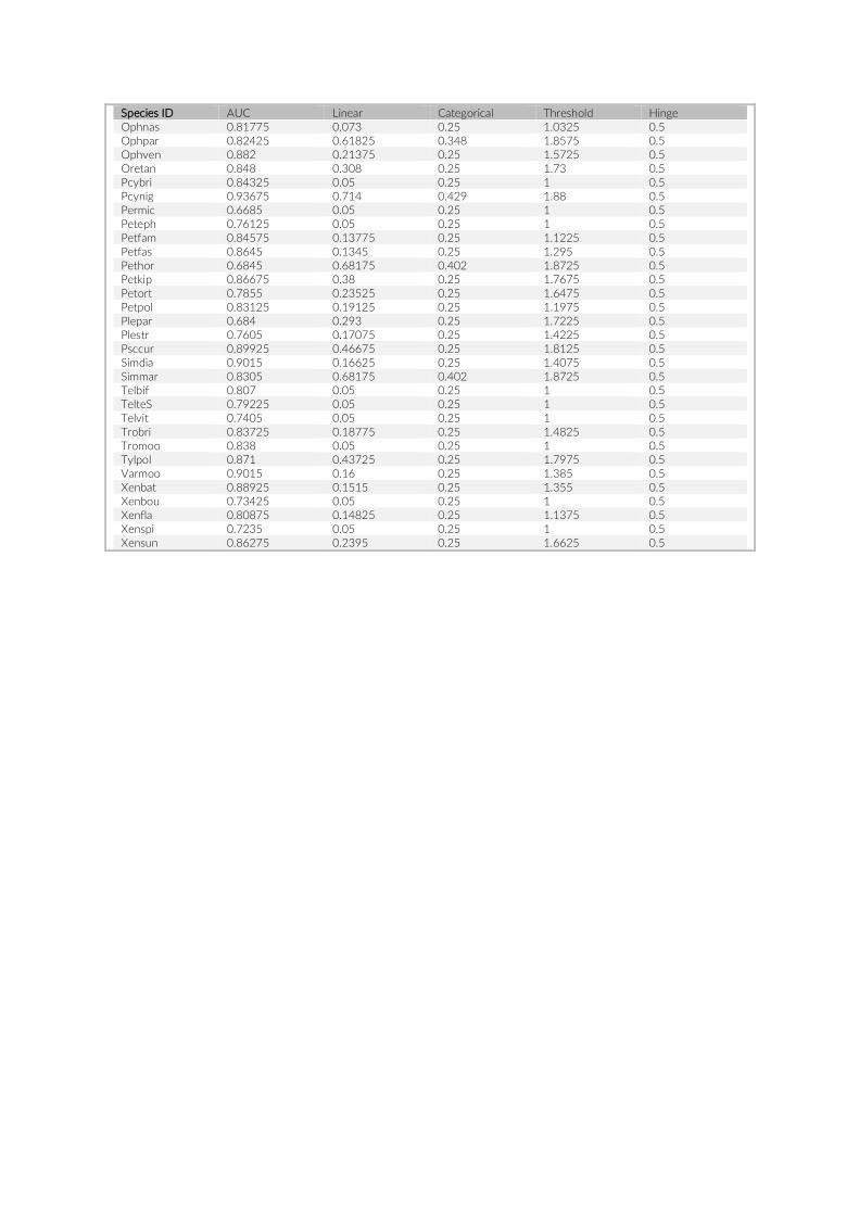
Species ID AUC Linear Categorical Threshold Hinge Ophnas 0.81775 0.073 0.25 1.0325 0.5 Ophpar 0.82425 0.61825 0.348 1.8575 0.5 Ophven 0.882 0.21375 0.25 1.5725 0.5 Oretan 0.848 0.308 0.25 1.73 0.5 Pcybri 0.84325 0.05 0.25 1 0.5 Pcynig 0.93675 0.714 0.429 1.88 0.5 Permic 0.6685 0.05 0.25 1 0.5 Peteph 0.76125 0.05 0.25 1 0.5 Petfam 0.84575 0.13775 0.25 1.1225 0.5 Petfas 0.8645 0.1345 0.25 1.295 0.5 Pethor 0.6845 0.68175 0.402 1.8725 0.5 Petkip 0.86675 0.38 0.25 1.7675 0.5 Petort 0.7855 0.23525 0.25 1.6475 0.5 Petpol 0.83125 0.19125 0.25 1.1975 0.5 Plepar 0.684 0.293 0.25 1.7225 0.5 Plestr 0.7605 0.17075 0.25 1.4225 0.5 Psccur 0.89925 0.46675 0.25 1.8125 0.5 Simdia 0.9015 0.16625 0.25 1.4075 0.5 Simmar 0.8305 0.68175 0.402 1.8725 0.5 Telbif 0.807 0.05 0.25 1 0.5 TelteS 0.79225 0.05 0.25 1 0.5 Telvit 0.7405 0.05 0.25 1 0.5 Trobri 0.83725 0.18775 0.25 1.4825 0.5 Tromoo 0.838 0.05 0.25 1 0.5 Tylpol 0.871 0.43725 0.25 1.7975 0.5 Varmoo 0.9015 0.16 0.25 1.385 0.5 Xenbat 0.88925 0.1515 0.25 1.355 0.5 Xenbou 0.73425 0.05 0.25 1 0.5 Xenfla 0.80875 0.14825 0.25 1.1375 0.5 Xenspi 0.7235 0.05 0.25 1 0.5 Xensun 0.86275 0.2395 0.25 1.6625 0.5
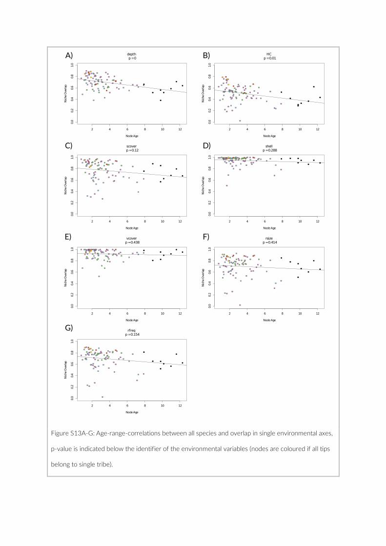
Figure S13A-G: Age-range-correlations between all species and overlap in single environmental axes,
p-value is indicated below the identifier of the environmental variables (nodes are coloured if all tips
belong to single tribe).
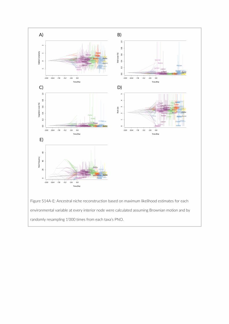
Figure S14A-E: Ancestral niche reconstruction based on maximum likelihood estimates for each
environmental variable at every interior node were calculated assuming Brownian motion and by
randomly resampling 1’000 times from each taxa’s PNO.
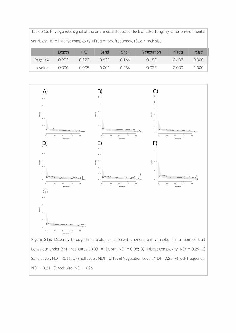
Table S15: Phylogenetic signal of the entire cichlid species-flock of Lake Tanganyika for environmental
variables; HC = Habitat complexity, rFreq = rock frequency, rSize = rock size.
Depth HC Sand Shell Vegetation rFreq rSize
Pagel’s l 0.905 0.522 0.928 0.166 0.187 0.603 0.000
p-value 0.000 0.005 0.001 0.286 0.037 0.000 1.000
Figure S16: Disparity-through-time plots for different environment variables (simulation of trait
behaviour under BM - replicates 1000), A) Depth, NDI = 0.08; B) Habitat complexity, NDI = 0.29; C)
Sand cover, NDI = 0.16; D) Shell cover, NDI = 0.15; E) Vegetation cover, NDI = 0.25; F) rock frequency,
NDI = 0.21; G) rock size, NDI = 026
Chapter 4
Where Am I? Niche constraints due to
morphological specialization in two
Tanganyikan cichlid fish species
Widmer L, Indermaur A, Egger B, Salzburger W
4.1 Manuscript pages 145 – 153
4.2 Supplementary Information pages 155 - 166

9410 | Ecology and Evolution. 2020;10:9410–9418.www.ecolevol.org
1 | INTRODUC TION
Adaptive radiation is the rapid ecological and morphological diver-sification of an ancestral—often generalist—species into an array of specialized descendants (Schluter, 2000). Such a burst of diversifica-tion can occur (a) after the emergence of a novel trait (in this context
termed “key innovation”) allowing the exploitation of previously in-accessible niches; (b) following the colonization of an empty or un-derutilized environmental space providing ecological opportunity; or (c) in the aftermath of extinction events carrying off antagonists and thus liberating previously occupied niches (Schluter, 2000). A common axis of morphological diversification during adaptive
Received: 19 June 2020 | Revised: 30 June 2020 | Accepted: 6 July 2020
DOI: 10.1002/ece3.6629
O R I G I N A L R E S E A R C H
Where Am I? Niche constraints due to morphological specialization in two Tanganyikan cichlid fish species
Lukas Widmer | Adrian Indermaur | Bernd Egger | Walter Salzburger
This is an open access article under the terms of the Creative Commons Attribution License, which permits use, distribution and reproduction in any medium, provided the original work is properly cited.© 2020 The Authors. Ecology and Evolution published by John Wiley & Sons Ltd
Department of Environmental Sciences, Zoological Institute, University of Basel, Basel, Switzerland
CorrespondenceLukas Widmer and Walter Salzburger, Department of Environmental Sciences, Zoological Institute, University of Basel, 4051 Basel, Switzerland.Emails: [email protected] (L.W.); [email protected] (W.S.)
Funding informationSchweizerischer Nationalfonds zur Förderung der Wissenschaftlichen Forschung, Grant/Award Number: 176039; European Research Council, ERC; StG INTERGENADAPT, Grant/Award Number: 201067; CoG CICHLID~X, Grant/Award Number: 617585
AbstractFood resource specialization within novel environments is considered a common axis of diversification in adaptive radiations. Feeding specializations are often coupled with striking morphological adaptations and exemplify the relation between mor-phology and diet (phenotype–environment correlations), as seen in, for example, Darwin finches, Hawaiian spiders, and the cichlid fish radiations in East African lakes. The cichlids' potential to rapidly exploit and occupy a variety of different habitats has previously been attributed to the variability and adaptability of their trophic struc-tures including the pharyngeal jaw apparatus. Here we report a reciprocal transplant experiment designed to explore the adaptability of the trophic structures in highly specialized cichlid fish species. More specifically, we forced two common but eco-logically distinct cichlid species from Lake Tanganyika, Tropheus moorii (rock-dweller), and Xenotilapia boulengeri (sand-dweller), to live on their preferred as well as on an unpreferred habitat (sand and rock, respectively). We measured their overall per-formance on the different habitat types and explored whether adaptive phenotypic plasticity is involved in adaptation. We found that, while habitat had no effect on the performance of X. boulengeri, T. moorii performed significantly better in its preferred habitat. Despite an experimental duration of several months, we did not find a shift in the morphology of the lower pharyngeal jaw bone that would be indicative of adap-tive phenotypic plasticity in this trait.
K E Y W O R D S
adaptive radiation, Cichlidae, Lake Tanganyika, phenotypic plasticity, reciprocal transplant experiment
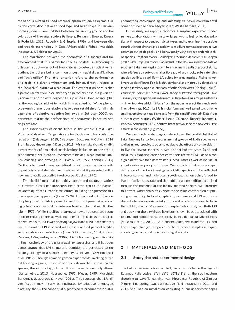
| 9411WIDMER Et al.
radiation is related to food resource specialization, as exemplified by the correlation between food type and beak shape in Darwin's finches (Snow & Grant, 2006), between the hunting ground and the coloration of Hawaiian spiders (Gillespie, Benjamin, Brewer, Rivera, & Roderick, 2018; Roderick & Gillespie, 1998), and between diet and trophic morphology in East African cichlid fishes (Muschick, Indermaur, & Salzburger, 2012).
The correlation between the phenotype of a species and the environment that this particular species inhabits is—according to Schluter (2000)—one out of four criteria to detect an adaptive ra-diation, the others being common ancestry, rapid diversification, and “trait utility.” The latter criterion refers to the performance of a trait in a given environment and, hence, directly relates to the “adaptive” nature of a radiation. The expectation here is that a particular trait value or phenotype performs best in a given en-vironment and/or with respect to a particular food source (that is, the ecological niche) to which it is adapted to. While pheno-type–environment correlations have been established for all main examples of adaptive radiation (reviewed in Schluter, 2000), ex-periments testing the performance of phenotypes in natural set-tings are rare.
The assemblages of cichlid fishes in the African Great Lakes Victoria, Malawi, and Tanganyika are textbook examples of adaptive radiations (Salzburger, 2018; Salzburger, Bocxlaer, & Cohen, 2014; Sturmbauer, Husemann, & Danley, 2011). African lake cichlids exhibit a great variety of ecological specializations including, among others, sand filtering, scale-eating, invertebrate picking, algae grazing, mol-lusk cracking, and preying fish (Fryer & Iles, 1972; Konings, 2015). On the other hand, many specialized cichlid species are inherently opportunistic and deviate from their usual diet if presented with a new, more easily accessible food source (Ribbink, 1990).
The cichlids' potential to rapidly exploit and occupy a variety of different niches has previously been attributed to the particu-lar anatomy of their trophic structures including the presence of a pharyngeal jaw apparatus (Liem, 1973). This second set of jaws in the pharynx of cichlids is primarily used for food processing, allow-ing a functional decoupling between food uptake and mastication (Liem, 1973). While modified pharyngeal jaw structures are found in other groups of fish as well, the ones of the cichlids are charac-terized by a sutured lower pharyngeal jaw bone (LPJ) (note that this trait of a unified LPJ is shared with closely related percoid families such as labrids or embiotocids (Liem & Greenwood, 1981; Galis & Drucker, 1996; Hulsey et al., 2006)). Cichlids show a great diversity in the morphology of the pharyngeal jaw apparatus, and it has been demonstrated that LPJ shape and dentition are correlated to the feeding ecology of a species (Liem, 1973; Meyer, 1989; Muschick et al., 2012). Through common garden experiments involving differ-ent feeding regimes, it has further been shown that in some cichlid species, the morphology of the LPJ can be experimentally altered (Gunter et al., 2013; Huysseune, 1995; Meyer, 1989; Muschick, Barluenga, Salzburger, & Meyer, 2011). This suggests that LPJ di-versification may initially be facilitated by adaptive phenotypic plasticity, that is, the capacity of a genotype to produce more suited
phenotypes corresponding and adapting to novel environmental conditions (Schneider & Meyer, 2017; West-Eberhard, 2005).
In this study, we report a reciprocal transplant experiment under semi-natural conditions within Lake Tanganyika to test for local adapta-tion with respect to benthic habitat types and to examine the possible contribution of phenotypic plasticity to medium-term adaptation in two common but ecologically and behaviorally very distinct endemic cich-lid species, Tropheus moorii (Boulenger, 1898) and Xenotilapia boulengeri (Poll, 1942). Tropheus moorii is abundant in the shallow rocky habitats of southern Lake Tanganyika (down to a maximum depth of around 20 m), where it feeds on aufwuchs (algal flora growing on rocky substrate); this species exhibits a papilliform LPJ suited for grinding algae, fitting its her-bivorous diet (Figure 1); it is highly territorial and vigorously defends its feeding territory against intrusion of other herbivores (Konings, 2015). Xenotilapia boulengeri occurs over sandy substrate throughout Lake Tanganyika; this species usually roams in large foraging groups and feeds on invertebrates which it filters from the upper layers of the sandy sed-iment (Konings, 2015); its LPJ is molariform and well suited to crush the small invertebrates that it extracts from the sand (Figure 1d). Data from a recent census study (Widmer, Heule, Colombo, Rueegg, Indermaur, Ronco & Salzburger, 2019) confirm that the two species show very little habitat niche overlap (Figure S1).
We used underwater cages installed over the benthic habitat of Lake Tanganyika to force experimental groups of both species—as well as mixed-species groups to evaluate the effect of competition—to live for several months in two distinct habitat types (sand and rock), thus exposing each species to their native as well as to a for-eign habitat. We then determined survival rates as well as individual growth rates as proxy for fitness. We predicted that resource spe-cialization of the two investigated cichlid species will be reflected in lower survival and individual growth rates when being forced to live on foreign substrate and that additional competition, exercised through the presence of the locally adapted species, will intensify this effect. Additionally, to explore the possible contribution of phe-notypic plasticity to local adaptation, we compared LPJ and body shape between experimental groups and a reference sample from the wild by means of geometric morphometric analyses. Both LPJ and body morphology/shape have been shown to be associated with feeding and habitat niche, respectively, in Lake Tanganyika cichlids (Muschick et al., 2012). As a consequence, we expected LPJ and body shape changes compared to the reference samples in exper-imental groups forced to live in foreign habitats.
2 | MATERIAL S AND METHODS
2.1 | Study site and experimental design
The field experiments for this study were conducted in the bay off Kalambo Falls Lodge (8°37′23″S, 31°12′1″E) at the southeastern shoreline of Lake Tanganyika near Mpulungu, Republic of Zambia (Figure 1a), during two consecutive field seasons in 2011 and 2012. We used an installation consisting of six underwater cages
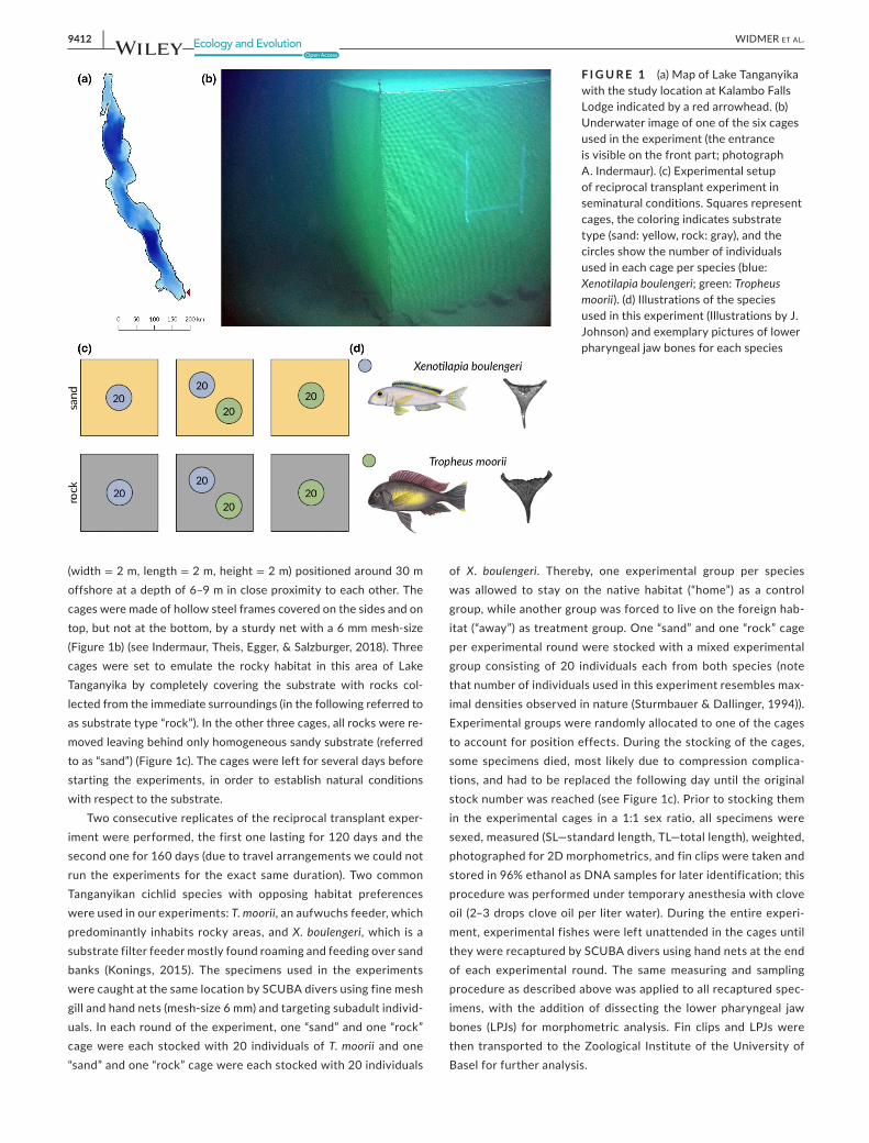
9412 | WIDMER Et al.
(width = 2 m, length = 2 m, height = 2 m) positioned around 30 m offshore at a depth of 6–9 m in close proximity to each other. The cages were made of hollow steel frames covered on the sides and on top, but not at the bottom, by a sturdy net with a 6 mm mesh-size (Figure 1b) (see Indermaur, Theis, Egger, & Salzburger, 2018). Three cages were set to emulate the rocky habitat in this area of Lake Tanganyika by completely covering the substrate with rocks col-lected from the immediate surroundings (in the following referred to as substrate type “rock”). In the other three cages, all rocks were re-moved leaving behind only homogeneous sandy substrate (referred to as “sand”) (Figure 1c). The cages were left for several days before starting the experiments, in order to establish natural conditions with respect to the substrate.
Two consecutive replicates of the reciprocal transplant exper-iment were performed, the first one lasting for 120 days and the second one for 160 days (due to travel arrangements we could not run the experiments for the exact same duration). Two common Tanganyikan cichlid species with opposing habitat preferences were used in our experiments: T. moorii, an aufwuchs feeder, which predominantly inhabits rocky areas, and X. boulengeri, which is a substrate filter feeder mostly found roaming and feeding over sand banks (Konings, 2015). The specimens used in the experiments were caught at the same location by SCUBA divers using fine mesh gill and hand nets (mesh-size 6 mm) and targeting subadult individ-uals. In each round of the experiment, one “sand” and one “rock” cage were each stocked with 20 individuals of T. moorii and one “sand” and one “rock” cage were each stocked with 20 individuals
of X. boulengeri. Thereby, one experimental group per species was allowed to stay on the native habitat (“home”) as a control group, while another group was forced to live on the foreign hab-itat (“away”) as treatment group. One “sand” and one “rock” cage per experimental round were stocked with a mixed experimental group consisting of 20 individuals each from both species (note that number of individuals used in this experiment resembles max-imal densities observed in nature (Sturmbauer & Dallinger, 1994)). Experimental groups were randomly allocated to one of the cages to account for position effects. During the stocking of the cages, some specimens died, most likely due to compression complica-tions, and had to be replaced the following day until the original stock number was reached (see Figure 1c). Prior to stocking them in the experimental cages in a 1:1 sex ratio, all specimens were sexed, measured (SL—standard length, TL—total length), weighted, photographed for 2D morphometrics, and fin clips were taken and stored in 96% ethanol as DNA samples for later identification; this procedure was performed under temporary anesthesia with clove oil (2–3 drops clove oil per liter water). During the entire experi-ment, experimental fishes were left unattended in the cages until they were recaptured by SCUBA divers using hand nets at the end of each experimental round. The same measuring and sampling procedure as described above was applied to all recaptured spec-imens, with the addition of dissecting the lower pharyngeal jaw bones (LPJs) for morphometric analysis. Fin clips and LPJs were then transported to the Zoological Institute of the University of Basel for further analysis.
F I G U R E 1 (a) Map of Lake Tanganyika with the study location at Kalambo Falls Lodge indicated by a red arrowhead. (b) Underwater image of one of the six cages used in the experiment (the entrance is visible on the front part; photograph A. Indermaur). (c) Experimental setup of reciprocal transplant experiment in seminatural conditions. Squares represent cages, the coloring indicates substrate type (sand: yellow, rock: gray), and the circles show the number of individuals used in each cage per species (blue: Xenotilapia boulengeri; green: Tropheus moorii). (d) Illustrations of the species used in this experiment (Illustrations by J. Johnson) and exemplary pictures of lower pharyngeal jaw bones for each species
| 9413WIDMER Et al.
2.2 | Specimen matching
In order to match individual samples and, hence, the measurements from before and after the experimental treatment, we genotyped each speci-men at four microsatellite loci following an established protocol (Theis, Ronco, Indermaur, Salzburger, & Egger, 2014). In brief, we extracted genomic DNA from fin clips using a MagNA Pure LC (Roche) with the DNA Isolation Kit II (Tissue) in the case of T. moorii and a 5% Chelex solution-based extraction protocol in the case of X. boulengeri samples (Casquet, Thebaud, & Gillespie, 2012). All four microsatellite loci were amplified in a single multiplex PCR using published primers (Ppun5, Ppun7, Ppun21 (Taylor et al., 2002), Pzeb3 for T. moorii only (Van Oppen et al., 1997), UNH130 for X. boulengeri only (Kocher, Lee, Sobolewska, Penman, & McAndrew, 1998)). We used the QIAGEN® Multiplex PCR Kit and 1 !L of DNA extract under the following PCR conditions: 95°C for 15 min and 40 3-step cycles of 94°C for 30 s, 57°C for 90 s and 72°C for 60 fol-lowed by the end step at 60°C for 30 min. 1 !l of PCR product was resus-pended in HiDi Formamide and, after the addition of a size standard (ABI LIZ(-250)), analyzed on a 3130xl Genetic Analyzer (Applied Biosystems). Microsatellite peaks (allele sizes) were evaluated using Peak Scanner™ v1.0 (Thermo Fisher Scientific) and rounded with Tandem (Matschiner & Salzburger, 2009). The rounded values were used for sample matching with the R package Allelematch version 2.5 (Galpern, Manseau, Hettinga, Smith, & Wilson, 2012), allowing us to trace individual fish and to obtain individual-level data for growth in length and weight.
2.3 | Morphometrics
For geometric morphometric analyses of body shape, we used 522 photographs (taken before and after experimental runs), including 65 photographs from wild-caught specimens as reference for body shape. Analysis of LPJ shape was based on 112 LPJs (including LPJs of 27 wild-caught adults as reference) from the two replicates of the seminatural reciprocal transplant experiment (37 T. moorii, 75 X. bou-lengeri). We used a desktop office scanner (EPSON perfection V30/V300, resolution: 4,800 dpi) to obtain digital images of the cleaned jaws. Each scan included a ruler as size reference.
Following the procedure described in Muschick et al. (2012), “x” and “y” coordinates of 17 homologous landmarks for body shape and eight homologous landmarks and of 20 semilandmarks for LPJ shape were acquired in tpsDig2 (Rohlf, 2018). Landmark sliding was performed in R using the package geomorph version 3.1.0 (Adams & Otárola-Castillo, 2013). From the initial 28 LPJ landmarks, we retained seven true landmarks and six semilandmarks, totaling in a set of 13 landmarks for morphometric analysis. Statistical analyses of the mor-phometric data of body shape as well as LPJ shape were performed in MorphoJ version 1.06d (Klingenberg, 2011).
2.4 | Statistical analysis
To evaluate survival rate in the cage experiment between species and experimental conditions, we applied generalized linear mixed effect
models (GLMM), with the dependent variable survival (0 = died and 1 = survived) and the fixed predictors initial weight, substrate (rock, sand), competition (single species cage or dual species cage), their interaction (substrate: competition), and sex (male, female). We in-cluded two variables as random effects: “replicate” in order to ac-count for the relatively low number of replicates in the study design and “cages” to include any possible variability among the six cages.
For each survivor, we calculated absolute growth rates in g/day as well as specific growth rates, SGR = 100 * (ln (final weight) − ln (initial weight))/days) as described previously (Rajkov, Weber, Salzburger, & Egger, 2018). We regressed SGR with initial weight to correct for po-tential differences. Following Scharsack, Kalbe, Harrod, and Rauch (2007), the residual SGR (rSGR) values were used as a measure of rel-ative growth performance. We evaluated relative growth between the different species and experimental conditions using linear mixed effect models, with the dependent variable rSGR and the fixed pre-dictors substrate (rock, sand), competition (single species cage or dual species cage), and sex (male, female). Replicate and cage were included as random effects. All statistical analyses were performed in R version 3.5.1 (R Development Core Team, 2016).
3 | RESULTS
3.1 | Survival
At the end of the first replicate, we retrieved 72 of the 81 initially stocked specimens of T. moorii and 32 of the 104 (including replace-ments) stocked X. boulengeri. After the second round, we retrieved 65 of the 81 stocked T. moorii and 29 of the 81 stocked X. boulengeri (see Widmer, Indermaur, Egger, & Salzburger, 2020 for data). Across the experimental rounds and cages, the survival rate was much higher in T. moorii (84.5%) as compared to X. boulengeri (33.1%) (GLMM, N = 324, zSpecies = −8.438, pSpecies > .000). Survival in T. moorii was not affected by any of our predictor variables. In X. boulengeri, we found a significant negative effect of competition and of the inter-action between substrate and competition on survival rate (GLMM, N = 162, zCompetition = 3.330, pCompetition = .001 and zSubstrate:Competition = −2.219, pSubstrate:Competition = .03).
3.2 | Growth
After genotyping the experimental fish (from before and after each round) at four microsatellite loci, 127 specimens of T. moorii and 55 specimens of X. boulengeri could be successfully matched using Allelematch (Galpern et al., 2012). These specimens were then used for growth rate analyses. The mean initial standard length of these specimens was 6.0 ± 0.9 cm for T. moorii and 8.0 ± 1.3 cm for X. boulengeri (Widmer et al., 2020). SGR was higher in T. moorii than in X. boulengeri across both experimental rounds and habitat types (ANOVA, F = 3,612, p < .001). For rSGR, there was no detect-able difference between the two species across both experimental rounds and habitat types. We found that T. moorii had a significantly
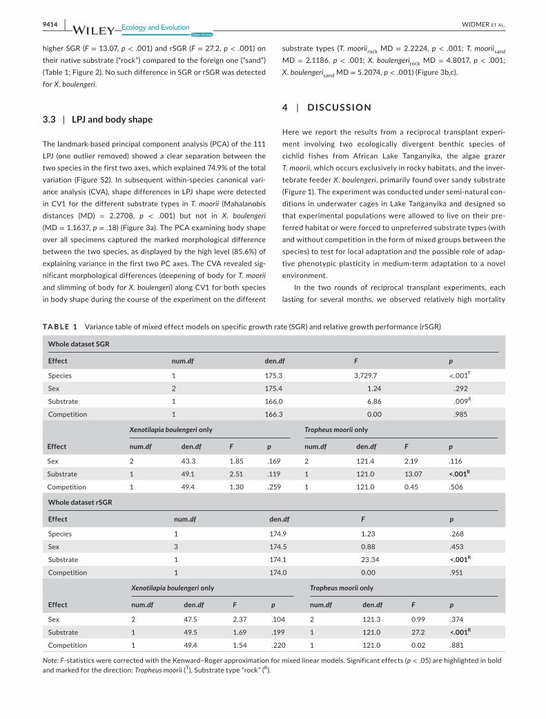
9414 | WIDMER Et al.
higher SGR (F = 13.07, p < .001) and rSGR (F = 27.2, p < .001) on their native substrate (“rock”) compared to the foreign one (“sand”) (Table 1; Figure 2). No such difference in SGR or rSGR was detected for X. boulengeri.
3.3 | LPJ and body shape
The landmark-based principal component analysis (PCA) of the 111 LPJ (one outlier removed) showed a clear separation between the two species in the first two axes, which explained 74.9% of the total variation (Figure S2). In subsequent within-species canonical vari-ance analysis (CVA), shape differences in LPJ shape were detected in CV1 for the different substrate types in T. moorii (Mahalanobis distances (MD) = 2.2708, p < .001) but not in X. boulengeri (MD = 1.1637, p = .18) (Figure 3a). The PCA examining body shape over all specimens captured the marked morphological difference between the two species, as displayed by the high level (85.6%) of explaining variance in the first two PC axes. The CVA revealed sig-nificant morphological differences (deepening of body for T. moorii and slimming of body for X. boulengeri) along CV1 for both species in body shape during the course of the experiment on the different
substrate types (T. mooriirock MD = 2.2224, p < .001; T. mooriisand MD = 2.1186, p < .001; X. boulengerirock MD = 4.8017, p < .001; X. boulengerisand MD = 5.2074, p < .001) (Figure 3b,c).
4 | DISCUSSION
Here we report the results from a reciprocal transplant experi-ment involving two ecologically divergent benthic species of cichlid fishes from African Lake Tanganyika, the algae grazer T. moorii, which occurs exclusively in rocky habitats, and the inver-tebrate feeder X. boulengeri, primarily found over sandy substrate (Figure 1). The experiment was conducted under semi-natural con-ditions in underwater cages in Lake Tanganyika and designed so that experimental populations were allowed to live on their pre-ferred habitat or were forced to unpreferred substrate types (with and without competition in the form of mixed groups between the species) to test for local adaptation and the possible role of adap-tive phenotypic plasticity in medium-term adaptation to a novel environment.
In the two rounds of reciprocal transplant experiments, each lasting for several months, we observed relatively high mortality
TA B L E 1 Variance table of mixed effect models on specific growth rate (SGR) and relative growth performance (rSGR)
Whole dataset SGR
Effect num.df den.df F p
Species 1 175.3 3,729.7 <.001T
Sex 2 175.4 1.24 .292
Substrate 1 166.0 6.86 .009R
Competition 1 166.3 0.00 .985
Effect
Xenotilapia boulengeri only Tropheus moorii only
num.df den.df F p num.df den.df F p
Sex 2 43.3 1.85 .169 2 121.4 2.19 .116
Substrate 1 49.1 2.51 .119 1 121.0 13.07 <.001R
Competition 1 49.4 1.30 .259 1 121.0 0.45 .506
Whole dataset rSGR
Effect num.df den.df F p
Species 1 174.9 1.23 .268
Sex 3 174.5 0.88 .453
Substrate 1 174.1 23.34 <.001R
Competition 1 174.0 0.00 .951
Effect
Xenotilapia boulengeri only Tropheus moorii only
num.df den.df F p num.df den.df F p
Sex 2 47.5 2.37 .104 2 121.3 0.99 .374
Substrate 1 49.5 1.69 .199 1 121.0 27.2 <.001R
Competition 1 49.4 1.54 .220 1 121.0 0.02 .881
Note: F-statistics were corrected with the Kenward–Roger approximation for mixed linear models. Significant effects (p < .05) are highlighted in bold and marked for the direction: Tropheus moorii (T), Substrate type “rock” (R).
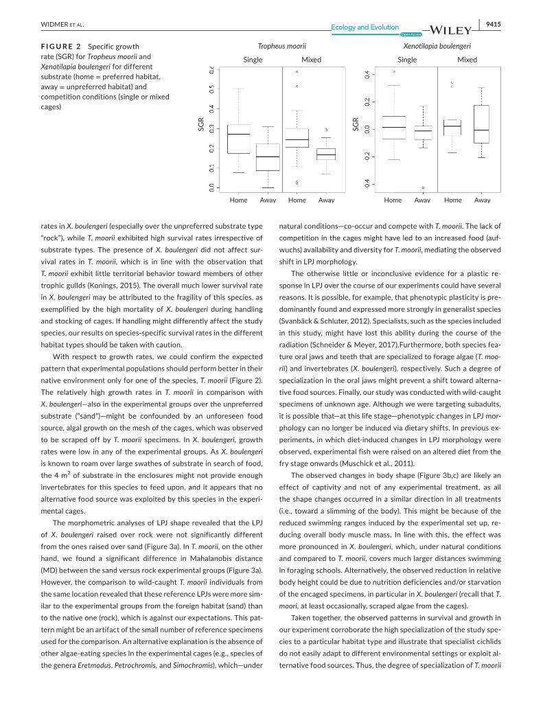
| 9415WIDMER Et al.
rates in X. boulengeri (especially over the unpreferred substrate type “rock”), while T. moorii exhibited high survival rates irrespective of substrate types. The presence of X. boulengeri did not affect sur-vival rates in T. moorii, which is in line with the observation that T. moorii exhibit little territorial behavior toward members of other trophic guilds (Konings, 2015). The overall much lower survival rate in X. boulengeri may be attributed to the fragility of this species, as exemplified by the high mortality of X. boulengeri during handling and stocking of cages. If handling might differently affect the study species, our results on species-specific survival rates in the different habitat types should be taken with caution.
With respect to growth rates, we could confirm the expected pattern that experimental populations should perform better in their native environment only for one of the species, T. moorii (Figure 2). The relatively high growth rates in T. moorii in comparison with X. boulengeri—also in the experimental groups over the unpreferred substrate (“sand”)—might be confounded by an unforeseen food source, algal growth on the mesh of the cages, which was observed to be scraped off by T. moorii specimens. In X. boulengeri, growth rates were low in any of the experimental groups. As X. boulengeri is known to roam over large swathes of substrate in search of food, the 4 m2 of substrate in the enclosures might not provide enough invertebrates for this species to feed upon, and it appears that no alternative food source was exploited by this species in the experi-mental cages.
The morphometric analyses of LPJ shape revealed that the LPJ of X. boulengeri raised over rock were not significantly different from the ones raised over sand (Figure 3a). In T. moorii, on the other hand, we found a significant difference in Mahalanobis distance (MD) between the sand versus rock experimental groups (Figure 3a). However, the comparison to wild-caught T. moorii individuals from the same location revealed that these reference LPJs were more sim-ilar to the experimental groups from the foreign habitat (sand) than to the native one (rock), which is against our expectations. This pat-tern might be an artifact of the small number of reference specimens used for the comparison. An alternative explanation is the absence of other algae-eating species in the experimental cages (e.g., species of the genera Eretmodus, Petrochromis, and Simochromis), which—under
natural conditions—co-occur and compete with T. moorii. The lack of competition in the cages might have led to an increased food (auf-wuchs) availability and diversity for T. moorii, mediating the observed shift in LPJ morphology.
The otherwise little or inconclusive evidence for a plastic re-sponse in LPJ over the course of our experiments could have several reasons. It is possible, for example, that phenotypic plasticity is pre-dominantly found and expressed more strongly in generalist species (Svanbäck & Schluter, 2012). Specialists, such as the species included in this study, might have lost this ability during the course of the radiation (Schneider & Meyer, 2017).Furthermore, both species fea-ture oral jaws and teeth that are specialized to forage algae (T. moo-rii) and invertebrates (X. boulengeri), respectively. Such a degree of specialization in the oral jaws might prevent a shift toward alterna-tive food sources. Finally, our study was conducted with wild-caught specimens of unknown age. Although we were targeting subadults, it is possible that—at this life stage—phenotypic changes in LPJ mor-phology can no longer be induced via dietary shifts. In previous ex-periments, in which diet-induced changes in LPJ morphology were observed, experimental fish were raised on an altered diet from the fry stage onwards (Muschick et al., 2011).
The observed changes in body shape (Figure 3b,c) are likely an effect of captivity and not of any experimental treatment, as all the shape changes occurred in a similar direction in all treatments (i.e., toward a slimming of the body). This might be because of the reduced swimming ranges induced by the experimental set up, re-ducing overall body muscle mass. In line with this, the effect was more pronounced in X. boulengeri, which, under natural conditions and compared to T. moorii, covers much larger distances swimming in foraging schools. Alternatively, the observed reduction in relative body height could be due to nutrition deficiencies and/or starvation of the encaged specimens, in particular in X. boulengeri (recall that T. moori, at least occasionally, scraped algae from the cages).
Taken together, the observed patterns in survival and growth in our experiment corroborate the high specialization of the study spe-cies to a particular habitat type and illustrate that specialist cichlids do not easily adapt to different environmental settings or exploit al-ternative food sources. Thus, the degree of specialization of T. moorii
F I G U R E 2 Specific growth rate (SGR) for Tropheus moorii and Xenotilapia boulengeri for different substrate (home = preferred habitat, away = unpreferred habitat) and competition conditions (single or mixed cages)
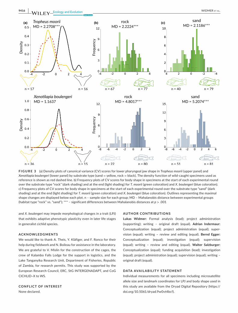
9416 | WIDMER Et al.
and X. boulengeri may impede morphological changes in a trait (LPJ) that exhibits adaptive phenotypic plasticity even in later life stages in generalist cichlid species.
ACKNOWLEDG MENTSWe would like to thank A. Theis, Y. Kläfiger, and F. Ronco for their help during fieldwork and N. Boileau for assistance in the laboratory. We are grateful to V. Mislin for the construction of the cages, the crew of Kalambo Falls Lodge for the support in logistics, and the Lake Tanganyika Research Unit, Department of Fisheries, Republic of Zambia, for research permits. This study was supported by the European Research Council, ERC, StG INTERGENADAPT, and CoG CICHLID~X to WS.
CONFLIC T OF INTERE STNone declared.
AUTHOR CONTRIBUTIONSLukas Widmer: Formal analysis (lead); project administration (supporting); writing – original draft (equal). Adrian Indermaur: Conceptualization (equal); project administration (equal); super-vision (equal); writing – review and editing (equal). Bernd Egger: Conceptualization (equal); investigation (equal); supervision (equal); writing – review and editing (equal). Walter Salzburger: Conceptualization (equal); funding acquisition (lead); investigation (equal); project administration (equal); supervision (equal); writing – original draft (equal).
DATA AVAIL ABILIT Y STATEMENTIndividual measurements for all specimens including microsatellite allele size and landmark coordinates for LPJ and body shape used in this study are available from the Dryad Digital Repository (https://doi.org/10.5061/dryad.9w0vt 4bcf).
F I G U R E 3 (a) Density plots of canonical variance (CV) scores for lower pharyngeal jaw shape in Tropheus moorii (upper panel) and Xenotilapia boulengeri (lower panel) by substrate type (sand = yellow, rock = black). The density function of wild-caught specimens used as reference is shown as red dashed line. b) Frequency plots of CV scores for body shape in specimens at the start of each experimental round over the substrate type “rock” (dark shading) and at the end (light shading) for T. moorii (green coloration) and X. boulengeri (blue coloration). c) Frequency plots of CV scores for body shape in specimens at the start of each experimental round over the substrate type “sand” (dark shading) and at the end (light shading) for T. moorii (green coloration) and X. boulengeri (blue coloration). Outlines representing the maximal shape changes are displayed below each plot. n – sample size for each group; MD – Mahalanobis distance between experimental groups (habitat type “rock” vs. “sand”); *** – significant differences between Mahalanobis distances at p > .001
(a) (b) (c)
| 9417WIDMER Et al.
ORCIDBernd Egger https://orcid.org/0000-0002-8928-2301 Walter Salzburger https://orcid.org/0000-0002-9988-1674
R E FE R E N CE SAdams, D. C., & Otárola-Castillo, E. (2013). geomorph: An r package
for the collection and analysis of geometric morphometric shape data. Methods in Ecology and Evolution, 4(4), 393–399. https://doi.org/10.1111/2041-210X.12035
Casquet, J., Thebaud, C., & Gillespie, R. G. (2012). Chelex with-out boiling, a rapid and easy technique to obtain stable am-plifiable DNA from small amounts of ethanol-stored spi-ders. Molecular Ecology Resources, 12(1), 136–141. https://doi.org/10.1111/j.1755-0998.2011.03073.x
Fryer, G., & Iles, T. (1972). Cichlid fishes of the great lakes of Africa. Retrieved from http://agris.fao.org/agris -searc h/search.do?recor dID=US201 30048 4047
Galis, F., & Drucker, E. G. (1996). Pharyngeal biting mechanics in centrar-child and cichlid fishes: Insights into a key evolutionary innovation. Journal of Evolutionary Biology, 9(5), 641–670. https://doi.org/10.1046/j.1420-9101.1996.90506 41.x
Galpern, P., Manseau, M., Hettinga, P., Smith, K., & Wilson, P. (2012). Allelematch: An R package for identifying unique multilocus gen-otypes where genotyping error and missing data may be pres-ent. Molecular Ecology Resources, 12(4), 771–778. https://doi.org/10.1111/j.1755-0998.2012.03137.x
Gillespie, R. G., Benjamin, S. P., Brewer, M. S., Rivera, M. A. J., & Roderick, G. K. (2018). Repeated diversification of ecomorphs in Hawaiian stick spiders. Current Biology, 28(6), 941–947.e3. https://doi.org/10.1016/J.CUB.2018.01.083
Gunter, H. M., Fan, S., Xiong, F., Franchini, P., Fruciano, C., & Meyer, A. (2013). Shaping development through mechanical strain: The tran-scriptional basis of diet-induced phenotypic plasticity in a cichlid fish. Molecular Ecology, 22(17), 4516–4531. https://doi.org/10.1111/mec.12417
Hulsey, C. D., Marks, J., Hendrickson, D. A., Williamson, C. A., Cohen, A. E., & Stephens, M. J. (2006). Feeding special-ization in Herichthys minckleyi: A trophically polymorphic fish. Journal of Fish Biology, 68(5), 1399–1410. https://doi.org/10.1111/j.0022-1112.2006.01021.x
Huysseune, A. (1995). Phenotypic plasticity in the lower pharyngeal jaw dentition of Astatoreochromis alluaudi (Teleostei: Cichlidae). Archives of Oral Biology, 40(11), 1005–1014. https://doi.org/10.1016/0003-9969(95)00074 -Y
Indermaur, A., Theis, A., Egger, B., & Salzburger, W. (2018). Mouth di-morphism in scale-eating cichlid fish from Lake Tanganyika ad-vances individual fitness. Evolution, 72(9), 1962–1969. https://doi.org/10.1111/evo.13552
Klingenberg, C. P. (2011). MorphoJ: An integrated software package for geometric morphometrics. Molecular Ecology Resources, 11(2), 353–357. https://doi.org/10.1111/j.1755-0998.2010.02924.x
Kocher, T. D., Lee, W. J., Sobolewska, H., Penman, D., & McAndrew, B. (1998). A genetic linkage map of a cichlid fish, the tilapia (Oreochromis niloticus). Genetics, 148, 1225–1232.
Konings, A. F. (2015). Tanganyika cichlids in their natural habitat (3rd ed.). El Paso, TX: Cichlid Press.
Liem, K. F. (1973). Evolutionary strategies and morphological innova-tions: Cichlid pharyngeal jaws. Systematic Zoology, 22(4), 425. https://doi.org/10.2307/2412950
Liem, K. F., & Greenwood, P. H. (1981). A functional approach to the phylogeny of the pharyngognath teleosts. American Zoologist, 21(1), 83–101. https://doi.org/10.1093/icb/21.1.83
Matschiner, M., & Salzburger, W. (2009). TANDEM: Integrating au-tomated allele binning into genetics and genomics workflows.
Bioinformatics, 25(15), 1982–1983. https://doi.org/10.1093/bioin forma tics/btp303
Meyer, A. (1989). Cost of morphological specialization: Feeding per-formance of the two morphs in the trophically polymorphic cichlid fish, Cichlasoma citrinellum. Oecologia, 80(3), 431–436. https://doi.org/10.1007/BF003 79047
Muschick, M., Barluenga, M., Salzburger, W., & Meyer, A. (2011). Adaptive phenotypic plasticity in the Midas cichlid fish pharyngeal jaw and its relevance in adaptive radiation. BMC Evolutionary Biology, 11(1), 116. https://doi.org/10.1186/1471-2148-11-116
Muschick, M., Indermaur, A., & Salzburger, W. (2012). Convergent evo-lution within an adaptive radiation of cichlid fishes. Current Biology, 22(24), 2362–2368. https://doi.org/10.1016/j.cub.2012.10.048
R Development Core Team (2016). R: A language and environment for statistical computing. Vienna, Austria: R Foundation for Statistical Computing. https://doi.org/10.1038/sj.hdy.6800737
Rajkov, J., Weber, A. A. T., Salzburger, W., & Egger, B. (2018). Adaptive phenotypic plasticity contributes to divergence between lake and river populations of an East African cichlid fish. Ecology and Evolution, 8(15), 7323–7333. https://doi.org/10.1002/ece3.4241
Ribbink, A. J. (1990). Alternative life-history styles of some African cich-lid fishes. Environmental Biology of Fishes, 28(1–4), 87–100. https://doi.org/10.1007/BF007 51029
Roderick, G. K., & Gillespie, R. G. (1998). Speciation and phylogeography of Hawaiian terrestrial arthropods. Molecular Ecology, 7(4), 519–531. https://doi.org/10.1046/j.1365-294x.1998.00309.x
Rohlf, J. F. (2018). tpsDig, version 2.31. Retrieved from and http://life.bio.sunysb.edu/morph/ index.htmlh ttps://ci.nii.ac.jp/naid/10022 02061 0/
Salzburger, W. (2018). Understanding explosive diversification through cichlid fish genomics. Nature Reviews Genetics, 19(11), 705–717. https://doi.org/10.1038/s4157 6-018-0043-9
Salzburger, W., Bocxlaer, B. V., & Cohen, A. S. (2014). Ecology and evo-lution of the African Great Lakes and their faunas. Annual Review of Ecology, Evolution and Systematics, 45(1), 519–545. https://doi.org/10.1146/annur ev-ecols ys-12021 3-091804
Scharsack, J. P., Kalbe, M., Harrod, C., & Rauch, G. (2007). Habitat-specific adaptation of immune responses of stickleback (Gastetosteus aculeatus) lake and river ecotypes. Proceedings of the Royal Society B: Biological Sciences, 274(1617), 1523–1532. https://doi.org/10.1098/rspb.2007.0210
Schluter, D. (2000). The ecology of adaptive radiation. Oxford, UK: Oxford University Press. https://doi.org/10.2307/3558417
Schneider, R. F., & Meyer, A. (2017). How plasticity, genetic assimila-tion and cryptic genetic variation may contribute to adaptive radi-ations. Molecular Ecology, 26(1), 330–350. https://doi.org/10.1111/mec.13880
Snow, D. W., & Grant, P. R. (2006). Ecology and evolution of Darwin's finches. The Journal of Animal Ecology, 57(1), 320. https://doi.org/10.2307/4785.
Sturmbauer, C., & Dallinger, R. (1994). Diurnal variation of spacing and foraging behaviour in Tropheus moorii (Cichlidae) in Lake Tanganyika, Eastern Africa. Netherlands Journal of Zoology, 45(3–4), 386–401. https://doi.org/10.1163/15685 4295X 00375
Sturmbauer, C., Husemann, M., & Danley, P. D. (2011). Explosive spe-ciation and adaptive radiation of East African Cichlid Fishes. In F. E. Zachos & J. C. Habel (Eds.), Biodiversity hotspots (pp. 333–362). Berlin and Heidelberg, Germany: Springer, Berlin Heidelberg. https://doi.org/10.1007/978-3-642-20992 -5_18
Svanbäck, R., & Schluter, D. (2012). Niche specialization influences adap-tive phenotypic plasticity in the threespine stickleback. The American Naturalist, 180(1), 50–59. https://doi.org/10.1086/666000
Taylor, M. I., Meardon, F., Turner, G., Seehausen, O., Mrosso, H. D. J., & Rico, C. (2002). Characterization of tetranucleotide microsatel-lite loci in a Lake Victorian, haplochromine cichlid fish: A Pundamilia
9418 | WIDMER Et al.
pundamilia × Pundamilia nyererei hybrid. Molecular Ecology Notes, 2(4), 443–445. https://doi.org/10.1046/j.1471-8286.2002.00272.x
Theis, A., Ronco, F., Indermaur, A., Salzburger, W., & Egger, B. (2014). Adaptive divergence between lake and stream populations of an East African cichlid fish. Molecular Ecology, 23(21), 5304–5322. https://doi.org/10.1111/mec.12939
Van Oppen, M. J. H., Turner, G. F., Rico, C., Deutsch, J. C., Ibrahim, K. M., Robinson, R. L., & Hewitt, G. M. (1997). Unusually fine–scale ge-netic structuring found in rapidly speciating Malawi cichlid fishes. Proceedings of the Royal Society of London. Series B: Biological Sciences, 264(1389), 1803–1812. https://doi.org/10.1098/rspb.1997.0248
West-Eberhard, M. J. (2005). Developmental plasticity and the origin of species differences. Proceedings of the National Academy of Sciences of the United States of America, 102(Supplement 1), 6543–6549. https://doi.org/10.1073/pnas.05018 44102
Widmer, L., Heule, E., Colombo, M., Rueegg, A., Indermaur, A., Ronco, F., & Salzburger, W. (2019). Point-CombinationTransect (PCT): Incorporation of small underwater cameras to study fish commu-nities. Methods in Ecology and Evolution, 10, 891–901. https://doi.org/10.1111/2041-210X.13163
Widmer, L., Indermaur, A., Egger, B., & Salzburger, W. (2020). Data from: Where Am I? Niche constraints due to morphological specialization in two Tanganyikan cichlid fish species. Dryad, Dataset, https://doi.org/10.5061/dryad.9w0vt 4bcf
SUPPORTING INFORMATIONAdditional supporting information may be found online in the Supporting Information section.
How to cite this article: Widmer L, Indermaur A, Egger B, Salzburger W. Where Am I? Niche constraints due to morphological specialization in two Tanganyikan cichlid fish species. Ecol Evol. 2020;10:9410–9418. https://doi.org/10.1002/ece3.6629


Chapter 4
Supplementary Information
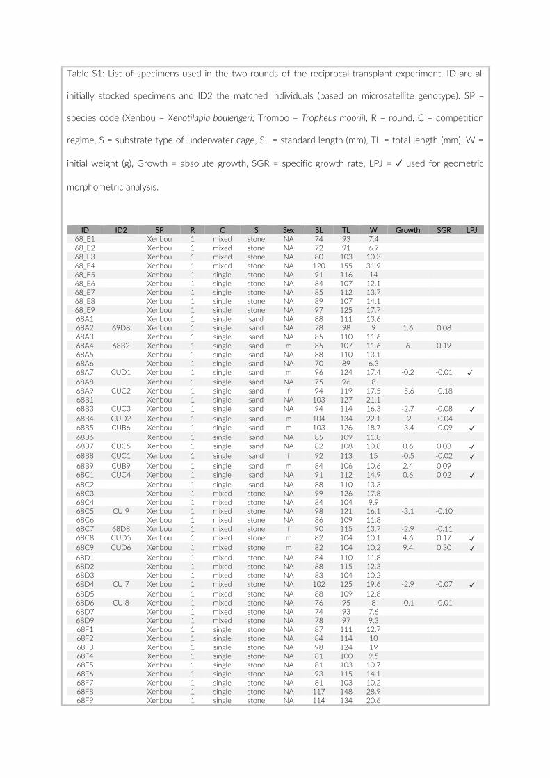
Table S1: List of specimens used in the two rounds of the reciprocal transplant experiment. ID are all
initially stocked specimens and ID2 the matched individuals (based on microsatellite genotype). SP =
species code (Xenbou = Xenotilapia boulengeri; Tromoo = Tropheus moorii), R = round, C = competition
regime, S = substrate type of underwater cage, SL = standard length (mm), TL = total length (mm), W =
initial weight (g), Growth = absolute growth, SGR = specific growth rate, LPJ = ✓ used for geometric
morphometric analysis.
ID ID2 SP R C S Sex SL TL W Growth SGR LPJ
68_E1
Xenbou 1 mixed stone NA 74 93 7.4
68_E2
Xenbou 1 mixed stone NA 72 91 6.7
68_E3
Xenbou 1 mixed stone NA 80 103 10.3
68_E4
Xenbou 1 mixed stone NA 120 155 31.9
68_E5
Xenbou 1 single stone NA 91 116 14
68_E6
Xenbou 1 single stone NA 84 107 12.1
68_E7
Xenbou 1 single stone NA 85 112 13.7
68_E8
Xenbou 1 single stone NA 89 107 14.1
68_E9
Xenbou 1 single stone NA 97 125 17.7
68A1
Xenbou 1 single sand NA 88 111 13.6
68A2 69D8 Xenbou 1 single sand NA 78 98 9 1.6 0.08
68A3
Xenbou 1 single sand NA 85 110 11.6
68A4 68B2 Xenbou 1 single sand m 85 107 11.6 6 0.19
68A5
Xenbou 1 single sand NA 88 110 13.1
68A6
Xenbou 1 single sand NA 70 89 6.3
68A7 CUD1 Xenbou 1 single sand m 96 124 17.4 -0.2 -0.01 ✓
68A8
Xenbou 1 single sand NA 75 96 8
68A9 CUC2 Xenbou 1 single sand f 94 119 17.5 -5.6 -0.18
68B1
Xenbou 1 single sand NA 103 127 21.1
68B3 CUC3 Xenbou 1 single sand NA 94 114 16.3 -2.7 -0.08 ✓
68B4 CUD2 Xenbou 1 single sand m 104 134 22.1 -2 -0.04
68B5 CUB6 Xenbou 1 single sand m 103 126 18.7 -3.4 -0.09 ✓
68B6
Xenbou 1 single sand NA 85 109 11.8
68B7 CUC5 Xenbou 1 single sand NA 82 108 10.8 0.6 0.03 ✓
68B8 CUC1 Xenbou 1 single sand f 92 113 15 -0.5 -0.02 ✓
68B9 CUB9 Xenbou 1 single sand m 84 106 10.6 2.4 0.09
68C1 CUC4 Xenbou 1 single sand NA 91 112 14.9 0.6 0.02 ✓
68C2
Xenbou 1 single sand NA 88 110 13.3
68C3
Xenbou 1 mixed stone NA 99 126 17.8
68C4
Xenbou 1 mixed stone NA 84 104 9.9
68C5 CUI9 Xenbou 1 mixed stone NA 98 121 16.1 -3.1 -0.10
68C6
Xenbou 1 mixed stone NA 86 109 11.8
68C7 68D8 Xenbou 1 mixed stone f 90 115 13.7 -2.9 -0.11
68C8 CUD5 Xenbou 1 mixed stone m 82 104 10.1 4.6 0.17 ✓
68C9 CUD6 Xenbou 1 mixed stone m 82 104 10.2 9.4 0.30 ✓
68D1
Xenbou 1 mixed stone NA 84 110 11.8
68D2
Xenbou 1 mixed stone NA 88 115 12.3
68D3
Xenbou 1 mixed stone NA 83 104 10.2
68D4 CUI7 Xenbou 1 mixed stone NA 102 125 19.6 -2.9 -0.07 ✓
68D5
Xenbou 1 mixed stone NA 88 109 12.8
68D6 CUI8 Xenbou 1 mixed stone NA 76 95 8 -0.1 -0.01
68D7
Xenbou 1 mixed stone NA 74 93 7.6
68D9
Xenbou 1 mixed stone NA 78 97 9.3
68F1
Xenbou 1 single stone NA 87 111 12.7
68F2
Xenbou 1 single stone NA 84 114 10
68F3
Xenbou 1 single stone NA 98 124 19
68F4
Xenbou 1 single stone NA 81 100 9.5
68F5
Xenbou 1 single stone NA 81 103 10.7
68F6
Xenbou 1 single stone NA 93 115 14.1
68F7
Xenbou 1 single stone NA 81 103 10.2
68F8
Xenbou 1 single stone NA 117 148 28.9
68F9
Xenbou 1 single stone NA 114 134 20.6
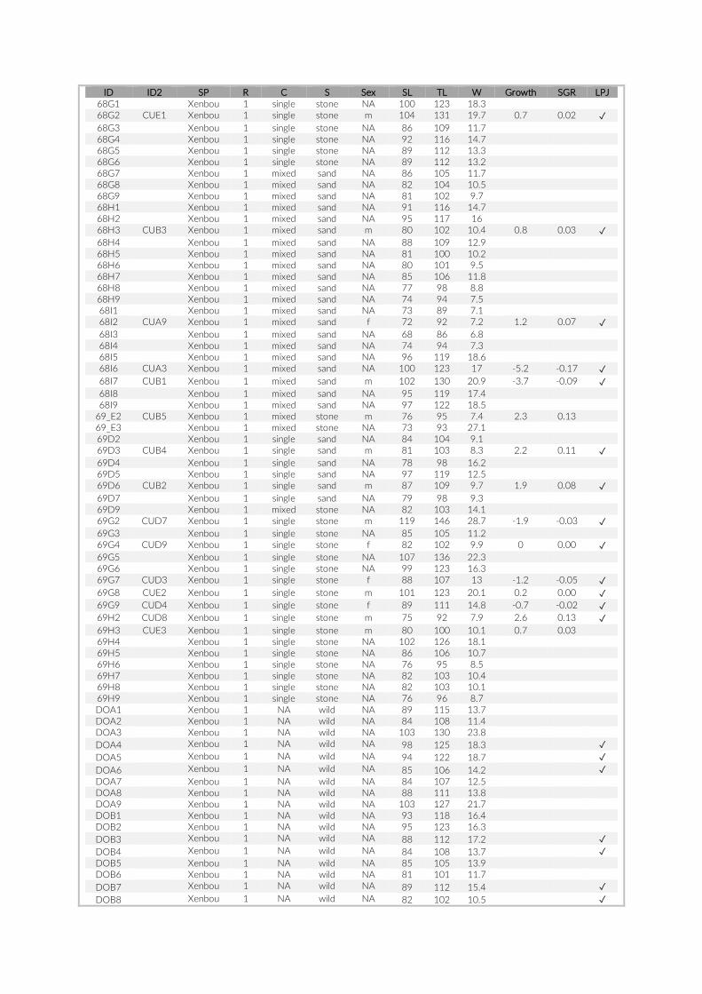
ID ID2 SP R C S Sex SL TL W Growth SGR LPJ 68G1
Xenbou 1 single stone NA 100 123 18.3
68G2 CUE1 Xenbou 1 single stone m 104 131 19.7 0.7 0.02 ✓ 68G3
Xenbou 1 single stone NA 86 109 11.7
68G4
Xenbou 1 single stone NA 92 116 14.7
68G5
Xenbou 1 single stone NA 89 112 13.3
68G6
Xenbou 1 single stone NA 89 112 13.2
68G7
Xenbou 1 mixed sand NA 86 105 11.7
68G8
Xenbou 1 mixed sand NA 82 104 10.5
68G9
Xenbou 1 mixed sand NA 81 102 9.7
68H1
Xenbou 1 mixed sand NA 91 116 14.7
68H2
Xenbou 1 mixed sand NA 95 117 16
68H3 CUB3 Xenbou 1 mixed sand m 80 102 10.4 0.8 0.03 ✓ 68H4
Xenbou 1 mixed sand NA 88 109 12.9
68H5
Xenbou 1 mixed sand NA 81 100 10.2
68H6
Xenbou 1 mixed sand NA 80 101 9.5
68H7
Xenbou 1 mixed sand NA 85 106 11.8
68H8
Xenbou 1 mixed sand NA 77 98 8.8
68H9
Xenbou 1 mixed sand NA 74 94 7.5
68I1
Xenbou 1 mixed sand NA 73 89 7.1
68I2 CUA9 Xenbou 1 mixed sand f 72 92 7.2 1.2 0.07 ✓ 68I3
Xenbou 1 mixed sand NA 68 86 6.8
68I4
Xenbou 1 mixed sand NA 74 94 7.3
68I5
Xenbou 1 mixed sand NA 96 119 18.6
68I6 CUA3 Xenbou 1 mixed sand NA 100 123 17 -5.2 -0.17 ✓ 68I7 CUB1 Xenbou 1 mixed sand m 102 130 20.9 -3.7 -0.09 ✓ 68I8
Xenbou 1 mixed sand NA 95 119 17.4
68I9
Xenbou 1 mixed sand NA 97 122 18.5
69_E2 CUB5 Xenbou 1 mixed stone m 76 95 7.4 2.3 0.13
69_E3
Xenbou 1 mixed stone NA 73 93 27.1
69D2
Xenbou 1 single sand NA 84 104 9.1
69D3 CUB4 Xenbou 1 single sand m 81 103 8.3 2.2 0.11 ✓ 69D4
Xenbou 1 single sand NA 78 98 16.2
69D5
Xenbou 1 single sand NA 97 119 12.5
69D6 CUB2 Xenbou 1 single sand m 87 109 9.7 1.9 0.08 ✓ 69D7
Xenbou 1 single sand NA 79 98 9.3
69D9
Xenbou 1 mixed stone NA 82 103 14.1
69G2 CUD7 Xenbou 1 single stone m 119 146 28.7 -1.9 -0.03 ✓ 69G3
Xenbou 1 single stone NA 85 105 11.2
69G4 CUD9 Xenbou 1 single stone f 82 102 9.9 0 0.00 ✓ 69G5
Xenbou 1 single stone NA 107 136 22.3
69G6
Xenbou 1 single stone NA 99 123 16.3
69G7 CUD3 Xenbou 1 single stone f 88 107 13 -1.2 -0.05 ✓ 69G8 CUE2 Xenbou 1 single stone m 101 123 20.1 0.2 0.00 ✓ 69G9 CUD4 Xenbou 1 single stone f 89 111 14.8 -0.7 -0.02 ✓ 69H2 CUD8 Xenbou 1 single stone m 75 92 7.9 2.6 0.13 ✓ 69H3 CUE3 Xenbou 1 single stone m 80 100 10.1 0.7 0.03
69H4
Xenbou 1 single stone NA 102 126 18.1
69H5
Xenbou 1 single stone NA 86 106 10.7
69H6
Xenbou 1 single stone NA 76 95 8.5
69H7
Xenbou 1 single stone NA 82 103 10.4
69H8
Xenbou 1 single stone NA 82 103 10.1
69H9
Xenbou 1 single stone NA 76 96 8.7
DOA1 Xenbou 1 NA wild NA 89 115 13.7 DOA2 Xenbou 1 NA wild NA 84 108 11.4 DOA3 Xenbou 1 NA wild NA 103 130 23.8 DOA4 Xenbou 1 NA wild NA 98 125 18.3 ✓ DOA5 Xenbou 1 NA wild NA 94 122 18.7 ✓ DOA6 Xenbou 1 NA wild NA 85 106 14.2 ✓ DOA7 Xenbou 1 NA wild NA 84 107 12.5 DOA8 Xenbou 1 NA wild NA 88 111 13.8 DOA9 Xenbou 1 NA wild NA 103 127 21.7 DOB1 Xenbou 1 NA wild NA 93 118 16.4 DOB2 Xenbou 1 NA wild NA 95 123 16.3 DOB3 Xenbou 1 NA wild NA 88 112 17.2 ✓ DOB4 Xenbou 1 NA wild NA 84 108 13.7 ✓ DOB5 Xenbou 1 NA wild NA 85 105 13.9 DOB6 Xenbou 1 NA wild NA 81 101 11.7 DOB7 Xenbou 1 NA wild NA 89 112 15.4 ✓ DOB8 Xenbou 1 NA wild NA 82 102 10.5 ✓
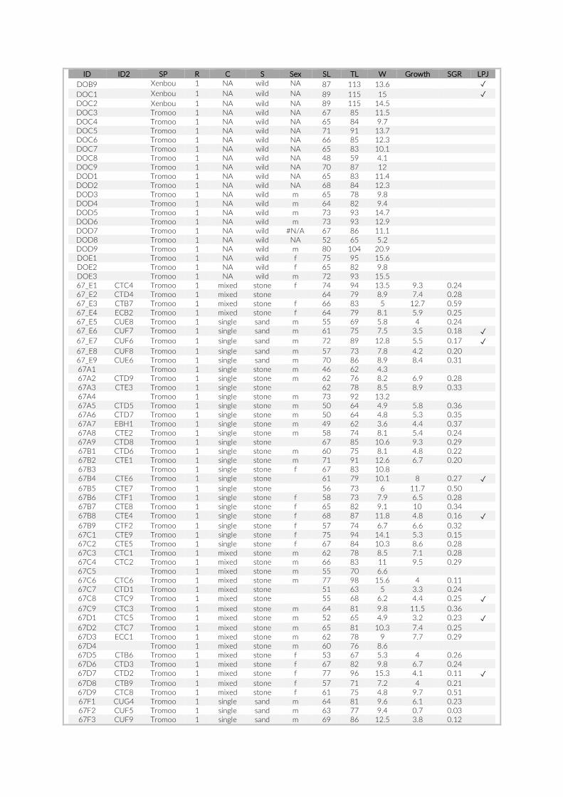
ID ID2 SP R C S Sex SL TL W Growth SGR LPJ
DOB9 Xenbou 1 NA wild NA 87 113 13.6 ✓
DOC1 Xenbou 1 NA wild NA 89 115 15 ✓
DOC2 Xenbou 1 NA wild NA 89 115 14.5
DOC3
Tromoo 1 NA wild NA 67 85 11.5
DOC4
Tromoo 1 NA wild NA 65 84 9.7
DOC5
Tromoo 1 NA wild NA 71 91 13.7
DOC6
Tromoo 1 NA wild NA 66 85 12.3
DOC7
Tromoo 1 NA wild NA 65 83 10.1
DOC8
Tromoo 1 NA wild NA 48 59 4.1
DOC9
Tromoo 1 NA wild NA 70 87 12
DOD1
Tromoo 1 NA wild NA 65 83 11.4
DOD2
Tromoo 1 NA wild NA 68 84 12.3
DOD3
Tromoo 1 NA wild m 65 78 9.8
DOD4
Tromoo 1 NA wild m 64 82 9.4
DOD5
Tromoo 1 NA wild m 73 93 14.7
DOD6
Tromoo 1 NA wild m 73 93 12.9
DOD7
Tromoo 1 NA wild #N/A 67 86 11.1
DOD8
Tromoo 1 NA wild NA 52 65 5.2
DOD9
Tromoo 1 NA wild m 80 104 20.9
DOE1
Tromoo 1 NA wild f 75 95 15.6
DOE2
Tromoo 1 NA wild f 65 82 9.8
DOE3
Tromoo 1 NA wild m 72 93 15.5
67_E1 CTC4 Tromoo 1 mixed stone f 74 94 13.5 9.3 0.24
67_E2 CTD4 Tromoo 1 mixed stone
64 79 8.9 7.4 0.28
67_E3 CTB7 Tromoo 1 mixed stone f 66 83 5 12.7 0.59
67_E4 ECB2 Tromoo 1 mixed stone f 64 79 8.1 5.9 0.25
67_E5 CUE8 Tromoo 1 single sand m 55 69 5.8 4 0.24
67_E6 CUF7 Tromoo 1 single sand m 61 75 7.5 3.5 0.18 ✓
67_E7 CUF6 Tromoo 1 single sand m 72 89 12.8 5.5 0.17 ✓
67_E8 CUF8 Tromoo 1 single sand m 57 73 7.8 4.2 0.20
67_E9 CUE6 Tromoo 1 single sand m 70 86 8.9 8.4 0.31
67A1
Tromoo 1 single stone m 46 62 4.3
67A2 CTD9 Tromoo 1 single stone m 62 76 8.2 6.9 0.28
67A3 CTE3 Tromoo 1 single stone
62 78 8.5 8.9 0.33
67A4
Tromoo 1 single stone m 73 92 13.2
67A5 CTD5 Tromoo 1 single stone m 50 64 4.9 5.8 0.36
67A6 CTD7 Tromoo 1 single stone m 50 64 4.8 5.3 0.35
67A7 EBH1 Tromoo 1 single stone m 49 62 3.6 4.4 0.37
67A8 CTE2 Tromoo 1 single stone m 58 74 8.1 5.4 0.24
67A9 CTD8 Tromoo 1 single stone
67 85 10.6 9.3 0.29
67B1 CTD6 Tromoo 1 single stone m 60 75 8.1 4.8 0.22
67B2 CTE1 Tromoo 1 single stone m 71 91 12.6 6.7 0.20
67B3
Tromoo 1 single stone f 67 83 10.8
67B4 CTE6 Tromoo 1 single stone
61 79 10.1 8 0.27 ✓
67B5 CTE7 Tromoo 1 single stone
56 73 6 11.7 0.50
67B6 CTF1 Tromoo 1 single stone f 58 73 7.9 6.5 0.28
67B7 CTE8 Tromoo 1 single stone f 65 82 9.1 10 0.34
67B8 CTE4 Tromoo 1 single stone f 68 87 11.8 4.8 0.16 ✓
67B9 CTF2 Tromoo 1 single stone f 57 74 6.7 6.6 0.32
67C1 CTE9 Tromoo 1 single stone f 75 94 14.1 5.3 0.15
67C2 CTE5 Tromoo 1 single stone f 67 84 10.3 8.6 0.28
67C3 CTC1 Tromoo 1 mixed stone m 62 78 8.5 7.1 0.28
67C4 CTC2 Tromoo 1 mixed stone m 66 83 11 9.5 0.29
67C5
Tromoo 1 mixed stone m 55 70 6.6
67C6 CTC6 Tromoo 1 mixed stone m 77 98 15.6 4 0.11
67C7 CTD1 Tromoo 1 mixed stone
51 63 5 3.3 0.24
67C8 CTC9 Tromoo 1 mixed stone
55 68 6.2 4.4 0.25 ✓
67C9 CTC3 Tromoo 1 mixed stone m 64 81 9.8 11.5 0.36
67D1 CTC5 Tromoo 1 mixed stone m 52 65 4.9 3.2 0.23 ✓
67D2 CTC7 Tromoo 1 mixed stone m 65 81 10.3 7.4 0.25
67D3 ECC1 Tromoo 1 mixed stone m 62 78 9 7.7 0.29
67D4
Tromoo 1 mixed stone m 60 76 8.6
67D5 CTB6 Tromoo 1 mixed stone f 53 67 5.3 4 0.26
67D6 CTD3 Tromoo 1 mixed stone f 67 82 9.8 6.7 0.24
67D7 CTD2 Tromoo 1 mixed stone f 77 96 15.3 4.1 0.11 ✓
67D8 CTB9 Tromoo 1 mixed stone f 57 71 7.2 4 0.21
67D9 CTC8 Tromoo 1 mixed stone f 61 75 4.8 9.7 0.51
67F1 CUG4 Tromoo 1 single sand m 64 81 9.6 6.1 0.23
67F2 CUF5 Tromoo 1 single sand m 63 77 9.4 0.7 0.03
67F3 CUF9 Tromoo 1 single sand m 69 86 12.5 3.8 0.12
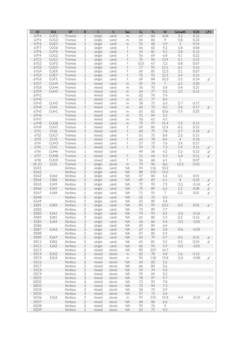
ID ID2 SP R C S Sex SL TL W Growth SGR LPJ 67F4 CUF2 Tromoo 1 single sand m 67 84 10.8 3.2 0.12
67F5 CUG3 Tromoo 1 single sand m 64 82 9 5.8 0.23
67F6 CUE5 Tromoo 1 single sand m 55 68 5.9 2 0.14
67F7 CUG6 Tromoo 1 single sand f 66 82 9.2 1.8 0.08
67F8 CUF4 Tromoo 1 single sand f 65 81 9.2 2.8 0.12
67F9 CUG2 Tromoo 1 single sand f 56 69 6.8 4.1 0.22
67G1 CUG1 Tromoo 1 single sand f 76 96 13.9 5.1 0.15
67G2 CUF3 Tromoo 1 single sand f 53.5 67 5.3 0.8 0.07
67G3 CUG5 Tromoo 1 single sand f 77 95 15.1 6.1 0.16
67G4 CUE9 Tromoo 1 single sand f 69 85 12.3 2.1 0.07
67G5 CUE7 Tromoo 1 single sand f 72 91 12.1 3.4 0.12
67G6 CUF1 Tromoo 1 single sand f 69 84 10.3 3.5 0.14 ✓ 67G7 CUH9 Tromoo 1 mixed sand m 59 74 7 6.2 0.30
67G8 CUH4 Tromoo 1 mixed sand m 56 70 5.8 3.4 0.21
67G9 CUH5 Tromoo 1 mixed sand m 64 77 9.2 3.5 0.15
67H1
Tromoo 1 mixed sand m 62 76 7.4
67H2
Tromoo 1 mixed sand m 61 77 8.4
67H3 CUH2 Tromoo 1 mixed sand m 58 72 6.3 2.7 0.17
67H4 CUI4 Tromoo 1 mixed sand m 60 72 8.3 3.6 0.17 ✓ 67H5 CUH1 Tromoo 1 mixed sand m 65 82 10.6 7.5 0.25
67H6
Tromoo 1 mixed sand m 51 64 5.3
67H7
Tromoo 1 mixed sand m 50 61 4.5
67H8 CUG8 Tromoo 1 mixed sand m 79 97 15.4 5.9 0.15
67H9 CUH7 Tromoo 1 mixed sand f 69 86 11.4 4.2 0.15
67I1 CUI2 Tromoo 1 mixed sand f 60 75 7.8 3.7 0.18 ✓ 67I2 CUG7 Tromoo 1 mixed sand f 61 75 8.8 2.3 0.11
67I3 CUI3 Tromoo 1 mixed sand f 63 78 8.4 4 0.18
67I4 CUH3 Tromoo 1 mixed sand f 57 73 7.6 3.4 0.17
67I5 CUI5 Tromoo 1 mixed sand f 59 72 7.3 1.9 0.11 ✓ 67I6 CUH6 Tromoo 1 mixed sand
49 58 4.2 1.2 0.12 ✓
67I7 CUH8 Tromoo 1 mixed sand f 51 64 5.3 1.4 0.11 ✓ 67I8 CUG9 Tromoo 1 mixed sand f 56 68 6.1 1 0.07
69_E1 CUI1 Tromoo 1 single stone m 74 96 8.6 13.3 0.43
EEA1
Xenbou 2 single sand NA 94 116 10.2
EEA2
Xenbou 2 single sand NA 88 110 14.2
EEA3 EJA6 Xenbou 2 single sand NA 67 84 5.4 0.1 0.01
EEA4 EJB4 Xenbou 2 single sand NA 69 87 6.1 4 0.23 ✓ EEA5 EJA9 Xenbou 2 single sand NA 72 93 7.2 -2.1 -0.16 ✓ EEA6 EJA5 Xenbou 2 single sand NA 70 89 6.2 1.2 0.08 ✓ EEA7 EJA8 Xenbou 2 single sand NA 71 91 7 0.2 0.01 ✓ EEA8
Xenbou 2 single sand NA 62 76 4.5
EEA9
Xenbou 2 single sand NA 65 80 4.8
EEB1 EJB3 Xenbou 2 single sand NA 81 99 10.2 0.3 0.01 ✓ EEB2
Xenbou 2 single sand NA 73 89 7.7
EEB3 EJA1 Xenbou 2 single sand NA 74 93 8.4 -2.5 -0.16
EEB4 EJB1 Xenbou 2 single sand NA 65 80 5.3 2.2 0.16 ✓ EEB5 EJA4 Xenbou 2 single sand NA 66 86 5.4 -0.5 -0.05
EEB6
Xenbou 2 single sand NA 69 84 6.4
EEB7 EJA3 Xenbou 2 single sand NA 67 86 5.8 -0.6 -0.05
EEB8
Xenbou 2 single sand NA 67 85 5.9
EEB9 EJA7 Xenbou 2 single sand NA 64 79 4.7 4.5 0.31 ✓ EEC1 EJB2 Xenbou 2 single sand NA 65 81 5.2 3.5 0.24 ✓ EEC2 EJA2 Xenbou 2 single sand NA 66 95 5.9 -0.3 -0.02
EEC3
Xenbou 2 mixed stone NA 89 107 14.7
EEC4 EJG2 Xenbou 2 mixed stone m 62 78 4.8 1.6 0.13
EEC5 EJG4 Xenbou 2 mixed stone m 92 118 15.8 -2.6 -0.08 ✓ EEC6
Xenbou 2 mixed stone NA 64 83 5.2
EEC7
Xenbou 2 mixed stone NA 66 84 5.6
EEC8
Xenbou 2 mixed stone NA 59 74 4.3
EEC9
Xenbou 2 mixed stone NA 55 69 3.2
EED1
Xenbou 2 mixed stone NA 78 97 9.7
EED2
Xenbou 2 mixed stone NA 73 92 7.8
EED3
Xenbou 2 mixed stone NA 72 94 7.3
EED4
Xenbou 2 mixed stone NA 58 73 3.9
EED5
Xenbou 2 mixed stone NA 57 72 3.4
EED6 EJG3 Xenbou 2 mixed stone m 92 115 15.8 -4.4 -0.15 ✓ EED7
Xenbou 2 mixed stone NA 68 86 6.3
EED8
Xenbou 2 mixed stone NA 59 76 4
EED9
Xenbou 2 mixed stone NA 62 75 4.3
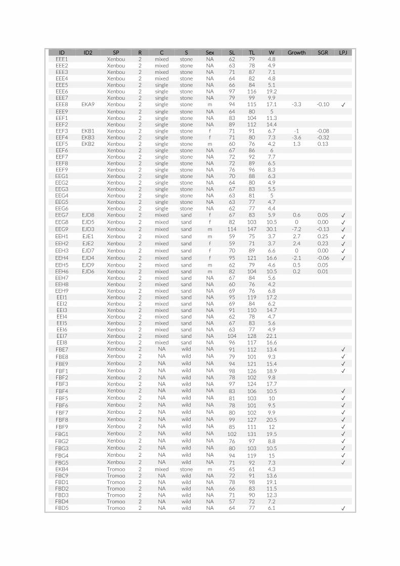
ID ID2 SP R C S Sex SL TL W Growth SGR LPJ EEE1
Xenbou 2 mixed stone NA 62 79 4.8
EEE2
Xenbou 2 mixed stone NA 63 78 4.9
EEE3
Xenbou 2 mixed stone NA 71 87 7.1
EEE4
Xenbou 2 mixed stone NA 64 82 4.8
EEE5
Xenbou 2 single stone NA 66 84 5.1
EEE6
Xenbou 2 single stone NA 97 116 19.2
EEE7
Xenbou 2 single stone NA 79 99 9.9
EEE8 EKA9 Xenbou 2 single stone m 94 115 17.1 -3.3 -0.10 ✓ EEE9
Xenbou 2 single stone NA 64 80 5
EEF1
Xenbou 2 single stone NA 83 104 11.3
EEF2
Xenbou 2 single stone NA 89 112 14.4
EEF3 EKB1 Xenbou 2 single stone f 71 91 6.7 -1 -0.08
EEF4 EKB3 Xenbou 2 single stone f 71 80 7.3 -3.6 -0.32
EEF5 EKB2 Xenbou 2 single stone m 60 76 4.2 1.3 0.13
EEF6
Xenbou 2 single stone NA 67 86 6
EEF7
Xenbou 2 single stone NA 72 92 7.7
EEF8
Xenbou 2 single stone NA 72 89 6.5
EEF9
Xenbou 2 single stone NA 76 96 8.3
EEG1
Xenbou 2 single stone NA 70 88 6.3
EEG2
Xenbou 2 single stone NA 64 80 4.9
EEG3
Xenbou 2 single stone NA 67 83 5.5
EEG4
Xenbou 2 single stone NA 63 81 5
EEG5
Xenbou 2 single stone NA 63 77 4.7
EEG6
Xenbou 2 single stone NA 62 77 4.4
EEG7 EJD8 Xenbou 2 mixed sand f 67 83 5.9 0.6 0.05 ✓ EEG8 EJD5 Xenbou 2 mixed sand f 82 103 10.5 0 0.00 ✓ EEG9 EJD3 Xenbou 2 mixed sand m 114 147 30.1 -7.2 -0.13 ✓ EEH1 EJE1 Xenbou 2 mixed sand m 59 75 3.7 2.7 0.25 ✓ EEH2 EJE2 Xenbou 2 mixed sand f 59 71 3.7 2.4 0.23 ✓ EEH3 EJD7 Xenbou 2 mixed sand f 70 89 6.6 0 0.00 ✓ EEH4 EJD4 Xenbou 2 mixed sand f 95 121 16.6 -2.1 -0.06 ✓ EEH5 EJD9 Xenbou 2 mixed sand m 62 79 4.6 0.5 0.05
EEH6 EJD6 Xenbou 2 mixed sand m 82 104 10.5 0.2 0.01
EEH7
Xenbou 2 mixed sand NA 67 84 5.6
EEH8
Xenbou 2 mixed sand NA 60 76 4.2
EEH9
Xenbou 2 mixed sand NA 69 76 6.8
EEI1
Xenbou 2 mixed sand NA 95 119 17.2
EEI2
Xenbou 2 mixed sand NA 69 84 6.2
EEI3
Xenbou 2 mixed sand NA 91 110 14.7
EEI4
Xenbou 2 mixed sand NA 62 78 4.7
EEI5
Xenbou 2 mixed sand NA 67 83 5.6
EEI6
Xenbou 2 mixed sand NA 63 77 4.9
EEI7
Xenbou 2 mixed sand NA 104 128 22.1
EEI8
Xenbou 2 mixed sand NA 96 117 16.6
FBE7 Xenbou 2 NA wild NA 91 112 13.4 ✓ FBE8 Xenbou 2 NA wild NA 79 101 9.3 ✓ FBE9 Xenbou 2 NA wild NA 94 121 15.4 ✓ FBF1 Xenbou 2 NA wild NA 98 126 18.9 ✓ FBF2 Xenbou 2 NA wild NA 78 102 9.8 FBF3 Xenbou 2 NA wild NA 97 124 17.7 FBF4 Xenbou 2 NA wild NA 83 106 10.5 ✓ FBF5 Xenbou 2 NA wild NA 81 103 10 ✓ FBF6 Xenbou 2 NA wild NA 78 101 9.5 ✓ FBF7 Xenbou 2 NA wild NA 80 102 9.9 ✓ FBF8 Xenbou 2 NA wild NA 99 127 20.5 ✓ FBF9 Xenbou 2 NA wild NA 85 111 12 ✓ FBG1 Xenbou 2 NA wild NA 102 131 19.5 ✓ FBG2 Xenbou 2 NA wild NA 76 97 8.8 ✓ FBG3 Xenbou 2 NA wild NA 80 103 10.5 ✓ FBG4 Xenbou 2 NA wild NA 94 119 15 ✓ FBG5 Xenbou 2 NA wild NA 71 92 7.3 ✓ EKB4
Tromoo 2 mixed stone m 45 61 4.3
FBC9
Tromoo 2 NA wild NA 72 91 13.6
FBD1
Tromoo 2 NA wild NA 78 98 19.1
FBD2
Tromoo 2 NA wild NA 66 83 11.5
FBD3
Tromoo 2 NA wild NA 71 90 12.3
FBD4
Tromoo 2 NA wild NA 57 72 7.2
FBD5
Tromoo 2 NA wild NA 64 77 6.1
✓
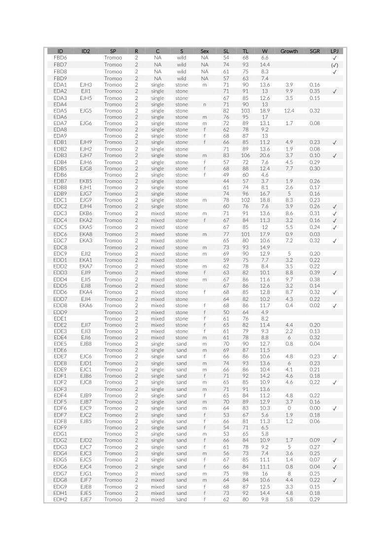
ID ID2 SP R C S Sex SL TL W Growth SGR LPJ FBD6
Tromoo 2 NA wild NA 54 68 6.6
✓
FBD7
Tromoo 2 NA wild NA 74 93 14.4
(✓) FBD8
Tromoo 2 NA wild NA 61 75 8.3
✓
FBD9
Tromoo 2 NA wild NA 57 63 7.4
EDA1 EJH3 Tromoo 2 single stone m 71 90 13.6 3.9 0.16
EDA2 EJI1 Tromoo 2 single stone
71 91 13 9.9 0.35 ✓ EDA3 EJH5 Tromoo 2 single stone
67 85 12.6 3.5 0.15
EDA4
Tromoo 2 single stone n 71 90 13
EDA5 EJG5 Tromoo 2 single stone
82 103 18.9 12.4 0.32
EDA6
Tromoo 2 single stone m 76 95 17
EDA7 EJG6 Tromoo 2 single stone m 72 89 13.1 1.7 0.08
EDA8
Tromoo 2 single stone f 62 78 9.2
EDA9
Tromoo 2 single stone f 68 87 13
EDB1 EJH9 Tromoo 2 single stone f 66 85 11.2 4.9 0.23 ✓ EDB2 EJH2 Tromoo 2 single stone
71 89 13.6 1.9 0.08
EDB3 EJH7 Tromoo 2 single stone m 83 106 20.6 3.7 0.10 ✓ EDB4 EJH6 Tromoo 2 single stone f 57 72 7.6 4.5 0.29
EDB5 EJG8 Tromoo 2 single stone f 68 88 12.4 7.7 0.30
EDB6
Tromoo 2 single stone f 49 60 4.6
EDB7 EKB5 Tromoo 2 single stone
44 57 3.7 1.9 0.26
EDB8 EJH1 Tromoo 2 single stone
61 74 8.1 2.6 0.17
EDB9 EJG7 Tromoo 2 single stone
74 96 16.7 5 0.16
EDC1 EJG9 Tromoo 2 single stone m 78 102 18.8 8.3 0.23
EDC2 EJH4 Tromoo 2 single stone
60 76 7.6 3.9 0.26 ✓ EDC3 EKB6 Tromoo 2 mixed stone m 71 91 13.6 8.6 0.31 ✓ EDC4 EKA2 Tromoo 2 mixed stone f 67 84 11.3 3.2 0.16 ✓ EDC5 EKA5 Tromoo 2 mixed stone
67 85 12 5.5 0.24 ✓
EDC6 EKA8 Tromoo 2 mixed stone m 77 101 17.9 0.9 0.03
EDC7 EKA3 Tromoo 2 mixed stone
65 80 10.6 7.2 0.32 ✓ EDC8
Tromoo 2 mixed stone m 73 93 14.9
EDC9 EJI2 Tromoo 2 mixed stone m 69 90 12.9 5 0.20
EDD1 EKA1 Tromoo 2 mixed stone
59 75 7.7 3.2 0.22
EDD2 EKA7 Tromoo 2 mixed stone m 62 78 8.4 3.5 0.22
EDD3 EJI9 Tromoo 2 mixed stone f 63 82 10.1 8.8 0.39 ✓ EDD4 EJI5 Tromoo 2 mixed stone m 67 86 11.6 9.7 0.38
EDD5 EJI8 Tromoo 2 mixed stone
67 86 12.6 3.2 0.14
EDD6 EKA4 Tromoo 2 mixed stone f 68 85 12.8 8.7 0.32 ✓ EDD7 EJI4 Tromoo 2 mixed stone
64 82 10.2 4.3 0.22
EDD8 EKA6 Tromoo 2 mixed stone f 68 86 11.7 0.4 0.02 ✓ EDD9
Tromoo 2 mixed stone f 50 64 4.9
EDE1
Tromoo 2 mixed stone f 61 76 8.2
EDE2 EJI7 Tromoo 2 mixed stone f 65 82 11.4 4.4 0.20
EDE3 EJI3 Tromoo 2 mixed stone f 61 79 9.3 2.2 0.13
EDE4 EJI6 Tromoo 2 mixed stone m 61 78 8.8 6 0.32
EDE5 EJB8 Tromoo 2 single sand m 70 90 12.7 0.8 0.04
EDE6
Tromoo 2 single sand m 69 87 11.5
EDE7 EJC6 Tromoo 2 single sand f 66 86 10.6 4.8 0.23 ✓ EDE8 EJD1 Tromoo 2 single sand m 74 93 13.6 6 0.23
EDE9 EJC1 Tromoo 2 single sand m 66 86 10.4 4.1 0.21
EDF1 EJB6 Tromoo 2 single sand f 71 92 14.2 4.6 0.18
EDF2 EJC8 Tromoo 2 single sand m 65 85 10.9 4.6 0.22 ✓ EDF3
Tromoo 2 single sand m 71 91 13.6
EDF4 EJB9 Tromoo 2 single sand f 65 84 11.2 4.8 0.22
EDF5 EJB7 Tromoo 2 single sand m 70 89 12.9 3.7 0.16
EDF6 EJC9 Tromoo 2 single sand m 64 83 10.3 0 0.00 ✓ EDF7 EJC2 Tromoo 2 single sand f 53 67 5.6 1.9 0.18
EDF8 EJB5 Tromoo 2 single sand f 66 81 11.3 1.2 0.06
EDF9
Tromoo 2 single sand f 54 71 6.5
EDG1
Tromoo 2 single sand m 53 65 5.8
EDG2 EJD2 Tromoo 2 single sand f 66 84 10.9 1.7 0.09 ✓ EDG3 EJC7 Tromoo 2 single sand f 61 78 9.2 5 0.27
EDG4 EJC3 Tromoo 2 single sand m 56 73 7.4 3.6 0.25
EDG5 EJC5 Tromoo 2 single sand f 67 85 11.1 1.4 0.07 ✓ EDG6 EJC4 Tromoo 2 single sand f 66 84 11.1 0.8 0.04 ✓ EDG7 EJG1 Tromoo 2 mixed sand m 75 98 16 8 0.25
EDG8 EJF7 Tromoo 2 mixed sand m 64 84 10.6 4.4 0.22 ✓ EDG9 EJE8 Tromoo 2 mixed sand f 68 87 12.5 3.3 0.15
EDH1 EJE5 Tromoo 2 mixed sand f 73 92 14.4 4.8 0.18
EDH2 EJE7 Tromoo 2 mixed sand f 62 80 9.8 5.8 0.29

ID ID2 SP R C S Sex SL TL W Growth SGR LPJ EDH3
Tromoo 2 mixed sand f 65 83 10.7
EDH4 EJE3 Tromoo 2 mixed sand m 69 87 12.7 3.9 0.17
EDH5 EJE6 Tromoo 2 mixed sand m 76 100 15.9 3.9 0.14
EDH6
Tromoo 2 mixed sand f 66 84 11
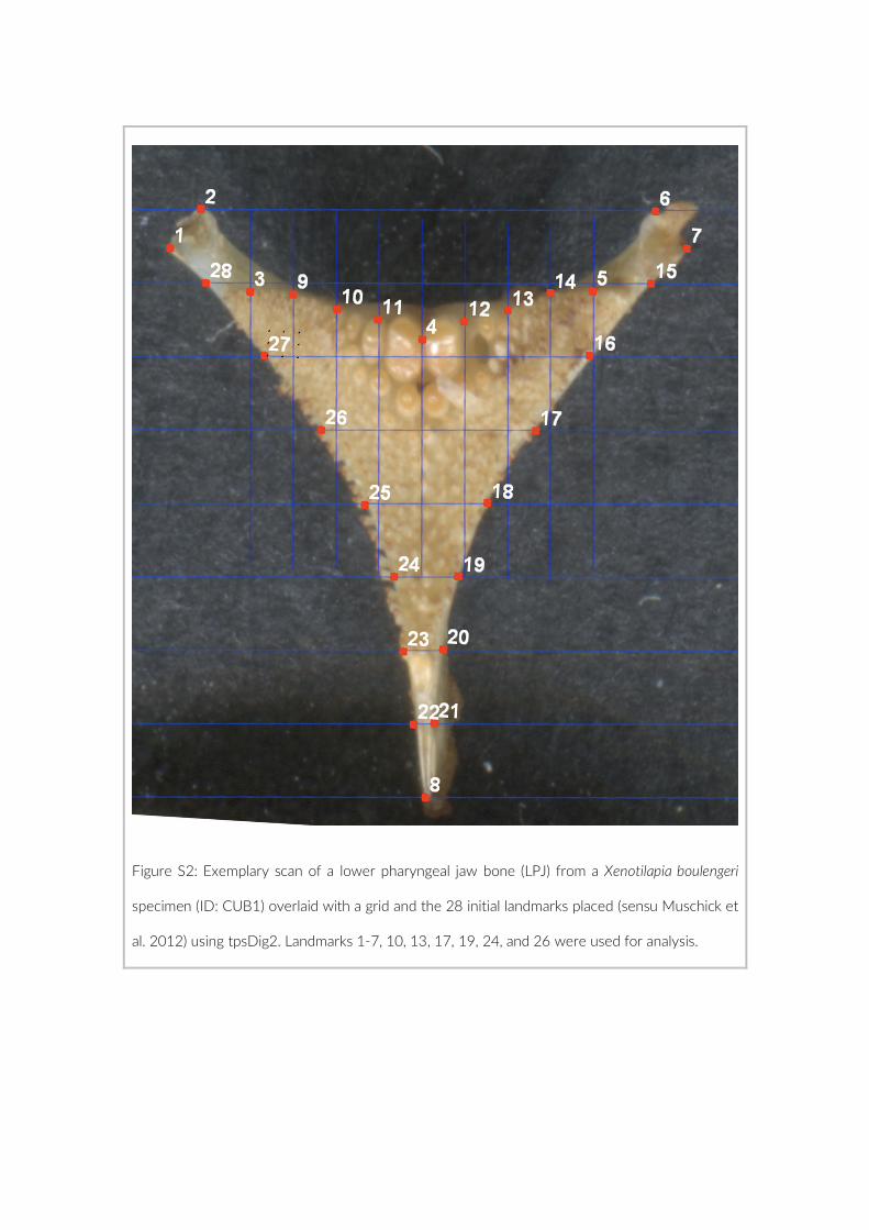
Figure S2: Exemplary scan of a lower pharyngeal jaw bone (LPJ) from a Xenotilapia boulengeri
specimen (ID: CUB1) overlaid with a grid and the 28 initial landmarks placed (sensu Muschick et
al. 2012) using tpsDig2. Landmarks 1-7, 10, 13, 17, 19, 24, and 26 were used for analysis.
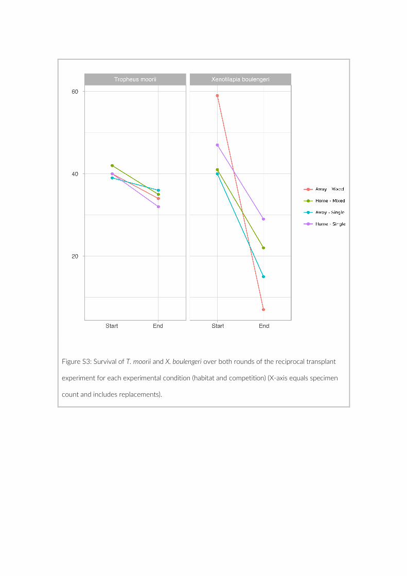
Figure S3: Survival of T. moorii and X. boulengeri over both rounds of the reciprocal transplant
experiment for each experimental condition (habitat and competition) (X-axis equals specimen
count and includes replacements).
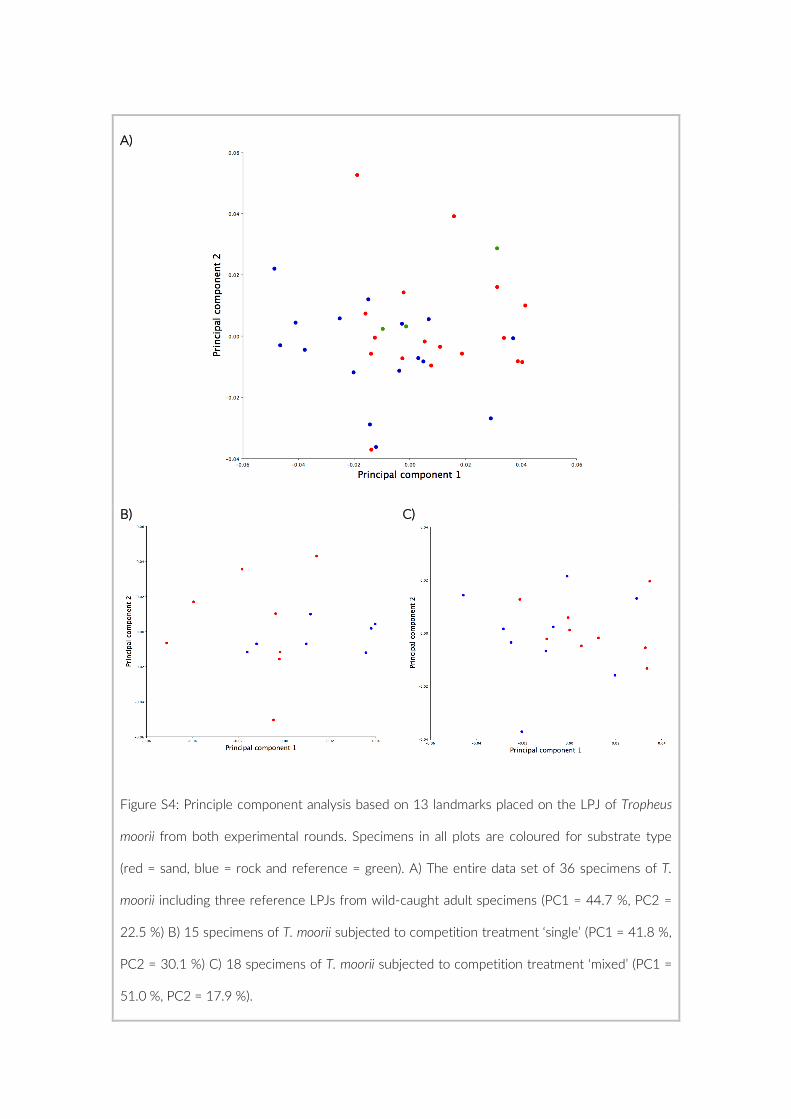
A)
B)
C)
Figure S4: Principle component analysis based on 13 landmarks placed on the LPJ of Tropheus
moorii from both experimental rounds. Specimens in all plots are coloured for substrate type
(red = sand, blue = rock and reference = green). A) The entire data set of 36 specimens of T.
moorii including three reference LPJs from wild-caught adult specimens (PC1 = 44.7 %, PC2 =
22.5 %) B) 15 specimens of T. moorii subjected to competition treatment ‘single’ (PC1 = 41.8 %,
PC2 = 30.1 %) C) 18 specimens of T. moorii subjected to competition treatment ‘mixed’ (PC1 =
51.0 %, PC2 = 17.9 %).
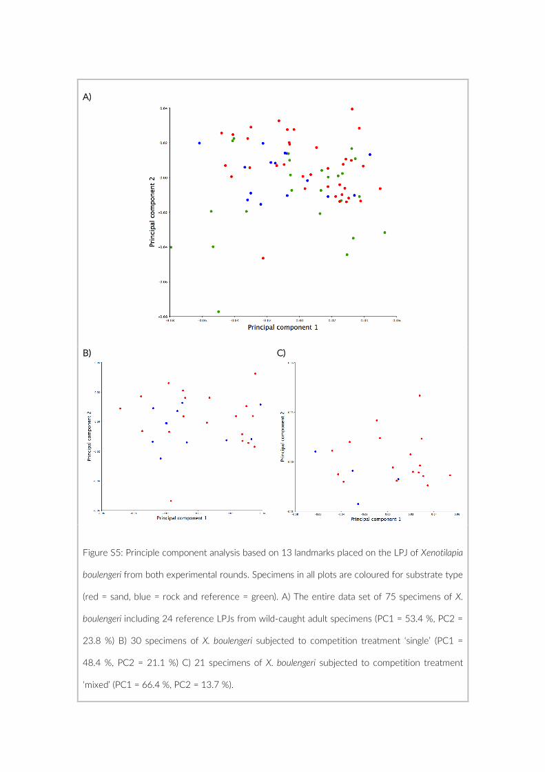
A)
B)
C)
Figure S5: Principle component analysis based on 13 landmarks placed on the LPJ of Xenotilapia
boulengeri from both experimental rounds. Specimens in all plots are coloured for substrate type
(red = sand, blue = rock and reference = green). A) The entire data set of 75 specimens of X.
boulengeri including 24 reference LPJs from wild-caught adult specimens (PC1 = 53.4 %, PC2 =
23.8 %) B) 30 specimens of X. boulengeri subjected to competition treatment ‘single’ (PC1 =
48.4 %, PC2 = 21.1 %) C) 21 specimens of X. boulengeri subjected to competition treatment
‘mixed’ (PC1 = 66.4 %, PC2 = 13.7 %).


Discussion
The focus of my doctoral thesis lies on examining the community structure and the
diversity of ecological niches exploited by the cichlid species-flock of Lake Tanganyika.
My thesis provides valuable insights into community assembly patterns and the
evolutionary history of niche use of this fantastically diverse adaptive radiation. In Part
One of my thesis, the methodological aspect of how to examine fish communities is
investigated and a novel approach is presented, the Point-Combination Transect (PCT)
method (Chapter 1). Further, we provide a proof of concept for the new methodology
of PCT through the use of environmental DNA (eDNA), extracted from sediment
samples (Chapter 2). Part Two, then, explores the community structure, co-occurrence
patterns and niche evolution of the cichlids in Lake Tanganyika (Chapter 3). This last
project examines the niche constraints due to specialisation of two common but
ecologically distinct cichlid species of Lake Tanganyika (Chapter 4).
In ‘Point-Combination Transect (PCT): Incorporation of small underwater cameras to
study fish communities’ (Chapter 1) we present our novel method, PCT, which is based
on five small digital cameras that are placed in the benthic environment of a water
body. Through a meticulous comparison to studies conducted within close proximity of
our own study site and that used line transects, a conventional underwater visual
census method (M. Samoilys & Carlos, 1992; M. A. Samoilys & Carlos, 2000), we were
able to illustrate the power of PCT’s ability to capture an undisturbed community. A
major component of PCT’s power is the markedly reduced effect of observer presence
(e.g. SCUBA diver) (Watson, Carlos, & Samoilys, 1995; Pereira, Leal, & de Araújo,
2016). This was impressively demonstrated, in that the PCT captured several species,
such as the African tigerfish Hydrocynus vittatus, which despite a decade of SCUBA
diving at the study site have never been directly observed. Furthermore, we can
suggest the applicability of PCT for broad use on fish communities as we did not find
evidence that our novel method would primarily target exclusively benthic species. PCT
presents a novel approach with several key advantages compared to other camera-
based methodologies, in that it is inconspicuous, cost effective and easy to handle,
while providing robust visual survey data of benthic fish communities.
The second study described in the draft manuscript entitled ‘Does eDNA within
sediments reflect local cichlid assemblages in Lake Tanganyika?’ (Chapter 2), uses
fragmented genomic DNA found in the environment, so-called eDNA, to provide a
proof of concept for the PCT. However, the species assignments based on eDNA from
61 sediment samples show large discrepancies between species captured by PCT and
by the eDNA metabarcoding approach and fails to deliver a proof of concept for PCT.
Difficulties with PCR amplification of target ND2 sequence resulting in cross reactions
and non-target amplifications might have impaired quality, exemplified by the heavy
loss of reads during filtering steps. The merits of eDNA metabarcoding approaches
have been illustrated by studies aiming for lower taxonomic resolution (Catalunya,
Velocimetry, & Correlation, 2016; Valentini et al., 2016), but for species identification
in an adaptive radiation, improvements might still be required.
In Part Two, we examined the environmental conditions influencing cichlids distribution
and community structure, and, in a phylogenetic framework, elucidated the general
assembly patterns in order to advance the current state of knowledge and contribute
to the discussion of what processes may underlie niche differentiation in the cichlid
species-flock of Lake Tanganyika. The main study (‘Community assembly patterns and
niche evolution in the species-flock of cichlid fishes from East African Lake
Tanganyika’) (Chapter 3) observed a consistent species per tribe ratio for the different
communities for the whole longitudinal range of Lake Tanganyika along the Zambian
and Tanzanian coast. Co-occurrence patterns of local communities revealed that
stochastic processes predominantly shape cichlid assemblies in Lake Tanganyika.
Nevertheless, a high degree of environmental filtering was observed indicating the
importance of niche-based assembly as well, as observed in a localised study (Janzen et
al., 2017). We found varying levels of niche overlap between the cichlid species of Lake
Tanganyika, illustrating the diversity of niches occupied by the cichlids (Konings, 1998;
Sturmbauer, Husemann, & Danley, 2011; Salzburger, 2018). Age-range correlations
and ancestral niche reconstructions suggest patterns of niche conservatism, which may
have contributed to diversification within lineages, something not found in other ‘old’
adaptive radiations, such as the Caribbean Anolis Lizards (Knouft, Losos, Glor, & Kolbe,
2006).
In the last chapter of my thesis (‘Where Am I? Niche constraints due to morphological
specialisation of two Tanganyikan cichlid species) (Chapter 4), we observed high
mortality in X. boulengeri during the reciprocal transplant experiments, possibly due to
the species’ sensitivity to handling. The experiments showed that forcing the
specimens from their preferred habitat had a significant effect on specific growth rates
in T. moorii but not in X. boulengeri. The different competition regimes did not appear to
affect the growth rates of either these two ecologically distinct species. Moreover, no
change in shape of the lower pharyngeal jaw bone (LPJ) was discovered after the
duration of the several months long experiment. We concluded that the degree of
specialisation of T. moorii and X. boulengeri might have reduced, the otherwise in
cichlids present (Meyer, 1989; Muschick, Barluenga, Salzburger, & Meyer, 2011),
capacity of phenotypic plasticity, in the trophic structure LPJ, to enable transitions to
alternative food sources.

The main contributions that are being made through my doctoral thesis are: 1) the
novel methodology of PCT, which will facilitate the monitoring of underwater
communities for fellow researchers; 2) the substantial census data of cichlids in Lake
Tanganyika; 3) the description of cichlid community patterns in a lake-wide context
showing the importance of niche-based processes shaping cichlid assemblies; and 4)
revealing patterns of niche conservatism, variable among tribes, that might have
contributed to the process of diversification in the cichlid species-flock of Lake
Tanganyika.
References
Catalunya, U. P. De, Velocimetry, P. I., & Correlation, D. I. (2016). Fish community
assessment with eDNA metabarcoding: effects of sampling design and
bioinformatic filtering. Canadian Journal of Fisheries and Aquatic Sciences.
Janzen, T., Alzate, A., Muschick, M., Maan, M. E., van der Plas, F., & Etienne, R. S.
(2017). Community assembly in Lake Tanganyika cichlid fish: quantifying the
contributions of both niche-based and neutral processes. Ecology and Evolution,
7(4), 1057–1067. doi:10.1002/ece3.2689
Knouft, J. H., Losos, J. B., Glor, R. E., & Kolbe, J. J. (2006). Phylogenetic analysis of the
evolution of the niche in lizards of the Anolis sagrei group. Ecology, 87, S29-38.
Konings, A. (1998). Tanganyika cichlids in their natural habitat (3rd ed.). Cichlid Press, El
Paso, USA.
Meyer, A. (1989). Cost of morphological specialization: feeding performance of the two
morphs in the trophically polymorphic cichlid fish, Cichlasoma citrinellum.
Oecologia, 80(3), 431–436. doi:10.1007/BF00379047
Muschick, M., Barluenga, M., Salzburger, W., & Meyer, A. (2011). Adaptive phenotypic
plasticity in the Midas cichlid fish pharyngeal jaw and its relevance in adaptive
radiation. BMC Evolutionary Biology, 11(1), 116. doi:10.1186/1471-2148-11-116
Pereira, P. H. C., Leal, I. C. S., & de Araújo, M. E. (2016). Observer presence may alter
the behaviour of reef fishes associated with coral colonies. Marine Ecology, 37(4),
760–769. doi:10.1111/maec.12345
Salzburger, W. (2018). Understanding explosive diversification through cichlid fish
genomics. Nature Reviews Genetics. doi:10.1038/s41576-018-0043-9
Samoilys, M. A., & Carlos, G. (2000). Determining methods of underwater visual census
for estimating the abundance of coral reef fishes. Environmental Biology of Fishes,
57(3), 289–304. doi:10.1023/A:1007679109359
Samoilys, M., & Carlos, G. (1992). Development of an Underwater Visual Census Method
for Assessing Shallow Water Reef Fish Stocks in the South West Pacific: Final Report.
Queensland: Queensland Dept. of Primary Industries. Retrieved from
http://www.worldcat.org/title/development-of-an-underwater-visual-census-
method-for-assessing-shallow-water-reef-fish-stocks-in-the-south-west-pacific-
final-report/oclc/32021136?referer=di&ht=edition
Sturmbauer, C., Husemann, M., & Danley, P. D. (2011). Explosive Speciation and
Adaptive Radiation of East African Cichlid Fishes. In Biodiversity Hotspots (pp.
333–362). Berlin, Heidelberg: Springer Berlin Heidelberg. doi:10.1007/978-3-
642-20992-5_18
Valentini, A., Taberlet, P., Miaud, C., Civade, R., Herder, J., Thomsen, P. F., … Dejean, T.
(2016). Next-generation monitoring of aquatic biodiversity using environmental
DNA metabarcoding. Molecular Ecology, 25(4), 929–942. doi:10.1111/mec.13428
Watson, R. A., Carlos, G. M., & Samoilys, M. A. (1995). Bias introduced by the non-
random movement of fish in visual transect surveys. Ecological Modelling, 77(2–3),
205–214. doi:10.1016/0304-3800(93)E0085-H


Acknowledgements
First and foremost, I would like to thank Walter Salzburger, whom I owe a great debt of
gratitude for giving me the chance to do my PhD in his lab at the University of Basel and for
his guidance and supervision during this unique experience. I am also incredibly grateful for the
opportunity to visit the many fantastic locations in Zambia and Tanzania during my fieldwork
around Lake Tanganyika.
Secondly, I would like to thank Prof. Dr. Christian Sturmbauer for taking the time to co-
examine my thesis.
I am grateful to all my co-authors for participating in my projects and their continuous support
during the field work, analysis and write up. Especially, Athimed El Taher, Adrian Indermaur,
and Fabrizia Ronco, which turned the field trips to Lake Tanganyika into such incredible
experiences. For valuable comments and discussions on the projects, methods, statistics and
manuscripts I am deeply grateful to Astrid Böhne.
For their help around the institute, in the lab and interesting/important discussions another big
thank you goes to Nicolas Boileau, Barbara Berli, Telma Laurentino, Jelene Rajkov, Alexandra
Weber, Brigitte Aeschbach, Daniel Berner, Bernd Egger, Attila Rüegg, Nicolas Lichilin Ortiz,
Daniel Lüscher and Elia Heule.
I would like to express my gratitude to the European Research Council (ERC), and the
University of Basel for the financial support during my PhD.

A big thank you also to Dr. Dr. hc Heinz Büscher, the entire staff of Kalambo Falls Lodge and
George Kazumbe and his crew for turning the field work in Zambia and Tanzania into such
amazing experiences.
I am incredible grateful to my past and present office mates for the serious discussion, for the
less serious discussions and the fantastic time together, on the LIGHT side, Adrian Indermaur
and Fabrizia Ronco and the office chicks on the DARK side, Athimed El Taher and Astrid
Böhne – It’s time for bubbles!
And finally, I want to say how enormously thankful I am to my parents (aka MaPi), my sisters
and my friends for their continued support during this entire time and for some final notes on
my writing.
A massive ‘Dankeschön’!


Curriculum Vitae Full Name: Lukas Benedikt Widmer Date of Birth: July 13th, 1987 Nationality: Switzerland Address: Steinenbachgässlein 42, CH-4051 Basel Mobile: +41 76 372 21 01 Mail: [email protected]
ProfileGraduated aquatic ecologist (PhD) experienced in ecological modelling and with a passion for understanding the environmental impacts of mankind on aquatic ecosystems.
Practical Experience 02/2020 – 04/2020 Postdoc – University of Basel Project work in the group of Prof. Dr. Walter Salzburger
§ Analysis of complex data of fish community structure 10/2019 – 11/2019 Postdoc – University of Basel Report for The Nature Conservancy (US) as contribution to The Tuungane Project
§ Habitat analysis Lake Tanganyika / Process and evaluate underwater images 11/2015 – 05/2019 PhD – University of Basel
Dissertation “Evolutionary community ecology in the cichlid species-flock of the East African Lake Tanganyika” defended with cum laude, supervised by Prof. Dr. Walter Salzburger § Development of novel transect methodology § Construction of ecological niche models for various fish species § Application of diverse modelling approaches § Lead of large-scale environmental DNA (eDNA) project § Design/Development of web-application for facilitated fish-identification § Development of SQL database § Supervision of MSc thesis of E. Heule
Courses during PhD
§ First steps in Python (SIB, Basel) § Ecological niche modelling using R (PR Statistics, Scotland, UK)
11/2014 – 04/2015 Assistant Dep. Energy (civil servant) - Bildungszentrum WWF, Bern, Switzerland
§ Planning/Running of workshops § Developing course offers
Education
09/2013 – 11/2014 Master of Science (MSc) in Marine Biology – Bangor University, Wales, United Kingdom § Fresh water habitat analyses (stream morphology, flow rate, PH value) of river sections in
Alsace, France § Record occurrences of Eurasian otter (Lutra lutra) in Alsace, France
09/2009 – 07/2013 Bachelor of Science (BSc) in Biology – University of Basel Major in animal and plant sciences
Skills
Core competence Multivariate data analysis Project management Biomolecular laboratory work IT-Skills Q-GIS / MS Office Inkscape (Illustrator) / Gimp (Photoshop) R Statistics / SQL / PHP / HTML / Java / Python
Languages German (native speaker) English (fluent) French (proficient) Various skills Swiss flora (“Bellis”- Certificate) & fauna SCUBA diving (PADI Open Water) Driver’s License Swiss Cat. B, C1, D1, BE, C1E, D1E
linkedin.com/in/widmerlukas/
Publications
Published Widmer et al. (2019): Point-Combination Transect (PCT): Incorporation of small underwater cameras to study fish communities. Methods Ecol Evol. 2019;00:1–11. https://doi.org/10.1111/2041-210X.13163
In revision Widmer et al. : Where Am I? Niche constraints due to morphological specialisation of two
Tanganyikan cichlid species El Taher et al. : Gene expression dynamics during rapid organismal diversification In preparation Widmer et al. : Community assembly patterns and niche evolution in the species-flock of cichlid
fishes from East African Lake Tanganyika. Widmer & El Taher, Salzburger: Does eDNA within sediments reflect local cichlid assemblages in Lake Tanganyika?
Presentations
02/2019 Biology 19, Zürich, Schweiz: Early differentiation along environmental axes in the adaptive radiation of Lake Tanganyika cichlid fishes
07/2018 Cichlid Symposium, Konstanz, Deutschland: Depth – The chief environmental shaper of the
cichlid community of Lake Tanganyika? 02/2018 Biology 18 (Poster und Flash Talk), Neuchâtel, Schweiz: Environmental drivers of community
structure in the cichlid species flock of Lake Tanganyika. 09/2017 Cichlid Science, Prag, Tschechische Republik: Community structure and niche conservatism in
the cichlid species flock of Lake Tanganyika Fieldwork
08/2017 – 09/2017 Lake Tanganyika, Tanzania – ca. 30 dives for the collection of cichlid abundance and diversity data
01/2017 – 02/2017 Lake Tanganyika, Tanzania– ca. 30 dives for the collection of cichlid abundance and diversity
data 08/2016 – 09/2016 Lake Tanganyika, Zambia – ca. 30 dives for the collection of cichlid abundance and diversity
data 06/2014 – 09/2014 Alsace, France – Evaluation of Eurasian otter (Lutra lutra) occurrences


