Embed Size (px)
Citation preview

Evolve
Version 2.04
User’s Manual
Frank Price Hamilton College
Virginia G. Vaughan BioQUEST Curriculum Consortium
A BioQUEST Library VII Online module published by the BioQUEST Curriculum Consortium
The BioQUEST Curriculum Consortium (1986) actively supports educators interested in the reform of undergraduate biology and engages in the collaborative development of curricula.
We encourage the use of simulations, databases, and tools to construct learning environments where students are able to engage in activities like those of practicing scientists.
Email: [email protected] Website: http://bioquest.org
Editorial Staff
Editor: John R. Jungck Beloit College Managing Editor: Ethel D. Stanley Beloit College, BioQUEST Curriculum Consortium Associate Editors: Sam Donovan University of Pittsburgh
Stephen Everse University of Vermont Marion Fass Beloit College Margaret Waterman Southeast Missouri State University Ethel D. Stanley Beloit College, BioQUEST Curriculum Consortium
Online Editor: Amanda Everse Beloit College, BioQUEST Curriculum Consortium Editorial Assistant: Sue Risseeuw Beloit College, BioQUEST Curriculum Consortium
Editorial Board
Ken Brown University of Technology, Sydney, AU Joyce Cadwallader St Mary of the Woods College Eloise Carter Oxford College Angelo Collins Knowles Science Teaching FoundationTerry L. Derting Murray State University Roscoe Giles Boston University Louis Gross University of Tennessee-Knoxville Yaffa Grossman Beloit College Raquel Holmes Boston University Stacey Kiser Lane Community College
Peter Lockhart Massey University, NZ Ed Louis The University of Nottingham, UK Claudia Neuhauser University of Minnesota Patti Soderberg Conserve School Daniel Udovic University of Oregon Rama Viswanathan Beloit College Linda Weinland Edison College Anton Weisstein Truman University Richard Wilson (Emeritus) Rockhurst College
William Wimsatt University of Chicago
Copyright © 1993 -2006 by Frank Price and Virginia G. Vaughan
All rights reserved.

Copyright, Trademark, and License Acknowledgments Portions of the BioQUEST Library are copyrighted by Annenberg/CPB, Apple Computer Inc., Beloit College, Claris Corporation, Microsoft Corporation, and the authors of individually titled modules. All rights reserved. System 6, System 7, System 8, Mac OS 8, Finder, and SimpleText are trademarks of Apple Computer, Incorporated. HyperCard and HyperTalk, MultiFinder, QuickTime, Apple, Mac, Macintosh, Power Macintosh, LaserWriter, ImageWriter, and the Apple logo are registered trademarks of Apple Computer, Incorporated. Claris and HyperCard Player 2.1 are registered trademarks of Claris Corporation. Extend is a trademark of Imagine That, Incorporated. Adobe, Acrobat, and PageMaker are trademarks of Adobe Systems Incorporated. Microsoft, Windows, MS-DOS, and Windows NT are either registered trademarks or trademarks of Microsoft Corporation. Helvetica, Times, and Palatino are registered trademarks of Linotype-Hell. The BioQUEST Library and BioQUEST Curriculum Consortium are trademarks of Beloit College. Each BioQUEST module is a trademark of its respective institutions/authors. All other company and product names are trademarks or registered trademarks of their respective owners. Portions of some modules' software were created using Extender GrafPak™ by Invention Software Corporation. Some modules' software use the BioQUEST Toolkit licensed from Project BioQUEST.

TABLE OF CONTENTSAcknowledgments ..........................................................................................................................i
TABLE OF CONTENTS .............................................................................................................. ii
LIST OF FIGURES........................................................................................................................ v
Part 1. LEARNING TO USE EVOLVE......................................................................................1
Preface. WHAT YOU NEED TO KNOW..................................................................................2
Chapter 1. INTRODUCTION....................................................................................................4
Chapter 2. GETTING STARTED................................................................................................6INTRODUCTION .............................................................................................................6THE HELP SYSTEM .........................................................................................................6EXERCISE 1: A Simple Experiment with Natural Selection.......................................7
Setting up the experiment....................................................................................8Doing the Experiment ........................................................................................10Looking at Results...............................................................................................11
LEAVING EVOLVE........................................................................................................14
Chapter 3. MORE ADVANCED FEATURES OF EVOLVE .................................................15INTRODUCTION: Doing Experiments with EVOLVE.............................................15EXERCISE 2. Comparing Selection in Small and Large Populations.....................16
Redoing the Experiment With Variations. ......................................................17Moving Results to Paper and Elsewhere.........................................................19
EXERCISE 3. Comparing Runs with Different Random Numbers ........................20EXERCISE 4. Changing the Evolutionary Situation During a Run ........................21
Chapter 4. BACKGROUND......................................................................................................23THE HYPOTHETICAL ORGANISMS.........................................................................23GENETIC CONCEPTS UNDERLYING THE MODEL..............................................25
An example ..........................................................................................................26THE NATURE OF EVOLUTIONARY FITNESS ........................................................28
PART 2. EXPERIMENTING WITH EVOLUTION................................................................31
Chapter 5. ELEMENTARY EXERCISES .................................................................................32FUNDAMENTALS.........................................................................................................32
Initial Population.................................................................................................32Survival and Reproductive Rates .....................................................................33Hardy-Weinberg Equilibrium...........................................................................33
EXERCISE 5. How long does it take to establish Hardy-Weinberg equilibriumstarting with a population that is not in equilibrium ................................................34
TABLE OF CONTENTS iii
EXERCISE 6. Set up a population in Hardy-Weinberg equilibrium. .....................36NATURAL SELECTION................................................................................................37
EXERCISE 7. What effect does increasing the strength of selection have onthe evolution of an advantageous, dominant allele? .....................................37EXERCISE 8. Does the evolution (the change of allele and genotypefrequencies) of an advantageous, dominant allele proceed more rapidlythan that of an advantageous, recessive allele with comparable survivaland reproductive rates?......................................................................................40EXERCISE 9. How does the evolution of incompletely dominant allelesdiffer from the evolution of completely dominant alleles?...........................41EXERCISE 10. What is the evolutionary fate of a population in which theheterozygote is the most fit genotype (heterosis)?.........................................41
GENETIC DRIFT.............................................................................................................43EXERCISE 11. What effects does population size have on allelefrequencies?..........................................................................................................43
GENE FLOW....................................................................................................................44EXERCISE 12. What is the effect of gene flow on evolution?......................44
MUTATION.....................................................................................................................45EXERCISE 13. What is the fate of advantageous mutant alleles? ...............45
COMBINING EVOLUTIONARY FORCES.................................................................46EXERCISE 14. Drift and Selection....................................................................46EXERCISE 15. Selection and gene flow...........................................................46
Chapter 6. INTERMEDIATE EXERCISES ..............................................................................48PRELIMINARY EXERCISES .........................................................................................48EXERCISE 16. Selection via reproduction vs selection via survival........................49EXERCISE 17. Exploring heterosis. ..............................................................................50EXERCISE 18. Modelling the real world — Sickle-cell anemia................................53EXERCISE 19. Plotting ∆q vs q......................................................................................53EXERCISE 20. Plotting ∆q vs population size.............................................................54EXERCISE 21. Examining q at a time t for a large number of populations of thesame size...........................................................................................................................54
Chapter 7. ADVANCED EXERCISES .....................................................................................55EXERCISE 22. The Model Underlying EVOLVE.......................................................55EXERCISE 23. Statistical Comparisons of EVOLVE’s Results With Theory ..........56EXERCISE 24. Inferring Pattern of Selection From Field Data................................57
Chapter 8. PROGRAM NOTES and SETTING UP EXPERIMENTS ..................................58INTRODUCTION ...........................................................................................................58GETTING HELP WITH EVOLVE.................................................................................58PROGRAM INPUT.........................................................................................................59
Title........................................................................................................................59Number of Generations......................................................................................60Starting Population.............................................................................................60Survival and Reproductive Rates: Selection, Pattern of Inheritance andPopulation Growth Rates...................................................................................61
Pattern of inheritance..............................................................................61Population growth rate............................................................................62Pattern of selection .................................................................................62

iv EVOLVE Manual
Gene Flow.............................................................................................................64Maximum Population and Post-Crash Population: Population Size ..........64
PROGRAM OUTPUT.....................................................................................................65The Copy Commands.........................................................................................65
Copy Window ...........................................................................................65Copy Window Graph...............................................................................65Copy Window Data .................................................................................66
The Notepad ........................................................................................................66The Variables You May Graph..........................................................................66
Chapter 9. THEORETICAL NOTES........................................................................................68THE CONCEPT OF AN EQUILIBRIUM POPULATION.........................................68
Assumptions ........................................................................................................68Evolutionary forces.............................................................................................69Importance of Hardy-Weinberg Equilibrium.................................................70
MODELS IN POPULATION GENETICS....................................................................70CALCULATING FITNESS AND SELECTION COEFFICIENTS.............................71LIMITATIONS OF EVOLVE .........................................................................................75
BIBLIOGRAPHY .........................................................................................................................77INTRODUCTORY TEXTS..............................................................................................77FULL LENGTH TEXTS ..................................................................................................77ADVANCED TEXTS.......................................................................................................78
GLOSSARY ..................................................................................................................................79

List of FiguresFigure 2-1. Problem Selection Window.....................................................................................8
Figure 2-2. Problem Summary Window....................................................................................8
Figure 2-3. Parameter Input Window. .......................................................................................9
Figure 2-4. Summary Window after Trial 1. ..........................................................................10
Figure 2-5. Graph of Allele Frequencies and Heterozygote Frequency vs Time..............11
Figure 2-6. Total Population Size vs Time..............................................................................13
Figure 3-1. Outline of an EVOLVE Session ............................................................................15
Figure 4-1. Outline of EVOLVE’s Simulation and the Hypothetical Life Cycle. ..............24
Figure 6-1. A Metaphorical Landscape For Exploring Heterosis........................................51


Part 1. Learning To Use Evolve
This manual has three major parts. Part 1 teaches you to use EVOLVE, Part 2 teachesyou something about asking evolutionary questions through suggested exercises withEVOLVE, and Part 3 contains reference material on EVOLVE and how it relates toevolutionary biology.
An additional manual, the Getting Started Manual, is available. The Getting StartedManual contains only Part 1: Learning to Use Evolve and may be all that most studentswill need to begin using EVOLVE. The full User's Manual should, however, be availablein lab or computer facility.
Preface. What You Need To Know
This manual assumes that you are familiar with operation of the Macintosh, includingpointing, clicking, dragging, double-clicking, editing text, opening applications, andsaving and opening documents. If not, you should learn these basic Macintoshoperations before continuing with this tutorial.
In Part 1: Learning To Use Evolve, you will do the sample exercise in Chapter 2,“Getting Started,” to get a feel for how to use EVOLVE. Chapter 3, “More AdvancedFeatures of EVOLVE,” contains three more sample exercises to give you experiencewith all of EVOLVE’s features. You should do at least the first two exercises; the lastmay be omitted unless you will need to model a changing environment. You could thenskim through Chapter 4, “Background,” to get some perspective on population geneticsand on the conceptual design of EVOLVE. Later, when you are more familiar with bothEVOLVE and evolution, you may find it worthwhile to reread Chapter 4 with morecare.
Part 2, Experimenting with Evolution, contains a number of sample exercises whichboth illustrate the capabilities of EVOLVE and demonstrate many features ofevolutionary processes. Your instructor may assign some of the exercises in Part 2,Chapters 5-7, or may have you do others of his or her design.
Chapter 5, “Elementary Exercises,” examines Hardy-Weinberg equilibrium and fourevolutionary forces (selection, mutation, drift, and gene flow) singly, then incombination. (If you don’t already know some of these technical words, there is aGlossary at the end of this manual.) The initial exercises are spelled out in detail, andsubsequent exercises leave more and more to be filled in by students. The intent of thischapter is to give you a rather qualitative exposure to evolution. Although you will belooking at numerical measures of allele and genotype frequencies, we don’t expect in-depth comparisons of EVOLVE’s output with theoretical predictions. This chapter willbe the meat of EVOLVE for the majority of students up through collegeundergraduates.
Chapters 6 and 7, “Intermediate Exercises” and “Advanced Exercises,” are rather brief,for they are intended to point the way to additional work for advanced undergraduatesand graduate students. Here the intent is to illustrate how to use EVOLVE as amicrocosm to provide experimental data that may be used to test quantitativelypredictions generated by equations. Although EVOLVE is a rather simplistic model, itcan rapidly generate data which can be compared with theoretical predictions. Again,the exercises are of gradually increasing difficulty and assume increasinglymathematical background. The last exercise in Chapter 7 can be a sobering experience,for it brings home the enormous difficulty of “proving” what is happening in a givenevolutionary situation.
Part 3, Further Considerations, contains reference information on EVOLVE’s menusand screen displays, setting up experiments, and some more advanced topics. The twochapters, “Setting Up Evolutionary Experiments” and “Theoretical Notes,” should beused as references when you have questions about using the program. Beginning

Preface — What You Need To Know 3
students may wish to read this material, but may find some of it heavy going. Moreadvanced students will find it useful even if it is not assigned.

Chapter 1. Introduction
EVOLVE is a computer program that allows you to experiment with evolution and toget quick results that are impossible to do in any other way. You may control thestarting population, overall population size, natural selection, pattern of inheritance,and migration in a hypothetical population. By experimenting with EVOLVE you willdevelop:
• a better understanding of evolutionary processes and their interactions,
• a firmer grasp of some important concepts of Mendelian genetics,
• a greater understanding of experimental design,
• a greater understanding of the use of models, and
• an appreciation for one of the many uses of computers in biology.
EVOLVE provides abundant opportunities to practice posing questions about evolutionand to try various strategies to answer those questions. It also provides data andgraphs that help answer the questions as well as help persuade others of the value ofthose answers.
Real experiments in evolutionary biology are difficult — you just cannot evolvesomething in a semester or even a lifetime! This point deserves emphasis, because itrequires the approach of evolutionary biologists to be somewhat different from that ofmany other biologists. Even learning about evolution is difficult because studentscannot “get their hands dirty” by doing experiments like those in, for example,physiology.
A common, naive view of science is that experiments are required to test hypotheses. Inmost scientific disciplines we note some aspect of the “real world,” formulatehypotheses about major factors involved in that phenomenon, and test thosehypotheses with experiments. In essence, experiments are simple models we constructof the real world that hold most factors constant. We then vary one or a few factors,and observe the results. In many areas of biology, experimental design has become asophisticated and elaborate affair of choosing such things as organisms, equipment, andstatistical methods.
Evolutionary biologists can apply that approach only with difficulty. We can test somehypotheses using small organisms with short life cycles. Occasionally we can find asituation in nature that approaches a true experiment, but it is hard to coax Ma Natureinto providing us with good experimental models. It is especially difficult to test suchhypotheses as, “birds evolved from dinosaurs.”
An alternative approach to experimental hypothesis testing is observational testing. Ifwe hypothesize that birds evolved from dinosaurs, then we might predict the existenceof fossils that show a mixture of bird-like and dinosaur-like characteristics. Such

Chapter 1: INTRODUCTION 5
observational tests of hypotheses are quite common in evolutionary biology and otherhistorical sciences such as geology and astronomy. However, some aspects ofevolutionary biology cannot be studied by observation or by experiment.
Despite (or perhaps because of) such difficulties, biologists continue to develop modelsof evolutionary processes, but many of their models are conceptual, often mathematical,rather than experimental or observational. In essence, we simulate some aspect of thereal world in mathematical, abstract form, and then manipulate the simulation toinvestigate its consequences. If the model is a good one, the consequences clarify thereal world and even suggest observational or experimental tests. The Hardy-Weinbergformula and the mathematical population genetics that evolved from it are excellentexamples of such models. (See Chapter 8 for a detailed discussion of the Hardy-Weinberg concept.) Many of these models can be programmed into computers, whichbrings us to EVOLVE.

6 EVOLVE Manual
Chapter 2. Getting Started
Introduction
Using EVOLVE is easy and will rapidly become second nature, In this chapter we willtake you through a simple experiment to give you a feel for the way the programworks. In this manual, special keys on the Apple keyboard are shown by words orsymbols enclosed in square brackets, [ and ]. For example, [tab] indicates the tab key,[return] denotes the key labeled as such, Directions are marked with a ☛ .
Three parts of this manual are more important than their page numbers suggest — youshould look them over soon and consult them when you have questions: Chapter 8(Program Notes and Setting up Evolutionary Experiments) will be useful inunderstanding EVOLVE itself and when you need to design experiments. Chapter 9(Theoretical Notes) contains background material on Hardy-Weinberg and populationgenetics, conceptual models, and the concepts of fitness and selection. Also, there is aGlossary of terms used in this manual — use it.
☛ Start EVOLVE: If the program is not already running, insert the EVOLVE disk,and turn on the computer. Open the disk icon, if it is closed, and double-click onthe EVOLVE icon. While the program is starting, continue reading.
The Help System
If you have questions or problems about using EVOLVE, help is available from withinthe program. There are three ways to get help.
1. Information about inactive (gray) menu items: If you do not understand why aparticular menu item is not available, you can click on an inactive item. A smallwindow will appear giving information on the item and indicating why it cannot bechosen at this time. For example, choosing the Cut item in the Edit menu displays thefollowing message: "This option is only active when some text is selected."
2. General information: For help with a particular menu item or about a window on thescreen, you can enter Help mode by holding down the Command (or ) key whiletyping a question mark. (If you have a [help] key on your keyboard this will have thesame effect.) The cursor will change to a question mark. Clicking on any item in a menu
Chapter 2: Getting Started 7
(all items are enabled in this mode) gives general information about that item, includingwhat would happen if that item were chosen.
Similarly, clicking anywhere in the front-most window while in Help mode will displaysome general information about that window. This information includes a descriptionof the contents of the window and explains the function of any buttons or other controlson the window.
Help mode will automatically turn off once you have clicked on an item.
3. To browse through all of the information available about EVOLVE: Choose Helpwith Evolve under the menu on the far left. This allows you to choose from a list oftopics and display information on the topic that interests you. Buttons at the bottom ofthe window let you move to additional topics in the list.
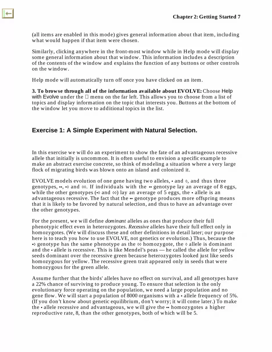
Exercise 1: A Simple Experiment with Natural Selection.
In this exercise we will do an experiment to show the fate of an advantageous recessiveallele that initially is uncommon. It is often useful to envision a specific example tomake an abstract exercise concrete, so think of modeling a situation where a very largeflock of migrating birds was blown onto an island and colonized it.
EVOLVE models evolution of one gene having two alleles, • and ◊, and thus threegenotypes, ••, •◊ and ◊◊. If individuals with the •• genotype lay an average of 8 eggs,while the other genotypes (•◊ and ◊◊) lay an average of 5 eggs, the • allele is anadvantageous recessive. The fact that the •• genotype produces more offspring meansthat it is likely to be favored by natural selection, and thus to have an advantage overthe other genotypes.
For the present, we will define dominant alleles as ones that produce their fullphenotypic effect even in heterozygotes. Recessive alleles have their full effect only inhomozygotes. (We will discuss these and other definitions in detail later; our purposehere is to teach you how to use EVOLVE, not genetics or evolution.) Thus, because the•◊ genotype has the same phenotype as the ◊◊ homozygote, the ◊ allele is dominantand the • allele is recessive. This is like Mendel’s peas — he called the allele for yellowseeds dominant over the recessive green because heterozygotes looked just like seedshomozygous for yellow. The recessive green trait appeared only in seeds that werehomozygous for the green allele.
Assume further that the birds' alleles have no effect on survival, and all genotypes havea 22% chance of surviving to produce young. To ensure that selection is the onlyevolutionary force operating on the population, we need a large population and nogene flow. We will start a population of 8000 organisms with a • allele frequency of 5%.(If you don’t know about genetic equilibrium, don’t worry; it will come later.) To makethe • allele recessive and advantageous, we will give the •• homozygotes a higherreproductive rate, 8, than the other genotypes, both of which will be 5.

8 EVOLVE Manual
Setting up the Experiment
☛ Look for a window similar to Figure 2-1 below. If you do not see one, pull downthe File menu and select New Problem, then click on the New button.
Figure 2-1. Problem Selection Window. This windowappears when you start EVOLVE or when you select the NewProblem command from the Fi le menu.
☛ Click on Sel. for recessive allele, and then Start Problem. You should see thefollowing window:
Trial PopUp Graph Controls
Graph
Data Table
Problem Control Buttons
Notepad icon
Pane Control
Figure 2-2. Problem Summary Window. This windowallows you to run and stop experiments, and display theirresults.
We will refer to the labels in this picture throughout this tutorial.
Chapter 2: Getting Started 9
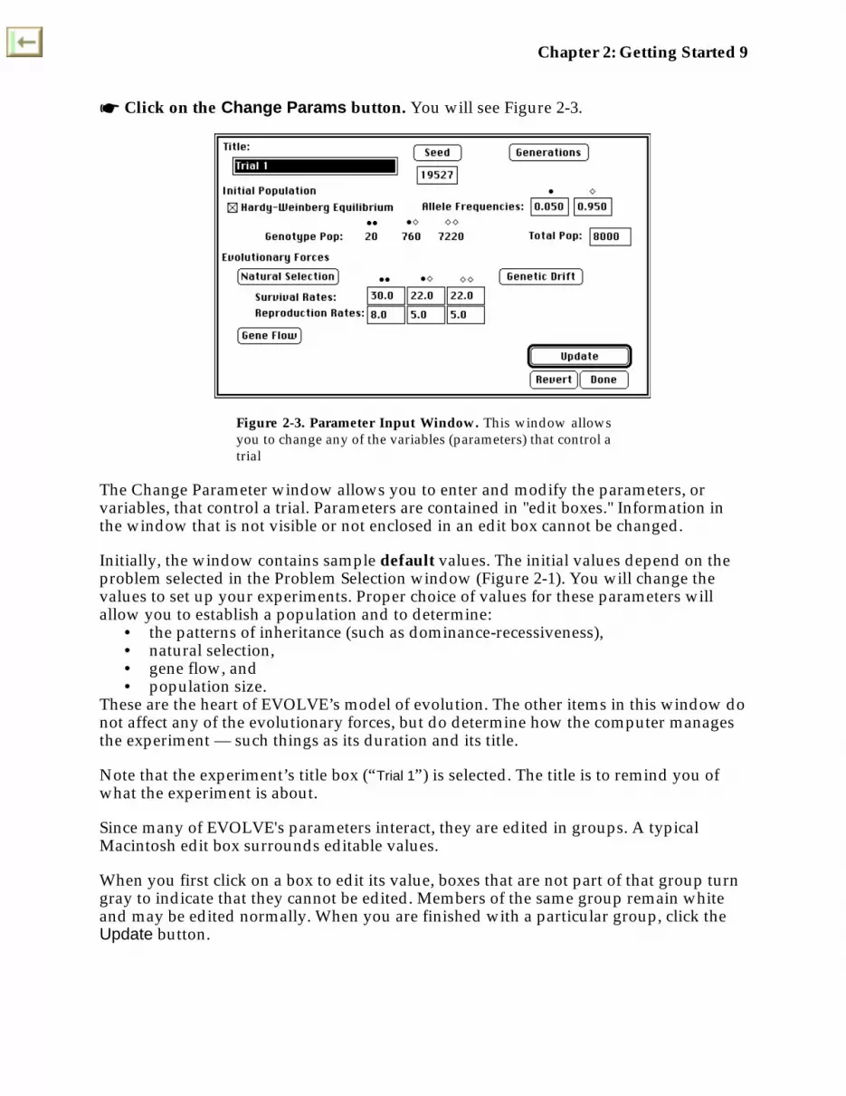
☛ Click on the Change Params button. You will see Figure 2-3.
Figure 2-3. Parameter Input Window. This window allowsyou to change any of the variables (parameters) that control atrial
The Change Parameter window allows you to enter and modify the parameters, orvariables, that control a trial. Parameters are contained in "edit boxes." Information inthe window that is not visible or not enclosed in an edit box cannot be changed.
Initially, the window contains sample default values. The initial values depend on theproblem selected in the Problem Selection window (Figure 2-1). You will change thevalues to set up your experiments. Proper choice of values for these parameters willallow you to establish a population and to determine:
• the patterns of inheritance (such as dominance-recessiveness),• natural selection,• gene flow, and• population size.
These are the heart of EVOLVE’s model of evolution. The other items in this window donot affect any of the evolutionary forces, but do determine how the computer managesthe experiment — such things as its duration and its title.
Note that the experiment’s title box (“Trial 1”) is selected. The title is to remind you ofwhat the experiment is about.
Since many of EVOLVE's parameters interact, they are edited in groups. A typicalMacintosh edit box surrounds editable values.
When you first click on a box to edit its value, boxes that are not part of that group turngray to indicate that they cannot be edited. Members of the same group remain whiteand may be edited normally. When you are finished with a particular group, click theUpdate button.

10 EVOLVE Manual
☛ Make sure that “Trial 1” in the Title rectangle is highlighted. If you clickedelsewhere by mistake and Trial 1 is not highlighted, use the mouse to select itbefore typing. Type: Trial 1- Sel For Recessive . If you make a typing error, usethe [delete], [ ], and [ ] keys and correct the error. Click on the Update button.
Note that when you update the window, the gray areas disappear. You should alwaysbe sure to enter a brief, descriptive title for your experiments. You will eventuallyaccumulate many different experiments and their titles will help you keep themstraight.
There is much to discuss about this window, but we will come back to it later. Now youshould actually run the experiment.
☛ Click on the Done button to return to the summary window.
Doing the Experiment
☛ Click on the Start button in the lower right-hand corner of the window. Notethat it changes to Stop.
While the experiment is running, the window will develop into something resemblingFigure 2-4.
Figure 2-4. Summary Window after Trial 1. When EVOLVEhas finished the experiment for Trial 1, your summary windowshould look like this.
Note that the display in Figure 2-4 shows a graph of the frequencies of each allele on thevertical axis, with time on the horizontal axis. There is also a table showing numericsummaries of each generation. As the experiment proceeds, the graph is updated,

Chapter 2: Getting Started 11
If you wish to pause for thought or discussion, or if you realize you have made amistake, press the Stop button. It changes to Continue, If you wish to display other graphsof current results, or start another experiment, you may do so, If you decide to continuea stopped experiment, click on the Continue button (you may not, however, exceed themaximum number of generations).
Before EVOLVE runs an experiment, you should try to predict what will happen on thescreen. Predicting the results of experiments is an essential part of science and youshould practice it whenever you can.
Looking at Results
Once the experiment is finished, you can examine the results in a variety of ways.
☛ Click on the Change Params button.
This returns to the parameters window (see Figure 2-3), which shows the parametersyou entered before you ran the trial. Note that the initial population parameters cannotbe changed (they do not have edit boxes around them) after the trial has been started. Ifyou forget the experiment’s initial inputs, you can go back to this window and refreshyour memory. You may also change some of the values and continue the trial.
☛ Click on the Graph menu and hold the mouse button down. Note that there arecheck marks beside the frequency of each allele plotted on the graph.
☛ Select Frequency • Allele; it is removed from the graph. Select it again and itreappears.
☛ Select Frequency of •◊ Genotype . This adds the check mark and the line on thegraph. The menu and graph should look like Figure 2-5.
Figure 2-5. Menu and Graph of allele and heterozygote genotype frequencies vs time.

12 EVOLVE Manual
There is a considerable amount of information to be gleaned from comparison of graphssuch as this and it will take you some time to become proficient in extracting all thatthere is to be seen. At this time we will just mention a few significant points.
☛ Point to the •Freq heading of the data table and hold the mouse button down.The line on the graph corresponding to the frequency of • allele remains black,and the others become gray. Point and press on the other column headings inturn (scroll the window to the right, or enlarge the window to see hiddencolumns). Each time, the appropriate line appears black and the others dim togray. If a variable is not on the graph, it appears as long as the mouse button isdown.
☛ Click slowly three times on the gridded box, , next to the BackgroundGraphs pull–down menu. This toggles grid marks on the graph.
You should be able to describe what happened in graphs such as these. A fulldescription of this graph might include the following points:• The frequency of the recessive • allele was initially low (about 0.05, or 5% in
generation 1) and climbed relatively slowly.• After roughly generation 20, the • allele reached 20% allele frequency.• It then rose more rapidly, becoming the most common allele after about generation
30.• After about generation 35, its rate of increase of the • allele slowed abruptly as its
frequency approached 100%.• The dominant, but disadvantageous, ◊ allele followed a mirror-image path and was
almost extinct in generation 50.• The frequency of the heterozygotes peaked just below 50% when the alleles were
equally common.
Note that your results will differ slightly from those shown in this manual. EVOLVEincorporates the randomness of evolution, hence each run will differ from others. Thedegree of difference will depend on a number of factors and will be discussed later. Forthis example, you should see little difference.
You can’t see precise details on graphs such as this, but you can scroll back through theResults table in the Summary Window if you want to look at specific generations orfrequencies. Here's how:
☛ Click on the pane control, hold the mouse button down, and drag the blackrectangle up. The data table is dragged up revealing a scroll bar. The graphbecomes shorter to accommodate the table.
You can now scroll through the data table to see exact figures for each generation.
☛ Scroll vertically until you can see the generations after 30.
Now you can see when the heterozygote frequency (•◊ Freq) peaked (roughly 46%around generations 35 in our trial). There are theoretical, mathematical reasons why theheterozygotes peaked, and the homozygotes crossed, at the time the allele frequencies
Chapter 2: Getting Started 13
crossed. They are worth discussing with fellow students or your instructor, but we willnot elaborate here.
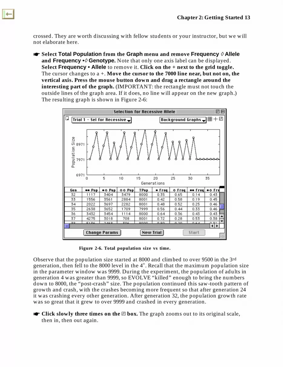
☛ Select Total Population from the Graph menu and remove Frequency ◊ Alleleand Frequency •◊ Genotype. Note that only one axis label can be displayed.Select Frequency • Allele to remove it. Click on the + next to the grid toggle.The cursor changes to a +. Move the cursor to the 7000 line near, but not on, thevertical axis. Press the mouse button down and drag a rectangle around theinteresting part of the graph. (IMPORTANT: the rectangle must not touch theoutside lines of the graph area. If it does, no line will appear on the new graph.)The resulting graph is shown in Figure 2-6:
Figure 2-6. Total population size vs time.
Observe that the population size started at 8000 and climbed to over 9500 in the 3rd
generation, then fell to the 8000 level in the 4th. Recall that the maximum population sizein the parameter window was 9999. During the experiment, the population of adults ingeneration 4 was greater than 9999, so EVOLVE “killed” enough to bring the numbersdown to 8000, the “post-crash” size. The population continued this saw-tooth pattern ofgrowth and crash, with the crashes becoming more frequent so that after generation 24it was crashing every other generation. After generation 32, the population growth ratewas so great that it grew to over 9999 and crashed in every generation.
☛ Click slowly three times on the box. The graph zooms out to its original scale,then in, then out again.

14 EVOLVE Manual
Examine any of the various graphs as much as you wish. If you have time, and haveread through Chapter 3, you may go on to the exercises in Chapter 4. If not, leaveEVOLVE as follows.
Leaving EVOLVE
☛ Select Quit from the File Menu. EVOLVE will quit and return you to the Mac’sdesktop. You will be given an opportunity to save your data. Click on the Quitbutton.
This completes our first quick look at EVOLVE. If you wish to continue exploring howto use EVOLVE, turn to Chapter 3. If you wish to examine some of the backgroundconcepts that lie behind EVOLVE, jump to Chapter 4, then come back to Chapter 3.

Chapter 3: MORE ADVANCED FEATURES OF EVOLVE 15
Chapter 3. More Advanced Features of EVOLVE
Introduction: Doing Experiments with EVOLVE
In the last two chapters we introduced you to the most basic uses of EVOLVE — settingup an experiment, running it, and looking at the results — and to some backgroundinformation on the conceptual design of EVOLVE’s model of evolution. In this chapterwe will build on those foundations, showing you some additional features of EVOLVEin the context of answering evolutionary questions by comparing a series ofexperiments.
Before jumping into experiments, however, it is important that you put experimentsinto their proper context. Experiments should not be done haphazardly; they should bedone in the context of a specific question (see Figure 3-1). The question should be ratherspecific and you should set up a set of at least two experiments to test it. One or moreexperiments should be designated “controls,” and used for comparisons with theother(s). You should also try to predict what the results will be in rather specific terms.
Analyze,Compare Results
AskQuestion
Design Set of ExperimentsDesignate control & experimental
runs, predict results
Do Set of Experiments
AnswerQuestion
Display results, store set & retrieve results
Figure 3-1. Outline of an EVOLVE session. Rectangularboxes represent actions performed using EVOLVE; roundedboxes and ovals show where user thought is involved.
After the experiments are designed, you will set up the first one and then do theexperiment. Once the results are in, you may want to store them in EVOLVE’s Notepad.You will then revise the evolutionary situation and do the next experiment. Comparingthe results of the experiments may lead you to revise and refine your experiments ormay give you enough information to answer your original question. Often, of course,

16 EVOLVE Manual
the answer to the original question will suggest additional questions and the cycle willrepeat.
With this additional perspective, in Exercise 2 you will be taken through the process ofanswering a question about the effect of population size on evolution. In Exercise 3, youwill investigate the effects of random factors on EVOLVE’s results (and evolution).Finally, in Exercise 4 you will be shown how to model more complex evolutionarysituations by changing the values of EVOLVE’s input parameters during a run.
Exercise 2. Comparing Selection in Small and Large Populations.
An important question in evolutionary biology has been, “what are the effects ofpopulation size on the evolution of populations?” A thorough answer to this questionhas required decades of work by many biologists, and some aspects of the answer arestill controversial. However, you can get a feel for some of the effects with a fewexperiments using EVOLVE.
As phrased, the question is a bit too general. Let us start by making it more specific.Since we have already done one experiment that provided data on natural selection in apopulation of 8000-10,000, let us answer the more limited question: “Does selection for arecessive allele proceed differently in a small population of 80-100 individuals than in alarge population of 8000-10,000?” Note that this rephrasing of the question essentiallycompletes the process of designing the experiment.
There remains only the prediction — how do you think the two experiments willcompare? If you believe that selection will operate the same in the two populations andthat population size has no effect, you might predict that the genotype frequencygraphs of the two experiments will be identical.
We will start with the experiment from Chapter 2. You will modify it to keep thepopulation small, run the experiment, and compare the first and second experiments.Finally, you will make a third run to observe random effects.
☛ If you do not have EVOLVE running, start it up just as you did in Chapter 2.
☛ If you just restarted EVOLVE, rerun Exercise 1. While the experiment isrunning, read on.

Chapter 3: MORE ADVANCED FEATURES OF EVOLVE 17
Redoing the Experiment with Variations.
To redo the first exercise with a smaller population, we will need to keep the survivaland reproduction rates the same, but change the factors related to population: the initialpopulation, maximum population, and post-crash size. We should also change the titleto distinguish this from other experiments.
☛ Click New Trial. The graph for Trial 1 becomes gray and the trial popup changesto "Trial 2."
☛ Click Change Parameters. If you have reached this point directly after doingExercise 1, the values in most of the boxes will be the same as in that experiment.If you have started EVOLVE again, then you will have to re-enter some of thevalues.
☛ Change the title to a convenient title, such as "Trial 2 Rec, small."
This reflects the fact that selection still favors the recessive allele and the population willbe small (between 80 and 100).
Now we'll look more closely at EVOLVE's error checking and help system.
☛ Click after the last zero in the 8000 of total population and press the [delete]key (or [backspace]) once to make it 800, then click on Update.
Note that the numbers of the genotypes change to reflect the reduced population.
EVOLVE checks the values you enter and will alert you if it detects any mistakes. To seewhat happens. make the following “mistake.”
☛ Change the Total Population parameter to 10000, then click on Update. Youwill hear a beep and a box will appear informing you that the value you enteredis “out of range” and that you should check the help messages for specifics. Clickon the OK button.
To learn the help system and find out what the possible values are for total population,do the following:
☛ Delete one zero, click the Update button, then the Done button to return to thesummary window. Select Help with EVOLVE… from the Apple ( ) menu.Scroll the window down past the Parameters Window until you see InitialPopulation. Click on Initial Population, then click on the Open button.
You will see some notes about the initial population, including the fact that the initialpopulation cannot total more than 9000.
☛ Click on the window's close box to return to the summary window and clickon the Change Params button to return to the parameters window.

18 EVOLVE Manual
The starting frequency of the • allele will be the same as in Exercise 1.
☛ Now click on the Genetic Drift button to show maximum and post-crashpopulation sizes. Change the post-crash size to 100 and the maximumpopulation to 80.
All of this is important because we will be comparing the results of our second run withthose of the first run — the first run will be our experimental “control.” If the onlydifference between the two experiments is size of population, then we can more easilydraw valid conclusions. If there were other differences, for example, if the post-crashsize was not eight-tenths of the maximum, we could not be sure that differences inresults were due to differences in population size. The ratio of post-crash size tomaximum population might have an effect.
☛ Check to make sure the other parameters are the same as those in Figure 2-2and fix any that are not. Click on the Done button, then the Start button tostart the experiment. As the lines march across the graph, try to predict whatwill happen next.
☛ When the experiment is finished, compare the allele frequency graphs from thetwo exercises.
Notice that while the trace of the small population (in black) is more jagged than thegray lines of the large population, it generally follows the same pattern of relativelygradual change, then rapid change. Your own graph may differ significantly from thatof the 1st trial.
☛ Compare plots of genotype frequency for both experiments.
Again, the two graphs are quite similar in overall shape, although the smallpopulation’s curves fluctuate a good deal more. We should note that there are moresophisticated ways to compare these curves quantitatively, and if you are an advancedstudent your instructor may have you make such comparisons. However, our purposehere is to accustom you to comparing different runs, not statistical curve fitting, so wewill make only qualitative comparisons.
☛ Plot total population size.
Compare the two populations. You will need to zoom in or change the front-most trialin the Trial popup to see the second one.
☛ Plot number of •• homozygotes and number of ◊◊ homozygotes
Notice that there are periods early in the experiment when the •• genotype did notoccur in the population. Not until later did the •• genotype return for keeps. Similarly,the ◊◊ homozygotes often decline to zero, then reappear before disappearing for good.Homozygotes, after all, may be generated by matings between heterozygotes, evenwhen the rare allele is too rare for significant numbers of homozygotes to mate witheach other and reproduce.

Chapter 3: MORE ADVANCED FEATURES OF EVOLVE 19
☛ Do a 3rd trial with maximum pop = 50 and post-crash = 40. How does this differfrom the previous 2 experiments?
☛ Click the New Trial button, then Continue. Do this 5 or 6 times. This shouldgive you a better idea of the effects of randomness in a small population.
Moving Results to Paper and Elsewhere
A major aspect of BioQUEST (and of science in general) involves persuading peers ofour conclusions. There are several ways to move EVOLVE’s results into other programsand to paper. Not only can you obtain printed results, “hardcopy” in computer jargon,but you can use EVOLVE’s results as input to other programs such as spreadsheets,statistics programs, and especially word processors.
Some of you may not have a printer connected to your computer. If so, don’t worry,you can do the vast majority of your work without one. If you really need a summary orcopies of graphs and don't have a printer, you may save screens to disk files, take thedisk to a computer that does have a printer, and print your results there.
If you do have a printer, the Notepad is more convenient. Here is the procedure forusing and printing the notepad.
☛ Select Copy Window Graph from the Edit menu. The graph is copied to theclipboard.
☛ Click on the small icon in the upper left-hand corner of the summary window.This opens EVOLVE’s Notepad window where you can paste the contents of theclipboard and can also type in your own notes.
☛ Select Paste from the Edit menu. The graph appears in the Notepad Window.
☛ Type a few words commenting on the graph. The text appears and can be editedin standard Macintosh fashion.
☛ Make sure you have used the Chooser to select a printer and that the printer isturned on. Select Print Notepad from the File menu. The contents of thenotepad are printed.
While the notepad is convenient, this version of EVOLVE cannot save it when you quitthe program. You can copy and paste data into word processors, spreadsheets, andstatistical packages with the Copy Window Data command in the Edit menu (it cannotbe pasted into the Notepad). Graphics can be copied into word processors andprograms that edit graphics. You may also use the Macintosh Scrapbook to savegraphics and data, then paste them into other programs.
20 EVOLVE Manual
Finally, the Save Window Data… command in the File menu will save the entirecontents of the data table to a text file that may be opened by a spreadsheet or statisticalpackage.
EXERCISE 3. Comparing Runs with Different Random Numbers
This exercise is designed to provide an illustration of how randomness may affectevolution. Any experiment is subject to variations, especially experiments with smallpopulations. We will rerun Trial 2, a second time to look at some random effects.
Before we do that, we need to remove the clutter of Trial 1.
☛ Point to the Background Graphs box and press the mouse button. A list oftrials pops up. Trial 1 appears with a check beside it. Select "Trial 1" and it isunchecked and its lines vanish from the graph.
☛ Click on the New Trial button and the Change Parameters button. The Trialnumber changes and the graph lines become gray. All of the parameter valuesexcept title remain the same.
☛ Click on the Seed button. A number appears that is the "random number seed"for this trial. The computer uses it to simulate random mating, the effects ofweather, and other “random” factors. EVOLVE will pick a different seed for eachtrial, or you can type a seed in if you wish. If you use the same seed in differentexperiments you can be sure that any variations in output are caused by changesin other variables. If you use different seeds with no change in other parameters,you can assess the influence of chance. In essence, this amounts to running thesame experiment again. A final point — if you have a trial that you wish torepeat exactly (e.g., to show your instructor), copy the seed along with the otherparameter values. A thorough understanding of the seed is not necessary for youto use EVOLVE, but a more thorough discussion is available in Chapter 8 of theUser's Manual.
☛ Click on the Done button, then the Start button to run the new trial.
Were the results what you expected? This phenomenon of random fluctuations ofgenotype and allele frequencies in small populations is an important, controversialevolutionary force called “genetic drift.” You should run additional trials to get a feelfor the variability of results. Obviously, chance can have a significant influence onevolution.

Chapter 3: MORE ADVANCED FEATURES OF EVOLVE 21
EXERCISE 4. Changing the Evolutionary Situation During a Run
One of the simplifications often made in modeling evolution is to assume that theevolutionary forces are constant, that is, the environment doesn’t change. Obviously,this is a gross oversimplification and EVOLVE will let you get around it by changingdata values during a run. In this final exercise of our tutorial, you will see how to dothis.
Suppose you wished to simulate a drastic drop in population size, such as would occurif there was a catastrophe like a flood that killed most of a population and reduced theirfood supply for a couple of years. This would simulate what is sometime called the“bottleneck effect.” In this scenario, 30 individuals are assumed to survive a disasterfrom a large population having both alleles in equal abundance. The alleles are assumedto be selectively neutral.
☛ Set up an experiment with the following data values (note that only 39generations are to be done) and then run the experiment:
Title: Ex. 4 - The Bottleneck EffectPost-crash size: 8000
Run to generation: 40Genotypes
• • • ◊ ◊ ◊Initial population: 2000 4000 2000
Survival rates: 22 22 22Reproductive rates: 5 5 5Immigrat., emigrat.: 0 0 0
☛ When the 40 generations are finished, click on the Change Parameters buttonand revise the parameters as follows:
Carrying capacity: 50Post-crash size: 30Run to generation: 43
☛ When EVOLVE stops in generation 43, go back and return the variables to thefollowing:
Carrying capacity: 9999Post-crash size: 8000Run to generation: 100
☛ Compare the graphs of allele frequency and total population size.
The allele frequencies changed relatively little during the first 40 generations when thepopulation cycles between 8000 and 10,000; during the 3-generation crash, however, the

22 EVOLVE Manual
allele frequencies “drifted” away from 0.50. Subsequently, as the population grew back,the generation-to-generation fluctuations tapered off.
The final population was different from the original because 1) the founders of the“new” larger population were a small sample from the original large population and 2)while the population was rebuilding, drift continued to operate, albeit to a lesser degreeas the population size increased.
This completes our tutorial on EVOLVE. We hope you have enjoyed learning to playthe game and will use it extensively enough to get a good feel for the interaction ofevolutionary forces. The next chapters list a series of exercises that will help you useEVOLVE to explore a variety of evolutionary phenomena. The last two chapters containadditional information on setting up experiments and on population genetics; don’toverlook them, for they provide more guidance on evolution and on EVOLVE.

Chapter 4. Background
Now that you have some feel for the way EVOLVE works, we must take time to go oversome fundamental concepts and background so you can make more effective use of it.As mentioned in the Introduction, simulations such as EVOLVE have a largemathematical component, and you should eventually work through the material inChapters 7 and 8. However, EVOLVE can be used effectively at an introductory levelwithout such details, for it embodies an intuitively simple, yet realistic, model ofevolution. The purpose of this chapter is to give you a better intuitive feel for EVOLVEand some of the fundamental genetic and evolutionary concepts behind it.
Also, while many evolutionary situations may be simulated with EVOLVE, it haslimitations, and you must understand the nature of the hypothetical population. Thenext sections discuss the genetic concepts and hypothetical organisms on whichEVOLVE is built; that is, the assumptions inherent in the program.
The Hypothetical Organisms
EVOLVE is not based on any particular animal or plant, but on a hypothetical organismwith several characteristics that make it useful for the sorts of experiments you will bedoing. The organisms live in a discrete habitat such as an island, lake, or mountain top,separated from other patches of habitat, and form a single local population withinwhich mating is random. The individuals in the population are diploid hermaphroditesand produce both eggs and sperm. Each adult normally mates with (or is pollinated by)one other adult at random and both produce offspring. If there is an odd number ofadults in the population, the last individual fertilizes itself. While this characteristic ofthe model population may seem odd, it avoids complications of sex-ratios and matingpatterns. Actually, this sort of population is fairly common among plants and evenexists in a few animals.
The life cycle of the hypothetical organism is a simple one (see Figure 4-1 for an outlineof the life cycle as it relates to EVOLVE’s simulation). During the short breeding season,all adults mate, produce offspring, and die. All members of the next generation hatch(are born, released as seeds, or whatever) during a short time. The young then matureover a period of time during which they may die or emigrate (fly, walk, blow or becarried away). At the end of the juvenile period all surviving individuals become adultsand some additional adults may immigrate from surrounding populations, or adultsmay emigrate, leaving the population. You may find it convenient to think of theorganism as having a one-year life cycle and generation time. You may specify any orall of the survival, reproduction, emigration, and immigration parameters for each ofthe three genotypes.

24 EVOLVE Manual
Enter Data: Initial PopulationReproductive Rates% EmigratingMax. Pop. Size
Survival Rates# ImmigratingPost-crash Size
Mating: Randomly mate adults
Reproduction: Determine number of young of each genotype
Remove emigrants
Emigration:
Adults dieSurvival:
Add immigrantsImmigration:
Is the number ofadults above Max.
Pop. Size?
Reduce Populationyes
no
ADULT POPULATION
Is Experiment finished?
no
yes
Stop
Figure 4-1. Outline of EVOLVE’s simulation and thehypothetical life cycle.
Given the above life cycle, the population usually will either grow or decline dependingon the values you give EVOLVE. If the product of percent survival and number ofyoung is greater than 100%, the population will tend to increase in numbers. In order tocontrol the size of the population, you may specify upper and lower bounds to it. If thepopulation of adults exceeds the upper limit, the number of adults is randomly reducedto the lower level. The numbers of each of the genotypes are reduced proportionately,so a population “crash” will not directly affect genotype or allele frequencies. If survivaland reproductive rates result in a negative growth rate (their product is less than 100%),then the population will decline to extinction, regardless of the population size limits. In

Chapter 4: BACKGROUND 25
essence, then, the population may be viewed as living in a finite environment with afixed amount of resources. If the population exceeds the resources, mortality is randomwith respect to genotype.
Note that given the above conditions, all individuals are identical with respect to sexand age, so the hypothetical population used by EVOLVE meets the assumptions ofHardy-Weinberg equilibrium. Mutation does not occur and mating is random. Becauseyou may specify values for all of the other assumptions, you may design a populationthat fits any experiment you want to do on selection, genetic drift, and gene flow. Forexample, since the habitat is a discrete patch, you can make it closed (no gene flow) ifyou wish.
Genetic Concepts Underlying the Model
In genetic terms, EVOLVE deals with a single gene having two alleles, • and ◊, Thusthere are three genotypes: ••, •◊ and ◊◊. The alleles may effect any or all of fourcharacteristics: survival and emigration rates of juveniles, and reproductive andimmigration rates of adults.
Rates of survival, reproduction, immigration, and emigration are not, strictly speaking,phenotypes of organisms in the same way that flower color is for a plant, or vestigialwings are for a fruit fly. Phenotype is classically defined as an observable characteristicof an organism, while the rates used by EVOLVE are statistical characteristics ofpopulations of organisms. Nevertheless, because phenotypes influence the ability of theirowners to survive and reproduce, we might think of the two alleles of our simulation asdetermining the probability of individuals surviving and reproducing. In a similar way,the color of a flower may influence how often insects pollinate it and hence the numberof young produced. Among fruit flies, individuals with vestigial wings cannot fly andget trapped more often in sticky food, hence their survival rate is lower than normalflies. You will find it easier to use EVOLVE if you make up phenotypes appropriate tothe question you are studying and attach them to the genotypes as we did in Chapter 2.
For the purposes of using EVOLVE, use the following definitions to determine thepattern of inheritance.
Dominant alleles produce their full phenotypic effect even in heterozygous condition,Recessive alleles have their full effect only when in homozygous condition. Thus, if the•◊ genotype has the same phenotype as the ◊◊ homozygote, then the ◊ allele isdominant and the • allele is recessive.
Incomplete dominance occurs when the phenotype of the heterozygote is intermediatebetween the phenotypes of the two homozygotes. Reproductive rates of 4, 6, and 8 forthe ••, •◊, and ◊◊ genotypes would simulate incomplete dominance.
Codominance occurs when both alleles produce their effects in heterozygotes. Supposeyou set survival rates to 30%, 30%, and 40% and reproductive rates to 4, 5, and 5

26 EVOLVE Manual
(offspring per adult). The • allele reduces both survival rates and reproductive rates,while the ◊ allele produces higher survival and reproduction. The • allele is dominantwith respect to survival, but recessive with respect to reproduction. The end result isthat both alleles produce their effects in heterozygotes when you consider survival andreproduction together. This is an example of pleiotropy — a single gene has multiplephenotypic effects.
Overdominant alleles produce a heterozygote which is more extreme than eitherhomozygote. If alleles are overdominant with respect to fitness, the terms heterosis orheterozygote superiority are often used. Reproductive rates of 40%, 60%, and 30%would exemplify overdominance and heterosis.
An Example
As an example of the relationship of alleles, genotypes, patterns of inheritance, andphenotypes to survival and reproductive rates, let us consider the gene for sickle-cellanemia. The s allele causes the substitution of valine for glutamic acid at position 6 ofthe beta chain of hemoglobin. People with the SS genotype have hemoglobin that isentirely normal; heterozygous (Ss) individuals have hemoglobin that is a mixture ofnormal and abnormal; those with the ss genotype have hemoglobin that is entirely ofthe sickling type. In this example, the fundamental effect (phenotype, if you will) of thes allele is the production of abnormal beta chains. Thus, at the level of hemoglobinphenotypes, the S and s alleles are codominant (heterozygotes show the effects of bothalleles).
Hemoglobin with s beta chains has reduced solubility under low oxygen concentrationsand tends to crystallize in capillaries. In homozygous ss individuals, sharp crystalsgrow within red blood cells, causing them to take the distorted sickle-shape that givesthe disease its name. The distorted blood cells interfere with circulation and cause avariety of unpleasant symptoms that usually result in painful death before puberty.Heterozygous individuals with the Ss genotype do not typically show any of thesymptoms of the disease, although their red blood cells will show some sickling undercertain conditions and they are said to have “sickle-cell trait.” Thus, the diseasephenotype and the s allele may be regarded as recessive to the “normal” phenotypeproduced by the S allele.
None of the phenotypes discussed above could be input for EVOLVE. Rather, thereduced survival of ss homozygotes would be modeled by giving ◊◊ individuals alower survival rate than •• and •◊ individuals. Again, note that EVOLVE incorporatesthe statistical effects of phenotypes on reproduction and survival, not the phenotypesthemselves.
No assumptions have been made as to the mode of inheritance of the characteristics ofthe three genotypes used by EVOLVE. By choosing suitable parameters you maysimulate any pattern of inheritance possible at a gene with two alleles. For the sickle-cell

Chapter 4: BACKGROUND 27
example, setting survival rates to 80%, 80%, and 0% for the ••, •◊, and ◊◊ genotypesrespectively would simulate the recessive lethal nature of the sickle-cell allele.
It should be clear by now that the distinctions between these different modes ofinheritance of phenotypes are somewhat arbitrary and not always clear-cut. In usingthese terms, we are dealing with patterns of inheritance of phenotypes, rather than thenature and function of genes at the molecular level. Because most (probably all) geneshave multiple effects, alleles may be codominant at the molecular level, dominant withrespect to one phenotype, recessive with respect to another, and heterotic for a third.EVOLVE simplifies this complexity by looking at the net effects of genes on survivaland reproductive rates.
Again, the sickle-cell allele is an instructive example. As discussed above, the twoalleles are codominant at the molecular level, but with respect to the disease phenotype,the s allele is recessive (the S allele is dominant). The s allele would seem to bedisadvantageous, and you might expect it to decline in frequency and eventuallybecome extinct (save for new mutations). However, the situation becomes morecomplicated and interesting when you consider additional information.
As you may know, the s allele occurs at a high frequency (over 20%) in somepopulations. Research has shown that such populations have a high incidence ofmalaria, and that heterozygous Ss individuals, those with sickle-cell trait, have a greatertolerance to malaria than homozygous SS individuals. Here is a summary of thegenotypes and their phenotypes as discussed so far:
Genotype Phenotype SS Ss ss
Hemoglobin Normal Mixture Sickle-cellBlood Normal Sickle-cell trait Sickle-cell anemia
Malaria Susceptible Resistant ResistantSurvival rate Low High Essentially zero
Note that, with respect to malarial resistance, the s allele is dominant andadvantageous, but with respect to hemoglobin phenotype, it is a deleterious recessive.Overall, the s allele displays heterosis (is “overdominant”) with respect to survival.
You might model such a population with the following inputs to EVOLVE:
Genotype Phenotype SS Ss ss
Survival Intermediate Highest Essentially zeroReproduction High High Essentially zero
(You might expect reproductive rates of Ss individuals to be somewhat lower thanthose of SS individuals, because 25% of the children of two heterozygotes would die ofsickle-cell anemia. However, it appears that such parents often have more children tomake up the difference.)

28 EVOLVE Manual
In an environment without malaria, however, the following would be an appropriatetable:
Genotype Phenotype SS Ss ss
Hemoglobin Normal Mixture Sickle-cellBlood Normal s-c trait Sickle-cell anemia
Malaria IrrelevantSurvival rate High High Essentially zero
You could model such a population with the following inputs to EVOLVE:
Genotype Phenotype SS Ss ss
Survival High High Essentially zeroReproduction High High Essentially zero
Thus, in a malaria-infested environment the sickle-cell allele is advantageous inheterozygotes and shows heterosis with respect to survival. As you will see later, allelesshowing heterosis tend to remain in a population no matter how deleterious they are inhomozygous condition. In a malaria-free environment the allele is recessive anddeleterious with respect to survival. In the latter environment, you would be correct inexpecting it to decrease in frequency.
The Nature of Evolutionary Fitness
Evolutionary biologists’ use of the term fitness differs significantly from common usage.It might have been better if someone had invented a long Latin word for this concept,for people would be more cautious about assuming they know its meaning. Instead,people assume that evolutionary fitness is like athletic fitness — robustness, strength,endurance. Instead, we will define evolutionary fitness as the ability of an allele or agenotype to gain representation in the next generation because of the ability of its phenotype tosurvive and reproduce. Because it is critical that you understand this definition and itsimplications, both to understand the behavior of EVOLVE and to understand evolution,we will spend some time discussing it.
The detailed measurement of the fitness of an allele in nature is difficult, for it requiresunderstanding genotype frequencies and the probabilities of different matings, alongwith survival and reproductive rates. If you work your way through the more advanceddiscussion of absolute and relative fitness in Chapters 7 and 8, you will come tounderstand this clearly. For now, note that evolutionary fitness involves bothreproduction and survival; you cannot look at either one alone. Thus, the evolutionaryfitness of a genotype, and its evolutionary fate, may have nothing to do with whetherthe organism is strong, swift, or “red in tooth and claw” if that organism does notreproduce. In some situations, slight, fragile individuals, even those with seemingdeficiencies, may have higher fitness than normal or more robust individuals.
Chapter 4: BACKGROUND 29
In caves, for example, eyes are a decided handicap, for they are potential sites ofinfection and require calories and nutrients to grow and maintain. Since foodavailability in caves is usually limited, individuals with mutations tending to reduceeye size would have higher survival rates. This could lead to higher reproductive rates,because the physiological effort saved from growing and supporting eyes could be putinto egg or sperm production. Therefore, individuals with reduced eyes would havehigher fitness than those with normal eyes. In time, the population would come toconsist of eyeless individuals.
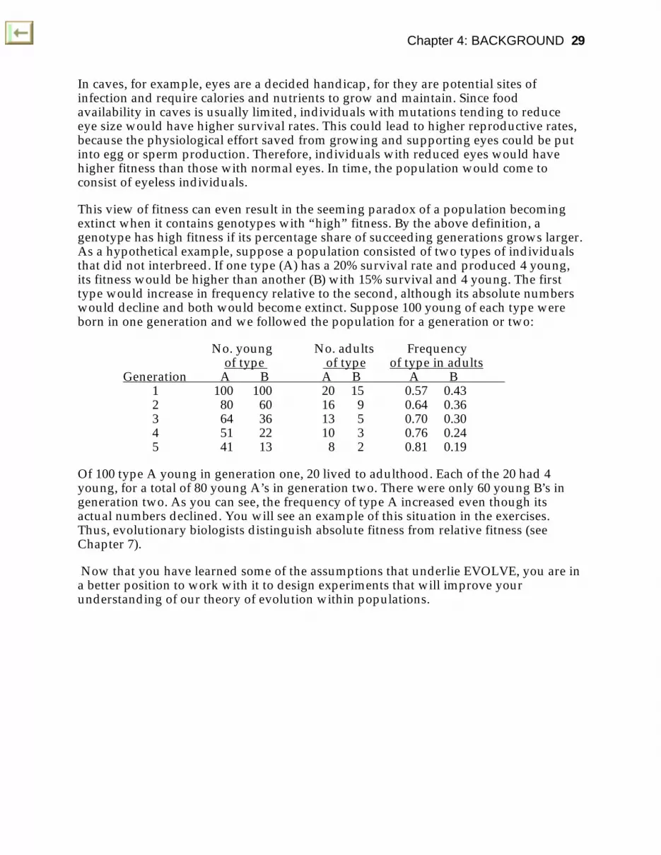
This view of fitness can even result in the seeming paradox of a population becomingextinct when it contains genotypes with “high” fitness. By the above definition, agenotype has high fitness if its percentage share of succeeding generations grows larger.As a hypothetical example, suppose a population consisted of two types of individualsthat did not interbreed. If one type (A) has a 20% survival rate and produced 4 young,its fitness would be higher than another (B) with 15% survival and 4 young. The firsttype would increase in frequency relative to the second, although its absolute numberswould decline and both would become extinct. Suppose 100 young of each type wereborn in one generation and we followed the population for a generation or two:
No. young No. adults Frequency of type of type of type in adults
Generation A B A B A B 1 100 100 20 15 0.57 0.432 80 60 16 9 0.64 0.363 64 36 13 5 0.70 0.304 51 22 10 3 0.76 0.245 41 13 8 2 0.81 0.19
Of 100 type A young in generation one, 20 lived to adulthood. Each of the 20 had 4young, for a total of 80 young A’s in generation two. There were only 60 young B’s ingeneration two. As you can see, the frequency of type A increased even though itsactual numbers declined. You will see an example of this situation in the exercises.Thus, evolutionary biologists distinguish absolute fitness from relative fitness (seeChapter 7).
Now that you have learned some of the assumptions that underlie EVOLVE, you are ina better position to work with it to design experiments that will improve yourunderstanding of our theory of evolution within populations.


Part 2. Experimenting with Evolution
These chapters are designed to give you a sampling of exercises that will enable you tomore easily realize the major goals of EVOLVE: a better understanding of evolutionaryprocesses and of how to study them.
This selection of exercises is not complete, nor will it be appropriate for all students; noone is likely to do all of them. Rather, it provides a sample of some of the waysEVOLVE may be used. Each instructor should select some of these exercises to go withothers of his or her own devising. The exercises that may be done with EVOLVE span atremendous range of evolutionary situations. But more than that, answers can bederived using methods of varying degrees of sophistication. The grouping of exercisesinto three chapters should give students some feeling for the open-ended nature ofevolution and of computer models.
Chapter 5 is a relatively intuitive, qualitative examination of Hardy-Weinbergequilibrium, selection, the fate of mutations, drift, and gene flow, along withcombinations of drift with selection and gene flow with selection. In the initialexercises, we provide all inputs to EVOLVE and in succeeding exercises more and moreof the values must be determined by the students. This gradually more difficult seriesof assignments is suitable for high school and freshman or sophomore college students.
Chapter 6 takes a more sophisticated, quantitative approach by having studentsconsider absolute and relative fitness coefficients in explaining EVOLVE’s results, andthe effects of evolution on mean fitness of a population and its growth rate (whatecologists call “intrinsic rate of natural increase”). This chapter concludes with anexercise aimed at getting students to use the literature to find published data on sickle-cell anemia; then they try to model evolution of the sickle-cell allele. Students also cancollect “data” from EVOLVE runs and then examine more abstract plots of change inallele frequency vs allele frequency, or examine allele frequency over time in a samplingof drifting populations with and without selection. Students will begin to get a betterfeel for the statistical nature of evolution. These exercises are appropriate for moreadvanced undergraduate students.
Chapter 7 outlines several statistical approaches to the study of evolution. Plots ofselection coefficients over time allow students to begin to examine the relationship offitness and selection coefficients derived from a priori survival and reproductive rateswith those that can be observed from data on changes in allele and genotypefrequencies over time. EVOLVE provides “field data” from which students try to inferthe pattern of selection. Students can also make statistical comparisons of EVOLVE’sresults with those predicted from deterministic equations of the effect of selection onallele frequency over time, or of the effects of drift on mean and variance of allelefrequency in a sampling of populations. These exercises would be useful formathematically sophisticated upperclass or graduate students.

Chapter 5. Elementary Exercises
This chapter is designed to lead you through elementary experiments with each of theevolutionary forces, singly and in combinations. The first part of the chapterreexamines fundamental concepts; the second looks at Hardy-Weinberg equilibrium inthe context of setting up EVOLVE experiments and reading the results; the thirdprovides a series of exercises that guide you through experiments with singleevolutionary processes; and the final section illustrates how pairs of evolutionary forcesinteract.
Fundamentals
Questions 1-6 below are intended to help you test your understanding of thefundamentals of EVOLVE’s simulation and do not require that you make any computerruns. We strongly recommend that you do these first six questions before you attemptany of the other exercises, because for them we will assume that you know the conceptsinvolved with these first exercises. Your instructor may suggest that you treat this as atake-home quiz after you finish Chapter 4, and have you bring in your answers fordiscussion or grading.
Initial Population
1. Calculate the number of each genotype in a Hardy-Weinberg equilibrium populationof 2330 individuals with an ◊ allele frequency of 0.63; write the number of eachgenotype in the spaces below:
No. •• = ________ No. •◊ = ________ No. ◊◊ = ________
2. Consider an initial population of 448 •• individuals, 1238 •◊ individuals, and 855 ••individuals.
a. What are the frequencies of the alleles?
Frequency of • = ________ Frequency of ◊ = ________
b. Given the allele frequencies you calculated above, determine the numbers of each ofthe genotypes you would expect if the population were in Hardy-Weinbergequilibrium:
No. •• = ________ No. •◊ = ________ No. ◊◊ = ________
c. Is the population in Hardy-Weinberg equilibrium? __________

Chapter 5: ELEMENTARY EXERCISES 33
Survival and Reproductive Rates
For Questions 3-6, use the following data. The tables below show possible survival andreproductive rates for five “runs” of EVOLVE. Survival rates are measured in terms ofpercent of each genotype surviving from birth (or hatching, germinating) toreproductive age. Reproductive rates are measured as the average number of youngborn per individual of each genotype.
a. Genotype b. GenotypePhenotype •• •◊ ◊◊ •• •◊ ◊◊Surviv. rate 25.0% 25.0% 20.0% 50.0% 30.0% 30.0%Reprod. rate 3.0 3.0 3.0 2.0 3.0 3.0
c. Genotype d. GenotypePhenotype •• •◊ ◊◊ •• •◊ ◊◊Surviv. rate 40.0% 40.0% 58.0% 12.0% 18.0% 24.0%Reprod. rate 1.0 2.0 3.0 9.0 9.0 9.0
e. Genotype f. None of abovePhenotype •• •◊ ◊◊Surviv. rate 60.0% 75.0% 65.0%Reprod. rate 2.0 1.0 1.0
3. In which of the tables is • dominant for survival rate?
a. b. c. d. e. f.
4. In which of the tables is • recessive for reproductive rates?
a. b. c. d. e. f.
5. In which of the tables are • and ◊ heterotic for survival rate?
a. b. c. d. e. f.
6. In which of the tables do the alleles show incomplete dominance for reproductiverates?
a. b. c. d. e. f.
Hardy-Weinberg Equilibrium
These next two exercises will illustrate what is required of you and give you anintroduction to the whole process. In particular, note the way the parameter values areset up, and how to examine the graphs of results and the types of questions asked.Also, note that for each question we have made one or more predictions about the

34 EVOLVE Manual
outcome of our experiments with EVOLVE. Subsequent exercises are more abbreviatedto encourage you to develop skill in using the program and in investigating problems.
You may wish to make several runs with each set of parameters. Note that there is to beno gene flow, nor will you need to change parameters during a run.
If you are uncertain about allele and genotype frequencies and how to calculate them,read appropriate sections of your text or in Chapter 9 of this manual. Also, if you donot understand the Hardy-Weinberg Law (better referred to as “Equilibrium”), consultyour text or read Chapter 9 in this manual.
Exercise 5. How Long Does It Take To Establish Hardy-WeinbergEquilibrium Starting with a Population That Is Not in Equilibrium?
Experiment and Prediction: A population in obvious disequilibrium would be oneconsisting entirely of heterozygotes. There are other ways to set up such an out-of-equilibrium population; can you think of several? On the basis of what you havelearned in this manual, it would be reasonable to predict that the population wouldreach Hardy-Weinberg equilibrium in one generation. More specifically: the allele andgenotype frequencies would remain stable from generation to generation, and withinone generation the genotype frequencies would approximate p2 for ••, 2pq for •◊, andp2 for ◊◊ .
Experiment: Make an EVOLVE run with the following data and either print asummary of each generation, or examine the appropriate graphs with care:
Title: 5. Estab. of H-W EquilibriumNumber of generations: 10
Carrying capacity: 9999Post-crash pop. size: 8000
• • • ◊ ◊ ◊Initial population: 0 8000 0
Survival rates: 26 26 26Reproductive rates: 4 4 4
Number immigrating: 0 0 0Percent emigrating: 0 0 0
Before you do this experiment, think about what you are being asked to do.
a. What is the frequency of the ◊ allele in the initial population? __________. Whatshould the allele frequency do from one generation to the next? _____________________
b. What should the genotype frequencies be in a population with the above allelefrequency? ••:_______ •◊:_______◊◊: _______

Chapter 5: ELEMENTARY EXERCISES 35
c. Why are the survival and reproductive rates equal for all genotypes?
d. Why is the maximum population set at 9999 and the post-crash size to 8000?
Results: Fill in the following data table from the data table displayed by EVOLVE.These first few exercises contain tables like these to help you learn what to look for inEVOLVE’s output; we will dispense with them later. If your are experienced withspreadsheets, you can also use Copy Window Data to copy the data to the Mac'sclipboard. Then Paste the results into a spreadsheet and generate the tables below withthat program.
Observed frequenciesGenotype frequency Allele frequency
Generation •• •◊ ◊◊ • ◊
Generation 1: ______ ______ ______ ______ ______
Generation 2: ______ ______ ______ ______ ______
Generation 3: ______ ______ ______ ______ ______
Generation 6: ______ ______ ______ ______ ______
Generation 7: ______ ______ ______ ______ ______
Generation 9: ______ ______ ______ ______ ______
Generation 10: ______ ______ ______ ______ ______
Now, subtract the appropriate value in the earlier generation from the value in latergeneration; record the result (with the sign) on the appropriate blank.
Change in frequenciesGenotype frequency Allele frequency
Generation •• •◊ ◊◊ • ◊
1 -> 2 ______ ______ ______ ______ ______
2 -> 3 ______ ______ ______ ______ ______
6 -> 7 ______ ______ ______ ______ ______
9 -> 10 ______ ______ ______ ______ ______
c. Describe the changes in genotype frequencies from one generation to another (besure to include specific data illustrating your point):
d. Describe the changes in allele frequencies from one generation to another (be sure toinclude specific data illustrating your point):

36 EVOLVE Manual
e. Were the genotype and allele frequencies stable from one generation to another (besure to give data that illustrate your point)?
f. Did the genotype and allele frequencies in generations 2-10 match your predictedvalues?
Conclusion:
g. Explain the changes in allele and genotype frequencies in this experiment.
h. This exercise dealt with only one form of disequilibrium: the initial populationconsisted entirely of heterozygotes. Would populations with other types ofdisequilibrium reach Hardy-Weinberg equilibrium in the same way? You may want totry some other experiments of your own devising to test your understanding. Can youthink of types of disequilibria that EVOLVE cannot model?
Exercise 6. Set up a Population in Hardy-Weinberg Equilibrium.
In the blanks below, set up another run in which the initial frequency of the ◊ alleleequals 25%, the initial genotype frequencies are in Hardy-Weinberg equilibrium, andthe population totals 4000 individuals. (Let the frequency of • = q = 0.25, then use theHardy-Weinberg genotype frequencies to calculate the predicted number of eachgenotype.) Use survival and reproductive rates that produces a slowly growingpopulation and in which there is no selection. Do not use the same rates as in Exercise5. If you wish, make such a run. You should be able to tell from the printout whetheryour initial population was in equilibrium. Do you understand the results you get?
Title ________________________Carrying capacity: _____
Post-crash pop. size: _____• • • ◊ ◊ ◊
Initial population: _____ _____ _____Survival rates: _____ _____ _____
Reproductive rates: _____ _____ _____Number immigrating: _____ _____ _____
Percent emigrating: _____ _____ _____
In all future runs of EVOLVE you should use initial populations that are in Hardy-Weinberg equilibrium — why?

Chapter 5: ELEMENTARY EXERCISES 37
Natural Selection
Natural selection is perhaps the most important of the evolutionary forces because it isthe one most likely to lead to adaptation. Hence, we will devote the majority of theremainder of this chapter to an examination of patterns of selection.
Exercise 7. What Effect Does Increasing the Strength of Selection Have on theEvolution of an Advantageous, Dominant Allele?
Prediction: Setting up two populations, one with large and one with small differencesbetween survival and/or reproductive rates of the two phenotypes, should show thatevolution (that is, change in allele and genotype frequencies) proceeds more rapidlywhen the differences are larger.
Experiment: Use the following data for your two runs of EVOLVE:
1st run:Title: 7A. Sel for Dominant Allele (◊)
Number of generations: 100Carrying capacity: 9999
Post-crash pop. size: 7000• • • ◊ ◊ ◊
Initial population: 1711 278 11Survival rates: 20 24 24
Reproductive rates: 6 6 6
2nd run:Title: 7A. Sel for Dominant Allele (◊ )
Number of generations: 100Carrying capacity: 9999
Post-crash pop. size: 7000• • • ◊ ◊ ◊
Initial population: 1711 278 11Survival rates: 20 34 34
Reproductive rates: 6 6 6
Results: Fill in the following tables from the data table produced by EVOLVE. Again,note that these tables are provided to help you learn what to look for and how to readEVOLVE’s graphs. You will soon be able to see most of the clues on the screen withouttranscribing the data onto paper. If your are experienced with spreadsheets, you canalso use Copy Window Data to copy the data to the Mac's clipboard. Then Paste theresults into a spreadsheet and generate the tables below with that program.
Enter data on rates of change of allele and genotype frequencies:

38 EVOLVE Manual
Run with strong selection:
Change in frequenciesGenotype frequency Allele frequency
Generation •• •◊ ◊◊ • ◊
1 -> 5 ______ ______ ______ ______ ______
6 -> 10 ______ ______ ______ ______ ______
11 -> 15 ____________ ______ ______ ______
16 -> 20 ____________ ______ ______ ______
21 -> 25 ____________ ______ ______ ______
31 -> 35 ____________ ______ ______ ______
51 -> 55 ____________ ______ ______ ______
71 -> 75 ____________ ______ ______ ______
Run with weak selection:
Change in frequenciesGenotype frequency Allele frequency
Generation •• •◊ ◊◊ • ◊
1 -> 5 ______ ______ ______ ______ ______
6 -> 10 ______ ______ ______ ______ ______
11 -> 15 ____________ ______ ______ ______
16 -> 20 ____________ ______ ______ ______
21 -> 25 ____________ ______ ______ ______
31 -> 35 ____________ ______ ______ ______
51 -> 55 ____________ ______ ______ ______
71 -> 75 ____________ ______ ______ ______
a. Describe the pattern of change of allele frequency in the:
Strong selection run:
Weak selection run:

Chapter 5: ELEMENTARY EXERCISES 39
b. Describe the pattern of change of genotype frequencies in the
Strong selection run:
Weak selection run:
c. Fill in the following table of data on population size changes using EVOLVE's datatable:
No. generations between crashesStrong selection Weak selection
Generation 1 -> 1st crash ____________ _____________
1st crash -> 2nd crash ____________ _____________
2nd crash -> 3rd crash ____________ _____________
3rd crash -> 4th crash ____________ _____________
4th crash -> 5th crash ____________ _____________
5th crash -> 6th crash ____________ _____________
Describe the pattern of population size changes in the:
Strong selection run:
Weak selection run:
d. Which run had the fastest rate of population growth at the end of the run?
Run with strong selection Run with weak selection
e. Describe the differences between runs with respect to:
Allele frequency changes:

40 EVOLVE Manual
Population size changes:
Conclusions: Finally, summarize the results. That is, compare the evolution ofdominant, advantageous alleles under strong and weak selection pressure.
Exercise 8. Does the Evolution (the Change of Allele and Genotype Frequencies)of an Advantageous, Dominant Allele Proceed More Rapidly Than That of anAdvantageous, Recessive Allele with Comparable Survival and ReproductiveRates?
Prediction: (enter your own):
Experiment: You may use the input data and results from Experiment 7A as the controlfor the experiment that follows. However, if you wish, you may repeat 7A — you willgain more experience with the effects of randomness.
Use the following data; they are the same as for 7A, but the title has been changed andthe advantageous allele (◊) is recessive:
Title: 8A. Sel for Recessive Allele (◊)Number of generations: 100
Carrying capacity: 9999Post-crash pop. size: 7000
• • • ◊ ◊ ◊Initial population: 1711 278 11
Survival rates: 20 24 24Reproductive rates: 6 6 6
Results: For both runs, compare the following (be sure to make specific comparisons):
Allele frequency changes:
Genotype frequency changes:
Population size changes:

Chapter 5: ELEMENTARY EXERCISES 41
Conclusion: Which type of allele evolved faster? Explain. Do you think the question,as it was initially phrased, was a useful one?
Exercise 9. How Does the Evolution of Incompletely Dominant Alleles Differ fromthe Evolution of Completely Dominant Alleles?
Not all alleles display dominance and recessiveness; perhaps the majority show morecomplex interactions. In this exercise you will look at another pattern of inheritance.We will define “incomplete dominance” as a situation where the heterozygote is exactlyintermediate between the two homozygous phenotypes.
Prediction: (enter your own):
Experiment: You will use the results from Experiments 7A and 8A as the controls forthis experiment, so change the title and make the survival rate of the heterozygote 22%compared to 20% and 24% for the homozygotes; leave all other variables the same.
Results: Compare the pattern of changes of allele and genotype frequencies, and ofpopulation size, of this experiment with those of 7A and 8A.
Conclusion: Summarize and explain these results.
Exercise 10. What Is the Evolutionary Fate of a Population in Which theHeterozygote Is the Most Fit Genotype (Heterosis)?
This question is a complex one and a complete exploration is beyond the scope of theseexercises. If you go on to more advanced exercises you will have a chance to study thisissue in more detail; here we will confine ourselves to a brief exploration with threeexperiments and then try to derive a general, qualitative conclusion.
a. Use the following data for your first run:
Title: 10A. Sel for HeterozygotesNumber of generations: 100
Carrying capacity: 9999Post-crash pop. size: 7000
• • • ◊ ◊ ◊Initial population: 1711 278 11
Survival rates: 20 24 20Reproductive rates: 6 6 6
Prediction: (enter your own):

42 EVOLVE Manual
Results: record your results in the table that follows 10C.
b. Now, try an experiment with these data (keep other variables the same as above):
Title 10B. Sel for Heterozygotes• • • ◊ ◊ ◊
Initial population: 11 278 1711
Prediction: (enter your own):
c. Now, try an experiment in which one homozygote is sterile:
Title: 10C. Sel for HeterozygotesNumber of generations: 100
Carrying capacity: 9999Post-crash pop. size: 7000
• • • ◊ ◊ ◊Initial population: 1711 278 11
Survival rates: 20 24 20Reproductive rates: 6 6 0
Prediction: (enter your own):
Results: What were the final allele and genotype frequencies?
Genotype frequency Allele frequencyExperiment •• •◊ ◊◊ • ◊
10A ______ ______ ______ ______ ______
10B ______ ______ ______ ______ ______
10C ______ ______ ______ ______ ______
Conclusion: Summarize your three experiments; what is the general fate of alleleswhen the heterozygote is most fit? Explain.

Chapter 5: ELEMENTARY EXERCISES 43
Genetic Drift
Genetic drift is defined as random changes of allele or genotype frequencies caused by“sampling error” in populations of finite size. In essence, the processes of survival andreproduction take some of the alleles and genotypes of a population to make up thenext generation. Even in a population that is not subject to selection or any otherevolutionary force, the laws of chance dictate that the frequencies in one generation willnot be exactly the same as those of the previous or succeeding generations. If thepopulation is small, then chance will play a bigger role. The same principle applieswhen you flip coins: if you tossed a coin 4 times, you wouldn’t be surprised to get 3heads and 1 tail, but if you tossed it 100 times you would be suspicious if you got 75heads and 25 tails.
Randomness is a difficult thing for us to grasp; if you tried to say 100 random digits,statistical tests would show that your numbers were biased in some way. Similarly,looking at graphs of allele frequencies, it is difficult to tell if there are random changes.The next experiments should help you get a better feel for randomness.
Exercise 11. What Effects Does Population Size Have on Allele Frequencies?
Experiments: Make at least two runs of EVOLVE to compare changes of allelefrequencies in populations of different sizes. To limit population sizes, you shouldinput appropriate values for maximum and post-crash population sizes. For example,runs with K and post-k set to 20 and 10, or 500 and 250, or 2000 and 1000, or 5000 and2500 would permit comparison of populations of very different sizes, yet all wouldsuffer crashes of 50%. Initial populations should be in Hardy-Weinberg equilibrium,have initial allele frequencies of 0.50, and be equal to the post-crash population size. Allgenotypes should, of course, have equal survival and reproductive rates — we do notwant selection to confuse our interpretation of the effects of population size.
Results: Describe the pattern of changes of allele and genotype frequencies shown byyour experiments.
If you did not know the data that had been used to start the experiments, would youthink that any of the graphs showed significant changes in allele or genotypefrequencies? Use your fingers to display 10- or 20-generation segments of your graphsand try to decide whether evolution occurred during that time.
Was there any pattern to which allele or genotypes increased in frequency?
Conclusions: What impact does population size have on evolution?

44 EVOLVE Manual
Gene Flow
Gene flow is the net movement of alleles from one population to another. Because ofuncertainty over the actual amount of gene flow in nature, there is considerable debateover its actual importance. Regardless of what actually happens, EVOLVE can illustratewhat might happen if gene flow were significant.
Exercise 12. What Is the Effect of Gene Flow on Evolution?
In this exercise we will conceive of our population as living on an island or mountaintop surrounded by an inhospitable area. Individuals which disperse away from ourpopulation may be regarded as having died (that is, having been removed by selection);although they may survive and contribute to another population, they are lost to theone we are studying.
Let us suppose our population initially contained only the ◊ allele, and began receivingimmigrants from another population that contained a high frequency of • alleles. If the• allele produced a phenotype which dispersed readily and had no effect on survival orreproduction, then the gene flow would favor that allele (that is, cause it to increase inthe population).
Set up you EVOLVE data as follows:
Title: 12. Gene FlowNumber of generations: 100
Carrying capacity: 9999Post-crash pop. size: 7000
• • • ◊ ◊ ◊Initial population: 0 0 8000
Survival rates: 20 20 20Reproductive rates: 6 6 6
Number immigrating: 1000 100 0Percent emigrating: 0 0 0
Prediction: (enter your own):
Results: Describe the changes in allele and genotype frequency.
Conclusion: What is the effect of gene flow on allele and genotype frequencies? In thisexperiment we neglected the fact that •-containing individuals would probably

Chapter 5: ELEMENTARY EXERCISES 45
emigrate at higher rates than ◊◊ individuals. How would the results of this experimentdiffer if the emigration rates were set to 30%, 30%, and 0% for the ••, •◊, and ◊◊genotypes, respectively?
Mutation
Mutation is of great interest to biologists because it is the ultimate source of the geneticvariability that is the raw material of evolution. As you might expect, the study ofmutation is a complex one and for many reasons EVOLVE cannot be used to examinesuch things as mutation rates and mutational equilibrium. However, it does allow youto study the fate of a mutation that has already occurred, and that is the objective of thisexercise.
Exercise 13. What Is the Fate of Advantageous Mutant Alleles?
You have already made runs with advantageous dominant and advantageous recessivealleles, using initial advantageous allele frequencies of 5%. Using the results of thoseruns as controls, compare the fate of an advantageous recessive mutant or that of anadvantageous dominant mutant and explain what happens.
Prediction: (enter your own):
Experiment: To simulate a population in which a mutation has just occurred, you willwant an initial population with many ••s, 1 •◊, and 0 ◊◊s. The phenotypes of thedominant and recessive advantageous alleles should be the same as those used inExercise 7 or 8 (whichever will be your control). You may wish to make additionalruns.
Results: Summarize the results of your runs.
Conclusion: What is the typical fate of a new, advantageous, dominant mutant? Mostmutations that affect the phenotype are believed to be recessive and deleterious. Whatthen is the fate of most such mutations? What about mutations that have no effect onthe phenotype?

46 EVOLVE Manual
Combining Evolutionary Forces
The exercises up to this point have attempted to help you gain a feel for how individualevolutionary forces operate by themselves. However, no real population is subject toonly one force at a time. In the following exercises you will compare the effects ofprevious experiments with ones in which more than one force is operating.
Exercise 14. Drift and Selection
The question of the relative importance of genetic drift and natural selection is a hottopic among evolutionary biologists these days. Here you will get a chance to see whatthe fuss is all about.
Set up an experiment which uses survival and reproductive rates from one of theexperiments in Exercises 7-10, and the smallest K and post-k values you used inExercise 11. Compare the results with each of the first two (which are now the controlsfor Exercise 14).
Prediction: (enter your own):
Results: Describe the overall changes in allele frequency and the generation-to-generation fluctuations. Compare them with the allele frequency changes in the twoearlier exercises. Compare your results with those of your classmates.
Conclusions: What is the effect of drift on selection? Can an advantageous allele be lostas a result of drift? Can a deleterious allele increase in frequency?
Exercise 15. Selection and Gene Flow
One of the major controversies in evolution is why differing selection regimes indifferent environments do not cause widely spaced populations of one species todiverge from each other.

Chapter 5: ELEMENTARY EXERCISES 47
The Osprey, for example, is a predatory bird that feeds on fish and is found aroundseashores, lakes, and rivers around the world in temperate and tropical regions. Onewould expect that natural selection over such a range of habitats must select fordifferent characteristics, yet Ospreys look the same all over the world. One possibility,of course, is that natural selection acts the same way in all Osprey populations. Manyevolutionists, however, have felt that gene flow can act to hold populations togethereven though natural selection would tend to cause them to become different. Otherevolutionists believe that there is not enough gene flow to counteract selection and thatthere must be other reasons for the similarity of species over wide geographic areas.Here is an experiment that addresses this controversy.
Experiment: Consider a population on an island where selection favors a recessiveallele, ◊. Perhaps individuals carrying the dominant • allele have seeds with long hairslike milkweed that tend to be blown off the island, while ◊◊ individuals produce seedswith short hairs that fall directly to the ground. The population in Experiment 8Aillustrates what would happen to the population if it were isolated — the • alleleswould decrease and the population would come to consist of plants with short-hairedseeds. To see the effect of gene flow, set up another set of experiment like the followingin which hairy seeds are blown onto the island from a mainland where selection favorsmobile seeds:
Title: 15A. Sel vs Gene Flow (0.5%)Number of generations: 100
Carrying capacity: 9999Post-crash pop. size: 7000
• • • ◊ ◊ ◊Initial population: 1711 278 11
Survival rates: 20 24 24Reproductive rates: 5 6 6
Number immigrating: 16 4 0Percent emigrating: 0 0 0
Title: 15B. Sel vs Gene Flow (5%)Number immigrating: 160 40 0
Title: 15C. Sel vs Gene Flow (50%)Number immigrating: 1600 400 0
Prediction: (enter your own):
Results: Describe the changes in allele and genotype frequencies in these populationsand compare them with the changes in Experiment 8A.
Conclusion: Does this experiment support the hypothesis that gene flow could reducethe divergence of populations?
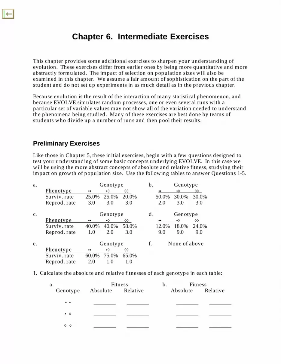
Chapter 6. Intermediate Exercises
This chapter provides some additional exercises to sharpen your understanding ofevolution. These exercises differ from earlier ones by being more quantitative and moreabstractly formulated. The impact of selection on population sizes will also beexamined in this chapter. We assume a fair amount of sophistication on the part of thestudent and do not set up experiments in as much detail as in the previous chapter.
Because evolution is the result of the interaction of many statistical phenomenon, andbecause EVOLVE simulates random processes, one or even several runs with aparticular set of variable values may not show all of the variation needed to understandthe phenomena being studied. Many of these exercises are best done by teams ofstudents who divide up a number of runs and then pool their results.
Preliminary Exercises
Like those in Chapter 5, these initial exercises, begin with a few questions designed totest your understanding of some basic concepts underlying EVOLVE. In this case wewill be using the more abstract concepts of absolute and relative fitness, studying theirimpact on growth of population size. Use the following tables to answer Questions 1-5.
a. Genotype b. GenotypePhenotype •• •◊ ◊◊ •• •◊ ◊◊Surviv. rate 25.0% 25.0% 20.0% 50.0% 30.0% 30.0%Reprod. rate 3.0 3.0 3.0 2.0 3.0 3.0
c. Genotype d. GenotypePhenotype •• •◊ ◊◊ •• •◊ ◊◊Surviv. rate 40.0% 40.0% 58.0% 12.0% 18.0% 24.0%Reprod. rate 1.0 2.0 3.0 9.0 9.0 9.0
e. Genotype f. None of abovePhenotype •• •◊ ◊◊Surviv. rate 60.0% 75.0% 65.0%Reprod. rate 2.0 1.0 1.0
1. Calculate the absolute and relative fitnesses of each genotype in each table:
a. Fitness b. FitnessGenotype Absolute Relative Absolute Relative
• • ________ ________ ________ ________
• ◊ ________ ________ ________ ________
◊ ◊ ________ ________ ________ ________

Chapter 6: INTERMEDIATE EXERCISES 49
c. Fitness d. FitnessGenotype Absolute Relative Absolute Relative
• • ________ ________ ________ ________
• ◊ ________ ________ ________ ________
◊ ◊ ________ ________ ________ ________
e. Fitness f.Genotype Absolute Relative
• • ________ ________
• ◊ ________ ________
◊ ◊ ________ ________
2. Which of the tables in Question 1 shows dominance with respect to relative fitness?
a. b. c. d. e. f.
3. Which of the tables in Question 1 shows heterosis for relative fitness?
a. b. c. d. e. f.
4. Which of the tables in Question 1 shows incomplete dominance for relative fitness?
a. b. c. d. e. f.
5. Which of the populations in Question 1 would become extinct if there were 4000individuals, the frequencies of both alleles were equal to 0.5, and the genotypes wereinitially in Hardy-Weinberg equilibrium?
a. b. c. d. e. f.
Exercise 16. Selection via Reproduction vs Selection via Survival.
In our formulation of the concepts of relative and absolute fitness, we multiplyreproductive rate by survival rate to obtain single coefficients of fitness for each alleleand genotype. We then compare and standardize those coefficients by dividing by thelargest. While this approach is a useful and powerful one, it is always worth asking ifthe technique used to study some phenomenon might obscure interesting points.
One such question is whether or not it makes a difference if a given pattern of selectionis achieved by survival rate or by reproductive rate, or by a combination of both. Forexample, the absolute fitness of a genotype with 20% survival and an average of 6

50 EVOLVE Manual
offspring = .2 x 6 = 1.2. The same fitness could be achieved by 40% survival and 3young, or 30% survival and 4 young, or 60% survival and 2 young.
Would evolution proceed the same in two populations with identical fitness andselection coefficients, if one achieved that pattern of selection with high survival andlow reproduction, and the other achieved it with low survival and high reproductiverates? Write down your predictions of what you expect to happen.
Set up and run a series of EVOLVE experiments to examine this question. Be sure toexamine graphs of genotype numbers and population size.
What do your results suggest about the usefulness of fitness and selection coefficients instudying the evolutionary biology of real organisms?
Ecologists studying life-history patterns (groups of traits related to longevity andreproduction) have found correlations of traits that make up alternative life-histories.For example, a short life-span is often correlated with rapid maturation, production oflarge numbers of small young with little parental care, and a single episode ofreproduction. Species exhibiting such traits are often “weedy” colonizers of unstablehabitats and are sometimes called r-selected. Opposite traits (long life-span, intensiveparental care of a few, large young, repeated reproductive attempts) are associated withK-selected species, which often live in stable habitats. How do your results bear on theecological concepts of r- and K-selected populations? Look up these concepts in yourtextbook if you need more background on these concepts.
Exercise 17. Exploring Heterosis.
In Exercise 10 you briefly examined the pattern of evolution of a population withheterosis. However, that did not really reveal the wealth of interesting phenomenainherent in this pattern of inheritance. This exercise is designed to give you aframework for exploring the phenomena of heterosis.
The basic question is: What is the evolutionary fate of a population showing heterosis?Compare the changes in allele frequencies in a populations where the heterozygous •◊genotype is more fit than either of the homozygotes.
A convenient metaphor that may be helpful in planning experiments is to think ofyourself as exploring a landscape on the plane illustrated in Figure 6-1 below. Thehorizontal axis represents the absolute fitnesses of the two homozygotes. On the farleft, the ◊◊ homozygote’s fitness is zero and the •• has very much higher fitness. In themiddle, the fitness of the two homozygotes is equal. On the right, the •• has a fitness ofzero and the ◊◊ is higher (but still less than that of the heterozygote).
Four runs are outlined for you on the figure and in the table below. In Run 1 and Run 2,the homozygotes have equal fitnesses of 1.5; the only difference between the two is thatRun 1 starts with an initial • frequency of 5%, while Run 2 starts with a • frequency of

Chapter 6: INTERMEDIATE EXERCISES 51
95%. Run 3 starts with the same low allele frequency as Run 1, but the fitness of the ◊ ◊homozygote is zero. In Run 4, the initial allele frequency is the same as Run 3, but the•• genotype has a lower (but non-zero) fitness and the ◊◊ genotype has a higher fitness.You should make these runs and other runs of your own design to fill in the unexploredopen areas of the figure.
Figure 6-1. A Metaphorical Landscape for ExploringHeterosis.
Make several runs in which the fitnesses of • and ◊ homozygotes are equal, but whichstart with different initial allele frequencies (for example, Runs 1 and 2 on the tablebelow and their corresponding numbers in the graph above). Next, make runs with theabsolute fitnesses indicated in Runs 3 and 4 on the next page and indicated by the “3”and “4” on the graph. Note the final allele frequencies of the populations and mentallysummarize the results. Make a prediction about the final allele frequencies at someother point on the plane and test your prediction with another run of EVOLVE. In thisway you can explore all of the regions on the surface before writing your answer to thequestion.
Initial Initialpopulation frequency
Run No. Max pop. Post-crash • • • ◊ ◊ ◊ of • allele
1 _____ _____ _____ _____ _____ 0.05
Survival rates Absolute fitness Frequency of • in• • • ◊ ◊ ◊ • • • ◊ ◊ ◊ generation 100
50 50 50 1.5 2.0 1.5 _____
Reproductive rates Relative fitness• • • ◊ ◊ ◊ • • • ◊ ◊ ◊
3 4 3 _____ _____ _____
Initial Initialpopulation frequency

52 EVOLVE Manual
Run No. Max pop. Post-crash • • • ◊ ◊ ◊ of • allele
2 _____ _____ _____ _____ _____ 0.95
Survival rates Absolute fitness Frequency of • in• • • ◊ ◊ ◊ • • • ◊ ◊ ◊ generation 100
50 50 50 1.5 2.0 1.5 _____
Reproductive rates Relative fitness• • • ◊ ◊ ◊ • • • ◊ ◊ ◊
_____ _____ _____ _____ _____ _____
Initial Initialpopulation frequency
Run No. Max pop. Post-crash • • • ◊ ◊ ◊ of • allele
3 _____ _____ _____ _____ _____ 0.05
Survival rates Absolute fitness Frequency of • in• • • ◊ ◊ ◊ • • • ◊ ◊ ◊ generation 100
_____ _____ _____ 1.5 2.0 0.0 _____
Reproductive rates Relative fitness• • • ◊ ◊ ◊ • • • ◊ ◊ ◊
_____ _____ _____ _____ _____ _____
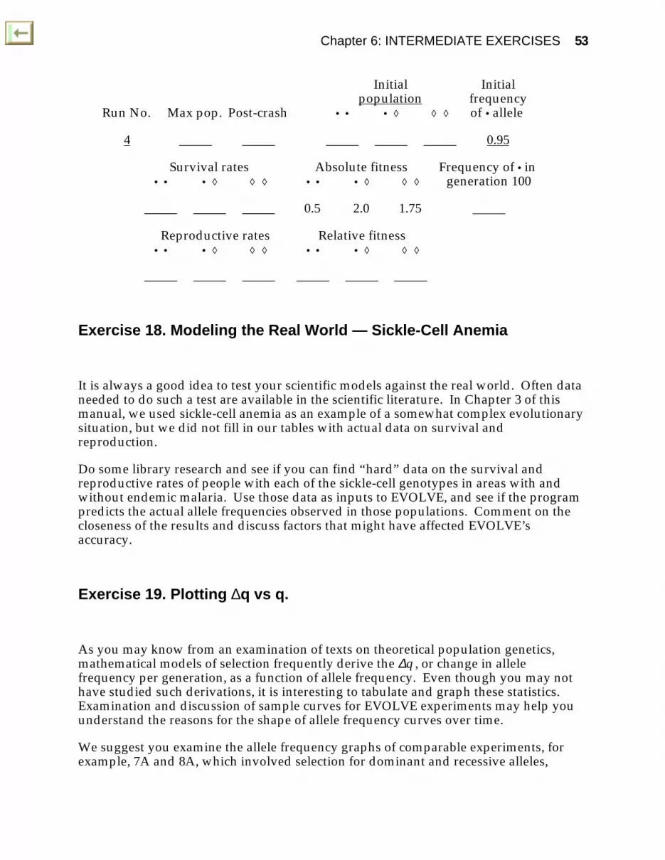
Chapter 6: INTERMEDIATE EXERCISES 53
Initial Initialpopulation frequency
Run No. Max pop. Post-crash • • • ◊ ◊ ◊ of • allele
4 _____ _____ _____ _____ _____ 0.95
Survival rates Absolute fitness Frequency of • in• • • ◊ ◊ ◊ • • • ◊ ◊ ◊ generation 100
_____ _____ _____ 0.5 2.0 1.75 _____
Reproductive rates Relative fitness• • • ◊ ◊ ◊ • • • ◊ ◊ ◊
_____ _____ _____ _____ _____ _____
Exercise 18. Modeling the Real World — Sickle-Cell Anemia
It is always a good idea to test your scientific models against the real world. Often dataneeded to do such a test are available in the scientific literature. In Chapter 3 of thismanual, we used sickle-cell anemia as an example of a somewhat complex evolutionarysituation, but we did not fill in our tables with actual data on survival andreproduction.
Do some library research and see if you can find “hard” data on the survival andreproductive rates of people with each of the sickle-cell genotypes in areas with andwithout endemic malaria. Use those data as inputs to EVOLVE, and see if the programpredicts the actual allele frequencies observed in those populations. Comment on thecloseness of the results and discuss factors that might have affected EVOLVE’saccuracy.
Exercise 19. Plotting ∆q vs q.
As you may know from an examination of texts on theoretical population genetics,mathematical models of selection frequently derive the ∆q , or change in allelefrequency per generation, as a function of allele frequency. Even though you may nothave studied such derivations, it is interesting to tabulate and graph these statistics.Examination and discussion of sample curves for EVOLVE experiments may help youunderstand the reasons for the shape of allele frequency curves over time.
We suggest you examine the allele frequency graphs of comparable experiments, forexample, 7A and 8A, which involved selection for dominant and recessive alleles,

54 EVOLVE Manual
respectively. You can use Copy Window Data to copy the summary data to the Mac’sclipboard, then paste them into a spreadsheet or statistics program. Tabulate the allelefrequency (q) of the allele that increases in frequency. Subtract adjacent generations’values of q to obtain ∆q; then do a scatter plot of ∆q vs q. Be sure to note the survivaland reproductive rates of the experiment. If members of a class each do a separateexperiment, you will have abundant material for discussion.
For example, ask yourself what values of q have the highest values of ∆q in Experiments7A and 8A. Can you see how the graphs of allele frequency vs time that EVOLVEproduced relate to the plots of ∆q vs q? Do the latter show you why the steep part of theallele frequency vs time graphs occur early and late in the experiment? Compare theresults from 7A with a similar graph of 7B. How does increasing the strength ofselection affect ∆q?
Comparison of other ∆q vs q graphs is also revealing. You might find it especiallyinteresting to look at 10A, 10B, and 10C.
Exercise 20. Plotting ∆q vs Population Size.
When you are studying drift, it is more useful to graph ∆q vs population size. Youshould take a sample of 10 or so pairs of years from the results of each experiment youdid for Exercise 11, tabulate population size and allele frequency, then do a scatterplotof allele frequency vs population size. You could also take the data from Exercise 4during the period when the population was expanding — it will fill in the spacebetween the points from Exercise 11. (Give some thought to whether you should plotthe size of the population in the first or last year, or if you should take the average of thetwo).
Exercise 21. Examining q at a Time t for a Large Number ofPopulations of the Same Size.
Another way to look at drift is to do a series of experiments like those in Exercise 11 butwith various random numbers. Pooling class data is especially useful here. Record theallele frequency of one allele every 25 generations. When you have results from 10 ormore experiments of the same size, make histograms of allele frequencies — you seegraphically that genetic drift can indeed result in significant changes in allele frequency.

Chapter 7. Advanced Exercises
The exercises in this chapter are designed to help you develop a more completeunderstanding of the basic design of EVOLVE, of the difficulties of determining whattypes of selection might be occurring in nature, and of how one might study evolutionstatistically.
Exercise 22. The Model Underlying EVOLVE
As noted in Chapter 1, theoretically minded evolutionists have continued to try todevelop models of evolutionary and ecological processes despite (or because of)difficulties with experimentation. Their models are conceptual, rather thanexperimental, often mathematically sophisticated, and a complete understanding ofsome of them requires the use of probability, calculus, matrix algebra, Markov Chains,and/or game theory. Such models clearly are beyond the scope of many biologycourses. Nevertheless, modeling is too useful a process to ignore.
By the time you get to this exercise you should have spent quite a bit of time usingEVOLVE, but you probably do not really understand how it can produce realisticresults in such a wide variety of evolutionary situations. What we shall do in thisexercise is establish a simple, intuitive model and explore the results it produces in oneevolutionary situation. This will give you an understanding of one approach tomodeling. An understanding of the basic approach of this type of model is veryimportant in more detailed analyses of its results.
Before going to class, consider how you would model the evolutionary situationdescribed below. Discuss this assignment with others before class if you wish. You arenot expected to produce a finished product, but should try to map out how you wouldapproach the problem. Take your notes to class and be prepared to discuss yourapproach. In class you can set up a model and run it by hand. After getting results wewill see how this model relates to EVOLVE. Please take a calculator to class.
Restrict your thinking to a species which is hermaphroditic (has both male and femaleorgans) and diploid, reproduces sexually, and must mate with another individual.
Consider a life cycle where individuals are born during a restricted breeding season,mature for one year, mate, produce young, and die. Consider only changes in thefrequency of two alleles (• and ◊) at one locus. If it helps you visualize an abstractproblem, think of the ◊ alleles producing spines which protect heterozygotes andhomozygotes against predation. However, in homozygotes the ◊ alleles produce ashorter copulatory organ; along with the spines, this reduces effectiveness ofcopulation. Consequently, ◊◊ individuals have a higher survival rate than •• and • ◊individuals, but a lower reproductive rate. Heterozygous individuals (•◊) have the best

56 EVOLVE Manual
of both effects — protection and a high reproductive rate. Start with a population withthe following composition and average survival and reproductive phenotypes:
Mean MeanGenotype Number survival rate reproductive rate
• • 245 0.2 5.1• ◊ 210 0.3 4.6◊ ◊ 45 0.3 4.1
Total 500
You need not try to formulate one equation for such a population; you may find iteasier to consider the basic population process of birth, survival, mating, and death.
Questions: (Bring brief, specific answers to class for discussion):
1. What do you predict will happen to the population size over time?
2. What do you predict will happen to the frequencies of the two alleles?
3. What do you predict will happen to the frequencies of the three genotypes?
4. How would you set out to convince a skeptic that your prediction is correct?
Your instructor will help you discuss your approaches and come up with an approachto model this evolutionary scenario. You can then calculate the results to see how youranswers compare to the model the class develops.
Exercise 23. Statistical Comparisons of EVOLVE’s Results withTheory
One of the major difficulties scientists have is to evaluate whether data that they havegathered in experiments “fit” the predictions of theory. Students with somebackground in statistics may find that EVOLVE provides an opportunity to gainexperience with statistical tests of “goodness of fit.” If you have not already done so,you may want to see the BioQUEST statistics module for some approaches.
Pick an evolutionary situation about which you can make mathematical predictions andcompute values of some parameter. Then do one or more EVOLVE experiments thatprovide you with data about that situation. Graph the predicted values against thoseprovided by EVOLVE and evaluate the “goodness-of-fit.” For example, when selectionoperates against a lethal or sterile recessive (that is, the selection coefficient = 1 andrelative fitness = 0), then the formula for change in gene frequency becomes:
∆q = -q2/(1+q)

Chapter 7: ADVANCED EXERCISES 57
You might calculate the values of ∆q at intervals of q between 0 and 1 according to thisequation, then plot the results from one or more EVOLVE experiments. What statisticaltests would let you test the hypothesis that the EVOLVE data resulted from apopulation subjected to selection against a lethal (or sterile) recessive? Do your resultsrefute the hypothesis?
Exercise 24. Inferring Pattern of Selection from “Field” Data
Another lesson about the difficulty of studying evolution can be learned fromexamining EVOLVE output without seeing the input data. If your instructor gives youprintouts of an EVOLVE experiment, either generation summaries or graphs, could youtell what the input values were? It is instructive to break your class or lab up intoseveral teams and for each team to solve the puzzle. You might test your ideas bymaking your own EVOLVE experiments to try to duplicate the result you were given.Would your task be easier or harder if the printout were from a trial with a smallpopulation?
Do all teams come up with the same ideas? Going one step further, what does yourexperience with this exercise (and other EVOLVE exercises, especially 22) tell you aboutscientists trying to explain real phenomena in nature?
Remember that in the “real world” we rarely have such good data on allele or genotypefrequencies as EVOLVE provides.

Chapter 8. Program Notes and Setting upExperiments
Introduction
This chapter contains reference material on each of the parameters you may input toEVOLVE, as well as notes on output and the help system. The emphasis is on how eachparameter relates to evolution, and on practical aspects of setting up experiments.There is also some discussion of how to interpret the various output graphs. As withmost reference works, you will probably not find it useful to read through this chaptertrying to absorb everything in it. Rather, skim through it to get an idea of its contents,then refer back to it when you have a particular question.
Getting Help with EVOLVE
There are three ways that the user can get help with the EVOLVE program.
1. Information about inactive (gray) menu items: If you do not understand why aparticular menu item is not available, you can click on an inactive item. A smallwindow will appear giving information on the item and indicating why it cannot bechosen at this time. For example, choosing the Cut item in the Edit menu displays thefollowing message: "This option is only active when some text is selected."
2. General information: For help with a particular menu item or about a window onthe screen, you can enter Help mode. To enter Help mode, hold down the Command(or ) key while typing a question mark. (If you have a help key on your keyboard thiswill have the same effect.) The cursor will change to a question mark. Clicking on anyitem in a menu (all items are enabled in this mode) gives general information about thatitem, including what would happen if that item were chosen. For example, in Helpmode, choosing the Cut item displays the following message: "This will delete the selectedmaterial from a notepad and retain it in the clipboard so that it can later be pasted into anothernotepad or into a word processor."
Similarly, clicking anywhere in the front-most window while in Help mode will displaysome general information about that window. This information includes a descriptionof the contents of the window and explains the function of any buttons or other controlson the window. For example, clicking on the Parameter History Window while in Helpmode displays the following message: "This is a scrollable list of all the parameters used inthe experiment so far. This is not editable but you can make an editable copy of it by choosingthe 'Copy Window Data' option on the 'Edit' menu."

Chapter 8: PROGRAM NOTES & SETTING UP EVOLUTIONARY EXPERIMENTS 59
Help mode will automatically turn off once you have clicked on an item.
3. To browse through all of the information available about EVOLVE: Choose Helpwith Evolve under the menu on the far left. This allows you to choose from a list oftopics and display information on the topic that interests you. Buttons at the bottom ofthe window let you move to additional topics in the list.
Program Input
Title
Be sure to enter a brief, descriptive title for your experiments. You will eventuallyaccumulate many different experiments and the titles will help you keep them straight.For example, if a number of people are storing their results on one disk, you should putyour initials in the title so you won't get your results mixed up with someone else's.
Seed
This is a whole number between 0 and 32767. It is used by the computer to simulaterandom mating, the effects of weather, and other “random” factors.
You may let EVOLVE pick the seed for you, or you can type a seed in if you wish. Ifyou use the same seed in different experiments you can be sure that any variations inoutput are caused by changes in other variables. If you use different seeds with nochange in other parameters, you can assess the influence of chance. In essence, thisamounts to running the same experiment again. A thorough understanding of the seedis not necessary for you to use EVOLVE, you may find the following backgroundhelpful.
EVOLVE takes the “seed” you enter in the Seed box and performs a series ofmathematical operations on it to produce a second “random” number. This number isused by EVOLVE in various ways — for example, to randomly pick pairs of parentsfrom the adult population, and to let the survival rate vary slightly from the averagevalues you entered in the Change Parameters Window. This second number is alsoused as the seed for the third “random” number, and so on.
These numbers are not really random, because the mathematical operations will alwaysproduce the same sequence of numbers if the same seed is used — the sequence ofnumbers is determined by the value of the initial seed. However, if you examine alisting of the numbers produced by such a “random number generator” you would notsee a relationship between them, so in this sense they are random.
This may become clearer if you consider another, more commonly used, randomnumber generator, a tossed coin. If you knew enough physics, and had enoughinformation on the initial position, size, shape, and mass of the coin, along with therotational velocity, angle, and velocity of the toss, and such things as wind direction

60 EVOLVE Manual
and velocity, you could predict heads or tails before the coin landed. In this sense, theresult of a coin toss is determined, yet for all practical purposes we can regard theoutcome as random.
Again, consider how EVOLVE uses random numbers. When the program reduces thenumber of young to obtain the number of adults, it takes the survival rate and seed yougave it and produces an actual “survival rate” that is multiplied by the number ofyoung to obtain the number of adults. The actual survival rates used by EVOLVE overa number of generations will have an average value very close to the value you gave it,although the value of a given generation will be uncertain. If you input 60% as thesurvival rate of a genotype, the rates used in 5 consecutive generations might be 61.8%,66.3%, 53.9%, 57.5%, and 60.3%, for an average of 59.96%. If you used another seed, the5 survival rates would be different, but would still average out to about 60%.
This may seem complicated, but it is a practical way of simulating the sort of variationsthat occur in nature. For example, weather might be mild for a couple of years, thenharsh, or predators that take advantage of one phenotype might be unusually abundantin one generation and unusually scarce in another. If climate is what you expect,weather is what you get; you enter “climate” into EVOLVE’s menus, the randomnumber generator gives you “weather.”
Number of Generations
EVOLVE will continue an experiment for the number of generations specified by thisnumber. Although you may stop an experiment at any time, it may be useful to haveEVOLVE stop at a predetermined time. Because it takes longer to run manygenerations, you may wish to explore combinations of data by running for, say, 50generations instead of the full 200. Also, there are times when you may want to changevariable values on a specific schedule.
Starting Population
These three numbers determine the composition and size of the starting adultpopulation of generation 1. They must not total more than 8000.
For example, suppose you wish to study the fate of a new mutant allele (◊) in apopulation of 1000 •• individuals. You should use 999, 1, and 0 as the initial numbersof ••, •◊, and ◊◊ genotypes, respectively. A new mutation obviously would first existin heterozygous condition.
If you wish to establish a population of 2000 with the frequency of the • allele equal to0.40, use 320, 960, and 720. These numbers can be obtained using the Hardy-Weinbergproportions — you should be able to determine them. (See “Calculation of Fitness andSelection Coefficients” in Chapter 9, or your textbook, if you do not know how to dothis.)

Chapter 8: PROGRAM NOTES & SETTING UP EVOLUTIONARY EXPERIMENTS 61
Survival and Reproductive Rates: Selection, Pattern of Inheritance, andPopulation Growth Rates
Survival rates determine the average number of young of a particular genotype thatsurvive to adulthood. They may vary from 0% for a lethal genotype to 100 for agenotype in which 100% of the young survive to adulthood. The former is not unusualin nature, but the latter is very unlikely.
Reproductive rates determine the average number of young per individual. They mayrange from 0 offspring per parent for a sterile genotype to 10 offspring per parent for afertile one. The limit of 10 young is arbitrary, imposed to make EVOLVE simpler andlet it run more quickly.
These are very important variables which determine the pattern of inheritance, and ofnatural selection, and greatly influence rate of population growth. To understandpopulation genetics and EVOLVE, you absolutely must understand them thoroughly.
Pattern of Inheritance — Choice of appropriate values for reproduction and survivalwill allow you to simulate any pattern of inheritance possible for a single locus with 2alleles (for example, dominance and recessiveness, codominance, or heterozygotesuperiority). One definition of a dominant allele is that it is one which produces thesame phenotype when heterozygous as when homozygous.
For example, if the survival rates were 20%, 20%, and 50% for ••, •◊, and ◊◊ genotypesrespectively, then the • allele would be dominant and the ◊ allele would be recessive.Note that dominance has nothing to do with which genotypes have the highest survivalor reproductive rates, only with the homozygote that the heterozygote resembles. Inthis case, the heterozygote has the same traits as the homozygous ••, so the • allele isdominant. To take another example, reproductive rates of 5, 4, and 3 would simulate apattern of inheritance where heterozygotes are intermediate between the homozygotes,that is, incomplete dominance. The following table provides more examples of the basicpatterns of inheritance:
GenotypeExample • • • ◊ ◊ ◊ Notes
1. Survival rate 30 30 20 • Dominant, advantageous;Reproductive rate 4 4 4 ◊ Recessive, deleterious
2. Survival rate 20 20 30 • Dominant, disadvantageous;Reproductive rate 4 4 4 ◊ Recessive, advantageous
3. Survival rate 30 30 20 • Dominant, advantageous;Reproductive rate 4 4 4 ◊ Recessive, deleterious

62 EVOLVE Manual
4. Survival rate 20 25 30 • Incompletely dominant,disadvantageous,
Reproductive rate 4 4 4 ◊ Incompletely dominant,advantageous
5. Survival rate 20 20 30 • Dominant, disadvantageous,◊ Recessive, advantageous;
Reproductive rate 4 5 5 ◊ Dominant, advantageous,• Recessive, deleterious
Overall, the alleles demonstrate pleiotropy (multiple effects) and codominance(both have their effects in heterozygotes).
6. Survival rate 20 40 30 • Dominant, disadvantageous,◊ Recessive, advantageous;
Reproductive rate 4 6 5 ◊ Dominant, advantageous,• recessive, deleterious;
Overall, the alleles demonstrate overdominance with respect to fitness and areheterotic (show heterosis, or heterozygote superiority).
7. Survival rate 20 10 30 • Overdominant, disadvantageous;Reproductive rate 4 6 5 ◊ Overdominant, advantageous;Overall, the alleles demonstrate overdominance with respect to fitness and showheterozygote inferiority.
Population Growth Rate — The relationship between reproductive rates and survivalrates, what evolutionary biologists call “absolute fitness,” determines the direction andrate of change of population size. You should choose survival and reproductive rates insuch a way that your populations grows slowly. For example, you wouldn’t normallyconsider an experiment where all genotypes have survival rates of 65% andreproductive rates of 1. For every 100 young born, there would be about 65 adults; eachadult would produce an average of 1 young for the next generation (a total of 65young). Given enough time, the population would decline to extinction.
In general, if the product of survival rates x reproductive rates is greater than 100, thepopulation will not become extinct. Of course, in most runs the survival andreproductive rates will not be the same, so the exact pattern of population change willdepend on the relative proportions of the various genotypes in the population as well ason the particular survival and reproductive rates.
Pattern of Selection — This also depends on the relative values of both survival andreproductive rates of each of the genotypes, what evolutionary biologists call “relativefitness.” Suppose the survival rates were 60%, 40%, 40%, and the reproductive rateswere 3, 2, 2 for the ••, •◊, and ◊◊ genotypes, respectively. The • allele would berecessive (because the heterozygote has the same characteristics as the ◊◊ homozygote),

Chapter 8: PROGRAM NOTES & SETTING UP EVOLUTIONARY EXPERIMENTS 63
but advantageous (because the •• homozygote has the highest survival andreproductive rates). Natural selection would favor the •• homozygotes.
As you work with EVOLVE you will gain a better feel for how these parametersinteract. From the start, however, you may easily determine the absolute fitness of agenotype by multiplying the number of young by the survival rate. Products greaterthan 100 indicate that the genotype will tend to increase in number, while products lessthan 100 indicate that the genotype will tend to decrease in number. Thus, absolutefitness tells you how the actual numbers of individual organisms are likely to change.However, the absolute fitness of a genotype does not necessarily tell you whether theproportion of that genotype in the population will rise — that is, whether that genotypeis favored by natural selection.
The relative sizes of the absolute fitnesses of the genotypes will indicate how theproportions of particular genotypes will tend to change over time. Dividing theabsolute fitness of each genotype by the highest absolute fitness yields the relativefitness. The maximum value of the relative fitness will, of course, be one. Genotypeswith relative fitnesses less than one will tend to decrease in frequency.
Take as an example the following:
GenotypePhenotype • • • ◊ ◊ ◊ Survival rate 20% 20% 14%Reproductive rate 5 6 7Absolute fitness 100% 120% 98%Relative fitness 0.83 1.0 0.82
In this table, the survival and reproductive rates would be input to EVOLVE. The •allele would be dominant and advantageous with respect to survival, but incompletelydominant and deleterious with respect to reproduction. What would happen to thepopulation? The ◊◊ genotype, although it has a low survival rate, has a highreproductive rate. Would the higher reproductive rate make up for the reducedsurvival? Would the ◊ allele increase or decrease in the population? Would it becomeextinct? Would the • allele become extinct? Or would both remain in the population?
Multiplying survival rates by reproductive rates gives us the third row — the absolutefitness. Here it is clear that the high reproductive capacity of the ◊◊ genotype does notcompletely compensate for the low survival, for the absolute fitness of 98 is less than100. By dividing all of the absolute fitnesses by 120 (the highest) you can see that the ••homozygotes have only 83% of the fitness of the heterozygotes, while the ◊◊individuals have only 82% relative fitness. By the time you finish your experimentswith EVOLVE, you should be able to predict the outcome of such an evolutionarysituation by calculating the relative fitnesses.

64 EVOLVE Manual
Gene Flow
To simulate gene flow, the movement of alleles from one population to another, youmust enter rates of immigration (arrival) and emigration (departure) for each genotype.The number immigrating may vary from 0 to 4000 adults of each genotype pergeneration. The percent emigrating may vary from 0% for stay-at-homes, to 100% forgenotypes with wanderlust.
Note that immigration is a constant and is independent of the density of the simulateddeme, while emigration removes a constant proportion of each genotype in eachgeneration. This may seem an unusual or odd situation, but it could be visualized inthe following way: Suppose our model population is a plant similar to a dandelion, andthe seeds have plumes for wind dispersal. The alleles might be conceived of asaffecting the length of the plumes, and therefore the tendency to disperse (be blownaway). Our model deme could be thought of as existing on a small island which isdownwind of a large island or continent with a stable population. In such a situation,immigration could be viewed as constantly adding a particular number of individualsof each genotype, with long-plumed seeds arriving at a higher rate than short-plumedseeds. The short-plumed seeds would emigrate, that is, be blown away, from the islandat a lower rate than the former.
Maximum Population and Post-Crash Population: Population Size
Along with rates of survival and reproduction (and gene flow, if any), the values youenter for maximum and post-crash population determine the size of the population. InEVOLVE, the maximum population may range from 10 to 5000, while post-crash sizemay range from 2 to 4000. Obviously, the maximum population must be larger than thepost-crash size.
The maximum population is roughly equivalent to the ecologist's Carrying Capacity(the greatest number of individuals of a population that can be sustained by theirenvironment, often symbolized by K). In EVOLVE, the maximum size is the one towhich the population of adults may grow. If the survival and reproductive rates (andgene flow) are such that the population grows and exceeds the number you typed formaximum population, EVOLVE reduces the population to the size of the post-crashvalue. “Mortality” during the population “crash” is random with respect to genotype.
For example, if the number of young were 20,000, and the survival rates were all 50%,you would expect the number of adults to be about 10,000, twice the largest possiblemaximum population. If the post-crash value was 2,500, EVOLVE would multiply thenumber of each genotype by 2,500/10,000 to determine the actual number of adults.
You should choose these variables carefully to ensure that the population size isappropriate to the evolutionary situation you wish to model. For example, if you wishto study the effects of genetic drift in a small population of 10-20 adults, let themaximum = 20 and post-crash = 10; provided the population does not become extinct, itwill remain within those limits. Setting maximum = 5000 and post-crash = 4000 wouldpermit you to simulate a population with very little random change.

Chapter 8: PROGRAM NOTES & SETTING UP EVOLUTIONARY EXPERIMENTS 65
Appropriate choice of these variables is useful in other ways. Suppose you find thatvalues for maximum and post-crash of 5000 and 4000 (coupled with high survivaland/or reproductive rates) produce such rapid population growth that populationcrashes occur in every generation (the graph of total population size would be flat andfill the screen). If you wanted to get a better idea of how evolution affected rate ofpopulation growth, you could set post-crash to a lower value, such as 1000, and itwould take longer for the population to exceed the maximum population of 5000.
Program Output
EVOLVE provides a number of ways of looking at experiments and their results. Eachexperiment has a Summary Window that is the control center for examining results. Itcontains a graph of genotype frequencies against time, a table of numerical results foreach generation, and buttons that allow users to review the input parameters andgenerate graphs.
Information from any of EVOLVE’s windows can be copied to the Mac’s clipboard.From there the information can be Pasted into EVOLVE’s Notepad, the Mac’sscrapbook, a graphics program, a spreadsheet, or a word processor.
Additional graphs may be generated in two ways: By using the Graphs menu you mayselect standardized plots. You may construct graphs with any axes by clicking on theMake new graph button on the Summary Window.
The Copy Commands
Rather than produce reams of printed output, EVOLVE allows you to pick and choosewhat information you wish to look at and where and how you use that information. Inthis version of EVOLVE, Copy commands in the Edit menu are the only wayinformation is moved. These commands can be used with any of the graph or datawindows to move either graphic or numeric information.
Copy Window will save a bit-mapped copy of a window. The image includes everydot in the window, including its title and borders. Copy Window images have only 72dots per inch (dpi) and do not have smooth lines when printed on a laser printer (unlessthe image is scaled down in size).
Copy Window Graph places a copy of the lines and text of a graph without thesurrounding window. The image is not stored as dots, but as what is called a PICT, andcan be printed with the full resolution of the printer you are using. When printed on alaser printer, Copy Window Graph images are free of the “jaggies” produced by CopyWindow images (there may, however, be some problems with symbols and text in somesituations).

66 EVOLVE Manual
Copy Window Data can be used to store numbers to the clipboard. The numbers areseparated by [tab] characters and can be Pasted into most statistics and spread sheetprograms where they can be subjected to more sophisticated analysis and graphing.They can also be copied into word processors if you need to report numerical results ina data table.
The Notepad
Each Summary Window has a Notepad that is a mini-word processor where you cantype in your own notes, questions, hypotheses, predictions, and reminders. In addition,you can paste material that you have copied from EVOLVE’s graphs and tables. TheNotepad can be printed using the Print Notepad command in the File menu.
Using the Notepad is simple: Just bring a Summary Window to the front, click on theNotepad icon ( ) in the upper left-hand corner, and start typing and pasting. Click onthe Notepad Window’s close box to get it out of your way when you are doing otherthings.
The Variables You May Graph
It is often useful to look at the results of experiments from a variety of points of view,and EVOLVE is well equipped to let you examine its results in many ways. Where theactual list of variables is lengthy, they fall into a few distinct categories: time, numbers,and frequencies.
Here is a list of the variables that can be graphed:
Time: from the start of the experiment measured in number of generations. Thisis so useful as the horizontal axis of graphs that it is the default.
The following group of variables are the actual number of adults in the total populationor the number of a particular genotype or group of genotypes. By selectingcombinations of the following, you can look either at genotypes or at phenotypes. Theactual variables are:
Total Population: the sum of the number of all genotypes, the total size of thepopulation. This is important when you want to look at drift or populationgrowth rate (mean fitness)
Size of •• Pop.
Size of •◊ P o p.
Size of ◊◊ P o p.
Graphs of individual genotypes are useful at the introductory level to show what ishappening to the population, and to show the Hardy-Weinberg relationship. Some

Chapter 8: PROGRAM NOTES & SETTING UP EVOLUTIONARY EXPERIMENTS 67
students ask for graphs of one or more genotypes when they have difficultyinterpreting particular runs. Beyond these introductory uses, genotype graphs areprobably of little value to most students. However, the steepness of the peaks, and thespacing between them, clearly illustrate that what ecologists call “intrinsic rate ofnatural increase” evolves over time and is a measure of the average absolute fitness of apopulation.
The last three population variables shown above can be used to graph the numbers of aphenotype. If, for example, • is recessive, then # •• would be the recessive phenotypeand # •◊ + ◊◊ would be the dominant phenotype.
Each of these variables can be graphed on a logarithmic scale by selecting the Log scalebox in the New Graph Window. A log plot enables you to look at numbers that varygreatly in size. For example, if the number of •• in an experiment went from 0 to 4000,a linear, non-log plot would not allow you to distinguish changes below severalhundred individuals; a log plot would let you distinguish generations with only one ortwo individuals.
While actual numbers of individuals are instructive, they are often less useful than therelative frequencies of subgroups of the population. EVOLVE can also calculate thefollowing as relative proportions of the population:
Frequency of ••
Frequency of •◊
Frequency of ◊◊
Because evolution may be defined as “change in allele frequency,” a graph of allelefrequency is often the single best summary of what happened to the population. ForEVOLVE, these allele frequencies are the most relevant measures:
Frequency of •
Frequency of ◊
The allele frequency graphs are always symmetrical about a horizontal line at 0.50because the frequencies of the two alleles must always add up to 1.0 (if p symbolizes thefrequency of the • allele, and q symbolizes the ◊ allele, then p + q = 1). The genotypefrequency curves are more involved, but generally follow the Hardy-Weinbergrelationship: p2 + 2pq + p2 = 1. Although this relationship does not apply preciselywhen selection, drift and/or gene flow operate, the actual frequencies are often fairlyclose.

Chapter 9. Theoretical Notes
The purpose of this chapter is to provide additional perspective on some of thetheoretical issues behind the use of programs like EVOLVE. Many of the details, suchas how to derive Hardy-Weinberg ratios, can be found in most textbooks and will notbe covered here. Be sure to read the appropriate section of your text if this materialseems unclear.
The Concept of an Equilibrium Population
The backbone of our theory of evolution in local populations, often called“microevolution,” is the Hardy-Weinberg equilibrium concept. In its simplestformulation, the Hardy-Weinberg concept deals with a population with two alleles (•and ◊ in EVOLVE's notation) of one gene, that are present in frequencies p and q,respectively. Given such a population, four predictions may be made:
1. Frequencies of the two alleles will not change;
2. The ratios of the frequencies of the three genotypes (••, •◊, and ◊◊) will be p2 :2pq : q2 respectively, and will add up to 1.0;
3. The frequencies of the genotypes will not change;
4. If the genotype frequencies are not in the equilibrium ratios in one generation,they will reach equilibrium in the next.
Note that there are within-generation and between-generation predictions. Betweengenerations, allele and genotype frequencies should not change (once equilibrium hasbeen established). Within any one generation, the ratio of the genotypes should be p2 :2pq : q2 (•• : •◊ : ◊◊). Thus the Hardy-Weinberg “law” states that populations willremain in genetic equilibrium, that is, evolution will not occur!
Assumptions
You may find it odd that the foundation of our theory of evolution states that evolutionwill not happen, but the Hardy-Weinberg concept has a number of assumptions thatinvalidate it for most, if not all, natural populations. It strictly applies only when thefollowing assumptions are true:
1. Individuals are diploid, reproduce sexually, and are identical with respect tosuch factors as age and sex;

Chapter 9: THEORETICAL NOTES 69
2. Genes do not change from one allele to another;
3. The population is closed and alleles do not enter or leave;
4. Gametes are produced and combine randomly;
5. All zygotes survive and reproduce equally;
6. The population size is infinite or at least very large.
Evolutionary Forces
In essence, then, the conditions necessary for Hardy-Weinberg equilibrium tell us thatfor sexual species there are only six evolutionary forces (factors, processes, orphenomena that change allele or genotype frequencies):
1. Individuals are not equivalent (for example, the gene is sex-linked);
2. Genes change from one allele to another (mutation);
3. Genes move between geographic populations (gene flow);
4. There is nonrandom mating or gamete production and survival are not equal (forexample, gametic mortality);
5. Individuals differ in their ability to survive and/or reproduce (natural selection);
6. Populations are of small size (genetic drift).
Obviously, populations that fit all of the above assumptions are rare, if they exist at all.However, some assumptions may not be important in particular populations, and it isoften possible to relax others. For example, for all practical purposes populations onremote islands may be regarded as closed to immigration (assumption 3), andemigration may be considered as mortality (natural selection, assumption 5). Also,assumption 6 (infinite population size) can be disregarded if the population is fairlylarge (over a few thousand). Mutation (assumption 2) may be disregarded for mostgenes because mutation rates are too low to affect allele frequencies significantly in theshort term. (Over the long haul, of course, mutation is critically important because it isthe ultimate source of all genetic variation.)
Finally, although it is usually discussed for a gene with two alleles, the Hardy-Weinberg formula may even be extended to genes with more than two alleles by usingthe polynomial expansion. If there are three alleles in a population, their frequenciesshould add up to one (p + q + r = 1), and the frequencies of the genotypes would be (p +q + r)2 = 12, or p2 + q2 + r2 + 2pq + 2pr + 2qr = 1.

70 EVOLVE Manual
Importance of Hardy-Weinberg Equilibrium
Despite its limitations and qualifications, the Hardy-Weinberg concept has been usefulin three major ways:
1. The Hardy-Weinberg concept makes mathematical predictions of what allele andgenotype frequencies should be in the absence of evolution. It thus provides the “NullHypothesis” needed for statistically rigorous tests of our ideas. See the BioQUESTstatistics module if you are uncertain of this. If we have a way to measure thosefrequencies, and if they do not match the predictions, then we know that evolution isoccurring. This obviously is important, because visible changes in populations happenso slowly.
2. The Hardy-Weinberg concept provides us with a conceptual framework forinvestigation. If evolution has occurred (that is, if allele or genotype frequencies deviatesignificantly from expected values) we know that one or more of the Hardy-Weinbergassumptions have been violated; we can proceed to determine which evolutionaryforce(s) have affected the population under study.
3. Finally, and perhaps most importantly, the Hardy-Weinberg concept provides thefoundation for a mathematically rigorous theory of population genetics and formathematical models of each of the evolutionary forces. Since most textbooks ofpopulation genetics illustrate these models in detail, we will not derive any here. Thesemodels may be used in turn as null hypotheses to evaluate the possibility that observedevolutionary changes are due to a specific evolutionary force.
Thus, although it paradoxically predicts no evolution, the Hardy-Weinberg equilibriumconcept allows us to measure evolution, provides a conceptual framework forinvestigation, and serves as the foundation for the mathematics on which much of ourtheory of microevolution is based.
Models in Population Genetics
As indicated above, we can use the Hardy-Weinberg equilibrium concept to formulatemathematical models in the form of equations that hold all factors but one constant. Wecan then vary that one factor to investigate its effects on allele and genotypefrequencies. Once we understand each of the forces by itself, we can combine it withother forces and examine interactions of more than one. In the absence of easyexperimentation, population geneticists have turned to such equations for theirexperiments.
Much of our theory of microevolution is based on such models. Models permit us toexplore the widest possible range of conceivable conditions — the theoretical maximaand minima of evolution. Thus the theory deals with “all possible universes”;experimental and observational studies must determine which universe actually exists.

Chapter 9: THEORETICAL NOTES 71
Despite the importance of mathematical models in population genetics, they presentproblems. Elegant mathematical equations are intellectually stimulating andmanipulating them can be instructive, but they require mathematical expertise and canbe time-consuming. Also, mathematics are too often a barrier for many beginningstudents of evolution. The advent of calculators and computers has reducedcomputation time, but sometimes at the expense of a full understanding of the models,which are hidden from students. In addition, most mathematical models deal only withone or two of the evolutionary forces; it is difficult for students to get a feel for the wayfactors interact in populations. The abstractness of most such models makes it hard forstudents to really grasp what they mean — just what is a selection coefficient of 0.3?Finally, most of the simple mathematical models are deterministic. That is, they do notincorporate randomness or chance. Since chance plays a major role in evolution,deterministic models can be misleading.
EVOLVE is an attempt to avoid these difficulties. It is an intuitively simple yet realisticmodel because students have a better grasp of survival and reproductive rates than ofselection coefficients. Depending on the values of input parameters, EVOLVE mayincorporate any or all of three major evolutionary factors: natural selection, drift, andgene flow. Study of the fate of mutant alleles is also possible.
One of the things which people often have trouble understanding is the way in whichchance events may affect evolution. Mutation, genetic drift, and stochastic (random)variation of environmental factors, such as weather and food supply, are examples ofrandom factors in evolution. EVOLVE incorporates randomness in three ways.
1. The user specifies the average survival, reproductive, and immigration rates of thegenotypes. Each time the program uses one of these parameters, a random-numbergenerator is used to determine the actual value used. Thus, the environment of themodel population may be regarded as varying slightly from generation to generation.
2. The size of the population may be made small enough for genetic drift to occur.Small sizes may be maintained over long periods of time, or may be temporary.
3. The pattern of random matings in a finite population, especially a small one, mayresult in deviations from the expected proportions of genotypes among offspring. Youmay find it helpful to make several runs with each set of data to get a feel for chancevariations.
Calculating Fitness and Selection Coefficients
Despite the importance of measuring actual fitness and selection in nature, availabilityof the conceptual tools provided by the Hardy-Weinberg concept, evolutionarybiologists have had difficulty actually collecting the data. Not until the advent ofelectrophoresis in the mid-1960's was there a method which gave clear data on thefrequency of alleles in natural populations. However, there is some doubt about theevolutionary significance of electrophoretic variants, so even these relatively clear data

72 EVOLVE Manual
are difficult to interpret. Some scientists would rather look at morphological or life-history traits (such as length of teeth, age of first reproduction) that are of more obviousevolutionary value. Unfortunately, it is almost impossible to measure the geneticvariability that underlies these phenotypes.
Aside from the difficulty of gathering the data, exactly how fitness and intensity ofselection might be calculated from real-world data is a matter of considerablecontroversy. There is a large body of literature devoted to this discussion.
We might point out here that our difficulties with collecting and interpreting data in noway invalidate the scientific nature of our theory of evolution. What matters is that inprincipal the data could be collected. There are many examples in science of theoriesthat could not be tested when they were proposed because of methodologicaldifficulties. Wegner's theory of continental drift, for example, was proposed before1920. We had to wait over 40 years until scientists had data on sea-floor spreading toindirectly support Wegner's hypothesis. We had to wait over 50 years before we couldmeasure distances accurately enough to measure actual rates of continental movement.
What follows is a simplistic approach that will give you an idea of what is involved inmeasuring these important parameters. More importantly, this approach will help youunderstand the derivation of the concepts and what they mean. Here is an outline ofthe method:
1. Calculate observed frequency of each genotype in generation 1
2. Calculate expected frequency of each genotype in generation 2
3. Calculate absolute fitness of each genotype (R = obs/exp)
4. Calculate relative fitness of each genotype (W = fitness relative to the genotypewith greatest absolute fitness)
5. Calculate selection coefficients of each genotype (s = 1 - W)
Here is an example that uses this approach. We will use the following data to calculatefitness and selection coefficients:
GenotypeAA Aa aa Total
Population in first generation(before selection) 4000 5000 3000 12000Population in secondgeneration (after selection) 3500 3000 1200 7700

Chapter 9: THEORETICAL NOTES 73
1. Calculate observed frequency of each genotype in generation 2:
Freq. of AA = 3500 /7700 = 0.455
Freq. of Aa = 3000 /7700 = 0.390
Freq. of aa = 1200 /7700 = 0.156
Check: sum = 1.001 (accurate to rounding error)
2. Calculate expected frequency of each genotype in generation 2. From the Hardy-Weinberg equilibrium, we expect the allele frequency in generation 2 to equal that ingeneration 1, and that the frequencies of the genotypes will be p2, 2pq and q2.
a. allele frequencies in generation 1 (= expected allele frequency in generation 2):
Freq. of A= p = [2(4000) + 5000] / 2(12000) = 0.542
Freq. of a = q = [2(3000) + 5000] / 2(12000) = 0.458
Check: sum = 1.000
b. Expected genotype frequencies in generation 2:
Freq. of AA = p2 = (0.542)2 = 0.294
Freq. of Aa = 2pq = 2(0.542 * 0.458) = 0.496
Freq. of aa = q2 = (0.458)2 = 0.210
Check: sum = 1.000
3. Calculate the absolute fitness of each genotype, Rgenotype, selection) as the observedfrequency divided by the expected.
RAA = 0.455 / 0.294 = 1.548
RAa = 0.390 / 0.496 = 0.746
Raa = 0.156 / 0.210 = 0.743

74 EVOLVE Manual
4. Calculate the relative fitness of each genotype, Wgenotype, as the absolute fitnessdivided by the highest absolute fitness.
WAA = 1.548 / 1.548 = 1.000
WAa = 0.746 / 1.548 = 0.508
Waa = 0.743 / 1.548 = 0.480
5. Calculate the selection coefficients of each genotype, s(genotype), as the relativefitnesses subtracted from one.
sAA = 1.000 – 1.000 = 0.000
sAa = 1.000 – 0.508 = 0.492
saa = 1.000 – 0.480 = 0.520
There are a few points we should note about the concepts involved in these calculations.Intuitively, the selection coefficient, s, is the relative decrease in frequency due tonatural selection. In this case, the Aa and aa genotypes are 49.2% and 52.0% lesscommon than would be expected. By this definition, selection is not operating on theAA genotype.
Note that fitness and selection, as typically used by evolutionary biologists, are relativeto the most fit genotype or allele in the population and are between 0.0 and 1.0. Inevery population at least one fitness coefficient must be 1.0 and the selection coefficientof that genotype must be 0.0. It is important to understand that these relative measuresof the intensity of selection are intended to be used in discussing the relative changes inallele and genotype frequencies — which alleles and genotypes are increasing ordecreasing in frequency.
Because these measures are relative, it is possible for a population to be declining innumbers at the same time that one or more alleles or genotypes have high relativefitness (indeed, one genotype must have a fitness of 1.0). Absolute fitness is the measurethat tells us something about whether or not an allele or genotype can increase innumbers. If none of the absolute fitnesses is greater than 1.0, then the population willbecome extinct.
Strictly speaking, these calculations apply when data are collected in one generationand again at the same stage in the life cycle of the next generation (for instance, justafter hatching, or at the start of mating). Data on the young of one generation cannot beused with adults of the next.
A similar approach may be used for calculating fitness and selection coefficients ofalleles. Absolute fitness of alleles would be the ratio of the allele frequencies ingeneration 2 divided by their frequencies in generation 1. Relative fitnesses andselection coefficients would be calculated as shown above.

Chapter 9: THEORETICAL NOTES 75
It is worth noting that science has a history, and that concepts developed at one timemay not be relevant later. The concepts of relative fitness and selection coefficientswere developed in the 1920s and 1930s because they made derivation of equations forpopulation genetics easier. Given that it is difficult to measure actual coefficients innature, this conceptualization of natural selection may in fact turn out to be unusable.
Limitations of EVOLVE
While it is important to understand the nature and value of the tools at your disposal,and simulation and mathematical models are powerful tools, it is also important tounderstand their limitations. In this section we try to clarify the nature of some ofEVOLVE's limitations.
Among the most obvious of EVOLVE's simplifications is that we can look only at onegene with two alleles. Most evolutionarily important characteristics are influenced bymany genes which often have many more than two alleles. Moreover, genes are notisolated — there are many types of interactions between genes. Even the interaction oftwo alleles at one locus may be affected by other loci; there is abundant evidence thatadvantageous alleles that are initially recessive can become dominant through theinfluence of such modifier genes. This over-simplification of the genetics of our modelis perhaps the biggest conceptual problem with EVOLVE.
For example, one of the major questions in evolutionary biology is how the manydiverse alleles seen in wild populations are maintained in natural populations. UsingEVOLVE, you might find a half-dozen ways to maintain two alleles in a populationover a long period of time. But, many evolutionary biologists don’t feel these sorts ofmechanisms would be sufficient and have extended their analysis to three alleles. Thisturns out to increase complexity significantly and to generate even more ways tomaintain more than one allele in a population. The current version of EVOLVE cannothandle three alleles, although a future version will.
EVOLVE is also ecologically naive. In the real world, Carrying Capacity is rarely anabsolute limit which is constant over time and which only influences a population whenthe limit is exceeded. Many limiting factors increase in severity as the CarryingCapacity is approached, and the Carrying Capacity itself changes over time. However,the J–shaped pattern of growth and crash illustrated in EVOLVE's population graphsdoes provide some measure of ecological reality as a consequence of the way limits arespecified for genetic drift. In addition, the steepness of the Js and the spacing betweenthem clearly illustrate that a population’s intrinsic rate of natural increase evolves overtime and is a measure of the average absolute fitness of a population.
EVOLVE'S concept of gene flow, the evolutionary consequence of the dispersal ofindividual organisms studied by ecologists, is an extremely simplistic one. For instance,the number of individuals immigrating is unlikely to be a constant: The sourcepopulation(s) that produce immigrants will probably fluctuate; when the population islow it will produce fewer immigrants for the population modeled by EVOLVE. Also,

76 EVOLVE Manual
the size of EVOLVE's population should influence the number of immigrants thatactually stay; if it is large, one would expect resources to be limiting and more potentialimmigrants to move on in search of more abundant food, shelter, or whatever. Finally,at high population densities when resources are in short supply, we would expect ahigher proportion of the population to emigrate.
Despite its simplicity, EVOLVE does provide an entry into the world of theoreticalpopulation genetics. Although that world has evolved quite far from the initialsimplicity of the Hardy-Weinberg equilibrium proposed eight decades ago, that view ofnature still provides a useful starting point, especially for new students. To the extentthat you develop some intuition and feel for the interaction of evolutionary forces, youmay be misled into thinking you really understand evolution. Should you then have toapply that intuition in real evolutionary studies, you may find that it falls short.Nevertheless, we believe that you are better off working with EVOLVE, learning tothink about allele frequencies and fitness, and designing and interpreting experiments,than merely reading a textbook.

Bibliography
Introductory Texts
Wilson, Edward O., and W. H. Bossert 1971. A Primer of Population Biology. Stamford,Connecticut: Sinauer Associates, Inc. Albeit old and dated, this is still the best,clearest, and shortest introduction to modeling in population biology.
Hartl, Daniel L. 1981. A Primer of Population Genetics. Sunderland, Massachusetts:Sinauer Associates, Inc. A more up-to-date, elaborate introduction to populationgenetics patterned after Wilson and Bossert.
Ayala, Francisco J. 1982. Population and Evolutionary Genetics: A Primer. Menlo Park,California: Benjamin Cummings. Another good introduction.
Spain, James D. 1982. BASIC Microcomputer Models in Biology. Reading, Massachusetts;Addison-Wesley Publishing Co. A superb, readable introduction to a widevariety of computer models in biology.
Full-Length Texts
Stansfield, William D. 1979. The Science of Evolution. New York: MacMillan PublishingCo. Although getting old as a survey of evolutionary biology, this text has a veryclear derivation of a number of simple population genetic models.
Futuyma, Douglas J. 1979. Evolutionary Biology. Sunderland, Massachusetts: SinauerAssociates, Inc. An excellent theoretical and experimental survey of populationgenetics, ecology, and evolution.
Spiess, Eliot B. 1977. Genes in Populations. New York: John Wiley & Sons. A lengthy,more complete treatment of population genetics.

78 EVOLVE Manual
Wallace, Bruce 1981. Basic Population Genetics. New York: Columbia University Press.Another good survey of population genetics.
Advanced Texts
Crow, James F., and M. Kimura. 1970. An Introduction to Population Genetics Theory.New York: Harper & Row. This is a standard, mathematically-oriented text thatis a classic in its field.
Wright, Sewell 1968-1978. Evolution and the Genetics of Populations. Vol. 1, Genetic andBiometric Foundations; Vol. 2, The Theory of Gene Frequencies; Vol. 3, ExperimentalResults and Evolutionary Deductions; Vol. 4, Variability Within and Among NaturalPopulations. Chicago, Univ. of Chicago Press. This series of volumes is the mostadvanced survey of the state of the art of population genetics.

Glossary
Allele One of two or more differing forms that exist at one gene locus.
Allele frequency A numerical measure of the commonness of an allele; theproportion of all alleles of a gene that are of a specified type. In a populationof 20 ••, 30 •◊, and 50 ◊◊ individuals, the frequency of the • allele would be((2 x 20) + 30)/(2 x (20 + 30 + 50)) = (40 + 30)/(2 x 100) = 70/200 = 0.35, or35%.
Carrying Capacity The number of individuals of a population that can be sustainedby their environment over time; often symbolized by K.
Codominance Pattern of inheritance where the heterozygote shows the phenotypiceffects of both alleles. A good example is the allele for sickle-cell anemia.Homozygous HbAHbA individuals are normal; homozygous HbsHbs havesevere, usually fatal sickle-cell anemia. Heterozygous HbAHbs individualshave sickle-cell trait, a mild anemia.
Deme A local population within which mating is random.
Diploid The condition of having two sets of chromosomes (2N), one inherited fromeach parent. The alternative condition, haploid (N), occurs when there is onlyone copy of each chromosome. Gametes are haploid; zygotes are diploid.
Directional Selection Pattern of selection that changes the frequency of an allele in aconstant direction, toward either fixation or extinction of the allele.
Dominance Pattern of inheritance in which an allele (the dominant) expresses itsphenotypic effect even when it is in heterozygous condition with anotherallele (the recessive). If allele ◊ is dominant, then ◊◊ and •◊ individuals willhave the same genotype, and •• homozygotes would have the recessivephenotype.
Electrophoresis A technique for separating proteins in an electrical field. It enablessmall samples of proteins from wild organisms to be rapidly screened fordifferences in protein structure and hence in DNA.
Emigration Movement of individual organisms out of a population.
Evolution Broadly speaking, the origin of life and gradual change anddiversification of living organisms over time. From the microscopic view of asingle population, evolution is a change over time of the genetic andphenotypic composition of the population due to selection, drift, gene flow,nonrandom mating, and mutation. From the macroscopic view of manypopulations, evolution is the splitting of populations and their gradualdivergence, coupled with extinction and other processes that give rise to thevast diversity of living forms that change over time.

80 EVOLVE Manual
Evolutionary Fitness The contribution of an allele or genotype to the gene pool ofsubsequent generations.
Absolute F. Ratio of the actual numbers of an allele or genotype in one generationdivided by the numbers in a subsequent generation. Numbers greater than1.0 indicate that the number of individuals with that allele or genotype isincreasing.
Relative F. Contribution of an allele or genotype to subsequent generationsrelative to alternate alleles or genotypes. Relative fitnesses greater than 1.0indicate that the frequency of the allele or genotype is increasing.
Fixation Condition in which all members of a population are homozygous for oneallele; alternative forms of the gene are extinct.
Gene The fundamental unit of heredity; recognizable by the variant effects ofdifferent alleles on the phenotypes of the organisms carrying them; asegment of DNA at a particular location (locus) on a chromosome that affectssome observable character(s) of the organism.
Gene frequency See Allele frequency.
Gene flow Net movement of individuals from one population to another due toemigration and immigration.
Genetic drift Random changes in allele frequencies due to sampling errors in finitepopulations; especially common in small populations where offspring arenot a random sample of the parents’ genes.
Gene pool Abstract conceptualization of a population as the sum of all alleles of agiven gene or of all genes together; subsequent generations are viewed asbeing drawn randomly from the gene pool.
Genotype The specific combination of alleles present in an individual cell ororganism.
Hardy-Weinberg equilibrium Condition of stability in which allele frequenciesof p and q will not change and the genotype frequencies will remain in a ratioof p2:2pq:q2. Hardy-Weinberg equilibrium requires that certain conditions bemet (large population size, equal survival and reproduction of all genotypes,no differential gene flow, no differential mutation, random mating), andprobably is rare in nature.
Heterozygote An individual with two different alleles at one gene locus on the pairof chromosomes present in a diploid organism.
Heterosis The condition of “hybrid vigor:” the superiority of crossbred individuals overcorresponding inbred individuals. Sometimes used to describe a conditionwhere heterozygotes have higher fitness than homozygotes (overdominancefor fitness). For example, in environments where malaria is prevalent,

GLOSSARY 81
heterozygotes for the sickle-cell anemia allele exhibit heterosis because theyare more resistant to malaria than normal homozygotes and do not suffer thesevere anemia of sickle-cell homozygotes.
Immigration Movement of individual organisms out of a population.
Incomplete dominance Pattern of inheritance in which a heterozygote shows aphenotype that is quantitatively intermediate between the phenotypes of thehomozygotes. In four-o'clock plants, homozygous RR individuals have redpetals, flowers of homozygous rr individuals are white, and heterozygous Rrindividuals have pink petals.
Intrinsic Rate of Natural Increase The difference between Birth Rate and Death Rate,often symbolized by r. Usually conceived of as the rate at which a populationcould grow in an environment with unlimited resources.
K See Carrying Capacity.
Macroevolution The evolution of large phenotypic changes, usually large enough thatthe changed organisms may be regarded as a distinct, new genus or highertaxon.
Microevolution Evolution within a local population, usually resulting in smallphenotypic changes; this is the level modeled by EVOLVE.
Mutation The process or event that produces an inheritable change in genetic material;at a single locus a mutation changes one allele to another. Also, the allele,chromosome, or individual that results from the process.
Mutation rate The number of mutation events per gene per unit of time; for example,per cell generation.
Natural selection The various processes that result in changes in the frequenciesof genes or genotypes due to differences in the ability of their phenotypes tosurvive and reproduce.
Overdominance The expression of two alleles in a heterozygote of a phenotype that isoutside the range of the corresponding homozygotes; see Heterosis.
Phenotype The physical, physiological, biochemical, behavioral, or otherproperties of an organism that develop through the interaction of genes andtheir environment.
Pleiotropy Condition in which a gene affects more than one phenotypiccharacteristic.
Population A group of organisms of the same species that occupy a more or lesswell defined region.
r See Intrinsic Rate of Natural Increase.

82 EVOLVE Manual
Recessiveness Condition in which one allele expresses its phenotype only when it ishomozygous; in heterozygous conditions, the recessive allele's effect ismasked by the phenotype of the dominant allele. See Dominance.
Species A group of organisms that actually (or potentially could) interbreed in natureand which is reproductively isolated from other such groups; the largestgroup within which gene flow could occur.


