University of Pennsylvania University of Pennsylvania

ScholarlyCommons ScholarlyCommons

Departmental Papers (ESE) Department of Electrical & Systems Engineering

5-16-2016

Exact Robot Navigation Using Power Diagrams Exact Robot Navigation Using Power Diagrams

Omur Arslan University of Pennsylvania, omur@seas.upenn.edu

Daniel E. Koditschek University of Pennsylvania, kod@seas.upenn.edu

Follow this and additional works at: https://repository.upenn.edu/ese_papers

Part of the Controls and Control Theory Commons, Control Theory Commons, Dynamic Systems

Commons, Geometry and Topology Commons, Non-linear Dynamics Commons, Robotics Commons, and

the Systems Engineering Commons

Recommended Citation Recommended Citation Omur Arslan and Daniel E. Koditschek, "Exact Robot Navigation Using Power Diagrams", 2016 IEEE International Conference on Robotics and Automation (ICRA) , 1-8. May 2016. http://dx.doi.org/10.1109/ICRA.2016.7487090

This paper is posted at ScholarlyCommons. https://repository.upenn.edu/ese_papers/724 For more information, please contact repository@pobox.upenn.edu.

Exact Robot Navigation Using Power Diagrams Exact Robot Navigation Using Power Diagrams

Abstract Abstract We reconsider the problem of reactive navigation in sphere worlds, i.e., the construction of a vector field over a compact, convex Euclidean subset punctured by Euclidean disks, whose flow brings a Euclidean disk robot from all but a zero measure set of initial conditions to a designated point destination, with the guarantee of no collisions along the way. We use power diagrams, generalized Voronoi diagrams with additive weights, to identify the robot’s collision free convex neighborhood, and to generate the value of our proposed candidate solution vector field at any free configuration via evaluation of an associated convex optimization problem. We prove that this scheme generates a continuous flow with the specified properties. We also propose its practical extension to the nonholonomically constrained kinematics of the standard differential drive vehicle.

For more information: Kod*lab

Keywords Keywords Collision-free robot navigation, Navigation functions, Collision avoidance, Sphere worlds, Differential-drive robots, Local free space, Generalized Voronoi diagrams, Power diagrams

Disciplines Disciplines Controls and Control Theory | Control Theory | Dynamic Systems | Electrical and Computer Engineering | Engineering | Geometry and Topology | Non-linear Dynamics | Robotics | Systems Engineering

This conference paper is available at ScholarlyCommons: https://repository.upenn.edu/ese_papers/724

Exact Robot Navigation Using Power Diagrams

Omur Arslan and Daniel E. Koditschek

Abstract— We reconsider the problem of reactive navigationin sphere worlds, i.e., the construction of a vector field overa compact, convex Euclidean subset punctured by Euclideandisks, whose flow brings a Euclidean disk robot from all buta zero measure set of initial conditions to a designated pointdestination, with the guarantee of no collisions along the way.We use power diagrams, generalized Voronoi diagrams withadditive weights, to identify the robot’s collision free convexneighborhood, and to generate the value of our proposedcandidate solution vector field at any free configuration viaevaluation of an associated convex optimization problem. Weprove that this scheme generates a continuous flow with thespecified properties. We also propose its practical extension tothe nonholonomically constrained kinematics of the standarddifferential drive vehicle.

I. INTRODUCTION

Among the many proposed methods of motion planning

in cluttered environments [1], [2], one actively researched

approach to reactive planners tackles the robot navigation

problem by attempting simultaneously to solve the motion

planning and control problems via the evaluation of a closed

loop vector field. In this paper, we introduce a new construc-

tion for such feedback planners using tools from computa-

tional geometry and convex optimization that have been more

traditionally associated with roadmap-style approaches. In so

doing, our construction raises the possibility of a “doubly

reactive,” scheme mixing some of the advantages of sensor-

based exploration [3] with those of hybrid real-time control

[4] in that not merely the integrated robot trajectory, but also

its generating vector field can be constructed on the fly in

real time.

A. Motivation and Prior Literature

The simple, computationally efficient artificial potential

field1 approach to real-time obstacle avoidance [5] incurs

topologically necessary critical points [6], which, in practice,

with no further remediation often include (topologically

unnecessary) spurious local minima. Actually constructively

removing these spurious attractors, e.g., via navigation func-

tions [7], or other methods [8] 2 has largely come at the

price of complete prior information and has been restricted

to topologically simple settings.

Extensions to the navigation function framework partially

overcoming the necessity of global prior knowledge of

The authors are with the Department of Electrical and Systems Engineer-ing, University of Pennsylvania, Philadelphia, PA 19104. E-mail: {omur,kod}@seas.upenn.edu. This work was supported by AFOSR under theCHASE MURI FA9550-10-1-0567.

1We adopt standard usage to denote by this term the use of the negativegradient field of a scalar valued function as the force or velocity controllaw for a fully actuated, kinematic (first order dynamics) robot.

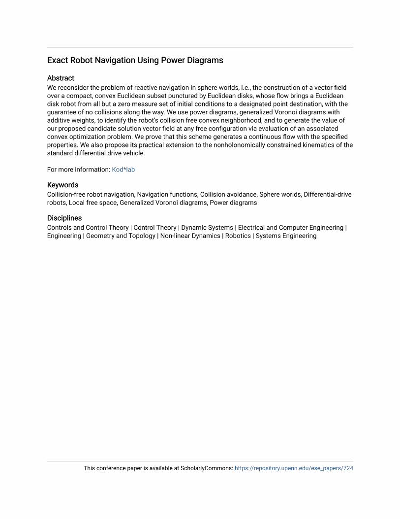
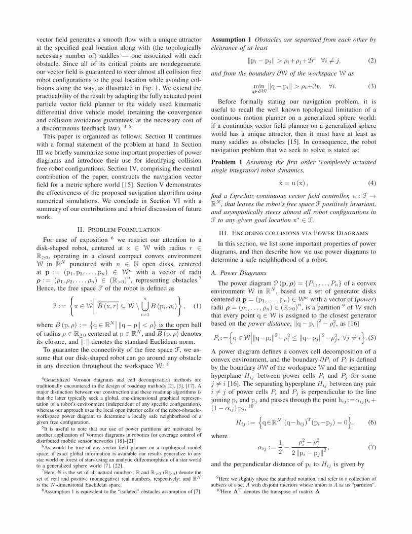
Fig. 1. Exact robot navigation using power diagrams, generated bydisks representing obstacles (black) and the robot (red at the goal). Thepower cell (yellow) associated with the robot defines its obstacle freeconvex local neighborhood, and the continuous feedback motion towardsthe metric projection of a given desired goal (red) onto this convex setasymptotically steers almost all robot configurations (green) to the goalwithout collisions along the way. The grey regions represent the augmentedworkspace boundary and obstacles, and the arrows show the direction ofthe resulting vector field.

(and consequent parameter tuning for) a topologically and

metrically simple environment [9], [10], and controlling

nonholonomically constrained kinematic systems [11], [12]

have appeared in the last decade. Sequential composition [13]

has been used to cover metrically complicated environments

with convex cell-based local potential decompositions [4]

(and extended to nonholonomically constrained finite size

robots [14]), but still necessitating prior global knowledge

of the environment.

B. Contributions and Organization of the Paper

This paper abandons the smooth potential field approach

to reactive planning, constructing a piecewise smooth vector

field with the same capabilities as navigation functions

for topologically and metrically simple environments (i.e.,

“sphere worlds” [15]), but relaxing the assumption of global

prior knowledge. We use power diagrams — generalized

Voronoi diagrams with additive weights [16] — to identify

a collision free convex neighborhood of a robot configura-

tion, and solve the safe navigation problem via continuous

evaluation of an associated convex optimization problem.

Our construction requires no parameter tuning and requires

only local knowledge of the environment in the sense that

the sensor needs only locate proximal obstacles — those

whose power cells are adjacent3 to the robot’s. The proposed

2It bears mentioning that harmonic functions are utilized to designpotential functions without local minima [8]; however, such intrinsicallynumerical constructions forfeit the reactive nature of feedback motionplanners under discussion here.

3 A pair of power cells in RN are said to be adjacent if they share aN − 1 dimensional face.

vector field generates a smooth flow with a unique attractor

at the specified goal location along with (the topologically

necessary number of) saddles — one associated with each

obstacle. Since all of its critical points are nondegenerate,

our vector field is guaranteed to steer almost all collision free

robot configurations to the goal location while avoiding col-

lisions along the way, as illustrated in Fig. 1. We extend the

practicability of the result by adapting the fully actuated point

particle vector field planner to the widely used kinematic

differential drive vehicle model (retaining the convergence

and collision avoidance guarantees, at the necessary cost of

a discontinuous feedback law). 4 5

This paper is organized as follows. Section II continues

with a formal statement of the problem at hand. In Section

III we briefly summarize some important properties of power

diagrams and introduce their use for identifying collision

free robot configurations. Section IV, comprising the central

contribution of the paper, constructs the navigation vector

field for a metric sphere world [15]. Section V demonstrates

the effectiveness of the proposed navigation algorithm using

numerical simulations. We conclude in Section VI with a

summary of our contributions and a brief discussion of future

work.

II. PROBLEM FORMULATION

For ease of exposition 6 we restrict our attention to a

disk-shaped robot, centered at x ∈ W with radius r ∈R≥0, operating in a closed compact convex environment

W in RN punctured with n ∈ N open disks, centered

at p := (p1, p2, . . . , pn) ∈ Wn with a vector of radii

ρ := (ρ1, ρ2, . . . , ρn) ∈ (R>0)n

, representing obstacles.7

Hence, the free space F of the robot is defined as

F :=

{

x ∈ W

∣∣∣∣B (x, r) ⊆ W \

n⋃

i=1

B (pi, ρi)

}

, (1)

where B (p, ρ) :={q ∈ R

N∣∣ ‖q− p‖ < ρ

}is the open ball

of radius ρ ∈ R≥0 centered at p ∈ RN , and B (p, ρ) denotes

its closure, and ‖.‖ denotes the standard Euclidean norm.

To guarantee the connectivity of the free space F, we as-

sume that our disk-shaped robot can go around any obstacle

in any direction throughout the workspace W: 8

4Generalized Voronoi diagrams and cell decomposition methods aretraditionally encountered in the design of roadmap methods [2], [3], [17]. Amajor distinction between our construction and these roadmap algorithms isthat the latter typically seek a global, one-dimensional graphical represen-tation of a robot’s environment (independent of any specific configuration),whereas our approach uses the local open interior cells of the robot-obstacle-workspace power diagram to determine a locally safe neighborhood of agiven free configuration.

5It is useful to note that our use of power partitions are motivated byanother application of Voronoi diagrams in robotics for coverage control ofdistributed mobile sensor networks [18]–[21]

6As would be true of any vector field planner on a topological modelspace, if exact global information is available our results generalize to anystar world or forest of stars using an analytic diffeomorphism of a star worldto a generalized sphere world [7], [22].

7Here, N is the set of all natural numbers; R and R>0 (R≥0) denote the

set of real and positive (nonnegative) real numbers, respectively; and RN

is the N -dimensional Euclidean space.8Assumption 1 is equivalent to the “isolated” obstacles assumption of [7].

Assumption 1 Obstacles are separated from each other by

clearance of at least

‖pi − pj‖ > ρi+ρj+2r ∀i 6= j, (2)

and from the boundary ∂W of the workspace W as

minq∈∂W

‖q− pi‖ > ρi+2r, ∀i. (3)

Before formally stating our navigation problem, it is

useful to recall the well known topological limitation of a

continuous motion planner on a generalized sphere world:

if a continuous vector field planner on a generalized sphere

world has a unique attractor, then it must have at least as

many saddles as obstacles [15]. In consequence, the robot

navigation problem that we seek to solve is stated as:

Problem 1 Assuming the first order (completely actuated

single integrator) robot dynamics,

x = u (x) , (4)

find a Lipschitz continuous vector field controller, u : F →R

N , that leaves the robot’s free space F positively invariant,

and asymptotically steers almost all robot configurations in

F to any given goal location x∗ ∈ F.

III. ENCODING COLLISIONS VIA POWER DIAGRAMS

In this section, we list some important properties of power

diagrams, and then describe how we use power diagrams to

determine a safe neighborhood of a robot.

A. Power Diagrams

The power diagram P (p,ρ) = {P1, . . . , Pn} of a convex

environment W in RN , based on a set of generator disks

centered at p = (p1, . . . , pn) ∈ Wn with a vector of (power)

radii ρ = (ρ1, . . . , ρn) ∈ (R≥0)n

, is a partition 9 of W such

that every point q ∈ W is assigned to the closest generator

based on the power distance, ‖q− pi‖2− ρ2i , as [16]

Pi :={

q ∈W

∣∣∣‖q−pi‖

2−ρ2i ≤ ‖q−pj‖

2−ρ2j , ∀j 6= i

}

. (5)

A power diagram defines a convex cell decomposition of a

convex environment, and the boundary ∂Pi of Pi is defined

by the boundary ∂W of the workspace W and the separating

hyperplane Hij between power cells Pi and Pj for some

j 6= i [16]. The separating hyperplane Hij between any pair

i 6= j of power cells Pi and Pj is perpendicular to the line

joining pi and pj and passes through the point hij :=αijpi+(1− αij) pj , 10

Hij :={

q∈RN∣∣∣(q−hij)

T(pi−pj) = 0

}

, (6)

where

αij :=1

2−

ρ2i − ρ2j

2 ‖pi − pj‖2 , (7)

and the perpendicular distance of pi to Hij is given by

9Here we slightly abuse the standard notation, and refer to a collection ofsubsets of a set A with disjoint interiors whose union is A as its “partition”.

10Here AT denotes the transpose of matrix A

d (pi, Hij) := minq∈Hij

‖q− pi‖ = (1− αij) ‖pi − pj‖ , (8a)

= ρi +(‖pi − pj‖ − ρi)

2− ρ2j

2 ‖pi − pj‖. (8b)

Note that a power diagram may yield empty power cells

associated with some generators and/or some generators

may not be contained in their nonempty power cells; and a

negative value of d (pi, Hij) indicates that pi is not contained

in Pi, i.e., pi 6∈ Pi iff d (pi, Hij) < 0 for some j 6= i [21].

Also observe that d (pi, Hij) ≥ ρi iff ‖pi − pj‖ ≥ (ρi + ρj).

B. A Safe Neighborhood of a Robot

Throughout the rest of the paper, we consider a disk-

shaped robot, centered at x ∈ W with radius r ∈ R≥0,

moving in a closed compact convex environment W ⊂ RN

populated with disk-shaped obstacles, centered at p ∈ Wn

with a vector of radii ρ ∈ (R>0)n

, satisfying Assumption 1.

Since the workspace and robot radius is fixed, we suppress

all mentions of the associated terms wherever convenient, in

order to simplify the notation.

Using the robot and obstacles as generator disks of a power

diagram of W, we define the local workspace, LW (x), of

the robot, illustrated in Fig. 2, as,

LW (x) :={

q∈W

∣∣∣‖q−x‖

2−r2 ≤ ‖q−pi‖

2−ρ2i ∀i

}

.(9)

Proposition 1 A robot placement x ∈ W \⋃n

i=1 {pi} is

collision free in F (1) if and only if the robot body is

contained in LW (x),

x ∈ F ⇐⇒ B (x, r) ⊆ LW (x) . (10)

Proof. Let p = (p0, p1, . . . , pn) ∈ Wn+1 be a disk

configuration in W with a vector of (power) radii ρ =(ρ0, ρ1, . . . , ρn) ∈ (R≥0)

n+1such that p0 = x, ρ0 = r,

and pi = pi, ρi = ρi for all i ∈ {1, 2, . . . , n}; and

let P (p, ρ) = {P0, P1, . . . , Pn} be the associated power

diagram of W. Note that LW (x) = P0.

The boundary ∂LW (x) of LW (x) is defined by the

boundary ∂W of the workspace W and the separating

hyperplane H0i between convex power cells LW (x) and

Pi for some i 6= 0; and, in general, any pair i 6= j of the

convex cells Pi and Pj are separated by the hyperlane Hij

[16]. Hence, using (1), (8), (9), and convexity of P (p, ρ),we obtain the result as

B (x, r) ⊆ LW (x) ⇐⇒

{x ∈ LW (x) ,

d (x, ∂LW (x)) ≥ r,(11)

⇐⇒︸︷︷︸

by (8) and convexityof P (p, ρ)

x ∈ LW (x) ,d (x, ∂W) ≥ r,

d (x, H0i) ≥ r ∀i 6= 0,(12)

⇐⇒︸︷︷︸

by (8) and (9)

x ∈ W,

d (x, ∂W) ≥ r,

‖x− pi‖2≥(ρ2i − r2

)∀i 6= 0,

‖x− pi‖ ≥ (r + ρi) ∀i 6= 0,

(13)

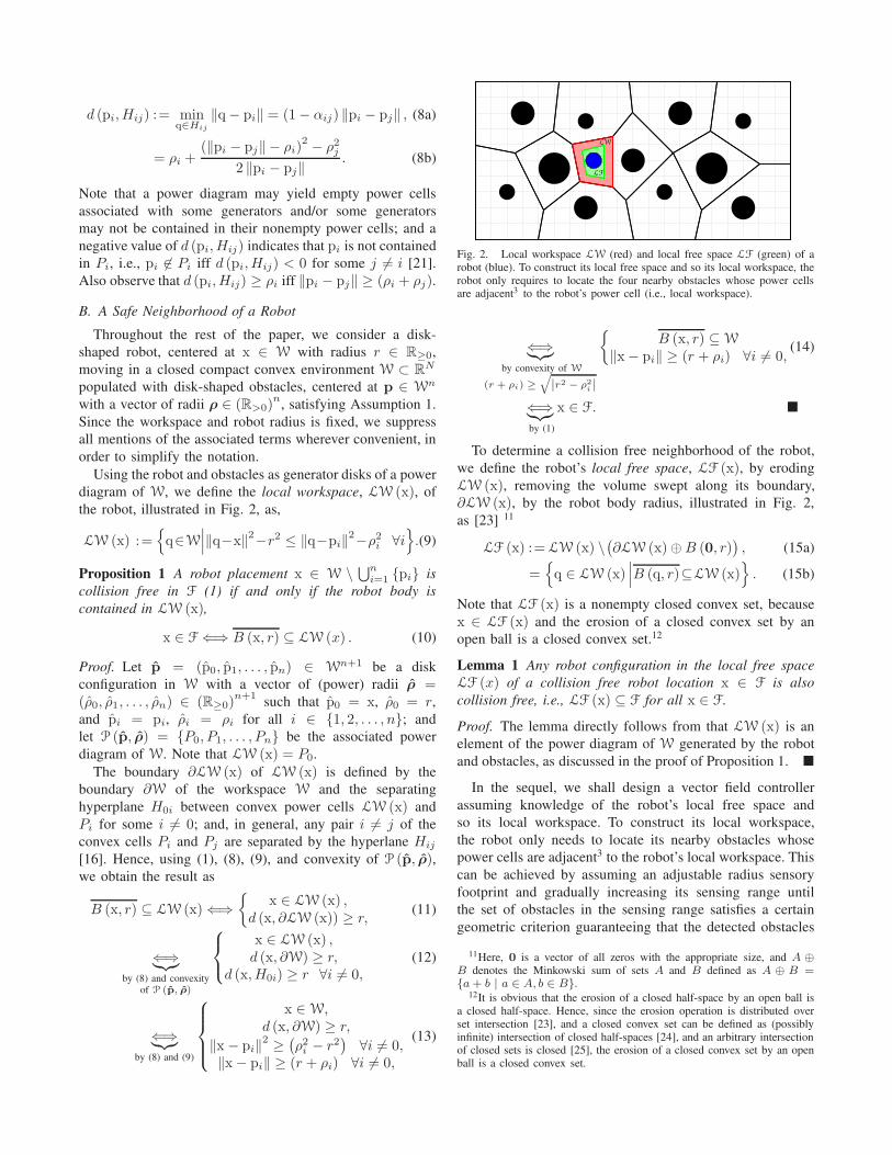
Fig. 2. Local workspace LW (red) and local free space LF (green) of arobot (blue). To construct its local free space and so its local workspace, therobot only requires to locate the four nearby obstacles whose power cellsare adjacent3 to the robot’s power cell (i.e., local workspace).

⇐⇒︸︷︷︸

by convexity of W

(r + ρi) ≥√

∣

∣r2 − ρ2

i

∣

∣

{

B (x, r) ⊆ W

‖x− pi‖ ≥ (r + ρi) ∀i 6= 0,(14)

⇐⇒︸︷︷︸

by (1)

x ∈ F. �

To determine a collision free neighborhood of the robot,

we define the robot’s local free space, LF (x), by eroding

LW (x), removing the volume swept along its boundary,

∂LW (x), by the robot body radius, illustrated in Fig. 2,

as [23] 11

LF (x) := LW (x) \(∂LW (x)⊕B (0, r)

), (15a)

={

q ∈ LW (x)∣∣∣B (q, r)⊆LW (x)

}

. (15b)

Note that LF (x) is a nonempty closed convex set, because

x ∈ LF (x) and the erosion of a closed convex set by an

open ball is a closed convex set.12

Lemma 1 Any robot configuration in the local free space

LF (x) of a collision free robot location x ∈ F is also

collision free, i.e., LF (x) ⊆ F for all x ∈ F.

Proof. The lemma directly follows from that LW (x) is an

element of the power diagram of W generated by the robot

and obstacles, as discussed in the proof of Proposition 1. �

In the sequel, we shall design a vector field controller

assuming knowledge of the robot’s local free space and

so its local workspace. To construct its local workspace,

the robot only needs to locate its nearby obstacles whose

power cells are adjacent3 to the robot’s local workspace. This

can be achieved by assuming an adjustable radius sensory

footprint and gradually increasing its sensing range until

the set of obstacles in the sensing range satisfies a certain

geometric criterion guaranteeing that the detected obstacles

11Here, 0 is a vector of all zeros with the appropriate size, and A ⊕B denotes the Minkowski sum of sets A and B defined as A ⊕ B ={a+ b | a ∈ A, b ∈ B}.

12It is obvious that the erosion of a closed half-space by an open ball isa closed half-space. Hence, since the erosion operation is distributed overset intersection [23], and a closed convex set can be defined as (possiblyinfinite) intersection of closed half-spaces [24], and an arbitrary intersectionof closed sets is closed [25], the erosion of a closed convex set by an openball is a closed convex set.

exactly defines the robot’s local workspace [18]. We leave

a comprehensive detailed study of constructing the robot’s

local workspace to a future discussion of specific sensor

model selections such as a fixed radius sensory footprint

and/or a (limited range) line-of-sight sensor.

IV. ROBOT NAVIGATION VIA POWER DIAGRAMS

In this section, we introduce a new provably correct vector

field controller for safe robot navigation in a locally sensed

metric sphere world (Problem 1), and list its important

qualitative properties. We also present its extension for the

nonholonomically constrained kinematic differential drive

robot model.

A. Feedback Robot Motion Planner

For a choice of a desired goal location x∗ ∈ F, we

propose a robot navigation strategy that steers the robot

x ∈ F towards the global goal x∗ through a safe local target

location, called “projected goal”, that solves the following

convex optimization problem,

minimize ‖q− x∗‖2

subject to q ∈ LF (x)(16)

where LF (x) (15) is the local free space around the robot

location x and is a nonempty closed convex set. It is well

known that the unique solution of (16) is given by [24,

Section 8.1.1]13

x∗ :=

{x∗ , if x∗ ∈ LF (x) ,ΠLF(x) (x

∗) , otherwise,(17)

where ΠC (q) denotes the metric projection of q ∈ RN

onto a convex set C ⊂ RN , and note that ΠC is piecewise

continuously differentiable [26].

Accordingly, for the single integrator robot dynamics (4),

our “move-to-projected-goal” law u : F → RN is defined as

u (x) = −k (x− x∗) , (18)

where k ∈ R>0 is a fixed control gain, and we assume that

LF (x) is continuously updated.

B. Qualitative Properties

We now continue with a list of its qualitative (continuity,

existence & uniqueness, invariance and stability) properties.

Proposition 2 The “move-to-projected-goal” law in (18) is

piecewise continuously differentiable.

Proof. An important property of power diagrams inherited

from standard Voronoi diagrams [28] is that the boundary

of a power cell is a piecewise continuously differentiable

13In general, the metric projection of a point onto a convex set can beefficiently computed using a standard convex programming solver [24].If W is a convex polytope, then the robot’s local free space, LF (x), isalso a convex polytope and can be written as a finite intersection of half-spaces. Hence, the metric projection onto a convex polytope can be recastas quadratic programming and can be solved in polynomial time [27]. Inthe case of a convex polygonal environment, LF (x) is a convex polygon,and the metric projection onto a convex polygon can be solved analytically,because the solution lies on one of its edges unless the input point is insidethe polygon.

function of generator locations. Similarly, for any x ∈ F,

we have that the boundary of the local free space LF (x)is piecewise continuously differentiable, because LF (x) is a

nonempty erosion of the local workspace LW (x) by a fixed

open ball, and LW (x) is an element of the power diagram of

the workspace W generated by disks representing the robot

and obstacles. Hence, one can conclude that the “move-to-

projected-goal” law is piecewise continuously differentiable

because metric projections onto (moving) convex cells are

piecewise continuously differentiable [26], [29], [30], and

the composition of piecewise continously differentiable func-

tions are also piecewise continuously differentiable [31]. �

Proposition 3 The free space F in (1) is positively invariant

under the “move-to-projected” law (18).

Proof. By construction (16), for any x ∈ F, the “move-to-

projected-goal” law always selects a safe local target location

x∗ (17) such that the line segment between x and x∗ is

free of collisions, because the local free space LF (x) is a

collision free convex set (Lemma 1) and contains both x and

x∗. Hence, at the boundary of F, the robot either stays on

the boundary or moves towards the interior of F, but never

crosses the boundary. �

Proposition 4 For any initial x ∈ F, the “move-to-projected-

goal” law (18) has a unique continuously differentiable flow

in F (1) defined for all future time.

Proof. The existence, uniqueness and continuous differen-

tiability of its flow follow from the Lipschitz continuity

of the “move-to-projected-goal” law in its compact domain

F, because a piecewise continuously differentiable function

is also locally Lipschitz on its domain [31], and a locally

Lipschitz function on a compact set is globally Lipschitz on

that set [32]. �

Proposition 5 The set of stationary points of the “move-to-

projected-goal” law (18) is {x∗} ∪ {si}i∈{1,2,...,n}, where

si := pi − (r + ρi)x∗ − pi

‖x∗ − pi‖. (19)

Proof. It follows from (17) and (18) that the goal location

x∗ is a stationary point, because x∗ ∈ LF (x∗). Note that,

for any x ∈ F, if x∗ ∈ LF (x), then x∗ = x∗. Hence, in

the sequel of the proof, we only consider the set of robot

locations satisfying x∗ 6∈ LF (x).To see that there is exactly one stationary point associated

with each obstacle, for any x ∈ F, consider the power

diagram P (p, ρ) = {P0, P1, . . . , Pn} of W associated with

p = (p0, p1, . . . , pn) ∈ Wn+1 and ρ = (ρ0, ρ1, . . . , ρn) ∈(R≥0)

n+1where p0 = x, ρ0 = r and pi = pi, ρi = ρi

for all i 6= 0. Recall that LW (x) = P0 and its boundary

∂LW (x) is defined by the boundary ∂W of W and the

separating hyperplane H0i between P0 and Pi for some

i 6= 0; and LF (x) is obtained by eroding LW (x) by an

open disk of radius r. Further, because of the convexity of

W, observe from (17) that the projected goal x∗ satisfies that

if x∗ 6∈ LF (x), then d (x∗, H0i) = r for some i 6= 0. Note

that d (x∗, H0i) = r if and only if d (pi, Hi0) = ρi (see (8))

and so ‖x∗ − pi‖ = r + ρi.

We have from (8) that if ‖x− pi‖ > (r + ρi) then

d (x, H0i) > r. Hence, if d (x, H0i) = r (i.e., d (pi, Hi0) =ρi and ‖x−pi‖ = r + ρi) for some i 6= 0, then, since

‖pi−pj‖ > (ρi+ρj+2r) (Assumption 1), ‖x− pj‖ >

r + ρj and so d (x, H0j) > r for all j 6= i. Therefore,

there is only one obstacle index i such that x = x∗ and

d (x∗, H0i) = r (i.e., ‖x∗ − pi‖ = r + ρi). Further, since x∗

the unique optimal solution of (16), H0i should be tangent

to the level curves of squared distance ‖x− x∗‖2 [24],

which is the case if x, pi and x∗ are all collinear. As a

result, by eliminating one of such antipodal points around

the obstacle, one can verify that the only stationary point siof (18) associated with ith obstacle is given by (19), which

completes the proof. �

Lemma 2 The “move-to-projected-goal” law (18) in a small

neighborhood of the goal x∗ is given by

u (x) = −k (x− x∗) , ∀ x ∈ B (x∗, ǫ) , (20)

for some ǫ > 0; and around the stationary point si (19),

associated with obstacle i, it is given by

u (x) = −k

(

x−x∗+(x−pi)

T(x∗−hi)

‖x−pi‖2 (x−pi)

)

, (21)

for all x ∈ B(si, ε) and some ε > 0, where hi := αix+

(1−αi) pi and αi =12 −

r2−ρ2

i

2‖x−pi‖2 + r

‖x−pi‖. 14

Proof. The result for the goal location x∗ follows from the

continuity of power diagrams and x∗ ∈ LF (x∗).To see the result for the stationary point si, recall from

the proof of Proposition 5 that si lies on the boundary of

LF (si) defined by the separating hyperplane between the

robot’s power cell (i.e., local workspace) and ith obstacle’s

power cell, and has a certain clearance between the boundary

segment of LF (si) defined by the separating hyperplane

between the robot’s power cell and any other obstacle’s

power cell. Hence, using the continuity of power partitions,

for any x ∈ B (si, ε) the projected-goal x∗ can be located

by taking the projection of x∗ onto (a shifted version of) the

separating hyperplane between the robot’s power cell and ith

obstacle’s as

x∗ = x∗ −(x− pi)

T(x∗ − hi)

‖x− pi‖2 (x− pi) , (22)

which completes the proof. �

Proposition 6 The goal x∗ is the only locally stable equi-

librium of the “move-to-projected-goal” law (18), and all

the stationary points, si (19), associated with obstacles are

nondegenerate saddles.

Proof. The goal x∗ is a locally stable point of the “move-to-

projected-goal” law, because its Jacobian at x∗ is the diagonal

matrix with all diagonal entries equal to −k (Lemma 2).

14 αi is a slightly different version of αij (7) because LF (x) is theerosion of LW (x) by the robot body radius r.

To determine the type of the stationary point si, without

loss of generality, let pi = (pi1, 0, . . . , 0) ∈ RN and

x∗ = (x∗1, 0, . . . , 0) ∈ R

N such that pi1 < x∗1, and so

si = (si1, 0, . . . , 0) ∈ RN satisfying si1 < pi1. Note that

since x∗ ∈ F and ‖si − pi‖ = r + ρi, we have x∗1 − pi1 ≥

pi1 − si1 = r + ρi and so x∗1 − si1 ≥ 2 (pi1 − si1). Hence,

using (21), one can verify that the Jacobian matrix of the

“move-to-projected-goal” at si is given by

J =du (x)

dx

∣∣∣∣x=si

=

−k ρi

r+ρi? ? . . . ?

0 β 0 . . . 0...

. . .. . .

. . ....

0 . . . 0 β 00 . . . . . . 0 β

(23)

where β = kx∗

1−pi1

r+ρi≥ k. Since it is in a triangular form,

the eigenvalues of J are its diagonal elements. Therefore, siis the nondegenerate saddle point of the “move-to-projected-

goal” law associated with ith obstacle, and this completes

the proof. �

Proposition 7 The goal location x∗ is an asymptotically sta-

ble equilibrium of the “move-to-projected-goal” law, whose

basin of attraction includes F, except a set of measure zero.

Proof. Consider the squared Euclidean distance to the

goal as a smooth Lyapunov function candidate, i.e.,

V (x) := ‖x− x∗‖2, and it follows from (16) and (18) that

V (x) = −k 2(x− x∗)T(x− x∗)

︸ ︷︷ ︸

≥‖x−x∗‖2

since x∈LF(x) and ‖x−x∗‖2≥‖x∗−x∗‖2

, (24)

≤ −k ‖x− x∗‖2≤ 0, (25)

which is zero if and only if x is a stationary point. Hence, we

have from LaSalle’s Invariance Principle [32] that all robot

configurations in F asymptotically reach the set of equilibria

of (18). Therefore, the result follows from Proposition 2 and

Proposition 6 since x∗ is the only stable stationary point

of the piecewise continuous “move-to-projected-goal” law

(18) and all other stationary points are nondegenerate saddles

whose stable manifolds have empty interiors [33]. �

Finally, we find it useful to summarize important qualita-

tive properties of “move-to-projected-goal” law as:15

Theorem 1 The piecewise continuously differentiable

“move-to-projected-goal” law in (18) leaves robot’s free

space F (1) positively invariant, and its unique continu-

ously differentiable flow, starting at almost any configuration

x ∈ F, asymptotically reaches the goal location x∗, while

strictly decreasing the squared Euclidean distance to the

goal, ‖x− x∗‖2, along the way.

15Since the “move-to-projected-goal” law is piecewise continously dif-ferentiable, it can be lifted to higher order dynamical models [34]–[36].

C. An Extension for Differential Drive Robots

Consider a disk-shaped differential drive robot described

by state (x, θ) ∈ F × (−π, π], centered at x ∈ F with body

radius r ∈ R≥0 and orientation θ ∈ (−π, π], moving in W.

The kinematic equations describing its motion are

x = v

[cos θsin θ

]

,

θ = ω,

(26)

where v ∈ R and ω ∈ R are, respectively, the linear

(tangential) and angular velocity inputs of the robot.

In contrary to the “move-to-projected-goal” law of a fully

actuated robot in (18), a differential drive robot can not

directly move towards the projected goal x∗ (17) of a given

goal location x∗ ∈ F, unless it is perfectly aligned with

x∗, because it is underactuated due to the nonholonomic

constraint[

− sin θcos θ

]T

x = 0. 16 In consequence, to determine

a linear velocity input that guarantees collision avoidance

and conforms to the nonholonomic constraint, we select

a safe target location that satisfies the following convex

optimization problem,

minimize ‖q− x∗‖2

subject to q ∈ LF (x) ∩HN

(27)

where

HN :=

{

q ∈ W

∣∣∣

[− sin θcos θ

]T

(q− x) = 0

}

(28)

is the straight line motion range due to the nonholonomic

constraint. Note that LF (x) ∩HN is a closed line segment

in W. Hence, once again, the unique solution of (27) is given

by

x∗v :=

{x∗ , if x∗ ∈ LF (x) ∩HN ,

ΠLF(x)∩HN(x∗), otherwise,

(29)

where ΠC is the metric projection map onto a convex set C.

Similarly, to determine the robot’s angular motion, we select

another safe target location that solves

minimize ‖q− x∗‖2

subject to q ∈ LF (x) ∩HG

(30)

where

HG :={

ωx + (1− ω) x∗ ∈ W

∣∣∣ ω ∈ R

}

(31)

is the line segment of W containing x and x∗, and the unique

solution of (30) is

x∗ω :=

{x∗ , if x∗ ∈ LF (x) ∩HG,

ΠLF(x)∩HG(x∗), otherwise.

(32)

Accordingly, based on a standard differential drive con-

troller [37], we propose the following “move-to-projected-

goal” law for a differential drive robot,17 18

16Here, F denotes the interior of F, and we particularly require the goal

location to be in F to guarantee that a robot can nearly align its orientationwith the (local) goal location in finite time.

17We follow [37] by resolving the indeterminacy through setting ω =

0 whenever x =x∗

ω+x∗

2. Note that this introduces the discontinuity

necessitated by Brockett’s condition [38].

v = −k[

cos θsin θ

]T

(x− x∗v) , (33a)

ω = k atan

[− sin θcos θ

]T (

x−x∗

ω+x∗

2

)

[cos θsin θ

]T (

x−x∗

ω+x∗

2

)

, (33b)

where k > 0 is fixed and x∗ is the projected goal as defined

in (17).

We summarize some important properties of the “move-

to-projected-goal” law of a differential drive robot as:

Proposition 8 The “move-to-projected-goal” law of a disk-

shaped differential drive robot in (33) asymptotically steers

almost all configurations in its positively invariant domain

F×(−π, π] towards any given goal location x∗ ∈ F, without

increasing the Euclidean distance to the goal along the way.

Proof. The positive invariance of F × (−π, π] under the

“move-to-projected-goal” law (33) and the existence and

uniqueness of its flow can be established using similar

patterns of the proofs of Proposition 2, Proposition 3 and

Proposition 4, and the flow properties of the differential drive

controller in [37].

Using the squared distance to goal, V (x) = ‖x− x∗‖2,

as a smooth Lypunov function candidate, one can establish

the stability properties from (26), (27) and (33) as follows:

for any (x, θ) ∈ F × (−π, π]

V (x) = −k 2(x− x∗)T(x− x∗v)

︸ ︷︷ ︸

≥‖x−x∗

v‖2

since x∈LF(x)∩HN and ‖x−x∗‖2≥‖x∗

v−x∗‖2

, (34)

≤ −k ‖x− x∗v‖2≤ 0. (35)

Hence, it follows from LaSalle’s Invariance Principle [32]

that all configurations in F × (−π, π] asymptotically reach

the set of configurations where robots are located at the

associated projected goal x∗v at any arbitrary orientation,

{(x, θ) ∈ F × (−π, π]

∣∣x = x∗v

}. (36)

Note that, for any fixed x∗v, x∗ω and x∗, the standard differ-

ential drive controller asymptotically aligns the robot withx∗

ω+x∗

2 , i.e.,[

− sin θcos θ

]T (

x−x∗

ω+x∗

2

)

= 0. Hence, using

(16), (27) and (30), one can conclude that x∗v = x∗ω = x∗,

whenever x = x∗v and[

− sin θcos θ

]T (

x−x∗

ω+x∗

2

)

= 0.

Therefore, using a similar approach to the proofs of

Proposition 5, Lemma 2 and Proposition 6, one can verify

that the set of stationary points of (33) is given by

{x∗}×(−π, π]⋃{

(si, θ)∈F×(−π, π]

∣∣∣∣

[− sin θcos θ

]T

(si−x∗)=0

}

,(37)

18In the design of angular motion, we particularly select a local target

location,x∗

ω+x∗

2∈ F given x∗ ∈ F, in the interior F of F to increase

the convergence rate of the resulting vector field. One can consider otherconvex combinations of x∗ω and x∗, and the resulting vector field retainsqualitative properties.

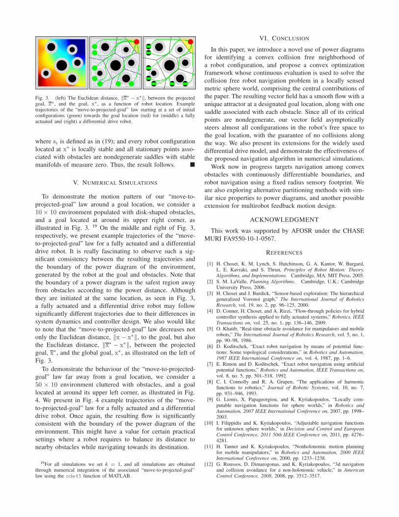
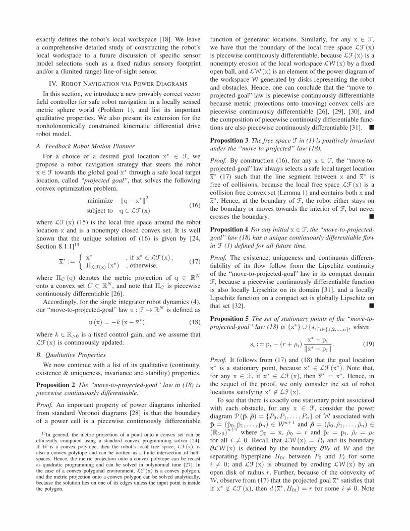
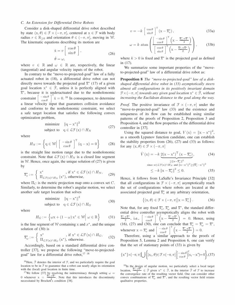
Fig. 3. (left) The Euclidean distance, ‖x∗ − x∗‖, between the projectedgoal, x∗, and the goal, x∗, as a function of robot location. Exampletrajectories of the “move-to-projected-goal” law starting at a set of initialconfigurations (green) towards the goal location (red) for (middle) a fullyactuated and (right) a differential drive robot.

where si is defined as in (19); and every robot configuration

located at x∗ is locally stable and all stationary points asso-

ciated with obstacles are nondegenerate saddles with stable

manifolds of measure zero. Thus, the result follows. �

V. NUMERICAL SIMULATIONS

To demonstrate the motion pattern of our “move-to-

projected-goal” law around a goal location, we consider a

10 × 10 environment populated with disk-shaped obstacles,

and a goal located at around its upper right corner, as

illustrated in Fig. 3. 19 On the middle and right of Fig. 3,

respectively, we present example trajectories of the “move-

to-projected-goal” law for a fully actuated and a differential

drive robot. It is really fascinating to observe such a sig-

nificant consistency between the resulting trajectories and

the boundary of the power diagram of the environment,

generated by the robot at the goal and obstacles. Note that

the boundary of a power diagram is the safest region away

from obstacles according to the power distance. Although

they are initiated at the same location, as seen in Fig. 3,

a fully actuated and a differential drive robot may follow

significantly different trajectories due to their differences in

system dynamics and controller design. We also would like

to note that the “move-to-projected-goal” law decreases not

only the Euclidean distance, ‖x− x∗‖, to the goal, but also

the Euclidean distance, ‖x∗ − x∗‖, between the projected

goal, x∗, and the global goal, x∗, as illustrated on the left of

Fig. 3.

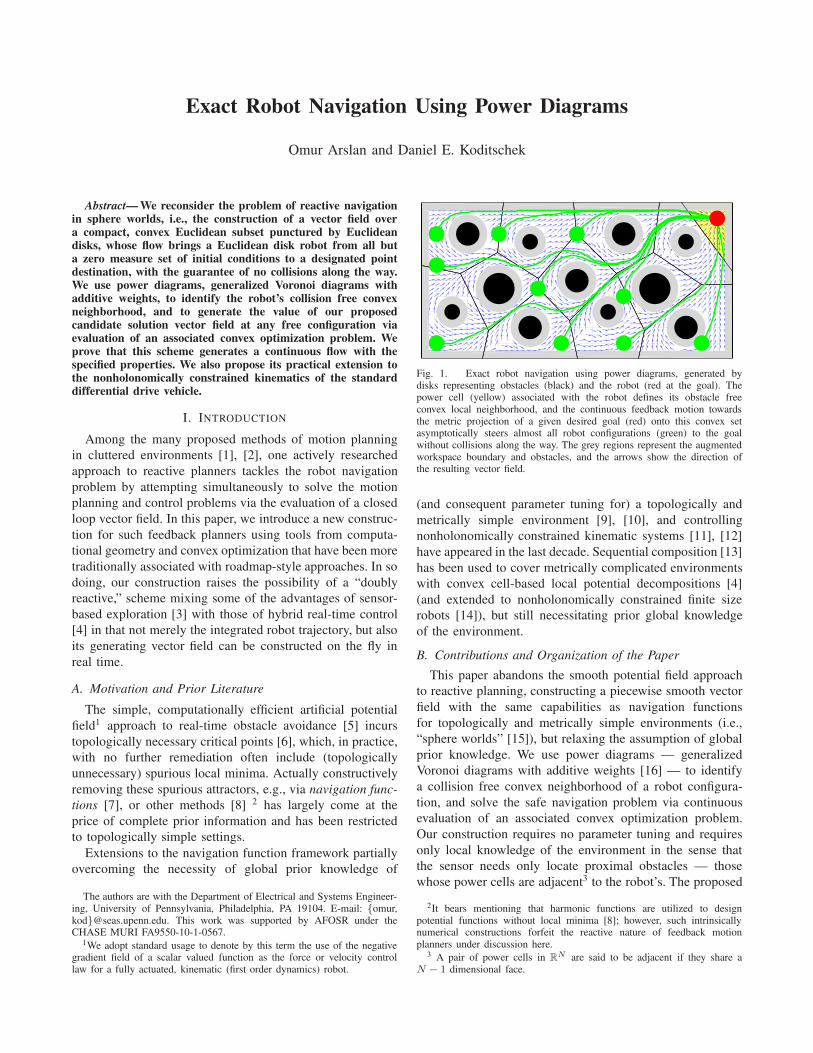
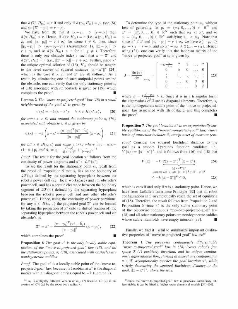
To demonstrate the behaviour of the “move-to-projected-

goal” law far away from a goal location, we consider a

50 × 10 environment cluttered with obstacles, and a goal

located at around its upper left corner, as illustrated in Fig.

4. We present in Fig. 4 example trajectories of the “move-

to-projected-goal” law for a fully actuated and a differential

drive robot. Once again, the resulting flow is significantly

consistent with the boundary of the power diagram of the

environment. This might have a value for certain practical

settings where a robot requires to balance its distance to

nearby obstacles while navigating towards its destination.

19For all simulations we set k = 1, and all simulations are obtainedthrough numerical integration of the associated “move-to-projected-goal”law using the ode45 function of MATLAB.

VI. CONCLUSION

In this paper, we introduce a novel use of power diagrams

for identifying a convex collision free neighborhood of

a robot configuration, and propose a convex optimization

framework whose continuous evaluation is used to solve the

collision free robot navigation problem in a locally sensed

metric sphere world, comprising the central contributions of

the paper. The resulting vector field has a smooth flow with a

unique attractor at a designated goal location, along with one

saddle associated with each obstacle. Since all of its critical

points are nondegenerate, our vector field asymptotically

steers almost all configurations in the robot’s free space to

the goal location, with the guarantee of no collisions along

the way. We also present its extensions for the widely used

differential drive model, and demonstrate the effectiveness of

the proposed navigation algorithm in numerical simulations.

Work now in progress targets navigation among convex

obstacles with continuously differentiable boundaries, and

robot navigation using a fixed radius sensory footprint. We

are also exploring alternative partitioning methods with sim-

ilar nice properties to power diagrams, and another possible

extension for multirobot feedback motion design.

ACKNOWLEDGMENT

This work was supported by AFOSR under the CHASE

MURI FA9550-10-1-0567.

REFERENCES

[1] H. Choset, K. M. Lynch, S. Hutchinson, G. A. Kantor, W. Burgard,L. E. Kavraki, and S. Thrun, Principles of Robot Motion: Theory,Algorithms, and Implementations. Cambridge, MA: MIT Press, 2005.

[2] S. M. LaValle, Planning Algorithms. Cambridge, U.K.: CambridgeUniversity Press, 2006.

[3] H. Choset and J. Burdick, “Sensor-based exploration: The hierarchicalgeneralized Voronoi graph,” The International Journal of Robotics

Research, vol. 19, no. 2, pp. 96–125, 2000.

[4] D. Conner, H. Choset, and A. Rizzi, “Flow-through policies for hybridcontroller synthesis applied to fully actuated systems,” Robotics, IEEE

Transactions on, vol. 25, no. 1, pp. 136–146, 2009.

[5] O. Khatib, “Real-time obstacle avoidance for manipulators and mobilerobots,” The International Journal of Robotics Research, vol. 5, no. 1,pp. 90–98, 1986.

[6] D. Koditschek, “Exact robot navigation by means of potential func-tions: Some topological considerations,” in Robotics and Automation,

1987 IEEE International Conference on, vol. 4, 1987, pp. 1–6.

[7] E. Rimon and D. Koditschek, “Exact robot navigation using artificialpotential functions,” Robotics and Automation, IEEE Transactions on,vol. 8, no. 5, pp. 501–518, 1992.

[8] C. I. Connolly and R. A. Grupen, “The applications of harmonicfunctions to robotics,” Journal of Robotic Systems, vol. 10, no. 7,pp. 931–946, 1993.

[9] G. Lionis, X. Papageorgiou, and K. Kyriakopoulos, “Locally com-putable navigation functions for sphere worlds,” in Robotics and

Automation, 2007 IEEE International Conference on, 2007, pp. 1998–2003.

[10] I. Filippidis and K. Kyriakopoulos, “Adjustable navigation functionsfor unknown sphere worlds,” in Decision and Control and European

Control Conference, 2011 50th IEEE Conference on, 2011, pp. 4276–4281.

[11] H. Tanner and K. Kyriakopoulos, “Nonholonomic motion planningfor mobile manipulators,” in Robotics and Automation, 2000 IEEEInternational Conference on, 2000, pp. 1233–1238.

[12] G. Roussos, D. Dimarogonas, and K. Kyriakopoulos, “3d navigationand collision avoidance for a non-holonomic vehicle,” in American

Control Conference, 2008, 2008, pp. 3512–3517.

Fig. 4. Example trajectories of the “move-to-projected-goal” law for a fully actuated (top) and a differential drive (bottom) robot starting at a set of initialconfigurations (green) towards a desired goal location (red).

[13] R. R. Burridge, A. A. Rizzi, and D. E. Koditschek, “Sequential com-position of dynamically dexterous robot behaviors,” The InternationalJournal of Robotics Research, vol. 18, no. 6, pp. 535–555, 1999.

[14] D. Conner, H. Choset, and A. Rizzi, “Integrating planning andcontrol for single-bodied wheeled mobile robots,” Autonomous Robots,vol. 30, no. 3, pp. 243–264, 2011.

[15] D. E. Koditschek and E. Rimon, “Robot navigation functions onmanifolds with boundary,” Advances in Applied Mathematics, vol. 11,no. 4, pp. 412 – 442, 1990.

[16] F. Aurenhammer, “Power diagrams: Properties, algorithms and appli-cations,” SIAM Journal on Computing, vol. 16, no. 1, pp. 78–96, 1987.

[17] C. O’Dunlaing and C. K. Yap, “A retraction method for planning themotion of a disc,” Journal of Algorithms, vol. 6, no. 1, pp. 104 – 111,1985.

[18] J. Cortes, S. Martınez, T. Karatas, and F. Bullo, “Coverage control formobile sensing networks,” Robotics and Automation, IEEE Transac-

tions on, vol. 20, no. 2, pp. 243–255, 2004.

[19] A. Kwok and S. Martnez, “Deployment algorithms for a power-constrained mobile sensor network,” International Journal of Robust

and Nonlinear Control, vol. 20, no. 7, pp. 745–763, 2010.

[20] L. Pimenta, V. Kumar, R. Mesquita, and G. Pereira, “Sensing andcoverage for a network of heterogeneous robots,” in Decision andControl, 2008 47th IEEE Conference on, 2008, pp. 3947–3952.

[21] O. Arslan and D. E. Koditschek, “Voronoi-based coverage con-trol of heterogeneous disk-shaped robots,” in Robotics and Au-

tomation, 2016 IEEE International Conference on (accepted), 2016,http://arxiv.org/abs/1509.03842.

[22] E. Rimon and D. E. Koditschek, “The construction of analytic diffeo-morphisms for exact robot navigation on star worlds,” Transactions

of the American Mathematical Society, vol. 327, no. 1, pp. 71–116,1991.

[23] R. Haralick, S. R. Sternberg, and X. Zhuang, “Image analysis usingmathematical morphology,” Pattern Analysis and Machine Intelli-

gence, IEEE Transactions on, vol. PAMI-9, no. 4, pp. 532–550, 1987.

[24] S. Boyd and L. Vandenberghe, Convex Optimization. CambridgeUniversity Press, 2004.

[25] J. Munkres, Topology, 2nd ed. Pearson, 2000.[26] L. Kuntz and S. Scholtes, “Structural analysis of nonsmooth mappings,

inverse functions, and metric projections,” Journal of Mathematical

Analysis and Applications, vol. 188, no. 2, pp. 346 – 386, 1994.[27] M. Kozlov, S. Tarasov, and L. Khachiyan, “The polynomial solvability

of convex quadratic programming,” USSR Computational Mathematicsand Mathematical Physics, vol. 20, no. 5, pp. 223–228, 1980.

[28] F. Bullo, J. Cortes, and S. Martinez, Distributed Control of Robotic

Networks: A Mathematical Approach to Motion Coordination Algo-rithms. Princeton University Press, 2009.

[29] A. Shapiro, “Sensitivity analysis of nonlinear programs and differen-tiability properties of metric projections,” SIAM Journal on Control

and Optimization, vol. 26, no. 3, pp. 628–645, 1988.[30] J. Liu, “Sensitivity analysis in nonlinear programs and variational

inequalities via continuous selections,” SIAM Journal on Control and

Optimization, vol. 33, no. 4, pp. 1040–1060, 1995.[31] R. W. Chaney, “Piecewise Ck functions in nonsmooth analysis,”

Nonlinear Analysis: Theory, Methods & Applications, vol. 15, no. 7,pp. 649 – 660, 1990.

[32] H. K. Khalil, Nonlinear Systems, 3rd ed. Prentice Hall, 2001.[33] M. W. Hirsch, S. Smale, and R. L. Devaney, Differential Equations,

Dynamical Systems, and an Introduction to Chaos, 2nd ed. Academicpress, 2003.

[34] D. E. Koditschek, “Adaptive techniques for mechanical systems,” inProc. 5th. Yale Workshop on Adaptive Systems, 1987, pp. 259–265.

[35] ——, “Some applications of natural motion control,” Journal of

Dynamic Systems, Measurement, and Control, vol. 113, pp. 552–557,1991.

[36] R. Fierro and F. L. Lewis, “Control of a nonholomic mobile robot:Backstepping kinematics into dynamics,” Journal of Robotic Systems,vol. 14, no. 3, pp. 149–163, 1997.

[37] A. Astolfi, “Exponential stabilization of a wheeled mobile robot viadiscontinuous control,” Journal of dynamic systems, measurement, and

control, vol. 121, no. 1, pp. 121–126, 1999.[38] R. W. Brockett, Asymptotic stability and feedback stabilization. De-

fense Technical Information Center, 1983.