arX

iv:c

ond-

mat

/000

4169

v1 [

cond

-mat

.sof

t] 1

1 A

pr 2

000

Exactness of the Annealed and the Replica Symmetric

Approximations for Random Heteropolymers

Ugo Bastolla(1,2) and Peter Grassberger(1)

(1)HLRZ, Forschungszentrum Julich, D-52425 Julich, Germany

(2)Max Planck Institute for Colloids and Interfaces, D-14424 Potsdam, Germany

PACS: 87.15.Aa

February 1, 2008

Abstract

We study a heteropolymer model with random contact interactions introduced sometime ago as a simplified model for proteins. The model consists of self-avoiding walks onthe simple cubic lattice, with contact interactions between nearest neighbor pairs. Foreach pair, the interaction energy is an independent Gaussian variable with mean valueB and variance ∆2. For this model the annealed approximation is expected to becomeexact for low disorder, at sufficiently high dimension and in the thermodynamic limit. Weshow that corrections to the annealed approximation in the 3-d high temperature phaseare small, but do not vanish in the thermodynamic limit, and are in good agreement withour replica symmetric calculations. Such corrections derive from the fact that the overlapbetween two typical chains is nonzero. We explain why previous authors had come tothe opposite conclusion, and discuss consequences for the thermodynamics of the model.Numerical results were obtained by simulating chains of length N ≤ 1400 by means of therecent PERM algorithm, in the coil and molten globular phases, well above the freezingtemperature.

1 Introduction

Apart from their extreme biological importance, proteins are also very interesting objects fromthe point of view of statistical mechanics. They possess a very well defined native structurewhich they are able to find in a short time among a potentially huge number of competingones, and in spite of many metastable states. How proteins reconcile the stability of the nativestructure with the requirement that this structure is rapidly reached constitutes the essence ofthe fascinating and still open protein folding problem [1]

An interesting question is whether the property of folding is a generic property of ran-domly assembled polypeptidic chains, regardless of their biological function, or is a specialproperty that has evolved through natural selection. This kind of question makes the protein

folding problem a bridge between theoretical biology and the statistical mechanics of disor-dered systems. Motivated by this, numerous authors have studied simple models of randomheteropolymers [2, 3, 4, 5, 6, 7, 8, 9, 10, 11, 12, 13, 14, 15, 16, 17, 18], see [19] for a review.

In the following, we shall discuss only the ‘random bond model’ introduced independentlyby Garel and Orland [3] and by Shakhnovich and Gutin [4]. More precisely, in our numericalsimulations we will study a lattice version of this model. Preliminary results of this work havealready been presented in [20]. A “protein” with N + 1 “amino acids” is represented as aself-avoiding walk [21] of N steps on the simple cubic lattice. Each pair (i, j) of non-bondedmonomers on nearest neighbor lattice sites contributes to the total energy an amount givenby an independent and identically distributed (iid) Gaussian variable Bij with mean B′ andvariance ∆′2. Formally, one defines the contact map of configuration C, σ(C), as the matrix ofbinary variables σij ∈ {0, 1}, with i, j ∈ {0, · · ·N}, such that

σij(C) =

{

1 if i and j are in contact and non-bonded0 otherwise.

(1)

The energy of the model can then be written as

E(C, {B}) =∑

i<j

σij(C)Bij , (2)

with Bij = B′, B2ij − Bij

2= ∆′2. For a given realization of the interaction energies Bij

(representing a protein sequence in the biological analogy), the partition sum ZN at temperatureT can be formally computed as

ZN{Bij} =∑

C

e−E(C,{B})/kBT , (3)

where the sum over configurations C runs over all self-avoiding N -step walks. Obviously, theabove expression depends only on the variables ∆ = ∆′/kBT and B = B′/kBT , i.e. we havea two-parameter phase diagram in the variables B and ∆. The main advantage in using B asone of the independent variables instead of T or β = 1/kBT is that we can pass continuouslyfrom positive (repulsive, hydrophilic) to negative (hydrophobic) B.

As usual with random models, we have to evaluate the quenched average of the free energy.This is a very difficult task, while it is rather easy to perform an annealed average over thedisorder. For several models of random spin systems it is well known that such an annealedapproximation becomes exact in the high temperature phase, in the thermodynamic limit andat sufficiently large dimension. The same is thought to be true for the present model. It wasindeed predicted in [4] that the annealed approximation becomes exact in 3 dimensions whenthe chain length tends to infinity. For this to be true it is necessary that the overlap between tworandomly chosen replicas with the same realization of disorder vanishes in the limit N → ∞.

Numerical tests of this prediction have been made in the past for chains of length ≤ 36,mostly by means of exact enumerations of maximally compact chains of length 27 [14, 15].These authors found deviations (replica overlap is non-zero) which seemed to decrease with N .A similar result even for d = 2 was found in [18], where also Monte Carlo simulations of veryshort chains were used (up to N = 64). But it is clear that tests with such short chains canhardly be significant. In the present paper we shall present Monte Carlo simulations for chainsof length up to N = 1400. These simulations are made with the PERM algorithm developed

recently by one of us [25], and applied successfully to a number of different polymer problems[26, 27, 28, 29].

We study the corrections to the annealed approximation using two different approaches.First, we compute them using the replica method and assuming replica symmetry, which isbelieved to hold for low disorder. Even if a full computation was not possible, the expectedbehavior was well confirmed by numerical simulations. Second, we notice that corrections to theannealed approximation in the weak disorder limit can be related exactly to the average overlapbetween pairs of homopolymers (without any disorder). We give strong theoretical argumentsthat this overlap does not vanish in the limit N → ∞. We also calculate it by means of MonteCarlo simulations. Unlike in the previous case, these simulations do not involve the averagingover the disorder and thus can be applied to larger systems.

The two methods agree with each other and show that the corrections to the annealedapproximation are small in d = 3, but do not vanish in the thermodynamic limit. Deviationsfrom the annealed approximation are larger in the coil (high-temperature) phase and very smallin the collapsed (globular) phase.

The annealed approximation is presented in sec.2 and compared to results of Monte Carlosimulations. In order to explain the observed deviations, we study in sec.3 a scenario where theoverlap is non-zero but replica symmetry is unbroken. We again compare theoretical predictionswith simulation results. The relationship between the weak disorder limit and homopolymeroverlap is discussed in sec.4. Additional thermodynamic considerations are presented in sec.5,and our final conclusions are drawn in sec.6. The PERM algorithm used for the simulations isdiscussed in an appendix.

2 Annealed Approximation

In thermodynamic systems with quenched disorder we have to consider the average of the freeenergy per monomer over individual realizations of disorder {Bij} which formally is given by

FN(B, ∆) = − 1

βNlog (ZN{Bij})) ≡ − 1

βN

∏

i<j

∫

dBije−(Bij−B)2/2∆2

∆√

2πZN{Bij} . (4)

As for most random systems, this cannot be evaluated in closed form. Much easier toevaluate is the annealed approximation

FN,ann(B, ∆) = − 1

Nlog ZN (5)

obtained by taking the disorder average before taking the log. Here the Gaussian integrals canbe done explicitly, with the result

ZN =∑

C

e−(B− 1

2∆2)

∑

i<jσij(C)

. (6)

Since this is the partition sum for a homopolymer with pair energy

B = B − 1

2∆2, (7)

we see that [4]FN,ann(B, ∆) = FN(B, 0) . (8)

Therefore, all thermodynamic variables can be expressed in the annealed approximationin terms of an equivalent homopolymer with shifted interaction strength. This relationshipis easiest for those observables whose definition does not involve a derivative with respect totemperature, such as the gyration and end-to-end radii, and the density of non-bonded nearestneighbor contacts c. The latter is defined as the average number of nn. contacts betweennon-consecutive monomers divided by N . For these observables, we have

RN,ann(B, ∆) = RN (B, 0) (9)

andcann(B, ∆) = c(B, 0) ≡ c, (10)

precisely as in eq.(8).For energy U and entropy S the relations are less simple, since these involve derivatives of

the free energy with respect to T which are changed into derivatives with respect to B and ∆by our convention of using T = 1. For the energy per monomer it holds

UN,ann(B, ∆) =B − ∆2

BUN(B, 0) =

(

B − ∆2

B

)

c , (11)

where we used the fact that the energy for homopolymers is UN(B, 0) = cB. For the specificentropy SN(B, ∆) = − ∂

∂TFN (B, ∆, T )|T=1 we use FN(B, ∆, T ) =

TFN(B/T, ∆/T, 1) together with eq.(8), and obtain

SN,ann(B, ∆) = SN (B, 0) − ∆2

2BUN(B, 0) . (12)

The number of configurations with fixed c should increase as exp(Nf(c)) for large N , i.e.f(c) is the entropy density in the fixed-N , fixed-c ensemble. For homopolymers, the ensemblewith fixed B becomes equivalent to the fixed-c ensemble in the limit N → ∞, Thus c becomesa non-fluctuating function of B, c = c(B) ≡ c, and the above formula becomes simply

SN,ann(B, ∆) = f(c) − ∆2

2c forN → ∞ , (13)

where c(B) is the solution of the saddle point equation

f ′(c) ≡ ∂f(c)

∂c|c=c = B. (14)

The condition for thermodynamic stability is that the second derivative of f should benegative, corresponding to F being minimal. This is equivalent to requiring that the specificheat is positive. In fact, the specific heat for a homopolymer is given by

CV = B∂c

∂T= −B2

(

∂2f

∂c2

)−1

, (15)

0.0 1.0 2.0∆

−1.0

0.0

1.0

BSwollen coil

Globule

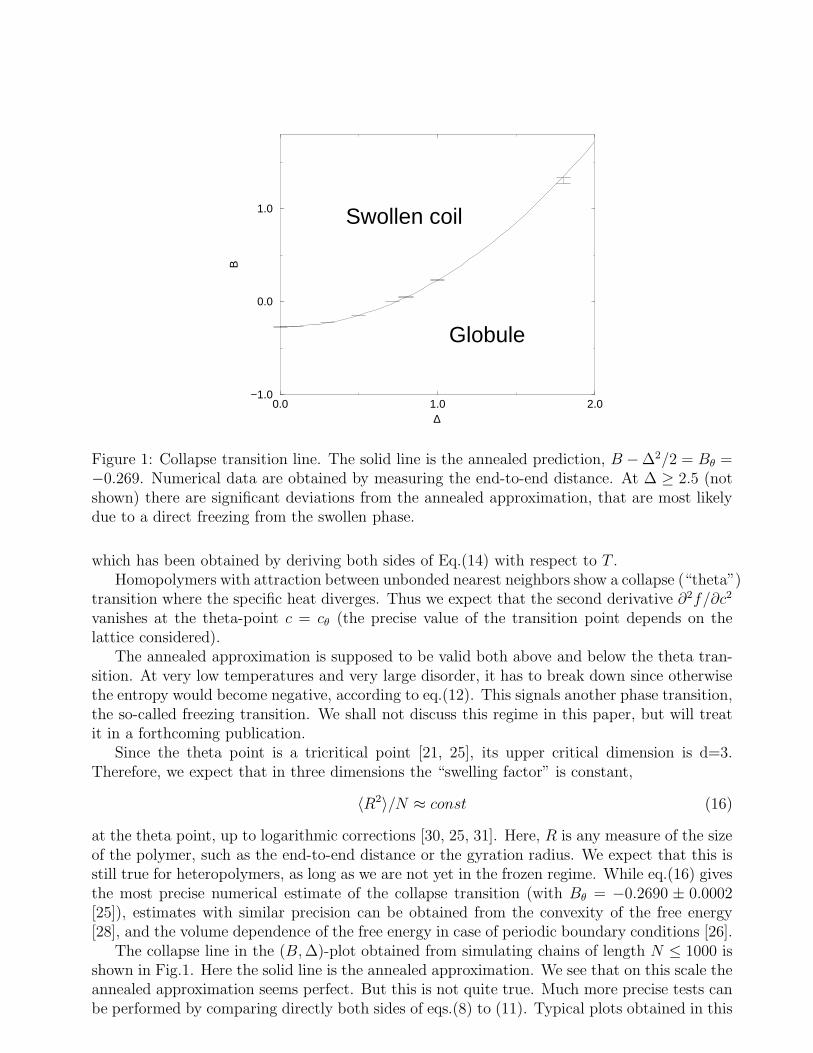
Figure 1: Collapse transition line. The solid line is the annealed prediction, B −∆2/2 = Bθ =−0.269. Numerical data are obtained by measuring the end-to-end distance. At ∆ ≥ 2.5 (notshown) there are significant deviations from the annealed approximation, that are most likelydue to a direct freezing from the swollen phase.

which has been obtained by deriving both sides of Eq.(14) with respect to T .Homopolymers with attraction between unbonded nearest neighbors show a collapse (“theta”)

transition where the specific heat diverges. Thus we expect that the second derivative ∂2f/∂c2

vanishes at the theta-point c = cθ (the precise value of the transition point depends on thelattice considered).

The annealed approximation is supposed to be valid both above and below the theta tran-sition. At very low temperatures and very large disorder, it has to break down since otherwisethe entropy would become negative, according to eq.(12). This signals another phase transition,the so-called freezing transition. We shall not discuss this regime in this paper, but will treatit in a forthcoming publication.

Since the theta point is a tricritical point [21, 25], its upper critical dimension is d=3.Therefore, we expect that in three dimensions the “swelling factor” is constant,

〈R2〉/N ≈ const (16)

at the theta point, up to logarithmic corrections [30, 25, 31]. Here, R is any measure of the sizeof the polymer, such as the end-to-end distance or the gyration radius. We expect that this isstill true for heteropolymers, as long as we are not yet in the frozen regime. While eq.(16) givesthe most precise numerical estimate of the collapse transition (with Bθ = −0.2690 ± 0.0002[25]), estimates with similar precision can be obtained from the convexity of the free energy[28], and the volume dependence of the free energy in case of periodic boundary conditions [26].

The collapse line in the (B, ∆)-plot obtained from simulating chains of length N ≤ 1000 isshown in Fig.1. Here the solid line is the annealed approximation. We see that on this scale theannealed approximation seems perfect. But this is not quite true. Much more precise tests canbe performed by comparing directly both sides of eqs.(8) to (11). Typical plots obtained in this

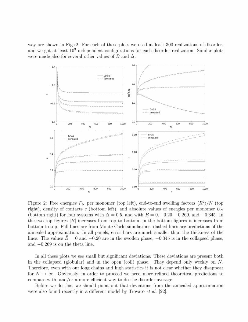
way are shown in Figs.2. For each of these plots we used at least 300 realizations of disorder,and we got at least 103 independent configurations for each disorder realization. Similar plotswere made also for several other values of B and ∆.

0 200 400 600 800 1000N

−1.7

−1.6

−1.5

−1.4

F

∆=0.5annealed

0 200 400 600 800 1000N

0.0

1.0

2.0

3.0

<R

2 >/N

∆=0.5annealed

0 200 400 600 800 1000N

0.0

0.2

0.4

0.6

c

∆=0.5annealed

0 200 400 600 800 1000N

0.00

0.10

0.20

0.30

−U

∆=0.5annealed

Figure 2: Free energies FN per monomer (top left), end-to-end swelling factors 〈R2〉/N (topright), density of contacts c (bottom left), and absolute values of energies per monomer UN

(bottom right) for four systems with ∆ = 0.5, and with B = 0,−0.20,−0.269, and −0.345. Inthe two top figures |B| increases from top to bottom, in the bottom figures it increases frombottom to top. Full lines are from Monte Carlo simulations, dashed lines are predictions of theannealed approximation. In all panels, error bars are much smaller than the thickness of thelines. The values B = 0 and −0.20 are in the swollen phase, −0.345 is in the collapsed phase,and −0.269 is on the theta line.

In all these plots we see small but significant deviations. These deviations are present bothin the collapsed (globular) and in the open (coil) phase. They depend only weekly on N .Therefore, even with our long chains and high statistics it is not clear whether they disappearfor N → ∞. Obviously, in order to proceed we need more refined theoretical predictions tocompare with, and/or a more efficient way to do the disorder average.

Before we do this, we should point out that deviations from the annealed approximationwere also found recently in a different model by Trovato et al. [22].

3 Replica Symmetric Approximation

To go beyond the annealed approximation, we will use the replica trick

ln ZN = limn→0

ZnN − 1

n. (17)

Alternatively, we could try a Taylor expansion

ln(ZN/ZN) = −1

2(Z2

N/ZN2 − 1) + . . . . (18)

This expansion is most likely divergent. It is nevertheless useful since its first term gives alreadya good indication of the leading corrections. Also, it suggests the inequality

FN(B, ∆) ≥ FN,ann(B, ∆) (19)

which can easily be derived exactly from convexity of the logarithm. The same inequality isexpected to hold for UN . This inequality is equivalent to the existence of a negative correlationbetween the average energy and the partition function.

To use eq.(17), we first have to evaluate disorder averages of ZnN for integer n ≥ 2. These are

performed similarly to the average over ZN , except that the Gaussian integrals give formallyrise to interactions between replicas [4],

Zn =∑

C1···Cn

exp

−Bn∑

α=1

∑

i<j

σαij

+∆2

2

∑

α6=β

∑

i<j

σαijσ

βij

. (20)

Here the Greek indeces α and β refer to the different replicas, Cα is a configuration of replica α,σα

ij is its contact map and B is given by equation (7). The annealed approximation is equivalentto neglecting the two-replicas term.

To proceed, we define the variables

cα =1

N

∑

i<j

σαij , qαβ =

1

N√

cαcβ

∑

i<j

σαijσ

βij , (21)

which are respectively the density of contacts for the contact map α and the overlap betweentwo contact maps α and β. The overlap is a measure of similarity, and it is equal to one if andonly if the two contact maps coincide. Furthermore, we assume that, for large N , the numberof configuration n-tuples with Nc1, . . . Ncn contacts and mutual overlaps {qαβ} grows as

exp

[

N

(

n∑

α=1

f(cα) −n∑

k=2

χk ({cα}, {qαβ}))]

. (22)

In other words, χk ({cα}, {qαβ}) is the entropy loss per monomer when we impose that thereplica Ck with density of contacts cα has overlaps q1,k · · · qk−1,k with the k−1 previous replicas.This quantity can be measured, for instance for k = 2.

We can then write

Zn ≈∫

d{cα}d{qαβ} × (23)

× exp

N

n∑

α=1

(

f(cα) − Bcα

)

+∆2

2

∑

α6=β

√cαcβqαβ −

n∑

k=2

χk ({cα}, {qαβ})

≈ exp [−NnFn ({cα}, {qαβ})] .

Here, Fn ({cα}, {qαβ}) is the free energy per monomer in a system with n replicas. To evaluateit, we approximate the integrals over cα and qαβ by their saddle points. We assume replicasymmetry which is expected to hold for low disorder: the saddle point is assumed to be givenby cα = c for all α and qαβ = q for all pairs α 6= β.

Now, in order to obtain the correct free energy, we have to take the limit n → 0. We obtain

F (B, ∆) = −f(c) + Bc +1

2∆2cq − χ(c, q). (24)

where χ(c, q) = − limn→0∑n

k=2 χn(c, q)/n is the average entropy gain per replica due to thecondition that the overlap among all replicas is equal to q. Note that this quantity is positivebecause, in the limit of vanishing n, the number of terms in the sum is -1. Finally, we have tocompute the values of c and q at which F is evaluated by imposing two saddle point conditions:

∂f(c)

∂c+

∂χ(c, q)

∂c= B +

1

2∆2q, (25)

1

2∆2c =

∂χ(c, q)

∂q. (26)

For ∆ = 0 (homopolymer) Eq.(26) just means that the value of the overlap is the mostprobable one for a given c, q0(c). Because of the normalization, it must be χ(c, q0) = 0, thusthe free energy of the homopolymer is just a special case of Eq.(24). Moreover, since χ(c, q0) = 0is an absolute minimum, also the derivative ∂χ/∂c must vanish at that point, thus the saddlepoint equation for c valid for the homopolymer is recovered for ∆ = 0. It also follows from thisargument that the second derivatives of χ(c, q) at the point (c, q0(c)) must be non-negative.

Notice that the free energy has to be maximized as a function of q because this variablerefers to a space with a negative number of dimensions in the limit n → 0. We thus get a firstcondition of thermodynamic stability ∂2χ/∂q2 > 0, which, from the above consideration, isexpected to be fulfilled for ∆ small enough. The situation is more complicated for the variablec. It enters both into the free energy of the replica interactions which has to be maximizedfor n → 0, and into the free energy of the homopolymer which has to be minimized, at leastfor ∆ = 0. We conjecture that the corresponding condition of thermodynamic stability is thatthe Hessian determinant of the free energy respect to the variables c and q, H(c, q), be nonpositive:

H(c, q) =

(

∂2f

∂c2+

∂2χ

∂c2

)

∂2χ

∂q2−(

∂2χ

∂c∂q− 1

c

∂χ

∂q

)2

≤ 0. (27)

For ∆ = 0 we have H(c, q) = (∂2f/∂c2) (∂2χ/∂q2) ≤ 0 as for homopolymers. In fact,at that point the first derivatives of χ(c, q) vanish. The Hessian determinant vanishes also,because χ(c, q) stays constant at the value zero along the line q = q0(c). Thus both conditionsof thermodynamic stability are fulfilled at ∆ small enough.

The energy and entropy per monomer are obtained in the same way as in the annealedapproximation. We find

UN(B, ∆) =(

B − ∆2(1 − q))

c, (28)

SN(B, ∆) = f(c) + χ(c, q) − ∆2

2c(1 − q). (29)

1 10 100 1000N

10−1

q

B~=0

B~=−0.20

B~=−0.269

B~=−0.345

∆=0.5

10 100 1000N

10−2

10−1

q

∆=0.2∆=0.3∆=0.4∆=0.5∆=0.6

B~=−0.345

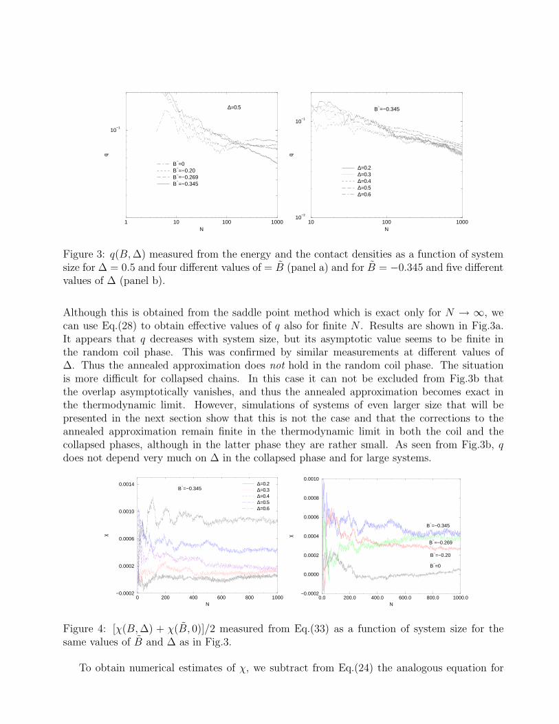
Figure 3: q(B, ∆) measured from the energy and the contact densities as a function of systemsize for ∆ = 0.5 and four different values of = B (panel a) and for B = −0.345 and five differentvalues of ∆ (panel b).

Although this is obtained from the saddle point method which is exact only for N → ∞, wecan use Eq.(28) to obtain effective values of q also for finite N . Results are shown in Fig.3a.It appears that q decreases with system size, but its asymptotic value seems to be finite inthe random coil phase. This was confirmed by similar measurements at different values of∆. Thus the annealed approximation does not hold in the random coil phase. The situationis more difficult for collapsed chains. In this case it can not be excluded from Fig.3b thatthe overlap asymptotically vanishes, and thus the annealed approximation becomes exact inthe thermodynamic limit. However, simulations of systems of even larger size that will bepresented in the next section show that this is not the case and that the corrections to theannealed approximation remain finite in the thermodynamic limit in both the coil and thecollapsed phases, although in the latter phase they are rather small. As seen from Fig.3b, qdoes not depend very much on ∆ in the collapsed phase and for large systems.

0 200 400 600 800 1000N

−0.0002

0.0002

0.0006

0.0010

0.0014

χ

∆=0.2∆=0.3∆=0.4∆=0.5∆=0.6

B~=−0.345

0.0 200.0 400.0 600.0 800.0 1000.0N

−0.0002

0.0000

0.0002

0.0004

0.0006

0.0008

0.0010

χ

B~=0

B~=−0.20

B~=−0.269

B~=−0.345

Figure 4: [χ(B, ∆) + χ(B, 0)]/2 measured from Eq.(33) as a function of system size for thesame values of B and ∆ as in Fig.3.

To obtain numerical estimates of χ, we subtract from Eq.(24) the analogous equation for

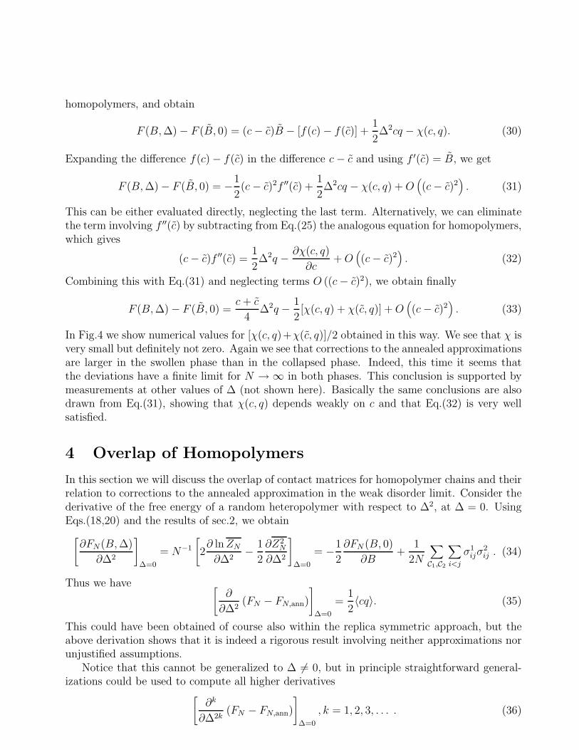
homopolymers, and obtain

F (B, ∆) − F (B, 0) = (c − c)B − [f(c) − f(c)] +1

2∆2cq − χ(c, q). (30)

Expanding the difference f(c) − f(c) in the difference c − c and using f ′(c) = B, we get

F (B, ∆) − F (B, 0) = −1

2(c − c)2f ′′(c) +

1

2∆2cq − χ(c, q) + O

(

(c − c)2)

. (31)

This can be either evaluated directly, neglecting the last term. Alternatively, we can eliminatethe term involving f ′′(c) by subtracting from Eq.(25) the analogous equation for homopolymers,which gives

(c − c)f ′′(c) =1

2∆2q − ∂χ(c, q)

∂c+ O

(

(c − c)2)

. (32)

Combining this with Eq.(31) and neglecting terms O ((c − c)2), we obtain finally

F (B, ∆) − F (B, 0) =c + c

4∆2q − 1

2[χ(c, q) + χ(c, q)] + O

(

(c − c)2)

. (33)

In Fig.4 we show numerical values for [χ(c, q)+χ(c, q)]/2 obtained in this way. We see that χ isvery small but definitely not zero. Again we see that corrections to the annealed approximationsare larger in the swollen phase than in the collapsed phase. Indeed, this time it seems thatthe deviations have a finite limit for N → ∞ in both phases. This conclusion is supported bymeasurements at other values of ∆ (not shown here). Basically the same conclusions are alsodrawn from Eq.(31), showing that χ(c, q) depends weakly on c and that Eq.(32) is very wellsatisfied.

4 Overlap of Homopolymers

In this section we will discuss the overlap of contact matrices for homopolymer chains and theirrelation to corrections to the annealed approximation in the weak disorder limit. Consider thederivative of the free energy of a random heteropolymer with respect to ∆2, at ∆ = 0. UsingEqs.(18,20) and the results of sec.2, we obtain

[

∂FN (B, ∆)

∂∆2

]

∆=0

= N−1

[

2∂ ln ZN

∂∆2− 1

2

∂Z2N

∂∆2

]

∆=0

= −1

2

∂FN (B, 0)

∂B+

1

2N

∑

C1,C2

∑

i<j

σ1ijσ

2ij . (34)

Thus we have[

∂

∂∆2(FN − FN,ann)

]

∆=0

=1

2〈cq〉. (35)

This could have been obtained of course also within the replica symmetric approach, but theabove derivation shows that it is indeed a rigorous result involving neither approximations norunjustified assumptions.

Notice that this cannot be generalized to ∆ 6= 0, but in principle straightforward general-izations could be used to compute all higher derivatives

[

∂k

∂∆2k(FN − FN,ann)

]

∆=0

, k = 1, 2, 3, . . . . (36)

Numerically, the rhs. of Eq.(35) can be estimated by simulating pairs of chains simultane-ously. For this we used a variant of the PERM algorithm where we add monomers alternativelyto the first and to the second chain [32]. In this way we guarantee that both chains have exactlythe same length (after having added an even number of monomers), and it is straightforwardto estimate their overlap.

Results from such simulations with chains of length up to 1400 are shown in Fig.5. Thesedata agree nicely with extrapolations of the overlaps for ∆ > 0 shown in the last section. Theyhave much smaller statistical errors, since we do not have to average over any disorder explicitly.This makes the present method much faster and allows us to study larger systems.

10 100 1000N

10−1

q 0

B~=−0.20

B~=−0.269 (Bθ)

B~=−0.35

B~=−0.50

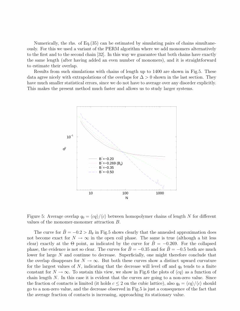
Figure 5: Average overlap q0 = 〈cq〉/〈c〉 between homopolymer chains of length N for differentvalues of the monomer-monomer attraction B.

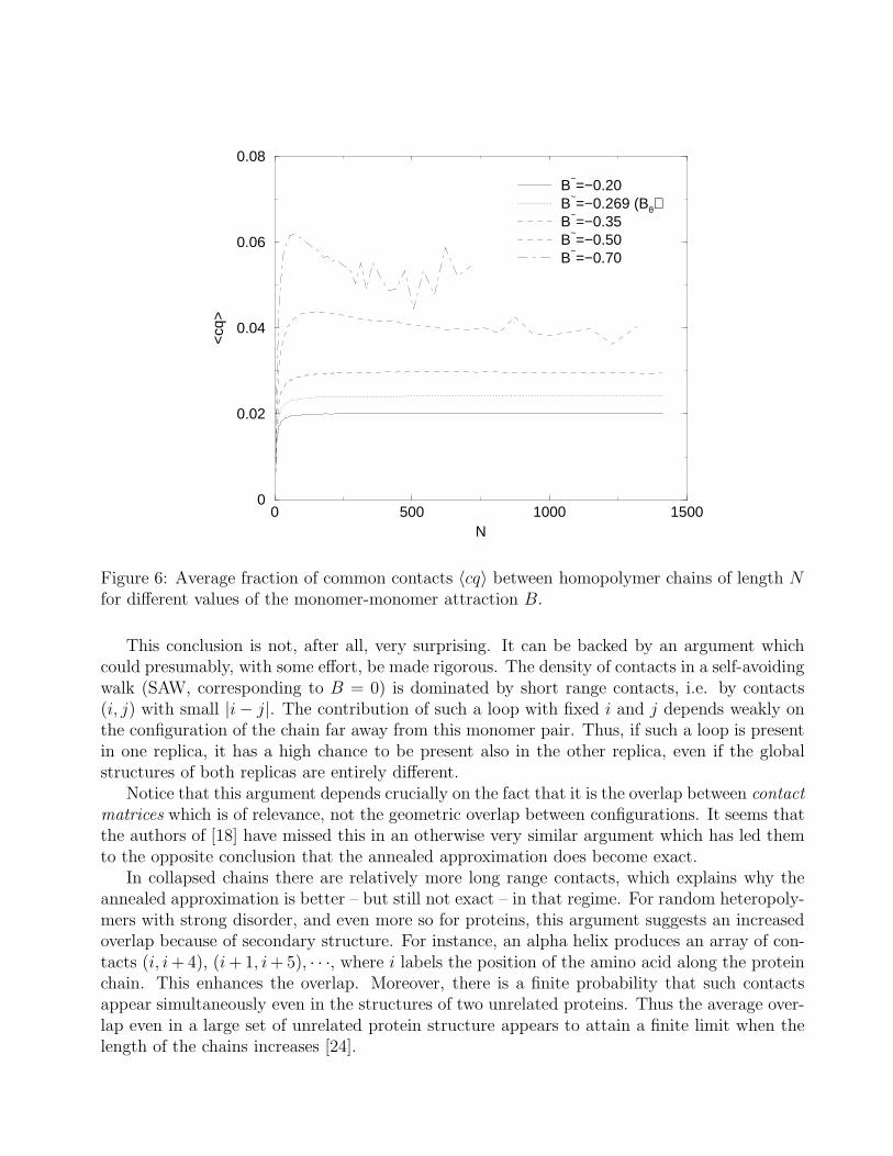
The curve for B = −0.2 > Bθ in Fig.5 shows clearly that the annealed approximation doesnot become exact for N → ∞ in the open coil phase. The same is true (although a bit lessclear) exactly at the Θ point, as indicated by the curve for B = −0.269. For the collapsedphase, the evidence is not so clear. The curves for B = −0.35 and for B = −0.5 both are muchlower for large N and continue to decrease. Superficially, one might therefore conclude thatthe overlap disappears for N → ∞. But both these curves show a distinct upward curvaturefor the largest values of N , indicating that the decrease will level off and q0 tends to a finiteconstant for N → ∞. To sustain this view, we show in Fig.6 the plots of 〈cq〉 as a function ofchain length N . In this case it is evident that the curves are going to a non-zero value. Sincethe fraction of contacts is limited (it holds c ≤ 2 on the cubic lattice), also q0 = 〈cq〉/〈c〉 shouldgo to a non-zero value, and the decrease observed in Fig.5 is just a consequence of the fact thatthe average fraction of contacts is increasing, approaching its stationary value.

0 500 1000 1500N

0

0.02

0.04

0.06

0.08

<cq

>

B~=−0.20

B~=−0.269 (Bθ)

B~=−0.35

B~=−0.50

B~=−0.70

Figure 6: Average fraction of common contacts 〈cq〉 between homopolymer chains of length Nfor different values of the monomer-monomer attraction B.

This conclusion is not, after all, very surprising. It can be backed by an argument whichcould presumably, with some effort, be made rigorous. The density of contacts in a self-avoidingwalk (SAW, corresponding to B = 0) is dominated by short range contacts, i.e. by contacts(i, j) with small |i − j|. The contribution of such a loop with fixed i and j depends weakly onthe configuration of the chain far away from this monomer pair. Thus, if such a loop is presentin one replica, it has a high chance to be present also in the other replica, even if the globalstructures of both replicas are entirely different.

Notice that this argument depends crucially on the fact that it is the overlap between contact

matrices which is of relevance, not the geometric overlap between configurations. It seems thatthe authors of [18] have missed this in an otherwise very similar argument which has led themto the opposite conclusion that the annealed approximation does become exact.

In collapsed chains there are relatively more long range contacts, which explains why theannealed approximation is better – but still not exact – in that regime. For random heteropoly-mers with strong disorder, and even more so for proteins, this argument suggests an increasedoverlap because of secondary structure. For instance, an alpha helix produces an array of con-tacts (i, i + 4), (i + 1, i + 5), · · ·, where i labels the position of the amino acid along the proteinchain. This enhances the overlap. Moreover, there is a finite probability that such contactsappear simultaneously even in the structures of two unrelated proteins. Thus the average over-lap even in a large set of unrelated protein structure appears to attain a finite limit when thelength of the chains increases [24].

5 Thermodynamics in the replica symmetric approxima-

tion

The two saddle point equations for c and q can not be explicitly solved, because we lack anexplicit expression for the functions f(c) and χ(c, q). Nevertheless, their qualitative behaviorcan be studied in more detail. This is done in the present section.

Deriving both equations (25,26) with respect to the thermodynamic parameters B and ∆we can compute the derivatives of c and q as

(

∂c

∂B

)

∆

=

∂2χ∂q2

H(c, q)≤ 0,

(

∂c

∂∆

)

B

=−∆

H(c, q)

∂

∂q

(

c∂χ

∂c− q

∂χ

∂q

)

. (37)

(

∂q

∂B

)

∆

= −∂2χ∂c∂q

− 1c

∂χ∂q

H(c, q),

(

∂q

∂∆

)

B

=∆

H(c, q)

[

c

(

∂2f

∂c2+

∂2χ

∂c2

)

− q

(

∂2χ

∂c∂q− 1

c

∂χ

∂q

)]

.

where H(c, q) is given by Eq.(27). From these, the specific heat can be computed as

Cv = ∂U/∂T

=(

B − ∆2(1 − q))

[

(B − ∆2)∂c

∂B+ ∆

∂c

∂∆

]

− ∆2c

[

(1 − q) + (B − ∆2)∂q

∂B+ ∆

∂q

∂∆

]

= − 1

H(c, q)

[

∂2F

∂c2(∆2c)2 − 2

∂2F

∂c∂q(∆2c)(B − ∆2(1 − q)) +

∂2F

∂q2(B − ∆2(1 − q))2

]

+∆2c(1 − q), (38)

where F (c, q) is the free energy evaluated at the saddle point. The three terms in the squarebrackets are the quadratic form whose determinant is expressed by H(c, q). Since ∂2F/∂q2 ispositive, they would give a negative contribution to the specific heat if H(c, q) were positive.Thus it is justified to require that H(c, q) is negative in order to get thermodynamic stability.

The behavior of the thermodynamic derivaties (37) can be partly studied using the fact thatthe function χ(c, q) attains its absolute minimum value χ(c, q) = 0 along the line q = q0(c).Thus, assuming that it is an analytic function of q for q > 0, it can be expressed in the form

χ(c, q) =∞∑

k=2

ak(c)

k!(q − q0(c))

k ≡∞∑

k=2

Ak(c)

k!(Q − Q0(c))

k , (39)

with a2(c) > 0. The typical overlap q0(c) is a small quantity and it is a decreasing functionof c, or q′0(c) < 0 (the prime indicates derivative with respect to c). The coefficients ak(c) areexpected to be quantities of order (q0(c))

−k+1, as it will be argued later. We also introducethe notation Q = cq, Q0(c) = cq0(c), Ak(c) = ak(c)c

−k. We can now develop the saddle pointequations for c close to the solution c of the annealed approximation given by f ′(c) = B:

(

∂2f

c2+

∆2

2

∂2Q0

∂c2

)

c=c

(c − c) +

(

∆2

2

∂Q0

∂c

)

c=c

+

(

∞∑

k=2

A′k(c)

k!(Q − Q0(c))

k

)

c=c

= 0

∞∑

k=1

Ak+1(c)

k!(Q − Q0(c))

k =1

2∆2 . (40)

From these expressions one sees that both Q − Q0(c) and c − c are quantities of order Q0(c),thus corrections to the annealed approximation are small but finite for finite ∆. Moreover,δq = (q − q0(c)) is positive for small ∆. From Eq.(39) we find, to zero-th order in δq:

(

∂c

∂B

)

∆

≈ a2(c)

H(c, q)≤ 0

(

∂c

∂∆

)

B

≈ ∆a2(c)

H(c, q)

∂Q0

∂c(41)

(

∂q

∂B

)

∆

≈ a2(c)

H(c, q)

∂q0

∂c≥ 0

(

∂q

∂∆

)

B

≈ ∆

H(c, q)

[

c∂2f

∂c2+ a2(c)

∂q0

∂c

∂Q0

∂c

]

(42)

H(c, q) must be computed at the first order in δq, because the zero-th order term vanishes atthe theta point c = cθ at which ∂2f/∂c2 vanishes. The result reads:

H(c, q) ≈ ∂2f

∂c2

∂2χ

∂q2− (Q − Q0(c)) c(A2(c))

2∂2Q0

∂c2. (43)

To proceed further, we first consider the simple case where the entropy χ(c, q) depends onlyon the product Q = cq representing the number of conditions that we have to impose in order tofix an overlap q: χ(c, q) = χ(cq). This form was assumed in the work of Shakhnovich and Gutin[4]. As it is easy to see, under the above hypothesis c = c(B) coincides with the value predictedby the annealed approximation and it is independent of ∆ at fixed B. Thus, in this case theannealed approximation would yield the correct value for the fraction of contacts. However, ournumerical results contradict this prediction. The overlap q is in this case an increasing functionof ∆, and its derivative with respect to B is proportional to (∂2f/∂c2)

−1, which is expected to

diverge at the theta point c = cθ. This fact can explain why the values of q are much smallerin the collapsed phase than in the coil phase.

A better theory for the function χ(c, q) was developed by Plotkin, Wang and Wolynes[13]. They computed the entropy loss for two replicas with density of contacts c being atoverlap q, χ2(c, q), in the mean field approximation and in the collapsed phase. Althoughthis can be different from χ(c, q), it is a good point for understanding its qualitative behavior.Unfortunately, we can not use the formula obtained in [13] because of several reasons: first, theresult is valid for finite N and becomes pathologic as N → ∞; second, it is not given in theform of a differentiable function; and third, it is assumed that the most probable overlap q0(c)is zero in the thermodynamic limit, while our calculations show that this is not the case. Weshall however use the fact that χ(c, q) is the sum of three contributions: the entropy loss due toimposing that Ncq contacts have to coincide, the loss due the fact that Nc(1−q) contacts have tobe different, and a combinatoric factor counting the number of different choices of Ncq contactsamong Nc. The last term can be approximated by χmix(c, q) = c [q ln q + (1 − q) ln(1 − q)], evenif this is an overestimate, since not all of the combinations of different common contacts canbe realized. Putting everything together we have:

χ(c, q) = χ(c, cq) + c [q ln q + (1 − q) ln(1 − q)] . (44)

In the computation by Plotkin et al. the mixed second derivative of χ(c, cq) with respectto Q = cq and c vanishes. This simplifies considerably formulas, and it will be assumed tohold for the rest of the paper. We shall thus introduce the notation χ′(Q) to denote thederivative of χ(c, Q) with respect to Q = cq at fixed c. Comparing Eq.(44) to Eq.(39), we

see that χ′′(Q) must be positive and that ∂χ/∂c = −(1 − 2q0) log(1 − q0). We also see thata2(c) = c/(q0(1 − q0)) + χ′′(Q) is likely to be a quantity of order q−1

0 , as it has been assumed

above. For the higher order coefficients one finds ak = O(

q−k+10

)

, as anticipated. We have now

to compute the derivatives of Q0(c) = cq0(c):

∂Q0

∂c= −∂2χ/∂c∂Q

∂2χ/∂Q2=

q0

1 + cq0χ′′(cq0) (1 − q0)≥ 0 , (45)

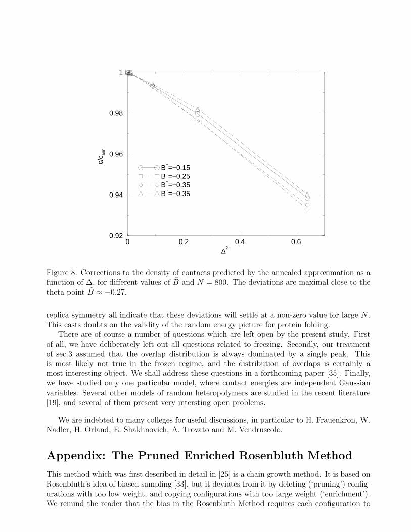
in qualitative agreement with Fig.6. Inserting the above result in the formulas (42) we seethat the density of contacts decreases with ∆ at fixed B. This behavior is confirmed by ournumerical results (see Fig.8), which also show that the decrease is maximal for B ≈ Bθ = −0.27,as expected from the fact that H(c, q0(c)) vanishes at c = cθ. The overlap q increases with B atfixed ∆,as expected from Eq.(42) (see Fig.7), and increases with ∆ at fixed B, as expected fromEq.(45) (see Fig.7 again). It can thus be understood why the overlap decreases with systemsize: as the number N of monomers increases the importance of surface effects is reduced (asN−1/3) and c(N) increases, thus decreasing the value of q.

We now examine the condition of thermodynamic stability, H(c, q) ≤ 0. As it was alreadyobserved, since at the point (c, q0(c)) both the gradient of χ(c, q) and its Hessian determinantvanish, we have H (c, q0(c)) = (∂2f/∂c2) (∂2χ/∂q2) ≤ 0. At the theta point this quantityvanishes, and H(cθ, q) is given by the deviations from the annealed approximation. Threesituations are possible: First, H(cθ, q) can be positive at the leading order in δq = q − q0(cθ).In this case the thermodynamic stability would be violated around the theta point, but oursimulations do not show anything strange in this region. Second, the leading order in δq can benegative. In this case, the specific heat would not diverge anymore at the theta point for finite∆, but it would show a peak proportional to some negative power of δq. Thus the disorderwould smear out the thermodynamic singularity at c = cθ, leaving unchanged the geometriccharacterization of the collapsed chains in terms of the gyration radius. It is rather difficult,if not impossible, to test this scenario by means of simulations. Third, H(cθ, q) can vanishidentically at c = cθ. It is easy to see that this condition, combined with the assumption thatχ(c, q) is of the form (44), is fulfilled if and only if χ′(cq) is of the form

χ′(cq) = log

(

1 − cq/B

cq/A

)

, (46)

where q ≥ q0(c), A < 0 and 0 < B < cq are two constants, and c is not too small so that thelast inequality can be fulfilled. In this case, one finds cq0(c) = B(c − A)/(B − A) ∈ [0, c], andit is easy to check that all previous results are recovered, while H(c, q) − H(c, q0(c)) vanishesfor all q and c, including the theta point.

Summarizing the discussion, we find that, if χ(c, q) is of the form (44), two possibilities areopen: either χ′(cq) is given by Eq.(46), in which case H(c, q) ≡ H(c, q0(c)) ≤ 0, or χ′(cq) hasa different form, in which case the specific heat is not anymore divergent at the theta pointc = cθ. Unfortunately, we are not able to decide among these alternatives.

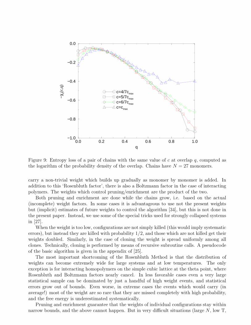
We conclude this section showing in Fig.9, for the sake of completeness, the entropy lossχ2(c, q) obtained from simulations of homopolymer chains with N = 27. Although the systemsize considered is definitely too small for quantitative considerations, the qualitative behavioris interesting and confirms the above considerations. The entropy χ2(c, q) was computed from

0 0.2 0.4 0.6 0.8∆2

0.02

0.04

0.06

0.08

0.1

q(B

~,∆

)

B~=−0.15

B~=−0.25

B~=−0.30

B~=−0.35

B~=−0.50

0.0 0.2 0.4 0.6 0.8∆2

0.000

0.010

0.020

0.030

χ(B

~ ,∆)

B~=−.15

B~=−.25

B~=−.30

B~=−.35

B~=−.50

Figure 7: Left: overlap q as a function of ∆2 for different values of B. Right: entropy [χ(B, ∆)+χ(B, 0)]/2 measured from Eq (33) as a function of ∆2 for different values of B.

χ2(c, q) = − 1

Nlog p2(c, q), (47)

where p2(c, q) is the probability density for a pair of chains, both with density of contacts c,being at overlap q.

6 Discussion

We have shown that the annealed approximation is very good but not exact for a particularmodel of random heteropolymers, and we have given simple physical arguments for it. We havealso computed the thermodynamics of the model using the replica symmetric approximation,and we have shown that such approach can explain very well, at least qualitatively, the observeddeviations from the annealed approximation in the high temperature phase. The replica sym-metric calculation also leaves open, surprisingly, the possibility that the disorder could cancelthe thermodynamic singularity at the theta point. A numerical test of this possibility is verydifficult, and it has been left out.

In our present study we have not addressed the most interesting aspect of the model – thefreezing of the system in a finite number of mesoscopic states. This transition should representsome features of the folding transition taking place for protein structures. Instead, we havestudied the model at higher temperatures and at smaller disorder. This should however beof interest also in the context of the freezing, since it was conjectured [4] that freezing canbe described in this model by the random energy model, a prerequisite for which is that theannealed approximation is exact.

In the present simulations we have studied chains of length up to N = 1400. Deviationsfrom the annealed approximation decrease fast for small N , which explains why studying veryshort chains has mislead several authors to the conclusion that these deviations vanish forN → ∞. But in the high-T (open coil) phase this decrease clearly stops, and deviations areroughly independent of N for N > 100. This is less clear in the collapsed phase. But also therenumerics, general arguments, and detailed calculations within a specific scenario with unbroken

0 0.2 0.4 0.6∆2

0.92

0.94

0.96

0.98

1

c/c an

n

B~=−0.15

B~=−0.25

B~=−0.35

B~=−0.35

Figure 8: Corrections to the density of contacts predicted by the annealed approximation as afunction of ∆, for different values of B and N = 800. The deviations are maximal close to thetheta point B ≈ −0.27.

replica symmetry all indicate that these deviations will settle at a non-zero value for large N .This casts doubts on the validity of the random energy picture for protein folding.

There are of course a number of questions which are left open by the present study. Firstof all, we have deliberately left out all questions related to freezing. Secondly, our treatmentof sec.3 assumed that the overlap distribution is always dominated by a single peak. Thisis most likely not true in the frozen regime, and the distribution of overlaps is certainly amost interesting object. We shall address these questions in a forthcoming paper [35]. Finally,we have studied only one particular model, where contact energies are independent Gaussianvariables. Several other models of random heteropolymers are studied in the recent literature[19], and several of them present very intersting open problems.

We are indebted to many colleges for useful discussions, in particular to H. Frauenkron, W.Nadler, H. Orland, E. Shakhnovich, A. Trovato and M. Vendruscolo.

Appendix: The Pruned Enriched Rosenbluth Method

This method which was first described in detail in [25] is a chain growth method. It is based onRosenbluth’s idea of biased sampling [33], but it deviates from it by deleting (‘pruning’) config-urations with too low weight, and copying configurations with too large weight (‘enrichment’).We remind the reader that the bias in the Rosenbluth Method requires each configuration to

0.0 0.2 0.4 0.6 0.8 1.0q

−1.0

−0.8

−0.6

−0.4

−0.2

0.0

−χ 2(

c,q)

c=4/7cmax

c=5/7cmax

c=6/7cmax

c=cmax

Figure 9: Entropy loss of a pair of chains with the same value of c at overlap q, computed asthe logarithm of the probability density of the overlap. Chains have N = 27 monomers.

carry a non-trivial weight which builds up gradually as monomer by monomer is added. Inaddition to this ‘Rosenbluth factor’, there is also a Boltzmann factor in the case of interactingpolymers. The weights which control pruning/enrichment are the product of the two.

Both pruning and enrichment are done while the chains grow, i.e. based on the actual(incomplete) weight factors. In some cases it is advantageous to use not the present weightsbut (implicit) estimates of future weights to control the algorithm [34], but this is not done inthe present paper. Instead, we use some of the special tricks used for strongly collapsed systemsin [27].

When the weight is too low, configurations are not simply killed (this would imply systematicerrors), but instead they are killed with probability 1/2, and those which are not killed get theirweights doubled. Similarly, in the case of cloning the weight is spread uniformly among allclones. Technically, cloning is performed by means of recursive subroutine calls. A pseudocodeof the basic algorithm is given in the appendix of [25].

The most important shortcoming of the Rosenbluth Method is that the distribution ofweights can become extremely wide for large systems and at low temperatures. The onlyexception is for interacting homopolymers on the simple cubic lattice at the theta point, whereRosenbluth and Boltzmann factors nearly cancel. In less favorable cases even a very largestatistical sample can be dominated by just a handful of high weight events, and statisticalerrors grow out of bounds. Even worse, in extreme cases the events which would carry (inaverage!) most of the weight are so rare that they are missed completely with high probability,and the free energy is underestimated systematically.

Pruning and enrichment guarantee that the weights of individual configurations stay withinnarrow bounds, and the above cannot happen. But in very difficult situations (large N , low T,

large disorder) it may happen that due to cloning the configurations are strongly correlated,and the weights of clusters of such correlated configurations play essentially a similar role as theweights of individual configurations in the above discussion. In the following we will call such acluster which is composed of all configurations having a common root a ‘tour’. In order to checkthat the weights of tours do not become too uneven, we have measured in their distribution. Letus call the weights W , and the distribution P (W ). We are on safe grounds if this distributionis so narrow that P (W ) and WP (W ) have basically the same support. In particular, we shouldrequire that the maximum of WP (W ) occurs at such values where P (W ) is still appreciable,and the distribution is well sampled. We have verified that this is the case for all data shown inthe present paper. Notice, however, that this is a very stringent requirement. If it is were notsatisfied, this would not necessarily mean that the data are wrong, since configurations withinone tour are only partially correlated.

The generalization of this algorithm to pairs of chains growing simultaneously is straightfor-ward [32]. One just has to add monomers alternatingly. When the total number of monomersin both chains is even, the addition of the next monomer is attempted at chain 1; when thisnumber is odd, the next monomer is added to chain 2.

References

[1] T.E. Creighton (1992), Protein Folding (W.H. Freeman, New York)

[2] J.D. Bryngelson, P.G. Wolynes (1987), Procl. Natl. Acad. Sci. USA 84, 7524

[3] T. Garel and H. Orland (1988), Europhys. Lett. 6, 307

[4] E.I. Shakhnovich and A.M. Gutin (1989), Biophys. Chem. 34, 187.

[5] Shakhnovich and Karplus (1992), in Protein Folding: Theoretical studies of thermodynam-

ics and dynamics, in T.E. Creighton, Protein Folding (W.H. Freeman, New York)

[6] E.I. Shakhnovich and A.M. Gutin (1990), J. Chem. Phys. 93, 5967

[7] E.I. Shakhnovich and A.M. Gutin (1990), Nature 346, 773.

[8] E.I. Shakhnovich and A.M. Gutin (1990), J. Mol. Bio. 3, 1614.

[9] C. Camacho, D. Thirumalai (1996), Proc. Natl. Acad. Sci. USA 90, 6369.

[10] E.I. Shakhnovich and A.M. Gutin (1993), Proc. Natl. Acad. Sci. USA, 90, 7195; E.I.Shakhnovich (1994), Phys. Rev. Lett. 24, 3907.

[11] G. Iori, E. Marinari and G. Parisi (1991), J. Phys. A: Math. Gen. 24, 5349; G. Iori, E.Marinari and G. Parisi (1994), Europhys. Lett. 25, 491.

[12] Y. Kantor and M. Kardar (1994), Europhys. Lett. 28, 169

[13] S.S. Plotkin, J. Wang and P.G. Wolynes (1996), Phys. Rev. E 53, 6271; S.S. Plotkin, J.Wang and P.G. Wolynes (1997), J. Chem. Phys. 53, 2932.

[14] V.S. Pande, A.Y. Grosberg, C. Joerg, M. Kardar and T. Tanaka (1996), Phys. Rev. Lett.

76, 3565

[15] V.S. Pande, A.Y. Grosberg, C. Joerg and T. Tanaka (1996), Phys. Rev. Lett. 76, 3987

[16] C.J. Camacho and T. Shanke (1997), Europhys. Lett. 37 603-608

[17] D.K. Klimov and D. Thirumalai (1997) Phys. Rev. Lett. 76, 4070.

[18] P. Monari, A.L. Stella, C. Vanderzande, and E. Orlandini, Phys. Rev. Lett. 83, 112 (1999)

[19] T. Garel, H. Orland and E. Pitard (1997), cond-mat/9706125

[20] U. Bastolla, H. Frauenkron and P. Grassberger (2000), Jour Mol Liq 84, 111-129.

[21] P.G. DeGennes, Scaling Concepts in Polymer Physics, Cornell Univ. Press, Ithaca 1979.

[22] A. Trovato, J. van Mourik, and A. Maritan (1998) Eur Phys J B 6 63-73

[23] T. Garel, H. Orland, and Leibler (1994), J. Phys. II France 4, 2139-2148.

[24] U. Bastolla, M. Vendruscolo and W. Knapp, in preparation.

[25] P. Grassberger (1997), Phys. Rev.E 56, 3682

[26] U. Bastolla and P. Grassberger (1997), J. Stat. Phys. 89, 1061

[27] H. Frauenkron, U. Bastolla, E. Gerstner, P. Grassberger, and W. Nadler Phys. Rev. Lett.

80, 3149 (1998)

[28] H. Frauenkron and P. Grassberger (1997), J. Chem. Phys. 107, 9599

[29] G.T. Barkema, U. Bastolla and P. Grassberger (1998), J. Stat. Phys. 90, 1311

[30] B. Duplantier, J. Chem. Phys. 86, 4233 (1987)

[31] J. Hager and L. Schafer (1999), Phys. Rev. E 60, 2071

[32] B. Coluzzi, M.S. Causo, and P. Grassberger (1999), cond-mat/9910188

[33] M.N. Rosenbluth and A.W. Rosenbluth (1955), J. Chem. Phys. 23, 356

[34] H. Frauenkron, M.S. Causo, and P. Grassberger (1999), Phys Rev E 59 R16-R19

[35] U. Bastolla, in preparation