Experimental Genetic Operators Analysis for

the Multi-objective Permutation Flowshop

Carlos A. Brizuela and Rodrigo Aceves

Computer Science Department, CICESE Research CenterKm 107 Carr. Tijuana-Ensenada, Ensenada, B.C., Mexico

{cbrizuel, raceves}@cicese.mx, +52–646–175–0500

Abstract. The aim of this paper is to show the influence of geneticoperators such as crossover and mutation on the performance of a geneticalgorithm (GA). The GA is applied to the multi-objective permutationflowshop problem. To achieve our goal an experimental study of a setof crossover and mutation operators is presented. A measure related tothe dominance relations of different non-dominated sets, generated bydifferent algorithms, is proposed so as to decide which algorithm is thebest. The main conclusion is that there is a crossover operator having thebest average performance on a very specific set of instances, and undera very specific criterion. Explaining the reason why a given operator isbetter than others remains an open problem.

1 Introduction

Optimization problems coming from the real world are, in most cases, multi-objective (MO) in nature. The lack of efficient methodologies to tackle theseproblems makes them attractive both theoretically and practically.

Among these real-world MO problems, scheduling (a combinatorial one)seems to be one of the most challenging. In a real scheduling problem we are in-terested not only in minimizing the latest completion time (makespan) but alsoin minimizing the total time all jobs exceed their respective due dates as well asthe total time the jobs remain in the shop (work-in-process). A few results onMO scheduling with a single-objective-like approaches reveal that there is muchto do in this research area.

On the other hand, the available methodologies in genetic algorithms (GA’s)have been focused more on function optimization rather than in combinatorialoptimization problems (COP’s). In order to fairly compare the performance oftwo given algorithms some metrics have been proposed. Recent results [17], [21]have shown that these metrics may mislead conclusions on the relative perfor-mance of algorithms. This situation forces us to find appropriate procedures tofairly compare two non-dominated fronts, at least in terms of dominance rela-tions.

The remainder of the paper is organized as follows. Section 2 states the prob-lem we are dealing with. Section 3 reviews some available results for this problem.Section 4 introduces the global algorithm used in the operators study. Section 5

explains the experimental setup and introduces the proposed performance mea-sure. Section 6 shows the experimental results. Finally, section 7 presents theconclusions of this work.

2 Problem Statement

Let Kn be the set of the n first natural numbers, i.e. Kn = {1, 2, · · · , n}. Thepermutation flow-shop problem consists of a set Kn of jobs (n > 1) that must beprocessed in a set of machines Km (m > 1). Each job j ∈ Kn has m operations.Each operation Okj , representing the k-th operation of job j, has an associatedprocessing time pkj . Each machine must finish the operation once it is started tobe processed (no preemption allowed). No machine can process more than oneoperation at the same time. No operation can be processed by more than onemachine at a time. Each job j is assigned a readiness time rj , and due date dj .All jobs must have the same routing through all machines. The goal is to find apermutation of jobs that minimizes a given objective function (since the orderof machines is fixed).

In order to understand the objective functions we want to optimize we needto set up some notation first. Let us denote the starting time of operation Okj

by skj . Define the permutations π = {π(1), π(2), · · · , π(n)} as a solution to theproblem.

With this notation a feasible solution must hold the following conditions:

skj > rj ∀k ∈ Km, j ∈ Kn , (1)

skπ(j) + pkπ(j) ≤ s(k+1)π(j)∀k ∈ Km−1, j ∈ Kn . (2)

All pairs of operations, of consecutive jobs, processed by the same machine kmust satisfy:

skπ(j) + pkπ(j) ≤ skπ(j+1)

for every machine k ∈ Km, and every job j ∈ Kn−1 . (3)

Now we are in position of defining the objective functions. First we considerthe makespan, which is the completion time of the latest job, i.e.

f1 = cmax = smπ(n) + pmπ(n) . (4)

The mean flow time, representing the average time the jobs remain in the shop,is the second objective.

f2 = fl = (1/n)

n∑

j=1

flj , (5)

where flj = {smj + pmj} − rj , i.e. the time job j spends in the shop after itsrelease. The third objective is the mean tardiness, i.e.

f3 = T = (1/n)

n∑

j=1

Tj , (6)

where Tj = max{0, Lj}, and Lj = smj + tmj − dj .Thus, we have the following MO problem:

Minimize (f1, f2, f3)

subject to (1)− (3) . (7)

This problem, considering only the makespan (Cmax) as the objective func-tion, was proven to be NP-hard [11]. This implies that the problem given by (7)is at least as difficult as the makespan problem.

2.1 Tradeoff among objectives

To show that “conflict” among objectives exists, it is necessary to define what“conflict” means. We give some definitions in order to understand why our prob-lem should be treated as a multi-objective one.

Definition 1. The Ideal Point or Ideal Vector is defined as the point z∗

composed of the best attainable objective values. This is,z∗j = max{fj(x)|x ∈ A}, A is the set (without constraints) of all possible x,

j ∈ Kq , where q > 1 is the number of objective functions.Definition 2. Two objectives are in conflict if the Euclidean distance from

the ideal point to the set of best values of feasible solutions is different from zero.Definition 3. Three or more objectives are in conflict if they are in conflict

pairwise.To show that the objectives are in conflict we are going to construct a counter-

example instance where we can enumerate all solutions and see that there is nota single solution with all its objective values being better than or equal to therespective objective values of the other solutions. This implies that the distancefrom the set of non-dominated solutions to the ideal point is positive.

Table 1 presents an instance of the PFSP with three jobs and two machines.All solutions for this problem are enumerated in Table 2, here we can see thatsolution 312 has the best makespan value, 231 the best tardiness, and 213 thebest mean flow time. The ideal point z∗ for this instance is given by z∗ =(44, 16, 87). Therefore, the Euclidean distance from the set of values in Table 2to the ideal point is positive.

It is not known whether or not, in randomly generated PFSP instances,it is enough to consider only two objectives, as the third one, in the Paretofront, will have the same behavior as one of the first two. We did not performany experimental study regarding the answer for this question because of therequired computational effort. However, in the experiments section we will seethat for all generated instances there are two objective functions which are notin conflict. It will be very interesting to know which instances will have threeconflicting objectives and which will not.

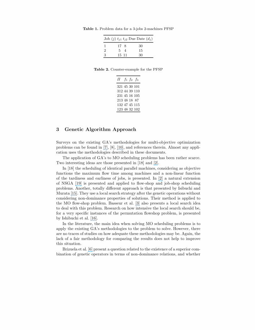
Table 1. Problem data for a 3-jobs 2-machines PFSP

Job (j) tj1 tj2 Due Date (dj)

1 17 8 302 5 4 153 15 11 30

Table 2. Counter-example for the PFSP

Π f1 f2 f3

321 45 30 101312 44 39 110231 45 16 105213 48 18 87132 47 45 115123 48 32 102

3 Genetic Algorithm Approach

Surveys on the existing GA’s methodologies for multi-objective optimizationproblems can be found in [7], [8], [10], and references therein. Almost any appli-cation uses the methodologies described in these documents.

The application of GA’s to MO scheduling problems has been rather scarce.Two interesting ideas are those presented in [18] and [2].

In [18] the scheduling of identical parallel machines, considering as objectivefunctions the maximum flow time among machines and a non-linear functionof the tardiness and earliness of jobs, is presented. In [2] a natural extensionof NSGA [19] is presented and applied to flow-shop and job-shop schedulingproblems. Another, totally different approach is that presented by Isibuchi andMurata [15]. They use a local search strategy after the genetic operations withoutconsidering non-dominance properties of solutions. Their method is applied tothe MO flow-shop problem. Basseur et al. [3] also presents a local search ideato deal with this problem. Research on how intensive the local search should be,for a very specific instances of the permutation flowshop problem, is presentedby Ishibuchi et al. [16].

In the literature, the main idea when solving MO scheduling problems is toapply the existing GA’s methodologies to the problem to solve. However, thereare no traces of studies on how adequate these methodologies may be. Again, thelack of a fair methodology for comparing the results does not help to improvethis situation.

Brizuela et al. [6] present a question related to the existence of a superior com-bination of genetic operators in terms of non-dominance relations, and whether

or not this superiority will persist over some set of instances for a given flowshopproblem. The work presented here try to answer this question.

The next section presents the algorithm we use to compare the performanceof different operators.

4 The Algorithm

A standard GA for MO [19] is used with some modifications. The fitness shareand dummy fitness assignment are standard. The main difference is in the re-placement procedure, where an elitist replacement is used.

The specific NSGA we use here as a framework is stated as follows.Algorithm 1. Multi-objective GA.

Step 1. Set r = 0. Generate an initial population POP [r] of g individ-uals.Step 2. Classify the individuals according to a non-dominance relation.Assign a dummy fitness to each individual.Step 3. Modify the dummy fitness by fitness sharing.Step 4. Set i=1.Step 5. Use RWS to select two individuals for crossover according totheir dummy fitness. Perform crossover with probability pc.Step 6. Perform mutation of individual i with probability pm.Step 7. Set i = i + 1. If i = g then go to Step 8 otherwise go to Step 5.Step 8. Set r = r + 1. Construct the new generation POP [r] of g

individuals. If r = rmax then STOP; otherwise go to STEP 2.

The procedures involved at each step of this algorithm are explained in thefollowing subsections.

4.1 Decoding

Each individual is represented by a string of integers representing job numbers tobe scheduled (a permutation of job numbers). In this representation individualr looks like:

ir = (i(r)1 i

(r)2 · · · i

(r)n ), r = 1, 2, · · · , g ,

where i(r)k ∈ Kn.

The schedule construction method for this individual is as follows:

1) Enumerate all machines in Km from 1 to m.

2) Select the first job (i(r)1 ) of ir and route it from the first machine

(machine 1) to the last (machine m).3) Select iteratively the second, third, · · ·, n-th job and route themthrough the machines in the same machine sequence adopted for the

first job i(r)1 (machines 1 to m). This must be done without violating the

restrictions imposed in (1) to (3).

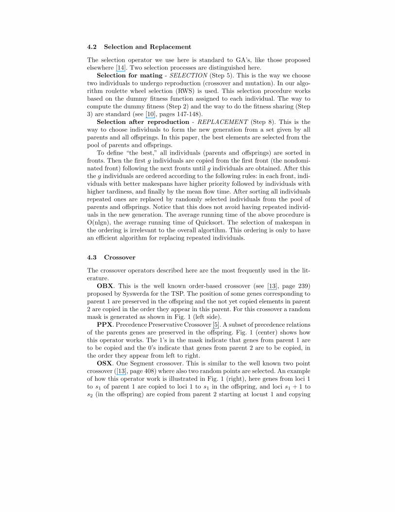
4.2 Selection and Replacement

The selection operator we use here is standard to GA’s, like those proposedelsewhere [14]. Two selection processes are distinguished here.

Selection for mating - SELECTION (Step 5). This is the way we choosetwo individuals to undergo reproduction (crossover and mutation). In our algo-rithm roulette wheel selection (RWS) is used. This selection procedure worksbased on the dummy fitness function assigned to each individual. The way tocompute the dummy fitness (Step 2) and the way to do the fitness sharing (Step3) are standard (see [10], pages 147-148).

Selection after reproduction - REPLACEMENT (Step 8). This is theway to choose individuals to form the new generation from a set given by allparents and all offsprings. In this paper, the best elements are selected from thepool of parents and offsprings.

To define “the best,” all individuals (parents and offsprings) are sorted infronts. Then the first g individuals are copied from the first front (the nondomi-nated front) following the next fronts until g individuals are obtained. After thisthe g individuals are ordered according to the following rules: in each front, indi-viduals with better makespans have higher priority followed by individuals withhigher tardiness, and finally by the mean flow time. After sorting all individualsrepeated ones are replaced by randomly selected individuals from the pool ofparents and offsprings. Notice that this does not avoid having repeated individ-uals in the new generation. The average running time of the above procedure isO(nlgn), the average running time of Quicksort. The selection of makespan inthe ordering is irrelevant to the overall algortihm. This ordering is only to havean efficient algorithm for replacing repeated individuals.

4.3 Crossover

The crossover operators described here are the most frequently used in the lit-erature.

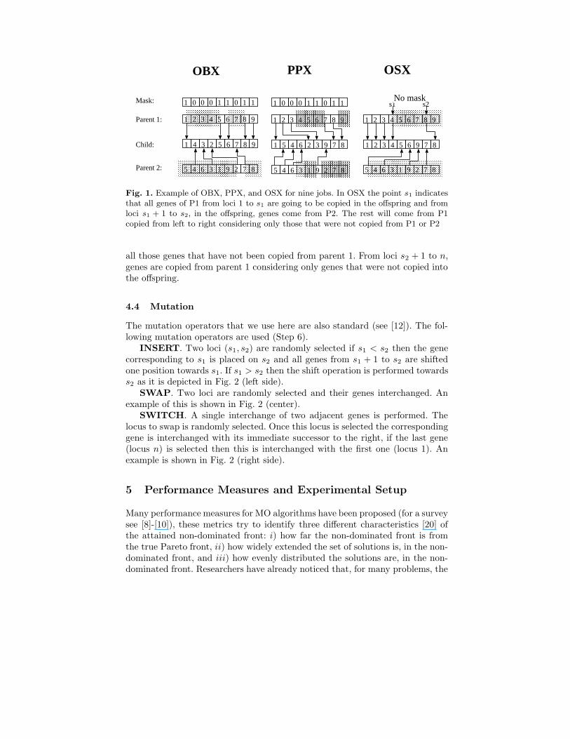
OBX. This is the well known order-based crossover (see [13], page 239)proposed by Syswerda for the TSP. The position of some genes corresponding toparent 1 are preserved in the offspring and the not yet copied elements in parent2 are copied in the order they appear in this parent. For this crossover a randommask is generated as shown in Fig. 1 (left side).

PPX. Precedence Preservative Crossover [5]. A subset of precedence relationsof the parents genes are preserved in the offspring. Fig. 1 (center) shows howthis operator works. The 1’s in the mask indicate that genes from parent 1 areto be copied and the 0’s indicate that genes from parent 2 are to be copied, inthe order they appear from left to right.

OSX. One Segment crossover. This is similar to the well known two pointcrossover ([13], page 408) where also two random points are selected. An exampleof how this operator work is illustrated in Fig. 1 (right), here genes from loci 1to s1 of parent 1 are copied to loci 1 to s1 in the offspring, and loci s1 + 1 tos2 (in the offspring) are copied from parent 2 starting at locust 1 and copying

1 2 3 4 5 6 7 8 9

5 4 6 3 1 9 2 7 8

Parent 1:

Child:

Parent 2:

1 0 0 0 1 1 0 1 1

1 4 3 2 5 6 7 8 9

Mask:

1 2 3 4 5 6 7 8 9

5 4 6 3 1 9 2 7 8

1 0 0 0 1 1 0 1 1

1 5 4 6 2 3 9 7 8

OBX PPX

1 2 3 4 5 6 7 8 9

5 4 6 3 1 9 2 7 8

1 2 3 4 5 6 9 7 8

s1 s2

OSX

No mask

Fig. 1. Example of OBX, PPX, and OSX for nine jobs. In OSX the point s1 indicatesthat all genes of P1 from loci 1 to s1 are going to be copied in the offspring and fromloci s1 + 1 to s2, in the offspring, genes come from P2. The rest will come from P1copied from left to right considering only those that were not copied from P1 or P2

all those genes that have not been copied from parent 1. From loci s2 + 1 to n,genes are copied from parent 1 considering only genes that were not copied intothe offspring.

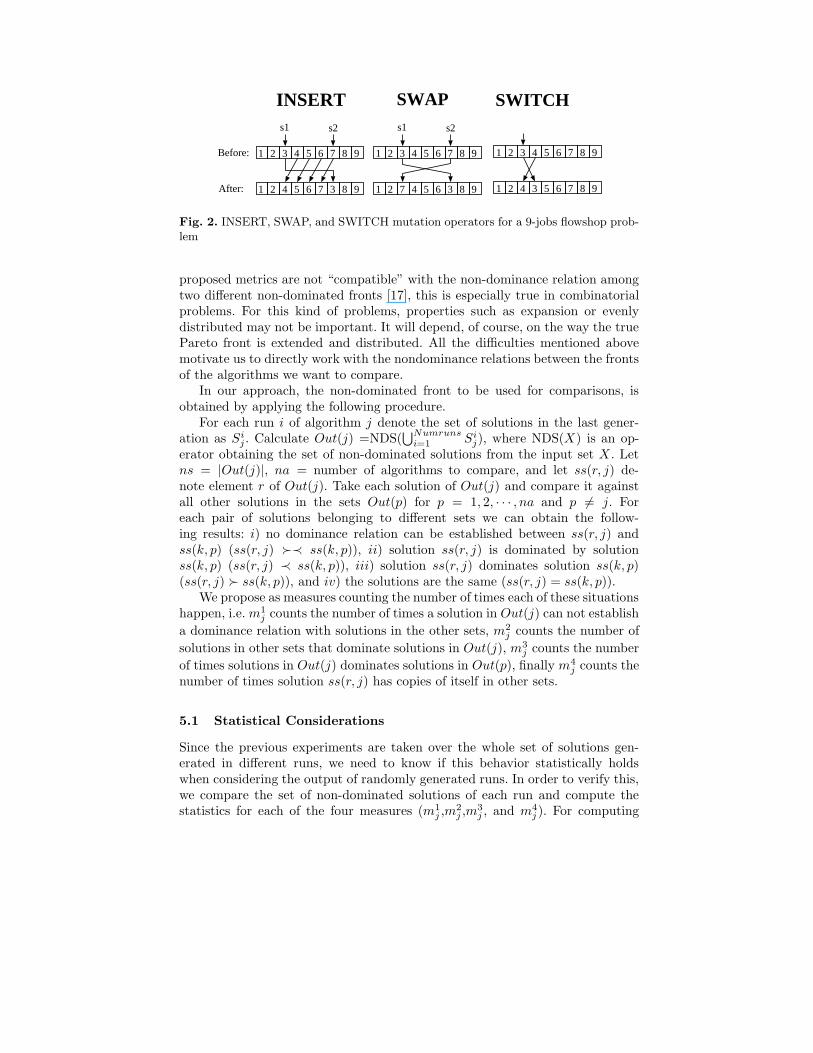
4.4 Mutation

The mutation operators that we use here are also standard (see [12]). The fol-lowing mutation operators are used (Step 6).

INSERT. Two loci (s1, s2) are randomly selected if s1 < s2 then the genecorresponding to s1 is placed on s2 and all genes from s1 + 1 to s2 are shiftedone position towards s1. If s1 > s2 then the shift operation is performed towardss2 as it is depicted in Fig. 2 (left side).

SWAP. Two loci are randomly selected and their genes interchanged. Anexample of this is shown in Fig. 2 (center).

SWITCH. A single interchange of two adjacent genes is performed. Thelocus to swap is randomly selected. Once this locus is selected the correspondinggene is interchanged with its immediate successor to the right, if the last gene(locus n) is selected then this is interchanged with the first one (locus 1). Anexample is shown in Fig. 2 (right side).

5 Performance Measures and Experimental Setup

Many performance measures for MO algorithms have been proposed (for a surveysee [8]-[10]), these metrics try to identify three different characteristics [20] ofthe attained non-dominated front: i) how far the non-dominated front is fromthe true Pareto front, ii) how widely extended the set of solutions is, in the non-dominated front, and iii) how evenly distributed the solutions are, in the non-dominated front. Researchers have already noticed that, for many problems, the

1 2 3 4 5 6 7 8 9

1 2 34 5 6 7 8 9

s1 s2

INSERT

1 2 3 4 5 6 7 8 9

1 2 34 5 67 8 9

s1 s2

Before:

After:

1 2 3 4 5 6 7 8 9

1 2 34 5 6 7 8 9

SWAP SWITCH

Fig. 2. INSERT, SWAP, and SWITCH mutation operators for a 9-jobs flowshop prob-lem

proposed metrics are not “compatible” with the non-dominance relation amongtwo different non-dominated fronts [17], this is especially true in combinatorialproblems. For this kind of problems, properties such as expansion or evenlydistributed may not be important. It will depend, of course, on the way the truePareto front is extended and distributed. All the difficulties mentioned abovemotivate us to directly work with the nondominance relations between the frontsof the algorithms we want to compare.

In our approach, the non-dominated front to be used for comparisons, isobtained by applying the following procedure.

For each run i of algorithm j denote the set of solutions in the last gener-ation as Si

j . Calculate Out(j) =NDS(⋃Numruns

i=1 Sij), where NDS(X) is an op-

erator obtaining the set of non-dominated solutions from the input set X . Letns = |Out(j)|, na = number of algorithms to compare, and let ss(r, j) de-note element r of Out(j). Take each solution of Out(j) and compare it againstall other solutions in the sets Out(p) for p = 1, 2, · · · , na and p 6= j. Foreach pair of solutions belonging to different sets we can obtain the follow-ing results: i) no dominance relation can be established between ss(r, j) andss(k, p) (ss(r, j) �≺ ss(k, p)), ii) solution ss(r, j) is dominated by solutionss(k, p) (ss(r, j) ≺ ss(k, p)), iii) solution ss(r, j) dominates solution ss(k, p)(ss(r, j) � ss(k, p)), and iv) the solutions are the same (ss(r, j) = ss(k, p)).

We propose as measures counting the number of times each of these situationshappen, i.e. m1

j counts the number of times a solution in Out(j) can not establish

a dominance relation with solutions in the other sets, m2j counts the number of

solutions in other sets that dominate solutions in Out(j), m3j counts the number

of times solutions in Out(j) dominates solutions in Out(p), finally m4j counts the

number of times solution ss(r, j) has copies of itself in other sets.

5.1 Statistical Considerations

Since the previous experiments are taken over the whole set of solutions gen-erated in different runs, we need to know if this behavior statistically holdswhen considering the output of randomly generated runs. In order to verify this,we compare the set of non-dominated solutions of each run and compute thestatistics for each of the four measures (m1

j ,m2j ,m

3j , and m4

j ). For computing

these statistics we randomly select, without replacement, NDS(S ij) uniformly

on i ∈ {1, · · · , NumRuns} for each j ∈ {1, · · · , na} until we have NumRunsnondominated fronts to compare. The average for each measure mi

j is computedover NumRuns different samples.

The experiment is performed for each combination of crossover and mutation.Three different crossover operators and three different mutation operators areconsidered (see subsections 4.3 and 4.4).

5.2 Benchmark Generation

In order to generate a set of benchmark instances we take one of the probleminstances in the library maintained by Beasly [4] and apply a procedure proposedby Armentano and Ronconi [1] for generating due-dates. The authors in [1]propose a way to systematically generate controlled due dates, following a certainstructure. The procedure is based on an estimation of a lower bound for themakespan (f1). This lower bound is defined as P , then due dates are randomlyand uniformly generated for each job in the range of P (1− T − R/2) to P (1−T + R/2), where T and R are parameters for generating different scenarios oftardiness and due date ranges, respectively.

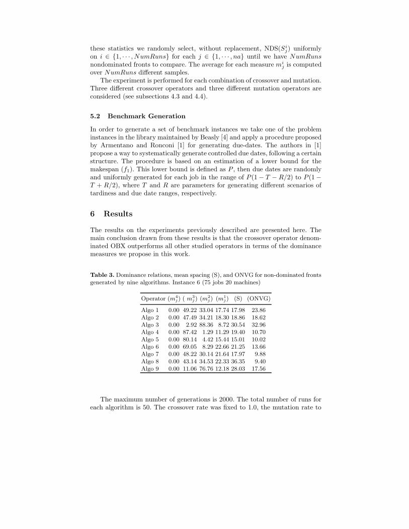
6 Results

The results on the experiments previously described are presented here. Themain conclusion drawn from these results is that the crossover operator denom-inated OBX outperforms all other studied operators in terms of the dominancemeasures we propose in this work.

Table 3. Dominance relations, mean spacing (S), and ONVG for non-dominated frontsgenerated by nine algorithms. Instance 6 (75 jobs 20 machines)

Operator (m4

j ) ( m3

j ) (m2

j ) (m1

j ) (S) (ONVG)

Algo 1 0.00 49.22 33.04 17.74 17.98 23.86Algo 2 0.00 47.49 34.21 18.30 18.86 18.62Algo 3 0.00 2.92 88.36 8.72 30.54 32.96Algo 4 0.00 87.42 1.29 11.29 19.40 10.70Algo 5 0.00 80.14 4.42 15.44 15.01 10.02Algo 6 0.00 69.05 8.29 22.66 21.25 13.66Algo 7 0.00 48.22 30.14 21.64 17.97 9.88Algo 8 0.00 43.14 34.53 22.33 36.35 9.40Algo 9 0.00 11.06 76.76 12.18 28.03 17.56

The maximum number of generations is 2000. The total number of runs foreach algorithm is 50. The crossover rate was fixed to 1.0, the mutation rate to

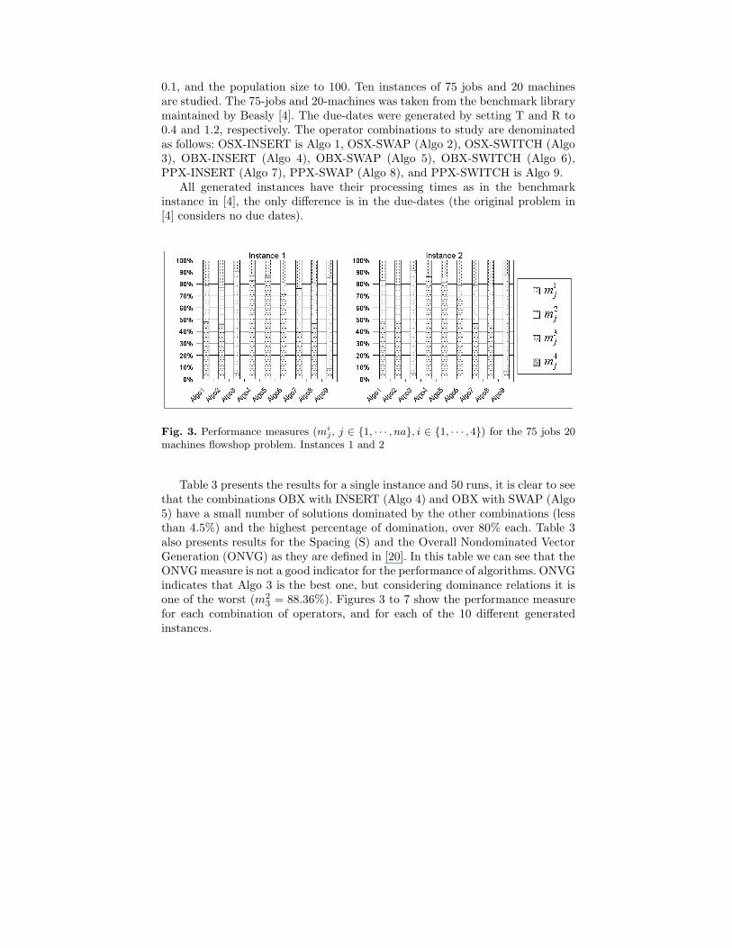
0.1, and the population size to 100. Ten instances of 75 jobs and 20 machinesare studied. The 75-jobs and 20-machines was taken from the benchmark librarymaintained by Beasly [4]. The due-dates were generated by setting T and R to0.4 and 1.2, respectively. The operator combinations to study are denominatedas follows: OSX-INSERT is Algo 1, OSX-SWAP (Algo 2), OSX-SWITCH (Algo3), OBX-INSERT (Algo 4), OBX-SWAP (Algo 5), OBX-SWITCH (Algo 6),PPX-INSERT (Algo 7), PPX-SWAP (Algo 8), and PPX-SWITCH is Algo 9.

All generated instances have their processing times as in the benchmarkinstance in [4], the only difference is in the due-dates (the original problem in[4] considers no due dates).

Fig. 3. Performance measures (mij , j ∈ {1, · · · , na}, i ∈ {1, · · · , 4}) for the 75 jobs 20

machines flowshop problem. Instances 1 and 2

Table 3 presents the results for a single instance and 50 runs, it is clear to seethat the combinations OBX with INSERT (Algo 4) and OBX with SWAP (Algo5) have a small number of solutions dominated by the other combinations (lessthan 4.5%) and the highest percentage of domination, over 80% each. Table 3also presents results for the Spacing (S) and the Overall Nondominated VectorGeneration (ONVG) as they are defined in [20]. In this table we can see that theONVG measure is not a good indicator for the performance of algorithms. ONVGindicates that Algo 3 is the best one, but considering dominance relations it isone of the worst (m2

3 = 88.36%). Figures 3 to 7 show the performance measurefor each combination of operators, and for each of the 10 different generatedinstances.

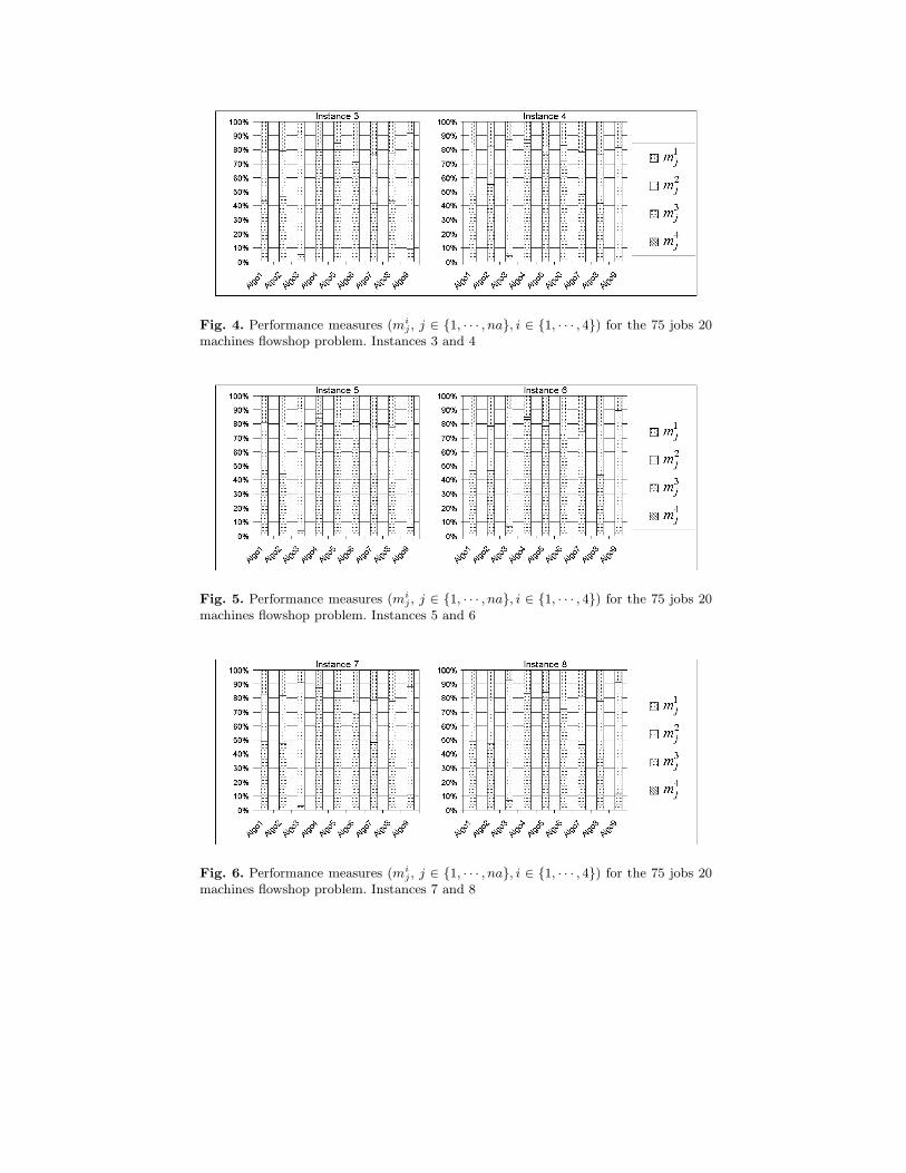
Fig. 4. Performance measures (mij , j ∈ {1, · · · , na}, i ∈ {1, · · · , 4}) for the 75 jobs 20

machines flowshop problem. Instances 3 and 4

Fig. 5. Performance measures (mij , j ∈ {1, · · · , na}, i ∈ {1, · · · , 4}) for the 75 jobs 20

machines flowshop problem. Instances 5 and 6

Fig. 6. Performance measures (mij , j ∈ {1, · · · , na}, i ∈ {1, · · · , 4}) for the 75 jobs 20

machines flowshop problem. Instances 7 and 8

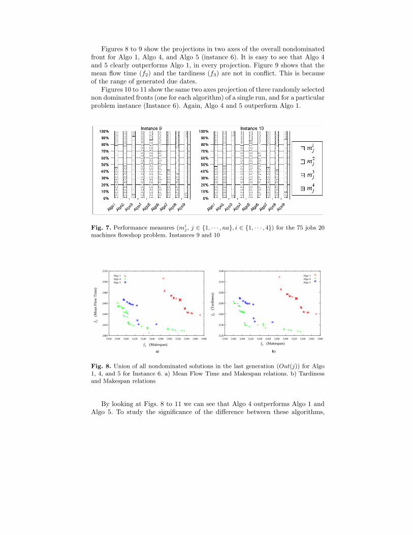
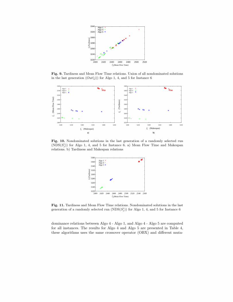
Figures 8 to 9 show the projections in two axes of the overall nondominatedfront for Algo 1, Algo 4, and Algo 5 (instance 6). It is easy to see that Algo 4and 5 clearly outperforms Algo 1, in every projection. Figure 9 shows that themean flow time (f2) and the tardiness (f3) are not in conflict. This is becauseof the range of generated due dates.

Figures 10 to 11 show the same two axes projection of three randomly selectednon dominated fronts (one for each algorithm) of a single run, and for a particularproblem instance (Instance 6). Again, Algo 4 and 5 outperform Algo 1.

Fig. 7. Performance measures (mij , j ∈ {1, · · · , na}, i ∈ {1, · · · , 4}) for the 75 jobs 20

machines flowshop problem. Instances 9 and 10

2400

2420

2440

2460

2480

2500

2520

5160 5180 5200 5220 5240 5260 5280 5300 5320 5340 5360 53803220

3240

3260

3280

3300

3320

3340

5160 5180 5200 5220 5240 5260 5280 5300 5320 5340 5360 5380

Algo 1Algo 4Algo 5

(Makespan)f1(Makespan)f1

(Tar

dine

ss)

f 3

(Mea

n Fl

ow T

ime)

f 2

a) b)

Algo 1Algo 4Algo 5

Fig. 8. Union of all nondominated solutions in the last generation (Out(j)) for Algo1, 4, and 5 for Instance 6. a) Mean Flow Time and Makespan relations. b) Tardinessand Makespan relations

By looking at Figs. 8 to 11 we can see that Algo 4 outperforms Algo 1 andAlgo 5. To study the significance of the difference between these algorithms,

3220

3240

3260

3280

3300

3320

3340

2400 2420 2440 2460 2480 2500 2520

Algo 1Algo 4Algo 5

(Tar

dine

ss)

f 3

(Mean Flow Time)f2

Fig. 9. Tardiness and Mean Flow Time relations. Union of all nondominated solutionsin the last generation (Out(j)) for Algo 1, 4, and 5 for Instance 6

2400

2420

2440

2460

2480

2500

2520

2540

2560

5200 5250 5300 5350 5400 5450

3220

3240

3260

3280

3300

3320

3340

3360

3380

5200 5250 5300 5350 5400 5450

(Makespan)f1(Makespan)f1

(Tar

dine

ss)

f 3

(Mea

n Fl

ow T

ime)

f 2

a) b)

Algo 1Algo 4Algo 5

Algo 1Algo 4Algo 5

Fig. 10. Nondominated solutions in the last generation of a randomly selected run(NDS(Si

j)) for Algo 1, 4, and 5 for Instance 6. a) Mean Flow Time and Makespanrelations. b) Tardiness and Makespan relations

3220

3240

3260

3280

3300

3320

3340

3360

3380

2400 2420 2440 2460 2480 2500 2520 2540 2560

(Mean Flow Time)f2

(Tar

dine

ss)

f 3

Algo 1Algo 4Algo 5

Fig. 11. Tardiness and Mean Flow Time relations. Nondominated solutions in the lastgeneration of a randomly selected run (NDS(Si

j)) for Algo 1, 4, and 5 for Instance 6

dominance relations between Algo 4 - Algo 1, and Algo 4 - Algo 5 are computedfor all instances. The results for Algo 4 and Algo 5 are presented in Table 4,these algorithms uses the same crossover operator (OBX) and different muta-

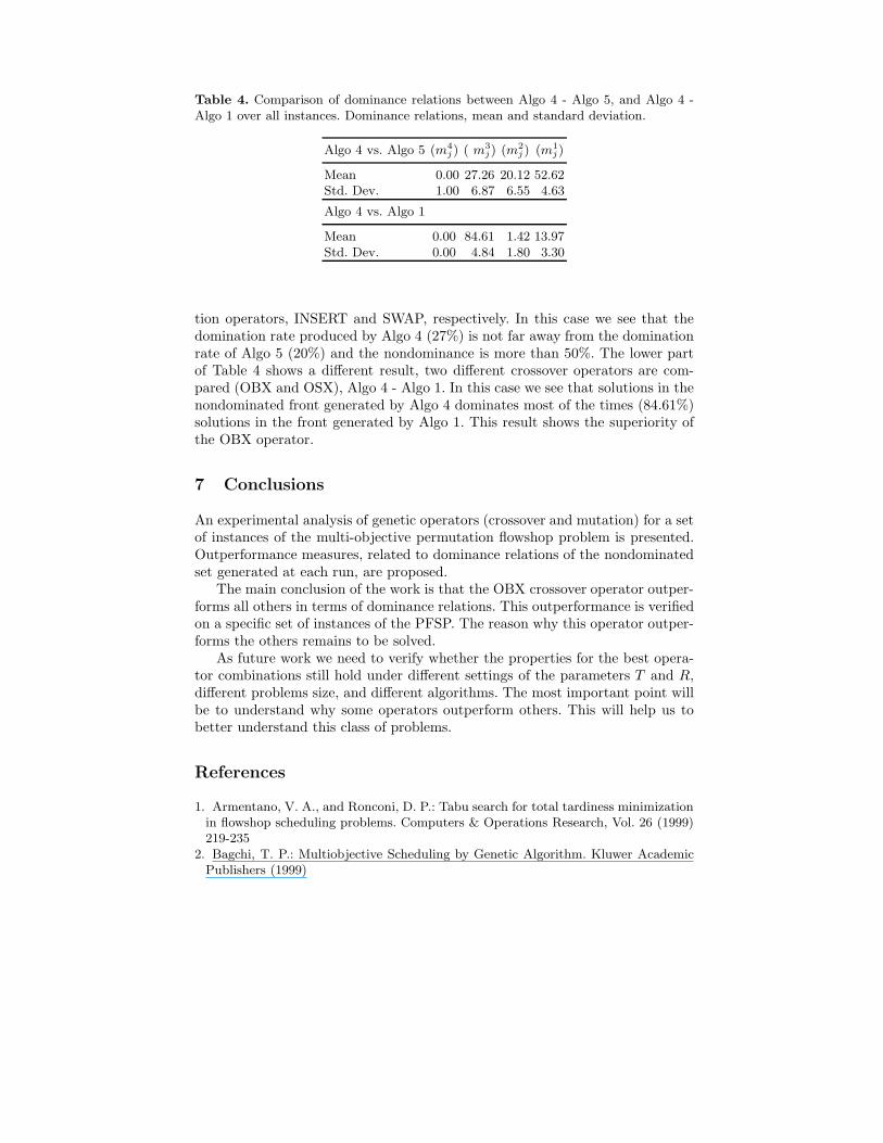
Table 4. Comparison of dominance relations between Algo 4 - Algo 5, and Algo 4 -Algo 1 over all instances. Dominance relations, mean and standard deviation.

Algo 4 vs. Algo 5 (m4

j ) ( m3

j ) (m2

j ) (m1

j )

Mean 0.00 27.26 20.12 52.62Std. Dev. 1.00 6.87 6.55 4.63

Algo 4 vs. Algo 1

Mean 0.00 84.61 1.42 13.97Std. Dev. 0.00 4.84 1.80 3.30

tion operators, INSERT and SWAP, respectively. In this case we see that thedomination rate produced by Algo 4 (27%) is not far away from the dominationrate of Algo 5 (20%) and the nondominance is more than 50%. The lower partof Table 4 shows a different result, two different crossover operators are com-pared (OBX and OSX), Algo 4 - Algo 1. In this case we see that solutions in thenondominated front generated by Algo 4 dominates most of the times (84.61%)solutions in the front generated by Algo 1. This result shows the superiority ofthe OBX operator.

7 Conclusions

An experimental analysis of genetic operators (crossover and mutation) for a setof instances of the multi-objective permutation flowshop problem is presented.Outperformance measures, related to dominance relations of the nondominatedset generated at each run, are proposed.

The main conclusion of the work is that the OBX crossover operator outper-forms all others in terms of dominance relations. This outperformance is verifiedon a specific set of instances of the PFSP. The reason why this operator outper-forms the others remains to be solved.

As future work we need to verify whether the properties for the best opera-tor combinations still hold under different settings of the parameters T and R,different problems size, and different algorithms. The most important point willbe to understand why some operators outperform others. This will help us tobetter understand this class of problems.

References

1. Armentano, V. A., and Ronconi, D. P.: Tabu search for total tardiness minimizationin flowshop scheduling problems. Computers & Operations Research, Vol. 26 (1999)219-235

2. Bagchi, T. P.: Multiobjective Scheduling by Genetic Algorithm. Kluwer AcademicPublishers (1999)

3. Basseur, M., Seynhaeve, F., Talbi E.: Design of multi-objective evolutionary algo-rithms: Application to the flow-shop scheduling problem. Congress on EvolutionaryComputation (2002) 459-465

4. http://mscmga.ms.ic.ac.uk/info.html5. Bierwirth, C., Mattfeld, D. C., Kopfer, H.: On Permutation Representations for

Scheduling Problems. In Proceedings of Parallel Problem Solving from Nature. Lec-ture Notes in Computer Science, Vol. 1141. Springer-Verlag, Berlin Heidelberg NewYork (1996) 310-318

6. C. Brizuela, Y. Zhao, N. Sannomiya.: Multi-Objective Flowshop: Preliminary Re-sults. In Zitzler, E., Deb, K., Thiele, L., Coello Coello, C. A., Corne D., eds., Evo-lutionary Multi-Criterion Optimization, First International Conference, EMO 2001,vol. 1993 of LNCS, Berlin:Springer-Verlag (2001) 443-457

7. Coello Coello, C. A.: A Comprehensive Survey of Evolutionary-Based MultiobjectiveOptimization Techniques. Knowledge and Information Systems, Vol. 1, No. 3 (1999)269-308

8. Coello Coello, C. A., Van Veldhuizen, D. A., and Lamont, G. B.: Evolutionary Al-gorithms for Solving Multi-Objective Problems. Kluwer Academic Publishers (2002)

9. Deb, K.: Multi-objective Genetic Algorithms: Problem Difficulties and Constructionof Test Problems. Evolutionary Computation, 7(3) (1999) 205-230

10. Deb, K.: Multi-Objective Optimization using Evolutionary Algorithms. John Wiley& Sons (2001)

11. M. R. Garey, D. S. Johnson and Ravi Sethi.: The Complexity of Flowshop andJobshop Scheduling. Mathematics of Operations Research, Vol. 1, No. 2 (1976) 117-129

12. Gen, M. and Cheng, R.: Genetic Algorithms & Engineering Design. John Wiley &Sons (1997)

13. Gen, M. and Cheng, R.: Genetic Algorithms & Engineering Optimization. JohnWiley & Sons (1997)

14. Golberg, D.: Genetic Algorithms in Search, Optimization, and Machine Learning,Addison-Wesley (1989)

15. Isibuchi, H. and Murata, T.: Multi-objective Genetic Local Search Algorithm. Pro-ceedings of the 1996 International Conference on Evolutionary Computation (1996)119-124

16. Isibuchi, H. and Murata, T.: Multi-objective Genetic Local Search Algorithm andits application to flowshop scheduling. IEEE Transactions on Systems, Man, andCybernetics - Part C: Applications and Reviews, 28(3) (1998) 392-403

17. Knowles J. and Corne D.: On Metrics for Comparing Nondominated Sets. Pro-ceedings of the 2002 Congress on Evolutionary Computation (2002) 711-716

18. Tamaki, H., and Nishino, E.: A Genetic Algorithm approach to multi-objectivescheduling problems with regular and non-regular objective functions. Proceedingsof IFAC LSS’98 (1998) 289-294

19. Srinivas, N. and Deb, K.: Multi-Objective function optimization using non-dominated sorting genetic algorithms. Evolutionary Computation, 2(3) (1995) 221-248

20. Van Veldhuizen, D. and Lamont, G.: On measuring multiobjective evolutionaryalgorithm performance. Proceedings of the 2000 Congress on Evolutionary Compu-tation (2000) 204-211

21. Zitzler E., Laumanns M., Thiele L., Fonseca C. M., Grunert da Fonseca V.: WhyQuality Assesment of Multiobjective Optimizers Is Difficult. Proceedings of the 2002Genetic and Evolutionary Computation Conference (GECCO2002) (2002) 666-673